
Wave Data Processing Toolbox Manual
By Charlene Sullivan¹, John Warner¹, Marinna Martin¹, Frances Lightsom¹, George Voulgaris², and Paul Work³
¹USGS, Woods Hole Science Center, Woods Hole, MA
²Dept. of Geological Sciences, University of South Carolina, Columbia, SC
³Georgia Institute of Technology, School of Civil and Environmental Engineering, Savannah Campus
Any use of trade, firm, or product names is for descriptive purposes only and does not imply endorsement by the U.S. Government.
O
pen-File Report 2005-1211
2006
U.S. Department of the Interior
U.S. Geological Survey
U.S. Department of the Interior
Gale A. Norton, Secretary
U.S. Geological Survey
P. Patrick Leahy, Acting Director
U.S. Geological Survey, Reston, Virginia
Contact:
John Warner
U.S. Geological Survey
384 Woods Hole Road
Woods Hole, MA 02543
Telephone: 508-457-237 or 508-548-8700
For product and ordering information:
World Wide Web: http://www.usgs.gov/pubprod
Telephone: 1-888-ASK-USGS
For more information on the USGS—the Federal source for science about the Earth,
its natural and living resources, natural hazards, and the environment:
World Wide Web: http://www.usgs.gov
Telephone: 1-888-ASK-USGS
Although this report is in the public domain, permission must be secured from the individual
copyright owners to reproduce any copyrighted material contained within this report.
Contents
1. Introduction ...............................................................................................................................................................4
2. Limitations.................................................................................................................................................................4
3. Software Prerequisites ...............................................................................................................................................5
4. Processing Overview .................................................................................................................................................5
5. Processing Waves Data – Step by Step Instructions..................................................................................................6
6. Wave Data Processing Toolbox M-files ..................................................................................................................14
7. References ...............................................................................................................................................................17
Appendix I: Metadata .................................................................................................................................................18
Appendix I: Metadata .................................................................................................................................................18
Appendix II: Description of variables in the burst NetCDF file.................................................................................19
Appendix III: Description of variables in the statistic NetCDF file ...........................................................................20
Appendix IV: M-files for RD Instruments ADCP......................................................................................................22

Wave Data Processing Toolbox Manual
By Charlene Sullivan, John Warner, Marinna Martini, Frances Lightsom, George Voulgaris, and Paul Work
1. Introduction
Researchers routinely deploy oceanographic equipment in estuaries, coastal nearshore environments, and
shelf settings. These deployments usually include tripod-mounted instruments to measure a suite of physical
parameters such as currents, waves, and pressure. Instruments such as the RD Instruments Acoustic Doppler Current
Profiler (ADCP™), the Sontek Argonaut, and the Nortek Aquadopp™ Profiler (AP) can measure these parameters.
The data from these instruments must be processed using proprietary software unique to each instrument to convert
measurements to real physical values. These processed files are then available for dissemination and scientific
evaluation. For example, the proprietary processing program used to process data from the RD Instruments ADCP
for wave information is called WavesMon. Depending on the length of the deployment, WavesMon will typically
produce thousands of processed data files. These files are difficult to archive and further analysis of the data
becomes cumbersome. More imperative is that these files alone do not include sufficient information pertinent to
that deployment (metadata), which could hinder future scientific interpretation.
This open-file report describes a toolbox developed to compile, archive, and disseminate the processed
wave measurement data from an RD Instruments ADCP, a Sontek Argonaut, or a Nortek AP. This toolbox will be
referred to as the Wave Data Processing Toolbox. The Wave Data Processing Toolbox congregates the processed
files output from the proprietary software into two NetCDF files: one file contains the statistics of the burst data and
the other file contains the raw burst data (additional details described below). One important advantage of this
toolbox is that it converts the data into NetCDF format. Data in NetCDF format is easy to disseminate, is portable
to any computer platform, and is viewable with public-domain freely-available software. Another important
advantage is that a metadata structure is embedded with the data to document pertinent information regarding the
deployment and the parameters used to process the data. Using this format ensures that the relevant information
about how the data was collected and converted to physical units is maintained with the actual data. EPIC-standard
variable names have been utilized where appropriate. These standards, developed by the NOAA Pacific Marine
Environmental Laboratory (PMEL) (
http://www.pmel.noaa.gov/epic/), provide a universal vernacular allowing
researchers to share data without translation.
2. Limitations
• This Wave Data Processing Toolbox has been developed specifically for use with wave data from:
o RD Instruments Workhorse ADCP
o Sontek Argonaut
o Nortek Aquadopp AP
• The user must provide metadata information in an ASCII-file with specific formatting (templates provided,
see discussion below). This information is read from the ASCII file and written to the NetCDF files.
• Wave information must be output from the instrument’s proprietary software in ASCII format (details
described below).
• For the RD Instruments ADCP, the Wave Data Processing Toolbox assumes the instrument is equipped
with the optional waves acquisition firmware.
• For the Sontek Argonaut, the Wave Data Processing Toolbox assumes the wave spectra collection package,
Sontek SonWave, is installed for collection of wave frequency spectra data. The user must also specify the
LONG data format and metric units during deployment setup for data output. The Wave Data Processing
Toolbox does not include provisions for reading the SHORT data format at this time.
4
4

3. Software Prerequisites
It is expected that the user has obtained all the proprietary software and necessary files to process the data
from their specific instrument. For example, this would include (but is not limited to) the user installing and running
the RD Instruments WavesMon software package to process all wave data from the RD Instruments ADCP.
Similarly, the user should install and run the ViewArgonaut software package for the Sontek Argonaut and the
AquaPro software for the Nortek AP. This manual provides some suggested guidance on program settings for these
proprietary software packages. However, the user is responsible for all processing and should consult the user’s
manual for their proprietary software to determine settings for their specific deployment.
The Wave Data Processing Toolbox described in this manual consists of a Matlab-based package of m-files
written in The Mathworks Inc., Matlab® programming language. We assume users have installed The Mathworks
Inc., Matlab® software on their operating system. Users must also have installed on their operating system the
USGS NetCDF Toolbox. This toolbox was developed by Dr. Charles R. Denham and is freely available for
download from:
http://woodshole.er.usgs.gov/staffpages/cdenham/public_html/MexCDF/nc4ml5.html or
http://mexcdf.sourceforge.net/.
NetCDF is the file-format of choice for the USGS due to its platform independence and relative ease of use.
Remote users on any number of computer platforms have the ability to load and visualize NetCDF data with a wide
variety of open-source software applications, which are freely-available on the World Wide Web.
For more information on NetCDF users are referred to
http://my.unidata.ucar.edu/content/software/netcdf/index.html.
ncBrowse is a utility for visualization of NetCDF data. It is freely-available at
http://www.epic.noaa.gov/java/ncBrowse/
The Wave Data Processing Toolbox has been tested exclusively with The Mathworks Inc., Matlab®
Release 14, Version 7, Service Pack 3 on a Windows XP operating system.
4. Processing Overview
Proprietary Software Waves Processing
Each instrument measures and records time series of velocity and pressure and processes these time series
via spectral analysis to provide estimates of directional and/or non-directional energy density spectra and wave
parameters. The wave height provided is Hmo, which is 4x the square root of the area under the non-directional
energy density spectrum. It typically corresponds closely to the significant wave height, which is the average of the
highest 1/3 of the waves in a record.
Other reported parameters include the peak period, which is the period at which the energy density is
maximized. If applicable, the peak wave direction is computed, which is the direction corresponding to the
maximum energy in the directional spectrum. The direction is defined as that from which the wave is coming
(nautical convention).
Each instrument manufacturer provides a software program for the user to extract measured wave data and
to convert (process) the data to engineering units. For the RD Instruments ADCP this software is called WavesMon.
For the Sontek Argonaut the software is called ViewArgonaut, and for the Nortek AP the software is called
AquaPro. These programs convert the raw binary data files into a series of (typically ASCII) text files containing the
time series of wave energy density spectra and wave parameters such as significant wave height, peak wave period,
and peak wave direction.
We assume users are familiar with their instrument’s proprietary software and will choose processing
options that are specific to their project. However, the Wave Data Processing Toolbox assumes that users have saved
all processed data to ASCII files. In this manual we include a detailed outline of the processing options chosen for
5
5

each instrument. However, the actual parameters that a user selects are expected to vary with their particular
application.
Matlab® Processing
The Wave Data Processing Toolbox m-files load the output from the proprietary processing software into
Matlab®. The toolbox contains provisions for the removal of out-of-water data collected during instrument
deployment and recovery. No additional data quality editing is provided at this stage. The statistical wave
parameters are converted into EPIC-standard variables and written to a NetCDF file for distribution and archiving.
Additionally, for the RD Instruments ADCP and the Nortek AP, individual bursts of velocity and pressure are
written to a NetCDF file for archiving.
5. Processing Waves Data – Step by Step Instructions
5.1 Install the Waves Data Processing System
The Wave Data Processing Toolbox m-files are packed in the file WVTOOLS.zip, Unpack the contents of
this zip file to a directory on your operating system’s hard drive. This will place a folder named WVTOOLS on
your hard drive. The m-files for this toolbox reside in the sub-folders named RDI, Sontek, Nortek, and AddOns.
Then start Matlab® and add the WVTOOLS directories to your Matlab® path.
If, for example, you unpacked the WVTOOLS folder to:
c:\MFILES\WVTOOLS
you should type the following at the Matlab® command prompt to add the WVTOOLS directories to your Matlab®
path:
>> addpath(genpath(‘c:\MFILES\WVTOOLS’))
5.2 Directory Setup
Users should run the proprietary software for their instrument and the Wave Data Processing Toolbox m-
files in a directory that contains the raw binary data file downloaded from their instrument. If a directory with this
file already exists on your operating system’s hard drive, we advise you to create a sub-directory and copy the
instrument’s raw binary file to this sub-directory. This will isolate processing of the waves data from other
processing that might occur using the file. As an example below, we create a sub-directory named ‘wavesmon’ in
which we run the WavesMon software package and the Wave Data Processing Toolbox m-files for the RD
Instruments ADCP. The raw binary data file from this instrument is copied into this directory from the directory
above, ‘7221wh’. Similarly, we would create sub-directories named ‘viewarg’ and ‘aquapro’ for the Sontek
Argonaut and Nortek AP, respectively.
Thus: C:\7221wh is a directory with raw binary data file downloaded from your instrument
C:\7221wh\wavesmon is a subdirectory with a copy of the raw binary data file, a metadata file, processed
data output from the instrument’s proprietary software, and NetCDF data files that will be output
by this Wave Data Processing Toolbox.
6
6
5.3 The Metadata File
Users should next create a metadata file and place it in the sub-directory created above in section 5.2. A
metadata file is a simple text file containing important information regarding the collection of the data. For example,
it will typically include the location, date, and time of data collection. This information is crucial for scientific data
interpretation. Common metadata fields are described in Appendix I. The Wave Data Processing Toolbox is
designed to read a metadata file that has specific formatting. These files are instrument-specific. We provide
example metadata files for each instrument in the Wave Data Processing Toolbox package of m-files. The files
include metaRDI.txt for the RD Instruments ADCP, metaNortek.txt for the Nortek Aquadopp AP and
metaSontek.txt for the Sontek Argonaut. It is recommended that users copy the included metadata file for their
instrument into the subdirectory created in section 5.2 and use it as a template for their metadata file.
Once the metadata file is created, users should run the proprietary software package specific to their
instrument in order to obtain ASCII file output of processed wave measurements. Step-by-step instructions for the
proprietary software are provided in sections 5.4 for the RD Instruments ADCP, in 5.5 for the Sontek Argonaut and
in 5.6 for the Nortek AP. Included in these instructions are suggested processing options (where available) for each
instrument.
5.4 Processing for an RD Instruments ADCP
The RD Instrument ADCP records three different types of time series from which wave properties may be
computed: pressure, range to the surface along each of its four beams (i.e., water level), and orbital velocities of the
surface waves taken from three bins nearest the surface in each of the four beams. It is possible to estimate non-
directional wave energy spectra, and thus wave height and period, from any of the three time series, but the velocity
time series are required for definition of the directional distribution of the wave energy.
The WavesMon software package processes the raw binary ADCP data file and produces a series of
computed data files. Pressure time series are output to files named Pressyyyynnddhhmmssxx.txt, where Press is
pressure, and the remaining characters are year (yyyy), month (nn), day(dd), hour (hh), minute (mm), second (ss),
and milli-second (xx). Time series of the range to surface are output to files named Strkyyyynnddhhmmssxx.txt,
whereas time series of orbital velocities are output to Velyyyynnddhhmmssxx.txt. The orbital velocity
measurements are used to calculate directional wave spectra, which are saved in output files called
DSpecyynnddhhmm.txt, where Dspec is directional spectra, and the remaining characters are year (yy), month (nn),
day (dd), hour (hh), and minute (mm) of the sample average. Data from all three methods are used to compute non-
directional spectra, which are saved in files called PSpecyynnddhhmm.txt, SSpecyynnddhhmm.txt, and
VSpecyynnddhhmm.txt where the PSpec* are derived from the pressure measurements, SSpec* are derived from the
range to surface measurements, and VSpec* are derived from the orbital velocity measurements. Time series of
wave parameters such as significant wave height, peak wave period, and peak wave direction are output in a file
called *_LogData.000.
Users are cautioned against re-running WavesMon in a directory in which WavesMon was previously run.
Doing so creates an additional time series of wave parameters called *_LogData.001, rather than overwriting the
previous time series. The Wave Data Processing Toolbox assumes WavesMon was run once in a directory and that
only one time series file called *_LogData.000 exists in the directory. Users are referred to RD Instrument’s Waves
User’s Guide and the RDI Waves Primer for detailed WavesMon processing instructions and information regarding
WavesMon’s various processing options.
5.4.1. Start WavesMon
Double-click the WavesMon icon on your desktop to start WavesMon. Alternatively click the start menu
and select all programs then RD Instruments and then WavesMon.
In the WavesMon File menu select New Setup. Then select Playback in the Choose a realtime or
playback dialogue and click OK. Click OK again if a Tip pops up.
7
7
In the Save Setup As dialog browse to the location of the directory you created during ‘Directory Setup’ in
section 5.2. Then enter a filename for your setup file. We use a filename that corresponds to our mooring number
and instrument, such as 722wh, where ‘722’ is the mooring number and ‘wh’ is for Workhorse ADCP. This file
name is added by default to the *_LogData.000 file that contains the time series of wave parameters (i.e.
722wh_LogData.000).
In the Setup Playback screen select Advanced. The Setup Playback (Advanced) screen should now
appear.
5.4.2 Designate Input and Output Options
In the Setup Playback (Advanced) screen select the Input tab. On the Input screen select Browse, then
select your raw binary adcp data file and click Open.
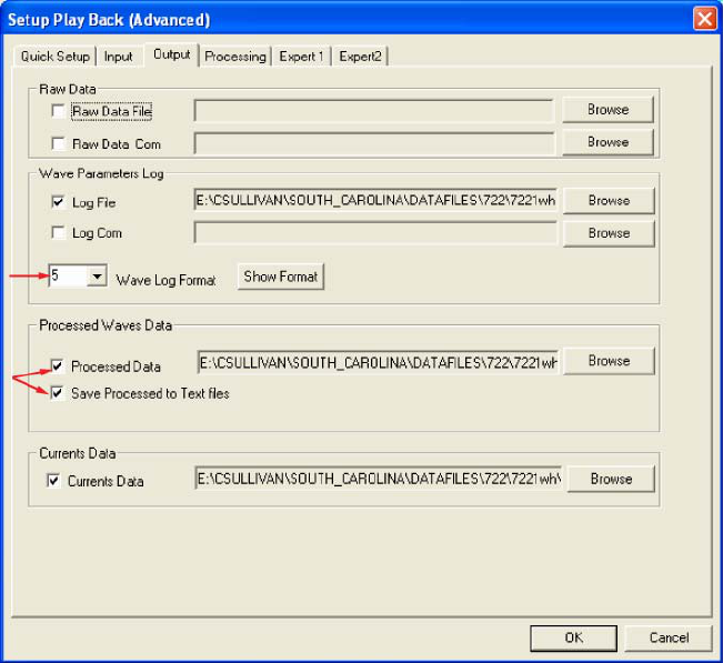
Next, select the Output (fig. 1) tab from the Setup Playback (Advanced) screen. Under Processed
Waves Data make sure both Processed Data and Save Processed Data to Text Files are checked (Required). Also
make sure the Wave Log Format is 5 (Required).
Figure 1: The Output tab from the WavesMon Setup Playback (Advanced) screen. Red arrows identify specific WavesMon
processing options described in text.
5.4.3 Select Processing Options
Select the Processing (fig. 2) tab from the Setup Playback (Advanced) screen. Under What to Process
make sure all boxes are checked. This will process and save the velocity, surface, and pressure time series and
spectra, the directional spectra, and the wave parameters (Required). Under How to Process change Lower Freq
Threshold from its default value (0.01) to 0.05. Change Upper Freq Threshold for velocity, V, from its default
8
8
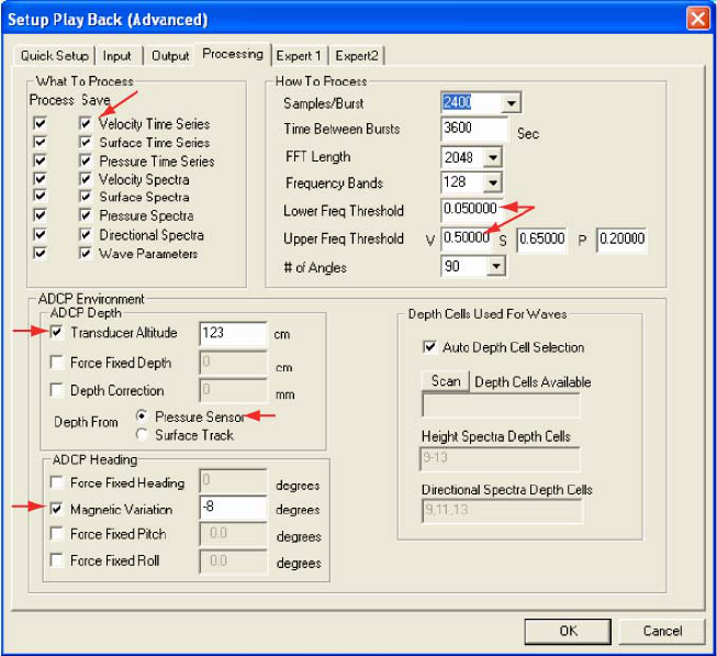
value (0.35) to 0.5. Under ADCP Environment check the Transducer Altitude box and enter the transducer’s
altitude in centimeters. If your pressure sensor was working and was not significantly biofouled, be sure that
Pressure Sensor is selected next to Depth From. Otherwise select Surface Track. Under ADCP Heading check
the Magnetic Variation box and enter your location’s magnetic variation in degrees. Magnetic variation is positive
east of true north and negative when west
Figure 2: The Processing tab from the WavesMon Setup Playback (Advanced) screen. Red arrows identify specific WavesMon
processing options described in text.
Next, select the Expert 1 (fig. 3) from the Setup Playback (Advanced) screen. In the box next to IMLM
Iterations click the down arrow to change the value from its default (1) to 3. Also check the box next to Output
Dir Spec in Power x Power (Required).
9
9
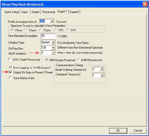
Figue 3: The Expert 1 tab from the WavesMon Setup Playback (Advanced) screen. Red arrows identify specific WavesMon
processing options described in text.
Lastly, select the Expert 2 (fig. 4) from the Setup Playback (Advanced) screen. Under Data Screening
check the box next to Use File Buffer for Data. Under Misc check the box next to Correct for Currents. Click
OK to close the Expert 2 tab. Click OK again to close the Setup Playback (Advanced) screen.
10
10
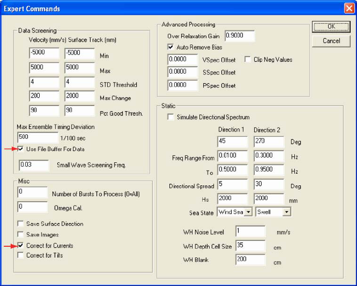
Figure 4: The Expert 2 tab from the WavesMon Setup Playback (Advanced) screen. Red arrows identify specific WavesMon
processing options described in text.
5.4.4 Start WavesMon Processing
The Setup Playback screen should now be displayed. Select OK on this screen to close it. Select the
green Go button on the main WavesMon screen to commence WavesMon processing. This processing produces the
Press*.txt, Strk*.txt, Vel*.txt, DSpec*.txt, PSpec*.txt, VSpec*.txt, SSpec*.txt, and *_LogData.000 ASCII output
files.
Once WavesMon has completed, the user should exit WavesMon and follow the step-by-step instructions
outlined in section 5.7 to run the Waves Data Processing Toolbox.
5.5 Processing for a Sontek Argonaut
The Sontek Argonaut measures wave pressure and computes a non-directional wave energy spectra. The
Waves Data Processing Toolbox assumes the user has specified the LONG data format with metric units during
system configuration. It also assumes the user has the wave spectra collection package, Sontek SonWave, installed
for collection of wave frequency spectra data. The software that is proprietary to the Sontek Argonaut is called
ViewArgonaut. The pressure signal is used to estimate wave height.
ViewArgonaut is used to convert a raw binary data file (*.arg) from the instrument to ASCII text files. It
produces output files called *.ctl, *.snr, *.std, *.vel, and *.dat, where ‘*’ is the name given to your deployment when
setting up the ADP for deployment. The file *.ctl is an ASCII file containing information on the system
configuration, and the contents of the other data files. The files *.snr, *.std, and *.vel contain multi-cell (profiling)
data output for all samples for all cells. The *.vel file includes the x- and y- components of mean velocity, and
speed and direction of the mean current. The *.std file includes the standard error in x- and y- components of mean
velocity. The *.snr file contains the signal to noise ratio and amplitude for each beam. The processed wave data is
11
11

written to the *.dat file and includes significant wave height, peak period, and non-directional wave energy spectra
information.
5.5.1 Start ViewArgonaut
Double-click the ViewArgonaut icon on your desktop to start the application. In the ViewArgonaut menu
select Processing.
5.5.2 Select Input
Next, select File then Open. In the open dialogue box browse to the directory created in section 5.2.0 that
contains the raw binary file from the instrument. Select the file and select Open. A box with Argonaut File
information is displayed. Preview the information and select Ok. It is now possible for the user to view different
displays of processed data if they choose to do so.
5.5.3 Select Output
In order to generate ASCII files with processed data, the user must export processed data from
ViewArgonaut. In ViewArgonaut’s File menu select Export Data. In the ASCII File Output box under Save
Files to Path be sure to save files to the same directory in which the raw binary file from the instrument resides (this
will be the directory created in section 5.2). It is important to check this path as the software defaults to the
directory specified in the previous ViewArgonaut session. Under Output File Name use the default, which should
be the same as your input file name without the .arg file extension. Under Samples make sure All Samples is
checked (this is the default).
5.5.4 Export Data
Select Export All Variables in the lower right corner of the ASCII File Output box. If a box pops up
regarding discharge data click ok to resume exporting data. A box titled Output Ascii File Messages should be
displayed. In that box should be three messages stating the configuration data, the time series data, and the multi-
cell data were successfully written. Click OK in this box. Then click Close on the ASCII File Output box.
At this point the user should exit ViewArgonaut and follow the step-by-step instructions outlined in section
5.7 to run the Waves Data Processing Toolbox.
5.6 Processing for a Nortek AP
The Nortek AP measures wave pressure and near-bed velocities. The proprietary software for the Nortek
AP is called AquaPro and is used to convert binary data files to ASCII text files. The software produces output files
called *.a1, *.a2, *.a3, *.hdr, *.sen, *.v1, *.v2, *.v3, *.whd, and *.wad. The files *.v1, *.v2, and *.v3 contain
current velocities in user-defined coordinates, which can be as beam coordinates, as orthogonal coordinantes in
relation to the sensor head or as geographic coordinates. The files *.a1, *.a2, and *.a3 contain amplitudes along the
instrument’s three beams. Instrument set-up information is located in the *.hdr file. A summary of each burst is
supplied in the file *.wad. Burst-by-burst data is provided in the file *.whd. The file *.sen, contains a summary of
sensor information, such as instrument heading, pitch, roll, and battery voltage. The m-files in this Wave Data
Processing Toolbox use the PUV method to estimate wave parameters. If current velocities were collected in beam
coordinates, they will be converted to geographical coordinates by the toolbox prior to the application of the PUV
method. The pressure signal is used to estimate wave height and the measurements of the waves’ orbital velocities
provide an estimate of the wave direction, after correction is performed for depth attenuation. Additional
information is provided at:
http://www.nortek-as.com/technotes/PUVWaves.pdf
12
12
5.6.1 Start AquaPro
Double-click the AquaPro icon on your desktop to start the application.
5.6.2 Select Input
Under the Deployment menu, select Data Conversion. In the Data Conversion pop-up box, select Add
File. Browse to the folder created in section 5.2 that contains the instrument’s raw binary data file (*.prf). Select
this file and then select Open.
5.6.3 Select Output
In order to generate ASCII files using processed data, the user must export processed data from AquaPro.
In the Data Conversion box next to Add prefix, enter a character string that will be pre-pended to the output files.
5.6.4. Export Data
Select the blue arrow in the center of the Data Conversion box. In the Data Conversion pop-up box, there
should be check marks next to the following boxes: Header, Velocity, Amplitude, Sensors, and Wave. Select OK
to commence exporting of data. When processing is completed, the output file names will be displayed under
Converted files in the Data Conversion box. Select Done and then close the AquaPro software. The *.a1, *.a2,
*.a3, *.hdr, *.sen, *.v1, *.v2, *.v3, *.whd, and *.wad should now exist in the directory containing the instrument’s
raw binary data file.
At this point the user should exit AquaPro and follow the step-by-step instructions outlined in section 5.7 to
run the Wave Data Processing Toolbox.
5.7 Matlab® Processing
5.7.1 Start Matlab®
Double-click the Matlab icon on your desktop to start Matlab®. Alternatively, click the start menu and
select all programs then Matlab x.xx, Matlab x.xx where ‘x.xx’ is the version of Matlab® installed on your
computer.
5.7.2 Change directories
At the Matlab command prompt change directories to the directory you created in section 5.2. This
directory should contain the raw binary data file from the instrument, the metadata file, and the ASCII output files
from your instrument’s proprietary software. For example, the directory created in section 5.2 contains the raw
binary data file from an RD Instruments ADCP, a metadata file, and WavesMon-generated ASCII output files.
Type the following at Matlab’s command prompt in order to change directories to this directory:
>> cd C:\7221wh\wavesmon
5.7.3 Run the Wave Data Processing Toolbox
The Wave Data Processing Toolbox is run by a driver m-file that calls a series of m-files (outlined below)
to load proprietary software output files, to convert data into EPIC-compatible variables where appropriate, and to
13
13

convert data to NetCDF. These m-files were developed by the authors, but they include calls to other user-
contributed m-files. We include all required m-files in the Wave Data Processing Toolbox package.
The driver m-files for the instruments supported by this package are called adcpWvs2nc.m (for the RD
Instruments adcp), argnWvs2nc.m (for the Sontek Argonaut), and aqdpWvs2nc.m (for the Nortek AP). The inputs
for these driver m-files include the metadata file name and a character string that represents the NetCDF file names
to which data will be written. To run the Wave Data Processing Toolbox the user would type the following at
Matlab’s command prompt:
For the RD Instruments ADCP
>> adcpWvs2nc(metaFile, outFileRoot)
For the Sontek Argonaut
>> argnWvs2nc(metaFile, outFileRoot)
For the Nortek AP
>> aqdpWvs2nc(metaFile, outFileRoot)
The input metaFile is a character string that specifies the name of your metadata file. This should be
surrounded by single quotes and specified without the file extension .txt. The input outFileRoot is a character string
that specifies the name of the netCDF files to which you would like to write the data. This string should be
surrounded by single quotes, and the NetCDF file extension, .nc, is not necessary.
The Wave Data Processing Toolbox consumes a large amount of computer memory when it accumulates
data into multi-dimensional arrays. We suggest users have no other programs running on their system while running
the toolbox, and use a clean start of Matlab to prevent Matlab out-of-memory errors. Users may also wish to turn
their hardware acceleration off before running the toolbox.
For the RD Instruments ADCP, bad data screening and removal are accomplished internally by
WavesMon. The entire time series of pressure, velocities, and wave parameters are converted to NetCDF and no
user-interaction is required. However, for both the Sontek Argonaut and the Nortek Aquadopp AP, user-interaction
is required. The user is asked to view a plot of pressures and velocities (for the Nortek), or wave parameters (for the
Sontek), and decide the first and last good bursts of data. All data between the first and last good bursts is converted
to NetCDF. This provision was included to exclude out-of-water data, collected during deployment and recovery of
the instruments, from the NetCDF files.
The NetCDF files outFileRootr-cal.nc and outFileRootp-cal.nc will be written to the directory you created
in section 5.2. The first NetCDF file contains the time series of pressure and velocities. Please note that this NetCDF
file is created only for the RD Instruments ADCP and the Nortek AP. We do not create this NetCDF file for the
Sontek Argonaut, as the pressure time series from which wave parameters and spectra are calculated is not output by
ViewArgonaut. The second NetCDF file contains the statistical wave parameters, and these files are created for all 3
supported instruments. Please refer to Appendix II and Appendix III for a listing of variables in the burst and
statistic NetCDF files, respectively. This completes wave data processing with the Wave Data Processing Toolbox.
6. Wave Data Processing Toolbox M-files
The m-files called by the Wave Data Processing Toolbox are outlined below. These m-files do NOT
require editing. Please report all bugs to John Warner at
mailto:hjcwarner@usgs.gov. The authors would like to
acknowledge NortekUSA for the inclusion of their m-files, wds.m, hs.m, logavg.m, and wavek.m in this processing
package. All of Nortek’s m-files were downloaded from
http://www.nortekusa.com/principles/Waves.html#MatlabToolkit. The mfiles hs.m, logavg.m, and wavek.m remain
unmodified from their original form. The mfile wds.m contains one modification to prevent erroring in Matlab®.
We would also like to acknowledge Dr. Richard P. Signell, who provided the functions julian.m, and gregorian.m.
14
14
6.1 M-files for RD Instruments ADCP
M-files called for the RD Instruments ADCP are located in the sub-folder RDI of the WVTOOLS folder
that was downloaded and installed in section 5.1.0. The m-files are also provided in this manual in Appendix IV. An
outline and a short description of each m-file are provided below.
A. adcpWvs2nc.m ~ Primary driver mfile, controls calls
to other m-files
B. nccreate_adcpWvs.m ~ a function to create and define
the raw and processed NetCDF files for RD Instruments
ADCP wave data storage, archival, and dissemination
C. read_adcpWvs.m ~ a function to load the WavesMon
data file *_LogData.000 containing the time series of
wave parameters
D. ncwrite_adcpWvs.m ~ a function to write the time series
of wave parameters to the processed NetCDF file
E. read_adcpWvs_spec.m ~ a function to load the WavesMon
data files Dspec*.txt, Pspec*.txt, Sspec*.txt, and
Vspec*.txt containing the time series of directional
and non-directional wave energy spectra
F. ncwrite_adcpWvs_spec.m ~ a function to write the time series
of directional and non-directional wave energy spectra to
the processed NetCDF file
G. read_adcpWvs_raw.m ~ a function to load the WavesMon data
files Press*.txt, Strk*.txt, and Vel*.txt containing the raw
time series of pressure, range to surface track, and orbital
velocity data
H. ncwrite_adcpWvs_raw.m ~ a function to write the raw
time series of pressure, range to surface track, and orbital
velocity data the raw NetCDF file
15
15
6.2 M-files for Sontek Argonaut
M-files called for the Sontek Argonaut are located in the sub-folder Sontek of the WVTOOLS folder that
was downloaded and installed in section 5.1. The m-files are also provided in this manual in Appendix V. An outline
and a short description of each m-file are provided below.
A. argnWvs2nc.m ~ Primary driver mfile, controls calls to other m files
B. get_meta_sontek.m ~ a function to load user-defined metadata and instrument setup information
C. nccreate_argnWvs.m ~ a function to create and define the raw and processed NetCDF files for
Sontek Argonaut wave data storage, archival, and dissemination
D. read_argnWvs.m ~ a function to load the ViewArgonaut file *.dat containing the time series of
wave parameters and non-directional wave energy spectra
E. ncwrite_argnWvs.m ~ a function to write the time series of wave parameters and non-directional
wave energy spectra to the processed NetCDF file
6.3 M-files for Nortek AP
M-files called for the Nortek AP are located in the sub-folder Nortek of the WVTOOLS folder that was
downloaded and installed in section 5.1. The m-files are also provided in this manual in Appendix VI. An outline
and a short description of each m-file are provided below.
A. aqdpWvs2nc.m ~ Primary driver mfile, controls calls to other m files
B. get_meta_nortek.m ~ a function to load user-defined metadata and instrument setup information
C. wad2puv.m ~ a function to read the Nortek Aquadopp AP file *.wad, split the file into individual bursts,
and perform PUV analysis
D. nccreate_aqdpWvs.m ~ a function to create and define the raw and processed NetCDF files for Nortek
AP wave data storage, archival, and dissemination
E. ncwrite_aqdpWvs.m ~ a function to write the time series of wave parameters and non-directional wave
energy spectra to the processed NetCDF file
F. ncwrite_aqdpWvs_raw.m ~ a function to write the time series of raw pressures and velocities to the raw
NetCDF file
16
16

7. References
RD Instruments Waves Primer: Wave Measurements and the RDI ADCP waves array technique.
http://www.rdinstruments.com/waves.html.
SonTek/YSI Argonaut Acoustic Doppler Current Meter Technical Documentation.
http://www.sontek.com/product/sw/viewarg/viewargonaut.htm.
Aquadopp Current Meter User manual.
http://www.nortek-as.com/support/manuals/Aquadopp_Manual.pdf
PUV Wave Directional Spectra: How PUV Wave Analysis Works.
http://www.nortek-as.com/technotes/PUVWaves.pdf
17
17

Appendix I: Metadata
The metadata file contains information regarding the instrument and the deployment. Example metadata
files with specific formatting are provided in the Wave Data Processing Toolbox for each instrument. See
metaRDI.txt, metaNortek.txt, and metaSontek.txt. Users may copy and edit these files to suit their project needs, or
create their own metadata files. Users may choose to add or remove metadata fields. However, they must keep in
mind that the metadata field’s description must start at column 20 and not exceed column 83 of the file. Example
metadata fields are described below.
Metadata Field Field Description Example
Mooring mooring identification number ‘7201’
Deployment_date date of instrument deployment ‘28-Oct-2003’
Recovery_date date of instrument recovery ’21-Jan-2004
INST_TYPE type of instrument and instrument manufacturer ‘RD Instruments ADCP’
history NetCDF file history
‘ADCP wave data processed with RDI
WavesMon software’
DATA_SUBTYPE description of data type ‘MOORED’
DATA_ORIGIN data originating institution ‘USGS/WHSC’
COORD_SYSTEM coordinate system of the data ‘GEOGRAPHIC’
WATER_MASS
water mass flag used for EPIC contouring
programs
‘?’
POS_CONST consistent position flag (1 = not consistent) ‘0’
DEPTH_CONST consistent depth flag (1 = not consistent) ‘0’
WATER_DEPTH water depth in meters ‘11.3 M’
DRIFTER drifter flag (=1 if drifter) ‘0’
VAR_FILL missing or bad data value identifier
‘1.0000000409184788E35’
EXPERIMENT experiment name ‘Myrtle Beach’
PROJECT project name ‘South Carolina Coastal Erosion Study’
DESCRIPT location and/or site of data collection ‘Site 1 ADCP’
longitude instrument location ‘-78.7893’
latitude instrument location ’33.6497’
FILL_FLAG data fill flag (=1 if data has fill values) ‘0’
COMPOSITE number of pieces in composite series ‘0’
magnetic_variation
degrees between magnetic and true north at data
location
‘-8.22’
18
18

Appendix II: Description of variables in the burst NetCDF file
)
The following tables list a description of the variables output to the burst NetCDF file (outFileRootr-cal.nc)
for the RD Instruments ADCP and the Nortek AP. A burst NetCDF file is not created for the Sontek Argonaut.
Time is stored in the variables ‘time’ and ‘time2’. The variable ‘time’ contains the Julian Day where Julian Day
2440000 begins at 0000 hours on May 23, 1968. The variable ‘time2’ contains milliseconds (msec) for each Julian
Day. These two variables can be combined as in (1) to yield the time of each observation in Julian Days.
(
3600/24/1000/2timetimejday +=
(1)
For RDI ADCP:
Variable Description Units
time Time in Julian Days Julian Day
time2 Time in Julian Days msec of each Julian Day
burst Burst number counts
lat Latitude degree_north
lon Longitude degree_east
sample Sample number counts
press Pressure sensor derived depth mm
strk Along-beam surface track mm
vel Along-beam velocity mm/s
For Nortek AP:
Variable Description Units
time Time in Julian Days Julian Day
time2 Time in Julian Days msec of each Julian Day
burst Burst number counts
lat Latitude degree_north
lon Longitude degree_east
sample Sample number counts
hght_18 Height of the sea surface relative to
sensor
m
u_1205 Eastward velocity cm/s
v_1206 Northward velocity cm/s
w_1204 Vertical velocity cm/s
amp Beam amplitude counts
19
19

Appendix III: Description of variables in the statistic NetCDF file
The following tables list a description of the variables output to the statistic NetCDF file (outFileRootp-
cal.nc) for the RD Instruments ADCP, the Nortek AP, and the Sontek Argonaut. Time is stored in the variables
‘time’ and ‘time2’. The variable ‘time’ contains the Julian Day where Julian Day 2440000 begins at 0000 hours on
May 23, 1968. The variable ‘time2’ contains milliseconds (msec) for each Julian Day. These two variables can be
combined as in (1) above to yield the time of each observation in Julian Days.
For the RDI ADCP:
Variable Description Units
time Time in Julian Days
Julian Day
time2 Time in Julian Days
msec of each Julian Day
burst Burst number
counts
lat Latitude
degree_north
lon Longitude
degree_east
wh_4061 Significant wave height
m
wp_4060 Mean wave period
s
hght_18 Height of the sea surface relative to
sensor
m
frequency Frequency at the center of each
frequency band
Hz
direction Direction at the center of each direction
slice
degrees True
mwh_4064 Maximum wave height
m
wp_peak Peak wave period
s
wvdir Peak wave direction from which waves
are propagating
degrees True
dspec Directional wave energy spectrum
mm
2
/Hz/degree
pspec Pressure-derived non-directional wave
height spectrum
mm/sqrt(Hz)
sspec Surface-derived non-directional wave
height spectrum
mm/sqrt(Hz)
vspec Velocity-derived non-directional wave
height spectrum
mm/sqrt(Hz)
For the Sontek Argonaut:
Variable Description Units
time Time in Julian Days Julian Day
time2 Time in Julian Days msec of each Julian Day
burst Burst number counts
lat Latitude degree_north
lon Longitude degree_east
wh_4061 Significant wave height m
hght_18 Height of the sea surface relative to
sensor
m
hght_std Standard deviation of height of the sea
surface
m
frequency Frequency at the center of each
frequency band
Hz
20
20
wp_peak Peak wave period s
pspec Pressure-derived non-directional wave
height spectrum
mm/sqrt(Hz)
For the Nortek AP:
Variable Description Units
time Time in Julian Days Julian Day
time2 Time in Julian Days msec of each Julian Day
burst Burst number counts
lat Latitude degree_north
lon Longitude degree_east
wh_4061 Significant wave height m
hght_18 Height of the sea surface relative to
sensor
m
frequency Frequency at the center of each
frequency band
Hz
dfreq Frequency band width Hz
wp_peak Peak wave period s
wvdir Peak wave direction from which waves
are propagating
degrees True
spread Peak spreading degrees
pspec Pressure-derived non-directional wave
height spectrum
mm/sqrt(Hz)
vspec Velocity-derived non-directional wave
height spectrum
mm/sqrt(Hz)
21
21
Appendix IV: M-files for RD Instruments ADCP
function adcpWvs2nc(metaFile,outFileRoot)
% adcpWvs2nc.m A driver M-file for post-processing RD Instruments
% WavesMon wave data in Matlab.
%
% usage: adcpWvs2nc(metaFile,outFileRoot);
%
% where: metaFile - a string specifying the ascii file in which
% metadata is defined, in single quotes
% excluding the .txt file extension
% outFileRoot - a string specifying the name given to the
% NetCDF output files, in single quotes
% excluding the NetCDF file extension .nc
%
% Written by Charlene Sullivan
% USGS Woods Hole Science Center
% Woods Hole, MA 02543
%
% Toolbox Functions:
% nccreate_adcpWvs.m
% read_adcpWvs.m
% ncwrite_adcpWvs.m
% read_adcWvs_spec.m
% ncwrite_adcpWvs_spec.m
% read_adcpWvs_raw.m
% ncwrite_adcpWvs_raw.m
%
% Add-on Functions:
% julian.m
% gregorian.m
% gmin.m
% gmax.m
% C. Sullivan 10/25/05, version 1.1
% Provide user additional feedback regarding code execution. File extension
% on metadata file no longer required for the input 'metaFile'.
% C. Sullivan 06/09/05, version 1.0
% This function assumes the user ran RD Instruments WavesMon
% software, output the WavesMon raw and processed data to text files, and
% created the file 'metaFile.dat' with important metadata. The function
% assumes you are in a directory with this data and the netcdf toolbox and
% the Wave Data Processing System toolbox exist on your Matlab path. Raw
% and processed data is written to individual netCDF files. An integer
% fill value (-32768) is used for the spectra data and the raw data.
% Clear statements interspersed throughout mfiles prevent out of memory
% errors.
more off
version = '1.1';
22
22
tic
% Check inputs
if ~ischar(metaFile) || ~ischar(outFileRoot)
error('File names should be surrounded in single quotes');
end
% Check existence of metadata file
l=ls([metaFile,'.txt']);
if isempty(l)
error(['The metafile ',metaFile,'.txt does not exist in this
directory']);
end
% Check WavesMon output
if isempty(dir('*_LogData.*'))
error(['WavesMon output does not exist in the directory ',pwd])
elseif length(dir('*_LogData.*')) > 1
error('Only one *_LogData.* file is permitted by this toolbox')
elseif isempty(dir('*Spec*.txt'))
error('WavesMon output must include spectra data as text files')
elseif isempty(dir('Strk*.txt'))
error('WavesMon output must include raw Range to surface data')
elseif isempty(dir('Press*.txt'))
error('WavesMon output must include raw pressure data')
elseif isempty(dir('Vel*.txt'))
error('WavesMon output must include raw orbital velocity data')
end
% Create and define your netcdf files
nccreate_adcpWvs(metaFile, outFileRoot);
% Load timeseries data
[logData] = read_adcpWvs;
% Write timeseries data to NetCDF
ncwrite_adcpWvs(logData, outFileRoot);
clear logData
% Load spectra data
[specData] = read_adcpWvs_spec;
% Write spectra data to NetCDF
ncwrite_adcpWvs_spec(specData, outFileRoot);
clear specData
% Load raw data
[rawData] = read_adcpWvs_raw;
% Write raw data to NetCDF
ncwrite_adcpWvs_raw(rawData, outFileRoot);
clear rawData
23
23
ncr.VAR_DESC = ncchar('press:vel:strk');
function nccreate_adcpWvs(metaFile,outFileRoot)
% nccreate_adcpWvs.m A function to create empty netCDF files that will
% store RD Instruments ADCP wave data.
%
% usage: nccreate_adcpWvs(metaFile,outFileRoot);
%
% where: metaFile - a string specifying the ascii file in which
% metadata is defined, in single quotes
% excluding the .txt file extension
% outFileRoot - a string specifying the name given to the
% NetCDF output files, in single quotes
% excluding the NetCDF file extension .nc
%
% Written by Charlene Sullivan
% USGS Woods Hole Science Center
% Woods Hole, MA 02543
% C. Sullivan 03/28/06, version 1.2
% Add EPIC keys for the variables: maximum wave height (new EPIC key 4064),
% peak wave period (use existing EPIC key 4063), and peak wave direction
% (use existing EPIC key 4062). Don't use EPIC keys for spectra variables,
% because EPIC isn't suited for the spectral domain. Perhaps CF conventions
% are better suited?
% C. Sullivan 10/25/05, version 1.1
% Provide user additional feedback regarding code execution. File extension
on
% metadata file no longer required in the input metaFile. Changed DATA_TYPE
% attribute description to be consistent with the documentation. Changed
% EPIC code and units on the variable lon to 502 and degree_east for
% consistency w/ longitude as specified in the metafile where west is
% negative. Add ADCP bin size attributes. Add selected bins for dspec and
% vspec to attributes. Define direction variable for directional spectra.
% Re-define frequency variable.
% C. Sullivan 06/09/05, version 1.0
% Now defining both a raw data and processed data NetCDF files. Including
% all information from the waves configuration file as metadata. Dimensions
% depth (=1), lat (=1), and lon (=1), beam (= 4), and beambin (=12) are
% hardwired.
version = '1.2';
ncr = netcdf([outFileRoot,'r-cal.nc'],'clobber');
ncp = netcdf([outFileRoot,'p-cal.nc'],'clobber');
% Gather and write NetCDF metadata
[userMeta, userMetaDefs] = textread([metaFile,'.txt'],'%s
%63c','commentstyle','shell');
userMetaDefs = cellstr(userMetaDefs);
[wvmnMeta, wvmnMetaDefs] = read_WavesMon_config;
write_adcpWvs_meta(ncr, userMeta, userMetaDefs, wvmnMeta, wvmnMetaDefs)
ncr.DATA_TYPE = ncchar('ADCP pressure and velocity timeseries');
24
24
write_adcpWvs_meta(ncp,userMeta, userMetaDefs, wvmnMeta, wvmnMetaDefs)
ncp.DATA_TYPE = ncchar('ADCP processed wave parameters and spectra');
ncp.VAR_DESC = ncchar('Hs:Tp:Dp:Hmax:Tm:dspec:pspec:sspec:vspec ');
% Define NetCDF dimensions
disp(['Defining NetCDF dimensions in ',outFileRoot,'r-cal.nc and ',...
outFileRoot,'p-cal.nc'])
define_adcpWvs_dims(ncr);
define_adcpWvs_dims(ncp);
% Define NetCDF variables
disp(['Defining NetCDF variables in ',outFileRoot,'r-cal.nc and ',...
outFileRoot,'p-cal.nc'])
disp(' ')
define_adcpWvs_vars(ncr);
define_adcpWvs_vars(ncp);
endef(ncr);
ncr=close(ncr);
endef(ncp);
ncp=close(ncp);
return
% --------- Subfunction: Gather WavesMon configuration data ------------- %
function [wvmnMeta,wvmnMetaDefs]=read_WavesMon_config;
disp(' ')
disp('Reading WavesMon configuration data ...')
configFile = ls('*Wvs.cfg');
ind = 1;
fid = fopen(configFile,'r');
while 1
tline = fgetl(fid);
eqpos = strfind(tline,'=');
if ~isempty(eqpos)
wvmnMeta{ind,1} = tline(1:eqpos-1);
wvmnMetaDefs{ind,1} = tline(eqpos+1:end);
%convert whitespace in wvmnMeta to underscores
ws = find(isspace(wvmnMeta{ind})==1);
wvmnMeta{ind}(ws) = '_';
%convert parenthesis in parameter names to underscores
op = strfind(wvmnMeta{ind},'(');
wvmnMeta{ind}(op) = '_';
cp = strfind(wvmnMeta{ind},')');
wvmnMeta{ind}(cp) = '_';
%convert commas in parameter names to underscores
c = strfind(wvmnMeta{ind},',');
wvmnMeta{ind}(c) = '_';
%make sure no parameter name is longer than 63 characters
%or Matlab complains
if length(wvmnMeta{ind})>63
wvmnMeta{ind} = wvmnMeta{ind}(1:63);
end
ind = ind + 1;
25
25
end
if ~ischar(tline), break, end
end
fclose(fid);
return
% --------- Subfunction: Write NetCDF metadata -------------------------- %
function write_adcpWvs_meta(nc, userMeta, userMetaDefs, wvmnMeta,
wvmnMetaDefs)
for a=1:length(userMeta)
theField = userMeta{a};
theFieldDef = userMetaDefs{a};
if str2num(theFieldDef)
nc.(theField) = str2num(theFieldDef);
else
nc.(theField) = theFieldDef;
end
end
for a=1:length(wvmnMeta)
theField = wvmnMeta{a};
theFieldDef = wvmnMetaDefs{a};
if str2num(theFieldDef) & ~isequal(theField,'VSpecBins')
nc.WavesMonCfg.(theField) = str2num(theFieldDef);
else
nc.WavesMonCfg.(theField) = theFieldDef;
end
end
return
% --------- Subfunction: Define NetCDF dimensions ----------------------- %
function define_adcpWvs_dims(nc)
%common dimensions for both raw and processed NetCDF files
nc('time') = 0;
nc('lat') = 1;
nc('lon') = 1;
if strcmp(nc.DATA_TYPE(:),'ADCP processed wave parameters and spectra')
%dimensions specific to processed NetCDF file
nc('frequency') = nc.WavesMonCfg.NFreqBins(:);
nc('direction') = nc.WavesMonCfg.NDir(:);
elseif strcmp(nc.DATA_TYPE(:),'ADCP pressure and velocity timeseries')
%dimensions specific to raw NetCDF file
nc('sample') = nc.WavesMonCfg.FFTLen(:);
nc('beam') = 4; %ADCP has 4 beams
nc('beambin') = 4*3; %WavesMon uses 3 bins for each beam
end
return
% --------- Subfunction: Define NetCDF variables ------------------------ %
function define_adcpWvs_vars(nc)
26
26
%coordinate variables are the same for both the raw and
%processed NetCDF files
nc{'time'} = nclong('time');
nc{'time'}.FORTRAN_format = ncchar('F10.2');
nc{'time'}.units = ncchar('True Julian Day');
nc{'time'}.type = ncchar('EVEN');
nc{'time'}.epic_code = nclong(624);
nc{'time2'} = nclong('time');
nc{'time2'}.FORTRAN_format = ncchar('F10.2');
nc{'time2'}.units = ncchar('msec since 0:00 GMT');
nc{'time2'}.type = ncchar('EVEN');
nc{'time2'}.epic_code = nclong(624);
nc{'burst'} = nclong('time');
nc{'burst'}.FORTRAN_format = ncchar('F10.2');
nc{'burst'}.units = ncchar('counts');
nc{'burst'}.type = ncchar('EVEN');
nc{'lat'} = ncfloat('lat');
nc{'lat'}.FORTRAN_format = ncchar('F10.4');
nc{'lat'}.units = ncchar('degree_north');
nc{'lat'}.type = ncchar('EVEN');
nc{'lat'}.epic_code = nclong(500);
nc{'lon'} = ncfloat('lon');
nc{'lon'}.FORTRAN_format = ncchar('F10.4');
nc{'lon'}.units = ncchar('degree_east');
nc{'lon'}.type = ncchar('EVEN');
nc{'lon'}.epic_code = nclong(502);
if strcmp(nc.DATA_TYPE(:),'ADCP processed wave parameters and spectra')
%Record variables for ONLY the processed data NetCDF file.
%EPIC variables
nc{'wh_4061'} = ncdouble('time','lat','lon');
nc{'wh_4061'}.long_name=ncchar('Significant Wave Height (m)');
nc{'wh_4061'}.generic_name=ncchar('wave_height');
nc{'wh_4061'}.units=ncchar('m');
nc{'wh_4061'}.epic_code=nclong(4061);
nc{'wh_4061'}.FORTRAN_format=ncchar('F10.2');
nc{'wh_4061'}.FillValue_ = ncfloat(1.0000000409184788E35);
nc{'wh_4061'}.minimum = ncfloat(0);
nc{'wh_4061'}.maximum = ncfloat(0);
nc{'wp_4060'} = ncdouble('time','lat','lon');
nc{'wp_4060'}.long_name=ncchar('Mean Wave Period (s)');
nc{'wp_4060'}.generic_name=ncchar('wave_period');
nc{'wp_4060'}.units=ncchar('s');
nc{'wp_4060'}.epic_code=nclong(4060);
nc{'wp_4060'}.FORTRAN_format=ncchar('F10.2');
nc{'wp_4060'}.FillValue_ = ncfloat(1.0000000409184788E35);
nc{'wp_4060'}.minimum = ncfloat(0);
nc{'wp_4060'}.maximum = ncfloat(0);
27
27
nc{'frequency'}.minimum = ncfloat(0);
nc{'mwh_4064'} = ncdouble('time','lat','lon');
nc{'mwh_4064'}.long_name=ncchar('Maximum Wave Height (m)');
nc{'mwh_4064'}.generic_name=ncchar('wave_height');
nc{'mwh_4064'}.units=ncchar('m');
nc{'mwh_4064'}.epic_code=nclong(4064);
nc{'mwh_4064'}.FORTRAN_format=ncchar('F10.2');
nc{'mwh_4064'}.FillValue_ = ncfloat(1.0000000409184788E35);
nc{'mwh_4064'}.minimum = ncfloat(0);
nc{'mwh_4064'}.maximum = ncfloat(0);
nc{'hght_18'} = ncdouble('time','lat','lon');
nc{'hght_18'}.long_name=ncchar('Height of the Sea Surface (m)');
nc{'hght_18'}.generic_name=ncchar('height');
nc{'hght_18'}.units=ncchar('m');
nc{'hght_18'}.epic_code=nclong(18);
nc{'hght_18'}.FORTRAN_format=ncchar('F10.2');
nc{'hght_18'}.NOTE=ncchar('height of sea surface relative to
sensor');
nc{'hght_18'}.FillValue_ = ncfloat(1.0000000409184788E35);
nc{'hght_18'}.minimum = ncfloat(0);
nc{'hght_18'}.maximum = ncfloat(0);
nc{'wp_peak'} = ncdouble('time','lat','lon');
nc{'wp_peak'}.long_name=ncchar('Peak Wave Period (s)');
nc{'wp_peak'}.generic_name=ncchar('wave_period');
nc{'wp_peak'}.units=ncchar('s');
nc{'wp_peak'}.epic_code=nclong(4063);
nc{'wp_peak'}.FORTRAN_format=ncchar('F10.2');
nc{'wp_peak'}.FillValue_ = ncfloat(1.0000000409184788E35);
nc{'wp_peak'}.minimum = ncfloat(0);
nc{'wp_peak'}.maximum = ncfloat(0);
nc{'wvdir'} = ncdouble('time','lat','lon');
nc{'wvdir'}.long_name=ncchar('Peak Wave Direction (degrees true
North)');
nc{'wvdir'}.generic_name=ncchar('wave_dir');
nc{'wvdir'}.units=ncchar('degrees T');
nc{'wvdir'}.epic_code=nclong(4062);
nc{'wvdir'}.FORTRAN_format=ncchar('F10.2');
nc{'wvdir'}.NOTE=ncchar('Direction FROM which waves are propagating,
measured clockwise from true north');
nc{'wvdir'}.FillValue_ = ncfloat(1.0000000409184788E35);
nc{'wvdir'}.minimum = ncfloat(0);
nc{'wvdir'}.maximum = ncfloat(0);
%non-EPIC variables
nc{'frequency'}=ncdouble('frequency');
nc{'frequency'}.name=ncchar('freq');
nc{'frequency'}.long_name=ncchar('Frequency (Hz)');
nc{'frequency'}.generic_name=ncchar('frequency');
nc{'frequency'}.units=ncchar('Hz');
nc{'frequency'}.type = ncchar('EVEN');
nc{'frequency'}.FORTRAN_format=ncchar('F10.2');
nc{'frequency'}.NOTE=ncchar('frequency at the center of each
frequency band');
28
28
nc{'vspec'}.VspecBins=nc.WavesMonCfg.VSpecBins(:);
nc{'frequency'}.maximum = ncfloat(0);
nc{'direction'}=ncdouble('direction');
nc{'direction'}.name=ncchar('dir');
nc{'direction'}.long_name=ncchar('Direction (degrees T)');
nc{'direction'}.generic_name=ncchar('direction');
nc{'direction'}.units=ncchar('degrees T');
nc{'direction'}.type = ncchar('EVEN');
nc{'direction'}.FORTRAN_format=ncchar('F10.2');
nc{'direction'}.NOTE=ncchar('direction at center of each direction
slice');
nc{'direction'}.minimum = ncfloat(0);
nc{'direction'}.maximum = ncfloat(0);
nc{'dspec'}=ncshort('time','frequency','direction','lat','lon');
nc{'dspec'}.name=ncchar('dspec');
nc{'dspec'}.long_name=ncchar('Directional Wave Energy Spectrum
(mm^2/Hz/degree)');
nc{'dspec'}.generic_name=ncchar('directional spectrum');
nc{'dspec'}.units=ncchar('mm^2/Hz/degree');
nc{'dspec'}.DspecBins=nc.WavesMonCfg.DirSpecBins(:);
nc{'dspec'}.bin_size=nc.ADCPBinSize(:);
nc{'dspec'}.FORTRAN_format=ncchar('F10.2');
nc{'dspec'}.FillValue_ = ncshort(-32768);
nc{'dspec'}.minimum = ncfloat(0);
nc{'dspec'}.maximum = ncfloat(0);
nc{'pspec'}=ncshort('time','frequency','lat','lon');
nc{'pspec'}.name=ncchar('pspec');
nc{'pspec'}.long_name=ncchar('Pressure-derived Non-directional Wave
Height Spectrum (mm/sqrt(Hz))');
nc{'pspec'}.generic_name=ncchar('pressure spectrum');
nc{'pspec'}.units=ncchar('mm/sqrt(Hz)');
nc{'pspec'}.FORTRAN_format=ncchar('F10.2');
nc{'pspec'}.FillValue_ = ncshort(-32768);
nc{'pspec'}.minimum = ncfloat(0);
nc{'pspec'}.maximum = ncfloat(0);
nc{'sspec'}=ncshort('time','frequency','lat','lon');
nc{'sspec'}.name=ncchar('sspec');
nc{'sspec'}.long_name=ncchar('Surface-derived Non-directional Wave
Height Spectrum (mm/sqrt(Hz))');
nc{'sspec'}.generic_name=ncchar('surface spectrum');
nc{'sspec'}.units=ncchar('mm/sqrt(Hz)');
nc{'sspec'}.FORTRAN_format=ncchar('F10.2');
nc{'sspec'}.FillValue_ = ncshort(-32768);
nc{'sspec'}.minimum = ncfloat(0);
nc{'sspec'}.maximum = ncfloat(0);
nc{'vspec'}=ncshort('time','frequency','lat','lon');
nc{'vspec'}.name=ncchar('vspec');
nc{'vspec'}.long_name=ncchar('Velocity-derived Non-directional Wave
Height Spectrum (mm/sqrt(Hz))');
nc{'vspec'}.generic_name=ncchar('velocity spectrum');
nc{'vspec'}.units=ncchar('mm/sqrt(Hz)');
29
29
nc{'vspec'}.bin_size=nc.ADCPBinSize(:);
nc{'vspec'}.FORTRAN_format=ncchar('F10.2');
nc{'vspec'}.FillValue_ = ncshort(-32768);
nc{'vspec'}.minimum = ncfloat(0);
nc{'vspec'}.maximum = ncfloat(0);
elseif strcmp(nc.DATA_TYPE(:),'ADCP pressure and velocity timeseries')
%Record variables for ONLY the raw data NetCDF file. There are no
%EPIC-compatible variables for these quantities.
nc{'sample'} = nclong('sample');
nc{'sample'}.FORTRAN_format = ncchar('F10.2');
nc{'sample'}.units = ncchar('counts');
nc{'sample'}.type = ncchar('EVEN');
nc{'press'}=ncshort('time','sample','lat','lon');
nc{'press'}.name=ncchar('press');
nc{'press'}.long_name=ncchar('Pressure Sensor Derived Depth (mm)');
nc{'press'}.generic_name=ncchar('pressure time series');
nc{'press'}.units=ncchar('mm');
nc{'press'}.FORTRAN_format=ncchar('F10.2');
nc{'press'}.FillValue_ = ncshort(-32768);
nc{'press'}.minimum = ncfloat(0);
nc{'press'}.maximum = ncfloat(0);
nc{'strk'}=ncshort('time','sample','beam','lat','lon');
nc{'strk'}.name=ncchar('strk');
nc{'strk'}.long_name=ncchar('Along-Beam Surface Track (mm)');
nc{'strk'}.generic_name=ncchar('surface track time series');
nc{'strk'}.units=ncchar('mm');
nc{'strk'}.FORTRAN_format=ncchar('F10.2');
nc{'strk'}.FillValue_ = ncshort(-32768);
nc{'strk'}.minimum = ncfloat(0);
nc{'strk'}.maximum = ncfloat(0);
nc{'vel'}=ncshort('time','sample','beambin','lat','lon');
nc{'vel'}.name=ncchar('vspec');
nc{'vel'}.long_name=ncchar('Along-Beam Velocity (mm/s)');
nc{'vel'}.generic_name=ncchar('velocity time series');
nc{'vel'}.units=ncchar('mm/s');
nc{'vel'}.bin_size=nc.ADCPBinSize(:);
nc{'vel'}.FORTRAN_format=ncchar('F10.2');
nc{'vel'}.FillValue_ = ncshort(-32768);
nc{'vel'}.minimum = ncfloat(0);
nc{'vel'}.maximum = ncfloat(0);
end
return
30
30
function [logData]=read_adcpWvs
% read_adcpWvs.m A function to load *LogData.000, which is output from RD
% Instrument's WavesMon software, and output the
% timeseries of wave parameters.
%
% usage: [logData]=read_adcpWvs;
%
% where: logData - a structure with the following fields
% file - name of the *_LogData.* file
% burst - burst number
% YY - 2-digit year
% MM - month
% DD - day
% hh - hours
% mm - minutes
% ss - seconds
% cc - 1/100ths seconds
% Hs - significant wave height, meters
% Hm - maximum wave height, meters
% Tp - peak wave period, seconds
% Tm - mean wave period, seconds
% Dp - peak wave direction, degrees true north
% ht - water depth from pressure sensor, millimeters
%
% Written by Charlene Sullivan
% USGS Woods Hole Science Center
% Woods Hole, MA 02543
% C. Sullivan 10/26/05, version 1.1
% Provide user additional feedback regarding code execution.
% C. Sullivan 06/09/05, version 1.0
% This function assumes you are in a directory with WavesMon-generated wave
% data and that the file *_LogData.000 exists in the directory. Bad data
% indicator (-1) is replaced with NaN. Don't do time conversion to julian
% days in here. Do that conversion when writing the data to NetCDF.
version = '1.1';
% Load the *_LogData.* file
logFile = dir('*LogData*');
logData.file = logFile.name;
disp(['Reading statistical wave parameters from ',logData.file])
data = csvread(logData.file);
% Burst numbers
logData.burst = data(:,1);
% Extract time
logData.YY = data(:,2)+2000;
logData.MM = data(:,3);
logData.DD = data(:,4);
logData.hh = data(:,5);
logData.mm = data(:,6);
31
31
logData.ss = data(:,7);
logData.cc = data(:,8);
% Extract wave parameters
logData.Hs = data(:,9);
logData.Tp = data(:,10);
logData.Dp = data(:,11);
logData.ht = data(:,12);
logData.Hm = data(:,13);
logData.Tm = data(:,14);
% Replace all values of -1 (WavesMon bad data indicator
% for data is the *LogData.000 file) with NaN
theVars = {'Hs','Tp','Dp','ht','Hm','Tm'};
for v = 1:length(theVars)
eval(['logData.',theVars{v},'(logData.',theVars{v},'== -1) = NaN;'])
end
return
32
32
stop_time=datenum([gregorian(time(end))]);
function ncwrite_adcpWvs(logData,outFileRoot)
% ncwrite_adcpWvs.m A function to write the timeseries of wave parameters,
% output from RD Instruments WavesMon software, to a
% netCDF file.
%
% usage: ncwrite_adcpWvs(logData,outFileRoot);
%
% where: logData - a structure with the following fields
% file - name of the *_LogData.* file
% burst - burst number
% YY - 2-digit year
% MM - month
% DD - day
% hh - hours
% mm - minutes
% ss - seconds
% cc - 1/100ths seconds
% Hs - significant wave height, meters
% Hm - maximum wave height, meters
% Tp - peak wave period, seconds
% Tm - mean wave period, seconds
% Dp - peak wave direction, degrees true north
% ht - water depth from pressure sensor, millimeters
% outFileRoot - name given to the processed data NetCDF file
%
% Written by Charlene Sullivan
% USGS Woods Hole Science Center
% Woods Hole, MA 02543
%
% Dependencies:
% julian.m
% gregorian.m
% gmin.m
% gmax.m
% C. Sullivan 03/29/06, version 1.2
% Now using EPIC variable mwh_4064 for maximum wave height. Reverse the
% chronology on the history attribute so the most recent processing step is
% listed first.
% C. Sullivan 10/26/05, version 1.1
% Provide user additional feedback regarding code execution. Use NetCDF
% variable objects to handle statistical wave parameters.
% C. Sullivan 06/09/05, version 1.0
% Do time conversion to julian days in here. Calculate min/max values and
% replacing nan's with the NetCDF fill value.
version = '1.2';
% Convert time from gregorian to julian and get
% start_time, stop_time, and number of records
time = julian([logData.YY, logData.MM, logData.DD,...
logData.hh, logData.mm, logData.ss+logData.cc/100]);
start_time=datenum([gregorian(time(1))]);
33
33
nrec=length(time);
% Write coordinate variables to NetCDF
nc=netcdf([outFileRoot,'p-cal.nc'],'write');
nc{'time'}(1:nrec) = floor(time);
nc{'time2'}(1:nrec) = (time-floor(time)).*(24*3600*1000);
nc{'burst'}(1:nrec) = logData.burst;
nc{'lat'}(1) = nc.latitude(:);
nc{'lon'}(1) = nc.longitude(:);
% Write record variables to NetCDF
disp(' ')
disp(['Writing statistical wave parameters to ',outFileRoot,'p-cal.nc'])
ncnames = {'wh_4061','wp_4060','mwh_4064','wp_peak','wvdir','hght_18'};
names = {'Hs','Tm','Hm','Tp','Dp','ht'};
nNames = length(names);
for i = 1:nNames
eval(['data = logData.',names{i},';'])
if strcmp(names{i},'ht')
data = data./1000;
end
eval(['nco = nc{''',ncnames{i},'''};'])
nco.maximum = gmax(data);
nco.minimum = gmin(data);
theFillVal = nco.FillValue_(:);
bads = find(isnan(data));
data(bads) = theFillVal;
nco(1:nrec) = data;
disp(['Finished writing ',nco.long_name(:)])
end
% Add the following NetCDF global attributes
nc.WavesMonCfg.LogDataFile = ncchar(logData.file);
nc.CREATION_DATE = ncchar(datestr(now,0));
nc.start_time = ncchar(datestr(start_time,0));
nc.stop_time = ncchar(datestr(stop_time,0));
% Update the NetCDF history attribute
history = nc.history(:);
history_new = ['Statistical wave parameters converted to NetCDF by ',...
'adcpWvs2nc:ncwrite_adcpWvs.m V ',version,' on ',...
datestr(now,0),'; ',history];
nc.history = ncchar(history_new);
% Close NetCDF file
nc = close(nc);
disp(['Finished writing statistical wave parameters. ',...
num2str(toc/60),' minutes elapsed'])
return
34
34
function [specData]=read_adcpWvs_spec
% read_adcpWvs_spec.m A function to load a series of ASCII files, which
% are output from RD Instrument's WavesMon
% software, and output the directional and non-
directional
% wave energy spectra.
%
% usage [specData]=read_adcpWvs_spec
%
% where: specData - a structure with the following fields
% dspec.data - directional wave energy spectra,
mm^2/(Hz)/deg
% dspec.time - dspec time, YYYYMMDDhhmm
% pspec.data - pressure-derived non-directional wave
energy
% spectra, mm/sqrt(Hz)
% pspec.time - pspec time, YYYYMMDDhhmm
% sspec.data - surface-derived non-directional wave energy
% spectra, mm/sqrt(Hz)
% sspec.time - sspec time, YYYYMMDDhhmm
% vspec.data - velocity-derived non-directional wave
energy
% spectra, mm/sqrt(Hz)
% vspec.time - vspec time
%
% Written by Charlene Sullivan
% USGS Woods Hole Science Center
% Woods Hole, MA 02543
% C. Sullivan 10/26/05, version 1.1
% Provide the user additional feedback regarding code execution. Get the
% direction at the start of the first direction slice in order to create a
% vector that is direction. This is useful for plotting the directional
% spectra.
% C. Sullivan 06/09/05, version 1.0
% This function assumes you are in a directory with WavesMon-generated wave
% data and that the files D-,P-,S-,VSpec*.txt exist in the directory. Bad
% data (0) is replaced with NaN. Don't do time conversion to julian
% days in here. Do that conversion when writing the data to NetCDF.
version = '1.1';
disp(' ')
disp(['Reading wave energy spectra'])
% Spectra types
specType = ['D', 'P', 'S', 'V'];
for s = 1:length(specType)
%get list of files for the spectra type
D = dir([specType(s),'Spec*.txt']);
nFiles = length(D);
35
35
%loop through the files and load the data. Also replace
%all values of 0 (WavesMon bad data indicator for spectra
%data) with NaN
for n = 1:nFiles
filename = D(n).name;
if strcmp(filename(6),'0')
filetime = str2num(filename(6:end-4)) + 200000000000;
else
filetime = str2num(filename(6:end-4)) + 190000000000;
end
switch specType(s)
case 'D'
if n == 1
%get the direction at which the first direction slice
%begins. this is determined by WavesMon and is the same
%throughout the deployment, but can vary between
%individual deployments
fid = fopen(filename,'r');
junk1 = fgetl(fid); junk2 = fgetl(fid); junk3 =
fgetl(fid);
junk4 = fgetl(fid); junk5 = fgetl(fid); info = fgetl(fid);
clear junk*
fclose(fid);
specData.Dspec.firstDirSlice = ...
sscanf(info', '%*s %*s %*s %*s %*s %*s %*s %d %*s');
end
data = textread(filename,'%n','headerlines',6);
data( data == 0 ) = nan;
specData.Dspec.time(n) = filetime;
specData.Dspec.data(:,n)=data;
otherwise
data = textread(filename,'%n','headerlines',3);
data( data == 0 ) = nan;
eval(['specData.',specType(s),'spec.time(n) = filetime;'])
eval(['specData.',specType(s),'spec.data(:,n)=data;'])
end
end
disp(['Finished reading wave energy spectra from ',specType(s),...
'Spec*.txt. '])
end
return
36
36
function ncwrite_adcpWvs_spec(specData, outFileRoot)
% ncwrite_adcpWvs_spec.m A function to write the timeseries of directional
% and non-directional spectra, output from RD
% Instruments WavesMon, to a netCDF file.
%
% usage: ncwrite_adcpWvs_spec(specData, outFileRoot);
%
% where: specData - a structure with the following fields
% dspec.data - directional wave energy spectra,
mm^2/(Hz)/deg
% dspec.time - dspec time, YYYYMMDDhhmm
% pspec.data - pressure-derived non-directional wave
energy
% spectra, mm/sqrt(Hz)
% pspec.time - pspec time, YYYYMMDDhhmm
% sspec.data - surface-derived non-directional wave energy
% spectra, mm/sqrt(Hz)
% sspec.time - sspec time, YYYYMMDDhhmm
% vspec.data - velocity-derived non-directional wave
energy
% spectra, mm/sqrt(Hz)
% vspec.time - vspec time
% outFileRoot - name given to the processed data NetCDF file
%
% Written by Charlene Sullivan
% USGS Woods Hole Science Center
% Woods Hole, MA 02543
%
% Dependencies:
% julian.m
% gregorian.m
% gmin.m
% gmax.m
% C. Sullivan 03/29/06, version 1.3
% Reverse the chronology on the history attribute so the most recent
% processing step is listed first. In calculating max and min attributes
% for the spectra, calculate the max and min over time for each frequency
% bin.
% C. Sullivan 03/08/06, version 1.2
% The function no longer assumes the times of the spectra data include
% seconds. When aligning spectra data with wave parameters just use year,
% month, day, hour, and minute.
% C. Sullivan 10/26/05, version 1.1
% Provide the user more feedback regarding code execution. Define the
% variable direction for the directional spectra. This direction is the
% direction at the center of each directional slice for the directional
% spectra.
% C. Sullivan 06/09/05, version 1.0
% This function assumes times on the spectra data include the 30 seconds
% that the times in the *_LogData* files have.
version = '1.3';
37
37
% reshape the dspec data array so that
nc = netcdf([outFileRoot,'p-cal.nc'],'write');
% Get dimensions from NetCDF file
theRecDim = nc('time');
nRec = size(theRecDim);
nRec = nRec(1);
theFreqDim = nc('frequency');
nFreq = size(theFreqDim);
nFreq = nFreq(1);
dFreq = 1/nFreq; % Frequency bands are 1/nFreq Hz wide
theDirDim = nc('direction');
nDir = size(theDirDim);
nDir = nDir(1);
dDir = 360/nDir; % Direction slices are nDir degrees wide
% Define a vector that is frequency. This vector consists of the frequency
% at the CENTER of each frequency band.
frequency = [0:dFreq:dFreq*(nFreq-1)]';
frequency = (frequency + (frequency+dFreq))/2;
% Define a vector that is direction for the directional spectra. This
% vector consists of the direction in the CENTER of each direction slice.
firstDir = specData.Dspec.firstDirSlice;
direction = [firstDir : dDir : dDir*(nDir-1)+firstDir]';
direction = (direction + (direction+dDir-1))/2;
f = find(direction > 360);
direction(f) = direction(f) - 360;
% Get time from the NetCDF file
nc_time = gregorian(nc{'time'}(:) + nc{'time2'}(:)/3600/1000/24);
nc_time = julian(nc_time);
% Write spectra data to the NetCDF file
disp(' ')
disp(['Writing wave energy spectra to ',outFileRoot,'p-cal.nc'])
theVars = var(nc);
for v = 1:length(theVars),
if strcmp(ncnames(theVars{v}),'frequency') || ...
strcmp(ncnames(theVars{v}),'direction') || ...
strcmp(ncnames(theVars{v}),'dspec') || ...
strcmp(ncnames(theVars{v}),'pspec') || ...
strcmp(ncnames(theVars{v}),'sspec') || ...
strcmp(ncnames(theVars{v}),'vspec')
if strcmp(ncnames(theVars{v}),'frequency')
% write frequency to NetCDF file
theVars{v}(1:nFreq) = frequency;
theVars{v}.minimum = gmin(frequency);
theVars{v}.maximum = gmax(frequency);
elseif strcmp(ncnames(theVars{v}),'direction')
% write direction to NetCDF file
theVars{v}(1:nDir) = direction;
theVars{v}.minimum = gmin(direction);
theVars{v}.maximum = gmax(direction);
else
if strcmp(ncnames(theVars{v}),'dspec')
38
38
% rows is time, columns is frequency, and the
% 3rd dimension is direction. this time dimension
% differs from that in the NetCDF file, so I'm
% initializing another array to which I will later align
% (in time) the dspec data.
data_new = nan(nRec, nFreq, nDir);
sz = size(specData.Dspec.data);
for i = 1:sz(2)
temp = reshape(specData.Dspec.data(:,i), nDir,
nFreq)';
data(i,:,:) = temp;
end
spec_time = specData.Dspec.time';
else
% reshape the p(s)(v)spec data arrays so that
% rows is time, and columns is frequency. this time
dimension
% differs from that in the NetCDF file, so I'm
% initializing another array to which I will later align
% (in time) the p(s)(v)spec data.
data_new = nan(nRec, nFreq);
spec = ncnames(theVars{v});
spec = upper(spec{1}(1));
eval(['data = specData.',spec,'spec.data'';'])
eval(['spec_time = specData.',spec,'spec.time'';']);
end
% convert times on the spectra from YYYYMMDDhhmm to
% julian. then align the spectra data (in time) with the
% time records in the NetCDF file. the time records in the
% NetCDF file are based on times in the *LogData.000 file
% (the wave parameters file).
spec_time = YYYYMMDDhhmm2julian(spec_time);
for rec=1:nRec
srec1 = find(spec_time>=nc_time(rec),1,'first');
dist1 = spec_time(srec1) - nc_time(rec);
srec2 = find(spec_time<=nc_time(rec),1,'last');
dist2 = nc_time(rec) - spec_time(srec2);
if ~isempty(srec1) && ~isempty(srec2)
if srec1 == srec2
srec = srec1;
elseif dist1 > dist2
srec = srec2;
elseif dist2 > dist1
srec = srec1;
elseif dist1 == dist2
srec = srec1;
end
else
srec = [];
end
if ~isempty(srec)
if strcmp(ncnames(theVars{v}),'dspec')
data_new(rec, :, :) = data(srec, :, :);
else
data_new(rec, :) = data(srec, :);
end
39
39
jd = julian([YYYY, MM, DD, hh, mm, zeros(size(YYYY))]);
end
end
clear data spec_time
% write the spectra data to NetCDF file and replace any
% nans in the data with the NetCDF fill value
if strcmp(ncnames(theVars{v}),'dspec')
theFillVal = theVars{v}.FillValue_(:);
bads = find(isnan(data_new));
data_new(bads) = nan;
theVars{v}.minimum = gmin(data_new(:));
theVars{v}.maximum = gmax(data_new(:));
data_new(bads) = theFillVal;
theVars{v}(1:nRec, 1:nFreq, 1:nDir) = data_new;
else
theFillVal = theVars{v}.FillValue_(:);
bads = find(isnan(data_new));
data_new(bads) = nan;
theVars{v}.minimum = gmin(data_new);
theVars{v}.maximum = gmax(data_new);
data_new(bads) = theFillVal;
theVars{v}(1:nRec, 1:nFreq) = data_new;
end
theVar = char(ncnames(theVars{v}));
disp(['Finished writing ',theVar])
clear data_new
end
end
end
% Update the history attribute
history = nc.history(:);
history_new = ['Wave energy spectra converted to NetCDF by ',...
'adcpWvs2nc:ncwrite_adcpWvs_spec V ',version,...
' on ',datestr(now,0),'; ',history];
nc.history = ncchar(history_new);
nc=close(nc);
disp(['Finished writing wave energy spectra. ',...
num2str(toc/60),' minutes elapsed'])
return
% ------------------------ Subfunctions --------------------------------- %
function [jd] = YYYYMMDDhhmm2julian(YYYYMMDDhhmm);
YYYY=floor(YYYYMMDDhhmm/100000000);
MM=floor((YYYYMMDDhhmm-YYYY.*100000000)./1000000 );
DD=floor((YYYYMMDDhhmm-(YYYY.*100000000)-(MM.*1000000))./10000);
hh=floor((YYYYMMDDhhmm-(YYYY.*100000000)-(MM.*1000000)-(DD.*10000))./100);
mm=floor((YYYYMMDDhhmm-(YYYY.*100000000)-(MM.*1000000)-(DD.*10000)-
(hh.*100)));
40
40
return
41
41
burstData.press.time(n) = filetime;
function [burstData]=read_adcpWvs_raw
% read_adcpWvs_raw.m A function to load Press*.txt, STrk*.txt, and
% Vel*.txt which is output from RD Instrument's
% WavesMon v. 2.01 software, and output the pressure,
% surface track, and velocity timeseries.
%
% usage: [burstData]=read_adcpWvs_raw;
%
% where: burstData - an structure w/ the following fields:
% burstData.press.data - the pressure timeseries,
% burstData.press.time - press time, YYYYMMDDhhmmsscc
% burstData.strk.data - the range-to-surface track
timeseries,
% burstData.strk.time - strk time, YYYYMMDDhhmmsscc
% burstData.vel.data - the velocity timeseries
% burstData.vel.time - vel time, YYYYMMDDhhmmsscc
%
% Written by Charlene Sullivan
% USGS Woods Hole Science Center
% Woods Hole, MA 02543
% C. Sullivan 10/26/06, version 1.1
% Provide the user more feedback regarding code execution.
% C. Sullivan 06/09/05, version 1.0
% This function assumes you are in a directory with WavesMon-generated
% wave data and that the files Press*.txt, STrk*.txt, and Vel*.txt exist in
% the directory.
version = '1.1';
disp(' ')
disp('Reading pressure and velocity timeseries')
% Raw data types
rawType = {'Press', 'Strk', 'Vel'};
for s = 1:length(rawType)
%get list of files for the raw data type
D = dir([rawType{s},'*.txt']);
nFiles = length(D);
%loop through the files and load the data.
for n = 1:nFiles
filename = D(n).name;
switch rawType{s}
case 'Press'
%load pressure timeseries
filetime = str2num(filename(6:end-4));
fid = fopen(filename,'r');
fgetl(fid); fgetl(fid); fgetl(fid);
data = fscanf(fid,'%f');
42
42
burstData.press.data(:,n) = int16(data);
fclose(fid);
case 'Strk'
%load range-to-surface track timeseries
filetime = str2num(filename(5:end-4));
fid=fopen(filename,'r');
fgetl(fid); fgetl(fid); fgetl(fid); fgetl(fid);
data = fscanf(fid,'%f %f %f %f');
burstData.strk.time(n) = filetime;
burstData.strk.data(:,n) = int16(data);
fclose(fid);
case 'Vel'
%load velocity timeseries
filetime = str2num(filename(4:end-4));
fid=fopen(filename,'r');
fgetl(fid); fgetl(fid); fgetl(fid);
fgetl(fid); fgetl(fid); fgetl(fid);
data = fscanf(fid,'%f %f %f %f %f %f %f %f %f %f %f %f');
burstData.vel.time(n) = filetime;
burstData.vel.data(:,n) = int16(data);
fclose(fid);
end
end
disp(['Finished reading ',rawType{s}])
end
disp(['Finished reading pressures and velocities'])
return
43
43
function ncwrite_adcpWvs_raw(burstData, outFileRoot);
% ncwrite_adcpWvs_spec.m A function to write the timeseries of raw data,
% output from RD Instruments WavesMon v. 2.01, to
% a netCDF file.
%
% usage: ncwrite_adcpWvs_raw(burstData, outFileRoot);
%
% where: burstData - an structure w/ the following fields:
% burstData.press.data - the raw pressure timeseries, mm
% burstData.press.time - time associated with pressure,
% YYYYMMDDhhmmsscc
% burstData.strk.data - the raw range-to-surface track
% timeseries, mm
% burstData.strk.time - time associated with range-to-
% surface track, YYYYMMDDhhmmsscc
% burstData.vel.data - the raw velocity timeseries (mm/s)
% burstData.vel.time - time associated with velocity,
% YYYYMMDDhhmmsscc
% outFileRoot - name given to the raw data NetCDF file
%
% Written by Charlene Sullivan
% USGS Woods Hole Science Center
% Woods Hole, MA 02543
%
% Dependencies:
% julian.m
% gmin.m
% gmax.m
% C. Sullivan 03/29/06, version 1.2
% Reverse the chronology on the history attribute so the most recent
% processing step is listed first. In calculating max and min attributes,
% calculate the max and min over time for each frequency bin.
% C. Sullivan 10/26/05, version 1.1
% Provide the user more feedback regarding code execution.
% C. Sullivan 06/09/05, version 1.0
% Do time conversion to julian days in here. Calculate min/max values. Do
% nothing with respect to replacing bad data values with fill values.
% This means the data in this raw data netcdf file is an exact
% representation of the data in the raw data ascii output files.
version = '1.2';
disp(' ')
disp(['Writing pressure and velocity timeseries to',...
outFileRoot,'r-cal.nc'])
nc=netcdf([outFileRoot,'r-cal.nc'],'write');
% Get dimensions from NetCDF file
theRecDim = nc('time');
nRec = size(theRecDim);
nRec = nRec(1);
theSampleDim = nc('sample');
44
44
% reshape the strk array so that
nSamples = size(theSampleDim);
nSamples = nSamples(1);
theBeamDim = nc('beam');
nBeams = size(theBeamDim);
nBeams = nBeams(1);
theBeamBinDim = nc('beambin');
nBeamBins = size(theBeamBinDim);
nBeamBins = nBeamBins(1);
clear *Dim
% Check raw data times, which ought to be equal
time_check = isequal(burstData.press.time, burstData.strk.time,
burstData.vel.time);
if true(time_check)
raw_time = burstData.press.time';
time = YYYYMMDDhhmmsscc2julian(raw_time);
nRec = length(time);
nc{'time'}(1:nRec) = floor(time);
nc{'time2'}(1:nRec) = (time-floor(time)).*(24*3600*1000);
clear raw_time time
else
error('Times on raw data files should be the same')
end
% Define sample number
sample = [1:nSamples]';
nc{'sample'}(:) = sample;
clear sample
% Define burst number
burst = [1:nRec]';
nc{'burst'}(:) = burst;
clear burst
% Write lat/long to NetCDF file
nc{'lat'}(1)=nc.latitude(:);
nc{'lon'}(1)=nc.longitude(:);
% Write raw data to the raw data netCDF file
theVars = var(nc);
for v = 1:length(theVars),
if strcmp(ncnames(theVars{v}),'press') || ...
strcmp(ncnames(theVars{v}),'strk') || ...
strcmp(ncnames(theVars{v}),'vel')
theVar = char(ncnames(theVars{v}));
eval(['data = burstData.',theVar,'.data;'])
for rec = 1:nRec
switch theVar
case 'press'
% reshape the press array so that
% rows is time and columns is sample
theVars{v}(rec, 1:nSamples) = data(:,rec)';
burstData.press.data = [];
case 'strk'
45
45
% rows is time, columns is sample, and
% the 3rd dimension is number of beams (4)
temp = reshape(data(:,rec), nBeams,
length(data(:,rec))/nBeams)';
theVars{v}(rec, 1:nSamples, 1:nBeams) = temp;
clear temp
burstData.strk.data = [];
case 'vel'
% reshape the vel array so that
% rows is time, columns is sample, and
% the 3rd dimension is number of beams (4)
% times number of bins used for waves (3),
% ergo, nBeamBins=12
temp = reshape(data(:,rec), nBeamBins,
length(data)/nBeamBins)';
theVars{v}(rec, 1:nSamples, 1:nBeamBins) = temp;
clear temp burstData
burstData.vel.data = [];
end
end
disp(['Finished writing ',theVar])
end
end
% Calculate min/max values
calc_min_max_vals(nc);
% Update the history attribute
history = nc.history(:);
history_new = ['Pressure and velocity timeseries converted ',...
'to NetCDF by adcpWvs2nc:ncwrite_adcpWvs_raw.m V ',...
version,' on ',datestr(now,0),'; ',history];
nc.history = ncchar(history_new);
nc=close(nc);
disp(['Finished writing pressure and velocities. ',...
num2str(toc/60), ' minutes elapsed'])
return
% ------------------------ Subfunctions --------------------------------- %
function [jd] = YYYYMMDDhhmmsscc2julian(YYYYMMDDhhmmsscc)
YYYY=floor(YYYYMMDDhhmmsscc/1000000000000);
MM=floor((YYYYMMDDhhmmsscc-YYYY.*1000000000000)./10000000000 );
DD=floor((YYYYMMDDhhmmsscc-(YYYY.*1000000000000)-
(MM.*10000000000))./100000000);
hh=floor((YYYYMMDDhhmmsscc-(YYYY.*1000000000000)-(MM.*10000000000)-
(DD.*100000000))./1000000);
mm=floor((YYYYMMDDhhmmsscc-(YYYY.*1000000000000)-(MM.*10000000000)-
(DD.*100000000)-(hh.*1000000))./10000);
46
46
sec=floor((YYYYMMDDhhmmsscc-(YYYY.*1000000000000)-(MM.*10000000000)-
(DD.*100000000)-(hh.*1000000)-(mm.*10000))./100);
hsec=floor((YYYYMMDDhhmmsscc-(YYYY.*1000000000000)-(MM.*10000000000)-
(DD.*100000000)-(hh.*1000000)-(mm.*10000)-(sec.*100))); %1/100ths second
jd = julian([YYYY, MM, DD, hh, mm, sec+(hsec/100)]);
return
function calc_min_max_vals(nc)
theVars = var(nc);
for v = 1:length(theVars),
if strcmp(ncnames(theVars{v}),'press') || ...
strcmp(ncnames(theVars{v}),'strk') || ...
strcmp(ncnames(theVars{v}),'vel')
% calculate min/max values
data = theVars{v}(:);
theVars{v}.minimum = min(data);
theVars{v}.maximum = max(data);
clear data
end
end
return
47
47
Appendix V: M-files for Sontek Argonaut
function argnWvs2nc(metaFile,outFileRoot);
% argnWvs2nc.m A driver m-file for post-processing wave data from a
% Sontek Argonaut.
%
% usage: argnWvs2nc(metaFile,outFileRoot);
%
% where: metaFile - a string specifying the ascii file in which
% metadata is defined, in single quotes
% excluding the .txt file extension
% outFileRoot - a string specifying the name given to the
% NetCDF output files, in single quotes
% excluding the NetCDF file extension .nc
%
% Written by Charlene Sullivan
% USGS Woods Hole Field Center
% Woods Hole, MA 02543
%
% Toolbox Functions:
% get_meta_sontek.m
% nccreate_argnWvs.m
% read_argnWvs.m
% ncwrite_argnWvs.m
%
% Add-on Functions:
% julian.m
% gregorian.m
% gmin.m
% gmax.m
% C.Sullivan 11/02/05, version 1.1
% Provide user additional feedback regarding code execution. File extension
% on metadata file no longer required for the input 'metaFile', but the
% metadata file must be a text file w/ the .txt file extension. Remove
% isunix loop b/c dir works on both Unix and Windows.
% C. Sullivan 06/01/05, version 1.0
% This Argonaut component of the Wave Data Processing System toolbox only
% writes a processed data NetCDF file, as the 1 hz pressure timeseries
% from which wave parameters are calculated, is not output by ViewArgonaut.
more off
version = '1.1';
tic
% Check that input and output file names are characters
if ~ischar(metaFile) || ~ischar(outFileRoot)
error('Input and output file names should be surrounded in single
quotes');
48
48
end
% Check existence of metadata file and ViewArgonaut output.
l = dir([metaFile,'.txt']);
if isempty(l)
error(['The metafile ',metaFile,'.txt does not exist in this
directory']);
end
ctl = dir('*.ctl');
if isempty(ctl)
error(['ViewArgonaut output files do not exist in this directory'])
else
ctlFile = ctl.name;
datFile = [ctlFile(1:end-4),'.dat'];
end
% Gather user-defined and instrument metadata
[userMeta, argnMeta] = get_meta_sontek(metaFile, ctlFile);
% Create and define your netcdf file
nccreate_argnWvs(userMeta, argnMeta, outFileRoot);
% Load data
[argnData]=read_argnWvs(datFile);
% Write data to netcdf file
ncwrite_argnWvs(argnData, outFileRoot);
49
49
function [userMeta, argnMeta] = get_meta_sontek(metaFile, ctlFile);
% get_meta_sontek.m A function to load user-defined metadata and
% instrument setup parameters from a Sontek Argonaut.
%
% usage: [userMeta, argnMeta] = get_meta_sontek(metaFile, ctlFile);
%
% where: metaFile - a string specifying the ascii file in which
% metadata is defined, in single quotes
% excluding the .txt file extension
% ctlFile - a string specifying the ascii file in which
% Argonaut setup parameters are defined, in single
% quotes including the file extension .ctl
% which contains Argonaut setup parameters
% userMeta - a structure with user-defined metadata
% argnMeta - a structure with Argonaut setup parameters
%
% Written by Charlene Sullivan
% USGS Woods Hole Field Center
% Woods Hole, MA 02543
% C. Sullivan 11/02/05, version 1.1
% Metadata file must be a .txt file. The .txt extension is not required in
% the input 'metaFile'. Provide the user additional feedback regarding code
% execution.
% C. Sullivan 05/31/05, version 1.0
% This function is coded to read a user-defined metadata file with specific
% formatting. See the toolbox documentation for more information. It is
% assumed that the comments in the Argonaut's .hdr file occupy no more than
% 3 lines.
version = '1.1';
% Gather user-defined metadata
disp(' ')
disp('Reading user metadata')
[atts, defs] = textread([metaFile,'.txt'],'%s %63c','commentstyle','shell');
defs = cellstr(defs);
for i = 1:length(atts)
theAtt = atts{i}(:)';
theDef = defs{i}(:)';
%deblank removes trailing whitespace
theAtt = deblank(theAtt);
theDef = deblank(theDef);
%check for and replace spaces in
%the attributes with underscores
f1 = find(isspace(theAtt));
f2 = strfind(theAtt,'-');
f = union(f1,f2);
if ~isempty(f)
theAtt(f) = '_';
end
%attribute definitions read in as characters; convert to
%numbers where appropriate
theDefNum = str2num(theDef);
50
50
if ~isempty(theDefNum)
theDef = theDefNum;
eval(['userMeta.',theAtt,' = theDef;'])
else
eval(['userMeta.',theAtt,'=''',theDef,''';'])
end
end
% Gather instrument setup parameters
disp('Reading Argonaut setup parameters')
fid = fopen(ctlFile,'r');
while 1
tline = fgetl(fid);
%comments are tricy to read. assume they
%use 3 lines for now
if strcmp(tline,'Comments:')
theDef=[fgetl(fid),'; ',fgetl(fid),'; ',fgetl(fid)];
eval(['argnMeta.Comments =''',theDef,''';'])
break
end
if ~isempty(tline) & ~strcmp(tline(1:8),'Argonaut') & ~strcmp(tline(1),'-
')
theAtt = tline(1:28);
theDef = tline(29:end);
%if the parameter contains units in parenthesis, the
%units will be written as theAtt.units = units
fs = strfind(theAtt,'(');
fe = strfind(theAtt,')');
if ~isempty(fs) & ~isempty(fe)
theUnits = theAtt(fs+1:fe-1);
theAtt=regexprep(theAtt,'\([^)]*\)','');
end
%check for and remove dashes in
%the parameters
f = strfind(theAtt,'-');
if ~isempty(f)
theAtt(f) = [];
end
%check for and remove slashes in
%the parameters
f = strfind(theAtt,'/');
if ~isempty(f)
theAtt(f)= [];
end
%deblank removes trailing whitespace
theAtt = deblank(theAtt);
theDef = deblank(theDef);
%replace whitespace with underscores in parameter
%names
f = isspace(theAtt);
theAtt(f) = '_';
%transformation matrix is tricky to read in
if strcmp(theAtt,'Transformation_Matrix')
temp = fscanf(fid,'%6f',[3,2]);
temp = temp';
51
51
temp = num2str(temp);
theDef = strvcat(theDef, temp);
end
%parameter values read in as characters; convert to
%numbers where appropriate
theDefNum = str2num(theDef);
if ~isempty(theDefNum) & isempty(strfind(theAtt,'Time'))
%parameter value is numeric
eval(['argnMeta.',theAtt,' = theDefNum;'])
else
%parameter value is ascii
eval(['argnMeta.',theAtt,'=''',theDef,''';'])
end
if exist('theUnits')
eval(['argnMeta.',theAtt,'Units=''',theUnits,''';'])
clear theUnits
end
end
end
fclose(fid);
return
52
52
function nccreate_argnWvs(userMeta, argnMeta, outFileRoot)
% nccreate_argnWvs.m A function to create empty netCDF files that will
% store wave data from a Sontek Argonaut.
%
% usage: nccreate_argnWvs(userMeta, argnMeta, outFileRoot);
%
% where: userMeta - a structure with user-defined metadata
% argnMeta - a structure with Argonaut setup parameters
% outFileRoot - a string specifying the name given to the
% NetCDF output files, in single quotes
% excluding the NetCDF file extension .nc
%
% Written by Charlene Sullivan
% USGS Woods Hole Field Center
% Woods Hole, MA 02543
% C. Sullivan 03/30/06, version 1.2
% Use EPIC keys 1239 and 4063 for the variables hght_std and wp_peak,
% respectively.
% C. Sullivan 11/02/05, version 1.1
% Provide the user additional feedback regarding code execution. Changed
% DATA_TYPE attribute description to be consistent w/ the documentation.
% Changed EPIC code and units on the variable lon to 502 and degree_east
% for consistency w/ longitude as specified in the metadata file where west
% is negative.
% C. Sullivan 06/01/05, version 1.0
% Instrument setup information is now included in the metadata. Only the
% processed data NetCDF file is created; the file includes wave parameters
% which were calculated from a 1 Hz pressure timeseries. No raw data
% NetCDF file is created as the 1 Hz pressure timeseries s not output by
% ViewArgonaut. It is assumed there are 10 frequency bands in the wave
% energy spectra.
version = '1.2';
ncp = netcdf([outFileRoot,'p-cal.nc'],'clobber');
write_argnWvs_meta(ncp, userMeta, argnMeta)
ncp.DATA_TYPE = ncchar('Argonaut processed wave parameters and spectra');
ncp.VAR_DESC = ncchar('Hs:Tp:Pspec');
% Define NetCDF dimensions
disp(' ')
disp(['Defining NetCDF dimensions in ',outFileRoot,'p-cal.nc.'])
define_argnWvs_dims(ncp);
% Define NetCDF variables
disp(['Defining NetCDF variables in ',outFileRoot,'p-cal.nc.'])
disp(' ')
define_argnWvs_vars(ncp);
endef(ncp);
ncp=close(ncp);
53
53
return
% --------- Subfunction: Write NetCDF metadata -------------------------- %
function write_argnWvs_meta(nc, userMeta, argnMeta)
theAtts = fieldnames(userMeta);
for a=1:length(theAtts)
eval(['theDef = userMeta.',theAtts{a},';'])
if ischar(theDef)
eval(['nc.',theAtts{a},' = ncchar(''',theDef,''');']);
else
eval(['nc.',theAtts{a},' = ncfloat([theDef]);']);
end
end
theAtts = fieldnames(argnMeta);
for a=1:length(theAtts)
eval(['theDef = argnMeta.',theAtts{a},';'])
if ischar(theDef)
eval(['nc.',theAtts{a},' = ncchar(''',theDef,''');']);
else
eval(['nc.',theAtts{a},' = ncfloat([theDef]);']);
end
end
return
% --------- Subfunction: Define NetCDF dimensions ----------------------- %
function define_argnWvs_dims(nc)
nc('time') = 0;
nc('lat') = 1;
nc('lon') = 1;
nc('frequency') = 10; % it is assumed there are 10 frequency bands
return
% --------- Subfunction: Define NetCDF variables ------------------------ %
function define_argnWvs_vars(nc)
%coordinate variables
nc{'burst'} = nclong('time');
nc{'burst'}.FORTRAN_format = ncchar('F10.2');
nc{'burst'}.units = ncchar('counts');
nc{'burst'}.type = ncchar('EVEN');
nc{'lat'} = ncfloat('lat');
nc{'lat'}.FORTRAN_format = ncchar('F10.4');
nc{'lat'}.units = ncchar('degree_north');
nc{'lat'}.type = ncchar('EVEN');
nc{'lat'}.epic_code = nclong(500);
nc{'lon'} = ncfloat('lon');
54
54
nc{'frequency'}.units=ncchar('Hz');
nc{'lon'}.FORTRAN_format = ncchar('F10.4');
nc{'lon'}.units = ncchar('degree_east');
nc{'lon'}.type = ncchar('EVEN');
nc{'lon'}.epic_code = nclong(502);
nc{'time'} = nclong('time');
nc{'time'}.FORTRAN_format = ncchar('F10.2');
nc{'time'}.units = ncchar('True Julian Day');
nc{'time'}.type = ncchar('EVEN');
nc{'time'}.epic_code = nclong(624);
nc{'time2'} = nclong('time');
nc{'time2'}.FORTRAN_format = ncchar('F10.2');
nc{'time2'}.units = ncchar('msec since 0:00 GMT');
nc{'time2'}.type = ncchar('EVEN');
nc{'time2'}.epic_code = nclong(624);
%record variables -- EPIC variables
nc{'wh_4061'} = ncdouble('time','lat','lon');
nc{'wh_4061'}.long_name=ncchar('Significant Wave Height (m)');
nc{'wh_4061'}.generic_name=ncchar('Hs');
nc{'wh_4061'}.units=ncchar('m');
nc{'wh_4061'}.epic_code=nclong(4061);
nc{'wh_4061'}.FORTRAN_format=ncchar('F10.2');
nc{'wh_4061'}.FillValue_ = 1.0000000409184788E35;
nc{'wh_4061'}.minimum = ncfloat(0);
nc{'wh_4061'}.maximum = ncfloat(0);
nc{'hght_18'} = ncdouble('time','lat','lon');
nc{'hght_18'}.long_name=ncchar('Height of the Sea Surface (m)');
nc{'hght_18'}.generic_name=ncchar('height');
nc{'hght_18'}.units=ncchar('m');
nc{'hght_18'}.epic_code=nclong(18);
nc{'hght_18'}.FORTRAN_format=ncchar('F10.2');
nc{'hght_18'}.NOTE=ncchar('height of sea surface relative to sensor');
nc{'hght_18'}.FillValue_ = 1.0000000409184788E35;
nc{'hght_18'}.minimum = ncfloat(0);
nc{'hght_18'}.maximum = ncfloat(0);
%record variables -- non-EPIC variables
nc{'hght_std'} = ncdouble('time','lat','lon');
nc{'hght_std'}.long_name=ncchar('Standard Deviation of Height of the Sea
Surface (m)');
nc{'hght_std'}.generic_name=ncchar('height std');
nc{'hght_std'}.units=ncchar('m');
nc{'hght_std'}.epic_code=nclong(1239);
nc{'hght_std'}.FORTRAN_format=ncchar('F10.2');
nc{'hght_std'}.FillValue_ = 1.0000000409184788E35;
nc{'hght_std'}.minimum = ncfloat(0);
nc{'hght_std'}.maximum = ncfloat(0);
nc{'frequency'}=ncdouble('frequency');
nc{'frequency'}.name=ncchar('freq');
nc{'frequency'}.long_name=ncchar('Frequency (Hz)');
nc{'frequency'}.generic_name=ncchar('frequency');
55
55
nc{'frequency'}.NOTE=ncchar('frequency at the center of each frequency
band');
nc{'frequency'}.FORTRAN_format=ncchar('F10.2');
nc{'frequency'}.minimum = ncfloat(0);
nc{'frequency'}.maximum = ncfloat(0);
nc{'wp_peak'} = ncdouble('time','lat','lon');
nc{'wp_peak'}.long_name=ncchar('Peak Wave Period (s)');
nc{'wp_peak'}.generic_name=ncchar('Tp');
nc{'wp_peak'}.units=ncchar('s');
nc{'wp_peak'}.epic_code=nclong(4063);
nc{'wp_peak'}.FORTRAN_format=ncchar('F10.2');
nc{'wp_peak'}.FillValue_ = 1.0000000409184788E35;
nc{'wp_peak'}.minimum = ncfloat(0);
nc{'wp_peak'}.maximum = ncfloat(0);
nc{'pspec'}=ncfloat('time','frequency','lat','lon');
nc{'pspec'}.name=ncchar('pspec');
nc{'pspec'}.long_name=ncchar('Pressure-derived Non-directional Wave
Height Spectrum (mm/sqrt(Hz))');
nc{'pspec'}.generic_name=ncchar('velocity spectrum');
nc{'pspec'}.units=ncchar('mm/sqrt(Hz)');
nc{'pspec'}.FORTRAN_format=ncchar('F10.2');
nc{'pspec'}.FillValue_ = 1.0000000409184788E35;
nc{'pspec'}.minimum = ncfloat(0);
nc{'pspec'}.maximum = ncfloat(0);
return
56
56
function [argnData]=read_argnWvs(datFile)
% read_aqdpWvs.m A function to read wave data from a Sontek Argonaut.
%
% usage: [argnData]=read_argnWvs;
%
% where: argnData - a structure with the following fields
% datFile - name of the .dat file to which ViewArgonaut
% output data
% burst - burst number
% YYYY - 4-digit year
% MM - month
% DD - day
% hh - hours
% mm - minutes
% ss - seconds
% Hs - significant wave height, cm
% Tp - peak wave period, s
% ht - water depth from pressure sensor, dBar
% ht_std - standard deviation water depth, dBar
% amp - wave amplitude, mm
%
% Written by Charlene Sullivan
% USGS Woods Hole Field Center
% Woods Hole, MA 02543
% C. Sullivan 11/02/05, version 1.1
% Provide user additional feedback regarding code execution.
% C. Sullivan 06/01/05, version 1.0
% Output the data in a structure. The data output in the structure will be
% in the same units as it is in the .dat file. All unit conversions and
% calculation of the wave energy spectra will take place when the data is
% written to NetCDF.
version = '1.1';
argnData.datFile = datFile;
disp(['Reading statistical wave parameters from ',argnData.datFile])
% Load the data
data = load(argnData.datFile);
argnData.burst = [1:size(data,1)]';
argnData.YYYY = data(:,1);
argnData.MM = data(:,2);
argnData.DD = data(:,3);
argnData.hh = data(:,4);
argnData.mm = data(:,5);
argnData.ss = data(:,6);
argnData.Hs = data(:,47);
argnData.Tp = data(:,48);
argnData.ht = data(:,30);
argnData.ht_std = data(:,31);
argnData.amp = data(:,37:46);
57
57
return
58
58
%and the standard deviation of pressure. the second subplot contains the
function ncwrite_argnWvs(argnData, outFileRoot)
% ncwrite_adcpWvs.m A function to write wave data from a Sontek Argonaut.
%
% usage: ncwrite_aqdpWvs(argnData, outFileRoot);
% where: argnData - a structure with the following fields
% datFile - name of the .dat file to which ViewArgonaut
% output data
% burst - burst number
% YYYY - 4-digit year
% MM - month
% DD - day
% hh - hours
% mm - minutes
% ss - seconds
% Hs - significant wave height, cm
% Tp - peak wave period, s
% ht - water depth from pressure sensor, dBar
% ht_std - standard deviation water depth, dBar
% amp - wave amplitude, mm
% outFileRoot - a string specifying the name given to the
% NetCDF output files, in single quotes
% excluding the NetCDF file extension .nc
%
% Written by Charlene Sullivan
% USGS Woods Hole Field Center
% Woods Hole, MA 02543
%
% Dependencies:
% julian.m
% gregorian.m
% gmin.m
% gmax.m
% C.Sullivan 03/30/06, version 1.3
% Reverse the chronology on the history attribute so the most recent
% processing step is listed first. For max and min attributes on the
% variable pspec, calculate the maxs and mins over time for each frequency
% band.
% C.Sullivan 11/02/05, version 1.2
% Provide the user additional feedback regarding code execution.
% C. Sullivan 06/09/05, version 1.1
% Users is interactively asked to view a plot to determine which bursts are
% good. Only good bursts are written to NetCDF.
% C. Sullivan 06/01/05, version 1.0
% Unit conversions and the calculation of wave spectra take place in this
% m-file. Data is written to the processed data NetCDF file. No raw data
% NetCDF file is produced as the 1 Hz pressure timeseries from which wave
% parameters are calculated is not output by ViewArgonaut.
version = '1.2';
% ---- Define good data to write to NetCDF ------------------------------ %
%display a figure with two subplots. the first subplot has mean pressure
59
59
%significant wave height, and the peak wave period. the user is asked to
%view these plots (zooming in and out) and determine the first and last
%good bursts of data. all data between the first and last
%good data points will be written to NetCDF.
F=figure;
set(F,'position',[200 100 800 800])
subplot(411)
plot(argnData.burst, argnData.ht)
ylabel({'Pressure','(dBar)'})
subplot(412)
plot(argnData.burst, argnData.ht_std)
ylabel({'Pressure Standard','Deviation (dBar)'})
subplot(413)
plot(argnData.burst, argnData.Hs)
ylabel({'Significant','Wave Height (cm)'})
subplot(414)
plot(argnData.burst, argnData.Tp)
ylabel({'Peak Wave','Period (s)'})
xlabel('Index')
disp(' ')
disp('Please view the figure (feel free to zoom!) and look for indices which
might be bad')
disp('Bad indices might include out-of-water indices, for example')
answer = input(['Would you like to write all indices (indices 1:',...
num2str(length(argnData.burst)),') to NetCDF? y/n : '],'s');
if ~strcmp(answer,'Y') & ~strcmp(answer,'y') & ...
~strcmp(answer,'N') & ~strcmp(answer,'n')
disp(['Valid answers are either yes ("y") or no ("n")'])
answer = input(['Would you like to write all indices (indices 1:',...
num2str(length(argnData.burst)),') to NetCDF? y/n :
'],'s');
end
if strcmp(answer,'Y') || strcmp(answer,'y')
first_good = 1;
last_good = length(argnData.burst);
disp(['Including indices 1 through ',num2str(length(argnData.burst)),' in
PUV analysis'])
elseif strcmp(answer,'N') || strcmp(answer,'n')
first_good = input('Please view the figure and enter the first good
indice: ');
if isempty(first_good)
disp('Valid answers are numeric only')
first_good = input('Please view the figure and enter the first good
indice: ');
end
last_good = input('Please view the figure and enter the last good indice:
');
if isempty(last_good)
disp('Valid answers are numeric only')
last_good = input('Please view the figure and enter the last good
indice: ');
end
disp(['Writing indices ',num2str(first_good),' to ',num2str(last_good),
...
' to NetCDF'])
60
60
end
goodBursts = [first_good:last_good];
nGoodBursts = length(goodBursts);
theVars = fieldnames(argnData);
for v = 1:length(theVars)
if ~strcmp(theVars{v},'datFile')
if strcmp(theVars{v},'amp')
argnData.amp = argnData.amp(goodBursts,:);
else
eval(['argnData.',theVars{v},' =
argnData.',theVars{v},'(goodBursts);'])
end
end
end
% ---- Calculate wave energy density ------------------------------------ %
%convert 'amplitude at 10 period bands' into energy density in mm/sqrt(Hz)
%according to P. Work's equations.
%wave period bands are 2 seconds wide. the first band begins at 2 seconds.
%the last bin is for periods > 20 seconds.
T_low = [2:2:20]';
T_high = [4:2:22]';
T_high(end) = 22; % <--- ??? larger period defining the last bin
dF = 1./T_low - 1./T_high;
totEnergy = 0.5 .* sum((argnData.amp.^2)); %total energy in each band
Hmo = 4 .* sqrt(totEnergy); % zero-moment wave height in each band
for i=1:length(dF)
E(:,i) = (0.5*(argnData.amp(:,i).^2)) ./ dF(i); %energy density
%(cm^2/Hz) in each band
end
argnData.pspec = sqrt(E).*10; %we call pressure-derived energy density
%'pspec' and the units we like are mm/sqrt(Hz)
argnData.frequency = 1./T_low + dF/2; %we also like to have the frequency
%at the center of each frequency band
% ---- Write data to to NetCDF ------------------------------------- %
disp(' ')
disp(['Writing statistical wave parameters and spectra to ',outFileRoot,'p-
cal.nc'])
nc=netcdf([outFileRoot,'p-cal.nc'],'write');
% Convert time from gregorian to julian and get
% start_time and stop_time
time = julian([argnData.YYYY, argnData.MM, argnData.DD,...
argnData.hh, argnData.mm, argnData.ss]);
start_time=datenum([gregorian(time(1))]);
stop_time=datenum([gregorian(time(end))]);
% Convert Hs from cm to m
61
61
argnData.Hs = argnData.Hs ./ 100;
% Get the number of records
nRec=length(time);
% Get the number of frequencies
theFreqDim = nc('frequency');
nFreq = size(theFreqDim);
nFreq = nFreq(1);
% Write data to netCDF file
% write coordinate variables
nc{'time'}(1:nRec) = floor(time);
nc{'time2'}(1:nRec) = (time-floor(time)).*(24*3600*1000);
nc{'burst'}(1:nRec) = argnData.burst;
nc{'lat'}(1)=nc.latitude(:);
nc{'lon'}(1)=nc.longitude(:);
% write record variables
ncvarnames = {'wh_4061','wp_peak','hght_18','hght_std','frequency','pspec'};
names = {'Hs','Tp','ht','ht_std','frequency','pspec'};
nNames = length(names);
for i = 1:nNames
eval(['data = argnData.',names{i},';'])
eval(['nco = nc{''',ncvarnames{i},'''};'])
nco.maximum = gmax(data);
nco.minimum = gmin(data);
theFillVal = nco.FillValue_(:);
bads = find(isnan(data));
data(bads) = theFillVal;
if strcmp(ncvarnames(i),'pspec')
nco(1:nRec, 1:nFreq) = data;
elseif strcmp(ncvarnames(i),'frequency')
nco(1:nFreq) = data;
else
nco(1:nRec) = data;
end
disp(['Finished writing ',nco.long_name(:)])
end
% Add the following netcdf file attributes
nc.CREATION_DATE = ncchar(datestr(now,0));
nc.start_time = ncchar(datestr(start_time,0));
nc.stop_time = ncchar(datestr(stop_time,0));
% Update the history attribute
history = nc.history(:);
history_new = ['Wave energy spectra calculated and data converted ',...
'to NetCDF by argnWvs2nc:ncwrite_argnWvs.m V ',version,...
' on ' datestr(now,0),'; ',history];
nc.history = history_new;
% Close netCDF file
nc=close(nc);
elapsed_time = toc;
62
62
disp(['Finished writing statistical wave parameters and spectra. ',...
num2str(toc/60),' minutes elapsed.'])
return
63
63
Appendix VI: M-files for Nortek AP
function aqdpWvs2nc(metaFile,outFileRoot);
% aqdpWvs2nc.m A driver M-file for post-processing Nortek Aquadopp wave
% data.
%
% usage: adcpWvs2nc(metaFile,outFileRoot);
%
% where: metaFile - a string specifying the ascii file in which
% metadata is defined, in single quotes
% excluding the .txt file extension
% outFileRoot - a string specifying the name given to the
% NetCDF output files, in single quotes
% excluding the NetCDF file extension .nc
%
% Written by Charlene Sullivan
% USGS Woods Hole Field Center
% Woods Hole, MA 02543
%
% Toolbox Functions:
% get_meta_nortek.m
% wad2puv.m
% nccreate_aqdpWvs.m
% ncwrite_aqdpWvs.m
% ncwrite_aqdpWvs_raw.m
%
% Add-on Functions:
% beam2enu.m
% wds.m
% hs.m
% julian.m
% gmean.m
% gmin.m
% gmax.m
% C. Sullivan 10/27/05, version 1.2
% Remove isunix loop b/c dir works on both unix and windows. Provide user
% additional feedback regarding code execution. Metadata file must be a
% .txt file. Don't require the .txt file extension in the input 'metaFile'.
% C. Sullivan 06/07/05, version 1.1
% I also need the name of the .whd file output from AquaPro. This file
% has heading, pitch, and roll information used to convert velocities
% from BEAM to ENU coordinates for PUV analysis.
% C. Sullivan 06/02/05, version 1.0
% This Aquadopp component of the Wave Data Processing System toolbox writes
% both processed data and raw data NetCDF files. All user-defined metadata
% and instrument information is included in these files. The raw data
% NetCDF file contains the raw pressures and velocities used in the PUV
% analysis. User interaction is required to define which raw pressures and
% velocities are good (ie: in the water). These good pressures and
% velocities are transformed from beam to geographic coordinates (if
% necessary) and then run through PUV analysis. The results are written to
64
64
% the processed data NetCDF file. Therefore, out-of-water data is excluded
% from PUV analysis and the processed data NetCDF file.
version = '1.2';
more off
tic
% Check inputs
if ~ischar(metaFile) || ~ischar(outFileRoot)
error('File names should be surrounded in single quotes');
end
% Check existence of metadata file and Aquapro v. 1.25 output
l = dir([metaFile,'.txt']);
if isempty(l)
error(['The metafile ',metaFile,'.txt does not exist in this
directory']);
end
wad = dir('*.wad');
whd = dir('*.whd');
hdr = dir('*.hdr');
if isempty(wad) || isempty(whd) || isempty(hdr)
error(['AquaPro output files do not exist in this directory'])
elseif length(wad) > 1 length(whd) > 1 || length(hdr) > 1
error(['Too many .wad or .hdr files exist in this directory'])
else
wadFile = wad.name;
whdFile = whd.name;
hdrFile = hdr.name;
end
% Gather user-defined and instrument metadata
[userMeta, aqdpMeta] = get_meta_nortek(metaFile, hdrFile);
% Perform PUV analysis
[burstData, puvData, aqdpMeta] = wad2puv(wadFile, whdFile, aqdpMeta,
userMeta);
% Create and define your netcdf files
nccreate_aqdpWvs(userMeta, aqdpMeta, outFileRoot);
% Write data from puv analysis to processed data netcdf file
ncwrite_aqdpWvs(puvData, outFileRoot);
% Write raw pressures and velocities to raw data netcdf file
ncwrite_aqdpWvs_raw(burstData, outFileRoot);
65
65
function [userMeta, aqdpMeta] = get_meta_nortek(metaFile, hdrFile);
% get_meta_nortek.m A function to load user-defined metadata and
% instrument setup parameters for a Nortek Aquadopp
% Profiler (AP).
%
% usage: [userMeta, aqdpMeta] = get_meta_nortek(metaFile, hdrFile);
%
% where: metaFile - a string specifying the ascii file in which
% metadata is defined, in single quotes
% excluding the .txt file extension
% hdrFile - a string specifying the ascii file in which
% Aquadopp setup parameters are defined, in single
% quotes including the extension .hdr
% userMeta - a structure with user-defined metadata
% aqdpMeta - a structure with Aquadopp setup parameters
%
% Written by Charlene Sullivan
% USGS Woods Hole Field Center
% Woods Hole, MA 02543
% C. Sullivan 10/27/05, version 1.1
% Metadata file must be a .txt file. The .txt extension is not required in
% the input 'metaFile'. Provide the user additional feedback regarding code
% execution.
% C. Sullivan 06/02/05, version 1.0
% This function is coded to read a user-defined metadata file with specific
% formatting. See the toolbox documentation for more information.
version = '1.1';
% Gather user-defined metadata
disp(' ')
disp('Reading user metadata')
[atts, defs] = textread([metaFile,'.txt'],'%s %63c','commentstyle','shell');
defs = cellstr(defs);
for i = 1:length(atts)
theAtt = atts{i}(:)';
theDef = defs{i}(:)';
%deblank removes trailing whitespace
theAtt = deblank(theAtt);
theDef = deblank(theDef);
%check for and replace spaces in
%the attributes with underscores
f1 = find(isspace(theAtt));
f2 = strfind(theAtt,'-');
f = union(f1,f2);
if ~isempty(f)
theAtt(f) = '_';
end
%attribute definitions read in as characters; convert to
%numbers where appropriate
theDefNum = str2num(theDef);
if ~isempty(theDefNum)
theDef = theDefNum;
66
66
eval(['userMeta.',theAtt,' = theDef;'])
else
eval(['userMeta.',theAtt,'=''',theDef,''';'])
end
end
% Gather instrument setup parameters
disp('Reading Aquadopp setup parameters')
fid = fopen(hdrFile,'r');
while 1
tline = fgetl(fid);
if ~isempty(tline) & ~strcmp(tline(1),'[') & ~strcmp(tline(1),'-') & ...
~strcmp(tline,'User setup') & ~strcmp(tline,'Hardware configuration')
& ...
~strcmp(tline,'Head configuration') & ~strcmp(tline,'Data file
format')
%deblank removes trailing whitespace
theAtt = deblank(tline(1:38));
theDef = deblank(tline(39:end));
%check for and replace spaces in
%the parameters with underscores
f = find(isspace(theAtt));
if ~isempty(f)
theAtt(f) = '_';
end
%check for and replace dashes in
%the parameters with underscores
f = strfind(theAtt,'-');
if ~isempty(f)
theAtt(f) = [];
end
%parameter values read in as characters; convert to
%numbers where appropriate
theDefNum = str2num(theDef);
if ~isempty(theDefNum) & ~strcmp(theAtt(1:4),'Time')
theDef = theDefNum;
eval(['aqdpMeta.',theAtt,' = theDef;'])
else
eval(['aqdpMeta.',theAtt,'=''',theDef,''';'])
end
end
%only read up to data file format in the .hdr file
if strcmp(tline,'Head configuration'), break, end
end
fclose(fid);
return
67
67
% user-defined metadata file are being applied. If user enters an erroneous
function [burstData, puvData, aqdpMeta] = wad2puv(wadFile, whdFile, aqdpMeta,
userMeta);
% wad2puv.m A function to run PUV analysis on wave data from a Nortek
% Aquadopp.
%
% usage: [burstData, puvData] = wad2puv(wadFile, aqdpMeta, userMeta);
%
% where: burstData - a structure with the following fields
% burst - a vector of burst numbers
% dn - time, ML datenum
% p - pressure, m
% u - east velocity, m/s
% v - north velocity, m/s
% w - vertical velocity, m/s
% a - amplitude, counts
% puvData - a structure with the following fields
% burst - a vector of burst numbers
% dn - time, ML datenum
% p - burst-mean pressure, m
% hsig - significant wave height, m
% peakF - wave frequency at the peak, Hz
% peakDir - wave direction at the peak, deg
% peakSpread - wave spreading at the peak, deg
% Su - surface elevation spectra based on
% velocity, m^2/Hz
% Sp - surface elevation spectra based on
% pressure, m^2/Hz
% Dir - wave direction, deg
% Spread - wave spreading
% F - center frequency of each frequency
% band
% dF - bandwidth of each frequency band
% wadFile - the name of the .wad file output by AquaPro
% whdFile - the name of the .whd file output by AquaPro
% aqdpMeta - a structure containing Aquadopp setup
% parameters
% userMeta - a structure containing user-defined metadata
%
% Written by Charlene Sullivan
% USGS Woods Hole Field Center
% Woods Hole, MA 02543
%
% Dependencies:
% beam2enu.m
% gmean.m
% wds.m
% hs.m
% C. Sullivan 10/27/05, version 1.2
% Provide user additional feedback regarding code execution. Add version
% number.
% C. Sullivan 06/06/05, version 1.1
% Velocities collected in beam coordinates must be converted to geographic
% coordinates prior to PUV analysis. Alert user that PUV parameters in
68
68
% ---- Load data -------------------------------------------------------- %
% input (anything non-numeric including carriage return) for either
% 'first_good' or 'last_good', they are now asked to re-enter their answers.
% C. Sullivan 06/02/05, version 1.0
% This function combines elements of George Voulgaris' function split_wad.m
% and puv_nortek.m. The idea is to read the Aquadopp's .wad file, split the
% pressure and velocity data into individual bursts, and perform PUV
% analysis burst by burst for only good bursts. It is assumed colums 8, 9,
% and 17 in the .wad file are empty. The pressure and velocity data is
% stored in arrays that are dimensioned [nSamples x nBursts]. The user is
% asked which bursts to perform the PUV analysis on. The mfiles for the PUV
% analysis are wds.m and hs.m, which were provided by Nortek. The data from
% PUV analysis is stored in arrays that are dimensioned [1 x nGoodBursts]
% for wave parameters and [nFreq x nGoodBursts] for wave spectra.
version = '1.2';
disp(' ')
% ---- User and istrument metadata -------------------------------------- %
nSamples = aqdpMeta.Wave__Number_of_samples; %number of
samples
nums = ~isletter(aqdpMeta.Wave__Sampling_rate);
sampleDt = 1 / str2num(aqdpMeta.Wave__Sampling_rate(nums)); %sampling rate,
sec
nums = ~isletter(aqdpMeta.Wave__Interval);
burstDt = str2num(aqdpMeta.Wave__Interval(nums)); %wave interval,
sec
nums = ~isletter(aqdpMeta.Wave__Cell_size);
cell_ht = str2num(aqdpMeta.Wave__Cell_size(nums)); %height of
velocity
% cell above bed,
m
xducer_ht = userMeta.sensor_height; %height of sensor
% head above
% bed, m
coord_sys = aqdpMeta.Coordinate_system; %coordinate
system
% of data
MagDev = userMeta.magnetic_variation*pi/180; %magnetic
variation,
% radians
% ---- PUV parameters --------------------------------------------------- %
lf = userMeta.lf; %low frequency cutoff, Hz
maxfac = userMeta.maxfac; %maximum value of factor scaling pressure to waves
minspec = userMeta.minspec; %minimum spectral level for computing direction
and spreading, mm^2/Hz
Ndir = userMeta.Ndir; %direction offset, deg (includes compass error and
misalignment of cable probe relative to case. (the offset for the Aquadopp
Profiler is 0)
nf = userMeta.nf; %nominal number of output frequencies
parms=[lf maxfac minspec Ndir];
69
69
burstData.burst = nan*ones(1, nBursts);
disp(['Loading Aquadopp pressure and velocity data from ',wadFile,...
'. This may take a few minutes.'])
data = load(wadFile);
mo = data(:,1);
day = data(:,2);
yy = data(:,3);
hh = data(:,4);
mi = data(:,5);
ss = data(:,6);
p = data(:,7); % meters
v1 = data(:,10); % beam1|X|East velocity (m/s)
v2 = data(:,11); % beam2|Y|North velocity (m/s)
v3 = data(:,12); % beam3|Z|UP velocity (m/s)
a1 = data(:,14); %Amplitude Beam 1 (counts)
a2 = data(:,15); %Amplitude Beam 2 (counts)
a3 = data(:,16); %Amplitude Beam 3 (counts)
data = load(whdFile);
hdg = data(:,12);
ptch = data(:,13);
roll = data(:,14);
% ---------------- Define time ------------------------------------------ %
%we use a time-based method for defining bursts in case the # of bursts
%recorded to the .wad file does not equal the length(.wad file)/nSamples
dnO = datenum(yy,mo,day,hh,mi,ss); %time stamp on samples, ML datenum
dnOff = datenum(yy(1),1,1,0,0,0);
dn = dnO - dnOff; %<--- Why is this done?
clear nums data mo day yy hh mi ss
% ---------------- Split data ------------------------------------------- %
%with a time-based method for defining bursts, the time between
%bursts should be > (burstDt - (nSamples*sampleDt)). this is only valid
%when (nSamples*sampleDt) < burstDt
time_btw_bursts = (burstDt - (nSamples * sampleDt)) / (3600*24); %days
%Istart (a vector) indicates the indices in the .wad file
%at which bursts begin. however be sure to include 0 as the
%first value in Istart or else you will miss the first burst!
burst_start_ind = find(diff(dn) > time_btw_bursts); %<--- why not just use
dnO?
burst_start_ind = [0; burst_start_ind];
%number of bursts is equal to the length of burst_start_ind
nBursts = length(burst_start_ind);
%sometimes instrument is stopped during a burst
if length(dn) < (burst_start_ind(end)+nSamples)
nBursts = nBursts-1;
end
%pre-allocate the structure burstData. pressure, velocities, amplitudes,
%and dates will be written to this structure as fields that are
%dimensioned [nSamples x nBursts]
70
70
burstData.dn = nan*ones(nSamples, nBursts);
burstData.p = nan*ones(nSamples, nBursts);
burstData.u = nan*ones(nSamples, nBursts);
burstData.v = nan*ones(nSamples, nBursts);
burstData.w = nan*ones(nSamples, nBursts);
burstData.a = nan*ones(nSamples, nBursts);
%loop through the bursts and assign all samples in each burst to
%burstData
for b=1:nBursts;
range = [ burst_start_ind(b)+1 : burst_start_ind(b)+nSamples ];
burstData.burst(1,b) = b;
burstData.dn(:,b) = dnO(range);
burstData.p(:,b) = p(range);
vv1 = v1(range); %all velocity samples in burst b
vv2 = v2(range);
vv3 = v3(range);
switch coord_sys
case 'BEAM'
%if data was collected in BEAM coordinates, convert data to
%geographic coordinates (and correct for magnetic variation).
%do the conversion for each burst, sample by sample
if mod(b,10)==0
disp(['Converting velocities in burst ',num2str(b),' from BEAM
to ',...
'ENU coordinates, and correcting for declination. ',...
num2str(toc/60),' minutes elapsed'])
end
for ii = 1:nSamples
vbeam = [vv1(ii) vv2(ii) vv3(ii)];
venu=beam2enu(vbeam,hdg(b),ptch(b),roll(b),0);
East(ii) = venu(1); %East
North(ii) = venu(2); %North
Up(ii) = venu(3); %Up
end
%correct for magnetic variation
East_mag = East*cos(MagDev) + North*sin(MagDev);
North_mag = -East*sin(MagDev) + North*cos(MagDev);
Up_mag = Up;
burstData.u(:,b) = East_mag';
burstData.v(:,b) = North_mag';
burstData.w(:,b) = Up_mag';
otherwise
burstData.u(:,b) = vv1; %East
burstData.v(:,b) = vv2; %North
burstData.w(:,b) = vv3; %Up
end
burstData.a(:,b) = a1(range)+a2(range)+a3(range);
end
71
71
%clear variables you no longer need
clear p v1 v2 v3 a1 a2 a3
% ---- Define good bursts to include in PUV analysis -------------------- %
%display a figure with burst-averaged pressure and velocities. ask the
%user if, based on the figure, they would like to include all bursts in the
%PUV analysis. if the answer is no, ask the user to enter the the first
%and last good bursts. all bursts between the first and last good bursts
%will be included in PUV analysis.
figure
subplot(211)
plot(burstData.burst, gmean(burstData.p))
ylabel('Burst-mean pressure (m)')
xlabel('Burst number')
subplot(212)
plot(burstData.burst, gmean(burstData.u))
hold on
plot(burstData.burst, gmean(burstData.v),'r')
plot(burstData.burst, gmean(burstData.w),'g')
ylabel('Burst-mean Velocity (m/s)')
xlabel('Burst number')
legend('Eastward Velocity','Northward Velocity','Vertical Velocity')
disp(' ')
disp('Please view the figure (feel free to zoom!) and look for bursts which
might be bad')
disp('Bad bursts might include out-of-water bursts, for example.')
answer = input(['Would you like to include all bursts (bursts 1:',...
num2str(nBursts),') in PUV analysis? y/n : '],'s');
if ~strcmp(answer,'Y') & ~strcmp(answer,'y') & ...
~strcmp(answer,'N') & ~strcmp(answer,'n')
disp(['Valid answers are either yes ("y") or no ("n")'])
answer = input(['Would you like to include all bursts (bursts 1:',...
num2str(nBursts),') in PUV analysis? y/n : '],'s');
end
if strcmp(answer,'Y') || strcmp(answer,'y')
first_good = 1;
last_good = nBursts;
disp(['Including bursts 1 through ',num2str(nBursts),' in PUV analysis'])
elseif strcmp(answer,'N') || strcmp(answer,'n')
first_good = input('Please view the figure and enter the first good
burst: ');
if isempty(first_good)
disp('Valid answers are numeric only')
first_good = input('Please view the figure and enter the first good
burst: ');
end
last_good = input('Please view the figure and enter the last good burst:
');
if isempty(last_good)
disp('Valid answers are numeric only')
last_good = input('Please view the figure and enter the last good
burst: ');
end
72
72
disp(['Including bursts ',num2str(first_good),' to ',num2str(last_good),
...
' in PUV analysis'])
disp(' ')
end
goodBursts = [first_good:last_good];
nGoodBursts = length(goodBursts);
% ---- Do PUV Analysis -------------------------------------------------- %
disp(' ')
disp(['Performing PUV analysis. This may take a few minutes'])
disp(' ')
disp('Users should have specified PUV parameters that suit their ')
disp('project needs in their metadata file.')
disp(['PUV parameter values defined the metadata file include:'])
disp([' lf = ',num2str(lf),' Hz'])
disp([' maxfac = ',num2str(maxfac)])
disp([' minspec = ',num2str(minspec),' mm^2/Hz'])
disp([' Ndir = ',num2str(Ndir),' deg'])
disp(' ')
%pre-allocate the structure puvData. results from the PUV analysis will
%will be written to this structure as fields
puvData.burst = nan*ones(1, nGoodBursts);
puvData.dn = nan*ones(1, nGoodBursts);
puvData.p = nan*ones(1, nGoodBursts);
puvData.Hsig = nan*ones(1, nGoodBursts);
puvData.peakF = nan*ones(1, nGoodBursts);
puvData.peakDir = nan*ones(1, nGoodBursts);
puvData.peakSpread = nan*ones(1, nGoodBursts);
puvData.Su = nan*ones(nf, nGoodBursts); %<--- use nF but the # of output
freq.
% is not necessarily nF.
puvData.Sp = nan*ones(nf, nGoodBursts);
puvData.Dir = nan*ones(nf, nGoodBursts);
puvData.Spread = nan*ones(nf, nGoodBursts);
puvData.F = nan*ones(nf, nGoodBursts);
puvData.dF = nan*ones(nf, nGoodBursts);
for b=1:nGoodBursts;
burst = goodBursts(b);
if mod(b,10) == 0
disp(['Finished PUV analysis on burst ',num2str(burst),'. ',...
num2str(toc/60),' minutes elapsed'])
end
dn = gmean(burstData.dn(:,burst)); %set time to time at center of burst
p = gmean(burstData.p(:,burst));
[Su,Sp,Dir,Spread,F,dF] =
WDS(burstData.u(:,burst),burstData.v(:,burst),...
burstData.p(:,burst),sampleDt,nf,xducer_ht,...
cell_ht,parms);
[Hsig,peakF,peakDir,peakSpread] = HS(Su,Sp,Dir,Spread,F,dF);
73
73
theVars = fieldnames(puvData);
for v=1:length(theVars)
eval(['[nf_out, col] = size(',theVars{v},');'])
if nf_out == 1
eval(['puvData.',theVars{v},'(1,b) = ',theVars{v},';'])
else
eval(['puvData.',theVars{v},'(1:nf_out,b) = ',theVars{v},';'])
if b == nGoodBursts & nf_out < nf
%remove extra rows (frequencies) if the number of
%output frequencies is less than the nominal number
%of frequencies (nf)
eval(['puvData.',theVars{v},'(nf_out+1:end,:) = [];'])
%add nf_out to instrument metatdata. this value will be
%used to dimension NetCDF variables
aqdpMeta.nf_out = nf_out;
end
end
end
end
disp(['Finished PUV analysis. ',num2str(toc/60),' minutes elapsed'])
return
74
74
function nccreate_aqdpWvs(userMeta, aqdpMeta, outFileRoot)
% nccreate_aqdpWvs.m A function to create empty netCDF files that will
% store Nortek Aquadopp wave data.
%
% usage: nccreate_aqdpWvs(userMeta, aqdpMeta, outFileRoot);
%
% where: userMeta - a structure with user-defined metadata
% aqdpMeta - a structure with Aquadopp setup parameters
% outFileRoot - a string specifying the name given to the
% NetCDF output files, in single quotes
% excluding the NetCDF file extension .nc
%
% Written by Charlene Sullivan
% USGS Woods Hole Field Center
% Woods Hole, MA 02543
% C. Sullivan 03/29/06, version 1.3
% Add EPIC codes to the variables wp_peak and wvdir.
% C. Sullivan 10/28/05, version 1.2
% Provide the user additional feedback regarding code execution. Changed
% DATA_TYPE attribute description to be consistent w/ the documentation.
% Changed EPIC code and units on the variable lon to 502 and degree_east
% for consistency w/ longitude as specified in the metadata file where west
% is negative.
% C. Sullivan 06/09/05, version 1.1
% The variables 'pspec' and 'vspec' will now have units of mm/sqrt(Hz) for
% consistency with RDI and SonTek spectra. (the old units were m^2/Hz)
% C. Sullivan 06/02/05, version 1.0
% PUV analysis now run as part of the toolbox. Instrument setup information
% is now included in the metadata. Two NetCDF output files are created;
% one file has the raw pressure and velocity data that was used in PUV
% analysis; the other has the processed data from the PUV analysis.
version = '1.2';
ncr = netcdf([outFileRoot,'r-cal.nc'],'clobber');
ncp = netcdf([outFileRoot,'p-cal.nc'],'clobber');
write_aqdpWvs_meta(ncr, userMeta, aqdpMeta)
ncr.DATA_TYPE = ncchar('Aquadopp pressure and velocity timeseries');
ncr.VAR_DESC = ncchar('u:v:w:p');
write_aqdpWvs_meta(ncp,userMeta, aqdpMeta)
ncp.DATA_TYPE = ncchar('Aquadopp processed wave parameters and spectra');
ncp.VAR_DESC = ncchar('Hs:Tp:Dp:Pspec:Vspec');
% Define NetCDF dimensions
disp(' ')
disp(['Defining NetCDF dimensions in ',outFileRoot,'r-cal.nc and ',...
outFileRoot,'p-cal.nc'])
define_aqdpWvs_dims(ncr);
define_aqdpWvs_dims(ncp);
% Define NetCDF variables
75
75
%dimensions specific to raw NetCDF file
disp(['Defining NetCDF variables in ',outFileRoot,'r-cal.nc and ',...
outFileRoot,'p-cal.nc'])
disp(' ')
define_aqdpWvs_vars(ncr);
define_aqdpWvs_vars(ncp);
endef(ncr);
ncr=close(ncr);
endef(ncp);
ncp=close(ncp);
return
% --------- Subfunction: Write NetCDF metadata -------------------------- %
function write_aqdpWvs_meta(nc, userMeta, aqdpMeta)
theAtts = fieldnames(userMeta);
for a=1:length(theAtts)
eval(['theDef = userMeta.',theAtts{a},';'])
if ischar(theDef)
eval(['nc.',theAtts{a},' = ncchar(''',theDef,''');']);
else
eval(['nc.',theAtts{a},' = ncfloat([theDef]);']);
end
end
theAtts = fieldnames(aqdpMeta);
for a=1:length(theAtts)
eval(['theDef = aqdpMeta.',theAtts{a},';'])
if ischar(theDef)
eval(['nc.',theAtts{a},' = ncchar(''',theDef,''');']);
else
eval(['nc.',theAtts{a},' = ncfloat([theDef]);']);
end
end
return
% --------- Subfunction: Define NetCDF dimensions ----------------------- %
function define_aqdpWvs_dims(nc)
%common dimensions for both raw and processed NetCDF files
nc('time') = 0;
nc('lat') = 1;
nc('lon') = 1;
if strcmp(nc.DATA_TYPE(:),'Aquadopp processed wave parameters and
spectra')
%dimensions specific to processed NetCDF file
nc('frequency') = nc.nf_out(:); %this is a result from the PUV
analysis
elseif strcmp(nc.DATA_TYPE(:),'Aquadopp pressure and velocity
timeseries')
76
76
nc{'hght_18'}.long_name=ncchar('Height of the Sea Surface (m)');
nc('sample') = nc.Wave__Number_of_samples(:);
end
return
% --------- Subfunction: Define NetCDF variables ------------------------ %
function define_aqdpWvs_vars(nc)
%coordinate variables are the same for both the raw and
%processed NetCDF files
nc{'burst'} = nclong('time');
nc{'burst'}.FORTRAN_format = ncchar('F10.2');
nc{'burst'}.units = ncchar('counts');
nc{'burst'}.type = ncchar('EVEN');
nc{'lat'} = ncfloat('lat');
nc{'lat'}.FORTRAN_format = ncchar('F10.4');
nc{'lat'}.units = ncchar('degree_north');
nc{'lat'}.type = ncchar('EVEN');
nc{'lat'}.epic_code = nclong(500);
nc{'lon'} = ncfloat('lon');
nc{'lon'}.FORTRAN_format = ncchar('F10.4');
nc{'lon'}.units = ncchar('degree_east');
nc{'lon'}.type = ncchar('EVEN');
nc{'lon'}.epic_code = nclong(502);
if strcmp(nc.DATA_TYPE(:),'Aquadopp processed wave parameters and
spectra')
%Record variables for ONLY the processed data NetCDF file.
%EPIC variables
nc{'time'} = nclong('time');
nc{'time'}.FORTRAN_format = ncchar('F10.2');
nc{'time'}.units = ncchar('True Julian Day');
nc{'time'}.type = ncchar('EVEN');
nc{'time'}.epic_code = nclong(624);
nc{'time2'} = nclong('time');
nc{'time2'}.FORTRAN_format = ncchar('F10.2');
nc{'time2'}.units = ncchar('msec since 0:00 GMT');
nc{'time2'}.type = ncchar('EVEN');
nc{'time2'}.epic_code = nclong(624);
nc{'wh_4061'} = ncdouble('time','lat','lon');
nc{'wh_4061'}.long_name=ncchar('Significant Wave Height (m)');
nc{'wh_4061'}.generic_name=ncchar('Hs');
nc{'wh_4061'}.units=ncchar('m');
nc{'wh_4061'}.epic_code=nclong(4061);
nc{'wh_4061'}.FORTRAN_format=ncchar('F10.2');
nc{'wh_4061'}.FillValue_ = 1.0000000409184788E35;
nc{'wh_4061'}.minimum = ncfloat(0);
nc{'wh_4061'}.maximum = ncfloat(0);
nc{'hght_18'} = ncdouble('time','lat','lon');
77
77
nc{'hght_18'}.generic_name=ncchar('height');
nc{'hght_18'}.units=ncchar('m');
nc{'hght_18'}.epic_code=nclong(18);
nc{'hght_18'}.FORTRAN_format=ncchar('F10.2');
nc{'hght_18'}.NOTE=ncchar('height of sea surface relative to
sensor');
nc{'hght_18'}.FillValue_ = 1.0000000409184788E35;
nc{'hght_18'}.minimum = ncfloat(0);
nc{'hght_18'}.maximum = ncfloat(0);
%non-EPIC variables
nc{'frequency'}=ncdouble('frequency');
nc{'frequency'}.name=ncchar('freq');
nc{'frequency'}.long_name=ncchar('Frequency (Hz)');
nc{'frequency'}.generic_name=ncchar('frequency');
nc{'frequency'}.units=ncchar('Hz');
nc{'frequency'}.type=ncchar('EVEN');
nc{'frequency'}.NOTE=ncchar('frequency at the center of each
frequency band');
nc{'frequency'}.FORTRAN_format=ncchar('F10.2');
nc{'frequency'}.minimum = ncfloat(0);
nc{'frequency'}.maximum = ncfloat(0);
nc{'dfreq'}=ncdouble('frequency');
nc{'dfreq'}.name=ncchar('freq');
nc{'dfreq'}.long_name=ncchar('Frequency Band Width (Hz)');
nc{'dfreq'}.generic_name=ncchar('freq band width');
nc{'dfreq'}.units=ncchar('Hz');
nc{'dfreq'}.FORTRAN_format=ncchar('F10.2');
nc{'dfreq'}.minimum = ncfloat(0);
nc{'dfreq'}.maximum = ncfloat(0);
nc{'dfreq'}.NOTE = ncchar('Bandwidth of each frequency band');
nc{'wp_peak'} = ncdouble('time','lat','lon');
nc{'wp_peak'}.long_name=ncchar('Peak Wave Period (s)');
nc{'wp_peak'}.generic_name=ncchar('Tp');
nc{'wp_peak'}.units=ncchar('s');
nc{'wp_peak'}.epic_code=nclong(4063);
nc{'wp_peak'}.FORTRAN_format=ncchar('F10.2');
nc{'wp_peak'}.FillValue_ = 1.0000000409184788E35;
nc{'wp_peak'}.minimum = ncfloat(0);
nc{'wp_peak'}.maximum = ncfloat(0);
nc{'wvdir'} = ncdouble('time','lat','lon');
nc{'wvdir'}.long_name=ncchar('Peak Wave Direction (degrees true
North)');
nc{'wvdir'}.generic_name=ncchar('Dp');
nc{'wvdir'}.units=ncchar('degrees');
nc{'wvdir'}.epic_code=nclong(4062);
nc{'wvdir'}.FORTRAN_format=ncchar('F10.2');
nc{'wvdir'}.NOTE=ncchar('Direction FROM which waves are
propagating');
nc{'wvdir'}.FillValue_ = 1.0000000409184788E35;
nc{'wvdir'}.minimum = ncfloat(0);
nc{'wvdir'}.maximum = ncfloat(0);
78
78
nc{'hght_18'}.units=ncchar('m');
nc{'spread'} = ncdouble('time','lat','lon');
nc{'spread'}.long_name=ncchar('Peak Spreading');
nc{'spread'}.generic_name=ncchar('spreading');
nc{'spread'}.units=ncchar('degrees');
nc{'spread'}.FORTRAN_format=ncchar('F10.2');
nc{'spread'}.FillValue_ = 1.0000000409184788E35;
nc{'spread'}.minimum = ncfloat(0);
nc{'spread'}.maximum = ncfloat(0);
nc{'pspec'}=ncfloat('time','frequency','lat','lon');
nc{'pspec'}.name=ncchar('pspec');
nc{'pspec'}.long_name=ncchar('Pressure-derived Non-directional Wave
Height Spectrum (mm/sqrt(Hz))');
nc{'pspec'}.generic_name=ncchar('pressure spectrum');
nc{'pspec'}.units=ncchar('mm/sqrt(Hz)');
nc{'pspec'}.FORTRAN_format=ncchar('F10.2');
nc{'pspec'}.FillValue_ = 1.0000000409184788E35;
nc{'pspec'}.minimum = ncfloat(0);
nc{'pspec'}.maximum = ncfloat(0);
nc{'vspec'}=ncfloat('time','frequency','lat','lon');
nc{'vspec'}.name=ncchar('vspec');
nc{'vspec'}.long_name=ncchar('Velocity-derived Non-directional Wave
Height Spectrum (mm/sqrt(Hz))');
nc{'vspec'}.generic_name=ncchar('velocity spectrum');
nc{'vspec'}.units=ncchar('mm/sqrt(Hz)');
nc{'vspec'}.FORTRAN_format=ncchar('F10.2');
nc{'vspec'}.FillValue_ = 1.0000000409184788E35;
nc{'vspec'}.minimum = ncfloat(0);
nc{'vspec'}.maximum = ncfloat(0);
elseif strcmp(nc.DATA_TYPE(:),'Aquadopp pressure and velocity
timeseries')
%Record variables for ONLY the raw data NetCDF file. There are no
%EPIC-compatible variables for these quantities.
nc{'time'} = nclong('time','sample');
nc{'time'}.FORTRAN_format = ncchar('F10.2');
nc{'time'}.units = ncchar('True Julian Day');
nc{'time'}.type = ncchar('EVEN');
nc{'time'}.epic_code = nclong(624);
nc{'time2'} = nclong('time','sample');
nc{'time2'}.FORTRAN_format = ncchar('F10.2');
nc{'time2'}.units = ncchar('msec since 0:00 GMT');
nc{'time2'}.type = ncchar('EVEN');
nc{'time2'}.epic_code = nclong(624);
nc{'sample'} = nclong('sample');
nc{'sample'}.FORTRAN_format = ncchar('F10.2');
nc{'sample'}.units = ncchar('counts');
nc{'sample'}.type = ncchar('EVEN');
nc{'hght_18'} = ncdouble('time','sample','lat','lon');
nc{'hght_18'}.long_name=ncchar('Height of the Sea Surface (m)');
nc{'hght_18'}.generic_name=ncchar('height');
79
79
nc{'hght_18'}.epic_code=nclong(18);
nc{'hght_18'}.FORTRAN_format=ncchar('F10.2');
nc{'hght_18'}.NOTE=ncchar('height of sea surface relative to
sensor');
nc{'hght_18'}.FillValue_ = 1.0000000409184788E35;
nc{'hght_18'}.minimum = ncfloat(0);
nc{'hght_18'}.maximum = ncfloat(0);
nc{'u_1205'}=ncfloat('time','sample','lat','lon');
nc{'u_1205'}.name=ncchar('u');
nc{'u_1205'}.long_name=ncchar('Eastward Velocity (cm/s)');
nc{'u_1205'}.generic_name=ncchar('u');
nc{'u_1205'}.units=ncchar('cm/s');
nc{'u_1205'}.epic_code=nclong(1205);
nc{'u_1205'}.FORTRAN_format=ncchar('');
nc{'u_1205'}.FillValue_ = 1.0000000409184788E35;
nc{'u_1205'}.minimum = ncfloat(0);
nc{'u_1205'}.maximum = ncfloat(0);
nc{'v_1206'}=ncfloat('time','sample','lat','lon');
nc{'v_1206'}.name=ncchar('v');
nc{'v_1206'}.long_name=ncchar('Northward Velocity (cm/s)');
nc{'v_1206'}.generic_name=ncchar('v');
nc{'v_1206'}.units=ncchar('cm/s');
nc{'v_1206'}.epic_code=nclong(1206);
nc{'v_1206'}.FORTRAN_format=ncchar('');
nc{'v_1206'}.FillValue_ = 1.0000000409184788E35;
nc{'v_1206'}.minimum = ncfloat(0);
nc{'v_1206'}.maximum = ncfloat(0);
nc{'w_1204'}=ncfloat('time','sample','lat','lon');
nc{'w_1204'}.name=ncchar('w');
nc{'w_1204'}.long_name=ncchar('Vertical Velocity (cm/s)');
nc{'w_1204'}.generic_name=ncchar('w');
nc{'w_1204'}.units=ncchar('cm/s');
nc{'w_1204'}.epic_code=nclong(1204);
nc{'w_1204'}.FORTRAN_format=ncchar('');
nc{'w_1204'}.FillValue_ = 1.0000000409184788E35;
nc{'w_1204'}.minimum = ncfloat(0);
nc{'w_1204'}.maximum = ncfloat(0);
nc{'amp'}=ncfloat('time','sample','lat','lon');
nc{'amp'}.units=ncchar('counts');
nc{'amp'}.long_name=ncchar('Beam amplitude');
nc{'amp'}.FillValue_ = 1.0000000409184788E35;
end
return
80
80
function ncwrite_aqdpWvs(puvData, outFileRoot)
% ncwrite_adcpWvs.m A function to write Aquadopp wave data, generated by
% PUV analysis, to a netCDF file.
%
% usage: ncwrite_aqdpWvs(puvData, outFileRoot);
% where: puvData - a structure with the following fields
% burst - a vector of burst numbers
% dn - time, ML datenum
% p - burst-mean pressure, m
% hsig - significant wave height, m
% peakF - wave frequency at the peak, Hz
% peakDir - wave direction at the peak, deg
% peakSpread - wave spreading at the peak, deg
% Su - surface elevation spectra based on
% velocity, m^2/Hz
% Sp - surface elevation spectra based on
% pressure, m^2/Hz
% Dir - wave direction, deg
% Spread - wave spreading
% F - center frequency of each frequency
% band
% dF - bandwidth of each frequency band
% outFileRoot - a string specifying the name given to the
% NetCDF output files, in single quotes
% excluding the NetCDF file extension .nc
%
% Written by Charlene Sullivan
% USGS Woods Hole Field Center
% Woods Hole, MA 02543
%
% Dependencies:
% julian.m
% gmean.m
% gmin.m
% gmax.m
% C. Sullivan 03/29/06, version 1.4
% Reverse the chronology on the history attribute so the most recent
% processing step is listed first. For spectra variables, calculate min
% and max attributes over time for each frequency.
% C. Sullivan 10/28/05, version 1.3
% ADCP wave direction is direction FROM!! Wave direction from PUV analysis
% is direction TO, so convert it do direction FROM to be consistent with
% ADCP waves.
% C. Sullivan 06/13/05, version 1.2
% Wave direction, 'wvdir', is output by PUV analysis as 'direction from'.
% Convert wave direction to 'direction to' for consistency with ADCP and
% Argonaut peak wave directions.
% C. Sullivan 06/09/05, version 1.1
% The variables 'pspec' and 'vspec' are converted from m^2/Hz to
% mm/sqrt(Hz)
% C. Sullivan 06/02/05, version 1.0
% This function writes the data from PUV analysis to the processed data
% NetCDF file.
81
81
eval(['nco = nc{''',ncvarnames{i},'''};'])
version = '1.4';
disp(' ')
disp(['Writing statistical wave parameters to ',outFileRoot,'p-cal.nc'])
nc=netcdf([outFileRoot,'p-cal.nc'],'write');
% Convert time from datenum to julian and get
% start_time, stop_time
time_greg = datevec(puvData.dn);
time = julian([time_greg]);
start_time=puvData.dn(1);
stop_time=puvData.dn(end);
% Convert peak wave direction from 'direction to' to 'direction from'
f=find(puvData.peakDir<0);
puvData.peakDir(f)=360+puvData.peakDir(f);
puvData.peakDir(f)=puvData.peakDir(f)-180;
% Convert spectra from m^2/Hz to mm/sqrt(Hz)
puvData.Su = sqrt(puvData.Su') .* 1000;
puvData.Sp = sqrt(puvData.Sp') .* 1000;
% Convert frequency to period
puvData.peakF = 1 ./ puvData.peakF;
% 'frequency' and 'dfreq' are the same for each burst, so just use the
% burst-mean.
puvData.F = gmean(puvData.F');
puvData.dF = gmean(puvData.dF');
% Get the number of records
nRec=length(time);
% Get the number of frequencies
theFreqDim = nc('frequency');
nFreq = size(theFreqDim);
nFreq = nFreq(1);
% Write data to netCDF file
% write coordinate variables
nc{'time'}(1:nRec) = floor(time);
nc{'time2'}(1:nRec) = (time-floor(time)).*(24*3600*1000);
nc{'burst'}(1:nRec) = puvData.burst;
nc{'lat'}(1)=nc.latitude(:);
nc{'lon'}(1)=nc.longitude(:);
% write record variables
ncvarnames = {'wh_4061','wp_peak','wvdir','spread','hght_18','vspec',...
'pspec','frequency','dfreq'};
names = {'Hsig','peakF','peakDir','peakSpread','p','Su','Sp','F','dF'};
nNames = length(names);
for i = 1:nNames
eval(['data = puvData.',names{i},';'])
82
82
nco.maximum = gmax(data);
nco.minimum = gmin(data);
theFillVal = nco.FillValue_(:);
bads = find(isnan(data));
data(bads) = theFillVal;
if strcmp(ncvarnames(i),'vspec') || strcmp(ncvarnames(i),'pspec')
nco(1:nRec, 1:nFreq) = data;
elseif strcmp(ncvarnames(i),'frequency') || strcmp(ncvarnames(i),'dfreq')
nco(1:nFreq) = data;
else
nco(1:nRec) = data;
end
disp(['Finished writing ',nco.long_name(:)])
end
% Add the following netcdf file attributes
nc.CREATION_DATE = ncchar(datestr(now,0));
nc.start_time = ncchar(datestr(start_time,0));
nc.stop_time = ncchar(datestr(stop_time,0));
% Update the history attribute
history = nc.history(:);
history_new = ['Data converted to NetCDF by aqdpWvs2nc:ncwrite_aqdpWvs.m V
',...
version,' on ', datestr(now,0),'; PUV analysis run by ',...
'aqdpWvs2nc:wad2puv.m V 1.2 on ',datestr(now,0),';
',history];
nc.history = ncchar(history_new);
% Close netCDF file
nc=close(nc);
disp(['Finished writing statistical wave parameters. ',num2str(toc/60),'
minutes elapsed'])
return
83
83
function ncwrite_aqdpWvs_raw(burstData, outFileRoot)
% ncwrite_adcpWvs_raw.m A function to write Aquadopp pressure and velocities
% to a netCDF file.
%
% usage: ncwrite_aqdpWvs_raw(burstData, outFileRoot);
% where: burstData - a structure with the following fields
% burst - a vector of burst numbers
% dn - time, ML datenum
% p - pressure, m
% u - east velocity, m/s
% v - north velocity, m/s
% w - vertical velocity, m/s
% a - amplitude, counts
% outFileRoot - a string specifying the name given to the
% NetCDF output files, in single quotes
% excluding the NetCDF file extension .nc
%
% Written by Charlene Sullivan
% USGS Woods Hole Field Center
% Woods Hole, MA 02543
%
% Dependencies:
% julian.m
% gmin.m
% gmax.m
% C. Sullivan 03/29/06, version 1.2
% Reverse the chronology on the history attribute so the most recent
% processing step is listed first. For spectra variables, calculate min
% and max attributes over time for each frequency.
% C. Sullivan 10/28/05, version 1.1
% Provide the user additional feedback regarding code execution. Add
% version number. Use NetCDF variable objects to write data to the NetCDF
% file.
% C. Sullivan 06/02/05, version 1.0
% This function writes the raw pressures and velocities to the raw data
% NetCDF file.
version = '1.2';
disp(' ')
disp(['Writing pressure and velocity timeseries to ',outFileRoot,'r-cal.nc'])
nc=netcdf([outFileRoot,'r-cal.nc'],'write');
% Convert time from datenum to julian and get
% start_time, stop_time
nRec=length(burstData.dn(1,:));
for i=1:nRec
dv = datevec(burstData.dn(:,i));
time(i,:) = julian([dv]);
end
start_time=burstData.dn(1,1);
stop_time=burstData.dn(end,end);
84
84
num2str(toc/60),' minutes elapsed'])
% Convert velocities from m/s to cm/s for EPIC-compatibility
burstData.u = burstData.u * 100;
burstData.v = burstData.v * 100;
burstData.w = burstData.w * 100;
% Get the number of records
nRec = size(time,1);
% Get the number of samples
theSampleDim = nc('sample');
nSamples = size(theSampleDim);
nSamples = nSamples(1);
% Write data to netCDF file
% write coordinate variables
nc{'time'}(1:nRec, 1:nSamples) = floor(time);
nc{'time2'}(1:nRec, 1:nSamples) = (time-floor(time)).*(24*3600*1000);
nc{'burst'}(1:nRec) = burstData.burst;
nc{'lat'}(1)=nc.latitude(:);
nc{'lon'}(1)=nc.longitude(:);
nc{'sample'}(1:nSamples) = [1:nSamples]';
% write record variables
ncvarnames = {'hght_18','amp','u_1205','v_1206','w_1204'};
names = {'p','a','u','v','w'};
nNames = length(names);
for i = 1:nNames
eval(['data = burstData.',names{i},';'])
eval(['nco = nc{''',ncvarnames{i},'''};'])
nco.maximum = gmax(data);
nco.minimum = gmin(data);
theFillVal = nco.FillValue_(:);
bads = find(isnan(data));
data(bads) = theFillVal;
nco(1:nRec, 1:nSamples) = data;
disp(['Finished writing ',nco.long_name(:)])
end
% Add the following netcdf file attributes
nc.CREATION_DATE = ncchar(datestr(now,0));
nc.start_time = ncchar(datestr(start_time,0));
nc.stop_time = ncchar(datestr(stop_time,0));
% Update the history attribute
history = nc.history(:);
history_new = ['Pressure and velocity timeseries converted to NetCDF by ',...
'aqdpWvs2nc:ncwrite_aqdpWvs_raw.m V ',version,' on ',...
datestr(now,0),'; ',history];
nc.history = ncchar(history_new);
% Close netCDF file
nc=close(nc);
disp(['Finished writing Aquadopp pressure and velocity timeseries. ',...
85
85
return
86
86
