
AN ANALYSIS OF SAMPLE ATTRITION
IN PANEL DATA:
THE MICHIGAN PANEL STUDY OF INCOME DYNAMICS
John Fitzgerald
Bowdoin College
Peter Gottschalk
Boston College
Robert Moffitt
Johns Hopkins University
December, 1996
Revised,
November, 1997
This research was supported by the National Science Foundation through a
grant to the PSID Board of Overseers.
We wish to thank Joseph Altonji,
Greg Duncan,
Guido Imbens,
Charles
Manski,
Gary Solon, Jeffrey
Wooldridge,
and three anonymous referees for comments on various drafts
as well as seminar participants at Berkeley, Michigan State, NYU,
Princeton, Stanford,
and the University of Wisconsin.
Excellent
research assistance was provided by Robert Reville, Lisa
Tichy,
and
Thomas Vanderveen.

Abstract
An Analysis of Sample Attrition in Panel Data:
Michigan Panel Study of Income Dynamics
By 1989 the Michigan Panel Study on Income Dynamics
(PSID)
had
experienced approximately 50 percent sample loss from cumulative
attrition from its initial 1968 membership.
We study the effect of this
attrition on the unconditional distributions of several socioeconomic
variables and on the estimates of several sets of regression
coefficients.
We provide a statistical framework for conducting tests
for attrition bias that draws a sharp distinction between selection on
unobservables and on observables and that shows that weighted least
squares can generate consistent parameter estimates when selection is
based on observables,
even when they are endogenous. Our empirical
analysis shows that attrition is highly selective and is concentrated
among lower socioeconomic status individuals.
We also show that
attrition is concentrated among those with more unstable earnings,
marriage,
and migration histories.
Nevertheless,
we find that these
variables explain very little of the attrition in the sample, and that
the selection that occurs is moderated by regression-to-the-mean effects
from selection on transitory components that fade over time.
Consequently, despite the large amount of attrition, we find no strong
evidence that attrition has seriously distorted the representativeness
of the PSID through 1989,
and considerable evidence that its
cross-
sectional representativeness has remained roughly intact.
The increased availability of panel data from household surveys
has been one of the most important developments in applied social
science research in the last thirty years.
Panel data have permitted
social scientists to examine a wide range of issues that could not be
addressed with cross-sectional data or even repeated cross sections.
Nevertheless, the most potentially damaging and frequently-mentioned
threat to the value of panel data is the presence of biasing attrition--
that is,
attrition that is selectively related to outcome variables of
interest.
In this paper we present the results of a study of attrition and
its potential bias in one of the most well-known panel data sets, the
Michigan Panel Study of Income Dynamics
(PSID).
The PSID has suffered a
large volume of attrition since it began in
1968--almost
50 percent of
initial sample members had attrited by 1989.
We study the effect of
attrition in the PSID on the means and variances of several important
socioeconomic variables
--such as individual earnings, educational level,
marital status, and welfare participation--
and on the coefficients of
variables in regressions for these variables.
We also examine whether
the likelihood of attrition is related to past instability of such
behaviors--
earnings instability, propensities to migrate or to change
marital status, and so on. A companion paper studies the effect of
attrition on estimates of intergenerational relationships (Fitzgerald et
al.,
199733).
An understanding of the statistical issues is important to
understanding our approach. We provide a statistical framework for the
analysis of attrition bias which shows that the common distinction
between selection on unobservables and observables is critical to the

development of tests for attrition bias and adjustments to eliminate it.
However,
we show that selection on observables is not the same as
exogenous selection, for selection can be based on endogenous
observables such as lagged dependent variables which are observed prior
to the point of attrition.
We note that the attrition bias generated by
this type of selection can be eliminated by the use of weighted least
squares,
using weights obtained from estimated equations for the
probability of attrition, and hence without the highly parametric
procedures used in much of the literature.
Many of our tests for
attrition bias are consequently based on whether lagged endogenous
variables affect attrition rates.
However,
we also conduct an implicit
test for selection on unobservables by comparing PSID distributions with
those from an outside data source,
the Current Population Survey (CPS).
We find that while the PSID has been highly selective on many
important variables of interest,
including those ordinarily regarded as
outcome variables,
attrition bias nevertheless remains quite small in
magnitude.
The major reasons for this lack of effect are that the
magnitudes of the attrition effect,
once properly understood, are quite
small (most attrition is random);
and that much attrition is based on
transitory components that fade away from regression-to-the-mean effects
both within and across generations.
We also find that
attrition-
adjusted weights play a small role in reducing attrition bias. We
conclude therefore that the PSID has stayed roughly representative
through
1989.l
1
A similar conclusion was reached by Becketti, Gould, Lillard,
and Welch (1988) for the PSID using data through 1981 (see also Duncan
and Hill,
1989, for an analysis of representativeness in 1980).
2
I. The PSID: General Attrition Patterns
The PSID began in 1968 with a sample of approximately 4800
families drawn from the U.S.
noninstitutional population (for a general
description of the PSID see Hill, 1992).
Since 1968 families have
been interviewed annually and a wide variety of socioeconomic
information has been collected. Adults and children in the original
PSID households or who are
descendents
of members of those households
are followed if they form or join new households, thereby providing the
survey the possibility of staying representative of the nonimmigrant
U.S. population.
A consequence of the self-replenishing nature of the
panel is that the sample has grown in size over time. There were
approximately 18,000 individuals in the 1968 families; by 1989,
information on about 26,800 individuals had been collected.'
About three-fifths of the 1968 families were drawn from a
representative sampling frame of the U.S. called the
"SRC"
sample, and
two-fifths were drawn from a set of individuals in low-income families
(mostly in
SMSAs)
known as the
"SEO"
sample. At the time the survey
began,
the PSID staff produced weights that were intended to allow users
to combine the two samples and to calculate statistics representive of
the general population. Those sample weights have been periodically
updated to take into account differential mortality as well as
differential attrition (see Institute for Social Research, 1992,
pp.82-
2
Institute for Social Research (1992, Table 14). The PSID also
interviews individuals who are not related to a 1968 family but who move
into interviewed households,
most commonly by marrying a PSID member.
Those individuals are termed "nonsample" observations and are assigned a
zero weight. Another 11,600 of these individuals had been interviewed by
1989, on top of the 26,800 mentioned in the text. Generally, such
individuals are no longer interviewed if they leave a PSID household.
However,
all children of a "sample" parent and
"nonsample"
parent are
kept in the survey, which causes the PSID sample size to grow over time;
see below.
3

98 for a recent discussion of nonresponse and other weighting
adjustments). We shall discuss the effect of this weight adjustment in
our paper.
Table 1 shows response and nonresponse rates of the original 1968
sample
members.3
The first three columns in the table show the number
of individuals remaining in the sample by year---the number in a family
unit,
the portion in
institutions--
whom we treat as respondents, to be
consistent with practice by PSID staff--and their sum, equal to 18,191
individuals in 1968.
As the table indicates in the fourth column, about
88 percent of these individuals remained after the second year, implying
an attrition rate of 12 percent.
The actual number attriting is shown
in the fifth column,
with conditional attrition rates shown in
parentheses below each count.
A smaller proportion left the PSID in
each year after the
first--generally about 2.5 or 3.0 percent annually.
By 1989,
only 49 percent of the original number were still being
interviewed,
corresponding to a cumulative attrition rate of 51 percent.
The table also shows the distribution of the attritors by reason--
either because the entire family became nonresponse ("family unit
nonresponse"),
because of death, or because of a residential move which
could not be successfully
followed.4
The distribution of attrition by
reason has not changed greatly over time,
although there is a slight
increase in the percent attriting because of death and a slight
reduction in the percent attriting because of mobility. Both of these
3
These attrition rates condition on being interviewed in 1968,
the initial year.
However,
only 76 percent of the families selected to
be interviewed were interviewed (Hill, 1992, p.25).
We return to this
issue below in our comparisons with the CPS.
4
Some of the "family unit nonresponse" observations may have
attrited because of migration or mortality unknown to the PSID.
4

trends are no doubt a result of the increasing age of the 1968 sample.
The final column in the table shows the number of individuals who came
back into the survey from nonresponse ("In from nonresponse") each year.
These figures are quite small because,
prior to the early
199Os,
the
PSID did not attempt to locate and reinterview attritors.
Figure 1 illustrates the overall attrition hazards graphically.
The Figure clearly shows the spike in the hazard in the first year. It
is also more
noticable
in the Figure that there has been a slight upward
trend in attrition rates over time, although not large in magnitude.
In a background report (Fitzgerald et al.,
1997a),
we show
cumulative rates of response among 1968 sample members by race, sex, and
age.
Cumulative nonresponse rates have been highest for races other
than black and white,
and next highest for blacks.
Nonresponse rates
are higher among men than among women.
Not surprisingly, nonresponse
rates are highest among the older 1968 sample members and among
respondents initially between 16 and 24. Among the oldest 1968 sample
members,
those 65 and over, only 7 percent were interviewed in 1989.
Nonresponse rates are also higher in the
SE0
subsample than in the SRC
subsample although not by a large amount.
That mortality should have a marked effect on the measured
response rate is not surprising,
but it does imply that the
51-percent
attrition rate in Table 1 overstates sample loss among the living
population.
When individuals who died while in the PSID are excluded,
overall nonresponse rates fall from 51 percent to 45 percent overall and
from 68 percent to 47 percent among those 55-64.
When an additional
adjustment is made for mortality among attritors after the point of
attrition (using national mortality rates by age, race, and sex), the
attrition rate for the older population falls another 12 percentage
5

points to 35 percent and the overall attrition rate falls to 44 percent
(i.e.,
the estimated percents of still-alive individuals who have left
the
PSID).5
II. Statistical Approach
Although a sample loss as high as 44 percent must necessarily
reduce precision of estimation,
there is no necessary relationship
between the size of sample loss from attrition and the existence or
magnitude of attrition bias.
Even a large amount of attrition causes no
bias if it is "random"
in a sense we will define formally
below.
In
this section we will outline our approach to addressing this issue by
presenting
a
statistical model that distinguishes between different
types of bias,
which discusses the different restrictions necessary to
detect and correct for each type, and which outlines which types we will
address in our empirical work.
Selection on Observables and Unobservables.
Attrition bias in the
econometric literature is associated with models of selection bias, and
the applicability of the selection bias model to attrition was
recognized early in the literature (e.g.,
Heckman,
1979).
But
recognition of the problem of nonresponse and the bias it can cause
dates from much earlier in the survey sampling literature (see Madow et
al.,
1983, for a review). Here we will present a model tied more
5
That is,
individuals who died after the point of attrition
cannot be identified as having died from the PSID data. This implies
that the attrition rates we have calculated,
even netting out those who
died while in the PSID,
overstate the fraction of the living population
that has attrited. We use national mortality rates by age, race, sex,
and year to estimate the number of attritors who have died, and then
recalculate our attrition rates accordingly.
6

closely to econometric formulations than to those in survey sampling
studies.
Our setup will initially be formulated as a cross-section
model but then will be modified for panel data.
We assume that the object of interest is a conditional population
density
f(ylx)
where y is a scalar dependent variable and x is (for
illustration) a scalar independent variable.
We will work at the
population level and ignore sampling considerations.
Define A as an
attrition dummy equal to 1 if an observation is missing its value of y
because of attrition and 0 if not (we assume for the moment that x is
observed for all, as would be the case if it were a time-invariant or
lagged variable). We therefore observe (or can estimate) only the
density
g(ylx,A=O).
The problem is how to infer f from g.
By necessity
this will require restrictions of some kind.
Although there are many restrictions possible (in fact, an
infinite number), we will focus only on a set of restrictions which can
be imposed directly on the attrition function, which we define as the
probability function
Pr(A=Oly,x,z).
Here z is an auxiliary variable
which is assumed to be observable for all units (e.g., a time-invariant
or lagged variable) but distinct from x,
and whose role will become
clear momentarily.
The variable y is partially unobserved in this
function because it is not observed if A=l.
The key distinction we make is between what we term selection on
observable8 and selection on
unobservables.6 We say that selection on
6
These terms have not, to our knowledge, been utilized in the
literature on sample selection models (i.e.,
models where a subset of
the population is missing information on y).
However,
the terms have
been used in the treatment-effects literature, most extensively and
explicitly
by
Heckman
and Hotz (1989) but also by
Heckman
and Robb
(1985,
p.190).
The concept of selection on observables, if not the
exact term,
appears much earlier in the treatment-effects literature.
We should also note that the survey sampling literature often uses the
7
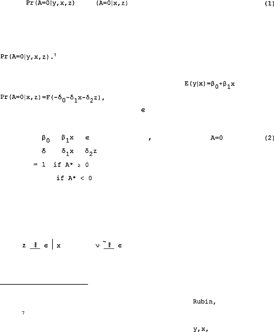
observables occurs
when
Pr(A=Oly,x,z
) = Pr
(A=Olx,z)
(1)
We say that selection on unobservables occurs simply when (1) fails to
hold; that is,
when the attrition function cannot be reduced from
Pr(A=Oly,x,z).'
These definitions may be more familiar when they are restated
within the textbook parametric model.
Letting
E(~~x)=~~+~,x
and
Pr(A=01x,z)=F(-60-61x-62z),
where F is a proper c.d.f., we can state the
model equivalently with error terms
e
and v as
Y
=
p,
+
p,x
+
e
I
y observed if
A=0
(2)
A* =
6
0
+
alx
+
622
+ v
(3)
A
=l
ifA*>
(4)
=0
ifA*<O
where v is the random variable whose c.d.f. is F. In the context
of this model, selection on unobservables occurs when
Z
IElX
but
V-La
x
I
(5)
and that selection on observables occurs when
terms
"ignorable" and "missing-at-random" selection to describe what we
are terming selection on observables (Little and
Rubin,
1987).
7
We could define selection on unobservables to occur when x and z
drop out of the probability function,
and then to define selection on
both observables and unobservables to occur when
y,x,
and z all appear
in the function, but we are not particularly interested in the former
case and hence will not maintain such usage.
8
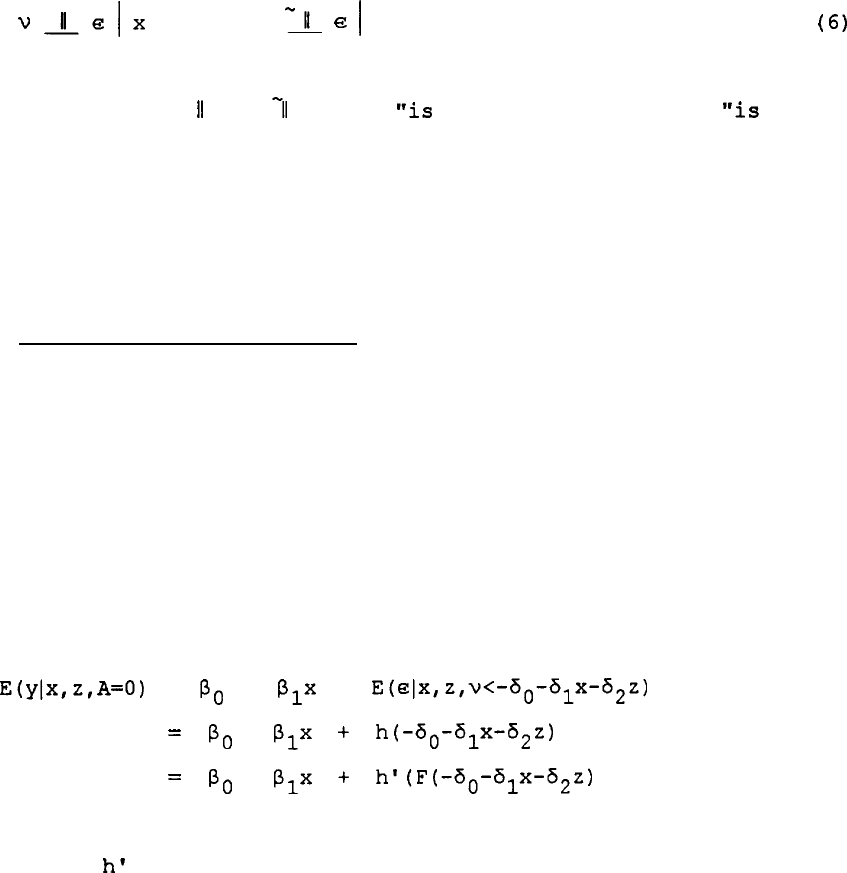
V
I&
but z
-11
e
1
x
(6)
where the symbols
11
and
71
denote
"is
independent of" and
"is
not
independent of," respectively.
The selection on observables case is
relatively unfamiliar in the econometrics literature but we will show
that it is relevant for the attrition problem.
However,
we will first
deal with the more familiar case of selection on unobservables.
Selection on Unobservables.
We will discuss this model only
briefly because of its familiarity.
Exclusion restrictions are the
usual method of identifying this model,
and our major goal here is to
discuss the difficulty in finding such restrictions for a nonresponse
model in the PSID.
Working from the parametric form of the model, the conditional
mean of y in the nonattriting sample can be written
E(ylx,z,A=O)
=
PO
+
plx
+
E(e~x,z,v<-60-~lx-62z)
=
PO
+
P,x
t
h(-60-61x-52z)
=
PO
+
P,x
t
h'(F(-50-61x-62z)
(7)
where h and
h'
are functions with unknown parameters.
Moving from the
first to the second line of the equation requires that the joint
distribution of a and v be independent of x and z, so that the
conditional expectation depends on x and z only through the index.
Moving from the second to the third line simply replaces the index by
its probability,
which is permissible since they have a one-to-one
correspondence.
Early implementations of this model assumed a specific bivariate
9

distribution for
e
and v,
leading to specific forms of the expectation
function (e.g., the inverse Mills ratio for bivariate normality), while
more recent implementations have relaxed some of the distributional
assumptions in the model by estimating functions h or
h'
whose arguments
are either the attrition index or the attrition probability,
respectively (see Maddala,
1983, for a textbook treatment of the early
approach and Powell, 1994,
pp.2509-2510,
for discussions of the more
recent approach).
Armed with estimates of the parameters of the
attrition index or of the predicted attrition probability, equation (7)
becomes a function whose parameters can be consistently estimated.*
However,
aside from nonlinearities in the h, h', and F functions,
identification of
p
requires an exclusion restriction, namely, that a z
exist satisfying the independence property from
e
and for which
a2
is
nonzero.
Such a variable is often loosely termed an "instrument,"
although most estimation methods proposed for eqn (7) do not take a
textbook instrumental-variables form.
Finding a suitable instrument for
unobservable selection is more difficult for the case of nonresponse
than in some other applications because there are few variables that
affect nonresponse that can be credibly excluded from the main equation
for y.
While this depends on the specific model under consideration, on
*
If nonparametric methods are used to estimate h and h', not all
of the parameters in
p
(e.g.,
the intercept) may be identifiable. We
should also note at this point that if x is time-varying then it is
necessarily missing for attritors and hence the attrition propensity
equation cannot be estimated as we have written it.
Additional
assumptions are then required to estimate the model.
For example,
adding time subscripts,
one could assume
x(t)=ao+a
x(t-1)ta
z+u(t), thus
letting x be a function of lagged x and z (some
di
4
ferent
z2
could be
specified,
alternatively). Substituting this equation for x(t) into the
attrition equation would permit estimation provided
x(t-1)
is available
for all observations. This procedure, however, introduces another
potential source of selection bias from non-independence of u(t) and
e(t)
-
10
a priori grounds personal characteristics such as those generally
included in x are unlikely to be promising sources of instruments
because most such characteristics are related to behavior in general and
hence to y.
More promising are variables external to the individual and not
under his control,
such as characteristics of the interviewer or the
interviewing process, or even interview payments.
Although we have
proposed no explicit behavioral model of attrition, a natural theory
would be a simple benefit-cost model in which an individual compares the
value of participating in the survey to the value of not participating.
Good interviewers or interviewing conditions lower the cost of
participation and interview payments directly increase the value of
participation.
However,
a suitable instrument must vary across
respondents,
and must vary in a manner independent of
y.
The staff at
the Institute for Survey Research who have administered the PSID have
assigned interviewers on the basis of respondent characteristics, and
have also varied interviewing conditions (length of interview, in-person
vs.
telephone,
number of callbacks, etc.) entirely and only on the basis
of respondent characteristics; consequently there is no exogenous
component to the variation intreatment.
This rules these variables out
as instruments.
Moreover,
there have also been no exogenous variations in
interview payments over the course of the PSID, for payments have been
adjusted only for inflation over time and vary within year only on the
basis of interview mode.
Based on these and other considerations we
discuss in our background report (Fitzgerald et al.,
1997a),
we conclude
that there are no instruments for nonresponse in the PSID which are
11

credibly exogenous to behavior in general.'
-I-.
Although we will therefore not test for selection on unobservables
directly,
or correct for such selection,
indirect tests for selection on
unobservables can be conducted whenever an outside data set is available
containing validation information. Administrative data on some variables
(e.g.,
earnings) are occasionally available but this is the exception
rather than the rule,
and they are not available for the
PS1D.l'
However,
the Current Population Survey (CPS) is a heavily-used outside
data set which is a repeated cross section and hence not subject to the
same type of attrition bias as the PSID.
The CPS is subject to
nonresponse itself, but not of the same order of magnitude as the 50
percent nonresponse rate in the
PSID.ll
Hence we will use the CPS as a
comparison data set and compare the marginal distributions of variables
in the CPS and PSID to one another as well as regression coefficients.
If selection on unobservables is present and it biases the coefficients,
for example (see eqn.
(7)),
estimates from the two data sets will be
different.
Unfortunately,
this method of comparison is useful only for
cross-sectionally-defined variables and not for variables which make use
of the panel nature of the PSID, and hence does not offer a general
'
Exclusion restrictions are only one form of information. For an
example of the use of other types of information, see
Manski
(1994).
Fitzgerald et al.
(1997a) provide some simple bounds calculations of one
type proposed by
Manski.
lo
See Hill (1992, p.29) and Bound et al.
(1994) for a discussion
of validation studies using the PSID.
11
While the magnitude of nonresponse does not map directly into
the amount of bias, as we noted earlier,
it would be unlikely for the
CPS to be more biased than the PSID given these differences in the
amounts of attrition.
12

solution to the
prob1em.l'
Selection on Observables. As we noted previously, the case of
selection on observables is relatively unfamiliar in the econometrics
literature.
Because of this unfamiliarity, and because, unlike
selection on unobservables,
it is something we can actually address, we
will discuss it at slightly greater length than we did the previous
case.
The critical variable in the selection on observables case is z, a
variable which affects attrition propensities but is presumed also to be
related to the density of y conditional on x (i.e., z is endogenous to
Y)
-
Such a variable can exist only if the investigator is interested in
a
"structural" y function which we interpret as a function of a variable
x that plays a causal role in a theoretical sense; other variables
(i.e.,
z) do not "belong" in the function.
More generally, this
situation will arise whenever the investigator is interested in (say)
the expectation of y conditional on x and simply does not wish to
condition on z. In cross-sectional data, for example, the standard
Mincerian theory of human capital proposes that earnings are a function
of education and experience;
other variables which are jointly
determined with earnings, like occupation and industry, should not be
conditioned on to obtain the "correct" estimates.
Yet use of any sample
that is selected on the basis of occupation and industry (e.g., only
certain occupations and industries are included) will clearly bias the
estimates of the earnings equation. The variable z is thus an
12
Imbens and Hellerstein (1996) show that such outside data sets,
if taken as 'truth,'
can be imposed on the data set of interest (e.g.,
the PSID) and can be used to formally test whether the data
distributions in the two data sets are the same. See related work by
Imbens and Lancaster (1994) and Hirano et al. (1996) along these lines.
13
"auxiliary"
endogenous variable.
As we will discuss below, in the panel
data case,
a lagged value of y can play the role of z if it is not in
the
"structural"
model and if it is related to attrition.
In the presence of selection on such an endogenous variable, it is
easy to show that least squares estimation of (2) on the nonattriting
sample will generate inconsistent estimates of
P
and, more generally,
that the estimable density
g(ylx,A=O)
will not correspond to the
complete-population density
f(ylx)
since the event
A=0
is related to y
through z.
Apart from this selection on observables bias, using as much
of the lagged information in the panel as possible helps reduce the
amount of residual,
unexplained attrition variation left over in the
data,
and this will reduce the scope for selection on unobservables.
Formally,
in the Appendix, we show that,
under the selection on
observables restriction given in equation
(l),
the complete-population
density
f(ylx)
can be computed from the conditional joint density of y
and z,
which we denote by g:
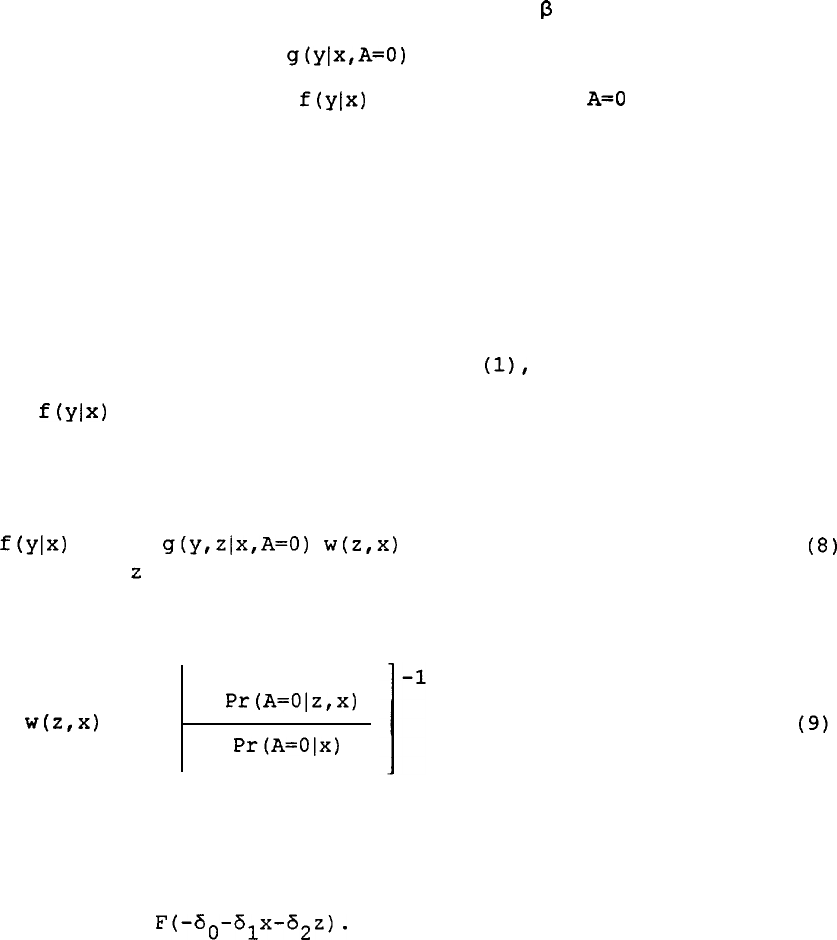
f(YlX)
=
I
g(y,zlx,A=O)
w(z,x)
dz
where
w(z,x)
=
Pr(A=Olz,x)
Pr(A=Olx)
(8)
are normalized weights. The numerator of (9) inside the brackets is the
probability of retention in the sample and is,
in the parametric model
described above,
F(-60-51~-62~).
Because both the weights and the
conditional density g are identifiable and estimable functions, the
14
complete-population density
f(ylx)
is estimable,
as are its moments such
as its expected value
(@,+p,x
in the parametric
model).13
Eqn(8) shows
that the complete-population density can be derived by weighting the
conditional density by the (normalized) inverse selection probabilities;
in the parametric model, it can be shown that this implies that weighted
least squares (WLS) can be applied to eqn(2) using the weights in (9).
We should emphasize that the application of WLS in this case is
unrelated to the heteroskedasticity rationale appearing in most
econometrics texts.
It is also not in conflict with the conventional
view among many applied economists that survey weights can be ignored
because they do not affect the consistency of OLS coefficients, for
survey weights are often intended only to adjust for sample designs
which have stratified the population or differentially sampled it by
variables that are exogenous.
Here, however, selection is indirectly on
the dependent variable, and not adjusting for attrition results in loss
of consistency.
If z is not a determinant of attrition, the weights in (9) equal
one and hence all conditional densities equal unconditional ones and no
attrition bias is present.
Alternatively,
if y and z are independent
conditional on x and A=O,
the density g in (8) factors and it can again
be shown that the unconditional density
f(ylx)
equals the conditional
density,
and there is no attrition bias.
While these results are relatively unfamiliar in the econometric
literature,
they are pervasive in the survey sampling literature, where
they form the intellectual justification for the construction and use of
13
As we noted in n.8,
if contemporaneous x is unobserved and
hence the attrition probability equation cannot be estimated, lagged x
or additional z variables are required.
15

attrition-based survey weights (Rao,
1963,197s;
Little and
Rubin,1987,pp.55-60).14'15
In the econometrics literature, while
weighting formulations are sometimes used as a framework for discussing
selection models (e.g.,
Heckman,
1987),
the main point of contact with
the models discussed here is the choice-based sampling literature (for
discrete
y,
see Manski and Lerman,
1977, for an early treatment and
Amemiya,
1985, for a textbook treatment; for continuous y, see Hausman
and Wise,
1981, Cosslett, 1993, and Imbens and Lancaster, 1996).
That
literature generally considers estimation and identification in samples
which are selected directly on the dependent variable, y; weighted
maximum likelihood or least squares procedures are often proposed to
'undo'
the disproportionate endogenous sampling. The difference in the
attrition case is that selection is on an auxiliary variable (z) and not
on y itself; but otherwise the solutions are closely
related.16
14
For an exception, see Cosslett (1993,
pp.31-32).
In addition,
after the first draft of this paper we discovered an independent
treatment of the selection on observables case by Horowitz and
Manski
(forthcoming),
who show that the mean of a function of y can be
consistently estimated with weights of the type we have discussed under
the same restrictions.
15
We should note that the weights discussed in the survey
sampling literature sometimes differ from the weights in our model in
two respects.
First,
many survey weights--
including those in the
PSID--
are also intended to capture non-random-sampling at the initial stage
(e.g.,
from stratified designs).
That is not the purpose of the weights
we have discussed and requires a slightly different formulation to
justify.
Second,
the weights in our model are not the type of
"universal"
weights generally computed for many survey data sets;
"universal"
weights are designed to be all-purpose and usable for any
variable or model, whereas our weights are model-specific because one
can easily imagine using different attrition-equations (e.g., with
different lagged y's) depending on the model being estimated and its
definition of y.
I6
We wish to emphasize that WLS is not the only estimation method-
-there are many (imputation,
GMM, various forms of maximum
likelihood)--
nor is it efficient; in addition, there are many issues connected with
the use of weights which we do not discuss here.
The major advantage of
WLS is that it produces consistent estimates and is relatively easy to
16

It should also be noted that simply conditioning on z does not
solve the problem.
This can be seen most simply by observing that the
object of interest in most models is
E(ylx),
not
E(ylx,z).
Including z
in the regressor set will generate "biased"
coefficients on x in a
linear-regression model, for example, in the sense that it will not
estimate the effect of x on y unconditional on z.
Because z is an
endogenous variable, it distorts the conditional distribution of y on x.
Hence correcting for selection on observables is to be sharply
distinguished from the corrections for unobservable selection shown in
eqn
(7),
which involve conditioning on functions of x and z; those
methods are not appropriate for this case.
Testing.
The application of the selection on observables model to
attrition in panel data is straightforward if a lagged value of y (e.g.,
y at the initial wave of the panel,
when all observations are present)
plays the role of z,
assuming that attrition is affected by such a
lagged value.
Lagged values of y will,
assuming serial correlation in
the y process,
be related to current values of y conditional on x.
The
use of lagged values of y in this role requires the same distinction we
noted earlier between structural and auxiliary determinants of
contemporaneous y, for the use of lagged y as a z makes sense only if
the investigator is interested,
for theoretical or other purposes, in
functions of y not conditioned on those lagged
va1ues.l'
implement.
I7
An investigator who posits a theoretical (i.e., structural)
model that includes all lags of y will necessarily have much reduced
scope for selection on observables.
Taking this point to its extreme, if
there are no observables in the data set that are excluded from the
structural y function, there is no role for for using observables to
adjust for selection. Selection on observables is a data-set-defined and
model-defined category, and what is an observable variable in one data
set or model may be an unobservable in another.
17

As noted previously, two sufficient conditions for the absence of
attrition bias on observables are either that the weights equal one
(i.e.,
z does not affect A) or that z is independent of y conditional on
X.
Specification tests for selection on observables can be based on
either of these two conditions. Thus one test is simply to determine
whether candidate variables for z (e.g., lagged values of y)
significantly affect A.
We will conduct these tests extensively in our
empirical work.
A second test would be to conduct specification tests
for whether OLS and WLS estimates of eqn (2) are significantly
different,
which is an indirect test for whether the identifying
variables used in the weights are endogenous (see Dumouchel and Duncan,
1983, for an example of such a test).
We will not conduct such tests
in our paper but instead leave them for future research. However, we
will determine whether using the universal weights provided by the PSID
staff affect the estimated coefficients of several models, even though
the "model-based"
weights we have been discussing are not necessarily
the same as the PSID universal weights (see n.15).
Another test for selection on observables which we will perform is
based on an exercise performed by Becketti et al. (1988) and which we
term the BGLW test. In the BGLW test,
the value of y at the initial
wave of the survey,
which we denote by
yo,
is regressed on x and on
future A (i.e.,
whether the individual later
attrites).
The test for
attrition selection is based upon the significance of A in that
equati0n.l'
This test must necessarily
be
closely related to the test we
18
We assume x to be time-invariant.
If it is not, this method
requires that only the values of x at the initial wave be included in
the equation.
18
have already described of regressing A on x and
y.
(which is z in this
case)
;
in fact,
the two equations are simply inverses of one another.
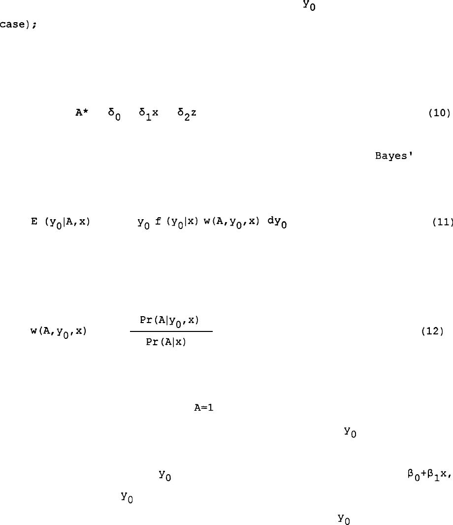
Formally,
suppose that the attrition function is taken as the
latent index in the parametric model, i.e.,
Af
=
a0
+
alx
+
a22
+ v
(10)
Inverting this equation, taking expectations, and applying
Bayes'
Rule,
it can be shown that
E
(yOIArx)
=
I
y.
f
(yolx)
w(A,Y~~x)
dye
(11)
where
w(A,yo,x)
=
Pr
(AIyO,x)
(12)
Pr (Alx)
which are essentially the same as the weights appearing in (9) but
including the probabilities of A=1 as well as A=O.
Eqn (11) shows that
if the weights all equal one,
the conditional mean of
y.
is independent
of A and hence A will be insignificant in a regression of y on x and A
(the conditional mean of
y.
in the absence of attrition bias is
B,+B,x,
so a regression of
y.
on x will yield estimates of this equation). As
noted previously,
the weights will equal one only if
y.
is not a
determinant of A conditional on x. Thus the BGLW method is an indirect
test of the same restriction as the direct method of estimating the
19
attrition function
itself.lg
However,
if the weights do not equal one,
it would be difficult
to
derive an explicit solution for
equation(l1)
from the estimates of (10)
that we will obtain in our attrition propensity models.
To do so would
require conducting directly the integration shown in (11).
It would be
simpler to just estimate a linear approximation to (11) by OLS, as did
Becketti et al.,
to determine the magnitude of the effect of A on the
intercept and coefficients of the equation for
y.
as a function of x.
We shall therefore also estimate such equations in our empirical work.
However,
it should be kept in mind that this is not an independent test
of attrition bias separate from that embodied in our estimates of
eqn(l0);
it is only a shorthand means of deriving the implications of
our estimates of eqn(lO) for the magnitudes of differences in 1968 y
conditional on X between attritors and nonattritors.
Panel Data and Permanent-Transitory Effects.
Finally,
we wish to
relate the selection on observables model we have been discussing to
more traditional models of attrition in panel data, and to point out a
connection with permanent-transitory distinctions which we will also
apply in our empirical work below.
The most well-known model of
attrition in the econometrics literature is the model of Hausman and
Wise (1979); that model has been generalized and extended by Ridder
(1990,1992),
Nijman and Verbeek
(1992),
Van den Berg et al.
(1994),
and
others (see Verbeek and Nijman, 1996, for a review).
These models
generally assume a components structure to the error term, sometimes
19
In general, of course, if
v=o+(3u+e,
regressing u on v instead
of v on u results in a "biased" coefficient on v (i.e., it is not a
consistent estimate of the inverse of
8).
Nothing here contravenes
that.
The
"coefficient"
on x in a regression of y on x and A bears no
simple relationship to 61 or
62
in
eqn(lO),
as can be from
eqn(l1).
20
including individual-specific time-invariant effects and sometimes
serially-correlated transitory effects, for example, and impose
restrictions on how attrition relates to the components of the
structure.
A common assumption in some studies in the literature, for
example,
is that the unobserved components of attrition propensities are
independent of the transitory effect but not the individual effect; in
that case,
simple first-differencing (among other methods) can eliminate
the bias.
Our approach differs from this past work because of our sharp
distinction between identifiability under selection on observables and
on unobservables, a distinction not made in these past studies.
Many
error components models which allow attrition propensities to covary
with individual components of the process can be treated within the
selection on observables framework because lagged values of y can be
mapped into those components.
If we let
z
in our model stand for a
vector of lagged values of y instead of a scalar, we have
Pr(A=Olx,yt-1,Yt-2,Yt-3r..
.,
y,)
as our attrition function.
Assume full
observability of those lagged values. Then any model in which the error
components of the y process which covary with attrition can be uniquely
mapped into the set of t values of lagged y can be captured by our
selection on observables model.
An example is the autoregressive model:
Yt
=P,
+
P,x
+
et
t-1
et
-
=,-$j
PTY
+
%
(13)
(14)
(15)
t-1
A* = 6
o
+
alx
+ c 6
r=O
2T%
+
vt
21
Estimation of (13) on the non-attriting sample results in bias because
et
is serially correlated and A*
is a function of the lagged values of
that error.
But solving
eqn(l3)
for
eT
in lagged periods, and
substituting into
eqn(l5)
for the lagged errors, leads to an equation
for A* where only lagged y appear.
This example also illustrates a case in which controlling for
lagged observables in the A*
equation is not sufficient to avoid
attrition bias,
for it is necessary that the contemporaneous shock at
(i.e.,
that which is not forecastable from lagged
y)
be independent of
vt
conditional on the observables.
For example,
shocks to earnings
which occur simultaneously with, not prior to, attrition from the
sample, cannot be captured by lagged values of y; attrition bias from
this source falls under the selection on unobservables rubric we
discussed earlier.
However,
a full conditioning on the available data
on the history of y reduces the scope of possible unobservable
selection,
as we noted earlier, because it isolates the only remaining
source of such bias to contemporaneous, non-forecastable shocks.
The general form of our attrition probability
Pr(A=Olx,yt-l,
Yt-2'Yt-3'*
.'I
y,)
is capable of capturing a large variety of
alternative forms of attrition dependence on lagged y other than the
simple linear form portrayed in the autoregressive case.
For example,
the mean of a set of lagged values of y,
7,
is a consistent estimator
(as
T-m)
for the individual effect,
after conditioning on observables
x and assuming mean-zero transitory disturbances.
The deviations of
each value of
y,
from
7
represent transitory disturbances in each
period
r.
By estimating flexible forms of the attrition function which
contain both
7
and the deviations of lagged y from
7
in different
periods,
we can determine whether attrition probabilities
covary
with
22

"permanent" levels of y and with transitory shocks one period, two
periods,
and more periods back in time.
The variance of
y,
over any
specified length of past periods is yet another transform of lagged y
values which may
covary
with attrition; this would occur if it is
variability per se,
not the mean or value of any set of individual
disturbances, that affects whether individuals stay in or out of the
sample.20
We will test these and other transforms of lagged y in our
models.
Summary of Analyses to be conducted.
To summarize, in the
following analysis of the PSID we will (i) conduct tests for the
presence of attrition on unobservables by comparing cross-sectional
marginals and regression coefficients in the CPS and the PSID; (ii)
conduct tests for the presence of selection on observables by estimating
attrition equations as a function of lagged y values as well as by
regressing first-period y on future attrition;
and (iii) we will conduct
tests for "dynamic" attrition effects by estimating attrition equations
as a function of lagged permanent, transitory,
and other moments of the
lagged y distribution.
We should note at this point that a problem with implementing
procedures using lagged values of y is that those measures are available
for the full sample only at the initial year of the PSID, 1968.
Conditioning on values of y after 1968 necessarily opens the door to
bias because some attrition has already occurred and estimation must be
restricted to observations for whom all data on all lagged variables in
the equation are available. Consequently, for the most part, we will
20
It is clear that formal modeling of the error process of y
could be conducted here but we will leave that for future research, and
will only test various transforms of lagged y in a reduced-form context.
23

restrict our tests of lags to only those available in the first year,
1968.
While this approach necessarily ignores much of the information
in the PSID on attritors prior to the point of attrition, it yields
results least subject to the post-1968 attrition bias problem.
Our
dynamic attrition analysis will be an exception, for there we will
estimate attrition hazards--that is, probabilities of exit conditional
on being in the sample
t-he
previous period--as a function of all the
lags available up to each decision point.
That analysis will be
conducted ignoring the potential bias induced by this sample restriction
(usually called "unobserved heterogeneity" in duration analyses);
consequently, no "structural"
interpretation will be given to the
estimated coefficients in those attrition
equations.*l
III. Observable Correlates of Attrition in the PSID
Rather than begin our analysis with the comparison of the PSID to
the CPS, we will first examine the observable correlates of attrition in
the PSID, primarily focusing on characteristics, any one of which could
be a
"y"
or a
"x",
in 1968.
We will also estimate attrition probability
equations as a function of 1968 characteristics for selected
"y"
variables and will conduct BGLW tests in this section.
The last year of the PSID available at the time our data files
were created is 1989. We focus on the seemingly simple question of
whether 1968 characteristics differ between those who were present in
21
Note,
however,
that a bias in the structural coefficients of
attrition hazards does not affect the consistency of the WLS estimator
using the predicted probabilities from those equations as weights.
The
selection on observables model does not require independence of z and v
in eqn(3).
24

1989 and those who were not (hence the distributions of x and y
conditional on A,
in a tabular
form)." For our analysis sample, we take
every individual who was present in a PSID household in 1968, or about
eighteen thousand individuals, as noted previously. We disaggregate the
sample by sex and 1968 household
headship
status, and focus on five
population subgroups: male heads, wives, female heads, male nonheads,
and female nonheads.
The asymmetric treatment of men and women is
required by the gender-specific definitions of
headship
in the PSID, and
the division of groups by
headship
in the first place is required
because sharply differential amounts of information were collected on
heads and
nonheads
(many variables are not available for the latter
group).23
We also exclude subfamily heads from the PSID because they were
defined inconsistently over time and also differently than in the CPS,
whose comparisons to the PSID are an important part of our analysis.
For the bulk of our work, we include the
SE0
oversample together
with the SRC representative sample.
We therefore use PSID-constructed
1968 sample weights whenever
appropriate.24
However, we also provide
22
In our background report,
we also conduct analyses of the
middle year,
1981, because that was the latest year analyzed by BGLW.
The issue that analysis addresses is whether any attrition bias we find
has arisen since the BGLW study was conducted.
23
The PSID makes no distinction between male heads similar to
that made between wives and female heads, for all married women are
automatically classified as wives.
The PSID also incorporates
cohabitation to a degree:
any couple living together in a "partner"
status for more than one interview is then and thereafter treated as
"married"
--the male is classified as a "head" and the female is
classified as a "wife".
We include them in our sample.
24
These weights reflect only the sample design of the PSID (and
initial nonresponse) and contain no adjustments for attrition.
Hence
they are not the types of weights we were discussing in Section II.
However,
they must be utilized because the
SE0
observations were sampled
on variables that are correlated with income,
which is closely related
to many of our dependent variables.
25

estimates on the SRC sample alone and show that attrition effects are
sometimes worse for that sample than for the combined SEO-SRC sample.
Distributions of 1968 Characteristics. Table 2 shows the mean
values of 1968 characteristics of men who were 25-64 and household heads
in 1968, by their attrition status as of
1989--"always
in" versus 'ever
out" by that
year.25
As the first two columns indicate, attritors and
non-attritors have many significant differences in characteristics.
Attritors are more likely to be on welfare,
less likely to be married,
and are older and more likely nonwhite.
In addition,
attritors have
lower levels of education, fewer hours of work, less labor income, and
are less likely to own a home and more likely to
rent.*'j
The clear
implication of this pattern is that attritors are concentrated in the
lower portion of the socioeconomic distribution.
The second moments for
labor income in the table indicate that the variance of labor income is
greater among attritors than among nonattritors, and, interestingly,
that the attritor labor income distribution is more dispersed at the
upper tail than the nonattritor distribution.
This suggests that, to
some degree,
some high labor-income families may be more likely to
attrite
than middle-income families."
The last two columns in the table provide an assessment of the
25
Because only a tiny fraction of attritors ever return--see
Table 1 above--
those individuals who were "always in' between 1968 and
1989 are almost identical to the set of individuals present in 1989, and
the set of individuals who were 'ever out' between 1968 and 1989 is
almost identical to those who were nonresponse in 1989.
26
All monetary figures in the paper are in real 1982 dollars using
the personal consumption expenditure deflator.
We should also note
that the top and bottom 1 percent of the labor income variable is
excluded to circumvent top-coding problems and to avoid distortion from
outliers.
27
A similar finding was reported by BGLW.
26

effect of mortality. The third and fourth columns disaggregate the "ever
out"
subsample into those "not dead" and those "dead" according to
whether individuals died while in the PSID (as noted previously,
some
individuals die after attriting,
of which we have no knowledge).
Comparing the third column (not dead) with the first two shows that the
gap between the Always In and Ever Out is sometimes narrowed by
excluding the dead from the attritors,
but rarely
by
very much; indeed,
in some circumstances,
the gap even increases.
The latter occurs when
mortality is related to a variable in opposite sign to its relation to
attrition conditional on being alive: consequently, ignoring mortality
actually makes the selectiveness of attrition
seem
milder than it
actually is.
Tables 3 and 4 show the corresponding tables for wives and female
heads.28
The general findings are the same as for male heads:
attritors and nonattritors frequently differ in their characteristics,
and the differences cannot be explained by mortality.
A few of the
details do differ across demographic groups, however.
Female heads have
much larger differences in welfare participation, for example (female
heads also have higher participation rates in the U.S. welfare system
than other groups).
Interestingly, the variance of labor income is
smaller among attritors than nonattritors among female heads, although
the differences among women are not significant. We conclude that the
many significant differences in attritors and non-attritors in the PSID
appear broadly across all
headship
and gender groups.
Attrition
Probits.
The first multivariate analysis we present
consists of estimates of binary-choice models for the determinants of
28
In our background report,
we also provide tabulations for
nonheads.
27

attrition,
using the same data in the tables we have been presenting
(i.e.,
whether having ever been nonresponse by 1989 as a function of
1968 characteristics).
We therefore estimate
probit
equations for the
probability of having ever been nonresponse by 1989." As in Tables 2-4,
the sample consists of all 1968 respondents 25-64 and all regressors are
measured in 1968.
We shall also make a distinction between
"x"
and
"y"
in this
analysis by focusing on three
"y"
variables: labor income, marital
status,
and welfare participation (female heads only).
We select these
three because they are some of the more common dependent variables used
by economists and sociologists,
and therefore their relations to
attrition are of particular interest.
Our tabular analysis in Tables 2-
4 showed some evidence of significant attrition effects for these key
variables,
which should generate some cause for concern for analysts who
study these
outcomes.30
One issue that can be addressed in a
multivariate analysis is whether these effects are attenuated when a set
of other socioeconomic variables is controlled for in a regression
framework.
Table 5 shows a set of expanding specifications of attrition
probits
which focus on the effect of our first
"y,"
labor income, on the
attrition of male heads.
The first two columns of the table 5 show the
effect of labor income on attrition without conditioning on any other
2g
Although we do not estimate a dynamic model of year-by-year
attrition,
these estimates can be viewed as a model of cumulative
attrition that reflects the working-out of a year-by-year model.
Since
all the regressors are held at their 1968 values, our equation can be
viewed as a approximation to the reduced-form model.
30
To repeat a point in Section II,
the concern arises because the
1968 values of these variables are likely to
covary
with their later
values.
28
regressors ("No Labor Income"
is a dummy equal to 1 if the individual
has no labor income).
The results show that the 1968 labor income levels
of male heads have a very strong correlation with future nonresponse.
Attrition probabilities are quadratic in labor income--lowest at middle
income levels and greatest at high and low income levels, a pattern
also found by BGLW, as noted earlier.
Individuals with no labor income
at all have higher attrition rates as well. The third column in the
table shows that when "standard"
earnings-determining variables are
added--race, age, and education
--labor income remains a significant
determinant of attrition. Implicitly, therefore, the residual in a labor
income equation containing these regressors is correlated with
attrition.
When a large number of other variables--income/needs,
home
ownership, SE0
status, and others--are added, the labor income effects
remain.
Table 6 shows the coefficients on the earnings variables in these
models (except for the first) for wives and female heads, and also the
coefficients for other 1968
"y"
variables.'l
For female heads and wives,
labor income effects are much weaker.
For neither group is there much
of an effect of labor income on nonresponse except for the effects of
having no labor income at all,
which continues to have a positive effect
on nonresponse.
For wives,
even this effect is relatively weak when the
larger set of covariates is included in the equation.
When the earnings
variables are replaced by our other two
"y"
variables--l968 marital
status and welfare participation
--rather similar patterns are found.
Again, there are some significant coefficients on these variables when
nothing else is controlled for,
but in all cases those effects fall to
31
The full set of regression coefficients on all models is
available in our background report.
29

insignificance at conventional levels in the most expanded
specification.
Table 7 shows the coefficients in attrition
probits
when all three
types of y variables are included.
Although including the variables
singly gives the best specification for comparison with the BGLW
specification (which inverts the attrition
probit
to solve for a single
Y)
I
there is no reason not to include all available data in an attrition
probit
intended for weight construction, or for general
interest.32
The
results in the table indicate that very little is changed when multiple
y variables are included;
most effects are insignificant, with the
absence of labor income continuing to be the one variable with
often-
significant effects even after controlling for other regressors.
We should also note that the R-squareds from these
probits
are
extremely
small.33
In Table 5 they never exceed
.069
and in the models
in Tables 6 and 7 they range from
.028
to
.071,
and even lower in Models
1,2,
and 3 when fewer other regressors are conditioned on.
Thus, even
in those cases where significant correlates of attrition are found, they
explain very little of the variation in attrition probabilities in the
data.
One implication of this result is that weights based on these
equations would,
in all likelihood, have little effect on estimated
32
As we stressed in Section II,
all these y variables are
potentially "endogenous"
in the sense that they might be related to a
contemporaneous y of interest,
and adding more lagged y variables to the
attrition equations increases the chances of capturing such endogeneity.
But it is only through the existence of such endogeneity that weights
can reduce attrition bias.
33
The R-squared measure we use is defined in the footnote to the
Table and is a common measure of fit in binary-choice models.
This
measure has recently been shown to have desirable properties relative to
other measures (Cameron and Windmeijer,
1997) and can be interpreted as
the proportionate reduction in uncertainty from the fitted model, where
uncertainty is defined by an entropy measure.
30

outcome
equations.34
We conclude from these results that the unconditional effects of
labor income,
welfare participation,
and marital status significantly
covary with attrition probabilities,
consistent with our conclusions
from the tabular analysis in Tables 2-4 (although the BGLW form of the
test,
reported next,
corresponds more closely to Tables 2-4).
However,
we also find that, in a majority of the cases,
these effects fall to
insignificance at conventional levels when a sufficiently broad set of
covariates are conditioned on.
The main exceptions to this occur for
various specifications of labor income models, particularly for male
heads but occasionally as well for female heads and for women in general
and for the occasional other model.
Thus these results provide support
for some concern for cross-sectional attrition bias in the PSID for
unconditional distributions, and for conditional distributions for
earnings,
especially of male heads.
BGLW Tests.
As
we noted in Section II, the inversion of our
attrition
probits-- the effect of future attrition on 1968 outcome
variables,
rather than the other way around--is also of interest.
Such
regressions were estimated by Becketti et al.
(1988) and used as a test
for attrition bias.
As we noted previously,
apart from nonlinearities
and some differences in the stochastic assumptions, the results should
have the same general tenor as the attrition
probits
but will show more
directly the degree to which regression coefficients in typical outcome
equations are affected.
34
This statement must be qualified because even weights with very
small variance could have a large impact if they are sufficiently highly
correlated with the error term and the regressors.
31

Table 8 shows 1968 log labor income regressions for male
heads.35
Separate regressions are estimated for individuals who were always in
the sample through our final year, 1989, and for the total sample in
1968.
We compare the total sample and the nonattriting sample--not
attritors and nonattritors
--because the issue is how different parameter
estimates would be from those in the total sample if only the
nonattriting sample is
used.36
We show results separately when the
SE0
sample is included and excluded. For male heads, none of the
coefficients on the variables of most past research interest--Black,
Ed<12,
College Degree, Age and Age-Squared
--are
significantly different
between the total and nonattriting samples in estimates including the
SEO, and the magnitudes of the differences in the coefficients are
seldom large from a substantive research point-of-view. Significant
differences do appear for the "Other Race" and "Some College" variables
(and one of the region variables), for reasons we have not been able to
determine. More significant difference appear for the estimates when
the
SE0
is excluded, but these are again not large in magnitude. In
summary,
at least for SRC-SE0 combined sample, we find very few
important effects of attrition on the
coefficients.37'3e
35
Individuals with zero labor income are excluded.
While this
introduces some noncomparability with our attrition
probits
as well as
raising well-known selection issues,
we wish to maintain correspondence
with the bulk of the earnings function literature, which also generally
conditions on positive income.
36
The two sets of differences are transforms of one another, but
they have different standard errors.
Under the null of equality of the
true coefficient vectors,
the variance of the difference in the
coefficients is the difference in the separate variances (the variance
in the smaller sample must be larger, necessarily, under the null).
37
Similar findings were reported by BGLW.
However, their
analysis only went through 1981 and, in addition, they tested the
difference in coefficients between attritors and nonattritors whereas we
properly test between the total sample and nonattritors.
32

_-
-
In our background report (Fitzgerald et al.,
1997a),
we show
estimates of labor income equations for wives and female heads; marital
status
probits
for men and women;
and welfare-status
probits
for female
heads,
all estimated in 1968 separately for the total and nonattriting
samples.
For wives,
the labor income results are essentially similar to
those for men although some significant differences in the magnitude
(though not the sign) appear for the education coefficients. For female
heads,
the only significant labor-income differences are for the
coefficients on age, but the separate coefficients for the total and
nonattritor samples are each insignificant (a sign that female heads
have very flat age-earnings profiles),
so it is not clear how important
this result is.
In the marital-status
probits,
some significant
differences appear for men (Black coefficient) and women (education
coefficient), generating some what more concern for these outcome
variables than for labor income.
The welfare
probits
show no
significant differences in any of the coefficients.
Wald tests for the joint significance of the differences in all
slope coefficients and intercepts generally reject the hypothesis of
equality between the vectors. However,
when test are conducted for the
equality of the slope coefficients allowing the intercepts to differ,
most fail to reject equality.
The estimated intercept differences
(i.e.,
constraining all coefficients on the other regressors to be the
same for the two groups) are shown in Table 9.
Thus we conclude that,
while the coefficients on
"standard" variables in labor income and
welfare-participation equations and, to a lesser extent, marital-status
3a
We calculated White standard errors for the coefficients but
found them to be only 5 percent higher, at most, than those shown. We
therefore do not calculate them for the remainder of the analysis.
33
equations,
are unaffected by attrition, there are still be differences
in the levels of these outcome variables conditional on the regressors.
IV. Cross-Sectional Comparisons to Census Data
The second piece of our analysis is to compare cross-sectional
distributions and regression coefficients between the PSID and the CPS,
allowing us to conduct a more direct analysis of the existence of
attrition bias for these types of variables.
Comparing the PSID and the
CPS has some difficulties, however.
The
most
important is that the
sampling frames are not identical,
for the CPS includes individuals and
families who have immigrated to the U.S. since 1968, while the PSID
excludes those
families.3g
We will find this issue to be of some
importance and, consequently,
we will present some tabulations on the
characteristics of immigrants since 1968 taken from the Decennial Census
in 1990. Second,
many of the variables are defined differently in the
two data sets (headship, for example,
as well as labor income) and hence
this will generate some noncomparability.
Tables 10 and 11 show PSID-CPS comparisons for male heads 25-64 in
1968 and 1989, respectively.
Table 10 compares the two data sets in
1968, and is thus relevant to the issue of whether the approximate
25-
percent nonresponse in the drawing of the PSID sample systematically
biased the first wave of the
data.
The table indicates that the
distributions of age, race, education, marital status, and regional
location in the CPS and PSID were roughly in line in 1968, both for the
SRC sample and the combined (weighted) SRC-SE0
sample.40
A few
3g
The PSID
Latin0
supplemental sample,
which includes a few
immigrants, was not begun until 1990.
34

miscellaneous divergences appear (e.g., in the educational distribution)
which may be a result of different questionnaire wording.
As for labor
force and earnings,
neither the CPS nor the PSID have unbracketed
variables for weeks worked or hours in 1968, so only the fraction of
those with positive weeks worked can be compared, and in this dimension
the PSID again lines up with the CPS. In addition, the PSID
unfortunately did not obtain an unbracketed earnings variable in 1968 so
we must rely on a measure of labor income, which includes some earned
income other than wages and
salaries.41
The means of the two earnings
measures are about $1,000 apart in the two data sets, and a bit farther
apart if the SRC sample is used. Whether this is a result of the
difference in the measures cannot be ascertained.
The table also shows
measures of dispersion in the two data sets,
although these are also
contaminated by the differences in measures. The log variance of
earnings is considerably smaller in the PSID than in the CPS, but the
measures of percentile points are not far apart, suggesting that
differences at the very lowest percentiles are driving the
difference.42
Statistical tests for the differences in the distributions almost
always reject equality of the distributions because the standard errors
4o
The PSID weights in 1968 were not obtained from direct
post-
stratification against Census or CPS distributions, but were derived
from combining the weights from the University of Michigan's SRC
sampling frame and the Census Bureau's
SE0
sampling weights.
The
weights for the combined SRC-SE0 sample were set to make the combined
SRC-SE0 sample representative.
41
The PSID procedure for creating labor income is described in
Institute for Social Research (1972,
pp.307+).
We exclude from our
calculations those with zero wage and salary income and those who said
on a separate question that they were self-employed.
Our CPS wage and
salary measure therefore also excludes individuals with self-employment
income.
42
The log variance is sensitive to changes in the lower tail of
the distribution.
35
from the CPS, with its very large sample sizes, are extremely small.
However,
the magnitudes of the differences in most of the variables are
small from a substantive research point of view, so we shall continue to
make comparisons along this dimension rather than through formal
statistical
tests.43
Table 11 shows the comparable distributions in 1989. In this table
we show two columns for the combined SEO-SRC PSID sample, one using 1968
weights and one using the 1989 weights calculated by the PSID staff and
including an attrition
adjustment.44
Some differences between the PSID
and CPS appear but they are not large,
and are often narrowed slightly
by the weights.
For example,
the higher attrition rate for blacks can
be seen from the slightly lower percent black for the
1968-weight
PSID
(.07)
versus the current-weight PSID
t.09).
The
SAC-only
sample is the
worst
(.06),
no doubt because no attrition-adjusted weights have been
calculated for that sample.
Nevertheless, both for race and for age,
education,
marital status, and region,
the differences between the CPS
and the PSID, and among the different PSID samples, is quite small and
gives an overall impression of fairly strongly continued
representativeness of the PSID for male heads, even through 1989.
In addition, the PSID has a wage and salary earnings variable in
1989 which can be compared to that in the CPS, allowing a better
comparison between the data sets on this score than was the case for
1968.
In 1989 the two are within $500 of each other, only half of the
43
However,
on the more important issue of differences in
regression coefficients,
we will rely more heavily on tests of
differences.
See below.
44
The construction of these attrition-adjusted weights is
described in Institute for Social Research (1992,
pp.82-98).
The
variables included in the attrition equation are age, gender, race,
education,
number of children, region, lagged family income, and others.
36
$1000 difference in 1968.
The continued difference with the labor
income variable suggests that much of the 1968 difference was indeed a
result of noncomparability of variables.
For earnings itself, the
current-weight PSID is the closest to the CPS, followed by the
1968-
weight PSID and followed by the SK-only,
which is the farthest from the
CPS.
As for dispersion,
the log variance measures in the PSID are still
smaller in 1989 when comparable measures are used (the SRC-only sample
continues to be the farthest from the CPS). Again, however, the
percentile point measures are reasonably close in the different data
sets, perhaps suggesting that the log variance measures are affected by
outliers at the bottom of the distribution.
It might also be noted that
the percentile measures show strong increases in dispersion over time
(compare Tables 10 and
111,
consistent with the evidence now recognized
of increasing earnings inequality among men in the U.S.
This
comparability was also noted previously by Gottschalk and Moffitt
(1992).
It is necessary to reconcile these findings, which indicate that
the PSID has roughly maintained representativeness through 1989 for the
unconditional means and distributions of major sociodemographic lines,
with those from the previous analysis indicating significant differences
between attritor and nonattritor unconditional characteristics in 1968
(Tables
2-4).45
Taking both results at face value, they necessarily
imply that the differences in the value of the variables for the two
45
Actually,
the differences are a bit exaggerated because Tables
2-4 compare attritors to nonattritors instead of the total sample to
nonattritors,
which is the implicit comparison in the CPS analysis. At
an approximate attrition rate of
SO%,
the differences shown in Tables 2-
4 should be halved for comparison with the CPS. This by itself reduces
the perceived seriousness of the discrepancy somewhat.
37

samples in 1968 must have converged over time.
Further investigation of
this possibility reveals it to indeed be the case, as we demonstrate in
Tables 12 and 13. Table 12 shows the characteristics of PSID males who
were 25-40 in 1968 and therefore were 46-61 in 1989, but including in
the 1968 sample only those men who responded in 1989; consequently, the
sample is composed of the same individuals in both years (unlike Tables
10 and 11, the former of which include some men who have attrited or
died by 1989 and the latter of which includes a second generation).
The
table also shows CPS tabulations of men in these same age groups in the
same years. It is clear that,
while time-invariant characteristics such
as race must necessarily remain as far apart between the data sets in
1989 as they were in 1968,
this is not the case for time-varying
characteristics.
Indeed, the distributions of education and marital
status change over time for the PSID men in a way that reduces the
initial selection and moves the distributions closer to the CPS.
The
initial selection on relatively high-educated men in the PSID is offset
by a slower rate of growth of education over the life cycle among
nonattriting individuals in the PSID than in the CPS; and the initial
selection on married men is partly offset by a more rapid decline in
marriage rates in the PSID than in the CPS.
The analysis of earnings is
complicated by the noncomparability of measures, but the growth of labor
income in the PSID was much smaller than the growth of earnings in the
CPS,
thus partly offsetting the initial selection on relatively
high-
income men in the PSID.
The simplest explanation for this pattern is that the time series
processes for education, marital status,
and earnings contain a serially
correlated component which at least partly regresses to the mean, and
that selection is at least partly based on that component.
The
38

existence of
ARMA
errors,
after a time-invariant or even unit root
component has been controlled for, has been amply demonstrated in the
literature on earnings dynamics
(MaCurdy,
1982; Abowd and Card, 1985;
Moffitt and Gottschalk, 1995);
the transitory components in these models
do not fade out very quickly over time, at least in levels.
In our next section, where we more directly examine attrition dynamics,
we will show explicitly that attrition is based upon lagged shocks which
are deviations from average levels, although contemporaneous shocks
cannot be directly examined.
A similar regression-to-the-mean effect appears to be at work in
the PSID across generations,
although milder in magnitude (see
Fitzgerald et al.,
1997b,
for a fuller examination of intergenerational
attrition issues). Table 13 shows the original Table 11 for 1989 split
out between those 25-45 and those 46-64; the former were mostly children
in 1968 and hence constitute the 'second generation' that was implicitly
contained in Table 11. The CPS-PSID differences are often slightly
narrower for the younger generation than for the old, as can been seen
from the percent with less than 12 years of education, the percent
married and the percent owning a home. The pattern is not uniform
across all categories, however.
Nevertheless,
for many categories the
data are consistent with an intergenerational model with similar
serially-correlated mean-regressing components.
Returning to Table 11,
it can be seen that a second explanation
for the comparability with CPS is a small role played by the updating of
the PSID weights for attrition on observables.
The PSID staff readjusts
its weights over time to take into account both differential mortality
by age, race,
and sex but also differential nonresponse (Institute for
Social
Research,1992,pp.82-98).
The latter adjustment is based on an
39
estimated nonresponse model in which nonresponse probabilities for
different time intervals since 1968 are made a function of past
socioeconomic characteristics such as age, race, sex, income, family
structure,
urban-rural location, and regional location.
The predicted
nonresponse probabilities from the model are used to adjust the weights
for each member of the sample on the basis of his or her
characteristics.
This procedure is capable, in principle, of adjusting
for attrition on observables, as discussed above in Section II, even
though these are "universal"
weights rather than model-specific
weights.46
Comparison of the columns for current-weight and
1968-weight
estimates in Table 11 shows that this adjustment has an effect on the
PSID means for only a few variables. The adjustments are generally
(though not always) in the "right" direction--that is, to move the PSID
means closer to those in the CPS.
This is particularly the case for the
race distribution, where the percent white is improved by this
adjustment. The labor force and income variables are likewise moved
slightly toward the CPS by the weight
adjustment.47
Nevertheless, the
46
We state
"in principle" because it is necessary that the
nonresponse model be properly specified for the adjustment to restore
representativeness. It is worth emphasizing that no outside benchmarks
from the CPS or other data set are used for these nonresponse
adjustments. The adjustments are all "internal," and result only in a
multiplication factor being applied to the prior year's weights to
obtain current weights.
See n.44.
47
However,
the table also suggests a problem with the PSID weight
because time-invariant characteristics, such as race, are capable of
perfect attrition adjustment because the true population means of those
variables must be the same as they were in 1968; hence it is easy to
calculate a weight that perfectly restores the 1968 mean. But if the
weights are based on nonresponse models which are parametric functions
of several variables (like race), and hence smooth over them, the
resulting weights will never fully adjust any single variable, even
time-invariant ones.
This is a problem with all universal weights.
40

magnitude of the changes resulting from the weight adjustment are
generally quite small.
The major reason for this result is that,
despite the correlation of observables with attrition propensities,
attrition remains mostly noise.
This was clear from the low R-squared
values reported in our attrition
probits.
The variances of the predicted
attrition rates from those
probits
are small,
which necessarily implies
that the variance of attrition-adjusted weights is small; weighting may
have little effect in this case (subject to the caveat mentioned
previously).
Although we have now provided explanations for the closeness of
the CPS and PSID cross-sectional distributions, we note that there are
some remaining differences.
These can be further narrowed once
immigration into the U.S. since 1968 is accounted for. The importance of
immigration is illustrated in Table 11,
which shows means for male heads
in 1989 taken from the 1990 Decennial Census Public Use Microdata sample
(PUMS).
Although the CPS did not, as of 1989, ask date-of-immigration
questions,
the Decennial Census did so. The PUMS figures in the table
introduce some additional complications because the PUMS means without
immigrants are not always equal to those of the CPS, in part because of
sampling error in the CPS and in part because the 1989 CPS sampling
frame is based on that of the 1980, not the 1990, Census.
Nevertheless,
in several instances the PUMS tabulations indicate that
immigrant/non-
immigrant differences in characteristics are in the direction that would
explain some of the CPS-PSID differences.
Immigrants are
disproportionately nonwhite,
for example, possibly explaining the
remaining gap between the CPS and PSID; and immigrants have lower labor
force activity and earnings,
consistent with the direction of the
PSID-
CPS gap (i.e.,
higher labor force activity and earnings levels in the
41

PSID).
Thus,
while the evidence is not conclusive, it does suggest that
immigration is part of the explanation for the remaining PSID-CPS
difference for some variables.
CPS-PSID comparisons for other demographic groups--wives, female
heads,
male non-heads, and female non-heads (see our background report)
indicate that the results for wives are quite similar to those for male
heads and,
if anything, the CPS-PSID differences are even smaller.
The
results for female heads show again small CPS-PSID differences, with a
few exceptions.
We conclude from this examination, therefore, that, despite the
seemingly large differences in characteristics of attritors and
non-
attritors in the PSID,
it nevertheless remains cross-sectionally
representative of the non-immigrant U.S. population.
CPS-PSID Regression Comparisons.
Table 14 shows estimates of
cross-sectional log earnings equations for male heads in the PSID and
CPS in 1968,
1981, and 1989, using current-year values for the
independent variables as well as dependent variable.
In general, the
differences in parameter estimates are larger than might be expected on
the basis of the unconditional means which,
as we just demonstrated, are
quite close to one another. The regression coefficients in the three
years show generally similar signs but a number of differences are
sizable in magnitude.
Two of these--the "other race" and "some
college
"--are probably due to differences in definitions of other race
and of post-high-school
education.4*
The same type of differences appear
48
In the PSID, "Hispanic"
was coded as a racial category prior to
1985 whereas in the CPS, "Hispanic" comes from a separate ethnicity
question.
For our regressions, we recoded "Hispanic" to "white" in the
PSID in years prior to 1985.
For the
"Some College" variable, the
treatment of junior colleges and vocational schools is different in the
two data sets. On the other hand, these coefficients are also those for
42
for earnings regressions of wives and female heads (see background
report).
Table 15 shows F and chi-squared statistics for the significance
of the differences between PSID and CPS earnings regressions as well as
probit
equations for marital status and welfare participation in each
year.
For the log earnings regressions for male heads, both the full
set of coefficients, those excluding the constant, and those excluding
the constant and the regional coefficients are significantly different
in the two data sets in 1968.
However,
interestingly, the size and
significance of the test statistics tends to fall over time, in general.
Indeed, by 1989, the coefficients other than the constant and region are
insignificantly different in the two data sets. This finding suggests
that attrition is not the cause of these differences in coefficient
vectors. We speculate that the initial selectivity of who consented to
be a part of the PSID (a 25-percent nonresponse rate) could have
generated the 1968 differences we observe.
That the dissimilarity then
tends to fade out over the length of the PSID may be the result of the
regression-to-mean phenomenon we demonstrated earlier for the
unconditional means. This is an area for future research."
The test statistics shown in Table 15 generally show somewhat
similar patterns in the test statistics for other demographic groups and
which differences appeared in Table 8.
4g
Becketti et al.
(1988) found the same result: through 1981, the
F-statistics for the difference in earnings regression coefficients
(they did not examine other dependent variables) tended to fall over
time.
They speculated that the cause might be a result of their
inclusion of nonsample individuals after 1968.
However,
we exclude
nonsample individuals and find the same result, so we conclude that the
pattern is a result of something else. We should also note that the
patterns in Table 15 are unaltered by either the exclusion of the
SE0
sample or estimation without weights.
43

for other dependent variables although the size of the statistics is
sometimes smaller and sometimes larger. For the earnings equations for
both wives and female heads, the coefficients in the two data sets are
insignificantly different from one another when the constant is excluded
(and when both the constant and the region coefficients are excluded) in
all three years. For the other dependent variables, the test statistics
are larger than for earnings but, like the male head earnings
statistics,
generally fall over time.
In addition,
in 1989 not a single
test statistic for any group or any dependent variable is significant
when coefficients other than the constant and region are
compared.50
In any case,
the major finding of our analysis is that, while the
PSID-CPS differences in regression coefficients are larger than would be
expected after our examination of the unconditional means, these
differences go back to 1968. Further investigation, particularly of the
causes of the initial, 1968 difference, would be warranted in future
research.
V. Dynamic Attrition Models
In the final piece of our analysis, we explore the dynamic
attrition issues we discussed in Section II concerning the effects of
permanent and transitory components of lagged
"y"
variables and make
use,
in general,
of the full y-history by estimating year-by-year
attrition hazards through 1989.
This exercise has interest for two
50
This general pattern of falling test statistics might be
thought to be partly the result of declining sample sizes, but in fact
the combined CPS-PSID sample size increases over time because the CPS
has been gradually expanded over time,
and more than enough to outweigh
PSID attrition.
44

reasons.
First, for the development of weights based on estimated
attrition functions, these equations may be superior to those based only
on the levels of the 1968 variables.
However,
given the results of our
analysis thus far,
attrition bias in the PSID does not appear to be very
severe for cross-sectionally defined variables.
The second reason is
therefore more important,
for these equations have implications for
attrition bias in equations used in past and future PSID studies which
use dynamic, or panel-defined,
outcome variables rather than
cross-
sectionally-defined ones (earnings and employment dynamics, welfare and
marital status transition models, etc.).
If
"y"
in our models in
Section II is reinterpreted as such a dynamic outcome variable, then
that analysis implies that if lags of those variables are significant
determinants of attrition then analyses which attempt to model the
contemporaneous values of those variables on the nonattriting sample may
produce inconsistent parameter estimates (namely, if the lagged values
of those variables covary with the contemporaneous values). Because
there is no counterpart to the CPS for panel-defined variables in the
PSID, this can be our only (indirect) test of attrition bias for PSID
dynamic analyses.
Although we have not developed a formal model of the causes of
attrition,
it is plausible to hypothesize that not only are
low-
socioeconomic-status individuals likely to
attrite
(as our results on
levels of the relevant variables have demonstrated thus far) but also
that individuals with a recent change in earnings, marital status, and
other variables are more likely to
attrite.
Taking this notion one step
further,
we hypothesize that individuals observed over their full past
history to have had above-average rates of fluctuations in earnings,
above-average numbers of transitions in marital status, or above-average
45
rates of geographic migration--to take the three which we will examine--
are more likely to
attrite.
We conjecture that it is plausible to
suppose that disruption in general may be related to attrition because
it may make individuals either more difficult to locate by the PSID
field staff, or less receptive to participation in the panel, or both.
To investigate this issue, we estimate attrition functions with a
latent index of the form:
Ait
=
f(Y
jJt-ltYi,t-2'
'*sf
YiO)
+
Xi00
+
Vit
(16)
where the outcome variable,
Ait,
equals 1 if the individual attrites at
time t,
conditional on still being a respondent at t-l.
The vector
Xi0
consists of time-invariant
"x"
variables, with coefficient vector
9.
Eqn(13) allows the lagged dependent variables to affect current
attrition propensities in a general way (function f) but, in our
empirical work,
we test functions which transform the lagged y into only
four different summary variables: (a) the individual-specific mean of
the variable over all years since 1968; (b) the individual-specific
variance of the variable over all years since 1968; (c) deviations of
lagged variables from the individual-specific means; and (d) durations
of time spent in various states defined by the variables in question.
The first of these measures tests whether attrition is affected by
individual-specific mean levels of earnings, marital status, and other
variables (we include family structure and geographic mobility as well).
This analysis should yield broadly similar findings to those in Section
III above,
for they only replace the 1968 values of these variables with
their means over a period of years.
The second of the statistics
46

measures individual heterogeneity in turnover (labor market, marital,
geographic location, etc.).
As we noted previously, if attrition
covaries
with lagged values for these variables, then it follows that
models estimated on nonattritors but using the contemporaneous
counterparts to these measures as dependent variables (turnover,
durations,
transition rates,
etc.) will be biased provided that the
contemporaneous and lagged measures
covary
as well.
The third of the
measures tests whether lagged changes ("shocks") to these variables
affect attrition.
This is logically separate from the question of
individual heterogeneity in turnover. It relates closely to the issue
of whether transitory events affect later attrition, although we cannot
be sure of that interpretation because we cannot, by definition,
determine whether recent events will persist in the future or not if the
individual attrites (and hence whether the events will, in retrospect,
be seen to be permanent or transitory shocks).
This analysis has
implications for bias in the estimation of transition rate models for
contemporaneous variables on the nonattriting sample. The fourth
measure is more familiar and tests whether durations in a state
(marriage,
migration) affect attrition propensities; these equations
have implications for the estimation of contemporaneous models for the
length of spells.
For our models we pool all observations on individuals 25-64 in
original 1968 sample families for all years 1970-1989 for which they are
observed.51
We estimate
logits
for whether the individual attrites in
51
We omit 1968 and 1969 so that we can construct at least two
lagged variables for individuals last observed in 1970.
We also make
no adjustment to the standard errors for the pooled nature of the data
(relatedly,
as we noted earlier, there are no adjustments for unobserved
heterogeneity).
However,
year-by-year estimation of the models reveal
qualitatively similar results;
hence the standard error issue does not
47
the next period as a function of the four summary measures discussed
above defined as of the current period.
We also include 1968 variables
for education, age,
and other socioeconomic characteristics.
In some
runs we include year dummies, which fully capture duration dependence.
Table 16 shows a series of estimated attrition equations focusing
on lagged earnings.
Column (1) shows that attrition propensities for
men are significantly negatively affected both by lagged mean earnings
as well as earnings in the prior period.
The latter implies that
negative deviations of current earnings from mean earnings raise the
likelihood of attrition. Column (2) shows that the effect of deviations
does not extend back beyond the current period. Column (3) tests the
effect of the individual-specific variance and finds that attrition
rates are positively affected by variances, even conditioning on current
period and lagged mean earnings. Column (4) shows that this result is
robust to the inclusion of age and year dummies, for it might be the
case that if attrition rates vary with calendar year or age, this might
create spurious estimates since earnings vary with year and
age.52
However,
column (5) shows that the inclusion of several standard
socioeconomic variables (education, race, etc.) is sufficient to render
insignificant the effect of lagged mean earnings on attrition rates, a
result not surprising inasmuch as permanent earnings are likely to be
more predictable by such regressors than are earnings deviations or
earnings variances.
The latter two remain significant even after
inclusion of the additional regressors.
The last column shows, in
addition,
that there are no significant effects of this kind for women.
affect our conclusions.
52
The year dummies show no significant duration dependence in the
hazard after 1970.
48

We speculate that earnings are not as good a predictor of instability of
other behaviors for women as for men because there are considerably more
planned fluctuations in earnings for
women.53
These results, therefore, are consistent, at least for men, with
attrition being selective on stability.
Therefore it should be expected
that measures of second moments,
of turnover and hazard rates, and of
related variables should be smaller in the nonattriting PSID sample than
in the population as a whole.
Tables 17 and 18 show that this result extends to marital, family
structure,
and migration behavior.
Table 17 demonstrates that men
recently experiencing a transition out of marriage (due to divorce,
separation,
or widowhood) are more likely to
attrite
than those not
experiencing such a transition.
In addition,
men who have experienced
larger numbers of marital transitions in the past are more likely to
attrite.
Interestingly, however,
no effects of this kind appear for
females.
Table 18 shows that men who have split off from other families
are more likely to attrite--
although the effects are insignificant when
other characteristics are controlled
--and that men who have moved
recently or who show a high average propensity to move are more likely
to
attrite.
Again, however,
no significant effects appear for women.
Although these results clearly demonstrate a tendency for men with
more unstable histories to
attrite,
the seriousness of the problem for
the PSID is difficult to judge. The R-squared values in these attrition
equations are uniformly very small, as shown in the tables, which
implies that attrition along these dimensions may not have a large
53
We thank a referee for suggesting as well that the female
results may reflect the existence of married-couple households in which
the husband's earnings is the dominant factor affecting the family's
attrition.
49

effect on the comparable contemporaneous measures on the nonattriting
sample from selection on these observables. This cannot be known for
certain because the size of the bias depends not only on the R-squared
values,
but also on the size of relation of these lagged instability
measures with both the regressors in the main outcome equation of
interest and with the error term in that equation (recall the model of
Section II).
However,
weights based on these equations could be
developed which would capture dynamic effects more adequately than do
the current,
universal PSID weights,
and these could be used in
specification tests to see the importance of their effect on estimates
of outcome equations.
Nevertheless,
this approach cannot capture any
bias from selection on unobservables in such equations (unfortunately,
as previously noted, there is no equivalent to the CPS for these
variables with which to gauge the presence of such selection).
VI. Conclusions
Our study of attrition in the PSID has yielded several findings:
0
The observed baseline characteristics of those who later do and
do not
attrite
from the PSID are quite different; these differences are
often statistically significant.
Attritors tend to have lower earnings,
lower education levels,
lower marriage propensities, and appear to be
generally drawn from the lower tail of the socioeconomic distribution.
a
These unadjusted differences fall in magnitude and are usually
rendered statistically insignificant as determinants of attrition
propensities after conditioning on a number of other socioeconomic
50

characteristics. In one leading case, however--
earnings
for male heads-
-a significant relationship continues to exist even after such
conditioning.
l
In a regression context, attrition appears to primarily affect
intercepts rather than slopes of regressions for earnings and welfare
participation, but also some slopes for marital-status regressions.
a
Cross-sectional comparisons of unconditional moments between
the PSID and the CPS show a close correspondence all the way through
1989.
We reconcile the seemingly inconsistent findings of, on the one
hand,
significant measured correlates of attrition and, on the other
hand, continued cross-sectional representativeness by showing that
regression-to-the-mean effects are present that cause initial
differences in characteristics to fade away over time both within and
across generations.
A small role is also played by PSID weights used to
adjust for attrition related to observables, although, because attrition
is mostly noise,
the weights do not alter PSID means by a very large
amount.
We also find that some portion of the remaining CPS-PSID
difference is a result of the exclusion of individuals who have
immigrated to the U.S.
since 1968 from the PSID sampling frame.
0
Regression coefficients in models for earnings, marital status,
and welfare participation in the CPS and the PSID are usually quite
similar in sign and magnitude but not always so,
and the differences in
coefficient vectors as a whole are usually significant in the baseline
year (1968).
However,
the test statistics for the difference in
coefficient vectors fall over time and imply that, by 1989, the CPS and
51
PSID coefficients are insignificantly different as a whole.
l
We find evidence that attrition propensities are correlated
with individual-specific levels of turnover and instability in earnings,
in marital status,
and in geographic mobility.
We also find that recent
unfavorable events along these dimensions--a drop in earnings,
a marital
dissolution, or a geographic move--induce more attrition.
The
magnitudes of the effects of these variables on attrition,
as measured
by R-squareds, are not large, which suggests that they are unlikely to
induce significant bias in studies which have such dynamic measures as
outcome variables. As noted earlier, however, this conclusion depends
on model specific correlations, and we recommend that authors of these
types of studies be aware of possible attrition biases and check the
sensitivity of their results accordingly.
52
APPENDIX
.*
-
Let
f(y,z(x)
be the complete-population joint density of y and
z
and let
g(y,zlx,A=O)
be the conditional joint density.
Then
g
(Y,
z,A=Olx)
9
(y,
zlx,A=O)
=
Pr(A=Olx)
Pr
(A=Oly,
2,~)
f
(y,
zlx)
=
Pr(A=OJx)
Pr(A=Olz,x)
f(y,zlx)
Pr(A=Olx)
f
(Y,
zlx)
=
w(z,x)
where
w(z,x)
is given in eqn (9) in the text.
Hence
f
(Y,
z/x)
=
w(z,x)
g(y,zlx,A=O).
Integrating both sides over z gives eqn (8) in the text.
53

REFERENCES
Abowd, J. and D. Card.
Hours Changes."
"On the Covariance Structure of Earnings and
Econometrica 57 (March 1989): 411-445.
Amemiya, T. Advanced Econometrics. Cambridge: Harvard University
Press, 1985.
Becketti, S.; W. Gould; L. Lillard; and F. Welch. "The Panel Study of
Income Dynamics after Fourteen Years: An Evaluation."
Journal of
Labor Economics 6 (October 1988): 472-492.
Bound, J.; C. Brown; G. Duncan; and W. Rogers. "Evidence on the
Validity of Cross-Sectional and Longitudinal Labor Market Data."
Journal of Labor Economics 12 (July 1994): 345-68.
Cameron,
A.C. and F.A.G. Windmeijer.
"An R-squared Measure of Goodness
of Fit for Some Common Nonlinear Regression Models." Journal of
Econometrics 77 (April 1997): 329-342.
Cosslett, S.
"Estimation from Endogenously Stratified Samples." In
Handbook of Statistics, Vol. 11, eds. G.S. Maddala, C.R. Rao, and
H.D. Vinod, eds.
Elsevier, 1993.
DuMouchel,
W. and G. Duncan.
"Using Sample Survey Weights in Multiple
Regression Analysis of Stratified Samples."
Journal of the
American Statistical Association 78 (September 1983): 535-543.
Duncan,
G. and D. Hill.
"Assessing the Quality of Household Panel
Data:
The Case of the Panel Study of Income Dynamics."
Journal
of Business and Economic Statistics 7 (October 1989): 441-452.
Fitzgerald, J.; P. Gottschalk; and R. Moffitt. A Study of Sample
Attrition in the Michigan Panel Study of Income Dynamics.
Mimeographed,
Johns Hopkins University, 1997a.
Fitzgerald, J.;
P. Gottschalk; and R. Moffitt.
The Impact of Attrition
on the Estimation of Intergenerational Relationships in the PSID.
Mimeographed, Johns Hopkins University, 1997b.
Gottschalk, P. and R. Moffitt.
"Earnings and Wage Distributions in the
NLS, CPS, and
PSID."
Part I of Final Report to the U.S.
Department of Labor. Providence: Brown University, 1992.
Hausman,
J. and D. Wise. "Attrition Bias in Experimental and Panel
Data: The Gary Income Maintenance Experiment."
Econometrica 47
(March 1979): 455-474.
.
"Stratification on Endogenous Variables and
Estimation:
The Gary Income Maintenance Experiment." In
Structural Analysis of Discrete Data with Econometric
Applications, eds.
C.
Manski
and D. McFadden.
Cambridge: MIT
Press, 1981.
54

Heckman,
J.
"Sample Selection Bias as a Specification Error."
Econometrica 47 (January 1979): 153-162.
Heckman,
J.
"Selection Bias and Self-Selection." In The New Palgrave:
A Dictionary of Economics, eds.
J.
Eatwell,
M. Milgate, and P.
Newman,
Vol.IV.
London: Macmillan, 1987.
Heckman,
J. and V. J. Hotz.
"Choosing Among Alternative Nonexperimental
Methods for Estimating the Impact of Social Programs.'* Journal of
the American Statistical Association 84 (December 1989): 862-874.
Heckman,
J. and R. Robb. "Alternative Methods for Evaluating the
Effects of Interventions."
In Longitudinal Analysis of Labor
Market Data, eds. J.
Heckman
and B. Singer. Cambridge: Cambridge
University Press, 1985.
Hill, M. The Panel Study of Income Dynamics: A User's Guide.
Park, Ca.:
Sage Publications, 1992.
Newbury
Hirano,
K; G. Imbens; G. Ridder; and D.
Rubin.
"Combining Panel Data
Sets with Attrition and Refreshment Samples." Mimeographed,
Harvard University, September 1996.
Holt,D.;
T.M.F. Smith; and P.D. Winter.
"Regression Analysis from
Complex Surveys."
Journal of the Royal Statistical Society
Series A 143 (1980): 474-487.
Horowitz,
J. and C.
Manski.
"Censoring of Outcomes and Regressors Due
to Survey Nonresponse:
Identification and Estimation Using
Weights and Imputations." Journal of Econometrics, forthcoming.
Imbens,
G. and T.
Lancaster.
"Combining Micro and Macro Data in
Microeconometric Models."
Review of Economic Studies 61 (October
1994):
655-680.
Imbens,
G. and T. Lancaster. "Efficient Estimation and Stratified
Sampling."
Journal of Econometrics 74 (October 1996): 289-318.
Imbens,
G. and J. Hellerstein.
"Imposing Moment Restrictions from
Auxiliary Data by Weighting."
Mimeo,
1996.
Harvard University, July
Institute for Social Research.
Design, Procedures,
A Panel Study of Income Dynamics: Study
Years,
Volume I.
and Available Data, 1968-1972 Interviewing
Ann Arbor, Michigan, 1972.
Institute for Social Research.
A Panel Study of Income Dynamics:
Procedures and Tape Codes, 1989 Interviewing Year, Vol. I,
Procedures and Tape Codes. Ann Arbor, Michigan, 1992.
Little,
R. and D.
Rubin.
Statistical Analysis with Missing Data. New
York: Wiley, 1987.
MaCurdy,
T.
"The Use of Time Series Processes to Model the Error
Structure of Earnings in a Longitudinal Data Analysis."
Journal
55

of Econometrics 18 (January 1982): 83-114.
Maddala,
G.S.
Limited-Dependent and Qualitative Variables in
Econometrics. Cambridge:
Cambridge University Press, 1983.
Madow,
W.; I. Olkin; and D.
Rubin,
eds.
Incomplete Data in Sample
Surveys,
3 volumes.
New York: Academic Press, 1983.
Manski,
C.
"The Selection Problem."
In Advances in Econometrics:
Sixth World Congress, Vol.
University Press, 1994.
I, ed. C. Sims. Cambridge: Cambridge
Manski,
C. and S. Lerman. "The Estimation of Choice Probabilities from
Choice-Based Samples."
Econometrica 45 (November, 1977): 1977-
1988.
Moffitt, R. and
P.
Gottschalk.
"Trends in the Autocovariance Structure
of Earnings in the U.S.: 1969-1987."
Working Paper 355, Johns
Hopkins University, 1995.
Nijman,
T. and M. Verbeek.
"Nonresponse in Panel Data:
Estimates of a Life Cycle Consumption Function."
The Impact on
Journal of
Applied Econometrics 7 (July-September 1992): 243-257.
Powell, J.
"Estimation of Semi-Parametric Models." In Handbook of
Econometrics, Vol. IV, eds. R. Engle and D. McFadden.
Amsterdam
and New York:
North-Holland, 1994.
Rao,
Rao,
C.R.
"On Discrete Distributions Arising Out of Methods of
Ascertainment."
In Classical and Contagious Discrete
Distributions, ed. G.P. Patil.
Calcutta:
Society, 1965.
Statistical Publishing
C.R.
"Weighted Distributions Arising Out of Methods of
Ascertainment:
What Population Does a Sample Represent?"
In A
Celebration of Statistics, eds.
A.Atkinson and S.Fienberg. New
York:
Springer-Verlag, 1985.
Ridder, G.
"Attrition in Multi-Wave Panel Data." In Panel Data and
Labor Market Studies, eds. J. Hartog, G. Ridder, and J. Theeuwes.
Amsterdam:
North-Holland, 1990.
.
"An Empirical Evaluation of Some Models for Non-Random
Attrition in Panel Data." Mimeographed,
University of Groningen,
1992.
Van den Berg, G.; M. Lindeboom; and G. Ridder. "Attrition in
Longitudinal Panel Data and the Empirical Analysis of Dynamic
Labour
Market Behavior." Journal of Applied Econometrics 9
(October-December 1994): 421-435.
Verbeek, M. and T. Nijman.
"Incomplete Panels and Selection Bias." In
The
Econometics
of Panel Data, eds. L. Matyas and P. Sevestre.
Dordrecht: Kluwer, 1996.
56
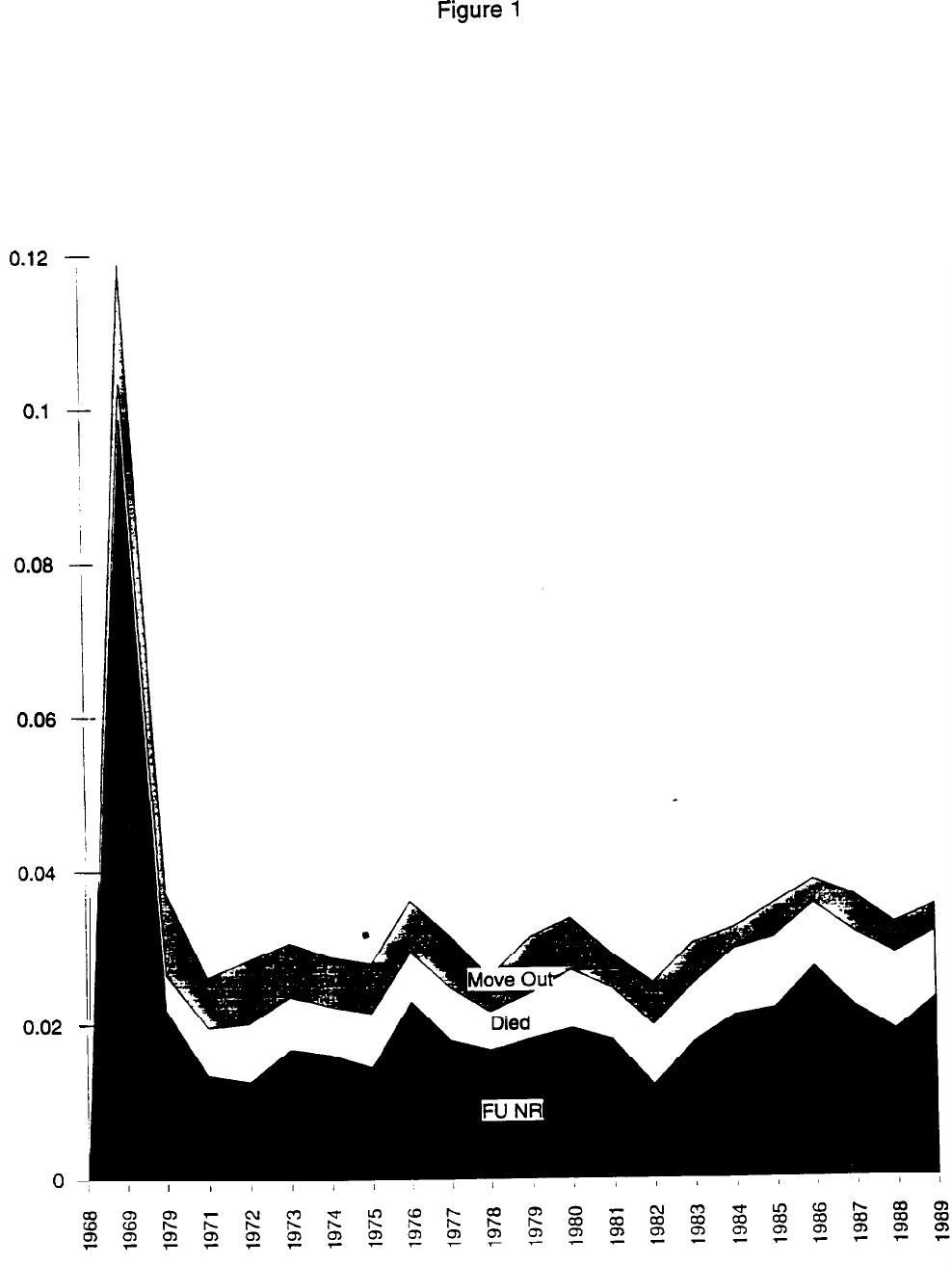
Figure
1
Attrition Hazards: Sample With No New Entrants
0.12
-
0.1
0.08
0.06
0.02
-
0
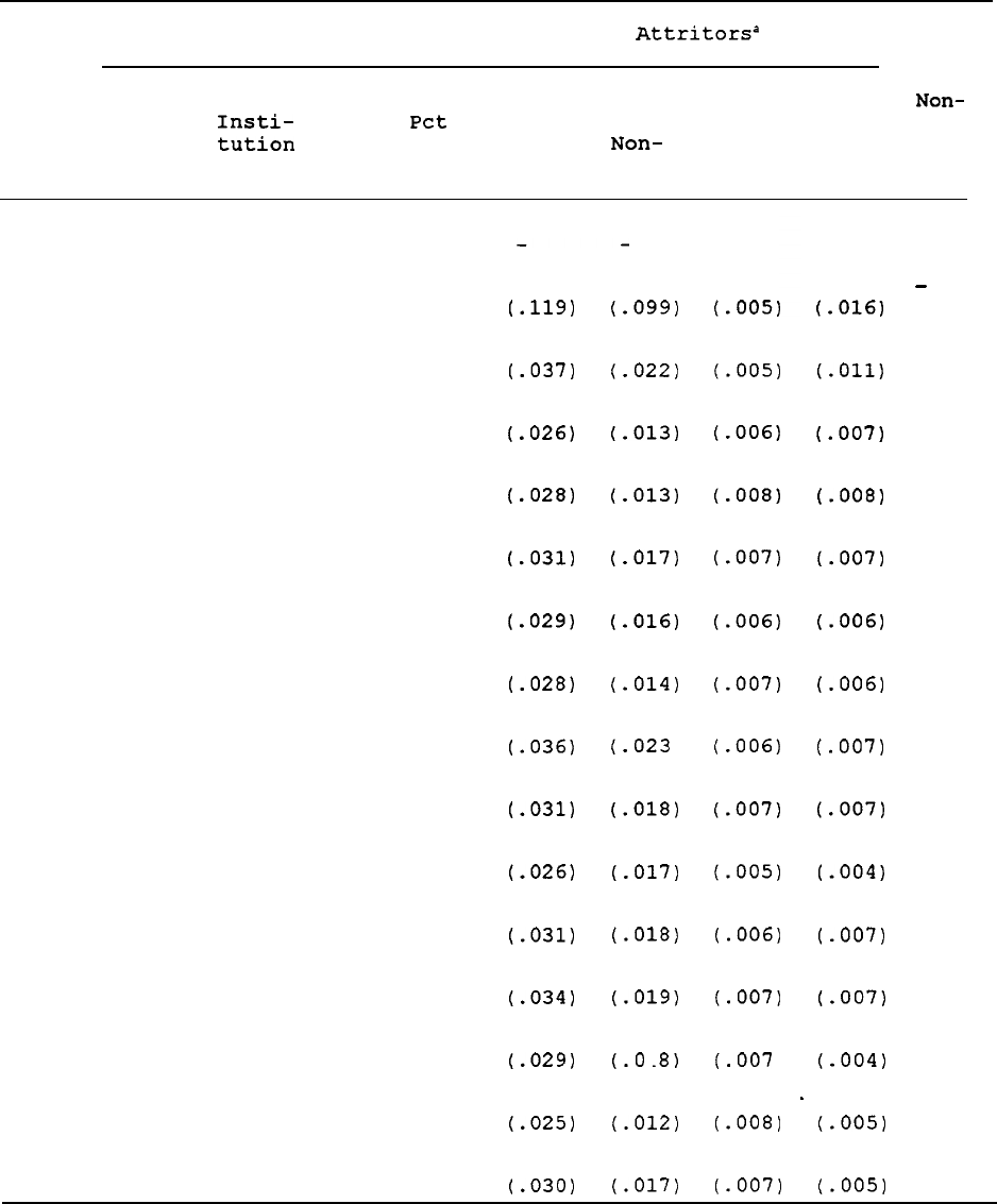
Table 1
Response and Nonresponse Rates in the PSID
Year
Remaining in Sample
Attritors=
In
from
In a
In an
Total
As a
Total
Fam.
Died
Moved
Non-
Family Insti-
Pet
of
Unit
Resp.
Unit tution
1968
Non-
Total
Resp.
1968 17807
384 18191 100.0
1969
15561
367
16028
88.1
1970
15126 333
15459
85.0
1971
14767
322 15089
82.9
1972
14400 293 14693
80.8
1973 13969
307
14276 78.5
1974
13581
307
13888
76.3
1975
13226
302
13528
74.4
1976
12785 291 13076 71.9
1977
12377 310
12687
69.7
1978
12078 320
12398
68.2
1979
11718
316 12034
66.2
1980
11357
305
11662
64.1
1981
11022 340
11362
62.5
1982
10780
326 11106
61.1
1983
10487
322
10809 59.4
2163
1797
(.119)
(-099)
600 351
(.037)
(-022)
404
208
(.026)
(-013)
429 190
(.028) (-013)
449
247
(.031)
(-017)
410
229
(.029) (-016)
386
200
(.028) (-014)
487
310
(.036)
(-023
411
234
(.031)
(.018)
330
210
(.026)
(.017)
387
224
(.031)
(.018)
405
233
90
82 33
(.034)
(.019) (.007) (-007)
337
208
(.029)
(.O
-8)
285
135
(.025)
(.012)
336 194
(.030)
(.017)
84
(.OOS)
282
-
t-016)
74
175
31
(.005)
(.Oll)
95
101
34
(.006)
(.007)
115
124
33
(.008)
(.008)
100
(.007)
89
(.006)
97
(.007)
86
(.006)
91
35
(.007)
88
(.007)
89
22
(.007)
63
(.005)
57
41
(-004)
73
90
23
(.006)
(-007)
77
(.007
88
(.008)
83
102
32
(.007)
92 22
(.006)
89
26
(.006)
52
37
(-004)
-
62
29
(.005)
59
39
(.007) (.005)
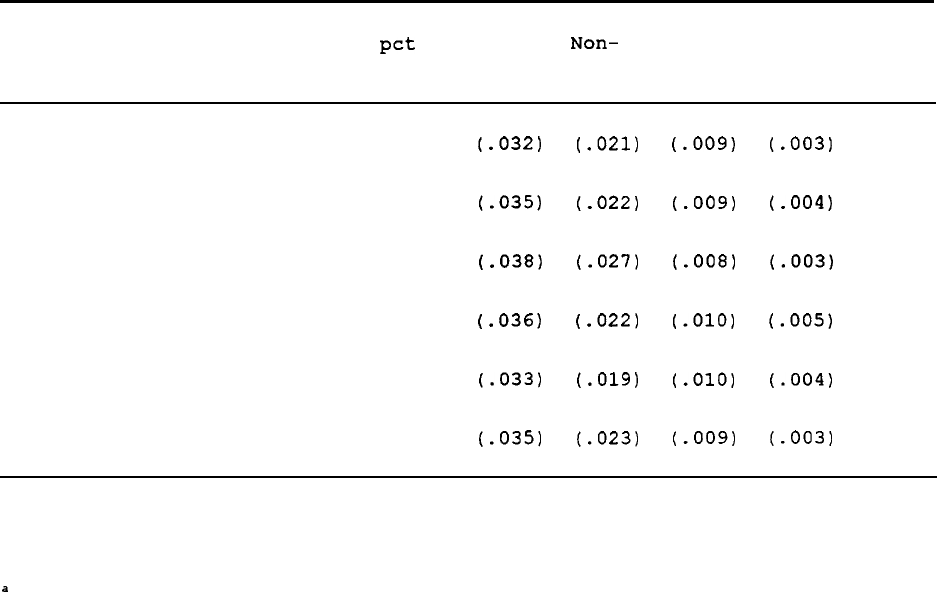
Year
In a
In an
Total
As a
Total
Fam Died
Moved In
Fam.
Inst.
Pot
Att.
Non-
from
Unit
of 68
Resp
Non
Resp
1984
10178
319
10497
1985
9891 275 10166
1986
9517
292
9809
1987
9230
257
9487
1988
9002
206
9208
1989
8743
170
8913
57.7
348
225
93
30
(.032)
(.021)
(.009) (.003)
55.9
371
(-035)
53.9 390
(.038)
52.2 357
(.036)
50.6
310
(.033)
49.0
323
(.035)
229
(-022)
275
(-027)
215
(.022)
178
(.019)
212
(.023)
96
(.009)
84
(-008)
94
(.OlO)
95
(.OlO)
79
(.009)
46
(-004)
31
(.003)
48
(.005)
37
(.004)
32
(-003)
36
40
33
35
31
28
Notes:
Excludes new births and nonsample entrants.
a
Figures in parentheses show attrition rates
as a percent of the total sample
remaining in the prior year (column four).
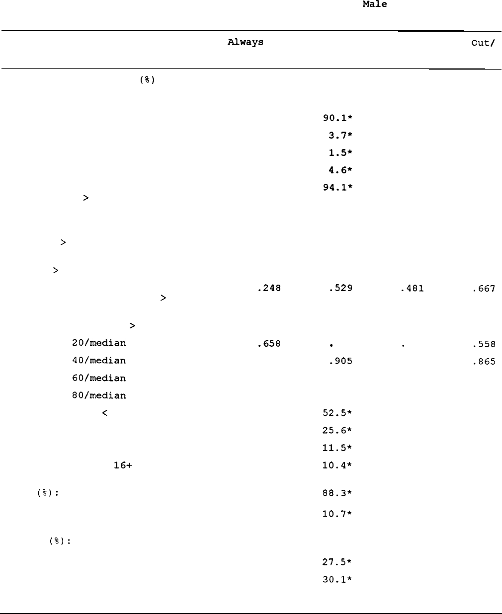
Table 2
1968 Characteristics by Attrition Status:
Male
Heads,
Age 25-64
Always
In
Ever Out Ever Out/
Ever
Out/
Not Dead
Dead
Welfare Participation
(%)
Marital Status(%):
married
never married
widowed
divorced/separated
Percent with Annual
Hours Worked
>
0
Annual Labor Income
Annual Labor Income for those
w/income
>
0
Annual Hours Worked for those
w/hours
>
0
Variance of log annual labor
income for those w/income
>
0
Labor income quintile ratios for
those w/labor income
>
0:
Quintile
20/median
Quintile
40/median
Quintile
60/median
Quintile
8O/median
Education (%):
<
12
12
12-15
16+
0.8
1.3
1.4
1.2
95.8 90.1*
87.1
98.1
2.4
3.7*
4.9
0.4
0.3
1.5*
2.0
0.1
1.2 4.6*
5.9
1.3
98.7 94.lf
95.7
89.8
21345
21631
17011 17277
16298
18152
18106
18281
2378 2246
2268
2182
.248 .529
.481
.667
-658
.
886
1.101
1.392
31.5
32.8
15.8
19.9
.
611
.
615
-905
.
923
1.139
1.123
1.498
1.462
52.5*
50.8
25.6*
27.3
11.5*
11.5
10.4*
10.4
.558
.865
1.164
1.493
57.2
21.0
11.5
10.4
Race
(%):
White
Black
92.7
6.6
88.3*
87.4
90.7
10.7*
11.5
8.0
Region
(%):
Northeast
24.7 25.8 26.9
22.3
North Central
32.2
27.5*
26.5
30.1
South
26.7
30.1*
29.6
31.2
West
16.4 16.7
17.0
15.7

Table 2 continued
Always In Ever Out Ever Out/
Ever Out/
Not Dead
Dead
Age
40.7
45.6*
Tenure(%): Own home
74.9 62.9*
Rent
21.5
33.8*
Number of Children in Family
2.0 1.5
Sample Size 1238 1533
Notes:
Sample weights used.
*: Significantly different from "Always In" at 10% level.
43.1 52.1
58.0 75.9
38.9 20.2
1.6
1.3
1116
417
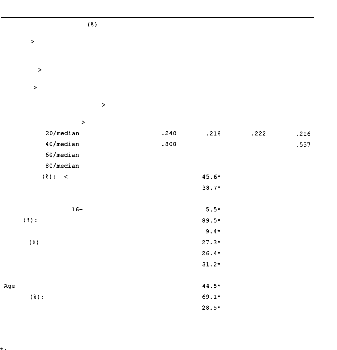
Table 3
1968 Characteristics by Attrition Status: Wives,
Age 25-64
Always In Ever Out Ever Out/
Ever Out/
Not Dead
Dead
Welfare Participation
(%)
Percent With Annual Hours
Worked
>
0
Annual Labor Income
Annual Labor Income for those
w/income
>
0
Annual Hours Worked for those
w/hours
>
0
Variance of log annual labor
income for those w/income
>
0
Labor income quintile ratios for
those w/labor income
>
0:
Quintile
20/median
Quintile
40/median
Quintile
60/median
Quintile
80/median
Education
(%):
<
12
12
12-15
16+
Race
(2):
White
Black
Region
(%)
: Northeast
North Central
South
West
Age
Tenure
(%):
Own home
Rent
Number of Children in Family
Sample Size
1.1
47.7
36308
7653
1311 1315
1342
1173
1.546 1.624
1.548
2.014
.240
-800
1.205
2.000
30.5
49.1
10.7
9.8
92.0
7.4
23.9
31.7
28.0
16.5
40.9
77.8
18.8
2.0
1377
1.6
1.4
2.2
44.0
44.4
42.3
3299 3366
2960
7509 7580
7128
.218
.222
.
611
.
622
1.164 1.667
1.637 2.078
45.6*
44.7
38.7*
39.9
10.2
9.6
5.5*
5.8
89.5*
90.0
9.4*
8.7
27.3*
28.3
26.4*
25.1
31.2* 31.8
15.1
14.8
44.5*
43.5
69.1*
67.9
28.5*
29.6
1.5
1.6
1043
847
.216
.557
1.195
1.670
50.0
32.8
12.7
4.5
86.6
12.5
22.4
32.8
27.9
16.9
49.6
75.5
22.6
1.4
196
Notes:
Sample weights used.
*.
. Significantly different from “Always In" at 10% level.
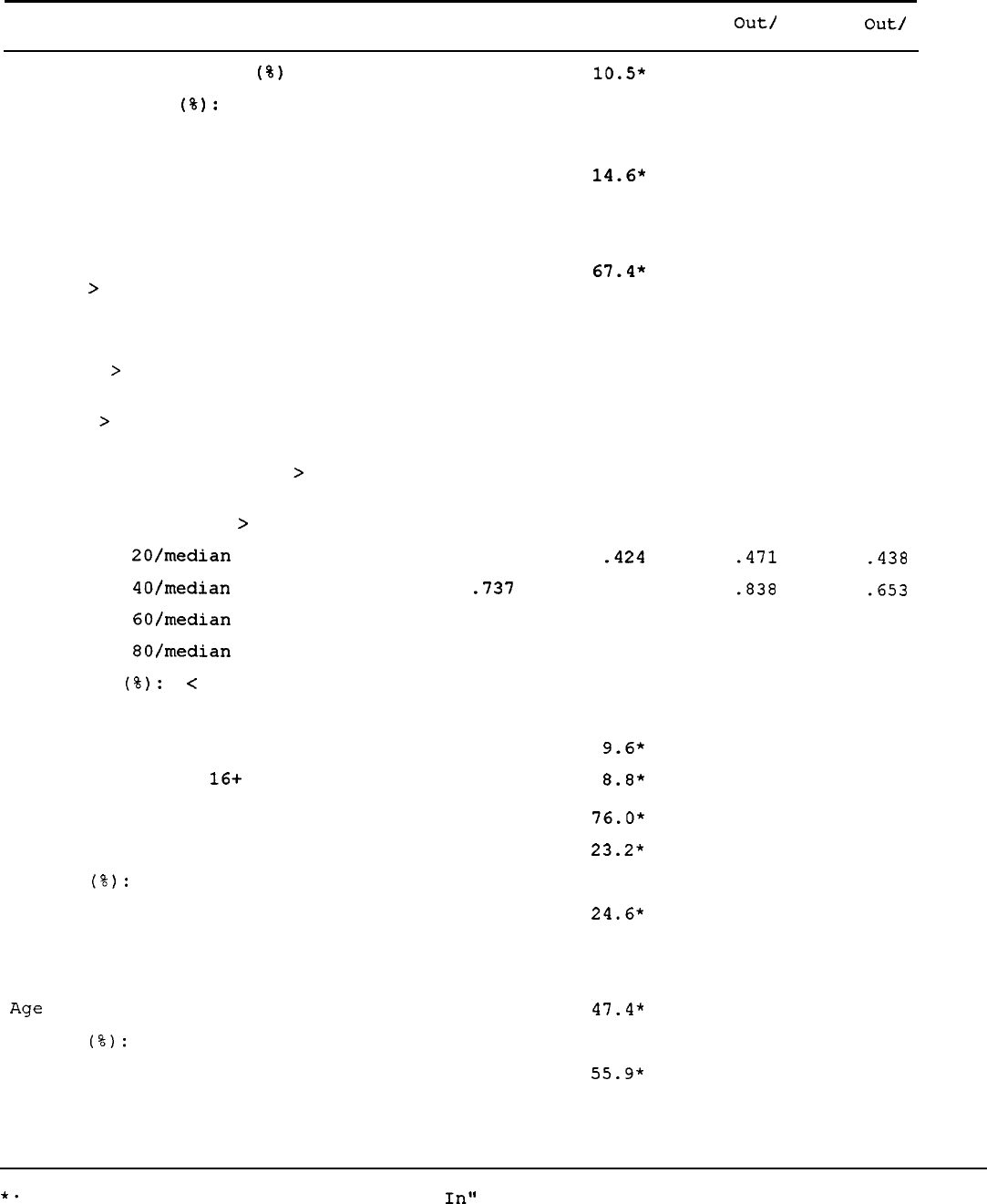
Table 4
1968 Characteristics by Attrition Status: Female Heads,
Age 25-64
Always In Ever Out
Ever
Out/
Ever
Out/
Not Dead
dead
Welfare Participation
(%)
Marital Status
(%):
married
never married
widowed
divorced/separated
Percent With Annual Hours
Worked
>
0
Annual Labor Income
Annual Labor Income for those
w/income
>
0
Annual Hours Worked for those
w/hours
>
0
Variance of log annual labor
income for those w/income
>
0
Labor income quintile ratios for
those w/labor income
>
0:
Quintile
20/median
Quintile
40/median
Quintile
60/median
Quintile
80/median
Education
(%):
<
12
12
12-15
16+
Race (8):
White
Black
Region
(%):
Northeast
North Central
South
West
Age
Tenure
(%):
Own home
Rent
Number of Children in Family
Sample Size
4.3 10.5*
10.0
17.9
1.4
1.8 1.7
2.5
21.2 14.6*
14.7
13.1
38.7 39.1
39.1
39.0
36.7 40.8
40.6
43.8
80.4 67.4*
67.0
73.7
8199
10214
6950 7167
3482
10296 10679
4723
1593
1645 1676
1203
1.426
1.185 1.045
1.739
.
316
.737
1.163
1.553
45.1
28.3
13.8
12.8
-424
.
800
1.178
1.468
49.2
32.4
9.6*
8.8*
.471
.438
.838
.653
1.178
2.483
1.440
5.724
46.8
88.4
33.7
11.6
10.2
0.00
9.3
0.00
80.3 76.0* 77.3
55.4
18.8 23.2*
21.9
44.6
25.2
26.2 26.3
24.8
30.0 24.6* 25.6
9.3
25.8 27.7
25.9
57.5
19.0 21.4
22.2
8.4
44.9 47.4*
47.2
50.4
45.0
40.3 40.3
40.7
50.3 55.9* 55.8
58.2
1.3 1.0 1.0
1.8
502
526
475
51
Notes:
Sample weights used.
*.
. Significantly different from "Always
In"
at 10% level.
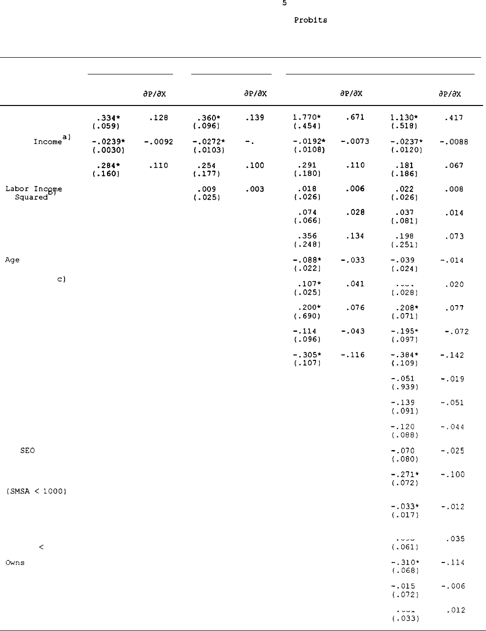
Table
5
Ever-Out Attrition
Probits
Male Heads Age 25-64,
Focus on Labor Income
Model 1
Model 2
Model 3 Model 4
Coeff.
aP/ax
Coeff.
ap/ax
Coeff.
ap/ax
Coeff.
ap/ax
Intercept
.334’
.128
1.059)
.360'
.139
1.770*
t.096)
(.454)
.671
1.130*
t-518)
Labor
Incomea)
-.0239*
-.0092
(.0030)
-.
0272*
-.
0105
(.0103)
.254
.lOO
(.177)
.009
.003
-.0192
(.0108
-.0237*
(.0120]
No Labor
Income
La;;:a:zpT=-
Black
.284*
-110
t.1601
.291
l.180)
*
-.0073
1
.110
.181
(.186)
.018
t.025)
f.026)
.074
f.066)
.006
.022
t.026)
.028
.037
(.081)
Other Race
-356
t.248)
.134
.198
t.251)
Age
-.088f
(.022)
-.033 -.039
c.024)
Age Squared
cl
Education < 12
Years
Some College
.107*
t.025)
.041
054f
[:028,
.076
.208*
i.071)
-.114
t.096)
-.043
-.195*
i.097)
College Degree
-.305*
(.107)
-.116
-.384'
I
.109)
Northeast
-.051
t.9391
North
-.139
Central
(.091)
South
-.120
t.088)
In SE0 Sample -.070
t.080)
Lives in Rural
Area
(SMSA
<
1000)
-.271*
t.072)
Number of
Children in
Family
Presence of
Child
<
6
-.033*
(.017)
095
(:061)
Cwns
House
-.310*
f.068)
Might Move
in Future
-.015
t.072)
Income/Needs
Ratio
031
(:033)
.417
-.0088
.067
.008
.014
.073
-.014
.020
.077
-.072
-.142
-.019
-.051
-.044
-.025
-.lOO
-.012
.035
-.114
-.006
.012
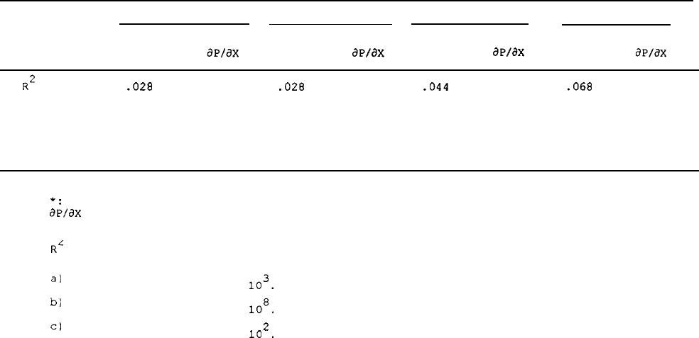
Table 5,
continued
Model 1 Model 2 Model 3
Model 4
R2
Coeff.
.028
ap/ax
Coeff.
ap/ax
Coeff.
ap/ax
Coeff.
ap/ax
.028 .044 .068
Sample
Size
2253
2253
2253 2253
Number
1074
1074
1074
1074
Ever Out
Loq Like.
-1516.05
-1515.99 -1490.27 -1453.02
Notes:
Excludes known dead. Characteristics measured in 1968.
':
Significant at 10% level.
aP/dX
signifies the effect of a unit change in the variable on the probability of attrition evaluated at
the mean.
R‘
equals one minus the ratio of the log likelihood of the fitted function to the log likelihood of a
function with only an intercept.
a)
Coefficients multiplied by
103.
bl
Coefficients multiplied by
108.
Cl
Coefficients multiplied by
102.
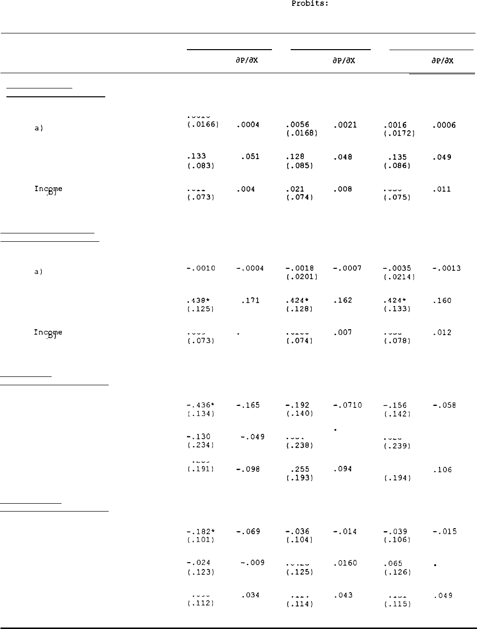
Table 6
Ever-Out Attrition
Probits:
Other Results
Model 2
Model 3
Coeff.
se/ax
Coeff.
se/ax
Model 4
Coeff.
de/ax
Wives, 25-64,
Focus on Labor Income
Labor
a)
Income
No Labor
Income
Labor
Incgye
Squared
Female Heads, 25-64,
Focus on Labor Income
Labor
a)
Income
No Labor
Income
Labor
Incgye
Squared
Men,
25-64,
Focus on Marital Status
Married
Widowed
Divorced/
Separated
i.0166)
0010
.0004
.0056
.0021 .0016 .0006
(.0168)
t.0172)
.133
.051
.128
.048
-135 .049
l.083) l.085) (.086)
011
i.073)
.004 .021 .008
030
.Oll
(.074) i.075)
-.OOlO
-.0004
-.0018
-.0007
-.0035 -.0013
1.0195) (.0201) (.0214)
438f
i.125)
.171
424*
.162
i.128)
424*
.160
i.133)
009
i.073)
*
004
0186
i.074)
.007
033
i.078)
.012
-.436+
-.165
-.192
-.0710
-.156
-.058
l.134) (.140)
C.142)
-.130
-.049
054
i.238)
*
020
026
.
009
t.234)
i-239)
I:1911
259
-.098
.255
.094
,288
.106
(.193)
C.194)
Women, 25-64,
Focus on Marital Status
Married
-.182f
-.069 -.036
-.014
-.039 -.015
t.1011
C.104)
C.106)
Widowed
-.024
-.009
0425
i.125)
.0160
.065
024
f.123) t.126)
*
Divorced/
Separated
090
(:112)
.034
114
(:114)
.043
131
(:115)
.049
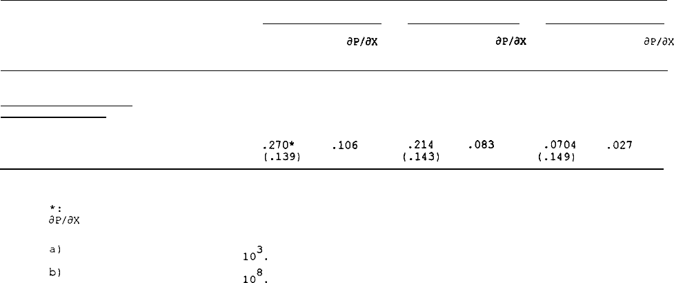
Table 6 continued
Model 2
Model 3
Model 4
Coeff.
se/ax
Coeff.
Be/ax
Coeff.
de/ax
Female Heads, 18-54,
Focus on Welfare
Welfare
.270* .106
.214
.083 .0704
.027
Receipt
1.139)
(.143) (.149)
Notes:
Excludes known dead. Characteristics measured in 1968.
f:
Significant at 10% level.
dP/aX
signifies the effect of a unit change in the variable on the probability of attrition evaluated at
the mean.
al
Coefficients multiplied by
103.
b)
Coefficients multiplied by
10'.
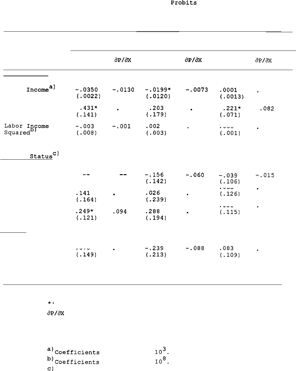
Table 7
Ever-Out Attrition
Probits
Multiple Focus Variables
Labor Income
Female Heads
Men
Women
18-54 25-64
18-54
Coeff.
apm
Coeff.
apm
Coeff.
awax
Labor
Incomea)
No Labor Income
Marital
Statusc)
Married
Widowed
Divorced/
Separated
Welfare
Welfare Receipt
-.0350
-.0130
l.0022)
,::z;
*
162
-.003 -.OOl
(.008)
-- --
;1;:4,
-
053
.249*
-094
l.121)
070
;.149,
-
027
-.0199*
-.0073
f.0120)
.203
(.179)
-
071
006
-.156
-.060
(.142)
iz9,
-
009
.288
(.194)
-
106
-.239
-.088
(.213)
0000
.221*
-082
(-071)
000
i.001)
*
000
-.039
-.015
l-106)
i.126)
065
-
024
i.115)
131
*
049
;";;9,
*
031
Notes:
Excludes known dead. Characteristics measured in 1968.
*.
.
Significant at 10% level.
aP/aX
signifies the effect of a unit change in the variable on
the probability of attrition evaluated at the mean.
Other variables included are those in Model (4) in Table 5.
a)Coefficients
multiplied by
103.
b)Coefficients
multiplied by
108.
c)
Omitted category for female heads is never-married.
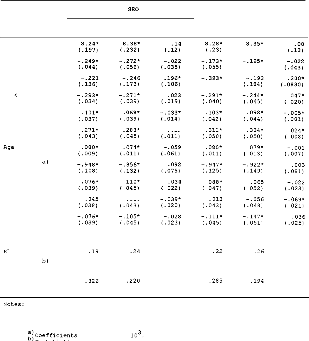
Table 8
1968 Log Labor Income Regresssions
Male Heads
SRC and SE0 Combined
SRC Only
Total
Always In
Difference
Total
Always In
Difference
Intercept
Black
Other Race
Ed
<
12
Some College
College Degree
Age
Age Squared
a)
Northeast
North Central
South
Sample Size
R2
F-statistic
b)
Variance of
Error
8.24*
(.197)
-.249*
(-044)
-.221
(.136)
-.293*
(.034)
(2;;
.271*
(.043)
,:::i;
-.
948*
(.108)
(:
E;
,x:
-.076*
(.039)
8.38*
(.232)
-.272*
(.056)
-.246
(.173)
-.271*
l.039)
068*
(:039)
.283*
(.045)
.074*
(-011)
-.856*
(-132)
(
:
ia:;
006
(.;)43)
-.105*
(.045)
.14
t.121
-.022
(.035)
.196*
(.106)
.023
(.019)
-.033*
(.014)
012
(.;)ll)
-.059
(.061)
(
.
,:3;
-.039*
(.020)
-.028
(.023)
8.28*
t.23)
-.173*
(.055)
-.393*
(0.164)
-.291*
(.040)
(:E;
,:::i;
080*
(:oll)
-.947*
(.125)
(
:
E;
(.il:i;
-.111*
(.045)
8.35*
(0.26)
-.195*
(0.070)
-.193
(-184)
-.244*
(.045)
,::i:;
,:Z;
(
:
E;
-.922*
(.149)
(
.
z:
-.056
(.048)
-.147*
(.051)
2182 1159
1406
788
.19
.24
-22
.26
50.5
35.7
38.8
27.8
.326
.220
.285
.194
.08
(.13)
-.022
(.043)
.200*
(.0830)
(
:
z;
-.005*
(.OOl)
(
:
z;
-.OOl
(.007)
-.022
(-023)
-.069*
(.021)
-.036
(.025)
votes:
Standard errors in parentheses.
Sample excludes known dead.
SRC+SEO sample are weighted.
*:
Significant at 10% level.
E;Coefficients
multiplied by
103.
F-statistic for hypothesis that all coefficients except the intercept are
equal to zero.
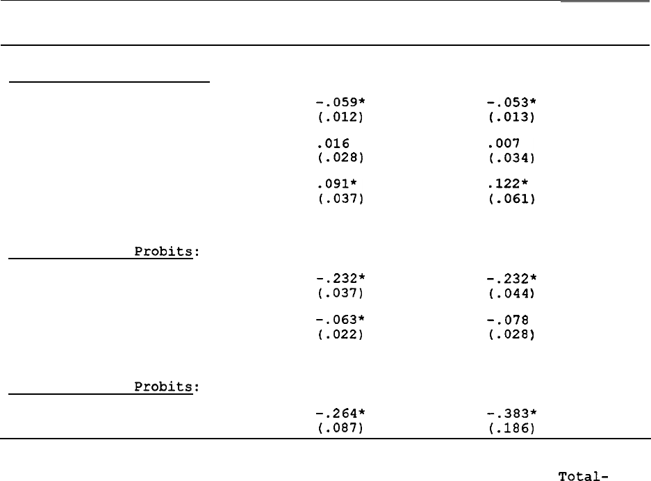
Table 9
1968 Income,
Marital Status, and Welfare Equations:
Difference in Total and Always-In Samples, Intercept-Only Model
SRC+SEO SRC Only
Labor Income Regressions:
Male Heads
Wives
Female Heads
-.059*
-.053*
(.012)
(.013)
.016
(.028)
;":',4,
Marital-Status
Probits:
Men
-.232*
-.232*
Women
Welfare-Status
Probits:
1
(.037)
(.044
-.063*
-.078
(.022)
(.028
*
1
Female Heads
-.264*
-.383*
(.087) (.186)
Notes:
Models include all variables shown in Table 8 but allow the intercept
to differ for the Total and Always-In Samples.
Coefficient equals
Total-
Sample intercept minus Always-In Sample intercept.
Standard errors in parentheses
Sample exludes known dead
SRC+SEO is weighted
*Significant at the 10% level
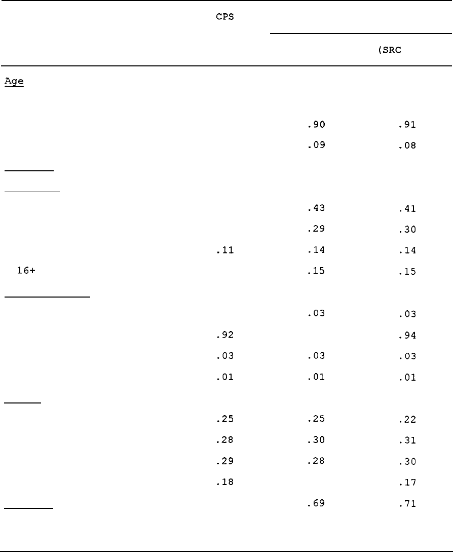
Table 10
Characteristics of Male Heads 25-64: 1968
PSID and CPS
e!F
Race
White
CPS
43.7
. 91
PSID
Weighted
Unweighted
(SRC and SEO)
(SRC
only)
43.3
43.6
.90
-91
Black
.
08
.09
-08
Hispanic
Education
--
--
--
Less than
12
.
42
.43
12
.
32
.29
13-15
.ll
.14
16+
. 15
-15
.41
.30
.14
-15
Marital Status
Never married
.
03 .03
Married
-92
.
93
Divorced/separated
.03 .03
Widowed
.Ol
.Ol
Region
Northeast
.25
-25
North Central
.28
.30
South
.29
-28
West
.18
.
17
Own Home
--
.69
.03
.94
.03
-01
.22
.31
.30
.17
.71
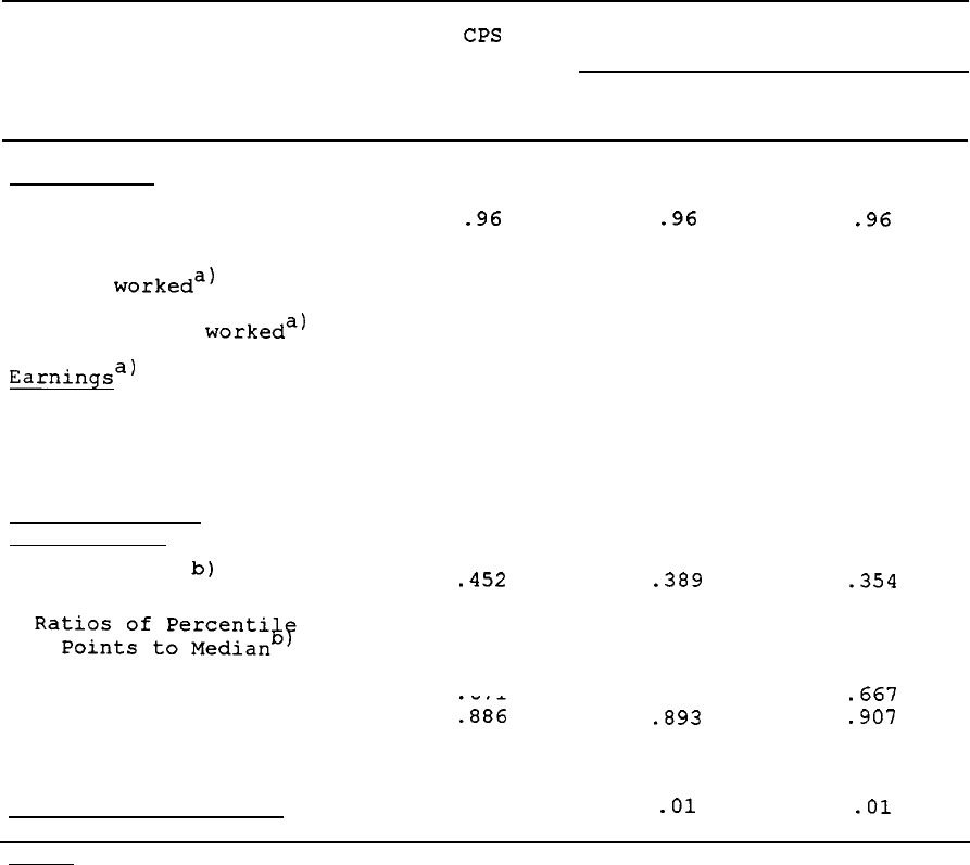
Table 10 continued
Labor Force
CPS
PSID
Weighted
Unweighted
(SRC and SEO)
(SRC only)
Positive weeks
worked
-96 -96
.96
Weeks
workeda)
--
--
--
Annual hours
workeda)
--
--
--
Earningsa)
Real wage and salary
$19478
--
--
Real labor income
--
$20460
$20709
Wage and Salary
Distribution"'
Log variance
b)
.452
.389
.354
20th
Percentile
671
. 667
.667
40th
Percentile
:886
.893
.907
60th
Percentile
1.114
1.087
1.107
80th
Percentile
1.429
1.373
1.400
Welfare Participation
Notes:
.
02
.Ol
.Ol
a) Workers only.
b) PSID figures use labor income rather than wage and salary income.
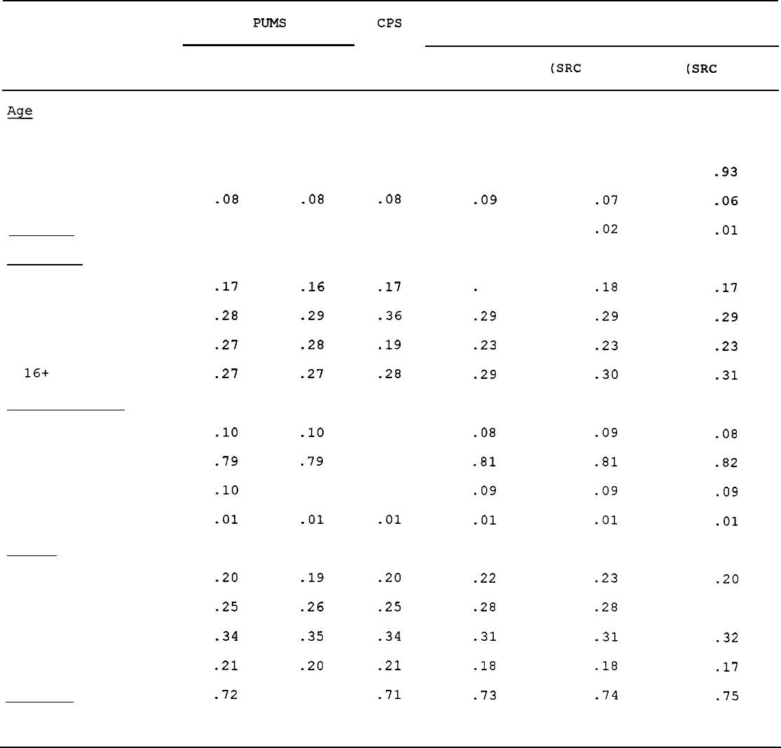
Table 11
Characteristics of Male Heads 25-64: 1989
PSID, CPS, and PUMS
PUMS CPS
PSID
with
without
Current Wgts.
1968 Wgts.
Unweighted
immignts
immignts
(SRC and SEO)
(SRC
and SEO)
(SRC
Only)
%E
Race
White
Black
Hispanic
Education
Less than 12
12
13-15
16+
Marital Status
Never married
Married
Divorced/separated
Widowed
Region
Northeast
North Central
South
West
Own Home
42.4
42.7
42.0
42.0 42.0
42.2
.
86
.
89
.
89
-08
-08
-08
.
07
.
05
.
07
.
90
.
92
-93
-09
.07
-06
.
03 .02
.Ol
-17
-16
.17
.
18
.28
.29 .36
.29
.27
.28
.19
.23
.27
.27 .28
.29
.18
.17
.29
.29
.23
.23
.30
.31
.lO
.79
.lO
.Ol
.lO
.79
.
10
.
79
.
09
.Ol
.08
.
10
.Ol
.81
.09
.Ol
.09
.08
.81
.82
.09
.09
.Ol
.Ol
-20
.25
.34
-21
-72
.19
.26
-35
.20
.
74
.20
.22
.23
.25
.28 .28
.34
.31
.31
-21
-18 -18
-71
.73
.74
.20
.
30
.32
.17
.75
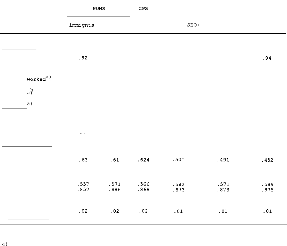
Table 11 continued
PUMS CPS PSID
with without
Current Wgts.
1968 Wgts.
Unweighted
irrunignts
immignts (SRC and
SEO)
(SRC and SEO)
(SRC Only)
Labor Force
-92
.
92
.
89
.
93
.
93
.94
Positive weeks
worked
Weeks
workeda) 48.1
Annual
af
ours
worked
2156
48.3
2164
49.0 46.6
46.6
46.7
2165 2172
2176
2199
Earnings
a)
Real wage and
salary
$24239 $24582
$22970 $23481
$23645
$23905
Real labor income
--
$24090
$24273
$24537
Wage and Salary
Distribution"'
Log Variance
.63 -61
.624
-501
.491
-452
Ratios of Percentile
Points to Median
20th Percentile
.557 .571
.566
40th Percentile
.857
.886
.868
60th Percentile
1.117 1.143 1.132
80th Percentile
1.500 1.525 1.509
Welfare
Participation
.02
-02 -02
.582 .571 .589
.873 -873
.875
1.163 1.143 1.143
1.519 1.500 1.500
.Ol -01 .Ol
Notes:
a)
Workers only.
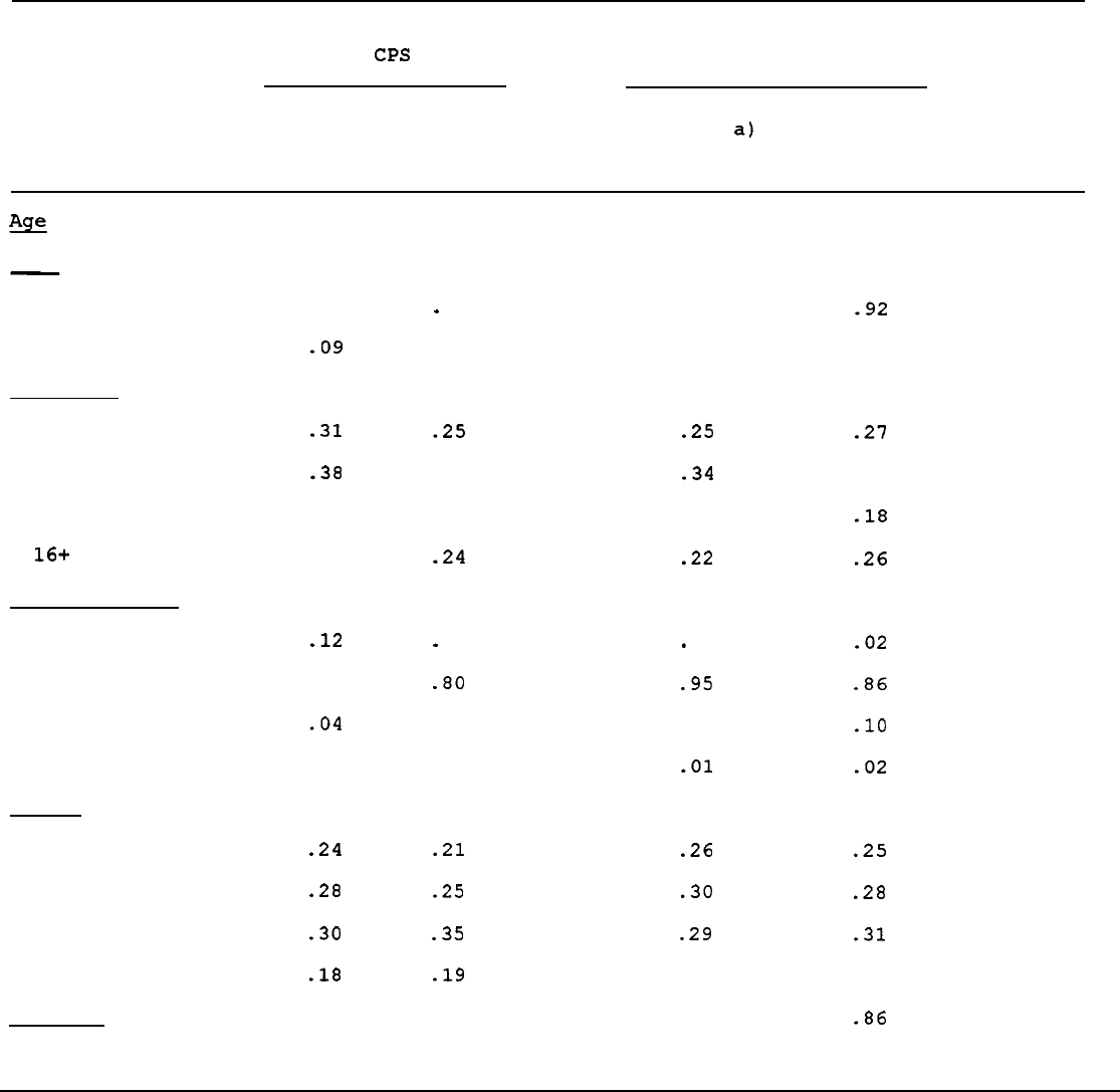
Table
12
Characteristics
of Males 25-40
in
1968 and 46-61
in 1989
PSID and CPS
CPS
PSID
25-40 46-61
25-40
in 1968
a)
46-61
in 1968
in 1989
in 1989
%!?
Race
White
Black
Education
Less than 12
12
13-15
16+
Marital Status
Never married
Married
Divorced/separated
Widowed
Region
Northeast
North Central
South
32.4
53.1
32.8
53.8
.
89
.
87
-09
.
10
.31
-38
.25
.
13
.
18
.
36
.
14
.24
-12
.
83
.04
.
06
-80
.
02
.
12
.
02
West
.24
.21
.28
-25
-30 -35
-18
-19
Own Home
--
.
89
.
93
.
06
.25
-34
.
17
.22
.
02
.95
.
01
-01
.26
.25
.30
.28
.29
.31
.
15
.
16
.
66
-86
-92
.
06
.27
.
30
.18
.26
-02
-86
-10
-02

Table 12 continued
CPS
25-40
46-61
in 1968
in 1989
PSID
46-61
in 1989
Earningsb)
Real wage and
salary
$18429
$24694
--
$25464
Real labor income
--
--
$21265 $24638
Notes:
PSID sample includes SE0 and SRC and both years use 1968 weights.
a)
Sample includes only those responding in 1989.
b)
Workers only.
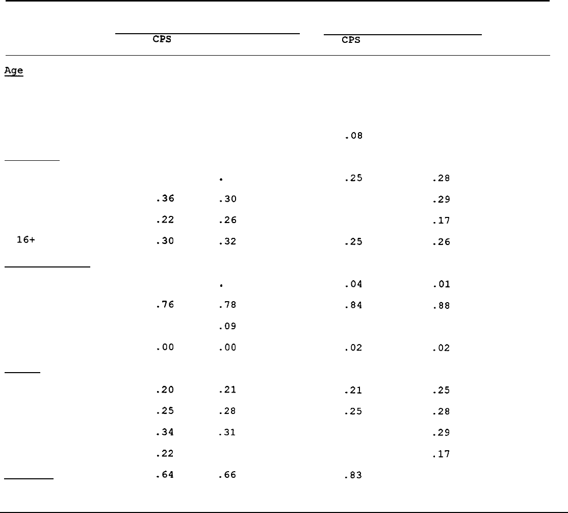
Table 13
Characteristics of Male Heads 25-45 and 46-64 in 1989
PSID and CPS
Age 25-45
Age 46-64
CPS
PSID
CPS
PSID
!e
Race
White
Black
Education
Less than 12
12
13-15
16+
Marital Status
Never married
Married
Divorced/separated
Widowed
Region
Northeast
North Central
South
West
Own Home
34.9
34.8
54.6
55.3
.
88
.
92
.
89
.
92
.
08
.
07
-08
.
06
.
12
.
12
-36
-30
-22 .26
.30
.32
.25
.
35
.
15
-25
.28
-29
-17
.26
.
14
.76
-04
.84
.
09
-00
.
12
.78
.09
-00
.
10
.02
-01
.88
.
09
.02
.20
-25
.34
.22
-64
.21
.28
.31
-21
-25
.
18
-66
.
34
.
19
.83
-25
-28
.29
.17
.
88

Table 13 continued
Earningsa)
Age 25-45
Age 46-64
CPS PSID
CPS PSID
Real wage and
salary
$22096
$23162
$24878 $25262
Real labor income
--
$23622
--
$25890
Notes:
PSID sample uses SRC-SE0 and 1968 weights.
a)
Workers only.
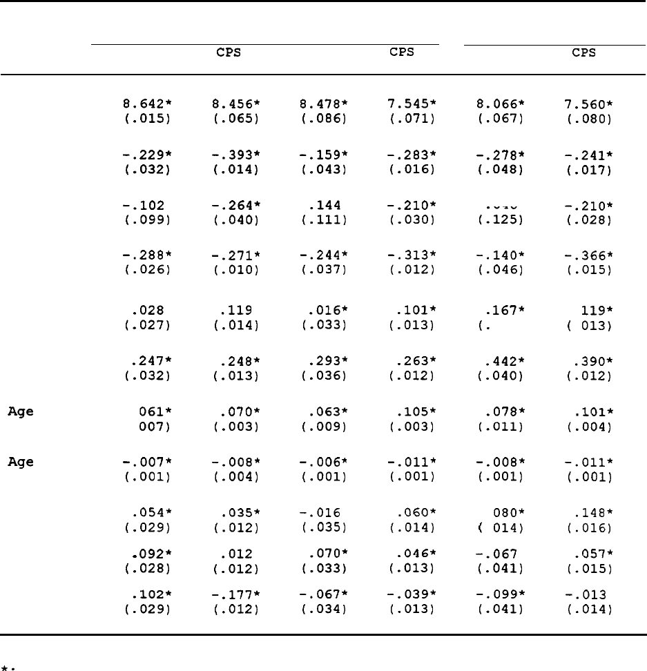
Table 14
PSID and CPS Log Earnings Regressions: Male Heads
1968
1981
1989
PSID
CPS
PSID CPS
PSID
CPS
Intercept
Black
Other
Low Ed
Some
College
College
Grad
Age
Age
Squared'
Northeast
North
Central
South
8.642*
(.015)
-.229*
(.032)
-.102
l.099)
-.288*
(.026)
,:E,
.247*
(.032)
( :
z:;
-.007*
(.OOl)
054*
(:029)
f
092*
(.028)
102*
(:029)
8.456*
(.065)
-.393*
(.014)
-.264*
(-040)
-.271*
(.OlO)
.119
(.014)
.248*
(.013)
.070*
(-003)
-.008*
(-004)
035*
(:012)
(:Z,
-.177*
(.012)
8.478*
(-086)
-.159*
(.043)
-.244*
(-037)
.016*
(.033)
.293*
(.036)
063*
(:009)
-.006*
(.OOl)
-.016
(.035)
-.067*
(.034)
7.545*
(.071)
-.283*
(.016)
-.210*
(-030)
-.313*
(.012)
101*
(:013)
.263*
(-012)
105f
(:003)
-.011*
(.OOl)
060*
(:014)
046*
(:013)
-.039*
(.013)
8.066*
(.067)
-.278*
(-048)
046
(:125)
-.140*
(.046)
167*
(:
039)
.442*
(-040)
078*
c:o11,
-.008*
(.OOl)
(
:
z;:;
-.067
(.041)
-.099*
(.041)
7.560*
(.080)
-.241*
(.017)
-.210*
(-028)
-.366*
(.015)
(
:
E;
.390*
(.012)
101*
(:004)
-.011*
(.OOl)
,:z;
057*
(:015)
-.013
(.014)
Standard errors in parentheses
*.
.
significant at 5% level
Combined SRC-SE0 sample (weighted) is used for PSID
Omitted categories for dummies are white, 12 years of education, and West.
'Coefficients multiplied by 10
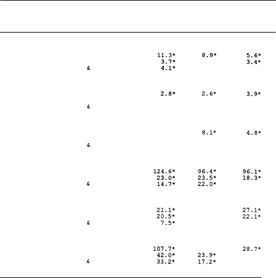
Table 15
Significance Tests for CPS-PSID Differences
1968
1981
1989
Earnings:
Male Heads
All Coeffs
All Coeffs but Const.
All Coeffs but Const.
&
Region
Earnings:
Female Heads
All Coeffs
All Coeffs but Const.
All Coeffs but Const.
&
Region
Earnings: Wives
All Coeffs
All Coeffs but Const.
All Coeffs but Const.
&
Region
Marital Status: Males
11.3*
3.7*
4.1*
8.9*
5.6*
2.5
3.4*
3.0
4.0
2.8*
2.6*
3.9*
1.2
1.3
1.6
1.6
1.5
2.2
1.5
8.1*
4.8*
1.5
0.9
2.4
1.5 0.9
2.3
All Coeffs
All Coeffs but Const.
All Coeffs but Const.
&
Region
Marital Status: Females
124.6* 96.4*
96-l*
23-O* 23.5*
18.3*
14.7* 22.0*
13.6
All Coeffs
All Coeffs but Const.
All Coeffs but Const.
&
Region
Welfare Part: Female Heads
21.1*
16.2
27.1*
20.5*
9.1
22.1*
7.5*
8.7
13.5
All Coeffs
107.7* 25.8"
28.7*
All Coeffs but Const.
42.0*
23.9*
18.4
All Coeffs but Const.
&
Region
33.2*
17.2*
14.2
Notes:
Earnings statistics are F-statistics;
are likelihood ratio statistics.
marital status and welfare participation
*: significant at the 5 percent level
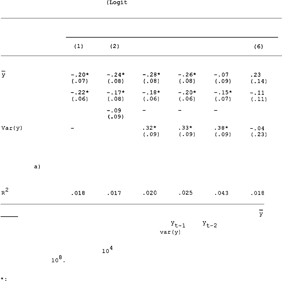
Table 16
Dynamic Attrition Models With Focus On Lagged Earnings
(Logit
Coefficients)
Males
Females
(1)
(2)
(3)
(4)
(5)
(6)
-.20*
(.07)
-.24*
t.08)
-.22* -.17*
t.06) t.08)
-.09
(
-
09)
-.28*
t.08)
-.18*
t-06)
-
-.26*
t.08)
-.20*
t-06)
-
-.07
(.
09)
-.15*
(.07)
-
.23
(.14)
-.11
(.ll)
yt-1
yt-2
Var
(y)
;“Z,
n
;?Z,
Y
38*
i.09,
Y
-.04
t.23)
Y
Time Dummies
and age
Other
Characts.
a)
n n
n
n
n
n
Y
Y
R2
-018
.017 .020
.025
.043
.018
Notes: Dep. var.
is 1 if individual attrites in next period, 0 if not.
7
is
the mean earnings from 1968 to current period;
ytwl
and
yt-2
are earnings in
the current period and one period back;
and
var(y)
is the variance of earnings
from 1968 to the current period.
The coefficients on the first three
variables are multiplied by
lo4
and the coefficient on the fourth is
multiplied by
108.
Standard errors in parentheses.
For R-squared definitions, see Table 5.
*:
significant at the 10 percent level.
a) Education, race, region, age of youngest child, rural residence, homeowner.
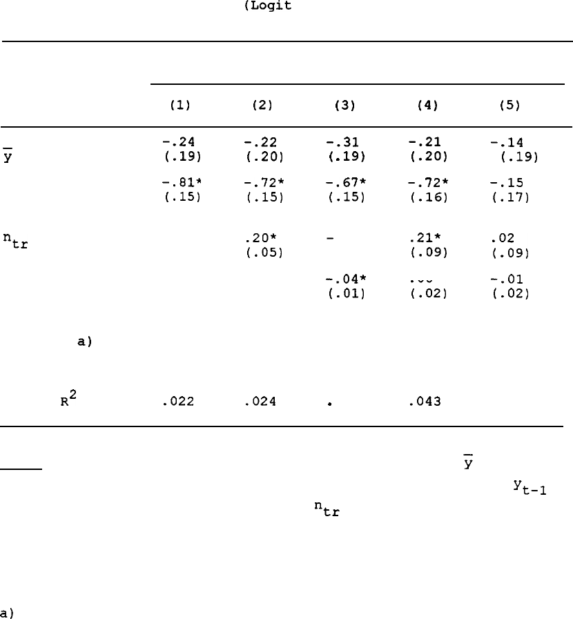
Table 17
Dynamic Attrition Models With Focus On Lagged Marital Status
(Logit
Coefficients)
Males
Females
(1)
(2)
(3)
(4)
(5)
-.24
7
t.19,
yt-1
-.81*
I.151
"tr
Duration
Other
a)
n
Characts.
Pseudo
R2
.022
-.22
I.201
-.31
(
-
19)
-.72* -.67*
t.151 t.151
.20*
t.051
n
.024
-.04*
t.011
n
.
023
-.21
t.201
-.72*
t.16)
.21*
l.09)
00
i.02)
Y
-043
-.14
f.19)
-.15
l.17)
39,
-.Ol
(-02)
Y
.
009
Notes:
Dependent variable is the same as in Table 16.
7
is the average
probability of being married from 1968 to the current period;
ytsl
is a
married dummy for the current period;
ntr
is the number of marital transitions
from 1968 to the current period; and, 'duration' is the number of years since
the last marital transition. All equations contain age and year dummies.
Standard errors in parentheses. For R-squared definitions, see Table 5.
*: significant at the 10 percent level.
a)
See Table 16.
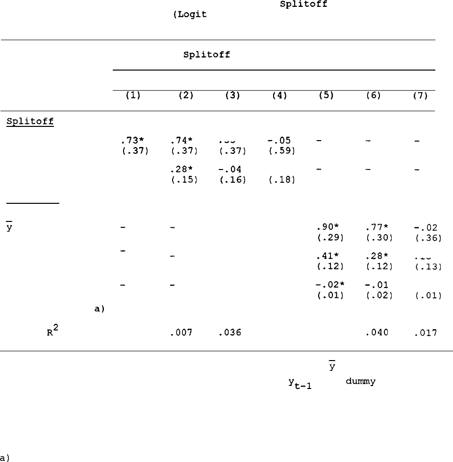
Table 18
Dynamic Attrition Models With Focus On Splitoff and Migration
(Logit
Coefficients)
(1)
Splitoff Migration
Male
Female
Male
Female
(2)
(3)
(4)
(5)
(6)
(7)
Splitoff
Split in t-l
Ever Split Off
.73*
.74*
t.371 t.371
.28*
t-151
Migration
u
yt-1
Duration
Other Characts.
a)
n n
Pseudo
R2
.
006
.007
35
i.37)
-.04
(
.16)
Y
.036
-.05
t.591
.oo
t.18)
Y
.
017
;‘,“*,,
ix,
-.02*
t.011
n
.
015
.77*
t.301
.28*
(-12)
-.Ol
t-021
Y
.040
-.02
t.36)
13
i.13)
-.oo
t.01,
Y
.017
Notes :
Dependent variable is the same as in Table 16.
7
is the average
number of moves from 1968 to the current period;
ytml
is a
dun-my
for having
moved in the current period; and 'duration'
is the number of years since the
last move.
All equations include age and year dummies.
Standard errors in parentheses. For R-squared definitions, see Table 5.
*: significant at the 10% level.
a)
See Table 16.
