
Regime Switches, Agents’Beliefs, and Post-World War
II U.S. Macroeconomic Dynamics
Francesco Bianchi
Princeton University
November 3, 2008
Abstract
This paper is focused on the evolution of in‡ation and output dynamics over the last
50 years, the changes in the behavior of the Federal Reserve, and the role of agents’
beliefs. I consider a new Keynesian dynamic stochastic general equilibrium model
with Markov-switching structural parameters and heteroskedastic shocks. Agents are
aware of the possibility of regime changes and they form expectations accordingly. The
results support the view that there were regime switches in the conduct of monetary
policy. However, the idea that US monetary policy can be described in terms of pre-
and post- Volcker proves to be misleading. The behavior of the Federal Reserve has
instead repeatedly ‡uctuated between a Hawk- and a Dove- regime. Counterfactual
simulations show that if agents had anticipated the appointment of Volcker, in‡ation
would not have reached the peaks of the late ‘70s and the in‡ation-output trade-o¤
would have been less severe. This result suggests that in the ‘70s the Federal Reserve
was facing a serious problem of credibility and that there are potentially important
gains from committing to a regime of in‡ation targeting. Finally, I show that in the
last year the Fed has systematically deviated from standard monetary practice. As a
technical c ontribution, the paper provides a Bayesian algorithm to estimate a Markov-
switching DSGE model.
I am grateful to Chris Sims, Mark Watson, Efrem Castelnuovo, Stefania D’Amico, Jean-Philippe Laforte,
Andrew Levin, David Lucca and all seminar participants at Princeton University and at the Board of
Gove rnors of the FRS for useful suggestions and comments. Correspondence: 001 Fisher Hall, Department
1
1 Introduction
This paper aims to explain the evolution of in‡ation and output dynamics over the last 50
years taking into account not only the possibility of regime switches in the behavior of the
Federal Reserve, but also agents’beliefs around these changes. To this end, I make use of
a Markov-Switching Dynamic Stochastic General Equilibrium (MS-DSGE) model in which
the behavior of the Federal Reserve is allowed to change across regimes. In such a model,
regime changes are regarded as stochastic and reversible, and agents’beliefs matter for the
law of motion governing the evolution of the economy.
In order to contextualize the results, I shall start with a brief description of the events
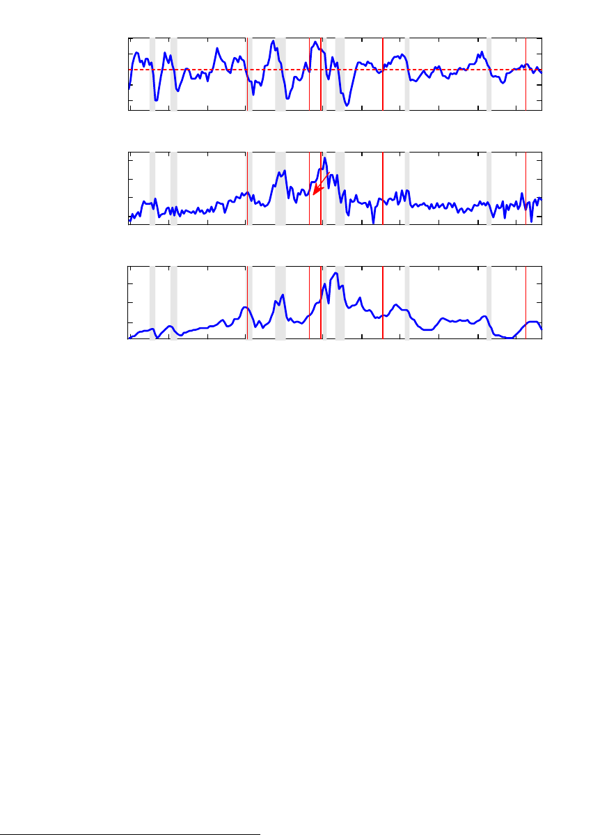
that this paper intends to interrelate. Figure 1 shows the series for output gap, annualized
quarterly in‡ation, and the Federal Funds rate for the period 1954:IV-2008:I. The shaded
areas represent the NBER recessions and the vertical lines mark the appointment dates of
the Federal Reserve chairmen. Some stylized facts stand out. Over the early years of the
sample in‡ation was relatively low and stable. Then, in‡ation started rising during the late
’60s and spun out of control in the late ’70s. At the same time the economy experienced
a deep and long recession following the oil crisis of 1974. During the …rst half of the ’80s
the economy went through a painful disin‡ation. In‡ation went back to the levels that were
prevailing before the ’70s at the cost of two severe recessions. From the mid-80s, until the
recent …nancial crisis the economy has been characterized by remarkable economic stability.
Economists like to refer to this last period with the term "Great Moderation", while the
name "Great In‡ation" is often used to label the turmoil of the ’70s. The sharp contrast
between the two periods is evident. Understanding the causes of these remarkable changes
in the reduced form properties of the macroeconomy is crucial, particularly now that policy
makers are facing a potentially devastating crisis, along with rising in‡ation. If these changes
are the result of exogenous shocks, events similar to those of the Great In‡ation could occur
again. If, on the other hand, p olicy makers currently posses a better understanding of the
economy, then we could be somewhat optimistic about the long run consequences of the
current economic crisis.
With regard to this, it can hardly go unnoticed that the sharp decline in in‡ation started
shortly after Paul Volcker was appointed chairman of the Federal Reserve in August 1979. It
is de…nitely tempting to draw a line between the two events and conclude that a substantial
change in the conduct of monetary policy must have occurred in those years. Even if several
economists would agree that this was in fact the case, there is much less consensus around
2

the notion that this event represented an unprecedented and once-and-for-all regime change.
Economists that tend to establish a clear link between the behavior of the Fed and the
performance of the economy would argue that the changes described above are the result of
a substantial switch in the anti-in‡ationary stance of the Federal Reserve ("Good Policy").
The two most prominent examples of this school of thought are Clarida et al. (2000) and
Lubik and Schorfheide (2004). These authors point out that the policy rule followed in the
’70s was one that, when embedded in a stochastic general equilibrium model, would imply
nonuniqueness of the equilibrium and hence vulnerability of the economy to self-ful…lling
in‡ationary shocks. Their estimated policy rule for the later period, on the other hand,
implied no such indeterminacy. Therefore, the Fed would be blamed for the high and volatile
in‡ation of the ’70s and to praise for the stability that has characterized the recent years.
On the other hand, Bernanke and Mihov (1998), Leeper and Zha (2003), and Stock and
Watson (2003) perform several econometric tests and do not …nd strong evidence against
stability of coe¢ cients. Moreover, Canova and Gambetti (2004), Kim and Nelson (2004),
Cogley and Sargent (2006) and Primiceri (2005) show little evidence in favor of the view that
the monetary policy rule has changed drastically. Similarly, Sims and Zha (2006), using a
Markov-switching VAR, identify changes in the volatilities of the structural disturbances as
the key driver b ehind the stabilization of the U.S. economy. Thus, at least to some extent,
the Great Moderation would be due to "Good Luck", i.e. to a reduction in the magnitude
of the shocks hitting the economy.
The …rst contribution of this paper is to shed new light on this controversy. I consider a
Dynamic Stochastic General Equilibrium (DSGE) model in which the Taylor rule parameters
characterizing the behavior of the Federal Reserve are allowed to change across regimes. In
the model agents are aware of the possibility of regime changes and they take this into
account when forming expectations. Therefore the law of motion of the variables of interest
depends not only on the traditional microfounded parameters, but also on the beliefs around
alternative regimes.
Two main results emerge from the estimates. First, the model supports the idea that
US monetary policy was indeed subject to regime changes. The best performing model is
one in which the Taylor rule is allowed to move between a Hawk- and a Dove- regime. The
former implies a strong response to in‡ation and little concern for the output gap, whereas
the latter comes with a weak response to in‡ation. In particular, while the Hawk regime, if
taken in isolation, would satisfy the Taylor principle, the Dove regime would not.
1
Following
1
The Taylor principle asserts that central banks can stabilize the macroeconomy by moving their interest
3
1955 1960 1965 1970 1975 1980 1985 1990 1995 2000 2005
-4
-2
0
2
4
Output gap
1955 1960 1965 1970 1975 1980 1985 1990 1995 2000 2005
0
5
10
15
Burns Volcker Greenspan Bernanke
Annualized quarterly Inflation
1955 1960 1965 1970 1975 1980 1985 1990 1995 2000 2005
5
10
15
Federal Funds Rate
Miller
Martin
Figure 1: Output gap, in‡ation, and policy interes rate for the US. Output gap is obtained
HP …ltering the series of real per capita GDP. The shaded areas represent NBER recessions,
while the vertical lines mark the appointment dates of the Chairmen.
an adverse technology shock, the Fed is willing to cause a deep recession to …ght in‡ation
only under the Hawk regime. Under the Dove regime, the Fed tries to minimize output
‡uctuations.
Second, the idea that US economic history can be divided into pre- and post- Volcker
turns out to be misleading. Surely the results corroborate the widespread belief that the
appointment of Volcker marked a change in the stance of the Fed toward in‡ation. In
fact, around 1980, right after his appointment, the Fed moved from the Dove to the Hawk
regime. However, the behavior of the Federal Reserve has repeatedly ‡uctuated between the
two alternative Taylor rules and regime changes have been relatively frequent. Speci…cally,
the Dove regime was certainly in place during the second half of the ’70s, but also during
the …rst half of the ’60s, again around 1991, and with high probability toward the end of the
sample.
The second contribution of the paper relates to the role of agents’beliefs in explaining
rate instrument more than one-for-one in response to a change in in‡ation.
4

the Great In‡ation. Were agents aware of the possibility of the appointment of an extremely
conservative chairman like Volcker? Were they expecting to go back to the Hawk regime any
time soon? Or were they making decisions assuming that the Burns/Miller regime would
have lasted forever?
Counterfactual simulations suggest that this last hypothesis is more likely to explain what
was occurring in the ’70s. It seems that in those years the Fed was facing a severe credibility
problem and beliefs about alternative monetary policy regimes were indeed playing a crucial
role. To address this hypothesis, I introduce a third regime, the Eagle regime, that is even
more hawkish than the Hawk regime. This regime is meant to describe the behavior of an
extremely conservative chairman like Volcker. It turns out that if agents had assigned a
relatively large probability to this hypothetical regime, in‡ation would not have reached the
peaks of the mid- and late- ’70s, independent of whether or not the Eagle regime occurred.
Furthermore, the costs in terms of lower output would have not been extremely large. Quite
interestingly, simply imposing the Hawk regime throughout the entire sample would have
implied modest gains in terms of in‡ation and a substantial output loss.
These last results point toward two important conclusions. First, beliefs about alternative
regimes can go a long way in modifying equilibrium outcomes. Speci…cally, in the present
model, the e¤ective sacri…ce ratio faced by the Federal Reserve depends on the alternative
scenarios that agents have in mind. If agents had anticipated the appointment of a very
conservative chairman, the cost of keeping in‡ation down would have been lower. Second,
monetary policy does not need to be hawkish all the time in order to achieve the desired
goal of low and stable in‡ation. What is truly necessary is a strong commitment to bring
the economy back to equilibrium as soon as adverse shocks disappear. It seems that in the
’70s the main problem was not simply that the Fed was accommodating a series of adverse
technology shocks, but rather that there was a lack of commitment to restoring equilibrium
once the economy had gone through the peak of the crisis.
The last contribution of this paper is methodological. I propose a Bayesian algorithm to
estimate a Markov Switching DSGE model via Gibbs sampling. The algorithm allows for
di¤erent assumptions regarding the transition matrix used by agents in the model. Specif-
ically, this matrix may or may not coincide with the one that is observed ex-post by the
econometrician. To the best of my knowledge this paper represents the …rst attempt to esti-
mate a fully speci…ed DSGE model in which the behavior of the Federal Reserve can switch
across regimes.
2
2
Schorfheide (2005), Ireland (2007), and Liu et al. (2007) consider models in which the target for in‡ation
5

I b elieve that a MS-DSGE model represents a promising tool to better understand the
Great Moderation as well as the rise and fall of in‡ation because it combines the advantages
of the previous approaches, as well as mitigating the drawbacks. Consider the Good Luck-
Good Policy literature. It is quite striking that researchers tend to …nd opposite results
moving from di¤erent starting points. The two most representative papers of the "Good
Policy" view are based on a subsample analysis: Clarida et al. (2000) draw their conclu-
sions according to instrumental variable estimators based on single equations. Lubik and
Schorfheide (2004) obtain similar results using Bayesian methods to construct probability
weights for the determinacy and indeterminacy regions in the context of a New Keynesian
business-cycle model. However, in both cases, estimates are conducted breaking the period
of interest into subsamples: pre- and post-Volcker. Instead, authors supporting the "Good
Luck" hypothesis draw their conclusions according to models in which parameter switches
are modeled as stochastic and reversible. In other words, they do not impose a one-time-only
regime change but they let the data decide if there was a break and if this break can be
regarded as a permanent change.
At the same time, both approaches have some important limitations when taking into
account the role of expectations. The Good Policy literature, based on subsample analysis,
falls short in recognizing that if a regime change occurred once, it might occur again, and
that agents should take this into account when forming expectations. At the same time,
reduced form models do not allow for the presence of forward-looking variables that play a
key role in dynamic stochastic general equilibrium models. This has important implications
when interpreting those counterfactual exercises which show that little would have changed
if more aggressive regimes had been in place during the ’70s.
In a MS-DSGE, regime changes are not regarded as once-and-for-all and expectations
are formed accordingly. Thus, the law of motion of the variables included in the model can
change in response to changes in beliefs. These could deal with the nature of the alternative
regimes or simply with the probabilities assigned to them. Consequently, counterfactual
simulations are more meaningful and more robust to the Lucas critique, because the model
is re-solved not only incorporating eventual changes in the parameters of the model, but also
taking into account the assumptions about what agents know or believe. This is particularly
relevant, for example, when imposing that a single regime be in place throughout the sample.
Furthermore, given that the model is microfounded, all parameters have a clear economic
can change. Justiniano and Primiceri (2008) and Laforte (2005) allow for heteroskedasticity. See section 2
for more details.
6
interpretation. This implies that a given hypothesis around the source(s) of the Great Mod-
eration can explicitly be tested against the others. The benchmark speci…cation considered
in this paper accommodates both explanations of the Great Moderation given that it allows
for a Markov-switching Taylor rule and heteroskedastic volatilities. As emphasized by Sims
and Zha (2006) and Cogley and Sargent (2006), it is essential to account for the stochastic
volatility of exogenous shocks when trying to identify shifts in monetary policy. In fact, it
turns out that a change in the volatilities of the structural shocks contributes to the broad
picture. A high volatility regime has been in place for a large part of the period that goes
from the early ’70s to the mid-80s. Interestingly, 1984 is regarded as the year in which the
Fed was …nally able to gain control of in‡ation.
Finally, I also consider a variety of alternative speci…cations that are meant to capture
the competing explanations of the Great Moderation. Speci…cally, I use a model in which
only the volatilities are allowed to change across regimes as a proxy for the ’Just Good Luck’
hypothesis, while the ’Just Good Policy’ is captured by a model with a once-and-for-all
regime change. All the models are estimated with Bayesian methods and model comparison
is conducted in order to determine which of them is favored by the data.
The content of this paper can be summarized as follows. Section 2 gives a brief summary
of the related literature. Section 3 contains a description of the model and an outline of
the solution method proposed by Farmer et al. (2006). Section 4 describes the estimation
algorithms. Section 5 presents the results for the benchmark model in which the behavior
of the Fed can switch between two Taylor rules. Section 6 displays impulse responses and
counterfactual exercises for the benchmark model. Section 7 considers alternative speci…ca-
tions that o¤er competing explanations for the source of the Great Moderation. Section 8
confronts the di¤erent models with the data computing the marginal data densities. Section
9 concludes.
2 Related literature
This paper is related to the growing literature that allows for parameter instability in micro-
founded models. Justiniano and Primiceri (2008) consider a DSGE model allowing for time
variation in the volatility of the structural innovations. Laforte (2005) models heteroskedas-
ticity in a DSGE model according to a Markov-switching process. Liu et al. (2007) test
empirical evidence of regime changes in the Federal Reserve’s in‡ation target. They also
allow for heteroskedastic shock disturbances. Along the same lines, Schorfheide (2005) es-
7
timates a dynamic stochastic general equilibrium model in which monetary policy follows
a nominal interest rate rule that is subject to regime switches in the target in‡ation rate.
Interestingly, he also considers the case in which agents use Bayesian updating to infer the
policy regime. Ireland (2007) also estimates a New Keynesian model in which Federal Re-
serve’s unobserved in‡ation target drifts over time. In a univariate framework, Castelnuovo
et al. (2008) combine a regime-switching Taylor rule with a time-varying policy target. They
…nd evidence in favor of regime shifts, time-variation of the in‡ation target, and a drop in
the in‡ation gap persistence when entering the Great Moderation period.
King (2007) proposes a method to estimate dynamic-equilibrium models subject to per-
manent shocks to the structural parameters. His approach does not require a model solution
or linearization. Time-varying structural parameters are treated as state variables that are
both exogenous and unobservable, and the model is estimated with particle …ltering. Davig
and Leeper (2006b) estimate Markov-switching Taylor and Fiscal rules, plugging them into
a calibrated DSGE model. The two rules are estimated in isolation (while here I estimate all
the parameters of the model jointly). Whereas Davig and Leeper (2006b) use the monotone
map method of Coleman (1991), the solution method employed in this paper is based on
the work of Farmer et al. (2006),. I shall postpone the discussion of the advantages and
disadvantages of the two approaches until section 3.5.
Finally, Bikbov (2008) estimates a structural VAR with restrictions imposed according to
an underlying New-Keynesian model with Markov-switching parameters. Regime changes are
identi…ed extracting information from the yield curve. The yield curve contains information
about expectations of future interest rates that in turn re‡ect the probabilities assigned to
di¤erent regimes. In this paper there is no attempt to attach an economic interpretation
to all parameters nor to conduct a rigorous investigation around the sources of the Great
Moderation through model comparison. The author is more interested in the e¤ects of regime
changes on the real economy and the nominal yield curve.
3 The Model
I consider a small size microfounded DSGE model resembling the one used by Lubik and
Schorfheide (2004). Details about the model can be found in appendix B.
8
3.1 General setting - Fixed parameters
Once log-linearized around the steady state, the model reduces to a system of three equations
(1)-(3), that, with equations (4) and (5), describe the evolution of the economy:
e
R
t
=
R
e
R
t1
+ (1
R
)(
1
e
t
+
2
ey
t
) +
R;t
(1)
e
t
= E
t
(e
t+1
) + (ey
t
z
t
) (2)
ey
t
= E
t
(ey
t+1
)
1
(
e
R
t
E
t
(e
t+1
)) + g
t
(3)
z
t
=
z
z
t1
+
z;t
(4)
g
t
=
g
g
t1
+
g;t
(5)
e
R
t
, ey
t
, and e
t
are respectively the monetary policy interest rate, output, and quarterly
in‡ation. The tilde denotes percentage deviations from a steady state or, in the case of
output, from a trend path. The process z
t
, captures exogenous shifts of the marginal costs of
production and can b e interpreted as a technology shock. Finally, the process g
t
summarizes
changes in preferences or a time-varying government spending.
In‡ation dynamics are described by the expectational Phillips curve (2) with slope .
Intuitively a boom, de…ned as a positive value for ey
t
; is in‡ationary only when it is not
supported by a (temporary) technology improvement (z
t
> 0):
The behavior of the monetary authority is described by equation (1). The central bank
responds to deviations of in‡ation and output from their respective target levels adjusting
the monetary policy interest rate. Unanticipated deviation from the systematic component
of the monetary policy rule are captured by
R;t
: Note that the Central Bank tries to stabilize
ey
t
, instead of ey
t
z
t
. Therefore, following a technology shock, a trade-o¤ arises: It is not
possible to keep in‡ation stable and at the same time have output close to the target.
Wo odford (2003) (chapter 6) shows that it is ‡uctuations in ey
t
z
t
rather than ey
t
that
are relevant for welfare. However, Woodford himself (Woodford (2003), chapter 4) points
out that there are reasons to doubt that the measure of output gap used in practice would
coincide with ey
t
z
t
. There are several measures of output gap and a Central Bank is likely to
look at all of them when making decisions. More importantly, the assumption that the Fed
responds to ey
t
z
t
is at odds with some recent contributions in the macro literature: Both
Primiceri (2006) and Orphanides (2002) show that during the ’70s there were important
misjudgments around the path of potential output. Admittedly, the ideal solution would
be to assume that the Fed faces a …ltering problem, perhaps along the lines of Boivin and
9

Giannoni (2008) and Svensson and Wo odford (2003). However, this approach would add a
substantial computational burden. Therefore, at this stage, the Taylor rule as speci…ed (1)
must be preferred.
Equation (3) is an intertemporal Euler equation describing the households’optimal choice
of consumption and bond holdings. Since the underlying model has no investment, output
is proportional to consumption up to the exogenous process g
t
. The parameter 0 < < 1 is
the households’discount factor and
1
> 0 can be interpreted as intertemporal substitution
elasticity.
The model can be solved using gensys.
3
The system of equations can be rewritten as:
0
S
t
=
1
S
t1
+ C +
t
+
t
where
S
t
=
h
ey
t
; e
t
;
e
R
t
; g
t
; z
t
; E
t
(ey
t+1
); E
t
(e
t+1
)
i
0
t
= [
R;t
;
g;t
;
z;t
]
0
t
N (0; Q) ; Q = diag
2
R
;
2
g
;
2
z
(6)
Let be the vector collecting all the parameters of the model:
=
; ;
1
;
2
;
r
;
g
;
z
; ln r
; ln
;
R
;
g
;
z
0
Gensys returns a …rst order VAR in the state variable:
S
t
= T ()S
t1
+ R()
t
(7)
The law of motion of the DSGE state vector can be combined with an observation equa-
tion:
y
t
= D() + ZS
t
+ v
t
(8)
v
t
N (0; U) ; U = diag
2
x
;
2
;
2
r
(9)
3
http://sims.princeton.edu/yftp/gensys/.
10

Y
t
=
2
6
4
x
t
ln P
t
ln R
A
t
3
7
5
D() =
2
6
4
0
ln
4(ln
+ ln r
)
3
7
5
Z =
2
6
4
1 0 0 0 0 0 0
0 1 0 0 0 0 0
0 0 4 0 0 0 0
3
7
5
where v
t
is a vector of observation errors and x
t
, ln P
t
, and ln R
A
t
represent respectively the
output gap, quarterly in‡ation, and the monetary policy interest rate.
4
Then the Kalman
…lter is used to evaluate the likelihood `
; M;
&
jY
T
.
3.2 Markov-switching Taylor rule
In this section I extend the model to allow for heteroskedasticity and switches in the parame-
ters describing the Taylor rule. This speci…cation is chosen as the benchmark case because
it nests the two alternative explanations of the Great Moderation. A change in the behavior
of the Fed is often regarded as the keystone to explain the Great Moderation, therefore the
model allows for two distinct Taylor rules. At the same time, the Good Luck argument
is captured by the Markov-switching volatilities. However, the solution method described
below holds true even when all structural parameters are allowed to switch.
As a …rst step partition the vector of parameters in three subvectors:
sp
,
ss
and
er
contain respectively the structural parameters, the steady state values and the standard
deviations of the shocks:
sp
=
; ;
1
;
2
;
r
;
g
;
z
0
ss
= [ln r
; ln
]
0
;
er
= [
r
;
g
;
z
]
0
Now suppose that the coe¢ cients of the Taylor rule describing the behavior of the Federal
Reserve can assume m
sp
di¤erent values:
e
R
t
=
R
(
sp
t
)
e
R
t1
+ (1
R
(
sp
t
))(
1
(
sp
t
) e
t
+
2
(
sp
t
) ey
t
) +
R;t
(10)
4
The time series are extracted from the Global Insight database. Output gap is measured as the percentage
deviations of real per capita GDP from a trend ob tained with the HP …lter. In‡ation is quarterly percentage
change of CPI (Urban, all items). Nominal interest rate is the average Federal Funds Rate in percent.
11
where
sp
t
is an unobserved state capturing the monetary policy regime.
Heteroskedasticity is modelled as an independent Markov-switching process. Therefore,
(6) becomes:
t
N (0; Q (
er
t
)) ; Q (
er
t
) = diag (
er
(
er
t
)) (11)
where
er
t
is an unobserved state that describes the evolution of the stochastic volatility
regime.
The unobserved states
sp
t
and
er
t
can take on a …nite number of values, j
sp
= 1; : : : ; m
sp
and j
er
= 1; : : : ; m
er
; and follow two independent Markov chains. Therefore the probability
of moving from one state to another is given by:
P [
sp
t
= ij
sp
t1
= j] = h
sp
ij
(12)
P [
er
t
= ij
er
t1
= j] = h
er
ij
(13)
The model is now described by (2)-(5), (10), (11), H
sp
= [h
sp
ij
] and H
er
= [h
er
ij
].
3.3 Solving the MS-DSGE model
The model with Markov-switching structural parameters is solved using the method proposed
by Farmer et al. (2006) (FWZ). The idea is to expand the state space of a Markov-switching
rational expectations model and to write an equivalent model with …xed parameters in
this expanded space. The authors consider the class of minimal state variable solutions
(McCallum (1983), MSV) to the expanded model and they prove that any MSV solution is
also a solution to the original Markov-switching rational expectations model. The class of
solutions considered by FWZ is large, but it is not exhaustive. The authors argue that MSV
solution is likely to be the most interesting class to study given that it is often stable under
real time learning (Evans and Honkapohja (2001), McCallum (2003)). They provide a set of
necessary and su¢ cient conditions for the existence of the MSV solution and show that the
MSV solution can be characterized as a vector-autoregression with regime switching, of the
kind studied by Hamilton (1989) and Sims and Zha (2006). This property of the solution
turns out to be extremely convenient when estimating the model.
In what follows I provide an outline of the solution method that should su¢ ce for those
readers interested in using the algorithm for applied work. Please refer to Farmer et al.
(2006) for further details.
12
The model described by equations (2)-(5), (10) and (11) can be rewritten as:
0
(
sp
t
)
2
6
4
0;1
(
sp
t
)
(nl)n
0;2
ln
3
7
5
S
t
n1
=
1
(
sp
t
)
2
6
4
1;1
(
sp
t
)
(nl)n
1;2
ln
3
7
5
S
t1
n1
+
(
sp
t
)
2
6
4
(
sp
t
)
(nl)k
0
lk
3
7
5
t
k1
+
2
4
0
(nl)n
ln
3
5
t
l1
(14)
where
sp
t
follows an m
sp
-state Markov chain,
sp
t
2 M
sp
f1; :::; m
sp
g, with stationary
transition matrix H
sp
, n is the number of endogenous variables (n = 7 in this case), k is
the number of exogenous shocks (k = 3), and l is the number of endogenous shocks (l = 2).
The fundamental equations of (14) are allowed to change across regimes but the parameters
de…ning the non-fundemental shocks do not depend on
sp
t
.
The …rst step consists in rewriting (14) as a …xed parameters system of equations in the
expanded state vector S
t
:
0
S
t
=
1
S
t1
+ u
t
+
t
(15)
where:
0
npnp
=
2
6
4
diag (a
1
(1) ; :::; a
1
(m
sp
))
a
2
; :::; a
2
3
7
5
(16)
1
npnp
=
2
6
4
[diag (b
1
(1) ; :::; b
1
(m
sp
))] (H
sp
I
n
)
b
2
; :::; b
2
0
3
7
5
(17)
npl
=
2
6
4
0
0
3
7
5
;
(m
sp
1)lnp
=
2
6
6
4
e
0
2
2
.
.
.
e
0
m
sp
m
sp
3
7
7
5
(18)
=
2
6
4
I
(nl)m
sp
diag ( (1) ; :::; (m
sp
))
0 0
0 0
3
7
5
S
t
=
2
6
6
4
(
sp
t
=1)
S
t
.
.
.
(
sp
t
=m
sp
)
S
t
3
7
7
5
13

where will be described later. The vector of shocks u
t
is de…ned as:
u
t
=
"
sp
t
e
sp
t1
(1
0
m
sp
I
n
) S
t1
e
sp
t
t
#
with
i
(nl)hnh
= (diag [b
1
(1) ; :::; b
1
(m
sp
)]) [(e
i
1
0
m
sp
H
sp
) I
n
]
The error term u
t
contains two types of shocks: the switching shocks and the normal
shocks. The normal shocks (e
sp
t
t
) carry the exogenous shocks that hit the structural
equations, while the switching shocks turn on or o¤ the appropriate blocks of the model to
represent the Markov-switching dynamics. Note that both shocks are zero in expectation.
De…nition 1 A stochastic process
S
t
;
t
1
t=1
is a solution to the model if:
1.
S
t
;
t
1
t=1
jointly satisfy equation (14)
2. The endogenous stochastic process f
t
g satis…es the property E
t1
f
t
g = 0
3. S
t
is bounded in expectation in the sense that
E
t
S
t+s
< M
t
for all s > 0
As mentioned above, FWZ focus on MSV solutions. They prove the equivalence be-
tween the MSV solution to the original model and the MSV solution to the expanded …xed
coe¢ cient model (15).
The matrix plays a key role. De…nition 1 requires boundness of the stochastic process
in solving the model. To accomplish this the solution of the expanded system is required to
lie in the stable linear subspace. This is accomplished by de…ning a matrix Z such that
Z
0
S
t
= 0 (19)
To understand how the matrix Z and are related, consider the impact of di¤erent
regimes. Supposing regime 1 occurs, the third block of (15) imposes a series of zero restric-
tions on the variables referring to regimes i = 2:::m
sp
. These restrictions, combined with the
ones arising from the …rst block of equations, set the correspondent element of S
t
to zero.
If regime i = 2:::m
sp
occurs, we would like a similar block of zero restrictions imposed on
regime 1. Here I describe the de…nition of such that, using (19), it is possible to accomplish
the desired result :
14

Algorithm 2 Start with a set of matrices
0
i
m
sp
i=2
and construct
0
. Next compute the
QZ decomposition of fA
0
; Bg: Q
0
T
0
Z
0
= B and Q
0
S
0
Z
0
= A
0
. Reorder the triangular
matrices S = (s
i;j
) and T = (t
i;j
) in such a way that t
i;i
=s
i;i
is in are in increasing order.
Let q 2 f1; 2:::; m
sp
g be the integer such that t
i;i
=s
i;i
< 1 if i q and t
i;i
=s
i;i
> 1 if i > q. Let
Z
u
be the last np q rows of Z. Partition Z
u
as Z
u
= [z
1
; :::; z
m
sp
] and set
1
i
= z
1
i
. Repeat
the procedure until convergence.
If convergence occurs the solution to (15) is also a solution to (14) and it can be written
as a VAR with time dependent coe¢ cients:
S
t
= T (
sp
t
;
sp
; H
m
) S
t1
+ R (
sp
t
;
sp
; H
m
)
t
(20)
Note that the law of motion of the DSGE states depends on the structural parameters
(
sp
), the regime in place (
sp
t
), and the transition matrix used by agents in the model (H
m
).
This does not necessarily coincide with the objective transition matrix that is observed ex-
post by the econometrician (H
sp
). From now on, a more compact notation will be used:
T (
sp
t
) = T (
sp
t
;
sp
; H
m
)
R (
sp
t
) = R (
sp
t
;
sp
; H
m
)
3.4 Alternative solution methods
The solution method described in the previous section is not the only one available. Davig
and Leeper (2006b) and Davig et al. (2007) consider models that are more general than the
linear-in-variables model that are considered here and, in certain special cases, they can be
solved explicitly. Their solution method makes use of the monotone map method, based on
Coleman (1991). The algorithm requires a discretized state space and a set of initial decision
rules that reduce the model to a set of nonlinear expectational …rst-order di¤erence equations.
A solution consists of a set of functions that map the minimum set of state variables into
values for the endogenous variables. This solution method is appealing to the extent that is
well suited for a larger class of models, but it su¤ers from a clear computational burden. This
makes the algorithm impractical when the estimation strategy requires solving the model
several times, as is the case in this paper. Furthermore, at this stage local uniqueness of a
solution must be proved perturbing the equilibrium decision rules.
Another solution algorithm for a large class of linear-in-variables regime-switching mod-
15

els is provided by Svensson and Williams (2007). This method returns the same solution
obtained with the FWZ algorithm when the equilibrium is unique. However, Svensson and
Williams (2007) do not provide conditions for uniqueness. Therefore, the algorithm can
converge to a unique solution, to one of a set of indeterminate solutions, or even to an
unbounded stochastic di¤erence equation that does not satisfy the transversality conditions.
Bikbov (2008) generalizes a method proposed by Moreno and Cho (2005) for …xed coe¢ -
cient New-Keynesian models, to the case of regime switching dynamics. The method returns
a solution in the form of a MS-VAR, as in FWZ. However, this is the only similarity between
the two approaches. In Bikbov (2008) there is no need to write an equivalent model in the
expanded state space: The solution is achieved by working directly on the original model
through an iteration procedure. For the …xed coe¢ cient case, Moreno and Cho (2005) report
that, in the case of a unique stationary solution, their method delivers the same solution as
obtained with the QZ decomposition method. If the rational expectations solution is not
unique the method yields the minimum state variable solution. Unfortunately, it is not clear
if a similar argument applies to the case with Markov-switching dynamics and how to check
if a unique stationary equilibrium exists. Furthermore, the algorithm imposes a "no-bubble
condition" that, to the best of my knowledge, must be veri…ed by simulation.
To summarize, the method of FWZ is preferred to the methods presented above for two
reasons. First, it is computationally e¢ cient: Usually the algorithm converges very quickly.
Second, it provides the conditions necessary to establish existence and boundness of the
minimum state variable solution. Obviously, uniqueness of the MSV solution does not imply
uniqueness in a larger class of solutions. However, the problem of indeterminacy/determinacy
in a MS-DSGE model is a very complicated one and, as far as I know, it has not yet been
solved. Davig and Leeper (2007) make a step in this direction, but, as shown by Farmer
et al. (2008), the generalization of the Taylor principle that they propose rules out only a
subset of indeterminate equilibria.
5
4 Estimation strategies
The solution method of FWZ returns the VAR with time dependent coe¢ cients (20). This
can be combined with the system of observation equations (8). The result is once again a
5
Davig and Leeper (2007) re-write the original model in an expanded state space and they provide
conditions for this model to have a unique solution. However, there are solutions of the original system that
do n ot solve the expanded model. Therefore, determinacy of the expanded model turns out to be only a
necessary condition for determinacy of the original system.
16

model cast in state space form:
y
t
= D(
ss
) + ZS
t
+ v
t
(21)
S
t
= T (
sp
t
) S
t1
+ R (
sp
t
)
t
(22)
t
N (0; Q (
er
t
)) ; Q (
er
t
) = diag (
er
(
er
t
)) (23)
v
t
N (0; U) ; U = diag
2
x
;
2
;
2
R
(24)
H
sp
(; i) D(a
sp
ii
; a
sp
ij
); H
er
(; i) D(a
er
ii
; a
er
ij
) (25)
For a DSGE model with …xed parameters the likelihood can be easily evaluated using
the Kalman …lter and then combined with a prior distribution for the parameters. When
dealing with a MS-DSGE model the Kalman …lter cannot be applied in its standard form.
Given an observation for Y
t
; the estimate of the underlying DSGE state vector S
t
is not
unique. At the same time, the Hamilton …lter, that is usually used to evaluate the likelihood
of Markov-switching models, cannot be applied because it relies on the assumption that
Markov states are history independent. This does not occur here: Given that we do not
observe S
t
, the probability assigned to a particular Markov state depends on the value of
S
t1
, whose distribution depends on the realization of
sp;t1
.
6
Note that if we could observe
sp;T
and
er;T
, then it would be straightforward to apply the
Kalman …lter because given Y
t
it would be possible to unequivocally up date the distribution
of S
t
. In the same way, if S
T
were observable, then the Hamilton …lter could be applied to
the MSVAR described by (22), (23) and (25). These considerations suggest that it is possible
to sample from the posterior using a Gibbs sampling algorithm. This algorithm is described
in section 4.1.
Because the posterior density function is very non-Gaussian and complicated in shape, it
is extremely important to …nd the posterior mode. The estimate at the mode represents the
most likely value and also serves as a crucial starting point for initializing di¤erent chains of
MCMC draws.
The standard method to approximate the posterior is based on Kim’s approximate eval-
uation of the likelihood (Kim and Nelson (1999)) and relies on an approximation of the
DSGE state vector distribution. This algorithm is illustrated in section 4.2.1. In section
4.2.2 I propose an alternative method to evaluate the likelihood: Instead of approximating
the DSGE state vector distribution, I keep track of a limited number of alternative paths for
6
Here and later on
sp;t1
stands for f
sp
s
g
t1
s=1
.
17

the Markov-switching states. Each of them is associated with a speci…c distribution for the
DSGE states. Paths that are unlikely are trimmed or approximated with Kim’s algorithm.
In the latter case, the trimming approximation is, by de…nition, more accurate. This ap-
proximation requires a larger computational burden, but might be more appropriate when
dealing with switches in the structural parameters of a DSGE model since the laws of motion
can vary quite a lot across regimes.
A detailed description of the prior distributions and the sampling method is given in
appendix A. Readers that are not interested into the technical details of the estimation
strategies might want to skip the following two sections (4.1 and 4.2).
4.1 Gibbs sampling algorithm
Here I summarize the basic algorithm which involves the following steps:
At the beginning of iteration n we have:
sp
n1
;
ss
n1
;
er
n1
; S
T
n1
;
sp;T
n1
;
er;T
n1
; H
m
n1
; H
sp
n1
;
and H
er
n1
:
1. Given S
T
n1
, H
sp
n1
and H
er
n1
, (22), (23) and (25) form a MSVAR. Use the Hamilton
…lter to get a …ltered estimate of the MS states and the then use the backward drawing
method to get
sp;T
n
and
er;T
n
.
2. Given
sp;T
n
and
er;T
n
, draw H
sp
n
and H
er
n
according to a Dirichlet distribution.
3. Conditional on
sp;T
n
and
er;T
n
, the likelihood of the state space form model (21)-(24)
can be evaluated using the Kalman …lter. Draw
e
H
sp;m
; #
sp
, #
ss
, and #
er
from the
proposal distributions. The proposal parameters are accepted or rejected according
to a Metropolis-Hastings algorithm. The new set of parameters are accepted with
probability min f1; rg where
r =
`
#
sp
; #
er
; #
ss
;
e
H
m
jY
T
;
sp;T
n1
;
er;T
n1
; ::
p
#
sp
; #
er
; #
ss
;
e
H
m
`
sp
n1
;
ss
n1
;
er
n1
; H
m
n1
jY
T
;
sp;T
n1
;
er;T
n1
; ::
p
sp
n1
;
er
n1
;
er
n1
; H
m
n1
This step also returns …ltered estimates of the DSGE states:
e
S
T
n
.
4. Draw S
T
n
: Start drawing the last DSGE state S
T;n
from the terminal density p
S
T;n
jY
T
; :::
and then use a backward recursion to draw p
S
t;n
jS
t+1;n
; Y
T
; :::
.
18
5. If n < n
sim
, go back to 1, otherwise stop, where n
sim
is the desired number of iterations.
In the algorithm described above no approximation of the likelihood is required, given
that the DSGE parameters are drawn conditional on the Markov-switching states. If agents
in the model know the transition matrix observed ex-post by the econometrician (i.e. H
sp
=
H
m
= H
sp;m
), step 4 needs to be modi…ed to take into account that a change in the transition
matrix also implies a change in the law of motion of the DSGE states. In this case, I employ
a Metropolis-Hastings step in which the DSGE states are regarded as observed variables.
Please refer to appendix A for further details.
4.2 Approximation of the Likelihood
This section contains a description of the two algorithms used to approximate the likelihood
when maximizing the posterior mode and computing the marginal data density.
4.2.1 Kim’s approximation
In this section I describe Kim’s approximation of the likelihood (Kim and Nelson (1999)).
Consider the model described by (21)-(25). Combine the MS states of the structural para-
meters and of the heteroskedastic shocks in a unique chain,
t
.
t
can assume m di¤erent
values, with m = m
sp
m
er
, and evolves according to the transition matrix H = H
sp
H
er
.
For a given set of parameters, and some assumptions about the initial DSGE state variables
and MS latent variables, we can recursively run the following …lter:
S
(i;j)
tjt1
= T
j
S
i
t1jt1
T
j
= T (
t
= j)
P
(i;j)
tjt1
= T
j
P
i
t1jt1
T
0
j
+ R
j
Q
j
R
0
j
Q
j
= Q (
t
= j) ; R
j
= R (
t
= j)
e
(i;j)
tjt1
= y
t
D ZS
(i;j)
tjt1
f
(i;j)
tjt1
= ZP
(i;j)
tjt1
Z
0
+ U
19

S
(i;j)
tjt
= S
(i;j)
tjt1
+ P
(i;j)
tjt1
Z
0
f
(i;j)
tjt1
1
e
(i;j)
tjt1
P
(i;j)
tjt
= P
(i;j)
tjt1
P
(i;j)
tjt1
Z
0
f
(i;j)
tjt1
1
Ze
(i;j)
tjt1
At end of each iteration the M M elements of S
(i;j)
tjt
and P
(i;j)
tjt
are collapsed into M
elements which are represented by S
j
tjt
and P
j
tjt
:
S
j
tjt
=
P
M
i=1
Pr
t1
= i;
t
= jjY
t
S
(i;j)
tjt
Pr [
t
= jjY
t
]
P
j
tjt
=
P
M
i=1
Pr
t1
= i;
t
= jjY
t
P
(i;j)
tjt
+
S
j
tjt
S
(i;j)
tjt
S
j
tjt
S
(i;j)
tjt
0
Pr [
t
= jjY
t
]
Finally, the likelihood density of observation y
t
is given by:
` (y
t
jY
t1
) =
m
X
j=1
m
X
i=1
f
y
t
j
t1
= i;
t
= j; Y
t1
Pr
t1
= i;
t
= jjY
t
f
y
t
j
t1
= i;
t
= j; Y
t1
= (2)
N=2
jf
(i;j)
tjt1
j
1=2
exp
1
2
e
(i;j)0
tjt1
f
(i;j)
tjt1
e
(i;j)
tjt1
4.2.2 Trimming approximation
This section proposes an alternative algorithm to approximate the likelihood of a MS-DSGE
model. This approach is computationally more intensive, but returns a better approximation
of the likelihood, especially when dealing with structural breaks. The idea is to keep track
of a limited number of alternative paths for the Markov-switching states. Paths that have
been assigned a low probability are trimmed or approximated using Kim’s algorithm.
Combine
sp
t
and
er
t
to obtain
t
.
t
can assume all values from 1 to m, where m =
m
sp
m
er
, and it evolves according to the transition matrix H = H
sp
H
er
. Suppose
the algorithm has reached time t. From previous steps, we have a ((t 1) l
t1
) matrix
L containing the l
t1
retained paths, a vector L
p
collecting the probabilities assigned to
the di¤erent paths, and a (n l
t1
) matrix L
S
and a (n n l
t1
) matrix L
P
containing
respectively means and covariance matrices of the DSGE state vector corresponding to each
of the l
t1
paths.
The goal is to approximate the likelihood for time t, ` (y
t
jY
t1
) for a given a set of
20

parameters:
1. 8 i = 1:::l
t1
, 8 j = 1:::m, compute a one-step-ahaed Kalman …lter with S
i
t1jt1
=
L
s
(:; i) and P
i
t1jt1
= L
P
(:; :; i). This will return f
y
t
j
t1
= i;
t
= j; Y
t1
, i.e. the
probability of observing y
t
given history i and
t
= j. At the end of this step we will
have a total of l
t1
m possible histories that are stored in L
0
. 8 i and 8 j save
e
S
(i;j)
tjt
and
e
P
(i;j)
tjt
and store them in L
0
S
and L
0
P
.
2. Compute the ex-ante probabilities for each of the l
t1
m possible paths using the
transition matrix H:
p
tjt1
(j; i) = p
t1jt1
(i) H (j; i)
p
t1jt1
(i) = L
p
(i)
3. Compute the likelihood density of observation y
t
as a weighted average of the condi-
tional likelihoo ds:
f (y
t
jY
t1
) =
m
X
j=1
l
t
X
i=1
p
tjt1
(j; i) f
y
t
j
t1
= i;
t
= j; Y
t1
4. Update the probabilities for the di¤erent paths:
ep
tjt
(i
0
) =
p
tjt1
(j; i) f
y
t
j
t1
= i;
t
= j; Y
t1
f (y
t
jY
t1
)
i
0
= 1:::l
t1
m
and store them in L
0
p
:
5. Reorder L
0
p
in decreasing order and rearrange L
0
S
, L
0
P
and L
0
accordingly. Retain l
t
of
the possible paths where l
t
= min fB; lg, where B is an arbitrary integer and l > 0 is
such that
l
X
i
0
=1
ep
tjt
(i
0
) tr
where tr > 0 is an arbitrary threshold (for example: B = 100, tr = 0:99). Update the
21

matrices L
P
, L
S
, and L:
L
P
= L
0
P
(:; :; 1 : l
t
)
L
S
= L
0
S
(:; 1 : l
t
)
L = L
0
(:; 1 : l
t
)
6. Rescale the probabilities of the retained paths and update L
p
:
L
p
(i) = p
tjt
(i) =
ep
tjt
(i)
P
l
t
j=1
ep
tjt
(j)
; i = 1:::l
t
Note that Kim’s approximation can be applied to the trimmed paths. In this case, the
algorithm explicitly keeps track of those paths that turn out to have the largest probability,
whereas all the others are approximated.
5 The Benchmark Model
The benchmark model allows for both explanations of the Great Moderation: Good Policy
and Good Luck. The structural parameters of the Taylor Rule are allowed to change across
regimes, while all the other structural parameters are kept constant. The model also allows
for heteroskedastic shocks. Taylor rule parameters and heteroskedastic shocks evolve accord-
ing to two independent chains
sp
t
and
er
t
. The transition matrix that enters the model and
is used by agents to form expectations, H
m
, is assumed to coincide with the one observed
by the econometrician, H
sp
.
5.1 Parameters estimates and regime probabilities
Table 1 reports means and 90% error bands for the DSGE parameters and the transition
matrices. Concerning the parameters of the Taylor rule, we …nd that under regime 1 (
sp
t
= 1)
the Federal Funds Rate reacts strongly to deviations of in‡ation from its target, while output
gap does not seem to be a major concern. The opposite occurs under regime 2. The degree
of interest rate smoothing turns out to be similar across regimes. For obvious reasons, I shall
refer to regime 1 as the Hawk regime, while regime 2 will b e the Dove regime. Interestingly
enough, if the two regimes were taken in isolation and embedded in a …xed coe¢ cient DSGE
model, only the former would imply determinacy.
22
1955 1960 1965 1970 1975 1980 1985 1990 1995 2000 2005
0.2
0.4
0.6
0.8
Structural parameters - prob regime 1
1955 1960 1965 1970 1975 1980 1985 1990 1995 2000 2005
0.2
0.4
0.6
0.8
Stochastic volatilities - prob regime 1
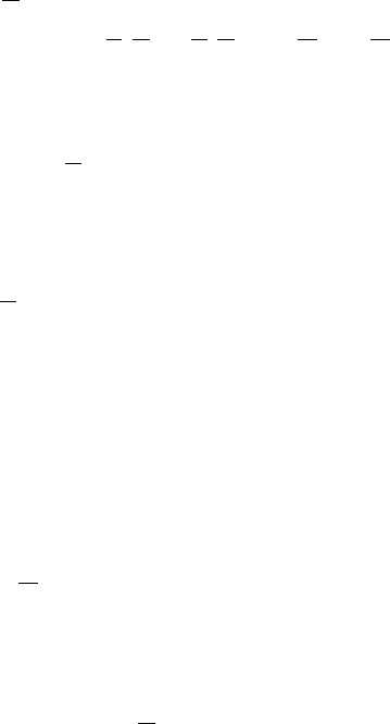
Figure 2: MSDSGE model, posterior mode estimates. Top panel, probability of regime 1
for the structural parameters, the Hawk regime; lower panel, probability of regime 1 for the
stochastic volatilities, high volatility regime.
Parameter
sp
t
= 1
sp
t
= 2
1
2:0651
(1:4054;2:6225)
0:6451
(0:4258;0:9189)
2
0:3212
(0:1744;0:5145)
0:2795
(0:1545;0:4188)
R
0:7919
(0:7296;0:8506)
0:7625
(0:6659;0:8375)
2:9227
(2:1497;3:8294)
0:0288
(0:0198;0:0374)
g
0:8359
(0:7962;0:8788)
z
0:8804
(0:8456;0:9182)
r
0:4552
(0:3459;0:5397)
0:8117
(0:6874;0:9374)
Parameter
er
= 1
er
= 2
R
0:3134
(0:2494;0:3872)
0:0763
(0:0623;0:0928)
g
0:3569
(0:2841;0:4532)
0:1494
(0:1156;0:1793)
z
1:9948
(1:3778;2:7163)
0:6292
(0:4563;0:8143)
y
0:0723
(0:0316;0:1526)
p
0:2968
(0:2632;0:3322)
r
0:0289
(0:0155;0:0470)
diag (H
sp
) diag (H
er
)
0:9254
(0:8237;0:9851)
0:8958
(0:8152;0:9564)
0:9162
(0:8322;0:9716)
0:9538
(0:9190;0:9802)
Table 1: Means and 90 percent error bands of the DSGE and transition matrix parameters
23
1955 1960 1965 1970 1975 1980 1985 1990 1995 2000 2005
0
5
10
15
Annualized quarterly Inflation
1955 1960 1965 1970 1975 1980 1985 1990 1995 2000 2005
-2
0
2
4
6
8
Real FFR
1955 1960 1965 1970 1975 1980 1985 1990 1995 2000 2005
-4
-2
0
2
4
6
Deviations of the FFR from TR values
DReg 1
DReg 2
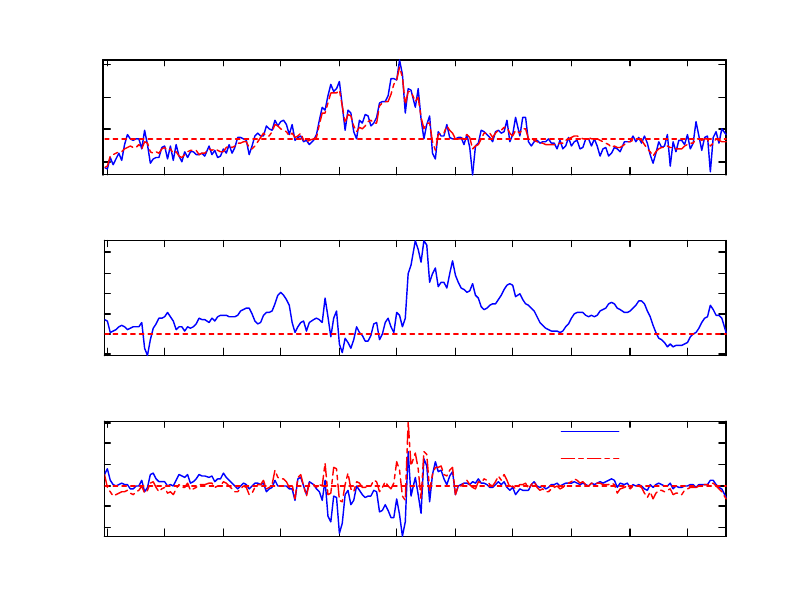
Figure 3: The top panel reports annualized quaterly in‡ation (observed and …ltered) and
the in‡ation target. The second panel contains the real FFR as implied by the model. The
last panel displays the di¤erences between the observed FFR and the ones implied by the
two alternative Taylor rules. Note how in the ’60s the interest rate was too high compared
to the one that would have prevailed if the Hawk regime had b een in place, while in the ’70s
the Hawk regime would have required a much higher interest rate.
The point estimate of the in‡ation target is 0.8117, implying a target for annual in‡ation
around 3:25%. The top panel of …gure 3 displays the series of quarterly annualized in‡a-
tion and the corresponding target/steady state value. There are some notable deviations,
especially during the ’60s and the ’70s.
As for the other parameters, I regard the low value of the slope of the Phillips curve
( = 0:0288) as particularly relevant, since such a small value implies a very high sacri…ce
ratio. In other words, in order to bring in‡ation down the Federal Reserve needs to generate
a severe recession.
Figure 2 shows the (smoothed) probabilities assigned to
sp
t
= 1 (top panel) and
er
t
= 1
(lower panel). Confronting these probabilities with narrative accounts of monetary policy
24

history is a way to understand how reasonable the results are. However, before proceeding,
a caveat is in order. In interpreting the probabilities assigned to the two regimes the reader
should take into account how these are related to the estimate of the in‡ation target. In
other words, a high probability assigned to the Dove regime does not automatically imply a
loose monetary policy, but only that the Fed is being relatively unresponsive to deviations
of in‡ation from the target. To facilitate the interpretation of the results, the third panel
of …gure 3 reports the di¤erence between the observed Federal Funds rate and the interest
rate that would be implied by the two Taylor rules. A large positive di¤erence between the
observed interest rate and its counterfactual value under regime 1 (DReg 1), implies that
the Fed is responding very strongly to in‡ation deviations, even under the assumption that
the Hawk regime is in place. On the other hand, a large negative value of this same variable
suggests that the Fed is not active enough.
Monetary policy turns out to be active during the early years of the sample, from 1955 to
1958, and with high probability during the following three years. Romer and Romer (2002)
provide narrative evidence in favor of the idea that the stance of the Fed toward in‡ation
during this period was substantially similar to that of the 90s. They also show that a
Taylor rule estimated over the sample 1952:1-1958:4 would imply determinacy. Furthermore,
after the presidential election of 1960, Richard Nixon blamed his defeat on excessively tight
monetary policy implemented by the Fed. At that time, Fed chairman Martin had clear
in mind that the goal of the Fed was "to take away the punch bowl just as the party gets
going", i.e. to raise interest rates in response to an overheated economy.
Over the period 1961-1965 the Dove regime was the rule. This should not be interpreted
as evidence of a lack of commitment to low in‡ation. In fact, the truth is exactly the
opposite. The Dove regime prevails because, given the target for in‡ation, the Hawk regime
would require lowering the FFR. The Hawk regime regains the lead over the last …ve years
of Martin’s chairmanship.
On February 1970, Arthur F. Burns was appointed chairman by Richard Nixon. Burns
is often regarded as responsible for the high and variable in‡ation that prevailed during the
’70s. It is commonly accepted that on several occasions he had to succumb to the requests
of the White House. In fact, for almost the entire duration of his mandate, the Fed followed
a passive Taylor rule. During these years, the Hawk regime would have required a much
higher monetary policy interest rate.
7
7
Here the use of the words active and passive follows Leeper (1991). Monetary policy is active when the
interest rate is highly responsive to in‡ation.
25
This long period of passive monetary policy ended in 1980, shortly after Paul Volcker
took o¢ ce in August 1979. Volcker was appointed with the precise goal of ending the
high in‡ation. The high probability of the Hawk regime during these years con…rms the
widespread belief that he delivered on his commitment.
The middle panel of …gure 3 contains the pattern of real interest rates as implied by the
model (computed as R
t
4 E
t
(
t+1
)). During Burns’chairmanship real interest rates were
negative or very close to zero, whereas, right after the appointment of Volcker, they suddenly
increased to unprecedented high values. During the following years, in‡ation started moving
down and the economy experienced a deep recession, while the Fed was still keeping the
FFR high. Note that the probability of the Dove regime from zero becomes slightly positive,
implying that, given the target for in‡ation, a lower FFR would have been desirable. In
other words, there is a non-zero probability, that Volcker set the FFR in a manner less
responsive to changes in in‡ation: Regardless of in‡ation being on a downward sloping path
and a severe recession, monetary policy was still remarkably tight.
For the remainder of the sample the Hawk regime has been the rule with a couple of
important exceptions. The …rst one occurred during the 1991 recession. In this case there
is no uncertainty regarding how the high probability assigned to the Dove regime should be
interpreted. On the other hand, the relatively high values for the probability of the Dove
regime during the second half of the 90s and toward the end of sample point toward a FFR
too high compared to what would be implied by the Hawk regime.
These results strongly support the idea that the appointment of Volcker marked a change
in Fed’s in‡ation stance and that the ’70s were characterized by a passive monetary policy
regime. At the same time, they question the wide spread-belief that US monetary policy
history can be described in terms of a permanent and one-time-only regime change: pre- and
post-Volcker. While a single regime prevails constantly during the chairmanships of Burns
and Volcker, the same cannot be said for the remainder of the sample.
Up to this point nothing has been said about the Good Luck hypothesis. Looking at the
second panel of …gure 2, it emerges that regime 1, characterized by large volatilities for all
shocks, prevails for a long period that go es from the early ’70s to 1985, with a break between
the two oil crises. This result is quite informative because 1984 is regarded as a turning
point in US economic history. There are two alternative ways to interpret this …nding. On
the one hand, even if a regime change occurred well before 1984, perhaps the conquest of
American in‡ation was actually determined by a break in the uncertainty characterizing
the macroeconomy. On the other hand, this same break might have occurred in response
26

to the renewed commitment of the Federal Reserve to a low and stable in‡ation. Both
interpretations require that the uncertainty characterizing the economy and the behavior of
the Fed are likely to be interdependent. Just as the Great In‡ation was characterized by high
volatilities and loose monetary policy, in a similar vein the Great Moderation emerged after
a reduction in the volatilities of the structural shocks and a drastic change in the conduct of
monetary policy.
Quite interestingly the probability of the high volatility regime rises again at the end of
the sample. To interpret this result, it might be useful to take a closer look at the third panel
of …gure 3. It cannot go unnoticed that in recent times both the Hawk and the Dove regime
would have required higher interest rates, implying that monetary policy has been relatively
loose.
8
This is not surprising, given that the Fed is currently dealing with a deep …nancial
crisis. However, should the Fed continue to deviate from standard monetary practice for a
long period of time, it would be fair to expect revisions in agents’beliefs.
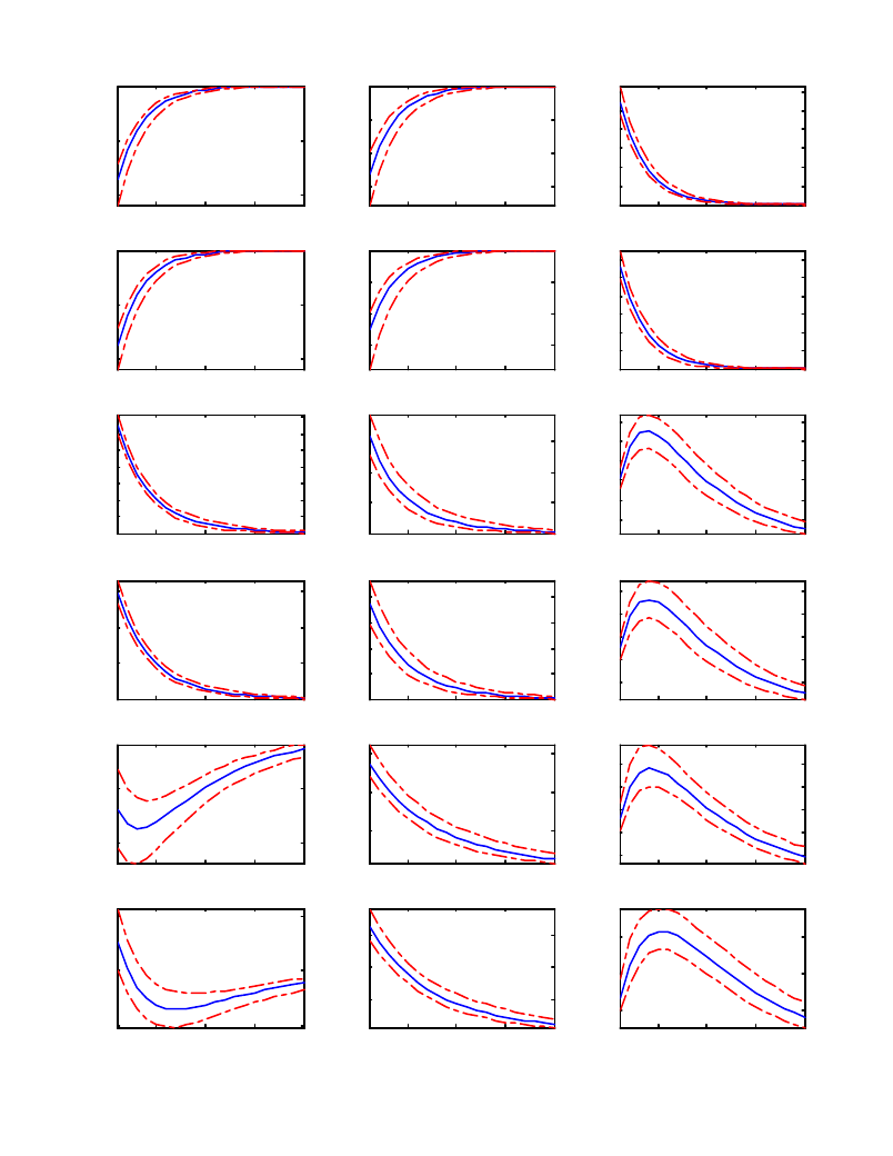
5.2 Impulse response analysis
The …rst two rows of …gure 4 show respectively the impulse responses to a monetary policy
shock under the Hawk and Dove regimes. The initial shock is equal to the standard deviation
of the monetary policy shock under regime 1, the high volatility regime. Both in‡ation and
output decrease following an increase in the FFR. The responses are remarkably similar
across the two regimes.
The third and the fourth rows illustrate the impulse responses to a demand shock. Output
and in‡ation increase under both regimes but their responses are stronger under the Dove
regime. This is consistent with the response of the Federal Funds rate that is larger under
the Hawk regime, both on impact and over time. Note that the dynamics of the variables are
otherwise similar across the two regimes. The Fed does not face any trade-o¤ when deciding
how to respond to a demand shock, therefore, the only di¤erence lies in the magnitude of
the response.
Finally, the last two rows contain the impulse responses to an adverse supply shock, i.e.
to an unexpected decrease in z
t
. This last set of results is particularly interesting given
that, as several economists would agree, one of the causes of the high in‡ation of the ’70s
was a series of unfavorable supply-side shocks. The behavior of the Federal Reserve di¤ers
substantially across the two regimes. Under the Hawk regime the Fed is willing to accept
8
This pattern is even more evident using the latest data.
27
5 10 15 20
-0.4
-0.2
R - Hawk
y
5 10 15 20
-0.4
-0.2
R - Dove
5 10 15 20
-0.15
-0.1
-0.05
p
5 10 15 20
-0.15
-0.1
-0.05
5 10 15 20
0.2
0.4
0.6
0.8
1
1.2
R
5 10 15 20
0.2
0.4
0.6
0.8
1
1.2
5 10 15 20
0.2
0.4
0.6
0.8
1
1.2
1.4
g - Hawk
5 10 15 20
0.5
1
1.5
g - Dove
5 10 15 20
0.2
0.4
0.6
5 10 15 20
0.2
0.4
0.6
0.8
5 10 15 20
0.2
0.4
0.6
0.8
1
1.2
5 10 15 20
0.2
0.4
0.6
0.8
1
5 10 15 20
-0.4
-0.2
z - Hawk
5 10 15 20
-0.2
0
0.2
z - Dove
5 10 15 20
0.5
1
1.5
5 10 15 20
0.5
1
1.5
5 10 15 20
0.2
0.4
0.6
0.8
1
5 10 15 20
0.2
0.4
0.6
Figure 4: Impulse response functions. The graph can b e divided in three blocks of two rows
each. The three blocks display respectively the impulse responses to a monetary policy shock
(R), a demand shock (g), and an adverse technology shock (z). For each block, the …rst row
shows the response of output gap, annualized quarterly in‡ation, and the FFR under the
Hawk regime, whereas the second one assumes that the Dove regime is in place.
28
a recession in order to contrast in‡ation. The Federal Funds rate reacts strongly on impact
and it keeps rising for one year. On the contrary, under the Dove regime the response of the
policy rate is much weaker because the Fed tries to keep the output gap around zero, at the
cost of higher in‡ation. Note that on impact the economy experiences a boom: the increase
in expected in‡ation determines a negative real interest rate that boosts the economy in the
short run.
Three considerations are in order. First, it is quite evident that the gains in terms of
lower in‡ation achieved under the Hawk regime are modest. This can be explained in light
of the low value of , the slope of the Phillips curve. Second, under the Dove regime the
Fed is not able to avoid a recession, but the recession turns out to be signi…cantly milder.
Third, it is commonly accepted that the ’70s were characterized by important supply shocks.
At the same time, the results of the previous section show that the Dove regime has been
in place for a large part of those years. Therefore, it might well be that in those years a
dovish monetary p olicy was perceived as optimal in consideration of the particular kind of
shocks hitting the economy. This seems plausible especially if the Fed was regarding the
sacri…ce ratio as particularly high, as suggested by Primiceri (2006). However, to explore
this argument more in detail the probability of moving across regimes should be endogenized
(Davig and Leeper (2006a)). This extension would further complicate the model, especially
for what concerns the solution algorithm. I regard it as a fascinating area for future research.
5.3 Counterfactual analysis
An interesting exercise when working with models that allow for regime changes consists of
simulating what would have happened if regime changes had not occurred, or had occurred at
di¤erent points in time, or had occurred when they otherwise did not. This kind of analysis
is even more meaningful in the context of the MS-DSGE model employed in this paper. First
of all, like a standard DSGE model, the MS-DSGE can be re-solved for alternative policy
rules to address the e¤ects of fundamental changes in the policy regime. The entire law of
motion changes in a way that is consistent with the new assumptions around the behavior
of the monetary policy authority. Furthermore, the solution depends also on the transition
matrix used by agents when forming expectations and on the nature the of alternative
regimes. Therefore, we can investigate what would have happened if agents’beliefs about
the probability of moving across regimes had been di¤erent. This has important implications
for counterfactual simulations in which a regime is assumed to have been in place throughout
29

the sample because the expectation mechanism and the law of motion are consistent with
the fact that no other regime would have been observed. Finally, it is also possible to
conduct counterfactual simulations in which agents are endowed with beliefs about regimes
that never occurred and that will never occur, but that could have important e¤ects on the
dynamics of the variables. An example that I will be explore concerns the appointment of
a very conservative Chairman whose behavior can be described by a remarkably hawkish
Taylor rule. This particular kind of counterfactual analysis is not possible in the context of
time-varying VAR models like the ones used by Primiceri (2005), Cogley and Sargent (2006),
and Sims and Zha (2006).
Two main conclusions can be drawn according to the results of this section. First, little
would have changed for the dynamics of in‡ation if the Hawk regime had been in place
through the entire sample or if agents had put a large probability on going back to it.
According to the results shown below, the only way to avoid high in‡ation would have been
to cause a long and deep recession. The reason is quite simple: The model attributes the
large increase in in‡ation to a technological slowdown that was not under the direct control
of the Fed. Second, if agents had put a large enough probability on the occurrence of an even
more hawkish regime, in‡ation would have not reached peaks as high as the ones observed
in the late ’70s. Furthermore, the cost of keeping in‡ation low would have been smaller with
respect to the counterfactual hypothesis of the Hawk regime being in place over the entire
sample, suggesting that expectations around alternative regimes can have important e¤ects
on the behavior of the economy. Considering that the Volcker era was characterized by a
remarkably hawkish monetary policy, we might want to rephrase this result in a suggestive
way: If agents had anticipated the appointment of Volcker, the Great In‡ation would have
been a much less spectacular phenomenon.
5.3.1 No Monetary Policy Shocks
The …rst set of counterfactual series is obtained by shutting down the monetary policy
shocks. For each draw from the posterior the disturbance in the Taylor rule is set to zero
independently from the regime in place. The parameters of the model, the sequence for the
monetary policy regimes, and the remaining disturbances are left unchanged. Therefore, if
the policy rule disturbances had not been set to zero, the simulations would have coincided
with the actual series.
Figure 5 shows the actual and counterfactual series.
9
The path for in‡ation is virtually
9
For clarity, the …gures report only the median of the counterfactual series. Analogous graphs endowed
30
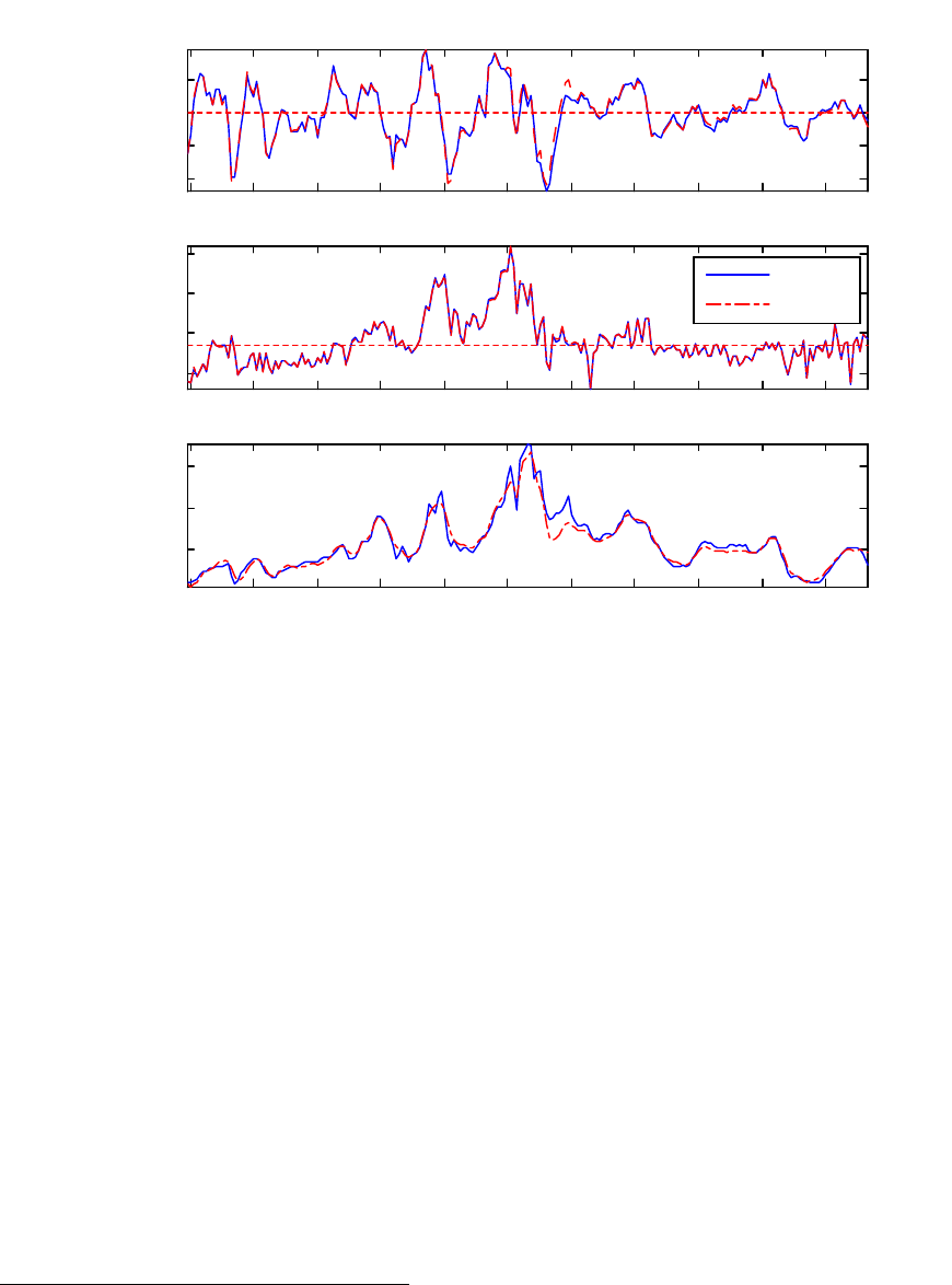
1955 1960 1965 1970 1975 1980 1985 1990 1995 2000 2005
-4
-2
0
2
y gap
No monetary policy shocks
1955 1960 1965 1970 1975 1980 1985 1990 1995 2000 2005
0
5
10
15
Inflation
Actual
Counterf
1955 1960 1965 1970 1975 1980 1985 1990 1995 2000 2005
5
10
15
FFR
Figure 5: Counterfactual simulation obtained setting the Taylor rule distrurbances to zero.
identical to the observed one. Deviations can be detected in the series for the output gap,
but they are negligible. Interestingly, the FFR would have been lower around the years 1983-
1984, suggesting that during those years monetary policy was extremely tight, even under
the assumption that the Hawk regime was in place. This result corroborates the …ndings of
section 5.1: To some extent Volcker made monetary policy less responsive to in‡ation. Note
that this is in line with the intent of building credibility for a renewed commitment to low
and stable in‡ation.
5.3.2 A Fixed Hawk regime
Figure 6 shows the results for the counterfactual simulations obtained by imposing the Hawk
regime over the entire sample. To make the results consistent with this assumption, the
model is solved assuming that agents regard the Hawk regime as the only possible one. In
with error bands can be found in appendix C.
31
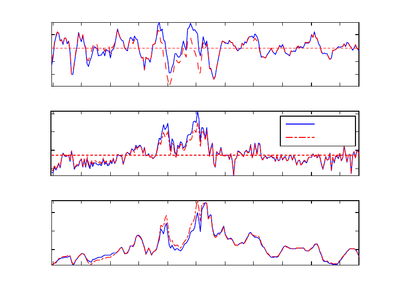
1955 1960 1965 1970 1975 1980 1985 1990 1995 2000 2005
-4
-2
0
2
y gap
Hawk always in place (FC)
1955 1960 1965 1970 1975 1980 1985 1990 1995 2000 2005
0
5
10
15
Inflation
Actual
Counterf
1955 1960 1965 1970 1975 1980 1985 1990 1995 2000 2005
5
10
15
FFR
Figure 6: Counterfactual simulation based on the Hawk regime being in place over the
entire sample. Consistently with this hypothesis, the solution is obtained assuming that
agents regard the Hawk regime as the only possible one.
other words, I solve a …xed coe¢ cient DSGE in which the behavior of the Fed is described
by the Hawk regime parameters. It is apparent that the Fed would not have been able
to completely avoid the rise in in‡ation, but only to partially contain it, at the cost of
a substantial and prolonged loss in terms of output. In particular, annualized quarterly
in‡ation would not have reached a peak as high as 15%, like it did in the …rst half of 1980.
During the mid-60s, output would have been slightly larger. This is in line with the …nding
that during those years monetary policy was too tight given a target for in‡ation around
3%. On the other hand, output would have been lower during the ’91 recession. However,
these di¤erences are not signi…cant, given that the 90% error bands for the counterfactual
series contain the actual ones.
Summarizing, the model does not attribute the rise in‡ation to changes in the conduct
of monetary policy. It seems that the Fed could have partially contained the rise of in‡ation
32
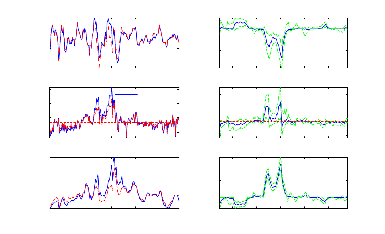
1960 1970 1980 1990 2000
-4
-2
0
2
y gap
Eagle behind the scenes - NMP
1960 1970 1980 1990 2000
0
5
10
15
Inflation
1960 1970 1980 1990 2000
5
10
15
FFR
1960 1970 1980 1990 2000
-1.5
-1
-0.5
0
0.5
Comparison with Hawk FC
1960 1970 1980 1990 2000
-0.5
0
0.5
1
1960 1970 1980 1990 2000
-2
0
2
4
6
8
Actual
Count.
Figure 7: Counterfactual simulation based on having a regime, the Eagle regime, that is
behind the scenes when the Dove regime is in place, but it never occurres.
causing a deep recession. Moreover, while the loss in terms of output would have been certain
and large, the gain in terms of in‡ation seems quite modest. This has to do with the …nding
that the high in‡ation was driven by a series of shocks on which the Fed had little, if any,
control.
5.3.3 An Eagle behind the scenes
From what has been shown so far it seems that no reduction in in‡ation could have been
achieved without a substantial output loss. However, the role of agents’beliefs about al-
ternative monetary policy regimes has not been explored yet. The simple and intriguing
exercise conducted in this section asks what would have happened if during the high in‡a-
tion of the ’70s agents had put a relatively large probability on the appointment of a very
conservative Chairman, willing to …ght in‡ation without any real concern for the state of
the real economy. I shall label this hypothetical third scenario Eagle regime. The Eagle
regime di¤ers from the Hawk regime in terms of the response to in‡ation, that is assumed
to be twice as large, and to output, that is halved. Note that this implies a strong response
to deviations of in‡ation from the target and makes the role of output gap secondary. The
33

Eagle regime never occurs over the sample, but I assume that when agents observe the Dove
regime, they regard the Eagle regime as the alternative scenario and they put a relatively
large probability on its occurrence. To that end, the probability of staying in the Dove
regime is reduced by 30 percent. The probability of staying in the Eagle regime is equal
to the persistence of the Hawk regime. From the Eagle regime the economy can move only
to the Hawk regime. These assumptions imply an interesting interpretation of the Eagle
regime: It is a regime that occurs with high probability after a period of passive monetary
policy in order to restore credibility, leading the way to the ordinary active regime.
10
The left column of …gure 7 contains the actual and counterfactual series. The results for
in‡ation look somehow similar to the ones obtained in the previous section. However, there
are some notable di¤erences for the output gap and the Federal Funds rate. The former
turns out to b e larger, while the latter is remarkably lower over the second half of the ’70s,
the years during which the Dove/Eagle regime prevails. To make this point stronger, the
right column of …gure 5 displays, for each series, the di¤erence b etween the Hawk- and the
Eagle- counterfactual. It turns out that the threat of the Eagle regime is enough to deliver
the same, if not b etter, results in terms of low in‡ation, with a substantial reduction in the
output loss. Note that all the results are driven by the high probability that agents assign
to the Eagle regime. The FFR is low not only because in‡ation is relatively low, but also
because agents are anticipating the possibility of extremely tight monetary policy.
The goal of this exercise is not to propose a new way to conduct monetary policy: Main-
tain loose policy today while trying to persuade the public that you are going to be extremely
active in the future. This kind of strategy clearly presents a problem of credibility. However,
two lessons can be learned from this experiment. First, it is quite possible that the problem
in the ’70s was not that the Fed was not reacting strongly enough to in‡ation, but that there
was a lack of con…dence around the possibility of a substantial change in the conduct of
monetary policy. In general, this exercise suggests that the alternative scenarios that agents
have in mind are at least as important as the regime that is in place.
5.3.4 An Eagle on stage
The …nal counterfactual simulation replaces the Hawk regime with the Eagle regime de-
scribed in the previous section. Even in this case, the transition matrix is twisted: The
probability of staying in the active regime is kept unchanged, while the persistence of the
10
Ideally, it would be nice to make the probability of moving to the Eagle regime endogenous, but the
algorithm used to solve the mod el is based on the assumption that the transition matrix is exogenous.
34
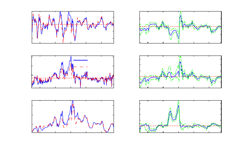
1960 1970 1980 1990 2000
-4
-2
0
2
y gap
Eagle on stage - NMP
1960 1970 1980 1990 2000
0
5
10
15
Inflation
Actual
Count.
1960 1970 1980 1990 2000
5
10
15
FFR
1960 1970 1980 1990 2000
-2
-1
0
1
Comparison with Hawk FC
1960 1970 1980 1990 2000
-0.5
0
0.5
1
1.5
1960 1970 1980 1990 2000
-2
0
2
4
6
8
Figure 8: Counterfactual simulation in which the Hawk regime is replaced with the Eagle
regime, i.e. a regime in which the response to in‡ation is two times larger, whereas the
response to output is half as large. The transition matrix is twisted: the probability of the
active regime is decreased by 30%.
passive regime is lowered by 30 percent.
The left column of …gure 8 contains the counterfactual and actual series. Note how
in‡ation and output would have been lower during the ’70s, without substantial increases in
the FFR. Even in this case the result is driven largely by the expectation mechanism. Then,
in the early ’80s the Eagle regime becomes e¤ective and we observe a jump in the FFR and
a further reduction in in‡ation. Quite interestingly, during the early ’80s, the path for the
FFR is hardly distinguishable from the actual one, suggesting that the Eagle regime does
a good in job in replicating the behavior of the Federal Reserve during the early years of
Volcker’s chairmanship.
How do these outcomes di¤er from the case in which the Hawk regime is assumed to be in
place throughout the sample? The right column of …gure 8 compares the two counterfactual
simulations. If the Hawk regime had been replaced by the Eagle regime, in‡ation would
have been lower and the slowdown of the early ’80s more abrupt. However, it is not clear
if the …nal cost in terms of output would have been di¤erent: Output is lower in the early
’80s, but it is higher in the second half of the ’70s, when the Dove regime is in place. In
35
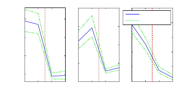
1 2 3 4
1
1.5
2
2.5
Output
1 2 3 4
1
2
3
4
5
Inflation
1 2 3 4
1
2
3
4
5
6
FFR
Median
68% Er bands
Figure 9: Analytical standard deviations of the macroeconomic variables for di¤erent regime
combinations (1 ![High volatility, Hawk], 2 ![High, Dove], 3 ![Low, Hawk], and 1 ![Low,
Dove]).
fact, it seems that the gains and costs are likely to cancel out. Therefore, the Eagle-Dove
combination could be preferable, given that it delivers lower in‡ation with a similar cost in
terms of lower output. The last two counterfactual simulations point toward an important
conclusion: If a Central Bank were able to commit to a ‡exible in‡ation targeting, in which
severe shocks are temporarily accommodated and followed by a strong commitment to bring
the economy back to the steady state, then it would be possible to achieve low in‡ation with
a substantially smaller cost in terms of output. In other words, the e¤ective sacri…ce ratio
would be much smaller. Admittedly, this kind of policy is not readily practicable. Among
other things, the duration of the passive regime matters a lot. When supply-side shocks are
large and persistent, like they were in the ’70s, if the Central Bank decides to implement a
dovish monetary policy, agents are likely to be discouraged about the possibility of moving
back to an active regime. In this context, there is not any immediate way to persuade them
that a regime change is around the corner.
5.4 Variance decomposition
In this section, I compute the contributions of the structural shocks to the volatility of the
macroeconomic variables for all possible combinations of the monetary policy and volatility
regimes. It is well known that high in‡ation is often associated with high volatility. This was
36
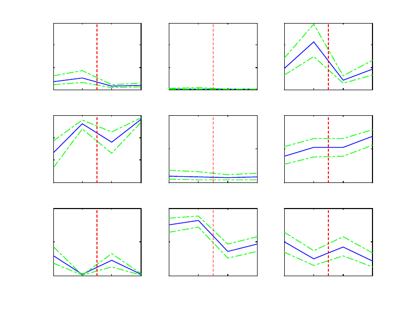
1 2 3 4
0
0.1
0.2
Output
R
1 2 3 4
0
0.1
0.2
Inflation
1 2 3 4
0
0.1
0.2
FFR
1 2 3 4
0.4
0.6
0.8
1
g
1 2 3 4
0
0.5
1
1 2 3 4
0
0.5
1
1 2 3 4
0
0.5
1
z
1 2 3 4
0
0.5
1
1 2 3 4
0
0.5
1
Figure 10: Contributions of the di¤erent structural shocks to the volatility of the macroeco-
nomic variables for di¤erent regime combinations (1 ![High volatility, Hawk], 2 ![High,
Dove], 3 ![Low, Hawk], and 1 ![Low, Dove]). The graph reports the median and the 68%
error bands.
37

surely the case in the ’70s. This exercise will help us understand what would have changed
if the Hawk regime had been in place during those years.
Consider the model in state space form (21)-(25). For each draw of the Gibbs sampling
algorithm we can compute the conditional covariance matrix as implied by the di¤erent
regime combinations (
sp
;
er
):
11
V (S
t
j) = T (
sp
t
)V (S
t
j) T (
sp
t
)
0
+ R(
sp
t
)Q (
er
) R(
sp
t
)
0
V (Y
t
j) = ZV (S
t
j
sp
;
er
;
sp
t
;
er
t
; H
m
) Z
0
+ U
where for each variable x
t
, V (x
t
j) stands for V (x
t
j
sp
;
er
;
sp
t
;
er
t
; H
m
) and V (S
t
j) is ob-
tained solving the discrete Lyapunov equation. The contribution of the shock i is obtained
replacing Q (
er
) with Q
i
(
er
) ; a diagonal matrix in which the only element di¤erent from
zero is the one corresponding to the variance of the shock i under regime
er
.
Figure 9 plots the analytical standard deviations for the three macroeconomic variables.
The …rst two values, on the left of the red dashed line, refer to the high volatility regime,
while the third and the fourth values assume that the low volatility regime is in place. In each
sub-group, the …rst point marks the standard deviation under the Hawk regime. It is evident
that the overall volatility is largely determined by the variance of the underlying structural
shocks: Moving from the left to the right side of the dashed line implies a remarkable
reduction in the volatility of all macroeconomic variables. Not surprisingly, being in the
Dove regime implies higher in‡ation volatility, but the di¤erence is not statistically relevant.
Figure 10 presents the variance decomposition for the four p ossible regime combinations.
It is quite evident that for in‡ation the monetary policy regime does not really matter: A
large fraction of volatility comes from the supply shocks independent of the behavior of
the Federal Reserve. Furthermore, monetary policy shocks play a marginal role. On the
other hand, the monetary policy regime is de…nitely important in explaining the volatility of
output. Demand shocks account for almost the entire output volatility when the Dove regime
is in place. More importantly, supply shocks are relevant only under the Hawk regime. Under
the Hawk-high volatility combination, supply shocks explain around 30% of output volatility,
while when the Dove regime is in place, their contribution is basically null, independent of
the volatility of the supply shock. This result is quite interesting and in line with the impulse
response analysis of the section 5.2. Under the Dove regime, the Fed accommodates supply
11
Here the term "conditional" refers to the regime combination. Note that in fact I am computing an
unconditional variance using the law of motion implied by a particular regime combination.
38
shocks in order to minimize output ‡uctuations. This seems to accurately describe what was
going on in the ’70s. As for the FFR, the volatility is largely determined by the systematic
component of the Taylor rule. Obviously, under the Hawk regime monetary policy shocks
explain a smaller fraction of the FFR volatility, given that the Fed has a stronger incentive
to bring the economy back on track.
6 Alternative speci…cations
In this section I consider two alternative speci…cations to capture alternative explanations
of the macroeconomic dynamics observed over the last …fty years.
6.1 Just Good Luck (Constant structural parameters)
A natural alternative to the benchmark speci…cation is represented by a model that allows
for heteroskedasticity but assumes no change at all in the behavior of the Federal Reserve.
Such a model would explain the Great Moderation invoking Good Luck, i.e. a substantial
reduction in the volatility of macroeconomic shocks. Table 2 reports posterior mode estimates
and 90% error bands for the DSGE parameters and the transition matrices, while …gure 11
plots the probability of regime 1 (
er
= 1). Once again, regime 1 is the low volatility regime.
It prevails around 1958 and between 1970 and 1985, with a break between the two oil crises.
Even the estimates of the volatilities are remarkably similar to the ones obtained under the
benchmark case.
As for the structural parameters, the response to in‡ation turns out to b e modest but
larger than 1, while the output gap coe¢ cient and the level of interest rate smoothing are
relatively large. Moreover, the steady state real interest rate and the target for in‡ation
are substantially una¤ected. The p oint estimates for the autocorrelation parameters of the
shocks are also very close to the ones obtained in the benchmark model, while the degree of
interest smoothing is somehow larger. The remaining structural parameters are substantially
unchanged when compared with the estimates obtained under the benchmark speci…cation.
In particular, the slope of the Phillips curve is still remarkably low, implying a very high
sacri…ce ratio.
39
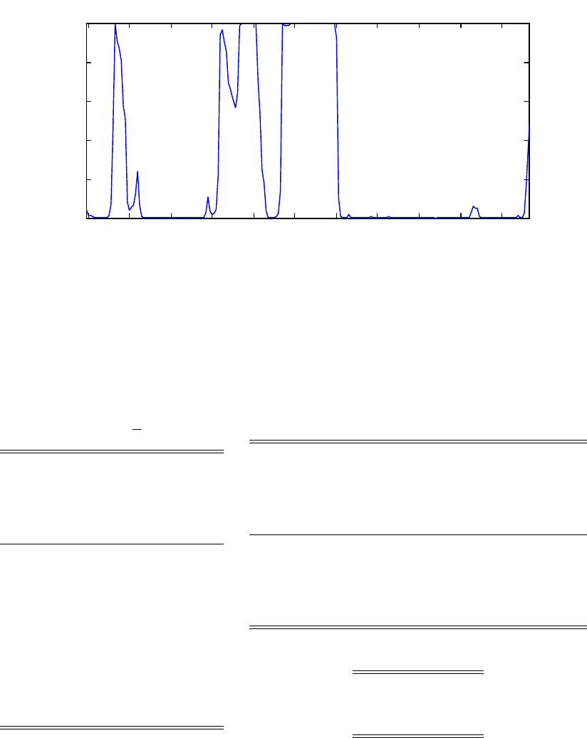
1955 1960 1965 1970 1975 1980 1985 1990 1995 2000 2005
0.2
0.4
0.6
0.8
1
Stochastic volatilities - prob regime 1
Figure 11: Posterior mode estimates: Probability of regime 1 (high volatility)
Parameter
sp
t
= 1
1
1:1710
(1:0156;1:3838)
2
0:4071
(0:3009;0:5332)
R
0:8380
(0:8045;0:8688)
3:0374
(2:2075;3:9877)
0:0289
(0:0183;0:0423)
g
0:8347
(0:7930;0:8746)
z
0:9005
(0:8630;0:9338)
r
0:4232
(0:3334;0:5117)
0:8065
(0:6475;0:9649)
Parameter
er
= 1
er
= 2
R
0:3674
(0:3085;0:4384)
0:0974
(0:0851;0:1110)
g
0:3716
(0:2853;0:4817)
0:1605
(0:1300;0:1959)
z
1:7961
(1:0941;2:6905)
0:5916
(0:3871;0:836)
y
0:0623
(0:0314;0:1143)
p
0:2782
(0:2439;0:3152)
r
0:0290
(0:0149;0:0523)
diag (H
er
)
0:8869
(0:8094;0:9222)
0:9555
(0:9490;0:9808)
Table 2: Posterior mode estimates of DSGE parameters and transition matrices
40

6.2 One-time-only switch
In their seminal contribution Lubik and Schorfheide (2004) consider a model analogous to
the one employed in this paper extending the solution for the case of indeterminacy. They
construct posterior weights for the determinacy and indeterminacy region of the parameter
space and estimates for the propagation of fundamental and sunspot shocks. According to
their results, U.S. monetary policy post-1982 is consistent with determinacy, whereas the
pre-Volcker policy is not.
Here I consider a speci…cation that is in the same spirit but with some important mod-
i…cations. First, I do not impose a turning date. I let the data decide when the regime
change occurred using a Markov-switching model with an absorbing state. Second, I con-
sider a larger sample, spanning the entire WWII postwar era (1954:IV-2008:I). On the other
hand, in line with the authors, I assume that: 1) There is only one regime change 2) The
regime change is once-for-all and fully credible
12
3) All parameters of the model are allowed
to change. This last assumption allows the steady levels to change across regimes. I im-
pose that regime 1 implies indeterminacy and I use the results of Lubik and Schorfheide
(2004) to compute the likelihood under this hypothesis. The solution under indeterminacy
is characterized by some additional parameters.
Table 3 contains the parameter estimates. The change across regimes is somehow more
extreme than the one found by Lubik and Schorfheide (2004) and suggested by the results of
the MS-DSGE model. The response to in‡ation jumps from 0:7191 to 2:4644 while the target
for (annualized) in‡ation decreases from 4:24 to 3:09. Along the same lines, the response to
output gap is substantially reduced: from 0:45 to 0:18. Furthermore, the slope of the Phillips
curve is remarkably larger under the current regime (0:0953 and 0:4067). The values of the
other structural parameters of the model do not present dramatic changes across regimes
and are also quite similar to the ones obtained under the previous speci…cations.
The time of the change is quite interesting. Figure 12 plots the probability of regime 2,
the current regime. This probability does not start moving before 1982 and hits 1 in 1985. In
section 4.1 the MS-DSGE picked up with remarkable precision the appointment of Volcker.
Here, the regime change seems to occur several years later. This shows a potential advantage
of the benchmark model that allows volatilities and monetary policy rules to evolve according
to two independent chains. The MS-DSGE model seems to be able to recognize when the
change in the intents of the Fed occurred, even if the control over in‡ation and the break in
12
An alternative approach would consist of using the solution algorithm of FWZ imposing an absorbing
state.
41

the volatility of the shocks took place only some years later.
7 Model comparison
Di¤erent speci…cations provide competing explanations regarding the causes of the Great
Moderation. In this section I compute the marginal data density for the di¤erent mod-
els. This is the most sensible way to determine which of them returns the most accurate
description of the data.
Bayesian model comparison is based on the posterior odds ratio:
P (M
i
jY
T
)
P (M
j
jY
T
)
=
P (Y
T
jM
i
)
P (Y
T
jM
j
)
P (M
i
)
P (M
j
)
The second term on the RHS is the prior odds ratio, i.e. the relative probability assigned
to the two models before observing the data, while the …rst term is the Bayes factor, the ratio
of marginal likelihoods. Assuming that all models are regarded as equally likely a priori, the
Bayes factor is all we need to conduct model comparison.
Let be a (k 1) vector containing all the parameters of model M
i
. Moreover denote
the likelihood function and the prior density by p(Y
T
j) and p() respectively. The marginal
data density is given by:
p(Y
T
) =
Z
p(Y
T
j)p()d (26)
The modi…ed harmonic mean (MHM) method of Gelfand and Dey (1994) can be used to
approximate (26) numerically. This method is based on the following result:
p(Y
T
)
1
=
Z
h()
p(Y
T
j)p()
p(jY
T
)d (27)
where is the support of the posterior probability density. The weighting function h() is
a probability density whose support is contained in : A numerical approximation of the
integral on the right hand side of (27) can be obtained by montecarlo integration:
bp(Y
T
)
1
=
1
N
N
X
i=1
m
i
m
i
=
h(
i
)
p(Y
T
j
i
; M
i
)p(
i
)
42

1955 1960 1965 1970 1975 1980 1985 1990 1995 2000 2005
0.2
0.4
0.6
0.8
1
Probability of regime 2
Figure 12: Lubik and Schorfheide speci…cation,
Parameter
sp
t
= 1
sp
t
= 2
1
0:6472
(0:3915;0:8741)
3:0000
(2:1296;4:0286)
2
0:5574
(0:3351;0:8092)
0:1704
(0:0499;0:3404)
R
0:8716
(0:8192;0:9124)
0:7855
(0:6874;0:8552)
2:3999
(1:7044;3:1923)
1:8087
(1:1561;2:5997)
0:0953
(0:0502;0:1654)
0:4067
(0:1483;0:7387)
g
0:8002
(0:7124;0:8753)
0:8918
(0:8461;0:93371)
z
0:7655
(0:6820;0:8333)
0:8222
(0:7556;0:8783)
r
0:4466
(0:2785;0:6262)
0:4684
(0:3133;0:6556)
0:8446
(0:6207;1:0860)
0:7443
(0:6470;0:8435)
Parameter
er
= 1
er
= 2
R
0:2470
(0:2211;0:2785)
0:0876
(0:0658;0:1180)
g
0:2626
(0:1780;0:3663)
0:1345
(0:1054;0:1694)
z
2:0845
(1:4473;2:9247)
0:4343
(0:3717;0:5096)
gz
0:4817
(0:2952;0:6914)
0:6756
(0:4026;0:5096)
0:0564
(0:0178;0:1218)
M
r
1:8032
(0:9258;2:7096)
M
g
0:7705
(0:3687;1:0948)
M
z
0:1966
(1:1046;0:1421)
y
0:0607
(0:0307;0:1184)
p
0:4023
(0:3638;0:4469)
r
0:0316
(0:0152;0:0540)
Table 3: Posterior mode estimates of DSGE parameters and transition matrices
43
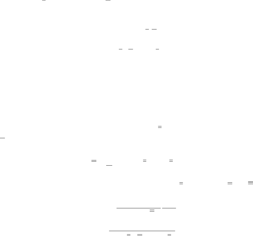
where
i
is the ith draw from the posterior distribution of p(jY
T
). As long as m () is
bounded above the montecarlo approximation converges at a reasonable rate.
Geweke (1999) suggests an implementation based on the posterior simulator. The weight-
ing function h() is a truncated multivariate Gaussian density.
The mean and the covariance are obtained from the posterior simulator. To ensure
the boundness condition, choose p 2 (0; 1) and take
h() = p
1
N
; ;
I
b
M
b
M
=
n
:
0
1
2
1p
(k)
o
where I
b
M
is an indicator function that is equal to one when 2
b
M
. If
b
M
, the
domain of integration needs to be rede…ned as
b
M
\ .
Sims et al. (2008) point out that while the approach proposed by Geweke works generally
well when dealing with …xed coe¢ cients models, problems can arise when it is applied to
Markov-switching models. When allowing for time variation of the parameters the posterior
tends to be Non-Gaussian. Therefore, they suggest replacing the Gaussian distribution with
elliptical distributions centered at the p osterior mode, . Then, the sample covariance matrix
is replaced with:
=
1
N
N
X
i=1
i
i
0
The density form of an elliptical distribution centered at and scaled by S =
p
is
g () =
(k=2)
2
k=2
det
S
f (r)
r
k1
where k is the dimension of , r =
r
i
0
1
i
, and f() is any one-dimensional
density de…ned on the positive reals. Sims et al. (2008) explain how to draw from the
elliptical distribution. In what follows I report the results based on this second method.
Table 4 reports the log marginal data density for di¤etent values of p. A smaller value of
p implies a better behavior of m () over the domain
b
M
, but also a greater simulation error
due to a smaller number of draws
i
2
b
M
. The best performing model coincides with the
benchmark speci…cation in which the Taylor rule parameters are allowed to switch across
44

Model p = 0:1 p = 0:3 p = 0:5 p = 0:7
MS T.R.+heter.+ind H
m
2; 385:9 2; 384:6 2; 383:7 2; 383:2
MS T.R.+heter. 2; 385:4 2; 383:3 2; 381:8 2; 380:6
Fixed parameters+heter. 2; 376:1 2; 375:8 2; 375:6 2; 375:4
One-time-only switch 2; 243:9 2; 243:5 2; 242:7 2; 241:9
Table 4: Marginal data density (log)
regimes. I consider two versions of this model. In one case agents are assumed to know the
transition matrix observed ex-post by the econometrician (H
m
= H
sp
), while in the other the
two matrices are allowed to di¤er. The second speci…cation returns slightly better results.
The third and fourth models correspond respectively to the "Just Good Luck" and "Just
Good Policy" speci…cations. Quite interestingly, the former dominates the latter. This result
suggests that there are important gains from allowing for heteroskedastic disturbances.
8 Conclusions
Many economists like to think about US monetary policy history in terms of pre- and post-
Volcker. The underlying idea is that since the Volcker disin‡ation the Fed has acquired a
better understanding of how to manage the economy and provide a stable and reliable anchor
for agents expectations.
This paper has shown that in fact the appointment of Volcker came with a substantial
change in the conduct of monetary policy, with the Fed moving from a passive to an active
regime. However, the assumption that this represented an unprecedented and once-and-for-
all regime change turns out to be misleading.
According to a Markov-switching model in which agents form expectations taking into
account the possibility of regime changes, the Fed has moved back and forth between a Hawk
and a Dove regime. Under the Hawk regime the Fed reacts strongly to deviations of in‡ation
from the target, while under the Dove regime output stability turns out to be at least equally
important.
The two regimes have very di¤erent implications for the dynamics of the economy. In
particular, given an adverse technology shock, the Fed is willing to cause a large recession
to contrast in‡ation only under the Hawk regime.
The ’70s were surely dominated by the Dove regime, with the Fed trying to minimize
output losses. However, this is not enough to explain the rise in in‡ation that occurred
45
in those years. In fact, little would have changed if the Hawk regime had been in place
over the entire sample: In‡ation would have been slightly lower, but with important losses
in terms of output. Furthermore, the estimates support the idea that a break in the shock
volatilities has a role in explaining the remarkable economic stability of recent years, whereas
uncertainty was much higher in the ’70s.
The paper then explored the role of agents’beliefs around the behavior of the monetary
authority. Through counterfactual simulations, I have shown that if agents had put a large
probability on the appointment of an extremely conservative Chairman, in‡ation would not
have reached the peaks of the late ’70s-early ’80s. Moreover, the cost in terms of lower output
would have been relatively low compared to the case in which the Hawk regime is assumed
to be in place over the entire sample. Therefore, it seems that the main problem in the ’70s
was a lack of con…dence in the possibility of quickly moving back to an active regime. If
agents had anticipated the appointment of Volcker, the Great In‡ation would have been a
less extreme event.
These results imply that there could be important gains in terms of low in‡ation and
stable output from committing to a ‡exible in‡ation targeting regime. In such a regime the
Fed would accommodate those shocks that would otherwise have pervasive e¤ects on the
economy. At the same time, once the shocks are gone, there should be a clear commitment
to generate a recession large enough to bring the economy back to equilibrium. Compared
to the case in which the Fed simply follows a hawkish regime, the …nal disin‡ation can be
more painful, but the cumulative cost is likely to b e smaller.
Even if the US did not enter an absorbing state, there is some hope that events like the
Great In‡ation will not occur again. Not because the Fed is likely to behave di¤erently on
impact, but because agents have now seen what follows a period of loose monetary policy.
Obviously, this is an optimistic view. First of all, it is not clear to what extent agents
learn from the past. More importantly, the probabilities attached to the di¤erent regimes
are likely to depend on the persistence of the shocks. Policy makers should avoid trying
to accommodate those shocks that are likely to persist for a long time because this would
determine a change in the probabilities that agents attach to the di¤erent regimes. These
considerations seem particularly relevant in light of the recent economic turmoil. In the past
year, the Federal Reserve has dealt with a pervasive and severe …nancial crisis. This led
to substantial deviations from common monetary policy practice, and monetary policy has
been remarkably loose. In light of the results of this paper, this deviation does not represent
a problem as long as agents do not revise their beliefs. Paraphrasing Leeper and Zha (2003),
46
modest regime changes are going to be well received, while long-lasting ones will trigger a
learning mechanism involving agents’expectations.
47
References
Bernanke, B. S. and I. Mihov, 1998, Measuring Monetary Policy, Quarterly Journal of Eco-
nomics 113(3), 862–902.
Bikbov, R., 2008, Monetary Policy Regimes and The Term Structure of Interest Rates,
Columbia Business School.
Boivin, J. and M. Giannoni, 2008, Optimal Monetary Policy in a Data-Rich Environment,
HEC and Columbia Business School.
Canova, Fabio and Luca Gambetti, 2004, On the Time Variations of US Mone-
tary Policy: Who is right?, Money Macro and Finance (MMF) Research Group
Conference 2004 96, Money Macro and Finance Research Group. available at
http://ideas.repec.org/p/mmf/mmfc04/96.html.
Carter, C. and P. Kohn, 1994, On Gibbs sampling for state space models, Biometrika 81, 541–
553.
Castelnuovo, E., L.G. Greco and D. Raggi, 2008, Time-Varying Targets and Policy Regimes:
An Empirical Investigation for the U.S., University of Padua, mimeo.
Clarida, R., J. Gali and M. Gertler, 2000, Monetary policy rules and macroeconomic stability:
evidence and some theory, Quarterly Journal of Economics 115, 147–180.
Cogley, T. and T. J. Sargent, 2006, Drifts and Volatilities: Monetary Policies and Outcomes
in the Post WWII U.S., Review of Economic Dynamics 8, 262–302.
Coleman, II W.J., 1991, Equilibrium in a Production Economy with an Income Tax, Econo-
metrica 59(4), 1091–1101.
Davig, T. and E. M. Leeper, 2006a, Endogenous Monetary Policy Regime Chabge, Indiana
University working paper.
Davig, T. and E. M. Leeper, 2006b, Fluctuating Macro Policies and the Fiscal Theory, NBER
Macroeconomics Annual 2006 pp. 247–298.
Davig, T. and E. M. Leeper, 2007, Generalizing the Taylor Principle, American Economic
Review 97(3), 607–635.
48
Davig, T., H. Chung and E. M. Leeper, 2007, Monetary and Fiscal Policy Switching, Journal
of Money, Credit, and Banking 39(4), 607–635.
Evans, G.W. and S. Honkapohja, 2001, Learning and Expectations In Macroeconims, Prince-
ton University Press, Princeton.
Farmer, R. E. A., D. Waggoner amd and T. Zha, 2006, Minimal State Variable Solutions
to Markov-Switching Rational Expectations Models, Federal Reserve Bank of Atlanta,
mimeo.
Farmer, R. E. A., D. Waggoner amd and T. Zha, 2008, Generalizing the Taylor Principle:
Comment, Federal Reserve Bank of Atlanta, mimeo.
Gelfand, A.E. and D.K. Dey, 1994, Bayesian Model Choice: Asymptotics and Exact Calcu-
lations, Journal of the Royal Statistical Society Series B 56, 501–514.
Geweke, J.F., 1999, Using Simulation Methods for Bayesian Econometric Models: Inference,
Development, and Communication, Econometric Reviews 18(1), 1–126.
Hamilton, J. D., 1989, A New Approach to the Economic Analysis of Nonstationary Time
Series and the Business Cycle, Econometrica 57, 357–384.
Ireland, P., 2007, Changes in the Federal Reserve’s In‡ation Target: Causes and Conse-
quences, working paper.
Justiniano, A. and G. Primiceri, 2008, The Time Varying Volatility of Macroeconomic Fluc-
tuations, American Economic Review . forthcoming.
Kim, C-J. and C. R. Nelson, 1999, State-Space Models with Regime Switching, MIT Press,
Cambridge, Massachusetts.
Kim, Chang-Jin and Charles R. Nelson, 2004, Estimation of a Forward-Looking Monetary
Policy Rule: A Time-Varying Parameter Model Using Ex-Post Data, Journal of Monetary
Economics 53(8), 1949–1966.
King, T.B., 2007, Stochastic Trends and Time-Varying Structural parameters in macroeco-
nomic models, Board of Governors of the FRS, mimeo.
Laforte, J.-P., 2005, DSGE Models and Heteroskedasticity: A Markov-Switching Approach,
Board of Governors of the Federal Reserve System, mimeo.
49
Leeper, E.M., 1991, Equilibria Under
´
SActiveŠ and
´
SPassiveŠ Monetary And Fiscal Policies,
Journal of Monetary Economics 27, 129–147.
Leeper, E.M. and T. Zha, 2003, Modest Policy Intervantion, Journal of Monetary Economics
50, 1673–1700.
Liu, Z., D. Waggoner and T. Zha, 2007, Has the Federal Reserve’s In‡ation Target Changed?,
Federal Reserve Bank of Atlanta, mimeo.
Lubik, T. and F. Schorfheide, 2004, Testing for Indeterminacy: An Application to U.S.
Monetary Policy, American Economic Review 94(1), 190–217.
McCallum, B.T., 1983, On Non-Uniqueness in Rational Expectations Models: An Attempt
at Perspective, Journal of Monetary Economics 11, 139–168.
McCallum, B.T., 2003, The unique minimum state variable re solution is e-stable in all well
formulated linear models, NBER Working Paper 9960.
Moreno, A. and S. Cho, 2005, A Small-Sample Study of the New-Keynesian Macro Model,
Journal of Money, Credit, and Banking 38(6), 1–45.
Orphanides, A., 2002, Monetary Policy Rules and the Great In‡ation, American Economic
Review 92(2), 115–120. (Proceedings issue).
Primiceri, G., 2005, Time varying structural vector autoregressions and monetary policy,
The Review of Economic Studies 72(3), 821–852.
Primiceri, G., 2006, Why In‡ation Rose and Fell: Policymakers’ Beliefs and US Postwar
Stabilization Policy, The Quarterly Journal of Economics 121(August), 867–901.
Schorfheide, F., 2005, Learning and monetary policy shifts, Review of Economic Dynamics
8(2), 392–419.
Sims, C. A., D. F. Waggoner and T. Zha, 2008, Methods for Inference in Large Multiple-
Equation Markov-Switching Models, Journal of Econometrics . forthcoming.
Sims, C. A. and T. Zha, 2006, Were there Regime Switches in US Monetary Policy?, Amer-
ican Economic Review 91(1), 54–81.
50
Stock, J. H. and M. W. Watson, 2003, Has the Business Cycle Changed? Evidence and
Explanations, Presented at Monetary Policy and Uncertainty: Adapting to a Changing
Economy, Federal Reserve Bank of Kansas City Symposium, Jackson Hole, Wyoming.
Svensson, L. E. O. and M. Woodford, 2003, Indicator Variables for Optimal Policy, Journal
of Monetary Economics 50, 691–720.
Svensson, L. E. O. and N. Williams, 2007, Monetary Policy with Model Uncertainty: Dis-
tribution Forecast Targeting.
Wo odford, M., 2003, Interest and prices: Foundations of a thory of monetary policy, Prince-
ton University Press, Princeton, New Jersey.
51

A Bayesian algorithms
A.1 Priors
This section describes the priors for the DSGE parameters and the transition matrices
DSGE parameters
The speci…cation of the prior distribution is summarized in Table 5, which reports prior
densities, means, and standard deviations. I assume that the parameters are a priori inde-
pendent. The priors are the same across the two regimes and they resemble the ones used
by Lubik and Schorfheide (2004).
Parameter Density Range Mean Std. deviation
1
Normal R
+
1 0:5
2
Normal R
+
0:25 0:15
R
Beta [0; 1) 0:5 0:2
Gamma R
+
2 0:5
Gamma R
+
0:3 0:15
g
Beta [0; 1) 0:8 0:1
z
Beta [0; 1) 0:7 0:1
r
Gamma R
+
0:6 0:3
Normal R
+
0:75 0:17
R
Inv. Gamma R
+
0:25 0:14
g
Inv. Gamma R
+
0:4 0:3
z
Inv. Gamma R
+
1 0:5
y
Inv. Gamma R
+
0:15 0:1
p
Inv. Gamma R
+
0:15 0:1
r
Inv. Gamma R
+
0:1 0:05
Table 5: Prior distributions for DSGE model parameters
Markov-switching transition matrices
Each column of H
sp
, H
m
, and H
er
is modeled according to a Dirichlet distribution:
H
sp
(; i) D(a
sp
ii
; a
sp
ij
)
H
er
(; i) D(a
er
ii
; a
er
ij
)
H
m
(; i) D(a
m
ii
; a
m
ij
)
I choose a
sp
ii
= a
er
ii
= a
m
ii
= 10; and a
sp
ij
= a
er
ij
= a
m
ij
= 1. The priors imply that the regimes
are fairly persistent.
52
A.2 Gibbs sampling algorithm
At the beginning of iteration n we have:
sp
n1
;
ss
n1
;
er
n1
; S
T
n1
;
sp;T
n1
;
er;T
n1
; H
sp
n1
; H
m
n1
; and
H
er
n1
:
Step 1: Sampling the Markov-switching states
sp;T
n
and
er;T
n
Conditional on the DSGE parameters and on S
T
n1
, we have a Markov-switching VAR
with known hyperparameters:
S
t
= T (
sp
t
) S
t1
+ R (
sp
t
)
t
(28)
t
N (0; Q (
er
t
)) ; Q (
er
t
) = diag (
er
(
er
t
)) (29)
H
sp
(; i) D(a
sp
ii
; a
sp
ij
); H
er
(; i) D(a
er
ii
; a
er
ij
) (30)
Therefore, for given H
sp
n1
and H
er
n1
, the Hamilton …lter can b e used to derive the …ltered
probabilities of the di¤erent regimes. Then, the multimove Gibbs-sampling of Carter and
Kohn (1994) can be used to draw
sp;T
n
and
er;T
n
(see step 4 for a description of method).
Step 2: Sampling the transition matrices (H
sp
n
and H
er
n
)
Given the draws for the MS state variables
sp;T
n
and
er;T
n
, the transition probabilities are
independent of S
T
n1
and the other parameters of the model and have a Dirichlet distribution.
For each column of H
sp
n
and H
er
n
the posterior distribution is given by
H
sp
n
(; i) D(a
sp
ii
+
sp
ii
; a
sp
ij
+
sp
ij
)
H
er
n
(; i) D(a
er
ii
+
er
ii
; a
er
ij
+
er
ij
)
where
sp
ij
and
er
ij
denote respectively the numbers of transitions from state i
sp
to state j
sp
and from state i
er
to state j
er
and
a
sp
ii
; a
sp
ij
; a
er
ii
; a
er
ij
are the parameters describing the prior.
Step 3.a: Sampling the DSGE parameters (
n
= f
sp
n
;
er
n
;
ss
n
g)
Start drawing a new set of parameters from the proposal distribution: #
sp
n
N
sp
n1
; c
sp
sp
;
#
er
n
N
er
n1
; c
er
er
; #
oe
n
N
oe
n1
; c
oe
oe
(if a block optimization algorithm has been
used to …nd the posterior mode) or vec (#) N
n1
; c
. Here
is the inverse of the
Hessian computed at the posterior mode and c is a scale factor. If n = 1, set
n1
=
+ c,
where
is the posterior mode estimate of the DSGE parameters. A Metropolis-Hastings
algorithm is used to accept/reject #. Conditional on
sp;T
n
and
er;T
n
there is no uncertainty
53

around the hyperparameters characterizing the state space form model:
y
t
= D(
ss
) + ZS
t
+ v
t
(31)
S
t
= T (
sp
t
) S
t1
+ R (
sp
t
)
t
(32)
t
N (0; Q (
er
t
)) ; Q (
er
t
) = diag (
er
(
er
t
)) (33)
v
t
N (0; U) ; U = diag
2
x
;
2
;
2
R
(34)
Therefore, the Kalman …lter can be used to evaluate the conditional likelihood according
to
n1
, the old set of parameters, and #, the proposed set of parameters. Then the condi-
tional likelihood is combined with the prior distributions of the DSGE parameters. Compute
cut = min f1; rg where
r =
`
#
sp
; #
er
; #
ss
jY
T
;
sp;T
n
;
er;T
n
; :::
p (#
sp
; #
er
; #
ss
)
`
sp
n1
;
er
n1
;
ss
n1
jY
T
;
sp;T
n
;
er;T
n
; :::
p
sp
n1
;
er
n1
;
ss
n1
Draw a random number d from an uniform distribution de…ned over the interval [0; 1]. If
d < r; (
sp
n
;
ss
n
;
er
n
) = (#
sp
; #
er
; #
ss
), otherwise set (
sp
n
;
ss
n
;
er
n
) =
sp
n1
;
ss
n1
;
er
n1
.
Step 3.b: Sampling the transition matrix used by agents H
m
n
Start drawing a new set of values for the columns of H
m
using a Dirichlet distribu-
tion:
e
H
m
(; i) D(b
m
ii;n1
; b
m
ij;n1
), where b
m
ii;n1
and b
m
ii;n1
depend on the columns of H
m
n1
.
This step de…nes the transition probability q
e
H
m
jH
m
n1
. Then, use a Metropolis-Hastings
algorithm to accept/reject
e
H
m
. Compute cut = min f1; rg where
r =
`
e
H
m
jY
T
;
n
;
sp;T
n
; :::
p
e
H
m
q
H
m
n1
j
e
H
m
`
H
m
n1
jY
T
;
n
;
sp;T
n
; :::
p
H
m
n1
q
e
H
m
jH
m
n1
Draw a random number d from an uniform distribution de…ned over the interval [0; 1]. If
d < r; H
m
n
=
e
H
m
, otherwise set H
m
n
= H
m
n1
.
Step 4: Sampling the DSGE state vector
S
T
n
For a given set of DSGE parameters and MS states, (31)-(34) form a state-space model
with known hyperparameters. Step 3 returns a …ltered estimate of the state variable: S
T
n
jY
T
.
The multimove Gibbs-sampling of Carter and Kohn (1994) can be used to draw the whole
54

vector of S
T
n
. Note that:
p
S
T
n
jY
T
= p
S
T;n
jY
T
T 1
Y
t=1
p
S
t
jS
t+1
; Y
T
Therefore, the whole vector S
T
n
jY
T
can be obtained drawing S
T;n
from p
S
T;n
jY
T
and
then using a backward algorithm to draw S
t;n
, t = 1:::T 1. Note that the state space model
(31)-(34) is linear and Gaussian. It follows that:
S
T;n
jY
T
N
S
T;njT
; P
T;njT
S
t
jY
T
; S
t+1
N
S
t;njt;S
t+1
;
; P
t;njt;S
t+1
where
S
T;njT
= E
S
T;n
jY
T
(35)
P
T;njT
= Cov
S
T;n
jY
T
(36)
S
t;njt;S
t+1
;
= E
S
t
jY
T
; S
t+1
(37)
P
t;njt;S
t+1
= Cov
S
t
jY
T
; S
t+1
(38)
Step 3 returns S
T;njT
and P
T;njT
, while S
T;njT
and P
T;njT
can be obtained updating the
estimate of S
t;n
combining S
t;njT
, the …ltered estimate from step 3, with the new information
contained in
e
S
t+1;n
, the drawn value of S
t+1;n
. See Kim and Nelson (1999) for further details.
Step 5
If n < n
sim
, go back to 1, otherwise stop, where n
sim
is the desired number of iterations.
Step 1, step 2 and step 3.b when H
m
= H
sp
= H
sp;m
In this case we cannot draw H
sp
n
simply counting the number of transitions across the
MS states, because a change in the transition matrix implies also a change in the law of
motion of the DSGE states. Instead, we can apply a Metropolis-Hastings algorithm treating
S
T
n1
as observed data and using the Hamilton …lter to evaluate the likelihood. In this case,
de…ne cut = min f1; rg where
r =
`
e
H
sp;m
jS
T
n1
;
n1
; :::
p
e
H
sp;m
q
H
sp;m
n1
j
e
H
sp;m
`
H
sp;m
n1
jS
T
n1
;
n1
; :::
p
H
sp;m
n1
q
e
H
sp;m
jH
sp;m
n1
55

As a side product, we obtain …ltered estimates for the MS states and we can use them to
draw
sp;T
n
and
er;T
n
with the usual backward drawing algorithm. Finally, H
er
can be drawn
according to the standard procedure described above.
B The model
The economy consists of a continuum of monopolistic …rms, a representative household, and
a monetary policy authority. The household maximizes the following utility function:
E
t
"
1
X
s=t
st
C
s
1
1
1
+ log
M
s
P
s
h
s
#
(39)
The household budget constraint is:
C
t
+
B
t
P
t
+
M
t
P
t
+
T
t
P
t
= W
t
h
t
+
M
t1
P
t
+ R
t1
B
t1
P
t
+ D
t
(40)
Each of the monopolistically competitive …rms face a downward-sloping demand curve:
Y
t
(j) =
P
t
(j)
P
t
1=
Y
t
(41)
The parameter 1= is the elasticity of substitution between two di¤erentiated goods. The
…rms take as given the general price level, P
t
, and level of activity, Y
t
. Whenever a …rm wants
to change its price, it faces quadratic adjustment costs represented by an output loss:
AC
t
(j) =
'
2
P
t
(j)
P
t1
(j)
2
Y
t
(j) (42)
Labor is the only input in a linear production function:
Y
t
(j) = A
t
h
t
(j) (43)
where total factor productivity A
t
evolves according to an exogenous unit root process:
ln A
t
= ln + ln A
t1
+ ea
t
(44)
ea
t
= ea
t1
+
a;t
(45)
56

Here ea
t
can be interpreted as an aggregate technology shock. This speci…cation deter-
mines a stochastic trend.
The …rm’s problem consists in choosing the price P
t
(j) to maximize the present value of
future pro…ts:
E
t
"
1
X
s=t
Q
s
P
s
(j)
P
s
Y
s
(j) W
s
h
s
(j)
'
2
P
s
(j)
P
s1
(j)
2
Y
s
(j)
!#
Where Q
s
is the marginal value of a unit of the consumption good: Q
s
=Q
t
= [u
c
(s)=u
c
(t)] =
st
(C
t
=C
s
)
:
The central bank sets the nominal interest rate in response to deviations of in‡ation and
output from their target levels:
R
t
R
=
R
t1
R
R
"
t
1
Y
t
Y
t
2
#
(1
R
)
e
R;t
R
is the steady-state nominal rate, Y
t
is the target for output and
is the target level
for in‡ation.
Government expenditure is a fraction
t
of total output and it is equally divided among
the J di¤erent goods. We de…ne g
t
= 1=(1
t
) and we assume that eg
t
= ln(g
t
=g
) follows
a stationary AR(1) process:
eg
t
=
g
eg
t1
+
g;t
(46)
Therefore
g;t
can be interpreted as a shock to Government expenditure. The government
collects a lump-sum tax (or provides a subsidy) to balance the …scal de…cit:
t
Y
t
+ R
t1
B
t1
P
t
+
M
t1
P
t
=
B
t
P
t
+
M
t
P
t
+
T
t
P
t
57
