Using a Disk Diffusion Assay to Introduce Statistical Methods

Resource Type: Curriculum: Laboratory

Publication Date: 2/17/2005

Authors

William Lorowitz

Weber State University

Ogden, Utah

Email:

wlorowitz@weber.edu

Elizabeth Saxton

Weber State University

Ogden, Utah

Email:

Karen Nakaoka

Weber State University

Ogden, Utah

USA

Email:

knakaoka@Weber.edu

Abstract

Students perform a disk diffusion assay according to the protocol recommended by the Clinical and Laboratory Standards

Institute (formerly National Committee for Clinical Laboratory Standards). They learn about the stringent guidelines,

including media preparation, culture preparation, inoculation with a swab, proper placement of antibiotic disks, and

incubation conditions, that are necessary for accurate interpretation of results. The protocol is modified to include a second,

more concentrated, inoculum. Differences in the diameters of the zones of inhibition produced by the two inocula are

compared with the t test. Each student in a group of four makes independent measurements of the zones of inhibition, and

the compiled data for each group are examined for differences using the analysis of variance test (ANOVA). Enumeration

data is used to check the accuracy of dilutions.

Activity

Invitation for User Feedback. If you have used the activity and would like to provide feedback, please send an e-mail to

MicrobeLibrary@asmusa.org. Feedback can include ideas which complement the activity and new approaches for

implementing the activity. Your comments will be added to the activity under a separate section labeled "Feedback."

Comments may be edited.

INTRODUCTION

Learning Objectives.

At the completion of this activity, students will

understand the importance of using standardized methods (i.e., antibiotic resistance analysis using the disk diffusion

method) and recognize important variables involved in antibiotic resistance analysis.

better understand the scientific method and its application to experimental investigations.

be more familiar with hypothesis testing and the use of inferential statistics.

be able to use spreadsheets for simple statistical functions.

have improved various lab skills, such as aseptic technique, preparing dilutions, making viable counts, inoculating

spread plates, and using pipettes.

This exercise requires the use of mathematics at both an elementary and more advanced level. Thus, the students’ math

skills and the application of common statistical tests will be enhanced by this exercise.

Basic microbiology laboratory skills include:

Properly use aseptic techniques for the transfer and handling of microorganisms and instruments, including

Sterilizing and maintaining sterility of transfer instruments

Performing aseptic transfer

Use appropriate microbiological media and test systems, including

Isolating colonies

Maintaining pure cultures

Accurately recording macroscopic observations

MicrobeLibrar

http://archive.microbelibrary.org/edzine/details_print.asp?id=1863&lang=

1 of 5 3/13/2012 3:55 P

Estimate the number of microbes in a sample using serial dilution techniques, including

Correctly choosing and using pipettes and pipetting devices

Correctly spreading diluted samples for counting

Estimating appropriate dilutions

Extrapolating plate counts to obtain the correct CFU or PFU in the starting sample

Use standard microbiology laboratory equipment correctly, including

Using the standard metric system for weights, lengths, diameters, and volumes

Lighting and adjusting a laboratory burner

Using an incubator

Background.

Students should have basic knowledge of and skills with aseptic techniques and dilutions. Students should have a working

familiarity with algebra. Experience with spreadsheets would be beneficial but is not essential.

PROCEDURE

Materials.

(per group of four students)

32 Mueller-Hinton agar plates

Sterile cotton swabs

1-ml sterile pipettes

Sterile tubes

Test tube racks

Overnight culture of Escherichia coli on tryptic soy agar

E. coli culture adjusted to 0.5 McFarland standard

Tubes of sterile saline for dilutions (4 x 9.9 ml, 6 x 9.0 ml, plus some for adjusting culture to McFarland standards)

McFarland standards (0.5, 1, 2, 4)

Gentamicin antibiotic disks (GM10)

Sulfamethoxazole-trimethoprim antibiotic disks (SXT)

Forceps

95% ethanol in a beaker

Bunsen burner

Vortex

Ruler or caliper

Magnifier

Sterile bent (L-shaped) plastic rods (i.e., hockey sticks)

Ice in small buckets or beakers

Instructor and Lab Preparation.

Although the Clinical and Laboratory Standards Institute (CLSI, formerly the National Committee for Clinical Laboratory

Standards) documents can be used to obtain this protocol (5), most manufacturers, such as Becton Dickinson BBL whose

products were used in this exercise, enclose the standardized protocol as a package insert along with their antibiotic disks

(2).

Sterilize and prepare all media and materials at least one day before the exercise.1.

On the day before the exercise, inoculate a streak plate of tryptic soy agar (or any other nonselective medium) with

E. coli, one per group plus one for you. Incubate overnight at 37

Prepare at least one set of McFarland standards (0.5, 1, 2, 4) per lab (6). On the day of the lab or prior to that, let

each group know the experimental cell density that they will make (1, 2, or 4 McFarland standard). Let them know

that they will be using the experimental culture they make for comparison with a control culture, adjusted to the 0.5

McFarland standard, that you will provide.

Just prior to the lab, prepare tubes of E. coli with turbidity equal to the 0.5 McFarland standard by suspending

colonies in sterile saline. Make enough of the cell suspension so that each group will have 5 ml of the inoculum. Each

group of students will prepare the other inoculum to the McFarland standard assigned to them.

Student Version.

Day 1 (Inoculations)

Divide into groups of four students each.1.

Each group will be given a culture diluted to 0.5 McFarland standard. This is the cell concentration recommended in

the Clinical and Laboratory Standards Institute (CLSI) protocol and will be considered the control culture in this

experiment. You will also be assigned another cell concentration based on the McFarland standard (1, 2, or 4) and

will need to make the appropriate suspension from an E. coli plate culture using sterile saline. Aseptically transfer

colonies from the plate into a tube of sterile saline, vortexing after each addition until the colony is completely

dispersed. Continue adding cells until the turbidity of your suspension matches the appropriate McFarland standard.

(Hint: looking at a line of print through the standard and the cell suspension is a good way to compare the density.)

The cell suspension you make will be considered the experimental culture. Keep both cultures on ice to inhibit growth

and keep cell concentrations from changing during the course of the experiment.

Each group will need two tubes of 9.9-ml sterile saline and three tubes of 9-ml sterile saline to enumerate each of

the two cell cultures. (Four tubes of 9.9-ml and six tubes of 9-ml saline, total.) Label each series of tubes with the

culture density (0.5 McFarland and your other density). Label the first 9.9-ml tube 10

-2

and the second 9.9-ml tube

MicrobeLibrar

http://archive.microbelibrary.org/edzine/details_print.asp?id=1863&lang=

2 of 5 3/13/2012 3:55 P

-4

. Label the three 9-ml tubes 10

-5

, 10

-6

, and 10

-7

. These tubes will be used to dilute the control and

experimental culture to make inocula for spread plates.

Plate counts should be performed by diluting the two cultures with the saline dilution blanks (step 3, above). Start by

transferring 0.1 ml from the control culture to the tube marked "10

-2

" using good aseptic technique, then vortex that

dilution. Using a new, sterile pipette, transfer 0.1 ml from the 10

-2

dilution to the tube marked "10

-4

" and vortex that

tube. Transfer 1 ml from the "10

-4

" tube to the tube labeled "10

-5

." Continue in this manner, inoculating the last two

dilutions. Repeat this entire process with the experimental culture.

Use your dilutions to inoculate spread plates in order to determine the viable cell count in your cultures. For the

control culture and experimental cultures adjusted to the 1 McFarland standard, inoculate duplicate plates each with

0.1 ml from the 10

-4

, 10

-5

, and 10

-6

dilutions. With the experimental cultures adjusted to the 2 or 4 McFarland

standard, inoculate duplicate plates each with 0.1 ml from the 10

-5

, 10

-6

, and 10

-7

dilutions. Use a sterile hockey

stick to spread the inoculum over the entire surface of the plate, using a fresh hockey stick for each dilution with

each culture.

For the disk diffusion assay, each group should swab 10 Mueller-Hinton agar plates from the control culture. Repeat

this, inoculating 10 more Mueller-Hinton agar plates from the experimental culture. Swabbing should be done by

following the CLSI protocol (2, 5):

Dip a sterile cotton swab into the appropriate liquid culture.A.

Press the swab against the inside of the tube to squeeze out excess fluid.B.

Lightly rub the swab over the entire surface of the Mueller-Hinton plate.C.

Rotate the plate 60

and swab the surface a second time.D.

Rotate the plate 60

and swab the surface a third and final time.E.

Roll the swab on the agar around the inside edge of the plate.F.

You can use the same swab to inoculate every plate in the series but you must dip it in the liquid culture before

swabbing each plate. Be sure to properly dispose of the cotton swab following inoculation.

After 5 minutes, but no more than 15 minutes, the two different antibiotic disks should be placed on the agar surface

of each of the 10 plates from each culture, at least 24 mm from each other and 10 mm from the edge of the plates,

and tapped down with sterile forceps. (Placement may be done using an automatic dispenser or by using loose disks

in a sterile petri plate, placing the disks with sterile forceps.) Sterilize forceps by dipping the tips in 95% ethanol and

igniting the ethanol by rapid passage through a flame. (Keep the tip pointed down, away from the ethanol reservoir,

and do not hold the forceps in the flame!) Invert the plates and incubate at 37

C for 18 hours.

Day 2 (Record data)

After 18 hours, the plates with the antibiotic disks should be removed from the incubator, and the diameters of the

zones of inhibition should be measured in mm by each student in the group (i.e., four sets of measurements for the

control culture and four sets of measurements for the experimental culture). The use of a magnifier, such as those on

colony counters, greatly improves accuracy. Record the results in your lab notebook and share your data with the

other members of your group.

Count the colonies on the enumeration plates, recording your counts. Calculate the viable cell concentration in the

two McFarland cultures and determine if their ratio matches the ratio between the McFarland values for the cultures.

Day 3 (Analyze data)

Determine if the sizes of the zones of inhibition with the two McFarland cultures are the same or different for each

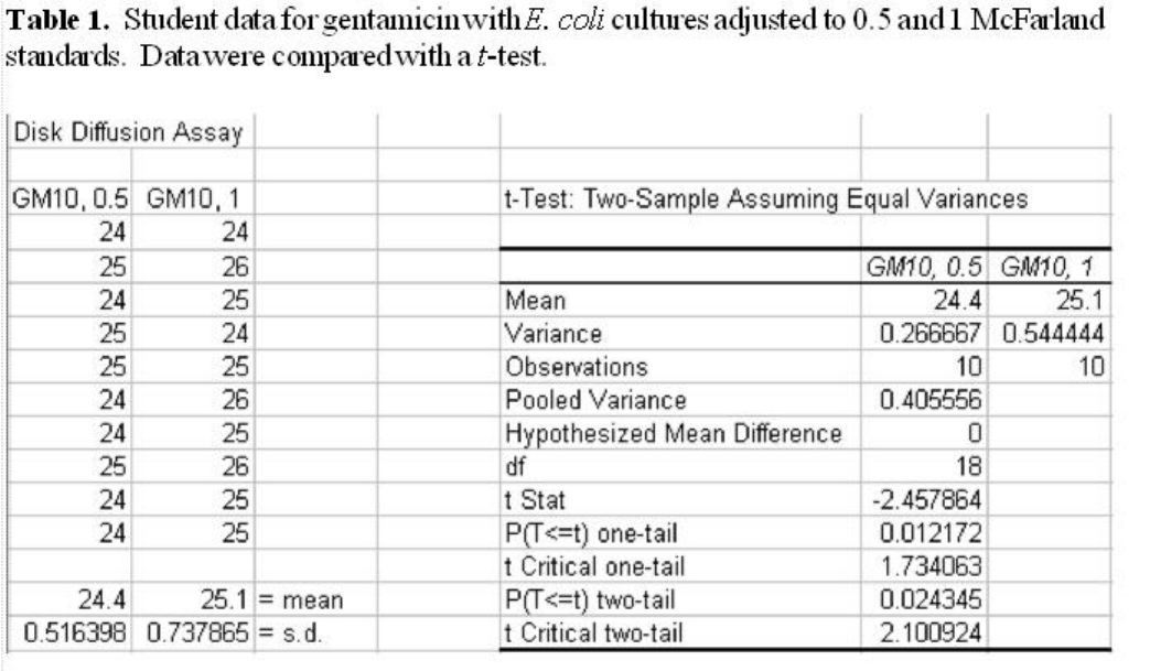
antibiotic using the t test. Typical student data is shown in

Table 1. This can be done manually using a calculator or

with a spreadsheet (recommended, see Appendix). The null hypothesis (no difference between the diameters of the

zones of inhibition for different concentrations of E. coli in the inocula) is accepted if the calculated t value is less

than the critical t value with an alpha of 0.5 and 18 degrees of freedom. A one-tailed test is appropriate since a

higher concentration of E. coli may produce a zone of inhibition that is equal to or smaller than a zone resulting with

a lower concentration of cells. Thus the critical value of t is 1.734.

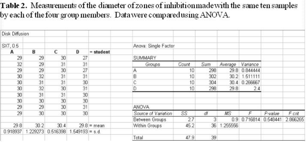
Determine if the individual measurements of the zones of inhibition made by each group member are the same or

different for each antibiotic using ANOVA. Student data for a control culture with trimethoprim-sulfamethoxazole is

shown in

Table 2. The null hypothesis that there is no significant difference between measurements of the diameter

of the zones of inhibition made by different students is accepted if the calculated F value is less than the critical F

value with an alpha value of 0.5 and 3 degrees of freedom, that is 2.866.

Instructor Version.

1. Lecture background. Antibiotic resistance is becoming an ever-increasing concern. Thus, the ability to accurately assess

the level of resistance of clinical isolates is of great importance, ultimately affecting patient outcome. Antibiotic resistance

testing using the disk diffusion technique was developed in the 1940s soon after the discovery of the first antibiotics. In

1966, Bauer et al. (1) published their paper which helped standardize this protocol. Today, CLSI provides periodic updates of

this protocol (5) and tables (4) so when performing this assay results are reproducible from day to day and from lab to lab if

using the same isolate and the same antibiotics. That is, if the directions are followed, the same results will always be

obtained with the same isolate, regardless of where or when the analysis is performed.

In this exercise we have modified the CLSI disk diffusion assay so that various concentrations of the inoculum are used in

addition to the standard inoculum concentration. After incubation for each inoculum, the diameter of the zone of inhibition of

each antibiotic disk is measured. Comparisons are made of the effect of inocula concentration on the diameter of the zone of

inhibition. By testing this variable (i.e., different concentrations of inocula) we hope to show the importance of following a

standardized protocol and to illustrate the use and the value of statistical analysis in microbiology. The null hypothesis, that

is the hypothesis of no difference, is that the diameters of the zones of inhibition will be the same regardless of E. coli

concentration in the inocula. The hypothesis is tested using the t test. In addition, each student in the group measures the

MicrobeLibrar

http://archive.microbelibrary.org/edzine/details_print.asp?id=1863&lang=

3 of 5 3/13/2012 3:55 P

zones of inhibition and their results are compared. In this instance, the null hypothesis, that there is no difference between

their measurements, is tested with ANOVA.

Students should read the protocol and organize their groups before the start of the experiment. In preparation for this

exercise, we recommend that the instructor have them address the following points:

Draw a flow diagram of the experiment noting how you would make the dilutions and then perform the plate counts.

This experiment investigates the effect of bacterial concentration in the disk diffusion assay. What other variables

could be investigated and which statistical tools would be appropriate for analysis?

What are the modes of action of the antibiotics used? Would they be expected to act against gram-positive or

gram-negative organisms or both?

Do you think that it would make a difference if more than one person inoculated the plates for antibiotic testing?

What statistical test would you use to test your hypothesis?

How is resistance or sensitivity to an antibiotic determined using the disk diffusion assay? Does this have clinical

relevance? What is the measurement that is used to determine this? Would a measurement of the same magnitude

imply resistance (or sensitivity) if the organism tested was a different species?

Would you expect bacteria in the stationary phase of growth to be more sensitive or resistant to an antibiotic as

compared to the same species in the exponential phase? (Hint: would preincubation of plates with the antibiotic

disks in place affect the size of the zone around the disk?)

List some ways in which antibiotic resistance can be transferred from one bacterium to another. Briefly describe each

mechanism.

2. Before beginning the lab work, a preliminary lecture outlining the objectives, describing the laboratory techniques, and

discussing how the data will be analyzed would be helpful. The emphasis should be on what are likely to be new techniques,

for example inoculating spread plates with a swab, as described above, and diluting cultures to a McFarland standard. It is

important that swabbing be done with a light touch or small channels will occur, making it difficult to measure the zone of

inhibition. Diluting to the McFarland standard seemed to be particularly stressful. The hint given above, to read a line of

print through the standard and the culture, is very helpful. Although students may want to use a spectrophotometer, it

should be emphasized that the method was developed using the 0.5 McFarland standard and that this is another skill to

learn. (For your benefit, the absorbance of a 0.5 McFarland standard at 625 nm in a cuvette with a 1-cm light path should be

0.08 to 0.10.)

3. Plates should be incubated at 37

C as soon as the antibiotic disks are in place. Preincubation at room temperature will

skew results.

4. A general lecture over the importance of statistics to data analysis may be used to introduce discussion of analyzing class

data. Several statistics books may be used as a reference but Introductory Biological Statistics (3) is recommended. Key

points to consider:

Select an alpha level of 0.05. This is the level usually selected as it offers a good compromise to avoid Type I

(rejecting a null hypothesis that is true) or Type II (not rejecting a null hypothesis that is false) errors.

The t test is a powerful and robust test for determining if two populations have different means when samples are

independent and random and the measured variable is continuous and normally distributed.

ANOVA (analysis of variance) is more appropriate (and less error prone) than running multiple t tests when there are

more than two samples to compare. In ANOVA there are two types of variance to consider: error variance (within-

groups variance) and treatment variance (between-groups variance). Since the zones of inhibition being measured by

each group member are the same, the within-groups variance should be the same. Therefore, any difference between

the variances of the measurements would be due to the treatment (individual making the measurement). ANOVA can

indicate a difference between the treatments but additional tests are necessary to find which treatments are

significantly different.

5. It is recommended to perform calculations with a spreadsheet rather than a calculator because

spreadsheets record the data entered, decreasing input mistakes and allowing the data to be distributed in a clear

format among coworkers and to instructors.

spreadsheets allow several analyses to be performed from one set of entered data.

spreadsheets simplify analyses, reducing mistakes.

spreadsheets are a powerful analytical instrument that have become a common scientific tool and, as such, should be

part of any education in science.

6. A tutorial on using Microsoft Excel to analyze the data in this exercise is available in the Appendix.

7. It may be possible to gather the entire class’ data and plot cell concentration versus zone of inhibition. It provides an

opportunity to discuss graphing and may demonstrate if the relationship between zone size and concentration is linear or

logarithmic.

Safety Issues.

E. coli is considered a biosafety level 2 pathogen. Although all students who are taking this class at our institution already

have knowledge of safe handling procedures for microorganisms, it is the responsibility of the instructor to review these

issues. Information on appropriate handling can be obtained from Centers for Disease Control and Prevention (7).

ASSESSMENT and OUTCOMES

Suggestions for Assessment.

The activity is assessed using written reports prepared by the students. The reports include the raw data, results of

statistical analyses, and interpretations of the statistical analyses. Students should also be able to describe, in their own

words, the importance of a standardized antibiotic testing protocol.

MicrobeLibrar

http://archive.microbelibrary.org/edzine/details_print.asp?id=1863&lang=

4 of 5 3/13/2012 3:55 P

Field Testing.

This activity is included in Microbiological Procedures, a lab-oriented course at the sophomore-junior level. There are usually

25 to 30 undergraduate microbiology majors enrolled. Based on pre- and posttests, students demonstrated increased

understanding of laboratory methods, including bacterial enumeration, the use of standardized protocols, and the

appropriate application of the t test and ANOVA. Students identified data analysis, especially using spreadsheets, as the

best part of this activity.

Student Data.

Table 1 displays typical student data for diameters of zones of inhibition from gentamicin for E. coli cultures adjusted to 0.5

and 1 McFarland standards. Results of the t test, performed using Microsoft Excel, indicate that the zones with the greater

cell density were significantly smaller than the zones with the less dense culture.

Table 2 displays typical student data for measurements of the diameters of zones of inhibition from gentamicin for an E. coli

culture adjusted to a 0.5 McFarland standard, made separately by four different students. ANOVA (using a spreadsheet)

suggests no significant difference between the sets of measurements.

SUPPLEMENTARY MATERIALS

References.

Bauer, A. W., W. M. M. Kirby, J. C. Sherris, and M. Turke. 1966. Antibiotic susceptibility testing by a standardized

single disk method. Am. J. Clin. Pathol. 45:493–496.

Becton Dickinson and Company. 2004. BBL Sensi-Disc antimicrobial susceptibility test discs. 2001/06. BD Diagnostic

Systems, Sparks, Md.

Hampton, R. E. 1994. Introductory biological statistics. WCB/McGraw-Hill, Dubuque, Ia.3.

National Committee for Clinical Laboratory Standards. 2004. Performance standards for antimicrobial susceptibility

testing: fourteenth informational supplement. M100-S14. National Committee for Clinical Laboratory Standards,

Wayne, Pa.

National Committee for Clinical Laboratory Standards. 2000. Performance standards for antimicrobial susceptibility

tests, 7th ed. National Committee for Clinical Laboratory Standards, Wayne, Pa.

Smibert, R. M., and N. R. Krieg. 1994. Phenotypic characterization, p. 607–654. In P. Gerhardt, R. G. E. Murray, W.

A. Wood, and N. R. Krieg (ed.), Methods for general and molecular biology. American Society for Microbiology,

Washington, D.C.

U.S. Department of Health and Human Services Public Health Service, Centers for Disease Control and

Prevention, and National Institutes of Health. 1999. Biosafety in microbiological and biomedical laboratories, 4th

ed. U.S. Department of Health and Human Services publication no. (CDC) 99-xxxx.

Appendices.

Appendix 1.

Using Microsoft Excel to Analyze Data from the Disk Diffusion Assay

MicrobeLibrar

http://archive.microbelibrary.org/edzine/details_print.asp?id=1863&lang=

5 of 5 3/13/2012 3:55 P

Using Microsoft Excel to Analyze Data from the Disk Diffusion Assay

Entering and Formatting Data

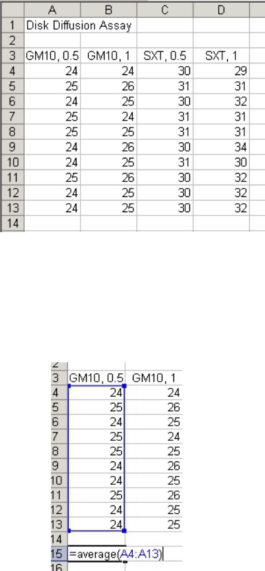
Open Excel. Set up the spreadsheet page (Sheet 1) so that anyone who reads it will understand

the page (Figure 1).

• Type a title in the cell in the upper lefthand corner, cell A1

• Label column A as the data from the 0.5 McFarland culture with gentamicin (GM10) in

cell A3

• Label column B as the data from the other McFarland culture with gentamicin. (In this

example, the 1 McFarland culture.)

• Repeat with the trimethoprim/sulfamethoxazole (SXT) data.

• Enter the appropriate data (diameter of zones of inhibition in mm) in each column

(Fig. 1).

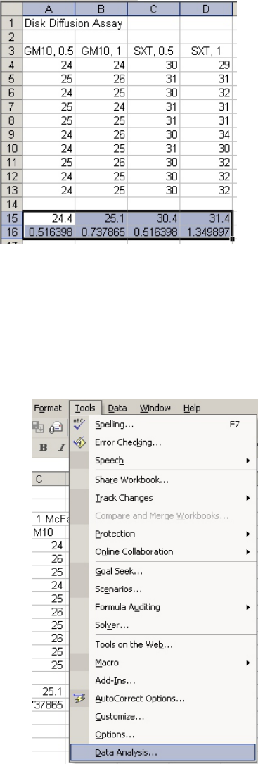
Calculating the Mean and Standard Deviation (should this be desired)

You can calculate the mean and standard deviation for each column using the functions

“=average( )” and “=stdev( )”, respectively (Fig 2).

Figure 1

Figure 2

• The data for each column goes inside the parentheses and may be entered by left-

clicking and dragging the mouse over the values after typing the open parenthesis.

• Finish by typing the close parenthesis and hitting the “Enter” button.

• Copy the functions (left-click and drag to select, right click and “Copy”) and paste them

under the other columns (left-click and drag to select, right click and “Paste”) (Fig 3).

The t-test

The easiest way to perform statistical analyses with a spreadsheet is to use the built-in

functions. With Excel, they can be found by clicking on “Tools” on the toolbar and selecting

“Data Analysis” (Fig. 4).

Figure 3

Figure 4

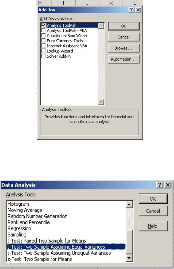
If the “Data Analysis” selection is not listed it means that the functions haven’t been installed.

To install them, you must have access to the installation program, either on CD or through a

network.

• Select “Add-Ins” under the “Tools” menu (Fig. 4).

• When the “Add-Ins” menu comes up, choose “Analysis ToolPak” (Fig. 5) and click on

“OK.”

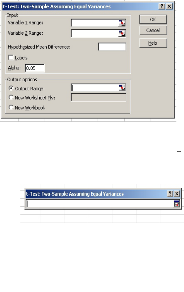
When you select “Data Analysis” on the “Tools” menu (Fig. 5), the “Data Analysis” menu pops

up (Fig. 6).

• Scroll down and select “t-test: Two-Sample Assuming Equal Variances.”

• After you click “OK,” the “t-test: Two-Sample Assuming Equal Variances” menu pops

up (Fig. 7) and you need to select your data.

Figure 5

Figure 6

• Click on the red arrow on the right side of the box next to the “Variable 1 Range:”

label.

• A menu pops up for data input (Fig. 8).

• Enter data by dragging the mouse over the values in the appropriate column, for

example Column A, cells 3-13. Hit “Enter” when done. This will input the values for

the zones of inhibition with gentamicin (GM10) on the plates inoculated from the 0.5

McFarland culture, as well as the column label.

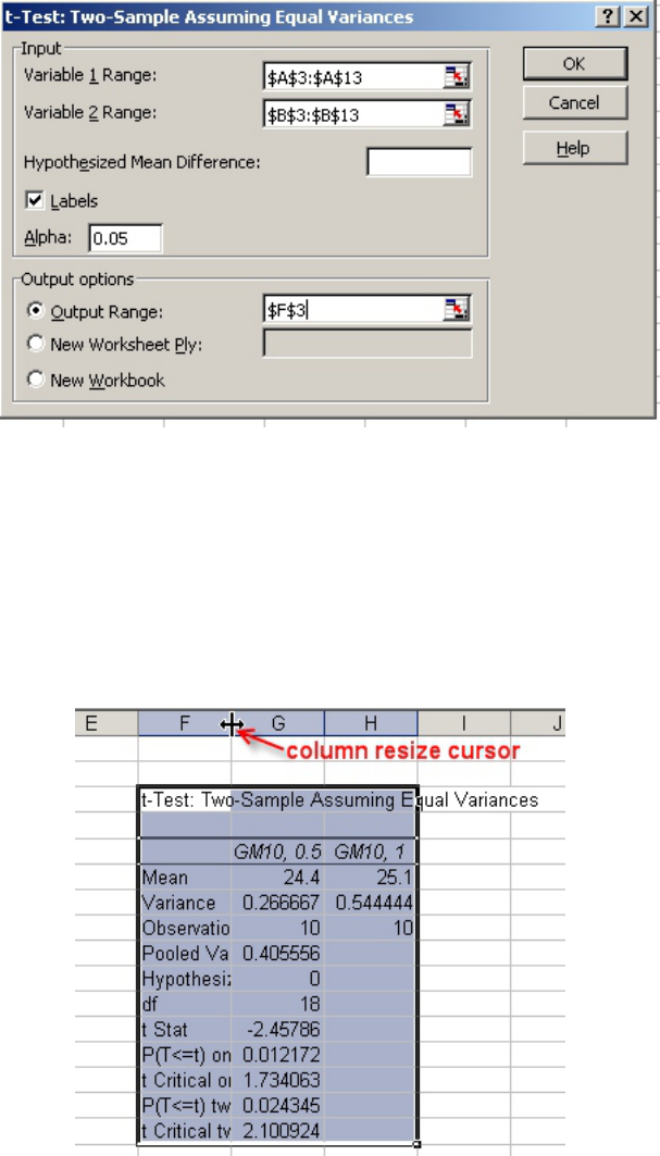
• Repeat this process, clicking on the arrow for “Variable 2 Range:” and entering the

other gentamicin data in Column B.

• Leave the “Hypothesized Mean Difference” selection blank, check the “Labels” box,

and leave “Alpha” at 0.05.

• Select a cell on the spreadsheet, for example F3, where you want the results of the t-test

to be placed.

• The completed “t-test: Two-Sample Assuming Equal Variances” menu should look

similar to Figure 9.

Figure 7

Figure 8

• Click on “OK” and the table of information for the t-test should appear, beginning in cell

F3.

• Move the cursor to the right hand border of the Column F label so that the column resize

cursor appears (Fig. 10).

• Drag the column to the right until the labels can be read (Fig. 11).

Figure 9

Figure 10

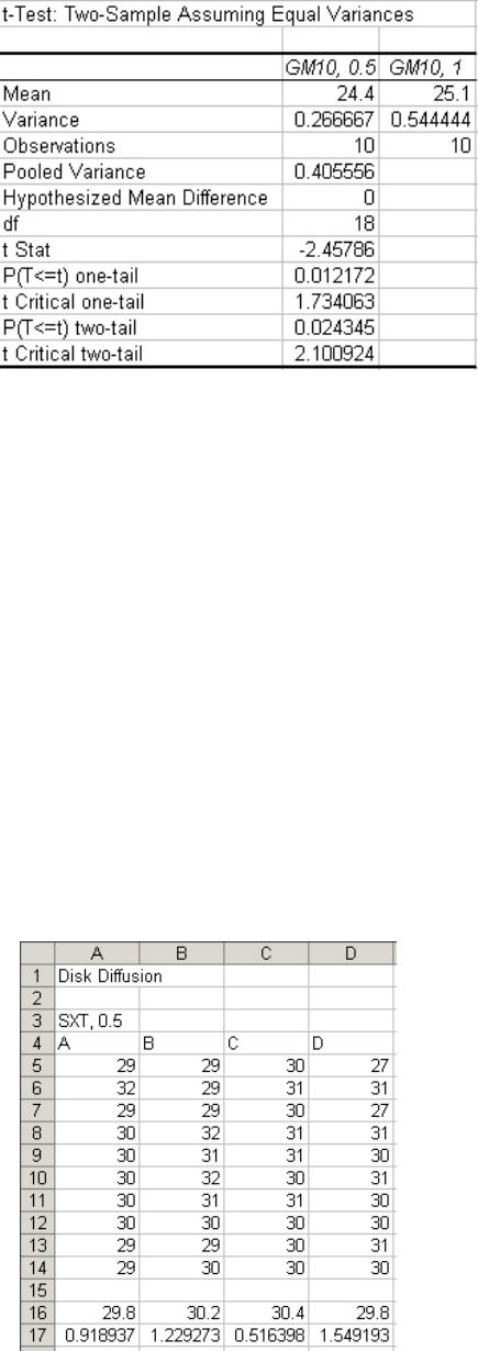
• Compare the calculated t value (t Stat) with the critical value for t (t Critical) for

alpha = 0.05 and with 18 degrees of freedom (df). We might expect that with a higher

concentration of cells the zone of inhibition would be equal to or smaller than the zone

produced with the 0.5 McFarland culture, so a one-tailed t-test would be appropriate.

Therefore, if the calculated t value (-2.45786, in this example) is less than the negative

critical value for t (-1.734073), we reject the null hypothesis that there is no difference

between the zones of inhibition from the 0.5 and 1 McFarland cultures.

ANOVA

To set up a spreadsheet for ANOVA, list the measurements of zones of inhibition made by

each student according to antibiotic and McFarland culture (Fig. 12). Calculate means and

standard deviations, if desired.

Figure 11

Figure 12

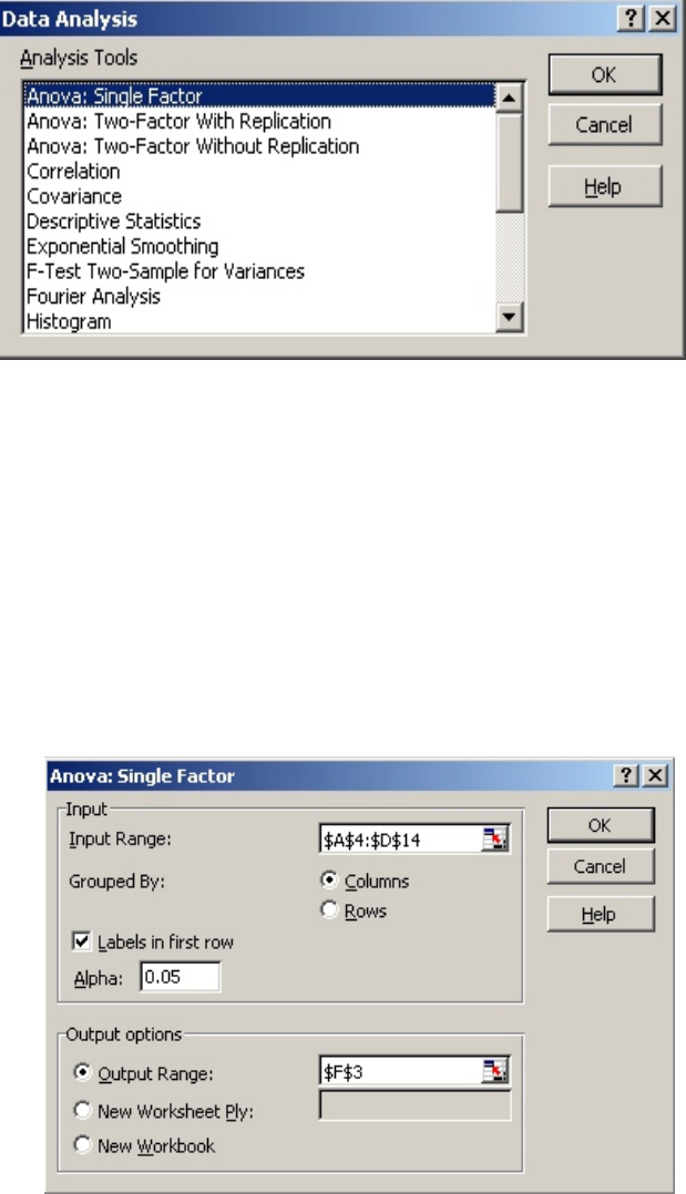
For ANOVA, use the “Data Analysis” menu under the “Tools” menu.

• Click on “Tools” on the toolbar

• Select “Data Analysis” (Fig. 4)

• Choose “ANOVA: Single Factor” (Fig. 13).

• For “Input Range:” select the data in all four columns, including the headings in Row

• Make sure that “Columns” is selected in “Grouped By:.”

• Select “Labels in First Row.”

•“Alpha:” should be 0.05.

• For “Output Range” select a cell near the data. (In this example, F3.)

• When complete, the “ANOVA: Single Factor” menu should look like Figure 14. Click

“OK” and a table will be generated, starting with Cell F3 (Fig. 15).

Figure 13

Figure 14

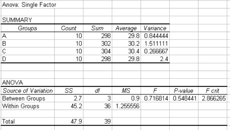
• Adjust column widths so that the table looks like Figure 15.

• Compare the calculated F value (0.716814, in this example) with the critical F value

(F crit)(2.866265). Since the F value is less than the critical F value, we cannot reject the

null hypothesis that there is no difference between the measurements of zones of

inhibition made by the four group members.

Figure 15