
3
CHAPTER
Conditional Expectation
Conditional expectation is much more important than one might at first think, both for finance and
probability theory. Indeed, conditional expectation is at the core of modern probability theory because
it provides the basic way of incorporating known information into a probability measure. In finance, we
treat asset price movements as stochastic processes when determining prices of derivatives, conditional
expectations appear in these dynamic settings. Therefore, if you do not have a solid understanding
of conditional expectation, the essential tool to process evolving information, you will never have a
penetrating understanding of modern finance.
Conditional expectation is presented in almost every textbook using Lebesgue integral, however,
Lebesgue integral is somewhat abstract, and most people are not familiar with it. Thus, I prepare a step
by step version that makes use of only unconditional expectation, which is much more accessible.
In this chapter, we will assume that random variables come from L
1
(Ω, F, P) (collection of random
variables with E(|X|) < ∞ for any random variable X), such that all expected values that are mentioned
exist (as real numbers).
85

86 Conditional Expectation
§ 3.1 Discrete Case
The definition of conditional expectation may appear somewhat abstract at first. This section is
designed to help the beginner step by step through several special cases, which become increasingly
involved. The first and simplest case to consider is that of the conditional expectation E(Y |E) of a
random variable Y given an event E. For example, the average score of female students is an easy to
understand case of conditional expectation: find the average score given the sex is female.
3.1.1 Conditioning on an Event
Example 3.1.1: In a family of six, the heights are as follows (old to young)
170
Grandpa
160
Grandma
180
Father
170
Mother
150
Girl
124
Boy
158
Suppose one person is randomly picked up, and is a male, what is the expected height?
The average height of males is
170 + 180 + 124
3
= 158
which equals to the expected height given that the gender is male: Let’s define the random variables as
follows
1 2 3 4 5 6 E (·)
Height Y 170 160 180 170 150 124 159
Gender S 1 0 1 0 0 1
Y 1
E
170 0 180 0 0 124 79
where E = {S = 1} means male. In elementary probability course, we have known that
E (Y |E) = E ( Y |S = 1) =
X
i
y
i
P (Y = y
i
|S = 1)
= 170 ·
1
3
+ 180 ·
1
3
+ 124 ·
1
3
= 158
Note that
E (Y 1
E
) =
1
6
(170 + 0 + 180 + 0 + 0 + 120) = 79 P (E) =
1
2
we find that
E(Y 1
E
)
E(1
E
)
=
E (Y 1
E
)
P (E)
=
79
1/2
= 158
In example 3.1.1, we have E(Y |E) =
E(Y 1
E
)
E(1
E
)
, this observation motivates the following definition.

Discrete Case 87
Definition 3.1: For any random variable Y on (Ω, F) and any event E ∈ F such that P(E) > 0, the
conditional expectation of Y given E is defined by
E(Y |E) =
E(Y 1
E
)
E(
1
E
)
=
E(Y 1
E
)
P(
E
)
(3.1)
Conditional expectation E(Y |E) is a constant (real number). Thus
E(1
E
E(Y |E)) = E( Y |E) E(1
E
) = E(1
E
Y )
Conditional expectation E(Y |E) is just a partial averaging: In Example 3.1.1, the average height of
male is E(Y
|
E) = 158, it is not the average height of the whole family E(Y ) = 159, that is why it is
called partial averaging. Conditional expectation E(Y |E) is a local mean, which refines the idea of the
expectation E(Y ) as a mean. Furthermore, since
E(Y ) = E(Y (1
E
+ 1
E
′
)) = E(Y 1
E
) + E(Y 1
E
′
) = E(Y |E)P(E) + E(Y |E
′
)P(E
′
)
the expectation E(Y ) is a probability weighted average of conditional expectations.
Compare to E(Y ) =
R
Ω
Y (w) dP (w), since E(1
E
· Y ) =
R
Ω
1
E
Y (w) dP (w) =
R
E
Y (w) dP (w),
which is restricted to a partial ter ritory of the whole sample space, E(1
E
· Y ) is a partial expectation of
Y . Analogously, E(Y ) =
E(1
Ω
·Y )
P(Ω)
is the average of Y , E( Y |E) =
E(1
E
·Y )
P(E)
is the partial average of Y
over event E.
A: Computation
In the definition of conditional expectation of Y given an event E, we do not restrict Y to be discrete,
it can be continuous.
• When Y is discrete
E (Y 1
E
) =
Z
Ω
Y (w)1
E
dP (w) =
X
w∈E
Y (w) P (w) =
X
i
y
i
P (Y = y
i
, E) (3.2)
The last equality means we collect the atoms in Y (w) = y
i
(grouping), which is left as an exercise
(Exercise 3.2).
• When Y is continuous
E(Y 1
E
) =
Z
Ω
Y (w)1
E
dP (w) =
Z
E
Y (w) dP (w) =
Z
Y (E)
y dF
Y
(y)
• When Y = c is a constant, E(Y |E) =
E(Y 1
E
)
E(1
E
)
=
Y E(1
E
)
E(1
E
)
= Y
Example 3.1.2: Three fair coins, 10, 20 and 50 cent coins are tossed. Let Y be the total amount
shown by these three coins (sum of the values of those coins that land heads up). What is the
expectation of Y given that two coins have landed heads up?
Let E denote the event that two coins have landed heads up. We want to find E(Y |E). Clearly, E
consists of three elements (H stands for heads and L for tails as in Example 2.1.1)
E = {HHL, HLH, LHH}

88 Conditional Expectation
each having the same probability
1
8
. The corresponding values of Y are
Y (HHL) = 10 + 20 = 30
Y (HLH) = 10 + 50 = 60
Y (LHH) = 20 + 50 = 70
Therefore
E(Y 1
E
) =
X
w∈E
Y (w) P (w) =
30
8
+
60
8
+
70
8
= 20
and
E(Y |E) =
E(Y 1
E
)
P(E)
=
20
3/8
=
160
3
B: Conditional Probability
Similarly to Equation (2.18), P (E) = E(1
E
), we have the following result.
Proposition 3.2: If P(F) > 0
P (E|F) = E (1
E
|F) (3.3)
Proof. By 1
EF
= 1
E
1
F
, we have
E (1
E
|F) =
E(1
E
1
F
)
P(F)
=
E(1
EF
)
P(F)
=
P(EF)
P(F)
= P (E|F)
In elementary probability theory, conditional probabilities are used in the computation of conditional
expectation: Given an event E, if Y is a discrete random variable
E (Y |E) ≡
X
i
y
i
P (Y = y
i
|E) (3.4)
Which is consistent with Definition 3.1, for (by Eq 3.2)
X
i
y
i
P (Y = y
i
|E) =
1
P (E)
X
i
y
i
P (Y = y
i
, E) =
E(Y 1
E
)
P(E)
If X is a discrete random variable and P(X = x) > 0 for some real number x, then {X = x} is an
event. In elementary probability theory: E( Y |X = x) ≡ E( Y |{X = x})
• If Y is discrete, let the conditional probability mass function be f (y |x) = P( Y = y |X = x),
then
E(Y |X = x) =
X
y
yf(y |x) =
X
y
yP(Y = y |X = x)
Which is a specific form of Equation (3.4)
• If Y is continuous
E(Y
|
X = x) =
Z
+∞
−∞
yf
(
y |
x
) d
y
where f(y
|
x) = f(x, y)/P(X = x) is the hybrid conditional density function, and f(x, y) is the
hybr id density function.

Discrete Case 89
Let X the number of heads in Example 3.1.2, then the expectation of Y given that two coins have
landed heads up is E(Y |X = 2) . Since
P(Y = 30 |X = 2) =
P(Y = 30, X = 2)
P(X = 2)
=
P({HHL} ∩ {HHL, HLH, LHH})
P({HHL, HLH, LHH})
=
1
3
Similarly, P( Y = 60 |X = 2) = P( Y = 70 |X = 2) =
1
3
, and
P(Y = y |X = 2) = 0 y = 0, 10, 20, 50, 80
thus
E(Y |X = 2) =
X
y
yP(Y = y |X = 2) =
1
3
(30 + 60 + 70) =
160
3
Undoubtedly, we can compute E(Y |X = 0), E(Y |X = 1), and E(Y |X = 3), thus conditional
expectations on all possible values of X are computed.
3.1.2 Conditioning on a Discrete Random Variable
Let X be a discrete random variable with possible values in {x
1
, x
2
, ···} such that P{X = x
i
} > 0
for each i. Because we do not know in advance which of events E
i
= {X = x
i
} will occur, we need to
consider all possibilities, involving a sequence of conditional expectations
E(Y |X = x
i
) ≡ E(Y |{X = x
i
}) = E(Y |E
i
) i = 1, 2, ···
Obviously, E(Y |X = x) is a function of x ∈ X(Ω) = {x
1
, x
2
, ···}. Let’s record this function by
r(x) = E(Y |X = x)
and denote
E(Y |X) ≡ r(X)
then E(Y |X) is a random variable, which is called the conditional expectation of Y given X. In more
details, R = E(Y |X) is a new discrete random variable such that
R(w) = E( Y |X)(w) =
E(Y |X = x
1
) w ∈ {X = x
1
}
E(Y |X = x
2
) w ∈ {X = x
2
}
.
.
.
.
.
.
E(Y |X = x
i
) w ∈ {X = x
i
}
.
.
.
.
.
.
(3.5)
In fact, we are computing conditional expectation on an event many times.
Definition 3.3: Let Y be a random variable and let X be a discrete random variable. Then the conditional
expectation of Y given X is defined by Equation (3.5).
Equation (3.5) says that E(Y |X) is a discrete random variable if X is discrete, E( Y |X) takes values
of the sequence of conditional expectation on {X = x
i
}. Because of E(Y |X) = r(X), the conditional
expectation E( Y |X) is a function of X. As a random variable, E(Y |X) has an expectation, we will
see that the expectation of E(Y |X) is E(Y ) in Proposition 3.4.

90 Conditional Expectation
Let’s define the conditional random variable Y
|X=x
to be the restriction of Y to the event {X = x}
Y
|X=x
=
Y (w) w ∈ {X = x}
undefined otherwise
(3.6)
Then, Y
|X=x
has its distribution, the conditional distribution
1
of Y given {X = x}. When Y is discrete
or continuous, because the conditional PMF/PDF f( y |x
i
) = 0 if y /∈ Y (X = x
i
), the expectation of
Y
|X=x
i
is equal to the conditional expectation of Y on event {X = x
i
}
E(Y
|X=x
i
) = E(Y |X = x
i
) = r(x
i
)
For this reason, the conditional random variable Y
|X=x
is also written as (Y |X = x).
The conditional expectation R = E(Y |X) is a constant over {X = x
i
}
R(w) = r(x
i
) = E(Y
|X=x
i
) ∀w ∈ {X = x
i
}
We see that the conditional expectation R is a partial average, an average over each partial sample space
{X = x
i
}. See figure 3.1 for an illustration.
Example 3.1.3: Three fair coins, 10, 20 and 50 cent coins are tossed as in Example 3.1.2. Let Y
be the total amount shown by these three coins, and X be the total amount shown by the 10 and 20
cent coins only. What is the conditional expectation of Y on X?
Clearly, X is a discrete random variable with four possible values: 0, 10, 20 and 30 cents. We find
the four corresponding conditional expectations in a similar way as in Example 3.1.2: For
{X = 0} = {LLH, LLL}
and
Y (LLH) = 50 Y (LLL) = 0
thus
E(Y |X = 0) =
E(Y 1
X=0
)
P(X = 0)
=
P
w∈{X=0}
Y (w) P (w)
2/8
=
50/8 + 0/8
2/8
= 25
similarly E( Y |X = 10) = 35, E( Y |X = 20) = 45 and E(Y |X = 30) = 55. Therefore
E(Y |X) =
25 w ∈ {LLH, LLL} = {X = 0}
35 w ∈ {HLH, HLL} = {X = 10}
45 w ∈ {LHH, LHL} = {X = 20}
55 w ∈ {HHH, HHL} = {X = 30}
Which shows that E(Y |X) is a random variable (a function of w ∈ Ω), and it is a function of X.
Example 3.1.4: Let Ω = [0, 1] with P the uniform measure (P(w 6 a) = a for a ∈ [0, 1]). Find
1
Recall that {X = x} can be thought of as the new sample space for the conditional probabilities here, in this sense, the
restriction version of Y , Y
|X=x
, can be thought of as the random variable define on the partial sample space {X = x}.

Discrete Case 91
E(Y |X) for
Y (w) = 2w
2
X(w) =
1 w ∈ [0,
1
3
]
2 w ∈ (
1
3
,
2
3
]
0 w ∈ (
2
3
, 1]
Clearly, X is discrete with three possible values 0, 1 and 2. The corresponding events are
{X = 0} = (
2
3
, 1] {X = 1} = [0,
1
3
] {X = 2} = (
1
3
,
2
3
]
The CDF of Y is
F
Y
(y) = P(Y (w) 6 y) = P(2w
2
6 y) = P( w 6
p
y/2) =
p
y/2 y ∈ [0, 2]
If w ∈ {X = 0}, then Y (w) ∈ (
8
9
, 2]. We obtain
{X = 0} = {8/9 < Y 6 2}
thus 1
X=0
= 1
8/9<Y 62
E(Y 1
X=0
) = E(Y 1
8/9<Y 62
) =
Z
2
8/9
y dF
Y
(y) =
Z
2
8/9
y ·
1
4
r
2
y
dy =
38
81
and
E(Y |X = 0) =
E(Y 1
X=0
)
P(X = 0)
=
38
27
similarly
E(Y |X = 1) =
2
27
E(Y |X = 2) =
14
27
We see that E(Y |X) is a discrete random variable even Y is continuous. The graph of E( Y |X) is
shown in Figure 3.1 with more interpretations.
On computation
2
of E(Y 1
X=0
), we can use mixed joint CDF: First find out F (x, y) with x ∈ {0, 1, 3},
for example when x = 0
F (0, y) = P(X = 0, Y (w) 6 y) = P(2/3 < w 6 1, 2w
2
6 y)
= P(2/3 < w 6
p
y/2) =
p
y/2 − 2/3 8/9 < y 6 2
and the hybrid/mixed density function f(x, y) =
∂F (x,y)
∂y
, then f(0, y) =
1
4
q
2
y
E(Y 1
X=0
) =
Z
+∞
−∞
∞
X
i=1
(y1
x
i
=0
) · f(x
i
, y) dy =
Z
+∞
−∞
yf(0, y) dy =
Z
2
8/9
y ·
1
4
r
2
y
dy =
38
81
2
Using Lebesgue integral, we have the following ways
•
B
Y (w) dP (w) =
B
Y (w) dw, (P (w) is Lebesgue measure on [0, 1], and Riemann and Lebesgue integrals agree)
E(Y 1
X=0
) =
X=0
Y (w) dP (w) =
1
2/3
2w
2
dw =
38
81
•
E
h(Y (w)) dP (w) =
Y (E)
h(y) dF
Y
(y). For Y (X = 0) = (8/9, 2]
E(Y 1
X=0
) =
X=0
Y (w) dP (w) =
Y (X=0)
y dF
Y
(y) =
2
8/9
y ·
1
4
2
y
dy =
38
81
92 Conditional Expectation
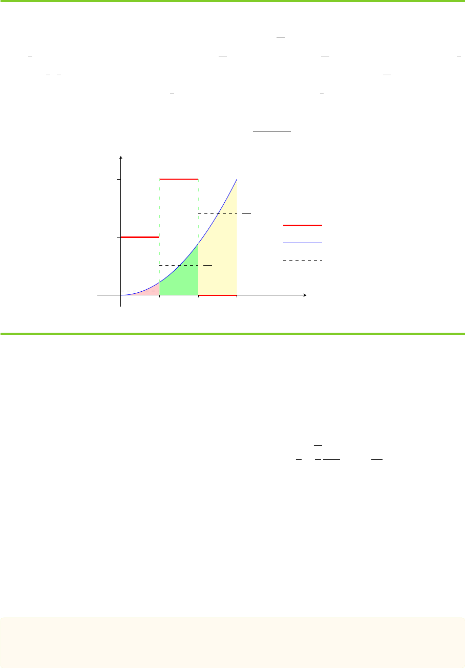
Figure 3.1: Conditioning on a Discrete Random Variable In Example 3.1.4, we see that conditional
expectation E( Y |X) is a partial average: E( Y |X = 0) =
38
27
is the average height of Y over the interval
(
2
3
, 1] = {X = 0}. Similarly, E(Y |X = 1) =
2
27
and E(Y |X = 2) =
14
27
are the average height over [0,
1
3
]
and (
1
3
,
2
3
] respectively. Because E(Y 1
X=0
) =
R
X(w)=0
Y (w) dw =
R
1
2/3
2w
2
dw =
38
81
is the area under
the graph Y = 2w
2
in the interval (
2
3
, 1] = {X = 0}, and P(X = 0) =
1
3
is the length of the corresponding
interval. Thus, let’s define a rectangle having same area as the region under the graph, whose width is the
length of the underlying interval, then E( Y |X = 0) =
E(Y 1
X=0
)
P(X=0)
is the height of this rectangle.
w
f(w)
Y (w) = 2w
2
14
27
38
27
1
2
1/3 2/3
1
X(w)
Y (w)
E(Y |X)
note that given hybrid density function f(x, y)
E(h(X, Y )) =
Z
+∞
−∞
∞
X
i=1
h(x
i
, y)f(x
i
, y) dy
where the discrete portion is compute by summation, and the continuous portion is compute by integral.
Besides, the conditional PDF of Y given X = x
i
is f(y |x
i
) = f(x
i
, y)/P(X = x
i
), thus
E(Y
|
X = 0) =
Z
+∞
−∞
yf
(
y |
0) d
y
=
Z
2
8/9
y ·
1
4
r
2
y
1
1/3
d
y
=
38
27
3.1.3 Properties
Toward a general definition and properties of conditional expectation, we explain some of the most
important properties of conditional expectation of Y given a discrete random variable X. We will show
that, what matters is the information contain in X, not the values taken by X.
A: Law of Total Expectation
Proposition 3.4: If X is a discrete random variable
E (E(Y |X)) = E(Y )

Discrete Case 93
Proof. If X is discrete, E( Y |X) is a discrete random variable, thus
E (E(Y |X)) =
X
i
E(Y |X = x
i
)P (X = x
i
) =
X
i
E (Y 1
X=x
i
)
= E
X
i
Y 1
X=x
i
= E
Y
X
i
1
X=x
i
= E(Y )
We do not assume that Y is a discrete random variable. The law of total expectation is an extremely
useful result that often enables us to compute unconditional expectations easily by first conditioning on
some appropriate random variable. The following examples demonstrate its use.
Example 3.1.5: A lucky wheel gives equal chance for $3, $5 and $7. You keep spinning until you
land on $3. What is the expected prize for this game?
Let Y be the amount of prize, and X be the prize on the first spin. Obviously, Y
|X=3
= 3 and
E(Y |X = 3) = 3
Note that if X = 5, we return to the wheel again, conditional random variable Y
|X=5
has the same
distribution as Y + 5, say, Y
|X=5
∼ Y + 5. Similarly, Y
|X=7
∼ Y + 7. We have
E(Y
|
X = 5) = 5 + E(Y )
E(Y |X = 7) = 7 + E(Y )
and
E (Y ) =
X
i∈{3,5,7}
E(Y |X = i)P (X = i) =
1
3
[3 + 5 + E(Y ) + 7 + E(Y )]
hence E (Y ) = 15.
Remark: If the player hits the second item, she obtains $5 and return to the wheel. But once she
return to the wheel, the problem is as before. Hence E(Y |X = 5) = 5 + E (Y ).
The divide and conquer is a key in the application of the law of total expectation.
Example 3.1.6: The game of craps is begun by rolling an ordinary pair of dice.
• If the sum of the dice is 2, 3, or 12, the player loses (denoted as Z = 0 ).
• If it is 7 or 11, the player wins (Z = 1).
• If it is any other number i ∈ I = {4, 5, 6, 8, 9, 10}, the player goes on rolling the dice until
the sum is either 7 (the player loses) or i (the player wins).
Let Y be the number of rolls of the dice in a game of craps. Find the expected number of rolls
E(Y ), the probability that the player wins P(Z = 1), and the expected number of rolls given that
the player wins, E(Y |Z = 1).
Let S
n
be the sum of dice on the nth roll, and P
i
= P(S
n
= i), then reading from the antidiagonals

94 Conditional Expectation
in Example 2.1.2
P
i
= P
14−i
=
i − 1
36
i = 2, 3, ··· , 7
Condition on the initial sum S
1
E(Y |S
1
= i) =
1 i = 2, 3, 7, 11, 12
1 +
1
P
i
+P
7
i ∈ I
for if S
1
= i ∈ I that does not end the game, then the dice will continue to be rolled until the sum is either
i or 7, and the number of rolls until this occurs is a geometric random variable with parameter P
i
+ P
7
.
Therefore
E(Y ) = E(E( Y |S
1
)) =
12
X
i=2
E(Y |S
1
= i)P(S
1
= i) =
12
X
i=2
E(Y |S
1
= i)P
i
= 1 +
X
i∈I
1
P
i
+ P
7
P
i
= 1 + 2
6
X
i=4
1
P
i
+ P
7
P
i
P
i
= P
14−i
= 1 + 2
1
3
+
2
5
+
5
11
=
557
165
≈ 3.3758
Now we compute P(Z = 1), since {Z = 1}∩{S
1
= 2} = ∅ and {S
1
= 7} ⊂ {Z = 1}, we see that
condition on the initial sum S
1
P(Z = 1|S
1
= i) =
0 i = 2, 3, 12
1 i = 7, 11
If i ∈ I, let q
i
= 1 − (P
i
+ P
7
), and (let (E, F) ≡ E ∩F)
V
2i
= (S
2
= i, S
1
= i) = {S
2
= i} ∩ {S
1
= i}
V
ni
= (S
n
= i, {S
n−1
, ··· , S
3
, S
2
} ∩ {i, 7} = ∅, S
1
= i) n > 2
be the event that the player wins on the nth roll. Then P(V
ni
) = P
2
i
q
n−2
i
,
{Z = 1 } = {S
1
= 7} + {S
1
= 11} +
X
i∈I
∞
X
n=2
V
ni
and
P(Z = 1 |S
1
= i) =
P(Z = 1 , S
1
= i)
P(S
1
= i)
=
P (
P
∞
n=2
V
ni
)
P
i
=
1
P
i
∞
X
n=2
P
2
i
q
n−2
i
= P
i
∞
X
k=0
q
k
i
=
P
i
P
i
+ P
7
i ∈ I
which confirms Equation (2.16). Thus, by Eq (2.3)
p = P(Z = 1) =
12
X
i=2
P(Z = 1 |S
1
= i)P
i
= (P
7
+ P
11
) +
X
i∈I
P
2
i
P
i
+ P
7
=
244
495
≈ 0.4929
Finally, we compute E(Y |Z = 1): It is easy to find that (Exercise 3.7)
P(Y = n |Z = 1) =
1
p
X
i∈I
P
2
i
q
n−2
i
n > 1 (3.7)
and
∞
X
n=2
nq
n−2
i
=
1 + P
i
+ P
7
(P
i
+ P
7
)
2
i ∈ I (3.8)

Discrete Case 95
thus
E(Y |Z = 1) =
∞
X
n=1
nP(Y = n |Z = 1) = P(Y = 1 |Z = 1) +
∞
X
n=2
nP(Y = n |Z = 1)
=
P
7
+ P
11
p
+
∞
X
n=2
n
1
p
X
i∈I
P
2
i
q
n−2
i
!
=
P
7
+ P
11
p
+
1
p
X
i∈I
P
2
i
∞
X
n=2
nq
n−2
i
!
=
P
7
+ P
11
p
+
1
p
X
i∈I
P
2
i
1 + P
i
+ P
7
(P
i
+ P
7
)
2
=
9858
3355
≈ 2.9383
B: Substitution Rule
Proposition 3.5 (Substitution Rule): Let h(x, y) be a function of x and y
E(h(X, Y ) |X = x) = E(h(x, Y ) |X = x)
Proof. Given X = x, we have w ∈ {X = x} and
h(X, Y ) = h(X(w), Y (w)) = h(x, Y (w))
which gives h(X, Y )1
X=x
= h(x, Y )1
X=x
, thus
E(h(X, Y ) |X = x) =
E(h(X, Y )1
X=x
)
P(X = x)
=
E(h(x, Y )1
X=x
)
P(X = x)
= E(h(x, Y ) |X = x)
We can think of h(X, Y ) as h(x, Y ) when compute conditional expectation given X = x. That is, if
we have known that X = x, we can replace every appearance of X to the left of the conditioning bar by
x, other random var iables are unchanged.
Remark: The substitution rule is valid for conditional expectation not only for discrete case, but for
general case. We are treating X as a constant x, since the sample space is restricted to {X = x}.
Proposition 3.6: If Y is σ(X)-measurable and X is a discrete random variable
E(Y |X) = Y
Proof. By Doob-Dynkin lemma, there exists a function h(x) such that Y = h(X). Following the
substitution rule, E(h(X) |X = x) = E(h(x) |X = x) = h(x). Which means h(X) = E(h(X) |X).
Accordingly
E(Y |X) = E(h(X) |X) = h(X) = Y
C: Conditional Information
What if conditioning on a independent random variable? The conditional information is useless, for
we do not able to improve the prediction, the conditional mean is equal to unconditional mean.

96 Conditional Expectation
Proposition 3.7: If random variable Y and discrete random variable X are independent, then
E(Y |X) = E(Y )
Proof. Given Y ⊥ X, we have Y ⊥ 1
X=x
i
. By Equation (3.1)
E(Y |X = x
i
) =
E (Y 1
X=x
i
)
P(X = x
i
)
=
E (Y ) E (1
X=x
i
)
P(X = x
i
)
= E(Y )
thus, E(Y |X) = E(Y ) follows from Equation (3.5).
Remark: If Y ⊥ X, we have E(Y |X = x
i
) = E(Y ), knowing the realizations of X has no effect
on the prediction of Y .
Example 3.1.7: Let Y
i
∼ N(i, 2i), Y
i
⊥ X, i = 0, 1. If P(X = 2) = P(X = 1) = 1/2, compute
E(Y
2
X
X = 1). By substitution rule
E(Y
2
X
X = 1) = E(Y
2
1
X = 1) = E(Y
2
1
) = [E(Y
1
)]
2
+ var(Y
1
) = 3
Note that U = Y
2
X
is a random variable, say
U(w) =
Y
2
1
(w) w ∈ {X = 1}
Y
2
2
(w) w ∈ {X = 2}
Suppose that X indicates day or night, and Y
i
is the position of a pollen grain in water, then U
|X=1
must be Y
2
1
, the square of particle position at night (X = 1).
If E(Y |X) = E(Z |X) = 0, we have E(Y ) = E(Z) = 0, but we do not have E(Y Z |X) = 0.
E(Y |X) = E(Z |X) = 0 ̸=⇒ E( Y Z |X) = 0
Furthermore (If r(x, z) = E( Y |X = x, Z = z), then E(Y |X, Z) = r(X, Z))
E(Y |X) = E(Y |Z) = 0 ̸=⇒ E(Y |X, Z) = 0
The following examples illustrate these points.
Example 3.1.8: Toss a fair dice Ω = {1, 2, 3, 4, 5, 6}, define
X =
1 w ∈ {1, 6}
0 w ∈ {2, 3, 4, 5}
Y = 7 −2w Z =
1 w ∈ {1, 3, 5}
−1 w ∈ {2, 4, 6}
then (f(x, z) = f(x)f (z) =⇒ X ⊥ Z)
E(Y |X) = E(Z |X) = 0
however
E(Y Z |X) =
5·1+(−5)·(−1)
6
/
2
6
= 5 X = 1
3·(−1)+1·1+(−1)·(−1)+(−3)·1
6
/
4
6
= −1 X = 0

Discrete Case 97
Example 3.1.9: Toss a fair dice Ω = {1, 2, 3, 4, 5, 6}, let
X =
1 w ∈ {1, 6}
0 w ∈ {2, 3, 4, 5}
Y =
1 w ∈ {1, 3, 5}
−1 w ∈ {2, 4, 6}
Z = 1
w>4
then (Y ⊥ X and Y ⊥ Z)
E(Y |Z) = E(Y |X) = 0
however
E(Y |X, Z) =
−1+1−1
6
/
3
6
= −
1
3
(X, Z) = (0, 0)
1
6
/
1
6
= 1 (X, Z) = (1, 0)
1
6
/
1
6
= 1 (X, Z) = (0, 1)
−1
6
/
1
6
= −1 (X, Z) = (1, 1)
w ∈ {2, 3, 4}
w ∈ {1}
w ∈ {5}
w ∈ {6}
D: Measurability and Partial Averaging
The essentials of the conditional expectation are the measurability and partial averaging.
Proposition 3.8: If Y is a random variable and X is a discrete random variable, let R = E(Y |X), then
1. Measurability: R is a σ(X)-measurable random variable
2. Partial averaging: For any E ∈ σ(X)
E(1
E
· R) = E(1
E
· Y )
Remark: Please note that Y is not necessary σ(X)-measurable. But if Y ∈ σ(X), by Proposition
3.6, we have E(Y |X) = Y
• For any simple event {X = x
i
} in σ(X), by partial averaging property, we have
E(Y |X = x
i
) = E(R |X = x
i
)
which states that, E(Y |X = x
i
), the partial average of Y over event {X = x
i
}, is equal to
E(R |X = x
i
), where R is σ(X)-measurable.
• We have known that E(Y |X) is the partial average over each simple event {X = x
i
}, the partial
averaging property states that this can be extended to any event E ∈ σ(X), thus for any E ∈ σ(X)
with P(E) > 0
E(Y |E) = E( R |E)
the partial average of Y is always equal to the partial average of R. (thus called the partial averaging
property)
• If E /∈ σ(X), the partial averaging property may fail. For an instance, in Example 3.1.4, let

98 Conditional Expectation
E = [0,
1
2
] /∈ σ(X), then E(1
E
Y ) ̸= E(1
E
R), because
E(1
E
Y ) =
Z
E
Y (w) dP (w) =
Z
1/2
0
Y (w) dw =
Z
1/2
0
2w
2
dw =
1
12
E(1
E
R) =
Z
E
R(w) dP (w) =
Z
1/2
0
R(w) dw =
Z
1/3
0
2
27
dw +
Z
1/2
1/3
14
27
dw =
1
9
where the computation of E(1
E
R) is better done by way of modern probability theory.
Figure 3.2: Prediction and Finer Information In Example 3.1.4, let Z(w) = 1
X=1
, then σ(Z) < σ(X).
As an estimation of Y, E(Y |X) is better than E( Y |Z): If X = 2 and Z = 0 are observed, then the
unobserved true state w must be in (
1
3
,
2
3
], hence Y ∈ (
2
9
,
8
9
]. We see that E( Y |Z = 0) =
26
27
is out of range
while E( Y |X = 2) =
14
27
is within range, undoubtedly, E( Y |X = 2) is a better estimation.
Y (w) = 2w
2
26
27
14
27
38
27
w
f(w)
1
2
1/3 2/3
1
E(Y |Z)
Y (w)
E(Y |X)
The partial averaging property ensures that E( Y |X) is indeed an estimate of Y , which is a valuable
prediction if Y is time and money costly to observe or even Y is not observable. In Example 3.1.4, let
Z(w) = 1
X=1
, then E(Y |Z = 0) =
26
27
and E(Y |Z = 1) = E(Y |X = 1) =
2
27
. In Figure 3.2, we
see that {X = 2} = (
1
3
,
2
3
] and {X = 0} = (
2
3
, 1] provide a finer resolution of the uncertainty of the
world than {Z = 0} = (
1
3
, 1] = X
−1
({0, 2}) does. As estimations of Y, the partial averaging proper ty
says that E( Y |X = 2) =
14
27
and E(Y |X = 0) =
38
27
are better than E(Y |Z = 0) =
26
27
.
E: Information Matters
Read carefully from Equation (3.5), we like to note that the conditional expectation E( Y |X) does
not depend on the actual values of X but just on the partition generated by X, or equivalently on the
event space σ(X). For example: toss a fair dice Ω = {1, 2, 3, 4, 5, 6}, define
Y = 7 −2w X =
1 w ∈ {1, 3, 5}
0 w ∈ {2, 4, 6}
Z =
135 w ∈ {1, 3, 5}
246 w ∈ {2, 4, 6}

Discrete Case 99
then σ(X) = σ(Z), and
E(Y |X) = E(Y |Z) =
5+1−3
6
/
3
6
= 1 w ∈ {1, 3, 5} = X
−1
(1) = Z
−1
(135)
3−1−5
6
/
3
6
= −1 w ∈ {2, 4, 6} = X
−1
(0) = Z
−1
(246)
What matters is the infor mation revealed by the random variables conditioned on, not the values
taken by them. When σ(X) = σ(Z), both random variables provide the identical amount of information.
Observing the realization of X or Z, we learn the underlying state of world. We care more on information
than the actual values, for infor mation is vital for financial market, most of the decision-making are based
on specific information. Needless to say, conditional expectation is an indispensable tool for financial
decisions.

100 Conditional Expectation
§ 3.2 General Case
When conditioning on a discrete random variable, conditional expectation has the following funda-
mental proper ties:
1. Measurability: E(Y |X) is a function of X, and thus it is a random variable and measurable to
σ(X). That is to say, the value of E( Y |X) can be determined from the information in X.
2. Partial averaging: E( Y |X) as a “best approximation”, the expected value of Y given the informa-
tion from X. Because σ(X) contains all the information from X, for discrete random variable Z,
if Z delivers less information such that σ(Z) < σ(X), then E(Y |X) provides better estimations
of Y than E(Y |Z) does.
Which culminate at the general definition of conditional expectation for general case.
3.2.1 Conditioning on an Arbitrary Random Variable
Let X be a uniformly distributed random variable on [0, 1]. Then the event {X = x} has probability
P(X = x) = 0 for every x ∈ [0, 1]. In such situations the former definition of E(Y |X = x) no
longer makes sense even when f
X
(x) > 0. We need a new style, a new approach to defining it by
means of certain properties which follow from the special case of conditioning with respect to a discrete
random variable. Proposition 3.8 provides the key to the definition of the conditional expectation given
an arbitrary random variable X.
Definition 3.9: Let Y be an integrable random variable and let X be an arbitrary random variable. Then
the conditional expectation of Y given X, denoted as E(Y |X), is any random variable R that satisfies
1. Measurability: R is σ(X)-measurable
2. Partial averaging: For any E ∈ σ(X)
E(1
E
· R) = E(1
E
· Y ) (3.9)
We are merely given the required property that a conditional expectation must satisfy. The existence
of E(Y |X) will be discussed later.
• Measurability: By Doob-Dynkin lemma, the measurability condition ensures that R = E(Y |X)
is a function of X. For example, if (X, Y ) follows bivariate normal, Equation (2.27) says that
E(Y |X) = a + bX, which is a linear function of X.
• Partial averaging: If P(E) > 0, Eq (3.9) is equivalent to
E (R |E) = E ( Y |E)
E (Y |E) is the par tial average of Y over event E. E ( Y |E) is indeed an estimate of Y , conditioning
on E ∈ σ(X), and it is equal to E ( R |E) with R = E(Y |X) ∈ σ(X).
• The partial averaging condition is equivalent to (Lebesgue integral is needed for a proof)
E (UR) = E (U Y )

General Case 101
for any random variable U ∈ σ(X).
• We can also define the conditional probability of an event E ∈ F given X by
P(E |X) ≡ E( 1
E
|X)
which is equivalent to the following equality in elementary probability
P(E |X = x) = E( 1
E
|X = x) (3.10)
When compute conditional expectation, often the Equation (3.9) is not used, for it does not give
explicit formula for E(Y |X). However, it is used to establish the fundamental properties given in §3.2.3.
As shown in Exercise 3.6, the Equation (2.22) introduced in elementary probability is consistent with our
Definition 3.9. Thus, once f(y |x) is known, we compute r(x) = E(Y |X = x), and then easily obtain
E(Y |X) = r(X).
Remark: E(Y |X) = r(X) is a random variable, the distribution of E(Y |X) is the distr ibution of
r(X), not the distribution of conditional random variable Y
|X=x
. For example, in the bivariate nor mal
case, from Equation (2.27)
E(Y |X) = r(X) = µ
Y
+ (X − µ
X
)ρσ
Y
/σ
X
∼ N(µ
Y
, σ
2
Y
ρ
2
)
with expectation E (E(Y |X)) = E(Y ) = µ
Y
. Which is different from the distribution of Y
|X=x
, the
conditional distribution of Y given {X = x} as in Equation (2.26)
Y
|X=x
∼ N(µ
Y
+ (x −µ
X
)ρσ
Y
/σ
X
, σ
2
Y
(1 − ρ
2
))
note that the expectation of Y
|X=x
equals the conditional expectation of Y on X = x
E(Y
|X=x
) = r(x) = E( Y |X = x)
Lemma 3.10: Let (Ω, F, P) be a probability space and let G be a σ-algebra contained in F. If Y is a
G-measurable random variable and for any G ∈ G
E (1
G
Y ) = 0
then P(Y = 0) = 1.
Following Lemma 3.10, conditional expectation is unique in the sense of almost surely. If R and R
∗
both satisfy the two conditions in Definition 3.9, then E (1
E
· (R −R
∗
)) = 0 for any E ∈ σ(X), and thus
P(R = R
∗
) = 1
or R = R
∗
a.s. Which means, versions of conditional expectation of Y given X will only differ on null
sets (event with zero probability).
According to the following proposition, we also note that, when conditioning on an arbitrary random
variable, the conditional expectation E(Y |X) is σ(X)-measurable and does not depend on the actual
values of X but just on the event space σ(X).
Proposition 3.11: If σ(X) = σ(X
∗
), then E(Y |X) = E(Y |X
∗
) a.s.

102 Conditional Expectation
Proof. Let R = E(Y |X) and R
∗
= E(Y |X
∗
), then for any E ∈ σ(X) = σ(X
∗
), we have
E (1
E
R) = E (1
E
Y ) = E (1
E
R
∗
)
or
E (1
E
· (R −R
∗
)) = 0
as an immediate consequence of Lemma 3.10, R = R
∗
a.s., that is E(Y |X) = E(Y |X
∗
) a.s.
3.2.2 Conditioning on an Event Space
Based on the observation that E(Y |X) depends only on the event space σ(X), the information
revealed by X, rather than on the actual values of X. It is reasonable to talk of conditional expectation
given an event space. We are now in a position to make the final step towards the general definition of
conditional expectation.
Definition 3.12: Let Y be a random variable on a probability space (Ω, F, P), and let G be a event space
contained in F. Then the conditional expectation of Y given G, denoted as E( Y |G), is any random
variable R that satisfies
1. Measurability: R is G-measurable
2. Partial averaging: For any G ∈ G
E(1
G
R) = E(1
G
Y )
Definition 3.12 is the general definition of conditional expectation: When conditioning on an arbitrary
random variable X, we can take G = σ(X). Particularly, if G = {∅, Ω}, G is the smallest event space
and contains no information, thus
E(Y |G) = E(Y )
the conditional expectation becomes an unconditional expectation. When conditioning on an event E
with P(E) > 0 and P(E
′
) > 0, let G = {∅, Ω, E, E
′
}, it is easy to verify that
R(w) = E( Y |G)(w) =
E(Y 1
E
)
P(E)
w ∈ E
E(Y 1
E
′
)
P(E
′
)
w ∈ E
′
We see that this explicit solution is used by Equation (3.1) in Definition 3.1. Similarly, Equation (3.5) of
Definition 3.3 is the explicit solution when X is a discrete random variable. When X is continuous, we
do not have an explicit formula for E( Y |X) in general.
• Measurability guarantees that, although the estimate of Y based on the information in G is itself a
random variable, the value of the estimate E(Y |G) can be determined from the information in G.
• The following property might seem stronger but in fact it is equivalent to the partial averaging
property
E (UR) = E (U Y ) (3.11)

General Case 103
for any random variable
3
U ∈ G.
• By the definition, E ( Y |G) ∈ G, and for any G ∈ G
E (1
G
· E(Y |G)) = E (1
G
· Y ) (3.12)
• If G is the event space generated by some other random variable X, i.e., G = σ(X), we generally
write E( Y |X) rather than E(Y |σ(X)).
• It is true that given σ-algebras G in F, there exists random variable X, such that G = σ(X) in
the sense that they are same up to null sub-sets (For any G ∈ G, there is E ∈ σ(X), such that
P(G\E) + P(E\G) = 0 and vice versa).
A: Existence and Uniqueness
The existence and uniqueness of the E(Y |G) come from the following proposition.
Proposition 3.13: E(Y |G) exists and is unique (in the almost surely sense).
Proof. By Corollary 3.20, there exists a random variable R
E (1
G
Y ) = E (1
G
R) ∀G ∈ G
The uniqueness follows from Lemma 3.10, or from the uniqueness of the Radon-Nikodým derivative,
up to equivalence. Recall that real-valued random variables Y and X are equivalent if P(Y = X) = 1,
or X = Y almost surely (a.s.).
B: Conditional Probability
The conditional probability of an event E ∈ F given a σ-algebra G is defined by
P(E |G) ≡ E(1
E
|G) (3.13)
Then, Equation (2.18) is a special case when G = {∅, Ω} is the smallest event space. Needless to say,
Equation (3.13) implies that for any F ∈ G
P(E |F) = E(1
E
|F)
which incorporates Equation (3.3) and (3.10).
For the conditional probability of E given F, P(E |F) defined in Equation (2.1), the restriction
P(F) > 0 is needed. However, in the generalized form of Equation (3.13), this restriction is removed, we
can compute P(E |F) even P(F) = 0. For example, let (X, Y ) ∼ N(µ
X
, µ
Y
, σ
2
X
, σ
2
Y
, ρ), and
E = {Y 6 µ
Y
+ (x −µ
X
)ρσ
Y
/σ
X
}
F = {X = x}
then P(F) = 0. However, by Equation (2.26), P(E |F) =
1
2
.
3
A random variable is approximated by a simple function. And a simple function is a finite sum of indicator functions times
constants.

104 Conditional Expectation
By partial averaging, for any G ∈ G
E(1
G
P(E |G)) = E(1
G
1
E
) = P(GE) (3.14)
As a consequence, for any discrete random variable Z
E(Z |G) =
X
i
z
i
P(Z = z
i
|G) (3.15)
if all P(Z = z
i
|G) are known.
Proposition 3.14: If the conditional probability of an event E ∈ F given a σ-algebra G ⊂ F is a
constant, P(E |G) = c, then
1. E ⊥ G (for any G ∈ G, there is E ⊥ G)
2. 1
E
⊥ G (which means σ(1
E
) ⊥ G)
3.2.3 General Properties
Assume that a, b are arbitrary real numbers, X, Y are integrable random variables on a probability
space (Ω, F, P) and G, H are σ-algebra on Ω contained in F. Then conditional expectation has the
following properties: All equalities and the inequalities hold almost surely under probability measure P.
1. Linearity
E(aX + bY |G) = a E(X |G) + b E( Y |G)
2. Taking out what is known (conditional determinism): If X is G-measurable
E(XY |G) = X E(Y |G) X ∈ G
3. Dropping independent information (“eat independence”): If Y is independent of G (σ(Y ) ⊥ G)
E(Y |G) = E(Y ) Y ⊥ G
4. Tower property (iterated conditioning, “small eat large”): If H ⊂ G
E(E(Y |G) |H) = E(Y |H) H ⊂ G
and for E(Y |H) is H-measurable, thus G-measurable, by taking out what is known
E(E(Y |H) |G) = E(Y |H) H ⊂ G
5. Positivity: If Y > 0, then E(Y |G) > 0. And if Y > 0, then E( Y |G) > 0. Note that
Y ⪈ 0 =⇒ E(Y ) > 0, but Y ⪈ 0 =⇒ E(Y |G) ⪈ 0.
Remark: The linearity and positivity make the operator of conditional expectation the natural choice
for the pricing function in financial market.
• Taking out what is known: For X ∈ σ(X), we have
E(XY |X) = X E(Y |X)
The idea here is that we are treating X as a constant, since the information of X is given.

General Case 105
– If X is G-measurable, then h(X) ∈ G. Since h(X) is determined by information in G
E(h(X)Y |G) = h(X) E(Y |G)
thus conditioning on the event space G, h (X) can be treated as a constant.
– There are some special and useful forms: If Y is G-measurable, then (Exercise 3.15)
E(Y |G) = Y Y ∈ G
In particular, E(c |G) = c for any constant c.
• Dropping independent information: If X ⊥ Y , then E(Y |X) = E(Y ). What is more, see
Exercise 3.17:
X ⊥ (Y, Z) =⇒ E(Y |X, Z) = E( Y |Z)
Where the information of X is independent and is dropped out.
– When there are Y ⊥ X and Y ⊥ Z, there is nothing to drop out in E(Y |X, Z). In Example
??, there are Y ⊥ X and Y ⊥ Z, however
E(Y |X, Z) ̸= E(Y ) = E(Y |Z) = E(Y |X) = 0
– Note that if X ⊥ (Y, Z), then X ⊥ Y |Z and thus (Exercise 3.18)
X ⊥ (Y, Z) =⇒ X ⊥ Y |Z =⇒ E(XY |Z) = E(X) E(Y |Z)
• Positivity: If Y ⪈ 0, we have E(Y |G) ⪈ 0, not E(Y |G) > 0. For example, tossing a fair dice and
let Y = 1
w>4
and X = 1
w<4
, there are E(Y |X = 1) = 0 and E(Y |X = 0) = 2/3. Moreover,
E(Y |Y = 0) = 0 by partial averaging or substitution rule. Clearly, for any non-null G ∈ G, if
Y (G) ⪈ 0, then E(Y |G) > 0.
We have known that E(Y |G) is a random variable defined on the coarser probability space (Ω, G, P)
and thus on (Ω, F, P). Because of the randomness, conditional Jensen’s inequality holds almost surely,
while Jensen’s inequality holds exactly.
Theorem 3.15 (Conditional Jensen’s Inequality): Let h : R → R be a convex function and let Y be an
integrable random variable on a probability space (Ω, F, P) such that h(Y ) is also integrable. Then
h(E(Y |G)) 6 E( h(Y ) |G) a.s.
for any σ-algebra G on Ω contained in F.
Proof. For R = E(Y |G) takes values in R, let y = h(R) + k(x − R) be a random supporting line for
h(·) at R, then (X > Y means X(w) > Y (w) for each w ∈ Ω)
h(Y ) > h(R) + k(Y − R)
and k ∈ G since k is depend on R. Taking conditional expectations given G through the inequality gives
E(h(Y )
|G
) > h(R) + E(k(Y − R)
|G
) = h(R) + k E(Y − R
|G
)
= h(R) = h(E(Y |G))

106 Conditional Expectation
A: Tower Proper ty
The tower property is also known as smoothing property of conditional expectation, or consistency
conditions. As a special case of tower property when H = {0, Ω}, we have the law of total expectation
E(E(Y |G)) = E(Y )
Which also follows by putting E = Ω in Eq (3.12).
When conditioning twice, with respect to nested σ-algebras, the smaller one (representing the smaller
amount of information) always prevails. As seen in Figure 3.2:
E(Y |X) =
2
27
w ∈ [0,
1
3
] = {X = 1}
14
27
w ∈ (
1
3
,
2
3
] = {X = 2}
38
27
w ∈ (
2
3
, 1] = {X = 0}
and
E(E(Y |Z) |X) = E( E(Y |X) |Z) = E(Y |Z) =
2
27
w ∈ [0,
1
3
] = {Z = 1}
26
27
w ∈ (
1
3
, 1] = {Z = 0}
Which confirms the tower property as σ(Z) < σ(X). In the region of (
1
3
, 1] = Z
−1
(0) = X
−1
{0, 2}
1. If it is first smoothed by Z, E(Y |Z = 0) =
26
27
is a constant, a second finer-region smooth by X
is invisible, due to the uneven has been levelled
2. If it is first smoothed by X, we have E(Y |X = 0) =
38
27
and E( Y |X = 2) =
14
27
. A second
full-region smooth by Z further irons the region out
the smaller information set applies a larger “iron”, the work of a smaller iron was concealed or wiped
out by the larger iron. Thus, when nested conditioning, only the result from the smaller information
set is revealed. It is now apparent that the tower property results from the partial averaging property of
conditional expectation.
The tower property is not only useful in theorem proofs, but also helpful in applications. For discrete
random variables X, Y and Z, the specific form of
E(Y |X) = E(E( Y |X, Z) |X) (3.16)
is (recall Equation 2.6)
E(Y |X = x) =
X
k∈K
E(Y |X = x, Z = z
k
)P(Z = z
k
|X = x) (3.17)
where K = {k : P(X = x, Z = z
k
) > 0}. For brevity, we write
E(Y |X) =
X
k
E(Y |X, Z = z
k
)P(Z = z
k
|X)
Furthermore, if X ⊥ Z
E(Y |X) =
X
k
E(Y |X, Z = z
k
)P(Z = z
k
)
For continuous random variables X, Y and Z, with join density f(x, y, z), Eq (3.16) leads to
Z
yf(y |x) dy =
Z
E(Y |X = x, Z = z)f(z |x) dz

General Case 107
Example 3.2.1: Let us consider independent Bernoulli trials each of which is a success with
probability p. We repeat these trials up to the point where n consecutive successes appear for the
first time. We are looking for the expected number of necessary trials for that.
We define the random variable Y
n
to denote the number of necessary trials to obtain n consecutive
successes. Let Z
k
be the Bernoulli random variables for k-th trial and m = Y
n−1
+ 1. Then
(Y
n
|Y
n−1
= y, Z
m
= 1) = y + 1
we have E(Y
n
|Y
n−1
= y, Z
m
= 1) = y + 1 and
E(Y
n
|Y
n−1
, Z
m
= 1) = Y
n−1
+ 1
For
(
Y
n
|
Y
n−1
=
y, Z
m
= 0)
∼
Y
n
+
y
+ 1
, we obtain
E(Y
n
|Y
n−1
, Z
m
= 0) = E(Y
n
) + Y
n−1
+ 1
Thus, by E(Y
n
|Y
n−1
) = E(E(Y
n
|Y
n−1
, Z
m
) |Y
n−1
), and Z
m
⊥ Y
n−1
E(Y
n
|Y
n−1
) =
1
X
i=0
E(Y
n
|Y
n−1
, Z
m
= i)P(Z
m
= i |Y
n−1
)
= E(Y
n
|Y
n−1
, Z
m
= 0)(1 − p) + E(Y
n
|Y
n−1
, Z
m
= 1)p
= (E(Y
n
) + Y
n
−
1
+ 1)(1 −p) + ( Y
n
−
1
+ 1)p
= E(Y
n
)(1 − p) + Y
n−1
+ 1
By law of total expectation
E (Y
n
) = E(E(Y
n
|Y
n−1
)) = E (Y
n
) (1 − p) + E (Y
n−1
) + 1
which yields
E (Y
n
) = E (Y
n−1
) /p + 1/p
Clearly, the random variable Y
1
represents the number of Bernoulli tr ials up to the first success, and
consequently, has the geometric distribution with parameter p, thus
E (Y
1
) = 1/p
and recursively, we arrive at
E (Y
n
) = 1/p
n
+ ··· + 1/p
2
+ 1/p =
1 − p
n
p
n
(1 − p)
B: Change of Measure
For any random variable Y , we have E
Q
(Y ) = E (GY ) if dQ = GdP where G is the Radon-
Nikodým derivative of Q with respect to P. However, E
Q
(Y |G) ̸= E(GY |G), we have the following
Equation (3.18) for conditional expectation under change of measure.

108 Conditional Expectation
Theorem 3.16: Let G be a sub-σ-algebra of F on which two probability measures Q and P are defined.
If dQ = GdP and Y is Q-integrable, then GY is P-integrable and Q-a.s
E
Q
(
Y
|G
) =
E(GY |G)
E(G |G)
(3.18)
Remark: Here G ⪈ 0, Q and P are not necessarily equivalent. If G > 0, then Q ∼ P. As a special
case, let G = {∅, Ω}, we have the unconditional version E
Q
(Y ) = E (GY ).
We have learned that conditional probability, P
F
(E) = P(E |F), is a probability measure. In Equation
(2.5), since Q(E) ≡ P
FG
(E) = P(E |FG) is a probability measure different from P, given event F and G
with P(FG) > 0, there is Q(EG) = Q(E), Q(G) = 1, and
Q(E |G) =
Q(EG)
Q(G)
= Q(E) = P(E |FG)
Let G =
1
FG
P(FG)
, Y = 1
E
and G = σ(1
G
), then dQ = GdP
E
Q
(Y |G) = E
Q
(1
E
|1
G
) =
Q(E |G) w ∈ G
Q(E |G
′
) w ∈ G
′
and
E(GY |G) = E( 1
FG
1
E
|1
G
)/P(FG) =
P(EF |G)/P(FG) w ∈ G
P(EF |G
′
)/P(FG) w ∈ G
′
E(G |G) = E(1
FG
|1
G
)/P(FG) =
P(F |G)/P(FG) w ∈ G
P(F |G
′
)/P(FG) w ∈ G
′
By Equation (3.18), when w ∈ G, there is Q(E |G) =
P( EF |G)
P( F |G)
. Thus
P(E |FG) = Q(E |G) =
P(EF |G)
P(F |G)
We have shown that Equation (2.5) is a special case of Equation (3.18).
Remark: Since G
′
< (FG)
′
, Q(G
′
) = 0, we can not compute Q( E |G
′
) in elementary probability
context. However, as an implication of Equation (3.18), when w ∈ G
′
, there is
Q(E |G
′
) =
P(EF |G
′
)
P(F |G
′
)
(3.19)
Which shows that we can define a conditional probability on a null event. Note that Q(E |G
′
) depends
on event F in Equation (3.19), where event F can be arbitrary as long as 0 < P(FG) < 1, thus it is not
unique. However, since Q(G
′
) = 0, there causes no trouble for Equation (3.18) in the sense of Q-a.s.
Corollary 3.17: If Y
t
is an adapted stochastic process (i.e. Y
t
∈ I
t
), let 0 6 t 6 u 6 T , then
E
Q
t
(Y
u
) =
1
G
t
E
t
(G
u
Y
u
) (3.20)
where G
t
= E(G |I
t
) is called the Radon-Nikodým derivative process.

General Case 109
C: Pricing Function
For continuous time or T -step discrete time model, if the market is free of arbitrage, there is an
equivalent martingale measure (risk-neutral measure) such that
4
X
t
= ℘
t,u
(X
u
) = B
t
E
Q
t
(X
u
/B
u
) = ℘
t,T
(X
T
) = B
t
E
Q
t
(X
T
/B
T
) 0 6 t 6 u 6 T (3.21)
for any primary asset when the number of primary assets is finite. Given any attainable payoff X
T
∈ I
T
at time T , the pricing function is represented by (Equation 1.17)
X
0
= ℘(X
T
) = E(ΨX
T
)
where the SDF
Ψ
∈
I
T
is a positive random variable. Let G = ΨB
T
/B
0
> 0, then dQ = GdP , and
X
t
= ℘
t,u
(X
u
) = B
t
E
Q
t
(X
u
/B
u
) = B
t
E
t
(GX
u
/B
u
)
E
t
(G)
= E
t
(G
u
X
u
/B
u
)B
t
/G
t
where G
t
= E(G |I
t
) = E
t
(ΨB
T
) is the Radon-Nikodým derivative process. For the forward measure,
since dQ = B
T
D
0,T
dO, we have
X
t
= ℘
t,u
(X
u
) = D
t,T
E
O
t
(X
u
/D
u,T
) = ℘
t,T
(X
T
) = D
t,T
E
O
t
(X
T
) 0 6 t 6 u 6 T (3.22)
3.2.4 The Best Predictor
We have said that E( Y |X) is a random variable measurable to σ(X), thus it is a function of X. In
this subsection, we will pursuit a deeper interpretation, E( Y
|
X) as a “best approximation” of Y by a
function of X. For this purpose, we assume that the random variables have finite variance.
If Y is a random variable then the ordinary expected value E (Y ) represents our best guess of the
value of Y if we have no prior information. But now suppose that X is a random variable that is not
independent of Y and that we can observe the value of X. Then one might expect that we can use that
extra information to our advantage in guessing where Y will end up.
A: Best Mean Square Predictor
One can show that the conditional expectation E (Y |G) is the best mean square G-measurable
predictor of Y :
E([Y − E ( Y |G)]
2
) = min
Z∈G
E((Y − Z)
2
)
If σ(X) = G, then E( Y |X) is best mean square predictor of Y among all functions of X. This is
fundamentally important in econometric problems where the predictor X can be observed but not the
response variable Y . Thus, the regression function of Y on X is defined by the conditional expectation
function, r(x) = E(Y |X = x).
4
Like multi-step binomial model and Black-Scholes model, we can setup a model such that the market is free of arbitrage.
For discrete models with finite number of primary assets and finite number of steps, Equation (3.21) is read from Harrison and
Pliska (1981) and Dalang et al. (1990). For continuous time model with finite number of primar y assets, it is straightforward
from Girsanov’s Theorem.

110 Conditional Expectation
B: Constant and Linear Predictor
For random variable Y , since
E([Y − E(Y )]
2
) = min
y∈R
E((Y − y)
2
)
the best constant predictor of Y is E (Y ) in the mean square sense, with mean square error var(Y ). The
best predictor of Y among the linear functions of X is the linear projection
5
of Y on 1 and X
Pj(Y |1, X) ≡ E
Y
1
X
′
E
1
X
1
X
′
−1
1
X
= E(Y ) +
cov(X, Y )
var(X)
(X − E(X))
for which minimizes
min
a,b∈R
E([Y − (a + bX)]
2
)
with mean square error var(Y )(1 − ρ
2
XY
). If X and Y follow a bivariate normal distribution, from
Eq (2.27), we see that the best linear predictor equals the conditional expectation E( Y |X), the linear
regression. Please note that if the regression function E(Y |X) is not linear, then the linear regression
model Y = α + βX + ϵ is misspecified, and the OLS (ordinary least square) recovers just the linear
projection coefficients
6
in Pj(Y |1, X) = a + bX as the sample size grows.
5
The linear projection of Y on 1 and X satisfies the orthogonality conditions
E (1 · ϵ) = E (X · ϵ) = 0
where ϵ = Y − Pj( Y | 1, X). If we think of Pj(Y | 1, X) as an approximation of Y , then ϵ is the error in that approximation.
The orthogonality conditions state that the error is orthogonal to the plane spanned by 1 and X.
6
Which could still be useful, because it is the mean square error minimising linear approximation of the conditional
expectation function. Let Y = a + bX + u and E( u | X) ̸= 0, but E (1 · u) = E (X · u) = 0 (orthogonality), then OLS
estimators are consistent.

Conditional Information 111
§ 3.3 Conditional Information
conditional independence, conditional correlation
In bull market, the returns of some assets are seen to be independent, however, in bear market, they
are usually correlated, and moving down in steps.
students play football together, and go home individually after school.
The more you know, the better your decision
3.3.1 Conditional Independence
The definition of conditional probability in Eq (3.13) generalizes the definition in Eq (2.1), thus, we
are able to compute the conditional probability when the given event has zero probability. Similarly,
conditional independence can be generalized by simply drop the requirement that the given event has
positive probability. We say events G and H are conditionally independent given K, denoted by G ⊥ H |K,
if
P (GH |K) = P (G |K) P (H |K)
We say events G and H are conditionally independent given σ-algebra K, denoted by G ⊥ H |K, if
P (GH |K) = P (G |K) P (H |K)
that is, for any K ∈ K, we have G ⊥ H |K.
A: Definition
We are ready to modify the Definition 2.6 to incorporate the conditional information.
Definition 3.18: We say that σ-algebras G and H in F are conditionally independent given σ-algebra
K, denoted by G ⊥ H|K, if for any G ∈ G, H ∈ H, and K ∈ K, the events G and H are conditionally
independent given K.
We can now say that random variables X and Y are conditionally independent given Z, denoted
by X ⊥ Y |Z, if and only if the σ-algebras σ(X) and σ(Y ) are conditionally independent given σ(Z).
This definition says that
X ⊥ Y |Z ⇐⇒ σ(X) ⊥ σ(Y ) |σ(Z) ⇐⇒ E ⊥ F |G
for any E ∈ σ(X), F ∈ σ(Y ), and G ∈ σ(Z). Or more practically, some textbooks use the following
definition
X ⊥ Y |Z ⇐⇒ P( EF |Z) = P(E |Z)P( F |Z)
for any E ∈ σ(X) and F ∈ σ(Y ).
Remark: Intuitively, if Y and X are conditionally independent given Z, then knowing Z renders X
statistically irrelevant for predicting Y .
112 Conditional Expectation
• Conditional independence is symmetric, that is
Y ⊥ X |Z ⇐⇒ X ⊥ Y |Z
• Random variables Y and X are independent given Z, if and only if
E(g(X)h(Y ) |Z) = E( g(X) |Z) E(h(Y ) |Z) (3.23)
for all choices of bounded (Borel measurable) functions g, h : R → R. Thus, if Y ⊥ X |Z, we
have
E(Y X |Z) = E( Y |Z) E( X |Z)
B: Conditional Probability Density Function
If X, Y and Z are jointly continuous with density f (x, y, z), then random variables Y and X are
said to be conditionally independent given Z, written X ⊥ Y |Z, if and only if, for all x, y and z with
f
Z
(z) > 0
f(x, y |z) = f (x |z)f(y |z)
where functions f( ·|z) are conditional probability density functions. If the random variables are jointly
discrete with probability mass function f(x, y, z) = P(X = x, Y = y, Z = z), the formulas are same
as the continuous case, with f(·|·) representing conditional probability mass function. For example
f(y |x, z) = P ( Y = y |X = x, Z = z)
The other useful ways to define conditional independence are
X ⊥ Y |Z ⇐⇒ f (x |y, z) = f(x |z) ⇐⇒ f(y |x, z) = f(y |z)
These forms are directly related to the widely used notion of Markov property: If we interpret Y as the
“future,” X as the “past,” and Z as the “present,” Y ⊥ X
|
Z says that, given the present the future is
independent of the past; this is known as Markov property.
Remark: X and Y are conditionally independent given Z if and only if, given any value of Z, the
probability distribution of X is the same for all values of Y and the probability distribution of Y is the
same for all values of X.
• For conditional PDF and PMF, we have
f(x, y|z) = f (x|z)f( y|z) ⇐⇒ f(y |x, z) = f (y |z)
However, if Y ⊥ X |Z, we have [f(x, y|z) → E( XY |Z)]
E(XY |Z) = E(X |Z) E( Y |Z)
and
E(Y |X, Z) = E( Y |Z)
Note that E(Y |X, Z) is not affected by X, for E( Y |X, Z) = E( Y |Z) is a function of Z only.
In particular,
E(Y |X, Z = z) = E(Y |Z = z)
is constant over X, the information of X is dropped out.

Conditional Information 113
• Without reference to conditional distributions
X ⊥ Y |Z ⇐⇒ f (x, y, z)f
Z
(z) = f(x, z)f(y, z)
• Using conditional cumulative distribution function
F (x, y |z) = P( X 6 x, Y 6 y |Z = z)
F (y |x, z) = P( Y 6 y |X = x, Z = z)
the following version is seemingly seemingly weaker than the general definition but equivalent
definition
Y ⊥ X |Z ⇐⇒ F (x, y |z) = F (x |z)F (y |z)
⇐⇒ F (x |y, z) = F (x |z) ⇐⇒ F (y |x, z) = F (y |z)
for any x, y and z.
For events E, F and G, the examples 2.1.8 and 2.1.9 show that E ⊥ F neither implies nor is implied
by E ⊥ F |G. For random variables X, Y and Z, it follows that X ⊥ Y neither implies nor is implied by
X ⊥ Y |Z.
Example 3.3.1: For discrete random variables X, Y and Z, assume P (Z = 1) = P (Z = 0) =
1/2, and f(x, y |z) set by the following table
Z = 1 Y f
X |Z
0 1
X 0 1/12 1/4 1/3
1 1/6 1/2 2/3
f
Y |Z
1/4 3/4
Z = 0 Y f
X |Z
0 1
X 0 3/10 9/20 3/4
1 1/10 3/20 1/4
f
Y |Z
2/5 3/5
Show that X ⊥ Y |Z, and verify E(Y |Z = 1) = E(Y |X, Z = 1); However, X ⊥ Y is not
true.
For any z ∈ {0, 1}, it is trivial to check that f (x, y |z) = f(x |z)f(y |z), thus X ⊥ Y |Z.
As a partial verification of f(y |x, z) = f (y |z) (X is dropped out if X ⊥ Y |Z), we see
P (Y = 1 |X = 0, Z = 1) =
f(x = 0, y = 1 |z = 1)
f(x = 0 |z = 1)
=
1/4
1/3
=
3
4
P (Y = 1 |X = 1, Z = 1) =
f(x = 1, y = 1 |z = 1)
f(x = 1 |z = 1)
=
1/2
2/3
=
3
4
P(Y = 1 |Z = 1) = f(y = 1 |z = 1) =
3
4
thus
E(Y |X = 0, Z = 1) =
X
y
=0
,
1
yP (Y = y |X = 0, Z = 1)
= P (Y = 1 |X = 0, Z = 1) =
3
4

116 Conditional Expectation
§ 3.4 Exercise
3.1 Show that
E(Y |Ω) = E(Y )
3.2 Prove Eq (3.2).
3.3 Show that if X is a constant function, then
E(Y |X) is constant and equal to E(Y ).
3.4 Show that if 0 < P(F) < 1
E (1
E
|1
F
) =
P(E |F) w ∈ F
P(E |F
′
) w /∈ F
3.5 If X is a discrete random variable, is it
true that the random variable E(Y |X) takes
the value E( Y |X = x
i
) with probability
P(X = x
i
)?
3.6 In elementary probability theory, we know
that for continuous random variables X and
Y
r(x) = E(Y |X = x)
=
Z
+∞
−∞
yf(y |x) dy
and E( Y |X) = r(X). Please show that
this definition is consistent with our Defini-
tion 3.9 of conditional expectation.
3.7 Prove Equation (3.7) and (3.8) in Example
3.1.6.
3.8 Given random variables X, Y and Z. For
any G ∈ σ(Z)
E(1
G
· E(X |Z) E(Y |Z))
= E(1
G
E(X |Z) ·E(Y |Z))
= E(1
G
E(X |Z) ·Y )
= E(1
G
· Y E(X |Z))
thus, by the definition of conditional expec-
tation
Y E(X |Z) = E( E(X |Z) E(Y |Z) |Z)
= E(X |Z) E(Y |Z)
Is it correct or not? Why?
3.9 Show that if G = {∅, Ω}, then E(Y |G) =
E(Y ).
3.10 Prove Equation (3.15).
3.11 Show that if E ∈ G, then E( E(Y |G) |E) =
E(Y |E).
3.12 Show that if Y ⪈ 0, then E( Y |G) ⪈ 0.
3.13 Show that for any event E ∈ G, Y −E(Y |G)
is orthogonal to 1
E
.
3.14 Show that for any random variable X ∈ G,
Y − E(Y |G) is orthogonal to X.
3.15 If Y is G-measurable, then E(Y |G) = Y .
3.16 If X and Y are independent, G and H are
independent. Then
E(E(XY |G) |H) = E( E(XY |H) |G)
= E(X) E(Y )
3.17 If X ⊥ (Y, Z), then E(Y |X, Z) =
E(Y |Z).
3.18 If X ⊥ (Y, Z), then E( XY |Z) =
E(X) E(Y |Z).
3.19 In Example 3.1.5, if we let N denote the
number of spins in a game, X
i
the prize in ith
spin, and Y
n
=
P
n
i=1
X
i
. Then Y
N
is a ran-
dom sum of random variables, it is the total
prize for the game. Find E(N), E(Y
N
|N =
n) and show that E(Y
N
) = E(N) E(X
i
).
3.20 In Example 3.2.1, let N denote the num-
ber of trials until the first occurrence of fail-
ure. Find E(Y
n
|N = i) and then compute
E (Y
n
) by E(E(Y
n
|N)).
3.21 Prove Equation (3.17).
3.22 Show that E(Y |X) is best mean square pre-
dictor of Y among all functions of X.
3.23 Independent but not conditionally indepen-

Exercise 117
dent: Suppose X ⊥ Y , each taking the
values 0 and 1 with probability 0.5. Let
Z = XY , then X ⊥ Y |Z is false.
3.24 Conditionally independent but not indepen-
dent: Suppose Z is 0 with probability 0.5
and 1 otherwise. When Z = 0 take X and
Y to be independent, each having the value
0 with probability 0.9 and the value 1 oth-
erwise. When Z = 1, X and Y are again
independent, but this time they take the value
1 with probability 0.9 and the value 0 other-
wise. Show that X and Y are conditionally
dependent given Z, but X and Y are not
independent.

118 Conditional Expectation
§ 3.5 Appendix
We study the conditional expectation of Y given X, which is a concept of fundamental importance
in probability, and a vital key to understand the theory of finance.
3.5.1 Review
We will using the two envelopes problem, also known as the exchange paradox, to review concepts
and methods in probability theory.
Exchange Paradox (Wikipedia’s basic setup): You are given two indistinguishable envelopes, each
of which contains a positive sum of money. One envelope contains twice as much as the other. You may
pick one envelope and keep whatever amount it contains. You pick one envelope at random but before
you open it you are given the chance to take the other envelope instead.
The switching argument: Now suppose you reason as follows:
1. I denote by X the amount in my selected envelope.
2. The probability that X is the smaller amount is 1/2, and that it is the larger amount is also 1/2.
3. The other envelope may contain either 2X or X/2.
4. If X is the smaller amount, then the other envelope contains 2X.
5. If X is the larger amount, then the other envelope contains X/2.
6. Thus the other envelope contains 2X with probability 1/2 and X/2 with probability 1/2.
7. So the expected value of the money in the other envelope is:
2X ·
1
2
+
X
2
·
1
2
=
5
4
X
8. This is greater than X, so I gain on average by swapping.
9. After the switch, I can denote that content by Y and reason in exactly the same manner as above.
I will conclude that the most rational thing to do is to swap back again. To be rational, I will thus end
up swapping envelopes indefinitely. As it seems more rational to open just any envelope than to swap
indefinitely, we have a contradiction. What has gone wrong?
The fallacy is the improper use of a symbol to denote at the same time a random variable and its
realizations, say, X for random variable X(w) and numbers like X(H) or X(L). In step 1 and 2, X is a
random variable, from step 3 to 6 take X as a realization. Let X(L) = a be the lower value of the two
amounts, then X(H) = 2a, Y (L) = 2a and Y (H) = a.
• Step 3 switch the meaning of X from a random variable to a realization. The expression Y = 2X
should be Y (L) = 2X(L) = 2a, and Y = X/2 should be Y (H) = X(H)/2 = a. If X is a
random variable, step 3 should be: The other envelope may contain Y = 3a −X.
• If the 2X in step 4 is read as conditional mean, say, E( Y |X < Y ) = 2X, it makes no sense. For
the conditional expectation of Y given an event {X < Y } is a number, not a random variable. In
fact, E(Y |X < Y ) = E(Y |X = a) = 2a.

Appendix 119
• Step 6 should be: the other envelope contains Y (L) = 2X(L) = 2a with probability 1/2 and
Y (H) = X(H)/2 = a with probability 1/2.
• If X is a random variable,
5
4
X is a random variable in step 7, can not be an expected value, for
expected value is a number. If X is a real number (realization), the first X is lower value X(L) = a
and the second X is higher value X(H) = 2a. They do not refer to the same thing, we are adding
apples and oranges.
Based on the above analysis, the expected value of the money in the other envelope is:
Y (H) ·
1
2
+ Y (L) ·
1
2
= 2X(L) ·
1
2
+
X(H)
2
·
1
2
=
3
2
a = E(X)
If the amount in the other envelope on step 4 and 5 is interpreted as conditional expectation, the
corrections should be: Let the amount be a and 2a, for X + Y = 3a, step 4 reads
E(Y |X = a) = E(3a −X |X = a) = E(3a − a |X = a) = 2a
Similarly, step 5 reads E(Y |X = 2a) = a. Thus step 7 says
E(Y ) = E(E( Y |X))
= E(Y |X = a)P(X = a) + E(Y |X = 2a)P(X = 2a)
= 2a ·
1
2
+ a ·
1
2
=
3
2
a = E(X)
Discuss: If you open the envelope, and find that the amount is x, then the expected value of the money
in the other envelope is:
2x ·
1
2
+
x
2
·
1
2
=
5
4
x > x
This is greater than x, so you gain on average by swapping. False! Let the total amount be c = 3a, then
if x is the lower value, x = a, and if x is the higher value, x = 2a. Both a and 2a are denoted by x, the
first x in 2x ·
1
2
+
x
2
·
1
2
is equal to a, and the second x is 2a. Thus, the expression 2x ·
1
2
+
x
2
·
1
2
exactly
means
(2 · a) ·
1
2
+
1
2
· 2a
·
1
2
=
3
2
a =
1
2
c
The expected value
1
2
· 2a +
1
2
· a =
3
2
a =
1
2
c is the same for both envelopes.
If you open the selected envelope and know the amount in the envelope, no information is added, the
expected money of the other envelope is still an unconditional expectation. For you still do not know the
state, say, the amount is a lower value or a higher value. It is the information (state of world) matters not
the values taken by random variable in the switching decision. No matter what the amount is, once the
state is known, your action is clear: If you know it is the lower value, sure you should switch, and if it is
the higher value, you should not switch.
To end this exchange paradox, I would like to emphasize the following points:
1. The key message is the state of world revealed by the random variables, not the values taken by
them.
2. Variables should be clearly defined, otherwise, we may easily get lost.

122 Conditional Expectation
then
E(1
X=x
i
R) = E(1
X=x
i
E(Y |X = x
i
)) = E(1
X=x
i
) E(Y |X = x
i
) = E(1
X=x
i
Y )
For each non-empty E ∈ σ (X) is a countable union of {X = x
i
}, which are pairwise disjoint. It
follows that for any E ∈ σ(X), E (1
E
· R) = E (1
E
· Y ).
Lemma 3.10
Observe that P{Y > ϵ} = 0 for any ϵ > 0 because
0 6 ϵP(Y > ϵ) = ϵ E(1
Y >ϵ
) = E(ϵ1
Y >ϵ
) 6 E(Y 1
Y >ϵ
) = 0
The last equality holds, since {Y > ϵ} ∈ G. Similarly, P{Y 6 −ϵ} = 0 for any ϵ > 0. As a consequence
P(−ϵ < Y < ϵ) = 1
for any ϵ > 0. Let us put
E
n
= {−1/n < Y < 1/n}
Then P(E
n
) = 1 and
{Y = 0} =
∞
\
n=1
E
n
Because the E
n
form a contracting sequence of events, it follows that
P(Y = 0) = lim
n→∞
P(E
n
) = 1
as required.
Proposition 3.14
For any G ∈ G
P(EG) = E(1
EG
)
= E(1
G
1
E
) = E (1
G
E(1
E
|G)) partial average
= E (1
G
P(E |G)) = E (1
G
c) = c E (1
G
) = cP(G)
Let G = Ω, c =
P(EΩ)
P(Ω)
= P(E). Or P(E) = c by
P(E) = E(1
E
) = E(E(1
E
|G)) = E(P( E |G)) = E(c) = c
Thus for any G ∈ G, P(EG) = cP(G) = P(E)P(G)
P(E
′
G) = P(G) − P(EG) G = EG + E
′
G
= P(G) − P(E)P(G)
= (1 − P(E))P(G) = P(E
′
)P(G)
thus σ(1
E
) ⊥ G. σ(1
E
) = {∅, Ω, E, E
′
}
Appendix 123
A: General Properties
1. Linearity: For any E ∈ G
E (1
E
[
a E(X
|G
) + b E( Y
|G
)])
= E (1
E
a E(X |G)) + E (1
E
b E(Y |G)) = a E (1
E
E(X |G)) + b E (1
E
E(Y |G))
= a E (1
E
X) + b E (1
E
Y ) = E (a1
E
X) + E (b1
E
Y ) = E (1
E
(aX + bY ))
By uniqueness this proves the desired equality.
2. Taking out what is known: For any G ∈ G, if X is G-measurable, then U = 1
G
X ∈ G, and by Eq
(3.11)
E(1
G
· XY ) = E(UY ) = E(U E(Y |G)) = E(1
G
· X E(Y |G))
By uniqueness, E(XY |G) = X E(Y |G).
Traditional method: We first verify the result for X = 1
G
, where G ∈ G. In this case
E (1
E
· 1
G
E(Y |G)) = E (1
EG
E(Y |G)) = E (1
EG
Y ) = E (1
E
· 1
G
Y )
for any E ∈ G, which implies that
E(1
G
Y |G) = 1
G
E(Y |G)
by uniqueness. In a similar way we obtain the result if X is a G-measurable simple function
X =
m
X
k=1
a
k
1
G
k
where G
k
∈ G for k = 1, 2, ..., m. Finally, the result in the general case follows by approximating
X by G-measurable simple functions.
3. Dropping independent information: Since Y is independent of G, the random variables Y and 1
E
are independent for any E ∈ G. It follows that
E(1
E
Y ) = E (1
E
) E(Y ) independent
= E (1
E
E(Y )) E(Y ) is constant
which proves the assertion E(Y |G) = E(Y ).
4. Tower property: Denote
R = E(Y |G) ∈ G
then for every E ∈ H, because H ⊂ G, it follows that E ∈ G, thus
E (1
E
Y ) = E (1
E
E(Y |G)) Eq (3.12)
= E (1
E
R) R = E(Y |G)
= E (1
E
E(R |H)) Eq (3.12)
E(R |H) ∈ H, by uniqueness
E(Y |H) = E(R |H) = E(E(Y |G) |H)
5. Positivity: For any n we put
G
n
= {E(Y |G) 6 −1/n}

124 Conditional Expectation
for the random variable E(Y |G) ∈ G, we have G
n
∈ G. If Y > 0 a.s., then 1
G
n
Y > 0
0 6 E(1
G
n
Y ) = E(1
G
n
E(Y |G)) 6 E(1
G
n
(−1/n)) = −
1
n
E (1
G
n
) = −
1
n
P(G
n
)
which means that P(G
n
) = 0. Because
{E(Y |G) < 0} =
∞
X
n=1
G
n
it follows that (G
n
increasing)
P(E(Y |G) < 0) = P
∞
X
n=1
G
n
!
= lim
n→∞
P (G
n
) = 0
B: Change of Measure
Equation (3.18): Let X =
E( GY |G)
E( G |G)
, by the definition of conditional expectation given G, for any
E ∈ G
E
Q
(1
E
X) = E (G1
E
X) E
Q
(X) = E(GX)
= E (E (G1
E
X |G)) = E (1
E
X E (G |G))
= E (1
E
E(GY |G)) = E (E( 1
E
GY |G))
= E(1
E
GY ) = E
Q
(1
E
Y )
thus X = E
Q
(Y |G).
Equation (3.20): For G
t
= E(G |I
t
)
E(GY
u
|I
t
) = E(E(GY
u
|I
u
) |I
t
) = E(E(G |I
u
)Y
u
|I
t
) = E(G
u
Y
u
|I
t
) = E
t
(G
u
Y
u
)
by Equation (3.18)
E
Q
t
(Y
u
) =
E(GY
u
|I
t
)
E(G |I
t
)
=
E
t
(G
u
Y
u
)
G
t
Equation (3.21): from Harrison and Pliska (1981) and Dalang et al. (1990), there is an EMM Q such
that
P
t
B
t
= E
Q
t
P
u
B
u
0 6 t 6 u 6 T
We see that P
t
= B
t
E
Q
t
(P
u
/B
u
) works for all the primary assets, thus
℘
t,u
(X
u
) = B
t
E
Q
t
(X
u
/B
u
)
is a pricing function.
Equation (3.22): Since dQ = D
0,T
B
T
dO
X
t
= ℘
t,u
(X
u
) = B
t
E
Q
t
(X
u
/B
u
) = B
t
E
O
t
(D
0,T
B
T
X
u
/B
u
)
E
O
t
(D
0,T
B
T
)
=
E
O
t
(X
u
B
T
/B
u
)
E
O
t
(B
T
/B
t
)
In par ticular
X
t
= ℘
t,T
(X
T
) =
E
O
t
(X
T
)
E
O
t
(B
T
/B
t
)

Bibliography 125
Let X
T
= 1, there is D
t,T
=
1
E
O
t
(B
T
/B
t
)
and D
u,T
=
1
E
O
u
(B
T
/B
u
)
. Thus
X
t
=
E
O
t
(X
u
B
T
/B
u
)
E
O
t
(B
T
/B
t
)
= D
t,T
E
O
t
(E
O
u
(X
u
B
T
/B
u
))
= D
t,T
E
O
t
(X
u
E
O
u
(B
T
/B
u
)) = D
t,T
E
O
t
(X
u
/D
u,T
)
Bibliography
Dalang, Robert C., Andrew Morton, and Walter Willinger, 1990. Equivalent Martingale Measures
and No-arbitrage in Stochastic Securities Market Models. Stochastics and Stochastic Reports, 29(2):
185–201
Harrison, J. Michael and Stanley R. Pliska, 1981. Martingales and Stochastic Integrals in the Theory of
Continuous Trading. Stochastic Processes and their Applications, 11(3):215–260
