
Structural Fiscal Policy in
Uruguay: A Proposal
Guillermo Le Fort
Inter-American
Development Bank
Fiscal and Municipal
Management Division
DISCUSSION PAPER
No. IDB-DP-298
July 2013

Structural F
i
scal Pol
i
cy
i
n Uruguay:
A Proposal
Gui
ll
ermo Le Fort
Inter-American Development Bank
2013

http://www.iadb.org
The opinions expressed in this publication are those of the authors and do not necessarily
reflect the views of the Inter-American Development Bank, its Board of Directors, or the
countries they represent.
The unauthorized commercial use of Bank documents is prohibited and may be punishable
under the Bank's policies and/or applicable laws.
Copyright © Inter-American Development Bank. All rights reserved; may be freely
reproduced for any non-commercial purpose.
2013

Abstract
*
This paper presents a design and simulation of a structural fiscal policy in
Uruguay. The design includes the derivation of a metric for the structural
balance that is most adequate for the country and the calculation of a
structural fiscal target. This target is associated to a goal for the net worth of
the public sector that ensures sustainability of the financial position of the
public sector, or at least reduces its historical vulnerabilities. The paper also
discusses the current situation in meeting the preconditions for the
establishment of a structural fiscal balance target, and makes some
recommendations on the policy reforms that appear to be needed to implement
a structural fiscal policy in Uruguay.
JEL Codes: E62, H60
Keywords: Fiscal Policy, Structural Fiscal Policy, Structural Balance,
Structural Fiscal Target
*
This report on a structural fiscal policy for Uruguay has been prepared at the request of the IDB and as part of
a larger effort that includes similar works for other countries in the region. The preparation of this report
included a five day visit to Montevideo in early March 2010, and has included a significant effort in compiling
and processing data under the efficient lead of Salvador Andino and the help from Agustina Sanguinetti from
Ceres. We are particularly grateful to Ernesto Talvi and his team from Ceres for helpful discussions and for
sharing with us their data set, and to the several current and former Uruguayan authorities who were kind
enough to share with me their views on the “optimal” design for fiscal policy. Finally, we acknowledge the
valuable comments of Teresa Ter-Minassian, Gustavo García, Antonio Fernández, and Alberto Barreix and
other seminar participants at the IDB.

2
INDEX
I.! Introduction ............................................................................................................................... 3!
II.! Uruguay Descriptive Statistics ................................................................................................. 5!
1.! Fiscal Revenues and Expenditures ........................................................................................... 5!
2.! Primary and Overall Fiscal Balances ...................................................................................... 9!
3.! Public Debt ............................................................................................................................. 10!
4.! Real GDP and Components .................................................................................................... 14!
5.! Volatility of Real GDP ............................................................................................................ 16!
6.! Volatility of Fiscal Revenues .................................................................................................. 18!
III.! Estimating and Projecting the Structural Fiscal Balance in Uruguay ................................... 21!
1.! Estimation of Trend or Structural GDP .................................................................................. 21!
2. Elasticities and the Structural Balance ..................................................................................... 27!
3. Fiscal Projections ..................................................................................................................... 34!
4. The Structural Fiscal Target ..................................................................................................... 35!
IV.!Preconditions and Recommendations for the Implementation of the Fiscal Rule .................. 42!
V. Uruguay Database .................................................................................................................... 50!
VI. Bibliography and References .................................................................................................. 51!

3
I. Introduction
The report for structural fiscal policy in Uruguay is divided in three parts. The first consists
of a presentation and interpretation of descriptive statistics for the Uruguayan fiscal accounts
and macroeconomic data. The time series were put into place compiling data from different
sources and ensuring its compatibility, but despite our best effort there are different
limitations, which may affect the results. First, the database was assembled with pieces of
data coming from several sources, which are considered individually reliable, however there
are no guarantees that the series are fully consistent. In addition, because of data gaps in the
series we had to use estimates for certain variables and parameters that could be inaccurate.
This is the case of depreciation, for which information was obtained from the World Penn
Tables, the weight of labor and capital in the Cobb Douglas production function, which was
estimated following academic work rather than statistics on functional income distribution.
Finally, the estimates of the elasticities of fiscal revenue with respect to actual and trend GDP
and the GDP gap are the result of regressing the aggregates, rather than building an estimate
from the aggregation of the elasticities of individual taxes and sources of income, owing to
data limitations.
The second part of the report presents a design and simulation of a structural fiscal
policy in Uruguay, including the derivation of a measurement for the structural balance that
is most adequate for the country and the calculation of a structural fiscal target. Considering
that the main source of volatility and deviations from trend of the fiscal revenue in Uruguay
is the GDP cycle, this second part presents an analytical framework for defining and
estimating trend GDP and the relevant structural fiscal variables, drawing from Chile’s
decade of experience in structural fiscal policy. Uruguay’s structural fiscal revenue was
estimated as a function of trend GDP, which was estimated on the basis of a Cobb Douglas
production function and time series on capital stock, labor force, unemployment, and total
factor productivity that go back to the 1960s.
The selection of the structural fiscal target was associated to a goal for the net worth
of the public sector that ensures sustainability of the financial position of the public sector, or
at least reduces its historical vulnerabilities. In the case of Uruguay, the goal for net worth is
more directly linked with the composition of the public debt in terms of currency of
denomination than with the level of debt. The ability to have a large portion of debt in
4
domestic currency is the main condition to minimize the financial vulnerabilities of the
public sector and ensure the conditions under which this debt is sustainable.
The third part of the report discusses the current situation in meeting the pre
conditions for the establishment of a structural fiscal balance target. The report makes some
recommendations on the policy reforms that appear to be needed to implement a structural
fiscal policy in Uruguay. That includes a budgeting process centralized in the ministry of
finance, and where the political discussions are focused on the composition of spending and
associated priorities rather than on the level of fiscal spending, which is defined by the
estimated structural revenue and the fiscal target. The level of total spending is defined by a
macroeconomic framework, the response of fiscal revenue to trend GDP and the target for
the structural fiscal balance. Finally, some important conditions for a successful structural
fiscal policy are discussed, including the need for further transparency of fiscal data, on
revenues and expenditures, as well as debt and contingent liabilities.
The final objective of introducing a structural fiscal policy in Uruguay is to improve
on the country’s macroeconomic resiliency, eliminating a major source of vulnerability to
macroeconomic and financial crisis. Creating fiscal institutions that may lead the definitions
associated to fiscal policy in consistency with macroeconomic stability would only attain this
objective. This would imply stabilizing the rate of growth of spending to avoid the forced
adjustments and eventually the economic crashes that result when the inter-temporal
restrictions are ignored.
5
II. Uruguay Descriptive Statistics
1. Fiscal Revenues and Expenditures
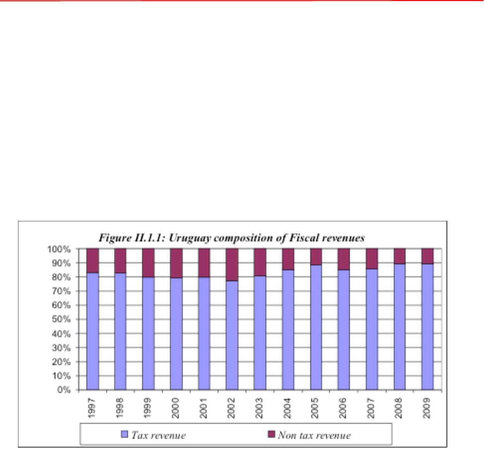
The main source of fiscal revenue in Uruguay is tax collections, which on average over the
last 10 years amounts for nearly 90 percent of total revenue, fluctuating around 16 percent of
GDP. Non-tax revenue contributes with an additional 3 percent of GDP to Uruguayan public
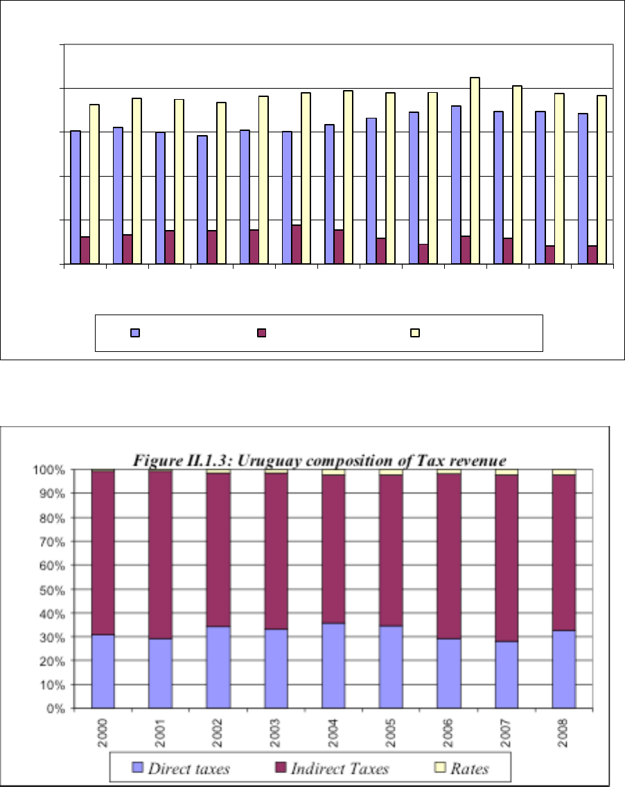
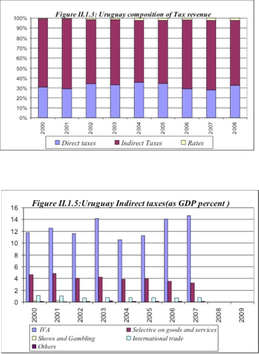
finances. Most of the tax revenues come from indirect taxes, and hence are associated to
domestic private spending. Indirect taxes represent an average of about 70 percent of total
revenue for the past 10 years. Indirect taxes are concentrated on taxes on goods and services,
and particularly the Value added tax, equivalent to 13 percent of GDP.
Source: LE&F, based in information of Contaduría general de Uruguay.
6
0
0.05
0.1
0.15
0.2
0.25
1997
1998
1999
2000
2001
2002
2003
2004
2005
2006
2007
2008
2009
Figure II.1.2: Uruguay Fiscal revenues (as GDP percent )
Tax revenue Non tax revenue Total revenue
Source: LE&F, based on information from Contaduría general de Uruguay.
S
Source: LE&F, based on information from Contaduría general de Uruguay.
7
Source: LE&F, based on information from Contaduría general de Uruguay.
Source: LE&F, based on information from Contaduría general de Uruguay.
8
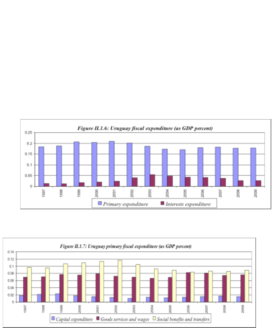
Primary fiscal expenditure expanded continuously reaching above 20 percent of GDP early
this decade, but has since declined converging towards 17 percent of GDP in the last few
years, while interest expenditure has risen from 2 percent of GDP to 5 percent of GDP over
the last decade. Operational expenditures represent the bulk of primary spending, about 90
percent of total, and capital represent the remaining 10 percent. In operational spending,
pension and other welfare benefits represent 40 percent of total expenditures and wages 20
percent. Finally, social benefits expenditure represent around 9 percent GDP while
expenditure on goods, services and wages close to 8 percent of GDP and both have remained
relatively stable over the last few years.
Source: LE&F, based on information from Banco Central de Uruguay.
Source: LE&F, based on information from Banco Central de Uruguay.
9
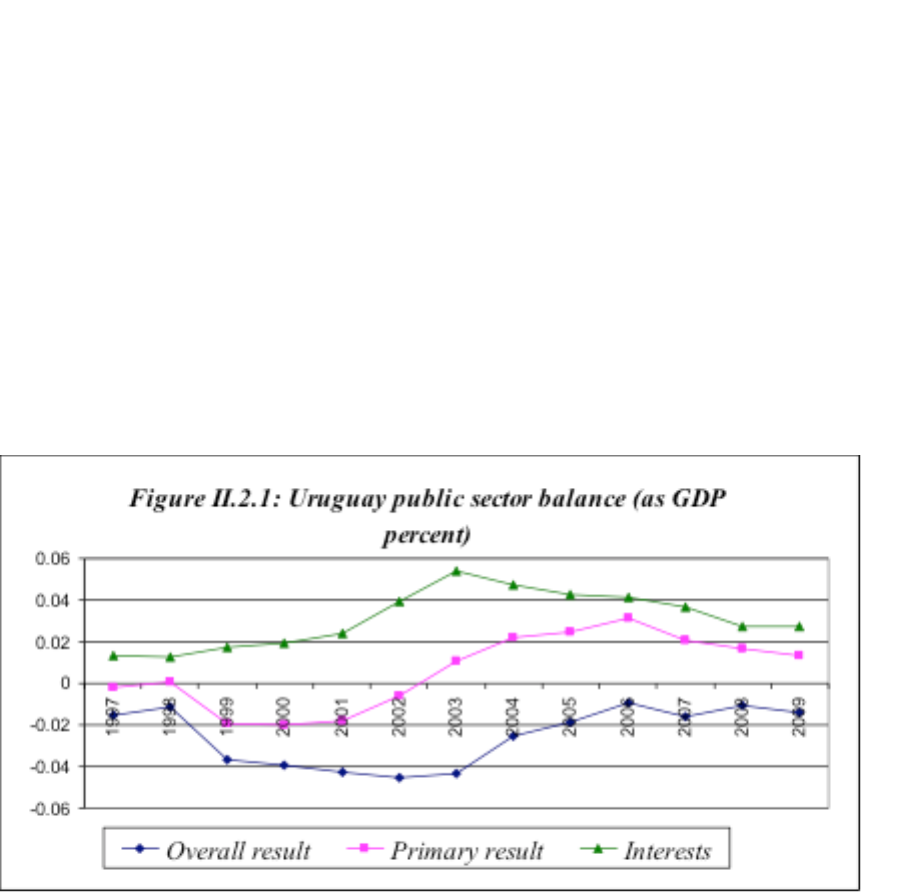
2. Primary and Overall Fiscal Balances
Uruguay’s primary fiscal balance went into deficit from 1999 to 2001 as the crisis ensued,
but with the adjustment and recovery begun in 2003 brought a succession of increasing
primary surpluses reaching up to 3 percent of GDP in 2006. Since then the primary surplus
has declined gradually just below 2 percent of GDP. Uruguay’s debt crisis resulted in a
sustained increase in interest expenditures, which reached a maximum of 5 percent of GDP
en 2003–2004. The adjustment, debt rescheduling and decline in international rates that
followed resulted in the continuous decline of interest spending to less than 3 percent of GDP
in 2009. The overall fiscal balance has remained in deficit throughout the decade, with a
significant improvement over the last few years when the overall balance stood at -1 percent
of GDP and the primary balance at a surplus just below 2 percent of GDP.
Source: LE&F, based on information from Banco Central de Uruguay.
10
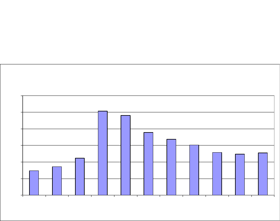
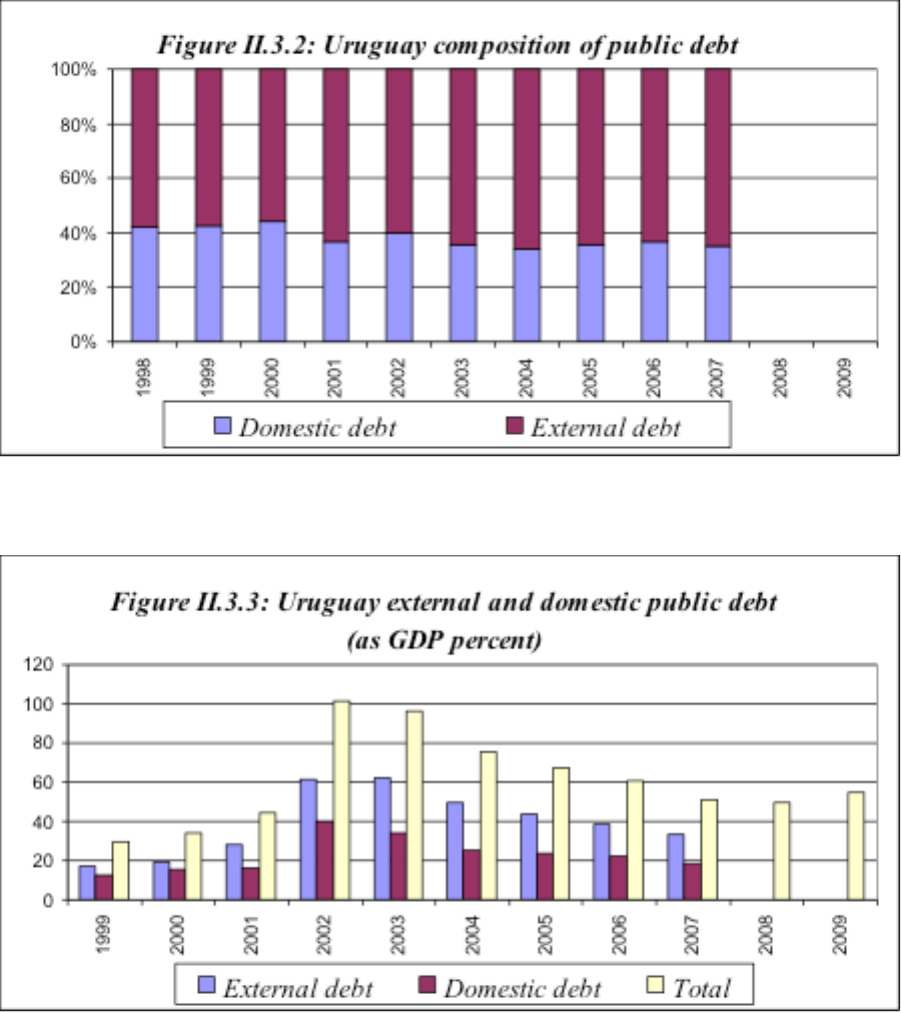
3. Public Debt
The financial crisis of 2002–2003 represented an explosion in the public debt, which
increased from less than 30 percent of GDP in 1999 to 100 percent of GDP by 2002.
Subsequently, with the rescheduling, recovery and adjustment, the public debt level has
gradually declined without reaching the pre crisis level; the debt ratio stood at about 50
percent of GDP in the period 2007–2009. The debt structure is characterized by an almost
even level of foreign and domestic debt, 60 percent and 40 percent of total debt, respectively.
External debt reached levels of over 60 percent of GDP in 2002 and 2003, and then
descended gradually to just over 30 percent in 2007. Domestic debt followed a similar
pattern, reaching levels of 40 percent in 2002 and falling gradually to just under 20 percent o
GDP in 2007.
0
20
40
60
80
100
120
1999
2000
2001
2002
2003
2004
2005
2006
2007
2008
2009
Figure II.3.1: Uruguay public debt (as GDP percent)
Source: LE&F, based on information from Contaduría general de Uruguay.
11
Source: LE&F, based on information from Contaduría general de Uruguay.
Source: LE&F, based on information from Contaduría general de Uruguay.
The composition of Uruguayan Public debt has improved over the last few years after the
crisis, the maturity of the debt has increased, the fixed interest rate has gained ground over
the flexible rate, and a lower percentage of debt is denominated in foreign currency. The
residual maturity of external debt instruments has increased over the last few years. Long-
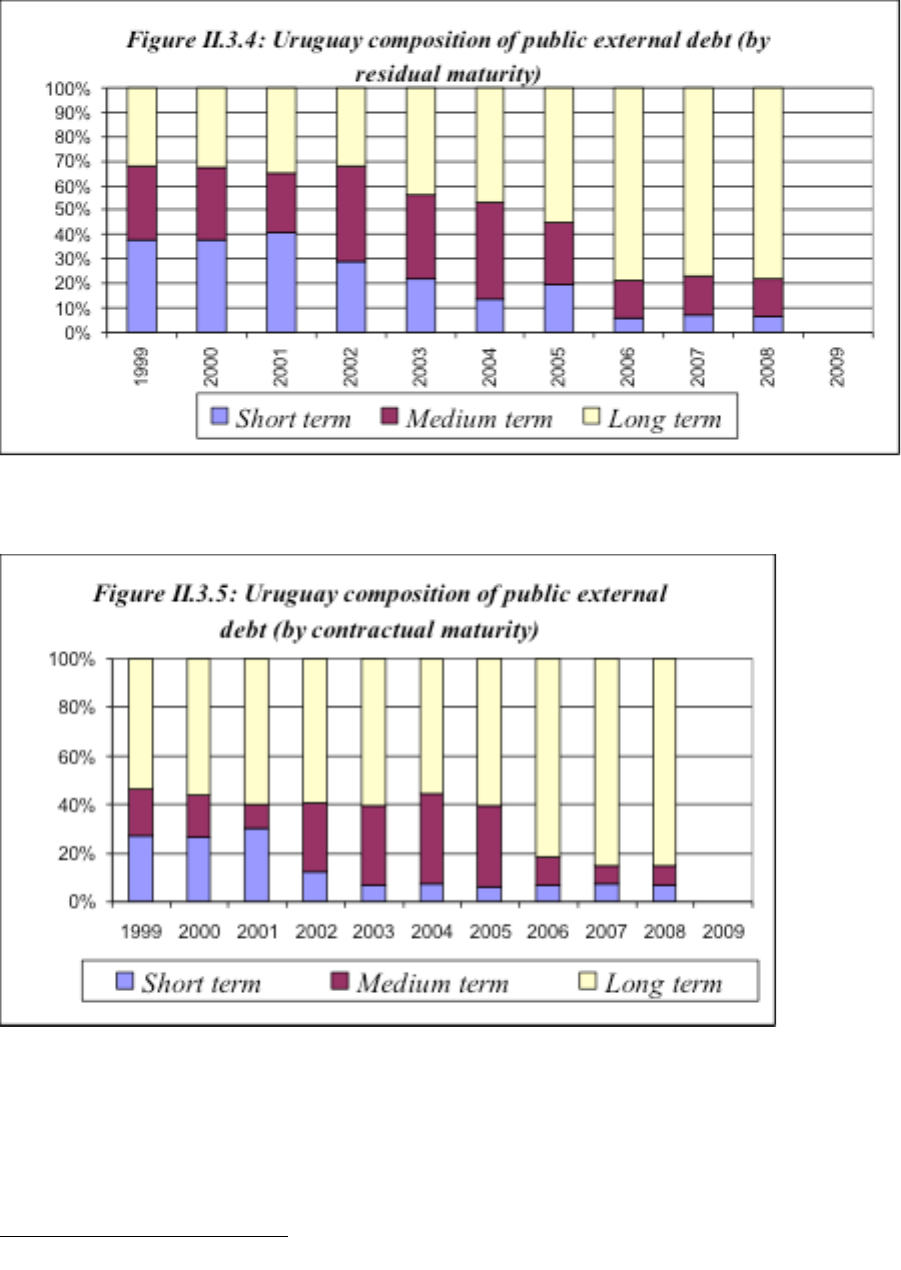
12
term
1
instruments represent almost 80 percent of total in 2008 after being only 30 percent
earlier in the decade.
Source: LE&F, based on information from Contaduría general de Uruguay.
Source: LE&F, based on information from Ministerio de Economía y Finanzas of Uruguay.
1
Long term: more than 5 years; medium term: 1-5 years; short term: less than 1 year
13
Fixed interest rates debt has increased from 30 percent of total in 1999 to 60 percent of total
in 2008.
0%
10%
20%
30%
40%
50%
60%
70%
80%
90%
100%
1999
2000
2001
2002
2003
2004
2005
2006
2007
2008
2009
Figure II.3.6: Uruguay composition of public external
debt (by interest rate)
Fixed rate Libor BID BIRF Others variables Net deposits and other liabilities
c
Source: LE&F, based on information from Ministerio de Economía y Finanzas of Uruguay.
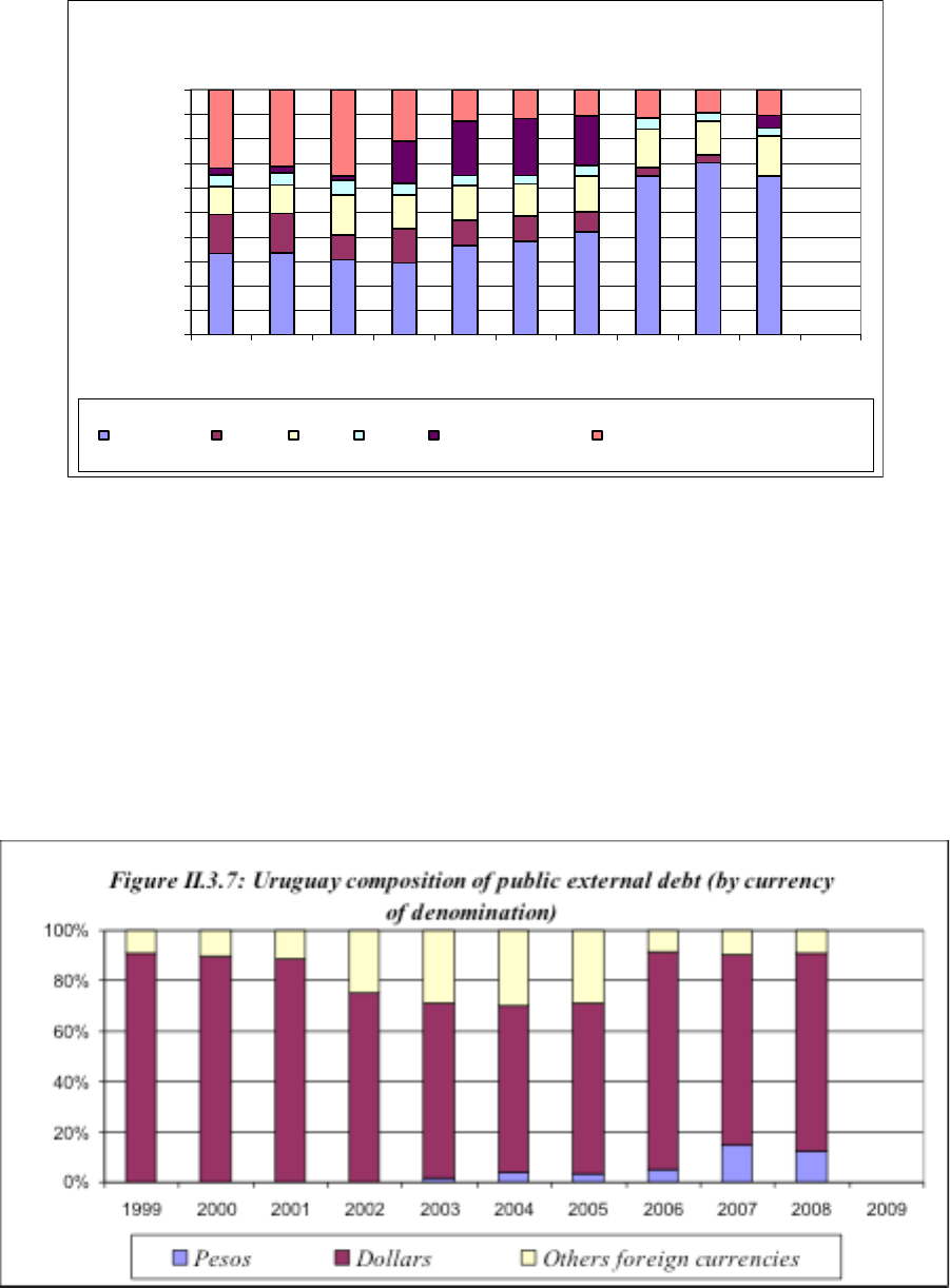
Currency composition: Foreign debt is denominated mostly in dollars, but it has declined
from around 90 percent of total in 1999 to less than 80 percent in 2008. A significant portion
of domestic debt is also denominated in US dollars, but its importance is declining, Actually,
in 2009, 30 percent of total debt is denominated in domestic currency, either nominal or
adjustable by the CPI inflation rate.
Source: LE&F, based on information from Ministerio de Economía y Finanzas de Uruguay
14
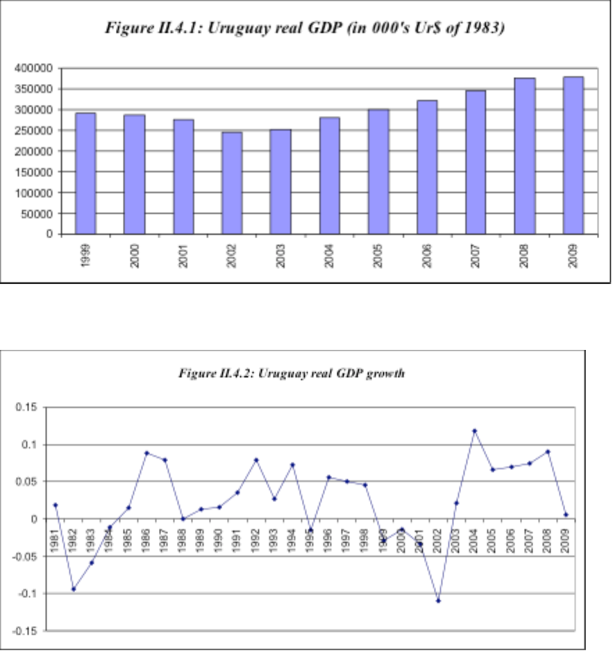
4. Real GDP and Components
As it is well known, Uruguay experienced another financial crisis and a major recession
earlier in this decade mostly as a result of contagion from the financial crisis of Argentina
through a very vulnerable domestic financial system. The recovery that was evident in the
data from 2004 on has been quite strong, with an annual GDP growth rate that averaged
around 8 percent per year in 2004-2008, but has since then declined to almost 0 in 2009,
partly as a result of the effects of the sub prime crisis in Uruguay’s international markets.
Source: LE&F, based on information from Banco Central de Uruguay.
Source: LE&F, based on information from Banco Central de Uruguay.
15
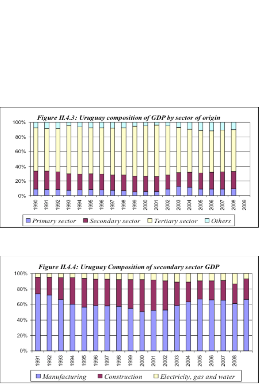
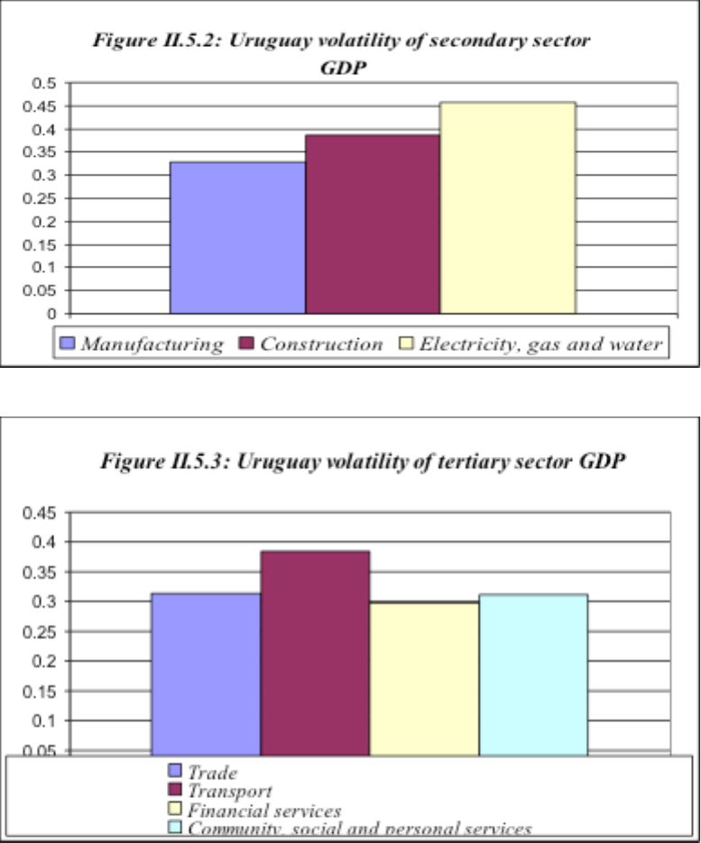
The composition of Uruguay’s GDP shows a certain bias towards services, with the tertiary
sector representing close to 60 percent of total GDP. Services like financing, insurance, real
estate and renting accounts for 1/3 of this total, business services other third, and community,
social and personal services the remaining. The secondary sector represents approximately 20
percent of GDP, with manufacturing, construction and electricity accounting for 70 percent,
20 percent and 10 percent of this total, respectively. Despite its agricultural export base, the
primary sector in Uruguay is about 10 percent of GDP, with agriculture representing over 80
percent of primary sector activity.
Source: LE&F, based on information from UN ECLAC.
Source: LE&F, based on information from UN ECLAC.
16
Source: LE&F, based on information from UN ECLAC.
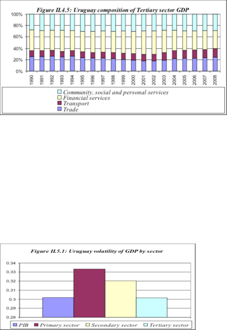
5. Volatility of Real GDP
In order to measure the variability of GDP, we use the coefficient of variation for total GDP
and its main sectors of origin. The primary sector presents the highest volatility, with a
coefficient of 0.33, higher than total GDP, 0.30. By individual sectors, electricity is the most
volatile, even more than agriculture. To a large extent the volatility of electricity is the result
of the weather, given that the value added of hydro-electrical generation, highly dependent on
rainfall, is much higher than that of thermo electrical generation. The rainfall changes the
composition of electrical generation and with that sectorial GDP.
Source: LE&F, based on information from UN ECLAC .
17
Source: LE&F, based on information from UN ECLAC.
Source: LE&F, based on information from UN ECLAC.
18
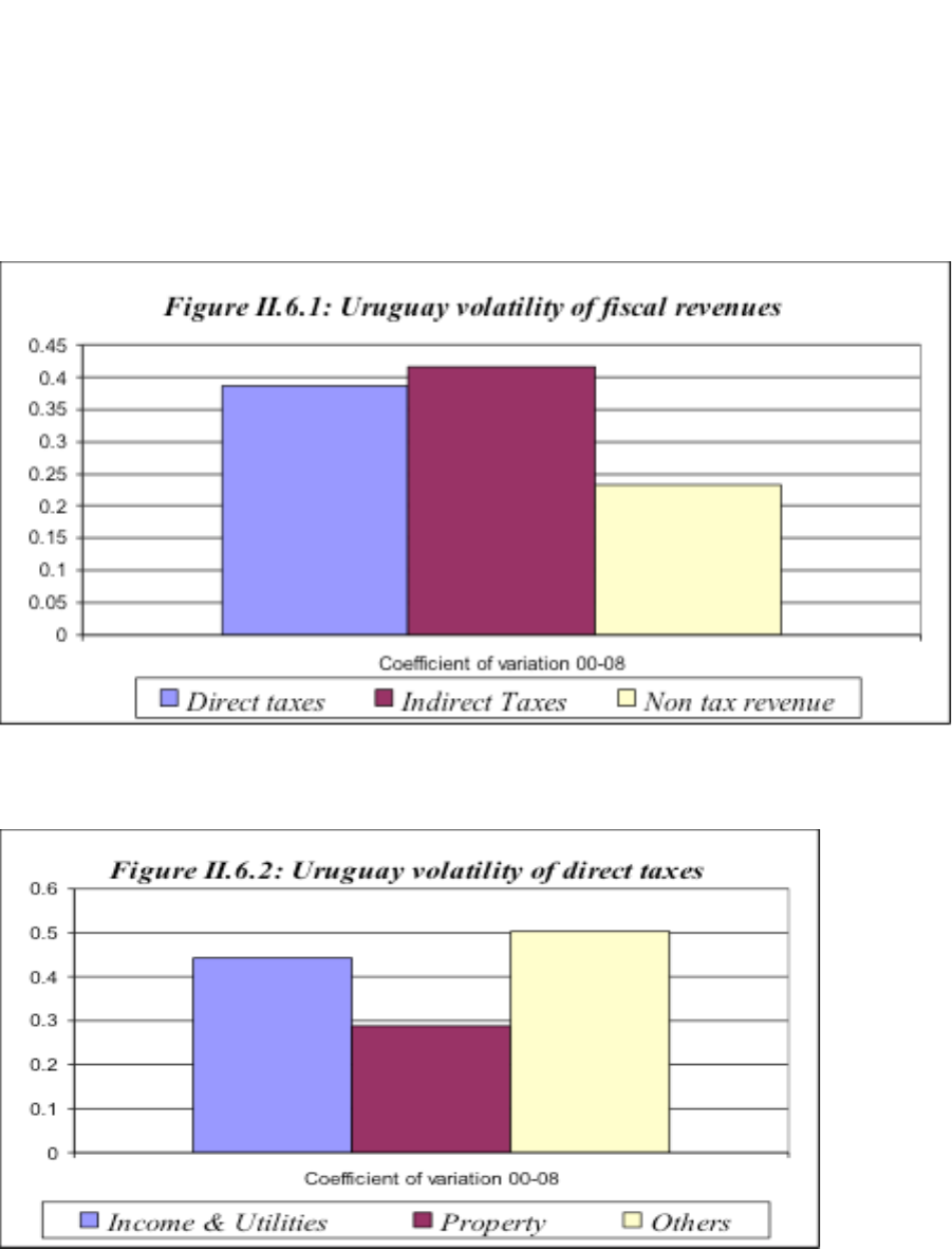
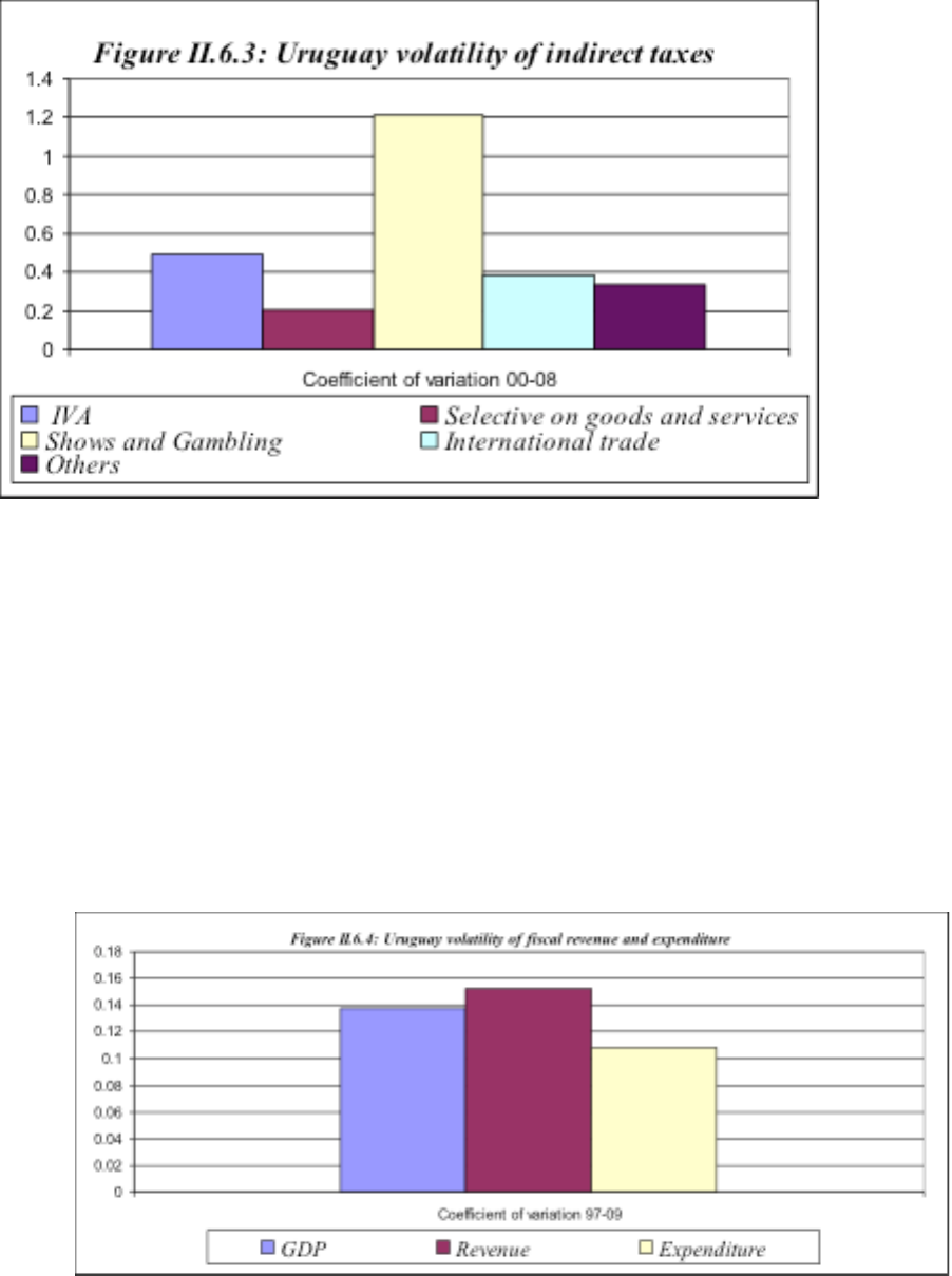
6. Volatility of Fiscal Revenues
Fiscal revenue is more volatile than fiscal expenditure. In turn, tax revenues are more volatile
than non-tax revenue. The revenue form the Value Added Tax (VAT) presents a slightly
higher volatility than total GDP, probably reflecting that the volatility of domestic demand is
higher than that of GDP, and that the VAT exemptions for exports imply that the VAT tax
base is domestic demand rather than output.
Source: LE&F, based on information from Contaduría general de Uruguay.
Source: LE&F, based on information from Contaduría general de Uruguay.
19
Source:
LE&F, based on information from Contaduría general de Uruguay.
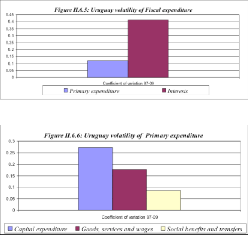
Interest expenditure is more volatile than primary expenditure, and within this item, both
spending on goods and services and capital spending have a volatility higher than that of
social spending which seems quite protected by policies from the ups and downs of domestic
activity and fiscal revenue. While the volatility of interest expenditure seems to reflect the
volatility of the exchange rate and of international interest rates, the volatility of capital
expenditure is residual, that is reflects the efforts of conforming the fiscal balance to
available resources.
Source: LE&F, based on information from Contaduría general de Uruguay.
20
Source: LE&F, based on information from Contaduría general de Uruguay.
Source: LE&F, based on information from Contaduría general de Uruguay.

21
III. Estimating and Projecting the Structural Fiscal Balance in Uruguay
Uruguay is an open economy that exports a variety of agricultural commodities, including
meat, rice, wool, leather and others. However, its degree of specialization is lower than that
of other Latin American countries where the main export item plays a significant role in the
generation of fiscal revenue. That is the case of oil in Venezuela, Ecuador and Trinidad and
Tobago, or of Copper in Chile and Peru. A combination of a tax structure focused on
domestic spending and the relative export diversification of Uruguay implies that the
volatility of total fiscal revenue is mostly associated to the cycle of GDP, and not to the
evolution of the price, cost and export of some of the agricultural commodities exported. The
methodology to estimate structural fiscal revenue will then focus in the estimation of trend
and transitory GDP and their effects on fiscal revenue and the fiscal balance. To the extent
that the information is available, we will follow the procedures identified by the OECD in a
similar way as it has been implemented by the Chilean government over the last decade.
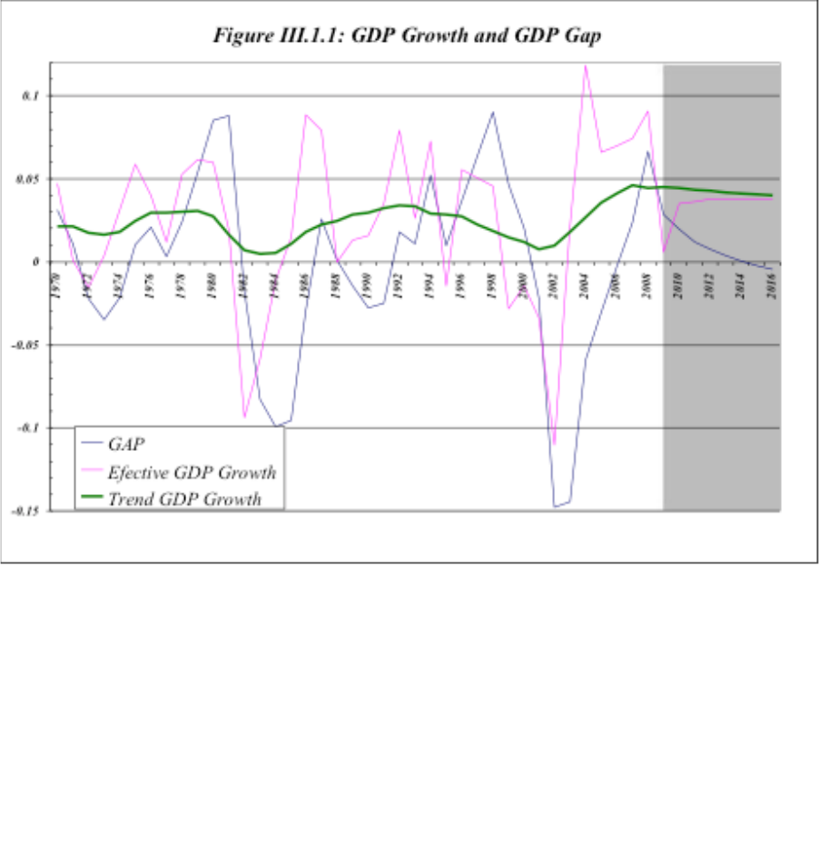
1. Estimation of Trend or Structural GDP
Real GDP (y) can be analytically decomposed in a permanent (Yp) and a transitory
component (Ytran). The log of transitory GDP, also called the GDP gap, is positive in
expansionary periods, negative during slow downs and recessions and cero during neutral or
normal periods, besides its mean is also cero.
Y
t
tran
t
P
tt
tran
t
P
tt
gapyyyyyy ==−+= logloglog;logloglog
Permanent GDP is estimated from a Cobb Douglas production function with constant returns
to scale, where A is total factor productivity, K capital, N effective labor and a the share of
capital in total income. The superscript P is used to represent the permanent or trend
component of the corresponding variable, total factor productivity, capital stock, and
effective labor. In selecting the capital and labor shares we use the results of previous works,
Theoduloz (2006), where a is a constant estimated equal to 0.27
2
.
P
t
P
t
P
t
P
t
P
t
P
t
PP
t
NKAy
NKAy
log)1(logloglog
;)()(
)1(
αα
αα
−++=
=
−
2
Ideally, alpha should be obtained from the national income accounts, considering it represents the share of
capital in the functional distribution of national income. Such source of data is not available in Uruguay.
22
Source: LE&F, based on information from ECLAC, INE and CERES.
Effective employment (N) can be defined as the total hours of effective work, and calculated
multiplying the number of employed workers (N#) by the average number of hours worked
(h) and by the average years of schooling (s). The series on the number of workers N# was
obtained from the ECLAC and INE for the period 1970-2009. Unfortunately the series on
average number of hours worked and average years of schooling of the labor force are not
available, thus we have assumed value 1 for all observations of both variables.
;# shNN
ttt
××=
23
Source: LE&F, based on information from ECLAC and INE.
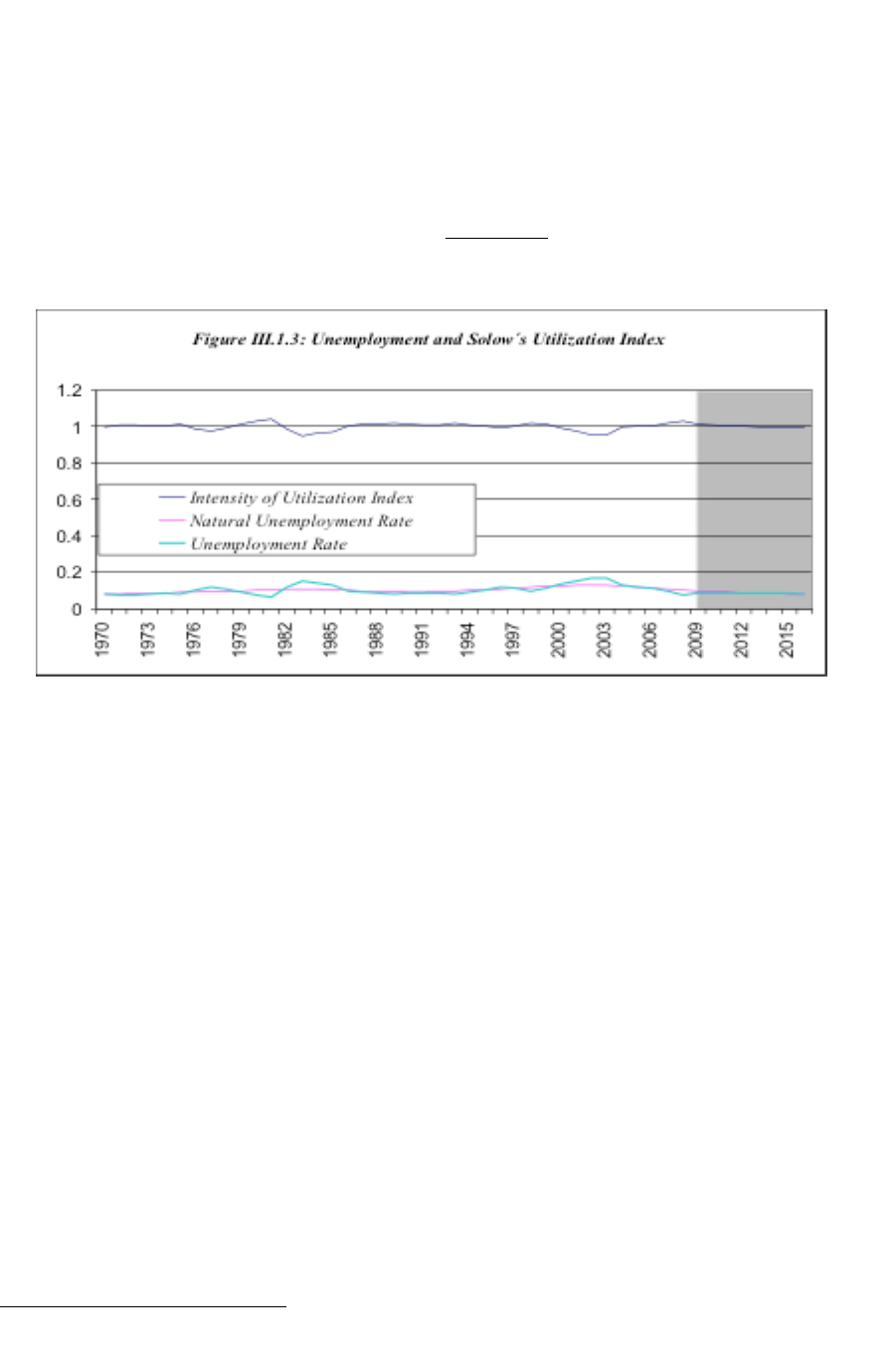
The degree of utilization of Labor and capital is derived from the unemployment rate (U)
which is defined as the difference between the labor force (L) and the number of people
employed N#, as a percent of the labor force
3
. Trend or natural unemployment is obtained
applying a HP filter to the unemployment rate series
4
.
)(
#
t
P
t
t
tt
t
UHPfilte rU
L
NL
U
=
−
=
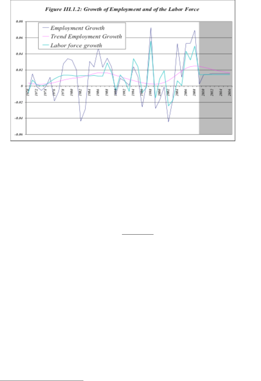
The trend value of effective employment is obtained applying a Hodrick and Prescott filter
(HP filter) to the series of labor force L, and multiplying it for one minus the natural
unemployment rate. Over the last years and with the recovery from the debt crisis, the rate of
growth of trend employment has increased reaching a maximum slightly above 2 percent per
year. Given the demographic projections the trend growth rate of employment will be
gradually declining below 2 percent over the next decade.
)1()(
P
tt
P
t
ULHPfilterN −×=
3
The source of the series on the labor force and employment is ECLAC and INE
4
The OECD recommendation is to use a lambda value of 100 for obtaining the trend unemployment rate, where
lambda is the HP filter parameter.
24
The Solow index of the intensity of use is defined on the basis of the regular and natural
unemployment ratios, so that the index value is 1 when the unemployment rate is equal to the
natural unemployment rate and less than one when effective unemployment is above the
natural rate.
)1(
)1(
P
t
t
t
U
U
S
−
−
=
Source: LE&F, based on information from ECLAC and INE.
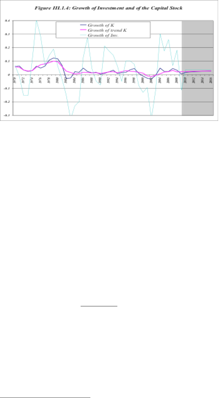
The estimation of the capital stock is based on the regular inventory accumulation equation,
where K is the capital stock, I is investment, defined as the fixed gross capital formation, and
d is the depreciation rate. The series on gross capital formation was obtained from the
ECLACC and CERES, and the depreciation rate was obtained from World Penn extended
table. The initial value for the capital stock implies a capital labor ratio equal to 1.6 in 1970.
5
On the basis of an estimated growth rate of Gross Capital formation of less than 4 percent
over the next few years, the trend growth rate of the capital stock remains slightly below 3
percent, implying a continuous decline in the capital-output ratio.
t
P
t
P
t
IKK +−=
−
)1(
1
δ
5
The initial estimate of the capital stock (1970) was obtained from the data on fixed capital formation and
depreciation using a regular inventory methodology see Haindl and Fuentes (1986).
25
Source: LE&F, based on information from ECLAC and CERES.
The estimation of the effective capital stock K is obtained by correcting the trend capital
stock K by the Solow intensity of use (S):
t
P
tt
SKK ×=
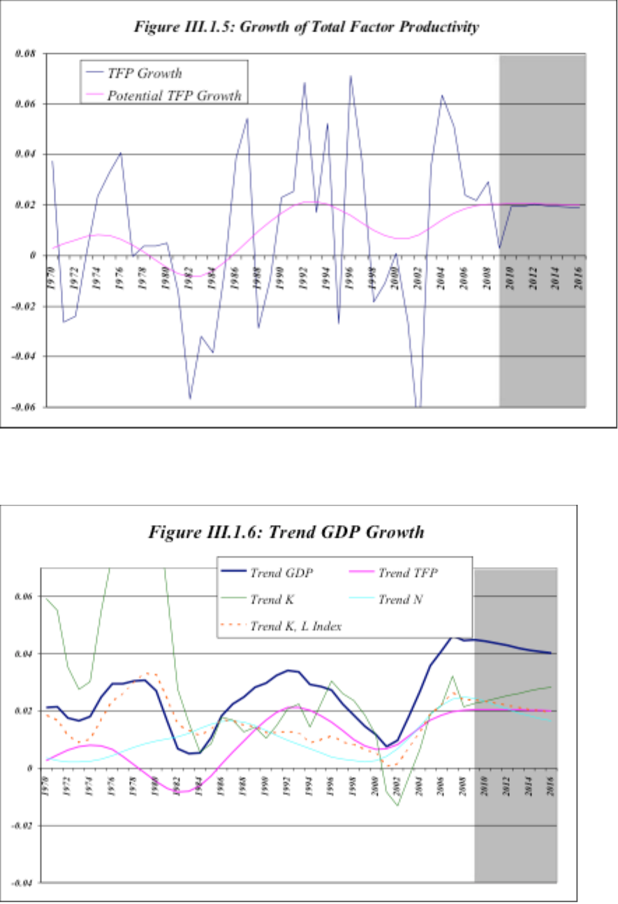
Finally, total factor productivity TFP is derived as a residual using the production function
and effective data on GDP, capital, adjusted by the intensity of use, and effective
employment. To obtain the permanent or trend total factor productivity we applied the
Hodrick and Prescott filter to the TFP series. Surprisingly enough, trend productivity growth
not only has increased to about 2 percent per year, but also is projected to remain at that
expansionary rate over the next few years.
6
tttt
tt
t
t
NKyA
NK
y
A
log)1(logloglog
;
)1(
αα
αα
−−−=
=
−
)(
t
P
t
AHPfilterA =
6
We have used the IMF WEO projections for real GDP growth through 2016, and assumed that the investment
to GDP ratio will continue at its average value of the last five years, thus deriving a gross capital formation
estimate. To project employment we assume that the unemployment rate will converge to the last observation of
the natural unemployment rate and considered that the labor force would increase with the working age
population.
26
Source: LE&F, based on information from ECLAC and CERES.
Source: LE&F, based on information from Banco Central de Uruguay.
27
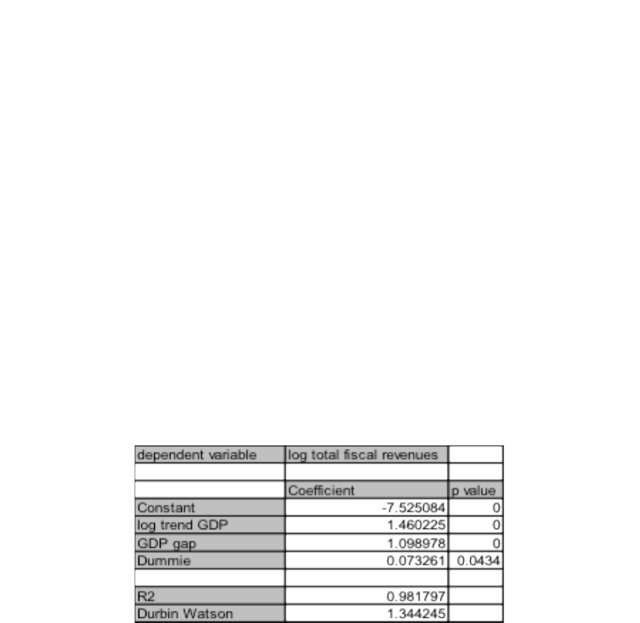
The results indicate that over the last few years, the growth of trend GDP in Uruguay has
been accelerating reaching a rate slightly above 4 percent per year. Growth has then
stabilized but our projections indicate a convergence of trend GDP growth to about 4 percent
during the second decade of the 21st century. The forecasted rate of expansion for trend GDP
is significantly above its historical value, with ups and downs around 2 percent, and could be
affected by the recent recovery. The assumptions used for future GDP, labor force and gross
capital investment growth are subject to discussion and for that reason should be derived
from the opinions of several experts on the Uruguayan economy, and revised annually.
2. Elasticities and the Structural Balance
The estimation of the structural fiscal balance requires the estimation of a stable relationship
between fiscal revenue and its components with trend GDP and the GDP gap. The elasticity
of fiscal revenue with respect to trend GDP is going to play a pivotal role in determining the
value of the structural revenue and the structural balance. The estimated regression is of the
following form,
tt
y
t
P
tt
DgapyT
εββββ
++++=
1997
3210
loglog
Where T represents the real fiscal revenue, total or components, Yp the permanent GDP, gap
y the GDP gap and D1997 a qualitative variable to represent the structural break that
represents the policy reaction that resulted in a structural break in the level of Public sector
revenue in Uruguay.
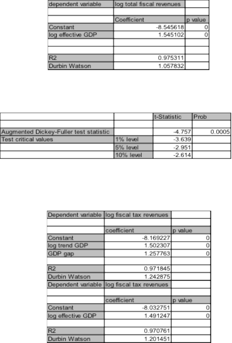
Table III.2.1: Regressions for Total Fiscal Revenue and GDP
28
Source: LE&F, based on information from ECLAC and CERES.
Table III.2.1.i: Co-integration Analysis (residual test)
Source: LE&F, based on information from ECLAC and CERES.
Table III.2.2: Regressions for Tax Revenue and GDP
Source: LE&F, based on information from ECLAC and CERES.
29
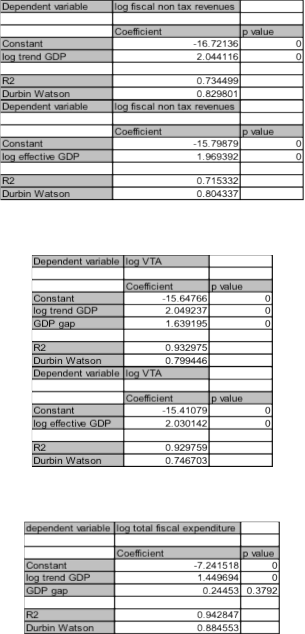
Table III.2.3: Regressions for Non-tax Fiscal revenue and GDP
Source: LE&F, based on information from ECLAC and CERES.
Table III.2.4: Regressions for the VAT and GDP
Source: LE&F, based on information from ECLAC and CERES.
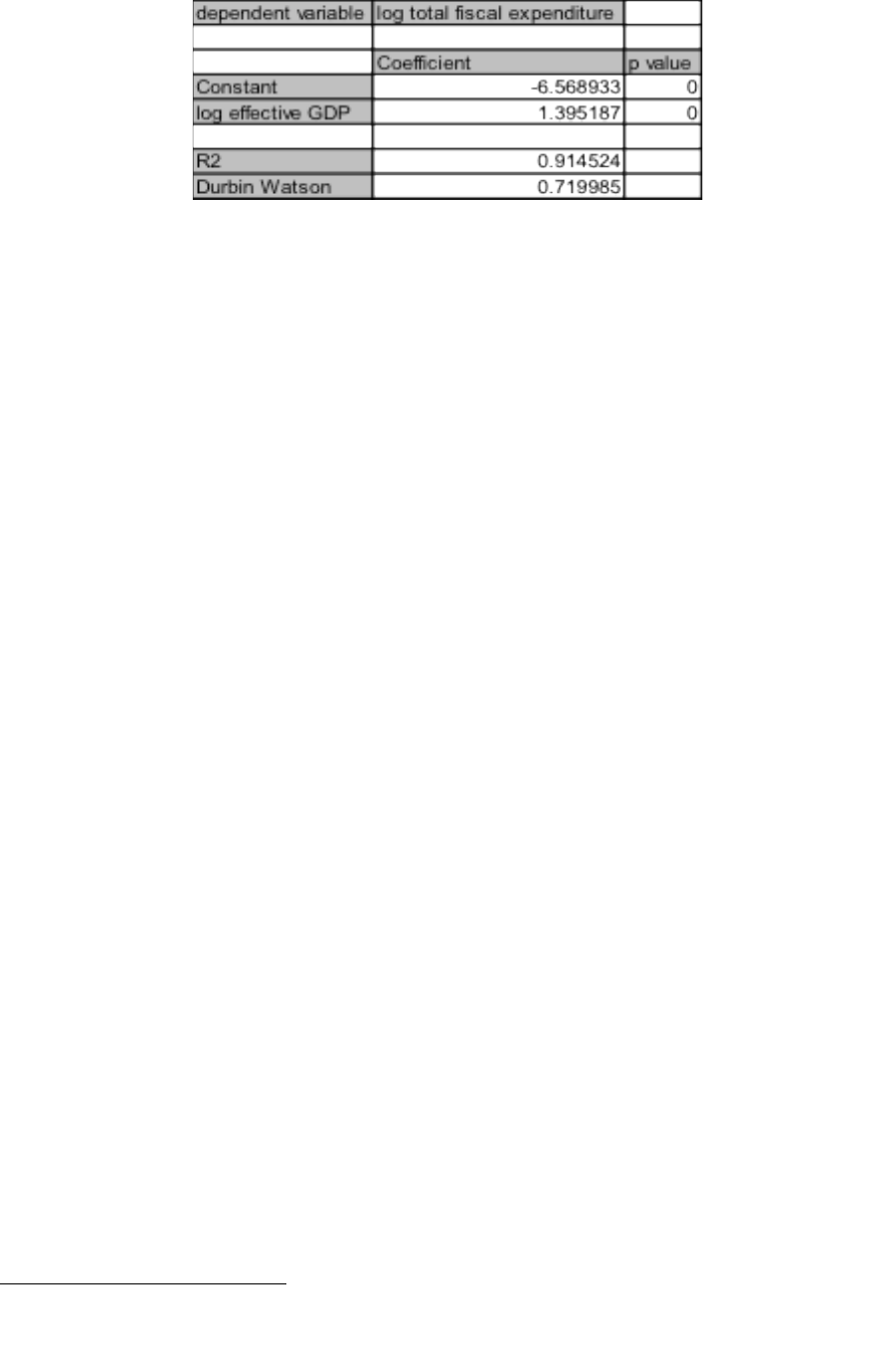
Table III.2.5: Regressions for Fiscal Expenditure and GDP
30
Source: LE&F, based on information from ECLAC and CERES.
The results of the estimation indicate that the elasticity of revenues to trend GDP is
somewhat greater than one in which the structural break is in general significant. Moreover,
both fiscal revenues and fiscal expenditures present a pro cyclical response to GDP, given the
positive and significant elasticity of revenue and expenditure with respect to the GDP gap.
7
Conceptually, the structural fiscal balance is the one that would have existed if GDP
were at its trend level. Correspondingly the structural fiscal revenue is the revenue that would
have been obtained under a zero gap. Then the structural fiscal balance is defined as the
difference between the total structural fiscal revenue and the total fiscal expenditure. The
estimation of the total structural revenue can be obtained using the estimated regression for
total revenue, and assuming a zero gap:
Thus the structural fiscal balance is
t
P
tt
GTSFB −=
Government revenue (T) has a permanent (TP) and a transitory (Ttran) component
tran
t
P
tt
TTT +=
Which can be expressed as a percent of GDP in lower case letters:
tran
t
P
tt
ttt +=
The primary fiscal balance is obtained by excluding the interest expenditures. The structural
primary balance, psb, is derived subtracting the transitory revenue.
7
In addition, the regular co-integration analysis was carried out for the fiscal revenues and tax equation, and it
was obtained that the residuals of the main regression (Table III.2.1) are stationary, so that these variables co-
integrate among themselves.
31
tranD
ttt
tranD
t
DP
tt
tpsbpgttpfb
,,
+=−+=
The structural fiscal balance (sfb) can be obtained subtracting from the primary surplus the
interest expenditure.
ttt
P
tt
igpsigpgtsfb −=−−=
*
The actual fiscal balance (fb) is the structural balance plus the transitory revenue, which can
be positive or negative. Any positive transitory revenue is to be saved in the form of a larger
fiscal balance, and any negative transitory revenue dis-saved through a smaller fb or larger
deficit.
tran
tttt
tran
t
P
tt
tsfbigpgttfb +=−−+=
In the case of Uruguay, permanent and transitory fiscal revenue stems from the business
cycle that gives rise to fluctuations in the domestic revenue (DT). The ups and downs in GDP
result in ups and downs in domestic revenue (DT):
t
P
tt
P
tt
YYYDT
εβββ
+−++= ]log[logloglog
210
Where bo, b1 and b2 are parameters to be estimated and e represent the disturbances of the
domestic revenue equation. In some specifications used by the OECD b2 is considered equal
to cero, however we consider that excluding the gap from this equation may bias the estimate
for the elasticity with respect to trend GDP. We can distinguish permanent or structural
revenue from transitory revenue.
P
ttt
P
tt
tran
t
P
t
P
t
DTDTYYDT
YDT
loglog]log[lo glog
loglog
2
10
−=+−=
+=
εβ
ββ
Presenting revenue in percent of GDP
32
t
P
tt
tran
t
P
tt
tran
t
tt
P
tt
tran
t
t
P
t
P
t
Y
DTDT
dt
DTDTDT
YYYdt
YYdt
−
=
−=
+−−=
−+=
εβ
ββ
log]log[loglog
logloglog
2
10
-0.1
-0.08
-0.06
-0.04
-0.02
0
0.02
0.04
1970
1973
1976
1979
1982
1985
1988
1991
1994
1997
2000
2003
2006
2009
2012
2015
2018
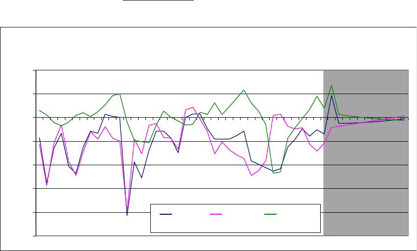
Figure III.2.1: Fiscal balance evolution (as GDP percent)
Effective
balance
Structural
balance
Cyclical
component
Source: LE&F, based on information from ECLAC and CERES.
Our estimates indicate that Uruguay’s total structural fiscal balance has remained in deficit
almost continuously, exception made for a brief period of zero structural balance in the early
1990s. The debt crisis of 1982 had implied a large widening of the structural fiscal deficit and
a continuous adjustment effort followed, reaching its peak results in terms of fiscal
consolidation in 1989-1992. From then on a sustained deterioration in the structural fiscal
balance took the deficit to a new local maximum of 4 percent of GDP in the years of the turn
of the century (1999-2002). The adjustment that followed the last debt crisis once again
reduced the structural fiscal deficit to 1 percent of GDP for a few years, but the structural
deficit has recently widened to about 2 percent of GDP in 2009. Despite the improvements in
public finances of the last 5 years by no means Uruguay is out of the woods, as it has
happened before the debt level may again rise to critical levels unless a structural fiscal
policy committed with the reduction of the vulnerabilities of the public finances is
33
implemented. That would require a return of the fiscal balance or slight surplus similar to the
one carried out during the early 1990s.
Source: LE&F, based on information from ECLAC and CERES.
Source: LE&F, based on information from ECLAC and CERES.
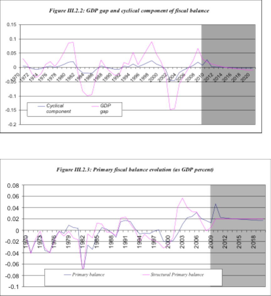
The structural primary balance in Uruguay has fluctuated around 0 with some periods of deep
deficits and a few years of sustained surpluses. The deficit periods are associated with the
debt crisis of 1982 and the debt crisis of 2002; actually a succession of primary deficit
preceded the last debt crisis. The most notable surplus periods are two, the first stabilization
effort of the early 1990s that resulted in a sustained reduction on the inflation rate. The
second is the recent adjustment that followed the debt crisis of 2002 generating large
34
structural primary surpluses, of up to 4 percent of GDP in the period 2004-2007. However,
since then the structural primary surplus has fallen below 1 percent of GDP in 2008 and
2009.
3. Fiscal Projections
In the fiscal projections exercise we assume an active policy scenario in which a structural
fiscal policy is implemented. Primary government expenditure as a percent of GDP (pg) is
budgeted on the basis of permanent revenue (tP) and the fiscal target for the primary balance
(ps*). Interest spending (ig) is predetermined by debt contracts, added to primary spending
we obtain total government expenditure (g).
*
pstpg
P
tt
−=
t
P
tttt
igpstigpgg +−=+=
*
To define the budget for primary expenditure (pg) it is necessary first to estimate the
structural fiscal revenue (tP) and then to set the fiscal target for the primary structural balance
ps*. The future structural fiscal revenue is to be obtained from the estimation of the future
trend GDP, for that purpose we use the estimated elasticity of fiscal revenue with respect to
trend GDP.
P
t
P
t
YDT
1101
loglog
++
+=
ββ
The future value of trend income has to be estimated on the basis of the production function,
using projected future values for trend productivity (Ap), trend Capital stock (Kp) and trend
employment (Np).
P
t
P
t
P
t
P
t
NKAy
1111
log)1(logloglog
++++
−++=
αα
)(
11 ++
=
t
P
t
AHPfilterA
Trend productivity can be obtained applying an HP filter to the series of actual and projected
productivity. For that purpose projections of A through 2020 were used.
itititit
NKyA
++++
−−−= log)1(logloglog
αα
35
For consistency the projected values for total factor productivity (A) should be obtained as a
residual from the projections of GDP, Capital and Labor.
11
)1(
++
+−=
t
P
t
P
t
IKK
δ
Trend capital is equal to total capital and the projections for K can be obtained on the basis of
the inventory equation and projections for gross capital formation. Again we projected the
capital stock adjusted for the intensity of use through 2020.
)1()(
11
P
tt
P
t
ULHPfilterN −×=
++
Finally, the projection of trend employment requires the projection of the trend labor force,
and of the trend unemployment rate. Summing up, projections through 2020 were used for
GDP, gross capital formation, labor force and the unemployment rate. From there the
budgeting process can derive trend GDP and thus the trend fiscal revenue. Given the target
for the structural balance, the budgeted primary fiscal expenditure is to be obtained. In this
exercise we used the WEO projections for GDP growth through 2016 and assumed a stable
growth rate afterwards at the level of the last observation. Investment was projected assuming
that the last five-year average for the investment GDP ratio will prevail in the future. Finally,
the projected expansion of the working age population was used to project labor force, and
the stabilization of the unemployment rate at the natural rate value was used to derive
effective employment.
4. The Structural Fiscal Target
The proposed structural fiscal target has to be derived for the structural primary balance. The
target for the structural primary balance should be defined so as to provide fiscal
sustainability by meeting certain goals for the relevant definition of the public sector net
financial wealth (B). The fiscal balance represents the change in financial wealth. It is equal
to the primary balance and net interest, where i is the nominal interest rate.

36
tttttt
IGPFBIGPGTFB −=−−=
111 −−−
+=+−=−
ttttttt
iBPSiBPGTBB
We can define the wealth equation for the primary surplus:
1
)1(
−
++=
ttt
BiPSB
Defining the variables as a percent of GDP, where p is inflation and l real GDP growth, and r
the real interest rate.
1
1
1
)1)(1(
)1(
)1(
−
−
−
++
+
+=×++=
t
tt
t
t
t
t
tttt
b
i
psb
Y
Y
bipsbb
πλ
11
)1(
)1(
)1(
−−
++=
+
+
+=
tttt
t
t
tt
bpsbb
r
psbb
ψ
λ
The idea is to find a permanent target for the primary structural surplus psb*, which we will
assume to be constant. In addition we will assume constant real interest rate and constant
growth rate, so that the wealth equation is transformed to:
1
)1(
−
++=
tt
bpsbb
ψ
Where the discount factor is:
)1(
)1(
)1(
λ
ψ
+
+
=+
r
Developing the wealth equation for future periods:
1
2
1
)1()]1(1[)1(
−+
++++=++=
ttt
bpsbbpsbb
ψψψ
1
32
2
)1(])1()1(1[
−+
++++++=
tt
bpsbb
ψψψ

37
1
1
0
]1[]1[
+
−
=
+
+++=
∑
N
t
j
N
j
Nt
bpsbb
ψψ
The value for the targeted psb* depends on the initial wealth level b(t-1), the discount factor,
the target for the wealth level b(t+N), and the number of periods to reach the target (N). If the
fiscal target were set to keep constant the wealth to GDP ratio at its initial level b(t-1), then
*
0
1
1
]1[
])1(1[
psb
b
j
N
j
N
t
=
+
+−
∑
=
+
−
ψ
ψ
Otherwise, a given target for the wealth to GDP ratio at a given horizon of N years into the
future b(t+N) would give the general result for the annual structural fiscal target.
*
0
1
1
*
]1[
]1[
psb
bb
j
N
j
N
tNt
=
+
+−
∑
=
+
−+
ψ
ψ
To calculate the fiscal target and as shown in the above equation, there are several
information requirements. First about debt or public sector wealth, including actual, in the
last period available, and targeted debt, second about the discount factor for which we need
the real interest rate and the real growth rate, and, finally, the horizon in which the debt target
is to be met. The debt information was obtained from the central bank of Uruguay; the
growth rate used is that obtained previously as the projected potential growth rate of the
economy. We recognize that different views are possible regarding the future growth of the
Uruguayan economy, our estimate of 4 percent sustained real GDP growth may seem high
for historical standards in this country
8
. However, the trend growth rate will be endogenous
to the policies implemented which can easily reduce or increase the sustained growth rate
through their effect on productivity growth, i.e. incentives for innovation, capital stock
8
Using the WEO projections for economic activity, and under assumptions for investment, working age
population and productivity growth rates
38
growth, i.e. incentives on savings and investment, and labor growth, incentives on migration
of the qualified labor force. Different views may exist about the future trend GDP growth of
the Uruguayan economy, and the views may change over time.
Given that Uruguay is a debtor country, we estimate the relevant real interest rate on
the basis of an indicator for the real return on global assets and a representative risk spread
for Uruguay. The real global rate of return in the long run is estimated on the basis of the
average annual growth rate of JPM Global Bond and MSCI all countries indices, both in real
terms. We assume an equal weight for both indices to represent a global portfolio and its
historical average real return in the long run of it is to be considered the global real interest
rate that will prevail in the future. Our estimation indicates a global long run real interest rate
of 4.65 percent. However that is not the relevant rate for the Uruguayan public sector that
borrows at that rate plus a risk spread. To estimate the relevant Uruguayan spread we
compare the actual returns of the Uruguayan debt (actual real interest rates) with the historic
global rate of return, yielding an average spread of 1.1 percent. Thus the Uruguayan log run
real interest rate on debt was estimated at 5.75 percent.
Again, as in the case of the real growth rate, the estimate for the interest rate of the
Uruguayan debt over the long term is subject to discussions and different views. The one
presented is our best guess with the information and expertise available, but the spread of he
Uruguayan debt is endogenous and in the future will reflect the risk that markets give to its
repayment. A virtuous cycle of lower deficit, lower debt, and lower spread is possible, but
also is possible a vicious one of higher deficit, debt and spread. A repeated assessment of the
debt risk is required to estimate the future values of the spread.
Given that it is not possible to determine a single horizon and a single debt target that
would be appropriate for Uruguay we present a table considering a range of possibilities for a
given value of the discount ratio psi, which was estimated at 1.549 percent. For the time
horizon we consider a wide range from 5 to 50 years, considering as a minimum the period of
one Uruguayan government, and as a maximum the period of ten governments. To set a
target for such a long period, a very solid political consensus should be developed to back the
structural fiscal policy. For the future public wealth target we also considered a relatively
large range of options, from -50 percent of GDP similar to the existing level of public debt, to
+10 percent of GDP similar to the public sector wealth accumulated by Chile at the end of
2009, before the earthquake.
39
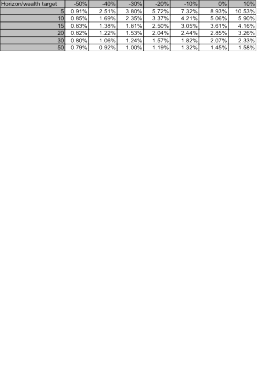
Table III.4.1: Fiscal targets for the primary balance as percent of GDP
Source: LE&F, based on information from ECLAC and CERES.
As is evident in Table III.4.1, the longer the time horizon to fulfill the fiscal target, the
lower is the required primary balance target. On the other hand, the more demanding is the
wealth target, the higher is the required primary balance. To attain a wealth target of -50
percent of GDP, that is a net debt level equivalent to 50 percent of GDP and similar to the
existing starting point, a sustained 1 percent (0.8 percent -0.9 percent) of GDP of structural
primary fiscal surplus is required regardless of the time horizon considered. That would be
the lowest possible primary balance target consistent with debt sustainability: one to conserve
the existing public debt level. On the other extreme, attaining a public sector wealth goal of
10 percent of GDP
9
in a 10 years horizon would require a sustained structural primary
surplus of almost 6 percent of GDP, and achieving the same goal in twice the time horizon
(20 years) would require a surplus slightly above half the previous, 3.3 percent of GDP.
From inspection the fiscal target cannot be less that a sustained primary surplus of 1
percent of GDP. However a desirable target ought to be higher than that one that only
maintains the wealth level at the actual one. Currently in Uruguay, 70 percent of the debt is
denominated in foreign currency, despite all the efforts applied by the authorities to change
debt denomination from US dollars to the unit indexed to GDP. Thus, an exchange rate shock
would increase the debt ratio very significantly. Under a real exchange rate shock of a 50
percent real depreciation, the debt to GDP ratio would jump from 49 percent of GDP to 66
percent of GDP even if the total fiscal balance is zero. A debt ratio of 66 percent of GDP is
already in the vulnerability zone, and is higher than the debt level that Uruguay had before
the last crisis.
A 50 percent increase of the real exchange rate is not unlikely considering the
country’s vulnerabilities as presented in the history of this variable in Uruguay. Moreover,
several analysts consider that currently the real exchange rate is 25 percent to 35 percent
overvalued as compared to its long-term equilibrium. If the debt ratio were to be reduced to
9
Similar to the wealth level of the Chilean public sector at the end of 2009.
40
20 percent of GDP it would be possible to concentrate the debt reduction (30 percent of
GDP) in eliminating debt denominated in foreign currency. Under those conditions of
reduced share of foreign currency debt and lower debt level, even if the domestic currency
debt cannot be increased, a similar 50 percent real exchange rate shock would increase the
debt ratio only marginally, from 20 percent to 22 percent of GDP.
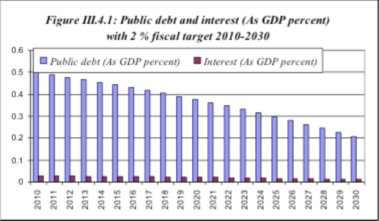
Our recommendation would be to set the debt goal in 20 percent of GDP (-20 percent
public sector wealth) and to give a total of 20 years to attain the debt goal. Under those
conditions the target for the structural primary fiscal balance would be a surplus of 2.0
percent of GDP. It can be verified on Table III.4.1 that a similar fiscal target would be
obtained to achieve the goal of a -40 percent of GDP fiscal wealth in more than 5 and less
than 10 years. Despite the recommendation, setting the fiscal target ought to be one of the
elements of the new institutional framework for fiscal policy in Uruguay.
Source: LE&F simulations.
41
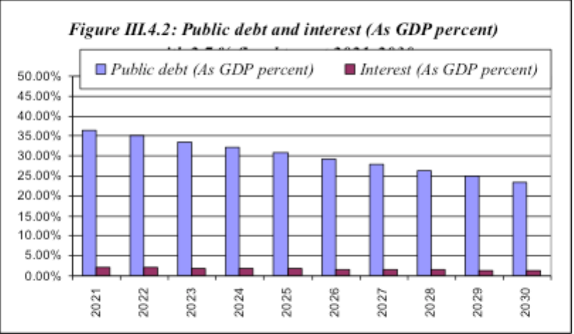
Source: LE&F simulations.
Introducing a structural fiscal policy in Uruguay would not just be a tool to reduce the
cyclical fluctuations of fiscal expenditure, which are significant but no extreme so as to
justify the effort to build a complex political commitment. The increasing vulnerability of the
fiscal position and risk of repeating yet another episode of fiscal insolvency and financial
crisis are considered sufficient motivation. No individual government or political group in the
country can carry by itself the costs of initiating a long term fiscal consolidation knowing that
all its efforts of reducing debt and deficits may reduce its chances to remain in power an open
the possibility to other political group to run an expenditure binge in the future. Fiscal
consolidation should be part of a concerted effort, a national policy built on the basis of
permanent institutions that would give guarantees of a sustained effort that would yield
benefits to all.

42
IV. Preconditions and Recommendations for the Implementation of the
Fiscal Rule
The structural fiscal policy is based upon a national agreement on the importance of a rules
based fiscal policy, which is expressed in a policy framework used in the definition of the
budget with an explicit target for the structural primary balance derived from a medium-term
debt goal and projections for the structural or trend fiscal revenue derived from a
macroeconomic framework. The structural fiscal target, the debt goal and the macroeconomic
framework for fiscal policy are political decisions that should be defined democratically, but
with the technical backing of a group of experts. Besides, fiscal accounts, including revenues,
expenditure, assets and liabilities and their components must be fully transparent and public,
so that the compliance or noncompliance with the fiscal target is information known by all.
1. Improving the Budgetary Process
One of the characteristics of fiscal policy in Uruguay is its decentralized nature and the lack
of a macroeconomic framework in the definition of the five-year budget and for its annual
revisions. The budget process in Uruguay can be characterized as a process of aggregation in
which individual entities either present their own budget proposal to Congress or lobby in
both chambers so as to modify the budget presented by the Ministry of Finance. The MEF
has to fight against the pressure of political interests, congressmen and often other Ministries
in an effort to trim down the budget coming out from that process so as to limit the departure
from the expenditure level originally proposed. Some times the support of the President of
the Republic allows the MEF to cut down to size the proposed budget resulting from the
interaction of Congress and interest groups, others the final budget is not much different from
the expression of will of the individual public sector entities. At the end of the aggregation
process the size of the budget as well as its composition are the result of the political game
played by Congress, the individual interests and the MEF. In a democratic setting that would
be appropriate for the budget composition, the budget size should obey a rational application
of an inter-temporal budget constraint for the Public Sector and not a political game.
At the heart of this decentralized and aggregative budget process is the idea that
expenditures can be financed generically from “general government revenue” or from a
deficit. Consequently, Congress can add to the budget by stating that the additional
expenditures are going to be financed by one of this “generic sources”. The application of a
structural fiscal policy requires setting up a macroeconomic framework that represents the

43
inter-temporal budget constraint. Under that idea, the MEF should define an initial budget
proposal, which is to be developed on the basis of a macroeconomic framework that
considers a projected level for the government revenue and the target for the structural
balance in similar fashion as the one presented in the previous section. For that, the rules of
the budget process should be modified.
10
The budget discussion should be developed on the
basis of that initial proposal, and the modifications by Congress may consider reallocating
expenditure from item to item, or increasing expenditure. However, in this latter case the
initiative should also include an increase in government revenue (some tax measure or sale of
assets) that the MEF considers sufficient to cover the added expenditure. In short the budget
discussion would consist in the selection and application of priorities to decide the
composition of government expenditures and only under exceptional circumstances would
also include initiatives to increase the level of total expenditure, and if that is the case it
would not modify the projected fiscal balance.
The budget should set up an authorization to spend in well-defined items, including
some contingencies to be defined later. In addition to the spending level and composition, the
budget should set a level of projected revenue, projected fiscal balance, and the uses and
sources of any additional financing or financing needs. The additional financing or financing
needs may arise from the deviations in the level of actual government revenue from the one
projected in the budget. An authorization to issue debt up to certain amount could take care
of the financing needs that may arise if there is a short fall in the projected revenue.
Contributions to a sovereign “debt reduction” fund may be consider for the allocation of an
unexpected fiscal surplus. The sovereign fund should consider a limited number of low risk
assets in which to be invested, including the purchase of Uruguayan public debt.
2. Setting the Macroeconomic Framework for Fiscal Policy
The structural fiscal framework requires a number of macroeconomic variables that are
required to setup the target for the annual structural primary balance, those are a goal for
public sector wealth, and the number of years needed to achieve that goal. Besides the
framework also requires the projections for the macroeconomic variables needed to estimate
10
Mr. Ignacio de Posadas, a well-respected lawyer and former Minister of Finance and Senator, believes that an
interpretative law can be used to improve fiscal discipline. In essence Mr. de Posadas proposal considers that
every spending initiative has to be financed by genuine resources, which are defined as well identified sources
of government revenue and not just general resources or deficit financing.
44
the fiscal target and the structural fiscal balance, the long term real interest rate relevant for
Uruguayan debt, and trend GDP growth.
In one extreme it would be possible that the technicians at the Ministry of Finance
(MEF) could carry out all the estimations by themselves under the guidance of the current
Minister. However, that would not be representative of a national and permanent policy
framework, since the structural policy would be entirely under the control of the current
administration. A better possibility would be to limit the action of the technicians of the MEF
by giving them certain parameters on which to base their work. The fiscal target and
macroeconomic projections for trend GDP growth and the real interest rate relevant for
Uruguayan debt could be agreed by a technical commission of 5 members. All of them
should be reputed economists, that would be nominated by the government with the approval
of the Senate and that would represent the different points of views on fiscal policy. They
would give to the government once every 5 years a target for the primary balance, supported
on a goal for the fiscal wealth, a time horizon to attain such goal, and estimates on the long
term relevant real interest rate and the long-term growth rate of GDP for Uruguay.
The technical commission would also give to the MEF annually their projections for
the next five years on real GDP, real gross capital formation, labor- force and unemployment
rate. On the basis of that macroeconomic framework and on the fiscal target, the MEF would
present its estimates for structural revenue and the annual expenditure budget, or the annual
revisions to the five-year budget used in Uruguay.
In case the technical commission cannot come to agreement on the values of certain
variables, each member would present his or hers individual estimate in the Committee
meeting. The committee should present to the MEF a summarized minute of the result of its
deliberations, the value and the way that the fiscal target was calculated, the points of
agreement and the divergences. The MEF would calculate the median value of the variable
excluding the two extremes from the calculation, and complete all the other technical
procedures to obtain the projected trend GPD and structural revenue. The MEF should
present to the parliament and the public a technical report explaining the methodology and
results obtained in the estimation of the structural revenue and of the structural balance, and
of the advance to meet the fiscal wealth goal, including at least:
• The determination of structural fiscal revenue and the projections of trend GDP in
which they are based. Those projections are generated by a group of fiscal experts,
representing different views on this matter.
45
• The fiscal target chosen and the real interest rates and growth rates estimates, based
on a comprehensive study done by the experts, that clearly states the consequences of
such target on fiscal wealth or fiscal debt over time, and the risks involved.
3. Dealing with the Embedded Procyclicality of Expenditure
In many countries fiscal expenditure presents a procyclical bias that result in a faster rate of
growth in real expenditure during the expansionary phase of the business cycle or when the
GDP gap is positive. It is to be expected that this procyclical bias will be eliminated when a
structural fiscal policy is introduced, then the growth of real expenditure would be stable
during the business cycle. The procyclical bias often result from a budgeting process that
starts from the forecasting of next year’s actual fiscal revenue, which in itself is a pro cyclical
variable, and the definition of expenditure on the basis of forecasted revenue. By using the
forecast of structural rather that actual fiscal revenue to define expenditure that procyclical
bias is eliminated.
However in Uruguay there are further complications to eliminate the cyclicality of
fiscal expenditure since the procyclical bias is generated at least in part from some
institutional characteristics of the social security system. According to the law, the value in
Uruguayan pesos of pension benefits is indexed to the economy wide wages and salaries.
Consequently, social security spending, which represents a large portion of total fiscal
expenditure, tends to increase faster during the expansionary phase of the cycle when wages
and salaries increase in real terms. That procyclical characteristic of a large portion of total
expenditure will not disappear by the introduction of a structural fiscal policy, and
consequently, the rest of expenditure will have to follow a counter cyclical bias to allow that
total expenditure is cyclically neutral. Considering that public sector wages and salaries in
effect follow a similar path, it is possible that the flexible portion of fiscal expenditure in
Uruguay is much reduced, imposing a significant rigidity to the introduction of a structural
fiscal policy. In effect only capital expenditure can be managed with flexibility.
The rigidity of current expenditure in Uruguay may require different sources of
flexibility to carry out a structural fiscal policy. One possible source of flexibility could be a
counter cyclical public investment policy and a pro cyclical tax rate. That is, during the
expansionary phase of the cycle when current fiscal expenditure by institutional design
becomes excessive and procyclical, then capital expenditure should contract to a minimum to
allow meeting the structural target on the fiscal balance.
46
If the flexibility of public investment were not enough, meeting the structural fiscal
target may require an additional source of flexibility in some tax rates, for example in the
VAT rate. This would provide additional fiscal revenue during the expansionary phase
helping to meet the fiscal target without investment cuts and even when current expenditure
is expanding faster. On the other hand the tax increase may help in softening the procyclical
impulse of public expenditure. In a similar fashion during the contractionary phase of the
cycle, public investment may take the slack generated by the lower growth rate in current
expenditure, and in addition tax rates may be lowered. During a relatively normal phase of
the cycle tax rates would return to its regular level. The changes in the VAT rate may
represent some practical problems and be a source of additional macroeconomic volatility. If
that is the view the only source of fiscal flexibility would be that of discretionary capital
expenditure.
The success in implementing variables taxes, that is, to raise taxes when expansionary
shocks occur and lower them when a contractionary shock occur, will depend on many
factors identified in the interesting paper of Kaufman (2000). The paper argues that the
existence of variable taxes increase welfare as long as two conditions are met: There are
restrictions on credit, and on the other side that tax distortions in the labor market are low
(especially the income tax). It is reasonable to expect that in Uruguay there are important
credit constraints as in may other developing countries. On the other hand it is difficult to
quantify the distorting effects of taxes in the Uruguayan labor market. In this sense a
variables tax policy in the Uruguayan economy may be positive in this context.
Notwithstanding, it is also necessary to analyze the direct costs involved in such a step, as is
the case of recurrent changes in prices, with the subsequent influence in the inflation, which
in a country with history inflation as in Uruguay can be very dangerous. At the same time it
must consider potential lags in economic activity; such changes may be injurious to the cycle.
4. Sustainability Path of Fiscal Policy in the Medium and Long Term
The recommended target for the structural primary fiscal balance of 2.0 percent of GDP
should be enough to generate a sustainability path for fiscal policy in the medium and long
run. Even some of the other target levels considered would also generate a sustainable fiscal
path although subject to some additional vulnerability. A 1 percent of GDP primary balance
would stabilize debt around 50 percent of GDP. Looking at Figure II.3.1 we note that from
1999 to 2001 the level of Uruguayan public debt was about 30 percent of GDP. However, the
47
crisis in Argentina in 2001 generated several shocks that resulted in an explosion in the level
of public debt that rose to more than 100 percent of GDP in the following years. The debt
increasing shocks include the exchange rate depreciation, the increase in refinancing costs,
the drop in real GDP due to the recession and the financial assistance given by the public
sector to the financial system. Other measures may take care of the exposure to the recession
and the financial system needs of assistance. However, the exposure to the exchange rate and
refinancing cost shocks depends directly on the level of debt. In that regard, debt levels of
around 50 percent of GDP are still insufficient to reduce vulnerabilities, and it would be
highly advisable to continue to lower that percentage even below the pre-crisis levels
mentioned above.
A primary structural balance of 2 percent of GDP would not be very different form
what has already been achieved over the last years. In that sense the introduction of a
structural fiscal policy with that target level would not represent a large shift in fiscal policy
but taking an explicit commitment with the policy being developed would eliminate the risk
of going down the slippery slope of increasing deficit like in past episodes. Such action
would reduce uncertainty about the future course of fiscal policy and may end up generating
significant benefits. Lower uncertainty would reduce the level financial spreads and the
refinancing cost, allowing for improvements in debt composition, more long-term debt and
more domestic currency debt, and a faster reduction in the debt level.
5. Information and Fiscal Transparency
A national fiscal policy should be backed by the availability of data on public sector
operations and assets and liabilities that is of good quality, consistent and plenty of details,
and that is opportunely distributed. Data shortcomings in Uruguay are significant, the series
cover a relatively short period; fiscal data is collected on a cash rather than accrual basis, and
consequently lacks consistency with national accounts and with data on assets and liabilities.
Fiscal transparency requires a very significant effort in the compilation and development of
fiscal statistics, which should encompass data on fiscal operations, revenues and expenditures
on an accrual basis, aggregate and by institutions, and data on the assets and liabilities
changes and positions that are resulting from such operations.
Transparency also requires that all fiscal operations are covered by the statistics. In
this regards operations by the National Development Corporation or by firms fully owned by
48
Public Enterprises should be consolidated into the fiscal accounts. Moreover, a serious effort
should be carried out to quantify all the contingent liabilities of the public sector, including
the guarantees given to private debt.

49
Annex Table 1: Estimates of Trend GDP and GDP Gap
1961 2.98% 2.82% 2.84%
1962 -1.65% 2.33% -2.30%
1963 -2.46% 1.32% 0.51%
1964 -1.30% 0.87% 2.04%
1965 -0.88% 0.77% 1.20%
1966 1.61% 0.81% 3.35%
1967 -3.81% 1.24% -4.10%
1968 -3.55% 1.34% 1.60%
1969 0.60% 1.76% 6.07%
1970 3.10% 2.12% 4.71%
1971 1.10% 2.15% 0.12%
1972 -2.20% 1.75% -1.55%
1973 -3.48% 1.66% 0.36%
1974 -2.18% 1.81% 3.14%
1975 1.06% 2.49% 5.86%
1976 2.06% 2.95% 3.98%
1977 0.31% 2.96% 1.17%
1978 2.44% 3.04% 5.26%
1979 5.40% 3.07% 6.17%
1980 8.55% 2.72% 6.00%
1981 8.80% 1.64% 1.90%
1982 -1.75% 0.69% -9.39%
1983 -8.28% 0.51% -5.85%
1984 -9.93% 0.55% -1.09%
1985 -9.54% 1.08% 1.48%
1986 -2.86% 1.82% 8.86%
1987 2.56% 2.24% 7.93%
1988 0.08% 2.49% -0.01%
1989 -1.44% 2.84% 1.29%
1990 -2.78% 2.97% 1.59%
1991 -2.49% 3.23% 3.54%
1992 1.78% 3.42% 7.93%
1993 1.09% 3.37% 2.66%
1994 5.23% 2.93% 7.28%
1995 0.96% 2.85% -1.45%
1996 3.70% 2.73% 5.58%
1997 6.40% 2.25% 5.05%
1998 9.01% 1.84% 4.54%
1999 4.68% 1.46% -2.85%
2000 2.05% 1.18% -1.44%
2001 -2.15% 0.76% -3.39%
2002 -14.81 % 0.97% -11.03%
2003 -14.44 % 1.80% 2.17%
2004 -5.92% 2.69% 11.82%
2005 -3.03% 3.59% 6.62%
2006 -0.28% 4.09% 7.00%
2007 2.34% 4.64% 7.42%
2008 6.64% 4.47% 9.06%
2009 2.85% 4.49% 0.60%
2010 1.95% 4.44% 3.50%
2011 1.21% 4.37% 3.60%
2012 0.74% 4.28% 3.80%
2013 0.36% 4.20% 3.80%
2014 0.04% 4.13% 3.80%
2015 -0.22% 4.07% 3.80%
2016 -0.43% 4.02% 3.80%
2017 -0.61% 3.99% 3.80%
2018 -0.77% 3.96% 3.80%
2019 -0.90% 3.94% 3.80%
2020 -0.94% 3.84% 3.80%
Avg. 60-20 -0.22% 2.58% 2.59%

50
V. Uruguay Database
Primera parte.xls
Segunda parte.xls

51
VI. Bibliography and References
Anderson Barry and Minarik Joseph (2006), Design Choices for Fiscal Policy Rules, OECD
Journal on Budgeting.
Banco Central de Uruguay, Informe al poder ejecutivo 2008, 2007, 2006, 2005, 2004, 2003,
2002, 2001, 2000.
Bertino Magdalena y Bertino Reto (2004), Más de un siglo de deuda pública uruguaya:
una historia de ida y vuelta. The Nordic Journal of Latin American and Caribbean
Studies, Vol. 34: 1-2, Estocolmo, Suecia.
Bezdek Vladimír, Dybzak Kamil and Kreejdl Aleš (2007), Cyclically Adjusted Fiscal
Balance OECD and ESCB Methods, Czech Journal of Economics and Finance.
Borchardt Michael, Rial Isabel y Sarmiento Adolfo (1998), Sostenibilidad de la política
fiscal en Uruguay. Estudios CERES.
De Brun Julio (1988), Deuda pública y función de consumo. Terceras jornadas anuales de
Economía, Banco central de Uruguay.
Dos Reis Laura, Manasse Paolo y Panizza Ugo (2007), Targeting the Structural Balance.
BID Working Paper #598
Engel Eduardo, Marcel Mario y Meller Patricio (2007), Meta de superávit estructural:
elementos para su análisis. Direccion de presupuestos Chile.
Fedelino Annalisa, Ivanova Anna and Horton Mark (2009), Computing Cyclically adjusted
balances and automatics stabilizers. Fiscal Affairs department, IMF.
Franken Helmut, Le Fort Guillermo y Parrado Eric (2006), Business cycle responses and
the resilience of the Chilean economy, External Vulnerability and Preventive
Policies. Banco Central de Chile.
Ford Benjamin (2005), Structural fiscal indicators: an overview. Economic Roundup
Giorno Claude, Richardson Pete, Roseveare Deborah and van den Noord Paul (1995),
Estimating potential output, output gaps and structural budget balances. OCDE
economics department working papers no. 152
Girouard Nathalie and André Cristophe (2005) Measuring Cyclically adjusted budget
balances for OECD countries. OECD Economics department, working paper 434.
Hagemann Robert (1999), The structural budget balance the IMF methodology. IMF
Working paper
52
Le Fort Guillermo (2006), Política Fiscal con Meta Estructural en la experiencia chilena.
Presentado en la Segunda Reunión Anual del Grupo Latinoamericano de Especialistas
en Manejo de Deuda Pública (LAC Debt Group) Cartagena, Colombia
Mailhos Jorge A. y Sosa Sebastián (2000), El Comportamiento Cíclico de la Política Fiscal
en Uruguay. Estudios CERES.
Marcel Mario, Tokman Marcelo, Valdés Rodrigo y Benavides Paula (2001), Balance fiscal:
La base para la nueva regla de política fiscal chilena. Economía Chilena
Marcel Mario, Tokman Marcelo, Valdés Rodrigo y Benavides Paula (2001), Balance
estructural del gobierno central: Metodología y estimaciones para Chile 1987-
2000. Dirección de presupuestos, Ministerio de Hacienda, Chile.
Marcel Mario (2009), La Regla De Balance Estructural En Chile Diez Años, Diez
Lecciones. CIEPLAN.
Ministerio de Finanzas de Dinamarca (2008) ,Danish Fiscal Policy in 2009 in view of the
European Economic Recovery Plan (Addendum to Denmark’s Convergence
Programme 2008)
Price Robert and Nluller Patrice, Structural Budget indicators and the interpretation of
fiscal policy stance in OECD economies.
Rodríguez Jorge, Tokman Carla and Vega Alejandra (2007), Structural Balance Policy in
Chile. OECD Journal on Budgeting
Schick Allen (2005), Sustainable Budget Policy: Concepts and Approaches. OECD
Journal on Budgeting
Ter-Minassian Teresa (2009), Preconditions for a successful introduction of structural
fiscal balance-based rules in Latin America and the Caribbean: a framework
paper.
Theoduloz Tania (2006), El producto potencial en la economía uruguaya. Estudios
CERES.
World Economics Outlook 2009, 2008, 2007. IMF.
