
Recursive Neyman Algorithm for Optimum Sample Allocation
under Box Constraints on Sample Sizes in Strata
Jacek Wesołowski
*
, Robert Wieczorkowski
†
, Wojciech Wójciak
‡
March 27, 2024
Abstract
The optimum sample allocation in stratified sampling is one of the basic issues of survey
methodology. It is a procedure of dividing the overall sample size into strata sample sizes in such a
way that for given sampling designs in strata the variance of the stratified π estimator of the
population total (or mean) for a given study variable assumes its minimum. In this work, we
consider the optimum allocation of a sample, under lower and upper bounds imposed jointly on
sample sizes in strata. We are concerned with the variance function of some generic form that, in
particular, covers the case of the simple random sampling without replacement in strata. The goal of
this paper is twofold. First, we establish (using the Karush-Kuhn-Tucker conditions) a generic form
of the optimal solution, the so-called optimality conditions. Second, based on the established
optimality conditions, we derive an efficient recursive algorithm, named RNABOX, which solves the
allocation problem under study. The RNABOX can be viewed as a generalization of the classical
recursive Neyman allocation algorithm, a popular tool for optimum allocation when only upper
bounds are imposed on sample strata-sizes. We implement RNABOX in R as a part of our package
stratallo which is available from the Comprehensive R Archive Network (CRAN) repository.
*
Programming, Coordination of Statistical Surveys and Registers Department, Statistics Poland, Aleja Niepodległo
´
sci
208, 00-925 Warsaw, Poland, and Faculty of Mathematics and Information Science, Warsaw University of Technology, ul.
Koszykowa 75, 00-662 Warsaw, Poland. E-mail: jacek.wesolowski@pw.edu.pl
†
Programming, Coordination of Statistical Surveys and Registers Department, Statistics Poland, Aleja Niepodległo
´
sci 208,
‡
Faculty of Mathematics and Information Science, Warsaw University of Technology, ul. Koszykowa 75, 00-662 Warsaw,
Poland. E-mail: wojciech.wojciak.dokt@pw.edu.pl
1
arXiv:2304.07034v4 [stat.ME] 26 Mar 2024

Key Words: Stratified sampling; Optimum allocation; Optimum allocation under box constraints;
Neyman allocation; Recursive Neyman algorithm.
1 Introduction
Let us consider a finite population U of size N. Suppose the parameter of interest is the population total
t of a variable y in U, i.e. t =
P
k∈U
y
k
, where y
k
denotes the value of y for population element k ∈ U.
To estimate t, we consider the stratified sampling with the π estimator. Under this well-known sampling
technique, population U is stratified, i.e. U =
S
h∈H
U
h
, where U
h
, h ∈ H, called strata, are disjoint
and non-empty, and H denotes a finite set of strata labels. The size of stratum U
h
is denoted N
h
, h ∈ H
and clearly
P
h∈H
N
h
= N . Probability samples s
h
⊆ U
h
of size n
h
≤ N
h
, h ∈ H, are selected
independently from each stratum according to chosen sampling designs which are often of the same
type across strata. The resulting total sample is of size n =
P
h∈H
n
h
≤ N. It is well known that the
stratified π estimator
ˆ
t
π
of t and its variance are expressed in terms of the first and second order inclusion
probabilities (see, e.g. Särndal, Swensson and Wretman, 1992, Result 3.7.1, p. 102). In particular, for
several important sampling designs
V ar(
ˆ
t
π
) =
X
h∈H
A
2
h
n
h
− B, (1.1)
where A
h
> 0, B do not depend on n
h
, h ∈ H. Among the most basic and common sampling designs
that give rise to the variance of the form (1.1) is the simple random sampling without replacement in
strata (abbreviated STSI). In this case, the stratified π estimator of t assumes the form
ˆ
t
π
=
X
h∈H
N
h
n
h
X
k∈s
h
y
k
, (1.2)
which yields in (1.1): A
h
= N
h
S
h
, where S
h
denotes stratum standard deviation of study variable y,
h ∈ H, and B =
P
h∈H
N
h
S
2
h
(see, e.g. Särndal et al., 1992, Result 3.7.2, p. 103).
The classical problem of optimum sample allocation is formulated as the determination of the
allocation vector n = (n
h
, h ∈ H) that minimizes the variance (1.1), subject to
P
h∈H
n
h
= n, for a
given n ≤ N (see, e.g. Särndal et al., 1992, Section 3.7.3, p. 104). In this paper, we are interested in the
classical optimum sample allocation problem with additional two-sided constraints imposed on sample
sizes in strata. We phrase this problem in the language of mathematical optimization as Problem 1.1.
2

Problem 1.1. Given a finite set H ̸= ∅ and numbers A
h
> 0, m
h
, M
h
, n, such that 0 < m
h
< M
h
≤
N
h
, h ∈ H and
P
h∈H
m
h
≤ n ≤
P
h∈H
M
h
,
minimize
x = (x
h
, h ∈H) ∈R
|H|
+
X
h∈H
A
2
h
x
h
(1.3)
subject to
X
h∈H
x
h
= n (1.4)
m
h
≤ x
h
≤ M
h
, h ∈ H. (1.5)
To emphasize the fact that the optimal solution to Problem 1.1 may not be an integer one, we denote
the optimization variable by x, not by n. The assumptions about n, m
h
, M
h
, h ∈ H, ensure that
Problem 1.1 is feasible.
The upper bounds imposed on x
h
, h ∈ H, are natural since for instance the solution with x
h
> N
h
for some h ∈ H is impossible. The lower bounds are necessary e.g. for estimation of population
strata variances S
2
h
, h ∈ H. They also appear when one treats strata as domains and assigns upper
bounds for variances of estimators of totals in domains. Such approach was considered e.g. in Choudhry,
Hidiroglou and Rao (2012), where apart of the upper bounds constraints x
h
≤ N
h
, h ∈ H, the additional
constraints
1
x
h
−
1
N
h
N
2
h
S
2
h
≤ R
h
, h ∈ H, where R
h
, h ∈ H, are given constants, have been imposed.
Obviously, the latter system of inequalities can be rewritten as lower bounds constraints of the form
x
h
≥ m
h
=
N
2
h
S
2
h
R
h
+N
h
S
2
h
, h ∈ H. The solution given in Choudhry et al. (2012) was obtained by the
procedure based on the Newton-Raphson algorithm, a general-purpose root-finding numerical method.
See also a related paper by Wright, Noble and Bailer (2007), where the optimum allocation problem
under the constraint of the equal precision for estimation of the strata means was considered.
It is convenient to introduce the following definition for feasible solutions of Problem 1.1.
Definition 1.1. Any vector x = (x
h
, h ∈ H) satisfying (1.4) and (1.5) will be called an allocation.
An allocation x = (x
h
, h ∈ H) is called a vertex one if and only if
x
h
=
m
h
, h ∈ L
M
h
, h ∈ U,
where L, U ⊆ H are such that L ∪ U = H and L ∩ U = ∅.
3

An allocation which is not a vertex one will be called a regular allocation.
The solution to Problem 1.1 will be called the optimum allocation.
Note that an optimum allocation may be of a vertex or of a regular form. The name vertex allocation
refers to the fact that in this case x is a vertex of the hyper-rectangle ×
h∈H
[m
h
, M
h
]. We note that
Problem 1.1 becomes trivial if n =
P
h∈H
m
h
or n =
P
h∈H
M
h
. In the former case, the solution is
x
∗
= (m
h
, h ∈ H), and in the latter x
∗
= (M
h
, h ∈ H). These two are boundary cases of the vertex
allocation. In real surveys with many strata, a vertex optimum allocation rather would not be expected.
Nevertheless, for completeness we also consider such a case in Theorem 3.1, which describes the form of
the optimum allocation vector. We also note that a regular optimum allocation x
∗
∈ ×
h∈H
(m
h
, M
h
) if
and only if it is the classical Tschuprow-Neyman allocation x
∗
= (A
h
n
P
v∈H
A
v
, h ∈ H) (see Neyman,
1934, Tschuprow, 1923).
The rest of this paper is structured as follows. Section 2 presents motivations for this research as well
as a brief review of the literature. In Section 3, we identify Problem 1.1 as a convex optimization problem
and then use the Karush-Kuhn-Tucker conditions to establish necessary and sufficient conditions for a
solution to optimization Problem 1.1. These conditions, called the optimality conditions, are presented
in Theorem 3.1. In Section 4, based on these optimality conditions, we introduce a new algorithm,
RNABOX, and prove that it solves Problem 1.1 (see Theorem 4.1). The name RNABOX refers to the fact
that this algorithm generalizes the recursive Neyman algorithm, denoted here RNA. The RNA is a well-
established allocation procedure, commonly used in everyday survey practice. It finds a solution to the
allocation Problem 2.1 (see below), which is a relaxed version of Problem 1.1. As we shall see in Section
4.4, a naive modification of the recursive Neyman approach, which works fine for the one-sided upper
bounds imposed on the sample strata sizes, does not give the correct solution in the case of two-sided
bounds. A more subtle approach is needed.
Finally, let us note that the implementation of RNABOX algorithm is available through our R package
stratallo (Wójciak, 2023b), which is published in CRAN repository (R Core Team, 2023).
4
2 Motivation and literature review
An abundant body of literature is devoted to the problem of optimum sample allocation, going back to
classical solution of Tschuprow (1923) and Neyman (1934), dedicated to STSI sampling without taking
inequality constraints (1.5) into account. In spite of this fact, a thorough analysis of the literature shows
that Problem 1.1 has not been completely understood yet and it suffers from the lack of fully satisfactory
algorithms.
Below, we briefly review existing methods for solving Problem 1.1, including methods that provide
integer-valued solutions.
2.1 Not-necessarily integer-valued allocation
An approximate solution to Problem 1.1 can be achieved through generic methods of non-linear
programming (NLP) (see, e.g. the monograph Valliant, Dever and Kreuter, 2018, and references
therein). These methods have been involved in the problem of optimum sample allocation since solving
the allocation problem is equivalent to finding the extreme (namely, stationary points) of a certain
objective function over a feasible set. Knowing the (approximate) extreme of the objective function, one
can determine the (approximate, yet typically sufficiently accurate) sizes of samples allocated to
individual strata.
In a similar yet different approach adopted e.g. in Münnich, Sachs and Wagner (2012), Problem 1.1
is transformed into root-finding or fixed-point-finding problems (of some properly defined function) to
which the solution is obtained by general-purpose algorithms like e.g. bisection or regula falsi.
Algorithms used in both these approaches would in principle have infinitely many steps, and are
stopped by an arbitrary decision, typically related to the precision of the iterates. There are two main
weaknesses associated with this way of operating: failure of the method to converge or slow
convergence towards the optimal solution for some poor starting points. In other words, performance of
these algorithms may strongly depend on an initial choice of a starting point, and such a choice is
almost always somewhat hazardous. These and similar deficiencies are discussed in details in Appendix
A.2 in the context of the allocation methods described in Münnich et al. (2012). Another drawback of
the algorithms of this type is their sensitivity to finite precision arithmetic issues that can arise in case
5

when the stopping criterion is not expressed directly in terms of the allocation vector iterates (which is
often the case).
Contrary to that, in the recursive algorithms (we are concerned with), the optimal solution is always
found by recursive search of feasible candidates for the optimum allocation among subsets of H. Hence,
they stop always at the exact solution and after finitely many iterations (not exceeding the number of
strata + 1, as we will see for the case of RNABOX in the proof of Theorem 4.1). An important example of
such an algorithm, is the recursive Neyman algorithm, RNA, dedicated for Problem 2.1, a relaxed version
of Problem 1.1.
Problem 2.1. Given a finite set H ̸= ∅ and numbers A
h
> 0, M
h
, n > 0, such that 0 < M
h
≤ N
h
, h ∈
H and n ≤
P
h∈H
M
h
,
minimize
x = (x
h
, h ∈H) ∈R
|H|
+
X
h∈H
A
2
h
x
h
subject to
X
h∈H
x
h
= n
x
h
≤ M
h
, h ∈ H.
Although RNA is popular among practitioners, a formal proof of the fact that it gives the optimal
solution to Problem 2.1 has been given only recently in Wesołowski, Wieczorkowski and Wójciak (2022).
For other recursive approaches to Problem 2.1, see also e.g. Stenger and Gabler (2005), Kadane (2005).
To the best of our knowledge, the only non-integer recursive optimum allocation algorithm
described in the literature that is intended to solve Problem 1.1 is the noptcond procedure proposed by
Gabler, Ganninger and Münnich (2012). In contrary to RNABOX, this method in particular performs
strata sorting. Unfortunately, the allocation computed by noptcond may not yield the minimum of the
objective function (1.3); see Appendix A.1 for more details.
2.2 Integer-valued allocation
Integer-valued algorithms dedicated to Problem 1.1 are proposed in Friedrich, Münnich, de Vries and
Wagner (2015), Wright (2017, 2020). The multivariate version of the optimum sample allocation
problem under box constraints in which m
h
= m, h ∈ H, for a given constant m, is considered in the
paper of de Moura Brito, do Nascimento Silva, Silva Semaan and Maculan (2015). The proposed
6

procedure that solves that problem uses binary integer programming algorithm and can be applied to the
univariate case. See also Brito, Silva and Veiga (2017) for the R-implementation of this approach.
Integer-valued allocation methods proposed in these papers are precise (not approximate) and
theoretically sound. However, they are relatively slow, when compared with not-necessarily
integer-valued algorithms. For instance, at least for one-sided constraints, the integer-valued algorithm
capacity scaling of Friedrich et al. (2015) may be thousands of times slower than the RNA (see
Wesołowski et al., 2022, Section 4). This seems to be a major drawback of these methods as the
differences in variances of estimators based on integer-rounded non-integer optimum allocation and
integer optimum allocation are negligible as explained in Section 6. The computational efficiency is of
particular significance when the number of strata is large, see, e.g. application to the German census in
Burgard and Münnich (2012), and it becomes even more pronounced in iterative solutions to
stratification problems, when the number of iterations may count in millions (see, e.g. Baillargeon and
Rivest, 2011, Barcaroli, 2014, Gunning and Horgan, 2004, Khan, Nand and Ahmad, 2008, Lednicki and
Wieczorkowski, 2003).
Having all that said, the search for a new, universal, theoretically sound and computationally effective
recursive algorithms of optimum sample allocation under two-sided constraints on the sample strata-
sizes, is crucial both for theory and practice of survey sampling.
3 Optimality conditions
In this section we establish optimality conditions, that is, a general form of the solution to Problem 1.1.
As it will be seen in Section 4, these optimality conditions are crucial for the construction of RNABOX
algorithm.
Before we establish necessary and sufficient optimality conditions for a solution to optimization
Problem 1.1, we first define a set function s, which considerably simplifies notation and calculations.
Definition 3.1. Let H, n, A
h
> 0, m
h
, M
h
, h ∈ H be as in Problem 1.1 and let L, U ⊆ H be such
that L ∩ U = ∅, L ∪ U ⊊ H. The set function s is defined as
s(L, U) =
n −
P
h∈L
m
h
−
P
h∈U
M
h
P
h∈H\(L∪U)
A
h
. (3.1)
7
Below, we will introduce the x
(L, U)
vector for disjoint L, U ⊆ H. It appears that the solution of
the Problem 1.1 is necessarily of the form (3.2) with sets L and U defined implicitly through systems of
equations/inequalities established in Theorem 3.1.
Definition 3.2. Let H, n, A
h
> 0, m
h
, M
h
, h ∈ H be as in Problem 1.1, and let L, U ⊆ H be such
that L ∩ U = ∅. We define the vector x
(L, U)
= (x
(L, U)
h
, h ∈ H) as follows
x
(L, U)
h
=
m
h
, h ∈ L
M
h
, h ∈ U
A
h
s(L, U), h ∈ H \ (L ∪ U).
(3.2)
The following Theorem 3.1 characterizes the form of the optimal solution to Problem 1.1 and
therefore is one of the key results of this paper.
Theorem 3.1 (Optimality conditions). The optimization Problem 1.1 has a unique optimal solution.
Point x
∗
∈ R
|H|
+
is a solution to optimization Problem 1.1 if and only if x
∗
= x
(L
∗
, U
∗
)
, with disjoint
L
∗
, U
∗
⊆ H, such that one of the following two cases holds:
CASE I: L
∗
∪ U
∗
⊊ H and
L
∗
=
n
h ∈ H : s(L
∗
, U
∗
) ≤
m
h
A
h
o
,
U
∗
=
n
h ∈ H : s(L
∗
, U
∗
) ≥
M
h
A
h
o
.
(3.3)
CASE II: L
∗
∪ U
∗
= H and
max
h∈U
∗
M
h
A
h
≤ min
h∈L
∗
m
h
A
h
if U
∗
̸= ∅ and L
∗
̸= ∅,, (3.4)
X
h∈L
∗
m
h
+
X
h∈U
∗
M
h
= n. (3.5)
Remark 3.1. The optimum allocation x
∗
is a regular one in CASE I and a vertex one in CASE II.
The proof of Theorem 3.1 is given in Appendix B. Note that Theorem 3.1 describes the general
form of the optimum allocation up to specification of take-min and take-max strata sets L
∗
and U
∗
. The
question how to identify sets L
∗
and U
∗
that determine the optimal solution x
∗
= x
(L
∗
, U
∗
)
is the subject
of Section 4.
8

4 Recursive Neyman algorithm under box constraints
4.1 The RNABOX algorithm
In this section we introduce an algorithm solving Problem 1.1. In view of Theorem 3.1 its essential task is
to split the set of all strata labels H into three subsets of take-min (L
∗
), take-max (U
∗
), and take-Neyman
(H \ (L
∗
∪ U
∗
)). We call this new algorithm RNABOX since it generalizes existing algorithm RNA in
the sense that RNABOX solves optimum allocation problem with simultaneous lower and upper bounds,
while the RNA is dedicated for the problem with upper bounds only, i.e. for Problem 2.1. Moreover,
RNABOX uses RNA in one of its interim steps. We first recall RNA algorithm and then present RNABOX.
For more information on RNA, see Wesołowski et al. (2022, Section 2) or Särndal et al. (1992, Remark
12.7.1, p. 466).
Algorithm RNA
Input: H, (A
h
)
h∈H
, (M
h
)
h∈H
, n.
Require: A
h
> 0, M
h
> 0, h ∈ H, 0 < n ≤
P
h∈H
M
h
.
Step 1: Set U = ∅.
Step 2: Determine
e
U = {h ∈ H \ U : A
h
s(∅, U) ≥ M
h
}, where set function s is defined in (3.1).
Step 3: If
e
U = ∅, go to Step 4 . Otherwise, update U ← U ∪
e
U and go to Step 2 .
Step 4: Return x
∗
= (x
∗
h
, h ∈ H) with x
∗
h
=
M
h
, h ∈ U
A
h
s(∅, U), h ∈ H \ U.
We note that in real life applications numbers (A
h
)
h∈H
are typically unknown and therefore their
estimates (
ˆ
A
h
)
h∈H
are used instead in the input of the algorithms.
Theorem 4.1 is the main theoretical result of this paper and its proof is given in Appendix C.
Theorem 4.1. The RNABOX algorithm provides the optimal solution to Problem 1.1.
4.2 An example of performance of RNABOX
We demonstrate the operational behaviour of RNABOX algorithm for an artificial population with 10
strata and for total sample size n = 5110, as shown in Table 4.1.
9

Algorithm RNABOX
Input: H, (A
h
)
h∈H
, (m
h
)
h∈H
, (M
h
)
h∈H
, n.
Require: A
h
> 0, 0 < m
h
< M
h
, h ∈ H,
P
h∈H
m
h
≤ n ≤
P
h∈H
M
h
.
Step 1: Set L = ∅.
Step 2: Run RNA[H, (A
h
)
h∈H
, (M
h
)
h∈H
, n] to obtain (x
∗∗
h
, h ∈ H).
Let U = {h ∈ H : x
∗∗
h
= M
h
}.
Step 3: Determine
e
L = {h ∈ H \ U : x
∗∗
h
≤ m
h
}.
Step 4: If
e
L = ∅ go to Step 5. Otherwise, update n ← n −
P
h∈
e
L
m
h
, H ← H \
e
L, L ← L ∪
e
L and go to
Step 2.
Step 5: Return x
∗
= (x
∗
h
, h ∈ L ∪ H) with x
∗
h
=
m
h
, h ∈ L
x
∗∗
h
, h ∈ H.
For this example, RNABOX stops after 6 iterations with take-min strata set L
∗
= {1, 2, 4, 6, 7, 9, 10},
take-max strata set U
∗
= {8} and take-Neyman strata set H \ (L
∗
∪ U
∗
) = {3, 5} (see column L
6
/U
6
).
The optimum allocation is a regular one and it is given in column x
∗
of Table 4.1. The corresponding
value of the objective function (1.3) is 441591.5. The details of interim allocations of strata to sets L, U
at each of 6 iterations of the algorithm are given in columns L
1
/U
1
- L
6
/U
6
.
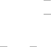
Results summarized in Table 4.1 are presented graphically in Fig. 4.1. The σ(H) axis corresponds
to strata assigned to set U, while τ(H) is for L. For the sake of clear presentation, the values on σ(H)
axis are ordered non-increasingly in
A
h
M
h
, h ∈ H, which gives
A
8
M
8
≥
A
5
M
5
≥
A
3
M
3
≥ . . . ≥
A
10
M
10
, while for
τ(H) axis the strata are ordered non-decreasingly in
A
h
m
h
, h ∈ H, which gives
A
10
m
10
≤
A
1
m
1
≤
A
2
m
2
≤ . . . ≤
A
8
m
8
. Squares in Fig. 4.1 represent assignments of strata into sets L or U, such that the corresponding
coordinate is the value of the last element (follow the respective axis) in the set. For example, ■ at
coordinate 6 on σ(H) axis means that in this iteration of the algorithm (iteration no. 3) we have U =
{8, 5, 3, 7, 4, 6}, while □ at coordinate 6 on τ(H) axis means that in this iteration (no. 5) we get L =
{10, 1, 2, 9, 6}. Directions indicated by the arrows correspond to the order in which the sets L and U are
built as the algorithm iterates. Numbers above the squares are the values of set function s(L, U) for L
and U with elements indicated by the coordinates of a given square. For example, for ■ at coordinates
(8, 7), we have s({10, 1, 2, 9, 6, 4, 7}, {8}) = 0.0622.
10

Table 4.1: An example of RNABOX performance for a population with 10 strata and total sample size
n = 5110. Columns L
r
/U
r
, r = 1, . . . , 6, represent the content of sets L, U respectively, in the r-th
iteration of the RNABOX (between Step 3 and Step 4): symbols □ or ■ indicate that the stratum with label
h is in L
r
or U
r
, respectively.
h A
h
m
h
M
h
L
1
/U
1
L
2
/U
2
L
3
/U
3
L
4
/U
4
L
5
/U
5
L
6
/U
6
x
∗
1 2700 750 900 □ □ □ □ 750
2 2000 450 500 ■ □ □ □ □ 450
3 4200 250 300 ■ ■ ■ ■ ■ 261.08
4 4400 350 400 ■ ■ ■ □ 350
5 3200 150 200 ■ ■ ■ ■ ■ 198.92
6 6000 550 600 ■ ■ ■ □ □ 550
7 8400 650 700 ■ ■ ■ □ 650
8 1900 50 100 ■ ■ ■ ■ ■ ■ 100
9 5400 850 900 ■ ■ □ □ □ 850
10 2000 950 1000 □ □ □ □ □ 950
SUM 5000 5600 0/8 1/7 3/6 4/3 5/3 7/1 5110
We would like to point out that regardless of the population and other allocation parameters chosen,
the graph illustrating the operations of RNABOX algorithm will always have a shape similar to that of the
right half of a Christmas tree with the top cut off when U
r
∗
̸= ∅. This property results from that fact that
L
r
⊊ L
r+1
(see (C.1)) and U
r
⊇ U
r+1
(see (C.16)) for r = 1, . . . , r
∗
− 1, r
∗
≥ 2. For the population
given in Table 4.1, we clearly see that L
1
= ∅ ⊊ L
2
= {10} ⊊ L
3
= {10, 1, 2} ⊊ L
4
= {10, 1, 2, 9} ⊊
L
5
= {10, 1, 2, 9, 6} ⊊ L
6
= L
∗
= {10, 1, 2, 9, 6, 4, 7} and U
1
= {8, 5, 3, 7, 4, 6, 9, 2} ⊃ U
2
=
{8, 5, 3, 7, 4, 6, 9} ⊃ U
3
= {8, 5, 3, 7, 4, 6} ⊃ U
4
= {8, 5, 3} = U
5
⊃ U
6
= U
∗
= {8}. Moreover,
regardless of the population and other allocation parameters chosen, subsequent values of set function
s, which are placed at the ends of branches of the Christmas tree, above ■, form a non-increasing
sequence while moving upwards. This fact follows directly from Lemma C.3. For the example allocation
illustrated in Fig. 4.1, we have s(L
1
, U
1
) = 0.3 > s(L
2
, U
2
) = 0.204 > s(L
3
, U
3
) = 0.122 >
s(L
4
, U
4
) = 0.0803 > s(L
5
, U
5
) = 0.075 > s(L
6
, U
6
) = 0.0622 (note that L
1
= ∅). The same
property appears for values of s related to the trunk of the Christmas tree, placed above □. In this case,
this property is due to (C.2), (C.15) and (C.1). For allocation in Fig. 4.1, we have s(L
1
, ∅) = 0.127 >
11
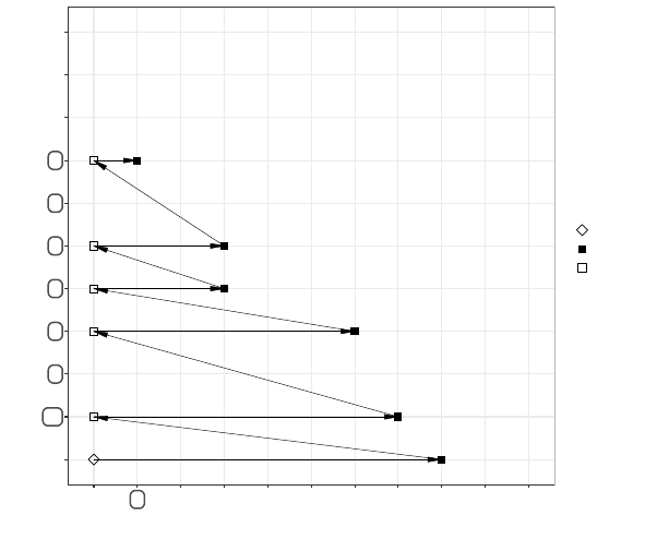
Figure 4.1: Assignments of strata into set L (take-min) and set U (take-max) in RNABOX algorithm for an
example of population as given in Table 4.1 and total sample size n = 5110. The σ(H) axis corresponds
to strata assigned to set U, while τ (H) is for L. Squares represent assignments of strata to L (□) or U
(■) such that the coordinate corresponding to a given square is the value of the last element (following
the order of strata, σ or τ, associated to the respective axis) in the set.
0.127 0.3
0.109 0.204
0.0884 0.122
0.0751 0.0803
0.0706 0.075
0.0602 0.0622
0
10
1
2
9
6
4
7
3
5
8
0 8 5 3 7 4 6 9 2 1 10
σ(W)
τ(W)
Init
U (take−max)
L (take−min)
s(L
2
, ∅) = 0.109 > s(L
3
, ∅) = 0.0884 > s(L
4
, ∅) = 0.0751 > s(L
5
, ∅) = 0.0706 > s(L
6
, ∅) =
0.0602.
4.3 Possible modifications and improvements
4.3.1 Alternatives for RNA in Step 2
The RNABOX algorithm uses RNA in its Step 2. However, it is not hard to see that any algorithm dedicated
to Problem 2.1 (like for instance SGA by Stenger and Gabler, 2005 or COMA by Wesołowski et al., 2022)
could be used instead. We chose RNA as it allows to keep RNABOX free of any strata sorting.
12

4.3.2 A twin version of RNABOX
Let us observe that the order in which L and U are computed in the algorithm could be interchanged.
Such a change, implies that the RNA used in Step 2 of the RNABOX, should be replaced by its twin
version, the LRNA, that solves optimum allocation problem under one-sided lower bounds. The LRNA is
described in details in Wójciak (2023a).
Algorithm LRNA
Input: H, (A
h
)
h∈H
, (m
h
)
h∈H
, n.
Require: A
h
> 0, m
h
> 0, h ∈ H, n ≥
P
h∈H
m
h
.
Step 1: Let L = ∅.
Step 2: Determine
e
L = {h ∈ H \ L : A
h
s(L, ∅) ≤ m
h
}, where set function s is defined in (3.1).
Step 3: If
e
L = ∅, go to Step 4 . Otherwise, update L ← L ∪
e
L and go to Step 2 .
Step 4: Return x
∗
= (x
∗
h
, h ∈ H) with x
∗
h
=
m
h
, h ∈ L
A
h
s(L, ∅), h ∈ H \ L.
Taking into account the observation above, Step 2 and Step 3 of RNABOX would read:
Step 2: Run LRNA[H, (A
h
)
h∈H
, (m
h
)
h∈H
, n] to obtain (x
∗∗
h
, h ∈ H).
Let L = {h ∈ H : x
∗∗
h
= m
h
}.
Step 3: Determine
e
U = {h ∈ H \ L : x
∗∗
h
≥ M
h
}.
The remaining steps should be adjusted accordingly.
4.3.3 Using prior information in RNA at Step 2
In view of Lemma C.2, using the notation introduced in Appendix C.1, in Step 2 of RNABOX, for r
∗
≥ 2
we have
U
r
= {h ∈ H \ L
r
: x
∗∗
h
= M
h
} ⊆ U
r−1
, r = 2, . . . , r
∗
.
This suggests that the domain of discourse for U
r
could be shrunk from H \ L
r
to U
r−1
⊆ H \ L
r
, i.e.
U
r
= {h ∈ U
r−1
: x
∗∗
h
= M
h
}, r = 2, . . . , r
∗
. (4.1)
Given the above observation and the fact that from the implementation point of view set U
r
is determined
internally by RNA, it is tempting to consider modification of RNA such that it makes use of the domain of
13

discourse U
r−1
for set U
r
. This domain could be specified as an additional input parameter, say J ⊆ H,
and then Step 2 of RNA algorithm would read:
Step 2: Determine
e
U = {h ∈ J \ U : A
h
s(∅, U) ≥ M
h
}.
From RNABOX perspective, this new input parameter of RNA should be set to J = H for the first
iteration, and then J = U
r−1
for subsequent iterations r = 2, . . . , r
∗
≥ 2 (if any).
4.4 On a naive extension of the one-sided RNA
By the analogy to the one-sided constraint case, one would expect that the optimum allocation problem
under two-sided constraints (1.5) is of the form (3.2) and hence it could be solved with the naive
modification of RNA as defined below.
Algorithm Naive modification of RNA
Input: H, (A
h
)
h∈H
, (m
h
)
h∈H
, (M
h
)
h∈H
, n.
Require: A
h
> 0, 0 < m
h
< M
h
, h ∈ H,
P
h∈H
m
h
≤ n ≤
P
h∈H
M
h
.
Step 1: Set L = ∅, U = ∅.
Step 2: Determine
e
U = {h ∈ H \ (L ∪ U) : A
h
s(L, U) ≥ M
h
}, where set function s is defined in (3.1).
Step 3: Determine
e
L = {h ∈ H \ (L ∪ U) : A
h
s(L, U) ≤ m
h
}.
Step 4: If
e
L ∪
e
U = ∅ go to Step 5. Otherwise, update L ← L ∪
e
L, U ← U ∪
e
U and go to Step 2.
Step 5: Return x
∗
= (x
∗
h
, h ∈ H) with x
∗
h
=
m
h
, h ∈ L
M
h
, h ∈ U
A
h
s(L, U), h ∈ H \ (L ∪ U).
This is however not true and the basic reason behind is that sequence (s(L
r
, U
r
))
r
∗
r=1
(where r
denotes iteration index, and L
r
and U
r
are taken after Step 3 and before Step 4), typically fluctuates. Thus,
it may happen that (C.13) - (C.15) are not met for U
r
,
e
L
r
defined by the above naive algorithm for some
r = 1, . . . , r
∗
≥ 1. Consequently, optimality conditions stated in Theorem 3.1 may not hold. To
illustrate this fact, consider an example of population as given in Table 4.2. For this population, a naive
version of the recursive Neyman stops in the second iteration and it gives allocation x with L = {3}
and U = {2, 5}, while the optimum choice is x
∗
with L
∗
= {3} and U
∗
= {5}. For non-optimum
allocation x, we have s({3}, {2, 5}) = 0.0714 ≱ 0.25 =
A
2
M
2
, i.e. U does not follow (3.3). Note that the
14

Table 4.2: Example population with 5 strata and the results of naive recursive Neyman sample allocation
(columns x and L/U/H \ (L ∪ U)) for total sample size n = 1489. Lower and upper bounds imposed
on strata sample sizes are given in columns m
h
and M
h
respectively. The optimum allocation with
corresponding strata sets are given in the last two columns. Squares in cells indicate that the allocation
for stratum h ∈ H = {1, . . . , 5} is of type take-min (□) or take-max (■).
h A
h
m
h
M
h
x L/U/H \ (L ∪ U) x
∗
L
∗
/U
∗
/H \ (L
∗
∪ U
∗
)
1 420 24 420 30 54.44
2 352 15 88 88 ■ 45.63
3 2689 1344 2689
1344 □ 1344 □
4 308 8 308 22 39.93
5 130 3 5 5 ■ 5 ■
SUM 1394 3510 1489 1/2/2 1489 1/1/3
allocation x is feasible in this case (it may not be in general), yet is not a minimizer of the objective
function (1.3) as f(x) = 20360 − B, and f(x
∗
) = 17091 − B, where B is some constant. Thus, it
appears that in the case of two-sided constraints, one needs a more subtle modification of RNA
procedure that lies in a proper update of the pair (L
r
, U
r
) in each iteration r = 1, . . . , r
∗
≥ 1 of the
algorithm, such as e.g. in RNABOX.
5 Numerical results
In simulations, using R Statistical Software (R Core Team, 2023) and microbenchmark R package
(Mersmann, 2021), we compared the computational efficiency of RNABOX algorithm with the
efficiency of the fixed-point iteration algorithm (FPIA) of Münnich et al. (2012). The latter one is
known to be an efficient algorithm dedicated to Problem 1.1 and therefore we used it as a benchmark.
The comparison was not intended to verify theoretical computational complexity, but was rather
concerned with quantitative results regarding computational efficiency for the specific implementations
of both algorithms.
To compare the performance of the algorithms we used the STSI sampling for several artificially
created populations. Here, we chose to report on simulation for two such populations with 691 and 703
15
strata, results of which are representative for the remaining ones. These two populations were constructed
by iteratively binding K sets of numbers, where K equals 100 (for the first population) and 200 (for the
second population). Each set, labelled by i = 1, . . . , K, contains 10000 random numbers generated
independently from log-normal distribution with parameters µ = 0 and σ = log(1 + i). For every set
i = 1, . . . , K, strata boundaries were determined by the geometric stratification method of Gunning and
Horgan (2004) with parameter 10 being the number of strata and targeted coefficient of variation equal
to 0.05. This stratification method is implemented in the R package stratification, developed by
Rivest and Baillargeon (2022) and described in Baillargeon and Rivest (2011). For more details, see the
R code with the experiments, which is placed in our GitHub repository (see Wieczorkowski, Wesołowski
and Wójciak, 2023).
Results of these simulations are illustrated in Fig. 5.1. From Fig. 5.1 we see that, while for majority
of the cases the FPIA is slightly faster than RNABOX, the running times of both of these algorithms are
generally comparable. The gain in the execution time of the FPIA results from the fact that it typically
runs through a smaller number of sets L, U ⊂ H (according to (A.6)), than RNABOX in order to find the
optimal L
∗
and U
∗
. Although this approach usually gives correct results (as in the simulations reported
in this section), it may happen that the FPIA misses the optimal sets L
∗
, U
∗
⊊ H. In such a case, FPIA
does not converge, as explained in Appendix A.2. Nevertheless, we emphasize that this situation rarely
happens in practice.
6 Concluding comments
In this paper we considered Problem 1.1 of optimum sample allocation under box constraints. The main
result of this work is the mathematically precise formulation of necessary and sufficient conditions for the
solution to Problem 1.1, given in Theorem 3.1, as well as the development of the new recursive algorithm,
termed RNABOX, that solves Problem 1.1. The optimality conditions are fundamental to analysis of the
optimization problem. They constitute trustworthy underlay for development of effective algorithms
and can be used as a baseline for any future search of new algorithms solving Problem 1.1. Essential
properties of RNABOX algorithm, that distinguish it from other existing algorithms and approaches to
the Problem 1.1, are:
16
Figure 5.1: Running times of FPIA and RNABOX for two artificial populations. Top graphs show the
empirical median of execution times (calculated from 100 repetitions) for different total sample sizes.
Numbers in brackets are the numbers of iterations of a given algorithm. In the case of RNABOX, it is
a vector with number of iterations of the RNA (see Step 2 of RNABOX) for each iteration of RNABOX.
Thus, the length of this vector is equal to the number of iterations of RNABOX. Counts of take-min,
take-Neyman, and take-max strata are shown on bottom graphs.
(6)
(5,5,6)
(6)
(6,6,6)
(6)
(7,6,6)
(7)
(7,7,7)
(7)
(7,7)
(7)
(7)
(7)
(7)
(8)
(8)
(9)
(9)
691 strata, N = 990403
40
60
80
100
120
140
160
Median Time [microseconds]
(5)
(6,5,5,5)
(6)
(6,6,6)
(7)
(7,6,6)
(7)
(7,7,7)
(8)
(8,8,8,8)
(8)
(7,8,8)
(8)
(9,8,8)
(10)
(9,10,10)
(12)
(12,12,12,12)
703 strata, N = 991226
100
150
200
250
300
Algorithm
FPIA
RNABOX
0.2 0.4 0.6 0.8 1.0
0
100
200
300
400
500
600
700
0%
20%
40%
60%
80%
100%
Total sample size (as fraction of N)
Number of strata
0.2 0.4 0.6 0.8 1.0
0
100
200
300
400
500
600
700
0%
20%
40%
60%
80%
100%
Total sample size (as fraction of N)
Strata Set
take−max
take−Neyman
take−min
1. Universality: RNABOX provides optimal solution to every instance of feasible Problem 1.1
(including the case of a vertex optimum allocation).
2. No initialization issues: RNABOX does not require any initializations, pre-tests or whatsoever that
could have an impact on the final results of the algorithm. This, in turn, takes places e.g. in case
of NLP methods.
3. No sorting: RNABOX does not perform any ordering of strata.
4. Computational efficiency: RNABOX running time is comparable to that of FPIA (which is probably
the fastest previously known optimum allocation algorithm for the problem considered).
17
5. Directness: RNABOX computes important quantities (including RNA internals) via formulas that
are expressed directly in terms of the allocation vector x
(L, U)
(see Definition 3.2). This reduces the
risk of finite precision arithmetic issues, comparing to the algorithms that base their key operations
on some interim variables on which the optimum allocation depends, as is the case of e.g. the NLP-
based method.
6. Recursive nature: RNABOX repeatedly applies allocation Step 2 and Step 3 to step-wise reduced set
of strata, i.e. "smaller" versions of the same problem. This translates to clarity of the routines and
a natural way of thinking about the allocation problem.
7. Generalization: RNABOX, from the perspective of its construction, is a generalization of the
popular RNA algorithm that solves Problem 2.1 of optimum sample allocation under one-sided
bounds on sample strata sizes.
Finally, we would like to note that Problem 1.1 considered in this paper is not an integer-valued
allocation problem, while the sample sizes in strata should be of course natural numbers. On the other
hand, the integer-valued optimum allocation algorithms are relatively slow and hence might be inefficient
in some applications, as already noted in Section 2. If the speed of an algorithm is of concern and non-
necessarily integer-valued allocation algorithm is chosen (e.g. RNABOX), the natural remedy is to round
the non-integer optimum allocation provided by that algorithm. Altogether, such procedure is still much
faster than integer-valued allocation algorithms. However, a simple rounding of the non-integer solution
does not, in general, yield the minimum of the objective function, and may even lead to an infeasible
solution, as noted in Friedrich et al. (2015, Section 1, p. 3). Since infeasibility can in fact arise only
from violating constraint (1.4), it can be easily avoided by using a rounding method of Cont and Heidari
(2014) that preserves the integer sum of positive numbers. Moreover, all numerical experiments that we
carried out, show that the values of the objective function obtained for non-integer optimum allocation
before and after rounding and for the integer optimum allocation are practically indistinguishable. See
Table 6.1 for the exact numbers.
The above observations suggest that fast, not-necessarily integer-valued allocation algorithms, with
properly rounded results, may be a good and reasonable alternative to slower integer algorithms when
speed of an algorithm is crucial.
18

Table 6.1: For populations used in simulations in Section 5, V
int
and V denote values of variance (1.1)
computed for integer optimum allocations and non-integer optimum allocations, respectively. Variances
V
round
are computed for rounded non-integer optimum allocations (with the rounding method of Cont
and Heidari (2014)).
691 strata (N = 990403) 703 strata (N = 991226)
fraction f n = f · N V/V
int
V
round
/V
int
n = f · N V/V
int
V
round
/V
int
0.1 99040 0.999997 1.000000 99123 0.999997 1.00000
0.2 198081 0.999999 1.000000 198245 0.999999 1.00000
0.3 297121 0.999999 1.000000 297368 0.999999 1.00000
0.4 396161 0.999999 1.000000 396490 0.999999 1.00000
0.5 495202 0.999999 1.000000 495613 0.999999 1.00000
0.6 594242 0.999999 1.000000 594736 0.999999 1.00000
0.7 693282 1.000000 1.000000 693858 0.999998 1.00000
0.8 792322 1.000000 1.000000 792981 0.999995 1.00000
0.9 891363 1.000000 1.000000 892103 0.999759 1.00000
A Appendix: On the existing allocation algorithms by GGM and MSW
A.1 Necessary vs. sufficient optimality conditions and the noptcond function of GGM
Problem 1.1 has been considered in Gabler et al. (2012) (GGM in the sequel). Theorem 1 in that paper
announces that there exist disjoint sets L, U ⊂ H with L
c
= H \ L, U
c
= H \ U, such that
max
h∈L
A
h
m
h
< min
h∈L
c
A
h
m
h
and max
h∈U
c
A
h
M
h
< min
h∈U
A
h
M
h
, (A.1)
and, if the allocation x = (x
h
, h ∈ H) is of the form (3.2) with L and U as above, then x is an optimum
allocation. An explanation on how to construct sets L and U is essentially given in the first part of the
proof of Theorem 1, p. 154-155, or it can be read out from the noptcond function. The noptcond is
a function in R language (see R Core Team, 2023) that was defined in Sec. 3 of GGM and it aims to
find an optimum sample allocation based on results of Theorem 1, as the authors pointed out. However,
as it will be explained here, (3.2) and (A.1) together, are in fact necessary but not sufficient conditions
for optimality of the allocation x. In a consequence, the noptcond function may not give an optimum
allocation.
19

By Theorem 3.1, CASE I, a regular allocation x is an optimum allocation if and only if it is of the
form (3.2) with disjoint sets L, U ⊊ H, L ∪ U ⊊ H, L
c
= H \ L, U
c
= H \ U such that the following
inequalities hold true:
max
h∈L
A
h
m
h
≤
1
s(L, U)
< min
h∈L
c
A
h
m
h
, (A.2)
max
h∈U
c
A
h
M
h
<
1
s(L, U)
≤ min
h∈U
A
h
M
h
. (A.3)
Clearly, (A.2) implies the first inequality in (A.1), and (A.3) implies the second one. Converse
implications do not necessary hold, and therefore sufficiency of condition (3.2) with (A.1) for Problem
1.1 is not guaranteed. In others words, (3.2) and (A.1) alone, lead to a feasible solution (i.e. the one that
does not violate any of the constraints (1.4) - (1.5)), which, at the same time, might not be a minimizer
of the objective function (1.3).
The proof of Theorem 1 in GGM gives an explicit, but somewhat informal algorithm that finds sets
L and U which define allocation (3.2). Sets L and U determined by this algorithm meet inequalities (4)
and (5) in GGM, which are necessary and sufficient conditions for an optimal (regular) solution. This
fact was noted by the authors, but unfortunately (4) and (5) are not given in the formulation of Theorem
1. Presumably, this was due to authors’ statement that (4) and (5) follow from (3.2) and (A.1): "From the
definition of L1, L2 in Eq. 3 we have ...", while in fact to conclude (4) and (5) the authors additionally
rely on the algorithm constructed at the beginning of the proof. Note that conditions (4) and (5) are the
same as those given in Theorem 3.1 for a regular solution (CASE I). Moreover, it is a matter of simple
observation to see that the allocation found by the algorithm described in the proof of Theorem 1 in GGM,
meets also optimality conditions (3.4) and (3.5) established in Theorem 3.1 for vertex solutions (CASE
II). Hence, the allocation computed by the algorithm embedded in the proof of the GGM’s Theorem 1 is
indeed an optimal one, though the formal statement of Theorem 1 is not correct.
Unfortunately, the noptcond function does not fully follow the algorithm from the proof of Theorem
1 of GGM. Consequently, the optimality of a solution computed by noptcond is not guaranteed. This can
be illustrated by a simple numerical Example A.1, which follows Wójciak (2019, Example 3.9).
Example A.1. Consider the allocation for an example population as given in Table A.1.
20
Table A.1: Two allocations for an example population with two strata: non-optimum x
noptcond
with
L = {1}, U = ∅, and optimum x
∗
with L
∗
= ∅, U
∗
= {1}. Set function s is defined in (3.1).
h A
h
m
h
M
h
A
h
m
h
A
h
M
h
s
−1
({1}, ∅) s
−1
(∅, {1}) x
noptcond
x
∗
1 2000 30 50 66.67 40
23.08 27.27
30 50
2 3000 40 200 75 15 130 110
The solution returned by noptcond function is equal to x = (30, 130), while the optimum allocation
is x
∗
= (50, 110). The reason for this is that conditions (A.2), (A.3) are never examined by the noptcond,
and for this particular example we have
A
1
m
1
= 66.67 ≰ 23.08 =
1
s(L, U)
as well as
A
1
M
1
= 40 ≮ 23.08 =
1
s(L, U)
, i.e. (A.2), (A.3) are clearly not met. A simple adjustment can be made to noptcond function so
that it provides the optimal solution to Problem 1.1. That is, a feasible candidate solution that is found
(note that this candidate is of the form x = (x
v
, v ∈ H \ (L ∪ U)) with x
v
= A
v
s(L, U)), should
additionally be checked against the condition
max
h∈L
A
h
m
h
≤
A
v
x
v
≤ min
h∈U
A
h
M
h
, v ∈ H \ (L ∪ U). (A.4)
We finally note that the table given in Section 4 of GGM on p. 160, that illustrates how noptcond
operates, is incorrect as some of the numbers given do not correspond to what noptcond internally
computes, e.g. for each row of this table, the allocation should sum up to n = 20, but it does not.
A.2 Fixed-point iteration of MSW
Theorem 1 of Münnich et al. (2012) (referred to by MSW in the sequel) provides another solution to
Problem 1.1 that is based on results partially similar to those stated in Theorem 3.1. Specifically, it states
that the allocation vector x = (x
h
, h ∈ H) can be expressed as a function x : R
+
→ R
|H|
+
of λ, defined
as follows
x
h
(λ) =
M
h
, h ∈ J
λ
M
:=
n
h ∈ H : λ ≤
A
2
h
M
2
h
o
A
h
√
λ
, h ∈ J
λ
:=
n
h ∈ H :
A
2
h
M
2
h
< λ <
A
2
h
m
2
h
o
m
h
, h ∈ J
λ
m
:=
n
h ∈ H : λ ≥
A
2
h
m
2
h
o
,
21

and the optimum allocation x
∗
is obtained for λ = λ
∗
, where λ
∗
is the solution of the equation:
˜g(λ) :=
X
h∈H
x
h
(λ) − n = 0. (A.5)
Here, we note that the optimum allocation x
∗
obtained is of the form x
(L, U)
, as given in (3.2), with
L = J
λ
∗
m
and U = J
λ
∗
M
. Since ˜g is continuous but not differentiable, equation (A.5) has to be solved by
a root-finding methods which only require continuity. In MSW, the following methods were proposed:
bisection, secan and regula falsi in few different versions. The authors reported that despite the fact that
some theoretical requirements for these methods are not satisfied by the function ˜g (e.g. it is not convex
while regula falsi applies to convex functions), typically the numerical results are satisfactory. However
this is only true when the values of the initial parameters are from the proper range, which is not known
a priori.
As these algorithms might be relatively slow (see Table 1 in MSW), the authors of MSW proposed
an alternative method. It is based on the observation that (A.5) is equivalent to
λ = ϕ(λ) :=
1
s
2
(J
λ
m
, J
λ
M
)
,
where set function s is as in (3.1) (see Appendix A, Lemma 2 in MSW). Note that ϕ is well-defined only
if J
λ
m
∪ J
λ
M
⊊ H. The authors note that the optimal λ
∗
is a fixed-point of the function ϕ : R
+
→ R
+
.
This clever observation was translated to an efficient optimum allocation fixed-point iteration algorithm,
FPIA, that was defined on page 442 in MSW. Having acknowledged its computational efficiency as well
as the fact that typically it gives the correct optimum allocation, the following two minor issues related
to FPIA can be noted:
• The FPIA is adequate only for allocation problems for which an optimum allocation is of a regular
type (according to Definition 1.1), as for vertex allocation J
λ
∗
m
∪ J
λ
∗
M
= H and therefore ϕ is not
well-defined for such λ
∗
.
• The FPIA strongly depends on the choice of initial value λ
0
of the parameter λ. If λ
0
is not chosen
from the proper range (not known a priori), two distinct undesirable scenarios can occur: the FPIA
may get blocked, or it may not converge.
To outline the blocking scenario which may happen even in case of a regular optimum allocation, let
I :=
λ ∈
min
h∈H
A
2
h
m
2
h
, max
h∈H
A
2
h
M
2
h
: s(J
λ
m
, J
λ
M
) = 0
,
22
and note that I ̸= ∅ is possible. If FPIA encounters λ
k
∈ I ̸= ∅ at some k = 0, 1, . . ., then the crucial
step of FPIA, i.e.:
λ
k+1
:=
1
s
2
J
λ
k
m
, J
λ
k
M
, (A.6)
yields λ
k+1
=
1
0
, which is undefined. Numerical Example A.2 illustrates this scenario.
Example A.2. Consider allocation for a population given in Table A.2. Initial value λ
0
= 6861.36 ∈
I = [2304, 6922.24] and therefore FPIA gets blocked since λ
1
=
1
0
is undefined.
Table A.2: Details of FPIA performance for a population with four strata. Here, λ
0
=
1
s
2
(∅, ∅)
, λ
1
=
1
s
2
(J
λ
0
m
, J
λ
0
M
)
, λ
∗
=
1
s
2
(J
λ
∗
m
, J
λ
∗
M
)
. Squares in cells indicate assignment of stratum h ∈ H = {1, 2, 3, 4} to
J
λ
m
(□) or J
λ
M
(■) for a given λ.
population FPIA optimum allocation
h A
h
m
h
M
h
A
2
h
m
2
h
A
2
h
M
2
h
J
λ
0
m
/J
λ
0
M
J
λ
1
m
/J
λ
1
M
J
λ
∗
m
/J
λ
∗
M
x
∗
1 4160 5 50 692224 6922.24 ■
-
44.35
2 240 5 50 2304 23.04 □ □ 5
3 530 5 50 11236 112.36 5.65
4 40 5 50 64 0.64 □ □ 5
total sample size n = 60 λ
0
= 6861.36 λ
1
=
1
0
λ
∗
= 8798.44
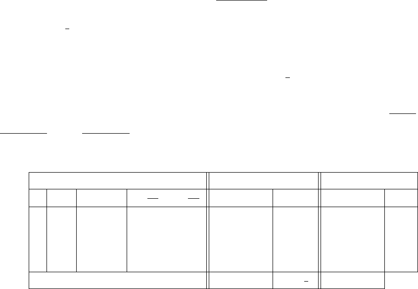
Figure A.1 shows the graphs of the functions g and ϕ for the problem considered in this example.
23
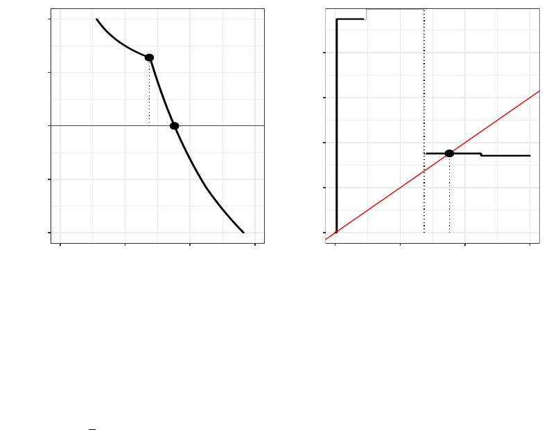
Figure A.1: Functions g and ϕ for Example A.2 of the allocation problem for which the FPIA gets
blocked.
λ
0
λ
∗
−10
−5
0
5
10
0 5000 10000 15000
λ
g(λ)
λ
0
λ
∗
0
5000
10000
15000
20000
0 5000 10000 15000
λ
φ(λ)
These graphs show that g is not differentiable, and ϕ has jump discontinuities. Moreover, there is an
interval I = [2304, 6922.24], such that ϕ is not well-defined on I.
We note that a simple remedy to avoid the blocking scenario in the case of a regular allocation is to
change λ to λ
new
=
1
λ
, with a corresponding redefinition of all the objects in the original algorithm.
The next Example A.3 illustrates a situation when FPIA does not converge.
Example A.3. Consider a population given in Table A.3. Initial value of λ
0
= 695.64 causes lack of
convergence of the FPIA due to oscillations:
λ
k
=
1444, k = 1, 3, 5, . . .
739.84, k = 2, 4, 6, . . . .
24
Table A.3: Details of FPIA performance for a population with four strata. Here, λ
0
=
1
s
2
(∅, ∅)
, λ
k+1
is as
in (A.6), and λ
∗
=
1
s
2
(J
λ
∗
m
, J
λ
∗
M
)
. Squares in cells indicate assignment of stratum h ∈ H = {1, 2, 3, 4} to
J
λ
m
(□) or J
λ
M
(■) for a given λ.
population FPIA optimum allocation
h A
h
m
h
M
h
A
2
h
m
2
h
A
2
h
M
2
h
J
λ
0
m
/J
λ
0
M
J
λ
1
m
/J
λ
1
M
J
λ
2
m
/J
λ
2
M
· · · J
λ
∗
m
/J
λ
∗
M
x
∗
1 380 10 50 1444 57.76 □
· · ·
13.1
2 140 10 50 196 7.84 □ □ □ □ 10
3 230 10 50 529 21.16 □ □ □ □ 10
4 1360 10 50 18496 739.84 ■ ■ 46.9
total sample size n = 80 λ
0
= 695.64 λ
1
= 1444 λ
2
= 739.84 · · · λ
∗
= 841
Figure A.2 shows the graphs of the functions g and ϕ for the problem considered in this example.
Figure A.2: Functions g and ϕ for Example A.2 of the allocation problem for which the FPIA does not
converge.
λ
0
λ
∗
λ
1
λ
2
−15
−10
−5
0
5
10
800 1200 1600
λ
g(λ)
λ
0
λ
∗
λ
1
λ
2
0
500
1000
1500
0 500 1000 1500
λ
φ(λ)
The issue of determining a proper starting point λ
0
was considered in MSW, with a recommendation
to choose λ
0
=
1
s
2
(∅, ∅)
. Alternatively, in case when
1
s
2
(∅, ∅)
is not close enough to the optimal λ
∗
(which
is not known a priori), MSW suggests to first run several iterations of a root finding algorithm to get the
starting point λ
0
for the FPIA.
25

B Appendix: Proof of Theorem 3.1
Remark B.1. Problem 1.1 is a convex optimization problem as its objective function f : R
|H|
+
→ R
+
,
f(x) =
X
h∈H
A
2
h
x
h
, (B.1)
and inequality constraint functions g
m
h
: R
|H|
+
→ R, g
M
h
: R
|H|
+
→ R,
g
m
h
(x) = m
h
− x
h
, h ∈ H, (B.2)
g
M
h
(x) = x
h
− M
h
, h ∈ H, (B.3)
are convex functions, whilst the equality constraint function w : R
|H|
+
→ R,
w(x) =
X
h∈H
x
h
− n
is affine. More specifically, Problem 1.1 is a convex optimization problem of a particular type in which
inequality constraint functions (B.2) - (B.3) are affine. See Appendix E for the definition of the convex
optimization problem.
Proof of Theorem 3.1. We first prove that Problem 1.1 has a unique solution. The optimization Problem
1.1 is feasible since requirements m
h
< M
h
, h ∈ H, and
P
h∈H
m
h
≤ n ≤
P
h∈H
M
h
ensure that
the feasible set F := {x ∈ R
|H|
+
: (1.4) - (1.5) are all satisfied} is non-empty. The objective function
(1.3) attains its minimum on F since it is a continuous function and F is closed and bounded. Finally,
uniqueness of the solution is due to strict convexity of the objective function on F .
As explained in Remark B.1, Problem 1.1 is a convex optimization problem in which the inequality
constraint functions g
m
h
, g
M
h
, h ∈ H are affine. The optimal solution for such a problem can be identified
through the Karush-Kuhn-Tucker (KKT) conditions, in which case they are not only necessary but also
sufficient; for further references, see Appendix E.
The gradients of the objective function (B.1) and constraint functions (B.2) - (B.3) are as follows:
∇f(x) = (−
A
2
h
x
2
h
, h ∈ H), ∇w(x) = 1, ∇g
m
h
(x) = −∇g
M
h
(x) = −1
h
, h ∈ H,
where, 1
is a vector with all entries 1 and 1
h
is a vector with all entries 0 except the entry with the label
26

h, which is 1. Hence, the KKT conditions (E.2) for Problem 1.1 assume the form
−
A
2
h
(x
∗
h
)
2
+ λ − µ
m
h
+ µ
M
h
= 0, h ∈ H, (B.4)
X
h∈H
x
∗
h
− n = 0, (B.5)
m
h
≤ x
∗
h
≤ M
h
, h ∈ H, (B.6)
µ
m
h
(m
h
− x
∗
h
) = 0, h ∈ H, (B.7)
µ
M
h
(x
∗
h
− M
h
) = 0, h ∈ H. (B.8)
To prove Theorem 3.1, it suffices to show that for x
∗
= x
(L
∗
, U
∗
)
with L
∗
, U
∗
satisfying conditions of
CASE I or CASE II, there exist λ ∈ R and µ
m
h
, µ
M
h
≥ 0, h ∈ H, such that (B.4) - (B.8) hold. It should
also be noted that the requirement m
h
< M
h
, h ∈ H, guarantees that L
∗
and U
∗
defined in (3.3) and
(3.4) are disjoint. Therefore, x
(L
∗
, U
∗
)
is well-defined according to Definition 3.2.
CASE I: Take x
∗
= x
(L
∗
, U
∗
)
with L
∗
and U
∗
as in (3.3). Then, (B.5) is clearly met after referring to
(3.2) and (3.1), while (B.6) follows directly from (3.2) and (3.3), since (3.3) for h ∈ H \ (L
∗
∪ U
∗
)
specifically implies m
h
< A
h
s(L
∗
, U
∗
) < M
h
. Take λ =
1
s
2
(L
∗
, U
∗
)
and
µ
m
h
=
λ −
A
2
h
m
2
h
, h ∈ L
∗
0, h ∈ H \ L
∗
,
µ
M
h
=
A
2
h
M
2
h
− λ, h ∈ U
∗
0, h ∈ H \ U
∗
.
(B.9)
Note that (3.3) along with requirement n ≥
P
h∈H
m
h
(the latter needed if U
∗
= ∅) ensure
s(L
∗
, U
∗
) > 0, whilst (3.3) alone implies µ
m
h
, µ
M
h
≥ 0, h ∈ H. After referring to (3.2), it is a
matter of simple algebra to verify (B.4), (B.7) and (B.8) for λ, µ
m
h
, µ
M
h
, h ∈ H defined above.
CASE II: Take x
∗
= x
(L
∗
, U
∗
)
with L
∗
, U
∗
satisfying (3.4) and (3.5). Then, condition (B.5) becomes
(3.5), while (B.6) is trivially met due to (3.2). Assume that L
∗
̸= ∅ and U
∗
̸= ∅ (for empty L
∗
or U
∗
,
(B.4), (B.7) and (B.8) are trivially met). Take an arbitrary ˜s > 0 such that
˜s ∈
max
h∈U
∗
M
h
A
h
, min
h∈L
∗
m
h
A
h
. (B.10)
Note that (3.4) ensures that the interval above is well-defined. Let λ =
1
˜s
2
and µ
m
h
, µ
M
h
, h ∈ H be as
in (B.9). Note that (B.10) ensures that µ
m
h
, µ
M
h
≥ 0 for all h ∈ H. Then it is easy to check, similarly
as in CASE I, that (B.4), (B.7) and (B.8) are satisfied.
27

C Appendix: Auxiliary lemmas and proof of Theorem 4.1
C.1 Notation
Throughout the Appendix C, by U
r
, L
r
,
e
L
r
, we denote sets U, L,
e
L respectively, as they are in the r-th
iteration of RNABOX algorithm after Step 3 and before Step 4. The iteration index r takes on values from
set {1, . . . , r
∗
}, where r
∗
≥ 1 indicates the final iteration of the algorithm. Under this notation, we have
L
1
= ∅ and in general, for subsequent iterations, if any (i.e. if r
∗
≥ 2), we get
L
r
= L
r−1
∪
e
L
r−1
=
r−1
[
i=1
e
L
i
, r = 2, . . . , r
∗
. (C.1)
As RNABOX iterates, objects denoted by symbols n and H are being modified. However, in this
Appendix C, whenever we refer to n and H, they always denote the unmodified total sample size and the
set of strata labels as in the input of RNABOX. In particular, this is also related to set function s (defined
in (3.1)) which depends on n and H.
For convenient notation, for any A ⊆ H and any set of real numbers z
h
, h ∈ A, we denote
z
A
=
X
h∈A
z
h
.
C.2 Auxiliary remarks and lemmas
We start with a lemma describing important monotonicity properties of function s.
Lemma C.1. Let A ⊆ B ⊆ H and C ⊆ D ⊆ H.
1. If B ∪ D ⊊ H and B ∩ D = ∅, then
s(A, C) ≥ s(B, D) ⇔ s(A, C)(A
B\A
+ A
D\C
) ≤ m
B\A
+ M
D\C.
(C.2)
2. If A ∪ D ⊊ H, A ∩ D = ∅, B ∪ C ⊊ H, B ∩ C = ∅, then
s(A, D) ≥ s(B, C) ⇔ s(A, D)(A
B\A
− A
D\C
) ≤ m
B\A
− M
D\C.
(C.3)
28

Proof. Clearly, for any α ∈ R, β ∈ R, δ ∈ R, γ > 0, γ + δ > 0, we have
α+β
γ+δ
≥
α
γ
⇔
α+β
γ+δ
δ ≤ β. (C.4)
To prove (C.2), take
α = n − m
B
− M
D
β = m
B\A
+ M
D\C
γ = A
H
− A
B∪D
δ = A
B\A
+ A
D\C
.
Then,
α
γ
= s(B, D),
α+β
γ+δ
= s(A, C), and hence (C.2) holds as an immediate consequence of (C.4).
Similarly for (C.3), take
α = n − m
B
− M
C
β = m
B\A
− M
D\C
γ = A
H
− A
B∪C
δ = A
B\A
− A
D\C
,
and note that γ + δ = A
H
− A
B∪C
+ A
B\A
− A
D\C
= A
H
− A
B
− A
C
+ A
B
− A
A
− A
D
+ A
C
=
A
H
−A
A∪D
> 0 due to the assumptions made for A, D, B, C, and A
h
> 0, h ∈ H. Then,
α
γ
= s(B, C),
α+β
γ+δ
= s(A, D), and hence (C.3) holds as an immediate consequence of (C.4).
The remark below describes some relations between sets L
r
and U
r
, r = 1, . . . , r
∗
≥ 1, appearing in
RNABOX algorithm. These relations are particularly important for understanding computations involving
the set function s (recall, that it is defined only for such two disjoint sets, the union of which is a proper
subset of H).
Remark C.1. For r
∗
≥ 1,
L
r
∩ U
r
= ∅, r = 1, . . . , r
∗
, (C.5)
and for r
∗
≥ 2,
L
r
∪ U
r
⊊ H, r = 1, . . . , r
∗
− 1. (C.6)
Moreover, let x
∗
be as in Step 5 of RNABOX algorithm. Then, for r
∗
≥ 1,
L
r
∗
∪ U
r
∗
⊊ H ⇔ x
∗
is a regular allocation, (C.7)
and
L
r
∗
∪ U
r
∗
= H ⇔ x
∗
is a vertex allocation. (C.8)
29

Proof. From the definition of set U in Step 2 of RNABOX, for r
∗
≥ 1,
U
r
⊆ H \ L
r
, r = 1, . . . , r
∗
, (C.9)
which proves (C.5). Following (C.1), for r
∗
≥ 2,
L
r
=
r−1
[
i=1
e
L
i
⊆ H, r = 2, . . . , r
∗
, (C.10)
where the inclusion is due to definition of set
e
L in Step 3 of RNABOX, i.e.
e
L
r
⊆ H \ (L
r
∪ U
r
) for
r = 1, . . . , r
∗
. Inclusions (C.9), (C.10) with L
1
= ∅ imply
L
r
∪ U
r
⊆ H, r = 1, . . . , r
∗
≥ 1. (C.11)
Given that r
∗
≥ 2, Step 4 of the algorithm ensures that set
e
L
r
⊆ H \ (L
r
∪ U
r
) is non-empty for
r = 1, . . . , r
∗
−1, which implies L
r
∪U
r
̸= H. This fact combined with (C.11) gives (C.6). Equivalences
(C.7) and (C.8) hold trivially after referring to Definition 1.1 of regular and vertex allocations.
The following two remarks summarize some important facts arising from Step 2 of RNABOX
algorithm. These facts will serve as starting points for most of the proofs presented in this section.
Remark C.2. In each iteration r = 1, . . . , r
∗
≥ 1, of RNABOX algorithm, a vector (x
∗∗
h
, h ∈ H \ L
r
)
obtained in Step 2, has the elements of the form
x
∗∗
h
=
M
h
, h ∈ U
r
⊆ H \ L
r
A
h
s(L
r
, U
r
) < M
h
, h ∈ H \ (L
r
∪ U
r
),
(C.12)
where the set function s is defined in (3.1). Equation (C.12) is a direct consequence of Theorem D.1.
Remark C.3. Remark C.2 together with Theorem D.1, for r
∗
≥ 2 yield
U
r
= {h ∈ H \ L
r
: A
h
s(L
r
, U
r
) ≥ M
h
}, r = 1, . . . , r
∗
− 1,(C.13)
whilst for r
∗
≥ 1,
U
r
∗
= {h ∈ H \ L
r
∗
: A
h
s(L
r
∗
, U
r
∗
) ≥ M
h
}, (C.14)
if and only if x
∗
(computed at Step 5 of RNABOX algorithm) is: a regular allocation or a vertex allocation
with L
r
∗
= H.
30
Moreover, for r
∗
≥ 1,
e
L
r
= {h ∈ H \ (L
r
∪ U
r
) : A
h
s(L
r
, U
r
) ≤ m
h
}, r = 1, . . . , r
∗
. (C.15)
Note that in Remark C.3, function s is well-defined due to Remark C.1. The need to limit the scope
of (C.14) to regular allocations only, is dictated by the fact that in the case of a vertex allocation we have
L
r
∗
∪ U
r
∗
= H (see (C.8)) and therefore s(L
r
∗
, U
r
∗
) is not well-defined.
Lemma C.2 and Lemma C.3 reveal certain monotonicity properties of sequence (U
r
)
r
∗
r=1
and
sequence (s(L
r
, U
r
))
r
∗
r=1
, respectively. These properties will play a crucial role in proving Theorem
4.1.
Lemma C.2. Sequence (U
r
)
r
∗
r=1
is non-increasing, that is, for r
∗
≥ 2,
U
r
⊇ U
r+1
, r = 1, . . . , r
∗
− 1. (C.16)
Proof. Let r
∗
≥ 2 and r = 1, . . . , r
∗
− 1. Then, by (C.6), L
r
∪ U
r
⊊ H. Following (C.13), the domain
of discourse for U
r
is H \ L
r
, and in fact it is H \ (L
r
∪
e
L
r
) = H \ L
r+1
, since U
r
̸⊂
e
L
r
as ensured
by Step 3 of RNABOX. That is, both U
r
and U
r+1
have essentially the same domain of discourse, which is
H \ L
r+1
. Given this fact and the form of the set-builder predicate in (C.13) - (C.14) as well as equality
U
r
∗
= H\L
r
∗
for the case when x
∗
is a vertex allocation (for which (C.14) does not apply), we conclude
that only one of the following two distinct cases is possible: U
r
⊇ U
r+1
or U
r
⊊ U
r+1
.
The proof is by contradiction, that is, assume that (C.16) does not hold. Therefore, in view of the
above observation, there exists r ∈ {1, . . . , r
∗
− 1} such that U
r
⊊ U
r+1
. Then,
∅ ̸= (U
r+1
\ U
r
) ⊊ H \ (L
r
∪ U
r
), (C.17)
and hence, due to (C.12),
A
h
s(L
r
, U
r
) < M
h
, h ∈ U
r+1
\ U
r
. (C.18)
On the other hand, from (C.15),
A
h
s(L
r
, U
r
) ≤ m
h
, h ∈
e
L
r
. (C.19)
Summing sidewise: (C.18) over h ∈ U
r+1
\ U
r
, (C.19) over h ∈
e
L
r
, and then all together, we get
s(L
r
, U
r
)(A
e
L
r
+ A
U
r+1
\U
r
) < m
e
L
r
+ M
U
r+1
\U
r
. (C.20)
31

Vector x
∗
is a regular allocation: In this case, following Remark C.1, we see that inequality (C.20) is
the right-hand side of equivalence (C.2) with
A = L
r
⊆ (L
r
∪
e
L
r
) = L
r+1
= B ⊊ H, (C.21)
C = U
r
⊊ U
r+1
= D ⊊ H. (C.22)
Then, following Lemma C.1, inequality (C.20) is equivalent to
s(L
r
, U
r
) > s(L
r+1
, U
r+1
). (C.23)
Combining
s(L
r+1
, U
r+1
) ≥
M
h
A
h
, h ∈ U
r+1
, (C.24)
(it follows from (C.13)-(C.14)) with inequalities (C.23) and (C.18), we get the contradiction
M
h
A
h
> s(L
r
, U
r
) > s(L
r+1
, U
r+1
) ≥
M
h
A
h
, h ∈ U
r+1
\ U
r
. (C.25)
Therefore, (C.16) holds true, given that L
r
∗
∪ U
r
∗
⊊ H.
Vector x
∗
is a vertex allocation: Since L
r+1
∪ U
r+1
⊊ H for r = 1, . . . , r
∗
− 2, the proof of (C.16) for
such r is identical to the proof for the case of regular allocation. Hence, we only need to show that
(C.16) holds for r = r
∗
− 1. For this purpose, we will exploit inequality (C.20), which in view of
Definition 3.1 of set function s, assumes the following form for r = r
∗
− 1,
n−m
L
r
∗
−1
−M
U
r
∗
−1
A
H
−A
L
r
∗
−1
∪U
r
∗
−1
(A
e
L
r
∗
−1
+ A
U
r
∗
\U
r
∗
−1
) < m
e
L
r
∗
−1
+ M
U
r
∗
\U
r
∗
−1
. (C.26)
Since A
H
− A
L
r
∗
−1
∪U
r
∗
−1
= A
e
L
r
∗
−1
+ A
U
r
∗
\U
r
∗
−1
, for L
r
∗
∪ U
r
∗
= H, inequality (C.26) simplifies
to
n < m
e
L
r
∗
−1
+ m
L
r
∗
−1
+ M
U
r
∗
\U
r
∗
−1
+ M
U
r
∗
−1
= m
L
r
∗
+ M
U
r
∗
= n, (C.27)
which is a contradiction. Note that the last equality follows from Step 2 of the RNABOX after referring
to (D.3) and using the fact that U
r
∗
= H \ L
r
∗
for a vertex allocation. Therefore, (C.16) holds true
also for L
r
∗
∪ U
r
∗
= H.
32

Lemma C.3. Let r
∗
≥ 3. Then
s(L
r
, U
r
) ≥ s(L
r+1
, U
r+1
), r = 1, . . . , r
∗
− 2. (C.28)
Moreover, if x
∗
(computed at Step 5 of RNABOX algorithm) is a regular allocation and r
∗
≥ 2, then
s(L
r
∗
−1
, U
r
∗
−1
) ≥ s(L
r
∗
, U
r
∗
). (C.29)
Proof. We first prove (C.28). Let r
∗
≥ 3 and r = 1, . . . , r
∗
−2. Following Lemma C.2 and using (C.13),
A
h
s(L
r
, U
r
) ≥ M
h
, h ∈ U
r
\ U
r+1
. (C.30)
On the other hand, from (C.15),
A
h
s(L
r
, U
r
) ≤ m
h
, h ∈
e
L
r
. (C.31)
Multiplying both sides of inequality (C.30) by −1, summing it sidewise over h ∈ U
r
\ U
r+1
and then
adding it to (C.31), which is previously summed sidewise over h ∈
e
L
r
, we get
s(L
r
, U
r
)(A
e
L
r
− A
U
r
\U
r+1
) ≤ m
e
L
r
− M
U
r
\U
r+1
. (C.32)
Relation (C.32) is the second inequality in (C.3) with
A = L
r
⊊ (L
r
∪
e
L
r
) = L
r+1
= B ⊊ H, (C.33)
C = U
r+1
⊆ U
r
= D ⊊ H. (C.34)
Based on Remark C.1, we see that A ∪ D ⊊ H, A ∩ D = ∅, and B ∪ C ⊊ H, B ∩ C = ∅, and thus the
first inequality in (C.3) follows, that is
s(L
r
, U
r
) ≥ s(L
r+1
, U
r+1
). (C.35)
Hence (C.28) is proved.
If x
∗
is a regular allocation, in view of Remark C.1, the same reasoning leading to inequality (C.35)
clearly remains valid for r = r
∗
− 1, r
∗
≥ 2.
C.3 Proof of Theorem 4.1
To prove Theorem 4.1, we have to show that:
33

(I) the algorithm terminates in a finite number of iterations, i.e. r
∗
< ∞,
(II) the solution computed at r
∗
is optimal.
The proof of part (I) is relatively straightforward. In every iteration r = 1, . . . , r
∗
− 1, r
∗
≥ 2, the
set of strata labels H is reduced by subtracting
e
L
r
. Therefore, r
∗
≤ |H| + 1 < ∞, where r
∗
= |H| + 1
if and only if |
e
L
r
| = 1, r = 1, . . . , r
∗
− 1. In words, the algorithm stops after at most |H| + 1 iterations.
In order to prove part (II), following Theorem 3.1 and Remark 3.1, it suffices to show that when x
∗
(computed at Step 5 of RNABOX algorithm) is a regular allocation, for all h ∈ H,
h ∈ L
r
∗
⇔ s(L
r
∗
, U
r
∗
) ≤
m
h
A
h
, (C.36)
h ∈ U
r
∗
⇔ s(L
r
∗
, U
r
∗
) ≥
M
h
A
h
, (C.37)
and when x
∗
is a vertex allocation
max
h∈U
r
∗
M
h
A
h
≤ min
h∈L
r
∗
m
h
A
h
, when U
r
∗
̸= ∅ and L
r
∗
̸= ∅, (C.38)
m
L
r
∗
+ M
U
r
∗
= n. (C.39)
Vector x
∗
is a regular allocation: Note that Remark C.1, implies that s(L
r
, U
r
) is well-defined. We start
with equivalence (C.36).
Necessity: For r
∗
= 1, we have L
r
∗
= ∅ and hence, the right-hand side of equivalence (C.36) is
trivially met. Let r
∗
≥ 2, and h ∈ L
r
∗
=
r
∗
−1
S
r=1
e
L
r
. Thus, h ∈
e
L
r
for some r ∈ {1, . . . , r
∗
− 1} and
then, due to (C.15), we have s(L
r
, U
r
) ≤
m
h
A
h
. Consequently, (C.28) with (C.29) yield s(L
r
∗
, U
r
∗
) ≤
m
h
A
h
.
Sufficiency: Since
e
L
r
∗
= ∅, (C.15) implies
{h ∈ H \ (L
r
∗
∪ U
r
∗
) : s(L
r
∗
, U
r
∗
) ≤
m
h
A
h
} = ∅, r
∗
≥ 1. (C.40)
On the other hand, (C.14) along with m
h
< M
h
, h ∈ H, yield
s(L
r
∗
, U
r
∗
) ≥
M
h
A
h
>
m
h
A
h
, h ∈ U
r
∗
, (C.41)
and hence, (C.40) reads
{h ∈ H \ L
r
∗
: s(L
r
∗
, U
r
∗
) ≤
m
h
A
h
} = ∅, r
∗
≥ 1. (C.42)
34

The proof of necessity in (C.37) is immediate in view of (C.14), whilst sufficiency follows by
contradiction. Indeed, let r
∗
≥ 1. Assume that the right-hand side of equivalence (C.37) holds and
h ̸∈ U
r
∗
. Then, in view of Remark C.1, either h ∈ H \ (L
r
∗
∪ U
r
∗
) and then from (C.12)
s(L
r
∗
, U
r
∗
) <
M
h
A
h
, (C.43)
a contradiction, or h ∈ L
r
∗
and then from (C.36), in view of m
h
< M
h
, h ∈ H,
s(L
r
∗
, U
r
∗
) ≤
m
h
A
h
<
M
h
A
h
, (C.44)
a contradiction.
Vector x
∗
is a vertex allocation: For r
∗
= 1, the only possibility is that U
r
∗
= H, L
r
∗
= ∅. Then,
(C.38) is clearly met, while (C.39) follows from Step 2 of the RNABOX after referring to (D.3). Let
r
∗
≥ 2. Then, by (C.13) we have
s(L
r
∗
−1
, U
r
∗
−1
) ≥
M
h
A
h
, h ∈ U
r
∗
−1
⊇ U
r
∗
, (C.45)
where the set inclusion is due to Lemma C.2. On the other hand, from (C.15), we get
s(L
r
∗
−1
, U
r
∗
−1
) ≤
m
h
A
h
, h ∈ L
r
∗
−1
∪
e
L
r
∗
−1
= L
r
∗
,(C.46)
where the fact that the above inequality is met for h ∈ L
r
∗
−1
follows from (C.28). By comparing
(C.45) and (C.46) we clearly see that (C.38) is satisfied. Lastly, equation (C.39) is fulfilled due to
n − m
e
L
1
− . . . − m
e
L
r∗−1
= n − m
L
r
∗
= M
U
r
∗
, (C.47)
where the first equality follows from (C.1) while the second one follows from Step 2 of the RNABOX
after referring to (D.3) and using the fact that U
r
∗
= H \ L
r
∗
for a vertex allocation.
D Appendix: Optimality conditions for Problem 2.1
The following Theorem D.1 provides necessary and sufficient conditions for the optimal solution to
Problem 2.1. It was originally given as Theorem 1.1 in Wesołowski et al. (2022) and it is crucial for the
proof of Theorem 4.1. Here, we will quote it in a slightly expanded form so that it also covers the case of
U
∗
= H. As usual, the set function s is defined as in Definition 3.1. The algorithm that solves Problem
2.1 is RNA and it is given in Section 4 of this paper.
35
Theorem D.1. The optimization Problem 2.1 has a unique optimal solution. Point x
∗
= (x
∗
h
, h ∈ H) ∈
R
|H|
+
is a solution to optimization Problem 2.1 if and only if x
∗
has entries of the form
x
∗
h
=
M
h
, h ∈ U
∗
A
h
s(∅, U
∗
), h ∈ H \ U
∗
,
(D.1)
with U
∗
⊆ H, such that one of the following two cases holds:
CASE I: U
∗
⊊ H and
U
∗
= {h ∈ H : A
h
s(∅, U
∗
) ≥ M
h
} . (D.2)
CASE II: U
∗
= H and
n =
X
h∈H
M
h
. (D.3)
E Appendix: Convex optimization scheme and the KKT conditions
A convex optimization problem is an optimization problem in which the objective function is a convex
function and the feasible set is a convex set. In standard form it is written as
minimize
x ∈D
f(x)
subject to w
i
(x) = 0, i = 1, . . . , k
g
j
(x) ≤ 0, j = 1, . . . , ℓ,
(E.1)
where x is the optimization variable, D ⊆ R
p
, p ∈ N
+
, the objective function f : D
f
⊆ R
p
→ R and
inequality constraint functions g
j
: D
g
j
⊆ R
p
→ R, j = 1, . . . , ℓ, are convex, whilst equality constraint
functions w
i
: D
w
i
⊆ R
p
→ R, i = 1, . . . , k, are affine. Here, D = D
f
∩
T
k
i=1
D
w
i
∩
T
ℓ
j=1
D
g
j
denotes
a common domain of all the functions. Point x ∈ D is called feasible if it satisfies all of the constraints,
otherwise the point is called infeasible. An optimization problem is called feasible if there exists x ∈ D
that is feasible, otherwise the problem is called infeasible.
In the context of the optimum allocation Problem 1.1 discussed in this paper, we are interested in
a particular type of the convex problem, i.e. (E.1) in which all inequality constraint functions g
j
, j =
1, . . . , ℓ, are affine. It is well known, see, e.g. the monograph Boyd and Vandenberghe (2004), that the
solution for such an optimization problem can be identified through the set of equations and inequalities
36
known as the Karush-Kuhn-Tucker (KKT) conditions, which in this case are not only necessary but also
sufficient.
Theorem E.1 (KKT conditions for convex optimization problem with affine inequality constraints). A
point x
∗
∈ D ⊆ R
p
, p ∈ N
+
, is a solution to the convex optimization problem (E.1) in which functions
g
j
, j = 1, . . . , ℓ, are affine if and only if there exist numbers λ
i
∈ R, i = 1, . . . , k, and µ
j
≥ 0,
j = 1, . . . , ℓ, called KKT multipliers, such that
∇f(x
∗
) +
k
X
i=1
λ
i
∇w
i
(x
∗
) +
ℓ
X
j=1
µ
j
∇g
j
(x
∗
) = 0
w
i
(x
∗
) = 0, i = 1, . . . , k
g
j
(x
∗
) ≤ 0, j = 1, . . . , ℓ
µ
j
g
j
(x
∗
) = 0, j = 1, . . . , ℓ.
(E.2)
References
Baillargeon, S. and Rivest, L.-P. (2011). The construction of stratified designs in R with the package
stratification, Survey Methodology, 37(1), pp. 53–65.
https://www150.statcan.gc.ca/n1/en/catalogue/12-001-X201100111447
Barcaroli, G. (2014). SamplingStrata: An R Package for the Optimization of Stratified Sampling,
Journal of Statistical Software, 61(4), pp. 1–24.
https://www.jstatsoft.org/index.php/jss/article/view/v061i04
Boyd, S. and Vandenberghe, L. (2004). Convex Optimization, Cambridge University Press, Cambridge.
Brito, J., Silva, P. and Veiga, T. (2017). stratbr: Optimal Stratification in Stratified Sampling. R
package version 1.2.
https://CRAN.R-project.org/package=stratbr
Burgard, J. P. and Münnich, R. T. (2012). Modelling over and undercounts for design-based Monte Carlo
studies in small area estimation: An application to the German register-assisted census, Computational
Statistics & Data Analysis, 56, pp. 2856–2863.
https://www.sciencedirect.com/science/article/pii/S0167947310004305
37
Choudhry, G. H., Hidiroglou, M. and Rao, J. (2012). On sample allocation for efficient domain
estimation, Survey Methodology, 38(1), pp. 23–29.
https://www150.statcan.gc.ca/n1/en/catalogue/12-001-X201200111682
Cont, R. and Heidari, M. (2014). Optimal rounding under integer constraints, , .
https://arxiv.org/abs/1501.00014
de Moura Brito, J. A., do Nascimento Silva, P. L., Silva Semaan, G. and Maculan, N. (2015). Integer
programming formulations applied to optimal allocation in stratified sampling, Survey Methodology,
41(2), pp. 427–442.
https://www150.statcan.gc.ca/n1/en/catalogue/12-001-X201500214249
Friedrich, U., Münnich, R., de Vries, S. and Wagner, M. (2015). Fast integer-valued algorithms for
optimal allocations under constraints in stratified sampling, Computational Statistics & Data Analysis,
92, pp. 1–12.
https://www.sciencedirect.com/science/article/pii/S0167947315001413
Gabler, S., Ganninger, M. and Münnich, R. (2012). Optimal allocation of the sample size to strata under
box constraints, Metrika, 75(2), pp. 151–161.
https://doi.org/10.1007/s00184-010-0319-3
Gunning, P. and Horgan, J. M. (2004). A New Algorithm for the Construction of Stratum Boundaries in
Skewed Populations, Survey Methodology, 30(2), pp. 159–166.
https://www150.statcan.gc.ca/n1/en/catalogue/12-001-X20040027749
Kadane, J. B. (2005). Optimal dynamic sample allocation among strata, Journal of Official Statistics,
21(4), pp. 531–541.
http://www.scb.se/contentassets/ca21efb41fee47d293bbee5bf7be7fb3/
optimal-dynamic-sample-allocation-among-strata.pdf
Khan, M. G. M., Nand, N. and Ahmad, N. (2008). Determining the optimum strata boundary points
using dynamic programming, Survey Methodology, 34(2), pp. 205–214.
https://www150.statcan.gc.ca/n1/en/catalogue/12-001-X200800210761
38
Lednicki, B. and Wieczorkowski, R. (2003). Optimal Stratification and Sample Allocation between
Subpopulations and Strata, Statistics in Transition, 6(2), pp. 287–305.
https://stat.gov.pl/download/gfx/portalinformacyjny/en/
defaultstronaopisowa/3432/1/1/sit_volume_4-7.zip
Mersmann, O. (2021). microbenchmark: Accurate Timing Functions. R package version 1.4.9.
https://CRAN.R-project.org/package=microbenchmark
Münnich, R. T., Sachs, E. W. and Wagner, M. (2012). Numerical solution of optimal allocation problems
in stratified sampling under box constraints, AStA Advances in Statistical Analysis, 96(3), pp. 435–
450.
https://doi.org/10.1007/s10182-011-0176-z
Neyman, J. (1934). On the Two Different Aspects of the Representative Method: the Method of Stratified
Sampling and the Method of Purposive Selection, Journal of the Royal Statistical Society, 97(4),
pp. 558–625.
R Core Team (2023). R: A Language and Environment for Statistical Computing, R Foundation for
Statistical Computing, Vienna, Austria.
https://www.R-project.org/
Rivest, L.-P. and Baillargeon, S. (2022). stratification: Univariate Stratification of Survey
Populations. R package version 2.2-7.
https://CRAN.R-project.org/package=stratification
Stenger, H. and Gabler, S. (2005). Combining random sampling and census strategies - Justification of
inclusion probabilities equal to 1, Metrika, 61(2), pp. 137–156.
https://doi.org/10.1007/s001840400328
Särndal, C.-E., Swensson, B. and Wretman, J. (1992). Model Assisted Survey Sampling, Springer, New
York.
Tschuprow, A. A. (1923). On the mathematical expectation of the moments of frequency distributions in
the case of correlated observation (Chapters 4-6), Metron, 2(4), pp. 636–680.
39
Valliant, R., Dever, J. A. and Kreuter, F. (2018). Practical Tools for Designing and Weighting Survey
Samples, 2nd edn, Springer Cham.
Wesołowski, J., Wieczorkowski, R. and Wójciak, W. (2022). Optimality of the Recursive Neyman
Allocation, Journal of Survey Statistics and Methodology, 10(5), pp. 1263–1275.
https://academic.oup.com/jssam/article-pdf/10/5/1263/46878255/
smab018.pdf
Wieczorkowski, R., Wesołowski, J. and Wójciak, W. (2023). Numerical Performance of the RNABOX
Algorithm.
https://github.com/rwieczor/recursive_Neyman_rnabox
Wright, S. E., Noble, R. and Bailer, A. J. (2007). Equal-precision allocations and other constraints
in stratified random sampling, Journal of Statistical Computation and Simulation, 77(12), pp. 1081–
1089.
https://doi.org/10.1080/10629360600897191
Wright, T. (2017). Exact optimal sample allocation: More efficient than Neyman, Statistics & Probability
Letters, 129, pp. 50–57.
https://www.sciencedirect.com/science/article/pii/S0167715217301657
Wright, T. (2020). A general exact optimal sample allocation algorithm: With bounded cost and bounded
sample sizes, Statistics & Probability Letters, 165, pp. 108829.
https://www.sciencedirect.com/science/article/pii/S0167715220301322
Wójciak, W. (2019). Optimal Allocation in Stratified Sampling Schemes, Master’s thesis, Warsaw
University of Technology, Warsaw, Poland.
http://home.elka.pw.edu.pl/~wwojciak/msc_optimal_allocation.pdf
Wójciak, W. (2023a). Another Solution for Some Optimum Allocation Problem, Statistics in Transition
new series, 24(5), pp. 203–219.
https://doi.org/10.59170/stattrans-2023-071
40
