Developing sampling weights for statistical analysis of parent-child

NATIONAL CENTER FOR HEALTH STATISTICS

Vital and Health Statistics

NCHS reports can be downloaded from:

https://www.cdc.gov/nchs/products/index.htm.

Series 2, Number 207 April 2024

Developing Sampling Weights for

Statistical Analysis of Parent–Child

Pair Data From the National Health

Interview Survey

Data Evaluation and Methods Research

All material appearing in this report is in the public domain and may be reproduced or

copied without permission; citation as to source, however, is appreciated.

Suggested citation

Zhang G, He Y, Parsons V, Moriarity C, Blumberg SJ, Zablotsky B, et al. Developing sampling

weights for statistical analysis of parent–child pair data from the National Health Interview

Survey. National Center for Health Statistics. Vital Health Stat 2(207). 2024. DOI:

https://dx.doi.org/10.15620/cdc/147884.

For sale by the U.S. Government Publishing Office

Superintendent of Documents

Mail Stop: SSOP

Washington, DC 20401–0001

Printed on acid-free paper.

Developing Sampling Weights for

Statistical Analysis of Parent–Child

Pair Data From the National Health

Interview Survey

Data Evaluation and Methods Research

U.S. DEPARTMENT OF HEALTH AND HUMAN SERVICES

Centers for Disease Control and Prevention

National Center for Health Statistics

Hyattsville, Maryland

April 2024

NATIONAL CENTER FOR HEALTH STATISTICS

Vital and Health Statistics

Series 2, Number 207 April 2024

National Center for Health Statistics

Brian C. Moyer, Ph.D., Director

Amy M. Branum, Ph.D., Associate Director for Science

Division of Research and Methodology

Jennifer D. Parker, Ph.D., Director

John Pleis, Ph.D., Associate Director for Science

Division of Health Interview Statistics

Stephen J. Blumberg, Ph.D., Director

Anjel Vahratian, Ph.D., M.P.H., Associate Director for Science

Series 2, Number 207 iii NATIONAL CENTER FOR HEALTH STATISTICS

Contents

Abstract . . . . . . . . . . . . . . . . . . . . . . . . . . . . . . . . . . . . . . . . . . . . . . . . . . . . . . . . . . . . . . . . . .1

Introduction . . . . . . . . . . . . . . . . . . . . . . . . . . . . . . . . . . . . . . . . . . . . . . . . . . . . . . . . . . . . . . .1

Deriving Sampling Weights for Sample Adult–Sample Child Pairs in the 2019 NHIS . . . . . . . . . . . . . . . . . . . . . . . .2

Deriving Adult–Child Pair Weights Among Eligible Households in the 2019 NHIS . . . . . . . . . . . . . . . . . . . . . . . .2

Adult–Child Pair-level Nonresponse Adjustment . . . . . . . . . . . . . . . . . . . . . . . . . . . . . . . . . . . . . . . . . .3

Trimming Extreme Pair-level Sampling Weights . . . . . . . . . . . . . . . . . . . . . . . . . . . . . . . . . . . . . . . . . .4

Statistical Properties of the Adult–Child Pair Weights in the 2019 NHIS . . . . . . . . . . . . . . . . . . . . . . . . . . . . .4

Producing Estimates for Mother–Child and Father–Child Pairs . . . . . . . . . . . . . . . . . . . . . . . . . . . . . . . . . . . .5

Examples of Statistical Analyses of the 2019 NHIS Pair Data . . . . . . . . . . . . . . . . . . . . . . . . . . . . . . . . . . . . .5

Example 1. Univariate Statistical Analysis of a Joint Outcome Created Between Parent and Child. . . . . . . . . . . . . . .6

Example 2. A Logistic Regression Model With the Composite Pair-level Health Status as the Dependent

Variable and Selected Covariates as Predictors . . . . . . . . . . . . . . . . . . . . . . . . . . . . . . . . . . . . . . . . . . .6

Example 3. A Repeated Measurement Model With the Individual-level Health Status as the Outcome

Variable and Selected Covariates as Predictors . . . . . . . . . . . . . . . . . . . . . . . . . . . . . . . . . . . . . . . . . . .7

Example 4. A Logistic Regression Model With the Sample Child’s Measurement as the Outcome Variable

and Selected Maternal Measurements as Predictors . . . . . . . . . . . . . . . . . . . . . . . . . . . . . . . . . . . . . . .9

Discussion . . . . . . . . . . . . . . . . . . . . . . . . . . . . . . . . . . . . . . . . . . . . . . . . . . . . . . . . . . . . . . . . .9

References. . . . . . . . . . . . . . . . . . . . . . . . . . . . . . . . . . . . . . . . . . . . . . . . . . . . . . . . . . . . . . . .11

Appendix I. SAS Code for the Examples in the Report . . . . . . . . . . . . . . . . . . . . . . . . . . . . . . . . . . . . . . . .12

Appendix II. Comparing Mean Estimates Using the Dyad Weights and the Sample Adult Weights . . . . . . . . . . . . . . . 24

Text Figure

Sample size flowchart for pair weights development: National Health Interview Survey, 2019 . . . . . . . . . . . . . . .3

Text Tables

A. Selected moments and quantiles of the adult–child pair weights among all adult–child pairs,

mother–child pairs, and father–child pairs: National Health Interview Survey, 2019 . . . . . . . . . . . . . . . . . . . .5

B. Unweighted sample size, weighted frequency, weighted percent distributions with standard errors, and

95% confidence interval estimates of mother–child and father–child pairs' health status using domain

estimation in Example 1: National Health Interview Survey, 2019 . . . . . . . . . . . . . . . . . . . . . . . . . . . . . . . 6

C. Odds ratio and 95% confidence interval estimates of the logistic regression model in Example 2

predicting adult–child pair-level composite health status given selected characteristics with results for

mother–child pairs: National Health Interview Survey, 2019 . . . . . . . . . . . . . . . . . . . . . . . . . . . . . . . . . . 7

D. Odds ratio and 95% confidence interval estimates of the repeated measurement model in Example 3

predicting individual-level health status given selected characteristics with results for mother–child pairs:

National Health Interview Survey, 2019 . . . . . . . . . . . . . . . . . . . . . . . . . . . . . . . . . . . . . . . . . . . . . . 8

E. Odds ratio and 95% confidence interval estimates of the logistic regression model in Example 4

predicting the child’s health status given selected characteristics with results for mother–child pairs:

National Health Interview Survey, 2019 . . . . . . . . . . . . . . . . . . . . . . . . . . . . . . . . . . . . . . . . . . . . . 10

Series 2, Number 207 1 NATIONAL CENTER FOR HEALTH STATISTICS

Developing Sampling Weights for Statistical

Analysis of Parent–Child Pair Data From the

National Health Interview Survey

by Guangyu Zhang, Ph.D., Yulei He, Ph.D., Van Parsons, Ph.D., and Chris Moriarity, Ph.D., Division of Research and

Methodology; and Stephen J. Blumberg, Ph.D., Benjamin Zablotsky, Ph.D., Aaron Maitland, Ph.D., Matthew D.

Bramlett, Ph.D., and Jonaki Bose, M.Sc., Division of Health Interview Statistics

Introduction

The National Health Interview Survey (NHIS) is a cross-

sectional survey conducted annually since 1957 by the

National Center for Health Statistics (NCHS). NHIS uses a

geographically-clustered design that results in a probability

sample of households. Through 2018, all families within a

selected household were included in the survey as part

of the NHIS family component. Within a family, one adult

age 18 or older (Sample Adult) and one child (if any)

(Sample Child) were randomly selected, and face-to-

face interviews that collected health-related information

were conducted with that Sample Adult and with an adult

respondent knowledgeable for the health of the Sample

Child (typically the parent). Starting in 2019, the NHIS

questionnaire was redesigned, and one Sample Adult and

one Sample Child (if any) were randomly selected within

a household instead of a family. The probability design of

NHIS results in a representative sampling of the U.S. civilian

noninstitutionalized population (1,2).

NCHS releases NHIS public-use data at the Sample Adult

level (Sample Adult file) and Sample Child level (Sample

Child file). To represent the distribution of the U.S.

population, sampling weights have been developed for each

of these public-use data sets. In recent years, a growing

interest in analysis of parent–child pair (or dyadic) data using

NHIS Sample Adult and Sample Child data files has been

observed. Dyadic relationships are used in social, behavioral,

and epidemiological research to study health and health

behaviors of dyadic members (3) as members of dyads can

influence each other. One of the main objectives of research

Abstract

Background

The National Health Interview Survey (NHIS), conducted

by the National Center for Health Statistics since 1957,

is the principal source of information on the health of

the U.S. civilian noninstitutionalized population. NHIS

selects one adult (Sample Adult) and, when applicable,

one child (Sample Child) randomly within a family

(through 2018) or a household (2019 and forward).

Sampling weights for the separate analysis of data

from Sample Adults and Sample Children are provided

annually by the National Center for Health Statistics. A

growing interest in analysis of parent–child pair data

using NHIS has been observed, which necessitated the

development of appropriate analytic weights.

Objective

This report explains how dyad weights were created such

that data users can analyze NHIS data from both Sample

Children and their mothers or fathers, respectively.

Methods

Using data from the 2019 NHIS, adult–child pair-level

sampling weights were developed by combining each

pair’s conditional selection probability with their

household-level sampling weight. The calculated pair

weights were then adjusted for pair-level nonresponse,

and large sampling weights were trimmed at the 99th

percentile of the derived sampling weights. Examples

of analyzing parent–child pair data by means of domain

estimation methods (that is, statistical analysis for

subpopulations or subgroups) are included in this report.

Conclusions

The National Center for Health Statistics has created

dyad or pair weights that can be used for studies using

parent–child pairs in NHIS. This method could potentially

be adapted to other surveys with similar sampling design

and statistical needs.

Keywords: parent–child pair data • pair weights •

domain analysis

NATIONAL CENTER FOR HEALTH STATISTICS 2 Series 2, Number 207

using dyadic data is to understand how the characteristics

and behaviors of one dyad member may be associated with

the other dyad member (4).

The NHIS Sample Adult and Sample Child questionnaires

collect detailed information on the health status, healthcare

services, and health behaviors of the Sample Adult and

Sample Child. As a result, NHIS parent–child pair data

are potentially a rich source to study dyadic relationships

between mothers or fathers and their children. Because

NHIS does not sample a parent–child pair from all possible

parent–child pairs within a family or a household, the

sampling weights for specific dyads (for example, father–

child and mother–child) cannot be developed. However,

sampling weights for adult–child pairs more generally can be

created. Once adult–child pair sampling weights are created,

domain estimation methods (that is, statistical analysis

for subpopulations or subgroups) can produce estimates

separately for mother–child and father–child pairs because

mother–child and father–child pairs are a subset of all adult–

child pairs (5–7). To meet the needs of data users, adult–child

pair sampling weights were developed in this study for use

in the analysis of mother–child and father–child pair data of

NHIS, and the weights will be released for public use.

The report describes how weights were created for Sample

Adult–Sample Child pairs using the 2019 NHIS and how to

use these weights in analyses. Four examples of univariate

and multivariate statistical analyses are applied to the NHIS

dyadic data.

Deriving Sampling Weights for

Sample Adult–Sample Child Pairs

in the 2019 NHIS

This report documents how the 2019 NHIS dyad weights

were created. All sampled households in the 2019 NHIS

had a "base" sampling weight associated with them, which

reflects their probability of selection (8). Because not all

selected households agreed to participate, NCHS conducted

household-level nonresponse adjustment using multilevel

regression models that included variables predictive of

both survey response and selected key health outcomes

(1,8). Building upon the nonresponse-adjusted household

sampling weights and given the independent sampling

feature of Sample Adults and Sample Children, adult–child

pair-level sampling weights can be developed by first deriving

each adult–child pair’s conditional selection probability and

then combining that with their household’s sampling weight,

as described in the next section.

The weights created using this method are for use in the

analysis of NHIS mother–child or father–child pair data

separately. These weights can be used when data from a

mother (or father separately) are incorporated in a child-

level analysis as an exposure or independent variable, or if

a joint mother–child or father–child outcome is used in the

analysis. An example of the former would be to examine the

association of maternal asthma on child obesity. An example

of the latter would be to examine factors associated with both

a father and a child having asthma. These weights should not

be used to analyze nonparent–child pairs due to either the

small sample size (for example, grandmother–child pair) or

other pairs that are not representative of any meaningful

groups (for example, nonrelative adult–child pair).

Deriving Adult–Child Pair Weights Among

Eligible Households in the 2019 NHIS

To derive sampling weights for adult–child pairs in the 2019

NHIS, an eligible household was first defined as a household

that participated in the 2019 NHIS with an adult–child pair

sampled, that is, with both a Sample Adult and a Sample

Child (younger than or equal to age 17 years) selected for the

Sample Adult and Sample Child interviews, regardless of the

pair’s responding status. Households without children were

excluded from the pair-level analysis, as were households

with no eligible adults (for example, all adults who are active-

duty Armed Forces personnel). Among the 36,160 responding

households in the 2019 NHIS, 10,322 households met the

eligibility criteria (Figure), that is, had at least one eligible

adult and one child. Among these eligible households, 8,052

households had completed Sample Adult and Sample Child

interviews. Among these 8,052 responding Sample Adult–

Sample Child pairs, 6,814 (84.6%) were parent–child pairs

(2,728 father–child pairs and 4,086 mother–child pairs). The

parent–child pairs consist of all degrees of the parent–child

relationship (biological, adoptive, or other nonbiological).

The variable SAPARENTSC_A (Sample Adult relationship to

Sample Child), which is available in the Sample Adult public-

use data file, can be used to identify parent–child pairs from

nonparent–child pairs.

To derive each Sample Adult–Sample Child pair’s sampling

weight, the adult–child pair’s conditional selection

probability, that is, each pair’s selection probability given

their household was in NHIS, was first derived, and then

the pair-level selection probability was combined with the

household-level sampling weight to derive the sampling

weight of each Sample Adult–Sample Child pair.

Let h be a household in the NHIS sample, and let W

household h’s sampling weight developed by NCHS. Let

i = 1, 2, …, I index the eligible adults in household h, where I

is the total number of eligible adults, and let P

i|h

be adult i’s

conditional selection probability given h; for the 2019 NHIS,

Series 2, Number 207 3 NATIONAL CENTER FOR HEALTH STATISTICS

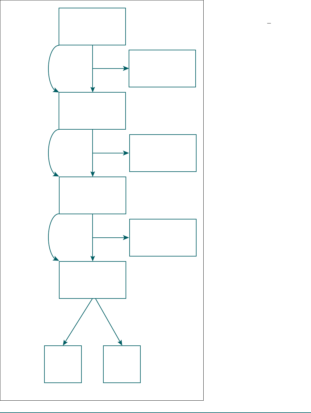
Figure. Sample size flowchart for pair weights development: National

Health Interview Survey, 2019

SOURCE: National Center for Health Statistics, 2019 National Health Interview Survey.

Eligible household

(with at least one eligible

adult and one child)

n = 10,322

Responding

adult–child pairs

n = 8,052

Parent–child pairs

n = 6,814

Household with one or

more nondeleted

household members

n = 36,160

Noneligible household

(household without

eligible adult–child pairs)

n = 25,838

Nonresponding

adult–child pairs

n = 2,270

Nonparent–child pairs

n = 1,238

Father–child

pairs

n = 2,728

Mother–child

pairs

n = 4,086

Calculate base

pair weights

Nonresponse

adjustment

Domain analysis

Let j = 1, 2, …, J index the J children in

household h, and let P

j|h

be child j’s

conditional selection probability given

h; for the 2019 NHIS,

The conditional selection probability

for pair k, where k = (i, j), given h is

Then pair k’s base sampling weight is

(1.1)

Adult–Child Pair-level

Nonresponse Adjustment

Among the 2019 NHIS eligible

households (n = 10,322), 8,052 adult–

child pairs (78.0%) completed both the

Sample Adult and Sample Child

interviews; the remaining households

completed only the Sample Adult

interview (n = 701, 6.8%), only the

Sample Child interview (n = 1,141,

11.1%), or neither interview (n = 428,

4.1%). To create dyad weights,

households who completed both the

Sample Adult and Sample Child

interviews were retained in the

analysis; the remaining households

were treated as nonrespondents

in terms of pair-level statistical

analysis. For the purpose of the

creation of adult–child pair weights,

nonresponding households were

eligible households with a responding

adult only [denoted as (RA, NC), where

RA denotes a responding adult and

NC denotes a nonresponse to the

Sample Child interview]; a completed

Sample Child interview only [denoted

as (NA, RC), where NA denotes a

nonresponse to the Sample Adult

interview and RC denotes a response

to the Sample Child interview]; or

neither an adult interview response

nor a child interview response (NA,

NC). The adult–child pair weights for

these households were set to 0, and

their sampling weights were

redistributed to households with both

| ||

kh ih jh

= 

/( )

h jh

W J





NATIONAL CENTER FOR HEALTH STATISTICS 4 Series 2, Number 207

adult- and child-completed interviews to the survey (RA, RC).

The adjustment factor was defined as:

( )

, ,,,

)

Adjustm

nt factor

(1.2

kkk k

RA NC NA RC RA RC NA NC

RA RC

www w

AF =

+++

∑∑∑∑

∑

where w

was pair k’s base sampling weight, which was

derived using formula (1.1),

was the summation of adult–child pairs’ sampling weights

over all households with responding adults only. The

remaining terms in (1.2) had similar definitions as those of

The nonresponse adjustment shown in (1.2) can be

performed across all eligible households. It is appropriate

when the nonresponse is not related to any factors, that is,

missing completely at random. However, if pair-level

nonresponse propensity is different among different groups,

then factors related to missingness should be considered for

nonresponse adjustment. Consequently, households with

responding pairs and households with nonresponding pairs

(that is, nonrespondents to the Sample Adult and/or Sample

Child interviews) were compared and factors related to

nonresponse were identified using chi-squared tests and

logistic regression models. The response propensity was

calculated from a logistic regression model that included all

the selected factors, including household type (one-adult

household versus multi-adult household); number of

families in a household (one family versus multiple families

in the household); metropolitan statistical area status;

census region; highest level of education among all

household members; Sample Adult’s age, sex, and race and

ethnicity; urban or rural status; and the median family

income within a census block group (results not shown).

Twenty adjustment cells were formed based on the

equidistant quantiles from the 5th percentile to the 100th

percentile of the predicted propensity of response, and the

pair-level nonresponse adjustment was conducted within

each adjustment cell. The adjustment factor was calculated

within each adjustment cell as:

where I

(q) was an indicator variable with I

(q) = 1 if pair

k was in cell q, and 0 otherwise, and q was an adjustment

cell defined by the propensity of response. The adjusted

RA NC

∑

RA NC

∑

( )

, ,,,

)

Adjustme

(

nt fact

() )

or within c

()

ell

()

, ( .3

(

)

kkk k

RA NC NA RC RA RC NA NC

RA RC

I qw I qw

I qw

qA =

+++

∑∑∑∑

∑

sampling weight for the responding adult–child pair data

was

(1.4)

where w

was defined in (1.1), AF

was defined in (1.3), and

was the nonresponse-adjusted pair weight for pair k.

Trimming Extreme Pair-level Sampling

Weights

Excessively large sampling weights are related to increased

variance estimates for weighted statistical analyses (9–11).

To reduce large variation in the final sampling weights, the

nonresponse-adjusted pair weights derived from (1.4) were

trimmed at the 99th quantile (denoted as w

) of the

nonresponse-adjusted sampling weights, that is, sampling

weights w

greater than w

were set as w

. Then the

trimmed sampling weights were readjusted by an adjustment

factor defined as,

where I () was an indicator variable that equaled 1 if the

event inside the paratheses was true, and 0 otherwise. The

final pair-level sampling weight was

(1.6)

where w

was the nonresponse-adjusted pair weight for

pair k defined in (1.4), AF

was the adjustment factor after

trimming the sampling weights at the 99th percentile, and

k,final

was the final pair-level sampling weights derived for

pair-level analysis.

Statistical Properties of the Adult–Child

Pair Weights in the 2019 NHIS

Table A shows selected statistical measures and quantiles of

the 2019 NHIS adult–child pair weights developed from the

procedures described above. Among the responding adult–

child pairs (n = 8,052), the mean of the sampling weights was

16,796 [standard deviation (SD) = 12,826] and the median

was 13,682. The range of the sampling weights was from 810

to 75,098. The maximal value of the sampling weight was the

same as the 99th percentile due to the trimming procedure

on the extreme sampling weights (the adjustment was done

for all adult–child pairs, so this result differed for mother–

child and father–child pairs). Among the mother–child pairs

(n = 4,086), the mean of the sampling weights was 14,636

(SD = 11,142) and the median was 12,181; among the father–

child pairs (n = 2,728), the mean of the sampling weights was

17,318 (SD = 11,974) and the median was 14,632.

qw w AF k= ∀∈

( )

99 99 99

)

djustment factor after trimming

, (1.5

()()

th th th

RA RC

kkk

RA RC RA RC

Iw w w Iw w w

+≥

∑

∑∑

99 99

[ ( )

( ) ] ,

th th

k final k k k

kk T

w Iw w w

IwwwAF

= <

+≥





Series 2, Number 207 5 NATIONAL CENTER FOR HEALTH STATISTICS

Producing Estimates for Mother–Child and

Father–Child Pairs

Mother–child and father–child pairs are a subset of all adult–child pairs, and

domain estimation methods can be used to produce estimates separately for

mother–child and father–child pairs using the adult–child pair weights (5–7). To

produce estimates for subpopulations using sample survey data, the survey design

feature needs to be incorporated for valid design-based variance estimation

(12,13). As a result, even if the analysis concentrates on a particular domain,

such as the mother–child domain, data from all dyadic pairs are needed for valid

variance estimation. Subsetting the data (for example, removing nonmother–child

pair data from the mother–child domain analysis) generally underestimates the

variances.

Let U represent the population of adult–child pairs among all households with

adult(s) and child(ren). To conduct a mother–child or father–child pair-level

analysis, U is partitioned into the relevant domains. Let U

represent the mother–

child pair domain, U

represent the father–child pair domain, and U

represent the

nonparent–child pair domain, and let z be a variable such that

= 1 if pair k is a mother–child pair (U

= 2 if pair k is a father–child pair (U

= 3 if pair k is a nonparent–child pair (U

Let g

be any pair-level measurement for pair k; for example, let g

be the reported

health status (NHIS variable PHSTAT, 1 = excellent, 2 = very good, 3 = good, 4 = fair,

and 5 = poor) of the Sample Adult and the Sample Child in a household, where

= 1 if both were in good to excellent health; g

= 0 if not. Using the mother–

child domain as an example, if data for all mother–child pairs in the population

are available, then the mother–child

domain total, the total number of

mother–child pairs in the population

with both mother and child in good to

excellent health is

(2.1)

From the 2019 NHIS Sample Adult

and Sample Child data, the estimated

total number of mother–child pairs

with both mother and child in good to

excellent health is

(2.2)

where n

s_AC

is the number of adult–

child pairs in the sample with

completed Sample Adult and Sample

Child interviews, w

k,final

is pair k’s final

sampling weight, and I () is an indicator

variable that equals 1 if the event

inside the paratheses is true, and 0

otherwise.

Other mother–child or father–child

level analyses follow the same

procedure, applying domain estimation

with the sampling weights of adult–

child pairs.

Examples of

Statistical Analyses

of the 2019 NHIS Pair

Data

This section contains four examples of

statistical analyses applied to the 2019

NHIS pair data using the adult–child

pair weights and domain estimation

methods: A univariate statistical

analysis on reported health status

of mother–child and father–child

pairs and three multivariable logistic

regression models with pair-level or

individual-level reported health status

as the outcome variables, respectively.

All statistical analyses in this report

were conducted using the survey

procedures in SAS version 9.4 (14),

and the code used to produce the

examples is included in Appendix I of

this report. Other software packages,

such as R, can also be used to analyze

the NHIS parent-pair data. For

( 1) .

U k kk

t g gIz= = =

∑∑

( 1),

s AC

U k final k k

t w gIz

= =

∑

Table A. Selected moments and quantiles of the adult–child pair weights

among all adult–child pairs, mother–child pairs, and father–child pairs:

National Health Interview Survey, 2019

Measure

Moment

All adult–child pairs Mother–child pairs Father–child pairs

Sample size

� � � � � � � � � � � 8,052 4,086 2,728

Mean

� � � � � � � � � � � � � � � � 16,796 14,636 17,318

Standard deviation

� � � � � � 12,826 11,142 11,974

Percent

Quantiles

All adult–child pairs Mother–child pairs Father–child pairs

100�00

� � � � � � � � � � � � � � 75,098 75,098 75,098

99�00 � � � � � � � � � � � � � � � � 75,098 59,217 63,689

95�00 � � � � � � � � � � � � � � � � 42,022 35,754 40,486

90�00 � � � � � � � � � � � � � � � � 32,519 27,744 32,519

75�00 � � � � � � � � � � � � � � � � 21,241 18,851 22,103

50�00

� � � � � � � � � � � � � � � 13,682 12,181 14,632

25�00 � � � � � � � � � � � � � � � � 7,852 7,004 8,599

10�00 � � � � � � � � � � � � � � � � 5,396 3,956 6,273

5�00 � � � � � � � � � � � � � � � � � 3,515 3,170 4,044

1�00 � � � � � � � � � � � � � � � � � 2,529 2,263 2,823

0�00

� � � � � � � � � � � � � � � � 810 976 810

Maximal value.

Median value.

Minimal value.

SOURCE: National Center for Health Statistics, 2019 National Health Interview Survey.

NATIONAL CENTER FOR HEALTH STATISTICS 6 Series 2, Number 207

example, the subset function from

the survey package in R can be used

with survey functions such as svymean

and svyglm for domain estimation

of the NHIS parent-pair data (15,16).

The complex survey features (strata,

primary sampling unit, and adult–child

sample weights) were incorporated

into the variance estimation for all

analyses in this report.

Example 1. Univariate

Statistical Analysis of a

Joint Outcome Created

Between Parent and Child

A composite adult–child pair health

status variable (denoted as HEALTH_

COMPOSITE) was created with two

levels, as follows,

HEALTH_COMPOSITE = 1 if both

members of a pair were in good

to excellent health (defined as

PHSTAT = 1, 2, 3 for both the

Sample Adult and Sample Child);

HEALTH_COMPOSITE = 0 if at least

one member of a pair was in poor

or fair health (PHSTAT = 4, 5 for at

least one member).

When domain estimation methods are

used, any recodes need to be

conducted for the entire adult–child

pair file. The weighted percentage of

both members in good to excellent

health (that is, HEALTH_COMPOSITE =

1) was calculated using the SAS

surveyfreq procedure. Multiway tables were used to conduct domain analysis,

that is, including the domain variable(s) (for example, variable z, with z = 1 denoted

a mother–child pair, 2 a father–child pair, and 3 otherwise) before the analytical

variable(s) (for example, HEALTH_COMPOSITE). The sample SAS code is in

Appendix I. Percentage and 95% confidence interval (95% CI) estimates for the

mother–child and father–child domains are shown in Table B. The percentage

estimates meet NCHS data presentation standards for proportions (17). Among

the mother–child and father–child pairs, 89.1% [95% CI = (87.7%, 90.5%)] and

90.0% [95% CI = (88.5%, 91.5%)] were in good to excellent health for both members

of a pair, respectively.

Example 2. A Logistic Regression Model With the

Composite Pair-level Health Status as the Dependent

Variable and Selected Covariates as Predictors

This section shows an example of a logistic regression model for mother–child

pairs using the pair-level measurement as the dependent variable. In particular,

the composite adult–child pair-level health status derived in Example 1 was the

dependent variable, and the predictors (NHIS variable name) included census

region (REGION), 2013 NCHS urban–rural classification (URBRRL) (18), adult’s age

(in years; AGEP_A), race and ethnicity (HISPALLP_R_A) and education (EDUC_R_A),

and child’s age (in years; AGEP_C) and sex (SEX_C). The example is for illustration

purposes and may not be the optimal model to study the associations of the

outcome and the covariates. The model was in the following form:

where

was the intercept and





were each either a scalar [that is, when

the covariate was a continuous variable (AGEP_A, AGEP_C) or a categorial variable

with two categories] or a vector (that is, when the covariate was a categorial

variable with more than two categories) of coefficients of the covariates. The SAS

surveylogistic procedure was used to fit the model, and the domain statement was

used for domain analysis for mother–child pairs. The sample SAS code (Example 2)

is shown in Appendix I, and the results of the mother–child pairs are in Table C.

Odds ratios (ORs) demonstrated significant associations between mother–child

pair-level health status and most 2013 NCHS urban–rural classification categories,

as well as mothers’ age, race and ethnicity, and education. That is, both members

logit

= PHEALTHCOMPOSITE REGION URBRRL_  





01 2

 

 

34 567

AGEP AHISPALLP RA EDUC RA AGEP CSEX_______ +  CC ,

Table B. Unweighted sample size, weighted frequency, weighted percent distributions with standard errors,

and 95% confidence interval estimates of mother–child and father–child pairs' health status using domain

estimation in Example 1: National Health Interview Survey, 2019

Domain and adult–child pair’s

composite health status

Unweighted

sample size

Weighted

frequency Percent

Standard

error

95% confidence

interval

Father–Child pairs

Both in good to excellent health

� � � � � � � � � � � � � � � � � 2,464 42,524,330 90�0 0�8 (88�5, 91�5)

At least one not in good health � � � � � � � � � � � � � � � � � � 263 4,716,691 10�0 0�8 (8�5, 11�5)

Mother–Child pairs

Both in good to excellent health

� � � � � � � � � � � � � � � � � 3,622 53,204,288 89�1 0�7 (87�7, 90�5)

At least one not in good health � � � � � � � � � � � � � � � � � � 457 6,520,731 10�9 0�7 (9�5, 12�3)

One father–child pair and seven mother–child pairs were excluded from the analyses due to missing data in composite health status.

Percentage estimates meet the National Center for Health Statistics data presentation standards for proportions.

NOTES: For father–child and mother–child pairs, Both in good to excellent health is dened as health status is excellent, very good, or good for both the

Sample Adult and Sample Child; At least one not in good health is dened as health status is fair or poor for at least one member of the Sample Adult–

Sample Child pair.

SOURCE: National Center for Health Statistics, 2019 National Health Interview Survey.

Series 2, Number 207 7 NATIONAL CENTER FOR HEALTH STATISTICS

of the mother–child pair were more likely to have good to excellent health when

the mother was younger [OR = 0.98, 95% CI = (0.96, 1.00)], the mother was White,

non-Hispanic [OR =1.65, 95% CI = (1.14, 2.39)], and the household was in a small,

medium, or large fringe metropolitan area [OR = 1.57, 95% CI = (1.04, 2.38), and

OR = 2.25, 95% CI = (1.42, 3.56), respectively], whereas both pair members were

less likely to have good to excellent health when the mother had some college or

a high school degree or less [OR = 0.29, 95% CI = (0.21, 0.42), and OR = 0.20, 95%

CI = (0.14, 0.30), respectively].

Example 3. A Repeated

Measurement Model With

the Individual-level Health

Status as the Outcome

Variable and Selected

Covariates as Predictors

The logistic regression model in

Example 2 used a composite dyadic-

level health status as the response

variable. Using the composite

measurement from a dyad as the

unit of analysis has a few limitations.

First, it only includes dyads in which

both members have no missing values

for the outcome variable. Second,

it studies the associations of the

covariates and the composite dyadic-

level response, but it does not examine

the associations of the covariates and

the individual-level response for each

member of the dyad.

This section shows an example of a

logistic regression with the individual-

level measurement as the response

variable, that is, data from the Sample

Adult and Sample Child were not used

to create a composite measurement.

Instead, they were included in the

analysis as two separate observations

for a household (that is, each

household had two rows of data, one

for the Sample Adult and one for the

Sample Child). Let HEALTH_SELF be a

sample person’s health status (Sample

Adult or Sample Child), where

HEALTH_SELF = 1 if a sample

person was in good to excellent

health (PHSTAT = 1, 2, 3);

HEALTH_SELF = 0, otherwise

(PHSTAT = 4, 5).

A logistic regression model was fit with

HEALTH_SELF as the response variable,

and the following predictors: Census

region (REGION), 2013 NCHS urban–

rural classification (URBRRL), sample

person’s age (in years; AGEP), race

and ethnicity (HISPALLP_R), Sample

Adult’s education (EDUC_R_A), and

an indicator variable to indicate if a

person was an adult or a child [that is,

I (ADULT) = 1 if the person was an adult,

and 0 otherwise]. In addition, to study

the association of the health status of a

Table C. Odds ratio and 95% confidence interval estimates of the

logistic regression model in Example 2 predicting adult–child pair-level

composite health status given selected characteristics with results for

mother–child pairs: National Health Interview Survey, 2019

Characteristic, (variable name),

and category

Mother–Child pairs

Odds ratio 95% confidence interval

Age of mother (AGEP_A)

� � � � � � � � � � � � � � � 0�98 0�96

1�00

Age of child (AGEP_C) � � � � � � � � � � � � � � � � � 0�97 0�94

1�00

Census region (REGION)

Northeast

� � � � � � � � � � � � � � � � � � � � � � � � � � � 0�70 0�42 1�18

Midwest � � � � � � � � � � � � � � � � � � � � � � � � � � � � 0�94 0�58 1�52

South � � � � � � � � � � � � � � � � � � � � � � � � � � � � � � 0�79 0�52 1�18

West � � � � � � � � � � � � � � � � � � � � � � � � � � � � � � � Ref … …

2013 NCHS

Urban–Rural Classification (URBRRL)

Large central metropolitan

� � � � � � � � � � � � � 1�44 0�91 2�27

Large fringe metropolitan

� � � � � � � � � � � � � � 2�25 1�42 3�56

Medium or small metropolitan

� � � � � � � � � � 1�57 1�04 2�38

Nonmetropolitan

� � � � � � � � � � � � � � � � � � � � � Ref … …

Sex of child (SEX_C)

Male

� � � � � � � � � � � � � � � � � � � � � � � � � � � � � � � 1�08 0�84 1�39

Female � � � � � � � � � � � � � � � � � � � � � � � � � � � � � Ref … …

Race and ethnicity of mother

(HISPALLP_R_A)

Black, non-Hispanic

� � � � � � � � � � � � � � � � � � � Ref … …

White, non-Hispanic

� � � � � � � � � � � � � � � � � � � 1�65 1�14 2�39

Other, non-Hispanic

� � � � � � � � � � � � � � � � � � 1�57 0�88 2�81

Hispanic

� � � � � � � � � � � � � � � � � � � � � � � � � � � 1�11 0�73 1�67

Education of mother (EDUC_R_A)

High school or less

� � � � � � � � � � � � � � � � � � � 0�20 0�14 0�30

Some college (including

associate’s degree) � � � � � � � � � � � � � � � � � � � 0�29 0�21 0�42

Bachelor’s degree and above � � � � � � � � � � � � Ref … …

… Category not applicable.

Rounded to 1.00 from 0.998.

Rounded to 1.00 from 1.001.

Counties in metropolitan statistical areas (MSAs) of 1 million or more population that contain the

entire population of the largest principal city of the MSA, have their entire population contained in the

largest principal city of the MSA, or contain at least 250,000 inhabitants of any principal city of the

MSA.

Counties in MSAs of 1 million or more population that did not qualify as large central metropolitan

counties.

Counties in MSAs of populations of 250,000 to 999,999 and counties in MSAs of populations less

than 250,000.

Counties in micropolitan statistical areas and nonmetropolitan counties that did not qualify as

micropolitan.

Includes other non-Hispanic people not shown separately due to smaller groups not being statistically

reliable.

People of Hispanic origin may be of any race.

NOTE: Ref is the reference group.

SOURCE: National Center for Health Statistics, 2019 National Health Interview Survey.

NATIONAL CENTER FOR HEALTH STATISTICS 8 Series 2, Number 207

Like the results of Example 2, ORs were significant between individual-level health

status (HEALTH_SELF) and most urban-rural categories, age, race and ethnicity,

and mothers’ education. In addition, a positive association was also observed

between a person’s health status and the health status of the other dyadic member

[OR = 3.51, 95% CI = (2.04, 6.02)]; and mothers were less likely to report good to

excellent health than their children [that is, OR = 0.51, 95% CI = (0.29, 0.91) for the

adult indicator variable].

person (HEALTH_SELF) with the health

status of the other dyadic member,

the health status of the other dyadic

member was included as a covariate

(denoted as HEALTH_OTHER). The

overall logistic regression model can

be written as:

Because two observations were

included for each household, the

model was a repeated measurement

model. For each household the model

was the following,

where _A and _C represented the

Sample Adult and Sample Child,

respectively (for example, HEALTH_A

was the Sample Adult’s health status);

was the intercept, and





were each either a scalar [that is, when

the covariate was a continuous variable

(AGEP_A, AGEP_C) or a categorial

variable with two categories] or a

vector (that is, when the covariate was

a categorial variable with more than

two categories) of coefficients of the

covariates. The model was fit using

the SAS surveylogistic procedure.

The Example 3 SAS code is shown

in Appendix I, and the results of the

mother–child pair domain analysis are

shown in Table D.

( )

logit _ 1

P HEALTH SELF

REGION

URBRRL AGEP

HISPALLP R

EDUC R A

I ADULT

HEALTH OTHER

ββ

= +

logit( ( _ 1))

P HEALTH A

P HEALTH C

REGION

URBRRL AGEP A

URBRRL AGEP C

HISPALLP R A

HISPALLP R C

ββ

= +







  

  

  

  

  

  







__ 1

__ 0

EDUC R A

HEALTH C

HEALTH A

ββ

  

  

  







Table D. Odds ratio and 95% confidence interval estimates of the

repeated measurement model in Example 3 predicting individual-level

health status given selected characteristics with results for mother–child

pairs: National Health Interview Survey, 2019

Characteristic, (variable name),

and category

Mother–Child pairs

Odds ratio 95% confidence interval

Age (AGEP)

� � � � � � � � � � � � � � � � � � � � � � � � � � � � � 0�97 0�95 0�98

Health status of the other dyadic

member (HEALTH_OTHER)

Excellent, very good, or good � � � � � � � � � � � � � � � 3�51 2�04 6�02

Fair or poor � � � � � � � � � � � � � � � � � � � � � � � � � � � � � Ref … …

Census region (REGION)

Northeast

� � � � � � � � � � � � � � � � � � � � � � � � � � � � � � � 0�75 0�48 1�18

Midwest � � � � � � � � � � � � � � � � � � � � � � � � � � � � � � � � 0�98 0�65 1�47

South � � � � � � � � � � � � � � � � � � � � � � � � � � � � � � � � � � 0�78 0�55 1�12

West � � � � � � � � � � � � � � � � � � � � � � � � � � � � � � � � � � � Ref … …

2013 NCHS

Urban–Rural Classification (URBRRL)

Large central metropolitan

� � � � � � � � � � � � � � � � � 1�41 0�97 2�07

Large fringe metropolitan

� � � � � � � � � � � � � � � � � � 2�05 1�38 3�05

Medium or small metropolitan

� � � � � � � � � � � � � � 1�53 1�07 2�17

Nonmetropolitan

� � � � � � � � � � � � � � � � � � � � � � � � � Ref … …

Race and ethnicity (HISPALLP_R)

Black, non-Hispanic

� � � � � � � � � � � � � � � � � � � � � � � Ref … …

White, non-Hispanic

� � � � � � � � � � � � � � � � � � � � � � � 1�48 1�06 2�05

Other, non-Hispanic

� � � � � � � � � � � � � � � � � � � � � � 1�52 0�92 2�50

Hispanic

� � � � � � � � � � � � � � � � � � � � � � � � � � � � � � � 1�09 0�77 1�54

Education of mother (EDUC_R_A)

High school or less

� � � � � � � � � � � � � � � � � � � � � � � 0�22 0�15 0�31

Some college (including associate’s degree) � � � � 0�30 0�22 0�43

Bachelor’s degree and above � � � � � � � � � � � � � � � � Ref … …

Adult indicator (ADULT_ID)

Mother

� � � � � � � � � � � � � � � � � � � � � � � � � � � � � � � � � 0�51 0�29 0�91

Child � � � � � � � � � � � � � � � � � � � � � � � � � � � � � � � � � � � Ref … …

… Category not applicable.

Counties in metropolitan statistical areas (MSAs) of 1 million or more population that contain the

entire population of the largest principal city of the MSA, have their entire population contained in the

largest principal city of the MSA, or contain at least 250,000 inhabitants of any principal city of the

MSA.

Counties in MSAs of 1 million or more population that did not qualify as large central metropolitan

counties.

Counties in MSAs of populations of 250,000 to 999,999 and counties in MSAs of populations less

than 250,000.

Counties in micropolitan statistical areas and nonmetropolitan counties that did not qualify as

micropolitan.

Includes other non-Hispanic people not shown separately due to smaller groups not being statistically

reliable.

People of Hispanic origin may be of any race.

NOTE: Ref is the reference group.

SOURCE: National Center for Health Statistics, 2019 National Health Interview Survey.

Series 2, Number 207 9 NATIONAL CENTER FOR HEALTH STATISTICS

Example 4. A Logistic Regression Model With the Sample

Child’s Measurement as the Outcome Variable and

Selected Maternal Measurements as Predictors

The logistic regression models described in Examples 2 and 3 used measurements

from both dyad members as the outcome of interest. The composite dyadic-level

measurement was the outcome variable in Example 2, and the individual-level

measurements from both dyad members were used as repeated measurements

in Example 3. This section uses the measurement from one dyadic member as the

outcome variable. In particular, the child’s health status was the outcome variable,

and the association of the child’s health status with the mother’s health status was

studied. A health status variable of the Sample Child (denoted as HEALTH_C) was

created, as follows,

HEALTH_C = 1 if the Sample Child was in good to excellent health

(PHSTAT = 1, 2, 3);

HEALTH_C = 0 if the Sample Child was in poor or fair health

(PHSTAT = 4, 5).

The Sample Adult’s health status (denoted as HEALTH_A) was defined in the same

way. A logistic regression model was fit with HEALTH_C as the response variable

and following predictors were included in the model: Census region (REGION),

2013 NCHS urban–rural classification (URBRRL), Sample Child’s age (in years;

AGEP_C), sex (SEX_C) and race and ethnicity (HISPALLP_R_C), the Sample Adult’s

education (EDUC_R_A), and health status (HEALTH_A). The model was

where

was the intercept and





were each either a scalar [that is, when

the covariate was a continuous variable (AGEP_C) or a categorial variable with

two categories] or a vector (that is, when the covariate was a categorial variable

with more than two categories) of coefficients of the covariates. The model was

fit using the SAS surveylogistic procedure. The Example 4 SAS code is shown in

Appendix I, and the results of the mother–child pair domain analysis are shown

in Table E.

ORs were significant between the child’s health status (HEALTH_C) and the

mother’s health status (HEALTH_A), the mother’s education, and the child’s sex.

The child was more likely to have good to excellent health when the mother was

in good to excellent health [OR = 4.07, 95% CI = (2.31, 7.17)], and less likely if the

mother had a high school degree or less [OR = 0.47, 95% CI = (0.25, 0.87)] and if

the child was male [OR = 0.46, 95% CI = (0.28, 0.75)].

Discussion

This report provides details of the methodology for creating sampling weights for

adult–child pairs in the 2019 NHIS and guidance on how to use and access these

weights. This report also provides examples of how mother–child or father–child

pair data can be analyzed. The availability of these weights creates new research

opportunities with NHIS data, which contain rich information on mother–child or

father–child pairs’ health status, health behaviors, and healthcare access and use.

Dyad weights starting with the 2019 NHIS will be available on the NCHS website.

Each year’s dyad weights will be in a file that includes a household ID (HHX, for

linking to Sample Adult and Sample Child data) and the pair weights (final_pair_

weight). After linking the pair weights to Sample Adult and Sample Child data

sets using HHX, users can derive mother–child, father–child, and nonparent–child

pairs using variables SAPARENTSC_A (Sample Adult relationship to Sample Child)

logit = PHEALTHC REGION URBRRL AGEP_1

01 23



 

 

__ ___

HISPALLP RC SEXC EDUC RA





4567

HHEALTH A_,

and SEX_A. These two variables are

available in the Sample Adult public-

use data files. The SAS code associated

with Example 1 demonstrates how to

prepare a file for analysis.

The adult–child pair weights

incorporate the sampling probability

at each level and are adjusted for

nonresponse. However, calibration

(that is, raking or poststratification)

to external control totals was not

used in the creation of these weights.

Calibration has been used in sample

surveys to adjust for the differences

between the sample and the population

(19,20). Proper use of additional

information for poststratification may

yield more efficient estimators if the

sample proportions are quite different

from the population proportions (21).

Unfortunately, no reliable independent

estimates for adult–child pairs in the

United States exist, so calibration to

independent external estimates was

not conducted.

The pair weights described in this

report are developed for parent–child

pair-level statistical analyses. This

method is expected to be used for

NHIS data files (2019 and forward),

and this document will continue to

serve as a reference. Households

(with children) that completed only

the Sample Adult interview (n = 701,

6.8%) or completed only the Sample

Child interview (n = 1,141, 11.0%) are

treated as nonresponse among the

eligible households in terms of pair-

level analyses. The pair weights should

not be used if the statistical analyses

focus exclusively on all Sample Adults

(or all Sample Children); instead,

the Sample Adult (or Sample Child)

sampling weights developed by NCHS

should be used for the corresponding

analyses. For example, Sample Child

sampling weights should be used for

an analysis of a health outcome for

children using data from all Sample

Children (that is, including those whose

families did not complete a Sample

Adult interview). Although the Sample

Adult (and Sample Child) sampling

weights are correlated with the pair

weights, pair-level statistical analyses

should use the pair-level sampling

NATIONAL CENTER FOR HEALTH STATISTICS 10 Series 2, Number 207

weights, as they incorporate the sampling probabilities of both the Sample Adult

and the Sample Child and are adjusted for pair-level nonresponse. Using Sample

Adult weights or Sample Child weights for pair-level statistical analysis may lead

to biased results. Appendix II compares mean estimates using the pair weights

and the Sample Adult weights under a simplified scenario. Factors found to be

related to the differences in the mean estimates using the two sampling weights

included the distribution of the outcome of interest, the number of children across

households, and the sampling weights of Sample Adults.

Three logistic regression models were

applied to the 2019 NHIS dyadic data,

which use the dyadic-level or the

individual-level measurement as the

response variables, respectively. Other

statistical models, such as structural

equation modeling (22) and multilevel

modeling (23,24), may also be applied

to the NHIS parent–child data. In

practice, different estimation methods

can be used for different research

goals; and more research is needed

to explore how to use the pair data

from NHIS (2019 and forward). Design-

based variance estimation was used

for the repeated measurement model

in this report, which incorporates the

survey design features (strata, PSU,

and sampling weights) for variance

estimation and is expected to yield

conservative variance estimates.

However, it does not reflect the nested

data structure of parent–child pairs

within a household. To control for the

additional parent–child correlation,

alternative statistical methods can be

used, for example, random or mixed-

effect models, which may incorporate

the correlation of the Sample Adult and

the Sample Child within a household. In

addition, resampling methods such as

Jackknife and Bootstrap methods may

also be used for variance estimation of

the dyadic data.

Although traditional household surveys

usually focus on the household-

level and the individual-level

measurements, dyadic data in national

household surveys are not uncommon.

The National Survey of Drug Use and

Health, conducted by the Substance

Abuse and Mental Health Services

Administration, collects detailed

information on tobacco, alcohol, and

drug use, as well as mental health-

related issues in the United States (25).

Zero, one, or two people are selected

within a household, and the sampling

weights for the selected pairs have

been developed. NHIS selects a Sample

Adult and a Sample Child (when

applicable) independently within a

family or a household. Because the

sampling weights for the selected pairs

are the inverse of the pairs’ selection

probabilities, the adult–child pair

Table E. Odds ratio and 95% confidence interval estimates of the logistic

regression model in Example 4 predicting the child’s health status given

selected characteristics with results for mother–child pairs: National

Health Interview Survey, 2019

Characteristic,

(variable name), and category

Mother–Child pairs

Odds ratio 95% confidence interval

Child’s age (AGEP_C)

� � � � � � � � � � � � � � � � � � � � � � 0�97 0�92 1�01

Census region (REGION)

Northeast

� � � � � � � � � � � � � � � � � � � � � � � � � � � � � � � 1�29 0�57 2�89

Midwest � � � � � � � � � � � � � � � � � � � � � � � � � � � � � � � � 0�69 0�30 1�59

South � � � � � � � � � � � � � � � � � � � � � � � � � � � � � � � � � � 0�58 0�32 1�04

West � � � � � � � � � � � � � � � � � � � � � � � � � � � � � � � � � � � Ref … …

2013 NCHS

Urban–Rural Classification (URBRRL)

Large central metropolitan

� � � � � � � � � � � � � � � � � 0�89 0�44 1�81

Large fringe metropolitan

� � � � � � � � � � � � � � � � � � 1�18 0�56 2�49

Medium or small metropolitan

� � � � � � � � � � � � � � 1�02 0�52 1�99

Nonmetropolitan

� � � � � � � � � � � � � � � � � � � � � � � � � Ref … …

Child’s sex (SEX_C)

Male

� � � � � � � � � � � � � � � � � � � � � � � � � � � � � � � � � � � 0�46 0�28 0�75

Female � � � � � � � � � � � � � � � � � � � � � � � � � � � � � � � � � Ref … …

Child’s race and ethnicity (HISPALLP_R_C )

Black, non-Hispanic

� � � � � � � � � � � � � � � � � � � � � � � Ref … …

White, non-Hispanic

� � � � � � � � � � � � � � � � � � � � � � � 1�19 0�54 2�64

Other, non-Hispanic

� � � � � � � � � � � � � � � � � � � � � � 1�76 0�65 4�79

Hispanic

� � � � � � � � � � � � � � � � � � � � � � � � � � � � � � � 0�63 0�29 1�38

Mother’s education (EDUC_R_A)

High school or less

� � � � � � � � � � � � � � � � � � � � � � � 0�47 0�25 0�87

Some college (including

associate’s degree) � � � � � � � � � � � � � � � � � � � � � � � 0�62 0�33 1�16

Bachelor’s degree and above � � � � � � � � � � � � � � � � Ref … …

Mother’s health status (HEALTH_A)

Excellent, very good, or good

� � � � � � � � � � � � � � � 4�07 2�31 7�17

Fair or poor � � � � � � � � � � � � � � � � � � � � � � � � � � � � � Ref … …

… Category not applicable.

Counties in metropolitan statistical areas (MSAs) of 1 million or more population that contain the

entire population of the largest principal city of the MSA, have their entire population contained in the

largest principal city of the MSA, or contain at least 250,000 inhabitants of any principal city of the

MSA.

Counties in MSAs of 1 million or more population that did not qualify as large central metropolitan

counties.

Counties in MSAs of populations of 250,000 to 999,999 and counties in MSAs of populations less

than 250,000.

Counties in micropolitan statistical areas and nonmetropolitan counties that did not qualify as

micropolitan.

Includes other non-Hispanic people not shown separately due to smaller groups not being statistically

reliable.

People of Hispanic origin may be of any race.

NOTE: Ref is the reference group.

SOURCE: National Center for Health Statistics, 2019 National Health Interview Survey.

Series 2, Number 207 11 NATIONAL CENTER FOR HEALTH STATISTICS

weights for the 2019 NHIS can be derived, and then domain

estimation can be used for inferences on mother–child and

father–child pairs. The methods used to produce NHIS pair

weights can easily be adapted to other surveys with similar

sampling designs in which one or more people within a

family have been sampled independently of their specified

relationships. Dyadic data in national surveys provide new

research opportunities to study the interdependence of

social behaviors and health status among members within

families or households.

References

1. National Center for Health Statistics. National Health

Interview Survey, 2019 survey description. 2020.

Available from: https://ftp.cdc.gov/pub/health_

statistics/nchs/dataset_documentation/NHIS/2019/

srvydesc-508.pdf.

2. Parsons VL, Moriarity C, Jonas K, Moore TF, Davis KE,

Tompkins L. Design and estimation for the National

Health Interview Survey, 2006–2015. National Center

for Health Statistics. Vital Health Stat 2(165):1–53.

2014.

3. Kenny DA, Kashy DA, Cook WL. Dyadic data analysis.

New York, NY: Guilford Press. 2006.

4. Zhang G, Yuan Y. Bayesian modeling longitudinal dyadic

data with nonignorable dropout, with application to a

breast cancer study. Ann Appl Stat 6(2):753–71. 2012.

5. Clement EP, Udofia GA, Enang EI. Estimation for

domains in stratified sampling design in the presence

of nonresponse. Am J Math Stat 4(2):65–71. 2014.

6. Hidiroglou MA, Patak Z. Domain estimation using

linear regression. Survey Methodology 30(1):67–78.

2006.

7. Yates F. Sampling methods for censuses and surveys.

London: Charles W. Griffin. 1953.

8. Bramlett MD, Dahlhamer JM, Bose J, Blumberg SJ. New

procedures for nonresponse adjustments to the 2019

National Health Interview Survey sampling weights.

National Center for Health Statistics. 2020.

9. Elliott MR. Model averaging methods for weight

trimming. J Off Stat 24(4):517–40. 2008.

10. Potter F. A study of procedures to identify and trim

extreme sample weights. In: Proceedings of the

American Statistical Association, Survey Research

Methods Section. Alexandria, VA: American Statistical

Association. 1990.

11. Kish L. Weighting for unequal P

. J Off Stat 8:183–200.

1992.

12. Chowdhury S, Machlin S. Variance estimation from

MEPS event files. Methodology Report No. 26. Agency

for Healthcare Research and Quality. 2011.

13. Kish L. Design and estimation for domains. J R Stat Soc

Series D (The Statistician) 29(4):209–22. 1980.

14. SAS Institute Inc. SAS 9.4 language reference:

Concepts. 6th ed. 2016.

15. Lumley T. Complex surveys: A guide to analysis using R.

John Wiley & Sons, Inc. 2010.

16. Lumley T. Survey: Analysis of complex survey samples.

R package (version 4.2.) [computer software]. 2023.

17. Parker JD, Talih M, Malec DJ, Beresovsky V, Carroll M,

Gonzalez JF, et al. National Center for Health Statistics

data presentation standards for proportions. Vital

Health Stat 2(175). 2017.

18. Ingram DD, Franco SJ. 2013 NCHS urban–rural

classification scheme for counties. National Center for

Health Statistics. Vital Health Stat 2(166). 2014.

19. Gelman A. Struggles with survey weighting and

regression modeling. Statist Sci 22(2):153–64. 2007.

20. Little RJA. Post-stratification: A modeler’s perspective.

J Am Statist Assoc 88(423):1001–12. 1993.

21. Kish L. Survey sampling. John Wiley & Sons, Inc. 1965.

22. Bollen KA. Structural equations with latent variables.

New York, NY: John Wiley & Sons, New York. 1989.

23. Gelman A, Hill J. Data analysis using regression

and multilevel/hierarchical models. New York, NY:

Cambridge University Press. 2007.

24. Veiga A, Smith PWF, James JJ. The use of sample

weights in multivariate multilevel models with an

application to income data collected by using a

rotating panel survey. J R Stat Soc Series C (Appl Stat)

63:65–84. 2014.

25. Center for Behavioral Health Statistics and

Quality. 2017 National Survey on Drug Use and

Health methodological resource book, section 12:

Questionnaire dwelling unit-level and person pair-

level sampling weight calibration. 2019. Available

from: https://www.samhsa.gov/data/sites/default/

files/cbhsq-reports/NSDUHmrbQDUPairWgt2017/

NSDUHmrbQDUPairWgt2017.pdf.

NATIONAL CENTER FOR HEALTH STATISTICS 12 Series 2, Number 207

Appendix I. SAS Code for the

Examples in the Report

Example 1 SAS Code

libname w “directory of the folder where the pair weights le is saved”;

libname public “directory of the folder where the Sample Adult and Sample Child data

is saved”;

**************************************

*Prepare pair weights data *

**************************************;

data nal_weight;

set w.nal_pair_weight2019;

eligible_familyID=1;

Keep HHX nal_pair_weight eligible_familyID;

run;

proc sort data= nal_weight;

by HHX ;

run;

********************************************

*Prepare Sample Adult and Sample Child data*

********************************************;

data adult;

set public.adult19 ;

format _all_;

HISPALLP_R_A=.;

if HISPALLP_A=1 then HISPALLP_R_A=1; /*Hispanic*/

else if HISPALLP_A=2 then HISPALLP_R_A=2; /*White, non-Hispanic*/

else if HISPALLP_A=3 then HISPALLP_R_A=3; /*Black, non-Hispanic*/

else HISPALLP_R_A=4; /*other, non-Hispanic */

Series 2, Number 207 13 NATIONAL CENTER FOR HEALTH STATISTICS

if 0<=EDUC_A <=4 then EDUC_R_A =1 ; /* high school or less*/

else if 5<=EDUC_A <=7 then EDUC_R_A =2 ; /* some college*/

else if 8<=EDUC_A <=11 then EDUC_R_A =3 ; /*Bachelors degree or higher*/

else EDUC_R_A =.;

keep

HHX PSTRAT PPSU

SAPARENTSC_A AGEP_A SEX_A

HISPALLP_R_A EDUC_R_A PHSTAT_A

REGION URBRRL;

run;

proc sort data=adult;

by HHX;

run;

data child;

set public.child19 ;

format _all_;

if SEX_C in ( 1 2) then SEX_C=SEX_C; else SEX_C=.;

keep

HHX AGEP_C SEX_C HISPALLP_C PHSTAT_C;

run;

proc sort data=child;

by HHX;

run;

data all1;

merge nal_weight adult child;

by HHX ;

if eligible_familyID=1;

NATIONAL CENTER FOR HEALTH STATISTICS 14 Series 2, Number 207

if SAPARENTSC_A=1 then parent_child=1;

else parent_child=0;

if parent_child=1 then do;

if SEX_A=1 then z= 2; /*father-child*/

else if SEX_A=2 then z= 1 ; /*mother-child*/

end;

if parent_child=0 then z= 3; /*non-parent-child*/

if PHSTAT_A in (7 9 )then PHSTAT_A=.;

if PHSTAT_C in (7 9 )then PHSTAT_C=.;

if PHSTAT_A ^ =. and PHSTAT_C ^= . then do;

if PHSTAT_A in (1 2 3 ) and PHSTAT_C in (1 2 3 ) then HEALTH_COMPOSITE =’Both mem-

bers of dyad in at least good health’;

else HEALTH_COMPOSITE =’at least one member has fair, poor health’;

end;

run;

*********************************

*Table B: Freq of health status *

*********************************;

title “Table B. Health status of the pair”;

proc surveyfreq data=all1 ;

stratum PSTRAT ;

cluster PPSU ;

weight nal_pair_weight;

table z*HEALTH_COMPOSITE/row CL NOCELLPERCENT ;

run;

*****************************************************************************

Series 2, Number 207 15 NATIONAL CENTER FOR HEALTH STATISTICS

*NOTE: *

*Denition of the variables: *

*z: 1 = mother-child pairs, 2 = father-child pairs, 3=non-parent-child pairs*

*HEALTH_COMPOSITE: composite adult-child pair health status variable. *

*nal_pair_weight: adult-child pair weight. *

*PSTRAT : strata variable. *

*PPSU : PSU variable. *

* *

*Data structure: one row each pair *

****************************************************************************;

Example 2 SAS Code

*************************************************************

*Refer to Example 1 SAS code for Data preparation procedure *

*************************************************************;

title “The logistic regression model with the composite pair level health status as

the response variable”;

proc surveylogistic data=all1;

stratum PSTRAT ;

cluster PPSU ;

weight nal_pair_weight;

class REGION URBRRL SEX_C HISPALLP_R_A (ref=’3’) EDUC_R_A ;

model HEALTH_COMPOSITE = REGION URBRRL AGEP_A AGEP_C SEX_C HISPALLP_R_A

EDUC_R_A ;

domain z;

run;

*****************************************************************************

*Denition of the variables: *

*HEALTH_COMPOSITE: composite adult-child pair health status variable. *

*REGION: region. *

*URBRRL: 2013 NCHS Urban-Rural Classication. *

*AGEP_A: age of Sample Adult. *

*AGEP_C: age of Sample Child. *

*SEX_C: sex of Sample Child. *

NATIONAL CENTER FOR HEALTH STATISTICS 16 Series 2, Number 207

*HISPALLP_R_A: race/ethnicity of Sample Adult. *

*EDUC_R_A: education of Sample Adult. *

*z: 1 = mother-child pairs, 2 = father-child pairs, 3=non-parent-child pairs*

*PSTRAT : strata variable. *

*PPSU : PSU variable. *

*nal_pair_weight: adult-child pair weight. *

* *

*Data structure: one row each pair *

****************************************************************************;

Example 3 SAS Code

**************************************

*Prepare pair weights data *

**************************************;

data nal_weight;

set w.nal_pair_weight2019;

eligible_familyID=1;

Keep HHX nal_pair_weight eligible_familyID;

run;

proc sort data= nal_weight;

by HHX ;

run;

********************************************

*Prepare Sample Adult and Sample Child data*

********************************************;

data adult;

set public.adult19 ;

format _all_;

if SAPARENTSC_A=1 then parent_child=1;

else parent_child=0;

Series 2, Number 207 17 NATIONAL CENTER FOR HEALTH STATISTICS

if parent_child=1 then do;

if SEX_A=1 then z= 2; /*father-child*/

else if SEX_A=2 then z= 1 ; /*mother-child*/

end;

if parent_child=0 then z= 3; /*non-parent-child */

AGEP =AGEP_A ;

SEX =SEX_A;

HISPALLP_R=.;

if HISPALLP_A=1 then HISPALLP_R=1; /*Hispanic*/

else if HISPALLP_A=2 then HISPALLP_R=2; /*White, non-Hispanic*/

else if HISPALLP_A=3 then HISPALLP_R=3; /*Black, non-Hispanic*/

else HISPALLP_R=4; /*other, non-Hispanic*/

if 0<=EDUC_A <=4 then EDUC_R_A =1 ; /* high school or less*/

else if 5<=EDUC_A <=7 then EDUC_R_A =2 ; /* some college*/

else if 8<=EDUC_A <=11 then EDUC_R_A =3 ;/*Bachelors degree or higher*/

else EDUC_R_A =.;

if PHSTAT_A in (7 9 )then PHSTAT_A=.;

else if PHSTAT_A in (1 2 3 ) then HEALTH_SELF =1 ;/*at least good*/

else if PHSTAT_A in (4 5 ) then HEALTH_SELF=0 ; /*fair or poor*/

ADULT_ID=1; /*adult indicator*/

keep

HHX PSTRAT PPSU

REGION URBRRL AGEP

SEX HISPALLP_R EDUC_R_A

HEALTH_SELF ADULT_ID z

;

run;

NATIONAL CENTER FOR HEALTH STATISTICS 18 Series 2, Number 207

proc sort data=adult;

by HHX;

run;

data child;

set public.child19 ;

format _all_;

AGEP =AGEP_C;

if SEX_C in ( 1 2) then SEX=SEX_C; else SEX=.;

HISPALLP_R=.;

if HISPALLP_C=1 then HISPALLP_R=1; /*Hispanic*/

else if HISPALLP_C=2 then HISPALLP_R=2; /*White, non-Hispanic*/

else if HISPALLP_C=3 then HISPALLP_R=3; /*Black, non-Hispanic*/

else HISPALLP_R=4; /*other, non-Hispanic*/

if PHSTAT_C in (7 9 )then PHSTAT_C=.;

else if PHSTAT_C in (1 2 3 ) then HEALTH_SELF=1 ;/* at least good*/

else if PHSTAT_C in (4 5 ) then HEALTH_SELF=0 ; /* fair or poor */

ADULT_ID=0; /*child indicator*/

keep

HHX AGEP SEX HISPALLP_R HEALTH_SELF ADULT_ID;

run;

proc sort data=child;

by HHX;

run;

data var_for_adult;

Series 2, Number 207 19 NATIONAL CENTER FOR HEALTH STATISTICS

set child;

HEALTH_OTHER=HEALTH_SELF; /*health of the other person (that is, the child)*/

keep HHX HEALTH_OTHER;

run;

data adult1;

merge nal_weight adult var_for_adult ;

by HHX ;

if eligible_familyID=1;

run;

data var_for_child;

set adult1;

HEALTH_OTHER= HEALTH_SELF; /*health of the other person(that is, the adult)*/

keep

HHX PSTRAT PPSU

nal_pair_weight

REGION URBRRL eligible_familyID

EDUC_R_A HEALTH_OTHER z;

run;

data child1;

merge child var_for_child;

by hhx;

if eligible_familyID=1;

run;

data adult_child;

set adult1 child1;

run;

proc sort data=adult_child;

by hhx;

run;

NATIONAL CENTER FOR HEALTH STATISTICS 20 Series 2, Number 207

**************************************

*Table D: repeated measurement model *

**************************************;

proc surveylogistic data=adult_child;

strata PSTRAT;

cluster PPSU ;

weight nal_pair_weight;

class HISPALLP_R (ref=’3’) EDUC_R_A REGION URBRRL ;

model HEALTH_SELF(descending ) = HEALTH_OTHER AGEP HISPALLP_R EDUC_R_A REGION

URBRRL ADULT_ID ;

domain z;

run;

****************************************************************

*Denition of the variables: *

*HEALTH_SELF: health status of self. *

*health_other:health status of the other dyadic member *

*REGION: region. *

*URBRRL: 2013 NCHS Urban-Rural Classication. *

*AGEP: age of sample person *

*HISPALLP_R: race/ethnicity of sample person. *

*EDUC_R_A: education of Sample Adult. *

*ADULT_ID = 1 if adult and 0 otherwise. *

*z: 1 = mother-child, 2 = father-child,3=non-parent-child pairs*

* *

*Data structure: one row each person, two rows each pair. *

****************************************************************;

Example 4 SAS Code

libname w “directory of the folder where the weights le is saved”;

libname public “directory of the folder where the Sample Adult and Sample Child data

is saved”;

**************************************

*Prepare pair weights data *

**************************************;

Series 2, Number 207 21 NATIONAL CENTER FOR HEALTH STATISTICS

data nal_weight;

set w.nal_pair_weight2019;

eligible_familyID=1;

Keep HHX nal_pair_weight eligible_familyID;

run;

proc sort data= nal_weight;

by HHX ;

run;

********************************************

*Prepare Sample Adult and Sample Child data*

********************************************;

data adult;

set public.adult19 ;

format _all_;

if SAPARENTSC_A=1 then parent_child=1;

else parent_child=0;

if parent_child=1 then do;

if SEX_A=1 then z= 2; /*father-child*/

else if SEX_A=2 then z= 1 ; /*mother-child*/

end;

if parent_child=0 then z= 3; /*adult-child*/

if 0<=EDUC_A <=4 then EDUC_R_A =1 ; /* high school or less*/

else if 5<=EDUC_A <=7 then EDUC_R_A =2 ; /* some college*/

else if 8<=EDUC_A <=11 then EDUC_R_A =3 ;/*Bachelors degree or higher */

else EDUC_R_A =.;

if PHSTAT_A in (7 9 )then HEALTH_A=.;

else if PHSTAT_A in (1 2 3 ) then HEALTH_A =1 ;/*at least good*/

NATIONAL CENTER FOR HEALTH STATISTICS 22 Series 2, Number 207

else if PHSTAT_A in (4 5 ) then HEALTH_A =0 ; /* fair or poor */

keep

HHX PSTRAT PPSU

REGION URBRRL AGEP_A

EDUC_R_A HEALTH_A z

;

run;

proc sort data=adult;

by HHX;

run;

data child;

set public.child19 ;

format _all_;

if SEX_C in (1 2) then SEX_C=SEX_C; else SEX_C=.;

HISPALLP_R_C =.;

if HISPALLP_C=1 then HISPALLP_R_C =1; /*Hispanic*/

else if HISPALLP_C=2 then HISPALLP_R_C =2; /*White, non-Hispanic*/

else if HISPALLP_C=3 then HISPALLP_R_C =3; /*Black, non-Hispanic*/

else HISPALLP_R_C =4; /*other, non-Hispanic*/

if PHSTAT_C in (7 9 )then HEALTH_C=.;

else if PHSTAT_C in (1 2 3 ) then HEALTH_C =1 ;/* at least good*/

else if PHSTAT_C in (4 5 ) then HEALTH_C =0 ; /* fair or poor */

keep HHX AGEP_C SEX_C HISPALLP_R_C HEALTH_C;

run;

proc sort data=child;

by HHX;

run;

Series 2, Number 207 23 NATIONAL CENTER FOR HEALTH STATISTICS

data adult_child;

merge adult child nal_weight;

by HHX;

if eligible_familyID=1;

run;

****************************************

*Table E: sample child as the response *

****************************************;

proc surveylogistic data=adult_child;

strata PSTRAT;

cluster PPSU ;

weight nal_pair_weight;

class REGION URBRRL HISPALLP_R_C (ref=’3’) SEX_C EDUC_R_A Health_A (ref=’0’) ;

model HEALTH_C(descending )= REGION URBRRL AGEP_C HISPALLP_R_C SEX_C EDUC_R_A

HEALTH_A;

domain z ;

run;

**************************************************************

*Denition of the variables: *

*HEALTH_C: health status of Sample Child *

*HEALTH_A: health status of Sample Adult *

*REGION: region *

*URBRRL: 2013 NCHS Urban-Rural Classication *

*AGEP_C: age of Sample Child *

*SEX_C: Sex of Sample Child *

*HISPALLP_R_C : race/ethnicity of Sample Child *

*EDUC_R_A: education of Sample Adult. *

*z: 1 = mother-child, 2 = father-child, 3=non-parent-child *

* *

*Data structure: one row each Sample Child *

**************************************************************;

NATIONAL CENTER FOR HEALTH STATISTICS 24 Series 2, Number 207

Appendix II. Comparing Mean

Estimates Using the Dyad Weights

and the Sample Adult Weights

Let h be a household in the NHIS sample, and let W

be household h’s sampling weight. Let P

i|h

be adult i’s

conditional selection probability, which is the inverse of the

number of eligible adults in household h; let P

j|h

be child

j’s conditional selection probability, which is the inverse of

the number of children in household h. Further, assume the

pair-level outcome of interest is Y and its value for pair (i,

j) in household h is Y

. To simplify the problem, assume a

perfect condition where no nonresponse is observed and no

poststratification is needed.

Consider two estimators for the mean of Y. The first one,

denoted as

, using the dyadic weights, can be expressed

(/ /)

h ih jh h h h h

h ih jh h h

W P P y WA C y

W P P WA C

= =

∑∑

where h = 1,..., H , H is the total number of households, WA

is the Sample Adult i’s sampling weight, and C

is the total

number of children in household h.

The other estimator, denoted as

, using the Sample

Adult weights, can be expressed as

WA y

∑

Let

∆

be the difference of the two estimators. After some

algebra:

( )( )

h qh q h q

h qh q

DW AW

h qh

WA WA C C y y

WA WA C

−−

∆= − =

∑∑

By examining the above expression, the following can be

concluded:

1. In general,

0∆≠

, and the asymptote of

∆

is not zero

H →∞

2. The magnitude of

∆

can be largely determined by the

distributions of Sample Adult weights (WA), the number

of children (C) in the household, and the outcome of

interest (y).

3. If the number of children across households is

homogeneous, that is,

CCh= ∀

and q, then

0,∆=

which means the pair weights and the Sample Adult

weights yield the same mean estimate because the two

weights are perfectly correlated.

4. If the outcome of interest (y) across households is

homogeneous, that is,

y yh= ∀

and q, then

0∆=

5. If the number of children (C) and the outcome of

interest (y) are positively correlated, then

∆

tends to

be positive; and if C and y are negatively correlated,

then

∆

tends to be negative; if C and y are independent

conditioning on Sample Adult weight, then

0∆=

The comparison between analyses using the dyad weights

and the Sample Child weights follow the same procedure, as

a result it is not shown.

Vital and Health Statistics

Series Descriptions

Active Series

Series 1. Programs and Collection Procedures

Reports describe the programs and data systems of the

National Center for Health Statistics, and the data collection

and survey methods used. Series 1 reports also include

denitions, survey design, estimation, and other material

necessary for understanding and analyzing the data.

Series 2. Data Evaluation and Methods Research

Reports present new statistical methodology including

experimental tests of new survey methods, studies of vital and

health statistics collection methods, new analytical techniques,

objective evaluations of reliability of collected data, and

contributions to statistical theory. Reports also include

comparison of U.S. methodology with those of other countries.

Series 3. Analytical and Epidemiological Studies

Reports present data analyses, epidemiological studies, and

descriptive statistics based on national surveys and data

systems. As of 2015, Series 3 includes reports that would

have previously been published in Series 5, 10–15, and 20–23.

Discontinued Series

Series 4. Documents and Committee Reports

Reports contain ndings of major committees concerned with

vital and health statistics and documents. The last Series 4

report was published in 2002; these are now included in

Series 2 or another appropriate series.

Series 5. International Vital and Health Statistics Reports

Reports present analytical and descriptive comparisons of

U.S. vital and health statistics with those of other countries.

The last Series 5 report was published in 2003; these are now

included in Series 3 or another appropriate series.

Series 6. Cognition and Survey Measurement

Reports use methods of cognitive science to design, evaluate,

and test survey instruments. The last Series 6 report was

published in 1999; these are now included in Series 2.

Series 10. Data From the National Health Interview Survey

Reports present statistics on illness; accidental injuries;

disability; use of hospital, medical, dental, and other services;

and other health-related topics. As of 2015, these are included

in Series 3.

Series 11. Data From the National Health Examination Survey, the

National Health and Nutrition Examination Surveys, and

the Hispanic Health and Nutrition Examination Survey

Reports present 1) estimates of the medically dened

prevalence of specic diseases in the United States and the

distribution of the population with respect to physical,

physiological, and psychological characteristics and 2)

analysis of relationships among the various measurements.

As of 2015, these are included in Series 3.

Series 12. Data From the Institutionalized Population Surveys

The last Series 12 report was published in 1974; these reports

were included in Series 13, and as of 2015 are in Series 3.

Series 13. Data From the National Health Care Survey

Reports present statistics on health resources and use of

health care resources based on data collected from health

care providers and provider records. As of 2015, these reports

are included in Series 3.

Series 14. Data on Health Resources: Manpower and Facilities

The last Series 14 report was published in 1989; these reports

were included in Series 13, and are now included in Series 3.

Series 15. Data From Special Surveys

Reports contain statistics on health and health-related topics

from surveys that are not a part of the continuing data systems

of the National Center for Health Statistics. The last Series 15

report was published in 2002; these reports are now included

in Series 3.

Series 16. Compilations of Advance Data From Vital and Health

Statistics

The last Series 16 report was published in 1996. All reports

are available online; compilations are no longer needed.

Series 20. Data on Mortality

Reports include analyses by cause of death and demographic

variables, and geographic and trend analyses. The last Series

20 report was published in 2007; these reports are now

included in Series 3.

Series 21. Data on Natality, Marriage, and Divorce

Reports include analyses by health and demographic

variables, and geographic and trend analyses. The last Series

21 report was published in 2006; these reports are now

included in Series 3.

Series 22. Data From the National Mortality and Natality Surveys

The last Series 22 report was published in 1973. Reports from

sample surveys of vital records were included in Series 20 or

21, and are now included in Series 3.

Series 23. Data From the National Survey of Family Growth

Reports contain statistics on factors that affect birth rates,

factors affecting the formation and dissolution of families, and

behavior related to the risk of HIV and other sexually

transmitted diseases. The last Series 23 report was published

in 2011; these reports are now included in Series 3.

Series 24. Compilations of Data on Natality, Mortality, Marriage, and

Divorce

The last Series 24 report was published in 1996. All reports

are available online; compilations are no longer needed.

For answers to questions about this report or for a list of reports published

in these series, contact:

Information Dissemination Staff

National Center for Health Statistics

Centers for Disease Control and Prevention

3311 Toledo Road, Room 4551, MS P08

Hyattsville, MD 20782

Tel: 1–800–CDC–INFO (1–800–232–4636)

TTY: 1–888–232–6348

Internet: https://www.cdc.gov/nchs

Online request form: https://www.cdc.gov/info

For e-mail updates on NCHS publication releases, subscribe

online at: https://www.cdc.gov/nchs/email-updates.htm.

U.S. DEPARTMENT OF

HEALTH & HUMAN SERVICES

Centers for Disease Control and Prevention

National Center for Health Statistics

3311 Toledo Road, Room 4551, MS P08

Hyattsville, MD 20782–2064

OFFICIAL BUSINESS

PENALTY FOR PRIVATE USE, $300

FIRST CLASS MAIL

POSTAGE & FEES PAID

CDC/NCHS

PERMIT NO. G-284

Series 2, No. 207

CS347217

For more NCHS Series Reports, visit:

https://www.cdc.gov/nchs/products/series.htm