
STRATIFIED MODESTLY-WEIGHTED LOG-RANK TESTS IN
SETTINGS WITH AN ANTICIPATED DELAYED SEPARATION OF
SURVIVAL CURVES
A PREPRINT
Dominic Magirr
Advanced Methodology and Data Science
Novartis Pharma AG
Basel, Switzerland
José L. Jiménez
Global Drug Development
Novartis Pharma AG
Basel, Switzerland
January 26, 2022
ABSTRACT
Delayed separation of survival curves is a common occurrence in confirmatory studies in immuno-
oncology. Many novel statistical methods that aim to efficiently capture potential long-term survival
improvements have been proposed in recent years. However, the vast majority do not consider
stratification, which is a major limitation considering that most (if not all) large confirmatory studies
currently employ a stratified primary analysis. In this article, we combine recently proposed weighted
log-rank tests that have been designed to work well under a delayed separation of survival curves,
with stratification by a baseline variable. The aim is to increase the efficiency of the test when the
stratifying variable is highly prognostic for survival. As there are many potential ways to combine
the two techniques, we compare several possibilities in an extensive simulation study. We also apply
the techniques retrospectively to two recent randomized clinical trials.
1 Introduction
The predominant method for analysing time-to-event endpoints in oncology randomized clinical trials (RCTs) is the
(stratified) Cox model or log-rank test. In immuno-oncology, and in particular for trials comparing immune-checkpoint
inhibitors with other forms of therapy, the Cox model has remained the default analysis choice despite a clear and
consistent pattern of non-proportional hazards across studies (Rahman et al. [2019]). More specifically, the form of
non-proportional hazards is typically a delayed separation (or perhaps even crossing) of survival curves. Although much
attention has been paid to alternative forms of analysis, including weighted log-rank tests that aim to capture long-term
improvements in survival, such methods are yet to be used in practice (Freidlin and Korn [2019, 2020], Huang et al.
[2020], Uno and Tian [2020]), with few exceptions (Wu et al. [2019], Kojima et al. [2020]). One practical limitation is
that most large phase 3 trials in oncology employ a stratified analysis in order to increase efficiency in the presence of
prognostic covariates. The vast majority of recent proposals for improved analysis in the presence of non-proportional
hazards ignore the issue of prognostic covariates. The goal of this paper is to establish whether or not it is possible
to retain the benefits of covariate adjustment and weighted log-rank tests when they are used together in a stratified
weighted log-rank test.
To motivate our investigations, we take advantage of the (de-identified) patient-level data available from the OAK
(
NCT02008227
) and POPLAR (
NCT01903993
) clinical trials (see Rittmeyer et al. [2017] and Fehrenbacher et al.
[2016]). Both (randomized) studies compare atezolizumab versus docetaxel in patients with non-small-cell lung cancer
and their Kaplan-Meier curves exhibit the late separation pattern often seen with immunotherapy agents. The data from
both studies is available in Gandara et al. [2018] and, apart from the survival data, it contains data on several covariates,
including the Eastern Cooperative Oncology Group (ECOG) performance status, which measures the physical capability
of patients Oken et al. [1982].
arXiv:2201.10445v1 [stat.ME] 25 Jan 2022

A PREPRINT - JANUARY 26, 2022
Figures 1 and 2 show the overall survival for the two treatment groups in the OAK and POPLAR trials, respectively,
stratified by ECOG status. One can see that there is a delay of several months before the separation of the survival curves.
This feature is not unique to OAK and POPLAR as it has been observed in many trials involving immune-checkpoint
inhibitors (see e.g., Owen et al. [2021]), and arguably, therefore, is predictable at the design stage. A second feature of
these figures is that patients with baseline ECOG=0 have, on average, longer survival times than patients with ECOG=1
at baseline.
These two features (i.e., a prognostic covariate and a delayed separation of survival curves) motivate the rest of this
paper. In isolation, both features have been studied extensively in the literature. Regarding the importance of adjusting
for prognostic covariates, we refer the reader to Hauck et al. [1998], Mehrotra et al. [2012], Xu et al. [2019]. Regarding
the use of weighted log-rank tests to increase power in situations with non-proportional hazards, we refer the reader to
Fleming and Harrington [2011], Jiménez et al. [2019], Magirr and Burman [2019], Lin et al. [2020], Jiménez [2020]. In
this paper, we wish to determine a good analysis strategy when both of these two features can be anticipated at the
design stage. To that end, we shall investigate multiple combinations of stratified and weighted log-rank tests.
The article is structured as follows. In section 2, we introduce the basic theory in order to build both the stratified
log-rank and stratified weighted log-rank tests. In section 3, we present a simulation study, where we thoroughly explore
the influence of a prognostic covariate on the power, varying both its prognostic strength and degree of treatment effect
modification. In Section 4, we describe the OAK and POPLAR data in more detail and apply a series of stratified and/or
weighted log-rank tests for illustration. We conclude with a discussion and recommendations in section 5.
Figure 1: Kaplan-Meier curves by strata and treatment group in the OAK trial.
+
+
+
+
++
+
+
++
+
+
+
+
+
+
+
+
+++++++++++++
+
++
+++
+++
++++
+
++++++++
++++++
+++++++++++++++
+++
++
+
+
+
+
+
+
+
+
+
+
+
+
+
+
+
+
+++++
+++
++++++++++++++++++++
0.00
0.25
0.50
0.75
1.00
0 2 4 6 8 101214161820222426
Time (months)
Survival probability
First stratum (ECOG = 1)
270 231 198 173 144 128 121 107 94 83 61 25 12 2
265 222 181 141 110 85 66 57 48 37 24 12 3 1
Atezolizumab
Docetaxel
0 2 4 6 8 101214161820222426
Time (months)
Number at risk
+
+
+
+
+
+++++++++
++++++++++++
++++
+++++++++++
++++++
+++
+++++++++++++++
+
+++
+
+
++
+
+
++++
+
+
++++
++++++++++
+++
++++++++
++++
+
++ +
0.00
0.25
0.50
0.75
1.00
0 2 4 6 8 101214161820222426
Time (months)
Second stratum (ECOG = 0)
155 151 144 132 116 106 97 91 81 74 55 29 16 2
160 143 130 122 109 94 85 75 68 61 46 25 13 2
Atezolizumab
Docetaxel
0 2 4 6 8 101214161820222426
Time (months)
Number at risk
+
+
+
+
++
+
+
+
++
+
+
+
+
+
+
+
+
+
+
+
+
++++++++++++++
+++++
+
++++
+++++
++++
+++++
++++
+++
++++++++
+
+
++++++++
++
++++++
++++++++++++++++++++++++
+++
+
+
+
+
++
+
+
++
+
+
+
+
+
+
+
+
+
+
+
++
+
+
+
+
+++++++
++
++
+
+
++
++++++++++++++
++++
++++++++++++++++
+++++
+
+++++
0.00
0.25
0.50
0.75
1.00
0 2 4 6 8 101214161820222426
Time (months)
+
+
Docetaxel
Atezolizumab
Overall
425 382 342 305 260 234 218 198 175 157 116 54 28 4
425 365 311 263 219 179 151 132 116 98 70 37 16 3
Atezolizumab
Docetaxel
0 2 4 6 8 101214161820222426
Time (months)
Number at risk
2 Stratified log-rank test
Our general strategy for constructing stratified weighted log-rank tests is to mimic the structure of the stratified log-rank
test. We shall therefore review this test for the specific case of two strata. Extensions to more strata are conceptually
straightforward. Throughout this manuscript we are assuming a very limited number of strata, perhaps between two and
six, say, with no issues regarding sparse data. This is likely reasonable for confirmatory oncology studies.
The null hypothesis that is generally considered when performing a stratified log-rank test is:
H
0,S
: S
E,i
(t) = S
C,i
(t) for all t > 0 and for all strata i (1)
where
S
E,i
and
S
C,i
denote the survival distributions on the experimental and control arms, respectively, in the
i
th
stratum (i = 1, 2). Though less conventional, one could also consider a one-sided null hypothesis:
˜
H
0,S
: S
E,i
(t) ≤ S
C,i
(t) for all t > 0 and for all strata i. (2)
Suppose in each stratum (
i = 1, 2
) we have ordered distinct event times
t
j
(
j = 1, . . . , d
i
). The test statistic is derived
by constructing
d
1
+ d
2
2x2 tables such as Table 1 depicting the data from stratum
i
at time
t
j
. Conditional on
the margins of each 2x2 table, and assuming identical survival curves on the two treatment arms within strata, the
2

A PREPRINT - JANUARY 26, 2022
Figure 2: Kaplan-Meier curves by strata and treatment group in the POPLAR trial.
++
+
+
+
+
++++++++++++
+++++++++
+ ++
+
+
+
+
+
++++
++
+++
++ +
0.00
0.25
0.50
0.75
1.00
0 2 4 6 8 101214161820222426
Time (months)
Survival probability
First stratum (ECOG = 1)
96 84 74 66 56 49 41 37 28 26 24 11 5 1
97 83 69 59 51 39 34 30 24 20 16 9 3 1
Atezolizumab
Docetaxel
0 2 4 6 8 101214161820222426
Time (months)
Number at risk
+
+
++++++++++++++++++++++
++
+
+
+
+ +
+
+ ++
0.00
0.25
0.50
0.75
1.00
0 2 4 6 8 1012141618202224
Time (months)
Second stratum (ECOG = 0)
48 47 43 40 34 29 29 27 26 24 22 13 6
46 40 37 33 31 26 21 16 12 9 8 3 2
Atezolizumab
Docetaxel
0 2 4 6 8 1012141618202224
Time (months)
Number at risk
+
++
+
+
+
+
+
++++++++++++++++
+++++++++++++++++++
++++++++
+
+
+
+
+
+
+
+
+
+
+++
+
+++
++
+++
++++ +
0.00
0.25
0.50
0.75
1.00
0 2 4 6 8 101214161820222426
Time (months)
+
+
Docetaxel
Atezolizumab
Overall
144 131 117 106 90 78 70 64 54 50 46 24 11 1
143 123 106 92 82 65 55 46 36 29 24 12 5 1
Atezolizumab
Docetaxel
0 2 4 6 8 101214161820222426
Time (months)
Number at risk
observed number of events on the experimental treatment at event time
t
j
in stratum
i
, denoted by
O
i,1,j
, follows a
hypergeometric distribution, where the expected number of events is
E
i,1,j
= O
i,j
× n
i,1,j
/n
i,j
, and the variance of
O
i,1,j
is
V
i,1,j
=
n
i,0,j
n
i,1,j
O
i,j
(n
i,j
− O
i,j
)
n
2
i,j
(n
i,j
− 1)
Table 1: A 2x2 table describing the situation at event time t
j
in stratum i.
Event = Y Event = N
Trt = 1 O
i,1,j
n
i,1,j
− O
i,1,j
n
i,1,j
Trt = 0 O
i,0,j
n
i,0,j
− O
i,0,j
n
i,0,j
O
i,j
n
i,j
− O
i,j
n
i,j
It can be shown that, asymptotically,
˜
U = U
1
+ U
2
∼ N (0, V
1
+ V
2
) (3)
where
U
i
=
P
d
i
j=1
(O
i,1,j
− E
i,1,j
)
and
V
i
=
P
d
i
j=1
V
i,1,j
. We shall let
˜
Z :=
˜
U/
√
V
1
+ V
2
denote the standardized
Z-statistic for stratified log-rank test.
2.1 Stratified weighted log-rank test
If we only had one stratum, then we could construct a weighted log-rank test statistic as
U
W
i
:=
d
i
X
j=1
w
i,j
(O
i,1,j
− E
i,1,j
) ∼ N(0, V
W
i
) (4)
where w
i,j
are a choice of weights, and V
W
i
=
P
d
i
j=1
w
2
i,j
V
i,1,j
.
When we have two strata, we need to combine
U
W
1
and
U
W
2
to create an overall test statistic. There are many ways one
could do this. We shall investigate three options:
i) Mimic the stratified log-rank test directly by taking the sum of the score statistics,
˜
U
W,u
:= U
W
1
+ U
W
2
∼ N (0, V
W
1
+ V
W
2
),
which we shall standardize to
˜
Z
W,u
.
3

A PREPRINT - JANUARY 26, 2022
ii)
Express the stratified log-rank test as a linear combination of standardized Z-statistics, and then replace the
Z-statistics with the standardized weighted log-rank statistics,
˜
U
W,z
:=
p
V
1
U
W
1
p
V
W
1
!
+
p
V
2
U
W
2
p
V
W
2
!
∼ N (0, V
1
+ V
2
) (5)
which we shall standardize to
˜
Z
W,z
.
iii)
Combine the log-hazard ratios according to the sample size in each stratum (
n
i
) as proposed by Mehrotra et al.
[2012]. We modify their approach slightly by replacing stratum specific maximum likelihood estimates with
stratum specific Peto estimates (Berry et al. [1991]) for the log-hazard ratio. The test statistic can be written as
˜
θ
n
∝ n
1
U
1
V
1
+ n
2
U
2
V
2
∼ N
0,
n
2
1
V
1
+
n
2
2
V
2
. (6)
We therefore propose to replace U
i
/V
i
with U
W
i
/V
W
i
, giving
˜
θ
W,n
∝ n
1
U
W
1
V
W
1
+ n
2
U
W
2
V
W
2
∼ N
0,
n
2
1
V
W
1
+
n
2
2
V
W
2
, (7)
which we shall standardize to
˜
Z
W,n
.
The first method,
˜
Z
W,u
, might appear the most obvious way to combine strata based on the structure of the stratified log-
rank test. However, there is heuristic justification for
˜
Z
W,z
, in the sense that
V
1
and
V
2
are approximately proportional
to the number of events in each stratum. Intuitively, the number of events might be a reasonable measure of how much
information each stratum is contributing, even under non-proportional hazards. Also, Mehrotra et al. have reported
good performance of
˜
θ
n
, which may translate to
˜
Z
W,n
.
In this article we focus on the modestly-weighted log-rank test proposed by Magirr and Burman [2019], although other
weights could be easily used if deemed more appropriate by the clinical team. The weights of the modestly-weighted
log-rank test that we use in this article are calculated as
w
j
= 1/ max
n
ˆ
S(t
j
−),
ˆ
S(t
∗
)
o
, where
ˆ
S
denotes the Kaplan-
Meier estimate from the pooled sample. The modestly-weighted test can be thought of as similar to an average landmark
analysis from time
t
∗
to the end of follow up Magirr [2021], Magirr and Jiménez [2021]. An important point is that
if we anticipate a delay of, for example, 6 months, this does not necessarily mean that we should choose
t
∗
= 6
. A
somewhat later
t
∗
(e.g.,
t
∗
= 12
) will tend to have higher power since it gives chance for the curves to separate. On the
other hand, if there is some uncertainty regarding the length of the delay, then choosing a value of
t
∗
closer to zero
protects the power in case the proportional hazards assumption holds. It is important to mention that
t
∗
= 0
is the same
as the standard log-rank test and that, for values of
t
∗
close to
0
, there will be little difference between these two tests.
For further discussion of the choice of
t
∗
and the choice of weights more generally, we refer the reader to the papers
Magirr and Burman [2019], Magirr and Jiménez [2021]. Also bear in mind that, while there are differences in terms
of performance between the modestly-weighted log-rank test and the use of other weighted tests (e.g., the Fleming
and Harrington class of weights (Fleming and Harrington [2011])), it is not in the scope of this article to make such
a comparison. We refer the reader to previous publications making these comparisons (Magirr and Burman [2019],
Magirr [2021]), as well as others discussing the properties of alternative weighting schemes (Fleming and Harrington
[2011], Yang and Prentice [2010], Garès et al. [2014], Karrison [2016], Roychoudhury et al. [2021], Jiménez et al.
[2019]).
3 Simulation study
We propose to evaluate the following test statistics:
• Z: unstratified log-rank test
• Z
W
: unstratified weighted log-rank test
•
˜
Z: stratified log-rank test
•
˜
Z
n
: stratified log-rank test (Mehrotra et al.)
•
˜
Z
W,u
: stratified weighted log-rank test (U-statistic scale)
•
˜
Z
W,z
: stratified weighted log-rank test (Z-statistic scale)
4

A PREPRINT - JANUARY 26, 2022
•
˜
Z
W,n
: stratified weighted log-rank test (sample size scale)
For the modestly-weighted log-rank test we shall use
t
∗
= 12
months. As discussed above, this may be reasonable when
survival curves are anticipated to separate at around
t = 6
. We choose not to test other values of
t
∗
in this simulation
study since its purpose is not to assess the sensitivity of the modestly-weighted log-rank test to the choice of
t
∗
, which
has already been shown to be robust (see Magirr and Burman [2019], Magirr [2021], Ghosh et al. [2021]).
It should be emphasized that the unstratified tests are usually testing the null hypothesis
H
0
: S
E
(t) = S
C
(t) for all t >
0
in the full trial population. However, because
H
0,S
is contained in
H
0
, one could use
Z
or
Z
W
to test
H
0,S
. The
reverse is not true, and it is not generally valid to test H
0
using any of the stratified test statistics.
The range of scenarios that we shall consider have been designed with the following features in mind which are all
predictable from theory:
• α control for H
0,S
for all tests.
• α
control for
H
0
using
U
and
U
W
, but not necessarily if one were to (incorrectly) use a stratified test statistic.
•
Superior power of stratified tests compared to unstratified tests when stratifying on a strong prognostic
covariate.
•
Superior power of weighted tests over unweighted tests under non-proportional hazards (delayed separation)
scenarios, and vice-versa under proportional hazards.
Beyond highlighting such features, the second aim of the simulation study is to highlight the trade-offs involved between
the various stratified-weighted tests described above. A third goal is to explore the relative importance of stratifying
versus weighting. In this respect we urge caution, however, since it is only possible to explore a relatively small number
of situations, and conclusions should not necessarily be extrapolated beyond the scenarios considered here.
3.1 Basic trial design
We consider a basic trial design with total duration of 24 months, including a recruitment period of 9 months. We
assume that 344 patients are enrolled at a uniform rate. The randomization ratio is 1:1. The censoring distribution is
driven purely by the recruitment times and the end of the study. We do not assume any other censoring. The sample
size was arrived at by considering base case survival distributions in the full population under experimental treatment
and control (Schoenfeld [1983]), namely an exponential distribution with median 8 months and 12 months, respectively.
With a one-sided
α
of 2.5% and power 90% this would require a total of
4 ×
Φ
−1
(0.9)+Φ
−1
(0.975)
− log(8/12)
2
≈ 256
events.
Based on the recruitment assumptions and desired total trial duration, this would require 344 patients, 172 in each arm.
Note that no stratifying variables are considered in this sample size calculation, as is typically the case. Also, we have
used an exponential assumption only to get the sample size in the right ballpark. In practice, under the assumption of
delayed separation, a simulation study to empirically estimate the power under a realistic (based on the prior knowledge)
time-to-event distribution (e.g., piecewise exponential) may be necessary, especially if the scenario is complex. Then, if
the power is too low, one could simply tweak either the sample size or the follow-up period as needed.
3.2 Simulation scenarios
We shall assume that there is a single binary baseline covariate of interest, so that there are only two strata, each with
a prevalence of 50%. A realistic example would be an ECOG performance status 0 or 1. Individuals with ECOG =
0 are fully active whereas individuals with ECOG = 1 have some sort of physical limitation. We shall consider three
scenarios for the survival distributions in the two strata on the control arm:
•
Non-prognostic: The survival distribution in each stratum is the same as the base case distribution (i.e., an
exponential distribution with a median of 8 months).
•
Moderate prognostic: The survival distributions in the first (ECOG = 1) and second (ECOG = 0) strata are
exponential with medians of 6 months and 10 months, respectively. In other words, the stratum ECOG = 1 has
slightly lower survival than the stratum ECOG = 0.
•
Strong prognostic: The survival distributions in the first (ECOG = 1) and second (ECOG = 0) strata are
exponential with medians of 3 months and 15 months, respectively. In other words, the stratum ECOG = 1 has
a much lower survival than the stratum ECOG = 0.
Apart from prognostic strength, we shall also consider the following (nine) scenarios for treatment effect modification:
5
A PREPRINT - JANUARY 26, 2022
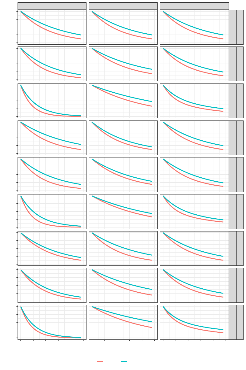
• Scenarios under proportional hazards (presented in Figure 4):
–
Scenario 1: Scenario with homogeneous survival distributions across strata (i.e., we have the same hazard
ratio in each stratum).
–
Scenario 2: Scenario in which the stratum with poor prognosis has a better (lower) hazard ratio than the
stratum with good prognosis.
–
Scenario 3: Scenario in which the stratum with poor prognosis has a worse (larger) hazard ratio than the
stratum with good prognosis.
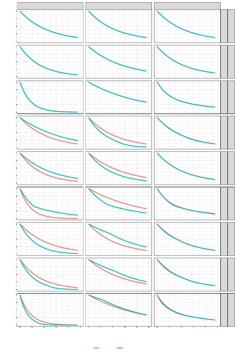
• Scenarios under delayed survival curve separation (presented in Figure 5):
–
Scenario 4: Scenario with homogeneous delayed separation of survival curves, where the delay is of
equal length in each stratum. The difference in survival probability (i.e., experimental - control) at late
follow-up times is also similar in the two strata.
–
Scenario 5: Scenario in which the stratum with poor prognosis has a better second-period treatment effect
than the stratum with good prognosis. There is also an equal delay in each stratum.
–
Scenario 6: Scenario in which the stratum with poor prognosis has a worse second-period treatment effect
than the stratum with good prognosis. There is also an equal delay in each stratum.
• Scenarios with null overall effect (presented in Figure 6):
– Scenario 7: Scenario with hazard ratio of 1 in each stratum as well as overall.
–
Scenario 8: Scenario in which there is positive difference in survival probability (i.e., experimental
better than control) in the poor prognosis stratum and a negative difference in survival probability (i.e.,
experimental worse than control) in the good prognosis stratum. The overall hazard ratio is equal to 1,
approximately.
–
Scenario 9: Scenario in which there is negative difference in survival probability (i.e., experimental
worse than control) in the poor prognosis stratum and a positive difference in survival probability (i.e.,
experimental better than control) in the good prognosis stratum. The overall hazard ratio is equal to 1,
approximately.
In total, combining the three options for the prognostic effect with the nine options for the treatment effects, we have
3 × 9 = 27
different scenarios to evaluate that we display graphically in the supplementary appendix. Scenarios 2 and
3, and scenarios 5 and 6 are essentially the same (symmetric) for the non-prognostic covariate case, so strictly speaking
there are only 25 unique scenarios, but we ignore this for ease of presentation.
3.3 Results
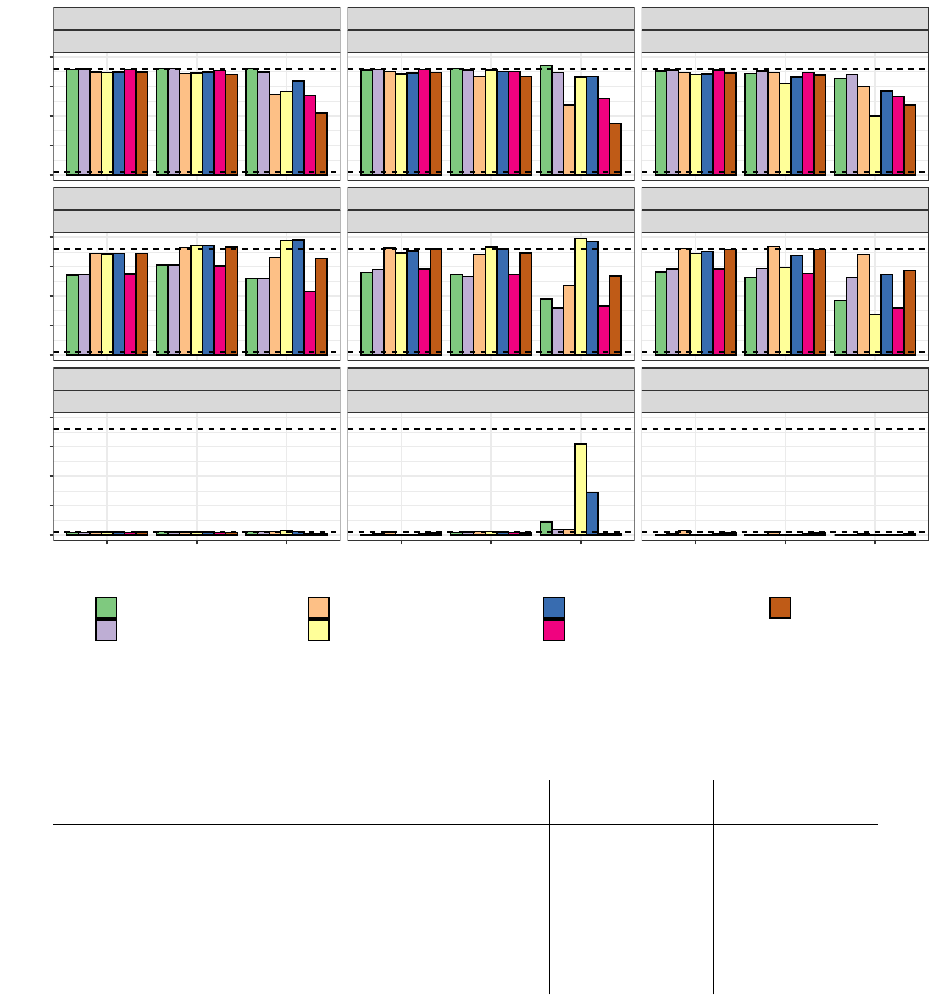
In Figure 3, we present the estimated power in each of the 27 scenarios described in section 3.2.
3.3.1 Null scenarios
The most striking result in Figure 3 is the "power" of the stratified tests when the marginal treatment effect is zero but
there is a strong prognostic effect, with the poor prognosis stratum having treatment benefit, and the better prognosis
stratum receiving a harmful treatment effect. In this scenario, for all the stratified tests, the power is above 2.5%,
sometimes massively so.
Two observations help to describe this phenomenon. Firstly, we can think about the stratified tests as a weighted
combination of two standardized z-statistics, one from each stratum. Even when this weighting is equal (as is the
case here for
˜
Z
W,n
and
˜
Z
n
), the z-statistic coming from the stratum with poor prognosis will be based on many more
events than the z-statistic from the better prognosis stratum. Even if the magnitude of treatment effect is similar (but
of opposite direction) in the two strata, the poor prognosis stratum will tend to have a standardized z-statistic with a
non-centrality parameter that is larger in magnitude than that of the better prognosis stratum. This explains why the
power for
˜
Z
n
and
˜
Z
W,n
is above 2.5%. It is a consequence of censoring: the better prognosis stratum is more heavily
censored (less mature) than the poor prognosis stratum. For other types of non-censored data analysed via generalized
linear models with canonical link functions, this phenomenon does not occur, and stratified test statistics would control
alpha also for the marginal null hypothesis, at least asymptotically (see Rosenblum and Steingrimsson [2016]).
The second observation is that as we move from
˜
Z
n
to
˜
Z
, and from
˜
Z
W,n
to
˜
Z
W,z
to
˜
Z
W,u
, the relative weighting of
the within-strata z-statistics gets more and more extreme in favour of the stratum with more events. This explains the
difference in power between the various stratified weighted tests.
6
A PREPRINT - JANUARY 26, 2022
When it is the better prognosis stratum that has the treatment benefit, the reverse happens, and the power of the stratified
tests is well below 2.5% (bottom right panel of Figure 3).
3.3.2 Proportional hazards scenarios
As one would expect, the stratified log-rank test (
˜
Z
) and Mehrotra et al’s stratified log-rank test (
˜
Z
n
) are the most
powerful methods, with the difference compared to unstratified tests most apparent when there is a strong prognostic
effect.
The stratified weighted log-rank tests remain competitive with the stratified log-rank tests, even under proportional
hazards, as long as the prognostic effect is moderate. However, for large prognostic effects, some substantial differences
emerge.
Among the subset of stratified weighted log-rank tests, there is no uniformly most (or least) powerful method. It depends
on whether the poor prognosis stratum has a larger treatment effect than the better prognosis stratum, or vice versa. The
test statistic that gives the most extreme weight to the stratum with more events "wins" in one scenario and "loses" in
the other. This is entirely analogous to the discussion above for the null scenarios. Something similar happens if we
compare
˜
Z
with
˜
Z
n
: the test that gives a more extreme weight in favour of the stratum with more events (
˜
Z
) performs
better when that stratum also has the larger treatment effect, and vice versa when the stratum with more events has
a smaller treatment effect. When the hazard ratio is equal in both strata then the standard stratified log-rank test is
optimal, of course.
3.3.3 Non-proportional hazards scenarios
When comparing power under scenarios with a delayed separation of survival curves, much of the above discussion
about the relative merits of the test statistics still applies. In this case, however, the weighted test statistics perform
much better than the unweighted versions, as one would expect.
Based on this particular simulation study, it appears that using a weighted log-rank test in anticipation of a delayed
separation has a greater impact on power than using a stratified test in anticipation of a prognostic effect. However, this
is only a small selection of scenarios, and something that should be judged on a case-by-case basis.
Of the tests that combine weighting and stratification, perhaps the combined test on the Z-scale (
˜
Z
W,z
) is most attractive.
Since it weights the strata in a manner that is intermediate out of
˜
Z
W,n
,
˜
Z
W,z
and
˜
Z
W,u
, it appears to be most robust
to the strength and direction of stratum-specific treatment effects. It performs consistently well across all the chosen
scenarios.
4 Cases studies: The OAK and POPLAR trials
As previously mentioned, the OAK and POPLAR trials are two (randomized) studies that compare atezolizumab versus
docetaxel in patients with non-small-cell lung cancer. Both trials exhibit a late separation pattern of their survival curves.
In Figures 1 and 2 we present the first stratum, second stratum and overall Kaplan-Meier curves from the OAK and
POPLAR trials, respectively.
In the OAK trial the survival curves in the first stratum are moderately lower than those from the second stratum (i.e.,
there is a moderate prognostic effect). We also see that the treatment effect in the stratum with worse prognosis appears
larger than the one from the stratum with better prognosis. These characteristics are similar to those evaluated in
scenario 5 (see Figure 5, scenario 5, moderate prognosis).
In the POPLAR trial the survival curves in the first stratum are also somewhat lower than those from the second stratum,
but the prognostic effect is less pronounced than for the OAK trial. In this case, we see that the treatment effect in the
stratum with worse prognosis appears smaller than the one from the stratum with better prognosis. These characteristics
are similar to those evaluated in scenario 6 (see Figure 5, scenario 6, for moderate (or no) prognostic effect).
For illustration purposes, we implement the stratified and unstratified tests described in section 3 using the OAK and
POPLAR trials’ data. The test statistics are presented in Table 2. Note that with the OAK and POPLAR datasets, we
use t
∗
= 6 and t
∗
= 12 in the modestly-weighted log-rank test. The reason is that Magirr and Jiménez (2021) already
used
t
∗
= 6
in the POPLAR trial and so, for consistency with both the existing literature and the simulation study we
present in this article, we show the values of the tests statistics with both t
∗
= 6 and t
∗
= 12.
With the OAK trial data, we observe that the stratified weighted log-rank test (combined on the U-statistic scale) has the
best z-statistic (smallest p-value). This is consistent with what we would expect based on the simulation study.
7
A PREPRINT - JANUARY 26, 2022
Figure 3: Power and type-I error using different stratified and unstratified log-rank and weighted log-rank tests. The
upper and lower dashed represent the value 0.9 and 0.025, respectively. The heading "poor prog. ’>’ good prog."
indicates that the stratum with the poor prognosis has a better treatment effect than the stratum with good prognosis.
Null Overall Treatment Effect
Scenario 7 (Homogeneous)
Null Overall Treatment Effect
Scenario 8 (poor prog. '>' good prog.)
Null Overall Treatment Effect
Scenario 9 (poor prog. '<' good prog.)
Anticipated Delayed Effects
Scenario 4 (Homogeneous)
Anticipated Delayed Effects
Scenario 5 (poor prog. '>' good prog.)
Anticipated Delayed Effects
Scenario 6 (poor prog. '<' good prog.)
Proportional Hazards
Scenario 1 (Homogeneous HRs)
Proportional Hazards
Scenario 2 (poor prog. '>' good prog.)
Proportional Hazards
Scenario 3 (poor prog. '<' good prog.)
None Moderate Strong None Moderate Strong None Moderate Strong
0.00
0.25
0.50
0.75
1.00
0.00
0.25
0.50
0.75
1.00
0.00
0.25
0.50
0.75
1.00
Prognostic effect
Power
Strat. LR (Z
~
)
Strat. LR from Mehrotra et al. (Z
n
)
Strat. WLR on sample size scale (Z
~
wn
)
Strat. WLR on U−statistic scale (Z
~
wu
)
Strat. WLR on Z−statistic scale (Z
~
wz
)
Unstrat. LR (Z)
Unstrat. WLR (Z
w
)
Table 2: Tests statistics obtained from the OAK and POPLAR datasets using t
∗
= 6 and t
∗
= 12.
Test Statistics
OAK Trial POPLAR Trial
t
∗
= 6 t
∗
= 12 t
∗
= 6 t
∗
= 12
Z (unstratified log-rank test) -3.78 -3.78 -2.77 -2.77
Z
W
(unstratified weighted log-rank test) -3.87 -3.89 -2.86 -3.17
˜
Z (stratified log-rank test) -4.02 -4.02 -2.64 -2.64
˜
Z
n
(stratified log-rank test (Mehrotra et al.)) -3.93 -3.93 -2.73 -2.73
˜
Z
W,u
(stratified weighted log-rank test (U-statistic scale)) -4.27 -4.35 -2.65 -2.83
˜
Z
W,z
(stratified weighted log-rank test (Z-statistic scale)) -4.20 -4.27 -2.71 -2.94
˜
Z
W,n
(stratified weighted log-rank test (sample size scale)) -3.94 -3.95 -2.83 -3.13
With the POPLAR trial data, we observe that the unstratified weighted log-rank test has the best Z statistic (smallest
p-value). This may be partly explained by the smaller observed prognostic effect of ECOG status in the POPLAR trial
as compared to OAK.
Overall, we observe that the weighted test statistics are lower with
t
∗
= 12
than with
t
∗
= 6
. This is sensible and due
to the fact that survival curves start to split at approximately
t = 4
and thus
t
∗
= 6
is perhaps too close to that moment
where the full treatment effect is not yet fully observable.
8
A PREPRINT - JANUARY 26, 2022
5 Discussion
Over recent years, with the development of immunotherapies, many novel statistical methods have been proposed that
aim to robustly capture potential long-term survival improvement following a delayed separation of survival curves.
These methods focus, mostly, on differences in marginal survival probabilities in the full population. Stratified testing
has received very little attention despite the fact that it is present in practically every large confirmatory trial.
Motivated by the OAK and POPLAR trials, two randomized studies with a delayed survival curve separation that
compare atezolizumab versus docetaxel in patients with non-small-cell lung cancer, we have proposed stratified versions
of weighted log-rank tests, and evaluated their properties in an extensive simulation study, taking into consideration
different prognostic levels as well as the possibility of different treatment effects across strata.
The results of the research are largely consistent with our expectations given that, when studied separately, we know
that stratification leads to greater efficiency under strong prognostic effects, and (carefully chosen) weighted log-rank
tests lead to greater efficiency under delayed separations of survival curves. Unsurprisingly, combining the two methods
leads to the greatest efficiency when strong prognostic effects and a delay in the separation of survival curves are both
present. However, we have also shown that the precise manner in which the two techniques are combined can have a
large impact on power. Based on our simulation study, together with theoretical understanding, our recommendation is
to use a stratified weighted log rank test where the strata are combined on the z-statistic scale. This method has robust
power performance across all the scenarios we considered.
It should be borne in mind that stratified tests correspond to the stratified null hypothesis
H
0,S
, and not the marginal null
hypothesis
H
0
. We have shown that it is possible to construct scenarios where there is no treatment effect marginally in
the full population (but there is a heterogeneous treatment effect across strata) and the power for testing
H
0,S
according
to an
α
level test is very much higher than
α
. To put this in context, however, the situations where this happens are
extreme. If considered at all plausible a-priori, one would not embark on such a trial in the full population. In addition, it
is standard practice to report results for the full population (in the form of a Kaplan-Meier plot, for example), as well as
separately by subgroup (for example using a forest plot). The chance of being grossly misled by a stratified test appears
small. Related to this discussion is the issue of treatment effect estimation. Already, when considering non-proportional
hazard situations for a homogeneous population, it is considered impossible to fully capture the treatment effect
using a single number (Zhao et al. [2016]), and instead it is recommended to report a spectrum of treatment effects
(Roychoudhury et al. [2021]), such as differences in quantiles, milestone survival probabilities, and restricted mean
survival times (Uno et al. [2014]). When adding a heterogeneous population into the mix, the task of capturing the
treatment effect adequately in a single number becomes doubly impossible. The only pragmatic way forward is to
present a range of Kaplan-Meier type plots and summary measures, for a range of relevant (sub)populations. In this
context, the value of the stratified weighted log-rank test statistic is simply to allow a pre-specified null hypothesis test
that can produce a valid p-value, allowing a first line of defence against being misled by randomness. This should be
considered one small, but important, part of the overall design and analysis of the experiment. A range of techniques
are required to achieve a reasonable inference.
References
G Berry, RM Kitchin, and PA Mock. A comparison of two simple hazard ratio estimators based on the logrank test.
Statistics in medicine, 10(5):749–755, 1991.
Louis Fehrenbacher, Alexander Spira, Marcus Ballinger, Marcin Kowanetz, Johan Vansteenkiste, Julien Mazieres,
Keunchil Park, David Smith, Angel Artal-Cortes, Conrad Lewanski, et al. Atezolizumab versus docetaxel for patients
with previously treated non-small-cell lung cancer (poplar): a multicentre, open-label, phase 2 randomised controlled
trial. The Lancet, 387(10030):1837–1846, 2016.
Thomas R Fleming and David P Harrington. Counting processes and survival analysis, volume 169. John Wiley &
Sons, 2011.
Boris Freidlin and Edward L Korn. Methods for accommodating nonproportional hazards in clinical trials: ready for
the primary analysis? Journal of Clinical Oncology, 37(35):3455, 2019.
Boris Freidlin and Edward L Korn. Reply to h. uno et al and b. huang et al. Journal of Clinical Oncology, 38(17):
2003–2004, 2020.
David R Gandara, Sarah M Paul, Marcin Kowanetz, Erica Schleifman, Wei Zou, Yan Li, Achim Rittmeyer, Louis
Fehrenbacher, Geoff Otto, Christine Malboeuf, et al. Blood-based tumor mutational burden as a predictor of clinical
benefit in non-small-cell lung cancer patients treated with atezolizumab. Nature medicine, 24(9):1441–1448, 2018.
Valérie Garès, Sandrine Andrieu, Jean-François Dupuy, and Nicolas Savy. A comparison of the constant piecewise
weighted logrank and fleming-harrington tests. Electronic journal of statistics, 8(1):841–860, 2014.
9
A PREPRINT - JANUARY 26, 2022
Pranab Ghosh, Robin Ristl, Franz König, Martin Posch, Christopher Jennison, Heiko Götte, Armin Schüler, and Cyrus
Mehta. Robust group sequential designs for trials with survival endpoints and delayed response. Biometrical Journal,
2021.
Walter W Hauck, Sharon Anderson, and Sue M Marcus. Should we adjust for covariates in nonlinear regression
analyses of randomized trials? Controlled clinical trials, 19(3):249–256, 1998.
Bo Huang, Lee-Jen Wei, and Ethan B Ludmir. Estimating treatment effect as the primary analysis in a comparative
study: Moving beyond p value. Journal of clinical oncology: official journal of the American Society of Clinical
Oncology, 38(17):2001–2002, 2020.
José L Jiménez. Quantifying treatment differences in confirmatory trials under non-proportional hazards. Journal of
Applied Statistics, pages 1–19, 2020.
José L Jiménez, Viktoriya Stalbovskaya, and Byron Jones. Properties of the weighted log-rank test in the design of
confirmatory studies with delayed effects. Pharmaceutical statistics, 18(3):287–303, 2019.
Theodore G Karrison. Versatile tests for comparing survival curves based on weighted log-rank statistics. The Stata
Journal, 16(3):678–690, 2016.
Takashi Kojima, Manish A Shah, Kei Muro, Eric Francois, Antoine Adenis, Chih-Hung Hsu, Toshihiko Doi, Toshikazu
Moriwaki, Sung-Bae Kim, Se-Hoon Lee, et al. Randomized phase iii keynote-181 study of pembrolizumab versus
chemotherapy in advanced esophageal cancer. Journal of Clinical Oncology, 38(35):4138–4148, 2020.
Ray S Lin, Ji Lin, Satrajit Roychoudhury, Keaven M Anderson, Tianle Hu, Bo Huang, Larry F Leon, Jason JZ Liao,
Rong Liu, Xiaodong Luo, et al. Alternative analysis methods for time to event endpoints under nonproportional
hazards: a comparative analysis. Statistics in Biopharmaceutical Research, 12(2):187–198, 2020.
Dominic Magirr. Non-proportional hazards in immuno-oncology: Is an old perspective needed? Pharmaceutical
Statistics, 20(3):512–527, 2021.
Dominic Magirr and Carl-Fredrik Burman. Modestly weighted logrank tests. Statistics in medicine, 38(20):3782–3790,
2019.
Dominic Magirr and José L Jiménez. Design and analysis of group-sequential clinical trials based on a modestly-
weighted log-rank test in anticipation of a delayed separation of survival curves: A practical guidance. arXiv preprint
arXiv:2102.05535, 2021.
Devan V Mehrotra, Shu-Chih Su, and Xiaoming Li. An efficient alternative to the stratified cox model analysis.
Statistics in medicine, 31(17):1849–1856, 2012.
Martin M Oken, Richard H Creech, Douglass C Tormey, John Horton, Thomas E Davis, Eleanor T McFadden, and
Paul P Carbone. Toxicity and response criteria of the eastern cooperative oncology group. American journal of
clinical oncology, 5(6):649–656, 1982.
CN Owen, X Bai, T Quah, SN Lo, C Allayous, Sophia Callaghan, C Martínez-Vila, R Wallace, P Bhave, ILM Reijers,
et al. Delayed immune-related adverse events with anti-pd-1-based immunotherapy in melanoma. Annals of Oncology,
32(7):917–925, 2021.
Rifaquat Rahman, Geoffrey Fell, Steffen Ventz, Andrea Arfé, Alyssa M Vanderbeek, Lorenzo Trippa, and Brian M
Alexander. Deviation from the proportional hazards assumption in randomized phase 3 clinical trials in oncology:
prevalence, associated factors, and implications. Clinical Cancer Research, 25(21):6339–6345, 2019.
Achim Rittmeyer, Fabrice Barlesi, Daniel Waterkamp, Keunchil Park, Fortunato Ciardiello, Joachim Von Pawel,
Shirish M Gadgeel, Toyoaki Hida, Dariusz M Kowalski, Manuel Cobo Dols, et al. Atezolizumab versus docetaxel in
patients with previously treated non-small-cell lung cancer (oak): a phase 3, open-label, multicentre randomised
controlled trial. The Lancet, 389(10066):255–265, 2017.
Michael Rosenblum and Jon Arni Steingrimsson. Matching the efficiency gains of the logistic regression estimator
while avoiding its interpretability problems, in randomized trials. 2016.
Satrajit Roychoudhury, Keaven M Anderson, Jiabu Ye, and Pralay Mukhopadhyay. Robust design and analysis of
clinical trials with nonproportional hazards: A straw man guidance from a cross-pharma working group. Statistics in
Biopharmaceutical Research, pages 1–15, 2021.
David A Schoenfeld. Sample-size formula for the proportional-hazards regression model. Biometrics, pages 499–503,
1983.
Hajime Uno and Lu Tian. Is the log-rank and hazard ratio test/estimation the best approach for primary analysis for all
trials? Journal of clinical oncology: official journal of the American Society of Clinical Oncology, 38(17):2000–2001,
2020.
10
A PREPRINT - JANUARY 26, 2022
Hajime Uno, Brian Claggett, Lu Tian, Eisuke Inoue, Paul Gallo, Toshio Miyata, Deborah Schrag, Masahiro Takeuchi,
Yoshiaki Uyama, Lihui Zhao, et al. Moving beyond the hazard ratio in quantifying the between-group difference in
survival analysis. Journal of clinical Oncology, 32(22):2380, 2014.
Yi-Long Wu, Shun Lu, Ying Cheng, Caicun Zhou, Jie Wang, Tony Mok, Li Zhang, Hai-Yan Tu, Lin Wu, Jifeng Feng,
et al. Nivolumab versus docetaxel in a predominantly chinese patient population with previously treated advanced
nsclc: Checkmate 078 randomized phase iii clinical trial. Journal of Thoracic Oncology, 14(5):867–875, 2019.
Rengyi Xu, Devan V Mehrotra, and Pamela A Shaw. Hazard ratio inference in stratified clinical trials with time-to-event
endpoints and limited sample size. Pharmaceutical statistics, 18(3):366–376, 2019.
Song Yang and Ross Prentice. Improved logrank-type tests for survival data using adaptive weights. Biometrics, 66(1):
30–38, 2010.
Lihui Zhao, Brian Claggett, Lu Tian, Hajime Uno, Marc A Pfeffer, Scott D Solomon, Lorenzo Trippa, and LJ Wei. On
the restricted mean survival time curve in survival analysis. Biometrics, 72(1):215–221, 2016.
Appendix
Software
The repository
github.com/dominicmagirr/stratified_weighted_log_rank_test
contains all R code to re-
produce the results in this paper.
11
A PREPRINT - JANUARY 26, 2022
Graphical display of simulated scenarios
Figure 4: Scenarios under proportional hazards.
First stratum
Second stratum
Overall
Non−prog.
Scenario 1
Moderate prog.
Scenario 1
Strong prog.
Scenario 1
Non−prog.
Scenario 2
Moderate prog.
Scenario 2
Strong prog.
Scenario 2
Non−prog.
Scenario 3
Moderate prog.
Scenario 3
Strong prog.
Scenario 3
0 5 10 15 20 25 0 5 10 15 20 25 0 5 10 15 20 25
0.00
0.25
0.50
0.75
1.00
0.00
0.25
0.50
0.75
1.00
0.00
0.25
0.50
0.75
1.00
0.00
0.25
0.50
0.75
1.00
0.00
0.25
0.50
0.75
1.00
0.00
0.25
0.50
0.75
1.00
0.00
0.25
0.50
0.75
1.00
0.00
0.25
0.50
0.75
1.00
0.00
0.25
0.50
0.75
1.00
Time
Survival
Control Experimental
12

A PREPRINT - JANUARY 26, 2022
Figure 5: Scenarios under non-proportional hazards.
First stratum
Second stratum
Overall
Non−prog.
Scenario 4
Moderate prog.
Scenario 4
Strong prog.
Scenario 4
Non−prog.
Scenario 5
Moderate prog.
Scenario 5
Strong prog.
Scenario 5
Non−prog.
Scenario 6
Moderate prog.
Scenario 6
Strong prog.
Scenario 6
0 5 10 15 20 25 0 5 10 15 20 25 0 5 10 15 20 25
0.00
0.25
0.50
0.75
1.00
0.00
0.25
0.50
0.75
1.00
0.00
0.25
0.50
0.75
1.00
0.00
0.25
0.50
0.75
1.00
0.00
0.25
0.50
0.75
1.00
0.00
0.25
0.50
0.75
1.00
0.00
0.25
0.50
0.75
1.00
0.00
0.25
0.50
0.75
1.00
0.00
0.25
0.50
0.75
1.00
Time
Survival
Control Experimental
13
A PREPRINT - JANUARY 26, 2022
Figure 6: Scenarios under null effect.
First stratum
Second stratum
Overall
Non−prog.
Scenario 7
Moderate prog.
Scenario 7
Strong prog.
Scenario 7
Non−prog.
Scenario 8
Moderate prog.
Scenario 8
Strong prog.
Scenario 8
Non−prog.
Scenario 9
Moderate prog.
Scenario 9
Strong prog.
Scenario 9
0 5 10 15 20 25 0 5 10 15 20 25 0 5 10 15 20 25
0.00
0.25
0.50
0.75
1.00
0.00
0.25
0.50
0.75
1.00
0.00
0.25
0.50
0.75
1.00
0.00
0.25
0.50
0.75
1.00
0.00
0.25
0.50
0.75
1.00
0.00
0.25
0.50
0.75
1.00
0.00
0.25
0.50
0.75
1.00
0.00
0.25
0.50
0.75
1.00
0.00
0.25
0.50
0.75
1.00
Time
Survival
Control Experimental
14
