1
Assessing risk due to small sample size in probability of detection
analysis using tolerance intervals
Ajay M. Koshti, NASA Johnson Space Center, Houston, U.S.A.
ABSTRACTCASE
Small sample size (e.g. 6-30) poses risk in results of probability of detection (POD) analysis using tolerance intervals. This
method is also called as the limited sample or LS POD. The analysis is performed either during NDE procedure
qualification or for assessment of reliability of an NDE procedure. The risk is primarily due to sampling error. Smaller
samples are not likely to be random to the population or representative of the population. The small samples are likely to
be biased. Biased samples have smaller standard deviation compared to the population. POD analysis with small biased
sample can lead to overestimation of POD. Many sampling schemes are available in statistics to mitigate sampling risk.
Primary objective of POD analysis is to determine a decision threshold from signal response measurements of a sample
such that it is less than or equal to population decision threshold for 90% POD. Sampling error implies that this NDE
reliability condition is violated. One of sampling types is called a representative sample. Representative samples reduce
variance in POD estimates but also reduce magnitude of the error. Sampling sensitivity analysis for some sampling types
is performed here using repetitive random sampling or Monte Carlo method. Six sampling types are considered for
comparison. Some of the sampling types are similar to drawing a representative sample. LS POD model assumes random
sampling. Therefore, random sampling is used as a basis for comparison with each sampling type. The sampling types
used in the analysis are, A. Nominal and worst-case sampling, B. Worst-case sampling, C. Nominal case sampling, D.
Random sampling, E. Random target, and sub-target sampling. F. Nominal target and sub-target sampling. Results of
Monte Carlo simulation indicate that type F sampling can mitigate sampling risk and is also more practical to implement.
Type A sampling may also mitigate the sampling risk, but it may be less practical to implement.
Keywords: nondestructive evaluation, probability of detection, statistical sampling
1. INTRODUCTION
MIL-HDBK-1823A
1
and associated mh1823
2
software address NDE POD testing for two types of datasets. The first type
of dataset is that of the signal response “â” (read as a-hat) versus known flaw size “a”. In analyzing such data, the â data
is represented on the y-axis and the “a” data on the x-axis and the data may be transformed using a logarithmic function,
if needed, to provide a linear relationship around the signal response decision threshold level. A generalized linear model
(GLM) is fitted to the data using maximum likelihood estimate (MLE) for analysis. In this analysis, noise data, defined as
the signal response in a region where there is no flaw, is also obtained. The noise data is used to estimate false call rate or
probability of false positive calls (POF).
The second type of dataset considered is called hit-miss data, which contains the known flaw size and the corresponding
detection result (i.e. hit or miss). For numerical analysis, a hit is assigned a numerical value of 1 while a miss has numerical
value of 0. False call data (i.e. a hit is recorded where no flaw exists) is also recorded and used to determine the POF using
the Clopper-Pearson binomial distribution function. Typically, POD increases with increasing flaw size and POF decreases
with increasing flaw size. POF shall be required to be less than a certain limit to prevent adverse impacts on cost and
schedule necessary to take corrective actions to address the false positive calls. ASTM E2862
3
also provides a hit-miss
POD data analysis method that is consistent with MIL-HDBK-1823A.
There are other POD analysis approaches that are not covered by MIL-HDBK-1823A. Binomial point estimate method of
verifying reliably detectable flaw size is given by Rummel
4
. Current work is in probability of detection (POD) analysis
using tolerance intervals
5,6
. This work is limited to POD analysis and simulation approach for single hit limited sample
POD
7
or LS POD. Broadly, LS POD covers signal response-based data for both single hit and multi-hit POD applications
including modeling of transfer functions
7-13
. Smaller sample size is usable in LS POD analysis. In practice, signal responses
from smaller sample size of flaws may not be random to the population. LS POD assumes that the sample is randomly
drawn from the population. Thus, there is increased risk that the small sample is non-representative to the population and
is a biased sample. In statistics, sampling bias is defined as a bias in which a sample is collected in such a way that some
members of the intended population have a lower or higher relative sampling probability than others. It results in a biased

2
sample, which is a non-random sample of a population. If sampling bias is not accounted for, results can be erroneously
attributed to the phenomenon or NDE technique under study rather than to the method of sampling.
Depending upon sample bias, results may be non-conservative. This paper explores several sampling schemes beyond
simple random sampling in the Monte Carlo simulation and performs sampling sensitivity analysis. Results of such
analysis may be used in choosing a sampling scheme for empirical LS POD analysis.
2. POPULATION AND SAMPLE SIGNAL RESPONSES
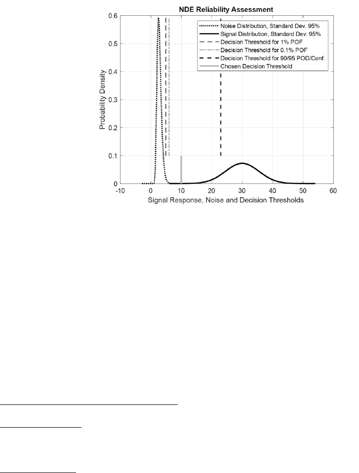
Fig. 1 illustrates how a decision threshold that is based on a simulated signal response for a sample of fixed size flaws
relates to a decision threshold for the simulated population of signal responses in achieving 90/95% POD/Conf. Sample
distribution is indicated by a dotted line and population distribution is indicated by a continuous line. For simplicity, these
are shown as smooth normal distribution curves. Sample decision threshold at 90/95% POD/conf. i.e.
is
indicated by a circle marker and population decision threshold at 90/95% POD/conf. i.e.
is indicated by a
diamond marker. The thicker outline area has 96.2% area of population distribution. Here, the decision threshold POD
margin over 90% is 6.2%.
In the example below, the sample estimated decision threshold
is conservative compared to the population
decision threshold
, meeting following condition termed as reliability condition 1 for POD,
. (1)
Fig. 1: Illustration of population and sample distributions in computation of POD
Thus, the sample in Fig. 1 has provided acceptable result for reliability condition 1. If maximum acceptable POF is 1%,
then decision threshold corresponding to 1% POF, is denoted by
. If sample size for noise measurements is
small then threshold computed for 1% POF with 95% confidence is denoted by
.
, should also
meet following condition termed as reliability condition 2 for POF to meet the maximum allowable POF requirement.
, or (2A)
. (2B)
Individual noise measurement is always linked to corresponding signal response measurement as it should be measured in
the unflawed areas immediately surrounding the corresponding signal measurement. This poses a difficulty in measuring
population of noise. However, sample size for noise measurement can be very large and a distribution defined by a very
large sample can be considered to be the population of noise. A large sample size is recommended for noise measurement
7
.
3
Either
or
can be used with likely insignificant differences in POF calculations in relation to
meeting condition 2.
An example of LS POD analysis
7
is provided in Fig. 2. It also illustrates calculation of
for checking condition
2.
Fig. 2: Plot for LS POD analysis for input data from Table 1
In practice, the population distribution is likely to be unknown. Therefore, such comparison is not practical. There is a
need to study factors or cases of signal variation that contribute to the signal variation. Moreover, there is also a need to
study distribution or sampling fraction of these cases. Since it is impractical to draw a small random sample from the
population, an option will be to draw a representative sample. Representative sample would cover all sections of the
population distribution approximately in their respective sampling fractions. Such sample would then provide results that
are as good or better than theoretical random sample. This hypothesis can be investigated using Monte Carlo modeling
which uses repetitive sampling to assess confidence in the chosen sampling scheme. Some types of sampling schemes will
be investigated. Objective of such investigation is to determine which sampling schemes provide reduction in sampling
error and provide conservative results such that there is a high confidence that reliability conditions are met. It is proposed
that Monte Carlo sampling sensitivity analysis may be performed to design a sampling protocol and mitigate or reduce
sampling risk.
3. PROBABILITY SAMPLING SCHEMES
There are many schemes in probability sampling.
1. Simple normal distribution random sampling:
-tolerance factor statistics is used in LS POD. A random sample is a
group or set chosen in a random manner from a larger population.
2. Systematic sampling: Systematic sampling (also known as interval sampling) relies on arranging the study population
according to some ordering scheme and then selecting elements at regular intervals through that ordered list.
Systematic sampling involves a random start and then proceeds with the selection of every k
th
element from then
onwards. This is currently not used in LS POD.
3. Stratified sampling: Stratified sampling scheme generates a representative sample. It is acceptable for
-tolerance
factor statistics used in LS POD. A representative sample (e.g. stratified sample) is a group or set chosen from a larger
statistical population according to specified characteristics. When the population embraces several distinct categories,
the population distribution can be organized by these categories into separate "strata." Each stratum is then sampled
as an independent sub-population, out of which individual elements can be randomly selected. The ratio of the size of
this random selection (or sample) to the size of the population is called a sampling fraction. There are several potential
benefits to stratified sampling. In computational statistics, stratified sampling is a method of variance reduction when
Monte Carlo methods are used to estimate population statistics from a known population. A representative sample is
4
generally expected to yield the best collection of results. Using stratified random sampling, researchers must identify
characteristics, divide the population into strata, and proportionally choose individuals for the representative sample.
A stratified sampling approach is most effective when following three conditions are met,
a. Variability within strata are minimized,
b. Variability between strata are maximized, and
c. The variables upon which the population is stratified are strongly correlated with the desired dependent variable.
Stratified sampling has advantages over other sampling methods. The advantages are,
a. Focuses on important subpopulations and ignores irrelevant ones,
b. Allows use of different sampling techniques for different subpopulations,
c. Improves the accuracy/efficiency of estimation, and
d. Permits greater balancing of statistical power of tests of differences between strata by sampling equal numbers
from strata varying widely in size.
Stratified sampling also has disadvantages. These are,
a. Requires selection of relevant stratification variables which can be difficult,
b. Is not useful when there are no homogeneous subgroups, and
c. Can be expensive to implement.
Other sampling schemes, such as probability proportional to size (PPS) sampling and multistage cluster sampling schemes,
are not covered here. If a sample is neither random nor representative, it may be a biased sample.
Signal response population can be divided into two strata, worst-case and nominal responses. One could divide the signal
response population in three strata too e.g. from left side to right side as worst-case, nominal-case and ideal-case. In this
work, for simplicity population is divided in two strata only. NDE signal response sample is likely to be a nominal response
sample, if nominal parameters are used to make flaw specimens. Thus, obtaining nominal response data is practical. Worst-
case or lower responses are attributed to off-nominal flaw part conditions with chance of occurrence ~30-50%. Thus,
obtaining worst-case response data is more difficult as it is difficult to control parameters that would consistently produce
flaws with worst-case responses.
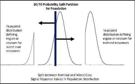
Fig. 3: Example of strata in population of signal responses with sampling fraction for a worst-case = 0.30 and sampling fraction for
nominal case = 0.70.
Goal of NDE procedure is to detect a target size flaw reliably i.e. with minimum 90/95% POD/Conf. Generally, signal
response is monotonic with flaw size in neighborhood of flaw size. This implies that smaller signal response is expected
for smaller size flaws and larger signal response is expected for larger size flaws. If smaller size flaws are used in NDE
procedure qualification and if smaller size flaws can be detected reliably, then the target size flaw should be detected
reliably too. The smaller size flaws are referred to as sub-target flaws and a mix of target and sub-target flaws can be used
as a sampling scheme too. Here, there will be difference in mean responses between the target and sub-target flaws. The
mean of responses may be same as that for assumed population (for simulation only) or may be representative of nominal
responses.
5
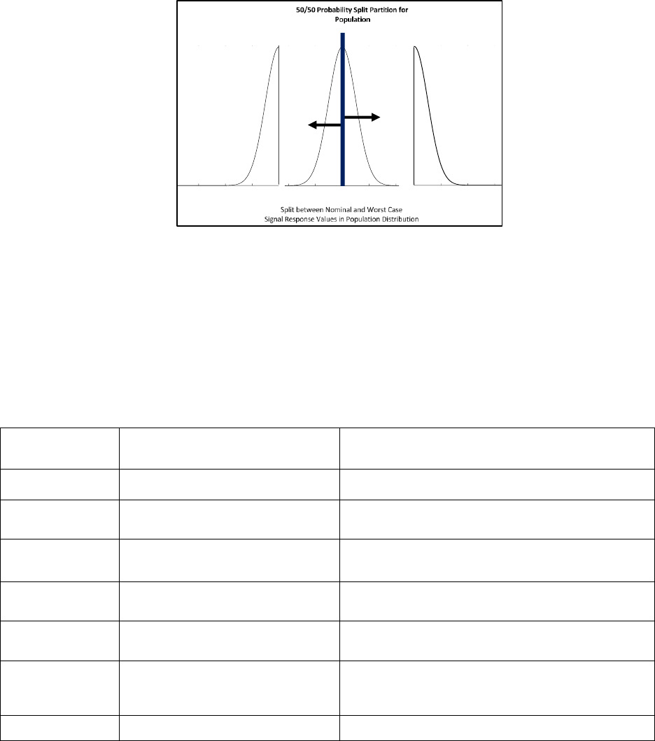
Fig. 4: Example of strata in population of signal responses with sampling fraction for worst-case = 0.50 and sampling fraction for
nominal case = 0.50.
4. SAMPLING CONCERNS IN LS POD
In LS POD analysis,
-factor statistics is used. It assumes that the signal response sample is random or representative of
the population. Assumption of random sample is likely to be met, if a large sample covering all sections of population is
used. However, for a large sample, other POD analysis methods are also available, which may be preferred over LS POD.
It may not be practical to draw a small random sample due to many factors. Comparison of factors affecting population
and sample signal responses is provided in Table 1 to elaborate that a sample may not be representative of the population,
especially a small sample.
Table 1: Comparison of factors affecting population and sample signal responses
Factor or Parameter
Population Signal Responses from
Target Size Flaws
Sample Signal Responses from Target Size Flaws
Flaw Type
Real flaws (naturally occurring)
Artificially manufactured flaws (ideal conditions)
Flaw Location
In real parts
Specimens made using controlled fabrication process
(ideal conditions)
Part Geometry
All part surface geometries (cylindrical,
spherical, and flat etc.)
Simple specimen surface geometry compared to part (e.g.
flat) (ideal conditions)
Material
All applicable material types
One or selected material type/alloy is used (nominal
condition)
Surface Finish
All applicable surface finishes
Fixed value smooth surface finish is assumed (nominal
condition)
Flaw Morphology
Applicable variation in flaw
morphology
Flaw morphology is controlled by controlling flaw
manufacturing process (nominal condition) to produce
predictable size flaws
Flaw Orientation
All applicable orientations of flaws
Nominal orientation of flaws is assumed
Many factors i.e., surface roughness, part geometry, grain structure, flaw morphology affect signal response to a different
degree individually. Each factor has its own variability (i.e. normal distribution). The variability of signal response is due
to combined effect of variability of all factors. A small sample is not representative of the population, because it cannot
capture the random variability of each factor affecting signal response. Small sample is also not random because the
specimens used are likely to be a mix of nominal and ideal conditions of the factors. Therefore, smaller sample is less
representative and non-random (or biased) to the population.

6
LS POD small sample data comes from flaw specimens designed specifically for LS POD. The specimens are produced
using controlled manufacturing process resulting in uniform flaw morphology and predictable flaw size. Specimens have
simple geometry and smooth surface. Material specification is usually nominal and has uniform material properties that
affect signal response. The LS POD specimens are a subset of overall population of signal responses. LS POD sample is
likely to provide higher signal response due to smooth surface, simple geometry and nominal material and, less signal
response variability due to uniform flaw morphology obtained using tightly controlled manufacturing process including
tight tolerance on specimen material, geometry, and surface finish. Such a sample, that has higher average signal response
value and lower standard deviation, would then be in the right side of the signal response distribution for the population.
It is described as nominal sample, as mostly nominal conditions are used in manufacturing of the flaw sample.
The left side of the signal response distribution for the population is described as worst-case signal responses. There is a
small probability that the real flaw/part conditions will provide lower signal response values compared to the nominal
signal response values during inspection of real parts. The worst-case values are likely to be captured in a carefully
designed large sample as flaws with off-nominal values of signal variation contributing factors can be included.
Concern 1: For random sampling, there is a higher variability of decision threshold and there is higher error in POD values
for smaller sample size (e.g. 6). In LS POD model, 90/95% POD/confidence is assured for both random and representative
samples.
Concern 2: A small sample generated using fabricated flaw specimens is not likely to be random due to well controlled
process of fabricating flaw specimens to nominal conditions. Such a process can provide predictable size flaws but the
flaws are likely to produce nominal signal responses.
Concern 3: If a sample is biased to higher signal response values, it causes overestimation error in POD estimation which
is further compounded by Concern 1 for the small sample size.
Decision threshold from sample is calculated as,
, (3)
where,
mean of signal responses,
σ = standard deviation of signal responses, and
=
tolerance factor.
5. SAMPLING CASES AND SIMULATION INPUTS AND OUTPUTS
Sampling types for Monte Carlo simulation are described below.
A. Nominal and worst-case sampling: A split percentage is chosen e.g. 50/50% split is chosen to divide population
between nominal and worst-case.
B. Worst-case sampling: A split percentage is chosen e.g. 50/50% split is chosen to divide population between
nominal and worst-case. Here, only worst-case samples are used.
C. Nominal (case) sampling: A split percentage is chosen e.g. 50/50% split is chosen to divide population between
nominal and worst-case. Here, only nominal samples are used.
D. Random sampling (theoretical or non-empirical)
E. Random target and sub-target sampling (theoretical or non-empirical)
F. Nominal target and sub-target sampling: A split percentage is chosen e.g. 50/50% split is chosen between target
and sub-target flaws.
Many factors provide variability and therefore the net effect needs to be modeled in Monte Carlo simulation. For simplicity,
it is assumed that all factors contribute equally to the signal variation. For “n” sources of signal variation, individual source
standard deviation is assumed to be
of the overall standard deviation. Typically, 3 sources are chosen in the
simulation. Using very high number of sources have smoothing effect. For crack like flaws, three independent factors
affecting signal response can be identified as flaw/crack tightness or gap between crack faces, flaw orientation, and flaw
shape morphology.
Sampling sensitivity analysis should be performed in conjunction with single hit LS POD analysis
7
. Input for LS POD
analysis is illustrated below.
1. Average signal response from target size flaws for sample (), e.g. 33

7
2. Standard deviation of signal response for sample, (
, e.g. 2.109
3. Sample size for identical flaws or replicates, (N), e.g. 6
4. Average signal response in unflawed areas, (
), e.g. 2.76
5. Standard deviation of noise, (σ), e.g. 0.698
6. Number of noise measurements (n), e.g. 1200
7. Selected decision threshold (
), e.g. 26.66
This input is then programmatically used in the sampling sensitivity analysis. There are additional fields in the sampling
sensitivity analysis. Sampling sensitivity analysis input fields are given below. These are variables, except where stated,
and valid values are within certain ranges. Sampling sensitivity analysis fields are provided below.
1. Average signal response from target size flaws for sample (), e.g. 33
2. Standard deviation of signal response for sample, (
, e.g. 2.109
3. Sample size for identical flaws or replicates, (N), e.g. 6. Although sensitivity analysis will use a range of sample
sizes.
4. Average signal response in unflawed areas, (
), e.g. 2.76
5. Standard deviation of noise, (σ), e.g. 0.698
6. Number of noise measurements (n), e.g. 1200
7. Selected decision threshold (
), e.g. 26.66
8. Decision threshold for 90/95% POD/Conf. (
), e.g. 26.66
9. Assumed standard deviation of signal response for population (
), e.g. 4.947
10. Estimated standard deviation of signal response for population with stated confidence (
), e.g. 4.947.
This estimate uses
and
factor for 90/95% POD/Conf. and sample size. This item is for reference
only.
11. Percentage of nominal values, e.g. 70%
12. Percentage of sub-target sample values, e.g. 100%
13. Sub-target average response factor, e.g. 0.85. This implies that if target mean response is 100, then sub-target
mean response is 85.
14. Sub-target standard deviation factor, e.g. 1. Sub-target standard deviation is obtained as target flaw standard
deviation multiplied by the factor.
15. Number of signal response variation sources, e.g. 3
16. Monte Carlo repeats, e.g. 25. 500 or more are recommended but smaller number is used to save computing time.
In Monte Carlo simulation, the population distribution is given in input field 9.
is computed. Also,
is computed. Sample size is varied from 3 to 30 at an interval of 1 unit.
A sample is drawn for sampling cases A through F. Then LS POD analysis is performed to determine sample decision
threshold
. The simulation is repeated for chosen number of times. See input field 16.
is compared with
and
. For successful sampling, reliability conditions 1 and 2 are
satisfied. Monte Carlo repeats provide percentage of times the two conditions are exceeded. Another comparison that is
possible is with respect to random sampling i.e. case D. Using data for all Monte Carlo repeats, percentage difference in
average signal response from that in case D is calculated. For example, for case A the difference is calculated using,
. (4)
The difference is calculated for cases A, B, C, E and F. Using data for all Monte Carlo repeats, percentage difference of
average standard deviation from that in case D is calculated. For example, for case A the difference is calculated using,
. (5)
The difference is calculated for cases A, B, C, E and F.
8
6. ANALYSIS EXAMPLES FOR VARIOUS CASES
Example input data from Section 5 is used here. An example of Monte Carlo simulation of decision threshold data for case
A is provided in Fig. 5. For LS POD, smaller sample size is attractive due to cost savings. Here, sample size of 6 or 7 is
chosen to highlight whether reliability conditions 1 and 2 are met for various sampling cases.
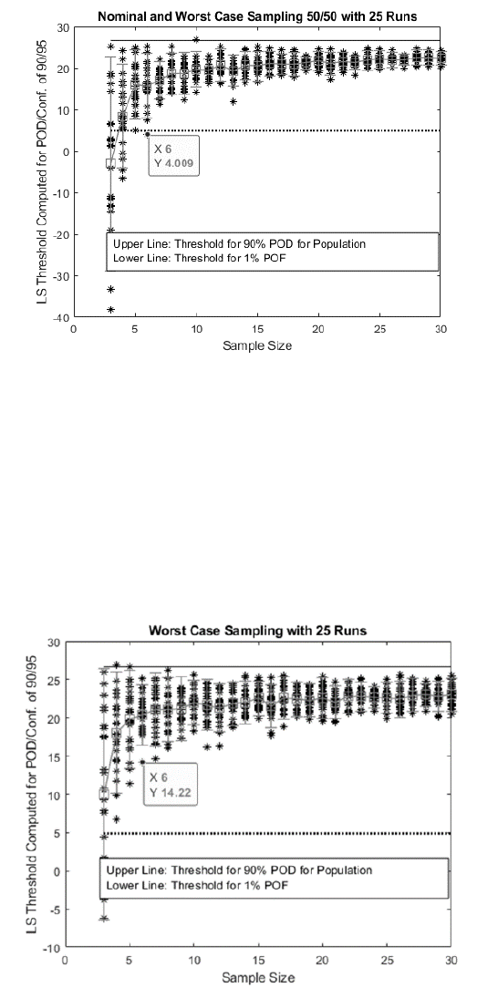
Fig. 5: Example of case A i.e. nominal and worst-case sampling results for Monte Carlo simulation
Each sample size has 25 data points corresponding to 25 Monte Carlo repeats. “Upper Line” in Fig. 5 is drawn at
. It is used to assess whether reliability condition 1 is met. “Lower Line” is drawn at
. It is used to
assess whether reliability condition 2 is met. The spread in LS POD computed decision threshold for each sample size is
shown by an error bar on the data. The box in the error bar is mean of the data and ends are at 95 percentiles of data from
the opposite end. The data range for the LS POD computed threshold decreases like an exponential decay curve with
increasing sample size. LS POD computed threshold mean increases like a saturating exponential curve with increasing
sample size. This indicates that, smaller size may provide larger error; and sometimes it may not meet the reliability
condition 1 and/or reliability condition 2.
An example of Monte Carlo simulation of decision threshold data for case B is provided in Fig. 6.
Fig. 6: Example of case B i.e. worst-case sampling results for Monte Carlo simulation
9
Worst case sampling seems to meet both reliability conditions 1 and 2 for sample size of 6 and larger; and provides smaller
range in decision threshold. Therefore, results for case B seem to be better than those for case A. Traditionally, the approach
for NDE procedure qualification is to choose worst-case flaws, such as fatigue cracks, as fatigue cracks provide
conservatism.
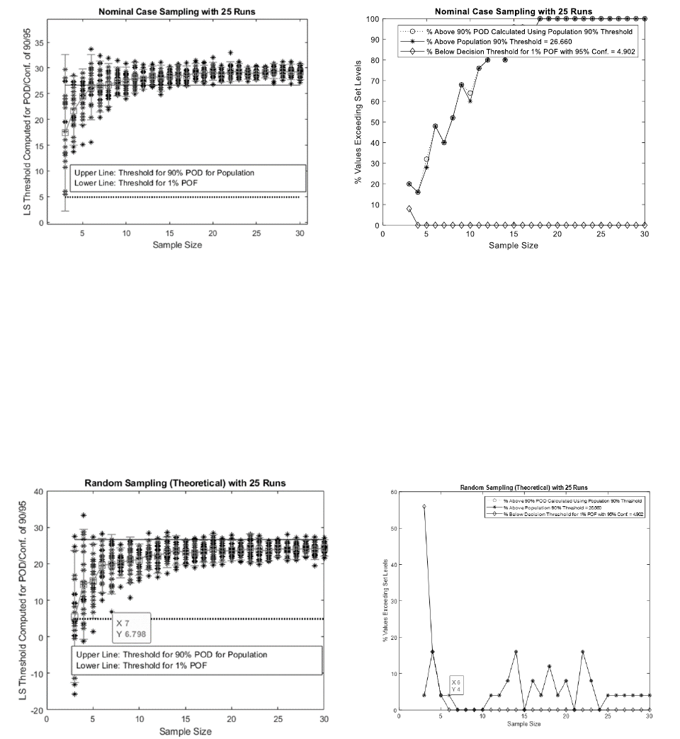
An example of Monte Carlo simulation of decision threshold data for case C is provided in Fig. 7.
Fig. 7: Left plot gives an example of case C i.e. nominal (case) sampling results for Monte Carlo simulation. Right plot gives
percentage of threshold values that do not meet reliability conditions 1 and 2; and percent values that do not meet 90% POD.
Percent threshold values providing POD less than 90% are indicated by marker “o”. This is similar to assessment of
reliability condition 1. This is a direct comparison to 90% POD. Percent threshold values exceeding the 90% POD
threshold are indicated by “*” markers. This is an assessment of reliability condition 1. The differences in corresponding
“*” and “o” marker values are due to computation procedure. Computing POD is an iterative process and has limitations
in accuracy.
Percent threshold values providing POF greater than 1% are indicated by diamond shaped markers. This is assessment of
reliability condition 2. This example indicates that nominal sampling may satisfy reliability condition 2 for POF, but has
high percentage failure in meeting reliability condition 1 for POD.
An example of Monte Carlo simulation of decision threshold data for case D is provided in Fig. 8.
Fig. 8: Left plot gives an example of case D sampling results for Monte Carlo simulation. Right plot gives percentage of threshold
values that do not meet reliability conditions 1 and 2 and percent values that do not meet 90% POD.
10
Since LS POD analysis assumes random sampling, results indicate that LS POD calculated threshold provides 90/95%
POD. For smaller sample size, the data indicates that POF may be higher than 1% rendering the NDE qualification of
decision threshold unusable. However, random sampling is not possible for a small sample size, therefore it is for
theoretical assessment only. Here, reliability condition1 is met.
An example of Monte Carlo simulation of decision threshold data for case E is provided in Fig. 9.
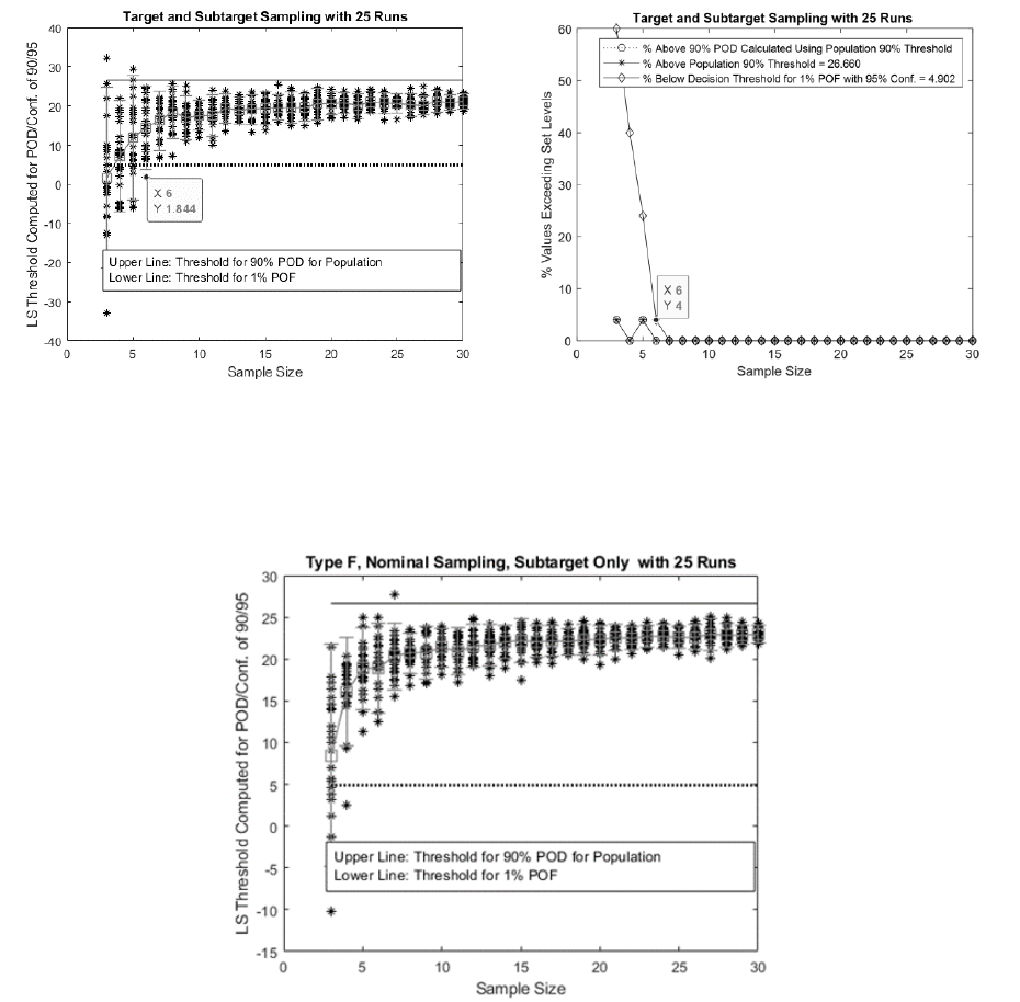
Fig. 9: Left plot gives an example of case E i.e. random target and sub-target sampling results for Monte Carlo simulation. Right plot
gives percentage of threshold values not meeting reliability conditions 1 and 2 and percent values that do not meet 90% POD.
The data for mixed target and sub-target sampling, i.e. case E, indicates that, for sample size > 6, reliability condition 1
and 2 are met. Thus, using Monte Carlo simulation, a sampling scheme (e.g. case E) may be validated to provide high
confidence in meeting condition 1 and 2.
Fig. 10: An example of case F i.e. nominal target and sub-target sampling results for Monte Carlo simulation. Nominal target fraction
is chosen to be 0% in this run.
The data indicates that 100% sub-target nominal flaw sampling, i.e. case F meets both condition 1 and 2 for sample size
of 5 and greater; and is set to provide higher than 90% POD. The case provides positive margin to 90/95% POD/Conf.
requirement. It is practical to make sub-target nominal flaws and therefore, this kind of sampling is attractive. It is similar
to the transfer function approach, where artificial flaws are used in part configuration specimens and simple geometry
specimens along with realistic morphology flaws in simple geometry specimens.

11
As an example, using data for all Monte Carlo repeats, percentage difference of average signal response from case D is
calculated using Eq. (4) and difference of average standard deviation from case D is calculated using Eq. (5). These
quantities are provided in Table 2. These values are calculated for values of input data for sampling sensitivity analysis in
Section 5.
Table 2: % Difference in mean signal response and standard deviation from case D
CASE
% Difference in Mean
Signal Response from
Case D
% Difference in Mean
Standard Deviation
from Case D
A. Nominal and worst-case sampling
-2.1
39.6
B. Worst-case sampling
-7.4
-48.6
C. Nominal (case) sampling
3.2
-29.8
E. Random target and sub-target sampling
(theoretical or non-empirical)
-20.0
0.0
F. Nominal target and sub-target sampling
-16.8
-29.8
Negative values in second column implies lower mean decision threshold compared to random sampling. Negative values
in third column implies lower standard deviation of decision threshold compared to random sampling. Therefore, lower
values are desirable if they meet condition 1 and 2; and provide a method of managing conservatism in LS POD sampling.
7. CONCLUSIONS
Estimating standard deviation of signal response is the most critical parameter for LS POD. Underestimation can lead to
claiming POD/Conf. 90/95% when it is not true. Therefore, the standard deviation of sample data should also agree with
other similar data to increase the confidence in the measured standard deviation of signal response.
Sampling sensitivity analysis can be performed to choose type of the sample. After sample is chosen, there is also a need
to assess what type of sample data was chosen and redo the analysis. Decision threshold calculation results depend upon
the type of sample chosen in NDE validation or POD assessment. Proportion for nominal to worst-case split affects the
results, where either nominal or worst-case signal response measurements or both are used. A 50-50 split ratio value is a
moderate value. An 80-20 split ratio is biased to the larger proportion. Similarly target flaw to sub-target flaw split
proportion affects results, where either target or sub-target flaw measurements or both measurements are used. A 50-50
split ratio value is a moderate value. An 20-80 split ratio will be biased to the larger proportion. In risk discussion, the
nominal to worst-case split ratio is an important factor and the ratio value shall be substantiated with empirical data.
Type A sampling, Nominal to worst case split proportion sampling: Type A (bimodal) sampling may provide an
approximate representative sample of the population. Here, estimation of standard deviation of signal response
measurement is robust and conservative. If worst-case values can be measured and included in the sample, this option
reduces risk and is recommended.
Type B, Worst-case sampling: This option also may provide adequate decision threshold for reliable flaw detection.
However, gathering a sample of worst-case flaws may be challenging.
Type C, Target flaw nominal case sampling: This sampling does not work in validating NDE procedure reliability and
should be avoided.
Type D, Random sampling: Random sampling with larger sample size can provide representative sample of the population.
It is impossible get a random sample for a small sample size.
Type E, Random target and sub-target sampling: This sampling scheme has benefits similar to that of type F sampling but
is not recommended, because it is impossible get a random sample for a small sample size.
Type F, Target and sub-target nominal sampling. This sampling scheme is practical. Although type F sampling does not
provide a representative sample, it can provide a conservative sample that can be used for LS POD analysis. It can be used
12
successfully to create equivalent random sample properties for sub-target flaws. It is recommended as a lower risk option,
if it is not practical to produce worst-case signal responses. 100% sub-target nominal flaws provide lower values of
decision threshold, but also sub-target flaws may have smaller standard deviation in repeated calculation of the decision
threshold. Thus, this option allows adjusting conservatism in choosing flaw sample used to validate NDE procedure by
meeting reliability conditions 1 and 2.
Sampling sensitivity analysis should be performed for appropriate sampling types to manage risk in LS POD results.
Sampling sensitivity analysis provides equivalent random sample properties (mean and standard deviation) which are used
in LS POD analysis. Sampling sensitivity analysis can be used to design sampling type and inputs for the selected sample
(e.g. nominal responses from a sub-target flaw size, sample size etc.) and creation of equivalent random sample so that
resulting LS POD analysis has low risk of not meeting reliability conditions.
REFERENCES
[1] MIL-HDBK-1823A, “Nondestructive Evaluation System Reliability Assessment,” Department of Defense, USA,
(2009).
[2] Annis, Charles, “mh1823 POD Software V5.2.1,” Statistical Engineering,
http://www.statisticalengineering.com/mh1823/, (2016).
[3] ASTM E 2862-12, “Standard Practice for Probability of Detection for Hit/Miss Data,” ASTM International, (2012).
[4] Rummel Ward D., “Recommended Practice for Demonstration of Nondestructive Evaluation (NDE) Reliability on
Aircraft Production Parts,” Materials Evaluation, August Issue 40 pp 922, (1988).
[5] NIST/ Dataplot, “SD Confidence Limits,”
https://www.itl.nist.gov/div898/software/dataplot/refman1/auxillar/sdconfli.htm
[6] NIST/SEMATECH e-Handbook of Statistical Methods, Section 7.2.6.3, May 29, 2020,
https://doi.org/10.18434/M32189, https://www.itl.nist.gov/div898/handbook/prc/section2/prc263.htm
[7] Koshti, A. M., “Using requirements on merit ratios for assessing reliability of NDE flaw detection,” SPIE Smart
Structures and NDE, Proc. SPIE 11593, (2021).
[8] Koshti, A. M., “Using requirements on merit ratios for assessing reliability of NDE flaw detection in multi-hit
detection in digital radiography,” SPIE Smart Structures and NDE, Proc. SPIE 11593, (2021).
[9] Koshti, A. M., “Assessment of flaw detectability using transfer function,” SPIE Smart Structures and NDE, Proc.
SPIE 11592, (2021).
[10] Koshti, A. M., “Modeling reliability of an NDE method providing a C-scan, a case of flaw field simulation,” SPIE
Smart Structures and NDE, Proc. SPIE 11593, (2021).
[11] Koshti, A. M., “Optimizing raster scanning parameters in nondestructive evaluation using simulation of probe
sensitivity field,” SPIE Smart Structures and NDE, Proc. SPIE 11592, (2021).
[12] Koshti, A. M., “Assessing Visual and System Flaw Detectability in Nondestructive Evaluation,” SPIE Smart
Structures and NDE, SPIE 11592, (2021).
[13] Koshti, A. M., “Probability of Detection Analysis in Multi-Hit Flaw Detection,” SPIE Smart Structures and NDE,
SPIE 11594, (2021).
