Contents
1 Introduction 6
1.1 Overview . . . . . . . . . . . . . . . . . . . . . . . . . . . . . . . . . . . . . . . 7
1.2 Relevant Partial Differential Equations . . . . . . . . . . . . . . . . . . . . . . . . 7
1.2.1 Magnetostatic Problems . . . . . . . . . . . . . . . . . . . . . . . . . . . 7
1.2.2 Time-Harmonic Magnetic Problems . . . . . . . . . . . . . . . . . . . . . 8
1.2.3 Electrostatic Problems . . . . . . . . . . . . . . . . . . . . . . . . . . . . 9
1.2.4 Heat Flow Problems . . . . . . . . . . . . . . . . . . . . . . . . . . . . . 10
1.2.5 Current Flow Problems . . . . . . . . . . . . . . . . . . . . . . . . . . . . 11
1.3 Boundary Conditions . . . . . . . . . . . . . . . . . . . . . . . . . . . . . . . . . 12
1.3.1 Magnetic and Electrostatic BCs . . . . . . . . . . . . . . . . . . . . . . . 12
1.3.2 Heat Flow BCs . . . . . . . . . . . . . . . . . . . . . . . . . . . . . . . . 13
1.4 Finite Element Analysis . . . . . . . . . . . . . . . . . . . . . . . . . . . . . . . . 13
2 Interactive Shell 15
2.1 DXF Import/Export . . . . . . . . . . . . . . . . . . . . . . . . . . . . . . . . . . 15
2.2 Magnetics Preprocessor . . . . . . . . . . . . . . . . . . . . . . . . . . . . . . . . 16
2.2.1 Preprocessor Drawing Modes . . . . . . . . . . . . . . . . . . . . . . . . 16
2.2.2 Keyboard and Mouse Commands . . . . . . . . . . . . . . . . . . . . . . 17
2.2.3 View Manipulation . . . . . . . . . . . . . . . . . . . . . . . . . . . . . . 17
2.2.4 Grid Manipulation . . . . . . . . . . . . . . . . . . . . . . . . . . . . . . 19
2.2.5 Edit . . . . . . . . . . . . . . . . . . . . . . . . . . . . . . . . . . . . . . 20
2.2.6 Problem Definition . . . . . . . . . . . . . . . . . . . . . . . . . . . . . . 21
2.2.7 Definition of Properties . . . . . . . . . . . . . . . . . . . . . . . . . . . . 22
2.2.8 Exterior Region . . . . . . . . . . . . . . . . . . . . . . . . . . . . . . . . 33
2.2.9 Analysis Tasks . . . . . . . . . . . . . . . . . . . . . . . . . . . . . . . . 34
2.3 Magnetics Postprocessor . . . . . . . . . . . . . . . . . . . . . . . . . . . . . . . 35
2.3.1 Postprocessor modes . . . . . . . . . . . . . . . . . . . . . . . . . . . . . 35
2.3.2 View and Grid Manipulation . . . . . . . . . . . . . . . . . . . . . . . . . 36
2.3.3 Keyboard Commands . . . . . . . . . . . . . . . . . . . . . . . . . . . . . 36
2.3.4 Mouse Actions . . . . . . . . . . . . . . . . . . . . . . . . . . . . . . . . 36
2.3.5 Miscellaneous Useful View Commands . . . . . . . . . . . . . . . . . . . 37
2.3.6 Contour Plot . . . . . . . . . . . . . . . . . . . . . . . . . . . . . . . . . 37
2.3.7 Density Plot . . . . . . . . . . . . . . . . . . . . . . . . . . . . . . . . . . 38
2.3.8 Vector Plots . . . . . . . . . . . . . . . . . . . . . . . . . . . . . . . . . . 38
2.3.9 Line Plots . . . . . . . . . . . . . . . . . . . . . . . . . . . . . . . . . . . 38
2
2.3.10 Line Integrals . . . . . . . . . . . . . . . . . . . . . . . . . . . . . . . . . 40
2.3.11 Block Integrals . . . . . . . . . . . . . . . . . . . . . . . . . . . . . . . . 41
2.3.12 Force/Torque Calculation . . . . . . . . . . . . . . . . . . . . . . . . . . . 44
2.3.13 Circuit Results . . . . . . . . . . . . . . . . . . . . . . . . . . . . . . . . 46
2.4 Electrostatics Preprocessor . . . . . . . . . . . . . . . . . . . . . . . . . . . . . . 46
2.4.1 Problem Definition . . . . . . . . . . . . . . . . . . . . . . . . . . . . . . 47
2.4.2 Definition of Properties . . . . . . . . . . . . . . . . . . . . . . . . . . . . 48
2.4.3 Analysis Tasks . . . . . . . . . . . . . . . . . . . . . . . . . . . . . . . . 53
2.5 Electrostatics Postprocessor . . . . . . . . . . . . . . . . . . . . . . . . . . . . . . 54
2.5.1 Contour Plot . . . . . . . . . . . . . . . . . . . . . . . . . . . . . . . . . 54
2.5.2 Density Plot . . . . . . . . . . . . . . . . . . . . . . . . . . . . . . . . . . 54
2.5.3 Vector Plots . . . . . . . . . . . . . . . . . . . . . . . . . . . . . . . . . . 55
2.5.4 Line Plots . . . . . . . . . . . . . . . . . . . . . . . . . . . . . . . . . . . 55
2.5.5 Line Integrals . . . . . . . . . . . . . . . . . . . . . . . . . . . . . . . . . 56
2.5.6 Block Integrals . . . . . . . . . . . . . . . . . . . . . . . . . . . . . . . . 57
2.5.7 Force/Torque Calculation . . . . . . . . . . . . . . . . . . . . . . . . . . . 58
2.5.8 Conductor Results . . . . . . . . . . . . . . . . . . . . . . . . . . . . . . 59
2.6 Heat Flow Preprocessor . . . . . . . . . . . . . . . . . . . . . . . . . . . . . . . . 60
2.6.1 Problem Definition . . . . . . . . . . . . . . . . . . . . . . . . . . . . . . 60
2.6.2 Definition of Properties . . . . . . . . . . . . . . . . . . . . . . . . . . . . 61
2.6.3 Analysis Tasks . . . . . . . . . . . . . . . . . . . . . . . . . . . . . . . . 66
2.7 Heat Flow Postprocessor . . . . . . . . . . . . . . . . . . . . . . . . . . . . . . . 67
2.7.1 Contour Plot . . . . . . . . . . . . . . . . . . . . . . . . . . . . . . . . . 67
2.7.2 Density Plot . . . . . . . . . . . . . . . . . . . . . . . . . . . . . . . . . . 67
2.7.3 Vector Plots . . . . . . . . . . . . . . . . . . . . . . . . . . . . . . . . . . 67
2.7.4 Line Plots . . . . . . . . . . . . . . . . . . . . . . . . . . . . . . . . . . . 68
2.7.5 Line Integrals . . . . . . . . . . . . . . . . . . . . . . . . . . . . . . . . . 69
2.7.6 Block Integrals . . . . . . . . . . . . . . . . . . . . . . . . . . . . . . . . 70
2.7.7 Conductor Results . . . . . . . . . . . . . . . . . . . . . . . . . . . . . . 70
2.8 Current Flow Preprocessor . . . . . . . . . . . . . . . . . . . . . . . . . . . . . . 70
2.8.1 Problem Definition . . . . . . . . . . . . . . . . . . . . . . . . . . . . . . 71
2.8.2 Definition of Properties . . . . . . . . . . . . . . . . . . . . . . . . . . . . 72
2.8.3 Analysis Tasks . . . . . . . . . . . . . . . . . . . . . . . . . . . . . . . . 76
2.9 Current Flow Postprocessor . . . . . . . . . . . . . . . . . . . . . . . . . . . . . . 77
2.9.1 Contour Plot . . . . . . . . . . . . . . . . . . . . . . . . . . . . . . . . . 77
2.9.2 Density Plot . . . . . . . . . . . . . . . . . . . . . . . . . . . . . . . . . . 78
2.9.3 Vector Plots . . . . . . . . . . . . . . . . . . . . . . . . . . . . . . . . . . 78
2.9.4 Line Plots . . . . . . . . . . . . . . . . . . . . . . . . . . . . . . . . . . . 78
2.9.5 Line Integrals . . . . . . . . . . . . . . . . . . . . . . . . . . . . . . . . . 79
2.9.6 Block Integrals . . . . . . . . . . . . . . . . . . . . . . . . . . . . . . . . 80
2.9.7 Conductor Results . . . . . . . . . . . . . . . . . . . . . . . . . . . . . . 80
2.10 Exporting of Graphics . . . . . . . . . . . . . . . . . . . . . . . . . . . . . . . . . 81
3
3 Lua Scripting 82
3.1 What Lua Scripting? . . . . . . . . . . . . . . . . . . . . . . . . . . . . . . . . . 82
3.2 Common Lua Command Set . . . . . . . . . . . . . . . . . . . . . . . . . . . . . 82
3.3 Magnetics Preprocessor Lua Command Set . . . . . . . . . . . . . . . . . . . . . 83
3.3.1 Object Add/Remove Commands . . . . . . . . . . . . . . . . . . . . . . . 84
3.3.2 Geometry Selection Commands . . . . . . . . . . . . . . . . . . . . . . . 84
3.3.3 Object Labeling Commands . . . . . . . . . . . . . . . . . . . . . . . . . 85
3.3.4 Problem Commands . . . . . . . . . . . . . . . . . . . . . . . . . . . . . 86
3.3.5 Mesh Commands . . . . . . . . . . . . . . . . . . . . . . . . . . . . . . . 86
3.3.6 Editing Commands . . . . . . . . . . . . . . . . . . . . . . . . . . . . . . 86
3.3.7 Zoom Commands . . . . . . . . . . . . . . . . . . . . . . . . . . . . . . . 88
3.3.8 View Commands . . . . . . . . . . . . . . . . . . . . . . . . . . . . . . . 88
3.3.9 Object Properties . . . . . . . . . . . . . . . . . . . . . . . . . . . . . . . 88
3.3.10 Miscellaneous . . . . . . . . . . . . . . . . . . . . . . . . . . . . . . . . 91
3.4 Magnetics Post Processor Command Set . . . . . . . . . . . . . . . . . . . . . . . 93
3.4.1 Data Extraction Commands . . . . . . . . . . . . . . . . . . . . . . . . . 93
3.4.2 Selection Commands . . . . . . . . . . . . . . . . . . . . . . . . . . . . . 96
3.4.3 Zoom Commands . . . . . . . . . . . . . . . . . . . . . . . . . . . . . . . 97
3.4.4 View Commands . . . . . . . . . . . . . . . . . . . . . . . . . . . . . . . 97
3.4.5 Miscellaneous . . . . . . . . . . . . . . . . . . . . . . . . . . . . . . . . 99
3.5 Electrostatics Preprocessor Lua Command Set . . . . . . . . . . . . . . . . . . . . 99
3.5.1 Object Add/Remove Commands . . . . . . . . . . . . . . . . . . . . . . . 100
3.5.2 Geometry Selection Commands . . . . . . . . . . . . . . . . . . . . . . . 100
3.5.3 Object Labeling Commands . . . . . . . . . . . . . . . . . . . . . . . . . 101
3.5.4 Problem Commands . . . . . . . . . . . . . . . . . . . . . . . . . . . . . 102
3.5.5 Mesh Commands . . . . . . . . . . . . . . . . . . . . . . . . . . . . . . . 102
3.5.6 Editing Commands . . . . . . . . . . . . . . . . . . . . . . . . . . . . . . 102
3.5.7 Zoom Commands . . . . . . . . . . . . . . . . . . . . . . . . . . . . . . . 103
3.5.8 View Commands . . . . . . . . . . . . . . . . . . . . . . . . . . . . . . . 104
3.5.9 Object Properties . . . . . . . . . . . . . . . . . . . . . . . . . . . . . . . 104
3.5.10 Miscellaneous . . . . . . . . . . . . . . . . . . . . . . . . . . . . . . . . 106
3.6 Electrostatics Post Processor Command Set . . . . . . . . . . . . . . . . . . . . . 107
3.6.1 Data Extraction Commands . . . . . . . . . . . . . . . . . . . . . . . . . 107
3.6.2 Selection Commands . . . . . . . . . . . . . . . . . . . . . . . . . . . . . 109
3.6.3 Zoom Commands . . . . . . . . . . . . . . . . . . . . . . . . . . . . . . . 110
3.6.4 View Commands . . . . . . . . . . . . . . . . . . . . . . . . . . . . . . . 110
3.6.5 Miscellaneous . . . . . . . . . . . . . . . . . . . . . . . . . . . . . . . . 111
3.7 Heat Flow Preprocessor Lua Command Set . . . . . . . . . . . . . . . . . . . . . 112
3.7.1 Object Add/Remove Commands . . . . . . . . . . . . . . . . . . . . . . . 113
3.7.2 Geometry Selection Commands . . . . . . . . . . . . . . . . . . . . . . . 113
3.7.3 Object Labeling Commands . . . . . . . . . . . . . . . . . . . . . . . . . 114
3.7.4 Problem Commands . . . . . . . . . . . . . . . . . . . . . . . . . . . . . 115
3.7.5 Mesh Commands . . . . . . . . . . . . . . . . . . . . . . . . . . . . . . . 115
3.7.6 Editing Commands . . . . . . . . . . . . . . . . . . . . . . . . . . . . . . 115
3.7.7 Zoom Commands . . . . . . . . . . . . . . . . . . . . . . . . . . . . . . . 116
4
3.7.8 View Commands . . . . . . . . . . . . . . . . . . . . . . . . . . . . . . . 117
3.7.9 Object Properties . . . . . . . . . . . . . . . . . . . . . . . . . . . . . . . 117
3.7.10 Miscellaneous . . . . . . . . . . . . . . . . . . . . . . . . . . . . . . . . 119
3.8 Heat Flow Post Processor Command Set . . . . . . . . . . . . . . . . . . . . . . . 120
3.8.1 Data Extraction Commands . . . . . . . . . . . . . . . . . . . . . . . . . 121
3.8.2 Selection Commands . . . . . . . . . . . . . . . . . . . . . . . . . . . . . 122
3.8.3 Zoom Commands . . . . . . . . . . . . . . . . . . . . . . . . . . . . . . . 123
3.8.4 View Commands . . . . . . . . . . . . . . . . . . . . . . . . . . . . . . . 123
3.8.5 Miscellaneous . . . . . . . . . . . . . . . . . . . . . . . . . . . . . . . . 125
3.9 Current Flow Preprocessor Lua Command Set . . . . . . . . . . . . . . . . . . . . 125
3.9.1 Object Add/Remove Commands . . . . . . . . . . . . . . . . . . . . . . . 126
3.9.2 Geometry Selection Commands . . . . . . . . . . . . . . . . . . . . . . . 126
3.9.3 Object Labeling Commands . . . . . . . . . . . . . . . . . . . . . . . . . 127
3.9.4 Problem Commands . . . . . . . . . . . . . . . . . . . . . . . . . . . . . 128
3.9.5 Mesh Commands . . . . . . . . . . . . . . . . . . . . . . . . . . . . . . . 128
3.9.6 Editing Commands . . . . . . . . . . . . . . . . . . . . . . . . . . . . . . 128
3.9.7 Zoom Commands . . . . . . . . . . . . . . . . . . . . . . . . . . . . . . . 130
3.9.8 View Commands . . . . . . . . . . . . . . . . . . . . . . . . . . . . . . . 130
3.9.9 Object Properties . . . . . . . . . . . . . . . . . . . . . . . . . . . . . . . 130
3.9.10 Miscellaneous . . . . . . . . . . . . . . . . . . . . . . . . . . . . . . . . 132
3.10 Current Flow Post Processor Command Set . . . . . . . . . . . . . . . . . . . . . 133
3.10.1 Data Extraction Commands . . . . . . . . . . . . . . . . . . . . . . . . . 134
3.10.2 Selection Commands . . . . . . . . . . . . . . . . . . . . . . . . . . . . . 136
3.10.3 Zoom Commands . . . . . . . . . . . . . . . . . . . . . . . . . . . . . . . 137
3.10.4 View Commands . . . . . . . . . . . . . . . . . . . . . . . . . . . . . . . 137
3.10.5 Miscellaneous . . . . . . . . . . . . . . . . . . . . . . . . . . . . . . . . 139
4 Mathematica Interface 141
5 ActiveX Interface 143
6 Numerical Methods 144
6.1 Finite Element Formulation . . . . . . . . . . . . . . . . . . . . . . . . . . . . . . 144
6.2 Linear Solvers . . . . . . . . . . . . . . . . . . . . . . . . . . . . . . . . . . . . . 144
6.3 Field Smoothing . . . . . . . . . . . . . . . . . . . . . . . . . . . . . . . . . . . . 145
A Appendix 149
A.1 Modeling Permanent Magnets . . . . . . . . . . . . . . . . . . . . . . . . . . . . 149
A.2 Bulk Lamination Modeling . . . . . . . . . . . . . . . . . . . . . . . . . . . . . . 152
A.3 Open Boundary Problems . . . . . . . . . . . . . . . . . . . . . . . . . . . . . . . 155
A.3.1 Truncation of Outer Boundaries . . . . . . . . . . . . . . . . . . . . . . . 155
A.3.2 Asymptotic Boundary Conditions . . . . . . . . . . . . . . . . . . . . . . 155
A.3.3 Kelvin Transformation . . . . . . . . . . . . . . . . . . . . . . . . . . . . 158
A.4 Nonlinear Time Harmonic Formulation . . . . . . . . . . . . . . . . . . . . . . . 160
5
Chapter 1
Introduction
FEMM is a suite of programs for solving lowfrequency electromagnetic problems on two-dimensional
planar and axisymmetric domains. The program currently addresses linear/nonlinear magneto-
static problems, linear/nonlinear time harmonic magnetic problems, linear electrostatic problems,
and steady-state heat flow problems.
FEMM is divided into three parts:
• Interactive shell (
femm.exe
). This program is a Multiple Document Interface pre-processor
and a post-processor for the various types of problems solved by FEMM. It contains a CAD-
like interface for laying out the geometry of the problem to be solved and for defining ma-
terial properties and boundary conditions. Autocad DXF files can be imported to facilitate
the analysis of existing geometries. Field solutions can be displayed in the form of contour
and density plots. The program also allows the user to inspect the field at arbitrary points, as
well as evaluate a number of different integrals and plot various quantities of interest along
user-defined contours.
•
triangle.exe
. Triangle breaks down the solution region into a large number of triangles,
a vital part of the finite element process. This program was written by Jonathan Shewchuk
and is available at www.cs.cmu.edu/ quake/triangle.html
• Solvers (
fkern.exe
for magnetics;
belasolv
for electrostatics);
hsolv
for heat flow prob-
lems; and
csolv
for current flow problems.. Each solver takes a set of data files that describe
problem and solves the relevant partial differential equations to obtain values for the desired
field throughout the solution domain.
The Lua scripting language is integrated into the interactive shell. Unlike previous versions of
FEMM (i.e. v3.4 and lower), only one instance of Lua is running at any one time. This single
instance of Lua can both build and analyze a geometry and evaluate the post-processing results,
simplifying the creation of various sorts of “batch” runs.
In addition, all edit boxes in the user interface are parsed by Lua, allowing equations or mathe-
matical expressions to be entered into any edit box in lieu of a numerical value. In any edit box in
FEMM, a selected piece of text can be evaluated by Lua via a selection on the right mouse button
menu.
The purpose of this document is to give a brief explanation of the kind of problems solved by
FEMM and to provide a fairly detailed documentation of the programs’ use.
6

1.1 Overview
The goal of this section is to give the user a brief description of the problems that FEMM solves.
This information is not really crucial if you are not particularly interested in the approach that
FEMM takes to formulating the problems. You can skip most of Overview, but take a look at
Section 1.3. This section contains some important pointers about assigning enough boundary
conditions to get a solvable problem.
Some familiarity with electromagnetism and Maxwell’s equations is assumed, since a review of
this material is beyond the scope of this manual. However, the author has found several references
that have proved useful in understanding the derivation and solution of Maxwell’s equations in
various situations. A very good introductory-level text for magnetic and electrostatic problems is
Plonus’s Applied electromagnetics [1]. A good intermediate-level review of Maxwell’s equations,
as well as a useful analogy of magnetism to similar problems in other disciplines is contained
in Hoole’s Computer-aided analysis and design of electromagnetic devices [2]. For an advanced
treatment, the reader has no recourse but to refer to Jackson’s Classical electrodynamics [3]. For
thermal problems, the author has found White’s Heat and mass tranfer [4] and Haberman’s Ele-
mentary applied partial differential equations [5] to be useful in understanding the derivation and
solution of steady-state temperature problems.
1.2 Relevant Partial Differential Equations
FEMM addresses some limiting cases of Maxwell’s equations. The magnetics problems addressed
are those that can be consided as “low frequency problems,” in which displacment currents can be
ignored. Displacement currents are typically relevant to magnetics problems only at radio frequen-
cies. In a similar vein, the electrostatics solver considers the converse case in which only the elec-
tric field is considered and the magnetic field is neglected. FEMM also solves 2D/axysymmetric
steady-state heat conduction problems. This heat conduction problem is mathematically very sim-
ilar to the solution of electrostatic problems.
1.2.1 Magnetostatic Problems
Magnetostatic problems are problems in which the fields are time-invariant. In this case, the field
intensity (H) and flux density (B) must obey:
∇×H = J (1.1)
∇·B = 0 (1.2)
subject to a constitutive relationship between B and H for each material:
B = µH (1.3)
If a material is nonlinear (e.g. saturating iron or alnico magnets), the permeability, µ is actually a
function of B:
µ =
B
H(B)
(1.4)
7

FEMM goes about finding a field that satisfies (1.1)-(1.3) via a magnetic vector potential ap-
proach. Flux density is written in terms of the vector potential, A, as:
B = ∇×A (1.5)
Now, this definition of B always satisfies (1.2). Then, (1.1) can be rewritten as:
∇×
1
µ(B)
∇×A
= J (1.6)
For a linear isotropic material (and assuming the Coulomb gauge, ∇·A = 0), eq. (1.6) reduces to:
−
1
µ
∇
2
A = J (1.7)
FEMM retains the form of (1.6), so that magnetostatic problems with a nonlinear B-H relationship
can be solved.
In the general 3-D case, A is a vector with three components. However, in the 2-D planar and
axisymmetric cases, two of these three components are zero, leaving just the component in the “out
of the page” direction.
The advantage of using the vector potential formulation is that all the conditions to be satis-
fied have been combined into a single equation. If A is found, B and H can then be deduced by
differentiating A. The form of (1.6), an elliptic partial differential equation, arises in the study of
many different types of engineering phenomenon. There are a large number of tools that have been
developed over the years to solve this particular problem.
1.2.2 Time-Harmonic Magnetic Problems
If the magnetic field is time-varying, eddy currents can be induced in materials with a non-zero
conductivity. Several other Maxwell’s equations related to the electric field distribution must also
be accommodated. Denoting the electric field intensity as E and the current density as J, E and J
obey the constitutive relationship:
J = σE (1.8)
The induced electric field then obeys:
∇×E = −
∂B
∂t
(1.9)
Substituting the vector potential form of B into (1.9) yields:
∇×E = −∇×
˙
A (1.10)
In the case of 2-D problems, (1.10) can be integrated to yield:
E = −
˙
A−∇V (1.11)
and the constitutive relationship, (1.8) employed to yield:
J = −σ
˙
A−σ∇V (1.12)
8

Substituting into (1.6) yields the partial differential equation:
∇×
1
µ(B)
∇×A
= −σ
˙
A+ J
src
−σ∇V (1.13)
where J
src
represents the applied currents sources. The ∇V term is an additional voltage gradient
that, in 2-D problems, is constant over a conducting body. FEMM uses this voltage gradient in
some harmonic problems to enforce constraints on the current carried by conductive regions.
FEMM considers (1.13) for the case in which the field is oscillating at one fixed frequency. For
this case, a phasor transformation [2] yields a steady-state equation that is solved for the amplitude
and phase of A. This transformation is:
A = Re[a(cosωt + jsinωt) =] = Re
ae
jwt
(1.14)
in which a is a complex number. Substituting into (1.13) and dividing out the complex exponential
term yields the equation that FEMM actually solves for harmonic magnetic problems:
∇×
1
µ
ef f
(B)
∇×a
= −jωσa+
ˆ
J
src
−σ∇V (1.15)
in which
ˆ
J
src
represents the phasor transform of the applied current sources.
Strictly speaking, the permeability µ should be constant for harmonic problems. However,
FEMM retains a nonlinear relationship in the harmonic formulation, allowing the program to ap-
proximate the effects of saturation on the phase and amplitude of the fundamental of the field
distribution. The form of the BH curve is not exactly the same as in the DC case. Instead, “effec-
tive permeability” µ
ef f
is selected to give the correct amplitude of the fundamental component of
the waveform under sinusoidal excitation. There are a number of subtleties to the nonlinear time
harmonic formulation–this formulation is addressed in more detail in Appendix A.4.
FEMM also allows for the inclusion of complex and frequency-dependent permeability in time
harmonic problems. These features allow the program to model materials with thin laminations
and approximately model hysteresis effects.
1.2.3 Electrostatic Problems
Electrostatic problems consider the behavior of electric field intensity, E, and electric flux density
(alternatively electric displacement), D. There are two conditions that these quantities must obey.
The first condition is the differential form of Gauss’ Law, which says that the flux out of any closed
volume is equal to the charge contained within the volume:
∇·D = ρ (1.16)
where ρ represents charge density. The second is the differential form of Ampere’s loop law:
∇×E = 0 (1.17)
Displacement and field intensity are also related to one another via the constitutive relationship:
D = εE (1.18)
9
where ε is the electrical permittivity. Although some electrostatics problems might have a nonlinear
constitutive relationship between D and E, the program only considers linear problems.
To simplify the computation of fields which satisfy these conditions, the program employs the
electric scalar potential, V, defined by its relation to E as:
E = −∇V (1.19)
Because of the vector identity ∇×∇ψ = 0 for any scalar ψ, Ampere’s loop law is automatically
satisfied. Substituting into Gauss’ Law and applying the constitutiverelationship yields the second-
order partial differential equation:
−ε∇
2
V = ρ (1.20)
which applies over regions of homogeneous ε. The program solves (1.20) for voltage V over a
user-defined domain with user-defined sources and boundary conditions.
1.2.4 Heat Flow Problems
The heat flow problems address by FEMM are essentially steady-state heat conduction problems.
These probelms are represented by a temperature gradient, G(analogous to the field intensity, E
for electrostatic problems), and heat flux density, F(analogous to electric flux density, D, for elec-
trostatic problems).
The heat flux density must obey Gauss’ Law, which says that the heat flux out of any closed
volume is equal to the heat generation within the volume. Analogous to the electrostatic problem,
this law is represented in differential form as:
∇·F = q (1.21)
where q represents volume heat generation.
Temperature gradient and heat flux density are also related to one another via the constitutive
relationship:
F = kG (1.22)
where k is the thermal conductivity. Thermal conductivity is often a weak function of temperature.
FEMM allows for the variation of conductivity as an arbitrary function of temperature.
Ultimately, one is generally interested in discerning the temperature, T, rather than the heat
flux density or temperature gradient. Temperature is related to the temperature gradient, G, by:
G = −∇T (1.23)
Substituting (1.23) into Gauss’ Law and applying the constitutiverelationship yields the second-
order partial differential equation:
−∇·(k∇T) = q (1.24)
FEMM solves (1.24) for temperature T over a user-defined domain with user-defined heat sources
and boundary conditions.
10
1.2.5 Current Flow Problems
The current flow problems solved by FEMM are essentially quasi-electrostatic problems in which
the magnetic field terms in Maxwell’s equations can be neglected but in which the displacement
current terms (neglected in magnetostatic and eddy current problems) are relevant.
Again restating Maxwell’s Equations, the electric and magnetic fields must obey:
∇×H = J +
˙
D (1.25)
∇·B = 0 (1.26)
∇×E = −
˙
B (1.27)
∇·D = ρ (1.28)
subject to the constitutive relations:
J = σE (1.29)
D = εE (1.30)
The divergence of (1.25) can be taken to yield:
∇·(∇×H) = ∇·J + ∇·
˙
D (1.31)
By application of a standard vector identity, the left-hand side of (1.31) is zero, leading to:
∇·J + ∇ ·
˙
D = 0 (1.32)
As before, we can assume an electric potential, V, that is related to field intensity, E, by:
E = −∇V (1.33)
Because the flux density, B, is assumed to be negligibly small, (1.26) and (1.27) are suitably satis-
fied by this choice of potential.
If a phasor transformation is again assumed, wherein differentiation with respect to time is
replaced by multiplication by jω, the definition of voltage can be substituted into (1.32) to yield:
−∇·((σ+ jωε) ∇V) = 0 (1.34)
If it is assumed that the material properties are piece-wise continuous, things can be simplified
slightly to:
−(σ+ jωε) ∇
2
V = 0 (1.35)
FEMM solves (1.35) to analyze current flow problems.
Eq. (1.35) also applies for the solution of DC current flow problems. At zero frequency, the
term associated with electrical permittivity vanishes, leaving:
−σ∇
2
V = 0 (1.36)
By simply specifing a zero frequency, this formulation solves DC current flow problems in a con-
sistent fashion.
11

1.3 Boundary Conditions
Some discussion of boundary conditions is necessary so that the user will be sure to define an
adequate number of boundary conditions to guarantee a unique solution.
1.3.1 Magnetic and Electrostatic BCs
Boundary conditions for magnetic and electrostatic problems come in five varieties:
• Dirichlet. In this type of boundary condition, the value of potential A or V is explicitly
defined on the boundary, e.g. A = 0. The most common use of Dirichlet-type boundary
conditions in magnetic problems is to define A = 0 along a boundary to keep magnetic flux
from crossing the boundary. In electrostatic problems, Dirichlet conditions are used to fix
the voltage of a surface in the problem domain.
• Neumann. This boundary condition specifies the normal derivative of potential along the
boundary. In magnetic problems, the homogeneous Neumann boundary condition, ∂A/∂n =
0 is defined along a boundary to force flux to pass the boundary at exactly a 90
o
angle to the
boundary. This sort of boundary condition is consistent with an interface with a very highly
permeable metal.
• Robin. The Robin boundary condition is sort of a mix between Dirichlet and Neumann,
prescribing a relationship between the value of A and its normal derivative at the boundary.
An example of this boundary condition is:
∂A
∂n
+ cA = 0
This boundary condition is most often in FEMM to define “impedance boundary conditions”
that allow a bounded domain to mimic the behavior of an unbounded region. In the context
of heat flow problems, this boundary condition can be interpreted as a convection boundary
condition. In heat flow problems, radiation boundary conditions are linearized about the
solution from the last iteration. The linearized form of the radiation boundary condition is
also a Robin boundary condition.
• Periodic A periodic boundary conditions joins two boundaries together. In this type of
boundary condition, the boundary values on corresponding points of the two boundaries
are set equal to one another.
• Antiperiodic The antiperiodic boundary condition also joins to gether two boundaries. How-
ever, the boundary values are made to be of equal magnitude but opposite sign.
If no boundary conditions are explicitly defined, each boundary defaults to a homogeneous
Neumann boundary condition. However, a non-derivative boundary condition must be defined
somewhere (or the potential must be defined at one reference point in the domain) so that the
problem has a unique solution.
For axisymmetric magnetic problems, A = 0 is enforced on the line r = 0. In this case, a valid
solution can be obtained without explicitly defining any boundary conditions, as long as part of the
boundary of the problem lies along r = 0. This is not the case for electrostatic problems, however.
For electrostatic problems, it is valid to have a solution with a non-zero potential along r = 0.
12

1.3.2 Heat Flow BCs
There are six types of boundary conditions for heat flow problems:
• Fixed Temperature The temperature along the boundary is set to a prescribed value.
• Heat Flux The heat flux, f, across a boundary is prescribed. This boundary condition can be
represented mathematically as:
k
∂T
∂n
+ f = 0 (1.37)
where n represents the direction normal to the boundary.
• Convection Convection occurs if the boundary is cooled by a fluid flow. This boundary
condition can be represented as:
k
∂T
∂n
+ h(T −T
o
) = 0 (1.38)
where h is the “heat transfer coefficient” and T
o
is the ambient cooling fluid temperature.
• Radiation Heat flux via radiation can be described mathematically as:
k
∂T
∂n
+ βk
sb
T
4
−T
4
o
= 0 (1.39)
where beta is the emissivity of the surface (a dimensionless value between 0 and 1) and k
sb
is the Stefan-Boltzmann constant.
• Periodic A periodic boundary conditions joins two boundaries together. In this type of
boundary condition, the boundary values on corresponding points of the two boundaries
are set equal to one another.
• Antiperiodic The antiperiodic boundary condition also joins to gether two boundaries. How-
ever, the boundary values are made to be of equal magnitude but opposite sign.
If no boundary conditions are explicitly defined, each boundary defaults an insulated condition
(i.e. no heat flux across the boundary). However, a non-derivative boundary condition must be
defined somewhere (or the potential must be defined at one reference point in the domain) so that
the problem has a unique solution.
1.4 Finite Element Analysis
Although the differential equations of interest appear relatively compact, it is typically very diffi-
cult to get closed-form solutions for all but the simplest geometries. This is where finite element
analysis comes in. The idea of finite elements is to break the problem down into a large number
regions, each with a simple geometry (e.g. triangles). For example, Figure 1.1 shows a map of the
Massachusetts broken down into triangles. Over these simple regions, the “true” solution for the
13
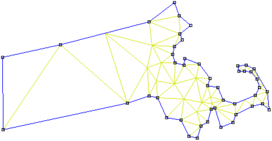
Figure 1.1: Triangulation of Massachusetts
desired potential is approximated by a very simple function. If enough small regions are used, the
approximate potential closely matches the exact solution.
The advantage of breaking the domain down into a number of small elements is that the prob-
lem becomes transformed from a small but difficult to solve problem into a big but relatively easy
to solve problem. Through the process of discretizaton, a linear algebra problem is formed with
perhaps tens of thousands of unknowns. However, algorithms exist that allow the resulting linear
algebra problem to be solved, usually in a short amount of time.
Specifically, FEMM discretizes the problem domain using triangular elements. Over each
element, the solution is approximated by a linear interpolation of the values of potential at the
three vertices of the triangle. The linear algebra problem is formed by minimizing a measure
of the error between the exact differential equation and the approximate differential equation as
written in terms of the linear trial functions.
14
Chapter 2
Interactive Shell
The FEMM Interactive Shell is currently broken into six major sections:
• Magnetics Preprocessor
• Electrostatics Preprocessor
• Heat Flow Preprocessor
• Magnetics Postprocessor
• Electrostatics Postprocessor
• Heat Flow Postprocessor
This section of the manual explains the functionality of each section in detail.
2.1 DXF Import/Export
A common aspect of all preprocessor modes is DXF Import/Export. For interfacing with CAD
programs and other finite element packages, femm supports the import and export of the Auto-
CAD dxf file format. Specifically, the dxf interpreter in femm was written to the dxf revision 13
standards. Only 2D dxf files can be imported in a meaningful way.
To import a dxf file, select
Import DXF
off of the
File
menu. A dialog will appear after the
file is seleted asking for a tolerance. This tolerance is the maximum distance between two points
at which the program considers two points to be the same. The default value is usually sufficient.
For some files, however, the tolerance needs to be increased (i.e. made a larger number) to import
the file correctly. FEMM does not understand all the possible tags that can be included in a dxf
file; instead, it simply strips out the commands involved with drawing lines, circles, and arcs. All
other information is simply ignored.
Generally, dxf import is a useful feature. It allows the user to draw an initial geometry using
their favorite CAD package. Once the geometry is laid out, the geometry can be imported into
femm and detailed for materials properties and boundary conditions.
Do not despair if femm takes a while to import dxf files (especially large dxf files). The reason
that femm can take a long time to import dxf files is that a lot of consistency checking must be
15

performed to turn the dxf file into a valid finite element geometry. For example, large dxf files
might take up to a minute or two to import.
The current femm geometry can be exported in dxf format by selecting the
Export DXF
option
off of the
File
menu in any preprocessor window. The dxf files generated from femm can then be
imported into CAD programs to aid in the mechanical detailing of a finalized design, or imported
into other finite element or boundary element programs.
2.2 Magnetics Preprocessor
The preprocessor is used for drawing the problems geometry, defining materials, and defining
boundary conditions. A new instance of the preprocessor can be created by selecting
File|New
off of the main menu and then selecting “Magnetics Problem” from the list of problem types which
then appears.
Drawing a valid geometry usually consists of four (though not necessarily sequential) tasks:
• Drawing the endpoints of the lines and arc segments that make up a drawing.
• Connecting the endpoints with either line segments or arc segments
• Adding “Block Label” markers into each section of the model to define material properties
and mesh sizing for each section.
• Specifying boundary conditions on the outer edges of the geometry.
This section will describe exactly how one goes about performing these tasks and creating a prob-
lem that can be solved.
2.2.1 Preprocessor Drawing Modes
The key to using the preprocessor is that the preprocessor is always in one of five modes: the Point
mode, the Segment mode, Arc Segment mode, the Block mode, or the Group mode. The first four
of these modes correspond to the four types of entities that define the problems geometry: nodes
that define all corners in the solution geometry, line segments and arc segments that connect the
nodes to form boundaries and interfaces, and block labels that denote what material properties and
mesh size are associated with each solution region. When the preprocessor is in a one of the first
four drawing modes, editing operations take place only upon the selected type of entity. The fifth
mode, the group mode, is meant to glue different objects together into parts so that entire parts can
be manipulated more easily.
One can switch between drawing modes by clicking the appropriate button on the Drawing
Mode potion of the toolbar. This section of the toolbar is pictured in Figure 2.1. The buttons
Figure 2.1: Drawing Mode toolbar buttons.
correspond to Point, Line Segment, Arc Segment, Block Label, and Group modes respectively.
The default drawing mode when the program begins is the Point mode.
16

2.2.2 Keyboard and Mouse Commands
Although most of the tasks that need to be performed are available via the toolbar, some important
functions are invoked only through the use of “hot keys”. A summary of these keys and their
associated functions is contained in Table 2.1.
Likewise, specific functions are associated with mouse button input. The user employs the
mouse to create new object, select obects that have already been created, and inquire about object
properties. Table 2.2 is a summary of the mouse button click actions.
2.2.3 View Manipulation
Generally, the user needs to size or movethe view of the problem geometry displayed on the screen.
Most of the view manipulation commands are available via buttons on the preprocessor toolbar.
The functionality of can generally also be accessed via the ‘View Manipulation Keys’ listed in
Table 2.1. The View Manipulation toolbar buttons are pictured in Figure 2.2. The meaning of the
Figure 2.2: View Manipulation toolbar buttons.
View Manipulation toobar buttons are:
• The arrows on the toolbar correspond to moving the view in the direction of the arrow ap-
proximately 1/2 of the current screen width.
• The “blank page” button scales the screen to the smallest possible view that displays the
entire problem geometry.
• The “+” and “-” buttons zoom the current view in and out, respectively.
• The “page with magnifying glass” button allows the view to be zoomed in on a user-specified
part of the screen. To use this tool, first push the toolbar button. Then, move the mouse
pointer to one of the desired corners of the “new” view. Press and hold the left mouse
button. Drag the mouse pointer to the opposite diagonal corner of the desired “new” view.
Last, release the left mouse button. The view will zoom in to a window that best fits the
user’s desired window.
Some infrequently used view commands are also available, but only as options off of the
Zoom
selection of the main menu. This menu contains all of the manipulations available from the toolbar
buttons, plus the options
Keyboard
,
Status Bar
, and
Toolbar
.
The
Keyboard
selection allows the user to zoom in to a window in which the window’s corners
are explicitly specified by the user via keyboard entry of the corners’ coordinates. When this
selection is chosen, a dialog pops up prompting for the locations of the window corners. Enter
the desired window coordinates and hit “OK”. The view will then zoom to the smallest possible
window that bounds the desired window corners. Typically, this view manipulation is only done
as a new drawing is begun, to initially size the view window to convenient boundaries.
17
Point Mode Keys
Key Function
Space Edit the properties of selected point(s)
Tab Display dialog for the numerical entry of coordinates for a new point
Escape Unselect all points
Delete Delete selected points
Line/Arc Segment Mode Keys
Key Function
Space Edit the properties of selected segment(s)
Escape Unselect all segments and line starting points
Delete Delete selected segment(s)
Block Label Mode Keys
Key Function
Space Edit the properties of selected block labels(s)
Tab Display dialog for the numerical entry of coordinates for a new label
Escape Unselect all block labels
Delete Delete selected block label(s)
Group Mode Keys
Key Function
Space Edit group assignment of the selected objects
Escape Unselect all
Delete Delete selected block label(s)
View Manipulation Keys
Key Function
Left Arrow Pan left
Right Arrow Pan right
Up Arrow Pan up
Down Arrow Pan down
Page Up Zoom in
Page Down Zoom out
Home Zoom “natural”
Table 2.1: Magnetics Preprocessor hot keys
18
Point Mode
Action Function
Left Button Click Create a new point at the current mouse pointer location
Right Button Click Select the nearest point
Right Button DblClick Display coordinates of the nearest point
Line/Arc Segment Mode
Action Function
Left Button Click Select a start/end point for a new segment
Right Button Click Select the nearest line/arc segment
Right Button DblClick Display length of the nearest arc/line segment
Block Label Mode
Action Function
Left Button Click Create a new block label at the current mouse pointer location
Right Button Click Select the nearest block label
Right Button DblClick Display coordinates of the nearest block label
Group Mode
Action Function
Right Button Click Select the group associated with the nearest object
Table 2.2: Magnetics Preprocessor Mouse button actions
The
Status Bar
selection can be used to hide or show the one-line status bar at the bottom
of the femm window. Generally, it is desirable for the toolbar to be displayed, since the current
location of the mouse pointer is displayed on the status line.
The
Toolbar
selection can be used to hide or show the toolbar buttons. The toolbar is not
fundamentally necessary to running femm, because any selection on the toolbar is also available
via selections off of the main menu. If more space on the screen is desired, this option can be
chosen to hide the toolbar. Selecting it a second time will show the toolbar again. It may be useful
to note that the toolbar can be undocked from the main screen and made to “float” at a user-defined
location on screen. This is done by pushing the left mouse button down on an area of the toolbar
that is not actually a button, and then dragging the toolbar to its desired location. The toolbar can
be docked again by moving it back to its original position.
2.2.4 Grid Manipulation
To aid in drawing your geometry, a useful tool is the Grid. When the grid is on, a grid of light blue
pixels will be displayed on the screen. The spacing between grid points can be specified by the
user, and the mouse pointer can be made to “snap” to the closest grid point.
The easiest way to manipulate the grid is through the used of the Grid Manipulation toolbar
19
buttons. These buttons are pictured in Figure 2.3. The left-most button in Figure 2.3 shows and
Figure 2.3: Grid Manipulation toolbar buttons.
hides the grid. The default is that the button is pushed in, showing the current grid. The second
button, with an icon of an arrow pointing to a grid point, is the “snap to grid” button. When this
button is pushed in, the location of the mouse pointer is rounded to the nearest grid point location.
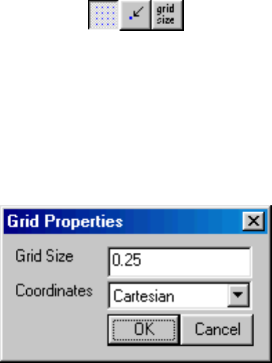
By default, the “snap to grid” button is not pressed. The right-most button brings up the Grid
Properties dialog. This dialog is shown in Figure 2.4.
Figure 2.4: Grid Properties dialog.
The Grid Properties dialog has an edit box for the user to enter the desired grid sizing. When
the box appears, the number in this edit box is the current grid size. The edit box also contains
a drop list that allows the user to select between Cartesian and Polar coordinates. If Cartesian
is selected, points are specified by their (x,y) coordinates for a planar problem, or by their (r,z)
coordinates for an axisymmetric problem. If Polar is selected, points are specified by an angle and
a radial distance from the origin. The default is Cartesian coordinates.
2.2.5 Edit
Several useful tasks can be performed via the
Edit
menu off of the main menu.
Perhaps the most frequently used is the
Undo
command. Choosing this selection undoes the
last addition or deletion that the user has made to the model’s geometry.
For selecting many objects quickly, the
Select Group
command is useful. This command
allows the user to select objects of the current type located in an arbitrary rectangular box. When
this command is selected, move the mouse pointer to one corner of the region that is to be selected.
Press and hold the left mouse button. Then, drag the mouse pointer to the opposite diagonal
corner of the region. A red box will appear, outlining the region to be selected. When the desired
region has been specified, release the left mouse button. All objects of the current type completely
contained within the box will become selected.
Any objects that are currently selected can be moved, copied, or pasted. To move or copy
selected objects, simply choose the corresponding selection off of the main menu’s
Edit
menu. A
dialog will appear prompting for an amount of displacement or rotation.
20
2.2.6 Problem Definition
The definition of problem type is specified by choosing the
Problem
selection off of the main
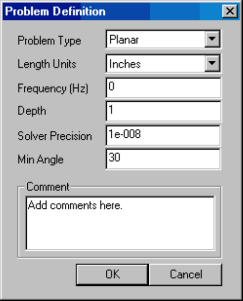
menu. Selecting this option brings up the Problem Definition dialog, shown in Figure 2.5
Figure 2.5: Problem Definition dialog.
The first selection is the
Problem Type
drop list. This drop box allows the user to choose from
a 2-D planar problem (the
Planar
selection), or an axisymmetric problem (the
Axisymmetric
selection).
Next is the
Length Units
drop list. This box identifies what unit is associated with the dimen-
sions prescribed in the model’s geometry. Currently, the program supports inches, millimeters,
centimeters, meters, mils, and µmeters.
The first edit box in the dialog is
Frequency (Hz)
. For a magnetostatic problem, the user
should choose a frequency of zero. If the frequency is non-zero, the program will perform a
harmonic analysis, in which all field quantities are oscillating at this prescribed frequency. The
default frequency is zero.
The second edit box is the
Depth
specification. If a Planar problem is selected, this edit box
becomes enabled. This value is the length of the geometry in the “into the page” direction. This
value is used for scaling integral results in the post processor (e.g. force, inductance, etc.) to the
appropriate length. The units of the Depth selection are the same as the selected length units. For
files imported from version 3.2, the Depth is chosen so that the depth equals 1 meter, since in
version 3.2, all results from planar problems ar e reported per meter.
21
The third edit box is the
Solver Precision
edit box. The number in this edit box specifies
the stopping criteria for the linear solver. The linear algebra problem could be represented by:
Mx = b
where M is a square matrix, b is a vector, and x is a vector of unknowns to be determined. The
solver precision value determines the maximum allowable value for ||b−Mx||/||b||. The default
value is 10
−8
.
The fourth edit box is labeled
Min Angle
. The entry in this box is used as a constraint in
the Triangle meshing program. Triangle adds points to the mesh to ensure that no angles smaller
than the specified angle occur. If the minimum angle is 20.7 degrees or smaller, the triangulation
algorithm is theoretically guaranteed to terminate (assuming infinite precision arithmetic – Triangle
may fail to terminate if you run out of precision). In practice, the algorithm often succeeds for
minimum angles up to 33.8 degrees. For highly refined meshes, however, it may be necessary
to reduce the minimum angle to well below 20 to avoid problems associated with insufficient
floating-point precision. The edit box will accept values between 1 and 33.8 degrees.
Lastly, there is an optional
Comment
edit box. The user can enter in a few lines of text that give
a brief description of the problem that is being solved. This is useful if the user is running several
small variations on a given geometry. The comment can then be used to identify the relevant
features for a particular geometry.
2.2.7 Definition of Properties
To make a solvable problem definition, the user must identify boundary conditions, block materials
properties, and so on. The different types of properties defined for a given problem are defined via
the
Properties
selection off of the main menu.
When the
Properties
selection is chosen, a drop menu appears that has selections for Ma-
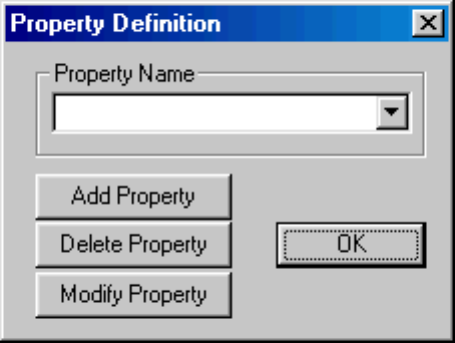
terials, Boundary, Point, and Circuits. When any one of these selections is chosen, the dialog
pictured in Figure 2.6 appears. This dialog is the manager for a particular type of properties. All
Figure 2.6: Property Definition dialog box
currently defined properties are displayed in the
Property Name
drop list at the top of the dia-
log. At the beginning of a new model definition, the box will be blank, since no properties have
22
yet been defined. Pushing the
Add Property
button allows the user to define a new property
type. The
Delete Property
button removes the definition of the property currently in view in the
Property Name
box. The
Modify Property
button allows the user to view and edit the property
currently selected in the
Property Name
box. Specifics for defining the various property types are
addressed in the following subsections.
In general, a number of these edit boxes prompt the user for both real and imaginary compo-
nents for entered values. If the problem you are defining is magnetostatic (zero frequency), enter
the desired value in the box for the real component, and leave a zero in the box for the imaginary
component. The reason that femm uses this formalism is to obtain a relatively smooth transition
from static to time-harmonic problems. Consider the definition of the Phasor transformation in
Eq. 1.14. The phasor transformation assumes that all field values oscillate in time at a frequence
of ω. The phasor transformation takes the cosine part of the field value and represents it as the real
part of a complex number. The imaginary part represents the magnitude of the sine component,
90
o
out of phase. Note what happens as the frequency goes to zero:
lim
ω→0
(a
re
cosωt −a
im
sinωt) = a
re
(2.1)
Therefore, the magnetostatic (ω = 0) values are just described by the real part the specified complex
number.
Point Properties
If a new point property is added or an existing point property modified, the
Nodal Property
dialog box appears. This dialog box is pictured in Figure 2.7
The first selection is the
Name
edit box. The default name is “New Point Property,” but this
name should be changed to something that describes the property that you are defining.
Next are edit boxes for defining the vector potential, A, at a given point, or prescribing a point
current, J, at a given point. The two definitions are mutually exclusive. Therefore, if there is a
nonzero value the J box, the program assumes that a point current is being defined. Otherwise, it
is assumed that a point vector potential is being defined.
There is an edit box for vector point vector potential, A. A can be defined as a complex value,
if desired. The units of A are Weber/Meter. Typically, A needs to be defined as some particular
values (usually zero) at some point in the solution domain for problems with derivative boundary
conditions on all sides. This is the typical use of defining a point vector potential.
Lastly, there is an edit box for the definition of a point current, J. The units for the point current
are in Amperes. The value of J can be defined as complex, if desired.
Boundary Properties
The
Boundary Property
dialog box is used to specify the properties of line segments or arc
segments that are to be boundaries of the solution domain. When a new boundary property is
added or an existing property modified, the
Boundary Property
dialog pictured in Figure 2.8
appears.
The first selection in the dialog is the
Name
of the property. The default name is “New Bound-
ary,” but you should change this name to something more descriptive of the boundary that is being
defined.
23
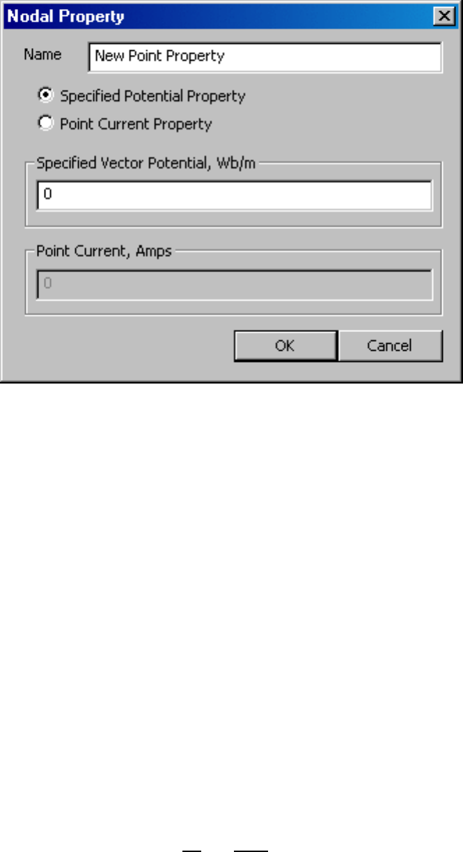
Figure 2.7: Nodal Property dialog.
The next selection is the
BC Type
drop list. This specifies the boundary condition type. Cur-
rently, FEMM supports the following types of boundaries:
•
Prescribed A
With this type of boundary condition, the vector potential, A, is prescribed
along a given boundary. This boundary condition can be used to prescribe the flux passing
normal to a boundary, since the normal flux is equal to the tangential derivative of A along
the boundary. The form for A along the boundary is specified via the parameters A
0
, A
1
,
A
2
and φ in the
Prescribed A parameters
box. If the problem is planar, the parameters
correspond to the formula:
A = (A
0
+ A
1
x+ A
2
y)e
jφ
(2.2)
If the problem type is axisymmetric, the parameters correspond to:
A = (A
0
+ A
1
r+ A
2
z)e
jφ
(2.3)
•
Small Skin Depth
This boundary condition denotes an interface with a material subject
to eddy currents at high enough frequencies such that the skin depth in the material is very
small. A good discussion of the derivation of this type of boundary condition is contained in
[2]. The result is a Robin boundary condition with complex coefficients of the form:
∂A
∂n
+
1+ j
δ
A = 0 (2.4)
24
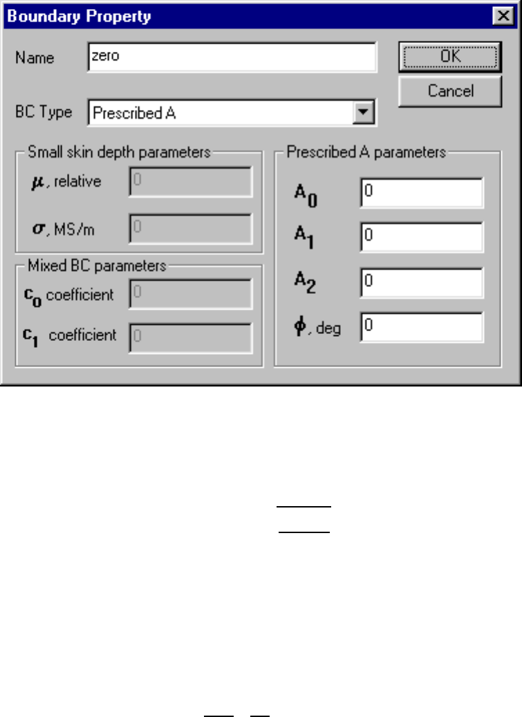
Figure 2.8: Boundary Property dialog.
where the n denotes the direction of the outward normal to the boundary and δ denotes the
skin depth of the material at the frequency of interest. The skin depth, δ is defined as:
δ =
s
2
ωµ
r
µ
o
σ
(2.5)
where µ
r
and σ are the relative permeability and conductivity of the thin skin depth eddy cur-
rent material. These parameters are defined by specifying µ and σ in the
Small skin depth
parameters
box in the dialog. At zero frequency, this boundary condition degenerates to
∂A/∂n = 0 (because skin depth goes to infinity).
•
Mixed
This denotes a boundary condition of the form:
1
µ
r
µ
o
∂A
∂n
+ c
o
A+ c
1
= 0 (2.6)
The parameters for this class of boundary condition are specified in the
MixedBC parameters
box in the dialog. By the choice of coefficients, this boundary condition can either be a Robin
or a Neumann boundary condition. There are two main uses of this boundary condition:
1. By carefully selecting the c
0
coefficient and specifying c
1
= 0, this boundary condi-
tion can be applied to the outer boundary of your geometry to approximate an up-
bounded solution region. For more information on open boundary problems, refer to
Appendix A.3.
25
2. The Mixed boundary condition can used to set the field intensity, H, that flows parallel
to a boundary. This is done by setting c
0
to zero, and c
1
to the desired value of H in
units of Amp/Meter. Note that this boundary condition can also be used to prescribe
∂A/∂n = 0 at the boundary. However, this is unnecessary–the 1
st
order triangle finite
elements give a ∂A/∂n = 0 boundary condition by default.
•
Strategic Dual Image
This is sort of an “experimental” boundary condition that I have
found useful for my own purposes from time to time. This boundary condition mimics
an “open” boundary by solving the problem twice: once with a homogeneous Dirichlet
boundary condition on the SDI boundary, and once with a homogeneous Neumann condition
on the SDI boundary. The results from each run are then averaged to get the open boundary
result. This boundary condition should only be applied to the outer boundary of a circular
domain in 2-D planar problems. Through a method-of-images argument, it can be shown
that this approach yields the correct open-boundary result for problems with no iron (i.e just
currents or linear magnets with unit permeability in the solution region).
•
Periodic
This type of boundary condition is applied to either two segments or two arcs to
force the magnetic vector potential to be identical along each boundary. This sort of bound-
ary is useful in exploiting the symmetry inherent in some problems to reduce the size of
the domain which must be modeled. The domain merely needs to be periodic, as opposed to
obeying more restrictive A = 0 or ∂A/∂n= 0 line of symmetry conditions. Another useful ap-
plication of periodic boundary conditions is for the modeling of “open boundary” problems,
as discussed in Appendix A.3.3. Often, a periodic boundary is made up of several different
line or arc segments. A different periodic condition must be defined for each section of the
boundary, since each periodic BC can only be applied to a line or arc and a corresponding
line or arc on the remote periodic boundary.
•
Antiperiodic
The antiperiodic boundary condition is applied in a similar way as the peri-
odic boundary condition, but its effect is to force two boundaries to be the negative of one
another. This type of boundary is also typically used to reduce the domain which must be
modeled, e.g. so that an electric machine might be modeled for the purposes of a finite
element analysis with just one pole.
Materials Properties
The
Block Property
dialog box is used to specify the properties to be associated with block la-
bels. The properties specified in this dialog have to do with the material that the block is composed
of, as well as some attributes about how the material is put together (laminated). When a new
material property is added or an existing property modified, the
Block Property
dialog pictured
in Figure 2.9 appears.
As with Point and Boundary properties, the first step is to choose a descriptive name for the
material that is being described. Enter it in the
Name
edit box in lieu of “New Material.”
Next decide whether the material will have a linear or nonlinear B-H curve by selecting the
appropriate entry in the
B-H Curve
drop list.
If
Linear B-H Relationship
was selected from the drop list, the next group of
Linear
Material Properties
parameters will become enabled. FEMM allows you to specify different
26
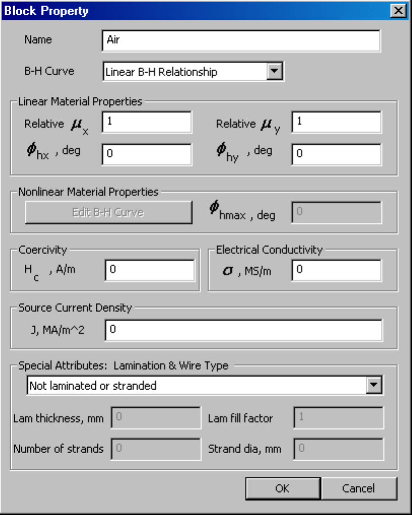
Figure 2.9: Block Property dialog.
27
relative permeabilities in the vertical and horizontal directions (µ
x
for the x- or horizontal direction,
and µ
y
for the y- or vertical direction).
There are also boxes for φ
hx
and φ
hy
, which denote the hysteresis lag angle corresponding to
each direction, to be used in cases in which linear material properties have been specified. A
simple, but surprisingly effective, model for hysteresis in harmonic problems is to assume that
hysteresis creates a constant phase lag between B and H that is independent of frequency. This is
exactly the same as assuming that hysteresis loop has an elliptical shape. Since the hysteresis loop
is not exactly elliptical, the perceived hysteresis angle will vary somewhat for different amplitudes
of excitation. The hysteresis angle is typically not a parameter that appears on manufacturer’s
data sheets; you have to identify it yourself from a frequency sweep on a toroidal coil with a core
composed of the material of interest. For most laminated steels, the hysteresis angle lies between 0
o
and 20
o
[6]. This same reference also has a very good discussion of the derivation and application
of the fixed phase lag model of hysteresis.
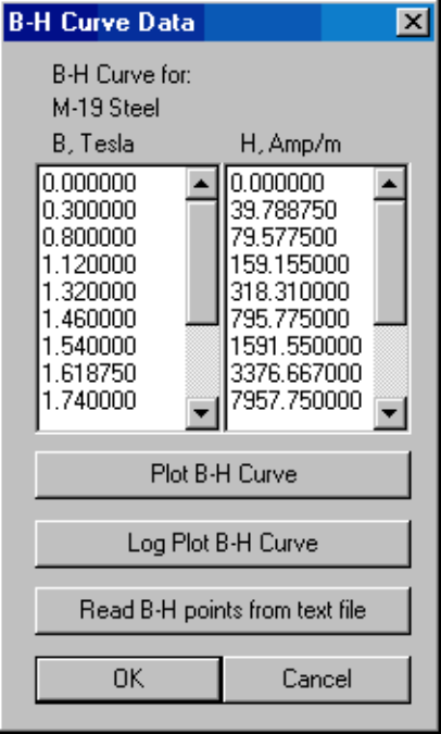
If
Nonlinear B-H Curve
was selected from the drop list, the
Nonlinear Material Properties
parameter group becomes enabled. To enter in points on your B-H curve, hit the
Edit B-H Curve
button. When the button is pushed a dialog appears that allows you to enter in B-H data (see Fig-
ure 2.10. The information to be entered in these dialogs is usually obtained by picking points off of
Figure 2.10: B-H data entry dialog.
manufacturer’s data sheets. For obvious reasons, you must enter the same number of points in the
28
“B” (flux density) column as in the “H” (field intensity) column. To define a nonlinear material,
you must enter at least three points, and you should enter ten or fifteen to get a good fit.
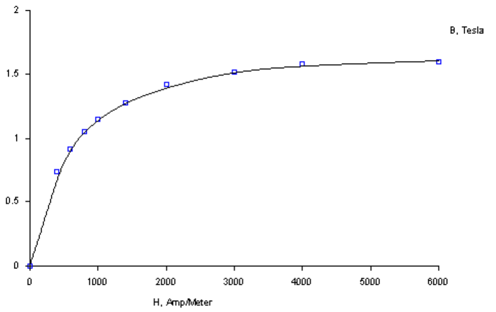
After you are done entering in your B-H data points, it is a good idea to view the B-H curve to
see that it looks like it is “supposed” to. This is done by pressing the
Plot B-H Curve
button or
the
Log Plot B-H Curve
button on the B-H data dialog. You should see a B-H curve that looks
something like the curve pictured in Figure 2.11. The boxes in the plot represent the locations of
Figure 2.11: Sample B-H curve plot.
the entered B-H points, and the line represents a cubic spline derived from the entered data. Since
FEMM interpolates between your B-H points using cubic splines, it is possible to get a bad curve
if you haven’t entered an adequate number of points. “Weird” B-H curves can result if you have
entered too few points around relatively sudden changes in the B-H curve. Femm “takes care of”
bad B-H data (i.e. B-H data that would result in a cubic spline fit that is not single-valued) by
repeatedly smoothing the B-H data using a three-point moving average filter until a fit is obtained
that is single-valued. This approach is robust in the sense that it always yields a single-valued
curve, but the result might be a poor match to the original B-H data. Adding more data points in
the sections of the curve where the curvature is high helps to eliminate the need for smoothing.
It may also be important to note that FEMM extrapolates linearly off the end of your B-H
curve if the program encounters flux density/field intensity levels that are out of the range of the
values that you have entered. This extrapolation may make the material look more permeable than
it “really” is at high flux densities. You have to be careful to enter enough B-H values to get an
accurate solution in highly saturated structures so that the program is interpolating between your
29
entered data points, rather than extrapolating.
Also in the nonlinear parameters box is a parameter, φ
hmax
. For nonlinear problems, the hys-
teresis lag is assumed to be proportional to the effective permeability. At the highest effective
permeability, the hysteresis angle is assumed to reach its maximal value of φ
hmax
. This idea can be
represented by the formula:
φ
h
(B) =
µ
ef f
(B)
µ
ef f,max
φ
hmax
(2.7)
The next entry in the dialog is H
c
. If the material is a permanent magnet, you should enter
the magnet’s coercivity here in units of Amperes per meter. There are some subtleties involved
in defining permanent magnet properties (especially nonlinear permanent magnets). Please refer
to the Appendix A.1 for a more thorough discussion of the modeling of permanent magnets in
FEMM.
The next entry represents J, the source current density in the block. The ”source current den-
sity” denotes the current in the block at DC. At frequencies other than DC in a region with non-zero
conductivity, eddy currents will be induced which will change the total current density so that it
is no longer equal to the source current density. Use ”circuit properties” to impose a value for the
total current carried in a region with eddy currents. Source current density can be complex valued,
if desired.
The σ edit box denotes the electrical conductivity of the material in the block. This value is
generally only used in time-harmonic (eddy current) problems. The units for conductivity are 10
6
Seymens/Meter (equivalent to 10
6
(Ω∗Meters)
−1
). For reference, copper at room temperature has
a conductivity of 58 MS/m; a good silicon steel for motor laminations might have a conductivity of
as low as 2 MS/m. Commodity-grade transformer laminations are more like 9 MS/m. You should
note that conductivity generally has a strong dependence upon temperature, so you should choose
your values of conductivity keeping this caveat in mind.
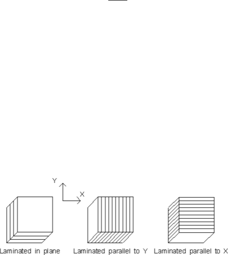
The last set of properties is the
Lamination and Wire Type
section. If the material is lami-
nated, the drop list in this section is used to denote the direction in which the material is laminated.
If the material is meant to represent a bulk wound coil, this drop list specifies the sort of wire from
which the coil is constructed.
The various selections in this list are illustrated in Figure 2.12 Currently, the laminations are
Figure 2.12: Different lamination orientation options.
30

constrained to run along a particular axis.
If some sort of laminated construction is selected in the drop list, the lamination thickness
and fill factor edit boxes become enabled. The lamination thickness, fill factor, and lamination
orientation parameters are used to implement a bulk model of laminated material. The result of
this model is that one can account for laminations with hysteresis and eddy currents in harmonic
problems. For magnetostatic problems, one can approximate the effects of nonlinear laminations
without the necessity of modeling the individual laminations separately. This bulk lamination
model is discussed in more detail in the Appendix (Section A.2).
The d
lam
edit box represents the thickness of the laminations used for this type of material. If
the material is not laminated, enter 0 in this edit box. Otherwise, enter the thickness of just the iron
part (not the iron plus the insulation) in this edit box in units of millimeters.
Associated with the lamination thickness edit box is the
Lam fill factor
edit box. This is
the fraction of the core that is filled with iron. For example, if you had a lamination in which the
iron was 12.8 mils thick, and the insulation bewteen laminations was 1.2 mils thick, the fill factor
would be:
Fill Factor =
12.8
1.2+ 12.8
= 0.914
If a wire type is selected, the
Strand dia.
and/or Number of strands edit boxes become
enabled. If the
Magnet wire
or
Square wire
types are selected, it is understood that there is can
only be one strand, and the
Number of strands
edit box is disabled. The wire’s diameter (or
width) is then entered in the
Strand dia.
edit box. For stranded and Litz wire, one enters the
number of strands and the strand diameter. Currently, only builds with a single strand gauge are
supported.
If a wire type is specified, the material property can be applied to a “bulk” coil region each
individual turn need not be modeled. In DC problems, the results will automatically be adjusted
for the implied fill factor. For AC problems, the the fill factor is taken into account, and AC
proximity and skin effect losses are taken into account via effective complex permeability and
conductivity that are automatically computed for the wound region.
Materials Library
Since one kind of material might be needed in several different models, FEMM has a built-in li-
brary of Block Property definitions. The user can access and maintain this library through the
Properties | Materials Library
selection off of the main menu. When this option is se-
lected, the
Materials Library
dialog pictured in Figure 2.13 appears. This dialog allow the user
to exchange Block Property definitions between the current model and the materials library via a
drag-and-drop interface.
A number of different options are available via a mouse button right-click when the cursor is
located on top of a material or folder. Materials can be edited by double-clicking on the desired
material.
Material from other material libraries or models can be imported by selecting the “Import
Materials” option from the right-button menu that appears when the pointer is over the root-level
folder of either the Library or Model materials lists.
The materials library should be located in the same directory as the FEMM executable files,
under the filename
mlibrary.dat
. If you move the materials library, femm will not be able to find
31
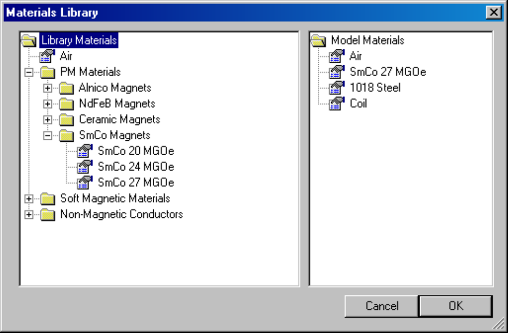
Figure 2.13: Materials Library dialog.
it.
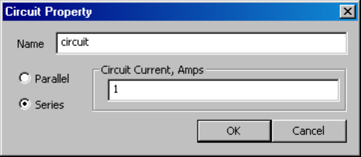
Circuit Properties
The purpose of the circuit properties is to allow the user to apply constraints on the current flowing
in one or more blocks. Circuits can be defined as either ”parallel” or ”series” connected.
If ”parallel” is selected, the current is split between all regions marked with that circuit property
on the basis of impedance ( current is split such that the voltage drop is the same across all sections
connected in parallel). Only solid conductors can be connected in parallel.
If ”series” is selected, the specified current is applied to each block labeled with that circuit
property. In addition, blocks that are labeled with a series circuit property can also be assigned a
number of turns, such that the region is treated as a stranded conductor in which the total current is
the series circuit current times the number of turns in the region. The number of turns for a region
is prescribed as a block label property for the region of interest. All stranded coils must be defined
as series-connected (because each turn is connected together with the other turns in series). Note
that the number of turns assigned to a block label can be either a positive or a negative number. The
sign on the number of turns indicated the direction of current flow associated with a positive-valued
circuit current.
For magnetostatic problems, one could alternatively apply a source current density over the
32
conductor of interest and achieve similar results. For eddy current problems, however, the “circuit”
properties are much more useful–they allow the user to define the current directly, and they allow
the user to assign a particular connectivity to various regions of the geometry. This information is
used to obtain impedance, flux linkage, etc., in a relatively painless way in the postprocessor.
By applying circuit properties, one can also enforce connectivity in eddy current problems.
By default, all objects in eddy current problems are “shorted together at infinity”–that is, there
is nothing to stop induced currents from returning in other sections of the domain that might not
be intended to be physically connected. By applying a parallel-connected circuit with a zero net
current density constraint to each physical “part” in the geometry, the connectivity of each part is
enforced and all is forced to be conserved inside the part of interest.
The dialog for entering circuit properties is pictured in Figure 2.14.
Figure 2.14: Circuit Property dialog
2.2.8 Exterior Region
One often desires to solve problems on an unbounded domain. Appendix A.3.3 describes an easy-
to-implement conformal mapping method for representing an unbounded domain in a 2D planar
finite element analysis. Essentially, one models two disks–one represents the solution region of
interest and contains all of the items of interest, around which one desires to determine the mag-
netic field. The second disk represents the region exterior to the first disk. If periodic boundary
conditions are employed to link the edges of the two disks, it can be shown (see Appendix A.3.3)
that the result is exactly equivalent to solving for the fields in an unbounded domain.
One would also like to apply the same approach to model unbounded axisymmetric problems,
as well as unbounded planar problems. Unfortunately, the Kelvin Transformation is a bit more
complicated for axisymmetric problems. In this case, the permeability of the external region has
to vary based on distance from the center of the external region and the outer radius of the external
region. The approach is described in detail in [20]. FEMM automatically implements the variation
of permeability in the exterior region, but a bit more information must be collected to perform
the permeability grading required in the external region. This is where the “External Region”
parameters come in–these are the parameters that the program needs to define the permeabilities
of elements in the external region for “unbounded” axisymmetric problems.
33

Specifically, there are three parametes that are collected in the dialog that appears when the
user selects the External Region properties. These are:
•
Center of Exterior Region
The location along the z-axis of the axisymmetric problem
where the center of the block representing the external region is located.
•
Radius of Exterior Region
Radius of the sphere representing the exterior region.
•
Radius of Interior Region
Radious of the spehre representing the interior region (i.e.
the region in which the items of interest are located).
To finish defining the axisymmetric external region, the
Block located in an external
region
check box must be selected in any block labels that are located in the region that is desired
to be the axisymmetric external region.
2.2.9 Analysis Tasks
Meshing the model, analyzing the model, and viewing the results are most easily performed by the
toolbar buttons pictured in Figure 2.15
Figure 2.15: Toolbar buttons for starting analysis tasks.
The first of these buttons (with the “yellow mesh” icon) runs the mesh generator. The solver
actually automatically calls the mesh generator to make sure that the mesh is up to date, so you
never have to call the mesher from within femm. However, it is almost always important to get
a look at the mesh and see that it “looks right.” When the mesh generation button is pressed,
the mesher is called. While the mesher is running, an entry labeled “triangle” will appear on
the Windows taskbar. After the geometry is triangulated, the finite element mesh is loaded into
memory and displayed underneath the defined nodes, segments, and block labels as a set of yellow
lines.
If you have a very large model, just keeping all of the mesh information in core can take up
a significant amount of memory. If you are about to analyze a very large problem, it might be a
good idea to choose the
Mesh | Purge Mesh
option off of the main menu. When this option is
selected, the mesh is removed from memory, and the memory that it occupied is freed for other
uses.
The second button, with the “hand-crank” icon, executes the solver,
fkern.exe
. Before fkern
is actually run, the Triangle is called to make sure the mesh is up to date. Then, fkern is called.
When fkern runs, it opens up a console window to display status information to the user. How-
ever, fkern requires no user interaction while it is running. When fkern is finished analyzing your
problem, the console window will disappear. The time that fkern requires is highly dependent
on the problem being solved. Solution times can range from less than a second to several hours,
depending upon the size and complexity of the problem. Generally, linear magnetostatic problems
take the least amount of time. Harmonic problems take slightly more time, because the answer is
in terms of complex numbers. The complex numbers effectively double the number of unknowns
34

as compared to a magnetostatic problem with the same mesh. The slowest problems to analyze
are nonlinear time-harmonic problems, since multiple successive approximation iterations must be
used to converge on the final solution. However, nonlinear problems almost never take more than
10 iterations. Later iterations in nonlinear problems are usually are quite fast compared to the first
iteration or two because the later iterations can be initialized with an approximate solution that is
very close to the “actual” solution.
For users who have a technical interest in what is “under the hood” in fkern, some details are
provided in the Appendix (Section 6).
The “big magnifying glass” icon is used to display the results in a postprocessing window
once the analysis is finished. A detailed description of the magnetics postprocessor addressed in
Section 2.3.
2.3 Magnetics Postprocessor
The the magnetics postprocessing functionality of femm is used to view solutions generated by the
fkern
solver. A magnetics postprocessor window can be opened either by loading some previously
run analyses via
File|Open
on the main menu, or by pressing the “big magnifying glass” icon from
within a preprocessor window to view a newly generated solution. Magnetics postprocessor data
files stored on disk have the
.ans
prefix.
2.3.1 Postprocessor modes
Similar to the preprocessor, the postprocessor always operates in one of three modes, depending
upon the task to be performed. These modes are:
• Point Values Mode In this mode, the user can click on various points in the solution region.
Local field values are then listed in the
FEMM Output
window.
• Contour Mode This mode allows the user to define arbitrary contours in the solution region.
Once a contour is defined, plots of field quantities can be produced along the contour, and
various line integrals can be evaluated along the contour.
• Block Mode The Block Mode lets the user define a subdomain in the solution region. Once
the block has been defined, a variety of area and volume integrals can be taken over the
defined subdomain. Integrals include stored energy (inductance), various kinds of losses,
total current in the block, and so on.
The current postprocessor mode is controlled via the Analysis Mode toolbar buttons, shown
in Figure 2.16. The buttons denote, respectively, Point Values mode, Contour Mode, and Block
Figure 2.16: Analysis Mode toolbar buttons
Mode. The depressed button denotes the current mode. The default mode when postprocessor
starts is Point Values mode.
35
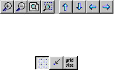
2.3.2 View and Grid Manipulation
The aspects of the current view and of the current grid are regulated via the use of toolbar buttons.
The view is manipulated by the following toolbar buttons: and the grid settings are manipulated by
Figure 2.17: View Manipulation toolbar buttons.
these grid manipulation toolbar buttons: The grid and view manipulation work in exactly the same
Figure 2.18: Grid Manipulation toolbar buttons.
fashion as these same features in the preprocessor. Refer to Section 2.2.4 for a detailed description
of grid manipulation, and to Section 2.2.3 for view manipulation.
2.3.3 Keyboard Commands
Unlike the preprocessor, postprocessor is not very dependent on keyboard commands.
In the Point Values mode, there is only one relevant keypress. In this mode, the Tab key allows
the user to enter the coordinates of a specific point. After the coordinates of a point are entered,
the field values at that point are displayed in the
FEMM Output
window.
In the Contours, there are four relevant keys. Pressing the Escape key wipes out any current
contour or block definition. Pressing the Delete removes the last point added to the current contour
or block edge. Pressing the Shift key allows the user to turn the last segment in the prescribed
contour from a straight line into an arc. A dialog pops up after the key is pressed that prompts for
attributes of the the desired arc. Last, pressing the Tab keys allows the user to numerically enter
the coordinates of a point to be included in the current contour.
In the Block mode, the Escape and Delete keys have the same definition as in Contours mode.
In the Block mode, the Tab key does not do anything, since all points on the contour must also be
Points defining the model’s geometry.
2.3.4 Mouse Actions
In contrast, the operation of the postprocessor is very dependent upon input from the mouse.
In the Point Values mode, a Left Button Click is used to display field values at the current
mouse location. If Snap to Grid is enabled, values are displayed at the closes grid point instead.
In the Contours mode, mouse clicks are used to define the contour. A Left Button Click adds
the closest Point in the model’s geometry. Via a Right Button Click, the current mouse pointer
location is added to the contour. A contour appears as a red line on the screen.
Blocks are defined in Block mode in a fashion very similar to the way in which contours are
defined. A block is defined by by drawing a contour around the region of interest. The contour
36
appears as a green line on the postprocessor screen. When the ends of the contour meet, the block
is defined. All elements enclosed by the contour (all elements that form the block) then turn green
in the postprocessor window.
A Left Button Click attempts to add the nearest Point in the input geometry to the Block’s con-
tour. However, a block can only be defined along line and arc segments from the input geometry.
Each node on the boundary of the block must be selected in order to form the Block boundary. In
Block mode, the Right mouse button has no function.
2.3.5 Miscellaneous Useful View Commands
There are some additional entries on the postprocessor
View
menu that might be useful to you from
time to time. These are:
•
Smoothing
By default, a smoothing algorithm is applied to the flux density solution. Be-
cause first-order triangles are used as trial functions for vector potential, the resulting flux
density and field intensity distributionsare piece-wise constant in each element. The smooth-
ing algorithm uses a nearest neighbor interpolation to obtain linear B and H distributions over
each element. The smoothed solution generally looks better on the screen, and somewhat
increases the accuracy of B and H near the vertices of each element. However, if you want
to toggle smoothing, this can be done by selecting the
Smoothing
option.
•
Show Points
Especially when making graphics for reports, presentations, etc, it may be
desirable to hide the small boxes on the screen that denote input node points. The
Show
Points
option allows the user to toggle whether or not the input points are shown.
•
ToolBar
Use this toggle to hide and show the floating toolbar.
•
Point Props
Use this toggle to hide and show the floating dialog box used to display point
property information.
2.3.6 Contour Plot
One of the most useful ways to get a subjective feel for a magnetics finite element solution is by
plotting the “flux lines.” These are the streamlines along which flux flows in the finite element
geometry. Where flux lines are close together, the flux density is high. In FEMM’s vector potential
formulation, flux lines are simply plots of the level contours of the vector potential, A, in planar
problems, or level contours of 2πrA in axisymmetric problems.
For harmonic problems, the contours are a little more subtle–A has both real and imaginary
components. In this case, postprocessor allows the user to plot contours of either the real or the
imaginary part of A. Real contours appear black, and Imaginary contours appear as grey.
By default, a set of 19 flux lines are plotted when a solution is initially loaded into postproces-
sor. The number and type of flux lines to be plotted can be altered using the Contours Plot icon in
the Graph Mode section of the toolbar (see Figure 2.19. The Contour Plot icon is the icon with the
black contours. When this button is pressed, a dialog pops up, allowing the choice of the number
of contours (between 4 and 100 are allowed), and which contours to plot (either real, imaginary, or
none).
37
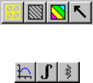
Figure 2.19: Graph Mode toolbar buttons.
Figure 2.20: Line Plot, Integration, and Circuit Results toolbar buttons
In the contour plot dialog, a check box is also present titled “Show stress tensor mask”. If this
box is checked, the contour lines associated with the last Weighted Stress Tensor integration are
also displayed, by default as orange flux lines.
2.3.7 Density Plot
Density plots are also a useful way to get a quick feel for the flux density in various parts of the
model. A density plot can be displayed by pressing the middle button in the Graph Mode section
of the toolbar (see Figure 2.19). A dialog the pops up that allows the user to turn density plotting
on. The user can choose to plot flux density, field intensity, or current density. If the solution is to
a harmonic problem, the user can choose to plot either the magnitude or just the real or imaginary
part of these quantities.
The flux density at each point is classified into one of twenty contours distributed evenly be-
tween either the minimum and maximum flux densities or user-specified bounds.
2.3.8 Vector Plots
A good way of getting a feel for the direction and magnitude of the field is with plots of the field
vectors. With this type of plot arrows are plotted such that the direction of the arrow indicates the
direction of the field and the size of the arrow indicates the magnitude of the field. The presence
and appearance of this type of plot can be controlled by pressing the “arrows” icon pictured in
Figure 2.19.
2.3.9 Line Plots
When postprocessor is in Contours Mode, various field values of interest can be plotted along the
defined contour. A plot of a field value defined contour is performed by pressing the “graphed
function” icon in the Plot, Integration, and Circuit Results group of toolbar buttons, shown in
Figure 2.20. When this button is pressed, the
X-Y Plot
dialog (see Figure 2.21) appears with a
drop list containing the types of line plots available. Choose the desired type of plot and press
“OK.”
After “OK” is pressed, the program computes the desired values along the defined contour.
These values are then plotted using the
femmplot
program, which is called automatically to display
the plot.
By default, the
Write data to text file
box is not checked. If the user selects this option,
the file selection dialog will appear and prompt for a filename to which to write the data. The
38
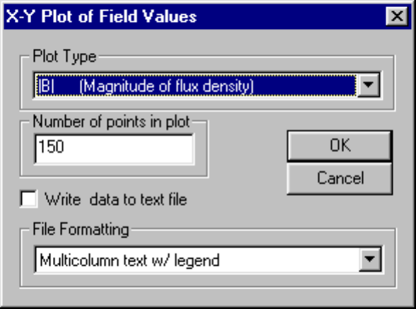
Figure 2.21: X-Y Plot dialog.
data is written in two-column text format. If
Write data to text file
is selected, a femmplot
window will not appear.
Currently, the type of line plots supported are:
• Vector potential along the contour;
• Magnitude of the flux density along the contour;
• Component of flux density normal to the contour;
• Component of flux density tangential to the contour;
• Magnitude of the field intensity along the contour;
• Component of field intensity normal to the contour;
• Component of field intensity tangential to the contour;
In all of these plots, the direction of the normal is understood to be as shown in Figure 2.22.
The tangential direction is understood to be the direction in which the contour was defined.
In certain cases, the quantity to be plotted can be ambiguous. This can occur, for example, if a
plot of the tangential field intensity is requested on a contour running along an interface between
air and a piece of iron. In this case, there is a discontinuity in the tangential field intensity, and
the value of this quantity is different on each side of the interface. The postprocessor resolves the
conflict by always evaluating the plots at a differentially small distance to the “normal” side of
the line. Therefore, by defining the same contour but reversing the order in which the points are
specified, plots of the quantity of interest on each side of a boundary can be obtained.
39
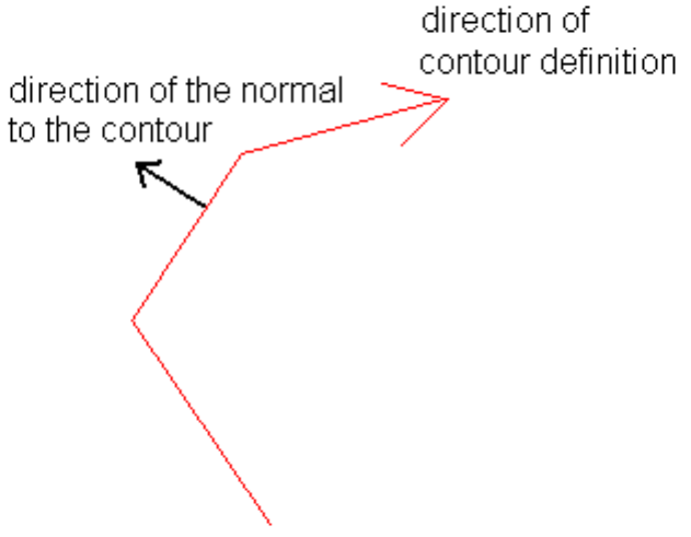
Figure 2.22: When in doubt plots and integrals taken on this side of a contour.
2.3.10 Line Integrals
Once a contour has been specified in Contours mode, Line Integrals can be performed along the
specified contour. These integrals are performed by evaluating a large number of points at evenly
spaced along the contour and integrating using a simple trapezoidal-type integration scheme.
To perform an integration, press the “integral” icon on the toolbar (as shown in Figure 2.20).
A small dialog will appear with a drop list. Choose the desired integral from the drop list and
press
OK
. The amount of time required to perform the integral will be virtually instantaneous for
some types of integrals; however, some types may require several seconds to evaluate. When the
evaluation of the integral is completed, the answer appears on the screen in a pop-up box.
One “tip” that may aid with the definition of contours of integration is that a curved integration
contour can be defined in a fairly painless fashion by hitting the Shift key. Hitting the Shift key
tells the program to turn the last segment in the defined integration contour into an arc segment. A
dialog then pops up that prompts for the desired attributes of the arc.
The line integrals currently supported are:
•
B.n
. This integral returns the total flux passing normal to the contour. This integral is useful
for determining the total flux in a bulk flux path. This result might then be compared to
predictions from a simpler magnetic circuit model, for example.
•
H.t
. The integral of the tangential field intensity along the contour yields the magnetomotive
force drop between the endpoints of the contour. Again, this integral is useful for comparison
to or validation of magnetic circuit models.
•
Contour Length
. This integral returns the length of the defined contour in meters.
40

•
Force from stress tensor
. This integral totals the force produced on the contour de-
rived from Maxwell’s stress tensor. Deriving meaningful force results requires some care in
the choice of integration path; refer to Section 2.3.12 for a detailed discussion of force and
torque calculation.
•
Torque from stress tensor
. This selection integrates the torque about the point (0,0)
inferred from Maxwell’s stress tensor. Again, some guidelines must be followed to get
accurate torque results (see Section 2.3.12).
•
B.nˆ2
. This selection evaluates the integral of the square of the normal flux along the line.
This integral is not so commonly used, but it has been useful in the past for some specialized
purposes, like determining the RMS amplitude of a periodic flux distribution.
2.3.11 Block Integrals
Once a closed contour has been specified in Block mode and the block appears highlighted in
green, Block Integrals over the specified area. These integrals are performed by analytically inte-
grating the specified kernel over each element in the defined region, and summing the results for
all elements.
To perform an integration, press the “integral” icon on the toolbar (as shown in Figure 2.20). A
small dialog will appear with a drop list. Choose the desired integral from the drop list and press
OK
. Generally, volume integrals take several seconds to evaluate, especially on dense meshes. Be
patient. When the evaluation of the integral is completed, the answer appears on the screen in a
pop-up box.
The block integrals currently supported are:
•
A.J
This integral is the evaluation of
R
A·JdV that is usually used evaluate inductance for
linear problems. Generally, the self-inductance of a coil is:
L
sel f
=
R
A·JdV
i
2
(2.8)
where i is the current flowing through the coil.
•
A
This integral, the evaluation of
R
AdV, can be used to evaluate mutual inductances between
coils. Similar to the formula for self inductance, mutual inductance is:
L
mutual
=
R
A
1
·J
2
dV
2
i
1
i
2
(2.9)
where A
1
is the component of A produced by the first coil, J
2
is the current in the second
coil, and i
1
and i
2
are the current in the first and second coils, respectively. dV
2
is meant to
denote that the integral is taken over the volume of the second coil. We can rearrange (2.9)
into a somewhat simpler form by noting that n
2
∗i
2
= J
2
∗a
2
. That is, the total amps times
turns for the second coil equals the current density in the second coil times the second coil’s
cross-section area. Substituting for J
2
in (2.9) yields:
L
mutual
=
n
2
i
1
a
2
Z
J
2+
A
1
dV
2
−
Z
J
2−
A
1
dV
2
(2.10)
41

where the first bracketed term in (2.10) is the contribution from the turns of coil 2 that are
pointed out of the page and the second term is the contribution from the turns of coil 2 that
are pointed into the page. To evaluate mutual inductance with FEMM, one substitutes values
into (2.10). First, run the model with only “coil 1” turned on. Then, integrate A over the
volume in which the second coil lies (although the second coil is not turned on). For planar
problems, you will typically have to make two separate integrations–one over the region
where the turns in “coil 2” are pointed out of the page (i.e. that part of the coil in which
a positive current results in current flowing in the out-of-the-page direction), and one over
the region in which the turns in “coil 2” are pointed into the page. Add these two results
together to get the total A
1
dV
2
integral. Lastly, multiply the integral result times n
2
/(i
1
a
2
) to
get mutual inductance.
•
Magnetic field energy
This selection calculates the energy stored in the magnetic field
in the specified region. This integral can be used as an alternate method of getting inductance
for problems that are linear (at least not heavily saturated). Denoting E as the energy stored
in the magnetic field, inductance can be obtained by solving the formula:
E =
Li
2
2
(2.11)
In the case of nonlinear materials, the energy is computed via:
W =
Z
Z
B
0
H(B
′
)dB
′
dV (2.12)
to take proper account of the energy under nonlinear conditions
•
Magnetic field coenergy
For linear problems, coenergy is numerically the same as en-
ergy. For nonlinear problems, coenergy is defined as:
W
c
=
Z
Z
H
0
B(H
′
)dH
′
dV (2.13)
Coenergy can be used in an alternative method of force and torque computation. To compute
force via coenergy, currents are held constant, and the position of the object upon which the
force is desired is perturbed slightly. The force can then be estimated by:
F =
W
c
(p+ δ) −W
c
(p)
δ
(2.14)
where p denotes the initial position, p+ δ denotes the perturbed position, and δ is the mag-
nitude of the perturbation. The component of force determined in this way acts along the
direction of the perturbation–one has to perform two such operations to get both horizontal
and vertical components of the force.
•
Hyst. and/or Laminated eddy current losses
. This selection is typically used to
obtain the core losses produced in laminated iron sections in harmonic problems.
•
Resistive losses
This selection integrates the i
2
R losses due to currents flowing in the
“z” direction (or θ direction, if you are evaluating an axisymmetric problem).
42
•
Block cross-section area
•
Total losses
This selection totals the losses from all possible loss mechanisms that might
apply over the given block. This is especially useful for finding losses in a region that might
enclose several different types of materials with different loss mechanisms.
•
Lorentz force (JxB)
Lorentz force is the force produced by a magnetic field acting upon
a current:
F
Lorentz
=
Z
J ×BdV (2.15)
Many devices (e.g. voice coil actuators) produce forces in a fashion that can be evaluated
using this integral.
•
Lorentz torque (rxJxB)
This selection computes the torque about (0,0) resulting from
Lorentz forces.
•
Integral of B over block
This integral can be useful in computing Lorentz forces. Since
Lorentz force is J×B, the force that would be produced if a coil were placed in a certain part
of the solution domain can be inferred by integrating B, and then scaling times an arbitrarily
chosen current density to get force.
•
Total current
This integral returns the total specified currents in the given block.
•
Block Volume
For axisymmetric problems, this selection returns the volume swept out by
the selected block.
•
Force via Weighted Stress Tensor
The Weighted Stress Tensor block is a volume in-
tegral version of Maxwell’s stress tensor that automatically picks a collection of paths for the
integration that yield “good” force results. This approach is similar to the weighted stress
tensor approach described in [7] and/or [8].
To compute the force on a region or set of regions, the user selects the blocks upon which
force result is desired and selects the
Force via Weighted Stress Tensor
integral. The
program then computes the weighting function by solving an additional Laplace equation
over the air surrounding the blocks upon which the force is to be computed. It may take a
few seconds to compute the weighting function–progress is be indicated by a progress bar
that is displayed while the weighting function is being computed. The stress tensor is then
evaluated as a volume integration, and the results are displayed. The results are typically
more accurate than the Maxwell Stress Tensor line integral, since in some sense, all possible
contours have been averaged to yield the Weighted Stress Tensor force result.
If the user is interested in the contours along which the integral was performed, the ”stress
tensor mask” box can be checked in the contour plot dialog. A set of orange (by default)
lines will be displayed that.
•
Torque via Weighted Stress Tensor
This integral is torque version of the
Force via
Weighted Stress Tensor
integral. Instead of force, torque about (0,0) is computed using
the same weighting function approach.
43

•
Rˆ2 (i.e. Moment of Inertia/density)
This integral is used to determine the moment
of inertial of the selected blocks. To obtain moment of inertia, the result of this integral must
be multiplied by the density of the selected region. For 2D planar problems, the moment of
inertia about the z-axis (i.e. about x=0,y=0) is computed. For axisymmetric problems, the
integral is computed about the r=0 axis.
2.3.12 Force/Torque Calculation
Ultimately, the estimation of magnetically produced forces and torques is often the goal of a finite
element analysis. This section discusses some of the different methods of deducing forces and
torques using FEMM.
Lorentz Force/Torque
If one is attempting to compute the force on a collection of currents in a region containing only
materials with a unit relative permeability, the volume integral of Lorentz torque is always the
method to employ. Lorentz force results tend to be very accurate. However, again, they are only
applicable for the forces on conductors of with unit permeability (e.g. coils in a voice coil actuator).
Weighted Stress Tensor Volume Integral
This volume integral greatly simplifies the computation of forces and torques, as compared to
evaluating forces via the stress tensor line integral of differentiation of coenergy. Merely select the
blocks upon which force or torque are to be computed and evaluate the integral. No particular “art”
is required in getting good force or torque results (as opposed to the Stress tensor line integral),
although results tend to be more accurate with finer meshing around the region upon which the
force or torque is to be computed.
One limitation of the Weighted Stress Tensor integral is that the regions upon which the force is
being computed must be entirely surrounded by air and/or abutting a boundary. In cases in which
the desired region abuts a non-air region, force results may be deduced from differentiation of
coenergy–see (2.14).
Maxwell Stress Tensor Line Integral
The indiscriminate use Maxwell’s Stress Tensor can result in bad predictions forces and torques.
The goal of this section is to explain how to set up problems and properly choose integration
paths so that good estimations of force and torque might be obtained via stress tensor methods.
Generally, you should not use the Stress Tensor line integral to compute forces and torques if it can
be avoided (i.e. use the volume integral version instead).
Maxwell’s stress tensor prescribes a force per unit area produced by the magnetic field on a
surface. The differential force produced is:
dF =
1
2
(H(B·n) + B(H ·n) −(H ·B)n) (2.16)
where n denotes the direction normal to the surface at the point of interest. The net force on an
object is obtained by creating a surface totally enclosing the object of interest and integrating the
magnetic stress over that surface.
44
While an integration of (2.16) theoretically gives the magnetic force on an object, numerical
problems arise when trying to evaluate this integral on a finite element mesh made of first-order
triangles. Though the solution for vector potential A is relatively accurate, the distributions of B
and H are an order less accurate, since these quantities are obtained by differentiating the trial
functions for A. That is, A is described by a linear function over each element, but B and H are
piece-wise constant over each element. Errors in B and H can be particularly large in elements in
which the exact solution for B and H changes rapidly–these areas are just not well approximated
by a piece-wise approximation. Specifically, large errors can arise in the tangential components
of B and H in elements adjacent to boundaries between materials of different permeabilites. The
worst errors arise on this sort of interface at corners, where the exact solution for B is nearly a
singularity.
If the stress tensor integral is evaluated on the interface between two different materials, the
results will be particularly erroneous. However, the stress tensor has the property that, for an
exact solution, the same result is obtained regardless of the path of integration, as long as that path
encircles the body of interest and passes only through air (or at least, every point in the contour
is in a region with a constant permeability). This implies that the stress tensor can be evaluated
over a contour a few elements away from the surface of an object–where the solution for B and
H is much more accurate. Much more accurate force results will be obtained by integrating along
the contour a few elements removed from any boundary or interface. The above discussion is the
rationale for the first guideline for obtaining forces via stress tensor:
Never integrate stress stress tensor along an interface between materials. Always de-
fine the integration contour as a closed path around the object of interest with the
contour displaced several elements (at least two elements) away from any interfaces
or boundaries.
As an example of a properly defined contour, consider Figure 2.23. This figure represents a
horseshoe magnet acting on a block of iron. The objective is to obtain the magnetic forces acting
upon the iron block. The red line in the figure represents the contour defined for the integration.
The contour was defined running clockwise around the block, so that the normal to the contour
points outward. Always define your contour in a clockwise direction to get the correct sign. Note
that the contour is well removed from the surface of the block, and the contour only passes through
air. To aid in the definition of a closed contour, grid and the “snap to grid” were turned on, and the
corners of the contour are grid points that were specified by right mouse button clicks.
The second rule of getting good force results is:
Always use as fine a mesh as possible in problems where force results are desired.
Even though an integration path has been chosen properly (away from boundaries and interfaces),
some significant error can still arise if a coarse mesh is used. Note that (2.16) is composed of B
2
terms – this means that stress tensor is one order worse in accuracy than B. The only way to get
that accuracy back is to use a fine mesh density. A good way to proceed in finding a mesh that is
“dense enough” is to solve the problem on progressively finer meshes, evaluating the force on each
mesh. By comparing the results from different mesh densities, you can get and idea of the level
of accuracy (by looking at what digits in the answer that change between various mesh densities).
You then pick the smallest mesh density that gives convergence to the desired digit of accuracy.
45
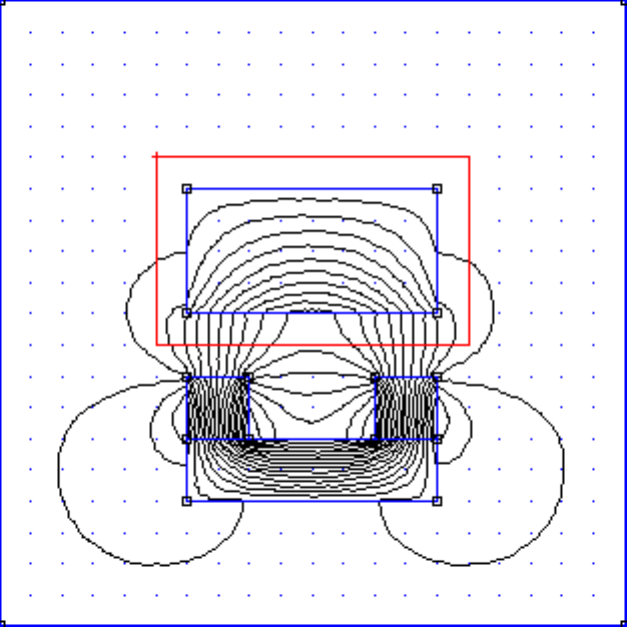
Figure 2.23: Properly defined contour for integration of Maxwell’s Stress Tensor
For torque computations, all the same rules apply as for force computations (i.e. define inte-
gration contours away from boundaries and interfaces, and use a dense mesh).
2.3.13 Circuit Results
If “circuit” properties are used to specify the excitation, a number of useful properties relative to
the circuit are automatically available. To view the circuit results, either press the ”Circuit Results”
button on the toolbar pictured in Figure 2.20 or select
View|Circuit
Props off of the postprocessor
main menu. A dialog, as pictured in Figure 2.24 will appear. There is a drop list on the dialog,
from which the user selects the circuit for which results are desired.
2.4 Electrostatics Preprocessor
The preprocessor is used for drawing the problems geometry, defining materials, and defining
boundary conditions. The process of construction of electrostatics problems is mechanically nearly
identical to the construction of magnetics problems–refer to Sections 2.2.1 through 2.2.5 for an
overview of the FEMM editing and problem creation commands. This section considers those
parts of problem definition that are unique to electrostatics problems.
46
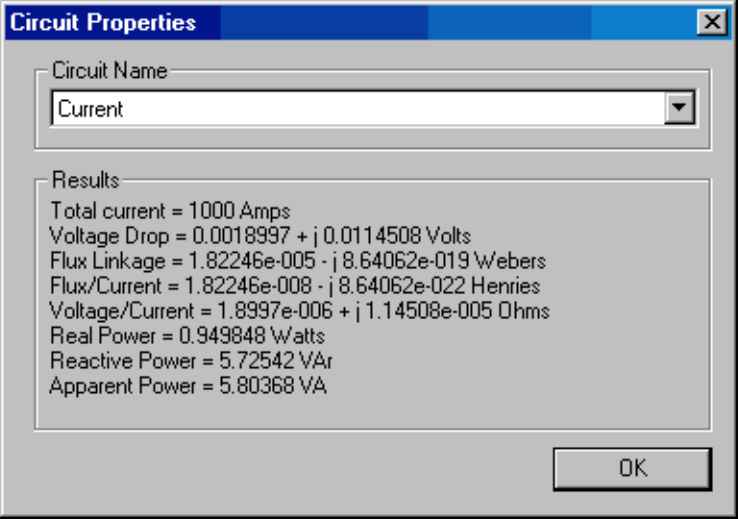
Figure 2.24: Circuit results dialog.
2.4.1 Problem Definition
The definition of problem type is specified by choosing the
Problem
selection off of the main
menu. Selecting this option brings up the Problem Definition dialog, shown in Figure 2.25.
The first selection is the
Problem Type
drop list. This drop box allows the user to choose from
a 2-D planar problem (the
Planar
selection), or an axisymmetric problem (the
Axisymmetric
selection).
Next is the
Length Units
drop list. This box identifies what unit is associated with the dimen-
sions prescribed in the model’s geometry. Currently, the program supports inches, millimeters,
centimeters, meters, mils, and µmeters.
The first edit box is the
Depth
specification. If a Planar problem is selected, this edit box
becomes enabled. This value is the length of the geometry in the “into the page” direction. This
value is used for scaling integral results in the post processor (e.g. force, inductance, etc.) to the
appropriate length. The units of the Depth selection are the same as the selected length units.
The second edit box is the
Solver Precision
edit box. The number in this edit box specifies
the stopping criteria for the linear solver. The linear algebra problem could be represented by:
Mx = b (2.17)
where M is a square matrix, b is a vector, and x is a vector of unknowns to be determined. The
solver precision value determines the maximum allowable value for ||b−Mx||/||b||. The default
value is 10
−8
.
The third edit box is labeled
Min Angle
. The entry in this box is used as a constraint in the
Triangle meshing program. Triangle adds points to the mesh to ensure that no angles smaller
47
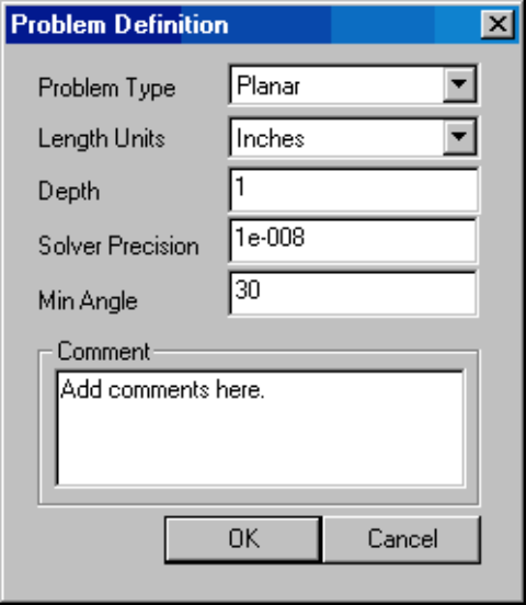
Figure 2.25: Problem Definition dialog.
than the specified angle occur. If the minimum angle is 20.7 degrees or smaller, the triangulation
algorithm is theoretically guaranteed to terminate (assuming infinite precision arithmetic – Triangle
may fail to terminate if you run out of precision). In practice, the algorithm often succeeds for
minimum angles up to 33.8 degrees. For highly refined meshes, however, it may be necessary
to reduce the minimum angle to well below 20 to avoid problems associated with insufficient
floating-point precision. The edit box will accept values between 1 and 33.8 degrees.
Lastly, there is an optional
Comment
edit box. The user can enter in a few lines of text that give
a brief description of the problem that is being solved. This is useful if the user is running several
small variations on a given geometry. The comment can then be used to identify the relevant
features for a particular geometry.
2.4.2 Definition of Properties
To make a solvable problem definition, the user must identify boundary conditions, block materials
properties, and so on. The different types of properties defined for a given problem are defined via
the
Properties
selection off of the main menu.
When the
Properties
selection is chosen, a drop menu appears that has selections for Ma-
terials, Boundary, Point, and Conductors. When any one of these selections is chosen, the dialog
pictured in Figure 2.26 appears.
This dialog is the manager for a particular type of properties. All currently defined properties
are displayed in the
Property Name
drop list at the top of the dialog. At the beginning of a new
model definition, the box will be blank, since no properties have yet been defined. Pushing the
Add
48
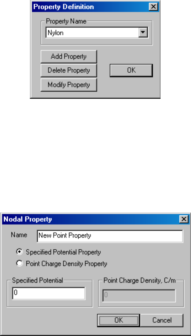
Figure 2.26: Property Definition dialog box.
Property
button allows the user to define a new property type. The
Delete Property
button
removes the definition of the property currently in view in the
Property Name
box. The
Modify
Property
button allows the user to view and edit the property currently selected in the
Property
Name
box. Specifics for defining the various property types are addressed in the following subsec-
tions.
Point Properties
If a new point property is added or an existing point property modified, the
Nodal Property
dialog box appears. This dialog box is pictured in Figure 2.27.
Figure 2.27: Nodal Property dialog.
The first selection is the
Name
edit box. The default name is “New Point Property,” but this
name should be changed to something that describes the property that you are defining.
49
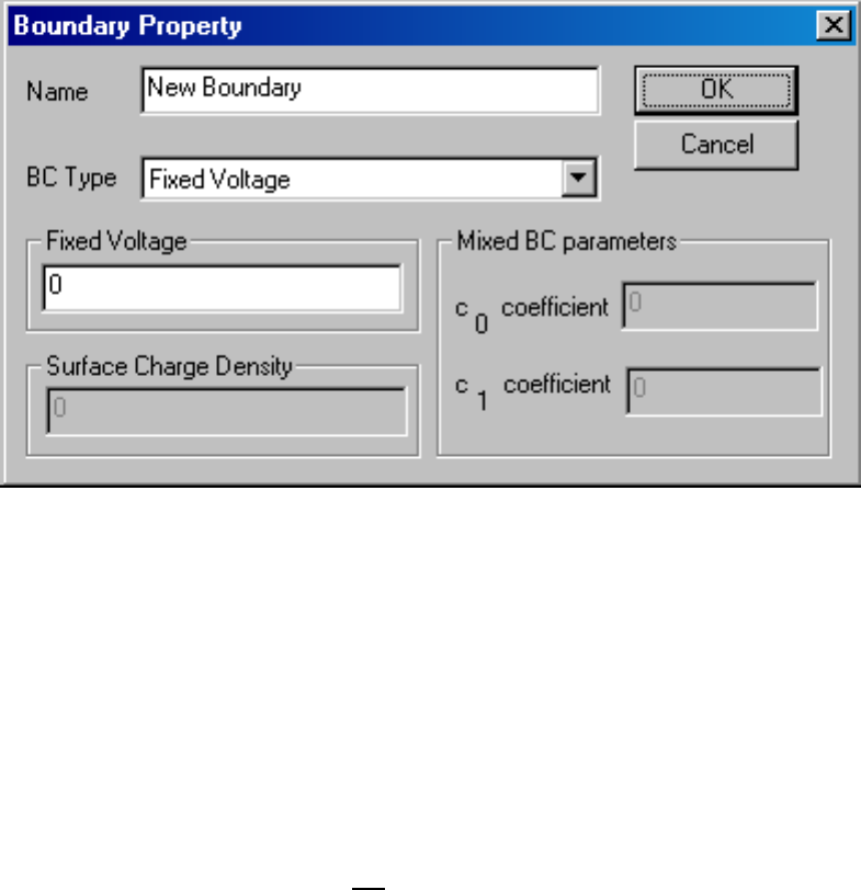
Next are edit boxes for defining the voltage at a given point, or prescribing a point charge
density at a given point. The type of point property is chosen via the radio buttons, and the value
is entered in the enabled edit box.
Boundary Properties
The
Boundary Property
dialog box is used to specify the properties of line segments or arc
segments that are to be boundaries of the solution domain. When a new boundary property is
added or an existing property modified, the
Boundary Property
dialog pictured in Figure 2.28
appears.
Figure 2.28: Boundary Property dialog.
The first selection in the dialog is the
Name
of the property. The default name is “New Bound-
ary,” but you should change this name to something more descriptive of the boundary that is being
defined.
The next selection is the
BC Type
drop list. This specifies the boundary condition type. Cur-
rently, FEMM electrostatics problems support the following types of boundaries:
Fixed Voltage
With this type of boundary condition, potential V is set to a prescribed along
a given boundary
Mixed
This denotes a boundary condition of the form:
ε
r
ε
o
∂V
∂n
+ c
o
V + c
1
= 0 (2.18)
The parameters for this class of boundary condition are specified in the
Mixed BC parameters
box in the dialog. By the choice of coefficients, this boundary condition can either be a Robin or
a Neumann boundary condition. By carefully selecting the c
0
coefficient and specifying c
1
= 0,
this boundary condition can be applied to the outer boundary of your geometry to approximate
50
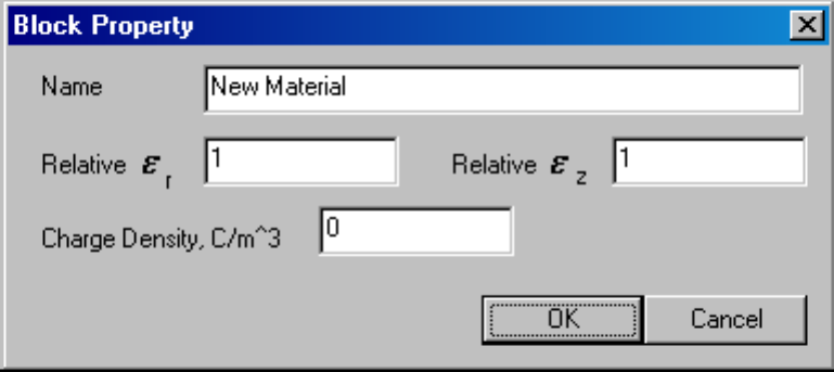
an unbounded solution region. For more information on open boundary problems, refer to the
Appendix.
Surface Charge Density
This selection is used to apply distributions of line charge to seg-
ments or arc segments in the problem. Unlike all of the other boundary conditions, this BC type is
often used on internal boundaries between materials or on isolated segments. Typically, other BCs
are only used on exterior boundaries.
Periodic
This type of boundary condition is applied to either two segments or two arcs to force
the potential to be identical along each boundary. This sort of boundary is useful in exploiting the
symmetry inherent in some problems to reduce the size of the domain which must be modeled. The
domain merely needs to be periodic, as opposed to obeying more restrictive V = 0 or ∂V/∂n = 0
line of symmetry conditions. Another useful application of periodic boundary conditions is for the
modeling of “open boundary” problems, as discussed in Appendix 3. Often, a periodic boundary
is made up of several different line or arc segments. A different periodic condition must be defined
for each section of the boundary, since each periodic BC can only be applied to a line or arc and a
corresponding line or arc on the remote periodic boundary.
Antiperiodic
The antiperiodic boundary condition is applied in a similar way as the periodic
boundary condition, but its effect is to force two boundaries to be the negative of one another. This
type of boundary is also typically used to reduce the domain which must be modeled, e.g. so that
an electric machine might be modeled for the purposes of a finite element analysis with just one
pole.
Materials Properties
The
Block Property
dialog box is used to specify the properties to be associated with block
labels. The properties specified in this dialog have to do with the material of which the block is
composed. When a new material property is added or an existing property modified, the
Block
Property
dialog pictured in Figure 2.29 appears.
Figure 2.29: Block Property dialog.
As with Point and Boundary properties, the first step is to choose a descriptive name for the
material that is being described. Enter it in the
Name
edit box in lieu of “New Material.”
51
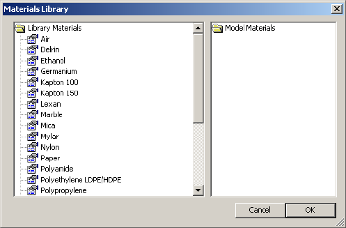
Next, permittivity for the material needs to be specified. FEMM allows you to specify different
relative permittivities in the vertical and horizontal directions (ε
x
for the x- or horizontal direction,
and ε
y
for the y- or vertical .
A volume charge density (ρ) can also be prescribed by filling in the appropriate box in the
material properties dialog.
Materials Library
Since one kind of material might be needed in several different models, FEMM has a built-in li-
brary of electrostatic Block Property definitions. The user can access and maintain this library
through the
Properties
|
Materials Library
selection off of the main menu. When this op-
tion is selected, the
Materials Library
dialog pictured in Figure 2.30 appears.
Figure 2.30: Materials Library dialog
This dialog allow the user to exchange Block Property definitions between the current model
and the materials library via a drag-and-drop interface.
A number of different options are available via a mouse button right-click when the cursor is
located on top of a material or folder. Materials can be edited by double-clicking on the desired
material.
Material from other material libraries or models can be imported by selecting the “Import
Materials” option from the right-button menu that appears when the pointer is over the root-level
folder of either the Library or Model materials lists.
The materials library should be located in the same directory as the femm executable files,
under the filename
statlib.dat
. If you move the materials library, femm will not be able to find
it.
Conductor Properties
The purpose of the conductor properties is mainly to allow the user to apply constraints on the
total amount of charge carried on a conductor. Alternatively, conductors with a fixed voltage can
be defined, and the program will compute the total charge carried on the conductor during the
solution process.
52

For fixed voltages, one could alternatively apply a
Fixed Voltage
boundary condition. How-
ever, applying a fixed voltage as a conductor allows the user to group together several physically
disjoint surfaces into one conductor upon which the total net charge is automatically computed.
The dialog for entering conductor properties is pictured in Figure 2.31.
Figure 2.31: Conductor Property dialog.
2.4.3 Analysis Tasks
Meshing the model, analyzing the model, and viewing the results are most easily performed by the
toolbar buttons pictured in Figure 2.32.
Figure 2.32: Toolbar buttons for starting analysis tasks.
The first of these buttons (with the “yellow mesh” icon) runs the mesh generator. The solver
actually automatically calls the mesh generator to make sure that the mesh is up to date, so you
never have to call the mesher from within femm. However, it is almost always important to get
a look at the mesh and see that it “looks right.” When the mesh generation button is pressed,
the mesher is called. While the mesher is running, an entry labeled “triangle” will appear on
the Windows taskbar. After the geometry is triangulated, the finite element mesh is loaded into
memory and displayed underneath the defined nodes, segments, and block labels as a set of yellow
lines.
If you have a very large model, just keeping all of the mesh information in core can take up a
significant amount of memory. If you are about to analyze a very large problem, it might be a good
idea to choose the
Mesh
|
Purge Mesh
option off of the main menu. When this option is selected,
the mesh is removed from memory, and the memory that it occupied is freed for other uses.
The second button, with the “hand-crank” icon, executes the solver,
Belasolv.exe
. Before
Belasolve is actually run, the Triangle is called to make sure the mesh is up to date. Then, Belasolve
is called. When Belasolve runs, it opens up a console window to display status information to the
user. However, Belasolve requires no user interaction while it is running. When Belasolve is
53

finished analyzing your problem, the console window will disappear. The time that Belasolve
requires is highly dependent on the problem being solved. Solution times are typically on the
order of 1 to 10 seconds, depending upon the size and complexity of the problem and the speed of
the machine analyzing the problem.
The “big magnifying glass” icon is used to run the postprocessor once the analysis is finished.
2.5 Electrostatics Postprocessor
The the electrostaticss postprocessing functionality of femm is used to view solutions generated
by the
belasolv
solver. An electrostatics postprocessor window can be opened either by loading
some previously run analyses via
File|Open
on the main menu, or by pressing the “big magnifying
glass” icon from within a preprocessor window to view a newly generated solution. Electrostatics
postprocessor data files stored on disk have the
.res
prefix.
Operation of the electrostatics postprocessor (i.e. modes, view manipulation) is very similar to
that of the magnetics postprocessor. Refer to Sections 2.3.1 through 2.3.5 for this information.
2.5.1 Contour Plot
One of the most useful ways to get a subjective feel for a solution is by plotting the eqipotentials
of voltage. By default, a set of 19 equipotential lines are plotted when a solution is initially loaded
into the postprocessor. The number and type of equipotential lines to be plotted can be altered
using the Contours Plot icon in the Graph Mode section of the toolbar (see Figure 2.33). The
Contour Plot icon is the icon with the black contours.
Figure 2.33: Graph Mode toolbar buttons.
When this button is pressed, a dialog pops up, allowing the choice of the number of contours.
In the contour plot dialog, a check box is also present titled “Show stress tensor mask”. If this
box is checked, the contour lines associated with the last Weighted Stress Tensor integration are
also displayed, by default as orange flux lines.
2.5.2 Density Plot
Density plots are also a useful way to get a quick feel for the flux density in various parts of the
model. By default, a flux density plot is not displayed when the postprocessor first starts. However,
the plot can be displayed by pressing the middle button in the Graph Mode section of the toolbar
(see Figure 2.33). A dialog the pops up that allows the user to turn density plotting on.
The user can select between density plots of Voltage (V) or the magnitude of Electric Field
Intensity (E) or Electric Flux Density (D). The field at each point is classified into one of twenty
contours distributed evenly between either the minimum and maximum flux densities or user-
specified bounds.
54
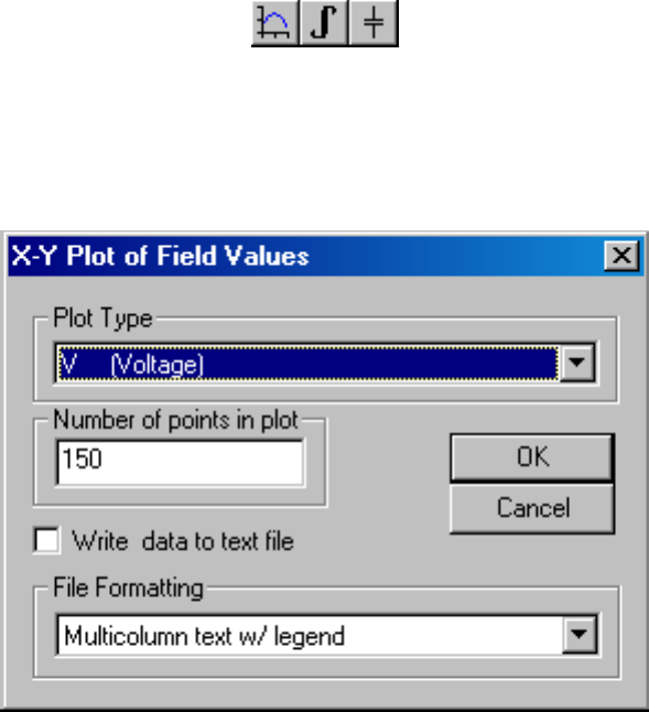
2.5.3 Vector Plots
A good way of getting a feel for the direction and magnitude of the field is with plots of the field
vectors. With this type of plot arrows are plotted such that the direction of the arrow indicates the
direction of the field and the size of the arrow indicates the magnitude of the field. The presence
and appearance of this type of plot can be controlled by pressing the “arrows” icon pictured in
Figure 2.33.
2.5.4 Line Plots
When the postprocessor is in Contours Mode, various field values of interest can be plotted along
the defined contour. A plot of a field value defined contour is performed by pressing the “graphed
function” icon in the Plot, Integration and Conductor Results group of toolbar buttons, shown in
Figure 2.34.
Figure 2.34: Line Plot, Integration, and Conductor Results toolbar buttons.
When this button is pressed, the
X-Y Plot
dialog (see Figure 2.35) appears with a drop list
containing the types of line plots available. Choose the desired type of plot and press “OK.”
Figure 2.35: X-Y Plot dialog.
After “OK” is pressed, the program computes the desired values along the defined contour.
These values are then plotted using the
femmplot
program, which is called automatically to display
the plot.
By default, the
Write data to text file
box is not checked. If the user selects this option,
the file selection dialog will appear and prompt for a filename to which to write the data. The
55

data is written in two-column text format. If
Write data to text file
is selected, a femmplot
window will not appear.
Currently, the type of line plots supported are: Potential along the contour; Magnitude of the
flux density along the contour; Component of flux density normal to the contour; Component of
flux density tangential to the contour; Magnitude of the field intensity along the contour; Compo-
nent of field intensity normal to the contour; Component of field intensity tangential to the contour;
In all of these plots, the direction of the normal is understood to be as shown in Figure 2.36.
The tangential direction is understood to be the direction in which the contour was defined.
Figure 2.36: When in doubt plots and integrals taken on this side of a contour.
In certain cases, the quantity to be plotted can be ambiguous. This can occur, for example, if a
plot of the tangential field intensity is requested on a contour running along an interface between
two materials of differing permittivity. In this case, there is a discontinuity in the tangential field
intensity, and the value of this quantity is different on each side of the interface. The postprocessor
resolves the conflict by always evaluating the plots at a differentially small distance to the “normal”
side of the line. Therefore, by defining the same contour but reversing the order in which the points
are specified, plots of the quantity of interest on each side of a boundary can be obtained.
2.5.5 Line Integrals
Once a contour has been specified in Contours mode, Line Integrals can be performed along the
specified contour. These integrals are performed by evaluating a large number of points at evenly
spaced along the contour and integrating using a simple trapezoidal-type integration scheme.
To perform an integration, press the “integral” icon on the toolbar (as shown in Figure 0).
A small dialog will appear with a drop list. Choose the desired integral from the drop list and
press
OK
. The amount of time required to perform the integral will be virtually instantaneous for
56

some types of integrals; however, some types may require several seconds to evaluate. When the
evaluation of the integral is completed, the answer appears on the screen in a pop-up box.
The line integrals currently supported are:
•
E.t
This integral returns the voltage drop along the defined contour
•
D.n
. This integral returns the total electrix flux passing through a volume defined by extrud-
ing or sweeping the defined contour. If this integral is performed over a closed contour, the
resulting quantity is equal to the charge contained inside the contour.
•
Contour Length/Area
. This integral returns the length of the defined contour in meters, as
well as the area of the extruded or swept volume associated with the defined contour.
•
Force from stress tensor
. This integral totals the force produced on the contour de-
rived from Maxwell’s stress tensor. Deriving meaningful force results requires some care in
the choice of integration path; refer to Section 2.5.7 for a detailed discussion of force and
torque calculation.
•
Torque from stress tensor
. This selection integrates the torque about the point (0,0)
inferred from Maxwell’s stress tensor. Again, some guidelines must be followed to get
accurate torque results.
2.5.6 Block Integrals
To select the regions over which a block integral is to be performed, left-click with the mouse in
the desired region. The selected region will appear highlighted in green. For some block integrals
(i.e. weighted stress tensor force and torque), one desires to select a conductor composed of lines
and points, rather than a block. In this case, the desired conductor can be selected by clicking on it
with the right mouse button. The selected conductor will appear in red.
To perform an integration, press the “integral” icon on the toolbar (as shown in Figure 2.34),
and a dialog will appear with a drop list. Choose the desired integral from the drop list and press
OK
.
The integral is then performed by analytically integrating the specified kernel over each element
in the defined region, and summing the results for all elements. Volume integrals may take several
seconds to evaluate, especially on dense meshes. Be patient. When the evaluation of the integral
is completed, the answer appears on the screen in a pop-up box.
The block integrals currently supported are:
•
Stored Energy
This selection calculates the energy stored in the electric field in the spec-
ified region by integrating (
1
2
D·E) over the selected area.
•
Block cross-section area
•
Block volume
•
Average D over volume
•
Average E over volume
57
•
Force via Weighted Stress Tensor
The Weighted Stress Tensor block integrals auto-
matically compute a weighting function over the finite element mesh that allows all possible
air elements to contribute to the stress tensor integration. This approach is similar to the
weighted stress tensor approach described in [7] and/or [8]. To compute the force on a re-
gion or set of regions, the user selects the blocks upon which force result is desired and
selects the
Force via Weighted Stress Tensor
integral. The program then computes
the weighting function by solving an additional Laplace equation over the air surrounding
the blocks upon which the force is to be computed. It may take a few seconds to compute
the weighting function–progress is be indicated by a progress bar that is displayed while
the weighting function is being computed. The stress tensor is then evaluated as a volume
integration, and the results are displayed. The results are typically more accurate than the
Maxwell Stress Tensor line integral, since in some sense, all possible contours have been
averaged to yield the Weighted Stress Tensor force result.
If the user is interested in the contours along which the integral was performed, the ”stress
tensor mask” box can be checked in the contour plot dialog. A set of orange (by default)
lines will be displayed that.
•
Torque via Weighted Stress Tensor
This integral is torque version of the
Force via
Weighted Stress Tensor
integral. Instead of force, torque about (0,0) is computed using
the same weighting function approach.
2.5.7 Force/Torque Calculation
Often, the calculation of electrostatic and torques is a goal of finite element analysis. This section
discusses some of the different methods of deducing electrostatic forces and torques.
Weighted Stress Tensor Volume Integral
This volume integral greatly simplifies the computation of forces and torques. Merely select the
blocks or conductors upon which force or torque are to be computed and evaluate the integral. No
particular “art” is required in getting good force or torque results (as opposed to the Stress tensor
line integral), although results tend to be more accurate with finer meshing around the region upon
which the force or torque is to be computed.
One limitation of the Weighted Stress Tensor integral is that the regions upon which the force is
being computed must be entirely surrounded by air and/or abutting a boundary. In cases in which
the desired region abuts a non-air region, force results may be deduced from differentiation of
stored electric field energy.
Maxwell Stress Tensor Line Integral
Generally, you should not use the Stress Tensor line integral to compute forces and torques if it can
be avoided (i.e. use the volume integral version instead). The indiscriminate use Maxwell’s Stress
Tensor can result in bad predictions forces and torques.
Maxwell’s stress tensor prescribes a force per unit area produced by the electric field on a
surface. The differential force produced is:
58
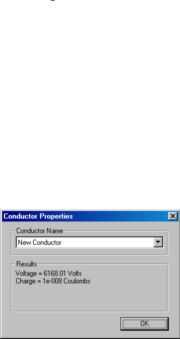
dF =
1
2
(D(E ·n) + E (D·n) −(D·E) n) (2.19)
where n denotes the direction normal to the surface at the point of interest. The net force on an
object is obtained by creating a surface totally enclosing the object of interest and integrating the
stress over that surface.
For best results, never integrate the stress tensor along an interface between materials. Al-
ways define the integration contour as a closed path around the object of interest with the contour
displaced several elements (at least two elements) away from any interfaces or boundaries.
Always use as fine a mesh as possible in problems where force results are desired. A good
way to proceed in finding a mesh that is “dense enough” is to solve the problem on progressively
finer meshes, evaluating the force on each mesh. By comparing the results from different mesh
densities, you can get and idea of the level of accuracy (by looking at what digits in the answer
that change between various mesh densities). You then pick the smallest mesh density that gives
convergence to the desired digit of accuracy.
For torque computations, all the same rules apply as for force computations (i.e. define inte-
gration contours away from boundaries and interfaces, and use a dense mesh).
2.5.8 Conductor Results
If conductor properties are used to specify the excitation, a useful byproduct is ready access to the
voltage and charge on the conductor. To view the conductor results, either press the “Conductor
Results” toolbar button pictured in Figure 2.34 or select
View
|
Conductor Props
off of the post-
processor main menu. A dialog, as pictured in Figure 2.37 will appear. There is a drop list on the
dialog, from which the user selects the conductor for which results are desired. When a conductor
is selected, the voltage and charge associated with that conductor are displayed.
Figure 2.37: Conductor results dialog.
59

2.6 Heat Flow Preprocessor
The preprocessor is used for drawing the problems geometry, defining materials, and defining
boundary conditions. The process of construction of heat flow problems is mechanically nearly
identical to the construction of magnetics problems–refer to Sections 2.2.1 through 2.2.5 for an
overview of the FEMM editing and problem creation commands. This section considers those
parts of problem definition that are unique to heat flow problems.
2.6.1 Problem Definition
The definition of problem type is specified by choosing the
Problem
selection off of the main
menu. Selecting this option brings up the Problem Definition dialog, shown in Figure 2.38.
Figure 2.38: Problem Definition dialog.
The first selection is the
Problem Type
drop list. This drop box allows the user to choose from
a 2-D planar problem (the
Planar
selection), or an axisymmetric problem (the
Axisymmetric
selection).
Next is the
Length Units
drop list. This box identifies what unit is associated with the dimen-
sions prescribed in the model’s geometry. Currently, the program supports inches, millimeters,
centimeters, meters, mils, and µmeters.
The first edit box is the
Depth
specification. If a Planar problem is selected, this edit box
becomes enabled. This value is the length of the geometry in the “into the page” direction. This
value is used for scaling integral results in the post processor (e.g. force, inductance, etc.) to the
appropriate length. The units of the Depth selection are the same as the selected length units.
60
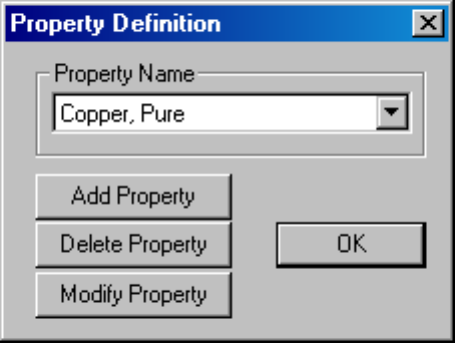
The second edit box is the
Solver Precision
edit box. The number in this edit box specifies
the stopping criteria for the linear solver. The linear algebra problem could be represented by:
Mx = b (2.20)
where M is a square matrix, b is a vector, and x is a vector of unknowns to be determined. The
solver precision value determines the maximum allowable value for ||b−Mx||/||b||. The default
value is 10
−8
.
The third edit box is labeled
Min Angle
. The entry in this box is used as a constraint in the
Triangle meshing program. Triangle adds points to the mesh to ensure that no angles smaller
than the specified angle occur. If the minimum angle is 20.7 degrees or smaller, the triangulation
algorithm is theoretically guaranteed to terminate (assuming infinite precision arithmetic – Triangle
may fail to terminate if you run out of precision). In practice, the algorithm often succeeds for
minimum angles up to 33.8 degrees. For highly refined meshes, however, it may be necessary
to reduce the minimum angle to well below 20 to avoid problems associated with insufficient
floating-point precision. The edit box will accept values between 1 and 33.8 degrees.
Lastly, there is an optional
Comment
edit box. The user can enter in a few lines of text that give
a brief description of the problem that is being solved. This is useful if the user is running several
small variations on a given geometry. The comment can then be used to identify the relevant
features for a particular geometry.
2.6.2 Definition of Properties
To make a solvable problem definition, the user must identify boundary conditions, block materials
properties, and so on. The different types of properties defined for a given problem are defined via
the
Properties
selection off of the main menu.
When the
Properties
selection is chosen, a drop menu appears that has selections for Ma-
terials, Boundary, Point, and Conductors. When any one of these selections is chosen, the dialog
pictured in Figure 2.39 appears.
Figure 2.39: Property Definition dialog box.
61
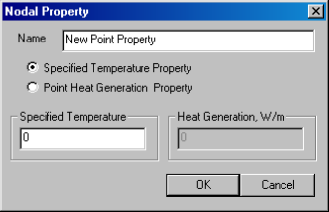
This dialog is the manager for a particular type of properties. All currently defined properties
are displayed in the
Property Name
drop list at the top of the dialog. At the beginning of a new
model definition, the box will be blank, since no properties have yet been defined. Pushing the
Add
Property
button allows the user to define a new property type. The
Delete Property
button
removes the definition of the property currently in view in the
Property Name
box. The
Modify
Property
button allows the user to view and edit the property currently selected in the
Property
Name
box. Specifics for defining the various property types are addressed in the following subsec-
tions.
Point Properties
If a new point property is added or an existing point property modified, the
Nodal Property
dialog box appears. This dialog box is pictured in Figure 2.40.
Figure 2.40: Nodal Property dialog.
The first selection is the
Name
edit box. The default name is
New Point Property
, but this
name should be changed to something that describes the property that you are defining.
Next are edit boxes for defining the temperature at a given point, or prescribing a heat gener-
ation at a given point. The type of point property is chosen via the radio buttons, and the value is
entered in the enabled edit box.
Boundary Properties
The
Boundary Property
dialog box is used to specify the properties of line segments or arc
segments that are to be boundaries of the solution domain. When a new boundary property is
added or an existing property modified, the
Boundary Property
dialog pictured in Figure 2.41
appears.
62
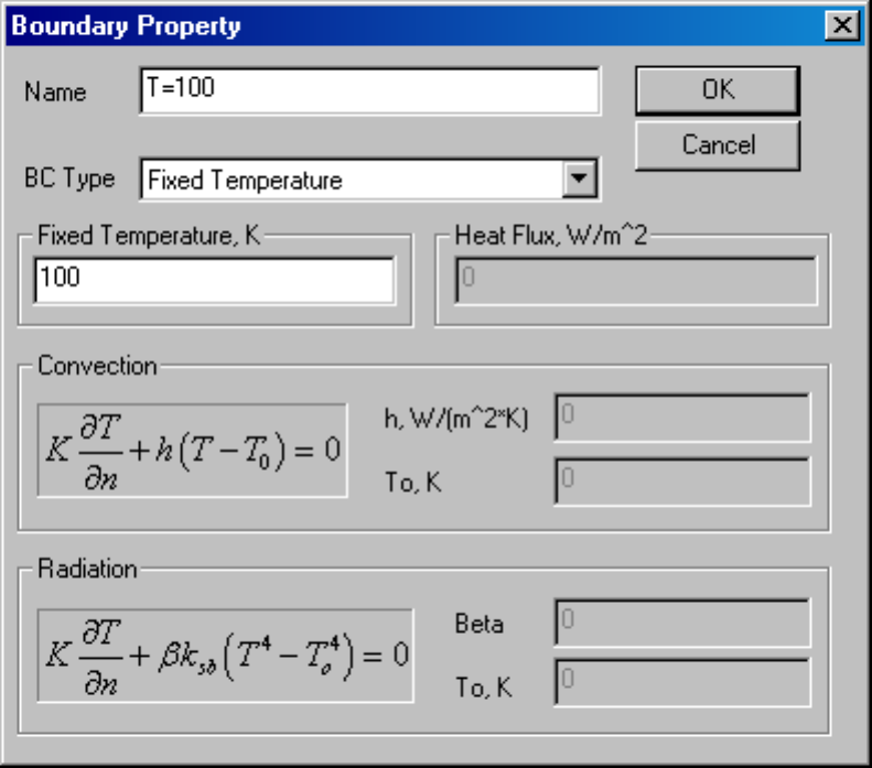
Figure 2.41: Boundary Property dialog.
The first selection in the dialog is the
Name
of the property. The default name is
New Boundary
,
but you should change this name to something more descriptive of the boundary that is being
defined.
The next selection is the
BC Type
drop list. This specifies the boundary condition type. Cur-
rently, FEMM heat flow problems support the following types of boundaries: Fixed Temperature,
Heat Flux, Convection, Radiation, Periodic, and Antiperiodic. These boundary conditions are
described in detail in Section 1.3.
Materials Properties
The
Block Property
dialog box is used to specify the properties to be associated with block
labels. The properties specified in this dialog have to do with the material of which the block is
composed. When a new material property is added or an existing property modified, the
Block
Property
dialog pictured in Figure 2.42 appears.
As with Point and Boundary properties, the first step is to choose a descriptive name for the
material that is being described. Enter it in the
Name
edit box in lieu of
New Material
.
Next, the thermal conductivity for the material needs to be specified. There is a drop list
63
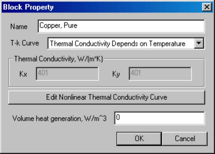
Figure 2.42: Block Property dialog.
on the dialog that allows the user to select either a contant thermal conductivity (i.e. indepen-
dent of temperature), or a thermal conductivity that is prescribed as a function of temperature.
If conductivity is selected, FEMM allows you to specify different conductivities in the verti-
cal and horizontal directions (ε
x
for the x- or horizontal direction, and ε
y
for the y- or verti-
cal. If
Thermal Conductivity Depends on Temperature
is selected, the
Edit Nonlinear
Thermal Conductivity Curve
becomes enabled. Press the button to enter temperature-conductivity
pairs. The program will interpolate linearly between the entered points. If the program must ex-
trapolate off the end of the defined curve, conductivity takes the value of the nearest defined T-k
point.
A volume heat generation can also be prescribed by filling in the appropriate box in the material
properties dialog.
Materials Library
Since one kind of material might be needed in several different models, FEMM has a built-in
library of thermal Block Property definitions. The user can access and maintain this library through
the
Properties
|
Materials Library
selection off of the main menu. When this option is
selected, the
Materials Library
dialog pictured in Figure 2.43 appears.
This dialog allow the user to exchange Block Property definitions between the current model
and the materials library via a drag-and-drop interface.
A number of different options are available via a mouse button right-click when the cursor is
located on top of a material or folder. Materials can be edited by double-clicking on the desired
material.
Material from other material libraries or models can be imported by selecting the “Import
64
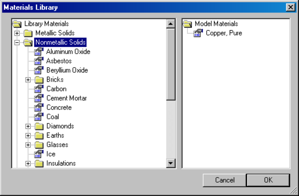
Figure 2.43: Materials Library dialog
Materials” option from the right-button menu that appears when the pointer is over the root-level
folder of either the Library or Model materials lists.
The materials library should be located in the same directory as the FEMM executable files,
under the filename
heatlib.dat
. If you move the materials library, FEMM will not be able to
find it.
Conductor Properties
The purpose of the conductor properties is mainly to allow the user to apply constraints on the total
amount of heat flowing in and out of a surface. Alternatively, conductors with a fixed temperature
can be defined, and the program will compute the total heat flow through the during the solution
process.
For fixed temperatures, one could alternatively apply a
Fixed Temperature
boundary con-
dition. However, applying a fixed temperature as a conductor allows the user to group together
several physically disjoint surfaces into one conductor upon which the total heat flux is automati-
cally computed.
The dialog for entering conductor properties is pictured in Figure 2.44.
65
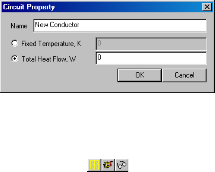
Figure 2.44: Conductor Property dialog.
2.6.3 Analysis Tasks
Meshing the model, analyzing the model, and viewing the results are most easily performed by the
toolbar buttons pictured in Figure 2.45.
Figure 2.45: Toolbar buttons for starting analysis tasks.
The first of these buttons (with the “yellow mesh” icon) runs the mesh generator. The solver
actually automatically calls the mesh generator to make sure that the mesh is up to date, so you
never have to call the mesher from within FEMM. However, it is almost always important to get
a look at the mesh and see that it “looks right.” When the mesh generation button is pressed,
the mesher is called. While the mesher is running, an entry labeled “triangle” will appear on
the Windows taskbar. After the geometry is triangulated, the finite element mesh is loaded into
memory and displayed underneath the defined nodes, segments, and block labels as a set of yellow
lines.
If you have a very large model, just keeping all of the mesh information in core can take up a
significant amount of memory. If you are about to analyze a very large problem, it might be a good
idea to choose the
Mesh
|
Purge Mesh
option off of the main menu. When this option is selected,
the mesh is removed from memory, and the memory that it occupied is freed for other uses.
The second button, with the “hand-crank” icon, executes the solver,
hsolv.exe
. Before hsolv
is actually run, the Triangle is called to make sure the mesh is up to date. Then, hsolv is called.
When hsolv runs, it opens up a console window to display status information to the user. However,
hsolv requires no user interaction while it is running. When hsolv is finished analyzing your
problem, the console window will disappear. The time that hsolv requires is highly dependent on
the problem being solved. Solution times are typically on the order of 1 to 10 seconds, depending
upon the size and complexity of the problem and the speed of the machine analyzing the problem.
The “big magnifying glass” icon is used to run the postprocessor once the analysis is finished.
66

2.7 Heat Flow Postprocessor
The the heat flow postprocessing functionality of FEMM is used to view solutions generated by the
hsolv
solver. A heat flow postprocessor window can be opened either by loading some previously
run analyses via
File|Open
on the main menu, or by pressing the “big magnifying glass” icon
from within a preprocessor window to view a newly generated solution. Heat flow postprocessor
data files stored on disk have the
.anh
prefix.
Operation of the heat flow postprocessor (i.e. modes, view manipulation) is very similar to that
of the magnetics postprocessor. Refer to Sections 2.3.1 through 2.3.5 for this information.
2.7.1 Contour Plot
One of the most useful ways to get a subjective feel for a solution is by plotting the eqipotentials
of temperature. The number and type of equipotential lines to be plotted can be altered using the
Contours Plot icon in the Graph Mode section of the toolbar (see Figure 2.46). The Contour Plot
icon is the icon with the black contours.
Figure 2.46: Graph Mode toolbar buttons.
When this button is pressed, a dialog pops up, allowing the choice of the number of contours.
2.7.2 Density Plot
Density plots are also a useful way to get a quick feel for the temperature, flux density, etc., in
various parts of the model. By default, a density plot denoting temperature is displayed when the
postprocessor first starts. (This behavior can be changed via Edit—Preferences on the main menu).
However, the plot can be displayed by pressing the “spectrum” button in the Graph Mode section
of the toolbar (see Figure 2.46). A dialog the pops up that allows the user to turn density plotting
on.
The user can select between density plots of temperature or the magnitude of temperature gra-
dient or heat flux density. The solution at each point is classified into one of twenty contours dis-
tributed evenly between either the minimum and maximum flux densities or user-specified bounds.
2.7.3 Vector Plots
A good way of getting a feel for the direction and magnitude of the field is with plots of the field
vectors. With this type of plot arrows are plotted such that the direction of the arrow indicates the
direction of the field and the size of the arrow indicates the magnitude of the field. The presence
and appearance of this type of plot can be controlled by pressing the “arrows” icon pictured in
Figure 2.46.
67

2.7.4 Line Plots
When the postprocessor is in Contours Mode, various field values of interest can be plotted along
the defined contour. A plot of a field value defined contour is performed by pressing the “graphed
function” icon in the Plot, Integration and Conductor Results group of toolbar buttons, shown in
Figure 2.47.
Figure 2.47: Line Plot, Integration, and Conductor Results toolbar buttons.
When this button is pressed, the
X-Y Plot
dialog (see Figure 2.48) appears with a drop list
containing the types of line plots available. Choose the desired type of plot and press “OK.”
Figure 2.48: X-Y Plot dialog.
After “OK” is pressed, the program computes the desired values along the defined contour.
When the computation is finished, a window will appear with a plot of the selected quantity.
By default, the
Write data to text file
box is not checked. If the user selects this option,
the file selection dialog will appear and prompt for a filename to which to write the data. The data
is written in two-column text format. If
Write data to text file
is selected, a plot window
will not appear.
Currently, the type of line plots supported are: Temperature along the contour; Magnitude of
the heat flux density along the contour; Component of heat flux density normal to the contour;
Component of heat flux density tangential to the contour; Magnitude of the temperature gradi-
ent along the contour; Component of temperature gradient normal to the contour; Component of
temperature gradient tangential to the contour;
In all of these plots, the direction of the normal is understood to be as shown in Figure 2.49.
The tangential direction is understood to be the direction in which the contour was defined.
68
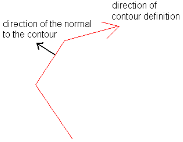
Figure 2.49: When in doubt plots and integrals taken on this side of a contour.
In certain cases, the quantity to be plotted can be ambiguous. This can occur, for example, if a
plot of the tangential field intensity is requested on a contour running along an interface between
two materials of differing permittivity. In this case, there is a discontinuity in the tangential field
intensity, and the value of this quantity is different on each side of the interface. The postprocessor
resolves the conflict by always evaluating the plots at a differentially small distance to the “normal”
side of the line. Therefore, by defining the same contour but reversing the order in which the points
are specified, plots of the quantity of interest on each side of a boundary can be obtained.
2.7.5 Line Integrals
Once a contour has been specified in Contours mode, Line Integrals can be performed along the
specified contour. These integrals are performed by evaluating a large number of points at evenly
spaced along the contour and integrating using a simple trapezoidal-type integration scheme.
To perform an integration, press the “integral” icon on the toolbar (as shown in Figure 0).
A small dialog will appear with a drop list. Choose the desired integral from the drop list and
press
OK
. The amount of time required to perform the integral will be virtually instantaneous for
some types of integrals; however, some types may require several seconds to evaluate. When the
evaluation of the integral is completed, the answer appears on the screen in a pop-up box.
The line integrals currently supported are:
•
Temperature Difference (G.t)
. This integral returns the temperature difference be-
tween the ends of the contour
•
Heat Flux (F.n)
. This integral returns the total heat flux passing through a volume defined
by extruding or sweeping the defined contour.
69
•
Contour length & area
. The length of the contour, and the area formed by extruding the
contour.
•
Average temperature
. The average temperature along the line.
2.7.6 Block Integrals
To select the regions over which a block integral is to be performed, left-click with the mouse in
the desired region. The selected region will appear highlighted in green.
To perform an integration, press the “integral” icon on the toolbar (as shown in Figure 2.47),
and a dialog will appear with a drop list. Choose the desired integral from the drop list and press
OK
.
The integral is then performed by analytically integrating the specified kernel over each element
in the defined region, and summing the results for all elements. Volume integrals may take several
seconds to evaluate, especially on dense meshes. Be patient. When the evaluation of the integral
is completed, the answer appears on the screen in a pop-up box.
The block integrals currently supported are:
•
Average temperature over volume
•
Block cross-section area
•
Block volume
•
Average F over volume
•
Average G over volume
2.7.7 Conductor Results
If conductor properties are used to specify the excitation, a useful byproduct is ready access to the
temperature of and heat flux through the conductor. To view the conductor results, either press the
“Conductor Results” toolbar button pictured in Figure 2.47 or select
View
|
Conductor Props
off
of the postprocessor main menu. A dialog, as pictured in Figure 2.50 will appear. There is a drop
list on the dialog, from which the user selects the conductor for which results are desired. When a
conductor is selected, the temperature and heat flux associated with that conductor are displayed.
2.8 Current Flow Preprocessor
The preprocessor is used for drawing the problems geometry, defining materials, and defining
boundary conditions. The process of construction of current flow problems is mechanically nearly
identical to the construction of magnetics problems–refer to Sections 2.2.1 through 2.2.5 for an
overview of the FEMM editing and problem creation commands. This section considers those
parts of problem definition that are unique to current flow problems.
70
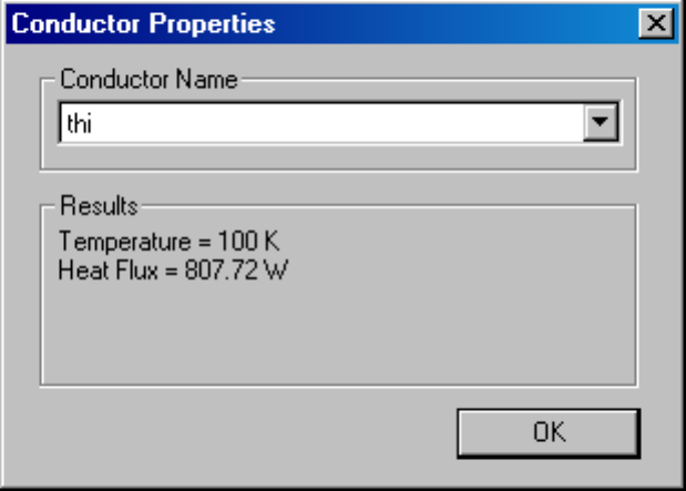
Figure 2.50: Conductor results dialog.
2.8.1 Problem Definition
The definition of problem type is specified by choosing the
Problem
selection off of the main
menu. Selecting this option brings up the Problem Definition dialog, shown in Figure 2.51.
The first selection is the
Problem Type
drop list. This drop box allows the user to choose from
a 2-D planar problem (the
Planar
selection), or an axisymmetric problem (the
Axisymmetric
selection).
Next is the
Length Units
drop list. This box identifies what unit is associated with the dimen-
sions prescribed in the model’s geometry. Currently, the program supports inches, millimeters,
centimeters, meters, mils, and µmeters.
The first edit box,
Frequency, Hz
, denotes the frequency at which the problem is to be ana-
lyzed.
The second edit box is the
Depth
specification. If a Planar problem is selected, this edit box
becomes enabled. This value is the length of the geometry in the “into the page” direction. This
value is used for scaling integral results in the post processor (e.g. force, inductance, etc.) to the
appropriate length. The units of the Depth selection are the same as the selected length units.
The second edit box is the
Solver Precision
edit box. The number in this edit box specifies
the stopping criteria for the linear solver. The linear algebra problem could be represented by:
Mx = b (2.21)
where M is a square matrix, b is a vector, and x is a vector of unknowns to be determined. The
solver precision value determines the maximum allowable value for ||b−Mx||/||b||. The default
value is 10
−8
.
The third edit box is labeled
Min Angle
. The entry in this box is used as a constraint in the
Triangle meshing program. Triangle adds points to the mesh to ensure that no angles smaller
than the specified angle occur. If the minimum angle is 20.7 degrees or smaller, the triangulation
71
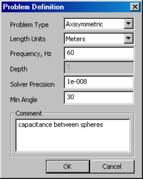
Figure 2.51: Problem Definition dialog.
algorithm is theoretically guaranteed to terminate (assuming infinite precision arithmetic – Triangle
may fail to terminate if you run out of precision). In practice, the algorithm often succeeds for
minimum angles up to 33.8 degrees. For highly refined meshes, however, it may be necessary
to reduce the minimum angle to well below 20 to avoid problems associated with insufficient
floating-point precision. The edit box will accept values between 1 and 33.8 degrees.
Lastly, there is an optional
Comment
edit box. The user can enter in a few lines of text that give
a brief description of the problem that is being solved. This is useful if the user is running several
small variations on a given geometry. The comment can then be used to identify the relevant
features for a particular geometry.
2.8.2 Definition of Properties
To make a solvable problem definition, the user must identify boundary conditions, block materials
properties, and so on. The different types of properties defined for a given problem are defined via
the
Properties
selection off of the main menu.
When the
Properties
selection is chosen, a drop menu appears that has selections for Ma-
terials, Boundary, Point, and Conductors. When any one of these selections is chosen, the dialog
pictured in Figure 2.52 appears.
This dialog is the manager for a particular type of properties. All currently defined properties
are displayed in the
Property Name
drop list at the top of the dialog. At the beginning of a new
72

Figure 2.52: Property Definition dialog box.
model definition, the box will be blank, since no properties have yet been defined. Pushing the
Add
Property
button allows the user to define a new property type. The
Delete Property
button
removes the definition of the property currently in view in the
Property Name
box. The
Modify
Property
button allows the user to view and edit the property currently selected in the
Property
Name
box. Specifics for defining the various property types are addressed in the following subsec-
tions.
Point Properties
If a new point property is added or an existing point property modified, the
Nodal Property
dialog box appears. This dialog box is pictured in Figure 2.53.
The first selection is the
Name
edit box. The default name is
New Point Property
, but this
name should be changed to something that describes the property that you are defining.
Next are edit boxes for defining the voltage at a given point, or prescribing a current generation
at a given point. The type of point property is chosen via the radio buttons, and the value is entered
in the enabled edit box.
Boundary Properties
The
Boundary Property
dialog box is used to specify the properties of line segments or arc
segments that are to be boundaries of the solution domain. When a new boundary property is
added or an existing property modified, the
Boundary Property
dialog pictured in Figure 2.54
appears.
The first selection in the dialog is the
Name
of the property. The default name is
New Boundary
,
but you should change this name to something more descriptive of the boundary that is being
defined.
The next selection is the
BC Type
drop list. This specifies the boundary condition type. Cur-
rently, FEMM supports the following types of boundaries: Fixed Voltage, Mixed, Prescribed sur-
face current density, Periodic, and Antiperiodic. These boundary conditions are described in detail
in Section 1.3.
73
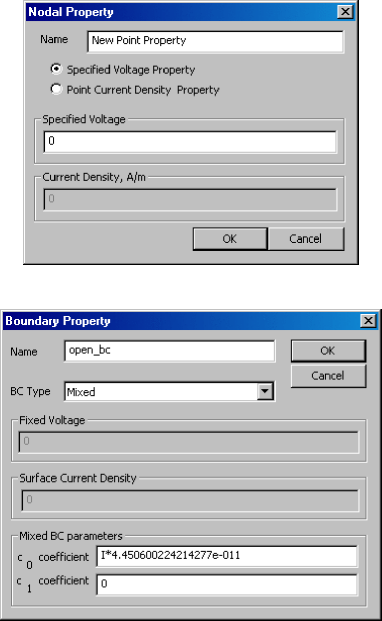
Figure 2.53: Nodal Property dialog.
Figure 2.54: Boundary Property dialog.
74
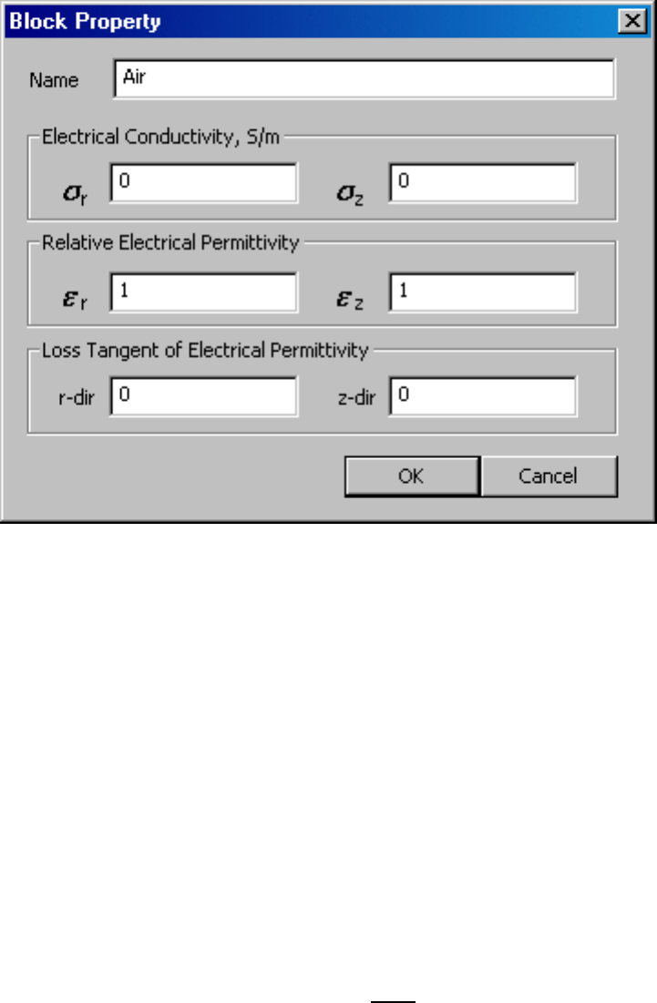
Materials Properties
The
Block Property
dialog box is used to specify the properties to be associated with block
labels. The properties specified in this dialog have to do with the material of which the block is
composed. When a new material property is added or an existing property modified, the
Block
Property
dialog pictured in Figure 2.55 appears.
Figure 2.55: Block Property dialog.
As with Point and Boundary properties, the first step is to choose a descriptive name for the
material that is being described. Enter it in the
Name
edit box in lieu of
New Material
.
Next, electrical conductivitiy for the material needs to be specified. FEMM allows you to
specify different electrical conductivities in the vertical and horizontal directions (σ
x
for the x- or
horizontal direction, and σ
y
for the y- or vertical direction.
The next pair of boxes represents the relative electrical permittivity for the material. Similar to
the electrical conducitvity, textitε
x
represents permittivity in the x- or horizontal direction, and ε
y
for the y- or vertical direction. If the material is a lossy dielectric, this value is considered to be the
amplitude of complex permittivity.
A common way of describing lossy dielectrics is via the “loss tangent”. Losses can be consid-
ered as resulting from a complex-valued electrical permittivity. If the complex-valued permittivity
is defined as:
ε = |ε|(cosφ− jsinφ) (2.22)
The loss tangent is then defined as:
loss tangent =
sinφ
cosφ
(2.23)
75
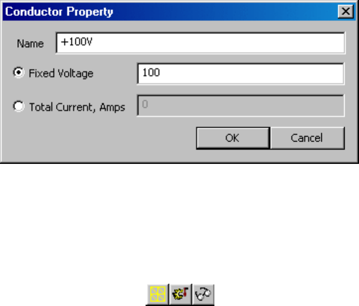
For material that are also conductive, FEMM combines the defined conductivity, permittivity,
and loss tangent to obtain the complex-valued effective electrical conductivities:
σ
x,ef f
= σ
x
+ jωε
o
ε
x
e
−jφ
(2.24)
σ
y,ef f
= σ
y
+ jωε
o
ε
y
e
−jφ
which takes into account resistive losses and addition dielectric losses due to the definition of a
non-zero loss tangent.
Conductor Properties
The purpose of the conductor properties is mainly to allow the user to apply constraints on the total
amount of current flowing in and out of a surface. Alternatively, conductors with a fixed voltage
can be defined, and the program will compute the total current flow through the during the solution
process.
For fixed voltages, one could alternatively apply a
Fixed Voltage
boundary condition. How-
ever, applying a fixed voltage as a conductor allows the user to group together several physically
disjoint surfaces into one conductor upon which the total current flow is automatically computed.
The dialog for entering conductor properties is pictured in Figure 2.56.
Figure 2.56: Conductor Property dialog.
2.8.3 Analysis Tasks
Meshing the model, analyzing the model, and viewing the results are most easily performed by the
toolbar buttons pictured in Figure 2.57.
Figure 2.57: Toolbar buttons for starting analysis tasks.
The first of these buttons (with the “yellow mesh” icon) runs the mesh generator. The solver
actually automatically calls the mesh generator to make sure that the mesh is up to date, so you
76

never have to call the mesher from within FEMM. However, it is almost always important to get
a look at the mesh and see that it “looks right.” When the mesh generation button is pressed,
the mesher is called. While the mesher is running, an entry labeled “triangle” will appear on
the Windows taskbar. After the geometry is triangulated, the finite element mesh is loaded into
memory and displayed underneath the defined nodes, segments, and block labels as a set of yellow
lines.
If you have a very large model, just keeping all of the mesh information in core can take up a
significant amount of memory. If you are about to analyze a very large problem, it might be a good
idea to choose the
Mesh
|
Purge Mesh
option off of the main menu. When this option is selected,
the mesh is removed from memory, and the memory that it occupied is freed for other uses.
The second button, with the “hand-crank” icon, executes the solver,
csolv.exe
. Before csolv
is actually run, the Triangle is called to make sure the mesh is up to date. Then, csolv is called.
When csolv runs, it opens up a console window to display status information to the user. How-
ever, csolv requires no user interaction while it is running. When csolv is finished analyzing your
problem, the console window will disappear. The time that csolv requires is highly dependent on
the problem being solved. Solution times are typically on the order of 1 to 10 seconds, depending
upon the size and complexity of the problem and the speed of the machine analyzing the problem.
The “big magnifying glass” icon is used to run the postprocessor once the analysis is finished.
2.9 Current Flow Postprocessor
The the current flow postprocessing functionality of FEMM is used to view solutions generated
by the
csolv
solver. A current flow postprocessor window can be opened either by loading some
previously run analyses via
File|Open
on the main menu, or by pressing the “big magnifying
glass” icon from within a preprocessor window to view a newly generated solution. Current flow
postprocessor data files stored on disk have the
.anh
prefix.
Operation of the current flow postprocessor (i.e. modes, view manipulation) is very similar to
that of the magnetics postprocessor. Refer to Sections 2.3.1 through 2.3.5 for this information.
2.9.1 Contour Plot
One of the most useful ways to get a subjective feel for a solution is by plotting the eqipotentials of
voltage. The number and type of equipotential lines to be plotted can be altered using the Contours
Plot icon in the Graph Mode section of the toolbar (see Figure 2.58). The Contour Plot icon is the
icon with the black contours.
Figure 2.58: Graph Mode toolbar buttons.
When this button is pressed, a dialog pops up, allowing the choice of the number of contours.
77
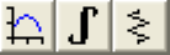
2.9.2 Density Plot
Density plots are also a useful way to get a quick feel for the voltage, current density, etc., in various
parts of the model. By default, a density plot denoting voltage is displayed when the postprocessor
first starts. (This behavior can be changed via Edit—Preferences on the main menu). However, the
plot can be displayed by pressing the “spectrum” button in the Graph Mode section of the toolbar
(see Figure 2.58). A dialog the pops up that allows the user to turn density plotting on.
The user can select between density plots of voltage or the magnitude of voltage gradient or
current density. The solution at each point is classified into one of twenty contours distributed
evenly between either the minimum and maximum densities or user-specified bounds.
2.9.3 Vector Plots
A good way of getting a feel for the direction and magnitude of the field is with plots of the field
vectors. With this type of plot arrows are plotted such that the direction of the arrow indicates the
direction of the field and the size of the arrow indicates the magnitude of the field. The presence
and appearance of this type of plot can be controlled by pressing the “arrows” icon pictured in
Figure 2.58.
2.9.4 Line Plots
When the postprocessor is in Contours Mode, various field values of interest can be plotted along
the defined contour. A plot of a field value defined contour is performed by pressing the “graphed
function” icon in the Plot, Integration and Conductor Results group of toolbar buttons, shown in
Figure 2.59.
Figure 2.59: Line Plot, Integration, and Conductor Results toolbar buttons.
When this button is pressed, the
X-Y Plot
dialog (see Figure 2.60) appears with a drop list
containing the types of line plots available. Choose the desired type of plot and press “OK.”
After “OK” is pressed, the program computes the desired values along the defined contour.
When computation of the values is finished, a plot window will appear with a graph of the selected
quantity. the plot.
By default, the
Write data to text file
box is not checked. If the user selects this option,
the file selection dialog will appear and prompt for a filename to which to write the data. The data
is written in two-column text format. If
Write data to text file
is selected, a plot window
will not appear.
Currently, the type of line plots supported are:
•
V
Voltage
•
|J|
Magnitude of current density
•
J.n
Normal current density
78
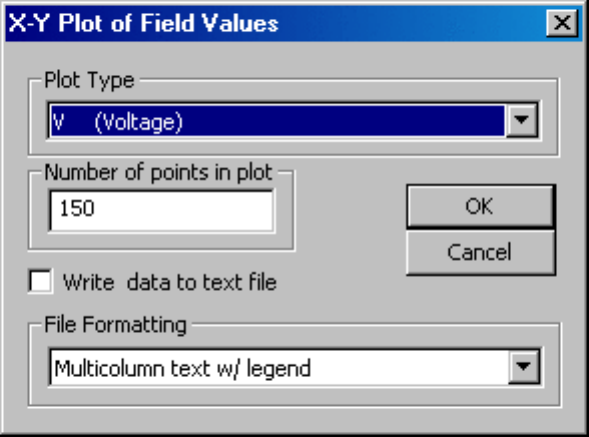
Figure 2.60: X-Y Plot dialog.
•
J.t
Tangential current density
•
|E|
Magnitude of electric field intensity
•
E.n
Normal electric field intensity
•
E.t
Tangential electric field intensity
•
|Jc|
Magnitude of conduction current density
•
Jc.n
Normal conduction current density
•
Jc.t
Tangential conduction current density
•
|Jd|
Magnitude of displacment current density
•
Jd.n
Normal displacement current density
•
Jd.t
Tangential displacement current density
2.9.5 Line Integrals
Once a contour has been specified in Contours mode, Line Integrals can be performed along the
specified contour. These integrals are performed by evaluating a large number of points at evenly
spaced along the contour and integrating using a simple trapezoidal-type integration scheme.
To perform an integration, press the “integral” icon on the toolbar (as shown in Figure 0).
A small dialog will appear with a drop list. Choose the desired integral from the drop list and
press
OK
. The amount of time required to perform the integral will be virtually instantaneous for
some types of integrals; however, some types may require several seconds to evaluate. When the
evaluation of the integral is completed, the answer appears on the screen in a pop-up box.
79
The line integrals currently supported are:
•
Voltage Difference (E.t)
. This integral returns the voltage difference between the ends
of the contour
•
Current Flow (J.n)
. This integral returns the total current passing through a volume
defined by extruding or sweeping the defined contour.
•
Contour length & area
. The length of the contour, and the area formed by extruding the
contour.
•
Average Voltage
. The average voltage along the line.
2.9.6 Block Integrals
To select the regions over which a block integral is to be performed, left-click with the mouse in
the desired region. The selected region will appear highlighted in green.
To perform an integration, press the “integral” icon on the toolbar (as shown in Figure 2.59),
and a dialog will appear with a drop list. Choose the desired integral from the drop list and press
OK
.
The integral is then performed by analytically integrating the specified kernel over each element
in the defined region, and summing the results for all elements. Volume integrals may take several
seconds to evaluate, especially on dense meshes. Be patient. When the evaluation of the integral
is completed, the answer appears on the screen in a pop-up box.
The block integrals currently supported are:
•
Real Power
•
Reactive Power
•
Apparent Power
•
Time-Average Stored Energy
•
Block cross-section area
•
Block volume
2.9.7 Conductor Results
If conductor properties are used to specify the excitation, a useful byproduct is ready access to
the voltage of and current through the conductor. To view the conductor results, either press the
“Conductor Results” toolbar button pictured in Figure 2.59 or select
View
|
Conductor Props
off
of the postprocessor main menu. A dialog, as pictured in Figure 2.61 will appear. There is a drop
list on the dialog, from which the user selects the conductor for which results are desired. When a
conductor is selected, the voltage and current associated with that conductor are displayed.
80
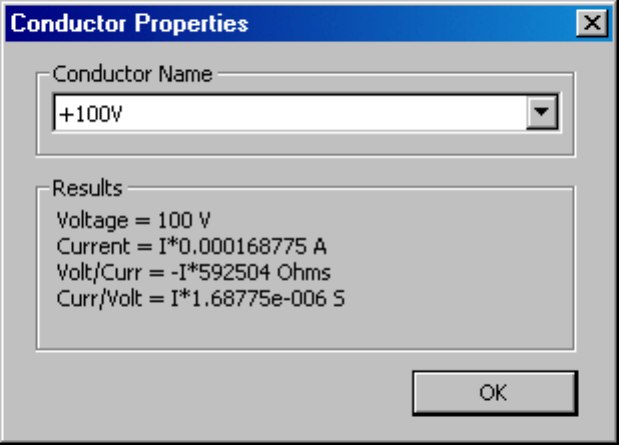
Figure 2.61: Conductor results dialog.
2.10 Exporting of Graphics
Ultimately, you may want to export graphics from FEMM for inclusion in reports and so on. It is
possible to get what you are seeing on the screen onto disk in several different graphics formats.
Probably the easiest way to get graphics out of FEMM is to use the
Copy as Bitmap
or
Copy
as Metafile
selections off of the main menu’s
Edit
list. These command takes whatever is
currently in the FEMM window and copies it to the clipboard as a Device Independent Bitmap
(
.bmp
format) and Extended Metafile (
.emf
format), respectively. The clipboard data can then be
pasted directly into most applications (e.g. Word, MS Paint, etc).
L
A
T
E
X afficionados typically find PostScript to be the most useful type of graphics output.
FEMM does not support postscript output directly, but it is still relatively easy to create postcript
figures with FEMM. To obtain a postscript version of the current view, you first must set up a
postscript printer driver that outputs to
File:
. This is done via the following steps: Choose +Set-
tings/Printers+ off of the Windows Start menu. A window containing the list of currently defined
printers will appear. Double click on the
Add Printer
icon in this list. The
Add Printer Wizard
will appear on the screen. Choose
Local Printer
; hit
Next
; A list of printers will appear. Choose
a postscript printer off of this list. The Apple Laserwriter II NT is a good choice. Select
FILE:
as the port which will be used with this printer. Accept the defaults for all remaining questions.
Now, when you want a postscript picture of the currently displayed screen, just choose +File/Print+
off of FEMM’s main menu. As the printer, choose the postscript printer that you have previously
defined. When you print to this printer, you will be prompted for a file name, and graphic will be
written as a postscript figure to the specified file name.
81
Chapter 3
Lua Scripting
3.1 What Lua Scripting?
The Lua extension language has been used to add scripting/batch processing facilities to FEMM.
The Interactive Shell can run Lua scripts through the
Open Lua Script
selection on the Files
menu, or Lua commands can be entered in directly to the Lua Console Window.
Lua is a complete, open-source scripting language. Source code for Lua, in addition to de-
tailed documentation about programming in Lua, can be obtained from the Lua homepage at
http://www.lua.org
. Because the scripting files are text, they can be edited with any text editor
(e.g. notepad). As of this writing, the latest release of Lua is version 5.0. However, the version of
Lua incorporated into FEMM is Lua 4.0.
In addition to the standard Lua command set described in [9], a number of FEMM-specific
functions have been added for manipulating files in both the pre- and post-processor. These com-
mands are described in the following sections.
3.2 Common Lua Command Set
A number of FEMM-specific Lua commands exist that are not associated with any particular prob-
lem type.
•
clearconsole()
Clears the output window of the Lua console.
•
newdocument(doctype)
Creates a new preprocessor document and opens up a new prepro-
cessor window. Specify
doctype
to be
0
for a magnetics problem,
1
for an electrostatics
problem,
2
for a heat flow problem, or
3
for a current flow problem. An alternative syntax
for this command is
create(doctype)
•
hideconsole()
Hides the floating Lua console window.
•
hidepointprops()
Hides the floating FEMM Properties display window.
•
messagebox("message")
displays the
"message"
string to the screen in a pop-up message
box.
82

•
open("filename")
Opens a document specified by
filename
.
•
pause()
Waits for the ok button to be pressed, a debug helper.
•
print()
This is standard Lua “print” command directed to the output of the Lua console
window. Any number of comma-separated items can be printed at once via the print com-
mand.
•
prompt("message")
This function allows a Lua script to prompt a user for input. When
this command is used, a dialog box pops up with the
"message"
string on the title bar of the
dialog box. The user can enter in a single line of input via the dialog box. prompt returns the
user’s input as a string. If a numerical valueis desired, the syntax
tonumber(prompt("message"))
can be used.
•
quit()
Close all documents and exit the the Interactive Shell at the end of the currently
executing Lua script.
•
setcompatibilitymode(value)
If
value
is set to
1
, various magnetics-related commands
with complex arguments revert to their definitions in the FEMM 4.1 manual. If
value
is
set to
0
, the FEMM 4.2 definitions are used. The default mode is compatibility mode
0
.
Affected functions include:
–
mi addmaterial
–
mi modifymaterial
–
mi addpointprop
–
mi modifypointprop
–
mi addcircprop
–
mi modifycircprop
–
mo getpointvalues
–
mo lineintegral
–
mo blockintegral
–
mo getcircuitproperties
•
showconsole()
Displays the floating Lua console window.
•
showpointprops()
Displays the floating FEMM Properties display window.
•
smartmesh(state)
Calling with a state of 0 turns off “smart mesh” functionality for the
present session; calling with a state of 1 turns “smarth meshing” on. The setting os not
permanent–using the Preferences setting to permanently turn on or off.
3.3 Magnetics Preprocessor Lua Command Set
A number of different commands are available in the preprocessor. Two naming conventions can
be used: one which separates words in the command names by underscores, and one that eliminates
the underscores.
83

3.3.1 Object Add/Remove Commands
•
mi addnode(x,y)
Add a new node at x,y
•
mi addsegment(x1,y1,x2,y2)
Add a new line segment from node closest to (x1,y1) to
node closest to (x2,y2)
•
mi addblocklabel(x,y)
Add a new block label at (x,y)
•
mi addarc(x1,y1,x2,y2,angle,maxseg)
Add a new arc segment from the nearest node
to (x1,y1) to the nearest node to (x2,y2) with angle ‘angle’ divided into ‘maxseg’ segments.
•
mi deleteselected
Delete all selected objects.
•
mi deleteselectednodes
Delete selected nodes.
•
mi deleteselectedlabels
Delete selected block labels.
•
mi deleteselectedsegments
Delete selected segments.
•
mi deleteselectedarcsegments
Delete selects arcs.
3.3.2 Geometry Selection Commands
•
mi clearselected()
Clear all selected nodes, blocks, segments and arc segments.
•
mi selectsegment(x,y)
Select the line segment closest to (x,y)
•
mi selectnode(x,y)
Select the node closest to (x,y). Returns the coordinates of the se-
lected node.
•
mi selectlabel(x,y)
Select the label closet to (x,y). Returns the coordinates of the se-
lected label.
•
mi selectarcsegment(x,y)
Select the arc segment closest to (x,y)
•
mi selectgroup(n)
Select the n
th
group of nodes, segments, arc segments and blocklabels.
This function will clear all previously selected elements and leave the editmode in 4 (group)
•
mi selectcircle(x,y,R,editmode)
selects objects within a circle of radius R centered at
(x,y). If only x, y, and R paramters are given, the current edit mode is used. If the editmode
parameter is used, 0 denotes nodes, 2 denotes block labels, 2 denotes segments, 3 denotes
arcs, and 4 specifies that all entity types are to be selected.
•
mi selectrectangle(x1,y1,x2,y2,editmode)
selects objects within a rectangle defined
by points (x1,y1) and (x2,y2). If no editmode parameter is supplied, the current edit mode is
used. If the editmode parameter is used, 0 denotes nodes, 2 denotes block labels, 2 denotes
segments, 3 denotes arcs, and 4 specifies that all entity types are to be selected.
84

3.3.3 Object Labeling Commands
•
mi setnodeprop("propname",groupno)
Set the selected nodes to have the nodal property
mi "propname"
and group number
groupno
.
•
mi setblockprop("blockname", automesh, meshsize, "incircuit", magdirection,
group, turns)
Set the selected block labels to have the properties:
– Block property
"blockname"
.
–
automesh
: 0 = mesher defers to mesh size constraint defined in
meshsize
, 1 = mesher
automatically chooses the mesh density.
–
meshsize
: size constraint on the mesh in the block marked by this label.
– Block is a member of the circuit named
"incircuit"
– The magnetization is directed along an angle in measured in degrees denoted by the
parameter
magdirection
. Alternatively,
magdirection
can be a string containing a
formula that prescribes the magnetization direction as a function of element position.
In this formula
theta
and
R
denotes the angle in degrees of a line connecting the center
each element with the origin and the length of this line, respectively;
x
and
y
denote
the x- and y-position of the center of the each element. For axisymmetric problems,
r
and
z
should be used in place of
x
and
y
.
– A member of group number
group
– The number of turns associated with this label is denoted by
turns
.
•
mi setsegmentprop("propname", elementsize, automesh, hide, group)
Set the se-
lect segments to have:
– Boundary property
"propname"
– Local element size along segment no greater than
elementsize
–
automesh
: 0 = mesher defers to the element constraint defined by
elementsize
, 1 =
mesher automatically chooses mesh size along the selected segments
–
hide
: 0 = not hidden in post-processor, 1 == hidden in post processor
– A member of group number
group
•
mi setarcsegmentprop(maxsegdeg, "propname", hide, group)
Set the selected arc
segments to:
– Meshed with elements that span at most
maxsegdeg
degrees per element
– Boundary property
"propname"
–
hide
: 0 = not hidden in post-processor, 1 == hidden in post processor
– A member of group number
group
•
mi setgroup(n)
Set the group associated of the selected items to n
85

3.3.4 Problem Commands
•
mi probdef(frequency,units,type,precision,(depth),(minangle),(acsolver)
changes
the problem definition. Set
frequency
to the desired frequency in Hertz. The
units
param-
eter specifies the units used for measuring length in the problem domain. Valid
"units"
en-
tries are
"inches"
,
"millimeters"
,
"centimeters"
,
"mils"
,
"meters
, and
"micrometers"
.
Set the parameter
problemtype
to
"planar"
for a 2-D planar problem, or to
"axi"
for an
axisymmetric problem. The
precision
parameter dictates the precision required by the
solver. For example, entering
1E-8
requires the RMS of the residual to be less than 10
−8
.
A fifth parameter, representing the depth of the problem in the into-the-page direction for
2-D planar problems, can also also be specified. A sixth parameter represents the minimum
angle constraint sent to the mesh generator. A seventh parameter specifies the solver type to
be used for AC problems.
•
mi analyze(flag)
runs
fkern
to solve the problem. The
flag
parameter controls whether
the
fkern
window is visible or minimized. For a visible window, either specify no value for
flag
or specify
0
. For a minimized window,
flag
should be set to
1
.
•
mi loadsolution()
loads and displays the solution corresponding to the current geometry.
•
mi setfocus("documentname")
Switches the magnetics input file upon which Lua com-
mands are to act. If more than one magnetics input file is being edited at a time, this com-
mand can be used to switch between files so that the mutiple files can be operated upon
programmatically via Lua.
documentname
should contain the name of the desired document
as it appears on the window’s title bar.
•
mi saveas("filename")
saves the file with name
"filename"
. Note if you use a path you
must use two backslashes e.g.
"c:\\temp\\myfemmfile.fem"
3.3.5 Mesh Commands
•
mi createmesh()
runs triangle to create a mesh. Note that this is not a necessary precursor
of performing an analysis, as
mi analyze()
will make sure the mesh is up to date before
running an analysis. The number of elements in the mesh is pushed back onto the lua stack.
•
mi showmesh()
shows the mesh.
•
mi purgemesh()
clears the mesh out of both the screen and memory.
3.3.6 Editing Commands
•
mi copyrotate(bx, by, angle, copies, (editaction) )
–
bx, by
– base point for rotation
–
angle
– angle by which the selected objects are incrementally shifted to make each
copy.
angle
is measured in degrees.
–
copies
– number of copies to be produced from the selected objects.
86

•
mi copytranslate(dx, dy, copies, (editaction))
–
dx,dy
– distance by which the selected objects are incrementally shifted.
–
copies
– number of copies to be produced from the selected objects.
–
editaction
0 –nodes, 1 – lines (segments), 2 –block labels, 3 – arc segments, 4- group
•
mi createradius(x,y,r)
turnsacornerlocatedat
(x,y)
intoacurveofradius
r
.
•
mi moverotate(bx,by,shiftangle (editaction))
–
bx, by
– base point for rotation
–
shiftangle
– angle in degrees by which the selected objects are rotated.
–
editaction
0 –nodes, 1 – lines (segments), 2 –block labels, 3 – arc segments, 4- group
•
mi movetranslate(dx,dy,(editaction))
–
dx,dy
– distance by which the selected objects are shifted.
–
editaction
0 –nodes, 1 – lines (segments), 2 –block labels, 3 – arc segments, 4- group
•
mi scale(bx,by,scalefactor,(editaction))
–
bx, by
– base point for scaling
–
scalefactor
– a multiplier that determines how much the selected objects are scaled
–
editaction
0 –nodes, 1 – lines (segments), 2 –block labels, 3 – arc segments, 4- group
•
mi mirror(x1,y1,x2,y2,(editaction))
mirror the selected objects about a line passing
through the points
(x1,y1)
and
(x2,y2)
. Valid
editaction
entries are 0 for nodes, 1 for
lines (segments), 2 for block labels, 3 for arc segments, and 4 for groups.
•
mi seteditmode(editmode)
Sets the current editmode to:
–
"nodes"
- nodes
–
"segments"
- line segments
–
"arcsegments"
- arc segments
–
"blocks"
- block labels
–
"group"
- selected group
This command will affect all subsequent uses of the other editing commands, if they are used
WITHOUT the
editaction
parameter.
87

3.3.7 Zoom Commands
•
mi zoomnatural()
zooms to a “natural” view with sensible extents.
•
mi zoomout()
zooms out by a factor of 50%.
•
mi zoomin()
zoom in by a factor of 200%.
•
mi zoom(x1,y1,x2,y2)
Set the display area to be from the bottom left corner specified by
(x1,y1
) to the top right corner specified by
(x2,y2)
.
3.3.8 View Commands
•
mi_showgrid()
Show the grid points.
•
mi_hidegrid()
Hide the grid points points.
•
mi_grid_snap("flag")
Setting
flag
to ”on” turns on snap to grid, setting
flag
to
"off"
turns off snap to grid.
•
mi_setgrid(density,"type")
Change the grid spacing. The
density
parameter speci-
fies the space between grid points, and the
type
parameter is set to
"cart"
for cartesian
coordinates or
"polar"
for polar coordinates.
•
mi refreshview()
Redraws the current view.
•
mi minimize()
minimizes the active magnetics input view.
•
mi maximize()
maximizes the active magnetics input view.
•
mi restore()
restores the active magnetics input view from a minimized or maximized
state.
•
mi resize(width,height)
resizes the active magnetics input window client area to width
× height.
3.3.9 Object Properties
•
mi getmaterial("materialname")
fetches the material specified by
materialname
from
the materials library.
•
mi addmaterial("materialname", mu x, mu y, H c, J, Cduct, Lam d, Phi hmax,
lam fill, LamType, Phi hx, Phi hy,NStrands,WireD
)adds a new material with called
"materialname"
with the material properties:
–
mu x
Relative permeability in the x- or r-direction.
–
mu y
Relative permeability in the y- or z-direction.
–
H c
Permanent magnet coercivity in Amps/Meter.
88

–
J
Real Applied source current density in Amps/mm
2
.
–
Cduct
Electrical conductivity of the material in MS/m.
–
Lam d
Lamination thickness in millimeters.
–
Phi hmax
Hysteresis lag angle in degrees, used for nonlinear BH curves.
–
Lam fill
Fraction of the volume occupied per lamination that is actually filled with
iron (Note that this parameter defaults to 1 the
femme
preprocessor dialog box because,
by default, iron completely fills the volume)
–
Lamtype
Set to
∗ 0 – Not laminated or laminated in plane
∗ 1 – laminated x or r
∗ 2 – laminated y or z
∗ 3 – Magnet wire
∗ 4 – Plain stranded wire
∗ 5 – Litz wire
∗ 6 – Square wire
–
Phi hx
Hysteresis lag in degrees in the x-direction for linear problems.
–
Phi hy
Hysteresis lag in degrees in the y-direction for linear problems.
–
NStrands
Number of strands in the wire build. Should be 1 for Magnet or Square wire.
–
WireD
Diameter of each wire constituent strand in millimeters.
Note that not all properties need be defined–properties that aren’t defined are assigned default
values.
•
mi addbhpoint("blockname",b,h)
Adds a B-H data point the the material specified by
the string
"blockname"
. The point to be added has a flux density of
b
in units of Teslas and
a field intensity of
h
in units of Amps/Meter.
•
mi clearbhpoints("blockname")
Clears all B-H data points associatied with the material
specified by
"blockname"
.
•
mi addpointprop("pointpropname",a,j)
adds a new point property of name
"pointpropname"
with either a specified potential
a
in units Webers/Meter or a point current
j
in units of Amps.
Set the unused parameter pairs to 0.
•
mi addboundprop("propname", A0, A1, A2, Phi, Mu, Sig, c0, c1, BdryFormat)
adds a new boundary property with name
"propname"
– For a “Prescribed A” type boundary condition, set the
A0, A1, A2
and
Phi
parameters
as required. Set all other parameters to zero.
– For a “Small Skin Depth” type boundary condtion, set the
Mu
to the desired relative
permeability and
Sig
to the desired conductivity in MS/m. Set
BdryFormat
to 1 and
all other parameters to zero.
89

– To obtain a “Mixed” type boundary condition, set
C1
and
C0
as required and
BdryFormat
to 2. Set all other parameters to zero.
– For a “Strategic dual image” boundary, set
BdryFormat
to 3 and set all other parameters
to zero.
– For a “Periodic” boundary condition, set
BdryFormat
to 4 and set all other parameters
to zero.
– For an “Anti-Perodic” boundary condition, set
BdryFormat
to 5 set all other parameters
to zero.
•
mi addcircprop("circuitname", i, circuittype)
adds a new circuit property with name
"circuitname"
with a prescribed current,
i
. The
circuittype
parameter is 0 for a parallel-connected circuit and 1 for a series-connected
circuit.
•
mi deletematerial("materialname")
deletes the material named
"materialname"
.
•
mi deleteboundprop("propname")
deletes the boundary property named
"propname"
.
•
mi deletecircuit("circuitname")
deletes the circuit named
circuitname
.
•
mi deletepointprop("pointpropname")
deletes the point property named
"pointpropname"
•
mi_modifymaterial("BlockName",propnum,value)
This function allows for modifica-
tion of a material’s properties without redefining the entire material (e.g. so that current can
be modified from run to run). The material to be modified is specified by
"BlockName"
.
The next parameter is the number of the property to be set. The last number is the value to
be applied to the specified property. The various properties that can be modified are listed
below:
propnum
Symbol Description
0
BlockName
Name of the material
1 µ
x
x (or r) direction relative permeability
2 µ
y
y (or z) direction relative permeability
3 H
c
Coercivity, Amps/Meter
4 J
r
Source current density, MA/m
2
5 σ Electrical conductivity, MS/m
6 d
lam
Lamination thickness, mm
7 φ
hmax
Hysteresis lag angle for nonlinear problems, degrees
8 LamFill Iron fill fraction
9 LamType 0 = None/In plane, 1 = parallel to x, 2=parallel to y
10 φ
hx
Hysteresis lag in x-direction for linear problems, degrees
11 φ
hy
Hysteresis lag in y-direction for linear problems, degrees
•
mi_modifyboundprop("BdryName",propnum,value)
This function allows for modifica-
tion of a boundary property. The BC to be modified is specified by
"BdryName"
. The next
parameter is the number of the property to be set. The last number is the value to be applied
to the specified property. The various properties that can be modified are listed below:
90

propnum
Symbol Description
0
BdryName
Name of boundary property
1 A
0
Prescribed A parameter
2 A
1
Prescribed A parameter
3 A
2
Prescribed A parameter
4 φ Prescribed A phase
5 µ Small skin depth relative permeability
6 σ Small skin depth conductivity, MS/m
7 c
0
Mixed BC parameter
8 c
1
Mixed BC parameter
9
BdryFormat
Type of boundary condition:
0 = Prescribed A
1 = Small skin depth
2 = Mixed
3 = Strategic Dual Image
4 = Periodic
5 = Antiperiodic
•
mi_modifypointprop("PointName",propnum,value)
This function allows for modifi-
cation of a point property. The point property to be modified is specified by
"PointName"
.
The next parameter is the number of the property to be set. The last number is the value to
be applied to the specified property. The various properties that can be modified are listed
below:
propnum
Symbol Description
0
PointName
Name of the point property
1 A Nodal potential, Weber/Meter
2 J Nodal current, Amps
•
mi_modifycircprop("CircName",propnum,value)
This function allows for modifica-
tion of a circuit property. The circuit property to be modified is specified by
"CircName"
.
The next parameter is the number of the property to be set. The last number is the value to
be applied to the specified property. The various properties that can be modified are listed
below:
propnum
Symbol Description
0
CircName
Name of the circuit property
1 i Total current
2
CircType
0 = Parallel, 1 = Series
3.3.10 Miscellaneous
•
mi savebitmap("filename")
saves a bitmapped screenshot of the current view to the file
specified by
"filename"
, subject to the
printf
-type formatting explained previously for
the
savefemmfile
command.
91

•
mi savemetafile("filename")
saves a metafile screenshot of the current view to the file
specified by
"filename"
, subject to the
printf
-type formatting explained previously for
the
savefemmfile
command.
•
mi refreshview()
Redraws the current view.
•
mi close()
Closes current magnetics preprocessor document and destroys magnetics pre-
processor window.
•
mi shownames(flag)
This function allow the user to display or hide the block label names
on screen. To hide the block label names,
flag
should be 0. To display the names, the
parameter should be set to 1.
•
mi readdxf("filename")
This function imports a dxf file specified by
"filename"
.
•
mi savedxf("filename")
This function saves geometry informationin a dxf file specified
by
"filename"
.
•
mi defineouterspace(Zo,Ro,Ri)
defines an axisymmetric external region to be used in
conjuction with the Kelvin Transformation method of modeling unbounded problems. The
Zo
parameter is the z-location of the origin of the outer region, the
Ro
parameter is the radius
of the outer region, and the
Ri
parameter is the radius of the inner region (i.e. the region
of interest). In the exterior region, the permeability varies as a function of distance from
the origin of the external region. These parameters are necessary to define the permeability
variation in the external region.
•
mi attachouterspace()
marks all selected block labels as members of the external region
used for modeling unbounded axisymmetric problems via the Kelvin Transformation.
•
mi detachouterspace()
undefines all selected block labels as members of the external
region used for modeling unbounded axisymmetric problems via the Kelvin Transformation.
•
mi attachdefault()
marks the selected block label as the default block label. This block
label is applied to any region that has not been explicitly labeled.
•
mi detachdefault()
undefines the default attribute for the selected block labels.
•
mi makeABC(n,R,x,y,bc)
creates a series of circular shells that emulate the impedance of
an unbounded domain (i.e. an Inprovised Asymptotic Boundary Condition). The
n
parame-
ter contains the number of shells to be used (should be between 1 and 10),
R
is the radius of
the solution domain, and
(x,y)
denotes the center of the solution domain. The
bc
parameter
should be specified as 0 for a Dirichlet outer edge or 1 for a Neumann outer edge. If the
function is called without all the parameters, the function makes up reasonablevaluesforthe-
missingparameters.
•
mi setprevious(filename)
defines the previous solution to be used as the basis for an
AC incremental permeability solution. The filename should include the
.ans
extension, e.g.
mi setprevious("mymodel.ans")
92

3.4 Magnetics Post Processor Command Set
There are a number of Lua scripting commands designed to operate in the postprocessor. As with
the preprocessor commands, these commands can be used with either the underscore naming or
with the no-underscore naming convention.
3.4.1 Data Extraction Commands
•
mo lineintegral(type)
Calculate the line integral for the defined contour
type
name values 1 values 2 values 3 values 4
0 B.n total B.n avg B.n - -
1 H.t total H.t avg H.t - -
2 Contour length surface area - -
3 Stress Tensor Force DC r/x force DC y/z force 2× r/x force 2× y/z force
4 Stress Tensor Torque DC torque 2× torque - -
5 (B.n)ˆ2 total (B.n)ˆ2 avg (B.n)ˆ2 - -
Returns typically two (possibly complex) values as results. For force and torque results, the
2× results are only relevant for problems where ω 6= 0. The 1× results are only relevant
for incremental permeability AC problems. The 1× results represent the force and torque
interactions between the steady-state and the incremental AC solution.
•
mo blockintegral(type)
Calculate a block integral for the selected blocks
93

Type Definition
0 A·J
1 A
2 Magnetic field energy
3 Hysteresis and/or lamination losses
4 Resistive losses
5 Block cross-section area
6 Total losses
7 Total current
8 Integral of B
x
(or B
r
) over block
9 Integral of B
y
(or B
z
) over block
10 Block volume
11 x (or r) part of steady-state Lorentz force
12 y (or z) part of steady-state Lorentz force
13 x (or r) part of 2× Lorentz force
14 y (or z) part of 2× Lorentz force
15 Steady-state Lorentz torque
16 2× component of Lorentz torque
17 Magnetic field coenergy
18 x (or r) part of steady-state weighted stress tensor force
19 y (or z) part of steady-state weighted stress tensor force
20 x (or r) part of 2× weighted stress tensor force
21 y (or z) part of 2× weighted stress tensor force
22 Steady-state weighted stress tensor torque
23 2× component of weighted stress tensor torque
24 R
2
(i.e. moment of inertia / density)
25 x (or r) part of 1× weighted stress tensor force
26 y (or z) part of 1× weighted stress tensor force
27 1× component of weighted stress tensor torque
28 x (or r) part of 1× Lorentz force
29 y (or z) part of 1× Lorentz force
30 1× component of Lorentz torque
This function returns one (possibly complex)value, e.g.:
volume = mo blockintegral(10)
•
mo getpointvalues(X,Y)
Get the values associated with the point at x,y RETURN values
in order
94

Symbol Definition
A vector potential A or flux φ
B1 flux density B
x
if planar, B
r
if axisymmetric
B2 flux density B
y
if planar, B
z
if axisymmetric
Sig electrical conductivity σ
E stored energy density
H1 field intensity H
x
if planar, H
r
if axisymmetric
H2 field intensity H
y
if planar, H
z
if axisymmetric
Je eddy current density
Js source current density
Mu1 relative permeability µ
x
if planar, µ
r
if axisymmetric
Mu2 relative permeability µ
y
if planar, µ
z
if axisymmetric
Pe Power density dissipated through ohmic losses
Ph Power density dissipated by hysteresis
Example: To catch all values at (0.01,0) use
A, B1, B2, Sig, E, H1, H2, Je, Js, Mu1, Mu2, Pe, Ph = mo getpointvalues(0.01,0)
For magnetostatic problems, all imaginary quantities are zero.
•
mo_makeplot(PlotType,NumPoints,Filename,FileFormat)
Allows Lua access to the
X-Y plot routines. If only
PlotType
or only
PlotType
and
NumPoints
are specified, the
command is interpreted as a request to plot the requested plot type to the screen. If, in addi-
tion, the
Filename
parameter is specified, the plot is instead written to disk to the specified
file name as an extended metafile. If the
FileFormat
parameter is also, the command is
instead interpreted as a command to write the data to disk to the specfied file name, rather
than display it to make a graphical plot. Valid entries for
PlotType
are:
PlotType
Definition
0 Potential
1 |B|
2 B·n
3 B·t
4 |H|
5 H ·n
6 H ·t
7 J
eddy
8 J
source
+ J
eddy
Valid file formats are
FileFormat
Definition
0 Multi-column text with legend
1 Multi-column text with no legend
2 Mathematica-style formatting
95

For example, if one wanted to plot B·n to the screen with 200 points evaluated to make the
graph, the command would be:
mo makeplot(2,200)
If this plot were to be written to disk as a metafile, the command would be:
mo_makeplot(2,200,"c:\\temp\myfile.emf")
To write data instead of a plot to disk, the command would be of the form:
mo_makeplot(2,200,"c:\\temp\myfile.txt",0)
•
mo_getprobleminfo()
Returns info on problem description. Returns four values:
Return value Definition
1 problem type
2 frequency in Hz
3 depth assumed for planar problems in meters
4 length unit used to draw the problem in meters
•
mo_getcircuitproperties("circuit")
Used primarily to obtain impedance information
associated with circuit properties. Properties are returned for the circuit property named
"circuit"
. Three values are returned by the function. In order, these results are:
–
current
Current carried by the circuit
–
volts
Voltage drop across the circuit
–
flux_re
Circuit’s flux linkage
3.4.2 Selection Commands
•
mo seteditmode(mode)
Sets the mode of the postprocessor to point, contour, or area mode.
Valid entries for
mode
are
"point"
,
"contour"
, and
"area"
.
•
mo selectblock(x,y)
Select the block that contains point (x,y).
•
mo groupselectblock(n)
Selects all of the blocks that are labeled by block labels that are
members of group
n
. If no number is specified (i.e.
mo groupselectblock()
), all blocks
are selected.
•
mo addcontour(x,y)
Adds a contour point at (x,y). If this is the first point then it starts a
contour, if there are existing points the contour runs from the previous point to this point.
The
mo addcontour
command has the same functionality as a right-button-click contour
point addition when the program is running in interactive mode.
•
mo bendcontour(angle,anglestep)
Replaces the straight line formed by the last two
points in the contour by an arc that spans
angle
degrees. The arc is actually composed
of many straight lines, each of which is constrained to span no more than
anglestep
de-
grees. The
angle
parameter can take on values from -180 to 180 degrees. The
anglestep
parameter must be greater than zero. If there are less than two points defined in the contour,
this command is ignored.
96

•
mo selectpoint(x,y)
Adds a contour point at the closest input point to (x,y). If the se-
lected point and a previous selected points lie at the ends of an arcsegment, a contour is added
that traces along the arcsegment. The
mo selectpoint
command has the same functional-
ity as the left-button-click contour point selection when the program is running in interactive
mode.
•
mo clearcontour()
Clear a prevously defined contour
•
mo clearblock()
Clear block selection
3.4.3 Zoom Commands
•
mo_zoomnatural()
Zoom to the natural boundaries of the geometry.
•
mo_zoomin()
Zoom in one level.
•
mo_zoomout()
Zoom out one level.
•
mo zoom(x1,y1,x2,y2)
Zoom to the windowdefined by lower left corner (x1,y1) and upper
right corner (x2,y2).
3.4.4 View Commands
•
mo_showmesh()
Show the mesh.
•
mo_hidemesh()
Hide the mesh.
•
mo_showpoints()
Show the node points from the input geometry.
•
mo_hidepoints()
Hide the node points from the input geometry.
•
mo smooth("flag")
This function controls whether or not smoothing is applied to the B
and H fields, which are naturally piece-wise constant over each element. Setting
flag
equal
to
"on"
turns on smoothing, and setting
flag
to
"off"
turns off smoothing.
•
mo_showgrid()
Show the grid points.
•
mo_hidegrid()
Hide the grid points points.
•
mo_grid_snap("flag")
Setting
flag
to ”on” turns on snap to grid, setting
flag
to
"off"
turns off snap to grid.
•
mo_setgrid(density,"type")
Change the grid spacing. The
density
parameter speci-
fies the space between grid points, and the
type
parameter is set to
"cart"
for cartesian
coordinates or
"polar"
for polar coordinates.
•
mo_hidedensityplot()
hides the flux density plot.
•
mo_showdensityplot(legend,gscale,upper_B,lower_B,type)
Shows the flux density
plot with options:
97

–
legend
Set to
0
to hide the plot legend or
1
to show the plot legend.
–
gscale
Set to
0
for a colour density plot or
1
for a grey scale density plot.
–
upper_B
Sets the upper display limit for the density plot.
–
lower_B
Sets the lower display limit for the density plot.
–
type
Type of density plot to display. Valid entries are
"bmag"
,
"breal"
, and
"bimag"
for magnitude, real component, and imaginary component of flux density (B), respec-
tively;
"hmag"
,
"hreal"
, and
"himag"
for magnitude, real component, and imaginary
component of field intensity (H); and
"jmag"
,
"jreal"
, and
"jimag"
for magnitude,
real component, and imaginary component of current density (J).
if
legend
is set to
-1
all parameters are ignored and default values are used e.g.:
mo_showdensityplot(-1)
•
mo_hidecontourplot()
Hides the contour plot.
•
mo_showcontourplot(numcontours,lower_A,upper_A,type)
shows the A contour plot
with options:
–
numcontours
Number of A equipotential lines to be plotted.
–
upper_A
Upper limit for A contours.
–
lower_A
Lower limit for A contours.
–
type
Choice of
"real"
,
"imag"
, or
"both"
to show either the real, imaginary of both
real and imaginary components of A.
If
numcontours
is
-1
all parameters are ignored and default values are used, e.g.:
mo_showcontourplot(-1)
•
mo showvectorplot(type,scalefactor)
controls the display of vectors denoting the field
strength and direction. The parameters taken are the
type
of plot, which should be set to 0
for no vector plot, 1 for the real part of flux density B; 2 for the real part of field intensity H;
3 for the imaginary part of B; 4 for the imaginary part of H; 5 for both the real and imaginary
parts of B; and 6 for both the real and imaginary parts of H. The
scalefactor
determines
the relative length of the vectors. If the scale is set to 1, the length of the vectors are chosen
so that the highest flux density corresponds to a vector that is the same length as the current
grid size setting.
•
mo minimize
minimizes the active magnetics output view.
•
mo maximize
maximizes the active magnetics output view.
•
mo restore
restores the active magnetics output view from a minimized or maximized state.
•
mo resize(width,height)
resizes the active magnetics output window client area to width
× height.
98

3.4.5 Miscellaneous
•
mo close()
Closes the current post-processor instance.
•
mo refreshview()
Redraws the current view.
•
mo reload()
Reloads the solution from disk.
•
mo savebitmap("filename")
saves a bitmapped screen shot of the current view to the file
specified by
"filename"
. Note that if you use a path you must use two backslashes (e.g.
"c:\\temp\\myfemmfile.fem"
). If the file name contains a space (e.g. file names like
c:\program files\stuff
) you must enclose the file name in (extra) quotes by using a
\"
sequence. For example:
mo_save_bitmap("\"c:\\temp\\screenshot.bmp\"")
•
mo savemetafile("filename")
saves a metafile screenshot of the current view to the file
specified by
"filename"
, subject to the
printf
-type formatting explained previously for
the
savebitmap
command.
•
mo shownames(flag)
This function allow the user to display or hide the block label names
on screen. To hide the block label names,
flag
should be 0. To display the names, the
parameter should be set to 1.
•
mo numnodes()
Returns the number of nodes in the in focus magnetics output mesh.
•
mo numelements()
Returns the number of elements in the in focus magnets output mesh.
•
mo getnode(n)
Returns the (x,y) or (r,z) position of the nth mesh node.
•
mo getelement(n)
MOGetElement[n] returns the following proprerties for the nth element:
1. Index of first element node
2. Index of second element node
3. Index of third element node
4. x (or r) coordinate of the element centroid
5. y (or z) coordinate of the element centroid
6. element area using the length unit defined for the problem
7. group number associated with the element
3.5 Electrostatics Preprocessor Lua Command Set
A number of different commands are available in the preprocessor. Two naming conventions can
be used: one which separates words in the command names by underscores, and one that eliminates
the underscores.
99

3.5.1 Object Add/Remove Commands
•
ei addnode(x,y)
Add a new node at x,y
•
ei addsegment(x1,y1,x2,y2)
Add a new line segment from node closest to (x1,y1) to
node closest to (x2,y2)
•
ei addblocklabel(x,y)
Add a new block label at (x,y)
•
ei addarc(x1,y1,x2,y2,angle,maxseg)
Add a new arc segment from the nearest node
to (x1,y1) to the nearest node to (x2,y2) with angle ‘angle’ divided into ‘maxseg’ segments.
•
ei deleteselected
Delete all selected objects.
•
ei deleteselectednodes
Delete selected nodes.
•
ei deleteselectedlabels
Delete selected block labels.
•
ei deleteselectedsegments
Delete selected segments.
•
ei deleteselectedarcsegments
Delete selects arcs.
3.5.2 Geometry Selection Commands
•
ei clearselected()
Clear all selected nodes, blocks, segments and arc segments.
•
ei selectsegment(x,y)
Select the line segment closest to (x,y)
•
ei selectnode(x,y)
Select the node closest to (x,y). Returns the coordinates of the se-
lected node.
•
ei selectlabel(x,y)
Select the label closet to (x,y). Returns the coordinates of the se-
lected label.
•
ei selectarcsegment(x,y)
Select the arc segment closest to (x,y)
•
ei selectgroup(n)
Select the n
th
group of nodes, segments, arc segments and block labels.
This function will clear all previously selected elements and leave the edit mode in 4 (group)
•
ei selectcircle(x,y,R,editmode)
selects objects within a circle of radius R centered at
(x,y). If only x, y, and R paramters are given, the current edit mode is used. If the editmode
parameter is used, 0 denotes nodes, 2 denotes block labels, 2 denotes segments, 3 denotes
arcs, and 4 specifies that all entity types are to be selected.
•
ei selectrectangle(x1,y1,x2,y2,editmode)
selects objects within a rectangle defined
by points (x1,y1) and (x2,y2). If no editmode parameter is supplied, the current edit mode is
used. If the editmode parameter is used, 0 denotes nodes, 2 denotes block labels, 2 denotes
segments, 3 denotes arcs, and 4 specifies that all entity types are to be selected.
100

3.5.3 Object Labeling Commands
•
ei setnodeprop("propname",groupno, "inconductor")
Set the selected nodes to have
the nodal property
"propname"
and group number
groupno
. The
"inconductor"
string
specifies which conductor the node belongs to. If the node doesn’t belong to a named con-
ductor, this parameter can be set to
"<None>"
.
•
ei setblockprop("blockname", automesh, meshsize, group)
Set the selected block
labels to have the properties:
Block property
"blockname"
.
automesh
: 0 = mesher defers to mesh size constraint defined in
meshsize
, 1 = mesher
automatically chooses the mesh density.
meshsize
: size constraint on the mesh in the block marked by this label.
A member of group number
group
•
ei setsegmentprop("propname", elementsize, automesh, hide, group, "inconductor",)
Set the select segments to have:
Boundary property
"propname"
Local element size along segment no greater than
elementsize
automesh
: 0 = mesher defers to the element constraint defined by
elementsize
, 1 = mesher
automatically chooses mesh size along the selected segments
hide
: 0 = not hidden in post-processor, 1 == hidden in post processor
A member of group number
group
A member of the conductor specified by the string
"inconductor".
If the segment is not
part of a conductor, this parameter can be specified as
"<None>"
.
•
ei setarcsegmentprop(maxsegdeg, "propname", hide, group, "inconductor")
Set
the selected arc segments to:
Meshed with elements that span at most
maxsegdeg
degrees per element
Boundary property
"propname"
hide
: 0 = not hidden in post-processor, 1 == hidden in post processor
A member of group number
group
A member of the conductor specified by the string
"inconductor".
If the segment is not
part of a conductor, this parameter can be specified as
"<None>"
.
•
ei setgroup(n)
Set the group associated of the selected items to n
101

3.5.4 Problem Commands
•
ei probdef(units,type,precision,(depth),(minangle))
changes the problem defi-
nition. The
units
parameter specifies the units used for measuring length in the problem
domain. Valid
"units"
entries are
"inches"
,
"millimeters"
,
"centimeters"
,
"mils"
,
"meters
, and
"micrometers"
. Set
problemtype
to
"planar"
for a 2-D planar problem,
or to
"axi"
for an axisymmetric problem. The
precision
parameter dictates the precision
required by the solver. For example, entering
1.E-8
requires the RMS of the residual to be
less than 10
−8
. A fourth parameter, representing the depth of the problem in the into-the-
page direction for 2-D planar problems, can also be specified for planar problems. A sixth
parameter represents the minimum angle constraint sent to the mesh generator.
•
ei analyze(flag)
runs
belasolv
to solve the problem. The
flag
parameter controls
whether the Belasolve window is visible or minimized. For a visible window, either specify
no value for
flag
or specify 0. For a minimized window,
flag
should be set to 1.
•
ei loadsolution()
loads and displays the solution corresponding to the current geometry.
•
ei setfocus("documentname")
Switches the electrostatics input file upon which Lua com-
mands are to act. If more than one electrostatics input file is being edited at a time, this
command can be used to switch between files so that the mutiple files can be operated upon
programmatically via Lua.
documentname
should contain the name of the desired document
as it appears on the window’s title bar.
•
ei saveas("filename")
saves the file with name
"filename"
. Note if you use a path you
must use two backslashes e.g.
c:\\temp\\myfemmfile.fee
3.5.5 Mesh Commands
•
ei createmesh()
runs triangle to create a mesh. Note that this is not a necessary precursor
of performing an analysis, as
ei analyze()
will make sure the mesh is up to date before
running an analysis. The number of elements in the mesh is pushed back onto the lua stack.
•
ei showmesh()
toggles the flag that shows or hides the mesh.
•
ei purgemesh()
clears the mesh out of both the screen and memory.
3.5.6 Editing Commands
•
ei copyrotate(bx, by, angle, copies, (editaction) )
bx, by
– base point for rotation
angle
– angle by which the selected objects are incrementally shifted to make each copy.
angle
is measured in degrees.
copies
– number of copies to be produced from the selected objects.
editaction
0 –nodes, 1 – lines (segments), 2 –block labels, 3 – arc segments, 4- group
102

•
ei copytranslate(dx, dy, copies, (editaction))
dx,dy
– distance by which the selected objects are incrementally shifted.
copies
– number of copies to be produced from the selected objects.
editaction
0 –nodes, 1 – lines (segments), 2 –block labels, 3 – arc segments, 4- group
•
mi createradius(x,y,r)
turnsacornerlocatedat
(x,y)
intoacurveofradius
r
.
•
ei moverotate(bx,by,shiftangle (editaction))
bx, by
– base point for rotation
shiftangle
– angle in degrees by which the selected objects are rotated.
editaction
0 –nodes, 1 – lines (segments), 2 –block labels, 3 – arc segments, 4- group
•
ei movetranslate(dx,dy,(editaction))
dx,dy
– distance by which the selected objects are shifted.
editaction
0 –nodes, 1 – lines (segments), 2 –block labels, 3 – arc segments, 4- group
•
ei scale(bx,by,scalefactor,(editaction))
bx, by
– base point for scaling
scalefactor
– a multiplier that determines how much the selected objects are scaled
editaction
0 –nodes, 1 – lines (segments), 2 –block labels, 3 – arc segments, 4- group
•
ei mirror(x1,y1,x2,y2,(editaction))
mirror the selected objects about a line passing
through the points
(x1,y1)
and
(x2,y2)
. Valid
editaction
entries are 0 for nodes, 1 for
lines (segments), 2 for block labels, 3 for arc segments, and 4 for groups.
•
ei seteditmode(editmode)
Sets the current editmode to:
"nodes"
– nodes
"segments"
- line segments
"arcsegments"
- arc segments
"blocks"
- block labels
"group"
- selected group
This command will affect all subsequent uses of the other editing commands, if they are used
WITHOUT the
editaction
parameter.
3.5.7 Zoom Commands
•
ei zoomnatural()
zooms to a “natural” view with sensible extents.
•
ei zoomout()
zooms out by a factor of 50%.
•
ei zoomin()
zoom in by a factor of 200%.
•
ei zoom(x1,y1,x2,y2)
Set the display area to be from the bottom left corner specified by
(x1,y1
) to the top right corner specified by
(x2,y2)
.
103

3.5.8 View Commands
•
ei showgrid()
Show the grid points.
•
ei hidegrid()
Hide the grid points points.
•
ei gridsnap("flag")
Setting flag to ”on” turns on snap to grid, setting flag to ”off”turns
off snap to grid.
•
ei setgrid(density,"type")
Change the grid spacing. The density parameter specifies
the space between grid points, and the type parameter is set to
"cart"
for Cartesian coordi-
nates or
"polar"
for polar coordinates.
•
ei refreshview()
Redraws the current view.
•
ei minimize()
minimizes the active magnetics input view.
•
ei maximize()
maximizes the active magnetics input view.
•
ei restore()
restores the active magnetics input view from a minimized or maximized
state.
•
ei resize(width,height)
resizes the active magnetics input window client area to width
× height.
3.5.9 Object Properties
•
ei getmaterial("materialname")
fetches the material specified by
materialname
from
the materials library.
•
ei addmaterial("materialname", ex, ey, qv)
adds a new material with called
"materialname"
with the material properties:
ex
Relative permittivity in the x- or r-direction.
ey
Relative permittivity in the y- or z-direction.
qv
Volume charge density in units of C/m
3
•
ei addpointprop("pointpropname",Vp,qp)
adds a new point property of name
"pointpropname"
with either a specified potential
Vp
a point charge density
qp
in units of C/m.
•
ei addboundprop("boundpropname", Vs, qs, c0, c1, BdryFormat)
adds a new bound-
ary property with name
"boundpropname"
For a “Fixed Voltage” type boundary condition, set the
Vs
parameter to the desired voltage
and all other parameters to zero.
To obtain a “Mixed” type boundary condition, set
C1
and
C0
as required and
BdryFormat
to
1. Set all other parameters to zero.
To obtain a prescribes surface charge density, set
qs
to the desired charge density in C/m
2
and set
BdryFormat
to 2.
104
For a “Periodic” boundary condition, set
BdryFormat
to 3 and set all other parameters to
zero.
For an “Anti-Perodic” boundary condition, set
BdryFormat
to 4 set all other parameters to
zero.
•
ei addconductorprop("conductorname", Vc, qc, conductortype)
adds a new con-
ductor property with name
"conductorname"
with either a prescribed voltage or a pre-
scribed total charge. Set the unused property to zero. The
conductortype
parameter is 0
for prescribed charge and 1 for prescribed voltage.
•
ei deletematerial("materialname")
deletes the material named
"materialname"
.
•
ei deleteboundprop("boundpropname")
deletes the boundary property named
"boundpropname"
.
•
ei deleteconductor("conductorname")
deletes the conductor named
conductorname
.
•
ei deletepointprop("pointpropname")
deletes the point property named
"pointpropname"
•
ei modifymaterial("BlockName",propnum,value)
This function allows for modifica-
tion of a material’s properties without redefining the entire material (e.g. so that current can
be modified from run to run). The material to be modified is specified by
"BlockName"
.
The next parameter is the number of the property to be set. The last number is the value to
be applied to the specified property. The various properties that can be modified are listed
below:
propnum Symbol Description
0
BlockName
Name of the material
1
ex
x (or r) direction relative permittivity
2
ey
y (or z) direction relative permittivity
3
qs
Volume charge
•
ei modifyboundprop("BdryName",propnum,value)
This function allows for modifica-
tion of a boundary property. The BC to be modified is specified by
"BdryName"
. The next
parameter is the number of the property to be set. The last number is the value to be applied
to the specified property. The various properties that can be modified are listed below:
propnum
Symbol Description
0
BdryName
Name of boundary property
1
Vs
Fixed Voltage
2
qs
Prescribed charge density
3
c0
Mixed BC parameter
4
c1
Mixed BC parameter
5
BdryFormat
Type of boundary condition:
0 = Prescribed V
1 = Mixed
2 = Surface charge density
3 = Periodic
4 = Antiperiodic
105

•
ei modifypointprop("PointName",propnum,value)
This function allows for modifica-
tion of a point property. The point property to be modified is specified by
"PointName"
.
The next parameter is the number of the property to be set. The last number is the value to
be applied to the specified property. The various properties that can be modified are listed
below:
propnum
Symbol Description
0
PointName
Name of the point property
1
Vp
Prescribed nodal voltage
2
qp
Point charge density in C/m
•
ei modifyconductorprop("ConductorName",propnum,value)
This function allows for
modification of a conductor property. The conductor property to be modified is specified by
"ConductorName"
. The next parameter is the number of the property to be set. The last
number is the value to be applied to the specified property. The various properties that can
be modified are listed below:
propnum
Symbol Description
0
ConductorName
Name of the conductor property
1
Vc
Conductor voltage
2
qc
Total conductor charge
3
ConductorType
0 = Prescribed charge, 1 = Prescribed voltage
3.5.10 Miscellaneous
•
ei savebitmap("filename")
saves a bitmapped screenshot of the current view to the file
specified by
"filename"
, subject to the
printf
-type formatting explained previously for
the
ei saveas
command.
•
ei savemetafile("filename")
saves a metafile screenshot of the current view to the file
specified by
"filename"
, subject to the
printf
-type formatting explained previously for
the
ei saveas
command.
•
ei refreshview()
Redraws the current view.
•
ei close()
closes the preprocessor window and destroys the current document.
•
ei shownames(flag)
This function allow the user to display or hide the block label names
on screen. To hide the block label names,
flag
should be 0. To display the names, the
parameter should be set to 1.
•
ei readdxf("filename")
This function imports a dxf file specified by
"filename"
.
•
ei savedxf("filename")
This function saves geometry informatoin in a dxf file specified
by
"filename"
.
•
ei defineouterspace(Zo,Ro,Ri)
defines an axisymmetric external region to be used in
conjuction with the Kelvin Transformation method of modeling unbounded problems. The
Zo
parameter is the z-location of the origin of the outer region, the
Ro
parameter is the radius
106

of the outer region, and the
Ri
parameter is the radius of the inner region (i.e. the region
of interest). In the exterior region, the permeability varies as a function of distance from
the origin of the external region. These parameters are necessary to define the permeability
variation in the external region.
•
ei attachouterspace()
marks all selected block labels as members of the external region
used for modeling unbounded axisymmetric problems via the Kelvin Transformation.
•
ei detachouterspace()
undefines all selected block labels as members of the external
region used for modeling unbounded axisymmetric problems via the Kelvin Transformation.
•
ei attachdefault()
marks the selected block label as the default block label. This block
label is applied to any region that has not been explicitly labeled.
•
ei detachdefault()
undefines the default attribute for the selected block labels.
•
ei makeABC(n,R,x,y,bc)
creates a series of circular shells that emulate the impedance of
an unbounded domain (i.e. an Inprovised Asymptotic Boundary Condition). The
n
parame-
ter contains the number of shells to be used (should be between 1 and 10),
R
is the radius of
the solution domain, and
(x,y)
denotes the center of the solution domain. The
bc
parameter
should be specified as 0 for a Dirichlet outer edge or 1 for a Neumann outer edge. If the
function is called without all the parameters, the function makes up reasonablevaluesforthe-
missingparameters.
3.6 Electrostatics Post Processor Command Set
There are a number of Lua scripting commands designed to operate in the postprocessor. As with
the preprocessor commands, these commands can be used with either the underscore naming or
with the no-underscore naming convention.
3.6.1 Data Extraction Commands
•
eo lineintegral(type)
Calculate the line integral for the defined contour
type
Integral
0 E ·t
1 D·n
2 Contour length
3 Force from stress tensor
4 Torque from stress tensor
This integral returns either 1 or 2 values, depending on the integral type, e.g. :
Fx, Fy = eo lineintegral(3)
•
eo blockintegral(type)
Calculate a block integral for the selected blocks
107
type
Integral
0 Stored Energy
1 Block Cross-section
2 Block Volume
3 Average D over the block
4 Average E over the block
5 Weighted Stress Tensor Force
6 Weighted Stress Tensor Torque
Returns one or two floating point values as results, e.g.:
Fx, Fy = eo blockintegral(4)
•
eo getpointvalues(X,Y)
Get the values associated with the point at x,y The return values,
in order, are:
Symbol
Definition
V
Voltage
Dx
x- or r- direction component of displacement
Dy
y- or z- direction component of displacement
Ex
x- or r- direction component of electric field intensity
Ey
y- or z- direction component of electric field intensity
ex
x- or r- direction component of permittivity
ey
y- or z- direction component of permittivity
nrg
electric field energy density
Example: To catch all values at (0.01,0) use
V,Dx,Dy,Ex,Ey,ex,ey,nrg= eo getpointvalues(0.01,0)
•
eo makeplot(PlotType,NumPoints,Filename,FileFormat)
Allows Lua access to the
X-Y plot routines. If only PlotType or only PlotType and NumPoints are specified, the com-
mand is interpreted as a request to plot the requested plot type to the screen. If, in addition,
the Filename parameter is specified, the plot is instead written to disk to the specified file
name as an extended metafile. If the FileFormat parameter is also, the command is instead
interpreted as a command to write the data to disk to the specfied file name, rather than
display it to make a graphical plot. Valid entries for PlotType are:
PlotType
Definition
0
V (Voltage)
1 |
D
|
(Magnitude of flux density)
2
D . n (Normal flux density)
3
D . t (Tangential flux density)
4 |
E
|
(Magnitude of field intensity)
5
E . n (Normal field intensity)
6
E . t (Tangential field intensity)
Valid file formats are:
108

FileFormat
Definition
0
Multi-column text with legend
1
Multi-column text with no legend
2
Mathematica-style formatting
For example, if one wanted to plot V to the screen with 200 points evaluated to make the
graph, the command would be:
eo makeplot(0,200)
If this plot were to be written to disk as a metafile, the command would be:
eo makeplot(0,200,"c:temp.emf")
To write data instead of a plot to disk, the command would be of the form:
eo makeplot(0,200,"c:temp.txt",0)
•
eo getprobleminfo()
Returns info on problem description. Returns three values: the
Problem type (0 for planar and 1 for axisymmetric); the depth assumed for planar problems
in units of meters; and the length unit used to draw the geometry represented in units of
meters.
•
eo getconductorproperties("conductor")
Properties are returned for the conductor
property named ”conductor”. Two values are returned: The voltage of the specified con-
ductor, and the charge carried on the specified conductor.
3.6.2 Selection Commands
•
eo seteditmode(mode)
Sets the mode of the postprocessor to point, contour, or area mode.
Valid entries for mode are
"point", "contour",
and
"area".
•
eo selectblock(x,y)
Select the block that contains point
(x,y).
•
eo groupselectblock(n)
Selects all of the blocks that are labeled by block labels that are
members of group n. If no number is specified (i.e.
eo groupselectblock()
), all blocks
are selected.
•
eo selectconductor("name")
Selects all nodes, segments, and arc segments that are part
of the conductor specified by the string
("name")
. This command is used to select con-
ductors for the purposes of the “weighted stress tensor” force and torque integrals, where the
conductors are points or surfaces, rather than regions (i.e. can’t be selected with
eo selectblock
).
•
eo addcontour(x,y)
Adds a contour point at
(x,y).
If this is the first point then it
starts a contour, if there are existing points the contour runs from the previous point to this
point. The
eo addcontour
command has the same functionality as a right-button-click
contour point addition when the program is running in interactive mode.
•
eo bendcontour(angle,anglestep)
Replaces the straight line formed by the last two
points in the contour by an arc that spans angle degrees. The arc is actually composed
of many straight lines, each of which is constrained to span no more than anglestep degrees.
109

The
angle
parameter can take on values from -180 to 180 degrees. The
anglestep
param-
eter must be greater than zero. If there are less than two points defined in the contour, this
command is ignored.
•
eo selectpoint(x,y)
Adds a contour point at the closest input point to
(x,y).
If the se-
lected point and a previous selected points lie at the ends of an arcsegment, a contour is added
that traces along the arcsegment. The
selectpoint
command has the same functionality as
the left-button-click contour point selection when the program is running in interactive mode.
•
eo clearcontour()
Clear a prevously defined contour
•
eo clearblock()
Clear block selection
3.6.3 Zoom Commands
•
eo zoomnatural()
Zoom to the natural boundaries of the geometry.
•
eo zoomin()
Zoom in one level.
•
eo zoomout()
Zoom out one level.
•
eo zoom(x1,y1,x2,y2)
Zoom to the window defined by lower left corner
(x1,y1)
and
upper right corner
(x2,y2).
3.6.4 View Commands
•
eo showmesh()
Show the mesh.
•
eo hidemesh()
Hide the mesh.
•
eo showpoints()
Show the node points from the input geometry.
•
eo hidepoints()
Hide the node points from the input geometry.
•
eo smooth("flag")
This function controls whether or not smoothing is applied to the D
and E fields which are naturally piece-wise constant over each element. Setting flag equal to
"on"
turns on smoothing, and setting flag to
"off"
turns off smoothing.
•
eo showgrid()
Show the grid points.
•
eo hidegrid()
Hide the grid points points.
eo gridsnap("flag")
Setting flag to ”on” turns on snap to grid, setting flag to ”off” turns
off snap to grid.
•
eo setgrid(density,"type")
Change the grid spacing. The density parameter specifies
the space between grid points, and the type parameter is set to
"cart"
for Cartesian coordi-
nates or
"polar"
for polar coordinates.
•
eo hidedensityplot()
hides the flux density plot.
110

•
eo showdensityplot(legend,gscale,type,upper D,lower D)
Shows the flux density
plot with options:
legend
Set to 0 to hide the plot legend or 1 to show the plot legend.
gscale
Set to 0 for a colour density plot or 1 for a grey scale density plot.
upper D
Sets the upper display limit for the density plot.
lower D
Sets the lower display limit for the density plot.
type
Sets the type of density plot. A value of 0 plots voltage, 1 plots the magnitude of D,
and 2 plots the magnitude of E
•
eo hidecontourplot()
Hides the contour plot.
•
eo showcontourplot(numcontours,lower V,upper V)
shows the V contour plot with
options:
numcontours
Number of equipotential lines to be plotted.
upper V
Upper limit for contours.
lower V
Lower limit for contours.
If
eo numcontours
is -1 all parameters are ignored and default values are used,
e.g.
show contour plot(-1)
•
eo showvectorplot(type,scalefactor)
controls the display of vectors denoting the field
strength and direction. The parameters taken are the
type
of plot, which should be set to
0 for no vector plot, 1 for flux density D, and 2 for field intensity E. The
scalefactor
determines the relative length of the vectors. If the scale is set to 1, the length of the vectors
are chosen so that the highest flux density corresponds to a vector that is the same length as
the current grid size setting.
•
eo minimize()
minimizes the active magnetics input view.
•
eo maximize()
maximizes the active magnetics input view.
•
eo restore()
restores the active magnetics input view from a minimized or maximized
state.
•
eo resize(width,height)
resizes the active magnetics input window client area to width
× height.
3.6.5 Miscellaneous
•
eo close()
close the current postprocessor window.
•
eo refreshview()
Redraws the current view.
•
eo reload()
Reloads the solution from disk.
111

•
eo savebitmap("filename")
saves a bitmapped screen shot of the current view to the
file specified by
"filename"
. Note that if you use a path you must use two backslashes
(e.g.
"c:
\\
temp
\\
myfile.bmp"
). If the file name contains a space (e.g. file names like
c:\program files\stuff) you must enclose the file name in (extra) quotes by using a \
"
se-
quence. For example:
eo savebitmap("
\
"c:
\\
temp
\\
screenshot.bmp
\
"")
•
eo savemetafile("filename")
saves a metafile screenshot of the current view to the file
specified by
"filename"
, subject to the printf-type formatting explained previously for the
savebitmap
command.
•
eo shownames(flag)
This function allow the user to display or hide the block label names
on screen. To hide the block label names,
flag
should be 0. To display the names, the
parameter should be set to 1.
•
eo numnodes()
Returns the number of nodes in the in focus electrostatics output mesh.
•
eo numelements()
Returns the number of elements in the in focus electrostatics output
mesh.
•
eo getnode(n)
Returns the (x,y) or (r,z) position of the nth mesh node.
•
eo getelement(n)
MOGetElement[n] returns the following proprerties for the nth element:
1. Index of first element node
2. Index of second element node
3. Index of third element node
4. x (or r) coordinate of the element centroid
5. y (or z) coordinate of the element centroid
6. element area using the length unit defined for the problem
7. group number associated with the element
3.7 Heat Flow Preprocessor Lua Command Set
A number of different commands are available in the preprocessor. Two naming conventions can
be used: one which separates words in the command names by underscores, and one that eliminates
the underscores.
112

3.7.1 Object Add/Remove Commands
•
hi addnode(x,y)
Add a new node at x,y
•
hi addsegment(x1,y1,x2,y2)
Add a new line segment from node closest to (x1,y1) to
node closest to (x2,y2)
•
hi addblocklabel(x,y)
Add a new block label at (x,y)
•
hi addarc(x1,y1,x2,y2,angle,maxseg)
Add a new arc segment from the nearest node
to (x1,y1) to the nearest node to (x2,y2) with angle ‘angle’ divided into ‘maxseg’ segments.
•
hi deleteselected
Delete all selected objects.
•
hi deleteselectednodes
Delete selected nodes.
•
hi deleteselectedlabels
Delete selected block labels.
•
hi deleteselectedsegments
Delete selected segments.
•
hi deleteselectedarcsegments
Delete selects arcs.
3.7.2 Geometry Selection Commands
•
hi clearselected()
Clear all selected nodes, blocks, segments and arc segments.
•
hi selectsegment(x,y)
Select the line segment closest to (x,y)
•
hi selectnode(x,y)
Select the node closest to (x,y). Returns the coordinates of the se-
lected node.
•
hi selectlabel(x,y)
Select the label closet to (x,y). Returns the coordinates of the se-
lected label.
•
hi selectarcsegment(x,y)
Select the arc segment closest to (x,y)
•
hi selectgroup(n)
Select the n
th
group of nodes, segments, arc segments and block labels.
This function will clear all previously selected elements and leave the edit mode in 4 (group)
•
hi selectcircle(x,y,R,editmode)
selects objects within a circle of radius R centered at
(x,y). If only x, y, and R paramters are given, the current edit mode is used. If the editmode
parameter is used, 0 denotes nodes, 2 denotes block labels, 2 denotes segments, 3 denotes
arcs, and 4 specifies that all entity types are to be selected.
•
hi selectrectangle(x1,y1,x2,y2,editmode)
selects objects within a rectangle defined
by points (x1,y1) and (x2,y2). If no editmode parameter is supplied, the current edit mode is
used. If the editmode parameter is used, 0 denotes nodes, 2 denotes block labels, 2 denotes
segments, 3 denotes arcs, and 4 specifies that all entity types are to be selected.
113

3.7.3 Object Labeling Commands
•
hi setnodeprop("propname",groupno, "inconductor")
Set the selected nodes to have
the nodal property
"propname"
and group number
groupno
. The
"inconductor"
string
specifies which conductor the node belongs to. If the node doesn’t belong to a named con-
ductor, this parameter can be set to
"<None>"
.
•
hi setblockprop("blockname", automesh, meshsize, group)
Set the selected block
labels to have the properties:
Block property
"blockname"
.
automesh
: 0 = mesher defers to mesh size constraint defined in
meshsize
, 1 = mesher
automatically chooses the mesh density.
meshsize
: size constraint on the mesh in the block marked by this label.
A member of group number
group
•
hi setsegmentprop("propname", elementsize, automesh, hide, group, "inconductor")
Set the select segments to have:
Boundary property
"propname"
Local element size along segment no greater than
elementsize
automesh
: 0 = mesher defers to the element constraint defined by
elementsize
, 1 = mesher
automatically chooses mesh size along the selected segments
hide
: 0 = not hidden in post-processor, 1 == hidden in post processor
A member of group number
group
A member of the conductor specified by the string
"inconductor".
If the segment is not
part of a conductor, this parameter can be specified as
"<None>"
.
•
hi setarcsegmentprop(maxsegdeg, "propname", hide, group, "inconductor")
Set
the selected arc segments to:
Meshed with elements that span at most
maxsegdeg
degrees per element
Boundary property
"propname"
hide
: 0 = not hidden in post-processor, 1 == hidden in post processor
A member of group number
group
A member of the conductor specified by the string
"inconductor".
If the segment is not
part of a conductor, this parameter can be specified as
"<None>"
.
•
hi setgroup(n)
Set the group associated of the selected items to n
114

3.7.4 Problem Commands
•
hi probdef(units,type,precision,(depth),(minangle))
changes the problem defi-
nition. The
units
parameter specifies the units used for measuring length in the problem
domain. Valid
"units"
entries are
"inches"
,
"millimeters"
,
"centimeters"
,
"mils"
,
"meters
, and
"micrometers"
. Set
problemtype
to
"planar"
for a 2-D planar problem,
or to
"axi"
for an axisymmetric problem. The
precision
parameter dictates the precision
required by the solver. For example, entering
1.E-8
requires the RMS of the residual to be
less than 10
−8
. A fourth parameter, representing the depth of the problem in the into-the-
page direction for 2-D planar problems, can also be specified for planar problems. A sixth
parameter represents the minimum angle constraint sent to the mesh generator.
•
hi analyze(flag)
runs
hsolv
to solve the problem. The
flag
parameter controls whether
the hsolve window is visible or minimized. For a visible window, either specify no value for
flag
or specify 0. For a minimized window,
flag
should be set to 1.
•
hi loadsolution()
loads and displays the solution corresponding to the current geometry.
•
hi setfocus("documentname")
Switches the heat flow input file upon which Lua com-
mands are to act. If more than one heat flow input file is being edited at a time, this command
can be used to switch between files so that the mutiple files can be operated upon program-
matically via Lua.
documentname
should contain the name of the desired document as it
appears on the window’s title bar.
•
hi saveas("filename")
saves the file with name
"filename"
. Note if you use a path you
must use two backslashes e.g.
c:\\temp\\myfile.feh
3.7.5 Mesh Commands
•
hi createmesh()
runs triangle to create a mesh. Note that this is not a necessary precursor
of performing an analysis, as
hi analyze()
will make sure the mesh is up to date before
running an analysis. The number of elements in the mesh is pushed back onto the lua stack.
•
hi showmesh()
toggles the flag that shows or hides the mesh.
•
hi purgemesh()
clears the mesh out of both the screen and memory.
3.7.6 Editing Commands
•
hi copyrotate(bx, by, angle, copies, (editaction) )
bx, by
– base point for rotation
angle
– angle by which the selected objects are incrementally shifted to make each copy.
angle
is measured in degrees.
copies
– number of copies to be produced from the selected objects.
editaction
0 –nodes, 1 – lines (segments), 2 –block labels, 3 – arc segments, 4- group
115

•
hi copytranslate(dx, dy, copies, (editaction))
dx,dy
– distance by which the selected objects are incrementally shifted.
copies
– number of copies to be produced from the selected objects.
editaction
0 –nodes, 1 – lines (segments), 2 –block labels, 3 – arc segments, 4- group
•
mi createradius(x,y,r)
turnsacornerlocatedat
(x,y)
intoacurveofradius
r
.
•
hi moverotate(bx,by,shiftangle (editaction))
bx, by
– base point for rotation
shiftangle
– angle in degrees by which the selected objects are rotated.
editaction
0 –nodes, 1 – lines (segments), 2 –block labels, 3 – arc segments, 4- group
•
hi movetranslate(dx,dy,(editaction))
dx,dy
– distance by which the selected objects are shifted.
editaction
0 –nodes, 1 – lines (segments), 2 –block labels, 3 – arc segments, 4- group
•
hi scale(bx,by,scalefactor,(editaction))
bx, by
– base point for scaling
scalefactor
– a multiplier that determines how much the selected objects are scaled
editaction
0 –nodes, 1 – lines (segments), 2 –block labels, 3 – arc segments, 4- group
•
hi mirror(x1,y1,x2,y2,(editaction))
mirror the selected objects about a line passing
through the points
(x1,y1)
and
(x2,y2)
. Valid
editaction
entries are 0 for nodes, 1 for
lines (segments), 2 for block labels, 3 for arc segments, and 4 for groups.
•
hi seteditmode(editmode)
Sets the current editmode to:
"nodes"
– nodes
"segments"
- line segments
"arcsegments"
- arc segments
"blocks"
- block labels
"group"
- selected group
This command will affect all subsequent uses of the other editing commands, if they are used
WITHOUT the
editaction
parameter.
3.7.7 Zoom Commands
•
hi zoomnatural()
zooms to a “natural” view with sensible extents.
•
hi zoomout()
zooms out by a factor of 50%.
•
hi zoomin()
zoom in by a factor of 200%.
•
hi zoom(x1,y1,x2,y2)
Set the display area to be from the bottom left corner specified by
(x1,y1
) to the top right corner specified by
(x2,y2)
.
116

3.7.8 View Commands
•
hi showgrid()
Show the grid points.
•
hi hidegrid()
Hide the grid points points.
•
hi gridsnap("flag")
Setting flag to ”on” turns on snap to grid, setting flag to ”off”turns
off snap to grid.
•
hi setgrid(density,"type")
Change the grid spacing. The density parameter specifies
the space between grid points, and the type parameter is set to
"cart"
for Cartesian coordi-
nates or
"polar"
for polar coordinates.
•
hi refreshview()
Redraws the current view.
•
hi minimize()
minimizes the active heat flow input view.
•
hi maximize()
maximizes the active heat flow input view.
•
hi restore()
restores the active heat flow input view from a minimized or maximized state.
•
hi resize(width,height)
resizes the active heat flow input window client area to width
× height.
3.7.9 Object Properties
•
hi getmaterial("materialname")
fetches the material specified by
materialname
from
the materials library.
•
hi addmaterial("materialname", kx, ky, qv, kt)
adds a new material with called
"materialname"
with the material properties:
kx
Thermal conductivity in the x- or r-direction.
ky
Thermal conductivity in the y- or z-direction.
qv
Volume heat generation density in units of W/m
3
.
kt
Volumetric heat capacity in units of MJ/(m
3
*K).
•
hi addpointprop("pointpropname",Tp,qp)
adds a new point property of name
"pointpropname"
with either a specified temperature
Tp
or a point heat generation density
qp
in units of W/m.
•
hi addboundprop("boundpropname", BdryFormat, Tset, qs, Tinf, h, beta)
adds
a new boundary property with name
"boundpropname"
.
– For a “Fixed Temperature” type boundary condition, set the
Tset
parameter to the
desired temperature and all other parameters to zero.
– To obtain a “Heat Flux” type boundary condition, set
qs
to be the heat flux density and
BdryFormat
to 1. Set all other parameters to zero.
117

– To obtain a convection boundary condition, set
h
to the desired heat transfer coefficient
and
Tinf
to the desired external temperature and set
BdryFormat
to 2.
– For a Radiation boundary condition, set
beta
equal to the desired emissivity and
Tinf
to the desired external temperature and set
BdryFormat
to 3.
– For a “Periodic” boundary condition, set
BdryFormat
to 4 and set all other parameters
to zero.
– For an “Anti-Perodic” boundary condition, set
BdryFormat
to 5 set all other parameters
to zero.
•
hi addconductorprop("conductorname", Tc, qc, conductortype)
adds a new con-
ductor property with name
"conductorname"
with either a prescribed temperature or a pre-
scribed total heat flux. Set the unused property to zero. The
conductortype
parameter is 0
for prescribed heat flux and 1 for prescribed temperature.
•
hi deletematerial("materialname")
deletes the material named
"materialname"
.
•
hi deleteboundprop("boundpropname")
deletes the boundary property named
"boundpropname"
.
•
hi deleteconductor("conductorname")
deletes the conductor named
conductorname
.
•
hi deletepointprop("pointpropname")
deletes the point property named
"pointpropname"
•
hi modifymaterial("BlockName",propnum,value)
This function allows for modifica-
tion of a material’s properties without redefining the entire material (e.g. so that current can
be modified from run to run). The material to be modified is specified by
"BlockName"
.
The next parameter is the number of the property to be set. The last number is the value to
be applied to the specified property. The various properties that can be modified are listed
below:
propnum Symbol Description
0
BlockName
Name of the material
1
kx
x (or r) direction thermal conductivity
2
ky
y (or z) direction thermal conductivity
3
qs
Volume heat generation
4
kt
Volumetric heat capacity
•
hi modifyboundprop("BdryName",propnum,value)
This function allows for modifica-
tion of a boundary property. The BC to be modified is specified by
"BdryName"
. The next
parameter is the number of the property to be set. The last number is the value to be applied
to the specified property. The various properties that can be modified are listed below:
118

propnum
Symbol Description
0
BdryName
Name of boundary property
1
BdryFormat
Type of boundary condition:
0 = Prescribed temperature
1 = Heat Flux
2 = Convection
3 = Radiation
4 = Periodic
5 = Antiperiodic
2
Tset
Fixed Temperature
3
qs
Prescribed heat flux density
4
Tinf
External temperature
5
h
Heat transfer coefficient
6
beta
Emissivity
•
hi modifypointprop("PointName",propnum,value)
This function allows for modifica-
tion of a point property. The point property to be modified is specified by
"PointName"
.
The next parameter is the number of the property to be set. The last number is the value to
be applied to the specified property. The various properties that can be modified are listed
below:
propnum
Symbol Description
0
PointName
Name of the point property
1
Tp
Prescribed nodal temperature
2
qp
Point heat generation in W/m
•
hi modifyconductorprop("ConductorName",propnum,value)
This function allows for
modification of a conductor property. The conductor property to be modified is specified by
"ConductorName"
. The next parameter is the number of the property to be set. The last
number is the value to be applied to the specified property. The various properties that can
be modified are listed below:
propnum
Symbol Description
0
ConductorName
Name of the conductor property
1
Tc
Conductor temperature
2
qc
Total conductor heat flux
3
ConductorType
0 = Prescribed heat flow, 1 = Prescribed temperature
•
hi addtkpoint("materialname",T,k)
adds the point
(T,k)
to the thermal conductivity
vs. temperature curve for the material specified by
"materialname"
.
•
hi cleartkpoints("materialname")
erases all of the thermal conductivity points that
have been defined for the material named
"materialname"
.
3.7.10 Miscellaneous
•
hi savebitmap("filename")
saves a bitmapped screenshot of the current view to the file
specified by
"filename"
, subject to the
printf
-type formatting explained previously for
the
hi saveas
command.
119

•
hi savemetafile("filename")
saves a metafile screenshot of the current view to the file
specified by
"filename"
, subject to the
printf
-type formatting explained previously for
the
hi saveas
command.
•
hi refreshview()
Redraws the current view.
•
hi close()
closes the preprocessor window and destroys the current document.
•
hi shownames(flag)
This function allow the user to display or hide the block label names
on screen. To hide the block label names,
flag
should be 0. To display the names, the
parameter should be set to 1.
•
hi readdxf("filename")
This function imports a dxf file specified by
"filename"
.
•
hi savedxf("filename")
This function saves geometry information in a dxf file specified
by
"filename"
.
•
hi defineouterspace(Zo,Ro,Ri)
defines an axisymmetric external region to be used in
conjuction with the Kelvin Transformation method of modeling unbounded problems. The
Zo
parameter is the z-location of the origin of the outer region, the
Ro
parameter is the radius
of the outer region, and the
Ri
parameter is the radius of the inner region (i.e. the region
of interest). In the exterior region, the permeability varies as a function of distance from
the origin of the external region. These parameters are necessary to define the permeability
variation in the external region.
•
hi attachouterspace()
marks all selected block labels as members of the external region
used for modeling unbounded axisymmetric problems via the Kelvin Transformation.
•
hi detachouterspace()
undefines all selected block labels as members of the external
region used for modeling unbounded axisymmetric problems via the Kelvin Transformation.
•
hi attachdefault()
marks the selected block label as the default block label. This block
label is applied to any region that has not been explicitly labeled.
•
hi detachdefault()
undefines the default attribute for the selected block labels.
•
hi makeABC(n,R,x,y,bc)
creates a series of circular shells that emulate the impedance of
an unbounded domain (i.e. an Inprovised Asymptotic Boundary Condition). The
n
parame-
ter contains the number of shells to be used (should be between 1 and 10),
R
is the radius of
the solution domain, and
(x,y)
denotes the center of the solution domain. The
bc
parameter
should be specified as 0 for a Dirichlet outer edge or 1 for a Neumann outer edge. If the
function is called without all the parameters, the function makes up reasonablevaluesforthe-
missingparameters.
3.8 Heat Flow Post Processor Command Set
There are a number of Lua scripting commands designed to operate in the postprocessor. As with
the preprocessor commands, these commands can be used with either the underscore naming or
with the no-underscore naming convention.
120
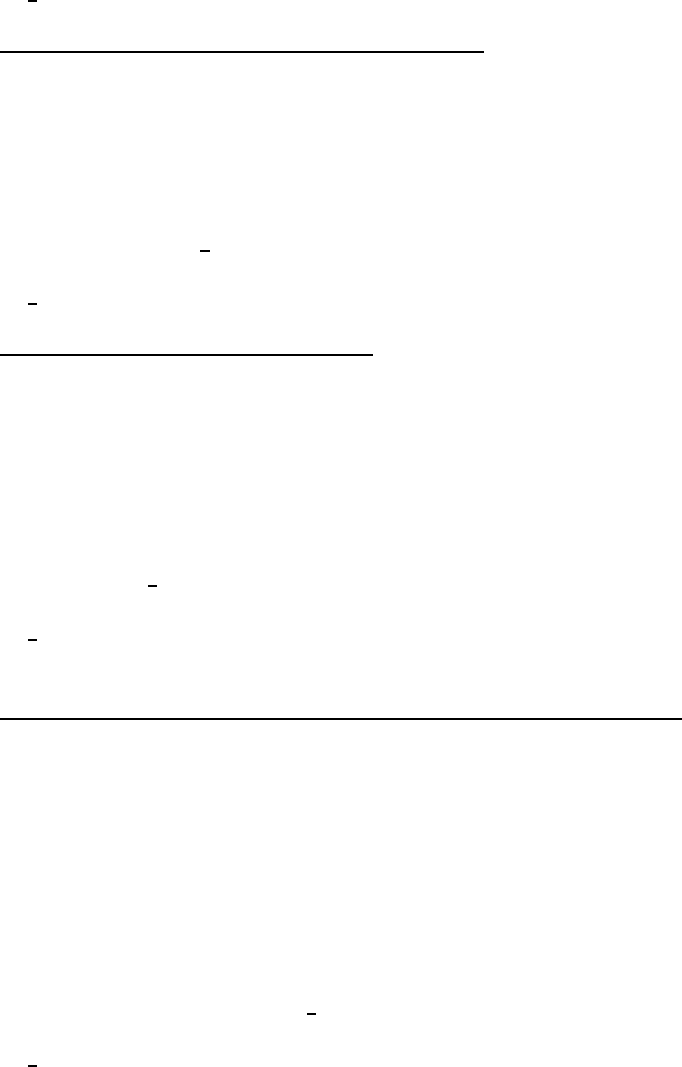
3.8.1 Data Extraction Commands
•
ho lineintegral(type)
Calculate the line integral for the defined contour
type
Integral
0 Temperature difference (G·t)
1 Heat flux through the contour (F ·n)
2 Contour length
3 Average Temperature
This integral returns either 1 or 2 values, depending on the integral type, e.g. :
Ftot, Favg = ho lineintegral(2)
•
ho blockintegral(type)
Calculate a block integral for the selected blocks
type
Integral
0 Average T over the block
1 Block Cross-section
2 Block Volume
3 Average F over the block
4 Average G over the block
Returns one or two floating point values as results, e.g.:
Gx, Gy = ho blockintegral(4)
•
ho getpointvalues(X,Y)
Get the values associated with the point at x,y The return values,
in order, are:
Symbol
Definition
V
Temperature
Fx
x- or r- direction component of heat flux density
Fy
y- or z- direction component of heat flux density
Gx
x- or r- direction component of temperature gradient
Gy
y- or z- direction component of temperature gradient
kx
x- or r- direction component of thermal conductivity
ky
y- or z- direction component of thermal conductivity
Example: To catch all values at (0.01,0) use
T,Fx,Fy,Gx,Gy,kx,ky= ho getpointvalues(0.01,0)
•
ho makeplot(PlotType,NumPoints,Filename,FileFormat)
Allows Lua access to the
X-Y plot routines. If only PlotType or only PlotType and NumPoints are specified, the com-
mand is interpreted as a request to plot the requested plot type to the screen. If, in addition,
the Filename parameter is specified, the plot is instead written to disk to the specified file
name as an extended metafile. If the FileFormat parameter is also, the command is instead
interpreted as a command to write the data to disk to the specfied file name, rather than
display it to make a graphical plot. Valid entries for PlotType are:
121

PlotType
Definition
0
V (Temperature)
1 |
D
|
(Magnitude of heat flux density)
2
D . n (Normal heat flux density)
3
D . t (Tangential heat flux density)
4 |
E
|
(Magnitude of field intensity)
5
E . n (Normal field intensity)
6
E . t (Tangential field intensity)
Valid file formats are:
FileFormat
Definition
0
Multi-column text with legend
1
Multi-column text with no legend
2
Mathematica-style formatting
For example, if one wanted to plot V to the screen with 200 points evaluated to make the
graph, the command would be:
ho makeplot(0,200)
If this plot were to be written to disk as a metafile, the command would be:
ho makeplot(0,200,"c:temp.emf")
To write data instead of a plot to disk, the command would be of the form:
ho makeplot(0,200,"c:temp.txt",0)
•
ho getprobleminfo()
Returns info on problem description. Returns three values: the
Problem type (0 for planar and 1 for axisymmetric); the depth assumed for planar problems
in units of meters; and the length unit used to draw the problem in meters.
•
ho getconductorproperties("conductor")
Properties are returned for the conductor
property named ”conductor”. Two values are returned: The temperature of the specified
conductor, and the total heat flux through the specified conductor.
3.8.2 Selection Commands
•
ho seteditmode(mode)
Sets the mode of the postprocessor to point, contour, or area mode.
Valid entries for mode are
"point", "contour",
and
"area".
•
ho selectblock(x,y)
Select the block that contains point
(x,y).
•
ho groupselectblock(n)
Selects all of the blocks that are labeled by block labels that are
members of group n. If no number is specified (i.e.
ho groupselectblock()
), all blocks
are selected.
•
ho selectconductor("name")
Selects all nodes, segments, and arc segments that are part
of the conductor specified by the string
("name")
. This command is used to select con-
ductors for the purposes of the “weighted stress tensor” force and torque integrals, where the
conductors are points or surfaces, rather than regions (i.e. can’t be selected with
ho selectblock
).
122

•
ho addcontour(x,y)
Adds a contour point at
(x,y).
If this is the first point then it
starts a contour, if there are existing points the contour runs from the previous point to this
point. The
ho addcontour
command has the same functionality as a right-button-click
contour point addition when the program is running in interactive mode.
•
ho bendcontour(angle,anglestep)
Replaces the straight line formed by the last two
points in the contour by an arc that spans angle degrees. The arc is actually composed
of many straight lines, each of which is constrained to span no more than anglestep degrees.
The
angle
parameter can take on values from -180 to 180 degrees. The
anglestep
param-
eter must be greater than zero. If there are less than two points defined in the contour, this
command is ignored.
•
ho selectpoint(x,y)
Adds a contour point at the closest input point to
(x,y).
If the se-
lected point and a previous selected points lie at the ends of an arcsegment, a contour is added
that traces along the arcsegment. The
selectpoint
command has the same functionality as
the left-button-click contour point selection when the program is running in interactive mode.
•
ho clearcontour()
Clear a prevously defined contour
•
ho clearblock()
Clear block selection
3.8.3 Zoom Commands
•
ho zoomnatural()
Zoom to the natural boundaries of the geometry.
•
ho zoomin()
Zoom in one level.
•
ho zoomout()
Zoom out one level.
•
ho zoom(x1,y1,x2,y2)
Zoom to the window defined by lower left corner
(x1,y1)
and
upper right corner
(x2,y2).
3.8.4 View Commands
•
ho showmesh()
Show the mesh.
•
ho hidemesh()
Hide the mesh.
•
ho showpoints()
Show the node points from the input geometry.
•
ho hidepoints()
Hide the node points from the input geometry.
•
ho smooth("flag")
This function controls whether or not smoothing is applied to the F
and G fields which are naturally piece-wise constant over each element. Setting flag equal
to
"on"
turns on smoothing, and setting flag to
"off"
turns off smoothing.
•
ho showgrid()
Show the grid points.
123

•
ho hidegrid()
Hide the grid points points.
ho gridsnap("flag")
Setting flag to ”on” turns on snap to grid, setting flag to ”off” turns
off snap to grid.
•
ho setgrid(density,"type")
Change the grid spacing. The density parameter specifies
the space between grid points, and the type parameter is set to
"cart"
for Cartesian coordi-
nates or
"polar"
for polar coordinates.
•
ho hidedensityplot()
hides the heat flux density plot.
•
ho showdensityplot(legend,gscale,type,upper,lower)
Shows the heat flux density
plot with options:
legend
Set to 0 to hide the plot legend or 1 to show the plot legend.
gscale
Set to 0 for a colour density plot or 1 for a grey scale density plot.
upper
Sets the upper display limit for the density plot.
lower
Sets the lower display limit for the density plot.
type
Sets the type of density plot. A value of 0 plots temperature, 1 plots the magnitude of
F, and 2 plots the magnitude of G
•
ho hidecontourplot()
Hides the contour plot.
•
ho showcontourplot(numcontours,lower V,upper V)
shows the V contour plot with
options:
numcontours
Number of equipotential lines to be plotted.
upper V
Upper limit for contours.
lower V
Lower limit for contours.
If
ho numcontours
is -1 all parameters are ignored and default values are used,
e.g.
show contour plot(-1)
•
ho showvectorplot(type,scalefactor)
controls the display of vectors denoting the field
strength and direction. The parameters taken are the
type
of plot, which should be set to 0 for
no vector plot, 1 for heat flux density F, and 2 for temperature gradient G. The
scalefactor
determines the relative length of the vectors. If the scale is set to 1, the length of the vectors
are chosen so that the highest flux density corresponds to a vector that is the same length as
the current grid size setting.
•
ho minimize()
minimizes the active heat flow input view.
•
ho maximize()
maximizes the active heat flow input view.
•
ho restore()
restores the active heat flow input view from a minimized or maximized state.
•
ho resize(width,height)
resizes the active heat flow input window client area to width
× height.
124

3.8.5 Miscellaneous
•
ho close()
close the current postprocessor window.
•
ho refreshview()
Redraws the current view.
•
ho reload()
Reloads the solution from disk.
•
ho savebitmap("filename")
saves a bitmapped screen shot of the current view to the
file specified by
"filename"
. Note that if you use a path you must use two backslashes
(e.g.
"c:
\\
temp
\\
myfile.bmp"
). If the file name contains a space (e.g. file names like
c:\program files\stuff) you must enclose the file name in (extra) quotes by using a \
"
se-
quence. For example:
ho savebitmap("
\
"c:
\\
temp
\\
screenshot.bmp
\
"")
•
ho savemetafile("filename")
saves a metafile screenshot of the current view to the file
specified by
"filename"
, subject to the printf-type formatting explained previously for the
savebitmap
command.
•
ho shownames(flag)
This function allow the user to display or hide the block label names
on screen. To hide the block label names,
flag
should be 0. To display the names, the
parameter should be set to 1.
•
ho numnodes()
Returns the number of nodes in the in focus heat flow output mesh.
•
ho numelements()
Returns the number of elements in the in focus heat flow output mesh.
•
ho getnode(n)
Returns the (x,y) or (r,z) position of the nth mesh node.
•
ho getelement(n)
MOGetElement[n] returns the following proprerties for the nth element:
1. Index of first element node
2. Index of second element node
3. Index of third element node
4. x (or r) coordinate of the element centroid
5. y (or z) coordinate of the element centroid
6. element area using the length unit defined for the problem
7. group number associated with the element
3.9 Current Flow Preprocessor Lua Command Set
A number of different commands are available in the preprocessor. Two naming conventions can
be used: one which separates words in the command names by underscores, and one that eliminates
the underscores.
125

3.9.1 Object Add/Remove Commands
•
ci addnode(x,y)
Add a new node at x,y
•
ci addsegment(x1,y1,x2,y2)
Add a new line segment from node closest to (x1,y1) to
node closest to (x2,y2)
•
ci addblocklabel(x,y)
Add a new block label at (x,y)
•
ci addarc(x1,y1,x2,y2,angle,maxseg)
Add a new arc segment from the nearest node
to (x1,y1) to the nearest node to (x2,y2) with angle ‘angle’ divided into ‘maxseg’ segments.
•
ci deleteselected
Delete all selected objects.
•
ci deleteselectednodes
Delete selected nodes.
•
ci deleteselectedlabels
Delete selected block labels.
•
ci deleteselectedsegments
Delete selected segments.
•
ci deleteselectedarcsegments
Delete selects arcs.
3.9.2 Geometry Selection Commands
•
ci clearselected()
Clear all selected nodes, blocks, segments and arc segments.
•
ci selectsegment(x,y)
Select the line segment closest to (x,y)
•
ci selectnode(x,y)
Select the node closest to (x,y). Returns the coordinates of the se-
lected node.
•
ci selectlabel(x,y)
Select the label closet to (x,y). Returns the coordinates of the se-
lected label.
•
ci selectarcsegment(x,y)
Select the arc segment closest to (x,y)
•
ci selectgroup(n)
Select the n
th
group of nodes, segments, arc segments and block labels.
This function will clear all previously selected elements and leave the edit mode in 4 (group)
•
ci selectcircle(x,y,R,editmode)
selects objects within a circle of radius R centered at
(x,y). If only x, y, and R paramters are given, the current edit mode is used. If the editmode
parameter is used, 0 denotes nodes, 2 denotes block labels, 2 denotes segments, 3 denotes
arcs, and 4 specifies that all entity types are to be selected.
•
ci selectrectangle(x1,y1,x2,y2,editmode)
selects objects within a rectangle defined
by points (x1,y1) and (x2,y2). If no editmode parameter is supplied, the current edit mode is
used. If the editmode parameter is used, 0 denotes nodes, 2 denotes block labels, 2 denotes
segments, 3 denotes arcs, and 4 specifies that all entity types are to be selected.
126

3.9.3 Object Labeling Commands
•
ci setnodeprop("propname",groupno, "inconductor")
Set the selected nodes to have
the nodal property
"propname"
and group number
groupno
. The
"inconductor"
string
specifies which conductor the node belongs to. If the node doesn’t belong to a named con-
ductor, this parameter can be set to
"<None>"
.
•
ci setblockprop("blockname", automesh, meshsize, group)
Set the selected block
labels to have the properties:
Block property
"blockname"
.
automesh
: 0 = mesher defers to mesh size constraint defined in
meshsize
, 1 = mesher
automatically chooses the mesh density.
meshsize
: size constraint on the mesh in the block marked by this label.
A member of group number
group
•
ci setsegmentprop("propname", elementsize, automesh, hide, group, "inconductor",)
Set the select segments to have:
Boundary property
"propname"
Local element size along segment no greater than
elementsize
automesh
: 0 = mesher defers to the element constraint defined by
elementsize
, 1 = mesher
automatically chooses mesh size along the selected segments
hide
: 0 = not hidden in post-processor, 1 == hidden in post processor
A member of group number
group
A member of the conductor specified by the string
"inconductor".
If the segment is not
part of a conductor, this parameter can be specified as
"<None>"
.
•
ci setarcsegmentprop(maxsegdeg, "propname", hide, group, "inconductor")
Set
the selected arc segments to:
Meshed with elements that span at most
maxsegdeg
degrees per element
Boundary property
"propname"
hide
: 0 = not hidden in post-processor, 1 == hidden in post processor
A member of group number
group
A member of the conductor specified by the string
"inconductor".
If the segment is not
part of a conductor, this parameter can be specified as
"<None>"
.
•
ci setgroup(n)
Set the group associated of the selected items to n
127

3.9.4 Problem Commands
•
ci probdef(units,type,frequency,precision,(depth),(minangle))
changes the prob-
lem definition. The
units
parameter specifies the units used for measuring length in the
problem domain. Valid
"units"
entries are
"inches"
,
"millimeters"
,
"centimeters"
,
"mils"
,
"meters
, and
"micrometers"
. Set
problemtype
to
"planar"
for a 2-D planar
problem, or to
"axi"
for an axisymmetric problem. The
frequency
parameter specifies
the frequency in Hz at which the analysis ois to be performed. The
precision
parame-
ter dictates the precision required by the solver. For example, entering
1.E-8
requires the
RMS of the residual to be less than 10
−8
. A fourth parameter, representing the depth of the
problem in the into-the-page direction for 2-D planar problems, can also be specified for pla-
nar problems. A sixth parameter represents the minimum angle constraint sent to the mesh
generator.
•
ci analyze(flag)
runs
belasolv
to solve the problem. The
flag
parameter controls
whether the Belasolve window is visible or minimized. For a visible window, either specify
no value for
flag
or specify 0. For a minimized window,
flag
should be set to 1.
•
ci loadsolution()
loads and displays the solution corresponding to the current geometry.
•
ci setfocus("documentname")
Switches the electrostatics input file upon which Lua com-
mands are to act. If more than one electrostatics input file is being edited at a time, this
command can be used to switch between files so that the mutiple files can be operated upon
programmatically via Lua.
documentname
should contain the name of the desired document
as it appears on the window’s title bar.
•
ci saveas("filename")
saves the file with name
"filename"
. Note if you use a path you
must use two backslashes e.g.
c:\\temp\\myfemmfile.fee
3.9.5 Mesh Commands
•
ci createmesh()
runs triangle to create a mesh. Note that this is not a necessary precursor
of performing an analysis, as
ci analyze()
will make sure the mesh is up to date before
running an analysis. The number of elements in the mesh is pushed back onto the lua stack.
•
ci showmesh()
toggles the flag that shows or hides the mesh.
•
ci purgemesh()
clears the mesh out of both the screen and memory.
3.9.6 Editing Commands
•
ci copyrotate(bx, by, angle, copies, (editaction) )
bx, by
– base point for rotation
angle
– angle by which the selected objects are incrementally shifted to make each copy.
angle
is measured in degrees.
copies
– number of copies to be produced from the selected objects.
128

editaction
0 –nodes, 1 – lines (segments), 2 –block labels, 3 – arc segments, 4- group
•
ci copytranslate(dx, dy, copies, (editaction))
dx,dy
– distance by which the selected objects are incrementally shifted.
copies
– number of copies to be produced from the selected objects.
editaction
0 –nodes, 1 – lines (segments), 2 –block labels, 3 – arc segments, 4- group
•
mi createradius(x,y,r)
turnsacornerlocatedat
(x,y)
intoacurveofradius
r
.
•
ci moverotate(bx,by,shiftangle (editaction))
bx, by
– base point for rotation
shiftangle
– angle in degrees by which the selected objects are rotated.
editaction
0 –nodes, 1 – lines (segments), 2 –block labels, 3 – arc segments, 4- group
•
ci movetranslate(dx,dy,(editaction))
dx,dy
– distance by which the selected objects are shifted.
editaction
0 –nodes, 1 – lines (segments), 2 –block labels, 3 – arc segments, 4- group
•
ci scale(bx,by,scalefactor,(editaction))
bx, by
– base point for scaling
scalefactor
– a multiplier that determines how much the selected objects are scaled
editaction
0 –nodes, 1 – lines (segments), 2 –block labels, 3 – arc segments, 4- group
•
ci mirror(x1,y1,x2,y2,(editaction))
mirror the selected objects about a line passing
through the points
(x1,y1)
and
(x2,y2)
. Valid
editaction
entries are 0 for nodes, 1 for
lines (segments), 2 for block labels, 3 for arc segments, and 4 for groups.
•
ci seteditmode(editmode)
Sets the current editmode to:
"nodes"
– nodes
"segments"
- line segments
"arcsegments"
- arc segments
"blocks"
- block labels
"group"
- selected group
This command will affect all subsequent uses of the other editing commands, if they are used
WITHOUT the
editaction
parameter.
129

3.9.7 Zoom Commands
•
ci zoomnatural()
zooms to a “natural” view with sensible extents.
•
ci zoomout()
zooms out by a factor of 50%.
•
ci zoomin()
zoom in by a factor of 200%.
•
ci zoom(x1,y1,x2,y2)
Set the display area to be from the bottom left corner specified by
(x1,y1
) to the top right corner specified by
(x2,y2)
.
3.9.8 View Commands
•
ci showgrid()
Show the grid points.
•
ci hidegrid()
Hide the grid points points.
•
ci gridsnap("flag")
Setting flag to ”on” turns on snap to grid, setting flag to ”off”turns
off snap to grid.
•
ci setgrid(density,"type")
Change the grid spacing. The density parameter specifies
the space between grid points, and the type parameter is set to
"cart"
for Cartesian coordi-
nates or
"polar"
for polar coordinates.
•
ci refreshview()
Redraws the current view.
•
ci minimize()
minimizes the active magnetics input view.
•
ci maximize()
maximizes the active magnetics input view.
•
ci restore()
restores the active magnetics input view from a minimized or maximized
state.
•
ci resize(width,height)
resizes the active magnetics input window client area to width
× height.
3.9.9 Object Properties
•
ci getmaterial("materialname")
fetches the material specified by
materialname
from
the materials library.
•
ci addmaterial("materialname", ox, oy, ex, ey, ltx, lty)
adds a new material
with called
"materialname"
with the material properties:
ox
Electrical conductivity in the x- or r-direction in units of S/m.
oy
Electrical conductivity in the y- or z-direction in units of S/m.
ex
Relative permittivity in the x- or r-direction.
ey
Relative permittivity in the y- or z-direction.
130

ltx
Dielectric loss tangent in the x- or r-direction.
lty
Dielectric loss tangent in the y- or z-direction.
•
ci addpointprop("pointpropname",Vp,qp)
adds a new point property of name
"pointpropname"
with either a specified potential
Vp
a point current density
qp
in units of A/m.
•
ci addboundprop("boundpropname", Vs, qs, c0, c1, BdryFormat)
adds a new bound-
ary property with name
"boundpropname"
For a “Fixed Voltage” type boundary condition, set the
Vs
parameter to the desired voltage
and all other parameters to zero.
To obtain a “Mixed” type boundary condition, set
C1
and
C0
as required and
BdryFormat
to
1. Set all other parameters to zero.
To obtain a prescribes surface current density, set
qs
to the desired current density in A/m
2
and set
BdryFormat
to 2.
For a “Periodic” boundary condition, set
BdryFormat
to 3 and set all other parameters to
zero.
For an “Anti-Perodic” boundary condition, set
BdryFormat
to 4 set all other parameters to
zero.
•
ci addconductorprop("conductorname", Vc, qc, conductortype)
adds a new con-
ductor property with name
"conductorname"
with either a prescribed voltage or a pre-
scribed total current. Set the unused property to zero. The
conductortype
parameter is 0
for prescribed current and 1 for prescribed voltage.
•
ci deletematerial("materialname")
deletes the material named
"materialname"
.
•
ci deleteboundprop("boundpropname")
deletes the boundary property named
"boundpropname"
.
•
ci deleteconductor("conductorname")
deletes the conductor named
conductorname
.
•
ci deletepointprop("pointpropname")
deletes the point property named
"pointpropname"
•
ci modifymaterial("BlockName",propnum,value)
This function allows for modifica-
tion of a material’s properties without redefining the entire material (e.g. so that current can
be modified from run to run). The material to be modified is specified by
"BlockName"
.
The next parameter is the number of the property to be set. The last number is the value to
be applied to the specified property. The various properties that can be modified are listed
below:
propnum Symbol Description
0
BlockName
Name of the material
1
ox
x (or r) direction conductivity
2
oy
y (or z) direction conductivity
3
ex
x (or r) direction relative permittivity
4
ey
y (or z) direction relative permittivity
5
ltx
x (or r) direction dielectric loss tangent
6
lty
y (or z) direction dielectric loss tangent
131

•
ci modifyboundprop("BdryName",propnum,value)
This function allows for modifica-
tion of a boundary property. The BC to be modified is specified by
"BdryName"
. The next
parameter is the number of the property to be set. The last number is the value to be applied
to the specified property. The various properties that can be modified are listed below:
propnum
Symbol Description
0
BdryName
Name of boundary property
1
Vs
Fixed Voltage
2
qs
Prescribed current density
3
c0
Mixed BC parameter
4
c1
Mixed BC parameter
5
BdryFormat
Type of boundary condition:
0 = Prescribed V
1 = Mixed
2 = Surface current density
3 = Periodic
4 = Antiperiodic
•
ci modifypointprop("PointName",propnum,value)
This function allows for modifica-
tion of a point property. The point property to be modified is specified by
"PointName"
.
The next parameter is the number of the property to be set. The last number is the value to
be applied to the specified property. The various properties that can be modified are listed
below:
propnum
Symbol Description
0
PointName
Name of the point property
1
Vp
Prescribed nodal voltage
2
qp
Point current density in A/m
•
ci modifyconductorprop("ConductorName",propnum,value)
This function allows for
modification of a conductor property. The conductor property to be modified is specified by
"ConductorName"
. The next parameter is the number of the property to be set. The last
number is the value to be applied to the specified property. The various properties that can
be modified are listed below:
propnum
Symbol Description
0
ConductorName
Name of the conductor property
1
Vc
Conductor voltage
2
qc
Total conductor current
3
ConductorType
0 = Prescribed current, 1 = Prescribed voltage
3.9.10 Miscellaneous
•
ci savebitmap("filename")
saves a bitmapped screenshot of the current view to the file
specified by
"filename"
, subject to the
printf
-type formatting explained previously for
the
ci saveas
command.
•
ci savemetafile("filename")
saves a metafile screenshot of the current view to the file
132

specified by
"filename"
, subject to the
printf
-type formatting explained previously for
the
ci saveas
command.
•
ci refreshview()
Redraws the current view.
•
ci close()
closes the preprocessor window and destroys the current document.
•
ci shownames(flag)
This function allow the user to display or hide the block label names
on screen. To hide the block label names,
flag
should be 0. To display the names, the
parameter should be set to 1.
•
ci readdxf("filename")
This function imports a dxf file specified by
"filename"
.
•
ci savedxf("filename")
This function saves geometry information in a dxf file specified
by
"filename"
.
•
ci defineouterspace(Zo,Ro,Ri)
defines an axisymmetric external region to be used in
conjuction with the Kelvin Transformation method of modeling unbounded problems. The
Zo
parameter is the z-location of the origin of the outer region, the
Ro
parameter is the radius
of the outer region, and the
Ri
parameter is the radius of the inner region (i.e. the region
of interest). In the exterior region, the permeability varies as a function of distance from
the origin of the external region. These parameters are necessary to define the permeability
variation in the external region.
•
ci attachouterspace()
marks all selected block labels as members of the external region
used for modeling unbounded axisymmetric problems via the Kelvin Transformation.
•
ci detachouterspace()
undefines all selected block labels as members of the external
region used for modeling unbounded axisymmetric problems via the Kelvin Transformation.
•
ci attachdefault()
marks the selected block label as the default block label. This block
label is applied to any region that has not been explicitly labeled.
•
ci detachdefault()
undefines the default attribute for the selected block labels.
•
ci makeABC(n,R,x,y,bc)
creates a series of circular shells that emulate the impedance of
an unbounded domain (i.e. an Inprovised Asymptotic Boundary Condition). The
n
parameter
contains the number of shells to be used (should be between 1 and 10),
R
is the radius of the
solution domain, and
(x,y)
denotes the center of the solution domain. The
bc
parameter
should be specified as 0 for a Dirichlet outer edge or 1 for a Neumann outer edge. If the
function is called without all the parameters, the function makes up reasonable values for the
missing parameters.
3.10 Current Flow Post Processor Command Set
There are a number of Lua scripting commands designed to operate in the postprocessor. As with
the preprocessor commands, these commands can be used with either the underscore naming or
with the no-underscore naming convention.
133

3.10.1 Data Extraction Commands
•
co lineintegral(type)
Calculate the line integral for the defined contour
type
Integral
0 E ·t
1 J ·n
2 Contour length
3 Average voltage over contour
4 Force from stress tensor
5 Torque from stress tensor
This integral returns either 1 or 2 values, depending on the integral type, e.g. :
Fx, Fy = co lineintegral(4)
•
co blockintegral(type)
Calculate a block integral for the selected blocks
type
Integral
0 Real Power
1 Reactive Power
2 Apparent Power
3 Time-Average Stored Energy
4 Block cross-section area
5 Block volume
6 x (or r) direction Weighted Stress Tensor force, DC component
7 y (or z) direction Weighted Stress Tensor force, DC component
8 x (or r) direction Weighted Stress Tensor force, 2x frequency component
9 y (or z) direction Weighted Stress Tensor force, 2x frequency component
10 Weighted Stress Tensor torque, DC component
11 Weighted Stress Tensor torque, 2x frequency component
Returns a value that can be complex, as necessary.
•
co getpointvalues(X,Y)
Get the values associated with the point at x,y The return values,
in order, are:
134

Symbol
Definition
V
Voltage
Jx
x- or r- direction component of current density
Jy
y- or z- direction component of current density
Kx
x- or r- direction component of AC conductivity
Ky
y- or z- direction component of AC conductivity
Ex
x- or r- direction component of electric field intensity
Ey
y- or z- direction component of electric field intensity
ex
x- or r- direction component of permittivity
ey
y- or z- direction component of permittivity
Jdx
x- or r- direction component of displacement current density
Jdy
y- or z- direction component of displacement current density
ox
x- or r- direction component of permittivity
oy
y- or z- direction component of permittivity
Jcx
x- or r- direction component of conduction current density
Jcy
y- or z- direction component of conduction current density
•
co makeplot(PlotType,NumPoints,Filename,FileFormat)
Allows Lua access to the
X-Y plot routines. If only PlotType or only PlotType and NumPoints are specified, the com-
mand is interpreted as a request to plot the requested plot type to the screen. If, in addition,
the Filename parameter is specified, the plot is instead written to disk to the specified file
name as an extended metafile. If the FileFormat parameter is also, the command is instead
interpreted as a command to write the data to disk to the specfied file name, rather than
display it to make a graphical plot. Valid entries for PlotType are:
PlotType
Definition
0
V (Voltage)
1 |
J
|
(Magnitude of current density)
2
J . n (Normal current density)
3
J . t (Tangential current density)
4 |
E
|
(Magnitude of field intensity)
5
E . n (Normal field intensity)
6
E . t (Tangential field intensity)
7 |
Jc
|
(Magnitude of conduction current density)
8
Jc . n (Normal conduction current density)
9
Jc . t (Tangential conduction current density)
10 |
Jd
|
(Magnitude of displacement current density)
11
Jd . n (Normal displacement current density)
12
Jd . t (Tangential displacement current density)
Valid file formats are:
FileFormat
Definition
0
Multi-column text with legend
1
Multi-column text with no legend
2
Mathematica-style formatting
For example, if one wanted to plot V to the screen with 200 points evaluated to make the
135

graph, the command would be:
co makeplot(0,200)
If this plot were to be written to disk as a metafile, the command would be:
co makeplot(0,200,"c:temp.emf")
To write data instead of a plot to disk, the command would be of the form:
co makeplot(0,200,"c:temp.txt",0)
•
co getprobleminfo()
Returns info on problem description. Returns four values:
Return value Definition
1 problem type
2 frequency in Hz
3 depth assumed for planar problems in meters.
4 length unit used to draw the problem, represented in meters
•
co getconductorproperties("conductor")
Properties are returned for the conductor
property named ”conductor”. Two values are returned: The voltage of the specified con-
ductor, and the current on the specified conductor.
3.10.2 Selection Commands
•
co seteditmode(mode)
Sets the mode of the postprocessor to point, contour, or area mode.
Valid entries for mode are
"point", "contour",
and
"area".
•
co selectblock(x,y)
Select the block that contains point
(x,y).
•
co groupselectblock(n)
Selects all of the blocks that are labeled by block labels that are
members of group n. If no number is specified (i.e.
co groupselectblock()
), all blocks
are selected.
•
co selectconductor("name")
Selects all nodes, segments, and arc segments that are part
of the conductor specified by the string
("name")
. This command is used to select con-
ductors for the purposes of the “weighted stress tensor” force and torque integrals, where the
conductors are points or surfaces, rather than regions (i.e. can’t be selected with
co selectblock
).
•
co addcontour(x,y)
Adds a contour point at
(x,y).
If this is the first point then it
starts a contour, if there are existing points the contour runs from the previous point to this
point. The
co addcontour
command has the same functionality as a right-button-click
contour point addition when the program is running in interactive mode.
•
co bendcontour(angle,anglestep)
Replaces the straight line formed by the last two
points in the contour by an arc that spans angle degrees. The arc is actually composed
of many straight lines, each of which is constrained to span no more than anglestep degrees.
The
angle
parameter can take on values from -180 to 180 degrees. The
anglestep
param-
eter must be greater than zero. If there are less than two points defined in the contour, this
command is ignored.
136

•
co selectpoint(x,y)
Adds a contour point at the closest input point to
(x,y).
If the se-
lected point and a previous selected points lie at the ends of an arcsegment, a contour is added
that traces along the arcsegment. The
selectpoint
command has the same functionality as
the left-button-click contour point selection when the program is running in interactive mode.
•
co clearcontour()
Clear a prevously defined contour
•
co clearblock()
Clear block selection
3.10.3 Zoom Commands
•
co zoomnatural()
Zoom to the natural boundaries of the geometry.
•
co zoomin()
Zoom in one level.
•
co zoomout()
Zoom out one level.
•
co zoom(x1,y1,x2,y2)
Zoom to the window defined by lower left corner
(x1,y1)
and
upper right corner
(x2,y2).
3.10.4 View Commands
•
co showmesh()
Show the mesh.
•
co hidemesh()
Hide the mesh.
•
co showpoints()
Show the node points from the input geometry.
•
co hidepoints()
Hide the node points from the input geometry.
•
co smooth("flag")
This function controls whether or not smoothing is applied to the D
and E fields which are naturally piece-wise constant over each element. Setting flag equal to
"on"
turns on smoothing, and setting flag to
"off"
turns off smoothing.
•
co showgrid()
Show the grid points.
•
co hidegrid()
Hide the grid points points.
co gridsnap("flag")
Setting flag to ”on” turns on snap to grid, setting flag to ”off” turns
off snap to grid.
•
co setgrid(density,"type")
Change the grid spacing. The density parameter specifies
the space between grid points, and the type parameter is set to
"cart"
for Cartesian coordi-
nates or
"polar"
for polar coordinates.
•
co hidedensityplot()
hides the current density plot.
137

•
co showdensityplot(legend,gscale,type,upper,lower)
Showsthe current density plot
with options:
legend
Set to 0 to hide the plot legend or 1 to show the plot legend.
gscale
Set to 0 for a colour density plot or 1 for a grey scale density plot.
upper
Sets the upper display limit for the density plot.
lower
Sets the lower display limit for the density plot.
type
Sets the type of density plot. Specific choices for the type of density plot include:
type
Description
0 |V|
1 |Re(V)|
2 |Im(V)|
3 |J|
4 |Re(J)|
5 |Im(J)|
6 |E|
7 |Re(E)|
8 |Im(E)|
•
co hidecontourplot()
Hides the contour plot.
•
co showcontourplot(numcontours,lower V,upper V),type
shows the V contour plot
with options:
numcontours
Number of equipotential lines to be plotted;
upper V
Upper limit for contours;
lower V
Lower limit for contours;
type
the type of contour plot to be rendered.
If
co numcontours
is -1 all parameters are ignored and default values are used,
e.g.
show contour plot(-1)
The type can take on the values of
"real"
,
"imag"
, or
"both"
, denoting the real part of
voltage, the imaginary part of voltage, or both components of voltage.
•
co showvectorplot(type,scalefactor)
controls the display of vectors denoting the field
strength and direction. The
type
parameter can take on the following values:
type
Description
0 No vector plot
1 Re(J)
2 Re(E)
3 Im(J)
4 Im(E)
5 Re(J) and Im(J)
6 Re(E) and Im(E)
The
scalefactor
determines the relative length of the vectors.
138

If the scale is set to 1, the length of the vectors are chosen so that the highest field magnitude
corresponds to a vector that is the same length as the current grid size setting.
•
co minimize()
minimizes the active magnetics input view.
•
co maximize()
maximizes the active magnetics input view.
•
co restore()
restores the active magnetics input view from a minimized or maximized
state.
•
co resize(width,height)
resizes the active magnetics input window client area to width
× height.
3.10.5 Miscellaneous
•
co close()
close the current postprocessor window.
•
co refreshview()
Redraws the current view.
•
co reload()
Reloads the solution from disk.
•
co savebitmap("filename")
saves a bitmapped screen shot of the current view to the
file specified by
"filename"
. Note that if you use a path you must use two backslashes
(e.g.
"c:
\\
temp
\\
myfile.bmp"
). If the file name contains a space (e.g. file names like
c:\program files\stuff) you must enclose the file name in (extra) quotes by using a \
"
se-
quence. For example:
co savebitmap("
\
"c:
\\
temp
\\
screenshot.bmp
\
"")
•
co savemetafile("filename")
saves a metafile screenshot of the current view to the file
specified by
"filename"
, subject to the printf-type formatting explained previously for the
savebitmap
command.
•
co shownames(flag)
This function allow the user to display or hide the block label names
on screen. To hide the block label names,
flag
should be 0. To display the names, the
parameter should be set to 1.
•
co numnodes()
Returns the number of nodes in the in focus current flow output mesh.
•
co numelements()
Returns the number of elements in the in focus current flow output
mesh.
•
co getnode(n)
Returns the (x,y) or (r,z) position of the nth mesh node.
•
co getelement(n)
MOGetElement[n] returns the following proprerties for the nth element:
1. Index of first element node
2. Index of second element node
3. Index of third element node
139
4. x (or r) coordinate of the element centroid
5. y (or z) coordinate of the element centroid
6. element area using the length unit defined for the problem
7. group number associated with the element
140
Chapter 4
Mathematica Interface
FEMM can interact with Mathematica via Mathematica’s MathLink API. Once Mathematica and
FEMM are connected, any any string sent by Mathematica is automatically collected and inter-
preted as a command to FEMM’s Lua interpreter. Results can be returned across the link by a
special Lua print command that sends the results to Mathematica as a list, rather than to the Lua
console screen.
The MathLink connection to FEMM can be initialized in two ways. The link can either be
established automatically on startup, or during a session via commands in the Lua console. To
establish the connection on startup, just use the LinkLaunch function in Mathematica, e.g.:
mlink = LinkLaunch["c:\\progra˜1\\femm42\\bin\\femm.exe"];
To initialize the link, some string must first be sent over the link from the Mathematica side,
e.g.:
LinkWrite[mlink, "print(0)"]
All strings sent to FEMM are then sent using the same sort of LinkWrite command. When it is
time to close the link, the link can be closed using the LinkClose command, e.g.:
LinkClose[mlink]
To start a link during a session, the Lua command
mlopen()
can be used. A dialog will then
appear, prompting for a name for the link. Choose any name that you want, e.g.
portname
. On the
Mathematica side, one connects to the newly formed link via the Mathematica command:
mlink = LinkConnect["portname"]
After this point, the link is used and closed in the same way as the link that is automatically
created on startup.
As previously noted, LinkWrite is used on the mathematica side to send a string to FEMM.
FEMM automatically monitors the link and interprets the string with no further user action re-
quired. To send results back to Mathematica, one uses the
mlput
command in Lua. This function
works exactly like the
print
command in lua, except that the result gets pushed back across the
link as a list of mixed reals and strings, as appropriate. To retrieve this information on the Mathe-
matica side, one uses the LinkRead command, e.g.:
result = LinkRead[mlink]
To automate the interaction between FEMM and Mathematica, a Mathematica package called
MathFEMM is available. This package implements a set of Mathematica functions similar to those
implemented in Lua. With MathFEMM, the the user does not have to deal with the specifics of
creating the Mathlink connection and manually transferring information across it. All MathLink
141
details are taken care of automatically by the package, and the Mathematica front-end can then be
used to directly control FEMM via a set of Mathematica function calls.
142
Chapter 5
ActiveX Interface
FEMM also allows for interprocess communication via ActiveX. FEMM is set up to act as an
ActiveX Automation Server so that other programs can connect to FEMM as clients and command
FEMM to perform various actions and analyses in a programmatic way.
FEMM registers itself as an ActiveX server under the name
femm.ActiveFEMM42
. An expla-
nation of how to connect to and manipulate an ActiveX server are beyond the treatment of this
manual, in part because the specifics depend upon what client platform is being used (e.g. VB,
VC++, Matlab, etc.)
The interface to FEMM contains no properties and only two methods:
•
BSTR call2femm(BSTR luacmd);
•
BSTR mlab2femm(BSTR luacmd);
In each case, a string is passed to the method, and a string is returned as a result. The incoming
string is sent to the Lua interpreter. Any results from the Lua command are returned as a string.
The difference between the two methods is that
call2femm
returns a string with each returned item
separated by a newline character, whereas
mlab2femm
returns the result formatted as a Matlab
array, with the total package enclosed by square brackets and the individual items separated by
spaces. FEMM assumes that it is the client’s responsibility to free the memory allocated for both
the input and output strings.
One program that can connect to FEMM as a client via Active X is Matlab. From Matlab,
one can send commands to the FEMM Lua interpreter and receive the results of the command.
To aid in the use of FEMM from Matlab, a toolbox called OctaveFEMM is available. This tool-
box implements Matlab commands that subsume the functionality of Lua using equivalent Matlab
commands, in a similar way to the fashion that MathFEMM works with Mathematica. Using the
toolbox, all details of the ActiveX interface are taken care of in a way that is completely transparent
to the user.
143
Chapter 6
Numerical Methods
For those of you interested in what’s going on behind the scenes in the solvers, this section is
meant as a brief description of the methods and techniques used by FEMM. References are cited
as applicable.
6.1 Finite Element Formulation
All elements were derived using variational formulations (based on minimizing energy, as opposed
to Galerkin, least squares residual, and so on). Explanations of the variational approach for 2-D
planar problems with first-order triangle elements are widely available in the literature ([10] in
particular was referred to during the creation of FEMM). The axisymmetric electrostatics solver
also uses the approach laid out in [10].
The axisymmetric case for magnetics, however, is oddly less well addressed. Hoole [2] and
Silvester [11] promote solving axisymmetric problems in terms of a modified vector potential.
The advantage of the modified vector potential is that closed-form expressions for each term in
the element matrices can be formed. An early version of FEMM used this technique, but it is
observed to yield relatively larger errors near r = 0. With the modified potential formulation, it
is also nontrivial to compute the average flux density associated with each element. However, the
formulation suggested by Henrotte in [12] gives good performance close to r = 0. FEMM uses a
formulation that is very similar to Henrotte for axisymmetric magnetic problems.
6.2 Linear Solvers
For all problems, variations of the iterative Conjugate Gradient solver are used. This technique is
appropriate for the sort of problem that FEMM solves, because the matrices are symmetric and very
sparse. A row-based storage scheme is used in which only the nonzero elements of the diagonal
and upper triangular part of the matrix are solved.
For magnetostatic and electrostatic problems, the preconditioned conjugate gradient (PCG)
code is based on the discussion in [11]. Minor modifications are made to this algorithm to avoid
computing certain quantities more than once per iteration. Although Silvester promotes the use
of the Incomplete Cholesky preconditioner, it is not used in FEMM, because it nearly doubles
the storage requirements–for each element of the matrix stored, a corresponding element of the
144
preconditioner must also be stored. Instead, the Symmetric Successive Over-Relaxation (SSOR)
preconditioner, as described in [13], is used. The advantage of this preconditioner is that it is built
on the fly in a simple way using only the matrix elements that are already in storage. In general,
the speed of PCG using SSOR is said to be comparable to the speed of PCG with Incomplete
Cholesky.
For harmonic problems, the regular PCG algorithm cannot be used; the matrix that arises in
the formulation of harmonic problems is Complex Symmetric (i.e. A = A
T
), rather than Hermitian
(i.e. A = A
∗
). Curiously, there is not much literature available on iterative solvers for complex
symmetric problems, given the number of diverse applications in which these problems arise.
However, there is a very good paper on the solution of linear problems with complex symmetric
matrices via various flavors of Conjugate Gradient by Freund [14]. The techniques discussed
by Freund allow one to operate directly on the complex symmetric matrix and take advantage
of the symmetric structure to minimize the number of computations that must be performed per
iteration. Although Freund supports Quasi-Minimum Residual approach, FEMM uses the complex
symmetric version of biconjugate gradient also described in [14]. After coding and comparing the
the speed of both BCG and QMR, it was found that BCG is somewhat faster due to a relatively
smaller number of computations that must be performed per iteration (even though QMR has better
convergence properties than BCG).
However, using the algorithms as described by [14], solution times were unacceptably long.
To decrease solution times, the complex symmetric BCG algorithm was modified to include the
SSOR preconditioner (built in exactly the same way as for magnetostatic problems). Including the
SSOR preconditioner in complex symmetric BCG problems usually yields an order of magnitude
improvement in speed over no preconditioner.
In all problems, a node renumbering scheme is used. Although the conjugate gradient schemes
work well without renumbering, the renumbering seems to roughly halve the solution time. There
is an overall advantage to using the renumbering, because the of time required to perform the
renumbering is small compared to the time required to run CG or BCG. Although there are many
possible approaches to renumbering, FEMM uses the Cuthill-McKee method as described in [2].
Although there are newer schemes that yield a tighter profile, Cuthill-McKee does a relatively good
job and requires very little to execute. The renumbering code is a hold-over from an early version
of FEMM that employed a banded Gauss Elimination solver in which a good node numbering is
essential to good performance. The renumbering speeds up CG and BCG by reducing the error
between the SSOR approximation of A
−1
and the exact A
−1
. An interesting paper on the effect of
the ordering of the unknowns on convergence in conjugate gradient methods is [15].
6.3 Field Smoothing
Since first-order triangles are used by FEMM, the resulting solution for B and H obtained by
differentiating A is constant over each element. If the raw B and H are used by the postprocessor,
density plots of B and 2-D plots of field quantities along user-defined contours look terrible. The
values of B and H also are not so accurate at points in an element away from the element’s centroid.
The use of smoothing to recover the accuracy lost by differentiating A is known as supercon-
vergence. Of the greatest interest to FEMM are so-called “patch recovery” techniques. The basic
idea is the the solutions for B are most accurate at the centroid of the triangular element (known as
145
its Gauss Point). One desires a continuous profile of B that can be interpolated from nodal values,
in the same way that vector potential A can be represented. The problem is, the “raw” solution of
B is multivalued at any node point, those values being the different constant values of B in each
element surrounding the node point. The general approach to estimating the “true” value of B at
any node point is to fit a least-squares plane through the values of B at the Gauss points of all
elements that surround a node of interest, and to take the value of the plane at the node point’s
location as its smoothed value of B [16].
However, this approach to patch recovery has a lot of shortcomings. For the rather irregular
meshes that can arise in finite elements, the least-squares fit problem can be ill-condition, or even
singular, at some nodes in the finite element mesh. Furthermore, the superconvergence solution can
actually be less accurate than the piece-wise constant solution in the neighborhood of boundaries
and interfaces.
One can note that the patch recovery method is merely a weighted average of the flux densi-
ties in all of the elements surrounding a given node. Instead of a least-squares fit, FEMM simply
weights the values of flux density in each adjacent element’s Gauss point with a value inversely
proportional to the distance from the Gauss point to the node point of interest. Away from bound-
aries, the results seem to be nearly as good as a least-squares fit. At boundaries and interfaces, the
smoothed solution is no worse than the unsmoothed solution.
A related approach is used for smoothing D and E in electrostatics problems. In electrostatics
problems, however, nodal values of D are found by taking the gradient of a best-fit plane through
the voltage of the neighboring nodes. A number of special cases must be caught so that reasonable
results are obtained at various boundaries and surfaces.
146
Bibliography
[1] M. Plonus, Applied electromagnetics. McGraw-Hill, 1978.
[2] S. R. Hoole, Computer-aided analysis and design of electromagnetic devices, Elsevier, 1989.
[3] J. D. Jackson, Classical electrodynamics, 2
nd
ed, Wiley, 1975.
[4] F. M. White, Heat and mass transfer, Addison-Wesley, 1988.
[5] R. Haberman, Elementary applied partial differential equations, Prentice-Hall, 1987.
[6] R. L. Stoll, The analysis of eddy currents, Oxford University Press, 1974.
[7] S. McFee, J. P. Webb, and D. A. Lowther, “A tunable volume integration formulation for
force calculation in finite-element based computational magnetostatics,” IEEE Transactions
on Magnetics, 24(1):439-442, January 1988.
[8] F. Henrotte, G. Deliege, and K. Hameyer, “The eggshell method for the computation of elec-
tromagnetic forces on rigid bodies in 2D and 3D,” CEFC 2002, Perugia, Italy, April 16-18,
2002. (pdf version)
[9] R. Ierusalimschy, L. H. de Figueiredo, and W. Celes, Reference Manual of the Programming
Language Lua 4.0
http://www.lua.org/manual/4.0/
[10] P. E. Allaire, Basics of the finite element method, 1985.
[11] P. P. Silvester, Finite elements for electrical engineers, Cambridge University Press, 1990.
[12] F. Henrotte et al, “A new method for axisymmetric linear and nonlinear problems,” IEEE
Transactions on Magnetics, MAG-29(2):1352-1355, March 1993.
[13] C. A. Fletcher, Computational techniques for fluid dynamics, Springer-Verlag, 1988.
[14] R. W. Freund, “Conjugate gradient-type methods for linear systems with complex symmetric
coefficient matrices,” SIAM Journal of Scientific and Statistical Computing, 13(1):425-448,
January 1992.
[15] E. F. D’Azevedo, P. A. Forsyth, and W. Tang, “Ordering methods for preconditioned conju-
gate gradient methods applied to unstructured grid problems,” SIAM J. Matrix Anal. Appl.,
12(4), July 1992.
147
[16] O. C. Zienkiewicz and J. Z. Zhu, “ The superconvergent patch recovery and a posteriori
estimates, part 1: the recovery technique,” International Journal for Numerical Methods in
Engineering, 33:1331-1364, 1992.
[17] Q. Chen and A. Konrad, “A review of finite element open boundary techniques for static and
quasistatic electromagnetic field problems,” IEEE Transactions on Magnetics, 33(1):663-
676, January 1997.
[18] E. M. Freeman and D. A. Lowther, “A novel mapping technique for open boundary finite
element solutions to Poissons equation,” IEEE Transactions on Magnetics, 24(6):2934-2936,
November 1988.
[19] D. A. Lowther, E. M. Freeman, and B. Forghani, “A sparse matrix open boundary method for
finite element analysis,” IEEE Transactions on Magnetics, 25(4)2810-2812, July 1989.
[20] E. M. Freeman and D. A. Lowther, “An open boundary technique for axisymmetric and
three dimensional magnetic and electric field problems,” IEEE Transactions on Magnetics,
25(5):4135-4137, September 1989.
[21] A. G. Jack and B. C. Mecrow, ”Methods for magnetically nonlinear problems involving
significant hysteresis and eddy currents,” IEEE Transactions on Magnetics, 26(2):424-429,
March 1990.
[22] D. O’Kelly, “Hysteresis and eddy current losses in steel plates with nonlinear magnetization
characteristics,” Proceedings of the IEE, 119(11):1675-1676, November 1972.
148
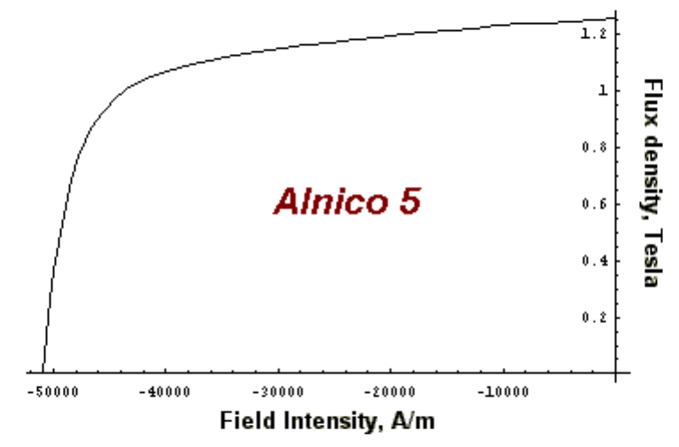
Appendix A
Appendix
A.1 Modeling Permanent Magnets
FEMM accommodates permanent magnets, but there are some special rules associated with prop-
erly modeling them. This appendix will explain how to distill enough information from a manu-
facturer’s literature to properly define the material in FEMM.
The manufacturer provides information about their material in the form of a demagnetization
curve. A sample curve for Alnico 5 is pictured in Figure A.1. The task is to get the appropriate
information out of the curve put in a FEMM Block Property model.
Magnets can be modeled from several different, but equally valid, points of view. From the
perspective finite element analysis, the most useful model is to think of the magnet as a volume of
ferromagnetic material surrounded by a thin sheet of current, as shown in Figure A.2. From this
Figure A.1: Sample demagnetization curve for Alnico 5
149

Figure A.2: Magnet as an equivalent current sheet.
point of view, the demagnetization curve is what occurs when different amounts of magnetomotive
force are applied to a long magnet, acting in the direction opposing the field of the magnet. When
enough MMF is applied so that the field is exactly cancelled out, the applied MMF must be exactly
the same as the MMF that is driving the magnet. The B-H profile that is traversed on the way to
the B = 0 point is just the B-H curve of the material inside the magnet.
Using these insights, the permanent magnet can be modeled. The coercivity (denoted H
c
) of
the magnet is the absolute value of the MMF that it takes to bring the the field in the magnet to
zero. This value (in units of Amps/Meter) is entered in the
H_c
box in the Block Property dialog
(see Figure 2.9). If the magnet material is nonlinear, the appropriate values to enter in the B-H data
dialog can be obtained by shifting the curve to the right by exactly H
c
, so that the B = 0 point lines
up with the origin. For example, the shifted demagnetization curve corresponding to Alnico 5 is
pictured in Figure A.3. If the demagnetization curve is straight enough to be considered linear, one
can obtain the appropriate permeability by taking the slope of the demagnetization curve.
Strong rare-earth materials at room temperature have a very linear demagnetization curve. Usu-
ally, a linear model is sufficient for these materials. In addition, these materials have a relative per-
meability very close to 1. The modeling of these materials can be simplified (while only incurring
small errors) by assuming that the permeability is exactly 1. Then, if you know the energy product
of the magnet material in units of MGOe (the unit in which the energy product is almost always
given), the appropriate H
c
can be determined via (A.1).
H
c
=
5(10
5
)
√
E
π
(A.1)
where E is the energy product in MGOe and the resulting H
c
is in units of A/m (e.g. 40 MGOe
≈ 10
6
A/m).
With alnico magnets, great care must be taken in interpreting the finite element results. Unlike
rare-earth magnets, these magnets exhibit a great degree of hysteresis when they are demagne-
tized. That is, when the flux density is pushed below the “knee” in the demagnetization curve, the
flux level does not recover to the previous magnitude when the opposing MMF is removed. This
hysteresis is illustrated in Figure A.4. This sort of demagntization and recoil can occur when the
150
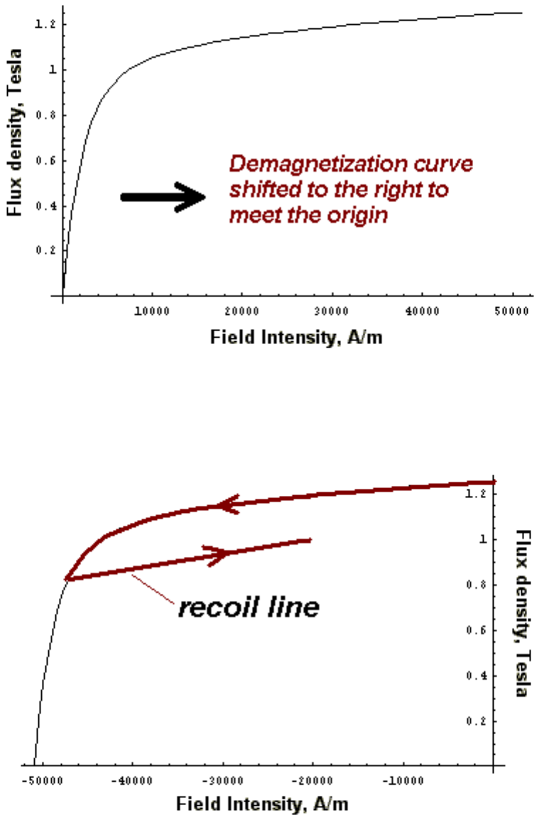
Figure A.3: Shifting the B-H curve of a permanent magnet
Figure A.4: Recoil in partially demagnetized Alnico 5.
151

magnets are being handled prior to assembly into a device. In a motor, the magnets will demag-
netize somewhat when the motor is first started. They will eventually end up running back and
forth along a recoil line that is below the “virgin” demagnetization curve. The point is that the
modeler cannot be sure exactly where the magnets are operating–an analysis that takes this sort
of hysteresis into account is beyond the scope of FEMM. Note, however, that this caution applies
only for nonlinear magnets; for practical purposes, rare-earth magnets generally do not exhibit this
sort of hysteresis behavior.
A.2 Bulk Lamination Modeling
A great number of magnetic devices employ cores built up out of thin laminations for the purpose of
reducing eddy current effects. One way to model these materials within a finite element framework
would be to model each discrete lamination (and the insulation between laminations) in the finite
element geometry. An alternative is to treat the laminated material as a continuum and derive
bulk properties that yield essentially the same results, while requiring a much less elaborate finite
element mesh. FEMM has implemented this bulk approach to laminations.
Consider that the flux can flow through the lamination in a combination of two ways: via the
“easy” direction down the laminations, or the “hard” way, across the thickness of the laminations.
The hard direction is difficult for flux for two reasons. First, the rolling process makes the iron
somewhat less permeable than in the easy direction. Second, and most importantly, the flux must
traverse the insulation between laminations, which typically has a unit permeability.
The first assumption in deriving the bulk permeability model is that the permeability in the
iron itself is isotropic. This isn’t quite true, but almost all of the reluctance in the hard direction
results from crossing the gap between laminations. Having a significant error in the hard direction
permeability in the iron itself only results in a trivial change in the bulk reluctance in the cross-
lamination direction.
Armed with this assumption, a circuit model can be produced for each direction of flux travel.
For the easy direction, the circuit model is pictured in Figure A.5. There are two reluctances in
parallel–one for flux that flows through the iron part of the laminations:
R
ez, fe
=
L
µ
r
µ
o
cW
(A.2)
and another reluctance for flux that flows through the air between laminations:
R
ez,air
=
L
µ
o
(1−c)W
(A.3)
where L and W are the length and width of the path traversed, and c is the fraction of the path filled
with iron. Adding these two reluctances in parallel yields:
R
ez
=
L
((1−c) + cµ
r
)µ
o
W
(A.4)
Since L and W are arbitrarily chosen, the bulk permeability of the section is:
µ
ez
= ((1−c) + cµ
r
)µ
o
(A.5)
152
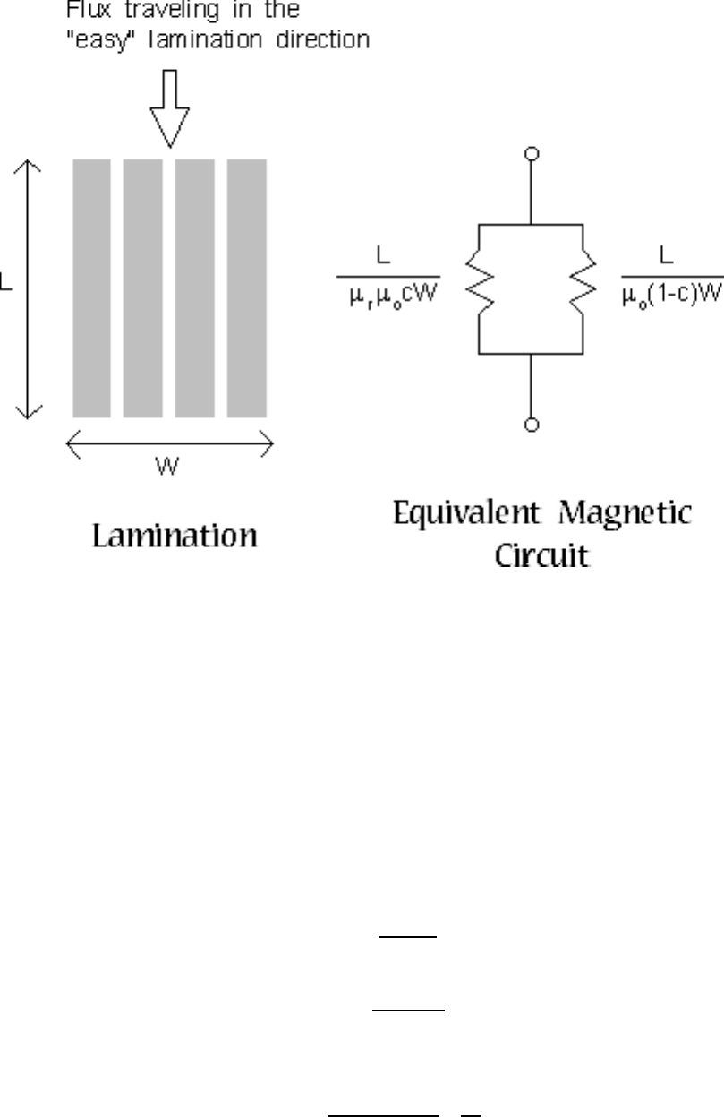
Figure A.5: Equivalent circuit for flux in the “easy” direction
For the solution of nonlinear problems, the derivation of the changes to Newton’s method to acco-
modate the bulk lamination model are greatly simplified if it is assumed that (1 −c) << cµ
r
. In
this case, µ
ez
can be approximated as:
µ
ez
≈ cµ
r
µ
o
(A.6)
This approximation leads to only trivial errors until the fill factor approaches zero. For example, if
µ
r
= 1000 with a 90% fill, the difference between (A.5) and (A.6) is only about 0.01%.
For the hard direction, a different equivalent circuit, pictured in Figure A.6 can be drawn. In
this case, the circuit is two reluctances in series, as the flux has to cross the insulation and the
lamination in succession. These reluctances are:
R
hard, f e
=
cL
µ
r
µ
o
W
(A.7)
R
hard,air
=
(1−c)L
µ
o
W
(A.8)
Adding these two reluctances together in series yields:
R
hard
=
c+ (1−c)µ
r
µ
r
µ
o
L
W
(A.9)
153
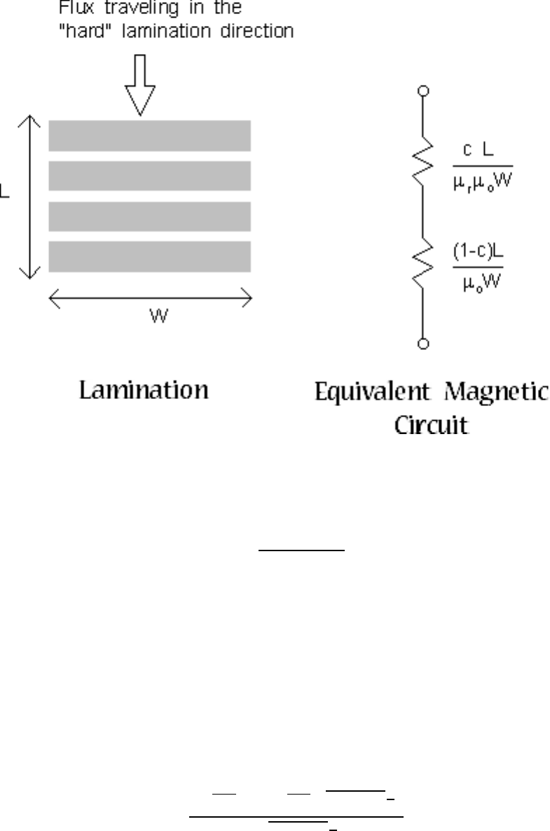
Figure A.6: Equivalent circuit for flux in the “hard” direction.
Since L and W are arbitrary, the bulk permeability in the hard direction is:
µ
hard
=
µ
r
µ
o
c+ (1−c)µ
r
(A.10)
If the material is laminated “in-plane,” all flux is flowing in the easy direction, and (A.6) is
used as the permeability for each element. In problems that are laminated parallel to x or y,
(A.6) and (A.10) are used as permeabilities in the standard fashion for elements with an anisotropic
permeability.
For harmonic problems, eddy currents flow in the laminations, and hysteresis causes additional
loss. If the laminations are thin compared to the other dimensions of the geometry, the effects
of eddy currents and hysteresis can be encapsulated in a frequency-dependent permeability [6].
In this case, the magnetostatic permeability, µ
r
is simply replaced by the frequency-dependent
permeability µ
fd
in (A.6) and (A.10):
µ
fd
=
µ
r
e
−jφ
h
2
tanh
h
e
−jφ
h
2
√
jωσµ
r
µ
o
d
2
i
√
jωσµ
r
µ
o
d
2
(A.11)
In (A.11), φ
h
represents a constant phase lag between B and H due to hysteresis, σ is the conduc-
tivity of the lamination material, d is the thickness of the iron part of the lamination, and ω is the
frequency of excitation in rad/s. Note that the concept of hysteresis-induced lag can be applied to
154

non-laminated materials as well, simply by multiplying the magnetostatic permeability by e
−jφ
h
for harmonic problems.
A.3 Open Boundary Problems
Typically, finite element methods are best suited to problems with well-defined, closed solution
regions. However, a large number of problems that one might like to address have no natural
outer boundary. A prime example is a solenoid in air. The boundary condition that one would like
to apply is A = 0 at r = ∞. However, finite element methods, by nature, imply a finite domain.
Fortunately, there are methods that can be applied to get solutions that closely approximate the
“open boundary” solution using finite element methods.
A.3.1 Truncation of Outer Boundaries
The simplest, but least accurate, way to proceed is to pick an arbitrary boundary “far enough”
away from the area of interest and declare either A = 0 or ∂A/∂n = 0 on this boundary. According
to [17], a rule of thumb is that the distance from the center of the problem to the outer boundary
should be at least five times the distance from the center to the outside of the objects of interest.
Truncation is the method employed by most magnetics finite element programs, because it requires
no additional effort to implement.
The down side to truncation is that get an accurate solution in the region of interest, a volume
of air much larger than the region of interest must also be modeled. Usually, this large region
exterior to the area of interest can be modeled with a relatively coarse mesh to keep solution times
to a minimum. However, some extra time and space is still required to solve for a region in which
one has little interest.
A.3.2 Asymptotic Boundary Conditions
A thorough review of open boundary techniques is contained in [17]. Perhaps the simple way to
approximate an “open” boundary (other than truncation) described in [17] is to use asymptotic
boundary conditions. The result is that by carefully specifying the parameters for the “mixed”
boundary condition, and then applying this boundary condition to a circular outer boundary, the
unbounded solution can be closely approximated. An example that employs an asymptotic bound-
ary condition to obtain an unbounded field solution is the
axi1.fem
example included in the dis-
tribution.
Consider a 2-D planar problem in polar coordinates. The domain is a circular shell of radius r
o
in an unbounded region. As r → ∞, vector potential A goes to zero. On the surface of the circle,
the vector is a prescribed function of θ. This problem has an analytical solution, which is:
A(r,θ) =
∞
∑
m=1
a
m
r
m
cos(mθ+ α
m
) (A.12)
where the a
m
and α
m
parameters are chosen so that the solution matches the prescribed potential
on the surface of the circle.
155

One could think of this solution as describing the solution exterior to a finite element problem
with a circular outer boundary. The solution is described inside the circle via a finite element
solution. The trick is to knit together the analytical solution outside the circle to the finite element
solution inside the circle.
From inspecting (A.12), one can see that the higher-numbered harmonic, the faster the magni-
tude of the harmonic decays with respect to increasing r. After only a short distance, the higher-
numbered harmonics decay to the extent that almost all of the open-space solution is described by
only the leading harmonic. If n is the number of the leading harmonic, the open-field solution for
large, but not infinite, r is closely described by:
A(r,θ) ≈
a
n
r
n
cos(nθ+ α
n
) (A.13)
Differentiating with respect to r yields:
∂A
∂r
= −
na
n
r
n+1
cos(nθ+ α
n
) (A.14)
If (A.14) is solved for a
n
and substituted into (A.13), the result is:
∂A
∂r
+
n
r
A = 0 (A.15)
Now, (A.15) is a very useful result. This is the same form as the “mixed” boundary condition
supported by FEMM. If the outer edge of the solution domain is circular, and the outer finite ele-
ment boundary is somewhat removed from the area of primary interest, the open domain solution
can be closely approximated by applying (A.15) the circular boundary.
To apply the Asymptotic Boundary Condition, define a new, mixed-type boundary condition.
Then, pick the parameters so that:
c
0
=
n
µ
o
r
o
(A.16)
c
1
= 0 (A.17)
where r
o
is the outer radius of the region in meters (regardless of the working length units), and
µ
o
= 4π(10
−7
).
Although the above derivation was specifically for 2-D problems, it turns out that when the
same derivation is done for the axisymmetric case, the definition of the mixed boundary condition
coefficients are exactly the same as (A.16).
To apply the Asymptotic Boundary Condition to electrostatics problems, pick the parameters
so that:
c
0
=
ε
o
n
r
o
(A.18)
c
1
= 0
where r
o
is the outer radius of the region in meters (regardless of the working length units), and
ε
o
= 8.85418781762e-012. Note that ε
o
is defined in the Lua implementation in both the pre-
and post-processors as the global variable
eo
, which can be used in any script or edit box in the
program.
156
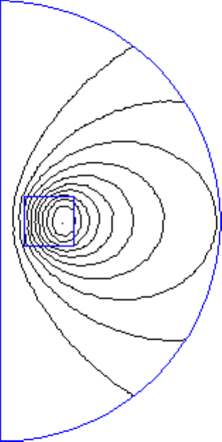
Figure A.7: Air-cored coil with “open” boundary condition
Just like magnetics problems, it turns out that 2-D problems are also described by (A.18). One
subtle difference, however, is that n =1 in the axisymmetric case corresponds to the case in which
there is a net charge with (i.e. the geometry looks like a point charge when viewed from a distance),
whereas the n = 1 case corresponds to a dipole charge distribution in 2D planar problems. If charge
is conserved in the geometry of interest in the axisymmetric case, one needs to use n =2 in Eq.
(A.18). It should be noted that this is a departure from the magnetostatic case with the vector
potential formulation in which n = 1 corresponds to a dipole arrangement in the axisymmetric
case.
Some care must be used in applying this boundary condition. Most of the time, it is sufficient
to take n = 1 (i.e the objects in the solution region look like a dipole when viewed from a large
distance). However, there are other cases (e.g. a 4-pole halbach permanent magnet array) in which
the leading harmonic is something other than n = 1. You need to use your insight into your specific
problem to pick the appropriate n for the leading harmonic. You also must put the objects of interest
roughly in the center of the circular finite element domain to minimize the magnitude higher-order
field components at the outer boundary.
Although the application of this boundary condition requires some thought on the part of the
user, the results can be quite good. Figure A.7, corresponding to the
axi1
example, represents
the field produced by an air-cored coil in free space. The asymptotic boundary condition has been
applied to the circular outer boundary. Inspecting the solution, flux lines appear to cross the circular
boundary as if the solution domain were truly unbounded.
157

A quick note on computational efficiency: applying the absorbing boundary condition im-
poses no additional computing cost on the problem. The ABC is computationally no more time-
consuming to apply than enforcing A = 0 at the outer boundary. Solution times for the PCG solver
are equivalent in either case. It can also readily be derived that the ABC works exactly the same
for harmonics problems. (To see this, just assume that the a
m
in (A.12) can be complex valued,
and follow the same derivation).
A.3.3 Kelvin Transformation
A particularly good approach to “open boundary” problems is the Kelvin Transformation, a tech-
nique first discussed in the context of computational magnetics in [18] and [19]. The strengths of
this technique are:
• the effects of the exterior region are, in theory, exactly modeled by this approach;
• a sparse matrix representation of the problem is retained (unlike FEM-BEM methods, which
give the same “exact solution” but densely couples together the boundary nodes).
• requires no “special” features in the finite element solver to implement the technique, other
than the ability to apply periodic boundary conditions.
The purposes of this note are to explain what the Kelvin transformation is derived and to show how
it is implemented in the context of the FEMM finite element program.
Derivation
In the “far field” region, the material is typically homogeneous (e.g. air and free of sources. In this
case, the differential equation that describes vector potential A is the Laplace equation:
∇
2
A = 0 (A.19)
If we write (A.19) in polar notation, A is described by:
1
r
∂
∂r
r
∂A
∂r
+
1
r
2
∂
2
A
∂θ
2
= 0 (A.20)
Assume that the “near field” region of the problem can be contained in a circle of radius r
o
centered
at the origin. The far-field region is then everything outside the circle.
One approach to unbounded problems is to attempt to map the unbounded region onto a
bounded region, wherein problems can more easilby be solved. Specifically, we desire a way
to transform the unbounded region outside the circle into a bounded region. One simple way to
make such a mapping is to define another variable, R, that is related to r by:
R =
r
2
o
r
(A.21)
By inspecting (A.21), it can be seen that this relationship maps the exterior region onto a circle of
radius r
o
.
158
The next step is to transform (A.19), the differential equation that the field must satisfy, into
the mapped space. That is, (A.19) must be written in terms of R and θ rather than r and θ. We can
evaluate derivatives in terms of R instead of r by employing the chain rule:
∂
∂r
=
∂
∂R
dR
dr
= −
∂
∂R
R
r
o
2
(A.22)
Now, we can note that at r = R = r
o
,
∂A
∂r
= −
∂A
∂R
(A.23)
and we can substitute (A.22) into (A.19) to yield, after some algebraic manipulation:
1
R
∂
∂R
R
∂A
∂R
+
1
R
2
∂
2
A
∂θ
2
= 0 (A.24)
Eq. (A.24), the transformed equation for the outer region, has exactly the same form as inner
region, only in terms of R rather than r. The implication is that for the 2-D planar problem, the
exterior can be modeled simply by creating a problem domain consisting of two circular regions:
on circular region containing the items of interest, and an additional circular region to represent
the “far field.” Then, periodic boundary conditions must be applied to corresponding edges of the
circle to enforce the continuity of A at the edges of the two regions. The is continuity of A at the
boundary between the exterior and interior regions. For a finite element formulation consisting
of first-order triangles, (A.23) is enforced automatically at the boundaries of the two regions. The
second circular region exactly models the infinite space solution, but does it on a bounded domain–
one could always back out the field for any point in space by applying the inverse of (A.21).
Kelvin Transformation Example –
open1.fem
As an example, consider an E-core lamination stack with a winding around it. Suppose that the
objective is to determine the field around the E-core in the absence of any flux return path (i.e.
when the magnetic circuit is open). In this case, the flux is not constrained to flow in a path that is
a priori well defined, because the laminations that complete the flux path have been removed.
The geometry was chosen arbitrarily, the purpose here being more the procedure than the actual
problem. The E-core was chosen to have a 0.5” thick center leg, 0.25” thick outer legs, and a slot
depth of 0.75”. The material for the core is linear with a relative permeability of 2500. The coil
carries a bulk current density of 2 MA/m
2
. The input geometry is picture in Figure A.8.
In Figure A.8, the core is placed within a circular region, and a second circular region is drawn
next to the region containing the core. Periodic boundary conditions are applied to the arcs that
define the boundaries as shown in Figure A.8. The way that periodic boundary conditions are
implemented in FEMM, each periodic boundary condition defined for the problem is to be applied
to two and only two corresponding entities. In this case, each boundary circle is composed of two
arcs, so two periodic boundary conditions must be defined to link together each arc with in the
domain with the core to its corresponding arc in the domain representing the exterior region.
Also notice that a point has been drawn in the center of the exterior region. A point property
has been applied to this point that specifies that A = 0 at this reference point. The center of the
circle maps to infinity in the analogous open problem, so it makes sense to define, in effect, A = 0
159
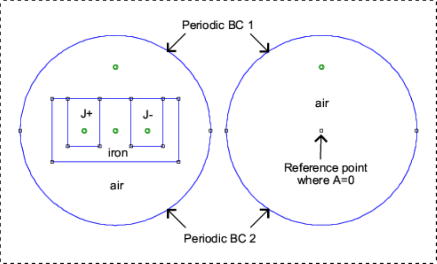
Figure A.8: Example input geometry.
at infinity. If no reference point is defined, it is fairly easy to see that the solution is only unique to
within a constant. The situation is analogous to a situation where Neumann boundary conditions
have been defined on all boundaries, resulting in a non-unique solution for A. Due to the type of
solver that FEMM employs, the problem can most likely be solved even if a reference point is not
defined. However, defining a reference point eliminates the possibility of numerical difficulties
due to uniqueness issues.
The resulting solution is shown in Figure A.9. As is the intention, the flux lines appear to
cross out of the of the region containing the core as if unaffected by the presence of the boundary.
The flux lines reappear in the domain representing the exterior region, completing their flux paths
through the exterior region.
A.4 Nonlinear Time Harmonic Formulation
Starting with the the 3.3 version of FEMM, the program includes a “nonlinear time harmonic”
solver. In general, the notion of a “nonlinear time harmonic” analysis is something of a kludge.
To obtain a purely sinusoidal response when a system is driven with a sinusoidal input, the system
must, by definition, be linear. The nonlinear time harmonic analysis seeks to include the effects
of nonlinearities like saturation and hysteresis on the fundamental of the response, while ignoring
higher harmonic content. This is a notion similar to “describing function analysis,” a widely used
tool in the analysis of nonlinear control systems. There are several subtly different variations of
the formulation that can yield slightly different results, so documentation of what has actually been
implement is important to the correct interpretation of the results from this solver.
An excellent description of this formulation is contained in [21]. FEMM formulates the nonlin-
160
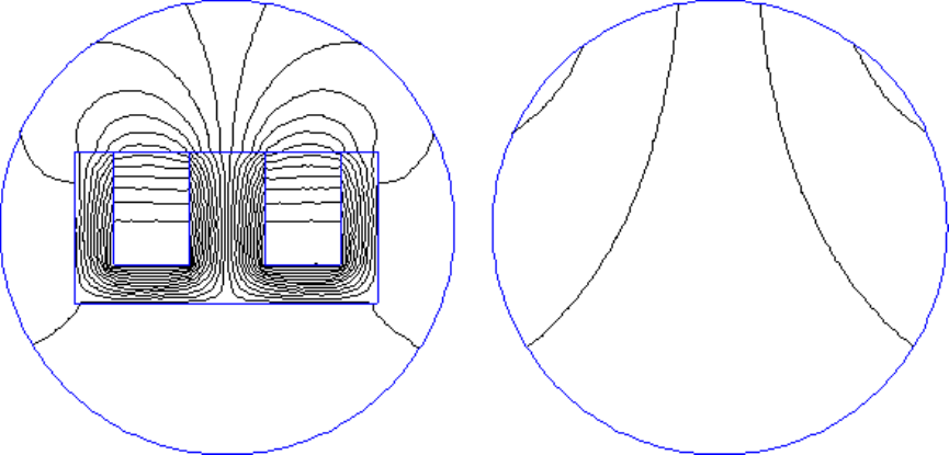
Figure A.9: Solved problem.
ear time harmonic problem as described in this paper. Similar to Jack and Mecrow, FEMM derives
an apparent BH curve by taking H to be the sinusoidally varying quantity. The amplitude of B is
obtained by taking the first coefficient in a Fourier series representation of the resulting B. For the
purposes of this Fourier series computation, FEMM interpolates linearly between the user-defined
points on the BH curve to get a set of points with the same H values as the input set, but with
an adjusted B level. The rationale for choosing H to be the sinusoidal quantity (rather than B) is
that choosing B to be sinusoidal shrinks the defined BH curve–the B values stay fixed while the H
values become smaller. It then becomes hard to define a BH curve that does not get interpolated.
In contrast, with H sinusoidal, the B points are typically larger than the DC flux density levels,
creating a curve with an expanded range.
A “nonlinear hysteresis lag” parameter is then applied to the effective BH curve. The lag
is assumed to be proportional to the permeability, which gives a hysteresis loss that is always
proportional to |B|
2
. This form was suggested by O’Kelly [22]. It has been suggested that that
the Steinmetz equation could be used to specify hysteresis lag, but the Steinmetz equation is badly
behaved at low flux levels (i.e. one can’t solve for a hysteresis lag that produces the Steinmetz
|B|
1.6
form for the loss as B goes to zero.)
For nonlinear in-plane laminations, an additional step is taken to obtain an effective BH curve
that also includes eddy current effects. At each H level on the user-defined BH curve, a 1D non-
linear time harmonic finite element problem is solved to obtain the total flux that flows in the
lamination as a function of the H applied at the edge of the lamination. Then dividing by the lam-
ination thickness and accounting for fill factor, and effective B that takes into account saturation,
hysteresis, and eddy currents in the lamination is obtained for each H.
161
