
EnSight User Manual
for Version 7.6
Table of Contents
1 Overview
2 Input/Output
3Parts
4 Variables
5 GUI Overview
6 Main Menu
7Features
8 Modes
9 Transformation Control
10 Preference File Formats
11 EnSight Data Formats
12 Utility Programs
13 Parallel Rendering and Virtual Reality
Index
How To Table of Contents
Computational Engineering International, Inc.
2166 N. Salem Street, Suite 101, Apex, NC 27523
USA • 919-363-0883 • 919-363-0833 FAX
http://www.ceintl.com
© Copyright 1994–2003, Computational Engineering International, Inc. All rights reserved.
Printed in the United States of America.
EN-UM Revision History
This document has been reviewed and approved in accordance with Computational Engineering
International, Inc. Documentation Review and Approval Procedures.
This document should be used only for Version 7.6 and greater of the EnSight program.
Information in this document is subject to change without notice. This document contains proprietary
information of Computational Engineering International, Inc. The contents of this document may not
be disclosed to third parties, copied, or duplicated in any form, in whole or in part, unless permitted by
contract or by written permission of Computational Engineering International, Inc. The Computational
Engineering International, Inc. Software License Agreement and Contract for Support and
Maintenance Service supersede and take precedence over any information in this document.
EnSight® is a registered trademark of Computational Engineering International, Inc. All registered
trademarks used in this document remain the property of their respective owners.
CEI’s World Wide Web addresses:
http://www.ceintl.com
or
http://www.ensight.com
Restricted Rights Legend
Use, duplication, or disclosure of the technical data contained in this document by the Government is
subject to restrictions as set forth in subparagraph (c)(1)(ii) of the Rights in Technical Data and
Computer Software clause at DFARS 252.227-7013. Unpublished rights reserved under the
Copyright Laws of the United States. Contractor/Manufacturer is Computational Engineering
International, Inc., 2166 N. Salem Street, Suite 101, Apex, NC 27523 USA
EN-UM:5.2-1 October 1994
EN-UM:5.2.2-1 January 1995
EN-UM:5.5-1 September 1995
EN-UM:5.5.1-1 December 1995
EN-UM:5.5.2-1 February 1996
EN-UM:6.0-1 June 1997
EN-UM:6.0-2 August 1997
EN-UM:6.0-3 October 1997
EN-UM:6.0-4 October 1997
EN-UM:6.1-1 March 1998
EN-UM:6.2-1 September 1998
EN-UM:6.2.1-1 November 1998
EN-UM:7.0-1 December 1999
EN-UM:7.1-1 April 2000
EN-UM:7.3-1 March 2001
EN-UM:7.4-1 March 2002
EN-UM:7.4-2 October 2002
EN-UM:7.6-1 May 2003
Table of Contents
EnSight 7 User Manual i
1 Overview
2 Input/Output
2.1 Internal Readers . . . . . . . . . . . . . . . . . . . . . . . . . . . . . . . . . . . . . . . . 2-2
Dataset Format Basics. . . . . . . . . . . . . . . . . . . . . . . . . . . . . . . . . . . . . . . . . . . . . 2-2
Reading and Loading Data Basics . . . . . . . . . . . . . . . . . . . . . . . . . . . . . . . . . . . 2-5
EnSight Case Reader . . . . . . . . . . . . . . . . . . . . . . . . . . . . . . . . . . . . . . . . . . . . . 2-8
EnSight5 Reader . . . . . . . . . . . . . . . . . . . . . . . . . . . . . . . . . . . . . . . . . . . . . . . . 2-15
ABAQUS Reader . . . . . . . . . . . . . . . . . . . . . . . . . . . . . . . . . . . . . . . . . . . . . . . . 2-18
ANSYS RESULTS Reader. . . . . . . . . . . . . . . . . . . . . . . . . . . . . . . . . . . . . . . . . 2-19
ESTET Reader. . . . . . . . . . . . . . . . . . . . . . . . . . . . . . . . . . . . . . . . . . . . . . . . . . 2-20
FAST UNSTRUCTURED Reader . . . . . . . . . . . . . . . . . . . . . . . . . . . . . . . . . . . 2-23
FIDAP NEUTRAL Reader . . . . . . . . . . . . . . . . . . . . . . . . . . . . . . . . . . . . . . . . . 2-23
FLUENT UNIVERSAL Reader . . . . . . . . . . . . . . . . . . . . . . . . . . . . . . . . . . . . . . 2-23
Movie.BYU Reader . . . . . . . . . . . . . . . . . . . . . . . . . . . . . . . . . . . . . . . . . . . . . . 2-24
MPGS 4.1 Reader . . . . . . . . . . . . . . . . . . . . . . . . . . . . . . . . . . . . . . . . . . . . . . . 2-25
N3S Reader . . . . . . . . . . . . . . . . . . . . . . . . . . . . . . . . . . . . . . . . . . . . . . . . . . . . 2-26
PLOT3D Reader . . . . . . . . . . . . . . . . . . . . . . . . . . . . . . . . . . . . . . . . . . . . . . . . 2-27
2.2 User Defined Readers . . . . . . . . . . . . . . . . . . . . . . . . . . . . . . . . . . . 2-31
2.3 Other External Data Sources . . . . . . . . . . . . . . . . . . . . . . . . . . . . . . 2-32
External Translators . . . . . . . . . . . . . . . . . . . . . . . . . . . . . . . . . . . . . . . . . . . . . . 2-32
Exported from Analysis Codes. . . . . . . . . . . . . . . . . . . . . . . . . . . . . . . . . . . . . . 2-32
2.4 Command Files . . . . . . . . . . . . . . . . . . . . . . . . . . . . . . . . . . . . . . . . 2-33
Saving the Default Command File for EnSight Session. . . . . . . . . . . . . . . . . . . 2-35
2.5 Archive Files . . . . . . . . . . . . . . . . . . . . . . . . . . . . . . . . . . . . . . . . . . 2-36
Saving and Restoring a Full backup . . . . . . . . . . . . . . . . . . . . . . . . . . . . . . . . . 2-36
2.6 Context Files . . . . . . . . . . . . . . . . . . . . . . . . . . . . . . . . . . . . . . . . . . 2-39
Saving a Context File . . . . . . . . . . . . . . . . . . . . . . . . . . . . . . . . . . . . . . . . . . . . . 2-39
Table of Contents
Table of Contents
ii EnSight 7 User Manual
Restoring a Context. . . . . . . . . . . . . . . . . . . . . . . . . . . . . . . . . . . . . . . . . . . . . . .2-39
2.7 Scenario Files . . . . . . . . . . . . . . . . . . . . . . . . . . . . . . . . . . . . . . . . . 2-41
2.8 Saving Geometry and Results Within EnSight. . . . . . . . . . . . . . . . . 2-43
Saving Geometric Entities . . . . . . . . . . . . . . . . . . . . . . . . . . . . . . . . . . . . . . . . . .2-43
2.9 Saving and Restoring View States. . . . . . . . . . . . . . . . . . . . . . . . . . 2-46
2.10 Saving and Printing Graphic Images . . . . . . . . . . . . . . . . . . . . . . . 2-47
Troubleshooting Saving an Image. . . . . . . . . . . . . . . . . . . . . . . . . . . . . . . . . . . .2-50
2.11 Saving and Loading XY Plot Data . . . . . . . . . . . . . . . . . . . . . . . . . 2-51
2.12 Saving and Restoring Animation Frames. . . . . . . . . . . . . . . . . . . . 2-52
2.13 Saving Query Text Information . . . . . . . . . . . . . . . . . . . . . . . . . . . 2-53
From Query/Plot Save... Formatted . . . . . . . . . . . . . . . . . . . . . . . . . . . . . . . . . .2-53
From Query/Plot Show Text . . . . . . . . . . . . . . . . . . . . . . . . . . . . . . . . . . . . . . . .2-53
From EnSight Message Window . . . . . . . . . . . . . . . . . . . . . . . . . . . . . . . . . . . . .2-54
2.14 Saving Your EnSight Environment. . . . . . . . . . . . . . . . . . . . . . . . . 2-55
3 Parts
3.1 Part Overview . . . . . . . . . . . . . . . . . . . . . . . . . . . . . . . . . . . . . . . . . . 3-2
Part Creation . . . . . . . . . . . . . . . . . . . . . . . . . . . . . . . . . . . . . . . . . . . . . . . . . . . . .3-3
Part Attributes . . . . . . . . . . . . . . . . . . . . . . . . . . . . . . . . . . . . . . . . . . . . . . . . . . . .3-4
3.2 Part Selection and Identification . . . . . . . . . . . . . . . . . . . . . . . . . . . . 3-6
3.3 Part Editing . . . . . . . . . . . . . . . . . . . . . . . . . . . . . . . . . . . . . . . . . . . . 3-7
Variable Color Palette Icon . . . . . . . . . . . . . . . . . . . . . . . . . . . . . . . . . . . . . . . . . .3-9
Variable Creation (Calculator) Icon . . . . . . . . . . . . . . . . . . . . . . . . . . . . . . . . . . . .3-9
3.4 Part Operations . . . . . . . . . . . . . . . . . . . . . . . . . . . . . . . . . . . . . . . . 3-20
4 Variables
General Description. . . . . . . . . . . . . . . . . . . . . . . . . . . . . . . . . . . . . . . . . . . . . . . .4-1
Table of Contents
EnSight 7 User Manual iii
4.1 Variable Selection and Activation . . . . . . . . . . . . . . . . . . . . . . . . . . . 4-3
4.2 Variable Summary & Palette . . . . . . . . . . . . . . . . . . . . . . . . . . . . . . . 4-5
4.3 Variable Creation . . . . . . . . . . . . . . . . . . . . . . . . . . . . . . . . . . . . . . . 4-10
5 GUI Overview
GUI Conventions . . . . . . . . . . . . . . . . . . . . . . . . . . . . . . . . . . . . . . . . . . . . . . . . . 5-5
6 Main Menu
6.1 File Menu Functions. . . . . . . . . . . . . . . . . . . . . . . . . . . . . . . . . . . . . . 6-2
6.2 Edit Menu Functions . . . . . . . . . . . . . . . . . . . . . . . . . . . . . . . . . . . . . 6-5
6.3 Query Menu Functions. . . . . . . . . . . . . . . . . . . . . . . . . . . . . . . . . . . 6-21
6.4 View Menu Functions. . . . . . . . . . . . . . . . . . . . . . . . . . . . . . . . . . . . 6-24
6.5 Tools Menu Functions . . . . . . . . . . . . . . . . . . . . . . . . . . . . . . . . . . . 6-29
6.6 Case Menu Functions . . . . . . . . . . . . . . . . . . . . . . . . . . . . . . . . . . . 6-39
6.7 Help Menu Functions . . . . . . . . . . . . . . . . . . . . . . . . . . . . . . . . . . . . 6-41
7 Features
7.1 Color . . . . . . . . . . . . . . . . . . . . . . . . . . . . . . . . . . . . . . . . . . . . . . . . . 7-2
7.2 Contour Create/Update . . . . . . . . . . . . . . . . . . . . . . . . . . . . . . . . . . . 7-4
7.3 Isosurface Create/Update . . . . . . . . . . . . . . . . . . . . . . . . . . . . . . . . . 7-8
7.4 Particle Trace Create/Update . . . . . . . . . . . . . . . . . . . . . . . . . . . . . 7-12
7.5 Clip Create/Update . . . . . . . . . . . . . . . . . . . . . . . . . . . . . . . . . . . . . 7-27
7.6 Vector Arrow Create/Update . . . . . . . . . . . . . . . . . . . . . . . . . . . . . . 7-45
7.7 Elevated Surface Create/Update . . . . . . . . . . . . . . . . . . . . . . . . . . . 7-50
7.8 Profile Create/Update . . . . . . . . . . . . . . . . . . . . . . . . . . . . . . . . . . . 7-53
Table of Contents
iv EnSight 7 User Manual
7.9 Developed Surface Create/Update . . . . . . . . . . . . . . . . . . . . . . . . . 7-57
7.10 Displacements On Parts . . . . . . . . . . . . . . . . . . . . . . . . . . . . . . . . 7-62
7.11 Query/Plot . . . . . . . . . . . . . . . . . . . . . . . . . . . . . . . . . . . . . . . . . . . 7-64
7.12 Interactive Probe Query . . . . . . . . . . . . . . . . . . . . . . . . . . . . . . . . . 7-74
7.13 Solution Time . . . . . . . . . . . . . . . . . . . . . . . . . . . . . . . . . . . . . . . . . 7-76
7.14 Flipbook Animation . . . . . . . . . . . . . . . . . . . . . . . . . . . . . . . . . . . . 7-80
7.15 Keyframe Animation. . . . . . . . . . . . . . . . . . . . . . . . . . . . . . . . . . . . 7-86
7.16 Subset Parts Create/Update . . . . . . . . . . . . . . . . . . . . . . . . . . . . . 7-95
7.17 Tensor Glyph Parts Create/Update . . . . . . . . . . . . . . . . . . . . . . . . 7-97
7.18 Material Parts Create/Update . . . . . . . . . . . . . . . . . . . . . . . . . . . 7-100
7.19 Vortex Core Create/Update . . . . . . . . . . . . . . . . . . . . . . . . . . . . . 7-104
7.20 Shock Surface/Region Create/Update. . . . . . . . . . . . . . . . . . . . . 7-108
7.21 Separation/Attachment Lines Create/Update . . . . . . . . . . . . . . . 7-114
7.22 Boundary Layer Variables Create/Update . . . . . . . . . . . . . . . . . . 7-118
8 Modes
8.1 Part Mode . . . . . . . . . . . . . . . . . . . . . . . . . . . . . . . . . . . . . . . . . . . . . 8-2
8.2 Annot Mode . . . . . . . . . . . . . . . . . . . . . . . . . . . . . . . . . . . . . . . . . . . 8-10
8.3 Plot Mode . . . . . . . . . . . . . . . . . . . . . . . . . . . . . . . . . . . . . . . . . . . . . 8-18
8.4 VPort Mode . . . . . . . . . . . . . . . . . . . . . . . . . . . . . . . . . . . . . . . . . . . 8-25
8.5 Frame Mode. . . . . . . . . . . . . . . . . . . . . . . . . . . . . . . . . . . . . . . . . . . 8-34
8.6 View Mode . . . . . . . . . . . . . . . . . . . . . . . . . . . . . . . . . . . . . . . . . . . . 8-44
Table of Contents
EnSight 7 User Manual v
9 Transformation Control
General Description . . . . . . . . . . . . . . . . . . . . . . . . . . . . . . . . . . . . . . . . . . . . . . . 9-1
9.1 Global Transform . . . . . . . . . . . . . . . . . . . . . . . . . . . . . . . . . . . . . . . . 9-3
9.2 Frame Definition. . . . . . . . . . . . . . . . . . . . . . . . . . . . . . . . . . . . . . . . . 9-8
9.3 Frame Transform . . . . . . . . . . . . . . . . . . . . . . . . . . . . . . . . . . . . . . . 9-11
9.4 Tool Transform. . . . . . . . . . . . . . . . . . . . . . . . . . . . . . . . . . . . . . . . . 9-15
9.5 Center Of Transform . . . . . . . . . . . . . . . . . . . . . . . . . . . . . . . . . . . . 9-16
9.6 Z-Clip . . . . . . . . . . . . . . . . . . . . . . . . . . . . . . . . . . . . . . . . . . . . . . . . 9-17
9.7 Look At/Look From. . . . . . . . . . . . . . . . . . . . . . . . . . . . . . . . . . . . . . 9-19
9.8 Copy/Paste Transformation State . . . . . . . . . . . . . . . . . . . . . . . . . . 9-22
10 Preference File Formats
10.1 Window Position File Format . . . . . . . . . . . . . . . . . . . . . . . . . . . . . 10-2
10.2 Connection Information File Format. . . . . . . . . . . . . . . . . . . . . . . . 10-3
10.3 Palette File Formats. . . . . . . . . . . . . . . . . . . . . . . . . . . . . . . . . . . . 10-4
Color Selector Palette File Format . . . . . . . . . . . . . . . . . . . . . . . . . . . . . . . . . . . 10-4
Function Palette File Format . . . . . . . . . . . . . . . . . . . . . . . . . . . . . . . . . . . . . . . 10-4
Predefined Function Palette. . . . . . . . . . . . . . . . . . . . . . . . . . . . . . . . . . . . . . . . 10-5
Default False Color Map File Format . . . . . . . . . . . . . . . . . . . . . . . . . . . . . . . . . 10-6
10.4 Default Part Colors File Format . . . . . . . . . . . . . . . . . . . . . . . . . . . 10-7
10.5 Data Reader Preferences File Format . . . . . . . . . . . . . . . . . . . . . . 10-8
10.6 MPEG Parameters File . . . . . . . . . . . . . . . . . . . . . . . . . . . . . . . . . 10-9
10.7 Parallel Rendering Configuration File . . . . . . . . . . . . . . . . . . . . . 10-10
Table of Contents
vi EnSight 7 User Manual
11 EnSight Data Formats
11.1 EnSight Gold Casefile Format . . . . . . . . . . . . . . . . . . . . . . . . . . . . 11-2
EnSight Gold General Description . . . . . . . . . . . . . . . . . . . . . . . . . . . . . . . . . . .11-2
EnSight Gold Geometry File Format . . . . . . . . . . . . . . . . . . . . . . . . . . . . . . . . . .11-5
EnSight Gold Case File Format. . . . . . . . . . . . . . . . . . . . . . . . . . . . . . . . . . . . .11-31
EnSight Gold Variable File Format . . . . . . . . . . . . . . . . . . . . . . . . . . . . . . . . . .11-40
EnSight Gold Per_Node Variable File Format. . . . . . . . . . . . . . . . . . . . . . . . . .11-40
EnSight Gold Per_Element Variable File Format . . . . . . . . . . . . . . . . . . . . . . .11-56
EnSight Gold Undefined Variable Values Format . . . . . . . . . . . . . . . . . . . . . . .11-70
EnSight Gold Partial Variable Values Format . . . . . . . . . . . . . . . . . . . . . . . . . .11-74
EnSight Gold Measured/Particle File Format . . . . . . . . . . . . . . . . . . . . . . . . . .11-79
EnSight Gold Material Files Format . . . . . . . . . . . . . . . . . . . . . . . . . . . . . . . . .11-80
11.2 EnSight6 Casefile Format . . . . . . . . . . . . . . . . . . . . . . . . . . . . . . 11-88
EnSight6 General Description . . . . . . . . . . . . . . . . . . . . . . . . . . . . . . . . . . . . . .11-88
EnSight6 Geometry File Format . . . . . . . . . . . . . . . . . . . . . . . . . . . . . . . . . . . .11-91
EnSight6 Case File Format . . . . . . . . . . . . . . . . . . . . . . . . . . . . . . . . . . . . . . . .11-96
EnSight6 Variable File Format . . . . . . . . . . . . . . . . . . . . . . . . . . . . . . . . . . . .11-103
EnSight6 Per_Node Variable File Format . . . . . . . . . . . . . . . . . . . . . . . . . . . .11-104
EnSight6 Per_Element Variable File Format. . . . . . . . . . . . . . . . . . . . . . . . . .11-107
EnSight6 Measured/Particle File Format. . . . . . . . . . . . . . . . . . . . . . . . . . . . .11-110
Writing EnSight6 Binary Files . . . . . . . . . . . . . . . . . . . . . . . . . . . . . . . . . . . . .11-110
11.3 EnSight5 Format . . . . . . . . . . . . . . . . . . . . . . . . . . . . . . . . . . . . 11-115
EnSight5 General Description . . . . . . . . . . . . . . . . . . . . . . . . . . . . . . . . . . . . .11-115
EnSight5 Geometry File Format . . . . . . . . . . . . . . . . . . . . . . . . . . . . . . . . . . .11-117
EnSight5 Result File Format . . . . . . . . . . . . . . . . . . . . . . . . . . . . . . . . . . . . . .11-121
EnSight5 Variable File Format . . . . . . . . . . . . . . . . . . . . . . . . . . . . . . . . . . . .11-123
EnSight5 Measured/Particle File Format. . . . . . . . . . . . . . . . . . . . . . . . . . . . .11-124
Writing EnSight5 Binary Files . . . . . . . . . . . . . . . . . . . . . . . . . . . . . . . . . . . . .11-127
11.4 FAST UNSTRUCTURED Results File Format. . . . . . . . . . . . . . 11-130
11.5 FLUENT UNIVERSAL Results File Format . . . . . . . . . . . . . . . . 11-134
Table of Contents
EnSight 7 User Manual vii
11.6 Movie.BYU Results File Format. . . . . . . . . . . . . . . . . . . . . . . . . 11-136
11.7 PLOT3D Results File Format. . . . . . . . . . . . . . . . . . . . . . . . . . . 11-139
11.8 Server-of-Server Casefile Format . . . . . . . . . . . . . . . . . . . . . . . 11-144
11.9 Periodic Matchfile Format . . . . . . . . . . . . . . . . . . . . . . . . . . . . . 11-148
11.10 XY Plot Data Format . . . . . . . . . . . . . . . . . . . . . . . . . . . . . . . . 11-151
11.11 EnSight Boundary File Format . . . . . . . . . . . . . . . . . . . . . . . . 11-153
11.12 EnSight Particle Emitter File Format. . . . . . . . . . . . . . . . . . . . 11-157
12 Utility Programs
12.1 EnSight5 Programs . . . . . . . . . . . . . . . . . . . . . . . . . . . . . . . . . . . . 12-2
12.2 MPGS4 Programs . . . . . . . . . . . . . . . . . . . . . . . . . . . . . . . . . . . . . 12-6
12.3 Movie.BYU Programs . . . . . . . . . . . . . . . . . . . . . . . . . . . . . . . . . . 12-7
12.4 Keyboard Macro Maker (macromake) . . . . . . . . . . . . . . . . . . . . . . 12-8
12.5 Web Publisher/Project Management (scenario_html_publisher) . . 12-9
13 Parallel Rendering and Virtual Reality
1 Overview
EnSight 7 User Manual 1-1
1Overview
EnSight (for Engineering inSight) provides engineers and scientists with an easy-
to-use graphics postprocessing package. EnSight supplies powerful, easy-to-use
tools through a user-friendly interface.
The purpose of this chapter is to give you an overview of the EnSight system and
its documentation. Because of the power and flexibility of EnSight, the synergy
between features provides a great many visualization techniques.
The Overview topics discussed are:
Part Concepts
Data Types
Graphical Environment
Transformations
Frames
Coloration
Created Parts
Queries
Transient Data
Animation
Implementation
Documentation
Contacting CEI
Part Concepts EnSight processing begins with your model. Usually the elements of your model
are grouped into parts. Within EnSight, nearly all information is associated with
parts, and nearly all actions are applied to parts.
Geometry A part consists of nodes and elements (elements are sets of nodes connected in a
particular geometric shape). Each node, which is shared by its adjoining elements,
is defined by its coordinate-location in the model frame of reference.
Var i a b le Va l u e s EnSight-compatible data files provide variable values either at each part’s nodes,
element centers, or both. When needed (or requested) EnSight will find any
variable’s value at any point on or within an element by utilizing the element’s
shape function.

1 Overview
1-2 EnSight 7 User Manual
Part Attributes Within EnSight, you can specify additional information about each part. These
part attributes tell EnSight how to display each part and how the part responds to
EnSight controls and display options. Part attributes include:
Part Operations Parts can be copied to show, for example, the same part colored by a different
variable. Model parts can be split along an arbitrary plane or any quadric surface,
and merged with other model parts. The geometry of parts can be simplified by
creating a new part by extracting a simpler representation of an existing part.
Part Representation Parts can be represented with simpler geometry, both to enhance visualization
performance and for special effects. Representation modes include:
Full mode, which represents all the part’s elements in the graphics window.
Border mode, which represents 3D elements with their 2D external faces.
Feature angle mode, which represents with 1D elements the “significant”
edges of the part (you control what is “significant”)
(see Section 3.3, Part Editing, and Section 8.1, Part Mode)
Category Includes attributes that control....
General Attributes Visibility
Susceptibility to Auxiliary Clipping
Reference frame
Response to changes in time (frozen or active)
Symmetry options
Color By Attributes Coloration (constant or by a palette associated with a
variable)
Node, Element, and Line
Attributes
Node visibility
Node type (dot, cross, or sphere)
Node size (constant or variable)
Node detail (for spheres)
Element-line visibility
Element-line width
Element-line style (solid, dotted, or dot-dash)
Element representation on client (full, border,
3D border/2D full, feature angle, or not loaded)
Element-size shrink-factor
Polygon Reduction
Surface Attributes Shaded Surface susceptibility
Surface shading (flat, Gouraud, smooth)
Fill density (for transparency)
Lighting (diffuse, shininess, and highlight intensity)
Displacement Attributes Displacement variable
Displacement scaling factor
Labeling Attributes Node, element, and part label visibility

1 Overview
EnSight 7 User Manual 1-3
Data Types EnSight supports a number of common data formats as well as interfaces to
various simulation packages. There are four different means to get your data into
EnSight.
Type 1 - Direct (built-in) Readers - Are accessed by choosing the desired format
in the Data Reader dialog. These include common data formats as well as a
number of readers for commercial software.
Type 2 - User-Defined readers - A library of routines is provided with EnSight to
allow users to create their own custom interfaces. Like Type 1, User-Defined
Readers have the advantage of not requiring a separate data translation step and
thus reduce user effort and disk storage requirements. A number of User-Defined
Readers are provided with EnSight; complete documentation and dummy routines
may be found in the directory $CEI_HOME/ensight76/src/readers.
Type 3 - Stand - Alone Translators - May be written by the user to convert data
into EnSight format files. A complete description of EnSight formats may be
found in Chapter 11 of the EnSight Online User Manual. Several translators are
provided with EnSight. These are found in the directory $CEI_HOME/ensight76/
translators. Translators must first be compiled before they may be used. Some
require links to libraries provided by the vendor of the program in question. See
the README files found in each translator’s directory.
Type 4 - EnSight Format - A growing number of software suppliers support the
EnSight format directly, i.e. an option is provided in their products to output data
in the EnSight format.
The table that follows summarizes all of the data formats and software packages
for which an interface of Type 1-4 exists. As this information changes frequently,
please consult our website (www.ensight.com) or your EnSight support
representative should you have any questions. If your format or program is not
listed here, there is the possibility that an interface does indeed exist. Contact
EnSight support for assistance. Should you create a User-Defined Reader or
Stand-Alone Translator and wish to allow its distribution with EnSight, please
send an email to this effect to support@ensight.com.
Data Format / Program Type Comments
ABAQUS 1 Direct reader for binary or ascii (.fil) files (ABAQUS STANDARD or
EXPLICIT
ACUSOLVE 2 Contact vendor for information
ADAGIO 2 Use Exodus II reader
ADINA 3 Use I-DEAS neutral files and translators
ALEGRA 2 Use Exodus II reader
ANSYS 1 Direct reader for binary .rst, .rth, .rmq, .rfl files
CASE (EnSight6/EnSight Gold) 1 Native EnSight formats, EnSight6 Case and EnSight Gold Case
CFD++ 4 Exports EnSight Case format
CFD-ACE 2 Contact vendor for DTF reader
CFD-FASTRAN 2 Contact vendor for DTF reader
CFDESIGN 2 Uses Tecplot files and reader
CFF 2 User reader for Common File Format from BOEING (WIND code)
CFX4 2, 3 User reader, and translator (useful if results contain massed particles)
CFX5 4 Code exports EnSight Case format
CFX-TASCflow 3 Converts TASCflow output to EnSight format (or use PLOT3D converter
from vendor)
CGNS 3 User reader

1 Overview
1-4 EnSight 7 User Manual
COBALT 2, 4 User reader (obtain from vendor) - or - Exports EnSight Case Gold format
CRAFT 4 Exports EnSight Case Gold format
CRUNCH 4 Exports EnSight Case Gold format
CTH 2 Use Exodus II reader
ECLIPSE 3 Contact CEI for details
ENSIGHT (EnSight 5) 1 Original EnSight format (unstructured)
ESTET 1 Direct reader
EXODUS II 2 User reader
FAST Unstructured 1 Direct reader for NASA FAST unstructured format
FEFLO 3 Contact vendor for information
FEMWATER 2 Use GMS reader
FENSAP 4 Contact vendor for information
FIDAP 1 Direct reader for FIDAP neutral (FDNEUT) files
FINE/Aero 1, 2 Use PLOT3D or CGNS files/reader
FINE/Turbo 1, 2 Use PLOT3D or CGNS files/reader
FIRE 4 Code exports EnSight format
FLOW-3D 2 User reader for FLOW-3D results (flsgrf) files
FLUENT (particle files) 3 Converts Fluent particle file to EnSight format
FLUENT 4 Code exports EnSight Casefile format
FOAM 4 Contact developer (Imperial College) for interface details
GASP 4 Exports EnSight Case format
GMS 2 User reader for GMS groundwater modeling framework, contact CEI for
information
GUST 4 Exports EnSight Case format
HDF 2 Contact CEI for information
I-DEAS 3 Translator for I-DEAS FEA neutral file
IO/API 2 User reader for MODELS 3 framework, contact CEI for information
KIVA 2, 3 Conversion routines to export EnSight format, contact CEI for info
LS-DYNA 2 User reader for d3plot files
MAYA ESC 4 Contact vendor for information
MODELS 3 2 Use IO/API reader
MOVIE.BYU 1 Direct reader for MOVIE.BYU format files
MPGS 4.1 1 Direct reader for MPGS, EnSight’s predecessor
MSC.DYTRAN 2 User reader for MSC/Dytran archive (.arc) or data (.dat) files
MSC.NASTRAN 2 User reader for binary OP2 files
MUSES/Prism 2 User reader from Thermoanalytics
NCC 2 User reader interface to National Combustion Code, contact CEI for info
N3S 1 Direct reader for the EDF code N3S
NetCDF 2 User reader, contact CEI for information
NSMB 2 User reader developed by CERFACS and CSCS
NSU2D / NSU3D 4 Contact CEI for information
PATRAN 3 Converts PATRAN neutral files to MOVIE.BYU format
PHOENICS 1 Use PLOT3D file/reader, contact CEI for information
PLOT3D 1 Direct reader for PLOT3D and FAST structured formats
POLY-3D 3 Contact vendor for information
POLYFLOW 4 Outputs EnSight Case format
POWERFLOW 3 Contact CEI for information on interfaces available
PRESTO 2 Use Exodus II reader
PRONTO 2 Use Exodus II reader
PXI 2 User reader for Parallel Exodus Interface format
RADIOSS 3 Contact vendor for interface details
RADTHERM 2 User reader from Thermoanalytics
RESCUE 2 User reader for Schlumberger reservoir modeling framework, contact CEI
for information
Data Format / Program Type Comments
1 Overview
EnSight 7 User Manual 1-5
Geometry EnSight reads unstructured and structured geometric data grouped by parts. Data
can be 0D, 1D, 2D or 3D.
Analysis Results EnSight reads scalar and vector variable values associated with each node and/or
element of the geometry. The loading of variable values is optional, and variables
can be unloaded to free memory.
Measured Data EnSight can read measured or computed particles (referred to as discrete particles
in EnSight). Particles can have the same variables as the model geometry, or their
own variables. Particles can be displayed as points, crosses, or spheres whose size
can vary according to a variable value. Sphere smoothness is also controllable.
Discrete particles can be time dependent with the geometry, or time dependent
with a steady geometry.
(See EnSight Gold Measured/Particle File Format, in Section 11.1)
Cases EnSight provides the capability to read and manipulate up to eight datasets or
models at a time. Each new “Case” is handled by its own Server process while the
Client appropriately deals with merged variables, solution times, etc. This option
allows both the recombination of models partitioned for parallel analysis and a
number of comparative operations.
Graphical Environment
Parts are visualized in a main Graphics Window. You can create additional
viewports and adjust their size to your needs. Each viewport has its own
transformations (global, local, look-at, look-from, and Z-clip locations). Part
visibility is also controllable in each viewport.
A separate “Show Selected Part(s)” window helps in identifying parts.
Hidden Lines and
Shaded Surfaces
You can choose to shade surfaces and/or hide hidden lines for realistic views of
your model. Visible element edges can be overlaid on shaded solid images.
Clipping In addition to user-control of the front and back clipping planes of your
workspace, you can cutaway parts or portions of parts along any plane using
Auxiliary Clipping. Individual parts can be made immune to the effect, enabling
you to look at parts inside of other parts.
Annotations EnSight can display text-strings, lines, arrows, logos, entity labels, and color-map
legends. Text annotations (which may include variables) can be made to
automatically update for time-dependent data.
SCRYU 2 User reader
SILO 2, 3 Reads various formats supported by SILO API
SPHINX 4 Code exports EnSight format
STAR-CD (Version 3.0.5 & up) 4 Code exports EnSight Casefile format (including particle data)
STL 2 User reader for STL geometry files (may also be exported)
TAHOE 4 Contact CEI for information on interfaces available
TECPLOT 2 User reader for TECPLOT structured and unstructured formats
Telluride 4 Code exports EnSight format
UNCLE 2 User reader, contact CEI for details
UNIC-CFD 3 Contact vendor for details
USM3D 4 Contact CEI for information
VECTIS 2, 3 User reader
Data Format / Program Type Comments
1 Overview
1-6 EnSight 7 User Manual
Image Output Screen images can be saved from within EnSight. Conversion to popular formats
is under user control as the image is saved.
Perspective You have your choice of a perspective view or an orthogonal view. The latter is
useful for comparing the position of parts and positioning EnSight tools.
Background Color You can specify a constant or blended color background for the main Graphics
Window and independently for any Viewports displayed in the Graphics Window.
Transformations
The standard transformations of rotate, translate, and scale are available, as well
as positioning of the Look-At and Look-From points. An automatic zoom control
is available. The transformation-state (the specific view in the Graphics Window
and Viewports) can be saved for later recall and use. Transformations can be
performed with precision in a dialog, or interactively with the mouse. For the
latter case, you can choose to represent the parts with bounding-boxes all the time
or only while they are moving. Transformations can individually be reset by type.
(see Chapter 9, Transformation Control)
Frames
Transformations actually apply to frames—the parts attached to the frames
transform right along with their frame. You can create new frames and transform
them like parts (in a dialog or with the mouse), and change to which frame a part
is attached. You control whether and how frames are displayed, enabling you to
use them as rulers. Frames can have rectangular, cylindrical, or spherical
coordinates.
Frames, and therefore all parts attached to them, can be “periodic”. Rotational or
translational periodicity (as well as mirror symmetry) attributes are under user
control allowing, for example, an entire pie to be built from one slice of the pie.
(see Section 8.5, Frame Mode and Section 9.3, Frame Transform)
Coloration
Parts can be colored according to the value of a variable. This “fringes” feature
works for both lines and surfaces. The coloration of each part is an attribute of that
part.
Variable Palettes You control the value-color correspondence with a palette. A palette’s scale can
be linear, logarithmic, or exponential. Palettes can have a continuous range of
colors, or color bands. Off-the-scale parts or portions of parts can be made
invisible.
(see Section 4.2, Variable Summary & Palette)
Created Parts
In addition to the model parts defined in the dataset, you can (and usually will)
define additional created parts based on both the geometry and variable-values of
existing parent-parts. Model parts and most kinds of created parts can be used as
parent parts. Created parts have their own part attributes, including the creation
attributes that define them, but remain dependent upon their parent-parts. A
created part automatically regenerates if any of its parent-parts are changed in a
way that will affect its representation.
Clips A clip is a plane, line, box, ijk surface, xyz plane, rtz surface, quadric surface
(cylinder, sphere, cone, etc.), or revolution surface passing through specified
1 Overview
EnSight 7 User Manual 1-7
parent-parts. The plane clip can either be limited to a specific area (finite), or clip
infinitely through the model. A line clip is finite and most other clips are infinite
in nature. You control the location of the various clips with an interactive Tool or
appropriate parameter or coefficient input.
A clip line has query points along the line (you control how many).
A clip plane will either be a true clip through the model, or can be made to be a
grid where the grid density is under your control.
Clip surfaces can be animated as well as manipulated interactively.
In most cases you will create a clip which is the intersection of the clip tool and
the parent parts. This clip can either be a true intersection or all elements that
cross the intersection surface (a “crinkly” surface). You can also choose to cut the
parent parts into half spaces.
(see Section 7.5, Clip Create/Update)
Contours Contours are created by specifying which parts are to be contoured, and which
function palette to use. The contour levels can be tied to those of the palette or can
be specified independently by the user.
(see Section 7.2, Contour Create/Update)
Developed Surfaces Developed Surfaces can be created from cylindrical, spherical, conical, or
revolution clip surfaces. You control the seam location and projection method that
will flatten the surface.
(see Section 7.9, Developed Surface Create/Update)
Elevated Surfaces Elevated Surfaces can be displayed using a scalar variable to elevate the displayed
surface of specified parts. The elevated surface can have side walls.
(see Section 7.7, Elevated Surface Create/Update)
Isosurfaces Isosurfaces can be created using a scalar, vector component, vector magnitude, or
coordinate. Isosurfaces can be manipulated interactively or animated by
incrementing the isovalue.
(see Section 7.3, Isosurface Create/Update)
Particle Traces Particle traces—both streamlines (steady state) and pathlines (transient)—trace
the path of either a massless or massed particle in a vector field. You control
which parts the particle trace will be computed through, the duration of the trace,
which vector variable to use during the integration, and the integration time-step
limits. Like other parts, the resulting particle trace part has nodes at which all of
the variables are known, and thus it can be colored by a different variable than the
one used to create it. Components of the vector field can be eliminated by the user
to force the trace to, for example, lie in a plane. The particle trace can either be
displayed as a line, a ribbon, or a square tube showing the rotational components
of the flow field. Streamlines can be computed upstream, downstream, or both.
Particle traces originate from emitters, which you create. An emitter can be a
point, rake, net, or can be the nodes of a part. Each emitter has a particle trace emit
time specified which you set, and a re-emit time (if the data case is transient) can
also be specified. Point, rake, and net emitters can be interactively positioned with
the mouse. For streamlines, the particle trace continues to update as the emitter
tool is positioned interactively by the user.
1 Overview
1-8 EnSight 7 User Manual
(see Section 7.4, Particle Trace Create/Update)
Profiles Profile plots can be created by scalar, vector component, or vector magnitude. You
control the orientation of the resulting profile plot.
(see Section 7.8, Profile Create/Update)
Subsets A subset Part can contain node and element ranges of any model Part.
(see Section 7.16, Subset Parts Create/Update)
Vec t o r A rrows Vector arrows show the direction and magnitude of a vector field. Vector arrows
originate from element vertices, element nodes (including mid-side nodes), or
from element centers. You specify which parts are to have arrows and which
vector variable to use for the arrows, as well as a scale factor. You can eliminate
components of the vector, and can also filter the arrows to eliminate high, low,
low/high, or banded vector arrow magnitudes. The vector arrows can be either
straight or curved, and can have arrow heads. The arrow heads are either
proportional to the arrow or can be of fixed size.
(see Section 7.6, Vector Arrow Create/Update)
Tensor Glyphs Tensor glyphs show the direction of the principal eigenvectors. You specify which
eigenvectors you wish to view and how you wish to view compression and
tension.
(see Section 7.17, Tensor Glyph Parts Create/Update)
Vortex Cores Vortex cores show the center of swirling flow in a flow field.
(see Section 7.19, Vortex Core Create/Update)
Shock Surfaces/
Regions
Shock surfaces or regions show the location and extent of shock waves in a
3Dflow field.
(see Section 7.20, Shock Surface/Region Create/Update)
Separation/
Attachment Lines
Separation and attachment lines show where flow abruptly leaves or returns to the
2D surface in 3D fields.
(see Section 7.21, Separation/Attachment Lines Create/Update)
Queries
In addition to visualizing information, you can make numerical queries.
You can query on information for a node, point, element, or a part.
You can query on information for a data set (such as size, no. of elements, etc.)
You can query scalar and vector information for a point or node over time.
You can query scalar and vector information along a line. The line can either be a
defined line in space, or a logical line composed of multiple 1D elements for a
part (for example query of a variable on a particle trace).
You can query to find the spatial or temporal mean as well as the min/max
information for a variable.
Where applicable, query information can be in the form of a Fast Fourier
Transform (FFT).
Plotting The plotter plots Y vs. X curves. The user controls line style, axis control, line
thickness and color. All query operations that result in multiple value output in
1 Overview
EnSight 7 User Manual 1-9
EnSight can be sent to the plotter for display. The user can control which curves to
plot. Multiple curve plots are possible. All plotable query information can be
saved to a disk file for use with other plotting packages.
(see Section 7.11, Query/Plot and Section 7.12, Interactive Probe Query)
Variable Creation New information can be computed resulting in a constant, a scalar, or a vector.
EnSight includes useful built-in functions for computing new variables:
Area Case Map
Coefficient Complex from real and imaginary
Complex Argument Complex Conjugate
Complex Imaginary Complex Modulus
Complex Transient Response Complex Real
Curl Density
Density, Normalized Density, Stagnation
Density, Normalized Stagnation Density, Log of Normalized
Distance Between 2 Nodes Divergence
Element to Node Energy, Total
Energy, Kinetic Enthalpy
Enthalpy, Normalized Enthalpy, Stagnation
Enthalpy, Normalized Stagnation Entropy
Flow Flow Rate
Fluid Shear Stress Fluid Shear Stress Max
Force Force1D
Gradient Gradient Approximation
Gradient Tensor Gradient Tensor Approximation
Helicity Density Helicity, Relative
Helicity, Relative Filtered Iblanking Values
Integral, Line Integral, Surface
Integral, Volume Length
Mach Number MakeScalElem
MakeScalNode Make Vector
Mass Flux Average Max
Min Moment
Moment Vector Momentum
Node to Element Normal
Normal Constraints Normalize Vector
Offset Field Offset Variable
Pressure Pressure Coefficient
Pressure, Dynamic Pressure, Normalized
Pressure, Log of Normalized Pressure, Pitot
Pressure, Pitot Ratio Pressure, Stagnation
Pressure, Normalized Stagnation Pressure, Stagnation Coefficient
Pressure, Total Rectangular to Cylindrical Vector
Shock Plot3d Spatial Mean
Speed Sonic Speed
Stream Function Swirl
Temperature Temperature, Normalized
Temperature, Stagnation Temperature, Normalized Stagnation
1 Overview
1-10 EnSight 7 User Manual
A calculator and built-in math functions also are useful for creating variables. Any
created variable is available throughout EnSight, and is automatically recomputed
if the user changes the current time (in case of transient data).
(see Section 4.3, Variable Creation)
In addition to the built-in general functions and the calculator options, variables
can be derived from user written external functions called User Defined Math
Functions (UDMF). The UDMF’s appear in EnSight’s calculator in the general
function list and can be used just as any calculator function.
Another feature of EnSight facilitates the creation of boundary layer variables.
(see Section 7.22, Boundary Layer Variables Create/Update)
Transient Data
EnSight handles transient (time dependent) data, including changing connectivity
for the geometry. You can easily change between time steps via the user interface.
All parts that are created are updated to reflect the current display time (you can
override this feature for individual parts). You can change to a defined time step,
or change to a time between two defined steps (EnSight will linearly interpolate
between steps), though the “continuous” option is only available for cases without
transient geometry.
Animation
You can animate your model in three ways: particle trace animation, flipbook
animation, and keyframe animation.
Particle Trace
Animation
Particle trace animation sends “tracers” down already created particle traces. You
control the color, line type, speed and length of the animated traces.
If transient data is being animated at the same time, animated traces will
automatically synchronize to the transient data time, unless you specifically
indicate otherwise.
Flipbook Animation Flipbook animation is simpler to do than keyframe animation, while allowing four
common types of animation:
Sequential presentation of transient data
Mode shapes based on a displacement variable
EnSight created parts with an animation delta that recreates the part at a new
location (i.e., moving isosurfaces and Clip surfaces).
Sequential displacement by linear interpolation from zero to maximum
vector value.
You can specify the display speed, and can step page-by-page through the
animation in either direction. You can load some, or all the desired data. If you
later load more data, you can choose to keep the already loaded data. With
transient data, you can create pages between defined time steps, with EnSight
linearly interpolating the data.
Temperature, Log of Normalized Temporal Mean
Tensor Component Tensor Determinate
Tensor Eigenvalue Tensor Eigenvector
Tensor Make Tensor Tresca
Tensor Von Mises Velocity
Volume Vorticity
1 Overview
EnSight 7 User Manual 1-11
Flipbooks can be created in two formats: a) Object animation where new objects
are created for each time step. The user can then manipulate the model during
animation play back or b) Image animation where a bitmap of the Main View
image is created and stored off for each animation page. For large models, image
animation can sometimes take less memory - while trading off the capability to
manipulate the model during animation.
(see Section 7.14, Flipbook Animation)
Keyframe
Animation
Keyframe animation performs linearly interpolated transformations between
specified key frames to create animation frames. Command language can be
executed at key frames to script your animation. Some minimal editing is possible
by deleting back to defined key frames. Animation key frames can be saved and
restored from disk. Animation can be done on transient data and can automatically
synchronize with simultaneous flipbook animation and particle trace animation.
“Fly-around”, “rotate-objects”, and “exploded-view” quick animations are
predefined for easy use.
Keyframe animation can be recorded to disk files using a format of your choice.
(see Section 7.15, Keyframe Animation)
Implementation
Interface EnSight uses the OSF/Motif graphical user interface conventions for the Unix
version and Win32 conventions under the Windows NT4.0sp3/2000/XP operating
system. Many aspects of the interface can be customized.
Client-Server EnSight is a distributed application—it runs as separate processes that
communicate with each other via a TCP/IP or similar connection. The Server
performs most CPU-intensive and data-handling functions, while the Client
performs the graphics-display and user-interface functions. The Client and Server
can run together on one host workstation in a “stand-alone” installation or on two
host systems with each hardware system performing the functions it does best.
When more than one case is loaded the Client communicates with multiple Server
processes.
A special server-of-servers (SOS) can be used in place of a normal server if you
have partitioned data. This SOS acts like a normal server to the client, but starts
and deals with multiple servers, each of which handle their portion of the dataset.
This provides significant parallel advantage for large datasets.
(see Section 11.8, Server-of-Server Casefile Format)
Command
Language
Each action performed with the graphical user interface has a corresponding
EnSight command. A session file is always being saved to aid in recovery from a
mistake or a program crash. The user will be prompted upon restart, after a crash,
whether or not to use a recovery file to restore the session. The command
language is human-readable and can easily be modified. Command files can be
played all the way through, or you can choose to stop the file and step through it
line-by-line.
Context Files You can define a “context” and apply it to similar datasets.
Graphics Hardware Many graphics functions of EnSight are performed by your workstation’s graphics
hardware. EnSight version 7 uses the OpenGL graphic libraries and is available
on a multitude of hardware platforms.
1 Overview
1-12 EnSight 7 User Manual
Solid image lighting can be done either in hardware, or in software. The software
option does not recalculate the lighting changes due to transformations (hence, the
light source seems to move with the model). While this is less realistic, it can
greatly increase performance and decrease memory requirements.
Parallel
Computation
EnSight supports shared-memory parallel computation via POSIX threads.
Threads are used to accelerate the computation of streamlines, clips, isosurfaces,
and other compute-intensive operations. (See How To Setup for Parallel
Computation for details on using.)
Macros You can define macros tied to mouse buttons or keyboard keys to automate
actions you frequently perform.
Saving and
Archiving
You can save the entire current status of EnSight for later use, and can save other
entities as well (including the geometry of created parts for use by your analysis
software).
(see Section 2.5, Archive Files)
Documentation
The printed EnSight documentation consists of the Getting Started manual.
The on-line EnSight documentation consists of the EnSight User Manual, a
Command Language Reference Manual, a How To Manual and the Getting
Started Manual. The online documentation is available via the Help menu.
User Manual The EnSight User Manual is organized as follows:
User Manual Table of Contents
Chapter 1 - Overview
Chapter 2 - Input/Output. This chapter describes the reading of model data
(with internal or user-defined readers), command files, archive files, context files,
scenario files, and various other input and output operations.
Chapter 3 - Parts. This chapter describes the various types of Parts, selection,
identification, and editing of Parts, and various Part operations,
Chapter 4 - Variables. This chapter describes the selection and activation of
variables, color palettes, and the creation of new variables.
Chapter 5 - GUI Overview. This chapter describes the EnSight Graphic User
Interface.
Chapter 6 - Main Menu. This chapter describes the features and functions
available through the buttons and pull-down menus of the Main Menu of the GUI.
Chapter 7 - Features. This chapter describes the features and functions available
through the Icon buttons of the Feature Icon Bar of the GUI.
Chapter 8 - Modes. This chapter describes the features and functions available
through the Icon Buttons of the Mode Icon Bar in the six different Modes.
Chapter 9 - Transformation Control. This chapter describes the Global
transformation of all Frames and Parts, the transformation of selected Frames and
Parts as well as selected Frames alone, the transformation of the various Tools,
and the adjustment of the Z-Clip planes and the Look At and Look From Points.
Chapter 10 - Preference File Formats. This chapter describes the format of
various preference files which the uses can affect.
Chapter 11 - EnSight Data Formats. This chapter describes in detail the format
1 Overview
EnSight 7 User Manual 1-13
of the various EnSight data formats.
Chapter 12 - Utility Programs. This chapter describes a number of unsupported
utility programs distributed with EnSight.
User Manual Index
Cross References in the User Manual will appear similar to:
(see Chapter __ or (see Section __
Clicking on these Cross References will automatically take you to the referenced
Chapter or Section.
Command
Language Reference
Manual
This manual describes each command of EnSight’s command language.
How To... The various How To documents available on-line provide detailed instructions
which explain how to perform various operations within EnSight such as creating
an isosurface or reading in data.
Ordering To order copies of EnSight documentation, contact CEI by telephone at the
numbers listed below or email ensight@ensight.com
Newsletter CEI periodically publishes an EnSight newsletter, called the EnSight Post. If you
would like to receive the newsletter, see our website:
www.ensight.com.
Contacting CEI
EnSight was created to make your work easier and more productive. If you have
any questions about or problems using EnSight, or have suggestions for
improvements, please contact CEI support:
Phone: (800) 551-4448 (USA)
(919) 363-0883 (Outside-USA)
Fax: (919) 363-0833
Email: support@ensight.com
EnSight 7 User Manual 2-1
2 Input/Output
This chapter provides information on data input and output for EnSight.
2.1 Internal Readers provides a brief description of the data formats that can be
read into EnSight using direct readers. It then describes how each format’s data
can be loaded into EnSight. Suggestions on minimizing memory usage is also
noted.
2.2 User Defined Readers describes how the user defined reader API can be used
to read data into EnSight.
2.3 Other External Data Sources describes other ways in which model data can
be prepared to be read into EnSight.
2.4 Command Files provides a description of the files that can be saved for
operations such as automatic restarting, macro generation, archiving, hardcopy
output, etc.
2.5 Archive Files describes options for saving and restoring the entire current
state of the program.
2.6 Context Files describes the options for saving and restoring context files.
2.7 Scenario Files describes the options for saving scenario files that can be
displayed in the EnLiten program.
2.8 Saving Geometry and Results Within EnSight describes how to save model
data, from any format which can be read into EnSight, as EnSight gold casefile
format.
2.9 Saving and Restoring View States describes options for saving and restoring
given view orientations.
2.10 Saving and Printing Graphic Images describes options for saving and
printing graphic images.
2.11 Saving and Loading XY Plot Data describes options for saving and loading
xy plot data.
2.12 Saving and Restoring Animation Frames describes options for saving and
restoring flipbook and keyframe animation frames.
2.13 Saving Query Text Information describes options for saving query
information to a text file.
2.14 Saving Your EnSight Environment describes options for saving various
environment settings which affect EnSight.
Note: Formats for EnSight related files are described in chapters 10 and 11.
Formats for the various Analysis codes are not described herein.
2.1 Internal Readers
2-2 EnSight 7 User Manual
2.1 Internal Readers
Included in this section:
Dataset Format Basics
Reading and Loading Data Basics
EnSight Case Reader
EnSight5 Reader
ABAQUS Reader
ANSYS RESULTS Reader
ESTET Reader
FAST UNSTRUCTURED Reader
FIDAP NEUTRAL Reader
FLUENT UNIVERSAL Reader
Movie.BYU Reader
MPGS 4.1 Reader
N3S Reader
PLOT3D Reader
Dataset Format Basics
EnSight is designed to be an engineering postprocessor, yet its many features can
be used in other areas as well. Its native data is defined as general finite elements
or curvilinear structured data. EnSight has been used to visualize and animate
results from simulations of diesel combustion, cardiovascular flow, petroleum
reservoir migration, pollution dispersion, meteorological flow, and from many
other disciplines. EnSight has three native data formats (EnSight5, EnSight6 and
EnSight Gold) which are defined so that they can be easily interfaced to your
analysis code.
(see Chapter 11, EnSight Data Formats)
EnSight reads node and element definitions from the geometry file and groups
elements into an entity called a Part. A Part is simply a group of nodes and
elements (the Part can contain different element types) which all behave the same
way within EnSight and share common display attributes (such as color, line
width, etc.).
EnSight allows you to read multiple datasets and work with them individually in
the same active session. Each dataset comprises a new “Case” and is handled by
its own Server process.
EnSight also supports data formats for popular engineering simulation codes and
generally used data formats.
2.1 Dataset Format Basics
EnSight 7 User Manual 2-3
Formats Used For Both Computational Fluid Dynamics and Structural Mechanics
•The EnSight6 and EnSight Gold formats support the following files:
Case Defines all of the variables, time steps, etc. that completely
describe the files which will be used for an EnSight Case.
Geometry Defines all geometric model Parts in terms of groups of
finite elements, or ijk blocks.
Variable A file for each variable, which contains either scalar or
vector information for every node defined in the geometry
file (per_node) or for elements of various parts
(per_element).
Measured/Particle Defines discrete Particles in space directly from a
simulation or measured information from an experiment.
The measured information can be used to compare actual
versus simulated results
Boundary Defines boundary portions within and across structured
blocks. (Can be EnSight’s boundary file definition or a
.fvbnd file.)
•The EnSight5 format supports the following files:
Geometry Defines all geometric model Parts in terms of groups of
finite elements.
Result Defines variable names such as Stress, Strain, and Velocity,
and indicates what files these are tied to. It also, defines
time information if you have a transient data case. This file
is optional (and is unnecessary if your geometry is static and
you have no results data).
Variable A file for each variable, which contains either scalar or
vector information for every node defined in the geometry
file.
Measured/Particle Defines discrete Particles in space directly from a
simulation or measured information from an experiment.
The measured information can be used to compare actual
versus simulated results.
• MPGS4 is composed of the following files:
Geometry Defines all geometric model Parts in a general n-sided
polygon format.
Result Utilizes the EnSight results file format. This file is optional.
Variable A file for each variable, which contains either scalar or
vector information for every node defined in the geometry
file.
Measured/Particle Utilizes the EnSight5 measured/Particle file.
2.1 Dataset Format Basics
2-4 EnSight 7 User Manual
Formats Generally Used For Computational Fluid Dynamics
• ESTET contains the geometry and results information in one file. This is the
native binary data format for the ESTET simulation code. The EnSight5
measured/Particle file can also be used in conjunction with these.
• FIDAP Neutral contains the geometry and results in one file. This file is
produced by a separate procedure defined in the FIDAP documentation. If the
data is time dependent this information is also defined here. The EnSight5
measured/Particle file can also be used in conjunction with these.
• N3S is native to the N3S simulation code and is composed of the files:
Geometry Defines the geometry.
Result Contains all result information describing variables and the
scalar and vector information. This file is required.
Measure/Particle Utilizes the EnSight5 measured/Particle files.
• PLOT3D is composed of the following files:
Geometry Defines the geometry. This is known as a GRID file in
PLOT3D and FAST. This file is a structured file format with
FAST enhancements.
Result Utilizes a modified EnSight results file format. This file is
optional.
Variable This file is a solution file (Q-file) defined in PLOT3D or a
function file as defined by FAST. The modified EnSight
results file provides access to multiple solution files that are
produced by time dependent simulations.
Measured/Particle Utilizes the EnSight5 measured/Particle files.
Boundary Utilizes the EnSight’s boundary file definition or a.fvbnd
file.
• FAST UNSTRUCTURED is composed of the following files:
Geometry Defines the geometry as unstructured triangles and/or
tetrahedrons. It is the FAST unstructured single block grid
file.
Result Utilizes a modified EnSight results file format. This file is
optional.
Variable This file is a solution file (Q-file) defined in PLOT3D or a
function file as defined by FAST, with I equal to the number
of points and J=K=1. The modified EnSight results file
provides access to multiple solution files that are produced
by time dependent simulations.
Measured/Particle Utilizes the EnSight5 measured/Particle files.
2.1 Reading and Loading Data Basics
EnSight 7 User Manual 2-5
Formats Generally Used For Structural Mechanics
• ABAQUS can produce a .fil file which contains the geometry and results
requested. EnSight can read this file in either ASCII or binary format. EnSight
will read the commonly used nodal and element based results contained in this
file.
• ANSYS RESULTS contains the geometry and results in one file. The files are
defined as .rst, .rth, rfl, and .rmg files in the ANSYS documentation (EnSight
5.5 supports only the .rst file). If the data is time dependent this information is
also defined here. The EnSight5 measured/Particle file can also be used in
conjunction with these.
• Movie.BYU is composed of the following files:
Geometry Defines all geometric model Parts in a general n-sided
polygon format.
Result Utilizes the EnSight results file format. This file is optional.
Variable A file for each variable, which contains either scalar or
vector information for every node defined in the geometry
file.
Measured/Particle Utilizes the EnSight5 measured/Particle files.
Data files are never altered by EnSight. They are used only for reading the dataset
information. EnSight can produce a set of files in its native format to save
geometric information that may have been read from another format or created
through the postprocessing techniques. Section 2.8, Saving Geometry and Results
Within EnSight
Reading and Loading Data Basics
Reading and then Loading Data into EnSight is a two step process. First, files are
specified through the File Selection Dialog and then read by EnSight to the
Server. Data from the files is then loaded to the Client using the Data Part Loader
dialog. All Parts or a subset of those available on the Server may be loaded to the
Client. You should try to reduce the amount of information that is being processed
in order to minimize required memory. Here are some suggestions:
• When writing out data from your analysis software, consider what information
will actually be required for postprocessing. Any filtering operation you can do
at this step greatly reduces the amount of time it takes to perform the
postprocessing.
• Load to the Client only those Parts that you need. For example, if you were
postprocessing the air flow around an aircraft you would normally not need to
see the flow field itself, but you would like to see the aircraft surface and Parts
created based on the flow field (which remains available on the Server).
• For each Part you do load to the Client, a representation must be chosen. This
visual representation can be made very simple (through the use of the Feature
Angle option), or can be made complex (by showing all of the surface
elements). The more you can reduce the visual representation, the faster the
graphics processing will occur on the Client (see Node, Element, and Line
Attributes in (see Section 3.3, Part Editing).
2.1 Reading and Loading Data Basics
2-6 EnSight 7 User Manual
• If you have multiple variables in your result file, activate only those variables
you want to work with. When you finish using a variable, consider deactivating
it to free up memory and thereby speed processing (see Section 4.1, Variable
Selection and Activation).
• When dealing with transient data in an EnSight flipbook, consider loading
initially only a sampling of the available time steps—you can always load the
in-between steps later if you find something interesting.

2.1 Reading and Loading Data Basics
EnSight 7 User Manual 2-7
Troubleshooting Loading Data
Problem Probable Causes Solutions
Data loads slowly Loading more Parts than needed For some models, especially external
fluid flow cases, there is a flow field
Part which does not need to be
visualized. Try eliminating the
loading of this Part.
Too many elements Make sure the default element
representation for Model Parts is set
to 3D Border/2D Full before loading
the data. In some cases it is helpful
to set the representation to Feature
Angle before loading.
Client is swapping because it does
not have enough memory to hold all
the Parts specified.
Try loading fewer Parts or installing
more memory to handle the dataset
size.
Server is swapping because it does
not have enough memory to hold all
of the Parts contained in the dataset.
Install more memory in your Server
host system, reduce the number of
variables activated, or somehow
reduce the geometry’s size. (If you
can get the data in, you can cut away
any area not now needed. What is
left can then be saved as a geometric
entity and that new dataset used for
future postprocessing.)
Error reading data Incorrect path or filename Reenter the correct information
Incorrect file permissions Change the permissions of the
relevant directories and files to be
readable by you.
Temporary file space is full Temporary files are written to the
default temporary directory or the
directory specified by the
environment variable TMPDIR for
both the Client and Server. Check
file space by using the command
“df” and remove unnecessary files
from the temporary directory or
other full file systems.
Format of the data is incorrect Recheck the data against the data
format definition. (Can use
ens_checker for Ensight6 or EnSight
Gold format checking.)
EnSight format scalar (or vector)
data loads, but appears incorrect.
Often range of values off by some
orders or magnitude.
Scalar (or vector) information not
formatted properly in data file
Format the file according to
examples listed under EnSight
Variable Files in Section 2.5 (Can
use ens_checker for Ensight6 or
EnSight Gold format checking.)
Extra white space appended to one
or more of the records
Check for and remove any extra
white space appended to each record
2.1 EnSight Case Reader
2-8 EnSight 7 User Manual
EnSight Case Reader
EnSight6 and EnSight Gold input data consists of the following files:
• Case file (required)
• Geometry file (required)
• Variable files (optional)
• Measured/Particle files (optional)
- Measured/Particle geometry files
- Measured/Particle variable files
The Case file is a small ASCII file which defines geometry and variable files and
names, as well as time information. The Case file points to all other files which
pertain to the model. The geometry file is a general finite-element format
describing nodes and Parts, each Part being a collection of elements, and/or
structured ijk blocks. Measured/Particle files contain data about discrete Particles
in space from the simulation code or information directly from experimental tests.
EnSight data is based on Parts. The Parts defined in the data are always available
on the Server. However, all Parts do not have to be loaded to the Client for display.
Large flow fields for CFD problems, for example, are needed for computation by
the Server, but do not generally need to be seen graphically.
EnSight data can have changing geometry, in which case the changing geometry
file names are contained in the Case file.
File Selection dialog
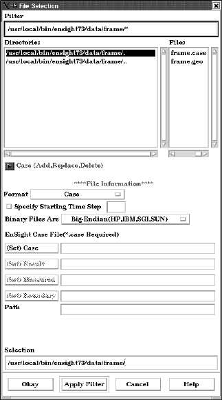
The File Selection dialog is used to specify which files you wish to read.
Figure 2-1
File Selection dialog for EnSight6 data
2.1 EnSight Case Reader
EnSight 7 User Manual 2-9
Access: Main Menu > File > Data (Reader)...
Filter
This field specifies the directory name that your data files reside in. Enter a /* at the end of
the name to list all of the files and directories contained there. To filter to a smaller file list
you can be more specific by entering Parts of the file names, such as /my* which will list
all files and directories starting with “my”. If you only enter a /, then only the directories
found will be listed. To apply the Filter, click the Apply Filter button and the Directories
and Files lists will be updated and the directory will be listed in the Selection field below
as the current selection.
Directories Selection of directories available to use in the current directory. Single click to place the
directory string in the Filter field. Double click to use the directory as the filter (same
effect as clicking once and then clicking Apply Filter button), the Directories and Files
lists will be updated and the directory will be listed in the Selection field below as the
current selection. The sliding controls to the right and bottom of the list let you view all
available directories.
Files Single click to select a file. This will insert the file name after the directory listed in the
Selection field. This list contains all unfiltered files that are in the filter directory.
Case
Add...
Specify an additional case. Additional data can be read into another connected Server.
Replace... Specify a new case to replace an existing case.
Delete Delete an existing case. Case 1 cannot be deleted, but it can be replaced.
Format Specifies the Format of the dataset. To read EnSight6 or EnSight Gold data, use the Case
format.
Specify Starting
Time Step
Specify starting time step. If not specified, EnSight will load the last step.
Binary Files Are If the file is binary, sets the byte order to:
Big-Endian - byte order used for HP, IBM, SGI, SUN, NEC, and IEEE Cray.
Little-Endian - byte order used for Intel and alpha based machines.
Native to Server Machine - sets the byte order to the same as the server machine.
(Set) Geometry Model file name for file containing at least the geometry. Clicking this button inserts the
file name shown in the Selection field and inserts the path information into the Path field.
File name can alternatively be typed into field.
(Set) Result Result file name corresponding to the geometry file. For most data formats this file is
optional. Clicking button inserts file name shown in Selection field and also inserts path
information into Path field. File name can alternatively be typed into field.
(Set) Measured Name of a measured file. This is an optional file. Clicking button inserts file name shown
in Selection field and also inserts path information into Path field. File name can
alternatively be typed into field.
Path Path to dataset location is inserted by clicking (Set) buttons or may be entered. If blank,
files are read from the Server‘s current working directory. Can use the tilde character (~)
to specify home directory on the Server host system.
Selection File or directory selected. Click the appropriate (Set) button to use information in this
field.
Okay Click to read the files specified in the (Set) fields and close the File Selection dialog.
Apply Filter Click to apply the string in the Filter field.
Cancel Click to close the File Selection dialog without reading the files specified in the (Set)
fields.
(see How To Read EnSight6 Data)
2.1 EnSight Case Reader
2-10 EnSight 7 User Manual
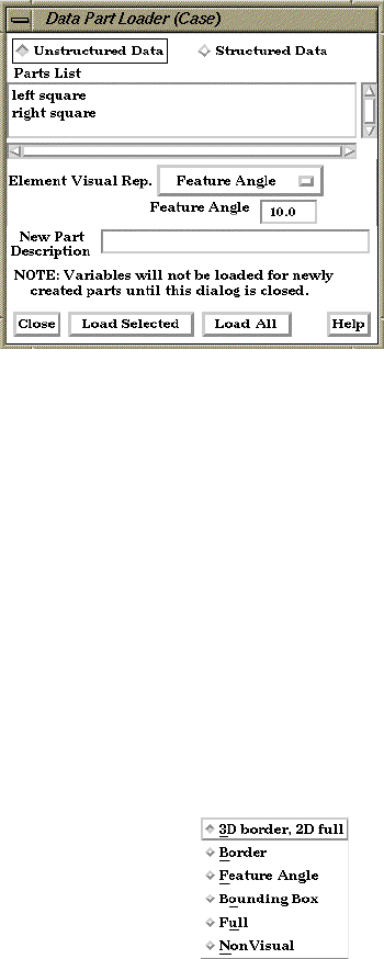
Loading Parts from EnSight6 or EnSight Gold Data
Data Part Loader dialog for Unstructured EnSight6 or EnSight Gold Data
You use the Data Part Loader dialog to control which Parts will be loaded to the Server
(and made available on) the EnSight Client. It will automatically open after you have read
in data and clicked Okay in the File Selection dialog.
Access: Main Menu > File > Data (Part Loader)...
Unstructured Data
This toggle indicates that the Part(s) listed in the Part List is(are) unstructured.
Parts List Lists all unstructured EnSight6 format Parts in the data files which may be loaded to the
Server (and subsequently to the Client). An EnSight6 or EnSight Gold data file can have
unstructured, structured, or both types of Parts.
Element Visual
Rep.
Parts are defined on the server as a collection of 1, 2, and 3D elements. EnSight can show
you all of the faces and edges of all of these elements, but this is usually a little
overwhelming, thus EnSight offers several different Visual Representations to simplify the
view in the graphics window. Note that the Visual Representation only applies to the
EnSight client—it has no affect on the data for the EnSight server.
3D Border, 2D
Full
In this mode, you will see all 1D and 2D elements, but only the outside surfaces of 3D
elements.
Border In Border mode all 1D elements will be shown. Only the unique (non-shared) edges of 2D
elements and the unique (non-shared) faces of 3D elements will be shown.
Feature Angle When EnSight is asked to display a Part in this mode it first calculates the 3D Border, 2D
Full representation to create a list of 1D and 2D elements. Next it looks at the angle
between neighboring 2D elements. If the angle is above the Angle value specified the
shared edge between the two elements is removed. Only 1D elements remain on the
EnSight client after this operation.
Bounding Box All Part elements are replaced with a bounding box surrounding the Cartesian extent of
the elements of the Part.
Figure 2-2
Data Part Loader dialog for EnSight6 or EnSight Gold Unstructured Data
Element Visual Rep.
Figure 2-3
Element Visual Representation pulldown
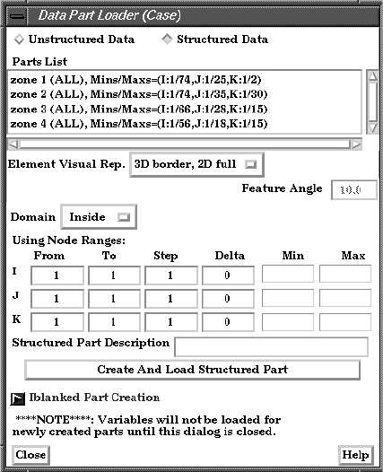
2.1 EnSight Case Reader
EnSight 7 User Manual 2-11
Full
In Full Representation mode all 1D and 2D elements will be shown. In addition, all faces
of all 3D elements will be shown.
Non Visual This specifies that the loaded Part will not be visible in the Graphics Window because it is
only loaded on the Server. Visibility can be turned on again later by changing the
representation.
Load Selected Loads Parts selected in Parts List to EnSight Server. The Parts are subsequently loaded to
the EnSight Client using the specified Visual Representation. If Non Visual is specified,
the selected Parts will be loaded to the Server, but not to the Client.
Load All Loads all Parts in Parts List to EnSight Server. The Parts are subsequently loaded to the
EnSight Client using the specified Visual Representation. If Non Visual is specified, the
selected Parts will be loaded to the Server, but not to the Client.
Data Part Loader dialog for Structured EnSight6 or EnSight Gold data
You use the Data Part Loader dialog to control which structured Parts will be loaded to the
EnSight Server (and subsequently to the EnSight Client). It will automatically open after
you have read in data and clicked Okay in the File Selection dialog.
Access: Main Menu > File > Data (Part Loader)...
Structured Data
This toggle indicates that the Part data listed is structured.
Parts List Lists all structured Parts on Server which may be loaded to the EnSight Server (and
subsequently to the EnSight Client). When one part is highlighted in this list, the Domain
and Node Range fields are updated accordingly.
Element Visual
Rep
.Parts are defined on the server as a collection of 1, 2, and 3D elements. EnSight can show
you all of the faces and edges of all of these elements, but this is usually a little
overwhelming, thus EnSight offers several different Visual Representations to simplify the
view in the graphics window. Note that the Visual Representation only applies to the
Figure 2-4
Data Part Loader dialog for EnSight6 or EnSight Gold Structured Data
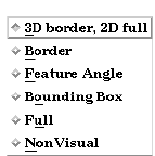
2.1 EnSight Case Reader
2-12 EnSight 7 User Manual
EnSight client—it has no affect on the data for the EnSight server.
3D Border, 2D
Full
In this mode, you will see all 1D and 2D elements, but only the outside surfaces of 3D
elements.
Border In Border mode all 1D elements will be shown. Only the unique (non-shared) edges of 2D
elements will be shown, and only unique (non-shared) faces of 3D elements will be
shown.
Feature Angle When EnSight is asked to display a Part in this mode it first calculates the 3D Border, 2D
Full representation to create a list of 1D and 2D elements. Next it looks at the angle
between neighboring 2D elements. If the angle is above the Angle value specified the
shared edge between the two elements is removed. Only 1D elements remain on the
EnSight client after this operation.
Bounding Box All Part elements are replaced with a bounding box surrounding the Cartesian extent of
the elements of the Part.
Full In Full Representation mode all 1D and 2D elements will be shown. In addition, all faces
of all 3D elements will be shown.
Non Visual This specifies that the loaded Part will not be visible in the Graphics Window because it is
already loaded on the EnSight Server. Visibility can be turned on again later by changing
the representation.
Domain Specifies the general iblanking option to use when creating a structured Part. If the model
does not have iblanking, InSide will be specified by default.
Inside Iblank value = 1 region
Outside Iblank value = 0 region
All Ignore iblanking and accept all nodes
Using Node Ranges:
From IJK
Specifies the beginning I,J,K values to use when extracting the structured Part, or a
portion of it. Must be >= Min value.
To IJK Specifies the ending I,J,K values to use when extracting the structured Part, or a portion of
it. Must be <= Max value.
Valid values for the From and To fields can be positive or negative. Positive numbers are
the natural 1 through Max values. Negative values indicate surfaces back from the max, so
-1 would be the max surface, -2 the next to last surface etc. There are therefore two ways
to indicate any of the range values; the positive number from the min towards the max, or
the negative number from the max toward the min. The negative method is provided for
ease of use because of varying max values per part. (Zero will be treated like a -1, thus it is
another way to get the max surface)
1, 2, 3,... ---> <--- ...-3, -2 ,-1
|---|---|---|---|---|---|---|---|---|---|---|---|---|---|---|
min max
(always 1) (varies per zone)
Step IJK Specifies the step increment through I,J,K. A Step value of 1 extracts all original data. A
Step value of 2 extracts every other node, etc.
Element Visual Rep.
Figure 2-5
Element Visual Representation pulldown
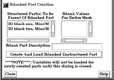
2.1 EnSight Case Reader
EnSight 7 User Manual 2-13
Delta IJK
Specifies the delta to use when creating more than one surface from the same ijk part.
Only one of the directions may be non-zero. Note that an unstructured part is the result of
any non-zero delta values.
Min IJK Minimum I,J,K values for Part chosen
Max IJK Maximum I,J,K values for Part chosen
Part Description Text field into which you can enter a description for the Part
Create And Load
Part
Extracts the data from the data files and creates a Part on the Server (and on the Client
unless NonVisual has been specified for Representation) based on all information
specified in the dialog.
If only one part is highlighted, the values shown in the From and To fields (as well as the
Min and Max fields) are the actual values for the selected part. Using the From and To
fields you can control whether an EnSight part will be created using the entire ijk ranges
or some subset of them. The Step field allows you to sample at a more coarse resolution.
And the Delta field allows for multiple “surfaces” in a given part (like blade rows of a jet
engine). Please note that use of a non-zero delta produces an unstructured part instead of a
structured one.
If more than one Part is highlighted, the values shown in the From and To fields are the
combined bounding maximums of the selected parts. The same basic functionality
described for a single part selection applies for multiple part selection, with one part being
created for each selected part in the dialog. If the specified ranges for the multiple
selection exceed the bounds of a given part, they are modified for that part so that its
bounds are not exceeded.
(see How To Do Structured Extraction)
Iblanked Part Creation section of Structured Part Loader dialog
You use this portion of the Part Loader dialog to further extract iblanked regions from
structured parts which were created either as inside, outside, or all portions of the model.
Structured Part(s)
To Be Parent of
Iblanked Part
Lists all structured parts that have been created thus far in the dialog above.
Iblank Values For
Entire Mesh
Lists all possible iblank values found in the model. This is a global list and may not apply
to all parts.
Iblank Part
description
Text field into which you can enter a description for the iblanked part.
Figure 2-6
Iblanked Part Creation Section of EnSight6 or EnSight Gold Structured Part Loader dialog
Bnd (2)
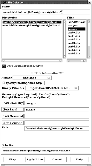
2.1 EnSight5 Reader
EnSight 7 User Manual 2-15
EnSight5 Reader
EnSight5 input data consists of the following files:
• Geometry file (required)
• Result file (optional)
• Variable files (optional)
• Measured Particle Files (optional)
- Measured/Particle geometry files
- Measured/Particle results files
- Measured/Particle variable files
The geometry file is a general finite-element format describing nodes and Parts,
each Part being a collection of elements. The result file is a small file allowing the
user to name variables and provide time information. The result file points to
variable files which contain the scalar or vector information for each node.
Measured/Particle files contain data about discrete Particles in space from the
simulation code or information directly from actual experimental tests.
EnSight5 data is based on Parts. The Parts defined in the data are always available
on the Server. However, all Parts do not have to be loaded to the Client for display.
Large flow fields for CFD problems, for example, are needed for computation by
the Server, but do not generally need to be seen graphically.
EnSight5 data can have changing geometry, in which case the changing geometry
file names are contained in the results file. However, it is still necessary to specify
an initial geometry file name.
File Selection dialog
Figure 2-7
File Selection dialog for EnSight5 data
2.1 EnSight5 Reader
2-16 EnSight 7 User Manual
The File Selection dialog is used to specify which files you wish to read.
Access: Main Menu > File > Data (Reader)...
Filter
This field specifies the directory name that your data files reside in. Enter a /* at the end of
the name to list all of the files and directories contained there. To filter to a smaller file list
you can be more specific by entering Parts of the file names, such as /my* which will list
all files and directories starting with “my”. If you only enter a /, then only the directories
found will be listed. To apply the Filter, click the Apply Filter button and the Directories
and Files lists will be updated and the directory will be listed in the Selection field below
as the current selection.
Directories Selection of directories available to use in the current directory. Single click to place the
directory string in the Filter field. Double click to use the directory as the filter (same
effect as clicking once and then clicking Apply Filter button), the Directories and Files
lists will be updated and the directory will be listed in the Selection field below as the
current selection. The sliding controls to the right and bottom of list let you view all
available directories.
Files Single click to select a file.This will insert the file name after the directory listed in the
Selection field. This list contains all unfiltered files that are in the filter directory.
Case
Add...
Specify an additional case. Additional data can be read into another connected Server.
Replace... Specify a new case to replace an existing case.
Delete Delete an existing case. Case 1 cannot be deleted, but it can be replaced.
Format Specifies the Format of the dataset. To read EnSight6 or EnSight Gold data, use the Case
format.
Specify Starting
Time Step
Specify starting time step. If not specified, EnSight will load the last step.
Binary Files Are If the file is binary, sets the byte order to:
Big-Endian - byte order used for HP, IBM, SGI, SUN, NEC, and IEEE Cray.
Little-Endian - byte order used for Intel and alpha based machines.
Native to Server Machine - sets the byte order to the same as the server machine.
(Set) Geometry Model geometry file name. Clicking button inserts file name shown in Selection field and
inserts path information into Path field. File name can alternatively be typed into field.
(Set) Result Result file name corresponding to the geometry file. For most data formats this file is
optional. Clicking button inserts file name shown in Selection field and also inserts path
information into Path field. File name can alternatively be typed into field.
(Set) Measured Name of a measured file. This is an optional file. Clicking button inserts file name shown
in Selection field and also inserts path information into Path field. File name can
alternatively be typed into field.
Path Path to dataset location is inserted by clicking (Set) buttons or may be entered. If blank,
files are read from the Server‘s current working directory. Can use the tilde character (~)
to specify home directory on the Server host system.
Selection File or directory selected. Click the appropriate (Set) button to use information in this
field.
Okay Click to read the files specified in the (Set) fields and close the File Selection dialog.
Apply Filter Click to apply the string in the Filter field.
Cancel Click to close the File Selection dialog without reading the files specified in the (Set)
fields.
(see How To Read EnSight5 Data)
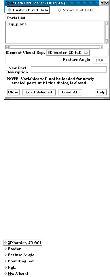
2.1 EnSight5 Reader
EnSight 7 User Manual 2-17
Loading Parts from EnSight5 data
Data Part Loader dialog
You use the Data Part Loader dialog to control which Parts will be loaded to the EnSight
Server (and subsequently, to the Client). It will automatically open after you have read in
data and clicked Okay in the File Selection dialog.
Access: Main Menu > File > Data (Part Loader)...
Unstructured Data This toggle indicates that Part data is unstructured. It must be on for EnSight5 format.
Structured Data This toggle is not available for EnSight5 data.
Parts List Lists all Parts in the data files which may be loaded to the EnSight Server (and
subsequently, to the Client).
Element Visual
Rep.
Parts are defined on the server as a collection of 1, 2, and 3D elements. EnSight can show
you all of the faces and edges of all of these elements, but this is usually a little
overwhelming, thus EnSight offers several different Visual Representations to simplify the
view in the graphics window. Note that the Visual Representation only applies to the
EnSight client—it has no affect on the data for the EnSight server.
3D Border, 2D
Full
In this mode, you will see all 1D and 2D elements, but only the outside surfaces of 3D
elements.
Border In Border mode all 1D elements will be shown. Only the unique (non-shared) edges of 2D
elements will be shown, and only unique (non-shared) faces of 3D elements will be
shown.
Feature Angle When EnSight is asked to display a Part in this mode it first calculates the 3D Border, 2D
Full representation to create with a list of 1D and 2D elements. Next it looks at the angle
between neighboring 2D elements. If the angle is above the Angle value specified the
Figure 2-8
Data Part Loader dialog for EnSight5 data
Figure 2-9
Element Visual Representation pulldown
2.1 ABAQUS Reader
2-18 EnSight 7 User Manual
shared edge between the two elements is removed. Only 1D elements remain on the
EnSight client after this operation.
Bounding Box All Part elements are replaced with a bounding box surrounding the Cartesian extent of
the elements of the Part.
Full In Full Representation mode all 1D and 2D elements will be shown. In addition, all faces
of all 3D elements will be shown.
Non Visual This specifies that the loaded Part will not be visible in the Graphics Window because it is
only loaded on the EnSight Server. Visibility can be turned on again later by changing the
representation.
Load Selected Loads Parts selected in Parts List to EnSight Server. The Parts are subsequently loaded to
the EnSight Client using the specified Visual Representation. If Non Visual is specified,
the selected Parts will be loaded to the Server, but not to the Client.
Load All Loads all Parts in Parts List to EnSight Server. The Parts are subsequently loaded to the
EnSight Client using the specified Visual Representation. If Non Visual is specified, the
selected Parts will be loaded to the Server, but not to the Client.
(see How To Read EnSight5 Data)
ABAQUS Reader
ABAQUS input data consists of the following files:
• Geometry/Results file (required). This file (the ABAQUS .fil file)
contains both the geometry and any requested results. It can be either
ASCII or binary.
• EnSight5 Measured/Particle Files (optional). The measured .res file
references the measured geometry and variable files.
EnSight will read ASCII or binary .fil files directly. Geometry and commonly
used results contained in the file will be read.
The element sets in the .fil file will be used for creating parts.
(see How To Read ABAQUS Data)
2.1 ANSYS RESULTS Reader
EnSight 7 User Manual 2-19
ANSYS RESULTS Reader
ANSYS input data consists of the following files:
• Geometry and Results file (required). The ANSYS .rst file (or similar
results files such as .rfl, .rmq, .rth) contains geometry and results and
should be entered in the geometry field of the Data dialog.
• EnSight5 Measured/Particle Files (optional). The measured .res file
references the measured geometry and variable files.
EnSight allows you to read the geometry and results data directly from an ANSYS
results data file. Not all element types possible in ANSYS can be converted to
EnSight format. However, EnSight will handle most practical cases just fine.
Note that certain variables may read slower than others. Displacement,
acceleration, and velocity vector variables, as well as nodal solution scalars
(pressure, temperature, etc.), read in quickly because they are provided at the
nodes directly. Stress and strain variables, on the other hand, can be quite time
consuming to read because the process involves:
1. getting the element nodal values,
2. if necessary, computing principal stresses (or strains),
3. if necessary, applying equivalent stress (or strain) and/or stress (or strain)
intensity equations,
4. if shell elements, using one side or the other (user selectable),
5. averaging the values at shared nodes, and,
6. if higher order elements, averaging to get mid-side node values.
ANSYS data is based on Parts. The Parts defined in the data are always read on
the Server. These Parts, however, do not all have to be loaded to the Client for
display.
(see How To Read ANSYS Data)
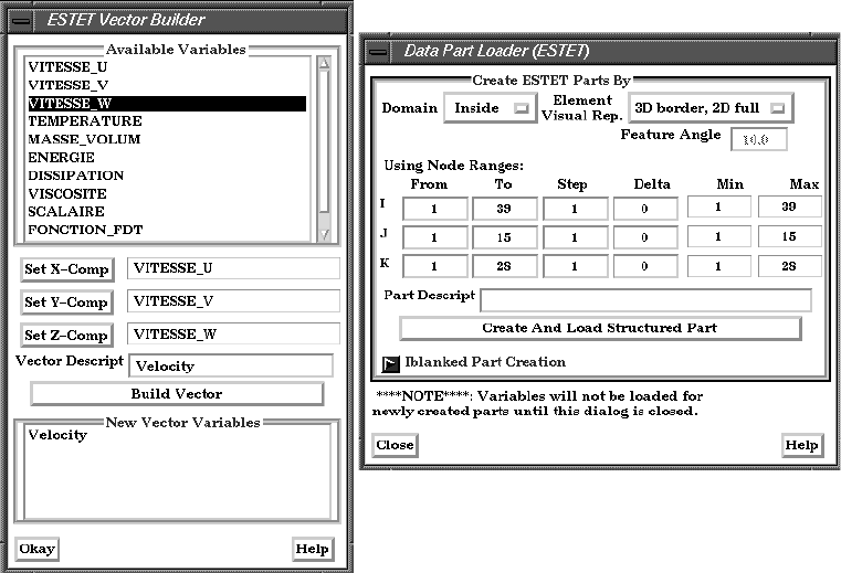
2.1 ESTET Reader
2-20 EnSight 7 User Manual
ESTET Reader
ESTET input data consists of one file that contains all geometry and results
information. The ESTET data is a structured grid. The data file is binary.
When reading this data into EnSight, you extract Parts from the mesh interactively
based on indices assigned to the nodes in the data. Currently, three domains are
possible for extracting Parts: inside, outside, and symmetry plane. As you extract
Parts, you can limit the domains according to ranges in I, J and K.
The data can be in rectangular, cylindrical, or curvilinear coordinates. EnSight
will interpret and convert properly for any of these types.
Once the desired geometry has been extracted as Parts, you are presented with a
list of the results variables contained in the file. There is no way to automatically
determine which of the results variables are actually vector components, so you
are given the opportunity to build the vectors from the variables. The descriptions
usually make this a straightforward process. All variables not used as components
to vectors are assumed to be scalar variables.
ESTET Vector Builder and Data Part Loader dialogs
You use the File Selection dialog to read ESTET data files, the ESTET Vector Builder
dialog to build vector variables from scalar components for an ESTET dataset, and the
Data Part Loader dialog to extract Parts from an ESTET dataset. The latter two dialogs
open in sequence automatically after you click Okay in the File Selection dialog.
Access: Main Menu > File > Data (Reader)…> ESTET
Create ESTET Parts By
Domain
Select domain to extract Part.
Inside Create a structured Part that contains elements whose nodes are flagged as being “inside”.
Outside Create a structured Part that contains elements whose nodes are flagged as “outside”.
All Create a structured Part that contains all elements because node iblanking is ignored.
Figure 2-10
ESTET Vector Builder and Data Part Loader dialogs
2.1 ESTET Reader
EnSight 7 User Manual 2-21
Using Node
Ranges:
Specification of node range when creating a Part. Values must be between Min and Max.
From IJK Specifies the beginning I,J,K values to use when extracting the structured Part, or a
portion of it.
To IJK Specifies the ending I,J,K values to use when extracting the structured Part, or a portion of
it.
Valid values for the From and To fields can be positive or negative. Positive numbers are
the natural 1 through Max values. Negative values indicate surfaces back from the max, so
-1 would be the max surface, -2 the next to last surface etc. There are therefore two ways
to indicate any of the range values; the positive number from the min towards the max, or
the negative number from the max toward the min. (Zero will be treated like a -1, thus it is
another way to get the max surface)
1, 2, 3,... ---> <--- ...-3, -2 ,-1
|---|---|---|---|---|---|---|---|---|---|---|---|---|---|---|
min max
(always 1) (varies per zone)
Step IJK Specifies the step increment through I,J,K. A Step value of 1 extracts all original data. A
Step value of 2 extracts every other node, etc.
Delta IJK Specifies the delta to use when creating more than one surface from the same ijk part.
Only one of the directions may be non-zero. Note that an unstructured part is the result of
any non-zero delta values.
Min IJK Minimum I,J,K values for zone chosen
Max IJK Maximum I,J,K values for zone chosen
Part Descrip Set the name of the Part. If empty, EnSight will assign a name.
Create Part Click to create a Part according to the range, step by, and delta specifications. Using the
From and To fields you can control whether an EnSight part will be created using the
entire ijk ranges or some subset of them. The Step field allows you to sample at a more
coarse resolution. And the Delta field allows for multiple “surfaces” in a given zone (like
blade rows of a jet engine). Please note that use of a non-zero delta produces an
unstructured part instead of a structured one.
Available Variables Selection to specify a variable to use for the next Set...Comp action.
Set X-Comp Click to set the current selection to be the X component of the vector to build.
Set Y-Comp Click to set the current selection to be the Y component of the vector to build.
Set Z-Comp Click to set the current selection to be the Z component of the vector to build.
Vector Descript Set the name of the vector variable.
Build Vector Click to define the vector variable.
New Vector
Variables
List of vector variables that have been defined.
Okay Click Okay to load the variable information.
WARNING: You should build all the vectors you are going to use before clicking
Okay, because you cannot return to this dialog. If you fail at this point to make all of
the vectors desired, it is possible to do so later using the Make Vector function
(see Section 4.3, Variable Creation)
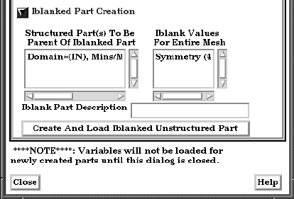
2.1 ESTET Reader
2-22 EnSight 7 User Manual
Iblanked Part Creation section of Data Part Loader (ESTET) dialog
You use this portion of the Part Loader dialog to further extract iblanked regions from
structured parts which were created either as inside, outside, or all portions of the model.
Structured Part(s)
To Be Parent of
Iblanked Part
Lists all structured parts that have been created thus far in the dialog above.
Iblank Values For
Entire Mesh
Lists all possible iblank values found in the model. This is a global list and may not apply
to all parts.
Iblank Part
description
Text field into which you can enter a description for the iblanked part.
Create And Load
Iblanked
Unstructured Part
Extracts a new iblanked part from an existing structured part. This new part will actually
be an unstructured part.
(see How To Read ESTET Data)
Figure 2-11
Iblanked Part Creation Section of Data Part Loader (ESTET) dialog
2.1 FAST UNSTRUCTURED Reader
EnSight 7 User Manual 2-23
FAST UNSTRUCTURED Reader
FAST UNSTRUCTURED input data consists of the following files:
• Geometry file (required) This is the FAST UNSTRUCTURED single
zone grid file.
• Modified Result file (optional)
• Variable files (optional) These are either a PLOT3D solution file (Q-file)
or FAST function file with I = number of points and J=K=1.
• EnSight5 Measured/Particle Files (optional). The measured .res file
references the measured geometry and variable files.
FAST UNSTRUCTURED is a format containing triangle and/or tetrahedron
elements. The triangles have tags indicating a grouping for specific purposes.
EnSight will read the unstructured single zone grid format for this data type,
placing all tetrahedral elements into the first Part, and the various triangle element
groupings into their own Parts.
The modified EnSight results file allows results to be read from PLOT3D-like Q-
files or FAST-like function files. They can be time dependent.
FAST UNSTRUCTURED data can have changing geometry. When this is the
case, the changing geometry file names are contained in the results file. However,
it is still necessary to specify an initial geometry file name.
(see How To Read FAST Unstructured Data)
FIDAP NEUTRAL Reader
A FIDAP Neutral file contains all of the necessary geometry and result
information for use with EnSight.
FIDAP data is based on Parts. The Parts defined in the data are always read on the
Server. They do not, however, all have to be loaded to the Client for display. Large
flow fields for CFD problems, for example, are needed for computation by the
Server, but do not generally need to be seen graphically.
EnSight5 Measured/Particle Files can also be read with a FIDAP model. The
measured .res file references the measured geometry and variable files.
(see How To Read FIDAP Neutral Data)
FLUENT UNIVERSAL Reader
FLUENT input data files consist of the following:
• Universal file (required)
• EnSight5 format Results file (optional)
• EnSight5 Measured/Particle Files (optional).
The FLUENT Universal file contains all of the necessary geometry and result
information for use with EnSight for a steady-state case. If the case is transient,
EnSight needs a Universal file for each time step of the analysis and a modified
version of the EnSight results file.
2.1 Movie.BYU Reader
2-24 EnSight 7 User Manual
FLUENT data is based on Parts. The Parts defined in the data are always read on
the Server. They do not, however, all have to be loaded to the Client for display.
Large flow fields for CFD problems, for example, are needed for computation by
the Server, but do not generally need to be seen graphically.
EnSight5 Measured/Particle Files can also be read with a FLUENT model. The
measured .res file references the measured geometry and variable files.
(see How To Read FLUENT Universal Data)
Movie.BYU Reader
Movie.BYU input data consists of the following files:
• Geometry file (required)
• Results file (optional)
• Variable files (optional)
• EnSight5 Measured/Particle Files (optional). The measured .res file
references the measured geometry and variable files.
Movie.BYU has a general n-sided polygon data format. In translating this format
to the element-based EnSight data format, not all elements possible in the
Movie.BYU format can be converted to EnSight format. However, for most
practical cases there are no problems.
Movie.BYU datasets can be read directly by EnSight. Additionally, an external
translator, “movieto5”, is provided if you wish to convert the actual data files to
EnSight format.
In order to read Movie.BYU data result files into EnSight, you must create a
results file of the same format as EnSight. The external translator, “mpgs4to5,”
can be used to generate a results file if you do not want to create your own using a
text editor.
Movie.BYU data is based on Parts. The Parts defined in the data are always read
on the Server. They do not, however, all have to be loaded to the Client for
display.
Movie.BYU data can have changing geometry. When this is the case, the
changing geometry file names are contained in the results file. However, it is still
necessary to specify an initial geometry file name.
(see How To Read MOVIE.BYU Data)
2.1 MPGS 4.1 Reader
EnSight 7 User Manual 2-25
MPGS 4.1 Reader
MPGS4 data files consist of the following:
• Geometry file (required)
• EnSight format Results file (optional)
• Variable files (optional)
• EnSight5 Measured/Particle Files (optional). The measured .res file
references the measured geometry and variable files.
MPGS4.x uses a general n-sided polygon, n-faced polyhedral data format. In
going from this format to the specific element data format of EnSight, you
encounter the problem associated with translating from a general format to a
specific format. Not all elements possible in MPGS4.x can be converted to
EnSight format. However, there will not be a problem in most situations.
MPGS4.x models of modest size can be read directly into EnSight. Size can
become an issue since the amount of memory needed to do the conversion in
EnSight to the internal data format in a reasonable length of time can become
excessive for large models. An external translator, “mpgs4to5”, is provided for the
larger models. You should also consider using the external translator to convert
MPGS4.x data to EnSight data if you need to continue loading the same dataset,
as this will perform the data conversion one time while reading it into EnSight
will continue to take resources each time the data is read. Converting it from
MPGS4.x to EnSight format also has the advantage of taking less disk space as
the EnSight format is more compact.
In order to read MPGS4.x results directly into EnSight, you must create a results
file of the same format as EnSight. The external translator, “mpgs4to5,” can be
used to generate a results file if you do not want to create your own using an
editor.
MPGS4.x data is based on Parts. The Parts defined in the data are always read on
the Server. They do not, however, all have to be loaded to the Client for display.
Large flow fields for CFD problems, for example, are needed for computation on
the Server, but do not generally need to be seen graphically.
MPGS4.x data can have changing geometry. When this is the case, the changing
geometry file names are contained in the results file. However, it is still necessary
to specify an initial geometry file name.
(see How To Read MPGS Data)
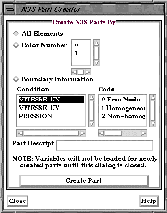
2.1 N3S Reader
2-26 EnSight 7 User Manual
N3S Reader
N3S input data consists of the following files:
• Geometry file (required)
• Results file (required)
• EnSight5 Measured/Particle Files (optional). The measured .res file
references the measured geometry and variable files.
N3S is a data format developed by Electricité de France (EDF) consisting of a
geometry file and a results file. For this data format, both files are always
required. Versions 3.0 and 3.1 are both supported.
When reading N3S data into EnSight, you extract Parts from the mesh
interactively based on different color numbers or boundary conditions. The
available color numbers and boundary conditions for the model are presented.
N3S Part Creator dialog
You use the File Selection dialog to read in N3S dataset files. You use the N3S Part
Creator dialog to extract Parts from a N3S dataset.
Access: Main Menu > File > Data (Reader)...> N3S
Create N3S Parts By
All Elements
Selection to create a Part using all of the elements available within the data file.
Color Number Selection to create a Part according to the color number associated with each element.
Boundary
Information
Selection to create a Part according to specified conditions and codes.
Condition Select boundary condition to use for Part creation.
Code Select Code to use for boundary condition.
Part Descript Specify name for Part.
Create Part Click to create a Part. The Part is listed in the main Parts list of the Parts & Frames dialog
and is displayed in the Main View window.
(see How To Read N3S Data)
Figure 2-12
N3S Part Creator dialog
2.1 PLOT3D Reader
EnSight 7 User Manual 2-27
PLOT3D Reader
PLOT3D is a commonly used structured data format and input data consists of the
following files:
• Geometry file. This is a required file. (Structured GRID file with FAST
enhancements)
• Modified EnSight Results file (optional). A standard plot3d Q-file can be
read in the results field in place of a modified EnSight Results file.
• Variable files, which are solution (PLOT3D) or function (FAST) files
(optional)
• EnSight5 Measured/Particle Files (optional). The measured .res file
references the measured geometry and variable files.
• EnSight Boundary File (optional). The boundary file defines boundary
portions within and/or across structured blocks. (Note: this can be
EnSight’s boundary file format or a .fvbnd file.)
When reading PLOT3D files into EnSight, you extract Parts from the mesh based
on a domain, a list of zones, and/or indices assigned to the nodes in the data.
Currently, three domains are possible for extracting structured Parts: (a) inside, (b)
outside, or (c) all. These options are dependent on what the file format is from the
parameters defined in the previous paragraph. For instance, when using single
zone, non-iblanked data the domain is fixed at “Inside” and the one zone listed in
the zones list is selected. As you extract Parts from a single zone file, however, it
is possible to limit the domains according to ranges in I, J, and K.
Once the desired structured Parts have been extracted from the geometry, further
iblanking options can be used to extract unstructured parts, such as for boundaries.
When the Data Reader (PLOT3D) dismissed, the user is presented with a list of
the result variables available from the result file
To successfully read PLOT3D data, the following information must be known
about the data:
1. format
- ASCII, C binary, or Fortran binary
2. whether single
or multizone
3. dimension - 3D, 2D, or 1D
4. whether iblanked
or not
5. precision
- single or double
EnSight attempts to determine these five settings automatically from the grid file.
The settings that were determined (for the first four) are shown in the Part Builder
dialog, where you can override them manually if needed.
The precision setting is not reflected in the dialog, but is echoed in the Server shell
window. The q (or function) file precision will by default be set the same as that of
the grid file. In the rare case where the automatic detection is wrong for the grid
file or the precision is different for the q (or function) file than for the grid file,
commands can be entered into the Command dialog to manually set the precision.
test:
plot3d_grid_single
t
o read grid file as single precision
test:
plot3d_grid_double
to read grid file as double precision
test:
plot3d_qr_single
to read q (or function) file as single precision
test:
plot3d_qr_double
to read q (or function) file as double precision
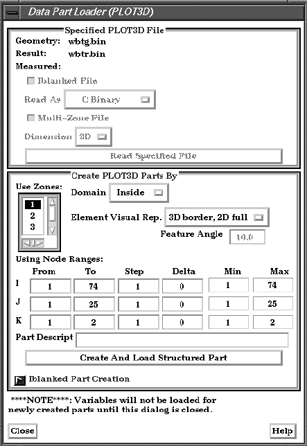
2.1 PLOT3D Reader
2-28 EnSight 7 User Manual
PLOT3D Part Loader dialog
You use the Part Data Loader (PLOT3D) dialog to read a specified PLOT3D file and to
extract parts out of the PLOT3D geometry.
Access: Main Menu > File > Data (Reader)... > PLOT3D
Geometry
Specifies name of file which geometry data will be read.
Result Specifies name of file which result data will be read.
Measured Specifies name of file which measured/discrete data will be read.
IBlanked File
Toggle
Turn on if geometry field has iblanking.
Read As Specifies file type. Choices are:
ASCII
C Binary (Note: Files may not be portable across hardware platforms).
FORTRAN Binary (Note: Files may not be portable across hardware platforms).
Multi-Zone File
Toggle
Turn on if dataset contains multiple zones. If Multi-zoned and you are not doing a
“between boundary” domain option (see below), a part can span several zones (see Use
Zone list below).
Dimension Specifies the dimension of the dataset. Options are 1D, 2D, or 3D. If multi-zone, the
dimension of the problem is forced to be 3D.
Read Specified File Click to initiate the reading process.
Use Zones List of Zones defined in the data that can be used to create Parts. If there are multiple
zones you can select one or more of them.
Figure 2-13
Part Data Loader (PLOT3D)
2.1 PLOT3D Reader
EnSight 7 User Manual 2-29
Domain
Select the domain to create a structured Part from. Options are:
Inside Create structured Part from grid points flagged with Iblanking = 1
Outside Create structured Part from grid points flagged with Iblanking = 0.
All Create part from all grid points (ignores Iblanking).
Using Node Ranges
From IJK
Specifies the beginning I,J,K values to use when extracting the structured Part, or a
portion of it.
To IJK Specifies the ending I,J,K values to use when extracting the structured Part, or a portion of
it.
Valid values for the From and To fields can be positive or negative. Positive numbers are
the natural 1 through Max values. Negative values indicate surfaces back from the max, so
-1 would be the max surface, -2 the next to last surface etc. There are therefore two ways
to indicate any of the range values; the positive number from the min towards the max, or
the negative number from the max toward the min. The negative method is provided for
ease of use because of varying max values per part. (Zero will be treated like a -1, thus it is
another way to get the max surface)
1, 2, 3,... ---> <--- ...-3, -2 ,-1
|---|---|---|---|---|---|---|---|---|---|---|---|---|---|---|
min max
(always 1) (varies per zone)
Step IJK Specifies the step increment through I,J,K. A Step value of 1 extracts all original data. A
Step value of 2 extracts every other node, etc.
Delta IJK Specifies the delta to use when creating more than one surface from the same ijk part.
Only one of the directions may be non-zero. Note that an unstructured part is the result of
any non-zero delta values.
Min IJK Minimum I,J,K values for Part chosen
Max IJK Maximum I,J,K values for Part chosen
Part Descrip Specify name of Part you wish to create.
Create Part Click to create a Part.
If only one part is highlighted, the values shown in the From and To fields (as well as the
Min and Max fields) are the actual values for the selected part. Using the From and To
fields you can control whether an EnSight part will be created using the entire ijk ranges
or some subset of them. The Step field allows you to sample at a more coarse resolution.
And the Delta field allows for multiple “surfaces” in a given part (like blade rows of a jet
engine). Please note that use of a non-zero delta produces an unstructured part instead of a
structured one.
If more than one Part is highlighted, the values shown in the From and To fields are the
combined bounding maximums of the selected parts. The same basic functionality
described for a single part selection applies for multiple part selection, with one part being
created for each selected part in the dialog. If the specified ranges for the multiple
selection exceed the bounds of a given part, they are modified for that part so that its
bounds are not exceeded.
(see How To Do Structured Extraction)
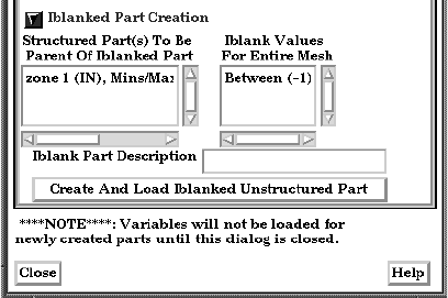
2.1 PLOT3D Reader
2-30 EnSight 7 User Manual
Iblanked Part Creation section of Data Part Loader (PLOT3D) dialog
You use this portion of the Part Loader dialog to further extract iblanked regions from
structured parts which were created either as inside, outside, or all portions of the model.
Structured Part(s)
To Be Parent of
Iblanked Part
Lists all structured parts that have been created thus far in the dialog above.
Iblank Values For
Entire Mesh
Lists all possible iblank values found in the model. This is a global list and may not apply
to all parts.
Iblank Part
description
Text field into which you can enter a description for the iblanked part.
Create And Load
Iblanked
Unstructured Part
Extracts a new iblanked part from an existing structured part. This new part will actually
be an unstructured part.
(see How To Read PLOT3D Data)
Figure 2-14
Iblanked Part Creation Section of Data Part Loader (PLOT3D) dialog
2.2 User Defined Readers
EnSight 7 User Manual 2-31
2.2 User Defined Readers
A user defined reader capability is included in EnSight which allows otherwise
unsupported structured or unstructured data to be read. In other words, the user
can create their own data readers. Each user defined reader utilizes a dynamic
shared library produced by the user. Once produced, these readers show up in the
list of data formats in the Data Reader Dialog just like an internal readers.
The readers are produced by creating the routines of an API. Two versions of the
userd defined API are available starting with EnSight version 7.2. The 1.0 API
(which has been available since EnSight version 6) was designed to be friendly to
those producing it, but requires more manipulation internally by EnSight and
accordingly requires more memory and processing time. The 2.0 API is
considerably more efficient, and was designed with that in mind. It requires that
all data be provided on a part basis, and as such lends itself closely to the EnSight
Gold type format. A few of the advantages of the new 2.0 API are:
• Considerably more memory efficient
• Considerably faster
• Tensor variables are supported
• Complex variables are supported
• Geometry and variables can be provided on different time lines
• If boundary representation is available, provides for its use instead of
having EnSight compute it.
The process for creating and using a user-defined reader is explained in detail in
the README files on the installation CD or in your installation directory.
On the CD: /CDROM/ensight76/src/readers
In installation
directory: $CEI_HOME/ensight76/src/readers
Therein you will also find a detailed description of each routine in the API and the
order in which the routines are called by EnSight. In the subdirectories at the same
location as the README’s, you will find source code for some sample readers
and a README file for working readers. The sample are often helpful examples
when producing your own reader.
Start EnSight (or EnSight server) with the command line option (-readerdbg), for
a step-by-step echo of reader loading progress.
The actual working user defined readers included in the EnSight distribution may
vary, but typically would include such formats as:
CFF
CFX4
Cobalt
MSC/Dytran
EXODUS II
CGNS
PXI
FLOW-3D
LS-DYNA
NASTRAN
OP2
RADIOSS
SCRYU
SILO
STL
TECPLOT
VECTIS
HDF5
2.3 Other External Data Sources
2-32 EnSight 7 User Manual
2.3 Other External Data Sources
External Translators
Translators supplied with the EnSight application enable you to use data files
from many popular engineering packages. These translators are found in the
translators directory on the EnSight distribution CD. A README file is supplied
for each translator to help you understand the operation of each Particular
translator. These translators are not supported by CEI, but are supplied at no-cost
and as source files, where possible, to allow user modification and porting.
Exported from Analysis Codes
Several Analysis codes can export data in EnSight file formats. Examples of these
include Fluent, STAR-CD, CFX and others.
2.4 Command Files
EnSight 7 User Manual 2-33
2.4 Command Files
Command files contain EnSight command language as ASCII text that can be
examined and even edited. They can be saved starting at any point and ending at
any point during an EnSight session. They can be replayed at any point in an
EnSight session. However, some command sequences require a certain state to
exist, such as connection to the Server, the data read, or a Part created with a
Particular Part number.
There are a multitude of applications for command files in EnSight. They include
such things as being able to play back an entire EnSight session, easily returning
to a standard orientation, connecting to a specific host, creating Particle traces,
setting up a keyframe animation, etc. Anything that you will want to be able to
repeatedly do is a candidate for a command file. Further, if it is a task that you
frequently do, you can turn the command file into a macro (see To Use Macros
below).
Documenting Bugs Command files are one of the best ways of documenting any bugs found in the
EnSight system. Hopefully that is a rare occasion, but if it occurs, a command file
provided to CEI will greatly facilitate the correction of the bug.
Nested Command
Files
Command files can be nested, which means that if you have a command file that
does a specific operation, you can play that command file from any other
command file, as long as any prerequisite requirements are completed. This is
done by adding the command
play: <filename>
in the command file.
Default Command
File
EnSight is always saving a command file referred to as the default command file
(unless the you have turned off this feature with a Client command line option).
This command file can be saved (and renamed) when exiting EnSight, as
described later in this section. The default command file is primarily intended to
be a crash recovery aid. If something unforeseen were to prematurely end your
EnSight session, you can recover to the last successfully completed command by
restarting EnSight and running the default command file. Saving the Default
Command File for EnSight Session
Command dialog
You use the Command dialog to control the execution of EnSight command language. The
language can be entered by hand, or as is most often the case, played from a file. This
Figure 2-15
Command dialog

2.4 Command Files
2-34 EnSight 7 User Manual
dialog also controls the recording of command files as well as Macro path definition.
Access: Main Menu > File > Command...
Command History
Displays most recent command language executed (or recorded). Can click on an entry
which will bring entry to the Command Entry field.
Command Entry Command language entry. Enter command and press RETURN. During file playback,
next command to be executed is shown here. Any command preceded by a # is a comment
line.
Record Select to start play file recording. Will be prompted for file name. Can simultaneously
record and play files. When engaged, all actions in EnSight are recorded to the specified
file.
Record Part
Selection By
Select the method by which parts will be recorded in the command language - either by
Number (default) or by Name.
Play Select to start playing a command file. You must provide the command language file
name. Command play continues as long as there are commands in file, an interrupt:
command has not been processed, or the Interrupt button has not been pressed.
Interrupt Interrupt playback of the command file.
Step Step though commands of play file. File playback must be stopped. Each click will
execute next command shown in Command Entry field.
Skip Skip over the playing command file’s next command (shown in Command Entry box).
Continue Continue playing interrupted command file.
Delay Between
Commands
Set the delay between commands in seconds when playing a command file.
Delay Refresh When enabled, will cause the EnSight graphics window to refresh only after the playfile
processing has completed or has been interrupted by the user.
Reload Macros Causes the Macro definitions to be reread from the site preferences directory and from the
user’s .ensight directory.
Troubleshooting Command Files
This section describes some common errors when running commands. If an error
is encountered while playing back a command file you can possibly retype the
command or continue without the command.
(see How To Record and Play Command Files)
Problem Probable Causes Solutions
Error in command category Incorrect spelling in the command
category
Check and fix spelling
Command does not exist Incorrect spelling in the command Check and fix spelling
Error in parameter Incorrect integer, float, range, or
string value parameter
Fix spelling or enter a legal value
Commands do not seem to play Command file was interrupted by an
error or an interrupt command
Click continue in the Command
dialog
2.4 Saving the Default Command File for EnSight Session
EnSight 7 User Manual 2-35
Saving the Default Command File for EnSight Session
EnSight is always saving a command file referred to as the default command file
(unless the you have turned off this feature with a Client command line option).
This default command file receives a default name starting with “ensigAAA” and
is written to your /usr/tmp directory (unless you set your TMPDIR environment
variable). This command file can be saved (and renamed) when exiting EnSight.
If you do not save this temporary file in the manner explained below, it will be
deleted automatically for you when you Quit EnSight. If Ensight crashes for some
reason, this temporary file can be used to autorecover when it is restarted.
Quit Confirmation dialog
You use the Quit Confirmation dialog to save either or both the default command file and
an archive file before exiting the program.
Access: Main Menu > File > Quit...
Save Command
Backup File To:
Toggle-on to save the default command file. Can also specify a new name for the
command file.
(see Section 2.4, Command Files for more information on using
command files.)
Save Full Backup Toggle-on and specify a name to create a Full Backup file.
Yes Click to save the indicated files and terminate the program.
(see How To Record and Play Command Files)
Figure 2-16
Quit Confirmation dialog
2.5 Archive Files
2-36 EnSight 7 User Manual
2.5 Archive Files
Saving and Restoring a Full backup
The current state of the EnSight Client and Server host systems may be saved to
files. An EnSight session may then be restored to this saved state after restarting at
a later time. A Full Backup consists of the following files. First, a small archive
information file is created containing the location and name of the Client & Server
files that will be described next. Second, a file is created on the Client host system
containing the entire state of the Client. Third, a file is created on each Server
containing the entire state of that Server. You have control over the name and
location of the first file, but only the directories for the other files.
Restoring EnSight to a previously saved state will leave the system in exactly the
state EnSight was in at the time of the backup. For a restore to be successful, it is
important that EnSight be in a “clean” state. This means that no data can be read
in before performing a restore. During a restore, any auto connections to the
Server(s) will be made for you. If manual connections were originally used, you
will need to once again make them during the restore. (If more than one case was
present when the archive was saved, then connection to all the Servers is
necessary).
An alternative to a Full Backup is to record a command file up to the state the user
wishes to restore at a later date, and then simply replaying the command file.
However, this requires execution of the entire command file to get to the restart
point. A Full Backup returns you right to the restart point without having to
recompute any previous actions.
A Full Backup restores very quickly. If you have very large datasets that take a
significant time to read, consider reading them and then immediately writing a
Full Backup file. Then, use the Full Backup file for subsequent session instead of
reading the data.
Important Note: Archives are intended to facilitate rapid reload of data and
context and are NOT intended for lon-term data storage. Therefore, archives are
likely NOT compatible between earlier EnSight versions and the current version
(see Release Notes for details). If EnSight fails to open an archive, it will state
that it failed and will write out a .cmd file and echo its location. As command files
ARE often compatible between earlier and later versions, the .cmd file can likely
be used to retrace the steps of the dataset.
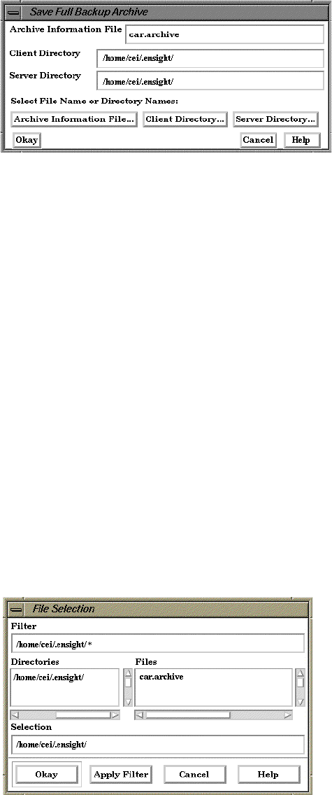
2.5 Saving and Restoring a Full backup
EnSight 7 User Manual 2-37
Save Full Backup Archive dialog
You use the Save Full Backup Archive dialog to control the files necessary to perform a
full archive on EnSight.
Access: Main Menu > File > Backup > Save Full Backup...
Archive Information
File
Specifies name of Full Backup control file.
Client Directory Specifies the directory for the Client archive file.
Server Directory Specifies the directory for the Server archive file.
Archive information
File...
Click to display the file selection dialog for specifying the Archive Information File.
Client Directory... Click to display the file selection dialog for specifying the Client Directory.
Server Directory... Click to display the file selection dialog for specifying the Server Directory (for the
selected case if there is more than one). Choose a common path if there is more than one.
Okay Click to perform the full backup.
NOTE: This command is written to the command file, but is preceded with a # (the
comment character). To make the archive command occur when you play the command
file back, uncomment the #.
(see How To Save and Restore an Archive)
File Selection for Restarting from an Archive
You use the Restore Full Archive Backup dialog to read and restore a previously stored
archive file.
Access: Main Menu > File > Backup > Restore Full...
Figure 2-17
Save Full Backup Archive dialog
Figure 2-18
File Selection for Restarting from an Archive

2.5 Saving and Restoring a Full backup
2-38 EnSight 7 User Manual
Troubleshooting Full Backup
Problem Probable Causes Solutions
Error message indicating that all
dialogs must be dismissed
When saving and restoring archives,
all EnSight dialogs, except for the
Client GUI, must be dismissed to
free up any temporary tables that are
in use. Temporary tables are not
written to the archive files.
Dismiss all the Motif dialogs except the
main Client GUI.
Backup fails for any reason Ran out of disk space on the Client
or Server host system
Check the file system you are writing
to, on both the Server and the Client
host systems, with the command “df”
then remove any unnecessary files to
free up disk space.
Directory specified is not writable Change permissions of destination
directory or specify alternate location.
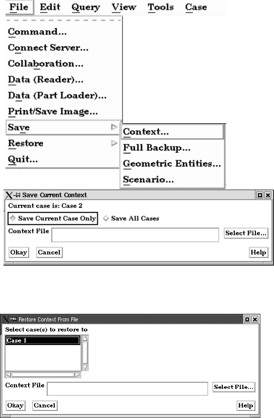
2.6 Context Files
EnSight 7 User Manual 2-39
2.6 Context Files
EnSight context files can be used to duplicate the current EnSight state with the
same or a different, but similar, dataset. The context file works best if the dataset
it is being applied to contains the same variable names and parts, but can also be
used when this is not the case.
Input and output of context files is described below as well as in How To Save or
Restore a Context File and under Save and Restore of Section 6.1, File Menu
Functions
Saving a Context File
To save the current context, simply entered the desired file name in the dialog
under: Access: File > Save > Context...
(and if you have multiple cases to save, select Save All Cases)
Restoring a Context
Figure 2-19
Saving a Context File
Figure 2-20
Restoring a Context File
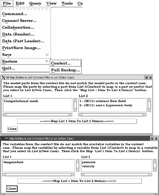
2.6 Restoring a Context
2-40 EnSight 7 User Manual
If you are restoring a context file containing information for a single case, you can
select the case or cases that you wish to apply the context to. If you are restoring
a context file containing information about multiple cases, the selection list will
be ignored.
When restoring a context you can 1) read the new dataset and build the new parts
and then restore the context file, or 2) read the new dataset, close the part builder
without building any parts and restore the context file (whereupon the context file
will build the same parts as existed when it was saved) or 3) restore the context
before reading any data (whereupon the previous state with the same dataset will
be restored). The way you decide to do this depends upon whether the same parts
exist in the new dataset.
If the same parts do not exist, you would typically read the new dataset and build
the desired parts in the normal way. Then:
Flipbook animations are not restored using the context file because it is unknown
at the time the context file is created what state existed when the flipbook was
saved.
Context files use EnSight’s command language and other state files (such as
palette, view, and keyframe animation).
Figure 2-21
Restoring a Context
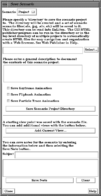
2.7 Scenario Files
EnSight 7 User Manual 2-41
2.7 Scenario Files
Scenario files are used by CEI’s EnLiten product which is capable of viewing all
geometry (such as parts, annotation, plots, etc.) that EnSight can display,
including flipbook, keyframe, and particle trace animations.
A “scenario” defines all visible entities you wish to view with EnLiten and
includes any saved views and notes that you want to make available to the
EnLiten user.
When you create a scenario, the following may be saved: (a) EnLiten file
containing geometric display information, saved views, and attached nodes. (b) A
palette file for each visible variable legend. (c) A JPEG image file (not used by
EnLiten). (d) A scenario description file (not used by EnLiten). (e) A EnSight
context file (not used by EnLiten).
When saving a scenario, either the scenario file itself can be saved, or the scenario
project - which includes all of the files in the previous paragraph.
EnLiten is a geometry viewer only. As such it is not capable of creating or
modifying any new/existing information such as variables or parts, or of changing
timesteps.
Since EnLiten is only a geometry viewer, only keyframe transformation
information is stored when saving a scenario file, i.e., no transient data
keyframing is possible (consider loading a flipbook instead)
.
Figure 2-22
Save Scenario Dialog
2.7 Scenario Files
2-42 EnSight 7 User Manual
You use the Save Scenario dialog to control the options of the scenario files to be saved in
EnSight for display in EnLiten.
Access: Main Menu > File > Save > Scenario...
Scenario
Project - will save the scenario file plus files mentioned on the previous page.
File - will save only the scenario file.
Scenario Directory/
File
Specifies the directory or file to which the scenario information will be written.
General
Description
Specifies the general description which will be used when a html page is generated for the
scenario.
Save Keyframe
Animation Toggle
Select to have any currently defined keyframe animation sequence saved to the scenario.
Save Flipbook
Animation Toggle
Select to have any currently defined flipbook animation saved to the scenario.
Save Particle Trace
Animation Toggle
Select to have any currently defined particle trace animation saved to the scenario.
Save Scenario Click to actually save the scenario.
Add Current View... After the scenario has been saved you may save additional views by setting the desired
view in EnSight, then selecting this button You will be asked to name the view in a
resulting pop-up dialog.
Save Note After the scenario has been saved you may write notes regarding the scenario by entering
a Subject line and typing in the notes input area. When satisfied, select this button.
(see How To Save Scenario)
2.8 Saving Geometry and Results Within EnSight
EnSight 7 User Manual 2-43
2.8 Saving Geometry and Results Within EnSight
Saving Geometric Entities
Sometimes you may wish to output geometric data or variable values from
EnSight to be included in a different analysis code, or to be used in a presentation.
EnSight has three internal writers that allow saving geometric data and variable
values in Brick of Values, Case (EnSight Gold) or VRML. EnSight also allows the
user to create their own writers.Each user-defined writer must be compiled into a
dynamic shared library that is loaded at runtime and listed in the Save Geometric
Entities dialog with the internal writer formats.
Both internal and user-defined writers have access only to the geometry of
selected parts and each of their active variables. Only parts located on the server
can be saved. This includes all original model parts, and the following created
parts: 2D-clips, Elevated Surfaces, Developed Surfaces, and Isosurfaces. The
VRML internal writer saves all the visible parts on the server (thus, particle traces,
vector arrows, contours, etc. will not be saved) in their current visible state except
for Parts which have limit fringes set to transparent. The VRML file will be saved
on the client.
The userd-defined writers can call the routines of an EnSight API to retrieve, to
get, for example, nodal coordinates, node ids, element ids of parts selected in the
Parts window to be passed by value to be used, manipulated and/or written out in
any format desired. User-defined writer dialog includes a Parameter field that
allows passing in a text field into the writer from the GUI for extra options.
Several example writers (including source code header files, Makefile and the
corresponding shared library) are included to demonstrate this capability.
The Case (Gold) Lite reader is included to demonstrate how to exercise most of
the API and output a subset of the Case (Gold) format. Complex numbers and
custom Gold format are not supported with this writer. While the writer is not
compiled, the source code of this writer, the required header files, and the
Makefile are included.
The Flatfile user-defined writer is designed to demonstrate the output selected part
nodal data (coordinates & IDs) as well as active variable values (scalar and/or
vector only) data in a comma delimited format easily imported into other
applications. If any of the keywords ‘ANSYS’ or ‘force’ or ‘body’ is entered into
the Parameter field, then Flatfile will output an ANSYS body force file.
The HDF 5.0 writer is designed to write out selected parts and their corresponding
active variables using the HDF 5.0 API which is compatible with the EnSight
HDF user-defined reader.
The STL user-defined writer is designed to write out the border geometry in the
form of triangular 2D elements of the selected part(s) at the beginning timestep.
The end time and the step time are ignored. The STL format does not support
multiple parts in a single binary file, but does support multiple parts in a single
ASCII file. Therefore, if multiple parts are selected and ascii is checked, the STL
writer outputs an ascii file with the border of each of the parts. If multiple parts
are selected and binary is checked, the STL writer outputs a binary file containing
a single border of the multiple parts.
More user-defined writers may be distributed with EnSight in the future.
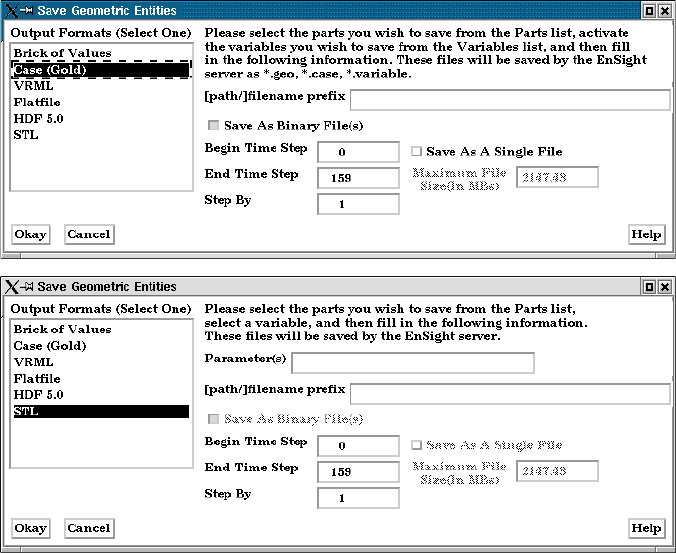
2.8 Saving Geometric Entities
2-44 EnSight 7 User Manual
Save Geometric Entities dialog
The Save Geometric Entities dialog is used to save Selected Model, 2D-Clip, Isosurface,
Elevated Surface, and Developed Surface Parts as EnSight Case (Gold) files. Thus
modified model Parts and certain classes of created Parts can become model Parts of a
new dataset.
Access: Main Menu > File > Save > Save Geometric Entities...
Output Format
Specify the desired format: Case(EnSight Gold), VRML, Flatfile, HDF5.0, STL, etc.
Parameter Allows passing a text field from the GUI to the writer for extra options. Some writers
make use of this field to modify their behavior (see Flatfile, for example) while others
ignore this field.
[path]/filename
prefix
Specify path and filename prefix name for the saved files. For Case(Gold) the saved
geometry file will be named filename.geo, the casefile will be filename.case, and the
active variables will be filename.variablename. The VRML file will be filename.wrl. The
other writers will vary.
Save As Binary
File(s)
Save as Binary File(s) specifies whether to save the data in ASCII (button toggled off -
default) or binary (button toggled on) format. Writers vary in their handling of this.
Begin Time Step Begin Time Step field specifies the initial time step for which information will be
available to save for all selected Parts and activated variables. Writers may vary in their
usage of this information.
End Time Step End Time Step field specifies the final time step for which information will be saved for
all selected Parts and activated variables. Writers may vary in their handling of this.
Step By Step By field specifies the time step increment for which information will be saved for all
selected Parts and activated variables starting with Begin Time Step and finishing with
End Time Step. The Step By value MUST be an integer. Writers may vary in their
handling of this.
Figure 2-23
Save Geometric Entities dialog
(Showing Case (Gold) internal writer, and STL external writer)

2.8 Saving Geometric Entities
EnSight 7 User Manual 2-45
Save as a Single
File
Toggle on to have a single file per variable - containing all values for all time steps for that
variable. The default is to have a file per variable per time step. Writers may vary in their
handling of this.
Maximum file Size For Single File option, can specify the maximum file size. Continuation files are created if
the file size would exceed this maximum. Writers may vary in their handling of this.
Okay Click ok to pass the GUI values to the selected writer, and begin executing the writer
routine
Troubleshooting Saving Geometric Entities
(see How To Save Geometric Entities)
Problem Probable Causes Solutions
A Part was not saved User attempted to save an
unsupported Part type.
Select only Model, Isosurface, 2D-
Clip, and Elevated Surface Parts.
Variable(s) not saved The variable was not activated or the
variable was a constant.
Activate all scalar and vector
variables you want saved.
Error saving File prefix indicates a directory that
is not writable or disk is out of space.
Re-specify a writable directory and
valid prefix name. Remove
unneeded files.
My custom user-defined writer
doesn’t show up on list of formats
Didn’t load at startup Start Ensight with -writerdbg option
EnSight loads user-defined writers at
startup from shared libraries found in
$CEI_HOME/ensight76/machines/
$CEI_ARCH/lib_writers
If your user-defined writer is not in
the default directory, tell EnSight
where to find it by:
setenv ENSIGHT7_UDW location
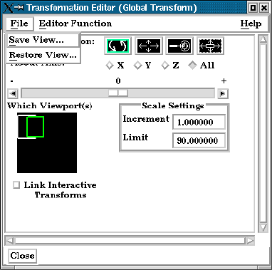
2.9 Saving and Restoring View States
2-46 EnSight 7 User Manual
2.9 Saving and Restoring View States
EnSight’s viewports provide a great deal of flexibility in how objects are
displayed in the Graphics Window. Given the complicated transformations that
can be performed, it is imperative that users be able to save and restore
accumulated viewport transforms.
View saving and restoring is accessed from the Transformations dialog.
Access: Desktop > Transformation Edit... > File
When either the Save View... or Restore View... selection is made, the user is
presented with the typical File Selection dialog from which the save or restore can
be accomplished. Save and Restore work on a single viewport.
(see also How To Save and Restore Viewing Parameters)
Figure 2-24
View Saving and Restoring in Transformation Dialog
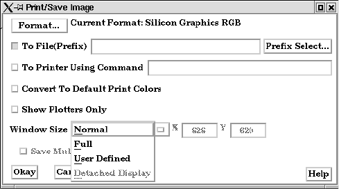
2.10 Saving and Printing Graphic Images
EnSight 7 User Manual 2-47
2.10 Saving and Printing Graphic Images
EnSight enables you to save an image of the Main View to a disk file or send it
directly to a printer. The choice of save file formats depends on the
implementation, but in all cases it is possible to obtain formats compatible with
printers and plotters. Currently EnVideo, Apple PICT, PCL, PostScript, SGI RGB,
CEI RGB(w/depth), TIFF, JPEG, MPEG, AVI, and TARGA formats are available.
EnSight also enables you to save images of an animation to disk files. These files
can then be converted and printed or recorded to video equipment (see Section
7.15, Keyframe Animation).
Print/Save Image dialog
You use the Print/Save Image dialog to specify the format and destination of an image to
save. The destination can be a disk file or a printer. You also access the Image Format
Options dialog for the various types from this dialog.
Access: Main Menu > File > Print/Save Image...
Format...
Click to select image format. (See next figure)
To File Toggle/Field The image will be saved to this disk file name if toggle is on. This is a filename prefix.
An appropriate suffix, according to the file format chosen, will be added.
To Printer Using
Command Toggle/
Field
The command to send a file to the printer if toggle is on. Make sure your printer is setup
for the format you’ve selected.
Convert to default
print colors
Clicking this toggle on will convert all black to white and all white to black but will leave
all other colors as they are.
Show Plotters Only Clicking this toggle will cause the graphics window to only display plotters.
Window Size Specifies the size of the Graphics Window and the resulting image size.
Normal Creates a window which is the size of the current Graphics Window.
Full Creates a window which is the size of the full screen.
User Defined Creates a window which is specified in terms of its width and height in the X and Y fields.
Detached Display Uses the detached display (as specified with - dconfig option) as the source for the output.
Figure 2-25
Print/Save Image dialog
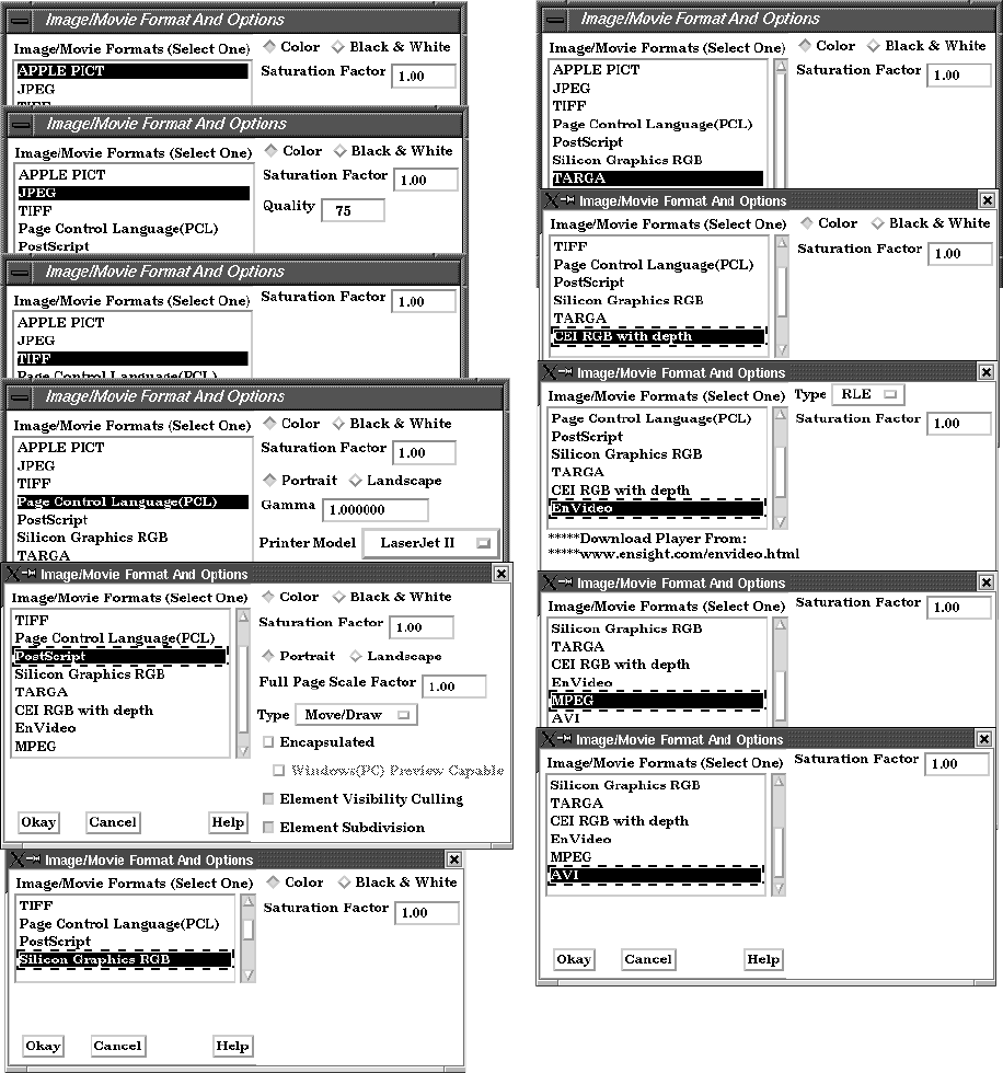
2.10 Saving and Printing Graphic Images
2-48 EnSight 7 User Manual
Format...
.
Color/Black &
White
(Several Formats)
Color versus Black and White toggle.
Saturation Factor
(all formats)
At a value of 1.0, no change to the image. At lower values, a proportionate amount of
white is added to each pixel. At a value of 0.0, the image would be all white.
Quality (JPEG) Specifies trade-off between fidelity & compression. 100 max fidelity; 0 max compression.
Portrait/Landscape
(PCL, Postscript)
Page Orientation for printing.
Gamma (PCL) Gamma correction factor.
Figure 2-26
Image/Movie Format Options dialogs
2.10 Saving and Printing Graphic Images
EnSight 7 User Manual 2-49
Full Page Scale
Factor (Postscript)
The percentage of full page scaling to do. This is according to Orientation as well. Values
are from 0.0 to 1.0.
Printer Model
(PCL)
The destination PCL printer model.
Type
(Postscript)
Type of Postscript output: Move/Draw (vector) or Image Pixels. If type is Image Pixels,
shaded 3D objects will be output as pixels while overlay graphics (annotation text, plots,
color legends) will be output Move/Draw for higher print quality.
Type
(EnVideo)
Type of EnVideo output: Run Length Encoded or Jpeg.
Encapsulated
Toggle
(Postscript)
Generate Encapsulated PostScript (EPS) for importing into other applications. (The
graphic typically will appear as a gray box in the importing application on all systems
unless the Windows(PC) Preview Capable toggle is also On).
Windows(PC)
Preview
Capable Toggle)
Create an Encapsulated PostScript (EPS) file which also has a preview image for use in
Windows® applications. (The graphic will still appear as a gray box in the importing
application on Macintosh systems).
Element Visibility
Culling Toggle
(Postscript)
Hidden geometry will be removed from the output stream if toggle is on. Valid for Move/
Draw output only. On by default.
Element
Subdivision
(Postscript)
Subdivide output primitives (lines and polygons) if toggle is on. Although the output file
will be larger, the color distribution will be far superior.Valid for Move/Draw output only.
On by default.
(see How To Print/Save an Image)

2.10 Troubleshooting Saving an Image
2-50 EnSight 7 User Manual
Troubleshooting Saving an Image
(see How To Print/Save an Image)
Problem Probable Causes Solutions
Image has blotches or ghosts of other
windows in it
A viewport or menu was popped in
front of the Main Graphics Window
as the image was being saved.
Do not perform any window
manager functions until image is
finished recording to disk file.
Error while saving image file Directory or file specified is not
writable
Rename the file or change the
permissions.
Ran out of disk space Check the file system you are
writing to with the “df” command
then remove any unnecessary files to
free up disk space.
Image format not selected Select an image format before
saving.
Image looks bad when printed Original on-screen image has low
resolution
Make the graphics window as large
as possible before saving the image
to increase the number of RGB
pixels used on the display.
Image has been dithered during
processing
Do not enlarge or reduce the image
until it is in your word processor.
Non-integral ratio of printer
resolution to image resolution at
final size
The image is a pixel-map image. For
best results, the number of printer-
dots per image-dot should be an
integer. For example, if the original
image resolution is 72 dpi, reduced
to 48% the final-size resolution is
72/.48 = 150 dpi. On a 600 dpi
printer, each image pixel is exactly 4
printer-dots on a side.
Move/Draw PostScript output
doesn’t look correct.
Primitives in Move/Draw PostScript
output sometimes suffer from sorting
problems.
Use Image Pixel type instead of
Move/Draw.
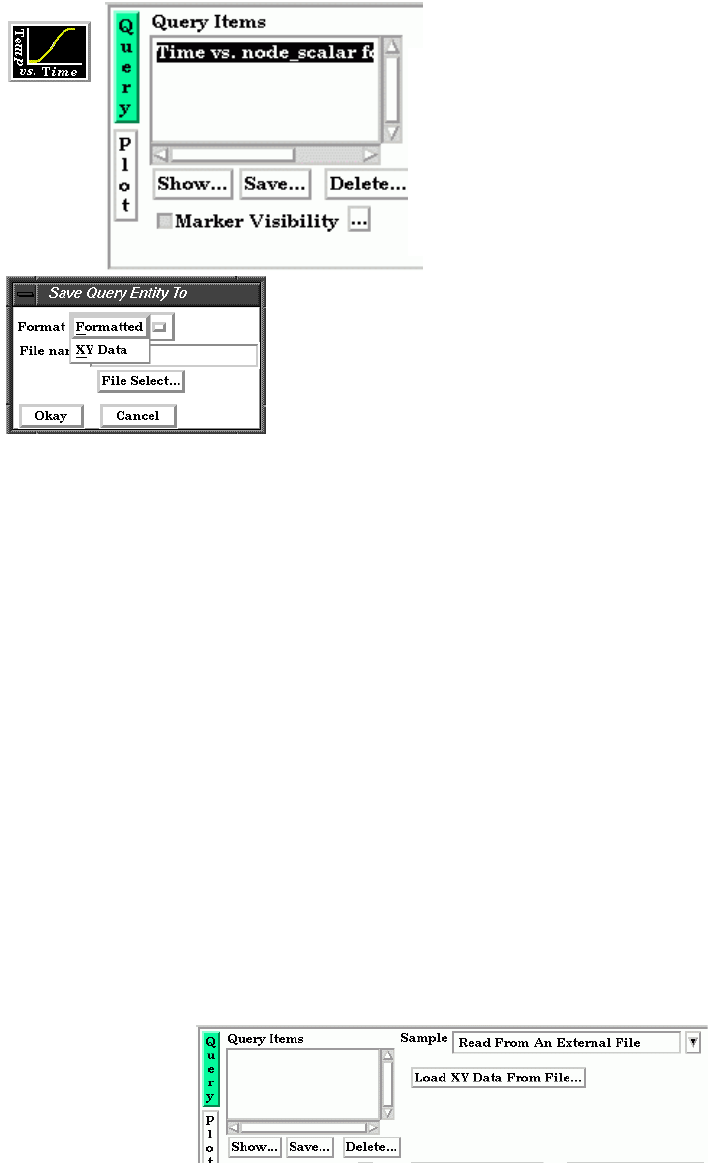
2.11 Saving and Loading XY Plot Data
EnSight 7 User Manual 2-51
2.11 Saving and Loading XY Plot Data
The xy data used for curves in EnSight’s plotter can be saved to a file for future re-
loading into EnSight or for use in other plotting packages.
The process is described below as well as in Section 7.11, Query/Plot
Access: Desktop > Query/Plot Feature
Once the desired query item (curve) is selected in the list, the user can perform a
Save operation by:
Save... Click this button in the Quick Interaction area of the Query/Plot feature to save the plotter
curve data.
Format Select the Format of the data to save.
Formatted is a table suitable for printing. (see Section 2.13, Saving Query Text
Information)
XY Data is the xy file format described in Section 11.10, XY Plot Data Format,
which is suitable for re-loading into EnSight.
File Name Enter the desired filename for the xy data file, or click File Select... to be presented with
the typical File Section dialog from which to perform the op8888eration.
Loading:
To Load a previously saved or externally generated xy data file (see Section 11.10,
XY Plot Data Format) into EnSight you choose the “Read From An External File”
Sample type (see How To Query/Plot). You will then be presented with the
typical File Selection dialog from which to select the file. Note: A MSC/Dytran
.ths file is also a valid entry for this option.
Figure 2-27
Saving or Loading XY Plot Data
Figure 2-28
Query/Plot Area for Read
From An External File.
2.12 Saving and Restoring Animation Frames
2-52 EnSight 7 User Manual
2.12 Saving and Restoring Animation Frames
Both Flipbook and Keyframe Animation processes have save and restore
capability. These are best described in the chapters devoted specifically to these
features.
For Flipbook Animations, see Section 7.14, Flipbook Animation and How To
Create a Flipbook Animation.
For Keyrame Animations, see Section 7.15, Keyframe Animation and How To
Create a Keyframe Animation.
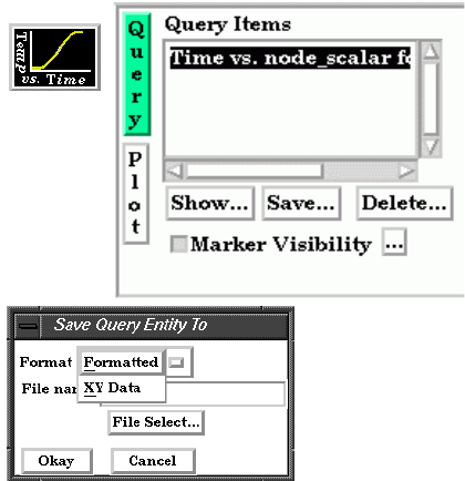
2.13 Saving Query Text Information
EnSight 7 User Manual 2-53
2.13 Saving Query Text Information
The data used for curves in EnSight’s plotter and any other information from a
query or otherwise which is presented in the EnSight Message Window can be
saved to a file suitable for printing.
From Query/Plot Save... Formatted
One place this can occur is in the Query/Plot Quick Interaction area as described
below as well as in Section 7.11, Query/Plot
Access: Desktop > Query/Plot Feature
Once the desired query item (curve) is selected in the list, the user can perform a
Save operation by:
Save... Click this button in the Quick Interaction area of the Query/Plot feature to save the plotter
curve data.
Format Select the Format of the data to save.
Formatted is a table suitable for printing.
XY Data is the xy file format described in Section 11.10, XY Plot Data Format,
which is suitable for re-loading into EnSight.
File Name Enter the desired filename for the xy data file, or click File Select... to be presented with
the typical File Section dialog from which to perform the operation.
From Query/Plot Show Text
Show ... Click this button to see the plotter curve information presented in the EnSight Message
Window.
Figure 2-29
Saving or Loading XY Plot Data
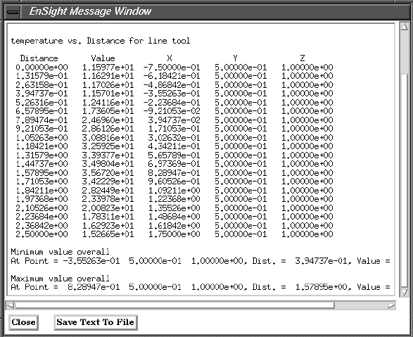
2.13 From EnSight Message Window
2-54 EnSight 7 User Manual
From EnSight Message Window
A file suitable for printing can be saved from any operation which places its
information into the EnSight Message Window, such as Show Information queries
and the Query/Plot Show Text... button described previously.
Save Text To File Brings up the typical File Selection dialog from which the information can be saved in the
file of your choice.
Figure 2-30
EnSight Message Window with Save Text To File Button
2.14 Saving Your EnSight Environment
EnSight 7 User Manual 2-55
2.14 Saving Your EnSight Environment
Every user has different postprocessing needs and personal preferences for how
the EnSight windows should be positioned and sized. EnSight allows you to save
dialog expandable section settings, and dialog size and position information to a
file called “ensight7.winpos.default”. EnSight looks for this file at start up (in the
current Client directory and if not there in the .ensight7 directory of the user’s
home directory) and will bring the user interface dialogs up according to your
saved settings (if the file is found).
Almost all major dialog windows are saved in the:
ensight7.winpos.default_XRESxYRES
file (where XRES and YRES are the resolution of the monitor when the
preferences were saved). The only exception are minor prompt dialogs. There are
also some dialogs for which you cannot save the size (such as the Tool Positions
dialog).
The ensight7.winpos.default file also contains the size and location for all of the
windows containing graphics.
A number of other settings, such as mouse and keyboard buttons and Icon Bar
settings can also be saved to a user preferences file.
(see Preferences... in Section 6.2, Edit Menu Functions and How to Save GUI
Settings)
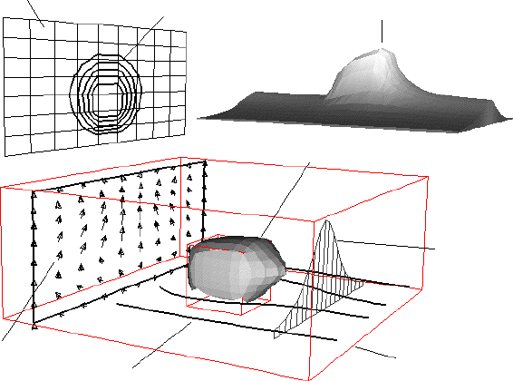
EnSight 7 User Manual 3-1
3Parts
The Part is the fundamental visualization entity in EnSight. Virtually every
postprocessing task you perform will involve a Part, thus it is vital to understand
how Parts work.
A Part is a collection of nodes and elements that are grouped together and share
the same attributes. When you start EnSight, you either read directly or
interactively extract Parts from the data files. Parts which come from the original
dataset are referred to as model Parts. Other Parts created within EnSight, are
referred to as created (or dependent) Parts.
In this chapter you will learn how to produce created Parts (parts derived from
other parts) and how to modify the attributes of all Part types.
Section 3.1, Part Overview is extremely important. It defines how Parts work
together to form other Parts and explains the dependencies which may exist
between model Parts and created Parts. Failure to understand the concept of Parts
as explained in this section will limit your ability to use EnSight. Please study this
section carefully.
Figure 3-1
V
arious EnSight Part Types
Clip Plane
Contours
Elevated Surface
Isosurface
Profile
Vector Arrows
Particle Traces
Model Part
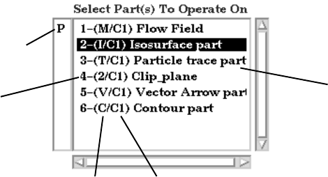
3.1 Part Overview
3-2 EnSight 7 User Manual
Included in this Chapter are:
Section 3.1, Part Overview
Section 3.2, Part Selection and Identification
Section 3.3, Part Editing
Section 3.4, Part Operations
3.1 Part Overview
In EnSight, a Part is simply a collection of nodes and elements which are grouped
together, will be manipulated together, and which share the same attributes. This
section defines Parts and how they are related. It gives you an overview of the Part
types and Part attributes that are available within EnSight.
Parts that are defined or extracted from your dataset are referred to as model Parts.
Parts that are created within EnSight are referred to as created (or dependent)
Parts. The types of Parts that you create depends on what features within EnSight
you choose to utilize. Any created Part is derived from Parts that already exist,
which is why the created Parts are sometimes called dependent Parts—they
depend on the Parts from which they were created. The Parts that are used to
create a dependent Part are referred to as parent Parts. Any time that a parent Part
changes, its dependent Parts must also change. A parent Part will change when
you change its attributes, or modify the current time in the case of transient data.
The Main Parts List contains all Parts that have been read in from your results data
or created within EnSight. Displayed are a Part ID Number, a Part symbol, a case
number, and a Part description. Table 3-1 lists all of the different types of Parts
and their associated symbols. The figure below of the Parts List shows a number
of different Part types.
Note that in the illustration above the Isosurface Part is selected and that there is a
“P” in the left column next to the Computational mesh (model) Part. This
indicates that the Computational mesh Part is the parent Part of the isosurface
Part. All parent Parts of a created Part will be so noted if that individual created
Part is highlighted in the Main Parts List.
Reassign Parent Parent Parts of any created Part can be changed by first selecting the created Part
in the Feature Detail Editor, then selecting a new parent Part in the Main Parts
List, and finally by clicking the Update Parent button in the Feature Detail Editor.
Figure 3-2
Main Parts List
Parent Part
Part ID
Part Symbol Case Number
Part Description
Indicator
Number

3.1 Part Creation
EnSight 7 User Manual 3-3
Table 3–1 Part Types, Symbols, and Descriptions
Part Creation
Part creation occurs on either the server or the client. Since the data that is
available on the client and server are different, it is useful to understand where
Parts are created and where the data structures are stored. By understanding this,
you will understand why some Parts can be created with certain parent Parts and
others cannot. This information can be gained by examining the following table.
Table 3–2 Part Creation and Data Location
Part Type Symbol Description
Clip (2)
A surface or line resulting from a clip of other Parts using the line,
plane, or quadric tools
Contour (C)
Lines of constant value on 2D elements
Developed Surface (D)
A planar surface derived by unrolling a surface of revolution (i.e.,
the unrolling of a cylinder clip Part produced by the cylinder
quadric tool)
Elevated Surface (E)
Surface created by elevating elements by a variable
Isosurface (I)
Surface of constant value through 3D elements of other Parts
Material Part (A)
A Part created according to the intersection of or domains of
material values
Model Part (M)
A Part that originated from the dataset
Particle Trace (T)
Path of a massless Particle through a vector field
Profile (P)
Plot of a variable along a line (Similar to a 2D elevated surface)
Separation/
Attachment Line
(L)
Line where flow separation or attachment is occurring
Shock Surface/
Region
(K)
Surface or region where shock is occurring
Subset (S)
Valid node and/or element label range(s) from model Part(s)
Tensor Glyph (G)
Glyph showing direction of first, second, and third eigenvectors of
a tensor field.
Vector Arrow (V)
Arrows showing direction and magnitude of vector field
Vortex Core (X)
Line representing center of a flow vortex
Part Type Where Created
Data on
Server
Data on Client
Clip Server Yes Depending on Part attributes
Contour Client No Yes
Developed Surface Server Yes Depending on Part Attributes
Discrete Particle Not Applicable Yes Depending on Part attributes
Elevated Surface Server Yes Depending on Part attributes
Isosurface Server Yes Depending on Part attributes
Model Not Applicable Yes Depending on Part attributes
Material Part Server Yes Depending on Part attributes

3.1 Part Attributes
3-4 EnSight 7 User Manual
(see Introduction to Part Creation)
Part Attributes
Each type of created Part has a unique set of attributes that are used to accomplish
its creation, the Creation Attributes. Model Parts (symbol: M) and discrete
Particle Parts (symbol: D) typically do not have creation attributes because they
are not created—they are read or extracted from the dataset. The one exception to
this is model parts originating from block structured datasets. These parts contain
the I,J,K and step attributes used to create the part.
All Parts have a set of Display Attributes that are used in visualizing the Part in the
Graphics Window. These can be modified using the Feature Detail Editor or by
utilizing the Part Mode Icons (See Section 8.4). The Feature Detail Editor for each
Part type will show you attributes grouped together under turndown sections.
They deal with such things as color, line width, symmetry operations, etc. Display
attributes do not control how the Part is created, only how it appears or how it
behaves in the Graphics Window.
Table 3–3 Display Attribute Sections
Particle Trace Server No Yes
Profile Client No Yes
Separation/
Attachment Line
Server Yes Depending on Part attributes
Shock Surface/
Region
Server Yes Depending on Part attributes
Subset Server Yes Depending on Part attributes
Tensor Glyph Client No Yes
Vector Arrow Client. Server if
necessary.
Maybe Yes
Vortex Core Server Yes Depending on Part attributes
Section: Includes controls for...
General Attributes
(see Section 3.3 Part Editing)
Visibility in Graphics Window and
individual Viewports
Symmetry options
Susceptibility to Auxiliary Clipping
Reference frame
Response to changes in time (frozen or
active)
Coloration (constant or by a palette
associated with a variable)
Shaded Surface and Hidden Line display
Surface shading (flat, Gouraud, smooth)
Opaqueness and Fill density
Part Type Where Created
Data on
Server
Data on Client

3.1 Part Attributes
EnSight 7 User Manual 3-5
Lighting (diffuse, shininess, and highlight
intensity)
Node, Element, and Line Attributes
(see Section 3.3, Part Editing)
General Visibility: Node, Line, and
Element
Label Visibility: Node and Element
Node Representation: Node type (dot,
cross, or sphere), Node Scale, Node Detail
(for spheres), and Node size (constant or
variable)
Line Representation: Line Width and Line
style (solid, dotted, or dot-dash)
Element representation on client (full,
border, 3D border/2D full, feature angle,
or non visual), Element-size, Shrink-
Factor, Element Angle and Polygon
Reduction factor
Displacement Attributes Displacement variable
(see Section 3.3, Part Editing) Displacement scaling factor
Section: Includes controls for...

3.2 Part Selection and Identification
3-6 EnSight 7 User Manual
3.2 Part Selection and Identification
In the process of creating a Part you will need to be able to select the parent Part(s)
from the Main Parts List. You will also find that it is possible to either read or
create so many Parts within EnSight that you become confused as to the identity
of each Part. This section describes Part selection and identification
Selecting Parts
Items in all Parts Lists are selected using standard Motif/Win32 methods:
(see How To Select Parts)
Identifying Parts
There are two quick ways to identify one or more Parts that have been selected in
the Main Parts List. You can identify them in the Graphics Window by toggling
visibility on/off while in Part Mode or you can select View > Show Selected
Parts... from the Main Menu to show only the selected Part(s) in the pop-up
Selected Part(s) Window.
To: Do This: Details
Select an item Select (or
single-click)
Place the mouse pointer over the item
and click the left mouse button. The item
is highlighted to reflect the “selected”
state.
Extend a contiguous
selection
Select-drag Place the mouse pointer over the first
item. Click and hold the left mouse
button as you drag over the remaining
items to be selected. Only contiguous
items may be selected in this fashion.
Extend a (possibly
long) contiguous
selection
Shift-click Select the first item. Place the mouse
pointer over the last item in the list to be
selected. Press the shift key and click the
left mouse button. This action will
extend a selection to include all those
items sequentially listed between the
first selection and this one.
Extend a non-
contiguous selection
Control-click Place the mouse pointer over the item.
Press the control key and click the left
mouse button. This action will extend a
selection by adding the new item, but
not those in-between any previously
selected items.
De-select an item Control-click Place the mouse pointer over the
selected item. Press the control key and
click the left mouse button. This action
will de-select the item.
Open the Quick
Interaction Area for a
Part
Double-click Place the mouse pointer over the item
and click the left mouse button twice in
rapid succession.
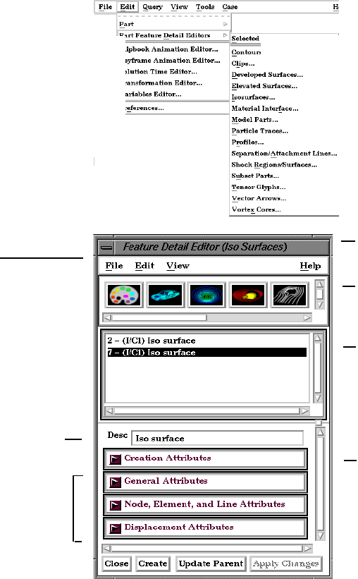
3.3 Part Editing
EnSight 7 User Manual 3-7
3.3 Part Editing
In EnSight, new Parts can be created and edited in the Quick Interaction Area
Editor or in the Feature Detail Editor specific to each type of Part. This process is
described in Sections 7.2 to 7.9. For editing, the Quick Interaction Area provides
access to the most common attributes; the Feature Detail Editor allow
modification of all attributes.
Whereas each individual change made in the Quick interaction Area Editor is
applied to the Part immediately, the Feature Detail Editor allows you to make a
number of changes to various attributes and then apply them all at one time. This
is done by toggling off View > Immediate Modification in the Feature Detail
Editor. The default behavior is to immediately apply a change when you press
Return.
The Feature Detail Editor for Parts is opened from the Main Menu (or by double
clicking on a Part creation Icon in the Main GUI Feature Icon Bar).
Figure 3-3
Feature Detail Editor (Isosurfaces)
Part Type Icon Bar
Parts List (of chosen
Description of Selected Part
Editor Main Menu
Creation Attributes Turndow
n
Display Attributes Turndowns
Part Type)
Editor Title Bar
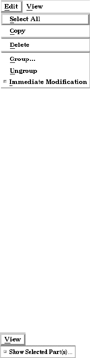
3.3 Part Editing
3-8 EnSight 7 User Manual
Feature Detail Editor Main Menu
File Not applicable when Feature Detail Editor is used for Parts - only applicable for Variables.
Edit Opens a pull down menu.
Select All Selects all Parts in Feature Detail Editor Parts List. (see Section 3.4, Part Operations)
Copy Makes a copy of all selected Parts. (see Section 3.4, Part Operations), also (see How To
Copy a Part)
Delete Deletes selected Parts. (see Section 3.4, Part Operations), also (see How To Delete a Part)
Group... Groups the selected parts into a new part and removes the original parts from the list.
Ungroup Extracts the original parts out of a group and removes the group part.
Immediate Toggles on/off the immediate modification of Parts when individual changes are made to
Modification Toggle Attributes within the Feature Detail Editor. Default is on. By toggling off, you can make
several changes within the Feature Detail Editor and then apply them all at one time by
clicking the Apply Changes button.
View Opens a pull-down menu.
Show Selected Opens the Selected Part(s) Window in which only Parts selected in the Feature Detail
Part(s) Toggle Editor’s Parts List are visible.
Figure 3-4
Feature Detail Editor Edit pull-down menu
Figure 3-5
Feature Detail Editor View pull-down menu
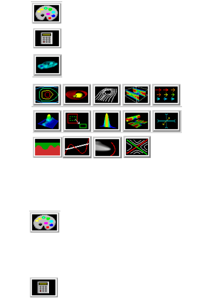
3.3 Variable Color Palette Icon
EnSight 7 User Manual 3-9
Part Type Icon Bar
The Feature Detail Editor is initially opened from EnSight’s Main Menu (or by double
clicking a Part creation icon in the Feature Icon Bar) and the Feature Detail Editor’s Parts
List contains all Parts of the type named in the Editor’s Title Bar. The type of Parts in the
Feature Detail Editor’s Parts List may be changed by clicking on the appropriate icon in
the Feature Detail Editor’s Part Type Icon Bar. The figure below describes the four types
of choices available.
Variable Color Palette Icon
Click this icon to edit color controls. See Section 4.1 Variable Selection and Activation for
further discussion.
Variable Creation (Calculator) Icon
Click this icon to use the calculator to create new variables for the parts selected in the
Main Parts window.
1. Variable Color Palette controls
2. Variable Creation (Calculator) controls
3. Model Part attribute controls
4. Created Parts
attribute controls
Figure 3-6
Feature Detail Editor Part Type Selection Icons
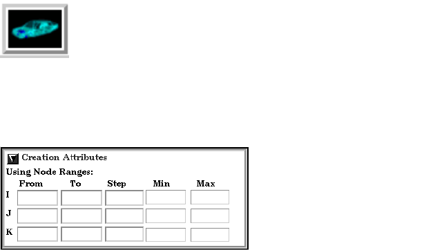
3.3 Variable Creation (Calculator) Icon
3-10 EnSight 7 User Manual
Creation Attributes
Creation Attributes are “specific” attributes used to create (or modify) model and created
Parts.
Model Parts
Creation Attributes for updating the I,J,K node range attributes of the selected block
structured Model Parts with proper updating of all dependent parts and variables. The
Creation Attributes area is inactive for unstructured Model Parts.
Access: Main Menu > Edit > Part Feature Detail Editors > Model Parts
Using Node Ranges
IJK From These fields specify the desired minimum interval value in the respective IJK
component direction of the Model Part.
IJK To These fields specify the desired maximum interval value in the respective IJK
component direction of the Model Part.
IJK Step These fields specify the desired interval stride value in the respective IJK
component direction of the Model part.
IJK Min These fields verify the minimum interval limit in the respective IJK component
direction of the Model part.
IJK Max These fields verify the maximum interval limit in the respective IJK component
direction of the Model part.
(see How To Create IJK Clips)
Figure 3-7
Feature Detail Editor (Model) Creation Attributes Area
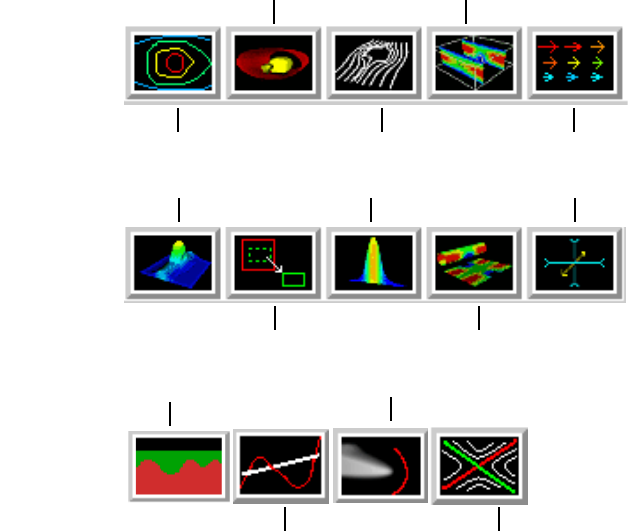
3.3 Variable Creation (Calculator) Icon
EnSight 7 User Manual 3-11
Created Parts
See the appropriate Section in Chapter 7 for a description of the Creation Attributes
section.
• (see Section 7.2, Contour Create/Update)
• (see Section 7.3, Isosurface Create/Update)
• (see Section 7.4, Particle Trace Create/Update)
• (see Section 7.5, Clip Create/Update)
• (see Section 7.6, Vector Arrow Create/Update)
• (see Section 7.7, Elevated Surface Create/Update)
• (see Section 7.8, Profile Create/Update)
• (see Section 7.9, Developed Surface Create/Update)
• (see Section 7.16, Subset Parts Create/Update)
• (see Section 7.17, Tensor Glyph Parts Create/Update)
• (see Section 7.19, Vortex Core Create/Update)
• (see Section 7.20, Shock Surface/Region Create/Update)
• (see Section 7.21, Separation/Attachment Lines Create/Update)
Isosurface Clip
Contour Particle Trace Vector Arrow
Elevated Surface Profile Tensor Glyph
Subset Developed Surface
Vortex Core
Shock Surface/Region
Separation/
Attachment
Line
Material Part
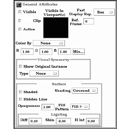
3.3 Variable Creation (Calculator) Icon
3-12 EnSight 7 User Manual
General Attributes
General Attributes are “general” in that: (a) all Parts have them, and (b) they can’t
be neatly categorized into any other attribute type. Like all Part attributes, they are
set individually for each Part.
Access: Main Menu > Edit > Part Feature Detail Editors > (Isosurfaces..., etc.) > General Attributes
Visible Toggle
Toggles-on/off whether Part is visible on a global basis (in the Graphics Window or in all
viewports). (Performs the same function as the Visibility Toggle in the Parts Mode Icon
Bar). Default is ON.
Visible In Viewports This small window allows you to control the visibility of the selected Part(s) on a per
Viewport basis. Each visible viewport is shown. A green outline around a Viewport
indicates that the selected Part(s) will be visible in this Viewport, while a red outline
indicates that the selected Part(s) will not be visible. Change the visibility (red to green,
green to red) by selecting a viewport with the mouse.
Fast Display Rep. This button opens a pop-up menu button for the selection of the fast display representation
used to display a part on the client. This attribute helps the display of complex data sets.
The part’s fast display representation displays according to whether the Fast Display
Mode (located in the View Menu or on the desktop) is on or off and on the state of the
Static Fast Display button located under Edit > Preferences..., Performance. For instance,
when the Fast Display Mode is Off (default) the part displays according to its specified
Element Representation. When on, the parts are displayed by the fast display
representation. The fast display representation will only be used while performing
transformations, unless the Static Fast Display option has been selected. The part detail
representations are:
Box a bounding (Cartesian extent) box of all part elements (default).
Off display according to specified Element Representation.
Points point cloud representation of the part (EnSight gold only).
Sparse Model display a percentage of the model in each display box (EnSight Gold
and not running with display lists only). You control this percentage in
the performance preferences. Note, that it is useful for large models, but
should probably not be used for small models.
(see How To Set Global Viewing)
Visual Symmetry This section contains controls which allow you to produce either rotational or mirror
Figure 3-8
Feature Detail Editor General Attributes Area
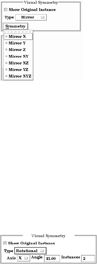
3.3 Variable Creation (Calculator) Icon
EnSight 7 User Manual 3-13
visually symmetric images of parts. In general, symmetry enables you to reduce the size of
your analysis problem while still visualizing the “whole thing.” Symmetry affects only the
displayed image, not the data, so you cannot query the image or use the image as a parent
Part. However, you can create the same effect by creating dependent Parts with the same
symmetry attributes as the parent Part.
Mirror visual symmetry includes the ability to toggle-on/off the display of a mirror image
of Parts (which are selected in the Feature Detail Editor’s Parts List) in each of the seven
other quadrants of the Part’s local frame. It also allows you to turn on or off the original
(non-symmetric) part representation. It performs the same function as the Visual
Symmetry Pull-down Icon in the Part Mode Icon Bar. You can mirror the Part to more
than one quadrant. If the Part occupies more than one quadrant, each portion of the Part
mirrors independently. Symmetry works as if the local frame is Rectangular, even if it is
cylindrical or spherical. The images are displayed with the same attributes as the Part. For
each toggle, the Part is displayed as follows. The default for all toggle buttons is OFF,
except for the original representation - which is ON.
Mirror X quadrant on the other side of the YZ plane.
Mirror Y quadrant on the other side of the XZ plane.
Mirror Z quadrant on the other side of the XY plane.
Mirror XY diagonally opposite quadrant on the same side of the XY plane.
Mirror XZ diagonally opposite quadrant on the same side of the XZ plane.
Mirror YZ diagonally opposite quadrant on the same side of the YZ plane.
Mirror XYZ quadrant diagonally opposite through the origin.
Show Original Instance the original part location.
Rotational visual symmetry allows for the display of a complete (or portion of a) “pie”
from one “slice” or instance. You control this option with:
Axis X rotates about the X axis
Y rotates about the Y axis
Z rotates about the Z axis
Angle specifies the angle (in degrees) to rotate each instance from the previous
Instances specifies the number of rotational instances.
Show Original Instance show the original instance or not
(see How To Set Symmetry)
Aux Clip Toggle Toggles-on/off whether Part(s) selected in the Part List of the Feature Detail Editor will be
affected by the Auxiliary Clipping Plane
feature, which enables you to make invisible
that portion of each Part on the negative side of the current position of the Plane
Figure 3-9
Mirror Visual Symmetry
Figure 3-10
Rotational Visual Symmetry
3.3 Variable Creation (Calculator) Icon
3-14 EnSight 7 User Manual
Tool. Performs the same function as the Part Mode: Auxiliary Clipping Toggle
Icon. A Part with its Aux Clip attribute toggled-off will not be cut away.
Default is
ON. (see Auxiliary Clipping in Section 6.4, View Menu Functions).
Active Toggle Toggles-on/off whether or not display of the Part automatically updates as the solution
time changes. When visualizing transient data, you may wish to “freeze” a Part in time
while other Parts continue to update. For example, you can create two identical vector-
arrow Parts, toggle-off Active for one of them, change the time step of the display, and see
how the vector arrows change from one time step to the other. Only the EnSight client Part
is frozen, the EnSight server Part is kept current. Default is ON.
Ref. Frame This field specifies which frame the Part is assigned to. Default is the frame of the Part’s
parent Part (Frame 0 for original model Parts). Enter a different frame number in the field
to change the assignment. Changing a Part’s frame causes the Part to be drawn in the new
coordinate frame. Once assigned to a different frame, the Part will transform with that
frame. The choice of frame does not affect variable values. The interpolated value of a
variable at point 0,0,0 in Frame 0 is the same as at point 0,0,0 in Frame 1, even though the
points may appear at different locations in the Main View Window.
(see Section 8.5, Frame Mode)
Color By This button opens a pop-up menu for the selection of the variable color palette by which
you wish to color the selected Part(s). Coloring a Part with a palette does not normally
affect graphics performance while in line drawing mode, but Shaded Surface mode
performance can become considerably slower. If you do not color by a palette (Color By >
None), the Part will be displayed according to the color specified in the R, G, B fields. If
you want to color Parts by palettes and want Shaded Surface mode, consider using the
Static Lighting option (see Static Lighting in Section 6.4, View Menu Functions).
R G B These fields allow you to specify a solid color for the selected Part(s) (applicable only if
Color By is None). Enter a numerical value from 0 to 1 for each component color (Red,
Green, and Blue).
Mix... Opens the Color Selector dialog for the selection of a solid color for the selected Part(s)
(applicable only if Color By is None). (see Section 7.1, Color)
Surface
Shaded Surface Toggles on/off surface shading for individual Parts. When global Shaded
Toggle Surface has been toggled on for the Graphics Window display (from Main Menu > View >
Shaded Surface or via the Global Shaded Surface Toggle in the View Mode Icon Bar),
individual Parts can be forced to stay in line drawing mode using this toggle. Default is
ON. (see Section 6.4, View Menu Functions)
Hidden Line Toggles on/off hidden line representation for individual Parts. When global
Togg l e Hidden Line has been toggled on for the Graphics Window display (from Main Menu >
View > Hidden Line
or via the Global Hidden Line Toggle in the View Mode Icon
Bar
), individual Parts can be forced not to appear as Hidden Line representation using this
toggle. (To have lines hidden behind surfaces, Parts must have surfaces, i.e. 2D elements)
Default is ON. (see Section 6.4, View Menu Functions)
Shading Opens a pop-up menu for selection of appearance of Part surface when Shaded Surface is
on. Normally the mode is set to Gouraud, meaning that the color and shading will
interpolate across the polygon in a linear scheme. You can also set the shading type to Flat,
meaning that each polygon will get one color and shade, or Smooth which means that the

3.3 Variable Creation (Calculator) Icon
EnSight 7 User Manual 3-15
surface normals will be averaged to the neighboring elements producing a “smooth”
surface appearance.Not valid for all Part types. Options are:
Flat Color and shading same for entire element
Gouraud Color and shading varies linearly across element
Smooth Normals averaged with neighboring elements to simulate smooth surfaces
Opaqueness This field specifies the opaqueness of the selected Part(s). A value of 1.0 indicates that the
Part is fully opaque, while a value of 0.0 indicates that it is fully transparent. Setting this
attribute to a value other than 1.0 can seriously affect the graphics performance.
Fill Pattern Opens a pop-up menu for selection of a fill pattern which can provide pseudo-
transparency for shaded surfaces
. Default is Fill 0 which uses no pattern (produces a
solid surface), while Fill patterns 1 through 3 produce a EnSight defined fill pattern.
Lighting
Diff This field specifies diffusion (minimum brightness or amount of light that a Part reflects).
(Some applications refer to this as ambient light.) The Part will reflect no light if value is
0.0. If value is 1.0, no lighting effects will be imposed and the Part will reflect all light and
be shown at full color intensity at every point. To change, enter a value from 0 to 1.
Shin This field specifies shininess.You can think of the shininess factor in terms of how smooth
the surface is. The larger the shininess factor, the smoother the object. A value of 0
corresponds to a dull finish and a value of 100 corresponds to a highly shiny finish. To
change, enter a value from 0 to 100.
H Int This field specifies highlight intensity (the amount of white light contained in the color of
the Part which is reflected back to the observer). Highlighting gives the Part a more
realistic appearance and reveals the shine of the surface. To change, enter a value from 0 to
1 with larger values representing more white light. Will have no effect if Shin parameter is
zero.
(see How To Set Attributes)
Troubleshooting Surface Attributes and Lighting
Problem Probable Causes Solutions
Part not in Shaded Surface mode Global Toggle not on, or if on,
Shaded Surface is turned off for
the Part in the Feature Detail
Editor
Turn on Shaded Surface toggle
from View menu of Main Menu
or turn and make sure Shaded
Surface is turned on for the Part
in the Feature Detail Editor.
Part contains only 1D elements No Solution
Part appears not to have any
lighting.
Diffuse light intensity too high Lower the Diff value.
3.3 Variable Creation (Calculator) Icon
3-16 EnSight 7 User Manual
Node, Element, and Line Attributes
Each Part’s Node, Element, and Line attributes control the representation of the
Part on the client, and how nodes, elements, and lines are displayed
.
Access: Main Menu > Edit > Part Feature Detail Editors > Node, Element, and Line Attributes
General Visibility
Node Toggle
Toggles-on/off display of Part’s nodes whenever the Part is visible. Default is OFF.
Line Toggle Toggles-on/off display of line (1D) elements in the client-representation whenever the Part
is visible. Default is ON.
Element Toggle Toggles-on/off display of 2D elements in the client-representation whenever the Part is
visible. Note that 3D elements are always represented as 2D elements on the client.
Default is ON.
Label Visibility
Node Toggle
Toggles-on/off display of Part’s node labels (if they exist) whenever the Part is visible.
Only model Parts may have node labels. Default is OFF.
Element Toggle Toggles-on/off display of Part’s element labels (if they exist) whenever the Part is
displayed in Full visual representation. Only model Parts may have element labels, and.
Default is OFF.
Node Representation
Type Opens a pop-up menu for the selection of symbol to use when displaying the Part’s nodes.
Default is Dot. Options are:
Dot to display nodes as one-pixel dots.
Cross to display nodes as three-dimensional crosses whose size you specify.
Sphere to display the nodes as spheres whose size and detail you specify.
Scale This field is used to specify scaling factor for size of node symbol. Values between 0 and 1
reduce the size, factors greater than one enlarge the size. Not applicable when node-
symbol Type is Dot. Default is 1.0.
Figure 3-11
Feature Detail Editor Node, Element, and Line Attributes Area
3.3 Variable Creation (Calculator) Icon
EnSight 7 User Manual 3-17
Detail This field is used to specify how round to draw the spheres when the node-symbol type is
Sphere. Ranges from 2 to 10, with 10 being the most detailed (e.g., roundest spheres).
Higher values take longer to draw, slowing performance. Default is 2.
Size By Opens a pop-up menu for the selection of variable-type to use to size each node-symbol.
For options other than Constant, the node-symbol size will vary depending on the value of
the selected variable at the node. Not applicable when node-symbol Type is Dot. Default is
Constant. Options are:
Constant sizes node using the Scale factor value.
Scalar sizes node using a scalar variable.
Vector Mag sizes node using magnitude of a vector variable.
Vector X-Comp sizes node using magnitude of X-component of a vector variable.
Vector Y-Comp sizes node using magnitude of Y-component of a vector variable.
Vector Z-Comp sizes node using magnitude of Z-component of a vector variable.
Variable Selection of variable to use to size the nodes. Activated variables of the appropriate Size
By type are listed. Not applicable when node-symbol Type is Dot or Size By is Constant.
Line Representation
Width Specification of width (in pixels) of line elements and edges of 2D elements whenever
they are visible. Range is from 1 to 20. Default is 1. Line widths other than 1 are not
available on all hardware. This performs the same function as the Part Line Width
Pulldown Icon in Part Mode.
Style Selection of style of line when lines are visible. Default is Solid. Options are:
Solid
Dotted
Dot-Dash
Element Representation
Visual Rep. Selection of representation of Part’s elements on the client. Saves memory and time to
download.
3D border, 2D full represents the Part’s 3D elements in Border representation, the
Part’s 1 and 2D elements in Full representation. The result is the outside
surfaces of the Part are displayed along with all bar elements.
Border represents the Part’s 3D elements with 2D elements corresponding to
unshared element faces, the Part’s 2D elements with 1D elements
corresponding to the unshared edges, and the Part’s 1D elements as 1D
elements. The result is the outside faces and edges of the Part’s elements.
Feature Angle first runs the 3D border, 2D full representation to get a list of 1 and
2D elements. The 1D elements and all non-shared 2D edges will be shown,
but only the shared edges above the Angle value will be shown. The result
consists of 1D elements visualizing the sharp edges of the Part.
Bounding Box represents all Part elements as a bounding box surrounding the Cartesian
extent of the elements of the Part.
Full represents all faces of the Part’s 3D elements, and all the 1 and 2D elements.
Non Visual means the Part exists on the server, but is not loaded on the client. Not
Loaded Parts may be used as parent Parts, but do not exist on the client.
Shrink Factor Specification of scaling factor by which to shrink every element toward its centroid. Enter
the fraction to shrink by in range from 0 to 1. Default is 0.0 for no shrinkage.
3.3 Variable Creation (Calculator) Icon
3-18 EnSight 7 User Manual
Angle Specification of lower limit for not displaying shared edges in Feature Angle
Representation. Value is in degrees.
Reduce Polygons Lower the polygon density used to represent the part. Useful for very large models. Toggle
on, then type in a value to reduce by, or slide the slider.
(see How To Set Attributes and How To Display Labels)
Troubleshooting Node, Element and Line Attributes
Displacement Attributes
Displacement Attributes specify how to displace the Part nodes based on a vector
variable. Each node of the Part is displaced by a distance and direction
corresponding to the value of a vector variable at the node. The new coordinate is
equal to the old coordinate plus the vector times the specified Factor, or:
C
new
= C
orig
+ Factor * Vector,
where C
new
is the new coordinate location, C
orig
is the coordinate location as
defined in the data files, Factor is a scale factor, and Vector is the displacement
vector.
You can greatly exaggerate the displacement vector by specifying a large Factor
value. Though you can use any vector variable for displacements, it certainly
makes the most sense to use a variable calculated for this purpose. Note that the
variable value represents the displacement from the original location, not the
coordinates of the new location
.
Access: Main Menu > Edit > Part Feature Detail Editors > Displacement Attributes
Displace by
Opens a pop-up menu for selection of vector variable to use for displacement (or None for
no displacement). Variable must be a vector and be activated.
Factor This field is used to specify a scale factor for the displacement vector. New coordinates are
calculated as: C
new
= C
orig
+ Factor*Vector, where C
new
is the new coordinate location,
C
orig
is the original coordinate location as defined in the data file, Factor is a scale factor,
and Vector is the displacement vector. Note that a value of 1.0 will give you “true”
displacements.
(see How To Display Displacements)
Problem Probable Causes Solutions
After changing to Feature Angle
representation, the Part is not
shown.
Angle value is to large Set Angle to smaller value.
Figure 3-12
Feature Detail Editor Displacement Attributes Area
3.3 Variable Creation (Calculator) Icon
EnSight 7 User Manual 3-19
Troubleshooting Displacement Attributes
Create Clicking this button creates a new Part using attributes currently selected/specified in the
Feature Detail Editor. This performs the same function as the Create button in the Quick
Interaction Area Editor for each type of created Part. Clicking Create updates the Graphics
Window and adds the new Part to the Main Parts List and to the Parts List in the Feature
Detail Editor for this type of Part. Not applicable for model Parts or discrete Particles.
(see Introduction to Part Creation)
Update Parent Clicking this button assigns the Part which is currently selected in the Main Parts List as
the new parent Part of the created Part(s) which is(are) currently selected in the Feature
Detail Editor’s Parts List.
Apply Changes Clicking this button applies all changes that have been made within the Feature Detail
Editor all at once if Immediate Modification has been toggled off above in the Feature
Detail Editor’s Edit pull-down menu. If Creation attributes have been changed, the Part
will be regenerated.
IJK Axis Display Attributes
All Model and clip parts will have these attributes shown, but they only apply to
to those model and clip parts which are structured.
Access: Main Menu > Edit > Part Feature Detail Editors > IJK Axis Display
Attributes
IJK Axis Visible Toggle on to display an IJK axis triad for the part. IJK axis triad only visible when part is
visible.
Scale The scale factor for the IJK Axis triad.
(see How To Set Attributes)
Troubleshooting IJK Axis Display Attributes
Problem Probable Causes Solutions
Displacement not visible Displace By attribute set to None
for Part that is not displacing.
Set the Displace By attribute
Factor value too small. Specify a larger Factor.
Problem Probable Causes Solutions
IJK Axis not visible IJK Axis Display toggle not on
for part of interest.
Toggle it on.
Scale value too small. Specify a larger scale.
Part is not a structured part. No IJK axis possible for this part.
Part is not visible Toggle on part visibility
Figure 3-13
Feature Detail Editor IJK Axis Display Attributes Area
3.4 Part Operations
3-20 EnSight 7 User Manual
3.4 Part Operations
This section will describe the Part operations accessible through “Edit > Part” in
the Main Menu and “Edit” in the Feature Detail Editor Menu. These include
Select All, Select, Delete, Assign to Single or Multiple Viewports, Group,
Ungroup, Copy, Cut, Extract, and Merge.
Select All Choosing this from the Main Menu > Edit >Part pull-down, selects all Parts in the Main
Parts List. Choosing this from the Edit pull-down in the Feature Detail Editor Menu
selects all Parts in the Feature Detail Editor Parts List.
Access: Main Menu > Edit > Part > Select All
Feature Detail Editor Menu > Edit > Select All
(see How to Select Parts)
Select ... Choosing this from the Main Menu > Edit >Part pull-down, opens the Select Part(s) By
Keyword dialog.
Find What This field is used to specify the keyword or regular expression to compare (match) against
Part names.
Match Whole Word When on, the entire Part name must match the keyword or regular expression.
Only Toggle When off, a Part name will be selected if only a substring of the Part name matches.
Match Case Toggle When on, the comparison is case sensitive. When off, case is ignored.
Figure 3-14
Part Operation Selection Menus
Figure 3-15
Select Part(s) By Keyword dialog
3.4 Part Operations
EnSight 7 User Manual 3-21
Use Regular When on, special characters in the keyword will be used to define a regular expression.
Expression Toggle When off, any special characters will be treated as a regular character during comparison.
Special Character Contains a list of special characters available to create a regular expression. Selecting an
Selection List item from the list will insert the special character into the “Find What” text field at the
cursor location.
* Match any number of characters in the part name
. Match any one character in the part name
~ Match part names that do not match the specified search criteria.
| Separates multiple search keywords or regular expressions. (extra spaces are not
allowed around “|”)
Examples: Find What: abc*xyz Match Whole Word Only: On
Select any Part who’s name starts with “abc” and ends with “xyz”
Find What: tom|jerry Match Whole Word Only: OFF
Select all Part s who’s names contain the string “tom” and/or the
string “jerry”
Add to Current When on, any matching Part names will be added to the list of Part names currently
Selection Toggle selected. When off, only the matching Part names will be selected.
Select Next Match Selects the next Part name which matches the keyword or regular expression.
Select All Matches Selects all Part names which match the keyword or regular expression.
Delete… If chosen from the Main Menu > Edit > Part pull-down, deletes all selected Parts in the
Main Parts List after you have confirmed in a pop-up dialog that you wish to do so. If
chosen from the Edit pull-down in the Feature Detail Editor Menu, deletes all selected
Parts in the Feature Detail Editor Parts List after you have confirmed in a pop-up dialog
that you wish to do so. If model Parts are deleted, they are no longer available for the
current session. Parts dependent upon selected Parts will also be deleted or modified
Access: Main Menu > Edit > Part > Delete...
Feature Detail Editor Menu > Edit > Delete...
(see How to Delete a Part)
Assign to Single Creates a new viewport and assigns all of the selected parts to the new viewport. The new
New Viewport viewport will be 2D if all of the selected parts are 2D and lie on the same plane.
Assign to Multiple Creates a new viewport for each of the selected parts. Each new viewport will show one
New Viewports part only. If the part is 2D, the viewport will be 2D. Further, if the part assigned to the new
viewport is a XYZ or IJK clip or an isosurface, annotation will be created in the lower left
corner of the viewport indicating the value of the clip or iso.
Group/Ungroup The group operation is used to collect any number of parts into a set which can be
modified and utilized as one entity. The operation is non-destructive and reversible, and is
used solely as a convenience to the user in order to organize a large number of parts.
Any attribute modification to a grouped part affects each of the parts in the group.
Similarly, if a grouped part is used as a parent part, each part in the group is used as a
parent in the creation process.
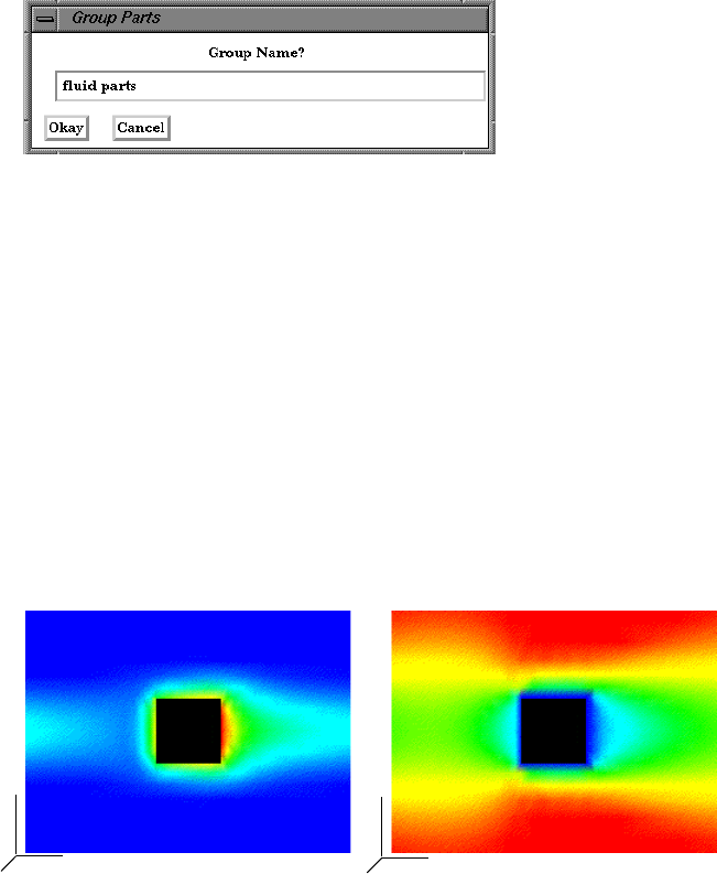
3.4 Part Operations
3-22 EnSight 7 User Manual
When group is selected, the dialog shown in the figure below will appear. A part name
must be input in order to complete the grouping operation.
Only parts of the same type and case can be grouped together. Further, groups can not
contain other part groups.
(see How To Group Parts)
Copy If chosen from the Main Menu > Edit > Part pull-down, makes a copy of selected Part(s)
in the Main Parts List. If chosen from the Edit pull-down in the Feature Detail Editor
Menu, makes a copy of selected Part(s) in the Feature Detail Editor Parts List.
The Copy operation creates a dependent copy of another (original) Part. The Copy is
created on the Client and its existence is not known to the EnSight Server process. A Copy
shares geometric data and variable data with the original Part. (This type of Part is
sometimes called a “shallow copy”.)
relationships The relationship between a Model Part and a Copy made from a Model Part will be one of
original and copy. That is, the Model Part will not be a Parent to the Copy as it is to a
Created Part such as a clip.
The relationship between a Created Part and a copy made from it will also be one of
original and copy since the Copy will initially regard as its Parent the same Part that the
original Created Part regards as its Parent. The Parent of individual Created Parts can of
course be reassigned (using the Update Parent button at the bottom of the Feature Detail
Editor) but the Parent of a Created Part Copy can Not be reassigned.
A copy can be used as a Parent Part for Parts created since the create operation will
operate on the original Part.
Figure 3-16
Group Parts Dialog
Figure 3-17
Part Copy Example
Original Clip Part - colored by temperature Copy of Clip Part, assigned to new Frame,
colored by velocitytranslated to right, and
at the same time step
Y
X
Z
Y
X
Z
0
1
3.4 Part Operations
EnSight 7 User Manual 3-23
attributes The initial attributes assigned to a Copy are the same as those of the original Part at the
time of copying. All attributes for the Copy except Element Representation (3D border,
2D full, border, Feature Angle, etc.) can be changed. The Element Representation of a
Copy cannot be changed independently; a change in Element Representation of the
original changes the copy as well.
description The description of the new Copy will be the same as the original Part with the suffix “-
COPY” added (of course, you can change this description in the Desc field in the Feature
Detail Editor).
copies of copies You can make multiple copies from a Model or Created Part, but you can Not make copies
of copies.
frame assignment A new frame is automatically created for each newly created Copy and the Copy is
assigned to the new frame so that it can easily be moved with a local transformation. The
location of the original Part and the Copy will initially coincide as well. Like all Parts,
Copies of Parts can be reassigned to different frames in the General Attributes Section of
the Feature Detail Editor (for that type of Part).
usefulness One of the most useful purposes for copies is a separation allowing for the side-by-side
display of different attributes (shown in Figure 3-11). Since all attributes except Element
Representation can be different, the original and the copy can be displaying different
variables, different displacements, etc.
(see How To Copy a Part)
Extract Extracts selected Part(s) into a new, true Part, using the Part representation in effect at the
time (full, border, or feature). If more than one Part is selected, then they are joined into a
single Part. If more than one Part is selected when extract is invoked, then all will have
their extracted geometry joined into a single new Part. The new Part is assigned to Frame
0.
The Extract option is closely tied to Element Representation. It creates a new Part using
the geometry of the current representation (what you see is what you get). Extracted Parts
which are in Full Representation are actual copies of the original, but extracted Parts
which are in Border Representation are only the shell or boundary of the original. Extract
is often used with the Save Geometric Entities feature to save extracted Parts (and not the
originals) into a smaller set of data. It is also used to create hollow Parts from solid Parts to
be able to look inside a solid Part after cutting it open with the Cut feature.
(see How To Extract Part Representations)
Merge If more than one Part is selected, the Merge operation creates a new model Part on the
Server host that is a combination of all selected. If only one Part is selected when Merge is
invoked, then a new Part is created on the Server host that is identical but fully
independent from the original Part (Note that this type of “copy” does not have the
restriction on Element Representation that Part Copy does, - all Attributes can be
reassigned - but it requires considerably more memory because it does not share the
geometry with the original but now has its own copy of the geometry). The merge
operation creates a new Part. The new Part is assigned the default Display Attributes and
is also assigned to Frame 0.
(see How To Merge Parts)
General Description
EnSight 7 User Manual 4-1
4Variables
Included in this chapter:
General Description
Section 4.1, Variable Selection and Activation
Section 4.2, Variable Summary & Palette
Section 4.3, Variable Creation
General Description
Variables are numerical values provided by your analysis software or created
within EnSight. Variables can be dependent on server part-geometry (for example,
the area of a part), and a part’s geometry can be dependent on its parent part’s
variable values (for example, an isosurface).
Variable Types There are four types of variables: tensor, vector, scalar, and constant. Scalars and
vectors can be real or complex. Symmetric tensors are defined by six values,
while asymmetric tensors are defined by nine values. Vectors, such as
displacement and velocity, have three values (the components of the vector) if
real, or six values if complex. Scalars, such as temperature or pressure, have a
single value if real, or two values if complex. Constants have a single value for
the model, such as analysis time or volume. All four types can change over time
for transient models.
Activation Before using a variable, it must be loaded by EnSight, a process called activation.
EnSight normally activates variables as they are needed. Section 4.1 describes
how to select, activate, and deactivate variables to make efficient use of your
system memory.
(see Section 4.1, Variable Selection and Activation)
Creation In addition to using the variables given by your analysis software, EnSight can
create additional variables based on any existing variables and geometric
properties of server parts. EnSight provides approximately 100 functions to make
this process simpler.(see Section 4.3, Variable Creation)
Color Palettes Very often you will wish to color a part according to the values of a variable.
EnSight associates colors to values using a color palette. You have control over
the number of value-levels of the palette and the type of scale, as well as control
over colors and method of color gradation. You also use function palettes to
specify a set of levels for a variable, such as when creating contours.
(see Section 4.2, Variable Summary & Palette)
Queries You can make numerical queries about variables and geometric characteristics of
Server-based parts. These queries can be at points, nodes, elements, parts, along
lines, and along 1D parts. If you have transient data, you can query at one time
step or over a range of time steps, looking at actual variable values or a Fast
Fourier Transform (FFT) of the values. (see Section 6.3, Query Menu Functions)
Plotting Once you have queried a variable, you can plot the result.
(see Section 8.3, Plot Mode)
General Description
4-2 EnSight 7 User Manual
From More than Variables can come from more than one case. If more than one case has a
One Case variable with the same name, this will be treated as one variable. If a variable is
applicable to one case but not another, it will not be applied to the non-applicable
case(s).
Parts When variables are activated or created, all parts except Particle Trace parts are
updated to reflect the new variable state. Particle Trace parts will always show
variables which are activated after the part’s creation as zero values.
The input to all of the predefined functions includes some type of server based
parts. Please be aware that parts which reside only on the client (contours,
particle traces, profiles, vector arrows, and tensor glyphs) will not be used.
Location Variables can be defined at the vertices, at the element centers, or undefined.
User Defined Users can write external variable calculator functions called User Defined Math
Math Functions Functions (UDMF) that can be dynamically loaded by EnSight. These functions
appear in EnSight’s calculator in the general function list and can be used just as
any other calculator function to derive new variables.
Several examples of UDMFs can be found in the directory
$CEI_HOME/ensight76/
src/math_functions/
. Please see these examples if you wish to create your own
UDMFs.
When the EnSight server starts it will look in the following subdirectories for
UDMF dynamic shared libraries:
./libudmf-devel.so (.sl) (.dll)
$ENSIGHT7_UDMF/libudmf-*.so (.sl) (.dll)
$CEI_HOME/ensight76/machines/$ENSIGHT7_ARCH/lib_udmf/libudmf-*.so (.sl)
(.dll)
Depending on the server platform, the dynamic shared library must have the
correct suffix for that platform (e.g.
.so, .sl, .dl
l
).
Currently, when a UDMF is used in the EnSight calculator, it in invoked for each
node in the specified part(s) if all the variables operated on for the specified
part(s) are node centered. If all of the variables are element centered, then the
UDMF is invoked for each element in the part(s). If the variables are a mix of
node and element centered values, then the node centered values are automatically
converted to element centered values and then the UDMF is invoked for each
element using element centered variables.
Arguments and the return type for the UDMF can be either scalar or vector
EnSight variables or constants. At this time, only variable quantities and constants
can be passed into UDMFs. There is no mechanism for passing in either part
geometry, neighboring variables, or other information.
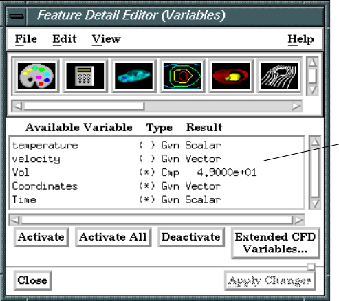
4.1 Variable Selection and Activation
EnSight 7 User Manual 4-3
4.1 Variable Selection and Activation
All available variables, both those read in and those created within EnSight, are
shown in the Feature Detail Editor (Variables), whether they have been activated
or not. In addition, a variable list is included in each function requiring a variable.
In this case, only the appropriate variable types are shown.
Feature Detail Editor Double clicking on the Color Icon in the Feature Icon Bar opens the Feature
(Variables) Detail Editor (Variables).
Feature Detail Editor This list shows all variables currently available, both those read from data and those you
Variables List have created within EnSight. Each row provides information about a variable.
Available Variable The description or name of the variable.
( ) or (*) Activation status. An asterisk indicates that the variable has been activated.
Type Type of the variable:
Gvn Scalar: real scalars read from the dataset (Given).
Cmp Scalar: real scalars created within EnSight (Computed).
Gvn Complex Scalar: complex scalars read from the dataset (Given).
Cmp Complex Scalar: complex scalars created within EnSight (Computed).
Gvn Vector: real vectors read from the dataset (Given).
Cmp Vector: complex vectors created within EnSight (Computed).
Gvn Complex Vector: complex vectors read from the dataset (Given).
Cmp Complex Vector: complex vectors created within EnSight (Computed).
Gvn Tensor: real tensors read from the dataset (Given).
Cmp Tensor: real tensors created within EnSight (Computed).
Gvn #: constants read from the dataset (Given).
Cmp #: constants created within EnSight (Computed).
Figure 4-1
Feature Detail Editor (Variables)
Feature Detail Editor
Variables List
4.1 Variable Selection and Activation
4-4 EnSight 7 User Manual
Result Current value of a constant variable (is blank for other types of variables). Changing the
current solution time will update the value in this column to the value for the new time.
Activate Clicking this button activates the variable(s) selected in the Feature Detail Editor
Variables List. Activation of a variable loads its values into the memory of the EnSight
Server host system. The EnSight Server then passes the necessary data to the Client. One
way you can control EnSight’s memory usage is to only activate the variables you want to
use. Once activated, a variable becomes available in the Main Variables List and, as is
described in Section 4.2, EnSight creates a default color palette for the variable.
Activate All Clicking this button activates all variables listed in the Feature Detail Editor Variables
List, regardless of which are selected.
Deactivate Clicking this button deactivates the variable(s) selected in the Feature Detail Editor
Variables List. Deactivating a variable frees up some memory on both the Client and the
Server. You can activate and deactivate variables as often as you like. For example, you
could activate one variable to color a part, deactivate that variable, then activate a different
variable to re-color the part. Of course, if you have enough memory and a small enough
model, you can simply activate all the variables and leave them activated.
Extended CFD Opens the Extended CFD Variable Settings dialog. If your data defines variables or
Variables... constants for density, Total Energy per unit volume, and momentum (or velocity), it is
possible to show new variables defined by these basic variables in the Main Variables List
of the GUI by utilizing the capabilities of this dialog. (See Preferences... in Section 6.2,
Edit Menu Functions).
WARNING If you deactivate a created variable or any of the variables used to define it, both the
values and the definition of the created variable are deleted. If you deactivate a variable
used to create a part’s geometry, the part will be deleted. If you deactivate a variable
who’s color palette has been used to color a part, the part’s appearance will change.
(see How To Activate Variables)
Figure 4-2
Extended CFD Variable Settings Dialog
4.2 Variable Summary & Palette
EnSight 7 User Manual 4-5
4.2 Variable Summary & Palette
You can visualize information about a model by representing variable values with
colors, often called fringes. Fringes are an extremely effective way to visualize
variable variations and levels. A variable color palette associates (or maps)
variable values to colors. Palettes are also used in the creation of contours. The
number of contour levels is based on the number of palette color levels, and the
contour values are based on the palette level values.
EnSight uses a variable’s color palette to convert numbers to colors, while you,
the viewer, use them in the opposite manner—to associate a visible color with a
number. If you wish, EnSight can display a color-value legend in the Main View
window.
Default Palettes At least one color palette—the Coordinate color palette—always exists, even if
your model has no variables. In addition, EnSight creates a color palette for each
real scalar and vector variable that you activate, giving the color palette the same
name as the variable. If the variable is a vector variable, the default color palette
uses the vector’s magnitude. Tensor variables have no palette.
Default color palettes have five color levels. Ranging from low to high, the colors
are blue, cyan, green, yellow, and red (the spectral order). The numerical values
mapped to these five levels are determined by first finding the value-range for the
variable at the current time step when the variable is activated. The value for the
lowest level is set to the minimum value. The value for the highest level is set to
the maximum value. The three middle levels are spaced evenly between the
lowest and highest values. For datasets with only one time step, the scheme just
described works well because the variable’s value range is not changing over
time. However, if you have transient data, the range could vary widely at
different times and since the default was based on one time step, it may not be
appropriate for other time steps. EnSight can show you a histogram of the variable
values over time to assist you in setting a palette for transient cases.
Value Levels A color palette can have up to 21 levels at which the variable value is specified.
Each color palette level’s value must be between the value at the adjoining levels,
with higher levels having higher variable-values. Between levels, you select
whether the scale is linear (the default), quadratic (2
x
), or logarithmic (log
10
).
Also, you can have EnSight use one of these scales to automatically assign values
to a range of levels.
Sometimes you may wish to only visualize areas whose palette-variable values are
in a limited range. You can choose to visualize other areas with a different,
uniform color, or to make those areas invisible.
Management The Feature Detail Editor (Variables) enables you to manage your color palettes.
You can copy, save to a file, and restore from a file existing palettes
4.2 Variable Summary & Palette
4-6 EnSight 7 User Manual
Clicking the Variable Summary and Palette turndown button opens that dialog
within the Feature Detail Editor (Variables) dialog.
File Menu Clicking this button opens a pull-down menu with the following options:
Save Selected Opens the file selection dialog for the specification of a filename in which to save the
Palette(s) selected color palette(s).
Figure 4-3
Feature Detail Editor: Variables, both Simple and
Advanced Interface Mode
Histogram Scale
Adjustment
Minimum Palette
Value Slider
Maximum Palette
Value
Variable Color
Legend
Minimum Palette
Value
Simple/Advanced
Interface Buttons
Variable Palette Histogram
Maximum Palette Value Slider
Advanced Interface Mode
Simple Interface Mode
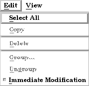
4.2 Variable Summary & Palette
EnSight 7 User Manual 4-7
Save All Palettes… Opens the file selection dialog for the specification of a filename in which to save all color
palette(s).
Restore Palette(s) Opens the file selection dialog for the specification of a filename from which to restore
previously saved color palettes.
Save Selected Opens the file selection dialog for the specification of a filename in which to save the
Constant(s) selected constant values.
Save All Opens the file selection dialog for the specification of a filename in which to save all
Constant(s) constant values.
Edit Menu Clicking this button opens a pulldown menu with the following choice:
Select All Clicking this selects all variables in the Feature Detail Editor Available Variables List.
Immediate Default is On. While on, any modification made in the Editor is immediately implemented
Modification Toggle by EnSight. For large problems, this may be impractical. In such instances, click this
toggle off, make all desired modifications, and then implement then all at once by clicking
the Apply Changes button at the bottom of the Editor dialog.
Simple/Advanced Buttons which allow the user to choose between a simple or advanced mode for this
Interface dialog. The advanced interface is shown in the figure. The simple interface is a small
subset of the advanced.
Variable Palette This histogram shows the relative number of nodes at which the value of the selected
Histogram variable is within the range represented by a particular color band. The two vertical white
slider bars are used to interactively set the minimum and maximum variable values to be
used in the variable’s color palette and these will show up in the Legend both within the
turndown area and within the Graphics Window. The small horizontal white line on the
left hand side can be used to interactively adjust the vertical scale of the histogram.
Over Time Step Toggles on/off the automatic assignment of values to palette levels using the palette-
Toggle & Beg, End variable’s value range over multiple time steps which are specified in the Beg and End
Fields fields to the right of the toggle. This function is only available when you are using
transient data. All other attributes of the color palette (including the number of levels,
colors, type, etc.) are not changed.
Magnitude, For vector variables, this controls which histogram and color palette will be displayed and
X,Y,Z, Toggles edited. By default, the vector magnitude is used, however, the X, Y, and Z components of
the vector are also available.
4.2 Variable Summary & Palette
4-8 EnSight 7 User Manual
Type This button opens a pop-up menu for the selection of the desired type of color gradation.
Both the legend in the turn-down area and the legend in the Graphics Window (if visible)
are affected. Options are:
Continuous displays graduated color variation across or along each element interpolating the color
across each element based on the value of the variable at the nodes. If the variable tied to
the palette is defined at the element centers it will be averaged to the nodes for display.
Banded displays discrete color values for each value range, but interpolates the location demarcation
line within an element.
Constant displays each element with one color for the entire element rather than interpolating the
color across the element using values at the nodes. The color of the first node encountered
is used.
Scale
This button opens a pop-up dialog for the selection of the desired type of scale for the
value-separation of levels and color gradation. The options are:
Linear scale divisions, where the value-separation of levels is uniform and values map linearly to the
colors.
Quadratic scale divisions, where the value-separations of levels are not equal, but instead are based
on the second order of the variable (value2). Level-values always increasing upwards. For
example, for five levels with a low-level value of 0 and a high-level value of 16, the linear
scale would be 0, 4, 8, 12, 16 while the quadratic scale would be 0, 1, 4, 9, 16.
Logarithmic scale divisions, where the value-separations of levels are not equal, but instead are
based on the base–10 logarithm of the variable value (log10). Level-values always
increasing upwards. For example, for five levels with a low-level value of 1 and a high-
level value of 10000, the linear scale would be 1, 2500, 5000, 7500, 10000 while the
logarithmic scale would be 1, 10, 100, 1000, 10000.
Limit Fringes
This button allows you to select how you wish to display elements with node values above
and below the range of the palette scale values. This option only works for hidden surface
mode. Options are:
No limit on values. Values above and below are colored with color of the corresponding end of the
range (no interpolation).
By Model Color option colors values outside the function range with the current part- color (the
color of the part when its Color By Palette attribute is None).
By Invisible option does not display elements whose node values are all above or below the value-
range of the palette.
Display Undefined
If the variable is not defined, the element cannot be colored according to the color palette.
In this case, the element will be colored by the Part Color, or the element will become
invisible.
# of Levels This field specifies the number of value-levels for the variable color palette, which are
shown beside the Legend color bar. The number of levels is independent of the Type and
Scale, and can range from 2 to 21 with the default being 5.
Min For the Simple Interface, this field is used to specify the variable value for the bottom
level.
Max For the Simple Interface, this field is used to specify the variable value for the top level.
Edit Level Selection of the level you wish to edit, selected with stepper buttons, by entering a value in
the field, or by clicking the mouse pointer on the desired level in the Variable Color
Legend area. Levels start at 1 and count up from lower end. You can change the variable-
value and color assigned to any level. Also, you can have EnSight interpolate value-levels
and colors over a range of levels.
Interpolate to Level If this option is toggled-on while you are specifying a value (or color), the value (or color)
Toggle and Field of EnSight adjusts the values (or colors) of intermediate levels between the current level
and the specified Interpolate To Level according the specified Scale type.
Value This field specifies the variable value for the current palette level.
4.2 Variable Summary & Palette
EnSight 7 User Manual 4-9
R G B Fields These fields are used to specify the color to use for the current palette level.
Mix... Clicking this button opens the Color Selector dialog which provides an alternative to the
RGB fields for the specification of the color to use for the current palette level.
(see Section 7.1, Color)
Predefined Palettes For the Simple Interface only, shows a list of all predefined color palettes.
Restore For the Simple Interface only. Restores the palette selected in the Predefined Palettes list.
Save... For the Simple Interface only. Will bring up a file dialog to allow saving of the currently
defined color palette.
Undo Restore For the Simple Interface only. Will set the color palette definition back to what existed
before the previous Restore.
Flip Colors Reverses colors in the palette.
Legend Display Clicking this button opens a pop-up message which reminds you that additional options
Attributes ... for
the modification of Legend display attributes may be found in the Annot Mode Icon
Bar.
(See How To Create Color Legends, How To Edit Color Palettes)
4.3 Variable Creation
4-10 EnSight 7 User Manual
4.3 Variable Creation
You can create additional variables based on existing data. Typical mathematical
operations, as well as many special built-in functions, enable you to produce
simple or complex equations for new variables. Some built-in functions enable
you to use values based on the geometric characteristics of server parts. In
general, created variables are available for any process, just like given variables.
If you have transient data, a time change will recompute the created variable
values.
Often an analysis program produces a set of basic results from which other results
can be derived. For example, if a computational fluid dynamics analysis gives you
density, momentum and total energy, you can derive pressure, velocity,
temperature, mach number, etc. EnSight provides many of these common
functions for you, or you can enter the equation(s) and build your own.
As another example, suppose you would like to normalize a given scalar or vector
variable according to its maximum value, or according to the value at a particular
node. Variable creation enables you to easily accomplish such a task. The more
familiar you become with this feature, the more uses you will discover.
EnSight allows variables to be defined at vertices (nodes) or element centers. If a
new variable is created from a combination of nodal and element based variables,
such a new variable will always be element based.
4.3 Variable Creation
EnSight 7 User Manual 4-11
Building Expressions The Feature Detail Editor (Variables) dialog Variable Creation turn-down section
provides function selection lists, calculator buttons, and feedback guidance to aid
you in building the working expression (or equation) for a new variable. You can
use three types of values in an expression: constants, scalars, and vectors.
Constants A constant in a variable expression can be a… for example…
• number 3.56
• constant variable from the Active Variables list Analysis_Time
• scalar variable at a particular node/element temperature[25]
(component and node/element number in brackets)
• vector variable component at a particular node velocity[Z][25]
/element (component and node/element number in brackets)
• coordinate component at a particular node/element coordinate[X][25]
(component and node/element number in brackets)
• any of the previous three at a particular time step temperature{15}[25]
(time step in braces right after the variable name) velocity{15}[Z][25]
(Note: This only works for model variables, not created ones) coordinate{15}[X][25]
• Math function COS(1.5708)
• General function that produces a constant AREA(plist)
Scalars A scalar in a variable expression can be a… for example…
• Scalar variable from the Active Variables list pressure
• vector variable component (component in brackets) velocity[Z]
• coordinate component (component in brackets) coordinate[Y]
• any of the previous three at a particular time step pressure{29}
(time step in braces right after the variable name) velocity{29}[Z]
(Note: This only works for model variables, not created ones) coordinate{29}[Y]
• General function that produces a scalar Divergence(plist,velocity)
Vec tor s A vector in a variable expression can be a… for example…
• vector variable from the Active Variables list velocity
• coordinate name from the Active Variables list coordinate
• any of the previous two at a particular time step velocity{9}
(time step in braces right after the variable name) coordinate{9}
(Note: This only works for model variables, not created ones)
• General function that produces a vector Vorticity(plist,velocity)

4.3 Variable Creation
4-12 EnSight 7 User Manual
Examples of Expressions and How To Build Them
The following are some example variable expressions, and how they can be built.
These examples assume Analysis_Time, pressure, density, and velocity are all
given variables.
Notice in the last example how a complex equation can be broken down into
several smaller expressions. This is necessary as EnSight can compute only one
variable at a time. Calculator limitations include the following:
1. The variable name cannot be used in the expression.
The following is invalid:
temperature = temperature + 100
Instead use new variable:
temperature2 = temperature + 100
Expression Discussion and How To Build It
-13.5/3.5 A true constant since it does not change over time. To build it,
type on the keyboard or click on the Variable Creation dialog
calculator buttons
-13.5/3.5
Analysis_Time/60.0 A simple example of modifying a given constant variable. If
Analysis_Time is in seconds, this expression would give you
the value in minutes. To build it, select Analysis_Time from
the Active variable list and then type or click /
60.0.
velocity*density This expression is momentum, which is a vector. To build it,
select velocity from the Active Variables list, type or click *,
then select density from the Active Variable list.
SQRT(pressure[73] *
2.5)+ velocity[X][73]
This says, take the pressure at node (or element if pressure is
an element center based variable) number 73, multiply it by
2.5, take the square root of the product, and then add to that
the x-component of velocity at node (or element) number 73.
To build it, select SQRT from the Math function list, select
pressure from the Active Variables list, type
[73]*2.5)+,
select velocity from the Active Variable list, then type
[X][73]
pressure{19} This is a scalar, the value of pressure at time step 19. It does
not change with time. To build it, select pressure from the
Active Variables list, then type
{19}. (Note: variable must be a
model variable, not a computed variable)
MAX(plist,pressure) MAX is one of the built-in General functions. This expression
calculates the maximum pressure value for all the nodes of
the selected parts. To build it, type or click (, select MAX from
the General function list and follow the interactive
instructions that appear in the Feedback area of this dialog (in
this case, to select the parts, click Okay, and select pressure
from the Active Variable list).
(pressure
/pressure_max)^2
This scalar is essentially the normalized pressure, squared. To
build it, first build the preceding MAX(plist,pressure)
expression and name it “pressure_max”. Then to build this
expression, select pressure from the Active Variables list,
type or click
/, select pressure_max from the Active
Variables list, then type or click )
^2.
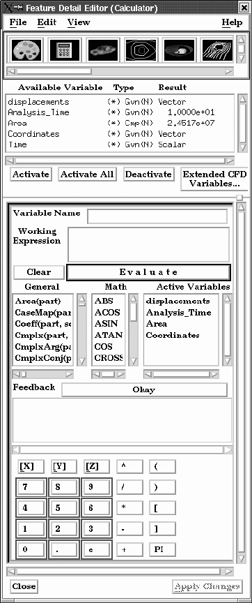
4.3 Variable Creation
EnSight 7 User Manual 4-13
2. The result of a function cannot be used in an expression.
The following is invalid:
norm_press_sqr = (pressure / MAX(plist,pressure) )^2
Instead use two steps:
p_max = MAX(plist,pressure)
then:
norm_press_sqr = (pressure / p_max)^2
3. Created parts (or changing geometry model parts) cannot be used with a time
calculation (using {}). If one of these parts is selected when you use {}, the
calculation will fail and an error message will be given.
4. Because calculations occur only on server based parts, client based parts are
ignored when included in the part list of the pre-defined functions, and variable
values may be undefined.
Clicking the Calculator Icon opens the Feature Detail Editor (Calculator) dialog.
Figure 4-4
Feature Detail Editor (Calculator) dialog

4.3 Variable Creation
4-14 EnSight 7 User Manual
Variable Name This field is used to specify the name for the variable being created. Built-in general
functions will provide a default, but they can be modified here. Variable names must not
start with a numeric digit and must not contain any of the following reserved characters:
([{+@ !*$
) ] }–space #^/
Working Expression The expression or equation for the new variable is presented in this area. Interaction with
the expression takes place here, either directly by typing in values and variable names,
etc., or indirectly by selecting built-in functions and clicking calculator buttons.
Clear Clicking this button clears the Variable name field, Working Expression area, Feedback
area, and deselects any built-in function.
Evaluate Clicking this button produces the new variable defined in the working expression area.
Until you click this button, nothing is really created. The selection commands specify to
which parts the new variable should be applied.
General Scroll this list of built-in functions provided for your convenience. Click on a function to
insert it into your Working Expression. For some functions, the Feedback Window
provides interactive instructions.
Area Area (any part(s))
Computes a constant variable whose value is the area of the selected parts. If a part
is composed of 3D elements, the area is of the border representation of the part. The
area of 1D elements is zero.
Case Map CaseMap (2D or 3D part(s), case to map from, scalar/vector/tensor)
Finds the specified scalar, vector, or tensor variable values for the specified part(s)
from the indicated case.
Coefficient Coeff (any 1D or 2D part(s), scalar, component)
Computes a constant variable whose value is a coefficient Cx , Cy, or Cz such that
where:
f = any scalar variable
S = 1D or 2D domain
= x component of normal
= y component of normal
= z component of normal
Specify [X], [Y], or [Z] to get the corresponding coefficient.
Note: Normal for a 1D part will be parallel to the plane of the plane tool.
Complex Cmplx(any part(s), scalar/vector(real portion), scalar/vector(complex portion), [optional
frequency(Degrees)])
Creates a complex scalar or vector from two scalar or vector variables. The
frequency is optional and is used only for reference.
Z = A + Bi
case to map from constant number
scalar/vector/tensor scalar, vector, or tensor variable
component [X], [Y], or [Z]
real portion scalar or vector variable
complex portion scalar or vector variable (but must be same as real portion)
[frequency] constant number (optional)
C
x
fn
x
Sd
S
= C
y
fn
y
Sd
S
= C
z
fn
z
Sd
S
=
n
x
n
y
n
z
4.3 Variable Creation
EnSight 7 User Manual 4-15
Complex CmplxArg (any part(s), complex scalar or vector)
Argument Computes the Argument of a complex scalar or vector. The resulting scalar is given
in degrees and will be in the range -180 and 180 degrees.
Arg = atan(Vi/Vr)
Complex CmplxConj (any part(s), complex scalar or vector)
Conjugate Computes the Conjugate of a complex scalar of vector. Returns a complex scalar or
vector where:
Nr = Vr
Ni = -Vi
Complex CmplxImag (any part(s), complex scalar or vector)
Imaginary Extracts imaginary portion of a complex scalar or vector into a real scalar or vector.
N = Vi
Complex CmplxModu (any part(s), complex scalar or vector)
Modulus Returns a real scalar/vector which is the modulus of the given scalar/vector
N = SQRT(Vr*Vr + Vi*Vi)
Complex CmplxReal(any part(s), complex scalar or vector)
Real Extracts the real portion of a complex scalar or vector into a real scalar or vector.
N = Vr
Complex CmplxTransResp(any part(s), complex scalar or vector, constant PHI(0.0-360.0 Degrees))
Transient Response Returns a real scalar or vector which is the real transient response:
Re(Vt) = Re(Vc)Cos(phi) - Im(Vc)Sin(phi)
which is a function of the transient phase angle “phi” defined by:
phi = 2 Pi f t
where
t = the harmonic response time parameter
f = frequency of the complex variable “Vc”
and the complex field “Vc”, defined as:
Vc = Vc(x,y,z) = Re(Vc) + i Im(Vc)
where
Vc = the complex variable field
Re(Vc) = the Real portion of Vc
Im(Vc) = the imaginary portion of Vc
i = Sqrt(-1)
Note, the transient complex function, was a composition of Vc and
Euler’srelation, namely:
Vt = Vt(x,y,z,t) = Re(Vt) + i Im(Vt) = Vc * e^(i phi)
where:
e^(i phi) = Cos(phi) + i Sin(phi)
The real portion Re(Vt), is as designated above:
Note: this function is only good for harmonic variations, thus fields with a
defined frequency!
Curl Curl (any part(s), vector)
Computes a vector variable which is the curl of the input vector
phi angle constant number between 0 and 360 degrees.
Curl
f
∇ f×
f
3
∂
y∂
-------
f
2
∂
z∂
-------
–
è
æö
i
ˆ
f
1
∂
z∂
-------
f
3
∂
x∂
-------
–
è
æö
j
ˆ
f
2
∂
x∂
-------
f
1
∂
y∂
-------
–
è
æö
k
ˆ
++==
4.3 Variable Creation
4-16 EnSight 7 User Manual
Density Density(any part(s), pressure, temperature, gas constant).
Computes a scalar variable which is the density , defined as:
where: p = pressure
T = temperature
R = gas constant
Normalized DensityNorm (any part(s), density, freestream density)
Density Computes a scalar variable which is the Normalized Density defined as:
where: = density
= freestream density
Log of DensityLogNorm (any part(s), density, freestream density)
Normalized Computes a scalar variable which is the natural log of Normalized Density
Density defined as:
where: = density
= freestream density
Stagnation DensityStag (any part(s), density, total energy, velocity, ratio of specific heats)
Density Computes a scalar variable which is the Stagnation Density defined as:
where: = density
γ = ratio of specific heats
= mach number
total energy must be a scalar
velocity must be a vector
pressure scalar variable
temperature scalar variable
gas constant scalar variable, constant variable, or constant number
density scalar variable, constant variable, or constant number
freestream density constant variable or constant number
density scalar variable, constant variable, or constant number
freestream density constant variable or constant number
density scalar variable, constant variable, or constant number
total energy scalar variable
velocity vector variable
ratio of specific heats scalar variable, constant variable, or constant number
ρ
ρ
p
TR
-------
=
ρ
n
ρ
n
ρρ
i
⁄=
ρ
ρ
i
ρ
n
ln ρρ
i
⁄()ln=
ρ
ρ
i
ρ
o
ρ
o
ρ 1
γ 1–
2
-----------
è
æö
+ M
2
è
æö
1 γ 1–()⁄()
=
ρ
M
4.3 Variable Creation
EnSight 7 User Manual 4-17
Normalized DensityNormStag (any part(s), density, total energy, velocity, ratio of specific heats,
Stagnation freestream density, freestream speed of sound, freestream velocity magnitude)
Density Computes a scalar variable which is the Normalized Stagnation Density
defined as:
where: = stagnation density
where: = freestream stagnation density
Distance Dist2Nodes(any part(s), nodeID1,nodeID2).
Between Nodes Computes a constant, positive variable that is the distance between any two nodes.
Searches down the part list until it finds nodeID1, then searches until it finds nodeID2 and
returns Undef if nodeID1 or nodeID2 cannot be found. Nodes are designated by their
node id’s, so the part must have node ids. (Note that most created parts do not have node
ids.)
Note: to find the distance between two nodes on different parts, or between two nodes if
one or both don’t have ids, or the ids are not unique for the model (namely, more than one
part has the same node id) use the line tool. See the Advanced Usage section of How To
Use the Line Tool.
Divergence Div (2D or 3D part(s), vector)
Computes a scalar variable whose value is the divergence defined as:
where u,v,w = velocity components in x,y,z directions.
Element to Node ElemToNode (any part(s), element-based scalar or vector).
Averages an element based variable to produce a node based variable.
density scalar variable, constant variable, or constant number
total energy scalar variable
velocity vector variable
ratio of specific heats scalar variable, constant variable, or constant number
freestream density constant variable or constant number
freestream speed of sound constant variable or constant number
freestream velocity magnitude constant variable or constant number
nodeID1 constant number
nodeID2 constant number
ρ
on
ρ
on
ρ
o
ρ
oi
⁄=
ρ
o
ρ
oi
Div
u∂
x∂
-----
v∂
y∂
-----
w∂
z∂
------
++=
4.3 Variable Creation
4-18 EnSight 7 User Manual
Energy:
Total Energy EnergyT (any part(s), density, pressure, velocity, ratio of specific heats).
Computes a scalar variable of total energy per unit volume
Kinetic Energy KinEn (any part(s), velocity, density)
Computes a scalar variable whose value is the kinetic energy defined as:
where ρ== density
V = Velocity variable
Enthalpy Enthalpy (any part(s), density, total energy, velocity, ratio of specific heats)
Computes a scalar variable which is Enthalpy defined as:
where: E = total energy per unit volume
ρ = density
V = velocity magnitude
γ = ratio of specific heats
density scalar variable, constant variable, or constant number
pressure scalar variable
velocity vector variable
ratio of specific heats scalar variable, constant variable, or constant number
velocity vector variable
density scalar variable, constant variable, or constant number
density scalar variable, constant variable, or constant number
total energy scalar variable
velocity vector variable
ratio of specific heats scalar variable, constant variable, or constant number
e ρ e
i
V
2
2
------
+
è
æö
=
e
i
e
0
V
2
2
------
–=
e
0
e
ρ
---
=
To t a l E n er g y
Internal Energy
Stagnation Energy
where:
ρ density=
V Velocity=
Or based on gamma, pressure and velocity:
e
p
γ 1–()
----------------
ρ
V
2
2
------
+=
E
k
E
k
1
2
---
ρ
V
2
=
h
h γ
E
ρ
---
V
2
2
------
–
è
æö
=
4.3 Variable Creation
EnSight 7 User Manual 4-19
Normalized EnthalpyNorm (any part(s), density, total energy, velocity, ratio of specific
Enthalpy heats, freestream density, freestream speed of sound)
Computes a scalar variable which is Normalized Enthalpy defined as:
where: h = enthalpy
= freestream enthalpy
Stagnation EnthalpyStag (any part(s), density, total energy, velocity, ratio of specific heats)
Enthalpy Computes a scalar variable which is Stagnation Enthalpy defined as:
where: = enthalpy
V = velocity magnitude
Normalized EnthalpyNormStag (any part(s), density, total energy, velocity, ratio of
Stagnation specific heats, freestream density, freestream speed of sound, freestream velocity
Enthalpy magnitude)
Computes a scalar variable which is Normalized Stagnation Enthalpy
defined as:
where: = stagnation enthalpy
= freestream stagnation enthalpy
density scalar variable, constant variable, or constant number
total energy scalar variable
velocity vector variable
ratio of specific heats scalar variable, constant variable, or constant number
freestream density constant variable or constant number
freestream speed of sound constant variable or constant number
density scalar variable, constant variable, or constant number
total energy scalar variable
velocity vector variable
ratio of specific heats scalar variable, constant variable, or constant number
density scalar variable, constant variable, or constant number
total energy scalar variable
velocity vector variable
ratio of specific heats scalar variable, constant variable, or constant number
freestream density constant variable or constant number
freestream speed of sound constant variable or constant number
freestream velocity magnitude constant variable or constant number
h
n
h
n
hh
i
⁄=
h
i
h
o
h
o
h
V
2
---
2
+=
h
h
on
h
on
h
o
h
oi
⁄=
h
o
h
oi

4.3 Variable Creation
4-20 EnSight 7 User Manual
Entropy Entropy (any part(s), density, total energy, velocity, ratio of specific heats, gas
constant, freestream density, freestream speed of sound)
Computes a scalar variable which is Entropy defined as:
where: R = gas constant
ρ = density
= freestream density
= pressure
= freestream pressure =
= velocity magnitude
γ = ratio of specific heats
Flow Flow (any 1D or 2D part(s), velocity).
Computes a constant variable whose value is the flow defined as:
where = Velocity value normal to the surface
S = 1D or 2D domain
Note: Normal for a 1D part will be parallel to the plane of the plane tool
Flow Rate FlowRate (any 1D or 2D part(s), velocity).
Computes a scalar variable defined as:
where V = Velocity
= Surface Normal
density scalar variable, constant variable, or constant number
total energy scalar variable
velocity vector variable
ratio of specific heats scalar variable, constant variable, or constant number
gas constant constant variable or constant number
freestream density constant variable or constant number
freestream speed of sound constant variable or constant number
velocity vector variable
velocity vector variable
s
s
p
p
i
----
ρ
ρ
i
----
è
æö
γ
------------
è
ç÷
ç÷
ç÷
æö
R
γ 1–
-----------
è
æö
ln=
ρ
i
p
p
i
ρ
i
c
i
2
()γ⁄
c
i
Q
c
Q
c
V
n
Sd
S
=
V
n
Q
QVn
ˆ
⋅=
n
ˆ
4.3 Variable Creation
EnSight 7 User Manual 4-21
Fluid Shear FluidShear(2D part(s), velocity magnitude gradient, viscosity)
Computes a scalar variable tau whose value is defined as:
tau = µ where tau = shear stress
µ = dynamic viscosity
= Velocity gradient in direction of surface normal
Hints: To compute fluid shear stress:
1. Use gradient function on velocity to obtain “Velocity Grad” variable in
the 3D part(s) of interest.
2. Use clip option (through the 3D part(s) used in 1.) to obtain a surfaceon
which you wish to see the fluid shear stress.
3. Compute Fluid Shear variable (on the 2D clip surface of 2.)
Fluid Shear FluidShearMax (2D or 3D part(s), velocity, density, turbulent kinetic energy, turbulent
Stress Max dissipation, laminar viscosity)
Computes a scalar variable defined as:
where F = force
A = unit area
= turbulent (eddy) viscosity
= laminar viscosity (treated as a constant)
E = local strain
The turbulent viscosity is defined as:
where =ρ = density
κ = turbulent kinetic energy
ε = turbulent dissipation
A measure of local strain E (i.e. local elongation in 3 directions) is given by
where
given the Euclidean norm defined by
;
and the rate of deformation tensor dij defined by
with = ¹u/¹x
= ¹v/¹y
= ¹w/¹z
= ¹u/¹y + ¹v/¹x =
= ¹u/¹z + ¹w/¹x =
= ¹v/¹z + ¹w/¹y =
velocity gradient vector variable
viscosity scalar variable, constant variable, or constant number
V∂
n∂
------
V∂
n∂
------
Σ
Σ
FA⁄ u
t
u
l
+()E==
u
t
u
l
u
t
u
t
ρ
0.09
κ
2
ε
--------------------
=
E2trDD⋅()()=
2tr D D⋅()2d
11
()
2
d
22
()
2
d
33
()
2
++()d
12
()
2
d
13
()
2
d
23
()
2
++()+=
tr D D⋅()d(
11
)
2
d
22
()
2
d
33
()
2 1
2
---
d
12
()
2
d
13
()
2
d
23
()
2
++()+++=
Dd
ij
[]
1
2
---
2d
11
d
12
d
13
d
21
2d
22
d
23
d
31
d
32
2d
33
==
d
11
d
22
d
33
d
12
d
21
d
13
d
31
d
23
d
32
4.3 Variable Creation
4-22 EnSight 7 User Manual
given the strain tensor defined by
Force Force(2D part(s), pressure)
Computes a vector variable whose value is the force F defined as:
where p = pressure
A = unit area
Note: The force acts in the surface normal direction.
Force 1D Force1D(1D planar part(s), pressure, surface normal)
Computes a vector variable whose value is the force F defined as:
where p = pressure
L = unit length times 1
Note: The force acts in the part’s normal direction (in plane).
Gradient Grad (2D or 3D part(s), scalar or vector(Magnitude will be used))
Computes a vector variable whose value is the gradient defined as:
where f = any scalar variable (or the magnitude of the specified vector)
x, y, z = coordinate directions
i, j, k = unit vectors in coordinate directions
Gradient GradApprox (2D or 3D part(s), scalar or vector(Magnitude will be used))
Approximation Same as Gradient, except all elements are first subdivided into triangles (for 2D) or
tetrahedrons (for 3D) and a closed-form solution is done on the subdivided
element’s nodal values (only applicable for per node variables). This is basically a
quicker, linear approximation of the regular gradient.
Gradient Tensor GradTensor (2D or 3D part(s), vector)
Computes a tensor variable whose value is the gradient defined as:
where F = any vector variable
x, y, z = coordinate directions
i, j, k = unit vectors in coordinate directions
Gradient Tensor GradTensorApprox (2D or 3D part(s), vector)
Approximation Same as Gradient Tensor, except all elements are first subdivided into triangles (for
2D) or tetrahedrons (for 3D) and a closed-form solution is done on the subdivided
element’s nodal values (only applicable for per node variables). This is basically a
quicker, linear approximation of the regular gradient tensor.
velocity vector variable
density scalar variable, constant variable, or constant number
turbulent kinetic energy scalar variable
turbulent dissipation scalar variable
laminar viscosity constant variable or constant number
pressure scalar variable
pressure scalar variable
surface normal vector variable
e
ij
e
ij
1
2
---
d
ij
=
FpA=
FpL=
GRAD
f
GRAD
f
f∂
x∂
-----
i
ˆ
f∂
y∂
-----
j
ˆ
f∂
z∂
-----
k
ˆ
++=
GRAD
F
GRAD
F
F∂
x∂
------
i
ˆ
F∂
y∂
------
j
ˆ
F∂
z∂
------
k
ˆ
++=
4.3 Variable Creation
EnSight 7 User Manual 4-23
Helicity:
Helicity Density HelicityDensity(any part(s), velocity)
Computes a scalar variable whose value is:
where: V = Velocity
= Vorticity
Relative Helicity HelicityRelative(any part(s), velocity)
Computes a scalar variable whose value is:
where: = the angle between the velocity vector and the vorticity vector.
Filtered Relative HelicityRelFilter(any part(s), velocity, freestream velocity magnitude).
Helicity
Computes a scalar variable whose value is:
, if
or , if
where = relative helicity (as described above)
= helicity density (as described above)
Iblanking Values IblankingValues (Any iblanked structured part(s))
Computes a scalar variable whose value is the iblanking flag of selected parts.
Integrals:
Line Integral
IntegralLine (1D part(s), scalar or (vector, component))
Computes a constant variable whose value is the integral of the input variable over
the length of the specified 1D part(s).
Surface Integral IntegralSurface (2D part(s), scalar or (vector, component))
Computes a constant variable whose value is the integral of the input variable over
the surface of the specified 2D part(s).
Volume Integral IntegralVolume (3D part(s), scalar or (vector, component))
Computes a constant variable whose value is the integral of the input variable over
the volume of the specified 3D part(s).
Length Length (any 1D part(s))
Computes a constant variable whose value is the length of selected parts. While any
part can be specified, it will only return a nonzero length if the part has 1D elements.
Line Integral See Line Integral under Integrals.
velocity vector variable
velocity vector variable
velocity vector variable
freestream velocity magnitude constant variable or constant number
H
d
H
d
V Ω•=
Ω
H
r
H
r
φ =
V Ω•
V Ω
--------------
cos=
φ
H
rf
H
rf
H
r
= H
d
filter≥
H
rf
0= H
d
filter<
H
r
H
d
filter 0.1 V
∞
()
2
=
4.3 Variable Creation
4-24 EnSight 7 User Manual
Mach Number Mach (any part(s), density, total energy, velocity, ratio of specific heats)
Computes a scalar variable whose value is the Mach number M defined as:
where m = momentum
ρ = density
u = speed, computed from velocity input.===
γ = ratio of specific heats (1.4 for air)
p = pressure (see Pressure below)
c = speed of sound
See Total Energy in this section for a description.
Make Scalar at MakeScalElem (any part(s), constant number or constant variable)
Elements Assigns the specified constant value to each element, making a scalar variable.
Make Scalar at MakeScalNode (any part(s), constant number or constant variable)
Nodes Assigns the specified constant value to each node, making a scalar variable.
Make Vector MakeVect (any part(s), scalar or zero, scalar or zero, scalar or zero)
Computes a vector variable formed from scalar variables. First scalar becomes the X
component of the vector, second scalar becomes the Y component, and the third
scalar becomes the Z component. A zero can be specified for some of the scalars,
creating a 2D or 1D vector field.
Massed Particle MassedParticle (massed particle trace part(s))
Scalar
This scalar creates a massed-particle per element scalar variable for each of the
parent parts of the massed-particle traces. This per element variable is the mass of
the particle times the sum of the number of times each element is exited by a mass-
particle trace. See Particle-Mass Scalar on Boundaries in Chapter 7
Mass-Flux MassFluxAvg (any 1D or 2D part(s), scalar, velocity, density)
Average Computes a constant variable whose value is the mass flux average b
avg
defined as:
where b = any scalar variable, i.e. pressure, mach, a vector component, etc.
ρ = density (constant or scalar) variable
V = velocity (vector) variable
dA = area of some 2D domain
N = unit vector normal to dA
density scalar variable, constant variable, or constant number
total energy scalar variable
velocity vector variable
ratio of specific heats scalar variable, constant variable, or constant number
scalar any scalar variable, i.e. pressure, mach, a vector component, etc
velocity a vector variable
density scalar variable, constant variable, or constant number
M
u
γ
p
ρ
-----
----------
u
c
---
==
bavg
ρbV N)dA•(
A
°
ρ V( N )dA•
A
°
------------------------------------
MassFluxOfScalar
MassFlux
--------------------------------------------------
Flow plist bρV,()
Flow plist ρV,()
--------------------------------------------
== =
4.3 Variable Creation
EnSight 7 User Manual 4-25
Max Max (any part(s), scalar or (vector, component))
Computes a constant variable whose value is the maximum value of the scalar (or
vector component) in the parts selected. The component is not requested if a scalar
is selected.
Min Min (any part(s), scalar or (vector, component))
Computes a constant variable whose value is the minimum value of the scalar (or
vector component) in the parts selected.
Moment Moment (any part(s), vector, component).
Computes a constant variable (the moment about the cursor tool location) whose
value is the x, y, or z component of Moment .
where = force vector component in direction i of vector F(x,y,z)
= (Fx,Fy,Fz)
= signed moment arm (the perpendicular distance from the
line of action of the vector component to the moment axis
(which is the current cursor tool position)).
MomentVector MomentVector (any part(s), force vector).
Computes a vector variable (the moment is computed about each point of the
selected parts) whose value is the x, y, or z component of Moment .
where = force vector component in direction i of vector F(x,y,z)
= (Fx,Fy,Fz)
= signed moment arm (the perpendicular distance from the
line of action of the vector component to the moment axis
(model point position)).
Momentum Momentum(any part(s), velocity, density).
Computes a vector variable m, which is:
where = density
V = velocity
Node to Element NodeToElem (any part(s), node-based scalar or vector).
Averages a node based variable to produce an element based variable.
[component] if vector variable, magnitude is the default, or specify [x], [y], or [z]
[component] if vector variable, magnitude is the default, or specify [x], [y], or [z]
vector any vector variable
component [X], [Y], or [Z]
velocity a vector variable
density scalar variable, constant variable, or constant number
M
M
x
Σ F
y
d
z
F
z
d
y
–()=
M
y
Σ F
z
d
x
F
x
d
z
–()=
M
z
Σ F
x
d
y
F
y
d
x
–()=
F
i
d
i
F
i
M
M
x
Σ F
y
d
z
F
z
d
y
–()=
M
y
Σ F
z
d
x
F
x
d
z
–()=
M
z
Σ F
x
d
y
F
y
d
x
–()=
F
i
d
i
F
i
m ρV=
ρ
4.3 Variable Creation
4-26 EnSight 7 User Manual
Normal Normal (2D part(s) or 1D planar part(s))
Computes a vector variable which is the normal to the surface at each node for 2D
parts, or for 1D planar parts - lies normal to the 1D elements in the plane of the part.
Normal NormC (2D or 3D part(s), pressure, velocity, viscosity)
Constraints Computes a constant variable whose value is the Normal Constraints NC defined as:
where p = pressure
V = velocity
µ = dynamic viscosity
n = direction of normal
S = border of a 2D or 3D domain
Normalize Vector NormVect (any part(s), vector)
Computes a vector variable whose value is a unit vector of the given vector .
U =
where: V = vector variable field
=
Offset Field OffsetField (2D or 3D part(s))
Computes a scalar field of offset values. The values will be in model distance units
perpendicular to the boundary of the part. Note that an isosurface created in this
field would mimic the part boundary, but at the offset distance into the field.
Offset Variable OffsetVar(2D or 3D part(s), scalar or vector, constant offset value)
Computes a scalar (or vector) variable defined as the offset value into the field of
that variable that exists in the normal direction from the boundary of the part.
Pressure Pres (any part(s), density, total energy, velocity, ratio of specific heats)
Computes a scalar variable whose value is the pressure p defined as:
where: m = momentum
E = internal energy
ρ = density
V = velocity = m/ρ
γ = ratio of specific heats (1.4 for air)
pressure scalar variable
velocity vector variable
viscosity scalar variable, constant variable, or constant number
constant offset value constant number (constant variable is not valid)
density scalar variable, constant variable, or constant number
total energy scalar variable
velocity vector variable
ratio of specific heats scalar variable, constant variable, or constant number
NC p–
µ
V∂
n∂
------
n
ˆ
+
è
æö
Sd
S
ò
=
UV
VV
x
V
y
, V
z
(
,
)
V
------------------------------
V V
x
2
V
y
2
V
z
2
++
p
γ 1–()ρ
E
ρ
---
1
2
---
V
2
–
è
æö
=
4.3 Variable Creation
EnSight 7 User Manual 4-27
Pressure PresCoef (any part(s), density, total energy, velocity, ratio of specific heats, freestream
Coefficient density, freestream speed of sound, freestream velocity magnitude)
Computes a scalar variable which is Pressure Coefficient defined as:
where: p = pressure
= freestream pressure
= freestream density
= freestream velocity magnitude
Dynamic PresDynam (any part(s), density, velocity)
Pressure Computes a scalar variable which is Dynamic Pressure defined as:
where: ρ = density
V = velocity magnitude
See also: Kinetic Energy
Normalized PresNorm (any part(s), density, total energy, velocity, ratio of specific heats,
Pressure freestream density, freestream speed of sound)
Computes a scalar variable which is Normalized Pressure defined as:
where: = freestream pressure =
= ratio of specific heats
= pressure
density scalar variable, constant variable, or constant number
total energy scalar variable
velocity vector variable
ratio of specific heats scalar variable, constant variable, or constant number
freestream density constant variable or constant number
freestream speed of sound constant variable or constant number
freestream velocity magnitude constant variable or constant number
density scalar variable, constant variable, or constant number
velocity vector variable
density scalar variable, constant variable, or constant number
total energy scalar variable
velocity vector variable
ratio of specific heats scalar variable, constant variable, or constant number
freestream density constant variable or constant number
freestream speed of sound constant variable or constant number
C
P
C
P
pp
i
–
ρ
i
V
i
2
2
-----------
--------------
=
p
i
ρ
i
V
i
q
q
ρV
2
2
---------
=
p
n
p
n
pp
i
⁄=
p
i
1 γ⁄
γ
p
4.3 Variable Creation
4-28 EnSight 7 User Manual
Log of PresLogNorm (any part(s), density, total energy, velocity, ratio of specific
Normalized heats, freestream density, freestream speed of sound)
Pressure Computes a scalar variable which is the natural log of Normalized Pressure
defined as:
where: = freestream pressure =
=ratio of specific heats
= pressure
Stagnation PresStag (any part(s), density, total energy, velocity, ratio of specific heats)
Pressure Computes a scalar variable which is the Stagnation Pressure defined as:
where: = pressure
γ = ratio of specific heats
= mach number
Normalized PresNormStag (any part(s), density, total energy, velocity, ratio of specific heats,
Stagnation freestream density, freestream speed of sound, freestream velocity magnitude)
Pressure Computes a scalar variable which is Normalized Stagnation Pressure
defined as:
where: = stagnation pressure
= freestream stagnation pressure
density scalar variable, constant variable, or constant number
total energy scalar variable
velocity vector variable
ratio of specific heats scalar variable, constant variable, or constant number
freestream density constant variable or constant number
freestream speed of sound constant variable or constant number
density scalar variable, constant variable, or constant number
total energy scalar variable
velocity vector variable
ratio of specific heats scalar variable, constant variable, or constant number
density scalar variable, constant variable, or constant number
total energy scalar variable
velocity vector variable
ratio of specific heats scalar variable, constant variable, or constant number
freestream density constant variable or constant number
freestream speed of sound constant variable or constant number
freestream velocity magnitude constant variable or constant number
p
n
ln p p
i
⁄()ln=
p
i
1 γ⁄
γ
p
p
o
p
o
p1
γ 1–
2
-----------
è
æö
+ M
2
è
æö
γγ1–()⁄()
=
p
M
p
on
p
on
p
o
p
oi
⁄=
p
o
p
oi
4.3 Variable Creation
EnSight 7 User Manual 4-29
Stagnation PresStagCoef (any part(s), density, total energy, velocity, ratio of
Pressure specific heats, freestream density, freestream speed of sound, freestream velocity
Coefficient magnitude)
Computes a scalar variable which is Stagnation Pressure Coefficient
defined as:
where: = stagnation pressure
= freestream pressure =
γ = ratio of specific heats
= freestream density
= velocity magnitude
Pitot PresPitot (any part(s), density, total energy, velocity, ratio of specific heats)
Pressure Computes a scalar variable which is Pitot Pressure defined as:
=
where γ = ratio of specific heats
Ε===total energy per unit volume
ρ = density
V = velocity magnitude
p = pressure
Note: For mach numbers less than 1.0, the Pitot Pressure is the same as the Stagnation
Pressure. For mach numbers greater than or equal to 1.0, the Pitot Pressure is
equivalent to the Stagnation Pressure behind a normal shock.
density scalar variable, constant variable, or constant number
total energy scalar variable
velocity vector variable
ratio of specific heats scalar variable, constant variable, or constant number
freestream density constant variable or constant number
freestream speed of sound constant variable or constant number
freestream velocity magnitude constant variable or constant number
density scalar variable, constant variable, or constant number
total energy scalar variable
velocity vector variable
ratio of specific heats scalar variable, constant variable, or constant number
C
p
o
C
p
o
p
o
p
i
–()
ρ
i
V
2
2
-----------
è
ç÷
æö
⁄=
p
o
p
i
1 γ⁄
ρ
i
V
p
p
p
p
sp=
s
γ 1+
2
-----------
è
æö
V
2
γγ 1–()
E
ρ
---
V
2
2
------
–
è
æö
-----------------------------------------
è
ç÷
ç÷
ç÷
æö
è
ç
ç
ç
æ
÷
÷
÷
ö
γγ1–()⁄()
2γ
γ 1+
-----------
è
æö
V
2
γγ 1–()
E
ρ
---
V
2
2
------
–
è
æö
-----------------------------------------
è
ç÷
ç÷
ç÷
æö
è
ç÷
ç÷
ç÷
æö
γ 1–
γ 1+
-----------
è
æö
–
è
ç÷
ç÷
ç÷
æö
1 γ 1–()⁄()
-------------------------------------------------------------------------------------------------------------------------
4.3 Variable Creation
4-30 EnSight 7 User Manual
Pitot PresPitotRatio (any part(s), density, total energy, velocity, ratio of specific heats,
Pressure freestream density, freestream speed of sound)
Ratio Computes a scalar variable which is Pitot Pressure Ratio defined as:
where s = (defined above in Pitot Pressure)
γ = ratio of specific heats
Ε===total energy per unit volume
ρ = density
V = velocity magnitude
Tota l PresT (any part(s), pressure, velocity, density)
Pressure Computes a scalar variable whose value is the total pressure defined as:
where ρ = density
V = velocity
p = pressure
Rectangular To RectToCyl (any part(s), vector)
Cylindrical Vector Produces a vector variable with cylindrical components according to frame 0.
(Intended for calculation purposes)
x = radial component, y = tangential component, z = z component
Shock Plot3d ShockPlot3d(2D or 3D part(s), density, total energy, velocity, ratio of specific heats).
computes a scalar variable ShockPlot3d, whose value is:
where V = velocity
c = speed of sound
p = pressure
grad(p) = gradient of pressure
density scalar variable, constant variable, or constant number
total energy scalar variable
velocity vector variable
ratio of specific heats scalar variable, constant variable, or constant number
freestream density constant variable or constant number
freestream speed of sound constant variable or constant number
pressure scalar variable
velocity vector variable
density scalar variable, constant variable, or constant number
density scalar variable, constant variable, or constant number
total energy scalar variable
velocity vector variable
ratio of specific heats scalar variable, constant variable, or constant number
p
pr
p
pr
s γ 1–()E
ρV
2
2
---------
–
è
æö
=
p
t
p
t
p ρ
V
2
2
------
è
æö
+=
ShockPlot3d
V
c
---
grad p()
grad p()
-----------------------
•=
4.3 Variable Creation
EnSight 7 User Manual 4-31
Spatial Mean SpaMean (any part(s), scalar or (vector, component))
Computes a constant variable whose value is the volume (or area) weighted mean
value of a scalar (or vector component) at the current time. This value can change
with time. The component is not requested if a scalar variable is used
The spatial mean is computed by summing the product of the volume (3D, or area
2D) of each element by the value of the scalar (or vector component) taken at the
centroid of the element, for each element over the entire part. The final sum is then
divided by the total volume (or area) of the part.
where: = Scalar taken at centroid of element i
= Volume (or Area) of element i
Speed Speed (any part(s), velocity)
Computes a scalar variable whose value is the Speed defined as:
where: u,v,w = velocity components in the x,y,z directions.
Sonic Speed SonicSpeed(any part(s), density, total energy, velocity, ratio of specific heats).
Computes a scalar variable c, whose value is:
where = ratio of specific heats
= density
p = pressure
Stream Function Stream (any 2D part(s), velocity, density)
Computes a scalar variable whose value is the Stream Function Ψ defined as:
where: u,v = velocity components in X, Y directions
Surface Integral See Surface Integral under Integrals.
Computes a constant variable whose value is the integral of the input variable over
the surface of the specified 2D part(s).
[component] if vector variable, magnitude is the default, or specify [x], [y], or [z]
velocity vector variable
density scalar variable, constant variable, or constant number
total energy scalar variable
velocity vector variable
ratio of specific heats scalar variable, constant variable, or constant number
velocity vector variable
density scalar variable, constant variable, or constant number
SpatialMean
s
i
vol
i
å
vol
i
å
---------------------
=
s
i
vol
i
Speed u
2
v
2
w
2
++=
c
γp
ρ
-----=
γ
ρ
ψ vdx– udy+=
4.3 Variable Creation
4-32 EnSight 7 User Manual
Swirl Swirl (any part(s), density, velocity).
Computes a scalar variable Swirl, whose value is:
where: = vorticity
= density
V = velocity
Temperature Tem per ature (any part(s), density, total energy, velocity, ratio of specific heats,
gas constant)
Computes a scalar variable whose value is the temperature T defined as:
where: m = momentum
E = total energy per unit volume
ρ = density
V = velocity = m/ρ
γ = ratio of specific heats (1.4 for air)
R = gas constant
Normalized Tem pe r No r m (any part(s), density, total energy, velocity, ratio of specific heats,
Temperature freestream density, freestream speed of sound, gas constant)
Computes a scalar variable which is Normalized Temperature defined as:
where: = temperature
= freestream temperature
density scalar variable, constant variable, or constant number
velocity vector variable
density scalar variable, constant variable, or constant number
total energy scalar variable
velocity vector variable
ratio of specific heats scalar variable, constant variable, or constant number
gas constant constant variable or constant number
density scalar variable, constant variable, or constant number
total energy scalar variable
velocity vector variable
ratio of specific heats scalar variable, constant variable, or constant number
freestream density constant variable or constant number
freestream speed of sound constant variable or constant number
gas constant constant variable or constant number
Swirl
Ω V•
ρV
2
--------------
=
Ω
ρ
T
γ 1–
R
-----------
E
ρ
---
1
2
---
V
2
–
è
æö
=
T
n
T
n
T
T
i
----
=
T
T
i

4.3 Variable Creation
EnSight 7 User Manual 4-33
Log of TemperLogNorm (any part(s), density, total energy, velocity, ratio of specific
Normalized heats, freestream density, freestream speed of sound, gas constant)
Temperature Computes a scalar variable which is the natural log of Normalized Temperature
defined as:
where: = temperature
= freestream temperature
Stagnation Tempe rStag (any part(s), density, total energy, velocity, ratio of specific heats, gas constant)
Temperature
Computes a scalar variable which is the Stagnation Pressure
defined as:
where: = temperature
γ = ratio of specific heats
= mach number
Normalized TemperNormStag (any part(s), density, total energy, velocity, ratio of
Stagnation specific heats, freestream density, freestream speed of sound, freestream velocity
Temperature magnitude, gas constant)
Computes a scalar variable which is Normalized Stagnation Temperature
defined as:
where: = stagnation temperature
= freestream stagnation temperature
Temporal Mean Tem pMean (any part(s), scalar or vector, timestep1, timestep2)
Computes a scalar or vector variable, depending on which type was selected, whose
value is the mean value at each node of a scalar or vector variable over the interval
density scalar variable, constant variable, or constant number
total energy scalar variable
velocity vector variable
ratio of specific heats scalar variable, constant variable, or constant number
freestream density constant variable or constant number
freestream speed of sound constant variable or constant number
gas constant constant variable or constant number
density scalar variable, constant variable, or constant number
total energy scalar variable
velocity vector variable
ratio of specific heats scalar variable, constant variable, or constant number
gas constant constant variable or constant number
density scalar variable, constant variable, or constant number
total energy scalar variable
velocity vector variable
ratio of specific heats scalar variable, constant variable, or constant number
freestream density constant variable or constant number
freestream speed of sound constant variable or constant number
freestream velocity magnitude constant variable or constant number
gas constant constant variable or constant number
T
n
ln T T
i
⁄()ln=
T
T
i
T
o
T
o
T1
γ 1–
2
-----------
è
æö
+ M
2
è
æö
=
T
M
T
on
T
on
T
o
T
oi
⁄=
T
o
T
oi
4.3 Variable Creation
4-34 EnSight 7 User Manual
from timestep1 to timestep2. Thus, the resultant scalar or vector is independent of
time.
Tensor:
Tensor TensorComponent(any part(s), tensor, tensor row(1-3), tensor col(1-3))
Component Creates a scalar variable which is the specified row and column of a tensor variable.
S = Tij
i = given row (1 to 3)
j = given column (1 to 3)
Tensor TensorDeterminant(any part(s), Tensor or 3 Principals or 6 Tensor Components)
Determinate Computes the determinate of a tensor variable. The tensor may be specified as
either a tensor, three principal values or six tensor components. If the three tensor
components are given they must be given in the order:
T11, T22, T33, T12, T13,T23.
Tensor TensorEigenvalue(any part(s), tensor, which number(1-3))
Eigenvalue Computes the number (1-3) eigenvalue of the given tensor. The first eigenvalue is
always the largest, while the third eigenvalue is always the smallest.
Tensor TensorEigenvector(any part(s), tensor, which number(1-3))
Eigenvector Computes the number (1-3) eigenvector of the given tensor.
Tensor Make TensorMake(any part(s), T11, T22, T33, T12, T13, T23)
Create a tensor from six scalars.
Tensor TensorTresca(any part(s), Tensor or 3 Principals or 6 Tensor Components)
Tresca Computes Tresca stress/strain from a tensor variable. The tensor may be specified
as either a tensor, three principal values or six tensor components. If the three tensor
components are given they must be given in the order:
T11, T22, T33, T12, T13, T23.
where: = yield stress
= greatest principal stress/strain
= least principal stress/strain
timestep1 constant number
timestep2 constant number
tensor row constant number (1 to 3)
tensor col constant number (1 to 3)
σ
yp
σ
1
σ
3
–=
σ
yp
σ
1
σ
3
4.3 Variable Creation
EnSight 7 User Manual 4-35
Tensor TensorVonMises(any part(s), Tensor or 3 Principals or 6 Tensor Components)
Von Mises Computes Von Mises stress/strain from a tensor variable. The tensor may be
specified as either a tensor, three principal values or six tensor components. If the
three tensor components are given they must be given in the order:
T11, T22, T33, T12, T13, T23.
where: = yield stress
= greatest principal stress/strain
= middle principal stress/strain
= least principal stress/strain
Velocity Ve l o (any part(s), momentum, density)
Computes a vector variable whose value is the velocity V defined as:
where ρ = density
m = momentum
Volume Vo l (3D part(s))
Computes a constant variable whose value is the volume of 3D parts.
Volume Integral See Volume Integral under Integrals.
Vorticity Vo r t (any 2D or 3D part(s), velocity)
Computes a vector variable with components ζ
x
, ζ
y
, ζ
z
defined as:
where u,v,w = velocity components in the X, Y, Z directions.
momentum vector variable
density scalar variable, constant variable, or constant number
velocity vector variable
σ
yp
σ
1
σ
2
–()
2
σ
2
σ
3
–()
2
σ
3
σ
1
–()
2
++=
σ
yp
σ
1
σ
2
σ
3
V
m
ρ
----
=
ζ
x
w∂
y∂
------
v∂
z∂
-----
–= ζ
y
u∂
z∂
-----
w∂
x∂
------
–= ζ
z
v∂
x∂
-----
u∂
y∂
-----
–=

4.3 Variable Creation
4-36 EnSight 7 User Manual
Math Math functions use the syntax: function (value or expression). All angle arguments are in
radians. For most functions the value can be either a constant, scalar, or vector and the
result of the function will be of corresponding type. When you select a math function
from the list, the function name and the opening “(“ appears in the Working Expression
for you. However, after defining the argument(s) for the function, you have to manually
provide any commas needed and a closing “)”. The Math functions include:
Routines which accept argument(s) of type constant, scalar, or vector and produce the
corresponding type of result: (function works on each component of a vector)
ABS(constant) absolute value = constant
or (scalar) scalar
or (vector) vector
ACOS(constant) arccosine = radian constant
or (scalar) radian scalar
or (vector) radian vector
ASIN(constant) arcsine = radian constant
or (scalar) radian scalar
or (vector) radian vector
ATAN(constant) arctangent = radian constant
or (scalar) radian scalar
or (vector) radian vector
ATAN2( y, x) calculates ATAN(y/x) where the signs of both variables are used to determine the quadrant of the result.
Returns the result in radians which is between -PI and PI (inclusive). So:
ATAN2(constant, constant) = radian constant
or (constant, scalar) = radian scalar
or (constant, vector) = radian vector
or (scalar ,scalar) = radian scalar
or (scalar, vector) = radian vector
or (vector, vector) = radian vector where:
ATAN2(vector1,vector2) = (ATAN2(vector1x/vector2x), ATAN2(vector1y/vector2y), ATAN2(vector1z/vector2z) )
COS(radian constant) cosine = constant
or (radian scalar) scalar
or (radian vector) vector
CROSS(vector, vector) cross product = vector
DOT(vector, vector) dot product = scalar
EXP(constant) e
value
= constant
or (scalar) scalar
or (vector) vector
GT(constant,constant) greater of = constant
or (constant,scalar) scalar
or (constant,vector) vector
or (scalar,scalar) scalar
or (scalar,vector) vector
or (vector,vector) vector where:
GT(vector1,vector2) = (GT(vector1x, vector2x), GT(vector1y, vector2y), GT(vector1z, vector2z) )
LOG(constant) ln = constant
or (scalar) scalar
or (vector) vector
LOG10(constant) log
10
= constant
or (scalar) scalar
or (vector) vector
LT(constant,constant) lesser of = constant
or (constant,scalar) scalar
or (constant,vector) vector
or (scalar,scalar) scalar
or (scalar,vector) vector
or (vector,vector) vector where:
LT(vector1,vector2) = (LT(vector1x, vector2x), LT(vector1y, vector2y), LT(vector1z, vector2z) )
RMS(vector) root-mean-square (magnitude) = scalar RND(constant) round to nearest = constant
or (scalar) scalar
or (vector) vector
SIN(radian constant) sine = constant
or (radian scalar) scalar
or (radian vector) vector
SQRT(constant) square root = constant
or (scalar) scalar
or (vector) vector
TAN(radian constant) tangent = constant
or (radian scalar) scalar
or (radian vector) vector

4.3 Variable Creation
EnSight 7 User Manual 4-37
Active Variables Selection list of all variables which are active and therefore available for use in
Expressions. You activate variables in the Feature Detail Editor Variables List.
Feedback This area displays interactive guidance when you select a General function, including
detailed instructions concerning the function’s arguments.
Okay Click this button when so prompted by the Feedback instructions. It basically signals the
completion of various intermediate tasks for general functions.
Calculator This on-screen calculator can usually be used in place of typing on your keyboard.
Button
Function
0 to 9 number digits
. decimal
e e for exponential notation
+ plus operator
– minus operator
* multiplication operator
/ division operator
^ exponentiation operator
PI value for
π
( opening parentheses. For function arguments and general grouping
) closing parentheses. For function arguments and general grouping
[ opening brackets. For components and node/element numbers
] closing brackets. For components and node/element numbers
[X] X component
[Y] Y component
[Z] Z component
(see How To Create New Variables)
EnSight 7 User Manual 5-1
5 GUI Overview
The Graphical User Interface for EnSight 7 has undergone a number of
improvements. These changes are not revolutionary in nature as compared to the
EnSight 6 interface, but are refinements intended to increase, even more, the ease
of use of EnSight. For example, the need for scrolling has been greatly reduced,
tool toggles are on the desktop, and some of the advanced modes are off by
default. Our experience has shown that current users of EnSight 6 have no
difficulty in running EnSight 7. The interface has been designed to allow the user
to access most commonly needed capabilities at the desktop level.
The purpose of this Chapter is to provide a brief overview of the EnSight 7 GUI.
When EnSight first comes up, the Graphical User Interface should appear
approximately as shown. The different sections of the GUI are used for specific
purposes.
Main Menu
Main Parts
List
Mode
Selection
Area
Mode Icon
Bar
Transformation
Control Area
Message
Area
Feature
Icon Bar
Quick
Interaction
Area
Graphics
Window
Figure 5-1
EnSight 6 Start-Up GUI
Quick Desktop
Buttons
Information
Area Button
Tool Tips
Toggle
“Desktop” - refers to the upper level of the GUI. It contains the following areas:
5-2 EnSight 7 User Manual
Main Menu In addition to providing access to high-level features such as Command File
Creation/Editing/Reading, Results Data Reading, File Printing, Saving/Restoring
a session, and Quitting, the Main Menu provides access to often-used
postprocessing features such as editing, querying variable data, part appearance
adjustment, and tool visibility.
Chapter 6 contains a complete description of each section of the Main Menu.
(see Chapter 6, Main Menu)
Main Parts List The Main Parts List contains the descriptions of all parts that have been read in
from your results data (model parts) or created within EnSight (created parts).
Displayed are a part number, a part symbol, a case number, and a part description.
You will find sub-sets of this Main Parts List in the Feature Detail Editor for each
type of part. For example, the Feature Detail Editor (Isosurface) will contain a
parts list of only isosurface parts.
For a complete description of the Main Parts List as well as a detailed discussion
about Part selection, editing, and operations thereon:
(see Section 3.1, Part Overview)
Feature Icon Bar This Icon Bar provides rapid access to color assignment, new part creation, part
displacement, 2D plot creation, data querying, time step control, flipbook
animation and keyframe animation. Clicking once on an icon opens its associated
editor in the Quick Interaction Area.
Double clicking on the Color icon will open the Feature Detail Editor for
Variables. Double clicking on a new part creation Icon (contours, isosurfaces,
particle traces, clips, vector arrows, elevated surfaces, profiles, developed
surfaces) will open the Feature Detail Editor for that type of created part.
Chapter 7 contains a detailed explanation of the features in the Quick Interaction
Area which are available through each of the Icons.
(see Chapter 7, Features)
Mode Selection Area The Mode Selection Area contains four to six buttons which allow you to choose
which of the “Modes” you wish to work in. The Mode selected will not only
determine which icons you see in the Mode Icon Bar but also the way in which
you work within the Graphics Window, The six possible Modes are:
• View Mode for the specification of how you wish to “view” parts and their
labels. By default this mode is not displayed. The most common
Figure 5-2
Main Parts List
Parent Part
Part Number
Part Symbol Case Number
Part Description
Indicator
EnSight 7 User Manual 5-3
uses of this mode are on the desktop. If needed, this mode can be
turned on under Edit > Preferences... Graphical User Interface -
View Mode Allowed.
• Annot Mode for the addition and editing of annotation lines, text, and logos to
the Graphics window as well as the editing of Variable legends
• VPort Mode for the creation and control of additional viewports within the
Graphics Window
• Part Mode for the specification of attributes for specific parts
• Plot Mode for the creation and specification of attributes for 2D Variable
plots
• Frame Mode for the creation and specification of attributes for additional
frames of reference within EnSight. By default this mode is not
displayed. If needed, this mode can be turned on under Edit >
Preferences... Graphical User Interface - Frame Mode Allowed.
Chapter 8 contains a detailed explanation of the features available and the
differences between the six modes.
(see Chapter 8, Modes)
Mode Icon Bar The vast majority of editing features available in EnSight are divided into six
different groups and are accessible through the Mode Icon Bar. The set of Icons
you see at any time are determined by which Mode has been selected in the Mode
Selection Area.
The various Mode Icon Bars can be customized by the user:
See Preferences... in Section 6.2, Edit Menu Functions)
Chapter 8 contains a detailed explanation of the features available and the
differences between the six modes.
(see Chapter 8, Modes)
Transformation Area This area determines how you will transform Parts within the Graphics Window
and also provides quick access to the Transformations Editor for precise control of
transformations. Buttons are available for quick viewing down any of the major
axes, for Storing/Recalling views and for undoing the last transformation.
Chapter 9 contains a detailed description of the features in the Transformation
Area.
(see Chapter 9, Transformation Control)
Message Area This area provides feedback on what EnSight is doing. If you are using Transient
data, this area will indicate which time step is currently in use.
Information Area This button will bring up a dialog which will display any output that EnSight
Button generates. When no new information is in the area, the button will be the typical
interface color. When new information has been placed in the area, the button will
be green in color. If warning information has been placed in the area, it will be
yellow in color. If error information has been placed in the area, it will be red in
color.
5-4 EnSight 7 User Manual
Quick Interaction Area This area provides quick access to the features associated with each of the Icons in
the Feature Icon Bar.
Chapter 7 contains a detailed explanation of the features in the Quick Interaction
Area which are available through each of the Icons.
(see Chapter 7, Features)
Quick Desktop Buttons This area contains some very commonly used toggles, such as the shading and
tools.
Graphics Window This area shows the model using the current display attributes. You perform all
interactive transformations in the Graphics Window.
Tool Tips Toggle This toggles on/off the Tool Tips (balloon help) for most icons. This option is
useful for new users, but it is on the Desktop so experienced users can easily turn
it off. (It’s state is a part of the user’s preferences - so it is remembered from
session to session.)
GUI Conventions
EnSight 7 User Manual 5-5
GUI Conventions
The EnSight graphical user interface (GUI) uses the OSF/Motif toolkit for menus,
dialogs, buttons, and other interface components. This section provides Motif
specific information, as well as a quick introduction to some of the features of
EnSight interface components.
Motif Window The Motif Window Manager (mwm) is commonly used on workstations
Manager supporting Motif. Its use is recommended with EnSight. Although not required,
the following values for mwm resources are strongly recommended:
Mwm*focusAutoRaise: false
Mwm*keyboardFocusPolicy: pointer
Without the first setting, windows may raise automatically when the mouse is
moved into a window (which is very distracting). The second setting causes
windows to be active (accept input) when the cursor is in the window, even if the
window is partially obscured or has not been selected. These and other mwm
resources are set in the appropriate X session resource file. See a local X Windows
expert if you don’t know where this file resides. See the references at the end of
this chapter for more information on Motif, mwm, and X Windows.
NOTE: The resources above prefixed with Mwm are specific to the Motif Window
Manager. If you are using a different window manager consult your Systems
Administrator for the equivalent settings. For instance, EnSight has been tested
and performs as described herein on the 4Dwm and CDE window managers.
Interface Components The EnSight GUI uses menus and dialogs that utilize and expand upon established
OSF/Motif conventions. This section provides some general information on the
operation of EnSight dialogs, menus, lists, buttons, and text fields.
Dialogs A dialog is a window that groups interface components based on function.
Dialogs are typically opened by making selections from a menu. Menu selections
that open dialogs always end with “...”. Most EnSight dialogs can be opened and
closed independently. In order to optimize scarce workstation screen real estate,
you should close dialogs that are not in use.
Dialogs typically consist of buttons, menus, lists, and areas to type in. Many
EnSight dialogs also have expandable sections that let you hide parts of the
interface that you use infrequently. Each expandable section consists of an
indicator button, a section title, and the contents of the section. The indicator
button and the section title are always visible. If the section is open, the contents
are visible as well.
GUI Conventions
5-6 EnSight 7 User Manual
Menus The EnSight documentation uses the following terms to describe various types of
menus.
Menu Bar A horizontal strip across the top of some dialogs
listing menu titles.
Pull-down menu A pull-down menu is one accessed directly from a
menu bar.
Cascade menu or submenu A submenu is accessed from another menu
selection. Submenu selections are indicated by a
right-pointing arrow.
Rectangular
Button
Square Button
Turndown Button
Menu Bar
Pull-down menu
Cascade menu
Diamond button
group (explained
below)
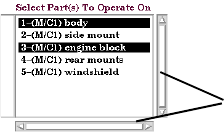
GUI Conventions
EnSight 7 User Manual 5-7
Lists EnSight provides access to the list of Model and Created Parts as well as Original
and Created Variables through the Main Parts List and the Main Variables List as
well as the sub-lists available in the various Feature Detail Editors. These lists are
presented as scrollable sections. Various mechanisms are used to select items from
a list for further action:
Buttons EnSight uses the following kinds of buttons:
Pop-up menu A pop-up menu is accessed by pressing the
associated rectangular button. The current selection
from the menu always appears as the button title.
(An example is the rectangular button labeled
“PRESSURE” beside the word Variable shown
above in the Feature Detail Editor.)
Select (or single-click) Place the mouse cursor over the item and click the
left mouse button. The item is highlighted to reflect
the “selected” state.
Select-drag Place the mouse cursor over the first item. Click
and hold the left mouse button as you drag over the
remaining items to be selected. Only contiguous
items may be selected in this fashion.
Shift-click Place the mouse cursor over the item. Depress the
shift key and click the left mouse button. This
action will extend a selection to include all those
items sequentially listed between the previous
selection and this one.
Control-click Place the mouse cursor over the item. Depress the
control key and click the left mouse button. This
action will extend a selection by adding the new
item, but not those in-between. Use this mechanism
to build a non-contiguous selection.
Double-click Place the mouse cursor over the item and click the
left mouse button twice in rapid succession.
Rectangular Place the mouse cursor in the button area and click
the left mouse button. Rectangular buttons typically
access the function described in the label. If the
label is followed by “...” then the button opens
another dialog. (Example shown above.)
Scroll Bars
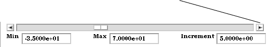
GUI Conventions
5-8 EnSight 7 User Manual
Text Fields EnSight utilizes three types of text fields:
Where appropriate, EnSight recognizes the following shortcut specifications for
UNIX directories:
Arrow Place the mouse cursor in the button area and click
the left mouse button. Arrow buttons typically have
an associated text field. Clicking the button
increments or decrements the text field value.
(Example shown below.)
Diamond Place the mouse cursor in the button area and click
the left mouse button. Diamond buttons (also called
radio buttons) are toggles that select an item from a
mutually exclusive list. Exactly one diamond button
of a group can be on at any given time. (Example
shown above.)
Square Place the mouse cursor in the button area and click
the left mouse button. Square buttons are toggles
that access the function indicated by the label
(Example shown above.).
Turndown Place the mouse cursor in the button area and click
the left mouse button. Turndown buttons are toggles
for opening and closing a section. A down pointing
arrow button indicates an open section. A right
pointing arrow button indicates a closed section.
(Example shown above.)
Information Text Fields These text fields are used to report information and
cannot be edited by the user. Information text fields
are surrounded with a single pixel border.
Editable Text Fields Place the mouse cursor in the text field and click to
insert a blinking insertion cursor. Several
techniques are available to accelerate text editing.
Select a single word by double-clicking or the entire
string by triple-clicking. Selected text is replaced by
subsequent typing. The left and right arrow keys
(on most systems) will move the insertion cursor.
EnSight does not recognize the change in the text
field until you press Return.
~/
Expands to your home directory
~username/
Expands to the home directory of username
./
Expands to the current working directory
../
Expands to the parent directory of the current
working directory
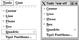
GUI Conventions
EnSight 7 User Manual 5-9
Tear-Off Menus If your window system allows it, the EnSight user interface supports “tear-off”
menus. Judicious use of tear-off menus can provide custom, rapid access to
frequently used functions. To use tear-off menus:
References
The following books provide more information on various aspects of OSF/Motif,
X Windows and the Motif Window Manager.
Kobara, Shiz, Visual Design with OSF/Motif, Addison-Wesley Publishing Co.,
Reading, MA, 1991.
Berlage, Thomas, OSF/Motif: Concepts and Programming, Addison-Wesley
Publishing Co., Wokingham, England, 1991.
Heller, Dan, Motif Programming Manual (for OSF/Motif Version 1.1), X Window
System, Vol. 6, O’Reilly & Associates, Inc., 1991.
Open Software Foundation, OSF/Motif Programmer’s Guide, Revision 1.2, and
OSF/Motif Programmer’s Reference Revision 1.2, P T R Prentice-Hall, Inc.,
Englewood Cliffs, NJ, 1993.
Quercia, Valerie and O’Reilly, Tim, “Appendix C: The OSF/Motif Window
Manager,” in X Window System User’s Guide (Volume Three) O’Reilly &
Associates, Inc., Sebastopol, CA, 1990.
Select (or single-click) Place the mouse cursor over a pulldown menu
button, then click and release the left mouse button.
This operation will open the pulldown menu.
Tear off Move the mouse cursor to the dotted lines on the
menu, and again click and release the left mouse
button. This will “tear off” the pulldown into a
separate window which can be placed anywhere on
the screen.
Closing a tear-off A tear-off menu can be closed by selecting Close
from the tear-off window’s frame menu which is
accessed clicking on the
button in the upper left of the dialog frame.
Dialog Control The window manager will normally allow you to
control some basic functions (Restore, Move,
Raise, Lower, Close) by clicking-holding the right
mouse button on a dialog or window border.
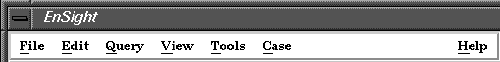
EnSight 7 User Manual 6-1
6Main Menu
This chapter describes the functions available from the Main Menu.
Section 6.1, File Menu Functions
Section 6.2, Edit Menu Functions
Section 6.3, Query Menu Functions
Section 6.4, View Menu Functions
Section 6.5, Tools Menu Functions
Section 6.6, Case Menu Functions
Section 6.7, Help Menu Functions
Figure 6-1
EnSight Main Menu
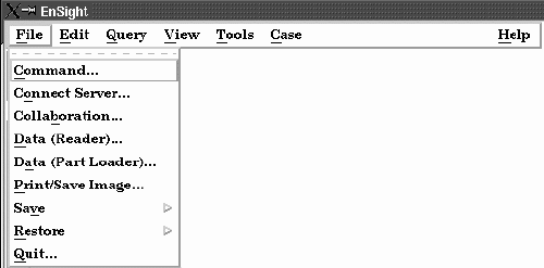
6.1 File Menu Functions
6-2 EnSight 7 User Manual
6.1 File Menu Functions
Clicking the File button in the Main Menu opens a pull-down menu which
provides access to capabilities which enable you to record and play command
files, connect the EnSight Client process to an EnSight Server process, read data
into the EnSight Server, load parts, print and save images, save and restore an
archive file, and quit from EnSight.
File Pull-down Menu
Command Opens the Command dialog which is used to record and play Command Files
Access: Main Menu > Command...
(see Section 2.4, Command Files and How To Record and Play Command Files)
Connect Server Opens the Connect Server dialog which is used to perform an Auto or Manual connection
from the EnSight Client process to an EnSight Server process.
Access: Main Menu > Connect...
For a complete description of the Connection process:
(see How To Connect Automatically)
Collaboration Opens the Collaboration dialog which is used to create a session that can be joined by a
colleague, or to join a session that a colleague has opened.
Access: Main Menu > Collaboration...
For a complete description of the Collaboration process:
(see How To Use Collaboration)
Data (Reader) Opens the File Selection dialog which is used to specify files you wish to read into
EnSight.
Access: Main Menu > Data (Reader)...
(see Reading and Loading Data Basics, in Section 2.1 and How To Read Data)
Data (Part Loader) Opens the Data Part Loader dialog which is used to load parts into EnSight.
Access: Main Menu > Data (Part Loader)...
(see Reading and Loading Data Basics, in Section 2.1 and How To Read Data)
Print/Save Image Opens the Print/Save Image dialog which is used to print or save images from EnSight.
Access: Main Menu > Print/Save Image...
(see Section 2.10, Saving and Printing Graphic Images and How To Print/Save an Image)
Figure 6-2
File pull-down menu
6.1 File Menu Functions
EnSight 7 User Manual 6-3
Save Opens a pull-down menu which allows you to choose between the following Save options:
Context, Full Backup or Geometric Entities.
Access: Main Menu > File > Save
Context... Opens the Save Current Context dialog where you can specify the name of a context file to
be created. This file saves information needed to reproduce the same basic imagery on a
different set of data.
Access: Main Menu > File > Save > Context...
(See How To Save or Restore a Context File)
Full Backup Opens the Save Full Backup Archive dialog which is used to save an entire session as an
Archive file which can later be used to restore EnSight to the same condition present when
the Archive file was made.
Access: Main Menu > File > Save > Full Backup
(see Section 2.5, Archive Files and How To Save and Restore an Archive)
Geometric Entities Opens the Save Geometric Entities Dialog which is used to save selected part geometric
information and active variable values from EnSight. EnSight Gold, VRML, Brick of
Values, or User-defined writer formats can be selected.
Access: Main Menu > File > Save > Geometric Entities
(see Section 2.8, Saving Geometry and Results Within EnSight and How To Save
Geometric Entities)
Scenario... Opens the Save Scenario dialog where you can create a scenario file which can be viewed
by CEI’s EnLiten product. EnLiten can display any scene created with EnSight and can be
run standalone or be embedded in Microsoft applications.
Access: Main Menu > File > Save > Scenario...
(See How To Save Scenario)
Restore Opens a pull-down menu which allows you to choose between the following Restore
options: Context or Full Backup. stored archive file.
Access: Main Menu > File > Restore
Context... Opens the Restore Context From File dialog where you can specify the name of a context
file to be applied and which case to apply it to. First read in your data, then restore the
context. This will do its best to create the same basic imagery (as that when the context
file was saved) to your current model.
Access: Main Menu > File > Restore > Context...
(See How To Save or Restore a Context File)
Full Backup Opens the Save Full Backup Archive dialog which is used to save an entire session as an
Archive file which can later be used to restore EnSight to the same condition present when
the Archive file was made.
Access: Main Menu > File > Restore > Full Backup
(see Section 2.5, Archive Files and How To Save and Restore an Archive)
Quit Opens the Quit Confirmation dialog which allows you to save a command file or/and an
archive file before exiting EnSight.
Access: Main Menu > Quit...
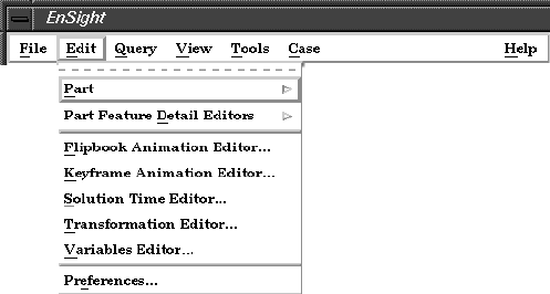
6.2 Edit Menu Functions
EnSight 7 User Manual 6-5
6.2 Edit Menu Functions
Clicking the Edit button in the Main Menu opens a pull-down menu which
provides access to the following features:
Part Opens a pull-down menu which allows you to choose between the following part
operations:
• Select All (see Section 3.4, Part Operations and How To Select Parts)
• Select ... (see Section 3.4, Part Operations and How To Select Parts)
• Delete (see Section 3.4, Part Operations and How To Delete a Part)
• Assign to Single New viewport (see Section 3.4, Part Operations)
• Assign to Multiple New viewports (see Section 3.4, Part Operations)
• Group & Ungroup (see Section 3.4, Part Operations and How To Group Parts)
• Copy (see Section 3.4, Part Operations and How To Copy a Part)
• Extract (see Section 3.4, Part Operations and How To Extract Part
Representations)
•Merge (see Section 3.4, Part Operations and How To Merge Parts)
Access: Main Menu > Edit > Part
Part Feature Detail
Opens a pull-down menu which allows you to choose between the following options to
Editors open the Feature Detail Editor:
• Selected Part Type (see Section 3.1, Part Overview and Introduction to
Part Creation)
• Contours (see Section 3.3, Part Editing, Section 7.2, Contour
Create/Update, and How To Create Contours)
•Clips (see Section 3.3, Part Editing, Section 7.5, Clip
Create/Update, How To Create Line Clips, How To
Create Plane Clips, How To Create Quadric Clips,
and How To Create IJK Clips)
• Developed Surfaces (see Section 3.3, Part Editing, Section 7.9, Developed
Surface Create/Update, and How to Create Developed
Surfaces)
• Elevated Surfaces (see Section 3.3, Part Editing, Section 7.7, Elevated
Figure 6-3
Edit pull-down menu
6.2 Edit Menu Functions
6-6 EnSight 7 User Manual
Surface Create/Update, and How to Create Elevated
Surfaces)
• Isosurfaces (see Section 3.3, Part Editing, Section 7.3, Isosurface
Create/Update, and How to Create Isosurfaces)
• Material Parts (see Section 3.3, Part Editing, Section 7.18, Material
Parts Create/Update, and How to Create Material
Parts)
•Model Parts (see Section 3.3, Part Editing and Introduction to Part
Creation)
• Particle Traces (see Section 3.3, Part Editing, Section 7.4, Particle
Trace Create/Update, and How to Create Particle
Traces)
•Profiles (see Section 3.3, Part Editing, Section 7.8, Profile
Create/Update, and How to Create Profile Plots)
• Shock Regions/Surfaces (see Section 3.3, Part Editing, Section 7.20, Shock
Surface/Region Create/Update, and How To Extract
Shock Surfaces)
• Separation/Attachment Lines (see Section 3.3, Part Editing, Section 7.21,
Separation/Attachment Lines Create/Update, and
How To Extract Separation/Attachment Lines)
•Subset Parts (see Section 3.3, Part Editing, Section 7.16, Subset
Parts Create/Update, and How to Create Subset Parts)
• Tensor glyphs (see Section 3.3, Part Editing, Section 7.17, Tensor
Glyph Parts Create/Update, and How to Create
Tensor Glyphs)
• Vector Arrows (see Section 3.3, Part Editing, Section 7.6, Vector
Arrow Create/Update, and How to Create Vector
Arrows)
•Vortex Cores (see Section 3.3, Part Editing, Section 7.19, Vortex
Core Create/Update, and How To Extract Vortex
Cores)
Access: Main Menu > Edit > Part Feature Detail Editors...
Flipbook Animation
Opens the Flipbook Animation editor in the Quick Interaction Area which is used to
Editor create, save, and restore Flipbook Animation sequences.
Access: Main Menu > Edit > Flipbook Animation Editor...
(see Section 7.14, Flipbook Animation and How To Create a Flipbook Animation)
Keyframe Animation Opens the Keyframe Animation editor in the Quick Interaction Area which is used to
Editor create, save, and restore Keyframe Animation sequences.
Access: Main Menu > Edit > Keyframe Animation Editor...
(see Section 7.15, Keyframe Animation and How To Create a Keyframe Animation)
Solution Time Opens the Solution Time Editor in the Quick Interaction Area which is used to specify the
Editor currently displayed time step in a transient dataset.
Access: Main Menu > Edit > Solution Time Editor...
(see Section 7.13, Solution Time and How To Animate Transient Data)
Transformation Editor Opens the Transformation Editor dialog which is used to precisely position parts, frames,
and tools in the Graphics Window and to Save and Restore Views.
Access: Main Menu > Edit > Transformation Editor...
(see Chapter 9, Transformation Control)
Variables Editor Opens the Feature Detail Editor (Variables) dialog which is used to obtain information
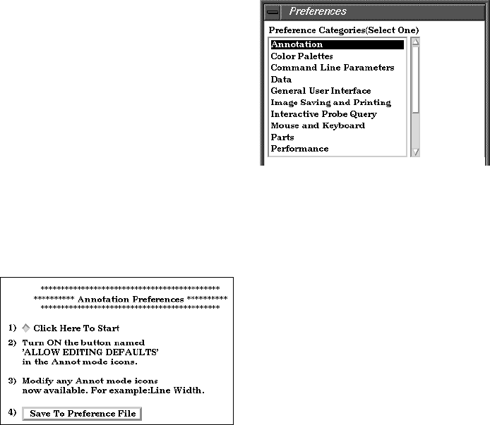
6.2 Edit Menu Functions
EnSight 7 User Manual 6-7
about variables, change the information, and to create new variables.
Access: Main Menu > Edit > Variables Editor...
(see Chapter 4, Variables)
Preferences... Opens the Preferences dialog which is used to set or modify preference values for the
various categories within EnSight.
In this area you can set default attributes and preferences which will be used for the
current EnSight session. You may also save any of these to the preference file(s) so that
they will be the defaults for future invocations of EnSight. Each of the preference
categories will now be explained.
Annotation
Preferences
Click Here To Start Will place you in Annotation mode in EnSight with no
annotations selected (default mode). You must do step 2) so
that you are allowed to edit annotation defaults. You can
then change any annotation attributes desired and they will
become the defaults for the session.
Save To Preference File Will write the current annotation preferences to the
preference file for future EnSight sessions.
(see How To Set Annotation Preferences:)
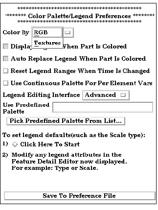
6.2 Edit Menu Functions
6-8 EnSight 7 User Manual
Color Palettes
Preferences
Color By Can select RGB or Texture color mode
Display Legend When Will cause the legend to automatically appear when you color
Part is Colored a part by a variable.
Auto Replace Legend Will cause legends to be automatically replaced when the
When Part is Colored current legend is no longer in use (i.e. no parts are colored by
the variable) and a new variable is in use.
Reset Legend Ranges Will cause legend ranges to be reset according to variable
When Time Is Changed values at the current time.
Use Continuous Palette By default the legend for Per Element variables has a “Type”
For Per Element Vars of Constant. Toggle this on to change the default “Type” to
Continuous.
Legend Editing Interface Can be EnSight’s Simple or Advanced interface.
Use Predefined Palette Allows you to enter a predefined palette name if you have
predefined color palettes.
Pick Predefined Palette Allows you to pick from your predefined palette list.
From List...
Legend Defaults:
Click Here To Start Will allow you to modify legend default attributes.
Save To Preference File Will write the current legend and palette preferences to the
preference file for future EnSight sessions.
(see How To Set Color Palette Defaults:)
6.2 Edit Menu Functions
EnSight 7 User Manual 6-9
Command Line
Parameter Preferences
By selecting arguments from the list and hitting:
Add Selected Item To You can build customized command line preferences.
Current Args Below
Save To Preference File Will save the command line preferences to the preference file
for future invocations of EnSight.
(see How To Set Command Line Preferences:)
Data Preferences
Default Data Directory Will allow you to specify a default directory for data files.
6.2 Edit Menu Functions
6-10 EnSight 7 User Manual
Binary Files Are Allows you to specify the default byte order for binary files.
The allowable settings are Big-Endian, Little-Endian, or
Native To Server Machine.
If Starting Time Step is Can be set so that the default starting time step for transient
not specified load data can be either Last Step or First Step.
When reading data Allows you to have EnSight automatically load All Parts,
automatically load First Part, Last Part, or No Parts at startup. If No Parts is
specified, the Part Loader dialog will be presented to the user
at startup.
New Data Notification Options for dealing with notification of a change in the
model dataset while EnSight is running. Please contact CEI
support if you have need of this.
Select Below To Toggle Allows you to specify which data formats will appear in the
Reader Visibility “Format” pull-down of the Data Reader dialog.
Default Reader Allows you to specify the default data reader format.
Save To Preference File Will save the data preferences to the preference file for future
invocations of EnSight.
(see How To Set Data Preferences:)
General User Interface
Preferences
Tool Tips Will cause pop-up help information to appear when the
mouse is placed over certain icons while running EnSight.
Large Parts List Will cause a separate, larger parts list dialog (which can be
expanded) to be used in place of the normal parts list.
Frame Mode Allowed Will display Frame as a managed mode.
View Mode Allowed Will display View Mode as a managed mode.
Record Part Selection in Allows you to specify whether the part selections recorded in
Command Language By command language will be by part Name or by part Number.
Save Above Items To Will save the preferences above to the preference file for
Preference File future invocations of EnSight.
6.2 Edit Menu Functions
EnSight 7 User Manual 6-11
Modify and Save Icon Opens the Icon Bar Preferences dialog
Layout....
Show Help Labels When toggled on, the Icon name will appear beneath each
For Mode Icons icon in the Mode Icon Bar. You can customize the EnSight
GUI by specifying which icons appear and their order in the
Feature and Mode Icon Bars. Do NOT modify the Menu ID
for any function. The other fields for each function may be
edited within the dialog. Customization options are:
Button Name Describes the function of the icon which would be displayed
if EnSight was started with no icons (command line
function). Further, this is the name which will appear below
the each Mode Icon when Show Help Labels For Mode Icons
is toggled on.
Visible Determines the visibility of a feature icon. Must be either ON
or OFF.
Order Determines the order in which the icons appear. A value of 1
will cause the icon to appear leftmost in the Main Feature
Icon Bar and uppermost in the Mode Icon Bars.
Description The text description of the button which will be displayed in
the Message Area when the icon is selected. You must click
the Save As Default button to save any changes you have
made. The Button Name and Order, if modified, will not take
effect until you restart EnSight. Changes to Visibility,
Description, and Show Help Labels however, will be
implemented immediately upon clicking the Save as Default
button (and will control these options in future EnSight
sessions as well).
When EnSight is started, the icon preferences are initially
read from the
$CEI_HOME/ensight76/site_preferences
directory and are then overwritten by any information in the
user’s preferences directory.
(see How To Customize Icon Bars)
Figure 6-4
Icon Bar Preferences
6.2 Edit Menu Functions
6-12 EnSight 7 User Manual
Save Size and Position Will record the location and size of the main GUI, and all
of Main Windows dialogs that have been opened during the session or are
currently open and will make those locations and sizes the
default for future sessions of EnSight. Be aware also that if
you had a turn-down section open in a dialog (such as
General Attributes in the Feature Detail Editor dialog) when
you closed it earlier in the session or at the time you choose
Save Window Positions, this will be recorded as well and
opening that dialog in future sessions will also open that turn-
down section within the dialog.
(see How To Save GUI Settings)
(see How To Set General User Interface Preferences:)
Image Saving and
Printing Preferences
Click Here To Start Will allow you to modify default attributes for image saving
and printing.
Save To Preference File Will write the current print/save preferences to the preference
file for future EnSight sessions.
(see How To Set Image Saving and Printing Preferences:)
Interactive Probe
Query Preferences
Click Here To Start Will allow you to modify default attributes for interactive
probe queries.
Save To Preference File Will write the current interactive probe query preferences to
the preference file for future EnSight sessions.
(see How To Set Interactive Probe Query Preferences:)
Mouse and Keyboard
Preferences
6.2 Edit Menu Functions
EnSight 7 User Manual 6-13
Here you can specify the actions of the three mouse buttons. Select the option you wish
to assign to each button. The options are as follows:
Transf. Action When this option is chosen (it is the default for the left
button), depressing the button and moving the mouse will
perform the transformation (rotate, translate, zoom) currently
selected in the Transformation Control Area on the model.
Rotate When this option is chosen, depressing the button and
moving the mouse will perform a rotate transformation on
the model.
Translate When this option is chosen, depressing the button and
moving the mouse will perform a translate transformation on
the model.
Zoom When this option is chosen, depressing the button and
moving the mouse will perform a zoom transformation on the
model.
Pick When this option is chosen, depressing the button will
perform a pick operation. If Pick has not been assigned to
one of the mouse buttons, the “p” key is used to perform the
operation. (see Pick Pull-down Icon in Section 8.1, Part
Mode)
Nothing When this option is chosen, no function is mapped to the
mouse button.
Note: One of the Mouse buttons must be assigned to Transf. Action. Macros cannot be
assigned to a mouse key which has a function assigned to it. (see How To Customize
Mouse Button Actions)
Zoom Style Choose method to use for zoom action. For either option,
zooming stops when the mouse button is released.
Manual Drag Zoom DISTANCE is based on the distance you move your
mouse when the mouse button is pressed.
Automatic Slide Zoom Velocity is based on the distance the mouse is moved
when the mouse button is pressed.
Save To Preference File Will write the current mouse and keyboard preferences to the
preference file for future EnSight sessions.
(see How To Set Mouse and Keyboard Preferences:)
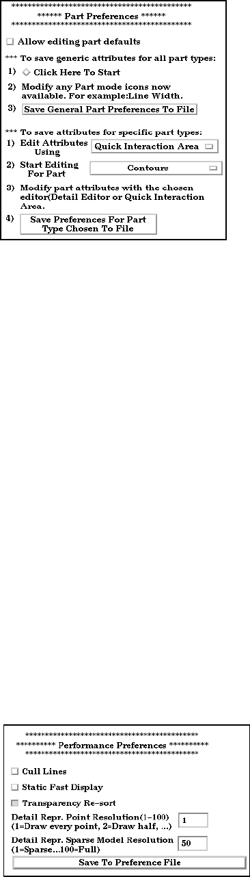
6.2 Edit Menu Functions
6-14 EnSight 7 User Manual
Parts
Allow Editing Part In EnSight 7.4 you can change a default attribute, such as line
Defaults
width, by making sure there are no parts selected in the main
part list and changing an icon under Part mode. We used to
pop up a message to warn the user that they are changing a
default instead of a particular part if they forgot to select one.
This preference now allows or disallows changing a default
attribute. These default attributes will be used for any part
created or loaded in the future, so that the user doesn’t have
to keep changing each new part.
Generic Attributes:
Click Here To Start Will allow you to modify default visual part attributes which
apply to all part types.
Save General Part Will write the current generic part preferences to the
Preferences To File preference file for future EnSight sessions.
Attributes For Specific Part Types:
Edit Attributes Using Allows you to specify which area to use for default attribute
modification - the Quick Interaction Area or the Detail
Editor Dialog.
Start Editing For Part Allows the user to specify the part type for which default
attributes will be modified.
Save Preferences For Will write the current specific part type preferences to the
Part Type Chosen preference file for future EnSight sessions.
To File
(see How To Set Part Preferences:)
Performance
Preferences
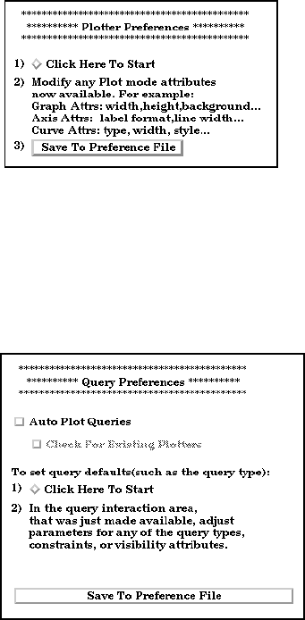
6.2 Edit Menu Functions
EnSight 7 User Manual 6-15
Cull Lines Will only draw shared lines between polygons once.
Static Fast Display Will cause the fast representation to always be displayed. If
this is off (the default), fast display will only be active during
a transformation.
Transparency Re-sort Causes polygons to be resorted with each transformation - so
the image is always correct. If not on, the polygons will not
be resorted while the mouse is down during transformations,
but will be resorted when the mouse is released.
Detail Repr. Point Allows specification of fraction of nodes to display in Fast
Resolution Display, point representation. (The default is “1”, indicating
all nodes, “2” would be every other node, “3” every third
node, etc.) (EnSight Gold only)
Detail Repr. Sparse Allows specification of the percentage of the model
Model Resolution geometry that will be displayed. (EnSight Gold and no
display list mode only)
Save To Preference File Will write the current performance preferences to the
preference file for future EnSight sessions.
(see How To Set Performance Preferences:)
Plotter Preferences
Click Here To Start Will allow you to modify defaults for the various plotter
graph, axis, and curve attributes.
Save To Preference File Will write the current plotter preferences to the preference
file for future EnSight sessions.
(see How To Set Plotter Preferences:)
Query Preferences
Auto Plot Queries Automatically plot a newly created query to a plotter. The
plot will go into a new or an existing plotter, depending on
the state of the “Check for Existing Plotters” toggle.
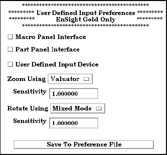
6.2 Edit Menu Functions
6-16 EnSight 7 User Manual
Check for Existing Check for plotters of the same type (same X and Y units) as
Plotters the new query is being autoplotted. If one exists, plot the
query to the existing plotter.
Click Here To Start Will allow you to modify defaults for the various query
attributes.
Save To Preference File Will write the current query preferences to the preference file
for future EnSight sessions.
(see How To Set Query Preferences:)
User Defined Input
Preferences
This area provides access to user defined input devices. The input devices include a
Macro Panel Interface (a grid of commands that displays in the Main Graphics window
and executes EnSight command files upon selection), and/or a User Defined Input
Device (a virtual input device designed for - but not limited to - use with VR
environments such as an Immersadesk)
Macro Panel Interface Toggles on/off the user defined macro panel (defined in your
~/.ensight7/macros/hum.define
file) to the Main
Graphics window. (An example hum.define file is located at
$CEI_HOME/ensight7/src/input/HUM/hum.define
on your client system.).
Part Panel Interface Display a part list in the graphics window. This is helpful
when in full screen mode or in a VR environment, to allow
picking of parts that can be operated on via macros.
User Defined Input Toggles on/off the User Defined Input Device that is linked
Device via a runtime library. (Steps outlining the implementation of
this library and input device are found in the file:
$CEI_HOME/ensight76/src/input/README
on your client system.).
Zoom Using Opens a pull-down menu for selection of the type of input
device used for zoom transformations. The type of devices
are:
Valuator a device that returns a value (like a virtual
joystick).
Position a device that returns delta movement in the Z
direction (like a wand).
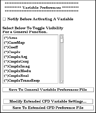
6.2 Edit Menu Functions
EnSight 7 User Manual 6-17
Sensitivity Specifies a positive scalar value that adjusts the Sensitivity of
the type of zoom input device selected in Zoom Using (i.e.
values < 1 are slower, and values > 1 are faster).
Rotate Using Opens a pull-down menu for selection of the type of input
device used to record rotation transformations.
Mixed Mode A device that returns virtual angle values
where the Z rotations correspond to
(literal) movement of the input device
about its local Z (or roll) axis; and where
the X and Y rotations correspond to
translational movements of the input
device with respect to its local X and Y
axes.
Direct Mode A device that returns virtual angle values
that correspond to (literal) rotational
movements of the input device about its
local X, Y, and Z axes.
Sensitivity Specifies a positive scalar value that adjusts the Sensitivity of
the type of rotation input device selected in Rotate Using (i.e.
values < 1 are slower, and values > 1 are faster).
(see How To Enable User Defined Input Devices)
Save To Preference File Will write the current user defined input preferences to the
preference file for future EnSight sessions.
(see How To Set User Defined Input Preferences:)
Variables Preferences
Notify Before Activating Will cause you to be notified before a variable, which was
A Variable going to be automatically activated, is actually activated.
Select Below To Toggle Toggle visibility of functions in the General Functions list of
Visibility For a General the new variable calculator dialog. There are many general
Function functions and this allows you to limit the list to only
functions that you wish to use.

6.2 Edit Menu Functions
6-18 EnSight 7 User Manual
Save To General Variable Will write the variable notification preference to the
Preferences File preference file for future EnSight sessions.
Modify Extended CFD Opens the Extended CFD Variable Settings dialog. If your
Variable Settings... data defines variables or constants for density, total energy
per unit volume, and momentum (or velocity), it is possible
to show new variables defined by these basic variables in the
Main Variables List of the GUI by utilizing the capabilities of
this dialog.
Save To Extended CFD Will write the current Extended CFD settings to the
Preference File preference file for future EnSight sessions.
Density Permits the selection of the density variable from the list
(click SET after selection) or the specification of a constant
value in the field provided.
Total Energy Per Permits the selection of the energy variable from the list.
Unit Volume Click SET after selection.
Ratio of Specific Permits the selection of the ratio of specific heats variable
Heats from the list (click SET after selection) or the specification of
a constant value in the field provided.
Momentum or Permits the selection of the momentum or velocity variable
Velocity from the list. Click SET after selection.
Freestream Mach # Permits the specification of the freestream mach number in
the field provided.
Gas Constant Permits the specification of the gas constant in the field
provided.
Figure 6-5
Extended CFD Variable Settings Dialog
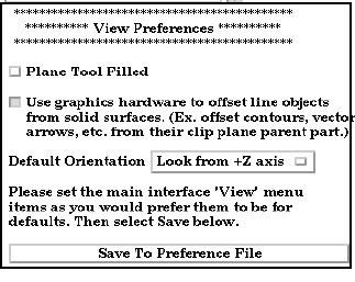
6.2 Edit Menu Functions
EnSight 7 User Manual 6-19
Freestream Density Permits the specification of the freestream density value in
the field provided.
Freestream Speed Permits the specification of the freestream speed of sound
of Sound value in the field provided.
Show Extended When selected, all of the variables that can be derived from
the information entered will be
CFD Variables Shown in the Main Variables List of the GUI. (will not take
effect until the Okay button is clicked.
Okay Clicking this button applies the changes made in the dialog.
(See How To Create New Variables)
Save To Extended CFD Will write the current extended CFD preferences to the
Preference File extended CFD preference file for future EnSight sessions.
(see How To Set Variable Preferences:)
View Preferences
Plane Tool Filled Will cause the plane tool to be a filled transparent surface. If
it is off, the plane tool will be in line drawing mode. You can
save this default to the preference file.
Save To Preference File Will write the current view preferences to the preference file
for future EnSight sessions.
Use Graphics Hardware There are two offsets employed in EnSight. This one,
to offset line objects hardware offset, is perpendicular to the monitor screen, and
done in hardware if this toggle is on. This will allow, for
example, contour lines to appear closer to the viewer than
their parent part so they are visible no matter what orientation
the part is viewed from. The second offset is the display
offset. The display offset can be set in the feature detail
editor for line parts such as contour lines, particle trace lines,
vector arrows, and separation/attachment lines. The display
offset is the distance in the direction of the element normal
(perpendicular to the surface).
Default Orientation The default axis for viewing can be selected and set.
(see How To Set View Preferences:)
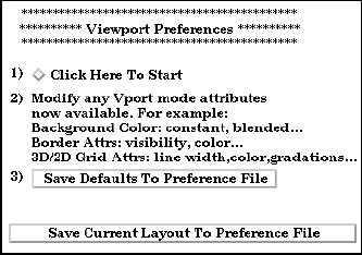
6.2 Edit Menu Functions
6-20 EnSight 7 User Manual
Viewport Preferences
Click Here To Start Will allow you to modify default viewport attributes.
Modify and Vport Select Vport along the left side of the main window. The
mode attributes now attributes for viewports will appear in the iconbar for you to
available modify. Attributes as shown above and many others may be
set.
Save Defaults To Will write the current viewport default values to a preference
Preference File file for future EnSight sessions.
Save Current Layout Will write out the current viewport screen layout to a file for
To Preference File future EnSight sessions.
6.3 Query Menu Functions
EnSight 7 User Manual 6-21
6.3 Query Menu Functions
Clicking the Query button in the Main Menu opens a pull-down menu which
provides access to the following features:
EnSight provides several ways to examine information about variable values. You can, of
course, visualize variable values with fringes, contours, vector arrows, profiles,
isosurfaces, etc. Only parts with data residing on the Server host system may be queried.
Thus, parts that reside exclusively on the Client host system (i.e. contours, particle traces,
profiles, vector arrows) may NOT be queried.
(see Table 3–2 Part Creation and Data Location)
Show Information Opens the following pull-down menu:
Access: Main Menu > Query > Show Information
(see How To Get Point, Node, Element and Part Information)
Cursor Provides the following information in the Status History Area about a Point inside of the
selected Part(s) who’s position you have specified with the cursor tool:
x,y,z coordinates, Frame assignment of Point, the Part that the Point is found in,
the closest Node to the Point, and the specified Variable value at the Point
Access: Main Menu > Query > Show Information > Point
(see How To Get Point, Node, Element and Part Information and How To Use the Cursor
(Point) Tool)
Node Opens the Query Prompt dialog which is used to specify Node ID number.
Figure 6-6
Query pull-down menu
Figure 6-7
Show Information pull-down menu
Figure 6-8
Query Prompt dialog
6.3 Query Menu Functions
6-22 EnSight 7 User Manual
When Okay button is pressed, the following information about the specified Node is
shown in the Status History Area:
x,y,z coordinates, Frame assignment of Node, the Part that the Node is found in,
and the specified Variable value at the Node
Access: Main Menu > Query > Show Information > Node...
(see How To Get Point, Node, Element and Part Information)
IJK Opens the Query Prompt dialog which is used to specify IJK values.
When Okay button is pressed, the following information about the Node specified by the
IJK values is shown in the Status History Area:
Node ID, Part in which the Node is located, x,y,z coordinates of the Node,
Frame assignment of the Node, and the specified Variable value at the Node.
Access: Main Menu > Query > Show Information > IJK...
(see How To Get Point, Node, Element and Part Information)
Element Opens the Query Prompt for Element ID.
When Okay button is pressed, the following information about the Element is shown in
the Status History Area:
Part in which Element is located, Type of Element, IJK bounds (if a structured
mesh), Number of Nodes, Node ID numbers, information on neighboring
Elements, and the specified Variable value at the Element.
Access: Main Menu > Query > Show Information > Element...
(see How To Get Point, Node, Element and Part Information)
Part Causes the following information about the Part to be shown in the Status History Area:
Part type (structured or unstructured), number of Nodes in Part, minimum and
maximum x,y,z coordinates, Element type, and the number of Elements.
Access: Main Menu > Query > Show Information > Part
(see How To Get Point, Node, Element and Part Information)
Over Time/Distance Opens the Query/Plot Editor in the Quick Interaction Area which is used to obtain
information about variables and to create plots of the information.
Access: Main Menu > Query > Over Time/Distance...
(see Section 7.11, Query/Plot, How To Query/Plot)
Figure 6-9
Query Prompt for IJK Values
Figure 6-10
Query Prompt for Element ID
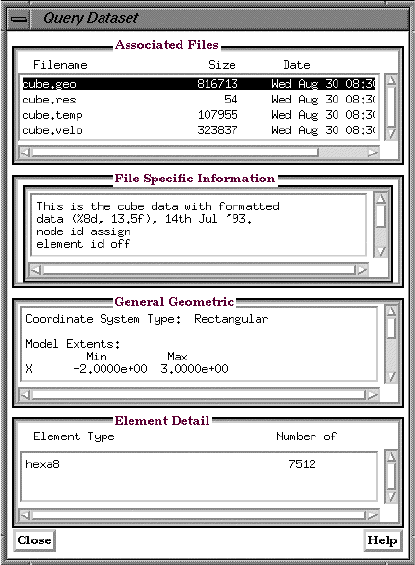
6.3 Query Menu Functions
EnSight 7 User Manual 6-23
Interactive Probe Opens the Interactive Probe Query Editor in the Quick Interaction Area which is used to
obtain information interactively about variables.
Access: Main Menu > Query > Interactive Probe...
(see Section 7.12, Interactive Probe Query and How To Probe Interactively)
Dataset Opens the Query Dataset dialog which is used to obtain information about datasets for the
selected case.
For the specified file, specific, general and detail information is provided.
Access: Main Menu > Query > Dataset...
(see Section 7.11, Query/Plot and How To Query Datasets)
Figure 6-11
Query Dataset dialog
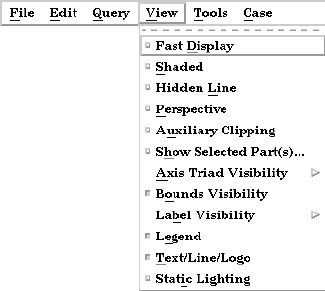
6.4 View Menu Functions
6-24 EnSight 7 User Manual
6.4 View Menu Functions
Clicking the View button in the Main Menu opens a pull-down menu which
provides access to the following features:
Fast Display Toggles the Fast Display mode.
Access: Main Menu > View > Fast Display
Fast Display in this pull-down is the same as the one located on the Desktop.
By default, EnSight displays all of the lines and elements for each part every time the
Main View window redraws. If you have very large models (or if you have slow graphics
hardware), each redraw can take significant time. As a result, interactive transformations
become jerky and lag behind the motion of the mouse. Ironically, the slower the graphics
performance, the harder it is to perform precise interactive transformations. To avoid this
problem, you can tell EnSight to show a lesser detailed part representation, i.e, a bounding
box surrounding each Part, or the Part as a point cloud. You can select to show the detail
representation all the time, or only while you are performing transformations. This
obviously displays much less information, but may be sufficient if you want to rotate a
very large model.
A lesser detail display is also useful when experimenting with keyframe-animation rates.
Using lesser detail, the display rate can be adjusted to approximate the video rate, thus you
can see how your scene will transform on the video tape
The default setting is off, indicating that all lines and elements of all visible parts will be
redrawn. When on, the redraw will show only the part’s Fast Display Representation (by
default a box). The fast display representation is only used while transformations are being
performed. The fast display representation will be continuously displayed if the Static Fast
Display option is turned on in:
Main Menu > Prefs > Graphics Window > Static Fast Display.
Shaded Toggle Toggles the Global Shaded mode for parts on and off. (The Shaded Toggle in the View
Mode Icon Bar performs the same action.) EnSight by default displays parts in line mode.
Shaded mode displays parts in a more realistic manner by making hidden surfaces
invisible while shading visible surfaces according to specified lighting parameters. Parts
in Shaded mode require more time to redraw than when in line mode, so you may wish to
Figure 6-12
View pull-down menu
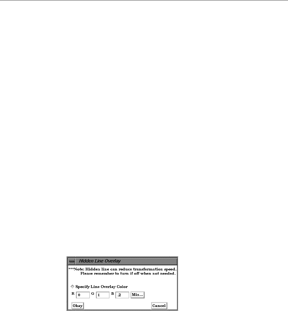
6.4 View Menu Functions
EnSight 7 User Manual 6-25
first set up the Graphics Window as you want it, then turn on Shaded to see the final result.
Access: EnSight dialog > View > Shaded
or View Mode Icon Bar: Shaded Toggle
or Desktop > Shaded
(see Section 8.6, View Mode and How To Set Drawing Style)
Troubleshooting Hidden Surfaces and Shading
Hidden Line Toggles the global Hidden Line display for all parts on/off. (The Hidden Line Toggle icon
Toggle in the View Mode Icon Bar performs the same action.) This simplifies a line drawing
display by making hidden lines - lines behind surfaces - invisible while continuing to
display other lines. Hidden Line can be combined with Shaded to display both surfaces
and the edges of the visible surface elements. Hidden Line can be toggled on/off for
individual parts by using the Hidden Line Toggle icon in the Part Mode Icon Bar.
To have lines hidden behind surfaces, you must have surfaces (2D elements). If the
representation of the in-front parts consists of 1D elements, the display is the same
whether or not you have Hidden Lines mode toggled-on. During interactive
transformations, the display reverts to displaying all lines. When you release the mouse
button, the Main View display automatically resumes Hidden Line mode. The Hidden line
option will not be active during playback of flipbook animations.
Hidden line overlay is disabled if transparency is turned on.
Access: Main Menu > View > Hidden Line
or View Mode Icon Bar: Hidden Line Toggle
(see Section 8.6, View Mode and How To Set Drawing Style)
Hidden Line Overlay dialog
Problem Probable Causes Solutions
Main View shows line drawing after
turning on Shaded.
Shaded is toggled off for each
individual part.
Toggle Shaded on for individual
parts with the Shaded Icon in Part
Mode or in the Feature Detail Editor
dialog.
There are no surfaces to shade—all
parts have only lines.
If parts are currently in Feature
Angle representation, change the
representation. If model only has
lines, you can not display shaded
images.
The element visibility attributes has
been toggled off for the part(s).
Toggle the element visibility on for
individual parts in the Feature Detail
Editor dialog.
Figure 6-13
Hidden Line Overlay dialog
6.4 View Menu Functions
6-26 EnSight 7 User Manual
If you combine Shaded mode with Hidden Line mode, the lines overlay the surfaces. The
Hidden Line Overlay dialog will pop-up on the screen if the Shaded option is currently on
and you then turn the Hidden Line option on. From this dialog you specify a color for the
displayed lines (you do not want to use the same color as the surfaces since they then will
be indistinguishable from the surfaces). The default is the part-color of each part, which
may be appropriate if the surfaces are colored by a color palette instead of their part-color.
Specify Overlay Toggle-on if you want to specify an overlay color. If off, the overlay line color will be the
same as the part color.
R, G, B The red, green, and blue components of the hidden line overlay. These fields will not be
accessible unless the Specify Overlay option is on.
Mix... Click to interactively specify the constant color used for the hidden line overlay using the
Color Selector dialog.
(see Section 7.1, Color and How To Change Color)
Okay Click to accept the hidden line overlay color options.
Perspective Toggles the view within each of the viewports within the Graphics Window between a
(Global)Toggle perspective view (the default) and an orthographic projection. Perspective is what gives
you the sense of depth when viewing a three dimensional scene on a two dimensional
surface. Objects that are far away look smaller and parallel lines seem to meet at infinity.
Orthographic projection removes the sense of depth in a scene. Lines that are parallel will
never meet and objects of the same size all appear the same no matter how far away they
are from you. Orthographic projection mode often helps when you are positioning the
Cursor, Line, and Plane tools using multiple viewports. This is the Global toggle. Each
viewport also has a Perspective Toggle.
Access: Main Menu > View > Perspective
(see Section 8.4, VPort Mode and see How To Set Global Viewing)
Auxiliary Clipping Toggles the Auxiliary Clipping feature on/off. (Default is Off). The Auxiliary Clipping
Global Toggle Global Toggle icon in the View Mode Icon Bar performs the same action. Like a Z-Clip
plane, Auxiliary Clipping cuts-away a portion of the model. When Auxiliary Clipping is
On, Parts (or portions of Parts) located on the back (negative-Z) side of the Plane Tool are
removed. Parts whose Clip attribute you have toggled off (in the General Attributes
section of the Feature Detail Editor dialog or with the Auxiliary Clipping Toggle Icon in
the Part Mode Icon Bar) remain unaffected.
Auxiliary Clipping is interactive—the view updates in real time as you move the Plane
Tool around
(see Section 6.5, Tools Menu Functions and How To Use the Plane Tool).
Unlike a Z-Clip plane, Auxiliary Clipping applies only to the parts you specify, and the
plane can be located anywhere with any orientation though it is always infinite in extent
(see Section 9.6, Z-Clip and How To Set Z Clipping).
Auxiliary Clipping is helpful, for example, with internal flow problems since you can
“peel” off the outside parts and look inside. This capability is also often useful in
animation.
The position of the Plane Tool and the status of Auxiliary Clipping is the same for all
displayed viewports.

6.4 View Menu Functions
EnSight 7 User Manual 6-27
Do not confuse Auxiliary Clipping with a 2D-Clip plane, which is a created part whose
geometry lies in a plane cutting through its parent parts or with the Part operation of
cutting a part.
(see Section 3.4, Part Operations, How to Create Plane Clips, and How To Cut a Part).
Troubleshooting Auxiliary Clipping
Axis Triad Visibility Opens the pull-down menu which allows you to toggle on/off the visibility of the Global
axis triad, the axis triads for all Frames, and the model axis triad.
Frame Toggle Toggles on/off (default is On) the display of all coordinate Frame axis triads. (The All
Frame Axis Triad Visibility Toggle icon in the Frame Mode Icon Bar performs the same
function.)The visibility of individual coordinate Frame axes can be selectively turned on/
off by clicking on the Frame’s axis triad and then clicking on the Frame Axis Triad
Visibility Toggle in the Frame Mode Icon Bar.
Access: Main Menu > View > Axis Visibility > Axis - Local
(see Section 8.5, Frame Mode)
Global Toggle Toggles on/off (default is Off) the display of the global coordinate frame axis. (The Global
Axis Visibility Toggle icon in the Frame Mode Icon Bar performs the same function.)The
global coordinate frame axis triad represents the Look-At Point.
Access: Main Menu > View > Axis Visibility > Axis - Global
(see Section 8.6, View Mode)
Label Visibility Opens the pull-down menu which allows you to toggle on/off the visibility of labels for
Elements or Nodes.
BoundsVisibility Toggles on/off (default is Off) the extents box for all parts.
Element Labeling Toggles on/off (default is Off) the global visibility of labels (if they are available in the
Toggle dataset) for elements in all parts. (The Element Label Toggle in the View Mode Icon Bar
performs the same function.) Visibility of element labels for individual parts can be
controlled in the Node, Element, and Line Attributes section of the Feature Detail Editor
(Model).
Access: Main Menu > View > Label Visibility > Element Labeling
(see Section 8.6, View Mode)
Problem Probable Causes Solutions
The Plane Tool does not appear to
clip anything
The Auxiliary Clipping toggle is off
for all parts.
Turn the Auxiliary Clipping toggle
on for individual parts in the Feature
Detail Editor (Model) dialog General
Attributes section.
The Plane Tool is not intersecting the
model
Change the position of the Plane
Tool.
The Main View window shows
nothing other than the Plane Tool
after Clipping is toggled-on.
All of the part(s) is(are) on the back
side of the Plane Tool and is(are)
thus clipped
Change the position of the Plane
Tool.
6.4 View Menu Functions
6-28 EnSight 7 User Manual
Node Labeling Toggles on/off (default is off) the global visibility of labels (if they are available in the
Togg l e dataset) for nodes in all parts. (The Node Label Toggle in the View Mode Icon Bar
performs the same function). Visibility of node labels for individual parts can be
controlled in the Node, Element, and Line Attributes section of the Feature Detail Editor
(Model).
Access:Main Menu > View > Label Visibility > Node Labeling
(see Section 8.6, View Mode)
Legend Toggle Toggles on/off (default is on) the global visibility of all legends. (the Legend Visibility
Toggle Icon in the Annotation Mode Icon Bar performs the same function). Visibility of
individual legends can be controlled by using the Show Legend button above the Feature
Icon Bar. Clicking the Show Legend button will make visible only those legends for
variables which are selected in the Variables List, and then only if Legend Visibility is
toggled on. If a Legend has been made visible by selecting a variable and then clicking the
Show Legend button, deselecting the variable and clicking the Show Legend button again
will turn visibility off for that individual legend.
Access: Main Menu > View > Legend
(see Section 4.2, Variable Summary & Palette, Section 8.2, Annot Mode and How To
Create Color Legends.
Text/Line/Logo Toggle Toggles on/off global visibility for text strings and lines which have been created and
logos which have been imported. (The Text/Line/Logo Visibility Icon in the Annotation
Mode Icon Bar performs the same function). Visibility of individual Text strings, Lines, or
Logos can be controlled by selecting the item while in Annotation Mode and clicking the
Visibility Toggle in the Annotation Mode Icon Bar. While in Annot Mode, you will notice
that the item does not disappear, but turns transparent. Such items will not appear in the
Graphics Window in any Mode except Annotation Mode, and then only if global visibility
has been turned on.
Access: Main Menu > View > Text/Line/Logo
(see Section 8.2, Annot Mode, How To Create Lines and Arrows, How To Create Text
Annotation, and How To Load Custom Logos.
Static Lighting Toggles on/off whether the light source moves as the model transforms, or instead remains
stationary. Static lighting only affects shaded surfaces (i.e., Hidden Surfaces mode is
toggled-on).When the Static Lighting option is off (the default), the light source remains
fixed as you transform the model. Your graphics hardware performs the lighting
calculations each time the Graphics Window redraws.
When the Static Lighting option is on, the light source moves with the model (it is the
lighting of the model that remains “static”). EnSight performs the lighting equations once.
This can greatly improve graphics performance, especially when color fringes are on in
which case the performance boost may be as much as a factor of five. Also, memory
requirements are somewhat less with Static Lighting, an important point to remember if
you are loading flipbook animation pages as objects. However, keep in mind that this
performance improvement comes at the cost of realism since the display’s lighting does
not update when the scene moves.
Access: Main Menu > View > Static Lighting
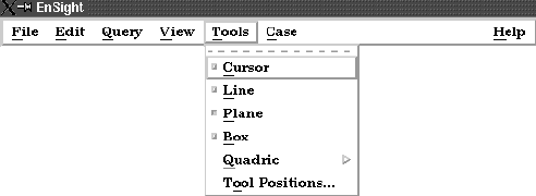
6.5 Tools Menu Functions
EnSight 7 User Manual 6-29
6.5 Tools Menu Functions
The Cursor, Line, Plane, and Quadric (cylinder, sphere, cone, and revolution)
Tools in EnSight are used for a variety of tasks, such as: positioning of clipping
planes and lines, query operations, particle trace emitters, etc. Collectively these
tools are referred to as Positioning Tools. Clicking the Tools button in the Main
Menu opens a pull-down menu which provides access to these features:
Cursor Tool Makes the Cursor Tool visible/invisible in the Graphics Window. The Cursor Tool appears
Toggle as a three-dimensional cross colored red, green, and blue. The red axis of the cross
corresponds to the X axis direction for the currently selected Frame, while green matches
the Y and blue matches up with the Z. The Cursor Tool is initially located at the Look-At
point and may be repositioned interactively in the Graphics Window by selecting and
dragging it or by selecting Pick Cursor Location from the Pick Pull-down Icon menu in
the Part Mode Icon Bar. Alternatively, you can reposition it precisely by specifying
coordinates in the Transformation Editor dialog (described in Tool Positions... Cursor
Mode below).
Access: Main Menu > Tools > Cursor
or Desktop > Cursor
(see Section 8.1, Part Mode and How to Use the Cursor (Point) Tool)
Line Tool Toggle Makes the Line Tool visible/invisible in the Graphics Window. The Line Tool appears as a
white line with a cross at the center point. The Line Tool is initially centered about the
Look-At point and sized so that it fills approximately 10% of the default view. You can
change its length and orientation interactively in the Graphics Window by selecting one of
its end points. You can reposition it interactively in the Graphics Window by selecting its
center and dragging it or by selecting Pick Line Location from the Pick Pulldown Icon
menu in the Part Mode Icon Bar. Alternatively, you can reposition it precisely by
specifying coordinates in the Transformation Editor dialog (described in Tool Positions...
Line Mode below).
Access: Main Menu > Tools > Line
or Desktop > Line
(see Section 8.1, Part Mode and How to Use the Line Tool)
Plane Tool Makes the Plane Tool visible/invisible in the Graphics Window. (Note: Its appearance
(line or filled) is controlled under Main Menu > Edit > Preferences > View)
Access: Main Menu > Tools > Plane
or Desktop > Plane
The Plane Tool is shown with an X, Y, Z axis system, is initially centered about the Look-
At point, and lies in the X-Y plane. You can reposition it interactively in the Graphics
Window by selecting its center point in the Graphics Window and dragging it or by
selecting Pick Plane Location from the Pick Pull-down Icon menu in the Part Mode Icon
Bar. Alternatively, you can reposition it precisely by specifying coordinates in the
Figure 6-14
Tools pull-down menu
6.5 Tools Menu Functions
6-30 EnSight 7 User Manual
Transformation Editor dialog (described in Tool Positions... Plane Mode below). You can
change its orientation interactively in the Graphics Window by selecting the X, Y, or Z
letters at the ends of the axes. You can resize the Plane Tool interactively in the Graphics
Window by selecting the corner or the plane between the ends of the X and Y axes.
(see Section 8.1, Part Mode and How to Use the Plane Tool)
Box Tool Makes the Box Tool visible/invisible in the Graphics Window.
Access: Main Menu > Tools > Box
The Box Tool is shown with an X, Y, Z axis system and is initially centered about the
Look-At point. You can resize it interactively in the Graphics Window by selecting any of
its corner points and dragging. You can reposition it interactively in the graphics window
by selecting the origin of the box and dragging. You can perform these types of operations
as well as rotations, in the Transformation Editor dialog (described in Tool Positions...
Box Mode below). You can even reposition it precisely by specifying coordinates in the
Transformation Editor dialog.
(see Section 8.1, Part Mode and How to Use the Box Tool)
Quadric Opens a pull-down menu which allows you to choose one of the Quadric Tools and make
it visible.
Access: Main Menu > Tools > Quadric
Cylinder Tool Makes the Cylinder Tool visible/invisible in the Graphics Window. The Cylinder Tool
Toggl e appears as thick direction line with center point and a circle around the line at the mid and
two end points. Thinner projection lines run parallel to the direction line through the three
circles outlining the surface of the cylinder. The Cylinder Tool is initially centered about
the Look-At point with the direction line pointing in the X direction. You can change its
length and orientation interactively in the Graphics Window by selecting one of its end
points. You can change its diameter by selecting the circle about the mid point. You can
reposition it interactively in the Graphics Window by selecting its center or alternatively,
you can reposition it precisely by specifying coordinates in the Transformation Editor
dialog (described in Tool Positions... Quadric below).
Access: Main Menu > Tools > Quadric
(see How to Use the Cylinder Tool)
Sphere Tool Makes the Sphere Tool visible/invisible in the Graphics Window. The Sphere Tool
Toggl e appears as thick direction line with several circles outlining the sphere. The Sphere Tool is
initially centered about the Look-At point with the direction line pointing in the X
direction. You can change its radius and orientation interactively in the Graphics Window
by selecting one of the thick direction line end points. You can reposition it interactively in
the Graphics Window by selecting its center or alternatively, you can reposition it
precisely by specifying coordinates in the Transformation Editor dialog (described in Tool
Positions... Quadric below).
Access:Main Menu > Tools > Quadric
(see How to Use the Sphere Tool)
Figure 6-15
Quadric Tool pull-down menu
6.5 Tools Menu Functions
EnSight 7 User Manual 6-31
Cone Tool Makes the Cone Tool visible/invisible in the Graphics Window. The Cone Tool appears as
Toggl e thick direction line with a circle at the end point. Thinner projection lines run from the
beginning point to the circle at the end point outlining the surface of the cone. The Cone
Tool is initially centered about the Look-At point with the direction line pointing in the X
direction. You can change its length and orientation interactively in the Graphics Window
by selecting one of the thick direction line end points. You can change its diameter by
selecting the largest circle about the end point. You can reposition it interactively in the
Graphics Window by selecting its center or alternatively, you can reposition it precisely by
specifying coordinates in the Transformation Editor dialog (described in Tool Positions...
Quadric below). The cone tool always operates as if the tool extends infinitely from the
origin at the half angle. The half angle of the cone tool is in degrees.
Access: Main Menu > Tools > Quadric
(see How to Use the Cone Tool)
Revolution Tool Makes the Surface of Revolution Tool visible/invisible in the Graphics Window. The
Toggl e Revolution Tool appears as thick direction line with several circles outlining each user
defined point along the tool. Thinner projection lines run through the circles to outline the
revolution surface. The Revolution Tool is initially centered about the Look-At point with
the direction line pointing in the X direction. You can change its length and orientation
interactively in the Graphics Window by selecting one of the thick direction line end
points. You can reposition it interactively in the Graphics Window by selecting its center
or alternatively, you can reposition it precisely by specifying coordinates in the
Transformation Editor dialog (described in Tool Positions... Quadric below).
Access: Main Menu > Tools > Quadric
(see How to Use the Surface of Revolution Tool)
Tool Positions... Opens the Transformation Editor dialog which allows you to precisely position the various
tools within the Graphics Window in reference to the selected Frame.
Access: Main Menu > Tools > Tool Positions...
Cursor Tool Clicking on Editor Function in the Transformation Editor dialog and then selecting Tools
> Cursor from the pull-down menu configures the dialog as shown below.
The Transformation Editor dialog provides three methods for the precise positioning of
the Cursor Tool. First, the Cursor Tool may be positioned within the Graphics Window by
entering coordinates in the X, Y, and Z fields. Pressing return causes the Cursor Tool to
relocate to the specified coordinates in the selected Frame (or, if more than one Frame is
Figure 6-16
Transformation Editor (Cursor)
6.5 Tools Menu Functions
6-32 EnSight 7 User Manual
selected, for Frame 0).
It is also possible to reposition the Cursor Tool from its present coordinate position by
specific increments. The Axis Button allows you to choose the axis of translation (X, Y, Z,
or All). The Slider Bar at Top allows you to quickly choose the increment by which to
move the position of the Cursor Tool. Dragging the slider in the negative (left) or positive
(right) directions and then releasing it will cause the X, Y, and Z coordinate fields to
increment as specified and the Cursor Tool to relocate to the new coordinates. The number
specified in the Limit field of the Scale Settings area determines the negative (-) and
positive (+) range of the slider. If the Limit is set to 1.0 as shown, then the numerical range
of the slider bar will be -1 to +1.
Alternatively, you can specify an increment for translation in the Increment field of the
Scale Settings area. Pressing return while the mouse pointer is in the Increment field will
cause the Cursor Tool to translate along the specified axis (or all axes) by the increment
specified.
Access: Transformation Editor > Editor Function > Tools > Cursor
(see How to Use the Cursor (Point) Tool)
Line Tool Clicking on Editor Function in the Transformation Editor dialog and then selecting Tools
> Line from the pull-down menu configures the dialog as shown below.
The Transformation Editor can control precisely the position and size of the line tool.
Position
The Transformation Editor dialog provides three methods for the precise positioning of
the Line Tool. First, the Line Tool may be positioned within the Graphics Window by
entering coordinates for the two endpoints in the X, Y, and Z fields. Pressing return causes
the Line Tool to relocate to the specified coordinates in the selected Frame (or if more than
one Frame is selected, in Frame 0).
It is also possible to reposition the Line Tool from its present coordinate position by
specific increments. First click on the translate icon. The Axis Button allows you to
choose the axis of translation for the center of the line (X, Y, Z, or All). The Slider Bar at
Top allows you to quickly choose the increment by which to move the position of the
center point of the Line Tool. Dragging the slider in the negative (left) or positive (right)
directions and then releasing it will cause the X, Y, and Z coordinate fields to increment as
specified and the Line Tool to relocate to the new coordinates. The number specified in the
Figure 6-17
Transformation Editor (Line Tool)
Translate Icon
Scale Icon
6.5 Tools Menu Functions
EnSight 7 User Manual 6-33
Limit field of the Scale Settings area determines the negative (-) and positive (+) range of
the slider. If the Limit is set to 1.0 as shown, then the numerical range of the slider bar will
be -1 to +1.
Alternatively, you can specify an increment for translation in the Increment field of
the Scale Settings area. Pressing return while the mouse pointer is in the Increment field
will cause the center point of the Line Tool to translate along the specified axis (or all
axes) by the increment specified.
Scale
First click on the scale icon. Next pick an increment and limit and slide the slider to scale
the line about its center, along its length.
Access: Transformation Editor > Editor Function > Tools > Line
(see How to Use the Line Tool)
Plane Tool Clicking on Editor Function in the Transformation Editor dialog and then selecting Tools
> Plane from the pull-down menu configures the dialog as shown below.
The Transformation Editor can control precisely the position, orientation, and size of the
plane tool.
Position
The Transformation Editor dialog provides four methods for the precise positioning of the
Plane Tool. First, the Plane Tool may be positioned within the Graphics Window by
entering coordinates for the three corners of the plane in the X, Y, and Z fields. Corner 1 is
defined as the -X, -Y corner of the plane, Corner 2 is defined as the +X, -Y corner of the
plane, and Corner 3 is defined as the +X, +Y corner of the plane. Pressing return causes
the Line Tool to relocate to the specified coordinates in the selected Frame (or if more than
one Frame is selected, in Frame 0).
You can also position the Plane Tool by entering a plane equation in the form
A
x
+ B
y
+ C
z
= D in the X+Y+Z fields and then pressing Return. The coefficients of the
plane equation are in reference to the selected Frame (or if more than one Frame is
Figure 6-18
Transformation Editor (Plane Tool)
Scale Icon
Rotate Icon
Translate Icon

6.5 Tools Menu Functions
6-34 EnSight 7 User Manual
selected, to Frame 0).
As with the Cursor and Line Tools, it is possible to reposition the Plane Tool from its
present coordinate position by specific increments. First click the translate icon at the top
of the Transformation Editor. The Axis Button allows you to choose the axis of
translation (X, Y, Z, or All) for the origin of the Plane Tool (intersection of the axes). The
Slider Bar at Top allows you to quickly choose the increment by which to move the
position of the origin. Dragging the slider in the negative (left) or positive (right)
directions and then releasing it will cause the X, Y, and Z coordinate fields to increment as
specified and the origin of the Plane Tool to relocate to the new coordinates. The number
specified in the Limit field of the Scale Settings area determines the negative (-) and
positive (+) range of the slider. If the Limit is set to 1.0 as shown, then the numerical range
of the slider bar will be -1 to +1.
Alternatively, you can specify an increment for translation in the Increment field of the
Scale Settings area. Pressing return while the mouse pointer is in the Increment field will
cause the center of the Plane Tool to translate along the specified axis (or all axes) by the
increment specified.
Orientation
First click on the rotate icon. Next, pick an axis about which to rotate. Next pick an
increment and limit (in degrees) and slide the slider to rotate the plane.
Scale
First click on the scale icon. Next pick an axis direction to scale (X or Y only). Finally
pick an increment and limit and slide the slider to scale the size of the plane.
Access: Transformation Editor > Editor Function > Tools > Plane
(see How to Use the Plane Tool)
Box Tool Clicking on Editor Function in the Transformation Editor dialog and then selecting Tools
> Box from the pull-down menu configures the dialog as shown below.
The Transformation Editor can control precisely the position, orientation, and size of the
box tool.
Position
The Transformation Editor dialog provides several methods for the precise positioning of
Figure 6-19
Transformation Editor (Box Tool)
Scale Icon
Rotate Icon
Translate Icon
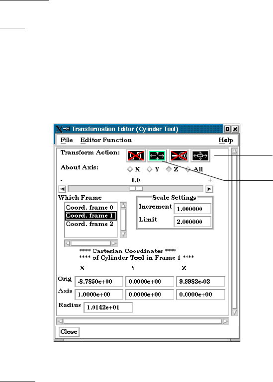
6.5 Tools Menu Functions
EnSight 7 User Manual 6-35
the Box Tool. First, the Box Tool may be positioned within the Graphics Window by
entering coordinates for the origin of the box in the X, Y, and Z fields and the length of the
each of the X, Y, and Z sides. Pressing return causes the Box Tool to relocate to the
specified location in the selected Frame (or if more than one Frame is selected, in Frame
0).
Additionally, you can modify the orientation of the Box Tool by entering the X, Y, and Z
orientation vectors of the box axis in regards to Frame 0.
As with other Tools, it is possible to reposition the Box Tool from its present coordinate
position by specific increments. First click the translate icon at the top of the
Transformation Editor. The Axis Button allows you to choose the axis of translation (X,
Y, Z, or All) for the origin of the Box Tool (intersection of the axes). The Slider Bar at Top
allows you to quickly choose the increment by which to move the position of the origin.
Dragging the slider in the negative (left) or positive (right) directions and then releasing it
will cause the X, Y, and Z coordinate fields to increment as specified and the origin of the
Box Tool to relocate to the new coordinates. The number specified in the Limit field of the
Scale Settings area determines the negative (-) and positive (+) range of the slider. If the
Limit is set to 1.0 as shown, then the numerical range of the slider bar will be -1 to +1.
Alternatively, you can specify an increment for translation in the Increment field of the
Scale Settings area. Pressing return while the mouse pointer is in the Increment field will
cause the origin of the Box Tool to translate along the specified axis (or all axes) by the
increment specified.
Orientation
First click on the rotate icon. Next, pick an axis about which to rotate. Next pick an
increment and limit (in degrees) and slide the slider to rotate the Box Tool.
Scale
First click on the scale icon. Next pick an axis direction to scale. Finally pick an
increment and limit and slide the slider to scale the size of the Box Tool.
Access: Transformation Editor > Editor Function > Tools > Box
(see How to Use the Box Tool)
Cylinder or Sphere Clicking on Editor Function in the Transformation Editor dialog and then selecting
To o l s Tools and then Cylinder or Sphere from the pull-down menu configures the dialog as
shown below.
The Transformation Editor can control precisely the position and size of the cylinder tool.
Position
The Transformation Editor dialog enables you to precisely control the coordinates of the
Cylinder or Sphere Tool origin (center point of the thick direction line) by specifying them
Figure 6-20
Transformation Editor (Cylinder Tool) or
(Sphere Tool)
Translate Icon
Scale Icon
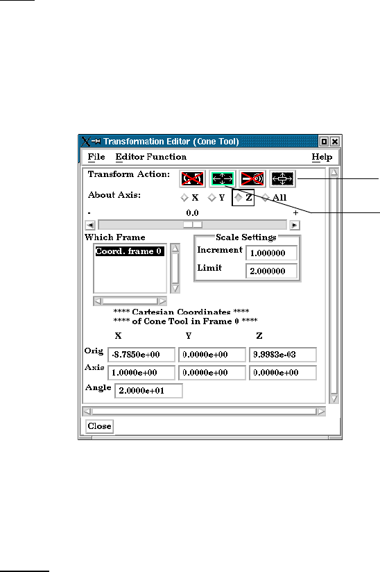
6.5 Tools Menu Functions
6-36 EnSight 7 User Manual
in the Orig. X, Y, and Z fields. You control the direction vector for the Cylinder or Sphere
Tool direction axes by specifying the coordinates in the Axis X, Y, and Z fields of the
selected Frame (or if more than one Frame is selected, in Frame 0). The Radius of each
tool may be specified in the Radius Field.
It is possible to reposition the Cylinder or Sphere Tool origins by specific increments. First
click on the translate icon. The Axis Button allows you to choose the axis of translation
(X, Y, Z, or All) for the origin of the tool. The Slider Bar at Top allows you to quickly
choose the increment by which to move the position of the origin. Dragging the slider it in
the negative (left) or positive (right) directions and then releasing it will cause the X, Y,
and Z coordinate fields to increment as specified and the origin of the Cylinder or Sphere
Tool to relocate to the new coordinates. The number specified in the Limit field of the
Scale Settings area determines the negative (-) and positive (+) range of the slider. If the
Limit is set to 1.0 as shown, then the numerical range of the slider bar will be -1 to +1.
Alternatively, you can specify an increment for translation in the Increment field of the
Scale Settings area. Pressing return while the mouse pointer is in the Increment field will
cause the origin of the Cylinder or Sphere Tool to translate along the specified axis (or all
axes) by the increment specified.
Scale
First click on the scale icon. Next pick an axis direction to scale. Can only scale in the X
(longitudinal) or Y (radial) directions. Finally pick an increment and limit and slide the
slider to scale the size of the cylinder or sphere Tool.
Access: Transformation Editor > Editor Function > Tools > Cylinder or Sphere
(see How To Use the Cylinder Tool and How To use the Sphere Tool)
Cone Tool Clicking on Editor Function in the Transformation Editor dialog and then selecting Tools
and then Cone from the pull-down menus configures the dialog as shown below.
The Transformation Editor dialog enables you to precisely control the coordinates of the
Cone Tool origin (the point of the cone) by specifying them in the Orig. X, Y, and Z fields.
You control the direction vector for the Cone Tool direction axis by specifying the
coordinates in the Axis X, Y, and Z fields for the selected Frame (or if more than one
Frame is selected, in Frame 0). The conical half angle may be specified in degrees in the
Angle Field.
Position
It is possible to reposition the Cone Tool origin by specific increments. The Axis Button
allows you to choose the axis of translation (X, Y, Z, or All) for the origin of the tool. The
Slider Bar at Top allows you to quickly choose the increment by which to move the
Figure 6-21
Transformation Editor (Cone Tool)
Translate Icon
Scale Icon
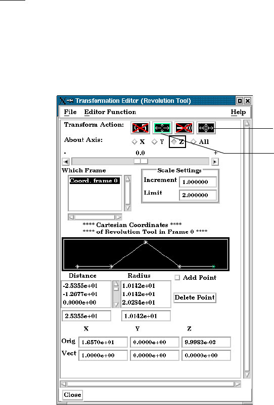
6.5 Tools Menu Functions
EnSight 7 User Manual 6-37
position of the origin. Dragging the slider in the negative (left) or positive (right)
directions and then releasing it will cause the X, Y, and Z coordinate fields to increment as
specified and the origin of the Cone Tool to relocate to the new coordinates. The number
specified in the Limit field of the Scale Settings area determines the negative (-) and
positive (+) range of the slider. If the Limit is set to 1.0 as shown, then the numerical range
of the slider bar will be -1 to +1.
Alternatively, you can specify an increment for translation in the Increment field of the
Scale Settings area. Pressing return while the mouse pointer is in the Increment field will
cause the center of the Cone Tool to translate along the specified axis (or all axes) by the
increment specified.
Scale
First click on the scale icon. Next pick an axis direction to scale. Can only scale in the X
(longitudinal) or Y (half conical angle) directions. Finally pick an increment and limit and
slide the slider to scale the size of the cone tool.
Access: Transformation Editor > Editor Function > Tools > Cone
(see How to Use the Cone Tool)
Revolution Tool Clicking on Editor Function in the Transformation Editor dialog and then selecting Tools
and then Revolution from the pull-down menu configures the dialog as shown below.
For the Revolution Tool, you not only control the origin and direction vector, but the
number of points and positions that are revolved about the axis.The desired coordinates of
the Revolution Tool origin (center point of the thick direction line) are specified in the
Orig. X, Y, and Z fields. The direction vector for the Revolution Tool direction axis is
specified by entering the desired coordinates in the Vect X, Y, and Z fields for the selected
Frame (or if more than one Frame is selected, in Frame 0).
Additional points may be added to the Revolution Tool by clicking on the Add Point(s)
toggle and then clicking at the desired location in the schematic for the tool. There is no
need to be overly precise in its placement since its location can be modified. Once you
have added all of the new points you wish, the Add Point(s) toggle should be turned off.
Figure 6-22
Transformation Editor (Revolution Tool)
Translate Icon
Scale Icon

6.5 Tools Menu Functions
6-38 EnSight 7 User Manual
A point may be deleted by selecting it in the schematic area and then clicking the Delete
button.
The position of any point may be modified interactively within the Revolution Tool
schematic window, Simply click on and drag the point to the desired location. The precise
location of any point may be specified by selecting the point in the schematic with the
mouse and then entering the desired Distance (from the Revolution Tool origin) or Radius
(from the axis) for the point in the text entry fields beneath the Distance and Radius Lists.
Pressing return will enter the new value in the list above for the selected point.
The Transformation Editor can control precisely the position and size of the revolution
tool.
Position
It is possible to reposition the Revolution Tool origin by specific increments. First click on
the translate icon. The Axis Button allows you to choose the axis of translation (X, Y, Z,
or All) for the origin of the tool. The Slider Bar at Top allows you to quickly choose the
increment by which to move the position of the origin. Dragging the slider in the negative
(left) or positive (right) directions and then releasing it will cause the X, Y, and Z
coordinate fields to increment as specified and the origin of the Revolution Tool to
relocate to the new coordinates. The number specified in the Limit field of the Scale
Settings area determines the negative (-) and positive (+) range of the slider. If the Limit is
set to 1.0 as shown, then the numerical range of the slider bar will be -1 to +1.
Alternatively, you can specify an increment for translation in the Increment field of the
Scale Settings area. Pressing return while the mouse pointer is in the Increment field will
cause the center of the Revolution Tool to translate along the specified axis (or all axes) by
the increment specified.
Scale
First click on the scale icon. Next pick an axis direction to scale. Can only scale in the X
(longitudinal) or Y (radial) directions. Finally pick an increment and limit and slide the
slider to scale the size of the revolution tool.
Redraw This button will cause the Revolution Tool schematic window to re-center to the currently
defined points of the tool.
Access: Transformation Editor > Editor Function > Tools > Revolution
(see How to Use the Surface of Revolution Tool)

6.6 Case Menu Functions
EnSight 7 User Manual 6-39
6.6 Case Menu Functions
EnSight allows you to work concurrently with up to sixteen different sets of
results data (computational or experimental). Each set of results data is read in as
a “Case”.
Clicking the Case button in the Main Menu opens a pull-down menu which
provides access to the following features:
Add, Replace, Delete... Opens the File Selection dialog.
Case Turndown Button
Add... Opens a dialog which allows you to specify a name and other options for the new Case.
The name will appear in the list of active Cases at the bottom of the Main Menu: Case
pull-down menu as shown in Figure 6-23 above. Adding a Case actually starts a new
EnSight Server and connects it to the EnSight Client. You then read and load data files for
Figure 6-23
Case pull-down menu
Figure 6-24
File Selection Dialog to Add, Replace or Delete a Case
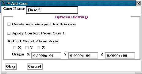
6.6 Case Menu Functions
6-40 EnSight 7 User Manual
the new Case and the data will be added to the data already present in the EnSight Client.
When adding a case, you can have some options. The new case can be placed in a new
viewport or added to the current. It can have the context of case1 applied to it, which will
cause it to basically inherit the positioning etc.of case 1. And you can even reflect the new
case about any of the major axes and specify the origin as it is read.
Replace... Replacing a Case causes all parts and variables associated with the active Case to be
deleted. The Server will be restarted and assigned the new Case name. Clicking the
Replace... button opens a small dialog which allows you to specify a name for the Case
you wish to use to replace the Case currently selected in the Main Menu: Case pull-down
menu as shown in Figure 6-23 above. You then read and load data for the new Case.
Delete Deleting a Case causes all parts and variables associated with the Case to be deleted and
terminates the Server associated with the Case. Clicking the Delete button opens a
Warning Dialog which asks you to confirm that you wish to delete the Case currently
selected in the Main Menu: Case pull-down menu as shown in Figure 6-23 above.
(see How To Load Multiple Datasets (Cases))
Viewport Visibility... Opens the Case Visible In Which Viewport dialog which allows you to specify in which
Viewports (including the Main Graphics Window) you wish to make the parts associated
with the currently selected Case visible. Parts associated with the selected Case will be
visible in the viewports outlined in green and invisible in those outlined in red. Visibility
for specific Parts can of course be toggled on/off using the Part Visibility Icon in the Part
Mode Icon Bar.
(see Part Visibility Toggle Icon in Section 8.1, Part Mode)
Restrict List Info. Toggling this menu selection on will restrict all lists displayed in EnSight (such as the
Per Case Toggle Parts and variables Lists) to show only information pertaining to the Case currently
selected in the Main Menu: Case pull-down menu as shown in Figure 6-23 above.
Finally, at the bottom of the pull-down menu you will find a list of active Cases,
The toggle buttons allow the selection of only one Case at a time. In Figure 6-23
above, Case 1 is the currently selected Case. The current selected Case is the one
which will be affected by the Data Reader, Querys, and many other operations.
Figure 6-25
Add Case Dialog
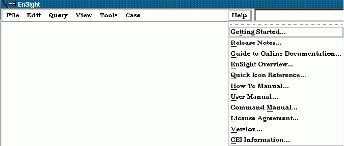
6.7 Help Menu Functions
EnSight 7 User Manual 6-41
6.7 Help Menu Functions
Clicking the Help button in the Main Menu opens a pull-down menu which
provides access to the following features:
Getting Started... Opens the Getting Started Manual on-line. Note that this document is not cross-referenced
within itself or to other documents.
Release Notes... Provides an overview of changes made since the last major EnSight release.
Guide to Online Provides a guide to the use of the On-Line Documentation.
Documentation...
EnSight Overview... Provides an overview of EnSight.
Quick Icon Provides a quick reference guide to all EnSight GUI icons, many of which have links to
Reference... appropriate How To documents
How To Manual... Opens the How To Manual on-line.
User Manual... Opens the User Manual on-line.
Command Manual... Opens the Command Language Manual on-line.
License Agreement... Opens up On-Line Documentation to the text of the EnSight End User License Agreement
and the EnSight Support and Maintenance Service Agreement.
Version... Opens up the Version Information dialog which states the version number of the EnSight
software currently running.
CEI Information... Opens up the CEI Information display which gives full CEI contact information.
Figure 6-26
Help pull-down menu
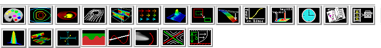
EnSight 7 User Manual 7-1
7 Features
This chapter describes the functions available through the Feature Icon Bar.
Section 7.1, Color
Section 7.2, Contour Create/Update
Section 7.3, Isosurface Create/Update
Section 7.4, Particle Trace Create/Update
Section 7.5, Clip Create/Update
Section 7.6, Vector Arrow Create/Update
Section 7.7, Elevated Surface Create/Update
Section 7.8, Profile Create/Update
Section 7.9, Developed Surface Create/Update
Section 7.10, Displacements On Parts
Section 7.11, Query/Plot
Section 7.12, Interactive Probe Query
Section 7.13, Solution Time
Section 7.14, Flipbook Animation
Section 7.15, Keyframe Animation
Section 7.16, Subset Parts Create/Update
Section 7.17, Tensor Glyph Parts Create/Update
Section 7.18, Material Parts Create/Update
Section 7.19, Vortex Core Create/Update
Section 7.20, Shock Surface/Region Create/Update
Section 7.21, Separation/Attachment Lines Create/Update
Section 7.22, Boundary Layer Variables Create/Update
Figure 7-1
EnSight Feature Icon Bar
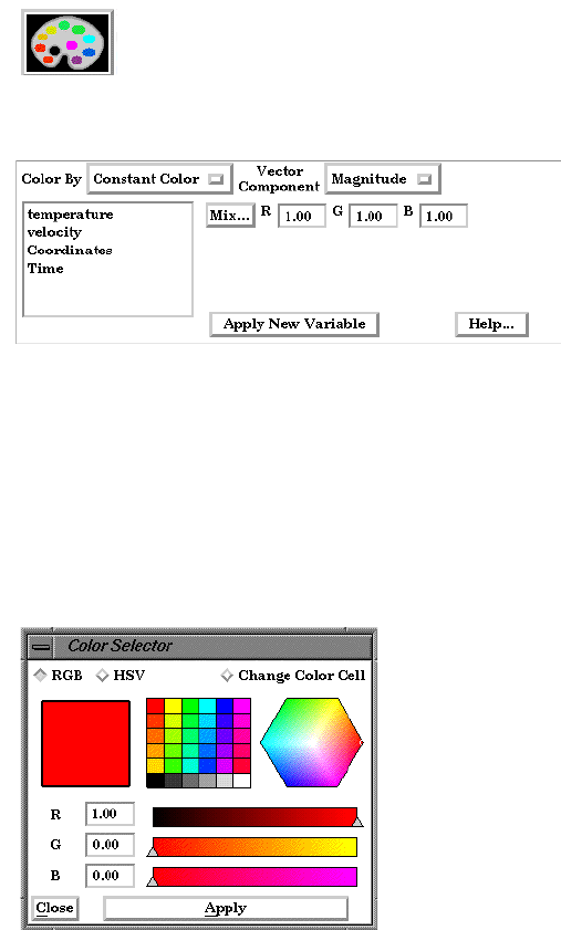
7.1 Color
7-2 EnSight 7 User Manual
7.1 Color
Clicking once on the Color Icon opens the Color Editor in the Quick Interaction
Area which allows you to assign color to the individual Part(s) which has(have)
been selected in the Parts List. If no Parts are selected, modifications will affect
the default Part color and all Parts subsequently loaded or created will be assigned
the new default color.
Color By Opens a pull-down menu which allows you to choose whether to color the selected Part(s)
by a Constant Color or by the Variable selected in the Variables List.
Constant Color The selected Part(s) may be assigned a constant color in two ways. First, the color may be
assigned by entering red, green, and blue numerical values (0.0 to 1.0) in the R,G,B fields
of the Quick Interaction Area and then pressing the return key.
Mix... Second, you can click on the Mix... button and the Color Selector dialog will open.
You can choose whether you wish to use the RGB color scheme or HSV. A color may be
chosen in one of four ways. First, a color may be chosen from one of the color cells (small
squares of constant color). Second, you can grab the small circle in the color assignment
hexagon and interactively pick the desired color. Third, you can pick a color by entering
numerical values (0.0 to 1.0) in the numerical (RGB or HSV) fields and then pressing
return key. Finally, you can interactively choose a color by using the slider bars to the right
of the numerical (RGB or HSV) fields which adjust the values therein (the color in the
slider bars indicates the effect that modifying the color components will have on the final
color).
Figure 7-2
Color Icon
Figure 7-3
Quick Interaction Area - Color Editor - Constant Color
Figure 7-4
Color Selector dialog
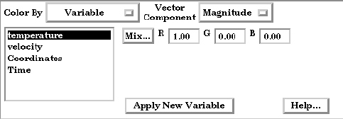
7.1 Color
EnSight 7 User Manual 7-3
It is possible to assign to the Color Cells area a color that you have specified in one of the
other three ways by clicking the Change Color Cell and then clicking on the cell to which
you wish to assign the currently defined color (as shown in the large rectangle to the left).
This reassignment will be retained for use in subsequent EnSight sessions.
Regardless of which method you use to define a color, it will not be applied to the selected
Part(s) unless and until you click the Apply button.
Variable Alternatively, the Part(s) may be colored by a variable selected in the Variables List
instead of by one constant color. The color palette for each Variable associates a color with
each value of the variable and these colors are used to color the selected Part(s).
Vector Component If you are coloring by a vector variable, this opens a pull-down menu which allows you to
choose whether you wish to color using the magnitude or a component of the vector.
Magnitude Color by the vector magnitude.
X Color by the vector’s X component.
Y Color by the vector’s Y component.
Z Color by the vector’s Z component.
Apply New Variable Changes the color palette used to color the selected Part(s) to that of the variable currently
chosen in the Variables List. If more than one variable is selected, then the color palette of
the first selected variable will be used.
Feature Detail Editor Double clicking on the Color Icon will open the Feature Detail Editor (Variables)
(Variables) dialog.
(see Section 4.1, Variable Selection and Activation, Section 4.2, Variable
Summary & Palette, and How To Edit Color Palettes)
Figure 7-5
Quick Interaction Area - Color Editor - Variable
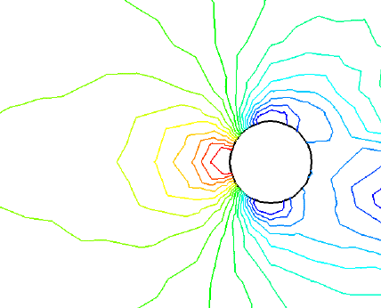
7.2 Contour Create/Update
7-4 EnSight 7 User Manual
7.2 Contour Create/Update
Contours are lines that trace out constant values of a variable across the surface(s)
of selected Part(s), just like contour lines on a topographical map.
The variable must be a node-based scalar, but can, of course, be a function of a
vector variable (i.e., the magnitude or a component). A Contour Part can consist
of one contour line, or a set of lines corresponding to the value-levels of the
variable palette. A Contour Part has its own attributes independent of those Parts
used to create it (the parent Part(s)).
Contours are drawn across the faces of parent Part elements (one-dimensional
elements are ignored). At each node along the edges of any one element face, the
contour’s variable has a value. If the range of these values includes the contour’s
value-level, the contour line crosses the face. EnSight draws the contour by
dividing the face into triangles each having the face’s centroid as one vertex. For
each triangle the contour crosses, it will cross only two sides. EnSight interpolates
to find the point on each of those two sides where the variable value equals the
contour value-level, then creates a bar element to connect the two points. Note
that a contour line can bend while crossing an element face.
Because Contour Parts are created on the EnSight Client, the Representation
attribute of the parent Part(s) greatly affects the result. Representations that reduce
Part elements to one-dimensional representations (Border applied to two-
dimensional Parts and Feature Angle), or do not download the Part (Not Loaded),
will eliminate those Part elements from the Contour creation process. On the other
hand, Full representation of three-dimensional elements will create contour lines
across hidden surfaces. Usually, you will want the Representation selection to be
3D Border, 2D Full.
Contour Parts are created on the Client, and so cannot be queried or used in
creating new variables. However, Contours can be used as parent Parts for Profiles
and Vector Arrows.
If you change the value-levels in the Feature Detail Editor (Variables) Summary
and Palette section, the Contour automatically regenerates using the new value-
levels.
Figure 7-6
Pressure Contours in a Flow Field around a Circular Obstruction
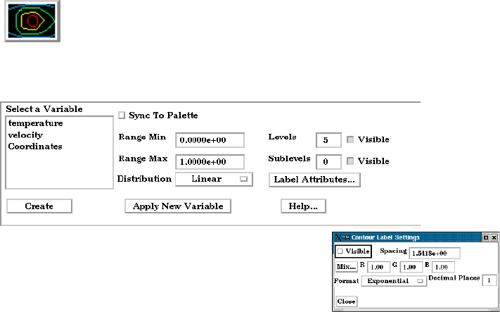
7.2 Contour Create/Update
EnSight 7 User Manual 7-5
Use care when simultaneously displaying contours based on different function
palettes so that you do not become confused as to which contours are which.
Coloring them differently and adding an on-screen legend can help.
Clicking once on the Contour Create/Update Icon opens the Contour Editor in the
Quick Interaction Area which is used to both create and update (make changes to)
contour Parts.
Sync To Palette Toggles on/off the contour line synchronization to the legend color palette.
Range Min This field is activated when Sync to Palette Toggle is Off.
Range Max This field is activated when Sync to Palette Toggle is Off.
Distribution This pop-up menu is activated when Sync to Palette Toggle is Off. Opens a pop-up menu
for the selection of a distribution function for the contour lines. Choices include Linear,
Logarithmic, and Quadratic.
Levels This field is activated when Sync to Palette Toggle is Off. This field determines the
number of contours between the Range Min and Range Max.
Visible Toggles whether the main level contours are visible or not.
Sublevels This field allows you to specify the number of sub-contours you wish to be drawn at
evenly spaced value-levels between the value-levels defined in the Variable Feature Detail
Editor Summary and Palette section. Leaving this field 0 will produce exactly the number
of contour lines for which value levels are specified in the Feature Detail Editor
(Variables) Summary and Palette.
Visible Toggles whether the sublevel contours are visible or not.
Label Attributes... Opens the Contour Label Settings dialog.
Visible Toggle Toggles on/off the visibility of number labels for contour lines.
Spacing Determines the spacing between number labels.
Mix... Opens the Color Selector dialog for the assignment of a color to number labels.
R,G,B Allows the specification of red, green, and blue values for the assignment of a color to
number labels.
Format This pop-up menu allows selection of format of number labels. Choices include
Figure 7-7
Contour Create/Update Icon
Figure 7-8
Quick Interaction Area - Contour Editor

7.2 Contour Create/Update
7-6 EnSight 7 User Manual
Exponential, and Floating Point.
Decimal Places This field allows the specification of the number of decimal places of the number labels.
Create Creates a Contour Part using the selected Part(s) in the Parts List and the color palette
associated with the Variable currently selected in the Main Variables List.
Apply New Variable Will change the Contour Part to show contours based on the color palette associated with
the Variable currently selected in the Variables List.
Feature Detail Editor Double clicking on the Contour Create/Update Icon opens the Feature Detail
(Contours) Editor (Contours), the Creation Attributes Section of which provides access to the
same functions available in the Quick Interaction Area, as well as one more. For a
detailed discussion of the remaining Feature Detail Editor turn-down sections
(which are the same for all Part types):
Display offset This field specifies the normal distance away from a surface to display the
contours. A positive value moves the contours away from the surface in the
direction of the surface normal. A negative value moves in the negative surface
normal direction.
Please note that there is a hardware offset that will apply to contours, vector arrows,
separation/attachment lines, and surface restricted particle traces that can be turned on
or off in the View portion of Edit->Preferences. This preference (“Use graphics hardware
to offset line objects...”) is on by default and generally gives good images for everything
except move/draw printing. This hardware offset differs from the display offset in that it is
in the direction perpendicular to the computer screen monitor (Z-buffer)
.
Thus, for viewing, you may generally leave the display offset at zero. But for
printing, a non-zero value may become necessary so the contours print cleanly.
(see Section 3.3, Part Editing and How to Create Contours)
Troubleshooting Contours
Problem Probable Causes Solutions
No contours created. Variable values on element faces are
outside range of palette function
value-levels.
Adjust palette function using the
Feature Detail Editor (Variables)
Summary and Palette section.
Parent Parts do not contain any 2D
elements.
Re-specify Parent Part list.
Parent Parts do not contain the
specified Variable.
Recreate the Variable for the selected
Parent Part(s).
Too many contours. Palette has too many function levels. Change the number of levels for the
palette using the Feature Detail
Editor (Variables) Summary and
Palette.
Specified too many sub-contours. Lower the sub-contour attribute.
Too few contours. The palette levels do not adequately
cover the function value range for
the Parent Parts.
Modify the palette using the Feature
Detail Editor (Variables) Summary
and Palette.
Sub-contour attribute set to 0. Modify the Sub-contour attribute.
Contour Part created but (empty) Parent Part is in Feature Angle
representation.
Change Parent Part to 3D border, 2D
full representation.

7.2 Contour Create/Update
EnSight 7 User Manual 7-7
Contours are fine at first, but later go
away.
Parent Parts representation changed
to Feature Angle, or Not Loaded.
The contours are created from the
Part representation on the EnSight
client. Modifying the representation
affects the Contour Parts.
Contour parts don’t print well See Display Offset above. Enter a display offset (may need to
be less than zero if viewed from
“backside”).
Problem Probable Causes Solutions
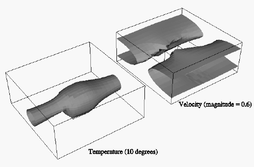
7.3 Isosurface Create/Update
7-8 EnSight 7 User Manual
7.3 Isosurface Create/Update
Isosurfaces are surfaces that follow a constant value of a variable through three-
dimensional elements. Hence, isosurfaces are to three-dimensional elements what
contour lines are to two-dimensional elements.
An isosurface may be based on a vector variable (magnitude or components), or a
scalar variable.
At each node of a three-dimensional element, the isosurface’s variable has a value.
If the range of these values includes the isosurface’s isovalue, the isosurface cuts
through the element. EnSight draws the isosurface through that element by first
determining which edges the isosurface crosses, and then interpolating to find the
point on each of those edges corresponding to the isovalue. EnSight connects
these points with triangle elements passing through the parent Part elements. If the
Parent Part(s) contain two-dimensional elements, a line is created across the
elements - just like a contour.
All the triangle elements created inside all the three-dimensional elements of all
the parent Part(s) together with all the lines created across the two-dimensional
elements of all the Parent Part(s) constitute the isosurface. One-dimensional
elements of the parent Part(s) are ignored. Because isosurfaces are generated by
the server, the Representation of the parent Part(s) is not important.
You can interactively manipulate the value of an isosurface with a slider allowing
you to scan through the min/max range of a variable. This scanning can also be
done automatically. The isosurface will change shape as the value is changed.
If you are using animation, you can specify an Animation Delta value by which
the isovalue is incremented for each animation frame or page. The isosurface is
automatically updated to appear as if it had been newly created at the new location
and time.
Figure 7-9

7.3 Isosurface Create/Update
EnSight 7 User Manual 7-9
Clicking once on the Isosurface Create/Update Icon opens the Isosurface Editor in
the Quick Interaction Area which is used to both create and update (make changes
to) isosurface Parts.
Value Specification of numerical isovalue of the isosurface. To avoid an empty Part, this value
must be in the range of the Variable within the Parent Parts. You can find this range using
the Variables dialog or by showing the Legend for the Variable. For vector-variable-based
isosurfaces, the vector magnitude is used.
Interactive Opens pull-down menu for selection of type of interactive manipulation of the isosurface
value. Options are:
Off Interactive isosurfaces are turned off.
Manual Value of the isosurface(s) selected are manipulated via the slider bar and the
isosurface is interactively updated in the Graphics Window to the new value.
Auto Value of the isosurface is incremented by the Auto Delta value from the minimum
range value to the maximum value when the cursor is moved into the Main
View. When reaching the maximum it starts again from the minimum.
Auto Cycle Value of the isosurface is incremented by the Auto Increment value from the
minimum range value to the maximum value. When reaching the maximum
it decrements back to the minimum.
Auto Delta Specification of the increment for the Auto and Auto Cycle options to use when
modifying the value between the minimum and maximum values.
Min Specification of the minimum isosurface value for the range used with the “Manual” slider
bar and the “Auto” and “Auto Cycle” options.
Max Specification of the maximum isosurface value for the range used with the “Manual”
slider and the “Auto” and “Auto Cycle” options.
Increment Specification of the increment/decrement the slider will move within the min and max,
each time the stepper buttons are clicked.
Create Creates an isosurface Part at the value specified for the variable selected in the Variables
List and from the Part(s) selected in the Parts List.
Apply New Variable Will recreate the isosurface Part at the value specified for the variable currently selected in
the Variables List.
Figure 7-10
Isosurface Create/Update Icon
Figure 7-11
Quick Interaction Area - Isosurface Editor
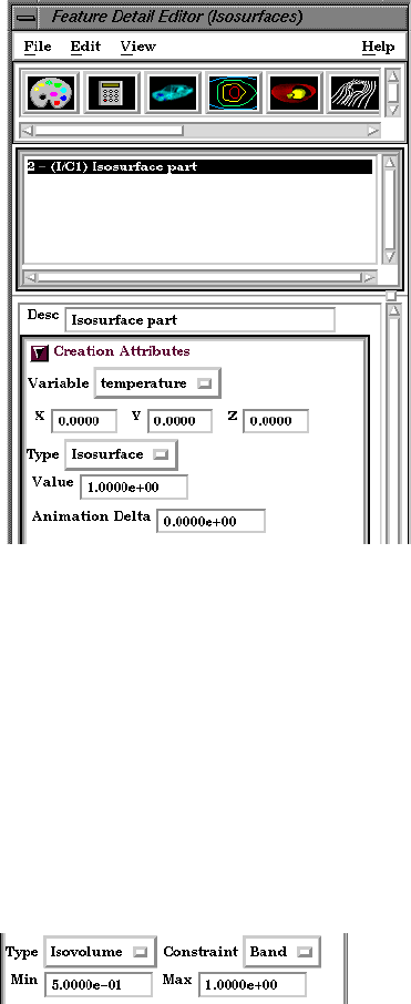
7.3 Isosurface Create/Update
7-10 EnSight 7 User Manual
Feature Detail Editor Double clicking on the Isosurface Create/Update Icon opens the Feature Detail
(Isosurfaces) Editor (Isosurfaces), the Creation Attributes Section of which provides access to
additional features for isosurface creation and modification:
Variable Opens a pop-up menu for the selection of an active Variable to use to calculate the
isosurface.
X Y Z These fields specify the vector- component coefficients. When the three fields are set to
0.0000, the vector magnitude is used for the isosurface calculation. Otherwise, the sum of:
(Vector
x
* X)+(Vector
y
*Y) + (Vector
z
*Z) is used as the isosurface value.
Type
Isosurface Specification that an Isosurface type part created from the specified Variable and selected
parts will have the isovalue of Value for all its elements.
Value Specification of the numerical isovalue of the Isosurface Part(s) selected in the Feature
Detail Editor's Parts List (or if none is selected, of the isosurface you are about to Create).
Isovolume Specification that an Isovolume type part created from the specified Variable and selected
parts will consist of elements with isovalues constrained to either below a Min, above a
Max, or within the specified interval of Min and Max.
Constraint Specification restricting the element isovalues of the Isovolume Part to an interval. The
Constraint options are:
Low all elements of Isovolume Part have isovalues below the specified Min value.
Band all elements of Isovolume Part have isovalues within the specified Min and
Max interval values.
High all elements of Isovolume Part have isovalues above the specified Max value.
Figure 7-12
Feature Detail Editor (Isosurfaces) Creation Attributes Area
Figure 7-13
Feature Detail Editor (Isovolume) Creation Attributes Area
7.3 Isosurface Create/Update
EnSight 7 User Manual 7-11
Min Specification of the minimum isovalue limit for the Isovolume Part.
Max Specification of the maximum isovalue limit for the Isovolume Part.
Animation Delta This field specifies the incremental change in isovalue for each frame or page of
animation. It can be negative.
(see Section 7.14, Flipbook Animation and Section 7.15, Keyframe Animation)
Create (At the bottom of the Feature Detail Editor) Creates an Isosurface Part at the value
specified for the variable selected in the Variable pop-up menu of the Creation Attributes
section and from the Part(s) selected in the Main Parts List.
The Feature Detail Editor also allows you to make changes in batch; that is, to
make several changes to the menus and fields which do not effect the Graphics
Window until you click in the Apply Changes button. It is sometimes quicker
(with respect to CPU time) to make several changes at once rather than one at a
time as in the Quick Interaction Area.
For a detailed discussion of the remaining Feature Detail Editor turn-down
sections (which are the same for all Parts):
(see Section 3.3, Part Editing and How To Create Isosurfaces
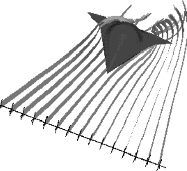
7.4 Particle Trace Create/Update
7-12 EnSight 7 User Manual
7.4 Particle Trace Create/Update
A Particle trace visualizes a vector field by displaying the path that a massless
Particle would follow if placed in that field. At each point on the Particle trace, the
direction of the trace is parallel to the vector field at that point and time.
A streamline is a Particle trace in a steady-state vector field, while a pathline is a
Particle trace in a time-varying vector field. Particle traces can be lines or
“ribbons” (that additionally visualize the rotation of the vector field around the
path of the trace).
EnSight is capable of computing a pathline through a model with changing
coordinates and/or changing connectivity. The variable values are assumed to
behave linearly between the known timesteps.
Particle Trace Parts have their own attributes, so you can, for example, trace a
flow field using the velocity variable, and then color the resulting trace using the
temperature variable.
Emitters A Particle Trace Part consists of one or more Particle traces originating from
points on one or more emitters. Each emitter is capable of emitting a Particle
starting at a specified time and continuing to emit Particles at given intervals.
When pathlines are generated with emitters emitting at multiple time intervals and
these traces are then animated, streaklines are displayed.
Emitters consist of single points, points along a line, points forming a grid in a
plane, or points corresponding to the nodes of a Part. You can define emitters
using the Cursor tool, the Line tool, the Plane tool, or a Part.
Emitters can be created using the cursor, line, and plane tools, using existing Part
nodes, or can be created in a surface restricted mode where the mouse can be used
to project points, rakes or nets directly onto the displayed surfaces of the model.
Pathlines, of course, must be drawn forward in time, but streamlines can be drawn
forward in time, backward in time, or both. Each Particle trace terminates when
either (1) the Particle trace moves outside the space in which the vector field is
defined, (2) a user-specified time limit is reached, (3) the massless Particle
becomes stationary in a place where the vector field is zero, or (4) the last
transient-data time step is reached. (4 applies only to pathlines)
Figure 7-14
Particle Trace Illustration
7.4 Particle Trace Create/Update
EnSight 7 User Manual 7-13
A Particle trace can pass through any point inside an element of the parent Part(s).
The vector field at any point is calculated from the shape function of the
containing element. Emitter points located outside the elements are ignored when
creating Particle traces.
Surface-Restricted A surface-restricted Particle trace is constrained to the surface of the selected
Traces Part(s) by using only the tangential component of the velocity. The velocity values
for this type of trace can be the velocity at the surface (if nonzero) or at some user
specified offset into the velocity field.
Interactive Traces A Particle trace can be updated interactively by entering interactive mode and
moving the tool used to create the emitter. When a trace is selected and interactive
emitter is turned on, the tool will appear at the location of the emitter. The user
then manipulates the tool interactively in the Graphics Window or using the
transformations dialog. (This option is not available for surface-restricted Particle
traces or traces emitted from a Part).
Integration Method EnSight creates Particle traces by integrating the vector field variable over time
using a Fourth Order Runge-Kutta method and utilizing a time varying integration
step. The integration step is lengthened or shortened depending on the flow field,
but you can control the minimum number of integration steps performed in any
element as well as other time step controls.
Normally, EnSight will perform the integration using all of the components of the
vector. However, it is possible to restrict the integration to a plane by specifying
which components of the vector to use. Typical uses of this feature would be to
restrict the Particle traces to a clip plane. Surface-restricted Particle traces provide
even greater flexibility in restricting a trace to planes or other surfaces.
Line-type Particle traces consist of bar elements. Ribbons consist of 4-noded quad
elements and originate with their end-edge parallel to the Z-axis of the global
frame. Then, at each integration step, the leading edge is rotated around the
current direction of the path by the same amount the vector field has rotated
around the path since the previous time step. Ribbons are not available for
surface-restricted Particle traces.
Particle Trace Parts are created on the server, so the Representation-type of the
parent Parts has no effect. The algorithm that creates Particle traces initially sets
up a cross-referencing map of adjoining elements. Hence, the first Particle trace
takes longer to generate than subsequent traces.
If you calculate pathlines, consider calculating as many as possible at a time, since
the process can be very time consuming (most of the time is taken in reading time
step information). However, the data for the Trace Part is sent to and stored on the
Client, Thus, you cannot label or make queries about Particle Trace Parts. Instead,
label or make queries about the Particle Trace’s parent Part(s). Line-type Particle
Traces can be parent Parts for Profiles. You can animate the motion of the
massless Particles along their Particle traces.
Transient Data By default the emission point is always set to emit the Particles at the current time
step. This can be a problem if you have a transient dataset with the current time set
at the last time step available. If you compute pathlines from this location, the
default emission time will be at the current time (last time step), thus no pathlines
will be generated. To solve this problem you will need to either change the current
time, or change the Start Time of the emitter.

7.4 Particle Trace Create/Update
7-14 EnSight 7 User Manual
The process of creating a Particle trace is always to specify an emission point
(location and time), specify the Part(s) to trace the Particle through and specify
which vector variable to integrate. There are quick ways of doing this process
which assume that the correct defaults are set, or there are more deliberate ways
which give you more control. Particle trace Parts carry only one set of attributes
for all of the traces in the Part, thus it is not possible, for example, to trace some of
the emission points forward in time and others backward in time.
Particle trace Parts are different from all other created Parts in that when the
parent Parts change (such as at a time step change), the Particle trace Part does not
change. This is due to the fact that the Particle trace has been created at a specified
time (the emission time), making the Part independent of time (after the trace has
been created).
Regular Particle traces can only be computed through a set of parent Parts
consisting of model Parts. Surface-restricted Particle traces can be created on
model Parts, clip Parts, elevated surface Parts, and developed surface Parts.
If your dataset contains 3D elements, the Particles for regular traces will be traced
through 3D element fields only. Surface-restricted traces would have to be used to
trace along 2D elements of such a data set.
Massed-Particle Traces A particle trace can be created or updated from a massless-particle trace to a
massed-particle trace, or visa-versa. Massed-particle traces are specified via their
appended section in the Feature Detailed Editor (Traces) dialog. Massed-particle
traces switch to massless-particle traces during interactive mode.
Definitions
Motion of a particle as a function of its velocity is defined as
d/dt(X
p
)=V
p
with initial conditions V
p
(t
0
)=V
p,0
and initial particle position
X
p
(t
0
)=X
p,0
(capital letters denote vectors unless otherwise indicated).
For massless particles, the particle velocity is always identical to the local fluid
velocity, V
p
=V
f
. For massed particles, additional forces acting on them result in a
different velocity for the V
p
than for the fluid, V
p
not equal to V
f
. This particle
velocity is determined from a momentum balance for the particle by
m
p
A
p
= F
p
,
or
m
p
d/dt(V
p
)=F
g
+F
p
+F
d
+F
e
,
where
A
p
= particle acceleration vector,
F
p
= total (particle) force vector,
F
g
= gravitational (body) force vector =m
p
bG,
F
p
= pressure (surface) force vector =-v
p
∇p
f
,
F
d
= drag (surface) force(s) vector =½ρ
f
a
p
c
d
|V
r
|V
r
,
F
e
= additional forces vector, here =0,

7.4 Particle Trace Create/Update
EnSight 7 User Manual 7-15
given the following definitions (Note: the underlined definitions are user
specified)
m
p
= particle mass = ρ
p
v
p
,
ρ
p
= particle density,
v
p
= particle volume =d
p
3
π/6,
d
p
= particle diameter,
b=particle buoyancy ratio =(ρ
p
- ρ
f
)/ρ
p
,
ρ
f
= fluid density (scalar or constant),
G=gravitational acceleration vector
,
∇p
f
= fluid pressure gradient vector, (computed from p
f
= fluid
pressure scalar variable)
a
p
= particle reference area =d
p
2
π/4,
V
r
= reference velocity vector =V
f
–V
p
,
c
d
= drag coefficient, typically given as a function of the local
relative Re, i.e. c
d
=c
d
(Re),
Re = Reynolds number = ρ
f
|V
r
|d
p
/ µ
f
,
µ
f
= fluid dynamic viscosity (scalar or constant).
Thus, the total mass balance equation for massed particles may be defined by:
m
p
d/dt(V
p
)=(m
p
bG)-(v
p
∇p
f
)+(½ρ
f
a
p
c
d
|V
r
|V
r
).
Drag Coefficient
Currently, the following Drag Coefficient (C
d
) table is provided as the default.
Re << 1 C
d
= 24/Re
1 < Re << 500 C
d
= 24/Re
0.646
500 < Re << 3e5 C
d
= 0.43
3e5 < Re << 2e6 C
d
= 3.66E-4 Re
.4275
2e6 < Re C
d
= 0.18
This table is also coded as an example for your reference and access via the User-
Defined Math Function DragCoefTable1(Re) which is found in
$CEI_HOME/ensight76/src/math_functions/drag_coef_table1/libudmf-drag_coef_table1.c
In addition, two other drag coefficient functions are provided for your selection
via the User-Defined Math Function facility.
DragCoefPoly(Re) = (a+bRe+cRe
2
+ d/Re )
Where: {a,b,c,d} are polynomial coefficients with default values of {1.,0.,0.,0},
respectively.
DragCoefPower(Re) = (1 + .15 Re
0.687
)24/Re
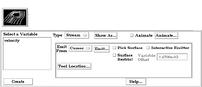
7.4 Particle Trace Create/Update
7-16 EnSight 7 User Manual
Both of these functions are located respectively in
$CEI_HOME/ensight76/src/math_functions/drag_coef_poly/libudmf-drag_coef_poly.cf
$CEI_HOME/ensight76/src/math_functions/drag_coef_power/libudmf-drag_coef_power.c
You may also code your own. (See UDMF in EnSight User Manual.)
Particle-Mass Scalar on Boundaries
Information to compute a particle-mass scalar on boundaries (m
P
= m
Pi
) is
provided each time massed-particle traces are created. This scalar is found and
computed via the New Computed Variables (NCV) functionality.
Massed Particle Scalar(massed-particle traced part(s))
This scalar creates a massed-particle per element scalar variable for each of the
parent parts of the massed-particle traces. This per element variable is the mass of
the particle times the sum of the number of times each element is exited by a
mass-particle trace.
References
The following references have contributed in part toward the development of the
massed-particle algorithm.
Donley, H. Edward
“The Drag Force on a Sphere”,
http:\\www.ma.iup.edu/projects/CalcDEMma/drag/drag.html
Lund, Christoph
“Vorgaben für die Berechnung und Visualisierung der Bahnlinien
massebehafteter Partikel im Postprozessor EnSight”, Volkswagen AG,
27.07.2001. English translation by Kent Misegades.
Fluid Dynamics International, Inc.
FIDAP 7.0 Theory Manual”, April 1993, pp12-3+
Clicking once on the Particle Trace Create/Update Icon opens the Particle Trace
Editor in the Quick Interaction Area which is used to both create and update
(make changes to) Particle trace Parts.
Type Opens a pull-down menu for specification of whether Particle trace calculation uses
steady-state data (streamlines) or transient data (pathlines).
Figure 7-15
Particle Trace Create/Update Icon
Figure 7-16
Quick Interaction Area - Particle Trace Editor
7.4 Particle Trace Create/Update
EnSight 7 User Manual 7-17
Stream Traces a massless Particle in a steady-sate vector field (for steady-state data or the current
time-step of transient data).
Path Traces a massless Particle through a time-varying vector field and so is only available
with transient results data. On certain systems, this selection can consume significant
quantities of CPU time to calculate the resulting Particle trace.
Show As Opens a dialog for specification of trace representation.
Line Depicts the trace as a line.
Ribbon Depicts trace as if it were a ribbon. The ribbon width is a specified fixed value, while the
twisting is determined by the rotation of the flow about the path of the trace at any
particular point on the trace.
Square Tubes Depicts trace as if it were a square tube. The tube width is a specified fixed value, while
the twisting is determined by the rotation of the flow about the path of the trace at any
particular point on the trace.
Animate Toggle Toggles on/off the animation of the motion of the Particles along the traces. In addition to
creating Particle traces based on vector variables, EnSight can also animate the motion of
the Particles along the Particle traces. To distinguish them from discrete Particles, we call
Particles moving along Particle traces “tracers.”
At any instant, each tracer consists of a portion of a Particle trace displayed with attributes
you specify separately from the attributes of the Particle trace. EnSight animates each
tracer by updating which portion of the Particle trace is currently displayed. You specify
the length of each tracer as a time value, so the tracer’s length varies dynamically as it
moves down the Particle trace (faster moving tracers are longer). This option can add
tremendously to the understanding of the flow field since relative speed can be
determined.
EnSight provides control over how the tracer looks and acts. You can animate one, some,
or all of the Particle traces you have created, but they are all animated in the one way you
specify. To help you get started, at the click of a button EnSight will suggest time-
specification values based on the Particle traces you have selected to animate. You can
specify the line width of the tracer, and choose to color it with a constant color or the same
calculated color used to color the Particle trace. You can also display a spherical “head” on
the leading-end of the tracer, and dynamically size the head according to any active
variable.
You control the speed of the motion and have the option to display multiple tracers on the
same Particle trace separated by a time interval. Hence, you can choose to view rapid-fire
pulses, slow moving “noodles,” or something in between. For steady-state Particle traces
(streamlines), “time” is the integration time with the emitters located at time zero. For
transient Particle traces (pathlines), you have the option to synchronize the animation time
to the solution time. The choice of whether a Particle trace is a streamline or a pathline is
made when you create the Particle trace.
You do not have to animate the entire Particle trace. You can specify where you want the
animation to start with a time value corresponding to a distance down the Particle trace
from the emitter, and where you want the animation to stop with a time value
corresponding to a distance farther down the Particle trace.
Tracers on all animated Particle traces are synchronized. If you combine Particle trace
animation with flipbook animation or keyframe animation, the animation time values are
automatically synchronized if you toggle-on Sync To Transient in the Trace Animation
Settings dialog.
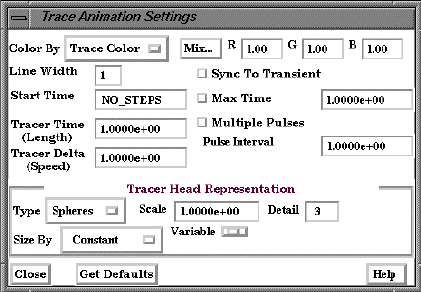
7.4 Particle Trace Create/Update
7-18 EnSight 7 User Manual
Animate... Opens the Trace Animation Settings dialog
Color By Opens a pull-down menu for selection of method by which to color the tracers.
Constant Displays tracers in the constant color specified in this dialog.
Mix… Opens the Color Selector dialog (See Figure 7-4 Color Selector dialog).
R,G,B Fields allow specification of constant color.
Trace Color Displays tracers in the same color as the Particle Trace Part from which they originate.
Line Width Specification of displayed width (in pixels) of tracers. Note: Line Width specification may
not be available on some workstation platforms.
Start Time Specification of how far down each Particle trace to begin displaying tracers. A Particle
trace is made up of line segments. Each segment that makes up a Particle trace has an
associated time value. The start time indicates where on the Particle trace the tracers will
begin animation.
Tracer Time (Length) Specification of length of tracers which varies as the tracer speed varies along the Particle
trace. The Particle Time Length parameter scales the length of all tracers at all times.
Tracer Delta (Speed) Specification of how fast tracers move. Longer times result in faster moving tracers. This
parameter is not applicable when using Sync To Transient and displaying transient data
through flipbook or keyframe animation.
Sync to Transient Toggles on/off synchronization of tracer position to solution time of transient data. When
Toggle toggled-on and transient data is in use, each tracer is displayed with its leading-end at the
correct location along the Particle trace for the current solution time. Traces only move
forward in time so cycling through transient data is not applicable here.
Max Time Toggle Toggles on/off maximum lifetime for all tracers. If toggled-off, tracers continue to end of
Particle trace. If toggled-on, each tracer stops after moving down the Particle trace for a
distance corresponding to the specified Max Time (or until one of the other conditions that
stop a tracer occurs).
Max Time Field specifies lifetime of all tracers when Set Max Time is toggled-on.
Multiple Pulses Toggle Toggles on/off multiple emission of tracers. When toggled-off, a single tracer for each
Particle trace appears at the specified Start Time. When toggled-on, additional tracers
appear after each specified Pulse Interval. Not applicable to pathlines.
Pulse Interval Field specifies time delay between tracers. Not applicable when Multiple Pulses is
toggled-off.
Tracer Head Representation
Type Opens a pull-down menu for selection of type of head for each tracer.
None Specifies that no head will appear.
Figure 7-17
Trace Animation Settings dialog

7.4 Particle Trace Create/Update
EnSight 7 User Manual 7-19
Spheres Specifies that a sphere will appear on the leading end of the tracer.
Scale Specification of scaling factor for head size. Values between 0 and 1 reduce the size,
factors greater than one enlarge the size. Not applicable when Head Type is None.
Detail Specification of detail-level of head in range from 2 to 10, with 10 being the most detailed
(e.g., rounder spheres because more polygons are used to create spheres). Higher values
take longer to draw, slowing performance. Not applicable when Head Type is None.
Size By Opens a pull-down menu for the selection of variable-type to use to size each tracer’s
head. If you select a variable, the head size is determined by multiplying the Scale factor
times the variable value, which will vary depending on the location of the tracer. Not
applicable when Head Type is None.
Constant Sizes head using just the Scale factor value.
Scalar Sizes head using a scalar variable.
Vector Mag Sizes head using magnitude a vector variable.
Vector X Sizes head using X-component of a vector variable.
Vector Y Sizes head using Y-component of a vector variable.
Vector Z Sizes head using Z-component of a vector variable.
Variable Selection of variable to use to size the tracer heads. Not applicable when Type is None or
Size By is Constant.
Get Defaults Click to set time-value specifications in this dialog to values suggested by EnSight based
upon the characteristics of the selected Particle traces.
See Also: How To Animate Particle Traces
Troubleshooting Animated Particle Traces
Problem Probable Causes Solutions
No motion. Can’t see any tracers. No Particle traces selected to
animate.
Select the traces you wish to animate
in the list at the top of the Animated
Trace Setup dialog.
Tracers colored same as Particle
traces and have same line width.
Change Color By or Line Width.
Animate Traces not toggled-on. Toggle Animate on in the Quick
Interaction Area.
Start Time > maximum Particle trace
time for all traces selected.
Change settings in the Trace
Animation Settings dialog.
Delta Time (Speed) set too high. Change settings in the Trace
Animation Settings dialog.
Particle Time (Length) set too small. Change settings in the Trace
Animation Settings dialog.
Motion too fast. Delta Time (Speed) set too high. Change settings in the Trace
Animation Settings dialog.
Can’t get multiple pulses at same
time.
Pulse interval too high. Decrease to have pulses start closer
together.
Have one big tracer, no pulses. Pulse interval too small, pulses start
right after each other with no
separation.
Increase the interval.

7.4 Particle Trace Create/Update
7-20 EnSight 7 User Manual
Quick Interaction Area Particle Trace Editor, continued,
Emit From Opens a pull-down menu for the specification of the emitter type.
Cursor Creates Particle trace beginning from the position of the Cursor tool.
Line Creates Particle traces beginning from the position of the Line tool.
# Points This field specifies the number of evenly spaced traces you want to emit from the Line
tool.
Plane Create Particle traces beginning from the position of the Plane tool.
# Points These fields specify the number of traces you want to emit from the Plane tool in the X
and Y axes of the tool.
Part Creates particle traces beginning from nodes of the Part specified by the Part ID Number
field.
Part ID This field specifies the Part you wish to use as an emitter for the creation of a particle
trace. The Part ID number for a Part is found in the Main Parts List.
Number of This field specifies the number of emitters desired. They will be randomly selected from
Emitters the nodes of the part. (see Section 3.1, Part Overview)
File Creates particle traces from the locations specified in an external file.
(see Section 11.12, EnSight Particle Emitter File Format)
Emit... Opens the Emission Detail Attributes dialog.
Direction Trace the Particle in positive time, meaning to trace with the vector field, or trace the
Particle in negative time, meaning to trace the Particle upstream. Option only applies to
streamlines. Pathlines must be traced in + time.
(+) Positive time option traces Particle(s) forward in time. (This is the only option for
pathlines.)
(–) Negative time option traces Particle(s) backward in time.
(+/–) Positive/Negative time option traces Particle(s) both forward and backward in time.
Total Time Limit This field specifies the maximum length of time the Particle trace may continue (it may
terminate sooner for other reasons). For vector fields with recirculation zones, this can be
important to keep from integrating a trace indefinitely.
Emission Time Start This field specifies the simulation time at which to begin Particle emission. Enter value
between beginning and ending time available.
Time Delta This field specifies the time interval between emissions of Particles from the emitters. If
“0”, only one set of emissions will occur at start time
Pick Surface Toggle Toggles on/off the feature which allows you to place the trace emitter at a point on a
surface directly below the mouse pointer by clicking the left mouse button.
Surface-Restrict Toggles on/off surface restricted feature for streamlines. The streamline will be
Toggle constrained to stay on the surface of the selected Part(s) by using only the tangential
Figure 7-18
Emission Detail Attributes dialog
7.4 Particle Trace Create/Update
EnSight 7 User Manual 7-21
component of velocity. Be sure to use the Pick Surface feature in locating the emitter for a
surface restricted particle trace to ensure that the emitter is located on the surface of a Part.
Variable Offset If Surface-Restrict toggled on, this field specifies the distance into the flow field at which
velocity (and other variables) are to be sampled for the surface restricted trace(s). If
velocity values are present at the surface, this offset can be set to zero.
Interactive Emitter Toggles on/off interactive Particle tracing. Manipulation of the Cursor, Line or Plane tool
will cause the Particle trace to be recreated at the new location and updated in the
Graphics Window. When manipulation of the tool stops, the Particle trace and any Parts
that are dependent on it will be updated. (Only available for non-surface-restricted
streamlines).
Tool Location... Opens Transformations Editor dialog which allows you to precisely position the Cursor,
Line or Plane tool.
Create Creates a Particle trace Part using the selected Part(s) in the Main Parts List and the vector
Variable selected in the Main Variables List.
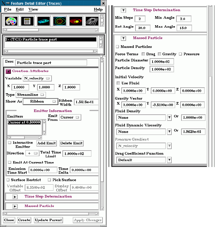
7.4 Particle Trace Create/Update
7-22 EnSight 7 User Manual
Feature Detail Editor Double clicking on the Particle Trace Create/Update Icon opens the Feature Detail
(Traces) Editor for Particle Traces, the Creation Attributes Section of which provides
access to additional functions for trace creation and modification:
Variable Opens a pop-up menu for the selection of an active variable to use to calculate the trace.
X Y Z These fields specify the fraction of each vector component to be used in the calculation.
Specify 1 to use the full value of the vector component. Specify 0 to ignore the
corresponding vector component (and thus confine the motion of the Particle to a plane
perpendicular to that axis). Values between 0 and 1 diminish the contribution of the
corresponding component, while values greater than 1 exaggerate them.
Type Opens a pull-down menu for specification of whether Particle trace calculation uses
steady-state data to produce a Streamline or transient data to produce a Pathline.
Stream Traces a massless Particle in a steady-sate vector field (for steady-state data or the current
time-step of transient data).
Path Traces a massless Particle through a time-varying vector field and so is only available
with transient results data. On certain systems, this selection can consume significant
quantities of CPU time to calculate the resulting Particle trace.
Show As Opens a dialog for specification of trace representation.
Figure 7-19
Feature Detail Editor (Traces)
Contents of Time Step Determination and
Massed Particle turn-downs.
7.4 Particle Trace Create/Update
EnSight 7 User Manual 7-23
Line Depicts the trace as a line.
Ribbon Depicts trace as if it were a ribbon. The ribbon width is a specified fixed value, while the
twisting is determined by the rotation of the flow about the path of the trace at any
particular point on the trace.
Ribbon Width This field only applies when Ribbon representation is chosen. Larger values in this field
produce wider ribbons.
Emitter Information
Emitters List This section shows a list of all emitters created for the currently selected Particle Trace
Part.
Emit From Opens a pull-down menu for the specification of the emitter type.
Cursor Creates Particle trace beginning from the position of the Cursor tool.
Line Creates Particle traces beginning from the position of the Line tool.
# Points This field specifies the number of traces you want to emit from the Line tool.
Plane Create Particle traces beginning from the position of the Plane tool.
# Points These fields specify the number of traces you want to emit from the Plane tool in the X
and Y axes of the tool.
Part Creates particle traces beginning from each node of the Part specified by the Part ID Number field.
Part ID Number This field specifies the Part you wish to use as an emitter for the creation of a particle
trace. The Part ID Number for a Part is found in the Main Parts List.
(see Section 3.1, Part Overview)
Density If 1.0, will emit from each node of the part. Lass than 1.0 values indicate a subset of nodes
to be used, randomly placed, as emitters.
Interactive Emitter Toggles on/off interactive Particle tracing. Manipulation of the emitter currently selected
in the Emitters List will cause the Particle trace to be recreated at the new location and
updated in the Graphics Window. When manipulation of the tool stops, the Particle trace
and any Parts that are dependent on it will be updated. (Only available for non-surface-
restricted streamlines) (Emitters created by picking a surface or from a Part can not be
made interactive).
Add Emit Adds an emitter of the type specified by Emit From to the currently selected Particle Trace
Part.
Delete Emit Deletes the emitter selected in the Emitters List from the selected Particle Trace Part.
Direction Trace the Particle in positive time, meaning to trace with the vector field, or trace the
Particle in negative time, meaning to trace the Particle upstream. Option only applies to
streamlines. Pathlines must be traced in + time.
(+) Positive time option traces Particle(s) forward in time. (This is the only option for time-
dependent datasets.)
(–) Negative time option traces Particle(s) backward in time.
(+/–) Positive/Negative time option traces Particle(s) both forward and backward in time.
Total Time Limit This field specifies the maximum length of time the Particle trace may continue (it may
terminate sooner for other reasons).
Emission Time Start This field specifies the solution time at which to begin Particle emission. Enter value
between beginning and ending time available.
Time Delta This field specifies the time interval between emissions of Particles from the emitters. If
“0”, only one set of emissions will occur at start time
Surface-Restrict Toggles on/off surface restricted feature for streamlines. The streamline will be
Toggle constrained to stay on the surface of the selected Part(s) by using only the tangential
component of velocity. Be sure to use the Pick Surface feature in locating the emitter for a
7.4 Particle Trace Create/Update
7-24 EnSight 7 User Manual
surface restricted particle trace to ensure that the emitter is located on the surface of a Part.
Pick Surface Toggle Toggles on/off the feature which allows you to place the trace emitter at a point on a
surface directly below the mouse pointer by clicking the left mouse button. This option is
forced on if the Surface Restricted Toggle is on.
Variable Offset This field specifies the distance into the flow field at which velocity (and other variables)
are to be sampled for the surface restricted trace(s). If velocity values are present at the
surface, this offset can be set to zero.
Display offset This field specifies the normal distance away from a surface to display the surface
restricted traces. A positive value moves the traces away from the surface in the
direction of the surface normal.
Please note that there is a hardware offset that will apply to contours, vector arrows,
separation/attachment lines, and surface restricted particle traces that can be turned on
or off in the View portion of Edit->Preferences. This preference (“Use graphics hardware
to offset line objects...”) is on by default and generally gives good images for everything
except move/draw printing. This hardware offset differs from the display offset in that it is
in the direction perpendicular to the computer screen monitor (Z-buffer)
.
Thus, for viewing, you may generally leave the display offset at zero. But for
printing, a non-zero value may become necessary so the traces print cleanly.
Time Step Opens a turn-down area for the specification of time-step parameters.
Determination
Min Steps This field is used to specify the minimum number of integration steps to perform in each
element.
Min Angle If angle between two successive line segments of the Particle trace is less than this value
EnSight will double the integration step.
Max Angle If angle between two successive line segments of the Particle trace is greater than this
value EnSight will half the integration step.
Rot Angle If the dot product between successive rotation vectors of the Particle trace is greater than
COS(Rot Angle), the integration step is halved.
Massed Particles Opens a turn-down area for the specification of massed-particle parameters.
Massed Particles Toggles on/off the massed-particle traces feature. The default is OFF.
Force Terms Determines which force terms are used in the momentum balance equation calculation.
Drag Term Toggle Toggles on/off the inclusion of the drag force term in the massed-particle computation.
The default is ON.
Gravity Term Toggle Toggles on/off the inclusion of the gravity force term in the massed-particle computation.
The default is ON.
Pressure Term Toggles on/off the inclusion of the pressure force term in the massed-particle
To g g le computation. The default is OFF.
Particle Diameter This field specifies the diameter of all particles. The default is 1.e-3.
Particle Density This field specifies the density value of all particles. The default is 1.e+3.
Initial Velocity Determines what initial velocity to use for all the particle emitters. The default is Use
Fluid Toggle ON.
Use Field Toggle Toggles on/off whether all particle emitters should use the fluid velocity at their
corresponding locations. The default is ON.
X, Y, Z These fields specify the initial velocity components of all particle emitters. Their default is
<0., 0., 0.>.
Gravity Vector These fields specify the gravity vector to be applied in the massed-particle computation.

7.4 Particle Trace Create/Update
EnSight 7 User Manual 7-25
The default gravity components are <0., -9.81, 0.>. This parameter only works with the
gravity force term.
Fluid Density This field specifies the fluid density variable to be used in the massed-particle
computation. The default is “None”.
Or This field specifies the fluid density value to be used in the computation if “None” is
specified as the variable name. The default value is 1.
Fluid Dynamic This field specifies the fluid dynamic viscosity variable to be used in the massed-particle
Viscosity computation. The default is “None”.
Or This field specifies the fluid dynamic viscosity value to be used in the computation if
“None” is specified as the variable name. The default value is 1.9620e-5. This parameter
only works with the drag force term.
Pressure Gradient This field specifies the fluid pressure gradient variable to be used in the massed-particle
computation. The default is “None”. This parameter only works with the pressure force
term.
Drag Coefficient This field specifies the drag coefficient function to be called each time the drag coefficient
Function is calculated. This function defaults to “None” which essentially defaults to the table
described above. Other functions may be accessed via the User-Defined Math Function
facility, i.e. DragCoefTable1(Re) (same as default), DragCoefPoly(Re),
DragCoefPower(Re). All functions must take the Reynolds Number as their only
argument. This parameter only works with the drag force terms.
Create (At the bottom of the Feature Detail Editor) Creates the Particle trace Part in the Graphics
Window as specified.
The Feature Detail Editor also allows you to make changes in batch; that is, to
make several changes to the menus and fields which do not effect the Graphics
Window until you click in the Apply Changes button. It is sometimes quicker
(with respect to CPU time) to make several changes at once rather than one at a
time as in the Quick Interaction Area.
(see Section 3.3, Part Editing for a detailed discussion of the remaining Feature
Detail Editor turn-down sections which are the same for all Parts),
(see How to Create Particle Traces)
Troubleshooting Particle Traces
Problem Probable Causes Solutions
Particle Trace Part is empty. Velocity is zero. Change time steps or change
location of emitters.
Emitter points are outside of flow
field.
Change location for emitter points.
Dataset is 3D and parent Parts are
2D, or dataset is 2D and parent Parts
are not planar.
Change parent Parts.
The created variable selected does
not exist for the parent Part(s)
Recreate the variable for the parent
Part(s) selected
Streamline is OK, but pathline is
empty.
Creating pathline with the emitter
emitting at the last time step.
Modify emitter time for the emitter
groups.
Particle trace terminates prematurely Velocity has gone to zero. None

7.4 Particle Trace Create/Update
7-26 EnSight 7 User Manual
Particle has been traced out of the
flow field.
None
Stopping point is at the boundary
between two Parts.
Change the parent Parts for the
Particle trace to include neighbor
Part.
Particle getting lost and EnSight’s
search algorithm failing.
Call CEI hotline support.
Total Time Limit reached. Change Total Time Limit.
Particle trace exists, then is removed
after deleting Parts.
The parent Part for the Particle trace
was deleted.
None
Particle trace creation requested, but
Particles don’t come back.
Requested a large number of Particle
traces and/or doing pathlines in large
transient dataset.
Be patient.
Particles are stuck in a recirculation
area.
Process will finish when Total Time
Limit is reached. Consider
terminating job and starting over
with a smaller Total Time Limit.
Interactive tracing is slow. The size of the model and density of
the mesh will affect the performance
of an interactive trace.
If you can, run on a faster, larger
memory workstation. Also, limit if
possible the area of interest by
cutting the mesh into pieces with the
Cut & Split Part editing operation.
Interactive trace does not enter the
next Part
Interactive tracing is only done
through the Part the emitter resides
in.
When you let go of the emitter the
full trace will be shown
Surface restricted Particle trace does
not appear
Zero velocity at chosen variable
offset
Select a Variable offset distance that
will give nonzero velocity
Display offset causing trace to be on
opposite side of a surface (hidden
surface on)
Change sign of the Display offset
Emitter does not lie on the surface of
selected Parts
Create emitters that lie on the surface
Surface Restricted particle trace does
not print well
See Display Offset discussion above Enter a non-zero display offset.
Problem Probable Causes Solutions
7.5 Clip Create/Update
EnSight 7 User Manual 7-27
7.5 Clip Create/Update
A Clip is a straight line (a Clip Line), a plane (a Clip Plane), a quadric surface
(cylinder, sphere, etc.), a constant x, y, or z plane, a box, or an i, j, or k plane that
passes through selected model Parts (or already created Clips, Isosurface, or
Developed Surface Parts). EnSight calculates the values of variables at the nodes
of the Clip. Clips can be parent Parts. For example, you can create a Clip Line
passing through a vector field, then create vector arrows originating from the
nodes of the Clip Line. Clips are created on the server, and so are not affected by
the selected Representation(s) of the parent Part(s). If you activate or create
variables after creating a Clip, the Clip automatically updates to include them.
You specify the location, orientation, and size of the Clip numerically in the
Transformations Editor dialog, or interactively using the Line, Plane, Box, or
Quadric surface tool. If you wish, EnSight will automatically extend the size of a
Clip Plane to include all the elements of the parent Part(s) that intersect the plane.
For a Clip Line, which is composed of bar elements, you specify how many
evenly spaced nodes are along the line. For a grid-type Clip Plane, which is
composed of rectangular elements, you specify the number of nodes in each
dimension, resulting in an evenly spaced grid of nodes across the plane.
If you request a mesh-type Clip Plane, an xyz clip, or any of the quadric surfaces,
EnSight finds the intersection of the specified plane or surface with the selected
parent Part(s) and creates elements of various dimensions, sizes, and shapes that
together form a cross-section of the parent Part(s). In this cross-section, three-
dimensional parent Part elements result in two-dimensional Clip Plane elements,
and two-dimensional parent Part elements result in one-dimensional Clip Plane
elements. Note that two-dimensional parent Part elements that are coplanar with
the cross-section are not included since they do not intersect the plane.
For XYZ, Plane, Quadric and Revolution Clips you can specify the resulting part
to be all elements that intersect the specified value - resulting in a “crinkly”
surface which can help analyze mesh quality.
For each Clip node on or inside an element of the selected parent Part(s), EnSight
calculates the value of each variable by interpolating from the variable’s values at
the surrounding nodes of the parent Part(s).
You can interactively manipulate the location of a clip Part by toggling on the
Interactive Tool button. When this toggle is on, the tool used to create the clip Part
will appear in the Graphics Window. Manipulation of this tool will cause the clip
Part to be recreated at the new location. This feature allows you to interactively
sweep a plane across your model or manipulate the size and location of the
cylinder, sphere, or cone.
You can animate a Clip by specifying an Animation Delta vector that moves the
Clip to a new location for each frame or page of the animation. The Clip updates
to appear as if it had been newly created at the new location and time.
For structured Parts, you can sweep through the Part with any of the i, j, or k
planes.
A Box Clip will create a part according to the Box Tool, and that can either be the
intersection of the Box Tool walls with the selected model parts (intersect), the
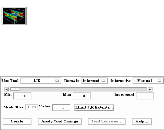
7.5 Clip Create/Update
7-28 EnSight 7 User Manual
crinkly intersection of the Box Tool walls with the selected model parts (crinkly),
the portion of the selected model parts that lie within the Box Tool (inside), or the
portion of the selected model parts which lie outside the Box Tool (outside).
Clicking once on the Clip Create/Update Icon opens the Clip Editor in the Quick
interaction Area which is used to both create and update clip Parts.
Use Tool
IJK The IJK clip tool is used with structured mesh results.
Domain Specification to extract the intersection of the specified mesh slice values. For IJK clips,
the only valid selection is “Intersect”.
Interactive Opens pull-down menu for selection of type of interactive manipulation of the IJK clip.
Options are:
Off Interactive IJK clips are turned off.
Manual Value of the IJK clip selected are manipulated via the slider bar and the
IJK clip is interactively updated in the Graphics Window to the new value.
Auto Value of the IJK clip is incremented by the Auto Delta value from the
minimum range value to the maximum value. When reaching the maximum it
starts again from the minimum.
Auto Cycle Value of the IJK clip is incremented by the Auto Increment value from the
minimum range value to the maximum value. When reaching the maximum
it decrements back to the minimum.
Slider Bar For IJK clips, the slider bar is used to increment / decrement the Mesh Slice Value
between its Minimum and Maximum value.
Min Specification of the minimum slice value for the range used with the “Manual” slider bar
and the “Auto” and “Auto Cycle” options.
Max Specification of the maximum slice value for the range used with the “Manual” slider and
the “Auto” and “Auto Cycle” options.
Increment Specification of the increment/decrement the slider will move within the min and max,
each time the stepper buttons are clicked.
Mesh Slice Opens a pull-down menu for selecting which of the IJK dimensions you wish to allow to
change. You will then specify Min, Max and Step limits for the two remaining “fixed”
dimensions.
Figure 7-20
Clip Create/Update Icon
Figure 7-21
Quick Interaction Area - Clip Editor - IJK tool
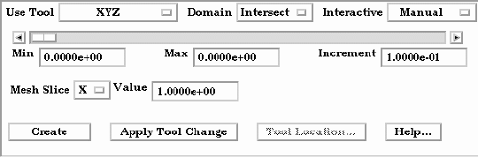
7.5 Clip Create/Update
EnSight 7 User Manual 7-29
Value This field specifies the I, J, or K plane desired for the dimension selected in Mesh Slice
Limit IJK Extents Opens the “Limits Extents of Current Slice By” dialog, in which the off dimension ranges
can be limited.
IJK D(2)Min This field specifies the minimum value for the second fixed dimension.
IJK D(2)Max This field specifies the maximum value for the second fixed dimension.
IJK D(2) Step This field specifies the step size through the second fixed dimension.
IJK D(3)Min This field specifies the minimum value for the third fixed dimension.
IJK D(3)Max This field specifies the maximum value for the third fixed dimension.
IJK D(3) Step This field specifies the step size through the third fixed dimension.
Show Parent IJK Will show the second and third dimension Min and Max extents as defined
Part Extents... for the clip parent Part.
Create Creates the Clip Part in the Graphics Window as specified.
Apply Tool Change Recreates the Clip Part selected in the Main Parts List at the current position of and of the
type specified by Use Tool.
Feature Detail Editor Double Clicking on the Clip Create/Update Icon brings up the Feature Detail
(Clips) - IJK Editor, the Creation attributes section of which offers the same features for the IJK
tool as the Quick Interaction Area Editor.
(see Section 3.3, Part Editing for a detailed discussion of the remaining Feature
Detail Editor turn-down sections which are the same for all Parts),
(see How To Create IJK Clips)
Use Tool
XYZ The XYZ tool is used to create a planar Part at a constant Cartesian component value that
is referenced according to the local frame of the part.
Domain Intersect will create the cross section of the selected parts at the specified X, Y, or Z
plane.
Crinkly will create a new part consisting of the parent part elements that intersect the
X, Y, or Z plane
Interactive Opens pull-down menu for selection of type of interactive manipulation of the XYZ clip.
Options are:
Off Interactive XYZ clips are turned off.
Manual Value of the XYZ clip selected are manipulated via the slider bar and the
XYZ clip is interactively updated in the Graphics Window to the new value.
Auto Value of the XYZ clip is incremented by the Auto Delta value from the
minimum range value to the maximum value. When reaching the maximum it
starts again from the minimum.
Auto Cycle Value of the XYZ clip is incremented by the Auto Increment value from the
minimum range value to the maximum value. When reaching the maximum
Figure 7-22
Quick Interaction Area - Clip Editor - XYZ Tool
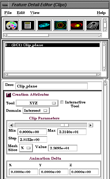
7.5 Clip Create/Update
7-30 EnSight 7 User Manual
it decrements back to the minimum.
Slider Bar For XYZ clips, the slider bar is used to increment / decrement the Mesh Slice Value
between its Minimum and Maximum value.
Min Specification of the minimum interval value of the interactive XYZ clip.
Max Specification of the maximum interval value of the interactive XYZ clip.
Increment Specification of the interval step of the interactive XYZ clip.
Mesh Slice Opens a pulldown menu for selecting which of the XYZ components you wish to clip, i.e. the X, the
Y, or the Z component.
Value This field specifies the coordinate desired for the Mesh Slice component.
Apply Tool Change
Recreates the Clip Part selected in the Main Parts List at the current position of and of the
type specified by Use Tool.
Create Creates the Clip Part in the Graphics Window as specified.
Feature Detail Editor Double Clicking on the Clip Create/Update Icon brings up the Feature Detail
(Clips) - XYZ Editor (Clips), the Creation attributes section of which offers access to the same
interactive clip parameters as found in the Quick Interaction Area Editor, along
with additional animation delta control of clips using the XYZ tool.
Animation Delta These X,Y,Z fields specify the incremental change in position of the clip for each page of
Flipbook or frame of Keyframe animation.
(see Section 3.3, Part Editing for a detailed discussion of the remaining Feature
Detail Editor turn-down sections which are the same for all Parts),
(see How To Create XYZ Clips)
Figure 7-23
Quick Interaction Area - Clip Editor - XYZ Tool - Creation Attributes
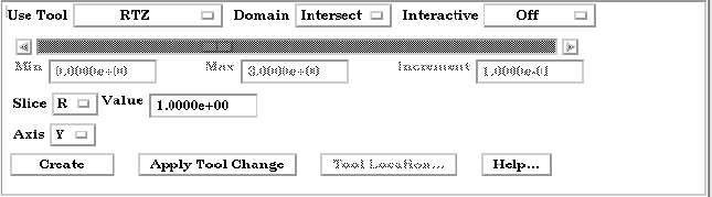
7.5 Clip Create/Update
EnSight 7 User Manual 7-31
Use Tool
RTZ The RTZ tool is used to create a Part using cylindrical coordinates at a constant radius
about an axis, angle around that axis or height along an axis..
Domain
Intersect Will create a cross section of the selected parts at the specified radius, angle, or distance
along the axis.
Crinkly Will create a new part consisting of the parent part elements that intersect the specified
radius, angle or distance.
Interactive Opens pull-down menu for selection of type of interactive manipulation of the RTZ clip.
Options are:
Off Interactive RTZ clips are turned off.
Manual Value of the RTZ clip selected are manipulated via the slider bar and the
RTZ clip is interactively updated in the Graphics Window to the new value.
Auto Value of the RTZ clip is incremented by the Auto Delta value from the
minimum range value to the maximum value. When reaching the maximum it
starts again from the minimum.
Auto Cycle Value of the RTZ clip is incremented by the Auto Increment value from the
minimum range value to the maximum value. When reaching the maximum
it decrements back to the minimum.
Slider Bar For RTZ clips, the slider bar is used to increment / decrement the Slice Value between its
Minimum and Maximum value.
Min Specification of the minimum slice value for the range used with the “Manual” slider bar
and the “Auto” and “Auto Cycle” options.
Max Specification of the maximum slice value for the range used with the “Manual” slider and
the “Auto” and “Auto Cycle” options.
Increment Specification of the increment/decrement the slider will move within the min and max,
each time the stepper buttons are clicked.
Slice Opens a pull-down menu for selecting which of the RTZ components to clip, i.e. the radial
(R), the angle theta (T) in degrees, or the distance along the longitudinal axis Z, (Z).
Value This field specifies the magnitude desired for the Slice component, (theta in degrees).
Axis The global axis with which to align the longitudinal (Z) RTZ axis.
Create Creates the Clip Part in the Graphics Window as specified.
Apply Tool Change Recreates the Clip Part selected in the Main Parts List at the current position of and of the
type specified by Use Tool.
Feature Detail Editor Double Clicking on the Clip Create/Update Icon brings up the Feature Detail
(Clips) - RTZ Editor, the Creation attributes section of which offers the same features for the
Figure 7-24
Quick Interaction Area - Clip Editor - RTZ tool
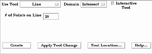
7.5 Clip Create/Update
7-32 EnSight 7 User Manual
RTZ tool as the Quick Interaction Area Editor.
(see Section 3.3, Part Editing for a detailed discussion of the remaining Feature
Detail Editor turn-down sections which are the same for all Parts),
(see How To Create RTZ Clips)
Use Tool
Line The Line tool is used to create a clip line.
Domain Specification to extract the intersection of the line tool with the selected part(s). For Line
clips, the only valid selection is “Intersect”.
Interactive Tool Toggles on/off interactive movement and updating of a clip Part. When toggled on, the
line tool used to create the 2D clip line will appear in the Graphics Window. Movement of
the tool will cause the Clip Part to be recreated at the new position. When manipulation of
the tool stops, the clip Part and any Parts that are dependent on it will be updated. During
movement, the Tool itself will not be visible, so as not to obscure the Line Clip Part. The
Tool will reappear when the mouse button is released.
# of Points on Line Specification of number of evenly spaced points on the line at which to create a node.
Tool Location... Opens the Transformation Editor dialog to permit precise positioning of the Line Tool
within the Graphics Window. (see Tool Positions... Line Tool in Section 6.5, Tools Menu
Functions and How To Use the Line Tool)
Apply Tool Change Recreates the Clip Part selected in the Main Parts List at the current position of and of the
type specified by Use Tool.
Create Creates the Clip Part in the Graphics Window as specified.
Figure 7-25
Quick Interaction Area - Clip Editor - Line Tool
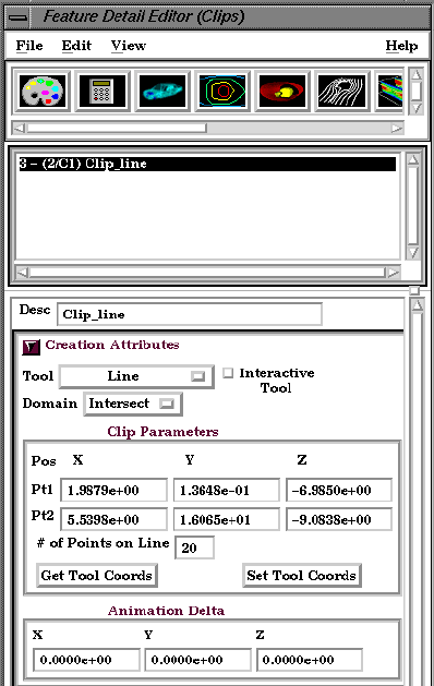
7.5 Clip Create/Update
EnSight 7 User Manual 7-33
Feature Detail Editor Double Clicking on the Clip Create/Update Icon brings up the Feature Detail
(Clips) - Line Editor (Clips), the Creation attributes section of which offers access to additional
features for the creation and modification of clips using the Line tool.
Clip Parameters
Pos of Pt1 Specification of XYZ endpoint-coordinates of Line Clip. The position of a Line Clip
Pos of Pt2 Part, if selected in the Feature Detail Editor’s Parts List, can be changed by entering values
in the numeric fields and then pressing Return.
Set Tool Coords The position of the Line Clip tool can be changed by entering values in the numeric fields
and then pressing Set Tool Coords.
Get Tool Coords The values in the numeric fields (and the position of a Line Clip Part, if selected in the
Feature Detail Editor’s Parts List) can be updated after moving the Line tool interactively
in the Graphics Window by clicking Get Tool Coords. If a Line Clip Part is selected in the
Feature Detail Editor Parts List, it will be repositioned to the new coordinates after
clicking Get Tool Coords. Coordinates are always in the original model frame (Frame 0).
Animation Delta These X,Y,Z fields specify the incremental change in position of the clip for each page of
Flipbook or frame of Keyframe animation.
The Feature Detail Editor also allows you to make changes in batch; that is, to
make several changes to the menus and fields which do not effect the Graphics
Window until you click in the Apply Changes button. It is sometimes quicker
(with respect to CPU time) to make several changes at once rather than one at a
time as in the Quick Interaction Area.
(see Section 3.3, Part Editing for a detailed discussion of the remaining Feature
Detail Editor turn-down sections which are the same for all Parts),
(see How To Create Line Clips)
Figure 7-26
Feature Detail Editor (Clips) - Line Tool
Creation Attributes
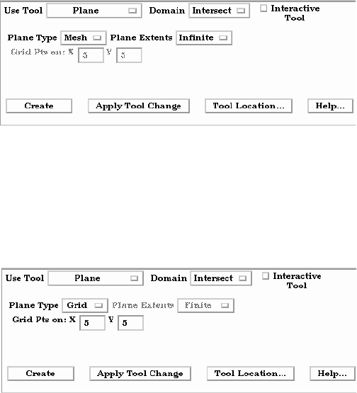
7.5 Clip Create/Update
7-34 EnSight 7 User Manual
Use Tool
Plane The Plane Tool is used to create a Plane Clip.
Domain Intersect will create the cross section of the selected parts where they intersect the plane
tool.
Crinkly will create a new part consisting of the parent part elements that intersect the
plane tool.
Inside will cut the parent parts and create a new part consisting of the portion on the
positive z side of the plane tool.
Outside will cut the parent parts and create a new part consisting of the portion on the
negative z side of the plane tool.
In/Out will cut the parent parts and create two new parts - namely an Inside and
Outside part.
Plane Type
Mesh
Will create a Plane Clip showing the cross section of the parent Part.
Plane Extents Opens a pull down menu for selection of the extent of the Plane Clip.
Finite limits the Plane Clip to the area specified by the Plane Tool corner coordinates.
Infinite extends the Plane Clip to include the intersection of the plane with all elements of
the selected model Parts.
Grid Will create a Plane Clip by discrete point sampling.
Grid Pts on:XY These fields specify the number of points on each edge of a Plane Clip at which to create
nodes. Additional nodes are located in the interior of the plane to form an evenly spaced
grid. The values must be positive integers. Applicable only to grid-type Plane Clips. Grid
Pts in X correspond to the x-direction on the Plane tool, while the number of Grid Pts in Y
correspond to the y-direction of the Plane tool.
Apply Tool Change Recreates the Clip Part selected in the Main Parts List at the current position of and of the
type specified by Use Tool.
Interactive Tool Toggles on/off interactive movement and updating of the clip Part. When toggled on, the
Plane Tool used to create the clip Part will appear in the Graphics Window. Movement of
the Plane Tool will cause the Plane Clip to be recreated at the new position. When
manipulation of the tool stops, the clip Part and any Parts that are dependent on it will be
updated. During movement, the Tool itself will not be visible, so as not to obscure the Line
Clip Part. The Tool will reappear when the mouse button is released.
Figure 7-27
Quick Interaction Area - Clip Editor - Plane Tool - Mesh Type
Figure 7-28
Quick Interaction Area - Clip Editor - Plane Tool - Grid Type

7.5 Clip Create/Update
EnSight 7 User Manual 7-35
Tool Location... Opens the Transformation Editor dialog to permit precise positioning of the Plane Tool.
(see Section 6.5, Tools Menu Functions and How To Use the Plane Tool)
Create Creates the Clip Part in the Graphics Window as specified.
Feature Detail Editor Double Clicking on the Clip Create/Update Icon brings up the Feature Detail
(Clips) - Plane Editor (Clips), the Creation attributes section of which offers access to additional
features for the creation and modification of clips using the Plane tool.
Clip Parameters
Pos of C1 Specification of the location, orientation, and size of the Plane Clip using the coordinates
Pos of C2 (in the Parts reference frame) of three corner points, as follows:
Pos of C3 Corner 1 is corner located in negative-X negative-Y quadrant
Corner 2 is corner located in positive-X negative-Y quadrant
Corner 3 is corner located in positive-X positive-Y quadrant
Set Tool Coords Will reposition the Plane Tool to the position specified in C1, C2, and C3.
Get Tool Coords Will update the C1, C2, and C3 fields to reflect the current position of the Plane Tool.
Animation Delta These X,Y,Z fields specify the incremental change in position of the clip for each page of
Flipbook or frame of Keyframe animation.
(see Section 3.3, Part Editing for a detailed discussion of the remaining Feature
Detail Editor turn-down sections which are the same for all Parts),
(see How To Create Plane Clips)
Figure 7-29
Feature Detail Editor (Clips) - Plane Tool Creation Attributes
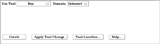
7.5 Clip Create/Update
7-36 EnSight 7 User Manual
Use Tool
Box This Clipping Tool extracts portions of the model that are inside, outside, or that intersect
a specified box.
Be aware that due to the alogorithm used, this clip can (and most often does) have
chamfered edges, the size of which depends on the coarseness of the model elements
Domain Intersect will create a new part consisting of the intersection of the box tool sides and
the selected parts.
Crinkly will create a new part consisting of the parent part elements that intersect the
box tool sides.
Inside will extract the volume portion of the parent parts that lie within the box.
Outside will extract the volume portion of the parent parts that do not lie within the
box.
In/Out will create two new parts - namely the Inside and Outside parts.
.
Apply Tool Change Recreates the Clip Part selected in the Main Parts List at the current position of and of the
type specified by Use Tool.
Tool Location... Opens the Transformation Editor dialog to permit precise positioning of the Box Tool. (see
Section 6.5, Tools Menu Functions and How To Use the Box Tool)
Create Creates the Clip Part in the Graphics Window as specified.
Feature Detail Editor Double Clicking on the Clip Create/Update Icon brings up the Feature Detail
(Clips) - Box Editor, the Creation attributes section of which offers the same features for the
Box tool as the Quick Interaction Area Editor.
(see Section 3.3, Part Editing for a detailed discussion of the remaining Feature
Detail Editor turn-down sections which are the same for all Parts),
(see How To Create Box Clips)
Figure 7-30
Quick Interaction Area - Clip Editor - Box Tool
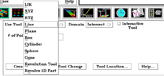
7.5 Clip Create/Update
EnSight 7 User Manual 7-37
Use Tool
Cylinder, Sphere, Cone These Tools are used to create a quadric clip surface
Domain Intersect will create the cross section of the selected parts where they intersect the
quadric tool.
Crinkly will create a new part consisting of the parent part elements that intersect the
quadric tool.
Inside will cut the parent parts and create a new part consisting of the portion on the
inside of the quadric tool.
Outside will cut the parent parts and create a new part consisting of the portion on the
outside of the quadric tool.
In/Out will cut the parent parts and create two new parts - namely an Inside and
Outside part.
.
Interactive Tool Toggles on/off interactive movement and updating of a clip Part. When toggled on, the
Quadric Tool used to create the Clip Part will appear in the Graphics Window at the
location of the Clip Part. Movement of the Quadric Tool will cause the Clip Part to be
recreated at the new position. When manipulation of the tool stops, the Clip Part and any
Parts that are dependent on it will be updated. During movement, the Tool itself will not
be visible, so as not to obscure the Line Clip Part. The Tool will reappear when the mouse
button is released.
Tool Location... Opens the Transformation Editor dialog to permit precise positioning of Quadric
Tools.(see Section 6.5, Tools Menu Functions and How To Use the Cylinder Tool, How
To Use the Sphere Tool, and How To Use the Cone Tool)
Apply Tool Change Recreates the Clip Part selected in the Main Parts List at the current position of and of the
type specified by Use Tool.
Create Creates the Clip Part in the Graphics Window as specified.
Figure 7-31
Quick Interaction Area - Clip Editor - Cylinder, Sphere, & Cone Tools
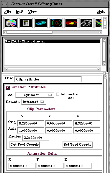
7.5 Clip Create/Update
7-38 EnSight 7 User Manual
Feature Detail Editor Double Clicking on the Clip Create/Update Icon brings up the Feature Detail
(Clips) Quadric Tool Editor (Clips), the Creation attributes section of which offers access to additional
features for the creation and modification of clips using the Quadric tools.
Clip Parameters
Cylinder
Orig XYZ Specification of the origin (the center point) of the Cylindrical Clip.
Axis Specification of the longitudinal axis direction of the Cylindrical Clip.
Radius Specification of the radius of the Cylindrical Clip.
Sphere
Orig Specification of the origin (the center point) of the Spherical Clip.
Axis Specification of the axis direction of the Spherical Clip. (Note: Axis is important if
Developed Surface is created from the spherical clip.)
Radius Specification of the radius of the Spherical Clip.
Cone
Orig
Specification of the origin (the tip of the cone) of the Conical Clip.
Axis Specification of the axis direction of the Conical Clip. Axis direction goes from tip to
base.
Angle Specification of the conical half angle (in degrees) of the Conical Clip.
Set Tool Coords Will reposition the Quadric Tool to the position specified in the Clip Parameter fields.
Get Tool Coords Will update the Clip Parameter fields to reflect the current position of the Quadric Tool.
Animation Delta These X,Y,Z fields specify the incremental change in position of the clip for each page of
Flipbook or frame of Keyframe animation.
Figure 7-32
Feature Detail Editor (Clips) - Quadric Tool Creation Attributes
7.5 Clip Create/Update
EnSight 7 User Manual 7-39
The Feature Detail Editor also allows you to make changes in batch; that is, to
make several changes to the menus and fields which do not effect the Graphics
Window until you click in the Apply Changes button. It is sometimes quicker
(with respect to CPU time) to make several changes at once rather than one at a
time as in the Quick Interaction Area.
(see Section 3.3, Part Editing for a detailed discussion of the remaining Feature
Detail Editor turn-down sections which are the same for all Parts),
(see How To Create Quadric Clips)
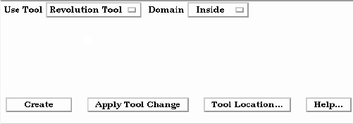
7.5 Clip Create/Update
7-40 EnSight 7 User Manual
Use Tool
Revolution Tool This clipping Tool is used to create custom clip surfaces which are defined by revolving a
set of lines about a defined axis.
Domain Intersect will create the cross section of the selected parts where they intersect the
revolved surface.
Crinkly will create a new part consisting of the parent part elements that intersect the
revolved surface.
Inside will cut the parent parts and create a new part consisting of the portion on the
inside of the revolved surface.
Outside will cut the parent parts and create a new part consisting of the portion on the
outside of the revolved surface.
In/Out will cut the parent parts and create two new parts - namely an Inside and
Outside part.
Tool Location... Opens the Transformation Editor dialog to permit precise location of the revolution tool
within the Graphics Window. It is here where you also can control the number and
positioning of the set of lines which make up the tool.
(see Section 6.5, Tools Menu Functions and How To Use the Surface of Revolution Tool)
Apply Tool Change Recreates the Clip Part selected in the Main Parts List at the current position of and of the
type specified by Use Tool.
Create Creates the Clip Part in the Graphics Window as specified.
Figure 7-33
Quick Interaction Area - Clip Editor - Revolution Tool
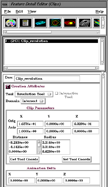
7.5 Clip Create/Update
EnSight 7 User Manual 7-41
Feature Detail Editor Double Clicking on the Clip Create/Update Icon brings up the Feature Detail
(Clips) - Revolution Editor (Clips), the Creation attributes section of which offers access to additional
Tool features for the creation and modification of clips using the Revolution tool.
Revolution Tool Clip Parameters
Orig These fields specify the XYZ coordinates of the origin (center point) of the Revolution
Clip.
Axis These fields specify the XYZ coordinates of the axis direction of the Revolution Clip.
Distance/Radius These lists specify the distance (from the origin) and radius for each point that defines the
Revolution Clip. The points can Not be edited within this dialog. You must edit the
Revolution Tool in the Transformations dialog.
Set Tool Coords Will reposition the Revolution Tool to the position specified in the Clip Parameter fields.
Get Tool Coords Will update the Clip Parameter fields to reflect the current position of the Revolution Tool.
Animation Delta These X,Y,Z fields specify the incremental change in position of the clip for each page of
Flipbook or frame of Keyframe animation.
The Feature Detail Editor also allows you to make changes in batch; that is, to
make several changes to the menus and fields which do not effect the Graphics
Window until you click in the Apply Changes button. It is sometimes quicker
(with respect to CPU time) to make several changes at once rather than one at a
time as in the Quick Interaction Area.
(see Section 3.3, Part Editing for a detailed discussion of the remaining Feature
Detail Editor turn-down sections which are the same for all Parts),
(see Section 6.5, Tools Menu Functions and How To Use the Surface of Revolution Tool)
Figure 7-34
Feature Detail Editor (Clips) - Revolution Tool Creation Attributes
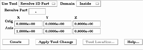
7.5 Clip Create/Update
7-42 EnSight 7 User Manual
Use Tool
Revolve 1D Part This option will create a clip surface by revolving a line, defined by a Part, about an axis.
Domain Intersect will create the cross section of the selected parts where they intersect the
revolved surface
Crinkly will create a new part consisting of the parent part elements that intersect the
revolved surface.
Inside will cut the parent parts and create a new part consisting of the portion on the
inside of the revolved surface.
Outside will cut the parent parts and create a new part consisting of the portion on the
outside of the revolved surface.
In/Out will cut the parent parts and create two new parts - namely an Inside and
Outside part.
Revolve Part This field specifies the Part number which will be revolved. The 1D Part must contain
only bar elements and must have only two free ends (i.e., there must be only one “logical”
line contained in the Part).
Orig These fields specify the XYZ coordinates of the axis line origin point.
Axis These fields specify the direction vector of the axis line. The “line” contained in the Part
specified by number in Revolve Part will be revolved about this axis to create the clip
surface Part.
Apply Tool Change Recreates the Clip Part selected in the Main Parts List at the current position of and of the
type specified by Use Tool.
Create Creates the Clip Part in the Graphics Window as specified.
Figure 7-35
Quick Interaction Area - Revolve 1D Part Clip Editor
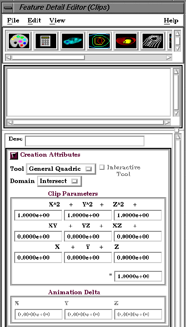
7.5 Clip Create/Update
EnSight 7 User Manual 7-43
General Quadric
Feature Detail Editor Double Clicking on the Clip Create/Update Icon brings up the Feature Detail
(Clips) Editor (Clips), the Creation attributes section of which offers access to one type of
clip creation which is not available in the Quick Interaction area. It is possible to
create a 3D Quadric clip using the General Quadric option by directly specifying
the coefficients of a general quadric equation.
The Feature Detail Editor also allows you to make changes in batch; that is, to
make several changes to the menus and fields which do not affect the Graphics
Window until you click in the Apply Changes button. It is sometimes quicker
(with respect to CPU time) to make several changes at once rather than one at a
time as in the Quick Interaction Area.
(see Section 3.3, Part Editing for a detailed discussion of the remaining Feature
Detail Editor turn-down sections which are the same for all Parts),
10 coefficient values These coefficient values represent the general equation of a Quadric surface. They can be
changed by modifying the values. No tool exists corresponding to this equation.
AX
2
+BY
2
+CZ
2
+DXY+EYZ+FXZ+GX+HY+IZ=J
Animation Delta Not available for General Quadric Clips.
The Feature Detail Editor also allows you to make changes in batch; that is, to
make several changes to the menus and fields which do not effect the Graphics
Figure 7-36
Feature Detail Editor (Clips) - Revolve 1D Part Creation Attributes

7.5 Clip Create/Update
7-44 EnSight 7 User Manual
Window until you click in the Apply Changes button. It is sometimes quicker
(with respect to CPU time) to make several changes at once rather than one at a
time as in the Quick Interaction Area.
(see Section 3.3, Part Editing for a detailed discussion of the remaining Feature
Detail Editor turn-down sections which are the same for all Parts),
Troubleshooting Clips
Problem Probable Causes Solutions
Clip does not move during animation
Animation deltas are not set, or
are too small.
Change the animation delta
values.
Clip results in an empty Part. Clip was taken outside of the
model.
Change the clip Tool location.
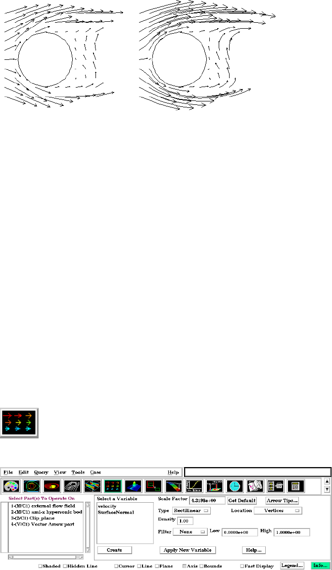
7.6 Vector Arrow Create/Update
EnSight 7 User Manual 7-45
7.6 Vector Arrow Create/Update
Vector Arrows visualize the magnitude and direction of a vector variable at
discrete points (at nodes, element vertices, or at the center of elements).
Other features can visualize magnitude, but Vector Arrows also show direction.
Vector arrow Parts are dependent Parts known only to the client. They cannot be
used as a parent Part for other Part types and cannot be used in queries. As
dependent Parts, they are updated anytime the parent Part and/or the creation
vector variable changes (unless the general attribute Active flag is off).
Vector arrows can be filtered according to low and/or high threshold values.
Vector arrows can emanate from the available nodes of the parent Part(s), the
available element vertex nodes of the parent Part(s), or the available element
centers of the parent Part(s) which pass through the filter successfully. The nodes
and elements available in the parent Part are based on the visual Representation of
the Part. Thus, for a border Representation of a Part, only the border elements and
associated nodes are candidates.
Vector arrows can have straight shafts representing the vector at the originating
location, or be the segment of a streamline emanating from the originating
location (curved). Straight vector arrows are displayed relatively quickly, while
curved vector arrows can be time consuming.
Different tip styles, sizes, and colors can be used to enhance vector arrow display.
Clicking once on the Vector Arrow Create/Update Icon opens the Vector Arrow
Editor section of the Quick interaction Area which is used to both create and
update (make changes to) vector arrow Parts.
Figure 7-37
Vector Arrow Create/Update Icon
Figure 7-38
Quick Interaction Area - Vector Arrow Editor
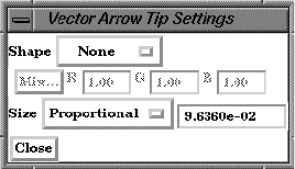
7.6 Vector Arrow Create/Update
7-46 EnSight 7 User Manual
Scale Factor / Time When Type is “Rectilinear”, this field specifies a scale factor to apply to the vector values
before displaying them. Scaling is usually necessary to control the visual length of the
vector arrows since the vector values may not relate well to the geometric dimensions.
Can be negative, causing the vector arrows to reverse direction.
When Type is “Rect. Fixed”, this field specifies the length of the arrows in units of the
model coordinate system. Can be negative, causing the vector arrows to reverse direction.
When Type is “Curved”, this field specifies the duration time for streamlines forming the
shaft of curved vector arrows. Is an indication of the length of the curved vector arrow.
Get Default Sets Scale or Time Factor value to a computed reasonable value based on the vector
variable values and the geometry.
Arrow Tips... Opens the Vector Arrow Tip Settings dialog.
Shape Opens a pop-up menu to select tip shape.
None option displays arrows as lines without tips.
Normal arrows have two short line tips, similar to the way many people draw
arrows by hand. The tip will lie in the X–Y, X–Z, or Y–Z plane depending on
the relative magnitudes of the X, Y, and Z components of each individual vector.
Suggested for 2D problems.
Triangles arrows have a tip composed of two intersecting triangles in the two
dominant planes. Good for both 2D and 3D fields.
Tipped arrows display the tip of the arrow in any user specified color. Good for both
2D and 3D fields. The color may be specified in the RGB fields or chosen from the
Color Selector dialog which is opened by pressing the Mix... button
Size Opens a pop-up menu for selecting tip size.
Fixed sized arrows have tips for which the length is specified in the data entry field to the
right of the pop-up menu button. Units are in the model coordinate system.
Proportional sized arrow tips change proportionally to the change in the magnitude of the
vector arrows.
Type Opens a pop-up menu for selection of shaft-type of vector arrows. Options are:
Rectilinear arrows have straight shafts. The arrow points in the direction of the
vector at the originating location. The length of the arrow shaft is determined
by multiplying the vector magnitude by the scale factor.
Rect. Fixed arrows have straight shafts. The arrow points in the direction of the
vector at the originating location. The length of the arrow shaft is determined
by the scale factor. It is independent of the vector variable.
Curved arrows have curved shafts. The arrow is actually a streamline emanating
from the originating location. It represents the path that a massless Particle
would follow if the flow field was steady state. For this option, the “Scale
Factor” changes to “Time”. Time is the amount of time the streamline is
allowed to take and is an indication of how long the arrow will be.
Hint: Since curved arrows can take a significant amount of time(depending on
the number of originating locations), the setting of a proper “Time” value is
Figure 7-39
Vector Arrow Tip Settings dialog
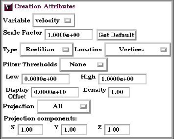
7.6 Vector Arrow Create/Update
EnSight 7 User Manual 7-47
critical. The best way to do this is to first do a single Particle trace at a
representative location with the estimated “Time” value as the Max Time. A
quick iteration or two on the value here could save considerable time for the
curved vector arrow computation.
Location Opens a pop-up dialog for the selection of root-location of arrow shafts. The options are:
Node arrows originate from each node of the parent Part(s).
Note: Discrete Particles Parts must use Node option.
Vertices arrows originate only from those nodes at the vertices of each element of
the parent Part(s) (i.e., arrows are not displayed at free nodes or mid-side
nodes).
Element Center arrows originate from the geometric center of each element of the
parent Part(s).
Density The fraction of the parent’s nodes/elements which will show a vector arrow. A value of
1.0 will result in a vector arrow at each node/element, while a value of 0.0 will result in no
arrows. If between these two values, the arrows will be distributed randomly at the
specified density. There is no check for duplicates in the random distribution of arrows. It
is entirely possible that when you specify a density of 0.25 in a model containing 100
nodes you only get 15 unique locations with 10 duplicates. It will appear that only 15
arrows show up, but there are actually 25 with 10 duplicates.
Filter Selection of pattern for filtering Vector Arrows according to magnitude. Options are:
None displays all the vector arrows. No filtering done.
Low displays only those arrows with magnitude above that specified in the Low
field. Filters low values out.
Band displays only those arrows with magnitude below that specified in the Low
field and above that specified in the High field. Filters the band out.
High displays only those arrows with magnitude below that specified in the High
field. Filters the high values out.
Low_High displays only those arrows with magnitude between that specified in the
Low field and that specified in the High field. Filters out low and high values.
Apply New Variable Changes the vector Variable used to create the Vector Arrows to that currently selected in
the Variables List.
Feature Detail Editor Double clicking on the Vector Arrow Create/Update Icon opens the Feature Detail
(Vector Arrows) Editor for Vector Arrows, the Creation Attributes Section of which provides
access to the functions available in the Quick Interaction Area plus three more:
Display offset This field specifies the normal distance away from a surface to display the vector
arrows. A positive value moves the vector arrows away from the surface in the
direction of the surface normal.
Figure 7-40
Feature Detail Editor (Vector Arrows)

7.6 Vector Arrow Create/Update
7-48 EnSight 7 User Manual
Please note that there is a hardware offset that will apply to contours, vector arrows,
separation/attachment lines, and surface restricted particle traces that can be turned on
or off in the View portion of Edit->Preferences. This preference (“Use graphics hardware
to offset line objects...”) is on by default and generally gives good images for everything
except move/draw printing. This hardware offset differs from the display offset in that it is
in the direction perpendicular to the computer screen monitor (Z-buffer)
.
Thus, for viewing, you may generally leave the display offset at zero. But for
printing, a non-zero value may become necessary so the arrows print cleanly.
Projection Opens a pop-up menu to allow selection of which vector components to include when
calculating both the direction and magnitude of the vector arrows. The vector components
at the originating point are always first multiplied by the Projection Components (see
below). Then one of the following options is applied:
All, to display a vector arrow composed of the Projection-Component-modified X,
Y, and Z components.
Normal, to display a vector which is the projection of the All vector in the direction
of the normal at the originating location.
Tangential, to display a vector which is the projection of the All vector into the
tangential plane at the originating location.
Component, to display both the Normal and the Tangential vectors
The All, Normal, and Tangential options produce a single vector per location, while the
Component option produces two vectors per location. If selection is not applicable to a
Particular element, that element’s vector arrow uses the All projection.
Projection These fields specify a scaling factor for each coordinate component of each vector arrow
Components X Y Z used in calculating both the magnitude and direction of the vector arrow. Specify 1 to use
the full value of a component. Specify 0 to ignore the corresponding vector component
(and thus confine all the vector arrows to planes perpendicular to that axis). Values
between 0 and 1 diminish the contribution of the corresponding component, while values
greater than 1 exaggerate them. Negative values reverse the direction of the component.
Always applied before the Projection options above.
The Feature Detail Editor also allows you to make changes in batch; that is, to
make several changes to the menus and fields which do not effect the Graphics
Window until you click in the Apply Changes button. It is sometimes quicker
(with respect to CPU time) to make several changes at once rather than one at a
time as in the Quick Interaction Area.
(see Section 3.3, Part Editing for a detailed discussion of the remaining Feature
Detail Editor turn-down sections which are the same for all Parts),
(see How to Create Vector Arrows)
Troubleshooting Vector Arrows
Problem Probable Causes Solutions
Vector arrows do not match up with
their originating locations on one or
more of the parent Parts.
Displacements are on for some of the
parent Parts, but not others. Or the
parent Parts have been assigned to
different coordinate frames
Create separate vector arrow Parts
for the parents that will be displaced
(or assigned to different frame) and
the ones that will not be displaced
(or assigned to different frames).

7.6 Vector Arrow Create/Update
EnSight 7 User Manual 7-49
You are displaying several different
vector arrow Parts at once and can’t
tell which is which.
Just too much similar information in
the same area.
Use different attributes for the
different vector arrow Parts, or better
yet, display the conflicting vector
arrow Parts on separate Part copies
which have been moved apart.
You are trying to display vector
arrows on a Discrete Particle Part,
but can’t get them to show up
Arrow Location set to Vertices (the
default).
Set the Arrow Location to Nodes.
No vector data provided for the
Discrete Particle dataset, thus values
all set to zero when read into
EnSight.
Provide vector data for the particles.
Specify in the Measured results file.
See Section 3.7.
Vector arrows do not print well See Display Offset discussion above. Enter a non-zero Display Offset.
Problem Probable Causes Solutions
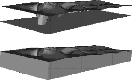
7.7 Elevated Surface Create/Update
7-50 EnSight 7 User Manual
7.7 Elevated Surface Create/Update
Elevated Surfaces visualize the value of a variable by creating a surface projected
away from the 2D elements of the parent Part. It is easiest to describe this feature
if you think of a planar Part as the parent Part. Now warp this surface up out of
plane proportionally to the value of a variable. The resultant surface is an Elevated
Surface. Elevated surfaces are to surfaces what Profiles are to lines. While planar
surfaces are perhaps the most useful parent Parts to use, parents do not have to be
planar. Model Parts containing 2D elements, Clip Planes, Isosurfaces, and even
other elevated surfaces are all valid parent Parts.
The parent Part is not actually changed, a new surface is created. As this new
surface is “raised”, projection (Sidewall) elements can be created stretching from
the parent to the elevated surface around the boundary of the surfaces if desired.
Just the surface, just the sidewalls, or both can be created.
The projection from a node on the parent Part will be in the direction of the
normal at the node. If the node is shared by multiple elements, the average normal
is used.
The projected distance from a parent Part’s node to the corresponding elevated
surface node is calculated by adding to the variable’s value an Offset value, then
multiplying the sum by a Scaling value. Adding the Offset enables you to shift the
zero location of the plane. An Offset performs a “shift”, but does not change the
“shape” of the resulting elevated surface. The Scaling factor changes the distance
between parent and elevated surface, a “stretching” effect. EnSight will provide
default values for both factors based on the variable’s values at the parent Part’s
nodes.
Figure 7-41
Elevated Surface example, with and without Sidewalls
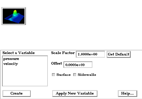
7.7 Elevated Surface Create/Update
EnSight 7 User Manual 7-51
Clicking once on the Elevated Surface Create/Update Icon opens the Elevated
Surface Editor in the Quick Interaction Area which is used to both create and
update (make changes to) elevated surface Parts.
Scale Factor This field specifies the scaling for magnitude of distance between the parent Part node and
the corresponding elevated surface node. The Factor is multiplied times the value of the
variable. Values larger than one increase the size and values smaller than one decease the
size. A negative value will have the effect of switching the direction of the projected
surface.
Get Default Click to set Scale Factor and Offset values to the calculated defaults based on the variable
values for the parent Part.
Offset Value specified is added to the variable values before the Scale Factor is applied to change
the magnitude of projected distance. Default offset is magnitude of most-negative
projection distance (will cause the surface to be projected positively). Has the effect of
shifting the surface plot, but does not change the surface plot shape.
Surface Toggle Toggles on/off the creation of the actual elevated surface. The sidewalls alone will be
created if this toggle is off.
Sidewalls Toggle Toggles on/off the creation of the sidewalls of the Elevated Surface. Elements will stretch
from the parent Part to the Elevated surface around the boundary of the surfaces. The
Elevated Surface alone will be created if this toggle is off.
Apply New Variable Changes the variable the Elevated Surface Part is based on to that currently selected in the
Vari a bl es Li st .
Figure 7-42
Elevated Surface Create/Update Icon
Figure 7-43
Quick Interaction Area - Elevated Surface Editor
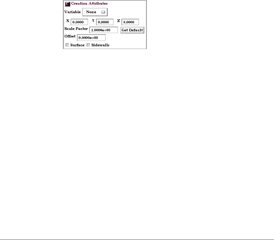
7.7 Elevated Surface Create/Update
7-52 EnSight 7 User Manual
Feature Detail Editor Double clicking on the Elevated Surfaces Create/Update Icon opens the Feature
(Elevated Surfaces) Detail Editor for Elevated Surfaces, the Creation Attributes Section of which
provides access to all of the functions available in the Quick Interaction Area plus
one more:
X Y Z For vector-based or coordinate-based elevated surfaces, specify vector components used
in creating the elevated surface. Not applicable to scalar-type elevated surfaces. Are
according to the reference frame of the Elevated Surface-Part. Letters labeling dialog data
entry fields depend on type of the reference frame (Rectangular, Spherical, or Cylindrical).
If all components are 0.0, the vector or coordinate magnitude will be used.
The Feature Detail Editor also allows you to make changes in batch; that is, to
make several changes to the menus and fields which do not effect the Graphics
Window until you click in the Apply Changes button. It is sometimes quicker
(with respect to CPU time) to make several changes at once rather than one at a
time as in the Quick Interaction Area.
(see Section 3.3, Part Editing for a detailed discussion of the remaining Feature
Detail Editor turn-down sections which are the same for all Parts),
(see How to Create Elevated Surfaces)
Troubleshooting Elevated Surfaces
Problem Probable Causes Solutions
The entire Elevated Surface is not
projected in the direction you
want
.
Change the sign of the scale factor.
You have a non-planar parent
Part and the elevated surface
seems to have strange
intersecting elements.
Sidewall elements are not
appropriate
Turn off sidewall toggle.
Scale factor too large. Lower the Scale Factor.
The Elevated Surface projection
appears to be “confused” at
various locations.
Inconsistently ordered elements,
such that the normals are not
“consistent”
Modify element ordering to be
consistent, if possible.
Figure 7-44
Feature Detail Editor (Elevated Surfaces)
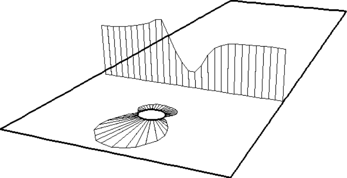
7.8 Profile Create/Update
EnSight 7 User Manual 7-53
7.8 Profile Create/Update
Profiles visualize values of a variable along a line with a plot projecting away
from the line. Projectors are parallel to a plane, but not necessarily in a plane.
Hence, Profile can follow the line.
You can scale and offset projectors. The positive direction is set with the center
point of the Plane Tool (away from center point is positive). Consider a base-line
(not necessarily straight) along which the value of a variable is known. Moving
along this base-line, you can “plot” the value of the variable on an “axis” whose
origin moves along the base-line and whose orientation varies so that it is always
both perpendicular to the base-line and parallel to a specified plane (but not
necessarily parallel to a line, enabling the plot-line to follow the curve of the base-
line in one dimension). A surface joining the base-line to the plot-line is called a
profile.
The parent Part of a Profile-Part can be a 2D-Clip Line, a Contour, a Particle
Trace, or a model Part consisting of a chain of bar elements. From each node of
the parent Part, EnSight draws a “projector” whose length is proportional to the
value of the variable at the node, and whose orientation makes it (1) parallel to a
specified plane, (2) pointing in a direction corresponding to the sign of the
variable’s value at the node (with the negative-direction determined by the
location of a specified point), and (3) perpendicular to the base-line elements
adjoining the node, or, if the base-line bends at the node, oriented so that its
projection into the plane defined by the base-line elements will bisect the angle
formed by the base-line elements. The outer-end of each projector is connected to
those of its neighbors, forming a series of four-sided polygons and hence a
surface.
The appearance of the profile depends greatly on the position of the specified
sign-direction point (From Point) and the orientation of the specified plane, which
you can specify numerically or with the Plane tool. EnSight calculates the
projectors using the vector cross-product of the specified-plane’s normal (the Z-
axis) and each parent Part element, thus you should orient the plane so that its
normal is not parallel to the parent Part elements.
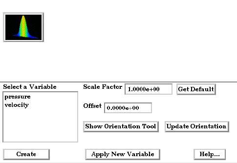
7.8 Profile Create/Update
7-54 EnSight 7 User Manual
The projector length is calculated by adding to the variable’s value an Offset
value, then multiplying the sum by a Scaling value. Adding the Offset enables you
to shift the zero location of the projectors, which might be useful if you wanted to
make all the projectors have the same sign. An offset performs a “shift”, but does
not change the “shape” of the resulting profile. The Scaling factor changes the
displayed size of the profile, a “stretching” type of action. EnSight will provide
default values for both factors based on the variable’s values at the parent Part’s
nodes.
Clicking once on the Profile Create/Update Icon opens the Profile Editor the
Quick Interaction Area which is used to both create and update (make changes to)
profile Parts.
Scale Factor This field specifies the scaling for magnitude of the projector. The Scale Factor is
multiplied times the value of the variable. Values larger than one increase the size and
values smaller than one decrease the size.
Offset The value specified in this field is added to the variable values before the Scale Factor is
applied to change the magnitude of projectors. Default offset is magnitude of most-
negative projector (making them all positive). Has the effect of shifting the plot, but does
not change the plot shape.
Get Default Click to set Scale Factor and Offset values to the calculated defaults based on the variable
values for the parent Part.
Show Orientation Tool Causes the Plane Tool to become visible in the Graphics Window at the location specified
Update Orientation Recreates the Profile Part at the current location and orientation of the Plane Tool.
Apply New Variable Changes the variable the Profile Part is based on to that currently selected in the Variables
List.
Figure 7-45
Profile Create/Update Icon
Figure 7-46
Quick Interaction Area - Profile Editor
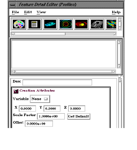
7.8 Profile Create/Update
EnSight 7 User Manual 7-55
Feature Detail Editor Double clicking on the Profile Create/Update Icon opens the Feature Detail Editor
(Profiles) for Profiles, the Creation Attributes Section of which provides access to additional
functions for the creation and modification of Profiles:
X Y Z These fields specify the vector components used in creating the Part for vector based or
coordinate-based Profiles. These fields are not applicable to Scalar-based Profiles. When
all fields are zero, the magnitude of the Variable value is used. If a value other than zero is
entered into a field, the sum of (Vector
X
*X)+(Vector
Y
*Y)+(Vector
Z
*Z) is used as the
variable value.
Orientation Plane
Pos of C1 Specification of the location, orientation, and size of the Plane Clip using the coordinates
Pos of C2 (in the Parts reference frame) of three corner points, as follows:
Pos of C3 Corner 1 is corner located in negative-X negative-Y quadrant
Corner 2 is corner located in positive-X negative-Y quadrant
Corner 3 is corner located in positive-X positive-Y quadrant
Set Tool Coords Will reposition the Plane Tool to the position specified in C1, C2, and C3.
Get Tool Coords Will update the C1, C2, and C3 fields to reflect the current position of the Plane Tool.
The Feature Detail Editor also allows you to make changes in batch; that is, to
make several changes to the menus and fields which do not effect the Graphics
Window until you click in the Apply Changes button. It is sometimes quicker
(with respect to CPU time) to make several changes at once rather than one at a
time as in the Quick Interaction Area.
(see Section 3.3, Part Editing for a detailed discussion of the remaining Feature
Detail Editor turn-down sections which are the same for all Parts),
(see How To Create Profile Plots)
Figure 7-47
Feature Detail Editor (Profiles)

7.8 Profile Create/Update
7-56 EnSight 7 User Manual
Troubleshooting Profiles
Problem Probable Causes Solutions
The entire profile is not projected the
direction you want.
The Plane is not oriented correctly. Turn on the Plane tool so you can see
its orientation. The projectors will be
parallel to this plane, so adjust its
orientation.
The From Point is not in a good
location
Turn on the Plane tool so you can see
the location of the center of the
plane. Positive projectors will go
away from this point, negative
towards.
Portions of the profile appear to be
projected in the wrong direction.
The From Point is not in a good
location.
Turn on the Plane tool so you can see
the location of the center of the
plane. Positive projectors will go
away from this point, negative
towards.
The normal to the Plane is parallel to
some of the elements of the parent
Part.
Turn on the Plane tool so you can see
its orientation. Try to make sure the
Z axis of the Plane tool does not lie
parallel to any portions of the parent
Part.
The Parent Part does not contain
elements which are consistently
ordered
None
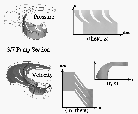
7.9 Developed Surface Create/Update
EnSight 7 User Manual 7-57
7.9 Developed Surface Create/Update
A Developed Surface is generated by treating any 2D Part (or parent Part) as a
surface of revolution, and mapping specific curvilinear coordinates of the
revolved surface into a planar representation.
A Developed Surface derives its name from the implied process that defines a
developable surface. A surface is considered “developable” if it can be unrolled
onto a plane without distortion. Although every 2D Part in EnSight is not by
definition a developable surface, each 2D Part can nevertheless be developed into
a planar surface which is distorted according to the type of developed projection
specified. For example, a Cylinder Clip Part is by definition a developable
surface, because it can be developed into planar surface without distortion.
Whereas, a Sphere Clip Part is not a developable surface, because it can not be
developed into a planar surface without distortion.
Parent Parts Only 2D Parts are developed. Also, only one Part is developed at a time. While all
2D Parts qualify as candidate parent Parts, only 2D Parts of revolution are
developed coherently. The current developed surface algorithm treats all parent
Parts as surfaces of revolution that are developed according to a local origin and
axis of revolution. These attributes are either inherited from the parent Part, or
must be specified according to the parent Part.
A developed surface permanently inherits the local origin and axis of revolution
information from any parent Part created via the cylinder, cone, sphere, or
revolution Clip tools. Whereas, surfaces developed from non-Clip Parts require
this information to be specified via the Orig. and Axis fields in the Attributes
(Developed Surfaces) dialog. The latter case is the only time the values in these
fields are used. Although default values are provided, it is up to you to make sure
that valid values are specified. In the former case, the Orig and Axis fields only
provide convenient feedback of the selected Clip Part. Note that developed
surfaces resulting from parent Parts of revolution created via the general quadric
Clip tool do not inherit the local origin and axis of revolution attributes from the
General Quadric Clip parent; rather, these attributes must be specified.
Figure 7-48
Developed
Surface
Examples
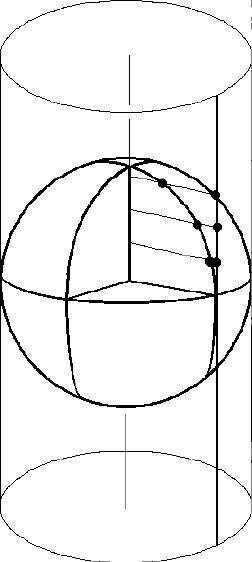
7.9 Developed Surface Create/Update
7-58 EnSight 7 User Manual
Developed Projections A parent Part is developed by specifying one of three curvilinear mappings called
developed projections; namely, an (r,z), (θ,z), or (m,θ) projection. The curvilinear
coordinates r,ςθ, z, and m stand for the respective radius,ςθ, z, and meridian (or
longitude) directional components which are defined relative to the local origin
and axis of revolution of the parent Part. The meridian component is defined as m
= SQRT(r
2
+ z
2
).
Seam Line A surface of revolution is developed about its axis, starting at its “seam” line (or
zero meridian) where the surface is to be slit. Surface points along the seam are
duplicated on both ends of the developed Part. The seam line is specified via a
vector that is perpendicular to and originates from the axis of revolution, and
which points toward the seam which is located on the surface at a constant value.
This vector can be specified either manually or interactively. Interactive seam line
display and manipulation is provided via a slider in the Attributes (Developed
Surfaces) dialog.
Figure 7-49
Developed Equiareal Projection
Essentially, each topological projection first
surrounds the parent Part of revolution with a
virtual cylinder of constant radius. The
curvilinear coordinates of the parent Part are
then projected along the normals of (and thus
onto) the virtual cylinder. Finally, the virtual
cylinder is slit along a straight line, or
generator, and unwrapped into a plane. This
process yields an equiareal, or area
preserving, mapping which means that the
area of any enclosed curve on the surface of
the parent Part is equal to the area enclosed
by the image of the enclosed curve on the
developed plane. Although equiareal
mappings provide reduced shape distortion,
they do suffer from angular distortions of
local scale.
Vector fields of the parent Part (for all three
developed projections) are developed such
that a vector’s angle to its surface normal is
preserved. For example, a vector normal to
the parent surface remains normal when
developed onto the planar surface.
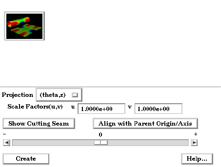
7.9 Developed Surface Create/Update
EnSight 7 User Manual 7-59
Clicking once on the Developed Surface Create/Update Icon opens the Developed Surface
Editor in the Quick Interaction Area
which is used to both create and update (make
changes to) developed surface Parts.
Projection Opens a pop-up dialog for the specification of which type of (u,v) projection, or mapping,
you wish to use for developing a surface of revolution; where u,v denotes curvilinear
components of the parent Part that are mapped into the xy-plane of reference Frame 0.
The options are:
(m,r) denotes the meridian and radial components of the revolved surface
(m,theta) denotes the meridian and theta components of the revolved surface.
(r,z) denotes the radial and z-directional components of the revolved surface
(theta,z) denotes the theta and z-directional components of the revolved surface.
(m,theta) denotes the meridian and theta components of the revolved surface.
The meridian component is the curvilinear component along a revolved
surface that runs in the direction of its axis of revolution (e.g. the meridonal
and z-directional components along a right cylinder are coincident, and for a
sphere the meridian is the longitude).
Scale Factors (u,v) These fields specify the scaling factors which will be applied to the u and v projections.
Show Cutting Seam Click this button to display the current seam line location about the circumference of the
revolved surface. The seam line is manipulated interactively via the Slider Bar.
Align with Parent Retrieves the Origin and Axis information from the Parent Part. Must be done if Parent
Origin/Axis
Part is a quadric clip.
Figure 7-50
Developed Surface Create/Update Icon
Figure 7-51
Quick Interaction Area - Developed Surface Editor
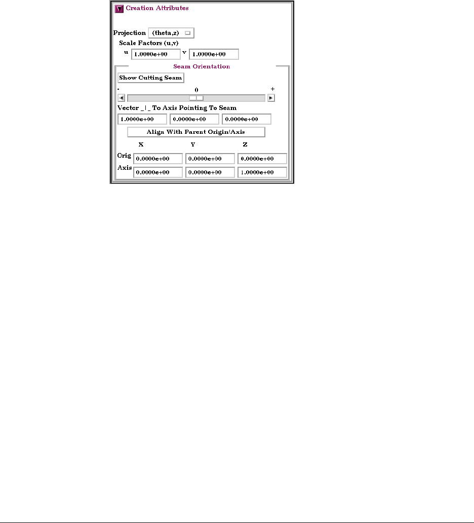
7.9 Developed Surface Create/Update
7-60 EnSight 7 User Manual
Feature Detail Editor Double clicking on the Developed Surface Create/Update Icon opens the Feature
(Developed Surfaces Detail Editor for Developed Surfaces, the Creation Attributes Section of which
provides access to all of the functions available in the Quick Interaction Area plus
several more:
Vector _|_ To Axis These fields allow you to precisely specify the position of the Cutting Seam Line
Pointing To Seam by specifying the direction of the vector perpendicular to the axis of revolution which
points in the direction of the seam line.
Orig X Y Z
These fields specify a point on the axis of revolution.
Axis X Y Z These fields specify a vector, which when used with the Axis Origin defines the axis of
revolution.
The Feature Detail Editor also allows you to make changes in batch; that is, to
make several changes to the menus and fields which do not effect the Graphics
Window until you click in the Apply Changes button. It is sometimes quicker
(with respect to CPU time) to make several changes at once rather than one at a
time as in the Quick Interaction Area.
(see Section 3.3, Part Editing for a detailed discussion of the remaining Feature
Detail Editor turn-down sections which are the same for all Parts),
(see How To Create Developed (Unrolled) Surfaces)
Troubleshooting Developed Surfaces
Problem Probable Causes Solutions
Error message is encountered while
creating a Developed Surface Part.
Parent Part is invalid. Only 2D Parts can be developed.
Figure 7-52
Feature Detail Editor (Developed Surfaces)

7.9 Developed Surface Create/Update
EnSight 7 User Manual 7-61
Developed Surface is created, but is
either not visible, Partially visible, or
obstructed by other Parts which may
be other developed Parts
Since all Developed Surfaces are
projected about the origin on the xy-
plane of the reference frame of the
parent Part, they may map outside
the viewport, intersect other Parts, or
pile up on each other.
Set the Developed Surface to be
viewed in its own viewport and
initialize the viewport.
Use different u/v scaling.
Assign the developed Part to its own
local reference frame and transform
it accordingly.
Developed Surface Part is a line. Wrong Projection type was
specified.
Select a different Projection.
Developed Surface Part does not
update to new Orig and/or Axis
values.
The Orig and Axis values can not be
specified if the Parent Part is created
from either a cylinder, sphere, cone,
or revolution quadric clip. These
values can only be specified if the
2D parent Part is not a quadric
clipped surface.
Since values entered for this
condition are not used, click the Get
Parent Part Defaults button to update
the fields based on the selected
parent Part in the Parts & Frames
list.
Problem Probable Causes Solutions
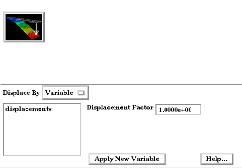
7.10 Displacements On Parts
7-62 EnSight 7 User Manual
7.10 Displacements On Parts
Each node of a Part is displaced by a distance and direction corresponding to the
value of a vector variable at the node. The new coordinate is equal to the old
coordinate plus the vector times the specified Factor, or:
C
new
= C
orig
+ Factor * Vector,
where C
new
is the new coordinate location, C
orig
is the coordinate location as
defined in the data files, Factor is a scale factor, and Vector is the displacement
vector.
You can greatly exaggerate the displacement vector by specifying a large Factor
value. Though you can use any vector variable for displacements, it certainly
makes the most sense to use a variable calculated for this purpose. Note that the
variable value represents the displacement from the original location, not the
coordinates of the new location.
Clicking once on the Displacements On Parts Icon opens the Displacements
Editor in the Quick Interaction Area which is used to specify how you wish to
displace Part nodes based on a vector variable.
Displace by This button allows selection of either None for no displacement or Variable (that selected
in the Variables List) to use for displacement. The selected Variable must be a node-based
vector and must be defined on the Parent Parts.
Displacement Factor This field specifies a scale factor for the displacement vector. New coordinates are
calculated as: C
new
= C
orig
+ Factor*Vector, where C
new
is the new coordinate location,
C
orig
is the original coordinate location as defined in the data file, Factor is a scale factor,
and Vector is the displacement vector. Note that a value of 1.0 will give you “true”
displacements.
Apply New Variable Changes the variable the Displacements are based upon to that currently selected in the
Vari a bl es Li st .
Figure 7-53
Displacements On Parts Icon
Figure 7-54
Quick Interaction Area - Displacements Editor

7.10 Displacements On Parts
EnSight 7 User Manual 7-63
Feature Detail Editor Double clicking on the Displacement on Parts Icon opens the Feature
(Model) Detail Editor for Model Parts, the Displacements Attributes turndown area of
which provides access to the same functions available in the Quick Interaction
Area.
(see Section 3.3, Part Editing for a detailed discussion of the other features
available in the Feature Detail Editor (Model)),
(see How To Display Displacements)
Troubleshooting Displacement Attributes
Problem Probable Causes Solutions
Displacement not visible Displace By set to None for Part that
is not displacing.
Set Displace By to Variable
Displacement Factor value too
small.
Specify a larger Displacement
Factor.
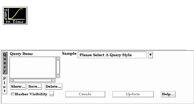
7.11 Query/Plot
7-64 EnSight 7 User Manual
7.11 Query/Plot
EnSight provides several ways to examine information about variable values. You
can, of course, visualize variable values with fringes, contours, vector arrows,
profiles, isosurfaces, etc. This section describes how to query variables
quantitatively:
Over Distance EnSight can query variables at points over distance for the following information:
• variable values inside Parts at evenly spaced points along a straight line
• variable values inside Parts at the nodes of a different 1D Part
Over Time EnSight can query variables over time for the following information:
• minimum and maximum variable values for Parts
• variable values at any number of sample times at any point inside of a Part or at
any labeled node or element.
Over-time queries can report actual variable values, or Fast Fourier Transform
(FFT) spectral values at the positive FFT frequencies.
Variable vs. EnSight can produce a scatter plot of one variable vs. another.
Variable
Operations on EnSight can scale query values and/or combine one set of query values with
another set to produce a new set of values.
Importing EnSight can import query values from external files.
Query Candidates Only Parts with data residing on the Server host system may be queried. Thus,
Parts that reside exclusively on the Client host system (i.e. contours, particle
traces, profiles, vector arrows) may NOT be queried.
(see Section 3.1, Part Overview)
Clicking once on the Query/Plot Icon opens the Query/Plot Editor in the Quick
Interaction Area which is used to query about the selected Variable on the selected
Part and, if you wish, assign a query entity to a plotter.
Query Items This is the list of query items that currently exist in EnSight. After creating a query item, it
will show up in this list and can be modified by selecting it in the list and changing the
displayed values. (Note, it is best to deselect any query items in the list when creating a
Figure 7-55
Query/Plot Icon
Figure 7-56
Quick Interaction Area - Query/Plot Editor
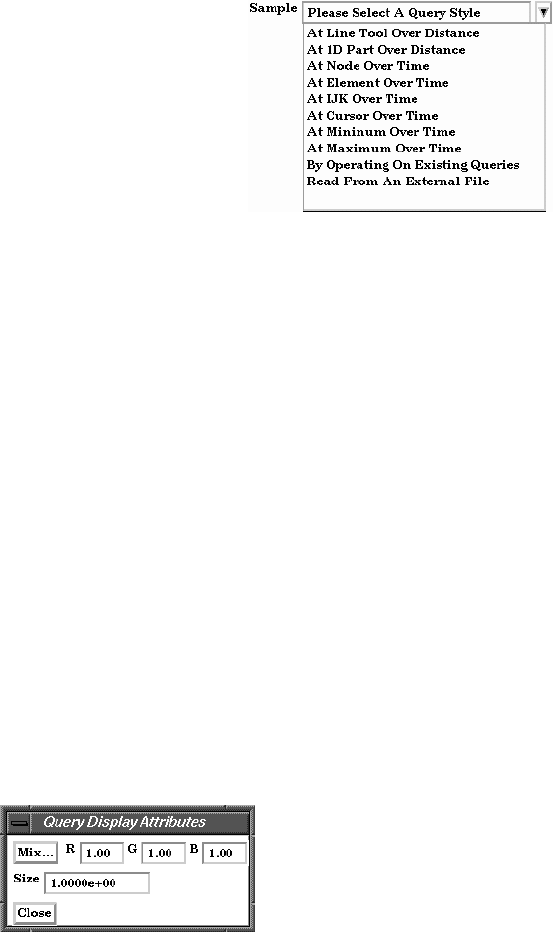
7.11 Query/Plot
EnSight 7 User Manual 7-65
new one, otherwise you may accidently modify values for the item with the left mouse
button.)
Sample This menu contains the types of queries that can be created. Selecting one of these changes
the interface to display controls related to the type.
General to Each Type of Query
Marker Visibility Toggles the visibility of the marker showing the location for the query. For distance
queries, a sphere marker will be shown indicating the beginning location for the query.
... Opens the Query Display Attributes dialog for the specification of the display attributes of
the query marker.
Mix... Opens the Color Selector to specify the color of the marker.
RGB The red, green, and blue color for the marker.
Size The size of the sphere marker. The value is a scale factor. Values larger than 1.0 will scale
the marker up, while values less than 1.0 (but greater than 0.0) will scale the marker down.
Update This button causes the query to be recomputed using any modified attributes or variables.
Please Select A Query Style
is displayed until a Sample selection is made.
At Line Tool Over Distance
queries at uniform points along the line tool.
At 1D Part Over Distance
queries at the nodes of a 1D part.
At Node Over Time
queries at a node over a range of times.
At Element Over Time
queries at an element over a range of times.
At IJK Over Time
queries at an IJK location over a range of times.
At Cursor Over Time
queries at the cursor tool location over a range of times.
At Minimum Over Time
queries the minimum of a variable over a range of times.
At Maximum Over Time
queries the maximum of a variable over a range of times.
By Operating On Existing Queries
forms new query by scaling and/or combining existing ones.
Read From An External File
imports previously saved or externally generated queries.
(This can be EnSight XY data format or MSC Dytran .ths
files.)
Figure 7-57
Query Sample Types
Figure 7-58
Query Display Attributes dialog
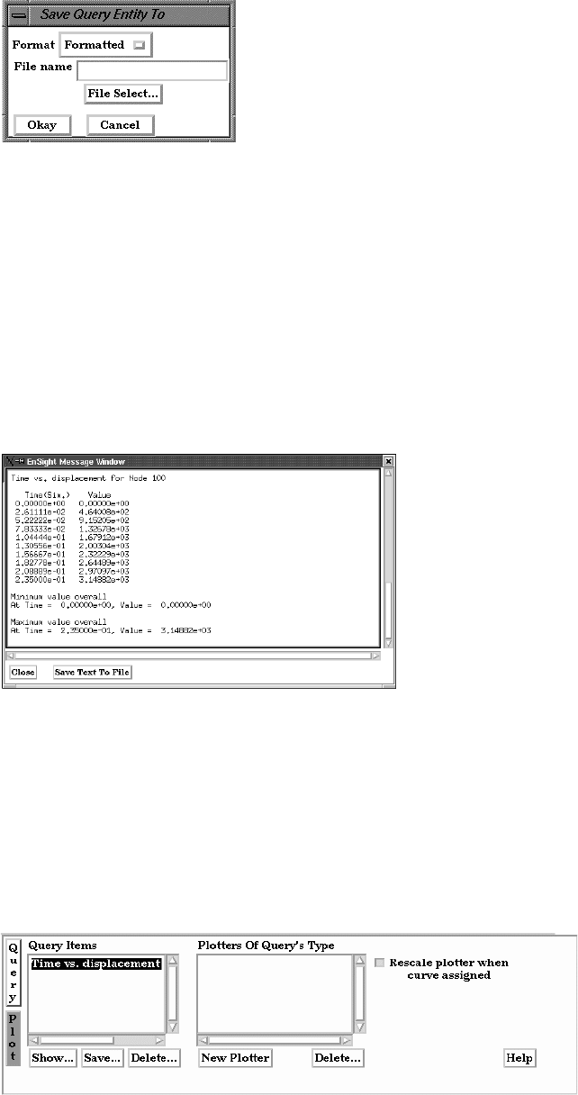
7.11 Query/Plot
7-66 EnSight 7 User Manual
Save... Opens the Save Entity Query To dialog for the specification of the format, and file name in
which you wish to save the query entity.
Format Opens a pop-up menu to allow specification of the format. Choices are:
Formatted Outputs the query information to the specified file in the same format as the
Show Text button.
XY Data Outputs the query information in a generic format which could be used to
export the information to a different plotting system.
File Name This field is used to specify the file name in which you wish to save the query entity.
File Select Opens up the File Selection dialog for specifying the File Name as an alternative to
entering it manually in the File Name field.
Show ... This button will display the results of the selected query in the EnSight Message Window.
Save Text To File Opens the File Selection dialog for specification of filename to save to.
Delete... This button will delete the selected query items. You must confirm the deletion before it as
actually done.
Create This button will create the query according to options and variables specified.
Plot Changes the Quick Interaction Area into the plotting section.
Figure 7-59
Save Query Entity To dialog
Figure 7-60
EnSight Message Window displaying query information
Figure 7-61
Plot Query Entity To dialog
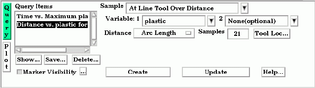
7.11 Query/Plot
EnSight 7 User Manual 7-67
Query Items Shows a list of current query items. As you select these, the plotters of the same type (if
any) will be displayed in the Plotters Of Query’s Type list. And if the query has been
assigned to one of these plotters, it will be highlighted.
Plotters Of Query’s Shows a list of currently defined Plotters which are of the same type as the selected query.
Type The selected query can be plotted on these or on a new plotter.
Rescale plotter If a query is assigned to an existing plotter by selecting one in the Plotter Of Query’s Type
when curve assigned list, enabling this option will rescale the axis of the Plotter to include all queries that are
assigned to it.
New Plotter Will create a new plotter, add the new plotter to the list, and display the plotter with its
query curve in the graphics window.
Delete ... Will delete the selected plotters. You must confirm the deletion before it is actually done.
Query
At Line Tool Over Distance
Variable: 1 A list of variables than can be chosen for the query. If plotted, this variable will be plotted
along the Y-Axis.
Variable: 2 If you leave this as “None”, DISTANCE will be the default X- Axis variable. If you
choose a variable form the list, a “scatter plot” query will result, and the X-Axis will be
the variable you have chosen.
Distance A menu of choices that control the distance parameter.
Arc Length The distance along the part from the first node to each subsequent node
(i.e. the sum of the 1D element lengths).
X Arc Length The X coordinate value of each node accumulated from the start.
Y Arc Length The Y coordinate value of each node accumulated from the start.
Z Arc Length The Z coordinate value of each node accumulated from the start.
From Origin The distance from the origin.
X from Origin The X distance from the origin.
Y from Origin The Y distance from the origin.
Z from Origin The Z distance from the origin.
Samples For queries over Distance using the Line Tool, this field specifies the number of equally
spaced points to query along the line.
Tool Loc... Brings up the Transformation Editor (Line Tool) dialog for feedback and manipulation of
the location of the line tool.
Figure 7-62
Quick Interaction Area - Query/Plot Editor - At Line Tool Over Distance
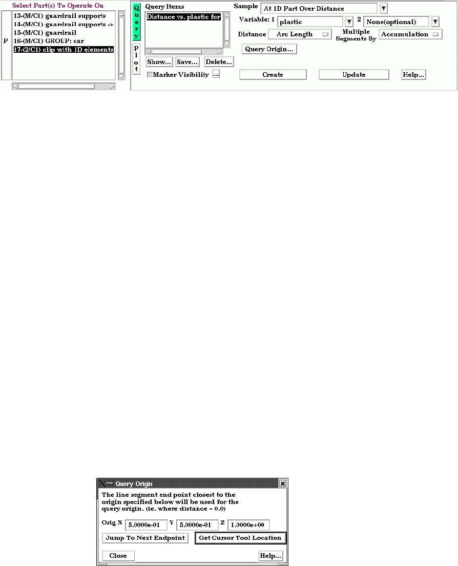
7.11 Query/Plot
7-68 EnSight 7 User Manual
At 1D Part Over Distance
Note that the 1D part to use for the query must be selected from the Part’s list.
Variable: 1
A list of variables than can be chosen for the query. If plotted, this variable will be plotted
along the Y-Axis.
Variable: 2 If you leave this as “None”, DISTANCE will be the default X- Axis variable. If you
choose a variable form the list, a “scatter plot” query will result, and the X-Axis will be
the variable you have chosen.
Distance A menu of choices that control the distance parameter.
Arc Length The distance along the part from the first node to each subsequent node
(i.e. the sum of the 1D element lengths).
X Arc Length The X coordinate value of each node accumulated from the start.
Y Arc Length The Y coordinate value of each node accumulated from the start.
Z Arc Length The Z coordinate value of each node accumulated from the start.
From Origin The distance from the origin.
X from Origin The X distance from the origin.
Y from Origin The Y distance from the origin.
Z from Origin The Z distance from the origin.
Multiple Segments By When the selected 1D part contains more than one contiguous segment, these are handled
by:
Accumulation Each segment’s query is appended to the previous. Thus a plot of this
query will be one extended curve, but the extents of individual segment
may not be obvious.
Reset Each Each segment’s query is treated like it is independent. Thus a plot of
this query will appear as several curves.
Query Origin ... Brings up the Query Origin dialog for feedback and manipulation of the location of the
query origin. .
Orig XYZ Coordinates of the location to use for query origin determination. The endpoint closest to
the origin specified will be used as the “origin” of the query, i.e., where distance is zero. If
the 1D part is s closed loop (i.e. there are no end points), the closest point on the loop is
used as the “origin”.
Figure 7-63
Quick Interaction Area - Query/Plot Editor - At 1D Part Over Distance
Figure 7-64
Query Origin dialog
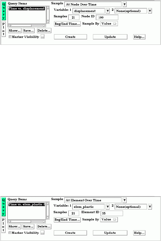
7.11 Query/Plot
EnSight 7 User Manual 7-69
Jump To Next When multiple segments are present, clicking this button jumps to the beginning of the
Endpoint next segment, placing that location in to the Orig XYZ fields.
Get Cursor Tool Places the current cursor tool location into the Orig XYZ fields so that point can be used
Location as the query origin.
At Node Over Time
Variable: 1 A list of variables than can be chosen for the query. If plotted, this variable will be plotted
along the Y-Axis.
Variable: 2 If you leave this as “None”, TIME will be the default X- Axis variable. If you choose a
variable form the list, a “scatter plot” query will result, and the X-Axis will be the variable
you have chosen.
Samples Specifies how many evenly timed moments over the specified range of time steps at which
to query (if left blank, you get a sample point at each time step). If you specify more or
fewer sample points than the number of time steps, EnSight linearly interpolates between
the adjoining time steps. If query is an FFT sampling, the number of frequencies output
will be less than or equal to the number of sample points.
Node ID Specifies a node ID.
Beg/End Time ... Opens up the Solution Time Editor in the Quick Interaction Area. Here you can specify
the start and end times for queries Over Time.
(see Section 7.13, Solution Time)
Sample By Opens a pop-up menu for specification of how to report values for Over Time queries.
Options are:
Va lu e reports values versus time.
FFT reports FFT spectral values versus FFT positive frequencies.
At Element Over Time
Variable: 1 A list of variables than can be chosen for the query. If plotted, this variable will be plotted
along the Y-Axis. (Note: only per_element variables can be used for this query type.)
Variable: 2 If you leave this as “None”, TIME will be the default X- Axis variable. If you choose a
variable form the list, a “scatter plot” query will result, and the X-Axis will be the variable
you have chosen.
Samples Specifies how many evenly timed moments over the specified range of time steps at which
Figure 7-65
Quick Interaction Area - Query/Plot Editor - At Node Over Time
Figure 7-66
Quick Interaction Area - Query/Plot Editor - At Element Over Time
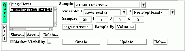
7.11 Query/Plot
7-70 EnSight 7 User Manual
to query (if left blank, you get a sample point at each time step). If you specify more or
fewer sample points than the number of time steps, EnSight linearly interpolates between
the adjoining time steps. If query is an FFT sampling, the number of frequencies output
will be less than or equal to the number of sample points.
Element ID Specifies an element ID.
Beg/End Time ... Opens up the Solution Time Editor in the Quick Interaction Area. Here you can specify
the start and end times for queries Over Time.
(see Section 7.13, Solution Time)
Sample By Opens a pop-up menu for specification of how to report values for Over Time queries.
Options are:
Va lu e reports values versus time.
FFT reports FFT spectral values versus FFT positive frequencies.
At IJK Over Time
Variable: 1 A list of variables than can be chosen for the query. If plotted, this variable will be plotted
along the Y-Axis.
Variable: 2 If you leave this as “None”, TIME will be the default X- Axis variable. If you choose a
variable form the list, a “scatter plot” query will result, and the X-Axis will be the variable
you have chosen.
Samples Specifies how many evenly timed moments over the specified range of time steps at which
to query (if left blank, you get a sample point at each time step). If you specify more or
fewer sample points than the number of time steps, EnSight linearly interpolates between
the adjoining time steps. If query is an FFT sampling, the number of frequencies output
will be less than or equal to the number of sample points.
IJK Specifies the IJK planes of the desired location.
Beg/End Time ... Opens up the Solution Time Editor in the Quick Interaction Area. Here you can specify
the start and end times for queries Over Time.
(see Section 7.13, Solution Time)
Sample By Opens a pop-up menu for specification of how to report values for Over Time queries.
Options are:
Va lu e reports values versus time.
FFT reports FFT spectral values versus FFT positive frequencies.
Figure 7-67
Quick Interaction Area - Query/Plot Editor - At IJK Over Time
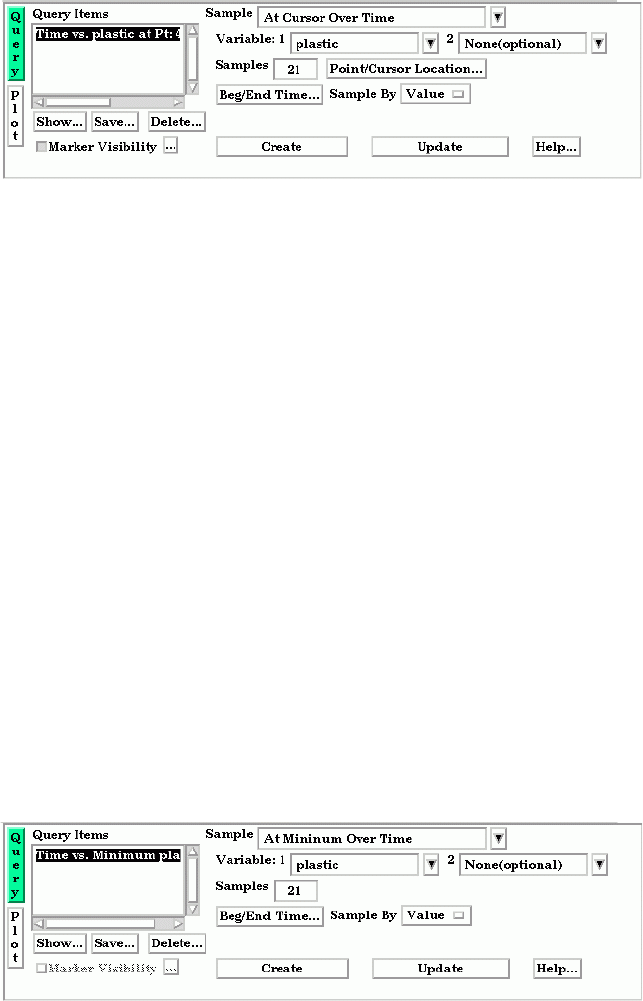
7.11 Query/Plot
EnSight 7 User Manual 7-71
At Cursor Over Time
Variable: 1 A list of variables than can be chosen for the query. If plotted, this variable will be plotted
along the Y-Axis.
Variable: 2 If you leave this as “None”, TIME will be the default X- Axis variable. If you choose a
variable form the list, a “scatter plot” query will result, and the X-Axis will be the variable
you have chosen.
Samples Specifies how many evenly timed moments over the specified range of time steps at which
to query (if left blank, you get a sample point at each time step). If you specify more or
fewer sample points than the number of time steps, EnSight linearly interpolates between
the adjoining time steps. If query is an FFT sampling, the number of frequencies output
will be less than or equal to the number of sample points.
Point/Cursor Can be used to open up the Transformation Editor (Cursor Tool) dialog for specification
Location ... of the cursor location. You can of course also set this location using interactive or picking
methods.
Beg/End Time ... Opens up the Solution Time Editor in the Quick Interaction Area. Here you can specify
the start and end times for queries Over Time.
(see Section 7.13, Solution Time)
Sample By Opens a pop-up menu for specification of how to report values for Over Time queries.
Options are:
Va lu e reports values versus time.
FFT reports FFT spectral values versus FFT positive frequencies.
At Minimum Over Time
Variable: 1 A list of variables than can be chosen for the query. If plotted, this variable will be plotted
along the Y-Axis.
Variable: 2 If you leave this as “None”, TIME will be the default X- Axis variable. If you choose a
variable form the list, a “scatter plot” query will result, and the X-Axis will be the variable
you have chosen.
Samples Specifies how many evenly timed moments over the specified range of time steps at which
to query (if left blank, you get a sample point at each time step). If you specify more or
fewer sample points than the number of time steps, EnSight linearly interpolates between
Figure 7-68
Quick Interaction Area - Query/Plot Editor - At Cursor Over Time
Figure 7-69
Quick Interaction Area - Query/Plot Editor - At Minimum Over Time
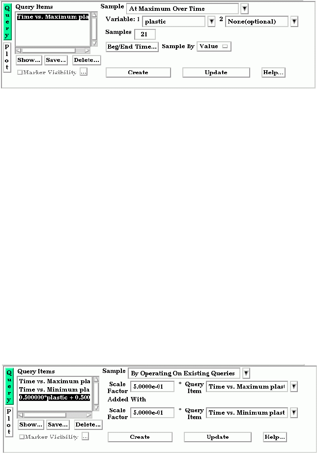
7.11 Query/Plot
7-72 EnSight 7 User Manual
the adjoining time steps. If query is an FFT sampling, the number of frequencies output
will be less than or equal to the number of sample points.
Beg/End Time ... Opens up the Solution Time Editor in the Quick Interaction Area. Here you can specify
the start and end times for queries Over Time.
(see Section 7.13, Solution Time)
Sample By Opens a pop-up menu for specification of how to report values for Over Time queries.
Options are:
Va lu e reports values versus time.
FFT reports FFT spectral values versus FFT positive frequencies.
At Maximum Over Time
Variable: 1 A list of variables than can be chosen for the query. If plotted, this variable will be plotted
along the Y-Axis.
Variable: 2 If you leave this as “None”, TIME will be the default X- Axis variable. If you choose a
variable form the list, a “scatter plot” query will result, and the X-Axis will be the variable
you have chosen.
Samples Specifies how many evenly timed moments over the specified range of time steps at which
to query (if left blank, you get a sample point at each time step). If you specify more or
fewer sample points than the number of time steps, EnSight linearly interpolates between
the adjoining time steps. If query is an FFT sampling, the number of frequencies output
will be less than or equal to the number of sample points.
Beg/End Time ... Opens up the Solution Time Editor in the Quick Interaction Area. Here you can specify
the start and end times for queries Over Time.
(see Section 7.13, Solution Time)
Sample By Opens a pop-up menu for specification of how to report values for Over Time queries.
Options are:
Va lu e reports values versus time.
FFT reports FFT spectral values versus FFT positive frequencies.
By Operating On Existing Queries
Scale Factor Scale factor for the Query Item selected. The values of the selected query will be
multiplied by this factor either before it is added to the second query or before the new
query is created (if only operating on a single query).
Figure 7-70
Quick Interaction Area - Query/Plot Editor - At Maximum Over Time
Figure 7-71
Quick Interaction Area - Query/Plot Editor - By Operating On Existing Queries
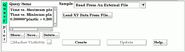
7.11 Query/Plot
EnSight 7 User Manual 7-73
Query Item The existing query item(s) to operate on. A new query will be create consisting of scaled
values one query, or the scaled, algebraic sum of two queries.
Read From An External File
Load XY Data Opens the File Selection dialog from which a previously saved or externally generated
From File query can be retrieved. EnSight’s XY data format or MSC Dytran .ths files can be read.
(See also How To Query/Plot)
Figure 7-72
Quick Interaction Area - Query/Plot Editor - Read From An External File
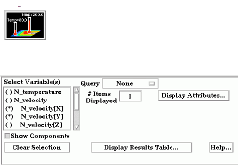
7.12 Interactive Probe Query
7-74 EnSight 7 User Manual
7.12 Interactive Probe Query
EnSight enables you to obtain scalar, vector, or coordinate information for the
model at a point directly under the mouse pointer, at the location of the cursor
tool, or at particular node, element, ijk, or xyz locations. The information is
normally displayed in the Interactive Probe Query section of the Quick Interaction
Area, but it can also be displayed in the Graphics Window. The performance of
Interactive Query operations is dependent on the refresh time of the Graphics
Window. Interactive query values are not echoed to EnSight command language
files.
Clicking once on the Interactive Probe Query Icon opens the Interactive Probe
Query Editor in the Quick Interaction Area which is used to specify parameters
for querying interactively.
Select Variable(s) List of variables and their components (if vector and Show Components is toggles on).
Query Selection of whether interactive query is on, or which method to use to indicate input.
Surface Pick will query the location under the mouse in the Main View. The query will be
performed when the “p” keyboard key is pressed (when “Pick Use ‘p’ ” is on) or
whenever the mouse moves to a new location in the Main View (when “Continuous” is
on).
Cursor will query the location indicated by the Cursor Tool in the Main View. The query
will be performed when the “p” keyboard key is pressed (when “Pick Use ‘p’ ” is on) or
whenever the Cursor Tool moves to a new location in the Main View (when “Continuous”
is on.
Node will query the node as specified in the “Node ID” field.
IJK will query the IJK node as specified in the “I J K” fields.
Element will query the element as specified in the “Element ID” field.
XYZ will query the x, y, z location as specified in the “x y z” fields.
None indicates that interactive query is off.
Search Selects the location for the query. (Only active for Surface Pick and Cursor queries.)
Exact indicates that the query will occur at the location of the mouse.
Closest Node indicates that the query will “snap” to the node closest to the mouse.
Pick (Use ‘p’ ) When the Action is Surface Pick or Cursor, controls whether the query will occur on a
keyboard ‘p’ key press (when on) or will occur continuously - tracking the mouse
location.
Figure 7-73
Interactive Probe Query Icon
Figure 7-74
Quick Interaction Area - Interactive Probe Query Editor
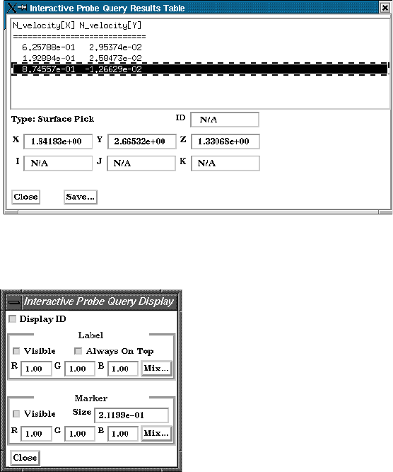
7.12 Interactive Probe Query
EnSight 7 User Manual 7-75
Node ID For Node Queries, specify the node id.
Element ID For Element Queries, specify the element id.
# Items Displayed Sets the number of query locations that are kept in memory and displayed to the user.
Clear Selection Clears all the selected variables.
Display Results Table... Opens the Interactive Probe Query Results Table dialog which shows a table of all
selected variables as well as the current query type, the latest xyz coordinates, the latest ijk
values (if applicable), and the latest node or element id (if applicable). Note that the
contents of this dialog can be saved to a file by using the Save... button.
Display Attributes... Opens the Interactive Probe Query Display dialog.
Display ID Toggle When toggled on, if an ID is appropriate for the type of search, will display the ID in the
query table and in the label on the model.
Label
Visible Toggle
When toggled on, query information will be displayed in the Graphics Window
Always on Top When on, query information in the Graphics Window will not be hidden from view behind
other geometry.
RGB These fields specify color values for the Labels.
Mix Opens the Color Selector dialog
(see Section 7.1, Color)
Marker
Visible When on, query location markers will be displayed in the Graphics Window.
Size The size of the markers.
RGB These fields specify color values for the markers.
Mix Opens the Color Selector dialog
(see Section 7.1, Color)
Figure 7-75
Interactive Probe Query Results Table
Figure 7-76
Interactive Probe Query Display dialog
7.13 Solution Time
7-76 EnSight 7 User Manual
7.13 Solution Time
Many analyses contain time dependent information, such as automobile crash
simulations and unsteady flow problems. The presence of time-dependent data is
indicated to EnSight through an EnSight result file, case file, or is determined
directly from the data files of other formats. EnSight has the capability of
displaying the model and results at any time provided for in the data. Linear
interpolation between given time steps is possible as long as the geometry does
not have changing connectivity over time.
EnSight keeps track of which variables and Parts have been created so that if you
change time steps, variables and Parts will update appropriately. For example,
assume you have created a clip plane through the combustion chamber of an
engine. From this clip plane you have created two constant variables Min
Temperature and Max Temperature and are displaying them in the Main View.
Now change time steps. First, the geometry updates to a new crank angle position.
Second, the clip plane will automatically be recalculated to fit the new geometry.
Third, the Min and Max values displayed in the Graphics Window are
recalculated and updated. This is all performed automatically by EnSight after
you change the current time value.
It is important to distinguish between time step and solution time. An example
will best illustrate this concept.
Consider a model with data for 5 different times:
Time Step Solution Time
0 1.0125
1 11.025
2 11.50
313.00
4 21.333
Note that the time steps coincide with the number of transient data files and are
integers. The solution time at each time step comes from the analysis, and does
not have to be at uniform intervals. The solution time can be in any units needed,
but must be consistent with the solution files. That is, if a velocity file was in
terms of meters per second, then the solution time must be in terms of seconds.
Hence it is not possible, for example, to have the solution time reported in degrees
crank angle for a combustion case unless the corresponding solution files were
also in terms of crank angle (otherwise velocity would be reported in the
meaningless units of meters-per-degree-crank-angle).
The Solution time must always be increasing in time. Failure to follow this rule
will result in an error.
A special Solution Time dialog gives you control over time and relates time step
to solution time. You can force the time information to conform to the actual time
data given at the steps, or you can allow interpolation to occur between time steps.
You must be aware of the implications of such an interpolation and choose the
method that is appropriate.
Also, you can see the ranges of time dependent data available and the current time
that is set for the Main View. You can change time steps by either entering a new
time to view, or using the Solution Time slider bar.
7.13 Solution Time
EnSight 7 User Manual 7-77
The Solution Time Dialog shows a composite timeline of all timesets from all
cases. For any case, a number of different timesets can exist. Each timeset can be
attached to multiple variables and/or geometry. This makes it possible to, for
example, have one variable defined at t = 1.0, 2.0, 3.5 and another variable
defined at t = 1.5, 2.0, 4.0. For each timeline, controls exist to specify how
EnSight should interpolate the variables when time is set to a value not defined for
a given timeset.
There are other places within EnSight where time information is requested. These
include, traces, emitters, animated traces, flip book transient data, key frame
animation transient data, and Query/Plot. Each of these use the specified Beg/End
values. For functions which do not explicitly specify the time step the current
display time (as defined in the Solution Time Dialog) is used.
Clicking once on the Solution Time Icon opens the Solution Time Editor in the
Quick Interaction Area which is used to specify time information.
The range of both Time Steps and Simulation Time is shown at the top of the Editor.
Beg Value for Beginning Time Step or Simulation Time depending on setting for Time As.
Cur Value for Current Time Step or Simulation Time depending on setting for Time As. The
slider bar can be used to select a value for the Current Time Step field.
End Value for Ending Time Step or Simulation Time depending on setting for Time As.
Scale Type Opens a pop-up menu to specify use of existing time steps, or allow EnSight to linearly
interpolate to show any time step. Choices are:
Discrete Can only change time to defined steps.
Continuous
Can change time to any time, including times between steps. Only
available if do not have changing geometry connectivity transient case.
Time As Opens pop-up menu to specify whether to use and display:
Steps which will be an integer showing time as step data. Will show NOSTEP if in
Continuous mode and current time is not at a given time step. Current time will
automatically change to keep within range Begin/End range. The default beginning
and ending simulation times correspond to the first and last time steps specified in
the results.
Figure 7-77
Solution Time Icon
Figure 7-78
Quick Interaction Area - Solution Time Editor
7.13 Solution Time
7-78 EnSight 7 User Manual
Simulation Time which will be a real number showing true simulation time.
Current time will automatically change to keep within the Begin/End range. The
default beginning and ending simulation times correspond to the first and last times
specified in the results.
Reset Time Range Will reset the Begin/End Time values to the minimum/maximum possible. Useful if you
have specified your own Begin/End time values.
Step Arrow Increment Species the incremental time which will be applied to the current time each time the slider
stepper buttons are used.
Animate Over Time... Opens the Flipbook Animation Editor.
(see Section 7.14, Flipbook Animation)
# of Cycles For cyclic transient analysis, the solution is often computed for one cycle only. It is often
desirable to be able to visualize more than one cycle. This is possible only if the first and
last timesteps contain the same information. By default, EnSight assumes one cycle.
Timeset Details... will open the Timeset Details dialog.
Which Timeset(s) Selects the timesets to be viewed.
Modify All Allows modification of all selected timesets.
Selected Timeset(s)
Range which time range to modify.
Update Step Defn. To Choose how to modify the selected Timeset’s Range.
Set Solution Time Will set the Solution Time Beg. and End. time values to correspond to the selected timeset.
To Timeset Range
Show Scale As “Full Time Range” will show the Timeset’s values in relation to the full composite
timeline. “Timeset’s Range” will adjust the beginning and ending boundaries of the
graphic timeset to correspond to the begin and end values for the timeset. The change will
not take effect until the “Update Selected Timeset(s)” button is pressed.
Figure 7-79
Timeset Details Dialog
7.13 Solution Time
EnSight 7 User Manual 7-79
Defined For Lists all of the variables and/or geometry attached to the Timeset.
Left/Right of When the Current time is less than the Timeset’s minimum time, the attached variables
Step Defn. will use the Nearest values or become Undefined.
Between Steps When the Current time is between the Timeset’s minimum and maximum time values, but
Step Defn. not defined, the attached variables will use the Right/ Left, Interpolate, or Nearest values,
or become Undefined.
Update Selected Must be selected in order to update any changed Timeset.
Timeset(s)
7.14 Flipbook Animation
7-80 EnSight 7 User Manual
7.14 Flipbook Animation
There are four common animation techniques which are easily accomplished with
Flipbook Animation. They are:
• animation of transient data, which can be any combination of scalar/
vector variables, geometry, and discrete Particles
• animation of mode shapes based on a mode-shape displacement variable
• animation of a Part moving or changing value during animation, such as
sweeping a 2D-Clip Plane or changing the value of an isosurface.
• animation applying a linear interpolation of a vector displacement field
value factor from 0 to 1.
You can combine any of these techniques with the animation of Particle traces
discussed in the previous Section 7.4.
The concept of a flipbook is similar to the stick figures you have probably seen in
books where each page contains a picture. When you flip through the pages
quickly you get the sense of motion. Flipbook animation stores a series of “pages”
in Client memory which are then rapidly played back to create the illusion of
motion. Pages can be loaded as graphic images, which may playback faster; or as
graphic objects, which can be transformed after creating the flipbook, even while
the flipbook is running.
For animation to be of interest, something must change from page to page. For
transient-data flipbooks, you must have visualized something about the model
that changes over time. For mode-shape flipbooks, you need to have set the
displacement attributes of the Parts for which you want to see mode shapes (see
Section 7.10 Displacement On Parts). For created-data flipbooks, you need to
have used the Start/Stop utility or specified Animation delta values for the Parts.
The number of pages in the flipbook determines the length and smoothness of the
animation. You directly or indirectly specify how many pages to create. While the
Server performs the calculations, the Client stores the flipbook pages in memory.
Just how many pages you can store depends on the amount of memory installed
on your Client workstation. Your choice to load graphic images or graphic objects
affects memory requirements, but the complexity of the model and the size of the
Graphics Window determine which will use less memory in any particular
situation.
You can control which original model Parts and created Parts will be updated for
each time increment as the user chooses. This feature takes all dependencies into
account. For example if an elevated surface was created from a 2D clip plane, the
clip plane would be updated first and then the elevated surface based on the new
clip. The ability to choose which Parts are or are not updated allows before and
after type comparisons of a Part.
After creating the flipbook, options for displaying it include: running all or only a
portion of it, adjusting the display speed, running under manual control or
automatically, and running from the beginning or cycling back-and-forth between
the two ends.
It is important to know that objects in the flipbook cannot be edited. If you wish to
7.14 Flipbook Animation
EnSight 7 User Manual 7-81
change something in the flipbook, you must reload it. If you decide to regenerate a
flipbook (after changing something), you can choose to discard all the old pages,
or keep any old page with the same page number as a new page.
This is very useful when you first load every tenth frame then decide to load them
all. EnSight will not have to reload every tenth frame that already exists. When
you are done with a flipbook, remember to click Delete All Pages. This will free
up memory for other uses.
Flipbook vs. Keyframe While you can implement any flipbook animation technique with keyframe
animation (described in the next section), flipbook animation has three
advantages. First, graphic-object-type flipbooks allow you to transform the model
interactively to see from many viewpoints. Second, graphic-image-type flipbooks
can be saved to a file and later replayed without having to have the dataset loaded,
or even being connected to the Server. Third, the speed of display can be more
interactive because the flipbook is in memory and can be flipped through
automatically or stepped through manually.
Flipbook animation has a few disadvantages. First, you cannot change any Part
attributes, except visibility and material properties, without regenerating the
flipbook. Second, each page is stored in Client memory, which limits the number
of pages and hence the duration of the animation.
Four Animation Techniques:
1.Transient Data Transient-data flipbooks have pages that correspond to particular solution times;
i.e. step or simulation. You specify at which time value to start and stop the
animation, and the time increment between each page. The time increment can be
more than one solution-time value; this is useful in finding a range of interest or
for a coarse review of the results. The increment can be a fraction, in which case
the data for a page is interpolated from the two adjoining solution-time values.
2. Mode Shapes Mode-shape flipbooks are used to show primary modes of vibration for a
structure. This is done by using a per node displacement, enabling the Part to
vibrate. While you can use any vector variable for a displacement, to see actual
mode shapes you need to have a Results-file vector variable corresponding to each
mode shape you wish to visualize. Note that you can create copies of Parts and
simultaneously display them with different mode-shape variables, or one at its
original state and the other with displacement for comparison.
The first page of a mode-shape flipbook shows the full displacement (as it is
normally shown in the Graphics Window). The last page shows the full
displacement in the opposite direction. The in-between pages show intermediate
displacements in proportion to the cosine of the elapsed-time of the animation.
3. Created Data Created-data flipbooks animate the motion of 2D-Clips and Isosurfaces according
to their animation attributes. This animation allows you to show clipping planes
sweeping through a model or to show a range of Isosurface values. The first page
shows the Part’s location as it appears in the normal Graphics Window. On each
subsequent page, each 2D-Clip is regenerated at the new location found by adding
the animation-delta displacement to the 2D-Clip’s location on the previous page.
Also, each Isosurface is regenerated with a new iso-value found by adding the
animation-delta increment to the iso-value of the previous page.
4.Linear Load Linear-loaded flipbooks are used to animate a displacement field of a part by
linearly interpolating the displacement field from its zero to its maximum value.
7.14 Flipbook Animation
7-82 EnSight 7 User Manual
The variable by which the part is colored also updates according to the linearly
displaced values. Like Mode Shapes, this utilizes a per node displacement. The
function can be applied to any static vector variable.
Clicking once on the Flipbook Animation Icon opens the Flipbook Animation
Editor in the Quick Interaction Area.
Load Type Opens a pop-up menu for the selection of type of flipbook animation to load. Options are:
Transient animates changes in data information resulting from changes in the transient
data. For example, changes in coloration resulting from changes in variable values,
or changes in displacement of Parts. See discussion in the introduction section.
Mode Shapes animates the mode shape resulting from a displacement variable. See
discussion in the introduction of this section.
Create Data animates Parts having nonzero animation-delta values or which have been
recorded with the Start/Stop utility. See discussion in the introduction of this section.
Linear Load animates the Displacement (vector) variable of a part by linearly
interpolating the displacement field from its zero to its maximum value. The Color
variables of the part also update according to the linearly displaced values.
Load As Opens a pop-up menu for the selection of whether to load flipbook pages as Graphic
Images or Graphic Objects.
Graphic Objects flipbooks enable you to transform objects after creating the flipbook. Playback
performance depends on the complexity of the model.
Graphic Images flipbooks may be saved for later recall, but they cannot be transformed,
nor can the window be resized. Playback performance depends on the Graphics
Window size.
Adjust Beg/End Time... Opens the Solution Time Editor in the Quick Interaction Area. To return to the Flipbook
Animation Editor from the Solution Time Editor, click on Animate Over Time... (When
loading Transient data, the flipbook will start and stop at the Beg/End values specified in
the Solution Time Editor.
(see Section 7.13, Solution Time)
Increment Time By In this field you specify the increment of each transient-data flipbook page which
corresponds to the range type specified in the Solution Time Editor,
Note: If you enter a Begin, End, or Increment value not corresponding exactly to a Step or
Simulation time value, EnSight will interpolate the values, affecting the appearance of
each page.
Figure 7-80
Flipbook Animation Icon
Figure 7-81
Quick Interaction Area - Flipbook Animation Editor

7.14 Flipbook Animation
EnSight 7 User Manual 7-83
Record Interactive
Allows you to define the change (isovalue change or clip plane movement) in an
Iso/Clip isosurface or clip plane which will take place during the Flipbook load. Only isosurfaces
and clip planes which are modified in interactive mode are tracked.
Start - Stop Start and stop the recording of interactive movement of isosurfaces or clip planes. Any
interactive isosurface or clip plane modified between the Start and Stop will be modified
during the flipbook load.
Run Type Opens a pop-up menu for selection of how the loaded flipbook will play
Auto makes flipbook play continuously.
Step activates Page and Time fields and stepper buttons for manual page control.
Off deactivates animation.
Modify Run... Opens the Auto Run Settings dialog.
You use the Flipbook Run Settings dialog to change the number of pages displayed, the
running speed, and whether or not the flipbook playback repeats from the beginning or
cycles playing forward and backward.
Current Page These fields display the minimum and maximum flipbook-page numbers currently loaded.
Min/Max
Show From Page These interactive fields specify the starting and ending flipbook pages to show when
Show To Page running flipbook.
Display Speed This field specifies the playback-speed factor. Varies from 1.0 (full speed of your
hardware) to 0.0 (stopped). Change by entering a value or clicking the stepper buttons.
Cycle Toggle Toggles-on/off whether, during automatic playback, to replay from the beginning
(toggled-off) or alternate playing forward and backward (toggled-on).
Regen. All Pages Toggles-on/off whether to regenerate already created flipbook pages. When toggled-on,
all
Toggle existing pages are overwritten. When toggled-off, existing pages are not replaced by new
pages having the same time value, and, if loading transient data, new pages can be
interleaved according to their solution-time value.
Load Clicking this button starts the loading flipbook pages and opens a pop-up dialog which
reports the progress of the load and then closes to signal load is complete. If you cancel the
load, the pages already created during the load remain in memory.
Figure 7-82
Auto Run Settings dialog
7.14 Flipbook Animation
7-84 EnSight 7 User Manual
Record...
Opens the Save Flipbook Pages To dialog where you specify the type and name of the
file in which you wish to save the flipbook animation pages you have created
.
Set Format... Brings up the Image/Movie Format and Options dialog. The flipbook will be recorded
using the selected format. (see Section 2.10, Saving and Printing Graphic Images and How
to Print/Save an Image)
Save Window Type When “Normal”, will save images of the same size as the Main View. When “User
Defined”, will allow a specified width and height.
File Prefix The location and filename prefix for the recorded images. The appropriate suffix will be
added automatically.
Delete... Opens a pop-up warning dialog which asks you if you really wish to delete all
loaded pages. Click Okay to delete all loaded flipbook pages and free the memory
for other use.
Figure 7-83
Save Flipbook Pages To dialog

7.14 Flipbook Animation
EnSight 7 User Manual 7-85
Troubleshooting Flipbook Animation
Problem Probable Causes Solutions
No motion No pages are loaded. Load flipbook pages.
All pages are the same visually. In order to see motion there must be
a difference between one page and
the next. Reload with differing Part
attributes, such as coloring by a
variable, using displacements, etc.
Run Type set to Step or Off Select Run Type to be Auto
Speed too fast Display Speed is set too fast. Change speed.
Speed too slow Display Speed is set too slow. Change speed.
Hardware bottleneck (computer
simply isn’t sufficiently powerful)
Reduce the number of pages.Load
pages as graphic images.
Speed erratic Virtual memory is swapping pages to
and from disk storage.
Only load the no.of pages that fit
into the workstation’s main memory.
Mode Shape(s) not visible Wrong Load Type setting Change Load Type to Mode Shapes
and reload.
Displacement attributes are
incorrect.
Change Displace by and Factor
attributes for the Part to animate.
2D Clip plane(s) not moving Wrong Load Type setting Change Load Type to Mode Shapes
and reload.
Plane was not moved interactively
between Start and Stop.
Isosurface(s) not moving Wrong Load Type setting Change Load Type to Mode Shapes
and reload.
Isosurface was not moved
interactively between Start and Stop.
Transient data ignored Wrong Load type
Solution time step specifications are
incorrect.
Change Load Type to Transient and
set Solution time values according to
available time steps.
Pages lost Show From or Show To pages are
not at ends of flipbook.
Old pages are being regenerated. Toggle-off Regen. All Pages
Delete All Pages is clicked. Recover using the session command
file.
Transformations do not work Flipbook pages are loaded as graphic
images.
Reload flipbook pages as Graphic
Objects
7.15 Keyframe Animation
7-86 EnSight 7 User Manual
7.15 Keyframe Animation
Since its initial release in 1987, EnSight has been used extensively for animation,
due to its easy-to-use keyframe animator and ability to handle transient data. This
mechanism allows you to create your own movie sequence to present your results
more easily. There seems to be two mind sets when it comes to animation. The
first group of people believe animation to be totally trivial—something that can be
completely finished in an hour or two by anyone. The other group of people seem
to believe that animation is something that takes many days, if not weeks to finish
and requires an “animation expert” to get done. Well, neither of these ideas are
correct. While animation is not trivial, it is also not overly complicated. Most
animation produced by EnSight is setup during a day, and recorded the same day
or during the night to be complete by the next morning. Engineers create and
record their own animations. The majority of the time involved takes place in the
recording of the frames to the recording device. EnSight is intended to be used by
end users—this includes the animation module. We do acknowledge, however,
that there is a difference between animation, and animation done well. The latter
comes with time and experience.
EnSight uses a modified keyframe technique. This technique enables the user to
define what the scene should look like at certain times called Keyframe. Each
keyframe can be different from a previous keyframe by using any combination of
rotate, translate, scale, zoom, look-at, or look-from operations. A given keyframe
can also be the same as the previous frame (the purpose of which will be
explained shortly). The keyframe technique only works on transformations, and is
not used for other items related to what the scene looks like (i.e., when to turn on
Parts, do isosurfaces, shading changes, etc.). EnSight actually keeps track of the
transformation commands performed between keyframes and linearly interpolates
these commands when creating frames between the keyframes. These in-between
frames are referred to as subframes.
Each keyframe includes the following information: (1) a set of transformation
matrix values, specifying each local frame, the global frame and the Look-At and
Look-From Points; (2) the value of all isosurfaces and position of all clip Parts
using the plane tool; (3) the specific keyframe attributes; and (4) the
transformation commands and isosurface values to get the scene and clip Parts to
the next keyframe.
When running keyframe animation, EnSight performs the following actions for
each keyframe: (1) any command language commands associated with the
keyframe are executed, (2) the specified number of subframes are displayed in
sequence, interpolating the transformation commands to get to the next keyframe.
To begin the process of creating an animation sequence, first define the scene you
desire for the first keyframe. Then, turn on keyframe animation and create this
scene as your first keyframe. You can then proceed to modify the orientation of
the model and create your other keyframes.
If you make mistakes during the keyframe definition, click Delete Keyframe ...
and enter the number of the last keyframe you were satisfied with. Then, proceed
to define the subsequent keyframes again. As soon as you have at least two
keyframes defined, you may play back the animation to see what it looks like. To
do this, select the Run Animation button in the Quick Interaction Area. The
7.15 Keyframe Animation
EnSight 7 User Manual 7-87
animation process generally proceeds with some keyframe definitions, running
what you have so far after some of those definitions, once in a while a delete back
to operation, more keyframe definitions, etc., until you are satisfied with the entire
animation sequence. You then set up the record information and set the process in
motion to produce the images.
Note, that when playing back the animation, you do not have to always play the
entire sequence. Run From, and To frame capability is provided. You also can
abort an animation run by entering the “a” key in the graphics window.
In order to get the length of animation you want on video, you will need to adjust
the number of sub-frames between keyframes in the Speed/Actions tab of the Run
Attributes dialog. The total number of frames displayed during animation is the
sum of the keyframes plus the sum of the subframes. The NTSC broadcasting
standard calls for 30 frames displayed per second. On most workstations, it is
unlikely that EnSight will be able to display this rapidly during playback on the
workstation. So it can be difficult to get a feel for how fast the animation will be
once recorded. The speed of the playback on the workstation is related both to its
graphics capability and the complexity of the scene, so reducing the complexity
will speed things up. Accordingly, you might consider options like making all but
a representative Part invisible, use the feature angle option to reduce the visual
complexity of the Parts, and/or use the dynamic/static box drawing modes.
Anything that is currently on will be on during the animation. That is, if contours,
vector arrows, Particle traces, shaded surfaces, flipbook animation, animated
traces, etc. are on, they will be on during animation. If any Parts have an
animation delta set or are dependent on a Part that has the delta set then they will
be regenerated and change through the animation. This enables you to do any of
the flipbook animation techniques within keyframe animation for recording
purposes, including the use of transient data (See Flipbook Animation). The
advantage for doing flipbook techniques within keyframe animation is that they
can be recorded and the amount of memory used is smaller because the whole
flipbook is not loaded into memory. This enables the recording of long sequences
of changing information that would not be able to be shown fully with flipbook
animation because of memory limits of the workstation. Short sequences that you
have already loaded into the flipbook can also be used by making sure that the
Flipbook Run toggle is on before running keyframe animation.
If dealing with transient data, you should set up the keyframes for display of the
model first, play it back, edit, etc. Then, after you are satisfied with the model
presentation, you can start dealing with displaying the transient data on the model.
You should be careful in doing movement of the model while transient data is
being displayed. It can be confusing to have the transient data changing at the
same time that the model in the scene is moving. When dealing with transient
data, we normally introduce the problem first with some keyframes, then run the
transient data without any transformations by defining two successive identical
keyframes. Between these two identical keyframes, we animate the transient data
using one of the several methods available.
We have attempted to create the animation module to be able to run in a set-up-
walk-away mode to create video. In order to do this, you can issue command
language lines at each keyframe (except the last one). For example, if you had a
case where you wanted to first show off some of the model, and then turn on
fringes to show results, you could issue a “view: fringes on” command at the
7.15 Keyframe Animation
7-88 EnSight 7 User Manual
keyframe. It is also possible to play a command language file using this option.
Care should be taken to not issue an
anim_keyframe: run command as Part of
this command language (which would cause an infinite loop).
When saving images to disk files, be aware that image files can take a great deal
of disk space. The file system that you are writing images to should be monitored
during the animation run to make sure it doesn’t run out of space.
Clicking once on the Keyframe Animation Icon opens the Keyframe Animation
Editor in the Quick Interaction Area.
Keyframing Toggle Toggles-on/off Keyframe animation feature. WARNING: If you toggle-off Keyframing,
all the keyframes previously created will be lost (see Save... below).
Create Keyframe Click this button to create a keyframe. If Keyframing toggle is not turned on then creating
the first keyframe will turn it on automatically. Keyframes are automatically numbered in
sequence of their creation. As each keyframe is created, a message appears in the Status
History Area.
Quick Animations... Opens the Quick Animations dialog which allows you to add keyframes of predefined
movement to your animation. Currently implemented are "fly around", "rotate objects",
and "exploded view"
Delete Keyframe… Opens the Delete Keyframes pop-up dialog which allows you to specify the number of the
last keyframe you wish to retain and then delete all keyframes back to that frame. The
keyframe whose number you specify is not deleted. To delete all keyframes enter 0 at the
prompt.
Run Animation Click to run the keyframe animation. If you click Run more than once, the animation will
play for the corresponding number of times. To abort the run, press the “a” key in the
Graphics Window.
Run Attributes... Gives the user access to the various controls of the animation, as explained in more detail
below.
Figure 7-84
Keyframe Animation Icon
Figure 7-85
Quick Interaction Area - Keyframe Animation Editor
7.15 Keyframe Animation
EnSight 7 User Manual 7-89
Speed/Actions Opens the Speed(Subframes)/Actions(Commands) portion of the Keyframe Run
attributes dialog.
Use Interactive By turning this toggle on, any clip or isosurface moved interactively during the keyframe
Iso/Clip will animate.
Animate By turning this toggle on, transparency changes to parts during the definition of the
Transparency keyframes will be part of the animation.
Change
Spline the By turning this toggle on, translations and look-at/from transforms will be interpolated
Translations and on a cubic spline.
Look From Points
For Keyfram
e This field and the stepper buttons are used to select which keyframe to edit.
Sub-Frames The Sub-Frames field specifies the number of subframes between that keyframe specified
and the next one. More subframes make the transformations to the next keyframe
smoother and slower.
Hold This field specifies the number of frames to hold at the keyframe.
Acceleration By turning on this toggle, acceleration will be used at the keyframe. If on for a previous
keyframe it will decelerate.
Commands to This command text area is used to specify up to 20 commands to execute before
Execute at displaying the keyframe referenced in the For Keyframe field (this can be used for all
Keyframe keyframes except the last one). You may use any command except commands
corresponding to nonpermitted actions, such as loading another dataset. Also, there is no
point in using
view_transf commands that transform frames, change the Look At and
Look From points, or move the Plane Tool since the next thing EnSight does is update the
Graphics Window to match the transformation matrix information stored as Part of the
keyframe. You may use
anim_keyframe commands, for example, to toggle-on using
transient data, but you should not use the
anim_keyframe: run command since then the
animation will enter an infinite loop. Commands frequently used here would be
view:
and annotation: commands. You may also play a command file, so there is really no
limit as to how many commands you can execute. The
shell: command is a special
command to issue a UNIX command.
Update This button will accept the commands entered above.
Commands
Figure 7-86
Speed(Subframes)/Actions(Commands) portion of the Keyframe Run Attributes dialog
7.15 Keyframe Animation
7-90 EnSight 7 User Manual
Viewing Window Opens the Viewing Window portion of the Keyframe Run Attributes dialog.
Type Selection of image type, including standard video formats. Options are:
Normal type is appropriate for display in the Graphics Window.
Full type is appropriate for a full-screen graphics window.
NTSC type is NTSC window size.
PA L type is PAL window size.
User Defined type enables you to specify the screen dimensions (see below).
Detached Display enables the specification of the detached display as the destination
of the animation rendering.
Min X Y If Type: User Defined, these fields allow you to specify the pixel dimensions for user-
Max X Y defined type of screen. Allowed values for X are 0 to 1279 and for Y from 0 to 1023.
Bottom left corner is 0,0. EnSight assumes a horizontal-to-vertical aspect ratio of 5-to-4.
Other aspect ratios will distort the images.
Save Multiple If Type: Detached Display, will save an image per display
Images
Run From/To Opens the Run From/To portion of the Keyframe Run Attributes dialog.
Figure 7-87
Viewing Window portion of Keyframe Run Attributes dialog
Figure 7-88
Run From/To portion of Keyframe Run Attributes dialog.
7.15 Keyframe Animation
EnSight 7 User Manual 7-91
Run From / Run To These fields specify the numbers of the keyframe to start from and the keyframe to run to
when Run button is pressed. Must be integer numbers of already created keyframes.
Default is Run From 1 and Run To number of keyframes you have created.
Transient Opens the Transient data synchronization portion of the Keyframe Run Attributes dialog.
Use Transient Data Toggles-on/off transient data as defined in the timelines (see below).
Toggle
Transient Timeline Transient data is always used according to the definitions of the transient timelines. In a
timeline you can specify the start and end time, how to increment time, etc.
By default a single timeline exists which spans the total number of keyframes. Only one
timeline can exist for each keyframe.
The timeline shown is the one being edited. The up/down arrows will advance/decrement
to the next/previous timeline if it exists.
New Will create a new timeline. If the previous timeline currently spans all available
keyframes a pop-up dialog will result and no new timeline will be created.
Delete Will delete the timeline indicated.
Start At Keyframe Transient data will start at the keyframe indicated.
End At Keyframe Transient data will end at the keyframe indicated.
Start Time Controls the time step to be shown at the Start Keyframe. The choices are:
Use Begin: Use the Begin time as defined in the Solution Time dialog
Use End: Use the End time as defined in the Solution Time dialog
Use Current: Use the current time value
Specify: Set the time value using the input field
End Time Controls the time step to be shown as the End Keyframe. The choices are the same as
Start Time.
Specify Time If off, EnSight will interpolate time such that the Start/End Time values match up with the
Increment Start/End keyframes specified. If on, you can specify the increment in time which occurs
for each frame during the timeline.
When Arrive At If you have specified a Time increment this option controls what will happen if you arrive
Start/End Time at the Start/End time. The choices are:
Loop - Jump to the begin/end time
Swing - Reverse direction
Figure 7-89
Transient Data Synchronization portion of Keyframe Run Attributes dialog.
7.15 Keyframe Animation
7-92 EnSight 7 User Manual
Quick Animations... Opens the Quick Animations dialog.
This dialog allows you to add keyframes of predefined movement to your animation.
Currently implemented are "fly around", "rotate objects", and "exploded view". One or a
combination of these can be used.
Total Frames When the Create Keyframes button is pressed one or more keyframes will be created. The
total frames (keyframes plus subframes) will be the number specified here.
Accelerate at If on, transformations will accelerate out of the first keyframe created when Create
first keyframe Keyframes is pressed.
Accelerate at If on, transformations will de-accelerate at the last keyframe created when Create
last keyframe Keyframes is pressed.
Fly Around If on the look-from point will be revolved around the scene by the number of revolutions
specified. The viewer can either rotate to the Right or the Left. The keyframes will be
added when the Create Keyframes button is pressed.
Rotate Objects If on the objects will be rotated about the x, y, and/or z axis by the number of revolutions
specified. The keyframes will be added when the Create Keyframes button is pressed.
Explode View If on the objects will be assigned local axis systems and animated Distance units in the
Direction given about the origin specified. The global axis direction is used.
About Origin XYZ The origin about which the explode will occur.
Get Transform Sets the About Origin to be at the current transform center.
Center
Direction
The direction of the explode transform. The choices are:
X - Translate in the x direction
Y - Translate in the y direction
Z - Translate in the z direction
XYZ - Translate in all three directions
Radial - Translate in the direction defined by a vector from the given origin through
the part centroid.
Figure 7-90
Keyframe Quick Animations dialog
7.15 Keyframe Animation
EnSight 7 User Manual 7-93
For example, if the origin given is 0,0,0 and the explode direction is X, a part with a
centroid at X=1 will translate in the positive X direction while a part with a centroid at
X=-1 will translate in the negative X direction
Distance The total translation to be used.
Create Keyframe Creates the keyframe(s) given the selections in the dialog. If keyframe animation is
currently not on it will turn it on and create an initial keyframe, then add the predefined
transform indicated.
Record... Opens the Keyframe Animation Recorder dialog.
Record To File When on, will record the keyframe animation images to the specified filename(s).
Set Format... Brings up the Image/Movie Format and Options dialog. The flipbook will be recorded
using the selected format. (see Section 2.10, Saving and Printing Graphic Images and How
to Print/Save an Image)
File Prefix Specification of filename prefix to use when saving frames to a disk file. Each frame is
saved in a different file according to the File Numbering. The prefix can also have a
directory path before it, such as /usr/tmp/prefix.
Save… Opens the File Selection dialog to allow you to save the specifications of the current
keyframe into a file. This saves only the keyframe specifications, not the animation
images or Part information. If you perform a Full Backup, the keyframe specifications are
saved as Part of the Backup.
Restore… Opens the File Selection dialog to allow you to restore keyframe specifications from a file.
This restores only the keyframe specifications; you must also load Part data and set the
Part attributes.
(see How To Create a Keyframe Animation)
Figure 7-91
Keyframe Animation Recorder dialog

7.15 Keyframe Animation
7-94 EnSight 7 User Manual
Troubleshooting Keyframe Animation
Problem Probable Causes Solutions
Graphics Window flashes at start of
animation run.
New graphics window is opened to
display the animation.
Hardware specific. Does not affect
frames sent to recorder.
Colors seem to bleed when I play the
recorded tape back.
The color display from tape has a
tendency to bleed colors that are
pure, such as full intensity red,
green, or blue.
Don’t use them. If you want a red
object don’t use full intensity, and
mix in some other components. For
example you may want to try RGB
=.9 .1 .1.
Lines “crawl” across the screen
when I play the recorded tape back.
Lines are only 1 pixel wide which
would cause crawling on video tape.
Use a line width greater than 1.
During playback the action of the
video starts as soon as the picture
comes up and it’s hard to recognize
what is happening that quickly and
then it goes away.
When creating a video it is best to
have the model come up with a hold
of 3 seconds or more before starting
the animation. The animation should
run for a reasonable length of time
and then it should hold for 3 or more
seconds again at the end. On
complex models the hold may need
to be as much as 10.
Holding a video at the beginning and
the end and showing enough frames
in-between will allow your
audiences eyes to adjust and increase
comprehension of the video. Adding
annotation strings and pointers to
point out areas of interest also helps.
Also, showing the whole model with
a hold and then zooming way in on
the area of interest will help
comprehension.
Video is too fast when played back
from a recorded tape, but it looked
fine on the monitor.
Video formats play back at rates that
are normally faster than the
workstation hardware can. For
example, NTSC plays back at 30
frames per second which can be
impossible for the workstation to
match on a fairly complex model.
Increase the number of frames
recorded by adding more subframes
or by possibly having your video
recording device record more than
one frame when EnSight tells it to
record.
Transformation of my object on the
recorded tape is not smooth.
Not enough subframes. Adding more subframes will cause
more finely interpolated scene
between keyframes. For instance the
model should probably not rotate
more than 3 degrees between frames
being recorded.
Model is being clipped away as the
animation proceeds.
Running into the Z-Clip plane or the
regular plane tool with Clipping on.
Make sure the Z-Clip planes and the
plane tool are far enough away from
the model for the whole animation
sequence. NOTE: The distance
between the Z-Clip planes could
affect the clarity of the image. The
Z-Clip should be kept as close to the
model and as close to each other as
possible for better results.
A slight pause occurs when
animation is played
EnSight has a 1 second pause to
ensure the animation window is
ready for animation.
7.16 Subset Parts Create/Update
EnSight 7 User Manual 7-95
7.16 Subset Parts Create/Update
EnSight enables you to create and modify Subset Parts from ranges of node and/or
element labels of model parts. The Subset Parts feature allows you to isolate
contiguous and/or non-contiguous regions of large data sets, and apply the full-
range of feature applications and inspection provided by EnSight.
Subset Parts can only be created from parts that have node and/or element labels.
Therefore, Subset Parts can not be created from any Created Parts, because the
only parts that can have node and element labels are Model Parts such as parts
built from file data, Merged Model Parts, or Computational Mesh Model Parts
(parts created via the periodic computational symmetry Frame attribute). Model
Parts that do not have given or assigned node and/or element labels can not be
used to create Subset Parts.
Subset Parts are created and reside on the server. They are Created Parts that
provide proper updating of all dependent parts and variables.
Subset Parts are created and modified by specifying parent parts, as well as their
node and/or element labels. Node and/or element labels can be displayed and
filtered interactively according to global View Mode and local Part Mode
attributes.
Clicking once on the Subset Parts Create/Update Icon open the Subset Parts
Editor in the Quick Interaction Area which is used to both create and update
Subset Parts.
From Part List reflecting the parent parts that have been added to the list. Selecting a part in this list
displays any corresponding element or node range specifications in the Show List.
Show Opens a pull-down menu for selecting which type of part entity you wish to include (or
have included) in your Subset Part. The Show options are:
Elements show any specified element label ranges
Nodes show any specified node label ranges
Figure 7-92
Subset Parts Create/Update Icon
Figure 7-93
Quick Interaction Area - Subset Parts Editor
7.16 Subset Parts Create/Update
7-96 EnSight 7 User Manual
Show List This field specifies the label ranges of Elements and/or Nodes wanted for the Subset Part
that correspond to the selected part in the From Part list. The Elements or Nodes are
specified as a range as the example indicates, i.e. (Ex. 1,3,8,9,100-250).
Add This field specifies the GUI part number you wish to add to the From Part list.
Delete This button deletes any selected entries in the From Part list along with any corresponding
element or node range specifications in the Show List.
Update Part Recreates the Subset Parts selected in the Main Parts List according to the selections in the
From Part List and the Show List.
Feature Detail Editor Double Clicking on the Subset Parts Create/Update Icon brings up the Feature Detail
(Subset Parts) Editor (Subset Parts), the Creation Attributes of which offers the same features for the
Subset Parts as the Quick Interaction Area Editor.
(see Section 3.3, Part Editing for a detailed discussion of the remaining Feature
Detail Editor turn-down sections which are the same for all Parts),
7.17 Tensor Glyph Parts Create/Update
EnSight 7 User Manual 7-97
7.17 Tensor Glyph Parts Create/Update
Tensor glyphs visualize the direction and tension/compression of the eigenvectors
at discrete points (at nodes or at element centers) for a given tensor variable.
Tensor glyph Parts are dependent Parts known only to the client. They cannot be
used as a parent Part for other Part types and cannot be used in queries. As
dependent Parts, they are updated anytime the parent Part and/or the creation
tensor variable changes (unless the general attribute Active flag is off).
Tensor glyphs can be filtered to show just the tensile or compressive eigenvectors.
Further, the visibility for each of the eigenvectors (Major, Middle, and Minor) can
be controlled.
Tensor glyphs will appear for each of the nodes/elements for the Parent part’s
visual Representation. Thus, for a border Representation of a Part, only the
border nodes/elements will be candidates for a tensor glyph.
The tensile and compressive eigenvectors can be visualized by modifying the
tensile/compressive component’s line width and color.
Clicking once on the Tensor Glyph Create/Update Icon opens the Tensor Glyph
Editor section of the Quick Interaction Area which is used to both create and
update (make changes to) tensor glyph Parts.
Scale Factor The size of the tensor glyph.
Display Which Controls which eigenvectors will be displayed
Compression Show the eigenvectors that are in compression
Tension Show the eigenvectors that are in tension
Major Show the major eigenvector
Middle Show the middle eigenvector
Minor Show the minor eigenvector
Figure 7-94
Tensor Glyph Parts Create/Update Icon
Figure 7-95
Quick Interaction Area - Tensor Glyph Parts Editor
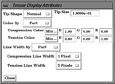
7.17 Tensor Glyph Parts Create/Update
7-98 EnSight 7 User Manual
Display Attributes Opens the Tensor Display Attributes dialog.
Tip Shape Opens a pop-up menu to select the tip shape
Tip Size Controls the size of the tips.
Color By The tensor glyphs can be colored according to the part color, or have a separate color for
compression and tension.
Line Width By The tensor glyphs can use the part line width, or have a separate line width for
compression and tension.
Apply New Variable Changes the tensor Variable used to create the Tensor Glyphs to that currently selected in
the “Select a Tensor Variable” list.
Feature Detail Editor Double clicking on the Tensor Glyph Create/Update Icon opens the Feature Detail
(Tensor Glyph) Editor for Tensor Glyphs, the Creation Attributes Section of which provides access to the
same functions available in the Quick Interaction Area. For a detailed discussion of the
remaining Feature Detail Editor turn-down sections (which are the same for all Part types)
(see Section 3.3, Part Editing and How to Create Tensor Glyphs)
None Displays eigenvectors as lines with no tips.
Normal Displays “classical” tips.
Triangles Displays triangle tips.
Compression Color Specify the compressive color
Tension Color Specify the tensile color
Compression Line Width Specify the compressive line width
Tension Line Width Specify the tensile line width
Figure 7-96
Tensor Display Attributes Dialog

7.17 Tensor Glyph Parts Create/Update
EnSight 7 User Manual 7-99
Troubleshooting Tensor Glyphs
Problem Probable Causes Solutions
No tensor glyphs created No real eigenvectors exist. None
Scale Factor too small. Increase Scale Factor.
Parent parts have non-visual
attributes.
Re-specify parent parts or modify
parent part’s Element Representation.
Parent parts do not contain selected
tensor variable.
Re-specify parent parts.
Too many glyphs Parent parts have too many points at
which tensor glyphs are to be
displayed.
Consider using a grid clip as the
parent part.
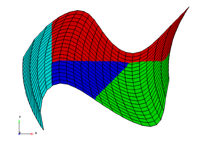
7.18 Material Parts Create/Update
7-100 EnSight 7 User Manual
7.18 Material Parts Create/Update
EnSight enables you to create and modify Material Parts from material
descriptions defined on model parts. The Material Parts feature allows you to
extract single or combined regions of specified materials, as well as boundary
interfaces between two or more specified materials.
Material Parts can only be created from model parts that have material ids
assigned to them. Therefore, Material Parts can not be created from any
Measured or Created Parts. In addition, material information is not transferred to
Created Parts.
Material Parts are created and reside on the server. They are Created Parts that
provide proper updating of all dependent parts and variables - except they do not
inherit any material data themselves.
Material Parts are created and modified by specifying parent model parts, as well
as selecting material descriptions listed in the Materials List. A Material Part is
extracted from only 2D and 3D elements. A Material Part is created as either a
Domain or an Interface.
Domain A material Domain defines a solid region composed of one or more specified
materials. Parts with 2D elements yield 2D material elements, and parts with 3D
elements yield 3D material elements.
Interface A material Interface defines a boundary region between at least two or more
adjacent specified materials. Parts with 2D elements yield 1D material elements,
and parts with 3D elements yield 2D material elements.
Null Materials Two categories of materials are reflected in the Materials List; namely, given
materials and a “null_material”. All given material descriptions correspond to a
material assigned a positive material number, or id. Any material that has an id
less than or equal zero (<= 0) is grouped under the “null_material” and assigned
the material id of zero (0). This allows the null material to act as a valid material.
The “null_material” description always appears in the Materials List whether or
not there are any null materials.
Figure 7-97
Material Parts Illustration
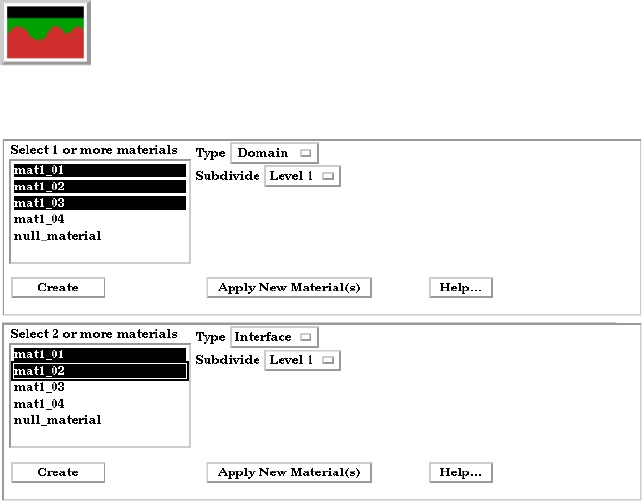
7.18 Material Parts Create/Update
EnSight 7 User Manual 7-101
Subdividing Each 3D (or 2D) element of the part is first decomposed into tetrahedrons (or
triangles) before it is processed. You can increase element resolution of the
Material Part by increasing the Subdivide level. There are three levels of
subdivision. The first level simply processes each of the decomposed (tetrahedral
or triangular) elements. The second level, subdivides each of the decomposed
elements into three sub-elements, and then processes all three of these sub-
elements in place of the decomposed element. The third level, subdivides each of
the decomposed elements into six sub-elements, and then processes these six sub-
elements in place of the original decomposed element.
Algorithm The algorithm implemented is based on a probability based approach to material
interface reconstruction (see reference below). Essentially volume fractions are
averaged for every cell to its nodes, edges/faces, and center. Each cell is then
decomposed and/or subdivided into subcells. Each subcell is then repeatedly
assigned, compared, and appropriately interpolated with volume fractions for each
material. The resulting material cells reflect the maximum volume fraction
portion(s) of the interpolated subcells.
References Meredith, Jeremy S. “A Probability Based Approach to Material Interface
Reconstruction for Visualization”, ECS277 Project 4, Spring 2001
Caveats Material resolution tends to diminish (and at times distorts) at boundary cells that
lack adjacent ghost cells. The volume fractions at these cells simply lack the
proper weighting. This is remedied by providing material ghost cells.
Thus, materials that contribute half or less of the total portion on a boundary
element, typically do not appear without ghost cells
Access Clicking once on the Material Parts Create/Update Icon opens the Material Parts
Editor in the Quick Interaction Area which is used to both create and update
(make changes to) the material parts.
Figure 7-98
Material Parts Create/Update Icon
Figure 7-98
Quick Interaction Area - for Material Parts Type Domain/Interface
7.18 Material Parts Create/Update
7-102 EnSight 7 User Manual
Materials List List reflecting the available materials in the model parts. Any material that has an id less
than or equal to zero (<= 0) comprises the “null_material”.
Type Opens a pull-down menu for specification of whether the Material Part results in a
Domain or Interface. Changing the Type of existing Material Parts will automatically
update them to the new specified type.
Subdivide Opens a pull-down menu for selection of the level to subdivide the decomposed
(tetrahedral and/or triangular) elements. Changing the Type of existing Material Parts will
automatically update them to the new specified type.
Apply New Material(s) Recreates the Material Part selected in the Main Parts List according to the selections in
the material list.
Feature Detail Editor (Material Parts)
Double Clicking on the Material Parts Create/Update Icon (or Edit > Part Feature
Detail Editors > Materials Parts...) opens the Feature Detail Editor (Material
Parts), the Creation Attributes of which offers the same options for the Material
Parts as the Quick Interaction Area Editor.
(See: How To Create Material Parts, and under Section 11.1, EnSight Gold
Casefile Format, see EnSight Gold Material Files Format)
Domain
Creates a solid region composed of one or more specified materials.
Parts with 2D elements yield 2D material elements, and parts with 3D
elements yield 3D material elements.
Interface
Creates a boundary region between at least two or more specified
materials. Parts with 2D elements yield 1D material elements, and
parts with 3D elements yield 2D material elements.
Level 1
Simply processes each of the original decomposed (tetrahedral and/or
triangular) elements.
Level 2
Subdivides each decomposed tetrahedral (and/or triangular) element
into 3 more tetrahedrons (and/or triangles) prior to processing.
Level 3
Subdivides each decomposed tetrahedral (and/or triangular) element
into 6 more tetrahedrons (and/or triangles) prior to processing.

7.18 Material Parts Create/Update
EnSight 7 User Manual 7-103
Troubleshooting Material Parts
Problem Probable Causes Solutions
No Type Domain Material Part
created for specified material
description(s)
Model part(s) not selected.
Model part(s) void of that material
Select only model part(s).
Nothing wrong.
No Type Interface Material Part
created for specified material
description(s)
Model parts not selected.
Two or more materials not selected.
Select only model part(s).
Select at least two (or more) materials.
Selected materials are not adjacent
across a 3D face or 2D edge.
Nothing wrong.
No “null_material” Material Part
created for a specified
“null_material” selection.
Model parts do not contain any null
materials.
Nothing wrong.
There are no null materials, but
selecting “null_material” produces
a visible region.
Incorrect indexing in the material ids
file.
Material ids file possibly has a
negative index to an incorrect position
into the mixed-material id file.
Increasing the Subdivide level
does not increase the material
fraction detail
Increasing the Subdivide level
typically only increases the element
resolution.
Typically nothing wrong.
Changing the Type and/or Level as
well while simultaneously
changing the material selections
did not update the selected
Material Part to the new material
selections.
Material reselection is only updated
via the Apply New Material(s)
button.
Update the new materials first, then
change the type.
Delete the Material Part. Make new
material(s) selection and Type and/or
Subdivide specification. Then Create
a new Material Part.
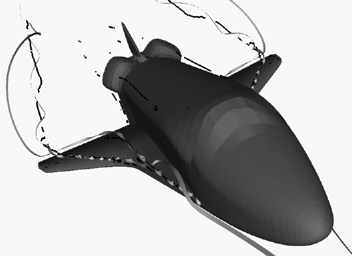
7.19 Vortex Core Create/Update
7-104 EnSight 7 User Manual
7.19 Vortex Core Create/Update
Vortex cores help visualize the centers of swirling flow in a flow field. EnSight
creates vortex core segments from the velocity gradient tensor of 3D flow field
part(s). Core segments can then be used as emitters for ribbon traces to help
visualize the strength and nature of the vortices.
Velocity Gradient EnSight automatically pre-computes the velocity gradient tensor for all 3D model
Tensor parts prior to creating the vortex cores. Since this variable is automatically
created, all subsequent 3D model parts created will also have this tensor
computed.
Note: The velocity gradient tensor variable will continue to be created and
updated for all 3D model parts until it is deactivated.
This tensor variable behaves like any other created tensor variable, and may be
deactivated via the Feature Detail Editor (Variables) dialog.
Thresholding Core segments may be filtered out according to the settings of a threshold
variable, value, and relational operator (see Access below for details). Most active
variables can be used as threshold variables. Thresholding was implemented to
help the user filter-out, or view portions of the core segments according to
variable values.
When vortex core parts are Created/Updated, the vorticity magnitude scalar
variable “
fx_vortcore_streng” is created to help you threshold unwanted
core segments according to these scalar values. (This is the magnitude (RMS) of
the vorticity as defined in chapter 4.)
Due to the difference in algorithms, some segments produced may not be vortex
cores (see Caveats). Thus, the need for a filtering mechanism that filters out
segments according to different variables arose and has been provided via
thresholding options.
7.19 Vortex Core Create/Update
EnSight 7 User Manual 7-105
Algorithms Currently, vortex cores are calculated according to two algorithms based on
techniques outlined by Sujudi, Haimes, and Kenwright (see References below).
Both techniques are linear and nodal. That is, they are based on decomposing
finite elements into tetrahedrons and then solving closed-form equations to
determine the velocity gradient tensor values at the nodes. Also, any variable with
values at element centers are first averaged to element nodes before processing.
The eigen-analysis algorithm uses classification of eigen-values and vectors to
determine whether the vortex core intersects any faces of the decomposed
tetrahedron. The vorticity based algorithm utilizes the fact of alignment of the
vorticity and velocity vectors to determine core intersection points.
References Please refer to the following references for more detailed explanations of pertinent
concepts and algorithms.
D. Banks, B. Singer, “Vortex Tubes in Turbulent Flows: Identification, Representation,
Reconstruction”, IEEE Visualization ‘94, 1994
D. Sujudi, R. Haimes, “Identification of Swirling Flow in 3-D Vector Fields”,
AIAA-95-1715, Jun. 1995
D. Kenwright, R. Haimes, “Vortex Identification - Applications in Aerodynamics”,
IEEE Visualization ‘97, 1997
M. Roth, R. Peikert, “A Higher-Order Method For Finding Vortex Core Lines”,
IEEE Visualization ‘98, 1998
R. Haimes and D. Kenwright, On the Velocity Gradient Tensor and Fluid Feature Extraction”,
AIAA-99-3288, Jan. 1999
R. Peikert, M. Roth, “The ‘Parallel Vectors’ Operator - a vector field visualization primitive”, IEEE
Visualization ‘99, 1999
D. Kenwright, T. Sandstrom, GEL, NASA Ames Research Center, 1999
R. Haimes, D. Kenwright, The Fluid Extraction Toll Kit,
Massachusetts Institute of Technology, 2000
R. Haimes, K. Jordan, “A Tractable Approach to Understanding the Results from Large-Scale 3D
Transient Simulations”, AIAA-2000-0918, Jan. 2001
Caveats Due to the linear implementation of both the eigen-analysis and vorticity
algorithms, they both have problems finding cores of curved vortices. In addition,
testing has shown that both algorithms usually fail to predict vortex core segments
in regions of weak vortices.
Since the eigen-analysis method finds patterns of swirling flow, it can also locate
swirling flow features that are not vortices (especially in the formation of
boundary layers). These non-vortex core type segments can be filtered out via
thresholding (see Thresholding). In addition, the eigen-analysis algorithm may
produce incorrect results when the flow is under more than one vortex, and has a
tendency to produce core locations displaced from the actual vortex core.
The vorticity based method does not seem to exhibit the problem of producing
core segments due to boundary layer formations, because the stress components
of the velocity gradient tensor have been removed in the formation of the vorticity
vector. Thus, the vorticity method seems to produce longer and more contiguous
cores - in most cases; and therefore, the reason for including both algorithms.
7.19 Vortex Core Create/Update
7-106 EnSight 7 User Manual
Access Clicking once on the Vortex Core Create/Update Icon opens the Vortex Core
Editor in the Quick Interaction Area which is used to both create and update
(make changes to) the vortex core parts.
Define Vortex Opens the Vortex Core Variable Settings dialog which allows the user to identify and set
Variables the dependent variables used in
computing the vortex cores. This dialog
has a list of current accessible variables
from which to choose. Immediately
below is a list of dependent variables
with corresponding text field and SET
button. The variable name in the list is
tied to a dependent variable below by
first highlighting a listed variable, and
then clicking the corresponding
dependent variables’s SET button,
which inserts the listed variable into its
corresponding text field.
All text fields are required, except you
may specify either Density and
Momentum (which permits velocity to
be computed on the fly), or just Velocity. A default constant value is supplied for the Ratio
of Specific Heats which may be changed or specified by a scalar variable name.
Clicking Okay activates all specified dependent variables and closes the dialog.
Figure 7-99
Vortex Core Create/Update Icon
Figure 7-100
Quick Interaction Area - Vortex Core Editor (before Create)
Figure 7-100
Quick Interaction Area - Vortex Core Editor (after Create)

7.19 Vortex Core Create/Update
EnSight 7 User Manual 7-107
Method Opens a pop-up dialog for the specification of which type of method to use to compute the
vortex cores in the 3D field. These options are:
Eigen Analysis - Scheme that uses eigen-analysis on the Velocity gradient tensor to
compute the vortex core segments. (See Algorithms above).
Vorticity - Scheme that uses the vorticity vector from the anti-symmetric portions of the
velocity gradient tensor to compute the vortex core segments. (See Algorithms above).
Threshold Filter Relational operators used to filter out vortex core segments.
< Filter out any core segments less than the Threshold Value (default).
> Filter out any core segments greater than the Threshold Value.
Threshold Value The value at which to filter the vortex core segments.
Select Threshold A list of possible variables that you may use to help filter out vortex core segments. This
Variable List list includes the vorticity magnitude scalar variable (named fx_vortcore_streng)
which gets created when you Create/Update a vortex core part.
Threshold Slider Bar Used to change the Threshold Value in increments dependent on the Min and Max
settings. The stepper button on the left (and right) of the slide bar is used to decrement
(and increment) the Threshold value.
Min - The minimum value of the Threshold Variable. The stepper button on the left (and
right) side of the Min text filed is used to decrease (and increase) the order of magnitude,
or the exponent, of the min value.
Max - The maximum value of the Threshold Variable. The stepper button on the left (and
right) side of the Max text field is used to decrease (and increase) the order of magnitude,
or the exponent, of the Max value.
Create Creates vortex cores that correspond to the selected 3D field in the part list, based on the
respective settings.
Apply New Variable Applies the threshold settings to the vortex core segments based on the threshold variable
that is highlighted in the Select Threshold Variable list.
Note: Vortex Core feature extraction does not work with multiple cases.
Troubleshooting Vortex Cores
Problem Probable Causes Solutions
Error creating vortex cores Non-3D part selected in part list Highlight 3D part
Undefined (colored by part color)
regions on vortex cores
Vortex core line segment node was
not mapped within a corresponding
3D field element
Make sure corresponding 3D field
part is defined.
7.20 Shock Surface/Region Create/Update
7-108 EnSight 7 User Manual
7.20 Shock Surface/Region Create/Update
The Shock Surface/Region feature helps visualize shock waves in a 3D flow field.
Shock waves are characterized by an abrupt increase in density, energy, and
pressure gradients, as well as a simultaneous sudden decrease in the velocity
gradient.
EnSight creates candidate shock surfaces in 3D (trans/super-sonic) flow fields
using a creation scalar variable (i.e. density, pressure) along with the velocity
vector (see Algorithms below).
Thresholding Due to the nature of the shock algorithms, other surfaces with similar
characteristics may be produced besides shock surfaces, i.e. expansion regions,
etc. Therefore, a filtering mechanism is necessary to help filter out these non-
shock regions.
Shock surfaces may be filtered out according to the settings of a threshold
variable, value, and relational operator (see Access below for details). Most active
variables can be used as threshold variables, but gradients of the density and
energy related scalar variables in the streamwise direction seem to work best.
When Shock parts are created via the Surface method, the scalar “
SHK_*”
variable (where * is the appended name of the variable, i.e.
SHK_Density) is
created to help threshold unwanted areas according to these scalar values. When
Shock parts are created via the Region method, the scalar “
SHK_Threshold”
variable is created to help threshold respective unwanted areas.
Currently, these
SHK_* variables consist of the gradient of an appropriate
creation variable (i.e.
SHK_Density, SHK_Pressure, etc.) in the streamwise
direction. For the Region method, the creation variable is always pressure.
EnSight tries to compute a reasonable default threshold value each time one of
these threshold variables is applied. By default this value is half of one
exponential order less than the maximum value of the threshold variable on the
Figure 7-101
Shock Surface (Data Courtesy of Craft Technology)
7.20 Shock Surface/Region Create/Update
EnSight 7 User Manual 7-109
shock part. This seems to produce a reasonable starting surface for the user to
threshold. By default, the smaller the threshold value, the larger the part.
The default threshold variable for non “
SHK_” variables is the minimum of the
specified variable on the shock part.
The default Min/Max slider values try to bound the default threshold value by
appropriate orders of magnitude. Min/Max slider values floor/ceil the min/max
values of the threshold variable of the shock part when these ranges are exceeded
(see Threshold Slider Bar below).
Algorithms Shock parts are calculated according to two algorithms, or methods. The first
algorithm (referred to by EnSight as the Surface method) is based on the work of
Pagendarm et. al., and the second algorithm (referred to by EnSight as the Region
method) is based on the work by Haimes et. al. (See References below.)
The Surface method utilizes the maximal gradient of a quantity like density or
pressure in the streamwise direction. This yields a surface that requires
thresholding to distinguish significant portions of the shock patterns from weak
numerical artefacts.
The Region method utilizes flow physics to define shocks in steady state and
transient solutions. The steady state equation is based on developing a scalar field
based on combining the mach vector with the normalized pressure gradient field.
The transient solution combines this term with appropriate correction terms. The
Region method produces iso-shock surfaces that form regions that bound the
shock wave.
Note: Both methods use dependent variables (See Define Shock Variables below).
If some of the dependent variables do not exist and are required, they will be
temporarily calculated based on other defined dependent variables (as defined in
Section 4.3, Variable Creation). The user has the responsibility to ensure these
variables have consistent units.
Both techniques have been implemented in a linear and nodal fashion. That is,
their gradient calculations are based on decomposing finite elements into
tetrahedrons to approximate the gradient values at the nodes. Also, any variables
with values at element centers are averaged to element nodes before processing.
Other Notes Pre-filtering flow field elements by Mach Number.
The Surface Method allows the user to filter-out any flow field elements less than
a specified mach number, by issuing the following command via the command
line processor (See Section 2.4, Command Files):
test: shock_mach_prefilter #
Where # is the corresponding mach-number value (>=0.0) by which to filter.
(Zero is the default value - which means this option is turned-off until activated by
a value > 0.0.) Ideally this mach-number value would be 1; and thus, would
eliminate any subsonic regions from being processed via the Surface method’s
algorithm. In some transonic cases, this has doubled the efficiency of the
algorithm by eliminating the calculation of the second derivative on many
elements. Unfortunately, other cases have been observed (especially noticed in
regions with normal shack waves) where this option (due to the grid resolution
and/or the numerical dissipation inherent in the shock algorithm - see 1999
reference by D. Lovely and R. Haimes) has eliminated some valid shock regions.
Although care is taken to provide an appropriate stencil of elements for the
7.20 Shock Surface/Region Create/Update
7-110 EnSight 7 User Manual
gradient calculations of values adjacent to these areas, it appears this value may
need to be < 1 to prevent these shock regions from being eliminated. This option
is therefore provided at the discretion and expertise of the user. This option only
takes effect when issued prior to a create or an update in shock method.
Post-filtering shock part elements by Mach Number.
Both methods allow the user to filter-out (prior to thresholding) any shock part
elements less than a specified mach number, by issuing the following command
via the command line processor (see Section 2.4, Command Files):
test: shock_mach_postfilter #
Where # is the corresponding mach-number value (>=0.0) by which to filter.
(Zero is the default value - which means this option is turned-off until activated by
a value > 0.0.) Ideally this mach number value would be 1; and thus, would
eliminate any subsonic regions from being displayed as part of the shock surface.
Unfortunately, some cases have been observed (especially noticed in regions with
normal shock waves) where this options (due to the grid resolution and/or the
numerical dissipation inherent in the shock algorithm - see 1999 reference by D.
Lovely and R. Haimes) has eliminated some valid shock regions. This option is
therefore provided at the discretion and expertise of the user. This option only
takes effect when issued prior to a create or an update in shock method.
Moving Shock.
Both methods compute the stationary shock based on the user specified
parameters. The Region Method has the capability of applying a correction term
to represent moving shocks in transient cases. This capability is toggled ON/OFF
by issuing the following command via the command line processor (see Section
2.4, Command Files).
test: toggle_moving_shock
Issuing the command a second time will toggle this option off. This option is
provided at the discretion and expertise of the user. This option only takes effect
when issued prior to a create or an update in shock method.
References Please refer to the following references for more detailed explanations of pertinent
concepts and algorithms.
H.G. Pagendarm, B. Seitz, S.I. Choudhry, “Visualization of Shock Waves in Hypersonic CFD
Solutions”, DLR, 1996
D. Lovely, R. Haimes, “Shock Detection from Computational Fluid Dynamics Results”,
AIAA-99-3285, 1999, 14th AIAA Computational Fluid Dynamics Conference, Vol 1 technical
papers.
R. Haimes and D. Kenwright, “On the Velocity Gradient Tensor and Fluid Feature Extraction”,
AIAA-99-3288, Jan. 1999, 14th AIAA Computational Fluid Dynamics Conference, Vol 1 technical
papers.
D. Kenwright, T. Sandstrom, GEL, NASA Ames Research Center, 1999
R. Haimes, D. Kenwright, The Fluid Extraction Tool Kit,
Massachusetts Institute of Technology, 2000, 39th Aerospace Sciences Meeting and Exhibit, Reno.
R. Haimes, K. Jordan, “A Tractable Approach to Understanding the Results from Large-Scale 3D
Transient Simulations”, AIAA-2000-0918, Jan. 2001
7.20 Shock Surface/Region Create/Update
EnSight 7 User Manual 7-111
Access Clicking once on the Shock Surface/Region Create/Update Icon opens the Shock
Editor in the Quick Interaction Area which is used to both create and update
(make changes to) the shock part.
Define Shock Opens the Shock Variable Settings dialog which allows the user to identify and set the
Variables... dependent variables used in
computing the shock parts. This
dialog has a list of current accessible
variables from which to choose.
Immediately below is a list of
dependent variables with
corresponding text field and SET
button. The variable name in the list
is tied to a dependent variable below
by first highlighting the listed
variable, and then clicking the
corresponding dependent variable’s
SET button, which inserts the listed
variable into its corresponding text
field.
Not all text fields are required.
Although you must specify either
Density or Pressure, Temperature,
and Gas Constant; either Energy or
Pressure; either Velocity or
Momentum; and the Ratio of
Specific Heats. A default constant
value is supplied for the Ratio of
Figure 7-102
Shock Surfaces/Regions Create/Update Icon
Figure 7-103
Quick Interaction Area - Shock Surfaces/Regions Editor (after Create)
Quick Interaction Area - Shock Surfaces/Regions Editor (before Create)

7.20 Shock Surface/Region Create/Update
7-112 EnSight 7 User Manual
Specific Heats and the Gas Constant which may be changed or specified by a scalar
variable name.
Clicking Okay activates all specified dependent variables and closes the dialog.
Method Opens a pop-up dialog for the specification of which type of method, to use to compute
the vortex cores in the 3D field. These options are:
Surface - Scheme that uses maximal density or pressure gradients in the streamwise
direction to locate candidate shock surfaces. (See Algorithms above).
Region - Scheme that uses flow physics based on the mach vector coupled with pressure
gradient to locate candidate shock regions. (See Algorithms above.)
Select Creation A list of variables used to create the shock surface via Surface method. These variable are
Variable specified via those SET in the Define Shock Variables list above.
Note: This list is not used for the Region method. The Region method only uses pressure
as the creation variable.
Threshold Filter Relational operators used to filter out shock areas.
< Filter out any areas less than the Threshold Value (default).
> Filter out any areas greater than the Threshold Value.
Threshold Value The value at which to filter the shock areas.
Select Threshold A list of possible variables that you may use to help filter out unwanted areas. This list
Variable List includes the shock threshold variables “SHK_*” which gets created when you Create/
Update a shock part.
Threshold Slider Bar Used to change the Threshold Value in increments dependent on the Min and Max
settings. The stepper button on the left (and right) of the slide bar is used to decrement
(and increment) the Threshold value.
Min - The minimum value of the Threshold Variable. The stepper button on the left (and
right) side of the Min text field is used to decrease (and increase) the order of magnitude,
or the exponent, of the Min value.
Max - The maximum value of the Threshold Variable. The stepper button on the left (and
right) side of the Max text field is used to decrease (and increase) the order of magnitude,
or the exponent, of the Max value.
Create Creates shock parts that correspond to the selected 3D field in the part list, based on the
respective settings.
Apply New Variable Applies the threshold settings to shock surfaces based on the threshold variable that is
highlighted in the Select Threshold Variable list.
Note: Shock Surface feature extraction does not work with multiple parts.
Troubleshooting Shock Surfaces/Regions
Problem Probable Causes Solutions
Error creating shock part Non-3D part selected in part list Highlight 3D flow field part
No shock part created Flow field part subsonic No shock in subsonic regions

7.20 Shock Surface/Region Create/Update
EnSight 7 User Manual 7-113
Shock dependent variables defined
with incorrect units, i.e. since
Region method uses density and
mach, if file variables are pressure,
temperature, and velocity, then
density (and thus mach) is
dependent on gas constant. By
default this value is 287 (Nm/KgK)
Make sure dependent variables have
correct units. i.e. gas constant may
need to be 1716(ft-lb/slugDegR), or
some other value rather than the
default
No to little shock part created Threshold value too large for <
operation
Decrease threshold value
Problem Probable Causes Solutions
7.21 Separation/Attachment Lines Create/Update
7-114 EnSight 7 User Manual
7.21 Separation/Attachment Lines Create/Update
Separation and Attachment Lines exist on 2D surfaces and help visualize areas
where flow abruptly leaves or returns to the 2D surface in 3D flow fields. These
lines are topologically significant curves on the 2D surface where flow converges
and then separates (separation lines) from the surface into the 3D flow field, and
where flow attaches and then diverges (attachment lines) to the surface from the
3D flow field.
These line segments can be used as emitters for ribbon traces to help visualize
flow interaction from the 2D surface into the 3D field, or displayed along with
surface-restricted traces to help visualize the topology of the 2D surface.
EnSight creates separation and attachment lines as two distinct parts so that each
may be assigned their own attributes. Although both are updated computationally
when changes are made to either one via the quick interaction area.
Separation/Attachment lines can be created on any 2D part, whether it is a
boundary surface or internal surface to a 3D flow field. These lines can also be
created on 3D flow field parts. However, computation of the separation/
attachment lines is restricted to only the boundary surfaces of the 3D flow field.
Velocity Gradient Ensight creates separation and attachment lines from the velocity gradient
Tensor tensor of the 3D flow field part. EnSight automatically pre-computes the velocity
gradient tensor for all 3D model parts prior to creating the separation and
attachment lines. These values are then mapped to any corresponding 2D model
part, or inherited by any created part.
Since this variable is automatically created, all subsequent 3D model parts created
will also have this tensor variable computed.
Note: The velocity gradient tensor variable will continue to be created and
updated for all 3D model parts until it is deactivated.
7.21 Separation/Attachment Lines Create/Update
EnSight 7 User Manual 7-115
This tensor variable behaves like any other created tensor variable, and may be
deactivated via the Feature Detail Editor (Variables) dialog.
Thresholding Separation/Attachment lines may be filtered out according to the settings of a
threshold variable, value, and relational operator (see Access below for details).
Most active variables can be used as threshold variables. Thresholding was
implemented to help the user to filter-out, or view portions of the line segments
according to variable values.
When separation and attachment line parts are Created/Updated, the scalar
variable “
fx_sep_att_strength” is created to help you threshold unwanted
core segments according to these scalar values.
Note: This scalar variable is currently set to the vorticity magnitude scalar, until a
better thresholding variable can be identified.
Since it has been observed that the current implementation of this algorithm may
produce additional lines that are not separation or attachment lines, the need for a
filtering mechanism that filters out segments according to different variables arose
and had been provided via thresholding options.
Algorithms Currently, separation and attachment lines are calculated according to the phase-
plane algorithm presented by Kenwright (see References below). This algorithm
detects both closed and open separation. Closed separation lines originate and
terminate at critical points. Whereas open separation lines do not need to start or
end at critical points.
This technique is linear and nodal. That is, 2D elements are decomposed into
triangles, and then closed-form equations are solved to determine the velocity
gradient tensor values for eigen-analysis at the nodes. Also, any variables with
values at element centers are averaged to element nodes before processing.
References Please refer to the following references for more detailed explanations of pertinent
concepts and algorithms.
J. Helman, L. Hesselink
“Visualizing Vector Field Topology in Fluid Flows”,
IEEE CG&A, May 1991
D. Kenwright, “Automatic Detection of Open and Closed Separation and Attachment Lines”, IEEE
Visualization ‘98, 1998, pp. 151-158
R. Haimes and D. Kenwright, “On the Velocity Gradient Tensor and Fluid Feature Extraction”,
AIAA-99-3288, Jan. 1999, pp. 315-324
S. Kenwright, C. Henze, C. Levit, “Feature Extraction of Separations and Attachment Liens”, IEEE
TVCG, Apr.-Jun. 1999, pp. 135-144
R. Peikert, M. Roth, “The ‘Parallel Vectors’ Operator - a vector field visualization primitive”, IEEE
Visualization ‘ 99, 1999
D. Kenwright, T. Sandstrom, GEL, NASA Ames Research Center, 1999
R. Haimes, D. Kenwright, The Fluid Extraction Tool Kit,
Massachusetts Institute of Technology, 2000
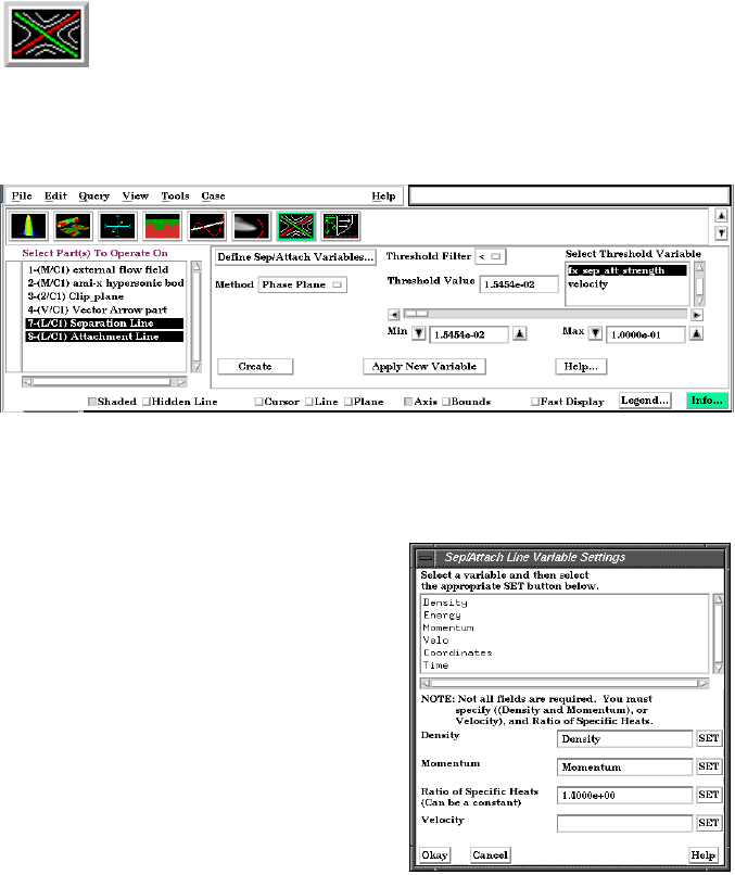
7.21 Separation/Attachment Lines Create/Update
7-116 EnSight 7 User Manual
Access Clicking once on the Separation and Attachment Lines Create/Update Icon opens
the Separation and Attachment Lines Editor in the Quick Interaction Area which
is used to both create and update (make changes to) the separation and attachment
line parts.
Define Sep/Attach Opens the Sep/Attach Line Variable Settings dialog which allows the user to identify and
Variables... set the dependent variables used in
computing separation and attachment
lines. This dialog has a list of current
accessible variables from which to
choose. Immediately below is a list of
dependent variables with corresponding
text field and SET button. The variable
name in the list is tied to a dependent
variable below by first highlighting a
listed variable, and then clicking the
corresponding dependent variable’s
SET button, which inserts the listed
variable into it’s corresponding text
field.
All text fields are required, except you may specify either Density and Momentum (which
permits velocity to be computed on the fly), or just Velocity. A default constant value is
supplied for the Ratio of Specific Heats which can be changed or specified by a scalar
variable name.
Clicking Okay activates all specified dependent variables and closes the dialog.
Method Opens a pop-up dialog for the specification of which type of method, to use to compute
the separation and attachment lines on the 2D surface. These options are:
Phase Plane - Scheme that uses eigen-analysis on the velocity gradient tensor along with
phase plane analysis to compute the separation and attachment line segments (see
Algorithms).
Threshold Filter Relational operators used to filter out line segments.
< Filter out any line segments less than the Threshold Value (default).
> Filter out any line segments greater than the Threshold Value.
Figure 7-104
Separation/Attachment Lines Create/Update Icon
Figure 7-105
Quick Interaction Area - Separation/Attachment Lines Editor

7.21 Separation/Attachment Lines Create/Update
EnSight 7 User Manual 7-117
Threshold Value The value at which to filter the line segments.
Select Threshold A list of possible variables that you may use to help filter out line segments. This
Variable List list includes the vorticity magnitude scalar variable (named fx_sep_att_strength) which
gets created when you Create/Update a separation and attachment part.
Threshold Slider Bar Used to change the Threshold Value in increments dependent on the Min and Max
settings. The stepper button on the left (and right) of the slide bar is used to decrement
(and increment) the Threshold value.
Min - The minimum value of the Threshold Variable. The stepper button on the left (and
right) side of the Min text filed is used to decrease (and increase) the order of magnitude,
or the exponent, of the min value.
Max - The maximum value of the Threshold Variable. The stepper button on the left (and
right) side of the Max text field is used to decrease (and increase) the order of magnitude,
or the exponent, of the Max value.
Create Creates separation and attachment lines that correspond to the selected 2D part in the part
list, based on the respective settings.
Apply New Variable Applies the threshold settings to the separation and attachment line segments based on the
threshold variable that is highlighted in the Select Threshold Variable list.
Feature Detail Editor Double clicking on the Separation/Attachment Lines Icon opens the Feature
(Separation/Attachment)Detail Editor (Separation/Attachment Lines), the Creation Attributes Section of
which provides access to the same functions available in the Quick Interaction
Area, as well as one more.
(see Section 3.3, Part Editing for a detailed discussion of the remaining Feature
Detail Editor turn-down sections which are the same for all Parts),
Display offset This field specifies the normal distance away from a surface to display the
separation/attachment lines. A positive value moves the lines away from the
surface in the direction of the surface normal.
Please note that there is a hardware offset that will apply to contours, vector arrows,
separation/attachment lines, and surface restricted particle traces that can be turned on
or off in the View portion of Edit->Preferences. This preference (“Use graphics hardware
to offset line objects...”) is on by default and generally gives good images for everything
except move/draw printing. This hardware offset differs from the display offset in that it is
in the direction perpendicular to the computer screen monitor (Z-buffer)
.
Thus, for viewing, you may generally leave the display offset at zero. But for
printing, a non-zero value may become necessary so the lines print cleanly.
Note: Separation and Attachment Line feature extraction does not work with multiple parts.
Troubleshooting Separation/Attachment Lines
Problem Probable Causes Solutions
Error creating separation and
attachment lines
Invalid part selected in part list Highlight 2D or 3D part
Undefined (colored by part color)
regions on sep/attach lines
Sep/Attach line segment node was
not mapped within a corresponding
3D field element
Make sure corresponding 3D field
part is defined.
Separation/attachment lines do not
print well.
See Display Offset discussion above Enter a non-zero Display Offset
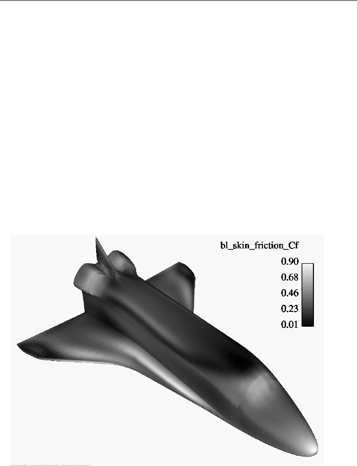
7.22 Boundary Layer Variables Create/Update
7-118 EnSight 7 User Manual
7.22 Boundary Layer Variables Create/Update
EnSight creates the following Boundary Layer Variables simultaneously on a 2D
boundary part directly from velocity information of its corresponding 3D flow
field part. Their corresponding variable names are included in all appropriate
EnSight variable lists, i.e. Color Parts variable list, etc.
Only nodal (values per node) variables are created. Any dependent elemental
variables (values per element) are averaged to nodal variables before processing.
(See Definitions below.)
Whether these variables are mapped onto the 2D boundary part, or used in
conjunction with other EnSight features (such as Elevated Surfaces of the
boundary layer thickness off the 2D boundary part, Vortex Cores, Separation and
Attachment Lines, Shock, etc.), these variables help provide valuable insight into
the formation and location of possible boundary layers.
Boundary Layer A boundary layer is a relatively thin region that confines viscous diffusion near
the surface of a flow field, where the velocity gradient in the normal direction to
the surface goes through an abrupt change. Although multiple boundary layers
Variable Name Description Symbol
(N) bl_thickness Boundary layer thickness
(N) bl_disp_thickness Displacement thickness
(N) bl_momen_thickness Momentum thickness
(N) bl_shape_parameter Shape parameter
(N) bl_skin_friction_Cf Skin friction coefficient
δ
δ*
Θ
H
C
f
Figure 7-106
Skin Friction Coefficient
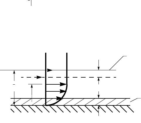
7.22 Boundary Layer Variables Create/Update
EnSight 7 User Manual 7-119
may be considered (especially in areas of flow separation), our current
implementation provides boundary layer parameters based on the former concept.
In these thin regions, the thickness of the boundary layer typically increases in the
downstream direction, and the velocity parallel to the surface is much larger than
the velocity normal to the surface.
Boundary Surfaces Boundary parts are typically 2D surface part(s) that correspond to a 3D field.
These surfaces may either be boundary parts defined directly from the data file, or
created parts (i.e. 2D IJK sweeps of a structured part, or an isosurface of zero
velocity of either an unstructured or structured part).
Velocity-Magnitude Changes of the velocity in the normal direction from the surface into the 3D flow
Gradient Vector field are utilized to determine the boundary layer. EnSight automatically creates a
velocity-magnitude gradient vector for all 3D model parts prior to creating the
boundary layer variables. These gradient values are then mapped to all
corresponding 2D model parts, and inherited by all created parts.
Note: The velocity-magnitude gradient vector variable will continue to be created
for all 3D model parts until it is deactivated.
This vector variable behaves like any other created variable, and may be
deactivated via the Feature Editor (Variables) dialog.
Definitions
Boundary Layer Thickness
The distance normal from the surface to where u/U = 0.995,
where: u = magnitude of the velocity at a given location in the boundary layer,
U = magnitude of the velocity just outside the boundary layer.
Displacement Thickness
Provides a measure for the effect of the boundary layer on the “outside” flow. The
boundary layer causes a displacement of the streamlines around the body.
Momentum Thickness
Relates to the loss of momentum in the air in the boundary layer.
δ n
u/U = 0.995
=
δ*
δ
δ*
U
n
Streamline position without
boundary layer
Shifted streamline
Extra Thickness
δ*
1
U
----
Uu–()nd
0
δ
=
Θ
1
U
2
------
Uu–()und
0
δ
=
7.22 Boundary Layer Variables Create/Update
7-120 EnSight 7 User Manual
Shape Parameter
Used to characterize boundary layer flows, especially to indicate potential for
separation.
This parameter increases as a separation point is approached, and varies rapidly
near a separation point.
Note: Separation has not been observed for H < 1.8 , and definitely has been
observed for H = 2.6; therefore, separation is considered in some analytical
methods to occur in turbulent boundary layers for H = 2.0.
In a Blasius Laminar layer (i.e. flat plate boundary layer growth with zero
pressure gradient), H = 2.605. Turbulent boundary layer, H ~= 1.4 to 1.5, with
extreme variations ~= 1.2 to 2.5.
Skin Friction Coefficient
where: = fluid shear stress at the wall.
= dynamic viscosity of the fluid.
May be spatially and/or temporarily varying quantity (usually a constant).
= distance normal to the wall.
= freestream density
= freestream velocity magnitude.
This is a non-dimensionalized measure of the fluid shear stress at the surface. An
important aspects of the Skin Friction Coefficient is:
, indicates boundary layer separation.
Other Notes: Factor Determining Velocity at Boundary-Layer Thickness (δ)
The factor (default = 0.995) which determines the velocity magnitude (u) at the
boundary-layer thickness (δ) with respect to the velocity magnitude (U) just
outside the boundary layer (i.e. δ is the distance normal to the surface at which
u = 0.995U), may be changed by issuing the following command via the
command line processor (see Section 2.4, Command Files):
test: blt_factor #
where # is the corresponding factor ( > 0.).
References Please refer to the following texts for more detailed explanations.
P.M. Gerhart, R.J. Gross, & J.I. Hochstein, Fundamentals of Fluid Mechanics, 2nd Ed.,
(Addison-Wesley: New York, 1992),
C.A.J. Fletcher, Computational Techniques for Fluid Dyanmics, Vol. 2, 2nd Ed.,
(Springer: New York, 1997)
δ*/Θ
C
f
τ
w
0.5ρ
∞
V
∞
()
2
--------------------------------
=
τ
w
µ
u∂
n∂
-----
è
æö
n0=
=
µ
n
ρ
∞
V
∞
C
f
0=
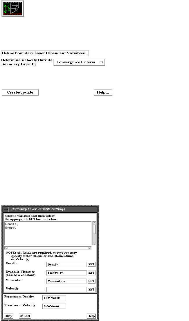
7.22 Boundary Layer Variables Create/Update
EnSight 7 User Manual 7-121
Access Clicking once on the Boundary Layer Variable Create/Update Icon opens the
Boundary Layer Variables Editor in the Quick Interaction Area, which is used to
both create and update (make changes to) the boundary layer variables.
Define Boundary Opens the Boundary Layer Variable Settings dialog which allows the user to identify and
Layer Dependent set the dependent variables used in computing the boundary layer variables (see
Variables... Definitions above). This dialog has a list of current accessible variables to choose from.
Immediately below is a list of dependent variables with corresponding text field and SET
button. The variable name in the list is tied to a dependent variable below by first
highlighting a the listed variable, and then clicking the corresponding dependent variable’s
SET button, which inserts the listed variable into its corresponding text field.
All text fields are required, except you may specify either Density and Momentum (which
permits velocity to be computed on the fly), or Velocity. Default constant values are
provided which may be changed by editing the text field.
Clicking Okay activates all specified dependent variables and closes the dialog.
Determine Velocity Opens a pop-up dialog for the specification of which type of method to determine the
Outside Boundary constant velocity just outside the boundary layer (U) (see Definitions above). The
Layer By following options determine (U) at each node of the surface in the direction normal from
the surface into the 3D field by:
Figure 7-107
Boundary Layer Variables Create/Update Icon
Figure 7-108
Quick Interaction Area - Boundary Layer Variables Editor
Figure 7-109
Boundary Layer Variable Settings Dialog

7.22 Boundary Layer Variables Create/Update
7-122 EnSight 7 User Manual
Convergence Criteria - monitoring the velocity profile until either the velocity magnitude
goes constant or its gradient goes to zero.
Distance From Surface - specifying the Normal Distance from the surface into the field at
which to extract the velocity and assign as U. Then monitor the velocity profile from the
surface into the field until U is obtained.
Normal Distance - Text field that contains the distance normal from the surface into
the 3D field at which to extract the velocity for U.
Velocity Magnitude - specifying the Velocity Magnitude to assign as U. Then monitor the
velocity profile from the surface into the field until U is obtained.
Velocity Magnitude - Text field that contains the specified velocity magnitude to
assign as U.
Note: Boundary Layer Variable feature extraction does not work with multiple parts.
Troubleshooting Boundary Layer Variables
Problem Probable Causes Solutions
Error creating boundary layer
variables.
Non-2D part selected in part list. Highlight 2D part.
Undefined (colored by part color)
regions on boundary surface.
2D boundary surface node was not
mapped to corresponding 3D field
boundary node.
Make sure corresponding 3D field
part is defined.

EnSight 7 User Manual 8-1
8Modes
This chapter describes the six different Modes through which you can work in the
Graphics Window. The “active” Mode determines both the configuration and
what functions are available through the Mode Icon Bar.
Section 8.1, Part Mode describes the layout of the Mode Icon Bar and the
functions available when Part is the active Mode.
Section 8.2, Annot Mode describes the layout of the Mode Icon Bar and the
functions available when Annot is the active Mode.
Section 8.3, Plot Mode describes the layout of the Mode Icon Bar and the
functions available when Plot is the active Mode.
Section 8.4, VPort Mode describes the layout of the Mode Icon Bar and the
functions available when VPort is the active Mode.
Section 8.5, Frame Mode describes the layout of the Mode Icon Bar and the
functions available when Frame is the active Mode. By default, this mode is not
available unless it has been enabled under Edit > Preferences... General User
Interface - Frame Mode Allowed
Section 8.6, View Mode describes the layout of the Mode Icon Bar and the
functions available when View is the active Mode. By default, this mode is not
available unless it has been enabled under Edit > Preferences... General User
Interface - View Mode Allowed.
Figure 8-1
Mode Choices
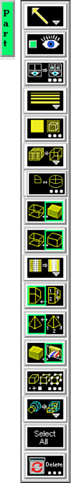
8.1 Part Mode
8-2 EnSight 7 User Manual
8.1 Part Mode
Part Mode is used to adjust a number of attributes for individual Parts and to
specify the desired type of Pick operation.
For a complete discussion about Parts:
(see Chapter 3, Parts)
Figure 8-2
Mode Selection Area - Part Selected
Pick Pulldown Icon
Part Visibility Toggle Icon
Part Visibility in Viewport Icon
Part Line Width Pulldown Icon
Transparency Attributes Icon
Element Representation Pulldown Icon
Visual Symmetry Icon
Part Shading Toggle Icon
Part Hidden Line Toggle Icon
Shading Type Pulldown Icon
Element Label Toggle Icon
Node Label Toggle Icon
Part Auxiliary Clipping Toggle Icon
Node Representation Icon
Fast Display Representation Pulldown Icon
Part Select All Icon
Part Delete Icon

8.1 Part Mode
EnSight 7 User Manual 8-3
Pick Pull-down Icon Opens a pull-down menu for the specification of the desired type of Pick operation. The
actual Pick operation is normally assigned to the “P” key on the keyboard, unless it has
been reassigned under Main Menu: Edit > Preferences... Mouse and Keyboard...
Pick Part When the Pick operation is performed (by default, pressing the “P” key), the Part directly
under the mouse cursor is selected. To select multiple Parts, hold down the Control Key
during the Pick operation. It is usually helpful to open and use the Selected Parts Window
while Picking Parts. This is done from Main Menu: View > Show Selected Part(s)...
Pick Plane (3 Pts) When the Pick operation is performed (by default, pressing the “P” key), the Plane Tool
Tool Location will be positioned at the Picked points. Three points must be Picked to position the Plane
Tool.
Pick Plane (2 Pts) When the Pick operation is performed (by default, pressing the “P” key), the view in the
Tool Location graphics window will change to an orthographic view. At this point, you can click and
drag the mouse to define a line. The Plane Tool will be positioned parallel to your current
viewing angle through the defined line. Consider using this option together with the F5,
F6, F7, and F8 keys which will transform the view to a standard orientation.
(see Section 9.1, Global Transform)
Pick Line Tool When the Pick operation is performed (by default, pressing the “P” key), the ends of the
Location Line Tool will be centered on a plane defined by the Picked points. Two points must be
Picked to position the Line Tool.
Pick Center of When the Pick operation is performed (by default, pressing the “P” key), the center of
Transformation global transformation is positioned at the Picked point.
Pick Cursor Tool When the Pick operation is performed (by default, pressing the “P” key), the Cursor Tool
Location will be positioned at the Picked point.
Pick Look At Point When the Pick operation is performed (by default, pressing the “P” key), the Look At
Point is positioned at the Picked point. The Look From Point is also adjusted to preserve
the distance (between the two Points) and vector that existed prior to the Pick operation.
(see Section 9.7, Look At/Look From)
Access: Part Mode : Pick Pull-down Icon
Part Visibility
Determines the global (in all viewports and in all Modes) visibility of the selected
Figure 8-3
Part Mode - Pick Pulldown Icon
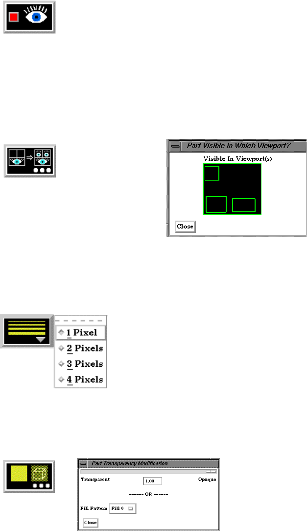
8.1 Part Mode
8-4 EnSight 7 User Manual
Toggle Icon Part(s).
Access: Part Mode : Part Visibility Toggle Icon
Part Visibility in
Opens the “Part Visible in Which Viewport?” dialog. If the global visibility of a Part is on,
Viewport Icon this dialog can be used to selectively turn on/off visibility of the selected Part(s) in
different viewports simply by clicking on a viewport’s border symbol within the dialog’s
small window. The selected Part(s) will be visible in the viewports outlined in green and
invisible in those outlined in red.
Access: Part Mode : Part Visibility in Viewport Icon
Part Line Width Opens a pulldown menu for the specification of the desired display width for Part lines.
Pulldown Icon Performs the same function as the Line Representation Width field in the Node, Element,
and Line Attributes section of the Feature Detail Editor (Model).
Access: Part Mode : Part Line Width Pull-down Icon
Transparency Attributes Icon
Opens the Part Transparency Modification dialog.
The degree of Opaqueness for the selected Parts when Hidden Surface is on for the Part(s)
may be adjusted by typing in a value from 0.0 to 1.0 in the field or by using the slider bar.
A value of 0.0 will render the selected Part(s) completely transparent whereas the default
value of 1.0 renders them completely opaque. This field performs the same function as the
Opaqueness field in the General Attributes section of the Feature Detail Editor (Model).
Fill Pattern Opens a pull-down menu to specify that a fill pattern be used to provide pseudo-
Figure 8-4
Part Mode - Part Visibility Toggle Icon
Figure 8-5
Part Mode - Part Visibility in Viewport Icon
and Part Visible in Which Viewport ? dialog
Figure 8-6
Part Mode - Part Line Width Pulldown Icon
Figure 8-7
Part Mode - Transparency Attributes Icon and Part Transparency Modification dialog
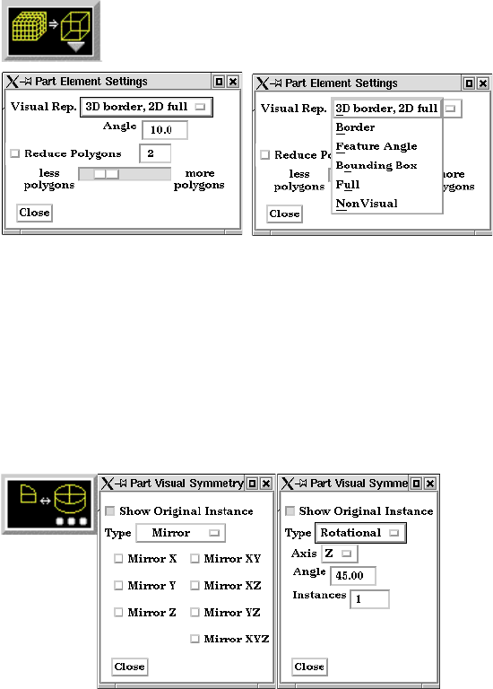
8.1 Part Mode
EnSight 7 User Manual 8-5
transparency for Hidden Surface shaded Part surfaces. The Default is Fill 0 which uses no
pattern (produces a solid surface), while Fill patterns 1 through 3 produce an EnSight
defined fill pattern. Performs the same function as the Fill Pattern pulldown menu in the
General Attributes section of the Feature Detail Editor (Model). Fill Pattern and
Transparency should not be used together.
Access: Part Mode : Transparency Attributes Icon
Element Visual
Opens a dialog for the specification of the desired representation for elements of
Representation the selected Part(s). Performs the same function as the Element Representation Visual
Pulldown Icon Rep. pulldown menu in the Node, Element, and Line Attributes section of the Feature
Detail Editor (Model).
(see Element Representation in Section 3.3, Part Editing)
Access: Part Mode : Element Representation Pull-down Icon
Visual Symmetry
Opens the Part Visual Symmetry dialog which allows you to control the display of mirror
Icon images of the selected Part(s) in each of the seven other quadrants of the Part’s local frame
or the rotationally symmetric instances of the selected parts. This performs the same
function as the Visual Symmetry menu in the General Attributes section of the Feature
Detail Editor (Model).
Symmetry enables you to reduce the size of your analysis problem while still visualizing
the “whole thing.” Symmetry affects only the displayed image, not the data, so you cannot
query the image or use the image as a parent Part. However, you can create the same
effect by creating dependent Parts with the same symmetry attributes as the parent Part.
You can mirror the Part to more than one quadrant. If the Part occupies more than one
quadrant, each portion of the Part mirrors independently. Symmetry works as if the local
frame is Rectangular, even if it is cylindrical or spherical. The images are displayed with
the same attributes as the Part. For each toggle, the Part is displayed as follows. The
default for all toggle buttons is OFF, except for the original representation - which is ON.
Mirror X quadrant on the other side of the YZ plane.
Figure 8-8
Part Mode - Element Representation Icon
Figure 8-9
Part Mode - Visual Symmetry Icon
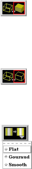
8.1 Part Mode
8-6 EnSight 7 User Manual
Mirror Y quadrant on the other side of the XZ plane.
Mirror Z quadrant on the other side of the XY plane.
Mirror XY diagonally opposite quadrant on the same side of the XY plane.
Mirror XZ diagonally opposite quadrant on the same side of the XZ plane.
Mirror YZ diagonally opposite quadrant on the same side of the YZ plane.
Mirror XYZ quadrant diagonally opposite through the origin.
Show Original Instance the original part instance
Rotational visual symmetry allows for the display of a complete (or portion of a) “pie”
from one “slice” or instance. You control this option with:
Axis X rotates about the X axis
Y rotates about the Y axis
Z rotates about the Z axis
Angle specifies the angle (in degrees) to rotate each instance from the previous
Instances specifies the number of rotational instances.
Show Original Instance show the original instance or not
Access: Part Mode : Visual Symmetry Icon
Part Shaded
Toggles on/off Shaded display of surfaces for the selected Part(s) assuming
Toggle Icon that Global Shaded has been toggled ON in the Main Menu > View > Shaded. Performs
the same function as the Shaded Toggle in the General Attributes section of the Feature
Detail Editor (Model). Default for all Parts is ON.
Access: Part Mode : Part Shaded Toggle Icon
Part Hidden Line
Toggles on/off hidden line display of surfaces for the selected Part(s) assuming
Toggle Icon that the Global Hidden Line has been toggled ON in the Main Menu > View > Hidden
Line. Performs the same function as the Hidden Line Toggle in the General Attributes
section of the Feature Detail Editor (Model). Default for all Parts is ON.
Access: Part Mode : Part Hidden Line Toggle Icon
Shading Type
Opens a pull-down menu for the selection of appearance of the surface of the selected
Pull-down Icon Part(s) when Hidden Surface is ON.
Normally the mode is set to Gouraud, meaning that the color and shading will interpolate
across the polygon in a linear scheme. You can also set the shading type to Flat, meaning
Figure 8-10
Part Mode - Part Shaded Toggle Icon
Figure 8-11
Part Mode - Part Hidden Line Toggle Icon
Figure 8-12
Part Mode - Shading Type Pulldown Icon
8.1 Part Mode
EnSight 7 User Manual 8-7
that each polygon will get one color and shade, or Smooth which means that the surface
normals will be averaged to the neighboring elements producing a “smooth” surface
appearance. Not valid for all Part types. Options are:
Flat Color and shading same for entire element
Gouraud Color and shading varies linearly across element
Smooth Normals averaged with neighboring elements to simulate smooth surfaces
Access: Part Mode : Shading Pull-down Icon
Element Label Toggles on/off the visibility of the element labels (assuming the result file contains them)
Toggle Icon for the selected Part(s). The Global Element Label Toggle (View Mode) must be on in
order to see any element labels. Performs the same function as the Label Visibility
Element toggle in the Node, Element, and Line Attributes section of the Feature Detail
Editor (Model). Default is OFF.
Access: Part Mode : Element Label Toggle Icon
Node Label
Toggles on/off the visibility of the node labels (assuming the result file contains them)
Toggle Icon for the selected Part(s). The Global Node Label Toggle (View Mode) must be on in order
to see any element labels. Performs the same function as the Label Visibility Node toggle
in the Node, Element, and Line Attributes section of the Feature Detail Editor (Model).
Default is OFF.
Access: Part Mode : Node Label Toggle Icon
Part Auxiliary Clipping
Toggles on/off whether the selected Part(s) will be affected by the Auxiliary
Toggle Icon Clipping Plane feature. Performs the same function as the Aux Clip toggle in the General
Attributes section of the Feature Detail Editor (Model). Default is ON.
Note: The Global Auxiliary Clipping Toggle (in the View Mode Icon Bar) must be on in
order for any Parts to be affected by the Aux Clip Plane.
Access: Part Mode : Part Auxiliary Clipping Toggle Icon
Node
Opens the Part Node Representation dialog. Performs the same function as the Node
Representation Icon Representation area in the Node, Element, and Line Attributes section of the Feature
Figure 8-13
Part Mode - Element Label Toggle Icon
Figure 8-14
Part Mode - Node Label Toggle Icon
Figure 8-15
Part Mode - Part Auxiliary Clipping Toggle Icon
8.1 Part Mode
8-8 EnSight 7 User Manual
Detail Editor (Model).
Node Visibility Toggle Toggles-on/off display of Part’s nodes whenever the Part is visible. Default is OFF.
Type Opens a pop-up menu for the selection of symbol to use when displaying the Part’s nodes.
Default is Dot. Options are:
Dot to display nodes as one-pixel dots.
Cross to display nodes as three-dimensional crosses whose size you specify.
Sphere to display the nodes as spheres whose size and detail you specify.
Scale This field is used to specify scaling factor for size of node symbol. If Size By is Constant,
this field will specify the size of the marker in model coordinates. If Size By is set to a
variable, this field will be multiplied by the variable value. Not applicable when node-
symbol Type is Dot.
Detail This field is used to specify how round to draw the spheres when the node-symbol type is
Sphere. Ranges from 2 to 10, with 10 being the most detailed (e.g., roundest spheres).
Higher values take longer to draw, slowing performance. Default is 2.
Size By Opens a pop-up menu for the selection of variable-type to use to size each node-symbol.
For options other than Constant, the node-symbol size will vary depending on the value of
the selected variable at the node. Not applicable when node-symbol Type is Dot. Default is
Constant. Options are:
Constant sizes node using the Scale factor value.
Scalar sizes node using a scalar variable.
Vector Mag sizes node using magnitude of a vector variable.
Vector X-Comp sizes node using magnitude of X-component of a vector variable.
Vector Y-Comp sizes node using magnitude of Y-component of a vector variable.
Vector Z-Comp sizes node using magnitude of Z-component of a vector variable.
Variable Selection of variable to use to size the nodes. Activated variables of the appropriate Size
By type are listed. Not applicable when node-symbol Type is Dot or Size By is Constant.
Access: Part Mode : Node Representation Icon
Figure 8-16
Part Mode - Node Representation Icon and Part Node Representation dialog
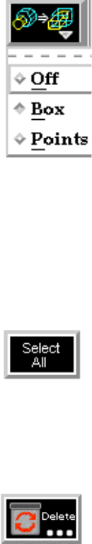
8.1 Part Mode
EnSight 7 User Manual 8-9
Fast Display Opens a pull-down menu for the specification of the desired fast display representation in
Toggle Icon which a Part is displayed. The Part fast display representation corresponds to whether the
view Fast Display Mode (located in the View Menu or as a View Mode icon) is on. The
Fast Display pull-down icon performs the same function as the Fast Display pop-up menu
button in the General Attributes section of the Feature Detail Editor (of all parts).
Box causes selected Part(s) to be represented by a bounding box of the Cartesian
extent of all Part elements (default).
Points causes selected Part(s) to be represented by a point cloud
(see General Attributes in Section 3.3, Part Editing, How To Set Global Viewing))
Access: Part Mode : Detail Representation Pull-down Icon
Select All
Selects all parts.
Delete Deletes the selected parts.
Figure 8-17
Part Mode - Detail Representation Pulldown Icon
Figure 8-18
Part Mode - Select All Icon
Figure 8-19
Part Mode - Delete Icon
8.2 Annot Mode
8-10 EnSight 7 User Manual
8.2 Annot Mode
Annot (Annotation) Mode is used to create and edit text strings, lines, and import
logos into the Graphics Window., and to adjust their visibility, size, color. and
position. It is also used to adjust the type, size, format, and position of legends.
When in Annot Mode, you are always modifying the objects selected in the
Graphics Window. Selected Annotation objects are outlined in the “selection
color”, while unselected objects are outlined in a white color. To select an object,
click the mouse over it. To select multiple objects, hold the Control key down
while clicking on the objects.
All annotation objects are positioned in the main Graphics Window; they are not
tied to specific viewports.
Figure 8-20
Mode Selection Area - Annot Selected
Text Creation Icon
Line Creation Icon
Logo Import Icon
Visibility Toggle Icon
Color Icon
Object Location Icon
Text Justification
Text Size Icon
Text Rotation Icon
Line Arrowhead
Line Width
Logo Size Icon
Legend Type
Legend Title Position
Legend Label Position
Legend Text
Legend Label
Delete Icon
Pulldown Icon
Pulldown Icon
Format Icon
Pulldown Icon
Pulldown Icon
Pulldown Icon
Pulldown Icon
Size Icon
Legend Orientation
Icon
Select All Icon
Allow Editing of
Defaults Icon
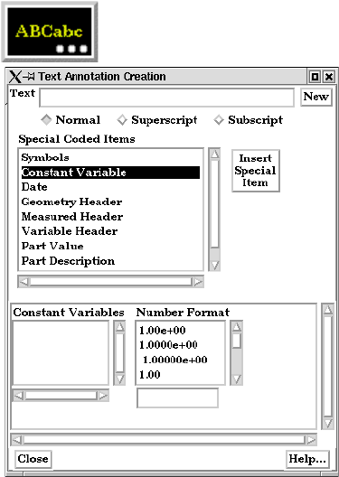
8.2 Annot Mode
EnSight 7 User Manual 8-11
Text Creation Icon Opens the Text Annotation Creation dialog.
Text strings may be created and inserted into the Graphics Window using the Text
Annotation Creation dialog.
Text This field specifies the desired text string.
Normal, Superscript Toggle one of these and subsequent text in the text field will be displayed as normal,
Subscript super or sub script.
New Clicking this button inserts the text in the Text field into the Graphics Window.
Special Coded Menu of eight different special strings used to insert information contained in results data
Items set or within EnSight into text string.
Insert Special Item Inserts selected Special String into Text field at position of cursor. Choices are:
Constant Variable inserts the value of the constant variable selected and displays it in the
selected format
Date inserts the Day of Week, Month, Date, Time, Year
Geometry Header inserts either the first or second header lines of the geometry file
Measured Header inserts the header line of the measured results file
Va r i ab l e H e a d e r inserts the header line of the selected variable data file
Part Value inserts the value used to create the Isosurface or Clip Plane Part. Only works
for Isosurface Parts, or XYZ, IJK, or RTZ Clip Plane Parts)
Part Description inserts the description of the Part selected in a Parts List which pops up
within the Text Annotation Creation dialog
Ve r si on inserts the EnSight version number, not including the (letter).
For example, 7.6.1 (a) would be 7.6.1
Access: Annot Mode : Text Creation Icon
Figure 8-21
Annot Mode - Text Creation Icon and Text Annotation Creation dialog

8.2 Annot Mode
8-12 EnSight 7 User Manual
Line Creation Icon Creates a new line in the Graphics Window.
This line may be interactively repositioned and its length adjusted within the Graphics
Window using the mouse cursor or these actions may be precisely done using the Object
Location Icon.
Access: Annot Mode : Line Creation Icon
Logo Import Icon
Clicking the Logo Import Icon opens the File Selection dialog for the specification of the
file name containing the desired logo. Files must be in xpm format (and cannot use color
names -colors must be hex numbers).
Access: Annot Mode : Logo Import Icon
Visibility Toggle
Toggles on/off the visibility of selected text strings, lines, logos, and legends.
This toggle affects only the individual text, line, or logo Annotation object(s) that is(are)
currently selected in the Graphics Window. Toggling visibility off for an object will cause
it to be “grayed-out” while in Annot Mode. These “grayed-out” objects will not be visible
in the Graphics Window in any of the other five Modes.
Be aware that selecting a legend in the Graphics Window and then clicking the Annot
Mode : Visibility Toggle will cause it to disappear (instead of become “grayed-out”) and
that clicking the Toggle again will NOT cause it to reappear. To make a legend visible
once again in the Graphics Window you must select the desired variable in the Main
Variables List and then click the Show Legend button just below the List.
Access: Annot Mode : Visibility Toggle
Color Icon
Opens the Color Selector dialog for the specification of the color you wish to assign to the
selected text strings, lines, logos, or legends (text and color bar border).
Access: Annot Mode : Color Icon
(see Section 7.1, Color)
Figure 8-22
Annot Mode - Line Creation Icon
Figure 8-23
Annot Mode - Logo Import Icon
Figure 8-24
Annot Mode - Visibility Toggle Icon
Figure 8-25
Annot Mode - Color Icon
8.2 Annot Mode
EnSight 7 User Manual 8-13
Location Attributes Opens the Annotation Item Location dialog for the specification (in X and Y coordinates)
Icon of the desired location of the text justification point for selected Annotation objects.
This method of positioning an Annotation object in the Graphics Window is an alternative
to interactively positioning it with the mouse cursor and can be more precise.
Access: Annot Mode : Location Attributes Icon
Text Justification
Opens a pull-down menu for the selection of the desired justification of the selected
Pulldown Icon text string(s). This icon will only be visible in the Annot Mode Icon Bar if a Text String
has been selected.
Access: Annot Mode : Text Justification Icon
Text Size Icon
Opens the Annotation Text Size/Rotation dialog for the specification of desired size of
selected text string(s) in the Graphics Window. Values specified should range from 1 to
100. This icon will only be visible in the Annot Mode Icon Bar if a Text String has been
selected.
Access: Annot Mode : Text Size Icon
Text Rotation Icon
Opens the Annotation Text Size/Rotation dialog (above) for the specification of desired
orientation of selected text string(s) in the Graphics Window. This icon will only be visible
in the Annot Mode Icon Bar if a Text String has been selected. The rotation is specified in
degrees and is applied in the counter clockwise direction about the justification point.
Access: Annot Mode : Text Rotation Icon
Figure 8-26
Annot Mode - Location Attributes Icon
Figure 8-27
Annot Mode - Text Justification Icon and resulting pull-down menu
Figure 8-28
Annot Mode - Text Size Icon and Annotation Text Size/Rotation dialog
Figure 8-29
Annot Mode - Text Rotation Icon
8.2 Annot Mode
8-14 EnSight 7 User Manual
Line Arrowhead Opens a pulldown menu for the placement of arrows on selected line objects.
Pulldown Icon This icon will only be visible in the Annot Mode Icon Bar if a line has been selected.
Access: Annot Mode : Line Arrowhead Pull-down Icon
Line Width Opens a pulldown menu for the specification of the desired width of the selected line
Pulldown Icon objects. This icon will only be visible in the Annot Mode Icon Bar if a line has been
selected.
Access: Annot Mode : Line Width Pull-down Icon
Logo Size Icon Opens the Annotation Logo Scaling dialog for the specification of the desired scaling of
selected logos. This icon will only be visible in the Annot Mode Icon Bar if a logo has
been selected. A scale factor of 1.0 keeps the logo in its original defined size, while values
less than 1.0 make it smaller and greater than 1.0 make it larger.
Access: Annot Mode : Logo Size Icon
Figure 8-30
Annot Mode - Line Arrowhead Pulldown Icon
Figure 8-31
Annot Mode - Line Width Pulldown Icon
Figure 8-32
Annot Mode - Logo Size Icon and Annotation Logo Scaling dialog
8.2 Annot Mode
EnSight 7 User Manual 8-15
Legend Type Opens a pull-down menu for the specification of the desired display type for selected
Pulldown Icon legends. Continuous will display a color interpolated bar, Discrete will display only colors
at specific levels. This icon will only be visible in the Annot Mode Icon Bar if a legend has
been selected.
Access: Annot Mode : Legend Type Pull-down Icon
Legend Title Position Opens a pull-down menu for the specification of the desired visibility and placement of
Pulldown Icon the title for selected legends. This icon will only be visible in the Annot Mode Icon Bar if
a legend has been selected.
Access: Annot Mode : Legend Title Pull-down Icon
Legend Label Position
Opens a pull-down menu for the specification of the desired visibility and placement of
Pulldown Icon value labels for selected legends.This icon will only be visible in the Annot Mode Icon
Bar if a legend has been selected.
Access: Annot Mode : Legend Label Pull-down Icon
Figure 8-33
Annot Mode - Legend Type Pulldown Icon
Figure 8-34
Annot Mode - Legend Title Position Pulldown Icon
Figure 8-35
Annot Mode - Legend Label Position Pulldown Icon
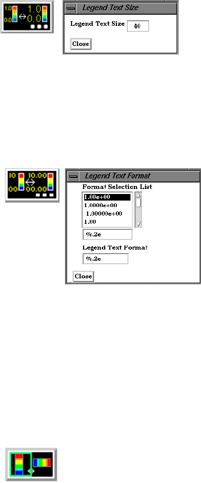
8.2 Annot Mode
8-16 EnSight 7 User Manual
Legend Text Size Icon Opens the Text Size Prompt dialog for the specification of the desired font size for the text
of selected legends. Values specified should range from 1 to 100. This icon will only be
visible in the Annot Mode Icon Bar if a legend has been selected.
Access: Annot Mode : Legend Text Size Icon
Legend Text
Opens the Text Size Prompt dialog for the specification of the desired font size for the text
Format Icon of selected legends. Values specified should range from 1 to 100. This icon will only be
visible in the Annot Mode Icon Bar if a legend has been selected.
Any legal C language printf format string for floating point numbers is permitted. The
Selection List shows how the value of 1.0 will appear using the selected format. (Note, if
you desire only the integer portion of the number, use something like: %4.0f)
Access: Annot Mode : Legend Label Format Icon
Legend Orientation
Toggles between a vertical legend and a horizontal legend.
Icon
Figure 8-36
Annot Mode - Legend Text Size Icon and dialog
Figure 8-37
Annot Mode - Legend Label Format Icon and dialog
Figure 8-38
Annot Mode - Legend Orientation Icon
8.2 Annot Mode
EnSight 7 User Manual 8-17
Select All... Brings up the Annotation Selection Options Dialog which allows selection of the various
annotation types.
Delete Icon Deletes selected text, line or logo Annotation object(s).
You cannot delete legends using the Delete Icon. Once a legend for a specific variable has
been made visible using the Show Legend button, it can be made non-visible using either
the Annot: Visibility Toggle or the Annot: Global Legend Visibility Toggle Icon.
Access: Annot Mode : Delete Icon
Allow Editing If on, all annotation icons are shown, so defaults can be edited without having to have an
Defaults object selected. Otherwise, only those icons which are applicable to the current selection
are displayed.
Legend... Clicking the Legend... button (located on the Desktop above the graphics window) will
allow the user to control which legends are visible.
Figure 8-39
Annot Mode - Select All... Icon and Annotation Selection Options Dialog
Figure 8-40
Annot Mode - Delete Icon
Figure 8-41
Annot Mode - Allow Editing Defaults
8.3 Plot Mode
8-18 EnSight 7 User Manual
8.3 Plot Mode
Plot Mode is used to adjust the attributes of 2D plotters and curves that you have
created. Most often, you will create plotters using the Query/Plot Editor in the
Quick Interaction Area, but you can create a new “empty” plotter using the Create
New Plotter Icon and then assign a title and data to its axes using the Query/Plot
Editor in the Quick Interaction Area
In Plot Mode, there are two things you can select.
1. You can click the plot window and the whole plot window will have a
highlighted box indicating its selection (green in color by default).
2. You can click on an individual curve to cause the curve line to thicken -
indicating selection..
The plotting capability is limited to simple x versus y data. Most often this data is
in the form variable value versus Time or Distance.
Figure 8-42
Mode Selection Area - Plot Selected
Plotter Visibility Toggle Icon - (select plot window)
Plotter Attributes Icon - (select plot window)
Axis Attributes Icon - (select plot window)
Curve Attributes Icon - (select plot window and curve)
Delete Icon
Plotter/Curve Select All Icon
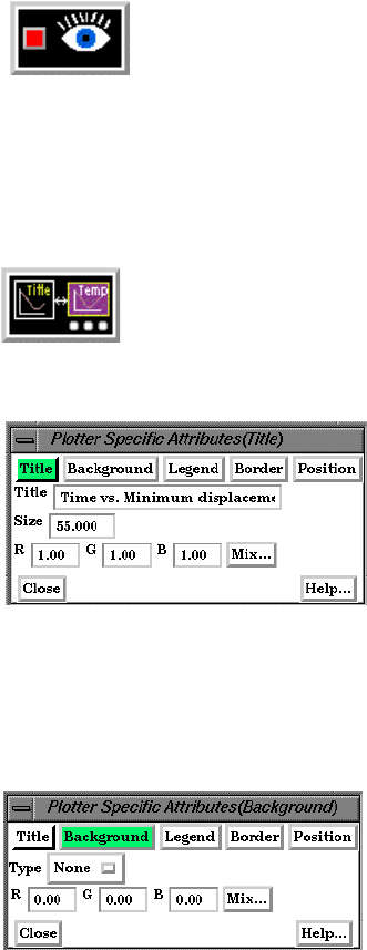
8.3 Plot Mode
EnSight 7 User Manual 8-19
Plotter Visibility Determines the visibility of the selected plotters. The selected plotters for which visibility
Toggle Icon has been toggled off will appear grayed-out in Plot Mode.
Access: Plot Mode : Plotter Visibility Toggle Icon
Plotter Attributes Icon
Opens the Plotter Specific Attributes dialog for the specification of attributes for Title,
background, legend, border and position of the selected plotters.
Title This field allows you to edit the existing plotter title.
Size This field allows you to specify the title text size.
RGB Mix... Color for the Title text may be specified using either the RBG fields or the Color Selector
dialog which is opened by clicking the Mix... button.
Type Opens a pop-up menu for the specification of plotter background color. Choices are:
None no background (the color of the Graphics Window or the viewport underneath will
show through the Plotter)
Solid allows a solid color to be specified for the Plotter Background
RGB Mix... Color for the Plotter background may be specified using either the RBG fields or the Color
Selector dialog which is opened by clicking the Mix... button.
Figure 8-43
Plot Mode - Plotter Visibility Toggle Icon
Figure 8-44
Plot Mode - Plotter Attributes Icon and Plotter Specific Attributes dialog
Title
Clicking the Title button causes the dialog
to configure itself for Plotter Title editing.
Background Clicking the Background Button causes the
dialog to configure itself for Plotter
Background editing.
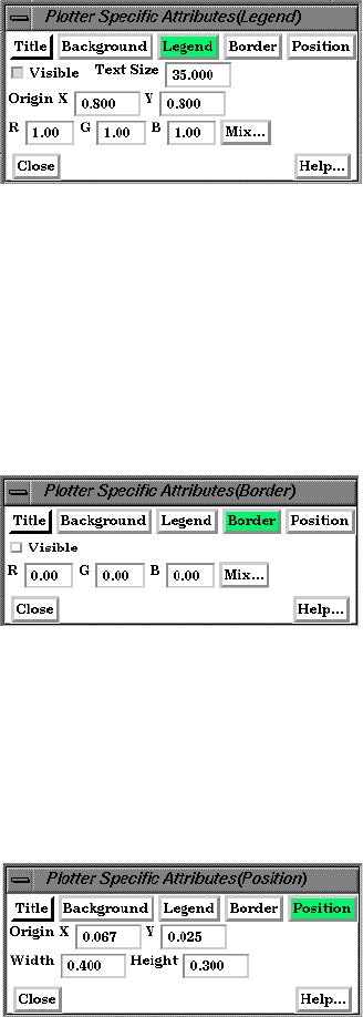
8.3 Plot Mode
8-20 EnSight 7 User Manual
Visible Toggle Toggles on/off the visibility of the legend for the selected Plotters.
Text Size This field specifies the desired size of the Legend text.
Origin X Y These fields specify the location of the Legend within a Plotter’s border. Values range
from 0.0 to 1.0 and resulting distances are measured from the Border origin (lower left
corner). These fields provide an alternative to interactively positioning the plotter Legend.
RGB Mix... Color for the Legend text may be specified using either the RBG fields or the Color
Selector dialog which is opened by clicking the Mix... button.
Visible Toggle Toggles on/off the visibility in the other five Modes of the Border for the selected Plotters.
RGB Mix... Color for the plotter border may be specified using either the RBG fields or the Color
Selector dialog which is opened by clicking the Mix... button. Note that the border color is
not shown while the plotter is selected - while selected the border is shown in green.
(see Section 7.1, Color)
Origin X Y These fields specify the location of the selected Plotter within the Graphics Window.
Values range from 0.0 to 1.0 and resulting distances are measured from the Graphics
Window origin (lower left corner). These fields provide an alternative to interactively
positioning the plotter which is done simply by clicking within the Plotter and dragging it
to the desired position.
Width, Height These fields specify the width and height of the Plotter. Resulting distances are measured
from the Border origin (lower left corner). These fields provide an alternative to
interactively resizing the plotter which is done simply by clicking on a side or corner and
dragging.
Access: Plot Mode : Plotter Attributes Icon
Legend Clicking the Legend Button causes the
dialog to configure itself for Plotter Legend
editing. The legend shows a line of the
appropriate color, width, and marker next to
the name of the curve plotted using this
line style.
Border Clicking the Border Button causes the
dialog to configure itself for Plotter Border
editing.
Position Clicking the Position Button causes the
dialog to configure itself for Plotter Position
editing.
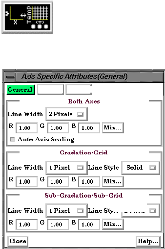
8.3 Plot Mode
EnSight 7 User Manual 8-21
Axis Attributes Icon Opens the Axis Specific Attributes dialog for the specification of attributes for axes of the
selected Plotters.
Both Axes
Line Width Opens a pop-up menu for the specification of the desired line width (1 to 4 Pixels) for
Plotter axes.
RGB Mix... Color for the axes may be specified using either the RBG fields or the Color Selector
dialog which is opened by clicking the Mix... button
Auto Axis When toggled on, the axis range and number of divisions will be scaled to make nice
Scaling Toggle “round” numbers.
Gradation/Grid
Line Width Opens a pop-up menu for the specification of the desired width (1-4 Pixels) for Gradation
Lines or Ticks.
Line Style Opens a pop-up menu for the specification of the style of line (Solid, Dotted, or Dashed)
desired for gradations. (The lines are normally not visible and so this specification is only
valid if Grad Type has been selected to Grid in the X-Axis and/or Y-Axis configuration of
the Axis Specific Attributes dialog.)
RGB Mix... Color for the Gradation Lines or Ticks may be specified using either the RBG fields or the
Color Selector dialog which is opened by clicking the Mix... button.
Sub-Gradation/Sub-Grid
Line Width Opens a pop-up menu for the specification of the desired line width (1-4 Pixels) for Sub-
Gradation Lines or Ticks (those between the Gradation Lines or Ticks).
Line Style Opens a pop-up menu for the specification of the style of line (Solid, Dotted, or Dashed)
desired for sub-gradations. (The lines are normally not visible and so this specification is
only valid if SubG Type has been selected to Grid in the X-Axis and/or Y-Axis
configuration of the Axis Specific Attributes dialog.)
RGB Mix... Color for the Sub-Gradation Lines or Ticks may be specified using either the RBG fields
or the Color Selector dialog which is opened by clicking the Mix... button.
Figure 8-45
Plot Mode - Axis Attributes Icon and Axis Specific Attributes dialog
General
Clicking the General button causes the
Axis editing.
dialog to configure itself for General Plotter
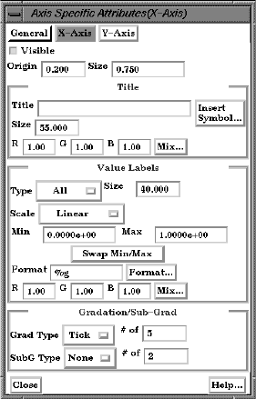
8.3 Plot Mode
8-22 EnSight 7 User Manual
Visible Toggle
Toggles on/off the visibility of the X (or Y) Axis line.
Origin This field specifies the location of the X (or Y) Axis origin. Values range from 0.0 to 1.0
and resulting distances are measured from the left side (or bottom) of the Plotter.
Size This field specifies the length of the X (or Y) Axis line. Values range from 0.0 to 1.0 and
resulting distances are measured from the X (or Y) Axis Origin.
Title
Title This
field allows you to edit the existing X (or Y) Axis title.
Size This field allows you to specify the title text size.
RGB Mix... Color for the Title text may be specified using either the RBG fields or the Color Selector
dialog which is opened by clicking the Mix... button.
Value Labels
Type
Opens a pop-up menu for selection of desired number (None, All, or Beg/End) of X (or Y)
Axis labels.
Size This field allows you to specify the size of X (or Y) Axis labels.
Scale This field allows you to specify a linear or log10 scale for the Axis.
Min This field contains the minimum value of the X (or Y) Axis. If Auto Axis Scaling is on, it
is only an approximation to the value which will be used.
Max This field contains the maximum value of the X (or Y) Axis. If Auto Axis Scaling is on, it
is only an approximation to the value which will be used.
Format This field specifies the format used to display the X (or Y) Axis. Any C language printf
format is valid in this field.
Format... This button will open the Format dialog which allows you to select a pre-defined format.
X-Axis or Y-Axis
Clicking the X-Axis or Y-Axis button causes
the dialog to configure itself for editing of
Attributes specific to either the X or the Y Axis.
If X-Axis ha s been clicked - all actions within
the dialog will affect the X-Axis attributes
only. Likewise for Y-Axis.

8.3 Plot Mode
EnSight 7 User Manual 8-23
Gradation/Sub-Grad
Grad Type
Opens a pop-up menu for selection of desired marker (None, Grid, or Tick) for major
# of gradations. # of field specifies the number of major gradations you wish along the X (or
Y) Axis. If Auto Axis Scaling is on, it is only an approximation to the value which will be
used.
SubG Type Opens a pop-up menu for selection of desired marker (None, Grid, or Tick) for sub
# of gradations (between the major gradations. # of field specifies the number of sub
gradations you wish between each major gradation along the X (or Y) Axis.
Access: Plot Mode : Axis Attributes Icon
Curve Attributes Icon
Opens the Curve Specific Attributes dialog for the specification of attributes for an
individual curve which has been selected in a Plotter. A curve is selected by clicking the
mouse cursor on top of the curve. The selected curve will be drawn by a wider line than is
normally used to display the curve.
Desc. This field initially contains the Legend description of the selected Curve which was
assigned to it when the Curve was created. Edit and press Return to change the
description.
Scale X/Y By Scales the respective X or Y values by the specified factor.
Line Width Opens a pop-up menu for the specification of the desired line width (1-4 Pixels) for the
selected Curve.
Line Style Opens a pop-up menu for the specification of the style of line (Solid, Dotted, or Dashed)
desired for the selected Curve.
Line Type Opens a pop-up menu for the specification of the type of line desired for the selected
Curve. Options are:
None No lines will be drawn between points
Connect Dot Lines will be drawn between the points
Smooth A piece wise spline will connect the points
Smooth Sub-points This field specifies the number of sub-points to use between data points in drawing the
curve when Smooth Line Type is selected.
Marker Type Opens a pop-up menu for the specification of the desired type of data point marker (None,
Dot, Circle, Triangle, Square) on the curve.
Scale This field specifies the size of the data point markers for the selected curve.
Figure 8-46
Plot Mode - Curve Attributes Icon and Curve Specific Attributes dialog
8.3 Plot Mode
8-24 EnSight 7 User Manual
RGB Mix... Color for the selected Curve may be specified using either the RBG fields or the Color
Selector dialog which is opened by clicking the Mix... button
Access: Plot Mode : Curve Attributes Icon
Select All... Brings up the Plot Selection Option Dialog which allows selection of all curves or all
plotters.
Delete Icon Deletes the selected Plotters.
Access: Plot Mode : Delete Icon
Figure 8-47
Plot Mode - Select All... Icon and Plot Selection Options Dialog
Figure 8-48
Plot Mode - Delete Icon
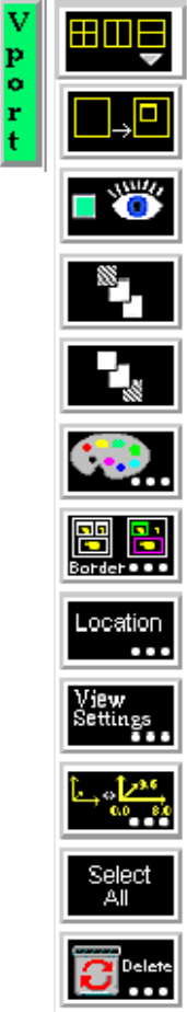
8.4 VPort Mode
EnSight 7 User Manual 8-25
8.4 VPort Mode
VPort Mode is used to create, adjust the attributes of, and delete viewports.
The default EnSight configuration shows one view of your model in the “main”
Graphics Window. This “initial viewport”, which covers the Graphics Window.
cannot be removed and is always used to clear (erase) the Graphics Window prior
to a redraw. Using the VPort Mode, you can create up to fifteen additional
viewports that will overlay the Graphics Window. These viewports can be
interactively resized and relocated within the Graphics Window using the mouse
and the visibility of each Part can be controlled on a per viewport basis.
Transformations, and Z-clip location settings can also be made independently in
each viewport.
Figure 8-49
Mode Selection Area - VPort Selected
New Viewport Icon
Viewport Visibility Icon
Viewport Forward Icon
Viewport Back Icon
Color Icon
Viewport Border Attributes Icon
Viewport Location Attributes Icon
Viewport Special Attributes Icon
Viewport Layouts Icon
Select All Icon
Delete Icon
Viewport Part Bounds Attributes Icon
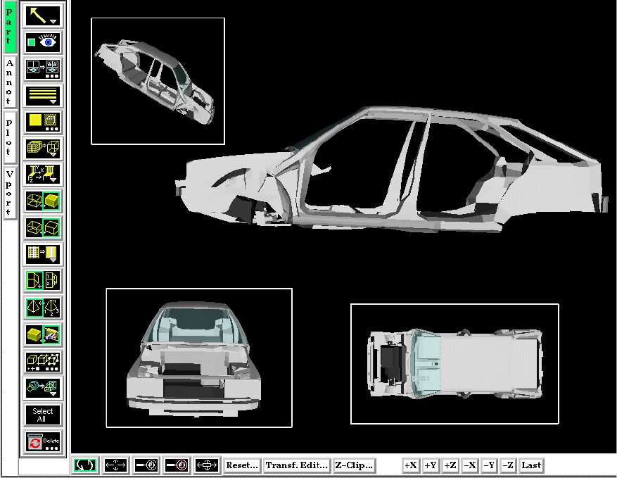
8.4 VPort Mode
8-26 EnSight 7 User Manual
When in VPort Mode, you are always modifying the viewports selected in the
Graphics Window. Selected viewports are outlined in the “selection color”, while
unselected objects are outlined in a white color. To select a viewport, click the
mouse over it. To select multiple viewports, hold the Control key down while
clicking on them.
Multiple viewports are helpful in showing the same object from multiple views,
showing different axes in each viewport, showing the same parts with different
attributes, etc.
Figure 8-50
Viewport Example
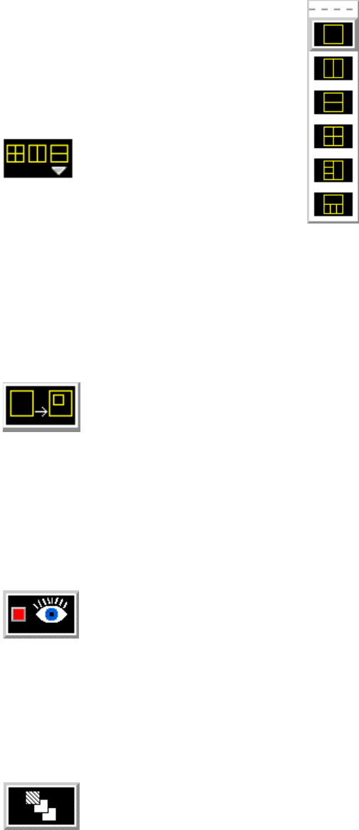
8.4 VPort Mode
EnSight 7 User Manual 8-27
Viewport Layouts Icon This icon opens a pull-down menu of icons which indicate standard viewport layouts.
Access: Vport Mode : Viewport Layouts Icon
New Viewport Icon
Clicking this button creates a new Viewport within (and on top of) the “main” Graphics
Window. The location and size of the viewport can be modified interactively in the
Graphics Window by a) clicking and dragging within the viewport to move it of b)
clicking and dragging the edge or corner to resize it. More precise modifications may be
performed using the Location ... Icon.
Access: VPort Mode : New Viewport Icon
Viewport Visibility
Determines the visibility of the selected viewport(s). The
Toggle Icon border of a viewport which, in the VPort Mode, has its visibility toggled off will still be
visible in the VPort Mode only - and then as a dotted rather than a solid line.
Access: VPort Mode : Viewport Visibility Toggle Icon
Viewport Forward Icon
Clicking this button moves the selected viewport(s) “forward” in the Graphics Window to
occlude any viewports which it (they) may overlap. Viewport 0 cannot be “popped”.
Access: VPort Mode : Viewport Forward Icon
Figure 8-51
Viewport Mode - Viewport Layouts Icon and Menu
Figure 8-52
VPort Mode - New Viewport Icon
Figure 8-53
VPort Mode - Viewport Visibility Toggle Icon
Figure 8-54
VPort Mode -Viewport Forward Icon
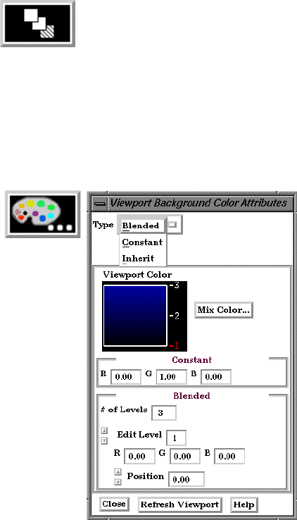
8.4 VPort Mode
8-28 EnSight 7 User Manual
Viewport Back Icon Clicking this button moves the selected viewport(s) “back” in the Graphics Window to be
occluded by any viewports which may overlap it (them). Viewport 0 cannot be “pushed”.
Access: VPort Mode : Viewport Back Icon
Color Icon Opens the Viewport Background Color Attributes dialog for the specification of the color
you wish to assign to the background of the selected viewport(s).
Type Opens a pull-down menu for the specification of the type of background you wish to
assign to a viewport.
Blended Allows you to specify a background comprised of 2 to 5 blended colors.
# of Levels
This field specifies the number of levels (from 2 to 5) at which a color will be specified.
The default is 2.
Edit Level This field specifies which of the levels you wish to edit. You may select the desired level
using the stepper buttons, by entering a value in the field, or interactively by clicking on
its number on the right side of the Viewport Color window.
Position This field specifies the vertical position of the edit level as a fraction (from 0 to 1) of the
vertical height of the Viewport Color window, where 0.0 is at the bottom and 1.0 is at the
top. You may adjust a level to the desired position using the stepper buttons, by entering a
value in the field, or interactively by selecting and dragging a level’s number on the right
side of the Viewport Color window. The position of any level can not be below the
position of the next lower level.
Figure 8-55
VPort Mode - Viewport Back Icon
Figure 8-56
VPort Mode - Color Icon
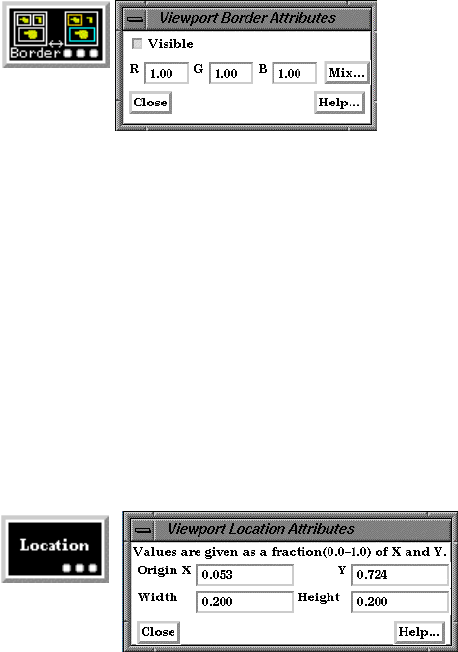
8.4 VPort Mode
EnSight 7 User Manual 8-29
Constant Allows you to specify a constant color using the RGB fields or the Color Selector dialog
which is accessed by clicking the Mix Color... button.
Inherit Causes the viewport to display the same background color attributes as the main Graphics
Window. Only applicable for created viewports, not the main Graphics Window.
Mix Color... Opens the Color Selector dialog. (see Section 7.1, Color)
Refresh Viewport Will redraw the selected viewport(s) with the defined viewport background settings.
Access: VPort Mode : Color Icon
Viewport Border
Opens the Viewport Border Attributes dialog for the specification of a constant color for
Attributes Icon the border of the selected viewports. Be aware that the color assigned will only be visible
in the other five Modes, not in VPort mode.
Visible Toggle Toggles on/off visibility of a viewport’s border in the other five Modes. The border of
each viewport will always be visible in VPort Mode.
RGB These fields specify the RGB values for the color you wish to assign.
Mix... Opens the Color Selector dialog. See Section 7.1 Color
Access: VPort Mode : Viewport Border Attributes Icon
Viewport Location
Opens the Viewport Location Attributes dialog for the specification of the desired location
Attributes Icon in the main Graphics Window for the selected viewports. This dialog provides a more
precise alternative to moving and resizing the viewports interactively.
Origin X Y These fields specify the location for the X and Y coordinates of the selected viewport’s
origin (lower left corner) in the main Graphics Window. Values range from 0.0 to 1.0.
Width, Height These fields specify the width and height of a selected viewport in X and Y coordinates
from the viewport’s origin. Values range from 0.0 to 1.0.
Access: VPort Mode : Viewport Location Attributes Icon
Figure 8-57
VPort Mode - Viewport Border Attributes Icon and Viewport Border Attributes dialog
Figure 8-58
VPort Mode - Viewport Location Attributes Icon and Viewport Location Attributes dialog
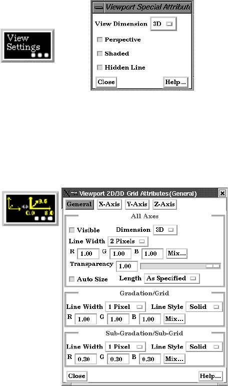
8.4 VPort Mode
8-30 EnSight 7 User Manual
Viewport Special Opens the Viewport Special Attributes dialog for the specification of whether the global
Attributes Icon settings for Perspective versus Orthographic display, hidden surface display, and hidden
line display will apply in the selected viewport(s). In addition, a viewport can be
designated as 2D, in which case only planar 2D parts can be displayed in the viewport
Note, Once you designate a viewport as a 2D viewport, all 3D parts are no longer visible
in that viewport. To see the 3D parts in that viewport again, you will need to make the
viewport 3D, select the 3D parts in the parts list, and make them visible again using the
visibility per viewport icon..
Access: VPort Mode : Viewport Special Attributes Icon
Part Bounds Attributes
Opens the Viewport Bounds Attributes dialog for the specification of part bounding box
gradation and labeling.
General Change the dialog to reflect overall extent grid attributes.
X-Axis Change the dialog to reflect X-Axis extent attributes (see below).
Y-Axis Change the dialog to reflect Y-Axis extent attributes (see below).
Z-Axis Change the dialog to reflect Z-Axis extent attributes (see below).
All Axes Section Contains parameters that affect attributes of all axes of the bounding extent.
Visible Toggle Toggles on/off visibility of the viewport 2D/3D extent axes.
Dimension Opens a menu for the specification of the desired dimension (2D or 3D) of the bounding
extent axis. Default is 3D. 2D is only available for 2D viewports and 3D viewports in
orthographic mode.
Line Width Opens a menu for the specification of the desired line width (1 - 4 pixels) of the bounding
Figure 8-59
VPort Mode - Viewport Special Attributes Icon and Viewport Special Attributes dialog
Figure 8-60
VPort Mode - Viewport Part Bounds Icon and
Viewport 2D/3D Grid Attributes (General) dialog
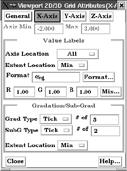
8.4 VPort Mode
EnSight 7 User Manual 8-31
extent axis. Default is 2.
RGB These fields specify the RGB values for the color you wish to assign.
Mix Color... Opens the Color Selector dialog. (see Chapter 7.1, Color)
Transparency Specifies the degree of opaqueness for the axes of the bounding extent. This value may be
adjusted by typing in a value from 0.0 to 1.0 in the field or by using the slider bar whose
current value is reflected in the field. A value of 0. or 1. will render the axes completely
transparent or completely opaque, respectively.
Auto Size Toggle Toggles on/off the scaling of the axis range to nice “round” numbers.
Length Opens a menu for the specification of the desired type of length gradation on the axes of
the bounding extent.
As Specified Divides the gradations evenly along the length of the axis. (default)
Rounded Tries to round to the units of the common order of magnitude.
Gradation/Grid Controls the specification of the gradation/grid of the axes of the bounding extent.
Section
Line Width Opens a menu for the specification of the desired line width (1 - 4 pixels) for the
gradation and grid of the bounding extent axis. Default is 1.
Line Style Opens a menu for the specification of the style of line (Solid, Dotted, or Dashed) desired
for the gradation and grid of the bounding extent axis. Default is Solid.
RGB These fields specify the RGB values for the color you wish to assign.
Mix Color... Opens the Color Selector dialog. (see Chapter 7.1, Color)
Sub-Gradation/ Controls the specification of the subgradation/subgrid of the axes of the bounding extent.
Sub-Grid Section
Line Width Opens a menu for the specification of the desired line width (1 - 4 pixels) for the
subgradation and subgrid of the bounding extent axis. Default is 1.
Line Style Opens a menu for the specification of the style of line (Solid, Dotted, or Dashed) desired
for the subgradation and subgrid of the bounding extent axis. Default is Solid.
RGB These fields specify the RGB values for the color you wish to assign.
Mix Color... Opens the Color Selector dialog. (see Chapter 7.1, Color)
Axis These fields reflect the Min and Max values of the selected axis.
Value Labels Section Controls attributes of the selected axis.
Figure 8-61
Viewports 2D/3D Grid Attributes (X-Axis or Y-Axis or Z-Axis dialog)
8.4 VPort Mode
8-32 EnSight 7 User Manual
Axis Location Opens a menu for the specification of the desired location (None, All (default), or Beg/
End) to place the labels of the selected axis.
Extent Location Opens a menu for the specification of the desired extent (Min (default), Max, or Both) on
which to display the labels of the selected axis.
Format This field specifies the format used to display the labels of the selected axis. Any C
language “printf” format is valid in this field.
Format... Opens the Viewport Axis Text Format dialog which allows you to select a pre-defined
format.
Format Selection List of pre-defined formats. You can also enter any legal C language format string for
floating point numbers.
List
Format Selection
The format specification.
Field
RGB
These fields specify the RGB values for the color you wish to assign.
Mix Color... Opens the Color Selector dialog. (see Chapter 7.1, Color)
Gradation/Sub-Grad Section
Grad Type Opens a menu for the selection of desired marker (None, Grid, or Tick (default)) for major
gradations of the selected axis.
# of Specifies the number of major gradations you wish along the selected axis. If Auto Size is
on, it is only an approximation to the value which will be used.
SubG Type Opens a menu for the selection of desired marker (None, Grid, or Tick (default)) for sub-
gradations (between the major gradations) along the selected axis.
# of Specifies the number of sub-gradations you wish between each major gradation along the
selected extent axis.
Extent Location Opens a menu for the specification of the desired extent (Min (default), Max, or Both) on
which to display the gradation/sub-gradations of the selected axis.
Access: VPort Mode : Viewport Part Bounds Attributes Icon
Select All
Selects all of the currently defined viewports.
Figure 8-62
Viewport Axis Text Format dialog
Figure 8-63
VPort Mode - Select All Icon
8.5 Frame Mode
8-34 EnSight 7 User Manual
8.5 Frame Mode
As EnSight reads in model Parts, they are all initially assigned to the same
“Frame” of reference: Frame 0. Frame 0 corresponds to the model coordinate
system (defined when the model was created). Using the Frame Mode, you can
create additional frames, reassign Parts to different Frames, and specify various
attributes of the Frames.
Transformations you make in View or Parts Mode (rotations, translations, etc.) are
performed globally; all Frames, Parts, and Tools are transformed with respect to
the Global Axis origin and orientation. Frame Mode, on the other hand, allows
you to perform transformations only on selected Parts. This is useful if you wish,
for example, to create an animation with Parts moving in different directions (such
as a door or hood opening to reveal Parts within) or to move Part copies away
from each other in order to color the Parts by different variables (in fact, if you
make a copy of a Part, a new Frame is automatically created and the Part copy is
assigned to it).
In Frame Mode, transformations are always about the selected Frame’s definition,
that is, its origin position (with respect to Frame 0) and the orientation of its axes
(with respect to Frame 0). Since this is the case, the Frame’s orientation must be
adjusted (if necessary) before any transformations are applied. If transformations
are applied first, and the Frame’s definition adjusted at a later time, the
transformations will likely cause unexpected results (since the transformations
originally performed were about a different axis definition than that about which
transformations performed after the Frames definition changed occur). The
necessary order is 1) define frame location and orientation, 2) assign part to frame,
3) perform transformations relative to the frame.
A Part can be assigned to only one Frame at a time. The Part will always be
transformed by the Frame’s transformation. A Part is not affected by a Frame’s
definition (other than transformations will be in reference to the definition). A
Part’s mirror symmetry operation (which can be thought of as a scaling
transformation) is always about the Frame to which the Part is assigned.
The Tools (Cursor, Line, Plane, etc.) are always shown in reference to the selected
Frame and are thus also transformed by the selected Frame’s transformations.
There are two transformation alternatives in Frame Mode: Frame Transform (the
default) and Frame Definition. As pointed out earlier, a frame should first be
defined (if necessary) before it is transformed.
In Frame Mode the axis triads for all Frames will be visible in the Graphics
Window. Invisible Frames will be shown with a dotted frame axis. Selected
Frames are shown in green. A Frame may be selected by clicking on its axis triad
or by selecting its description from the Frame List in the Transformation Editor
dialog (which is opened by clicking the Transf Edit... button in the Transformation
Control Area).
By default, Frame mode is not available unless it has been enabled under Edit >
Preferences... General User Interface - Frame Mode Allowed.
For further discussion concerning the transformation of Frames:
(see Section 9.3, Frame Transform and Section 9.2, Frame Definition)
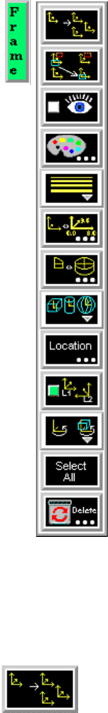
8.5 Frame Mode
8-36 EnSight 7 User Manual
When Frame Mode is selected, the Mode Icon Bar appears as follows.:
New Frame Icon Creates a new Frame to which you can assign Parts. Be aware that each time you make a
copy of a Part EnSight creates a new Frame and assigns the copy to the new Frame. If
Parts are selected in the Main Parts List, the new Frame’s origin will be positioned at the
center of the selected Parts.
Access: Frame Mode : Create New Frame Icon
Figure 8-66
Mode Selection Area - Frame Selected
New Frame Icon
Part Assignment Icon
Transform/Definition Pulldown Icon
Frame Axis Triad Visibility Toggle Icon
Color Icon
Frame Line Width Icon
Axis Triad Attributes Icon
Computational Symmetry Attributes Icon
Coordinate System Pulldown Icon
Frame Location Attributes Icon
All Frame Axis Triad Visibility Icon
Delete Icon
Frame Select All Icon
Figure 8-67
Frame Mode - Create New Frame Icon
8.5 Frame Mode
EnSight 7 User Manual 8-37
Part Assignment Clicking this icon reassigns Part(s) selected in the Main Parts List to the currently selected
Icon Frame. (An alternative method for reassigning Parts is to edit the Ref. Frame field in the
General Attributes section of the Feature Detail Editor.)
Access: Frame Mode : Part Assignment Icon
Frame Axis Triad Determines the visibility of the axis triad(s) of selected Frame(s). Invisible Frames are
Visibility Toggle Icon drawn in dotted lines while in Frame Mode. Default is Off.
Access: Frame Mode : Frame Axis Triad Visibility Toggle Icon
Color Icon
Opens the Color Selector dialog for the specification of the color you wish to assign to a
selected Frame’s axis triad A selected Frame will always be shown in the selection color
while in Frame Mode.
Access: Frame Mode : Color Icon
Frame Line Width
Opens a pulldown menu for the specification of the width for Frame axis triad lines for the
Pulldown Icon selected Frame(s).
Access: Frame Mode : Frame Line Width Icon
Figure 8-68
Frame Mode - Part Assignment Icon
Figure 8-69
Frame Mode - Frame Axis Triad Visibility Toggle Icon
Figure 8-70
Frame Mode - Color Icon
Figure 8-71
Frame Mode - Frame Line Width Pulldown Icon
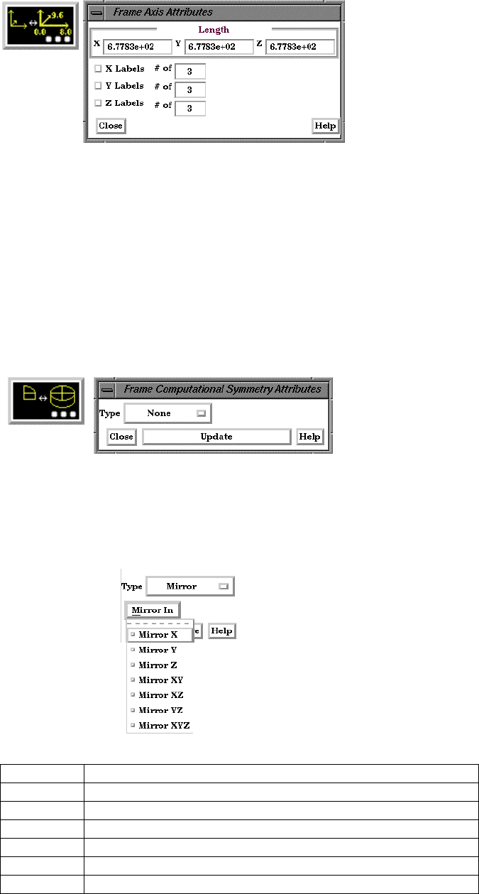
8.5 Frame Mode
8-38 EnSight 7 User Manual
Axis Triad Opens the Frame Axis Attributes dialog for the specification of axis triad line length and
Attributes Icon labels for the selected Frame(s).
X Y Z These fields allow you to specify the desired length, in model coordinates, of each of the
three axes of the selected Frame’s axis triad.
X Y Z Labels Toggles on/off the display of Labels on the respective line of a selected Frame’s axis triad.
Toggles Labels show distance along each axis.
X Y Z # of These fields specify the number of Labels which will appear on the respective axis.
Access: Frame Mode : Axis Triad Attributes Icon
Computational Opens the Frame Computational Symmetry Attributes dialog for the specification of
Symmetry Attributes the type of periodic conditions which will be applied to all assigned Model Parts of the
Icon selected Frame. (Note, computational symmetry does NOT work on created parts.)
(see How To Set Symmetry)
Type Opens a pop-up menu for the selection of whether you wish the selected Frame to have no
periodicity (None as shown above) or to be mirror, rotational, or translational periodic.
Mirror In Specification of the type of mirror periodicity.
Mirror X face-sharing quadrant on other side of the Y-Z plane
Mirror Y face-sharing quadrant on other side of the X-Z plane
Mirror Z face-sharing quadrant on other side of the X-Y plane
Mirror XY diagonally opposite quadrant on same side of the X-Y plane
Mirror XZ diagonally opposite quadrant on same side of the X-Z plane
Mirror YZ diagonally opposite quadrant on same side of the Y-Z plane
Mirror XYZ quadrant diagonally opposite through origin
Figure 8-72
Frame Mode - Axis Triad Attributes Icon
Figure 8-73
Frame Mode - Computational Symmetry Attributes Icon
Mirror
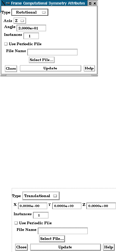
8.5 Frame Mode
EnSight 7 User Manual 8-39
Axis The Frame axis about which to rotate.
Angle This field specifies the rotational angle (in degrees) about the selected Frame’s z-axis for
rotational periodicity.
Instances This field specifies the number of periodic instances for rotational periodicity.
Use Periodic If toggled On, the periodic match file specified in File Name is used for rotational
symmetry.
File Name This field specifies the name of the periodic match file you wish to use.
Select File... Opens the File Selection dialog for the selection of a periodic match file.
(see Section 11.9, Periodic Matchfile Format)
Update Changes made in the dialog will not be applied until this button is clicked.
X Y Z These fields specify the translational offset in reference to the selected Frame’s
orientation.
Instances This field specifies the number of periodic instances for translational periodicity.
Use Periodic If toggled On, the periodic match file specified in File Name is used for translational
symmetry.
File Name This field specifies the name of the periodic match file you wish to use.
Select File... Opens the File Selection dialog for the selection of a periodic match file.
(see Section 11.9, Periodic Matchfile Format)
Update Changes made in the dialog will not be applied until this button is clicked.
Access: Frame Mode : Computational Symmetry Attributes Icon
Rotational
Translational
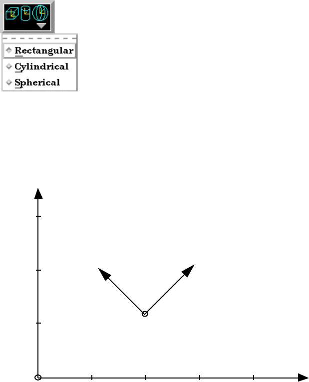
8.5 Frame Mode
8-40 EnSight 7 User Manual
Coordinate System Opens a pulldown menu for the selection of the type of coordinate system (rectangular,
Pull-down Icon cylindrical, spherical) you wish to use for a selected Frame. All three are defined in
reference to Frame 0, which is rectangular. Note that each frame’s orientation vectors
(which describe its orientation to Frame 0) are rectangular (as is their on-screen
representation) no matter what the frame’s coordinate system type. However, functions
that access the frame will behave different depending on the frame’s coordinate system
type.
Rectangular The Figure below shows a rectangular frame. The origin is in reference to the Frame 0
origin, while the orientation is in reference to Frame 0’s orientation.
Figure 8-74
Frame Mode - Coordinate System Pulldown Icon
Y
3.0
2.0
1.0
1.0 2.0 3.0
4.0
Frame 0
Frame Orientation for Rectangular Frames
Origin: 2.0 1.0 0.0
Orientation Vectors:
X: .707 .707 0
Y: -.707 .707 0
Z: 0 0 1
X
Z
Z
X
Y
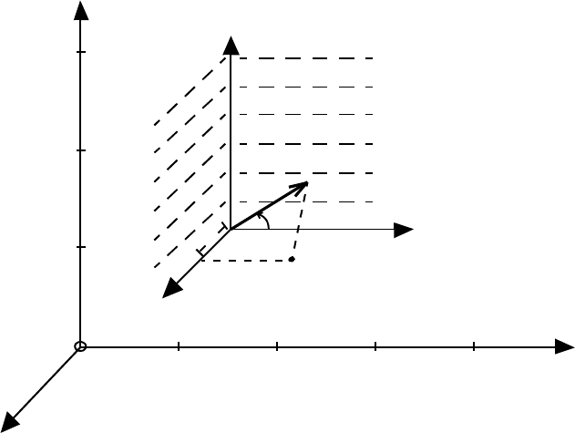
8.5 Frame Mode
EnSight 7 User Manual 8-41
Cylindrical The figure below shows a cylindrical frame. The origin is in reference to the Frame 0
origin, while the orientation is in reference to Frame 0’s orientation. Any function which
accesses a cylindrical frame will do so in cylindrical coordinates:
r The distance from the origin to projection point in the X–Y plane.
Θ The angle from the X-axis to the projection point in the X–Y plane.
Z The Z-coordinate
Y
3.0
2.0
1.0
1.0 2.0 3.0
4.0Frame 0
Frame Orientation and Coordinate System Key for Cylindrical Frames
r = distance in x-y plane
= angle from x-axis to
projection pt. in x-y
Origin: 2.0 1.0 0.0
Orientation Vectors:
X: 1 0 0
Y: 0 1 0
Z: 0 0 1
X
Z
Z
Z
r
X
Y
P(r, ,z)θ
θ
θ
plane
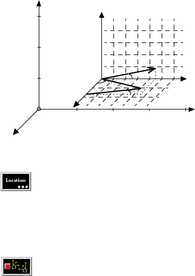
8.5 Frame Mode
8-42 EnSight 7 User Manual
Spherical
The figure below shows a spherical frame. The origin is in reference to the Frame
0 origin, while the orientation is in reference to Frame 0’s orientation. Any
function which accesses a spherical frame will do so in spherical coordinates
:
ρς The distance from the origin to the point in question.
Φ The angle measured from the Z-axis towards the projection point in the
X–Z plane.
Θ The angle from the X-axis to the projection point in the X–Y plane.
Access: Frame Mode : Coordinate System Pull-down Icon
Frame Location
Opens the Transformations Editor dialog to permit precise definition of the selected
Frame(s).
(see Section 9.3, Frame Transform)
Access: Frame Mode : Frame Location Attributes Icon
All Frame Axis Triad
Determines the visibility of the axis triads of all Frame(s). Default is On.
Visibility Toggle Icon
Access: Frame Mode : All Frame Axis Triad Visibility Toggle Icon
O
Frame Orientation and Coordinate System Key for Spherical Frames
= distance from origin
to point P
r = distance in x-y plane
= angle from z-axis to
line OP
= angle from x-axis to
projection point in
x-y plane
Origin: 2.0 1.0 0.0
Orientation Vectors
X: 1 0 0
Y: 0 1 0
Z: 0 0 1
X
Z
r
P
Y
3.0
2.0
1.0
Frame 0
Z
1.0 2.0
3.0
4.0
r
ρ
ρ==
Y
X
θ
θ
θ
φ
φ
Figure 8-75
Frame Mode - Frame Location Attributes Icon
Figure 8-76
Frame Mode - All Frame Axis Triad Visibility Toggle Icon
8.5 Frame Mode
EnSight 7 User Manual 8-43
Transform/Definition Opens a pop-up menu for selection of desired method of Frame transformation.
Transform - Transformations will cause the Parts assigned to the selected Frame(s)
to be transformed as well as the selected Frame’s axis triad. Translations will move
the Frames’ axis triad(s) and the assigned Parts. Rotations of Parts will take place
about the selected Frame(s) axis origin.
Definition - User interaction in the Graphics Window or Transformation Editor will
modify the selected Frame(s) origin location and/or axis orientation.
Access: Frame Mode : Transform/Definition Pull-down Icon
(see Section 9.3, Frame Transform and Section 9.2, Frame Definition)
Select All Selects all frames.
Delete Icon Deletes the selected Frame(s). (Will be prohibited if currently used by a part).
Access: Frame Mode : Delete Icon
Figure 8-77
Frame Mode - Transform/Definition Pulldown Icon
Pulldown Icon
Figure 8-78
Frame Mode - Select All Icon
Figure 8-79
Frame Mode - Delete Icon

8.6 View Mode
8-44 EnSight 7 User Manual
8.6 View Mode
View Mode is used to adjust the appearance of Parts in the Graphics Window, the visibility
and appearance of Labels, to adjust Auxiliary Clipping status, and to toggle visibility of
the Global Axis triad.
By default, this mode is not available unless it has been
enabled under Edit > Preferences... General User Interface - View Mode Allowed,
as all of the attributes under this mode are available either on the Desktop or from
the Main Menu > View pulldown.
Figure 8-80
Mode Selection Area - View Selected
Global Hidden Surface Toggle Icon
Global Hidden Line Toggle Icon
Global Element Label Toggle Icon
Global Node Label Toggle Icon
Labeling Attributes Icon
Global Auxiliary Clipping Toggle Icon
Global Axis Triad Visibility Toggle Icon
8.6 View Mode
EnSight 7 User Manual 8-45
Global Shaded Toggles on/off global Shaded (default is off) which displays all Parts in a more
Toggle Icon realistic manner by making hidden surfaces invisible while shading visible surfaces
according to specified lighting parameters. Performs the same function as Main Menu >
View > Shaded toggle button and the Desktop > Shaded button.
When toggled-off, all visible Parts are shown as line drawings. Shaded may be turned off
for individual Parts using the Shaded toggle in the Parts Mode Icon Bar or the Feature
Detail Editor for each type of Part. It can also be turned off for a Particular viewport in the
Viewport Special Attributes Icon under VPort Mode.
Shaded require more time to redraw than a line-mode display (the default), so you may
wish to first set up the Graphics Window as you want it, then turn on Shaded to see the
final result. It is possible to improve graphics performance when Shaded is on by also
toggling on Static Lighting (Main Menu > View > Static Lighting). To shade surfaces, a
Part’s representation on the Client must include surfaces - (2D elements). Any 1D
elements of Parts displayed with Shaded on will continue to be drawn as lines. Lighting
parameters for brightness and reflectivity are specified independently in the Feature Detail
Editor for each type of Part.
Access: View Mode Icon Bar: Shaded Toggle Icon
or: EnSight dialog > View > Shaded
or: Desktop > Shaded
(see Section 6.4, View Menu Functions and How To Set Drawing Style)
Troubleshooting Hidden Surfaces
Problem Probable Causes Solutions
Graphics Window shows
line drawing after toggling
on Shaded.
Shaded is toggled off for some or all
individual Parts.
Toggle Shaded on for individual Parts with the
Shaded Icon in Part Mode or in the Feature
Detail Editor dialog.
There are no surfaces to shade—all
Parts have only lines.
If Parts are currently in Feature Angle
representation, change the representation. If
model only has lines, you can not display
shaded images.
Element Visibility has been toggled
off for some or all Parts.
Toggle Element Visibility on for individual
Parts in the Feature Detail Editor dialog.
Figure 8-81
View Mode - Shaded Toggle Icon
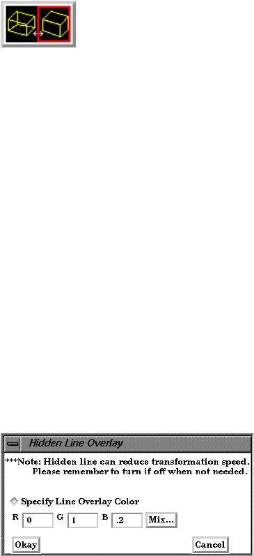
8.6 View Mode
8-46 EnSight 7 User Manual
Global Hidden Line Toggles on/off global Hidden Line (default is off) which simplifies a line-drawing display
Toggle Icon by making hidden lines—lines behind surfaces—invisible while continuing to display
other lines. Performs the same function as Main Menu > View > Hidden Line Toggle and
the Desktop > Hidden Line button.
Hidden Line can be combined with Shaded to display both shaded surfaces and the edges
of the visible surface elements. Hidden Line applies to all Parts displayed in the Graphics
Window but it can be toggled-on/off for individual Parts using the Feature Detail Editor or
the Part Mode: Hidden Line Toggle button.
To have lines hidden behind surfaces, you must have surfaces (2D elements). If the
representation of the in-front Parts consists of 1D elements, the display is the same
whether or not you have Hidden Lines mode toggled-on.
During interactive transformations, the display reverts to displaying all lines. When you
release the mouse button, the Main View display automatically resumes Hidden Line
mode (assuming it is toggled on at that time).
The Hidden line option will not be active during playback of flipbook objects animations.
Hidden Line If you toggle Hidden Line on while Shaded is already on, the lines overlay the
Overlay surfaces. EnSight will prompt you to specify a color for the displayed lines (you do not
want to use the same color as the surfaces since they then will be indistinguishable from
the surfaces). The default is the Part-color of each Part, which may be appropriate if the
surfaces are colored by a color palette instead of their Part-color.
Specify Line Toggle-on if you want to specify an overlay color. If off, the overlay line color will be the
Overlay Toggle same as the Part color.
R, G, B The red, green, and blue components of the hidden line overlay. These fields will not be
accessible unless the Specify Overlay option is on.
Mix... Click to interactively specify the constant color used for the hidden line overlay using the
Color Selector dialog. (see Section 7.1, Color and How To Change Color)
Access: View Mode Icon Bar: Global Hidden Line Toggle Icon
or: Main Menu > View > Hidden Line
or: Desktop > Hidden Line
(See How To Set Attributes)
Figure 8-82
View Mode - Global Hidden Line Toggle Icon
Figure 6-83
Hidden Line Overlay dialog
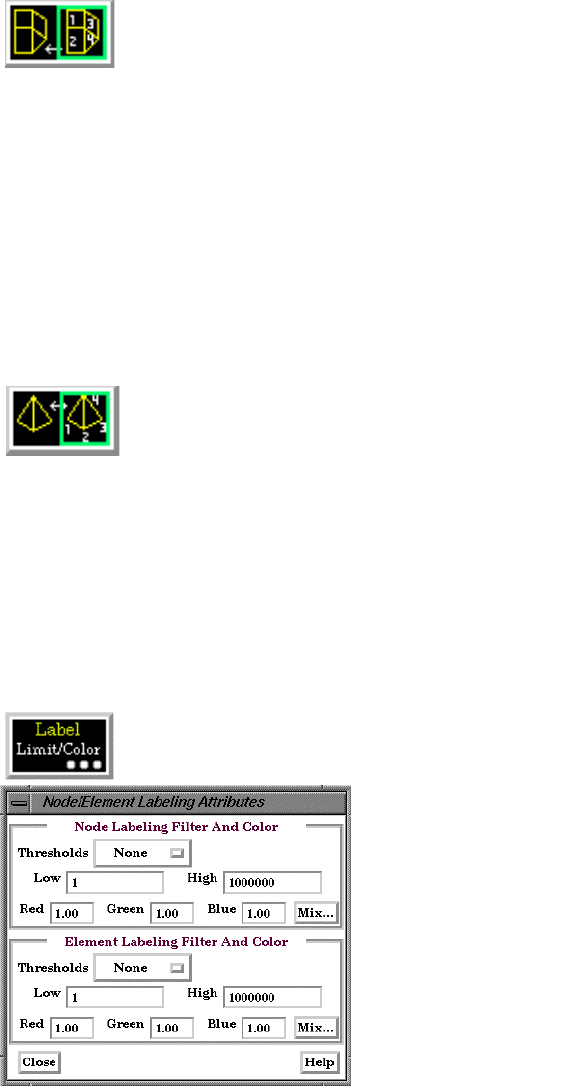
8.6 View Mode
EnSight 7 User Manual 8-47
Global Element Label
Toggles on/off the global visibility (default is on) of element labels (if they are available in
Toggle Icon the data set) for all Parts. Performs the same function as Main Menu > View > Label
Visibility > Element Labeling.
Visibility of element labels for individual Parts can be controlled in the Node, Element,
and Line Attributes section of the Feature Detail Editor (Model) or using the Element
Label Toggle under Part Mode.
Access:‘ View Mode : Global Element Label Icon
or: Main Menu > View > Label Visibility > Element Labeling
Global Node Label Toggles on/off the global visibility (default is on) of node labels (if they are available in
Toggle Icon the data set) for all Parts. Performs the same function as Main Menu > View > Label
Visibility > Node Labeling.
Visibility of node labels for individual Parts can be controlled in the Node, Element, and
Line Attributes section of the Feature Detail Editor (Model) or using the Node Label
Toggle under Part Mode.
Access: View Mode : Global Node Label Icon
or: Main Menu > View > Label Visibility > Node Labeling
Label Attributes Icon Opens the Node/Element Labeling Attributes dialog.
It is often useful to limit the visibility of node and element labels to a subset of those
available in order to identify areas of interest. Coloring the labels can also make
identification easier. The Node/Element Labeling Attributes dialog is used for these two
purposes.
Figure 8-84
View Mode - Global Element Label Toggle Icon
Figure 8-85
View Mode - Global Node Label Toggle Icon
Figure 8-86
View Mode - Labeling Attributes Icon and Node/Element Labeling Attributes dialog
8.6 View Mode
8-48 EnSight 7 User Manual
Node Labeling Filters and Color
Thresholds Selection of pattern for filtering node labels according to the label number. Options are:
None displays all the node labels. (No filtering done)
Low displays only the node numbers that are above Low. (Filters low numbers out)
High displays only the node numbers that are below High. (Filters high numbers out)
Band displays only the node numbers that are below Low and above High. (Filters
the band out)
Low_High displays only the node numbers between Low and High. (Filters the low
and high node numbers out)
Low This field specifies the lowest node number you wish to display.
High This field specifies the highest node number you wish to display.
R G B These fields may be used to specify node label color by RGB values between 0 and 1.
Mix… Opens the Color Selector dialog. (see Section 7.1, Color)
Element Labeling Filters and Color
Thresholds Selection of pattern for filtering element labels according to the label number. Options are:
None displays all the element labels. (No filtering done)
Low displays only the element numbers that are above Low. (Filters low numbers
out)
High displays only the element numbers that are below High. (Filters high numbers
out)
Band displays only the element numbers that are below Low and above High.
(Filters the band out)
Low_High displays only the element numbers between Low and High. (Filters the
low and high node numbers out)
Low This field specifies the lowest element number you wish to display.
High This field specifies the highest element number you wish to display.
R G B These fields may be used to specify element label color by RGB values between 0 and 1.
Mix… Opens the Color Selector dialog. (see Section 7.1, Color)
Access: View Mode : Labeling Attributes Icon
or: Main Menu > View > Label Visibility > Labeling Attributes...
Global Auxiliary Toggles the global Auxiliary Clipping feature on/off (Default is off). Performs the
Clipping Toggle Icon same function as Main Menu > View > Auxiliary Clipping.
Like a Z-Clip plane, Auxiliary Clipping cuts-away a portion of the model. Unless
Auxiliary Clipping (Aux. Clip) has been toggled off for specific Parts in the Feature Detail
Editor dialog General Attributes section or with the Auxiliary Clipping Toggle Icon in the
Part Mode Icon Bar, Parts (or portions of Parts) located on the back (negative-Z) side of
the Plane Tool are removed. Individual Parts whose Aux Clip attribute you have toggled
off remain unaffected.
Figure 8-87
View Mode - Global Auxiliary Clipping Toggle Icon
8.6 View Mode
EnSight 7 User Manual 8-49
Auxiliary Clipping is helpful, for example, with internal flow problems since you can
“peel” off the outside Parts and look inside. This capability is also often useful in
animation.
Auxiliary Clipping is interactive—the view updates in real time as you move the Plane
Tool around. Unlike a Z-Clip plane, Auxiliary Clipping applies only to the Parts you
specify, and the plane can be located anywhere with any orientation though it is always
infinite in extent. The position of the Plane Tool and the status of Auxiliary Clipping is the
same for all displayed viewports.
Do not confuse Auxiliary Clipping with a 2D-Clip plane, which is a created Part whose
geometry lies in a plane cutting through its parent Parts or with the Part-operation of
cutting a Part.
Access: View Mode : Global Auxiliary Clipping Toggle Icon
or: Main Menu > View > Label Visibility > Auxiliary Clipping
(see Section 6.5, Tools Menu Functions and How To Use the Plane Tool)
Troubleshooting Auxiliary Clipping
Global Axis Triad Toggles on/off the visibility (default is off) of the Global Axis triad. Performs
Visibility Toggle Icon the same function as Main Menu > View > Axis Visibility > Axis - Global.
The Global Axis triad shows the point and axes around which Global rotations occur.
Access: View Mode : Global Axis Triad Visibility Toggle Icon
or: Main Menu > View > Axis Triad Visibility > Global
Problem Probable Causes Solutions
The Plane Tool does not appear to
clip anything
The Aux Clip toggle is off for each
individual Part.
Turn the Aux Clip toggle on for
individual Parts in the Feature Detail
Editor (Model) General Attributes
section.
The Plane Tool is not intersecting the
model
Change the position of the Plane
Tool.
The Graphics Window shows
nothing other than the Plane Tool
after Clipping is toggled-on.
All of the Part(s) is(are) on the back
side of the Plane Tool and is(are)
thus clipped
Change the position of the Plane
Tool.
Figure 8-88
View Mode - Global Axis Triad Visibility Toggle Icon
General Description
EnSight 7 User Manual 9-1
9 Transformation Control
Included in this chapter:
General Description
Section 9.1, Global Transform
Section 9.2, Frame Definition
Section 9.3, Frame Transform
Section 9.4, Tool Transform
Section 9.5, Center Of Transform
Section 9.6, Z-Clip
Section 9.7, Look At/Look From
Section 9.8, Copy/Paste Transformation State
General Description
An essential feature of postprocessing is the reorientation of the visualized model
in order to see it from a number of different vantage points. Basic transformations
include rotating (about an axis or axis origin point), translating (up, down, left,
right), and zooming (moving the model toward or away from you). When EnSight
reads in a geometry file, it assigns all model parts to the same Frame of reference:
Frame 0. Frame 0 corresponds to the model coordinate system (defined when the
model was created).
Using the Frame Mode, it is possible to create additional frames and reassign parts
to them. In fact, when you copy a part, a new Frame is automatically created and
the part copy is assigned to the new Frame. (See Section 8.6 Frame Mode for
further discussion).
Just after all parts of your model have been read in, EnSight centers the model in
the Graphics Window by placing the geometric center of the model at the Look At
Point which is always located in the center of the Graphics Window. Initially -
before any Global translations are made -the origin for the Global Axis is located
at the Look At Point.
There are seven Editor Functions available within the Transformation Editor,
Global Transform, Frame, Tools, Z-Clip, Look At/Look From, Copy
Transformation State, and Paste Transformation State. (The Transformation Editor
dialog is opened by clicking the Transf Edit... button)
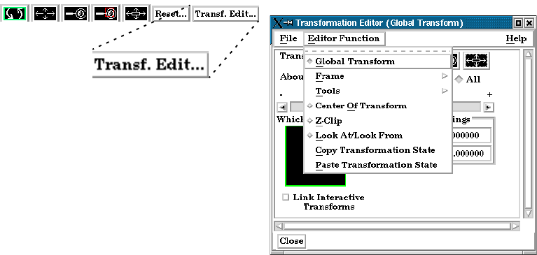
General Description
9-2 EnSight 7 User Manual
.
Transformations performed within the Editor affect the selected viewports and/or
frames. The transforms from one viewport can be copied to another by selecting
the viewport to be copied, selecting Copy Transformation State, selecting the
viewport(s) to be modified, and selecting Paste Transformation State.
File button Pull-down Menu
File > Save View
This opens the Save View dialog which allows you to save in a file the view (orientation)
of the model you have created in the Graphics Window and any Viewports by selecting
Save View and then entering the name of the file.
File > Restore View Opens the Restore View dialog which allows you to specify the name of a file in which
you previously stored a view. Clicking Okay in this dialog restores the view only
in the
selected Viewports.
Figure 9-1
Transf Edit... button and Transformation Editor dialog
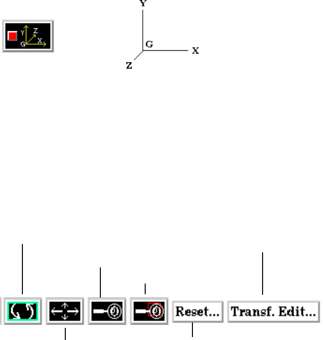
9.1 Global Transform
EnSight 7 User Manual 9-3
9.1 Global Transform
Transformations you make while in Part or View Modes (rotations, translations,
zoom, scale) are performed globally. Global transformations affect the entire
model as a unit and move all Frames, parts, and visible tools relative to the Global
Axis. You can make the Global Axis triad (which pinpoints the Global Axis
Origin) visible by selecting Axis Visibility > Axis - Global from View in the Main
Menu or by clicking the Global Axis Visibility Toggle Icon in the View Mode
icon bar.
You can also show the global frame orientation by toggling it on from Desktop >
Axis.
Most Global transformations you will make will be done interactively. Interactive
Transformations normally affect only the single, selected viewport (the one which
the mouse pointer is in when you click the left mouse button). The exception to
this is if when you toggle on Link Interactive Transforms, causing the selected
viewports in the Transformation Editor dialog to all transform together. You
choose the type of transformation you wish to perform from among the
Transformation Control Icons.
Rotate Toggle
Interactive Rotation When this toggle is on, clicking the left mouse button and dragging horizontally will rotate
the scene (including any tools that are visible) about the Global Y axis.
Clicking the left mouse button and dragging vertically will rotate the scene (including any
tools that are visible) about the Global X axis.
Holding the Control Key down and then clicking the left mouse button and dragging will
rotate the scene (including any tools that are visible) about the Global Z Axis.
Rotation Using Pressing the F1, F2, or F3 function keys will rotate the scene 45 degrees about the X, Y, or
Function Keys Z axis respectively. Holding the Control Key down while pressing these keys will rotate
the scene by -45 degrees. The mouse must be located in the graphics window for these
Figure 9-2
Global Axis Visibility Toggle Icon and Global Axis triad
Figure 9-3
Transformation Control Area in View or Part Mode
Rotate Toggle Icon
Zoom Toggle Icon
Transformation Editor
Button Icon
Translate Toggle Icon
Band Zoom Icon
Reset Tools and Viewport(s) Button Icon
9.1 Global Transform
9-4 EnSight 7 User Manual
keys to work.
Precise Rotation When the Transformation Editor is open under Global Transform and the Rotate toggle is
selected, the dialog will be configured to permit precise Rotation.
You may rotate the entire scene (including any tools that are visible) precisely about the X,
Y, Z, or All axes by clicking on the appropriate axis of rotation toggle and:
entering the desired rotation in (+ or -) degrees in the Increment field and pressing Return,
clicking the stepper buttons at each end of the slider bar (each click will rotate the model
by the number of degrees specified in the Increment field), or
dragging the slider in the positive or negative direction to the desired number of degrees
you wish to rotate the model (the Limit Field specifies the maximum number of
degrees of rotation performed when the slider is pulled to either end of the slider bar).
Translate Toggle
When this toggle is on, you can transform objects interactively in the Global X-Y
Interactive plane (or by holding down the Control key, in Z). Clicking the left mouse button and
Translation dragging will translate the scene (including any tools that are visible) up, down, left or
right (or forward or backward).
Precise Translation When the Transformation Editor is open under Global Transform and the Translate toggle
is selected, the dialog will be configured to permit precise Translation.
You may translate the entire scene (including any tools that are visible) precisely along the
X, Y, Z, or All axes by clicking on the appropriate direction toggle and:
entering the desired translation in (+ or -) model coordinate units in the Increment field
and pressing Return,
Figure 9-4
Transformation Editor for Exact Global
Rotation
Figure 9-5
Transformation Editor for Exact Global
Translation
9.1 Global Transform
EnSight 7 User Manual 9-5
clicking the stepper buttons at each end of the slider bar (each click will translate the
model by the number of model coordinate units specified in the Increment field), or
dragging the slider in the positive or negative direction to the desired number of model
coordinate units you wish to translate the model and then releasing the slider (the Limit
Field specifies the maximum number of model coordinate units that the model is
translated when the slider is pulled to either end of the slider bar).
Zoom Toggle
A Zoom transform is really an adjustment of the Look From Point, which you might also
Interactive Zooming think of as the Camera Position. When this toggle is on, clicking and dragging to the left
or down will zoom-in, that is it will move the Look From Point closer to the Look At
Point. Clicking and dragging to the right or up will zoom-out, that is it will move the Look
From Point farther away from the Look At Point. If you hold down the Control key while
interactively zooming, you will “pan”, i.e. move both the Look At and Look From Points
in the direction of the mouse movement.
(see Section 9.7, Look At/Look From)
As you Zoom in or out, be aware that you may clip the model with the Front or Back
Z-Clip planes since they move in relationship to the Look From Point, always maintaining
the distance from the Look From Point specified in the Transformation Editor dialog:
Editor Function > Z-Clip.
(see Section 9.6, Z-Clip)
Precise Zooming When the Transformation Editor is open under Global Transform and the Zoom toggle is
selected, the dialog will be configured to permit precise Zoom.
You may precisely adjust the position of the Look From Point (with respect to the Look At
Point) by:
entering in the Increment Field the desired modification (+ or -) in the distance between
the two Points (a value of .5 will increase the distance to be equal to 1.5 the current
distance, a value of 1.0 will double the current distance),
clicking the stepper buttons at each end of the slider bar (each click will increase or
decrease the distance between the two Points by the factor specified in the Increment
field), or
dragging the slider in the positive or negative direction to the desired modification factor
and then releasing the slider (the Limit Field specifies the maximum modification
factor for the distance between the two Points when the slider is pulled to either end of
the slider bar).
Band Zoom Button You specify the area of interest by clicking and dragging the white rectangle (rubber band)
around the area you wish to zoom in on. Immediately after you perform the Band Zoom
Figure 9-6
Transformation Editor for Exact Global
Zoom

9.1 Global Transform
9-6 EnSight 7 User Manual
operation however, EnSight will switch to the regular Zoom Transformation. So, each
time you click on the Band Zoom button, EnSight allows you to perform one Band Zoom
operation and subsequent clicking/dragging actions you make in the Graphics Window
perform regular Zoom transformations.
Band Zoom combines the functionality of a zoom-in transform as described above with a
panning operation. The effect of performing a Band Zoom is that the area of interest that
you specify will be centered in and will fill the selected viewport. EnSight adjusts the
transformation center to be in the center of the area you specified.
The Transformation Editor is inactive for the Band Zoom Operation.
Scale Toggle Interactive modifications to scale are not permitted. When the Transformation Editor is
open under Global Transform and the Scale toggle is selected, the dialog will be
configured to permit precise adjustments to the scale of the scene.
You may precisely rescale the scene in the X, Y, Z, or All axes by clicking on the
appropriate scaling direction and:
entering in the Increment Field the desired rescale factor and pressing Return (A value of
.5 will reduce the scale of the scene in the chosen axis by half. A value of 2 will double
the scale in the chosen axis. Be aware that entering a negative number will invert the
model coordinates in the chosen axis.),
clicking the stepper buttons at each end of the slider bar (Clicking the left stepper button
will apply 1/Increment value to the scale. Clicking the right stepper button will apply
the entire Increment value to the scale), or
dragging the slider in the positive or negative direction to the desired scale factor and then
releasing the slider. (Dragging the slider to the leftmost position will apply 1/Limit
value to the scale. Dragging the slider to the rightmost position will apply the entire
Limit value to the scale.)
Figure 9-7
Transformation Editor for Exact Global
Scaling
9.1 Global Transform
EnSight 7 User Manual 9-7
Reset Tools & Clicking the Reset Tools and Viewport(s) button in the Transformation Control Area will
Viewports Button open the Reset Tools and Viewport(s) dialog
By Global XYZ When enabled, clicking a Reset button will cause the Cursor, Line, Plane, or Quadric Tool
Space Toggle to reset to its initial default position.
By Selected When enabled, clicking a Reset button will cause the Cursor, Line, Plane, or Quadric Tool
Viewport Toggle to be repositioned in the center of the geometry for the selected viewport.
Reset Cursor Clicking this button will cause the Cursor Tool to reset according to the “By” toggle.
Reset Line Clicking this button will cause the Line Tool to reset according to the “By” toggle.
Reset Plane Clicking this button will cause the Plane Tool to reset according to the “By” toggle.
Reset Quadric Clicking this button will cause the currently selected Quadric Tool to reset according to
the “By” toggle.
Reset Box Clicking this button will cause the currently selected Box Tool to reset according to the
“By” toggle.
Reset By Selected Clicking this button will cause the transformation selected in the Transformation Control
Transform Only Area to reset for the viewports selected in the dialog’s Viewport(s) area.
Reset Rotate/ Clicking this button will cause the rotate, translate, and scale transformations to reset for
Translate/Scale the viewports selected in the dialog’s Viewport(s) area.
Reinitialize Clicking this button will cause the viewports selected in the dialog’s Viewport(s) area to
reset and recenter on the Parts which are visible in the Viewport(s).
Reset using Pressing the F5 button will change the scene in the current viewport to the standard “right
Function Keys side” view. Similarly, pressing F6 will show a “top” view and F7 a “front” view. Pressing
F8 will restore the view to the one which existed before F5, F6, or F7 were pressed. If the
Control Key is pressed at the same time as F5, F6, or F7, then the current view will be
stored to the selected button.
Figure 9-8
Reset Tools and Viewport(s) dialog
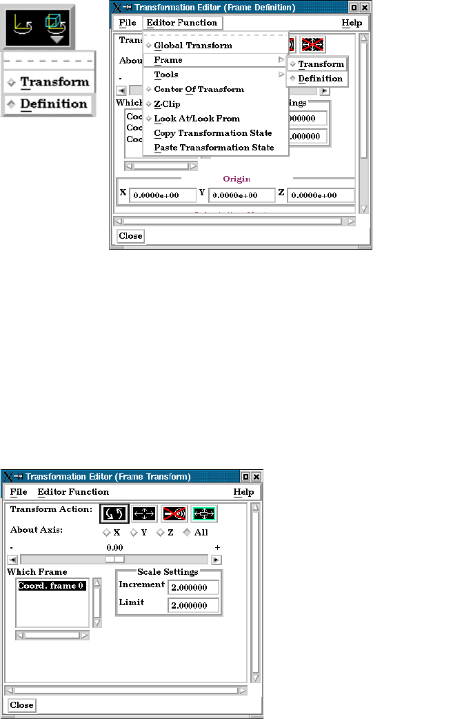
9.2 Frame Definition
9-8 EnSight 7 User Manual
9.2 Frame Definition
When Frame Definition has been chosen from the Transform/Definition button
Pulldown menu or from the Editor Function menu in the Transformation Editor
dialog, then actions you make will affect only the definition (origin and
orientation) of the selected Frame(s). Frame 0’s definition however, can not be
changed.
A Frame’s definition should be adjusted before it is transformed under Frame
Transform (as described in the previous pages). Transformations under Frame
Transform are always about the Frame’s origin and orientation. Failure to define
the proper origin position and orientation of a Frame will result in unexpected
transformation behavior.
You choose the type of transformation you wish to perform (rotate or translate)
from the Transformation Control Icons. Note that you cannot perform zoom,
scale, or reset operations under Frame Definition.
Figure 9-9
Two ways to choose Frame Definition
Figure 9-10
Transformation Control Area in Frame Mode under Frame Definition
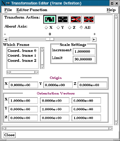
9.2 Frame Definition
EnSight 7 User Manual 9-9
Rotate Toggle
Interactive When this toggle is on, clicking the left mouse button and dragging modifies the
Modification of orientation of the selected Frame(s). Clicking on the end of the X axis will limit the
Orientation rotation to be about the Y axis. Similarly, clicking on the end of the Y axis will limit the
rotation to be about the X axis.
Precise Modification When the Transformation Editor is opened under Frame Definition and the Rotate toggle
of Orientation is selected, the dialog will be configured to permit precise rotation (modification of the
orientation) of the selected Frame(s).
You may rotate the selected Frame(s) precisely about their X, Y, Z, or All axes by clicking
on the desired axis and:
entering the desired rotation in (+ or -) degrees in the Increment field and pressing Return,
clicking the stepper buttons at each end of the slider bar (each click will rotate the selected
Frame(s) by the number of degrees specified in the Increment field), or
dragging the slider in the positive or negative direction to the desired number of degrees
you wish to rotate the selected Frame(s) (the Limit Field specifies the maximum
number of degrees of rotation performed when the slider is pulled to either end of the
slider bar).
Origin XYZ You may precisely position both the origin and the axis of a selected Frame by entering in
Orientation XYZ the desired coordinates in the Origin and Orientation Vector X Y Z fields and then
pressing Return. These fields can be used regardless of whether the Rotate or the Translate
toggle is selected.
Figure 9-11
Transformation Editor for Exact Rotation for Selected Frame(s) Only
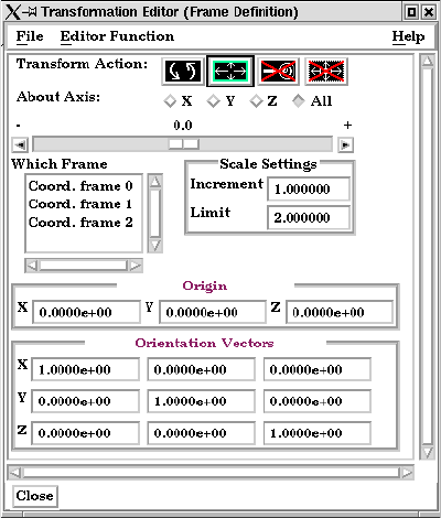
9.2 Frame Definition
9-10 EnSight 7 User Manual
Translate Toggle
Interactive When this toggle is on, clicking the left mouse button and dragging will translate the
Translation of selected Frame(s) (other than Frame 0) up, down, left, or right within the viewport.
Origin Position
Holding down the Control key while dragging will translate the selected Frame(s) forward
or backward.
Precise Translation When the Transformation Editor is open under Frame Definition and the Translate toggle
of Origin Position is selected, the dialog will be configured to permit precise Translation (modification of the
origin position) of the selected Frame(s).
You may translate the selected Frame(s) precisely along the X, Y, Z, or All axes by
clicking on the desired axis direction and:
entering the desired translation in (+ or -) model coordinate units in the Increment field
and pressing Return,
clicking the stepper buttons at each end of the slider bar (each click will translate the
selected Frame(s) by the number of model coordinate units specified in the Increment
field), or
dragging the slider in the positive or negative direction to the desired number of model
coordinate units you wish to translate the selected Frame(s) and then releasing the
slider (the Limit Field specifies the maximum number of model coordinate units that
the Frame is translated when the slider is pulled to either end of the slider bar).
Figure 9-12
Transformation Editor for Exact Translation of Selected Frames
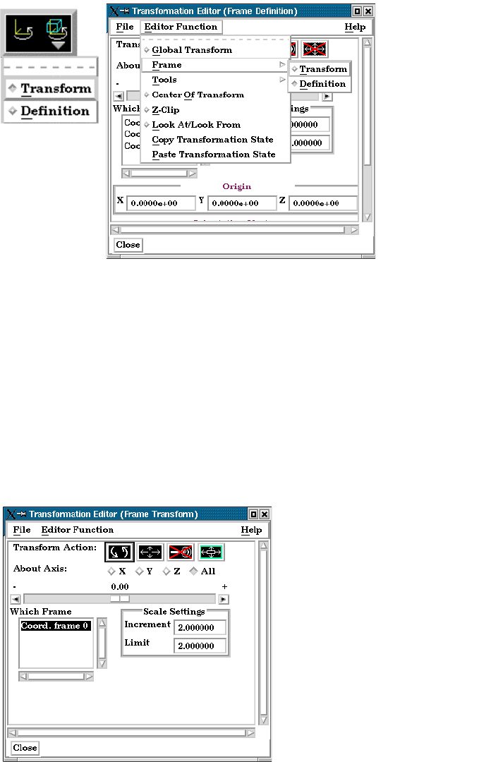
9.3 Frame Transform
EnSight 7 User Manual 9-11
9.3 Frame Transform
When Frame Transform has been chosen from the Transform/Definition button
Pulldown menu or from the Editor Function menu in the Transformation Editor
dialog, transformations you make will affect the selected Frame(s) and the Parts
assigned to them.
Note: Before any transformations are performed on a Frame, its definition should be
modified (if necessary) as described later in this section. Transformations always
occur about a Frame’s origin and orientation. Failure to define the proper
position and orientation of the Frame will result in unexpected transform
behavior. Thus, the order of dealing with things should be 1) define the frame, 2)
assign parts to the frame, 3) transform according to the frame.
You choose the type of transformation you wish to perform from among the
Transformation Control Icons in the Transformation Editor dialog. Note that
under Frame Transform, you cannot perform the zoom operation.
Figure 9-13
Two ways to choose Frame Transform
Figure 9-14
Transformation Control Area in Frame Mode under Frame Transform
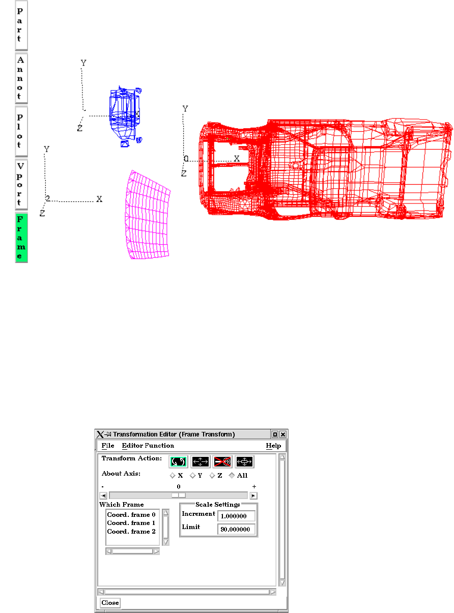
9.3 Frame Transform
9-12 EnSight 7 User Manual
Rotate Toggle
Interactive Rotation When this toggle is on, clicking the left mouse button and dragging causes the selected
Frame(s) and all Parts assigned to the Frame(s) to rotate about the Origins of each Frame
Axis. Holding down the Control key while dragging will rotate the selected Frame(s) and
all assigned Parts about a Z axis perpendicular to the screen.
Precise Rotation
When the Transformation Editor is open under Frame Transform and the Rotate toggle is
selected, the dialog will be configured to permit precise Rotation.
You may rotate the selected Frame(s) and assigned Part(s) precisely about the X, Y, Z, or
All axes, as the orientation of the axes were defined when the Frame was first created by:
entering the desired rotation in (+ or -) degrees in the Increment field and pressing Return,
Figure 9-15
Frame axis triads for Frame 0, Frame 1, and Frame 2
Figure 9-16
Transformation Editor for Precise Rotation
under Frame Transform
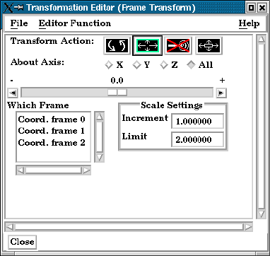
9.3 Frame Transform
EnSight 7 User Manual 9-13
clicking the stepper buttons at each end of the slider bar (each click will rotate the selected
Frame(s) and assigned Part(s) by the number of degrees specified in the Increment
field), or
dragging the slider in the positive or negative direction to the desired number of degrees
you wish to rotate the selected Frame(s) and assigned Part(s) (the Limit Field specifies
the maximum number of degrees of rotation performed when the slider is pulled to
either end of the slider bar).
Translate Toggle
Interactive When this toggle is on, you can transform objects interactively in the X-Y plane (or by
Translation holding down the Control key, in Z). Clicking the left mouse button and dragging will
translate the selected Frame(s) and all assigned Part(s) up, down, left or right (or forward
or backward) within the selected viewport.
Precise Translation When the Transformation Editor is open under Frame Transform and the Translate toggle
is selected, the dialog will be configured to permit precise Translation.
You may translate the selected Frame(s) and all Parts assigned to them precisely along the
X, Y, Z, or All axes by:
entering the desired translation in (+ or -) model coordinate units in the Increment field
and pressing Return,
clicking the stepper buttons at each end of the slider bar (each click will translate the
selected Frame(s) and assigned Part(s) by the number of model coordinate units
specified in the Increment field), or
dragging the slider in the positive or negative direction to the desired number of model
coordinate units you wish to translate the selected Frame(s) and assigned Part(s) and
then releasing the slider (the Limit Field specifies the maximum number of model
coordinate units that the model is translated when the slider is pulled to either end of
the slider bar).
Figure 9-17
Transformation Editor for Precise
Translation under Frame Transform
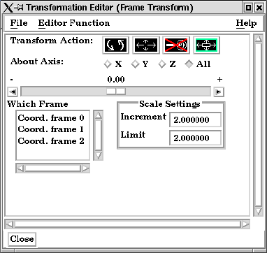
9.3 Frame Transform
9-14 EnSight 7 User Manual
Scale Toggle When the Transformation Editor is open under Frame Transform and the Scale toggle is
selected, the dialog will be configured to permit precise scale.
You may precisely rescale the selected Frame(s) and assigned Part(s) in the X, Y, Z, or All
axes by:
entering in the Increment Field the desired rescale factor and pressing Return (A value of
.5 will reduce the scale of the selected Frame(s) and assigned Part(s) in the chosen axis
by half. A value of 2 will double the scale in the chosen axis. Be aware that entering a
negative number will invert the model coordinates in the chosen axis.),
clicking the stepper buttons at each end of the slider bar (Clicking the left stepper button
will apply 1/Increment value to the scale. Clicking the right stepper button will apply
the entire Increment value to the scale), or
dragging the slider in the positive or negative direction to the desired scale factor and then
releasing the slider. (Dragging the slider to the leftmost position will apply 1/Limit
value to the scale. Dragging the slider to the rightmost position will apply the entire
Limit value to the scale.)
Figure 9-18
Transformation Editor for Exact Scaling
under Frame Transform
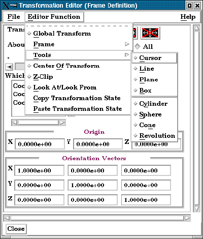
9.4 Tool Transform
EnSight 7 User Manual 9-15
9.4 Tool Transform
Transformation of the Cursor, Line, Plane, Box, and Quadric (cylinder, sphere,
cone, and revolution) Tools is covered in depth in Chapter 6.
(see Tool Positions in Section 6.5, Tools Menu Functions)
Figure 9-19
Transformation Editor Tools Selections
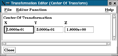
9.6 Z-Clip
EnSight 7 User Manual 9-17
9.6 Z-Clip
EnSight displays the scene in a three-dimensional, rectangular workspace that has
finite boundaries on all sides. Even if you rotate the model, you are always
looking into the workspace from the front side. The top-to-bottom and side-to-
side boundaries of the workspace are analogous to looking out a real window—
the window frame limits your view. In addition, since the memory of your
computer is finite, your workspace also has limits in the front-and-back direction.
The front boundary is the Front Clipping Plane (or the Near Plane) and the rear
boundary is the Back Clipping Plane (or the Far Plane). Only the portion of the
scene between these two planes is visible—the rest of the model (if any) is clipped
and therefore invisible. By convention, the front-to-back direction of the
workspace is the Z direction. Hence, the front and back clipping planes are
together called the Z-Clip Planes. Note that the Z-direction in the workspace is
always in-and-out of the screen and is completely independent of the Z-direction
of the model Frame (Frame 0).
Z-Clip Positions The position of the Z-Clip planes is specified in terms of their distance from the
Look From Point in the distance units implied by the model-geometry data. By
default, the planes automatically move as the model moves.
Initially, EnSight positions the Z-Clip Planes based on the dimensions of the
model parts read to the Client, with some extra space for you to perform
transformations. You can reposition the planes when doing so becomes necessary
or desirable.
Each viewport has its own independently adjustable set of Z-Clip Planes.
Using Z-Clip Planes You can use Z-Clip planes to deliberately clip-away portions of the model you are
not interested in, or which are getting in the way of what is of interest. For
example, you can clip-away both a front-portion and a back-portion of a model to
reduce the number of node and element labels displayed. Z-Clip Planes and
EnSight uses your workstation’s graphics hardware to perform all graphics
Hidden Surfaces manipulations, including the display of solid surfaces. The appearance of a solid
model is created by not displaying hidden surfaces—surfaces hidden behind
nearer surfaces. The algorithm used by the graphics hardware to do this task— Z-
buffering—is a simple algorithm which compares Z-values to calculate which
surfaces are closest to you and thus visible. Z-buffering is normally performed in
integer arithmetic, and on most graphics systems is confined to 24 bits of
resolution. Hence, the coordinates in Z must be mapped into this 24-bit space. To
achieve the maximum resolution possible in the 24 bits available, the graphics
hardware maps the Z-distance between the Front and Back Clipping Planes into
the 24 bits available. Hence, the larger the distance between the Z-Clip Planes, the
lower the Z resolution, which can affect image quality for solid images. If you see
problems with your solid images, move the front and back clipping planes in as
close as possible.
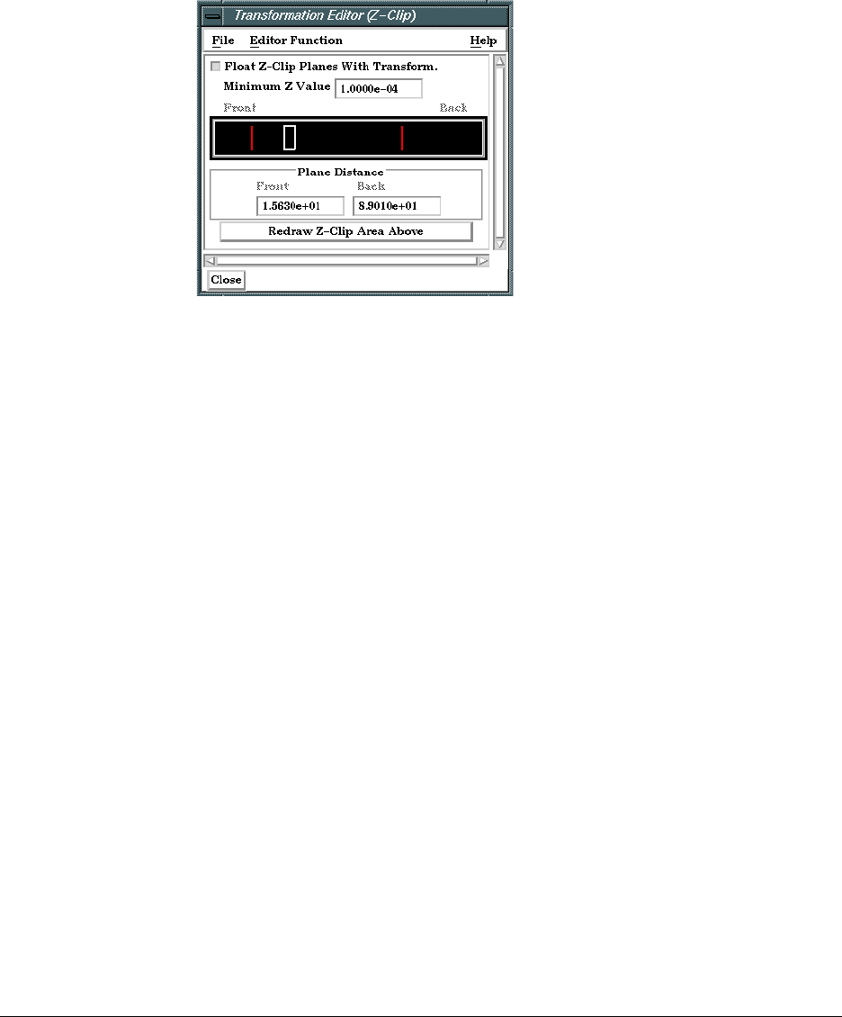
9.6 Z-Clip
9-18 EnSight 7 User Manual
The Transformation Editor (Z-Clip) is used to adjust the distances of the Front and Back
Clipping Planes from the Look-From Point.
Float Z Clip Planes When on, will automatically adjust the front and back Z-Clip planes away from the model.
With Transform
Minimum Z Value Minimum distance the Front Clipping Plane is allowed to float to from the Look From
Point (model coordinates). Used only if Float Z Clip Planes with Transform toggle is on.
Z-Clip Area Display Displays position of Z-Clip planes relative to model-part Z-range (shown as a rectangle)
and allows interactive positioning (by clicking and dragging) of the Z-Clip planes. If lines
are inside model rectangle, that part of model is clipped from the display. Values update in
data fields as you move sliders. Active viewports of the Main View update automatically
as you move sliders.
Plane Distance
Front
Distance of the Front Clipping Plane from Look From Point in model coordinates.
Precisely specify by typing in desired distance and pressing Return. Not used if the Float
Z Clip Planes With Transform toggle is on.
Back Distance of the Back Clipping Plane from the Look From Point in model coordinates.
Precisely specify by typing in desired distance and pressing Return. Not used if the Float Z
Clip Planes With Transform toggle is on.
Redraw The Plane Position Display does not automatically update if you perform transformations
in the active viewport. Click this button to update the Plane Position Display.
Troubleshooting Z-Clip Planes
Problem Probable Causes Solutions
Main View is empty No parts located between Front
and Back Z-Clip Planes.
Adjust Z-Clip plane locations
Model degenerates to irregular
polygons or the front Z-Clip line
is locked in the model extent box
You have moved the front Z-Clip
plane too close to (or on) the
Look From Point.
Move the front Z-Clip plane
away from the Look From Point.
Figure 9-21
Transformation Editor for Z-Clip Plane Positions
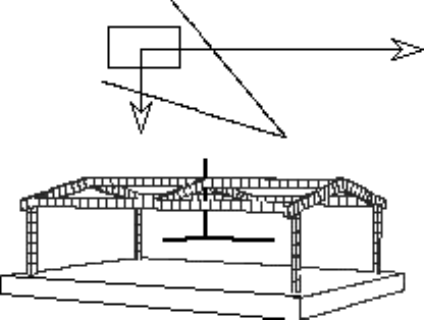
9.7 Look At/Look From
EnSight 7 User Manual 9-19
9.7 Look At/Look From
Using the Transformation Editor with Editor Function > Look At/Look From
chosen, you can reposition the point from which you are observing the model (the
Look From Point) and the point at which you are looking (the Look At Point).
Both the Look-From and Look-At points are specified in the coordinates of the
Model Frame (Frame 0).
Initially, the Look At Point is at the geometric center of the initial model parts
read by the EnSight Client. The Look From Point is on the positive Z-axis at a
distance appropriate to display the model in the Main View window.
If you increased only the X position of the Look From Point, in the Graphics
Window (or selected Viewport), it would appear that the model had rotated about
the Global Y axis. In fact, the model has not rotated at all, which is shown by the
visible Global Axis triad in the figure below. What has happened is that you are
now viewing the model from a position farther to the right than previously.
Figure 9-22
Image showing view of model from negative X axis towards positive X axis
Eye Position
Model
Schematic
Plan View
X
Y
X
Z
Z
G
(Look From Point)
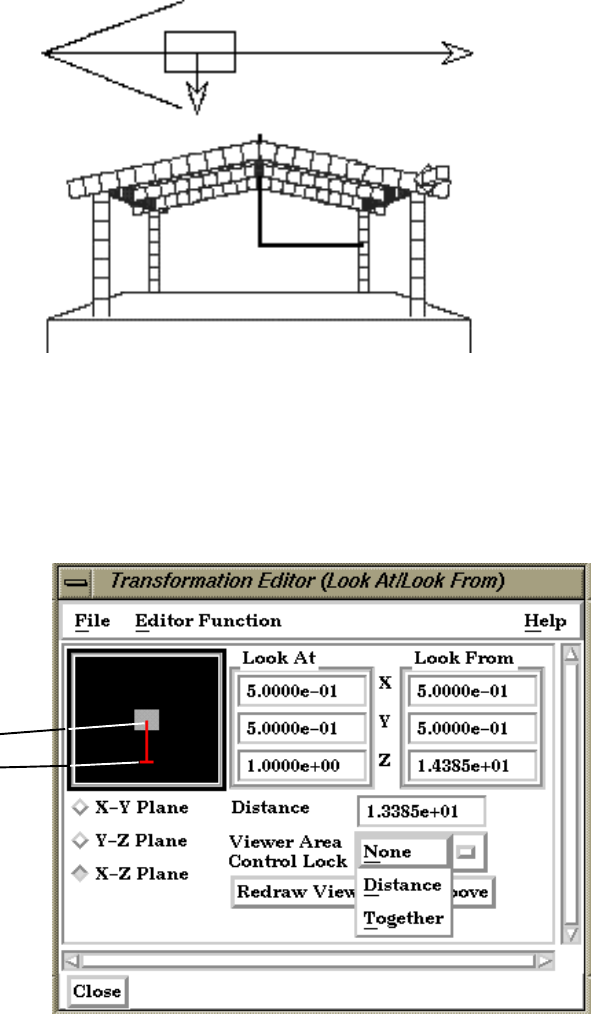
9.7 Look At/Look From
9-20 EnSight 7 User Manual
If the Y and Z coordinates of the Look From point were made to be the same as
those of the Look At point, but the X coordinate of Look From point was specified
as a much smaller value than that of the Look At point, it would appear in the
Graphics Window (or selected Viewport) that the model had rotated 90 degrees
about the Global Y axis. As before, the model has actually not rotated at all, which
is shown by the visible Global Axis triad in the figure below. What has happened
is that you are now viewing the model from a position on the negative Global X
axis looking in the positive X direction.
The position of the Look-At and Look-From points can be interactively or
precisely specified using the Transformation Editor dialog with Editor Function >
Look At/Look From.
Figure 9-23
Image showing view of model from negative X axis towards positive X axis
Eye Position
Model
Schematic
Plan View
X
Y
X
Z
Z
G
(Look From Point)
Figure 9-24
Transformation Editor for Look At/Look From
Interactive Viewer
Area
Look At Point
Look From Point
9.7 Look At/Look From
EnSight 7 User Manual 9-21
Interactive The position of the Look At and Look From Points may be positioned interactively in the
Interactive Viewer Area by grabbing the Look At or Look From Point and dragging it to
the desired location. These interactive modifications can be made in the X-Z Plane, the X-
Y Plane, or the Y-Z Plane, depending upon which of the three toggles are selected. The
Graphics Window as well as the Look At and Look From coordinate fields updates as you
drag either Point to a new location.
Precise The position of the Look At and Look From Points may be positioned precisely by
specifying the desired coordinate values in the X Y Z fields and pressing Return.
Distance The distance in model coordinates may be precisely specified by entering the desired
value in this field and pressing Return.
Viewer Area Opens a pop-up menu for the selection of how interactive actions taken in the Viewer Area
Control Lock will be limited. Choices are:
None No locks are applied
Distance The distance between the two Points is locked
Together The distance and direction vector between the two Points is locked
Redraw Viewer This button redraws the Viewer Area. This button should be clicked after a transformation
Area Above is performed in the selected viewport while this dialog is active.
9.8 Copy/Paste Transformation State
9-22 EnSight 7 User Manual
9.8 Copy/Paste Transformation State
This transformation option can be used to apply the transformation state of one
viewport to other viewports. Useful if you want multiple viewports to have the
model oriented the same, and you did not link the viewports for transformations
before applying any transformations.
The use of this option consists of:
1. Selecting the viewport (one only) containing the transformation state desired.
(You can do this in Vport mode in the graphics screen, or under Editor Function ->
Global Transform in the Transformation Editor Dialog.)
2. Selecting Copy Transformation State under Editor Function in the
Transformation Editor dialog.
3. Selecting the one or more viewports to receive this transformation state.
(As in 1. above)
4. Selecting Paste Transformation State under Editor Function in the
Transformation Editor dialog.
EnSight 7 User Manual 10-1
10 Preference File Formats
This chapter provides information about the various file formats associated with
different preference options within EnSight.
Section 10.1, Window Position File Format describes the format of the file
which contains your saved window positions and sizes.
Section 10.2, Connection Information File Format describes the format of the
file which contains your auto-connection information.
Section 10.3, Palette File Formats describes the format of the color selector
palette, saved function palettes, and the default false color function palette.
Section 10.4, Default Part Colors File Format describes the file format for the
default colors for parts.
Section 10.5, Data Reader Preferences File Format describes the format for the
data reader preferences file.
Section 10.6, MPEG Parameters File describes the format of the MPEG
parameters file.
Section 10.7, Parallel Rendering Configuration File points to the location
where the format of the parallel rendering configuration file is described.
10.1 Window Position File Format
10-2 EnSight 7 User Manual
10.1 Window Position File Format
To save a window position file, click Edit >Preferences... from the Main Menu
and select the “General User Interface” option. Then select the Save Size and
Position of Main Windows button. When you select this button, the current
position of major dialog windows is saved to the
ensight7.winpos.default.XRESxYRES
file. In general, this file contains dialog position and size information, along with
information about the states of the expandable sections of dialogs.
This file is normally saved to and read from the .ensight7 directory of the users
home directory. If the file is in the Client working directory it will be read from
and saved to that directory instead.
Only major dialogs are affected; the miscellaneous pop-up dialogs are not
specified. You do not have to include every dialog and every section listed.
EnSight will process the ones provided.
Window File Format The format of the EnSight window position file is as follows:
• Line 1: Font Size
Integer specifying font size for dialog labels.
• Lines 2 to N: Dialog Title, Size, & Location
String: [IntegerXInteger+]Integer+Integer
specifying
Dialog title: Width x Height + Xloc + Yloc. The dialog title of each
window can be shortened using the * as a meta character. For example,
the string title Transformation Editor: 0+815 can be shortened to
*Transform*: 0+815. Be careful that your abbreviated name does not
match any other names, or the position of all those names will be
changed.
• Line N+1: List Separator String
Character string
—Section Expansion Information—
to separate dialog size
and location information from section-open information.
• Lines N+2 to End: Section Expansion Toggles
Dialog->Section[->Section]: open|closed
character strings indicating
whether corresponding dialog section is open or closed.
The following is an example window position file:
fontsize: 13
EnSight: 910x984+369+31
Transformation Editor: 390x381+180+368
Command: 300x0+0+682
Connect Server: 137+0
Query Dataset: 0+0

10.2 Connection Information File Format
EnSight 7 User Manual 10-3
10.2 Connection Information File Format
EnSight saves a file on the Client host system, called
ensight.connect.default
whenever you connect the Server via the auto connect feature. The next time you
start EnSight, it will read this file and display your previous connection
information. This file is normally saved to and read from the .ensight7 directory of
the users home directory. But, any local file will override this location process.
The complete ASCII text file contains the following Server and/or plotter system
information.
server
machine SERVER_SYSTEM_ID
executable [SERVER_EXE_PATH/]ensight.server
directory SERVER_WORKING_DIRECTORY
login_id SERVER_LOGIN_ID
Each line of the file consists of a descriptive keyword that is usually followed by
an appropriate system variable. The system variables are shown above with
generic abbreviations in capital letters.
Keyword Description
server
Denotes that following keywords and variables pertain to how the
program
ensight7.server
is started via an automatic connection.
machine
The id or hostname of the system where the program is executed. This
defaults to your Client host system hostname.
executable
The complete path to the executable program. This defaults to executing
ensight7.server (which must be in your defined UNIX search path).
This path is normally defined in your .login or .cshrc file in your home
directory (for C shell users).
directory
The directory that you wish the Server to execute from on the Server
host system. You may want to specify the directory that contains your
data files on the Server host system. This defaults to your home
directory on the (Server or plotter) host system for a distributed
connection. It defaults to the Client’s working directory when in
standalone mode.
login_id
Your alternate login id on the Server host system. This defaults to your
Client host system login id. (This option is only applicable to distributed
connections).
10.3 Palette File Formats
10-4 EnSight 7 User Manual
10.3 Palette File Formats
The following palette formats are discussed in this section:
Color Selector Palette File Format
Function Palette File Format
Predefined Function Palette
Default False Color Map File Format
Color Selector Palette File Format
This file defines the colors that are used with the EnSight Color Selector. If
EnSight does not find a definition file it uses a default palette. If, however, it does
find a file (the file must be called ensight.colpal.default and be located in the
.ensight7 directory of the users home directory) at start-up it will read your colors
and show them in the Color Selector.
The format of the ensight.colpal.default file is as follows:
• Line 1: “Version 6.0” (Note, this need not match EnSight’s version
number.)
• Line 2 through Line 37
Three integers, one for each color (red, green, blue), ranging from
0 (no intensity) to 255 (full intensity).
Function Palette File Format
A function palette file is saved using the Function Editor when you save (one or
more) function color palettes. The following is an example function palette file:
palette ‘velocity’
variable_type vector
variable ‘velocity’
type continuous
limit_fringes no
scale linear
number_of_levels 5
colors
0.000000 0.000000 1.000000
0.000000 1.000000 1.000000
0.000000 1.000000 0.000000
1.000000 1.000000 0.000000
1.000000 0.000000 0.000000
values
0.100341
0.301022
0.501704
0.702385
0.903067
Many lines of the file consists of a descriptive keyword followed by an
appropriate value. In other areas the keyword is used to start a block of

10.3 Predefined Function Palette
EnSight 7 User Manual 10-5
information. The values are all free format real or integer numbers or string
constants. The palette name must have single quotes around each name. The string
keywords and constant values must match exactly.
Predefined Function Palette
When EnSight starts, it looks for user defined function color palettes located
under
$CEI_HOME/ensigh74/site_preferences/palettes and in the
.ensight7/palettes directory found in the user’s home directory. These files
must be named
palette_name.cpal, where the palette_name is the name of the
color palette in the Simple Interface area of the function dialog.
The format of the
.cpal file is as follows:
• Line 1: The string “
number_of_levels x”, where x is an integer.
• Line 2: The string “
colors”
• Line 3 through x + 2: Three float values in range 0.0 to 1.0, indicating
red, green, and blue color components.
An example color palette file:
number_of_levels 5
colors
.008 0. 0.
.5 0. 0.
1. 0. 0.
1. 1. 0.
1. 0. 1.
Keyword Description
palette
Name of the palette when one name is present. Name of the
subpalette when two names are present (ex. palette ‘velocity’
’xcomp’)
variable
Name of the variable used with the palette.
variable_type
Type of the variable, scalar or vector.
type
Type of the palette, continuous or banded.
limit_fringes
Indicates if the palette is set up for limiting fringe. If it is, the
options are
by_Part
or
by_invisible
.
scale
Indicates whether the palette scale is linear, logarithmic, or
quadratic.
number_of_levels Indicates the number of levels defined for the palette.
colors Indicates the start of a block of RGB triplets, 1 triplet per line.
There will be the same number of lines as there are levels.
values Indicates the start of a block of level values. There will be the
same number of values as there are levels.
10.3 Default False Color Map File Format
10-6 EnSight 7 User Manual
Default False Color Map File Format
This file defines the default false-color map color range that is assigned by
EnSight to each palette when variables are activated. If EnSight does not find a
definition file, it uses an internal default list. If, however, EnSight does find a file
(the file must be called
ensight.false_color.default
and be located in the
.ensight7
directory of the user's home directory or be located in
$CEI_HOME/ensight76/
site_preferences
) at start-up, EnSight will read your colors as the default palette
colors.
The format of the
ensight.false_color.default
file is as follows:
• Line 1: "Version 6.0" (Note, this need not match EnSight’s version
number.)
• Line 2: One integer, the number default false color map colors
• Line 3 on: three floats (each ranging between 0. and 1.), the (red, green,
blue) color triplet of each color, each listed on separate lines.
An example default file can be found in:
$CEI_HOME/ensight76/site_preferences/ensight.false_color.default
on your client system.
The following is an example default false color map file with 5 colors; blue, cyan,
green, yellow, and red:
Version 6.0
5
0. 0. 1.
0. 1. 1.
0. 1. 0.
1. 1. 0.
1. 0. 0.
10.4 Default Part Colors File Format
EnSight 7 User Manual 10-7
10.4 Default Part Colors File Format
This file defines default Constant Colors that are assigned (and cycled through) by
EnSight when parts are built. If EnSight does not find a definition file it uses an
internal default list. If, however, EnSight does find a file (the file must be called
ensight.part.colors.default
and be located in the
.ensight7
directory of the user's
home directory or be located in
$CEI_HOME/ensight76/site_preferences
) at start-up,
EnSight will read your colors as the default Constant Colors.
The format of the
ensight.part.colors.default
file is as follows:
• Line 1: "Version 6.0" (Note, this need not match EnSight’s version
number.)
• Line 2: One integer, the number of default part colors
• Line 3 on: three floats (each ranging between 0. and 1.), the (red, green,
blue) color triplet of each color, each listed on separate lines.
An example default file can be found in:
$CEI_HOME/ensight76/site_preferences/ensight.part.colors.default
on your client system.
The following is an example default part colors file with 6 colors (blue, cyan,
green, yellow, red, and magenta):
Version 6.0
6
0. 0. 1.
0. 1. 1.
0. 1. 0.
1. 1. 0.
1. 0. 0.
1. 0. 1.
10.5 Data Reader Preferences File Format
10-8 EnSight 7 User Manual
10.5 Data Reader Preferences File Format
This is an optional file that will be created when the user saves preferences under
Main Menu > Edit > Preferences... Data. It can contain two basic things: 1) the
reader name desired to be the default Format in the Data Reader dialog, and/or 2)
any reader names that the user does NOT want to appear in the Format list. The
default data Format will be “Case” unless this file exists and overrides it. Also, by
default, all readers (both internal and User-Defined) will appear in the list of
available reader Formats unless specifically set to be removed in this file. The file
must be called
ensight_reader_prefs.def
and be located in the
.ensight7
directory of
the user's home directory or be located in
$CEI_HOME/ensight76/site_preferences.
The format of the
ensight_readers_prefs.def
file is as follows:
• Line 1: "Version 7.1" (Note, this need not match EnSight’s version
number.)
• Line 2: “select readername” Where readername is the name of the
reader that will be used as the default
• Line 3 on: “remove readername” Where readername is the name of a
reader that will NOT be shown in the data reader Format list.
The following is an example data reader preferences file which sets EnSight 5 as
the default Format, and causes the Movie, MPGS 4.1, and the SCRYU readers to
NOT be available in the list.
Version 7.1
select Ensight 5
remove Movie
remove MPGS 4.1
remove SCRYU
10.6 MPEG Parameters File
EnSight 7 User Manual 10-9
10.6 MPEG Parameters File
This file sets the parameters used by the MPEG Encoder. MPEG is a lossy video
compression standard. As such, there are trade-offs to be made regarding the
degree of compression vs. image quality. The MPEG Encoder utilizes a
parameters file to set numerous options that affect quality, compression, and other
attributes. Three sample parameter files can be found in:
$CEI_HOME/ensight76/site_preferenses/
These files roughly correspond to:
high quality/low compression (
cei_mpeg_hi_q.param
)
medium quality/medium compression (
cei_mpeg_med_q.param
)
and low quality/high compression (
cei_mpeg_lo_q.param
).
The format of the parameters file is documented in the PostScript document:
$CEI_HOME/ensight76/doc/mpeg/mpeg_encode_doc.ps
The Encoder will read the parameters from
~/.ensight7/cei_mpeg.param
if it exists,
otherwise it will use
$CEI_HOME/ensight76/site_preferences/cei_mpeg.param
which is a
link to
cei_mpeg_hi_q.param
; thus high quality/low compression is the default.
Please see the file:
$CEI_HOME/ensight76/doc/mpeg/README.mpeg
for further information.
EnSight 7 User Manual 11-1
11 EnSight Data Formats
This section describes the format for all readable and writable files in EnSight
which you may need access to. The formats described are only for those files that
are specific to EnSight. We do not describe data formats not developed by CEI
(for example, data formats for various analysis codes). For information about
these formats, consult the applicable creator.
Note: If you are using this documentation to produce your own data translator, please
make sure that you follow the instructions exactly as specified. In many cases,
EnSight reads data in blocks to improve performance. If the format is not
followed, the calculations of how much to read for a block will be thrown off.
EnSight does little in the way of error checking data files when they are read. In
this respect, EnSight sacrifices robustness for performance.
Section 11.1, EnSight Gold Casefile Format describes in detail the EnSight
Gold case, geometry, and variable file formats.
Section 11.2, EnSight6 Casefile Format describes in detail the EnSight6 case,
geometry, and variable file formats.
Section 11.3, EnSight5 Format describes in detail the EnSight5 geometry and
variable file formats.
Section 11.4, FAST UNSTRUCTURED Results File Format describes the
“executive” .res file that can be used with FAST unstructured solution and
function files.
Section 11.5, FLUENT UNIVERSAL Results File Format describes the
“executive” .res file that can be used with FLUENT Universal files for transient
models.
Section 11.6, Movie.BYU Results File Format describes the “executive” .res file
that can be used with Movie.BYU files.
Section 11.7, PLOT3D Results File Format describes the “executive” .res file
that can be used with PLOT3D solution and function files.
Section 11.8, Server-of-Server Casefile Format describes the format of the
casefile used with the server-of-server capability of EnSight.
Section 11.9, Periodic Matchfile Format describes the format of the file which
can be used to explicitly specify which nodes match from one periodic instance to
the next.
Section 11.10, XY Plot Data Format describes the format of the file containing
XY plot data.
Section 11.11, EnSight Boundary File Format describes the format of the file
which can define unstructured boundaries of structured data.
Section 11.12, EnSight Particle Emitter File Format describes the format of the
optional file containing particle trace emitter time and location information.
11.1 EnSight Gold Casefile Format
11-2 EnSight 7 User Manual
11.1 EnSight Gold Casefile Format
Include in this section:
EnSight Gold General Description
EnSight Gold Geometry File Format
EnSight Gold Case File Format
EnSight Gold Wild Card Name Specification
EnSight Gold Variable File Format
EnSight Gold Per_Node Variable File Format
EnSight Gold Per_Element Variable File Format
EnSight Gold Undefined Variable Values Format
EnSight Gold Partial Variable Values Format
EnSight Gold Measured/Particle File Format
EnSight Gold Material Files Format
EnSight Gold General Description
EnSight Gold data consists of the following files:
• Case (required) (points to all other needed files including model
geometry, variables, and possibly measured geometry and variables)
EnSight makes no assumptions regarding the physical significance of the scalar,
vector, 2nd order symmetric tensor, and complex variables. These files can be
from any discipline. For example, the scalar file can include such things as
pressure, temperature, and stress. The vector file can be velocity, displacement, or
any other vector data, etc.
In addition, EnSight Gold format handles "undefined" as well as "partial" variable
values. (See appropriate subsections later in this chapter for details.)
All variable results for EnSight Gold format are contained in disk files—one
variable per file. Additionally, if there are multiple time steps, there must either be
a set of disk files for each time step (transient multiple-file format), or all time
steps of a particular variable or geometry in one disk file each (transient single-file
format).
Sources of EnSight Gold format data include the following:
• Data that can be translated to conform to the EnSight Gold data format
(including being written from EnSight itself using the Save Geometric
Entities option under File->Save)
• Data that originates from one of the translators supplied with the EnSight
application
The EnSight Gold format supports an unstructured defined element set as shown
in the figure on the following page. Unstructured data must be defined in this
element set. Elements that do not conform to this set must either be subdivided or
11.1 EnSight Gold General Description
EnSight 7 User Manual 11-3
discarded.
The EnSight Gold format also supports the same structured block data format as
EnSight6, which is very similar to the PLOT3D format. Note that for this format,
the standard order of nodes is such that I’s advance quickest, followed by J’s, and
then K’s.
A given EnSight Gold model may have either unstructured data, structured data,
or a mixture of both.
This format is somewhat similar to the EnSight6 format, but differs enough to
allow for more efficient reading of the data. It is intended for 3D, binary, big data
models.
Note: While an ASCII format is available, it is not intended for use with large
models and is in fact subject to limitations such as integer lengths of 10 digits.
Use the binary format if your model will exceed 10 digits for node or element
numbers or labels.
Starting with version 7, EnSight writes out all model and variable files in EnSight
Gold format. Thus, it can be read by all version 7 EnSight licenses (i.e. standard,
gold, and custom licenses).
ens_checker A program is supplied with EnSight which attempts to verify the integrity of the
format of EnSight 6 and EnSight Gold files. If you are producing EnSight
formatted data, this program can be very helpful, especially in your development
stage, in making sure that you are adhering to the published format. It makes no
attempt to verify the validity of floating point values, such as coordinates, variable
values, etc. This program takes a casefile as input. Thus, it will check the format
of the casefile, and all associated geometry and variable files referenced in the
casefile. See How To Use ens_checker.
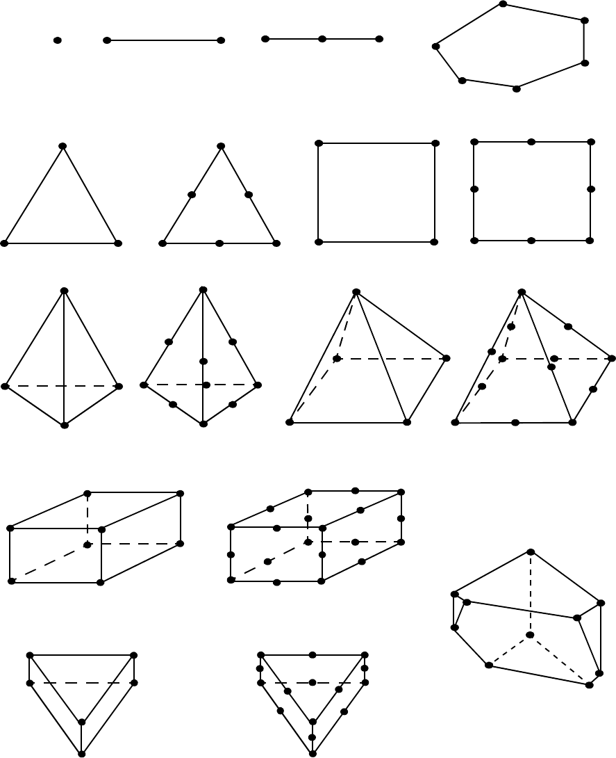
11.1 EnSight Gold General Description
11-4 EnSight 7 User Manual
Supported EnSight Gold Elements
The elements that are supported by the EnSight Gold format are:
eight node hexahedron twenty node hexahedron
six node pentahedron
9
10
7
8
12123
1
2
3
12
3
4
56
1
2
3
4
12
3
45
6
7
8
12
3
4
5
6
1
2
3
4
5
6
9
10
7
8
1
2
3
4
56
11
12
13
14
15
16
17
18
19
20
two node bar three node bar
three node triangle six node triangle four node quadrangle eight node quadrangle
four node tetrahedron ten node tetrahedron
1
point
1
2
3
4
1
4
8
2
3
5
6
7
5 node pyramid 13 node pyramid
11
2
2
3
3
44
5
5
6
7
8
9
10
11
12
13
fifteen node pentahedron (wedge)
1
2
3
4
5
6
7
8
9
10
11
12
13
14
15
(wedge)
Figure 11-1
Supported EnSight Gold Elements
1 .
.
.
n
2
n-sided polygon
convex n-faced polyhedron
(described by n, n-sided faces)
11.1 EnSight Gold Geometry File Format
EnSight 7 User Manual 11-5
EnSight Gold Geometry File Format
The EnSight Gold format is part based for both unstructured and structured data.
There is no global coordinate array that each part references, but instead - each
part contains its own local coordinate array. Thus, the node numbers in element
connectivities refer to the coordinate array index, not a node id or label. This is
different than the EnSight6 format!
The EnSight Gold format consists of keywords followed by information. The
following items are important when working with EnSight Gold geometry files:
1. Node ids are optional. In this format they are strictly labels and are not used in
the connectivity definition. The element connectivities are based on the local
implied node number of the coordinate array in each part, which is sequential
starting at one. If you let EnSight assign node IDs, this implied internal
numbering is used. If node IDs are set to off, they are numbered internally,
however, you will not be able to display or query on them. If you have node
IDs given in your data, you can have EnSight ignore them by specifying
“node id ignore.” Using this option may reduce some of the memory taken up
by the Client and Server, but display and query on the nodes will not be
available. Note, prior to EnSight 7.4, node ids could only be specified for
unstructured parts. This restriction has been removed and user specified node
ids are now possible for structured parts.
2. Element ids are optional. If you specify element IDs, or you let EnSight
assign them, you can show them on the screen. If they are set to off, you will
not be able to show or query on them. If you have element IDs given in your
data you can have EnSight ignore them by specifying “element id ignore.”
Using this option will reduce some of the memory taken up by the Client and
Server. This may or may not be a significant amount, and remember that
display and query on the elements will not be available. Note, prior to EnSight
7.4, element ids could only be specified for unstructured parts. This restriction
has been removed and user specified element ids are now possible for
structured parts.
3. Model extents can be defined in the file so EnSight will not have to determine
these while reading in data. If they are not included, EnSight will compute
them, but will not actually do so until a dataset query is performed the first
time.
4. The format of integers and real numbers must be followed (See the Geometry
Example below).
5. ASCII Integers are written out using the following integer format:
From C:
10d
format
From FORTRAN:
i10
format
Note: this size of integer format places a limitation on the number of nodes
and the node and element labels that can make up a model. Use the
binary format for large models!
ASCII Real numbers are written out using the following floating-point format:
From C:
12.5e
format
From FORTRAN:
e12.5
format

11.1 EnSight Gold Geometry File Format
11-6 EnSight 7 User Manual
The number of integers or reals per line must also be followed!
6. By default, a Part is processed to show the outside boundaries. This
representation is loaded to the Client host system when the geometry file is
read (unless other attributes have been set on the workstation, such as feature
angle).
7. Coordinates for unstructured data must be defined within each part. This is
normally done before any elements are defined within a part, but does not
have to be. The different elements can be defined in any order (that is, you can
define a hexa8 before a bar2).
8. A Part containing structured data cannot contain any unstructured element
types or more than one block. Each structured Part is limited to a single
block (or some subset of that block). A structured block is indicated by
following the Part description line with a ‘block’ line. By default, a block will
be curvilinear, non-iblanked, non-ghost, complete range. However, by
suppling one or more of the following options on the ‘block’ line, rectilinear
or uniform blocks can be specified, nodal iblanking for the block can be used,
cells within the block can be flagged as ghosts (used for computations, but not
displayed), subset ranges can be specified (useful for partitioned data). The
options include:
Only one of these can be used on the ‘block’ line
curvilinear
Indicates that coordinates of all ijk locations of the block will be
specified (default)
rectilinear
Indicates that i,j,k delta vectors for a regular block with possible
non-regular spacing will be specified
uniform
Indicates that i,j,k delta values for a regular block with regular
spacing will be specified
Any, none, or all of these can be used
iblanked
An “iblanked” block must contain an additional integer array of
values at each node, traditionally called the iblank array. Valid iblank
values for the EnSight Gold format are:
0 for nodes which are exterior to the model, sometimes
called blanked-out nodes
1 for nodes which are interior to the model, thus in the
free stream and to be used
<0 or >1 for any kind of boundary nodes
In EnSight’s structured Part building dialog, the iblank option
selected will control which portion of the structured block is
“created”. Thus, from the same structured block, the interior flow
field part as well as a symmetry boundary part could be “created”.
Note: By default EnSight does not do any “partial” cell iblank
processing. Namely, only complete cells containing no “exterior”
nodes are created. It is possible to obtain partial cell processing by
issuing the “test:partial_cells_on” command in the Command
Dialog before reading the file.

11.1 EnSight Gold Geometry File Format
EnSight 7 User Manual 11-7
Note that for structured data, the standard order of nodes is such that I’s advance
quickest, followed by J’s, and then K’s.
with_ghost
A block with ghosts must contain an additional integer array of flags
for each cell. A flag value of zero indicates a non-ghost cell. A flag
value of non-zero indicates a ghost cell.
range
A block with ranges will contain an extra line, following the ijk line,
which gives min and max planes for each of the ijk directions.
Thus, normally a 6 x 5 x 1 block part would start something like:
part
1
description
block
6 5 1
0.00000e+00
...
(The coordinate information for the 30 nodes of the block must
follow.)
But if only the top 6 x 3 x 1portion was to be represented in the file,
you can use “range” like:
part
1
description for top only
block range
6 5 1
1 6 3 5 1 1
0.00000e+00
...
(The coordinate information for the 18 nodes of the top portion of
the block must follow. Note that the ijk line following the block line
contains the size of the original block - which is needed to properly
deal with node and element numbering. The next line contains the
imin, imax, jmin, jmax, kmin, kmax defining the subset ranges. The
actual size of the block being defined is thus computed from these
ranges:
size_i = imax - imin + 1
size_j = jmax - jmin + 1
size_k = kmax - kmin + 1
11.1 EnSight Gold Geometry File Format
11-8 EnSight 7 User Manual
Generic Format Usage Notes:
In general an unstructured
part
can contain several different
element type
s.
#
= a part number
nn
= total number of nodes in a part
ne
= number of elements of a given type
np
= number of nodes per element for a given element type
nf
= number of faces per nfaced element
id_*
= node or element id number
x_*
= x component
y_*
= y component
z_*
= z component
n*_e*
= node number for an element
f*_e*
= face number for an nfaced element
ib_*
= iblanking value
gf_e*
= ghost flag for a structured cell
[]
contain optional portions
<>
contain choices
‘
indicates the beginning of an unformatted sequential FORTRAN binary write
’
indicates the end of an unformatted sequential FORTRAN binary write
element type
can be any of:
point g_point
bar2 g_bar2
bar3 g_bar3
tria3 g_tria3
tria6 g_tria6
quad4 g_quad4
quad8 g_quad8
tetra4 g_tetra4
tetra10 g_tetra10
pyramid5 g_pyramid5
pyramid13 g_pyramid13
penta6 g_penta6
penta15 g_penta15
hexa8 g_hexa8
hexa20 g_hexa20
nsided g_nsided
nfaced g_nfaced
11.1 EnSight Gold Geometry File Format
EnSight 7 User Manual 11-9
C Binary form:
C Binary 80 chars
description line 1 80 chars
description line 2 80 chars
node id <off/given/assign/ignore> 80 chars
element id <off/given/assign/ignore> 80 chars
[extents
80 chars
xmin xmax ymin ymax zmin zmax]
6 floats
part 80 chars
# 1 int
description line 80 chars
coordinates
80 chars
nn 1 int
[id_n1 id_n2 ... id_nn] nn ints
x_n1 x_n2 ... x_nn nn floats
y_n1 y_n2 ... y_nn nn floats
z_n1 z_n2 ... z_nn nn floats
element type 80 chars
ne 1 int
[id_e1 id_e2 ... id_ne] ne ints
n1_e1 n2_e1 ... np_e1
n1_e2 n2_e2 ... np_e2
.
.
n1_ne n2_ne ... np_ne ne*np ints
element type 80 chars
.
.
part 80 chars
.
.
part 80 chars
# 1 int
description line 80 chars
block [iblanked] [with_ghost] [range] 80 chars
i j k # nn = i*j*k, ne = (i-1)*(j-1)*(k-1) 3 ints
[imin imax jmin jmax kmin kmax] # if range used: 6 ints
nn =
(imax-imin+1)*
(jmax-jmin+1)* (kmax-kmin+1)
ne = (imax-imin)*(jmax-jmin)*(kmax-kmin)
x_n1 x_n2 ... x_nn nn floats
y_n1 y_n2 ... y_nn nn floats
z_n1 z_n2 ... z_nn nn floats
[ib_n1 ib_n2 ... ib_nn] nn ints
[ghost_flags] 80 chars
[gf_e1 gf_e2 ... gf_ne] ne ints
[node_ids] 80 chars
[id_n1 id_n2 ... id_nn] nn ints
[element_ids] 80 chars
[id_e1 id_e2 ... id_ne] ne ints
part 80 chars
# 1 int
description line 80 chars
block rectilinear [iblanked] [with_ghost] [range] 80 chars
i j k # nn = i*j*k, ne = (i-1)*(j-1)*(k-1) 3 ints
[imin imax jmin jmax kmin kmax] # if range used: 6 ints
nn =
(imax-imin+1)*
(jmax-jmin+1)* (kmax-kmin+1)
ne = (imax-imin)*(jmax-jmin)*(kmax-kmin)
x_1 x_2 ... x_i i floats
y_1 y_2 ... y_j j floats
11.1 EnSight Gold Geometry File Format
11-10 EnSight 7 User Manual
z_1 z_2 ... z_k k floats
[ib_n1 ib_n2 ... ib_nn] nn ints
[ghost_flags] 80 chars
[gf_e1 gf_e2 ... gf_ne] ne ints
[node_ids] 80 chars
[id_n1 id_n2 ... id_nn] nn ints
[element_ids] 80 chars
[id_e1 id_e2 ... id_ne] ne ints
part 80 chars
# 1 int
description line 80 chars
block uniform [iblanked] [with_ghost] [range] 80 chars
i j k # nn = i*j*k, ne = (i-1)*(j-1)*(k-1) 3 ints
[imin imax jmin jmax kmin kmax] # if range used: 6 ints
nn =
(imax-imin+1)*
(jmax-jmin+1)* (kmax-kmin+1)
ne = (imax-imin)*(jmax-jmin)*(kmax-kmin)
x_origin y_origin z_origin 3 floats
x_delta y_delta z_delta 3 floats
[ib_n1 ib_n2 ... ib_nn] nn ints
[ghost_flags] 80 chars
[gf_e1 gf_e2 ... gf_ne] ne ints
[node_ids] 80 chars
[id_n1 id_n2 ... id_nn] nn ints
[element_ids] 80 chars
[id_e1 id_e2 ... id_ne] ne ints
Fortran Binary form:
‘Fortran Binary’
‘description line 1’ 80 chars
‘description line 2’ 80 chars
‘node id <off/given/assign/ignore>’ 80 chars
‘element id <off/given/assign/ignore>’ 80 chars
[‘extents’
80 chars
‘xmin xmax ymin ymax zmin zmax’]
6 floats
‘part’ 80 chars
‘#’ 1 int
‘description line’ 80 chars
‘coordinates’
80 chars
‘nn’ 1 int
[‘id_n1 id_n2 ... id_nn’] nn ints
‘x_n1 x_n2 ... x_nn’ nn floats
‘y_n1 y_n2 ... y_nn’ nn floats
‘z_n1 z_n2 ... z_nn’ nn floats
‘element type’ 80 chars
‘ne’ 1 int
[‘id_e1 id_e2 ... id_ne’] ne ints
‘n1_e1 n2_e1 ... np_e1
n1_e2 n2_e2 ... np_e2
.
.
n1_ne n2_ne ... np_ne’ ne*np ints
‘element type’ 80 chars
.
.
‘part’ 80 chars
.
.
‘part’ 80 chars
11.1 EnSight Gold Geometry File Format
EnSight 7 User Manual 11-11
‘#’ 1 int
‘description line’ 80 chars
‘block [iblanked] [with_ghost] [range]’ 80 chars
‘i j k’ # nn = i*j*k, ne = (i-1)*(j-1)*(k-1) 3 ints
[‘imin imax jmin jmax kmin kmax’] # if range used: 6 ints
nn =
(imax-imin+1)*
(jmax-jmin+1)* (kmax-kmin+1)
ne = (imax-imin)*(jmax-jmin)*(kmax-kmin)
‘x_n1 x_n2 ... x_nn’ nn floats
‘y_n1 y_n2 ... y_nn’ nn floats
‘z_n1 z_n2 ... z_nn‘ nn floats
[‘ib_n1 ib_n2 ... ib_nn’] nn ints
[‘ghost_flags’] 80 chars
[‘gf_e1 gf_e2 ... gf_ne’] ne ints
[‘node_ids’] 80 chars
[‘id_n1 id_n2 ... id_nn’] nn ints
[‘element_ids’] 80 chars
[‘id_e1 id_e2 ... id_ne’] ne ints
‘part’ 80 chars
‘#’ 1 int
‘description line’ 80 chars
‘block rectilinear [iblanked] [with_ghost] [range]’ 80 chars
‘i j k’ # nn = i*j*k, ne = (i-1)*(j-1)*(k-1) 3 ints
[‘imin imax jmin jmax kmin kmax’] # if range used: 6 ints
nn =
(imax-imin+1)*
(jmax-jmin+1)* (kmax-kmin+1)
ne = (imax-imin)*(jmax-jmin)*(kmax-kmin)
‘x_1 x_2 ... x_i’ i floats
‘y_1 y_2 ... y_j’ j floats
‘z_1 z_2 ... z_k’ k floats
[‘ib_n1 ib_n2 ... ib_nn’] nn ints
[‘ghost_flags’] 80 chars
[‘gf_e1 gf_e2 ... gf_ne’] ne ints
[‘node_ids’] 80 chars
[‘id_n1 id_n2 ... id_nn’] nn ints
[‘element_ids’] 80 chars
[‘id_e1 id_e2 ... id_ne’] ne ints
‘part’ 80 chars
‘#’ 1 int
‘description line’ 80 chars
‘block uniform [iblanked] [with_ghost] [range]’ 80 chars
‘i j k’ # nn = i*j*k, ne = (i-1)*(j-1)*(k-1) 3 ints
[‘imin imax jmin jmax kmin kmax’] # if range used: 6 ints
nn =
(imax-imin+1)*
(jmax-jmin+1)* (kmax-kmin+1)
ne = (imax-imin)*(jmax-jmin)*(kmax-kmin)
‘x_origin y_origin z_origin 3 floats
x_delta y_delta z_delta’ 3 floats
[‘ib_n1 ib_n2 ... ib_nn’] nn ints
[‘ghost_flags’] 80 chars
[‘gf_e1 gf_e2 ... gf_ne’] ne ints
[‘node_ids’] 80 chars
[‘id_n1 id_n2 ... id_nn’] nn ints
[‘element_ids’] 80 chars
[‘id_e1 id_e2 ... id_ne’] ne ints
ASCII form:
description line 1 A (max of 79 typ)
description line 2 A
node id <off/given/assign/ignore> A
element id <off/given/assign/ignore> A
11.1 EnSight Gold Geometry File Format
11-12 EnSight 7 User Manual
[extents
A
xmin xmax 2E12.5
ymin ymax 2E12.5
zmin zmax] 2E12.5
part A
# I10
description line A
coordinates
A
nn I10
[id_n1 I10 1/line (nn)
id_n2
.
.
id_nn]
x_n1 E12.5 1/line (nn)
x_n2
.
.
x_nn
y_n1 E12.5 1/line (nn)
y_n2
.
.
y_nn
z_n1 E12.5 1/line (nn)
z_n2
.
.
z_nn
element type A
ne I10
[id_e1 I10 1/line (ne)
id_e2
.
.
id_ne]
n1_e1 n2_e1 ... np_e1 I10 np/line
n1_e2 n2_e2 ... np_e2 (ne lines)
.
.
n1_ne n2_ne ... np_ne
element type A
.
.
part A
.
.
part A
# I10
description line A
block [iblanked] [with_ghost] [range] A
i j k # nn = i*j*k, ne = (i-1)*(j-1)*(k-1) 3I10
[imin imax jmin jmax kmin kmax] # if range used: 6I10
nn =
(imax-imin+1)*
(jmax-jmin+1)* (kmax-kmin+1)
ne = (imax-imin)*(jmax-jmin)*(kmax-kmin)
x_n1 E12.5 1/line (nn)
x_n2
.
.
x_nn
y_n1 E12.5 1/line (nn)
11.1 EnSight Gold Geometry File Format
EnSight 7 User Manual 11-13
y_n2
.
.
y_nn
z_n1 E12.5 1/line (nn)
z_n2
.
.
z_nn
[ib_n1 I10 1/line (nn)
ib_n2
.
.
ib_nn]
[ghost_flags] 80 chars
[gf_e1 I10 1/line (ne)
gf_e2
.
.
gf_ne]
[node_ids] 80 chars
[id_n1 I10 1/line (nn)
id_n2
.
.
id_nn]
[element_ids] 80 chars
[id_e1 I10 1/line (ne)
id_e2
.
.
id_ne]
part A
# I10
description line A
block rectilinear [iblanked] [with_ghost] [range] A
i j k # nn = i*j*k, ne = (i-1)*(j-1)*(k-1) 3I10
[imin imax jmin jmax kmin kmax] # if range used: 6I10
nn =
(imax-imin+1)*
(jmax-jmin+1)* (kmax-kmin+1)
ne = (imax-imin)*(jmax-jmin)*(kmax-kmin)
x_1 E12.5 1/line (i)
x_2
.
.
x_i
y_1 E12.5 1/line (j)
y_2
.
.
y_j
z_1 E12.5 1/line (k)
z_2
.
.
z_k
[ib_n1 I10 1/line (nn)
ib_n2
.
.
ib_nn]
[ghost_flags] 80 chars
11.1 EnSight Gold Geometry File Format
11-14 EnSight 7 User Manual
[gf_e1 I10 1/line (ne)
gf_e2
.
.
gf_ne]
[node_ids] 80 chars
[id_n1 I10 1/line (nn)
id_n2
.
.
id_nn]
[element_ids] 80 chars
[id_e1 I10 1/line (ne)
id_e2
.
.
id_ne]
part A
# I10
description line A
block uniform [iblanked] [with_ghost] [range] A
i j k # nn = i*j*k, ne = (i-1)*(j-1)*(k-1) 3I10
[imin imax jmin jmax kmin kmax] # if range used: 6I10
nn =
(imax-imin+1)*
(jmax-jmin+1)* (kmax-kmin+1)
ne = (imax-imin)*(jmax-jmin)*(kmax-kmin)
x_origin E12/5
y_origin E12/5
z_origin E12/5
x_delta E12.5
y_delta E12.5
z_delta E12.5
[ib_n1 I10 1/line (nn)
ib_n2
.
.
ib_nn]
[ghost_flags] 80 chars
[gf_e1 I10 1/line (ne)
gf_e2
.
.
gf_ne]
[node_ids] 80 chars
[id_n1 I10 1/line (nn)
id_n2
.
.
id_nn]
[element_ids] 80 chars
[id_e1 I10 1/line (ne)
id_e2
.
.
id_ne]
11.1 EnSight Gold Geometry File Format
EnSight 7 User Manual 11-15
Notes:
•If
node id
is
given
or
ignore
, the [id] section must be there for each part.
•If
element id
is
given
or
ignore
, the [id] section must be there for each
element type
of each part
•If
iblanked
is there, the [ib] section must be there for the block.
• x, y, and z coordinates are mandatory, even if a 2D problem.
•If
block rectilinear
, then the x, y, z coordinates change to the x, y, and z
delta vectors.
•If
block uniform
, then the x, y, z coordinates change to the x, y, z
coordinates of the origin and the x, y, and z delta values.
•If
block range
, the ijk min/max range line must follow the ijk line. And the
number of nodes and elements is based on the ranges. The ijk line
indicates the size of the original block.
•If
with_ghost
is on the
block
line, then the
ghost_flag
section must be there
• Ids are just labels, the coordinate (or element) order is implied.
• The minimum needed for unstructured empty parts is the three lines:
part
# (use the actual part number)
description
• The minimum needed for structured empty parts is the five lines:
part
# (use the actual part number)
description
block
000
• Element blocks for nsided elements contain an additional section - the
number of nodes in each element. See below.
C Binary form of element block, if nsided:
nsided 80 chars
ne 1 int
[id_n1 id_n2 ... id_ne] ne ints
np1 np2 ... npne This data is needed ne ints
e1_n1 e1_n2 ... e1_np1
e2_n1 e2_n2 ... e2_np2
.
.
ne_n1 ne_n2 ... ne_npne np1+np2+...+npne ints
Fortran Binary form of element block, if nsided:
‘nsided’ 80 chars
‘ne’ 1 int
[‘id_n1 id_n2 ... id_ne’] ne ints
‘np1 np2 ... npne’ This data is needed ne ints
‘e1_n1 e1_n2 ... e1_np1
11.1 EnSight Gold Geometry File Format
11-16 EnSight 7 User Manual
e2_n1 e2_n2 ... e2_np2
.
.
ne_n1 ne_n2 ... ne_npne’ np1+np2+...+npne ints
Ascii form of element block, if nsided:
nsided A
ne I10
[id_n1 I10 1/line (ne)
id_n2
.
id_ne]
np1 This data is needed I10 1/line (ne)
np2 .
. .
npne .
e1_n1 e1_n2 ... e1_np1 I10 np*/line
e2_n1 e2_n2 ... e2_np2 (ne lines)
.
ne_n1 ne_n2 ... ne_npne
• Element blocks for nfaced elements are more involved since they are
described by their nsided faces. Thus, there is the optional section for ids
(id_e*), a section for the number of faces per element (nf_e*), a section
for number of nodes per face per element (np(f*_e*)), and a section for
the connectivity of each nsided face of each element (n*(f*_e*)). See
below.
C Binary form of element block, if nfaced:
nfaced 80 chars
ne 1 int
[id_e1 id_e2 ... id_ne] ne ints
nf_e1 nf_e2 ... nf_ne ne ints
np(f1_e1) np(f2_e1) ... np(nf_e1)
np(f1_e2) np(f2_e2) ... np(nf_e2)
.
.
np(f1_ne) np(f2_ne) ... np(nf_ne) nf_e1+nf_e2+...+nf_ne ints
n1(f1_e1) n2(f1_e1) ... n(np(f1_e1))
n1(f2_e1) n2(f2_e1) ... n(np(f2_e1))
.
n1(nf_e1) n2(nf_e1) ... n(np(nf_e1))
n1(f1_e2) n2(f1_e2) ... n(np(f1_e2))
n1(f2_e2) n2(f2_e2) ... n(np(f2_e2))
.
n1(nf_e2) n2(nf_e2) ... n(np(nf_e2))
.
.
n1(f1_ne) n2(f1_ne) ... n(np(f1_ne))
n1(f2_ne) n2(f2_ne) ... n(np(f2_ne))
.
n1(nf_ne) n2(nf_ne) ... n(np(nf_ne)) np(f1_e1)+np(f2_e1)+...+np(nf_ne) ints
Fortran Binary form of element block, if nfaced:
‘nfaced’ 80 chars
‘ne’ 1 int
[‘id_e1 id_e2 ... id_ne’] ne ints
‘nf_e1 nf_e2 ... nf_ne’ ne ints
11.1 EnSight Gold Geometry File Format
EnSight 7 User Manual 11-17
‘np(f1_e1) np(f2_e1) ... np(nf_e1)
np(f1_e2) np(f2_e2) ... np(nf_e2)
.
.
np(f1_ne) np(f2_ne) ... np(nf_ne)’ nf_e1+nf_e2+...+nf_ne ints
‘n1(f1_e1) n2(f1_e1) ... n(np(f1_e1))
n1(f2_e1) n2(f2_e1) ... n(np(f2_e1))
.
n1(nf_e1) n2(nf_e1) ... n(np(nf_e1))
n1(f1_e2) n2(f1_e2) ... n(np(f1_e2))
n1(f2_e2) n2(f2_e2) ... n(np(f2_e2))
.
n1(nf_e2) n2(nf_e2) ... n(np(nf_e2))
.
.
n1(f1_ne) n2(f1_ne) ... n(np(f1_ne))
n1(f2_ne) n2(f2_ne) ... n(np(f2_ne))
.
n1(nf_ne) n2(nf_ne) ... n(np(nf_ne))’ np(f1_e1)+np(f2_e1)+...+np(nf_ne) ints
Ascii form of element block, if nfaced:
nfaced A
ne I10
[id_e1 I10 1/line
id_e2 (ne lines)
.
id_ne]
nf_e1 I10 1/line
nf_e2 (ne lines)
.
nf_ne
np(f1_e1) I10 1/line
np(f2_e1) (nf_e1+nf_e2+...+nf_ne lines)
.
np(nf_e1)
np(f1_e2)
np(f2_e2)
.
np(nf_e2)
.
.
np(f1_ne)
np(f2_ne)
.
np(nf_ne)
n1(f1_e1) n2(f1_e1) ... n(np(f1_e1)) I10 np*/line
n1(f2_e1) n2(f2_e1) ... n(np(f2_e1)) (nf_e1+nf_e2+...+nf_ne lines)
.
n1(nf_e1) n2(nf_e1) ... n(np(nf_e1))
n1(f1_e2) n2(f1_e2) ... n(np(f1_e2))
n1(f2_e2) n2(f2_e2) ... n(np(f2_e2)).
.
n1(nf_e2) n2(nf_e2) ... n(np(nf_e2))
.
.
n1(f1_ne) n2(f1_ne) ... n(np(f1_ne))
n1(f2_ne) n2(f2_ne) ... n(np(f2_ne))
.
n1(nf_ne) n2(nf_ne) ... n(np(nf_ne))
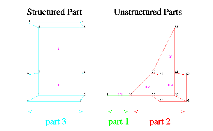
11.1 EnSight Gold Geometry File Format
11-18 EnSight 7 User Manual
EnSight Gold The following is an example of an ASCII EnSight Gold geometry file: This is the
Geometry File Example same example model as given in the EnSight6 geometry file section (only in Gold
format) with 11 defined unstructured nodes from which 2 unstructured parts are
defined, and a 2x3x2 structured part as depicted in the above diagram.
Note: The example file below (
engold.geo) and all example variable files in the gold
section (also prefixed with
engold) may be found under your EnSight installation
directory (path:
$CEI_HOME/ensight76/data/user_manual).
Note: The appended “#” comment lines are for your reference only, and are not valid
format lines within a geometry file as appended below. Do NOT put these #
comments in your file!!!
This is the 1st description line of the EnSight Gold geometry example
This is the 2nd description line of the EnSight Gold geometry example
node id given
element id given
extents
0.00000e+00 2.00000e+00
0.00000e+00 2.00000e+00
0.00000e+00 2.00000e+00
part
1
2D uns-elements (description line for part 1)
coordinates
10 # nn
Do NOT put these # comments in your file!!
15 # node ids
20
40
22
44
55
60
61
62
63
4.00000e+00 # x components
5.00000e+00
6.00000e+00
11.1 EnSight Gold Geometry File Format
EnSight 7 User Manual 11-19
5.00000e+00
6.00000e+00
6.00000e+00
5.00000e+00
6.00000e+00
6.00000e+00
5.00000e+00
0.00000e+00 # y components
0.00000e+00
0.00000e+00
1.00000e+00
1.00000e+00
3.00000e+00
0.00000e+00
0.00000e+00
1.00000e+00
1.00000e+00
0.00000e+00 # z components
0.00000e+00
0.00000e+00
0.00000e+00
0.00000e+00
0.00000e+00
2.00000e+00
2.00000e+00
2.00000e+00
2.00000e+00
tria3 # element type
2#ne
102 # element ids
103
124
456
hexa8
1
104
235478910
part
2
1D uns-elements (description line for part 2)
coordinates
2
15
31
4.00000e+00
3.00000e+00
0.00000e+00
0.00000e+00
0.00000e+00
0.00000e+00
bar2
1
101
21
part
3
3D struct-part (description line fro part 3)
block iblanked
232
0.00000e+00 # i components
2.00000e+00
0.00000e+00
2.00000e+00
0.00000e+00
2.00000e+00
0.00000e+00
2.00000e+00
11.1 EnSight Gold Geometry File Format
11-20 EnSight 7 User Manual
0.00000e+00
2.00000e+00
0.00000e+00
2.00000e+00
0.00000e+00 # j components
0.00000e+00
1.00000e+00
1.00000e+00
3.00000e+00
3.00000e+00
0.00000e+00
0.00000e+00
1.00000e+00
1.00000e+00
3.00000e+00
3.00000e+00
0.00000e+00 # k components
0.00000e+00
0.00000e+00
0.00000e+00
0.00000e+00
0.00000e+00
2.00000e+00
2.00000e+00
2.00000e+00
2.00000e+00
2.00000e+00
2.00000e+00
1 # iblanking
1
1
1
1
1
1
1
1
1
1
1
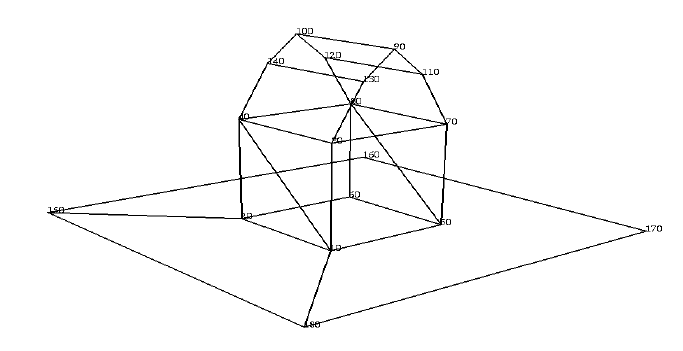
11.1 EnSight Gold Geometry File Format
EnSight 7 User Manual 11-21
Simple example The following is an example of an ASCII EnSight Gold geometry file with nsided
using nsided/ and nfaced data. It is a non-realistic, simple model which is intended only to
nfaced elements illustrate the format. Two nsided elements and three nfaced elements are used,
even though the model could have been represented with a single nsided and
single nfaced element.
Note: The appended “#” comment lines are for your reference only, and are not valid
format lines within a geometry file as appended below. Do NOT put these #
comments in your file!!!
simple example for nsided/nfaced
element types in EnSight Gold Format
node id given
element id given
extents
-2.00000e+00 4.00000e+00
0.00000e+00 3.50000e+00
-2.00000e+00 4.00000e+00
part
1
barn
coordinates
18 # nn Do NOT put these # comments in your file!!
10 # node ids
20
30
40
50
60
70
80
90
100
110
120
130
140
150
160
170
180
0.00000e+00 # x components
2.00000e+00
0.00000e+00
2.00000e+00
11.1 EnSight Gold Geometry File Format
11-22 EnSight 7 User Manual
0.00000e+00
2.00000e+00
0.00000e+00
2.00000e+00
0.00000e+00
2.00000e+00
0.00000e+00
2.00000e+00
0.00000e+00
2.00000e+00
4.00000e+00
4.00000e+00
-2.00000e+00
-2.00000e+00
0.00000e+00 # y components
0.00000e+00
2.00000e+00
2.00000e+00
0.00000e+00
0.00000e+00
2.00000e+00
2.00000e+00
3.50000e+00
3.50000e+00
3.00000e+00
3.00000e+00
3.00000e+00
3.00000e+00
0.00000e+00
0.00000e+00
0.00000e+00
0.00000e+00
0.00000e+00 # x components
0.00000e+00
0.00000e+00
0.00000e+00
2.00000e+00
2.00000e+00
2.00000e+00
2.00000e+00
1.00000e+00
1.00000e+00
1.50000e+00
1.50000e+00
0.50000e+00
0.50000e+00
-2.00000e+00
4.00000e+00
4.00000e+00
-2.00000e+00
nsided
2 # 2 nsided elements
101 # element ids
202
4 # 4 nodes in first element
8 # 8 nodes in second element
2 15 18 1 # connectivity of element 1
118171615265#connectivity of element 2
nfaced
3 # 3 nfaced polyhedra elements
1001 # element ids
1002
1003
5 # number of faces in element 1
5 # number of faces in element 2
7 # number of faces in element 3
3 # number of nodes in face 1 of element 1
11.1 EnSight Gold Geometry File Format
EnSight 7 User Manual 11-23
3 # face 2 of element 1
4 # face 3 of element 1
4 # face 4 of element 1
4 # face 5 of element 1
3 # number of nodes in face 1 of element 2
3 # face 2 of element 2
4 # face 3 of element 2
4 # face 4 of element 2
4 # face 5 of element 2
5 # number of nodes in face 1 of element 3
5 # face 2 of element 3
4 # face 3 of element 3
4 # face 4 of element 3
4 # face 5 of element 3
4 # face 6 of element 3
4 # face 7 of element 3
5 6 8 # connectivity of face 1 of element 1
2 1 4 # face 2 of element 1
6 2 4 8 # face 3 of element 1
8 4 1 5 # face 4 of element 1
1 2 6 5 # face 5 of element 1
5 8 7 # connectivity of face 1 of element 2
1 3 4 # face 2 of element 2
7 8 4 3 # face 3 of element 2
7 3 1 5 # face 4 of element 2
5 1 4 8 # face 5 of element 2
8 4 14 10 12 # connectivity of face 1 of element 3
7 11 9 13 3 # face 2 of element 3
7 8 12 11 # face 3 of element 3
11 12 10 9 # face 4 of element 3
9 10 14 13 # face 5 of element 3
13 14 4 3 # face 6 of element 3
7 3 4 8 # face 7 of element 3
11.1 EnSight Gold Geometry File Format
11-24 EnSight 7 User Manual
Simple examples The following two ASCII EnSight Gold geometry file examples show use of
using ghost cells ghost cells in unstructured and structured models. First the geometry file for the
total model, composed of four parts, is given without any ghost cells. Then, two of
four separate geometry files – each containing just one of the original parts (and
appropriate ghost cells) will be given. This is supposed to simulate a decomposed
model, such as you might provide for EnSight’s Server-of-Servers.
Note: For unstructured models, ghost cells are simply a new element type. For
structured models, ghost cells are an “iblank”-like flag.
Unstructured model
Total Unstructured Model Geometry File:
EnSight Model Geometry File
EnSight 7.1.0
node id given
element id given
extents
0.00000e+00 4.00000e+00
0.00000e+00 4.00000e+00
0.00000e+00 0.00000e+00
part
1
bottom left
coordinates
9
1
2
3
6
7
8
11
12
13
0.00000e+00
1.00000e+00
2.00000e+00
0.00000e+00
1.00000e+00
2.00000e+00
0.00000e+00
1.00000e+00
2.00000e+00
0.00000e+00
0.00000e+00
0.00000e+00
1.00000e+00
1.00000e+00
1.00000e+00
2.00000e+00
2.00000e+00
2.00000e+00
0.00000e+00
0.00000e+00
0.00000e+00
0.00000e+00
0.00000e+00
0.00000e+00
0.00000e+00
0.00000e+00
0.00000e+00
quad4
4
1
2
5
6
1254
2365
4587
5698
part
2
bottom right
coordinates
9
3
4
5
8
123
4
5
678910
11 12 13 14 15
16 17 18 19 20
21 22 23 24 25
Nodes Elements
part 1 part 2
part 3 part 4
1234
5678
9101112
13 14 15 16
part 3 part 4
part 1 part 2

11.1 EnSight Gold Geometry File Format
EnSight 7 User Manual 11-25
9
10
13
14
15
2.00000e+00
3.00000e+00
4.00000e+00
2.00000e+00
3.00000e+00
4.00000e+00
2.00000e+00
3.00000e+00
4.00000e+00
0.00000e+00
0.00000e+00
0.00000e+00
1.00000e+00
1.00000e+00
1.00000e+00
2.00000e+00
2.00000e+00
2.00000e+00
0.00000e+00
0.00000e+00
0.00000e+00
0.00000e+00
0.00000e+00
0.00000e+00
0.00000e+00
0.00000e+00
0.00000e+00
quad4
4
3
4
7
8
1254
2365
4587
5698
part
3
top left
coordinates
9
11
12
13
16
17
18
21
22
23
0.00000e+00
1.00000e+00
2.00000e+00
0.00000e+00
1.00000e+00
2.00000e+00
0.00000e+00
1.00000e+00
2.00000e+00
2.00000e+00
2.00000e+00
2.00000e+00
3.00000e+00
3.00000e+00
3.00000e+00
4.00000e+00
4.00000e+00
4.00000e+00
0.00000e+00
0.00000e+00
0.00000e+00
0.00000e+00
0.00000e+00
0.00000e+00
0.00000e+00
0.00000e+00
0.00000e+00
quad4
4
9
10
13
14
1254
2365
4587
5698
part
4
top right
coordinates
9
13
14
15
18
19
20
23
24
25
2.00000e+00
3.00000e+00
4.00000e+00
2.00000e+00
3.00000e+00
4.00000e+00
2.00000e+00
3.00000e+00
4.00000e+00
2.00000e+00
2.00000e+00
2.00000e+00
3.00000e+00
3.00000e+00
3.00000e+00
4.00000e+00
4.00000e+00
4.00000e+00
0.00000e+00
0.00000e+00
0.00000e+00
0.00000e+00
0.00000e+00
0.00000e+00
0.00000e+00
0.00000e+00
0.00000e+00
quad4
4
11
12
15
16
1254
2365
4587
5698
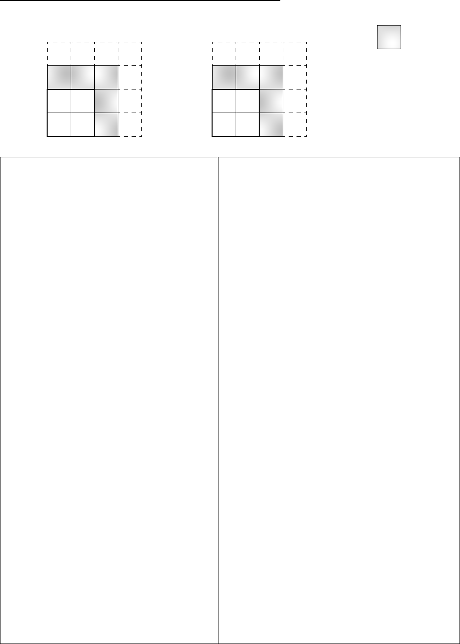
11.1 EnSight Gold Geometry File Format
11-26 EnSight 7 User Manual
Portion with part 1 containing ghost cells (other parts are empty)
EnSight Model Geometry File
part 1 portion
node id given
element id given
extents
0.00000e+00 4.00000e+00 0.00000e+00
4.00000e+00
0.00000e+00 0.00000e+00
part
1
bottom left
coordinates
16
1
2
3
4
6
7
8
9
11
12
13
14
16
17
18
19
0.00000e+00
1.00000e+00
2.00000e+00
3.00000e+00
0.00000e+00
1.00000e+00
2.00000e+00
3.00000e+00
0.00000e+00
1.00000e+00
2.00000e+00
3.00000e+00
0.00000e+00
1.00000e+00
2.00000e+00
3.00000e+00
0.00000e+00
0.00000e+00
0.00000e+00
0.00000e+00
1.00000e+00
1.00000e+00
1.00000e+00
1.00000e+00
2.00000e+00
2.00000e+00
2.00000e+00
2.00000e+00
3.00000e+00
3.00000e+00
3.00000e+00
3.00000e+00
0.00000e+00
0.00000e+00
0.00000e+00
0.00000e+00
0.00000e+00
0.00000e+00
0.00000e+00
0.00000e+00
0.00000e+00
0.00000e+00
0.00000e+00
0.00000e+00
0.00000e+00
0.00000e+00
0.00000e+00
0.00000e+00
quad4
4
1
2
5
6
1265
2376
56109
6 7 11 10
g_quad4
5
1
1
1
1
1
3487
7 8 12 11
9101413
10 11 15 14
11 12 16 15
part /* Empty part */
2
bottom right
part /* Empty part */
3
top left
part /* Empty part */
4
top right
123
4
6789
11 12 13 14
16 17 18 19
Nodes Elements
part 1
123
567
91011
part 1
Ghost Cell
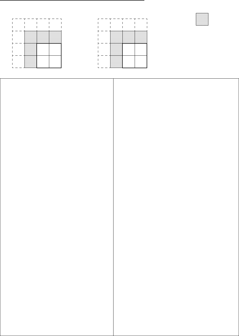
11.1 EnSight Gold Geometry File Format
EnSight 7 User Manual 11-27
Portion with part 2 containing ghost cells (other parts are empty)
EnSight Model Geometry File
part 2 portion
node id given
element id given
extents
0.00000e+00 4.00000e+00
0.00000e+00 4.00000e+00
0.00000e+00 0.00000e+00
part /* Empty part */
1
bottom left
part
2
bottom right
coordinates
16
2
3
4
5
7
8
9
10
12
13
14
15
17
18
19
20
1.00000e+00
2.00000e+00
3.00000e+00
4.00000e+00
1.00000e+00
2.00000e+00
3.00000e+00
4.00000e+00
1.00000e+00
2.00000e+00
3.00000e+00
4.00000e+00
1.00000e+00
2.00000e+00
3.00000e+00
4.00000e+00
0.00000e+00
0.00000e+00
0.00000e+00
0.00000e+00
1.00000e+00
1.00000e+00
1.00000e+00
1.00000e+00
2.00000e+00
2.00000e+00
2.00000e+00
2.00000e+00
3.00000e+00
3.00000e+00
3.00000e+00
3.00000e+00
0.00000e+00
0.00000e+00
0.00000e+00
0.00000e+00
0.00000e+00
0.00000e+00
0.00000e+00
0.00000e+00
0.00000e+00
0.00000e+00
0.00000e+00
0.00000e+00
0.00000e+00
0.00000e+00
0.00000e+00
0.00000e+00
quad4
4
3
4
7
8
2376
3487
6 7 11 10
7 8 12 11
g_quad4
5
1
1
1
1
1
1265
56109
9101413
10 11 15 14
11 12 16 15
part /* Empty part */
3
top left
part /* Empty part */
4
top right
23
4
5
78910
12 13 15
17 18 19 20
Nodes Elements
part 2
1234
5678
9101112
13 14 15 16
Ghost Cell
14
part 2

11.1 EnSight Gold Geometry File Format
11-28 EnSight 7 User Manual
Structured model
(using essentially the same model, but in structured format) :
EnSight Model Geometry File
Total Structured Model
node id assign
element id assign
extents
0.00000e+00 4.00000e+00
0.00000e+00 4.00000e+00
0.00000e+00 0.00000e+00
part
1
left bottom
block uniform range
551
131311
0.00000e+00
0.00000e+00
0.00000e+00
1.00000e+00
1.00000e+00
0.00000e+00
part
2
bottom right
block uniform range
551
351311
2.00000e+00
0.00000e+00
0.00000e+00
1.00000e+00
1.00000e+00
0.00000e+00
part
3
top left
block uniform range
551
133511
0.00000e+00
2.00000e+00
0.00000e+00
1.00000e+00
1.00000e+00
0.00000e+00
part
4
top right
block uniform range
551
353511
2.00000e+00
2.00000e+00
0.00000e+00
1.00000e+00
1.00000e+00
0.00000e+00
123
4
5
678910
11 12 13 14 15
16 17 18 19 20
21 22 23 24 25
Nodes Elements
part 1 part 2
part 3 part 4
1234
5678
9101112
13 14 15 16
part 3 part 4
part 1 part 2
5 x 5 x 1 Total Structured Model
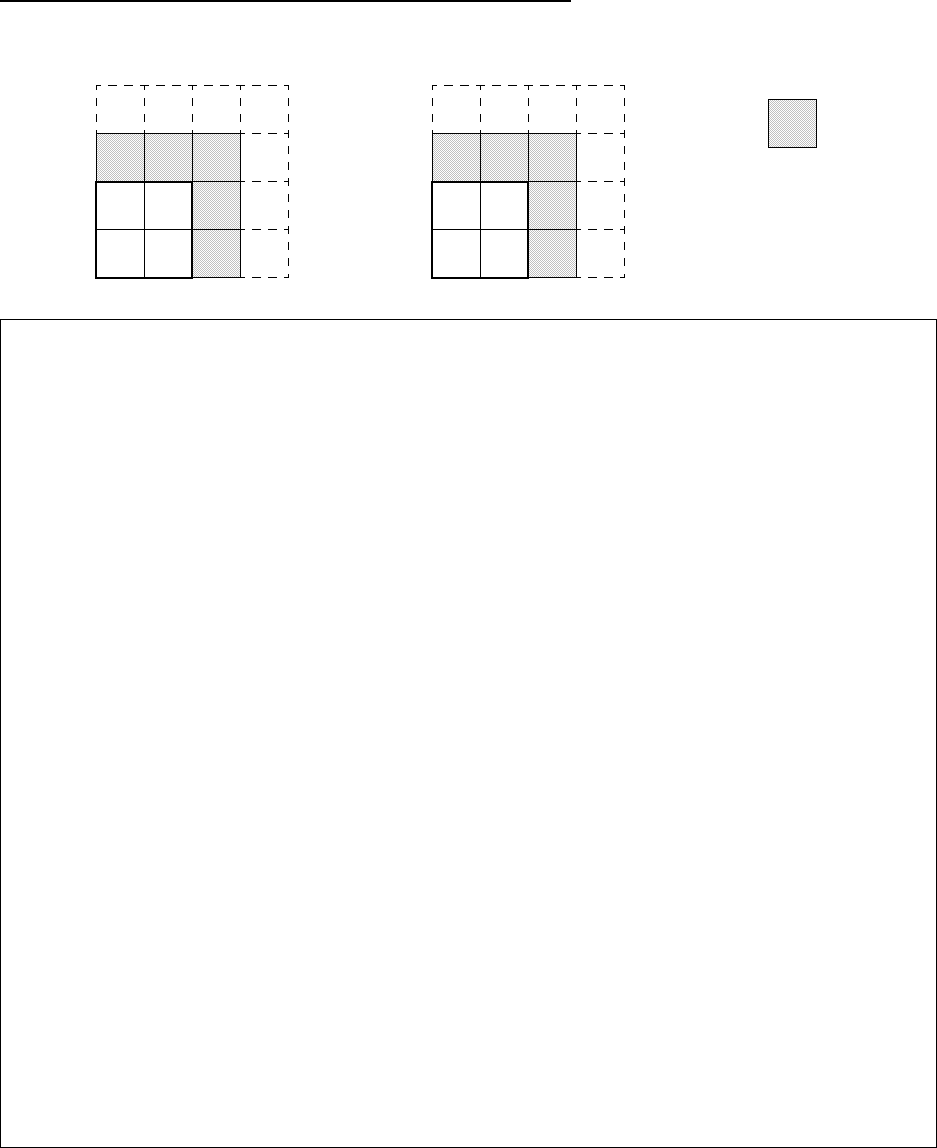
11.1 EnSight Gold Geometry File Format
EnSight 7 User Manual 11-29
Portion with part 1 containing ghost cells (other parts are empty)
EnSight Model Geometry File
part 1 portion only
node id assign
element id assign
extents
0.00000e+00 4.00000e+00
0.00000e+00 4.00000e+00
0.00000e+00 0.00000e+00
part
1
left bottom
block uniform range with_ghost
441
141411
0.00000e+00
0.00000e+00
0.00000e+00
1.00000e+00
1.00000e+00
0.00000e+00
ghost_flags
0
0
1
0
0
1
1
1
1
Part /* Empty Part */
2
right bottom
block
000
part /* Empty Part */
3
left top
block
000
part /* Empty Part */
4
right top
block
000
123
4
6789
11 12 13 14
16 17 18 19
Nodes Elements
part 1
123
567
91011
part 1
Ghost Cell
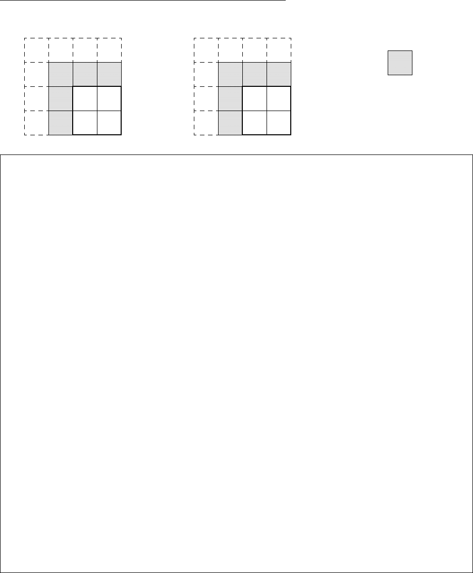
11.1 EnSight Gold Geometry File Format
11-30 EnSight 7 User Manual
Portion with part 2 containing ghost cells (other parts are empty)
Note: For both the unstructured and the structured model above, only the first two
files (parts 1 and 2) are given. The portion files for parts 3 and 4 are not given, but
would be similar to those for parts 1 and 2.
EnSight Model Geometry File
part 2 portion only
node id assign
element id assign
extents
0.00000e+00 4.00000e+00
0.00000e+00 4.00000e+00
0.00000e+00 0.00000e+00
part
1
left bottom
block
000
part
2
right bottom
block uniform range with_ghost
441
251411
1.00000e+00
0.00000e+00
0.00000e+00
1.00000e+00
1.00000e+00
0.00000e+00
ghost_flags
1
0
0
1
0
0
1
1
1
part /* Empty Part */
3
left top
block
000
part /* Empty Part */
4
right top
block
000
23
4
5
78910
12 13 15
17 18 19 20
Nodes Elements
part 2
1234
5678
9101112
13 14 15 16
Ghost Cell
14
part 2

11.1 EnSight Gold Case File Format
EnSight 7 User Manual 11-31
EnSight Gold Case File Format
The Case file is an ASCII free format file that contains all the file and name
information for accessing model (and measured) geometry, variable, and time
information. It is comprised of five sections (
FORMAT, GEOMETRY, VARIABLE,
TIME, FILE
) as described below:
Notes: All lines in the Case file are limited to 79 characters.
The titles of each section must be in all capital letters.
Anything preceded by a “#” denotes a comment and is ignored. Comments may
append information lines or be placed on their own lines.
Information following “:” may be separated by white spaces or tabs.
Specifications encased in “[]” are optional, as indicated.
Format Section This is a required section which specifies the type of data to be read.
Usage:
FORMAT
type: ensight gold
Geometry Section This is a required section which specifies the geometry information for the model
(as well as measured geometry if present, and periodic match file (see Section
11.9, Periodic Matchfile Format) if present).
Usage:
GEOMETRY
model: [ts] [fs] filename [change_coords_only]
measured: [ts] [fs] filename [change_coords_only]
match: filename
boundary: filename
where: ts = time set number as specified in TIME section. This is optional.
fs = corresponding file set number as specified in FILE section below.
(Note, if you specify
fs, then ts is no longer optional and must also be
specified.)
filename = The filename of the appropriate file.
-> Model or measured filenames for a static geometry case, as well as match
and boundary filenames will not
contain “*” wildcards.
-> Model or measured filenames for a changing geometry case will
contain “*” wildcards.
change_coords_only = The option to indicate that the changing geometry (as
indicated by wildcards in the filename) is coords only.
Otherwise, changing geometry connectivity will be
assumed.
Variable Section This is an optional section which specifies the files and names of the variables.
Constant variable values can also be set in this section.
Usage:
VARIABLE
constant per case: [ts] description
const_value(s)
constant per case file: [ts] description
cvfilename
scalar per node: [ts] [fs] description filename
vector per node: [ts] [fs] description filename
tensor symm per node: [ts] [fs] description filename
tensor asym per node: [ts] [fs] description filename
scalar per element: [ts] [fs] description filename
11.1 EnSight Gold Case File Format
11-32 EnSight 7 User Manual
vector per element: [ts] [fs] description filename
tensor symm per element: [ts] [fs] description filename
tensor asym per element: [ts] [fs] description filename
scalar per measured node: [ts] [fs] description filename
vector per measured node: [ts] [fs] description filename
complex scalar per node: [ts] [fs] description
Re_fn Im_fn freq
complex vector per node: [ts] [fs] description
Re_fn Im_fn freq
complex scalar per element: [ts] [fs] description
Re_fn Im_fn freq
complex vector per element: [ts] [fs] description
Re_fn Im_fn freq
where:
ts
= The corresponding time set number (or index) as specified in TIME
section below. This is only required for transient constants and
variables.
fs
= The corresponding file set number (or index) as specified in FILE
section below.
(Note, if you specify
fs, then ts is no longer optional and must
also be specified.)
description = The variable (GUI) name (ex. Pressure, Velocity, etc.)
const_value(s) = The constant value. If constants change over time, then ns (see
TIME section below) constant values of
ts.
cv
filename
= The filename containing the constant values, one value per time step.
filename
= The filename of the variable file. Note: only transient filenames
contain “*” wildcards.
Re_fn
= The filename for the file containing the real values of the complex
variable.
Im_fn
= The filename for the file containing the imaginary values of the
complex variable.
freq
= The corresponding harmonic frequency of the complex variable.
For complex variables where harmonic frequency is undefined,
simply use the text string: UNDEFINED.
Note: As many variable description lines as needed may be used.
Note: Variable descriptions have the following restrictions:
The variable description is limited to 19 characters in the current release.
Duplicate variable descriptions are not allowed.
Leading and trailing white space will be eliminated.
Variable descriptions must not start with a numeric digit.
Variable descriptions must not contain any of the following reserved characters:
( [ + @ ! * $
) ] - space # ^ /
Time Section This is an optional section for steady state cases, but is required for transient
cases. It contains time set information. Shown below is information for one time
set. Multiple time sets (up to 16) may be specified for measured data as shown in
Case File Example 3 below.
Usage:
TIME
time set: ts [description]
number of steps: ns
filename start number: fs
filename increment: fi
time values: time_1 time_2 .... time_ns
11.1 EnSight Gold Case File Format
EnSight 7 User Manual 11-33
or
TIME
time set: ts [description]
number of steps: ns
filename numbers: fn
time values: time_1 time_2 .... time_ns
or
TIME
time set: ts [description]
number of steps: ns
filename numbers file: fnfilename
time values file: tvfilename
where:
ts
= timeset number. This is the number referenced in the GEOMETRY
and VARIABLE sections.
description
= optional timeset description which will be shown in user
interface.
ns
= number of transient steps
fs
= the number to replace the “*” wildcards in the filenames, for the first step
fi
= the increment to fs for subsequent steps
time
= the actual time values for each step, each of which must be separated
by a white space and which may continue on the next line if needed
fn
= a list of numbers or indices, to replace the “*” wildcards in the filenames.
fnfilename
= name of file containing ns filename numbers (fn).
tvfilename
= name of file containing the time values(time_1 ... time_ns).
File Section This section is optional for expressing a transient case with single-file formats.
This section contains single-file set information. This information specifies the
number of time steps in each file of each data entity, i.e. each geometry and each
variable (model and/or measured). Each data entity’s corresponding file set might
have multiple continuation files due to system file size limit, i.e. ~2 GB for 32-bit
and ~4 TB for 64-bit architectures. Each file set corresponds to one and only
one time set, but a time set may be referenced by many file sets.
The following
information may be specified in each file set. For file sets where all of the time set
data exceeds the maximum file size limit of the system, both
filename index
and
number of steps
are repeated within the file set definition for each continuation
file required. Otherwise
filename index
may be omitted if there is only one file.
File set information is shown in Case File Example 4 below.
Usage:
FILE
file set: fs
filename index: fi # Note: only used when data continues in other files
number of steps: ns
where:
fs
= file set number. This is the number referenced in the GEOMETRY
and VARIABLE sections above.
ns
= number of transient steps
fi
= file index number in the file name (replaces “*” in the filenames)
11.1 EnSight Gold Case File Format
11-34 EnSight 7 User Manual
Material Section This is an optional section for material interface part case. It contains material set
information. Shown below is information for one material set. (Note, currently
only one material set is supported.) An example of this material set information
is appended to EnSight Gold Material Files Format.
Usage:
MATERIAL
material set number: ms [description]
material id count: nm
material id numbers: matno_1 matno_2 ... matno_nm
material id names: matdesc_1 mat_2 ... mat_nm
material id per element: [ts] [fs] filename
material mixed ids: [ts] [fs] filename
material mixed values: [ts] [fs] filename
where:
ts = The corresponding time set number (or index) as specified in TIME section
above. This is only required for transient materials.
fs = The corresponding file set number (or index) as specified in FILE section
above. (Note, if you specify fs, then ts is no longer optional and must also
be specified.)
ms = Material set number. (Note, currently there is only one, and it must be a
positive number.)
description = Optional material set description which will be reflected in the file
names of exported material files.
nm = Number of materials for this set.
matno = Material number used in the material and mixed-material id files. There
should be nm of these. Non-positive numbers are grouped as the “null
material”. See EnSight Gold Material Files Format
matdesc = GUI material description corresponding to the nm matno’s.
filename = The filename of the appropriate material file. Note, only transient
filenames contain “*” wildcards. The three required files are the
material id per element, the mixed-material ids, and the mixed-material
values files.
Note: Material descriptions are limited to 19 characters in the current release. Material
descriptions and file names must not start with a numeric digit and must not
contain any of the following reserved characters:
(
[+@!*$
)]-#^/space
Case File Example 1 The following is a minimal EnSight Gold case file for a steady state model with some
results.
Note: this (
engold.case) file, as well as all of its referenced geometry and variable
files (along with a couple of command files) can be found under your installation directory
(path:
$CEI_HOME/ensight76/data/user_manual). The EnSight Gold
Geometry File Example and the Variable File Examples are the contents of these files.
FORMAT
type: ensight gold
GEOMETRY
model: engold.geo
VARIABLE
constant per case: Cden .8
11.1 EnSight Gold Case File Format
EnSight 7 User Manual 11-35
scalar per element: Esca engold.Esca
scalar per node: Nsca engold.Nsca
vector per element: Evec engold.Evec
vector per node: Nvec engold.Nvec
tensor symm per element: Eten engold.Eten
tensor symm per node: Nten engold.Nten
complex scalar per element: Ecmp engold.Ecmp_rengold.Ecmp_i2.
complex scalar per node: Ncmp engold.Ncmp_rengold.Ncmp_i4.
Case File Example 2 The following is a Case file for a transient model. The connectivity of the geometry is also
changing.
FORMAT
type: ensight gold
GEOMETRY
model: 1 exgold2.geo**
VARIABLE
scalar per node: 1 Stress exgold2.scl**
vector per node: 1 Displacement exgold2.dis**
TIME
time set: 1
number of steps: 3
filename start number: 0
filename increment: 1
time values: 1.0 2.0 3.0
The following files would be needed for Example 2:
exgold2.geo00 exgold2.scl00 exgold2.dis00
exgold2.geo01 exgold2.scl01 exgold2.dis01
exgold2.geo02 exgold2.scl02 exgold2.dis02
Case File Example 3 The following is a Case file for a transient model with measured data.
This example has pressure given per element.
FORMAT
type: ensight gold
GEOMETRY
model: 1 exgold3.geo*
measured: 2 exgold3.mgeo**
VARIABLE
constant per case: Gamma 1.4
constant per case: 1 Density .9 .9 .7 .6 .6
scalar per element 1 Pressure exgold3.pre*
vector per node: 1 Velocity exgold3.vel*
scalar per measured node: 2 Temperature exgold3.mtem**
vector per measured node: 2 Velocity exgold3.mvel**
TIME
time set: 1
number of steps: 5
filename start number: 1
filename increment: 2
time values: .1 .2 .3 # This example shows that time
11.1 EnSight Gold Case File Format
11-36 EnSight 7 User Manual
.4 .5 # values can be on multiple lines
time set: 2
number of steps: 6
filename start number: 0
filename increment: 2
time values:
.05 .15 .25 .34 .45 .55
The following files would be needed for Example 3:
exgold3.geo1 exgold3.pre1 exgold3.vel1
exgold3.geo3 exgold3.pre3 exgold3.vel3
exgold3.geo5 exgold3.pre5 exgold3.vel5
exgold3.geo7 exgold3.pre7 exgold3.vel7
exgold3.geo9 exgold3.pre9 exgold3.vel9
exgold3.mgeo00 exgold3.mtem00 exgold3.mvel00
exgold3.mgeo02 exgold3.mtem02 exgold3.mvel02
exgold3.mgeo04 exgold3.mtem04 exgold3.mvel04
exgold3.mgeo06 exgold3.mtem06 exgold3.mvel06
exgold3.mgeo08 exgold3.mtem08 exgold3.mvel08
exgold3.mgeo10 exgold3.mtem10 exgold3.mvel10
Case File Example 4 The following is Case File Example 3 expressed in transient single-file formats.
In this example, the transient data for the measured velocity data entity happens
to be greater than the maximum file size limit. Therefore, the first four time steps
fit and are contained in the first file, and the last two time steps are ‘continued’ in
a second file.
FORMAT
type: ensight gold
GEOMETRY
model: 1 1 exgold4.geo
measured: 2 2 exgold4.mgeo
VARIABLE
constant per case: Density .5
scalar per element: 1 1 Pressure exgold4.pre
vector per node: 1 1 Velocity exgold4.vel
scalar per measured node: 2 2 Temperature exgold4.mtem
vector per measured node: 2 3 Velocity exgold4.mvel*
TIME
time set: 1 Model
number of steps: 5
time values: .1 .2 .3 .4 .5
time set: 2 Measured
number of steps: 6
time values: .05 .15 .25 .34 .45 .55
FILE
file set: 1
number of steps: 5
file set: 2
11.1 EnSight Gold Case File Format
EnSight 7 User Manual 11-37
number of steps: 6
file set: 3
filename index: 1
number of steps: 4
filename index: 2
number of steps: 2
The following files would be needed for Example 4:
exgold4.geo exgold4.pre exgold4.vel
exgold4.mgeo exgold4.mtem exgold4.mvel1
exgold4.mvel2
Contents of Each file contains transient data that corresponds to the specified number of time steps.
Transient The data for each time step sequentially corresponds to the simulation time values
Single Files
(time values)
found listed in the TIME section. In transient single-file format, the data for
each time step essentially corresponds to a standard EnSight gold geometry or variable
file (model or measured) as expressed in multiple file format. The data for each time step
is enclosed between two wrapper records, i.e. preceded by a
BEGIN TIME STEP
record and followed by an END TIME STEP record. Time step data is not split
between files. If there is not enough room to append the data from a time step to the file
without exceeding the maximum file limit of a particular system, then a continuation file
must be created for the time step data and any subsequent time step. Any type of user
comments may be included before and/or after each transient step wrapper.
Note 1: If transient single file format is used, EnSight expects all files of a dataset
to be specified in transient single file format. Thus, even static files must be
enclosed between a
BEGIN TIME STEP and an END TIME STEP wrapper.
This includes the condition where you have transient variables with static
geometry. The static geometry file must have the wrapper.
1. Note 2: For binary geometry files, the first
BEGIN TIME STEP wrapper
must follow the <C Binary/Fortran Binary> line. Both
BEGIN TIME STEP
and
END TIME STEP wrappers are written according to type (1) in binary.
Namely: This is a write of 80 characters to the file:
in C:
char buffer[80];
strcpy(buffer,”BEGIN TIME STEP”);
fwrite(buffer,sizeof(char),80,file_ptr);
in FORTRAN: character*80 buffer
buffer = ”BEGIN TIME STEP”
Note 3: Efficient reading of each file (especially binary) is facilitated by
appending each file with a file index. A file index contains appropriate
information to access the file byte positions of each time step in the file. (EnSight
automatically appends a file index to each file when exporting in transient single
file format.) If used, the file index must follow the last
END TIME STEP
wrapper in each file.
File Index Usage:
ASCII Binary Item Description
“%20d\n” sizeof(int) n Total number of data time steps in the file.
“%20d\n” sizeof(long) fb
1
File byte loc for contents of 1
st
time step
*
“%20d\n” sizeof(long) fb
2
File byte loc for contents of 2
nd
time step
*
11.1 EnSight Gold Case File Format
11-38 EnSight 7 User Manual
*
Each file byte location is the first byte that follows the BEGIN TIME STEP record.
Shown below are the contents of each of the above files, using the data files from Case
File Example 3 for reference (without
FILE_INDEX for simplicity).
Contents of file exgold4.geo_1:
BEGIN TIME STEP
Contents of file
exgold3.geo1
END TIME STEP
BEGIN TIME STEP
Contents of file
exgold3.geo3
END TIME STEP
BEGIN TIME STEP
Contents of file
exgold3.geo5
END TIME STEP
BEGIN TIME STEP
Contents of file
exgold3.geo7
END TIME STEP
BEGIN TIME STEP
Contents of file
exgold3.geo9
END TIME STEP
Contents of file exgold4.pre_1:
BEGIN TIME STEP
Contents of file
exgold3.pre1
END TIME STEP
BEGIN TIME STEP
Contents of file
exgold3.pre3
END TIME STEP
BEGIN TIME STEP
Contents of file
exgold3.pre5
END TIME STEP
BEGIN TIME STEP
Contents of file
exgold3.pre7
END TIME STEP
BEGIN TIME STEP
Contents of file
exgold3.pre9
END TIME STEP
Contents of file exgold4.vel_1:
BEGIN TIME STEP
Contents of file
exgold3.vel1
END TIME STEP
BEGIN TIME STEP
Contents of file
exgold3.vel3
END TIME STEP
BEGIN TIME STEP
Contents of file
exgold3.vel5
END TIME STEP
BEGIN TIME STEP
Contents of file
exgold3.vel7
END TIME STEP
BEGIN TIME STEP
Contents of file
exgold3.vel9
END TIME STEP
Contents of file exgold4.mgeo_1:
BEGIN TIME STEP
Contents of file
exgold3.mgeo00
END TIME STEP
BEGIN TIME STEP
Contents of file
exgold3.mgeo02
END TIME STEP
BEGIN TIME STEP
Contents of file
exgold3.mgeo04
END TIME STEP
BEGIN TIME STEP
Contents of file
exgold3.mgeo06
END TIME STEP
BEGIN TIME STEP
Contents of file
exgold3.mgeo08
. . . . . . . . . . . .
“%20d\n” sizeof(long) fb
n
File byte loc for contents of n
th
time step
*
“%20d\n” sizeof(int) flag Miscellaneous flag (= 0 for now)
“%20d\n” sizeof(long) fb of item n File byte loc for Item n above
“%s\n” sizeof(char)*80
“FILE_INDEX”
File index keyword
ASCII Binary Item Description
11.1 EnSight Gold Case File Format
EnSight 7 User Manual 11-39
END TIME STEP
BEGIN TIME STEP
Contents of file
exgold3.mgeo10
END TIME STEP
Contents of file exgold4.mtem_1:
BEGIN TIME STEP
Contents of file
exgold3.mtem00
END TIME STEP
BEGIN TIME STEP
Contents of file
exgold3.mtem02
END TIME STEP
BEGIN TIME STEP
Contents of file
exgold3.mtem04
END TIME STEP
BEGIN TIME STEP
Contents of file
exgold3.mtem06
END TIME STEP
BEGIN TIME STEP
Contents of file
exgold3.mtem08
END TIME STEP
BEGIN TIME STEP
Contents of file
exgold3.mtem10
END TIME STEP
Contents of file exgold4.mvel1_1:
BEGIN TIME STEP
Contents of file
exgold3.mvel00
END TIME STEP
BEGIN TIME STEP
Contents of file
exgold3.mvel02
END TIME STEP
BEGIN TIME STEP
Contents of file
exgold3.mvel04
END TIME STEP
BEGIN TIME STEP
Contents of file
exgold3.mvel06
END TIME STEP
Contents of file exgold4.mvel2_1:
Comments can precede the beginning wrapper here.
BEGIN TIME STEP
Contents of file
exgold3.mvel08
END TIME STEP
Comments can go between time step wrappers here.
BEGIN TIME STEP
Contents of file
exgold3.mvel10
END TIME STEP
Comments can follow the ending time step wrapper.
Note: Each of these files could (and should for efficency reasons) have the FILE_INDEX information following
the last END TIMESTEP. See the previous discussion for it usage.
EnSight Gold Wild Card Name Specification
If multiple time steps are involved, the file names must conform to the EnSight
wild-card specification. This specification is as follows:
• File names must include numbers that are in ascending order from
beginning to end.
• Numbers in the files names must be zero filled if there is more than one
significant digit.
• Numbers can be anywhere in the file name.
• When the file name is specified in the EnSight case file, you must replace
the numbers in the file with an asterisk(*). The number of asterisks
specified is the number of significant digits. The asterisk must occupy the
same place as the numbers in the file names.

11.1 EnSight Gold Variable File Format
11-40 EnSight 7 User Manual
EnSight Gold Variable File Format
EnSight Gold variable files can either be per_node or per_element. They cannot
be both. However, an EnSight model can have some variables which are per_node
and others which are per_element.
EnSight Gold Per_Node Variable File Format
EnSight Gold variable files for per_node variables contain values for each
unstructured node and for each structured node. First comes a single description
line. Second comes a part line. Third comes a line containing the part number.
Fourth comes a ‘coordinates’ line or a ‘block’ line. If a ‘coordinates’ line, the
value for each unstructured node of the part follows. If it is a scalar file, there is
one value per node, while for vector files there are three values per node (output in
the same component order as the coordinates, namely, all x components, then all y
components, then all z components). If it is a ‘block’ line, the value(s) for each
structured node follows. The values for each node of the structured block are
output in the same IJK order as the coordinates. (The number of nodes in the part
are obtained from the corresponding EnSight Gold geometry file.)
Note: If the geometry of given part is empty, nothing for that part
needs to be in
the variable file.
C Binary form:
SCALAR FILE:
description line 1 80 chars
part 80 chars
# 1 int
coordinates
80 chars
s_n1 s_n2 ... s_nn nn floats
part 80 chars
.
.
part 80 chars
# 1 int
block # nn = i*j*k 80 chars
s_n1 s_n2 ... s_nn nn floats
VECTOR FILE:
description line 1 80 chars
part 80 chars
# 1 int
coordinates
80 chars
vx_n1 vx_n2 ... vx_nn nn floats
vy_n1 vy_n2 ... vy_nn nn floats
vz_n1 vz_n2 ... vz_nn nn floats
part 80 chars
.
.
part 80 chars
# 1 int
block # nn = i*j*k 80 chars
vx_n1 vx_n2 ... vx_nn nn floats
11.1 EnSight Gold Per_Node Variable File Format
EnSight 7 User Manual 11-41
vy_n1 vy_n2 ... vy_nn nn floats
vz_n1 vz_n2 ... vz_nn nn floats
TENSOR FILE:
description line 1 80 chars
part 80 chars
# 1 int
coordinates
80 chars
v11_n1 v11_n2 ... v11_nn nn floats
v22_n1 v22_n2 ... v22_nn nn floats
v33_n1 v33_n2 ... v33_nn nn floats
v12_n1 v12_n2 ... v12_nn nn floats
v13_n1 v13_n2 ... v13_nn nn floats
v23_n1 v23_n2 ... v23_nn nn floats
part 80 chars
.
.
part 80 chars
# 1 int
block # nn = i*j*k 80 chars
v11_n1 v11_n2 ... v11_nn nn floats
v22_n1 v22_n2 ... v22_nn nn floats
v33_n1 v33_n2 ... v33_nn nn floats
v12_n1 v12_n2 ... v12_nn nn floats
v13_n1 v13_n2 ... v13_nn nn floats
v23_n1 v23_n2 ... v23_nn nn floats
TENSOR9 FILE:
description line 1 80 chars
part 80 chars
# 1 int
coordinates
80 chars
v11_n1 v11_n2 ... v11_nn nn floats
v12_n1 v12_n2 ... v12_nn nn floats
v13_n1 v13_n2 ... v13_nn nn floats
v21_n1 v21_n2 ... v21_nn nn floats
v22_n1 v22_n2 ... v22_nn nn floats
v23_n1 v23_n2 ... v23_nn nn floats
v31_n1 v31_n2 ... v31_nn nn floats
v32_n1 v32_n2 ... v32_nn nn floats
v33_n1 v33_n2 ... v33_nn nn floats
part 80 chars
.
.
part 80 chars
# 1 int
block # nn = i*j*k 80 chars
v11_n1 v11_n2 ... v11_nn nn floats
v12_n1 v12_n2 ... v12_nn nn floats
v13_n1 v13_n2 ... v13_nn nn floats
v21_n1 v21_n2 ... v21_nn nn floats
v22_n1 v22_n2 ... v22_nn nn floats
v23_n1 v23_n2 ... v23_nn nn floats
v21_n1 v21_n2 ... v21_nn nn floats
v22_n1 v22_n2 ... v22_nn nn floats
v23_n1 v23_n2 ... v23_nn nn floats
COMPLEX SCALAR FILES (Real and/or Imaginary):
11.1 EnSight Gold Per_Node Variable File Format
11-42 EnSight 7 User Manual
description line 1 80 chars
part 80 chars
# 1 int
coordinates
80 chars
s_n1 s_n2 ... s_nn nn floats
part 80 chars
.
.
part 80 chars
# 1 int
block # nn = i*j*k 80 chars
s_n1 s_n2 ... s_nn nn floats
COMPLEX VECTOR FILES (Real and/or Imaginary):
description line 1 80 chars
part 80 chars
# 1 int
coordinates
80 chars
vx_n1 vx_n2 ... vx_nn nn floats
vy_n1 vy_n2 ... vy_nn nn floats
vz_n1 vz_n2 ... vz_nn nn floats
part 80 chars
.
.
part 80 chars
# 1 int
block # nn = i*j*k 80 chars
vx_n1 vx_n2 ... vx_nn nn floats
vy_n1 vy_n2 ... vy_nn nn floats
vz_n1 vz_n2 ... vz_nn nn floats
Fortran Binary form:
SCALAR FILE:
‘description line 1’ 80 chars
‘part’ 80 chars
‘#’ 1 int
‘coordinates’
80 chars
‘s_n1 s_n2 ... s_nn’ nn floats
‘part’ 80 chars
.
.
‘part’ 80 chars
‘#’ 1 int
‘block’ # nn = i*j*k 80 chars
‘s_n1 s_n2 ... s_nn’ nn floats
VECTOR FILE:
‘description line 1’ 80 chars
‘part’ 80 chars
‘#’ 1 int
‘coordinates’
80 chars
‘vx_n1 vx_n2 ... vx_nn’ nn floats
11.1 EnSight Gold Per_Node Variable File Format
EnSight 7 User Manual 11-43
‘vy_n1 vy_n2 ... vy_nn’ nn floats
‘vz_n1 vz_n2 ... vz_nn’ nn floats
‘part’ 80 chars
.
.
‘part’ 80 chars
‘#’ 1 int
‘block’ # nn = i*j*k 80 chars
‘vx_n1 vx_n2 ... vx_nn’ nn floats
‘vy_n1 vy_n2 ... vy_nn’ nn floats
‘vz_n1 vz_n2 ... vz_nn’ nn floats
TENSOR FILE:
‘description line 1‘ 80 chars
‘part’ 80 chars
‘#’ 1 int
‘coordinates‘
80 chars
‘v11_n1 v11_n2 ... v11_nn’ nn floats
‘v22_n1 v22_n2 ... v22_nn’ nn floats
‘v33_n1 v33_n2 ... v33_nn’ nn floats
‘v12_n1 v12_n2 ... v12_nn’ nn floats
‘v13_n1 v13_n2 ... v13_nn’ nn floats
‘v23_n1 v23_n2 ... v23_nn’ nn floats
‘part’ 80 chars
.
.
‘part’ 80 chars
‘#’ 1 int
‘block’ # nn = i*j*k 80 chars
‘v11_n1 v11_n2 ... v11_nn’ nn floats
‘v22_n1 v22_n2 ... v22_nn’ nn floats
‘v33_n1 v33_n2 ... v33_nn’ nn floats
‘v12_n1 v12_n2 ... v12_nn’ nn floats
‘v13_n1 v13_n2 ... v13_nn’ nn floats
‘v23_n1 v23_n2 ... v23_nn’ nn floats
TENSOR9 FILE:
‘description line 1‘ 80 chars
‘part’ 80 chars
‘#’ 1 int
‘coordinates‘
80 chars
‘v11_n1 v11_n2 ... v11_nn’ nn floats
‘v12_n1 v12_n2 ... v12_nn’ nn floats
‘v13_n1 v13_n2 ... v13_nn’ nn floats
‘v21_n1 v21_n2 ... v21_nn’ nn floats
‘v22_n1 v22_n2 ... v22_nn’ nn floats
‘v23_n1 v23_n2 ... v23_nn’ nn floats
‘v31_n1 v31_n2 ... v31_nn’ nn floats
‘v32_n1 v32_n2 ... v32_nn’ nn floats
‘v33_n1 v33_n2 ... v33_nn’ nn floats
‘part’ 80 chars
.
.
‘part’ 80 chars
‘#’ 1 int
‘block’ # nn = i*j*k 80 chars
‘v11_n1 v11_n2 ... v11_nn’ nn floats
‘v12_n1 v12_n2 ... v12_nn’ nn floats
11.1 EnSight Gold Per_Node Variable File Format
11-44 EnSight 7 User Manual
‘v13_n1 v13_n2 ... v13_nn’ nn floats
‘v21_n1 v21_n2 ... v21_nn’ nn floats
‘v22_n1 v22_n2 ... v22_nn’ nn floats
‘v23_n1 v23_n2 ... v23_nn’ nn floats
‘v31_n1 v31_n2 ... v31_nn’ nn floats
‘v32_n1 v32_n2 ... v32_nn’ nn floats
‘v33_n1 v33_n2 ... v33_nn’ nn floats
COMPLEX SCALAR FILES (Real and/or Imaginary):
‘description line 1’ 80 chars
‘part’ 80 chars
‘#’ 1 int
‘coordinates’
80 chars
‘s_n1 s_n2 ... s_nn’ nn floats
‘part’ 80 chars
.
.
‘part’ 80 chars
‘#’ 1 int
‘block’ # nn = i*j*k 80 chars
‘s_n1 s_n2 ... s_nn’ nn floats
COMPLEX VECTOR FILES (Real and/or Imaginary):
‘description line 1’ 80 chars
‘part’ 80 chars
‘#’ 1 int
‘coordinates’
80 chars
‘vx_n1 vx_n2 ... vx_nn’ nn floats
‘vy_n1 vy_n2 ... vy_nn’ nn floats
‘vz_n1 vz_n2 ... vz_nn’ nn floats
‘part’ 80 chars
.
.
‘part’ 80 chars
‘#’ 1 int
‘block’ # nn = i*j*k 80 chars
‘vx_n1 vx_n2 ... vx_nn’ nn floats
‘vy_n1 vy_n2 ... vy_nn’ nn floats
‘vz_n1 vz_n2 ... vz_nn’ nn floats
ASCII form:
SCALAR FILE:
description line 1 A (max of 79 typ)
part A
# I10
coordinates
A
s_n1 E12.5 1/line (nn)
s_n2
.
.
s_nn
part A
.
11.1 EnSight Gold Per_Node Variable File Format
EnSight 7 User Manual 11-45
.
part A
# I10
block # nn = i*j*k A
s_n1 E12.5 1/line (nn)
s_n2
.
.
s_nn
VECTOR FILE:
description line 1 A (max of 79 typ)
part A
# I10
coordinates
A
vx_n1 E12.5 1/line (nn)
vx_n2
.
.
vx_nn
vy_n1 E12.5 1/line (nn)
vy_n2
.
.
vy_nn
vz_n1 E12.5 1/line (nn)
vz_n2
.
.
vz_nn
part A
.
.
part A
# I10
block # nn = i*j*k A
vx_n1 E12.5 1/line (nn)
vx_n2
.
.
vx_nn
vy_n1 E12.5 1/line (nn)
vy_n2
.
.
vy_nn
vz_n1 E12.5 1/line (nn)
vz_n2
.
.
vz_nn
TENSOR FILE:
description line 1 A (max of 79 typ)
part A
# I10
coordinates
A
11.1 EnSight Gold Per_Node Variable File Format
11-46 EnSight 7 User Manual
v11_n1 E12.5 1/line (nn)
v11_n2
.
.
v11_nn
v22_n1 E12.5 1/line (nn)
v22_n2
.
.
v22_nn
v33_n1 E12.5 1/line (nn)
v33_n2
.
.
v33_nn
v12_n1 E12.5 1/line (nn)
v12_n2
.
.
v12_nn
v13_n1 E12.5 1/line (nn)
v13_n2
.
.
v13_nn
v23_n1 E12.5 1/line (nn)
v23_n2
.
.
v23_nn
part A
.
.
part A
# I10
block # nn = i*j*k A
v11_n1 E12.5 1/line (nn)
v11_n2
.
.
v11_nn
v22_n1 E12.5 1/line (nn)
v22_n2
.
.
v22_nn
v33_n1 E12.5 1/line (nn)
v33_n2
.
.
v33_nn
v12_n1 E12.5 1/line (nn)
v12_n2
.
.
v12_nn
v13_n1 E12.5 1/line (nn)
v13_n2
.
.
v13_nn
11.1 EnSight Gold Per_Node Variable File Format
EnSight 7 User Manual 11-47
v23_n1 E12.5 1/line (nn)
v23_n2
.
.
v23_nn
TENSOR9 FILE:
description line 1 A (max of 79 typ)
part A
# I10
coordinates
A
v11_n1 E12.5 1/line (nn)
v11_n2
.
.
v11_nn
v12_n1 E12.5 1/line (nn)
v12_n2
.
.
v12_nn
v13_n1 E12.5 1/line (nn)
v13_n2
.
.
v13_nn
v21_n1 E12.5 1/line (nn)
v21_n2
.
.
v21_nn
v22_n1 E12.5 1/line (nn)
v22_n2
.
.
v22_nn
v23_n1 E12.5 1/line (nn)
v23_n2
.
.
v23_nn
v31_n1 E12.5 1/line (nn)
v31_n2
.
.
v31_nn
v32_n1 E12.5 1/line (nn)
v32_n2
.
.
v32_nn
v33_n1 E12.5 1/line (nn)
v33_n2
.
.
v33_nn
part A
.
.
part A
11.1 EnSight Gold Per_Node Variable File Format
11-48 EnSight 7 User Manual
# I10
block # nn = i*j*k A
v11_n1 E12.5 1/line (nn)
v11_n2
.
.
v11_nn
v12_n1 E12.5 1/line (nn)
v12_n2
.
.
v12_nn
v13_n1 E12.5 1/line (nn)
v13_n2
.
.
v13_nn
v21_n1 E12.5 1/line (nn)
v21_n2
.
.
v21_nn
v22_n1 E12.5 1/line (nn)
v22_n2
.
.
v22_nn
v23_n1 E12.5 1/line (nn)
v23_n2
.
.
v23_nn
v31_n1 E12.5 1/line (nn)
v31_n2
.
.
v31_nn
v32_n1 E12.5 1/line (nn)
v32_n2
.
.
v32_nn
v33_n1 E12.5 1/line (nn)
v33_n2
.
.
v33_nn
COMPLEX SCALAR FILES (Real and/or Imaginary):
description line 1 A (max of 79 typ)
part A
# I10
coordinates
A
s_n1 E12.5 1/line (nn)
s_n2
.
.
s_nn
part A
11.1 EnSight Gold Per_Node Variable File Format
EnSight 7 User Manual 11-49
.
.
part A
# I10
block # nn = i*j*k A
s_n1 E12.5 1/line (nn)
s_n2
.
.
s_nn
COMPLEX VECTOR FILES (Real and/or Imaginary):
description line 1 A (max of 79 typ)
part A
# I10
coordinates
A
vx_n1 E12.5 1/line (nn)
vx_n2
.
.
vx_nn
vy_n1 E12.5 1/line (nn)
vy_n2
.
.
vy_nn
vz_n1 E12.5 1/line (nn)
vz_n2
.
.
vz_nn
part A
.
.
part A
# I10
block # nn = i*j*k A
vx_n1 E12.5 1/line (nn)
vx_n2
.
.
vx_nn
vy_n1 E12.5 1/line (nn)
vy_n2
.
.
vy_nn
vz_n1 E12.5 1/line (nn)
vz_n2
.
.
vz_nn

11.1 EnSight Gold Per_Node Variable File Format
11-50 EnSight 7 User Manual
The following variable file examples reflect scalar, vector, tensor, and complex
variable values per node for the previously defined EnSight6 Gold Geometry File
Example with 11 defined unstructured nodes and a 2x3x2 structured Part (Part
number 3). The values are summarized in the following table.
Note:
These are the same values as listed in the EnSight6 per_node variable file section. Subsequently, the
following example files contain the same data as the example files given in the EnSight6 section -
only they are listed in gold format
. (No asymmetric tensor example data given)
Per_node (Scalar) Variable Example 1: This shows an ASCII scalar file (engold.Nsca) for the gold
geometry example.
Per_node scalar values for the EnSight Gold geometry example
part
1
coordinates
1.00000E+00
3.00000E+00
4.00000E+00
5.00000E+00
6.00000E+00
7.00000E+00
8.00000E+00
9.00000E+00
1.00000E+01
1.10000E+01
part
2
coordinates
1.00000E+00
2.00000E+00
Complex Scalar
Node Node Scalar Vector Tensor (2nd order symm.) Real Imaginary
Index Id Value Values Values Value Value
Unstructured
1 15 (1.) (1.1, 1.2, 1.3) (1.1, 1.2, 1.3, 1.4, 1.5, 1.6) (1.1) (1.2)
2 31 (2.) (2.1, 2.2, 2.3) (2.1, 2.2, 2.3, 2.4, 2.5, 2.6) (2.1) (2.2)
3 20 (3.) (3.1, 3.2, 3.3) (3.1, 3.2, 3.3, 3.4, 3.5, 3.6) (3.1) (3.2)
4 40 (4.) (4.1, 4.2, 4.3) (4.1, 4.2, 4.3, 4.4, 4.5, 4.6) (4.1) (4.2)
5 22 (5.) (5.1, 5.2, 5.3) (5.1, 5.2, 5.3, 5.4, 5.5, 5.6) (5.1) (5.2)
6 44 (6.) (6.1, 6.2, 6.3) (6.1, 6.2, 6.3, 6.4, 6.5, 6.6) (6.1) (6.2)
7 55 (7.) (7.1, 7.2, 7.3) (7.1, 7.2, 7.3, 7.4, 7.5, 7.6) (7.1) (7.2)
8 60 (8.) (8.1, 8.2, 8.3) (8.1, 8.2, 8.3, 8.4, 8.5, 8.60 (8.1) (8.2)
9 61 (9.) (9.1, 9.2, 9.3) (9.1, 9.2, 9.3, 9.4, 9.5, 9.6) (9.1) (9.2)
10 62 (10.) (10.1,10.2,10.3) (10.1,10.2,10.3,10.4,10.5,10.6) (10.1) (10.2)
11 63 (11.) (11.1,11.2,11.3) (11.1,11.2,11.3,11.4,11.5,11.6) (11.1) (11.2)
Structured
1 1 (1.) (1.1, 1.2, 1.3) (1.1, 1.2, 1.3, 1.4, 1.5, 1.6) (1.1) (1.2)
2 2 (2.) (2.1, 2.2, 2.3) (2.1, 2.2, 2.3, 2.4, 2.5, 2.6) (2.1) (2.2)
3 3 (3.) (3.1, 3.2, 3.3) (3.1, 3.2, 3.3, 3.4, 3.5, 3.6) (3.1) (3.2)
4 4 (4.) (4.1, 4.2, 4.3) (4.1, 4.2, 4.3, 4.4, 4.5, 4.6) (4.1) (4.2)
5 5 (5.) (5.1, 5.2, 5.3) (5.1, 5.2, 5.3, 5.4, 5.5, 5.6) (5.1) (5.2)
6 6 (6.) (6.1, 6.2, 6.3) (6.1, 6.2, 6.3, 6.4, 6.5, 6.6) (6.1) (6.2)
7 7 (7.) (7.1, 7.2, 7.3) (7.1, 7.2, 7.3, 7.4, 7.5, 7.6) (7.1) (7.2)
8 8 (8.) (8.1, 8.2, 8.3) (8.1, 8.2, 8.3, 8.4, 8.5, 8.6) (8.1) (8.2)
9 9 (9.) (9.1, 9.2, 9.3) (9.1, 9.2, 9.3, 9.4, 9.5, 9.6) (9.1) (9.2)
10 10 (10.) (10.1,10.2,10.3) (10.1,10.2,10.3,10.4,10.5,10.6) (10.1) (10.2)
11 11 (11.) (11.1,11.2,11.3) (11.1,11.2,11.3,11.4,11.5,11.6) (11.1) (11.2)
12 12 (12.) (12.1,12.2,12.3) (12.1,12.2,12.3,12.4,12.5,12.6) (12.1) (12.2)
11.1 EnSight Gold Per_Node Variable File Format
EnSight 7 User Manual 11-51
part
3
block
1.00000E+00
2.00000E+00
3.00000E+00
4.00000E+00
5.00000E+00
6.00000E+00
7.00000E+00
8.00000E+00
9.00000E+00
1.00000E+01
1.10000E+01
1.20000E+01
Per_node (Vector) Variable Example 2: This example shows an ASCII vector file (engold.Nvec) for
the gold geometry example.
Per_node vector values for the EnSight Gold geometry example
part
1
coordinates
1.10000E+00
3.10000E+00
4.10000E+00
5.10000E+00
6.10000E+00
7.10000E+00
8.10000E+00
9.10000E+00
1.01000E+01
1.11000E+01
1.20000E+00
3.20000E+00
4.20000E+00
5.20000E+00
6.20000E+00
7.20000E+00
8.20000E+00
9.20000E+00
1.02000E+01
1.12000E+01
1.30000E+00
3.30000E+00
4.30000E+00
5.30000E+00
6.30000E+00
7.30000E+00
8.30000E+00
9.30000E+00
1.03000E+01
1.13000E+01
part
2
coordinates
1.10000E+00
2.10000E+00
1.20000E+00
2.20000E+00
1.30000E+00
2.30000E+00
part
3
block
1.10000E+00
11.1 EnSight Gold Per_Node Variable File Format
11-52 EnSight 7 User Manual
2.10000E+00
3.10000E+00
4.10000E+00
5.10000E+00
6.10000E+00
7.10000E+00
8.10000E+00
9.10000E+00
1.01000E+01
1.11000E+01
1.21000E+01
1.20000E+00
2.20000E+00
3.20000E+00
4.20000E+00
5.20000E+00
6.20000E+00
7.20000E+00
8.20000E+00
9.20000E+00
1.02000E+01
1.12000E+01
1.22000E+01
1.30000E+00
2.30000E+00
3.30000E+00
4.30000E+00
5.30000E+00
6.30000E+00
7.30000E+00
8.30000E+00
9.30000E+00
1.03000E+01
1.13000E+01
1.23000E+01
Per_node (Tensor) Variable Example 3: This example shows an ASCII 2nd order symmetric tensor file
(
engold.Nten) for the gold geometry example.
Per_node symmetric tensor values for the EnSight Gold geometry example
part
1
coordinates
1.10000E+00
3.10000E+00
4.10000E+00
5.10000E+00
6.10000E+00
7.10000E+00
8.10000E+00
9.10000E+00
1.01000E+01
1.11000E+01
1.20000E+00
3.20000E+00
4.20000E+00
5.20000E+00
6.20000E+00
7.20000E+00
8.20000E+00
9.20000E+00
1.02000E+01
1.12000E+01
1.30000E+00
3.30000E+00
4.30000E+00
11.1 EnSight Gold Per_Node Variable File Format
EnSight 7 User Manual 11-53
5.30000E+00
6.30000E+00
7.30000E+00
8.30000E+00
9.30000E+00
1.03000E+01
1.13000E+01
1.40000E+00
3.40000E+00
4.40000E+00
5.40000E+00
6.40000E+00
7.40000E+00
8.40000E+00
9.40000E+00
1.04000E+01
1.14000E+01
1.50000E+00
3.50000E+00
4.50000E+00
5.50000E+00
6.50000E+00
7.50000E+00
8.50000E+00
9.50000E+00
1.05000E+01
1.15000E+01
1.60000E+00
3.60000E+00
4.60000E+00
5.60000E+00
6.60000E+00
7.60000E+00
8.60000E+00
9.60000E+00
1.06000E+01
1.16000E+01
part
2
coordinates
1.10000E+00
2.10000E+00
1.20000E+00
2.20000E+00
1.30000E+00
2.30000E+00
1.40000E+00
2.40000E+00
1.50000E+00
2.50000E+00
1.60000E+00
2.60000E+00
part
3
block
1.10000E+00
2.10000E+00
3.10000E+00
4.10000E+00
5.10000E+00
6.10000E+00
7.10000E+00
8.10000E+00
9.10000E+00
1.01000E+01
1.11000E+01
1.21000E+01
11.1 EnSight Gold Per_Node Variable File Format
11-54 EnSight 7 User Manual
1.20000E+00
2.20000E+00
3.20000E+00
4.20000E+00
5.20000E+00
6.20000E+00
7.20000E+00
8.20000E+00
9.20000E+00
1.02000E+01
1.12000E+01
1.22000E+01
1.30000E+00
2.30000E+00
3.30000E+00
4.30000E+00
5.30000E+00
6.30000E+00
7.30000E+00
8.30000E+00
9.30000E+00
1.03000E+01
1.13000E+01
1.23000E+01
1.40000E+00
2.40000E+00
3.40000E+00
4.40000E+00
5.40000E+00
6.40000E+00
7.40000E+00
8.40000E+00
9.40000E+00
1.04000E+01
1.14000E+01
1.24000E+01
1.50000E+00
2.50000E+00
3.50000E+00
4.50000E+00
5.50000E+00
6.50000E+00
7.50000E+00
8.50000E+00
9.50000E+00
1.05000E+01
1.15000E+01
1.25000E+01
1.60000E+00
2.60000E+00
3.60000E+00
4.60000E+00
5.60000E+00
6.60000E+00
7.60000E+00
8.60000E+00
9.60000E+00
1.06000E+01
1.16000E+01
1.26000E+01
11.1 EnSight Gold Per_Node Variable File Format
EnSight 7 User Manual 11-55
Per_node (Complex) Variable Example 4: This example shows ASCII complex real (engold.Ncmp_r)
and imaginary (
engold.Ncmp_i) scalar files for the gold geometry example. (The
same methodology would apply for complex real and imaginary vector files.)
Real scalar File:
Per_node complex real scalar values for the EnSight Gold geometry example
part
1
coordinates
1.10000E+00
3.10000E+00
4.10000E+00
5.10000E+00
6.10000E+00
7.10000E+00
8.10000E+00
9.10000E+00
1.01000E+01
1.11000E+01
part
2
coordinates
1.10000E+00
2.10000E+00
part
3
block
1.10000E+00
2.10000E+00
3.10000E+00
4.10000E+00
5.10000E+00
6.10000E+00
7.10000E+00
8.10000E+00
9.10000E+00
1.01000E+01
1.11000E+01
1.21000E+01
Imaginary scalar File:
Per_node complex imaginary scalar values for the EnSight Gold geometry example
part
1
coordinates
1.20000E+00
3.20000E+00
4.20000E+00
5.20000E+00
6.20000E+00
7.20000E+00
8.20000E+00
9.20000E+00
1.02000E+01
1.12000E+01
part
2
coordinates
1.20000E+00
2.20000E+00
part
3
block

11.1 EnSight Gold Per_Element Variable File Format
11-56 EnSight 7 User Manual
1.20000E+00
2.20000E+00
3.20000E+00
4.20000E+00
5.20000E+00
6.20000E+00
7.20000E+00
8.20000E+00
9.20000E+00
1.02000E+01
1.12000E+01
1.22000E+01
EnSight Gold Per_Element Variable File Format
EnSight Gold variable files for per_element variables contain values for each
element of designated types of designated Parts. First comes a single description
line. Second comes a Part line. Third comes a line containing the part number.
Fourth comes an element type line and then comes the value for each element of
that type and part. If it is a scalar variable, there is one value per element, while
for vector variables there are three values per element. (The number of elements
of the given type are obtained from the corresponding EnSight Gold geometry
file.)
Note: If the geometry of given part is empty, nothing for that part
needs to be in
the variable file.
C Binary form:
SCALAR FILE:
description line 1 80 chars
part 80 chars
# 1 int
element type
80 chars
s_e1 s_e2 ... s_ne ne floats
element type
80 chars
.
.
part 80 chars
.
.
part 80 chars
# 1 int
block # nn = (i-1)*(j-1)*(k-1) 80 chars
s_n1 s_n2 ... s_nn nn floats
VECTOR FILE:
description line 1 80 chars
part 80 chars
# 1 int
element type
80 chars
vx_e1 vx_e2 ... vx_ne ne floats
vy_e1 vy_e2 ... vy_ne ne floats
vz_e1 vz_e2 ... vz_ne ne floats
11.1 EnSight Gold Per_Element Variable File Format
EnSight 7 User Manual 11-57
element type
80 chars
.
.
part 80 chars
.
.
part 80 chars
# 1 int
block # nn = (i-1)*(j-1)*(k-1) 80 chars
vx_n1 vx_n2 ... vx_nn nn floats
vy_n1 vy_n2 ... vy_nn nn floats
vz_n1 vz_n2 ... vz_nn nn floats
TENSOR FILE:
description line 1 80 chars
part 80 chars
# 1 int
element type
80 chars
v11_e1 v11_e2 ... v11_ne ne floats
v22_e1 v22_e2 ... v22_ne ne floats
v33_e1 v33_e2 ... v33_ne ne floats
v12_e1 v12_e2 ... v12_ne ne floats
v13_e1 v13_e2 ... v13_ne ne floats
v23_e1 v23_e2 ... v23_ne ne floats
element type
80 chars
.
.
part 80 chars
.
.
part 80 chars
# 1 int
block # nn = (i-1)*(j-1)*(k-1) 80 chars
v11_n1 v11_n2 ... v11_nn nn floats
v22_n1 v22_n2 ... v22_nn nn floats
v33_n1 v33_n2 ... v33_nn nn floats
v12_n1 v12_n2 ... v12_nn nn floats
v13_n1 v13_n2 ... v13_nn nn floats
v23_n1 v23_n2 ... v23_nn nn floats
TENSOR9 FILE:
description line 1 80 chars
part 80 chars
# 1 int
element type
80 chars
v11_e1 v11_e2 ... v11_ne ne floats
v12_e1 v12_e2 ... v12_ne ne floats
v13_e1 v13_e2 ... v13_ne ne floats
v21_e1 v21_e2 ... v21_ne ne floats
v22_e1 v22_e2 ... v22_ne ne floats
v23_e1 v23_e2 ... v23_ne ne floats
v31_e1 v31_e2 ... v31_ne ne floats
v32_e1 v32_e2 ... v32_ne ne floats
v33_e1 v33_e2 ... v33_ne ne floats
element type
80 chars
.
.
11.1 EnSight Gold Per_Element Variable File Format
11-58 EnSight 7 User Manual
part 80 chars
.
.
part 80 chars
# 1 int
block # nn = (i-1)*(j-1)*(k-1) 80 chars
v11_n1 v11_n2 ... v11_nn nn floats
v12_n1 v12_n2 ... v12_nn nn floats
v13_n1 v13_n2 ... v13_nn nn floats
v21_n1 v21_n2 ... v21_nn nn floats
v22_n1 v22_n2 ... v22_nn nn floats
v23_n1 v23_n2 ... v23_nn nn floats
v31_n1 v31_n2 ... v31_nn nn floats
v32_n1 v32_n2 ... v32_nn nn floats
v33_n1 v33_n2 ... v33_nn nn floats
COMPLEX SCALAR FILES (Real and/or Imaginary):
description line 1 80 chars
part 80 chars
# 1 int
element type
80 chars
s_e1 s_e2 ... s_ne ne floats
element type
80 chars
.
.
part 80 chars
.
.
part 80 chars
# 1 int
block # nn = (i-1)*(j-1)*(k-1) 80 chars
s_n1 s_n2 ... s_nn nn floats
COMPLEX VECTOR FILES (Real and/or Imaginary):
description line 1 80 chars
part 80 chars
# 1 int
element type
80 chars
vx_e1 vx_e2 ... vx_ne ne floats
vy_e1 vy_e2 ... vy_ne ne floats
vz_e1 vz_e2 ... vz_ne ne floats
element type
80 chars
.
.
part 80 chars
.
.
part 80 chars
# 1 int
block # nn = (i-1)*(j-1)*(k-1) 80 chars
vx_n1 vx_n2 ... vx_nn nn floats
vy_n1 vy_n2 ... vy_nn nn floats
vz_n1 vz_n2 ... vz_nn nn floats
Fortran Binary form:
SCALAR FILE:
11.1 EnSight Gold Per_Element Variable File Format
EnSight 7 User Manual 11-59
‘description line 1’ 80 chars
‘part’ 80 chars
‘#’ 1 int
‘element type’
80 chars
‘s_e1 s_e2 ... s_ne’ ne floats
‘element type’
80 chars
.
.
‘part’ 80 chars
.
.
‘part’ 80 chars
‘#’ 1 int
‘block’ # nn = (i-1)*(j-1)*(k-1) 80 chars
‘s_n1 s_n2 ... s_nn’ nn floats
VECTOR FILE:
‘description line 1’ 80 chars
‘part’ 80 chars
‘#’ 1 int
‘element type‘
80 chars
‘vx_e1 vx_e2 ... vx_ne’ ne floats
‘vy_e1 vy_e2 ... vy_ne’ ne floats
‘vz_e1 vz_e2 ... vz_ne’ ne floats
‘element type’
80 chars
.
.
‘part’ 80 chars
.
.
‘part’ 80 chars
‘#’ 1 int
‘block’ # nn = (i-1)*(j-1)*(k-1) 80 chars
‘vx_n1 vx_n2 ... vx_nn’ nn floats
‘vy_n1 vy_n2 ... vy_nn’ nn floats
‘vz_n1 vz_n2 ... vz_nn’ nn floats
TENSOR FILE:
‘description line 1’ 80 chars
‘part’ 80 chars
‘#’ 1 int
‘element type‘
80 chars
‘v11_e1 v11_e2 ... v11_ne’ ne floats
‘v22_e1 v22_e2 ... v22_ne’ ne floats
‘v33_e1 v33_e2 ... v33_ne’ ne floats
‘v12_e1 v12_e2 ... v12_ne’ ne floats
‘v13_e1 v13_e2 ... v13_ne’ ne floats
‘v23_e1 v23_e2 ... v23_ne’ ne floats
‘element type’
80 chars
.
.
‘part’ 80 chars
.
.
‘part’ 80 chars
‘#’ 1 int
11.1 EnSight Gold Per_Element Variable File Format
11-60 EnSight 7 User Manual
‘block’ # nn = (i-1)*(j-1)*(k-1) 80 chars
‘v11_n1 v11_n2 ... v11_nn’ nn floats
‘v22_n1 v22_n2 ... v22_nn’ nn floats
‘v33_n1 v33_n2 ... v33_nn’ nn floats
‘v12_n1 v12_n2 ... v12_nn’ nn floats
‘v13_n1 v13_n2 ... v13_nn’ nn floats
‘v23_n1 v23_n2 ... v23_nn’ nn floats
TENSOR9 FILE:
‘description line 1’ 80 chars
‘part’ 80 chars
‘#’ 1 int
‘element type‘
80 chars
‘v11_e1 v11_e2 ... v11_ne’ ne floats
‘v12_e1 v12_e2 ... v12_ne’ ne floats
‘v13_e1 v13_e2 ... v13_ne’ ne floats
‘v21_e1 v21_e2 ... v21_ne’ ne floats
‘v22_e1 v22_e2 ... v22_ne’ ne floats
‘v23_e1 v23_e2 ... v23_ne’ ne floats
‘v31_e1 v31_e2 ... v31_ne’ ne floats
‘v32_e1 v32_e2 ... v32_ne’ ne floats
‘v33_e1 v33_e2 ... v33_ne’ ne floats
‘element type’
80 chars
.
.
‘part’ 80 chars
.
.
‘part’ 80 chars
‘#’ 1 int
‘block’ # nn = (i-1)*(j-1)*(k-1) 80 chars
‘v11_n1 v11_n2 ... v11_nn’ nn floats
‘v12_n1 v12_n2 ... v12_nn’ nn floats
‘v13_n1 v13_n2 ... v13_nn’ nn floats
‘v21_n1 v21_n2 ... v21_nn’ nn floats
‘v22_n1 v22_n2 ... v22_nn’ nn floats
‘v23_n1 v23_n2 ... v23_nn’ nn floats
‘v31_n1 v31_n2 ... v31_nn’ nn floats
‘v32_n1 v32_n2 ... v32_nn’ nn floats
‘v33_n1 v33_n2 ... v33_nn’ nn floats
COMPLEX SCALAR FILES (Real and/or Imaginary):
‘description line 1’ 80 chars
‘part’ 80 chars
‘#’ 1 int
‘element type’
80 chars
‘s_e1 s_e2 ... s_ne’ ne floats
‘element type’
80 chars
.
.
‘part’ 80 chars
.
.
‘part’ 80 chars
‘#’ 1 int
‘block’ # nn = (i-1)*(j-1)*(k-1) 80 chars
11.1 EnSight Gold Per_Element Variable File Format
EnSight 7 User Manual 11-61
‘s_n1 s_n2 ... s_nn’ nn floats
COMPLEX VECTOR FILES (Real and/or Imaginary):
‘description line 1’ 80 chars
‘part’ 80 chars
‘#’ 1 int
‘element type‘
80 chars
‘vx_e1 vx_e2 ... vx_ne’ ne floats
‘vy_e1 vy_e2 ... vy_ne’ ne floats
‘vz_e1 vz_e2 ... vz_ne’ ne floats
‘element type’
80 chars
.
.
‘part’ 80 chars
.
.
‘part’ 80 chars
‘#’ 1 int
‘block’ # nn = (i-1)*(j-1)*(k-1) 80 chars
‘vx_n1 vx_n2 ... vx_nn’ nn floats
‘vy_n1 vy_n2 ... vy_nn’ nn floats
‘vz_n1 vz_n2 ... vz_nn’ nn floats
ASCII form:
SCALAR FILE:
description line 1 A (max of 80 typ)
part A
# I10
element type
A
s_e1 12.5 1/line (ne)
s_e2
.
.
s_ne
element type
A
.
.
part A
.
.
part A
# I10
block # nn = (i-1)*(j-1)*(k-1) A
s_n1 E12.5 1/line (nn)
s_n2
.
.
s_nn
VECTOR FILE:
description line 1 A (max of 80 typ)
part A
# I10
element type
A
11.1 EnSight Gold Per_Element Variable File Format
11-62 EnSight 7 User Manual
vx_e1 E12.5 1/line (ne)
vx_e2
.
.
vx_ne
vy_e1 E12.5 1/line (ne)
vy_e2
.
.
vy_ne
vz_e1 E12.5 1/line (ne)
vz_e2
.
.
vz_ne
element type
A
.
.
part A
.
.
part A
# I10
block # nn = (i-1)*(j-1)*(k-1) A
vx_n1 E12.5 1/line (nn)
vx_n2
.
.
vx_nn
vy_n1 E12.5 1/line (nn)
vy_n2
.
.
vy_nn
vz_n1 E12.5 1/line (nn)
vz_n2
.
.
vz_nn
TENSOR FILE:
description line 1 A (max of 80 typ)
part A
# I10
element type
A
v11_e1 E12.5 1/line (ne)
v11_e2
.
.
v11_ne
v22_e1 E12.5 1/line (ne)
v22_e2
.
.
v22_ne
v33_e1 E12.5 1/line (ne)
v33_e2
.
.
v33_ne
11.1 EnSight Gold Per_Element Variable File Format
EnSight 7 User Manual 11-63
v12_e1 E12.5 1/line (ne)
v12_e2
.
.
v12_ne
v13_e1 E12.5 1/line (ne)
v13_e2
.
.
v13_ne
v23_e1 E12.5 1/line (ne)
v23_e2
.
.
v23_ne
element type
A
.
.
part A
.
.
part A
# I10
block # nn = (i-1)*(j-1)*(k-1) A
v11_n1 E12.5 1/line (nn)
v11_n2
.
.
v11_nn
v22_n1 E12.5 1/line (nn)
v22_n2
.
.
v22_nn
v33_n1 E12.5 1/line (nn)
v33_n2
.
.
v33_nn
v12_n1 E12.5 1/line (nn)
v12_n2
.
.
v12_nn
v13_n1 E12.5 1/line (nn)
v13_n2
.
.
v13_nn
v23_n1 E12.5 1/line (nn)
v23_n2
.
.
v23_nn
TENSOR9 FILE:
description line 1 A (max of 80 typ)
part A
# I10
element type
A
11.1 EnSight Gold Per_Element Variable File Format
11-64 EnSight 7 User Manual
v11_e1 E12.5 1/line (ne)
v11_e2
.
.
v11_ne
v12_e1 E12.5 1/line (ne)
v12_e2
.
.
v12_ne
v13_e1 E12.5 1/line (ne)
v13_e2
.
.
v13_ne
v21_e1 E12.5 1/line (ne)
v21_e2
.
.
v21_ne
v22_e1 E12.5 1/line (ne)
v22_e2
.
.
v22_ne
v23_e1 E12.5 1/line (ne)
v23_e2
.
.
v23_ne
v31_e1 E12.5 1/line (ne)
v31_e2
.
.
v31_ne
v32_e1 E12.5 1/line (ne)
v32_e2
.
.
v32_ne
v33_e1 E12.5 1/line (ne)
v33_e2
.
.
v33_ne
element type
A
.
.
part A
.
.
part A
# I10
block # nn = (i-1)*(j-1)*(k-1) A
v11_n1 E12.5 1/line (nn)
v11_n2
.
.
v11_nn
v12_n1 E12.5 1/line (nn)
v12_n2
11.1 EnSight Gold Per_Element Variable File Format
EnSight 7 User Manual 11-65
.
.
v12_nn
v13_n1 E12.5 1/line (nn)
v13_n2
.
.
v13_nn
v21_n1 E12.5 1/line (nn)
v21_n2
.
.
v21_nn
v22_n1 E12.5 1/line (nn)
v22_n2
.
.
v22_nn
v23_n1 E12.5 1/line (nn)
v23_n2
.
.
v23_nn
v31_n1 E12.5 1/line (nn)
v31_n2
.
.
v31_nn
v32_n1 E12.5 1/line (nn)
v32_n2
.
.
v32_nn
v33_n1 E12.5 1/line (nn)
v33_n2
.
.
v33_nn
COMPLEX SCALAR FILES (Real and/or Imaginary):
description line 1 A (max of 80 typ)
part A
# I10
element type
A
s_e1 12.5 1/line (ne)
s_e2
.
.
s_ne
element type
A
.
.
part A
.
.
part A
# I10
block # nn = (i-1)*(j-1)*(k-1) A
11.1 EnSight Gold Per_Element Variable File Format
11-66 EnSight 7 User Manual
s_n1 E12.5 1/line (nn)
s_n2
.
.
s_nn
COMPLEX VECTOR FILES (Real and/or Imaginary):
description line 1 A (max of 80 typ)
part A
# I10
element type
A
vx_e1 E12.5 1/line (ne)
vx_e2
.
.
vx_ne
vy_e1 E12.5 1/line (ne)
vy_e2
.
.
vy_ne
vz_e1 E12.5 1/line (ne)
vz_e2
.
.
vz_ne
element type
A
.
.
part A
.
.
part A
# I10
block # nn = (i-1)*(j-1)*(k-1) A
vx_n1 E12.5 1/line (nn)
vx_n2
.
.
vx_nn
vy_n1 E12.5 1/line (nn)
vy_n2
.
.
vy_nn
vz_n1 E12.5 1/line (nn)
vz_n2
.
.
vz_nn

11.1 EnSight Gold Per_Element Variable File Format
EnSight 7 User Manual 11-67
The following variable file examples reflect scalar, vector, tensor, and complex
variable values per element for the previously defined EnSight Gold Geometry
File Example with 11 defined unstructured nodes and a 2x3x2 structured Part
(Part number 3). The values are summarized in the following table
Note: These are the same values as listed in the EnSight6 per_element variable file section. Subsequently,
the following example files contain the same data as the example files in the EnSight6 section - only
they are listed in gold format.
(No asymmetric tensor example data given)
Per_element (Scalar) Variable Example 1: This example shows an ASCII scalar file (engold.Esca) for
the gold geometry example.
Per_elem scalar values for the EnSight Gold geometry example
part
1
tria3
2.00000E+00
3.00000E+00
hexa8
4.00000E+00
part
2
bar2
1.00000E+00
part
3
block
5.00000E+00
6.00000E+00
Per_element (Vector) Variable Example 2: This example shows an ASCII vector file (engold.Evec) for
the gold geometry example.
Per_elem vector values for the EnSight Gold geometry example
part
1
tria3
2.10000E+00
3.10000E+00
2.20000E+00
3.20000E+00
Complex Scalar
Element Element Scalar Vector Tensor (2nd order symm.) Real Imaginary
Index Id Value Values Values Value Value
Unstructured
bar2
1 101 (1.) (1.1, 1.2, 1.3) (1.1, 1.2, 1.3, 1.4, 1.5, 1.6) (1.1) (1.2)
tria3
1 102 (2.) (2.1, 2.2, 2.3) (2.1, 2.2, 2.3, 2.4, 2.5, 2.6) (2.1) (2.2)
2 103 (3.) (3.1, 3.2, 3.3) (3.1, 3.2, 3.3, 3.4, 3.5, 3.6) (3.1) (3.2)
hexa8
1 104 (4.) (4.1, 4.2, 4.3) (4.1, 4.2, 4.3, 4.4, 4.5, 4.6) (4.1) (4.2)
Structured
block 1 1 (5.) (5.1, 5.2, 5.3) (5.1, 5.2, 5.3, 5.4, 5.5, 5.6) (5.1) (5.2)
11.1 EnSight Gold Per_Element Variable File Format
11-68 EnSight 7 User Manual
2.30000E+00
3.30000E+00
hexa8
4.10000E+00
4.20000E+00
4.30000E+00
part
2
bar2
1.10000E+00
1.20000E+00
1.30000E+00
part
3
block
5.10000E+00
6.10000E+00
5.20000E+00
6.20000E+00
5.30000E+00
6.30000E+00
Per_element (Tensor) Variable Example3: This example shows an ASCII 2nd order symmetric tensor
file (
engold.Eten) for the gold geometry example.
Per_elem symmetric tensor values for the EnSight Gold geometry example
part
1
tria3
2.10000E+00
3.10000E+00
2.20000E+00
3.20000E+00
2.30000E+00
3.30000E+00
2.40000E+00
3.40000E+00
2.50000E+00
3.50000E+00
2.60000E+00
3.60000E+00
hexa8
4.10000E+00
4.20000E+00
4.30000E+00
4.40000E+00
4.50000E+00
4.60000E+00
part
2
bar2
1.10000E+00
1.20000E+00
1.30000E+00
1.40000E+00
1.50000E+00
1.60000E+00
part
3
block
11.1 EnSight Gold Per_Element Variable File Format
EnSight 7 User Manual 11-69
5.10000E+00
6.10000E+00
5.20000E+00
6.20000E+00
5.30000E+00
6.30000E+00
5.40000E+00
6.40000E+00
5.50000E+00
6.50000E+00
5.60000E+00
6.60000E+00
Per_element (Complex) Variable Example 4: This example shows ASCII complex real (engold.Ecmp_r)
and imaginary (
engold.Ecmp_i) scalar files for the gold geometry example. (The
same methodology would apply for complex real and imaginary vector files.)
Real scalar File:
Per_elem complex real scalar values for the EnSight Gold geometry example
part
1
tria3
2.10000E+00
3.10000E+00
hexa8
4.10000E+00
part
2
bar2
1.10000E+00
part
3
block
5.10000E+00
6.10000E+00
Imaginary scalar File:
Per_elem complex imaginary scalar values for the EnSight Gold geometry example
part
1
tria3
2.20000E+00
3.20000E+00
hexa8
4.20000E+00
part
2
bar2
1.20000E+00
part
3
block
5.20000E+00
6.20000E+00
11.1 EnSight Gold Undefined Variable Values Format
11-70 EnSight 7 User Manual
EnSight Gold Undefined Variable Values Format
Undefined variable values are allowed in EnSight Gold scalar, vector, tensor and
complex variable file formats. Undefined values are specified on a “per section”
basis (i.e.
coordinates, element_type, or block) in each EnSight Gold variable
file. EnSight first parses any undefined keyword “undef” that may follow the
sectional keyword (i.e.
coordinates undef, element_type undef, or block
undef
) on its line. This indicates that the next floating point value is the undefined
value used in that section. EnSight reads this undefined value, reads all
subsequent variable values for that section; and then converts any undefined (file
section) values to an internal undefined value (currently -1.345e-10) recognized
computationally by EnSight (Note: the internal, or computational, undefined
value can be changed by the user via the “
test: change_undef_value”
command before any data is read.)
Note: EnSight’s undefined capability is for variables only - not for geometry!
Also, in determining internally whether a vector or tensor variable is undefined at
a node or element, the first component is all that is examined. You cannot have
some components defined and others undefined.
The following per_node and per_element ASCII scalar files contain examples of
undefined values. For your comparison, these two files are the files
engold.Nsca
and
engold.Esca written with some undefined values specified. Note that the
undefined values per section need not be the same value; rather, it may be any
value - usually outside the interval range of the variable. The same methodology
applies to vector, tensor, and complex files.
C Binary form: (Per_node)
SCALAR FILE:
description line 1 80 chars
part 80 chars
# 1 int
coordinates undef 80 chars
undef_value
1f
loat
s_n1 s_n2 ... s_nn nn floats
part 80 chars
.
.
part 80 chars
# 1 int
block undef # nn = i*j*k 80 chars
undef_value
1
float
s_n1 s_n2 ... s_nn nn floats
Fortran Binary form: (Per_node)
SCALAR FILE:
‘description line 1’ 80 chars
‘part’ 80 chars
‘#’ 1 int
‘coordinates undef’
80 chars
‘
undef_value
’1
float
‘s_n1 s_n2 ... s_nn’ nn floats
‘part’ 80 chars
11.1 EnSight Gold Undefined Variable Values Format
EnSight 7 User Manual 11-71
.
.
‘part’ 80 chars
‘#’ 1 int
‘block undef’ # nn = i*j*k 80 chars
‘
undef_value
’1
float
‘s_n1 s_n2 ... s_nn’ nn floats
ASCII form: (Per_node)
SCALAR FILE:
description line 1 A (max of 79 typ)
part A
# I10
coordinates undef
A
undef_value E12.5
s_n1 E12.5 1/line (nn)
s_n2
.
.
s_nn
part A
.
.
part A
# I10
block undef # nn = i*j*k A
undef_value E12.5
s_n1 E12.5 1/line (nn)
s_n2
.
.
s_nn
Undefined per_node (Scalar) Variable Example: This example shows undefined data in an ASCII scalar
file (
engold.Nsca_u) for the gold geometry example.
Per_node undefined scalar values for the EnSight Gold geometry example
part
1
coordinates undef
-1.00000E+04
-1.00000E+04
3.00000E+00
4.00000E+00
5.00000E+00
6.00000E+00
7.00000E+00
8.00000E+00
9.00000E+00
1.00000E+01
1.10000E+01
part
2
coordinates
1.00000E+00
2.00000E+00
part
3
11.1 EnSight Gold Undefined Variable Values Format
11-72 EnSight 7 User Manual
block undef
-1.23450E-10
1.00000E+00
2.00000E+00
3.00000E+00
4.00000E+00
5.00000E+00
-1.23450E-10
7.00000E+00
8.00000E+00
9.00000E+00
1.00000E+01
1.10000E+01
1.20000E+01
C Binary form: (Per_element)
SCALAR FILE:
description line 1 80 chars
part 80 chars
# 1 int
element type undef
80 chars
undef_value
1
float
s_e1 s_e2 ... s_ne ne floats
element type undef
80 chars
undef_value
1
float
.
.
part 80 chars
.
.
part 80 chars
# 1 int
block undef # nn = (i-1)*(j-1)*(k-1) 80 chars
undef_value
1
float
s_n1 s_n2 ... s_nn nn floats
Fortran Binary form: (Per_element)
SCALAR FILE:
‘description line 1’ 80 chars
‘part’ 80 chars
‘#’ 1 int
‘element type undef’
80 chars
‘undef_value’
1
float
‘s_e1 s_e2 ... s_ne’ ne floats
‘element type undef’
80 chars
‘undef_value’
1
float
.
.
‘part’ 80 chars
.
.
11.1 EnSight Gold Undefined Variable Values Format
EnSight 7 User Manual 11-73
‘part’ 80 chars
‘#’ 1 int
‘block undef’ # nn = (i-1)*(j-1)*(k-1) 80 chars
‘undef_value’
1
float
‘s_n1 s_n2 ... s_nn’ nn floats
ASCII form: (Per_element)
SCALAR FILE:
description line 1 A (max of 80 typ)
part A
# I10
element type undef
A
undef_value E12.5
s_e1 E12.5 1/line (ne)
s_e2
.
.
s_ne
element type undef
A
undef_value E12.5
.
.
part A
.
.
part A
# I10
block undef # nn = (i-1)*(j-1)*(k-1) A
undef_value E12.5
s_n1 E12.5 1/line (nn)
s_n2
.
.
s_nn
Undefined per_element (Scalar) Variable Example: This example shows undefined data in an ASCII
scalar file (
engold.Esca_u) for the gold geometry example.
Per_elem undefined scalar values for the EnSight Gold geometry example
part
1
tria3 undef
-1.00000E+02
2.00000E+00
-1.00000E+02
hexa8
4.00000E+00
part
2
bar2
1.00000E+00
part
3
block undef
-1.23450E-10
-1.23450E-10
6.00000E+00
11.1 EnSight Gold Partial Variable Values Format
11-74 EnSight 7 User Manual
EnSight Gold Partial Variable Values Format
Partial variable values are allowed in EnSight Gold scalar, vector, tensor and
complex variable file formats. Partial values are specified on a “per section” basis
(i.e.
coordinates, element_type, or block) in each EnSight Gold variable file.
EnSight first parses any partial keyword “
partial” that may follow the sectional
keyword (i.e.
coordinates partial, element_type partial, or block
partial
) on its line. This indicates that the next integer value is the number of
partial values defined in that section. EnSight reads the number of defined partial
values, next reads this number of integer partial indices, and finally reads all
corresponding partial variable values for that section. Afterwords, any variable
value not specified in the list of partial indices is assigned the internal “undefined”
(see previous section) value. Values interpolated between time steps must be
defined for both time steps; otherwise, they are undefined.
The following per_node and per_element ASCII scalar files contain examples of
partial values. For your comparison, these two files are the files
engold.Nsca and
engold.Esca written with some partial values specified. The same methodology
applies to vector, tensor, and complex files.
C Binary form: (Per_node)
SCALAR FILE:
description line 1 80 chars
part 80 chars
# 1 int
coordinates partial 80 chars
nn 1 int
i_n1 i_n2 ... i_nn nn ints
s_n1 s_n2 ... s_nn nn floats
part 80 chars
.
.
part 80 chars
# 1 int
block partial # nn = i*j*k 80 chars
nn 1 int
i_n1 i_n2 ... i_nn nn ints
s_n1 s_n2 ... s_nn nn floats
Fortran Binary form: (Per_node)
SCALAR FILE:
‘description line 1’ 80 chars
‘part’ 80 chars
‘#’ 1 int
‘coordinates partial’
80 chars
‘
nn’
1
int
‘
i_n1 i_n2 ... i_nn’ nn ints
‘s_n1 s_n2 ... s_nn’ nn floats
‘part’ 80 chars
.
11.1 EnSight Gold Partial Variable Values Format
EnSight 7 User Manual 11-75
.
‘part’ 80 chars
‘#’ 1 int
‘block partial’ # nn = i*j*k 80 chars
‘
nn’
1
int
‘
i_n1 i_n2 ... i_nn’ nn ints
‘s_n1 s_n2 ... s_nn’ nn floats
ASCII form: (Per_node)
SCALAR FILE:
description line 1 A (max of 79 typ)
part A
# I10
coordinates partial
A
nn I10
i_n1 I10 1/line (nn)
i_n2
.
.
i_nn
s_n1 E12.5 1/line (nn)
s_n2
.
.
s_nn
part A
.
.
part A
# I10
block partial # nn = i*j*k A
nn I10
i_n1 I10 1/line (nn)
i_n2
.
.
i_nn
s_n1 E12.5 1/line (nn)
s_n2
.
.
s_nn
Partial per_node (Scalar) Variable Example: This example shows partial data in an ASCII scalar file
(
engold.Nsca_p) for the gold geometry example.
Per_node partial scalar values for the EnSight Gold geometry example
part
1
coordinates partial
9
2
3
4
5
6
7
8
11.1 EnSight Gold Partial Variable Values Format
11-76 EnSight 7 User Manual
9
10
3.00000E+00
4.00000E+00
5.00000E+00
6.00000E+00
7.00000E+00
8.00000E+00
9.00000E+00
1.00000E+01
1.10000E+01
part
2
coordinates
1.00000E+00
2.00000E+00
part
3
block
1.00000E+00
2.00000E+00
3.00000E+00
4.00000E+00
5.00000E+00
6.00000E+00
7.00000E+00
8.00000E+00
9.00000E+00
1.00000E+01
1.10000E+01
1.20000E+01
C Binary form: (Per_element)
SCALAR FILE:
description line 1 80 chars
part 80 chars
# 1 int
element type partial
80 chars
ne
1
int
i_n1 i_n2 ... i_ne ne ints
s_e1 s_e2 ... s_ne ne floats
element type partial
80 chars
ne
1
int
i_n1 i_n2 ... i_ne ne ints
.
.
part 80 chars
.
.
part 80 chars
# 1 int
block partial # me= (i-1)*(j-1)*(k-1) 80 chars
m
e
1
int
i_n1 i_n2 ... i_me me ints
s_n1 s_n2 ... s_me me floats
11.1 EnSight Gold Partial Variable Values Format
EnSight 7 User Manual 11-77
Fortran Binary form: (Per_element)
SCALAR FILE:
‘description line 1’ 80 chars
‘part’ 80 chars
‘#’ 1 int
‘element type partial’
80 chars
‘
ne’
1
int
‘
i_n1 i_n2 ... i_ne’ ne ints
‘s_e1 s_e2 ... s_ne’ ne floats
‘element type partial’
80 chars
‘
ne’ 1 int
‘
i_n1 i_n2 ... i_ne’ ne ints
.
.
‘part’ 80 chars
.
.
‘part’ 80 chars
‘#’ 1 int
‘block partial’ # me = (i-1)*(j-1)*(k-1) 80 chars
‘
me’
1
int
‘
i_n1 i_n2 ... i_me’ me ints
‘s_n1 s_n2 ... s_me’ me floats
ASCII form: (Per_element)
SCALAR FILE:
description line 1 A (max of 80 typ)
part A
# I10
element type partial
A
ne I10
i_n1 I10 1/line (ne)
i_n2
.
.
i_ne
s_e1 E12.5 1/line (ne)
s_e2
.
.
s_ne
element type partial
A
ne I10
i_n1 I10 1/line (ne)
i_n2
.
.
i_ne
.
.
part A
.
.
part A
11.1 EnSight Gold Partial Variable Values Format
11-78 EnSight 7 User Manual
# I10
block partial # me = (i-1)*(j-1)*(k-1) A
me I10
i_n1 I10 1/line (me)
i_n2
.
.
i_me
s_n1 E12.5 1/line (me)
s_n2
.
.
s_me
Partial per_element (Scalar) Variable Example: This example shows partial data in an ASCII scalar file
(
engold.Esca_p) for the gold geometry example.
Per_elem partial scalar values for the EnSight Gold geometry example
part
1
tria3 partial
1
1
2.00000E+00
hexa8
4.00000E+00
part
2
bar2
1.00000E+00
part
3
block partial
1
2
6.00000E+00
11.1 EnSight Gold Measured/Particle File Format
EnSight 7 User Manual 11-79
EnSight Gold Measured/Particle File Format
The format of a Measured/Particle geometry file is as follows:
•Line 1
This line is a description line.
•Line 2
Indicates that this file contains particle coordinates. The words “
particle
coordinates
” should be entered on this line without the quotes.
•Line 3
Specifies the number of Particles.
• Line 4 through the end of the file.
Each line contains the ID and the X, Y, and Z coordinates of each Particle.
The format of this line is “integer real real real” written out in the
following format:
From C:
%8d%12.5e%12.5e%12.5e
format
From FORTRAN:
i8, 3e12.5
format
A generic measured/Particle geometry file is as follows:
A description line
particle coordinates
#_of_Particles
id xcoord ycoord zcoord
id xcoord ycoord zcoord
id xcoord ycoord zcoord
.
.
.
Measured Geometry The following illustrates a measured/Particle file with seven points:
Example
This is a simple measured geometry file
particle coordinates
7
101 0.00000E+00 0.00000E+00 0.00000E+00
102 1.00000E+00 0.00000E+00 0.00000E+00
103 1.00000E+00 1.00000E+00 0.00000E+00
104 0.00000E+00 1.00000E+00 0.00000E+00
205 5.00000E-01 0.00000E+00 2.00000E+00
206 5.00000E-01 1.00000E+00 2.00000E+00
307 0.00000E+00 0.00000E+00-1.50000E+00
Measured Variable Measured variable files are the same as EnSight6 case per_node variable files.
Files Please note that they are NOT the same as the EnSight gold per_node variable
files. (see EnSight6 Per_Node Variable File Format, in Section 11.2)
11.1 EnSight Gold Material Files Format
11-80 EnSight 7 User Manual
EnSight Gold Material Files Format
This section contains descriptions of the three EnSight Gold material files; i.e.
material id file, mixed-material id file, and mixed-material values file. A simple
example dataset is also appended for quick reference.
All three EnSight Gold material files correlate to and follow the same syntax of
the other EnSight Gold file formats.
Material Id File
The material id file follows the same syntax as the per_element variable files,
except that its values are integers for each element of designated types of
designated parts. First comes a single description line. Second comes a Part line.
Third comes a line containing the part number. Fourth comes an element type line
(Note, this is the only material file that has an element type line). And then
comes the corresponding integer value for each element of that type and part (and
so on for each part).
The integer value is either positive or negative. A positive integer is the material
number/id for the entire element. A negative integer indicates that this element is
composed of multiple, or mixed, materials. The absolute value of this negative
number is a relative (1-bias) index into the mixed ids file that points to the mixed
material data for each element under its part (see example below).
Mixed (Material) Ids File
The mixed-material id file also contains integer values, and follows EnSight Gold
syntax with exceptions as noted below. First comes a single description line.
Second comes a Part line. Third comes a line containing the part number. Fourth
comes a “mixed ids” keyword line. Fifth comes the size of the total mixed id
array for all the mixed elements of this part. Next comes the mixed id element
data for each of the elements with mixed materials for this part (and so on for each
part).
The mixed id data for each of the “mixed elements” has the following order of
syntax. First comes the number of mixed materials. Second comes a list of
material ids that comprise that element. Next comes a negative number whose
absolute value is a relative (1-bias) index into the mixed values file that points to
the group of mixed-material fraction values that correspond to each listed material
of that element under its part (see example below).
Mixed (Material) Values File
The mixed-material values file contains float values, and also follows EnSight
Gold syntax with exceptions as noted below. First comes a single description line.
Second comes a Part line. Third comes a line containing the part number. Fourth
comes a “mixed values” keyword line. Fifth comes the size of the total mixed
values array for all the mixed elements of this part. Next comes the mixed
material fraction values whose order corresponds to the order of the material ids
listed for that element in the mixed ids file.
11.1 EnSight Gold Material Files Format
EnSight 7 User Manual 11-81
C Binary form:
MATERIAL ID FILE:
description line 1 80 chars
part 80 chars
# 1 int
element type 80 chars
matid_e1 matid_e2 ... matid_ne ne ints
element type 80 chars
.
.
part 80 chars
.
.
part 80 chars
# 1 int
block # nbe = (i-1)*(j-1)*(k-1) 80 chars
matid_e1 matid_e2 ... matid_nbe nbe ints
MIXED IDS FILE:
description line 1 80 chars
part 80 chars
# 1 int
mixed ids 80 chars
ni 1 int
mixid_1 mixid_2 ... mixid_ni ni ints
.
.
part 80 chars
.
.
part 80 chars
# 1 int
mixed ids 80 chars
ni 1 int
mixid_1 mixid_2 ... mixid_ni ni ints
MIXED VALUES FILE:
description line 1 80 chars
part 80 chars
# 1 int
mixed values 80 chars
nf 1 int
mixval_1 mixval_2 ... mixval_nf nf floats
.
.
part 80 chars
.
.
part 80 chars
# 1 int
mixed values 80 chars
nf 1 int
mixval_1 mixval_2 ... mixval_nf nf floats
11.1 EnSight Gold Material Files Format
11-82 EnSight 7 User Manual
Fortran Binary form:
MATERIAL ID FILE:
‘description line 1’ 80 chars
‘part’ 80 chars
‘#’ 1 int
‘element type’ 80 chars
‘matid_e1 matid_e2 ... matid_ne’ ne ints
‘element type’ 80 chars
.
.
‘part’ 80 chars
.
.
‘part’ 80 chars
‘#’ 1 int
‘block’ # nbe = (i-1)*(j-1)*(k-1) 80 chars
‘matid_e1 matid_e2 ... matid_nbe’ nbe ints
MIXED IDS FILE:
‘description line 1’ 80 chars
‘part’ 80 chars
‘#’ 1 int
‘mixed ids’ 80 chars
‘ni’ 1 int
‘mixid_1 mixid_2 ... mixid_ni’ ni ints
.
.
‘part’ 80 chars
.
.
‘part’ 80 chars
‘#’ 1 int
‘mixed ids’ 80 chars
‘ni’ 1 int
‘mixid_1 mixid_2 ... mixid_ni’ ni ints
MIXED VALUES FILE:
‘description line 1’ 80 chars
‘part’ 80 chars
‘#’ 1 int
‘mixed values’ 80 chars
‘nf’ 1 int
‘mixval_1 mixval_2 ... mixval_nf’ nf floats
.
.
‘part’ 80 chars
.
.
‘part’ 80 chars
‘#’ 1 int
‘mixed values’ 80 chars
‘nf’ 1 int
‘mixval_1 mixval_2 ... mixval_nf’ nf floats
11.1 EnSight Gold Material Files Format
EnSight 7 User Manual 11-83
ASCII form:
MATERIAL ID FILE:
description line 1 A (max of 79 typ)
part A
# I10
element type A
matid_e1 I10 1/line (ne)
matid_e2
...
matid_ne
element type A
.
.
part A
.
.
part A
# I10
block # nbe = (i-1)*(j-1)*(k-1) A
matid_e1 I10 1/line (nbe)
matid_e2
...
matid_nbe
MIXED IDS FILE:
description line 1 A (max of 79 typ)
part A
# I10
mixed ids A
ni I10
mixid_1 I10 1/line (ni)
mixid_2
...
mixid_ni . .
part A
.
.
part A
# I10
mixed ids A
ni I10
mixid_1 I10 1/line (ni)
mixid_2
...
mixid_ni
MIXED VALUES FILE:
description line 1 A (max of 80 typ)
part A
# I10
mixed values A
nf I10
mixval_1 E12.5 1/line (nf)
mixval_2
...
mixval_nf
.
.
part A
.
.
part A
# I10
mixed values A
nf I10
mixval_1 E12.5 1/line (nf)
mixval_2
...
mixval_nf
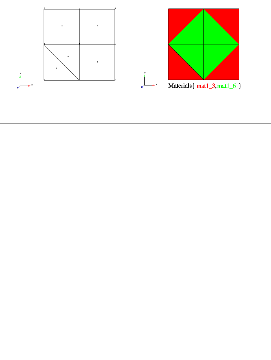
11.1 EnSight Gold Material Files Format
11-84 EnSight 7 User Manual
Example Material Dataset
The following example dataset of ASCII EnSight Gold geometry and material
files show the definition of material fractions for an unstructured model.
Case file
# Sample Case File for 2D Material Dataset
# Created: 03Apr03:mel
#
FORMAT
type: ensight gold
GEOMETRY
model: zmat2d.geo
VARIABLE
scalar per node: scalar zmat2d.sca
MATERIAL
material set number: 1 Mat1
material id count: 2
material id numbers: 3 6
material id names: mat1_3 mat1_6
material id per element: zmat2d.mati
material mixed ids: zmat2d.mixi
material mixed values: zmat2d.mixv
#y
#
#^
# | Case Material ids = {3,6}
#
# 6. 7-----------8-----------9
# | /|\ |
#| /|\ |
# | e2/|\e3 |
#|/|\|
#|/|\|
#|q0|q2|
#|/|\|
# | {.5,.5} | {.5,.5} |
#|/|\|
#|/ | \|
#|/ | \|
# 3. 4-----------5-----------6
#|\ | /|
# | \ {0.,1.} | / |
# |\ | e4/|
# |\t1| /|
#|\|/|
# | e0\e1 | q3 |
#|\|/|
# | t0 \ | {.5,.5} |
#|\|/|
# | {1.,0.} \ | / |
# | \|/ |
# 0. 1-----------2-----------3 -> x
#
#0. 3. 6.
#
Figure 11-2
Geometry for Example Material Dataset
Figure 11-2
Materials for Example Material Dataset

11.1 EnSight Gold Material Files Format
EnSight 7 User Manual 11-85
Geometry File (zmat2d.geo)
Geometry file
Example 2D Material Dataset
node id given
element id given
part
1
2d-mesh
coordinates
9
1
2
3
4
5
6
7
8
9
0.00000e+00
3.00000e+00
6.00000e+00
0.00000e+00
3.00000e+00
6.00000e+00
0.00000e+00
3.00000e+00
6.00000e+00
0.00000e+00
0.00000e+00
0.00000e+00
3.00000e+00
3.00000e+00
3.00000e+00
6.00000e+00
6.00000e+00
6.00000e+00
0.00000e+00
0.00000e+00
0.00000e+00
0.00000e+00
0.00000e+00
0.00000e+00
0.00000e+00
0.00000e+00
0.00000e+00
tria3
2
0
1
124
254
quad4
3
2
3
4
4587
8569
2365
11.1 EnSight Gold Material Files Format
11-86 EnSight 7 User Manual
Scalar File (zmat2d.sca)
Scalar File
part
1
coordinates
0.00000e+00
1.00000e+00
2.00000e+00
1.00000e+00
2.00000e+00
3.00000e+00
2.00000e+00
3.00000e+00
4.00000e+00
Material Number/Id File
part
1
tria3
3
6
quad4
-1
-5
-9
Mixed Ids File
part
1
mixed ids
12
2
3
6
-1
2
3
6
-3
2
3
6
-5
Mixed Values File
part
1
mixed values
6
0.50000e+00
0.50000e+00
0.50000e+00
0.50000e+00
0.50000e+00
0.50000e+00
Material Number/ID File
(
zmat2d.mati)
Mixed Material Ids File
(
zmat2d.mixi)
Mixed Material Values File
(
zmat2d.mixv)
11.2 EnSight6 Casefile Format
11-88 EnSight 7 User Manual
11.2 EnSight6 Casefile Format
Included in this section:
EnSight6 General Description
EnSight6 Geometry File Format
EnSight6 Case File Format
EnSight6 Wild Card Name Specification
EnSight6 Variable File Format
EnSight6 Per_Node Variable File Format
EnSight6 Per_Element Variable File Format
EnSight6 Measured/Particle File Format
Writing EnSight6 Binary Files
EnSight6 General Description
EnSight6 data consists of the following files:
• Case (required) (points to all other needed files including model
geometry, variables, and possibly measured geometry and variables)
EnSight6 supports constant result values as well as scalar, vector, 2nd order
symmetric tensor, and complex variable fields.
EnSight makes no assumptions regarding the physical significance of the variable
values in the files. These files can be from any discipline. For example, the scalar
file can include such things as pressure, temperature, and stress. The vector file
can be velocity, displacement, or any other vector data. And so on.
All variable results for EnSight6 are contained in disk files—one variable per file.
Additionally, if there are multiple time steps, there must either be a set of disk files
for each time step (transient multiple-file format), or all time steps of a particular
variable or geometry in one disk file (transient single-file format). Thus, all
EnSight6 transient geometry and variable files can be expressed in either multiple
file format or single file format.
Sources of EnSight6 data include the following:
• Data that can be translated to conform to the EnSight6 data format
• Data that originates from one of the translators supplied with the EnSight
application
The EnSight6 format supports an unstructured defined element set as shown in the
figure on the following page. Unstructured data must be defined in this element
set. Elements that do not conform to this set must either be subdivided or
discarded. The EnSight6 format also supports a structured block data format
which is very similar to the PLOT3D format. For the structured format, the
standard order of nodes is such that I’s advance quickest, followed by J’s, and then
K’s. A given EnSight6 model may have either unstructured data, structured data,
or a mixture of both.
11.2 EnSight6 General Description
EnSight 7 User Manual 11-89
ens_checker A program is supplied with EnSight which attempts to verify the integrity of the
format of EnSight 6 and EnSight Gold files. If you are producing EnSight
formatted data, this program can be very helpful, especially in your development
stage, in making sure that you are adhering to the published format. It makes no
attempt to verify the validity of floating point values, such as coordinates, variable
values, etc. This program takes a casefile as input. Thus, it will check the format
of the casefile, and all associated geometry and variable files referenced in the
casefile. See How To Use ens_checker.
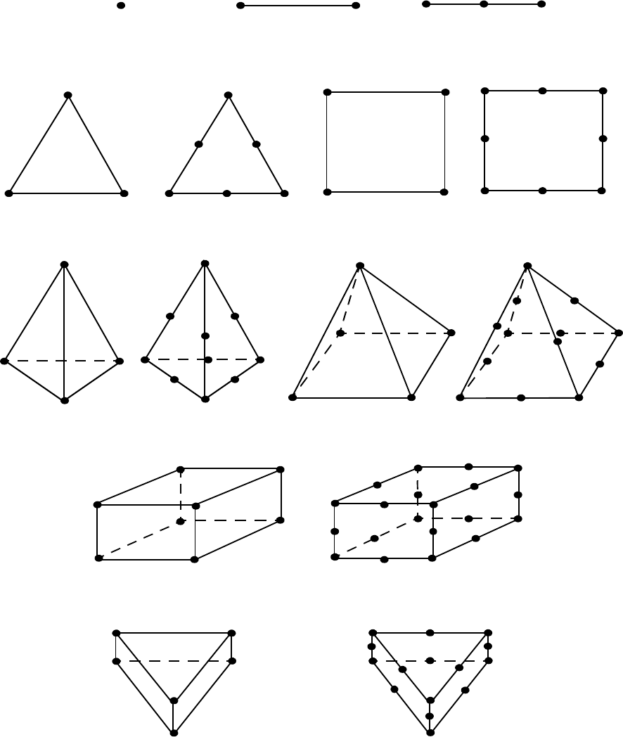
11.2 EnSight6 General Description
11-90 EnSight 7 User Manual
Supported EnSight Elements
The elements that are supported by the EnSight6 format are:
eight node hexahedron twenty node hexahedron
six node pentahedron
9
10
7
8
12123
1
2
3
12
3
4
56
1
2
3
4
12
3
45
6
7
8
12
3
4
5
6
1
2
3
4
5
6
9
10
7
8
1
2
3
4
56
11
12
13
14
15
16
17
18
19
20
two node bar three node bar
three node triangle six node triangle four node quadrangle eight node quadrangle
four node tetrahedron ten node tetrahedron
1
point
1
2
3
4
1
4
8
2
3
5
6
7
5 node pyramid 13 node pyramid
11
2
2
3
3
44
5
5
6
7
8
9
10
11
12
13
fifteen node pentahedron (wedge)
1
2
3
4
5
6
7
8
9
10
11
12
13
14
15
(wedge)
Figure 11-3
Supported EnSight6 Elements
11.2 EnSight6 Geometry File Format
EnSight 7 User Manual 11-91
EnSight6 Geometry File Format
The EnSight6 format consists of keywords followed by information. The
following seven items are important when working with EnSight6 geometry files:
1. You do not have to assign node IDs. If you do, the element connectivities are
based on the node numbers. If you let EnSight assign the node IDs, the nodes
are considered to be sequential starting at node 1, and element connectivity is
done accordingly. If node IDs are set to off, they are numbered internally;
however, you will not be able to display or query on them. If you have node
IDs in your data, you can have EnSight ignore them by specifying “node id
ignore.” Using this option may reduce some of the memory taken up by the
Client and Server, but display and query on the nodes will not be available.
2. You do not need to specify element IDs. If you specify element IDs, or you let
EnSight assign them, you can show them on the screen. If they are set to off,
you will not be able to show or query on them. If you have element IDs in
your data you can have EnSight ignore them by specifying “element id
ignore.” Using this option will reduce some of the memory taken up by the
Client and Server. This may or may not be a significant amount, and
remember that display and query on the elements will not be available.
3. The format of integers and real numbers must be followed (See the Geometry
Example below).
4. Integers are written out using the following integer format:
From C:
8d
format
From FORTRAN:
i8
format
Real numbers are written out using the following floating-point format:
From C:
12.5e
format
From FORTRAN:
e12.5
format
The number of integers or reals per line must also be followed!
5. By default, a Part is processed to show the outside boundaries. This
representation is loaded to the Client host system when the geometry file is
read (unless other attributes have been set on the workstation, such as feature
angle).
6. Coordinates for unstructured data must be defined before any Parts can be
defined. The different elements can be defined in any order (that is, you can
define a hexa8 before a bar2).
7. A Part containing structured data cannot contain any unstructured element
types or more than one block. Each structured Part is limited to a single
block. A structured block is indicated by following the Part description line
with either the “block” line or the “block iblanked” line. An “iblanked” block
must contain an additional integer array of values at each node, traditionally
called the iblank array. Valid iblank values for the EnSight format are:
0 for nodes which are exterior to the model, sometimes called blanked-out nodes
1 for nodes which are interior to the model, thus in the free stream and to be used
<0 or >1 for any kind of boundary nodes
11.2 EnSight6 Geometry File Format
11-92 EnSight 7 User Manual
In EnSight’s structured Part building dialog, the iblank option selected will control
which portion of the structured block is “created”. Thus, from the same structured
block, the interior flow field part as well as a symmetry boundary part could be
“created”.
Note: By default EnSight does not do any “partial” cell iblank processing.
Namely, only complete cells containing no “exterior” nodes are created. It is
possible to obtain partial cell processing by issuing the “test:partial_cells_on”
command in the Command Dialog before reading the file.
Note also that for the structured format, the standard order of nodes is such that
I’s advance quickest, followed by J’s, and then K’s.
Generic Format Not all of the lines included in the following generic example file are necessary:
description line 1 |
description line 2 |
node id <off/given/assign/ignore> |
All geometry files mus
t
element id <off/given/assign/ignore> |
contain these first six lines
coordinates |
# of unstructured nodes |
id x y z
id x y z
id x y z
.
.
.
part #
description line
point
number of points
id nd
id nd
id nd
.
.
.
bar2
number of bar2’s
id nd nd
id nd nd
id nd nd
.
.
.
bar3
number of bar3’s
id nd nd nd
id nd nd nd
id nd nd nd
.
.
.
tria3
number of three node triangles
id nd nd nd
id nd nd nd
id nd nd nd
.
.
.
11.2 EnSight6 Geometry File Format
EnSight 7 User Manual 11-93
tria6
number of six node triangles
id nd nd nd nd nd nd
.
.
.
quad4
number of quad 4’s
id nd nd nd nd
id nd nd nd nd
id nd nd nd nd
id nd nd nd nd
.
.
.
quad8
number of quad 8’s
id nd nd nd nd nd nd nd nd
id nd nd nd nd nd nd nd nd
id nd nd nd nd nd nd nd nd
id nd nd nd nd nd nd nd nd
.
.
.
tetra4
number of 4 node tetrahedrons
id nd nd nd nd
id nd nd nd nd
id nd nd nd nd
id nd nd nd nd
.
.
.
tetra10
number of 10 node tetrahedrons
id nd nd nd nd nd nd nd nd nd nd
id nd nd nd nd nd nd nd nd nd nd
id nd nd nd nd nd nd nd nd nd nd
id nd nd nd nd nd nd nd nd nd nd
.
.
.
pyramid5
number of 5 node pyramids
id nd nd nd nd nd
id nd nd nd nd nd
id nd nd nd nd nd
id nd nd nd nd nd
.
.
.
pyramid13
number of 13 node pyramids
id nd nd nd nd nd nd nd nd nd nd nd nd nd
id nd nd nd nd nd nd nd nd nd nd nd nd nd
id nd nd nd nd nd nd nd nd nd nd nd nd nd
id nd nd nd nd nd nd nd nd nd nd nd nd nd
.
.
.
11.2 EnSight6 Geometry File Format
11-94 EnSight 7 User Manual
hexa8
number of 8 node hexahedrons
id nd nd nd nd nd nd nd nd
id nd nd nd nd nd nd nd nd
id nd nd nd nd nd nd nd nd
id nd nd nd nd nd nd nd nd
.
.
.
hexa20
number of 20 node hexahedrons
id nd nd nd nd nd nd nd nd nd nd nd nd nd nd nd nd nd nd nd nd
id nd nd nd nd nd nd nd nd nd nd nd nd nd nd nd nd nd nd nd nd
id nd nd nd nd nd nd nd nd nd nd nd nd nd nd nd nd nd nd nd nd
id nd nd nd nd nd nd nd nd nd nd nd nd nd nd nd nd nd nd nd nd
id nd nd nd nd nd nd nd nd nd nd nd nd nd nd nd nd nd nd nd nd
.
.
.
penta6
number of 6 node pentahedrons
id nd nd nd nd nd nd
id nd nd nd nd nd nd
id nd nd nd nd nd nd
id nd nd nd nd nd nd
id nd nd nd nd nd nd
.
.
.
penta15
number of 15 node pentahedrons
id nd nd nd nd nd nd nd nd nd nd nd nd nd nd nd
id nd nd nd nd nd nd nd nd nd nd nd nd nd nd nd
id nd nd nd nd nd nd nd nd nd nd nd nd nd nd nd
id nd nd nd nd nd nd nd nd nd nd nd nd nd nd nd
id nd nd nd nd nd nd nd nd nd nd nd nd nd nd nd
.
.
.
part #
description line
block #nn=i*j*k
ijk
x_n1 x_n2 x_n3 ..... x_nn (6/line)
y_n1 y_n2 y_n3 ..... y_nn “
z_n1 z_n2 z_n3 ..... z_nn “
part #
description line
block iblanked #nn=i*j*k
ijk
x_n1 x_n2 x_n3 ..... x_nn (6/line)
y_n1 y_n2 y_n3 ..... y_nn “
z_n1 z_n2 z_n3 ..... z_nn “
ib_n1 ib_n2 ib_n3 .... ib_nn (10/line)
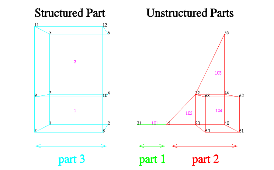
11.2 EnSight6 Geometry File Format
EnSight 7 User Manual 11-95
EnSight6 Geometry
The following is an example of an ASCII EnSight6 geometry file with 11 defined
File Example unstructured nodes from which 2 unstructured parts are defined, and a 2x3x2
structured part as depicted in the above diagram. (See Case File Example 1 for
reference to this file.)
This is the 1st description line of the EnSight6 geometry example
This is the 2nd description line of the EnSight6 geometry example
node id given
element id given
coordinates
11
15 4.00000e+00 0.00000e+00 0.00000e+00
31 3.00000e+00 0.00000e+00 0.00000e+00
20 5.00000e+00 0.00000e+00 0.00000e+00
40 6.00000e+00 0.00000e+00 0.00000e+00
22 5.00000e+00 1.00000e+00 0.00000e+00
44 6.00000e+00 1.00000e+00 0.00000e+00
55 6.00000e+00 3.00000e+00 0.00000e+00
60 5.00000e+00 0.00000e+00 2.00000e+00
61 6.00000e+00 0.00000e+00 2.00000e+00
62 6.00000e+00 1.00000e+00 2.00000e+00
63 5.00000e+00 1.00000e+00 2.00000e+00
part 1
2D uns-elements (description line for part 1)
tria3
2
102 15 20 22
103 22 44 55
hexa8
1
104 20 40 44 22 60 61 62 63
part 2
1D uns-elements (description line for part 2)
bar2
1
101 31 15
part 3

11.2 EnSight6 Case File Format
11-96 EnSight 7 User Manual
3D struct-part (description line for part 3)
block iblanked
232
0.00000e+00 2.00000e+00 0.00000e+00 2.00000e+00 0.00000e+00 2.00000e+00
0.00000e+00 2.00000e+00 0.00000e+00 2.00000e+00 0.00000e+00 2.00000e+00
0.00000e+00 0.00000e+00 1.00000e+00 1.00000e+00 3.00000e+00 3.00000e+00
0.00000e+00 0.00000e+00 1.00000e+00 1.00000e+00 3.00000e+00 3.00000e+00
0.00000e+00 0.00000e+00 0.00000e+00 0.00000e+00 0.00000e+00 0.00000e+00
2.00000e+00 2.00000e+00 2.00000e+00 2.00000e+00 2.00000e+00 2.00000e+00
1111111111
11
EnSight6 Case File Format
The Case file is an ASCII free format file that contains all the file and name
information for accessing model (and measured) geometry, variable, and time
information. It is comprised of five sections (
FORMAT, GEOMETRY, VARIABLE,
TIME, FILE) as described below:
Notes: All lines in the Case file are limited to 79 characters.
The titles of each section must be in all capital letters.
Anything preceded by a “#” denotes a comment and is ignored. Comments may
append information lines or be placed on their own lines.
Information following “:” may be separated by white spaces or tabs.
Specifications encased in “[]” are optional, as indicated.
Format Section This is a required section which specifies the type of data to be read.
Usage:
FORMAT
type: ensight
Geometry Section This is a required section which specifies the geometry information for the model
(as well as measured geometry if present, and periodic match file (see Section
11.9, Periodic Matchfile Format) if present).
Usage:
GEOMETRY
model: [ts] [fs] filename [change_coords_only]
measured: [ts] [fs] filename [change_coords_only]
match: filename
boundary: filename
where: ts = time set number as specified in TIME section. This is optional.
fs = corresponding file set number as specified in FILE section below.
filename = The filename of the appropriate file.
-> Model or measured filenames for a static geometry case, as well as match
and boundary filenames will not
contain “*” wildcards.
-> Model or measured filenames for a changing geometry case will
contain “*” wildcards.
change_coords_only = The option to indicate that the changing geometry (as
indicated by wildcards in the filename) is coords only.
Otherwise, changing geometry connectivity will be
assumed.
11.2 EnSight6 Case File Format
EnSight 7 User Manual 11-97
Variable Section This is an optional section which specifies the files and names of the variables.
Constant variable values can also be set in this section.
Usage:
VARIABLE
constant per case: [ts] description
const_value(s)
scalar per node: [ts] [fs] description filename
vector per node: [ts] [fs] description filename
tensor symm per node: [ts] [fs] description filename
scalar per element: [ts] [fs] description filename
vector per element: [ts] [fs] description filename
tensor symm per element: [ts] [fs] description filename
scalar per measured node: [ts] [fs] description filename
vector per measured node: [ts] [fs] description filename
complex scalar per node: [ts] [fs] description
Re_fn Im_fn freq
complex vector per node: [ts] [fs] description
Re_fn Im_fn freq
complex scalar per element: [ts] [fs] description
Re_fn Im_fn freq
complex vector per element: [ts] [fs] description
Re_fn Im_fn freq
where:
ts
= The corresponding time set number (or index) as specified in TIME
section below. This is only required for transient constants and
variables.
fs
= The corresponding file set number (or index) as specified in FILE
section below.
description = The variable (GUI) name (ex. Pressure, Velocity, etc.)
const_value(s) = The constant value. If constants change over time, then ns (see
TIME section below) constant values of
ts.
filename
= The filename of the variable file. Note: only transient filenames
contain “*” wildcards.
Re_fn
= The filename for the file containing the real values of the complex
variable.
Im_fn
= The filename for the file containing the imaginary values of the
complex variable.
freq
= The corresponding harmonic frequency of the complex variable.
For complex variables where harmonic frequency is undefined,
simply use the text string: UNDEFINED.
Note: As many variable description lines as needed may be used.
Note: Variable descriptions have the following restrictions:
The variable description is limited to 19 characters in the current release.
Duplicate variable descriptions are not allowed.
Leading and trailing white space will be eliminated.
Variable descriptions must not start with a numeric digit.
Variable descriptions must not contain any of the following reserved characters:
( [ + @ ! * $
) ] - space # ^ /
Time Section This is an optional section for steady state cases, but is required for transient
cases. It contains time set information. Shown below is information for one time
set. Multiple time sets (up to 16) may be specified for measured data as shown in
Case File Example 3 below.
Usage:
TIME
11.2 EnSight6 Case File Format
11-98 EnSight 7 User Manual
time set: ts [description]
number of steps: ns
filename start number: fs
filename increment: fi
time values: time_1 time_2 .... time_ns
or
TIME
time set: ts [description]
number of steps: ns
filename numbers: fn
time values: time_1 time_2 .... time_ns
where:
ts
= timeset number. This is the number referenced in the GEOMETRY
and VARIABLE sections.
description
= optional timeset description which will be shown in user
interface.
ns
= number of transient steps
fs
= the number to replace the “*” wildcards in the filenames, for the first step
fi
= the increment to fs for subsequent steps
time
= the actual time values for each step, each of which must be separated
by a white space and which may continue on the next line if needed
fn
= a list of numbers or indices, to replace the “*” wildcards in the filenames.
File Section This section is optional for expressing a transient case with single-file formats. This
section contains single-file set information. This information specifies the number of time
steps in each file of each data entity, i.e. each geometry and each variable (model and/or
measured). Each data entity’s corresponding file set might have multiple continuation
files due to system file size limit, i.e. ~2 GB for 32-bit and ~4 TB for 64-bit architectures.
Each file set corresponds to one and only one time set, but a time set may be referenced by
many file sets. The following information may be specified in each file set. For file sets
where all of the time set data exceeds the maximum file size limit of the system, both
filename index
and
number of steps
are repeated within the file set definition for each
continuation file required. Otherwise
filename index
may be omitted if there is only one
file. File set information is shown in Case File Example 4 below.
Usage:
FILE
file set: fs
filename index: fi # Note: only used when data continues in other files
number of steps: ns
where:
fs
= file set number. This is the number referenced in the GEOMETRY
and VARIABLE sections above.
ns
= number of transient steps
fi
= file index number in the file name (replaces “*” in the filenames)
Case File Example 1 The following is a minimal EnSight6 case file for a steady state model with some results.
Note: this (en6.case) file, as well as all of its referenced geometry and variable files (along with a
couple of command files) can be found under your installation directory (path:
$CEI_HOME/
ensight76/data/user_manual
). The EnSight6 Geometry File Example and the Variable File
Examples are the contents of these files.
FORMAT
type: ensight
11.2 EnSight6 Case File Format
EnSight 7 User Manual 11-99
GEOMETRY
model: en6.geo
VARIABLE
constant per case: Cden .8
scalar per element: Esca en6.Esca
scalar per node: Nsca en6.Nsca
vector per element: Evec en6.Evec
vector per node: Nvec en6.Nvec
tensor symm per element: Eten en6.Eten
tensor symm per node: Nten en6.Nten
complex scalar per element: Ecmp en6.Ecmp_r en6.Ecmp_i 2.
complex scalar per node: Ncmp en6.Ncmp_r en6.Ncmp_i 4.
Case File Example 2 The following is a Case file for a transient model. The connectivity of the geometry is also
changing.
FORMAT
type: ensight
GEOMETRY
model: 1 example2.geo**
VARIABLE
scalar per node: 1 Stress example2.scl**
vector per node: 1 Displacement example2.dis**
TIME
time set: 1
number of steps: 3
filename start number: 0
filename increment: 1
time values: 1.0 2.0 3.0
The following files would be needed for Example 2:
example2.geo00 example2.scl00 example2.dis00
example2.geo01 example2.scl01 example2.dis01
example2.geo02 example2.scl02 example2.dis02
Case File Example 3 The following is a Case file for a transient model with measured data.
This example has pressure given per element.
FORMAT
type: ensight
GEOMETRY
model: 1 example3.geo*
measured: 2 example3.mgeo**
VARIABLE
constant per case: Gamma 1.4
constant per case: 1 Density .9 .9 .7 .6 .6
scalar per element 1 Pressure example3.pre*
vector per node: 1 Velocity example3.vel*
scalar per measured node: 2 Temperature example3.mtem**
vector per measured node: 2 Velocity example3.mvel**
11.2 EnSight6 Case File Format
11-100 EnSight 7 User Manual
TIME
time set: 1
number of steps: 5
filename start number: 1
filename increment: 2
time values: .1 .2 .3 # This example shows that time
.4 .5 # values can be on multiple lines
time set: 2
number of steps: 6
filename start number: 0
filename increment: 2
time values:
.05 .15 .25 .34 .45 .55
The following files would be needed for Example 3:
example3.geo1 example3.pre1 example3.vel1
example3.geo3 example3.pre3 example3.vel3
example3.geo5 example3.pre5 example3.vel5
example3.geo7 example3.pre7 example3.vel7
example3.geo9 example3.pre9 example3.vel9
example3.mgeo00 example3.mtem00 example3.mvel00
example3.mgeo02 example3.mtem02 example3.mvel02
example3.mgeo04 example3.mtem04 example3.mvel04
example3.mgeo06 example3.mtem06 example3.mvel06
example3.mgeo08 example3.mtem08 example3.mvel08
example3.mgeo10 example3.mtem10 example3.mvel10
Case File Example 4 The following is Case File Example 3 expressed in transient single-file formats.
In this example, the transient data for the measured velocity data entity happens
to be greater than the maximum file size limit. Therefore, the first four time steps
fit and are contained in the first file, and the last two time steps are ‘continued’ in
a second file.
FORMAT
type: ensight
GEOMETRY
model: 1 example4.geo
measured: 2 example4.mgeo
VARIABLE
constant per case: Density .5
scalar per element: 1 1 Pressure example4.pre
vector per node: 1 1 Velocity example4.vel
scalar per measured node: 2 2 Temperature example4.mtem
vector per measured node: 2 3 Velocity example4.mvel*
TIME
time set: 1 Model
number of steps: 5
time values: .1 .2 .3 .4 .5
time set: 2 Measured
number of steps: 6

11.2 EnSight6 Case File Format
EnSight 7 User Manual 11-101
time values: .05 .15 .25 .34 .45 .55
FILE
file set: 1
number of steps: 5
file set: 2
number of steps: 6
file set: 3
filename index: 1
number of steps: 4
filename index: 2
number of steps: 2
The following files would be needed for Example 4:
example4.geo example4.pre example4.vel
example4.mgeo example4.mtem example4.mvel1
example4.mvel2
Contents of Each file contains transient data that corresponds to the specified number of time steps.
Transient The data for each time step sequentially corresponds to the simulation time values
Single Files
(time values)
found listed in the TIME section. In transient single-file format, the data for
each time step essentially corresponds to a standard EnSight6 geometry or variable file
(model or measured) as expressed in multiple file format. The data for each time step is
enclosed between two wrapper records, i.e. preceded by a
BEGIN TIME STEP record
and followed by an
END TIME STEP record. Time step data is not split between files.
If there is not enough room to append the data from a time step to the file without
exceeding the maximum file limit of a particular system, then a continuation file must be
created for the time step data and any subsequent time step. Any type of user comments
may be included before and/or after each transient step wrapper.
Note 1: If transient single file format is used, EnSight expects all files of a dataset
to be specified in transient single file format. Thus, even static files must be
enclosed between a
BEGIN TIME STEP and an END TIME STEP wrapper.
Note 2: For binary geometry files, the first
BEGIN TIME STEP wrapper must
follow the <C Binary/Fortran Binary> line. Both
BEGIN TIME STEP and END
TIME STEP
wrappers are written according to type (1) in binary. (see Writing
EnSight6 Binary Files, in Section 11.2)
Note 3: Efficient reading of each file (especially binary) is facilitated by
appending each file with a file index. A file index contains appropriate
information to access the file byte positions of each time step in the file. (EnSight
automatically appends a file index to each file when exporting in transient single
file format.) If used, the file index must follow the last
END TIME STEP
wrapper in each file.
File Index Usage:
ASCII Binary Item Description
“%20d\n” sizeof(int) n Total number of data time steps in the file.
“%20d\n” sizeof(long) fb
1
File byte loc for contents of 1
st
time step
*
“%20d\n” sizeof(long) fb
2
File byte loc for contents of 2
nd
time step
*
. . . . . . . . . . . .
“%20d\n” sizeof(long) fb
n
File byte loc for contents of n
th
time step
*
“%20d\n” sizeof(int) flag Miscellaneous flag (= 0 for now)
11.2 EnSight6 Case File Format
11-102 EnSight 7 User Manual
*
Each file byte location is the first byte that follows the BEGIN TIME STEP record.
Shown below are the contents of each of the above files, using the data files from Case
File Example 3 for reference (without
FILE_INDEX for simplicity).
Contents of file example4.geo_1:
BEGIN TIME STEP
Contents of file
example3.geo1
END TIME STEP
BEGIN TIME STEP
Contents of file
example3.geo3
END TIME STEP
BEGIN TIME STEP
Contents of file
example3.geo5
END TIME STEP
BEGIN TIME STEP
Contents of file
example3.geo7
END TIME STEP
BEGIN TIME STEP
Contents of file
example3.geo9
END TIME STEP
Contents of file example4.pre_1:
BEGIN TIME STEP
Contents of file
example3.pre1
END TIME STEP
BEGIN TIME STEP
Contents of file
example3.pre3
END TIME STEP
BEGIN TIME STEP
Contents of file
example3.pre5
END TIME STEP
BEGIN TIME STEP
Contents of file
example3.pre7
END TIME STEP
BEGIN TIME STEP
Contents of file
example3.pre9
END TIME STEP
Contents of file example4.vel_1:
BEGIN TIME STEP
Contents of file
example3.vel1
END TIME STEP
BEGIN TIME STEP
Contents of file
example3.vel3
END TIME STEP
BEGIN TIME STEP
Contents of file
example3.vel5
END TIME STEP
BEGIN TIME STEP
Contents of file
example3.vel7
END TIME STEP
BEGIN TIME STEP
Contents of file
example3.vel9
END TIME STEP
Contents of file example4.mgeo_1:
BEGIN TIME STEP
Contents of file
example3.mgeo00
END TIME STEP
BEGIN TIME STEP
Contents of file
example3.mgeo02
END TIME STEP
BEGIN TIME STEP
Contents of file
example3.mgeo04
END TIME STEP
BEGIN TIME STEP
Contents of file
example3.mgeo06
END TIME STEP
BEGIN TIME STEP
Contents of file
example3.mgeo08
END TIME STEP
BEGIN TIME STEP
Contents of file
example3.mgeo10
END TIME STEP
Contents of file example4.mtem_1:
“%20d\n” sizeof(long) fb of item n File byte loc for Item n above
“%s\n” sizeof(char)*80
“FILE_INDEX”
File index keyword
ASCII Binary Item Description
11.2 EnSight6 Variable File Format
EnSight 7 User Manual 11-103
BEGIN TIME STEP
Contents of file
example3.mtem00
END TIME STEP
BEGIN TIME STEP
Contents of file
example3.mtem02
END TIME STEP
BEGIN TIME STEP
Contents of file
example3.mtem04
END TIME STEP
BEGIN TIME STEP
Contents of file
example3.mtem06
END TIME STEP
BEGIN TIME STEP
Contents of file
example3.mtem08
END TIME STEP
BEGIN TIME STEP
Contents of file
example3.mtem10
END TIME STEP
Contents of file example4.mvel1_1:
BEGIN TIME STEP
Contents of file
example3.mvel00
END TIME STEP
BEGIN TIME STEP
Contents of file
example3.mvel02
END TIME STEP
BEGIN TIME STEP
Contents of file
example3.mvel04
END TIME STEP
BEGIN TIME STEP
Contents of file
example3.mvel06
END TIME STEP
Contents of file example4.mvel2_1:
Comments can precede the beginning wrapper here.
BEGIN TIME STEP
Contents of file
example3.mvel08
END TIME STEP
Comments can go between time step wrappers here.
BEGIN TIME STEP
Contents of file
example3.mvel10
END TIME STEP
Comments can follow the ending time step wrapper.
EnSight6 Wild Card Name Specification
For transient data, if multiple time files are involved, the file names must conform
to the EnSight wild-card specification. This specification is as follows:
• File names must include numbers that are in ascending order from
beginning to end.
• Numbers in the files names must be zero filled if there is more than one
significant digit.
• Numbers can be anywhere in the file name.
• When the file name is specified in the EnSight result file, you must
replace the numbers in the file with an asterisk(*). The number of
asterisks specified is the number of significant digits. The asterisk must
occupy the same place as the numbers in the file names.
EnSight6 Variable File Format
EnSight6 variable files can either be per_node or per_element. They cannot be
both. However, an EnSight model can have some variables which are per_node
and other variables which are per_element.
11.2 EnSight6 Per_Node Variable File Format
11-104 EnSight 7 User Manual
EnSight6 Per_Node Variable File Format
EnSight6 variable files for per_node variables contain any values for each
unstructured node followed by any values for each structured node.
First comes a single description line.
Second comes any unstructured node value. The number of values per node
depends on the type of field. An unstructured scalar field has one, a vector field
has three (order: x,y,z), a 2nd order symmetric tensor field has 6 (order: 11, 22, 33,
12, 13, 23), and a 2nd order asymmetric tensor field has 9 values per node (order:
11, 12, 13, 21, 22, 23, 31, 32, 33). An unstructured complex variable in EnSight6
consists of two scalar or vector fields (one real and one imaginary), with scalar
and vector values written to their separate files respectively.
Third comes any structured data information, starting with a part # line, followed
by a line containing the “block”, and then lines containing the values for each
structured node which are output in the same IJK component order as the
coordinates. Briefly, a structured scalar is the same as an unstructured scalar, one
value per node. A structured vector is written one value per node per component,
thus three sequential scalar field blocks. Likewise for a structured 2nd order
symmetric tensor, written as six sequential scalar field blocks, and a 2nd order
tensor, written as nine sequential scalar field blocks. The same methodology
applies for a complex variable only with the real and imaginary fields written to
separate structured scalar or vector files.
The values must be written in the following floating point format (6 per line as
shown in the examples below):
From C:
12.5e
format
From FORTRAN:
e12.5
format
The format of a per_node variable file is as follows:
•Line 1
This line is a description line.
• Line 2 through the end of the file contains the values at each node in the
model.
A generic example for per_node variables:
One description line for the entire file
*.*****E+** *.*****E+** *.*****E+** *.*****E+** *.*****E+** *.*****E+**
*.*****E+** *.*****E+** *.*****E+** *.*****E+** *.*****E+** *.*****E+**
*.*****E+** *.*****E+** *.*****E+** *.*****E+**
part #
*.*****E+** *.*****E+** *.*****E+** *.*****E+** *.*****E+** *.*****E+**
*.*****E+** *.*****E+** *.*****E+** *.*****E+** *.*****E+** *.*****E+**
*.*****E+** *.*****E+** *.*****E+** *.*****E+** *.*****E+** *.*****E+**
part #
*.*****E+** *.*****E+** *.*****E+** *.*****E+** *.*****E+** *.*****E+**
*.*****E+** *.*****E+**
*.*****E+** *.*****E+** *.*****E+** *.*****E+** *.*****E+** *.*****E+**
*.*****E+** *.*****E+**
*.*****E+** *.*****E+** *.*****E+** *.*****E+** *.*****E+** *.*****E+**

11.2 EnSight6 Per_Node Variable File Format
EnSight 7 User Manual 11-105
*.*****E+** *.*****E+**
The following variable file examples reflect scalar, vector, tensor, and complex
variable values per node for the previously defined EnSight6 Geometry File
Example with 11 defined unstructured nodes and a 2x3x2 structured Part (Part
number 3). The values are summarized in the following table.
Per_node (Scalar) Variable Example 1 This example shows ASCII scalar file (
en6.Nsca) for the
geometry example.
Per_node scalar values for the EnSight6 geometry example
1.00000E+00 2.00000E+00 3.00000E+00 4.00000E+00 5.00000E+00 6.00000E+00
7.00000E+00 8.00000E+00 9.00000E+00 1.00000E+01 1.10000E+01
part 3
block
1.00000E+00 2.00000E+00 3.00000E+00 4.00000E+00 5.00000E+00 6.00000E+00
7.00000E+00 8.00000E+00 9.00000E+00 1.00000E+01 1.10000E+01 1.20000E+01
Per_node (Vector) Variable Example 2 This example shows ASCII vector file (en6.Nvec) for the
geometry example.
Per_node vector values for the EnSight6 geometry example
1.10000E+00 1.20000E+00 1.30000E+00 2.10000E+00 2.20000E+00 2.30000E+00
3.10000E+00 3.20000E+00 3.30000E+00 4.10000E+00 4.20000E+00 4.30000E+00
5.10000E+00 5.20000E+00 5.30000E+00 6.10000E+00 6.20000E+00 6.30000E+00
7.10000E+00 7.20000E+00 7.30000E+00 8.10000E+00 8.20000E+00 8.30000E+00
9.l0000E+00 9.20000E+00 9.30000E+00 1.01000E+01 1.02000E+01 1.03000E+01
1.11000E+01 1.12000E+01 1.13000E+01
part 3
block
1.10000E+00 2.10000E+00 3.10000E+00 4.10000E+00 5.10000E+00 6.10000E+00
Complex Scalar
Node Node Scalar Vector Tensor (2nd order symm.) Real Imaginary
Index Id Value Values Values Value Value
Unstructured
1 15 (1.) (1.1, 1.2, 1.3) (1.1, 1.2, 1.3, 1.4, 1.5, 1.6) (1.1) (1.2)
2 31 (2.) (2.1, 2.2, 2.3) (2.1, 2.2, 2.3, 2.4, 2.5, 2.6) (2.1) (2.2)
3 20 (3.) (3.1, 3.2, 3.3) (3.1, 3.2, 3.3, 3.4, 3.5, 3.6) (3.1) (3.2)
4 40 (4.) (4.1, 4.2, 4.3) (4.1, 4.2, 4.3, 4.4, 4.5, 4.6) (4.1) (4.2)
5 22 (5.) (5.1, 5.2, 5.3) (5.1, 5.2, 5.3, 5.4, 5.5, 5.6) (5.1) (5.2)
6 44 (6.) (6.1, 6.2, 6.3) (6.1, 6.2, 6.3, 6.4, 6.5, 6.6) (6.1) (6.2)
7 55 (7.) (7.1, 7.2, 7.3) (7.1, 7.2, 7.3, 7.4, 7.5, 7.6) (7.1) (7.2)
8 60 (8.) (8.1, 8.2, 8.3) (8.1, 8.2, 8.3, 8.4, 8.5, 8.60 (8.1) (8.2)
9 61 (9.) (9.1, 9.2, 9.3) (9.1, 9.2, 9.3, 9.4, 9.5, 9.6) (9.1) (9.2)
10 62 (10.) (10.1,10.2,10.3) (10.1,10.2,10.3,10.4,10.5,10.6) (10.1) (10.2)
11 63 (11.) (11.1,11.2,11.3) (11.1,11.2,11.3,11.4,11.5,11.6) (11.1) (11.2)
Structured
1 1 (1.) (1.1, 1.2, 1.3) (1.1, 1.2, 1.3, 1.4, 1.5, 1.6) (1.1) (1.2)
2 2 (2.) (2.1, 2.2, 2.3) (2.1, 2.2, 2.3, 2.4, 2.5, 2.6) (2.1) (2.2)
3 3 (3.) (3.1, 3.2, 3.3) (3.1, 3.2, 3.3, 3.4, 3.5, 3.6) (3.1) (3.2)
4 4 (4.) (4.1, 4.2, 4.3) (4.1, 4.2, 4.3, 4.4, 4.5, 4.6) (4.1) (4.2)
5 5 (5.) (5.1, 5.2, 5.3) (5.1, 5.2, 5.3, 5.4, 5.5, 5.6) (5.1) (5.2)
6 6 (6.) (6.1, 6.2, 6.3) (6.1, 6.2, 6.3, 6.4, 6.5, 6.6) (6.1) (6.2)
7 7 (7.) (7.1, 7.2, 7.3) (7.1, 7.2, 7.3, 7.4, 7.5, 7.6) (7.1) (7.2)
8 8 (8.) (8.1, 8.2, 8.3) (8.1, 8.2, 8.3, 8.4, 8.5, 8.6) (8.1) (8.2)
9 9 (9.) (9.1, 9.2, 9.3) (9.1, 9.2, 9.3, 9.4, 9.5, 9.6) (9.1) (9.2)
10 10 (10.) (10.1,10.2,10.3) (10.1,10.2,10.3,10.4,10.5,10.6) (10.1) (10.2)
11 11 (11.) (11.1,11.2,11.3) (11.1,11.2,11.3,11.4,11.5,11.6) (11.1) (11.2)
12 12 (12.) (12.1,12.2,12.3) (12.1,12.2,12.3,12.4,12.5,12.6) (12.1) (12.2)
11.2 EnSight6 Per_Node Variable File Format
11-106 EnSight 7 User Manual
7.10000E+00 8.10000E+00 9.10000E+00 1.01000E_01 1.11000E+01 1.21000E+01
1.20000E+00 2.20000E+00 3.20000E+00 4.20000E+00 5.20000E+00 6.20000E+00
7.20000E+00 8.20000E+00 9.20000E+00 1.02000E+01 1.12000E+01 1.22000E+01
1.30000E+00 2.30000E+00 3.30000E+00 4.30000E+00 5.30000E+00 6.30000E+00
7.30000E+00 8.30000E+00 9.30000E+00 1.03000E+01 1.13000E+01 1.23000E+01
Per_node (Tensor) Variable Example 3 This example shows an ASCII 2nd order symmetric tensor file
(
en6.Nten) for the geometry example.
Per_node symmetric tensor values for the EnSight6 geometry example
1.10000E+00 1.20000E+00 1.30000E+00 1.40000E+00 1.50000E+00 1.60000E+00
2.10000E+00 2.20000E+00 2.30000E+00 2.40000E+00 2.50000E+00 2.60000E+00
3.10000E+00 3.20000E+00 3.30000E+00 3.40000E+00 3.50000E+00 3.60000E+00
4.10000E+00 4.20000E+00 4.30000E+00 4.40000E+00 4.50000E+00 4.60000E+00
5.10000E+00 5.20000E+00 5.30000E+00 5.40000E+00 5.50000E+00 5.60000E+00
6.10000E+00 6.20000E+00 6.30000E+00 6.40000E+00 6.50000E+00 6.60000E+00
7.10000E+00 7.20000E+00 7.30000E+00 7.40000E+00 7.50000E+00 7.60000E+00
8.10000E+00 8.20000E+00 8.30000E+00 8.40000E+00 8.50000E+00 8.60000E+00
9.10000E+00 9.20000E+00 9.30000E+00 9.40000E+00 9.50000E+00 9.60000E+00
1.01000E+01 1.02000E+01 1.03000E+01 1.04000E+01 1.05000E+01 1.06000E+01
1.11000E+01 1.12000E+01 1.13000E+01 1.14000E+01 1.15000E+01 1.16000E+01
part 3
block
1.10000E+00 2.10000E+00 3.10000E+00 4.10000E+00 5.10000E+00 6.10000E+00
7.10000E+00 8.10000E+00 9.10000E+00 1.01000E+01 1.11000E+01 1.21000E+01
1.20000E+00 2.20000E+00 3.20000E+00 4.20000E+00 5.20000E+00 6.20000E+00
7.20000E+00 8.20000E+00 9.20000E+00 1.02000E+01 1.12000E+01 1.22000E+01
1.30000E+00 2.30000E+00 3.30000E+00 4.30000E+00 5.30000E+00 6.30000E+00
7.30000E+00 8.30000E+00 9.30000E+00 1.03000E+01 1.13000E+01 1.23000E+01
1.40000E+00 2.40000E+00 3.40000E+00 4.40000E+00 5.40000E+00 6.40000E+00
7.40000E+00 8.40000E+00 9.40000E+00 1.04000E+01 1.14000E+01 1.24000E+01
1.50000E+00 2.50000E+00 3.50000E+00 4.50000E+00 5.50000E+00 6.50000E+00
7.50000E+00 8.50000E+00 9.50000E+00 1.05000E+01 1.15000E+01 1.25000E+01
1.60000E+00 2.60000E+00 3.60000E+00 4.60000E+00 5.60000E+00 6.60000E+00
7.60000E+00 8.60000E+00 9.60000E+00 1.06000E+01 1.16000E+01 1.26000E+01
Per_node (Complex) Variable Example 4 This example shows the ASCII complex real (en6.Ncmp_r)
and imaginary (
en6.Ncmp_i) scalar files for the geometry example. (The same
methodology would apply for complex real and imaginary vector files.)
Real scalar File:
Per_node complex real scalar values for the EnSight6 geometry example
1.10000E+00 2.10000E+00 3.10000E+00 4.10000E+00 5.10000E+00 6.10000E+00
7.10000E+00 8.10000E+00 9.10000E+00 1.01000E+01 1.11000E+01
part 3
block
1.10000E+00 2.10000E+00 3.10000E+00 4.10000E+00 5.10000E+00 6.10000E+00
7.10000E+00 8.10000E+00 9.10000E+00 1.01000E+01 1.11000E+01 1.21000E+00
Imaginary scalar File:
Per_node complex imaginary scalar values for the EnSight6 geometry example
1.20000E+00 2.20000E+00 3.20000E+00 4.20000E+00 5.20000E+00 6.20000E+00
7.20000E+00 8.20000E+00 9.20000E+00 1.02000E+01 1.12000E+01
part 3
block
1.20000E+00 2.20000E+00 3.20000E+00 4.20000E+00 5.20000E+00 6.20000E+00
7.20000E+00 8.20000E+00 9.20000E+00 1.02000E+01 1.12000E+01 1.22000E+00
11.2 EnSight6 Per_Element Variable File Format
EnSight 7 User Manual 11-107
EnSight6 Per_Element Variable File Format
EnSight variable files for per_element variables contain values for each element
of designated types of designated Parts. First comes a single description line.
Second comes a Part line. Third comes an element type line and fourth comes the
value for each element of that type and part. If it is a scalar variable, there is one
value per element, while for vector variables there are three values per element.
(The number of elements of the given type are obtained from the corresponding
EnSight6 geometry file.)
The values must be written in the following floating point format (6 per line as
shown in the examples below):
From C:
12.5e
format
From FORTRAN:
e12.5
format
The format of a per_element variable file is as follows:
• Line 1 This line is a description line.
• Line 2 Part line, with part number corresponding to the geometry file.
• Line 3 Element type line ( example: tria3, hexa8, ... )
• Line 4 Repeats until next element type line, part line, or end of file is
reached. Lists values for each element of this part and type.
A generic example for per_element variables:
One description line for the entire file
part #
element type
*.*****E+** *.*****E+** *.*****E+** *.*****E+** *.*****E+** *.*****E+**
*.*****E+** *.*****E+**
part #
block
*.*****E+** *.*****E+** *.*****E+** *.*****E+** *.*****E+** *.*****E+**
*.*****E+** *.*****E+** *.*****E+** *.*****E+**
*.*****E+** *.*****E+** *.*****E+** *.*****E+** *.*****E+** *.*****E+**
*.*****E+** *.*****E+** *.*****E+** *.*****E+**
*.*****E+** *.*****E+** *.*****E+** *.*****E+** *.*****E+** *.*****E+**
*.*****E+** *.*****E+** *.*****E+** *.*****E+**

11.2 EnSight6 Per_Element Variable File Format
11-108 EnSight 7 User Manual
The following variable file examples reflect scalar, vector, tensor, and complex
variable values per element for the previously defined EnSight6 Geometry File
Example with 11 defined unstructured nodes and a 2x3x2 structured Part (Part
number 3). The values are summarized in the following table.
Per_element (Scalar) Variable Example 1 This example shows an ASCII scalar file (
en6.Esca) for the
geometry example.
Per_elem scalar values for the EnSight6 geometry example
part 1
tria3
2.00000E+00 3.00000E+00
hexa8
4.00000E+00
part 2
bar2
1.00000E+00
part 3
block
5.00000E+00 6.00000E+00
Per_element (Vector) Variable Example 2 This example shows an ASCII vector file (en6.Evec) for the
geometry example.
Per_elem vector values for the EnSight6 geometry example
part 1
tria3
2.10000E+00 2.20000E+00 2.30000E+00 3.10000E+00 3.20000E+00 3.30000E+00
hexa8
4.10000E+00 4.20000E+00 4.30000E+00
part 2
bar2
1.10000E+00 1.20000E+00 1.30000E+00
part 3
block
5.10000E+00 6.10000E+00
5.20000E+00 6.20000E+00
5.30000E+00 6.30000E+00
Complex Scalar
Element Element Scalar Vector Tensor (2nd order symm.) Real Imaginary
Index Id Value Values Values Value Value
Unstructured
bar2
1 101 (1.) (1.1, 1.2, 1.3) (1.1, 1.2, 1.3, 1.4, 1.5, 1.6) (1.1) (1.2)
tria3
1 102 (2.) (2.1, 2.2, 2.3) (2.1, 2.2, 2.3, 2.4, 2.5, 2.6) (2.1) (2.2)
2 103 (3.) (3.1, 3.2, 3.3) (3.1, 3.2, 3.3, 3.4, 3.5, 3.6) (3.1) (3.2)
hexa8
1 104 (4.) (4.1, 4.2, 4.3) (4.1, 4.2, 4.3, 4.4, 4.5, 4.6) (4.1) (4.2)
Structured
block 1 1 (5.) (5.1, 5.2, 5.3) (5.1, 5.2, 5.3, 5.4, 5.5, 5.6) (5.1) (5.2)
11.2 EnSight6 Per_Element Variable File Format
EnSight 7 User Manual 11-109
Per_element (Tensor) Variable Example 3 This example shows the ASCII 2nd order symmetric tensor file
(
en6.Eten) for the geometry example.
Per_elem symmetric tensor values for the EnSight6 geometry example
part 1
tria3
2.10000E+00 2.20000E+00 2.30000E+00 2.40000E+00 2.50000E+00 2.60000E+00
3.10000E+00 3.20000E+00 3.30000E+00 3.40000E+00 3.50000E+00 3.60000E+00
hexa8
4.10000E+00 4.20000E+00 4.30000E+00 4.40000E+00 4.50000E+00 4.60000E+00
part 2
bar2
1.10000E+00 1.20000E+00 1.30000E+00 1.40000E+00 1.50000E+00 1.60000E+00
part 3
block
5.10000E+00 6.10000E+00
5.20000E+00 6.20000E+00
5.30000E+00 6.30000E+00
5.40000E+00 6.40000E+00
5.50000E+00 6.50000E+00
5.60000E+00 6.60000E+00
Per_element (Complex) Variable Example 4 This example shows the ASCII complex real (en6.Ecmp_r)
and imaginary (
en6.Ecmp_i) scalar files for the geometry example. (The same
methodology would apply for complex real and imaginary vector files).
Real scalar File:
Per_elem complex real scalar values for the EnSight6 geometry example
part 1
tria3
2.10000E+00 3.10000E+00
hexa8
4.10000E+00
part 2
bar2
1.10000E+00
part 3
block
5.10000E+00 6.10000E+00
Imaginary scalar File:
Per_elem complex imaginary scalar values for the EnSight6 geometry example
part 1
tria3
2.20000E+00 3.20000E+00
hexa8
4.20000E+00
part 2
bar2
1.20000E+00
part 3
block
5.20000E+00 6.20000E+00
11.2 EnSight6 Measured/Particle File Format
11-110 EnSight 7 User Manual
EnSight6 Measured/Particle File Format
The format of a Measured/Particle geometry file is as follows:
•Line 1
This line is a description line.
•Line 2
Indicates that this file contains particle coordinates. The words “
particle
coordinates” should be entered on this line without the quotes.
•Line 3
Specifies the number of Particles.
• Line 4 through the end of the file.
Each line contains the ID and the X, Y, and Z coordinates of each Particle.
The format of this line is “integer real real real” written out in the
following format:
From C:
%8d%12.5e%12.5e%12.5e
format
From FORTRAN:
i8, 3e12.5
format
A generic measured/Particle geometry file is as follows:
A description line
particle coordinates
#_of_Particles
id xcoord ycoord zcoord
id xcoord ycoord zcoord
id xcoord ycoord zcoord
.
.
.
Measured Geometry The following illustrates a measured/Particle file with seven points:
Example
This is a simple measured geometry file
particle coordinates
7
101 0.00000E+00 0.00000E+00 0.00000E+00
102 1.00000E+00 0.00000E+00 0.00000E+00
103 1.00000E+00 1.00000E+00 0.00000E+00
104 0.00000E+00 1.00000E+00 0.00000E+00
205 5.00000E-01 0.00000E+00 2.00000E+00
206 5.00000E-01 1.00000E+00 2.00000E+00
307 0.00000E+00 0.00000E+00-1.50000E+00
Measured Variable Measured variable files use the same format as EnSight6 per_node variable files.
Files
Writing EnSight6 Binary Files
This section describes the EnSight6 binary files. This format is used to increase
the speed of reading data into EnSight.
11.2 Writing EnSight6 Binary Files
EnSight 7 User Manual 11-111
For binary files, there is a header that designates the type of binary file. This
header is: “C Binary” or “Fortran Binary.” This must be the first thing in the
geometry file only. The format for the file is then essentially the same format as
the ASCII format, with the following exceptions:
The ASCII format puts the node and element ids on the same “line” as the
corresponding coordinates. The BINARY format writes all node id’s then
all coordinates.
The ASCII format puts all element id’s of a type within a Part on the same
“line” as the corresponding connectivity. The BINARY format writes all
the element ids for that type, then all the corresponding connectivities of
the elements.
FORTRAN binary files should be created as sequential access
unformatted files.
Float arrays (such as coordinates and variable values) must be single
precision. Double precision is not supported.
In all the descriptions of binary files that follow, the number on the left end of the
line corresponds to the type of write of that line, according to the following code:
1. This is a write of 80 characters to the file:
C example:
char buffer[80];
strcpy(buffer,”C Binary”);
fwrite(buffer,sizeof(char),80,file_ptr);
FORTRAN:
character*80 buffer
buffer = “Fortran Binary”
write(10) buffer
2. This is a write of a single integer:
C example:
fwrite(&num_nodes,sizeof(int),1,file_ptr);
FORTRAN:
write(10) num_nodes
3. This is a write of an integer array:
C example:
fwrite(node_ids,sizeof(int),num_nodes,file_ptr);
FORTRAN:
write(10) (node_ids(i),i=1,num_nodes)
4. This is a write of a float array:
C example:
fwrite(coords,sizeof(float),3*num_nodes,file_ptr);
FORTRAN:
write(10) ((coords(i,j),i=1,3),j=1,num_nodes)
Note: For EnSight6 format, when using Fortran binary, and writing arrays composed of
components, such as coordinates, or vector values, it is very important that they all be
written with a single Fortran write statement. If you instead were to write the coords in the
statement above with a loop per component, such that the write statement is executed three
times, like the following, EnSight will not be able to read it!
FORTRAN: do 200 i=1,3
write(10) (coords(i,j),j=1,num_nodes)
200 continue
11.2 Writing EnSight6 Binary Files
11-112 EnSight 7 User Manual
EnSight6 Binary An EnSight binary geometry file contains information in the following order:
Geometry
(1) <C Binary/Fortran Binary>
(1) description line 1
(1) description line 2
(1) node id <given/off/assign/ignore>
(1) element id <given/off/assign/ignore>
(1) coordinates
(2) #_of_points
(3) [point_ids]
(4) coordinate_array
(For FORTRAN make sure only one write statement is used)
(1) part #
(1) description line
(1) element_type
(2) #_of_element_type
(3) [element_ids] for the element_type
(3) connectivities for the element_type
(1) element_type
(2) #_of_element_type
(3) [element_ids] for the element_type
(3) connectivities for the element_type
:
(1) part #
(1) description line
(1) element_type
(2) #_of_element_type
(3) [element_ids] for the element_type
(3) connectivities for the element_type
(1) element_type
(2) #_of_element_type
(3) [element_ids] for the element_type
(3) connectivities for the element_type
(1) part #
(1) description line
(1) block [iblanked]
(3) i j k
(4) all i coords, all j coords, all k coords
(For FORTRAN make sure only one write
statement is used)
(3) [iblanking]
:
Per_node Binary Scalar An EnSight6 binary scalar file contains information in the following order:
(1) description line
(4) scalar_array for unstructured nodes
(1) part #
(1) block
(4) scalar_array for part’s structured nodes
Per_node Binary Vector An EnSight6 binary vector file contains information in the following order:
(1) description line
(4) vector_array for unstructured nodes
(For FORTRAN make sure only one write
statement is used)
11.2 Writing EnSight6 Binary Files
EnSight 7 User Manual 11-113
(1) part #
(1) block
(4) vector_array for part’s structured nodes
(For FORTRAN make sure only one write
statement is used)
Per_node Binary Tensor An EnSight6 binary tensor file contains information in the following order:
(1) description line
(4) tensor_array for unstructured nodes
(For FORTRAN make sure only one write
statement is used)
(1) part #
(1) block
(4) tensor_array for part’s structured nodes
(For FORTRAN make sure only one
write statement is used)
Per_node Binary Complex An EnSight6 binary complex real and imaginary scalar files contain
information in the following order: (The same methodology applies for the
complex real and imaginary vector files.)
Real scalar file:
(1) description line
(4) real scalar_array for unstructured nodes
(1) part #
(1) block
(4) real scalar_array for part’s structured nodes
Imaginary scalar file:
(1) description line
(4) imaginary scalar_array for unstructured nodes
(1) part #
(1) block
(4) imaginary scalar_array for part’s structured nodes
Per_element Binary Scalar An EnSight6 binary scalar file contains information in the following order:
(1) description line
(1) part #
(1) element type (tria3, quad4, ...)
(4) scalar_array for elements of part and type
(1) part #
(1) block
(4) scalar_array for structured elements of part
Per_element Binary Vector An EnSight6 binary vector file contains information in the following order:
(1) description line
(1) part #
(1) element type (tria3, quad4, ...)
(4) vector_array for elements of part and type
(For FORTRAN make sure only one
write statement is used)
(1) part #
(1) block
(4) vector_array for structured elements of part
(For FORTRAN make sure only one
write statement is used)
Per_element Binary Tensor An EnSight6 binary tensor file contains information in the following order:
11.2 Writing EnSight6 Binary Files
11-114 EnSight 7 User Manual
(1) description line
(1) part #
(1) element type (tria3, quad4, ...)
(4) tensor_array for unstructured elements of part and type
(For FORTRAN make
sure only one write
statement is used)
(1) part #
(1) block
(4) tensor_array for structured elements of part and type
(For FORTRAN make sure
only one write statement is
used)
Per_element Binary Complex EnSight6 binary complex real and imaginary scalar files contain
information in the following order: (The same methodology applies for the
complex real and imaginary vector files.)
Real scalar file:
(1) description line
(1) part #
(1) element type (tria3, quad4, ...)
(4) real scalar_array for unstructured elements of part and type
(1) part #
(1) block
(4) real scalar_array for structured elements of part and type
Imaginary scalar file:
(1) description line
(1) part #
(1) element type (tria3, quad4, ...)
(4) imaginary scalar_array for unstructured elements of part and type
(1) part #
(1) block
(4) imaginary scalar_array for structured elements of part and type
Binary Measured An EnSight6 binary measured/particle geometry file contains information in the
Geometry following order:
(1) <C Binary/Fortran Binary>
(1) description line 1
(1) particle coordinates
(2) #_of_points
(3) point_ids
(4) coordinate_array
(For FORTRAN make sure only one write statement is used)
Binary Measured EnSight6 binary measured/discrete particle scalar and vector files follow the same
Variable Files binary formats as EnSight6 model per-node scalar and vector files.
11.3 EnSight5 Format
EnSight 7 User Manual 11-115
11.3 EnSight5 Format
Included in this section:
EnSight5 General Description
EnSight5 Geometry File Format
EnSight5 Result File Format
EnSight5 Wild Card Name Specification
EnSight5 Variable File Format
EnSight5 Measured/Particle File Format
Writing EnSight5 Binary Files
EnSight5 General Description
Note: The EnSight6 format replaces and includes all aspects of the older EnSight5 format.
This description is included for completeness but use of the EnSight6 format with
EnSight 6.x and later versions is encouraged!
EnSight5 data consists of the following files:
• Geometry (required)
• Results (optional) (points to other variable files and possibly to changing
geometry files)
• Measured (optional) (points to measured geometry and variable files)
The results file contains information concerning scalar and vector variables.
EnSight makes no assumptions regarding the physical significance of the scalar
and vector variables. These files can be from any discipline. For example, the
scalar file can include such things as pressure, temperature, and stress. The vector
file can be velocity, displacement, or any other vector data.
All variable results for EnSight5 are contained in disk files—one variable per file.
Additionally, if there are multiple time steps, there must be a set of disk files for
each time step.
Sources of EnSight5 data include the following:
• Data that can be translated to conform to the EnSight5 data format
• Data that originates from one of the translators supplied with the EnSight
application
The EnSight5 format supports a defined element set as shown below. The data
must be defined in this element set. Elements that do not conform to this set must
either be subdivided or discarded.
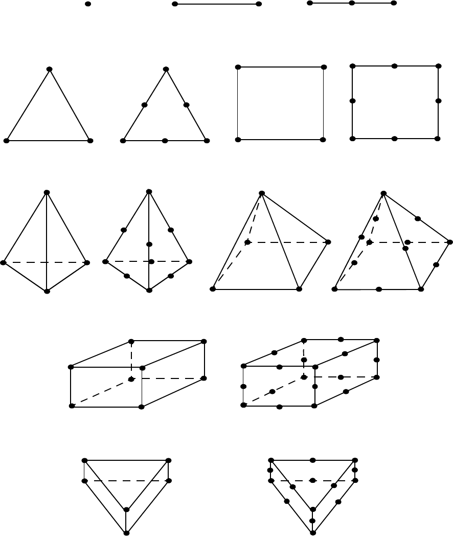
11.3 EnSight5 General Description
11-116 EnSight 7 User Manual
Supported EnSight5 Elements
The elements that are supported by the EnSight5 format are:
eight node hexahedron twenty node hexahedron
six node pentahedron
9
10
7
8
12123
12
3
12
3
4
56
1
2
3
4
12
3
45
6
7
8
12
3
4
5
6
1
2
3
4
5
6
9
10
7
8
1
2
3
4
56
11
12
13
14
15
16
17
18
19
20
two node bar three node bar
three node triangle six node triangle four node quadrangle eight node quadrangle
four node tetrahedron ten node tetrahedron
1
point
1
2
3
4
1
4
8
2
3
5
6
7
5 node pyramid 13 node pyramid
11
2
2
3
3
44
5
5
6
7
8
9
10
11
12
13
fifteen node pentahedron (wedge)
1
2
3
4
5
6
7
8
9
10
11
12
13
14
15
(wedge)
Figure 11-4
Supported EnSight5 Elements
11.3 EnSight5 Geometry File Format
EnSight 7 User Manual 11-117
EnSight5 Geometry File Format
The EnSight5 format consists of keywords followed by information. The
following items are important to remember when working with EnSight5
geometry files:
1. You do not have to assign node IDs. If you do, the element connectivities are
based on the node numbers. If you let EnSight assign the node IDs, the nodes
are considered to be sequential starting at node 1, and element connectivity is
done accordingly. If node IDs are set to off, they are numbered internally;
however, you will not be able to display or query on them. If you have node
IDs in your data, you can have EnSight ignore them by specifying “node id
ignore.” Using this option may reduce some of the memory taken up by the
Client and Server, but remember that display and query on the nodes will not
be available.
2. You do not need to specify element IDs. If you specify element IDs, or you let
EnSight assign them, you can show them on the screen. If they are set to off,
you will not be able to show or query on them. If you have element IDs in
your data you can have EnSight ignore them by specifying “element id
ignore.” Using this option will reduce some of the memory taken up by the
Client and Server. This may or may not be a significant amount, and
remember that display and query on the elements will not be available.
3. The format of integers and real numbers must be followed (See the Geometry
Example below).
4. Integers are written out using the following integer format:
From C:
8d
format
From FORTRAN:
i8
format
Real numbers are written out using the following floating-point format:
From C:
12.5e
format
From FORTRAN:
e12.5
format
The number of integers or reals per line must also be followed!
5. By default, a Part is processed to show the outside boundaries. This
representation is loaded to the Client host system when the geometry file is
read (unless other attributes have been set on the workstation, such as feature
angle).
6. Coordinates must be defined before any Parts can be defined. The different
elements can be defined in any order (that is, you can define a hexa8 before a
bar2).
Generic Format Not all of the lines included in the following generic example file are necessary:
description line 1
description line 2
node id <off/given/assign/ignore>
element id <off/given/assign/ignore>
coordinates
# of points
id x y z
id x y z
11.3 EnSight5 Geometry File Format
11-118 EnSight 7 User Manual
id x y z
.
.
.
part #
description line
point
number of points
id nd
id nd
id nd
.
.
.
bar2
number of bar2’s
id nd nd
id nd nd
id nd nd
.
.
.
bar3
number of bar3’s
id nd nd nd
id nd nd nd
id nd nd nd
.
.
.
tria3
number of three node triangles
id nd nd nd
id nd nd nd
id nd nd nd
.
.
.
tria6
number of six node triangles
id nd nd nd nd nd nd
.
.
.
quad4
number of quad 4’s
id nd nd nd nd
id nd nd nd nd
id nd nd nd nd
id nd nd nd nd
.
.
.
quad8
number of quad 8’s
id nd nd nd nd nd nd nd nd
id nd nd nd nd nd nd nd nd
id nd nd nd nd nd nd nd nd
id nd nd nd nd nd nd nd nd
.
.
11.3 EnSight5 Geometry File Format
EnSight 7 User Manual 11-119
.
tetra4
number of 4 node tetrahedrons
id nd nd nd nd
id nd nd nd nd
id nd nd nd nd
id nd nd nd nd
.
.
.
tetra10
number of 10 node tetrahedrons
id nd nd nd nd nd nd nd nd nd nd
id nd nd nd nd nd nd nd nd nd nd
id nd nd nd nd nd nd nd nd nd nd
id nd nd nd nd nd nd nd nd nd nd
.
.
.
pyramid5
number of 5 node pyramids
id nd nd nd nd nd
id nd nd nd nd nd
id nd nd nd nd nd
id nd nd nd nd nd
.
.
.
pyramid13
number of 13 node pyramids
id nd nd nd nd nd nd nd nd nd nd nd nd nd
id nd nd nd nd nd nd nd nd nd nd nd nd nd
id nd nd nd nd nd nd nd nd nd nd nd nd nd
id nd nd nd nd nd nd nd nd nd nd nd nd nd
.
.
.
hexa8
number of 8 node hexahedrons
id nd nd nd nd nd nd nd nd
id nd nd nd nd nd nd nd nd
id nd nd nd nd nd nd nd nd
id nd nd nd nd nd nd nd nd
.
.
.
hexa20
number of 20 node hexahedrons
id nd nd nd nd nd nd nd nd nd nd nd nd nd nd nd nd nd nd nd nd
id nd nd nd nd nd nd nd nd nd nd nd nd nd nd nd nd nd nd nd nd
id nd nd nd nd nd nd nd nd nd nd nd nd nd nd nd nd nd nd nd nd
id nd nd nd nd nd nd nd nd nd nd nd nd nd nd nd nd nd nd nd nd
id nd nd nd nd nd nd nd nd nd nd nd nd nd nd nd nd nd nd nd nd
.
.
.
penta6
number of 6 node pentahedrons
id nd nd nd nd nd nd
id nd nd nd nd nd nd
id nd nd nd nd nd nd
11.3 EnSight5 Geometry File Format
11-120 EnSight 7 User Manual
id nd nd nd nd nd nd
id nd nd nd nd nd nd
.
.
.
penta15
number of 15 node pentahedrons
id nd nd nd nd nd nd nd nd nd nd nd nd nd nd nd
id nd nd nd nd nd nd nd nd nd nd nd nd nd nd nd
id nd nd nd nd nd nd nd nd nd nd nd nd nd nd nd
id nd nd nd nd nd nd nd nd nd nd nd nd nd nd nd
id nd nd nd nd nd nd nd nd nd nd nd nd nd nd nd
.
.
.
EnSight5 Geometry The following is an example of an EnSight geometry file:
Example
this is an example problem
this is the second description line
node id given
element id given
coordinates
10
5 1.00000e+00 0.00000e+00 0.00000e+00
100 0.00000e+00 1.00000e+00 0.00000e+00
200 0.00000e+00 0.00000e+00 1.00000e+00
40 1.00000e+00 1.00000e+00 0.00000e+00
22 1.00000e+00 0.00000e+00 1.00000e+00
1000 2.00000e+00 0.00000e+00 0.00000e+00
55 0.00000e+00 2.00000e+00 0.00000e+00
44 0.00000e+00 0.00000e+00 2.00000e+00
202 2.00000e+00 2.00000e+00 0.00000e+00
101 2.00000e+00 0.00000e+00 2.00000e+00
part 1
This is Part 1, a pretty strange Part
tria3
2
101 100 200 40
201 101 5 1000
tetra4
1
102 100 202 101 1000
part 2
This is Part 2, it’s pretty strange also
bar2
1
103 101 1000
11.3 EnSight5 Result File Format
EnSight 7 User Manual 11-121
EnSight5 Result File Format
The Result file is an ASCII free format file that contains variable and time step
information that pertains to a Particular geometry file. The following information
is included in this file:
• Number of scalar variables
• Number of vector variables
• Number of time steps
• Starting file number extension and skip-by value
• Flag that specifies whether there is changing geometry
• Names of the files that contain the values of scalar and vector variables
• The names of the geometry files that will be used for the changing
geometry.
The format of the EnSight5 result file is as follows:
•Line 1
Contains the number of scalar variables, the number of vector variables
and a geometry-changing flag. (If the geometry-changing flag is 0, the
geometry of the model does not change over time. If it is 1, then there is
connectivity changing geometry. If it is 2, then there is coordinate only
changing geometry.)
•Line 2
Indicates the number of time steps that are available.
•Line 3
Lists the time that is associated with each time step. There must be the
same number of values as are indicated in Line 2. This “line” can actually
span several lines in the file. You do not have to have one very long line.
•Line 4
Specified only if more than one time step is indicated in Line 2. The two
values on this line indicate the file extension value for the first time step
and the offset between files. If the values on this line are 0 5, the first time
step available has a subscript of 0, the second time step available has a
subscript of 5, the third time step has a subscript of 10, and so on.
•Line 5
Contains the names of the geometry files that will be used for changing
geometry. This line exists only if the flag on Line 1 is set to 1 or 2. The
geometry file name must follow the EnSight5 wild card specification.
• Line 6 through Line [5+N] where N is the number of scalar variables
specified in Line 1.
List BOTH the file names AND variable description that correspond to
each scalar variable. There must be a file name for each scalar variable
that is specified in Line 1.
11.3 EnSight5 Result File Format
11-122 EnSight 7 User Manual
If there is more than one time step, the file name must follow the
EnSight5 wild card specification. See Note below.
• Lines that follow the scalar variable files.
List the file names that correspond to each vector variable. There must be
a file name for each vector variable that is specified in Line 1. If there is
more than one time step, the file name must follow the EnSight5 wild
card specification. See Note below.
Note: Variable descriptions have the following restrictions:
The variable description is limited to 19 characters in the current release.
Duplicate variable descriptions are not allowed.
Leading and trailing white space will be eliminated.
Variable descriptions must not start with a numeric digit.
Variable descriptions must not contain any of the following reserved characters:
( [ + @ ! * $
) ] - space # ^ /
The generic format of a result file is as follows:
#_of_scalars #_of_vectors geom_chang_flag
#_of_timesteps
time1 time2 time3 .....
start_file_# skip_by_value
geometry_file_name.geo**
scalar0_file_name** description (19 characters max)
scalar1_file_name** description
.
.
.
vector0_file_name** description (19 characters max)
vector1_file_name** description
.
EnSight5 Result
File Example 1 The following example illustrates a result file specified for a non-changing
geometry file with only one time step:
210
1
0.0
exone.scl0 pressure
exone.scl1 temperature
exone.dis0 velocity
EnSight5 Result
File Example 2 This example illustrates a result file that specifies a connectivity changing
geometry that has multiple time steps.
121
4
1.0 2.0 2.5 5.0
01
extwo.geom**
pres.scl** pressure
vel.dis** velocity
grad.dis** gradient
The following files would be needed for example 2:
11.3 EnSight5 Variable File Format
EnSight 7 User Manual 11-123
extwo.geom00 pres.scl00 vel.dis00 grad.dis00
extwo.geom01 pres.scl01 vel.dis01 grad.dis01
extwo.geom02 pres.scl02 vel.dis02 grad.dis02
extwo.geom03 pres.scl03 vel.dis03 grad.dis03
EnSight5 Wild Card Name Specification
If multiple time steps are involved, the file names must conform to the EnSight5
wild-card specification. This specification is as follows:
• File names must include numbers that are in ascending order from
beginning to end.
• Numbers in the files names must be zero filled if there is more than one
significant digit.
• Numbers can be anywhere in the file name.
• When the file name is specified in the EnSight5 result file, you must
replace the numbers in the file with an asterisk(*). The number of
asterisks specified is the number of significant digits. The asterisk must
occupy the same place as the numbers in the file names.
EnSight5 Variable File Format
Variables files have one description line followed by a value for each node. For a
scalar file there is one value per node, while for vector files there are three values
per node.
The values must be written in the following floating point format (6 per line as
shown in the examples below):
From C:
12.5e
format
From FORTRAN:
e12.5
format
The format of a variables file is as follows:
•Line 1
This line is a description line.
• Line 2 through the end of the file contains the values at each node in the
model. A generic example:
A description line
*.*****E+** *.*****E+** *.*****E+** *.*****E+** *.*****E+** *.*****E+**
*.*****E+** *.*****E+** *.*****E+** *.*****E+** *.*****E+** *.*****E+**
*.*****E+** *.*****E+** *.*****E+** *.*****E+** *.*****E+** *.*****E+**
EnSight5 Variable
File Example 1 This example shows a scalar file for a geometry with seven defined nodes.
These are the pressure values for a 7 node geometry
1.00000E+00 2.00000E+00 3.00000E+00 4.00000E+00 5.00000E+00 6.00000E+00
7.00000E+00
EnSight5 Variable
File Example 2 This example shows the vector file for a geometry with seven defined nodes.
These are the velocity values for a 7 node geometry
1.00000E+00 1.00000E+00 1.00000E+00 2.00000E+00 2.00000E+00 2.00000E+00
3.00000E+00 3.00000E+00 3.00000E+00 4.00000E+00 4.00000E+00 4.00000E+00
11.3 EnSight5 Measured/Particle File Format
11-124 EnSight 7 User Manual
5.00000E+00 5.00000E+00 5.00000E+00 6.00000E+00 6.00000E+00 6.00000E+00
7.00000E+00 7.00000E+00 7.00000E+00
EnSight5 Measured/Particle File Format
This file allows you to define Particle locations, sizes, etc. to display with the
geometry. Typical uses are fuel droplets for combustion analysis or data derived
from experiments on prototypes.
The measured/Particle files consist of the following:
• Measured/Particle geometry file (referenced by the measured results file)
• Measured/Particle results file (the filename which is put into the Data
Reader’s “(Set) Measured” field)
• Measured/Particle variables file (referenced by the measured results file)
The format of the EnSight5 Measured/Particle geometry file is described below.
Note that there is only one description line and there must be an ID for each
measured point.
Note also that the number of Particles can be different in each of the geometry file
(if you have transient data), however, the number of values in each of the
corresponding variable files must coincide, and the IDs of the Particles must be
consistent in order to track the Particles at intermediate times or locations.
The format of an EnSight5 Measured/Particle geometry file is as follows:
•Line 1
This line is a description line.
•Line 2
Indicates that this file contains Particle coordinates. The words “particle
coordinates” should be entered on this line without the quotes.
•Line 3
Specifies the number of Particles.
• Line 4 through the end of the file.
Each line contains the ID and the X, Y, and Z coordinates of each Particle.
The format of this line is “integer real real real” written out in the
following format:
From C:
%8d%12.5e%12.5e%12.5e
format
From FORTRAN:
i8, 3e12.5
format
A generic measured/Particle geometry file is as follows:
A description line
particle coordinates
#_of_Particles
id xcoord ycoord zcoord
id xcoord ycoord zcoord
id xcoord ycoord zcoord
11.3 EnSight5 Measured/Particle File Format
EnSight 7 User Manual 11-125
.
.
.
EnSight5 Measured
Geometry/Particle The following illustrates an EnSight5 Measured Geometry/Particle file with seven
File Example points:
This is a simple ensight5 measured geometry/particle file
particle coordinates
7
101 0.00000E+00 0.00000E+00 0.00000E+00
102 1.00000E+00 0.00000E+00 0.00000E+00
103 1.00000E+00 1.00000E+00 0.00000E+00
104 0.00000E+00 1.00000E+00 0.00000E+00
205 5.00000E-01 0.00000E+00 2.00000E+00
206 5.00000E-01 1.00000E+00 2.00000E+00
307 0.00000E+00 0.00000E+00-1.50000E+00
EnSight5 Measured/ The format of the EnSight5 Measured/Particle results file is as follows:
Particle File Format
•Line 1
Contains the number of scalar variables, the number of vector variables,
and a measured geometry changing flag. If the measured geometry
changing flag is 0, only one time step is indicated.
•Line 2
Indicates the number of available time steps.
•Line 3
Lists the time that is associated with each time step. The time step
information does not have to coincide with the model time step
information. This “line” can actually span several lines in the file. You do
not have to have one very long line.
•Line 4
Specified only if Line 2 specifies more than one time step. The line
contains two values; the first value indicates the file extension value for
the first time step, and the second value indicates the offset between files.
If this line contains the values 0 and 5, the first time step has a subscript of
0, the second of 5, the third of 10, and so on.
•Line 5
Contains the name of the measured geometry file. If there is more than
one time step, the file name must follow the EnSight wild card
specification.
• Line 6 through Line [5+N] where N is the number of scalar variables
specified in Line 1.
List the file names that correspond to each scalar variable. There must be
a file name for each scalar variable that is specified in Line 1. If there is
more than one time step, the file name must follow the EnSight wild card
11.3 EnSight5 Measured/Particle File Format
11-126 EnSight 7 User Manual
specification.
• Lines that follow the scalar variable files.
List the names of the files that correspond to each vector variable. There
must be a file name for each vector variable that is specified in Line 1. If
there is more than one time step, the file name must follow the EnSight
wild card specification.
A generic EnSight5 Measured/Particle results file is as follows:
#_of_scalars #_of_vectors geom_chang_flag
#_of_timesteps
time1 time2 time3 .....
start_file_# skip_by_value
measured_geom_file_name**
scalar0_file_name** description
scalar1_file_name** description
.
.
.
vector0_file_name** description
vector1_file_name** description
.
.
.
Measured/Particle
Results File This example illustrates an EnSight5 Measured/Particle result file that specifies a
Example 1 non-changing geometry with only one time step:
210
1
0.0
exone.geom
exone.scl0 pressure
exone.scl1 temperature
exone.dis0 velocity
Measured/Particle
Results File This example illustrates an EnSight5 Measured/Particle result file that specifies a
Example 2 changing geometry with multiple time steps:
121
4
1.0 2.0 2.5 5.0
01
extwo.geom**
pres.scl** pressure
vel.dis** velocity
grad.dis** gradient
The following files are needed for Example 2:
extwo.geom00pres.scl00vel.dis00 grad.dis00
extwo.geom01pres.scl01vel.dis01 grad.dis01
extwo.geom02pres.scl02vel.dis02 grad.dis02
extwo.geom03pres.scl03vel.dis03 grad.dis03
Measured /Particle The EnSight5 Measured/Particle variable files referred to in the measured Results
Results Variable files file follow the same format as EnSight5 Variable files. The number of values in
11.3 Writing EnSight5 Binary Files
EnSight 7 User Manual 11-127
each of these variable files must correspond properly to the number of Particles in
the corresponding measured geometry files.
Writing EnSight5 Binary Files
This section describes the EnSight5 binary files. This format is used to increase
the speed of reading data into EnSight. A utility exists for converting EnSight5
ASCII files to EnSight5 binary files—it is called asciitobin5 and is found on the
release tape under ensight/server/utilities/asciitobin5.
For binary files, there is a header that designates the type of binary file. This
header is: “C Binary” or “Fortran Binary.” This must be the first thing in the file.
The format for the file is then essentially the same format as the ASCII format,
with the following exceptions:
The ASCII format puts the node and element ids on the same “line” as the
corresponding coordinates. The BINARY format writes all node id’s then
all coordinates.
The ASCII format puts all element id’s of a type within a Part on the same
“line” as the corresponding connectivity. The BINARY format writes all
the element ids for that type, then all the corresponding connectivities of
the elements.
In all the descriptions of binary files that follow, the number on the left end of the
line corresponds to the type of write of that line, according to the following code:
1. This is a write of 80 characters to the file:
C example:
char buffer[80];
strcpy(buffer,”C Binary”);
fwrite(buffer,sizeof(char),80,file_ptr);
FORTRAN:
character*80 buffer
buffer = “Fortran Binary”
write(10) buffer
2. This is a write of a single integer:
C example:
fwrite(&num_nodes,sizeof(int),1,file_ptr);
FORTRAN:
write(10) num_nodes
3. This is a write of an integer array:
C example:
fwrite(node_ids,sizeof(int),num_nodes,file_ptr);
FORTRAN:
write(10) (node_ids(i),i=1,num_nodes)
4. This is a write of a float array:
C example:
fwrite(coords,sizeof(float),3*num_nodes,file_ptr);
FORTRAN:
write(10) ((coords(i,j),i=1,3),j=1,num_nodes)
11.3 Writing EnSight5 Binary Files
11-128 EnSight 7 User Manual
(Note: Coords is a single precision array, double precision will not work!)
EnSight5 Binary
Geometry File Format An EnSight5 binary geometry file contains information in the following order:
(1) <C Binary/Fortran Binary>
(1) description line 1
(1) description line 2
(1) node id <given/off/assign/ignore>
(1) element id <given/off/assign/ignore>
(1) coordinates
(2) #_of_points
(3) [point_ids]
(4) coordinate_array
(1) part #
(1) description line
(1) element_type
(2) #_of_element_type
(3) [element_ids] for the element_type
(3) connectivities for the element_type
(1) element_type
(2) #_of_element_type
(3) [element_ids] for the element_type
(3) connectivities for the element_type
.
.
.
(1) part #
(1) description line
(1) element_type
(2) #_of_element_type
(3) [element_ids] for the element_type
(3) connectivities for the element_type
(1) element_type
(2) #_of_element_type
(3) [element_ids] for the element_type
(3) connectivities for the element_type
.
.
.
Binary Scalar An EnSight5 binary scalar file contains information in the following order:
(1) description line
(4) scalar_array
Binary Vector An EnSight5 binary vector file contains information in the following order:
(1) description line
(4) vector_array
11.4 FAST UNSTRUCTURED Results File Format
11-130 EnSight 7 User Manual
11.4 FAST UNSTRUCTURED Results File Format
FAST UNSTRUCTURED input data consists of the following:
• Geometry file (required) (GRID file).
• Results file (optional).
• EnSight5 Measured/Particle Files (optional). The measured .res file
references the measured geometry and variable files.
FAST UNSTRUCTURED data files can be read as:
Workstation: ASCII, C Binary, or FORTRAN binary
Cray: ASCII, C Binary, or COS-Blocked FORTRAN binary
Due to the different number of representations on a Cray Research vector system
and workstations, binary files created on a Cray Research vector system can not
be read on the workstation, and visa versa.
EnSight reads the geometry (grid files) directly. However, an EnSight-like results
file is needed in order to read the results unless a “standard” Q-file is provided in
its place. See FAST UNSTRUCTURED Result File below.
FAST UNSTRUCTURED Geometry file notes
Only the single zone format can be read into EnSight. Any tetrahedral elements
will be placed into the first “domain” Part. Triangular elements are placed into
Parts based on their “tag” value.
The FAST UNSTRUCTURED solution file or function file formats can be used
for variable results. The I J K values need to be I=Number of points and J=K=1.
This does require the use of a modified EnSight results file as explained below.
Node and element numbers are assigned sequentially allowing for queries to be
made within EnSight. Tetrahedron elements will be assigned before triangular
elements.
FAST UNSTRUCTURED Result file format
The FAST UNSTRUCTURED result file was defined by CEI and is very similar
to the EnSight results file and contains information needed to relate variable
names to variable files, step information, etc. There is a slight variation from the
normal EnSight results file because of the differences between the solution (Q
file) and function files. The difference lies on the lines which relate variable
filenames to a description. These lines have the following format:
<filename> <type> <number(s)> <description>
See FAST UNSTRUCTURED Result File below for the definition of each.
The following information is included in a FAST UNSTRUCTURED result file:
• Number of scalar variables
• Number of vector variables
• Number of time steps
11.4 FAST UNSTRUCTURED Results File Format
EnSight 7 User Manual 11-131
• Starting file number extension and skip-by value
• Flag that specifies whether there is changing geometry.
• Names of the files that contain the values of scalar and vector variables.
An indication as to the type of the file being used for the variable, which
variable in the file and the name given to that variable.
• The names of the geometry files that will be used for the changing
geometry.
Generic FAST UNSTRUCTURED Result File Format
The format of the Result file is as follows:
•Line 1
Contains the number of scalar variables, the number of vector variables
and a geometry changing flag. If the geometry changing flag is 0, the
geometry of the model does not change over time. If the flag is 1, the
geometry can change connectivity. If the flag is 2, only coordinates can
change.
•Line 2
Indicates the number of time steps that are available. If this number is
positive, then line 3 information must be present. If this number is
negative, then Line 3 information must not be present and the times will
be read from the solution file. Thus, one must have a solution file in one
of the lines from Line 6 on.
•Line 3
Lists the time that is associated with each time step. There must be the
same number of values as are indicated in Line 2. This “line” can actually
span several lines in the file. Specify only if Line 2 value is positive.
•Line 4
Specified only if more than one time step is indicated in Line 2. The two
values on this line indicate the file extension value for the first time step
and the offset between files. If the values on this line are 0 5, the first time
step available has a subscript of 0, the second time step available has a
subscript of 5, the third time step has a subscript of 10, and so on.
•Line 5
This line exists only if the changing geometry flag on Line 1 has been set
to 1 or 2. Line contains name of the FAST UNSTRUCTURED grid file.
The file name must follow the EnSight wild card specification.
• Line 6 through Line [5+N] where N is the number of scalar variables
specified in Line 1.
List the file names that correspond to each scalar variable. There must be
a file name for each scalar variable that is specified in Line 1. If there is
more than one time step, the file name must follow the EnSight wild card
specification.
These lines also contain the type of file being used, solution or function,
and the location of the variable value in the file. The contents are:
11.4 FAST UNSTRUCTURED Results File Format
11-132 EnSight 7 User Manual
<filename> <type> <number> <description>
where filename is the name of solution file or function file containing the
variable; type is “S” for solution file, or “F” for function file; numberis
which variable in the file to use (specify just one number); and
description
is the Description of the variable.
The solution file (“s”) is the traditional .q file in which normally the first
variable is density, the second through fourth variables are the
components of momentum, and the fifth variable is total energy.
• Lines that follow the scalar variable files.
List the file names that correspond to each vector variable. There must be
a file name for each vector variable that is specified in Line 0. If there is
more than one time step, the file name must follow the EnSight wild card
specification.
These lines also contain the type of file being used, solution or function,
and the location(s) of the variable values in the file. The contents are:
<filename> <type> <numbers> <description>
where filename is the name of solution file or function file containing the
variable; type is “S” for solution file, or “F” for function file; numbersare
which variables in the file to use (specify just three numbers); and
description is the Description of the variable.
The generic format of the result file is as follows:
#_of_scalars #_of_vectors geom_chng_flag
#_of_timesteps
time1 time2 time3 .....
start_file_# skip_by_value
geometry_file_name.geo**
scalar0_file_name** type # description
scalar1_file_name** type # description
.
.
.
vector0_file_name** type###description
vector1_file_name** type###description
.
.
.
FAST UNSTRUCTURED This example illustrates a result file that specifies a non-changing geometry with
Example only one time step.
320
1
0.0
block.sol S 1 Density
block.sol S 5 Total_Energy
block.scl F 1 Temperature
block.varF123Displacement
block.solS234Momentum
Thus, this model will get two scalars from the solution file (block.sol). The first is
Density in the first location in the file and the next is Total energy in the fifth
11.4 FAST UNSTRUCTURED Results File Format
EnSight 7 User Manual 11-133
location in the solution file. It will also get a Temperature scalar from the first
location in the function file (block.scl).
It will get a Displacement vector from the function file called block.var. The three
components of this vector are in the 1st, 2nd, and 3rd locations in the file. Finally,
a Momentum vector will be obtained from the 2nd, 3rd, and 4th locations of the
solution file.
Example 2 is somewhat similar, except that it is transient, with coordinate
changing geometry. Note also that the times will come from the solution file.
322
-10
01
block***.grid
block***.sol S 1 Density
block***.sol S 5 Total_Energy
block***.scl F 1 Temperature
block***.varF123Displacement
block***.solS234Momentum
11.5 FLUENT UNIVERSAL Results File Format
11-134 EnSight 7 User Manual
11.5 FLUENT UNIVERSAL Results File Format
This section describes the FLUENT results file format and provides an example of
this file. For transient cases, you must supply this result file. For static models this
file is not required. The FLUENT result file is a slightly modified EnSight5
results file and provides a way to describe multiple time-step FLUENT Universal
files to EnSight.
When using multiple FLUENT files with this result file definition, you must make
sure that the files contain the same defined variables. In other words, any variable
that exists in one must exist in all.
The Result file is an ASCII free format file that contains time step and universal
file information for each available time step. The following information is
included in this file:
• Number of time steps
• Simulation Time Values
• Starting file number extension and skip-by value
• Name of the universal file with EnSight wild card specification.
The format of the Result file is as follows:
•Line 1
Indicates the number of time steps that are available.
•Line 2
Lists the time that is associated with each time step. There must be the
same number of values as are indicated in Line 1. This “line” can actually
span several lines in the file. You do not have to have one very long line.
•Line 3
Specified only if more than one time step is indicated in Line 1. The two
values on this line indicate the file extension value for the first time step
and the offset between files. If the values on this line are 0 5, the first time
step available has a subscript of 0, the second time step available has a
subscript of 5, the third time step has a subscript of 10, and so on.
•Line 4
Contains the names of the universal file that will be used for the changing
time step information. The universal file name must follow the EnSight5
wild card specification.
The generic format of the result file is as follows:
#_of_timesteps
time1 time2 time3 .....
start_file_# skip_by_value
universal_file_name***
11.6 Movie.BYU Results File Format
11-136 EnSight 7 User Manual
11.6 Movie.BYU Results File Format
For transient cases, you must supply an EnSight result file. The result file for the
Movie.BYU case is exactly the same as for EnSight5 (it is repeated below for
your ease).
The Result file is an ASCII free format file that contains variable and time step
information that pertains to a Particular geometry file. The following information
is included in this file:
• Number of scalar variables
• Number of vector variables
• Number of time steps
• Starting file number extension and skip-by value
• Flag that specifies whether there is changing geometry
• Names of the files that contain the values of scalar and vector variables
• The names of the geometry files that will be used for the changing
geometry.
The format of the Movie.BYU (EnSight5) result file is as follows:
•Line 1
Contains the number of scalar variables, the number of vector variables
and a geometry-changing flag. (If the geometry-changing flag is 0, the
geometry of the model does not change over time. If it is 1, then there is
connectivity changing geometry. If it is 2, then there is coordinate only
changing geometry.)
•Line 2
Indicates the number of time steps that are available.
•Line 3
Lists the time that is associated with each time step. There must be the
same number of values as are indicated in Line 2. This “line” can actually
span several lines in the file. You do not have to have one very long line.
•Line 4
Specified only if more than one time step is indicated in Line 2. The two
values on this line indicate the file extension value for the first time step
and the offset between files. If the values on this line are 0 5, the first time
step available has a subscript of 0, the second time step available has a
subscript of 5, the third time step has a subscript of 10, and so on.
•Line 5
Contains the names of the geometry files that will be used for changing
geometry. This line exists only if the flag on Line 1 is set to 1 or 2. The
geometry file name must follow the EnSight5 wild card specification.
• Line 6 through Line [5+N] where N is the number of scalar variables
specified in Line 1.
11.6 Movie.BYU Results File Format
EnSight 7 User Manual 11-137
List BOTH the file names AND variable description that correspond to
each scalar variable. There must be a file name for each scalar variable
that is specified in Line 1.
If there is more than one time step, the file name must follow the
EnSight5 wild card specification. See Note below.
• Lines that follow the scalar variable files.
List the file names that correspond to each vector variable. There must be
a file name for each vector variable that is specified in Line 1. If there is
more than one time step, the file name must follow the EnSight5 wild
card specification. See Note below.
Note: Variable descriptions have the following restrictions:
The variable description is limited to 19 characters in the current release.
Duplicate variable descriptions are not allowed.
Leading and trailing white space will be eliminated.
Variable descriptions must not start with a numeric digit.
Variable descriptions must not contain any of the following reserved characters:
( [ + @ ! * $
) ] - space # ^ /
The generic format of a result file is as follows:
#_of_scalars #_of_vectors geom_chang_flag
#_of_timesteps
time1 time2 time3 .....
start_file_# skip_by_value
geometry_file_name.geo**
scalar0_file_name** description (19 characters max)
scalar1_file_name** description
.
.
.
vector0_file_name** description (19 characters max)
vector1_file_name** description
.
Movie.BYU Result
File Example 1 The following example illustrates a result file specified for a non-changing
geometry file with only one time step:
210
1
0.0
exone.scl0 pressure
exone.scl1 temperature
exone.dis0 velocity
Movie.BYU Result
File Example 2 This example illustrates a result file that specifies a connectivity changing
geometry that has multiple time steps.
121
4
1.0 2.0 2.5 5.0
01
extwo.geom**
pres.scl** pressure
11.6 Movie.BYU Results File Format
11-138 EnSight 7 User Manual
vel.dis** velocity
grad.dis** gradient
The following files would be needed for example 2:
extwo.geom00 pres.scl00 vel.dis00 grad.dis00
extwo.geom01 pres.scl01 vel.dis01 grad.dis01
extwo.geom02 pres.scl02 vel.dis02 grad.dis02
extwo.geom03 pres.scl03 vel.dis03 grad.dis03
11.7 PLOT3D Results File Format
EnSight 7 User Manual 11-139
11.7 PLOT3D Results File Format
PLOT3D input data consists of the following:
• Geometry file (required) (GRID file).
• Results file (optional).
• EnSight5 Measured/Particle Files (optional). The measured .res file
references the measured geometry and variable files.
PLOT3D data files can be read as:
Workstation: ASCII, C Binary, or FORTRAN binary
Cray: ASCII, C Binary, or COS-Blocked FORTRAN binary
(see PLOT3D Reader, in Section 2.1)
Due to the different number of representations on a Cray Research vector system
and workstations, binary files created on a Cray Research vector system can not
be read on the workstation, and visa versa.
EnSight attempts to ensure that the format of the file being read matches the
format you have selected in the Data Reader dialog. However, if you specify that
the file is C binary, and it is really FORTRAN binary, this will not be detected and
erroneous values will be loaded.
EnSight reads the geometry (xyz files) directly. However, an EnSight-like results
file (described below) is needed in order to read the results, unless a “standard” Q-
file is provided in its place.
PLOT3D Geometry file notes
The following information is required in order to read PLOT3D files correctly:
1. whether there is Iblanking information in the file
2. whether files are in ASCII, C Binary, or FORTRAN binary
3. whether the file is “Single Zone” or Multi-Zoned”
4. whether the model is 1D, 2D, or 3D in nature.
Iblanking can be one of the following:
0 = Outside (Blanked Out)
1 = Inside
2 = Interior boundaries
<0 = zone that neighbors
If single zone with Iblanking, you can build EnSight Parts from the inside
portions, blanked-out portions, or internal boundary portions. If single zone, you
can also specify I, J, K limiting ranges for Parts to be created.
If Multi-zoned with Iblanking, you can additionally build Parts that are the
boundary between two zones. (For boundary you must specify exactly two zones.)
If Multi-zoned and not using the “between boundary” option, a Part can span
several zones.
11.7 PLOT3D Results File Format
11-140 EnSight 7 User Manual
If Multi-zoned, the dimension of the problem is forced to be 3D.
There can be nodes in different zones which have the same coordinates. No
attempt has been made to merge these. Thus, on shared zone boundaries, there
will likely be nodes on top of nodes. One negative effect of this is that node labels
will be on top of each other.
Currently EnSight only prints out the global conditions in the solution file,
fsmach, alpha, re, and time. It does not do anything else with them.
Node and element numbers are assigned in a sequential manner. Queries can be
made on these node and element numbers or on nodes by I, J, and K.
PLOT3D Result file format
The PLOT3D result file was defined by CEI and is very similar to the EnSight
results file and contains information needed to relate variable names to variable
files, step information, etc. There is a slight variation from the normal EnSight
results file because of the differences between the solution (Q file) and function
files. The difference lies on the lines which relate variable filenames to a
description. These lines have the following format:
<filename> <type> <number(s)> <description>
See PLOT3D Result File below for the definition of each.
The following information is included in a PLOT3D result file:
• Number of scalar variables
• Number of vector variables
• Number of time steps
• Starting file number extension and skip-by value
• Flag that specifies whether there is changing geometry.
• Names of the files that contain the values of scalar and vector variables.
An indication as to the type of the file being used for the variable, which
variable in the file and the name given to that variable.
• The names of the geometry files that will be used for the changing
geometry.
Generic PLOT3D Result File Format
The format of the Result file is as follows:
•Line 1
Contains the number of scalar variables, the number of vector variables
and a geometry changing flag. If the geometry changing flag is 0, the
geometry of the model does not change over time. Only the coordinates
can change for a PLOT3D file at present time.
•Line 2
Indicates the number of time steps that are available.
11.7 PLOT3D Results File Format
EnSight 7 User Manual 11-141
•Line 3
Lists the time that is associated with each time step. There must be the
same number of values as are indicated in Line 2. This “line” can actually
span several lines in the file.
•Line 4
Specified only if more than one time step is indicated in Line 2. The two
values on this line indicate the file extension value for the first time step
and the offset between files. If the values on this line are 0 5, the first time
step available has a subscript of 0, the second time step available has a
subscript of 5, the third time step has a subscript of 10, and so on.
•Line 5
This line exists only if the changing geometry flag on Line 1 has been set
to 1. Line contains name of the PLOT3D xyz file. The file name must
follow the EnSight wild card specification.
• Line 6 through Line [5+N] where N is the number of scalar variables
specified in Line 1.
List the file names that correspond to each scalar variable. There must be
a file name for each scalar variable that is specified in Line 1. If there is
more than one time step, the file name must follow the EnSight wild card
specification.
These lines also contain the type of file being used, solution or function,
and the location of the variable value in the file. The contents are:
<filename> <type> <number> <description>
where filename is the name of solution file or function file containing the
variable; type is “S” for solution file, or “F” for function file; numberis
which variable in the file to use (specify just one number); and description
is the Description of the variable.
The solution file (“s”) is the traditional .q file in which normally the first
variable is density, the second through fourth variables are the
components of momentum, and the fifth variable is total energy.
• Lines that follow the scalar variable files.
List the file names that correspond to each vector variable. There must be
a file name for each vector variable that is specified in Line 1. If there is
more than one time step, the file name must follow the EnSight wild card
specification.
These lines also contain the type of file being used, solution or function,
and the location(s) of the variable values in the file. The contents are:
<filename> <type> <numbers> <description>
where filename is the name of solution file or function file containing the
variable; type is “S” for solution file, or “F” for function file; numbersare
which variables in the file to use (specify just three numbers); and
description is the Description of the variable.
11.7 PLOT3D Results File Format
11-142 EnSight 7 User Manual
The generic format of the result file is as follows:
#_of_scalars #_of_vectors geom_chng_flag
#_of_timesteps
time1 time2 time3 .....
start_file_# skip_by_value
geometry_file_name.geo**
scalar0_file_name** type # description
scalar1_file_name** type # description
.
.
.
vector0_file_name** type###description
vector1_file_name** type###description
.
.
.
PLOT3D Example This example illustrates a result file that specifies a non-changing geometry with
only one time step.
320
1
0.0
block.sol S 1 Density
block.sol S 5 Total_Energy
block.scl F 1 Temperature
block.varF123Displacement
block.solS234Momentum
Thus, this model will get two scalars from the solution file (block.sol). The first is
Density in the first location in the file and the next is Total energy in the fifth
location in the solution file. It will also get a Temperature scalar from the first
location in the function file (block.scl).
It will get a Displacement vector from the function file called block.var. The three
components of this vector are in the 1st, 2nd, and 3rd locations in the file. Finally,
a Momentum vector will be obtained from the 2nd, 3rd, and 4th locations of the
solution file.
Vectors can be 1D, 2D, or 3D. For a vector, always provide three numbers, but a
zero will indicate that a component is empty, thus:
block.varF103XZ_Displacement
would be a 2D vector variable with components only in the X–Z plane.
If the above example had transient variables (but not geometry), with 3 time steps,
it would appear as:
320
3
0.0 1.5 4.0
1 1
block.sol** S 1 Density
block.sol** S 5 Total_Energy
block.scl** F 1 Temperature
block.var**F123Displacement
block.sol**S234Momentum
11.7 PLOT3D Results File Format
EnSight 7 User Manual 11-143
The files needed would then be:
And if the geometry changed as well as the variables, it would appear as:
321
3
0.0 1.5 4.0
1 1
block.geo**
block.sol** S 1 Density
block.sol** S 5 Total_Energy
block.scl** F 1 Temperature
block.var**F123Displacement
block.sol**S234Momentum
The files needed would then be:
Note: A “standard” Q-file can be substituted for PLOT3D result file format if
desired. A “standard” Q-file has 5 variable components (First is density, then the
three components of momentum, and last is energy).
block.sol01 block.scl01 block.var01
block.sol02 block.scl02 block.var02
block.sol03 block.scl03 block.var03
block.sol01 block.scl01 block.var01 block.geo01
block.sol02 block.scl02 block.var02 block.geo02
block.sol03 block.scl03 block.var03 block.geo03
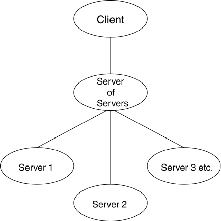
11.8 Server-of-Server Casefile Format
11-144 EnSight 7 User Manual
11.8 Server-of-Server Casefile Format
EnSight7 (with gold license key) has the capability of dealing with partitioned
data in an efficient distributed manner by utilizing what we call a server-of-servers
(SOS for short). An SOS server resides between a normal client and a number of
normal servers. Thus, it appears as a normal server to the client, and as a normal
client to the various normal servers.
This arrangement allows for distributed parallel processing of the various portions
of a model, and has been shown to scale quite well.
Currently, EnSight SOS capability is only available for EnSight5, EnSight6,
EnSight Gold, Plot3d, and any EnSight User-Defined Reader data. (It is not
directly available for Fidap Neutral, Fluent Universal, N3S, Estet, MPGS4,
Movie, Ansys, Abaqus, or FAST Unstructured data.)
Please recognize that your data must be partitioned in some manner (hopefully in
a way that will be reasonably load balanced) in order for this approach to be
useful. (The one exception to this is the use of the auto_distribute capability for
structured data. This option can be used if the data is structured and is available to
all servers defined. It will automatically distribute each structured block over the
defined servers - without the user having to partition the data.)
(Included in the EnSight distribution is an unsupported utility that will take most
EnSight Gold binary unstructured datasets and partition it for you. The source for
this utility (called “chopper”) can be found in the
$CEI_HOME/ensight76/
unsupported/partitioner
directory.)
Note: If you do your own partitioning of data into EnSight6 or EnSight Gold
format, please be aware that each part must be in each partition - but, any given
part can be “empty” in any given partition. (All that is required for an empty part
is the “part” line, the part number, and the “description” line.)
You should place each partitioned portion of the model on the machine that will
compute that portion. Each partitioned portion is actually a self contained set of
11.8 Server-of-Server Casefile Format
EnSight 7 User Manual 11-145
EnSight data files, which could typically be read by a normal client - server
session of EnSight. For example, if it were EnSight gold format, there will be a
casefile and associated gold geometry and variable results file(s). On the machine
where the EnSight SOS will be run, you will need to place the sos casefile. This is
a simple ascii file which informs the SOS about pertinent information need to run
a server on each of the machines that will compute the various portions.
The format for the SOS casefile is as follows: (Note that [ ] indicates optional
information, and a blank line or a line with # in the first column are comments.)
FORMAT (Required)
type: master_server datatype (Required)
where: datatype is required and is one of the formats of EnSight’s
internal readers (which use the Part builder), namely:
gold ensight6 ensight5 plot3d
or it can be the string used to name any of the user-defined readers.
Note: For user-defined readers, the string must be exactly that which is
defined in the USERD_get_name_of_reader routine of the reader
(which is what is presented in the Format pulldown of the Data Reader
dialog).
If datatype is blank, it will default to EnSight6 data type.
[auto_distribute: on/off] (Optional for structured, Ignored for unstructured)
For structured data only, EnSight will automatically distribute data to
the servers specified below if this option is present and set to “on”. This
will require that each of the servers have access to the same data (or
identical copies of it).
[plot3d_iblanked: true/false] (Required only if datatype is plot3d)
[plot3d_multi_zone: true/false] (Required only if datatype is plot3d)
[plot3d_dimension: 1d/2d/3d] (Required only if datatype is plot3d)
[plot3d_source: ascii/cbin/fortranbin] (Required only if datatype is plot3d)
[plot3d_grid_double: true/false] (Required only if datatype is plot3d)
[plot3d_results_double: true/false] (Required only if datatype is plot3d)
where: iblanking, multi_zone, dimension, source type, grid file double
precision, and results file double precision information should be
provided. If it is not provided, it will default to the following (which is
likely not to be correct):
plot3d_iblanked: false
plot3d_muti_zone: false
plot3d_dimension: 3d
plot3d_source: cbin
plot3d_grid_double: false
plot3d_results_double: false
NETWORK_INTERFACES (Note: this whole section is optional. It is
needed only when more than one network
interface to the sos host is available and it is
desired to use them. Thus distributing the
servers to sos communication over more than
one network interface)
number of network interfaces: num (Required - if section used)
11.8 Server-of-Server Casefile Format
11-146 EnSight 7 User Manual
where: num is the number of network interfaces to be used for the sos
host.
network interface: sos_network_interface_name1(Required - if section is used)
network interface: sos_network_interface_name2(Required - if section is used)
.
.
network interface: sos_network_interface_name
num(Required - if section used)
SERVERS (Required)
number of servers: num (Required)
where: num is the number of servers that will be started and run
concurrently.
#Server 1 (Comment only)
machine id: mid (Required)
where: mid is the machine id of the server.
executable: /.../ensight7.server (Required, must use full path)
[directory: wd] (Optional)
where: wd is the working directory from which ensight7.server will be
run
[login id: id] (Optional)
where: id is the login id. Only needed if it is different on this machine.
[data_path: /.../dd] (Optional)
where: dd is the data where the data resides. Full path must be provided
if you use this line.
casefile: yourfile.case (Required, but depending on format, may vary
as to whether it is a casefile, geometry file,
neutral file, universal file, etc. Relates to the
first data field of the Data Reader Dialog.)
[resfile: yourfile.res] (Depends on format as to whether required or
not. Relates to the second data field of the Data
Reader Dialog.)
[measfile: yourfile.mea] (Depends on format as to whether required or
not. Relates to the third data field of the Data
Reader Dialog.)
[bndfile: yourfile.bnd] (Depends on format as to whether required or
not. Relates to the fourth data field of the Data
Reader Dialog.)
#Server 2 (Comment only)
--- Repeat pertinent lines for as many servers as declared to be in this file ---
Example This example deals with a EnSight Gold dataset that has been partitioned into 3
portions, each running on a different machine. The machines are named joe, sally,
and bill. The executables for all machines are located in similar locations, but the
data is not. Note that the optional data_path line is used on two of the servers, but
not the third.
11.8 Server-of-Server Casefile Format
EnSight 7 User Manual 11-147
FORMAT
type: master_server gold
SERVERS
number of servers: 3
#Server 1
machine id: joe
executable: /usr/local/bin/ensight76/bin/ensight7.server
data_path: /usr/people/john/data
casefile: portion_1.case
#Server 2
machine id: sally
executable: /usr/local/bin/ensight76/bin/ensight7.server
data_path: /scratch/sally/john/data
casefile: portion_2.case
#Server 3
machine id: bill
executable: /usr/local/bin/ensight76/bin/ensight7.server
casefile: /scratch/temp/john/portion_3.case
If we name this example sos casefile - “all.sos”, and we run it on yet another
machine - one named george, you would want the data distributed as follows:
On george: all.sos
On joe (in /usr/people/john/data): portion_1.case, and all files referenced by it.
On sally (in /scratch/sally/john/data): portion_2.case, and all files referenced by it.
On bill (in /scratch/temp/john): portion_3.case, and all file referenced by it.
By starting EnSight with the -sos command line option (which will autoconnect
using ensight7.sos instead of ensight7.server), or by manually running
ensight7.sos in place of ensight7.server, and providing all.sos as the casefile to
read in the Data Reader dialog - EnSight will actually start three servers and
compute the respective portions on them in parallel.
Optional NETWORK_INTERFACES section notes
If the machine named george had more than one network interface (say it had its
main one named george, but also had one named george2), we could add the
section shown below to our casefile example:
NETWORK_INTERFACES
number of network interfaces: 2
network interface: george
network interface: george2
This would cause machine joe to connect back to george, machine sally to connect
back to george2, and machine bill to connect back to george. This is because the
sos is cycling through its available interfaces as it connects the servers.
Remember that this is an optional section, and most users will probably not use it.
Also, the contents of this section will be ignored if the -soshostname
command line option is used.
Additional Note: The EnSight SOS provided with release 7.6 supports most EnSight features.
Some query operations with constants are not yet supported, but should be in a future release.

11.9 Periodic Matchfile Format
11-148 EnSight 7 User Manual
11.9 Periodic Matchfile Format
This is an optional file which can be used in conjunction with models which have
rotational or translational computational symmetry (or periodic boundary
conditions). It is invoked in the GEOMETRY section of the EnSight casefile,
using the “match: filename” line. (see Section , EnSight6 Case File Format).
When a model piece is created with periodic boundary conditions, there is usually
a built-in correspondence between two faces of the model piece. If you transform
a copy of the model piece properly, face 1 of the copy will be at the same location
as face 2 of the original piece. It is desirable to know the corresponding nodes
between face 1 and face 2 so border elements will not be produced at the matching
faces. This correspondence of nodes can be provided in a periodic match file as
indicated below. (Please note that if a periodic match file is not provided, by
default EnSight will attempt to determine this correspondence using a float
hashing scheme. This scheme has been shown to work quite well, but may not
catch all duplicates. The user has some control over the “capture” accuracy of the
hashing through the use of the command: “test: float_hash_digits”. If this
command is issued from the command dialog, the user can change the number of
digits, in a normalized scheme, to consider in the float hashing. The lower the
number of digits, the larger the “capture” distance, and thus the higher the number
of digits, the smaller the capture distance. The default is 4, with practical limits
between 2 and 7 or 8 in most cases.)
The transformation type and delta value are contained in the file. The periodic
match file is an ASCII free format file. For unstructured data, it can be thought of
as a series of node pairs, where a node pair is the node number of face 1 and its
corresponding node number on face 2. For structured blocks, all that is needed is
an indication of whether the i, j, or k planes contain the periodic face. The min
plane of this “direction” will be treated as face 1, and the max plane will be treated
as face 2.
The file format is as follows:
rotate_x/y/z / translate
The first line is either rotate_x, rotate_y, rotate_z
or translate
theta / dx dy dz
The second line contains rotation angle in degrees
or the three translational delta values.
np
n
11
n
21
n
12
n
22
. .
. .
. .
n
1np
n
2np
If any unstructured pairs, the third line contains
the number of these pairs (np).
And the node ids of each pair follow. (The first
subscript indicates face, the second is pair.)
blocks b
min
b
max
i/j/k
Last in the file comes as many of these “blocks”
lines as needed. b
min
and b
max
are a range of
block numbers. For a single block, b
min
and b
max
would be the same. Only one of i, j, or k can be
specified for a given block.
11.9 Periodic Matchfile Format
EnSight 7 User Manual 11-149
Simple unstructured rotational example:
The periodic match file for a rotation of this model about point 1 would be:
rotate_z
45.0
3
11
28
39
Thus, face 1 of this model is made up of nodes 1, 2, and 3 and face 2 of this model
is made up of nodes 1, 8, and 9. So there are 3 node pairs to define, with node 1
corresponding to node 1 after a copy is rotated, node 2 corresponding to node 8,
and node 3 corresponding to node 9.
Simple structured translational model:
translate
2.0 0.0 0.0
blocks 1 1 i
blocks 2 3 j
2
4
5
8
3
7
9
6
1
8
6
4
2
Original
face 2
face 1
Figure 11-5
Model Duplication by rotational symmetry
Figure 11-6
Model Duplication by translational symmetry
of structured blocks (3 instances)
block 1
block 2
block 3
J
I
J
I
2.0
11.9 Periodic Matchfile Format
11-150 EnSight 7 User Manual
Since block 1 is oriented differently than blocks 2 and 3 in terms of ijk space, two
“blocks” lines were needed in the match file.
Special Notes / Limitations:
1. This match file format requires that the unstructured node ids of the model be
unique. This is only an issue with EnSight Gold unstructured format, since it is
possible with that format to have non-unique node ids.
2. The model instance (which will be duplicated periodically) must have more
than one element of thickness in the direction of the duplication. If it has only one
element of thickness, intermediate instances will have all faces removed. If you
have this unusual circumstance, you will need to turn off the shared border
removal process, as explained in note 3.
3. The shared border removal process can be turned off, thereby saving some
memory and processing time, by issuing the “test: rem_shared_bord_off”
command in the command dialog. The effect of turning it off will be that border
elements will be left between each periodic instance on future periodic updates.
4. The matching and hashing processes actually occur together. Thus, matching
information does not have to be specified for all portions of a model. If no
matching information is specified for a given node, the hashing process is used.
By the same token, if matching information is provided, it is used explicitly as
specified - even if it is has been specified incorrectly.
11.10 XY Plot Data Format
EnSight 7 User Manual 11-151
11.10XY Plot Data Format
This file is saved using the Save section of the Query Entity dialog. The file can
contain one or more curves. The following is an example XY Data file:
Line Contents of Line
12
2 Distance vs. Temperature for Line Tool
3 Distance
4Temperature
51
65
7 0.0 4.4
8 1.0 5.8
9 2.0 3.6
10 3.0 4.6
11 4.0 4.8
12 Distance vs. Pressure for Line Tool
13 Distance
14 Pressure
15 2
16 4
17 0.00 1.2
18 0.02 1.1
19 0.04 1.15
20 0.06 1.22
21 3
22 1.10 1.30
23 1.12 1.28
24 1.14 1.25
Line 1 contains the (integer) number of curves in the file.
Line 2 contains the name of the curve.
Line 3 contains the name of the X-Axis.
Line 4 contains the name of the Y-Axis.
Line 5 contains the number of curve segments in this curve.
11.10 XY Plot Data Format
11-152 EnSight 7 User Manual
Line 6 contains the number of points in the curve segment.
Lines 7-11 contain the X-Y information.
Line 12 contains the name of the second curve.
Line 13 contains the name of the X-Axis
Line 14 contains the name of the Y-Axis
Line 15 contains the number of curve segments in this curve. (For the second
curve, the first segment contains 4 points, the second 3 points.)

11.11 EnSight Boundary File Format
EnSight 7 User Manual 11-153
11.11 EnSight Boundary File Format
This file format can be used to represent boundary surfaces of structured data as
unstructured parts. The boundaries defined in this file can come from sections of
several different structured blocks. Thus, inherent in the file format is a grouping
and naming of boundaries across multiple structured blocks.
Additionally, a delta can be applied to any boundary section to achieve the
creation of repeating surfaces (such as blade rows in a jet engine).
Note: There is no requirement that the boundaries actually be on the surface of
blocks, but they must define either 2D surfaces or 1D lines. You may not use this
file to define 3D portions of the block.
The boundary file is read if referenced in the casefile of EnSight data models, or
in the boundary field of the Data Reader Dialog for other data formats. Any
boundaries successfully read will be listed in the Unstructured Data Part List of
the Data Part Loader Dialog.
The format of the EnSight Boundary File is as follows:
Line (1):
Required header keyword and version number. ENSBND is required
exactly, but the version number could change in the future.
ENSBND 1.00
Line (2) through Line (NumBoundaries+1): The names of the boundaries to be
defined. (Each name must be no greater than 79 characters.)
For example:
inflow
wall
Chimera Boundary
outflow
Line (NumBoundaries+2): Required keyword indicating the end of the boundary
names and the beginning of the boundary section definitions.
BOUNDARIES
Line (NumBoundaries+3) through the end of the file: The boundary section
definitions. Each line will have the following information:
bnd_num blk_num imin imax jmin jmax kmin kmax [di dj dk n_ins]
where:
bnd_num
is the number of the boundary in the list of names above.
(For example: inflow is 1, wall is 2, Chimera Boundary is 3, etc.)
blk_num
is the parent structured block for this boundary section.
imin,imax, jmin,jmax, kmin,kmax
are the ijk ranges for the boundary section.
At least one of the min,max pairs must refer to the same plane. A wildcard (“$”)
can be used to indicate the maximum i, j, or k value of that block (the far plane).
Additionally, negative numbers can be used to indicate plane values from the far
side toward the near side. (-1 = far plane, -2 = one less than the far plane, etc.)
[di,dj,dk
and
n_ins]
are optional delta information which can be used to extract
repeating planes. The appropriate di, dj, or dk delta value should be set to the
11.11 EnSight Boundary File Format
11-154 EnSight 7 User Manual
repeating plane offset value, and the other two delta values must be zero. The non-
zero delta must correspond to a min,max pair that are equal. The n_ins value is
used to indicate the number of repeating instances desired. A (“$”) wildcard can
be used here to indicate that the maximum number of instances that fit in the block
should be extracted.
All numbers on the line must be separated by spaces.
Finally, comment lines are allowed in the file by placing a “#” in the first column.
Below is a simple example of a boundary file for two structured blocks, the first of
which is a 3 x 3 x 3 block, and the second is a 10 x 10 x 10 block. We will define a
boundary which is the front and back planes of each block(K planes) and one that
is the top and bottom planes of each block(J planes). We will also define some
repeating x planes, namely, planes at i=1 and 3 for block one and at i=1, 4, 7, and
10 for block two. The image below shows the blocks in wire frame and the
boundaries shaded and slightly cut away, so you can see the interior x-planes.
11.11 EnSight Boundary File Format
EnSight 7 User Manual 11-155
The file to accomplish this looks like:
ENSBND 1.00
front_back
top_bottom
x-planes
middle lines
BOUNDARIES
#bnd blk imin imax jmin jmax kmin kmax di dj dk n_ins
#--- --- ---- ---- ---- ---- ---- ---- -- -- -- -----
111313$$
121$1$1010
211$$$1$
221 1010101 10
11131311
121$1$11
2113111$
221$111$
3 1 1 1 1 $ 1 $ 2002
3 2 1 1 1 $ 1 $ 300$
41222213
421105555
Interpreting the 12 boundary definition lines:
111313$$
defines a part of the boundary called front_back, on block 1, where I=1 to 3, J=1
to 3, and K=3. Thus, the far K plane of block 1.
121$1$1010
defines another part of the front_back boundary, on block 2, where I=1 to 10, J=1
to 10, and K = 10. Thus, the far K plane of block 2.
211$$$1$
defines a part of the boundary called top_bottom, on block 1, where I=1 to 3, J=3,
and K=1 to 3. Thus, the far J plane of block 1.
221 1010101 10
defines another part of the top_bottom boundary, on block 2, where I=1 to 10,
J=10, and K=1 to 10. Thus, the far J plane of block 2.
11131311
defines another part of the front_back boundary, on block 1, where I=1 to 3, J=1 to
3, and K=1. Thus, the near K plane of block 1.
121$1$11
defines another part of the front_back boundary, on block 2, where I=1 to 10, J=1
to 10, and K=1. Thus the near K plane of block 2.
2113111$
defines another part of the top_bottom boundary, on block 1, where I=1 to 3, J=1,
and K=1 to 3. Thus, the near J plane of block 1.
221$111$
defines another part of the top_bottom boundary, on block 2, where I=1 to 10,
J=1,and K=1 to 10. Thus, the near J plane of block 2.
11.11 EnSight Boundary File Format
11-156 EnSight 7 User Manual
3 1 1 1 1 $ 1 $ 2002
defines a part of the boundary called x-planes, on block 1, where I=1, J=1 to 3,
K=1 to 3, then again where I=3, J=1 to 3, and K=1 to 3. Thus, both the near and
far I planes of block 1.
3 2 1 1 1 $ 1 $ 300$
defines another part of the x-planes boundary, on block 2, where I=1, J=1 to 10,
and K=1 to 10, then again where I=4, J=1 to 10, and K=1 to 10, then again where
I=7, J=1 to 10, and K=1 to 10, then again where I=10, J=1 to 10, and K=1 to 10.
Thus, the I = 1, 4, 7, and 10 planes of block 2.
41222213
defines a part of the boundary called middle lines, on block 1, where I=2, J=2, and
K=1 to 3. Thus, line through the middle of block 1 in the K direction.
421105555
defines another part of the middle lines boundary, on block 2, where I=1 to 10,
J=5, and K=5. Thus a line through the middle of the block2 in the I direction.
Please note that the “$” wildcard was used rather randomly in the example, simply
to illustrate how and where it can be used.
The use of negative numbers for ijk planes is indicated below - again rather
randomly for demonstration purposes. This file will actually produce the same
result as the file above.
ENSBND 1.00
front_back
top_bottom
x-planes
middle lines
BOUNDARIES
#bnd blk imin imax jmin jmax kmin kmax di dj dk n_ins
#--- --- ---- ---- ---- ---- ---- ---- -- -- -- -----
111 3 1 3-1-1
1 2 -3 -1 1 -1 10 10
211-1-1-1 1-1
221 1010101 10
11131311
121-11-111
2113111-1
221-1 1 1 1-1
3 1 1 1 1 -1 1 -1 2002
3 2 1 1 1 -1 1 -1 300$
412-2-2 2 1 3
421 105 5-6-6
11.12 EnSight Particle Emitter File Format
EnSight 7 User Manual 11-157
11.12 EnSight Particle Emitter File Format
This file can be used to specify the location of emitter points. It is most useful
when the user has specific (and many) emit points to use for particle traces.
Rather than type them all in one at a time as a cursor emitter, this file can be used.
Note the following:
1. The first two lines need to be exactly as shown.
Version 1.0
EnSight Particle Emitter File
2. #’s as the first character on a line, are comment lines. Comment lines can be
used anywhere in the file after the first two mandatory lines.
3.
Time
lines contain the emitter release time (simulation time, NOT time step).
4.
Emit
lines contain the coordinates of an emitter. The emitter will be associated
with the previously specified
Time
.
Sample File:
Version 1.0
EnSight Particle Emitter File
#
Time 0.249063
Emit 0.0669737 0.0134195 -0.013926
Emit 0.0669737 0.0131277 -0.0141079
Emit 0.0669737 0.0128642 -0.0143178
Emit 0.0669737 0.0155969 -0.0113572
Emit 0.0669737 0.0150344 -0.0122012
Emit 0.0669737 0.0146967 -0.0123587
#
Time 0.249113
Emit 0.0669737 0.0137097 -0.0136404
Emit 0.0669737 0.0134218 -0.0138284
Emit 0.0669737 0.0131628 -0.0140438
Emit 0.0669737 0.0158325 -0.0110264
Emit 0.0669737 0.0152879 -0.011882
Emit 0.0669737 0.0149536 -0.0120466
#
Time 0.249163
Emit 0.0669737 0.0139938 -0.0133488
Emit 0.0669737 0.01371 -0.0135428
Emit 0.0669737 0.0134555 -0.0137636
Emit 0.0669737 0.0160612 -0.0106906
Emit 0.0669737 0.0155347 -0.0115575
Emit 0.0669737 0.0152039 -0.0117291
#
Time 0.249213
Emit 0.0669737 0.0142718 -0.0130512
Emit 0.0669737 0.013992 -0.0132511
Emit 0.0669737 0.0137423 -0.0134773
Emit 0.0669737 0.0162827 -0.0103501
Emit 0.0669737 0.0157745 -0.0112279
Emit 0.0669737 0.0154475 -0.0114064
#
EnSight 7 User Manual 12-1
12 Utility Programs
This chapter describes the utility programs that accompany EnSight. The Server
utility programs are located in
$CEI_HOME/ensight76/server_utilities and
the Client utility programs are located in
$CEI_HOME/ensight76/
client_utilities
.
Utility programs are supplied on an “as is” basis and are unsupported. CEI will,
however, try to assist in problem resolution.
Each utility program is presented below and accompanied with a brief overview
that describes the function of the utility.
Section 12.1, EnSight5 Programs
Section 12.2, MPGS4 Programs
Section 12.3, Movie.BYU Programs
Section 12.4, Keyboard Macro Maker (macromake)
Section 12.5, Web Publisher/Project Management (scenario_html_publisher)
12.1 EnSight5 Programs
12-2 EnSight 7 User Manual
12.1 EnSight5 Programs
EnSight5 ASCII-to-Binary File Converter (asciitobin5)
The asciitobin5 program runs on a Server host system to read ASCII EnSight 5.x files and
convert them to C binary format files, which read much faster than ASCII files. Use this
utility to facilitate the reading of large data files, especially when these files are read
repeatedly.
EnSight Data Translation Library
The EnSight interface library (“libeio”) provides a C API for reading and writing both the
ASCII and the binary versions of the EnSight 5 format for geometry and results data. You
can use it to simplify the process of writing translators or output modules for the EnSight
format, as well as utilities that operate on the format.
Before using this library, you should be reasonably familiar with the EnSight 5 format
described in section 2.5 of the EnSight User Manual.
The library (C source) can be found in the $CEI_HOME/ensight76/translators/libeio
directory in your EnSight distribution. A translator for the unstructured “FAST” format
that makes use of libeio can be found in $CEI_HOME/ensight76/translators/unf.
EnSight provides both ASCII and binary versions of its native data format. There are
really only two reasons to use the ASCII format: if you need to actually look at the files or
if you need to move a dataset to a computer system with a different binary format for
numbers. Always use the binary format if possible. Not only does the I/O occur much
faster, but the files will be smaller and will load into EnSight much faster as well.
You specify ASCII or binary output via the
SetFileType() call. By default, output is set
to binary.
Building the library
This library has been compiled and tested (to a limited extent) on the following systems:
SGI IRIX 4.0.5
SGI IRIX 5.3
HPUX 9.0.5
Solaris 2.3
1. Edit the Makefile for your system (as shipped, it is configured for IRIX).
2. To build the library, type “make”. If you are porting the library to a new platform or
operating system release, you may have to make some minor modifications to the
Makefile and/or the source code.
3. To build executables that call routines in the library either include “
.../libeio.a” in
your final link command or add the “
-leio” option to the link command (which assumes
the linker knows where to find the library).
Warnings
The following caveats apply to this initial release of libeio:
1. Error checking is a little skimpy at this point. It needs to be improved, especially for the
input routines. In general, the input routines assume that a correctly formatted EnSight
file is being read.
2. The input routines will only handle C binary files – not Fortran!
12.1 EnSight5 Programs
EnSight 7 User Manual 12-3
Hints
When reading EnSight format files into EnSight, you have the option of whether to load
all parts, all but the first part, or the first part only. You can sometimes take advantage of
this and save loading time as well as memory on the EnSight Client if you can load all but
the first part. In many 3D applications (particularly CFD) one part can contain all 3D
elements of the computational domain. Other parts typically contain boundary or shell
elements. Since you don’t really need to look at a graphical representation of the
computational domain (if you have a boundary representation), you can avoid its initial
load and display on the Client by having the 3D computational domain part as the first part
in the EnSight geometry file and using the “all but the first part” load option in EnSight.
Output Routines
void SetFileType(int type)
SetFileType() sets the output type for subsequent calls to I/O routines. The type
parameter is either
ASCII or BINARY (as defined in eio.h). NOTE: the ReadGeometry()
and
ReadParticleGeometry() input routines will reset the type based on the type of
the file last read.
The output routines are divided into two types: those that operate on the EnSight-based
data structures (defined in eio.h) and those that accept raw arrays for output. The first four
routines operate on the defined data structures:
int WriteGeometry(char *filename,Geometry *geo)
int WriteParticleGeometry(char *filename,ParticleGeometry *geo)
int WriteScalar(char *filename,Scalar *scl)
int WriteVector(char *filename,Vector *vec)
These routines take a completed structure for the corresponding item and write it to the
file specified by “
filename”. See the definitions for Geometry, ParticleGeometry,
Scalar, and Vector in eio.h for more info.
The remaining routines accept raw arrays for output.
int WriteGeoHeader(char *filename,char *des1,char *des2,int nodeid,int elemid)
WriteGeoHeader()
begins the process of geometry file output. The des1 and des2
parameters are description lines for the model. The
nodeid and elemid parameters
should be set to one of the defined constants (e.g.
ID_OFF or ID_ASSIGN) in eio.h.
WriteGeoHeader() should be followed by WriteGeoCoords().
int WriteParticleGeoHeader(char *filename, char *des)
WriteParticleGeoHeader()
begins the process of particle geometry file output.
Although particle files have two description lines in the header, the second one is
ALWAYS “particle coordinates”.
WriteParticleGeoHeader() should be followed by
a call to
WriteGeoCoords(). Note that particle files must always have coordinate IDs!
void WriteGeoCoords(int partcoords, int num, int *id, float *coords)
WriteGeoCoords()
appends coordinates to the geometry file opened by the previous
call to
WriteGeoHeader(). If the nodeid parameter to WriteGeoHeader() was either
ID_GIVEN or ID_IGNORE then the id pointer must point to a list of num integers. The
coords parameter must point to a list of 3*num floats in order
X1,Y1,Z1,X2,Y2,Z2,...,Xn,Yn,Zn.
WriteGeoCoords() should be followed by a call to
12.1 EnSight5 Programs
12-4 EnSight 7 User Manual
WriteGeoPart().
WriteGeoCoords() is also used to output particle coordinates (e.g. following a call to
WriteParticleGeoHeader()). Be sure to set the partcoords parameter to True when
writing particle coordinates!
void WriteGeoPart(char *line)
WriteGeoPart()
begins the process of part definition. A part header will be output to
the file opened in the previous call to
WriteGeoHeader(). WriteGeoPart() must be
followed by one or more calls to
WriteGeoElem().
void WriteGeoElem(int elemtype, int num, int *id, int *nd)
WriteGeoElem()
outputs a set of elements of the same type to the current part (as
defined by the most recent call to
WriteGeoPart()). The elemtype parameter must be
one of the types defined in eio.h (e.g.
HEXA8 or QUAD4). num is the number of elements to
output. If the
elemid parameter to WriteGeoHeader() was either ID_GIVEN or
ID_IGNORE then the id pointer must point to a list of num integers containing element ID
numbers. The nd pointer points to a list of N*num integers, where N is the number of
nodes in the particular type of element (e.g. 8 for a
HEXA8 type). Node ordering is defined
section 3.8.
You can call
WriteGeoElem() as many times as you like between calls to
WriteGeoPart() to define different element sets belonging to a particular part.
int WriteRawScalar(char *filename, char *descrip, char *varname, int num, float
*data)
WriteRawScalar()
writes a scalar variable to the file named filename. The varname
parameter will be saved and used in a subsequent call to
WriteResults(). num is the
number of values.
data is a pointer to num floating point values. The values must be
ordered the same as the coordinates in the corresponding geometry file.
int WriteRawVector(char *filename, char *descrip, char *varname, int num, float
*data)
WriteRawVector()
writes a vector variable to the file named filename. The
varname parameter will be saved and used in a subsequent call to WriteResults().
num is the number of values. data is a pointer to 3*num floating point values. The values
must be ordered the same as the coordinates in the corresponding geometry file.
int WriteResults(char *filename, Result *rp)
WriteResults()
will output an EnSight “results” file describing a complete geometry
plus results dataset.
rp points to a Result structure (defined in eio.h) containing the
desired information.
12.1 EnSight5 Programs
EnSight 7 User Manual 12-5
Input Routines
The input routines read a particular type of EnSight file and load the contents to a structure
defined in eio.h.
Geometry *ReadGeometry(char *filename)
The ReadGeometry() routine reads a complete geometry file and returns the various
components in the Geometry structure. It returns
NULL on error. ReadGeometry() will
automatically determine if the file is ASCII or binary and will set the type for subsequent
reads.
ParticleGeometry *ReadParticleGeometry(char *filename)
The ReadParticleGeometry() routine reads a complete particle geometry file and
returns the various components in the
ParticleGeometry structure. It returns NULL on
error.
ReadParticleGeometry() will automatically determine if the file is ASCII or
binary and will set the type for subsequent reads.
Scalar *ReadScalar(char *filename, int num)
ReadScalar()
will read a scalar file and return a pointer to a Scalar structure (or NULL
on error).
num must equal the number of values to read. ReadScalar() will assume the
file type (ASCII or binary) is the same as that determined in
ReadGeometry() (but you
can override with a call to
SetFileType()).
Vector *ReadVector(char *filename, int num)
ReadVector() will read a vector file and return a pointer to a Vector structure (or NULL
on error).
num must equal the number of values (nodes) to read, i.e. there should be 3*num
floats in the file.
ReadVector() will assume the file type (ASCII or binary) is the same
as that determined in
ReadGeometry() (but you can override with a call to
SetFileType()).
Result *ReadResults(char *filename)
ReadResults()
will read an EnSight results file and return the information in an
allocated
Result structure.
12.2 MPGS4 Programs
12-6 EnSight 7 User Manual
12.2 MPGS4 Programs
MPGS4 ASCII-to-Binary File Converter (asciitobin4)
The asciitobin4 program runs on a Server host system to read ASCII MPGS 4 data files
and convert them to binary files, which read much faster than ASCII files. Use this utility
to facilitate the reading of large data files, especially when these files are read repeatedly.
See also asciitobin5 above.
MPGS4 File Concatenater-Transformer
The programs under the cat_transform4 directory run on a Server host system and
perform various concatenation and transformation operations on MPGS 4 dataset files.
For example, the following two utility programs are included in this directory:
cat_mpgs concatenates two or more MPGS 4 data files.
tform_mpgs translates and rotates MPGS 4 data files.
MPGS4 Geometry File Debug Filter (filter4)
The filter4 program runs on a Server host system to read an MPGS 4 geometry file (either
ASCII or binary). After reading the file, you can perform queries to aid in debugging
connectivity information. You are prompted for a solid number, after which filter4 will
print all known information for that solid. If filter4 cannot read the data, there is probably
a problem with the data formatting.
MPGS4 Min-Max Scalar Finder (minmaxs4)
The minmaxs4 program runs on a Server host system to scan a set of MPGS 4 (multiple
time step) scalar files, and print the minimum and maximum scalar information. See also
minmaxv4 below.
MPGS4 Min-Max Vector Finder (minmaxv4)
The minmaxv4 program runs on a Server host system to scan a set of MPGS 4 (multiple
time step) vector files, and print the minimum and maximum vector information. See also
minmaxs4 above.
MPGS4 Structured Mesh Generator (structmesh4)
The structmesh4 program runs on a Server host system, and creates an MPGS 4 geometry
file that contains a 3D (cube) structured mesh.
12.3 Movie.BYU Programs
EnSight 7 User Manual 12-7
12.3 Movie.BYU Programs
Movie.BYU File Polygon Reducer (reducemovie)
The reducemovie program runs on a Server host system to read Movie.BYU geometry,
and output a geometry file with shared face information removed. This program is
especially useful when dealing with geometry files that were created from FEM solid
elements.
Depending on how smart a FEM translator is, the faces shared between two solid elements
might be described twice in the geometry file. If reducemovie finds two faces (polygons in
the Movie.BYU file) that share the same node numbers, both polygons are removed
because they are both interior faces and should not be visible to the observer (unless the
geometry is clipped open using the Z-clipping planes).
Running a FEM geometry that has been created using solid elements through this filtering
program can reduce the number of polygons in the model dramatically, thus speeding
postprocessing.
12.4 Keyboard Macro Maker (macromake)
12-8 EnSight 7 User Manual
12.4 Keyboard Macro Maker (macromake)
The macromake program runs on the Client host system and assigns a keyboard key to a
prerecorded EnSight command file (or files). The macro key code and command file
name(s) are updated in the
macro.define file, which stores your macro definitions.
The command file(s) can contain any sequence of valid EnSight commands that will
execute each time the macro key is pressed while running EnSight. You can assign one
command file to a repeatable macro key—the contents of the command file plays as long
as the macro key is depressed. Macros are currently limited to single key definitions.
See: How To Define and Use Macros.
12.5 Web Publisher/Project Management (scenario_html_publisher)
EnSight 7 User Manual 12-9
12.5 Web Publisher/Project Management
(scenario_html_publisher)
The ‘scenario_html_publisher’ program runs on the client host system. It provides a way
to generate HTML files that describe EnSight scenario projects and can be used with a
web browser to ease access to the information contained there. The publisher program will
create an HTML file with links to project description, EnLiten scenario, image, EnVideo
movie, MPEG movie, and EnSight restart files. The web browser reads the main HTML
file for the project directory or set of directories. The user can then select the links to view
further information contained throughout the project which might start up helper
applications EnVideo, EnLiten, and EnSight. In the case of EnSight the context file will be
read to restore EnSight to the point that you saved the scenario project. This arrangement
does not require you to have a web server handle the pages. The user can have there own
little area that can be accessed with the web browser by providing it with a URL of
file:/home/users/joe/projects/shuttle1.htm. The user, of course, would
provide the true path to the starting HTML file produced by the
‘scenario_html_publisher’ program. The user can also collaborate with their colleagues
by pointing them to this ‘
file:’ URL if they have access to the same directory or they
can work with their local Web Master to put copy the directory structure into the location
served by a local web server. This area could then be accessed by colleagues around the
world with their browser. The area may be a password protected area or it could be wide
open to the world to view the exciting images, movies, and information that it contains.
Work with your Web Master to protect the area as you see fit. To use the publisher please
read the header of the ‘scenario_html_publisher’ script. It can be found in the installation
directory for EnSight under scenario_tools/unix. The ‘scenario_html_publisher’ program
is currently only available for Unix but the pages that it produces are readable by any web
browser on any type of computer.
EnSight 7 User Manual 2-1
13 Parallel Rendering and Virtual Reality
EnSight Gold 7.6 supports general parallel rendering for increased performance,
increased display resolution, and arbitrary screen orientations. Combined with
support for 6 DOF (degree-of-freedom) input devices, EnSight Gold provides an
immersive virtual reality interface. This chapter describes the configuration file
format and command-line parameters required for parallel rendering and 6D
input. Using hardware accelerated rendering, the features described are supported
on SGI Irix 6.5, Sun Solaris 8, and HP-UX 11.0. Using software rendering
(
ensight7 -X) these features are supported on all Unix/Linux platforms. Six
DOF input is supported on all Unix platforms, with pre-compiled trackd support
for Irix, Solaris, and Linux (x86).
In order to make use of parallel rendering with EnSight, the user must create a
configuration file. This file is specified on the command line using the argument
-dconfig <file>. If <file> is not a fully-qualified path EnSight will
search for the file in the following directories:
1. ~/.ensight7/dconfig/
2. $CEI_HOME/ensight76/site_preferences/dconfig/
These options allow for user-level and site-level configurations, respectively.
There are two logical displays which can be configured in EnSight. The GUI
display is always active, and consists of the main rendering window embedded in
the user-interface. The detached display is external to the user-interface, and may
consist of 1-16 regions configured to form a large continuous display. The
configuration file contains information about both the GUI display and the
detached display, as well as tracking calibration information and options for using
6D input devices. The remaining sections will address each of the capabilities
related to parallel rendering and VR. The sample configurations described in this
chapter can be found in the directory
$CEI_HOME/ensight76/src/
input/dconfig
. There are also examples of ‘simulated’ configuration files,
which allow you to simulate display to multiple graphics pipes on a single display.
CONFIGURATION FILE FORMAT
MULTI-PIPE PARALLEL RENDERING
DISPLAY WALLS
IMMERSIVE DISPLAYS
TRACKING
ANNOTATIONS
STEREO DISPLAY
TIPS
2-2 EnSight 7 User Manual
CONFIGURATION FILE FORMAT
Configuration files are entirely text-based beginning with the line:
PRSd 2.0
# after the first line, anything following a '#' is a comment
The remainder of the file consists of one or more sections describing the displays
and options. In describing the format of the file, portions which are optional will
be surrounded by
[].
MULTI-PIPE PARALLEL RENDERING
The default mode of EnSight uses only a single graphics pipe for rendering to the
GUI display. When run on a multi-pipe machine, EnSight can be configured to
use the additional pipes to accelerate the display through parallel rendering. The
format of the configuration for the GUI display is as follows:
guidisplay
worker <p
1
>
worker <p
2
>
...
worker <p
n
>
where:
<p
i
> = an X display (i.e. localhost:0.2)
Example 1:
PRSd 2.0
# This configuration uses 4 graphics pipes to
# accelerate rendering
guidisplay
worker :0.1
worker :0.2
worker :0.3
In the example above, there is one X server (:0) which manages four graphics
pipes. Note that the configuration file does not include the pipe to which the
EnSight GUI is displayed. The GUI is always displayed on the pipe indicated by
the $DISPLAY environment variable, and it is not necessary to specify this screen
in the configuration file. Parallel software rendering is available on all Unix/
Linux platforms with the -X option. The same configuration file format is used in
this case, although the displays themselves are not actually opened.
There are two convenience mechanisms for common configurations. When
running EnSight on an X server with multiple screens, it is possible to configure
EnSight to use all of the pipes for accelerating the GUI display using the
command-line option:
-dconfig mpipe. This will detect how many pipes are
available and configure them appropriately. This auto-configuration option will
not be able to configure multiple screens which belong to multiple X servers (i.e.
:0.0, :1.0, :2.0).
EnSight 7 User Manual 2-3
When using software rendering, if the named file is not found and “<file>” is a
number, this number will be interpreted as the number of parallel rendering
workers. For example:
ensight7 -X -batch -dconfig 3 -p <cmdfile>
will run a batch session with a total of 4 threads performing parallel rendering.
DISPLAY WALLS
Another type of parallel rendering available in EnSight allows for the use of
multiple graphics pipes to create large, flat tiled displays. Commonly referred to
as display walls, this is the first example of a "detached display" supported by
EnSight. The advantage of a display wall configuration is that the file
specification is easy to create. The disadvantage is that display walls cannot be
used for tracking and 6d input. In order to use tracking, it will be necessary to use
the more general immersive configuration format described later.
The specification for a display wall consists of:
wallresolution
<x-res> <y-res>
numpipes
<num>
pipe
xserver <p
1
>
resolution <x-res> <y-res>
wallorigin <wall-x> <wall-y>
[ xorigin <xo> <yo> ]
[ lefteye
or
righteye
]
[ worker <p
2
>
...
worker <p
n
>]
[ repeat 'pipe' section (num-1) more times ]
The wallresolution section gives the total pixel resolution of the display
wall. The
numpipes parameter specifies how many separate regions will be
configured. For each region, there will be a
pipe section that describes the size
(
resolution) and position (wallorigin) of the region within the global
display. The
xserver parameter specifies the X display (i.e. :0.1). The
xorigin is an optional parameter to specify the origin of the window on the
given pipe (default (0,0)). Note that
xorigin is a position relative to the origin
of a given xserver, while
wallorigin is a position relative to the origin of the
global display. Changing
wallorigin will change the region of the wall that is
visible in a given window, while changes to
xorigin simply move the window
on the screen without changing the contents. Example 5a will demonstrate a
situation when the use of
xorigin is useful. The lefteye/righteye
optional designation can be used for passive stereo displays, in which separate
graphics pipes render the left and right images. Note that each pipe in a detached

2-4 EnSight 7 User Manual
display can have one or more worker pipes configured to accelerate the
rendering, just as described in the previous section.
Example 2
In this example there is one X server with five graphics pipes. The GUI is
displayed on pipe :0.0, with the other four pipes used for the detached display.
Four projectors are configured in a 2x2 array to form a large continuous wall as
illustrated::
PRSd 2.0
#
# conference room display wall
#
wallresolution
2560 2048
numpipes
4
pipe # lower-left
xserver :0.1
resolution 1280 1024
wallorigin 0 0
pipe # lower-right
xserver :0.2
resolution 1280 1024
wallorigin 1280 0
pipe # upper-left
xserver :0.3
resolution 1280 1024
wallorigin 0 1024
pipe # upper-right
xserver :0.4
resolution 1280 1024
wallorigin 1280 1024
Example 3
It is not uncommon for displays walls to use overlapping images with edge-
blending to smooth the otherwise sharp transition between projector images. The
edge-blending is performed by the projectors directly. This is easily configured as
:0.3 :0.4
:0.1 :0.2
EnSight 7 User Manual 2-5
a detached display by specifying pipes with overlapping pixel regions. Consider
an example of two pipes at 1280x1024 resolution each, with an overlap of 128
pixels.
PRSd 2.0
#
# edge-blending example
#
wallresolution
2432 1024
numpipes
2
pipe # left
xserver :0.1
resolution 1280 1024
wallorigin 0 0
pipe # right
xserver :0.2
resolution 1280 1024
wallorigin 1024 0
Note that in this case the total resolution of the wall in the x direction is decreased
by the amount of overlap.
Example 4
Passive stereo displays achieve stereo by projecting overlapping polarized images
from multiple projectors. This can be achieved using detached displays with a
distinct rendering region for each screen and eye. Consider for this example a
single screen with two projectors. For illustration purposes we will assume that
we have five graphics pipes. One pipe (:0.0) renders the GUI and is not listed.
Two pipes use parallel rendering to render the left eye image, and two pipes render
the right eye image.
PRSd 2.0
#
# passive stereo display
#
wallresolution
1280 1024
numpipes
2
pipe # left-eye
xserver :0.1
resolution 1280 1024
wallorigin 0 0
lefteye
worker :0.2
pipe # right-eye
xserver :0.3
resolution 1280 1024
wallorigin 0 0
2-6 EnSight 7 User Manual
righteye
worker :0.4
Note that the lefteye/righteye parameters are NOT necessary when using
traditional quad-buffered stereo to drive the projectors. Some systems have a
signal splitter which takes the frame-sequential stereo signal and generates
separate signals for left and right eye. In this case a conventional configuration
file without the “eye” designations will work fine. Passive stereo displays are
always in stereo mode.
IMMERSIVE DISPLAYS
True immersive display requires more information than is present in the display
wall configuration files previously described. The key factors are that (1)
immersive displays are often not flat and (2) the rendered images must be co-
registered with the coordinates of a 6d input tracking system.
The basic syntax of the immersive display configuration is going to look very
similar to the display wall format:
numpipes
<num>
pipe
xserver <p
1
>
resolution <x-res> <y-res>
[ xorigin <xo> <yo> ]
[ bottomleft <x> <y> <z>
bottomright <x> <y> <z>
topleft <x> <y> <z>
]
[ lefteye
or
righteye
]
[ worker <p
2
>
...
worker <p
n
>]
[ repeat 'pipe' section (num-1) more times ]
The important difference is that the position of the screen is measured in 3d
physical coordinates, rather than 2d pixel coordinates. Note that all 3d
coordinates given in the file are unit-less, but they must be consistent and in the
same frame of reference, which is referred to as "display coordinate space".
The designations bottom/top refer to the minimum Y/maximum Y of the region,
and left/right refer to the minimum X/maximum X of the region. In some cases
'bottom' may be near the ceiling, and 'top' may be near the floor, such as when a
projector is mounted in an inverted position.
When determining the proper coordinates to use it is invaluable to sketch out the
display environment, label the corners of each screen, and mark the location of the
origin of the coordinate system. While it is possible to choose a coordinate
system arbitrarily, it is usually easier to make the display coordinate system and
the tracking coordinate system the same.
EnSight 7 User Manual 2-7
Example 5
For the purpose of illustration consider the following example. Two projectors are
pointed at screens which form a right angle, as illustrated below. The projected
images are 10 feet wide by 7.5 feet high. The tracking system is calibrated in
units of feet with the origin on the floor in the middle of the room.
PRSd 2.0
numpipes
2
pipe
xserver :0.2
resolution 1024 768
bottomleft -5 0.0 -5
bottomright 5 0.0 -5
topleft -5 7.5 -5
pipe
xserver :0.1
resolution 1024 768
bottomleft 5 7.5 -5
bottomright 5 7.5 5
topleft 5 7.5 -5
Without head-tracking, this example is not yet very useful. The default position
of the viewer is at (0,0,0), which is on the floor in the chosen coordinate system.
There is an optional
view section that can be inserted before the numpipes
keyword of the configuration file to change these defaults:
view
[ origin <x> <y> <z> ]
[ zaxis <nx> <ny> <nz> ]
[ yaxis <nx> <ny> <nz> ]
[ center <x> <y <z> ]
[ scale <factor> ]
[ eyesep <d> ]
The origin specifies the position of the viewer, and is only used if head-
tracking has not been enabled. The
zaxis and yaxis are unit vectors that allow
the specification of a default orientation for objects placed in the scene. The
2-8 EnSight 7 User Manual
default values are (0,0,-1) for zaxis and (0,1,0) for yaxis. From the origin
vantage point, it is useful to think of
zaxis as the direction that the viewer is
looking and
yaxis as the 'up' direction.
The
center and scale parameters allow you to position and size the scene for
your display. If these parameters are not given, EnSight will compute a bounding
box from the 3d coordinates given in the
bottomleft, bottomright, and
topleft parameters for the screens. The default center will be at the center of
this box and the default scale will be computed so that your EnSight scene will fill
the 3d space. Specifying a scale factor of 1.0 may be useful if your display
coordinates were designed to coincide with your model coordinates. This will
allow you to view your models life-sized.
The
eyesep parameter allows an exact setting of the stereo separation between
the eyes.
Example 5a
Extending our example, we can position the viewer at the opposite corner of the
room at a height of 5.75 feet:
PRSd 2.0
view
origin -5 5.75 5
numpipes
2
pipe
xserver :0.2
resolution 1024 768
bottomleft -5 0.0 -5
bottomright 5 0.0 -5
topleft -5 7.5 -5
pipe
xserver :0.1
resolution 1024 768
bottomleft 5 0.0 -5
bottomright 5 0.0 5
topleft 5 7.5 -5
Example 5a-sim
It is relatively straightforward to test large displays and VR environments on a
smaller system with a different number of graphics pipes. This can be
accomplished by creating a configuration file that maps the pipes to smaller
regions on a single monitor. As an example we will take the immersive
configuration from Example 5a and modify it to run on a single display, with the
modified regions shown in bold text.
PRSd 2.0
view
origin -5 5.75 5
numpipes
2
EnSight 7 User Manual 2-9
pipe
xserver :0.0
resolution 320 240
bottomleft -5 0.0 -5
bottomright 5 0.0 -5
topleft -5 7.5 -5
pipe
xserver :0.0
xorigin 320 0
resolution 320 240
bottomleft 5 0.0 -5
bottomright 5 0.0 5
topleft 5 7.5 -5
Note that this method makes use of the xorigin parameter so that the resulting
windows do not overlap. The default value for xorigin is (0,0) for each pipe. In a
similar manner it is also possible to simulate large display walls on a single pipe.
TRACKING
EnSight supports tracking and input with 6 DOF devices through a defined API.
Pre-built libraries are provided to interface with trackd ((C) VRCO, Inc.,
www.vrco.com) on SGI, Sun, and Linux(x86), or the user may write a custom
interface to other devices or libraries. The tracking library is specified with the
ENSIGHT7_INPUT environment variable. To select trackd, use:
setenv ENSIGHT7_INPUT trackd (for csh or equivalent users)
The value of
ENSIGHT7_INPUT can either be a fully-qualified path and
filename or simply the name of the driver, in which case EnSight will load the
library libuserd_input.so from directory:
$CEI_HOME/ensight76/machines/$CEI_ARCH/lib_input/
$ENSIGHT7_INPUT
/
For the trackd interface you will also need to set:
ENSIGHT7_TRACKER_KEY <num>
ENSIGHT7_CONTROLLER_KEY <num>
in order to specify the shared-memory keys for the input library to interact with
trackd. You should be able to find these values in your trackd.conf configuration
file. For information on the API which allows you to interface to other tracking
libraries or devices, please see the
README.v2 file in $CEI_HOME/
ensight76/src/input
.
With the environment variables set, you are ready to activate tracking. There are
two parts to this. First, trackd operates as a daemon that is run independent of
EnSight. If your input interface includes a separate program, you can run it at this
time. For trackd users, it is often useful during configuration to invoke trackd
with the –
status option, so that you can see the information on your input
devices. Once any external programs are started, you can enable tracking in
2-10 EnSight 7 User Manual
EnSight. From the ‘Preferences->User Defined Input’ menu, there
is a toggle button which turns tracking on and off.
The trackd driver shipped with EnSight also has a debug mode that can be
activated as follows:
setenv ENSIGHT7_TRACKD_DEBUG 1
This is similar to the trackd -status option, but it reports the input as seen by the
EnSight trackd interface.
Once the EnSight client has been correctly interfaced to a tracking system you can
add a section to the configuration file in order to calibrate the tracking with the
display frame and customize the behavior of various interactions. The syntax for
the section is:
tracker
[ origin <x> <y> <z> ]
[ zaxis <x> <y> <z> ]
[ yaxis <x> <y> <z> ]
[ headtracker <i> ]
[ cursortracker <i> ]
[ selectbutton <i> ]
[ rotatebutton <i> ]
[ transbutton <i> ]
[ zoombutton <i> ]
[ xformbutton <i> ]
[ transxval <i> ]
[ transyval <i> ]
[ transzval <i> ]
The origin, zaxis and yaxis parameters allow you to calibrate the tracker to
your defined display coordinate space. Many tracking libraries (including trackd)
have options to perform similar transformations, and you may omit these
parameters if you have defined your display coordinate frame in terms of the
native tracker coordinate frame. The
zaxis and yaxis vectors need not be unit
length. If your tracker coordinates are in inches but you find it more convenient to
specify your display coordinate in centimeters, you might include:
tracker
zaxis 0.00 0.00 -2.54
yaxis 0.00 2.54 0.00
The headtracker and cursortracker parameters allow you to specify
which tracking device is tracking head position and which is tracking the
controller. At this time only two devices can be tracked by EnSight – one for the
head position and one for the position of the controller. All button/valuator input
is interpreted as having come from the controller. Note that the EnSight API for
input devices uses 0-based indices for trackers, buttons, and valuators. Trackd
uses 1-based indices, and other libraries may differ as well.
EnSight 7 User Manual 2-11
The remaining options allow you to customize the behavior of buttons and
valuators on the 6D input device. The input device can be used for:
1. Selecting items from the 3D GUI, which includes the heads-up macro (HUM)
panel, the part list, variable list, and value slider.
2. Performing transformations on the geometry in the scene.
3. Manipulating the cursor, line, plane, and quadric tools.
The input device has a local coordinate system which is relevant for some forms
of 6d interaction:
The default mode defines button 0 as the select button. When the 3D GUI is
visible, you can point at the 3D buttons and the item that you are pointing at will
be displayed in a highlight color. When you press the select button you will
activate the current selection. For the HUM panel, this means that you will
activate the macro that is defined for the selected button. You will find example
macro files and additional instructions in
$CEI_HOME/ensight76/src/
input/README.v2
. Clicking on an item in the part list will select or unselect
the item in the list. Combined with macros in the HUM, this will allow you to
modify visibility or other attributes on a part or collection of parts. If there are
many parts in the part list, you can also select the scrollbar and move the
controller up and down to scroll through the list. Similarly, the part-value slider
can be used to modify part attributes for certain part types. For isosurfaces you
can select the part slider and move left to right to change the isovalue. When no
parts are selected, the part-value slider can be used to modify the time in a
transient simulation.
The
rotatebutton, transbutton, and zoombutton allow you to
perform the selected transformations using gestures with the 6d input device. The
xformbutton allows you to link a button to the current transformation mode,
similar to the mouse button configurations for the main GUI interactions. You
may want to add buttons on the heads-up-macro (HUM) panel to switch between
modes. This is useful for 6D input devices with a smaller number of buttons.
Note that it is possible (and encouraged) to re-use the
selectbutton for a
transformation. The
selectbutton is only used when you are pointing at a
heads-up menu. When you are not pointing at a menu, the same button could be
used as the
xformbutton, for example.
All 6d transformations have a ‘sensitivity’ which can be set to control the speed at
which the transformation occurs. These values can be set from the ‘Edit-
>Preferences->User Defined Input’ dialog. There are also two forms of rotation
2-12 EnSight 7 User Manual
available. In ‘Mixed Mode’, the 6d device acts similar to a mouse for rotation.
Once you click the rotatebutton, your movement is tracked in the X-Y plane of the
input device. Your translation in this space is mapped to a rotation in the 3D
space. In ‘Direct Mode’ it is the orientation of the device, rather than the position
of the device, which controls the rotation.
The
transxval, transyval, and transzval parameters configure the
valuators to allow for translation of the scene by pressing the valuator in a given
direction. The 'x', 'y', and 'z' designations refer to a local coordinate system which
is fixed to the controller input device. As you hold the device in your hand,
positive x is to the right, positive y is up, and positive z is toward the viewer. This
local coordinate system depends on the orientation of the tracking device attached
to the input device. It may be necessary to align the tracking device properly or
modify the trackd (or other tracking library) configuration to achieve the proper
orientation.
Example 6
For the most basic configuration with head-tracking and a 6d input device, there
are only three lines added to Example 5 to create the
tracking section:
PRSd 2.0
numpipes
2
view
origin -5 5.75 5
tracker
headtracker 0
cursortracker 1
pipe
xserver :0.2
resolution 1024 768
bottomleft -5 0.0 -5
bottomright 5 0.0 -5
topleft -5 7.5 -5
pipe
xserver :0.1
resolution 1024 768
bottomleft 5 0.0 -5
bottomright 5 0.0 5
topleft 5 7.5 -5
Example 6a
There are many different input devices available, and some have additional
buttons and valuators that can be used for navigation and selection in immersive
environments. In this example the configuration file is extended to use different
buttons for rotation, translation, zoom, and selection. We also configure a
‘thumbwheel’ input to provide translation in the X-Z plane.
PRSd 2.0
numpipes
2
view
EnSight 7 User Manual 2-13
origin -5 5.75 5
tracker
headtracker 0
cursortracker 1
selectbutton 4
rotatebutton 0
transbutton 1
zoombutton 2
xtransval 0
ztransval 1
pipe
xserver :0.2
resolution 1024 768
bottomleft -5 0.0 -5
bottomright 5 0.0 -5
topleft -5 7.5 -5
pipe
xserver :0.1
resolution 1024 768
bottomleft 5 0.0 -5
bottomright 5 0.0 5
topleft 5 7.5 -5
ANNOTATIONS
Annotations in EnSight include the heads-up macro panel, text, lines, logos,
legends, and plots. In the GUI display these items appear as an overlay which is
fixed in screen space. In an immersive display environment it is useful to be able
to specify the locations of these objects. In EnSight 7.6, these items continue to
occupy a plane in the 3D world. By default, this plane will coincide with the first
pipe in the configuration file. The user may choose to specify the position and
orientation of this plane with the following addition to the configuration file:
annot
[ pipe <n> ]
OR
[
center <x> <y> <z>
zaxis <x> <y> <z>
yaxis <x> <y> <z>
xscale <float>
yscale <float>
]
Example 7
To continue with Example 6, suppose that the user would prefer for the
annotations to appear on the right wall instead of the left wall. The following
configuration file defines an annot section with the appropriate parameters to do
this:
PRSd 2.0
numpipes
2-14 EnSight 7 User Manual
2
view
origin -5 5.75 5
tracker
headtracker 0
cursortracker 1
selectbutton 4
rotatebutton 0
transbutton 1
zoombutton 2
xtransval 0
xtransval 1
annot
pipe 1
pipe
xserver :0.2
resolution 1024 768
bottomleft -5 0.0 -5
bottomright 5 0.0 -5
topleft -5 7.5 -5
pipe
xserver :0.1
resolution 1024 768
bottomleft 5 0.0 -5
bottomright 5 0.0 5
topleft 5 7.5 -5
Fixing the annotations to a pipe is merely provided as a convenience. Internally
this is identical to using the explicit form:
annot
center 5 3.75 0
zaxis100
yaxis010
xscale 10
yscale 7.5
STEREO DISPLAY
When using a detached display (either a wall or an immersive configuration) the
created windows will be monoscopic by default. If you want the display to be
initialized in stereo, you can simply add the keyword to the configuration file
between any of the other sections.
stereo
This keyword is not necessary for passive stereo displays, which are always in
stereo.
TIPS
1. Use the -bbox command-line option when using a detached display. This
will cause EnSight to draw only bounding boxes in the GUI window, which
EnSight 7 User Manual 2-15
will improve performance.
2. Make sure that the displays that are in your configuration files are valid.
An X display identifier looks like:
<host>:<server>.<screen>. If
you have constructed a valid X display you should be able to set the
$DISPLAY environment variable with the given string and run xterm or
another X11 application.
3. Tracking is the most difficult part of configuring a system. Make sure that
you are confident in the display configuration before you activate tracking.
It may be useful to manually position the view origin in several different
locations in order to verify that the display coordinate system is as you
expected. In the examples installed from your CD-ROM example 5 is
extended with several different view origins to demonstrate this technique.
Index
EnSight 7 User Manual Index-1
A
animation
flipbook
advantages 7-81
Auto Run Settings dialog 7-83
created data 7-81
definition 7-80
disadvantages 7-81
graphic image pages 7-80
graphic object pages 7-80
linear load 7-81
mode shapes 7-81
Save Pages To dialog 7-84
transient data 7-81
troubleshooting 7-85
Flipbook Animation Editor 7-82
Flipbook Animation Icon 7-82
keyframe
definition 7-86
Keyframe Animation Editor 7-88
Quick Animations dialog 7-92
Recorder dialog 7-93
Run From/To dialog 7-90
Transient data dialog 7-91
troubleshooting 7-94
Viewing Window dialog 7-90
line clip animation delta 7-33
particle trace 7-17
troubleshooting 7-19
plane clip animation delta 7-35
quadric clip animation delta 7-38
revolution clip animation delta 7-41
saving and restoring frames 2-52
Annot Mode 8-10
annotation
delete text, line or logo 8-17
line arrowheads 8-14
line creation 8-12
line width 8-14
logo importing 8-12
logo size 8-14
Parallel Rendering 13-13
precise positioning 8-13
preferences 6-7
text creation 8-11
text justification 8-13
text rotation 8-13
text size 8-13
text, line, logo, legend color 8-12
text, line, logo, legend visibility 8-12
Virtual Reality 13-13
Annotation Item Location dialog 8-13
Apple Pict output 2-47
archive files 2-36
Area variable 4-14
auxiliary clipping
by part 8-7
global 8-48
global toggle 6-26
troubleshooting 6-27, 8-49
AVI output 2-47
Axis Specific Attributes dialog 8-21
axis triad
global axis visibility toggle 6-27
global frame visibility toggle 6-27
B
balloon help (Tool Tips) 5-4
Boundary File
format 11-153
boundary layer thickness 7-119
Boundary Layer Variables 7-118
access 7-121
boundary layer 7-118
boundary surfaces 7-119
define dependent variables 7-121
definitions
boundary layer thickness 7-119
displacement thickness 7-119
momentum thickness 7-119
shape parameter 7-120
skin friction coefficient 7-120
method 7-121
references 7-120
velocity magnitude gradient 7-119
Box Clip 7-36
Box clip part
Feature Detail Editor for 7-36
box tool
positioning 6-34
visibility toggle 6-30
C
Calculator operations in created variables 4-37
case
delete 6-39
read data for new 6-39
replace existing 6-39
restrict list info to individual 6-40
selecting a 6-40
viewport visibility specification 6-40
Case Map variable 4-14
CEI
email address 1-13
telephone numbers 1-13
clip
Index
Index
Index-2 EnSight 7 User Manual
interactive using Cone Tool 7-37
interactive using Cylinder Tool 7-37
interactive using IJK Tool 7-28, 7-31
interactive using Line Tool 7-32
interactive using Plane Tool 7-34
interactive using Sphere Tool 7-37
interactive using XYZ Tool 7-29
Clip Create/Update Icon 7-28
Clip Editor 7-28
clip part
creating and updating 7-28
creation by revolution of 1D part 7-42
creation troubleshooting 7-44
creation using Box tool 7-36
creation using cylinder tool 7-37
creation using general quadric equation 7-43
creation using IJK clip tool 7-28
creation using line tool 7-32
creation using plane tool 7-34
creation using quadric tool 7-37
creation using revolution tool 7-40
creation using RTZ clip tool 7-31
creation using sphere tool 7-37
creation using XYZ clip tool 7-29
definition 7-27
Coefficient variable 4-14
Collaboration
opening 6-2
Web Publishing 12-9
color
by a variable 7-3
selection of constant 7-2, 7-3
Color Editor 7-2
Color Icon 7-2
Color Palette preferences 6-8
Color Selector Palette File format 10-4
Command dialog 2-33
opening 6-2
command files 2-33
Command Line Parameter preferences 6-9
Command Manual
opening 6-41
Complex
Argument variable 4-15
Conjugate variable 4-15
Imaginary variable 4-15
Modulus variable 4-15
Real variable 4-15
Transient Response variable 4-15
Complex variable 4-14
Component tensor variable 4-34
cone tool
positioning 6-36
visibility toggle 6-31
Connect Server dialog
opening 6-2
Connection Information File format 10-3
Context Files 2-39
restoring 2-39
saving 2-39
Context files
restoring 6-3
saving 6-3
Contour Create/Update Icon 7-5
Contour Editor 7-5
contour part
creating & updating 7-5
creation 7-6
creation troubleshooting 7-6
description 7-4
Feature Detail Editor for 7-6
sublevels 7-5
Copy Transformation State 9-2
Creation Attributes
Created Parts 3-11
IJK Node Ranges 3-10
Model Parts 3-10
cross references in User Manual 1-13
Curl variable 4-15
cursor tool
positioning 6-31
visibility toggle 6-29
Curve Specific Attributes dialog 8-23
cylinder tool
positioning 6-35
visibility toggle 6-30
D
data
Color Selector Palette file 10-4
Connection Information file 10-3
Data Reader Preferences file 10-8
Default False Color Map file format 10-6
Default Part Colors file 10-7
ens_checker
EnSight Gold case file format 11-31
EnSight Gold geometry file format 11-5
EnSight Gold variable file format 11-40
EnSight Gold Wild Card Name Specification 11-39
EnSight5 binary file writing 11-127
EnSight5 geometry file format 11-117
EnSight5 measured/particle file format 11-124
EnSight5 Part Loader dialog 2-17
EnSight5 result file format 11-121
EnSight5 variable file format 11-123
EnSight5 wild card specification 11-123
EnSight6 binary file writing 11-110
EnSight6 case file format 11-96
EnSight6 geometry file format 11-91
EnSight6 measured/particle file format 11-110
EnSight6 variable file format 11-103
exported from analysis codes 2-32
File Selection dialog 2-8, 6-2
formats 1-3
Function Palette file format 10-4
Index
EnSight 7 User Manual Index-3
interfaces to 1-3
loading parts from EnSight5 data 2-17
loading parts from EnSight6/EnSight Gold data 2-10
loading parts from EnSight6/Ensight Gold Structured
data 2-11
MPEG Paramters file 10-9
palette file formats 10-4
Parallel Rendering Configuration file 10-10
Preference file formats 10-1
reader types 1-3
reading ABAQUS data 2-18
reading ANSYS data 2-19
reading ESTET data 2-20
reading FAST UNSTRUCTURED data 2-23
reading FIDAP data 2-23
reading FLUENT UNIVERSAL data 2-23
reading Movie.BYU data 2-24
reading MPGS4 data 2-25
reading N3S data 2-26
reading PLOT3D data 2-27
supported elements 11-4, 11-90, 11-116
transient 7-76
translators 2-32
troubleshooting loading of 2-7
Window Position file 10-2
Data Part Loader dialog
opening 6-2
Data preferences 6-9
Data Reader Preferences File Format 10-8
dataset query 6-23
dconfig 13-1
Default False Color Map File format 10-6
Default Part Colors File format 10-7
Density
Normalized 4-16
Normalized (log of) 4-16
Normalized Stagnation 4-17
Stagnation 4-16
variable 4-16, 4-17
Desktop 5-1
detached display 13-1
Determinate tensor variable 4-34
Developed Surface Create/Update Icon 7-59
developed surface part
creating and updating 7-59
definition 7-57
developed projection definition 7-58
Feature Detail Editor for 7-60
open Developed Surface Editor 7-59
troubleshooting 7-60
Displacements Editor 7-62
Displacements On Parts Icon 7-62
displacment thickness 7-119
Display Walls 13-3
Divergence variable 4-17
documentation on-line guide 6-41
E
Eigenvalue tensor variable 4-34
Eigenvector tensor variable 4-34
element
global label visability toggle 6-27
global label visibility 8-47
label visibility by part 8-7
query 6-22
representation 3-17
Element to Node variable 4-17
elements
supported 11-4, 11-90, 11-116
Elevated Surface Create/Update Icon 7-51
Elevated Surface Editor 7-51
elevated surface part
creating and updating 7-51
definition 7-50
Feature Detail Editor for 7-52
troubleshooting 7-52
email address for CEI 1-13
Empty parts
element variables for 11-56
nodal variables for 11-40
structured 11-15
unstructured 11-15
EnLiten Output 12-9
scenario files 2-41
ens_checker
EnSight
documentation 1-12
gui overview 5-1
version in use 6-41
EnSight Data Formats 11-1
Boundary File Format 11-153
EnSight Gold Format 11-2
casefile 11-31
geometry file 11-5
Material Files Format 11-80
measured/particle file 11-79
partial variable values format 11-74
per_element variable file 11-56
per_node variable file 11-40
supported elements 11-4
transient single files 11-37
undefined variable values format 11-70
variable files 11-40
wild card name specification 11-39
EnSight5 Format 11-115
geometry file 11-117
measured/particle files 11-124
result file 11-121
supported elements 11-116
variable files 11-123
wild card name specification 11-123
writing binary files 11-127
EnSight6 Format 11-88
casefile 11-96
Index
Index-4 EnSight 7 User Manual
geometry file 11-91
measured/particle file 11-110
per_element variable files 11-107
per_node variable files 11-104
supported elements 11-90
transient single files 11-101
variable files 11-103
wild card name specification 11-103
writing binary files 11-110
FAST UNSTRUCTURED Results File Format 11-130
FLUENT UNIVERSAL Results File Format 11-134
Material File Format 11-80
Movie.BYU Results File Format 11-136
Particle Emitter File Format 11-157
Periodic Matchfile Format 11-148
PLOT3D Results File Format 11-139
Server-of-Servers Casefile Format 11-144
XY Plot Data File Format 11-151
EnSight Environment
saving 2-55
EnSight Gold Format 11-2
EnSight5 Utility Programs 12-2
Enthalpy
Normalized 4-19
Normalized Stagnation 4-19
Stagnation 4-19
variable 4-18
Entropy variable 4-20
EnVideo output 2-47
ESTET Data Part Loader dialog 2-20
ESTET Vector Builder dialog 2-20
F
Fast Display representation 8-9
FAST UNSTRUCTURED Results File format 11-130
Feature Detail Editor
for Box clip parts 7-36
for contour parts 7-6
for developed surface parts 7-60
for elevated surface parts 7-52
for IJK clip parts 7-29
for isosurface parts 7-10
for isovolume parts 7-10
for line clip parts 7-33
for particle trace parts 7-22
for parts 6-5
for plane clip parts 7-35
for profile parts 7-55
for quadric equation clip parts 7-43
for quadric tool clip parts 7-38
for revolution clip parts 7-41
for RTZ clip parts 7-31
for Separation/Attachment Lines 7-117
for subset parts 7-95
for vector arrow parts 7-47
for XYZ clip parts 7-30
open for variables 7-3
feature extraction
boundary layer variables 7-118
separation/attachment lines 7-114
shock surfaces/regions 7-108
vortex cores 7-104
Feature Icon Bar 7-1
file
archiving 2-36
Color Selector Palette file 10-4
command 2-33
command playback troubleshooting 2-34
Connection Information file 10-3
context 2-39
Data Reader Preferences file 10-8
default command saving 2-33, 2-35
Default False Color Map file 10-6
Default Part Colors file 10-7
full backup saving 2-36
full backup troubleshooting 2-38
Function Palette file 10-4
MPEG Paramters file 10-9
palette file formats 10-4
Parallel Rendering Configuration file 10-10
scenario 2-41
Window Position file 10-2
File Selection dialog 2-8
opening 6-2
Filtered Relative Helicity variable 4-23
Flipbook Animation Editor 7-82
created data 7-81
created load 7-82
linear load 7-81, 7-82
mode shape load 7-82
mode shapes 7-81
transient data 7-81
transient load 7-82
Flipbook Animation Icon 7-82
Flow Rate variable 4-20
Flow variable 4-20
FLUENT UNIVERSAL Results File format 11-134
Fluid Shear Stress Max variable 4-21
Fluid Shear variable 4-21
Force variable 4-22
frame
axis triad attributes 8-38
axis triad color 8-37
axis triad line width 8-37
axis triad visibility 8-37
computational symmetry 8-38
coordinate system 8-40
creation 8-36
definition 9-8
delete 8-43
description 8-34
global axis triad visibility 8-42
global axis triad visibility toggle 6-27
part assignment 8-37
precise positioning 8-42
transform 9-11
Index
EnSight 7 User Manual Index-5
rotation 9-12
translation 9-13
transformation type 8-43
translation scale 9-14
Frame Axis Attributes dialog 8-38
Frame Computational Symmetry Attributes dialog 8-38
Frame Mode 8-34
Frame Transform 9-11
full backup
Restoring Full Backup Archive files 6-3
Save Full Backup Archive dialog 6-3
Function Palette File format 10-4
G
General Attributes Feature Detail Editor 3-12
General User Interface preferences 6-10
geometric entities
Save Geometric Entities dialog 6-3
saving 2-43
saving troubleshooting 2-45
Getting Started Manual
opening 6-41
global axis
triad visibility 8-49
triad visibility toggle 6-27
Gradient Approximation variable 4-22
Gradient Tensor Approximation variable 4-22
Gradient Tensor variable 4-22
Gradient variable 4-22
graphic images 7-80
graphic objects 7-80
group operation 3-21
GUI overview 5-1
H
Helicity (relative filtered) variable 4-23
Helicity (relative) variable 4-23
Helicity Density variable 4-23
Help
Main Menu button functions 6-41
hidden line
by part 8-6
global toggle 6-25, 8-46
overlay 8-46
Hidden Line Overlay dialog 8-46
How To Manual
opening 6-41
I
Iblanking
Creating Parts form ESTET 2-22
Creating Parts from EnSight6 2-13
Creating Parts from PLOT3D 2-30
part creation 2-13
Values in EnSight Gold 11-6
Values in EnSight6 11-91
Values in PLOT3D 11-139
Iblanking Values variable 4-23
Icon Bar Preferences dialog 6-11
IJK clip part
Feature Detail Editor for 7-29
interactive creation 7-28, 7-31
Image
Saving and Printing preferences 6-12
image
ouptut formats 2-47
Print/Save Image dialog 6-2
printing 2-47
saving 2-47
saving troubleshooting 2-50
Immersive Displays 13-6
Integral
Line 4-23
Surface 4-23
Volume 4-23
Interactive Probe Query
Display dialog 7-75
Editor 7-74
Icon 7-74
IJK 7-74
Node 7-74
Point 7-74
preferences 6-12
Surface 7-74
XYZ 7-74
Isosurface Create/Update Icon 7-9
isosurface part
creating and updating 7-9
definition 7-8
interactive creation 7-9
open Feature Detail Editor for 7-10
open Isosurface Editor 7-9
isovolume part 7-10
J
JPEG output 2-47
K
key function assignment 12-8
Keyboard Macro Maker 12-8
Keyframe Animation 7-86
Keyframe Animation Speed/Actions dialog 7-89
Kinetic Energy variable 4-18
L
label
global element visibility toggle 6-27
global node visibility toggle 6-28
legend
Index
Index-6 EnSight 7 User Manual
color 8-12
global visibility toggle 6-28
label format 8-16
label position 8-15
Show Legend 8-17
text size 8-16
title position 8-15
type 8-15
Length variable 4-23
License Agreement 6-41
light source position 6-28
lighting
static lighting toggle 6-28
line
representation 3-17
Line Integral variable 4-23
line tool
positioning 6-32
visibility toggle 6-29
Look At Point 9-19
Look From Point 9-19
M
Mach Number variable 4-24
macromake 12-8
Main Menu
Case button functions 6-39
Edit button functions 6-5
File button functions 6-2
Help button functions 6-41
Query button functions 6-21
Tools button functions 6-29
View button functions 6-24
Make Vector variable 4-24
Massed Particle Scalar variable 4-24
Mass-Flux Average variable 4-24
Material Parts 7-100
Materials Data
File format 11-80
Math functions 4-36
Max variable 4-25
Min variable 4-25
Mode
Annot 8-10
Frame 8-34
Part 8-2
Plot 8-18
View 8-44
VPort 8-25
Moment variable
about a point 4-25
Vector 4-25
momentum thickness 7-119
Momentum variable 4-25
Mouse and Keyboard preferences 6-12
Movie.BYU Results File format 11-136
Movie.BYU Utility Programs 12-7
MPEG
output 2-47
Parameters File 10-9
MPGS4 Utility Programs 12-6
Multi-pipe Parallel Rendering 13-2
N
N3S Part Creator dialog 2-26
node
display type 8-7
global label visibility 8-47
global label visibility toggle 6-28
label visibility by part 8-7
query 6-21
query (IJK) 6-22
Node to Element variable 4-25
Node/Element Labeling Attributes dialog 8-47
Normal Constraints variable 4-26
Normal vector variable 4-26
Normalize Vector variable 4-26
Nsided
Additional data for element block 11-15
O
Offset Field 4-26
Offset Variable 4-26
on-line
Command Language Manual 6-41
documentation guide 6-41
Getting Started Manual 6-41
How To Manual 6-41
icon reference 6-41
license agreement 6-41
overview of EnSight 6-41
Release Notes 6-41
User Manual 6-41
orthographic view toggle 6-26
output formats 2-47
P
Palette File format 10-4
Parallel Rendering 13-1
Annotations 13-13
Configuration File 10-10
Configuration File Format 13-2
dconfig 13-1
detached display 13-1
Display Walls 13-3
Immersive Displays 13-6
Multi-pipe 13-2
Stereo Display 13-14
Tips 13-14
Tracking 13-9
Index
EnSight 7 User Manual Index-7
part
assign color 7-2
auxiliary clipping 8-7
auxiliary clipping global 8-48
auxiliary clipping global toggle 6-26
computational symmetry in frame 8-38
Concepts 1-1
copy 3-22
created 3-2
creation of new 3-3
creation of new parts from ESTET iblanked data 2-22
creation of new parts from PLOT3D iblanked data 2-30
creation of new structured parts from iblanked data
2-13
Data Part Loader dialog 6-2
definition 3-1
delete 3-21
displacement 7-62
Displacement Attributes 3-18
displacement troubleshooting 7-63
Displacements Editor 7-62
display all in hidden line 6-25
editing 3-7
element bounding box representation 3-17
element label visibility 8-7
element visual representation 8-5
empty
element variables 11-56
nodal variables 11-40
structured 11-15
unstructured 11-15
extract 3-23
fast display representation 8-9
frame assignment 8-37
General Attributes 3-12
global visibility 8-3
Group 3-21
hidden line 8-6
hidden surface 8-6
identification of 3-6
IJK refinement 3-10
Lighting 3-15
line width 8-4
Main Parts List 3-2
merge 3-23
mirror symetry in frame 8-38
model 3-2
node display type 8-7
node label visibility 8-7
Node, Element, and Line Attributes 3-16
open Feature Detail for 6-5
operations on 3-20
overview 3-2
parent 3-2
preferences 6-14
query 6-22
Query/Plot Editor 7-64
reassign parent 3-2
rotational symmetry in frame 8-39
select all 3-20
select by keyword 3-20
selection of 3-6
separation/attachment lines 7-114
shock surfaces/regions 7-108
symmetry 8-5
translational symmetry in frame 8-39
transparency 8-4
types, symbols, and descriptions 3-3
Ungroup 3-21
visibility by viewport 8-4
vortex core 7-104
Part Mode 8-2
Part Node Representation dialog 8-7
Part Transparency Modification dialog 8-4
Particle Emitter Data
File format 11-157
Particle Trace Create/Update Icon 7-16
Particle Trace Editor 7-16
particle trace part
animation 7-17
troubleshooting 7-19
creating and updating 7-16
creation with transient data 7-13
definition 7-12
Emission Detail Attributes dialog 7-20
emitter placement by picking 7-20
emitters 7-12
Feature Detail Editor for 7-22
integration method 7-13
interactive tracing 7-21
surface-restricted definition 7-13
troubleshooting 7-25
Parts
Materia 7-100
Paste Transformation State 9-2
PCL output 2-47
Performance preferences 6-14
Periodic Matchfile format 11-148
perspective view toggle 6-26
pick
Center of Transformation location 8-3
Cursor Tool location 8-3
Line Tool location 8-3
Look At Point 8-3
part 8-3
part position 8-3
Plane Tool location 8-3
Pick Center of Transformation 8-3
plane tool
appearance 6-29
positioning 6-33
visibility toggle 6-29
Plot Mode 8-18
plot queried data 7-66
PLOT3D
Part Loader dialog 2-28
Results File format 11-139
plotter
Index
Index-8 EnSight 7 User Manual
attributes 8-19
axis attributes 8-21
curve attributes 8-23
delete 8-24
preferences 6-15
visibility 8-19
Plotter Specific Attributes dialog 8-19
point query 6-21
Postscript ouput 2-47
Preference File Formats 10-1
Preference Functions
icon bars 6-11
Preferences 6-7
Annotation 6-7
Color Palettes 6-8
Command Line Parameters 6-9
Data 6-9
General User Interface 6-10
Image Saving and Printing 6-12
Interactive Probe Query 6-12
Mouse and Keyboard 6-12
Parts 6-14
Performance 6-14
Plotter 6-15
Query 6-15
User Defined Input 6-16
Variables 6-17
View 6-19
Pressure
Coefficient 4-27
Dynamic 4-27
Normalized 4-27
Normalized (Log of) 4-28
Normalized Stagnation 4-28
Pitot 4-29
Pitot Ratio 4-30
Stagnation 4-28
Stagnation Coefficient 4-29
Total 4-30
variable 4-26
Print/Save Image dialog
opening 6-2
Profile Create/Update Icon 7-54
Profile Editor 7-54
profile part
creating and updating 7-54
definition 7-53
open Feature Detail Editor for 7-55
troubleshooting 7-56
Project Management 12-9
Q
quadric tool
positioning 6-35, 6-36
visibility toggle 6-30
query
At 1D Part Over Distance 7-68
At Cursor Over Time 7-71
At Element Over Time 7-69
At IJK Over Time 7-70
At Line Tool Over Distance 7-67
At Maximum Over Time 7-72
At Minimum Over Time 7-71
At Node Over Time 7-69
By Operating On Existing Queries 7-72
cursor 6-21
dataset 6-23
element 6-22
interactive probe 7-74
node 6-21
over distance 7-64
over time/distance 6-22
part 6-22
Read From An External File 7-73
Save Entity Query To dialog 7-66
variable data over distance 7-64
variable data over time 7-64
Query Dataset dialog 6-23
Query preferences 6-15
Query Prompt dialog 6-21
Query Text Information
from EnSight Message window 2-54
saving 2-53
Query/Plot Editor 7-64
Query/Plot Icon 7-64
Quit Confirmation dialog 2-33, 2-35
opening 6-3
R
reader types 1-3
readers
internal 2-2
user defined 2-31
ens_checker
Rectangular to Cylindrical Vector variable 4-30
Relative Helicity variable 4-23
Release Notes
opening 6-41
reset
tools 9-7
viewports 9-7
Reset Tools and Viewport(s) dialog 9-7
restoring context files 6-3
revolution tool
positioning 6-37
visibility toggle 6-31
rotation
frame 9-12
global 9-3
using function keys 9-3
RTZ clip part
Feature Detail Editor for 7-31
Index
EnSight 7 User Manual Index-9
S
save
context files 6-3
geometric entities in EnSight Gold format 6-3
geometric information in VRML format 6-3
open Print/Save Image dialog 6-2
queried data 7-66
Save Full Backup Archive dialog 6-3
Save Geometric Entities dialog 6-3
scenario files 6-3
window positions 6-12
scale
frame 9-14
global 9-6
Scenario Files 2-41
saving 6-3
Web Publishing/Project Management 12-9
Separation/Attachement Line part
Feature Detail Editor for 7-117
Separation/Attachment Lines 7-114
access 7-116
algorithms 7-115
define variables 7-116
method 7-116
references 7-115
thresholding 7-115, 7-116
velocity gradient tensor 7-114
Server-of-Servers 1-11
Casefile format 11-144
SGI RGB output 2-47
shaded surface
by part 8-6
global 8-45
global toggle 6-24
shading type 8-6
troubleshooting 6-25, 8-45
shape parameter 7-120
Shock Plot3d variable 4-30
Shock Surfaces/Regions 7-108
access 7-111
algorithms 7-109
define variables 7-111
method 7-112
references 7-110
thresholding 7-108, 7-112
skin friction coefficient 7-120
solution time definition 7-76
Solution Time Editor 7-77
Solution Time Icon 7-77
Sonic Speed variable 4-31
SOS (Server-of-Servers) 1-11
Spatial Mean variable 4-31
Speed (sonic) variable 4-31
Speed variable 4-31
sphere
tool positioning 6-35
tool visibility toggle 6-30
static lighting toggle 6-28
Stereo Display 13-14
Stream Function variable 4-31
structured data, loading parts from 2-11
Subset Parts Creation Editor 7-95
Swirl variable 4-32
T
TARGA output 2-47
telephone numbers for CEI 1-13
Temperature
Normalized 4-32
Normalized (log of) 4-33
Normalized Stagnation 4-33
Stagnation 4-33
variable 4-32
Temporal Mean variable 4-33
tensor
data location 3-4
EnSight per node variable files 11-104
EnSight per-element variable files 11-67, 11-108
glyph part
create/update 7-97
symbol 3-3
variable
Component 4-34
Determinate 4-34
Eigenvalue 4-34
Eigenvector 4-34
Make 4-34
Tresca 4-34
VonMises 4-35
variable type 4-3
Text Annotation Creation dialog 8-11
thresholding
separation/attachment lines 7-115
shock surfaces/regions 7-108
vortex cores 7-104
TIFF ouput 2-47
time-dependent data 7-76
tool
box tool positioning 6-34
box visibility toggle 6-30
cone tool positioning 6-36
cone visibility toggle 6-31
cursor visibility toggle 6-29
cylinder tool positioning 6-35
cylinder visibility toggle 6-30
line tool positioning 6-32
line visibility toggle 6-29
plane tool positioning 6-33
plane visibility toggle 6-29
positioning cursor tool 6-31
quadric tool positioning 6-35, 6-36
quadric visibility toggle 6-30
reset 9-7
Index
Index-10 EnSight 7 User Manual
revolution tool positioning 6-37
revolution visibility toggle 6-31
sphere tool positioning 6-35
sphere visibility toggle 6-30
Tool Tips 5-4
Trace Animation Settings dialog 7-18
Tracking 13-9
transformation
frame 9-11
global band zoom 9-5
global definition 9-3
global rotate 9-3
global scale 9-6
global translate 9-4
global zoom 9-5
Transformation Editor dialog
opening 9-1
transient data 7-76
translation
frame 9-13
global 9-4
translators 2-32
Tresca tensor variable 4-34
Tresca variable 4-34
U
Undefined variable 11-70
Ungroup 3-21
unstructured data, loading parts from 2-10
User Defined Input preferences 6-16
User Defined Readers 2-31
User Manual
opening 6-41
Utility Programs 12-1
V
variable
activation 4-4
boundary layer variables 7-118
color palette 4-5
color palette editing 4-6
created
Area 4-14
Calculator operations 4-37
Case Map 4-14
Coefficient 4-14
Complex 4-14
Complex Argument 4-15
Complex Conjugate 4-15
Complex Imaginary 4-15
Complex Modulus 4-15
Complex Real 4-15
Complex Transient Response 4-15
Curl 4-15
Density 4-16, 4-17
Divergence 4-17
Dynamic Pressure 4-27
Element to Node 4-17
Enthalpy 4-18
Entropy 4-20
Filter Relative Helicity 4-23
Flow 4-20
Flow Rate 4-20
Fluid Shear 4-21
Fluid Shear Stress Max 4-21
Force 4-22
Gradient 4-22
Gradient Approximation 4-22
Gradient Tensor 4-22
Gradient Tensor Approximation 4-22
Helicity Density 4-23
Iblanking Values 4-23
Kinetic Energy 4-18
Length 4-23
Line Integral 4-23
Log of Normalized Density 4-16
Log of Normalized Pressure 4-28
Log of Normalized Temperature 4-33
Mach Number 4-24
Make Vector 4-24
Massed Particle Scalar 4-24
Mass-Flux Average 4-24
Math functions 4-36
Max 4-25
Min 4-25
Moment about a point 4-25
Moment Vector 4-25
Momentum 4-25
Node to Element 4-25
Normal 4-26
Normal Constraints 4-26
Normalize Vector 4-26
Normalized Density 4-16
Normalized Enthalpy 4-19
Normalized Pressure 4-27
Normalized Stagnation Density 4-17
Normalized Stagnation Enthalpy 4-19
Normalized Stagnation Pressure 4-28
Normalized Stagnation Temperature 4-33
Normalized Temperature 4-32
Offset Field 4-26
Offset Variable 4-26
Pitot Pressure 4-29
Pitot Pressure Ratio 4-30
Pressure 4-26
Pressure Coefficient 4-27
Rectangular To Cylindrical Vector 4-30
Relative Helicity 4-23
Shock Plot3d 4-30
Sonic Speed 4-31
Spatial Mean 4-31
Speed 4-31
Stagnation Density 4-16
Stagnation Enthalpy 4-19
Stagnation Pressure 4-28
Stagnation Pressure Coefficient 4-29
Stagnation Temperature 4-33
Index
EnSight 7 User Manual Index-11
Stream Function 4-31
Surface Integral 4-23
Swirl 4-32
Temperature 4-32
Temporal Mean 4-33
Tensor Component 4-34
Tensor Determinate 4-34
Tensor Eigenvalue 4-34
Tensor Eigenvector 4-34
Tensor Make 4-34
Tensor Tresca 4-34
Tensor VonMises 4-35
Total Pressure 4-30
Velocity 4-35
Volume 4-35
Volume Integral 4-23
Vorticity 4-35
creation of new 4-10
Extended CFD Settings dialog 4-4, 6-18
Feature Detail Editor 4-6
query over distance 7-64
query over time 7-64
Query/Plot Editor 7-64
types of 4-1
Variables preferences 6-17
Vector Arrow Create/Update Icon 7-45
Vector Arrow Editor 7-45
vector arrow part
creating and updating 7-45
definition 7-45
density 7-47
open Feature Detail Editor for 7-47
Tip Settings dialog 7-46
toubleshooting 7-48
velocity gradient tensor
separation/attachment lines 7-114
vortex cores 7-104
velocity magnitude gradient vector 7-119
Velocity variable 4-35
Version of EnSight in use 6-41
view
perspective/orthographic toggle 6-26
View Mode 8-44
View preferences 6-19
view states
saving/restoring 2-46
viewport
2D 8-30
background color 8-28
border color 8-29
creation 8-27
delete 8-33
description 8-25
move back 8-28
move forward 8-27
precise positioning 8-29
reset 9-7
standard layouts 8-27
visibility 8-27
visual attributes 8-30
Viewport Background Color Attributes dialog 8-28
Viewport Border Attributes dialog 8-29
Viewport Location Attributes dialog 8-29
Viewport Special Attributes dialog 8-30
Virtual Reality 13-1
Annotations 13-13
Configuration File Format 13-2
dconfig 13-1
detached display 13-1
Display Walls 13-3
Immersive Displays 13-6
Muti-pipe Parallel Rendering 13-2
Stereo Display 13-14
Tips 13-14
Tracking 13-9
Volume Integral variable 4-23
Volume variable 4-35
VonMises variable 4-35
Vortex Cores 7-104
access 7-106
algorithms 7-105
caveats 7-105
define variables 7-106
method 7-107
references 7-105
thresholding 7-104, 7-107
velocity gradient tensor 7-104
Vorticity variable 4-35
VPort Mode 8-25
VRML format 6-3
W
Web Publishing 12-9
Window Position File format 10-2
X
XY Plot Data
File format 11-151
saving and loading 2-51
XYZ clip part
Feature Detail Editor for 7-30
interactive creation 7-29
Z
Z-Clip 9-17
float with transform 9-18
zoom
band global 9-5
global 9-5
ENSIGHT
®
VERSION 7 END
U
SER LICENSE AGREEMENT
UNLESS A SEPARATE LICENSE OR TRIAL
AGREEMENT DOCUMENT EXISTS BETWEEN THE
LICENSEE AND CEI OR AN AUTHORIZED CEI
DISTRIBUTOR, THE TERMS AND CONDITIONS OF
THIS AGREEMENT SHALL GOVERN YOUR USE OF
VERSION 7 OF THE EnSight SOFTWARE. READ
THIS LICENSE CAREFULLY BEFORE USING THE
EnSight SOFTWARE. BY USING THE EnSight
SOFTWARE YOU AGREE TO BE BOUND BY THIS
AGREEMENT. IF YOU DO NOT ACCEPT OR AGREE
TO BE BOUND BY THE TERMS OF THIS
AGREEMENT, PROMPTLY RETURN THE EnSight
SOFTWARE UNUSED WITHIN THIRTY (30) DAYS OF
PURCHASE FOR A REFUND.
1. LICENSE GRANT. The Licensee is hereby granted
by Computational Engineering International, Inc.
(“CEI”) a single, non-transferable and non-exclusive
license to use the EnSight Software under the terms
and conditions set forth below, in binary form only,
and at the major release level indicated on the
media used to deliver the licensed EnSight
Software.
2. DEFINITIONS.
“Ancillary Software” includes translators, user
defined data readers, tools, or other software which
may from time to time be delivered with, but
separate from, the “EnSight Software”.
“End User” means one individual running an
EnSight process.
“EnSight Purchase Agreement” means the
document provided by Licensee to CEI which
describes the type of installation Licensee is
authorized to make.
“EnSight Documentation” means manuals, release
or installation notes related to the EnSight Software,
including electronic versions thereof.
“EnSight Software” means all of the CEI computer
programs that constitute standard EnSight or
EnSight Gold, the EnSight Documentation, the
Third-Party Libraries (if licensed through CEI), and
any backups or other copies.
“Maximum Seats” means the maximum authorized
number of End Users who may simultaneously use
the licensed copy of the EnSight Software as
identified in the EnSight Purchase Agreement.
“Major Release Level” means all versions of the
EnSight Software which are denoted by the same
integer number to the left of the first decimal point in
the specification of the release. For example, all
versions denoted as EnSight 7.x are regarded as the
same Major Release Level.
3. USAGE LIMITATIONS. Licensee acknowledges that
the EnSight Software is proprietary and shall remain
the property of CEI. This License is not a sale. Title
to and ownership of the EnSight Software and any
copies thereof, any patents, trademarks or
copyrights incorporated therein and to the CEI
Proprietary information shall at all times remain with
CEI. No rights to rent, loan, transfer, relicense,
distribute, or otherwise assign any or all of
Licensee's rights in the EnSight Software are
granted. All rights not specifically granted to
Licensee by this license shall remain in CEI. CEI
may include features in the EnSight Software which
prevent unlicensed use or use after license
expiration. The license granted herein does not
include provision of support and maintenance
service or future releases or versions of the EnSight
Software.
4. INSTALLATION. EnSight may be installed and
used by the Licensee only in the manner indicated
in the EnSight Purchase Agreement. End User may
use EnSight only at his immediate workplace,
unless otherwise authorized by CEI. Subject to
request of and approval by CEI, Licensee may
permanently or temporarily change the systems and
/or networks upon which Licensee is authorized to
use the EnSight Software. In either case, such
change may result in additional charges to the
Licensee. Licensee may duplicate the EnSight
Software for backup, archiving, or security, provided
that each copy includes all of the copyright or
proprietary notices of the original. Licensee shall not
clone, reverse assemble, or reverse compile any
part of the EnSight Software or adopt any part of the
EnSight Software as its own. CEI reserves the right
to charge an upgrade fee for future Major Release
versions of the EnSight Software.
5. PATENTS AND COPYRIGHTS. EnSight is
copyrighted under the laws of the United States and
international treaty provisions. Notwithstanding the
copyright, the EnSight Software contains trade
secrets and proprietary information of CEI. Licensee
acknowledges that CEI owns these copyrights and
has the following exclusive rights with regard to the
EnSight Software: to reproduce it; to adapt,
transform or rearrange it; to prepare derivative
works from it; and to control its distribution.
Licensee agrees not to act in contravention of any
of CEI’s intellectual property rights.
6. EnSight DOCUMENTATION. Licensee may use the
EnSight Documentation only in support of its use of
the licensed EnSight Software and may print or
duplicate the Documentation (except any marked as
proprietary), but only for its internal use and
provided that each copy includes all of the copyright
or related notices of the original. CEI will provide
one (1) printed copy of the EnSight “Getting Started”
document with each license purchased by Licensee
for the EnSight Software. Additional printed copies
of the “Getting Started” document and copies of the
on-line EnSight Documentation may be purchased
from CEI.
7. WARRANTY; DISCLAIMER. CEI warrants that for a
period of thirty (30) days after delivery of the
EnSight Software, it will substantially conform in all
material respects to the specifications set forth in
CEI’s published EnSight Documentation. If the
EnSight Software does not meet this requirement,
and Licensee notifies CEI within thirty (30) days
after delivery, CEI will, at its option, repair or replace
the effected EnSight Software. This warranty
excludes problems caused by acts of Licensee,
unauthorized use of or causes external to the
EnSight Software, and items which would be
covered under Support and Maintenance service.
CEI specifically does not warrant, guarantee, or
make any representations regarding the use, or the
results of the use, of the EnSight Software or
Documentation in terms of correctness, accuracy,
reliability, currentness, or otherwise. The entire risk
as to the result produced by and the performance of
the EnSight Software is assumed by the End User.
CEI does not warrant that the execution of the
EnSight Software will be uninterrupted or error free.
CEI WARRANTS THE ANCILLARY SOFTWARE
ACCORDING TO THE TERMS FOUND IN THE
LICENSE_AND_WARRANTY_AND_SUPPORT
FILE OF THE src DIRECTORY OF THE
SOFTWARE INSTALLATION. THE ABOVE
WARRANTIES ARE CEI’S ONLY WARRANTIES
AND ARE IN LIEU OF ALL IMPLIED
WARRANTIES, INCLUDING BUT NOT LIMITED TO
THE IMPLIED WARRANTIES OF
MERCHANTABILITY AND FITNESS FOR A
PARTICULAR PURPOSE, AND THE ABOVE
REMEDIES ARE THE EXCLUSIVE REMEDIES
FOR ANY BREACH OF WARRANTY. NO ORAL OR
WRITTEN INFORMATION OR ADVICE GIVEN BY
CEI OR ITS EMPLOYEES SHALL CREATE A
WARRANTY OR IN ANY WAY INCREASE THE
SCOPE OF THIS WARRANTY, AND LICENSEE
MAY NOT RELY ON SUCH INFORMATION OR
ADVICE. LICENSEE’S SOLE REMEDY AND CEI’S
SOLE OBLIGATION SHALL BE GOVERNED BY
THIS AGREEMENT. LICENSEE EXPRESSLY
AGREES THAT IN NO EVENT SHALL CEI BE
LIABLE FOR ANY CONSEQUENTIAL,
INCIDENTAL, OR SPECIAL DAMAGES ARISING
FROM THE BREACH OF WARRANTY,
NEGLIGENCE, OR ANY OTHER LEGAL THEORY,
WHETHER IN TORT OR CONTRACT, EVEN IF CEI
HAS BEEN APPRISED OF THE LIKELIHOOD OF
SUCH DAMAGES OCCURRING, INCLUDING
WITHOUT LIMITATION DAMAGES FROM
INTERRUPTION OF BUSINESS, LOSS OF
PROFITS OR BUSINESS OPPORTUNITIES, LOSS
OF USE
OF SOFTWARE, LOSS OF DATA, COST OF
RECREATING DATA, COST OF CAPITAL, COST
OF ANY SUBSTITUTE PRODUCTS, OR LOSSES
CAUSED BY DELAY. FURTHER, CEI SHALL NOT
BE RESPONSIBLE FOR ANY DAMAGES OR
EXPENSES RESULTING FROM ALTERATION OR
UNAUTHORIZED USE OF THE EnSight
SOFTWARE OR FROM THE UNINTENDED AND
UNFORESEEN RESULTS OBTAINED BY
LICENSEE AND RESULTING FROM SUCH USE.
IN ANY EVENT, CEI’S MAXIMUM LIABILITY
UNDER ANY LICENSE OR OTHERWISE FOR ANY
REASON SHALL NOT EXCEED THE TOTAL
AMOUNT PAID BY LICENSEE FOR THE CEI
EnSight SOFTWARE, EXCLUSIVE OF ANY
SUPPORT AND MAINTENANCE FEES PAID. THE
EXISTENCE OF MORE THAN ONE CLAIM WILL
NOT ENLARGE OR EXTEND THE LIMIT.
8. THIRD-PARTY RIGHTS AND LICENSE. If Third-
Party owned graphics libraries are sublicensed to
Licensee by CEI, it will be so noted in the EnSight
Purchase Agreement. All terms related to the
EnSight Software, including and without limitation,
terms related to limitation of remedies and
restrictions on use, apply to the Third-Party
Software.
9. LICENSE MANAGER SOFTWARE. If Licensee is
authorized to install and use License Manager
Software to enable the EnSight Software to execute
on multiple computer systems on a network, it will
be so noted in the EnSight Purchase Agreement. All
terms related to the EnSight Software, including and
without limitation, terms related to limitation of
remedies and restrictions on use, apply to the
License Manager Software. Licensees authorized to
use License Manager Software may install multiple
redundant license servers on the same network
subnet node. Installation of multiple redundant
license servers on different subnet nodes requires
Licensee to submit a written request to CEI, stating
that the use of multiple servers will not enable more
than the maximum seats of the software to be used.
Furthermore, Licensee agrees to submit License
Manager log files upon request to CEI for
verification. Use of EnSight on a network is
restricted to one geographic location, unless
otherwise authorized by CEI.
10.U. S. GOVERNMENT RESTRICTED RIGHTS. If the
Licensee is the USA Department of Defense
(“DOD”), the licensed EnSight Software is subject to
“Restricted Rights” as that term is defined in the
DOD Supplement to the Federal Acquisition
Regulations (“DFARS”) section 252.227-7013(c). If
the Licensee is any unit or agency of the U.S.
Government other than the DOD, the Government’s
rights in the EnSight Software will be defined in
paragraph 52.227-19(c)(2) of the Federal
Acquisition Regulations (“FAR”). Use, duplication,
reproduction, or disclosure by the U.S. Government
is subject to such restrictions. Contractor/
Manufacturer is: Computational Engineering
International, Inc., 2166 N. Salem Street, Suite 101,
Apex, NC 27523, USA.
11. INVOICES; PAYMENT; TAXES. Licensee agrees to
pay the License Fee(s) owed for this Software
License as shown on a separate Invoice(s) from
CEI. All Payments will be in U. S. Dollars. Payment
is due within thirty (30) days after the date of each
Invoice. Payment is considered made when good
funds are received by CEI. To those Licensees
leasing an EnSight Software License, future
Invoices for the EnSight Software Lease Fee will be
issued yearly in the month prior to that in which the
initial payment of the EnSight Software Lease Fee
was made to CEI. Licensees located in the State of
North Carolina, USA are responsible for payment to
CEI of all applicable State and Local sales taxes.
Licensees located in any State other than North
Carolina in the USA are directly responsible for
payment of all State and Local sales taxes
applicable at their location. Licensees located in any
Country other than the USA are directly responsible
for payment of all import and sales taxes to the
responsible government(s) at their location.
Licensees who have obtained a License through an
authorized Distributor of CEI agree to comply with
the Distributor’s payment terms and conditions.
12.SEVERABILITY. If any provision of this Agreement
shall be held by a court of competent jurisdiction to
be contrary to law or not enforceable, the remaining
provisions of this Agreement shall remain in full
force and effect.
13.EXPORT. This License and the rights granted
hereunder are subject to compliance by Licensee
with all laws, regulations, orders, or other
regulations relative to export or redistribution of
Licensed Software that may now or in the future be
imposed by the government of the United States or
any agency thereof or of any other country into
which licensed EnSight Software may be
transported and any act of noncompliance shall
immediately terminate this License. If the Licensee
imports the licensed copy of the EnSight Software
into a country in which CEI has an authorized
Distributor, then if the License was purchased the
Licensee shall pay to CEI a Penalty Fee equal to
one half the cost of the original Purchased License
Fee.
14.TERM. If a License for the EnSight Software was
purchased by Licensee, then this license is valid
upon the date of initial payment of the Purchase
License Fee to CEI by Licensee and shall continue
until an event of Termination. If a License for the
EnSight Software was leased by Licensee, then this
license is valid for twelve (12) months from the date
of initial payment of the Lease License Fee to CEI
by Licensee and shall renew for subsequent twelve
(12) month periods from the date Licensee pays the
amounts indicated on each yearly invoice, according
to Section11, unless an event of Termination occurs.
15.TERMINATION. This Software License Agreement
shall terminate upon occurrence of any of the
following events: (i) the failure of Licensee to
observe or perform any of the material covenants,
terms, and conditions of this Agreement where such
nonperformance is not fully remedied by Licensee
within thirty (30) days after written notice by CEI; (ii)
any breach of Sections 3, 4, 6, 7, 8, 9, or 10 hereof
(effective immediately); (iii) the filing of a petition for
Licensee’s bankruptcy, whether voluntary or
involuntary, or an assignment of Licensee’s assets
made for the benefit of creditors, or the appointment
of a trustee or receiver to take charge of the
business of Licensee for any reason, or Licensee’s
becoming insolvent or voluntarily or involuntarily
being dissolved; or (iv) the use of a license
purchased at an academic discount for purposes
other than teaching or academic research.
Termination of this Agreement under Section 15
shall be in addition to, and not a waiver of, any
remedy at law or in equity. Notwithstanding the
foregoing, the provisions of Sections 4, 6, 7, 8, 9,
and 10 shall survive the termination of this
agreement. Upon termination of this Software
License Agreement, Licensee shall promptly cease
to use and shall return to CEI all copies of the
EnSight Software, the Ancillary Software, and
EnSight Documentation.
16.GENERAL. Licensee may not assign or transfer its
rights or obligations under this Agreement without
the prior written consent of CEI. The parties agree
that this Agreement shall be governed and
construed by the laws of the State of North Carolina,
USA, and that no conflict-of-laws provision shall be
invoked to permit the laws of any other state or
jurisdiction. Any legal action must be filed within one
(1) year after the cause for such action arises with
the court of jurisdiction in the State of North
Carolina, USA. All preprinted additional or different
terms on any purchase order forms or other
documents received from Licensee are deemed
deleted and Licensee agrees that such terms shall
be void even if the Licensee’s documentation
indicates the terms therein take precedence over
other documents. This Software License
Agreement, together with the most recent EnSight
Purchase Agreement delivered to CEI by Licensee,
constitutes the entire agreement of the parties and
supersedes any prior understandings relating to the
subject matter, and may be amended or
supplemented only in a written agreement signed by
both an officer of CEI and the Licensee.
17.RESTRICTION ON USE OF TrackdAPI
SOFTWARE, developed and owned by VRCO Inc.,
an Illinois corporation, with principal place of
business at 330 S. Wells Street, Suite 1200,
Chicago, IL 60606; here after referred to as
“VRCO”. Licensee is prohibited from the
distribution, transfer, modification, or alteration of
the TrackdAPI software and associated written
materials and/or documentation (“TrackdAPI
Software”) and shall abide by the following:
I. PROPRIETARY RIGHTS. Licensee agrees that its
use of TrackdAPI Software is a license only and
VRCO owns all right, title, and interest in the
TrackdAPI Software including any patents,
trademarks, trade names, inventions, copyrights,
know-how and trade secrets relating to the design,
manufacture, operation or service of the TrackdAPI
Software. Nothing in this agreement should be
construed as transferring any aspects of such rights
to Licensee or any third party.
II. WARRANTY DISCLAIMER. THE LICENSED
TrackdAPI Software IS PROVIDED “AS IS”
WITHOUT WARRANTY OF ANY KIND, EXPRESS
OR IMPLIED, INCLUDING BUT NOT LIMITED TO
THE IMPLIED WARRANTIES OR
MERCHANTABILITY AND FITNESS FOR A
PARTICULAR PURPOSE. THE ENTIRE RISK AS
TO THE QUALITY AND PERFORMANCE OF THE
LICENSED TrackdAPI Software IS ON THE
LICENSEE.
III. LIMITATION OF LIABILITY. IN NO EVENT
SHALL VRCO BE LIABLE FOR COSTS OF
PROCUREMENT OF SUBSTITUTE GOODS OR
SERVICES OR FOR ANY SPECIAL,
CONSEQUENTIAL, INCIDENTAL, OR INDIRECT
DAMAGES OR LOST PROFITS ARISING OUT OF
THIS AGREEMENT OR USE OF THE TrackdAPI
Software, HOWEVER CAUSED, ON ANY THEORY
OF LIABILITY, AND EVEN IF VRCO HAS BEEN
ADVISED OF THE POSSIBILITY OF SUCH
DAMAGES. LICENSEE AGREES VRCO’S
LIABILITY ARISING OUT OF CONTRACT,
NEGLIGENCE, STRICT LIABILITY IN TORT OR
WARRANTY SHALL NOT EXCEED ANY
AMOUNTS PAID BY LICENSEE FOR THE
TrackdAPI Software IDENTIFIED ABOVE.
ENSIGHT
®
VERSION 7 SUPPORT
AND MAINTENANCE SERVICE
A
GREEMENT
UNLESS A SEPARATE AGREEMENT FOR SUPPORT
AND MAINTENANCE SERVICES EXISTS BETWEEN
THE LICENSEE AND CEI OR AN AUTHORIZED CEI
DISTRIBUTOR, THE TERMS AND CONDITIONS OF
THIS AGREEMENT SHALL GOVERN CEI'S
PROVISION OF AND LICENSEE'S USE OF AND
PAYMENT FOR SUCH SERVICES.
1. GENERAL. The EnSight Software Licensee and
Computational Engineering International, Inc.,
(“CEI”) agree that the following terms and conditions
apply to the provision of Software Support and
Maintenance Service.
2. DEFINITIONS.
“Ancillary Software” includes translators, user
defined data readers, tools, or other software which
may from time to time be delivered with, but
separate from, the “EnSight Software”.
“EnSight Purchase Agreement” means the
document provided by Licensee to CEI which
describes the type of installation Licensee is
authorized to make.
“EnSight Documentation” means manuals, release
or installation notes related to the EnSight Software
including electronic versions thereof.
“EnSight Software” means all of the CEI computer
programs that constitute standard EnSight or
EnSight Gold, the EnSight Documentation, the
Third-Party Libraries (if licensed through CEI, as
called out on Schedule A), and any backup or copies
thereof.
“Major Release Level” means all versions of the
EnSight Software which are denoted by the same
integer number to the left of the first decimal point in
the specification of the release.
3. SOFTWARE SUPPORT SERVICE. During the term
of this Agreement CEI will provide technical support
as described below to the EnSight Software
Licensee in its use of the EnSight Software,
provided that Licensee has an active License to use
the EnSight Software from CEI. CEI will provide
telephone consultation on problems encountered in
using the EnSight Software during the Prime Time
period defined as Monday through Friday, from 8:00
AM to 5:00 PM, USA Eastern Standard Time or
Eastern Daylight Time, excluding U. S. Holidays.
Licensee is limited to five (5) hours per month of
telephone consultation. Alternatively, support
requests can be made to CEI via FAX or Electronic
mail.
EnSight U.S. Support Telephone Number:(800) 551-4448
Outside U.S. Support Telephone Number:(919) 363-0883
EnSight Support FAX Number: (919) 363-0833
EnSight Support Email address:
4. SOFTWARE MAINTENANCE SERVICE. During the
term of this Agreement CEI will maintain the
EnSight Software provided that Licensee has an
active License to use the EnSight Software from
CEI. CEI will distribute to Licensee one copy of new
minor releases of the major release listed on the
media used to deliver the EnSight Software
including EnSight Documentation as they become
available, subject to the terms and conditions of this
Agreement. CEI may modify the terms, conditions,
and prices for services applicable to future major
releases.
5. EXCLUDED SOFTWARE. NO SUPPORT OR
MAINTENANCE SERVICE FOR THE ANCILLARY
SOFTWARE IS OFFERED OR PROVIDED BY
THIS AGREEMENT EXCEPT AS NOTED IN THE
LICENSE_AND_WARRANTY_AND_SUPPORT
FILE OF THE src DIRECTORY OF THE
SOFTWARE INSTALLATION.
6. LICENSEE AGREEMENTS FOR SOFTWARE
SUPPORT AND SOFTWARE MAINTENANCE. In
order to permit CEI to supply the Software Support
and Software Maintenance specified above:
(i). If third party graphic libraries accompanied the
EnSight Software delivered to Licensee, as noted in
the EnSight Purchase Agreement, and such third
party issues a new version of such library software
which CEI incorporates into the Software, then
Licensee must comply with any additional licensing
or fee requirements imposed by such third party.
(ii). Licensee agrees to install minor releases, fixes,
circumventions, and corrective code to the EnSight
Software in a reasonable time after receipt thereof.
(iii). Licensee agrees to be responsible for the
installation and administration of the EnSight
Software.
(iv). Upon request by CEI, Licensee will provide the
name, address, telephone and FAX number, and
Email address (if available) of the Licensee’s contact
individual for communicating problems and
solutions.
7. FEES. If Licensee is Leasing an EnSight Software
License, then the cost of the Software Support and
Maintenance Service is included in the annual
EnSight Software License Lease Fee.
If Licensee has Purchased an EnSight Software
license, then there is no separate fee for Software
Support and Maintenance Service for a period of
twelve (12) months from the date of the initial
payment of the EnSight Software License Purchase
Fee to CEI. Licensee agrees to subsequently pay
the annual EnSight Software Support and
Maintenance Service Fee(s) for subsequent twelve
(12) month periods at the then current rates when
invoiced. If an additional yearly charge for Support
and Maintenance Service for third-party graphics
libraries of license manager software accompanying
the EnSight Software is required, Licensee agrees to
pay the additional charges at the same time and at
the then current rates.
Licensees located in any State other than North
Carolina in the USA are directly responsible for
payment of all State and Local taxes applicable at
their location for this Service. Licensees located in
any Country other than the U.S. are directly
responsible for payment of all taxes to the
government(s) at their location for this Service.
Licensees who have obtained a License through an
authorized Distributor of CEI agree to comply with
the Distributor’s payment terms and conditions.
8. LIMITATION OF REMEDY AND DISCLAIMER. CEI
WILL USE ITS DILIGENT EFFORTS TO PROVIDE
THE SUPPORT AND MAINTENANCE SERVICES
SPECIFIED HEREIN. CEI MAKES NO OTHER
WARRANTY OF ANY KIND OR NATURE WITH
REGARD TO THE SERVICES TO BE
PERFORMED BY CEI UNDER THE TERMS OF
THIS AGREEMENT AND ANY IMPLIED
WARRANTIES, INCLUDING THE IMPLIED
WARRANTIES OF FITNESS FOR A PARTICULAR
PURPOSE AND MERCHANTABILITY, ARE
HEREBY DISCLAIMED. THE REMEDIES SET
FORTH IN THIS AGREEMENT ARE LICENSEE’S
EXCLUSIVE REMEDIES FOR ANY BREACH OF
THE TERMS OF THIS AGREEMENT. CEI WILL
NOT BE LIABLE IN ANY EVENT FOR LOSS OF
OR DAMAGE TO REVENUES, PROFITS, OTHER
ECONOMIC LOSS OR GOODWILL OR OTHER
CONSEQUENTIAL, SPECIAL, INCIDENTAL OR
INDIRECT DAMAGES ARISING OUT OF OR IN
CONNECTION WITH THE PERFORMANCE OF
ITS OBLIGATIONS HEREUNDER, INCLUDING
ANY LIABILITY FOR NEGLIGENCE WITH
RESPECT TO SERVICE PROVIDED UNDER THIS
AGREEMENT EVEN IF CEI HAS BEEN ADVISED
OF THE POSSIBILITY OF SUCH DAMAGES. IN
ANY AND ALL CASES, CEI’S MAXIMUM
LIABILITY IN CONNECTION WITH OR ARISING
OUT OF THIS AGREEMENT SHALL NOT EXCEED
THE EQUIVALENT OF ONE (1) YEAR OF
CHARGES FOR THE RELEVANT SERVICE. THE
EXISTENCE OF MORE THAN ONE CLAIM WILL
NOT ENLARGE OR EXTEND THE LIMIT.
9. INVOICES AND PAYMENT. To those Licensees
who have purchased an EnSight Software License,
future Invoices for the EnSight Software Support
and Maintenance Fee(s) will be issued yearly in the
month prior to that in which the initial payment of the
EnSight Software License Purchase Fee was made
to CEI. Invoices shall be due and payable within
thirty (30) days of date of invoice. All payments will
be in U. S. Dollars.
Payment of invoice is considered made when good
funds are received by CEI.
10.OBSOLETE PRODUCTS. CEI will continue to
provide Software Support Service for the release
prior to the most current release for a period of
twelve (12) months after the release date of the
most current release. At that time, the previous
release is designated as Obsolete and Software
Support Service for the Obsolete release shall
thereafter be discontinued.
11. TERM. The Term of this Agreement shall be from
the date payment from Licensee is first received by
CEI for the EnSight Software License Purchase Fee
or the EnSight Software License Lease Fee,
whichever is applicable, until an event of
Termination.
12.TERMINATION. EnSight Software Support and
Software Maintenance Service hereunder may be
terminated as follows: (A) by Licensee or CEI to be
effective during or after the first year of such Service
upon giving ninety (90) days written notice; (B) by
CEI with respect to Obsolete Products; (C) by CEI
immediately and without notice, with respect to the
EnSight Software, the license for which has expired
or been terminated; (D) by CEI after ten (10) days
subsequent to providing notice to Licensee upon
either (i) nonpayment by Licensee of any Invoiced
amount due under this Agreement or the EnSight
End User License Agreement; or (ii)
nonperformance by Licensee of any other material
term or condition of this Agreement.
13.ASSIGNMENTS. The Licensee may not assign or
transfer its rights or obligations under this
Agreement, in whole or in part, without the written
consent of CEI.
14.APPLICABLE LAW. The parties agree that this
Agreement shall be governed and construed by the
laws of the State of North Carolina, USA, and that
no conflict-of-laws provision shall be invoked to
permit the laws of any other state or jurisdiction. Any
legal action must be filed within one (1) year after
the cause for such action arises with the court of
jurisdiction in the State of North Carolina, USA.
15.GENERAL. The terms and conditions stated in this
Agreement constitute the complete and exclusive
statement of the Agreement between Licensee and
CEI and supersede all prior oral and written
statements of any kind whatsoever made by either
party or their representatives.
All preprinted additional or different terms on any
purchase order forms or other documents received
from Licensee are deemed deleted and Licensee
agrees that such terms shall be void even if the
Licensee’s documentation indicates the terms
therein take precedence over other documents.
Any waivers of or amendments to the terms and
conditions of this Agreement, to be effective, must
be in writing and signed by an officer of CEI and
Licensee.
CEI Address:
Computational Engineering International, Incorporated
2166 N. Salem Street, Suite 101, Apex, North Carolina
27523
USA
