Linear Regression using Stata
(v. 6.3)
Oscar Torres-Reyna
otorres@princeton.edu
December 2007 http://www.princeton.edu/~otorres/

PU/DSS/OTR
Regression: a practical approach (overview)
We use regression to estimate the unknown effect of changing one variable
over another (Stock and Watson, 2003, ch. 4)
When running a regression we are making two assumptions, 1) there is a linear
relationship between two variables (i.e. X and Y) and 2) this relationship is
additive (i.e. Y= x1 + x2 + …+xN).
Technically, linear regression estimates how much Y changes when X changes
one unit.
In Stata use the command regress, type:
regress [dependent variable] [independent variable(s)]
regress y x
In a multivariate setting we type:
regress y x1 x2 x3 …
Before running a regression it is recommended to have a clear idea of what you
are trying to estimate (i.e. which are your outcome and predictor variables).
A regression makes sense only if there is a sound theory behind it.
2

PU/DSS/OTR
Regression: a practical approach (setting)
Example: Are SAT scores higher in states that spend more money on education
controlling by other factors?*
– Outcome (Y) variable – SAT scores, variable csat in dataset
– Predictor (X) variables
• Per pupil expenditures primary & secondary (expense)
• % HS graduates taking SAT (percent)
• Median household income (income)
• % adults with HS diploma (high)
• % adults with college degree (college)
• Region (region)
*Source: Data and examples come from the book Statistics with Stata (updated for version 9) by Lawrence C. Hamilton (chapter
6). Click here to download the data or search for it at http://www.duxbury.com/highered/.
Use the file states.dta (educational data for the U.S.).
3

PU/DSS/OTR
Regression: variables
It is recommended first to examine the variables in the model to check for possible errors, type:
use http://dss.princeton.edu/training/states.dta
describe csat expense percent income high college region
summarize csat expense percent income high college region
region byte %9.0g region Geographical region
college float %9.0g % adults college degree
high float %9.0g % adults HS diploma
income double %10.0g Median household income, $1,000
percent byte %9.0g % HS graduates taking SAT
expense int %9.0g Per pup il expenditures prim&sec
csat int %9.0g Mean composite SAT score
variable name type format label variable label
storage display value
. describe csat expense percent income high college region
region 50 2.54 1.128662 1 4
college
51 20.02157 4.16578 12.3 33.3
high 51 76.26078 5.588741 64.3 86.6
income
51 33.95657 6.423134 23.465 48.618
percent
51 35.76471 26.19281 4 81
expense
51 5235.961 1401.155 2960 9259
csat
51 944.098 66.93497 832 1093
Variable
Obs Mean Std. Dev. Min Max
. summarize csat expense percent income high college region
4
PU/DSS/OTR
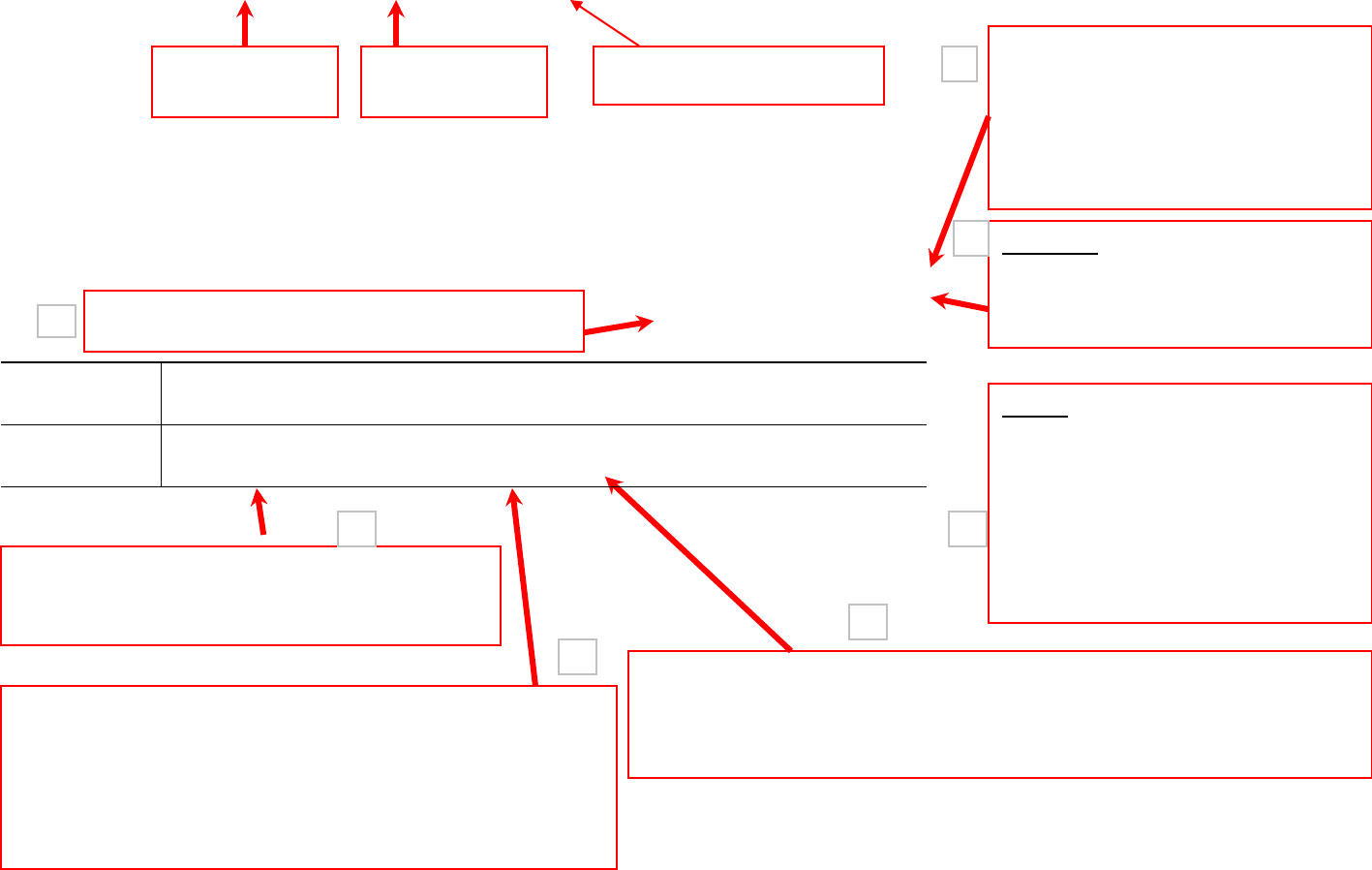
Regression: what to look for
This is the p-value of the model. It
tests whether R
2
is different from
0. Usually we need a p-value
lower than 0.05 to show a
statistically significant relationship
between X and Y.
R-square shows the amount of
variance of Y explained by X. In
this case expense explains 22%
of the variance in SAT scores.
Lets run the regression:
regress csat expense, robust
Adj R
2
(not shown here) shows
the same as R
2
but adjusted by
the # of cases and # of variables.
When the # of variables is small
and the # of cases is very large
then Adj R
2
is closer to R
2
. This
provides a more honest
association between X and Y.
Two-tail p-values test the hypothesis that each coefficient is different
from 0. To reject this, the p-value has to be lower than 0.05 (you
could choose also an alpha of 0.10). In this case, expense is
statistically significant in explaining SAT.
The t-values test the hypothesis that the coefficient is
different from 0. To reject this, you need a t-value greater
than 1.96 (for 95% confidence). You can get the t-values
by dividing the coefficient by its standard error. The t-
values also show the importance of a variable in the
model.
csat = 1061 - 0.022*expense
For each one-point increase in expense, SAT
scores decrease by 0.022 points.
Outcome
variable (Y)
Predictor
variable (X)
1
2
3
4
5
6
Robust standard errors (to control
for heteroskedasticity)
_cons
1060.732 24.35468 43.55 0.000 1011.79 1109.675
expense
-.0222756 .0036719 -6.07 0.000 -.0296547 -.0148966
csat
Coef. Std. Err. t P>|t| [95% Conf. Interval]
Robust
Root MSE = 59.814
R-squared = 0.2174
Prob > F = 0.0000
F( 1, 49) = 36.80
Linear regression Number of obs = 51
. regress
csat expense, robust
Root MSE: root mean squared error, is the sd of the
regression. The closer to zero better the fit.
7
5
PU/DSS/OTR
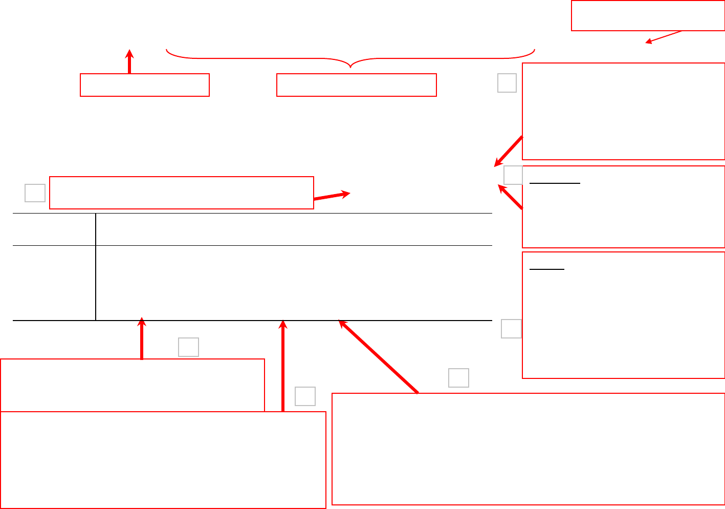
Regression: what to look for
This is the p-value of the model. It
indicates the reliability of X to
predict Y. Usually we need a p-
value lower than 0.05 to show a
statistically significant relationship
between X and Y.
R-square shows the amount of
variance of Y explained by X. In
this case the model explains
82.43% of the variance in SAT
scores.
Adding the rest of predictor variables:
regress csat expense percent income high college, robust
Adj R
2
(not shown here) shows
the same as R
2
but adjusted by
the # of cases and # of variables.
When the # of variables is small
and the # of cases is very large
then Adj R
2
is closer to R
2
. This
provides a more honest
association between X and Y.
Two-tail p-values test the hypothesis that each coefficient is different
from 0. To reject this, the p-value has to be lower than 0.05 (you
could choose also an alpha of 0.10). In this case, expense,
income, and college are not statistically significant in explaining
SAT; high is almost significant at 0.10. Percent is the only variable
that has some significant impact on SAT (its coefficient is different
from 0)
The t-values test the hypothesis that the coefficient is
different from 0. To reject this, you need a t-value greater
than 1.96 (at 0.05 confidence). You can get the t-values
by dividing the coefficient by its standard error. The t-
values also show the importance of a variable in the
model. In this case, percent is the most important.
csat = 851.56 + 0.003*expense
– 2.62*percent + 0.11*income + 1.63*high
+ 2.03*college
Output variable (Y) Predictor variables (X)
1
2
3
4
5
6
Robust standard errors (to control
for heteroskedasticity)
_cons 851.5649 57.28743 14.86 0.000 736.1821 966.9477
college
2.030894 2.113792 0.96 0.342 -2.226502 6.28829
high
1.630841 .943318 1.73 0.091 -.2690989 3.530781
income
.1055853 1.207246 0.09 0.931 -2.325933 2.537104
percent
-2.618177 .2288594 -11.44 0.000 -3.079123 -2.15723
expense
.0033528 .004781 0.70 0.487 -.0062766 .0129823
csat Coef. Std. Err. t P>|t| [95% Conf. Interval]
Robust
Root MSE = 29.571
R-squared = 0.8243
Prob > F = 0.0000
F( 5, 45) = 50.90
Linear regression Number of obs = 51
. regress csat expense percent income high college, robust
Root MSE: root mean squared error, is the sd of the
regression. The closer to zero better the fit.
7
6

Regression: using dummy variables/selecting the reference category
If using categorical variables in your regression, you need to add n-1 dummy variables. Here ‘n’ is the number of categories in the variable.
In the example below, variable ‘industry’ has twelve categories (type tab industry, or tab industry, nolabel)
The easiest way to include a set of dummies in a regression is by
using the prefix “i.” By default, the first category (or lowest value) is
used as reference. For example:
sysuse nlsw88.dta
reg wage hours i.industry, robust
To change the reference category to “Professional services”
(category number 11) instead of “Ag/Forestry/Fisheries” (category
number 1), use the prefix “ib#.” where “#” is the number of the
reference category you want to use; in this case is 11.
sysuse nlsw88.dta
reg wage hours ib11.industry, robust
_cons 3.126629 .8899074 3.51 0.000 1.381489 4.871769
Public Administration 3.232405 .8857298 3.65 0.000 1.495457 4.969352
Professional Services 2.094988 .8192781 2.56 0.011 .4883548 3.701622
Entertainment/Rec Svc 1.111801 1.192314 0.93 0.351 -1.226369 3.449972
Personal Services -1.018771 .8439617 -1.21 0.228 -2.67381 .6362679
Business/Repair Svc 1.990151 1.054457 1.89 0.059 -.0776775 4.057979
Finance/Ins/Real Estate 3.92933 .9934195 3.96 0.000 1.981199 5.877461
Wholesale/Retail Trade .4583809 .8548564 0.54 0.592 -1.218023 2.134785
Transport/Comm/Utility 5.432544 1.03998 5.22 0.000 3.393107 7.471981
Manufacturing 1.415641 .849571 1.67 0.096 -.2503983 3.081679
Construction 1.858089 1.281807 1.45 0.147 -.6555808 4.371759
Mining 9.328331 7.287849 1.28 0.201 -4.963399 23.62006
industry
hours .0723658 .0110213 6.57 0.000 .0507526 .093979
wage Coef. Std. Err. t P>|t| [95% Conf. Interval]
Robust
Root MSE = 5.5454
R-squared = 0.0800
Prob > F = 0.0000
F( 12, 2215) = 24.96
Linear regression Number of obs = 2228
_cons 5.221617 .4119032 12.68 0.000 4.41386 6.029374
Public Administration 1.137416 .4176899 2.72 0.007 .3183117 1.956521
Entertainment/Rec Svc -.983187 .9004471 -1.09 0.275 -2.748996 .7826217
Personal Services -3.113759 .3192289 -9.75 0.000 -3.739779 -2.48774
Business/Repair Svc -.1048377 .7094241 -0.15 0.883 -1.496044 1.286368
Finance/Ins/Real Estate 1.834342 .6171526 2.97 0.003 .6240837 3.0446
Wholesale/Retail Trade -1.636607 .3504059 -4.67 0.000 -2.323766 -.949449
Transport/Comm/Utility 3.337556 .6861828 4.86 0.000 1.991927 4.683185
Manufacturing -.6793477 .3362365 -2.02 0.043 -1.338719 -.019976
Construction -.2368991 1.011309 -0.23 0.815 -2.220112 1.746314
Mining 7.233343 7.245913 1.00 0.318 -6.97615 21.44284
Ag/Forestry/Fisheries -2.094988 .8192781 -2.56 0.011 -3.701622 -.4883548
industry
hours .0723658 .0110213 6.57 0.000 .0507526 .093979
wage Coef. Std. Err. t P>|t| [95% Conf. Interval]
Robust
Root MSE = 5.5454
R-squared = 0.0800
Prob > F = 0.0000
F( 12, 2215) = 24.96
Linear regression Number of obs = 2228
The “ib#.” option is available since Stata 11 (type help fvvarlist for more options/details). For older Stata versions you need to
use “xi:” along with “i.” (type help xi for more options/details). For the examples above type (output omitted):
xi: reg wage hours i.industry, robust
char industry[omit]11 /*Using category 11 as reference*/
xi: reg wage hours i.industry, robust
To create dummies as variables type
tab industry, gen(industry)
To include all categories by suppressing the constant type:
reg wage hours bn.industry, robust hascons
PU/DSS/OTR
Regression: ANOVA table
If you run the regression without the ‘robust’ option you get the ANOVA table
xi: regress csat expense percent income high college i.region
A = Model Sum of Squares (MSS). The closer to TSS the better fit.
B = Residual Sum of Squares (RSS)
C = Total Sum of Squares (TSS)
D = Average Model Sum of Squares = MSS/(k-1) where k = # predictors
E = Average Residual Sum of Squares = RSS/(n – k) where n = # of observations
F = Average Total Sum of Squares = TSS/(n – 1)
R
2
shows the amount of observed variance explained by the model, in this case 94%.
The F-statistic, F(9,40), tests whether R
2
is different from zero.
Root MSE shows the average distance of the estimator from the mean, in this case 18 points in estimating SAT scores.
Total
212961.38 49 4346.15061 Root MSE = 17.813
Adj R-squared = 0.9270
Residual
12691.5396 40 317.28849 R-squared = 0.9404
Model
200269.84 9 22252.2045 Prob > F = 0.0000
F( 9, 40) = 70.13
Source
SS df MS Number of obs = 50
(A)
(B)
(C)
(D)
(E)
13.70
28849.317
2045.22252
40
5396.12691
9
84.200269
)1(
====
−
−
=
E
D
kn
RSS
k
MSS
F
( )
9404.0
.212961.38
84.200269
1
2
2
2
===
−
−==
∑
∑
C
A
yy
e
TSS
MSS
R
i
i
813.17
4040
5396.12691
)(
===
−
=
B
kn
RSS
Root
MSE
(F)
9270.0
15061.4346
28849.317
11)9404.01(
40
49
1)1(
1
1
22
=−=−=−−=−
−
−
−=
F
E
R
kn
n
AdjR
Source: Kohler, Ulrich, Frauke Kreuter, Data Analysis Using Stata, 2009
8

PU/DSS/OTR
Regression: estto/esttab
To show the models side-by-side you can use the commands estto and esttab:
regress csat expense, robust
eststo model1
regress csat expense percent income high college, robust
eststo model2
xi: regress csat expense percent income high college i.region, robust
eststo model3
esttab, r2 ar2 se scalar(rmse)
Type help eststo and help esttab
for more options.
* p<0.05, ** p<0.01, *** p<0.001
Standard errors in parentheses
rmse 59.81 29.57 21.49
adj. R-sq 0.201 0.805 0.894
R-sq 0.217 0.824 0.911
N 51 51 50
(24.35) (57.29) (67.86)
_cons 1060.7*** 851.6*** 808.0***
percent2
(9.450)
_Iregion_4
34.58***
(12.53)
_Iregion_3 25.40*
(18.00)
_Iregion_2 69.45***
(2.114) (1.600)
college
2.031 4.671**
(0.943) (1.027)
high 1.631 1.815
(1.207) (1.196)
income 0.106 -0.167
(0.229) (0.236)
percent
-2.618*** -3.008***
(0.00367) (0.00478) (0.00359)
expense -0.0223*** 0.00335 -0.00202
csat csat csat
(1) (2) (3)
. esttab, r2 ar2 se scalar(rmse)
9

PU/DSS/OTR
Regression: correlation matrix
Below is a correlation matrix for all variables in the model. Numbers are Pearson
correlation coefficients, go from -1 to 1. Closer to 1 means strong correlation. A negative
value indicates an inverse relationship (roughly, when one goes up the other goes down).
0.0070 0.0000 0.0000 0.0000 0.0001
college
-0.3729* 0.6400* 0.6091* 0.7234* 0.5319* 1.0000
0.5495 0.0252 0.3226 0.0001
high
0.0858 0.3133* 0.1413 0.5099* 1.0000
0.0005 0.0000 0.0000
income
-0.4713* 0.6784* 0.6733* 1.0000
0.0000 0.0000
percent
-0.8758* 0.6509* 1.0000
0.0006
expense
-0.4663* 1.0000
csat
1.0000
csat expense percent income high college
. pwcorr csat expense percent income high college, star(0.05) sig
10
PU/DSS/OTR
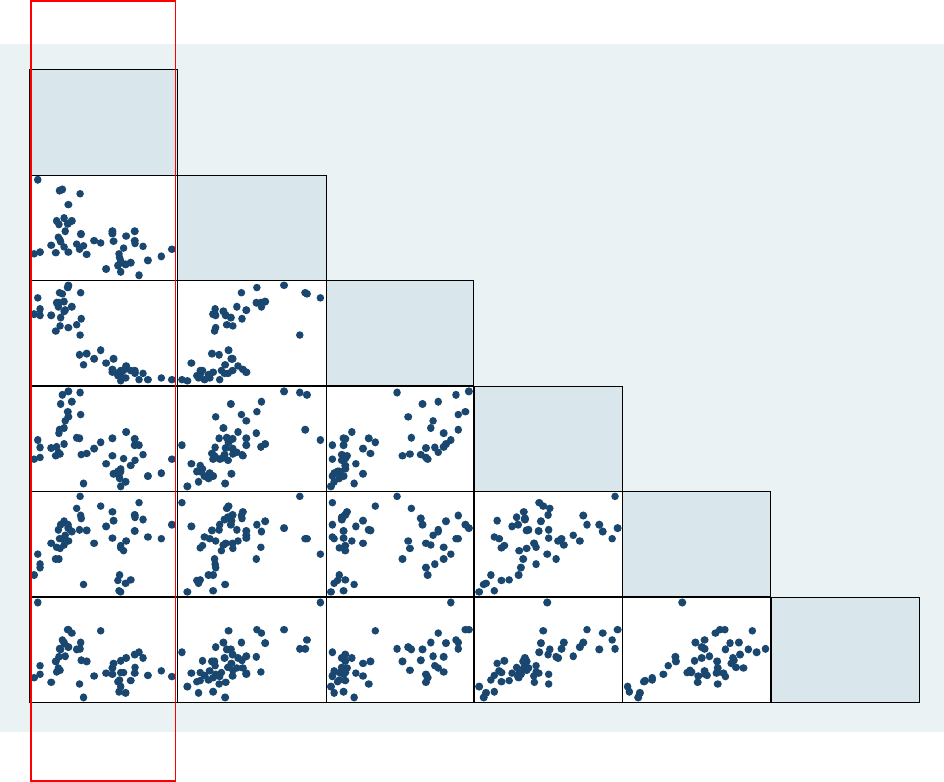
Command graph matrix produces a graphical representation of the correlation matrix by
presenting a series of scatterplots for all variables. Type:
graph matrix csat expense percent income high college, half
maxis(ylabel(none) xlabel(none))
Mean
composite
SAT
score
Per pupil
expenditures
prim&sec
% HS
graduates
taking
SAT
Median
household
income,
$1,000
%
adults
HS
diploma
% adults
college
degree
Regression: graph matrix
Y
11
PU/DSS/OTR
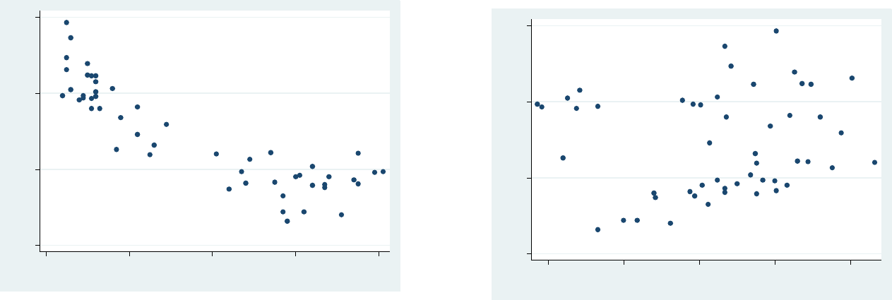
Regression: exploring relationships
800 900
1000 1100
Mean composite SAT score
0 20 40 60 80
% HS graduates taking SAT
800
900 1000 1100
Mean composite SAT score
65 70 75 80
85
% adults HS diploma
scatter csat percent
scatter csat high
There seem to be a curvilinear relationship between csat and percent, and slightly linear
between csat and high. To deal with U-shaped curves we need to add a square version of
the variable, in this case percent square
generate percent2 = percent^2
12
PU/DSS/OTR
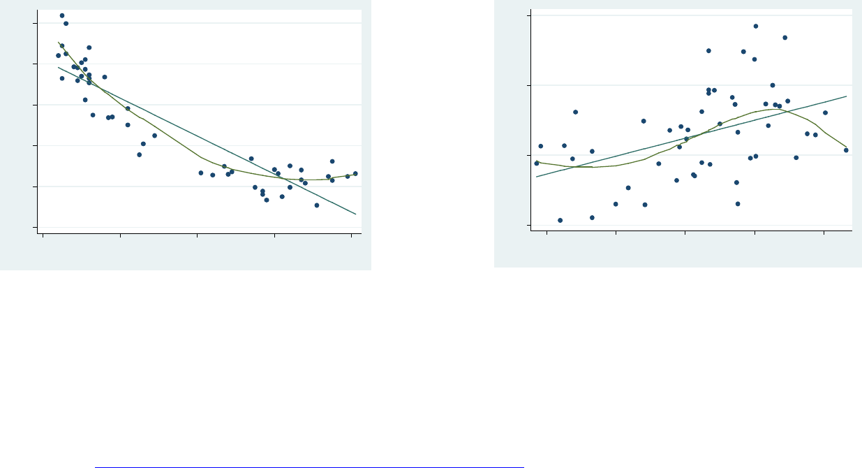
The command acprplot (augmented component-plus-residual plot) provides another graphical way to examine the
relationship between variables. It does provide a good testing for linearity. Run this command after running a
regression
regress csat percent high /* Notice we do not include percent2 */
acprplot percent, lowess
acprplot high, lowess
Regression: functional form/linearity
Form more details see http://www.ats.ucla.edu/stat/stata/webbooks/reg/chapter2/statareg2.htm, and/or type help acprplot and help lowess.
450 500 550 600
Augmented component plus residual
65
70 75
80 85
% adults HS diploma
-250 -200 -150 -100 -50 0
Augmented component plus residual
0
20 40
60 80
% HS graduates taking SAT
acprplot percent, lowess acprplot high, lowess
The option lowess (locally weighted scatterplot smoothing) draw the observed pattern in the data to help identify
nonlinearities. Percent shows a quadratic relation, it makes sense to add a square version of it. High shows a
polynomial pattern as well but goes around the regression line (except on the right). We could keep it as is for now.
The model is:
xi: regress csat expense percent percent2 income high college i.region, robust
13

PU/DSS/OTR
Regression: models
xi: regress csat expense percent percent2 income high college i.region, robust
eststo model4
esttab, r2 ar2 se scalar(rmse)
* p<0.05, ** p<0.01, *** p<0.001
Standard errors in parentheses
rmse 59.81 29.57 21.49 17.81
adj. R-sq 0.201 0.805 0.894 0.927
R-sq 0.217 0.824 0.911 0.940
N 51 51 50 50
(24.35) (57.29) (67.86) (58.13)
_cons 1060.7*** 851.6*** 808.0*** 874.0***
(0.0102)
percent2 0.0460***
(9.450) (8.110)
_Iregion_4 34.58*** 19.25*
(12.53) (10.42)
_Iregion_3 25.40* 5.209
(18.00) (20.75)
_Iregion_2 69.45*** 5.077
(2.114 ) (1.600) (1.145)
college 2.031 4.671** 3.418**
(0.943) (1.027) (0.931)
high 1.631 1.815 1.869
(1.207) (1.196) (0.973)
income 0.106 -0.167 -0.914
(0.229) (0.236) (0.641)
percent -2.618*** -3.008*** -5.945***
(0.00367) (0.00478) (0.00359) (0.00372)
expense -0.0223*** 0.00335 -0.00202 0.00141
csat csat csat csat
(1) (2) (3) (4)
. esttab, r2 ar2 se scalar(rmse)
14

PU/DSS/OTR
Regression: getting predicted values
How good the model is will depend on how well it predicts Y, the linearity of the model and the behavior of
the residuals.
There are two ways to generate the predicted values of Y (usually called Yhat) given the model:
Option A, using generate after running the regression:
xi: regress csat expense percent percent2 income high college i.region, robust
generate csat_predict = _b[_cons] + _b[percent]*percent + _b[percent]*percent + _b[percent2]*percent2
+ _b[high]*high + …
Option B, using predict immediately after running the regression:
xi: regress csat expense percent percent2 income high college i.region, robust
predict csat_predict
label variable csat_predict "csat predicted"
. label variable csat_predict "csat predicted"
(1 missing value generated)
(option xb assumed; fitted values)
. predict csat_predict
15
PU/DSS/OTR
800
900 1000 1100
Mean composite SAT score
850 900 950 1000 1050
csat predicted
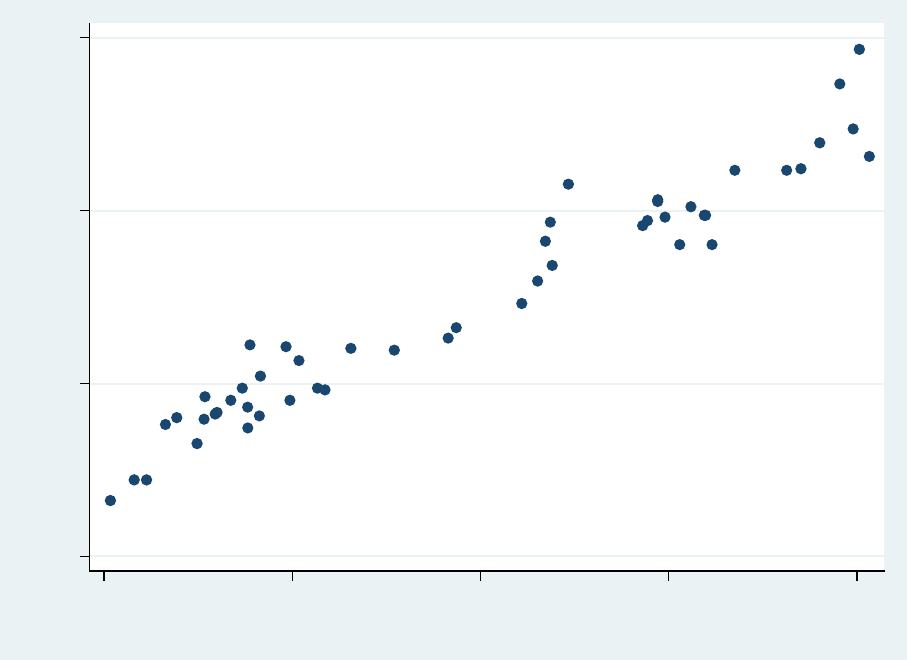
Regression: observed vs. predicted values
For a quick assessment of the model run a scatter plot
scatter csat csat_predict
We should expect a 45 degree pattern in the data. Y-axis is the observed data and x-axis the predicted
data (Yhat).
In this case the model seems to be doing a good job in predicting csat
16
PU/DSS/OTR
Regression: testing for homoskedasticity
An important assumption is that the variance in the residuals has to be homoskedastic or constant. Residuals
cannot varied for lower of higher values of
X
(i.e. fitted values of
Y
since
Y=Xb
). A definition:
“The error term [e] is homoskedastic if the variance of the conditional distribution of [e
i
] given X
i
[var(e
i
|X
i
)], is constant for
i=1…n, and in particular does not depend on x; otherwise, the error term is heteroskedastic” (Stock and Watson, 2003,
p.126)
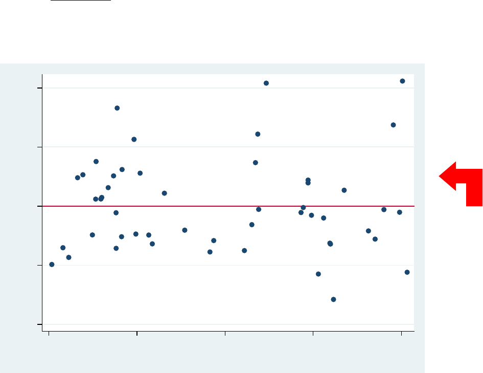
When plotting residuals vs. predicted values (
Yha
t) we
should not observe
any pattern at all. In Stata we do this
using rvfplot right after
running the regression, it will automatically draw a scatterplot between residuals and
predicted values.
rvfplot, yline(0)
Residuals seem to slightly
expand at higher levels of
Yhat.
-40 -20 0 20 40
Residuals
850
900 950 1000 1050
Fitted values
17
PU/DSS/OTR
Regression: testing for homoskedasticity
estat hettest
A non-graphical way to detect heteroskedasticiy is the Breusch-Pagan test. The null hypothesis is that
residuals are homoskedastic. In the example below we fail to reject the null at 95% and concluded that
residuals are homogeneous. However at 90% we reject the null and conclude that residuals are not
homogeneous.
The graphical and the Breush-Pagan test suggest the possible presence of heteroskedasticity in our model. The
problem with this is that we may have the wrong estimates of the standard errors for the coefficients and
therefore their t-values.
There are two ways to deal with this problem, one is using heteroskedasticity-robust standard errors, the other
one is using weighted least squares (see Stock and Watson, 2003, chapter 15). WLS requires knowledge of the
conditional variance on which the weights are based, if this is known (rarely the case) then use WLS. In practice
it is recommended to use heteroskedasticity-robust standard errors to deal with heteroskedasticity.
By default Stata assumes homoskedastic standard errors, so we need to adjust our model to account for
heteroskedasticity. To do this we use the option robust in the regress command.
xi: regress csat expense percent percent2 income high college i.region, robust
Following Stock and Watson, as a rule-of-thumb, you should always assume heteroskedasticiy in your model
(see Stock and Watson, 2003, chapter 4) .
Prob > chi2 = 0.0993
chi2(1) = 2.72
Variables: fitted values of csat
Ho: Constant variance
Breusch-Pagan / Cook-Weisberg test for heteroskedasticity
. estat hettest
18
PU/DSS/OTR
Regression: omitted-variable test
How do we know we have included all variables we need to explain Y?
Testing for omitted variable bias is important for our model since it is related to the assumption that the error
term and the independent variables in the model are not correlated (E(e|X) = 0)
If we are missing variables in our model and
• “is correlated with the included regressor” and,
• “ the omitted variable is a determinant of the dependent variable” (Stock and Watson, 2003, p.144),
…then our regression coefficients are inconsistent.
In Stata we test for omitted-variable bias using the ovtest command:
xi: regress csat expense percent percent2 income high college i.region, robust
ovtest
The null hypothesis is that the model does not have omitted-variables bias, the p-value is higher than the
usual threshold of 0.05 (95% significance), so we fail to reject the null and conclude that we do not need
more variables.
Prob > F = 0.3068
F(3, 37) = 1.25
Ho: model has no omitted variables
Ramsey RESET test using powers of the fitted values of csat
. ovtest
19
PU/DSS/OTR
_cons
-68.69417 712.388 -0.10 0.924 -1501.834 1364.446
_hatsq
-.0000761 .0007885 -0.10 0.923 -.0016623 .0015101
_hat
1.144949 1.50184 0.76 0.450 -1.876362 4.166261
csat
Coef. Std. Err. t P>|t| [95% Conf. Interval]
Total
212961.38 49 4346.15061 Root MSE = 16.431
Adj R-squared = 0.9379
Residual
12689.0209 47 269.979169 R-squared = 0.9404
Model
200272.359 2 100136.18 Prob > F = 0.0000
F( 2, 47) = 370.90
Source
SS df MS Number of obs = 50
. linktest
Another command to test model specification is linktest. It basically checks whether we need more
variables in our model by running a new regression with the observed Y (csat) against Yhat
(csat_predicted or Xβ) and Yhat-squared as independent variables
1
.
The thing to look for here is the significance of _hatsq. The null hypothesis is that there is no
specification error. If the p-value of _hatsq is not significant
then we fail to reject the null and
conclude that our model is correctly specified. Type:
xi: regress csat expense percent percent2 income high college i.region, robust
linktest
Regression: specification error
1
For more details see http://www.ats.ucla.edu/stat/stata/webbooks/reg/chapter2/statareg2.htm, and/or type help linktest.
20
PU/DSS/OTR
An important assumption for the multiple regression model is that independent variables are not perfectly
multicolinear. One regressor should not be a linear function of another.
When multicollinearity is present standand errors may be inflated. Stata will drop one of the variables to avoid
a division by zero in the OLS procedure (see Stock and Watson, 2003, chapter 5).
The Stata command to check for multicollinearity is vif (variance inflation factor). Right after running the
regression type:
Regression: multicollinearity
Form more details see http://www.ats.ucla.edu/stat/stata/webbooks/reg/chapter2/statareg2.htm, and/or type help vif.
A vif> 10or a 1/vif < 0.10 indicates trouble.
We know that percent and percent2are related since one is the square of the other. They are ok since percent
has a quadratic relationship with Y, but this would be an example of multicolinearity.
The rest of the variables look ok.
Mean VIF 17.04
_Iregion_4 2.14 0.467506
expense
3.33 0.300111
college
4.52 0.221348
high
4.71 0.212134
_Iregion_3
4.89 0.204445
income
4.97 0.201326
_Iregion_2
8.47 0.118063
percent
49.52 0.020193
percent2
70.80 0.014124
Variable
VIF 1/VIF
. vif
21

PU/DSS/OTR
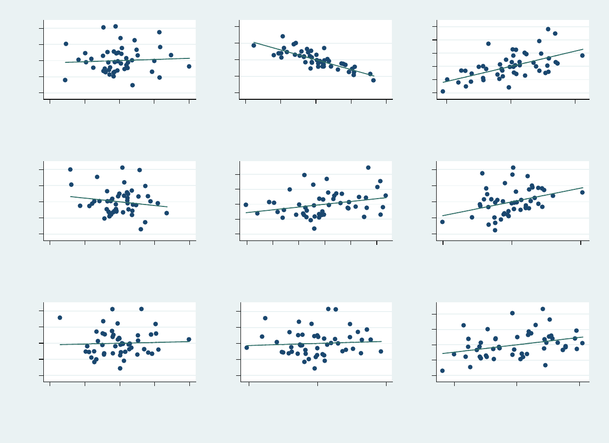
Regression: outliers
To check for outliers we use the avplots command (added-variable plots). Outliers are data points
with extreme values that could have a negative effect on our estimators. After running the regression
type:
These plots regress each variable against all others, notice the coefficients on each. All data points
seem to be in range, no outliers observed.
For more details and tests on this and influential and leverage variables please check
http://www.ats.ucla.edu/stat/stata/webbooks/reg/chapter2/statareg2.htm
Also type help diagplots in the Stata command window.
-100 -50 0 50 100
e( csat | X )
-10 -5 0 5 10
e( percent | X )
coef = -5.9452674, (robust) se = .64055286, t = -9.28
avplot percent
-40 -20 0
20 40
e( csat | X )
-2000 -1000 0 1000 2000
e( expense | X )
coef = .00141156, (robust) se = .00371641, t = .38
avplot expense
22
PU/DSS/OTR
-40-20 0 20 40
e( csat | X )
-2000 -1000 0 1000 2000
e( expense | X )
coef = .00141156, (robust) se = .00371641, t = .38
-100-50 0 50 100
e( csat | X )
-10 -5 0 5 10
e( percent | X )
coef = -5.9452674, (robust) se = .64055286, t = -9.28
-40-20 0 2040 60
e( csat | X )
-500 0 500
e( percent2 | X )
coef = .0460468, (robust) se = .01019105, t = 4.5
-40-20 0 20 40
e( csat | X )
-10 -5 0 5 10
e( income | X )
coef = -.9143708, (robust) se = .97326373, t = -.94
-40-20 0 20 40
e( csat | X )
-6 -4 -2 0 2 4
e( high | X )
coef = 1.8691679, (robust) se = .93111302, t = 2.01
-40-20 0 20 40
e( csat | X )
-5 0 5
e( college | X )
coef = 3.4175732, (robust) se = 1.1450333, t = 2.
-40-20 0 20 40
e( csat | X )
-.4 -.2 0 .2 .4
e( _Iregion_2 | X )
coef = 5.0765963, (robust) se = 20.753948, t = .24
-40-20 0 20 40
e( csat | X )
-.5 0 .5
e( _Iregion_3 | X )
coef = 5.2088169, (robust) se = 10.422781, t = .5
-40-20 0 20 40
e( csat | X )
-.5 0 .5
e( _Iregion_4 | X )
coef = 19.245404, (robust) se = 8.1097615, t = 2.
Regression: outliers
avplots
23

PU/DSS/OTR
Regression: summary of influence indicators
DfBeta
Measures the influence of
each observation on the
coefficient of a particular
independent variable (for
example, x1). This is in
standard errors terms.
An observation is influential if
it has a significant effect on
the coefficient.
A case is an influential outlier
if
|DfBeta|> 2/SQRT(N)
Where N is the sample size.
Note: Stata estimates
standardized DfBetas.
In Stata type:
reg y x1 x2 x3
dfbeta x1
Note: you could also type:
predict DFx1, dfbeta(x1)
To estimate the dfbetas
for all predictors just
type:
dfbeta
To flag the cutoff
gen cutoffdfbeta = abs(DFx1) >
2/sqrt(e(N)) & e(sample)
In SPSS: Analyze-Regression-
Linear; click Save. Select under
“Influence Statistics” to add as a
new variable (DFB1_1) or in
syntax type
REGRESSION
/MISSING LISTWISE
/STATISTICS COEFF OUTS
R ANOVA
/CRITERIA=PIN(.05)
POUT(.10)
/NOORIGIN
/DEPENDENT Y
/METHOD=ENTER X1 X2 X3
/CASEWISE PLOT(ZRESID)
OUTLIERS(3) DEFAULTS
DFBETA
/SAVE MAHAL COOK LEVER
DFBETA SDBETA DFFIT
SDFIT COVRATIO .
DfFit
Indicator of leverage and
high residuals.
Measures how much an
observation influences the
regression model as a whole.
How much the predicted
values change as a result of
including and excluding a
particular observation.
High influence if
|DfFIT| >2*SQRT(k/N)
Where k is the number of
parameters (including the
intercept) and N is the
sample size.
After running the regression type:
predict dfits if e(sample), dfits
To generate the flag for the cutoff type:
gen cutoffdfit=
abs(dfits)>2*sqrt((e(df_m)
+1)/e(N)) & e(sample)
Same as DfBeta above (DFF_1)
Covariance ratio
Measures the impact of an
observation on the standard
errors
High impact if
|COVRATIO-1| ≥ 3*k/N
Where k is the number of
parameters (including the
intercept) and N is the
sample size.
In Stata after running the regression type
predict covratio if e(sample),
covratio
Same as DfBeta above
(COV_1)
24

PU/DSS/OTR
Regression: summary of distance measures
Cook’s distance
Measures how much an
observation influences the
overall model or predicted
values.
It is a summary measure of
leverage and high residuals.
.
High influence if
D > 4/N
Where N is the sample size.
A D>1 indicates big outlier
problem
In Stata after running the
regression type:
predict D, cooksd
In SPSS: Analyze-Regression-Linear;
click Save. Select under “Distances”
to add as a new variable (COO_1) or
in syntax type
REGRESSION
/MISSING LISTWISE
/STATISTICS COEFF OUTS R
ANOVA
/CRITERIA=PIN(.05) POUT(.10)
/NOORIGIN
/DEPENDENT Y
/METHOD=ENTER X1 X2 X3
/CASEWISE PLOT(ZRESID)
OUTLIERS(3) DEFAULTS DFBETA
/SAVE MAHAL COOK LEVER
DFBETA SDBETA DFFIT SDFIT
COVRATIO.
Leverage
Measures how much an
observation influences
regression coefficients.
High influence if
leverage h > 2*k/N
Where k is the number of
parameters (including the
intercept) and N is the sample size.
A rule-of-thumb: Leverage goes
from 0 to 1. A value closer to 1 or
over 0.5 may indicate problems.
In Stata after running the
regression type:
predict lev, leverage
Same as above (LEV_1)
Mahalanobis distance
It is rescaled measure of
leverage.
M = leverage*(N-1)
Where N is sample size.
Higher levels indicate higher
distance from average values.
The M-distance follows a Chi-
square distribution with k-1 df and
alpha=0.001 (where k is the
number of independent variables).
Any value over this Chi-square
value may indicate problems.
Not available Same as above (MAH_1)
25

PU/DSS/OTR
Sources for the summary tables:
influence indicators and distance measures
• Statnotes:
http://faculty.chass.ncsu.edu/garson/PA765/regress.htm#outlier2
• An Introduction to Econometrics Using Stata/Christopher F. Baum, Stata
Press, 2006
• Statistics with Stata (updated for version 9) / Lawrence Hamilton,
Thomson Books/Cole, 2006
• UCLA
http://www.ats.ucla.edu/stat/stata/webbooks/reg/chapter2/statareg2.htm
26
PU/DSS/OTR
Regression: testing for normality
Another assumption of the regression model (OLS) that impact the validity of all tests (p, t and F) is that residuals behave
‘normal’. Residuals (here indicated by the letter “e”) are the difference between the observed values (Y) and the predicted values
(Yhat): e = Y – Yhat.
In Stata you type: predict e, resid. It will generate a variable called “e” (residuals).
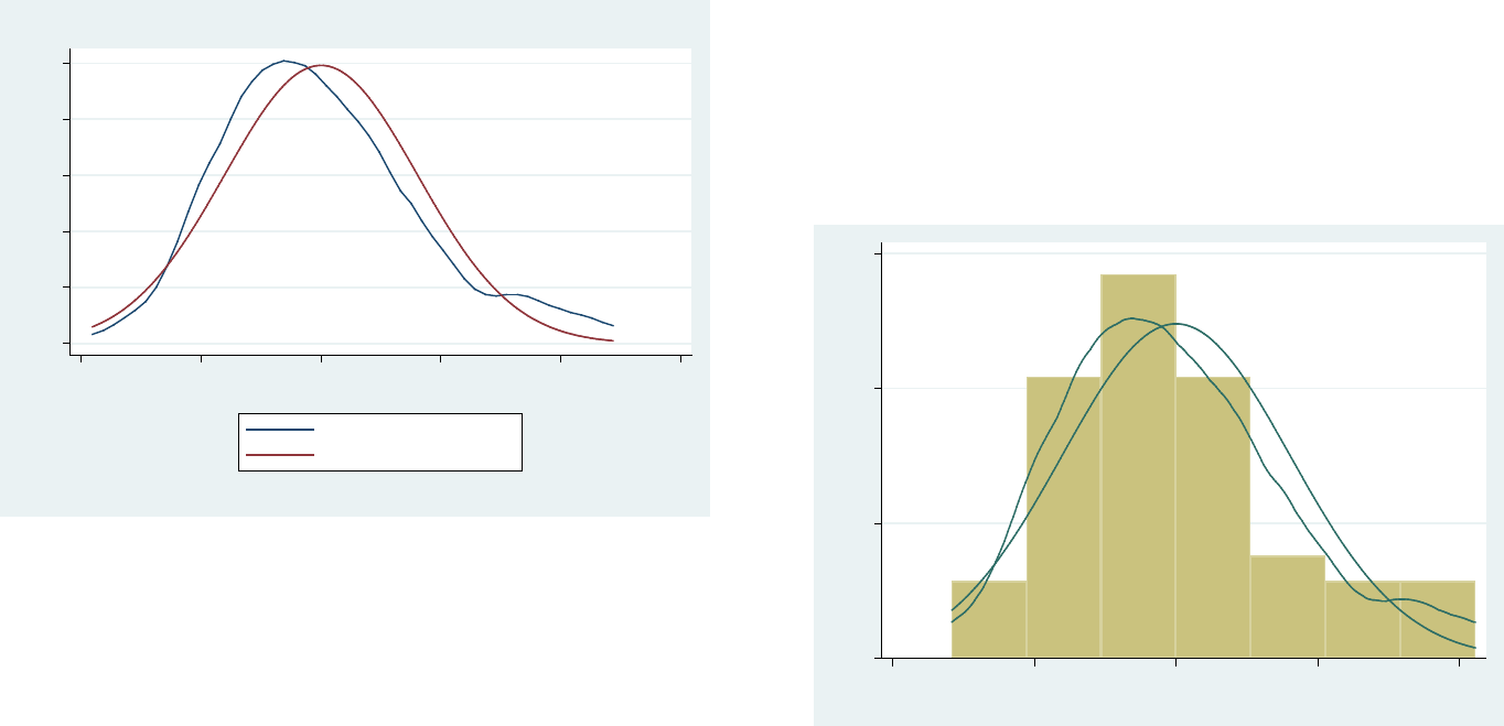
Three graphs will help us check for normality in the residuals: kdensity, pnorm and qnorm.
kdensity e, normal
A kernel density plot produces a kind of histogram for the
residuals, the option normal overlays a normal distribution to
compare. Here residuals seem to follow a normal distribution.
Below is an example using histogram.
histogram e, kdensity normal
If residuals do not follow a ‘normal’ pattern then you should
check for omitted variables, model specification, linearity,
functional forms. In sum, you may need to reassess your
model/theory. In practice normality does not represent much of a
problem when dealing with really big samples.
0 .005 .01 .015 .02 .025
Density
-40
-20 0 20
40 60
Residuals
Kernel density estimate
Normal density
kernel = epanechnikov, bandwidth = 6.4865
Kernel density estimate
0
.01 .02 .03
Density
-40 -20 0 20 40
Residuals
27
PU/DSS/OTR
Regression: testing for normality
A non-graphical test is the Shapiro-Wilk test for normality. It tests the hypothesis that the distribution is normal, in this case the
null hypothesis is that the distribution of the residuals is normal. Type
swilk e
The null hypothesis is that the distribution of the residuals is normal, here the p-value is 0.06 we failed to reject the null (at 95%).
We conclude then that residuals are normally distributed, with the caveat that they are not at 90%.
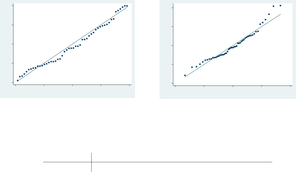
Quintile-normal plots (qnorm) check for non-normality in the
extremes of the data (tails). It plots quintiles of residuals vs
quintiles of a normal distribution. Tails are a bit off the normal.
qnorm epnorm e
Standardize normal probability plot (pnorm) checks
for non-normality in the middle range of residuals.
Again, slightly off the line but looks ok.
0.00
0.25 0.50 0.75 1.00
Normal F[(e-m)/s]
0.00 0.25 0.50 0.75
1.00
Empirical P[i] = i/(N+1)
-40 -20 0 20 40
Residuals
-40
-20
0
20 40
Inverse Normal
e 50 0.95566 2.085 1.567 0.05855
Variable Obs W V z Prob>z
Shapiro-Wilk W test for normal data
. swilk e
28
PU/DSS/OTR
Regression: joint test (F-test)
To test whether two coefficients are jointly different from 0 use the command test (see Hamilton, 2006,
p.175).
xi: quietly regress csat expense percent percent2 income high college i.region, robust
Note ‘quietly’ suppress the regression output
To test the null hypothesis that both coefficients do not have any effect on csat (β
high
= 0 and β
college
= 0), type:
test high college
The p-value is 0.0000, we reject the null and conclude that both variables have indeed a significant effect on
SAT.
Some other possible tests are (see Hamilton, 2006, p.176):
test income = 1
test high = college
test income = (high + college)/100
Note: Not to be confused with ttest. Type help test and help ttest for more details
Prob > F = 0.0000
F( 2, 40) = 17.12
( 2) college = 0
( 1) high = 0
. test high college
29

PU/DSS/OTR
Regression: saving regression coefficients
Stata temporarily stores the coefficients as _b[varname], so if you type:
gen percent_b = _b[percent]
gen constant_b = _b[_cons]
You can also save the standard errors of the variables _se[varname]
gen percent_se = _se[percent]
gen constant_se = _se[_cons]
constant_se
51 58.12895 0 58.12895 58.12895
constant_b
51 873.9537 0 873.9537 873.9537
percent_se
51 .6405529 0 .6405529 .6405529
percent_b
51 -5.945267 0 -5.945267 -5.945267
Variable
Obs Mean Std. Dev. Min Max
. summarize percent_b percent_se constant_b constant_se
30
PU/DSS/OTR
Regression: saving regression coefficients/getting predicted values
You can see a list of stored results by typing after the regression ereturn list:
e(sample)
functions:
e(V) : 10 x 10
e(b) : 1 x 10
matrices:
e(vcetype) : "Robust"
e(estat_cmd) : "regress_estat"
e(model) : "ols"
e(predict) : "regres_p"
e(properties) : "b V"
e(cmd) : "regress"
e(depvar) : "csat"
e(vce) : "robust"
e(title) :
"Linear regression"
e(cmdline) : "regress csat expense percent percent2 income high college _Iregion_*, robust"
macros:
e(ll_0) = -279.8680043669825
e(ll) = -209.3636234584767
e(r2_a) = .9269955143414049
e(rss) = 12691.53960166909
e(mss) = 200269.8403983309
e(rmse) = 17.81259357987284
e(r2) = .9404045015031877
e(F) = 76.92400040408057
e(df_r) = 40
e(df_m) = 9
e(N) = 50
scalars:
. ereturn list
i.region _Iregion_1-4 (naturally coded; _Iregion_1 omitted)
. xi: quietly regress csat expense percent percent2 income high college i.region, robust
Type help return for more details
31
PU/DSS/OTR
Regression: general guidelines
The following are general guidelines for building a regression model*
1. Make sure all relevant predictors are included. These are based on your
research question, theory and knowledge on the topic.
2. Combine those predictors that tend to measure the same thing (i.e. as an
index).
3. Consider the possibility of adding interactions (mainly for those variables
with large effects)
4. Strategy to keep or drop variables:
1. Predictor not significant and has the expected sign -> Keep it
2. Predictor not significant and does not have the expected sign -> Drop it
3. Predictor is significant and has the expected sign -> Keep it
4. Predictor is significant but does not have the expected sign -> Review, you may need
more variables, it may be interacting with another variable in the model or there may
be an error in the data.
*Gelman, Andrew, Jennifer Hill, Data Analysis Using Regression and Multilevel/Hierarchical Models,
2007, p. 69
32
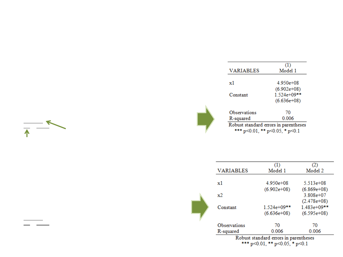
Regression: publishing regression output (outreg2)
The command outreg2 gives you the type of presentation you see in academic papers. It is important to notice that outreg2
is not a Stata command, it is a user-written procedure, and you need to install it by typing (only the first time)
ssc install outreg2
Follow this example (letters in italics you type)
use "H:\public_html\Stata\Panel101.dta", clear
reg y x1, r
outreg2 using myreg.doc, replace ctitle(Model 1)
You can add other model (using variable x2) by using the option append
(NOTE: make sure to close myreg.doc)
reg y x1 x2, r
outreg2 using myreg.doc, append ctitle(Model 2)
You also have the option to export to Excel, just use the extension *.xls.
For older versions of outreg2, you may need to specify the option word or excel (after comma)
dir : seeout
myreg.doc
. outreg2 using myreg.doc, replace ctitle(Model 1)
Mac users click here to go to the directory where myreg.doc is saved, open it with Word
(you can replace this name with your own)
Windows users click here to open the file myreg.doc in Word (you
can replace this name with your own) . Otherwise follow the Mac
instructions.
dir : seeout
myreg.doc
. outreg2 using myreg.doc, append ctitle(Model 2)
PU/DSS/OTR
33
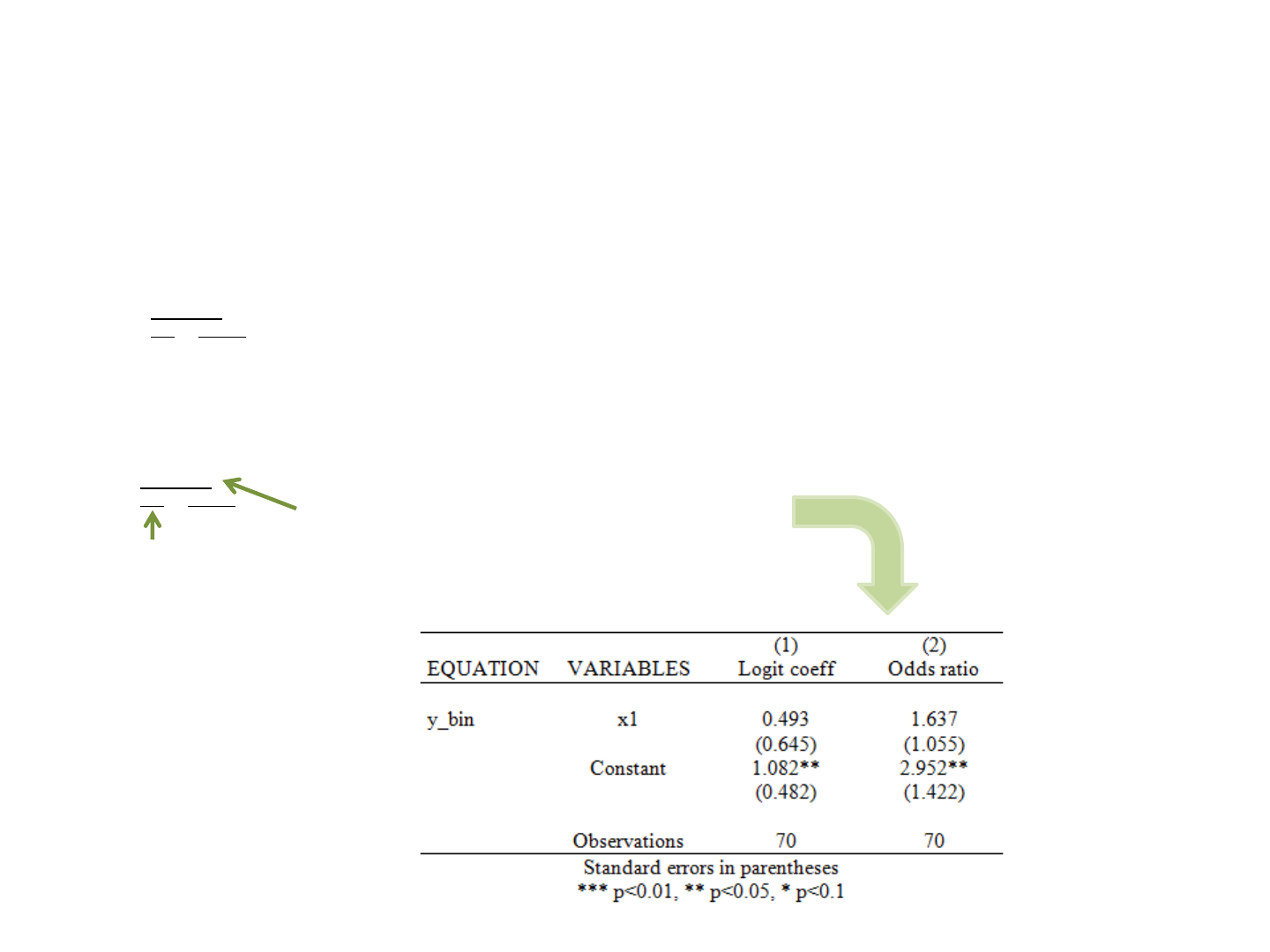
Regression: publishing regression output (outreg2)
You can use outreg2 for almost any regression output (linear or no linear). In the case of logit models with odds ratios, you
need to add the option eform, see below
use "H:\public_html\Stata\Panel101.dta", clear
logit y_bin x1
outreg2 using mymod.doc, replace ctitle(Logit coeff)
logit y_bin x1, or
outreg2 using mymod.doc, append ctitle(Odds ratio) eform
For more details/options type
help outreg2
PU/DSS/OTR
34
dir : seeout
mymod.doc
. outreg2 using mymod.doc, replace ctitle(Logit coeff)
dir : seeout
mymod.doc
. outreg2 using mymod.doc, append ctitle(Odds ratio) eform
Mac users click here to go to the directory where mymod.doc is saved, open it with Word
(you can replace this name with your own)
Windows users click here to open the file mymod.doc in Word (you
can replace this name with your own) . Otherwise follow the Mac
instructions.

Regression: publishing regression output (outreg2)
For predicted probabilities and marginal effects, see the following document
http://dss.princeton.edu/training/Margins.pdf
PU/DSS/OTR
35
PU/DSS/OTR
Interaction terms are needed whenever there is reason to believe that the effect of one independent variable depends on the value of
another independent variable. We will explore here the interaction between two dummy (binary) variables. In the example below there
could be the case that the effect of student-teacher ratio on test scores may depend on the percent of English learners in the district*.
– Dependent variable (Y) – Average test score, variable testscr in dataset.
– Independent variables (X)
• Binary hi_str, where ‘0’ if student-teacher ratio (str) is lower than 20, ‘1’ equal to 20 or higher.
– In Stata, first generate hi_str = 0 if str<20. Then replace hi_str=1 if str>=20.
• Binary hi_el, where ‘0’ if English learners (el_pct) is lower than 10%, ‘1’ equal to 10% or higher
– In Stata, first generate hi_el = 0 if el_pct<10. Then replace hi_el=1 if el_pct>=10.
• Interaction term str_el = hi_str * hi_el. In Stata: generate str_el = hi_str*hi_el
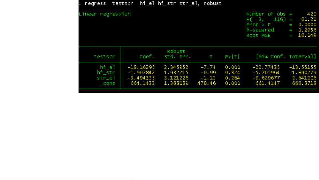
We run the regression
regress testscr hi_el hi_str str_el, robust
Regression: interaction between dummies
*The data used in this section is the “California Test Score” data set (caschool.dta) from chapter 6 of the book Introduction to Econometrics from Stock and Watson, 2003. Data can be downloaded from
http://wps.aw.com/aw_stock_ie_2/50/13016/3332253.cw/index.html
.For a detailed discussion please refer to the respective section in the book.
The equation is testscr_hat = 664.1 – 18.1*hi_el – 1.9*hi_str – 3.5*str_el
The effect of hi_str on the tests scores is -1.9 but given the interaction term (and assuming all coefficients are significant), the net effect is
-1.9 -3.5*hi_el. If hi_el is 0 then the effect is -1.9 (which is hi_str coefficient), but if hi_el is 1 then the effect is -1.9 -3.5 = -5.4.
In this case, the effect of student-teacher ratio is more negative in districts where the percent of English learners is higher.
See the next slide for more detailed computations.
36
PU/DSS/OTR
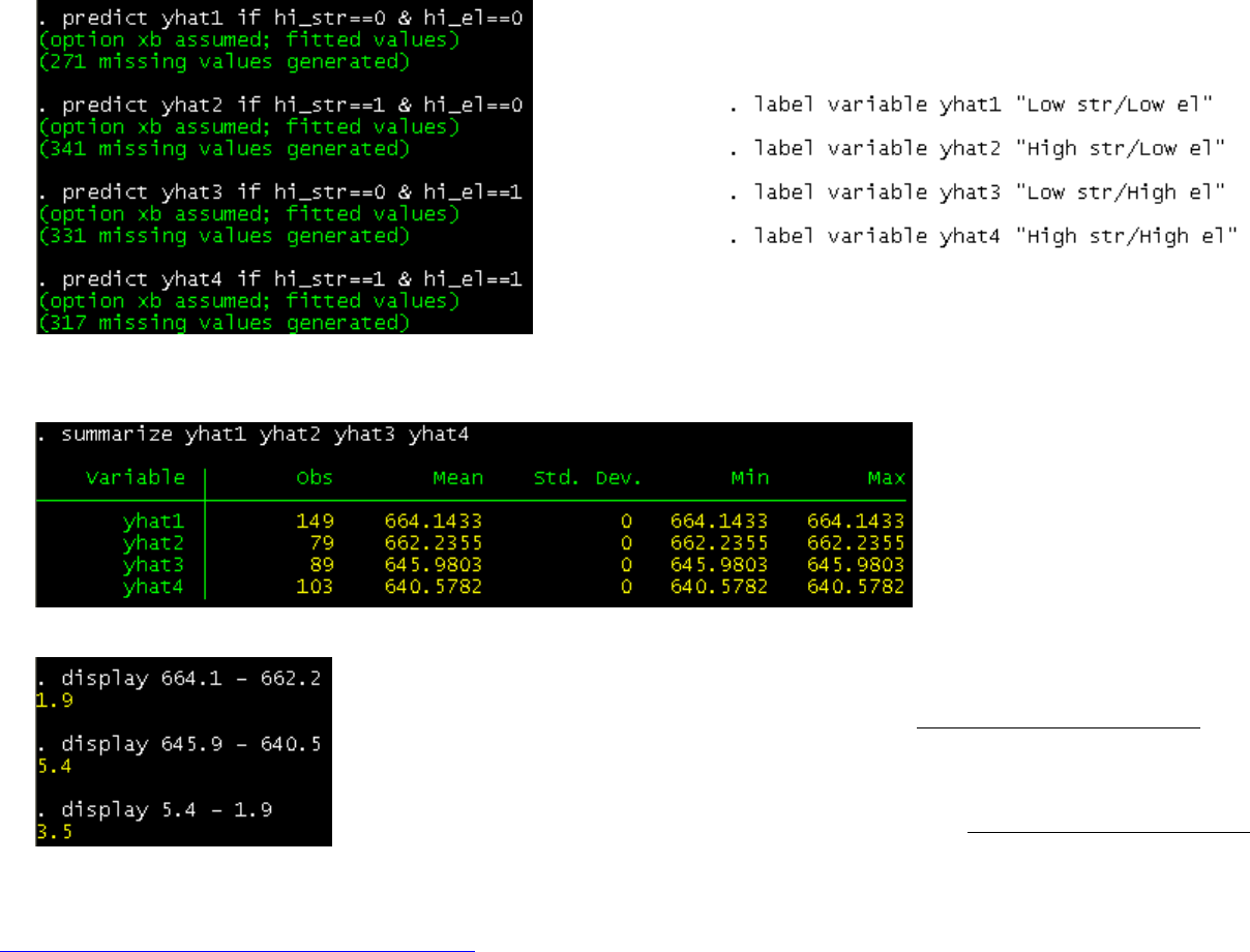
You can compute the expected values of test scores given different values of hi_str and hi_el. To see the effect of hi_str given
hi_el type the following right after running the regression in the previous slide.
Regression: interaction between dummies (cont.)
*The data used in this section is the “California Test Score” data set (caschool.dta) from chapter 6 of the book Introduction to Econometrics from Stock and Watson, 2003. Data can be downloaded from
http://wps.aw.com/aw_stock_ie_2/50/13016/3332253.cw/index.html
.For a detailed discussion please refer to the respective section in the book.
These are different scenarios holding constant hi_el and varying
hi_str. Below we add some labels
We then obtain the average of the estimations for the test scores (for all four scenarios, notice same values for all cases).
Here we estimate the net effect of low/high student-teacher ratio holding constant the percent of
English learners. When hi_el is 0 the effect of going from low to high student-teacher ratio goes
from a score of 664.2 to 662.2, a difference of 1.9. From a policy perspective you could argue that
moving from high str to low str improve test scores by 1.9 in low English learners districts.
When hi_el is 1, the effect of going from low to high student-teacher ratio goes from a score of
645.9 down to 640.5, a decline of 5.4 points (1.9+3.5). From a policy perspective you could say
that reducing the str in districts with high percentage of English learners could improve test scores
by 5.4 points.
37
PU/DSS/OTR
Lets explore the same interaction as before but we keep student-teacher ratio continuous and the English learners variable as binary. The
question remains the same*.
– Dependent variable (Y) – Average test score, variable testscr in dataset.
– Independent variables (X)
• Continuous str, student-teacher ratio.
• Binary hi_el, where ‘0’ if English learners (el_pct) is lower than 10%, ‘1’ equal to 10% or higher
• Interaction term str_el2 = str * hi_el. In Stata: generate str_el2 = str*hi_el
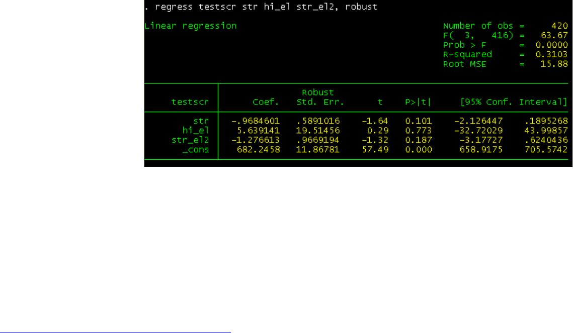
We will run the regression
regress testscr str hi_el str_el2, robust
Regression: interaction between a dummy and a continuous variable
*The data used in this section is the “California Test Score” data set (caschool.dta) from chapter 6 of the book Introduction to Econometrics from Stock and Watson, 2003. Data can be downloaded from
http://wps.aw.com/aw_stock_ie_2/50/13016/3332253.cw/index.html
.For a detailed discussion please refer to the respective section in the book.
The equation is testscr_hat = 682.2 – 0.97*str + 5.6*hi_el – 1.28*str_el2
The effect of str on testscr will be mediated by hi_el.
– If hi_el is 0 (low) then the effect of str is 682.2 – 0.97*str.
– If hi_el is 1 (high) then the effect of str is 682.2 – 0.97*str + 5.6 – 1.28*str = 687.8 – 2.25*str
Notice that how hi_el changes both the intercept and the slope of str. Reducing str by one in low EL districts will increase test scores by
0.97 points, but it will have a higher impact (2.25 points) in high EL districts. The difference between these two effects is 1.28 which is the
coefficient of the interaction (Stock and Watson, 2003, p.223).
38
PU/DSS/OTR
Lets keep now both variables continuous. The question remains the same*.
– Dependent variable (Y) – Average test score, variable testscr in dataset.
– Independent variables (X)
• Continuous str, student-teacher ratio.
• Continuous el_pct, percent of English learners.
• Interaction term str_el3 = str * el_pct. In Stata: generate str_el3 = str*el_pct
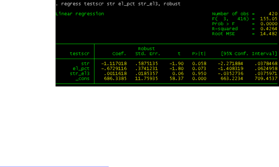
We will run the regression
regress testscr str el_pct str_el3, robust
Regression: interaction between two continuous variables
*The data used in this section is the “California Test Score” data set (caschool.dta) from chapter 6 of the book Introduction to Econometrics from Stock and Watson, 2003. Data can be downloaded from
http://wps.aw.com/aw_stock_ie_2/50/13016/3332253.cw/index.html
.For a detailed discussion please refer to the respective section in the book.
The equation is testscr_hat = 686.3 – 1.12*str - 0.67*el_pct + 0.0012*str_el3
The effect of the interaction term is very small. Following Stock and Watson (2003, p.229), algebraically the slope of str is
–1.12 + 0.0012*el_pct (remember that str_el3 is equal to str*el_pct). So:
– If el_pct = 10, the slope of str is -1.108
– If el_pct = 20, the slope of str is -1.096. A difference in effect of 0.012 points.
In the continuous case there is an effect but is very small (and not significant). See Stock and Watson, 2003, for further details.
39
PU/DSS/OTR
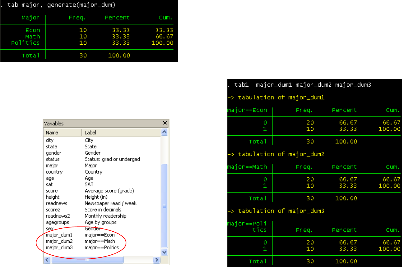
You can create dummy variables by either using recode or using a combination of tab/gen commands:
tab major, generate(major_dum)
Creating dummies
Check the ‘variables’ window, at the end you will see
three new variables. Using tab1 (for multiple
frequencies) you can check that they are all 0 and 1
values
40
PU/DSS/OTR
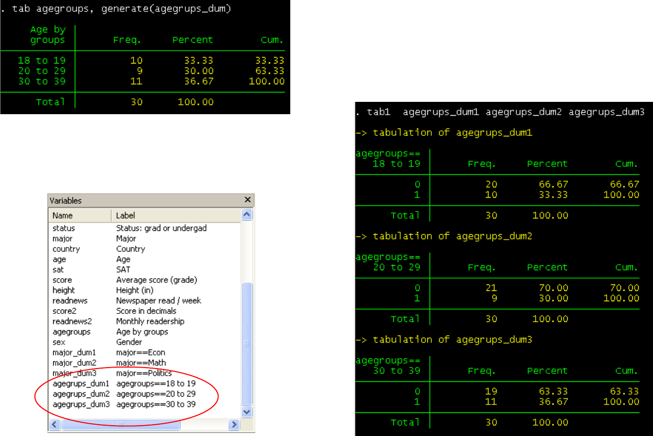
Here is another example:
tab agregroups, generate(agegroups_dum)
Creating dummies (cont.)
Check the ‘variables’ window, at the end you will see
three new variables. Using tab1 (for multiple
frequencies) you can check that they are all 0 and 1
values
41

PU/DSS/OTR
Category Stata commands
Getting on-line help
help
search
Operating-system interface
pwd
cd
sysdir
mkdir
dir / ls
erase
copy
type
Using and saving data from disk
use
clear
save
append
merge
compress
Inputting data into Stata
input
edit
infile
infix
insheet
The Internet and Updating Stata
update
net
ado
news
Basic data reporting
describe
codebook
inspect
list
browse
count
assert
summarize
Table (tab)
tabulate
Data manipulation
generate
replace
egen
recode
rename
drop
keep
sort
encode
decode
order
by
reshape
Formatting
format
label
Keeping track of your work
log
notes
Convenience
display
Source: http://www.ats.ucla.edu/stat/stata/notes2/commands.htm
Frequently used Stata commands
Type help [command name] in the windows command for details
42

PU/DSS/OTR
Regression diagnostics: A checklist
http://www.ats.ucla.edu/stat/stata/webbooks/reg/chapter2/statareg2.htm
Logistic regression diagnostics: A checklist
http://www.ats.ucla.edu/stat/stata/webbooks/logistic/chapter3/statalog3.htm
Times series diagnostics: A checklist (pdf)
http://homepages.nyu.edu/~mrg217/timeseries.pdf
Times series: dfueller test for unit roots (for R and Stata)
http://www.econ.uiuc.edu/~econ472/tutorial9.html
Panel data tests: heteroskedasticity and autocorrelation
– http://www.stata.com/support/faqs/stat/panel.html
– http://www.stata.com/support/faqs/stat/xtreg.html
– http://www.stata.com/support/faqs/stat/xt.html
– http://dss.princeton.edu/online_help/analysis/panel.htm
Is my model OK? (links)
43

PU/DSS/OTR
Data Analysis: Annotated Output
http://www.ats.ucla.edu/stat/AnnotatedOutput/default.htm
Data Analysis Examples
http://www.ats.ucla.edu/stat/dae/
Regression with Stata
http://www.ats.ucla.edu/STAT/stata/webbooks/reg/default.htm
Regression
http://www.ats.ucla.edu/stat/stata/topics/regression.htm
How to interpret dummy variables in a regression
http://www.ats.ucla.edu/stat/Stata/webbooks/reg/chapter3/statareg3.htm
How to create dummies
http://www.stata.com/support/faqs/data/dummy.html
http://www.ats.ucla.edu/stat/stata/faq/dummy.htm
Logit output: what are the odds ratios?
http://www.ats.ucla.edu/stat/stata/library/odds_ratio_logistic.htm
I can’t read the output of my model!!! (links)
44

PU/DSS/OTR
What statistical analysis should I use?
http://www.ats.ucla.edu/stat/mult_pkg/whatstat/default.htm
Statnotes: Topics in Multivariate Analysis, by G. David Garson
http://www2.chass.ncsu.edu/garson/pa765/statnote.htm
Elementary Concepts in Statistics
http://www.statsoft.com/textbook/stathome.html
Introductory Statistics: Concepts, Models, and Applications
http://www.psychstat.missouristate.edu/introbook/sbk00.htm
Statistical Data Analysis
http://math.nicholls.edu/badie/statdataanalysis.html
Stata Library. Graph Examples (some may not work with STATA 10)
http://www.ats.ucla.edu/STAT/stata/library/GraphExamples/default.htm
Comparing Group Means: The T-test and One-way ANOVA Using STATA, SAS, and
SPSS
http://www.indiana.edu/~statmath/stat/all/ttest/
Topics in Statistics (links)
45

PU/DSS/OTR
Useful links / Recommended books
• DSS Online Training Section http://dss.princeton.edu/training/
• UCLA Resources to learn and use STATA http://www.ats.ucla.edu/stat/stata/
• DSS help-sheets for STATA http://dss/online_help/stats_packages/stata/stata.htm
• Introduction to Stata (PDF), Christopher F. Baum, Boston College, USA. “A 67-page description of Stata, its key
features and benefits, and other useful information.” http://fmwww.bc.edu/GStat/docs/StataIntro.pdf
• STATA FAQ website http://stata.com/support/faqs/
• Princeton DSS Libguides http://libguides.princeton.edu/dss
Books
• Introduction to econometrics / James H. Stock, Mark W. Watson. 2nd ed., Boston: Pearson Addison
Wesley, 2007.
• Data analysis using regression and multilevel/hierarchical models / Andrew Gelman, Jennifer Hill.
Cambridge ; New York : Cambridge University Press, 2007.
• Econometric analysis / William H. Greene. 6th ed., Upper Saddle River, N.J. : Prentice Hall, 2008.
• Designing Social Inquiry: Scientific Inference in Qualitative Research / Gary King, Robert O.
Keohane, Sidney Verba, Princeton University Press, 1994.
• Unifying Political Methodology: The Likelihood Theory of Statistical Inference / Gary King, Cambridge
University Press, 1989
• Statistical Analysis: an interdisciplinary introduction to univariate & multivariate methods / Sam
Kachigan, New York : Radius Press, c1986
•
Statistics with Stata (updated for version 9) / Lawrence Hamilton, Thomson Books/Cole, 2006
46
