Benefits and drawbacks of an “expenditure rule”, as well as of a

External author:

Wolf Heinrich REUTER

Benefits and

drawbacks of an

“expenditure rule”, as

well as of a "golden

rule", in the EU fiscal

framework

Euro Area Scrutiny

STUDY

Requested by the ECON committee

Economic Governance Support Unit (EGOV)

Directorate-General for Internal Policies

PE 645.732- September 2020

IPOL | Economic Governance Support Unit

2 PE 645.732

Benefits and drawbacks of an “expenditure rule”, as well as of a "golden rule", in the EU fiscal framework

PE 645.732 3

Abstract

Focusing the EU fiscal framework on an expenditure rule could

help to increase transparency, compliance and ownership. In

various other respects, like estimation errors or counter-

cyclicality of prescribed fiscal policy, an expenditure rule is similar

to a structural balance rule.

If the EU decides to go beyond the current focus on fiscal

aggregates, a two-rule system aimed at safeguarding specific

expenditures could be placed at the centre of the EU fiscal

framework. The key challenge is to define and measure the

protected expenditures.

Benefits and

drawbacks of an

“expenditure rule”, as

well as of a "golden

rule", in the EU fiscal

framework

Euro Area Scrutiny

IPOL | Economic Governance Support Unit

4 PE 645.732

This document was requested by the European Parliament's Committee on Economic and Monetary

Affairs.

AUTHORS

Wolf Heinrich REUTER

Staff of the German Council of Economic Experts*

* This paper reflects the personal views of the author and not necessarily those of the German Council of

Economic Experts. The author would like to thank Patricia Bucher and Paul Mannschreck for their research

assistance as well as Mustafa Yeter for the very helpful detailed comments on drafts of the paper.

ADMINISTRATOR RESPONSIBLE

Jost ANGERER

EDITORIAL ASSISTANT

Donella BOLDI

LINGUISTIC VERSIONS

Original: EN

ABOUT THE EDITOR

The Economic Governance Support Unit provides inhouse and external expertise to support EP

committees and other parliamentary bodies in shaping legislation and exercising democratic scrutiny

over EU internal policies.

To contact the Economic Governance Support Unit or to subscribe to its newsletter please write to:

Economic Governance Support Unit

European Parliament

B-1047 Brussels

Email: egov@ep.europa.eu

Manuscript completed in August 2020

This document and other supporting analyses are available on the internet at:

http://www.europarl.europa.eu/supporting-analyses

DISCLAIMER AND COPYRIGHT

The opinions expressed in this document are the sole responsibility of the author- and do not necessarily

represent the official position of the European Parliament.

Reproduction and translation for non-commercial purposes are authorised, provided the source is

acknowledged and the European Parliament is given prior notice and sent a copy.

Benefits and drawbacks of an “expenditure rule”, as well as of a "golden rule", in the EU fiscal framework

PE 645.732 5

CONTENTS

LIST OF ABBREVIATIONS 6

LIST OF FIGURES 7

LIST OF TABLES 7

EXECUTIVE SUMMARY 8

1. INTRODUCTION 9

2. TYPES OF FISCAL RU LES 9

2.1. Budget Balance, Structural Balance and Expenditure Rules 9

2.1.1. Cyclically-Adjusted Expenditures and Revenues 9

2.1.2. Budget Balance or Deficit Rules 10

2.1.3. Cyclically-Adjusted or Structural Balance Rules 10

2.1.4. Expenditure Rules 11

2.2. Golden Rules and Exceptions 12

2.2.1. Expenditure Categories Worth Protecting 12

2.2.2. Relationship with Fiscal Rules 13

3. EXPERIENCE WITH THE CURRENT EU FISCAL FRAMEWORK 14

3.1. Current Fiscal Rules at the European Level 14

3.2. Forecast and Real-Time Errors 15

3.2.1. Mean Absolute Errors 17

3.2.2. Mean Errors 18

3.2.3. Other Forecast and Estimation Errors 19

3.3. Exceptions and Compliance 19

3.4. Composition of Public Expenditures 21

3.5. Pro-Cyclicality of the Current Framework 22

4. FOCUSING THE EU FRAMEWORK ON AN EXPENDITURE RULE 23

4.1. Proposals for Expenditure Rules 23

4.2. Assessment of Rule Performance Based on Past Data 25

4.3. Calibration 26

5. CONVERTING AN EU FISCAL RULE INTO A GOLDEN RU LE 27

5.1. Proposals for Safeguarding Specific Expenditure Categories 27

5.2. Limits Set by Golden Rules 30

6. CONCLUSIONS 31

IPOL | Economic Governance Support Unit

6 PE 645.732

REFERENCES 32

ANNEX 36

6.1. Formal Description of Cyclically-Adjusted Balance and Expenditure Rules 36

6.2. Additional Details on Composition of Public Expenditures in the EU 36

6.2.1. Development of Specific Expenditure Categories 36

6.2.2. Specific Expenditure Categories during Fiscal Consolidations 40

6.3. Forecast Errors based on AMECO Vintages 41

6.4. Calculation of past growth rates of cyclically-adjusted revenue, potential GDP and

expenditures 42

6.5. Additional results regarding forecast and real-time estimation errors 46

LIST OF ABBREVIATIONS

AMECO

European Commission’s annual macro-economic database

EDP

Excessive deficit procedure

European Union

EU15

15 Member States of the EU (Austria, Belgium, Denmark, Finland, France, Germany,

Greece, Italy, Ireland, Luxembourg, Netherlands, Portugal, Spain, Sweden, United

Kingdom)

GDP

Gross domestic product

IMF

International Monetary Fund

MTO

Medium-term objective

OECD Organisation for Economic Co-operation and Development

Output gap

R&D

Research and development

SGP

Stability and Growth Pact

Benefits and drawbacks of an “expenditure rule”, as well as of a "golden rule", in the EU fiscal framework

PE 645.732 7

LIST OF FIGURES

Figure 1: Main variables necessary for evaluating compliance with EU fiscal rules 16

Figure 2: Mean (absolute) errors of forecasts and real-time estimates (EU15, 2005-2015) 17

Figure 3: Number and average size of exceptions granted between 2012 and 2018 20

Figure 4: Public investment and education expenditures in the EU15 from 1995 to 2019 21

Figure 5: Comparison of limits set for expenditure growth with observed fiscal policy (EU15) 25

Figure 6: Public investment expenditures in the EU15 from 1995 to 2019 37

Figure 7: Public investment expenditures in EU27 from 1995 to 2019 37

Figure 8: Public education expenditures in EU15 from 1995 to 2018 38

Figure 9: Public education expenditures in EU27 from 1995 to 2018 38

Figure 10: Public basic research and R&D expenditures in the EU15 from 2001 to 2018 39

Figure 11: Public basic research and R&D expenditures in EU25 from 2001 to 2018 39

Figure 12: Comparison of measures of potential GDP growth (forecast, real-time, ex-post) 44

Figure 13: Comparison of growth rates of different measures of public expenditure 45

LIST OF TABLES

Table 1: Differences between types of fiscal rules 12

Table 2: Comparison of expenditure rule proposals 24

Table 3: Comparison of proposals related to a ‘Golden Rule’ in the context of the EU fiscal framework29

Table 4: Fiscal consolidations and specific public expenditure categories 41

Table 5: Mean absolute errors and mean errors of forecasts and real-time estimates 46

IPOL | Economic Governance Support Unit

8 PE 645.732

EXECUTIVE SUMMARY

This paper discusses two possible avenues for reforming the EU fiscal framework: focusing the framework

on an expenditure rule to reduce complexity, and introducing a Golden Rule to safeguard specific public

expenditures. An overarching challenge when reforming the EU fiscal framework is to increase

compliance with its fiscal rules. The best-designed rules are no good if they are not complied with or if

the leeway granted by these rules is not used where it would be advisable. A more transparent, more

predictable and less complex fiscal framework could make a significant contribution to enhancing

compliance and the role of fiscal rules. The most important lever is to increase national governments’

ownership as well as the visibility of rules for politicians, the general public and the media.

Expenditure Rule

The benefits of expenditure rules are often discussed in comparison to observed fiscal policy, but not in

relation to other possible rules or rule designs. Because fiscal policy is often chosen not purely in line with

the limits set by fiscal rules, however, analysing observed fiscal policy to evaluate the current fiscal

framework might be misleading. For example, expenditure and structural balance rules per se would have

both prescribed a more counter-cyclical fiscal policy in the EU over the past few decades. Under the

current framework it appears to be not the rule design itself but, rather, political decisions outside the

scope of the fiscal rules, non-compliance with these rules, and accompanying regulations like the use of

exceptions that tended to foster pro-cyclical fiscal policy.

Expenditure rules are also similar to structural balance rules in various other respects. Like structural

balance rules, expenditure rules are associated with significant challenges when forecasting and

estimating the variables necessary for their operationalisation. These errors are substantial and biased in

the case of variables required to operationalise structural balance rules. They are smaller, although still

significant, and less biased, in the case of expenditures. However, the operationalisation of expenditure

rules also requires other variables, such as discretionary revenue measures, which involve cumbersome

estimates and are associated with a high degree of uncertainty.

The main advantages of expenditure rules are that the constrained variable is more directly controlled by

governments, it is more transparent and the ceiling set by the rule for fiscal policy is less volatile.

Golden Rule

This paper discusses options for converting a fiscal rule under the EU fiscal framework into a Golden Rule,

which would allow debt issuance to finance specific expenditure categories. There is a concern that needs

to be adressed first, which is that such a rule would go beyond the current focus of the EU fiscal framework

on fiscal aggregates and distinguishes between different expenditures in Member States.

The main challenge when introducing a Golden Rule is to clearly and narrowly define the deductible

expenditures. Ideally, each spending decision involves a cost-benefit analysis and a subsequent decision

to engage irrespective of the category it belongs to. One proposed workaround is to identify expenditure

categories which on average exhibit certain growth effects or future benefits. This identification, however,

can be very difficult in practice. Furthermore, governments need to be prevented from using ‘creative

accounting’ to shift other expenditures into the defined deductible categories.

Addressing the bias of politicians towards too low investment expenditures does not remove the bias

towards excessively high deficits in general. Furthermore, long-term fiscal sustainability still implies that

there is a limit to the amount of annual debt issuance, which, however, might be higher with a Golden

Rule. This suggests that a cap should be set on the amount of expenditures that is deductible, which

would result in a system of two rules: one setting a limit on total expenditures (deductible and non-

deductible) and a second one setting a lower limit on the non-deductible portion of expenditures.

Benefits and drawbacks of an “expenditure rule”, as well as of a "golden rule", in the EU fiscal framework

PE 645.732 9

1. INTRODUCTION

Ever since the European (Monetary) Union was launched, a framework for the surveillance and

coordination of its Member States’ fiscal policies has been in place. The aim behind the various types of

fiscal rules set under this framework is to ensure sustainable public finances of the Member States. This

framework has been reformed and amended in various stages over the years. Among academics,

policymakers and the general public, there has been an ongoing debate about the need for further

reforms to reduce complexity, enhance transparency, increase compliance with the rules, ensure

sustainable public finances, while supporting economic growth and stabilisation, and improve the quality

of public finances. The EU’s economic governance and fiscal framework have been under official review

since the beginning of this year.

Fiscal rules are introduced to counteract the deficit bias of politicians and governments. Empirical and

theoretical studies have shown that various politico-economic incentives tend to encourage

governments to run deficits which are higher than would be optimal (literature surveys e.g. in Feld, 2018;

Wyplosz, 2012). These incentives relate, among other things, to various interest groups’ access to a

common budgetary resource (‘common pools´), political budget cycles and asymmetric information.

Spillover effects of high debt ratios also play a role in a monetary union. It has empirically been shown

that, in general, fiscal rules can curb the deficit bias and reduce deficits (e.g. Badinger and Reuter, 2015,

2017; Eyraud et al., 2018b; Heinemann et al., 2018; Caselli and Reynaud, 2020).

Despite having fiscal rules in place, however, fiscal policy in the EU has been pro-cyclical and debt levels

have not sharply decreased across Member States. Furthermore, (net) public investment ratios have not

increased considerably and fiscal rules are not complied with in many years. At the same time the fiscal

framework has become more comprehensive and complex. Against this background, this paper analyses

two prominently discussed reforms. First, the refocusing of the EU fiscal framework on one rule – namely

an expenditure rule. Broadly, this rule would set a limit for expenditure growth which is related to

medium-term potential GDP growth. And, second, the conversion of an existing or reformed fiscal rule,

like an expenditure or structural balance rule, into a Golden Rule, which would allow debt issuance

specifically to finance particular expenditures that benefit current and, especially, future generations,

such as investment expenditures or expenditures to mitigate climate change.

Section 2 discusses the differences between various types of fiscal rules and the design of Golden Rules.

The current EU fiscal framework is presented in Section 3, which also investigates the implementation

and challenges associated with it, based on past data. Section 4 compares various proposals for a new

expenditure rule and Section 5 the proposals for Golden Rules. Section 6 concludes, and the Annexes

provide further details on calculations and methodology as well as additional figures and estimates.

2. TYPES OF FISCAL RULES

2.1. Budget Balance, Structural Balance and Expenditure Rules

2.1.1. Cyclically-Adjusted Expenditures and Revenues

To investigate the relationship between different types of fiscal rules, a distinction based on their

properties between different components of public revenues and expenditures is useful. Some sub-

components of public expenditures are directly linked to the position in the economic cycle. For example,

expenditures related to unemployment tend to be higher if the economy is in a downturn, as there are

more people unemployed, and they tend to be lower if the economy is in an upswing. While in some

countries other expenditure categories, such as old-age or other social security expenditures, are also

sensitive to the economic cycle (Christofzik et al., 2018), unemployment-related expenditures (EU28

IPOL | Economic Governance Support Unit

10 PE 645.732

average: 3.1 per cent of total expenditures) are the main cyclical component of public expenditures

(European Commission, 2019a). Thus, the European Commission estimates cyclically-adjusted

expenditures as total public expenditures net of cyclical unemployment-related expenditures, where the

latter would be observed if the output gap were fully closed or, more intuitively, that would on average

materialise over the medium term, i.e. across the economic cycle.

Public revenues can also be split into sub-components which are sensitive to the economic cycle and

those which are not. In comparison with expenditures, a much larger portion of public revenues is

sensitive in this way, as tax revenues depend strongly on the level of activity by firms and households.

Thus, when estimating cyclically-adjusted revenues, the European Commission assumes only non-tax

revenues (EU28 average: 11.4 per cent of total revenues) to be independent of the economic cycle

(European Commission, 2019a). Again, cyclically-adjusted revenues correspond to the level of revenues

that would be observed if the output gap were fully closed, i.e. when GDP is at its potential.

2.1.2. Budget Balance or Deficit Rules

One of the most common types of fiscal rules worldwide is a budget balance or deficit rule. It sets a limit

on the gross budget balance, i.e. the difference between public revenues and public expenditures. Many

of the rules introduced at a fairly early stage, e.g. shortly after World War II, were such rules (Eyraud et al.,

2018b), with the 3 per cent deficit rule in the Maastricht Treaty being a prominent example. The

advantage of such a budget balance rule is that it is very simple and the variable constrained by the rule

– the budget balance – is directly observable. No adjustments or estimates are necessary. This is also why

forecasting the variables and compliance with the rule is typically easier for budget balance rules than for

other types of rule. Apart from the effects of the economic cycle on the cyclical components, governments

usually have fairly direct control over revenue and expenditure aggregates.

The main problem with this type of rule, however, is its pro-cyclicality. Governments often do not apply

the limit set by a budget balance rule as an upper bound, but rather as some kind of target (Reuter, 2015;

Caselli and Wingender, 2018). Rules are not complied with in a significant proportion of years.

Consequently, the constrained budget balance is often right at its limit in many years – even those in

which economic conditions are benign. This allows no buffers or fiscal headroom for economically

challenging times. Applied in this way, budget balance rules can lead to pro-cyclical fiscal policy.

Downturns are usually accompanied by a cyclical reduction in revenues and a cyclical increase in

unemployment-related expenditures. To comply with such a rule, the government would therefore need

to pro-cyclically increase revenues or cut expenditures during downturns. During upturns, on the other

hand, the limit set by the rule is complied with more easily because revenues and budget balances tend

to increase in such cases. Governments, especially if they perceive rules as targets, are tempted to pro-

cyclically loosen fiscal policy at a time when they could build up fiscal buffers.

2.1.3. Cyclically-Adjusted or Structural Balance Rules

To address the pro-cyclicality, newer ‘second-generation’ fiscal rules set a limit for the cyclically-adjusted

budget balance or structural balance (Eyraud et al., 2018b). The former represents the difference between

cyclically-adjusted revenues and cyclically-adjusted expenditures. It is the budget balance that would

theoretically be observed if the output gap were fully closed. The structural balance is the cyclically-

adjusted balance net of temporary one-off measures (European Commission, 2019a).

The advantage here is that – compared with budget balance rules – such a rule automatically permits

larger deficits in downturns and restricts fiscal policy more strongly during upturns. The portions of

revenues and expenditures that automatically change together with the economic cycle (‘automatic

stabilisers’) are not constrained by the rule and are thus not restricted in supporting the stabilisation of

Benefits and drawbacks of an “expenditure rule”, as well as of a "golden rule", in the EU fiscal framework

PE 645.732 11

the economy. The rule only aims to place constraints on government policy with respect to discretionary

decisions on revenues and expenditures.

The main problem with such a rule is that the cyclically-adjusted budget balance is not directly observable

but, rather, has to be estimated. In addition to the variables necessary to forecast and calculate the budget

balance, the output gap and (semi-)elasticities of various revenue and expenditure categories are needed

for such estimates (plus one-off measures for the structural balance). The errors in forecast and real-time

estimates of the output gap and potential GDP can be quite large (see Section 3.2). As a result, evaluation

of rule compliance is very complex and the rule might prescribe different policy stances at different points

in time, e.g. in real-time compared with ex-post reassessments. Consequently, this causes difficulties in

fiscal planning and the real-time implementation of fiscal policy. In addition, this adversely affects

transparent communication with the general public and policymakers.

2.1.4. Expenditure Rules

Reforms focusing on expenditure rules are proposed (see Section 4.1) in an attempt to address the

challenges posed by the implementation of cyclically-adjusted budget balance rules. Expenditure rules

are in force in different forms across the world, including the EU’s current Stability and Growth Pact (SGP).

However, the most commonly proposed expenditure rule restricts the growth rate in public expenditures

to some limit related to potential GDP growth, net of some cyclical expenditure components and net of

discretionary changes in revenues. The latter are subtracted so that countries can choose the size of

government in terms of the ratio of expenditures to GDP according to the political preferences of the

electorate. This allows governments to permanently increase (cut) expenditures as a share of GDP if the

change is offset by permanent tax increases (cuts).

The properties of such an expenditure rule are similar to a rule constraining the cyclically-adjusted budget

balance (also discussed e.g. in Cottarelli, 2018). With the latter, aside from the initial starting position,

cyclically-adjusted expenditures are allowed to increase as much as cyclically-adjusted revenues to

comply with the rule. Growth in cyclically-adjusted expenditures is approximately equal to the growth in

expenditures net of (cyclical) unemployment-related expenditures. Because – without any discretionary

changes (e.g. in the tax code) – revenues are closely aligned with GDP, cyclically-adjusted revenues are

closely related to potential GDP. Thus, growth in cyclically-adjusted revenues net of discretionary revenue

changes is approximately equal to growth in potential GDP. Taken together, aside from the initial st arting

position, both rule types restrict the growth in expenditures net of cyclical unemployment-related

expenditures and discretionary revenue measures to potential GDP growth. The EU fiscal framework also

recognises the similarity between the two rules, as expenditure rules are used to operationalise

adjustment of the structural balance (see Section 3.1).

As far as pro-cyclicality is concerned, expenditure rules work similarly to structural balance rules because

cyclical revenue shortfalls do not have to be compensated for by expenditure cuts. With structural

balance rules, this is due to the cyclical adjustment of revenues, while in the case of expenditure rules it

is because the constrained variable is only affected by discretionary changes in revenues. A difference

arises where revenues cyclically rise (fall) more sharply than what is mechanically calculated based on

output increases (declines) and elasticities. In that case, a cyclically-adjusted balance rule would restrict

fiscal policy too much in a downturn and an expenditure rule would restrict it too little in an upswing.

Despite the similarities, one reason why expenditure rules are currently preferred in the literature is that

expenditures net of some expenditure items and their growth rate are directly observable and are mostly

directly controlled by the government. Furthermore, the greater part of the constrained variable is easy

to communicate and forecast errors for expenditures tend to be smaller. For expenditure rules as well,

however, some components need to be estimated and they involve complexity and uncertainty: i) growth

IPOL | Economic Governance Support Unit

12 PE 645.732

rate of potential GDP; ii) effects and size of discretionary revenue measures; iii) (for some rule proposals)

cyclical adjustment of (unemployment-related) expenditures.

Table 1: Differences between types of fiscal rules

Budget balance

Cyclically-adjusted (or

structural) balance

Expenditure growth

Problem

Pro-cyclicality

Measurement/ estimation

Dealing with

the economic

cycle

None

Cyclical adjustment of

expenditures and

revenues based on the

output gap

Cyclical revenue changes

not part of rule, (possible)

cyclical adjustment of

expenditures

Variables

necessary to

assess rule

compliance

Revenues, expenditures

Revenues, expenditures,

elasticities, output gap,

potential GDP, (one-off

measures)

Expenditure growth,

discretionary revenue

measures, potential GDP

growth

Source: own illustration

2.2. Golden Rules and Exceptions

2.2.1. Expenditure Categories Worth Protecting

Within the context of reforming fiscal frameworks there is also a debate about the quality of public

finances and how the framework can contribute to improving it. Higher quality is typically associated with

a larger share of expenditures that are more beneficial to economic growth, development and future

generations than others. The European Commission identifies expenditures with growth and value added

for the future in its proposals for a multiannual financial framework and its country-specific

recommendations for the Member States. Among these are expenditures for infrastructure investment

(especially digital infrastructure), public research, research and development (R&D), climate-related

investment, regional policy, investment in education and training, and public employment agencies.

Romp and De Haan (2007) and Bom and Ligthart (2014) survey the extensive literature on the effects of

public investment on output (growth). Although not all studies find a positive effect, there seems to be a

consensus that an increase in public capital increases economic growth in the short run and the effect is

stronger in the long run. However, there is a high degree of uncertainty about the estimated size of this

impact. It is heterogeneous across countries, regions, sectors and types of investment, and it depends on

the level and quality of the public capital stock in place (Romp and De Haan, 2007). Besides the long-term

effects, investment expenditures also seem to have a greater impact on demand than other expenditure

categories (Auerbach and Gorodnichenko, 2012; Gechert and Will, 2012). Increasing or reducing the

former rather than the latter therefore also has an effect on output in the short-term.

Investment expenditures as defined in the national accounts (‘gross fixed capital formation by the

government’) focus on physical capital such as infrastructure, housing and machinery. They als o include

spending on defence and intangible non-financial assets such as software. However, they do not include

maintenance spending or investment by state-owned enterprises (Barbiero and Darvas, 2014).

Furthermore, they do not include expenditure categories for example related to mitigating climate

change, education, or the accumulation of human capital. However, similar to investment expenditures,

Benefits and drawbacks of an “expenditure rule”, as well as of a "golden rule", in the EU fiscal framework

PE 645.732 13

these categories also incur costs today, and their benefits – such as reduced future losses due to climate

change and educational benefits – also accrue to future generations.

While studies seem to confirm the generally positive impact of some expenditure categories, it appears

that the main challenge is to clearly and narrowly define which expenditure categories are identified as

beneficial or worth protecting and which expenditures belong to each category. Furthermore, not every

project or expenditure within an identified category has a positive effect. And not every expenditure

category that is not listed above does not contain expenditures with positive longer-term effects. Ideally,

each spending decision involves a cost-benefit analysis and a subsequent decision to engage irrespective

of the expenditure category it belongs to. In addition, there are most probably strong interdependencies.

As an example, expenditures on the implementation of the rule of law do not form part of the categories

above, but they enable the other categories to have a positive effect. It is not always possible to

differentiate between productive and unproductive expenditures as, in many cases, both will be needed.

A proposed workaround is to identify expenditure categories which on average exhibit certain growth

effects or future benefits and accept the inaccuracy when it comes to each single expenditure item. In

general, however, it can be very difficult to identify the growth effects or future benefits of specific

categories over time and across countries, especially if politicians reallocate expenditures. Furthermore,

the identification of specific expenditures is usually made non-specifically and without reference to the

level of expenditures already implemented in that particular category. Consequently, the underlying

assumption is that spending in the respective category will always be associated with positive growth

contributions of equal size, irrespective of how and for what specific purpose the relevant expenditures

are made. However, this is not necessarily the case.

Even after categories have been identified, the issue of measurement is challenging. In many cases data

on the stock of public capital is not available and needs to be constructed based on historical series of

flow figures (Eurostat and OECD, 2014; Christofzik et al., 2019). While the latter are currently available for

physical capital, they might be more difficult to obtain for other categories, like mitigation of climate

change or human capital. In addition, replacement investment does not automatically increase the assets

available. Usage and time depreciate capital. Only if investment expenditure is higher than the

depreciation of existing assets are additional assets created for future generations. Depreciation has to

be estimated in order to obtain net investment figures, which is even more difficult than measuring gross

investment (Barbiero and Darvas, 2014). International comparisons of net investment figures are

especially difficult as various necessary assumptions differ across countries, such as the institutional

division of labour, frameworks and assumed usage periods (Christofzik et al., 2019). In the absence of any

double accounting systems for governments, reliable workarounds would need to be found.

2.2.2. Relationship with Fiscal Rules

The question is whether fiscal rules cause policymakers to put less emphasis on the expenditures

discussed above than would be optimal. The reasons given can broadly be grouped into two categories.

First, some of the expenditures identified above might be easier to cut than others. Thus, if compliance

with fiscal rules requires some expenditures to be reduced, these categories are cut not because they are

the lowest priority but because it is easier timewise and politically to do so. While it may be easy to

postpone the start of a new investment project today, for example, it might be hard to reduce public-

sector employment and wages or social benefits, which tend to be fixed for years ahead. Given the various

effects on demand, moreover, a reduction based on investment expenditure would tend to have a

stronger negative impact on economic growth than a similar reduction based on other expenditures.

Second, expenditures in the categories above either partially or mainly benefit future generations. This

means that, in one sense, they should also bear a share of the costs. This can be achieved by financing

IPOL | Economic Governance Support Unit

14 PE 645.732

them through debt issuance. If they are not financed by debt, all of the costs are borne by the current

generation, which has to pay for them in the form of higher taxes or lower spending in other areas. This

can lead to less investment than would be ideal. A low-interest-rate environment makes it cheaper to shift

costs into the future. On the other hand, however, future generations are not able to fully participate in

the current political process. Thus although they cannot choose which investments are implemented,

their fiscal headroom is reduced. For example, while the current generation might choose to build roads,

which count as investment, future generations might want to reduce the scope for individual mobility.

Furthermore, policymakers might attach less importance to the future side-effects of higher debt and

might therefore opt for a higher level of debt than is ideal in order to gain some of the short-term benefits.

Some would argue that specific expenditures should be safeguarded through the design of fiscal rules.

This could be achieved by setting different limits to different expenditure aggregates. The most

prominent example would be a Golden Rule, which sets a limit to expenditures excluding investment

expenditures and allows borrowing to finance the latter. More generally, it sets a limit on a fiscal

aggregate net of a measure of deductible expenditures. Golden Rules have been implemented in various

countries and can come in different forms with respect to the rule type and the expenditures excluded. A

Golden Rule can essentially be designed based on any rule type, which means that there could be a

Golden expenditure rule or a Golden structural balance rule. Another option for safeguarding

expenditures is to add exceptions to fiscal rules, which either temporarily or permanently allow

exceptional and limited breaches of the fiscal rules and permit specific expenditures. The current EU rules

have exceptions added to them (see Section 3.3). Any rule containing an exception that permanently

allows non-compliance with the fiscal rule to the extent of specific expenditures would be equivalent to

a Golden Rule as described above.

One of the most serious challenges in implementing Golden Rules is associated with adverse incentives

for governments to engage in ‘creative accounting’. In cases where an exception in the form of a Golden

Rule is granted too casually, this could provide incentives to relabel public expenditures or to use

accounting tricks in order to (over-) exploit the leeway provided by the rule (Milesi-Ferretti, 2004). Burret

and Feld (2018) show how Swiss cantons, where a debt brake is in force, shift expenditures from

constrained parts of the budget to unconstrained parts for investment expenditure purposes. Von Hagen

and Wolff (2006) and Buti et al. (2006) provide empirical evidence that stock-flow adjustments have been

used in the EU to hide deficits from the SGP rules. Koen and Noord (2005) show for the EU Member States

that budgetary gimmickry is more likely the more binding fiscal rules become. Governments somehow

need to be prevented from shifting expenditures into the defined deductible categories. In addition,

categories need to be defined so as to minimise the incentives to increase one type of expenditure

benefiting future generations in favour of other expenditures that also benefit future generations. If, for

example, investment in physical capital is deductible but education expenditures are not, governments

might opt to invest a higher proportion of the total in physical capital rather than investing in human

capital.

3. EXPERIENCE WITH THE CURRENT EU FISCAL FRAMEWORK

3.1. Current Fiscal Rules at the European Level

Fiscal rules have been part of the European governance framework since the Treaty of Maastricht in 1992.

However, the framework has gradually evolved as a result of major reforms and has been augmented

considerably over time. These changes introduced ‘second-generation fiscal rules’, increased the

flexibility of the framework and amended institutional monitoring and governance. Whereas the

framework started out with just two simple fiscal rules – the 3 per cent deficit rule and the 60 per cent

Benefits and drawbacks of an “expenditure rule”, as well as of a "golden rule", in the EU fiscal framework

PE 645.732 15

debt-to-GDP rule – it has evolved into a complex web of rules and regulations today. Various rules coexist

with a multitude of exceptions and escape clauses as well as comprehensive provisions for assessing

compliance with the rules. In addition to the EU fiscal framework, policymakers also face fiscal rules at the

national and subnational levels when taking fiscal policy decisions.

In 2005, a rule restricting the structural balance and, in 2011, a rule on expenditure growth were

introduced in the preventive arm of the SGP. The former rule states that the structural balance should be

larger than or equal to a medium-term objective (MTO), which each country sets in its Stability or

Convergence Programme (European Commission, 2019b). The MTO for countries which signed the Fiscal

Compact must be larger than -0.5 per cent of GDP, unless their debt ratio is significantly below 60 per

cent of GDP and their sustainability risks are low, in which case the MTO needs to be larger than -1 per

cent of GDP. Furthermore, the European Commission calculates a minimum MTO for each country.

The two rules in the EU framework are connected, as the expenditure rule basically implements the path

towards the MTO set by the structural balance rule: i) In the case of a country which complies with the

latter rule, i.e. for which the structural balance is higher than or equal to their MTO, the expenditure rule

states that the growth in net expenditures should be less than or equal to the medium-term growth rate

of potential GDP (European Commission, 2019b). As described in Section 2.1.4, this is equivalent to a rule

which states that the structural balance should be improving or remaining constant. ii) If the country does

not comply, net expenditure growth should be less than the medium-term growth in potential GDP by a

‘convergence margin’, which means that the structural balance should improve by a specific margin.

The expenditure rule in the EU fiscal framework defines net expenditures as total expenditures net of the

following items: i) discretionary revenue measures, ii) interest expenditures, iii) expenditures on EU

programmes matched by EU funds and iv) cyclical unemployment-related expenditures. By excluding

some investment expenditures, the expenditure rule in its current form already resembles a very limited

form of Golden Rule. Investment expenditures not matched by EU funds are smoothed over a four-year

period. The medium-term growth rate of potential GDP, which serves as the limit on expenditure growth,

is calculated for each country as the average of potential GDP over the past five years, the current year

and the forecasts for the next four years.

3.2. Forecast and Real-Time Errors

A series of variables are necessary to evaluate compliance with EU fiscal rules. When deciding on fiscal

policy ex-ante or in real-time, policymakers need to rely on forecasts and estimates of those variables.

Forecast errors can lead to incorrect policy prescriptions which were not originally intended by the fiscal

rules. Furthermore, most variables are also revised considerably ex-post such that any assessment of

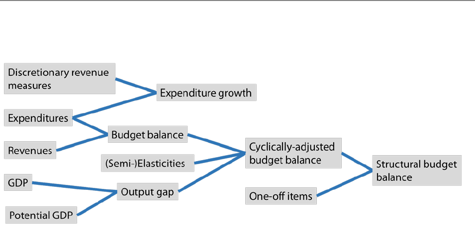
compliance – even without changes in policy – can change over time. Figure 1 depicts the main variables

needed in the EU fiscal framework and their relationships. The latter are still underrepresented though,

as, e.g., a forecast of GDP is also necessary to forecast the cyclical parts of expenditures or revenues.

When interpreting the results below it is also important to note that errors in the estimation of variables

used to operationalise fiscal rules might also be influencing the ex-post observations of certain variables.

For example, an erroneous reduction in potential GDP during a downturn could – as a result of overly

restrictive fiscal rules – lead to procyclical policies such as expenditure cuts, which in turn reduce GDP.

This could make the error self-fullfilling in the sense that lower GDP also lowers potential GDP estimates

(Fatás, 2019). In this case, therefore, the errors calculated from the difference between values published

for potential GDP in forecasts and ex-post might seem lower than they actually were.

IPOL | Economic Governance Support Unit

16 PE 645.732

Figure 1: Main variables necessary for evaluating compliance with EU fiscal rules

Source: own illustration

In the following, the European Commission’s macro-economic database (AMECO) is used to calculate the

forecast and real-time errors for some of the main variables. The figures compare the forecast of a variable

for a specific year (t) from two years ahead (t-2), one year ahead (t-1) and in real-time (t) with the variable

value which was published four years after the specific year (t+4). The mean error is defined as the mean

difference between the two points in time across years and countries. As this difference can be positive

or negative, however, some of the errors might cancel each other out when a simple mean is taken. Mean

absolute errors are therefore also calculated, which take the mean of the absolute values of the

differences across countries and years. Annex 6.1 provides a more detailed methodological background.

Figure 2 presents the two measures of errors for the EU15 from 2005 to 2015. The timeframe is chosen to

have a consistent dataset which only compares data which is availabe for all countries and years across

all variables in forecast and ex-post data. However, Table 5 in Annex 6.5 presents the results for other

country and time samples (e.g. for the EU27 or excluding the years of the financial crisis), as well as for the

structural balance (for which data is only available for a shorter time period). For the years where data

overlaps, errors for the structural and the cyclically-adjusted balance are very similar.

Benefits and drawbacks of an “expenditure rule”, as well as of a "golden rule", in the EU fiscal framework

PE 645.732 17

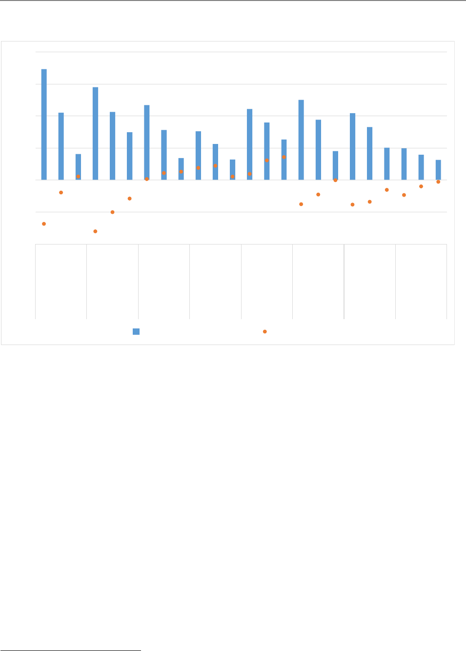
Figure 2: Mean (absolute) errors of forecasts and real-time estimates (EU15, 2005-2015)

Notes: Calculations are based on 164 observations (no data for Luxembourg in 2002). Mean errors are calculated as mean across

countries and time of the difference between values for year t values in autumn vintage of year t+4 and in autumn vintage of

year t-2, t-1 and t. Mean absolute errors are the mean of the absolute value of the differences. To make results comparable only

years and vintages are included which are available for all variables in all years and countries. More details on calculations can be

found in Annex 6.1. Budget balance: net lending or borrowing. pp.: differences in percentage points.

Sources: European Commission’s AMECO database, Firstrun project, own calculations

3.2.1. Mean Absolute Errors

Figure 2 shows that, comparable to findings in other studies

, mean absolute errors are substantial,

especially in the case of forecasts for two years ahead. For real GDP this amounts to about 3.5 per cent of

GDP. Even for the variable which shows the lowest mean absolute error, i.e. expenditures, the two-year

ahead forecasts are associated with mean absolute errors of 1.5 per cent of GDP. Mean absolute errors in

real-time are substantially smaller than in forecasts, but are still quite significant. Whereas in the cases of

real GDP, revenues, expenditures and the budget balance the mean absolute errors for real-time

estimates are below 1 per cent of GDP, they are still larger than 1 per cent for all measures that involve

estimates of potential GDP. The mean absolute errors for the growth rate of potential GDP are only about

half the size of the errors for the level of potential GDP. The reason seems to be that errors for potential

Merola and Pérez (2013) calculate a mean absolute error for real GDP of around 1.3 per cent of GDP for the one-year ahead forecast and

between 0.7 per cent and 1.2 per cent for real-time estimates for 15 European countries (1999 - 2007). De Deus and de Mendonça (2015)

find very similar errors in real-time based on data from the IMF, the OECD and the European Commission (1998 - 2011).

-2.0

-1.0

0.0

1.0

2.0

3.0

4.0

t-2 t-1 t t-2 t-1

t t-2 t-1 t t-2 t-1 t t-2 t-1

t t-2 t-1 t t-2 t-1 t t-2 t-1 t

Real GDP

(% of GDP)

Potential GDP

(% of GDP)

Revenues

(% of GDP)

Expenditures

(% of GDP)

Output Gap

(pp.)

Budget

balance

(pp.)

Cyclically-

adjusted

budget

balance

(pp.)

Growth of

potential GDP

(pp.)

Mean Absolute Error Mean Error

IPOL | Economic Governance Support Unit

18 PE 645.732

GDP are correlated over time

, i.e. if the value is revised for one year the previous year is very likely to also

be revised in the same direction.

The smallest mean absolute errors for forecasts and real-time estimates can be observed for expenditures.

Especially in forecasts the mean absolute errors for expenditures are substantially smaller (1.5 per cent for

two-year ahead and 1.1 per cent for one-year ahead forecasts) than, for example, the ones for real GDP.

In real-time, the mean absolute error for expenditures was equal to 0.6 per cent of GDP. However, when

interpreting these numbers one needs to bear in mind that expenditures are only a fraction of GDP. As a

percentage of expenditures, therefore, the mean absolute errors for the same sample would be much

higher (3.1 per cent in two-year ahead forecasts and 1.3 per cent in real-time).

As a percentage of the

variable itself, the errors are comparable to the errors for real GDP. Nevertheless, the errors expressed as

a percentage of GDP might be more relevant in terms of policy prescriptions.

3.2.2. Mean Errors

Besides the large size of the mean absolute errors, a bias in the errors can be observed for some of the

variables as well. The mean errors for real and potential GDP are strongly negative. This means that GDP

forecasts were too optimistic during the time period considered here. While for real GDP, however, the

bias vanishes from forecasts to estimates in real-time and the mean error in real-time is close to zero, there

remains a bias of -0.6 per cent of GDP for the real-time estimates of potential GDP. So while real GDP in

real-time was on average neither too optimistic nor too pessimistic, potential GDP estimates remained

too optimistic. This translates into a bias in the estimates of the output gap, which in real-time was on

average 0.7 percentage points of GDP too low compared with the estimates of four years later. Put

differently, the cyclical position in real-time was on average estimated to be worse than it turned out to

be ex-post. This confirms findings in other studies for different countries and time periods.

This pessimistic error in output gap estimates translates into errors in the estimation of the cyclically-

adjusted measures of the budget balance, which are based on output gaps. While the real-time mean

error for revenues, expenditures and the budget balance is close to zero, it is -0.3 percentage points for

the cyclically-adjusted budget balance, and it is -0.8 percentage points in the two-year-ahead forecasts.

Thus, the cyclically-adjusted fiscal position looked better in real-time than it did ex-post, and it looked

even better in forecasts. This means that cyclically-adjusted or structural balance rules in the time period

considered here were on average too lax in forecasts and real-time compared with ex-post estimates.

The estimation of potential GDP is often based on filtering techniques (such as the methods currently

used by the European Commission). These are prone to revisions especially because of end-of-sample

problems, i.e. they are sensitive to the latest available forecasts or observations of actual GDP (GCEE,

2019). A series of improvements to the currently used methods are discussed, such as using other

indicators, different models and estimation methods. However, ultimately, any revision of GDP is likely to

be composed of cyclical and structural factors, such that potential GDP also needs to be revised when

actual GDP is, although the exact extent of this will remain uncertain. Recognising the uncertain nature

The correlation of the value for a specific year () and the year before (  1) for the two-year ahead forecasts is 0.69.

The same applies to revenues, for which Buettner and Kauder (2010), for example, calculate a mean absolute error of 4.5 per cent of

revenues in forecasts. This is comparable to the results presented for revenues in this section (error of 2.3 per cent of GDP).

Some of the studies are surveyed in Navarini and Zoppè (2020). Eyraud and Wu (2015) find a similar mean error for real-time output gap

estimates of 1.2 percentage points of GDP for the Eurozone countries between 2003 and 2013 and Kempkes (2012) finds a mean error of

1.0 to 1.3 percentage points for the EU15 between 1996 and 2011.

Eyraud and Wu (2015) and Claeys et al. (2016) show similar results for the structural balance (-0.5 per cent of GDP for Eurozone countries

between 2003 and 2013, and -0.7 per cent of GDP for core EU15 countries from 2003 to 2014 respectively). Frankel and Schreger (2013) also

document over-optimism on the part of European countries when forecasting fiscal balances between 1999 and 2011.

Benefits and drawbacks of an “expenditure rule”, as well as of a "golden rule", in the EU fiscal framework

PE 645.732 19

of potential GDP estimates, the EU has added a (constrained) judgement component to the

implementation of the rules and is trying to mitigate the implications of uncertainty (Buti et al., 2019).

3.2.3. Other Forecast and Estimation Errors

An additional source of uncertainty on top of those discussed in the previous sections is hidden in the

estimation of (semi-)elasticities and weights used to translate the cyclical position of GDP measured by

the output gap into cyclically-adjusted budget balance figures. Elasticities are revised every nine years

and weights are revised every six years (European Commission, 2019a). The currently used elasticities are

estimated based on data from 1990 to 2013 (Mourre et al., 2014). Between 2005 and 2014 changes in

budgetary semi-elasticities for the EU27 ranged between -0.02 and 0.15, with an average change of 0.05

(Girouard and André, 2005; Price et al., 2014). Given that the average budgetary semi-elasticity is 0.50,

these changes have quite significant effects on cyclically-adjusted variables.

To evaluate compliance with an expenditure rule, discretionary revenue measures – and their impact in a

specific year, but also in subsequent years – have to be estimated. Estimates of discretionary revenue

measures have only very recently been published in the AMECO dataset, starting with the vintages of

2014. It is therefore not yet possible to conduct a comparable analysis to the one above of forecast or real-

time errors. However, it appears that they can potentially become quite substantial.

A series of

assumptions and projections are necessary to estimate e.g. the impact of a change in the tax code (e.g.

changes in tax rates or the tax base) on current and future revenues. This involves, among others things,

estimating the microeconomic behavioural reactions to tax changes, e.g. changes in labour supply in

response to changes in labour taxation. Although the European Commission relies on national estimates

of discretionary revenue measures, it defines a procedure and common methodology as to how Member

States should assess the budgetary effects (European Commission, 2019b). This bottom-up approach is

used to evaluate compliance with the EU expenditure rule. This could be problematic as there is an

information asymmetry between Member States and the European Commission, estimations depend on

national budgeting practices and there is an incentive for Member States to present biased estimates.

Furthermore, as also discussed by Deutsche Bundesbank (2019), it would be desirable to conduct an in-

depth and independent ex-post examination of the quality and errors inherent in estimates of

discretionary revenue measures, e.g. at the European level.

3.3. Exceptions and Compliance

Many fiscal rules have exceptions and escape clauses added to them. The European rules allow larger

deficits or expenditures in the context of an escape clause for unusual events and severe economic

downturns (EC Regulations 1466/1997 and 1467/1997). Furthermore, there are exceptions, for exa mple,

for public investment, major structural or pension reforms (EC Regulation 1055/2005; EU COM (2015) 12

final) and small and temporary deviations. The activation of such an escape clause or exception allows, to

a certain extent, a deviation from limits set by the rules. This does not mean that the rules are not complied

with, because the exceptions and escape clauses are essential parts of the rules’ design and deviations

from the limits in such cases are intended. One of the most important goals of fiscal rules is precisely to

build up fiscal buffers so as to be able to spend more than what the rules would allow in extraordinary

times for events such as natural disasters and severe economic crises. Nevertheless, poorly designed or

excessive numbers of exceptions could undermine the goals of fiscal rules.

The mean absolute change in the estimate of discretionary revenue measures from one vintage to the next for the years between 2014 and

2019 across the EU15 was 0.09 percentage points of GDP. This number is quite large when one considers that the other errors presented in

this section were calculated across several vintages and that the mean absolute value of discretionary revenue measures in the same

sample is only 0.33 percentage points of GDP.

IPOL | Economic Governance Support Unit

20 PE 645.732

The EU’s escape clause for severe economic downturns had never been activated until the COVID-19

pandemic (Council of the EU, 2020). As shown in Figure 3, however, the escape clause for unusual events

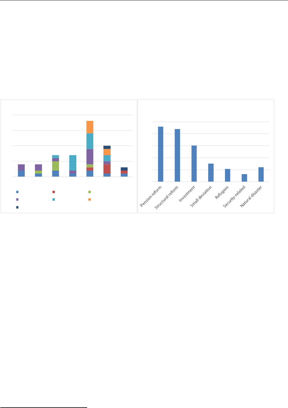
and other exceptions have been used quite extensively in recent years. A total of 18 exceptions were

granted in 2016. Nonetheless, the investment clause has only been used five times since 2012 (Bulgaria

in 2013 and 2014, Romania and Slovakia in 2014, and Italy in 2016). These exceptions can be quite

substantial and have meant that, on average, some countries have been allowed to run deficits in excess

of the limits of the rules by 0.46 per cent of GDP due to pension reforms, 0.44 per cent due to structural

reforms and 0.30 per cent due to exceptions for investment expenditures between 2012 and 2018.

Figure 3: Number and average size of exceptions granted between 2012 and 2018

Notes: Numbers are based on figures reported in Assessments of the Stability Programmes by the EU Commission. Preliminary

numbers for 2018. Exceptions for refugees, security-related measures and natural disasters constitute exceptions for unusual

events. No size figures are reported for exceptions for small deviations.

Sources: Christofzik et al. (2018), EU Commisson assessments of stability programmes of Member States, own compilation

The use of escape clauses and exceptions is intended by the fiscal rules, and exceeding the limit to the

extent approved is still in compliance with the rules. In addition to this, however, countries seem to often

not comply with the rules, at least in terms of economic not legal compliance. According to calculations

by the European Fiscal Board (2019), average economic compliance with EU fiscal rules was only 57 per

cent between 1998 and 2018. Studies on fiscal rules at the national level (Reuter, 2019) and worldwide

(Lledó and Reuter, 2018) find similar compliance rates of around 50 per cent. Examining the types of fiscal

rules, Cordes et al. (2015) and Reuter (2019) find that expenditure rules at the national level tend to be

complied with more often than budget or structural balance rules. According to the European Fis cal

Board (2019), this seems not to be the case for the EU fiscal rules. Contrary to the general intention behind

fiscal rules, countries do not seem to treat rules as ceilings, but rather as targets which are aimed at over

the medium term (Reuter, 2015). If rules were designed to be targets from the outset, however, their

design and, especially, their calibration would be different. Furthermore, the low level of compliance has

to be taken into account when analysing the effects of fiscal rules on observed fiscal policy, e.g. within

the context of the pro-cylicallity of fiscal policy.

These numbers are close to the maximum amount which can be granted for structural reforms and investment per adjustment period,

which is 0.5 per cent of GDP (there is no such cap for the pension reform exception).

2012 2013 2014 2015 2016 2017 2018*

Number of granted exceptions

Pension reform

Structural reform Investment

Small deviation Refugees Security-related

Natural disaster

0.1

0.2

0.3

0.4

0.5

Average size of granted exceptions

(2012-2018, % of GDP)

Benefits and drawbacks of an “expenditure rule”, as well as of a "golden rule", in the EU fiscal framework

PE 645.732 21

3.4. Composition of Public Expenditures

Overall the share of public investment (here represented by ‘gross fixed capital formation by the

government’) and public education expenditures in total expenditures in the EU15 are on average at

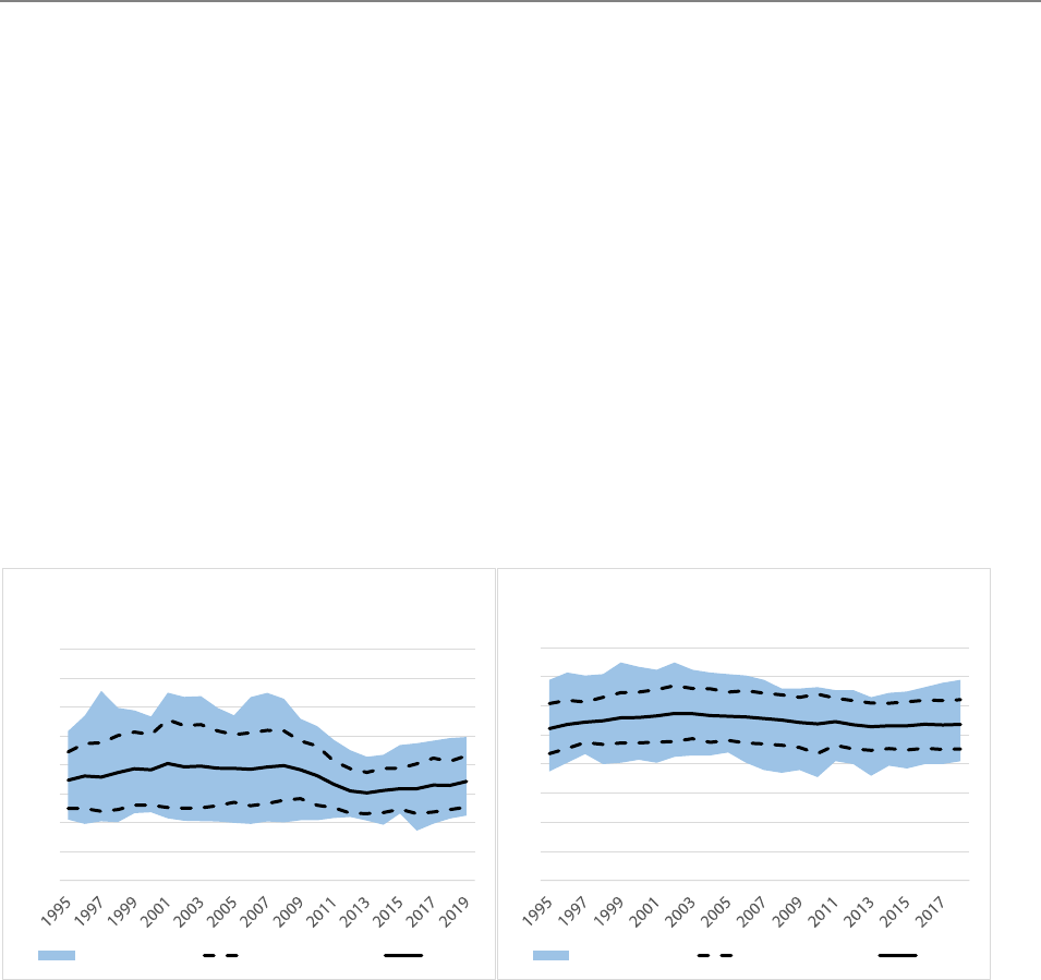
around the same level in 2019 as in 1995 (Figure 4). The shares increased up until the mid of the 2000s,

decreased around the financial crisis and caught up some of the loss since then. Spending on basic

research and R&D increased as a percentage of total expenditures between 2001 and 2018 (Figure 10).

Annex 6.2 discusses the development of the shares also as a percentage of GDP in more detail. The

development was quite heterogenous across countries. For example, the sharpest drops in the share of

investment expenditures between 2008 and 2013 were observed in Member States that had financial

assistance programmes. Furthermore, many countries in an excessive deficit procedure (EDP) seemed to

have reduced their investment shares (European Fiscal Board, 2019). However, any comparison of

investment figures across countries – even between the group of EU Member States – is problematic

(Christofzik et al., 2019). For example, the reliance on outsourced public services is quite heterogenous

across Member States and across time.

Figure 4: Public investment and education expenditures in the EU15 from 1995 to 2019

Notes: Investment expenditures are represented by gross fixed capital formation by the government. Education expenditures by

the government according to COFOG classification. Blue areas represent the range between the maximum and minimum values

in each year. Lines represent the mean and mean plus and minus one standard deviation across Member States.

Sources: European Commission’s AMECO database, Eurostat, own calculations

To what extent the EU fiscal rules played a role in the reduction of these investment shares is an open

question. So far the rules, especially if they are cyclically-adjusted, do not directly interfere in the

composition of public expenditures. Initial studies which try to identify the possible effects of fiscal rules

on public investment have not come up with clear-cut findings across the studies (Turrini, 2004; Perée

and Välilä, 2005; Bacchiocchi et al., 2011; Dahan and Strawczynski, 2013; Hauptmeier et al., 2015).

However, specific expenditures like investment and the ones discussed in the previous section might be

reduced (relative to others) first and most sharply during fiscal consolidations. Annex 6.2 discusses the

empirical relationship across the past 23 years in detail. Overall, the results suggest that expenditures on

investment and, to a smaller extent, on education as well as basic research and R&D are reduced as a

percentage of GDP during periods of fiscal consolidation. However, expenditures on education as well as

basic research and R&D are affected less than other expenditure categories, which means that their share

of total expenditures increases. Overall, the share in total expenditures accounted for by investment

10%

12%

14%

16%

General government gross fixed capital

formation (% of Total Expenditure)

Max-Min-Range Mean +/- Std.Dev. Mean

Public Education

(% of Total Expenditure)

Max-Min-Range Mean +/- Std.Dev. Mean

IPOL | Economic Governance Support Unit

22 PE 645.732

expenditures does not seem to be systematically related to periods of fiscal consolidation or expansion

over the past 23 years.

3.5. Pro-Cyclicality of the Current Framework

Section 2.1.1 introduced a distinction between cyclical and structural parts of public finances. Any change

in the cyclical part has, by definition, a counter-cyclical effect. In a downturn this automatically r esults in

a larger deficit, lower revenues and higher expenditures. Fiscal rules which exclude cyclical components

from the variables constrained by the rule – such as cyclically-adjusted or structural budget balance rules

as well as expenditure rules which exclude (cyclical) unemployment-related expenditures – theoretically

do not prevent these counter-cyclical effects from happening. However, this counter-cyclical effect can

be weakened or even reversed if discretionary fiscal measures counteract the automatic stabilisation of

the cyclical component. Indeed, Fatas (2019), for example, shows that discretionary policy in the euro area

eliminated the benefits of automatic stabilisers between 2010 and 2014 and turned fiscal policy pro-

cyclical.

Within the context of fiscal rules, one or several of the following reasons could lead discretionary fiscal

policy to counteract the automatic stabilisers and thus turn fiscal policy pro-cyclical:

1. A bias in forecasts of the cyclical part of public finances might force discretionary fiscal policy to

take countermeasures to comply with fiscal rules. As seen in Section 3.2, assessments of the

position in the economic cycle both in forecasts and real-time have shown a bias and have been

too pessimistic over the past few years. Consequently, rules limiting cyclically-adjusted measures

have been too loose both in forecasts and real-time relative to ex-post assessments. In this

respect, therefore, rules seem to have on average not forced discretionary fiscal policy to

counteract automatic stabilisers owing to a bias in forecasts. On the contrary, these rules would

have actually made it possible to strengthen cyclical components by pursuing discretionary

policy in a downturn. Although the rules have not been restrictive enough during upturns,

discretionary policy has not needed to use all of the additional leeway granted by the rules.

2. The limits of fiscal rules might be changed pro-cyclically such that discretionary fiscal policy needs

to adjust. There appears to be no sign of any systematic changes in line with the economic cycle

to the limits of the EU fiscal rules, e.g. the minimum MTOs which are set for Member States. The

six-pack and two-pack reforms under the European fiscal framework tend to provide more fiscal

headroom to Member States for economic stabilisation purposes.

3. Exceptions and escape clauses might be applied pro-cyclically. Under the EU fiscal framework the

average change in the output gap during the years when the 64 exceptions were granted

between 2012 and 2018 (see Section 3.3) was a positive 0.49 percentage points. The average level

of the output gap was close to zero (0.08 per cent). 70 per cent of the years in which exceptions

were granted to countries saw a positive change in the output gap. It seems that exceptions were

granted especially for years in which there was an economic upturn (positive change in the

output gap). This would enable policymakers to expand discretionary fiscal policy pro-cyclically.

However, exceptions have only very recently been used extensively, which means that this

observation is severely limited because it is based on a very short time period.

4. Non-compliance with fiscal rules might be pro-cyclical. The European Fiscal Board (2019) points

out that compliance with cyclically-adjusted rules under the EU framework was relatively low

before 2008 and in recent years, which are both periods with fairly benign economic conditions.

By not complying with the rules, discretionary policy fostered a pro-cyclical fiscal stance, which

the rules would not have prescribed. Larch et al. (2020) look at the role of compliance with fiscal

Benefits and drawbacks of an “expenditure rule”, as well as of a "golden rule", in the EU fiscal framework

PE 645.732 23

rules as part of a more systematic approach. They find that compliance with fiscal rules would

have been associated with a more counter-cyclical fiscal stance, i.e. that non-compliance with the

cyclically-adjusted rules increases the likelihood of running pro-cyclical fiscal policies.

5. Aside from fiscal rules, policymakers face a variety of challenges which can lead them to pursue

pro-cyclical discretionary policies. Potential reasons could be high debt levels which mean that,

even in a downturn and although the rules would allow it, discretionary fiscal policy is used not

counter-cyclically but pro-cyclically. The European Fiscal Board (2019) points to the possibility

that concerns about fiscal sustainability may have pushed governments to consolidate more than

the fiscal rules would prescribe. The failure to build up buffers in the EU by running a pro-cyclically

expansionary discretionary fiscal policy in fairly good economic times before the financial crisis

was followed by pro-cyclical restrictive discretionary fiscal policy to try to rein in debt increases in

2012 and 2013. In both periods the fiscal rules per se did not force policymakers to act pro-

cyclically: on the contrary they would have allowed policy to be counter-cyclical.

In summary: It seems that political decisions outside the scope of the fiscal rules, non-compliance with

the rules and the use of exceptions – rather than rule design or forecast errors – tended to foster pro-

cyclical fiscal policy in the EU.

4. FOCUSING THE EU FRAMEWORK ON AN EXPENDITURE RULE

4.1. Proposals for Expenditure Rules

Many authors and institutions have suggested reforming the EU fiscal framework by focusing it on an

expenditure rule (Ayuso-i-Casals, 2012; Carnot, 2014; Andrle et al., 2015; Christofzik et al., 2018; Cottarelli,

2018; Darvas et al., 2018; Eyraud et al., 2018b; Kopits, 2018). Table 2 presents some of the proposals for

which a more detailed description of the proposed rule is available and compares their features with the

existing expenditure rule under the EU fiscal framework.

The proposed rules all set a limit on the growth rate of a derivative of gross expenditures, which in most

cases is net of interest expenditures, some measure of unemployment-related expenditures and an

estimate of discretionary revenue measures. The limit set by the rule is in most cases directly or indirectly

related to the growth rate of potential GDP. Furthermore, all proposals combine the expenditure rule with

some mechanism related to the debt ratio or debt reduction targets.

Differences between the proposals are only visible in the details, which suggests that there already seems

to be a consensus on the broad design of an expenditure rule on which the EU fiscal framework could be

focused. The proposals differ, e.g., in the details of how limits are set and in the extent of debt correction,

either driven by formulas or by a process involving national governments, fiscal councils or the European

Commission. Another dimension in which the proposals differ is the design and usage of an adjustment

account, which in some proposals captures deviations between planned and actual expenditures and in

others also includes estimation errors or deviations from medium-term targets.

IPOL | Economic Governance Support Unit

24 PE 645.732

Table 2: Comparison of expenditure rule proposals

Limit Excluded items Debt correction Adjustment account Special features

Other

Current EU rule

Medium-term potential GDP

growth

√ √ √

EU-funded investment

Implicit by relation to

MTOs

National investment

averaged over four

years

European Fiscal Board

(2018, 2019)

Trend rate of potential GDP

growth (limit fixed for a three-

year period)

√ √ √

EU-funded investment

Debt ratio within

range of long-run

objective within

maximum number of

years

Deviations of planned

expenditure growth;

subject to maximum;

decumulates in case of

windfall gain

Member States with

debt ratio below 60%

of GDP not subject to

net expenditure

ceiling

Christofzik et al. (2018)

Medium-term potential GDP

growth

√ √ √

Relative to difference

between present debt

levels and long-term

limit

Non-compliance

margin with structural

balance rule;

estimation errors;

small deviations in

budgetary process

Claeys et al. (2016)

Medium-term potential GDP

growth

√

All labour-market-re lated

expenditure; one-off

expenditure

0.02 times difference

between debt level in

previous year and 60 %

debt criterion

Difference between

actual expenditure

growth and the

expenditure growth

limit

Public investment

smoothed over

several years and

accounted for similarly

to corporate

investment

Darvas et al. (2018)

(very similar to

Bénassy-Quéré et al.,

2018)

Medium-term debt reduction

target set by national

government

(based on

potential GDP growth)

√

All unemployment

spending (except when

due to discretionary

changes)

Limit directly takes

care of debt correction

Limited deviations

between actual and

budgeted spending

I interest payments; U cyclical unemployment-related expenditures; R discretionary revenue measures:

Sources: Studies as indicated in first column of table, own compilation

Benefits and drawbacks of an “expenditure rule”, as well as of a "golden rule", in the EU fiscal framework

PE 645.732 25

4.2. Assessment of Rule Performance Based on Past Data

A starting point for investigating the possible performance of the proposed expenditure rules is to

compare limits that would have been set by different rule types with actual expenditure growth based

on past data. To isolate the effect of the rule type from the exact numerical calibration, both rules

considered in this exercise set a limit which would keep the cyclically-adjusted budget balance

constant over the medium-term. Policymakers can decide to calibrate the rules such that, for exa mple,

they improve the cyclically-adjusted budget balance (e.g. in relation to the debt ratio) or constantly

allow some borrowing. However, this is independent of the rule type and is discussed in Section 4.3.

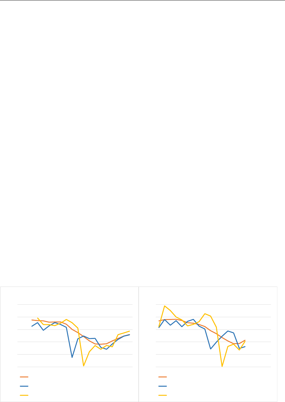
Figure 5 presents the following three variables as published in real-time, i.e. data for year  from the

autumn vintage in year , and ex-post, i.e. data from the autumn vintage in year  + 4:

1. Growth rate of primary expenditures, which represents observed fiscal policy. Expenditures net

of cyclical unemployment-related expenditures and discretionary revenue measures would be

needed for an exact representation of most proposed expenditure rules. However, the latter

two variables are only available for a very short time period. Annex 6.2 discusses the differences

for the years in which data overlaps. When interpreting the following results it is important to

bear in mind the sizeable differences between different expenditure measures.

2. Five-year moving average of potential GDP growth, which represents the limit set by an

expenditure rule. The five-year average is just one possible way of calculating the limit in

relation to potential GDP. Annex 6.2 discusses other averages proposed for expenditure rules

in comparison with annual potential GDP estimates.

3. Growth rate of the sum of cyclically-adjusted revenues and the cyclical component of

expenditures, which represents the limit on expenditure growth to keep the cyclically-adjusted

balance constant in a specific year. A detailed discussion of this calculation can be found in

Annex 6.2. It is important to remember that this measure does not capture the actual limit set

by a cyclically-adjusted balanced budget rule. This measure shows by how much expenditures

could have grown without the cyclically-adjusted balance deteriorating.

Figure 5: Comparison of limits set for expenditure growth with observed fiscal policy (EU15)

Notes: Average potential GDP refers to backward-looking five-year moving average; calculation details in Annex 6.2.

Sources: European Commission’s AMECO database, Firstrun project, own calculations

-2%

2000 2002 2004 2006 2008 2010 2012 2014 2016 2018

Real-Time

Average potential GDP growth

Constant cyclically-adjusted balance

Observed primary expenditure growth

-2%

2000 2002 2004 2006 2008 2010 2012 2014 2016 2018

Ex-Post

Average potential GDP growth

Constant cyclically-adjusted balance

Observed primary expenditure growth

IPOL | Economic Governance Support Unit

26 PE 645.732

The values depicted in Figure 5 represent averages across the EU15. Although a country-by-country

analysis would be too comprehensive for this paper, it could reveal interesting country-specific

insights, which are ignored in the following discussion. Furthermore, the discussion below is based on

a single, fairly short time series. More systematic analysis would be necessary to draw more robust

conclusions.

The first observation to make here is that average potential GDP growth and the average limit which

keeps the cyclically-adjusted balance constant were closely aligned over the medium term (especially

in the ex-post data), which confirms the similarity between expenditure and cyclically-adjusted balance

rules over the medium term (Section 2.1.4). The latter is, however, more volatile and seems to fluctuate

around medium-term potential GDP growth. A clear outlier in this regard is 2009. In that year, much

lower expenditure growth would have been necessary to keep the cyclically-adjusted balance constant

compared with medium-term potential GDP growth. To a large extent this is a feature of taking the

average for potential GDP growth, as annual potential GDP also decreased sharply in 2009 (see Figure

12 in Annex 6.2). As far as rule design is concerned, however, an escape clause was activated anyway in

that year, so the limits set by the rules were not applicable. This is also evident in the continuing high

level of expenditure growth observed in that year.

Second, both limits would have been lower than the expenditure growth observed before the financial

crisis in the early 2000s and in most recent years 2017 and 2018. Furthermore, both would have allowed

more expenditure growth between 2010 and 2014. The sharp drop in expenditure growth observed in

2011 and 2012 would not have been necessary to keep the cyclically-adjusted balance constant.

Consequently, both limits would have prescribed a more counter-cyclical fiscal policy over the past 18

years if they had been complied with and if the leeway granted by the rules had been used. This general

result confirms the findings presented by Andrle et al. (2015), who use model simulations to show that,

apart from measurement uncertainty, expenditure and structural balance rules operate similarly in

stabilising the economy.

Third, in the years when there was an ex-post negative change in the output gap, the limit based on

potential GDP growth would have allowed: i) slightly more expenditure growth in 2001-2003 than

necessary to keep the cyclically-adjusted balance constant, ii) much more in 2008 and 2009 when,

however, an escape clause would have been applicable to both rules, and iii) less in 2012 and 2013. In

years when there were significant positive changes in the output gap (2000, 2006, 2007, 2010, 2015)

average potential GDP growth would have set a slightly looser limit than a constant cyclically-adjusted

balance in real-time (also for ex-post data except for 2006). This suggests on the whole that, in relative

terms, the cyclically-adjusted balance seems to set a more restrictive limit during upturns, while

medium-term potential GDP growth sets a more expansionary limit during downturns. However, it

should be remembered that this assessment is based on a single, fairly short time series and a more

systematic evaluation across countries and settings would therefore be desireable.

4.3. Calibration

The preceding analysis abstracts from the actual calibration of the fiscal rules, i.e. the exact numerical

limits and how they are determined. The various calibrations in place and proposed do not alter the

basic characteristics of rule types. Consequently, the numerical calibration can be decided

independently of the rule type.

The choice of numerical calibration requires a risk assessment and the balancing of various trade-offs

and is therefore mainly a political decision. There is a trade-off between overly restrictive limits, which

might hamper growth and investment, and overly lax limits, which reduce the fiscal headroom

Benefits and drawbacks of an “expenditure rule”, as well as of a "golden rule", in the EU fiscal framework

PE 645.732 27

available during times of crisis and increase vulnerability to shocks (Eyraud et al., 2018a). A key measure

here is the public debt-to-GDP ratio to which public debt would converge in the long run if the rule

were always complied with. The selection of the respective ratio depends on the maximum debt limit

below which it is highly probable that the debt dynamics can be controlled by the government, m inus

a safety margin. The maximum debt limit is very uncertain and depends on many factors like long-term

growth rates, interest rates as well as the country-specific environment and institutions (Ghosh et al.,

2013; D’Erasmo et al., 2016). The safety margin is necessary because of the high uncertainty and

because negative shocks, such as severe economic crises, can trigger exceptions and increase the ratio

by fairly large amounts.

However not only the targeted debt-to-GDP ratio, i.e. the long-run point of convergence, but also the

desired speed of convergence play a role in determining the numerical limits for fiscal rules. The

process of converging to the long-run ratio can take quite a long time. Given an initial debt ratio of 80

per cent, for example, with a constant government deficit of 0.5 per cent of GDP and a steady nominal

growth rate of 3 per cent, the debt-to-GDP ratio would converge to 17 per cent in the long term.

However, it will take 53 years for the ratio to fall below 30 per cent, and after twelve years it will still be

above 60 per cent.

In order to lower the debt ratio faster for countries with higher debt ratios, all proposals on expenditure

rules involve some kind of deduction from the limit set by the rule relative to the level of debt ratio. In

choosing this deduction, one is again faced with the above-mentioned trade-off. The feedback

mechanism could also take care of medium-term changes in structural public revenues which are not

related to discretionary revenue measures.

Furthermore, the process of calibrating the speed of

convergence would vary depending on whether governments use the limits set by the rules as ceilings

or targets, even if they merely misuse them as targets.

When an expenditure rule is introduced, some transitory adjustment mechanism will be necessary, as

not all countries will be starting from the same cyclically-adjusted budget balance. A specific limit on

expenditure growth could therefore mean very different things to different countries in terms of their

medium-term budget balance.

5. CONVERTING AN EU FISCAL RULE INTO A GOLDEN RULE

5.1. Proposals for Safeguarding Specific Expenditure Categories

A wide range of publications propose that specific expenditure categories, such as investment

expenditures, should be treated differently in terms of debt financing in the context of the EU fiscal

framework (Fitoussi and Creel, 2002; Blanchard and Giavazzi, 2004; Barbiero and Darvas, 2014; Truger,

2015; Claeys, 2019; Deutsche Bundesbank, 2019; European Fiscal Board, 2019). Table 3 presents an

overview of some of the more detailed proposals. Such a provision, often referred to as a ‘Golden Rule’,

can be added to the various types of fiscal rules, such as structural balance rules and expenditure rules,

and thus does not really represent a new type of rule. As the EU framework already involves different

types of rules, the goal of such a reform would be to modify an existing or reformed rule (as shown in

Table 3). This could be achieved either by changing the variable constrained by the rule or by reforming

the use and extent of exceptions (see Section 2.2.2).

As Heinemann (2018) describes, such changes could be due to factors such as tax competition, which could give rise to structurally lower

revenues despite the fact that the tax code and statutory tax rates remain unchanged.

IPOL | Economic Governance Support Unit

28 PE 645.732

All proposals focus on some form of investment expenditures. However, the general term conceals

differences between what these expenditures actually represent. Whereas the European Fiscal Board

(2019), for example, would only count expenditures which top up the co-financing of EU investment

projects, others use the investment concept as defined in the internationally harmonised national

accounts (some with minor adaptations, such as Truger, 2015), while others still propose a more open

approach where some institution or institutional process decides which expenditures are deductible

and which are not. Similar to the latter, Pisani-Ferry (2019) argues that the EU should define goals that

justify public spending that is temporarily above the limits set by fiscal rules (although this is

conditional on the availability of low long-term interest rates and a country not being in a financially

precarious situation).

As one of the main arguments in favour of a Golden Rule is that investment expenditures also generate

assets which counterbalance debt increases, most proposals focus on net rather than gr oss investment

expenditures (as described in Section 2.2.1). Only the creation of additional assets would thus allow

debt financing. Blanchard and Giavazzi (2004) point out that if, under a Golden Rule, debt financing is

only allowed for net investment expenditures over time, the level of public debt would approach that

of the stock of public capital. Consequently, Deutsche Bundesbank (2019) proposes that such a rule be

applied symmetrically so that negative net investment would not only not allow any debt financing

but would also require budgetary surpluses in relation to negative net investment. One caveat of using

net rather than gross investment figures is that this poses significant methological challenges for

estimating the measure (see Section 2.2.1).

Some proposals set a limit (cap) on the amount of expenditures that can be deducted. This is achieved

either by choosing a fixed amount of, say, 0.5 per cent of GDP (Deutsche Bundesbank, 2019), or,

alternatively, 1 per cent or 1.5 per cent of GDP (Truger, 2015), or by transferring the identification of the

cap to other measures such as the ‘green investment gap’ identified in the European Semester (Claeys,

2019) or projects identified in the EU Budget (European Fiscal Board, 2019).

Most proposals do not mention any changes to the limits of existing rules after allowing the deduction

of (net) investment expenditures, which means that these proposals seem to place investment

expenditures on top of the existing limits. Consequently, if the current rule sets a limit of 0.5 per cent

of GDP on the structural balance, the new rule would set the same limit of 0.5 per cent of GDP on a

structural balance from which net investment expenditures are subtracted. In contrast, Deutsche

Bundesbank (2019) suggests to reduce previous limits on the residual structural balance by the

maximum amount deductible for net investment purposes.

Furthermore, most proposals would implement the deduction of net investment regardless of the

economic cycle. In contrast, Barbiero and Darvas (2014) argue in favour of an asymmetric Golden R ule,

which provides extra scope for investment only in adverse economic times (and gradually reduces it

again in more benign times). However, this approach might be challenging given the estimation errors

associated with output gaps (see Section 3.2) and the objective of keeping investment levels r elatively

stable over the economic cycle.

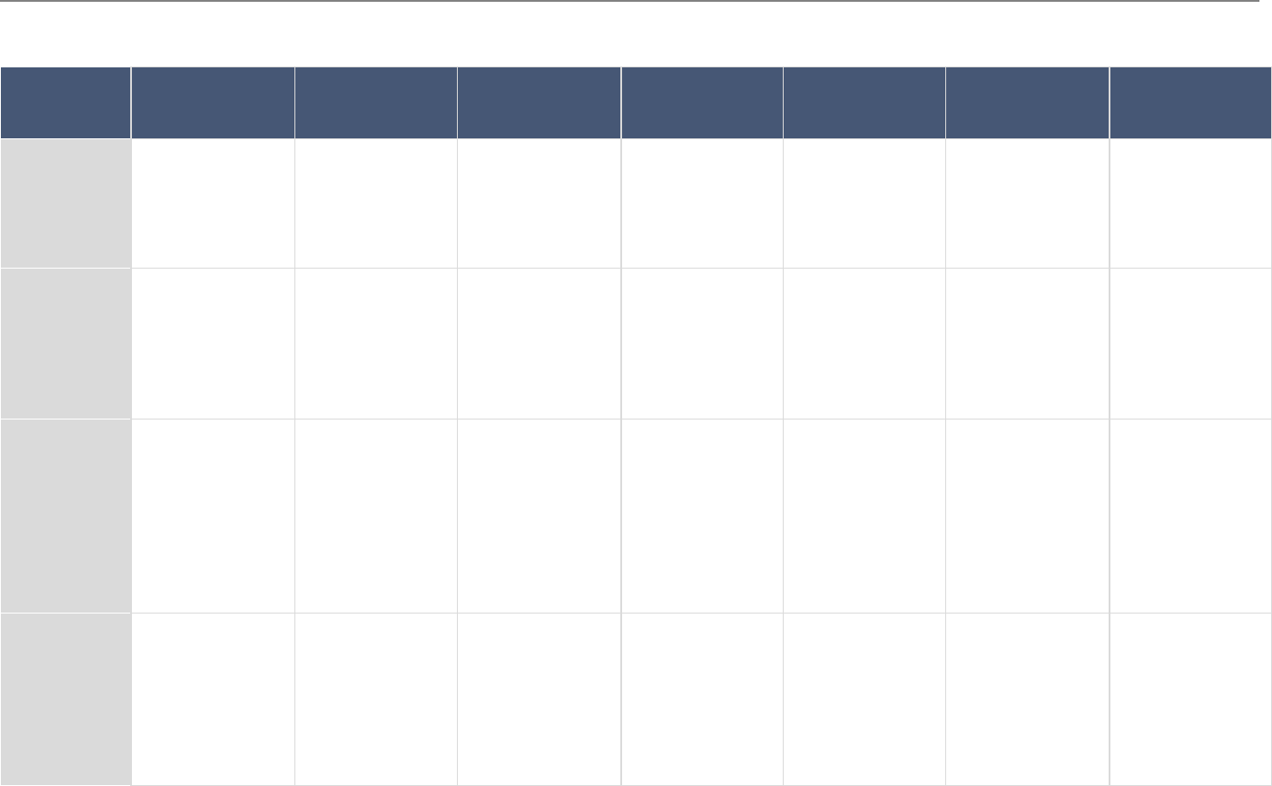
Benefits and drawbacks of an “expenditure rule”, as well as of a "golden rule", in the EU fiscal framework

PE 645.732 29

Table 3: Comparison of proposals related to a ‘Golden Rule’ in the context of the EU fiscal framework

Barbiero and

Darvas (2014)

Blanchard and

Giavazzi (2004)

Claeys (2019) Deutsche

Bundesbank

European Fiscal

Board (2019)

Fitoussi and

Creel (2002)

Truger (2015)

Type of rule

Structural balance

rule in current EU

framework

Based on rules in

2004 EU

framework (i.e. no

structural balance

rule yet)

Adapting

investment

exception clause

in current EU

framework

Structural balance

rule, but limit on

non-investment

reduced (same

MTOs still apply)

New expenditure

rule (see Table 2)

Structural balance

rule

Deficit or

structural balance

rule as in current

EU framework

Deductible

If negative output

gap exceeds a

determined

threshold, net

public investment

Net public

investment

Green investment

related to level of

‘green investment

gap’ (identified in

European

Semester)

Net public

investment,

capped at max of

0.5 % of GDP

Top-up

expenditures on

national

investment

projects beyond

co-financing

Public investment

Net public

investment, max.

of 1 % or 1.5 % of

GDP

Identification

expenditures

Not specified

Delegated to

Eurostat, should

especially deal

with the incentive

to re-define

current spending

as public

investment

Clear accounting

rules needed, a.o.

taxonomy for

sustainable

finance and rules

for issuance of

green bonds

As in national

accounts

Projects which are

growth-enhancing

and adding pan-

European value as

in EU budget,

opinions by

independent fiscal

institutions

Decision by

European Council

(based on policy

areas that have

been highlighted

as European

priorities)

As in national

accounts minus

military

investment plus

investment grants

to private firms

and non-profit

organisations

Special

features

If negative output

gap is eliminated:

transition period

during which extra

room for deficit is

gradually

eliminated

Specific

investment

agencies for

transparency and

better

management

Issuance of green

bonds to finance

investment

expenditures

Higher deficits if

net investment is

positive, if net

investment

negative

budgetary

objectives stricter

Notes: Net investment figures are broadly defined as gross investment figures net of deprecation.

Sources: Studies as indicated in top row of table, own compilation

IPOL | Economic Governance Support Unit

30 PE 645.732

5.2. Limits Set by Golden Rules

In general, cyclically-adjusted budget balance rules or expenditure rules do not prevent policymakers

from choosing a composition of public expenditures according to their political priorities. In addition

to specific expenditures – such as investment – as a share of total expenditures, these rules do not place

limits on the level of specific expenditure categories either, as policymakers can alter the level of total

expenditures within the limits of the rules by using discretionary measures on the revenue side.

However, the rules do place limits on the amount of expenditures that can be financed by debt issuance

rather than annual revenues.

Fiscal rules are introduced because there are various forms of deficit bias on the part of politicians and

governments, which means that, without any rules, the amount financed by debt issuance would be

higher than is optimal (see Section 1). In addition to this deficit bias, there are various factors that could

create a bias towards less-than-optimal levels of specific expenditures, such as the discrepancy

between which generation has to bear the costs and who benefits from investment expenditures (see

Section 2.2.1). If it were possible to show that politicians are biased in this way when deciding on

specific expenditure categories, this could justify a rule which differentiates between expenditure

categories. A Golden Rule sets a limit to the amount of non-deductible expenditures that can be

financed by debt issuance and either none or a different limit for deductible, like investment,

expenditures.

When deciding on the introduction of a Golden Rule, there is a trade-off to be addressed. Governments

would still be able to choose any composition and level of expenditures, but not independent of the

amount of debt issuance relative to annual revenues. For a given amount of debt issuance and annual

revenues, governments would not be able to freely choose a level of expenditures in specific categories

anymore. Although the general trade-off between rules and choices for governments is similar for any

fiscal rule, a Golden Rule goes beyond the current focus of the EU fiscal framework on cons training

fiscal aggregates and distinguishes between different expenditures in Member States.

Under a Golden Rule there is still a maximum total amount of debt financing which is consistent with

sustainable public finances. The numerical calibration follows the same considerations as described in

Section 4.3. However, the maximum debt limit might be higher if a Golden Rule credibly leads to a

better composition of public expenditures which increases long-term growth rates or reduces interest

rates, e.g. through higher investors’ confidence. For Golden Rules which do not set a limit to the

deductible expenditures, the implicit assumption might be that those can only increase within a range,

e.g. due to capacity constraints, and are thus constrained also without an explicit limit. However,

addressing the bias towards excessively low investment expenditures would not remove the bias

towards excessively high deficits in general. The deficit bias is relevant not only for total expenditures

but also for specific expenditure categories that are not constrained. If current expenditures are limited

by a fiscal rule but investment expenditures are not, it is likely that a bias towards excessively high

deficits will remain, except that it will then be based on investment expenditures or might foster the

usage of ‘creative accounting’. For example, common-pool problems and political budget cycles could

then be concentrated on investment expenditures potentially also leading to the realization of less

efficient investments and a weakening of their growth contribution.

This suggests setting a cap on the amount of expenditure that is deductible (as also discussed in some

proposals). It should be noted that this does not set a limit on the maximum level of expenditures in a

Depending on the rules’ design this amount can also be negative, i.e. require a budgetary surplus, in some or all years.

Benefits and drawbacks of an “expenditure rule”, as well as of a "golden rule", in the EU fiscal framework

PE 645.732 31

specific category; it merely sets a limit on the amount which can be deducted. If policymakers want to

increase the expenditures in that category beyond what is deductible, they would be able to do so in

full compliance with the rule, e.g. by reducing other non-deductible expenditures or increasing

revenues.

To guarantee the intended effect of the introduction of a Golden Rule, i.e. to increase the quality of

public finances by increasing the share of growth-friendly or future-oriented expenditures, the limit set

for the remaining part of the budget, i.e. for the non-deductible expenditures, would most likely need

to be reduced in accordance with the change of the maximum amount of total debt issuance.

Otherwise, this remaining part would be allowed to increase even without a respective increase in

revenues or deductible expenditures. This could lead to a higher structural deficit due to an increase in

non-deductible expenditures, without necessarily an improvement of the quality of public

expenditures.

A system which allows specific expenditures to be deducted up to a cap and lowers the original rule

limit for the remaining expenditures would effectively constitute two fiscal rules: one setting a limit on

total expenditures (deductible and non-deductible) and a second one setting a limit on the non-

deductible portion of expenditures, with the difference between the two limits being the cap on how

much of the safeguarded expenditures can be deducted. This also shows that such a system can be

designed in a way that does not jeopardise long-term fiscal sustainability.

6. CONCLUSIONS

This paper, first, discusses the benefits of focusing the European fiscal framework on an expenditure

rule. Discussions of reforms often focus on the benefits of expenditure rules in relation to observed

fiscal policy rather than other possible rules or rule designs. However, fiscal policy is often chosen not

only in accordance with the limits set by fiscal rules, but also because of other considerations, s uch that

analysing observed fiscal policy to evaluate the current fiscal framework might be misleading.

Expenditure rules are similar to structural balance rules in various respects. Although there are minor

differences from year to year, both rules per se would have prescribed that fiscal policy in the EU should

have been more-counter cyclical over the past few years. However, expenditure rules achieve this by

imposing a less volatile limit on expenditure growth which, in terms of output stabilisation, can be

either a benefit or a drawback depending on the direction in which the economy is heading. Under the

current framework, it appears not to be the rule design itself but, rather, political decisions outside the

scope of the fiscal rules, non-compliance with these rules, and accompanying regulations like the use

of exceptions that tended to foster pro-cyclical fiscal policy. Like structural balance rules, expenditure

rules are also associated with significant challenges when forecasting and estimating the variables

needed for implementation. These errors are substantial and biased in the case of variables required to

operationalise structural balance rules. They are smaller, although still significant, and less biased, in

the case of expenditures. However, the operationalisation of expenditure rules also requires other

variables, such as discretionary revenue measures, which involve cumbersome estimates and are

associated with a high degree of uncertainty.

The main advantage of expenditure rules is that (almost all) expenditures and discretionary revenue

measures are directly controlled by policymakers. Governments can therefore ensure compliance with

fiscal rules more directly. With the exception of cyclical unemployment-related expenditures and

discretionary revenue measures, most of the expenditure measures are easy to communicate and

involve less complex explanations. This is especially helpful when communicating rule compliance to

IPOL | Economic Governance Support Unit

32 PE 645.732

the general public and the media, which in turn is the most promising lever for increasing the

accountability of politicians and compliance with fiscal rules.

Second, the paper discusses ways of converting a fiscal rule under the European fiscal framework into

a Golden Rule. There is a concern that needs to be adressed first, which is that such a rule would go

beyond the current focus of the EU fiscal framework on fiscal aggregates and distinguish between

different expenditures in Member States. If a Golden Rule is introduced nonetheless, the main

challenge is to clearly and narrowly define the deductible expenditures or expenditure categories

(Section 2.2.1). Once these have been identified, a two-rule system could implement the Golden Rule:

one rule for total (deductible and non-deductible) expenditures and one rule for non-deductible

expenditures only.

One of the main overarching challenges when reforming the EU fiscal framework is to increase

compliance with its fiscal rules. The best-designed fiscal rules are no good if they are not complied with

or if the leeway granted by these rules is not used where it would be advisable. As has been seen in

recent years, discretionary fiscal policy actions – rather than fiscal rule design – have often tended to

make fiscal policy more pro-cyclical and less focused on fiscal sustainability. A more transparent, more

predictable and less complex framework could make a significant contribution to enhancing

compliance and the role of fiscal rules. Furthermore, it is important to have supporting institutions –

such as independent and vocal fiscal councils at the national and European level – explaining fiscal

policy and rules. The most important lever is to increase ownership of national governments as well as

the visibility of rules and their compliance for politicians, the general public and the media. This could

give the fiscal rules more impact than any complex system of sanctions or enforcement mechanisms.

REFERENCES

Andrle, M. et al. (2015), Reforming fiscal governance in the European Union, IMF Staff Discussion Note

15/09, International Monetary Fund, Washington, DC.

Auerbach, A.J. and Y. Gorodnichenko (2012), Measuring the Output Responses to Fiscal Policy,

American Economic Journal: Economic Policy 4 (2), 1–27.

Ayuso-i-Casals, J. (2012), National Expenditure Rules – Why, How and When, European Economy 473,

Directorate General Economic and Financial Affairs (DG ECFIN), European Commission,

December.

Bacchiocchi, E., E. Borghi and A. Missale (2011), Public investment under fiscal constraints, Fiscal

Studies 32 (1), 11–42.

Badinger, H. and W.H. Reuter (2017), The case for fiscal rules, Economic Modelling 60, 334–343.

Badinger, H. and W.H. Reuter (2015), Measurement of fiscal rules: Introducing the application of

partially ordered set (POSET) theory, Journal of Macroeconomics 43, 108–123.

Barbiero, F. and Z. Darvas (2014), In sickness and in health: Protecting and supporting public

investment in Europe, Bruegel Policy Contribution 2014/02, Bruegel, Brussels.

Bénassy-Quéré, A. et al. (2018), Reconciling risk sharing with market discipline: a constructive

approach to euro area reform, CEPR Policy Insight 91, Centre for Economic Policy Research,

London.

Blanchard, O.J. and F. Giavazzi (2004), Improving the SGP through a proper accounting of public

investment, CEPR Discussion Paper 4220, Centre for Economic Policy Research, London.

Bom, P.R.D. and J.E. Ligthart (2014), What Have We Learned From Three Decades Of Research On The

Productivity Of Public Capital?, Journal of Economic Surveys 28 (5), 889–916.

Buettner, T. and B. Kauder (2010), Revenue Forecasting Practices: Differences across Countries and

Consequences for Forecasting Performance, Fiscal Studies 31 (3), 313–340.

Burret, H.T. and L.P. Feld (2018), (Un-)intended effects of fiscal rules, European Journal of Political

Economy 52, 166–191.

Benefits and drawbacks of an “expenditure rule”, as well as of a "golden rule", in the EU fiscal framework

PE 645.732 33

Buti, M., N. Carnot, A. Hristov, K.M. Morrow, W. Roeger and V. Vandermeulen (2019), Potential output

and EU fiscal surveillance, VoxEU.org.

Buti, M., J.N. Martins and A.A. Turrini (2006), From Deficits to Debt and Back: Political Incentives under

Numerical Fiscal Rules, CEPR Discussion Papers 5809, Centre for Economic Policy Research,

August.

Carnot, N. (2014), Evaluating Fiscal Policy - A Rule of Thumb, European Economy 52, Directorate

General Economic and Financial Affairs (DG ECFIN), European Commission.

Caselli, F. and J. Reynaud (2020), Do fiscal rules cause better fiscal balances? A new instrumental

variable strategy, European Journal of Political Economy 63, 101873.

Caselli, F. and P. Wingender (2018), Bunching at 3 Percent: The Maastricht Fiscal Criterion and

Government Deficits, IMF Working Papers 18/182, International Monetary Fund, August.

Christofzik, D.I., L.P. Feld, W.H. Reuter and M. Yeter (2018), Uniting European fiscal rules: How to

strengthen the fiscal framework, Arbeitspapier 04/2018, Sachverständigenrat zur

Begutachtung der gesamtwirtschaftlichen Entwicklung, Wiesbaden.

Christofzik, D.I., L.P. Feld and M. Yeter (2019), Öffentliche Investitionen: Wie viel ist zu wenig?,

Schweizer Monat – Die Autorenzeitschrift für Politik, Wirtschaft und Kultur 1064 (März).

Claeys, G. (2019), The European Green Deal needs a reformed fiscal framework, Bruegel Blog Post.

Claeys, G., Z.M. Darvas and A. Leandro (2016), A proposal to revive the European fiscal framework,

Bruegel Policy Contribution 2016/07, Bruegel, Brussels.

Cordes, T. et al. (2015), Expenditure Rules: Effective Tools for Sound Fiscal Policy?, IMF Working Papers

15 (29).

Cottarelli, C. (2018), How could the Stability and Growth Pact be simplified?, IN-DEPTH ANALYSIS

Requested by the ECON committee, Economic Governance Support Unit, Brussels, April.

Council of the EU (2020), Statement of EU ministers of finance on the Stability and Growth Pact in

light of the COVID-19 crisis.

Dahan, M. and M. Strawczynski (2013), Fiscal rules and the composition of government expenditures

in OECD countries, Journal of Policy Analysis and Management 32 (3), 484–504.

Darvas, Z.M., P. Martin and X. Ragot (2018), European fiscal rules require a major overhaul, Les notes

du conseil d’analyse économique No. 47, French Council of Economic Analysis, Paris.

D’Erasmo, P., E.G. Mendoza and J. Zhang (2016), What is a sustainable public debt?, in: Taylor, J. B. and

H. Uhlig (eds.), Handbook of Macroeconomics, vol. 2, Amsterdam, 2493–2597.

de Deus, J.D.B.V. and H.F. de Mendonça (2015), Empirical evidence on fiscal forecasting in Eurozone

countries, Journal of Economic Studies 42 (5), 838–860.

Deutsche Bundesbank (2019), European Stability and Growth Pact: individual reform options,

Monthly Report, April.

European Commission (2019a), Report on Public Finances in EMU 2018, January.

European Commission (2019b), Vade Mecum on the Stability and Growth Pact, Institutional Paper

101, European Commission, Directorate-General for Economic and Financial Affairs, Brussels,

April.

European Fiscal Board (2019), Assessment of EU fiscal rules with a focus on the six and two-pack

legislation, August.

European Fiscal Board (2018), Annual Report 2018, September.

Eurostat and OECD (2014), EUROSTAT-OECD Survey of National Practices in Estimating Net Stocks of

Structures.

Eyraud, L. et al. (2018a), How to Calibrate Fiscal Rules, International Monetary Fund, Washington, D.C.

Eyraud, L., X. Debrun, A. Hodge, V.D. Lledo and C. Pattillo (2018b), Second-generation fiscal rules:

Balancing simplicity, flexibility, and enforceability, IMF Staff Discussion Note SDN/18/04,

Internationaler Währungsfonds, Washington, DC.

Eyraud, L. and T. Wu (2015), Playing by the Rules: Reforming Fiscal Governance in Europe, IMF

Working Paper WP/15/67, IMF Working Paper WP/15/67, March.

Fatás, A. (2019), Fiscal Policy, Potential Output, and the Shifting Goalposts, IMF Economic Review 67

(3), 684–702.

IPOL | Economic Governance Support Unit

34 PE 645.732

Fatas, A. (2019), Are the current “automatic stabilisers” in the Euro Area Member States sufficient to

smooth economic cycles?, IN-DEPTH ANALYSIS Requested by the ECON committee, Economic

Governance Support Unit, Brussels, May.

Fatás, A. and L.H. Summers (2018), The permanent effects of fiscal consolidations, Journal of

International Economics 112, 238–250.

Feld, L.P. (2018), The quest for fiscal rules, Freiburg Discussion Papers on Constitutional Economics

18/9, Walter Eucken Institut, Freiburg.

Fitoussi, J.-P. and J. Creel (2002), How to reform the European Central Bank, Centre for European

Reform, London.

Frankel, J. and J. Schreger (2013), Over-optimistic official forecasts and fiscal rules in the eurozone,

Review of World Economics 149 (2), 247–272.

GCEE, ‘German Council of Economic Experts’ (2019), Dealing with Structural Change, Annual Report

2019/20.

Gechert, S. and H. Will (2012), Fiscal Multipliers: A Meta Regression Analysis, IMK Working Paper 97, 36.

Ghosh, A.R., J.I. Kim, E.G. Mendoza, J.D. Ostry and M.S. Qureshi (2013), Fiscal Fatigue, Fiscal Space and

Debt Sustainability in Advanced Economies, The Economic Journal 123 (566), F4–F30.

Girouard, N. and C. André (2005), Measuring Cyclically-adjusted Budget Balances for OECD Countries,

OECD Economics Department Working Papers 434, OECD Publishing, Paris, 4. July.

von Hagen, J. and G.B. Wolff (2006), What do deficits tell us about debt? Empirical evidence on

creative accounting with fiscal rules in the EU, Journal of Banking & Finance 30 (12), 3259–

3279.

Hauptmeier, S., A.J. Sánchez-Fuentes and L. Schuknecht (2015), Spending dynamics in euro area

countries: Composition and determinants, Hacienda Pública Española / Review of Public

Economics 215 (4/2015), 119–138.

Heinemann, F., M.-D. Moessinger and M. Yeter (2018), Do fiscal rules constrain fiscal policy? A meta-

regression-analysis, European Journal of Political Economy 51, 69–92.

Kempkes, G. (2012), Cyclical adjustment in fiscal rules: some evidence on real-time bias for EU-15

countries, Discussion paper 15, Deutsche Bundesbank, Frankfurt am Main.

Koen, V. and P. van den Noord (2005), Fiscal Gimmickry in Europe: One-Off Measures and Creative

Accounting, OECD Economics Department Working Papers 417, OECD Publishing, Paris,

February.

Kopits, G. (2018), How could the Stability and Growth Pact be simplified?, IN-DEPTH ANALYSIS

Requested by the ECON committee, Economic Governance Support Unit, Brussels, April.

Larch, M., E. Orseau and W. van der Wielen (2020), Do EU Fiscal Rules Support or Hinder Counter-

Cyclical Fiscal Policy?, JRC Technical Reports.

Lledó, V. and W.H. Reuter (2018), The Dynamics of Fiscal Rule Compliance, Second-Generation Fiscal

Rules - Background Papers, IMF Staff Discussion Note, SDN/18/04, International Monetary

Fund, Washington, D.C.

Merola, R. and J.J. Pérez (2013), Fiscal forecast errors: Governments versus independent agencies?,

European Journal of Political Economy 32, 285–299.

Milesi-Ferretti, G.M. (2004), Good, bad or ugly? On the effects of fiscal rules with creative accounting,

Journal of Public Economics 88 (1), 377–394.

Mourre, G., C. Astarita and S. Princen (2014), Adjusting the budget balance for the business cycle: the

EU methodology, European Economy - Economic Papers 2008 - 2015 536, Directorate General

Economic and Financial Affairs (DG ECFIN), European Commission, Brüssel.

Navarini, L. and A. Zoppè (2020), Potential output estimates and their role in the EU fiscal policy

surveillance, Briefing, European Parliament, Economic Governance Support Unit (EGOV),

Brussels.

Perée, E. and T. Välilä (2005), Fiscal rules and public investment, Economic and Financial Report

2005/02, Europäische Investitionsbank, Luxemburg.

Pisani-Ferry, J. (2019), When Facts Change, Change the Pact, Project Syndicate Blog.

Benefits and drawbacks of an “expenditure rule”, as well as of a "golden rule", in the EU fiscal framework

PE 645.732 35

Price, R., T.-T. Dang and Y. Guillemette (2014), New Tax and Expenditure Elasticity Estimates for EU

Budget Surveillance, (1174).

Reuter, W.H. (2019), When and why do countries break their national fiscal rules?, European Journal of

Political Economy 57, 125–141.

Reuter, W.H. (2015), National numerical fiscal rules: Not complied with, but still effective?, European

Journal of Political Economy 39, 67–81.

Romp, W. and J. De Haan (2007), Public Capital and Economic Growth: A Critical Survey, Perspektiven

der Wirtschaftspolitik 8 (S1), 6–52.

Truger, A. (2015), Implementing the Golden Rule for Public Investment in Europe Safeguarding Public

Investment and Supporting the Recovery, Materialien zu Wirtschaft und Gesellschaft 138,

Working Paper-Reihe der AK-Wien, March.

Turrini, A. (2004), Public investment and the EU fiscal framework, European Economy Economic Paper

202, Europäische Kommission, Brüssel.

Wyplosz, C. (2012), Fiscal Rules: Theoretical Issues and Historical Experiences, Working Paper Series,

Working Paper 17884, National Bureau of Economic Research, March.

IPOL | Economic Governance Support Unit

36 PE 645.732

ANNEX

6.1. Formal Description of Cyclically-Adjusted Balance and Expenditure

Rules

The main part of public expenditures () which systematically changes with the economic cycle are

expenditures related to unemployment (



). Based on estimates of the output gap ( ) the

cyclical unemployment-related expenditures (

 .

) can be estimated. Cyclically-adjusted

expenditures (

 .

), e.g. as calculated by the European Commission, are total expenditures net of

cyclical unemployment-related expenditures:

 = 

.

+ 



(



)

 

 .

=   



(



)

   

.

(



)

(1)

Cyclical revenues 



(



)

which depend on the economic cycle make up a much larger part of public

revenues (). The cyclically-adjusted revenues (

.

) are total revenues net of cyclical revenues:

 = 

.

+ 



(



)

(2)

A budget balance or deficit rule sets a limit () on the gross budget balance, i.e. the difference between

public revenues and public expenditures. Using Equations 1 and 2 this is equivalent to the sum of the

difference between the cyclically-adjusted revenues and cyclically-adjusted expenditures and the

difference in the cyclical components of revenues and expenditures:

 <    = 

.

 

.

+ 



(



)

 

.

()

(3)

A cyclically-adjusted balance rule takes the economic cycle into account and sets a limit only to the

parts of revenues and expenditures which are independent of the economic cycle, i.e. the level of

revenues and expenditures which would be observed if the output gap was exactly closed. Thus, it sets

a limit () for the difference between cyclically-adjusted revenues and cyclically-adjusted expenditures:

 < 

.

 

 .

     



(



)

 

.

()

(4)

A structural balance rule is similar but in addition takes temporary, one-off items into account.

Most proposals of expenditure rules would restrict the growth rate in public expenditures net of

(cyclical) unemployment-related expenditures to some limit related to potential GDP growth (







>  (  

.

(



)

(5)

The growth of revenues over the medium-term (cyclically-adjusted revenues) is closely related to the

growth of the tax base, which grows approximately with potential GDP. Rearanging Equation 4 and

taking first differences shows the similarity between cyclically-adjusted budget balance and

expenditure rules:





 

.

>  (  

.

(



)

)  

.

(6)

6.2. Additional Details on Composition of Public Expenditures in the EU

6.2.1. Development of Specific Expenditure Categories

The share of public investment expenditures (here represented by gross fixed capital formation by the

government) in the EU declined over the long term from 1970 until 1995, which was broadly in line

with the decline seen in other advanced economies (Barbiero and Darvas, 2014). Figure 6 s ho ws that

this share on average is at the same level in 2019 as in 1995 in the EU15. It was equal to 6.9 per cent of

total expenditures in 1995 and 2019. It increased significantly up until the financial crisis and had

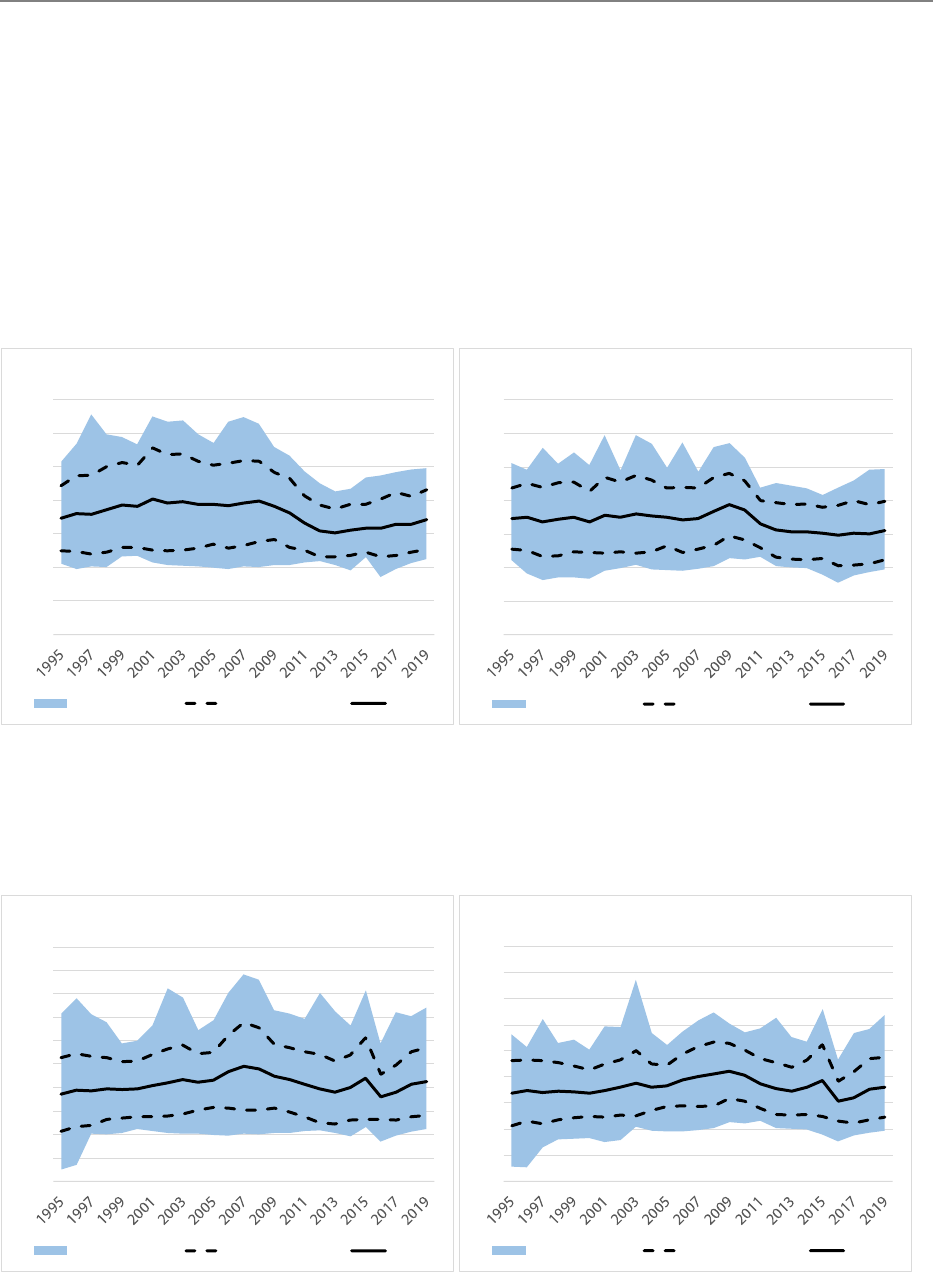
Benefits and drawbacks of an “expenditure rule”, as well as of a "golden rule", in the EU fiscal framework

PE 645.732 37

compensated for its decline by 2019. As a share of GDP, however, this catch-up was not evident, which

is why investment as a percentage of GDP declined over the time horizon from 3.5 per cent in 1995 to

3.1 per cent in 2019.

The sharpest drops between 2008 and 2013 were observed in Member States that had financial

assistance programmes, i.e. Ireland (-3.25 pp of GDP), Spain (-2.38 pp), Greece (-2.14 pp) and Portugal

(-1.54 pp), where the relevant shares fell from above-average levels of, for example, more than 5 per

cent in Greece and Ireland to below-average values of close to 2 per cent of GDP. The Eur opean Fis cal

Board (2019) points out that this reduction shows how rapid fiscal consolidations can be accompanied

by a decline in investment.

Figure 6: Public investment expenditures in the EU15 from 1995 to 2019

Notes: Investment expenditures are represented by gross fixed capital formation by the government. Blue areas represent the

range between the maximum and minimum values in each year. Lines represent the mean and mean plus and minus one

standard deviation across Member States.

Sources: European Commission’s AMECO database, own calculations

Figure 7: Public investment expenditures in EU27 from 1995 to 2019

Notes: Investment expenditures represented by gross fixed capital formation of general government. Blue areas represent

range between maximum and mimum value in each year. Lines represent mean and mean plus and minus one standard

deviation across Member States.

Sources: European Commission’s AMECO database, own calculations

10%

12%

14%

% of Total Expenditure

Max-Min-Range Mean +/- Std.Dev. Mean

% of GDP

Max-Min-Range

Mean +/- Std.Dev. Mean

10%

12%

14%

16%

18%

20%

% of Total Expenditure

Max-Min-Range Mean +/- Std.Dev. Mean

% of GDP

Max-Min-Range Mean +/- Std.Dev. Mean

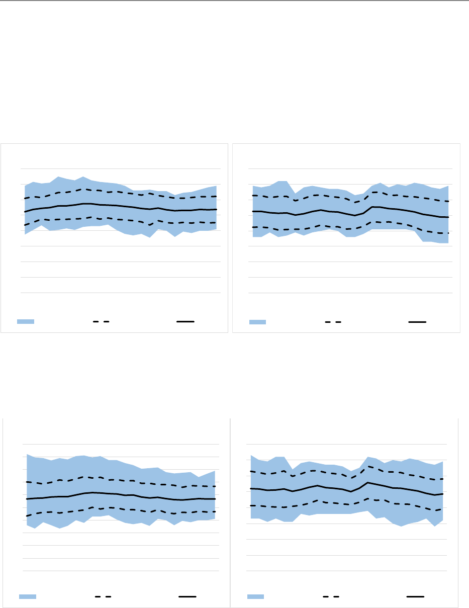
IPOL | Economic Governance Support Unit

38 PE 645.732

Spending on education has on average also remained stable over the past 22 years in the EU15. The

average relevant share of total expenditures was 10.5 per cent in 1995 and 10.7 per cent in 2018 (Figure

8). At the peak of the current sample – in 2002 and 2003 – this share was 11.5 per cent. Since then this

share has decreased especially in Portugal (-3.8 pp), the United Kingdom (-2.7 pp) and Finland (-2.3 pp),

all three of which had above-average shares in 2003 (Portugal 14.3 per cent, the United Kingdom 14.5

per cent and Finland 12.7 per cent). The countries with the lowest shares in 2018 were Italy (8.2 per

cent) and Greece (8.3 per cent), which had already had the lowest shares back in 1996.

Figure 8: Public education expenditures in EU15 from 1995 to 2018

Notes: Education expenditures of general government according to COFOG classification. Blue areas represent range

between maximum and mimum value in each year. Lines represent mean and mean plus and minus one standard deviation

across Member States.

Source: Eurostat, own calculations

Figure 9: Public education expenditures in EU27 from 1995 to 2018

Notes: Education expenditures of general government according to COFOG classification. Blue areas represent range

between maximum and mimum value in each year. Lines represent mean and mean plus and minus one standard deviation

across Member States.

Source: Eurostat, own calculations

1995

1996

1997

1998

1999

2000

2001

2002

2003

2004

2005

2006

2007

2008

2009

2010

2011

2012

2013

2014

2015

2016

2017

2018

Public Education (% of Total Expenditure)

Max-Min-Range Mean +/- Std.Dev. Mean

1995

1996

1997

1998

1999

2000

2001

2002

2003

2004

2005

2006

2007

2008

2009

2010

2011

2012

2013

2014

2015

2016

2017

2018

Public Education (% of GDP)

Max-Min-Range Mean +/- Std.Dev. Mean

199519971999

200120032005

200720092011201320152017

% of Total Expenditure

Max-Min-Range Mean +/- Std.Dev. Mean

19951997199920012003

2005

20072009201120132015

2017

% of GDP

Max-Min-Range Mean +/- Std.Dev. Mean

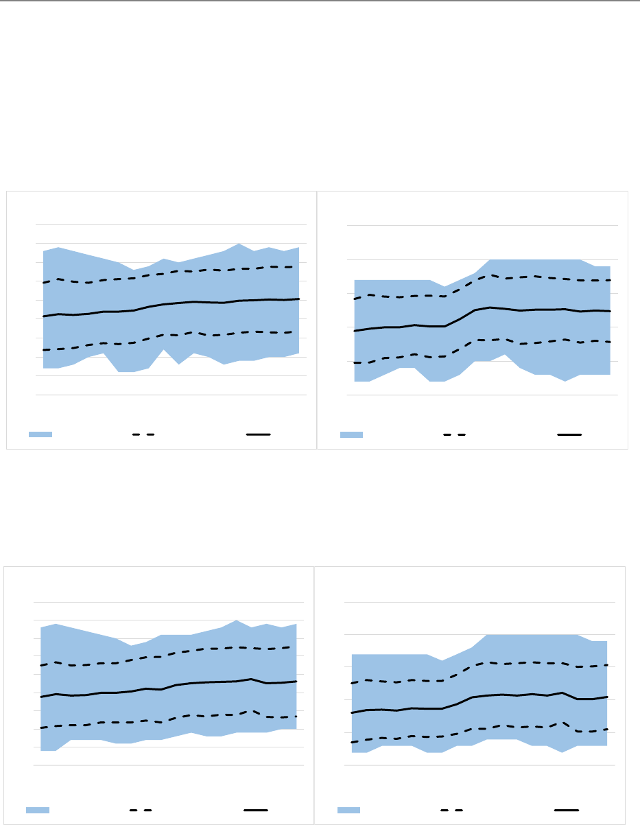
Benefits and drawbacks of an “expenditure rule”, as well as of a "golden rule", in the EU fiscal framework

PE 645.732 39

Spending on basic research and R&D as a percentage of total expenditures in the EU15 increased on

average by 0.46 percentage points between 2001 and 2018 (Figure 10). In contrast to investment and

education expenditures this spending did not drop sharply during the financial crisis. As a percentage

of GDP (shown in Figure 10), there was actually a pronounced increase during the financial crisis, i.e.

while GDP decreased during these years, R&D expenditures increased or at least remained stable. In

Germany, for example, research expenditures formed part of the fiscal stimulus packages introduced

in response to the crisis.

Figure 10: Public basic research and R&D expenditures in the EU15 from 2001 to 2018

Notes: Share of the sum of expenditures on basic research and research & development (R&D) by the government in various

categories according to COFOG classification. Blue areas represent the range between the maximum and minimum values in

each year. Lines represent the mean and mean plus and minus one standard deviation across Member States.

Sources: Eurostat, own calculations

Figure 11: Public basic research and R&D expenditures in EU25 from 2001 to 2018

Notes: Share of sum of expenditures on basic research and research and development (R&D) of general government in

various categories according to COFOG classification. EU27 without Bulgaria and Lithuania. Blue areas represent range

between maximum and mimum value in each year. Lines represent mean and mean plus and minus one standard deviation

across Member States.

Source: Eurostat, own calculations

0.5

1.5

2.5

3.5

4.5

2001

2002

2003

2004

2005

2006

2007

2008

2009

2010

2011

2012

2013

2014

2015

2016

2017

2018

Basic research and R&D (% of Total Expenditure)

Max-Min-Range Mean +/- Std.Dev. Mean

0.5

1.5

2.5

2001

2002

2003

2004

2005

2006

2007

2008

2009

2010

2011

2012

2013

2014

2015

2016

2017

2018

Basic research and R&D (% of GDP)

Max-Min-Range Mean +/- Std.Dev. Mean

0.5

1.5

2.5

3.5

4.5

2001

2002

2003

2004

2005

2006

2007

2008

2009

2010

2011

2012

2013

2014

2015

2016

2017

2018

% of Total Expenditure

Max-Min-Range

Mean +/- Std.Dev.

Mean

0.5

1.5

2.5

2001

2002

2003

2004

2005

2006

2007

2008

2009

2010

2011

2012

2013

2014

2015

2016

2017

2018

% of GDP

Max-Min-Range Mean +/- Std.Dev. Mean

IPOL | Economic Governance Support Unit

40 PE 645.732

6.2.2. Specific Expenditure Categories during Fiscal Consolidations

Specific expenditures like the ones discussed in the previous section might be reduced (relative to

others) first and most sharply during fiscal consolidations. The upper panel of Table 4 presents the

correlation of changes in these expenditures with changes in the cyclically-adjusted fiscal balance. If

the latter is positive, this is a period of discretionary fiscal consolidation (not due to the economic cycle),

while if it is negative it corresponds to periods of discretionary fiscal expansion. The results show that

these expenditure categories – when measured as a percentage of GDP – do indeed seem to be

negatively correlated. Investment expenditures in particular tend to decrease as a share of GDP in times

of consolidation and increase in times of expansion. This also becomes evident in the lower panel of

Table 4, which shows that, during fiscal consolidations, investment expenditures have on average

decreased by 0.17 percentages points as a share of GDP. In the case of education and R&D

expenditures, correlations and average changes in times of fiscal consolidation are very small, which

means that the development of these categories seems to be largely independent of phases of

consolidation and expansion.

During periods of fiscal consolidation one would usually expect expenditures to grow more slowly or

to be reduced, so the observation of decreases in levels or percentages of GDP in expenditure

categories is not surprising. However, the question is whether specific expenditure categories are

reduced relative to other categories. Looking at expenditure categories as a share of total expenditures

reveals that – based on correlations (upper panel) and averages (lower panel) – education and R&D

expenditures as a share of total expenditures increased during fiscal consolidations. In other words,

these categories were less affected than other categories. The positive correlation is relatively high for

education expenditures in particular. The correlation is virtually zero in the case of investment

expenditures, so there seems to be no clear relationship between changes in the cyclically-adjusted

budget balance and the relevant share of investment expenditures.

Overall, the results suggest that expenditures on investment and, to a smaller extent, on education as

well as basic research and R&D are reduced as a percentage of GDP during periods of fiscal

consolidation. However, expenditures on education as well as basic research and R&D are affected less

than other expenditure categories, which means that their share of total expenditures increases.

Overall, the share accounted for by investment expenditures does not seem to be systematically

related to periods of fiscal consolidation or expansion.

Benefits and drawbacks of an “expenditure rule”, as well as of a "golden rule", in the EU fiscal framework

PE 645.732 41

Table 4: Fiscal consolidations and specific public expenditure categories

Investment

Education

Basic research, R&D

1995-2018

2001-2018

Correlation of changes in the cyclically-adjusted fiscal balance (% of potential GDP) with changes in…

% of total

expenditures

EU15 0.003 0.608 0.201

EU27

-0.045

0.467

0.126

% of GDP

EU15

-0.296

-0.122

-0.094

EU27

-0.231

-0.102

-0.117

Average change during years of fiscal consolidation (cyc.-adj. fiscal balance improved by more than 0.5 pp)

% of total

expenditures

EU15 -0.148 0.173 0.053

EU27

-0.203

0.180

0.061

% of GDP

EU15

-0.166

-0.060

0.003

EU27

-0.185

-0.065

-0.002

Sources: European Commission’s AMECO database, Eurostat, own calculations

6.3. Forecast Errors based on AMECO Vintages

The European Commission publishes its macro-economic database AMECO twice a year (in spring and

in autumn) including forecasts for the coming years. Each publication is called “vintage” of the AMECO

database and currently the vintages from spring 2011 to autumn 2019 can be downloaded from the

European Commission’s website. For some key variables data from older vintages are available to

download at the website of the EU funded Horizon 2020 project “Firstrun”. The project publishes data

from AMECO vintages starting in spring 2000.

In the context of this paper, the two-year ahead forecast error (



) of variables measured in Euros, like

expenditures, revenues or GDP, () for a specific year  is defined as the percentage of GDP ()

difference between the value of the variable in the vintage of autumn four years after that specific year,

i.e. in  + 4, and the forecast in the vintage of autumn two years ahead of the specific year, i.e.   2.



,









 











where 





is the variable  for year  observed in the autumn vintage of year  + 4. The vintage in  +

4 is used as benchmark, instead of e.g. the last currently available vintage, to guarantee that the same

time has passed between the forecast and ex-post data for all observations. The largest revisions

usually happen within the first four years. Afterwards revisions still occur but in general they are

considerably smaller.

When comparing data across vintages data revisions, changes of base years and changes of accounting

rules pose a problem. To deal with this, this paper follows Fatás and Summers (2018) and rebases the

variables using an adjustment factor. This approach uses the ratio of observations for a year for which

the data lies in the past in both vintages, i.e.   3, to adjust the values in the older vintage.

IPOL | Economic Governance Support Unit

42 PE 645.732





 

= 





















,

 







 



 





 

For potential GDP also data of past years are still an estimation at the time of the publication of a

vintage. Therefore, in case of potential GDP the adjustment factor as in Fatás and Summers (2018) is

based on past values for actual GDP.

The exercises in this paper do not only use two-year ahead forecast errors, but also one-year ahead

(



) and real-time (



) errors. The latter calculates the error based on the values published in the

vintage in autumn of year  for this year .



,

 







 



 





 

For variables, which are differences and are expressed in percentage of (potential) GDP, like fiscal

balance, growth rates, structural balance or output gap, the approach described above is not feasible.

However, as for percentages of GDP the numerator and denominator are both within one vintage,

problems of different base years or changes of accounting rules are of less concerns. Thus, for those

variables the forecast error is defined as the simple percentage point difference between the value in

the autumn vintage of  + 4 and the forecast of the variable in the autumn vintage of   2,   1 or .

6.4. Calculation of past growth rates of cyclically-adjusted revenue,

potential GDP and expenditures

The calculations in this section are based on the same dataset as described in Annex 6.3. As cyclically-

adjusted revenues and the cyclical component of expenditures are both not part of the Firstrun dataset

(i.e. older vintages), a workaround is used to calculate the limit for expenditure growth which would

keep the cyclically-adjusted budget balance constant. By summing up total expenditures (UUTGE) and

the cyclically-adjusted budget balance (UBLGAP), which are both available for the longer time period,

the sum of cyclically-adjusted revenues and the cyclical component of expenditures is obtained.

Expenditures are allowed to increase by the growth rate of this sum to keep the cyclically-adjusted

balance constant.



 .

= 

.

 

 .

=     



(



)

 

.

(



)





.

  = 

.

 

 .

(



)

The cyclically-adjusted budget balance (UBLGAP) is only available in percent of GDP for the longer time

series (based on Firstrun data), while total expenditures (UUTGE) are measured in nominal terms. Thus,

the former is multiplied with nominal GDP (UVGDH) to receive the cyclically-adjusted budget balance

in nominal terms. As a cross-check for the time period in which data overlaps, the direct sum of

cyclically-adjusted revenues (URTGAP) and the cyclical component of expenditures (UUCGCP) is

compared with the measures obtained through above described workaround. The values (except for

rounding differences) are identical.

Most expenditure rules discussed in this paper use some measure related to potential GDP growth as

limits. If expenditures are measured in nominal terms, so should be potential GDP (OVGDP). Thus, for

Benefits and drawbacks of an “expenditure rule”, as well as of a "golden rule", in the EU fiscal framework

PE 645.732 43

the calculations in this section it is multiplied with the BIP deflator (UVGDH / OVGD). Furthermore, some

proposals use contemporaneous potential GDP growth, others some averages across past or future

years. Figure 12 first compares nominal potential GDP between forecast, real-time and ex-post for

annual data and for a moving average. It seems that forecasted growth rates lag developments seen in

ex-post numbers. I.e. while forecast potential GDP growth was (much) higher than ex-post figures

between 2008 and 2015, it was lower afterwards. This observeration remains valid when taking

averages, but the difference becomes smaller. In contrast to forecasts the difference between real-time

and ex-post estimates of potential GDP growth seems small, especially when taking averages it is very

small. Figure 12 also compares different averages at various estimation points with the annual potential

GDP growth rates. As intended, taking averages over longer time periods smoothens changes in

potential GDP growth and if growth rates are lower for more than a few years this lower growth rates

become visible in the averages later. Thus, in the period between 2000 and 2019, various averages of

growth rates were approximately equal or higher than actual potential GDP growth for most years until

2016. The strong increase in potential GDP in ex-post data in 2014 can be attributed to Ireland, without

Ireland the growth rate in 2014 would be 2.1 %.

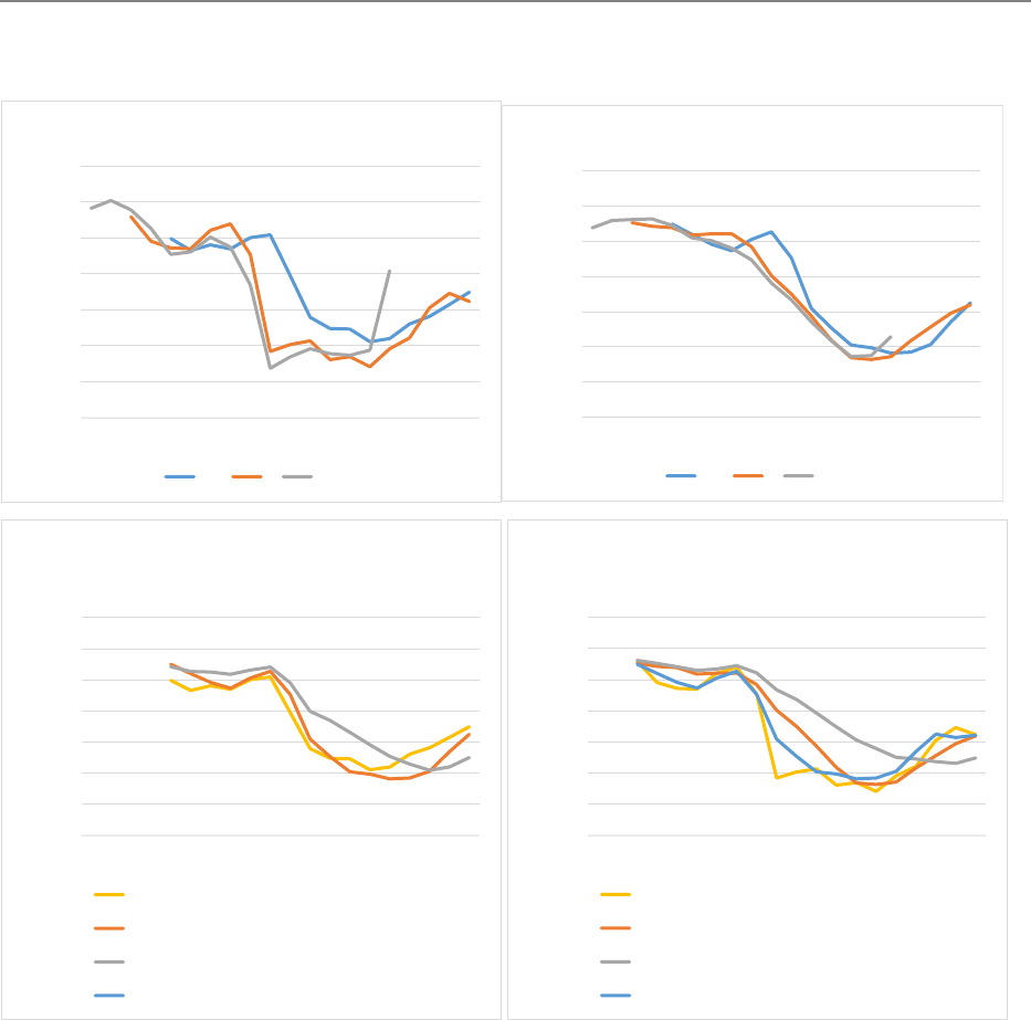
IPOL | Economic Governance Support Unit

44 PE 645.732

Figure 12: Comparison of measures of potential GDP growth (forecast, real-time, ex-post)

Source: European Commission’s AMECO database, Firstrun project, own calculations

Most expenditure rules do not set a limit to gross total public expenditures, but to some adjusted

measure subtracting and estimating various parts. Figure 13 compares growth rates of different

measures of expenditures. However, some of the more detailed variables are not available over longer

time periods. For primary expenditures, i.e. total expenditures net of interest payments, the interest

payments are calculated as difference between net lending excluding interest (UBLGIE) and net lending

(UBLGE), which are both available in the longer dataset. Those interest payments are then subtracted

from total expenditures (UUTGE) to receive primary expenditures. Estimates of the cyclical component

of expenditures (UUCGCP) are available for vintages since 2011 and estimates of discretionary revenues

measures only since 2014. Figure 13 shows that growth rates for primary expenditures in real-time and

ex-post seem to be very close, which confirms the findings regarding forecast and real-time errors in

Section 3.2. Furthermore, at least in real-time there seems to be almost no difference between total

expenditure and primary expenditure growth rates. However, the difference of those to the estimates

subtracting the cyclical component and discretionary revenues measures can be quite large, with the

0.00%

1.00%

2.00%

3.00%

4.00%

5.00%

6.00%

7.00%

2000 2002 2004 2006

2008 2010 2012 2014 2016 2018

Nominal potential GDP growth

t-2 t t+4

0.00%

1.00%

2.00%

3.00%

4.00%

5.00%

6.00%

7.00%

2000 2002 2004 2006 2008 2010 2012 2014 2016 2018

Average nominal pot. GDP growth

t-2 t t+4

0.00%

1.00%

2.00%

3.00%

4.00%

5.00%

6.00%

7.00%

2000 2002 2004 2006 2008 2010 2012 2014 2016 2018

Nominal potential GDP growth:

Forecast

Nominal potential GDP in t

5-year backward looking average

10-year backward looking average

2year back & 2 year front

0.00%

1.00%

2.00%

3.00%

4.00%

5.00%

6.00%

7.00%

2000 2002 2004 2006 2008 2010 2012 2014 2016 2018

Nominal potential GDP growth:

Real-time

Nominal potential GDP in t

Average potential GDP growth

10-year backward looking average

2year back & 2 year front

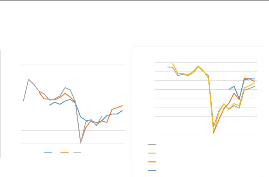
Benefits and drawbacks of an “expenditure rule”, as well as of a "golden rule", in the EU fiscal framework

PE 645.732 45

most comprehensive measure showing a growth rate which is on average 1.2 percentage points higher

between 2014 and 2019 in real-time than for primary expenditure.

Figure 13: Comparison of growth rates of different measures of public expenditure

Source: European Commission’s AMECO database, Firstrun project, own calculations

Only growth rates are compared in the exercises of this section and each growth rate is calculated only

within one vintage of the database. Thus, no adjustment is applied to the data. However, it cannot be

excluded that changes of accounting rules or changes of base years might still have an effect also on

growth rates across different vintages. Nevertheless, the issue should be much less severe than when

comparing levels across vintages.

-2.00%

0.00%

2.00%

4.00%

6.00%

8.00%

10.00%

2000 2002 2004 2006 2008 2010 2012 2014 2016 2018

Primary expenditures

t-2 t t+4

-2.00%

-1.00%

0.00%

1.00%

2.00%

3.00%

4.00%

5.00%

6.00%

2000 2002 2004 2006 2008 2010 2012 2014 2016 2018

Expenditure growth rates (Real-time)

Expenditures

Primary expenditure

… net of cyclical component

... net of discretionary revenues measures

IPOL | Economic Governance Support Unit

46 PE 645.732

6.5. Additional results regarding forecast and real-time estimation errors

Table 5: Mean absolute errors and mean errors of forecasts and real-time estimates

Notes: Calculations based on number of observations stated in N. Errors calculated as difference between values for year t in autumn vintage of year t-2, t-1 and t compared to values in

autumn vintage of year t+4. Mean errors are calculated as mean across countries and time of the difference between values for year t values in autumn vintage of year t+4 and in autumn

vintage of year t-2, t-1 and t. Mean absolute errors are the mean of the absolute values of the differences. To make results comparable only years and vintage are included which are

available for all variables (or a specific variable in last column) in all years and countries. More details on calculations can be found in Annex 6.3. Abs.: Mean absolute error. Budget balance:

Net lending or borrowing. pp.: differences in percentage points. Sources: European Commission’s AMECO database, Firstrun project, own calculations

EU 15, 2005-2015 EU13 (wo EL, IE), 2005-2015 EU15, without 2007 & 2008 EU27, 2007-2015 Max. obs. for each variable

Abs. Mean N Abs. Mean N Abs. Mean N Abs. Mean N Abs. Mean N

Real GDP t-2 3.46 -1.37 164 2.87 -1.18 142 3.74 -1.76 134 4.74 -1.96 239 4.10 -0.96 379

(% of GDP) t-1 2.10 -0.39 164 1.74 -0.37 142 2.20 -0.33 134 2.72 -0.53 239 2.36 0.10 379

t 0.81 0.11 164 0.61 0.03 142 0.79 0.25 134 0.91 0.21 239 0.85 0.34 379

Potential GDP t-2 2.90 -1.60 164 2.37 -1.62 142 2.94 -1.40 134 3.96 -2.09 239 3.54 -1.81 295

(% of GDP) t-1 2.13 -1.00 164 1.77 -1.09 142 1.90 -0.54 134 2.78 -1.08 239 2.54 -0.98 295

t 1.49 -0.58 164 1.26 -0.74 142 1.29 -0.17 134 1.75 -0.36 239 1.72 -0.52 295

Revenues t-2 2.34 0.03 164 2.13 0.18 142 2.35 -0.33 134 2.29 0.25 219

(% of GDP) t-1 1.56 0.22 164 1.40 0.31 142 1.63 0.21 134 1.65 0.43 219

t 0.69 0.26 164 0.63 0.29 142 0.70 0.33 134 0.73 0.38 219

Expenditures t-2 1.52 0.38 164 1.22 0.23 142 1.47 0.21 134 1.65 0.37 219

(% of GDP) t-1 1.12 0.45 164 0.81 0.18 142 1.11 0.38 134 1.26 0.48 219

t 0.64 0.11 164 0.56 0.01 142 0.64 0.06 134 0.75 0.24 219

Output Gap t-2 2.22 0.19 164 2.02 0.40 142 2.07 -0.41 134 2.53 0.08 239 2.46 0.40 294

(pp.) t-1 1.80 0.61 164 1.69 0.72 142 1.63 0.19 134 2.05 0.58 239 2.06 0.82 294

t 1.27 0.72 164 1.16 0.78 142 1.11 0.43 134 1.42 0.63 239 1.48 0.82 294

Budget balance t-2 2.50 -0.75 164 2.10 -0.32 142 2.59 -0.97 134 2.56 -0.73 239 2.36 -0.45 300

(pp.) t-1 1.88 -0.45 164 1.51 -0.02 142 1.95 -0.44 134 1.87 -0.50 239 1.78 -0.26 300

t 0.90 0.00 164 0.77 0.18 142 0.89 0.11 134 0.98 -0.10 239 0.97 -0.03 300

Cyclically-adjusted t-2 2.09 -0.77 164 1.65 -0.46 142 2.12 -0.67 134 2.31 -0.63 239 2.15 -0.62 283

budget balance (pp.) t-1 1.65 -0.68 164 1.28 -0.32 142 1.58 -0.44 134 1.81 -0.64 239 1.71 -0.57 283

t 1.01 -0.31 164 0.87 -0.18 142 0.89 -0.03 134 1.16 -0.29 239 1.12 -0.30 283

Growth of potential t-2 0.99 -0.47 164 0.66 -0.50 142 1.03 -0.39 134 1.42 -0.73 239 1.25 -0.64 295

GDP (p.p.) t-1 0.79 -0.20 164 0.51 -0.26 142 0.77 -0.04 134 1.08 -0.34 239 0.96 -0.32 295

t 0.63 -0.05 164 0.39 -0.14 142 0.62 0.08 134 0.74 -0.05 239 0.70 -0.11 295

Structural balance t-2 2.35 -0.30 215

(pp.) t-1 1.66 -0.15 215

t 1.04 0.20 215

Benefits and drawbacks of an “expenditure rule”, as well as of a "golden rule", in the EU fiscal framework

PE 645.732

IP/A/ECON-ED/IC/2020-055

Print ISBN 978-92-846-6868-7 | doi: 10.2861/222285 | QA-01-20-416-EN-C

PDF ISBN 978-92-846-6869-4 | doi: 10.2861/147212 | QA-01-20-416-EN-N

Focusing the EU fiscal framework on an expenditure rule could help to increase transparency,

compliance and ownership. In various other respects, like estimation errors or counter-cyclicality of

the prescribed fiscal policy, an expenditure rule is similar to a structural balance rule.

If the EU decides to go beyond the current focus on fiscal aggregates, a two-rule system aimed at

safeguarding specific expenditures could be placed at the centre of the EU fiscal framework. The key

challenge is to define and measure the protected expenditures.

This document was provided by the Economic Governance Support Unit at the request of the ECON

Committee).