
The University of Southern Mississippi The University of Southern Mississippi
The Aquila Digital Community The Aquila Digital Community
Undergraduate Theses
5-2013
Chebyshev Polynomial Approximation to Solutions of Ordinary Chebyshev Polynomial Approximation to Solutions of Ordinary
Differential Equations Differential Equations
Amber Sumner Robertson
University of Southern Mississippi
Follow this and additional works at: https://aquila.usm.edu/undergraduate_theses
Part of the Mathematics Commons
Recommended Citation Recommended Citation
Robertson, Amber Sumner, "Chebyshev Polynomial Approximation to Solutions of Ordinary Differential
Equations" (2013).
Undergraduate Theses
. 1.
https://aquila.usm.edu/undergraduate_theses/1
This Article is brought to you for free and open access by The Aquila Digital Community. It has been accepted for
inclusion in Undergraduate Theses by an authorized administrator of The Aquila Digital Community. For more
information, please contact [email protected].
The University of Southern Mississippi
CHEBYSHEV POLYNOMIAL APPROXIMATION TO
SOLUTIONS OF ORDINARY DIFFERENTIAL EQUATIONS
By
Amber Sumner Robertson
May 2013
i
ABSTRACT
CHEBYSHEV POLYNOMIAL APPROXIMATION TO SOLUTIONS OF
ORDINARY DIFFERENTIAL EQUATIONS
By
Amber Sumner Robertson
May 2013
In this thesis, we develop a method for finding approximate particular so-
lutions for second order ordinary differential equations. We use Chebyshev
polynomials to approximate the source function and the particular solution of
an ordinary differential equation. The derivatives of each Chebyshev polyno-
mial will be represented by linear combinations of Chebyshev polynomials, and
hence the derivatives will be reduced and differential equations will become al-
gebraic equations. Another advantage of the method is that it does not need the
expansion of Chebyshev polynomials. This method is also compared with an
alternative approach for particular solutions. Examples including approxima-
tion, particular solution, a class of variable coefficient equation, and initial value
problem are given to demonstrate the use and effectiveness of these methods.
ii
Copyright
by
Amber Sumner Robertson
2013
iii

The University of Southern Mississippi
CHEBYSHEV POLYNOMIAL APPROXIMATION TO SOLUTIONS OF
ORDINARY DIFFERENTIAL EQUATIONS
by
Amber Sumner Robertson
Approved by
May 2013
iv
ACKNOWLEDGEMENTS
I would like to reserve this section to thank all of those who made this
paper possible. I owe a huge debt of gratitude to my advisor, Dr. Haiyan
Tian, for guiding me through this endeavor. Without her, this would not have
been possible. I would like to thank Dr. Joseph Kolibal for encouraging me to
pursue an undergraduate research project and for reminding me that education
is truly about the pursuit of knowledge. I would also like to thank Dr. James
Lambers for his interest in this project, and his helpful comments, suggestions,
and encouragement along the way. I would like to thank Dr. Karen Kohl who
taught me how to do mathematical computing and helped in this endeavor as
well. I owe thanks to all of the professors and instructors whom I have studied
under here at the University of Southern Mississippi. Lastly, I would like to
thank Mr. Corey Jones and Mrs. Kerri Pippin from Jones County Junior
College for sparking a lifelong interest in learning Mathematics.
v
TABLE OF CONTENTS
ABSTRACT. . . . . . . . . . . . . . . . . . . . . . . . . . . . . . . . . . . . . . . . . . . . . . . . . . . . . . . . . . .ii
ACKNOWLEDGEMENTS . . . . . . . . . . . . . . . . . . . . . . . . . . . . . . . . . . . . . . . . . . v
LIST OF ILLUSTRATIONS . . . . . . . . . . . . . . . . . . . . . . . . . . . . . . . . . . . . . . . vii
LIST OF TABLES . . . . . . . . . . . . . . . . . . . . . . . . . . . . . . . . . . . . . . . . . . . . . . . . . . viii
LIST OF ABBREVIATIONS . . . . . . . . . . . . . . . . . . . . . . . . . . . . . . . . . . . . . . . ix
1. INTRODUCTION . . . . . . . . . . . . . . . . . . . . . . . . . . . . . . . . . . . . . . . . . . . . . . . . . 1
1.1 Applications of Second Order Ordinary Differential Equations . . . . . . . 1
1.2 Particular Solution of an Ordinary Differential Equation . . . . . . . . . . . . . 2
2. APPROXIMATION USING CHEBYSHEV POLYNOMIALS3
2.1 Method of Chebyshev Polynomial Approximation . . . . . . . . . . . . . . . . . . . .4
2.2 Illustrations of Chebyshev Polynomial Approximation . . . . . . . . . . . . . . . 6
3. AN APPROXIMATE PARTICULAR SOLUTION . . . . . . . . . . . . 9
3.1 Method of Reduction of Order . . . . . . . . . . . . . . . . . . . . . . . . . . . . . . . . . . . . . . .9
3.2 Examples of Approximation . . . . . . . . . . . . . . . . . . . . . . . . . . . . . . . . . . . . . . . . 11
4. AN ALTERNATIVE METHOD . . . . . . . . . . . . . . . . . . . . . . . . . . . . . . . 20
4.1 Method of Superposition . . . . . . . . . . . . . . . . . . . . . . . . . . . . . . . . . . . . . . . . . . . . 20
4.2 Examples of Approximation. . . . . . . . . . . . . . . . . . . . . . . . . . . . . . . . . . . . . . . . .21
5. CONCLUSIONS . . . . . . . . . . . . . . . . . . . . . . . . . . . . . . . . . . . . . . . . . . . . . . . . . 23
vi
LIST OF ILLUSTRATIONS
1. Plot of Chebyshev polynomials T
n
, n = 1, 2, ··· , 6 . . . . . . . . . . . . . . . . . . .5
2. Plot of P
3
. . . . . . . . . . . . . . . . . . . . . . . . . . . . . . . . . . . . . . . . . . . . . . . . . . . . . . . . . . . .7
3. Plot of f(x) with T
1
. . . . . . . . . . . . . . . . . . . . . . . . . . . . . . . . . . . . . . . . . . . . . . . . . 7
4. Plot of f(x) with T
4
. . . . . . . . . . . . . . . . . . . . . . . . . . . . . . . . . . . . . . . . . . . . . . . . . 8
5. Plot of f(x) with T
9
. . . . . . . . . . . . . . . . . . . . . . . . . . . . . . . . . . . . . . . . . . . . . . . . . 8
6. Plot of f(x) with T
16
. . . . . . . . . . . . . . . . . . . . . . . . . . . . . . . . . . . . . . . . . . . . . . . . 9
7. Plot of the right hand side function in Example 3.1.1 . . . . . . . . . . . . . . . . . 7
8. Plot of the particular solution for Example 3.1.1 . . . . . . . . . . . . . . . . . . . . 14
9. Plot of f(t) and P
4
with T
1
for Example 3.1.3 . . . . . . . . . . . . . . . . . . . . . . . 16
10. Plot of an approximate particular solution for Example 3.1.3 . . . . . . . 17
11. Plot of f(t) and P
4
for Example 3.1.4 . . . . . . . . . . . . . . . . . . . . . . . . . . . . . .19
12. Plot of an approximate particular solution for Example 3.1.4 . . . . . . .20
vii
LIST OF TABLES
1. Coefficients for T
0
j
(x), j = 0, 1, ··· , 4 . . . . . . . . . . . . . . . . . . . . . . . . . . . . . . . 12
2. Coefficients for T
00
j
(x), j = 0, 1, ··· , 4 . . . . . . . . . . . . . . . . . . . . . . . . . . . . . . .12
viii
LIST OF ABBREVIATIONS
ODE - Ordinary Differential Equations
PDE - Partial Differential Equations
MPS - Method of Particular Solutions
IVP - Initial Value Problem
ix

1
1 Introduction
In this thesis, we consider a linear second order ordinary differential equation
(ODE),
L(y) = ay
00
(x) + by
0
(x) + cy(x) = f(x) (1)
where f(x) is a continuous function, a, b, and c are given constants, and a 6= 0.
We are interested to find a particular solution y
p
for Equ. (1).
1.1 Applications of Second Order Ordinary Differential
Equations
The second order ordinary differential equation (1) can model many different
phenomena that we encounter every day. For example, the equation
d
2
y
dt
2
= −ky, with k > 0
represents what happens when an object is subject to a force towards an equilib-
rium position with the magnitude of the force being proportional to the distance
from equilibrium. The above equation can be considered as an approximation
to the equation of motion of a particular point on the basilar membrane, or
anywhere else along the chain of transmission between the outside air and the
cochlea [10]. Thus the solution of the differential equation can help explain the
perception of pitch and intensity of musical instruments by human ears.
We may also use a second order ODE to model at what altitude a skydiver’s
parachute must open before he reaches the ground so that he lands safely. To
model this phenomenon, we let y denote the altitude of the skydiver. We con-
sider Newton’s second law
F = ma (2)
where F represents the force, m represents the mass of the skydiver and a rep-
resents the acceleration. We assume that the only forces acting on the skydiver
are air resistance and gravity when the skydiver falls through the air toward
the earth. We also assume that the air resistance is proportional to the speed
of the skydiver with b being the positive constant of proportionality known as
the damping constant. The Newton’s second law (2) then translates to
y
00
+
b
m
y
0
= g. (3)
If we know the initial height y
0
and velocity v
0
at the time of jump, we have
an initial value problem which is the equation (3) together with the initial
conditions,
y(0) = y
0
,
y
0
(0) = v
0
.

2
As another application, the second order ODE can model a damped mass-
spring oscillator that consists of a mass m that is attached to a spring fixed at
one end [?, 6]. Taking into account the forces acting on the spring due to the
spring elasticity, damping friction, and other external influences, the motion of
the mass-spring oscillator is governed by the differential equation
my
00
+ by
0
+ ky = F
ext
(t) (4)
where b ( ≥ 0 ) is the damping coefficient and k ( ≥ 0 ) is known as the stiffness
of the spring. The differential equation (4) is derived by using Newton’s second
law and Hooke’s law.
Yet another application the equation (1) can model is an electrical circuit
consisting of a resistor, capacitor, inductor, and an electromotive force [6]. With
charge being the function, we can obtain an initial value problem of the form,
Lq
00
(t) + Rq
0
(t) +
q(t)
C
= E(t),
q(0) = q
0
,
q
0
(0) = I
0
,
where L is the inductance in henrys, R is the resistance in ohms, C is the
capacitance in farads, E(t) is the electromotive force in volts, and q(t) is the
charge in coulombs on the capacitor at time t.
We can easily see that the applications of the second order ODE has a wide
scope that it is applicable in many fields of study. A general form of these
equations is given by Eq. (1). When the right hand side function f(x) is zero,
it is a homogeneous equation; otherwise, it is a nonhomogeneous equation.
1.2 Particular Solution of an Ordinary Differential Equa-
tion
We hope to be able to find a particular solution for Eq. (1) that is nonhomo-
geneous. A particular solution of Eq. (1) is a function that satisfies Eq. (1).
The particular solution to an ordinary differential equation can be obtained by
assigning numerical values to the parameters in the general solution [3]. We
note that there are many possible answers for a particular solution.
A particular solution y
p
will allow us to reduce, for example, an initial value
problem
L(y) = ay
00
(x) + by
0
(x) + cy(x) = f(x),
y(x
0
) = y
0
, y
0
(x
0
) = y
1
,
(5)
to a homogeneous equation that is subject to a different initial data
L(y
h
) = ay
00
h
(x) + by
0
h
(x) + cy
h
(x) = 0,
y
h
(x
0
) = y
0
− y
p
(x
0
) , y
0
h
(x
0
) = y
1
− y
0
p
(x
0
) ,
(6)
with y
h
= y −y
p
. The method of particular of solutions (MPS) allows us to split
the solution y into a particular solution y
p
and a homogeneous solution y
h
.

3
In this thesis, we use Chebyshev polynomials for approximating equations
and their particular solutions. Chebshev polynomials [1] of the first kind are
solutions to the Chebyshev differential equations
1 − x
2
d
2
y
dx
2
− x
dy
dx
+ n
2
y = 0 for |x| < 1,
and Chebshev polynomials of the second kind are solutions to the Chebyshev
differential equations
1 − x
2
d
2
y
dx
2
− 3x
dy
dx
+ n (n + 2) y = 0 for |x| < 1.
The Chebyshev polynomials of either kind are a sequence of orthogonal poly-
nomials that can also be defined recursively. The motivation for Chebyshev in-
terpolation is to improve control of the interpolation error on the interpolation
interval [9]. The MPS and Chebyshev polynomials have been used for solving
partial differential equations (PDE). For example, the paper [13] solved elliptic
partial differential equation boundary value problems; the paper [11] studied
two dimensional heat conduction problems and the authors used Chebyshev
polynomials and the trigonometric basis functions to approximate their equa-
tions for each time step. In their two-stage approximation scheme, the use of
Chebyshev polynomials in stage one is because of the high accuracy (spectral
convergence) of Chebyshev interpolation.
If the right hand side function f(x) in Eq. (1) is a polynomial of degree n,
i.e.,
f(x) = P
n
(x)
= d
n
x
n
+ d
n−1
x
n−1
+ ... + d
1
x + d
0
where d
n
6= 0, we can find a particular solution of Eq. (1) that is a polynomial.
If f(x) is not a polynomial, we approximate it using Chebyshev polynomials.
We then look for a particular solution that is expressed as a linear combination
of Chebyshev polynomials. Our choice of Chebyshev polynomials is because of
their high accuracy. The Chebyshev polynomial is very close to the minimax
polynomial which (among all polynomials of the same degree) has the smallest
maximum deviation from the true function f (x). The minimax criterion is
that P
n
(x) is the polynomial of degree n for which the maximum value of the
error, which is defined by e
n
(x) = f(x) − P
n
(x), is a minimum within the
specified range of −1 ≤ x ≤ 1 [1]. This is extremely ideal for polynomial
approximations.
In our approach, the derivatives of each Chebyshev polynomial will be rep-
resented by the linear combinations of Chebyshev polynomials, and hence the
differential equations will become algebraic equations. In Chapter 2, we intro-
duce the approximation method and illustrations using Chebyshev polynomials.
In Chapter 3, we describe our method for finding a particular solution or an ap-
proximate particular solution by the approximation and reduction of order. An

4
alternative method by superposition principle is used in Chapter 4 for ODEs.
These two methods are compared through examples. Conclusions are made in
Chapter 5.
2 Approximation using Chebyshev Polynomials
The Chebshev polynomials of the first and second kind are denoted by T
n
(x)
and U
n
(x) respectively. The subscript n is the degree of these polynomials.
The Chebshev polynomials of the first and second kind are closely related. For
example, a Chebyshev polynomial of first kind can be represented as a linear
combination of two Chebyshev polynomials of second kind,
T
n
(x) =
1
2
(U
n
(x) − U
n−2
(x)) ,
and the derivative of a Chebyshev polynomial of first kind can be written in
terms of a Chebyshev polynomial of second kind,
T
0
n
(x) = nU
n−1
(x), n = 1, 2, ··· .
In this paper, we direct our attentation to the Chebyshev polynomials of first
kind and we use them for approximating a function and a particular solution
for second order ODEs.
2.1 Method of Chebyshev Polynomial Approximation
In this section, we give an introduction to the Chebyshev polynomials and their
basic properties. See the references [1, 9, 5, 2] for more details.
Chebyshev polynomials of the first kind are denoted by T
n
and the first
several polynomials are listed below:
T
0
(x) = 1,
T
1
(x) = x,
T
2
(x) = 2x
2
− 1,
T
3
(x) = 4x
3
− 3x,
T
4
(x) = 8x
4
− 8x
2
+ 1,
T
5
(x) = 16x
5
− 20x
3
+ 5x,
T
6
(x) = 32x
6
− 48x
4
+ 18x
2
− 1,
··· .
The first six Chebyshev polynomials T
j
, j = 0, 1, ··· , 6 are shown in Figure 1.
A Chebyshev polynomial can be found using the previous two polynomials
by the recursive formula
T
n+1
= 2xT
n
(x) − T
n−1
(x), for n ≥ 1.
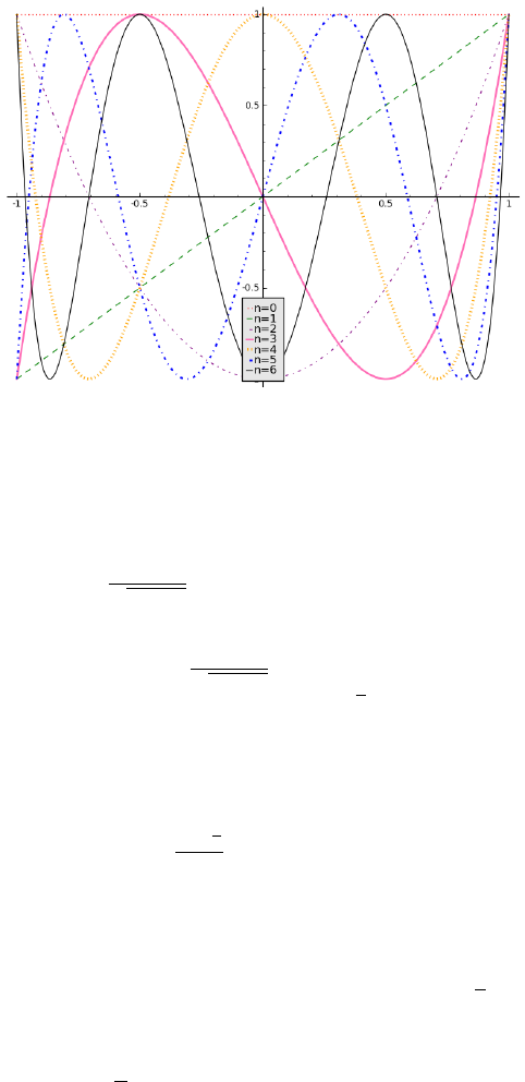
5
Figure 1: Plot of Chebyshev polynomials T
n
, n = 1, 2, ··· , 6
[1] The leading coefficient of the T
n
(x) is 2
n−1
for n ≥ 1 as we can see from the
recursive formula shown above. These polynomials are orthogonal with respect
to the weight function
1
√
1 − x
2
on the interval [−1, 1],
Z
1
−1
T
i
(x) T
j
(x)
1
√
1 − x
2
dx =
0, i 6= j,
π, i = j = 0,
π
2
, i = j 6= 0.
As we have mentioned, T
n
(x) denotes the Chebyshev polynomial of degree
n. It has n roots, which are also known as Chebyshev nodes. These nodes [5]
can be calculated by the formula
x
i
= cos
i −
1
2
n
π, for i = 1, 2, . . . , n.
A function f(x) can be approximated [4] by an n-th degree polynomial P
n
(x)
expressed in terms of T
0
, . . . , T
n
,
P
n
(x) = C
0
T
0
(x) + C
1
T
1
(x) + . . . + C
n
T
n
(x) −
1
2
C
0
(7)
where
C
j
=
2
n
n+1
X
k=1
f(x
k
)T
j
(x
k
), j = 0, 1, ··· , n. (8)
and x
k
, k = 1, . . . , n + 1 are zeros of T
n+1
.
Since
T
j
(x) = cos (j arccos x) ,

6
we have
T
j
(x
k
) = cos (j arccos x
k
)
= cos
j
k −
1
2
n + 1
π
!
.
Let f (x) be a continuous function defined on the interval [−1, 1], that we
want to approximate by a polynomial P
n
defined by (7) and (8). We can measure
how good an approximation is of f (x) by the uniform norm,
||f − P
n
|| = max
−1≤x≤1
|f(x) − P
n
(x)|.
This means that the measure of the error of the approximation is given by the
greatest distance between f(x) and P
n
(x) with x going through the interval
[−1, 1][5].
For m that is much less than n, f(x) ≈ C
0
T
0
(x)+C
1
T
1
(x)+. . .+C
m
T
m
(x)−
1
2
C
0
, is a truncated approximation with C
m+1
T
m+1
(x) + . . . + C
n
T
n
(x) being
the truncated part of the sum. The error in this approximation is dominated
by the leading term of the truncated part C
m+1
T
m+1
(x) since typically the
coefficients C
k
are repidly decreasing. We know that the m + 2 equal extrema
of T
m+1
(x) spread out smoothly over the interval [−1, 1], thus the error spreads
out smoothly over the interval [−1, 1].
The equations. (7) and (8) are used to approximate a function f(x) defined
on the interval [−1, 1]. For a function f (x) that is defined on an interval [a, b],
we can obtain f(y) with y ∈ [−1, 1] by a change of variable
y ≡
x −
1
2
(b + a)
1
2
(b − a)
.
2.2 Illustrations of Chebyshev Polynomial Approximation
Let P
n
be the n
th
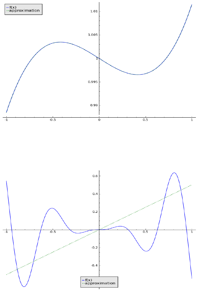
degree polynomial approximation to the function f(x). Ex-
ample 2.2.1. Let f(x) =
3
125
x
3
−
x
80
+ 1. The function f(x) and its Chebyshev
polynomial approximation P
3
are shown in Figure 2. The approximation poly-
nomial is identical to the function f(x) as we expected.
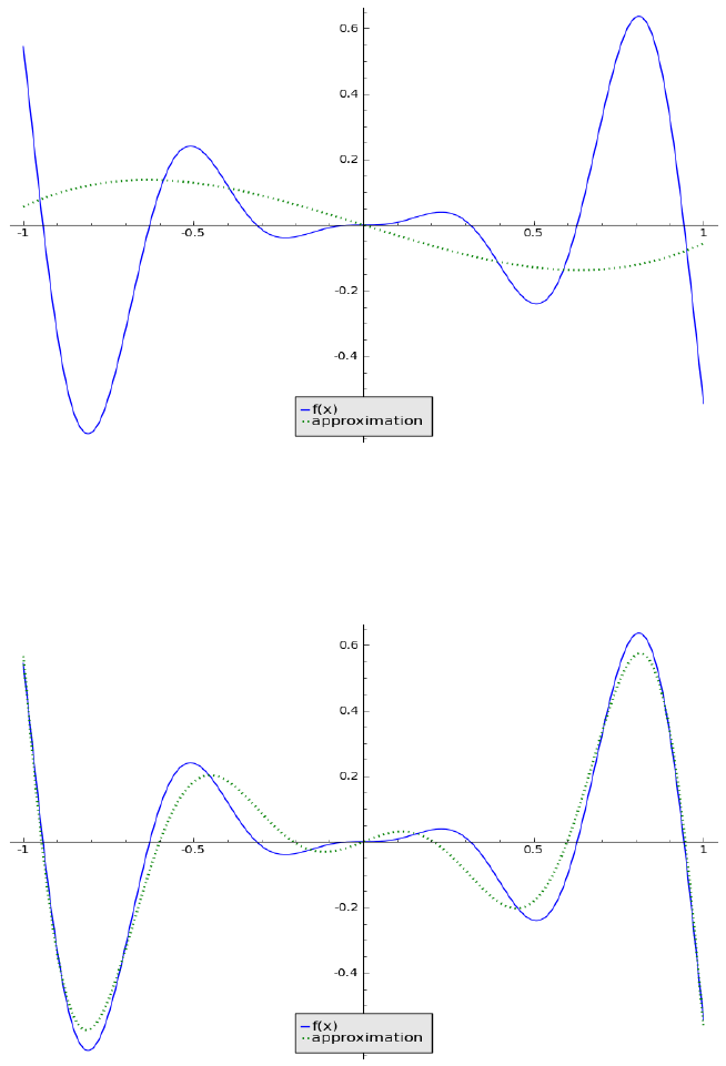
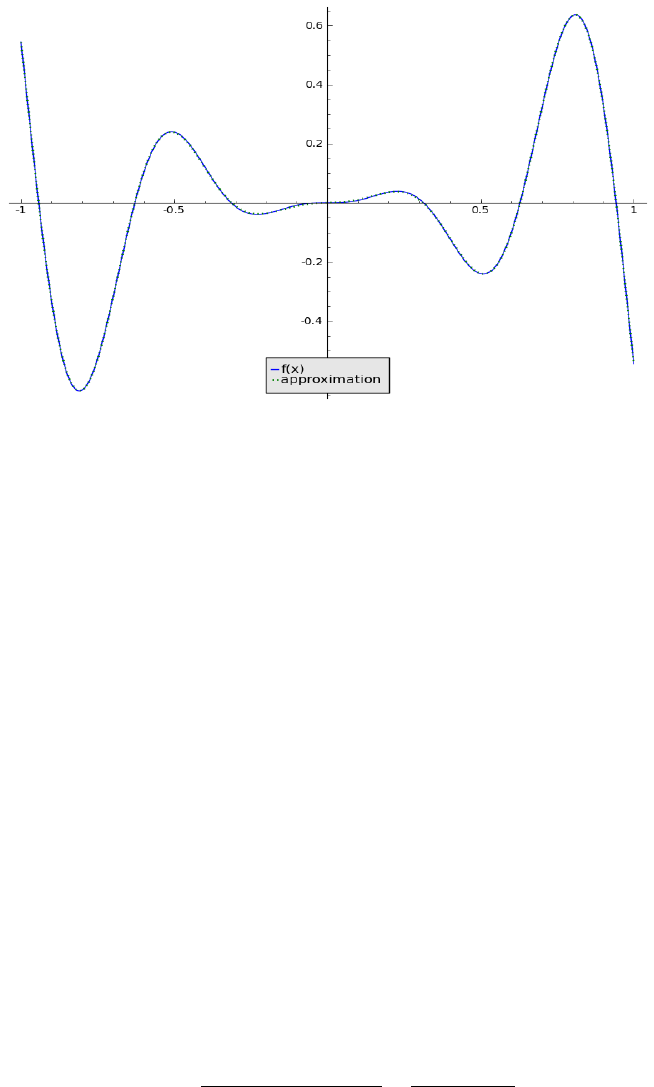
Example 2.2.2. Let f(x) = x
2
sin(10x). Its Chebyshev polynomial approxi-
mation P
n
with n = 1, 4, 9, 16 are shown in Figures 3-6. As n increases, the
error of the approximation polynomial decreases.
3 An Approximate Particular Solution
3.1 Method of Reduction of Order
We recall that we can reduce an initial value differential equation problem to
an albegraic equation through the Laplace transform [12, 6]. Here we propose
7
Figure 2: Plot of P
3
Figure 3: Plot of f(x) with T
1
8
Figure 4: the plot of f(x) with T
4
Figure 5: the plot of f(x) with T
9
9
Figure 6: the plot of f(x) with T
16
a method that achieves the similar goal using Chebyshev polynomial approxi-
mation and order reduction techniques.
By defining the Laplace transform to f(t),
L{f(t)} =
Z
∞
0
e
−st
f(t)dt = F (s),
we get a new function F (s). Assume that the functions f, f
0
, . . . , f
(n−1)
are
continuous and that f
(n)
is piecewise continous on any interval 0 ≤ t ≤ A.
Suppose further that there exist constants K, a, and M such that |f(t)| ≤ Ke
at
,
and |f
0
(t)| ≤ Ke
at
, ··· , |f
(n−1)
(t)| ≤ Ke
at
for t ≥ M . Then L
f
(n)
(t)
exists
for s > a and is given by,
L
n
f
(n)
(t)
o
= s
n
L{f(t)} − s
n−1
f(0) − . . . − sf
(n−2)
(0) − f
(n−1)
(0).
If the solution y(t) of the equation (1) , when substituted for f, satisfies the
above condition for n = 2, we can apply the Laplace transform to (1) to get the
following algebraic equation,
a[s
2
Y (s) − sy(0) − y
0
(0)] + b[sY (s) − y(0)] + cY (s) = F (s)
where Y (s) and F (s) are respectively the Laplace transforms of y(t) and f(t).
By solving the above equation for Y (s), we find that
Y (s) =
(as + b)y(0) + ay
0
(0)
as
2
+ bs + c
+
F (s)
as
2
+ bs + c
.

10
With the given initial conditions y(0) and y
0
(0), we can find a unique solution
Y (s). The inverse Laplace transform L
−1
{Y (s)} will give the solution to the
original initial value problem.
When employing the Laplace transform for an initial value problem, we first
transform a differential equation into an algebraic one by taking into account the
given initial data. Then we obtain the solution by inverse Laplace transform. In
our proposed MPS, we express a particular solution and the derivatives of the
particular solution by Chebyshev polynomials. Then using identities to obtain
a system of algebraic equations the coefficients should satisfy. Thus we find a
particular solution by solving algebraic equations. To get the solution of an
IVP, we need to get the solution of the corresponding homogenous problem.
We first approximate f (x) in Eq. (1) by P
n
(x) using Chebyshev polynomials.
Then we find a particular solution y
p
of the equation
ay
00
(x) + by
0
(x) + cy(x) = P
n
(x). (9)
We let the particular solution be in the form of
y
p
=
m
X
j=0
q
j
T
j
(x). (10)
The coefficients q
j
for (10) are to be determined. We let m = n if c 6= 0 in Equ.
(9); m = n + 1 if c = 0, b 6= 0; m = n + 2 if c = 0, b = 0.
Substituting (10) into (9),
a
m
X
j=0
q
j
T
00
j
(x) + b
m
X
j=0
q
j
T
0
j
(x) + c
m
X
j=0
q
j
T
j
(x) = P
n
(x).
Our next goal is to use linear combinations of Chebyshev polynomials to repre-
sent T
0
j
(x) and T
00
j
(x) for each j. That is, the first and second order derivatives
of Chebyshev polynomials T
0
j
(x) and T
00
j
(x) are represented in terms of T
k
(x),
k = 0, ··· , j. Then we arrive at a system of algebraic equations of q
j
by eqating
coefficients to find the solution y
p
given by (10).
According to [8] and its tables for representation coefficients, we reduce the
first and second order derivatives as follows
T
0
j
(x) =
j−1
X
k=0
b
k
T
k
(x), (11)
where
b
2l
= 0, for l = 0, 1, . . . ,
j
2
− 1,
b
2l+1
= 2j, for l = 0, 1, . . . ,
j
2
− 1,

11
for even j, and
b
0
= j,
b
2l
= 2j, for l = 1, . . . ,
j − 1
2
,
b
2l+1
= 0, for l = 0, 1, . . . ,
j − 3
2
,
for odd j.
Next, we expand the second order derivative T
00
j
(x) in terms of Chebyshev
polynomials T
i
(x), i = 0, . . . , j −2. With c
i
being the representation coefficients
for T
00
j
(x), that is,
T
00
j
(x) =
j−2
X
i=0
c
i
T
i
(x). (12)
We use the tables provided in [8] to calculate c
i
, for i = 0, . . . , j − 2. By Eq.
(11),
T
00
j
(x) =
T
0
j
(x)
0
(13)
=
j−1
X
k=0
b
k
T
k
(x)
!
0
=
j−1
X
k=0
b
k
T
0
k
(x)
=
j−1
X
k=0
b
k
k−1
X
i=0
b
i
T
i
(x)
!
=
j−1
X
k=0
k−1
X
i=0
b
k
b
i
T
i
(x)
3.2 Examples of Approximation
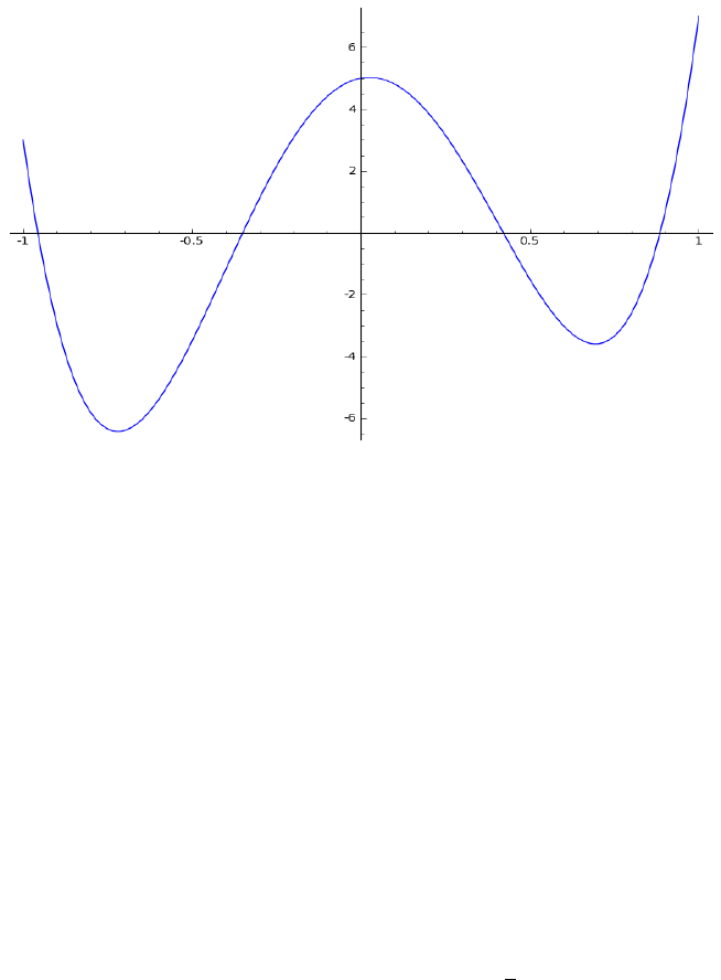
Example 3.1. 1. We consider the equation
y
00
(x) + 2y(x) = P
4
(x)
with P
4
(x) = 2T
1
(x)+5T
4
(x). We look for a particular solution y
p
=
4
P
j=0
q
j
T
j
(x).
By (11)-(13), we list the coefficients for T
0
j
(x), j = 0, 1, ··· , 4 in Table
1,which is equivalent to the following,
(T
0
)
0
= 0,
(T
1
)
0
= T
0
(x),
(T
2
)
0
= 4T
1
(x),
(T
3
)
0
= 3T
0
(x) + 6T
2
(x),
(T
4
)
0
= 8T
1
(x) + 8T
3
(x).

12
j=0
j=1 b
0
= 1
j=2 b
0
= 0 b
1
= 4
j=3 b
0
= 3 b
1
= 0 b
2
= 6
j=4 b
0
= 0 b
1
= 8 b
2
= 0 b
3
= 8
Table 1: Coefficients for T
0
j
(x), j = 0, 1, ··· , 4
j = 0
j = 1
b
0
= 1,
j = 2
b
0
= 0
b
1
= 4, b
1
· b
0
= 4 · 1
j = 3
b
0
= 3,
b
1
= 0, b
1
· b
0
= 0 · 1
b
2
= 6, b
2
· b
0
= 6 · 0, b
2
· b
1
= 6 · 4
j = 4
b
0
= 0,
b
1
= 8, b
1
· b
0
= 8 · 1
b
2
= 0, b
2
· b
0
= 0 · 0, b
2
· b
1
= 0 · 4
b
3
= 8, b
3
· b
0
= 8 · 3, b
3
· b
1
= 8 · 0, b
3
· b
2
= 8 · 6
Table 2: Coefficients for T
00
j
(x), j = 0, 1, ··· , 4
Thus,
y
0
p
= (q
1
+ 3q
3
)T
0
(x) + (4q
2
+ 8q
4
) T
1
(x) + 6q
3
T
2
(x) + 8q
4
T
3
(x). (14)
The coefficients for second order derivatives T
00
j
(x), j = 0, 1, ··· , 4 are listed in
Table 2 below,
Now we obtain the second order derivatives for T
j
, j = 0, 1, ··· , 4. We list
the results as follows:
(T
0
)
00
= 0,
(T
1
)
00
= 0,
(T
2
)
00
= 4T
0
(x),
(T
3
)
00
= 24T
1
(x),
(T
4
)
00
= 32T
0
(x) + 48T
2
(x).
We notice, for example, c
0
= 32, c
1
= 0, and c
2
= 48 for (12) when j = 4.
Therefore,
y
00
p
= 4q
2
T
0
(x) + 24q
3
T
1
(x) + 32q
4
T
0
(x) + 48q
4
T
2
(x)
= (4q
2
+ 32q
4
) T
0
(x) + 24q
3
T
1
(x) + 48q
4
T
2
(x).
13
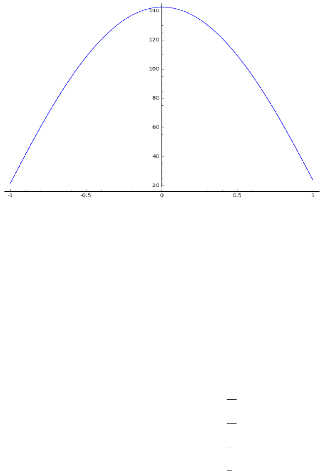
Figure 7: Plot of the right hand side function in Example 3.1.1
We obtain the following linear system of equations by comparing coefficients of
T
j
, j = 0, 1, ··· , 4.
2q
0
+ 4q
2
+ 32q
4
= 0,
2q
1
+ 24q
3
= 2,
2q
2
+ 48q
4
= 0,
2q
3
= 0,
2q
4
= 5.
(15)
The solution for (15) is q
4
= 5/2, q
3
= 0, q
2
= −60, q
1
= 1, q
0
= 80. The plots
of the right hand side function and the particular solution are shown in Figures
7-8.
Assume we use P
n
defined by (7)-(8) with n = 4 to approximate the function
f(x) in Eq. (1). Without loss of generality, we assume c 6= 0 in (1). Using our
method of reduction of order, the coefficients q
j
, j = 0, 1, ··· , 4 of the particular
solution satisfy the following system of equations,
cq
0
+ bq
1
+ 4aq
2
+ 3bq
3
+ 32aq
4
=
1
2
C
0
, (16)
cq
1
+ 4bq
2
+ 24aq
3
+ 8bq
4
= C
1
,
cq
2
+ 6bq
3
+ 48aq
4
= C
2
,
cq
3
+ 8bq
4
= C
3
,
cq
4
= C
4
.
Example 3.1. 2. In this example, we consider
y
00
(x) + y
0
(x) + 1.25y(x) = 3x
3
+ x
2
+ 2x + 7.
14
Figure 8: Plot of the particular solution for Example 3.1.1
We notice here the function f(x) = 3x
3
+ x
2
+ 2x + 7. We can still look for a
particular solution in the form of y
p
=
4
P
j=0
q
j
T
j
(x), but q
4
will be 0 as expected.
The Chebyshev polynomial representation for f (x) is
f(x) =
3
X
j=0
p
j
T
j
(x)
with p
0
= 15/2, p
1
= 17/4, p
2
= 1/2, p
3
= 3/4. According to the system of
equations (16), we obtain the following system for q
j
, j = 0, . . . , 4,
1.25q
0
+ q
1
+ 4q
2
+ 3q
3
+ 32q
4
=
15
2
,
1.25q
1
+ 4q
2
+ 24q
3
+ 8q
4
=
17
4
,
1.25q
2
+ 6q
3
+ 48q
4
=
1
2
,
1.25q
3
+ 8q
4
=
3
4
,
1.25q
4
= 0.
Using backward substitution, we get q
4
= 0, q
3
= 3/5, q
2
= −62/25, q
1
=
−23/125, q
0
= 7902/625.
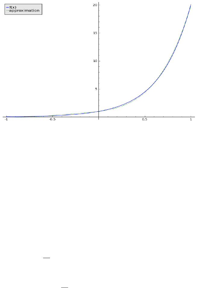
Example 3.1.3. In this example, we consider the Cauchy-Euler equations

15
that are expressible in the form of
ax
2
y
00
(x) + bxy
0
(x) + cy(x) = h(x),
where a, b and c are constants. This important class of variable coefficient differ-
ential equations can be solved by the particular solutions method of reduction of
order. As an illustration, we solve a specific Cauchy-Euler equation as follows,
x
2
y
00
(x) − 2xy
0
(x) + 2y(x) = x
3
. (17)
By a change of variable x = e
t
, the equation (17) can be transformed into the
constant coefficient equation in the new independent variable t,
y
00
(t) − 3y
0
(t) + 2y(t) = e
3t
.
Using the method described above, we approximate the right hand side function
by Chebyshev polynomial approximation, then we use the reduction of order
method to solve for the approximate particular solution.
The approximation to f(t) = e
3t
by P
4
is
f(t) =
C
0
2
T
0
(x) + C
1
T
1
(x) + C
2
T
2
(x) + C
3
T
3
(x) + C
4
T
4
(x),
where the numerical values of C
0
, . . . , C
4
are given as follows,
C
0
2
= 4.88075365707809,
C
1
= 7.90647046809621,
C
2
= 4.48879683378407,
C
3
= 1.9105629481,
C
4
= 0.608043176705983.
Solving the resulting system of equations,
2q
0
− 3q
1
+ 4q
2
− 9q
3
+ 32q
4
=
1
2
C
0
,
2q
1
− 12q
2
+ 24q
3
− 24q
4
= C
1
,
2q
2
− 18q
3
+ 48q
4
= C
2
,
2q
3
− 24q
4
= C
3
,
2q
4
= C
4
,
we get
q
0
= 344.481628331765,
q
1
= 170.637487061598,
q
2
= 36.3797465297907,
q
3
= 4.60354053428590,
q
4
= 0.304021588352991,
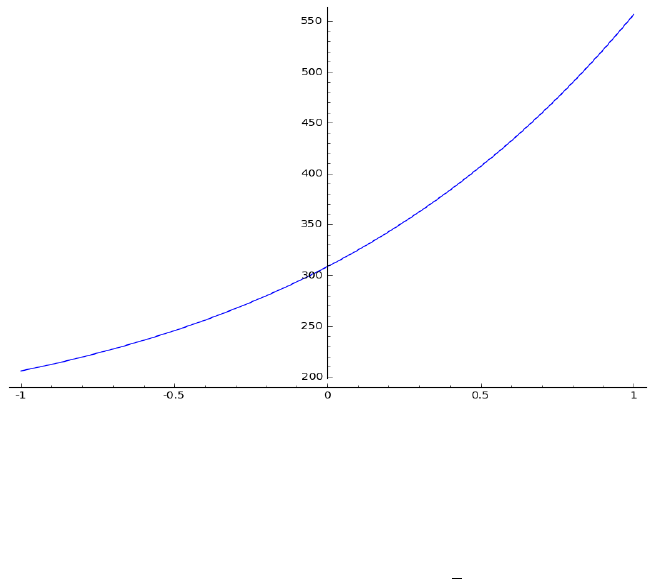
16
Figure 9: Plot of f(t) and P
4
of Example 3.1.3
which are coefficients of T
j
(x) for an approximate particular solution y
p
(t) of
the constant coefficient equation. The plots of the right hand side function and
the particular solution are shown in Figures 9-10. An approximate particular
solution of the Cauchy-Euler equation is y
p
(ln x).
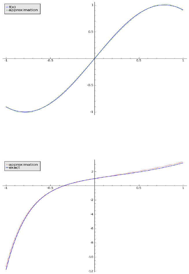
Example 3.1.4. As another example we consider the initial value problem,
y
00
+ 3y
0
− 4y = sin(2x),
with initial data,
y(0) = 1,
y
0
(0) = 2.
First, the Chebyshev approximation of sin(2x) by P
4
is,
sin(2x) ≈
C
0
2
T
0
(x) + C
1
T
1
(x) + C
2
T
2
(x) + C
3
T
3
(x) + C
4
T
4
(x),
where the coefficients C
0
, . . . , C
4
are
C
0
2
= 5.55111512312578e
−17
,
C
1
= 1.15344467691257,
C
2
= 0,
C
3
= 0.257536611098051,
C
4
= 2.22044604925031e
−16
.
17
Figure 10: Plot of an approximate particular solution of Example 3.1.3
The resulting system by the reduction of order method with n = 4 gives
−4q
0
+ 3q
1
+ 4q
2
+ 9q
3
+ 32q
4
=
1
2
C
0
,
−4q
1
+ 12q
2
+ 24q
3
+ 24q
4
= C
1
,
−4q
2
+ 18q
3
+ 48q
4
= C
2
,
−4q
3
+ 24q
4
= C
3
,
−4q
4
= C
4
.
The coefficients q
0
, . . . , q
4
for the particular solution of the IVP is given by
q
0
= 1.15994038863409
q
1
= 0.9671298098748495
q
2
= 0.289728687485306
q
3
= 0.0643841527745125
q
4
= −5.55111512312578e
−17
So we arrive at the particular solution,
y
p
(x) = q
0
T
0
(x) + q
1
T
1
(x) + q
2
T
2
(x) + q
3
T
3
(x) + q
4
T
4
(x).

18
The derivative of y
p
is given by (14) and thus
y
0
p
(0) = (q
1
+ 3q
3
)T
0
(0) + (4q
2
+ 8q
4
) T
1
(0) + 6q
3
T
2
(0) + 8q
4
T
3
(0)
= (q
1
+ 3q
3
) ∗ 1 + (4q
2
+ 8q
4
) ∗ 0 + 6q
3
∗ (−1) + 8q
4
∗ 0
= q
1
− 3q
3
.
This together with
y
p
(0) = q
0
T
0
(0) + q
1
T
1
(0) + q
2
T
2
(0) + q
3
T
3
(0) + q
4
T
4
(0)
= q
0
∗ 1 + q
1
∗ 0 + q
2
∗ (−1) + q
3
∗ 0 + q
4
∗ 1
= q
0
− q
2
+ q
4
gives the initial data for the corresponding homogeneous problem,
y
00
+ 3y
0
− 4y = 0,
that is subject to the initial data,
y(0) = 1 − y
p
(0) = 1 − q
0
+ q
2
− q
4
=,
y
0
(0) = 2 − y
0
p
(0) = 2 − q
1
+ 3q
3
= .
We need to find the solution y
h
to the above homogeneous problem so that we
can obtain the numerical solution to the original IVP. The homogenous solution
is,
y
h
= c
1
e
−4x
+ c
2
e
x
where c
1
= −0.219246869919495 and c
2
= 0.349035168770711.
Now we obtain the numerical solution of the IVP as follows,
ey(x) = y
p
− 0.219246869919495e
−4x
+ 0.349035168770711e
x
The exact solution of the problem is
y(x) =
1
20
cos(2x) −
1
20
sin(2x) −
9
40
e
−4x
+
6
5
e
x
.
Figure 11 shows the right hand side function and its approximation, and Figure
12 shows an approximate particular solution together with the exact solution of
the IVP.
4 An Alternative Method
4.1 Method of Superposition
In this section, we use the idea of paper [13] to solve our 1-D problem. We want
to be able to find a particular solution for Eq. (1). Assume that f (x) has the
Chebyshev polynomial approximation P
n
(x) given by (7) and (8), i.e.,
Ly = ay
00
+ by
0
+ cy = P
n
(x). (18)
19
Figure 11: Plot of f(t) and P
4
for Example 3.1.4.
Figure 12: Plot of the numerical solution and the exact solution for Example
3.1.4.

20
We first look for a particular solution y
k
for
ay
00
+ by
0
+ cy = T
k
(x), (19)
with k = 0, 1, ··· , n.
To find a particular solution for (19), we expand the polynomial T
k
(x) in
terms of the polynomial basis {1, x, x
2
, ··· , x
k
}. That is, T
k
(x) = d
k
x
k
+
d
k−1
x
k−1
+ ··· + d
1
x + d
0
.
For the equation (19), we consider three cases:
Case 1) If c 6= 0, we look for a particular solution that is in the form of
y
p
= e
k
x
k
+ e
k−1
x
k−1
+ ··· + e
1
x + e
0
; (20)
Case 2) If c = 0 and b 6= 0, we look for a particular solution that is in the
form of
y
p
= e
k+1
x
k+1
+ e
k
x
k
+ ··· + e
1
x + e
0
;
Case 3) If c = b = 0, the particular solution is
y
p
= e
k+2
x
k+2
+ e
k+1
x
k+1
+ ··· + e
1
x + e
0
.
We consider case 1) with the assumption c 6= 0 in the following since other
cases can be handled similarly. We The particular solution (20) is substituted
into (19),
a(
k
X
j=0
e
j
x
j
)
00
+ b(
k
X
j=0
e
j
x
j
)
0
+ c(
k
X
j=0
e
j
x
j
) =
k
X
j=0
d
j
x
j
.
By comparing coefficients, the e
j
should satisfy the following system of equations
ce
k
= d
k
,
ce
k−1
+ bke
k
= d
k−1
,
ce
i
+ b (i + 1) e
i+1
+ a (i + 2) (i + 1) e
i+2
= d
i
, for i = k − 2, ··· , 0.
Using backward substitution, we obtain the coefficients
e
k
=
d
k
c
, (21)
e
k−1
=
d
k−1
− bke
k
c
,
e
i
=
d
i
− b (i + 1) e
i+1
− a (i + 2) (i + 1) e
i+2
c
, for i = k − 2, ··· , 0.
Since y
k
is the particular solution corresponding to the Chebyshev polynomial
T
k
and L = a
d
2
dx
2
+ b
d
dx
+ c is a linear differential operator,
L(
n
X
k=0
c
k
y
k
(x)) =
n
X
k=0
c
k
L(y
k
(x))

21
which is,
L(
n
X
k=0
c
k
y
k
(x)) =
n
X
k=0
c
k
T
k
(x) , (22)
The equation (22) means that
y
p
=
n
X
k=0
c
k
y
k
(x)
is a particular solution of Ly = P
n
(x), with P
n
(x) =
n
P
k=0
c
k
T
k
(x).
4.2 Examples of Approximation
Example 4.2. 1 We consider the differential equation
y
00
(x) + y
0
(x) + 1.25y(x) = 3x
3
+ x
2
+ 2x + 7.
Due to the polynomial form of the right hand side function, the coefficients for
particular solution can be directly determined by (21), that is,
e
3
=
d
3
c
=
12
5
,
e
2
=
d
2
− 3be
3
c
= −
124
25
,
e
1
=
d
1
− 2be
2
− 6ae
3
c
= −
248
125
e
0
=
d
0
− be
1
− 2ae
2
c
=
9452
625
Thus, a particular solution for the equation is y
p
= e
0
+ e
1
x + e
2
x
2
+ e
3
x
3
.
This verifies the result we obtained in Example 3.1.2.
Example 4.2. 2 We consider
y
00
(x) + y
0
(x) + 1.25y(x) = f(x)
where f (x) has Chebyshev polynomial approximation P
3
(x) =
15
2
T
0
+
17
4
T
1
+
1
2
T
2
+
3
4
T
3
. We must find particular solutions y
(0)
, y
(1)
, y
(2)
, y
(3)
with respect
to the corresponding Chebyshev polynomials T
0
, T
1
, T
2
, T
3
. The coefficients for
y
(3)
is
e
3
=
d
3
c
=
4
1.25
=
16
5
,
e
2
=
d
2
− 3be
3
c
=
0 − 3e
3
1.25
= −
192
25
,
e
1
=
d
1
− 2be
2
− 6ae
3
c
=
−3 − 2e
2
− 6e
3
1.25
= −
684
125
,
e
0
=
d
0
− be
1
− 2ae
2
c
=
0 − e
1
− 2e
2
1.25
=
10416
625
.

22
The coefficients for y
(2)
is
e
2
=
d
2
c
=
2
1.25
=
8
5
,
e
1
=
d
1
− b2e
2
c
=
0 − 2e
2
1.25
= −
64
25
,
e
0
=
d
0
− be
1
− 2ae
2
c
=
−1 − e
1
− 2e
2
1.25
= −
164
125
.
The coefficients for y
(1)
is
e
1
=
d
1
c
=
1
1.25
=
4
5
,
e
0
=
d
0
− be
1
c
=
0 − e
1
1.25
= −
16
25
.
The coefficients for y
0
is
e
0
=
1
1.25
=
4
5
.
We list these particular solutions as follows:
y
0
=
4
5
y
1
=
4
5
−
16
25
x
y
2
=
−164
125
−
64
25
x +
8
5
x
2
y
3
=
10416
625
−
685
125
x −
192
25
x
2
+
16
5
x
3
Hence we find an approximate particular solution for the equation as
y
p
=
15
2
y
0
+
17
4
y
1
+
1
2
y
2
+
3
4
y
3
=
9452
625
−
248
125
x −
124
25
x
2
+
12
5
x
3
.
The alternative approach further verifies the result obtained by the reduction
of order method in Example 3.1.2.
5 Conclusions
The Chebyshev polynomials have been in existence for over a hundred years and
they have been used for solving many different problems. In this thesis, we have
a new strategy using chebyshev polynomials for a common problem. We obtain
satisfactory results because of the excellent convergence rate of Chebyshev ap-
proximation, which is very close to the minimax polynomial which minimizes
the maximum error in approximation. We find approximate particular solu-
tions by Chebyshev polynomial approximation and the reduction of order for
23
the derivatives of Chebyshev polynomials. For comparison purpose, we solve
same problems using an existing approach as an alternative approach. The first
approach does not need the expansion of Chebyshev polynomials. We end up
with an algebraic system of equations by expressing the derivatives of Chebyshev
polynomials in terms of these polynomials. We can compare the coefficients of
the Chebyshev polynomials in the resulting system of equations so that we can
determine the coefficients of the particular solution. The second approach uses
the approximation of a right hand side function, which we need to do expansion
for each Chebyshev polynomial basis function. We use the particular solutions
corresponding to each Chebyshev polynomial to construct a particular solution
of the differential equation by superposition principle. Since we are approximat-
ing a particular solution with polynomials in both cases, a particular solution by
either approach will be exact if the right hand function is already a polynomial.
References
[1] L. Fox and I. B. Parker, Chebyshev Polynomials in Numerical Analysis,
Oxford University Press (C) 1968.
[2] William Karush, The Crescent Dictionary of Mathematics, 7th Edition,
MacMillan Publishing Co., Inc., 1974.
[3] Philip Hartman, Ordinary Differential Equations, Birkhauser Boston, 1982.
[4] M. C. Seiler and F. A. Seiler, Numerical Recipes in C: The art of scientific
computing, Cambridge University Press. Programs Copyright (C) 1988-
1992 by Numerical Recipes Software.
[5] Theodore J. Rivlin, Chebyshev Polynomials: From Approximation Theory
to Algebra and Number Theory, Wiley and Sons Copyright (C) 1990 by
Wiley-Interscience.
[6] R. K. Nagle, E. B. Saff and A. D. Snider, Fundamentals of Differential
Equations, 6th Edition, Pearson, 2004.
[7] S. Reutskiy and C.S. Chen,.Approximation of multivariate functions and
evaluation of particular solutions using Chebyshev polynomial and trigono-
metric basis functions International Journal for Numerical Methods in En-
gineering 2006, 67: 1811-1829
[8] H.Y. Tian, Reducing order of derivatives and derivation of coefficients for
Chebyshev polynomial approximation, preprint, 2006.
[9] Timothy Sauer, Numerical Analysis, Pearson Education Inc. (C) 2006 -
2012.
[10] David J. Benson, Music, a mathematical offering, Cambridge, 2007.
24
[11] S. Reutskiy, C.S. Chen and H.Y. Tian, A boundary meshless method us-
ing Chebyshev interpolation and trigonometric basis function for solving
heat conduction problems, International Journal for Numerical Methods in
Engineering, 2008, 74: 1621-1644.
[12] W. E. Boyce and R. C. DiPrima, Elementary Differential Equations and
Boundary Value Problems, John Wiley & Sons, Inc, 2009.
[13] J. Ding, H.Y. Tian and C.S. Chen, The recursive formulation of particular
solutions for inhomogeneous elliptic PDEs with Chebyshev basis functions,
Communications in Computational Physics, 2009, 5, 942-958.
