Wave-number Space Networks in Plasma Turbulence

HAL Id: hal-04212188

https://hal.science/hal-04212188

Submitted on 20 Sep 2023

HAL is a multi-disciplinary open access

archive for the deposit and dissemination of sci-

entic research documents, whether they are pub-

lished or not. The documents may come from

teaching and research institutions in France or

abroad, or from public or private research centers.

L’archive ouverte pluridisciplinaire HAL, est

destinée au dépôt et à la diusion de documents

scientiques de niveau recherche, publiés ou non,

émanant des établissements d’enseignement et de

recherche français ou étrangers, des laboratoires

publics ou privés.

Wave-number Space Networks in Plasma Turbulence

Ö. Gürcan

To cite this version:

Ö. Gürcan. Wave-number Space Networks in Plasma Turbulence. Reviews of Modern Plasma Physics,

2023, 7 (1), pp.20. �10.1007/s41614-023-00122-7�. �hal-04212188�

Springer Nature 2021 L

X template

Wave-number Space Networks in Plasma

Turbulence

Ö. D. Gürcan

Laboratoire de Physique des Plasmas, CNRS, Ecole

Polytechnique, Sorbonne Université, Université Paris-Saclay,

Observatoire de Paris, F-91120 Palaiseau, France.

Contributing authors: [email protected]olytechnique.fr;

Abstract

Turbulence commonly described in Fourier space due to its multi-scale

nature can be formulated using wave number space networks where each

node represents a wave-vector on a discretized wave-number space grid

that are connected to one another through triadic interactions denoted

as three body connections. This description that we call wave-number

space network formulation, while being very ineﬃcient for numerical

implementation as compared for example to a pseudo-spectral formu-

lation of the same equations on a regular grid, provides an alternative

perspective and has conceptual advantages, such as the separation of

the equations and the nonlinear interactions. The network represents,

through its connections, the nonlinear interactions, and can be trun-

cated by dropping nodes, or connections corresponding to considering

only certain kinds of wave-numbers or certain kinds of interactions,

without modifying the equations themselves. This guarantees that the

underlying Hamiltonian structure of the equations remains unchanged,

and therefore one has the same conservation laws as the original system.

Wave-number space networks can also be reduced by lumping nodes that

have some similar characteristics together, in which case a reduction of

the equations through some sort of closure becomes necessary, for which

some possibilities are discussed. The network formulation can also be

used for analysing direct numerical simulations, and may be used for

discovering key nodes as well as training models for constructing reduced

systems. The goal of this review is to stimulate interest in thinking in

terms of networks, while dealing with problems in plasma turbulence

Springer Nature 2021 L

X template

2 Wave-number Space Networks in Plasma Turbulence

through a survey of what has been done in this subﬁeld and what is pos-

sible for future studies, especially in the context of plasma turbulence.

1 Introduction

Transport of heat, particles and momentum in tokamak plasmas can be caused

by micro-turbulence, and regulated by meso-scale coherent structures such as

zonal ﬂows[1, 2], geodesic acoustic modes (GAMs)[3, 4] or Alfvén eigenmodes

[5, 6] that the turbulence in these devices naturally generates (or regulates),

and their interactions. This makes the detailed understanding of plasma tur-

bulence and its self-regulation through these ﬂow patterns one of the key

academic challenges that face the fusion community. Since the goal of the mag-

netized fusion program is to heat hydrogen ions to high enough temperatures

in order to overcome the Coulomb barrier and instigate fusion reactions, the

core of a magnetized fusion device, is to be extremely hot. On the other hand,

the region where the plasma touches the wall of the device, or the edge, should

be kept at lower temperatures in order to avoid melting the wall or other

plasma facing components. Details of this engineering problem, confounded by

the complexities of heating, operation, and large scale magnetohydrodynamic

(MHD) stability, results in a narrow range of available temperature gradients

between the edge and the core regions, driving a multitude of small scale in-

stabilities, such as the ion and electron temperature gradient driven modes

(ITG [7, 8]and ETG[9, 10]), where the source of the free energy is this back-

ground temperature gradient, trapped electron modes or dissipative drift waves

[11, 12]where the instability is a result of the non-adiabatic electron response

or interchange [13, 14] or resistive balooning modes[15, 16], where the insta-

bility source is the combination of magnetic curvature and pressure gradient

forces.

There is actually a whole zoology of similar modes where the free en-

ergy sources may be the gradients of more exotic quantities (such as parallel

velocity[17], current or resistivity[18]), or any number of combinations of those.

Given their potential importance, both linear and nonlinear physics of these

diﬀerent instability mechanisms and the resulting “micro-turbulence” have

been studied thoroughly in the past[19, 20], using various approaches, from

linear to quasi-linear theory[21, 22], using analytical methods as well as direct

numerical simulations from simpler ﬂuid systems[23], to gyro-kinetics[24, 25].

Albeit this multiplicity of physical mechanisms for small-scale instabilities

in tokamaks, the variety of parameters that control their behavior, and the

number of ﬂuctuating ﬁelds that are involved in each instability, the generally

agreed upon view seems to be that the “plasma turbulence” is nevertheless a

generic notion that is somehow common in all these particular examples[26].

That is, while the instability mechanism that drives the system unstable, and

Springer Nature 2021 L

X template

Wave-number Space Networks in Plasma Turbulence 3

the waves that it generates are very diﬀerent, the nonlinear “mode coupling”

mechanism that is triggered as a result of the interactions of these unstable

waves has a universal aspect[27]. However, it is also clear that plasma turbu-

lence, especially the kind we ﬁnd in tokamaks, is not exactly the “universal”

in the same sense as the neutral ﬂuid turbulence, which is usually described

using the Kraichnan-Kolmogorov phenomenology of the turbulent cascade[28].

Plasma turbulence is both similar to and diﬀerent from neutral ﬂuid turbu-

lence and is peculiar in various respects such as the importance of waves and

instabilities and therefore various resonant mechanisms[29, 30] or the fact that

the kinetic system provides a multitude of damping mechanisms [31, 32] and

hence the coexistence of unstable and damped modes[33], which results in a

turbulent “cascade”, without the presence of a clear inertial range.

In its most general formulation, the turbulent “cascade” in a bounded sys-

tem can be thought of as percolation of a triad interaction network with a

conserved quantity, like energy, where the network consists of discretized wave-

numbers[34]. In such a network, where each wave-number is a distinct node,

each node interacts with a set of pairs, with which it satisﬁes the triadic in-

teraction condition (i.e. k + p + q = 0 where k, p and q are the interacting

wave-numbers). For wave turbulence[35], additional constraints such as reso-

nance (or near resonance) among the frequencies of these wave-number nodes

[e.g . ω (k) + ω (p) − ω (q) ≈ 0 ] can be invoked36. Due to their triadic na-

ture, the interactions in such a network are three body interactions, and the

resulting network is a three body interaction network. We call such networks,

wave-number space networks.

Consider a standard spectral formulation in a bounded system where the

nonlinear term is computed through convolution sums. One can view the con-

volution, as a sum over the underlying three body network consisting of all

possible combinations of triadic interactions. The introduction of the concept

of the “network” in this case is an equivalent but trivial reformulation of the

convolution sum. The network in such an example can be a regular grid, that

does not change and is made up of a huge number of elements. Treating a

convolution sum on a regular k-space grid as over an extended (but still some-

what regular) three body network where each triadic interaction is handled as

a separate connection, increases the computational complexity of the problem

considerably while introducing no apparent advantage. However when we want

to reduce the system, either dropping inactive nodes, or by lumping together

nodes that play similar roles, the network approach, provides some advantages

as well as an interesting perspective.

Networks appear in many problems in nature, and the discipline that is

devoted to their study is called the network science[37]. As neural-networks

have become extremely popular tools[38] for multivariate multiple regression

in science, policy and technology in recent years, and the study of topol-

ogy, structure and dynamics[39, 40] of biological[41], ecological[42], social [43]

and computer networks[44] has shown regular features in their complex self-

adaptation[45, 46], network science has become a central player in our quest to

Springer Nature 2021 L

X template

4 Wave-number Space Networks in Plasma Turbulence

understanding complex aspects of natural systems[47]. Network science gives

us tools that may provide insight into self organizing principles of these sys-

tems, such as the remarkable self-similarity that turbulent systems commonly

demonstrate. It has been argued recently that turbulence can be formulated

as a percolation on an evolving complex network, and some aspects of its be-

havior including intermittency can be related to generalities shared by other

complex networks, such as food webs, or the internet.

Use of the network abstraction to study nonlinear dynamics of turbulence

also provides interesting prospects[48, 49] especially in the context of plasma

turbulence. It may sometimes be possible to reduce complex networks by lump-

ing together certain similar elements. It is common, for example, to describe

food webs with species that play similar roles lumped together instead of la-

beling each distinct species separately (e.g. “whales” as a single node instead of

every single species of whale as separate nodes). In the context of networks of

wave-numbers, some regions in the wave-number domain may play similar roles

and can be lumped together. For example a description in terms of scales, is

a conceptual example of lumping together the wave-numbers that play similar

roles in the turbulent cascade, relevant to homogeneous, isotropic turbulence.

In the case of strong anisotropy, modes with wave-numbers, which has a

vanishing component (e.g. zonal ﬂows as k

= 0 modes in geophysical ﬂuid dy-

namics or k

= 0 modes in fusion plasmas) can be considered as an important

conceptual element of the anisotropic energy transfer in k-space[50, 51].

We know that in the study of plasma turbulence, particular meso-scale

structures play special roles in the turbulent self-organization. For example

the interactions between zonal ﬂows and drift-wave turbulence, are commonly

referred to in the fusion community as predator-prey interactions[52], where

the zonal ﬂows play the role of the predator and the underlying drift-wave

turbulence that drives them, play the role of the prey. One can even use the

Lotka-Volterra equation to model this state, and it is actually not unique to

fusion plasmas, or zonal ﬂows, but is a feature of turbulent systems that are

not very far from marginal stability conditions, such as the conditions one

ﬁnds in transition to turbulence where only a ﬁnite number of modes would be

initially excited[53]. In fact, also in fusion plasmas, one observes these predator-

prey oscillations most clearly in near marginal stability conditions[54], or in

transitions, such as the Low to High conﬁnement transition[55, 56]. The ex-

istence of this well established analogy between a particular state of plasma

turbulence -dominated by zonal ﬂows- and an ecological system, nicely paves

the way towards the extended analogy of plasma turbulence as a network of

predator-prey relations, or a food web as it is called in ecology, and the con-

secutive natural step of abstraction of plasma turbulence in terms of “complex

dynamical networks” of which food web is just an example.

The remainder of the paper is organized as follows. The introduction con-

tinues with a simple, concrete example commonly used in plasma physics to

provide the context for the discussion on more abstract concepts into network

formulation. Section 2 is devoted to primitive wave-number space networks

Springer Nature 2021 L

X template

Wave-number Space Networks in Plasma Turbulence 5

(i.e. on regular rectangular grids), where the basic formulation is given in

Section 2.1, and the network concepts of energy transfer among nodes is dis-

cussed through conservation laws in Section 2.2. Section 2.3 discusses the

triadic instability assumption and phase dynamics, and section 2.4 considers

wave turbulence, and section 2.5 examines how this basic formulation can be

extended to multiple ﬁelds or kinetic systems, with section 2.6 focusing on

the eﬀects of magnetic geometry, and localization of modes around rational

surfaces. Section 3 gives some examples of truncated network models, with

nested polyhedra models for ﬂuids and MHD discussed in Section 3.1 and spi-

ral chain models for two dimensional turbulence discussed in Section 3.2. In

section 3.3, self-consistent quasi-linear models are discussed from the point of

view of truncated network models. In Section 4, reduction of triadic networks

are considered, with Section 4.1 describing how to deal with energy transfer

in reduced networks and Section 4.2 illustrating closure on reduced networks

through an eddy damped quasi-normal Markovian approximation. Section 5

provides some examples of ad-hoc models, which starts by reinterpreting shell

models as network models in Section 5.1 and then discussing small-world net-

work versions of those and their dynamics in Section 5.2. Section 6 is dedicated

to the use of wave-number space networks in analysis, with a short discussion

of model extraction in Section 6.1. Section 7 is summary and discussions.

1.1 Elementary Example: Modulational Instability

One of the earlier examples of reduced network models in fusion plasmas

were based on what is sometimes called the i-delta equations, as the weakly

non-adiabatic version of the Charney-Hasegawa-Mima system, using “a low

order k-space”, consisting of a basic wave-number space network of 10 or so

modes[57]. An even simpler example is the so-called modulational instability

calculation, which requires at the minimum the most unstable mode, a zonal

mode, and two sidebands, which means a minimum of 4 modes. The usual ex-

ample of a modulational instability calculation involves considering the most

unstable mode as the pump, and looking at the coupled evolution of the zonal

ﬂow and sidebands assuming the energy in these are initially much smaller com-

pared to the pump mode, so that a linear stability analysis can be performed.

Such a linear stability analysis of the coupled zonal-ﬂow/sidebands system in

the presence of the pump can be used to obtain the growth rate of the modu-

lational instability as well as the most unstable k

. Of course, one can instead

solve this low order system numerically, however in this case if want the system

to saturate, we need to add a second k

mode together with its sidebands (so

a minimum of 7 modes), which will act as the sink. A similar system of inter-

actions between zonal ﬂows and drift waves were also considered in the past,

using balooning formalism and the gyrokinetic equation[58]. More recently, a

general network version similar to these systems was studied in detail for the

Hasegawa-Wakatani model[59]. Here we use the Hasegawa-Wakatani case in

the adiabatic (e.g. in the i-delta limit) as a simple elementary example in order

to provide a “plasma physics” introduction to the topic. Consider:

Springer Nature 2021 L

X template

6 Wave-number Space Networks in Plasma Turbulence

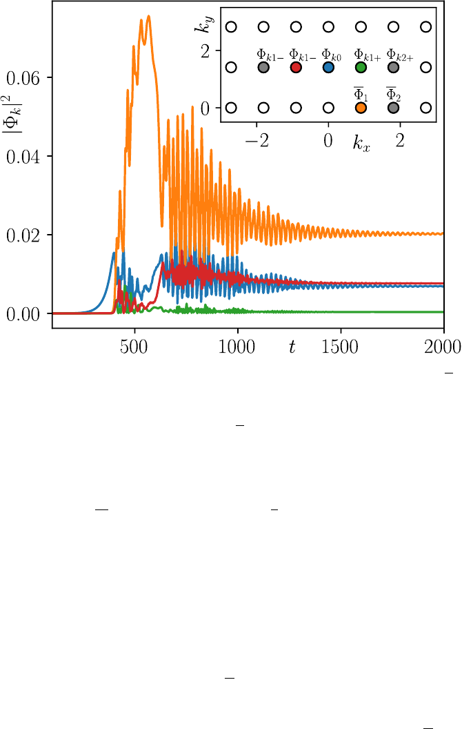
Figure 1 The dynamics and the network structure for the modulational instability exam-

ple. The most unstable mode (i.e. Φ

) acts as a pump, exciting the zonal mode (i.e. Φ

)

and the sidebands (i.e. Φ

k1±

). The nodes are shown in a reduced k

-k

grid on the top

right plot, which also acts as a legend for the main plot. The outer modes that are shown

in grey circles are artiﬁcially damped, hence play the role of sink. In the ﬁnal steady state,

without any large scale friction, the energy in Φ

, causes the interaction to eﬀectively turn

oﬀ. Introduction of large scale friction would result in predator-prey like oscillations.

∂

∂t

(1 + χ

) Φ

= −iκk

△

kpq

∗

(1)

where Φ

is the normalized electrostatic potential, χ

≡ k

− iδ

, where δ

is deﬁned through the relationship between the electron density and the elec-

trostatic potential n

= (1 − iδ

) Φ

, κ is the normalized diamagnetic velocity

and M

kpq

is the nonlinear interaction coeﬃcient whose form is not important

for this example (see Section 6 for more details on deﬁnitions and normaliza-

tions). In order to study modulational instability it is common to consider a

subset of modes, such as:

= Φ

ℓ



ℓ

+ Φ

kℓ+

+ Φ

kℓ−



(2)

where Φ

is the most unstable mode (withk

= k

and k

= 0), Φ

ℓ

are

the zonal modes (with k

= k

xℓ

and k

= 0) and Φ

kℓ±

are the sidebands

Springer Nature 2021 L

X template

Wave-number Space Networks in Plasma Turbulence 7

(with k

= k

and k

= ±k

xℓ

) labeled by ℓ considering multiple radial wave-

numbers. In general we have 3n + 1 modes where n is the number of k

modes

considered. We can of course also add other k

modes, but having only a single

mode is suﬃcient for studying modulational instability. Note that for each

mode k = k

ℓ

, its Hermitian conjugate k = −k

ℓ

should also be considered.

In order to have a stationary solution, we at least need to go to n = 2,

and choose the k

and k

to correspond to the most unstable modes of the

modulational instability and the linear instability respectively, and introduce

artiﬁcial damping on the equations for Φ

k±2

and Φ

. Such a system in the

absence of zonal ﬂow damping (that is damping of the Φ

, which is the primary

modulationally unstable zonal component), evolves to a state of ﬁnite zonal

ﬂows and stays at that ﬁnal state with stationary zonal ﬂows. Figure 1 shows

the results of the numerical integration of the low order dynamical system that

one gets from such a system (actually we have used the full Hasegawa-Wakatani

system with C = 10, κ = 1, see Section 6 for details).

2 Primitive Wave-number Space Networks

2.1 Basic Formulation

Consider a complex ﬁeld ψ

, which represents the Fourier transform of a real

one through ψ

≡

ψ (x) e

ik·x

x in a bounded domain L, for which we

can write:

∂

+ iω

△

kpq

∗

(3)

where ω

is the complex frequency, whose imaginary part may represent the

instability -or dissipation in small scales- and M

kp q

is the symmetrized non-

linear interaction coeﬃcient. This template form may represent a number of

diﬀerent single ﬁeld systems, such as for instance the Charney-Hasegawa-Mima

system with ω

∗

1+k

and M

kpq

≡

z×p·q

(

−p

)

(1+k

)

where v

∗

is the normalized

background density gradient, L

and L

are the box dimensions.

The wave-number on a two dimensional regular square grid can be de-

ﬁned using two integer indices ℓ

and ℓ

as k

= 2π (ℓ

− N

/2) /L

and

= 2π (ℓ

− N

/2) /L

, where L

x,y

is the size of the domain and N

x,y

are

the number of grid elements in each direction. We can ﬂatten the two index

variables into a single integer using for example the column major order lin-

ear storage formula ℓ = ℓ

+ ℓ

and use this as the node index. Note that

in the general case of n dimensions we can deﬁne the ﬂattened node index via

the usual ℓ = ℓ

i=2

ℓ

i−1

j=1

. This allows us to deﬁne the node wave-

number k

ℓ

≡

(ℓ

) +

(ℓ

) as a vector and node variable ψ

ℓ

≡ ψ

ℓ

as a

complex number denoted by the node label ℓ. This way, the whole regular grid

of the n-dimensional wave-number domain can be thought of as a collection of

N =

j=1

wave-number nodes.

Springer Nature 2021 L

X template

8 Wave-number Space Networks in Plasma Turbulence

We can thus write (3) as a dynamical equation for ψ

ℓ

on a three body

network:



∂

∂t

+ iω

ℓ



ℓ

′

,ℓ

′′

∈i

ℓ

ℓℓ

′

ℓ

′′

∗

ℓ

′

∗

ℓ

′′

(4)

where i

ℓ

denote the list of pairs that interact with the node ℓ. The list of pairs

ℓ

needs to be computed by going over all the nodes that satisfy the triad

interaction condition k

ℓ

+ k

ℓ

′

+ k

ℓ

′′

= 0. Written in this way, the equation (4)

is exactly the same as the Eqn. (3) on a regular k-space grid. However, the

former can be extended to irregular grids, or to a decimated Fourier space

and can be more easily modiﬁed to incorporate the dynamics of an equivalent

variable on a reduced network. Note also that the formulation of Eqn. (4) can

also be extended to windowed Fourier transforms, or wavelet coeﬃcients, or

any other similar decomposition such as the Galerkin decomposition, except

that in that case ω

ℓ

would be replaced by a non-diagonal matrix, representing

an operator and constructing the interaction network (that is i

ℓ

as connections

and M

ℓℓ

′

ℓ

′′

as weights) may be nontrivial.

In practice, the formulation in (4) using a regular grid can be implemented

in two steps. First, for each ℓ we ﬁnd all possible ℓ

′

, ℓ

′′

pairs that satisfy the

triad interaction condition k

ℓ

+ k

ℓ

′

+ k

ℓ

′′

= 0 and compute and record the

interaction coeﬃcients M

ℓℓ

′

ℓ

′′

. This constitutes our “network”, in that it is a

list of all three body connections between all the nodes of the network with

particular weights for each connection in the form of interaction coeﬃcients.

Once the network is constructed, it can be stored and the complex dynamical

variables ψ

ℓ

, corresponding to Fourier coeﬃcients can be advanced on this

network using (4).

Searching for all possible pairs that satisfy the triadic interaction condition

is time consuming, but it can be ameliorated by scanning ℓ and ℓ

′

while using

ℓ

± k

ℓ

′

± k

ℓ

′′

= 0 to solve for ℓ

′′

, keeping only k

ℓ

′

< k

ℓ

′′

part of the k-space

consisting of only k

≥ 0 modes (since the initial data is real). Notice that

one can also impose additional resonance conditions in this step in order to

implement weak wave-turbulence as a sparse network on a discrete regular

grid[60, 61].

On a properly constructed regular grid, (4) and (3) are mathematically

equivalent. This means that a numerical implementation of (4) as described

above, and say a pseudo-spectral implementation of (3) with the same forcing,

dissipation and initial and boundary conditions, should give exactly the same

evolution up to numerical precision. This can be veriﬁed, for example on a reg-

ular grid of resolution N

×N

= 256×256, beyond which the network method

starts to be impractical. This implies N

ℓ

= (N

/2) × (N

/2) + (N

/2 − 1) ×

/2 − 1) independent nodes, since in a real-to-complex transform, we have

/2 + 1 independent wave-numbers in the y direction, with the last one be-

ing the Nyquist wave-number and Φ

= Φ

∗

−k

on the k

= 0 axis due to

Hermitian symmetry. In such a network, the node that has the most connec-

tions is the smallest wave-number node that has N

= (N

− 2) × (N

− 2)/2

connections (i.e. triads that are connected to that node). Note also that for

Springer Nature 2021 L

X template

Wave-number Space Networks in Plasma Turbulence 9

standard 2D turbulence ℓ = 0 is unconnected since |k

ℓ

′

| = |k

ℓ

′′

| makes the in-

teraction coeﬃcient vanish. Since M

ℓℓ

′

ℓ

′′

= M

ℓℓ

′′

ℓ

′

, by choosing ℓ

′

> ℓ

′′

, and

dropping the 1/2 in (4), we can reduce the maximum number of triads to

= (N

− 2) ×(N

− 2) /4.

Network formulation on a regular rectangular grid is extremely impractical

for any kind of meaningful resolution since its computational cost for a causal

formulation scales with N

ℓ

, which would scale with N

(i.e. N

= N

N ) for three dimensions, and there exists many eﬃcient techniques for dealing

with turbulence on a regular grid. However since the same approach can be

used on a sparse network obtained from reduction such as the nested polyhedra

models that we will see in Section 3.1, which can describe a very large range

of scales using a relatively small number of nodes even in three dimensions,

they can be extremely powerful for computations as well. We argue that the

eﬀort of writing down the network formulation on a regular rectangular grid is

nonetheless useful for establishing the connection to standard techniques, and

to provide a basis on which we can apply network reduction. For example, if we

know how to go from a regular rectangular grid to a particular reduced network

form, we can apply the same reduction to the data from direct numerical

simulations (DNS) that are usually on a rectangular grid (see section 6 for

some examples).

2.2 Conservation laws

If the nonlinear interaction coeﬃcients in Eqn (4) have the symmetry

ℓ

ℓℓ

′

ℓ

′′

+ σ

ℓ

′

ℓ

′

ℓ

′′

ℓ

+ σ

ℓ

′′

ℓ

′′

ℓℓ

′

= 0 (5)

where σ

ℓ

is a coeﬃcient that is a function of the node label ℓ, (i.e. a function

of the wave-number), the quadratic quantity deﬁned as:

total

≡

ℓ

|ψ

ℓ

can be shown to be conserved by the nonlinear dynamics, since

∂

ℓ

′

,ℓ

′′

∈i

ℓ

ℓℓ

′

ℓ

′′

+ P

ℓ

− D

ℓ

(6)

where P

ℓ

is the production and D

ℓ

is the dissipation of the conserved quantity

labeled by σ at the site of node ℓ. If we use Eqn. (4), we get:

ℓ

− D

ℓ

= 2γ

ℓ

since both energy injection at instability scales and the dissipation at small

scales come from the form of the “linear growth rate” [i.e. γ

ℓ

= Im (ω

ℓ

)] as a

function of k

ℓ

which actually becomes negative as we go to small scales due to

Springer Nature 2021 L

X template

10 Wave-number Space Networks in Plasma Turbulence

123

134

Figure 2 The energy transfers in a network of triadic interactions between nodes 1 − 4,

connected by two triads 123 and 134. The triad interactions are show in the form of little

triangles, the transfer terms such as t

123

denote the energy transfer from node 1 to node 2

through the triad 123, which can also be denoted by t

. The total energy transfer between

two nodes is the sum of the transfers through each triad, as shown for the case of two triads

here with t

≡ t

134

− t

123

dissipation. The transfer rate T

ℓℓ

′

ℓ

′′

in Eqn. (6) represents the energy transfer

from the nodes ℓ

′

and ℓ

′′

to the node ℓ, which can be deﬁned explicitly as

ℓℓ

′

ℓ

′′

≡ Re [σ

ℓ

ℓℓ

′

ℓ

′′

ℓ

′

ℓ

′′

] .

Since the interactions always appear as three body interactions, we have

ℓℓ

′

ℓ

′′

+ T

ℓ

′

ℓ

′′

ℓ

+ T

ℓ

′′

ℓℓ

′

= 0 as implied by Eqn. (5). When we sum the Eqn. (6)

over all nodes, we ﬁnd that the total amount of conserved quantity (e.g. en-

ergy) increases or decreases only as a result of the diﬀerence between its total

injection and its total dissipation.

Dropping the label σ for convenience (e.g. considering energy), we can also

write

∂

ℓ

′

,ℓ

′′

ℓ

′′

ℓℓ

′

+ P

ℓ

− D

ℓ

(7)

where t

ℓ

′′

ℓℓ

′

ℓℓ

′

ℓ

′′

− T

ℓ

′

ℓ

′′

ℓ

) represents the energy transfer from ℓ

′

to ℓ

mediated by ℓ

′′

. Note that for a given triad, with the node labels 1 , 2 and 3,

we have T

123

= t

−t

, meaning that the energy transferred from

the nodes 3 and 2 to node 1 is the diﬀerence of the energy transferred from 2

to 1 mediated by 3 and the energy transferred from 1 to 3 mediated by 2. (see

ﬁgure 2) This allows us to transform the three body interaction network to a

simple network with edges that are weighted by the other components of the

triad, with multiple channels between the nodes.

Springer Nature 2021 L

X template

Wave-number Space Networks in Plasma Turbulence 11

We may further reduce the many connections between two nodes mediated

by diﬀerent third nodes, by summing over the third node as:

∂

ℓ

′

ℓℓ

′

+ P

ℓ

− D

ℓ

(8)

where t

ℓℓ

′

≡

ℓ

′′

ℓ

′′

ℓℓ

′

. In ﬁgure 2 this corresponds to writing t

= t

+ t

−t

= t

134

−t

123

. The two connections in this example, t

134

and t

123

, are

part of two separate triad interactions, and therefore has two diﬀerent phases

(see below). Summing over all these diﬀerent connections belonging to diﬀerent

triad interactions, having diﬀerent phases, allows us to transform the system

from a multigraph (a graph which has multiple edges between two nodes) to a

simple graph (a graph with only one edge between two nodes) is an important

reduction of the network topology. However it results in loss of information

since once we sum multiple edges between two nodes into a single edge, there

is no way to get back the diﬀerent edges that make up that single combined

edge. We also loose detailed information about the three-way relative phases

that determine the direction of the ﬂux through a given triad, since we sum

over many triads in order to obtain the transfer between two nodes mediated

by all possible third nodes.

2.3 Triadic Instability Assumption and Phase dynamics

While the necessary condition for the existence of a link between the nodes in a

three body spectral network, representing turbulent mode coupling, is the triad

interaction condition between the wave vectors, this link accommodating an

actual transfer of energy between the nodes requires additional circumstances.

Given three nodes and a triad, one may usually estimate the direction of

energy transfer, through an analysis called the “instability assumption”[62, 63].

In the fusion context it would probably make more sense to call this “triadic

instability assumption”, since instability in that context rather refers to the

linear instability of the underlying system. In any case, the triadic instability

condition suggests that, if we start with an initial state such that ψ

ℓ

∼ O (1)

but ψ

ℓ

′

∼ ψ

ℓ

′′

∼ O (ϵ), a linear stability analysis for the perturbations ψ

ℓ

′

and

ℓ

′′

gives an instability condition:

ℓ

′

ℓ

′′

ℓ

′′

ℓℓ

′

> 0 (9)

which results in the growth of ψ

ℓ

′

and ψ

ℓ

′′

resulting in a transfer of energy.

The growth can then be argued to continue until some kind of equipartition

between the three nodes ℓ, ℓ

′

and ℓ

′′

. For example for incompressible two

dimensional turbulence the interactions coeﬃcients are M

kpq

z×p·q

(

−p

)

[i.e. with ℓ, ℓ

′

, ℓ

′′

→ k, p, q] so that the instability condition M

pqk

qkp

> 0

implies



− q



− k



> 0, which is satisﬁed only if k is the middle wave-

number. This is a consequence of the intermediate axis theorem for rigid body

rotation and the equivalence of these two systems. More generally, the triadic

Springer Nature 2021 L

X template

12 Wave-number Space Networks in Plasma Turbulence

instability assumption means that the transfer is from the node ℓ which has

the interaction coeﬃcient M

ℓℓ

′

ℓ

′′

that has the opposite sign to the other two

ℓ

′

ℓ

′′

ℓ

and M

ℓ

′′

ℓℓ

′

, which has the same sign because of Eqn. (9) resulting in

ℓℓ

′

ℓ

′′

< 0 while T

ℓ

′

ℓ

′′

ℓ

> 0 and T

ℓ

′′

ℓℓ

′

> 0. This works even in the presence

of linear growth and damping as long as the pump mode keeps increasing in

amplitude, at some point the nonlinear transfer mechanism will kick in. Note

that while the actual three wave system without any linear instability can

be solved exactly using Jacobi elliptic functions[64], the implications of these

solutions to the triadic instability assumption, where we only consider the

initial trends, which gives us an idea about the direction of the trasfers, until

we reach a stationary state either through statistical equipartition, or through

the non-equilibrium steady state between production and dissipation through

the nonlinear cascade processes.

However as it invokes statistical steady states such as the equipartition,

the analysis is usually based on the assumption that the phases are random

in a turbulent ﬁeld. This is reasonable as long as the phases of the legs of the

triad that we are considering are not involved in some complicated conspiracy,

like for example all three nodes of the triad staying in a phase-locked state for

an extended period of time. For a system with internal free energy sources as

it is usually the case for plasma turbulence, linear frequencies can provide the

dominant term in the phase evolution of a given wave-number node. It may

be that these frequencies, possibly modiﬁed by nonlinear eﬀects such as the

Doppler shift from large scale ﬂows etc., reorganize themselves locally in order

to induce these phase-coherent states, which is in stark contrast to the case of

random phase.

Substituting ψ

ℓ

= A

ℓ

iϕ

ℓ

in (4) and assuming M

ℓℓ

′

ℓ

′′

∈ R for simplicity, we

get:

∂

ℓ

= γ

ℓ

′

,ℓ

′′

∈i

ℓ

ℓℓ

′

ℓ

′′

ℓ

′

ℓ

′′

cos (ϕ

ℓ

+ ϕ

ℓ

′

+ ϕ

ℓ

′′

) (10)

∂

ℓ

= −ω

rℓ

−

ℓ

′

,ℓ

′′

∈i

ℓ

ℓℓ

′

ℓ

′′

ℓ

′

ℓ

′′

ℓ

sin (ϕ

ℓ

+ ϕ

ℓ

′

+ ϕ

ℓ

′′

) (11)

Note that for the more general case of complex M

ℓℓ

′

ℓ

′′

the argument of the

sine and cosine in Eqn.(10-11) would be replaced by



ℓℓ

′

ℓ

′′

+ ϕ

ℓ

+ ϕ

ℓ

′

+ ϕ

ℓ

′′



where ϕ

ℓℓ

′

ℓ

′′

= arg (M

ℓℓ

′

ℓ

′′

). The complete problem of plasma turbulence,

that we call the “primitive network”, that we usually solve in direct numerical

simulations involves Eqn. (4) or equivalently the Eqns. (11) and (10) or (6) on

a network constructed from a regular rectangular grid of wave-number nodes

in Fourier space.

However the point of the network formulation is reduction, and there are

many diﬀerent ways one can reduce such a system depending on what the dom-

inant processes are and what one wants to describe. For example a blunt way

to do reduction is to directly truncate the Fourier space, so that we have a re-

duced system, that is somehow supposed to represent the full system. If such a

reduction is done using the original equations (i.e. Eqn. 4), it can typically give

Springer Nature 2021 L

X template

Wave-number Space Networks in Plasma Turbulence 13

us a sense of what the coupled system does qualitatively, but unless the trun-

cation is done respecting the statistical characteristics of the initial network, it

would modify things like energy equipartition solutions etc. In the same vein,

we can keep the nodes but reduce the links, which corresponds to keeping the

full regular rectangular grid in Fourier space, but only considering a certain

class of interactions (e.g. certain kinds of triads). Self-consistent quasi-linear

theory, commonly used in fusion and geophysical ﬂuid dynamics applications

where one keeps interactions with large scales (zonal ﬂows, and proﬁles) but

drops the interactions among small-scale ﬂuctuations can be considered as an

example of this.

A diﬀerent way to reduce the initial primitive network may be to use a

closure scheme, which would allow us to lump diﬀerent nodes and links to-

gether in groups instead of using truncation or dropping links. Such a lumping

together of the nodes requires a closure that can represent multiple triadic in-

teractions as a single triadic (or two-body) interaction, which in turn requires

handling the statistics of phase relations. We can do this, for example by in-

voking the random phase approximation, which would allow us to use direct

interaction approximation (DIA)[65, 66] or the eddy damped quasi-normal

Markovian approximation (EDQNM)[67, 30], thus resulting in a reduced sys-

tem (say EDQNM equations) on a reduced network when we sum over groups

of nodes.

Another interesting case arises, when the dynamics is dominated by inter-

acting linear waves. In this limit, the resonant interactions between the linear

frequencies ω

ℓ

result in a phase-locked state, which provides a natural closure

for the system of equations. It would also provide a natural reduction of the

network, since only those modes that also satisfy the resonant interaction con-

dition, i.e. ω

ℓ

± ω

ℓ

′

± ω

ℓ

′′

= 0 are necessary and we can drop the others. It

can also be argued, without actually invoking wave-turbulence closure, that

the justiﬁcation for using quasi-linear models in fusion plasmas is in fact the

idea that the system lacks obvious three-wave-resonances without large scale

ﬂows, which can be zonal ﬂows, Geodesic acoustic modes (GAMs), or other

large scale structures, so that the resonant interactions always have to involve

one of these ﬂow structures[68].

2.4 Wave turbulence

Practicality of the network formulation rely on a suitable reduction of either

the nodes or the interactions of its underlying wave-number space network.

In this sense wave-turbulence provides a compelling scenario, since it allows

one to consider only a very small subset of all possible interactions due to the

resonance condition. While, wave turbulence, which describes the evolution of

an ensemble of weakly interacting waves[35, 69], obeying a linear dispersion

relation, is strictly applicable only in the asymptotic limit with linearly stable

waves, at the limit of inﬁnite box size, it still presents a very powerful tool

for understanding the role the resonant or quasi-resonant interactions play in

the turbulent cascade. It can describe multiple statistical quantities using only

Springer Nature 2021 L

X template

14 Wave-number Space Networks in Plasma Turbulence

a conserved quantity called the wave-quanta, commonly denoted by N

≡

/ω

where E

is the energy, which is equivalent to potential enstrophy

in the Charney-Hasegawa-Mima case with proper zonal ﬂow response [apart

from a factor of 1/|k

|, which depends on the zonal ﬂow response]. Network

formulation in the case of wave-turbulence is of great interest, and has been

studied in some detail in the past, as one can obviously decouple the geometric

study of the resonant manifold and the evolution of the wave-quanta on the

said manifold resulting in a major conceptual simpliﬁcation.

Being an asymptotic theory, it is common to make the assumption of in-

ﬁnite size in the study of wave-turbulence, which also sidesteps the issue of

whether or not the discrete modes that are available in a ﬁnite system actu-

ally satisfy the resonance condition, since in that limit one has a continuous

k-space, hence an inﬁnite number of nearly-resonant modes[69]. The usual

wave-kinetic equation for the Charney-Hasegawa-Mima system can be written

following Connaughton [70] as:

∂n

∂t

= S [n

] + f

− γ

(12)

where the collision integral has the form:

S [n

] = 4π

kpq



− σ



× δ

(k − p −q) δ (ω

− ω

) d

q (13)

and σ denote the sign of its subscript, and the W

kpq

denote the nonlinear

interaction coeﬃcient in the wave interaction representation:

kpq

= −

z × p ·q



− q



(1 + p

) (1 + q

)

Some interesting observations for the Charney-Hasegawa-Mima system came

out of the study of the wave-kinetic equation, such as the identiﬁcation of an

additional conservation law dubbed zonostrophy[71, 70]:

≡ arctan



√



− arctan



−

√



−

√

(1 + k

)

In the study of fusion plasmas, on the other hand, it is more common to use

what is sometimes called weak-turbulence-theory (WTT), which is essentially

the same thing as it involves the same underlying assumptions, except that

one keeps the linear instability term, and the resulting kinetic equation is seen

as a Markovian statistical closure in the same vein as the EDQNM. We can

write the general form of the WTT equations somewhat symbolically as [30]:

∂

− 2γ

lin

+ 2Reη

= 2F

(14)

Springer Nature 2021 L

X template

Wave-number Space Networks in Plasma Turbulence 15

where C

≡



|Φ



≈ −

△

kpq

∗

pkq

∗

kpq

(t) C

, (15)

and

≈

△

kpq

Re [θ

kpq

(t)] C

(16)

with

kpq

(t) ≡ πδ (ω

− ω

) .

Note that the ﬁrst term in (13) corresponds to the incoherent term, given in

WTT by (16), and the last two term in (13) can be combined, by exchanging

p and q in one of the terms into the coherent term given in (15) [i.e. when

multiplied by n

as it appears in (14)]. Multiplying C

by σ

we can write

the equation for a conserved quantity E

≡ C

. The advantage of this

formulation is that we can use it on a reduced network, exactly same way as

we would use any other closure. An example for the EDQNM closure on a

reduced network can be found in Section 4.2.

Wave turbulence on a discrete wave-number space network is also some-

times studied using the original equations (for example the Charney-Hasegawa-

Mima system) directly on a wave-number space network consisting of clusters

of triads[36, 70]. In this case, using the wave interaction representation ap-

pears to be a mere convenience since the equations are the same. However since

the resonance conditions, even including resonance broadening[72], makes the

topology of the k-space network, very sparse since the large majority of in-

teractions are eﬀaced as a result of the resonance condition. This leads to the

creation of clusters of connected triads, that may be isolated or weakly con-

nected to one another, resulting in the blocking of the k-space cascade. Unlike

strong turbulence case, each wavenumber node in a wave-number space net-

work of wave-turbulence is involved in only a few (if any) triads. This is a

manifestation of the fact that the resonance condition, for example written for

the Charney-Hasegawa-Mima case as:

+ q

1 + p

+ q

+ 2p ·q

−

(1 + p

)

−

(1 + q

)

= 0

deﬁnes a curve for a given q = k

ℓ

, and only the points p = k

ℓ

′

that lie both

on the discrete k-space grid and on the resonance manifold gets connected

to this node. This makes it possible and somewhat practical to consider the

wave-turbulence as a network of “triads” that are connected by nodes, in an

inverted perspective to the point of view generally advocated in this review.

A key observation in this case is that since unconnected clusters will inde-

pendently conserve the quadratically conserved quantities, one has as many

conserved quantities as the number of clusters × the number of nonlinearly

conserved quantities if the system was fully connected[36]. This makes the

Springer Nature 2021 L

X template

16 Wave-number Space Networks in Plasma Turbulence

wave-turbulence cascade dependent on the topology of the network, getting

blocked if the clusters remain unconnected, and with an explicit percolation

phenomenon as the number of triads are increased[73].

The case of inhomogeneous wave-kinetics [74, 50] is also of particular inter-

est, especially in the context of self-consistent drift-wave/zonal ﬂow evolution,

with radial propagation as well as scattering in wave-number due to the eﬀects

of zonal ﬂows. The wave-kinetic system that results is isomorphic to the Vlasov

Equation, with wave quanta playing the role of the distribution function:

∂

∂t

∂ω

∂k

∂N

∂x

−

∂ω

∂x

∂N

∂k

= C (N, N) + F

where ω = ω

− u

(x) k

is the basic drift wave frequency Doppler shifted

by the zonal ﬂow u

(x), C (N, N) represents a collision integral describing

mode coupling similar to (13) and F

is the forcing and dissipation which can

be provided by a linear instability as well as external forcing and small scale

dissipation. The inhomogeneous wave-kinetic equation has proved extremely

useful in the study of transport and turbulence in fusion plasmas, being ap-

plied in various problems ranging from momentum transport[75] to turbulence

spreading[76]. Network formulation of the general class of kinetic systems, of

which the wave-kinetics is a member is discussed in the next section.

2.5 Formulation of Kinetic Theory

Going back to regular plasma or ﬂuid turbulence, the form of Eqn. (4) given in

Section 2.1 is really strictly valid only for a single ﬁeld system. Many plasma

problems even when reduced ﬂuid equations are used, involve multiple ﬁelds.

In this more general case, the diﬀerent ﬁelds at a given node are likely to be

coupled linearly, allowing also for the possibility of linear interactions between

nodes (e.g. toroidal mode coupling in tokamak plasmas), we can write the more

general network equation as:

∂

ℓ

′

αβ

ℓℓ

′

ℓ

′

ℓ

′

,ℓ

′′

∈i

ℓ

αβγ

ℓℓ

′

ℓ

′′

β∗

ℓ

′

γ∗

ℓ

′′

= 0 (17)

where L

αβ

ℓℓ

′

is an arbitrary linear matrix, i

ℓ

is the interaction network and M

αβγ

ℓℓ

′

ℓ

′′

are the nonlinear interaction coeﬃcients. In the usual spectral formulation

αβ

ℓℓ

′

= L

αβ

ℓ

ℓℓ

′

, and one can in general deﬁne a set of alternative variables say

ℓ

that diagonalizes the Greek indices in order to write the problem in terms

its eigenmodes, in that particular case we can write

(∂

+ iω

ℓ

) χ

ℓ

′

,ℓ

′′

∈i

ℓ

αβγ

ℓℓ

′

ℓ

′′

β∗

ℓ

′

γ∗

ℓ

′′

= 0

of course with a diﬀerent M that describes the interactions between the

eigenmodes, which can be computed using standard rules of linear algebra.

Springer Nature 2021 L

X template

Wave-number Space Networks in Plasma Turbulence 17

A ﬂuid system with a ﬁnite number of moments is in fact a closure of

the full kinetic system, so in general a distribution function, can be written

as a combination of a number of suitable functional forms. For instance it is

common to describe the distribution function of the Vlasov equation using

Hermite polynomials[77, 78] as in

f (x, v, t) =

ℓ,α

ℓ

(t) H

(v) e

ℓ

x−v

(18)

where N

is a normalization factor, H

is the Hermite polynomial of (in-

teger) order α, with hopefully only a ﬁnite number of Hermite polynomials

being suﬃcient to describe its evolution. When used in conjunction with Eqn.

(18) the network equation of (17) describes the interactions between wave-

number nodes that satisfy the triadic interaction conditions, where each node

has a number of complex variables (indicated by the Greek indices) represent-

ing the coeﬃcients of Hermite polynomials, which correspond to consecutive

derivatives of Maxwellians.

In the same spirit, one can use a combination of Fourier-Bessel-Hermite

[79, 80] (or Fourier-Laguerre-Hermite [81] ) expansion which handles, spatial,

perpendicular and parallel velocity directions respectively:



x, v

∥

, v

⊥

, t



ℓ,m,α

ℓm

(t) J

(κ

⊥

) H



∥



ℓ

·x−v

∥

(19)

At this point we can either ﬂatten the indices α and m as before so that we

are left with a single index ℓ which represents the generalized wave-number

in x, v space so that some version of Eqn. (4) can be used, or keep the form

of Eqn. (19) in order to write the wave-number space network equation in its

general form as:

∂

ℓm

ℓ

′

αβ

ℓℓ

′

ℓ

′

ℓ

′

; ℓ

′′

∈i

ℓ

αβγ

ℓℓ

′

ℓ

′′

; mm

′

′′

β∗

ℓ

′

γ∗

ℓ

′′

= 0

note that in gyrokinetics v

⊥

appears as a label in the linear term (so no

coupling between m’s), and the coupling condition for the triadic interactions

can be written as k

+ k

′

+ k

′′

= 0 where κ

≡ |k

| for v

⊥

space as well.

Even though the condition for interaction in m is actually the same for that

in ℓ , because of the details of the way the system may be discretized in these

diﬀerent variables makes the actual computation of the interaction network

topology rather complicated. There are actually many diﬀerent alternatives

to the above approach and the usual velocity space formulation with ﬁnite

diﬀerence discretization can also be formulated as a complicated interaction

Springer Nature 2021 L

X template

18 Wave-number Space Networks in Plasma Turbulence

matrix, however since our focus is wave-number space networks, we pick a

spectral formulation also in the velocity space variable as the natural choice.

Note ﬁnally, that energy conservation for Eqn. (17) can still be written

using Eqn. (6), with:

ℓ

≡ ξ

ℓ

αβ

ℓ

∗β

ℓ

ℓℓ

′

ℓ

′′

≡ 2Re

βλµ

ℓℓ

′

ℓ

′′

αβ

ℓ



∗α

ℓ

∗λ

ℓ

′

∗µ

ℓ

′′



ℓ

≡ −

ℓ

′

2Re



αλ

ℓℓ

′

αβ

ℓ

′

∗β

ℓ



so that we can write:

ℓ

(

ℓ

if F

ℓ

> 0

0 if F

ℓ

> 0

and D

ℓ

(

0 if F

ℓ

> 0

−F

ℓ

if F

ℓ

> 0

where σ

αβ

ℓ

= σ

βα

ℓ

deﬁnes the conserved quantity.

2.6 Magnetic Shear and Rational Surfaces

Strictly speaking, the examples that are given up to this point were written

in Cartesian coordinates, and are therefore valid only in slab geometry. While

one can easily transform everything to arbitrary curvilinear geometry, for ex-

ample where one of the directions is aligned with the magnetic ﬁeld as the

natural geometry in magnetic fusion devices[82], the actual details of using

such coordinates is in fact non-trivial. This is partly due to the way some lin-

ear eﬀects work in fusion plasmas, naturally allows an important reduction of

the number of degrees of freedom. Among these eﬀects, that of the magnetic

shear stands out.

In order to understand the eﬀect of magnetic shear, ﬁrst consider the case of

a sheared magnetic ﬁeld in slab geometry with B = B

z +

. The parallel

wave-number is then deﬁned as k

∥

= k

x/L

, and is therefore a function

of the spatial variable x. We know that the Landau damping kills oﬀ any

ﬂuctuation with k

∥

> ω, resulting in a reduction of the amplitude for any

Fourier mode with k

∥

> ω/v

. This results in the amplitude of the ﬂuctuations

being localized to the region between the two Landau turning points x

±|

ωL

|. Of course a proper eigenmode analysis may incorporate various other

eﬀects, including the eﬀect of an external, or self-generated ﬂow shear, and thus

give a more complete picture, but the basic concept of the localization of the

drift-wave eigenmode due to Landau damping of higher k’s is rather generic.

A sheared slab, can model the geometry of the magnetic ﬁeld as a local

approximation. For example, choosing the poloidal ﬂux ψ as a radial variable,

θ as a poloidal variable with a period 2π, and ζ as the toroidal variable, we

can construct a generic toroidal coordinate system. Perturbations in such a

Springer Nature 2021 L

X template

Wave-number Space Networks in Plasma Turbulence 19

system can be written in the general form as:

Φ (ψ, θ, ζ) =

n,m

(ψ) e

i(nζ−mθ)

. (20)

Since the magnetic ﬁeld is a function of ψ and has the form of a helix wrapped

around a torus, it is customary to deﬁne the toroidal winding number q (ψ) ≡

dζ

dθ

, which is the ratio of the number of times the magnetic ﬁeld turns around

the toroidal direction to the number of turns it makes in the poloidal direction,

as “the safety factor” because of its importance in magnetic stability. For an

axisymmetric tokamak with circular ﬂux surfaces, this takes the familiar form

q =

, where r and R are the minor and major radius variables. One

can also deﬁne the eﬀect of magnetic shear using the dimensionless parameter

ˆs ≡ rq

′

/q. More generally, the rate of change of the safety factor as a function

of the poloidal ﬂux ψ determines the strength of the shear in the magnetic

ﬁeld in the ψ direction. If we use a coordinates system that aligns itself to

the magnetic ﬁeld locally (like the so-called Clebsch coordinates described in

some detail in Ref. 82), the eﬀect enters through the non-diagonal terms in

the metric tensor. However, at least in tokamaks, it is more customary to use

toroidal coordinate ϕ as the direction of axisymmetry.

Since the magnetic ﬁeld is sheared, each ﬂux surface ψ has a diﬀerent pitch

angle. The perturbations tend to be aligned to the ﬁeld line (i.e. have k

∥

≈ 0)

as we discussed above. However since they are also periodic in θ and ζ, this

can happen exactly, only when the perturbation is centered at what is called a

“rational surface”, where q (ψ) = m/n. This allows a perturbation of the form

(20) to align itself to the magnetic ﬁeld:

Φ (ψ, θ, ζ) =

(ψ) e

in(ζ−qθ)

(21)

and because of Landau damping, the perturbation with n and m such that

q (ψ) = m/n will be localized to its rational surface ψ = ψ

deﬁned by this

relation.

The fact that plasma “turbulence” in tokamaks consists of modes localized

to their rational surfaces, has important implications for their network for-

mulation. In this picture, the usual mode coupling through triads is largely

restricted by the additional constraint that the interacting modes must have

spatial overlap. So while the standard two dimensional turbulence presents a

very densely coupled network of interactions, the quasi-two-dimensional tur-

bulence (since k

∥

≈ 0) of tokamaks have a sparser interaction topology. This is

true even when one includes a large number of toroidal and poloidal modes, so

that rational surfaces are densely packed (i.e. each rational surface has many

nearby neighbors).

Note that the nonlinear term of the underlying ﬂuid equations due to ad-

vection by the E × B velocity, represented by the Poisson bracket, can be

written in the coordinate system consisting of ψ and α [so that B = ∇ψ ×∇α

Springer Nature 2021 L

X template

20 Wave-number Space Networks in Plasma Turbulence

say with α = ζ − q (ψ) θ] as:

[Φ, Ω] =

b × ∇Φ ·∇Ω = B



∂Φ

∂ψ

∂Ω

∂α

−

∂Φ

∂α

∂Ω

∂ψ



2.6.1 Ballooning representation

When a perturbation of the form (20) is considered for a given n but for

diﬀerent values of m in toroidal geometry with a standard (e.g. increasing)

proﬁle of q, the e

imθ

factors from consecutive rational surfaces superpose in

such a way that while at θ = 0 they add up, at θ = π they cancel. This

causes an envelope-like dependence in θ direction with a maximum at θ = 0

direction, or the low ﬁeld side of the tokamak (also called the bad curvature

side). This envelope structure, which makes the modes expanded towards the

low ﬁeld side is called the “ballooning” structure. Details of the functional form

of ballooning depends on the functional form of the localization of the Fourier

modes around their rational surfaces. Since this ballooning structure suggests

a slow variation of the envelope of the amplitude in θ variable [i.e. f (θ) e

inqθ

where the dependence of f (θ) on θ is “slow”], we are tempted to use an eikonal

approximation. However the fact that the θ variable is periodic, complicates

the issue.

In order to see this consider a Gaussian centered at θ = 0 as the ballooning

function f (θ). For a periodic θ, we can not write this simply as f (θ) = e

−θ

/2σ

as it would have a discontinuity at θ = 0. Instead a basic ﬁrst order form

f (θ) = e

−

2σ

+ e

−

(θ−2π)

2σ

could be used (makes sense especially for σ ≪ 2π), in order to remove the

jump at θ = 0. However going back to (21), in order to avoid a jump in Φ, the

phase should also be continuous across the cut at θ = 0 (or θ = 2π), and thus

the actual form can be obtained by replacing θ → θ − 2π in f (θ) e

inqθ

and

adding this to itself. In other words the ballooning function that removes the

discontinuity at θ = 0 can be written as:

f (θ) = e

−

2σ

+ e

−

(θ−2π)

2σ

−i2πnq(r)

Note that this particular example extends the range of θ from [0, 2π) to

[0, 4π) or equivalently (−2π, 2π]. If the ballooning function has a larger sup-

port, we need to extend the range of θ until the support is fully contained in

the extended range. This leads us to introduce, what is called the ballooning

representation, or the ballooning transform [83, 84] as:

Φ = e

−in(ϕ−qθ)

p=−N

Φ (θ − 2πp) e

−i2πnq(r)p

Springer Nature 2021 L

X template

Wave-number Space Networks in Plasma Turbulence 21

where the function

Φ (θ − 2πj) →

Φ (η) is deﬁned as a function of the extended

ballooning angle η, such that the functional dependence on η is simpler (e.g.

the basic Gaussian form of f (η) = e

−η

/2σ

in the example above). Note that

here we have used a discrete version of the more common, continuum version

of the ballooning transform for consistency with the network picture as well

as the conventions used in the rest of the paper.

The use of ballooning representation, as well as localization of the drift in-

stabilities to rational surfaces, seems better adapted to the global physics of

low n modes as opposed to high n micro-turbulence. However the basic mech-

anism is independent of scale, and the approach is in fact used for gyrokinetic

simulations of small scale instabilities such as the ion temperature gradient

driven (ITG) turbulence, or even those at electron gyro-radius scales, such as

the electron temperature gradient driven (ETG) turbulence through the use

of ﬂux tube geometry[85].

The introduction of the concept of the ﬂux tube, indeed allows the refor-

mulation of the problem of plasma turbulence using only a small portion of

the whole toroidal volume. First using magnetic ﬂux coordinates, one switches

to a coordinate system in which the magnetic ﬁeld is a straight line (at each

ﬂux surface ψ), and then the dependence of the magnetic ﬁeld pitch angle to

ψ through q (ψ), generates a “sheared slab” like coordinate system in these

variables. This means that following Ref. 85, we can deﬁne

x =

(ψ −ψ

) , y = −

(α − α

) , z = θ

where q

= q (ψ

), B

is the ﬁeld at the magnetic axis and r

is the distance

from the magnetic axis to the center of the box, in order to map the ﬂux tube

coordinates x, y and z, to the magnetic geometry of the tokamak. In this system

the equations go back to being quasi-two dimensional, with the possibility of

a network formulation using k

, k

etc. as discussed in earlier sections.

3 Truncation

The wave-number space network formulation is particularly useful for com-

ing up with a reduction of the full system, when only a small number of

wave-number nodes and/or triads are involved in the interaction. While in the

general case, a proper reduction requires some kind of closure for the eﬀects

of the modes that are dropped in the reduced system, be it in the form of

wave-number space nodes that do not contain much energy, higher moments

of a kinetic distribution function or damped eigenmodes of a ﬂuid system, a

direct truncation of the system without any closure (or some kind of ad-hoc

closure) is sometimes the simplest solution. Truncation may focus on drop-

ping i) wave-number space nodes (i.e. Fourier space truncation), ii) triads (i.e.

considering only a subset of interactions) or iii) ﬁeld variables (i.e. dropping

higher order moments, or damped eigenmodes), or a combination of those.

Springer Nature 2021 L

X template

22 Wave-number Space Networks in Plasma Turbulence

For example, quasi-linear theory is an example of dropping triadic interac-

tions while keeping only those interactions with the large scales (proﬁles or

zonal ﬂows), without any attempt of closure for the eﬀects of the rest of the

modes. In contrast, if one uses eddy damping in such a system, this choice may

represent an ad-hoc closure for the truncated modes. A straightforward trun-

cation of the Fourier space using a geometrically scaled subset of wave-vectors

is called the reduced wave vector approximation (sometimes abbreviated as

REWA) [86, 87] and is the archetypical example of the truncated models that

we discuss in this section. Such models tend to give very small intermittency

corrections, as they have built-in self-similarity, but they can be very powerful

for studying turbulence across a large range of scales.

3.1 Nested Polyhedra Models in 3D

Nested polyhedra models (NPMs) are self-similar truncations of Fourier space

based on nested polyhedra[88, 89], resulting naturally in a ﬁnite set of complete

triadic interactions at each scale. In these models, the wave-number space

is discretized using nested, alternating icosahedron-dodecahedron pairs that

are organized in such a way that the nodes of the resulting network form

complete triads with nodes of the polyhedra from neighboring scales (see ﬁgure

3) . Since the truncation is done at the level of the network, the underlying

system of equations remains unchanged, and as there is only a ﬁnite number of

nodes and links (i.e. three body interactions), the resulting truncated system

naturally respects the conservation properties of the original system. It is a nice

example of the use of a truncated network in order to describe certain aspects

(e.g. scale by scale energy transfer) of the complete system. It also illustrates

neatly the separation of the issues of network topology (i.e. the regular grid is

replaced by a Fourier space made up of vertices of the nested polyhedra) from

those of model reduction (i.e. here the equations are kept exactly the same, so

there is no attempt at introducing even an ad-hoc closure). Nested polyhedra

models can also be considered as an anisotropic generalization of shell models,

used in studies of turbulence[90]. Below, we discuss the NPM for both the

Navier-Stokes and the MHD cases. The latter being more relevant for plasmas

and providing a somewhat more general example than the Navier-Stokes case.

While in both cases, the model has the ability to represent anisotropy, since

there is no source of anisotropy, the resulting turbulence remains isotropic.

The Navier-Stokes equation in Fourier space:

∂

+ ik



−



p+q=−k

κ∗

j∗

= 0. (22)

can be discretized using a logarithmic alternating icosahedral/dodecahedral

basis where k = k

with k

= g

λk

is the logarithmically spaced wave-

number magnitude with g =

√

φ =



1 +

√



/2 and λ =

√

5/3 for an

icosahedron and λ = 1 for a dodecahedron. The unit vector can be written as

Springer Nature 2021 L

X template

Wave-number Space Networks in Plasma Turbulence 23

Figure 3 The numbering n

of the vertices of the a) icosahedron (for an even m) as in

table 1 on the left and b) dodecahedron (for an odd m) as in table 2 on the right.

= e

= [sin θ

cos ϕ

, sin θ

sin ϕ

, cos θ

] where θ

and ϕ

are to be

picked from the angles corresponding to the icosahedral and the dodecahedral

vertices. This choice comes from imposing the condition of forming triads with

the vertices of three consecutive polyhedra. Deﬁning

iκj

= k



−



The nested polyhedra model can be written as

∂

n,m

+ iM

κij

′

′′

}



κ∗

n−2,m

′

j∗

n−1,m

′′

+ u

κ∗

n−1,m

′

j∗

n+1,m

′′

+ u

κ∗

n+1,m

′

j∗

n+2,m

′′



(23)

where the nth polyhedron is either an icosahedron or a dodecahedron, with

iκj

= M

iκj

+ M

ijκ

and the sum is computed over pairs of interacting nodes

′

, m

′′

of the consecutive shells as given in the interaction tables table 1 and 2.

When written in this form, the model has a clear resemblance to shell models

and can actually be transformed into one by choosing the phases in a particular

way. It can also be written using ﬂattened indices and keeping only half of the

nodes in each scale due to Hermitian symmetry:



∂

+ νk

ℓ



ℓ

′

,ℓ

′′

ℓ

αβλ

ℓ

βc

ℓ

′

ℓ

′

λc

ℓ

′′

ℓ

′′

Springer Nature 2021 L

X template

24 Wave-number Space Networks in Plasma Turbulence

(n,m)

= {m

n−2

, m

n−1

} i

(n,m)

= {m

n−1

, m

n+1

} i

(n,m)

= {m

n+1

, m

n+2

}



4, 0





5, 1





1, 2





2, 3





3, 4



5, 0





6, 1





7, 2





8, 3





9, 4



5, 4





6, 5





7, 1





8, 2





9, 3





3, 0





4, 4





5, 5





0, 7





2, 9



1, 0





3, 4





8, 5





2, 7





6, 9



1, 3





3, 4





8, 5





2, 0





6, 2





5, 0





4, 1





3, 5





1, 6





0, 8



4, 0





2, 1





7, 5





9, 6





3, 8



4, 5





2, 4





7, 3





9, 1





3, 0





1, 1





5, 2





4, 6





2, 7





0, 9



0, 1





3, 2





8, 6





5, 7





4, 9



0, 1





3, 5





8, 4





5, 2





4, 0





0, 5





1, 3





2, 2





3, 8





5, 7



0, 5





4, 3





1, 2





6, 8





9, 7



0, 0





4, 1





1, 2





6, 3





9, 5





0, 6





1, 8





2, 4





3, 3





4, 9



1, 6





5, 8





0, 4





2, 3





7, 9



1, 0





5, 1





0, 2





2, 3





7, 4



Table 1 ℓ = 8n + m

, where m

, which denotes the mth vertex of the nth polyhedron, is

shown on the leftmost column, interacts with

(ℓ)

= {i

, i

} = {8n − 16 + m

n−2

, 8n − 10 + m

n−1

}, {8n − 10 + m

n−1

, 8n + 6 + m

n+1

}

and {8n + 6 + m

n+1

, 8n + 16 + m

n+2

} for an even n (i.e. an icosahedron node) where m

n±1

and m

n±2

are to be taken from their corresponding columns. Note that a bar over

the integer value m

indicates c

= 0 (i.e. not conjugated), whereas no bar means c

= 1

(i.e. conjugated).

ℓ

j=0

αβλ

ℓ

βc

λc

where the Greek indices denote vector components, i

and i

are the two

nodes ℓ

′

and ℓ

′′

that interact with the node ℓ in the interaction triad t

(i.e.

≡



ℓ, i

ℓ

, i

ℓ



) that are to be taken from tables 1 and 2 that gives i

ℓ



ℓ

, i

ℓ



. Here we also deﬁned

αc

ℓ

≡

(

α∗

ℓ

if c

ℓ

= 1

ℓ

if c

ℓ

= 0

on the right hand side. This is needed because we one only keep half of the

nodes of each polyhedra as in Fig. 3, which consist of 6 nodes for the icosa-

hedron and 10 nodes for the dodecahedron, and the rest of the nodes can be

obtained by reﬂection with respect to the origin [since u (−k) = u

∗

(k)]. The

interaction tables are given in tables 1 and 2, which replaces the adjacency

matrix for this kind of network, and the ﬂattened node index can be written as:

ℓ =

(

8n + m

n : even

ℓ = 8n + m

+ 2 n : odd

with m

being the node number within the polyhedron (basically the label of

the discretized angle denoted by

). Here each node ℓ is connected to N

ℓ

= 9

triads if it is an icosahedron node (i.e. n is even) or N

ℓ

= 15 triads if it is

a dodecahedron node (i.e. n is odd). A python implementation of the nested

polyhedra model can be found at [91].

Springer Nature 2021 L

X template

Wave-number Space Networks in Plasma Turbulence 25

n,m

= {m

n−2

, m

n−1

} i

n,m

= {m

n−1

, m

n+1

} i

n,m

= {m

n+1

, m

n+2

}



5, 0





1, 1





4, 2



4, 0





3, 1





5, 2



4, 5





3, 1





5, 4





6, 0





2, 2





0, 3



5, 0





4, 2





1, 3



5, 6





4, 2





1, 0





7, 0





3, 3





1, 4



1, 0





5, 3





2, 4



1, 7





5, 3





2, 1





8, 0





4, 4





2, 5



2, 0





1, 4





3, 5



2, 8





1, 4





3, 2





9, 0





3, 1





0, 5



3, 0





4, 1





2, 5



3, 9





4, 3





2, 0





8, 1





7, 2





0, 4



5, 1





3, 2





0, 4



5, 8





3, 7





0, 0





9, 2





8, 3



, (1, 5)



1, 2





4, 3





0, 5



1, 9





4, 8





0, 1





2, 1





5, 3





9, 4



0, 1





2, 3





5, 4



0, 2





2, 5





5, 9





3, 2





6, 4





5, 5



0, 2





3, 4





1, 5



0, 3





3, 6





1, 5





6, 1





4, 3





7, 5



2, 1





0, 3





4, 5



2, 6





0, 4





4, 7



Table 2 ℓ = 8n + m

+ 2 where m

is shown on the leftmost column, interacts with

ℓ

= {i

, i

} = {8n − 14 + m

n−2

, 8n − 4 + m

n−1

}, {8n − 4 + m

n−1

, 8n + 12 + m

n+1

} and

{8n + 12 + m

n+1

, 8n + 18 + m

n+1

} for an odd n (i.e. a dodecahedron node) where m

n±1

and m

n±2

are to be taken from their corresponding columns. As in table 1, if the

integer value m

has a bar over it c

= 0 (i.e. not conjugated), whereas no bar means

= 1 (i.e. conjugated).

3.1.1 MHD

The three dimensional MHD equations can be written in the same wave-

number space network as



∂

+ νk

ℓ



ℓ

j=0

αβλ

ℓ



βc

ℓ

λc

ℓ

− b

βc

ℓ

λc

ℓ





∂

+ ηk

ℓ



ℓ

j=0

δM

αβλ

ℓ



βc

ℓ

λc

ℓ

− b

βc

ℓ

λc

ℓ



(24)

where M

αβλ

ℓ

= M

αβλ

ℓ

+ M

αλβ

ℓ

, δM

αβλ

ℓ

= M

αβλ

ℓ

− M

αλβ

ℓ

and

αβλ

ℓ

(k) = −ik

ℓ



αλ

−

ℓ



Note that the ratio of the largest wave-number to the smallest in an interact-

ing triad in a nested polyhedra model is a constant around 62% (i.e. 1/φ where

φ =



1 +

√



/2 is the golden ratio). Applying random forcing only on the ve-

locity ﬁeld at all the nodes of the shells n = 4 and n = 5 using a ﬁxed time step

∼ 10

−3

, larger than the maximum step size for the adaptive time stepping

normally used, gives a steady state wave-number spectrum that is consistent

with Kolmogorov’s k

−5/3

spectrum as can be seen in ﬁgure 4. It is probably

worth noting that the model is self-similar by construction (i.e. mono-fractal),

shows no sign of intermittency in the sense that it follows the S

) ∼ k

−p/3

scaling in the inertial range, where S

) =

ℓ



nℓ



p/2

with ⟨·⟩

denoting time average. The nested polyhedra approach for the MHD shows

that such a model can easily handle the spectral evolution over 6 decades

with a large possible variation of magnetic Prandtl number and describe one

Springer Nature 2021 L

X template

26 Wave-number Space Networks in Plasma Turbulence

Figure 4 The wave-number spectrum with P r

= 1, ν = 10

−9

, N = 60 and h

= 10

−3

where P r

≡ ν/η is the magnetic Prandtl number, N is the number of polyhedra, and h

the random forcing time step. Kinetic (solid line) and magnetic (dotted line) energy spectra,

both follow the Kolmogorov’s k

−5/3

spectrum. The result is averaged over the polyhedra

nodes and also from t = 460 to t = 500.

of the mechanisms by which the system can reach equipartition between ki-

netic and magnetic energies, when only the velocity ﬁeld is stirred (i.e. dynamo

action)[89]. Interestingly the system reaches steady state only when the veloc-

ity ﬁeld is stirred through random forcing, whereas if the forcing is coherent,

the large scale magnetic ﬁeld keeps accumulating.

3.2 Spiral Chain Models for 2D

In two dimensions, the basic equation of turbulence is that of Navier-Stokes,

which can be written in wave-number space as a scalar equation for the Fourier

transform of the stream function:

∂

△

z × p ·q



− p



∗

− D

where the sum over △ represents a sum over p and q such that k + p + q = 0

(with p < q, since the interaction coeﬃcient is symmetrized).

If it happens that a particular triad with k < p < q satisﬁes the condition

that η ≡

ln(q/k)

ln(p/k)

∈ Q (i.e. is rational), we can write p = kg

ℓ

and q = kg

(i.e.

η = m/ℓ and g > 1 with g ∈ R). Since not all triangles satisfy the condition

Springer Nature 2021 L

X template

Wave-number Space Networks in Plasma Turbulence 27

Figure 5 The spiral chain ℓ = 2, m = 3 with g =

√

ρ. The counter clockwise primary spiral

chain is shown in black dashed lines while the clockwise secondary spirals are shown in gray

dashed lines. Note that as the energy travels along the primary chain, it gets exchanged

between the 5 secondary chains. Finally an interacting triad with k = k

(black arrow,

pointing right), p = k

n−2

(red arrow, pointing up) and q = k

n+1

(blue arrow, pointing

left) is shown (i.e. k + q − p = 0).

η ∈ Q, especially if we consider low order rationals, only a select class of

triangles can be represented by p = kg

ℓ

and q = kg

with ℓ and m integers.

If we consider a “triad triplet”, that is a set of three triads that are obtained

by scaling and rotating a given triad such that the wave-vector k appears ﬁrst

as the smaller, then as the middle and ﬁnally as the larger leg of the resulting

triad and the contributions of each of those three triads to the equation for

the wave-vector k, we can write:

∂

= k

sin α



m+ℓ



− g

2ℓ



∗

n+ℓ

∗

n+m

+ g

m−3ℓ



1 − g



∗

n−ℓ+m

∗

n−ℓ

+ g

ℓ−3m



2ℓ

− 1



∗

n−m

∗

n−m+ℓ



. (25)

Springer Nature 2021 L

X template

28 Wave-number Space Networks in Plasma Turbulence

writing k = k

so that Φ

→ Φ

. The equation (25) is what we call the

spiral chain model [92] of two dimensional turbulence and it appears as a direct

generalization of the two dimensional shell models, since m = 2, ℓ = 1 gives the

usual Gledzer-Okhitani-Yamada [93] model. Strictly speaking the spiral chain

models must have rotation by the same angle between its elements, which is

true only for certain very particular values of g, ℓ and m even though the

general form is also interesting but does not have a regular spiral structure in

the wave-number space.

Considering for example ℓ = 2, m = 3 in (25), with θ

= nα, so that

= 2α, α

= α and α

= 3α. We can write the equations using the law of

cosines for each angle, which gives two polynomial relations for g, which can

be solved for example for the case k + p − q = 0 with g =

√

ρ where ρ is the

plastic number deﬁned as

ρ =





1/3





1 −

1/3

1 +

1/3





and an angle α = π − arccos



−g



. This particular spiral chain is shown in

ﬁgure 5.

Generally speaking, spiral chain models are wave-number space networks

where the nodes are organized in the form of spirals, and interact through

exact triadic interactions. Since the structure is self-similar, if we take three

nodes that interact, when we scale and rotate the system, the scaled versions of

those three nodes also interact. If the spiral chain consists of a single set of ℓ, m

and g values, it means that the whole spiral is constructed from a single triad

that is rotated and scaled accordingly. However there are cases where multiple

values of m and ℓ can be possible for a given value of g. Note that spiral chains

can also be used to construct domain partitions instead of truncation.

Unfortunately as numerical models, the spiral chain models suﬀer the same

shortcomings as the shell models for describing 2D or quasi-2D systems. Phase

evolution tending towards random make these systems unable to reproduce

a proper equipartition, since they lack the dependence of the number of de-

grees of freedom to scale that the linear grid has, and therefore they fail, in

particular in reproducing the inverse cascade[94]. Note that this is a general

problem related to the use of logarithmic spacing without paying attention to

the statistical weight of each element, and not a problem related to the network

formulation. However this can be remedied by using a closure that somehow

gets rid of the phase dynamics, in which case the models become similar to

diﬀerential approximation models[95, 96], but local over a fractal structure in

wave-number space instead of the usual 1D k-space grid.

3.3 Self-consistent Quasi-Linear Models

The usual formulation of quasi-linear theory deals with the computation of

ﬂuxes of transported quantities like particle density, temperature or angular

Springer Nature 2021 L

X template

Wave-number Space Networks in Plasma Turbulence 29

momentum using linear evolution equations for the ﬂuctuations. When the

proﬁles of these transported quantities also evolve in time, and the linear rela-

tions are computed at each time step given the local gradients of these evolving

proﬁles (which may also include zonal ﬂows and or other meso-scale ﬂow

structures), the resulting system is what we call self-consistent quasi-linear the-

ory. One can also improve such a formulation by introducing renormalization

[29, 97] in order to allow for nonlinear saturation through mode coupling. Oth-

erwise, the saturation mechanism of the regular quasi-linear models are based

on proﬁle ﬂattening and/or corrugation coupled with turbulent generation and

dissipation in diﬀerent regions. In any case, self-consistent quasi-linear models

without renormalization are also examples of truncation of the Fourier space

and one can also formulate them using a single poloidal mode, where only a

single (usually most unstable) mode is considered[98, 99] whose evolution is

then coupled to the k

= 0 modes that represent the proﬁles and meso-scales.

In order to study general features of such a system, consider the generic

system of equations

∂

+ L

αβ

= NL

(26)

where ξ

are diﬀerent ﬁelds which could be Φ

and n

etc. for example in the

Hasegawa-Wakatani model, or may represents various moments of a kinetic

system and L

αβ

is a linear matrix operator. In general the wave-number space

network formulation focuses on computing, approximating or modeling the

nonlinear term NL

, which usually comes from an advection term in real space.

A single mode self consistent quasi-linear model consists of a formulation

where the wave-number space grid consists of a single k

(e.g. the most unsta-

ble) mode in addition to the k

= 0 (e.g. zonal) mode. The equations remain

the same even though depending on the formulation one may have diﬀerent

equations for zonal and non-zonal modes to begin with. One interesting aspect

of such a system is that one can take a 2D pseudo-spectral solver and reduce

the resolution N

× N

→ N

× 1. Note that in practice a padded resolution

of N

= 6 is needed in order to have a single non-zonal mode that is resolved

(i.e. excluding the Nyquist frequency and the modes that are zeroed out as

part of the 2/3 padding rule). This is a major truncation of the initial system,

and the equations are not usually renormalized to take this truncation into ac-

count. The resulting self-consistent quasi-linear system describes the evolution

of zonal modes, or “proﬁles” in the presence of a single most unstable mode

that represents the ﬂuctuations. The most unstable mode can not couple to it-

self, because it is impossible to satisfy triadic interactions with three modes all

having the same k

but it can couple to the zonal modes, which in this context

are indistinguishable from proﬁles even though the radial spatial resolution

can be very high and therefore their spatiotemporal evolution very detailed.

Note that the matrix L

αβ

contains the linear physics, and computing its

eigenvalues and eigenvectors we can perform a simple local linear stability

analysis. Once its N

eigenvalues, (N

is the number of independent ﬁelds), are

computed, and sorted with respect to their growth rates at each wave-number,

we can pick the most unstable mode k

. We would then setup the system so

Springer Nature 2021 L

X template

30 Wave-number Space Networks in Plasma Turbulence

that it would have a single k ≡ k

(by choosing the box size L

= 2π/k

)

and run it as a nonlinear system given by (26). Assuming the nonlinear term

comes from E ×B advection (or advection by a velocity ﬁeld obtainable from

a stream-function Φ) we can write the equations by computing the inverse

Fourier transforms in x as

∂

+ L

αβ

(∂

) ξ

= −∂

∂

(27)

∂

αβ

(∂

, ik)

= −∂

Φ · ∂

+ ∂

∂

(28)

where k ≡ k

is used for simplicity. We can usually obtain Φ from ξ

using

something like F (ξ

, Φ) = 0, maybe through the relation between vorticity and

potential if one of ξ

represent the plasma vorticity as in Hasegawa-Wakatani

system, or through the Poisson’s equation when ξ

represent parts of the

distribution function. Here the linear operators for the “proﬁles”

αβ

(∂

) are

usually simple diagonal operators (unless we consider oﬀ diagonal transport

terms due to geometry) representing diﬀusion or friction terms. In contrast,

the linear operators

αβ

(∂

, ik) are usually not diagonal and contain the full

linear physics for the mode most unstable mode k. Nonlinearly, the quasi-linear

system contains i) the local advection (hence including the eﬀects of shear

suppression) of the ﬂuctuations by a background zonal ﬂow proﬁle, which is

represented by the ﬁrst term on the RHS of Eqn. (28), ii) drive due to gradients

∇ξ

as well as the corrections by the corrugations in ∇ξ

represented by

the second term on the RHS of Eqn. (28) and iii) the radial self-consistent

quasi-linear ﬂuxes of the ξ

’s represented by the RHS of Eqn. (27). The roles

of these diﬀerent terms can be made clear by considering ξ

to be the ion

temperature for example, i) advection and shear suppression of ﬂuctuations,

ii) corrections due to ∇T to the linear dynamics normally imposed by the

background temperature gradient and iii) the self-consistent quasi-linear ﬂuxes

Q = −

∂

that can be computed using these ﬂuctuations.

Considering multiple modes, (already considering only two modes k

and

) the system starts to include mode coupling, even though it remains to

be severely truncated. As a wave-number space model (i.e. going back to k

space), the truncation with respect to a full 2D system is rather clear. The same

also applies to going from 3D to 2D by truncation, which works exactly the

same way, or keeping only a few modes in the k

direction. All these examples

can be seen as truncations of the wave-number space.

Another interesting example of the wave-number space truncation is the

multi-mode self-consistent quasi-linear model, which results when we keep the

full k-space resolution (i.e. N

× N

modes) but consider only interactions

between zonal ﬂows and ﬂuctuations dropping interactions among ﬂuctuations

themselves. This can be done by re-writing Eqns. (27) and (28) by putting a

sum over k in front of the RHS term of Eqn. (27) and interpreting Eqn. 28 as

an equation valid for all k → k

instead of a single k

. The linear operator

becomes a function of k and the physical meanings of the RHS terms remain

Springer Nature 2021 L

X template

Wave-number Space Networks in Plasma Turbulence 31

the same. The only diﬀerence is that the self-consistent quasi-linear ﬂuxes now

include contributions from all the diﬀerent k’s. The resulting multi-mode self-

consistent quasi-linear model is equivalent to what is called the generalized

quasi-linear theory in geophysical ﬂuid dynamics. These models are truncations

of the primitive wave-number space networks not the in the sense that we

drop nodes from the network as in all the previous examples of this section

including the single mode self-consistent quasi-linear models, but in the sense

that we drop links (i.e. triad interactions). In fact we drop the overwhelming

majority of the interactions, and keep only one kind of interaction, that is

the interaction with the zonal modes hoping that this is the dominant kind of

interaction in the full network.

4 Reduction

Since the turbulent cascade involves the nonlinear transfer of a conserved quan-

tity (Energy, Enstrophy etc.) from one scale to another, a reduced description

of it can be based on the evolution of the relevant conserved quantity. The

budget for the conserved quantity in a primitive network is given in Eqn. (6).

We will use energy in Navier Stokes turbulence as an example, but the reduc-

tion procedure, which applies to the nonlinear term can be invoked for any

conserved quantity.

4.1 Energy transfer

Recalling Eqn. (6) explicitly for energy E

ℓ

of node ℓ:

∂

ℓ

′

,ℓ

′′

∈i

ℓ

ℓℓ

′

ℓ

′′

+ P

ℓ

− D

ℓ

(29)

where P

ℓ

is the production and D

ℓ

is the dissipation at node ℓ and T

ℓℓ

′

ℓ

′′

is the

energy transfer from the nodes ℓ

′

, ℓ

′′

to the node ℓ. As the energy is conserved

nonlinearly, we have T

ℓℓ

′

ℓ

′′

ℓ

′

ℓ

′′

ℓ

′′

ℓℓ

′

= 0. Since Eqn. (29) is written on a

primitive network, each node ℓ represents a distinct discretized wave-number

and we only have three body interactions. In order to reduce it to a manageable

size one can consider a collection of subsets denoted by L that forms, what is

called an exact cover of the set of nodes of the initial primitive network. This

collection of subsets provides a partition of the wave-number space and the

energy in each subset L can be computed simply as the sum of the energies of

its constituents:

≡

ℓ∈L

ℓ

Similarly the total production P

ℓ∈L

ℓ

and dissipation D

ℓ∈L

ℓ

in the partition can be deﬁned as the sum of production and dissipation terms

from each element contained within the partition. Note that for some sys-

tems with internal free energy source, it may be diﬃcult to disentangle the

two, and one may instead have to write the net production as P

− D

ℓ∈L

ℓ

− D

ℓ

). In order to write a budget equation for E

similar to Eqn.

Springer Nature 2021 L

X template

32 Wave-number Space Networks in Plasma Turbulence

Figure 6 Example of a network reduction. Here a) shows the complete primitive network

with only triadic interactions, b) shows the collection of subsets, or lumps that are used

to construct the reduced network, and c) shows the resulting reduced network with both

triadic and direct connections. Notice how the highlighted triad (blue if in color), gives rise

to a direct interaction between the lumps L and L

′

since both of its legs denoted by ℓ and

ℓ

′

are in L, while only one of its legs denoted by ℓ

′′

is in L

′′

(29) we also need to consider all possible channels of energy transfer to and

from the partition L. Considering ℓ, ℓ

′

and ℓ

′′

, and noting that by deﬁnition

we have ℓ ∈ L, we have four distinct possibilities, i) all the nodes are in diﬀer-

ent partitions, i.e. ℓ

′

∈ L

′

and ℓ

′′

∈ L

′′

, ii) one of the interacting nodes is in L

[e.g. ℓ

′

∈ L

′

while ℓ

′′

∈ L] iii) both ℓ

′

and ℓ

′′

are in the same partition, which

is diﬀerent from L [e.g. ℓ

′

∈ L

′

and ℓ

′′

∈ L

′

] iii) both ℓ

′

and ℓ

′′

is also in L. In

the ﬁrst case if T

ℓℓ

′

ℓ

′′

is positive, the energy is transferred from L

′

and L

′′

the partition L as a three body interaction. The net contributions of all such

nodes gives us the net energy transfer between these three partitions, which

we can write as T

′

′′

. The second and third cases give the transfer between

two partitions L and L

′

, and a sum over the transfers due to all such nodes

gives us the net energy transfer from L

′

to L, which can be denoted by T

′

Note that unlike T

′

′′

, this is a two body interaction term, and it appears

Springer Nature 2021 L

X template

Wave-number Space Networks in Plasma Turbulence 33

only in reduced networks. In the last case where all the nodes are in the same

subset, since the energy is transferred from one internal node to another, there

is no transfer in or out of L (see Figure 6 as an example).

The resulting equation for reduced energy E

can be written as:

∂

− P

+ D

L,L

′′

′

′′

′

(30)

where

′

′′

ℓ∈L,ℓ

′

∈L

′

,ℓ

′′

∈L

′′

ℓℓ

′

ℓ

′′

is the three body energy transfer from L

′

and L

′′

to L, while

′

ℓ∈L

ℓ

′

∈L

′

ℓ

′′

∈L

′

ℓℓ

′

ℓ

′′

−

ℓ∈L

′

ℓ

′

∈L

ℓ

′′

∈L

ℓℓ

′

ℓ

′′

is the “direct” energy transfer from L

′

to L, which we can also write as:

′

= T

′

− T

′

so that it is obvious that T

′

= −T

′

Note that as the network is reduced, two-body interaction terms become

more and more prevalent, and in the limit of only 2 partitions, we end up with

a single direct energy transfer term between those two regions, which may

represent a generalized predator-prey model as the ultimate reduced network

dynamics. One interesting topological metric, which reveals the degree of re-

duction of a given k-space partition network is thus the ratio of the number of

two to three body interactions, which would range from 0, no reduction to 1,

complete reduction.

4.2 EDQNM Closure on Reduced Networks

While reduction through lumping the nodes together, or partitioning allows us

to lower the number of nodes and links in our wave-number space network, in

general it is not possible to write the transfer terms T

′

′′

using the reduced

variables E

. This means that Eqn. (30) as written is not closed, and one has

to make an assumption in order to close it. Actually, this is also true for (29),

since we can not write T

ℓℓ

′

ℓ

′′

in terms of E

ℓ

, however one can always write an

equation for the phase, ϕ

ℓ

similar to Eqn. (11) and couple it to the Energy

equation in order completely describe the system. In contrast since the reduced

transfer terms T

′

′′

involve many diﬀerent nodes, each of which having a

diﬀerent phase, and while it is possible to add energies, it is not meaningful to

add phases in order to write single net phase for the whole partition, the closure

in the reduced network becomes a necessity as opposed to a convenience that

it was in the primitive network.

Springer Nature 2021 L

X template

34 Wave-number Space Networks in Plasma Turbulence

One of the simplest closures that is commonly used in the study of turbu-

lence is the so-called eddy damped quasi-normal Markovian (EDQNM) closure.

In the context of the wave-number space network formulation, the EDQNM

allows us to write:

ℓℓ

′

ℓ

′′

= −



ℓℓ

′

ℓ

′′

ℓℓ

′

ℓ

′′

ℓ

′

ℓ

′′

ℓ

′

ℓ

′′

+ 2Θ

ℓℓ

′

ℓ

′′

ℓℓ

′

ℓ

′′

ℓ

′

ℓ

′′

ℓ

′′

ℓ

′′



through a set of assumptions equivalent to random phases and Markovian

statistics. This form allows us to write the transfer terms for the reduced

network as:

′

′′

= Θ

′

′′



′

′′

′

′′

+ b

′

′′

+ b

′′

′



(31)

where

′

′′

≡

ℓ∈L,ℓ

′

∈L

′

,ℓ

′′

∈L

′′

ℓℓ

′

ℓ

′′

ℓℓ

′

ℓ

′′

ℓ

′

ℓ

′′

ℓ

′

ℓ

′′

′

′′

′

′′

′

′′

≡

ℓ∈L,ℓ

′

∈L

′

,ℓ

′′

∈L

′′

ℓℓ

′

ℓ

′′

ℓℓ

′

ℓ

′′

ℓ

′

ℓ

′′

ℓ

′′

ℓ

′′

′

′′

and

′

′′

≡

ℓ∈L,ℓ

′

∈L

′

,ℓ

′′

∈L

′′

ℓℓ

′

ℓ

′′

and using T

′

= T

′

− T

′

we can write:

′



′

+ 2Θ

′

− 2Θ

′

− Θ

′



. (32)

Here the network version of the triad interaction time can be written using

its evolution equation:

∂

′

′′

+ [η

+ η

′

+ η

′′

] Θ

′

′′

= 1 (33)

with Θ

′

′′

(0) = 0 and with

= ν

′

′′

′

′′

′

′′

+ b

′′

′

)

Springer Nature 2021 L

X template

Wave-number Space Networks in Plasma Turbulence 35

′

(Θ

′

− Θ

′

) E

′

−

′

(34)

Note that on an arbitrary network partitioning, we can not use the heuristic

estimate [i.e. θ

kpq

1−e

(

+η

)

+η

with η

≈ νk

+ c

E (k

′

) k

′2

′

] for the

eddy damping commonly used in this kind of closure since the integral from

0 to k is meaningless on an arbitrary network. Instead, if we really must, we

can use the even simpler one based on dimensional analysis:

≈ ν

+ λE

1/2

3/2

(35)

together with the “solution” of (33) written as:

′

′′

1 − e

(η

+η

′

+η

′′

+ η

′

+ η

′′

. (36)

The practical usefulness of the closure depend in practice on our ability to write

its coeﬃcients a

′

′′

, b

′

′′

and Θ

′

′′

in terms of some average variables

that we can associate with each subset L, such as the average wave-number

for example.

5 Ad-hoc Models

Turbulent cascade can also be modeled through simpler models that do not

necessarily come from a systematic reduction or truncation but are proposed

based on a general idea of the cascade process and some aspects of conservation

properties of the considered system. Dimensional analysis may be the simplest

such example, but applying it directly to networks is not likely to provide

us with any new insight. Shell models are another example, and they can

actually be reformulated from a network perspective and allow us to talk about

network-topology vs. cascade in a simple framework[100]. We have also shown

some examples of models that were obtained through truncation, such as the

nested polyhedra models or the spiral chain models that basically had the

same structure as the shell models, so the shell models can also be seen as

generic versions of these models. It is also possible to use a formulation in

terms of shells in order to describe the cascade processes of the full system as

characterized by the data from direct numerical simulations. In this sense, the

generic dynamical complex network model that uses shells as its nodes can be

seen as a prototype of the cascade processes of the full system.

Springer Nature 2021 L

X template

36 Wave-number Space Networks in Plasma Turbulence

5.1 Shell Models as Networks

A straightforward generalization of the shell model concept to arbitrary range

(i.e. m) interactions can be achieved by using a set of wave-numbers k

= k

where g is a logarithmic scaling factor (e.g. g = 2 ) and writing:

∂

= iα



∗

n+m

∗

n+m+1

+ b

∗

n+1

∗

n−m

+ c

∗

n−1

∗

n−1−m



+ f

− ν

, (37)

with

≡ M

n,n+m,n+m+1

≡ M

n,n−m,n+1

≡ M

n,n−1−m,n−1

so that we have:

+ σ

n+m

+ σ

n+m+1

= 0

as a consequence of the conservation law:

n,n+m,n+m+1

+ σ

n+m

n+m,n,n+m+1

+σ

n+m+1

n+m+1,n,n+m

= 0 . (38)

Since the interaction coeﬃcients are symmetrized, so that M

ℓnm

= M

ℓmn

construction, it is obvious that Eqn. (38) is directly equivalent to Eqn. (5).

The choice of M

ℓnm

(and therefore the σ

) deﬁne the kind of turbulence that

can be described by Eqn. (37). For example the choice

n,ℓ,ℓ

′

(

ℓ

+ k

ℓ

′

if n < ℓ

−



(−1)

n−ℓ

ℓ

+ k

ℓ

′



if ℓ < n

corresponds to the usual three dimensional Navier-Stokes turbulence which

conserves energy

E =

u_{n}

and what can be called helicity in the context of a shell model:

H =

(−1)

−1

u_{n}

The overall factor α

in front of the nonlinearity in Eqn. (37) denotes the

average contribution from the geometric factor, and can be taken to have the

Springer Nature 2021 L

X template

Wave-number Space Networks in Plasma Turbulence 37

form α

= g

−m

(e.g. [101]), f

is the forcing usually localized to a few shells

and −ν

is the viscosity, which may have the form of hyper or hypo viscosity

depending on the details of the problem.

Note that the three terms in Eqn. (37) come from a single triad form t

(n, n + m, n + m + 1) similarity transformed to t

n−m

= (n − m, n, n + 1) and

n−m−1

= (n − m − 1, n − 1, n). Each of these triads introduce corresponding

terms in the equations for each of its nodes. In other words, the triad t

(n, n + m, n + m + 1) contributes a term (i.e. a

∗

n+m

∗

n+m+1

) to the equation

for u

, a second term (i.e. b

n+m

∗

n+m+1

) in the equation for u

n+m

and a

third term (i.e. c

n+m+1

∗

n+m

) in the equation for u

n+m+1

. By keeping all

the legs of all the triads, we can guarantee that we respect the conservation

properties of the system with no additional eﬀort.

Eqn. (37) is actually a network model with the simple interac-

tion table i

= {(n + m, n + m + 1) , (n − m, n + 1) , (n − m − 1, n − 1)},

that is to be obtained from the triad list t

{(n, n + m, n + m + 1) , (n −m, n, n + 1) , (n − m −1, n − 1, n)} for each n.

The way it is written Eqn. (37) has a single, ﬁxed value of m, which deﬁnes

the elongation of the triangles involved in the reduction. Note that as we

commonly take g = 2, Eqn. (37) can not be a truncation (since it would be

impossible to satisfy k

+ k

n+m

+ k

n+m+1

= 0 with k

= k

). It can be

reduction however, since the wave-numbers are consistent with k + p + q = 0

where k

< k < k

n+1

, k

n+m

< p < k

n+m+1

and k

n+m+1

< q < k

n+m+2

5.2 Small World Network Shell Models

Picking m = 1 in Eqn. (37) gives us only local interactions, and the resulting

model is exactly equivalent to the usual GOY model. The resulting regular

lattice of the GOY model can be represented as a list of N − 2 local triads

012

, t

123

, t

234

, ··· , t

N−2,N−2,N

]. Going over this list and either replacing some

of the local interactions with nonlocal ones (Watts-Strogatz strategy [40] ), or

simply adding nonlocal interactions on top of existing local ones (Newman-

Watts strategy [39] ), we get a small world network from a regular lattice (see

ﬁgure 7). In practice this is done by going over each of the elements of the list

of triads and replacing or adding a nonlocal interaction with a probability p.

Since the links are three-body interactions (and not two body as in simpler

networks) we also need to choose in which sense the triad is elongated. A

triad that is elongated “forward”, has the form t

= (n, n + m, n + m + 1)

and describes interactions with small scales where the scale n plays the role

of large scale. On the other hand a triad that is elongated backward has the

form t

= (n, n − m, n − 1) where the node n plays the role of one of the small

scale legs in an interaction involving a large scale mode at n − m. In practice

each time we are adding a non-local interaction or replacing a local interaction

with a non-local one, we pick its direction to be forward with a probability p

or backward with a probability 1 −p

. In the end we can choose p

= 0, 0.5 or

1 and it does not seem to matter since n itself is just a random node among

all the possible nodes, so apart from the slight diﬀerence it makes for the edge

Springer Nature 2021 L

X template

38 Wave-number Space Networks in Plasma Turbulence

Figure 7 The topology of a small world network generated using the Newman-Watts strat-

egy. The local triads are shown with shaded lines whereas the non-local triads are shown in

solid black. While the network is shown in a circular form, familiar in small world network

studies, here the nodes represents wave-number space shells with k

= k

and as a result

n = 0 is not connected back to n = 23 by a local interaction.

nodes, we can choose all the non-local nodes to be forward without loss of

generality. Note that the range of interaction m is also chosen to be a random

number between 2 and N − n − 2 for the forward interaction (or between 3

and n − 2 for backward).

The act of reorganizing the nodes either by supplementing or replacing the

local interactions with non-local ones is called rewiring. Note that in the pro-

cess of rewiring one goes back to the initial regular lattice of local interactions,

and then applies the small world construction algorithm (either Watts-Strogatz

or Newman-Watts as described above) so that interactions do not accumulate

or turn all the interactions into non-local ones. Rewiring acts on the list of

triads. Once it is ﬁnished, we can compute the list of interactions i

ℓ

= {ℓ

′

, ℓ

′′

}

and the nonlinear interaction coeﬃcients M

ℓℓ

′

ℓ

′′

for each node using the tri-

ads that contain that node. This can be done in practice by going over the list

of triads and when considering the triad t

= (n, n + m, n + m + 1) adding

{n + m, n + m + 1} to i

, {n, n + m + 1} to i

n+m

and {n, n + m} to i

n+m+1

with the interaction coeﬃcients (i.e. weights) M

n,n+m,n+m+1

, M

n+m,n+m+1,n

and M

n+m+1,n,n+m

. As a result, one would have a diﬀerent number of inter-

actions for each node, and some of those interactions would be non-local, yet

Springer Nature 2021 L

X template

Wave-number Space Networks in Plasma Turbulence 39

Figure 8 The steady state spectra from the dynamical complex network models based on

WS and NW rewiring strategies, compared with the GOY model, showing that all three

models capture the k

−5/3

spectrum, while NW is slightly lower in amplitude as opposed to

the other two, probably as a result of its extra connections, and therefore higher transfer

eﬃciency.

the energy would be conserved trivially since we always consider all the con-

tributions from each triad. For the Watts-Strogatz case the model can be said

to go from a regular shell model for p = 0 to a shell model with random scale

interactions for p = 1.

As the network is being manipulated by wiring and rewiring, the variables

evolve according to the usual form of the equations, that we can write for

instance as:



∂

+ νk



ℓ

′

,ℓ

′′

n,ℓ

′

,ℓ

′′

∗

ℓ

′

∗

ℓ

′′

+ f

. (39)

It may be argued that while Eqn. (39) represents the cascade of energy (or

some other conserved quantity) in a given network topology, the random-

ized evolution of the network topology itself can be a proxy for further phase

evolution that would enhance or impede energy transfer depending on the

momentary alignment and synchronization of the phases of the (primitive) tri-

ads involved in the interaction. Notice that the variables u

already has some

complex phases and their alignment already has consequences for the cascade,

which already randomizes the evolution of shell models. However since each

shell model node does not represent a single wave-number node, those phases

are ad-hoc replacements for some kind of average phase for a whole region.

Springer Nature 2021 L

X template

40 Wave-number Space Networks in Plasma Turbulence

Energy transfer is actually enhanced or not, depending on the phase relations

among many primitive triads that are involved in the interactions between

three regions that are represented as a single three body interaction among

three shells. The turning on and oﬀ of nonlocal interactions may thus model

a momentary phase synchronization in a nonlocal triad resulting in a burst of

nonlocal transfer.

Further studies are needed in order to clarify both the meaning and the

details of the evolution of wave number space network topology in turbulent

systems. Even if it is true that network topology can be used to represent

phase synchronization, it is not clear how to describe the phase evolution of a

turbulent system using rewiring rules. The question is similar to percolation,

but is more complex as it involves three body interactions. Here we use ran-

dom rewiring using one of the strategies described above in order to generate

regularly rewired small world network topologies, and solve Eqn (39) in such

an evolving network, choosing the network rewiring time step to be larger than

the time step for the evolution of the ﬁeld variables. The results can be seen

in ﬁgure 8.

Another interesting option would be to use quadratic conserved quantities,

instead of the shell variables u

. This requires the use of a closure, -for

example the EDQNM closure discussed in Section 4.2- which gets rid of the

complex phases completely. In such a formulation the argument that the net-

work evolution describes the phase dynamics becomes more transparent. For

example for a two body interaction, If the phases of dominant triads involv-

ing nodes from the two regions L and L

′

are aligned, the edge between L and

′

would be activated. An activate two body interaction would add T

′

deﬁned in Eqn. (32) and the corresponding term (e.g. T

′

) in the equation

for E

′

. It can be seen that in the limit that most active interactions are two

body interactions, the problem of the turbulent cascade, becomes that of per-

colation through a dynamical network, as the conserved quantity tries to go

from the scale of injection to that of dissipation through a system represented

by mostly neighboring interactions that can be turned on and oﬀ. The caveat

is that the real system has an increasingly large number of triads as we go to

smaller scales, allowing many possible paths for the cascade, and this is a key

aspect of the statistical nature of the unreduced system.

6 Wave-number space Networks for Analysis

We can also use wave-number space networks for analysis of the data from

numerical simulations (and possibly experiment as long as enough high qual-

ity data is available). This usually involves projecting the full DNS data onto

some reduced wave-number space consisting of a partition denoted by L, in

order to study the injection, transfer, and dissipation of some conserved quan-

tity within that partition. For example we can take Eqn. (30) and compute

each of its terms from their deﬁnitions using the data that we obtain from

direct numerical simulations. Depending on the partitions, this may gives us

Springer Nature 2021 L

X template

Wave-number Space Networks in Plasma Turbulence 41

concrete information about the energy transfer between diﬀerent parts of the

k–space. For a given problem, say the dissipative drift waves described by the

Hasegawa-Wakatani equations, diﬀerent transfer terms may indicate energy

transfer from energy containing scales, corresponding to most unstable modes

to zonal ﬂows and small scale isotropic perturbations. In a wave-number space

network formulation with three variables representing injection scales, zonal

ﬂows and isotropic small scales, we can answer questions such as how much

energy is transferred among diﬀerent modes, or if the tertiary instability is

actually important in zonal ﬂow saturation.

We can also do a primitive wave-number space network analysis, in which

case we would compute each component of T

ℓℓ

′

ℓ

′′

in Eqn. (29) for a reasonably

low resolution numerical simulation. However this is hard to represent graphi-

cally, and therefore can only be used to extract other useful information later

on. For example we can compute t

ℓℓ

′

, the net energy transfer between two

nodes from all possible triadic interactions, as deﬁned in Section 2.2, which can

actually be represented graphically, or used in further reductions. An example

of the network representation of the transfer tensor t

ℓℓ

′

, for a Hasegawa-

Wakatani simulation with the minimum resolution of 16 × 16, is shown in

Figure 9. We can see that this is a zonal ﬂow dominated case, where the en-

ergy is either transferred to zonal ﬂows or is refracted to higher k

suggesting

that a generalized quasi-linear description where only the interactions with

the zonal ﬂows are considered can be suﬃcient for describing this system in

this limit. However note that the implication that k

scattering comes mainly

from zonal ﬂows need to be shown by looking explicitly at the t

ℓ

′′

ℓℓ

′

where ℓ

′′

(i.e. the mediator) is zonal vs. non-zonal for each pair. ℓ, ℓ

′

that is signiﬁcant

in the transfer network.

Recall that the two dimensional Hasegawa-Wakatani system[11] consists of

an equation of plasma vorticity

∂

∂t

∇

Φ +

z × ∇Φ ·∇∇

Φ = C



Φ − en



+ D



∇



(40)

coupled to an equation of continuity

∂

∂t

n +

z × ∇Φ ·∇n + κ∂

Φ = C



Φ − en



+ D

(n) , (41)

where Φ is the electrostatic potential normalized to T/e, and n is the ﬂuctuat-

ing part of the plasma density normalized to a background density n

, x and

y are the radial and the (locally) poloidal directions normalized to the sound

Larmor radius ρ

, κ is the background density gradient that is assumed to be

constant, normalized to the speed of sound and C is the so called adiabaticity

parameter, which is a measure of the electron mobility in the parallel direc-

tion. With these, the E ×B velocity is deﬁned as v

z×∇Φ and the plasma

vorticity becomes ∇

Φ. Here ⟨Φ⟩ = Φ denotes averaging in y (i.e. poloidal)

direction, so that

Φ ≡ Φ −⟨Φ⟩ . Finally D

and D

are functions representing

Springer Nature 2021 L

X template

42 Wave-number Space Networks in Plasma Turbulence

Figure 9 The primitive wave-number space network of a 16 × 16 k- space grid, where

each node represents a separate k vector. The colored boxes in the background show the

linear growth rate. The node size indicate the magnitude of kinetic energy and the node

color indicate kinetic energy injection at that node. The arrows indicate the direction, with

their width and color indicating the strength of energy transfer between the nodes. Energy

transfer is shown as an arrow only if it is above a certain threshold, and zonal nodes with

< 0 are removed because of Hermitian symmetry. We can see that most of the energy is

localized at the zonal mode around k

≈ 1, even though this mode is removing energy from

the system. We also see that the linearly most unstable mode is not the node that has the

highest energy injection nonlinearly, and the injected energy either couples directly to the

zonal ﬂows or is refracted towards higher k probably by the action of the sheared ﬂow.

viscosity and particle diﬀusion respectively. For the standard form of kine-

matic viscosity, we can take D



∇



= ν∇

Φ for ﬂuctuations. In contrast,

it makes sense to argue that for zonal ﬂows, the dominant mechanism is large

scale friction, so that we can write D



∇



= −ν

∇

Φ . Normally D

should be zero, but it is usually taken to have the same form with diﬀusion

(en) = D∇

en for numerical stability.

The Hasegawa Wakani model can be considered as a minimum non-trivial

model of plasma turbulence, as it has all the key ingredients such as the linear

instability and the ability to generate waves and zonal ﬂows, but is otherwise

one of the simplest possible models in plasma physics that describes the evo-

lution of dissipative drift instabilities in the tokamak edge [102, 12]. It has

the same nonlinear structure as that of the two dimensional Navier Stokes

equations coupled with a passive scalar, or that of thermal convection in two

dimensions. Therefore, the study of the Hasegawa-Wakatani system from a

wave-number space network perspective is useful as a characteristic example

Springer Nature 2021 L

X template

Wave-number Space Networks in Plasma Turbulence 43

for the kind of turbulence that one ﬁnds in fusion plasmas, as well as in other

ﬁelds where similar equations are commonly used, such as solar or geophys-

ical ﬂuid dynamics. A simple pseudo-spectral implementation of this model

provides us with a primitive network in the wave-number space.

Increasing the wave-number space resolution without increasing the wave

number space domain corresponds to increasing the box size and the number of

grid elements by the same factor, resulting in a larger box with an unchanged

real space grid element size as shown in top plot of ﬁgure 10. This allows us

to increase the resolution in wave number space, which can then be reduced

as in the bottom plot of ﬁgure 10 in order to “go back” to the low resolution

case shown in ﬁgure 9. Of course the details of the partitioning matters, and

the choice shown in ﬁgure 10 implies a reduction where each reduced node

represents a grid of 4 × 4 primitive nodes apart from the k

= 0 or k

= 0

nodes, which represent 1×4 and 4×1 primitive nodes respectively. The results

from this reduced network are shown in ﬁgure 11 and is qualitatively consistent

with the primitive network, with maybe more statistics and larger total energy

because of the larger spatial extent.

In order to compute the transfer term from DNS, consider a simulation

algorithm that advances the ﬁelds ξ

according to Eqn. (26), with the nonlinear

term written explicitly as

∂

+ L

αβ

= NL (ξ

, Φ)

where L is the linear part of the problem and NL (ξ

, Φ)

is the nonlinear part,

which may for example represent the Poisson bracket as:

NL (ξ

, Φ)

≡ (

z × ∇ξ

· ∇Φ)

We would also usually have a relation between Φ

and ξ

for example as in the

case where one of the ﬁelds, say ξ

represents vorticity so that ξ

= −k

In this formulation we can write

[∂

]

lin

= −L

αβ

and

[∂

]

= NL (ξ

, Φ)

Net injection of E

≡ Re

α∗

αα

′

can then be written as:

− D

≡ Re



∗α

αα

′

∂

′

lin



whereas the total transfer of E

from all the other wave-numbers to the wave-

number k takes the form

′

≡ Re



α∗

αα

′

∂

′



Springer Nature 2021 L

X template

44 Wave-number Space Networks in Plasma Turbulence

Figure 10 The box size and the resulting wave-number space resolution. The top plot

shows the ﬁnal snapshots, at t = 200, of the vorticity on the left and the density on the right

of the two runs with the 64 × 64 grid as the full box and the 16 × 16 grid as the smaller

box at the lower left corner. In order to construct the same network as in ﬁgure 9 through

reduction, we partition the wave-number space grid as shown in the bottom plot (note that

only a part of the k-space is shown for clarity). Both the k

= 0 and the k

= 0 modes have

1 × 4 wave-number elements, whereas the rest of the nodes have 4 × 4 elements each. The

resulting network is shown in ﬁgure 11.

consistent with Eqn. (8). Most of the numerical algorithms that deal with the

Poisson bracket nonlinearity, does so in real space because of the eﬃciency

of doing so, either using ﬁnite diﬀerences directly using real space ﬁelds, or

through the pseudo-spectral formulation based on back-and-forth fast Fourier

transforms. This means that, we have a quantity that is already summed over

p and q as a result of the computation of

∂

′

. In order to separate this, we

Springer Nature 2021 L

X template

Wave-number Space Networks in Plasma Turbulence 45

Figure 11 The reduced wave-number space network of a 64 ×64 wave-number space grid.

Here each node represents a partition containing 4 × 4 wave-numbers (with the k

= 0 and

= 0 nodes containing 1 × 4 and 4 × 1 elements as shown in the bottom plot of ﬁgure 10.

As in Figure 9, the background color shows the linear growth rate and the node size and

color indicate the magnitude and production rate of kinetic energy at that node. Again as

in Figure 9, the arrows indicate the direction and the width and color of the lines indicate

the strength of energy transfer between the nodes. Note also that the arrow lines are always

curved in the counter clock-wise direction, so that we can infer their direction even when the

arrow tip is not visible because of crowding. We used suitable thresholds and normalizations

for both the nodes and the edges. Again, most of the energy is localized at the zonal mode

around k

≈ 1. The relative diﬀerences between the zonal modes (an the transfer to them)

and the others between ﬁgure 9 and the current ﬁgure, suggests that when the resolution is

increased by increasing the system size, so that the wave-number space resolution increases

without changing the wave-number domain, the zonal ﬂow generation increases.

can deﬁne a “band pass” ﬁlter that contains a single Fourier mode as φ

ℓ

′

(ξ

) =

ℓ

′

ℓ

′

·x

, which sets all the other Fourier coeﬃcients to zero. We can then

compute:

ℓℓ

′

≡ Re

α∗

ℓ

αα

′

ℓ



′

ℓ

′

ℓ

·x

, Φ



ℓ

(42)

switching to the node notation Φ

ℓ

≡ Φ

ℓ

≡

Φ (k

xℓ

, k

yℓ

), as the net transfer of

from ℓ

′

to ℓ (summed over all possible ℓ

′′

). In order to do the same for a

reduced network, we can either sum over t

ℓℓ

′

by writing t

′

ℓ∈L,ℓ

′

∈L

′

ℓℓ

′

or use the “band pass” ﬁlter for the region L, deﬁned as:

(ξ

) =

ℓ∈L

ℓ

·x

Springer Nature 2021 L

X template

46 Wave-number Space Networks in Plasma Turbulence

so that we can write using the larger ﬁlter:

′

ℓ∈L

α∗

ℓ

αα

′

ℓ



′



′



, Φ



ℓ

. (43)

In other words if we have a nonlinear function NL (ξ, Φ) that computes the

nonlinear terms of our system, we basically send it the band pass ﬁltered

′

= φ

′

(ξ) as the input variable NL



′

, Φ



in order to compute the eﬀective

nonlinear term involving the modes in that region L

′

. Then we multiply by

σ and ξ

∗α

ℓ

and sum over ℓ ∈ L as in Eqn. (43) to obtain the net transfer of

the conserved quantity from the region L

′

to region L. Repeating this for all

possible L

′

and L we get the full network as shown in ﬁgure 11.

6.1 Model Extraction

In some cases where a reduced wave-number space network can actually be

described by a closed system of equations of its reduced variables, say E

the numerical analysis can be used to “extract” that model directly from the

data. Extraction of reduced models from data, especially “identiﬁcation” when

the data actually comes from a nonlinear dynamical system with a reasonable

number of degrees of freedom has been a subject of great interest recently and

is one of the more interesting methods of the booming ﬁeld of data science,

especially from the perspective of the study of complex dynamical systems. In

this sense, the idea of using the data to in order to extract a reduced model

is simply an application of one of these methods to the problem in question

somehow formulated in terms of networks.

However methods such as SINDy[103, 104], applies directly to the data,

and not exploit the advantage of having a model that we can query in dif-

ferent ways. The data that comes out of a numerical simulation as discussed

in the previous section would be a combination of many terms, linear and

nonlinear terms, interactions with diﬀerent ﬁelds, interactions with diﬀerent

wave-number space nodes etc. All these are combined to form a single output

data, or a list of outputs equal to the number of evolving ﬁeld variables at

each grid elements. For example we may have a model for the linear physics,

so that we can subtract that and concentrate on the nonlinear part, and try

to decipher it using diﬀerent nonlinear forms such as polynomials or a library

of other nonlinear functions. The goal would be to minimize the diﬀerence be-

tween the [∂

ξ]

data

and the [∂

ξ]

model

= F

model

(ξ

data

), where F is a functional,

while keeping the system as sparse as possible.

From a network perspective, where the primary objective may be to reduce

a full system (i.e. the DNS) that we master completely, and can query as we

want, by sending it ﬁltered input in order to compute data that is separated

into parts, the constraints on what can be done is quite diﬀerent. We can for

instance separate the linear and the nonlinear parts of [∂

ξ] = [∂

ξ]

lin

+ [∂

ξ]

explicitly. We can also write [∂

ξ]

′

and compute each of t

′

using

ﬁltered inputs as discussed earlier in this section as a function of time. We

Springer Nature 2021 L

X template

Wave-number Space Networks in Plasma Turbulence 47

can then do a linear regression, or nonlinear optimization in order to minimize

the diﬀerence between the data [t

′

]

data

and the model for [t

′

]

model

(ξ

, ξ

′

). Following SINDy, we can pose the optimization problem in

such a way as to favor a sparse model. The advantage of being able to separate

the data into its constituents that describe distinct interaction terms among

its elements is weighed against the usual complexity of the underlying system

and the fact that the reduction is almost never exact. Obviously a complex

nonlinear system, displaying multi-scale chaotic behavior, is unlikely to be

ﬁtted nicely with a close-enough reduced model. The slight error between the

reduced model and the full system would probably result in a large diﬀerence

in terms of the actual time traces. Note that the optimization can be done

either by computing the diﬀerences in [d

ξ]

model

− [d

ξ]

data

, or the diﬀerences

between ξ

model

− ξ

data

by integrating the model in time with the given initial

conditions from the data using ξ

model

= ξ

dat

(t = 0) +

[∂

ξ]

model

dt.

Of course in cases where the system reduces itself to a nonlinear dynamical

system of a very small degrees of freedom, the diﬀerence between the above

methods where each interaction pair (or triple) is computed explicitly and

compared to a model of that interaction explicitly vs. the sum of all the terms

that contribute to a ﬁeld variable is compared to a model of all the terms

on the right hand side for that variable is academic and both methods work

equally well. The simplest such example is probably the case of the reduction

of the data form four dimensional gyrokinetic simulations near the instability

threshold to a Lotka-Volterra predator prey model[54]. In this case, because

the system excites only a ﬁnite number of modes, which then interact with

the zonal ﬂows and saturate rapidly, the many degrees of freedom involved in

these high resolution simulations of the gyrokinetic equation reduces itself to

an eﬀective system of only two degrees of freedom corresponding roughly to

the most unstable mode, and the zonal ﬂow. The reduction to a predator-prey

like system works also in the case of interchange, and can be performed within

the SINDy framework[105].

A similar case can be made for the use of machine learning for the de-

velopment of reduced network models. Consider for example the case of a

pseudo-spectral formulation with only two non-zonal modes in k

space (say

k and k

′

= 2k) , whose evolution can be written in real space as:

∂

(x) = N

(x) + N

′

(x)

∂

(x) = N

(x) + N

′

(x)

∂

′

(x) = N

′

(x) + N

′

(x)

where

= ⟨[Φ

, ξ

]⟩ , N



Φ, ξ





, ξ



′

= [Φ

′

, ξ

∗

] + [Φ

∗

, ξ

′

] , N

′

= [Φ

, ξ

] + [Φ

, ξ

]

Springer Nature 2021 L

X template

48 Wave-number Space Networks in Plasma Turbulence

If we are to reduce this to a single mode system

∂

(x) = N

(x) + F

(x, k, ξ

, ξ

, ···)

∂

(x) = N

(x) + F

(x, k, ξ

, ξ

, ···)

where F

and F

represent the eﬀect of the eﬀaced mode k

′

on the two re-

maining modes; the zonal mode and the mode with the poloidal wave-number

k. The argument for machine learning would be that we can train two “mod-

els” F

and F

, which would allow for a closure of the system, using the data

for N

′

(x) and N

′

(x) respectively. Furthermore, since such a simulation is

reasonably cheap, the training data can be generated on demand in chunks.

7 Summary and Conclusion

The goal of this review was to provide a diﬀerent perspective into a well known

problem in nonlinear dynamics of ﬂuids and plasmas. In order to achieve that,

the basic formulation of the plasma turbulence in the context of fusion plasmas

is revisited using wave-number space networks without going into particulars

of the models or the physical systems in question. In their primitive form,

these networks consist of nodes that represent elements in a discretized wave-

number space grid and three body interactions connecting those nodes. The

ﬁelds, generally representing the Fourier coeﬃcients of various moments of

the distribution function are evolved on this three body interaction network

where each node interacts with all the pairs with whom it satisﬁes the triadic

interaction condition of k + p + q = 0 imposed by the convolutions in Fourier

space. Each link in such a three body network is represented as a triangular

node that is linked to three nodes that it links together, and each of its legs

has an associated weight which is the nonlinear interaction coeﬃcient. It is

argued that the network formulation where we consider a list of nodes, and

list of triads, provides a solid framework for model reduction. It is shown for

instance that using a truncated wave-number space network that is obtained by

dropping nodes, or triads from the original primitive network, one still respects

all the same conservation laws as the original system without any eﬀort.

Even though this review focuses on simple nonlinear models, such as two

dimensional Navier-Stokes equations or the Hasegawa-Wakatani system for

plasma turbulence, some issues about the application of the network formalism

to fusion plasmas, such as the eﬀect of magnetic shear on mode localization

around rational surfaces, or the link between the wave-number space and the

ﬂux tube formulation are brieﬂy mentioned. Studies about the details of par-

ticular systems in realistic tokamak geometry is probably essential for future

studies, if the wave-number space network formulation is to be useful for fusion

applications.

Considering truncated networks, various examples from rather exotic,

nested polyhedra models, to the well-known example of quasi-linear theory are

Springer Nature 2021 L

X template

Wave-number Space Networks in Plasma Turbulence 49

evoked. It is clear that such models can reach incredible resolutions in compari-

son to direct numerical simulations on a regular rectangular grid. However due

to the fact that the number of triads increase as a function of scale on a regular

grid whereas it remains constant on a logarithmically scaled truncated net-

work, they tend to underestimate intermittency and tend toward an incorrect

statistical equipartition solution, which can be remedied by invoking simple

closures. A detailed discussion of network reduction clariﬁes various mecha-

nisms for the transfer of the quadratic conserved quantities (energy, enstrophy

etc.) of the original system. It is shown in particular that while a primitive

network only has three body interactions, a reduced network which groups to-

gether primitive nodes, may also have two body interactions as a result of two

of the nodes of an interacting triad ending up in the same partition. Ad-hoc

models that separate the evolution of the network topology and the evolution

of the ﬁeld variable on that network are discussed, in particular in the form

of small-world network shell models, where the small-world aspect is achieved

by randomly introducing some nonlocal interactions to the usual shell models

of turbulence. It was argued that the evolution of the network topology could

be used to model phase coherences that appear randomly in the evolution of a

turbulent system. The (rather trivial) example of the EDQNM closure on a re-

duced network is also discussed, and it was shown that a simple reduced model

based on random phase approximation that assumes Markovian statistics can

be derived on a network. Finally, a discussion of how the transfer terms either

in terms of transfer between three nodes ℓ, ℓ

′

and ℓ

′′

in a primitive network

or L and L

′

and L

′′

in a reduced network can be computed from a direct nu-

merical simulation by properly ﬁltering the input ﬁelds in the nonlinear term.

An example of this is given for the Hasegawa-Wakatani system. Possible ap-

plication of the network formulation to model extraction or model training

using machine learning algorithms is brieﬂy discussed at the end, leaving the

perspective open for future studies.

Declarations

Conﬂict of interest The author states that there is no conﬂict of interest.

References

[1] Diamond, P.H., S.-I. Itoh, Itoh, K., Hahm, T.S.: Zonal ﬂows in plasma

- a review. Plasma Physics and Controlled Fusion 47(5), 35–161 (2005).

https://doi.org/10.1088/0741-3335/47/5/R01

[2] Gürcan, Ö.D., Diamond, P.H.: Zonal ﬂows and pattern formation. Jour-

nal of Physics A: Mathematical and Theoretical 48(29), 293001 (2015).

https://doi.org/10.1088/1751-8113/48/29/293001

[3] Winsor, N., Johnson, J.L., Dawson, J.M.: Geodesic acoustic waves in

hydromagnetic systems. Physics of Fluids 11(11), 2448–2450 (1968).

https://doi.org/10.1063/1.1691835

Springer Nature 2021 L

X template

50 Wave-number Space Networks in Plasma Turbulence

[4] Conway, G.D., Smolyakov, A.I., Ido, T.: Geodesic acoustic modes in

magnetic conﬁnement devices. Nuclear Fusion 62(1), 013001 (2021).

https://doi.org/10.1088/1741-4326/ac0dd1

[5] Mett, R.R., Mahajan, S.M.: Kinetic theory of toroidicity-induced alfvén

eigenmodes. Physics of Fluids B: Plasma Physics 4(9), 2885–2893 (1992).

https://doi.org/10.1063/1.860459

[6] Chen, L., Zonca, F.: Physics of alfvén waves and energetic particles in

burning plasmas. Rev. Mod. Phys. 88, 015008 (2016). https://doi.org/

10.1103/RevModPhys.88.015008

[7] Coppi, B., Rosenbluth, M.N., Sagdeev, R.Z.: Instabilities due to temper-

ature gradients in complex magnetic ﬁeld conﬁgurations. Phys. Fluids

10(3), 582–587 (1967). https://doi.org/10.1063/1.1762151

[8] Romanelli, F.: Ion temperature-gradient-driven modes and anomalous

ion transport in tokamaks. Physics of Fluids B: Plasma Physics 1(5),

1018–1025 (1989). https://doi.org/10.1063/1.859023

[9] Horton, W., Hong, B.G., Tang, W.M.: Toroidal electron temperature

gradient driven drift modes. Phys. Fluids. 31, 2971 (1988). https://doi.

org/10.1063/1.866954

[10] Jenko, F., Dorland, W., Kotschenreuther, M., Rogers, B.N.: Electron

temperature gradient driven turbulence. Phys. Plasmas 7(5), 1904–1910

(2000). https://doi.org/10.1063/1.874014

[11] Hasegawa, A., Wakatani, M.: Plasma edge turbulence. Pys. Rev. Lett

50(9), 682–686 (1983). https://doi.org/10.1103/PhysRevLett.50.682

[12] Koniges, A.E., Crotinger, J.A., Diamond, P.H.: Structure formation

and transport in dissipative drift-wave turbulence. Physics of Fluids

B: Plasma Physics 4(9), 2785–2793 (1992). https://doi.org/10.1063/1.

860151

[13] Sarazin, Y., Ghendrih, P.: Intermittent particle transport in two-

dimensional edge turbulence. Physics of Plasmas 5(12), 4214–4228

(1998). https://doi.org/10.1063/1.873157

[14] Scott, B.D.: Drift wave versus interchange turbulence in tokamak geom-

etry: Linear versus nonlinear mode structure. Physics of Plasmas 12(6),

062314 (2005). https://doi.org/10.1063/1.1917866

[15] Zeiler, A., Biskamp, D., Drake, J.F., Guzdar, P.N.: Three-dimensional

ﬂuid simulations of tokamak edge turbulence. Physics of Plasmas 3(8),

2951–2960 (1996). https://doi.org/10.1063/1.871630

[16] Beyer, P., Sarazin, Y., Garbet, X., Ghendrih, P., Benkadda, S.: 2d and

3d boundary turbulence studies. Plasma Physics and Controlled Fusion

41(3A), 757 (1999). https://doi.org/10.1088/0741-3335/41/3A/068

[17] D’Angelo, N.: Kelvin-helmholtz instability in a fully ionized plasma in

a magnetic ﬁeld. The Physics of Fluids 8(9), 1748–1750 (1965). https:

//doi.org/10.1063/1.1761496

[18] Garcia, L., Diamond, P.H., Carreras, B.A., Callen, J.D.: Theory of

resistivity-gradient-driven turbulence. The Physics of Fluids 28(7),

2147–2158 (1985). https://doi.org/10.1063/1.865396

Springer Nature 2021 L

X template

Wave-number Space Networks in Plasma Turbulence 51

[19] Kadomtsev, B.B.: Plasma Turbulence. Academic Press, London, UK

(1965)

[20] Horton, W.: Drift waves and transport. Rev. Mod. Phys. 71(3), 735–778

(1999). https://doi.org/10.1103/RevModPhys.71.735

[21] Vedenov, A.A.: Quasi-linear plasma theory (theory of a weakly turbulent

plasma). Journal of Nuclear Energy. Part C, Plasma Physics, Accelera-

tors, Thermonuclear Research 5(3), 169 (1963). https://doi.org/10.1088/

0368-3281/5/3/305

[22] Bourdelle, C., Garbet, X., Imbeaux, F., Casati, A., Dubuit, N., Guirlet,

R., Parisot, T.: A new gyrokinetic quasilinear transport model applied

to particle transport in tokamak plasmas. Phys. Plasmas 14(11), 112501

(2007). https://doi.org/10.1063/1.2800869

[23] Beer, M.A., Hammett, G.W.: Toroidal gyroﬂuid equations for simu-

lations of tokamak turbulence. Physics of Plasmas 3(11), 4046–4064

(1996). https://doi.org/10.1063/1.871538

[24] Lee, W.W.: Gyrokinetic approach in particle simulation. Physics of

Fluids 26(2), 556–562 (1983). https://doi.org/10.1063/1.864140

[25] Brizard, A.J., Hahm, T.S.: Foundations of nonlinear gyrokinetic the-

ory. Rev. Mod. Phys. 79, 421–468 (2007). https://doi.org/10.1103/

RevModPhys.79.421

[26] Yoshizawa, A., Itoh, S.-I., Itoh, K., Yokoi, N.: Turbulence theories and

modelling of ﬂuids and plasmas. Plasma Physics and Controlled Fusion

43(3), 1 (2001). https://doi.org/10.1088/0741-3335/43/3/201

[27] Sagdeev, R.Z., Galeev, A.A.: Nonlinear Plasma Theory. ed: T. M. O’Neil,

D. L. Book, W. A. Benjamin Inc., New York (1969)

[28] Frisch, U.: Turbulence: The Legacy of A. N. Kolmogorov. Cambridge

University Press, Cambridge (1995)

[29] Dupree, T.H.: Nonlinear theory of drift-wave turbulence and enhanced

diﬀusion. Physics of Fluids 10(5), 1049–1055 (1967). https://doi.org/10.

1063/1.1762220

[30] Krommes, J.A.: Fundamental statistical descriptions of plasma turbu-

lence in magnetic ﬁelds. Physics Reports 360(1-4), 1–352 (2002). https:

//doi.org/10.1016/S0370-1573(01)00066-7

[31] Kadomtsev, B.B.: Landau damping and echo in a plasma. So-

viet Physics Uspekhi 11(3), 328 (1968). https://doi.org/10.1070/

PU1968v011n03ABEH003837

[32] On the vibration of the electronic plasma. In: TER HAAR, D. (ed.)

Collected Papers of L.D. Landau, pp. 445–460. Pergamon (1965). https:

//doi.org/10.1016/B978-0-08-010586-4.50066-3

[33] Terry, P.W., Baver, D.A., Gupta, S.: Role of stable eigenmodes in satu-

rated local plasma turbulence. Physics of Plasmas 13(2), 022307 (2006).

https://doi.org/10.1063/1.2168453

[34] Gürcan, Ö.D., Li, Y., Morel, P.: Turbulence as a network of

fourier modes. Mathematics 8(4), 530 (2020). https://doi.org/10.3390/

math8040530

Springer Nature 2021 L

X template

52 Wave-number Space Networks in Plasma Turbulence

[35] Newell, A.C., Rumpf, B.: Wave turbulence. Annual Review of

Fluid Mechanics 43(1), 59–78 (2011). https://doi.org/10.1146/

annurev-ﬂuid-122109-160807

[36] Harper, K.L., Bustamante, M.D., Nazarenko, S.V.: Quadratic invariants

for discrete clusters of weakly interacting waves. Journal of Physics A:

Mathematical and Theoretical 46(24), 245501 (2013). https://doi.org/

10.1088/1751-8113/46/24/245501

[37] Barabási, A.-L., Pósfai, M.: Network Science. Cambridge University

Press, Cambridge (2016). http://barabasi.com/networksciencebook/

[38] LeCun, Y., Bengio, Y., Hinton, G.: Deep learning. Nature 521(7553),

436–444 (2015). https://doi.org/10.1038/nature14539

[39] Newman, M.E.J., Watts, D.J.: Scaling and percolation in the small-world

network model. Phys. Rev. E 60, 7332–7342 (1999). https://doi.org/10.

1103/PhysRevE.60.7332

[40] Watts, D.J., Strogatz, S.H.: Collective dynamics of small-world networks.

Nature 393, 440–442 (1998). https://doi.org/10.1038/30918

[41] Junker, B.H.: 1. Networks in Biology, pp. 1–14. John Wiley &

Sons, Ltd, Hoboken, New Jersey, USA (2008). https://doi.org/10.1002/

9780470253489.ch1

[42] Landi, P., Minoarivelo, H.O., Brännström, Å., Hui, C., Dieckmann, U.:

Complexity and stability of ecological networks: a review of the the-

ory. Population Ecology 60(4), 319–345 (2018). https://doi.org/10.1007/

s10144-018-0628-3

[43] Wasserman, S., Faust, K.: Social Network Analysis: Methods and Appli-

cations. Structural Analysis in the Social Sciences. Cambridge University

Press, New York (1994). https://doi.org/10.1017/CBO9780511815478

[44] Broder, A., Kumar, R., Maghoul, F., Raghavan, P., Rajagopalan,

S., Stata, R., Tomkins, A., Wiener, J.: Graph structure in the web.

Computer Networks 33(1), 309–320 (2000). https://doi.org/10.1016/

S1389-1286(00)00083-9

[45] Barabási, A.-L., Albert, R., Jeong, H.: Scale-free characteristics of ran-

dom networks: the topology of the world-wide web. Physica A: Statistical

Mechanics and its Applications 281(1), 69–77 (2000). https://doi.org/

10.1016/S0378-4371(00)00018-2

[46] Boccaletti, S., Latora, V., Moreno, Y., Chavez, M., Hwang, D.-U.: Com-

plex networks: Structure and dynamics. Physics Reports 424(4), 175–308

(2006). https://doi.org/10.1016/j.physrep.2005.10.009

[47] Barabasi, A.-L.: The network takeover. Nature Physics 8, 14–16 (2011).

https://doi.org/10.1038/nphys2188

[48] Taira, K., Nair, A.G., Brunton, S.L.: Network structure of two-

dimensional decaying isotropic turbulence. Journal of Fluid Mechanics

795, 2 (2016). https://doi.org/10.1017/jfm.2016.235

[49] Taira, K., Nair, A.G.: Network-based analysis of ﬂuid ﬂows: Progress

and outlook. Progress in Aerospace Sciences 131, 100823 (2022). https:

//doi.org/10.1016/j.paerosci.2022.100823

Springer Nature 2021 L

X template

Wave-number Space Networks in Plasma Turbulence 53

[50] Smolyakov, A.I., Diamond, P.H.: Generalized action invariants for drift

waves-zonal ﬂow systems. Phys. Plasmas 6(12), 4410–4413 (1999). https:

//doi.org/10.1063/1.873725

[51] Gürcan, Ö.D., Garbet, X., Hennequin, P., Diamond, P.H., Casati,

A., Falchetto, G.L.: Wave-number spectrum of drift-wave turbulence.

Phys. Rev. Lett. 102(25), 255002 (2009). https://doi.org/10.1103/

PhysRevLett.102.255002

[52] Malkov, M.A., Diamond, P.H., Rosenbluth, M.N.: On the nature of

bursting in transport and turbulence in drift wave–zonal ﬂow sys-

tems. Phys. Plasmas 8(12), 5073–5076 (2001). https://doi.org/10.1063/

1.1415424

[53] Goldenfeld, N., Shih, H.-Y.: Turbulence as a problem in non-equilibrium

statistical mechanics. Journal of Statistical Physics 167(3), 575–594

(2017). https://doi.org/10.1007/s10955-016-1682-x

[54] Kobayashi, S., Gürcan, Ö.D., Diamond, P.H.: Direct identiﬁcation of

predator-prey dynamics in gyrokinetic simulations. Physics of Plasmas

22(9), 090702 (2015). https://doi.org/10.1063/1.4930127

[55] Kim, E.-J., Diamond, P.H.: Zonal ﬂows and transient dynamics of the

L-H transition. Phys. Rev. Lett. 90, 185006 (2003). https://doi.org/10.

1103/PhysRevLett.90.185006

[56] Miki, K., Diamond, P.H., Fedorczak, N., Gürcan, Ö.D., Malkov, M.,

Lee, C., Kosuga, Y., Tynan, G., Xu, G.S., Estrada, T., McDonald, D.,

Schmitz, L., Zhao, K.J.: Spatio-temporal evolution of the L->H and H-

>L transitions. Nuclear Fusion 53(7), 073044 (2013). https://doi.org/

10.1088/0029-5515/53/7/073044

[57] Terry, P.W., Horton, W.: Drift wave turbulence in a low-order k space.

The Physics of Fluids 26(1), 106–112 (1983). https://doi.org/10.1063/

1.863997

[58] Chen, L., Lin, Z., White, R.: Excitation of zonal ﬂow by drift waves

in toroidal plasmas. Physics of Plasmas 7(8), 3129–3132 (2000). https:

//doi.org/10.1063/1.874222

[59] Gürcan, Ö.D., Anderson, J., Moradi, S., Biancalani, A., Morel, P.: Phase

and amplitude evolution in the network of triadic interactions of the

hasegawa-wakatani system. Physics of Plasmas 29(5), 052306 (2022).

https://doi.org/10.1063/5.0089073

[60] Kartashova, E.: Discrete wave turbulence. Europhysics Letters 87(4),

44001 (2009). https://doi.org/10.1209/0295-5075/87/44001

[61] Kartashova, E.: Nonlinear resonance analysis. Nonlinear Resonance

Analysis, by Elena Kartashova, Cambridge, UK: Cambridge University

Press, 2010 1 (2010)

[62] Waleﬀe, F.: Inertial transfers in the helical decomposition. Physics of Flu-

ids A: Fluid Dynamics 5(3), 677–685 (1993). https://doi.org/10.1063/1.

858651

[63] Alexakis, A., Biferale, L.: Cascades and transitions in turbulent ﬂows.

Physics Reports 767-769, 1–101 (2018). https://doi.org/10.1016/j.

Springer Nature 2021 L

X template

54 Wave-number Space Networks in Plasma Turbulence

physrep.2018.08.001. Cascades and transitions in turbulent ﬂows

[64] Abramowitz, M., Stegun, I.A.: Handbook of Mathematical Functions

with Formulas, Graphs, and Mathematical Tables, ninth dover printing,

tenth gpo printing edn. Dover, New York City (1964)

[65] Kraichnan, R.H.: The structure of isotropic turbulence at very high

reynolds numbers. Journal of Fluid Mechanics 5(4), 497–543 (1959).

https://doi.org/10.1017/S0022112059000362

[66] Lesieur, M.: Turbulence in Fluids, Fourth edition edn. Springer, Dor-

drecht (1997). https://doi.org/10.1007/978-1-4020-6435-7

[67] Kraichnan, R.H.: Eddy viscosity in two and three dimensions. Journal

of Atmospheric Sciences 33(8), 1521–1536 (1976). https://doi.org/10.

1175/1520-0469(1976)033<1521:EVITAT>2.0.CO;2

[68] Holland, C., Diamond, P.H., Champeaux, S., Kim, E., Gurcan, O.,

Rosenbluth, M.N., Tynan, G.R., Crocker, N., Nevins, W., Candy, J.: In-

vestigations of the role of nonlinear couplings in structure formation and

transport regulation: experiment, simulation, and theory. Nuclear Fusion

43(8), 761 (2003). https://doi.org/10.1088/0029-5515/43/8/319

[69] Nazarenko, S.: Wave Turbulence vol. 825. Springer, ??? (2011). https:

//doi.org/10.1007/978-3-642-15942-8

[70] Connaughton, C., Nazarenko, S., Quinn, B.: Rossby and drift wave tur-

bulence and zonal ﬂows: The charney-hasegawa-mima model and its

extensions. Physics Reports 604, 1–71 (2015). https://doi.org/10.1016/

j.physrep.2015.10.009

[71] Balk, A.M., Nazarenko, S.V., Zakharov, V.E.: New invariant for drift

turbulence. Physics Letters A 152(5), 276–280 (1991). https://doi.org/

10.1016/0375-9601(91)90105-H

[72] Dupree, T.H.: A Perturbation Theory for Strong Plasma Turbulence.

The Physics of Fluids 9(9), 1773–1782 (1966). https://doi.org/10.1063/

1.1761932

[73] Bustamante, M.D., Hayat, U.: Complete classiﬁcation of discrete reso-

nant rossby/drift wave triads on periodic domains. Communications in

Nonlinear Science and Numerical Simulation 18(9), 2402–2419 (2013).

https://doi.org/10.1016/j.cnsns.2012.12.024

[74] Dubrulle, B., Nazarenko, S.: Interaction of turbulence and large-scale

vortices in incompressible 2d ﬂuids. Physica D 110(1-2), 123–138 (1997)

[75] Diamond, P.H., McDevitt, C.J., Gürcan, Ö.D., Hahm, T.S., Naulin, V.:

Transport of parallel momentum by collisionless drift wave turbulence.

Physics of Plasmas 15(1) (2008). https://doi.org/10.1063/1.2826436

[76] Gürcan, Ö.D., Diamond, P.H., Hahm, T.S., Lin, Z.: Dynamics of tur-

bulence spreading in magnetically conﬁned plasmas. Physics of Plasmas

12(3) (2005). https://doi.org/10.1063/1.1853385

[77] Grad, H.: On the kinetic theory of rareﬁed gases. Communications on

Pure and Applied Mathematics 2(4), 331–407 (1949). https://doi.org/

10.1002/cpa.3160020403

[78] Holloway, J.P.: Spectral velocity discretizations for the vlasov-maxwell

Springer Nature 2021 L

X template

Wave-number Space Networks in Plasma Turbulence 55

equations. Transport Theory and Statistical Physics 25(1), 1–32 (1996).

https://doi.org/10.1080/00411459608204828

[79] Plunk, G.G., Cowley, S.C., Schekochihin, A.A., Tatsuno, T.: Two-

dimensional gyrokinetic turbulence. Journal of Fluid Mechanics 664,

407–435 (2010). https://doi.org/10.1017/S002211201000371X

[80] Parker, J.T.: Gyrokinetic simulations of fusion plasmas using a

spectral velocity space representation. PhD thesis, University of

Oxford (2016). https://doi.org/10.48550/ARXIV.1603.04727. https://

arxiv.org/abs/1603.04727

[81] Mandell, N.R., Dorland, W., Landreman, M.: Laguerre-hermite pseudo-

spectral velocity formulation of gyrokinetics. Journal of Plasma Physics

84(1), 905840108 (2018). https://doi.org/10.1017/S0022377818000041

[82] D’haeseleer, W.D.: Flux Coordinates and Magnetic Field Structure [E-

Book] : A Guide to a Fundamental Tool of Plasma Theory. Springer

Series in Computational Physics, p. 241. Springer, Berlin, Heidelberg

(1991). https://doi.org/10.1007/978-3-642-75595-8

[83] Connor, J.W., Taylor, J.B.: Ballooning modes or fourier modes in a

toroidal plasma? The Physics of Fluids 30(10), 3180–3185 (1987). https:

//doi.org/10.1063/1.866493

[84] Connor, J.W., Hastie, R.J., Taylor, J.B.: Stability of toroidal plas-

mas: the inﬂuence of magnetic shear, periodicity and rotation. Plasma

Physics and Controlled Fusion 46(12B), 1 (2004). https://doi.org/10.

1088/0741-3335/46/12B/001

[85] Beer, M.A., Cowley, S.C., Hammett, G.W.: Field-aligned coordinates for

nonlinear simulations of tokamak turbulence. Physics of Plasmas 2(7),

2687–2700 (1995). https://doi.org/10.1063/1.871232

[86] Eggers, J., Grossmann, S.: Does deterministic chaos imply intermittency

in fully developed turbulence? Physics of Fluids A: Fluid Dynamics 3(8),

1958–1968 (1991). https://doi.org/10.1063/1.857926

[87] Grossmann, S., Lohse, D., Reeh, A.: Developed turbulence: From full

simulations to full mode reductions. Phys. Rev. Lett. 77, 5369–5372

(1996). https://doi.org/10.1103/PhysRevLett.77.5369

[88] Gürcan, Ö.D.: Nested polyhedra model of turbulence. Phys. Rev. E 95,

063102 (2017). https://doi.org/10.1103/PhysRevE.95.063102

[89] Gürcan, Ö.D.: Nested polyhedra model of isotropic magnetohydrody-

namic turbulence. Phys. Rev. E 97(6), 063111 (2018). https://doi.org/

10.1103/PhysRevE.97.063111

[90] Biferale, L.: Shell models of energy cascade in turbulence. Ann. Rev.

Fluid Mech. 35, 441–468 (2003). https://doi.org/10.1146/annurev.ﬂuid.

35.101101.161122

[91] Gürcan, Ö.D.: nestp3d. GitHub (2017)

[92] Gürcan, Ö.D., Xu, S., Morel, P.: Spiral chain models of two-dimensional

turbulence. Phys. Rev. E 100, 043113 (2019). https://doi.org/10.1103/

PhysRevE.100.043113

[93] Ohkitani, K., Yamada, M.: Temporal intermittency in the energy cascade

Springer Nature 2021 L

X template

56 Wave-number Space Networks in Plasma Turbulence

process and local lyapunov analysis in fully-developed model turbulence.

Progress of Theoretical Physics 81(2), 329–341 (1989). https://doi.org/

10.1143/PTP.81.329

[94] Aurell, E., Boﬀetta, G., Crisanti, A., Frick, P., Paladin, G., Vulpiani,

A.: Statistical mechanics of shell models for two-dimensional turbulence.

Phys. Rev. E 50, 4705–4715 (1994). https://doi.org/10.1103/PhysRevE.

50.4705

[95] Lilly, D.K.: Two-dimensional turbulence generated by energy sources at

two scales. J. Atmos. Sci. 46(13), 2026–2030 (1989). https://doi.org/10.

1175/1520-0469(1989)046<2026:TDTGBE>2.0.CO;2

[96] L’vov, V.S., Nazarenko, S.: Diﬀerential model for 2D turbu-

lence. JETP Letters 83(12), 541–545 (2006). https://doi.org/10.1134/

S0021364006120046

[97] Gültekin, Ö., Gürcan, Ö.D.: Generalized curvature modiﬁed plasma dis-

persion functions and dupree renormalization of toroidal ITG. Plasma

Physics and Controlled Fusion 62(2), 025018 (2019). https://doi.org/10.

1088/1361-6587/ab56a7

[98] Bian, N., Benkadda, S., Garcia, O.E., Paulsen, J.-V., Garbet, X.: The

quasilinear behavior of convective turbulence with sheared ﬂows. Physics

of Plasmas 10(5), 1382–1388 (2003). https://doi.org/10.1063/1.1566442

[99] Sarazin, Y., Dif-Pradalier, G., Garbet, X., Ghendrih, P., Berger, A.,

Gillot, C., Grandgirard, V., Obrejan, K., Varennes, R., Vermare, L.,

Cartier-Michaud, T.: Key impact of phase dynamics and diamagnetic

drive on reynolds stress in magnetic fusion plasmas. Plasma Physics

and Controlled Fusion 63(6), 064007 (2021). https://doi.org/10.1088/

1361-6587/abf673

[100] Gürcan, Ö.D.: Dynamical network models of the turbulent cascade.

Physica D: Nonlinear Phenomena 426, 132983 (2021). https://doi.org/

10.1016/j.physd.2021.132983

[101] Plunian, F., Stepanov, R.: A non-local shell model of hydrodynamic and

magnetohydrodynamic turbulence. New Journal of Physics 9(8), 294

(2007). https://doi.org/10.1088/1367-2630/9/8/294

[102] Scott, B.D.: An implicit simulation of drift-wave turbulence in a sheared

magnetic ﬁeld. Journal of Computational Physics 78(1), 114–137 (1988).

https://doi.org/10.1016/0021-9991(88)90040-X

[103] Brunton, S.L., Proctor, J.L., Kutz, J.N.: Discovering governing equations

from data by sparse identiﬁcation of nonlinear dynamical systems. Pro-

ceedings of the National Academy of Sciences 113(15), 3932–3937 (2016).

https://doi.org/10.1073/pnas.1517384113

[104] Kaptanoglu, A.A., Morgan, K.D., Hansen, C.J., Brunton, S.L.: Physics-

constrained, low-dimensional models for magnetohydrodynamics: First-

principles and data-driven approaches. Phys. Rev. E 104, 015206 (2021).

https://doi.org/10.1103/PhysRevE.104.015206

[105] Dam, M., Brøns, M., Juul Rasmussen, J., Naulin, V., Hesthaven, J.S.:

Sparse identiﬁcation of a predator-prey system from simulation data of

Springer Nature 2021 L

X template

Wave-number Space Networks in Plasma Turbulence 57

a convection model. Physics of Plasmas 24(2), 022310 (2017). https:

//doi.org/10.1063/1.4977057