
The Impact of Reimbursement Policy on Patient Welfare,
Readmission Rate and Waiting Time in a Public Healthcare System:
Fee-for-Service vs. Bundled Payment
Pengfei Guo
Faculty of Business, the Hong Kong Polytechnic University, Hong Kong, pengfei.guo@polyu.edu.hk
Christopher S. Tang
Anderson School of Management, University of California, Los Angeles, California 90095,
Yulan Wang
Faculty of Business, the Hong Kong Polytechnic University, Hong Kong, yulan.wang@polyu.edu.hk
Ming Zhao
Faculty of Business, the Hong Kong Polytechnic University, Hong Kong; and
School of Economics and Management, Southwest Jiaotong University, Chengdu, China,
lighting.zhao@connect.polyu.hk
Abstract
This paper examines the impact of two reimbursement schemes on patient welfare,
readmission rate, and waiting time in a three tiered public healthcare system compris-
ing (a) a public funder who decides on the reimbursement rate to maximize patient
welfare, (b) a public healthcare provider (HCP) who decides on the service rate (which
affects readmission rate and operating cost), and (c) a pool of (waiting time sensitive)
patients who decide whether or not to seek elective treatments. We focus our analysis
on (1) a Fee-For-Service (FFS) scheme under which the HCP receives payment each
time a patient is admitted (or readmitted); and (2) a Bundled Payment (BP) scheme
under which the HCP receives a lump sum payment for the entire episode of care for
each patient (regardless of the number of readmissions). By considering an M/M/1
queueing model with endogenous arrivals and readmissions, we analyze a three-stage
Stackelberg game to determine the patient’s initial admission rate, the HCP’s service
rate (which affects the readmission rate), and the funder’s reimbursement rate. This
analysis enables us to compare the equilibrium outcomes (patient welfare, readmission
rate and waiting time) associated with the FFS and BP schemes. We find that, when
the patient pool is large, the BP scheme dominates in terms of higher patient welfare
and lower readmission rate, but the FFS scheme dominates in terms of waiting time.
However, when the patient pool is small, the BP scheme dominates the FFS scheme in
all three performance measures.
Keywords: Healthcare operations, Fee-For-Service, Bundled Payment, Queueing.
1

1 Introduction
Public healthcare systems are facing many challenges: operating cost escalates, service qual-
ity deteriorates, and waiting time lengthens. For example, the cost of public healthcare
insurance for the average Canadian family increased by 48.5% from 2005 to 2015, which is
1.6 times of the national salary increase over the same period (Palacios et al. 2015). At the
same time, Canadian patients often wait for 18.2 weeks for elective treatments (Barua and
Fathers 2014). In the UK, waiting times for elective surgery are considered by the public as
the second most important failing of the public healthcare system: the average waiting time
is 95 days for knee replacements, 68.8 days for cataract surgeries, and 80.7 days for hernia
repairs (Hurst and Sicilliani 2003).
1
In Hong Kong, the waiting time for cataract surgery is
longer than eight months.
2
Because excessive long waiting time causes patient dissatisfac-
tion, some public healthcare systems (such as the UK) include waiting time (especially for
elective surgeries) as a key performance measure (Dimakou 2013), and others (such as South
Australia) are committed to reduce waiting time.
3
Many healthcare professionals believe that an effective reimbursement scheme can entice
healthcare providers (HCPs) to reduce waiting time, contain cost and improve service quality.
Currently, the predominant scheme is called Fee-For-Service (FFS) under which a HCP
receives payment each time a patient is admitted (or re-admitted). The FFS scheme creates
incentives for HCPs to urge their doctors to rush through their appointments so as to treat
more patients per day (Rabin 2014), even though it is known to be an effective scheme for
reducing waiting time (Blomqvist and Busby 2013). Without resolving patients’ problems
completely, higher readmissions will ensue (Kociol et al. 2012); and the FFS scheme creates
major concerns including: (1) excessive treatments (Davis 2007); (2) high readmissions
(Fenter and Lewis 2008); and (3) low service quality at high cost (Calsyn and Lee 2012).
To improve service quality and contain cost, the Centers for Medicare and Medicaid
Services (CMS) in the United States is shifting gradually from the FFS scheme to the Bundled
Payment (BP) scheme under which the HCP receives a lump sum payment for the entire
episode of care (within a specified time window), regardless of the number of times a patient
is readmitted (Tsai et al. 2015). A recent survey study claimed that, relative to FFS, the
BP reimbursement scheme can reduce the cost per episode of care by 3% (Japsen 2015).
1
See “NHS patients waiting longer for routine operations under coalition” at
http://www.theguardian.com/society/2014/jul/04/nhs-patients-waiting-longer-for-routine-operations-
under-coalition.
2
See “Waiting Time for Cataract Surgery”, released on the Hong Kong government website at
http://www.ha.org.hk/visitor/ha visitor text index.asp?Parent ID=214172&Content ID=214184.
3
See “Elective surgery services”, posted on the South Australian Government website at
http://www.sahealth.sa.gov.au/wps/wcm/connect/Public+Content/SA+Health+Internet/Health+services
/Elective+surgery+services/.
2

At the same time, Ontario (Canada) is examining the effectiveness of the BP scheme since
2011
4
; and the Australian government is considering the BP scheme in 2015
5
.
While the BP scheme has been adopted by some public healthcare systems, many public
systems continue to operate under the FFS scheme because the underlying implications are
not well understood. Therefore, it is important to gain a deeper understanding about the
implications of these two schemes on certain performance measures including patient wel-
fare and service quality (readmissions and waiting time). In this paper, we compare these
performance measures associated with the FFS and BP schemes for providing outpatient
elective care services in a public healthcare system that consists of a funder, a HCP and a
population of patients. To facilitate our comparative analysis, we use a three-stage Stack-
elberg game to capture the dynamic interactions among all three parties. Specifically, in
our model, the funder acts as the first leader who determines the reimbursement rate to
maximize the patient welfare. Given the reimbursement rate, the HCP acts as the second
leader who decides on the service rate to maximize its profit, where a higher service rate
yields a higher readmission rate. Finally, given the HCP’s service rate, each patient decides
whether or not to seek elective care from the HCP by taking other patients’ admissions into
consideration. Hence, the patient’s admission rate is endogenously determined according to
a Nash equilibrium.
6
Embedded in our three-stage Stackelberg game is an M/M/1 queueing model with en-
dogenous patient arrivals and readmissions. This queueing model enables us to determine
the service rate (decided by the HCP) and the corresponding patient arrival rate, readmis-
sion rate, waiting time and patient welfare for any given reimbursement rate (specified by
the funder) under both FFS and BP schemes. By comparing the equilibrium outcomes (the
patient welfare, readmission rate and waiting time) associated with these two schemes, we
find that the dominance of one scheme over the other depends heavily on the size of the
patient population as follows:
1. When the patient population is sufficiently large, the BP scheme dominates the FFS
scheme in terms of higher patient welfare and lower readmission rate. However, the
4
See “Ontario Funds Bundled Care Teams to Improve Patient Experience” at
https://news.ontario.ca/mohltc/en/2015/09/ontario-funds-bundled-care-teams-to-improve-patient-
experience.html.
5
See the report of the 2015 Primary Health Care Advisory Group, released on the Australian government
website at http://www.health.gov.au/internet/main/publishing.nsf/Content/primary-phcag-report.
6
For elective care service in a public system, each patient can seek help from the HCP or elsewhere.
For example, starting in 2013 and partly in order to address the issue of long waiting time, the European
Union (EU) has decided to grant European citizens the freedom to choose the member-state from which
they receive care while being entitled to reimbursement from their home insurance systems (Andritsos and
Tang 2014).
3
FFS scheme outperforms the BP scheme in terms of both shorter waiting time per visit
and shorter total waiting time in the system.
2. When the patient population is sufficiently small, the BP scheme dominates the FFS
scheme in terms of higher patient welfare, lower readmission rate and shorter waiting
times.
3. When the patient population is medium, we identify exact conditions under which the
BP scheme and the FFS scheme yield identical performance.
This paper makes two contributions to the healthcare operations literature. First, our
paper represents a new attempt to examine the implications of two reimbursement schemes
by incorporating issues of endogenous patient elected admissions and random readmissions
arising from a public healthcare system that provides elective care. Second, our analysis
provides insights regarding the conditions under which one scheme outperforms the other in
terms of patient welfare, readmission rate and waiting time.
This paper is organized as follows. §2 reviews the relevant literature. In §3, we present
our queuing model and establish some preliminary results. In §4, we analyze our three-stage
Stackelberg game by determining the equilibrium outcomes associated with the FFS and
BP schemes when the patient population is large, while in §5, we compare the equilibrium
outcomes under two schemes when the patient population is small. Concluding remarks are
provided in §6. All proofs are relegated to the online Appendix A.
2 Literature Review
This paper is related to the healthcare operations management literature that examines
the performance of different payment schemes. Specifically, there is a stream of literature
that examines various performance-based payment schemes. So and Tang (2000) examine
the impact of an outcome-oriented drug reimbursement policy on the patient’s health. By
using a dynamic principal-agent game theoretic model, Fuloria and Zenios (2001) find that
a patient outcome-based reimbursement scheme is effective for improving service quality.
Lee and Zenios (2012) empirically show that an evidence-based payment system with risk
adjustment can induce the HCP to improve its service quality. Other research papers in this
stream include Jiang et al. (2012), Ata et al. (2013) and Bavafa et al. (2013).
As public funders in different countries are contemplating whether they shall change the
payment scheme from FFS to BP, researchers are developing different models to compare
the performance measures associated with these two schemes. The first paper in this area is
by Adida et al. (2014). They consider a healthcare system in which a risk-averse HCP can
4
select the type of patients to admit and decide the treatment intensity for each admitted
patient. By analysing a two-stage model, they examine the impact of the FFS and BP
schemes on patient selection and treatment intensity. They find that, due to risk aversion of
the HCP, the HCP has the incentive to provide excessive treatments under FFS and to incur
suboptimal patient selection under BP. To alleviate the shortcomings of FFS and BP, they
propose two alternative payment systems that may induce system optimal decisions. Next,
in a different setting, Andritsos and Tang (2015) consider a situation in which the patient
care can be co-managed by the HCP and the patient so that the readmission depends on the
effort exerted by both the HCP and the patient. They show that the BP scheme outperforms
the FFS scheme in terms of patient welfare because the BP scheme can induce the HCP and
the patient to exert more readmission-reduction efforts. Finally, Gupta and Mehrotra (2015)
examine the BP scheme for Care Improvement (BPCI) initiative initiated by the CMS. The
BPCI invites HCPs to propose bundles of services along with target payments per episode,
quality targets, etc. By considering the proposal selection process adopted by the BPCI,
they derive an optimal strategy for the CMS to consider.
Although we also focus on the comparison of performance measures associated with the
FFS and BP schemes, our paper complements the above work in the following manner. First,
unlike the setting examined in Adida et al. (2014) in which the HCP selects which type of
patients to admit, we consider a situation in which patients are sensitive to waiting time and
they can elect not to seek elective care from the public HCP so that the patient’s arrival rate
is endogenously determined by the patients (not the HCP). Second, unlike those two-stage
models developed by Adida et al. (2014) and Andritsos and Tang (2015) in which a patient
can only be readmitted at most once, we use a queueing model with random readmissions
over time to determine the patient’s total waiting time in the system. Third, while Gupta
and Mehrotra (2015) examine the auction-like mechanism adopted by the CMS, we are
interested in comparing the patient welfare, readmission rate, and waiting times associated
with FFS and BP.
Besides the healthcare operations management literature, our paper is related to the
queueing literature that examines the issue of speed-quality trade-off (i.e., the service quality
depends on the service rate) so that the service rate is endogenously determined. First,
when the service quality depends on the service rate, Hopp et al. (2007) find that capacity
expansion can make waiting time longer. Second, when the service quality is decreasing in
the service rate and when the arrival rate is endogenously determined by the customers,
Anand et al. (2011) investigate the optimal pricing strategy for the service provider. While
Anand et al. (2011) find that a lower service rate will increase both the waiting time and the
service quality, it is interesting to note that this finding continues to hold in our model when
5

the patient population is large. However, due to the fact that there are two inter-related
customer arrival streams (initial admissions and readmissions) in our model, we obtain a
different result when the patient population is so small that all patients will seek (initial)
admissions. In this case, a (slightly) lower service rate will not affect the initial admission
rate; however, it will reduce the waiting time due to a lower readmission rate (i.e., higher
service quality).
Along the same vein, Kostami and Rajagopalan (2014) analyze the quality-speed trade-off
in a dynamic setting. Tong and Rajagopalan (2014) compare the fixed fee and time-based
fee schemes and identify conditions under which one scheme dominates the other. Li et
al. (2016) consider the quality-speed trade-off with bounded rational customers. While the
above papers examine the issue of speed-quality trade-off in a general context, there are
papers that deal with this issue in industry-specific contexts including diagnostic services
(Pa¸c and Veeraraghavan 2010, Wang et al. 2010, Alizamir et al. 2013), service quality
variability (Xu et al. 2015), call center (de Vericourt and Zhou 2005, Hasija et al. 2009) and
health care staffing (Yom-Tov and Mandelbaum 2014). While de Vericourt and Zhou (2005),
Chan et al. (2014) and Yom-Tov and Mandelbaum (2014) consider returning customers, we
consider the case where the arrival process is endogenously determined by the patients while
the readmission rate is endogenously determined by the HCP (via its selection of service
rate). Also, our focus is on the comparison of various performance measures associated with
the FFS and BP schemes, and our results enable us to specify the conditions under which
one scheme dominates the other.
3 Model Preliminaries
Consider a public healthcare system consisting of a funder who sets the reimbursement
rate subject to a limited budget, a HCP who determines its service rate, and a pool of
homogeneous patients who decide whether or not to seek elective treatments from the public
HCP
7
. The HCP provides a single outpatient elective treatment (e.g., hernia repairs). We
model the HCP operation as an M/M/1 queue with random readmissions (via Bernoulli
trials). Specifically, we consider the case when potential patients arrive at the HCP according
to a Poisson process with a rate of Λ. However, due to balking patients, the initial arrival
rate to the HCP is exogenously given by λ in the base model. (However, we shall examine
the case when the initial arrival rate to the HCP is endogenously determined by the patients
7
The assumption about homogeneous patients is reasonable given that, in many countries such as France,
Germany and the United States, patients are classified into different diagnosis-related groups according to
their respective symptoms, and the patients in the same group demand similar resources and services (e.g.,
Street et al. 2011).
6

in §4.1.)
In our queueing model, the HCP serves patients on a first-come-first-serve (FCFS) basis,
where the service takes an exponentially distributed service time at rate µ.
8
Akin to Anand
et al. (2011), we shall assume that the HCP’s manpower capacity (i.e., the number of
doctors) is fixed.
9
However, the HCP can change its service rate µ by adjusting the service
time per patient. To capture the speed-quality trade-off, we shall consider the case in which
the patient readmission is more likely to occur when the HCP increases its service rate.
10
After discharge, the patient is either cured or readmitted with probability δ(µ). For
tractability, we make the following assumptions about the readmission rate δ(µ):
Assumption 1: The readmission rate δ(µ) is increasing in the service rate µ, where δ(µ) ∈
[0, 1], δ(0) = 0 and δ(∞) = 1.
Assumption 2: The cure rate (1 − δ(µ)) is logconcave in µ; i.e., log(1 − δ(µ)) is concave so
that g(µ) = δ
0
(µ)/(1 − δ(µ)) is increasing in µ.
Assumption 1 captures an empirical fact that the readmission rate is increasing in the
service rate µ (Kociol et al. 2012). By noting that the elasticity of the cure rate (1 − δ(µ))
equals µg(µ), assumption 2 guarantees that the cure rate is more sensitive to the change in
the service rate when the service rate is larger. Observe that the logistic function δ(µ) =
1/(1 + e
−aµ+b
) with parameters a > 0 and b > 0 satisfy both assumptions, where the
logistic function is a standard approach to measure the relationship between the readmission
rate and other variables in the healthcare management literature (e.g., Fethke et al. 1986,
Morrow-Howell and Proctor 1993).
Based on above assumptions, we can model the healthcare system as an M/M/1 queue
with random readmissions (via Bernoulli trials) as depicted in Figure 1. Note that the
service rate for new patients and that for readmitted patients are assumed to be the same.
This assumption is reasonable for outpatient elective care service (such as hernia repair
operations) where the appointment block for each patient is normally fixed, regardless of
whether the patient is new or readmitted.
11
8
Both the Poisson arrival process and exponential service time have been well-tested in the healthcare
operations management literature. For instance, Kim et al. (1999) empirically verify that the arrival process
to a hospital intensive care unit follows a Poisson process, and the service time follows an exponential
distribution.
9
In practice, the capacity change due to increasing the number of doctors is costly and time consuming.
For example, the supply of primary care physicians in the United States, measured by the number per
100,000 population, remains stable from 2002 to 2012 (Hing and Hsiao 2014).
10
Kociol et al. (2012) find empirical evidence that the readmission rate is increasing in the service rate µ.
11
For example, the appointments with primary care doctors are normally scheduled at 15-minute
intervals in the United States (see https://www.washingtonpost.com/opinions/when-medical-care-
is-delivered-in-15-minute-doses-theres-not-much-time-for-caring/2015/11/13/85ddba3a-818f-11e5-a7ca-
7

joining
µ
cured patients
1 − δ(µ)
uncured patients
δ(µ)
balking
potential initial arrival
rate
Λ
effective arrival/admission
rate
initial arrival/admission
rate
λ
λ
e
Figure 1: A Schematic of the Model
3.1 Cure Service Rate
Observe from Figure 1 that the probability that a patient is cured after a visit is equal to
1 − δ(µ), where µ is the HCP’s service rate. Therefore, µ(1 − δ(µ)) is the effective service
rate that the HCP cures its patients. This observation motivates us to introduce a term that
we refer to as the cure service rate o(µ), where
o(µ) = µ · (1 − δ(µ)). (1)
As we shall see in our subsequent analysis, the cure service rate o(µ) allows us to interpret
our results intuitively.
Let µ
o
be the service rate that maximizes the cure service rate o(µ); i.e., µ
o
= argmax{o(µ) :
µ ≥ 0}. Using the first order condition along with assumption 2, we get the following result.
Lemma 1. The cure service rate o(µ) is quasi-concave in µ. The optimal µ
o
is attained
when the elasticity of the cure rate equals 1; i.e., when
µ
o
· g(µ
o
) = 1. (2)
Also, the cure service rate o(µ) is concave in µ for µ ≤ µ
o
.
Lemma 1 shows that the cure service rate o(µ) has a unique mode µ
o
that has the “elasticity”
of cure rate 1 − δ(µ) (i.e., µ · g(µ) equals one). This result can be explained by using the
following intuition. When µ · g(µ) < 1, i.e., when the cure rate 1 − δ(µ) is inelastic, 1 − δ(µ)
changes slowly so that an increase in the service rate µ will cause a net increase in the cure
service rate o(µ). By using the same logic, an increase in the service rate µ will cause a net
decrease in the cure service rate o(µ) when µ · g(µ) > 1. Consequently, the optimal point is
attained at the service rate that has µ · g(µ) = 1.
6ab6ec20f839 story.html). In the United Kingdom, the physicians allocate almost the same amount of time
for the initial visits (i.e., slightly less than 11 minutes) and the follow-up ones (i.e., slightly less than 10
minutes) (Konrad et al. 2010).
8

3.2 Total Waiting Time
By considering the queueing network as depicted in Figure 1, we now determine the total
waiting time that a patient spends in the system before being cured. Here, the total waiting
time includes the waiting time of the initial admission and the waiting time of all potential
subsequent readmissions during a medical episode. Let λ and λ
e
denote the patients’ initial
arrival rate (i.e., the arrival rate of newly admitted patients)
12
and the patients’ effective
arrival rate (that includes initial admissions and all subsequent readmissions), respectively.
In steady state, the departure rate of the system is equal to the effective arrival rate λ
e
,
which, in turn, equals the sum of the initial arrival rate λ and the arrival rate associated
with the readmissions (which is equal to δ(µ) · λ
e
). Therefore,
λ
e
= λ + δ(µ) · λ
e
⇒ λ
e
=
λ
1 − δ(µ)
. (3)
Given µ, let N represent the number of visits that a patient endures before being cured. It
can be shown that the expected number of visits that a patient endures before being cured,
denoted by n(µ) can be expressed as (see Ross 2007, Example 2.18)
n(µ) = E[N] =
1
1 − δ(µ)
. (4)
From (3) and (4), we have λ
e
= n(µ) · λ, which implies that the effective arrival rate equals
the initial arrival rate λ times the expected number of visits per medical episode n(µ).
By considering an M/M/1 queue with instantaneous Bernoulli feedback (Ross (2007)),
it is well known that the average number of customers in the system is equal to L =
λ
e
µ−λ
e
=
λ
o(µ)−λ
. Let W and T denote the expected waiting time per visit and the expected total
waiting time per medical episode; respectively. By using the Little’s law, we have L =
λ
e
· W = λ · T . By combining these two observations, we get:
W (λ, µ) =
1
µ − λ
e
=
1 − δ(µ)
o(µ) − λ
, (5)
T (λ, µ) =
1
o(µ) − λ
. (6)
Note that we can interpret T given in (6) as the expected waiting time associated with the
classic M/M/1 queue with a corresponding arrival rate λ and service rate o(µ).
12
To be consistent with the terminology used in the healthcare industry, we shall refer the effective arrival
rate of newly admitted patients as the “initial admission rate” throughout this paper.
9

3.3 Patient Utility
For any given service rate µ, a waiting time sensitive patient who seeks admission from the
HCP derives her utility U(λ, µ), where
U(λ, µ) = R − [n(µ) · t + θ · T (λ, µ)] = R −
t
1 − δ(µ)
−
θ
o(µ) − λ
, (7)
in which n(µ) is the number of admissions a patient expects to experience per medical episode
given in (4), T (λ, µ) is the expected total waiting time per medical episode given in (6), R is
the patient’s reward for being cured after the entire episode, t is the patient’s non-pecuniary
disutility associated with each admission, and θ is the imputed cost associated with waiting.
Here, we assume that the waiting time will not cause adverse effects (i.e., worsening patients’
symptoms). This assumption is reasonable for elective surgeries and it is supported by the
empirical evidence established by Hurst and Siciliani (2003).
Knowing the readmission rate and waiting time,
13
each patient will seek admission if and
only if the utility associated with the admission U(λ, µ) ≥ 0.
14
By using the fact that the
utility U(λ, µ) given in (7) is strictly decreasing in λ, we can determine the initial admission
rate
˜
λ(µ) when admissions are endogenously decided by the patients. First, consider the case
when the potential initial admission rate Λ (i.e., the potential arrival rate of newly admitted
patients) is sufficiently large so that U(Λ, µ) < 0 (because U(λ, µ) is strictly decreasing in
λ). In this case, the initial admission rate
˜
λ in equilibrium satisfies U(
˜
λ, µ) = 0, where
˜
λ < Λ, and the balking rate equals (Λ −
˜
λ) (Hassin and Haviv 2003). We shall refer to
this case as the partial coverage scenario. Next, consider the case when the potential initial
admission rate Λ is sufficiently small so that U(Λ, µ) ≥ 0. In this case, all potential patients
will seek admissions so that
˜
λ = Λ. We shall refer to this case as the full coverage scenario.
To avoid repetition and to ease our exposition, we shall present our analysis for the cases
where potential patients are either partially covered or fully covered under both schemes
in the main text, and provide similar analysis for the case where patients are fully covered
under one scheme but are partially covered under the other scheme in the online Appendix
B.
So far, we have established the relationships among the initial admission rate λ, the
readmission rate δ(µ), the patient utility U(., .), the patient’s waiting time per visit W(., .),
13
In many countries, the readmission rate and waiting time are common knowledge. For example, the Aus-
tralian government releases the Australian hospital statistics report at http://www.aihw.gov.au/publication-
detail/?id=60129553174, in which the information regarding the waiting time and the readmission rate for
the elective surgery can be found on page 35 and page 52, respectively.
14
When the imputed disutility associated with each admission or the waiting cost is large enough such
that R−θ ·T (0, µ)−t ·n(µ) < 0 for all µ > 0, the patients’ utility is always negative and therefore, no patient
will seek admission. To avoid this trivial case, hereafter we assume that max
µ>0
{R − θ · T (0, µ) − t · n(µ)} > 0
so that some patients will seek admission in equilibrium.
10

and the patient’s total waiting time T (., .). Next, we are going to use these relationships to
analyze the three-stage Stackelberg game that involves the funder, the HCP and the patients.
In this game, the funder (the government or a private insurer) first selects the payment
scheme (FFS or BP) and the reimbursement rate. Anticipating the funder’s reimbursement
rate, the HCP determines its service rate µ. Finally, given the service rate µ, the patients
decide whether to seek elective treatments from the HCP or not (i.e., patients may balk).
4 Reimbursement Schemes under Partial Coverage: FFS
and BP
In this section, we consider the case in which potential patients are partially covered. This
case is commonly observed in many overcrowding public healthcare systems with long waiting
time. We shall use backward induction to analyze the three-stage Stackelberg game for each
payment scheme. First, each patient will decide whether or not to seek admission based on
her expected utility. Anticipating the patients’ initial admission rate and effective admission
rate in equilibrium
˜
λ(µ) and
˜
λ
e
(µ), we shall derive the HCP’s service rate decisions and the
funder’s reimbursement decisions under the FFS and BP schemes, respectively. Specifically,
for each scheme s, s = f, b (where f and b represent the FFS scheme and the BP scheme,
respectively), we first determine the HCP’s optimal service rate ˜µ
s
. Then, by anticipating the
HCP’s service rate ˜µ
s
and the corresponding admission rates
˜
λ(˜µ
s
) and
˜
λ
e
(˜µ
s
), we determine
the funder’s optimal reimbursement rate ˜r
s
. Table 1 describes the decision sequences under
the FFS and BP schemes.
15
Table 1: Reimbursement Schemes and Sequence of Decisions
Fee-For-Service (FFS) Bundled Payment (BP)
1. The funder determines the optimal reimbursement 1. The funder determines the optimal reimbursement
rate r
f
for each visit. rate r
b
for each episode.
2. The HCP determines the optimal service rate µ
f
. 2. The HCP determines the optimal service rate µ
b
.
3. The patients decide to join or balk and the initial 3. The patients decide to join or balk and the initial
admission rate in equilibrium is equal to
˜
λ(µ
f
). admission rate in equilibrium is equal to
˜
λ(µ
b
).
15
Under the FFS scheme, the HCP receives payment for different types of treatments it provides during
each visit. However, as our model focuses on a single type of treatment, we can treat the FFS payment as
the payment per visit.
11

4.1 Patients’ Joining Decision under Partial Coverage
Under the partial coverage scenario, it is well known that the patient utility in equilibrium
equals zero (Hassin and Haviv 2003). By considering the utility function given in (7) and
solving U(
˜
λ, µ) = 0, we can obtain the initial admission rate
˜
λ in equilibrium under the
partial coverage case as
˜
λ(µ) = o(µ) −
θ(1 − δ(µ))
R(1 − δ(µ)) − t
. (8)
Note that
˜
λ(µ) is decreasing in t, the disutility associated with each admission, which is
intuitive.
By accounting for the number of visits over the entire episode n(µ) given in (4), we can
use (3) and (8) to obtain the effective admission rate
˜
λ
e
in equilibrium as follows:
˜
λ
e
(µ) = n(µ) ·
˜
λ(µ) = µ −
θ
R(1 − δ(µ)) − t
. (9)
It is worth noting from (5) that, to ensure the stability of the system (i.e.,
˜
λ
e
(µ) ≤ µ), the
optimal service rate selected by the HCP should satisfy R(1 − δ(µ)) > t.
In the next section, we shall utilize the initial admission rate
˜
λ(µ) and the effective
admission rate
˜
λ
e
(µ) in equilibrium to derive the HCP’s optimal service rate under different
payment schemes. In preparation, let us differentiate
˜
λ(µ) and
˜
λ
e
(µ) given in (8) and (9)
with respect to µ, getting:
Corollary 1. Under the partial coverage scenario (i.e., U(Λ, µ) < 0), in equilibrium both
the initial admission rate
˜
λ(µ) and the effective admission rate
˜
λ
e
(µ) are unimodal in µ.
Moreover, the mode of
˜
λ(µ) is smaller than that of
˜
λ
e
(µ).
Corollary 1 is induced by the two opposite effects caused by the service rate µ. On one
hand, a higher service rate enables the HCP to treat more patients per unit time, which may
reduce the waiting time and encourage more patients to seek admissions (Rabin 2014). On
the other hand, a higher service rate will cause a higher readmission rate, which discourages
patients from seeking admissions.
16
Since the cure rate (1 − δ(µ)) is log-concave, it is less
sensitive to the change in µ when µ is small than when it is large. Therefore, when µ is
small (large, respectively), the first (second, respectively) effect dominates such that
˜
λ(µ)
and
˜
λ
e
(µ) are increasing (decreasing, respectively) in µ. Hence,
˜
λ(µ) and
˜
λ
e
(µ) are unimodal
in µ as depicted in Figure 2.
16
The readmission rate can affect a patient’s joining-or-balking decision. For example, Varkevisser et al.
(2012) show that patients prefer hospitals with low readmission rates and a 1% reduction in the readmission
rate is associated with a 12% increase in hospital demand.
12
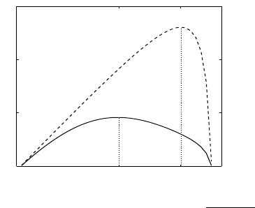
0 4
0
1
2
3
µ
˜
λ
e
(µ)
˜
λ(µ)
Figure 2: Initial and effective admission rates
δ(µ) =
1
1+e
−µ+2
, θ = 0.5, t = 1, R = 8
Corollary 1 (along with Figure 2) has two implications. First, when µ is large, having
the physicians to work faster can discourage patients to seek admissions (i.e., both
˜
λ(µ) and
˜
λ
e
(µ) will decrease) since the readmission rate is too high. Second, when µ is moderate, as
the mode of
˜
λ(µ) is smaller than that of
˜
λ
e
(µ), having the physicians work faster can reduce
the initial admission rate
˜
λ(µ) but it can increase the effective admission rate
˜
λ
e
(µ) (due to
the significant increase in the readmission rate δ(µ)). Therefore, when choosing the service
rate µ under different payment schemes, the HCP should take into account the impact of
µ on the initial admission rate and the effective admission rate in equilibrium. We shall
consider this issue in the next section.
4.2 The HCP’s Service Rate Decision under Partial Coverage
Given any reimbursement rate r
s
, s ∈ {f, b}, and anticipating the equilibrium initial admis-
sion rate
˜
λ(µ) and the equilibrium effective admission rate
˜
λ
e
(µ) as given in (8) and (9), the
HCP needs to determine its service rate µ
s
to maximize its expected profit that is composed
of two components: (a) the total amount of reimbursement received from the funder; and
(b) the variable cost associated with each patient. First, recall that the HCP is paid r
f
for
each admission under the FFS scheme and r
b
for each episode under the BP scheme. Hence,
the HCP receives r
f
˜
λ
e
(µ) under the FFS scheme and r
b
˜
λ(µ) under the BP scheme from the
funder. Second, recall that the capacity (i.e., the number of doctors) under our setting is
fixed. Hence, the variable cost is mainly attributed to the length of patients’ outpatient
visits (i.e., personnel, nurse, consumable items, etc.) so that the variable cost per patient
visit is c · (1/µ), where 1/µ is the mean length of outpatient visit and c is the correspond-
ing unit time variable cost incurred by the HCP for treating the patient. Combining these
13

observations, we can formulate the HCP’s problem under the two schemes as
(F F S) max
µ
Π
f
(µ) = r
f
·
˜
λ
e
(µ) − c ·
1
µ
·
˜
λ
e
(µ) =
r
f
−
c
µ
·
˜
λ
e
(µ); (10)
(BP ) max
µ
Π
b
(µ) = r
b
·
˜
λ(µ) − c ·
1
µ
·
˜
λ
e
(µ) =
r
b
−
c
o(µ)
·
˜
λ(µ). (11)
By considering the first order conditions, we get the following results.
Proposition 1. For any given reimbursement rate r
s
, s ∈ {f, b}, the HCP’s expected profit
Π
s
(µ) is unimodal in the service rate µ. In equilibrium,
1. the optimal service rate ˜µ
f
(r
f
) under the FFS scheme is the unique solution that solves
d log
˜
λ
e
(µ)
dµ
=
c
cµ − r
f
µ
2
, (12)
and ˜µ
f
(r
f
) must be larger than the mode of
˜
λ
e
(µ).
2. the optimal service rate ˜µ
b
(˜r
b
) under the BP scheme is the unique solution that solves
d log
˜
λ(µ)
dµ
=
c · o
0
(µ)
o(µ) · (c − r
b
· o(µ))
, (13)
and ˜µ
b
(r
b
) must be larger than the mode of
˜
λ(µ) and smaller than µ
o
, the service rate
that maximizes o(µ), i.e., ˜µ
b
(r
b
) < µ
o
. Furthermore,
˜
λ(r
b
) =
˜
λ(˜µ
b
(r
b
)) >
˜
λ(µ
o
).
First, observe that the unimodality of Π
s
(µ) for s = f, b follows immediately from the
unimodality of
˜
λ
e
(µ) and
˜
λ(µ) as stated in Corollary 1. Second, by substituting the optimal
˜µ
s
(r
s
) (given in (12) and (13) respectively) into δ(µ),
˜
λ(µ) given in (8),
˜
λ
e
(µ) given in
(9), and Π
s
(µ) given in (10) and (11), we can express these quantities as functions of the
reimbursement rate r
s
so that δ(r
s
) = δ(˜µ
s
(r
s
)),
˜
λ(r
s
) =
˜
λ(˜µ
s
(r
s
)), and Π
s
(r
s
) = Π
s
(˜µ
s
(r
s
)).
(For ease of exposition, we shall suppress the arguments when convenient.) We shall use
these quantities to determine the funder’s reimbursement decision r
s
, s = f, b, under the two
schemes. In preparation, let us examine the properties of these quantities with respect to
the reimbursement rate r
s
.
Corollary 2. The reimbursement rate r
s
, s ∈ {f, b}, has the following impact on the fol-
lowing quantities:
1. The HCP’s optimal service rate ˜µ
s
(r
s
) and the corresponding readmission rate δ(r
s
)
are decreasing in r
s
.
14
2. The initial admission rate
˜
λ(r
s
), the waiting time per visit W (r
s
), the total waiting
time T (r
s
), and the HCP’s profit Π
s
(r
s
) are increasing in r
s
.
The first statement of Corollary 2 reveals that, under both the FFS and BP schemes,
when the funder offers a higher reimbursement rate r
s
, the HCP will set a lower service rate
so that physicians spend more time on treating each patient and therefore, less patients are
readmitted to the system. To explain this result intuitively, with a higher reimbursement
rate r
s
, the HCP has a stronger desire to attract more patients to seek admissions (i.e., to
increase the effective admission rate
˜
λ
e
(µ) under the FFS scheme and to increase the initial
admission rate
˜
λ(µ) under the BP scheme). Having this desire in mind, it is easy to observe
from (12) and (13) that, in order to increase
˜
λ
e
(µ) under FFS and
˜
λ(µ) under BP, the HCP
has to lower its service rate µ. This explains the first statement.
Next, the second statement informs us that a higher reimbursement rate will encourage
more patients to seek admission (i.e., the initial admission rate
˜
λ(r
s
) is increasing in r
s
),
thereby increasing the congestion level of the healthcare system (i.e., both the waiting time
per visit W (r
s
) and the total waiting time T (r
s
) are increasing in r
s
). This result can be
explained as follows. Recall from above that, with a higher reimbursement rate r
s
, the HCP
will reduce its service rate so as to increase the effective admission rate
˜
λ
e
(µ) under FFS
and increase the initial admission rate
˜
λ(µ) under BP. Also, with a lower service rate and a
higher effective admission rate
˜
λ
e
(µ) under FFS, it is easy to check from (3) that the initial
admission rate
˜
λ(µ) under FFS is also higher. Therefore, when the funder offers a higher
reimbursement rate r
s
, the HCP will lower its service rate so that the initial admission
rate and the effective admission rate become higher under both schemes. Consequently,
the waiting time per visit and the total waiting time will increase. However, the HCP will
earn a higher profit due to higher admission rate and higher reimbursement rate under both
schemes.
In summary, Corollary 2 highlights the trade-off between readmission rate and waiting
time that the funder needs to strike a balance when considering the reimbursement rate,
which we analyze next.
4.3 The Funder’s Reimbursement Decision under Partial Cover-
age
Anticipating the HCP’s service rate ˜µ
s
(r
s
), s ∈ {f, b} given in (12) and (13) respectively,
we now turn our attention to the funder’s decision regarding the reimbursement rate r
s
.
Essentially, the funder selects r
s
to maximize the patient welfare S(r
s
). When the patient
initial admission rate is endogenous, the patient welfare generally consists of two components:
15

(a) the utility of those patients who seek admissions; and (b) the penalty cost associated
with those patients who balk (without seeking admissions). As stated in the introduction, it
is common that patients who demand for public care abandon and seek help elsewhere due
to the long waiting time. Therefore, accessibility is central to the performance of the public
healthcare systems (Levesque et al. 2013, and Adritsos and Tang, 2014). To incorporate
accessibility into the funder’s objective, we impose a penalty cost β for each balking patient.
Under the partial coverage case, we know that
˜
λ(r
s
) is the initial admission rate, and
(Λ −
˜
λ(r
s
)) is the balking rate. By noting that each admitted patient obtains a utility
U(
˜
λ(µ), µ) and each balking patient incurs a disutility β, the patient welfare S(r
s
) =
˜
λ(r
s
) ·
U(
˜
λ(r
s
), ˜µ
s
(r
s
))−β(Λ−
˜
λ(r
s
)). By taking the funder’s budget B and the HCP’s participation
constraint into consideration, we can formulate the funder’s problem as follows:
max
r
s
S(r
s
) =
˜
λ(r
s
)U(
˜
λ(r
s
), ˜µ
s
(r
s
)) − β(Λ −
˜
λ(r
s
)) = −β(Λ −
˜
λ(r
s
)), (14)
s.t. Budget constraint :
(
(F F S) r
f
·
˜
λ
e
(r
f
) ≤ B,
(BP ) r
b
·
˜
λ(r
b
) ≤ B,
(15)
P articipation constraint : Π
s
(r
s
) ≥ 0.
Recall from §4.1 that U(
˜
λ(r
s
), ˜µ
s
(r
s
)) = 0 under the partial coverage case, it is easy to
check from (14) that the funder’s objective is equivalent to maximizing the initial admission
rate
˜
λ(r
s
).
17
This is consistent with the practice that, in many public healthcare systems
that serve a large patient population, the government’s overarching objective is to improve
accessibility by maximizing
˜
λ(r
s
) (Aboolian et al. 2016). Combining this observation and
the fact that
˜
λ(r
s
) is increasing in r
s
(Corollary 2), we obtain the following result.
Proposition 2. The patient welfare S(r
s
) given in (14) is increasing in r
s
. The funder’s
budget constraint (15) is binding so that the funder’s optimal reimbursement rate ˜r
s
satisfies:
˜r
f
·
˜
λ
e
(˜r
f
) = B under the FFS scheme, and ˜r
b
·
˜
λ
e
(˜r
b
) = B under the BP scheme.
Proposition 2 implies that when serving a large patient population (e.g., the UK), the public
healthcare system can only provide partial coverage, and the funder always exhausts its
budget under both FFS and BP schemes (Donnelly and Swinford 2013).
18
We can further
establish the following comparative statics with respect to the budget B.
Corollary 3. Under both the FFS and BP schemes, the HCP’s optimal service rate ˜µ
s
(˜r
s
)
and the corresponding readmission rate δ(˜r
s
) are decreasing in B. However, the optimal
17
Under the full coverage case, each patient can obtain a positive utility (i.e., U(Λ, µ) > 0). Therefore,
the funder’s objective is no longer equivalent to maximizing the initial admission rate.
18
See “NHS is about to run out of cash top official warns” at http://www.telegraph.co.uk/news/health/
news/10162848/NHS-is-about-to-run-out-of-cash-top-official-warns.html.
16
reimbursement rate ˜r
s
, the initial admission rate
˜
λ(˜r
s
), the waiting time per visit W (˜r
s
) and
the total waiting time T (˜r
s
) are increasing in B.
Corollary 3 reveals that, under the partial coverage case, the funder can afford to offer a
higher reimbursement rate with a higher budget. By considering this key result, we can apply
Corollary 2 to interpret all other results as stated in Corollary 3. To avoid repetition, we
omit the details. Hence, under both the FFS and BP schemes, increasing the funder’s budget
B can improve the patient access and reduce the readmission rate, but it can increase the
waiting time. This implication will play a role when we compare the performance between
the FFS scheme and the BP scheme.
4.4 Performance Comparison under Partial Coverage: FFS v.s.
BP
So far, we have derived the equilibrium outcomes of different performance metrics (the patient
welfare, initial admission rate, service rate, readmission rate and waiting times) associated
with both payment schemes under the partial coverage scenario as presented in Propositions
1 and 2. We now compare these performance outcomes between the FFS scheme and the
BP scheme. Specifically, our comparison yields the following results.
Proposition 3. Consider the case in which potential patients are partially covered under
both FFS and BP schemes. Then, relative to the FFS scheme,
1. both the patient welfare and the initial admission rate are higher under the BP scheme
(i.e., S(˜r
b
) > S(˜r
f
) and
˜
λ(˜r
b
) >
˜
λ(˜r
f
));
2. both the service rate and the readmission rate are lower under the BP scheme (i.e.,
˜µ
b
(˜r
b
) < ˜µ
f
(˜r
f
) and δ(˜r
b
) < δ(˜r
f
)); and
3. both the waiting time per visit and the total waiting time are higher under the BP
scheme (i.e., W (˜r
b
) > W (˜r
f
) and T (˜r
b
) > T (˜r
f
)).
Proposition 3 implies that when potential patients are partially covered under both FFS
and BP schemes, the BP scheme dominates the FFS scheme in terms of the patient welfare
and service quality, but the FFS scheme outperforms the BP scheme in terms of the waiting
time. These results can be explained as follows. Recall that the BP scheme pays the HCP a
fixed amount for each admitted patient no matter how many times the patient is readmitted
to the system. Hence, the HCP under the BP scheme has incentives to reduce the service
rate so as to reduce the readmission rate. However, reducing the readmission rate attracts
higher initial admission rate under the BP scheme. Furthermore, from (7), if the potential
17

patients are partially covered, then the initial admission rate solves U(
˜
λ, µ) = 0. Due to
a lower readmission rate, admitted patients under the BP scheme can tolerate a longer
waiting time in equilibrium such that W (˜r
b
) > W (˜r
f
) and T (˜r
b
) > T (˜r
f
). As maximizing
the patient welfare is equivalent to maximizing the initial admission rate under the partial
coverage scenario, the patient welfare under the BP scheme is also larger.
Proposition 3 is consistent with the findings of previous studies showing that the FFS
scheme is effective for reducing the waiting time but not for improving service quality. For
example, Blomqvist and Busby (2013) show that the FFS scheme is effective for reducing
the waiting time in Canada. Mot (2002) finds that, in the Netherlands, the abolition of the
FFS scheme has caused the waiting time to increase for the elective surgery.
In summary, by considering the partial coverage case that occurs when the patient popu-
lation is large, we find that there is no dominant scheme. The BP scheme is more effective for
improving the patient welfare and reducing the readmission rate; however, the FFS scheme
is more effective for reducing the waiting time. Next, we examine the full coverage case
that occurs when the patient population is small. As we shall see, the results as stated in
Propositions 2 and 3 no longer hold.
5 Reimbursement Schemes under Full Coverage: FFS
and BP
We now consider the case when the potential patients are fully covered under both FFS and
BP schemes. This case is suitable for the public HCP in the rural area, which normally
has a low patient volume (DiChiara 2015).
19
Recall that under the full coverage scenario,
U(Λ, µ) ≥ 0 (see §4.1). This condition can be further simplified as
˜
λ(µ) ≥ Λ after some
algebra, where
˜
λ(µ) is given in (8). In other words, when the condition under the partial
coverage scenario is infeasible (i.e.,
˜
λ(µ) ≥ Λ), the healthcare system will achieve the full
coverage scenario.
Under the full coverage scenario, the initial admission rate is given by Λ and the effective
admission rate is Λ/(1 − δ(µ)). By noting that the average variable cost associated with
each patient’s visit is c · (1/µ), we can formulate the HCP’s problems under the full coverage
19
See “Rural Hospitals Address Medicare Reimbursement Cut Concerns” at
http://revcycleintelligence.com/news/rural-hospitals-address-medicare-reimbursement-cut-concerns.
18

scenario as follows:
(F F S) max
µ
Π
f
(µ) =
r
f
−
c
µ
Λ
1 − δ(µ)
, (16)
s.t.
˜
λ(µ) ≥ Λ,
(BP ) max
µ
Π
b
(µ) =
r
b
−
c
o(µ)
Λ, (17)
s.t.
˜
λ(µ) ≥ Λ,
where the constraint
˜
λ(µ) ≥ Λ guarantees that the healthcare system offers full coverage to
all potential patients.
Proposition 4. Consider the case in which all potential patients are fully covered under
both FFS and BP schemes. Then, for any given reimbursement rate r
s
, s ∈ {f, b},
1. the HCP’s optimal service rate under the FFS scheme satisfies ˜µ
f
= max{µ, subject to,
˜
λ(µ) ≥
Λ}, where
˜
λ(µ) is given as in (8).
2. the HCP’s optimal service rate under the BP scheme satisfies
˜µ
b
=
(
µ
o
, if
˜
λ(µ
o
) ≥ Λ,
max{µ :
˜
λ(µ) ≥ Λ} if
˜
λ(µ
o
) < Λ.
Under both schemes, the optimal service rate ˜µ
s
, s = f, b, is independent of the funder’s
reimbursement rate r
s
.
The intuition behind Proposition 4 is as follows. First, observe from (16) that, the HCP’s
variable cost c/µ decreases in µ while its effective arrival rate Λ/(1 − δ(µ)) increases in µ.
Hence, the HCP’s profit Π
f
(µ) under the FFS scheme is always increasing in µ. These
observations imply that the HCP will choose the largest service rate in equilibrium that
ensures that the potential patients are fully covered (i.e., max{µ :
˜
λ(µ) ≥ Λ}). Our results
reveal that, when the patient population is small, the FFS scheme creates an incentive for
the HCP to increase its service rate so as to generate as much revenue as possible.
Next, under the BP scheme, observe from (17) that the HCP’s objective is equivalent
to minimizing the variable cost c/o(µ). According to Lemma 1, the cure service rate o(µ)
is unimodal in µ and reaches its maximum at µ
o
. Therefore, Π
b
(µ) given in (17) is also
unimodal in µ and its corresponding mode is also µ
o
. When µ
o
is feasible under the full
coverage scenario (i.e.,
˜
λ(µ
o
) ≥ Λ), it is natural that the HCP will choose µ
o
in equilibrium.
Whereas, when µ
o
is infeasible under the full coverage scenario(i.e.,
˜
λ(µ
o
) < Λ), the HCP
will choose the largest service rate that ensures that the potential patients are fully covered
(i.e., max{µ :
˜
λ(µ) ≥ Λ}).
19

Finally, unlike the partial coverage scenario, Proposition 4 implies that, under the full
coverage scenario, the HCP’s optimal service rate is independent of the funder’s reimburse-
ment rate. Because the funder cannot regulate the HCP’s service rate decision under both
schemes, the funder will select the smallest feasible reimbursement rate. Because all of the
performance metrics that we are going to compare such as the patient welfare, the initial
admission rate and the total waiting time only depend on the service rate and the initial ad-
mission rate, for ease of exposition, we thus omit the analysis of the funder’s reimbursement
rate decisions under the full coverage case. (See the online Appendix B for details.)
To guarantee that the healthcare system in equilibrium achieves the full coverage, the
equilibrium outcome under the partial coverage must be infeasible; that is, Λ ≤
˜
λ(˜r
s
),
s ∈ {f, b}, where
˜
λ(˜r
s
) represents the initial admission rate under the partial coverage case.
According to Proposition 3, this condition is equivalent to Λ ≤
˜
λ(˜r
f
). By comparing different
performance metrics associated with the FFS and BP schemes under the full coverage (i.e.,
Λ ≤
˜
λ(˜r
f
)), we get the following results.
Corollary 4. Suppose that potential patients are fully covered under both FFS and BP
schemes (i.e., when Λ ≤
˜
λ(˜r
f
)). Then,
1. If the potential patient population Λ is medium so that
˜
λ(µ
o
) ≤ Λ ≤
˜
λ(˜r
f
)
20
, then
the optimal service rates under the FFS and BP schemes are equal (i.e., ˜µ
f
= ˜µ
b
=
max{µ :
˜
λ(µ) ≥ Λ}). Consequently, the patient welfare, the readmission rate, the
initial admission rate, the waiting time per visit and the total waiting time are the
same under both FFS and BP schemes.
2. If the potential patient population Λ is small so that Λ < min{
˜
λ(µ
o
),
˜
λ(˜r
f
)}, then the
BP scheme dominates the FFS scheme in terms of the patient welfare, service quality
and the total waiting time (i.e., S(˜µ
f
) < S(˜µ
b
), δ(˜µ
f
) > δ(˜µ
b
) and T (˜µ
f
) > T (˜µ
b
)).
The first statement of Corollary 4 reveals that the FFS and BP schemes are equally
efficient if the patient population is medium (i.e.,
˜
λ(µ
o
) ≤ Λ ≤
˜
λ(˜r
f
)). However, when the
patient population is very small (i.e., Λ < min{
˜
λ(µ
o
),
˜
λ(˜r
f
)}), the BP scheme dominates the
FFS scheme in terms of the patient welfare, service quality and the congestion level. These
results can be explained as follows. When
˜
λ(µ
o
) ≤ Λ ≤
˜
λ(˜r
f
), Proposition 4 reveals that
the HCP will select the largest service rate that makes the potential patients fully covered
under both FFS and BP schemes so that ˜µ
f
= ˜µ
b
. Therefore, the FFS and BP schemes are
equally efficient in terms of all the performance metrics.
20
Note that the existence of
˜
λ(µ
o
) ≤ Λ ≤
˜
λ(˜r
f
) implicitly requires that
˜
λ(µ
o
) ≤
˜
λ(˜r
f
). We have shown in
Appendix A that there exist thresholds
¯
t and
¯
B (where the expression of
¯
t and
¯
B can be found in (27) in
Appendix A) such that
˜
λ(µ
o
) ≤
˜
λ(˜r
f
) if and only if t ≥
¯
t and B ≥
¯
B.
20

Next, when Λ < min{
˜
λ(µ
o
),
˜
λ(˜r
f
)}, µ
o
is feasible under the full coverage and thus,
˜µ
b
= µ
o
. Because the optimal service rate under the FFS scheme ˜µ
f
is the largest one that
makes the potential patients fully covered, ˜µ
f
> ˜µ
b
= µ
o
. As the readmission rate δ(µ) is
increasing in µ, δ(˜µ
f
) > δ(˜µ
b
). From (6) we can easily know that the total waiting time T is
decreasing in o(µ). As o(µ) is maximized at µ
o
, T (˜µ
b
) < T (˜µ
f
). Thus, compared with the
FFS scheme, the service quality is better and the total waiting cost is smaller under the BP
scheme. Therefore, the patient welfare under the BP scheme is also larger than that under
the FFS scheme.
In summary, we can conclude from Corollary 4 that under the full coverage scenario, when
the patient population is medium, both schemes yield the same performance. However, when
the patient population is very small, the BP scheme dominates the FFS schemes in terms of
the patient welfare, service quality and the total waiting time.
Remark. When
˜
λ(˜r
f
) < Λ ≤
˜
λ(˜r
b
) so that the potential patients are fully covered under
the BP scheme but are partially covered under the FFS scheme, the comparison results are
similar to Proposition 3 and Corollary 4.
21
Specifically, when
˜
λ(µ
o
) ≤
˜
λ(˜r
f
), the results given
in Proposition 3 still hold: the BP scheme dominates the FFS scheme in terms of the patient
welfare and service quality but the FFS scheme outperforms the BP scheme in terms of the
congestion level. However, when
˜
λ(µ
o
) >
˜
λ(˜r
f
), there exists a threshold
¯
Λ ∈ [
˜
λ(˜r
f
),
˜
λ(µ
o
)]
such that when Λ is relatively large (i.e., Λ >
¯
Λ), the results given in Proposition 3 hold;
and when Λ is relatively small (i.e., Λ ≤
¯
Λ), the results given in the second statement of
Corollary 4 hold (i.e., the BP scheme dominates the FFS scheme in terms of the patient
welfare, service quality and the total waiting time).
6 Conclusion Remarks
In this paper, we have presented a queueing model with endogenous arrival rate selected by
the patient and endogenous readmission rate controlled by the HCP (via the selected ser-
vice rate). By analysing a three-stage Stackelberg game with an embedded queueing model,
we compare the performance associated with the FFS and BP reimbursement schemes. By
considering the trade-off between service rate and service quality (in terms of the readmis-
sion rate), we obtain the following managerial insights. First, when potential patients are
partially covered, we find that a higher service rate may reduce both the initial admission
rate and the effective admission rate under both schemes. Second, we show that under the
partial coverage, a higher reimbursement rate can improve the service quality in terms of the
21
See Proposition B7 in the online Appendix B for details.
21
readmission rate but it can increase the waiting time under both FFS and BP reimbursement
schemes.
More importantly, by investigating the funder’s reimbursement decisions and comparing
the equilibrium outcomes associated with the two schemes, we find that the BP reimburse-
ment scheme may not always dominate the FFS reimbursement scheme. Specifically, when
the potential patients are partially covered, the BP scheme dominates the FFS scheme in
terms of the patient welfare and service quality (i.e., the readmission rate); however, the
FFS scheme outperforms the BP scheme in terms of the waiting time per visit and the total
waiting time.
When the potential patients are fully covered, the BP scheme weakly dominates the
FFS scheme in terms of the patient welfare, service quality and the total waiting time. In
particular, when the patient population is medium, the FFS and BP schemes are equally
efficient in terms of all performance metrics including the readmission rate, the waiting time
per visit, the total waiting time and the patient welfare. Overall, the implications of our
findings are as follows. First, when the size of the patient population is large, shifting from
FFS to BP can improve the patient welfare and reduce readmissions, but it can increase the
waiting time. Second, when potential patients are fully covered and the size of the patient
population is moderate, the two schemes yield the same outcomes. In such case, it seems
unnecessary to move from FFS to BP. However, when the size of the patient population is
very small, the BP scheme dominates the FFS scheme.
Our analysis represents an initial attempt to examine the performance of the healthcare
reimbursement scheme by capturing the strategic interactions among the patients, the HCP,
and the funder and by taking into account the relationship between service quality (in terms
of the readmission rate) and service speed. However, our model has several limitations that
we shall leave them as future research for further investigation. First, we have assumed
that patients have perfect information about the HCP’s service quality and it is of interest
to examine a situation when there is information asymmetry between patients and HCPs.
Second, our model is more suitable for elective non-urgent outpatient care. However, future
research is needed to examine the implications of different payment schemes on urgent care
especially when the patient’s health condition may deteriorate rapidly over time so that
longer waiting time may adversely affect patient’s health quality outcomes.
Another important area is to consider the competition among different HCPs. In the
presence of the market competition, the non-cured patients may seek admissions from other
HCPs. (For example, Andritsos and Tang (2014) examine the impact of competition between
the private and public HCPs on the patient welfare in Europe.) Therefore, the HCP may
not generate more demand by reducing readmission rate. In view of this, it is of interest
22
to investigate the impact of competition on the HCPs’ choices of service rate and other
performance metrics such as the waiting time, the patient welfare and the admission rate.
Finally, another possible extension is to add the mortality rate into our analysis. An implicit
assumption in our model is that patients can definitely be cured in the long run. This
assumption is realistic for the elective surgeries. However, for serious illness such as diabetes
mellitus, the increase in the mortality rate is an inevitable consequence of the low service
quality (i.e., high readmission rate and/or long waiting time).
References
Aboolian, R., O. Berman, V. Verter. 2016. Maximal accessibility network design in the
public sector. Transportation Science 50(1) 336-347.
Adida, E., H. Mamaniy, S. Nassiri. 2014. Bundled payment vs. Fee-for-Service: impact of
payment scheme on performance. Forthcoming in Management Science.
Alizamir, S., F. de V´ericourt, P. Sun. 2013. Diagnostic accuracy under congestion. Man-
agement Science 59(1) 157-171.
Anand, K. S., M. F. Pac, S. Veeraraghavan. 2011. Quality-speed conundrum: Tradeoff in
customer-intensive services. Management Science 57(1) 40-56.
Andritsos, D. A., C. S. Tang. 2014. Introducing competition in healthcare services: The role
of private care and increased patient mobility European Journal of Operational Research,
234(3) 898-909.
Andritsos, D. A., C. S. Tang. 2015. Incentive programs for reducing readmissions when
patient care is co-produced. Working Paper, UCLA Anderson School.
Ata, B., B. L. Killaly, T. L. Olsen, R. P. Parker. 2013. On hospice operations under medicare
reimbursement policies. Management Science 59(5) 1027-1044.
Bavafa, H., S. Savin, C. Terwiesch. 2013. Managing office revisit intervals and patient panel
sizes in primary care. Working Paper.
Barua, B., F. Fathers. 2014. Waiting your turn: wait times for health care in Canada 2014
report. Studies in Health Policy. Vancouver: Fraser Institute.
Blomqvist, A., C. Busby. 2013. Paying Hospital-Based Doctors: Fee for Whose Service?
Commentary 392. Toronto: C.D. Howe Institute.
Calsyn, M., E. O. Lee. 2012. Alternatives to Fee-for-Service payments in health care. Center
for American Progress.
Chan, C. W., G. B. Yom-Tov, G. Escobar. 2014. When to use speedup: an examination of
23
service systems with returns. Operations Research 62(2) 462-482.
Davis, K. 2007. Paying for care episodes and care coordination. The New England Journal
of Medicine 356(11) 1166-1168.
Dimakou, S. 2013. Waiting time distributions and national targets for elective surgery in UK:
theoretical modelling and duration analysis. Doctoral thesis, Department of Economics,
City University London, UK.
de Vericourt, F., Y. Zhou. 2005. Managing response time in a call-routing problem with
service failure. Operations Research 53(6) 968-981.
Fenter, T., S. Lewis. 2008. Pay-for-performance initiatives. Journal of Managed Care
Pharmacy. 14(6)(suppl S-c) s12-s15.
Fethke, C. C., I. M. Smith, N. Johnson. 1986. “Risk” factors affecting readmission of the
elderly into the health care system. Medical Care 24(5) 429-437.
Fuloria, P. C., S. A. Zenios. 2001. Outcomes-adjusted reimbursement in a health-care
delivery system. Management Science 47(6) 735-751.
Gupta, D., M. Mehrotra. 2015. Bundled payments for healthcare services: proposer selection
and information sharing. Operations Research 63(4) 772-788.
Hasija, S., E. Pinker, R. A. Shumsky. 2009. Work expands to fill the time available: Ca-
pacity estimation and staffing under parkinson’s law. Manufacturing Service Operations
Management 12(1) 1-18.
Hassin, R., M. Haviv. 2003. To queue or not to queue: equilibrium behavior in queueing
systems. Kluwer Academic Publishers, Norwell, MA.
Hopp, W. J., S. M. R. Iravani, G. Y. Yuen. 2007. Operations systems with discretionary
task completion. Management Science 53(1) 61-77.
Hing, E., C. J. Hsiao. 2014. State variability in supply of office-based primary care providers:
United States, 2012. NCHS Data Brief 151.
Hurst, J., L. Siciliani. 2003. Tackling excessive waiting times for elective surgery: a com-
parison of policies in twelve OECD countries. OECD Health Working Papers, No 6,
Paris.
Japsen, B. 2015. Medicare bundled payment gains momentum with hospitals, nursing homes.
Forbes. Published on August 21, 2015.
Jiang, H., Z. Pang, S. Savin. 2012. Performance-based contracts for outpatient medical
services. Manufacturing Service Operations Management 14(4) 654-669.
Kim, S., I. Horowitz, K. K. Young, T. A. Buckley. 1999. Analysis of capacity management
24
of the intensive care unit in a hospital. European Journal of Operational Research 115(1)
36-46.
Kociol, R. D., R. D. Lopes, R. Clare, L. Thomas, R. H. Mehta, P. Kaul, et al. 2012. Inter-
national variation in and factors associated with hospital readmission after myocardial
infarction. The Journal of the American Medical Association 307(1) 66-74.
Konrad, T. R., C. L. Link, R. J. Shackelton et al. 2010. It’s about time: physicians’ per-
ceptions of time constraints in primary care medical practice in three national healthcare
systems. Med Care 48(2) 95-100.
Kostami, V., S. Rajagopalan. 2014. Speed quality tradeoff in a dynamic model. Manufac-
turing & Service Operations Management 16(1) 104-118.
Lee, DK. K., S. A. Zenios. 2012. An evidence-based incentive system for Medicare’s End-
Stage Renal Disease program. Management Science 58(6) 1092-1105.
Levesque, J. F., M. F. Harris, G. Russell. 2013. Patient-centred access to health care:
conceptualising access at the interface of health systems and populations. International
Journal for Equity in Health 12(18) 16-28.
Li, X., P. Guo, Z. Lian. 2015. Speed-quality competition in customer-intensive services with
boundedly rational customer. Forthcoming in Production and Operations Management .
Morrow-Howell, N., E. K. Proctor. 1993. The use of logistic regression in social work
research. Journal of Social Service Research 16(1-2) 87-104.
Mot, E. S. 2002. Paying the medical specialist: the eternal puzzle: experiments in the
Netherlands. PhD Thesis page 176, Amsterdam.
Pa¸c, M. F., S. Veeraraghavan. 2010. Strategic diagnosis and pricing in expert services.
Working paper, Wharton School, University of Pennsylvania, Philadelphia.
Palacios, M., B. Barua, F. Ren. 2015. The price of public health care insurance. Fraser
Research Bulletin. Published on August 2015.
Rabin, R. 2014. 15-minute Doctor Visits Take a Toll on a Patient-Physician Relationship.
PBS Newshour. April 21.
Ross, S. 2007. Introduction to Probability Models. Academic Press, USA.
So, K. C., C. S. Tang. 2000. Modeling the impact of an outcome-oriented reimbursement
policy on clinic, patients, and pharmaceutical firms. Management Science 46(7) 875-892.
Street, A., J. O’Reilly, P. Ward, A. Mason. 2011. DRG-based hospital payment and ef-
ficiency: Theory, evidence, and challenges. In Diagnosis-Related Groups in Europe -
Moving Towards Transparency, Efficiency and Quality in Hospitals, Busse R, Geissler,
25
A, Quentin W, Wiley M (eds). Open University Press: Maidenhead; 93-114.
Tsai, T. C., K. E. Joynt, R. C. Wild, E. J. Orav, A. K. Jha. 2015. Medicares Bundled
Payment initiative: most hospitals are focused on a few high-volume conditions. Health
Affairs 34(3) 371-380.
Tong, C., S. Rajagopalan. 2014. Pricing and operational performance in discretionary
services. Production and Operations Management 23(4) 689-703.
Varkevisser, M., S. A. van der Geest, F. T. Schut. 2012. Do patients choose hospitals
with high quality ratings? Empirical evidence from the market for angioplasty in the
Netherlands. Journal of Health Economics 31(2) 371-378.
Wang, X., L. G. Debo, A. Scheller-Wolf, S. F. Smith. 2010. Design and analysis of diagnostic
service centers. Management Science 56(11) 1873-1890.
Xu, Y., A. Scheller-Wolf, K. Sycara. 2015. The benefit of introducing variability in quality
based service domains. Operations Research 63(1) 233-246.
Yom-Tov, G. B., A. Mandelbaum. 2014. Erlang-R: A time-varying queue with reentrant
customers, in support of healthcare staffing. Manufacturing & Service Operations Man-
agement 16(2) 283-299.
26

Online Appendices
“The Impact of Reimbursement Policy on Patient Welfare,
Readmission Rate and Waiting Time in a Public Healthcare System:
Fee-for-Service vs. Bundled Payment”
Appendix A: Proofs of Lemmas and Propositions
Proof of Lemma 1. Taking the first order condition (FOC) of o(µ) over µ yields
do(µ)
dµ
= 1 − δ(µ) − µδ
0
(µ) = 0,
which can be rewritten as
(1 − δ(µ))(1 − µg(µ)) = 0.
As g(µ) is increasing in µ, do(µ)/dµ crosses zero only once from above. Therefore, o(µ) is
quasi-concave in µ and the optimal service rate µ
o
solves µ
o
g(µ
o
) = 1.
Next, we prove that when µ ≤ µ
o
, o(µ) is concave in µ. As g(µ) is increasing in µ,
dg(µ)
dµ
=
δ
00
(µ)(1 − δ(µ)) + (δ
0
(µ))
2
(1 − δ(µ))
2
> 0, (18)
which yields δ
00
(µ)(1 − δ(µ)) + (δ
0
(µ))
2
> 0. Then we can show that
d
2
o(µ)
dµ
2
= −2δ
0
(µ) − µδ
00
(µ)
= −2δ
0
(µ) +
µ(δ
0
(µ))
2
1 − δ(µ)
−
µδ
00
(µ)(1 − δ(µ)) + µ(δ
0
(µ))
2
1 − δ(µ)
= −δ
0
(µ) −
δ
0
(µ)
1 − δ(µ)
do(µ)
dµ
−
µδ
00
(µ)(1 − δ(µ)) + µ(δ
0
(µ))
2
1 − δ(µ)
.
As o(µ) is increasing in µ when µ ≤ µ
o
, the above equation is negative for all µ ≤ µ
o
.
Therefore, o(µ) is concave in µ for µ ≤ µ
o
.
Proof of Corollary 1. Denote µ
1
= max{
˜
λ(µ)} and µ
2
= max{
˜
λ
e
(µ)}. By noting that
o(µ) = µ(1 − δ(µ)) and o
0
(µ) = 1 − δ(µ) − µδ
0
(µ), we have o(µ) − µo
0
(µ) = µ
2
δ
0
(µ). Hence,
taking derivative of
˜
λ(µ) with respect to µ yields
d
˜
λ(µ)
dµ
= o
0
(µ) −
θo
0
(µ)
Ro(µ) − µt
+
θo(µ)(Ro
0
(µ) − t)
[Ro(µ) − µt]
2
= o
0
(µ) −
θδ
0
(µ)t
[R(1 − δ(µ)) − t]
2
. (19)
1

Comparison of Reimbursement Schemes: FFS vs BP Online Appendices
From Lemma 1, we can show that d
˜
λ(µ)/dµ < 0 for µ ≥ µ
o
. Thus µ
1
< µ
o
. Using Lemma
1 again, o
00
(µ
1
) < 0. Recall from (18) that δ
00
(µ)(1 − δ(µ)) + (δ
0
(µ))
2
> 0. Therefore,
d
2
˜
λ(µ)
dµ
2
µ=µ
1
= o
00
(µ
1
) −
θtδ
00
(µ
1
)
[R(1 − δ(µ
1
)) − t]
2
−
2Rθ(δ
0
(µ
1
))
2
t
[R(1 − δ(µ
1
)) − t]
3
= o
00
(µ
1
) +
θt(δ
0
(µ
1
))
2
(1 − δ(µ
1
))[R(1 − δ(µ
1
)) − t]
2
−
2Rθ(δ
0
(µ
1
))
2
t
[R(1 − δ(µ
1
)) − t]
3
−
θt[δ
00
(µ
1
)(1 − δ(µ
1
)) + (δ
0
(µ
1
))
2
]
(1 − δ(µ
1
))[R(1 − δ(µ
1
)) − t]
2
= o
00
(µ
1
) −
θt[δ
00
(µ
1
)(1 − δ(µ
1
)) + (δ
0
(µ
1
))
2
]
(1 − δ(µ
1
))[R(1 − δ(µ
1
)) − t]
2
−
θt(δ
0
(µ
1
))
2
(R(1 − δ(µ
1
)) + t)
(1 − δ(µ
1
))[R(1 − δ(µ
1
)) − t]
3
(20)
< 0,
which shows that
˜
λ(µ) is quasi-concave in µ. Taking derivative of
˜
λ
e
(µ) with respect to µ
and using (18),
d
˜
λ
e
(µ)
dµ
= 1 −
θRδ
0
(µ)
[R(1 − δ(µ)) − t]
2
, (21)
d
2
˜
λ
e
(µ)
dµ
2
= −
θRδ
00
(µ)
[R(1 − δ(µ)) − t]
2
−
2θR
2
(δ
0
(µ))
2
[R(1 − δ(µ)) − t]
3
=
−Rθ
(1 − δ(µ))
(δ
0
(µ))
2
(R(1 − δ(µ)) + t)
[R(1 − δ(µ)) − t]
3
+
δ
00
(µ)(1 − δ(µ)) + (δ
0
(µ))
2
[R(1 − δ(µ)) − t]
2
< 0. (22)
Thus
˜
λ
e
(µ) is concave in µ. We next show that the mode of
˜
λ(µ) is smaller than the mode
of
˜
λ
e
(µ), that is, µ
1
< µ
2
. By noting that o
0
(µ) = 1 − δ(µ) − µδ
0
(µ), (21) can be rewritten as
d
˜
λ
e
(µ)
dµ
= 1 −
θ
µ[R(1 − δ(µ)) − t]
+
θ(Ro
0
(µ) − t)
µ[R(1 − δ(µ)) − t]
2
=
˜
λ
e
(µ)
µ
+
θ(Ro
0
(µ) − t)
µ[R(1 − δ(µ)) − t]
2
.
Obviously, the maximum effective admission rate should be positive; that is,
˜
λ
e
(µ
2
) > 0.
Because µ
2
should satisfy the FOC of
˜
λ
e
(µ, ), namely, d
˜
λ
e
(µ
2
)/dµ = 0, we have Ro
0
(µ
2
)−t <
0. Using (21) and substituting d
˜
λ
e
(µ
2
)/dµ = 0 into (19), we have
dλ(µ)
dµ
µ=µ
2
=
Ro
0
(µ
2
) − t
R
< 0, (23)
which implies that µ
2
> µ
1
.
2

Comparison of Reimbursement Schemes: FFS vs BP Online Appendices
Proof of Proposition 1. With a slight abuse of notion, we interchangeably use ˜µ
s
(r
s
) and
˜µ
s
. From (10), the FOC of Π
f
(µ) can be written as
dΠ
f
(µ)
dµ
=
c
˜
λ
e
(µ)
µ
2
+
r
f
−
c
µ
d
˜
λ
e
(µ)
dµ
= 0, (24)
which can be rewritten as (12). Furthermore, the optimal service rate ˜µ
f
(r
f
) should satisfy
d
˜
λ
e
(µ)
dµ
|
µ=˜µ
f
< 0. By recalling from Corollary 1 that
˜
λ
e
(µ) is concave in µ, ˜µ
f
(r
f
) is larger
than the mode of
˜
λ
e
(µ). Furthermore,
d
2
Π
f
(µ)
dµ
2
µ=˜µ
f
=
2c
˜µ
2
f
d
˜
λ
e
(µ)
dµ
µ=˜µ
f
−
2c
˜
λ
e
(˜µ
f
)
˜µ
3
f
+
r
f
−
c
˜µ
f
d
2
˜
λ
e
(µ)
dµ
2
µ=˜µ
f
< 0,
which shows that Π
f
(µ) is quasi-concave in µ and therefore, ˜µ
f
maximizes Π
f
(µ).
From (11), taking the derivative of Π
b
(µ) with respect to µ yields
dΠ
b
(µ)
dµ
=
co
0
(µ)
˜
λ(µ)
(o(µ))
2
+
r
b
−
c
o(µ)
d
˜
λ(µ)
dµ
. (25)
From (19) and Lemma 1, we can know that o
0
(µ) < 0 and d
˜
λ(µ)/dµ < 0 for µ > µ
o
. To
ensure that Π
b
(µ) > 0, r
b
> c/o(µ) is required. Hence, if ˜µ
b
≥ µ
o
, dΠ
b
(µ)/dµ < 0. Therefore,
the optimal service rate selected by the HCP satisfies ˜µ
b
< µ
o
. According to Lemma 1, then
we have o
0
(˜µ
b
) > 0 and o
00
(˜µ
b
) < 0. Then from (20) and (25), we can get
d
2
˜
λ(˜µ
b
)
dµ
2
< 0;
d
˜
λ(˜µ
b
)
dµ
< 0.
As
˜
λ(µ) is unimodal in µ, ˜µ
b
is larger than the mode of
˜
λ(µ). From (19), we have
d
˜
λ(µ
o
)
dµ
< 0 as
o
0
(µ
o
) = 0. Because ˜µ
b
< µ
o
and
˜
λ(µ) is unimodal in µ, we have
˜
λ(µ
o
) <
˜
λ(˜µ
b
). Furthermore,
d
2
Π
b
(µ)
dµ
2
µ=˜µ
b
=
c(o
00
(˜µ
b
)o(˜µ
b
) − 2(o
0
(˜µ
b
))
2
)
˜
λ(˜µ
b
)
(o(˜µ
b
))
3
+
2co
0
(˜µ
b
)
(o(˜µ
b
))
2
d
˜
λ(˜µ
b
)
dµ
+
r
b
−
c
o(˜µ
b
)
d
2
˜
λ(˜µ
b
)
dµ
2
< 0.
Therefore, Π
b
(µ) is unimodal in µ and the optimal service rate ˜µ
b
satisfies dΠ
b
(˜µ
b
)/dµ = 0,
which can be rewritten as (13).
Proof of Corollary 2. With a slight abuse of notion, we interchangeably use ˜µ
s
(r
s
) and
˜µ
s
. Differentiating (24) with respect to r
f
, we have
∂
2
Π
f
(µ)
∂µ∂r
f
=
d
˜
λ
e
(µ)
dµ
. Recall from the proof
of Proposition 1 that
d
˜
λ
e
(µ)
dµ
|
µ=˜µ
f
< 0. According to the implicit function theory,
d˜µ
f
dr
f
= −
∂
2
Π
f
(µ)
∂µ∂r
f
∂
2
Π
f
(µ)
∂µ
2
µ=˜µ
f
< 0.
3

Comparison of Reimbursement Schemes: FFS vs BP Online Appendices
Therefore, ˜µ
f
is decreasing in r
f
. As δ(µ) is increasing in µ, δ(r
f
) is also decreasing in r
f
.
Next, substituting ˜µ
f
into (9) and taking the derivative of
˜
λ
e
(r
f
) over r
f
yields
d
˜
λ
e
(r
f
)
dr
f
=
d
˜
λ
e
(˜µ
f
)
dµ
d˜µ
f
dr
f
> 0.
By using (3),
d
˜
λ(r
f
)
dr
f
= −δ
0
(˜µ
f
)
d˜µ
f
dr
f
˜
λ
e
(˜µ
f
) + (1 − δ(˜µ
f
))
d
˜
λ
e
(r
f
)
dr
f
> 0.
Differentiating (25) with respect to r
b
, we have
∂
2
Π
b
(µ)
∂µ∂r
b
µ=˜µ
b
=
d
˜
λ(˜µ
b
)
dµ
. Recall from the proof
of Proposition 1 that
d
˜
λ(˜µ
b
)
dµ
< 0 and
d
2
Π
b
(˜µ
b
)
dµ
2
< 0. Using the implicit function theory again,
we have
d˜µ
b
dr
b
= −
∂
2
Π
b
(µ)
∂µ∂r
b
∂
2
Π
b
(µ)
∂µ
2
µ=˜µ
b
< 0.
Therefore, ˜µ
b
is decreasing in r
b
. As δ(µ) is increasing in µ, δ(r
b
) is also decreasing in r
b
.
Next, substituting ˜µ
b
into (8) and taking the derivative of
˜
λ(r
b
) over r
b
yields
d
˜
λ(r
b
)
dr
b
=
d˜µ
b
dr
b
d
˜
λ(˜µ
b
)
dµ
> 0.
Finally, plugging
˜
λ
e
(˜µ
s
) into (5) and (6), we get
W (r
s
) =
R(1 − δ(˜µ
s
))
θ
−
t
θ
; T (r
s
) =
R
θ
−
t
θ(1 − δ(˜µ
s
))
.
Differentiating W (r
s
) and T (r
s
) with respect to r
s
yields
dW (r
s
)
dr
s
= −
Rδ
0
(˜µ
s
)
θ
d˜µ
s
dr
s
> 0;
dT (r
s
)
dr
s
= −
tδ
0
(˜µ
s
)
θ(1 − δ(˜µ
s
))
2
d˜µ
s
dr
s
> 0.
Proof of Proposition 2. According to Corollary 2,
˜
λ(r
f
) and r
f
˜
λ
e
(r
f
) are increasing in
r
f
, and
˜
λ(r
b
) and r
b
˜
λ(r
b
) are increasing in r
b
. From (14), the funder’s objective is equivalent
to maximizing the initial admission rate
˜
λ(r
s
). Therefore, the budget constraint (15) will
be binding and the funder’s optimal reimbursement rate satisfies ˜r
f
˜
λ
e
(˜r
f
) = B under FFS
scheme and ˜r
b
˜
λ(˜r
b
) = B under BP scheme.
Proof of Corollary 3. According to Proposition 2, ˜r
f
˜
λ
e
(˜r
f
) = B and ˜r
b
˜
λ(˜r
b
) = B. Recall
from the proof of Corollary (2) that
˜
λ
e
(r
f
) is increasing in r
f
, and
˜
λ(r
b
) is increasing in r
b
.
Therefore, as B increases, ˜r
s
should increase. Using Corollary (2) again, we can easily show
that the total waiting time T (˜r
s
), the waiting time per visit W (˜r
s
), and the initial admission
rate
˜
λ(˜r
s
) are increasing in B, while ˜µ
s
(˜r
s
) and δ(˜r
s
) are decreasing in B.
4

Comparison of Reimbursement Schemes: FFS vs BP Online Appendices
Proof of Proposition 3. We show
˜
λ(˜r
f
) <
˜
λ(˜r
b
) by contradiction. Suppose this is not
true so that
˜
λ(˜r
f
) ≥
˜
λ(˜r
b
). Recall from Corollary 2 that
˜
λ(r
f
) is increasing in r
f
. As ˜µ
f
(r
f
)
is decreasing in r
f
and
d
˜
λ(r
f
)
dr
f
=
d
˜
λ(˜µ
f
(r
f
))
dµ
d˜µ
f
(r
f
)
dr
f
,
we can obtain
d
˜
λ(˜µ
f
(r
f
))
dµ
< 0.
From the proof of Proposition 1 we have
d
˜
λ(˜µ
b
(˜r
b
))
dµ
< 0. Because
˜
λ(µ) is unimodal in µ and
˜
λ(˜r
f
) =
˜
λ(˜µ
f
(˜r
f
)) ≥
˜
λ(˜µ
b
(˜r
b
)) =
˜
λ(˜r
b
), this implies that ˜µ
f
(˜r
f
) ≤ ˜µ
b
(˜r
b
). Furthermore,
according to Propositions 2, under the partial coverage, the budget constraints associated
with both FFS and BP schemes are binding, that is, ˜r
f
˜
λ
e
(˜r
f
) = ˜r
b
˜
λ(˜r
b
) = B. Recall that
˜
λ
e
(˜r
f
) =
˜
λ(˜r
f
)/(1 − δ(˜µ
f
(˜r
f
))). Then we have
˜r
f
˜r
b
=
˜
λ(˜r
b
)
˜
λ
e
(˜r
f
)
=
˜
λ(˜r
b
)
˜
λ(˜r
f
)
(1 − δ(˜µ
f
(˜r
f
)) ≤ 1 − δ(˜µ
f
(˜r
f
))
since
˜
λ(˜r
f
) ≥
˜
λ(˜r
b
). Taking a close look at (10) and (11), when r
b
= ˜r
b
, we can utilize (3) to
rewrite the profit function of the HCP under the BP scheme as
Π
b
(µ) =
˜r
b
−
˜r
f
1 − δ(µ)
˜
λ(µ) + Π
f
(µ).
Note that ˜µ
f
(˜r
f
) maximizes Π
f
(µ) and
d
˜
λ(˜µ
f
(˜r
f
))
dµ
< 0. As
˜r
f
˜r
b
≤ 1 − δ(˜µ
f
(˜r
f
)),
dΠ
b
(µ)
dµ
µ=˜µ
f
(˜r
f
)
=
˜r
b
−
˜r
f
1 − δ(˜µ
f
(˜r
f
))
d
˜
λ(µ)
dµ
µ=˜µ
f
(˜r
f
)
−
˜r
f
δ
0
(˜µ
f
(˜r
f
))
˜
λ(˜r
f
)
(1 − δ(˜µ
f
(˜r
f
)))
2
< 0.
As Π
b
(µ) is unimodal in µ (Proposition 1), this implies that ˜µ
f
(˜r
f
) > ˜µ
b
(˜r
b
), which leads
to a contradiction. Thus,
˜
λ(˜r
f
) <
˜
λ(˜r
b
) and ˜µ
f
(˜r
f
) > ˜µ
b
(˜r
b
). As δ(µ) is increasing in µ,
δ(˜r
f
) > δ(˜r
b
). From (14), we have
S(˜r
f
) = −β(Λ −
˜
λ(˜r
f
)) < −β(Λ −
˜
λ(˜r
b
)) = S(˜r
b
).
As
W (µ) =
R(1 − δ(µ))
θ
−
t
θ
; T (µ) =
R
θ
−
t
θ(1 − δ(µ))
, (26)
it can be easily shown that both W (µ) and T (µ) are decreasing in µ. Since ˜µ
f
(˜r
f
) > ˜µ
b
(˜r
b
),
W (˜r
f
) < W (˜r
b
) and T (˜r
f
) < T (˜r
b
).
5

Comparison of Reimbursement Schemes: FFS vs BP Online Appendices
Proof of Proposition 4. Differentiating Π
f
(µ) given in (16) with respect to µ yields
dΠ
f
(µ)
dµ
=
c
µ
2
Λ
1 − δ(µ)
+
r
f
−
c
µ
Λδ
0
(µ)
(1 − δ(µ))
2
> 0.
Thus, Π
f
(µ) is increasing in µ. The HCP will select the largest service rate that satisfies the
full coverage requirement (i.e., max{µ|
˜
λ(µ) ≥ Λ}).
Differentiating Π
b
(µ) given in (17) with respect to µ yields
dΠ
b
(µ)
dµ
=
co
0
(µ)
o
2
(µ)
Λ,
which equals zero at µ = µ
o
. According to Lemma 1, o
00
(µ
o
) < 0. Thus,
d
2
Π
b
(µ)
dµ
2
µ=µ
o
=
co
00
(µ
o
)
o
2
(µ
o
)
Λ < 0.
That is, Π
b
(µ) is unimodal in µ. Therefore, when µ
o
satisfies the full coverage requirement
(i.e., λ(µ
o
) ≥ Λ), the HCP’s optimal service rate under the full coverage equals µ
o
. Otherwise,
if
˜
λ(µ
o
) < Λ, the full coverage requirement
˜
λ(µ) ≥ Λ should be binding. Since
˜
λ(µ) is
unimodal in µ, there exist two solutions that satisfy
˜
λ(µ) = Λ. We denote these two solutions
as µ and ¯µ, respectively. Without loss of generality, we assume that µ < ¯µ. Taking the
derivative of the second term of
˜
λ(µ) in (8) with respect to µ, we have
d
dµ
θ(1 − δ(µ))
R(1 − δ(µ)) − t
=
tθδ
0
(µ)
(R(1 − δ(µ)) − t)
2
> 0.
Therefore,
θ(1 − δ(µ))
R(1 − δ(µ)) − t
<
θ(1 − δ(¯µ))
R(1 − δ(¯µ)) − t
.
Because
˜
λ(µ) =
˜
λ(¯µ) = Λ, o(µ) < o(¯µ). Since Π
b
(µ) is increasing in o(µ), Π
b
(µ) < Π
b
(¯µ).
Thus, when
˜
λ(µ
o
) ≤ Λ, the HCP’s optimal service rate under the full coverage equals
¯µ = max{µ|
˜
λ(µ) ≥ Λ}.
Proof of Corollary 4. According to Proposition 4, when
˜
λ(µ
o
) ≤
˜
λ(˜r
f
) and
˜
λ(µ
o
) ≤ Λ ≤
˜
λ(˜r
f
), ˜µ
f
= ˜µ
b
= max{µ|
˜
λ(µ) ≥ Λ}. While when Λ < min{
˜
λ(µ
o
),
˜
λ(˜r
f
)}, ˜µ
b
= µ
o
and
˜µ
f
= max{µ|
˜
λ(µ) ≥ Λ}. Since max{µ|
˜
λ(µ) ≥ Λ} is the larger solution of
˜
λ(µ) = Λ and
Λ <
˜
λ(µ
o
), ˜µ
b
= µ
o
< ˜µ
f
. And from (6) we have that the total waiting time T is decreasing
in o(µ). As o(µ) is maximized at µ
o
, T (Λ, ˜µ
b
) < T (Λ, ˜µ
f
). Also, since δ(µ) is increasing in
µ, δ(˜µ
f
) > δ(˜µ
b
).
In addition, we can show that n(˜µ
b
) < n(˜µ
f
) as n(µ) is increasing in µ. As n(˜µ
b
) < n(˜µ
f
)
and T (Λ, ˜µ
b
) < T (Λ, ˜µ
f
), we can show the following relationship about the patient’s utility:
U(Λ, ˜µ
f
) = R − [n(˜µ
f
) · t + θ · T (Λ, ˜µ
f
)] < R − [n(˜µ
b
) · t + θ · T (Λ, ˜µ
b
)] = U(Λ, ˜µ
b
).
6

Comparison of Reimbursement Schemes: FFS vs BP Online Appendices
In consequence, S(˜µ
f
) = Λ · U(Λ, ˜µ
f
) < Λ · U(Λ, ˜µ
b
) = S(˜µ
b
).
Below we will show that there exist thresholds
¯
t and
¯
B such that under the partial
coverage scenario,
˜
λ(˜r
f
) ≥
˜
λ(µ
o
) if and only if (iff) t ≥
¯
t and B ≥
¯
B. To this end, we first
show that when
d
˜
λ
e
(µ)
dµ
µ=µ
o
≥ 0,
˜
λ(˜r
f
) <
˜
λ(µ
o
). We have shown in the proof of Proposition
1 that
d
˜
λ
e
(µ)
dµ
µ=˜µ
f
(˜r
f
)
< 0. Because
˜
λ
e
(µ) is unimodal in µ,this implies that µ
o
< ˜µ
f
(˜r
f
).
Also, from the proof of Proposition 3 we have
d
˜
λ(˜µ
f
(˜r
f
))
dµ
< 0. In addition, from (19), we get
d
˜
λ(µ
o
)
dµ
< 0 since o
0
(µ
o
) = 0. As
˜
λ(µ) is unimodal in µ and µ
o
< ˜µ
f
(˜r
f
), we have
˜
λ(˜r
f
) <
˜
λ(µ
o
).
Thus,
˜
λ(˜r
f
) ≥
˜
λ(µ
o
) requires that
d
˜
λ
e
(µ)
dµ
µ=µ
o
< 0.
Next, we show that
d
˜
λ
e
(µ)
dµ
µ=µ
o
< 0 iff t > R · (1 − δ(µ
o
)) −
p
θRδ
0
(µ
o
). Substituting
t = R · (1 − δ(µ
o
)) −
p
θRδ
0
(µ
o
) into (21), we have
d
˜
λ
e
(µ)
dµ
µ=µ
o
= 0. From (21),
∂
2
˜
λ
e
(µ)
∂µ∂t
= −
2θRδ
0
(µ)
[R(1 − δ(µ)) − t]
3
< 0.
Thus,
d
˜
λ
e
(µ)
dµ
µ=µ
o
< 0 iff t > R · (1 − δ(µ
o
)) −
p
θRδ
0
(µ
o
).
Finally, we show that when
d
˜
λ
e
(µ)
dµ
µ=µ
o
< 0, there exists a
¯
B such that
˜
λ(˜r
f
) ≥
˜
λ(µ
o
) iff
B ≥
¯
B. To this end, we first show that there exists a r
0
f
such that ˜µ
f
(r
0
f
) = µ
o
. First, we
can show that when r
f
= c/µ
o
, the HCP’s corresponding optimal service rate should satisfy
˜µ
f
(r
f
)|r
f
= c/µ
o
> µ
o
as the HCP’s marginal profit (i.e., r
f
− c/µ) shall be positive. Next,
the FOC (24) implies that when r
f
goes to infinity,
d
˜
λ
e
(˜µ
f
(r
f
))
dµ
→ 0. As now
d
˜
λ
e
(µ)
dµ
µ=µ
o
< 0,
lim
r
f
→+∞
˜µ
f
(r
f
) < µ
o
. Since ˜µ
f
(r
f
) is decreasing in r
f
(Corollary 2), there exists a r
0
f
such
that ˜µ
f
(r
0
f
) = µ
o
. Recall from Proposition 2 that in equilibrium, the budget constraint under
the partial coverage is binding, that is, ˜r
f
˜
λ
e
(˜r
f
) = B. Because
˜
λ(r
f
) is increasing in r
f
and
˜µ
f
(r
0
f
) = µ
o
, when B ≥ r
0
f
˜
λ
e
(µ
o
), ˜r
f
≥ r
0
f
. As ˜µ
f
(r
f
) is decreasing in r
f
, ˜µ
f
(˜r
f
) ≤ ˜µ
f
(r
0
f
) =
µ
o
. We have shown in the proof of Proposition 3 that
d
˜
λ(˜µ
f
(˜r
f
))
dµ
< 0. And from (19), we get
d
˜
λ(µ
o
)
dµ
< 0 as o
0
(µ
o
) = 0. As
˜
λ(µ) is unimodal in µ and ˜µ
f
(˜r
f
) ≤ µ
o
,
˜
λ(˜r
f
) ≥
˜
λ(µ
o
). Similarly,
when B < r
0
f
˜
λ
e
(µ
o
), we can show that ˜r
f
< r
0
f
, ˜µ
f
(˜r
f
) > ˜µ
f
(r
0
f
) = µ
o
and
˜
λ(˜r
f
) <
˜
λ(µ
o
).
Let
¯
t = R · (1 − δ(µ
o
)) −
p
θRδ
0
(µ
o
) and
¯
B = r
0
f
˜
λ
e
(µ
o
), where ˜µ
f
(r
0
f
) = µ
o
. (27)
Then
˜
λ(˜r
f
) ≥
˜
λ(µ
o
) iff t ≥
¯
t and B ≥
¯
B.
Appendix B: The Analysis of the Scenario When the
Potential Arrival Rate is Small
In this appendix, we study the scenario under which the potential patient size is relatively
small such that it is possible that no patients will leave without being treated. Again we
7

Comparison of Reimbursement Schemes: FFS vs BP Online Appendices
apply the backward induction to derive the patients’ queueing-joining decisions, the HCP’s
service rate decisions and the funder’s reimbursement decisions under both the FFS and BP
schemes.
B.1: Endogenous Patient Initial Admissions
Recall that if the potential initial admission rate is relatively large such that U(Λ, µ) < 0,
the potential patients are partially covered and the health care system reaches the partial
coverage scenario. While if the potential initial admission rate is relatively small such that
U(Λ, µ) ≥ 0, all the patients choose to seek admissions from the HCP and the health care
system reaches the full coverage scenario. We have derived the initial admission rate
˜
λ(µ) and
the effective admission rate
˜
λ
e
(µ) under the partial coverage case in the main context of this
paper. In this appendix, we still use
˜
λ(µ) and
˜
λ
e
(µ) to represent the initial admission rate
and the effective admission rate under the partial coverage scenario, respectively. However,
to avoid confusion, hereafter we let
ˆ
λ(µ) and
ˆ
λ
e
(µ) represent the initial admission rate and
the effective admission rate in equilibrium, respectively. Taking into account that the full
coverage case may occur in the equilibrium, based on (7), (8) and (9), we then have
ˆ
λ(µ) = min{Λ,
˜
λ(µ)} and
ˆ
λ
e
(µ) = min{n(µ)Λ,
˜
λ
e
(µ)}. (28)
Next, we will use (28) to derive the HCP’s service rate decision and the funder’s reimburse-
ment decision. To facilitate our analysis, we shall analyze both the partial coverage scenario
and the full coverage scenario separately. Since we have analyzed the partial coverage sce-
nario in the main context, here we will focus on analyzing the full coverage scenario. To be
consistent, we still use “
˜
· ” to indicate the variables associated with the partial coverage
scenario and use “
ˆ
· ” to indicate the equilibrium outcomes.
B.2 The FFS Scheme
We first consider the FFS scheme. In this section, we first determine the HCP’s optimal
service rate ˆµ
f
. Then, by anticipating the HCP’s service rate decision and the patient’s
admission behavior, we determine the funder’s reimbursement decision ˆr
f
.
B.2.1 The HCP’s Service Rate Decision
From (28), we know that the potential patients are fully covered iff
˜
λ(µ) ≥ Λ. When the
patients are fully covered,
ˆ
λ(µ) = Λ and
ˆ
λ
e
(µ) = Λ/(1 − δ(µ)). By substituting
ˆ
λ(µ) = Λ
and
ˆ
λ
e
(µ) = Λ/(1 − δ(µ)) into (10) and taking the full coverage requirement
˜
λ(µ) ≥ Λ into
8

Comparison of Reimbursement Schemes: FFS vs BP Online Appendices
account, we can write the the HCP’s optimization problem under the full coverage case as
max
µ
Π
f
(µ) =
r
f
−
c
µ
Λ
1 − δ(µ)
, (29)
s.t.
˜
λ(µ) ≥ Λ. (30)
A close look of (29) reveals that as the service rate µ increases, the variable cost c/µ decreases
while the demand Λ/(1 − δ(µ)) increases. Therefore, the HCP’s profit Π
f
(µ) is increasing in
µ. Because
˜
λ(µ) is unimodal in µ (according to Corollary 1), there exist at most two service
rates such that the constraint (30) is binding (i.e.,
˜
λ(µ) = Λ). And
˜
λ(µ) ≥ Λ iff µ is located
between them. As the HCP’s profit Π
f
(µ) increases in µ, the optimal service rate under
the full coverage shall be the larger root of
˜
λ(µ) = Λ. In other words, the HCP chooses the
largest service rate that satisfies the full coverage requirement.
Proposition B1. Suppose the potential patients are fully covered such that
ˆ
λ(µ) = Λ. Under
the FFS scheme, for a given reimbursement rate r
f
, the HCP’s profit Π
f
(µ) given in (29) is
increasing in µ. The optimal service rate equals ¯µ, where ¯µ is the larger root of
˜
λ(µ) = Λ
and is independent of r
f
.
B.2.1.1 Equilibrium Service Rate
So far we have derived the HCP’s optimal service rate and the corresponding expected profit
under both partial and full coverage scenarios. By comparing the HCP’s expected profit
under these two scenarios, we can derive the HCP’s optimal service rate under the FFS
scheme as follows.
Proposition B2. Under the FFS scheme, for a given reimbursement rate r
f
, the HCP’s
optimal service rate satisfies
ˆµ
f
(r
f
) =
(
˜µ
f
(r
f
), if
˜
λ(r
f
) < Λ,
¯µ, if
˜
λ(r
f
) ≥ Λ.
(31)
Proposition B2 reveals that if the potential patient size is relatively large (i.e.,
˜
λ(r
f
) < Λ),
then some patients will balk and the system reaches the partial coverage. While if the
potential patient size is relatively small (i.e.,
˜
λ(r
f
) ≥ Λ), then the system ends up being
fully covered.
B.2.2 The Funder’s Reimbursement Decision
Anticipating the HCP’s service rate ˆµ
f
(r
f
) given in (31), we now turn our attention to
determining the funder’s reimbursement decision. Similarly, we first discuss the partial
9

Comparison of Reimbursement Schemes: FFS vs BP Online Appendices
coverage scenario and the full coverage scenario separately. Then, by comparing the patient
welfare associated with these two scenarios, we can figure out under which conditions which
scenario appears as the equilibrium outcome. Since we have analyzed the partial coverage
scenario in the main context, we now focus on the full coverage scenario. Plugging
˜
λ(µ) = Λ
and ¯µ into (14), the funder’s problem under the full coverage scenario is
max
r
f
S(r
f
) = Λ · U(Λ) = Λ · (R − θ · T (Λ, ¯µ) − t · n(¯µ)), (32)
s.t. r
f
·
Λ
1 − δ(¯µ)
≤ B, (33)
Recall from Proposition B1 that the HCP’s optimal service rate ¯µ under the full coverage
is independent of r
f
. Therefore, the funder fails to regulate the HCP’s service rate decision
when the potential patients are fully covered. However, the threshold
˜
λ(r
f
) (in (31)) which
determines when the full coverage scenario occurs does depend on r
f
. Thus, the funder can
indirectly control the full coverage scenario by regulating the threshold
˜
λ(r
f
).
B.2.3 Equilibrium Outcome
So far we have derived the optimal equilibrium outcomes associated with the partial coverage
scenario and the full coverage scenario, respectively. Below we further investigate under
which conditions which scenario appears as the equilibrium outcome.
Proposition B3. The equilibrium outcome associated with the FFS scheme can be charac-
terized as follows.
1. When
˜
λ(˜r
f
) < Λ, the potential patients under the FFS scheme in equilibrium are
partially covered. Therefore, in equilibrium, the funder’s reimbursement rate ˆr
f
satisfies
ˆr
f
= ˜r
f
and the HCP’s service rate ˆµ
f
(ˆr
f
) satisfies ˆµ
f
(ˆr
f
) = ˜µ
f
(˜r
f
).
2. When
˜
λ(˜r
f
) ≥ Λ, the potential patients under the FFS scheme in equilibrium are fully
covered. Thus, in equilibrium, the funder’s reimbursement rate ˆr
f
satisfies ˜µ
f
(ˆr
f
) = ¯µ
and the HCP’s service rate ˆµ
f
(ˆr
f
) = ¯µ.
Proposition B3 reveals that when the potential initial arrival rate Λ is large enough such
that
˜
λ(˜r
f
) < Λ, some patients in equilibrium will leave without being treated and the health
care system will end up with the partial coverage (i.e., ˆr
f
= ˜r
f
and ˆµ
f
(ˆr
f
) = ˜µ
f
(˜r
f
)). While
if the potential initial arrival rate Λ is relatively small such that
˜
λ(˜r
f
) ≥ Λ, all the patients
can receive the treatment and the health care system will end up with the full coverage.
Recall from Proposition B1 that the HCP’s optimal service rate under the full coverage ¯µ
satisfies
˜
λ(¯µ) = Λ and is independent of r
f
. The patient welfare under the full coverage
10

Comparison of Reimbursement Schemes: FFS vs BP Online Appendices
remains the same for any feasible reimbursement rate r
f
. However, the funder will not be
more generous than it has to be. Therefore, it will choose the smallest feasible reimbursement
rate under the full coverage. Since
˜
λ(r
f
) is increasing in r
f
(according to Corollary 3), the
funder will select the reimbursement rate that just satisfies the full coverage requirement
˜
λ(˜µ
f
(ˆr
f
)) =
˜
λ(¯µ) = Λ.
B.3 The BP Scheme
In this section, we study the BP scheme. Similar to §B.2, to solve the equilibrium outcome
associated with the BP scheme, we first determine the HCP’s optimal service rate ˆµ
b
. Then
by anticipating the HCP’s service rate decision and the patient’s admission behavior, we
determine the funder’s reimbursement decision ˆr
b
. Also, we will consider the partial coverage
scenario and the full coverage scenario separately. Since the partial coverage scenario has
been analyzed in the main context, we will focus on the full coverage scenario in the following.
B.3.1 The HCP’s Service Rate Decision
From (28), we know that to ensure the full coverage of potential patients, the HCP’s service
rate should satisfy
˜
λ(µ) ≥ Λ. Plugging
ˆ
λ(µ) = Λ and
ˆ
λ
e
(µ) = Λ/(1 − δ(µ)) into (11) and
taking the full coverage requirement
˜
λ(µ) ≥ Λ into consideration, the HCP’s problem under
the full coverage becomes
max
µ
Π
b
(µ) = max
µ
r
b
−
c
o(µ)
Λ, (34)
s.t.
˜
λ(µ) ≥ Λ. (35)
In (34), the HCP’s objective under the full coverage is equivalent to minimizing the variable
cost c/o(µ). According to Lemma 1, the cure service rate o(µ) is unimodal in µ and reaches
its maximum at µ = µ
o
. Therefore, Π
b
(µ) given in (34) is also unimodal in µ and reaches
its maximum at µ = µ
o
. When the size of potential patients is small (i.e.,
˜
λ(µ
o
) ≥ Λ), the
service rate µ
o
that maximizes Π
b
(µ) given in (34) is feasible under the full coverage. Thus,
the HCP will set µ = µ
o
in equilibrium. Whereas, when the potential initial admission
rate is large (i.e.,
˜
λ(µ
o
) < Λ), µ
o
is infeasible and therefore, the full coverage requirement
˜
λ(µ) ≥ Λ will be binding. Since
˜
λ(µ) is unimodal in µ, there exist two roots of
˜
λ(µ) = Λ.
As one can easily show that the second term of
˜
λ(µ) in (8) (i.e., θ(1 − δ(µ))/R(1 − δ(µ)) − t)
is increasing in µ, o(µ) associated with the larger root of
˜
λ(µ) = Λ shall be larger. Recall
that under the full coverage scenario, the HCP’s objective associated with the BP scheme
is equivalent to minimizing the variable cost c/o(µ). The HCP then shall choose the larger
root of
˜
λ(µ) = Λ. Thus, we obtain the following results.
11

Comparison of Reimbursement Schemes: FFS vs BP Online Appendices
Proposition B4. Suppose the potential patients are fully covered such that
ˆ
λ(µ) = Λ. Under
the BP scheme, for a given reimbursement rate r
b
, the HCP’s profit Π
b
(µ) given in (34) is
unimodal in µ. Furthermore,
the HCP
0
s optimal service rate =
(
¯µ, if
˜
λ(µ
o
) < Λ,
µ
o
, if
˜
λ(µ
o
) ≥ Λ,
(36)
where ¯µ is the larger root of
˜
λ(µ) = Λ and is independent of r
b
.
B.3.1.2 Equilibrium Service Rate
In this section, we will derive the HCP’s optimal service rate under the BP scheme by
comparing the HCP’s expected profit associated with the partial and full coverage scenarios,
respectively. When the potential initial admission rate is very large (i.e.,
˜
λ(r
b
) < Λ), the
optimal service rate ˜µ
b
(r
b
) under the partial coverage is feasible and it is the equilibrium
service rate. When the potential initial admission rate is relatively small such that the
optimal service rate under the partial coverage is infeasible (i.e.,
˜
λ(r
b
) ≥ Λ), the system ends
up with the full coverage. In this case, by noting from Proposition 1 that
˜
λ(µ
o
) <
˜
λ(r
b
),
then if the potential initial admission rate is small enough (i.e.,
˜
λ(µ
o
) > Λ), the HCP will
select the service rate µ
o
to minimize its variable cost. But if the potential initial admission
rate is in a moderate range (i.e,
˜
λ(µ
o
) ≤ Λ ≤
˜
λ(r
b
)), the full coverage requirement will be
binding (i.e.,
˜
λ(˜µ
b
(r
b
)) =
˜
λ(¯µ) = Λ). We then have the following results.
Proposition B5. Under the BP scheme, for a given reimbursement rate r
b
, the HCP’s
optimal service rate satisfies
ˆµ
b
(r
b
) =
˜µ
b
(r
b
), if
˜
λ(r
b
) < Λ,
¯µ, if
˜
λ(µ
o
) < Λ ≤
˜
λ(r
b
),
µ
o
, if
˜
λ(µ
o
) ≥ Λ.
(37)
B.3.2 The Funder’s Reimbursement Decision
We now turn our attention to determining the funder’s reimbursement decision under the
BP scheme. Anticipating the HCP’s service rate ˜µ
b
(r
b
) given in (37), the funder selects
the reimbursement rate r
b
to maximize the patient welfare S(r
b
) in equilibrium. Plugging
˜
λ(µ) = Λ and the HCP’s optimal service rate given in (36) into (14), the funder’s problem
under the full coverage becomes
max
r
b
S(r
b
) = Λ · U(Λ) =
(
Λ · (R − θ · T (Λ, ¯µ) − t · n(¯µ)), if
˜
λ(µ
o
) < Λ,
Λ · (R − θ · T (Λ, µ
o
) − t · n(µ
o
)), if
˜
λ(µ
o
) ≥ Λ,
(38)
s.t.
(
r
b
·
Λ
1−δ(¯µ)
≤ B, if
˜
λ(µ
o
) < Λ,
r
b
·
Λ
1−δ(µ
o
)
≤ B, if
˜
λ(µ
o
) ≥ Λ.
(39)
12

Comparison of Reimbursement Schemes: FFS vs BP Online Appendices
Because both ¯µ and µ
o
are independent of r
b
, the funder fails to regulate the HCP’s service
rate decisions when the potential initial patients are fully covered. However, the threshold
˜
λ(r
b
) in (37) which determines when the full coverage scenario occurs does depend on r
b
.
Therefore, the funder can control the occurrence of the full coverage scenario by regulating
the threshold
˜
λ(r
b
).
B.3.2.1 Equilibrium Outcome
Based on the optimal decisions of the patients, the HCP, and the funder associated with the
partial and full coverage scenarios, we now investigate under which conditions which scenario
appears as the equilibrium outcome.
Proposition B6. The equilibrium outcome associated with the BP scheme can be charac-
terized as follows.
1. When
˜
λ(˜r
b
) < Λ, the potential patients under the BP scheme in equilibrium are partially
covered . Therefore, in equilibrium, the funder’s reimbursement rate ˆr
b
satisfies ˆr
b
= ˜r
b
and the HCP’s service rate ˆµ
b
(ˆr
b
) satisfies ˆµ
b
(ˆr
b
) = ˜µ
b
(˜r
b
).
2. When
˜
λ(µ
o
) < Λ ≤
˜
λ(r
b
), the potential patients under the BP scheme in equilibrium
are fully covered. In equilibrium, the funder’s reimbursement rate ˆr
b
satisfies ˜µ
b
(ˆr
b
) = ¯µ
and the HCP’s service rate ˆµ
b
(ˆr
b
) = ¯µ.
3. When Λ ≤
˜
λ(µ
o
), the potential patients under the BP scheme in equilibrium are also
fully covered. In equilibrium, the funder’s reimbursement rate ˆr
b
satisfies ˜µ
b
(ˆr
b
) = µ
o
and the HCP’s service rate ˆµ
b
(ˆr
b
) = µ
o
.
Proposition B6 shows that when the results under the partial coverage is feasible (i.e.,
˜
λ(˜r
b
) < Λ), the health care system will end up with the partial coverage (i.e., ˆr
b
= ˜r
b
and ˆµ
b
(ˆr
b
) = ˜µ
b
(˜r
b
)). Otherwise, all the potential initial patients in equilibrium will seek
admissions from the HCP. Recall that the patient welfare under the full coverage (given in
(38)) is independent of r
b
. Note that the funder will not be more generous than it has to be.
Thus, under the full coverage it will choose the smallest feasible reimbursement rate. Since
˜
λ(¯µ) = Λ and
˜
λ(r
b
) is increasing in r
b
, ˆr
b
that satisfies ˜µ
b
(ˆr
b
) = ¯µ is the smallest feasible
reimbursement rate under the full coverage.
B.4 Performance Comparison: FFS vs BP
So far, we have obtained the equilibrium outcomes of different performance metrics associated
with the FFS and BP schemes, respectively. Because both the FFS and BP schemes may
13

Comparison of Reimbursement Schemes: FFS vs BP Online Appendices
achieve either the partial or the full coverage scenario, to compare the equilibrium outcomes
under these two schemes, we shall first figure out the conditions under which which scenario
may occur. The corresponding conditions are characterized in the following lemma.
Lemma B1. 1. When Λ >
˜
λ(˜r
b
), the potential patients are partially covered under both
FFS and BP schemes. Also, the initial admission rate associated with the BP scheme
is higher than that of the FFS scheme; i.e.,
˜
λ(˜r
b
) >
˜
λ(˜r
f
).
2. When
˜
λ(˜r
f
) < Λ ≤
˜
λ(˜r
b
), the potential patients are fully covered under the BP scheme
but are partially covered under the FFS scheme.
3. When Λ ≤
˜
λ(˜r
f
), the potential patients are fully covered under both FFS and BP
schemes so that the endogenous initial arrival rate equals Λ.
Lemma B1 implies that to compare the performance of the two schemes, we should
consider three cases: 1) when Λ >
˜
λ(˜r
b
), the potential patients are partially covered under
both FFS and BP schemes; 2) when Λ <
˜
λ(˜r
f
), the potential patients are fully covered
under both FFS and BP schemes; 3) when
˜
λ(˜r
f
) < Λ ≤
˜
λ(˜r
b
), the potential patients are
fully covered under the BP scheme but are partially covered under the FFS scheme. We
have examined the first two cases in the main body of this paper. In the following we will
only examine the third case
˜
λ(˜r
f
) < Λ ≤
˜
λ(˜r
b
).
Proposition B7. When
˜
λ(˜r
f
) < Λ ≤
˜
λ(˜r
b
) such that the potential patients are fully covered
under the BP scheme but are partially covered under the FFS scheme, relative to the FFS
scheme,
1. when max{
˜
λ(˜r
f
),
˜
λ(µ
o
)} ≤ Λ ≤
˜
λ(˜r
b
), the BP scheme dominates the FFS scheme in
terms of the patient welfare (i.e., S(ˆr
b
) > S(ˆr
f
)) and service quality (i.e, the readmis-
sion rate δ(ˆr
b
) < δ(ˆr
f
)), while the FFS scheme outperforms the BP scheme in terms
of the waiting time per visit and the total waiting time (i.e., W (ˆr
b
) > W (ˆr
f
) and
T (ˆr
b
) > T (ˆr
f
)).
2. if
˜
λ(˜r
f
) <
˜
λ(µ
o
), there exists a
¯
Λ ∈ [
˜
λ(˜r
f
),
˜
λ(µ
o
)] such that
(a) if Λ ∈ [
˜
λ(˜r
f
),
¯
Λ], the BP scheme dominates the FFS scheme in terms of the
patient welfare, service quality and the total waiting time (i.e., S(ˆr
f
) < S(ˆr
b
),
δ(ˆr
f
) > δ(ˆr
b
) and T (ˆr
f
) > T (ˆr
b
)).
(b) if Λ ∈ [
¯
Λ,
˜
λ(µ
o
)], the BP scheme dominates the FFS scheme in terms of the
patient welfare and service quality (i.e., S(ˆr
f
) < S(ˆr
b
), δ(ˆr
f
) > δ(ˆr
b
)), while the
FFS scheme outperforms the BP scheme in terms of the total waiting time (i.e.,
T (ˆr
f
) < T (ˆr
b
)).
14
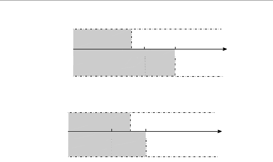
Comparison of Reimbursement Schemes: FFS vs BP Online Appendices
BP
Λ
FFS
Partial Coverage ˆµ
f
= ˜µ
f
Partial Coverage
ˆµ
b
= ˜µ
b
0
Full Coverage
˜
λ(˜r
b
)
Full Coverage ˆµ
f
= ¯µ
˜
λ(µ
o
)
˜
λ(˜r
f
)
II: ˆµ
b
= ¯µ
I: ˆµ
b
= µ
o
(a) t <
¯
t or/and B <
¯
B; ¯µ = max{µ :
˜
λ(µ) = Λ}
BP
0
Λ
FFS
Partial Coverage ˆµ
f
= ˜µ
f
I: ˆµ
b
= µ
o
Partial Coverage ˆµ
b
= ˜µ
b
II: ˆµ
b
= ¯µ
˜
λ(˜r
b
)
˜
λ(˜r
f
)
Full Coverage ˆµ
f
= ¯µ
Full Coverage
˜
λ(µ
o
)
(b) t ≥
¯
t and B ≥
¯
B; ¯µ = max{µ :
˜
λ(µ) = Λ}
Figure 3: The Comparison of the Equilibrium Outcomes: FFS vs BP
As illustrated in Figure 3, when Λ ≥ max{
˜
λ(˜r
f
),
˜
λ(µ
o
)}, ˆµ
b
(ˆr
b
) = ¯µ and ˆµ
f
(ˆr
f
) = ˜µ
f
(˜r
f
).
In this case, the first statement of Proposition B7 implies that the results for the case under
which the potential patients are partially covered uner both the FFS and BP schemes still
hold. That is, the BP scheme dominates the FFS scheme in terms of the service quality and
the patient welfare, while the FFS scheme is better in terms of the congestion level. However,
when
˜
λ(˜r
f
) <
˜
λ(µ
o
) and Λ ∈ [
˜
λ(˜r
f
),
˜
λ(µ
o
)], ˆµ
b
(ˆr
b
) = µ
o
(see Figure 3(a)). Then the second
statement of Proposition B7 implies that if the potential arrival rate Λ is relatively large
(i.e., Λ ∈ [
¯
Λ,
˜
λ(µ
o
)]), the results for the case under which the potential patients are partially
covered uner both the FFS and BP schemes hold. While if the potential arrival rate Λ
is relatively small (i.e., Λ ∈ [
˜
λ(˜r
f
),
¯
Λ]), the results for the case under which the potential
patients are fully covered uner both the FFS and BP schemes hold.
Proof of Propositions in Appendix B
Proof of Proposition B3. When
˜
λ(˜r
f
) < Λ, the results given in Proposition 2 are feasible.
Therefore, ˆr
f
= ˜r
f
and ˆµ
f
(ˆr
f
) = ˜µ
f
(˜r
f
). When
˜
λ(˜r
f
) ≥ Λ, the results under the partial
coverage scenatio are infeasible. The health care system will end up with the full coverage in
equilibrium. Recall that the patient welfare under the full coverage is independent of r
f
; see
15

Comparison of Reimbursement Schemes: FFS vs BP Online Appendices
(32). Therefore, the patient welfare remains the same for any given r
f
under the full coverage.
However, the funder will not be more generous than it has to be. Therefore, it will choose
the smallest feabile reimbursement rate. We next show that ˆr
f
, where ˜µ
f
(ˆr
f
) = ¯µ, is the
smallest one in the feasible set of the funder’s problem under the full coverage. According to
Proposition B1, the HCP’s optimal service rate ¯µ under the full coverage satisfies
˜
λ(¯µ) = Λ.
Since
˜
λ(ˆr
f
) =
˜
λ(¯µ) = Λ, and
˜
λ(r
f
) is increasing in r
f
, ˆr
f
is the smallest one that satisfies
the full coverage requirement. Furthermore, because
˜
λ(ˆr
f
) = Λ ≤
˜
λ(˜r
f
), ˜r
f
≥ ˆr
f
. Thus,
ˆr
f
˜
λ(ˆr
f
) ≤ ˜r
f
˜
λ(˜r
f
) = B, which implies that ˆr
f
also satisfies the budget constraint (33).
Therefore, ˆr
f
is the feasible solution under the full coverage scenario. As ˆr
f
is the smallest
one that satisfies the full coverage requirement, it is also the smallest one in the feasible set
of the funder’s problem under the full coverage.
Proof of Proposition B6. When
˜
λ(˜r
b
) < Λ, the results given in Proposition 2 are feasi-
ble. Therefore, ˆr
b
= ˜r
b
and ˆµ
b
(ˆr
b
) = ˜µ
b
(˜r
b
). When
˜
λ(˜r
b
) ≥ Λ, the results under the partial
coverage are infeasible. The health care system will end up with the full coverage in equi-
librium. As the patient welfare under the full coverage is independent of r
b
(see (38)), the
patient welfare remains the same for any given feasible r
b
under the full coverage. However,
the funder will not be more generous than it has to be. Therefore, under the full coverage it
will choose the smallest feasible reimbursement rate. We next show that when Λ ≤
˜
λ(˜r
b
), ˆr
b
,
where ˜µ
b
(ˆr
b
) = ¯µ, is the smallest feasible reimbursement rate. Since
˜
λ(ˆr
b
) =
˜
λ(¯µ) = Λ and
˜
λ(r
b
) is increasing in r
b
, ˆr
b
is the smallest one that satisfies the full coverage requirement.
Furthermore, as
˜
λ(ˆr
b
) = Λ ≤
˜
λ(˜r
b
), ˆr
b
≤ ˜r
b
. Thus, ˆr
b
˜
λ(ˆr
b
) ≤ ˜r
b
˜
λ(˜r
b
) = B, which implies that
ˆr
b
also satisfies the budget constraint (39). As ˆr
b
is the smallest one that satisfies the full
coverage requirement, it is also the smallest one in the feasible set of the funder’s problem
under the full coverage.
Proof of Proposition B7. When
˜
λ(˜r
f
) < Λ ≤
˜
λ(˜r
b
), the potential patients are partially
covered under the FFS scheme and are fully covered under the BP scheme. We first consider
the case when
˜
λ(˜r
b
) ≥ Λ >
˜
λ(˜r
f
) ≥
˜
λ(µ
o
). From Propositions B3 and B6, we know that
in equilibrium, ˆµ
f
(ˆr
f
) = ˜µ
f
(˜r
f
), ˆµ
b
(ˆr
b
) = ¯µ, and
ˆ
λ(ˆr
f
) =
˜
λ(˜r
f
) < Λ =
ˆ
λ(ˆr
b
). Because
˜
λ(µ) is unimodal in µ, ¯µ is the larger root of
˜
λ(µ) = Λ,
d
˜
λ(˜µ
f
(˜r
f
))
dµ
< 0 (shown in the
proof of Proposition 3) and
˜
λ(˜r
f
) ≤ Λ, ¯µ < ˜µ
f
(˜r
f
). Hence, δ(ˆr
b
) < δ(ˆr
f
). Since both
W (µ) and T (µ) are decreasing in µ (see (26)), W (ˆr
f
) = W(˜r
f
) < W(¯µ) = W(ˆr
b
) and
T (ˆr
f
) = T (˜r
f
) < T (¯µ) = T (ˆr
b
). As n(µ) increases in µ, n(ˆr
b
) < n(ˆr
f
). When patients are
fully covered, U(Λ, ˆµ
b
(ˆµ
b
)) > 0. Based on (14) and (38), we have S(ˆr
f
) = −β(Λ − ˜µ
f
(˜r
f
)) <
0 < Λ · U(Λ, ˆµ
b
(ˆµ
b
)) = S(ˆr
b
).
We next consider the scenario
˜
λ(˜r
f
) <
˜
λ(µ
o
). First, when
˜
λ(˜r
b
) ≥ Λ >
˜
λ(µ
o
), from
Propositions B3 and B6, ˆµ
f
(ˆr
f
) = ˜µ
f
(˜r
f
), ˆµ
b
(ˆr
b
) = ¯µ, and
ˆ
λ(ˆr
f
) =
˜
λ(˜r
f
) < Λ =
ˆ
λ(ˆr
b
).
16

Comparison of Reimbursement Schemes: FFS vs BP Online Appendices
Similar to the above analysis, we can show that δ(ˆr
b
) < δ(ˆr
f
), W(ˆr
f
) < W (ˆr
b
), T(ˆr
f
) < T (ˆr
b
)
and S(ˆr
f
) < S(ˆr
b
).
When Λ ∈ [
˜
λ(˜r
f
),
˜
λ(µ
o
)], utilizing Propositions B3 and B6 again, we have ˆµ
f
(ˆr
f
) =
˜µ
f
(˜r
f
), ˆµ
b
(ˆr
b
) = µ
o
,
ˆ
λ(ˆr
f
) =
˜
λ(˜r
f
) < Λ =
ˆ
λ(ˆr
b
). Because ¯µ is the larger solution of
˜
λ(µ) = Λ,
˜
λ(µ) is unimodal in µ and Λ ≤
˜
λ(µ
o
), µ
o
< ¯µ. We have shown above that
¯µ < ˜µ
f
(˜r
f
). Thus, ˆµ
b
(ˆr
b
) = µ
o
< ˜µ
f
(˜r
f
) = ˆµ
f
(ˆr
f
) and δ(ˆr
b
) < δ(ˆr
f
). Based on (14) and
(38), we have S(ˆr
f
) = −β(Λ − ˜µ
f
(˜r
f
)) < 0 < Λ · U(Λ, ˆµ
b
(ˆµ
b
)) = S(ˆr
b
).
Finally, we show that there exists a
¯
Λ such that T (ˆr
b
) < T (ˆr
f
) iff Λ <
¯
Λ. First, because
potential patients are fully covered under the BP scheme but are partially covered under the
FFS scheme, from (6) and (26), we get
T (ˆr
b
) = T (Λ, ˆµ
b
(ˆr
b
)) = T (Λ, µ
o
) =
1
o(µ
o
) − Λ
,
T (ˆr
f
) = T (
˜
λ(˜r
f
), ˜µ
f
(˜r
f
)) =
R
θ
−
t
θ(1 − δ(˜r
f
))
,
where T (ˆr
b
) is increasing in Λ while T (ˆr
f
) is independent of Λ. Therefore, if there exist Λ
1
and Λ
2
such that T (ˆr
b
) = T (Λ
1
, ˆµ
b
(ˆr
b
)) > T (ˆr
f
) and T (ˆr
b
) = T (Λ
2
, ˆµ
b
(ˆr
b
)) < T (ˆr
f
), then
there must exist a
¯
Λ such that T(ˆr
b
) < T (ˆr
f
) iff Λ <
¯
Λ. Denote Λ
1
=
˜
λ(µ
o
) and Λ
2
=
˜
λ(˜r
f
).
Then, when Λ = Λ
1
, we can show that
T (ˆr
b
) = T (
˜
λ(µ
o
), µ
o
) =
R
θ
−
t
θ(1 − δ(µ
o
))
>
R
θ
−
t
θ(1 − δ(˜r
f
))
= T (ˆr
f
),
where the inequality is due to that δ(µ) is increasing in µ and µ
o
< ˜µ
f
(˜r
f
). When Λ = Λ
2
,
based on (6) and (8), we can show that
T (ˆr
f
) =
1
o(˜r
f
) −
˜
λ(˜r
f
)
>
1
o(µ
o
) −
˜
λ(˜r
f
)
= T (
˜
λ(˜r
f
), ˆµ
b
(ˆr
b
)) = T (ˆr
b
),
where the inequality is due to that o(µ) achieves its maximum at µ
o
. We thus complete the
proof.
17
