
Integrated M.Sc. Physics
Laboratory Manual
Dr. S. Shailajha
Dr. S. Arunavathi
Department of Physics
Manonmaniam Sundaranar University
Tirunelveli – 627 012
2020
I
PREFACE
The purpose of the laboratory manual is the long felt need of the students
and teachers for a single book that deals with experiments in Physics for
undergraduate students. The book will be extremely useful for the students of
Physics major and also for allied students and ensure that they master the lab
skills necessary to be competitive in the job market. The book is suitable for
all colleges coming under universities or under autonomous stream.
The Physics part of the book covers most of the experiments under Heat
and Electricity, Basic Electronics, Optics, Digital electronics and General
experiments which the students are expected to do in the span of three years.
All fundamental experiments in Physics such as digital circuits and
electronic circuits are included in this part of the book. Finally, some basic
assembly language programs of ‘C’ are also given with simple algorithm.
We hope that this book will be well received by both the students and
Professors.
Suggestions for improvement from Professors and students will be
appreciated.
Authors
II
ACKNOWLEDGEMENTS
We take immense pleasure in thanking MHRD, Pandit Madan Mohan Malavia
National mission on Teachers and Teaching (PMMMNMTT), School of Education under
the project budget head for sanctioning the fund to prepare this Laboratory Manual.
We express our sincere thanks to Dr. B. William Dharma Raja for selecting our
proposal and giving an opportunity to do the work.
We wish to extend our thanks to Professor & Head and other colleagues from the
Department of Physics, M.S. University for their kind support to finish this work.
We wish to acknowledge and thank to Dr. M.Veera Gajendra Babu, Assistant
Professor and Mrs. M.S. Kairon Mubina, Mr. R. Sankaranarayanan, Research scholars and
C.S. Chaithra, A.S. Abarna, E. Esakki Ramesh who are the students of our Department for
their moral support which helped me to accomplish this work successfully.
We wish to thank the students of Physics who have been insisting on a book of this
nature.
We extremely grateful to DTP workers for the neat and clear diagrams throughout
this book.
We also express our sincere gratitude to Printers and Publishers Pvt. Ltd., for
entrusting the work of this magnitude to us.
Authors
III
CONTENTS
PRACTICAL-I: General Experiments
1. RIGIDITY MODULUS – TORSIONAL PENDULUM ....................................................... 1
2. YOUNG’S MODULUS – NON UNIFORM BENDING OPTIC LEVER ........................... 4
3. YOUNG’S MODULUS CANTILEVER PIN AND MICROSCOPE ................................... 7
4. NEWTON LAW OF COOLING ......................................................................................... 10
5. DETERMINATION OF FREQUENCY OF AN AC SOURCE USING SONOMETER –
BRASS WIRE ..................................................................................................................... 13
6. TORSIONAL PENDULUM- IDENTICAL MASSES MOMENT OF INERTIA – RIGIDITY
MODULUS ......................................................................................................................... 15
7. YOUNGS MODULUS PIN AND MICROSCOPE – NON-UNIFORM BENDING ......... 17
8. DETERMINATION OF ‘G’ BY COMPOUND PENDULUM .......................................... 20
9. VISCOSITY OF A LIQUID – CONSTANT PRESSURE HEAD METHOD.................... 22
PRACTICAL-II: Optics
1. DISPERSIVE POWER OF THE PRISM ............................................................................ 25
2. DIFFRACTION GRATING – NORMAL INCIDENCE .................................................... 29
3. FOCAL LENGTH OF CONCAVE LENS .......................................................................... 34
4. FOCAL LENGTH OF CONVEX LENS ............................................................................ 38
5. AIR WEDGE ....................................................................................................................... 43
6. REFRACTIVE INDEX OF A CONVEX LENS – NEWTON’S RING ............................. 46
7. REFRACTIVE INDEX OF THE MEDIUM – HOLLOW PRISM .................................... 49
8. SPECTROMETER – I-D CURVE ...................................................................................... 53
9. SPECTROMETER GRATING – OBLIQUE INCIDENCE ............................................... 56
10. SPECTROMETER – SMALL ANGLED PRISM .............................................................. 60
11. LIQUID LENS – REFRACTIVE INDEX OF A LIQUID .................................................. 63
12. FABRY PEROT INTERFEROMETER .............................................................................. 67
13. FRESNEL’S BIPRISM SPECTROMETER ....................................................................... 70
IV
PRACTICAL-III: Heat and Electricity
1. POTENTIOMETER CALIBRATION OF VOLTMETER (LOW RANGE) –
STANDARDISATION ....................................................................................................... 74
2. POTENTIOMETER CALIBRATION OF AMMETER ..................................................... 78
3. SPECIFIC HEAT CAPACITY OF WATER ...................................................................... 82
4. THERMAL CONDUCTIVITY BAD CONDUCTOR (CARD BOARD) – LEE’S DISC
METHOD ............................................................................................................................ 85
5. THERMAL CONDUCTIVITY BAD CONDUCTOR (GLASS) – LEE’S DISC METHOD89
6. SPECIFIC HEAT OF SOLIDS ........................................................................................... 94
7. DE SAUTY BRIDGE CAPACITORS – SERIES AND PARALLEL ................................ 98
8. CAREY – FOSTER’S BRIDGE – COIL RESISITANCE AND SPECIFIC RESISITANCE
........................................................................................................................................... 104
9. FIGURE OF MERIT OF CHARGE – BALLISTIC GALVANOMETER ....................... 109
10. COMPARISON OF EMF’S USING BALLISTIC GALVANOMETER ......................... 112
11. POTENTIOMETER MEASUREMENT OF RESISTANCE............................................ 115
12. BALLISTIC GALVANOMETER – COMPARISON OF CAPACITANCE ................... 118
13. OWEN’S BRIDGE – INDUCTANCES IN SERIES AND PARALLEL ......................... 121
14. LCR-SERIES CIRCUIT .................................................................................................... 125
15. MEASUREMENT OF INDUCTANCE USING BALLISTIC GALVANOMETER ....... 128
PRACTICAL-IV: Electronics
1. DUAL REGULATED POWER SUPPLIES USING IC'S ................................................ 132
2. HIGH PASS AND LOW PASS FILTER CIRCUIT ......................................................... 134
3. TRANSISTOR CHARACTERISTICS ............................................................................ 137
4. INTEGRATOR .................................................................................................................. 140
5. DIFFERENTIATOR ......................................................................................................... 142
6. CLIPPERS USING DISCRETE COMPONENTS ............................................................ 144
7. BAND PASS FILTER CIRCUIT ...................................................................................... 148
8. BRIDGE RECTIFIER USING DIODES .......................................................................... 150
9. CLIPPER USNG IC 741 ................................................................................................... 152
10. ZENER DIODE CHARACTERISTICS ............................................................................ 155
V
PRACTICAL-V: Digital Electronics and Computer Programming
1. VERIFICATION OF LOGIC GATES USING IC'S ......................................................... 159
2. CONSTRUCTION OF LOGIC GATES USING DISCRETE COMPONENTS .............. 162
3. REALIZATION OF LOGIC GATES USING NAND ...................................................... 164
4. BINARY ADDER & SUBTRACTOR .............................................................................. 166
5. VERIFICATION OF BOOLEAN LAWS ......................................................................... 169
6. WRITE A 'C' PROGRAM TO FIND THE LARGEST AND SMALLEST NUMBER IN A
SET OF NUMBERS ......................................................................................................... 171
7. WRITE A 'C' PROGRAM TO CHECK WHETHER GIVEN STRING IS PALINDROME
OR NOT ............................................................................................................................ 173
8. WRITE A 'C' PROGRAM TO FIND THE PRIME NUMBER ........................................ 174
9. WRITE A C PROGRAM TO GENERATE FIBONACCI SERIES ................................. 175
10. WRITE A 'C' PROGRAM TO FIND THE SUM, AVERAGE AND STANDARD
DEVIATION FOR THE GIVEN SET OF NUMBERS .................................................... 176
PRACTICAL-I
General Experiments

Laboratory manual
1 | P a g e
1. RIGIDITY MODULUS – TORSIONAL PENDULUM
AIM
To determine the rigidity modulus of the given wire by using torsional pendulum.
APPARATUS REQUIRED
Torsional pendulum, Circular disc, wire, screw gauge, stopwatch.
FORMULA
η =
I =
MR
2
η - the Rigidity modulus (Nm
-2
)
I - Moment of inertia (Kg m
2
)
r - Radius of the wire (m)
R - Radius of the disc (m)
L = Length of the wire (m)
M = Mass of the disc. (m)
THEORY
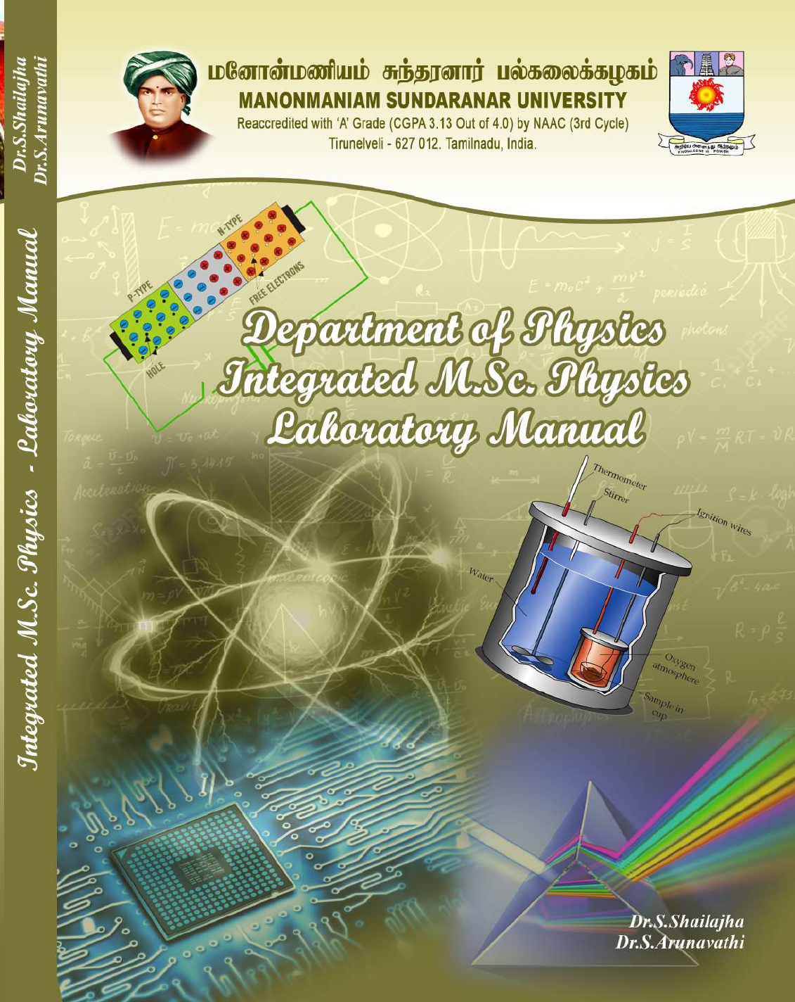
Torsional pendulum consists of a metal wire clamped to a rigid support at one end and carries
a heavy circular disc at the other end. When the suspension wire of the disc is slightly twisted, the
disc at the bottom of the wire executes torsional oscillations such that the angular accelerations of
the disc is directly proportional to angular displacement and the oscillations are simple harmonic.
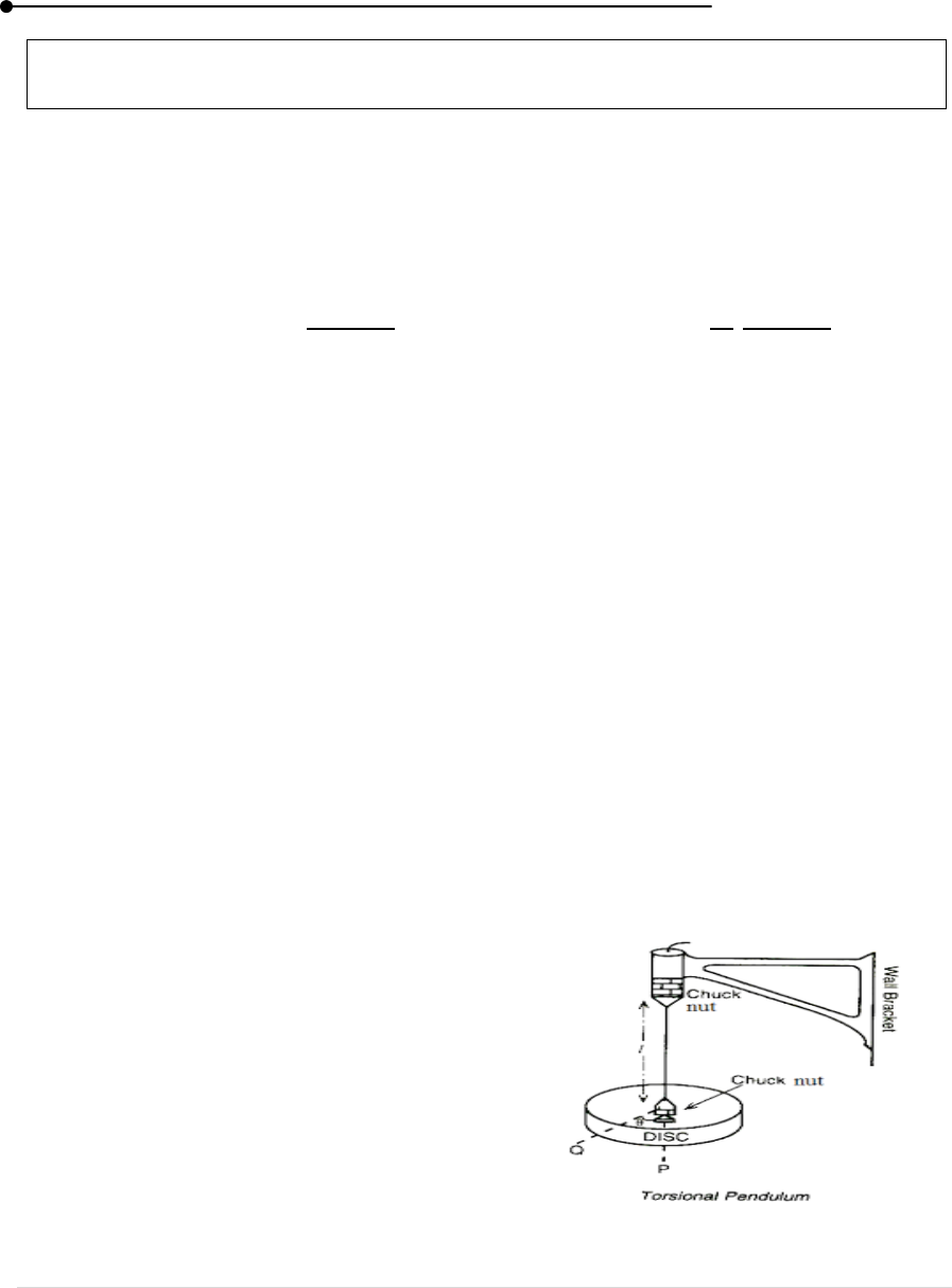
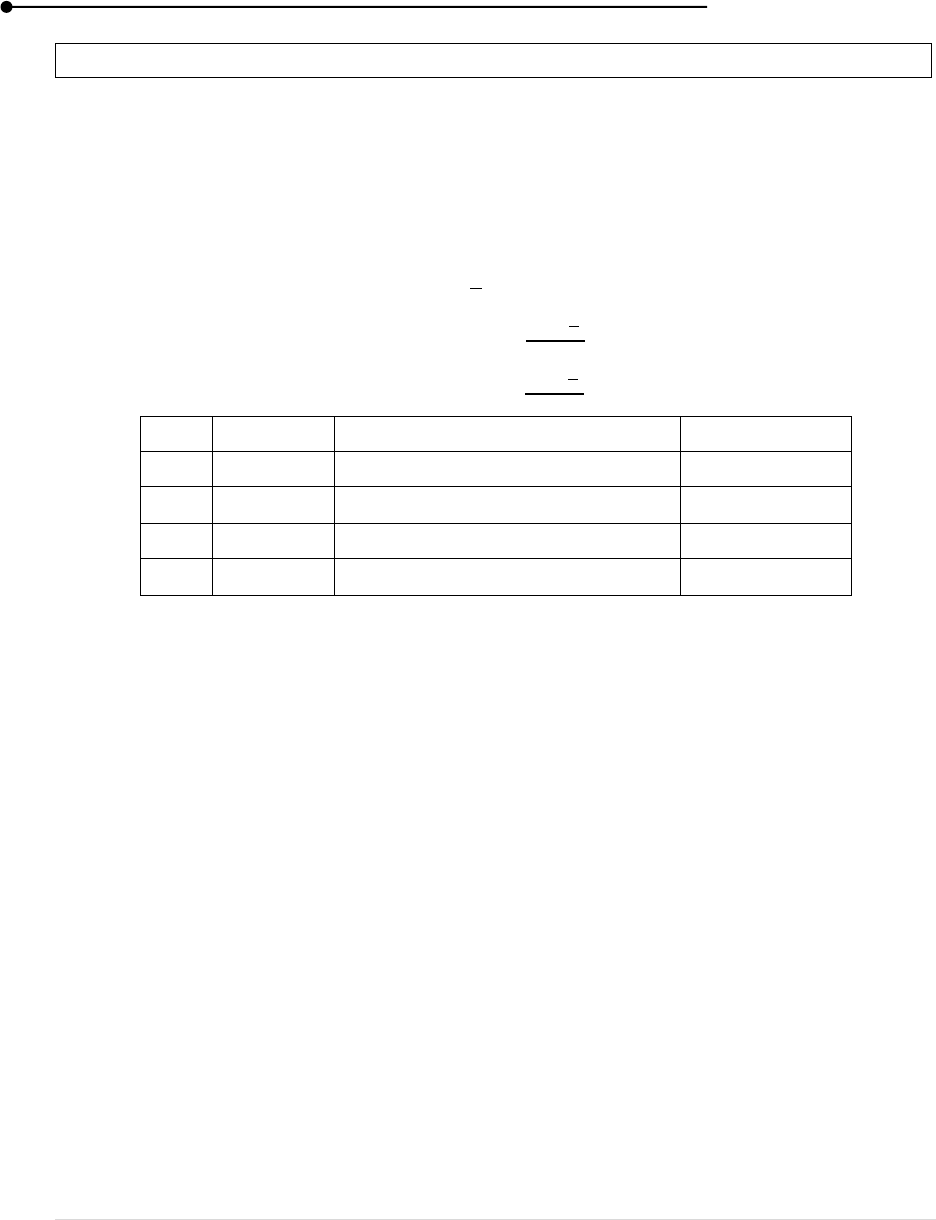
PROCEDURE
One end of a long uniform wire is clamped by a vertical chuck, whose rigidity modulus is
to be determined. The lower end, a heavy uniform circular disc is attached by another chuck. The
length of the suspension wire is fixed to 60 cm. The suspended disc is slightly twisted so that it
executes torsional oscillations. The few oscillations are omitted. By using stopwatch, the time taken
for 10 complete oscillations are noted. Two trials are taken. Then the mean time period T is found.
The above procedure is repeated for the different length of the pendulum wire. From the above values
of L and T calculate L/T
2
. The diameter of the wire is accurately measured at various places of the
wire. The circumference of the disc is measured and from that the radius of the disc is calculated.
The moment of inertia of the disc and the rigidity modulus of the wire are calculated using the given
formulae.
Laboratory manual
2 | P a g e
Figure 1: Torsional Pendulum
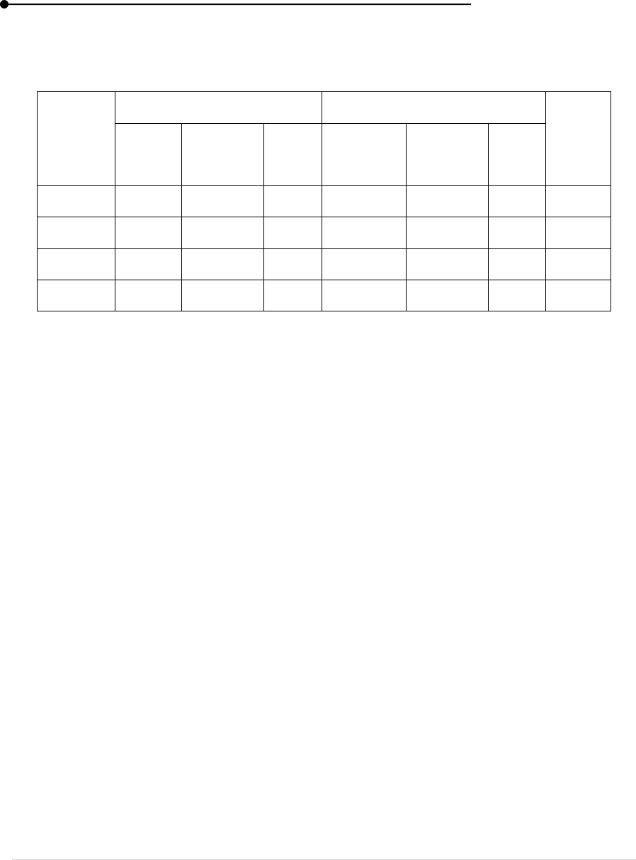
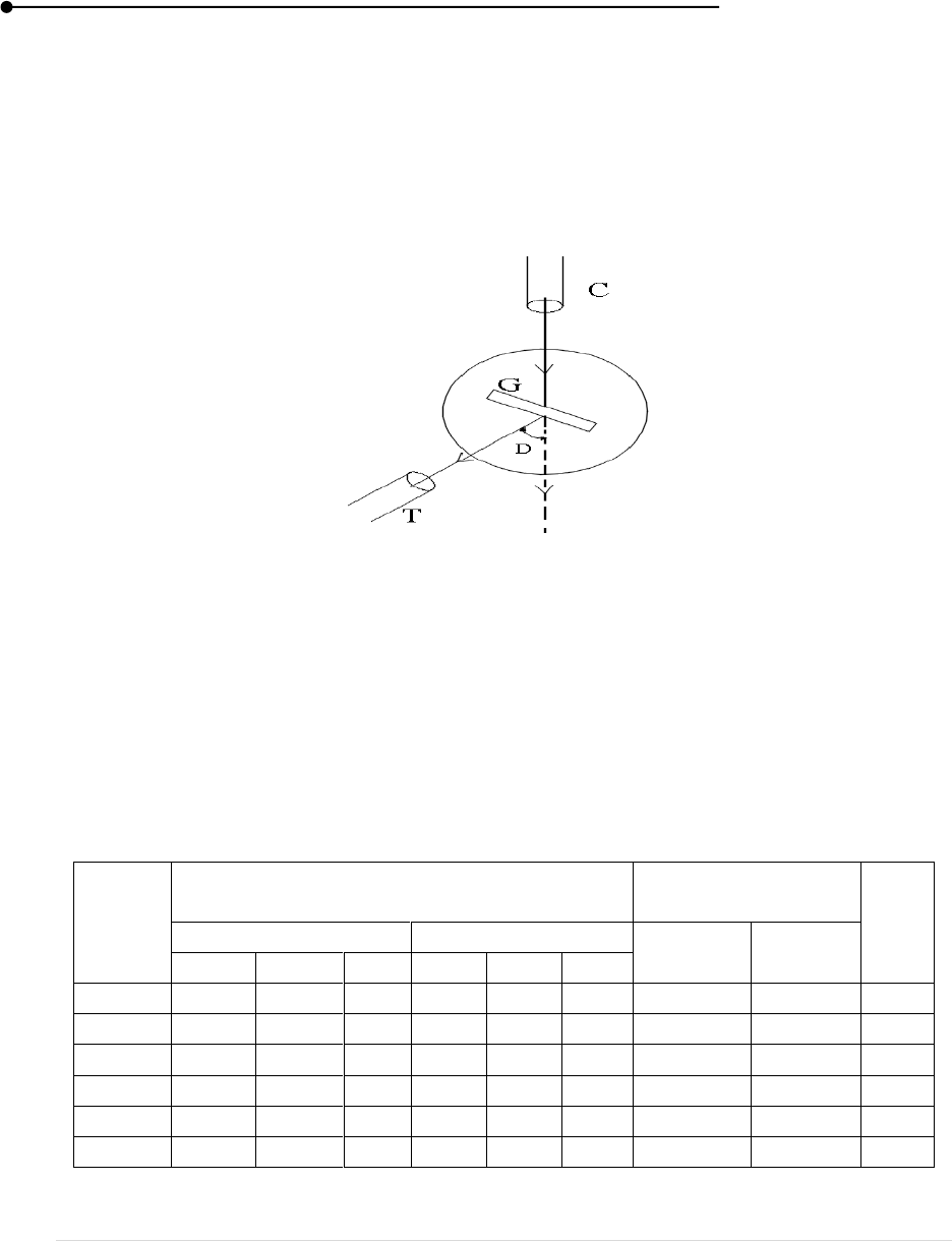
Table 1: To determine the time for oscillations for various length
S. No
Length
(cm)
For 10 Oscillations (sec)
Period
(sec)
T
2
(sec
2
)
L/T
2
(m sec
-2
)
T
1
T
2
Mean (T)
1
2
3
4
5
6
Mean = __________
Laboratory manual
3 | P a g e
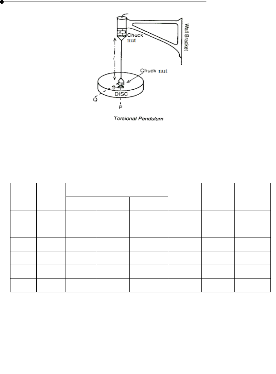
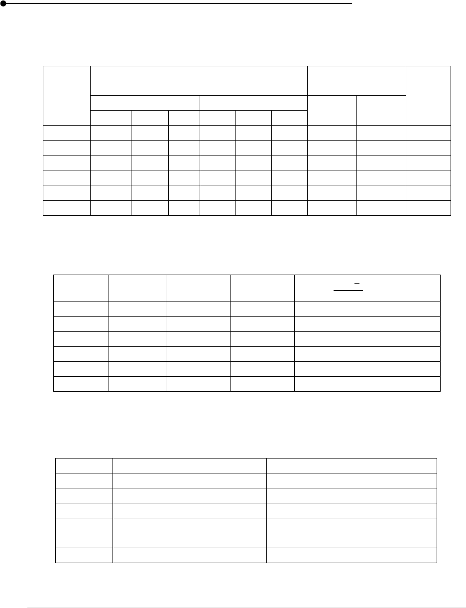
Table 2: To determine the radius of the suspension wire using screw gauge
L.C= _______ Z.E = ______ div Z.C = ______ mm
S.
No
Pitch
scale
Reading
(mm)
Head
Scale
coincide
(div)
Head Scale
Reading
(mm)
PSR +
HSR
(mm)
(PSR + HSR) ±
ZC
(mm)
1.
2.
3.
4.
5.
6.
Mean = _________
RESULT
Rigidity modulus of the given wire using torsional pendulum method is __________
Moment of inertia of the disc is ________
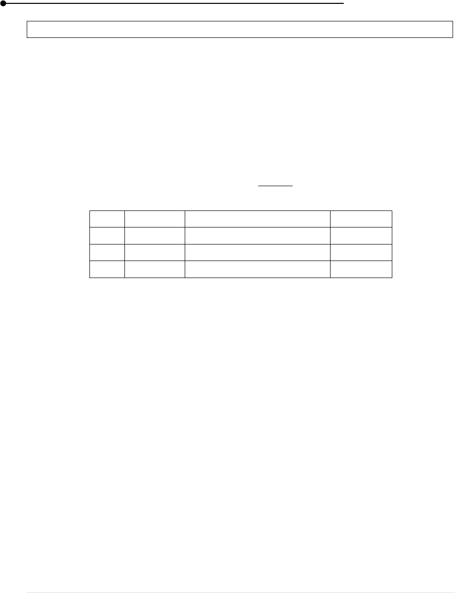
VIVA-VOCE
1. What is rigidity modulus
2. Explain torsional oscillation
3. What is least count
4. Define moment of Inertia.

Laboratory manual
4 | P a g e
2. YOUNG’S MODULUS – NON UNIFORM BENDING OPTIC LEVER
AIM
To determine the young’s modulus of the bar by non-uniform bending optic lever method.
APPARATUS REQUIRED
Rectangular bar, knife edge, weight hanger, slotted weights, scale and telescope, optic lever,
screw gauge, Vernier calliper.
FORMULA
m – Applied mass for the shift (kg)
g – acceleration due to gravity (ms
-2
)
l – Distance between knife edges. (m)
b – Breadth of the bar (m)
t – Thickness of the bar (m)
S – Mean change in scale reading (m)
X – Perpendicular distance of the front leg and the line joining the legs of the optic lever.
D- Distance between the scale and optic lever.
THEORY
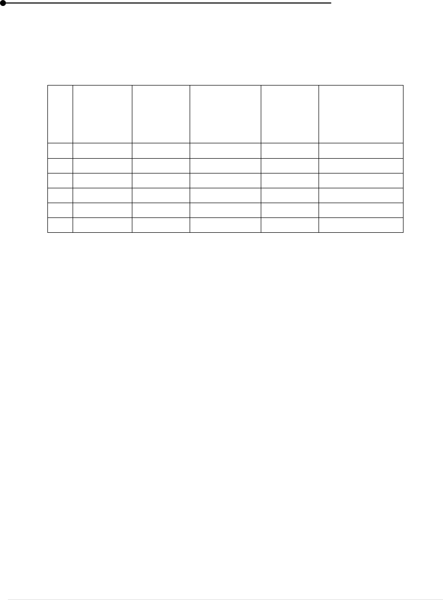
If a rectangular bar is placed symmetrically on two knife edges and a slotted weight are
suspended at middle of the bar, the bar experiences a bending downward. This is called non uniform
bending. By using this depression for a mass m, we can calculate the young’s modulus of the bar.
PROCEDURE
The experimental bar is symmetrically placed on two knife edges AA’ at a distance l (60cm)
apart. A weight hanger is suspended at the centre C of the bar. The optic lever PQR is placed on a
single leg P rests on the experimental bar at the midpoint and the other two legs Q and R rests on the
other meter scale. The scale and telescope are arranged at distance 1m front of the mirror of the optic
lever. Adjust the eyepiece of the telescope to view the crosswire without parallax. Focus the
telescope on the mirror, such that the image of scale can be seen through it. Align the mirror and
also height of the scale if necessary and make that sure no readings will go outside the range of the
Laboratory manual
5 | P a g e
scale while bar is loaded. By repeatedly loading and unloading the bar is brought into an elastic
mood.
Figure 2: Bending of Optic Lever
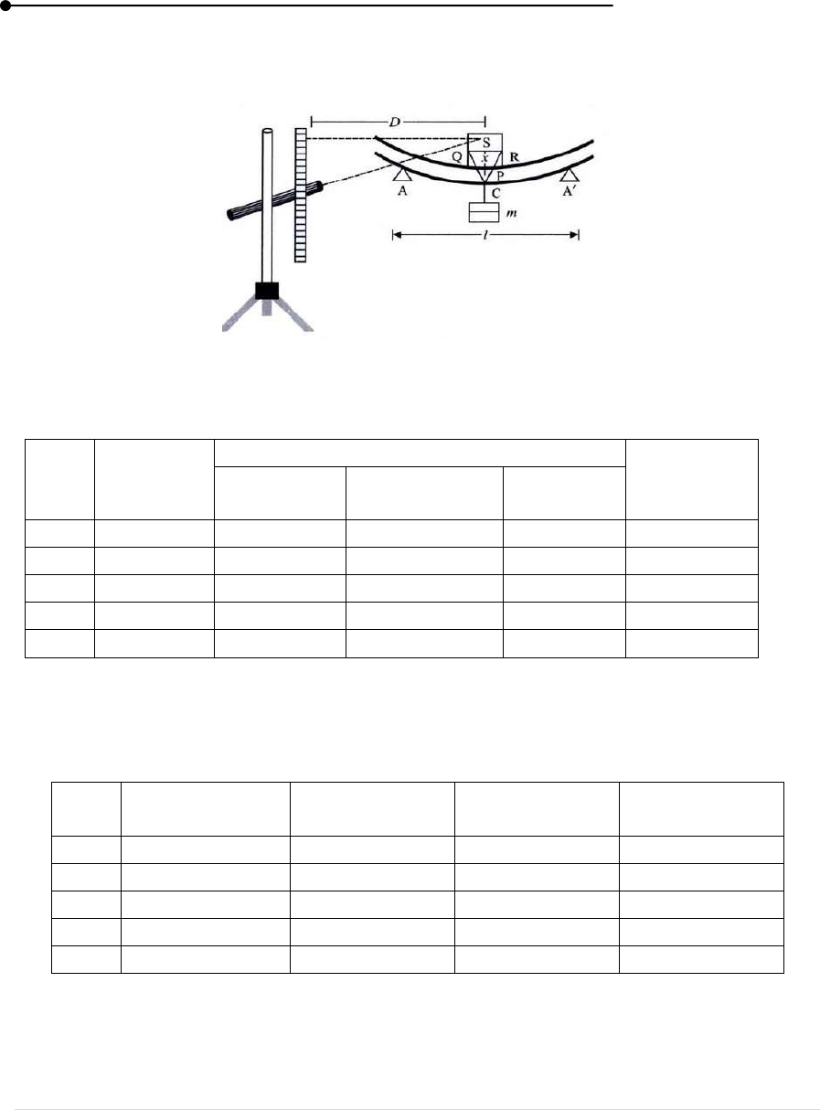
Table 3: To determine the shift for load
S. No
Load (Kg)
Reading of the Telescope (cm)
Shift for
Load
(cm)
Loading
Unloading
Mean
Table 4: To determine the breadth of the beam using Vernier calliper .
L.C = _______
S. No
Main Scale
Reading(cm)
Vernier Scale
Coincide (div)
V.S.C x L.C
(cm)
MSR + VSR
(cm)
1
2
3
4
5
Mean = __________
Laboratory manual
6 | P a g e
Table 5: To determine the thickness of the beam using screw gauge:
L.C= _______ Z.E = ______ div Z.C = ______ mm
S. No
Pitch scale
Reading
(mm)
Head Scale
coincide
(div)
Head Scale
Reading
(mm)
PSR + HSR
(mm)
(PSR + HSR)
± ZC
(mm)
1.
2.
3.
4.
5.
Mean = ________
RESULT
Young’s modulus of the given bar by non-uniform bending optic lever method is _______
VIVA-VOCE
1. What is non uniform bending?
2. What is Young’s modulus?
3. Explain what happens when loading is done non-uniformly.

Laboratory manual
7 | P a g e
3. YOUNG’S MODULUS CANTILEVER PIN AND MICROSCOPE
AIM
To determine the young’s modulus of the given bar using it’s the depression of its loaded
end which used as cantilever.
APPARATUS REQUIRED
Travelling microscope, Rectangular bar, Slotted weights, clamp, pin.
FORMULA
m – Applied mass for the shift (kg)
g – acceleration due to gravity (ms
-2
)
l – Distance between knife edges. (m)
b – Breadth of the bar (m)
t – Thickness of the bar (m)
y – Shift for the load
THEORY
Young’s modulus is defined as the ratio of the longitudinal stress over longitudinal strain,
in the range of elasticity the hook’s law holds (stress is directly proportional to strain). It is measure
of stiffness of elastic material.
PROCEDURE
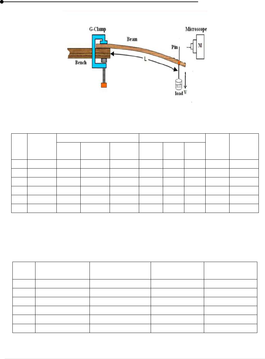
One end of the beam is rigidly clamped to the edge of the table using G-clamp. A pin ‘P’ is
fixed vertically at the free end on the bar. A loop of cotton string is attached to this end of the bar
and a weight hanger is suspended from it. A travelling microscope is focused on the tip of the pin as
shown in fig 3. A dead load without any slotted weight is attached to the hook. The microscope is
adjusted such that the horizontal cross wire coincides with the tip of the image of the pin and the
reading in the vertical scale is taken. Loads are added to the hanger is steps of 50 g, each time the
readings are noted on the vertical scale. A travelling microscope is focused on the tip of the pin as
shown in fig 3. These observations are also repeated while unloading in the same steps and the
readings are tabulated. The mean depression ‘y’ for a load ‘m’ is found from the tabulated readings.
The breath of the scale is measured using Vernier calliper and values are noted in Table 6. The
screw gauge is used to measure the thickness of the scale and noted in Table 8. The known values
are substituted in formula and young’s modulus ‘E’ is found.
Laboratory manual
8 | P a g e
Figure 3: Bending of Cantilever Beam
Table 6: To determine the shift for load of the given beam
S.
No
Load
(Kg)
Loading (cm)
Un Loading (cm)
Mean
(cm)
Shift
for load
(cm)
MSR
VSR
TR
MSR
VSR
TR
1.
W
2.
W + 50
3.
W + 100
4.
W + 150
5.
W + 200
6.
W + 250
Mean = _______
Table 7: To determine the breadth of the beam using Vernier calliper.
L.C = _______
S. No
Main Scale
Reading (cm)
Vernier Scale
Coincide (div)
V.S.C x L.C
(cm)
MSR + VSR
(cm)
1
2
3
4
5
6
Mean = __________
Laboratory manual
9 | P a g e
Table 8: To determine the thickness of the beam using screw gauge
L.C= _______ Z.E = ______ div Z.C = ______ mm
S. No
Pitch scale
Reading
(mm)
Head Scale
coincide
(div)
Head Scale
Reading
(mm)
PSR + HSR
(mm)
(PSR + HSR)
± ZC
(mm)
1.
2.
3.
4.
5.
6.
Mean = ________
RESULT
Young’s modulus of the given bar by using method cantilever pin and microscope is
_________
VIVA-VOCE
1. What is a cantilever
2. Explain positive and negative zero error
3. Give any two uses of finding the youngs modulus of the cantilever
Laboratory manual
10 | P a g e
4. NEWTON LAW OF COOLING
AIM
To verify newton’s law of cooling.
APPARATUS REQUIRED
A spherical calorimeter, stopwatch. Stand, a kettle.
THEORY AND FORMULA
The rate of the temperature change is proportional to the difference between the temperature
and its surroundings.
Rate of cooling α Mean difference of temperature
PROCEDURE
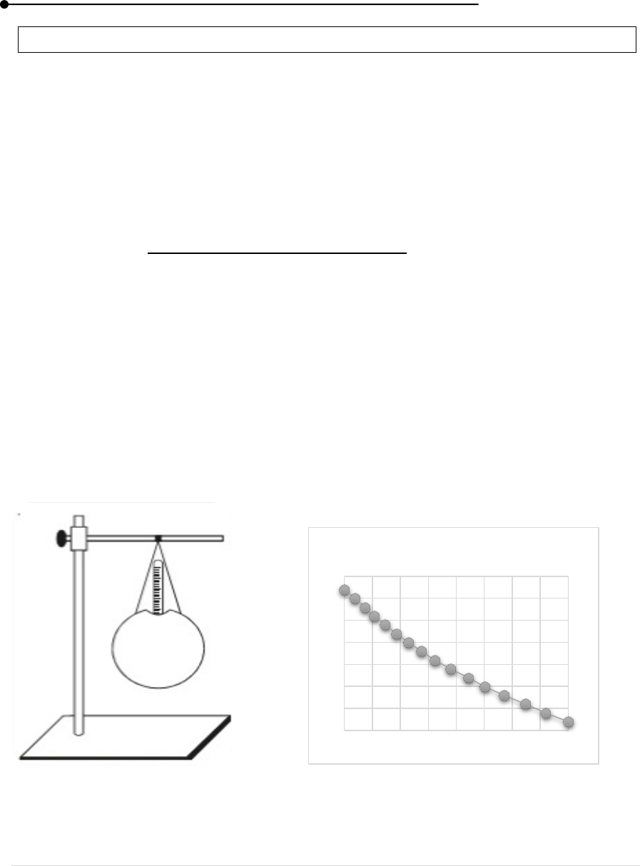
The copper calorimeter is filled with hot water of about 90ºC. Place the calorimeter in a
stand. Suspend the thermometer inside the hot water in the calorimeter from the clamp and stand
(Fig.4). Stir water continuously to make it cool uniformly, when the temperature of hot water falls
to 86ºC, start the stop watch. Note the stopwatch reading at every 2ºC of temperature fallen.
Continue the time temperature observation till temperature become 56ºC. Plot a graph between time
along X-axis and temperature along Y-axis. This graph is called cooling curve. The graph is an
exponential curve and it shows that the temperature falls quickly at the beginning and then slowly
as the difference of temperature goes on decreasing. This verifies Newton’s law of cooling.
Figure 4: Copper calorimeter Figure 5: Cooling Curve
54
59
64
69
74
79
84
89
0 200 400 600 800 1000120014001600
Temperature in c
Laboratory manual
11 | P a g e
Table 9: To tabulate the time for falling temperature 2ºC
Table 10: Verification of Newton’s law of cooling:
Laboratory Temperature, θ = ________
S.
No
Range of
Temperature
Time
taken to
fall by
2ºC
Rate of
Cooling
R= 2/t
Mean
Temperature
Excess
Temperature
(R/θ – θ
0
)
x 10
-4
)
1.
86-84
85
2
84-82
83
3
82-80
81
4
80-78
79
5
78-76
77
6
76-74
75
7
74-72
73
8
72-70
71
9
70-68
69
10
68-66
67
11
66-64
65
12
64-62
63
13
62-60
61
14
60-58
59
15
58-56
57
Temperature (ºC)
Time (Sec)
Temperature
(ºC)
Time (Sec)
86
70
84
68
82
66
80
64
78
62
76
60
74
58
72
56

Laboratory manual
12 | P a g e
RESULT
The rate of cooling linearly varies with the excess temperature. Thus newton law of cooling
is verified.
VIVA-VOCE
1. What is Newton’s law of cooling
2. State Newton’s law of cooling
3. The rate of cooling linearly varies with excess temperature why?
Laboratory manual
13 | P a g e
5. DETERMINATION OF FREQUENCY OF AN AC SOURCE USING SONOMETER
– BRASS WIRE
AIM
To determine the frequency of an AC source using sonometer.
APPARATUS REQUIRED
Sonometer, Brass wire, magnet, weight hanger with slotted weights, knife edges.
FORMULA
Where,
n – Frequency of the AC source (Hz)
T – Tension applied (Newton)
M – Applied mass (Kg)
l – Vibrating length (m)
m – Linear Density = πr
2
֩ρ (kg/m)
r – Radius of the wire (m)
THEORY
Basically, sonometer is a device based on the principle of resonance. It is used to verify the
laws of vibrations of stretched strings and to determine the frequency of tuning fork and AC source.
“When the frequency of the applied force is equal to the natural frequency of the body, the body
vibrates very large amplitude”.
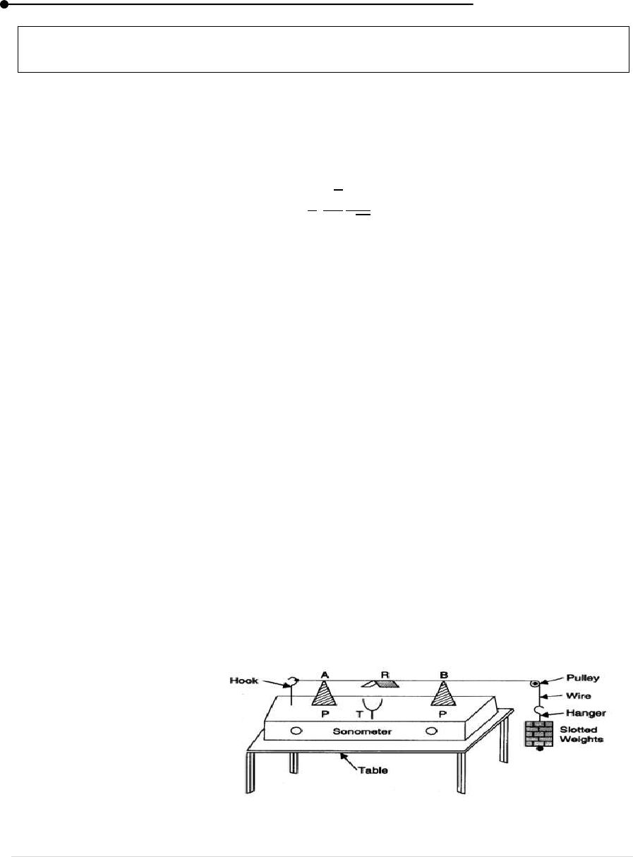
PROCEDURE
Place the sonometer on table. Attach a weight hanger at the free end of the string which
passes through the pully. Stretch the wire by loading a suitable maximum mass on the weight hanger.
The ends of the secondary of a transformer connected to the two ends A and B of the wire (Fig. 6).
The wire is set between the poles of a powerful horse shoe magnet or the opposite poles of two equal
bar magnets, so that the magnetic field is in a horizontal plane and at right angles to the length of the
wire. The light paper rider is placed on the wire between the bridges of the sonometer. The AC
supply is switched on. The wire begins to vibrate. Length between the two bridges is vibrating length.
By using the screw gauge determine the accurate radius of the brass wire and to calculate the linear
density m. By loading and
unloading the above procedure
will be repeated and to
calculate the square root of
tension for each vibrating
length. With this calculate the
frequency of AC mains.
Figure 6: Sonometer in Experimental Setup
Laboratory manual
14 | P a g e
Table 11: To determine the value of
S. No
Mass
(Kg)
Vibrating length (m)
T= mg
(Newton)
(Nm
-2
)
Loading
Unloading
Mean
1.
2.
3.
4.
5.
Mean = _________
Table 12: To determine the radius of the wire using screw gauge.
L.C= _______ Z.E = ______ div Z.C = ______ mm
S.
No
Pitch
scale
Reading
(mm)
Head
Scale
coincide
(div)
Head Scale
Reading
(mm)
PSR + HSR
(mm)
(PSR + HSR) ±
ZC
(mm)
1.
2.
3.
4.
5.
Mean = _________
RESULT
Frequency of given AC source by using sonometer is _________
VIVA-VOCE
1. Define frequency.
2. What is sonometer?
3. How does sonometer works?
Laboratory manual
15 | P a g e
6. TORSIONAL PENDULUM- IDENTICAL MASSES MOMENT OF INERTIA –
RIGIDITY MODULUS
AIM
To determine the moment of inertia of the given disc by torsional oscillations and to
calculate the rigidity modulus of the given material of the suspension wire.
APPARATUS REQUIRED
Circular disc, steel or brass wire, two identical masses, screw gauge.
FORMULA
Where,
T
0
– Time period without mass (sec)
I
0
– Moment of inertia of the disc (kg m
2
)
M – Mass of the disc (kg)
d
1
, d
2
– Distance from the centre of the disc to the centre of load. (m)
T
1
, T
2
– Time period with mass at a distance d
1
, d
2
respectively (sec)
η – Rigidity modulus (Pascal)
r – Radius of the suspension wire (m)
THEORY
Torsional pendulum consists of a metal wire clamped to a rigid support at one end one end
an carries a heavy circular disc at the other end, When the suspension wire of the disc is slightly
twisted, the disc at the bottom of the wire executes torsional oscillations such that the angular
acceleration of the disc is directly proportional to its angular displacement and the oscillations ae
simple harmonic.
PROCEDURE
One end of a long, uniform wire whose rigidity modulus is to be determined is clamped by
a vertical chuck. To the lower end, a heavy uniform circular dis is attached by another chuck. The
length of the suspension is l from top portion is fixed to a constant value say 80cm. The suspended
disc is slightly twisted so that it executes torsional
oscillations. The first few oscillations are omitted. By
using stopwatch, the time taken for 20 oscillations are
noted. Two trials are taken. Then the mean time period
T
0
is found. The above procedure is repeated for two
identical masses at a distance d
1
, d
2
from the centres of
the disc and T1, T
2
are found. The diameter of the wire
is accurately measured at various places along its length
with screw gauge. From this Rigidity modulus of the
wire can be calculated. Figure 7: Torsional Pendulum

Laboratory manual
16 | P a g e
Table 13: To determine the time for the oscillations for various masses
S.
No
Position of identical mass
Time taken for 20 oscillations
(sec)
Period (sec)
Trail 1
Trial 2
Mean
1.
Without Masses
2.
With a mass at a distance d
1
(T
1
)
3.
With mass at a distance d
2
(T
2
)
Table 14: To determine the radius of the suspension wire using screw gauge.
L.C= _______ Z.E = ______ div Z.C = ______ mm
S.
No
Pitch scale
Reading
(mm)
Head Scale
coincide (div)
Head Scale
Reading (mm)
PSR +
HSR
(mm)
(PSR + HSR)
± ZC (mm)
1.
2.
3.
4.
5.
6.
Mean = _________
RESULT
Moment of inertia of the disc is _________
Rigidity modulus of the disc is __________
VIVA-VOCE
1. What is moment of inertia?
2. Define Rigidity modulus.
3. How the torsional pendulum works?

Laboratory manual
17 | P a g e
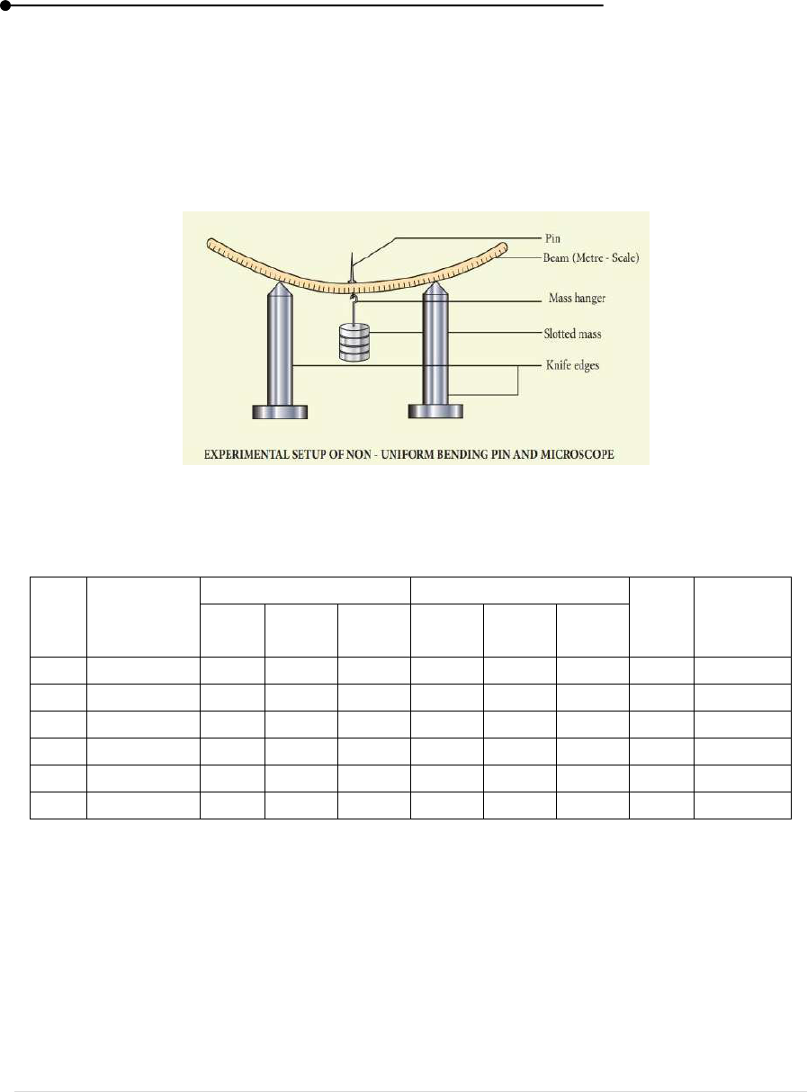
7. YOUNGS MODULUS PIN AND MICROSCOPE – NON-UNIFORM BENDING
AIM
To determine the young’s modulus of the given bar by using the method pin and microscope.
APPARATUS REQUIRED
A rectangular uniform cross section bar, travelling microscope, pin, slotted weights, screw
gauge, Vernier calliper.
FORMULA
Where,
E – Young’s modulus of the given bar (Pascal)
G – Acceleration due to gravity 9.8ms
-2
b – Breadth of the given bar (m)
t – Thickness of the given bar (m)
y – Elevation for the mass (m)
M – Loaded mass (kg)
THEORY
If a uniform cross section beam is placed on two knife edge and load is suspend at middle
of the bar, it bends. The load acting vertically downwards. The external bending couples must be
balanced by another equal and opposite couple shih comes into play inside the body dude to elastic
nature of the body. So, young’s modulus is measure of elasticity, equal to the ratio of the stress acting
on a substance to the strain produced.
PROCEDURE
The given beam is placed over the two knife edges (A & B) at a distance of 80 cm. A weight
hanger is suspended in middle of the bar. Since the load is applied at middle point of the beam, the
bending is non-uniform throughout the beam and the bending of the beam is called Non-Uniform
Bending. A pin is fixed vertically exactly at the centre of the beam. A travelling microscope is placed
in front of this arrangement. Taking the weight hangers alone as the dead load, the tip of the pin is
focused by the microscope and is adjusted in such a way that the tip of the pin just touches the
horizontal cross wire. The reading on the vertical scale of the traveling microscope is noted. Now,
equal weights are added on both the weight hangers, in steps of 50 grams. Each time the position of
Laboratory manual
18 | P a g e
the pin is focused and the readings are noted from the microscope. The procedure is followed until
the maximum load is reached. The same procedure is repeated by unloading the weight from both
the weight hanger in steps of same 50 grams and the readings are tabulated in the table 15. From the
readings, the mean of (M/y) is calculated. The thickness and the breadth of the beam are measured
using screw gauge and Vernier callipers respectively and are tabulated. By substituting all the values
in the given formula, the Young’s modulus of the given material of the beam can be calculated.
Figure 8: Experimental Setup of Non-Uniform Bending Pin and Microscope
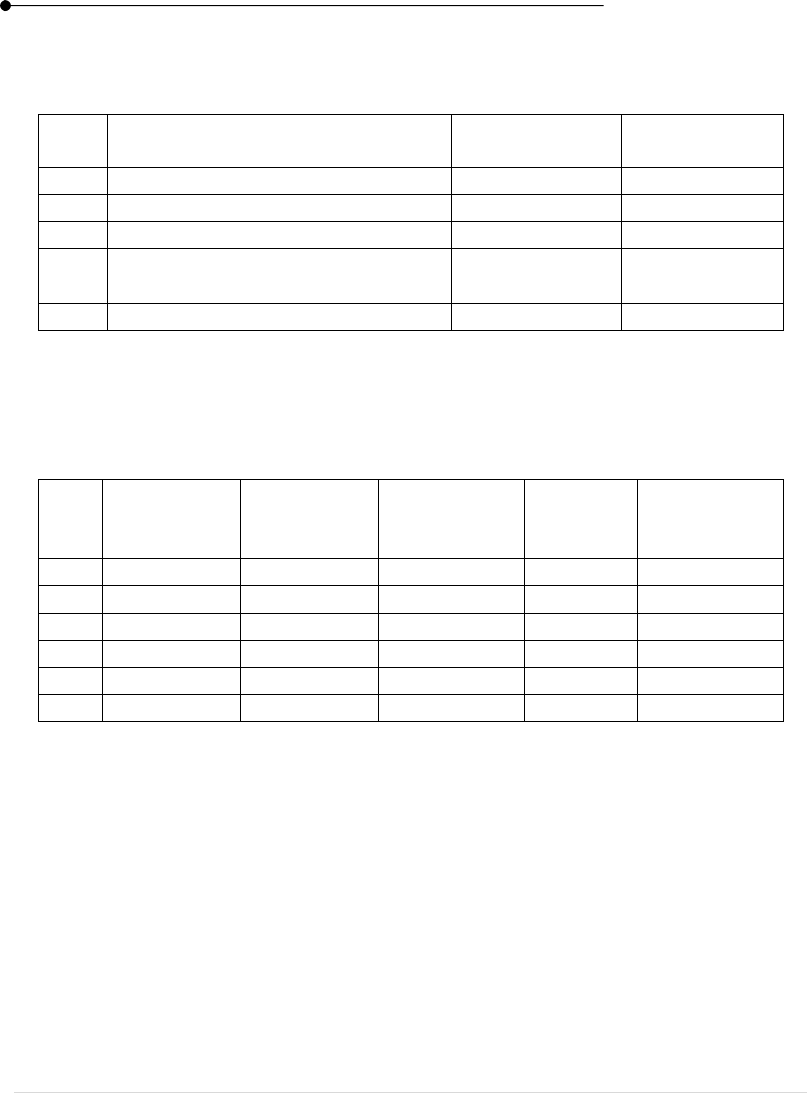
Table 15: To determine the shift for load of the given beam
S.
No
Load (Kg)
Loading (cm)
Un Loading (cm)
Mea
n
(cm)
Shift for
load
(cm)
MSR
VSR
TR
MSR
VSR
TR
1.
W
2.
W + 50
3.
W + 100
4.
W + 150
5.
W + 200
6.
W + 250
Mean = _______
Laboratory manual
19 | P a g e
Table 16: To determine the breadth of the beam using Vernier calliper
. L.C = ______
S. No
Main Scale
Reading (cm)
Vernier Scale
Coincide(div)
V.S.C x L.C
(cm)
MSR + VSR
(cm)
1
2
3
4
5
6
Mean = __________
Table 17: To determine the thickness of the beam using screw gauge
L.C= _______ Z.E = ______ div Z.C = ______ mm
S.
No
Pitch scale
Reading
(mm)
Head Scale
coincide (div)
Head Scale
Reading (mm)
PSR +
HSR (mm)
(PSR + HSR)
± ZC (mm)
1.
2.
3.
4.
5.
6.
Mean = _________
RESULT
Young’s modulus of the given bar using pin and microscope method is ____________
VIVA-VOCE
1. What is Young’s modulus?
2. When the thickness of the bar is increased what happens to the Young’s modulus of the
bar?
3. What happens to the Young’s modulus of the bar when length of the bar increases?
Laboratory manual
20 | P a g e
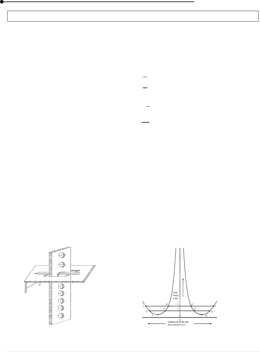
8. DETERMINATION OF ‘G’ BY COMPOUND PENDULUM
AIM
To determine the acceleration due to gravity, radius of gyration and moment of inertia of a
bar about an axis passing through the centre of gravity perpendicular to the plane of bar.
APPARATUS REQUIRED
Bar pendulum, Stopwatch, Pointer
FORMULA
Where
g – Acceleration due to gravity.
l – Length of equivalent simple pendulum
T – Period of oscillation corresponding to L in seconds.
THEORY
Any sinning rigid body true the rotate about a fixed horizontal axis is called a compound
pendulum. This point is located under a mass at a distance from the point traditionally called radius
of gyration which depends on mass distribution of the pendulum.
PROCEDURE
The compound pendulum bar pendulum AB is suspended by passing a knife edges through
the mass and a hole which is in the compound pendulum is suspended and determine the time for 20
oscillations. Above procedure is repeated for various point of suspension and draw a graph as shown.
Then calculate the value of l/T
2
. Then substitute all values in the given formula and determine the
acceleration due to gravity radius of gyration.
Figure 9: Compound Pendulum Figure 10: Model Curve
Laboratory manual
21 | P a g e
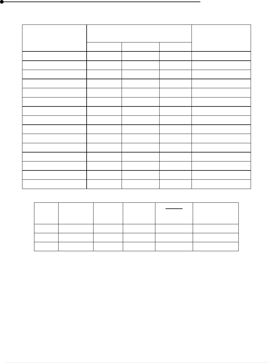
Table 18:
Distance of the hole
from its near
end(cm)
Time taken for 20 Oscillations
(Sec)
Period of
oscillations(Sec)
Trial 1
Trial 2`
Mean
5
10
15
20
25
30
35
40
45
45
40
35
.
.
5
Table 19:
S. No
Period
(sec)
AD
(cm)
BE
(cm)
(cm)
l/T
2
(10
-2
m/sec)
1.
2
3
Mean = ___________
RESULT
Acceleration due to gravity by using the method compound pendulum is ________
VIVA-VOCE
1. What is a compound pendulum?
2. What is period of oscillation?
3. State moment of inertia
4. What is radius of gyration?
Laboratory manual
22 | P a g e
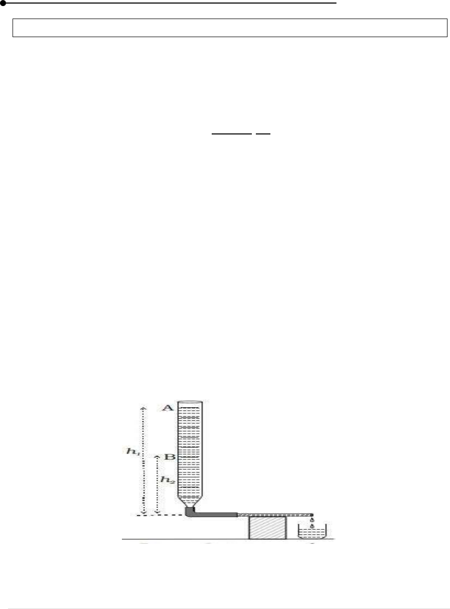
9. VISCOSITY OF A LIQUID – CONSTANT PRESSURE HEAD METHOD
AIM
To determine the co-efficient of water by constant pressure head method.
APPARATUS REQUIRED
Burette, Rubber tube, Capillary tube, stop clock.
FORMULA
Where,
η – Co-efficient of viscosity
ρ – Density of water (Kg/m
3
)
g – Acceleration due to gravity (ms
-2
)
h – Mean head Pressure (m)
v – Volume of water that flows through tube in‘t’ seconds
THEORY
The co-efficient of viscosity is the ratio of applied stress to the rate of straining change of
strain with time. It is measured in units of poise one poise equals one dyne per unit second.
PROCEDURE
Connect the capillary tube to burette by a rubber tube and arrange it as shown in the figure
11. Fill the liquid. The clip in the rubber tube is adjusted for a slow and steady flow of liquid into
the measuring jar. The heights from the centre of the capillary tube is measured. The experiment is
repeated for constant h at different time. The mean value of ht/v is calculated. The length of the
capillary tube is measured as l using a meter scale and the radius is measured using travelling
microscope.
Figure 11: Experimental Setup to Determine Viscosity of Liquid
Laboratory manual
23 | P a g e
Table 20: To determine the ht/v value.
Time of flow ‘t’
(Sec)
Volume of liquid
collected (10
-6
m
3
)
Ht/v
(10
-6
m
-2
s)
2
4
6
8
10
12
14
16
18
20
Table 21: To determine the radius of the capillary tube using travelling microscope
Mean = _________
RESULT
Co-efficient of water by constant pressure head method is _______
VIVA-VOCE
1. What is Co-efficient of viscosity
2. Explain the constant pressure head method
3. Give the co-efficient of viscosity of water.
Position of
Microscope
Microscope Reading (Cm)
Diameter
(cm)
Radius
(Cm)
Main
Scale
Reading
Vernier
Scale
Reading
Total
Reading

24 | P a g e
PRACTICAL-II
Optics

Laboratory manual
25 | P a g e
1. DISPERSIVE POWER OF THE PRISM
AIM
To determine the dispersive power of a prism using spectrometer.
APPARATUS REQUIRED
Spectrometer, Prism, Mercury Vapour Lamp etc.
FORMULA
The dispersive power of the prism is given by
where
Parameter
Explanation
Unit
Dispersive power of the prism
No unit
Refractive index for blue colour
No unit
Refractive index for green colour
No unit
Average refractive index
No unit
A
Angle of the prism
Deg.
Angle of minimum deviation for green colour
Deg.
Angle of minimum deviation for blue colour
Deg.
PRINCIPLE
The power of the medium to separate different colours of light by refraction.
Laboratory manual
26 | P a g e
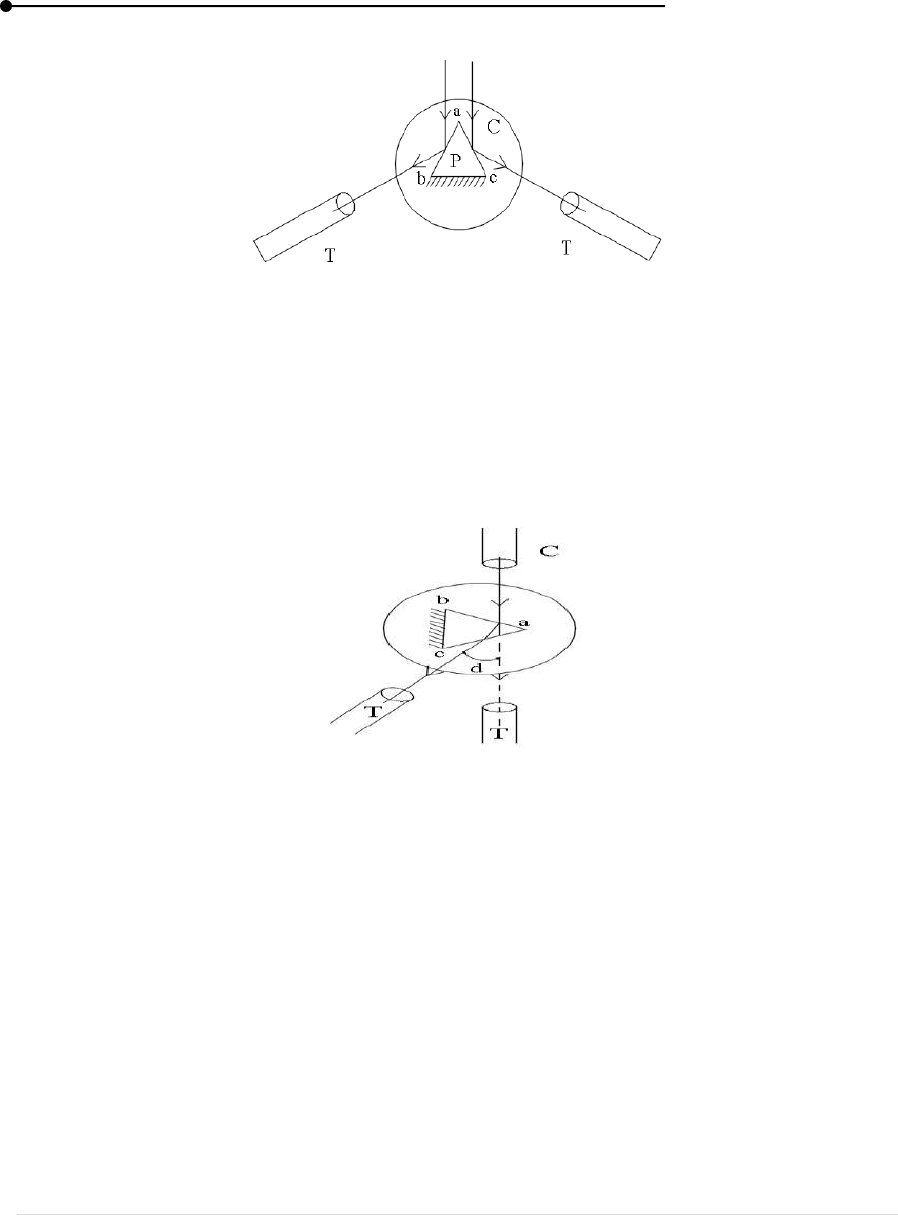
T Telescope ; C Collimator ; P Prism
Figure 12: Angle of prism
T Telescope ; C Collimator ; abc Prism
Figure 13: Minimum Deviation Geometry
PROCEDURE
(i) Adjustment of the collimator and the telescope
Level the prism table, telescope and collimator with sprit level such that telescope
axis and collimator axis intersect the principle vertical axis of the spectrometer. A
prism may be used for the purpose.
Focus the eye piece of the telescope on the cross wire by drawing it in (or) cut of the
telescope tube until the cross wire is seen closely.
Use Schuster’s method for focusing telescope and collimator for parallel rays.
Laboratory manual
27 | P a g e
(ii) Angle of the prism
Place a prism on the prism table, with grounded force towards the telescope.
Rotate the telescope towards left side
Fix the telescope where the slit coincides with cross wire of the eye piece and note
the Vernier reading
Do the same in right side
(iii) Finding angle of minimum deviation (D
m
)
Unblock the prism table for the measurement of the angle of minimum deviation
(d
m
) locate the image of the slit after refraction through the prism.
Keeping the image always in the field of view, rotate the prism table till the position
where the deviation of the image of the slit is smallest.
At this position, it will go backward, even when you keep rotating the prism table
in the same direction. Look both the telescope and the prism table and to use the
fine adjustment screw for finer settings. Note the angular position of the prism.
In this position is set for minimum deviation without disturbing the prism table,
remove the prism and turn the telescope (now unlock t), towards the direct rays from
the collimator. Note the scale reading of this position. The angle of minimum
angular deviation viz. D
m
is difference between the readings of these last two
settings.
Table 22: To find the Angle of Prism
Vernier – 1 (V
1
)
Vernier – 2 (V
2
)
MSR
VSR
TR
MSR
VSR
TR
Left (θ
1
)
Right (θ
2
)
θ = θ
1
- θ
2
Angle of the prism 2A =
A =
Laboratory manual
28 | P a g e
Table 23: To find the Angle of Minimum Deviation
Colour
of the
spectrum
Vernier A
Vernier B
Avg. D
Direct
reading
(R)
Minimum
deviation
(D)
D
m
=
(R-D)
Direct
reading
(R)
Minimum
deviation
(D)
D
m
=
(R-D)
Green
Blue
Violet
Red
RESULT
1. Dispersive power between blue and green is ________
2. Dispersive power between violet and red is _________
VIVA-VOCE
1. Define spectrometer.
2. Define refractive index.
3. Define dispersive power of a prism.
4. How does refractive index change with wavelength of light?
5. Does the deviation depend on the angle of prism?

Laboratory manual
29 | P a g e
2. DIFFRACTION GRATING – NORMAL INCIDENCE
AIM
To determine the wavelength of the prominent lines of mercury by a plane transmission
diffraction grating hence to find the dispersive power of the grating.
APPARATUS REQUIRED
Spectrometer, Plane Transmission Grating, Mercury Vapour Lamp, Spirit Level.
FORMULA
S. No.
Parameter
Explanation
Unit
1
Wavelength of spectral lines
m
2
Angle of diffraction
deg.
3
N
Lines per inch of the grating
Lines/metre
4
n
Order of the spectrum
No unit
PRINCIPLE
When a wave strikes an obstacle, the light ray will bend at the corners and edges of it, which
causes the spreading of light waves into the geometrical shadow of the obstacle. The phenomenon
is termed as diffraction.
PROCEDURE
(i) Adjustment of the collimator and the telescope
Level the prism table, telescope and collimator with spirit level such that telescope
axis and collimator axis interact that the principal vertical axis of the spectrometer.
A prism may be used for this purpose.
Focus the eyepiece of the telescope on the cross wire by drawing it in or out of the
telescope tube until the cross wire is seen closely.
Use Schuster’s method for focusing telescope and collimator for parallel rays.
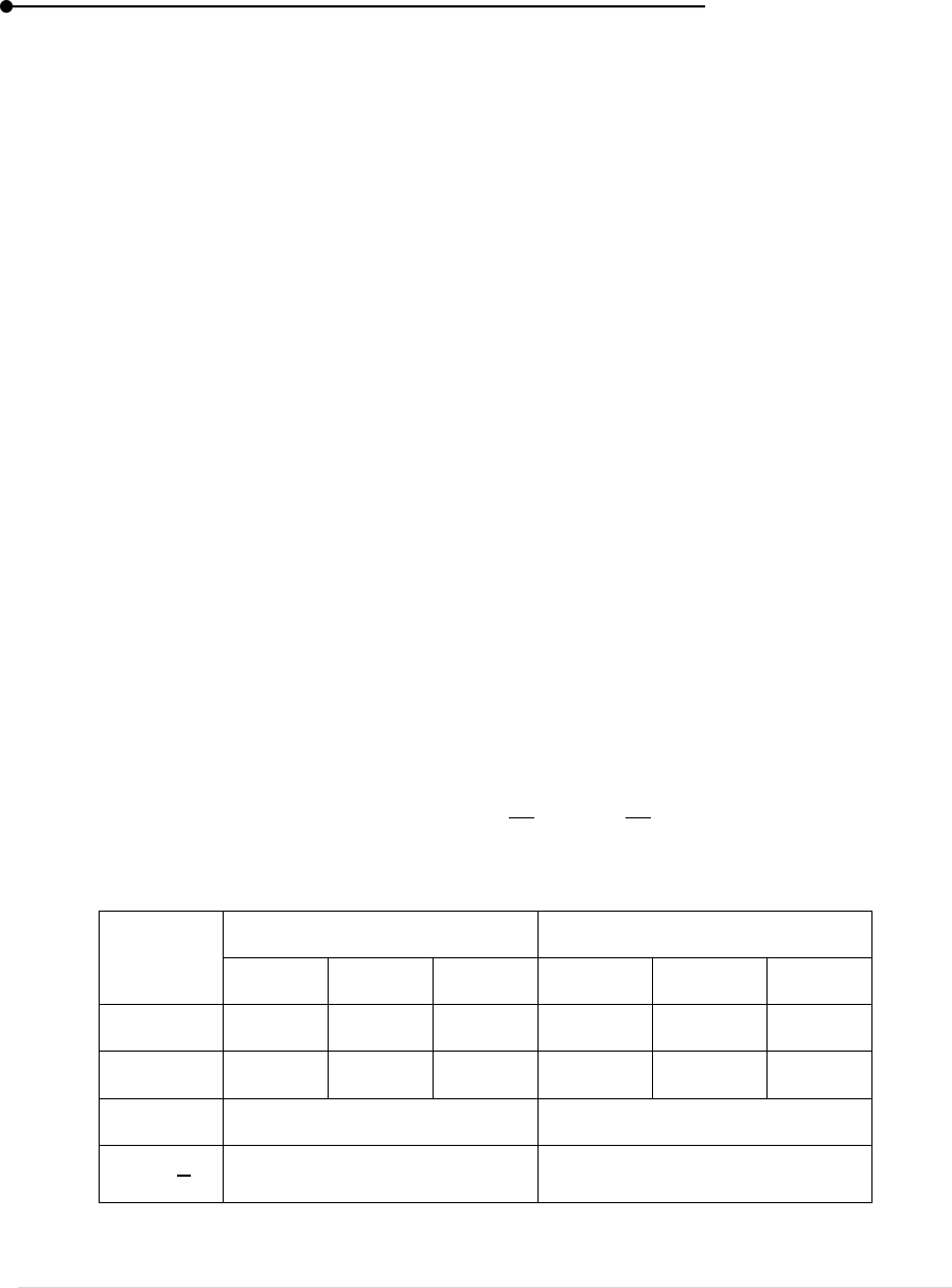
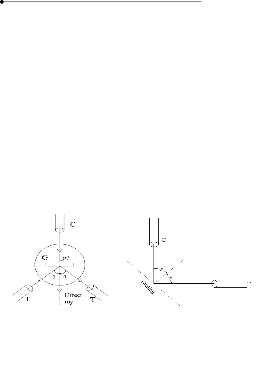
(ii) Adjustment of the grating
The grating is to be adjusted on the prism table such that light from the collimator
falls normally on it for achieving this.
Laboratory manual
30 | P a g e
First the collimator and the telescope are brought in one line and the image of the
slit is focused on the vertical crosswire. The corresponding reading on both the
Vernier is noted.
The telescope is rotated through 90°.
Mount the grating on the prism table and rotate the prism table, so that the reflected
image is seen on the vertical crosswire in the telescope. Take the vernier readings.
Turn the prism table from this position through 45° or 135° so that writing on the
grating is away from the collimator. In this position grating is normal to the incident
beam.
The slit is rotated in its plane till the spectral lines are very sharp and bright. This
brings the slit parallel to the linear of grating.
(iii) Measuring the diffraction angles
Rotate the telescope to the left side of the direct image and adjust it on different
spectral lines starting with first order blue lines and finishing with second order
yellow lines, turn by turn. It should be taken care that the movement of telescope is
in one direction.
Note the vernier readings V
1
and V
2
.
Now, rotate the telescope to the right side of the direct image and repeat steps. The
difference of corresponding vernier readings with given twice of the angle of
diffraction.
Find angle of diffraction for prominent lines in the first and the second order spectra.
C Collimator; G Grating table; C Collimator; T Telescope at 90°
T Telescope; Angle of diffraction
Figure 14: Spectrometer grating Figure 15: Normal Incidence Position of
the Diffraction Grating
Laboratory manual
31 | P a g e
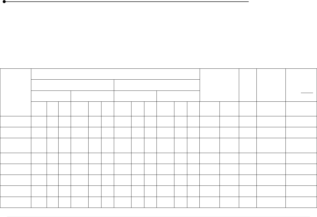
Table 24: To Determine the wavelength of various Spectral Lines
LC = MSD – VSD
Least count = 1ʹ, N = 4.9744 x 10
5
lines/meter, Order of spectrum = 1
Spectral
lines
Reading of the diffracting image
Difference
between two
reading
Mean
2θ
Mean of
angle of
diffractio
n θ
Left
Right
A
1
B
1
A
2
B
2
MS
R
V
R
TR
MSR
VR
TR
MSR
VR
TR
MSR
VR
TR
A
1
~A
2
B
1
~B
2
Violet
Blue
Bluish
green
Green
Yellow-1
Yellow-2
Orange
Red
Laboratory manual
32 | P a g e
CALCULATION
(i) No. of lines per inch of the grating (N):
n = 1, λ for green is 5461 x 10
-10
m
N =
lines/m
(ii) Wavelength of various spectral lines
λ =
m
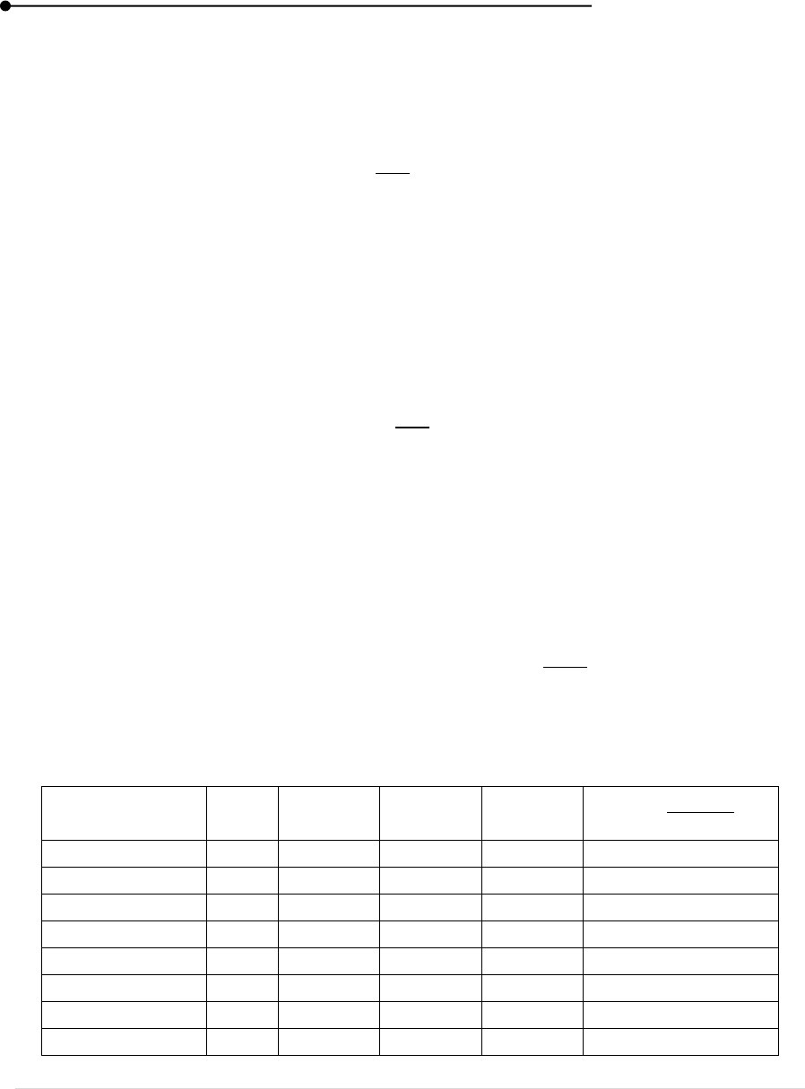
(iii) Dispersive Power of Grating
From table 25 four values of θ
2
-θ
1
and
λ
2
-λ
1
is calculated and corresponding
dispersive power is calculated using formula
Table 25: Dispersive Power of Grating
Spectral lines
θ
λ
θ
2
-θ
1
λ
2
-λ
1
Violet
Blue
Bluish green
Green
Yellow-1
Yellow-2
Orange
Red
Laboratory manual
33 | P a g e
Table 26: Wavelength of various Spectral Lines
Colour
Common wavelength
Experimental wavelength
Violet
3800-4200
Blue
4500-4900
Green
4900-5700
Yellow
5700-5900
Orange
5900-6300
Red
6300-7500
RESULT
The wavelength and the dispersive power of the spectral lines are determined and values are
tabulated.
VIVA VOCE
1. Define Diffraction.
2. What is the principle of Physics involved in this experiment?
3. In the present experiment, what class of diffraction does occur and how?
4. What type of grating do you use for your experiment?
5. What is plane transmission diffraction grating?

Laboratory manual
34 | P a g e
3. FOCAL LENGTH OF CONCAVE LENS
AIM
To find the focal length of concave lens using convex lens of known focal length.
APPARATUS REQUIRED
Concave lens, Convex lens of suitable focal length, Lens holder, Illuminated wire gauge,
White paper screen etc.
FORMULA
The focal length of concave lens
S. No.
Parameter
Explanation
Unit
1
f
2
Focal length of concave lens
metre
2
f
1
Focal length of convex lens
metre
3
F
Focal length of combination
metre
PROCEDURE
(i) Convex lens in contact
A convex lens of known focal length f
1
is taken. The given concave lens of focal
length say f
2
and the convex lens are put together vertically in a lens holder.
The combination of lenses in contact must be convergent. Therefore, the focal length
of the convex lens should be appreciably smaller than that of the convex lens.
The focal length F of the combination is determined by one of the methods described
in the previous experiment.
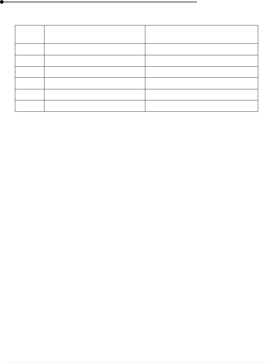
(ii) Auxiliary convex lens method
A convex lens L
1
is mounted in front of an illuminated wire gauge O and a well-
defined clear image of almost same size as that of object is formed on the screen S.
The given concave lens L
2
on other holder is placed in between L
1
& S nearer to
convex lens. The image formed by convex lens now become virtual object for
concave lens and therefore the distance between concave lens and the screen (L
2
S)
is object u.
Laboratory manual
35 | P a g e
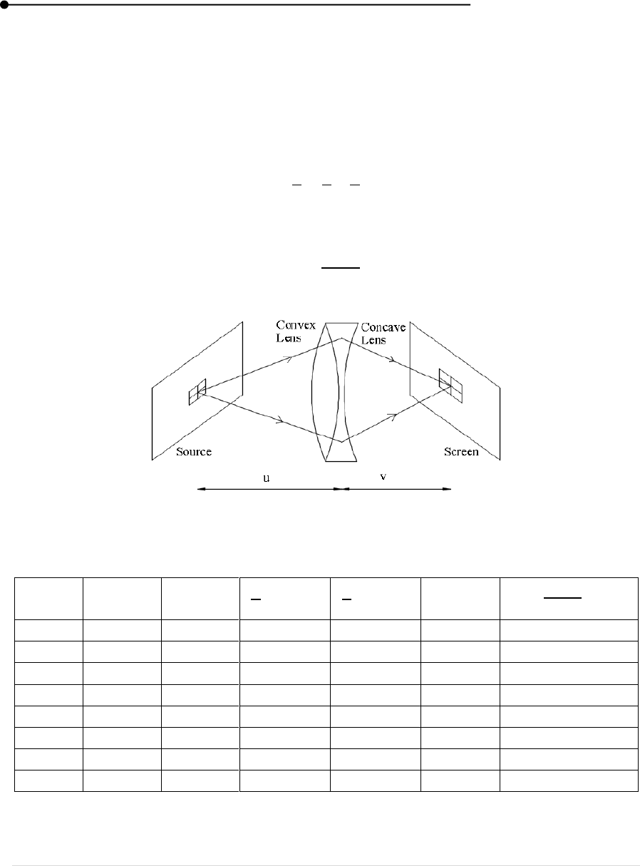
Now, the screen is moved away from lens (L
2
) so as to get a well-defined and clear
image of the gauge on the screen (S
1
) the distance L
2
S
1
between the concave lens
and the screen is measured and taken as the distance of image V. The experiment is
repeated by changing the position of concave lens and readings are recorded.
Since for concave lens, the virtual object distance is negative, the focal length of the
lens is calculated by the formula,
Therefore, the focal length of the concave lens
Figure 16: Convex Lens in Contact
Table 27: To Find the Focal Length of the Convex Lens
S. No.
u (cm)
v (cm)
u + v
1
2
3
4
5
6
7
8
Mean,
= m
Laboratory manual
36 | P a g e
Figure 17: In Auxilliary Convex Lens Method
Table 28: u – v Reading
S. No.
Trial
L
2
S
‘u’ (cm)
L
2
S
’
‘v’ (cm)
1
2
3
4
5
Mean, f = m
CALCULATION
F = cm; f
1
= cm

Laboratory manual
37 | P a g e
RESULT
The focal length of the concave lens
1. In contact with convex lens = ____________ m
2. In contact with concave lens = ____________ m
VIVA VOCE
1. What is a lens and how many principal foci are there for a lens?
2. What is concave lens?
3. What is the difference between a convex lens and a concave lens?
4. What is the maximum distance of the image formed by a concave lens?
5. What are other uses of concave lenses?
6. What is the distance of the image formed by the concave lens from the concave mirror
when the parallax is removed?

Laboratory manual
38 | P a g e
4. FOCAL LENGTH OF CONVEX LENS
AIM
To determine the focal length of convex lens using u-v and conjugate method.
APPARATUS REQUIRED
Convex lens, Lens holder, Illuminated wire gauge, White paper screen, Meter scale etc.
FORMULA
Focal length of convex lens by
(i) u-v method
(ii) Displacement method
S.No.
Parameter
Explanation
Unit
1
f
Focal length of the convex lens
m
2
D
Distance between the object and screen
cm
3
u
Distance between the source and lens
m
4
v
Distance between the lens and object
m
5
d
Displacement (A-B)
cm
PRINCIPLE
Convex lens is thicker at middle. Rays of light that pass through the lens are brought closer
together i.e. they converge convex lens act as a converge lens.
PROCEDURE
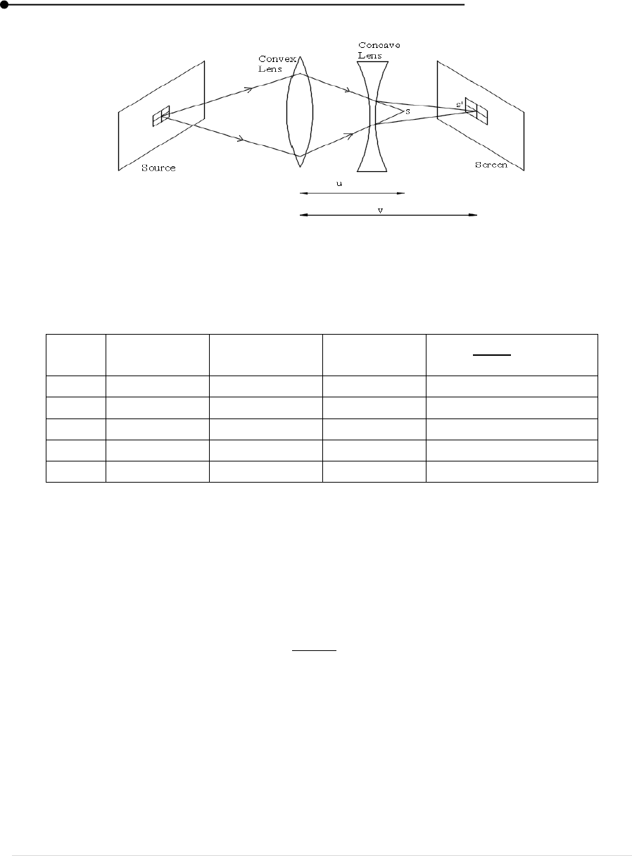
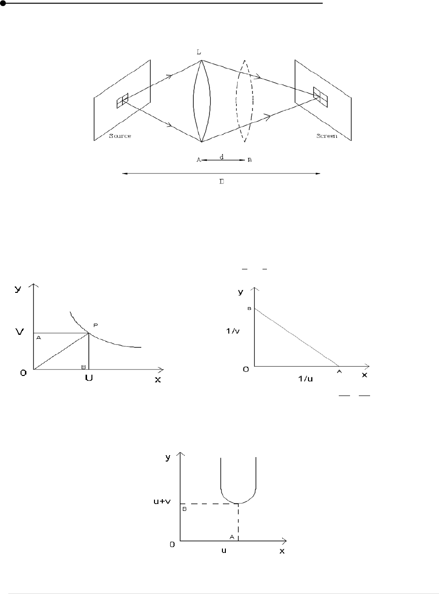
(i) Distant Object Method
An object is focused on white screen by a convex lens.
A clear image is formed on the screen placed behind the lens.
The distant between screen and lens gives the focal length of convex lens.
This value may be taken as approximate focal length of the lens.

Laboratory manual
39 | P a g e
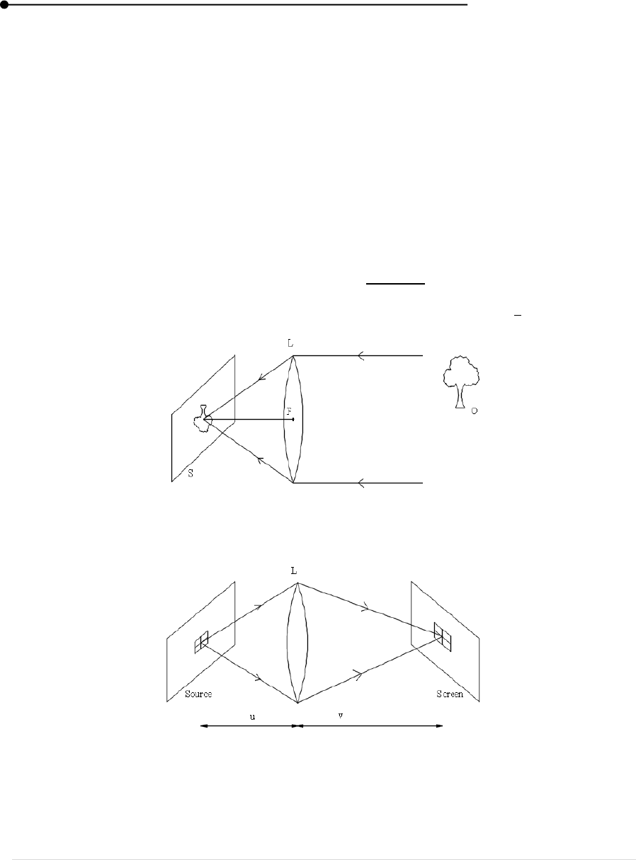
(ii) u - v Method
The convex lens in a holder is placed vertically infront of the illuminated wire
gauge.
The distance between the lens and the gauge should be more than f but less than
2f.
A white screen is placed on the other side of the lens.
Its position is adjusted to get clear and enlarge image of gauge.
The distance u and v are measured.
The experiment is repeated for different value of u (< 2f) to get enlarged image.
The screen is now placed in front of the lens and adjust to get a well-defined, clear
and diminished image.
The distance v is noted.
The experiment is repeated for different value of u < 2f, u > 2f and one with u =
2f.
The readings are tabulated and focal length of given convex lens is determined using
formula
Using u,v readings u-v,
and u – (u+v) graphs are drawn and focal length is
obtained by graphical method.
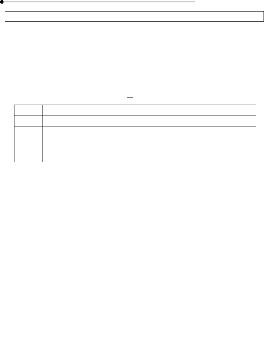
Graphical method
(i) u-v graph
A graph is drawn by taking u along x axis and v along y axis to get a rectangular
parabola origin O.
a straight line is drawn making an angle 45⁰ with x axis.
Let the line cut the parabola at the point P.
From B perpendicular BA and BB are drawn on x axis and y axis respectively.
The length OA = OB = 2f and hence the focal length can be calculated.
(ii)
graph
A straight line graph is drawn. By taking
along x axis and
along y axis.
The straight line AB makes equal intercept OA and OB along x axis and y axis
respectively.
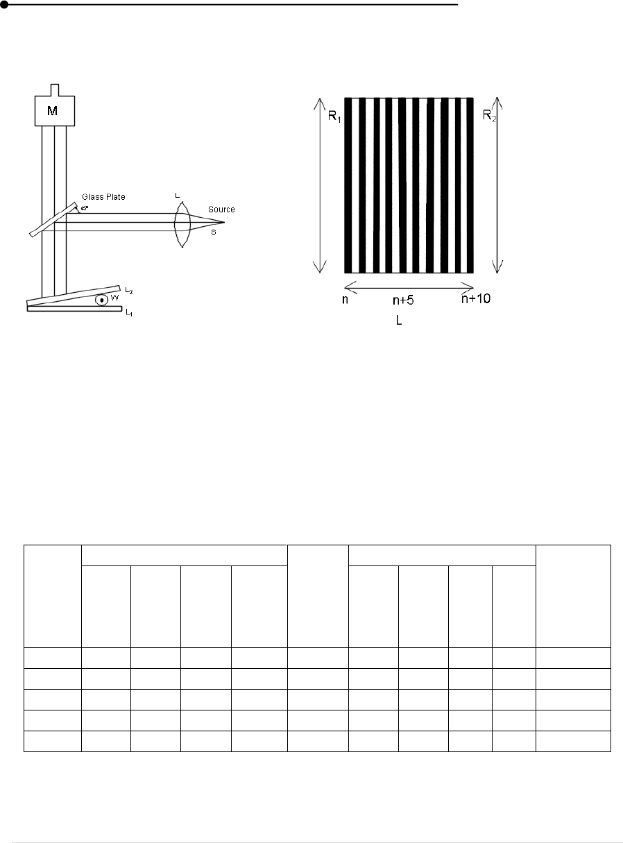
(iii) u – (u+v) graph
A graph of u along x axis and u + v along y axis and a perpendicular PA is drawn
to curve from x axis.
OA gives 2f and OB gives 4f, the mean of focal length f is calculated.
Displacement Method (Conjugate focii)
The illuminated wire was O and the white screen S are placed at a distance D
greater than 4f from each other.
Laboratory manual
40 | P a g e
The convex lens L mounted vertically on a holder is kept in between the gauge and
the screen. So as tool lie on same straight line.
The position A of the lens is adjusted to get a clear, enlarged image of the gauge
on the screen, then lens is adjusted.
To get a clear diminished image of the gauge on the screen. The position B of the
lens is noted.
The difference d = A – B between two conjugated position of the lens is
determined.
The observations are recorded in table.
The experiment is repeated for different values of B.
The focal length is calculated using the formula
The focal length f is calculated from the intercept OA = OB =
.
S Screen ; O Object ; L Lens (Convex)
Figure 18: Distant Object Method
S Source ; L Lens (Convex) ; u Distance between lens and source
v Distance between lens and screen
Figure 19: u – v Method
Laboratory manual
41 | P a g e
L Convex lens ; A Position of Diminished Image
B Position of Enlarged Image ;D Distance between source and screen
Figure 20: Displacement (Conjugate Foci) Method
Model Graphs
(i) u – v graph (ii)
graph
2f = OA = OB f =
=
(iii) u – (u + v) graph
OA = 2f; OB = 4f

Laboratory manual
42 | P a g e
Table 29: u – v Reading
f = m
S.No.
u (cm)
v (cm)
(cm)
(cm)
u + v (cm)
(cm)
1
2
3
4
5
6
7
Table 30: Conjugate Reading
S.No.
Distance b/w
the object &
screen D (cm)
Position for
enlarged
image
B (cm)
Position for
diminished
image A
(cm)
Displacemen
t d =(A - B)
(cm)
(cm)
1
2
3
4
5
6
RESULT
Focal length of convex lens
1. By calculation =
2. By u - v graph =
3. By
graph =
4. Byu – (u + v) graph =
5. By conjugate foci. =
VIVA VOCE
1. Define focal length.
2. Define and explain the lens formula.
3. What is convex lens?
4. Which convex lens has more focal length thick or thin?
5. What are the practical uses of a convex mirror?
Laboratory manual
43 | P a g e
5. AIR WEDGE
AIM
To determine the thickness of a thin object using air wedge method.
APPARATUS REQUIRED
Two optically rectangular glass plate, Thin wire, Travelling microscope, Reading lens,
Sodium vapour lamp, Condensing lens with stand, Wooden box with glass plate inclined at 45°.
FORMULA
The thickness of the thin object,
metre
S.No.
Parameter
Explanation
Unit
1.
t
Thickness of the thin object
metre
2.
l
Distance of the thin object from the edge contact
metre
3.
Wave length of sodium light (58.9x10
-9
m)
metre
4.
β
The width of one fringe
metre
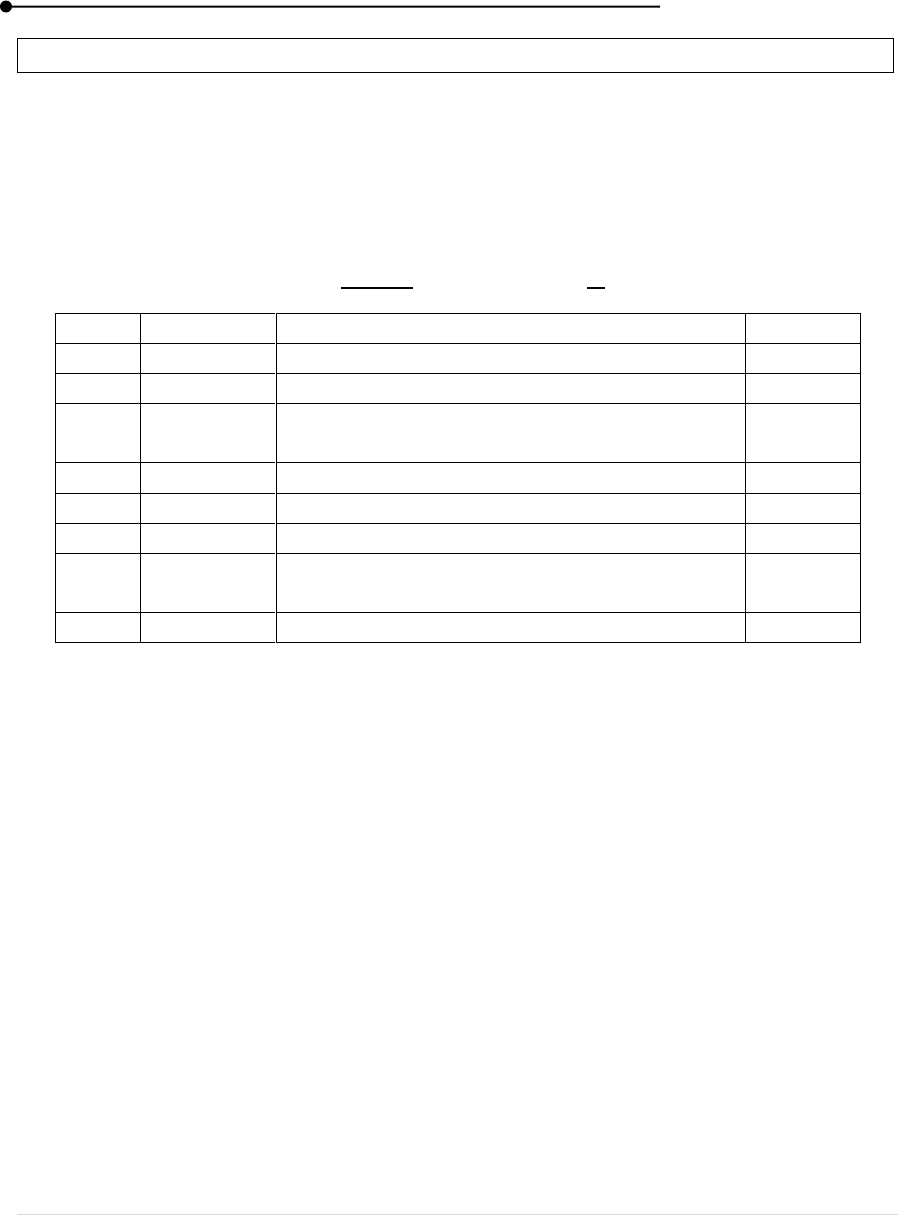
PROCEDURE
The experimental and fringe pattern are shown in the figure 21 & 22. Two optically plane
glass plate are placed one over other and tied together by means of a rubber band at one end.
A thin object is inserted between the plates at the other end. Now a wedge shaped air film is
formed between the two glass plates.
Two slide system kept on the platform of a travelling microscope. The light from a sodium
vapour lamp is rendered parallel with a condensing lens and is made to incident on a plane
glass sheet held over the wedge at an angle of 45° with the vertical.
The light falling on the sheet is partially reflected which is in turn incident normally on the
air wedge. Adjusting the arrangement properly, the microscope field of view is made bright
to the maximum extent.
The microscope is moved vertically and down fall parallel fringes are visible which are
located on the surface of the air film. By moving the microscope in a horizontal direction,
the cross wire of the microscope are set on one of the dark (n
th
) fringe in the pattern. Its
position is noted down in the horizontal scale.
The microscope is moved further using the tangential screw along the length of the air film.
After counting 5 dark fringes, the cross wire is coincided with the (n+5)
th
fringes and its
position is noted. The measurements are repeated similarly for every alternate dark fringes
are noted.
The width of 10 dark fringes are calculated from the table and the mean width of 25 fringes
with β is calculated as the distance between the fringes of contact and the inner edge of the
Laboratory manual
44 | P a g e
wire. The measurement can be done using the travelling microscope (or) with the calculation
scale.
S Source (Sodium vapour lamp) Edge contact Specimen
L Condensing lens (Rubber band) (Thin object)
G Glass plate inclined at 45
o
L
1
& L
2
Transparent plane glass plate
w Object
Figure 21: Experimental Arrangement Figure 22: Fringe Pattern
Table 31: To find the fringe width (β)
Least Count = 1MSR – 1 VSR
LC = 0.001 cm
Order
of
fringe
s
Microscope reading
Order
of
fringes
Microscope reading
Width of
25
fringes
(cm)
MSR
(cm)
VSC
(div.)
VSR
(cm)
TR
(cm)
MSR
(cm)
VSC
(div.)
VS
R
(cm
)
TR
(cm
)
N
n+25
n+5
n+30
n+10
n+35
n+15
n+40
n+20
n+45
Width of 25 fringes =m
Width of one fringes =m

Laboratory manual
45 | P a g e
Table 32: Length between the edges of contact to the specimen hair
Least count = 0.001 cm
MSR
(cm)
VSC (div)
VSR (cm)
TR (cm)
l(cm)
R
2
– R
1
Edge of contact R
1
Specimen hair R
2
CALCULATION
Thickness of the hair
metre
RESULT
Thickness of the hair using air wedge method, t = ____________ m
VIVA VOCE
1. What is an Air wedge?
2. What is meant by interference of light?
3. What are interference fringes?
4. Is there is any energy loss in interference phenomenon?
5. What if sodium light is replaced with white light?
Laboratory manual
46 | P a g e
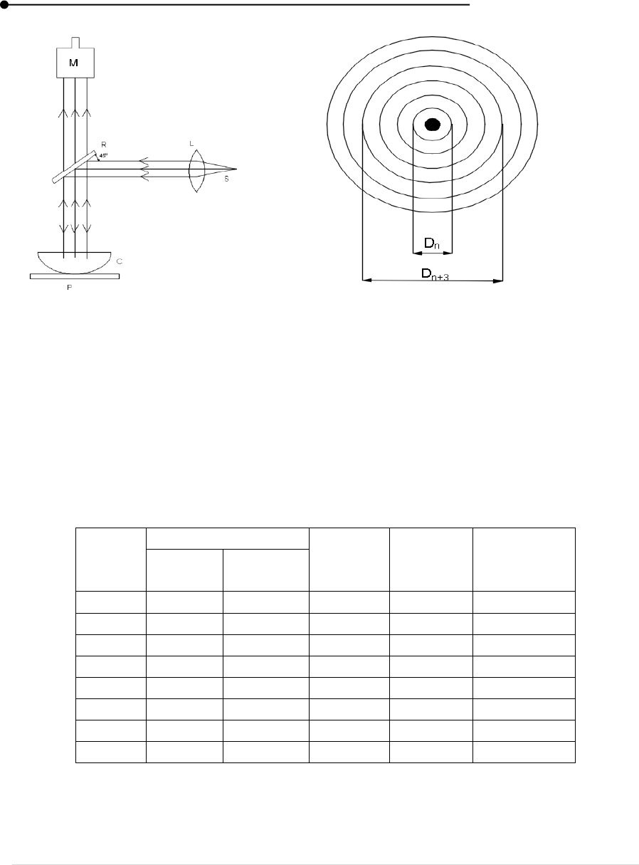
6. REFRACTIVE INDEX OF A CONVEX LENS – NEWTON’S RING
AIM
To determine radii of curvature of a plano convex lens by forming Newton’s ring and to
calculate the refractive index of the material of the lens.
APPARATUS REQUIRED
Plano convex lens, Glass plate, Sodium vapour lamp, 45
o
slot, Travelling microscope etc.
FORMULA
R =
m ;µ = 1+
m
S.No.
Parameter
Explanation
Unit
1
R
Radius of curvature of the surface of the lens
m
2
m
Order of the spectrum
m
3
Wavelength of light used for sodium light (589.3 x
10
-9
m)
m
4
d
n
Diameter of the n
th
fringe
m
5
d
n+m
Diameter of (n+m)
th
fringe
m
6
µ
Refractive index of the material
(no unit)
7
F
Focal length of the plano convex lens (f=100x10
-
2
m)
m
8
R
Radius of curvature of the surface of the lens
m
PRINCIPLE
Newton’s rings are formed due to interference between the light waves reflected from the
top and bottom surfaces of the air film formed between the lens and glass sheet. An air film of
varying thickness is formed between the lens and the glass sheet.
PROCEDURE
Turn on the sodium vapour lamp, the planoconvex lens on the plane glass plate with curved
surface in contact with a glass plate in a stand.
Place a reflector locator in a travelling microscope.
Use a reflector to direct light into the optical system.
Adjust the inclination of the reflector to get maximum brightness.
Hence fringes are obtained.
Focus that to use that bright and dark newton’s ring carefully, insert the thin film between
the planoconvex lens and glass plate until paper stops moving.
Now look through the microscope and start from the number of dark fringes to the fringes
that is adjacent to the thin film keeping the reading as n+5+10..... from left and right fringes
Mean values are obtained.
Laboratory manual
47 | P a g e
M Microscope; L Lens
S Sodium vapour lamp
R Reflecting glass plate
CPlanoconvex lens
P Plane glass plate
Figure 23: Newton’s ring setup Figure 24: Newton’s ring
Table 33: To find d
2
n+m
– d
2
n
LC = 1MSD – 1VSD
LC = 0.001 cm
Order
of
fringes
Microscope reading
d
n
x10
-2
(m)
d
2
n
x10
-4
(m
2
)
d
2
n+m
- d
2
n
(m=20) (m
2
)
Left (cm)
Right
(cm)
N
n+5
n+10
n+15
n+20
n+25
n+30
n+35
Mean, d
2
n+m
- d
2
n
= cm
Mean, d
2
n+m
- d
2
n
= m
2

Laboratory manual
48 | P a g e
CALCULATION
R =
m
d
2
n+m
- d
2
n
=
m =
=
From these values R is calculated and substitute in the formula,
µ = 1+
RESULT
The refractive index of the material of the planoconvex lens by newton’s ring method is,
µ = __________
VIVA VOCE
1. What do you mean by interference of light?
2. Why does the sodium lamp give out red light in the beginning?
3. How are these rings formed?
4. Why are the rings circular?
5. What are the uses of Newton’s rings?
Laboratory manual
49 | P a g e
7. REFRACTIVE INDEX OF THE MEDIUM – HOLLOW PRISM
AIM
To determine the refractive index of different liquid such as kerosene, water using hollow
prism.
APPARATUS REQUIRED
Spectrometer, Hollow prism, Sodium vapour lamp, Water, Kerosene.
FORMULA
The refractive index of the prism,
µ =
S.No.
Parameter
Explanation
Unit
1.
µ
Refractive index of the prism
no unit
2.
A
Angle of the prism is 60
o
deg.
3.
D
Angle of minimum deviation
deg.
PROCEDURE
(i) To determine the angle of minimum deviation
The prism is filled with water. The prism table is now released and rotated so as to
have the edge of the prism turned away from the collimator on looking through the
prism in proper direction in refracted image in the field of view.
The prism table is slightly rotated in either direction of the prism should be rotated
so that the angle of minimum deviation decreases, at a particular position the image
is founded to remain stationary for a moment on rotating the prism in the same
direction as before.
The image turns back and moves in the opposite direction.
The position is turned back in the minimum deviation position, the prism table and
the telescope are fixed in this position.
The main scale and vernier scale readings are taken for both verniers. The total
reading is calculated for each vernier.
Let the reading R
3
for both the cases. The prism is then removed. The telescope is
brought in line with the collimator to catch the direct image and the readings are
taken. The distance between the readings R
3
+R
4
given D, the angle of minimum
deviation. Similarly the procedure repeated for kerosene.
Laboratory manual
50 | P a g e
ABC Prism ; C Collimator ; T
1
and T
2
Telescope
Figure 25: Angle of minimum deviation
Laboratory manual
51 | P a g e
Table 34: Angle of minimum deviation for water and kerosene
LC = 1′
Medium
Vernier A
Vernier B
Average
D
Direct
reading
Minimum deviation
D
m
(R-D)
Direct
reading
Minimum deviation
D
m
(R-D)
MSR
VSR
TR
MSR
VSR
TR
Water
Left
Right
D=
Kerosene
Left
Right
D=
Laboratory manual
52 | P a g e
CALCULATION
(i) Determination of refractive index of the water
µ =
A= ; D=
µ =
Refractive index of water, µ
w
=
(ii) Determination of refractive index of kerosene
µ =
A = ; D =
µ =
Refractive index of kerosene, µ
k
=
RESULT
The refractive index of medium of liquid such as,
(i) Refractive index of water, µ
w
=
(ii) Refractive index of kerosene, µ
k
=
VIVA VOCE
1. Define refractive index.
2. What is angle of minimum deviation?
3. On what factor does the angle of deviation depend?
4. What is angle of prism?
5. Will the angle of minimum deviation change, if the prism is immersed in water?
Laboratory manual
53 | P a g e
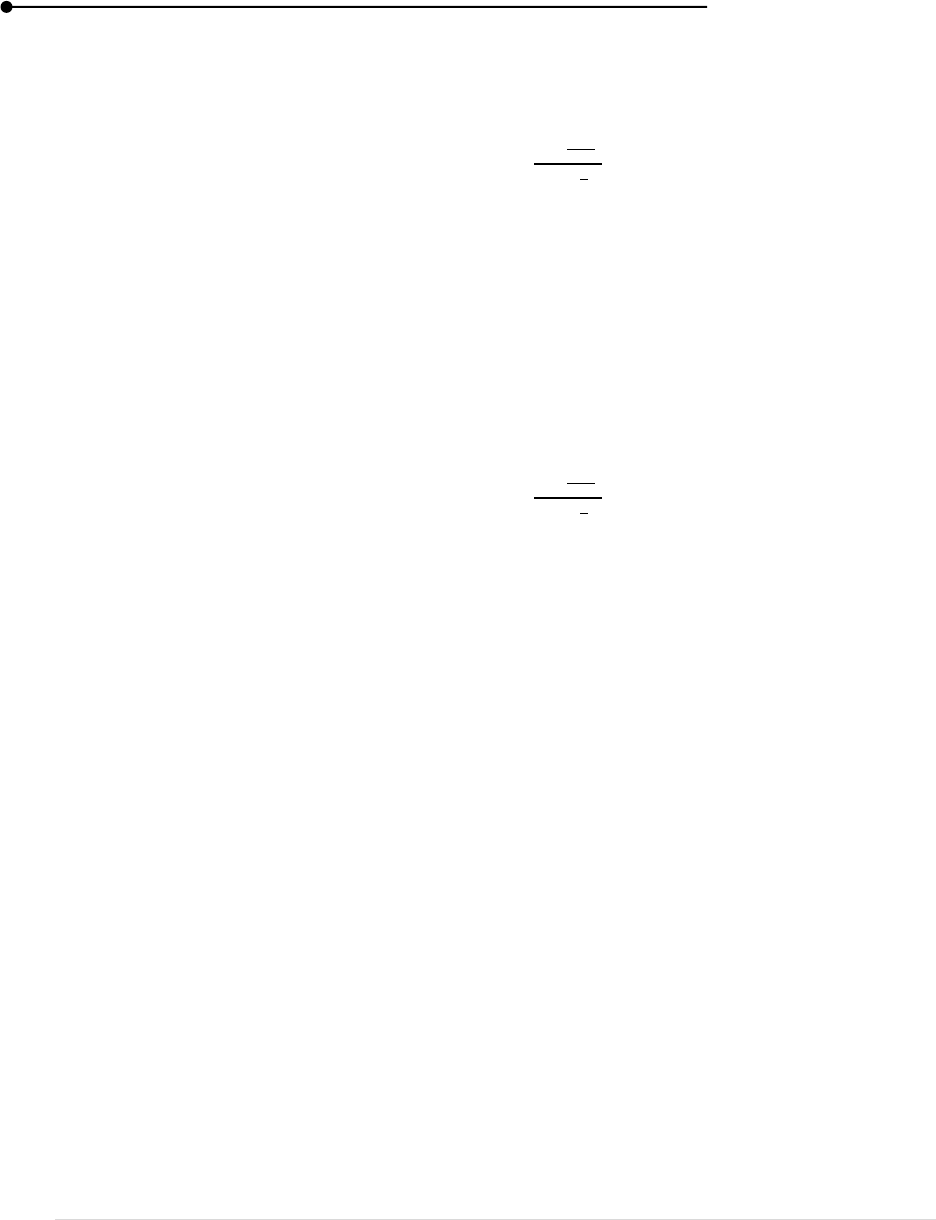
8. SPECTROMETER – I-D CURVE
AIM
To draw a curve connecting the angle of incidence and the angle of deviation in a prism i.e.
I-D curve using a spectrometer and to calculate the refractive index of the prism.
APPARATUS REQUIRED
Spectrometer, Prism, Sodium vapour lamp, etc.
FORMULA
µ =
S.No.
Parameter
Explanation
Unit
1
µ
Refractive index of the prism
no unit
2
A
Angle of the prism is 60⁰
deg
3
D
Angle of minimum deviation
deg
PRINCIPLE
When a beam of light strikes on the surface of transparent material (glass, water, quartz
crystal, etc.,) the position of the light is transmitted and other portion is reflected. The transmitted
light ray has small deviation of the path from the incident angle.
PROCEDURE
After the preliminary adjustment of the spectrometer, telescope is focused directly
to see the image of the slit by working on the tangential screw, vertical cross wire
is made to coincide with the fixed edge of the image of the slit.
At this position, the telescope is clamped rigidly.
Two verniers are then fixed firmly to read 0
o
and 180
o
.
So that throughout the experiment, the direct reading of the verniers remain same.
Next, the prism abc is mounted as shown in figure, with its base be almost parallel
to the axis of the collimator.
Now to set the prism, so that a ray of light from collimator falls on the refracting
face ab with a particular angle of incidence i, the telescope from its direct position
is rotated towards ab through an angle θ = 180-2i and it is fixed in that position by
using the radial screw.
The prism is adjusted by slowly rotating the plate till the fixed angle of the reflected
image of the slit from the light ray incident on ab at angle i to the normal at the point
of the incidence.
The telescope is released and now turned towards the base to observe the refracted
image from the face ac.
Finally adjusting the position of the telescope, the vertical axis cross wire is made
to coincide with the same fixed edge of the image.
Laboratory manual
54 | P a g e
The readings of the vernier v
1
and v
2
are noted.
The difference with the direct reading gives angle of deviation d for the given angle
of incidence.
The experiment is performed for various angles the readings of the verniers
corresponding to respective refracted rays are tabled as given in table.
T Telescope; C Collimator; abc Prism
d angle of deviation; i angle of incidence
Figure 26: Angle of minimum deviation
A = (i
1
+ i
2
) - d
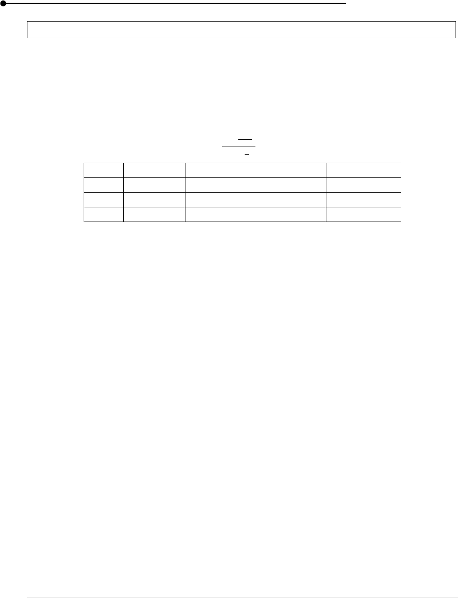
Figure 27: Model graph of I - D graph
Laboratory manual
55 | P a g e
Table 35: To find the angle of minimum deviation
LC = 1MSD – 1VSD LC=1′
Ver A = Ver B=
Angle of
incidenc
e
180 –
2i
Reading
corresponding to
refracted image
Angle of deviation
Mean D
Vernier
A
Vernier B
Vernier A
Vernier
B
40
50
60
70
80
Table 36: Angle of Prism
D
i
1
i
2
i
1
+i
2
A= (i
1
+i
2
-d)
CALCULATION
From the graph A and D is found. This is substituted in the formula
µ =
RESULT
From the I-D curve graph using spectrometer
(i) Angle of prism, A =
(ii) Angle of minimum deviation, D =
(iii) Refractive index of the prism, µ =
VIVA VOCE
1. What is a prism?
2. Define angle of deviation (D).
3. What is the relation between the angle of incidence and the angle of deviation?
4. When light enters into the prism is there any change in the frequency of wave length?
5. What is angle of prism in this experiment?
Laboratory manual
56 | P a g e
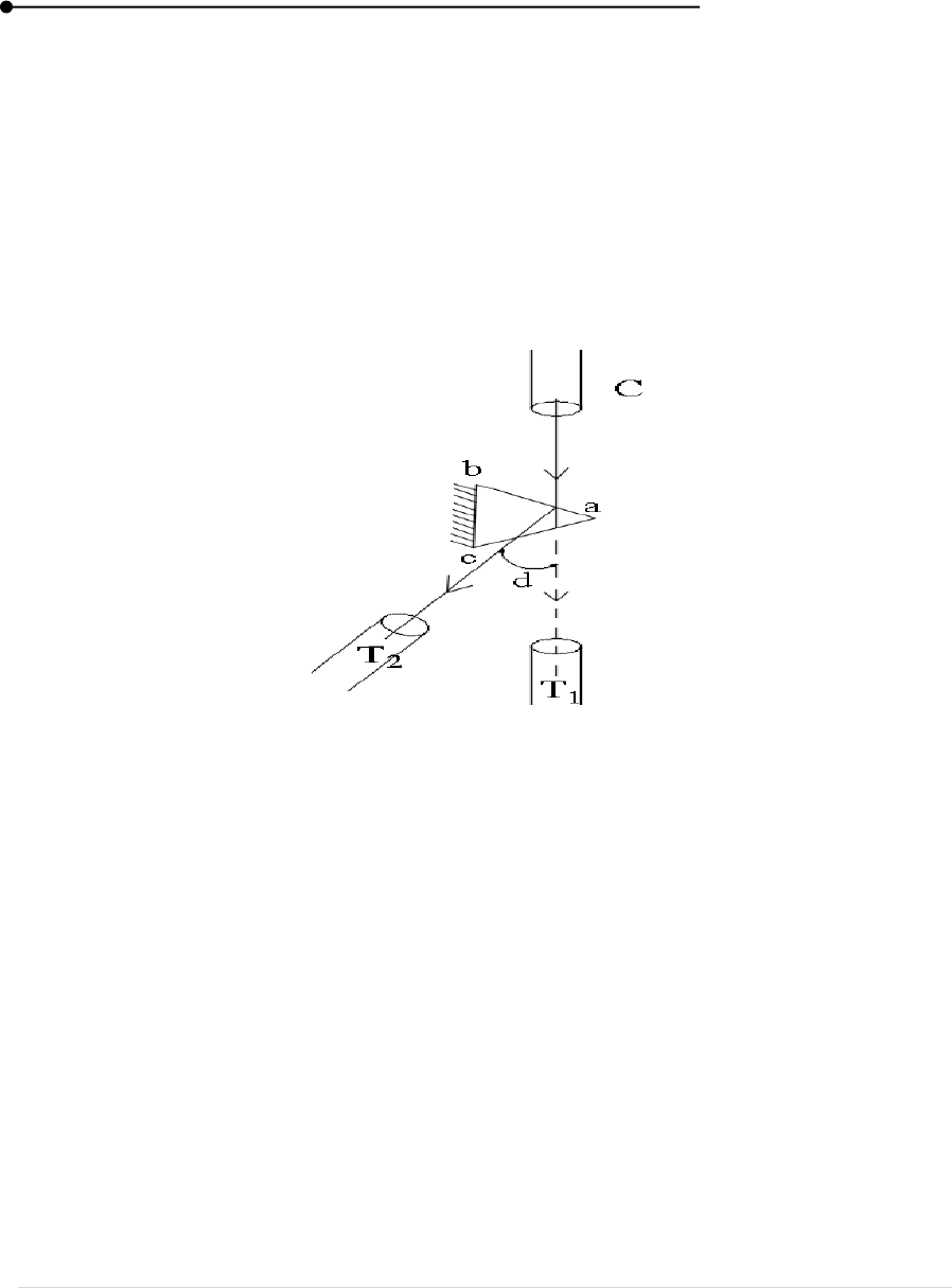
9. SPECTROMETER GRATING – OBLIQUE INCIDENCE
AIM
To determine the wavelength of various coloursof mercury spectrum using grating by
oblique incidence method.
APPARATUS REQUIRED
Spectrometer, Plane transmission diffraction grating, Mercury lamp etc.,
FORMULA
2 sin
= nN (m)
=
(m)
N =
(lines/m)
S.No.
Parameter
Explanation
Unit
1.
n
Order of diffraction
no unit
2.
N
Number of lines per metre
lines/m
3.
D
Angle of minimum deviation
deg
4.
Wavelength of light
m
PRINCIPLE
When a wave strikes an obstacle, the light ray will bend at the corners and edges of it, which
causes the spreading of light waves into the geometrical shadow of the obstacle. This phenomenon
is termed as diffraction.
PROCEDURE
As in the previous experiment after the initial adjustments of spectrometer, the slit is
illuminated by mercury lamp, the grating is mounted vertically at the centre of the prism.
The grating is placed almost normal to the initial ray from collimator.
The telescope is adjusted to view the direct reading of the slit and the vertical cross wire is
made to coincide with the image.
After clamping, the telescope of two verniers are adjusted to the direct reading 0⁰
and 180⁰ verniers are clamped.
Finally at this position the telescope is now turned left to direct ray and mercury spectrum
is observed due to first order diffraction.
The telescope is now adjusted to focus the bright green line of the spectrum rotating prism
table alone; such that the green line moves towards the direct image side still it reaches the
minimum deviation position.
Further slight rotation of the table makes the line from direct image side.
At this position lining the prism table, the grating is set into minimum deviation position.
Laboratory manual
57 | P a g e
Now making the vertical cross wire to coincide with each and every prominent lines of
spectrum starting from violet, the Vernier readings are noted.
The telescope is now taken to other side of direct ray.
By rotating the prism table alone, grating is set in minimum deviation position for green
line.
Experiment is repeated and the Vernier readings for all colors are tabulated.
T Telescope ; C Collimator ; G Grating
D angle of minimum deviation
Figure 28: Oblique incidence
Table 37: Determination of minimum deviation (left side)
LC = 1MSD – 1VSD LC=1′
Ver A = Ver B =
Colour
of light
Reading of minimum deviation position
Angle of minimum
deviation
Mea
n D
2
Vernier A
Vernier B
Vernier
A
Vernier
B
MSR
VSR
TR
MSR
VSR
TR
violet
Blue
Green
Yellow
Orange
Red
Laboratory manual
58 | P a g e
Table 38: Determination of minimum deviation (right side)
LC=1′
Ver A = Ver B =
Colour
of light
Reading of minimum deviation position
Angle of minimum
deviation
Mean
D
1
Vernier A
Vernier B
Vernier
A
Vernier
B
MSR
VSR
TR
MSR
VSR
TR
violet
Blue
Green
Yellow
Orange
Red
Table 39: Determination of Wavelength ()
n = 1 ; N = lines/metre
Colour
Mean D
1
Mean D
2
Mean D
=
x 10
-10
(m)
Violet
Blue
Green
Yellow
Orange
Red
Table 40: Wavelength of various Spectral Lines
Light
Common wavelength x10
-10
m
Experimental wavelength x10
-10
m
Violet
3800 - 4200
Blue
4500 - 4900
Green
4900 - 5700
Yellow
5700 - 5900
Orange
5900 - 6300
Red
6300 - 7500

Laboratory manual
59 | P a g e
CALCULATION
To find N
N =
(lines/m)
For green, D
g
=
=
n = 1
N = lines/metre
Wavelength of violet, blue, green, yellow, orange and red is found using the formula, =
; where, D is obtained from table
RESULT
(i) Number of lines per unit length of the grating N= lines/metre
(ii) Wavelength of various colours of mercury spectrums are determined using oblique
incidence method and the values are tabulated.
VIVA VOCE
1. What is called Standardization of Grating?
2. What is diffraction?
3. What is the principle of physics involved in this experiment?
4. Define oblique incidence.
5. How many lines per cm does the grating have?
Laboratory manual
60 | P a g e
10. SPECTROMETER – SMALL ANGLED PRISM
AIM
To determine the refractive index of a small angled prism, by measuring (i) angle of prism
(ii) angle of incidence for normal emergence using spectrometer.
APPARATUS REQUIRED
Spectrometer, Small angled prism etc.
FORMULA
Refractive index of the prism
μ =
S.No.
Parameter
Explanation
Unit
1
μ
Refractive index of prism
-
2
d
Angle of deviation
deg.
3
A
Angle of prism
deg.
PRINCIPLE
The prism refracts light into its different colours. The dispersion occurs because the angle
of refraction is dependent on the refractive index of the prism’s material, which in turn is slightly
dependent on the wavelength of light that is travelling through it.
PROCEDURE
(i) Angle of Prism
The narrow angled prism abc is mounted vertically on the prism table using prism
holder. The prism table is turned so that parallel rays from the collimator to get
reflected from one of refracting faces ab of the prism. Rotating the telescope
through 90 degree, the image is viewed. The telescope is fixed and then readings
of Vernier V
1
and V
2
are noted.
The Vernier is rotated till the image reflected from other face ac coincides with
vertical cross wire.
Hence the angle of prism is determined.
(ii) Angle of deviation‘d’ for normal incidence
The prism is removed from the prism table and the slit is viewed.
Telescope is adjusted to read 0
o
and 180
o
respectively.
The small angled prism abc is mounted on the table and is adjust to get reflected
image from one of the face ab to coincide with the vertical cross wire.
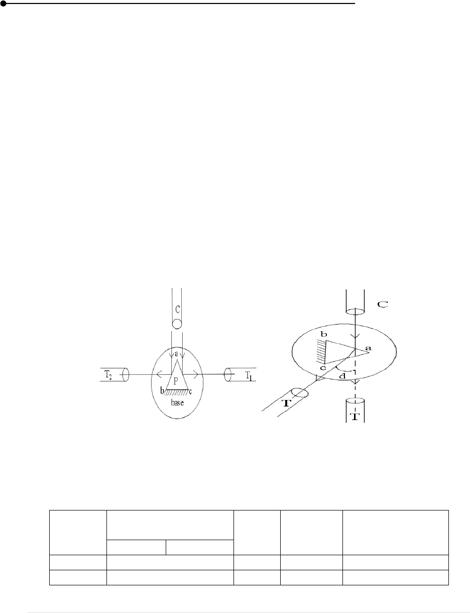
Laboratory manual
61 | P a g e
The angle of incidence at the face ab now becomes equal to 45⁰ .
The Vernier is released and it is turned 45⁰ towards collimator to make angle of
incidence equal to 0.
Releasing the telescope, it is rotated to get the refracted image from the other face
ac.
The difference between the direct reading and refracted ray reading of each of the
Vernier gives the angle of deviation d.
(iii) Angle of incidence ‘i’ for normal emergence
The small angled prism abc is mounted on the prism table and is adjusted for
normal incidence on one of the face ab.
The refracted image is viewed in the image.
The prism table alone is rotated slowly so that refracted image moves towards the
minimum deviation
The prism is rotated till the image coincide with the vertical cross wire.
The ray of light them comes out at right angle to face ac.
The readings of the verniers are noted.
C Collimator; abc Prism; T Telescope
Figure 29: Angle of the Prism Figure 30: Minimum Deviation Diagram
Table 41: Angle of the prism A
Verniers
Readings for reflected
image
θ
(div.)
Mean θ
(div.)
A = 180 – θ (div.)
I face
II face
V
1
V
2
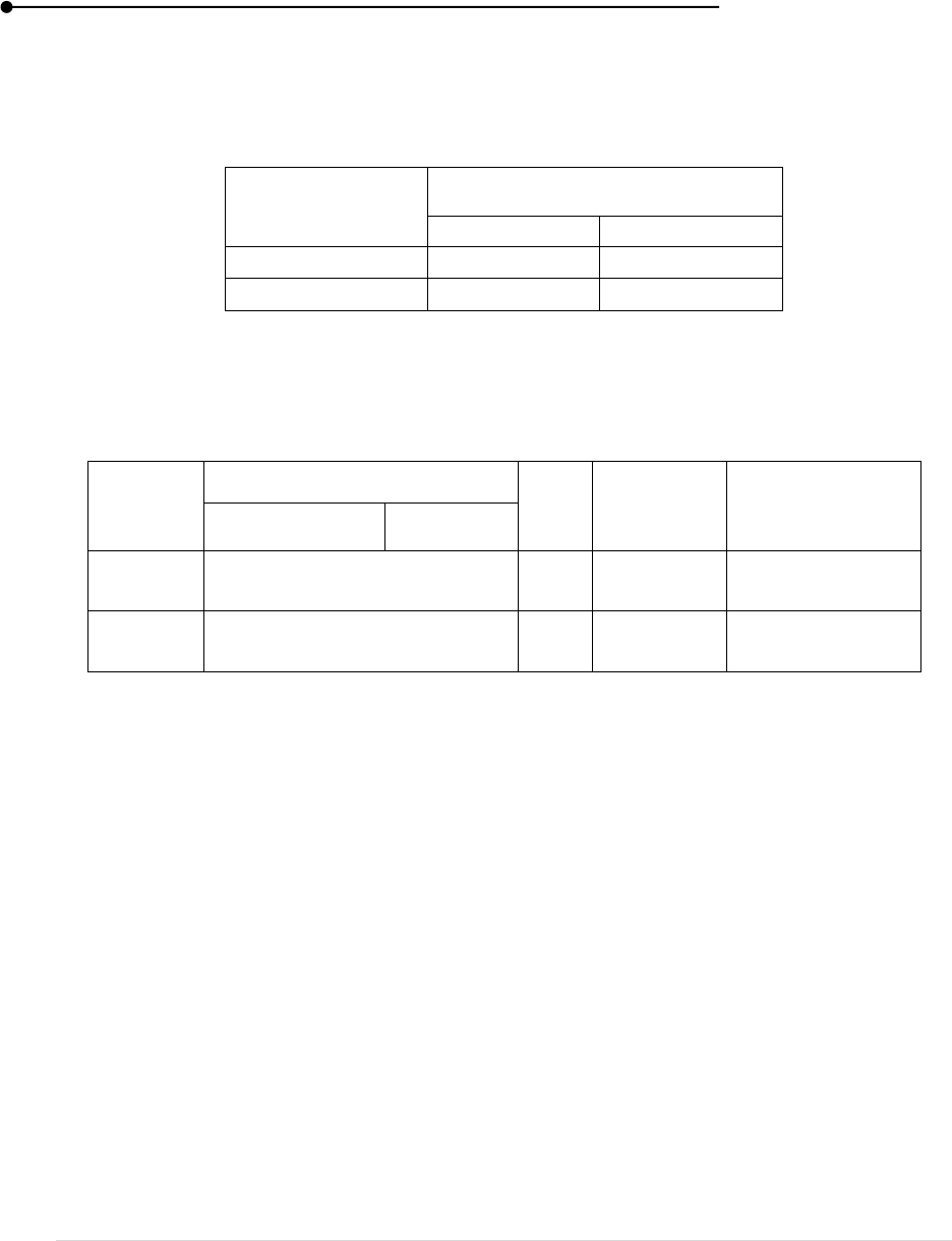
Laboratory manual
62 | P a g e
Table 42: Angle of deviation d – normal incidence
Image
Telescope readings
V
1
V
2
Refracted direct
Difference, d
Mean, d =
Table 43: Angle of incidence i for normal emergence
Verniers
Telescope readings
θ
Mean θ
Mean i = 90 –
(θ/2)
Reflected ray
Direct ray
V
1
V
2
RESULT
(i) Angle of small angled prism =
(ii) Angle of deviation for normal incidence =
(iii) Angle f incidence for normal emergence =
(iv) Refractive index of the prism by
1) Normal incidence =
2) Normal emergence =
VIVA VOCE
1. What is unit of refractive index?
2. Why is it recommended that the prism be set at the angle of minimum deviation?
3. What is the relation between the angle of incidence and the angle of deviation?
4. How angle of prism is related with the angle of deviation?
5. What is the relation between the speed of light (C) frequency (υ) and wavelength
(λ)?
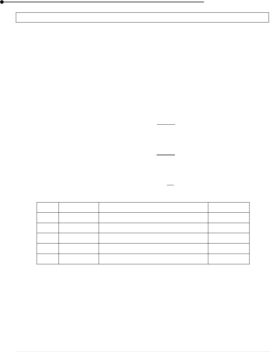
Laboratory manual
63 | P a g e
11. LIQUID LENS – REFRACTIVE INDEX OF A LIQUID
AIM
To determine the refractive index of the given liquid such us water or glycerine by forming
a liquid lens.
APPARATUS REQUIRED
Transparent liquid, Convex lens, Plane mirror, Retort stand with clamp, Bright thick needle
etc.
FORMULA
(i) Focal length of liquid lens
(ii) The radius of curvature R of the lens
(iii) Refractive index of the liquid
S.No.
Parameter
Explanation
Unit
1
f
2
Focal length of the liquid lens
m
2
f
1
Focal length of the convex lens
m
3
F
Focal length of combination
m
4
R
Radius of the curvature
m
5
d
Distance between the lens and needle
m
PRINCIPLE
The angle of refraction will be smaller than the angle of incidence and the light will be
refracted towards the normal of the surface. The higher the refractive index, the closer to the normal
direction the light till travel.
PROCEDURE
(i) Determination of focal length of the convex lens
A plan mirror M is placed on the base of vertical retort stand, with its reflecting
surface facing up as shown in fig.

Laboratory manual
64 | P a g e
A convex lens L approximately focal length 20 cm to 30 cm is placed on the plan
mirror.
A bright needle B is held horizontally by a clamp vertically above the lens.
The position of the needle is adjust slowly till a well-defined inverted image I of
the same size as the object is seem when viewed directly from above.
Now, by final adjustment of the needle, the tip of it made to coincide with that of
the image without parallax.
This can be checked by slightly moving the eye and fro.
The object and the image should not be separated from each other.
The distance from the tip of the needle to the top and bottom surface of the lens
are measured.
The mean of these two reading gives the focal length f
1
of the given convex lens.
The experiment is repeated three or four times and the readings are tabulated as
given in table.
(ii) Determination of focal length of the combination
In the next part of the experiment the convex lens is removed and the large drop
of the given liquid is placed on the plan mirror M.
The convex lens is then placed on the drop so that a compound lens of focal length,
say F is formed.
The compound lens is due to the combination of the convex lens of glass and a
plan concave lens of the liquid.
As in the previous case, by adjusting the position of the needle, the image is made
to coincide the object without any parallax.
The distance from the tip of the pin to the top and bottom of the lens are measured
with three or four trials.
The readings are tabulated as in table the mean value of length F of the
combination, from which the focal length f
2
of liquid lens can be determined.
(iii) Radius of curvature of the liquid lens mercury float method
The radius of curvature of the concave surface of the plano-concave liquid lens is
same as that of the surface of convex lens which is in contact with the liquid.
The radius of curvature of the liquid length is determined by mercury float method.
A small quantity of mercury is taken in a china disc and the convex lens of focal
length f
1
is placed on the surface of the mercury.
The china dish containing mercury and convex lens is placed below the needle.
As in the previous experiment the position of the needle is adjusted so that the size
of the image formed is equal to the size of the object and there is no parallax
between the needle and image.
The distance between the needle and the lens is measured as d.
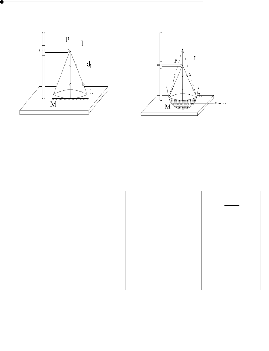
Laboratory manual
65 | P a g e
M Plane mirror ; P Bright needle ; L Convex lens
Figure 31: Experimental set- up
Table 44: Determination of focal length of the convex lens
Trial
No.
Distance from tip to top
surface d
1
: (cm)
Distance from tip to
bottom surface d
1
: (cm)
Mean,
(cm)

Laboratory manual
66 | P a g e
Table 45: Determination of focal length of the combination
Trial
No.
Distance from tip to top
surface D
1
: (cm)
Distance from tip to
bottom surface D
1
: (cm)
Mean
(cm)
RESULT
The refractive index of the given liquid =
VIVA VOCE
1. Define focal length.
2. What is refractive index?
3. What is the refractive index of water?
4. What is the focal length of convex and concave lens?
5. What is the focal length of plane mirror?
12. FABRY PEROT INTERFEROMETER
Laboratory manual
67 | P a g e
AIM
To determine the thickness of air film by forming interference using Fabry Perot
interferometer and hence to calculate fine structure speed of spectral line.
APPARATUS REQUIRED
Spectrometer, Fabry Perot Interferometer, Sodium Vapour Lamp, Scale and Telescope
Arrangements etc.
FORMULA
The thickness of air film in Fabry Perot interference is given by
m
The fine structure spread of spectral line is
m
where
m
Parameter
Explanation
Unit
t
Thickness of air film
m
Wavelength of spectral line
m
s
Distance between the scale and the mirror
m
Fine structure spread
m
PRINCIPLE
The Fabry-Perot interferometer uses the phenomenon of multiple beam interference that
arise when light shines through a cavity bounded by two reflective parallel surfaces.
PROCEDURE
A Fabry Perot interferometer consists of two semi silvered optically plane glass plates held
parallel to each other, on closing a thin air film
Silvered faces of plates are facing each other. The complete arrangement is enclosed in a
cell having circular openings both the opposite faces.
The plates are made exactly parallel, and vertical by means of three levelling screws
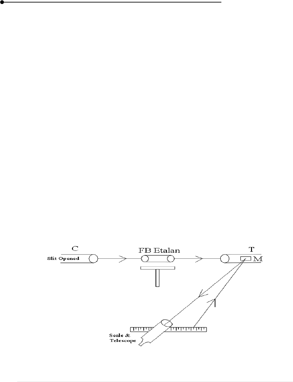
Laboratory manual
68 | P a g e
The Fabry Perot interference is mounted vertically on levelled prism table of spectrometer.
The collimating lenses from collimator is removed and slit is made as wide as possible.
The slit is then illuminated uniformly using sodium vapour lamp.
The light incident on front face of interferometer, undergoes multiple reflection through the
air film and by interference, alternate bright and dark concentric circular fringes with central
spot are formed. By focusing the telescope and adjusting it, inference pattern can be
observed.
A small mirror strip is attached to the spectrometer telescope.
The scale and telescope arrangement is placed in front of mirror at a distance of around one
meter, so as to see reflected image of the scale from the mirror at a field of the view of the
telescope.
The bring rings are called main fringes and dark rings are called satellite fringes, the vertical
cross wire of spectrometer telescope is made tangent to nth bright fringe (main) on the left
side of the centre and the scale reading is noted. Now by using tangential screw, the cross
wire is made tangent to the adjacent dark ring (satellite) and reading is taken.
Experiment is performed by making the cross-wire tangent to (n+2), (n+4), …, (n+10) bright
fringes and adjacent dark fringes.
The respective scale readings are noted observations are repeated in same order on right side
of the centre.
Readings are recorded in the given table.
The distance s between the scale and the mirror is measured.
The difference between left and right readings give the diameter D and d of main and satellite
fringes respectively. Let us take
is the diameter of the nth main fringe and
is the
diameter of nth satellite fringe.
Figure 32: Experimental set- up
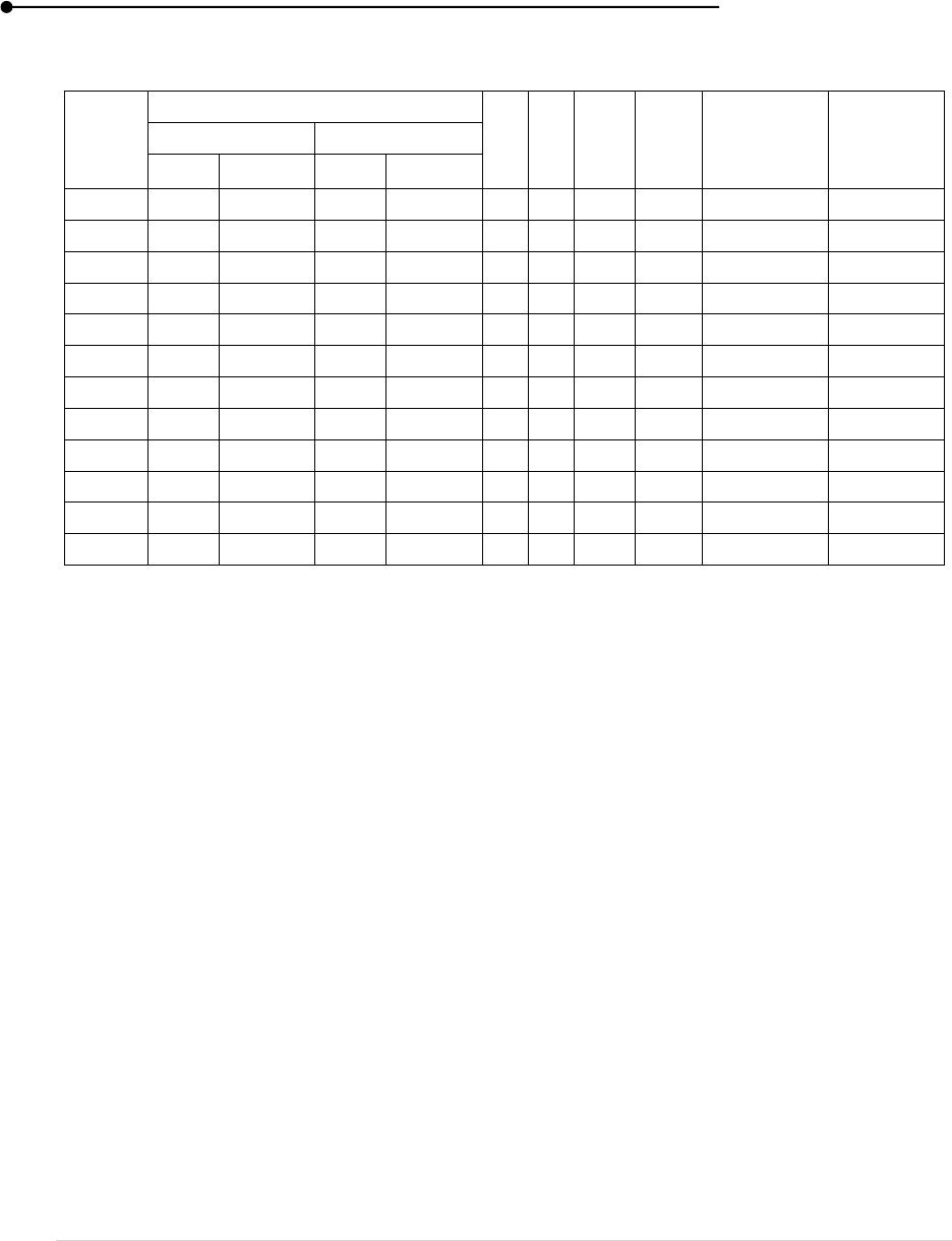
Laboratory manual
69 | P a g e
Table 46:
Order
of
fringes
Scale reading in cm
cm
cm
cm
2
cm
2
cm
2
cm
2
Left
Right
Main
Satellite
Main
Satellite
n
n+2
n+4
RESULT
1. Thickness of air film = __________ m
2. Fine structure spread = __________ m
VIVA VOCE
1. What is interferometer?
2. Who invented interferometer?
3. Define Interference.
4. What is multiple-beam interference and how does a Fabry-Perot interferometer work?
5. What is the wavelength of sodium vapour lamp?

Laboratory manual
70 | P a g e
13. FRESNEL’S BIPRISM SPECTROMETER
AIM
To determine the wavelength of monochromatic source of light using a Fresnel’s Biprism
and a spectrometer
APPARATUS REQUIRED
Spectrometer, Biprism, Scale, Telescope etc.
FORMULA
1. By divergent rays method
2. By parallel rays method
S. No.
Parameter
Explanation
Unit
1
a
Distance between the slit and the centre of the biprism
m
2
b
Distance between the centre of the biprism and cross
wire of the eyepiece
m
3
X
o
Distance between two virtual image
m
4
D
Distance between the scale and the mirror
m
5
d
Wavelength of the given mass chromatic source
applied (sodium vapour lamp)
m
6
β
Mean fringe width of divergent rays
m
PRINCIPLE
A triangular prism with vertex angle of nearly 180° used to obtain images of a single source
in observing the interference of light.
PROCEDURE
The bed of the optical bench is levelled and the levelling screws
Light source and slit is arranged in order to get maximum light incident on the slit
The centre of slit, biprism and eye piece is arranged at same height
The slit and biprism edge are made vertical and in line parallel to the bench
Observe the interference fringes with eye piece for clear fringe pattern adjust the edge of
biprism by rotating screw.
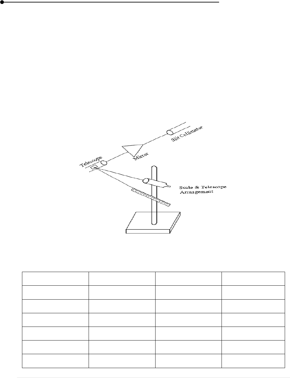
Laboratory manual
71 | P a g e
If the line joining the slit and the central edge of the biprism is not parallel to length of the
bench, fringes would shift laterally as the eyepiece is moved.
To remove, this the biprism is moved a small distance transversely to the bench in a direction
opposite to the direction of the shift till this lateral shift vanishes.
Now measure the position of fringes by putting the cross wire at mid position of each bright
fringe.
For measurement of d, a lens of short focal length is inserted between the slit and the
eyepiece.
The eyepiece is moved away from the slit so that the distance between the slit and the eye-
piece is greater than four times the focal length of the convex lens used for the measurement
of ‘d’.
Figure 33: Spectrometer Biprism
Table 47: To find β for parallel rays
Order of fringes
Scale readings
Shift for fringes
Bandwidth β
n
n+11
n+22
n+33
n+44
n+55

Laboratory manual
72 | P a g e
Table 48: To find β for divergent rays
Order of fringes
Scale readings
Shift for fringes
Bandwidth β
n
n+11
n+22
n+33
n+44
n+55
CALCULATION
(i)
m
(ii)
m
RESULT
The means wavelength of a given monochromatic source of light sodium vapour lamp, λ =
_____________ m.
VIVA VOCE
1. What is Fresnel biprism?
2. Why slit should be narrow and vertical in experiment?
3. What is fringes?
4. What is the use of biprism?
5. Define interference.

73 | P a g e
PRACTICAL-III
Heat & Electricity
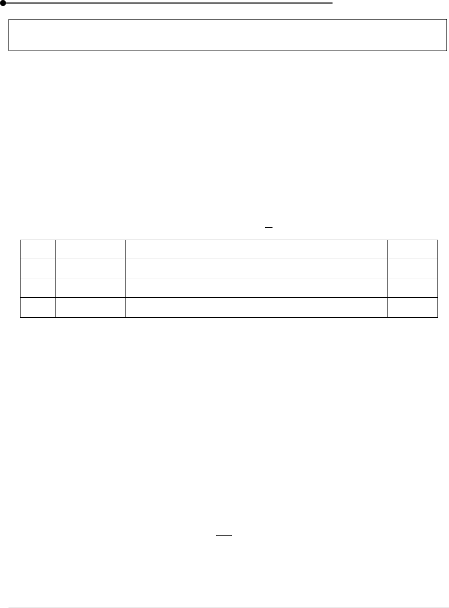
Laboratory manual
74 | P a g e
1. POTENTIOMETER CALIBRATION OF VOLTMETER
(LOW RANGE) – STANDARDISATION
AIM
To calibrate the voltmeter using potentiometer and draw a calibration and correction graph.
APPARATUS REQUIRED
Potentiometer, Voltmeter, Plug Key, Daniel Cell, Galvanometer, High Resistance, Jockey,
Rheostat, Battery.
FORMULA
emf of the Daniel cell = 1.08 eV.
emf developed in the potentiometer between l and
emf (E) = 1.08 x
volt
S.No.
Parameter
Explanation
Unit
1
E
emf developed in the potentiometer between l and
volt
2
l
Balancing length
cm
3
Balancing length of the Daniel cell
cm
PRINCIPLE
Principle of potentiometer is that potential drop across segment of wire of uniform cross
section carrying a constant current is directly proportional to its length.
PROCEDURE
(i) To determine the potential drop per metre of potentiometer wire
The primary circuit of potentiometer is made by connecting positive terminal of
battery to the end A and negative terminal to end B through a key and a rheostat.
The secondary circuit is made by connecting positive terminal of Daniel cell to the
end A and negative terminal to jockey through a galvanometer and high resistance.
Closing the key K and adjusting the jockey, the balancing length
for the Daniel
cell of emf 1.08 V is determined. Then the potential drop per meter of potentiometer
wire is given by
e =
vm
-1
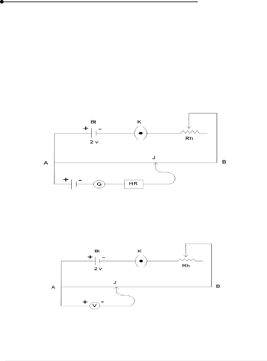
Laboratory manual
75 | P a g e
(ii) To calibrate low range voltmeter
Keeping the primary circuit undisturbed, the Daniel cell and galvanometer with high
resistance in secondary circuit are now replaced by given low range voltmeter.
It should be noted that positive signal terminal of voltmeter must be connected to
the end A of potentiometer wire.
The position of the jockey J is adjusted so that when it is pressed the voltmeter
reading become 0.1 V, 0.2 V, ……..etc.
The length of potentiometer wire corresponding to each voltmeter reading is noted
and tabulated.
Finally, the values are calculated and the calibration, correction graph are drawn.
HR High Resistance ; Rh Rheostat ; K Key
Bt Battery ; G Galvanometer ; J Jockey
Figure 34: Standaradisation of Potentiometer
Rh Rheostat; K Key; Bt Battery; V Voltmeter; J Jockey
Figure 35: To calibrate the voltmeter
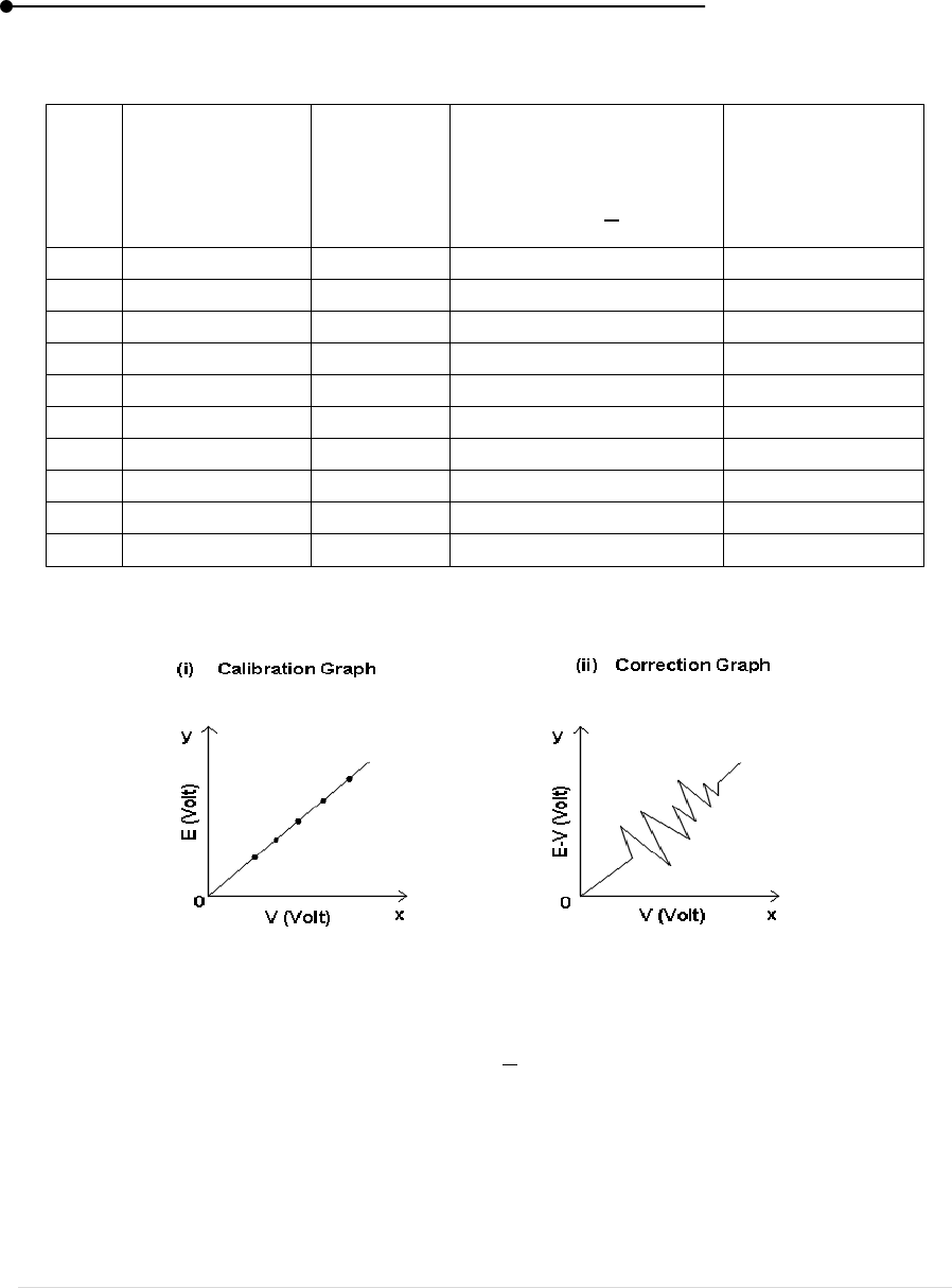
Laboratory manual
76 | P a g e
Table 49: Determine corrected reading E –V
Balancing length of Daniel cell,
= cm
S.No.
Voltmeter
reading, V (volt)
Balancing
length, l cm
Calculated potential
difference between l and
E = 1.08 x
volt
Corrected
reading E – V (V)
1
0.1
2
0.2
3
0.3
4
0.4
5
0.5
6
0.6
7
0.7
8
0.8
9
0.9
10
1.0
Figure 36: Model Graph
CALCULATION
E = 1.08 x
volt
where (i)
= cm
(ii) V = 0.1 V
(iii) l = cm
E = volt

Laboratory manual
77 | P a g e
Correction graph (E-V)
E = volt, V = 0.1 V, E – V = volt
RESULT
1. The potentiometer is standardized.
2. The voltmeter is calibrated and the correction and calibration graphs are drawn.
VIVA VOCE
1. What are the uses of potentiometer?
2. Which is an example of primary cell?
3. What is the principle behind potentiometer?
4. Potentiometer is often called as ideal voltmeter. Why?
5. State some applications of potentiometer.

Laboratory manual
78 | P a g e
2. POTENTIOMETER CALIBRATION OF AMMETER
AIM
To calibrate the given ammeter using potentiometer and draw a calibration and correction
graph.
APPARATUS REQUIRED
Potentiometer, Battery 2V and 6V, Key, Rheostat, Daniel Cell, Galvanometer, High
Resistance, Jockey, Standard Resistant, Ammeter.
FORMULA
(i) Theory of potentiometer
=
(ii) Electric current in secondary circuit
J =
x
amp
S. No.
Parameter
Explanation
Unit
1
I
Calibrated value of electric current in the
secondary circuit
amper (A)
2
Balancing length of Daniel cell of emf
1.08 volt
cm
3
Balancing length of potential across R
cm
4
emf of battery standard resistance
ohm (Ω)
5
R
Standard resistance
ohm (Ω)
PRINCIPLE
Principle of potentiometer is that potential drop across segment of wire of uniform cross
section carrying a constant current is directly proportional to the length.
PROCEDURE
(i) Standaradisation of Potentiometer
The primary circuit of potentiometer is made by connecting positive terminal of
battery to the end A and negative terminal to end B through a key and rheostat.
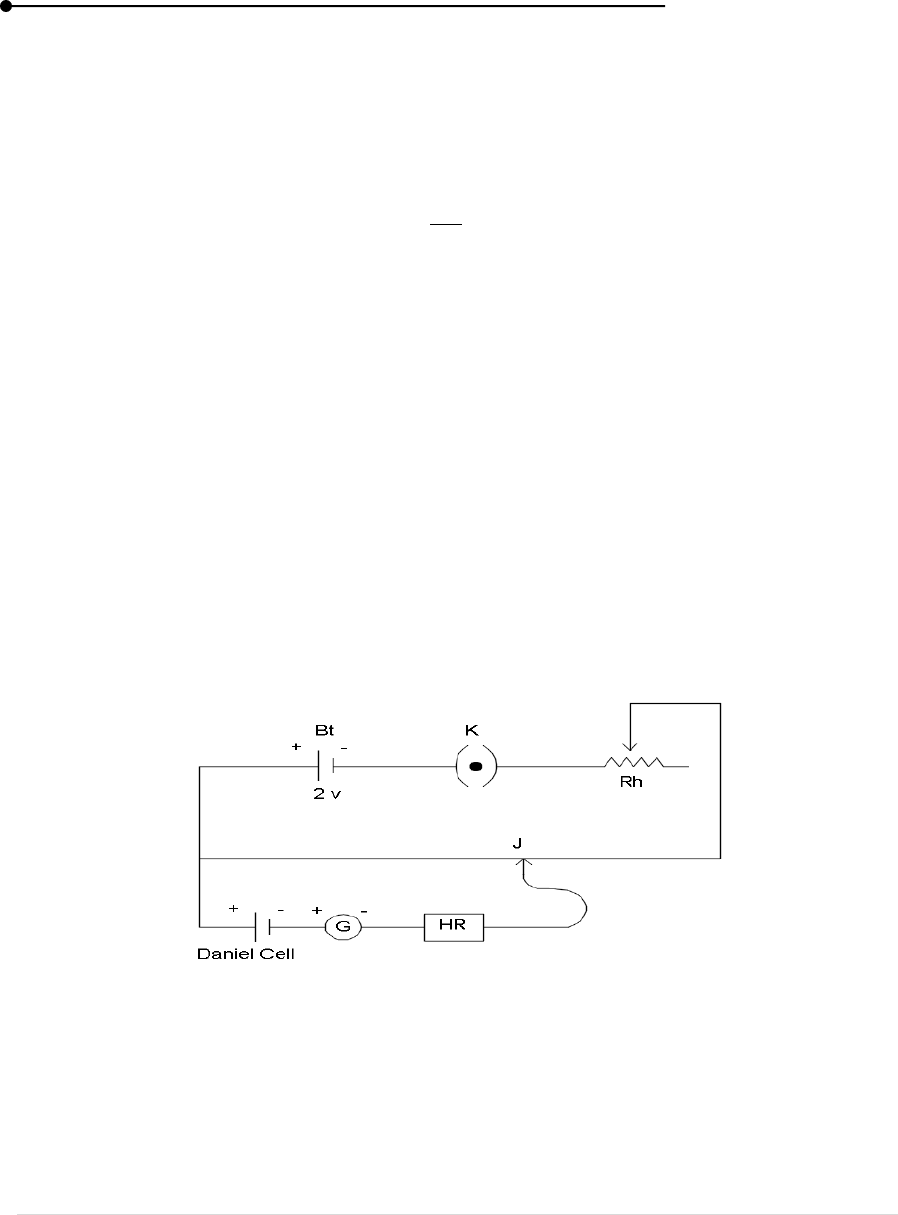
Laboratory manual
79 | P a g e
The secondary circuit is made by connecting positive terminal of Daniel cell to the
end A and negative terminal to jockey through a galvanometer and high resistance.
Closing the key K and adjusting the jockey balancing length
for the Daniel cell
of emf 1.08v is determined.
Then the potential drop per meter of potentiometer wire is given by
e =
v
(ii) To calibrate the given ammeter
The primary circuit is kept undisturbed.
The secondary circuit is made by connecting standard resistance R(1Ω) in series
with regulated power supply, given ammeter (A), rheostat (Rh) and plug key
The potential difference across (R= 1Ω) is projected over the potentiometer by
connecting positive side of R to the end of A and the negative end to the jockey J
through the galvanometer with high resistance (HR).
By closing the key K and the rheostat is adjusted so that the ammeter reads 0.3A.
The position of jockey is adjusted to get null deflection in galvanometer and the
balancing length
is determined.
The procedure is repeated for various ammeter reading 0.4, 0.5…...1.2 A by
adjusting the rheostat and corresponding balancing length are noted and tabulated.
Finally the values are calculated, calibrated correction graphs are drawn.
Figure 37: Standaradisation of Potentiometer
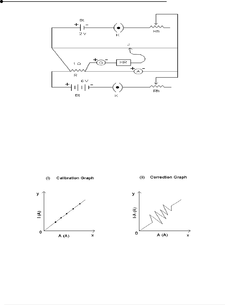
Laboratory manual
80 | P a g e
HR High Resistance ; Rh Rheostat ; K Key
Bt Battery ; G Galvanometer; J Jockey
A Ammeter ; R Standard Resistance
Figure 38: Calibration of Ammeter
Figure 39: Model Graph
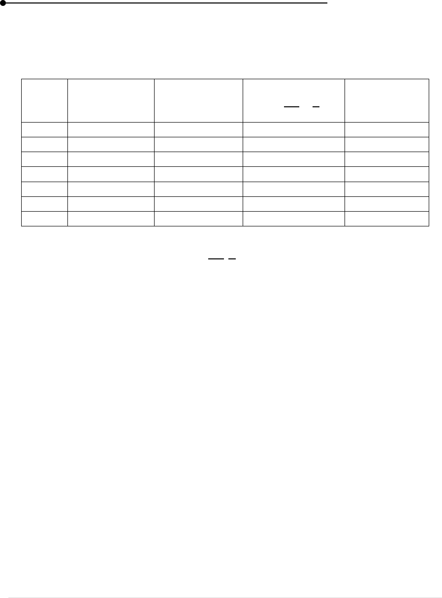
Laboratory manual
81 | P a g e
Table 50:
Balancing length of Daniel cell,
= cm
Standard resistance, R =
S.No
Ammeter
reading
(amp)
Balancing length
(cm)
Calculated current
I =
Correction
graph
I-A (amp)
1
2
3
4
5
6
10
CALCULATION
I =
amp
R = Ω
;
= cm;
= cm
I = amp
(ii) Calibration graph
I = A; A = A; I – A = amp
RESULT
1. The given potentiometer is standardized.
2. The given ammeter is calibrated.
3. The calibration and correction graphs are drawn.
VIVA VOCE
1. What is the balancing point?
2. What is Galvanometer?
3. How Ammeter is connected in a circuit?
4. Names the main parts of galvanometer.
5. What is Resistance of Galvanometer?

Laboratory manual
82 | P a g e
3. SPECIFIC HEAT CAPACITY OF WATER
AIM
To determine the specific heat of a given liquid (top water) using calorimeter.
APPARATUS REQUIRED
Joule’s Calorimeter, Ammeter, 6v Battery, Voltmeter, Rheostat, Thermometer, Stirrer, Plug
key, Coil, Tap water.
FORMULA
The specific heat capacity of the liquid (tap water)
S=
PRINCIPLE
The heat energy required to raise the temperature of the unit mass of a given substance by
given amount.
PROCEDURE
The coil C of Joule’s calorimeter is connected to a battery 6v in series with a rheostat (Rh),
an ammeter (A) and a plug key (K).
The voltage between the ends of the coil is measured by a voltmeter (v) connected in parallel
to the coil, as in the circuit diagram.
When the key is closed current starts flowing through the coil heats heated.
S. No.
Paramet
er
Explanation
Unit
1
S
Specific heat of liquid (tap water)
2
Mass of calorimeter with stirrer
kg
3
Mass of calorimeter with stirrer and liquid
kg
4
Initial temperature of calorimeter and its
contents
o
5
Current temperature
o
6
Specific heat capacity of calorimeter (4.186
J/
)
J/
7
I
Steady ammeter reading
A
8
V
steady voltmeter reading
V
9
t
Time steady of passage of current
s
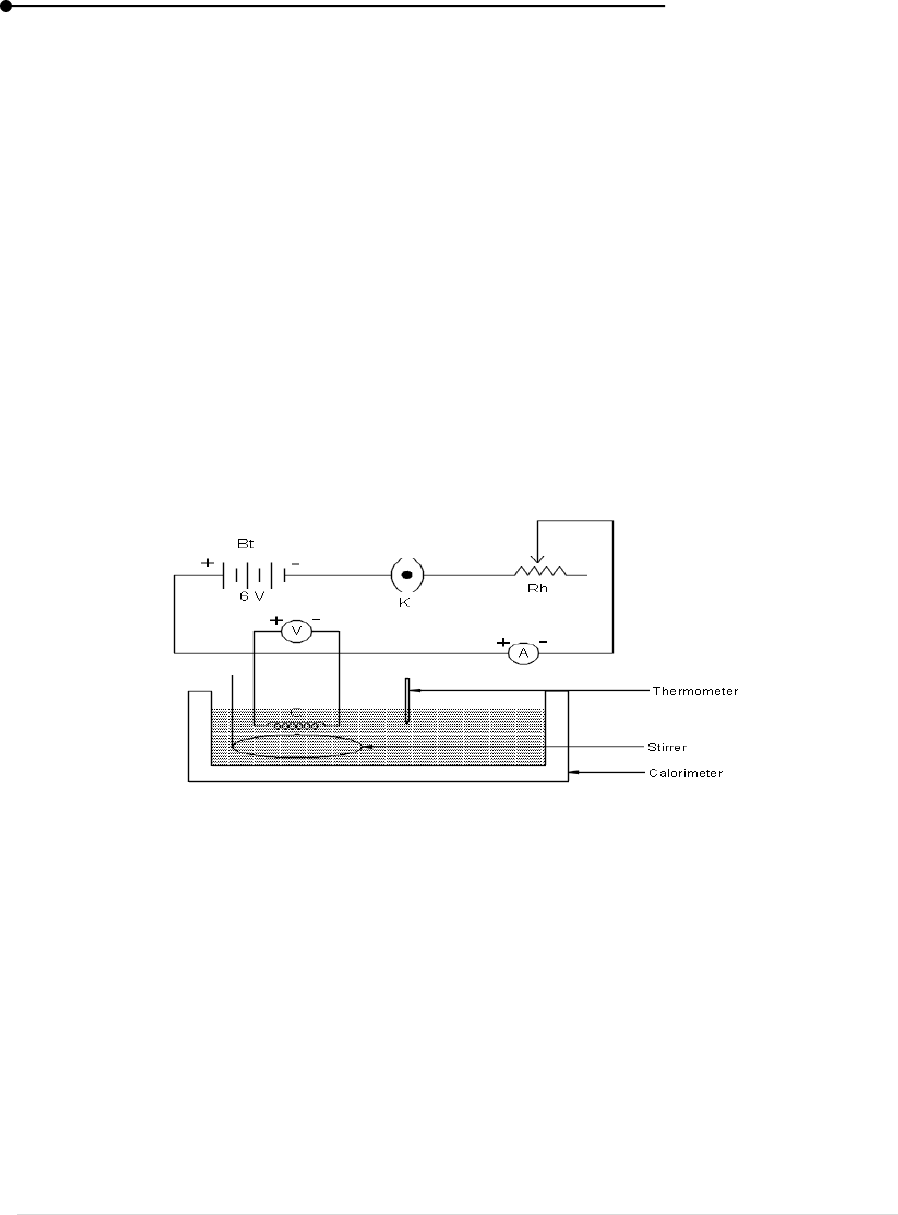
Laboratory manual
83 | P a g e
Therefore it is used to heat the liquid taken in calorimeter.
A clean empty calorimeter with stirrer is dried and weighted.
Let its mass
be noted.
The calorimeter is filled with sufficient quantity of given liquid (tap water).
So that the coil C should be immersed completely.
The mass
of the calorimeter with stirer and the liquid is noted.
It is placed inside a wooden box and the coil is immersed in it.
The initial temperature of the calorimeter and its contents is measured.
By adjusting the rheostat, suitable current is passed and simultaneously a stop clock
is started.
The content of the calorimeter is gently stirred.
The current is passed till the temperature is raised by given degree Celsius.
The final temperature is noted as
The current is switched off and time interval of passage of current t is noted.
A Ammeter ; Rh Rheostat ; K Key
Bt Battery ; V Voltmeter ; C Coil
Figure 40: Experimental Setup

Laboratory manual
84 | P a g e
CALCULATION
S=
= kg;
= kg;
=
o
;
=
o
;
t = min.; I = amp; S
1
=
RESULT
The specific heat of the liquid (tap water) by using Joule’s calorimeter is
VIVA VOCE
1. Which liquid have higher specific heat?
2. Define specific heat capacity.
3. What is the specific heat capacity of water?
4. The specific heat capacity of water is more than that of iron. What do you mean by it?
5. You can eat hot pudding on a large plate easily but you feel difficulty in a bowl. Why?
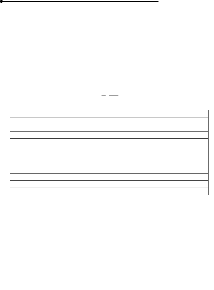
Laboratory manual
85 | P a g e
4. THERMAL CONDUCTIVITY BAD CONDUCTOR (CARD BOARD) – LEE’S DISC
METHOD
AIM
To determine the thermal conductivity of the bad conductor (card board) using Lee’s disc
method.
APPARATUS REQUIRED
Lee’s Disc, Steam Chamber, Thermometer, Thread, Rubber Tube, Cooker, Induction Stove,
Card Board (Bad Conductor), Screw Gauge, Vernier Calliper, Stand, Stop Clock.
FORMULA
Thermal conductivity of a bad conductor
λ =
W/mk
PRINCIPLE
At the steady state, heat conducted through the bad conductor is equal to heat radiated from
the Lee’s disc.
PROCEDURE
The apparatus is arranged as it is given in the figure.
Same amount of water is taken in a cooker and it is boiled using induction stove.
The steam from the cooker is passed into a steam chamber using a rubber tube.
The steam chamber is placed over a Lee’s disc and in between a card board is placed.
The steam passing through the chamber makes the chamber hot.
The Lee’s disc also become hot due to heat passing to the Lee’s disc though card board.
The temperature of the Lee’s disc and the steam chamber is noted using thermometer.
S.No.
Parameter
Explanation
Unit
1
Thermal conductivity of the bad conductor (card
board)
W/mk
2
m
Mass of Lee’s disc
kg
3
c
Specific heat capacity of Lee’s disc (375 J/kg)
J/kg
4
Rate of cooling
5
r
Radius of Lee’s disc
m
6
d
Thickness of card board
m
7
h
Thickness of Lee’s disc
m
8
Steady temperature of steam
9
Steady temperature of Lee’s disc
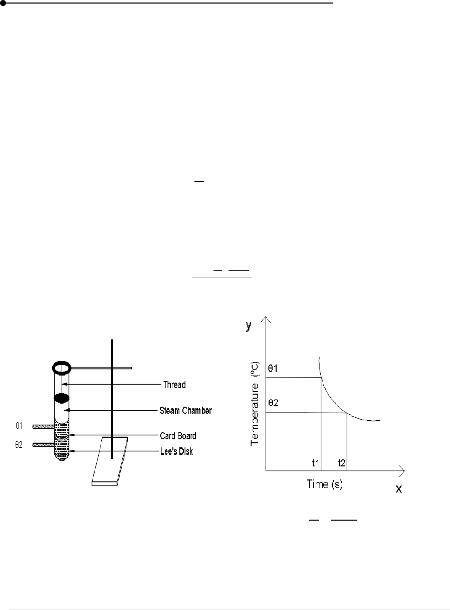
Laboratory manual
86 | P a g e
The steam is continuously passed until the chamber and the Lee’s disc reaches a steady
temperature and it is noted as
and
After reaching the steady temperature the card board between the chamber and the Lee’s
disc is removed.
Now allow the Lee’s disc to increase its temperature (eg: 5) more than steady temperature.
Now stop boiling and remove the steam chamber.
Now the temperature starts decreasing.
Note the time for the decrease of every degree from steady temperature of Lee’s disc up to
a certain value.
Tabulate the readings and plot a graph between time and temperature. It is a curve.
Find the value of rate of cooling (
) from the graph.
The thickness of Lee’s disc and card board is measured using screw guage.
The radius of Lee’s disc is measured using vernier caliper.
The readings are noted and tabulated.
The conductivity of the card board (bad conductor) calculated by the formula
λ =
W/mk.
and
Thermometer
=
o
C/s
Figure 41: Experimental Setup Figure 42: Model Graph

Laboratory manual
87 | P a g e
Table 51:
= ;
=
Constant temperature of the upper disc ;
= Constant temperature of the lower disc
Temperature
Time (s)
Minutes
Seconds
Table 52: To find the thickness of the Lee’s disc using screw gauge
LC = 0.01 mm ; ZE = ; ZC =
S.N
o
PSR
(mm
)
HSC
(div)
HSR=HSC x
LC
(mm)
Original reading
(OR) PSR+(HSC x
LC)
(mm)
Corrected reading
(OR
(mm)
Mean, h = mm
Table 53: To find the thickness of cardboard using screw gauge
LC = 0.01 mm ; ZE = ; ZC =
S.NO
PSR
(mm)
HSC
(div)
HSR = HSC
(mm)
Original reading
PSR+ (HSC
(mm)
Corrected
reading
OR (mm)
1
2
3
4
5
Mean, d =
mm
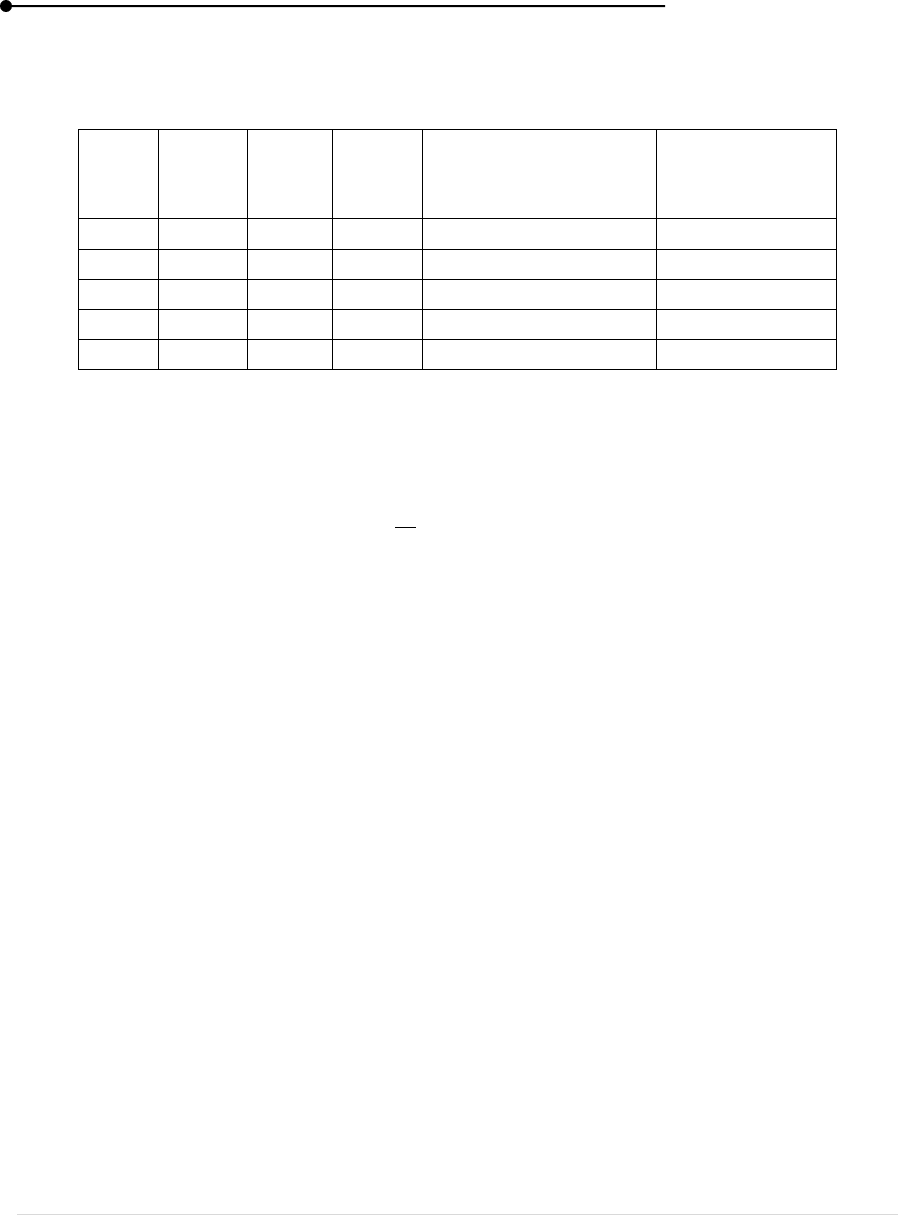
Laboratory manual
88 | P a g e
Table 54: To find the diameter of Lee’s disc using vernier calliper
LC = 0.01cm ; ZE = ; ZC =
S.NO
MSR
(cm)
VSC
(cm)
VSR
(cm)
Original reading
MSR+ (VSC )
(cm)
Corrected
reading (OR +
ZC) (cm)
1
2
3
4
5
Mean d =
cm
CALCULATION
By substituting the values m, c, d,
, r, h,
and
thermal conductivity is calculated.
RESULT
The thermal conductivity of the cardboard bad conductor by using Lee’s disc method is
____________ W/mk.
VIVA VOCE
1. What is thermal conductivity?
2. SI unit for thermal conductivity?
3. Does thermal conductivity change with thickness?
4. What is Lee’s Disc method?
5. Can Lee’s Disc method used for good conductor?

Laboratory manual
89 | P a g e
5. THERMAL CONDUCTIVITY BAD CONDUCTOR (GLASS) – LEE’S DISC
METHOD
AIM
To determine the thermal conductivity of the bad conductor (glass) using Lee’s disc method.
APPARATUS REQUIRED
Lee’s Disc, Steam Chamber, Thermometer, Thread, Rubber Tube, Cooker, Induction Stove,
Glass (Bad Conductor), Screw Gauge, Vernier Caliper, Stand, Stop Clock.
FORMULA
Thermal conductivity of a bad conductor
λ =
W/mk
PRINCIPLE
At the steady state, heat conducted from the bad conductor is equal to the heat radiated from
the Lee’s disc.
PROCEDURE
The apparatus is set up as in the figure. The cooker filled with water is boiled.
The steam from the cooker is connected to the steam chamber through a rubber tube.
The steam chamber is placed over a Lee’s disc and in between them a glass is placed.
S. No.
Paramete
r
Explanation
Unit
1
Thermal conductivity of the bad conductor
(glass)
W/mk
2
m
Mass of Lee’s disc
kg
3
c
Specific heat capacity of Lee’s disc
J/kg
4
Rate of cooling at the steady state
5
r
Radius of Lee’s disc
m
6
d
Thickness of glass
m
7
h
Thickness of Lee’s disc
m
8
Steady temperature of steam chamber
9
Steady temperature of Lee’s disc
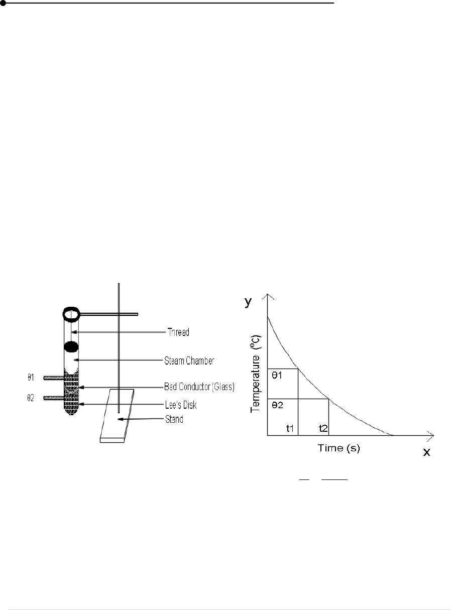
Laboratory manual
90 | P a g e
The steam passing through the steam chamber makes the chamber hot. The heat passes to
the Lee’s disc though card board.
The temperature of the Lee’s disc and the steam chamber is noted using thermometer.
The steam is continuously passed until the chamber and the Lee’s disc reaches a steady
temperature.
After reaching the steady temperature the glass is removed from the arrangement.
Now, the heat of the chamber’s heat gets transferred to the Lee’s disc directly.
The Lee’s disc temperature is increased more than the steady temperature, say 10.
Now the steam chamber is removed and the temperature of Lee’s disc is noted.
The readings are noted for every 1and tabulated the readings.
The radius of Lee’s disc is measured using vernier caliper and the thickness of the Lee’s disc
is also measured by vernier caliper.
The thickness of the Lee’s disc is calculated by screw gauge.
The Temperature – Time graphs are drawn.
and
thermometer
=
o
C/s
Figure 43: Experimental Setup Figure 44: Model Graph
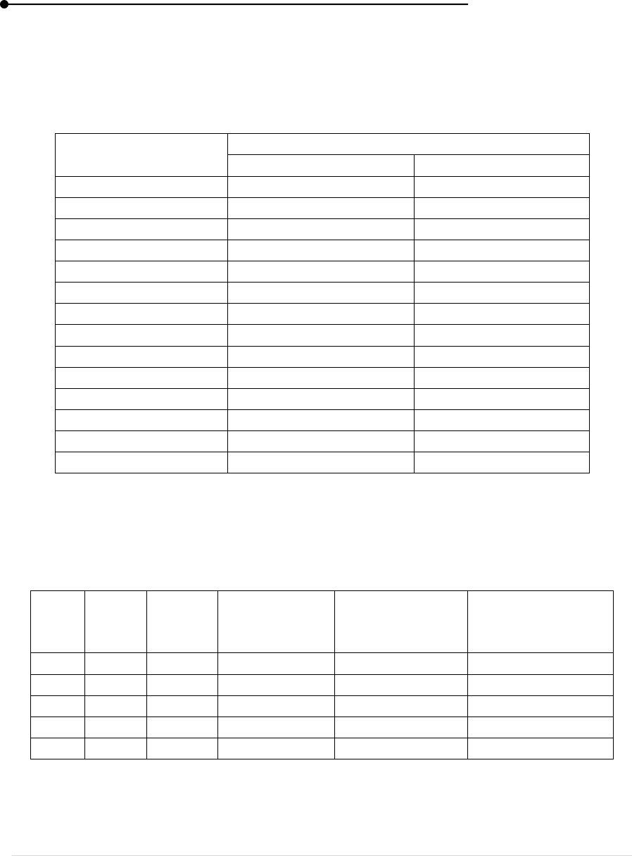
Laboratory manual
91 | P a g e
Table 55:
= ;
=
Constant temperature of the upper disc
= Constant temperature of the lower disc
Temperature ()
Time (s)
Minutes
Seconds
Table 56: To find the thickness of glass using Screw gauge
LC= 0.01 mm ; ZE= ; ZC=
S.No.
PSR
(mm)
HSC
(div)
HSR=HSC x
LC
(mm)
Original reading
PSR+HSR (mm)
Corrected reading
(OR (mm)
1
2
3
4
5
Mean d = mm
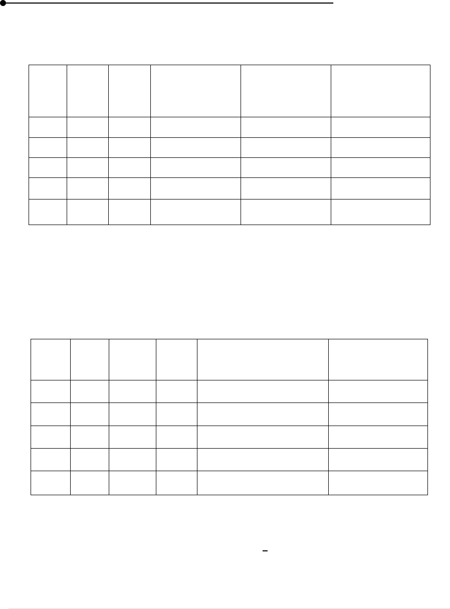
Laboratory manual
92 | P a g e
Table 57: To find the thickness of Lee’s disc using Screw gauge
LC = 0.01 mm ; ZE = ; ZC =
S.No.
PSR
(mm)
HSC
(div)
HSR = HSC
(mm)
Original reading
PSR+ HSR
(mm)
Corrected reading
TR
(mm)
1
2
3
4
5
Mean, h = mm
Table 58: To find the diameter of Lee’s disc using Vernier calliper
LC = 0.01cm ; ZE = nil ; ZC = nil
S.No.
MSR
(cm)
VSC
(cm)
VSR
(cm)
Total reading
MSR+ (VSC ) (cm)
Corrected reading
TR + ZC (cm)
1
2
3
4
5
Mean d = cm
= r = cm

Laboratory manual
93 | P a g e
CALCULATION
λ =
W/mk
m = kg; c = J/kg; d = m; r = m
h = m;
= ;
= ;
=
λ =
RESULT
The thermal conductivity of the bad conductor (glass) by using Lee’s disc method
λ = _______________W/mk.
VIVA VOCE
1. Examples for thermal conductivity?
2. Name the material having highest & least thermal conductivity?
3. Is glass a good conductor?
4. Define thermal conductivity.
5. Heat Transfer takes place according to which law of thermodynamics?
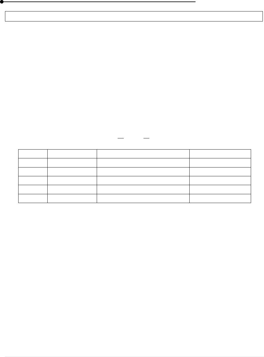
Laboratory manual
94 | P a g e
6. SPECIFIC HEAT OF SOLIDS
AIM
To determine the specific heat of given solid (graphite).
APPARATUS REQUIRED
Variable Voltmeter, Digital Thermometer, Stop Watch, Voltmeter, Ammeter.
FORMULA
(i) To find the supplying heat energy
Q= MST calories
(ii) To find the heat rate
= mS (
)
S. No.
Parameters
Explanation
Unit
1
S
Specific heat capacity of solid
J/kg
2
m
Mass of the sample
Kg
3
T
Resulting temperature
4
t
Time
s
5
Q
Heat energy
calories
PRINCIPLE
The heat energy required to raise the temperature of the unit mass of a given substance by a
given amount.
PROCEDURE
Set the thermocouple to zero using the pat and record room temperature.
Make connections for the experiment and given an AC voltage of about 25 – 35V by using
variable voltmeter to heat the graphite.
Record the room temperature while heating and plot it simultaneously till the temperature
of graphite becomes constant and estimate the equilibrium temperature.
As displaced respectively by the voltmeter and ammeter
The reading is noted from digital thermometer.
At the end of the experiment replace ammeter and variable voltmeter and measured the
temperature after reaching the equilibrium increase the voltage by 5V and observe the
temperature increases by few degrees.
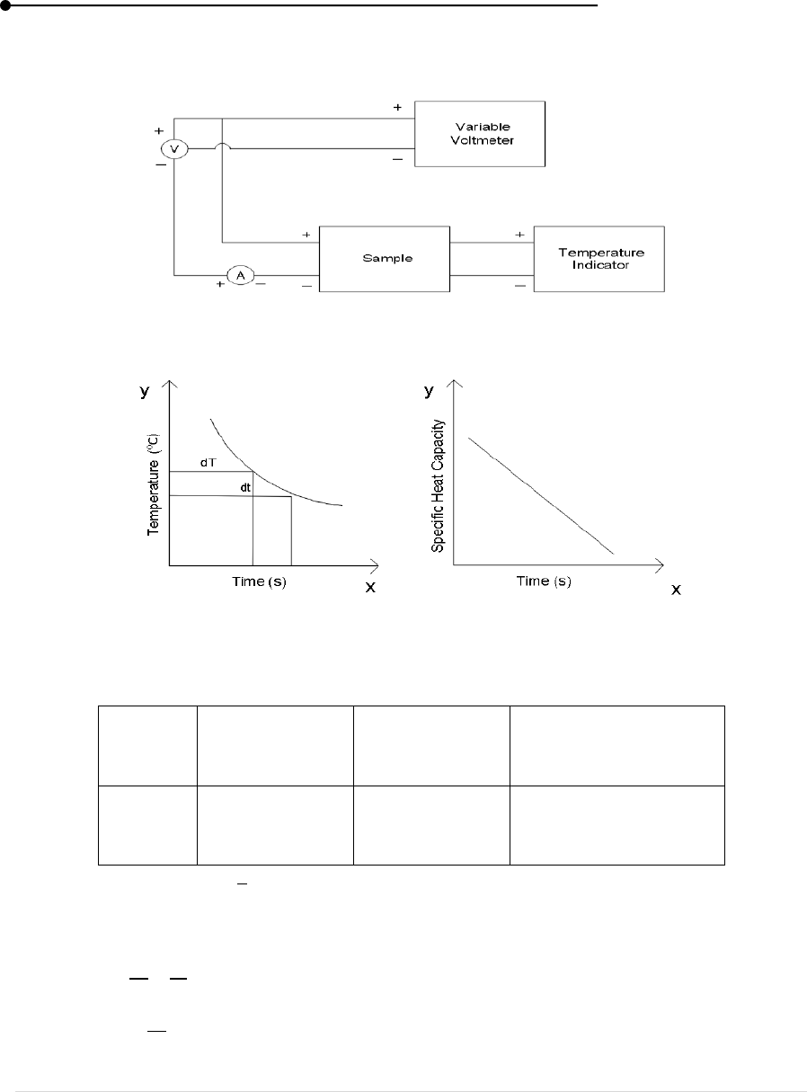
Laboratory manual
95 | P a g e
Switch off the lower supply and record the temperature decreasing.
Figure 45: Experimental Setup
Figure 46: Model Graph
Table 59: To find the equilibrium temperature
Set
voltage
(v)
Voltmeter
reading
(v)
Ammeter
reading
(A)
Equilibrium
temperature
()
By ohm’s law R =
=
Mass of graphite =
Heat
=
=
Heat
=
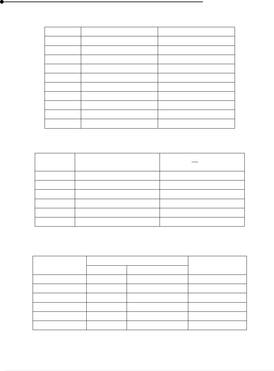
Laboratory manual
96 | P a g e
Table 60: To find the capacity
S.No.
Time (min)
Temperature
Table 61: To obtain the specific heat from various temperature
Time (min)
Temperature (dt)
()
Table 62: To find the specific heat of solid for different temperatures
Temperature
()
Graph
Specific heat
J/kg
Time (min)
Temp ()

Laboratory manual
97 | P a g e
CALCULATION
= calories ; mass = g
S =
/ m (
) J/g
RESULT
Thus, the specific heat of solid at different temperature is found and the graphs
are drawn.
VIVA VOCE
1. What is specific heat capacity?
2. What is a conductor?
3. Does the temperature increases or decreases as the time increases after we stopped
heating?
4. Does a conductor have high or low specific heat?
5. What is the SI unit for specific heat?
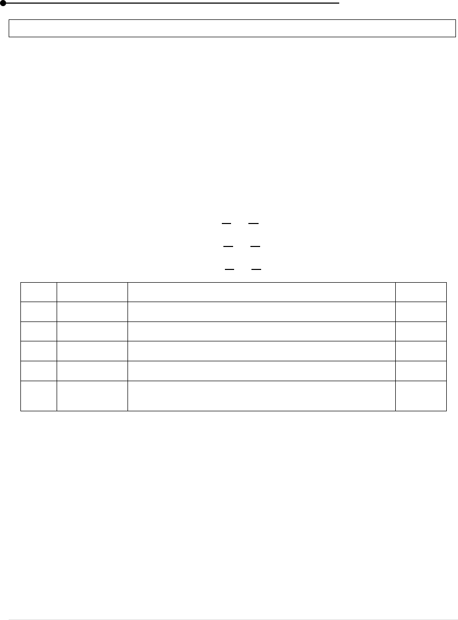
Laboratory manual
98 | P a g e
7. DE SAUTY BRIDGE CAPACITORS – SERIES AND PARALLEL
AIM
(i) To compare the capacitance of two given capacitors by forming De-Sauty bridge.
(ii) To find the effective value of capacitance by connecting them in series and parallel by
forming De-Sauty bridge.
APPARATUS REQUIRED
Resistance boxes (R
1
and R
2
), Capacitors (C
1
, C
2
, C
3
), Ear phone, AF oscillator (Audio
frequency).
FORMULA
(i)
(ii)
(iii)
S.No.
Parameter
Explanation
Unit
1
C
1
, C
2
Two given capacitor
F
2
C
P
Effective value of capacitor in parallel
F
3
C
S
Effective value of capacitor in series
F
4
C
Known capacitance
F
5
R
1
, R
2
The resistance in other branches in order to get bridge
balance
Ω
PRINCIPLE
De Sauty Bridge measures an unknown capacitor in terms of standard capacitance. Two
ratio are of this bridge consists of pure resistor and two capacitor where one is known value and
another is standard capacitance.
PROCEDURE
(i) To find the capacitance of two given capacitors
In the figure, two resistance R
1
and R
2
and two capacitors C
1
and C
2
form four arms
of the De Sauty Bridge.
The common junction of R
1
and R
2
and that of C
1
and C
2
are connected to the audio
frequency oscillator.
The circuit is completed by connecting the head phone across the bridge.

Laboratory manual
99 | P a g e
A resistance say 100 Ω is unplugged from R
2
, a random value in R
2
is noted.
The capacitance value for C
1
and C
2
is assumed (C
1
= 2 μF,C
2
= 0.5 μF).
The resistor R
2
is adjusted until the sound waves becomes zero (i.e) no sound waves
occurs.
The experiment is repeated for different values of R
1
= 100 Ω, 200 Ω, 300 Ω …. and
the readings R
2
are recorded.
The capacitors value C
1
and C
2
are calculated.
(ii) To find the capacitance of capacitors in parallel
From the figure, two resistances R
1
and R
2
are connected in two arms and the
capacitors C
1
and C
2
are connected in two arms and the capacitors C
1
and C
2
are
connected in parallel at the opposite arm and the standard capacitor is connected.
The common junction of resistors and the capacitors are connected to the audio
frequency oscillator.
The circuit is completed by connecting the head phone across the bridge.
A resistance say 100 Ω is unplugged from R
2
a random value in R
2
is noted.
The capacitance value for C
1
and C
2
is applied which was calculated from the
observed table.
The resistors R
2
is adjusted until the sound waves becomes zero (i.e) no sound
waves occurs.
The experiment is repeated for different values of R
1
= 100 Ω, 200 Ω, 300 Ω. and
the readings R
2
are recorded.
The capacitance value C
1
and C
2
is calculated by
.
(iii) To find the capacitance of capacitors in series
From the figure, two resistances R1 and R2 are connected in two arms and the
capacitor C1 and C2 are connected in series at the opposite arm and the standard
capacitances is connected.
The common junction of resistors and the capacitors are connected to the audio
frequency oscillator.
The circuit is completed by connecting the head phone across the bridge.
A resistance say 100 Ω is unplugged from R
2
, a random value in R
2
is noted.
The capacitance value for C
1
and C
2
is applied which was calculated from the
observed table.
The resistors R
2
is adjusted until the sound waves becomes zero (i.e) no sound waves
occurs.
The experiment is repeated for different values of R
1
= 100 Ω, 200 Ω, 300 Ω ……
and the readings R
2
are recorded.
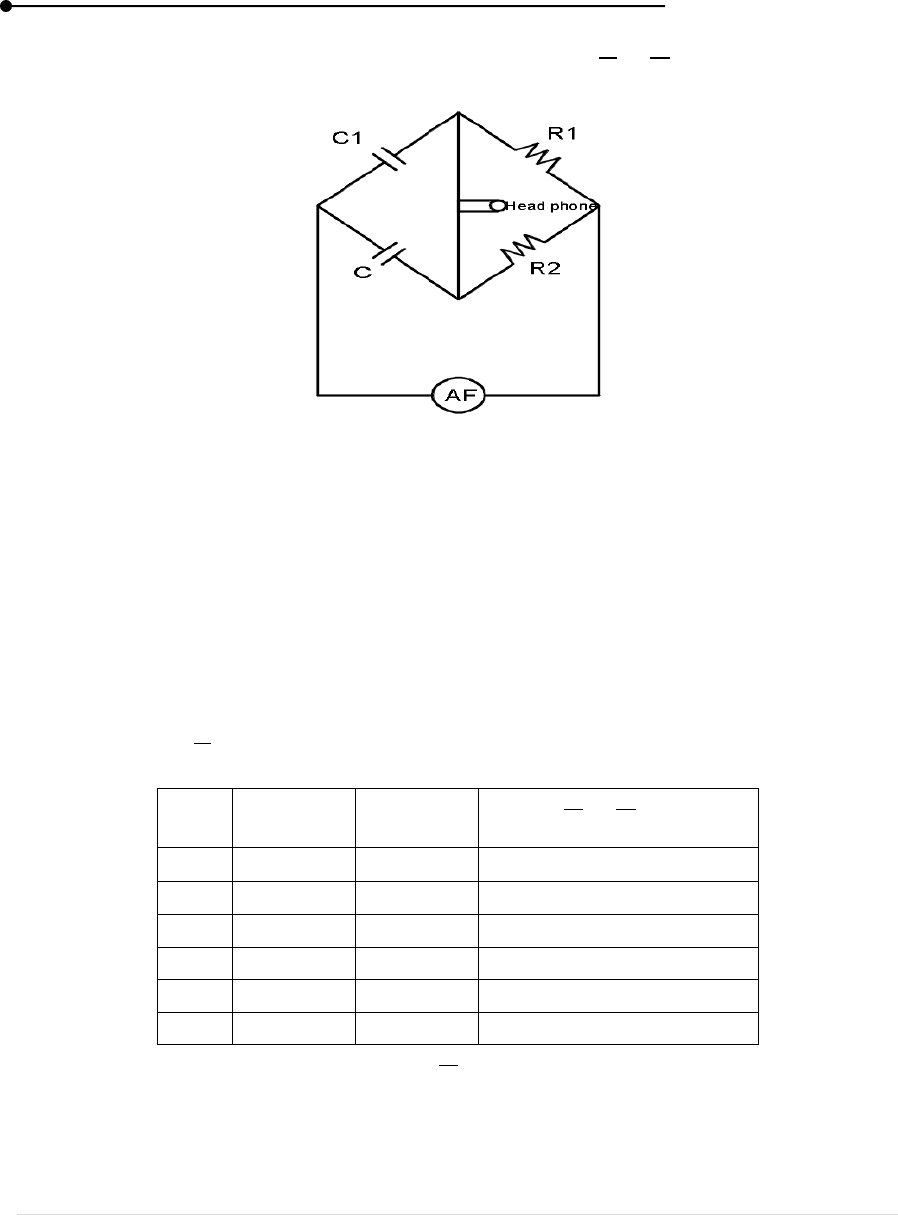
Laboratory manual
100 | P a g e
The capacitance value C
1
and C
2
is calculated by
.
C
1
and C
2
Capacitors; R
1
and R
2
Resistors; AF Audio frequency oscillator
Figure 47: Determination of two given capacitors
(i) To find the capacitance of the two given capacitors
C
1
= μF ; C
2
= μF
Table 63: To find
S.
No.
R
1
(Ω)
R
2
(Ω)
μF
Mean
= μF
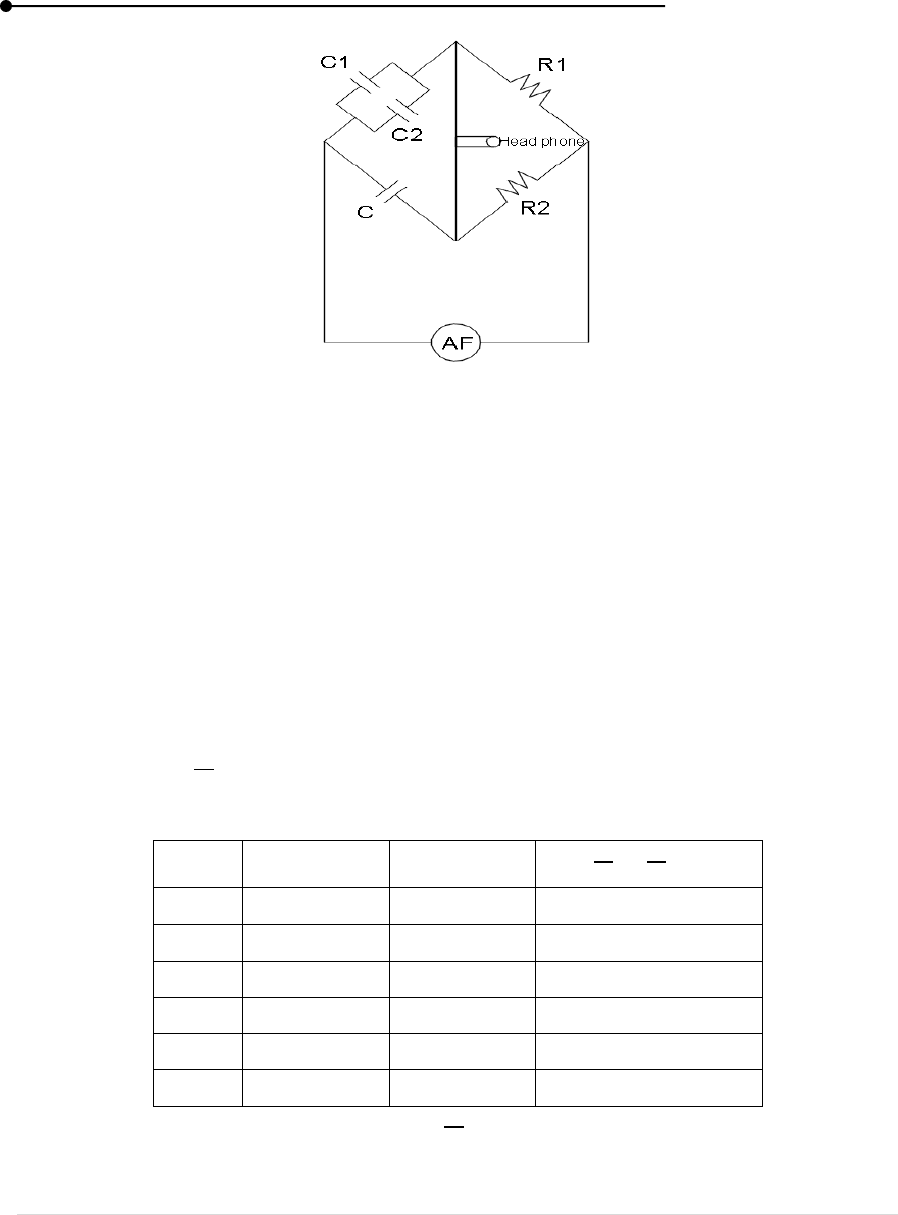
Laboratory manual
101 | P a g e
C
1
and C
2
Capacitors; C Given capacitor; R
1
and R
2
Resistors;
AF Audio frequency oscillator
Figure 48: Capacitance of capacitors in parallel
(ii) To determine the capacitance of capacitors in parallel
C
1
= μF ; C
2
= μF ; C = μF
C
P
= C
1
+ C
2
;
C
P
= μF
Table 64: To find
S. No.
R
1
(Ω)
R
2
(Ω)
μF
Mean
= μF
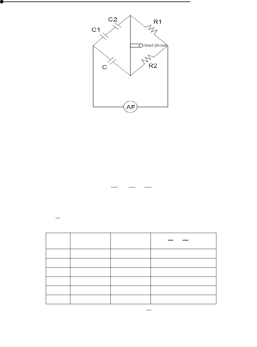
Laboratory manual
102 | P a g e
C
1
and C
2
Capacitors; C Given capacitor; R
1
and R
2
Resistors;
AF Audio frequency oscillator
Figure 49: Capacitance of capacitors in series
(iii) To determine the capacitance of capacitors in series
C
1
= μF ; C
2
= μF ; C = μF
μF
Table 65: To find
S. No.
R
1
(Ω)
R
2
(Ω)
μF
Mean
= μF

Laboratory manual
103 | P a g e
RESULT
1. The capacitance of the two given capacitors is compared by forming De-Sauty bridge
= μF.
2. The capacitance of the capacitor in parallel is found by forming De-Sauty bridge
C
P
= μF.
3. The capacitance of the capacitor in parallel is found by forming De-Sauty bridge
C
S
= μF.
VIVA VOCE
1. Does it work on ac or dc current source?
2. What is a standard capacitor?
3. What is a De Sauty’s bridge?
4. What is a series connection?
5. What is a parallel connection?
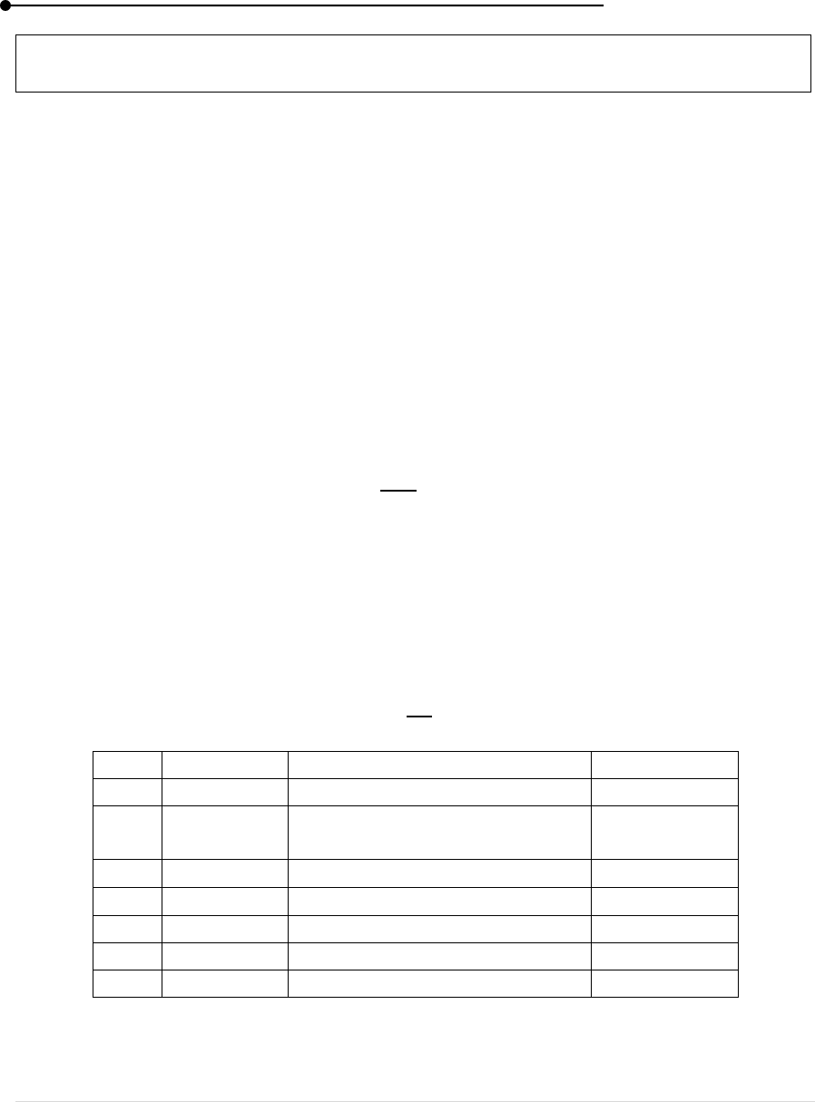
Laboratory manual
104 | P a g e
8. CAREY – FOSTER’S BRIDGE – COIL RESISITANCE AND SPECIFIC
RESISITANCE
AIM
To find the resistance of a given coil using Carey fosters bridge and hence to determine the
specific resistance of the coil.
APPARATUS REQUIRED
Carey Foster’s Bridge, Given coil, Two standard Resistance of 1 Ω each, Fractional
Resistance Box, Two Dial (0.1 Ω – 10 Ω), (1 Ω – 10 Ω) Resistance Box, Lechlanche Cell, Plug Key,
Galvanometer, High Resistance, Jockey.
FORMULA
(i) Determine the resistance per meter of bridge wire
The resistance per metre of the bridge wire is given by
P =
Ωm
-1
(ii) Determine the resistance X of the coil
The resistance X of the coil is calculated by
X = R + P (l
2
– l
1
) Ω
(iii) Determine the specific resistance of the coil
ρ = X
Ωm
S.No.
Parameter
Explanation
Unit
1
R
Resistance of the coil
volt
2
P
Resistance per metre of bridge
wire
Ωm
-1
3
Balancing length (AJ
1
)
m
4
Balancing length (AJ
2
)
m
5
X
Resistance of the coil
Ω
6
L
Length of the coil
m
7
r
Radius of the coil
m

Laboratory manual
105 | P a g e
PRINCIPLE
The potential fall is directly proportional to the length of the wire. The potential fall is nearly
equal to the potential fall across the resistance connected in parallel to battery.
PROCEDURE
(i) Determination of resistance per meter of bridge wire
In Carey-Foster’s bridge, the fractional resistance box R is connected in between
the extreme gap and a copper strip is connected across right extreme gap.
Two equal resistance P and Q each of 1 Ω are included in inner gaps. The circuits
with battery and galvanometer is completed as shown in the figure.
Now to start with a resistance of 0.1 Ω is unplugged from R and the balancing length
l
1
(AJ
1
) for which galvanometer shows null deflection is determined.
The experiment is repeated by interchanging the resistance R and the copper strip.
The balancing length l
2
(AJ
2
) for null deflection is determined.
The readings per metre of the bridge wire is given by P =
Ωm
-1
(ii) Determination of resistance X of the coil
Now the coil of unknown resistance X is connected to right extreme gap and
resistance per R is to be included in the left extreme gap.
With suitable resistance R, the balancing length l
1
(AJ
1
) for null deflection is found.
The resistance R is adjusted to get the balancing length is approximately equal to 50
cm.
Now R is changed about the previous value and the experiment is performed for
different values of resistance R and the corresponding length l
1
is measured in each
case.
The experiment is repeated by interchanging the coil X and resistance box R.
The observations are noted and tabulated. The resistance of the coil is calculated by
using the formula, X = R + P (l
2
– l
1
) Ω
For certain values of R
1
(l
1 >
l
2
) and for some other values (l
1 <
l
2
).
As the balancing point always moves towards higher resistance side (l
1 –
l
2
) may be
either negative (or) positive.
In both cases, the sign must be maintained throughout the calculations.
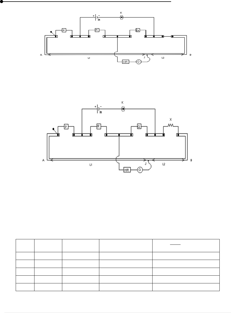
Laboratory manual
106 | P a g e
K Key; Bt Battery; P,Q,R Resistance (1Ω);
,
Balancing length
HR High resistance; G Galvanometer
Figure 50: Determine the resistance per metre of bridge wire
K Key; Bt Battery; P,Q,R Resistance boxes;
,
Balancing length
HR High resistance; G Galvanometer; X Coil resistance
Figure 51: Determine the resistance X of the coil
Table 66: Determine the resistance per metre of the bridge wire
S.No.
R (Ω)
l
1
(cm)
l
2
(cm)
P =
x 10
-2
Ωm
-1
1
2
3
4
5
Mean, P = Ωm
-1

Laboratory manual
107 | P a g e
Table 67: Determine the resistance X of the coil
S.No.
R (Ω)
l
1
(cm)
l
2
(cm)
X = R + P (l
2
– l
1
) Ω
1
2
3
4
5
Mean, X = Ω
Table 68: Determine the radius of the coil using screw gauge
Least count = 0.01 mm, ZE = , ZC =
S.No.
PSR (mm)
HSC
(div.)
HSR (mm)
TR = (PSR + HSR) ZC
(mm)
1
2
3
4
5
d = m
Radius of the coil = m
CALCULATION
1. Determine the resistance per meter of bridge wire
P =
Ωm
-1
R = Ω, l
1
= m, l
2
= m,
P = Ωm
-1

Laboratory manual
108 | P a g e
2. Determine the resistance X of the coil
X = R + P (l
2
– l
1
) Ω
R = Ω, l
1
= m, l
2
= m, X =
3. Determine the specific resistance of the coil
ρ = X
Ωm
By substituting X, r, L, ρ is calculated
RESULT
1. Mean resistance per metre of bridge wire, P = Ωm
-1
P =
2. Mean resistance of unknown resistance of the coil, X = Ω
3. Specific resistance of the coil, ρ = Ωm
VIVA VOCE
1. What is resistance?
2. What is specific resistance?
3. What is the principle of Carey Foster Bridge?
4. When is Carey Foster Bridge most sensitive?
5. What is the minimum difference in resistances that can be measured by Carey
Foster Bridge?
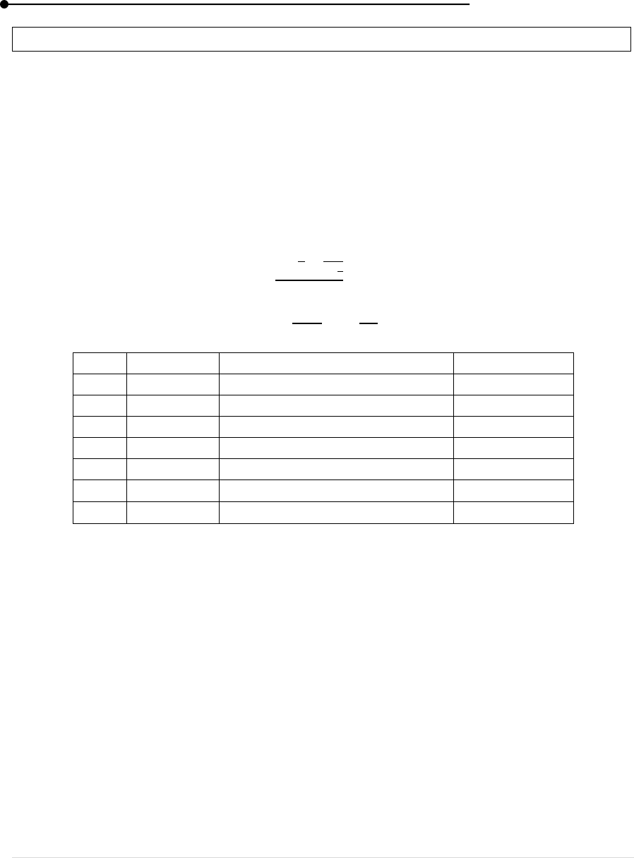
Laboratory manual
109 | P a g e
9. FIGURE OF MERIT OF CHARGE – BALLISTIC GALVANOMETER
AIM
To determine the figure of the given ballistic galvanometer by the method of charging and
discharging a capacitor.
APPARATUS REQUIRED
Ballistic Galvanometer (BG), two standard resistance boxes, standard condenser,
charge – discharge key.
FORMULA
The ballistic constant of the figure of merit of the BG is given by
K =
C/mm
λ =
PRINCIPLE
It depends on the deflection of the coil which is directly proportional to the charge passes
through it. The galvanometer measures the majority of the charge inspite of current.
PROCEDURE
The preliminary adjustments of given ballistic galvanometer are made so that the suspension
coil of the galvanometer executes free torsional oscillation.
When no charge is passed the vertical cross wire in reflected light spot is adjusted to coincide
with zero division.
The circuit is made as shown in the figure. Battery is connected in series with resistance
boxes P and Q through a plug key K.
The potential difference across P is applied to a condenser C through charge – discharge key
when the current lever N is passed against the terminal charge. The condenser gets charged
S.No.
Parameter
Explanation
Unit
1
E
emf of the cell
volt
2
C
Capacity of the condenser
μF
3
P, Q
Resistance in the boxes
Ω
4
θ
Kick produced in BG
mm
5
λ
Logarithm decimal
No unit
6
Deflection of the first throw
div.
7
Deflection of the eleventh throw
div.
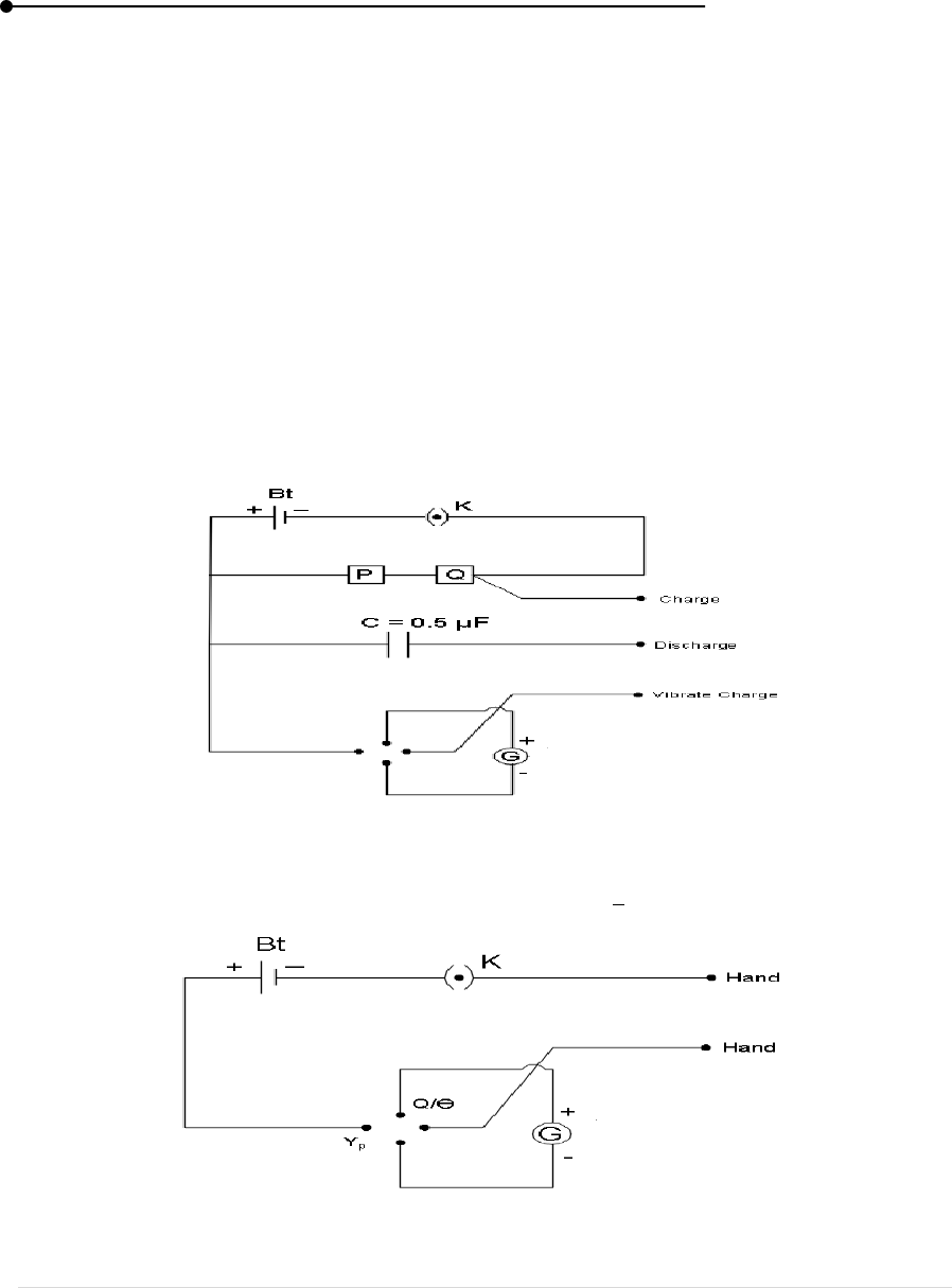
Laboratory manual
110 | P a g e
by the potential difference of P. On releasing the key, the lever contacts the terminated
discharge condenser is discharged through the BG.
A suitable resistance say 1000 Ω is unplugged in P and 9000 Ω in Q, such that P + Q =
10000 Ω. Closing the plug key K, the contact lever N is pressed against the terminal charge
for about 60 seconds to charge the condenser is discharged through the BG.
By releasing the charge- discharge key. A sudden kick is produced one side of the zero
division in the BG and is observed in a next.
Reversing the commutator and beginning the high speed to coincide with zero division, the
experiment is performed to charge and discharge the condenser.
The kick θ is now observed in the opposite side and hence means kick with P= 1000 Ω and
Q = 9000 Ω is calculated.
Experiment is repeated by taking P = 2000 Ω, Q = 8000 Ω, such that P + Q = 10000 Ω and
the readings are tabulated.
K Key; Bt Battery; P,Q Resistance boxes; C Condenser
Figure 52: To find the ratio
K Key; Bt Battery; G Galvanometer
Figure 53: To find
and
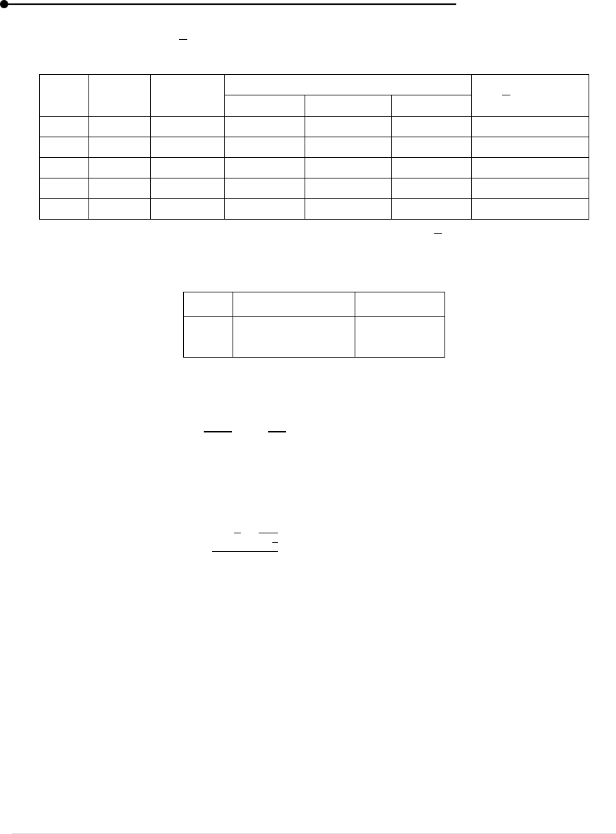
Laboratory manual
111 | P a g e
Table 69: To find the ratio
E = 2 V, C = 0.5 μF , P + Q = 10000 Ω
S.No.
Q (Ω)
P (Ω)
Kick produced (div.)
Ω/div.
Left
Right
Mean
1
2
3
4
5
Mean,
= Ω/div
Table 70: To find first and eleventh throw
S.No.
(div.)
(div.)
1
CALCULATION
(i) λ =
(ii) K =
c/mm
RESULT
The figure of merit of given Ballistic Galvanometer by the method of charging and
discharging K = c/mm
VIVA VOCE
1. What is meant by the figure of merit of a galvanometer?
2. What is the unit of figure of merit of a galvanometer?
3. How can you recognize the ballistic galvanometer?
4. What is meant by charging and discharging?
5. What is galvanometer current (Ig) and current sensitivity?

Laboratory manual
112 | P a g e
10. COMPARISON OF EMF’S USING BALLISTIC GALVANOMETER
AIM
To compare the emf’s of two cells (i.e. Daniel and Lechlanche cells) using Ballistic
Galvanometer.
APPARATUS REQUIRED
Ballistic Galvanometer, Daniel cell, Lechlanche cell, Double Pole Double Throw (DPDT)
switch, Commutator, Plug Key, Charge – Discharge Key.
FORMULA
S.No.
Parameter
Explanation
Unit
1
Kick produced for the Daniel cell of emf (
)
V
2
Kick produced for the Daniel cell of emf (
)
V
3
and
Kick produced for the battery of emf.
V
PRINCIPLE
It depends on the deflection of the coil which is directly proportional to the charge passes
through it. The galvanometer measure the majority of the charge passes through it inspite of current.
PROCEDURE
The circuit made with two resistance boxes P and Q are connected in series through a plug
key K to the common terminals of the DPDT switch.
The Lechlanche cell of emf E to bottom pair of terminals as shown in figure.
A condenser C is connected across the resistance P through a charge – discharge key as
discussed in this experiment.
The condenser discharge through the ballistic galvanometer (BG) connected through a
commutator.
To start with a resistance of 1000 Ω is introduced in P and 9000 Ω introduced in Q, so that
P + Q = 10000 Ω.
The DPDT switch is thrown to one side so that the Lechlanche cell of emf E
1
is connected
using the key K, the circuit is closed.
The charge – discharge key is pressed for about a minute so that condenser is charged to the
potential developed across P.
On releasing the key the condenser discharge through the BG.
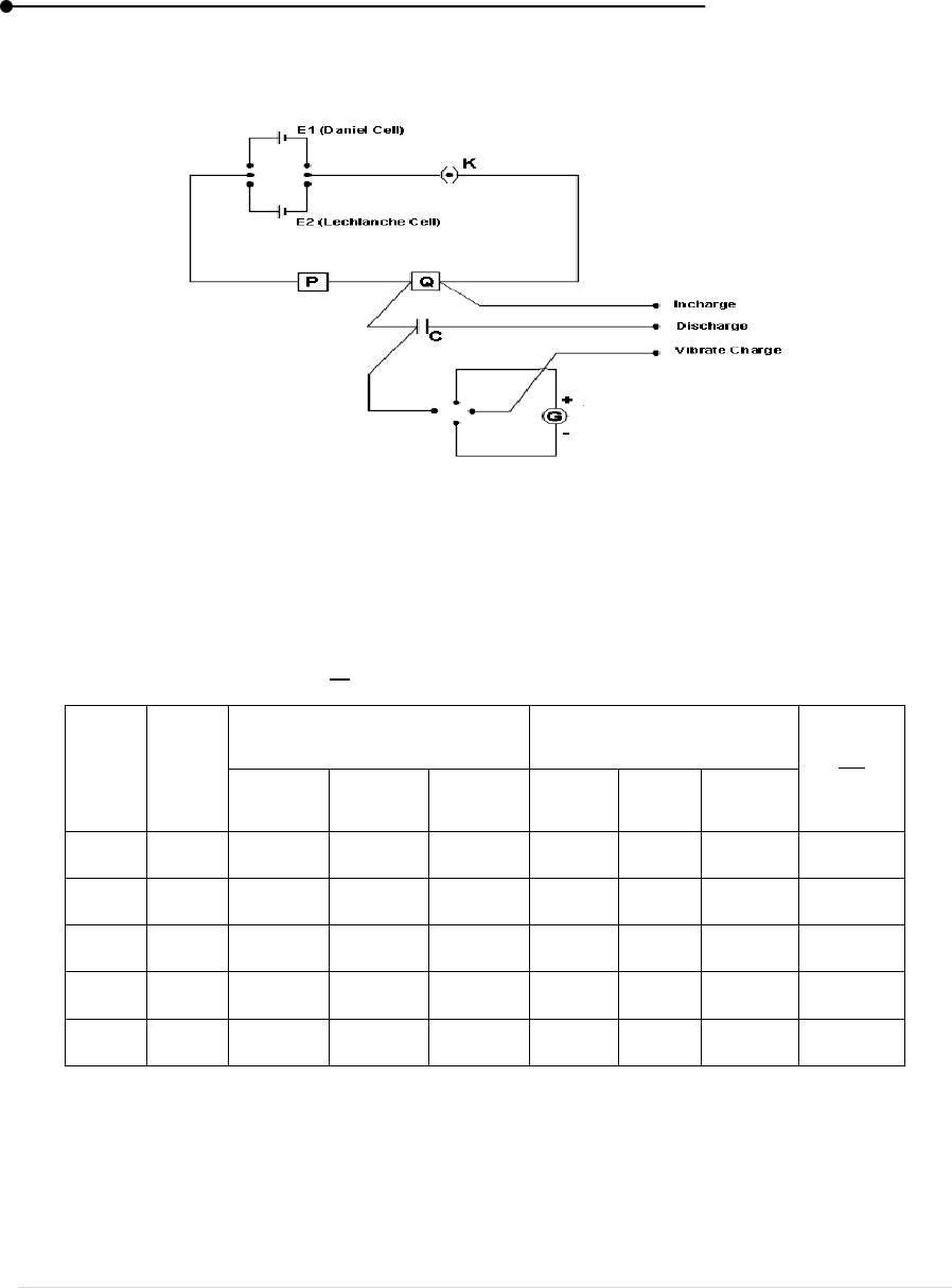
Laboratory manual
113 | P a g e
The first throw is noted. The commutator is reversed, experiment is repeated and mean throw
is determined.
K Key; C Condenser; G Galvanometer; P,QResistances
Figure 54: Experimental Setup
Table 71: Kick produced in Ballistic galvanometer
E
1
= 1.08 V, E
2
= 1.5 V,
= 0.72 V
P (Ω)
Q (Ω)
Kick produced for the
battery of emf E
1
(V)
Kick produced for the
battery of emf E
2
(V)
Left
(div.)
Right
(div.)
Mean
(div.)
Left
(div.)
Right
(div.)
Mean
(div.)
1000
9000
2000
8000
3000
7000
4000
6000
5000
5000
Mean =

Laboratory manual
114 | P a g e
CALCULATION
When P = 1000 Ω, Q = 9000 Ω
=
RESULT
The ratio of emf of the Daniel and Lechlanche cell is determined.
(i) By calculation
= V
(ii) By experiment
= V
VIVA VOCE
1. What is EMF?
2. Why does the coil of the ballistic galvanometer stops on pressing the tapping key?
3. How can you recognize the ballistic galvanometer?
4. What is Daniel and Lechlanche cell?
5. What is DPDT switch?
Laboratory manual
115 | P a g e
11. POTENTIOMETER MEASUREMENT OF RESISTANCE
AIM
To determine resistance of a coil and its specific resistance using potentiometer.
APPARATUS REQUIRED
Potentiometer, Lead Accumulator, Plug Keys, Rheostat, Galvanometer, High Resistance,
Jockey, Resistance Box, Given Coil, DPDT Switch, etc.
FORMULA
IR
I
=
X = R
S.No.
Parameter
Explanation
Unit
1
I
Current in secondary circuit
amp
2
R
Resistance
3
Balancing length
m
PRINCIPLE
Principle of potentiometer is that potential drop across segment of wire of uniform cross
section carrying a constant current is directly proportional to its length.
PROCEDURE
The primary circuit consists of an accumulator (ACC.1) connected across the two ends of
the potentiometer wire AB.
In the secondary circuit the second accumulator (ACC.2) is connected across a resistance
box R and the given coil connected in series through a rheostat and key
.
The top central terminal of a DPDT switch is connected to one end A of the potentiometer
wire.
The bottom central terminal of DPDT switch is connected to jockey though a high resistance
and galvanometer.
The left pair of terminals of DPDT switch is connected to the resistance R and right pair to
the coil X.
The proper polarity of the terminals must be ensured such that top row terminals as shown
in the circuit, should be positive and bottom row terminals negative.
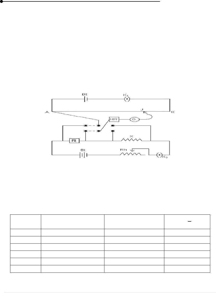
Laboratory manual
116 | P a g e
Now a suitable resistance R is included in the secondary circuit. The rheostat is adjusted to
get opposite side deflections in galvanometer when the jockey J is in contact at two extreme
ends of the potentiometer wire by projecting the potential drops across R and X separately.
The DPDT switch is thrown to one side so that the resistance R is included and the balancing
length
is measured.
Next without changing the rheostat the switch is thrown to the opposite side so that the coil
X is repeated for different values of resistance R. In each value of R, the rheostat should be
adjusted to get opposite deflections both for potential drops across R and X separately.
The readings are recorded. The length L of the wire of the coil is noted.
The radius r of cross section of the wire is determined accurately using screw gauge.
HR High Resistance ; Rh Rheostat ; K
1
and K
2
Key
Bt Battery ; AB Potentiometer ; J Jockey
R Resistance ; X Unknown Resistance
Figure 55: Experimental Setup
Table 72: Find Balancing lengths
R
(Ω)
Balancing length for
R:
(m)
Balancing length for
X :
(m)
X = R
(Ω)
Mean X = Ω

Laboratory manual
117 | P a g e
RESULT
Resistance of the given coil = Ω
Specific resistance of the material of the coil = Ω m
VIVA VOCE
1. What is potentiometer?
2. What is principal of potentiometer?
3. The electric current should not pass through potentiometer wire for long time. Why?
4. What is ohm’s law?
5. Define specific resistance.

Laboratory manual
118 | P a g e
12. BALLISTIC GALVANOMETER – COMPARISON OF CAPACITANCE
AIM
To compare the capacitance of two capacitors using Ballistic Galvanometer.
APPARATUS REQUIRED
Lead Accumulator, Two Resistance Box (1 – 1000 Ω Range), Given Condensers (Two),
Plug Key, Charge – Discharge Key, Commutator, Ballistic Galvanometer, Double Pole Double
Throw (DPDT), Switch etc.
FORMULA
S.No.
Parameter
Explanation
Unit
1
Capacitance of first condenser
μF
2
Capacitance of second condenser
μF
3
and
Kick produced in ballistic galvanometer
no unit
PRINCIPLE
The working of the Ballistic galvanometer is very simple. It depends on the deflection of the
coil which is directly proportional to the charge passes through it. The galvanometer measure the
majority of the charge passes through it inspite of current.
PROCEDURE
The preliminary adjustment of given ballistic galvanometer is made of accumulator (ACC)
is connected in series with two resistance boxes P and Q through a plug key.
One end of P is connected one of the mid terminals of DPDT. The other end of P is connected
to the Ch point of the charge discharge key, respectively.
The other end mid terminal of the DPDT switch is connected to the contact lever N of the
charge discharge key.
The top pair and bottom apir of DPDT terminals are connected to the two given condensers
of capacitors
and
, respectively.
Each condenser is discharged through a ballistic galvanometer connected across the
commutator.
A suitable resistance, say 1000 Ω is introduced in resistance box P and a resistance of 9000
Ω in Q so that P+Q = 1000 Ω.
After closing the key K, the condenser
is included in the circuit using the DPDT switch.
The charge discharge is pressed for about a minute so that the capacitor
is charge fully
by a potential difference across the resistance P.
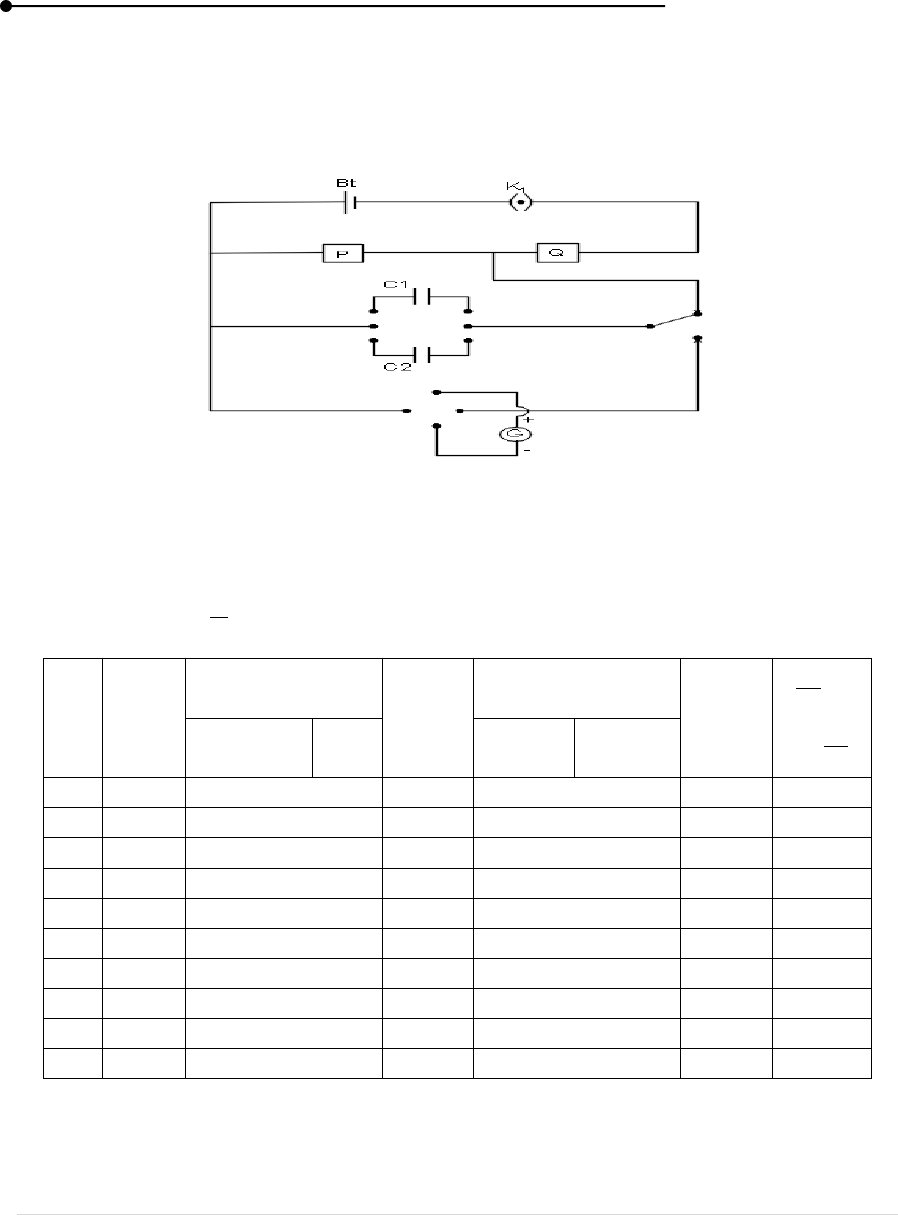
Laboratory manual
119 | P a g e
Then, by releasing the charge discharge key, the capacitor
is discharge through the
ballistic galvanometer.
The throw is observed on one side of the zero scale division. The commutator is now
reversed.
K Key; C Capacitors; Bt Battery; P,QResistance box
G Ballistic galvanometer
Figure 56: Experimental Setup
Table 73: Determine
P
Ω
Q
Ω
Throw for
capacitor
Mean
Throw for
capacitor
Mean
Left
Righ
t
Left
Right

Laboratory manual
120 | P a g e
RESULT
The capacitance of two given capacitors compared and their ratio
is determined,
=
VIVA VOCE
1. What does a ballistic galvanometer measure?
2. What is DPDT switch and its uses?
3. What is the difference between galvanometer and ballistic galvanometer?
4. What is the purpose of ballistic galvanometer?
5. What is the use of charge – discharge key?
Laboratory manual
121 | P a g e
13. OWEN’S BRIDGE – INDUCTANCES IN SERIES AND PARALLEL
AIM
To determine the self-inductance of the given two coils using Owen’s bridge and hence to
find the effective self-inductance of the two coils connected in series and in parallel.
APPARATUS REQUIRED
Resistor, Inductor, Capacitors, Ear phone, AF oscillator (Audio frequency).
FORMULA
L = PRC Henry
S.No.
Parameter
Explanation
Unit
1
L
Self-inductance of the coil
Henry
2
P
Resistance value in the arm AD such that P = Q
Ω
3
C
Capacitance value of the capacitor C
1
such that C
1
=
C
2
μF
4
R
Resistance value to be included in R to balance the
bridge.
Ω
PRINCIPLE
The Bridge which measures the inductance in terms of capacitance is known as Owen’s
bridge. It works on the principle of comparison (i.e) the value of the unknown inductor is compared
with the standard capacitor.
PROCEDURE
The circuit is made as shown in figures.
Suitable resistance are in P and Q such that P = Q.
Suitable value of capacitance are also in C
1
and C
2
such that C
1
= C
2.
Now the resistance value in R is adjusted to balance the bridge i.e. the sound produced by
the headphone goes to zero or minimum.
The experiment can be repeated by changing the value of P keeping the capacitors value as
constant.
Using the observed data, the self-inductance of the coil L
1
may be determined.
The same procedure is followed to determine the self-inductance of the coil L
2
and the
effective self-inductance of the two coils by connecting them in series or in parallel.
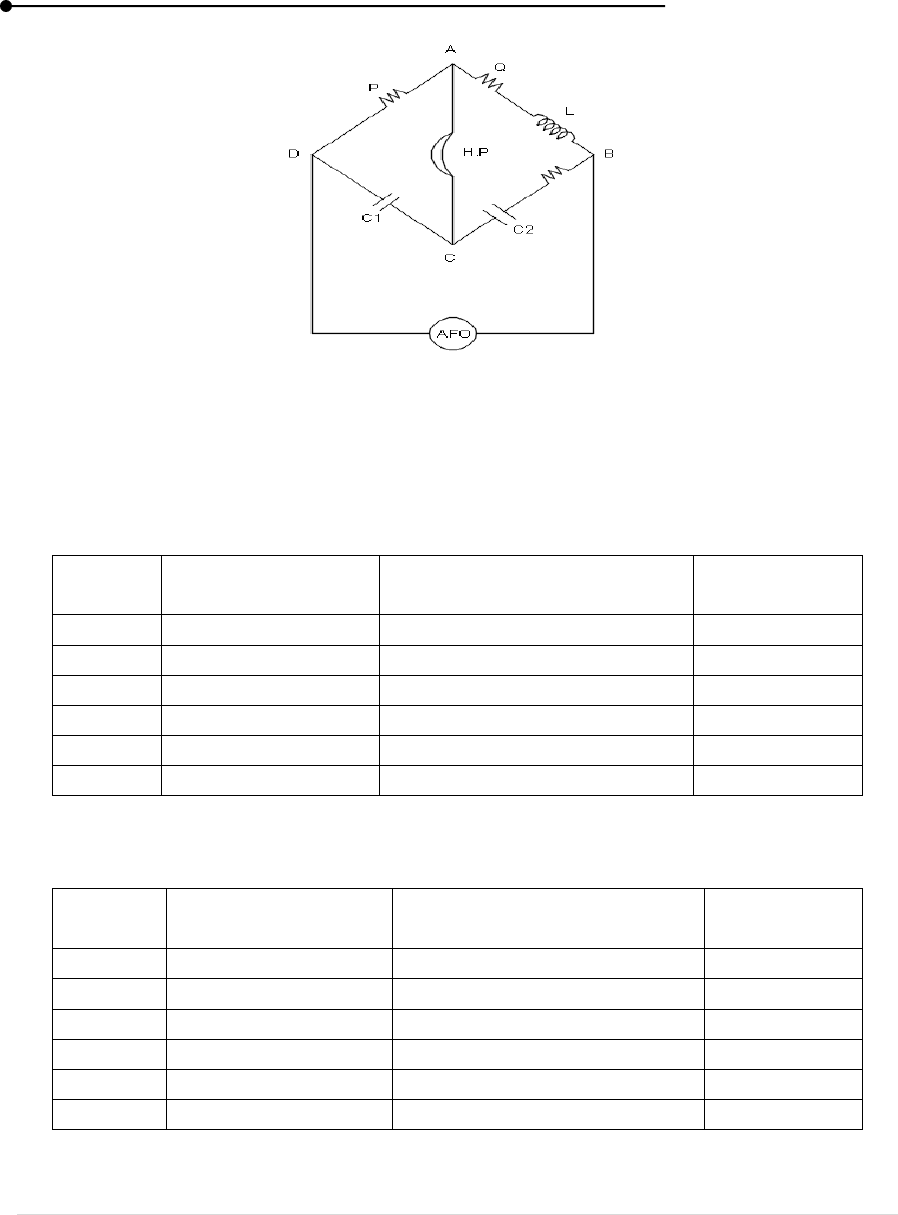
Laboratory manual
122 | P a g e
P, Q Resistances; C
1
and C
2
Capacitors; H.P Headphones
AFO Audio frequency oscillator; L Inductor
Figure 57: Experimental Setup
Table 74: To find L
1
: C
1
= C
2
= C
S. No.
Resistance value in
P = Q (Ω)
Resistance value included in R
to balance the bridge (Ω)
Henry
1
2
3
4
5
6
Mean =
Table 75: To find L
2
: C
1
= C
2
= C
S. No.
Resistance value in P
= Q (Ω)
Resistance value included in R
to balance the bridge (Ω)
Henry
1
2
3
4
5
6
Mean =
Laboratory manual
123 | P a g e
Table 76: To find effective self-inductance in series L
S
: C
1
= C
2
= C
S. No.
Resistance value in P
= Q (Ω)
Resistance value included in R
to balance the bridge (Ω)
Henry
1
2
3
4
5
6
Mean =
Table 77: To find effective self-inductance in series L
P
: C
1
= C
2
= C
S. No.
Resistance value in P
= Q (Ω)
Resistance value included in R
to balance the bridge (Ω)
Henry
1
2
3
4
5
6
Mean =
CALCULATION
= ;
=
=
+
=

Laboratory manual
124 | P a g e
RESULT
1. Self-inductance of the coil
=
2. Self-inductance of the coil
=
3. Effective self-inductance of the two coils connected in series
=
4. Effective self-inductance of the two coils connected in parallel
=
VIVA VOCE
1. What is the purpose of Owens bridge?
2. What is self-inductance?
3. What is the advantages of Owen’s bridge?
4. Explain balance condition of the bridge.
5. What is inductor?
6. Define one henry.
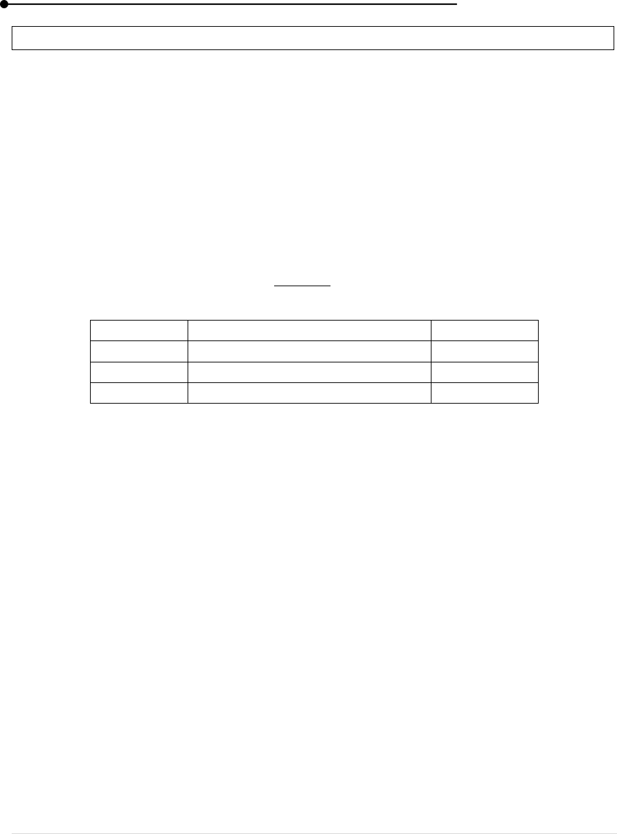
Laboratory manual
125 | P a g e
14. LCR-SERIES CIRCUIT
AIM
To study the frequency response of a LCR series circuit and hence to determine the resonant
frequency, self-inductance of the coil and Q-factor.
APPARATUS REQUIRED
Inductance, capacitance, resistance, audio frequency oscillator, milli ampere
FORMULA
Self-inductance of the given coil
Parameter
Explanation
Unit
L
Self-inductance of the coil
Henry
f
r
Resonant frequency of the coil
Hertz
c
Capacitance of the circuit
μF
PRINCIPLE
The LCR series circuit consists of resistance, inductor, and capacitor which are connected
in series in the series LCR circuit. At this frequency movement, the impedance of the circuit has low
magnitude and phase angle of zero, it is called as the resonant frequency of the circuit.
PROCEDURE
Milli ampere and audio frequency oscillator are connected in series. Inductor, capacitor and
resistance are connected in series. LCR circuit is made as shown figure.
The frequency f of the AFO is slowly varied and the current shown by the ammeter is noted.
The circuit shows maximum current for a particular frequency (resonant frequency). The
experiment is repeated by changing the value R.
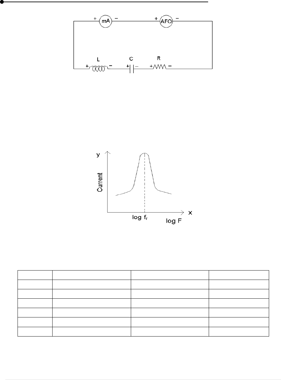
Laboratory manual
126 | P a g e
mA milliampere; L Inductor; C Capacitor; R Resistor AFO Audio frequency
oscillator
Figure 58: Experimental Setup
Figure 59: Model Graph
Table 78: R = __________ ohm
S. No.
Frequency F
Log f
Current (mA)
1
2
3
4
5
6

Laboratory manual
127 | P a g e
Table 79: R = __________ ohm
S. No.
Frequency F
Log f
Current mA
1
2
3
4
5
6
CALCULATION
Capacitance value of the capacitance used, C = _____________ μF
Ohmic resistance of the coil, r = ________ Ohm
Resonant frequency, f
r
_________ Hertz
To determine L:
To determine Q-factor
RESULT
1. The frequency response of LCR series circuit is studied.
2. The resonant frequency of the circuit = ____________ Hertz
3. Self-inductance of the coil, L = ____________ Henry
4. Q-factor of the coil = ____________
VIVA VOCE
1. What is meant by resonance?
2. What is resonance frequency?
3. Define quality factor of a series circuit.
4. What is the importance of series resonance circuits?
5. What is the function of A.F. oscillator?

Laboratory manual
128 | P a g e
15. MEASUREMENT OF INDUCTANCE USING BALLISTIC GALVANOMETER
AIM
To determine the coefficient of self-induction of a given coil using the ballistic
galvanometer.
APPARATUS REQUIRED
Lechlanche cell, ballistic galvanometer, fractional resistance boxes (two), self-inductance
coil, tap keys (two) etc.
FORMULA
The self-inductance of the coil
L = C [QR + 2rR] H
S. No.
Parameter
Explanation
Unit
1
L
Self-inductance of the coil
Henry
2
C
Capacitance of the condenser
μF
3
Q, R, r
Resistance introduced
Ω
PRINCIPLE
The working of the Ballistic Galvanometer is very simple. It depends on the deflection of
the coil, which is directly proportional to the charge passes through it. The galvanometer measure
the majority of the charge passes through it in spite of current.
PROCEDURE
A Wheatstone bridge is made with three resistance P, Q, R of post office box and the fourth
arm is being the induction coil L and fractional resistance in series are shown.
Let the bridge be ABCD, the four arms being AB, BC, CD and AD. The arms AB, BC and
AD contain resistance boxes P, Q and R respectively.
The arm CD contain the resistance box S and the inductance coil L whose self-inductance
is to be determined.
The ballistic galvanometer series with a fractional resistance r through a tap key K
3
is
connected across B and D.
A standard condenser C included in the circuit shown in figure.
The lechlanche cell is connected A and C through a tap key K
1.
Equal resistance are included in the arms P and Q.
The resistance R and S are suitably adjust, so that when the battery, key K and then
galvanometer key K
2
are pressed, the galvanometer shows null reflection.
The value of resistance R and S are noted.

Laboratory manual
129 | P a g e
The Wheatstone bridge then is balanced for steady current.
Next, the galvanometer key K
2
is closed first followed by the key K
1.
A kick is observed in the galvanometer.
Now, the resistance r is adjusted to get deflection.
When the galvanometer circuit is closed due to breaking of battery circuit.
The bridge is then balanced for varying current.
P, Q, R, r, S Resistances ; C Capacitance of the condenser; G Galvanometer
LC Lechlanche cell ; K
1
, K
2
Kick produced
Figure 60: Circuit Diagram
Table 80: Capacitance of the condenser, C = _____________F
P
(Ω)
Q
(Ω)
R
(Ω)
S
(Ω)
r
(Ω)
Resistance of
coil
= (R - S)
(Ω)
Self-inductance
L = C [QR + 2Rr]
(H)
Mean resistance of the coil
= _________ Ω
Mean self-inductance of the coil L = _________ H

Laboratory manual
130 | P a g e
RESULT
The coefficient of self-induction of given coil = ________________ H.
VIVA VOCE
1. Define self-inductance.
2. What is Wheatstone’s bridge?
3. What does a ballistic galvanometer measure?
4. What is absolute capacity of condenser?
5. Difference between and Inductance and capacitance.

131 | P a g e
PRACTICAL-IV
Electronics

Laboratory manual
132 | P a g e
1. DUAL REGULATED POWER SUPPLIES USING IC'S
AIM
To construct a 12-0-12 dual power supply with a bridge rectifier using IC7812 and 7912.
APPARATUS REQUIRED
A centre tapped transformer, 4 diodes, IN4004, IC7812, IC7912, 100 μF /24V capacitors
connecting wires etc.,
THEORY
Power Supply
A power supply is an electrical device that supplies electric power to an electric load. The
primary function of a power to an electric is to convert electric current from a source to the correct
voltage current and frequency to power the load.
The term DC is used to refer to power systems that use only one polarity of voltage or current
and to refer to the constant zero frequency or slowly varying local man value of a voltage or current
for example the voltage across a DC voltage source is constant as is the current though a DC current
source
PROCEDURE
Firstly, 220V AC is converted into 12AC by using simple step down transformer.
Secondary output of this transformer is given to the rectifier circuit which will convert the
ac supply voltage into dc contains the ripples in the output voltage to filter out mess rippled capacitor
of 1000 μF 25V is used. The output of the capacitor that is DC is given to voltage regulator IC 7812
and IC 7912 which will regulate the output voltage at 12v and -12V despite the change in input
voltage.
Connect these according to circuit diagram the outer two terminals of the centre tapped
transformer circuit is a converter which converts ac supply into dc supply it is generally made up of
diodes switches as shown in circuit diagram. To convert ac into dc we can make two types of rectifier
one is half bridge rectifier and second is full rectifier. In half bridge output voltage is half the input
voltage. For e.g. it input voltage is 24V then output dc voltage is 12V and number of diodes used in
this type of rectifier is 2. In full bridge rectifier number of diodes is 4 and it is connected as shown
in figure and output voltage is same as the input voltage. Now 24V DC output which contains peak
to peak ripples can’t be connected directly to the load. So to remove ripples from the supply filter
capacitor are used now. Two filter capacitor of 1000 μ F and 25V are used as shown in circuit
diagram, the connections of both capacitors are such that the common terminal of the capacitors is
connected directly to the centre terminal of the centre tapped transformer.
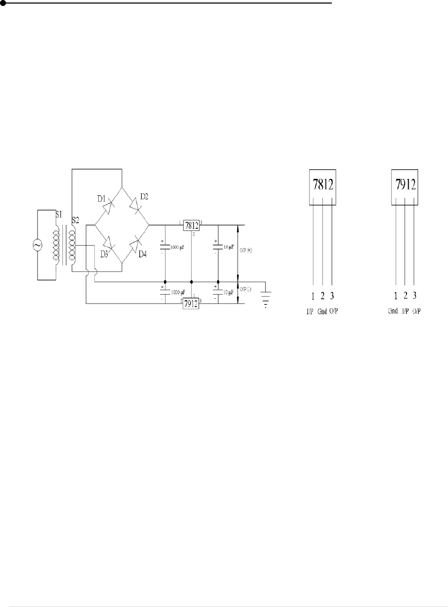
Laboratory manual
133 | P a g e
The capacitors will remove the ripples from the DC power supply and give a pure dc output.
But the output of both the capacitors are not regulated. So, to make the supply regulated output of
the capacitors are given to the voltage regular ICs
Regulate the 12V DC Power Supply
The voltage regulator ICs are used, if we need the +5V output voltage 7805 IC is used first
tow digit of the IC gives output voltage rating third last digit shows voltage is positive. Or negative
for positive voltage and for negative number is used so IC7812 is used for +12V regulator and
IC7912 is used for -12V regulator.
Figure 61: Circuit Diagram
RESULT
A (12-0-12) V dual power supply with a bridge rectifier is constructed and their AC and
DC voltages are measured.
The input AC voltage is ___________________
The output DC voltage is ___________________
VIVA-VOCE
1. What is the function of IC7812 and IC7912 ?
2. What is the meaning of regulated power supply?
3. Give the function of the transformer.
4. What are the types of transformer?
5. What is a dual power supply?

Laboratory manual
134 | P a g e
2. HIGH PASS AND LOW PASS FILTER CIRCUIT
AIM
To construct a high pass and low pass filter using discrete components.
APPARATUS REQUIRED
Capacitance (0.01 μ F), Resistance (5 Ω), waveform generator, CRO, connecting wires.
FORMULA
Cut off frequency
R – Resistance of resistor (Ω)
C - Capacitance of Capacitor ( farad)
THEORY
There are different types of filters
1. Low pass filer
2. High-pass filter
Low Pass Filter:
Low pass filter circuit passes low frequencies but stops high frequency. The low pass filter
allows only low frequency from 0 Hz to a certain cut off frequency f
c
without attenuation. All
frequencies above f
c
are attenuated.
High Pass Filter:
The high pass filter only allows high frequencies but stops low ones. It is designed such that
it transmits all frequencies lying between infinity and a certain cut-off frequency f
C .
All other
frequencies below f
C
are attenuated.
PROCEDURE
Low pass filter:
A simple passive RC low pass filter can be easily made by connection together series of
single resistor and capacitor as shown in figure. In this type of filter arrangement, the input signal
(V
in
) is applied to the series combination both the resistor and capacitor together but the output
signal (V
out
) is taken across the capacitor only.
High pass filter:
In this circuit arrangement the resistor of the capacitor is very high at low frequency so the
capacitor acts as an open circuit and blocks any input signals at V
in
until the cut off frequency is
reached. Above this cut off frequency the resistor of capacitor has reduced sufficiently as to now act
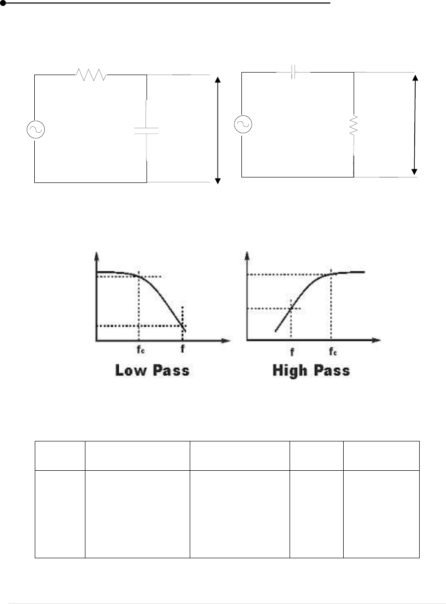
Laboratory manual
135 | P a g e
more like a short circuit allowing all the input signal to pass directly to output as shown below in the
filters response curve.
Low pass circuit High pass circuit
Figure 62: Low pass and high pass filters
Figure 63: Model Graph
Table 81: Low pass Filter
S.No
Input Frequency
(Hz)
Output voltage
(V)
Log F
Voltage Gain
AFO
+
-
+
-
0.01
f
R-5k
AFO
+
-
CRO
Vout
Vin
f
R-5k
Vout
CRO
Vin
+
-
Laboratory manual
136 | P a g e
Table 82: High pass Filter
S.NO
Input Frequency
(Hz)
Output voltage
(V)
Log F
Voltage
Gain
RESULT
The low pass and high pass filter circuits are constructed and corresponding frequency
response graphs are drawn.
The cut off frequency of low pass filter circuit:
By experiment _____
By graph ____
The cut off frequency of high pass filter circuit
By experiment ____
By graph _____
VIVA-VOCE
1. What are filters?
2. What is the application of filters?
3. What is low pass and high pass filters
4. What is the function of AFO?
5. Explain the frequency response curve.

Laboratory manual
137 | P a g e
3. TRANSISTOR CHARACTERISTICS
AIM
To study the characteristics of a transistor under common emitter configuration.
APPARATUS REQUIRED
Low range DC power supply, Transistor (BC107), Milliammeter (0-50mA), Micrometer (0-
10 μA), linear potentiometer (10K pot), voltmeter or digital multimeter, connecting wires.
FORMULA
Input Characteristics V
BE
Vs I
B
:
Input impedance
Output Characteristics V
CE
Vs I
c
:
Output admittance V
0 =
I
B
- base current
THEORY
A transistor has essentially three regions known as emitter collector and base. All these
three regions are provided with terminals which are labelled as E, B, C respectively. The pin
configuration of the transistor is shown in figure. The transistor characteristics curves are helpful in
studying the operation of a transistor when connected in a circuit. The three important characteristics
of a transistor are
1. Input characteristic
2. Output characteristic
3. Constant – current transfer characteristic
These are the curves which represent relationship between different dc currents and voltages of
a transistor
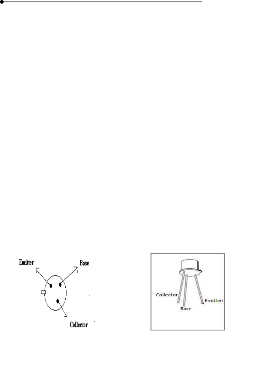
Laboratory manual
138 | P a g e
PROCEDURE
Common Emitter
The static characteristics of a transistor connected in CE configuration may be determined
from the circuit diagram shown in fig. 65. A milliammeter (or a microammeter in the case of a low
power transistor) is connected in series with the base to measure I
b
. Similarly an ammeter is included
in the collector circuit to measure I
c
. A voltmeter with a typical range of 0.1V is connected across
base and emitter terminals for measuring V
BE.
Potentiometer R
2
connected across dc supply V
BB
is
used to vary I
B
and V
BE.
A second voltmeter with a typical range of 0-20V is connected across
collector – emitter terminals to measure the output collector – emitter voltage V
CE
Input characteristics
It shows how I
B
varies with changes in V
BE
when V
CE
is held constant at a particular value.
To begin with V
CE
is maintained constant at a convenient value and then V
BE
is increased in steps.
Corresponding values of I
B
are noted in each step. The procedure is then repeated for a different but
constant value of V
CE.
A typical input characteristics graph is shown in fig. 65. The reciprocal of
the slope gives the input resistance R
in
of the transistor.
R
in =
Δ V
BE
/ ΔI
B
Output Characteristics
It indicates how I
C
varies with changes in V
CE
when I
B
is held constant. For obtaining this
characteristic, first I
B
is set to a convenient value and maintained constant and then V
CE
is measured
from zero in steps, I
C
is noted at each step. Next V
CE
is reduced to zero and I
B
increased to another
convenient value and the whole procedure repeated. The typical graph is shown in the
View from top of pins View from side of casing
Figure 64: Pin configuration of Transistor
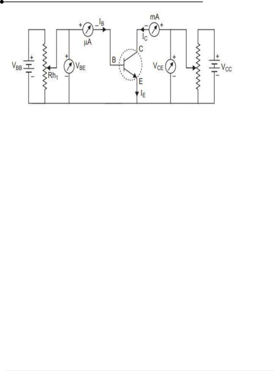
Laboratory manual
139 | P a g e
Figure 65: Transistor characteristics in common emitter configuration
RESULT
Thus the input and output characteristics of a transistor in CE mode is studied and the
characteristics graphs are drawn.
The input impedance is ___________
The output admittance is _________
VIVA-VOCE
1. What is a transistor?
2. How is a transistor fabricated?
3. State input and output characteristics of a transistor.
4. What is input impedance?
5. What is output admittance?

Laboratory manual
140 | P a g e
4. INTEGRATOR
AIM
To construct an integrator using operational amplifier and trace its wave form.
APPARATUS REQUIRED
IC741, 10KΩ resistor, 0.01 μ F capacitor, signal generator connecting wires.
THEORY
Operational amplifier:
An Op-amp is basically a three terminals device which consists of two high impedance
inputs, one is called the inverting input, marked with negative sing and the other one is called non
inverting input marked with positive sign.
Offset Null:
Due to high gain provided by IC741 even slight difference in voltages at the inverting and
non-inverting inputs, caused due to reregulating in manufacturing process or external disturbance
can influence the output. The multiply this effect on effect voltage can be applied at pin 1 and pin 5
using a 10K potentiometer.
Op- Amp integrator:
In an integrator circuit, the output voltage is integral of the signal. The output of an integrator
is given by
At low frequencies the gain becomes infinite, so the capacitor is fully charges and behaves
like an open circuit. The gain of integrator at low frequency can be limited by connecting a resistor
in shunt with capacitor.
PROCEDURE
Connect the circuit as shown in circuit diagram. Apply sine wave, square wave and
triangular, as the input in the function generator and measure the voltage and time in CRO. Then
study the output waves displayed on CRO measure its voltage and time in CRO. Trace the respective
input and output waveforms.
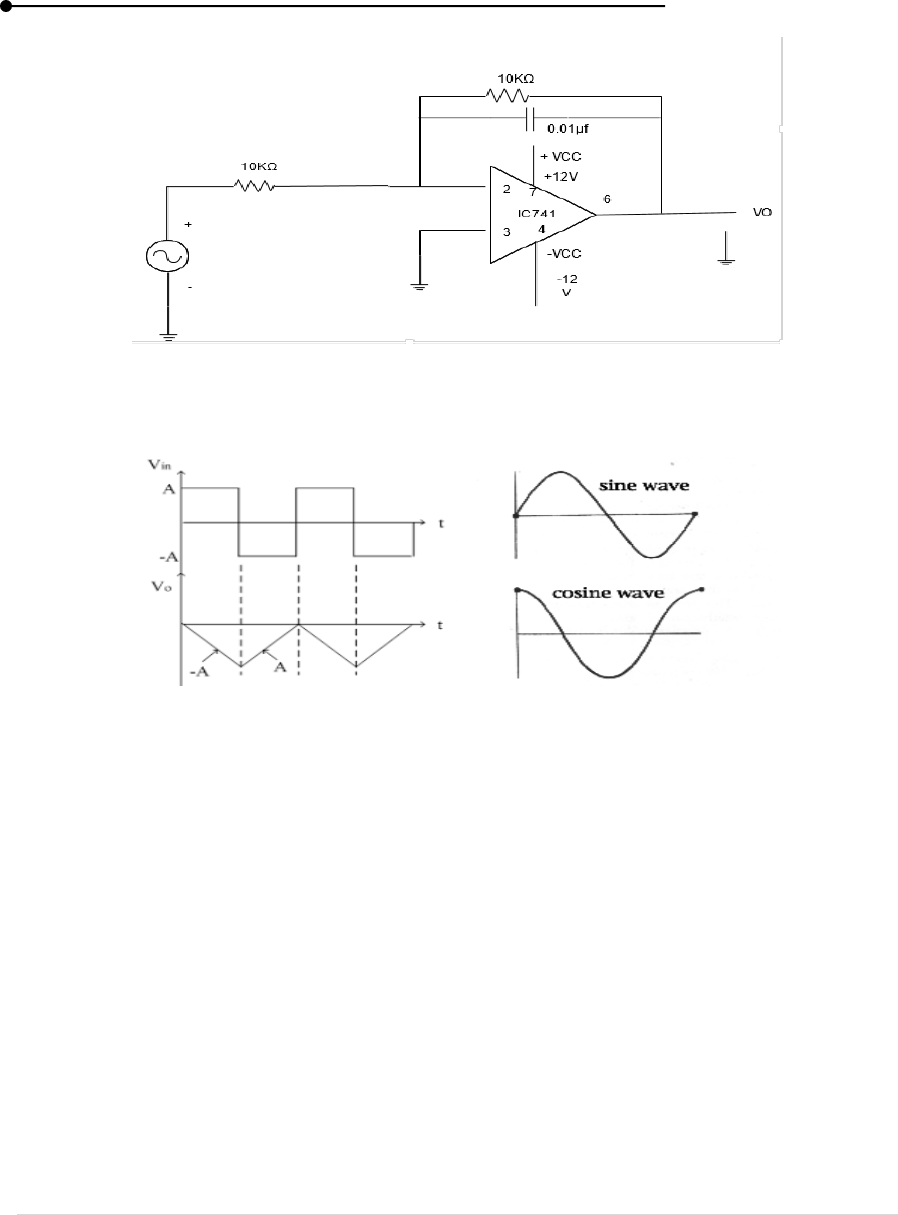
Laboratory manual
141 | P a g e
Figure 66: Integrator input and output wave forms
RESULT
The integrator circuit is constructed using operational amplifier IC741
The Input and output waves of integrator are traced out.
VIVA-VOCE
1. What is a integrator?
2. What is offset null?
3. What is the function of the capacitor used?

Laboratory manual
142 | P a g e
5. DIFFERENTIATOR
AIM
To construct a differentiator using operational amplifier and trace its wave form.
APPARATUS REQUIRED
IC741, resistor, 10K, capacitors μ F, AFO, CRO, Signal generator (AFO).
THEORY
Operational amplifier
Operational amplifiers were used for mathematical operations such as addition, subtraction,
integration and differentiation. An OP-Amp is used to amplify both alternating and direct current
signals at the input. It is fundamentally a voltage amplifying device designed to be used with external
feedback components. Such as resistors and capacitors between its output and input terminals.
An Op-amp is basically a three terminals device which consists of two high impedance
inputs, one is called the inverting input, marked with negative sing and the other one is called non
inverting input marked with positive sign.
Offset Null:
Due to high gain provided by IC741 Op amp even slight difference in voltages at the
inverting and non-inverting inputs, caused due to irregulating in manufacturing process or external
disturbance can influence the output. The multiply this effect on effect voltage can be applied at pin
1 and pin 5 using a 10K potentiometer.
Op amp differentiator:
The circuit which produce the differentiation of the input voltage at its output is called
differentiator. The following circuit diagram, shows the differentiation using op amp. Output voltage
is nothing but time differentiation of the input signal and hence acting as differentiator here R
c
is the
time constant of the differentiator.
PROCEDURE
Connect the circuit as shown in the circuit diagram. Then apply sinewave as input in CRO
using function generator. A Cosine wave will be displayed in CRO. Then measure the voltage and
time of input and output wave. Then trace the input and output waveform. Repeat the same procedure
for various input wave.
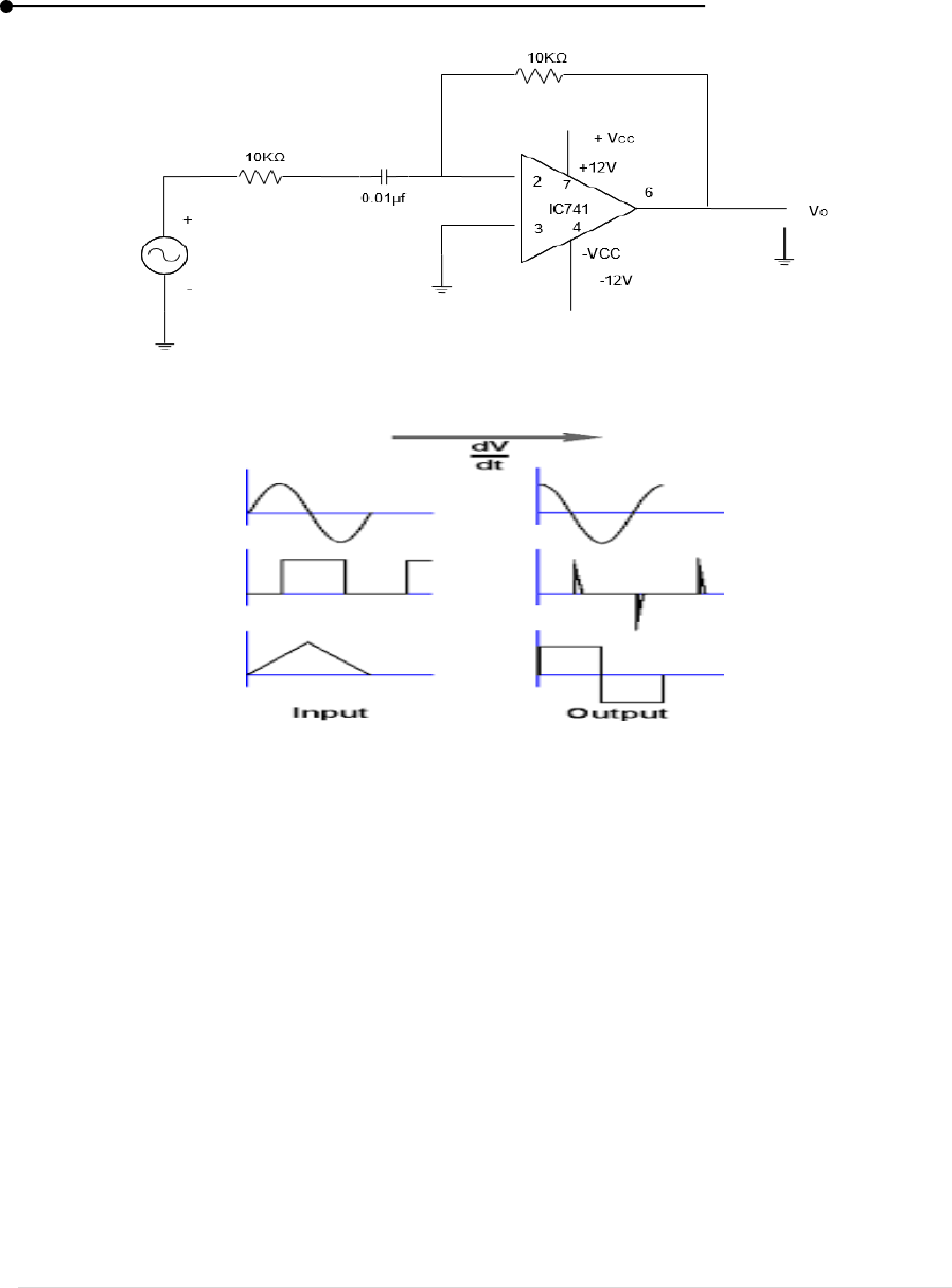
Laboratory manual
143 | P a g e
Figure 67: Differentiator input and output wave forms
RESULT
The differentiator is constructed using operational amplifier IC741.
Input and output waves of differentiator are traced out.
VIVA-VOCE
1. What is a differentiator
2. How does a opamp function as a differentiator
3. What is the function of CRO?
4. What is amplitude?

Laboratory manual
144 | P a g e
6. CLIPPERS USING DISCRETE COMPONENTS
AIM
To construct positive clipper, negative clipper, positive biased, and negative biased clippers
and to trace the output waveforms for the different clippers.
APPARATUS REQUIRED
IN4007, Audio Frequency Oscillator, CRO, 10K Ω, 1M Ω, Battery, connecting wires.
THEORY
These are diode wave clamping circuits. The circuits meant to control the shape of the
voltage and current waveforms to suit various purposes. Each performs the wave shaping function
indicated by its name. The output of the clipping circuit appears as if a portion of the input signal
were clipped off. A clipping circuit requires a minimum of two components a diode and a resistor.
Often dc battery is also used to fix the clipping level. The input waveform can be clipped at different
levels by simply changing the battery voltage and by interchanging the position of various elements.
There are different types of clippers they are
1) Positive clipper:
A circuit which removes portion of positive half cycle is called positive clipper.
2) Negative Clipper:
A clipper which removes a portion of negative half cycle of the input signal is called negative
clipper.
3) Positive Biased clipper:
A small portion of positive half cycle will be removed the negative half cycles will appear
as such across the load. This type of clipper is called positive biased clipper.
4) Negative Biased clipper:
A small portion of negative half cycle will be removed the positive half cycles will appear
as such across the load. This type of clipper is called negative biased clipper.
PROCEDURE
Positive and negative clipper:
Connections are made as per circuit diagram. AFO positive is connected to the
positive of the diode and resistance (10K Ω). The negative terminal is connected to the
negative of the diode and other resistance and it is grounded. The output is connected to 1M
Ω resistance and another end is grounded. The output of the wave forms is traced from CRO.
For negative clipper the connections are made as shown in figure. The conditions
ae same as positive clipper and diode terminal is interchanged.
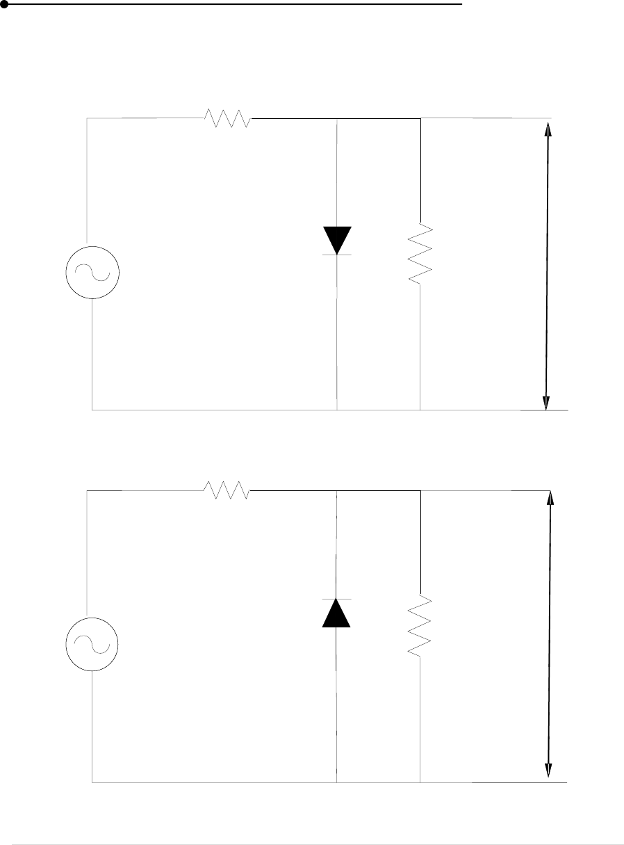
Laboratory manual
145 | P a g e
Positive and negative biased Clipper:
The positive and negative biased circuit connections are made as shown in figure. The output
waveforms are traced out.
Figure 68: Positive clippers
Figure 69: Negative clippers
10kΩ
1MΩ
+
-
+
-
+
-
CRO
AFO
10kΩ
1MΩ
-
+
+
-
+
-
CRO
AFO
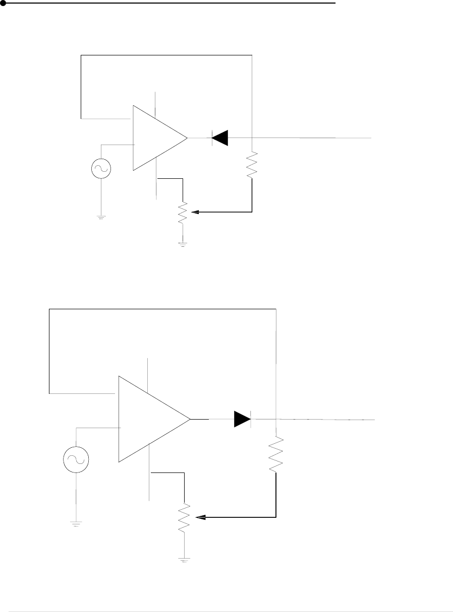
Laboratory manual
146 | P a g e
Figure 70: Positive biased clippers
Figure 71: Negative biased clippers
2
3
7
4
6
Vo
+12v
-12v
D
R-10KΩ
+
-
AFO
IC741
2
3
7
4
6
Vo
+12v
-12v
D
R-10KΩ
+
-
IC741

Laboratory manual
147 | P a g e
RESULT
Thus, positive clippers, negative clippers and positive biased and negative biased clippers
are constructed using discrete components.
The respective input and output waveforms are traced out.
VIVA-VOCE
1. What are clippers?
2. What is positive and negative clippers?
3. What is negative biased clippers?
4. What is the application of clippers?

Laboratory manual
148 | P a g e
7. BAND PASS FILTER CIRCUIT
AIM
To construct a band pass filter circuit using discrete components and to find its bandwidth.
APPARATUS REQUIRED
Two 0.02 μ F capacitors, 24.7K Ω resistance, signal generator, CRO
FORMULA
Voltage gain
V
0
– Output voltage (v)
V
in
– Input voltage (v)
β - Band width (Antilog l
2
– Antilog l
1)
R
1
, R
2
– Resistance (Ω)
C
1
, C
2
– Capacitors (μf)
BAND PASS FILTER
The bandpass filter allows signals falling with a certain frequency band between f
c1
and fc
2
while blocking other lower and higher frequencies either side of this frequency band. The difference
between upper and lower cut off frequency is called Bandwidth.
PROCEDURE
The circuit is connected as shown in Fig.1. The input is given from AFO. The input sine
wave is given by adjusting the amplitude and frequency. Now the XY button on the CRO is switched
on and the wave appear as horizontal line. The corresponding output wave is traced and the readings
are noted and tabulated (Input voltage x volt/div). The same procedure is followed for different
values and the graph is plotted. Here a
0
is constant.
is the mid band gain of the amplifier and band
width β is calculated from the formula.
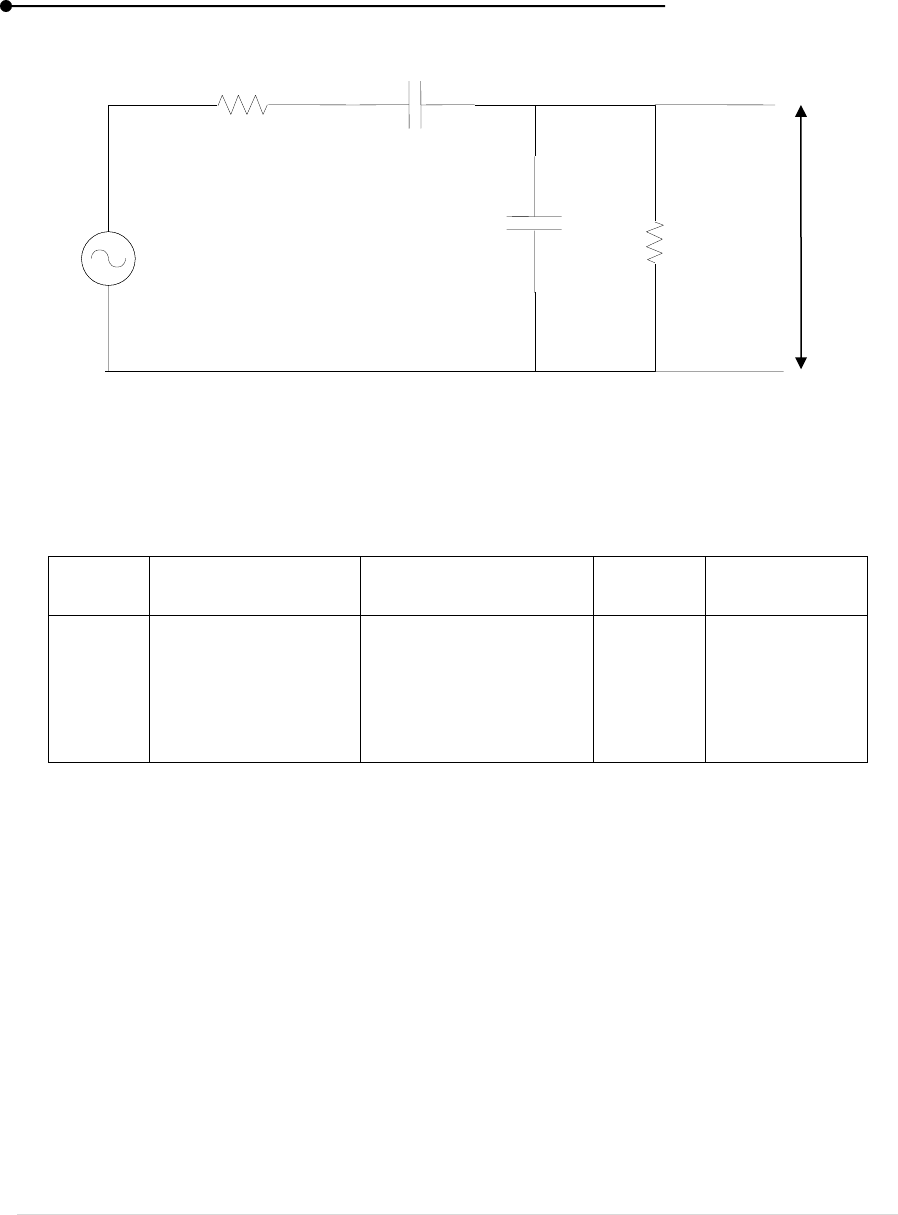
Laboratory manual
149 | P a g e
Figure 72: Bandpass fllter circuit
Table 83: Band pass Filter
S.NO
Input Frequency
(Hz)
Output voltage
(V)
Log F
Voltage Gain
RESULT
The bandpass filter circuit is constructed and the frequency response graphs are drawn.
The bandwidth β is _______________
VIVA-VOCE
1. What is band pass filter
2. Give the application of this filter
3. What is bandwidth
4. What is frequency and amplitude.
5. What is voltage gain
+
-
AFO
R 5KΩ
0.01
µf
0.01µf
R 5kΩ
+
-

Laboratory manual
150 | P a g e
8. BRIDGE RECTIFIER USING DIODES
AIM
To construct a 12V DC Power supply with a bridge rectifier and measure AC and DC
voltage.
APPARATUS REQUIRED
A Step-down transformer, 4 diodes. 2 electrolyte condensers of 1000μF/24V at 230V,
10KΩ resistor.
THEORY
Bridge rectifier are widely used in power supplies that provide necessary DC voltage for
the electronic component s or devices. They can be constructed with four or more diodes its most
common applications for conversion of an alternating current input into direct current output it is
known as Bridge rectifier.
The bridge rectifier circuit diagram consists of various stages of devices like transformer, Diode
Bridge, filtering and regulators.
The first stage of the circuit is a transformer which is a step-down type that changes the amplitude
of the input voltage..
1. Next stage is a diode-bridge rectifier which uses four or more diodes depending on the type
of bridge rectifier.
2. Since the output after the diode bridge rectifiers is of pulsating nature, and for producing it
as a pure DC, filtering is necessary. Filtering is normally performed with one or
more capacitors attached across the load,
PROCEDURE
The bridge rectifier is constructed ass shown in the figure. The bridge rectifier is made up
of four diodes namely D
1
, D
2
, D
3
, D
4
and load resistor R
L
. The four diodes are connected in a closed
loop (Bridge) configuration to efficiently convert the Alternating Current (AC) into Direct Current
(DC).
The input AC signal is applied across two terminals A and B and the output DC signal is
obtained across the load resistor R
L
which is connected between the terminals C and D.
The four diodes D
1
, D
2
, D
3
, D
4
are arranged in series with only two diodes allowing electric
current during each half cycle. For example, diodes D
1
and D
3
are considered as one pair which
allows electric current during the positive half cycle whereas diodes D
2
and D
4
are considered as
another pair which allows electric current during the negative half cycle of the input AC signal
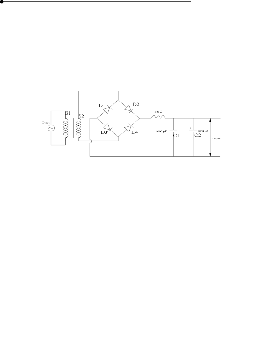
Laboratory manual
151 | P a g e
During the Positive half cycle of the input AC waveform diodes D1 and D2 are forward biased and
D3 and D4 are reverse biased. When the voltage, more than the threshold level of the diodes D1 and
D2, starts conducting – the load current starts flowing through it. During the negative half cycle of
the input AC waveform, the diodes D3 and D4 are forward biased, and D1 and D2 are reverse biased.
Load current starts flowing through the D3 and D4 diodes when these diodes starts conducting as
shown in the figure.
The output at the load with this bridge rectifier is pulsating in nature, but for producing a
pure DC requires additional filter like capacitor.
Figure 73: Experimental Setup
USES
Bridge rectifier is widely used in power supplies that provide necessary DC voltage.
We can find this rectifier in a wide variety of electronic AC power devices like home
appliances, motor controllers, modulation process, welding applications, etc
RESULT
The DC power supply using Bridge rectifier is constructed and the input and output voltages
measured.
i) The AC Voltage ____________
ii) The DC ____________
VIVA-VOCE
1. What is a bridge rectifier?
2. What are the function of diodes?
3. Give the application of bride rectifier
4. What is the function of the capacitor?

Laboratory manual
152 | P a g e
9. CLIPPER USNG IC 741
AIM
To construct the positive and negative clippers using IC7 41 and trace out their respective
input and output waveforms.
APPARATUS REQUIRED
IC741, IN4001, Resistance (10K Ω), part potentiometer (10K Ω ), power supply etc.,
THEORY
A clipper is an electronic circuit that produces on output by removing a part of input above
r below reference value. That mean, the output of a clipper will be as same as that of input for other
than the clipped part. Due to this, peak to peak amplitude of the output of a clipper will be always
less than that of input. The main advantage of clipper is that they eliminate unwanted noise present
in the amplitude of AC signal.
PROCEDURE
Positive clipper:
A positive clipper is a clipper that clips only the positive portions of input signal. The circuit
diagram for positive clipper is shown in the diagram.
A sinusoidal input voltage signal is applied to non-inverting terminal of op amp the value
of reference voltage V
ref
can be choosen by adjusting the 10K pot.
If the value of V
c
< Value of V
ref,
diode D conducts, output voltage is same as input voltage
for V
i
< V
ref
If the value of V
i
> Value of V
ref
, diode D, is off. The op amp operates as open loop since
feedback path is open. Output voltage is equal to reference voltage.
The corresponding input and output waveforms are traced out.
Negative clipper:
A negative clipper that clips only negative portion of input signal. The circuit is as same as
positive clipper circuit, but we reverse the diode and taking reverse polarity of reverse
voltage.
If the value of V
c
> Value of V
ref,
diode D conducts, output voltage is same as input voltage
for V
i
< V
ref
If the value of V
i
< Value of V
ref
, diode D, is off. The op amp operates as open loop since
feedback path is open. Output voltage is equal to reference voltage.
The corresponding input and output waveforms are traced out.
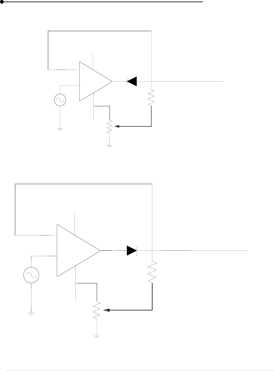
Laboratory manual
153 | P a g e
Figure 74: Positive clipper
Figure 75: Negative clipper
2
3
7
4
6
Vo
+12v
-12v
D
R-10KΩ
+
-
AFO
IC741
2
3
7
4
6
Vo
+12v
-12v
D
R-10KΩ
+
-
IC741

Laboratory manual
154 | P a g e
RESULT
Thus, the positive and negative clipper circuits are constructed using IC741 and their
respective waveforms are traced out.
VIVA-VOCE
1. Give the application of positive and negative clippers
2. What is the function of the diode
3. What is an operational amplifier
4. What is offset null
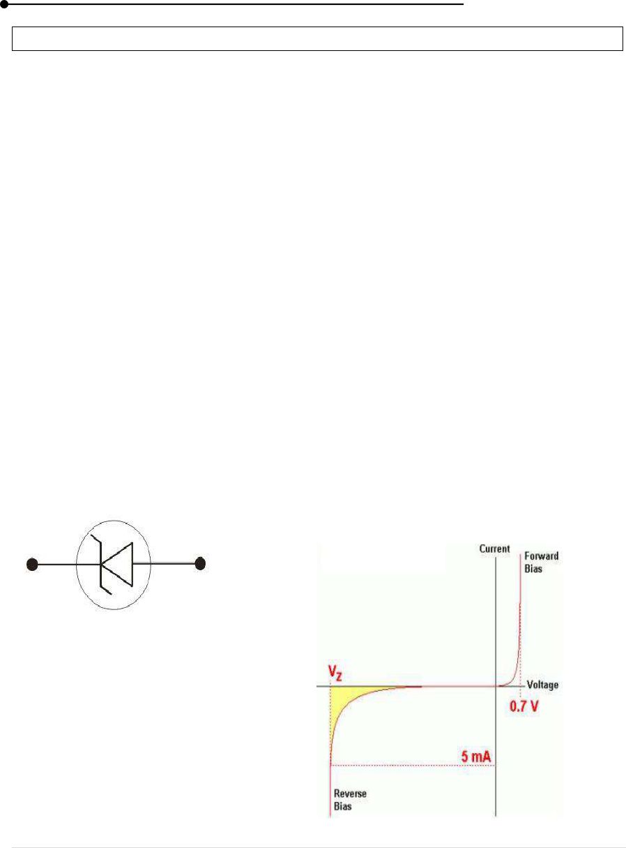
Laboratory manual
155 | P a g e
10. ZENER DIODE CHARACTERISTICS
AIM
To Study and verify the functionality of Zener diode in forward and reverse bias to find
Zener breakdown voltage in revere biased conditions.
APPARATUS REQUIRED
Low range DC power supply, rheostat, milliammeter (0.5mA), Voltmeter (0.3V) (0-10V),
Zener diode, Bread board, 330 Ω resistance, connecting wires.
THEORY
The diode is one of the basic components in electronic circuits. The diode is basically made
up of semiconductors which have two characteristics, ‘P’ type and ‘N’ type. The ‘P’type and ‘N’
type semiconductors. ‘P’type semiconductor will have excess amount of holes in configuration and
‘N’ type semiconductor will have excess amount of electrons. If both types of characteristics present
in a single crystal then it can be termed as a diode. The positive terminal of the battery connects with
the ‘P’ side and the negative side is connected with the ‘N’ side. The special property of the diode is
that there will be a breakdown in the circuit if the voltage applied across a reversely biased circuit.
This does not allow the current to flow across it. When the voltage across the diode is increased,
temperature also increases and the crystal ions vibrate with greater amplitude and all these leads to
the breakdown of the depletion layer. The layer at the junction of ‘P’ type and ‘N’ type. When the
applied voltage exceeds an specific amount Zener breakdown takes place.
Characteristics of a Zener Diode
The above diagram shows the V-I
characteristics of the Zener diode behavior. When
the diode is connected in forward bias diode acts
as a normal diode. When the reverse bias
voltage is greater than a predetermined voltage then
the Zener breakdown voltage occurs. In the V-I
characteristics above Vz is the Zener voltage. And
also the knee voltage because at this point the
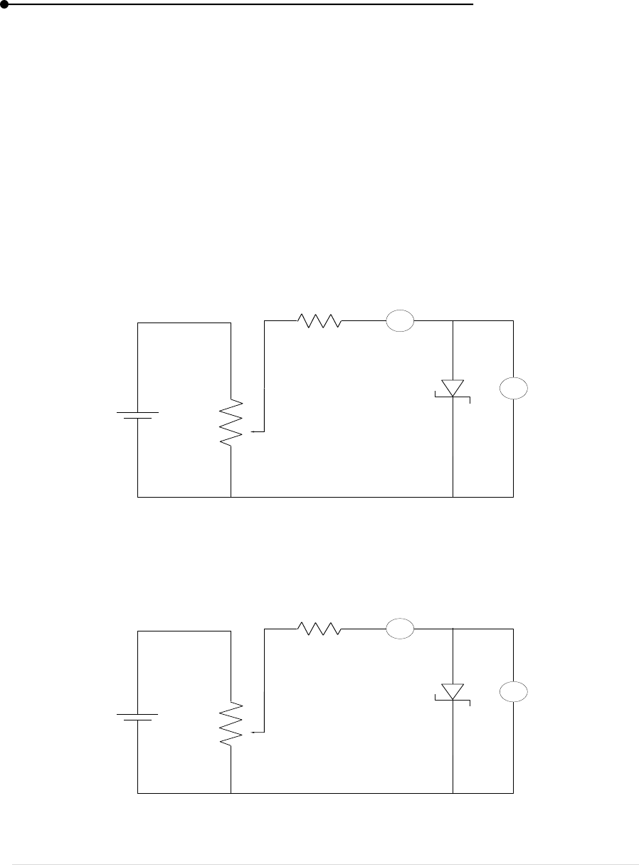
Laboratory manual
156 | P a g e
current is very rapid. At reverse voltages less than 6V, Zener effect predominates whereas above 6V,
avalanche effect is predominant
Avalanche Break down:
When the diode is in the reverse bias condition, the width of the depletion region is more. If
both p-side and n-side of the diode are lightly doped, depletion region at the junction widens. In
reverse bias, the minority charge carrier current flows through junction. As the applied reverse
voltage increases the minority carriers acquire sufficient energy to collide with the carriers in the
covalent bonds inside the depletion region. As a result, the bond breaks and electron hole pairs are
generated. The process becomes cumulative and leads to the generation of a large number of charge
carriers resulting in Avalanche Breakdown.
Figure 76: Forward bias
Figure 77: Backward bias
-
A
V
-
+
-
330
+
-
+
-
-
A
V
-
+
-
330
+
-
+
-

Laboratory manual
157 | P a g e
PROCEDURE
a) Forward Bias Condition:
1. Connect the circuit as shown in Fig
2. Initially vary V
s
in steps of 0.1V. Once the current starts increasing vary V
s
in steps of 1V
up to 12V. Note down the corresponding readings of V
zf
and I
zf
.
b) Reverse Bias Condition:
1. Connect the circuit as shown in Fig. 2.
2. Vary V
s
gradually in steps of 1V up to 12V and note down the corresponding readings of
V
zr
and I
zr
.
Tabulate different reverse currents obtained for different reverse voltages
RESULT
The functionally of Zener diode in forward and reverse bias ae studies and the VI characteristic
of Zener diode is drawn.
Zener breakdown voltage in reverse bias is _______
VIVA-VOCE
1. What is zener breakdown voltage
2. What is avalanche effect
3. What are P –type and N-type semiconductors?
4. Give the application of zener diode.

158 | P a g e
PRACTICAL-V
Digital Electronics & Computer Programming
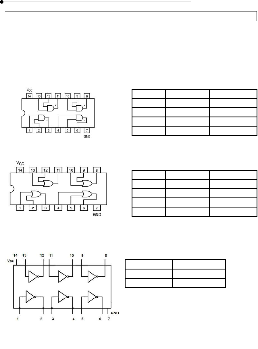
Laboratory manual
159 | P a g e
1. VERIFICATION OF LOGIC GATES USING IC'S
AIM
To study and verify the Truth Tables of AND, OR, NOT, NAND, NOR, EXOR and EX-
NOR logic gates using IC's
APPARATUS REQUIRED
IC 7400, IC 7402, IC 7404, IC 7408, IC 7432, IC 7486 and digital trainer kit
PIN CONFIGURATION AND TRUTH TABLE OF AND GATE
PIN
CONFIGURATION & TRUTH TABLE OF
OR GATE
PIN CONFIGURATION & TRUTH TABLE OF NOT GATE
A
Y=
0
1
A
B
Y=A.B
0
0
0
1
1
0
1
1
A
B
Y=A+B
0
0
0
1
1
0
1
1
IC 7408
IC 7432
IC 7404
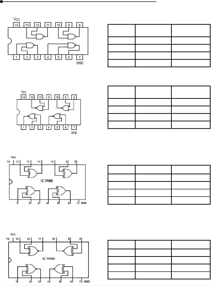
Laboratory manual
160 | P a g e
PIN CONFIGURATION & TRUTH TABLE OF NAND GATE
PIN CONFIGURATION & TRUTH TABLE OF NOR GATE
PIN CONFIGURATION & TRUTH TABLE OF EX-OR GATE
PIN
CONFIGURATION & TRUTH TABLE OF
EX-OR GATE
A
B
Y=
________
.BA
0
0
0
1
1
0
1
1
A
B
Y=
________
BA
0
0
0
1
1
0
1
1
A
B
Y=
BA
0
0
0
1
1
0
1
1
A
B
Y=
BA
0
0
0
1
1
0
1
1
IC 7400
IC 7402

Laboratory manual
161 | P a g e
PROCEDURE
1. Connect the trainer kit to AC power supply.
2. Connect the input of the any one logic gate to the source and its output to the logic indicator.
3. Apply various inputs combinations and observe outputs for each one.
4. Verify the truth tables for each inputs and outputs combinations.
5. Repeat the process for all logic gates.
6. Switch off the power supply.
RESULT
Truth tables of the given Logic Gates are verified
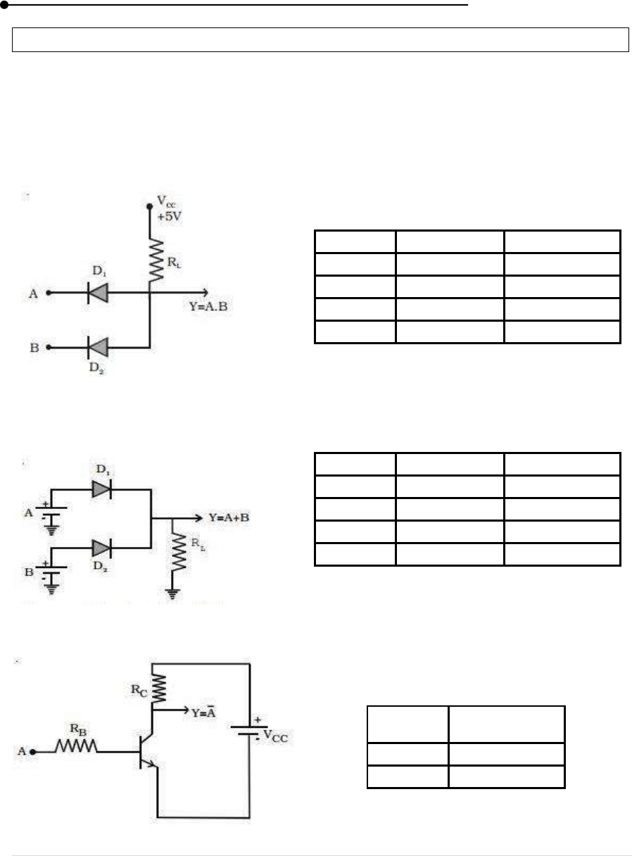
Laboratory manual
162 | P a g e
2. CONSTRUCTION OF LOGIC GATES USING DISCRETE COMPONENTS
AIM
To construct logic gates using discrete components and verify their Truth Tables
APPARATUS REQUIRED
Diode IN4001, Connecting wires, Resistors 10 k and 2.2kΩ, Transistor BC107 and
Trainer kit
CIRCUIT DIAGRAM AND TRUTH TABLE (AND GATE)
CIRCUIT DIAGRAM AND TRUTH TABLE (OR GATE)
CIRCUIT DIAGRAM AND TRUTH TABLE (NOT GATE)
A
B
Y=A.B
0
0
0
1
1
0
1
1
A
B
Y=A+B
0
0
0
1
1
0
1
1
A
___
AY
0
1
10kΩ
10kΩ
10kΩ
2.2 kΩ
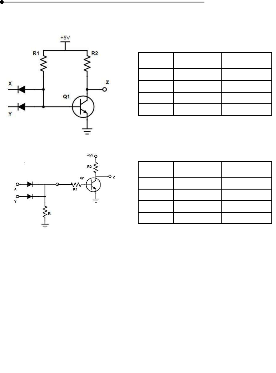
Laboratory manual
163 | P a g e
CIRCUIT DIAGRAM AND TRUTH TABLE (NAND GATE)
CIRCUIT DIAGRAM AND TRUTH TABLE (NOR
GATE)
PROCEDURE
1. Connections are made as shown in the diagram.
2. Different inputs are given and the outputs are noted.
3. Truth table is tabulated for the gates.
RESULT
The truth tables are verified for the logic gates using discrete components.
A
B
________
.BAY
0
0
0
1
1
0
1
1
A
B
________
BAY
0
0
0
1
1
0
1
1
2.2 kΩ
10kΩ
10kΩ
2.2kΩ
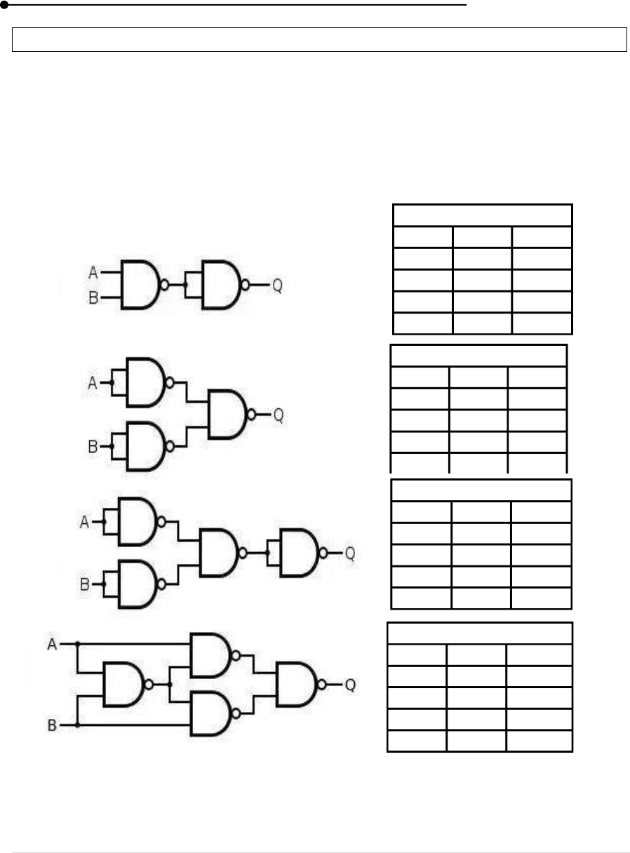
Laboratory manual
164 | P a g e
3. REALIZATION OF LOGIC GATES USING NAND
AIM
To construct Logic Gates using NAND Gate
APPARATUS REQUIRED
IC 7400, Trainer kit and connecting wires
Circuit Diagram and Truth Table of Logic Gates Using NAND
ANDR GATE
A
B
Q
0
0
0
1
1
0
1
1
OR GATE
A
B
Q
0
0
0
1
1
0
1
1
NOR GATE
A
B
Q
0
0
0
1
1
0
1
1
EX-OR GATE
A
B
Q
0
0
0
1
1
0
1
1
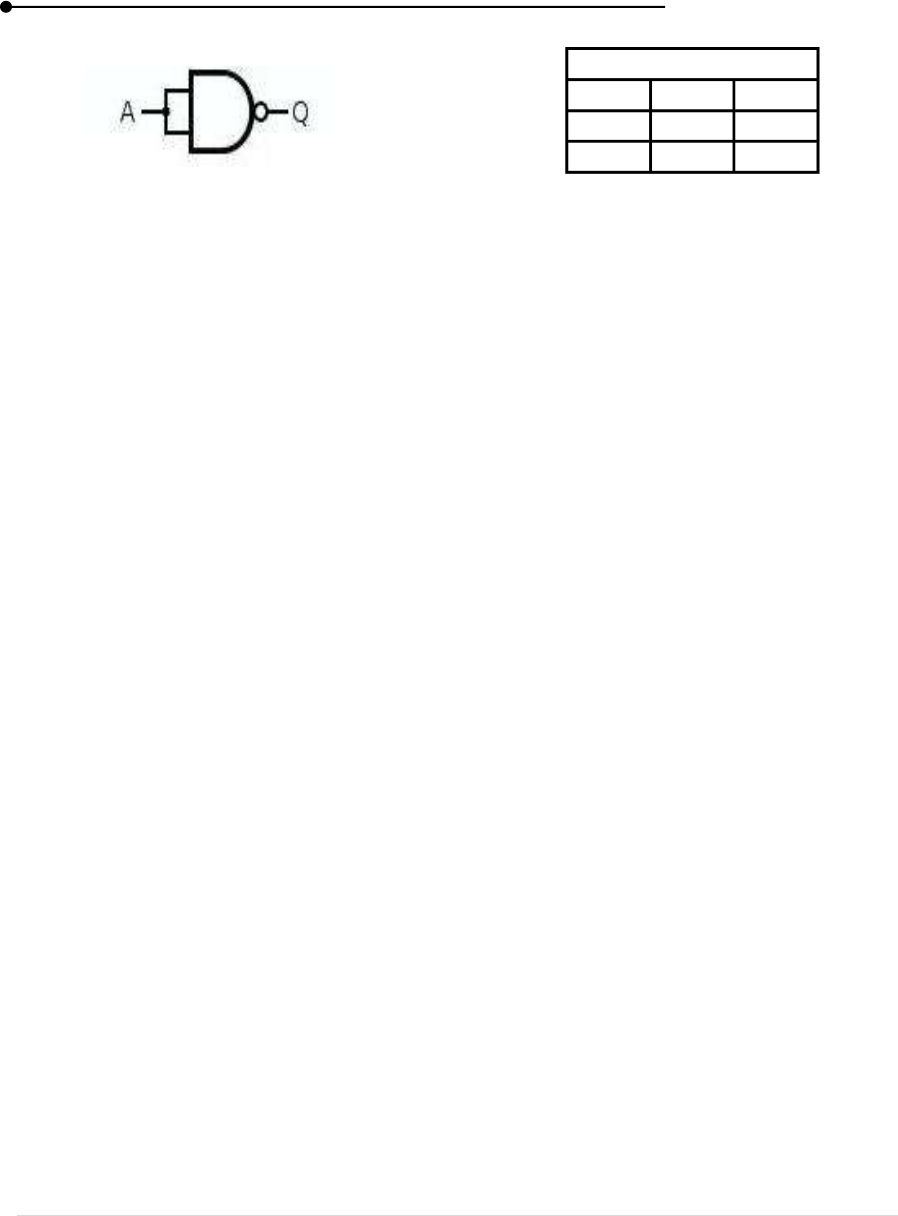
Laboratory manual
165 | P a g e
PROCEDURE
1. Connections are made as shown in the diagram.
2. Different inputs are given and the outputs are noted.
3. Truth table is tabulated for the gates.
RESULT
Logic Gates such as AND, OR, NOT, NOR & EX-OR are realized using NAND Gate
NOT GATE
A
B
Q
0
0
0
1
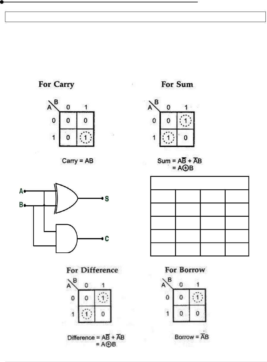
Laboratory manual
166 | P a g e
4. BINARY ADDER & SUBTRACTOR
AIM
To construct and verify the truth tables of half adder and full adder
APPARATUS REQUIRED
IC 7408, IC 7432, IC 7486 and digital trainer kit
CIRCUIT DIAGRAM AND TRUTH TABLE OF HALF ADDER AND SUBTRACTOR
HALF ADDER
A
B
S
C
0
0
0
1
1
0
1
1
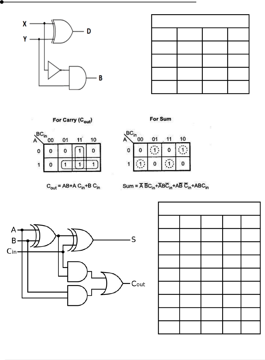
Laboratory manual
167 | P a g e
CIRCUIT DIAGRAM AND TRUTH TABLE OF FULL ADDER AND SUBTRACTOR
FULL ADDER
A
B
C
in
S
C
out
0
0
0
0
0
1
0
1
0
0
1
1
1
0
0
1
0
1
1
1
0
1
1
1
HALF SUBTRACTOR
X
Y
D
B
0
0
0
1
1
0
1
1
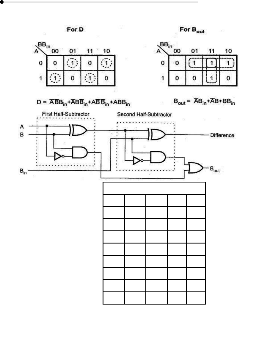
Laboratory manual
168 | P a g e
RESULT
Binary adder and subtractor circuits are constructed and their Truth tables are verified
FULL SUBTRACTOR
A
B
B
in
D
B
out
0
0
0
0
0
1
0
1
0
0
1
1
1
0
0
1
0
1
1
1
0
1
1
1
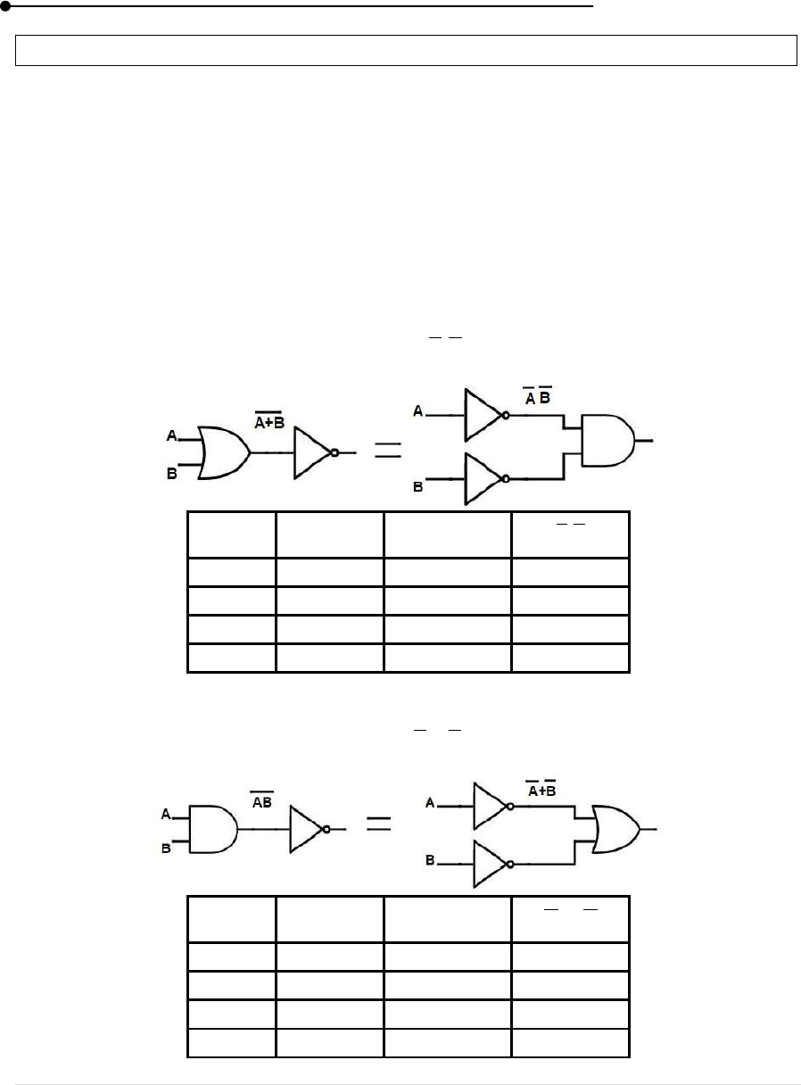
Laboratory manual
169 | P a g e
5. VERIFICATION OF BOOLEAN LAWS
AIM
To verify the Demorgan's laws and Associative laws
APPARATUS REQUIRED
IC 7400, IC 7402, IC 7404, IC 7408, IC 7432, IC 7486, digital trainer kit
DEMORGAN'S LAWS
(i) The complement of a sum equals to the product of the complements
BABA .
______
A
B
______
BA
BA.
0
0
0
1
1
0
1
1
(ii) The complement of a product equals to the sum of the complements
BABA
______
.
A
B
______
.BA
BA
0
0
0
1
1
0
1
1
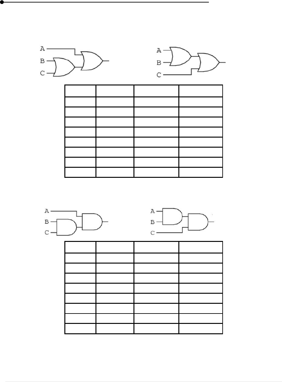
Laboratory manual
170 | P a g e
ASSOCIATIVE LAWS
(i)
)()( CBACBA
A
B
)( CBA
CBA )(
0
0
0
0
0
1
0
1
1
0
1
0
1
1
1
1
(ii)
)..()..( CBACBA
A
B
)..( CBA
CBA )..(
0
0
0
0
0
1
0
1
1
0
1
0
1
1
1
1
RESULT
DeMorgan's laws and Associative laws are verified
=
=

Laboratory manual
171 | P a g e
6. WRITE A 'C' PROGRAM TO FIND THE LARGEST AND SMALLEST NUMBER
IN A SET OF NUMBERS
AIM
To find the largest and smallest number in the set of numbers using C program
PROGRAM
#include<stdio.h>
#include<conio.h>
void main()
{
int a[10], n, i, small, large;
clrscr ();
printf (“Enter the number of terms”);
scanf (“%d”, &n);
for(i=0; i<n; i++)
{
printf (“Enter the numbers \n”);
scanf(“%d”, & a[i]);
}
small = a [0];
large = a [0];
for(i = 0; i<n; i++)
{
if (a[i] < small)
small = a [i];
if (a[i] > large)
large =a [i];
}
printf (“\n Largest Number is %d”, large);
printf(“\n Smallest Number is %d”, small);
getch();
return 0;
}

Laboratory manual
172 | P a g e
OUTPUT
Enter the number of terms:4
1
2
3
4
Largest Number is 4
Smallest Number is 1
RESULT
C program has been written to find the largest and smallest number in a set of numbers

Laboratory manual
173 | P a g e
7. WRITE A 'C' PROGRAM TO CHECK WHETHER GIVEN STRING IS
PALINDROME OR NOT
AIM
To write a C program to check whether the given string is palindrome or not
PROGRAM
#include<stdio.h>
#include<conio.h>
#include<string.h>
void main()
{
char a[100], b[100];
printf(“Enter a string to check if it is a palindrome: \n”);
gets(a);
strcpy(b, a);
strrev(b);
if(strcmp(a, b) == 0)
printf(“The given string is a palindrome”):
else
printf(“The given string is not a palindrome”);
getch();
}
OUTPUT
Enter the string to check if it is a palindrome:
Malayalam
The given string is a palindrome
RESULT
C program has been written to find whether the given string is a palindrome or not

Laboratory manual
174 | P a g e
8. WRITE A 'C' PROGRAM TO FIND THE PRIME NUMBER
AIM
To find whether a given number is prime using C program
PROGRAM
#include<stdio.h>
#include<conio.h>
int main()
{
int i, n, p=0;
clrscr();
printf(“Enter the numbers:\n”);
scanf(“%d”, &n);
for(i=0; i<n; i++)
{
if(n % i==0)
p++;
}
if(p==2)
printf(“It is a prime number”);
else
printf(“It is not a prime number”);
getch();
return 0;
}
OUTPUT
Enter the number:
3
It is a prime number
RESULT
Thus a C program has been written to find whether a number is prime or not

Laboratory manual
175 | P a g e
9. WRITE A C PROGRAM TO GENERATE FIBONACCI SERIES
AIM
Write a 'C' program to find the Fibonacci series
PROGRAM
#include<stdio.h>
#inlude<conio.h>
int main ()
{
int n, first=0, second=1, next, c;
printf(“Enter the number of terms: \n”);
scanf(“%d”, &n);
printf(“First %d terms of the Fibonacci series are:\n”, n);
for(i=0; i<n; i++)
{
if(c<=1)
next=c;
else
{
next=first + second;
first=second;
second=next;
}
printf(“%d\n”, next);
}
getch();
return 0;
}
OUTPUT
Enter the number of terms:
5
First 5 numbers of the Fibonacci series are:
0
1
1
1
2
3
RESULT
Thus a 'C' program has been written to generate Fibonacci series

Laboratory manual
176 | P a g e
10. WRITE A 'C' PROGRAM TO FIND THE SUM, AVERAGE AND STANDARD
DEVIATION FOR THE GIVEN SET OF NUMBERS
AIM
To write a C program to find the average for a given number of values and to find the
standard deviation of the numbers
PROGRAM
#include<stdio.h>
#include<conio.h>
#inlcude<math.h>
#include<float.h>
void main()
{
int i;
float n;
float a[20], b[20], c[20];
float sum=0, sum2=0, avg, var, std;
clrscr();
printf(“Enter the number if terms:\n”);
scanf(“%f”, &n);
printf(“Enter the numbers”\n)l
for(i=0; i<n; i++)
{
scanf(“%f”, &a[i]);
}
for(i=0; i<n; i++)
sum=sum + a[i];
printf(“The sum of the given numbers is %f”, sum);
avg=sum/n;
printf(“The average of the given numbers is %f”, avg);
for(i=0; i<n; i++)
b[i]=a[i]-avg;
for(i=0; i<n; i++)
c[i]=b[i]*b[i];
for(i=0; i<n; i++)
sum2=sum2 + c[i];
var=sum2/n;
std=sqrt (var);
printf(“The standard deviation of the given numbers is %f”, std);

Laboratory manual
177 | P a g e
getch();
}
OUTPUT
Enter the number of terms: 5
Enter the numbers:
1
2
3
4
5
The sum of the given numbers is 15.000000
The average of the given numbers is 3.000000
The standard deviation of the given numbers is 1.414214
RESULT
Thus a 'C' program has been written to find the sum, average and standard deviation for
the given set of number.