Econometric Methods for Program Evaluation

EC10CH18_Abadie ARI 28 June 2018 11:30

Annual Review of Economics

Econometric Methods

for Program Evaluation

Alberto Abadie

and Matias D. Cattaneo

Department of Economics, Massachusetts Institute of Technology, Cambridge,

Massachusetts 02142, USA; email: [email protected]

Department of Economics and Department of Statistics, University of Michigan,

Ann Arbor, Michigan 48109, USA; email: [email protected]

Annu. Rev. Econ. 2018. 10:465–503

The Annual Review of Economics is online at

economics.annualreviews.org

https://doi.org/10.1146/annurev-economics-

080217-053402

 2018 by Annual Reviews.

JEL codes: C1, C2, C3, C54

Keywords

causal inference, policy evaluation, treatment effects

Abstract

Program evaluation methods are widely applied in economics to assess the

effects of policy interventions and other treatments of interest. In this article,

we describe the main methodological frameworks of the econometrics of

program evaluation. In the process, we delineate some of the directions

along which this literature is expanding, discuss recent developments, and

highlight speciﬁc areas where new research may be particularly fruitful.

465

Annu. Rev. Econ. 2018.10:465-503. Downloaded from www.annualreviews.org

Access provided by Massachusetts Institute of Technology (MIT) on 03/19/19. For personal use only.

EC10CH18_Abadie ARI 28 June 2018 11:30

1. INTRODUCTION

The nature of empirical research in economics has profoundly changed since the emergence in the

1990s of a new way to understand identiﬁcation in econometric models. This approach emphasizes

the importance of heterogeneity across units in the parameters of interest and of the choice of the

sources of variation in the data that are used to estimate those parameters. Initial impetus came from

empirical research by Angrist, Ashenfelter, Card, Krueger and others, while Angrist, Heckman,

Imbens, Manski, Rubin, and others provided many of the early methodological innovations (see, in

particular, Angrist 1990, Angrist & Krueger 1991, Angrist et al. 1996, Card 1990, Card & Krueger

1994, Heckman 1990, Manski 1990; for earlier contributions, see Ashenfelter 1978, Ashenfelter

& Card 1985, Heckman & Robb 1985).

While this greater emphasis on identiﬁcation has permeated all brands of econometrics and

quantitative social science, nowhere have the effects been felt more profoundly than in the ﬁeld

of program evaluation—a domain expanding the social, biomedical, and behavioral sciences that

studies the effects of policy interventions. The policies of interest are often governmental pro-

grams, like active labor market interventions or antipoverty programs. In other instances, the term

policy is more generally understood to include any intervention of interest by public or private

agents or by nature.

In this article, we offer an overview of classical tools and recent developments in the economet-

rics of program evaluation and discuss potential avenues for future research. Our focus is on ex

post evaluation exercises, where the effects of a policy intervention are evaluated after some form

of the intervention (such as a regular implementation of the policy, an experimental study, or a

pilot study) is deployed and the relevant outcomes under the intervention are measured. Many

studies in economics and the social sciences aim to evaluate existing or experimentally deployed

interventions, and the methods surveyed in this article have been shown to have broad applicability

in these settings. In many other cases, however, economists and social scientists are interested in

ex ante evaluation exercises, that is, in estimating the effect of a policy before such policy is im-

plemented on the population of interest (e.g., Todd & Wolpin 2010). In the absence of measures

of the outcomes under the intervention of interest, ex ante evaluations aim to extrapolate outside

the support of the data. Often, economic models that precisely describe the behavior of economic

agents serve as useful extrapolation devices for ex ante evaluations. Methods that are suitable for

ex ante evaluation have been previously covered in the Annual Review of Economics (Arcidiacono &

Ellickson 2011, Berry & Haile 2016).

This distinction between ex ante and ex post program evaluations is closely related to often-

discussed differences between the so-called structural and causal inference schools in econometrics.

The use of economic models as devices to extrapolate outside the support of the data in ex ante

program evaluation is typically associated with the structural school, while ex post evaluations

that do not explicitly extrapolate using economic models of behavior are often termed causal or

reduced form.

Given that they serve related but quite distinct purposes, we ﬁnd the perceived

conﬂict between these two schools to be rather artiﬁcial, and the debates about the purported

superiority of one of the approaches over the other largely unproductive.

Our goal in this article is to provide a summary overview of the literature on the econometrics

of program evaluation for ex post analysis and, in the process, to delineate some of the directions

As argued by Imbens (2010), however, reduced form is a misnomer relative to the literature on simultaneous equation models,

where the terms structural form and reduced form have precise meanings. Moreover, terms like structural model or causal

inference are nomenclature, rather than exclusive attributes of the literatures and methods that they refer to.

466 Abadie

Cattaneo

Annu. Rev. Econ. 2018.10:465-503. Downloaded from www.annualreviews.org

Access provided by Massachusetts Institute of Technology (MIT) on 03/19/19. For personal use only.

EC10CH18_Abadie ARI 28 June 2018 11:30

along which it is expanding, discussing recent developments and the areas where research may be

particularly fruitful in the near future.

Other recent surveys on the estimation of causal treatment effects and the econometrics of

program evaluation from different perspectives and disciplines include those by Abadie (2005a),

Angrist & Pischke (2008, 2014), Athey & Imbens (2017c), Blundell & Costa Dias (2009), DiNardo

& Lee (2011), Heckman & Vytlacil (2007), Hern

an & Robins (2018), Imbens & Rubin (2015),

Imbens & Wooldridge (2009), Lee (2016), Manski (2008), Pearl (2009), Rosenbaum (2002, 2010),

Van der Laan & Robins (2003), and VanderWeele (2015), among many others.

2. CAUSAL INFERENCE AND PROGRAM EVALUATION

Program evaluation is concerned with the estimation of the causal effects of policy interven-

tions. These policy interventions can be of very different natures depending on the context of the

investigation, and they are often generically referred to as treatments. Examples include condi-

tional transfer programs (Behrman et al. 2011), health care interventions (Finkelstein et al. 2012,

Newhouse 1996), and large-scale online A/B studies in which IP addresses visiting a particular

web page are randomly assigned to different designs or contents (see, e.g., Bakshy et al. 2014).

2.1. Causality and Potential Outcomes

We represent the value of the treatment by the random variable W. We aim to learn the effect of

changes in treatment status on some observed outcome variable, denoted by Y. Following Neyman

(1923), Rubin (1974), and many others, we use potential outcomes to deﬁne causal parameters:

represents the potential value of the outcome when the value of the treatment variable, W,is

set to w. For each value of w in the support of W, the potential outcome Y

is a random variable

with a distribution over the population. The realized outcome, Y, is such that, if the value of the

treatment is equal to w for a unit in the population, then for that unit, Y = Y

, while other

potential outcomes Y



with w



= w remain counterfactual.

A strong assumption lurks implicit in the last statement. Namely, the realized outcome for

each particular unit depends only on the value of the treatment of that unit and not on the

treatment or on outcome values of other units. This assumption is often referred to as the stable

unit treatment value assumption (SUTVA) and rules out interference between units (Rubin 1980).

SUTVA is a strong assumption in many practical settings; for example, it may be violated in an

educational setting with peer effects. However, concerns about interference between units can

often be mitigated through careful study design (see, e.g., Imbens & Rubin 2015).

The concepts of potential and realized outcomes are deeply ingrained in economics. A demand

function, for example, represents the potential quantity demanded as a function of price. Quantity

demanded is realized for the market price and is counterfactual for other prices.

While, in practice, researchers may be interested in a multiplicity of treatments and outcomes,

we abstract from that in our notation, where Y and W are scalar random variables. In addition

to treatments and potential outcomes, the population is characterized by covariates X,a(k × 1)

vector of variables that are predetermined relative to the treatment. That is, while X and W may

not be independent (perhaps because X causes W, or perhaps because they share common causes),

the value of X cannot be changed by active manipulation of W. Often, X contains characteristics

of the units measured before W is known.

Although the notation allows the treatment to take on an arbitrary number of values, we

introduce additional concepts and notation within the context of a binary treatment, that is,

W ∈{0, 1}.Inthiscase,W = 1 often denotes exposure to an active intervention (e.g., participation

www.annualreviews.org

•

Econometric Methods for Program Evaluation 467

Annu. Rev. Econ. 2018.10:465-503. Downloaded from www.annualreviews.org

Access provided by Massachusetts Institute of Technology (MIT) on 03/19/19. For personal use only.

EC10CH18_Abadie ARI 28 June 2018 11:30

in an antipoverty program), while W = 0 denotes remaining at the status quo. For simplicity of

exposition, our discussion mostly focuses on the binary treatment case. The causal effect of the

treatment (or treatment effect) can be represented by the difference in potential outcomes, Y

−Y

Potential outcomes and the value of the treatment determine the observed outcome

Y = WY

+ (1 − W )Y

. 1.

Equation 1 represents what is often termed the fundamental problem of causal inference (Holland

1986). The realized outcome, Y, reveals Y

if W = 1andY

if W = 0. However, the unit-level

treatment effect, Y

−Y

, depends on both quantities. As a result, the value of Y

−Y

is unidentiﬁed

from observing (Y, W, X).

Beyond the individual treatment effects, Y

− Y

, which are identiﬁed only under assumptions

that are not plausible in most empirical settings, the objects of interest, or estimands, in program

evaluation are characteristics of the joint distribution of (Y

, Y

, W, X) in the sample or in the

population. For most of this review, we focus on estimands deﬁned for a certain population of

interest from which we have extracted a random sample. Like in the work of Abadie et al. (2017a),

we say that an estimand is causal when it depends on the distribution of the potential outcomes,

, Y

) beyond its dependence on the distribution of (Y, W, X). This is in contrast to descriptive

estimands, which are characteristics of the distribution of (Y, W, X).

The average treatment effect (ATE),

ATE

= E[Y

− Y

and the average treatment effect on the treated (ATET),

ATET

= E[Y

− Y

|W = 1],

are causal estimands that are often of interest in the program evaluation literature. Under SUTVA,

ATE represents the difference in average outcomes induced by shifting the entire population from

the inactive to the active treatment. ATET represents the same object for the treated. To improve

the targeting of a program, researchers often aim to estimate ATE or ATET after accounting for a

set of units’ characteristics, X. Notice that ATE and ATET depend on the distribution of (Y

, Y

)

beyond their dependence on the distribution of (Y, W, X). Therefore, they are causal estimands

under the deﬁnition of Abadie et al. (2017a).

2.2. Confounding

Consider now the descriptive estimand,

τ = E[Y |W = 1] − E[Y |W = 0],

which is the difference in average outcomes for the two different treatment values. ATE and ATET

are measures of causation, while the difference in means, τ , is a measure of association. Notice

that

τ = τ

ATE

+ b

ATE

= τ

ATET

+ b

ATET

,2.

Abadie et al. (2017a) provide a discussion of descriptive and causal estimands in the context of regression analysis.

468 Abadie

Cattaneo

Annu. Rev. Econ. 2018.10:465-503. Downloaded from www.annualreviews.org

Access provided by Massachusetts Institute of Technology (MIT) on 03/19/19. For personal use only.

EC10CH18_Abadie ARI 28 June 2018 11:30

where b

ATE

and b

ATET

are bias terms given by

ATE

(

E[Y

|W = 1] − E[Y

|W = 0]

)

Pr(W = 0) 3.

(

E[Y

|W = 1] − E[Y

|W = 0]

)

Pr(W = 1) 4.

and

ATET

= E[Y

|W = 1] − E[Y

|W = 0]. 5.

Equations 2–5 combine into a mathematical representation of the often-invoked statement that

association does not imply causation, enriched with the statement that lack of association does

not imply lack of causation. If average potential outcomes are identical for treated and nontreated

units, an untestable condition, then the bias terms b

ATE

and b

ATET

disappear. However, if potential

outcomes are not independent of the treatment, then, in general, the difference in mean outcomes

between the treated and the untreated is not equal to the ATE or ATET. Lack of independence

between the treatment and the potential outcomes is often referred to as confounding. Confound-

ing may arise, for example, when information that is correlated with potential outcomes is used for

treatment assignment or when agents actively self-select into treatment based on their potential

gains.

Confounding is a powerful notion, as it explains departures of descriptive estimands from causal

ones. Directed acyclic graphs (DAGs; see Pearl 2009) provide graphical representations of causal

relationships and confounding.

A DAG is a collection of nodes and directed edges among nodes, with no directed cycles. Nodes

represent random variables, while directed edges represent causal effects not mediated by other

variables in the DAG. Moreover, a causal DAG must contain all causal effects among the variables

in the DAG, as well as all variables that are common causes of any pair of variables in the DAG

(even if common causes are unobserved).

Consider the DAG in Figure 1. This DAG includes a treatment, W, and an outcome of interest,

Y.InthisDAG,W is not a cause of Y, as there is no directed edge from W to Y. The DAG also

includes a confounder, U. This confounder is a common cause of W and Y. Even when W does not

cause Y, these two variables may be correlated because of the confounding effect of U. A familiar

example of this structure in economics is Spence’s (1973) job-market signaling model, where W

is worker education; Y is worker productivity; and there are other worker characteristics, U,that

cause education and productivity (e.g., worker attributes that increase productivity and reduce

the cost of acquiring education). In this example, even when education does not cause worker

productivity, the two variables may be positively correlated.

The DAG in Figure 1 implies that Y

does not vary with w because W does not cause Y.

However, Y and W are not independent, as they share a common cause, U. Confounding may

arise in more complicated scenarios. In Section 4, we cover other forms of confounding that may

arise in DAGs. Confounding, of course, often coexists with true causal effects. That is, the DAG

in Figure 1 implies the presence of confounding regardless of whether there is a directed edge

from W to Y.

Figure 1

Confounding in a directed acyclic graph. The graph includes a treatment, W ; an outcome of interest, Y ;and

a confounder, U.

www.annualreviews.org

•

Econometric Methods for Program Evaluation 469

Annu. Rev. Econ. 2018.10:465-503. Downloaded from www.annualreviews.org

Access provided by Massachusetts Institute of Technology (MIT) on 03/19/19. For personal use only.

EC10CH18_Abadie ARI 28 June 2018 11:30

Beyond average treatment effects, other treatment parameters of interest depend on the dis-

tribution of (Y

, Y

). These include treatment effects on characteristics of the distribution of the

outcome other than the average (e.g., quantiles), as well as characteristics of the distribution of

the treatment effect, Y

− Y

(e.g., variance), other than its average. In Section 3, we elaborate

further on the distinction between treatment effects on the distribution of the outcome versus

characteristics of the distribution of the treatment effect.

3. RANDOMIZED EXPERIMENTS

Active randomization of the treatment provides the basis of what is arguably the most successful and

extended scientiﬁc research design for program evaluation. Often referred to as the gold standard

of scientiﬁc evidence, randomized clinical trials play a central role in the natural sciences, as well

as in the drug approval process in the United States, Europe, and elsewhere (Bothwell et al. 2016).

While randomized assignment is often viewed as the basis of a high standard of scientiﬁc evidence,

this view is by no means universal. Cartwright (2007), Heckman & Vytlacil (2007), and Deaton

(2010), among others, challenge the notion that randomized experiments occupy a preeminent

position in the hierarchy of scientiﬁc evidence, while Angrist & Pischke (2010), Imbens (2010),

and others emphasize the advantages of experimental designs.

3.1. Identiﬁcation Through Randomized Assignment

Randomization assigns treatment using the outcome of a procedure (natural, mechanical, or elec-

tronic) that is unrelated to the characteristics of the units and, in particular, unrelated to potential

outcomes. Whether randomization is based on coin tossing, random number generation in a

computer, or the radioactive decay of materials, the only requirement of randomization is that

the generated treatment variable is statistically independent of potential outcomes. Complete (or

unconditional) randomization implies

, Y

) ⊥⊥ W,6.

where the symbol ⊥⊥ denotes statistical independence. If Equation 6 holds, we say that the treat-

ment assignment is unconfounded. In Section 4, we consider conditional versions of uncon-

foundedness where the value of the treatment W for each particular unit may depend on certain

characteristics of the units, and Equation 6 holds conditional on those characteristics.

The immediate consequence of randomization is that the bias terms in Equations 4 and 5 are

equal to zero:

ATE

= b

ATET

= 0,

which, in turn, implies

ATE

= τ

ATET

= τ = E[Y |W = 1] − E[Y |W = 0]. 7.

Beyond average treatment effects, randomization identiﬁes any characteristic of the marginal

distributions of Y

and Y

. In particular, the cumulative distributions of potential outcomes

(y) = Pr(Y

≤ y)andF

(y) = Pr(Y

≤ y) are identiﬁed by

(y) = Pr(Y ≤ y|W = 1)

and

(y) = Pr(Y ≤ y|W = 0).

470 Abadie

Cattaneo

Annu. Rev. Econ. 2018.10:465-503. Downloaded from www.annualreviews.org

Access provided by Massachusetts Institute of Technology (MIT) on 03/19/19. For personal use only.

EC10CH18_Abadie ARI 28 June 2018 11:30

While the average effect of a treatment can be easily described using τ

ATE

, it is more complicated

to establish a comparison between the entire distributions of Y

and Y

. To be concrete, suppose

that the outcome variable of interest, Y, is income. Then, an analyst may want to rank the income

distributions under the active intervention and in the absence of the active intervention. For that

purpose, it is useful to consider the following distributional relationships: (a) equality of distribu-

tions, F

(y) = F

(y) for all y ≥ 0; (b) ﬁrst-order stochastic dominance (with F

dominating F

(y) − F

(y) ≤ 0 for all y ≥ 0; and (c) second-order stochastic dominance (with F

dominating



(z) − F

(z)) dz ≤ 0 for all y ≥ 0.

Equality of distributions implies that the treatment has no effect on the distribution of the

outcome variable, in this case income. It implies τ

ATE

= 0 but represents a stronger notion of

null effect. Under mild assumptions, ﬁrst- and second-order stochastic dominance imply that the

income distribution under the active treatment is preferred to the distribution of income in the

absence of the active treatment (see, e.g., Abadie 2002, Foster & Shorrocks 1988).

Equivalently, the distributions of Y

and Y

can be described by their quantiles. Quantiles of

and Y

are identiﬁed by inverting F

and F

or, more directly, by

(θ) = Q

Y |W =1

(θ),

(θ) = Q

Y |W =0

(θ),

with θ ∈ (0, 1), where Q

(θ) denotes the θ quantile of the distribution of Y. The effect of the

treatment on the θ quantile of the outcome distribution is given by the quantile treatment effect,

(θ) − Q

(θ). 8.

Notice that, while quantile treatment effects are identiﬁed from Equation 6, quantiles of the

distribution of the treatment effect, Q

−Y

(θ), are not identiﬁed. Unlike expectations, quantiles

are nonlinear operators, so in general, Q

−Y

(θ) = Q

(θ) − Q

(θ). Moreover, while quantile

treatment effects depend only on the marginal distributions of Y

and Y

, which are identiﬁed

from Equation 6, quantiles of the distribution of treatment effects are functionals of the joint

distribution of (Y

, Y

), which involves information beyond the marginals. Because, even in a

randomized experiment, the two potential outcomes are never both realized for the same unit, the

joint distribution of (Y

, Y

) is not identiﬁed. As a result, quantiles of Y

− Y

are not identiﬁed

even in the context of a randomized experiment.

To gain intuitive understanding of this lack of identiﬁcation result, consider an example where

the marginal distributions of Y

and Y

are identical, symmetric around zero, and nondegenerate.

Identical marginals are consistent with a null treatment effect, that is, Y

− Y

= 0 with probability

one. In this scenario, all treatment effects are zero. However, identical marginals and symmetry

around zero are also consistent with Y

=−Y

or, equivalently, Y

− Y

=−2Y

with probability

one, which leads to positive treatment effects for half of the population and negative treatment

effects for the other half. In the ﬁrst scenario, the treatment does not change the value of the

outcome for any unit in the population. In contrast, in the second scenario, the locations of units

within the distribution of the outcome variable are reshufﬂed, but the shape of the distribution

does not change. While these two different scenarios imply different distributions of the treatment

effect, Y

− Y

, they are both consistent with the same marginal distributions of the potential

outcomes, Y

and Y

, so the distribution of Y

− Y

is not identiﬁed.

Although the distribution of treatment effects is not identiﬁed from randomized assignment

of the treatment, knowledge of the marginal distributions of Y

and Y

can be used to bound

functionals of the distribution of Y

− Y

(see, e.g., Fan & Park 2010, Firpo & Ridder 2008). In

www.annualreviews.org

•

Econometric Methods for Program Evaluation 471

Annu. Rev. Econ. 2018.10:465-503. Downloaded from www.annualreviews.org

Access provided by Massachusetts Institute of Technology (MIT) on 03/19/19. For personal use only.

EC10CH18_Abadie ARI 28 June 2018 11:30

particular, if the distribution of Y is continuous, then for each t ∈ R,

max



sup

y∈R



(y) − F

(y − t)





≤ F

−Y

(t) ≤ 1 + min



inf

y∈R



(y) − F

(y − t)





provides sharp bounds on the distribution of Y

− Y

. This expression can be applied to bound

the fraction of units with positive (or negative) treatment effects. B ounds on Q

−Y

(θ)canbe

obtained by inversion.

3.2. Estimation and Inference in Randomized Studies

So far, we have concentrated on identiﬁcation issues. We now turn to estimation and infer-

ence. Multiple modes of statistical inference are available for treatment effects (see Rubin 1990),

and our discussion mainly focuses on two of them: (a) sampling-based frequentist inference and

(b) randomization-based inference on a sharp null. We also brieﬂy mention permutation-based

inference. However, because of space limitations, we omit Bayesian methods (see Rubin 1978,

2005) and ﬁnite-sample frequentist methods based on randomization (see Abadie et al. 2017a,

Neyman 1923). Imbens & Rubin (2015) give an overview of many of these methods.

3.2.1. Sampling-based frequentist inference. In the context of sampling-based frequentist

inference, we assume that data consist of a random sample of treated and nontreated units, and

that the treatment has been assigned randomly. For each unit i in the sample, we observe the value

of the outcome, Y

; the value of the treatment, W

; and, possibly, the values of a set of covariates,

. Consider the common scenario where randomization is carried out with a ﬁxed number of

treated units, n

, and untreated units, n

, such that n = n

+ n

is the total sample size. We

construct estimators using the analogy principle (Manski 1988). That is, estimators are sample

counterparts of population objects that identify parameters of interest. In particular, Equation 7

motivates estimating τ = τ

ATE

= τ

ATET

using the difference in sample means of the outcome

between treated and nontreated,

τ =



i=1

−



i=1

(1 − W

Under conventional regularity conditions, a large sample approximation to the sampling distri-

bution of τ is given by

τ − τ

se(τ )

−→ N (0, 1), 10.

where

se(τ ) =



σ

Y |W =1

σ

Y |W =0



1/2

, 11.

and σ

Y |W =1

and σ

Y |W =0

are the sample counterparts of the conditional variance of Y given W = 1

and W = 0, respectively.

The estimator τ coincides with the coefﬁcient on W from a regression of Y on W and a con-

stant, and se(τ ) is the corresponding heteroskedasticity-robust standard error. Inference based on

Equations 10 and 11 has an asymptotic justiﬁcation but can perform poorly in ﬁnite samples, espe-

cially if n

and n

differ considerably. Imbens & Koles

ar (2016) discuss small sample adjustments

to the t-statistic and its distribution and demonstrate that such adjustments substantially improve

coverage rates of conﬁdence intervals in ﬁnite samples. In addition, more general sampling pro-

cesses (e.g., clustered sampling) or randomization schemes (e.g., stratiﬁed randomization) are

472 Abadie

Cattaneo

Annu. Rev. Econ. 2018.10:465-503. Downloaded from www.annualreviews.org

Access provided by Massachusetts Institute of Technology (MIT) on 03/19/19. For personal use only.

EC10CH18_Abadie ARI 28 June 2018 11:30

possible. They affect the variability of the estimator and, therefore, the standard error formulas

(for details, see Abadie et al. 2017b, Imbens & Rubin 2015).

Estimators of other quantities of interest discussed in Section 2 can be similarly constructed

using sample analogs. In particular, for any θ ∈ (0, 1), the quantile treatment effects estimator is

given by



Y |W =1

(θ) −



Y |W =0

(θ),

where



Y |W =1

(θ)and



Y |W =0

(θ) are the sample analogs of Q

Y |W =1

(θ)andQ

Y |W =0

(θ), respectively.

Sampling-based frequentist inference on quantile treatment effects follows from the results of

Koenker & Bassett (1978) on quantile inference for quantile regression estimators. Bounds on the

distribution of F

−Y

can be computed by replacing the cumulative functions F

Y |W =1

and F

Y |W =0

in Equation 9 with their sample analogs,



Y |W =1

and



Y |W =0

, respectively. The estimators of the

cumulative distribution functions F

and F

(or, equivalently, estimators of the quantile functions

and Q

) can also be applied to test for equality of distributions and ﬁrst- and second-order

stochastic dominance (see, e.g., Abadie 2002).

3.2.2. Randomization inference on a sharp null. The testing exercise in Section 3.2.1 is based

on sampling inference. That is, it is based on the comparison of the value of a test statistic for the

sample at hand to its sampling distribution under the null hypothesis. In contrast, randomization

inference takes the sample as ﬁxed and concentrates on the null distribution of the test statistic

induced by the randomization of the treatment. Randomization inference originated with Fisher’s

(1935) proposal to use the physical act of randomization as a reasoned basis for inference.

Consider the example in Panel A of Table 1. This panel shows the result of a hypothetical

experiment where a researcher randomly selects four individuals out of a sample of eight individuals

to receive the treatment and excludes the remaining four individuals from the treatment. For each

of the eight sample individuals, i = 1, ..., 8, the researcher observes treatment status, W

,and

the value of the outcome variable, Y

. For concreteness, we assume that the researcher adopts

the difference in mean outcomes between the treated and the nontreated as a test statistic for

randomization inference. The value of this statistic in the experiment is τ = 6.

The sample observed by the researcher is informative only about the value of τ obtained under

one particular realization of the randomized treatment assignment: t he one observed in practice.

There are, however, 70 possible ways to assign four individuals out of eight to the treatment group.

Let  be the set of all possible randomization realizations. Each element ω of  has probability

1/70. Consider Fisher’s null hypothesis that the treatment does not have any effect on the outcomes

of any unit, that is, Y

= Y

for each experimental unit. Notice that Fisher’s null pertains to the

Table 1 Randomization distribution of a difference in means

Panel A: Sample and sample statistic

12 4 6 10 6 0 1 1

1 1 1 1 0 0 0 0 τ = 6

Panel B: Randomization distribution τ (ω)

ω = 1 1 1 1 1 0 0 0 0 6

ω = 2 1 1 1 0 1 0 0 0 4

ω = 3 1 1 1 0 0 1 0 0 1

ω = 4 1 1 1 0 0 0 1 0 1.5

...ω = 70 0 0 0 0 1 1 1 1 −6

www.annualreviews.org

•

Econometric Methods for Program Evaluation 473

Annu. Rev. Econ. 2018.10:465-503. Downloaded from www.annualreviews.org

Access provided by Massachusetts Institute of Technology (MIT) on 03/19/19. For personal use only.

EC10CH18_Abadie ARI 28 June 2018 11:30

−8−6−4−202468

Dierence

in means

Frequency

τ(ω)

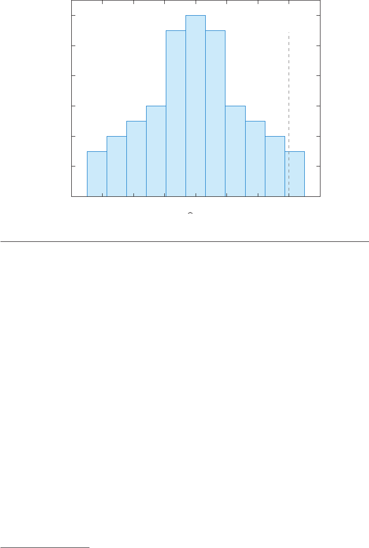
Figure 2

Randomization distribution of the difference in means. The vertical line represents the sample value of τ.

sample and not necessarily to the population. Under Fisher’s null, it is possible to calculate the value

τ (ω) that would have been observed for each possible realization of the randomized assignment,

ω ∈ . The distribution of τ (ω)inPanelBofTable 1 is called the randomization distribution

of τ. A histogram of the randomization distribution of τ is depicted in Figure 2. p-values for

one-sided and two-sided tests are calculated in the usual fashion: Pr(τ (ω) ≥ τ ) = 0.0429 and

Pr(|τ (ω)|≥|τ |) = 0.0857, respectively. These probabilities are calculated over the randomization

distribution. Because the randomization distribution under the null can be computed without

error, these p-values are exact.

Fisher’s null hypothesis of Y

− Y

= 0 for every experimental unit is an instance of a sharp

null, that is, a null hypothesis under which the values of the treatment effect for each unit in the

experimental sample are ﬁxed. Notice that this sharp null, if extended to every population unit,

implies but is not implied by Neyman’s null, E[Y

]− E[Y

] = 0. However, a rejection of Neyman’s

null, using the t-statistic discussed above in the context of sampling-based frequentist inference,

does not imply that Fisher’s test will reject. This is explained by Ding (2017) using the power

properties of the two types of tests and illustrated by Young (2017).

3.2.3. Permutation methods. Some permutation methods are related to randomization tests

but rely on a sampling interpretation. They can be employed to evaluate the null hypothesis that

and Y

have the same distribution. Notice that this is not a sharp hypothesis and that it pertains

to the population rather than to the sample at hand. These tests are based on the observation

that, under the null hypothesis, the distribution of the vector of observed outcomes is invariant

In a setting with many experimental units, it may be computationally costly to calculate the value of the test statistic under

all possible assignments. In those cases, the randomization distribution can be approximated from a randomly selected subset

of assignments.

474 Abadie

Cattaneo

Annu. Rev. Econ. 2018.10:465-503. Downloaded from www.annualreviews.org

Access provided by Massachusetts Institute of Technology (MIT) on 03/19/19. For personal use only.

EC10CH18_Abadie ARI 28 June 2018 11:30

under permutations. Ernst (2004) provides more discussion and comparisons between Fisher’s

randomization inference and permutation methods, and Bugni et al. (2018), who also include

further references on this topic, describe a recent application of permutation-based inference in

the context of randomized experiments.

3.3. Recent Developments

Looking ahead, the literature on the analysis and interpretation of randomized experiments re-

mains active, with several interesting developments and challenges still present beyond what is

discussed in this section. Athey & Imbens ( 2017a) provide a detailed introduction to the econo-

metrics of randomized experiments. Some recent topics in this literature include (a) decision

theoretic approaches to randomized experiments and related settings (Banerjee et al. 2017);

(b) design of complex or high-dimensional experiments accounting for new (big) data environments

such as social media or networks settings (Bakshy et al. 2014); (c) the role of multiple hypothesis

testing and alternative inference methods, such as model selection, shrinkage, and empirical Bayes

approaches (see, e.g., Abadie & Kasy 2017); and (d ) subgroup, dynamic, and optimal treatment

effect analysis, as well as related issues of endogenous stratiﬁcation (see, e.g., Abadie et al. 2017c,

Athey & Imbens 2017b, Murphy 2003).

4. CONDITIONING ON OBSERVABLES

4.1. Identiﬁcation by Conditional Independence

In the absence of randomization, the independence condition in Equation 6 is rarely justiﬁed,

and the estimation of treatment effect parameters requires additional identifying assumptions.

In this section, we discuss methods based on a conditional version of the unconfoundedness

assumption in Equation 6. We assume that potential outcomes are independent of the treatment

after conditioning on a set of observed covariates. The key underlying idea is that confounding, if

present, is fully accounted for by observed covariates.

Consider an example where newly admitted college students are awarded a scholarship on

the basis of the result of a college entry exam, X, and other student characteristics, V.Weusethe

binary variable W to code the receipt of a scholarship award. To investigate the effect of the award

on college grades, Y, one may be concerned about the potential confounding effect of precollege

academic ability, U, which may not be precisely measured by X. Confounding may also arise if V

has a direct effect on Y.

This setting is represented in the DAG in Figure 3a. Precollege academic ability, U, is a cause

of W, the scholarship award, through its effect on the college entry exam grade, X. Precollege

ability, U, is also a direct cause of college academic grades, Y. The confounding effect of U induces

statistical dependence between W and Y that is not reﬂective of the causal effect of W on Y.

In a DAG, a path is a collection of consecutive edges (e.g., X → W → Y ), and confounding

can generate from backdoor paths, that is, paths from the treatment, W, to the outcome, Y,that

start with incoming arrows. The path W ← X ← U → Y is a backdoor path in Figure 3a.An

additional backdoor path, W ← V → Y, emerges if other causes of the award, aside from the

college entry exam, also have a direct causal effect on college grades. The presence of backdoor

paths may create confounding, invalidating Equation 6.

Consider a conditional version of unconfoundedness,

, Y

) ⊥⊥ W |X. 12.

www.annualreviews.org

•

Econometric Methods for Program Evaluation 475

Annu. Rev. Econ. 2018.10:465-503. Downloaded from www.annualreviews.org

Access provided by Massachusetts Institute of Technology (MIT) on 03/19/19. For personal use only.

EC10CH18_Abadie ARI 28 June 2018 11:30

UXWY

a Confounding by U and V

UXWY

b Confounding by U only

Figure 3

Causal effect and confounding. The graphs show the result of a college entrance exam, X; other student

characteristics affecting college admission, V ; receipt of a scholarship award, W ; precollege academic ability,

U; and college grades, Y.(a) Confounding by U and V.(b) Confounding by U alone.

Equation 12 states that (Y

, Y

) is independent of W given X.

This assumption allows identiﬁcation

of treatment effect parameters by conditioning on X. That is, controlling for X makes the treatment

unconfounded.

Along with the common support condition

0 < Pr(W = 1|X) < 1, 13.

Equation 12 allows identiﬁcation of treatment effect parameters. Equation 12 implies

E[Y

− Y

|X] = E[Y |X , W = 1] − E[Y |X, W = 0].

Then, the common support condition in Equation 13 implies

ATE

= E



E[Y |X, W = 1] − E[Y |X, W = 0]



14.

and

ATET

= E



E[Y |X, W = 1] − E[Y |X, W = 0]|W = 1



. 15.

Other causal parameters of interest, like the quantile treatment effects in Equation 8, are identiﬁed

by the combination of unconfoundedness and common support (Firpo 2007).

The common support condition can be directly assessed in the data, as it depends on the

conditional distribution of X given W, which is identiﬁed by the joint distribution of (Y, W, X).

Unconfoundedness, however, is harder to assess, as it depends on potential outcomes that are

not always observed. Pearl (2009) and others have investigated graphical causal structures that

allow identiﬁcation by conditioning on covariates. In particular, Pearl’s backdoor criterion (Pearl

1993) provides sufﬁcient conditions under which treatment effect parameters are identiﬁed via

conditioning.

In our college ﬁnancial aid example, suppose that other causes of the award, aside from the

college entry exam, do not have a direct effect on college grades (that is, all the effect of V on Y

is through W ). This is the setting in Figure 3b.

Using Pearl’s backdoor criterion, and provided

that a common support condition holds, it can be shown t hat the causal structure in Figure 3b

For the identiﬁcation results stated below, it is enough to have unconfoundedness in terms of the marginal distributions of

potential outcomes, that is, Y

⊥⊥ W |X for w ={0, 1}.

The unconfoundedness assumption in Equation 12 is often referred to as conditional independence, exogeneity, selection

on observables, ignorability, or missing at random.

Pearl (2009) and Morgan & Winship (2015) provide detailed introductions to identiﬁcation in DAGs, and Richardson

& Robins (2013) discuss the relationship between identiﬁcation in DAGs and statements about conditional independence

between the treatment and potential outcomes similar to that in Equation 12.

Notice that the node representing V disappears from the DAG in Figure 3b. Because V causes only one variable in the

DAG, it cannot create confounding. As a result, it can be safely excluded from the DAG.

476 Abadie

Cattaneo

Annu. Rev. Econ. 2018.10:465-503. Downloaded from www.annualreviews.org

Access provided by Massachusetts Institute of Technology (MIT) on 03/19/19. For personal use only.

EC10CH18_Abadie ARI 28 June 2018 11:30

implies that treatment effect parameters are identiﬁed by adjusting for X, as in Equations 14 and

15. The intuition for this result is rather immediate. Precollege ability, U, is a common cause of W

and Y, and the only confounder in this DAG. However, conditioning on X blocks the path from

U to X. Once we condition on X, the variable U is no longer a confounder, as it is not a cause of

W. In contrast, if other causes of the award, aside from the college entry exam, have a direct effect

on college grades, as in Figure 3a, then Pearl’s backdoor criterion does not imply Equations 14

or 15. Additional confounding, created by V, is not controlled for by conditioning on X alone.

4.2. Regression Adjustments

There exists a wide array of methods for estimation and inference under unconfoundedness.

However, it is important to notice that, in the absence of additional assumptions, least squares

regression coefﬁcients do not identify ATE or ATET. Consider a simple setting where X takes

on a ﬁnite number of values x

, ..., x

. Under Equations 12 and 13, ATE and ATET are given

ATE



k=1



E[Y |X = x

, W = 1] − E[Y |X = x

, W = 0]



Pr(X = x

)

and

ATET



k=1



E[Y |X = x

, W = 1] − E[Y |X = x

, W = 0]



Pr(X = x

|W = 1),

respectively. These identiﬁcation results form the basis for the subclassiﬁcation estimators of ATE

and ATET in the work of Cochran (1968) and Rubin (1977). One could, however, attempt to

estimate ATE or ATET using least squares. In particular, one could consider estimating τ

OLS

least squares in the regression equation

= τ

OLS



k=1

OLS,k

+ ε

under the usual restrictions on ε

,whereD

is a binary variable that takes value one if X

= x

and zero otherwise. It can be shown that, in the absence of additional restrictive assumptions, τ

OLS

differs from τ

ATE

and τ

ATET

. More precisely, it can be shown that

OLS



k=1

(

E[Y |X = x

, W = 1] − E[Y |X = x

, W = 0]

)

where

var(W |X = x

)Pr(X = x

)



r=1

var(W |X = x

)Pr(X = x

)

That is, τ

OLS

identiﬁes a variance-weighted ATE (see, e.g., Angrist & Pischke 2008).

Even in this

simple setting, with a regression speciﬁcation that is fully saturated in all values of X (including

a dummy variable for each possible value), τ

OLS

differs from τ

ATE

and τ

ATET

except for special cases

(e.g., when E[Y |X = x

, W = 1] − E[Y |X = x

, W = 0] is the same for all k).

It can be shown that var(W |X = x

) is maximal when Pr(W = 1|X = x

) = 1/2 and is decreasing as this probability moves

toward zero or one. That is, τ

OLS

weights up groups with X = x

, where the size of the treated and untreated populations are

roughly equal, and weights down groups with large imbalances in the sizes of these two groups.

www.annualreviews.org

•

Econometric Methods for Program Evaluation 477

Annu. Rev. Econ. 2018.10:465-503. Downloaded from www.annualreviews.org

Access provided by Massachusetts Institute of Technology (MIT) on 03/19/19. For personal use only.

EC10CH18_Abadie ARI 28 June 2018 11:30

4.3. Matching Estimators

Partly because of the failure of linear regression to estimate conventional treatment effect param-

eters like ATE and ATET, researchers have resorted to ﬂexible and nonparametric methods like

matching.

4.3.1. Matching on covariates. Matching estimators of ATE and ATET can be constructed in

the following manner. First, for each sample unit i, select a unit j(i) in the opposite treatment

group with similar covariate values. That is, select j (i) such that W

j(i)

= 1 − W

and X

j(i)

 X

Then, a one-to-one nearest-neighbor matching estimator of ATET can be obtained as the average

of the differences in outcomes between the treated units and their matches,

τ

ATET



i=1

− Y

j(i)

). 16.

An estimator of ATE can be obtained in a similar manner, but using the matches for both treated

and nontreated:

τ

ATE



i=1

− Y

j(i)

) −



i=1

(1 − W

)(Y

− Y

j(i)

). 17.

Nearest-neighbor matching comes in many varieties. It can be done with replacement (that is,

potentially using each unit in the control group as a match more than once) or without, with only

one or several matches per unit (in which case, the outcomes of the matches for each unit are

usually averaged before inserting them into Equations 16 and 17), and there exist several potential

choices for the distance that measures the discrepancies in the values of the covariates between

units [like the normalized Euclidean distance and the Mahalanobis distance (see Abadie & Imbens

2011, Imbens 2004)].

4.3.2. Matching on the propensity score. Matching on the propensity score is another com-

mon variety of matching method. Rosenbaum & Rubin (1983) deﬁne the propensity score as the

conditional probability of receiving the treatment given covariate values

p(X) = Pr(W = 1|X).

Rosenbaum & Rubin (1983) prove that, if the conditions in Equations 12 and 13 hold, then the

same conditions hold after replacing X with the propensity score p(X). An implication of this

result is that, if controlling for X makes the treatment unconfounded, then controlling for p(X)

makes the treatment unconfounded, as well. Figure 4 provides intuition for this result. The entire

effect of X on W is mediated by the propensity score. Therefore, after conditioning on p(X ), the

covariate X is no longer a confounder. In other words, conditioning on the propensity score blocks

p(X)

Figure 4

Identiﬁcation by conditioning on the propensity score, p(X).

478 Abadie

Cattaneo

Annu. Rev. Econ. 2018.10:465-503. Downloaded from www.annualreviews.org

Access provided by Massachusetts Institute of Technology (MIT) on 03/19/19. For personal use only.

EC10CH18_Abadie ARI 28 June 2018 11:30

the backdoor path between W and Y. Therefore, any remaining statistical dependence between

W and Y is reﬂective of the causal effect of W on Y. The propensity score result of Rosenbaum

& Rubin (1983) motivates matching estimators that match on the propensity score, p(X), instead

of matching on the entire vector of covariates, X. Matching on the propensity score reduces the

dimensionality of the matching variable, avoiding biases generated by curse of dimensionality

issues (see, e.g., Abadie & Imbens 2006). In most practical settings, however, the propensity score

is unknown. Nonparametric estimation of the propensity score brings back dimensionality issues.

In some settings, estimation of the propensity score can be guided by institutional knowledge about

the process that produces treatment assignment (elicited from experts in the subject matter). In

empirical practice, the propensity score is typically estimated using parametric methods like probit

or logit.

Abadie & Imbens (2006, 2011, 2012) derive large sample results for estimators that match

directly on the covariates, X. Abadie & Imbens (2016) provide large sample results for the case

where matching is done on an estimated propensity score (for reviews and further references on

propensity score matching estimators, see I mbens & Rubin 2015, Rosenbaum 2010).

4.4. Inverse Probability Weighting

Inverse probability weighting (IPW) methods (see Hirano et al. 2003, Robins et al. 1994) are also

based on the propensity score and provide an alternative to matching estimators. This approach

proceeds by ﬁrst obtaining estimates of propensity score values, p(X

),andthenusingthose

estimates to weight outcome values. For example, an IPW estimator of ATE is

τ

ATE



i=1

p(X

)

−



i=1

(1 − W

) Y

1 − p(X

)

This estimator uses 1/p(X

) to weigh observations in the treatment group and 1/(1 − p(X

)) to

weigh observations in the untreated group. Intuitively, observations with large p(X

) are overrep-

resented in the treatment group and thus weighted down when treated. The same observations

are weighted up when untreated. The opposite applies to observations with small p(X

). This

estimator can be modiﬁed so that the weights in each treatment arm sum to one, which produces

improvements in ﬁnite sample performance (see, e.g., Busso et al. 2014).

4.5. Imputation and Projection Methods

Imputation and projection methods (e.g., Cattaneo & Farrell 2011, Heckman et al. 1998, Im-

bens et al. 2006, Little & Rubin 2002) provide an alternative class of estimators that rely on the

assumptions in Equations 12 and 13. Regression imputation estimators are based on prelimi-

nary estimates of the outcome process, that is, the conditional distribution of Y given (X, W ).

Let μ

(x)andμ

(x) be parametric or nonparametric estimators of E[Y |X = x, W = 1] and

E[Y |X = x, W = 0], respectively. Then, an empirical analog of Equation 14 provides a projec-

tion and imputation estimator of ATE:

τ

ATE



i=1

(

μ

) − μ

)

Similarly, a projection and imputation estimator of ATET is given by the empirical analog of

Equation 15.

www.annualreviews.org

•

Econometric Methods for Program Evaluation 479

Annu. Rev. Econ. 2018.10:465-503. Downloaded from www.annualreviews.org

Access provided by Massachusetts Institute of Technology (MIT) on 03/19/19. For personal use only.

EC10CH18_Abadie ARI 28 June 2018 11:30

4.6. Hybrid Methods

Several hybrid methods combine matching and propensity score weighting with projection and

imputation techniques. Among them are the doubly robust estimators (or, more generally, locally

robust estimators) of Van der Laan & Robins (2003), Bang & Robins (2005), Cattaneo (2010),

Farrell (2015), Chernozhukov et al. (2016), and Sloczynski & Wooldridge (2017). In the case of

ATE estimation, for example, they can take the form

τ

ATE



i=1



− μ

))

p(X

)

+ μ

)



−



i=1



(1 − W

)(Y

− μ

))

1 − p(X

)

+ μ

)



This estimator is doubly robust in the sense that consistent estimation of p(·) or consistent estima-

tion of μ

(·)andμ

(·) is required for the validity of the estimator. Part of the appeal of doubly and

locally robust methods comes from the efﬁciency properties of the estimators. However, relative

to other methods discussed in this section, doubly robust methods require estimating not only p(·)

or μ

(·)andμ

(·), but all of these functions. As a result, relative to other methods, doubly robust

estimators involve additional tuning parameters and implementation choices. Closely related to

doubly and locally robust methods are the bias-corrected matching estimators of Abadie & Imbens

(2011). These estimators include a regression-based bias correction designed to purge matching

estimators from the bias that arises from imperfect matches in the covariates,

τ

ATE



i=1



− Y

j(i)

) − (μ

) − μ

j(i)

))



−



i=1

(1 − W

)



− Y

j(i)

) − (μ

) − μ

j(i)

))



4.7. Comparisons of Estimators

Busso et al. (2014) study the ﬁnite sample performance of matching and IPW estimators, as well

as some of their variants. Kang & Schafer (2007) and the accompanying discussions and rejoinder

provide ﬁnite sample evidence on the performance of double robust estimators and other related

methods.

As these and other studies demonstrate, the relative performance of estimators based on con-

ditioning on observables depends on the features of the data generating process. In ﬁnite samples,

IPW estimators become unstable when the propensity score approaches zero or one, while regres-

sion imputation methods may suffer from extrapolation biases. Estimators that match directly on

covariates do not require speciﬁcation choices but may incorporate nontrivial biases if the quality

of the matches is poor. Hybrid methods, such as bias-corrected matching estimators or doubly ro-

bust estimators, include safeguards against bias caused by imperfect matching and misspeciﬁcation

but impose additional speciﬁcation choices that may affect the resulting estimate.

Apart from purely statistical properties, estimators based on conditioning on covariates differ

in the way they are related to research transparency. In particular, during the design phase of

a study (i.e., sample, variable, and model selection), matching and IPW methods employ only

Dehejia & Wahba (1999), Smith & Todd (2005), and others evaluate the performance of some of the estimators in this

section against an experimental benchmark.

480 Abadie

Cattaneo

Annu. Rev. Econ. 2018.10:465-503. Downloaded from www.annualreviews.org

Access provided by Massachusetts Institute of Technology (MIT) on 03/19/19. For personal use only.

EC10CH18_Abadie ARI 28 June 2018 11:30

information about treatment, W, and covariates, X. That is, the matches and the speciﬁcation

for the propensity score can be constructed without knowledge or use of the outcome variable.

This feature of matching and IPW estimators provides a potential safeguard against speciﬁcation

searches and p-hacking, a point forcefully made by Rubin (2007).

4.8. Recent Developments and Additional Topics

All of the estimation and inference methods discussed above take the covariates, X, as known and

small relative to the sample size, although, in practice, researchers often use high-dimensional

models with the aim of using a setting where the conditional independence assumption is deemed

appropriate. In most applications, X includes both raw preintervention covariates and transfor-

mations thereof, such as dummy variable expansions of categorical variables, power or other series

expansions of continuous variables, higher-order interactions, or other technical regressors gen-

erated from the original available variables. The natural tension between standard theory (where

the dimension of X is taken to be small) and practice (where the dimension of X tends to be large)

has led to a new literature that aims to develop estimation and inference methods in program

evaluation that account and allow for high-dimensional X.

Belloni et al. (2014) and Farrell (2015) develop new program evaluation methods employing

machinery from the high-dimensional literature in statistics. This methodology, which allows for

very large X (much larger than the sample size), proceeds in two steps. First, a parsimonious

model is selected from the large set of preintervention covariates employing model selection

via least absolute shrinkage and selection operator (LASSO). Then, treatment effect estimators

are constructed using only the small (usually much smaller than the sample size) set of selected

covariates. More general methods and a review of this literature are given by Belloni et al. (2017)

and Athey et al. (2016), among others. Program evaluation methods proposed in this literature

employ modern model selection techniques, which require a careful analysis and interpretation but

often ultimately produce classical distributional approximations (in the sense that these asymptotic

approximations do not change relative to results in low-dimensional settings).

Cattaneo et al. (2017a; 2018c,d) develop program evaluation methods where the distributional

approximations do change relative to low-dimensional results due to the inclusion of many covari-

ates in the estimation. These results can be understood as giving new distributional approximations

that are robust to (i.e., also valid in) cases where either the researcher cannot select out covariates

(e.g., when many multiway ﬁxed effects are needed) or many covariates remain included in the

model even after model selection. These high-dimensional methods not only are valid when many

covariates are included, but also continue to be valid in cases where only a few covariates are used,

thereby offering demonstrable improvements for estimation and inference in program evaluation.

Related kernel-based methods are developed by Cattaneo & Jansson (2018).

All of the ideas and methods discussed above are mostly concerned with average treatment

effects in the context of binary treatments. Many of these results have been extended to multivalued

treatments (Cattaneo 2010, Farrell 2015, Hirano & Imbens 2004, Imai & van Dyk 2004, Imbens

2000, Lechner 2001, Yang et al. 2016), to quantiles and related treatment effects (Cattaneo 2010,

Firpo 2007), and to the analysis and interpretation of counterfactual distributional treatment

effects (Chernozhukov et al. 2013, DiNardo et al. 1996, Firpo & Pinto 2016). We do not discuss

this work due to space limitations.

Space restrictions also prevent us from discussing in detail other strands of the literature on es-

timation of treatment effects based on conditioning on covariates. In particular, in the biostatistics

literature, structural nested models, marginal structural models, and optimal treatment regimes

estimators are employed to estimate treatment effects in contexts with time-varying treatments and

www.annualreviews.org

•

Econometric Methods for Program Evaluation 481

Annu. Rev. Econ. 2018.10:465-503. Downloaded from www.annualreviews.org

Access provided by Massachusetts Institute of Technology (MIT) on 03/19/19. For personal use only.

EC10CH18_Abadie ARI 28 June 2018 11:30

confounders (see, e.g., Lok et al. 2004, Murphy 2003, Robins 2000). Also, a large literature on sen-

sitivity to unobserved confounders analyzes the impact of departures from the unconfoundedness

assumption in Equation 12 (see, e.g., Altonji et al. 2005, Imbens 2003, Rosenbaum 2002).

5. DIFFERENCE IN DIFFERENCES AND SYNTHETIC CONTROLS

5.1. Difference in Differences

In the previous section, we consider settings where treatment assignment is confounded but where

there exists a set of observed covariates, X, such that treatment assignment becomes unconfounded

after conditioning on X. In many applied settings, however, researchers confront the problem of the

possible existence of unobserved confounders. In these settings, difference-in-differences models

aim to attain identiﬁcation by restricting the way in which unobserved confounders affect the

outcome of interest over time. Consider the following panel data regression model,

= W

+ μ

+ δ

+ ε

where only Y

and W

are observed. We regard the mapping represented in this equation as

structural (or causal). That is, the equation describes potential outcomes, which are now indexed

by time period, t,

0it

= μ

+ δ

+ ε

1it

= τ

+ μ

+ δ

+ ε

. 18.

Then, we have τ

= Y

1it

− Y

0it

. To simplify the exposition, and because it is a common setting in

empirical practice, we assume that there are only two time periods. Period t = 0 is the pretreatment

period, before the treatment is available, so W

= 0 for all i. Period t = 1 is the posttreatment

period, when a fraction of the population units are exposed to the treatment. δ

is a time effect,

common across units. We treat μ

as a time invariant confounder, so μ

and W

are not inde-

pendent. In contrast, we assume that ε

are causes of the outcome that are unrelated to selection

for treatment, so E[ε

] = E[ε

]. This condition can be weakened to E[ε

] = E[ε

where  is the ﬁrst difference operator, so ε

= ε

− ε

. This type of structure is the same as

the widespread linear ﬁxed effect panel data model (see, e.g., Arellano 2003). Then, we have

E[Y

= 1] = E[τ

= 1] + E[μ

= 1] + δ

+ E[ε

]

E[Y

= 1] = E[μ

= 1] + δ

+ E[ε

]

E[Y

= 0] = E[μ

= 0] + δ

+ E[ε

]

E[Y

= 0] = E[μ

= 0] + δ

+ E[ε

In this model, the effect of the unobserved confounders on the average of the outcome variable

is additive and does not change in time. It follows that

ATET

= E[τ

= 1]



E[Y

= 1] − E[Y

= 0]



−



E[Y

= 1] − E[Y

= 0]





E[Y

= 1] −



[

Y

= 0

]



. 19.

The reason for the name difference in differences is apparent from Equation 19. Notice that τ

ATET

is deﬁned here for the posttreatment period, t = 1. Intuitively, identiﬁcation in the difference-

in-differences model comes from a common trends assumption implied by Equation 18. It can be

482 Abadie

Cattaneo

Annu. Rev. Econ. 2018.10:465-503. Downloaded from www.annualreviews.org

Access provided by Massachusetts Institute of Technology (MIT) on 03/19/19. For personal use only.

EC10CH18_Abadie ARI 28 June 2018 11:30

t = 0

Time

t = 1

E[τ

= 1]

E[Y

= 1]

E[Y

= 0]

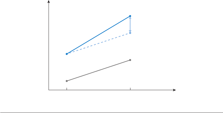
Figure 5

Identiﬁcation in a difference-in-differences model. The dashed line represents the outcome that the treated

units would have experienced in the absence of the treatment.

easily seen that Equation 18, along with E[ε

] = E[ε

], implies

E[Y

0i1

= 1] = E[Y

0i1

= 0]. 20.

That is, in the absence of the treatment, the average outcome for the treated and the average

outcome for the nontreated would have experienced the same variation over time.

Figure 5 illustrates how identiﬁcation works in a difference-in-differences model. In this set-

ting, a set of untreated units identiﬁes the average change that the outcome for the treated units

would have experienced in the absence of the treatment. The set of untreated units selected to

reproduce the counterfactual trajectory of the outcome for the treated is often called the control

group in this literature (borrowing from the literature on randomized controlled trials).

Notice also that the common trend assumption in Equation 20 is not invariant to nonlinear

transformations of the dependent variable. For example, if Equation 20 holds when the outcome is a

wage rate measured in levels, then the same equation will not hold in general for wages measured

in logs. In other words, identiﬁcation in a difference-in-differences model is not invariant to

nonlinear transformations in the dependent variable.

In a panel data regression (that is, in a setting with repeated pre- and posttreatment observations

for t he same units), the right-hand side of Equation 19 is equal to the regression coefﬁcient on W

in a regression of Y

on W

and a constant. Consider, instead, a regression setting with pooled

cross-sections for the outcome variable at t = 0andt = 1 and information on W

for all of the

units in each cross-section. In this setting, one cross-section contains information on (Y

, W

)

and the other cross-section contains information on (Y

, W

). Let T

be equal to zero if unit i

belongs to the pretreatment sample and equal to one if it belongs to the posttreatment sample.

Then, the right-hand side of Equation 19 is equal to the coefﬁcient on the interaction W

a regression of the outcome on a constant, W

, T

, and the interaction W

for a sample that

pools the preintervention and postintervention cross-sections.

Several variations of the basic difference-in-differences model have been proposed in the lit-

erature. In particular, the model naturally extends to a ﬁxed-effects regression in settings with

more than two periods or models with unit-speciﬁc linear trends (see, e.g., Bertrand et al. 2004).

www.annualreviews.org

•

Econometric Methods for Program Evaluation 483

Annu. Rev. Econ. 2018.10:465-503. Downloaded from www.annualreviews.org

Access provided by Massachusetts Institute of Technology (MIT) on 03/19/19. For personal use only.

EC10CH18_Abadie ARI 28 June 2018 11:30

Logically, estimating models with many time periods or trends imposes greater demands on the

data.

The common trends restriction in Equation 20 is clearly a strong assumption and one that

should be assessed in empirical practice. The plausibility of this assumption can sometimes be

evaluated using (a) multiple preintervention periods (like in Abadie & Dermisi 2008) or (b) popu-

lation groups that are not at risk of being exposed to the treatment (like in Gruber 1994). In both

cases, a test for common trends is based on the difference-in-differences estimate of the effect of

a placebo intervention, that is, an intervention that did not happen. In the ﬁrst case, the placebo

estimate is computed using the preintervention data alone and evaluates the effect of a nonexistent

intervention taking place before the actual intervention period. Rejection of a null effect of the

placebo intervention provides direct evidence against common trends before the intervention.

The second case is similar but uses an estimate obtained for a population group known not to be

amenable to receiving the treatment. For example, Gruber (1994) uses difference in differences to

evaluate the effect of the passage of mandatory maternity beneﬁts in some US states on the wages

of married women of childbearing age. In this context, Equation 20 means that, in the absence of

the intervention, married women of childbearing age would have experienced the same increase in

log wages in states that adopted mandated maternity beneﬁts and states that did not. To evaluate

the plausibility of this assumption, Gruber (1994) compares the changes in log wages in adopting

and nonadopting states for single men and women over 40 years old.

The plausibility of Equation 20 may also be questioned if the treated and the control groups

are different in the distribution of attributes that are known or suspected to affect the outcome

trend. For example, if average earnings depend on age or on labor market experience in a nonlinear

manner, then differences in the distributions of these two variables between treated and nontreated

in the evaluation of an active labor market program pose a threat to the validity of the conventional

difference-in-differences estimator. Abadie (2005b) proposes a generalization of the difference-in-

differences model for the case when covariates explain the differences in the trends of the outcome

variable between treated and nontreated. The resulting estimators adjust the distribution of the

covariates between treated and nontreated using propensity score weighting.

Finally, Athey & Imbens (2006) provide a generalization of the difference-in-differences model

to the case when Y

0it

is nonlinear in the unobserved confounder, μ

. Identiﬁcation in this model

comes from strict monotonicity of Y

0it

with respect to μ

and from the assumption that the distri-

bution of μ

is time invariant for the treated and the nontreated (although it might differ between

the two groups). One of the advantages of their approach is that it provides an identiﬁcation result

that is robust to monotonic transformations of the outcome variable [e.g., levels, Y

, versus logs,

log(Y

)].

5.2. Synthetic Controls

Difference-in-differences estimators are often used to evaluate the effects of events or interventions

that affect entire aggregate units, such as states, school districts, or countries (see, e.g., Card 1990,

Card & Krueger 1994). For example, Card (1990) estimates the effect of the Mariel Boatlift, a

large and sudden inﬂux of immigrants to Miami, on the labor market outcomes of native workers

in Miami. In a difference-in-differences design, Card (1990) uses a combination of four other cities

in the south of the United States (Atlanta, Los Angeles, Houston, and Tampa-St. Petersburg) to

approximate the change in native unemployment rates that would have been observed in Miami in

the absence of the Mariel Boatlift. Studies of this type are sometimes referred to as comparative case

studies because a comparison group is selected to evaluate an instance or case of an event or policy

of interest. In the work of Card (1990), the case of interest is the arrival of Cuban immigrants to

484 Abadie

Cattaneo

Annu. Rev. Econ. 2018.10:465-503. Downloaded from www.annualreviews.org

Access provided by Massachusetts Institute of Technology (MIT) on 03/19/19. For personal use only.

EC10CH18_Abadie ARI 28 June 2018 11:30

Miami during the Mariel Boatlift, and the comparison is provided by the combination of Atlanta,

Los Angeles, Houston, and Tampa-St. Petersburg.

The synthetic control estimator of Abadie & Gardeazabal (2003) and Abadie et al. (2010,

2015) provides a data-driven procedure to create a comparison unit in comparative case studies. A

synthetic control is a weighted average of untreated units chosen to reproduce characteristics of

the treated unit before the intervention. The idea behind synthetic controls is that a combination

of untreated units, as in the work of Card (1990), may provide a better comparison to the treatment

unit than any untreated unit alone.

Synthetic controls are constructed as follows. For notational simplicity, we assume that there

is only one treated unit. This is without loss of generality because, when there is more than

one treated unit, the procedure described below can be applied for each treated unit separately.

Suppose that we observe

J + 1 units in periods 1, 2, ..., T . Unit 1 is exposed to the intervention

of interest during periods T

+ 1, ..., T . The remaining J units are an untreated reservoir of

potential controls (a donor pool). Let w = (w

, ..., w

J+1

)



be a collection of weights, with w

≥ 0

for j = 2, ...,

J + 1andw

+···+w

J+1

= 1. Each value of w represents a potential synthetic

control. Let X

be a (k × 1) vector of preintervention characteristics for the treated unit. Similarly,

let X

be a (k × J) matrix which contains the same variables for the unaffected units. The vector

∗

= (w

∗

, ..., w

∗

J+1

)



is chosen to minimize X

− X

w, subject to the weight constraints. The

synthetic control estimator of the effect of the treatment for the treated unit in a postintervention

period t (t ≥ T

)is

α

= Y

−

J+1



j=2

∗

A weighted Euclidean norm is commonly employed to measure the discrepancy between the

characteristics of the treated unit and the characteristics of the synthetic control

X

− X

w=



− X



V (X

− X

w),

where V is a diagonal matrix with nonnegative elements in the main diagonal that control the

relative importance of obtaining a good match between each value in X

and the corresponding

value in X

∗

. Abadie & Gardeazabal (2003) and Abadie et al. (2010, 2015) propose data-driven

selectors of V. Abadie et al. (2010) propose an inferential method for synthetic controls based on

Fisher’s randomization inference.

It can be shown that, in general (that is, ruling out certain degenerate cases), if X

does not

belong to the convex hull of the columns of X

,thenw

∗

is unique and sparse. Sparsity means that

∗

has only a few nonzero elements. However, in some applications, especially in applications

with a large number of treated units, there may be synthetic controls that are not unique or sparse.

Abadie & L’Hour (2017) propose a variant of the synthetic control estimator that addresses this

issue. Their estimator minimizes

X

− X

w

+ λ

J+1



j=2

X

− X



with λ>0, subject to the weight constraints. This estimator includes a penalization for pairwise

matching discrepancies between the treated unit and each of the units that contribute to the

synthetic control. Abadie & L’Hour (2017) show that, aside from special cases, if λ>0, then the

synthetic control estimator is unique and sparse. Hsiao et al. (2012) and Doudchenko & Imbens

(2016) propose variants of the synthetic control framework that extrapolate outside of the support

of the columns of X

. Recent strands of the literature extend synthetic control estimators using

www.annualreviews.org

•

Econometric Methods for Program Evaluation 485

Annu. Rev. Econ. 2018.10:465-503. Downloaded from www.annualreviews.org

Access provided by Massachusetts Institute of Technology (MIT) on 03/19/19. For personal use only.

EC10CH18_Abadie ARI 28 June 2018 11:30

matrix completion techniques (see Amjad et al. 2017, Athey et al. 2017) and propose sampling-

based inferential methods (Hahn & Shi 2017).

6. INSTRUMENTAL VARIABLES

6.1. The Framework

Instrumental variables (IV) methods are widely used in program evaluation. They are easiest to

motivate in the context of a randomized experiment with imperfect compliance, that is, a setting

where experimental units may fail to comply with the randomized assignment of the treatment.

Other settings where IV methods are used include natural experiments in observation studies;

measurement error; nonlinear models with endogeneity; and dynamic, panel data, or time series

contexts (for an overview and further references, including material on weak and many instruments,

see, e.g., Imbens 2014, Wooldridge 2010).

Imperfect compliance with a randomized assignment is commonplace in economics and other

disciplines where assignment affects human subjects, so compliance may be difﬁcult to enforce

or not desirable (for example, in active labor market programs for the unemployed, where the

employment status of the individuals participating in the experiment may change between ran-

domization and treatment). In settings where the experimenter is the only possible provider of the

treatment, randomized assignment can be enforced in the control group. Such a setting is often

referred to as one-sided noncompliance.

In randomized experiments with noncompliance, randomization of treatment intake fails be-

cause of postrandomization selection into the treatment. Assignment itself remains randomized,

and the average effect of assignment on an observed outcome is identiﬁed. Assignment effects are

often referred to as intention-to-treat effects. In some settings, the most relevant policy decision

is whether or not to provide individuals with access to treatment, so intention-to-treat effects have

direct policy relevance. In other instances, researchers and policy makers are interested in the

effects of treatment intake, rather than on the effects of eligibility for treatment. I n such cases, IV

methods can be used to identify certain treatment effects parameters.

IV methods rely on the availability of instruments, that is, variables that affect treatment intake

but do not directly affect potential outcomes. In the context of randomized experiments with

imperfect compliance, instruments are usually provided by randomized assignment to treatment.

We use Z to represent randomized assignment, so Z = 1 indicates assignment to the treatment

group, and Z = 0 indicates assignment to the control group. As in previous sections, actual

treatment intake is represented by the binary variable, W.

Figure 6 offers a DAG representation of the basic IV setting. The treatment, W, is affected

directly by an unobservable confounder, U, which also directly affects the outcome variable, Y.

Because U is unobserved, conditioning on U is unfeasible. However, in this case, there is an

instrument, Z, that affects treatment, W, and only affects the outcome, Y, through W.

The key idea underlying IV methods is that the exogenous variation in the instrument, Z,

which induces changes in the treatment variable, W, can be used to identify certain parameters of

Figure 6

Instrumental variable in a directed acyclic graph. The graph shows the treatment, W ; an unobservable

confounder, U; the outcome variable, Y ; and an instrument, Z, affecting the treatment.

486 Abadie

Cattaneo

Annu. Rev. Econ. 2018.10:465-503. Downloaded from www.annualreviews.org

Access provided by Massachusetts Institute of Technology (MIT) on 03/19/19. For personal use only.

EC10CH18_Abadie ARI 28 June 2018 11:30

interest in program evaluation and causal inference. Variation in Z is exogenous (or unconfounded)

because Z affects Y only through W andbecausetherearenocommoncausesofZ and Y. Chalak

& White (2011) provide a detailed account of identiﬁcation procedures via IV.

6.2. Local Average Treatment Effects

Employing a potential outcomes framework, Imbens & Angrist (1994) and Angrist et al. (1996)

provide a formal setting to study identiﬁcation and estimation of treatment effects under imperfect

compliance. The observed treatment status is

W = ZW

+ (1 − Z)W

where W

and W

denote the potential treatment status under treatment and control assign-

ment, respectively. Perfect compliance corresponds to Pr(W

= 1) = Pr(W

= 0) = 1, so

Pr(W = Z) = 1. One-sided noncompliance corresponds to the case when Pr(W

= 0) = 1 but

Pr(W

= 1) < 1. In this case, units assigned to the control group never take the treatment, while

units assigned to the treatment group may fail to take the treatment.

More generally, in the absence of perfect or one-sided compliance, the population can be

partitioned into four groups deﬁned in terms of the values of W

and W

. Angrist et al. (1996) deﬁne

these groups as compliers (W

> W

or W

= 0andW

= 1), always-takers (W

= W

= 1),

never-takers (W

= W

= 0), and deﬁers [W

< W

= 1andW

= 0)]. Experimental units

that comply with treatment assignment in both treatment arms are called compliers. Always-takers

and never-takers are not affected by assignment. Deﬁers are affected by assignment in the opposite

direction as expected: They take the treatment when they are assigned to the control group but

refuse to take it when they are assigned to the treatment group.

We assume that treatment assignment is not trivial (in the sense that assignment is not always

to the treatment group or always to the control group). In addition, we assume that the assignment

has an effect on treatment intake:

0 < Pr(Z = 1) < 1and Pr(W

= 1) = Pr(W

= 1). 21.

A key assumption in the IV setting is that potential outcomes, Y

and Y

, do not depend on the value

of the instrument. This is called the exclusion restriction. In Figure 6, the exclusion restriction

is manifested in that the effect of Z on Y is completely mediated by W. The combination of

the exclusion restriction with the assumption that the instrument is randomized (or as good as

randomized) implies

, Y

, W

) ⊥⊥ Z. 22.

In the language of IV estimation of linear regression models with constant coefﬁcients, Equa-

tions 21 and 22 amount to the assumptions of instrument relevance and instrument exogeneity,

respectively (see, e.g., Stock & Watson 2003).

Consider the IV parameter

cov(Y, Z)

cov(D, Z)

E[Y |Z = 1] − E[Y |Z = 0]

E[W |Z = 1] − E[W |Z = 0]

. 23.

Under the assumptions in Equations 21 and 22, it can be shown that

E[(Y

− Y

)(W

− W

)]

E[W

− W

]

. 24.

www.annualreviews.org

•

Econometric Methods for Program Evaluation 487

Annu. Rev. Econ. 2018.10:465-503. Downloaded from www.annualreviews.org

Access provided by Massachusetts Institute of Technology (MIT) on 03/19/19. For personal use only.

EC10CH18_Abadie ARI 28 June 2018 11:30

It follows that, if the treatment does not vary across units, that is, if Y

− Y

is constant, τ

is equal

to the constant treatment effect.

The sample analog of τ

τ





i=1





i=1



−





i=1

(1 − Z





i=1

(1 − Z

)







i=1





i=1



−





i=1

(1 − Z





i=1

(1 − Z

)



provides an estimator of the constant treatment effect. This is often called the Wald estimator.

In the presence of treatment effect heterogeneity, however, it can be easily shown that τ

may

fail to identify an average treatment effect for a well-deﬁned population. In particular, it is easy

to construct examples where Y

− Y

> 0 with probability one but τ

= 0. The reason is that

positive values of (Y

− Y

)(W

− W

) given by positive values of W

− W

may cancel out with

negative values in the expectation in the numerator of the expression for τ

in Equation 24.

Imbens & Angrist (1994) deﬁne the local average treatment effect (LATE) as

LATE

= E[Y

− Y

> W

That is, in the terminology of Angrist et al. (1996), LATE is the average effect of the treatment for

compliers, or the average effect of the treatment for those units that would always be in compliance

with the assignment no matter whether they are assigned to the treatment or to the control group.

Suppose that the assumptions in Equations 21 and 22 hold. Suppose also that

Pr(W

≥ W

) = 1. 25.

The assumption in Equation 25 is often referred to as monotonicity, and it rules out the existence

of deﬁers. Then, we have

= τ

LATE

. 26.

Monotonicity implies that W

− W

is binary, so the result in Equation 26 follows easily from

Equation 24.

LATE represents average treatment effect for the units that change their treatment status

according to the their treatment assignment. Notice that, in the absence of additional restrictions,

compliers are not individually identiﬁed because only W

or W

, but not both, are observed in

practice. However, the result in Equation 26 implies that average treatment effects are identiﬁed

for compliers.

A key identifying assumption for LATE is the monotonicity condition (Equation 25), which

rules out deﬁers. Balke & Pearl (1997), Imbens & Rubin (1997), Heckman & Vytlacil (2005), and

Kitagawa (2015) discuss testable implications of this assumption.

One-sided noncompliance, Pr(W

= 1) = 0, is fairly common in settings where the experi-

menter is the only potential provider of the treatment. It has important practical implications. In

particular, one-sided noncompliance implies monotonicity. It also implies that LATE is equal to

ATET. That is, under one-sided noncompliance, we obtain

LATE

= τ

ATET

More generally, however, LATE is not the same as ATE or ATET, and the interest in and

interpretation of the LATE parameter has to be judged depending on the application at hand.

More generally, if Y

− Y

is mean independent of W

− W

,thenτ

is equal to ATE.

488 Abadie

Cattaneo

Annu. Rev. Econ. 2018.10:465-503. Downloaded from www.annualreviews.org

Access provided by Massachusetts Institute of Technology (MIT) on 03/19/19. For personal use only.

EC10CH18_Abadie ARI 28 June 2018 11:30

Suppose, for example, that granting access to treatment represents a policy option of interest.

Then, in a randomized experiment with imperfect compliance (and if monotonicity holds), the

LATE parameter recovers the effect of the treatment for those units affected by being granted

access to treatment, which is the policy decision under consideration (for further discussion, see,

e.g., Imbens 2010).

Angrist et al. (2000) extend the methods described in this section to estimation in simulta-

neous equation models. This work connects with the marginal treatment effect (MTE) estimators

discussed in Section 6.4. The local nature of LATE—that is, the fact that it applies only to

compliers—raises the issue of under what conditions LATE estimates can be generalized to larger

or different populations (for a discussion of extrapolation of LATE estimates and related problems,

see Angrist & Fernandez-Val 2013).

6.3. General Identiﬁcation and Estimation Results for Compliers (Kappa)

Abadie (2003) proposes a general class of estimators of LATE-type parameters (that is, parame-

ters deﬁned for the population of compliers). Like in the work of Imbens & Angrist (1994) and

Angrist et al. (1996), Abadie (2003) adopts a context akin to a randomized experiment with imper-

fect compliance, where the instrument and treatment are binary, extending it to the case where

conditioning on covariates may be needed for instrument validity. In particular, in the absence of

unconditional randomization of the treatment, there may be common causes, X, that affect the

instrument and the outcome. In this case, the instrument will not be valid unless validity is assessed

after conditioning on X.

Consider versions of Equations 21, 22, and 25, where the same assumptions hold after condi-

tioning on X. Deﬁne

= (1 − W )

(1 − Z) − Pr(Z = 0|X)

Pr(Z = 0|X)Pr(Z = 1|X)

= W

Z − Pr(Z = 1|X)

Pr(Z = 0|X)Pr(Z = 1|X)

κ = 1 −

W (1 − Z)

Pr(Z = 0|X)

−

(1 − W )Z

Pr(Z = 1|X)

Abadie (2003) shows that

E[h(Y

, X)|W

> W

] =

Pr(W

> W

)

E[κ

h(Y , X)], 27.

E[h(Y

, X)|W

> W

] =

Pr(W

> W

)

E[κ

h(Y , X)], 28.

and

E[g(Y , W , X)|W

> W

] =

Pr(W

> W

)

E[κ g(Y , W , X)], 29.

where h and g are arbitrary functions ( provided that the expectations exist), and

Pr(W

> W

) = E[κ

] = E[κ

] = E[κ].

Equations 27–29 provide a general identiﬁcation result for compliers. In particular, Equations 27–

29 identify the distribution of attributes, X, for compliers, e.g.,

E[X|W

> W

] = E[κ X]/E[κ].

www.annualreviews.org

•

Econometric Methods for Program Evaluation 489

Annu. Rev. Econ. 2018.10:465-503. Downloaded from www.annualreviews.org

Access provided by Massachusetts Institute of Technology (MIT) on 03/19/19. For personal use only.

EC10CH18_Abadie ARI 28 June 2018 11:30

This result allows a more detailed interpretation of the LATE parameter of Imbens & Angrist

(1994) and Angrist et al. (1996). Although, as indicated above, compliers are not identiﬁed

individually, the distribution of any observed characteristic can be described for the population of

compliers. More generally, Equations 27–29 allow identiﬁcation of regression models for com-

pliers. Such models can be used to describe how the average effect of the treatment for compliers

changes with X (for details, see Abadie 2003). Equations 27 and 28 can be applied to the identiﬁ-

cation of average complier responses to treatment or no treatment, as well as identiﬁcation of the

ATE for compliers. In particular, making h(Y, X ) = Y, we obtain

E[Y

> W

] =

E[κ

Y ]

E[κ

]

E[Y

> W

] =

E[κ

Y ]

E[κ

]

Therefore, we have

LATE

E[κ

Y ]

E[κ

]

−

E[κ

Y ]

E[κ

]



Z − Pr(Z = 1|X)

Pr(Z = 0|X)Pr(Z = 1|X)





Z − Pr(Z = 1|X)

Pr(Z = 0|X)Pr(Z = 1|X)



Kappa-based estimators are sample analogs of the identiﬁcation results in this section. They

require ﬁrst-step estimation of Pr(Z = 1|X). For the same setting, Fr

olich (2007) derives an

alternative estimator of τ

LATE

based on the sample analog of the identiﬁcation result

LATE

[

E[Y |X, Z = 1] − E[Y |X , Z = 0]

]

[

Pr(W = 1|X, Z = 1) − Pr(W = 1|X , Z = 0)

]

An estimator of τ

LATE

based on this result requires ﬁrst-step estimation of E[Y |X, Z = 1],

E[Y |X, Z = 0], Pr(W = 1|X, Z = 1), and Pr(W = 1|X, Z = 0).

Hong & Nekipelov (2010) derive efﬁcient instruments for kappa-based estimators. Ogburn

et al. (2015) propose doubly robust estimators of LATE-like parameters. Abadie (2002), Abadie

et al. (2002), and Fr

olich & Melly (2013) propose estimators of distributional effects for compliers.

Chernozhukov & Hansen (2005, 2013) propose a rank similarity condition under which they

derive an estimator of quantile treatment effects for the entire population (rather than for

compliers alone).

6.4. Marginal Treatment Effects

A closely related causal framework for understanding IV (and other program evaluation) settings

was introduced by Bj

orklund & Mofﬁtt (1987); later developed and popularized by Heckman &

Vytlacil (1999, 2005) and Heckman et al. (2006); and more recently studied by Kline & Walters

(2016) and Brinch et al. (2017), among others. In this approach, the main parameters of interest

are the MTEs and certain functionals thereof.

To describe the model and MTE estimand, we continue to employ potential outcomes but

specialize the notation. In this setting, the instrument, Z , may be a vector of discrete or continuous

random variables, and the observed data are assumed to be generated according to the following

model. Let X be a vector of covariates. Conditional on X = x,wehave

W = 1(p(Z) ≥ V ), V |Z ∼ Uniform[0, 1], 30.

490 Abadie

Cattaneo

Annu. Rev. Econ. 2018.10:465-503. Downloaded from www.annualreviews.org

Access provided by Massachusetts Institute of Technology (MIT) on 03/19/19. For personal use only.

EC10CH18_Abadie ARI 28 June 2018 11:30

= μ

(x) + U

, Y

= μ

(x) + U

, 31.

where μ

() and μ

() are unknown functions, 1(A) is the indicator function that takes value one

if A occurs and value zero otherwise, and (U

, U

, V ) have mean zero and are independent of Z

(given X = x). The condition V |Z ∼ Uniform[0, 1] can be obtained as a normalization provided

that V has an absolutely continuous distribution. Equation 30 implies p(Z) = Pr(W = 1|Z), the

propensity score, which is, in this setting, a function of Z. For expositional simplicity, we assume

that Z includes all elements of X.

Conditional on X = x, the MTE at level v is deﬁned as

MTE

(v|x) = E[Y

− Y

|X = x, V = v].

The parameter τ

MTE

(v|x) is understood as the treatment effect for an individual who is at the margin

of being treated when p(Z) = v and X = x. From a conceptual perspective, the MTE is useful

because other treatment and policy effects can be recovered as weighted integrals of the MTE,

where the weighting scheme depends on the parameter of interest (e.g., τ

ATE

, τ

ATET

,orτ

LATE

). From

a practical perspective, the MTE can be used to conduct certain counterfactual policy evaluations,

sometimes going beyond what can be learned from the more standard treatment effect parameters

in the IV literature, provided additional assumptions hold (for more details and discussion, see

Heckman & Vytlacil 1999, 2005).

The key identifying assumptions for the MTE and r elated parameters are that, conditional on

X = x, Z is nondegenerate and (U

, U

, V ) ⊥⊥ Z, together with the common support condition

0 < p(Z) < 1. Deﬁne the local IV (LIV) parameter as

LIV

(p|x) =

∂

∂p

E[Y |X = x, p(Z) = p].

The parameter τ

LIV

can be seen as a limiting version of LATE. For a continuous p(Z), let

(p, h, x) =

E[Y |X = x, p(Z) = p + h] − E[Y |X = x, p(Z) = p − h]

E[W |X = x, p(Z) = p + h] − E[W |X = x, p(Z) = p − h]

, 32.

where E[W |X = x, p(Z) = p + h] − E[W |X = x, p(Z) = p − h] = 2h. By the LATE result, it

follows that

(p, h, x) = E[Y

− Y

|X = x, p − h < V ≤ p + h]. 33.

Consider any x in the support of X and any limit point p of the support of p(Z)|X = x. Taking

limits as h → 0, on the right-hand sides of Equations 32 and 33, we have

MTE

(p|x) = τ

LIV

(p|x).

As a result, the MTE is nonparametrically identiﬁed by the LIV parameter.

In practice, because of the difﬁculties associated with nonparametric estimations of functions,

researchers often employ parametric forms E[Y |X = x, p(Z) = p] = m(x, p, θ) for the estimation

of the MTE and functionals thereof. Then, the MTE is estimated as τ

MTE

(p|x) = ∂m(x, p,



θ)/∂p,

where



θ is an estimator of θ ,andp(Z) is estimated in a ﬁrst step.

An alternative approach to LIV estimation of the MTE is given by a control function rep-

resentation of the estimand (for a review of control function methods in econometrics, see

Wooldridge 2015). This produces a two-step estimator of the MTE but with two regression

functions, E[Y |X = x, p(Z) = p, W = 1] and E[Y |X = x, p(Z ) = p, W = 0], estimated

separately [both depending on the ﬁrst-step estimate of p(Z)]. For recent examples and further

www.annualreviews.org

•

Econometric Methods for Program Evaluation 491

Annu. Rev. Econ. 2018.10:465-503. Downloaded from www.annualreviews.org

Access provided by Massachusetts Institute of Technology (MIT) on 03/19/19. For personal use only.

EC10CH18_Abadie ARI 28 June 2018 11:30

developments, including the study of cases with discrete instruments, the reader is referred to

Kline & Walters (2016) and Brinch et al. (2017).

7. THE REGRESSION DISCONTINUITY DESIGN

The regression discontinuity (RD) design allows researchers to learn about causal effects in settings

where the treatment is not explicitly randomized and unobservables cannot be ruled out. In its most

basic form, this design is applicable when each unit receives a score, also called a running variable

or index, and only units whose scores are above a known cutoff point are assigned to treatment

status, while the rest are assigned to control status. Examples include antipoverty social programs

assigned on a need basis after ranking units based on a poverty index and educational programs

assigned on a performance basis after ranking units based on a test score (for early reviews, see

Imbens & Lemieux 2008, Lee & Lemieux 2010; for an edited volume with a recent overview, see

Cattaneo & Escanciano 2017; for a practical introduction, see Cattaneo et al. 2018a,b).

The RD treatment assignment mechanism is W = 1(X ≥ c), where X denotes the score, and

c denotes the cutoff point. The key idea underlying any RD design is that units near the cutoff

are comparable. At the core of the design is the assumption that units are not able to precisely

manipulate their score to systematically place themselves above or below the cutoff. The absence

of such endogenous sorting into treatment and control status is a crucial identifying assumption

in the RD framework.

There is a wide variety of RD designs and closely related frameworks. Sharp RD designs are

settings where treatment assignment, as determined by the value of the running variable relative to

the cutoff, and actual treatment status coincide. This is akin to perfect compliance in randomized

experiments. Fuzzy RD designs are settings where compliance with treatment assignment, as

determined by the value of the running variable, is imperfect. This is analogous to the IV setting

but for units with values of the running variable close to the cutoff. Kink RD designs are sharp

or fuzzy settings where the object of interest is the derivative, rather than the level of the average

outcome near or at the cutoff (see Card et al. 2015). Multicutoff RD designs are settings where

the treatment assignment rule depends on more than one cutoff point (see Cattaneo et al. 2016).

Multiscore and geographic RD designs are settings where the t reatment assignment rule depends

on more than one score variable (see Keele & Titiunik 2015, Papay et al. 2011).

In the canonical sharp RD design with a continuously distributed score, the most common

parameter of interest is

SRD

= E[Y

− Y

|X = c] = lim

x↓c

E[Y |X = x] − lim

x↑c

E[Y |X = x], 34.

which corresponds to the average causal treatment effect at the score level X = c. Figure 7 provides

a graphical representation of the RD design. If the score variable satisﬁes X < c, then units are

assigned to the control group (W = 0) and E[Y

|X = x] is observed, while if X ≥ c, then units are

assigned to the treatment group (W = 1) and E[Y

|X = x] is observed. The parameter of interest

is the jump at the point X = c, where treatment assignment changes discontinuously.

Underlying the second equality in Equation 34 is the key notion of comparability between units

with very similar values of the score but on opposite sides of the cutoff. This idea dates back to the

original landmark contribution of Thistlethwaite & Campbell (1960) but was formalized more

recently from a continuity-at-the-cutoff perspective by Hahn et al. (2001). To be speciﬁc, under

regularity conditions, if the regression functions E[Y

|X = x]andE[Y

|X = x] are continuous at

x = c,thenτ

SRD

is nonparametrically identiﬁed. The continuity conditions imply that the average

response of units just below the cutoff provides a close approximation to the average response that

would have been observed for units just above the cutoff had they not been assigned to treatment.

492 Abadie

Cattaneo

Annu. Rev. Econ. 2018.10:465-503. Downloaded from www.annualreviews.org

Access provided by Massachusetts Institute of Technology (MIT) on 03/19/19. For personal use only.

EC10CH18_Abadie ARI 28 June 2018 11:30

W = 1W = 0

E[Y

|X ]

E[Y|X ]

E[Y

|X ]

SRD

= E[Y

− Y

|X = c]

Figure 7

Regression discontinuity design. The outcome of interest is Y ;thescoreisX, and the cutoff point is c.

Treatment assignment and status is W = 1(X ≥ c ). The graph includes the estimable regression functions

(solid lines) and their corresponding unobservable portions (dotted lines).

7.1. Falsiﬁcation and Validation

An important feature of all RD designs is that their key identifying assumption can be supported

by a variety of empirical tests, which enhances the plausibility of the design in applications. The

most popular approaches for validating RD designs in practice include (a) testing for balance on

preintervention covariates among units near the cutoff (Lee 2008), (b) testing for continuity of the

score’s density function near the cutoff (Cattaneo et al. 2017a, McCrary 2008), and (c) graphing

an estimate of E[Y |X = x] at the cutoff and away from the cutoff ( Calonico et al. 2015). Other

falsiﬁcation and validation methods are also used in practice, although these are usually tailored

to special cases (for a practical introduction to these methods, see Cattaneo et al. 2018a).

7.2. Estimation and Inference

The continuity assumptions on conditional expectations at the cutoff, which necessarily rely on

the score variable being continuously distributed near the cutoff, imply that extrapolation is un-

avoidable in canonical RD designs. Observations near the cutoff are used to learn about the

fundamentally unobserved features of the conditional expectations E[Y

|X = c]andE[Y

|X = c]

at the cutoff. Local polynomial regression methods are the most common estimation approaches

in this context, as they provide a good compromise between ﬂexibility and practicality.

The core idea underlying local polynomial estimation and inference involves three simple steps:

(a) Localize the sample near the cutoff by discarding observations with scores far from the cutoff,

(b) employ weighted least-squares to approximate the regression functions on either side of the

cutoff separately, and (c) predict and extrapolate the value of the regression functions at the cutoff.

More formally, assuming a random sample of size n, the standard local-linear RD estimator τ

SRD

is obtained by the local (to the cutoff c) weighted linear least squares regression

⎡

⎢

⎣



τ

SRD



⎤

⎥

⎦

= arg min

,τ ,β

,β



i=1



− β

− W

τ − (X

− c)β

− (X

− c)W





−



www.annualreviews.org

•

Econometric Methods for Program Evaluation 493

Annu. Rev. Econ. 2018.10:465-503. Downloaded from www.annualreviews.org

Access provided by Massachusetts Institute of Technology (MIT) on 03/19/19. For personal use only.

EC10CH18_Abadie ARI 28 June 2018 11:30

where



β = (



)



, K (·) denotes a compact-supported (kernel) weighting function, and h denotes

the bandwidth around the cutoff c. Thus, this is a local regression that employs only observa-

tions X

∈ [c − h, c + h] with weights according to the kernel function; the two more common

weighting schemes are equal weights (uniform kernel) and linear decreasing weights (triangular

kernel). The coefﬁcient



is an estimator of E[Y

|X = c] and can be used to assess the economic

signiﬁcance of the RD treatment effect estimate τ

SRD

. The coefﬁcients



β capture the nonconstant,

linear relationship between the outcome and score variables on either side of the cutoff.

Localization near the cutoff via the choice of bandwidth h is crucial and should be implemented

in a systematic and objective way; ad hoc bandwidth s election methods can hamper empirical work

using RD designs. Principled methods for bandwidth selection have been recently developed (for

an overview, see Cattaneo & Vazquez-Bare 2016). Imbens & Kalyanaraman (2012) develop mean-

squared-error (MSE) optimal bandwidth selection and RD point estimation, while Calonico et al.

(2014) propose a robust bias-correction approach leading to valid inference methods based on the

MSE-optimal bandwidth and RD point estimator. Using higher-order distributional approxima-

tions, Calonico et al. (2018a,b) show that robust bias-corrected inference is demonstrably better

than other alternatives and optimal in some cases. They also develop coverage optimal band-

width selection methods to improve RD inference in applications. Calonico et al. (2018c) study

inclusion of preintervention covariates using local polynomial methods in RD designs. A practical

introduction to these methods is given by Cattaneo et al. (2018a,b), who also provide additional

references.

While the continuity-based approach to RD designs is the most popular in practice, researchers

often explicitly or implicitly rely on a local randomization interpretation of RD designs when it

comes t o the heuristic conceptualization of RD empirical methods and results (see, e.g., Lee

2008, Lee & Lemieux 2010). The two methodological frameworks are, however, substantively

distinct because they generally require different assumptions (Sekhon & Titiunik 2016, 2017). At

an intuitive level, the local randomization RD approach states that, for units with scores sufﬁciently

close to the cutoff, the assignment mechanism resembles that in a randomized controlled trial.

However, because the RD treatment assignment rule W = 1(X ≥ c) implies a fundamental lack

of common support among control and treatment units, the local randomization RD framework

requires additional assumptions for identiﬁcation, estimation, inference, and falsiﬁcation.

Cattaneo et al. (2015) introduce a Fisherian model for inference in RD designs using a local

randomization assumption. The key assumption in this model is the existence of a neighborhood

around the cutoff where two conditions hold: (a) The treatment assignment mechanism is known

(e.g., complete randomization), and (b) the nonrandom potential outcomes are a function of the

score only through treatment status (i.e., an exclusion restriction). Under these assumptions, they

develop ﬁnite-sample exact randomization inference methods for the sharp null hypothesis of no

treatment effect, construct conﬁdence intervals under a given treatment effect model, and discuss

several falsiﬁcation methods. They also propose data-driven methods for neighborhood selection,

based on the local randomization assumptions.

Cattaneo et al. (2017c) extend the basic Fisherian RD randomization inference framework, al-

lowing for parametric adjustments of potential outcomes as functions of the score. This approach

resembles the continuity-based approach and basic parametric regression adjustment methods.

Cattaneo et al. (2017c) also discuss other approaches for RD analysis based on the analysis of

experiments under a local randomization assumption and compare these methods to the

continuity-based approach with local polynomial ﬁtting. Relevant to the comparison between RD

approaches is that the parameter of interest differs depending on the approach. In the continuity-

based approach, τ

SRD

is the only nonparametrically identiﬁed estimand. In the local randomization

494 Abadie

Cattaneo

Annu. Rev. Econ. 2018.10:465-503. Downloaded from www.annualreviews.org

Access provided by Massachusetts Institute of Technology (MIT) on 03/19/19. For personal use only.

EC10CH18_Abadie ARI 28 June 2018 11:30

approach, other parameters are identiﬁable and may be of equal or greater interest. In particular,

a parameter of interest in some settings is

(h) = E[Y

− Y

|c − h ≤ X ≤ c + h].

is the average treatment effect for units with scores falling within the local randomization

window [c − h, c + h] for some choice of window length 2h > 0.

7.3. Extensions, Modiﬁcations, and Recent Topics

Another situation in which the distinction between parameters and methodological approaches

is important is when the score variable is discrete. In this case, τ

SRD

is not identiﬁed nonparamet-

rically, which renders the basic continuity-based approach for identiﬁcation inapplicable. Local

polynomial ﬁts can still be used if the score variable takes on many discrete values because this

estimation method takes the number of mass points as the effective sample size. The discrete

nature of the score, however, changes the interpretation of the canonical RD parameter, τ

SRD

.In

this setting, estimation and inference employs a ﬁxed region or bandwidth around the cutoff, so

identiﬁcation relies on a local parametric extrapolation (see Lee & Card 2008).

Alternatively, when the score variable X is discrete (and more so when it has only a few mass

points), it may be more natural to consider an alternative RD parameter:

= E[Y

|X = x

] − E[Y

|X = x

−

where x

and x

−

denote the closest mass points above and below the cutoff c, respectively (with

either x

= c or x

−

= c). Under a local randomization assumption, τ

is nonparametrically

identiﬁed, and estimation and inference can be conducted using any of the methods discussed

above. Whether τ

is of interest will necessarily depend on each speciﬁc application, but one

advantage of focusing on this parameter is that no parametric extrapolation is needed because

the object of interest is no longer the fundamentally (nonparametrically) unidentiﬁed parameter

SRD

= E[Y

|X = c] − E[Y

|X = c] (for further discussion, illustrations, and references, see

Cattaneo et al. 2018b).

While the RD design has recently become one of the leading program evaluation methods,

there are still several important methodological challenges when it comes to its implementation

and interpretation. To close this section, we brieﬂy mention two of these outstanding research

avenues. First, a crucial open question concerns the extrapolation of RD treatment effects. The

RD design often offers very credible and robust results for the local subpopulation of units whose

scores are near or at the cutoff but is not necessarily informative about the effects at score values far

from the cutoff. In other words, while RD treatment effects are regarded as having high internal

validity, their external validity is usually suspect. The lack of external validity is, of course, a major

cause of concern from a program evaluation and policy prescription perspective. While there is

some very recent work that addresses the issue of extrapolation of RD treatment effects (e.g.,

Angrist & Rokkanen 2015, Bertanha & Imbens 2017, Cattaneo et al. 2017b, Dong & Lewbel

2015), more work is certainly needed, covering both methodological and empirical issues.

A second important open area of research concerns the formalization and methodological

analysis of recently developed RD-like research designs. One prominent example is the recent

literature on bunching and density discontinuities ( Jales & Yu 2017, Kleven 2016), where the

objects of interest are related to discontinuities and other sharp changes in a probability density

function. Another example is the dynamic RD design (e.g., Cellini et al. 2010), where different

units cross the cutoff point at different times, and therefore, other parameters of interest, as

www.annualreviews.org

•

Econometric Methods for Program Evaluation 495

Annu. Rev. Econ. 2018.10:465-503. Downloaded from www.annualreviews.org

Access provided by Massachusetts Institute of Technology (MIT) on 03/19/19. For personal use only.

EC10CH18_Abadie ARI 28 June 2018 11:30

well as identifying assumptions, are considered. These and other RD-like designs have several

common features and can be analyzed by employing ideas and tools from the classical RD literature.

So far, most of the work in this area has been primarily empirical, but it contains interesting

methodological ideas that should now be formalized and analyzed i n a principled way. Important

issues remain unresolved, ranging from core identiﬁcation questions to case-speciﬁc empirical

implementation methods.

8. THE ROAD AHEAD

In this review, we provide an overview of some of the most common econometric methods for

program evaluation, covering ideas and tools related to randomized experiments, selection on

observables, difference in differences and synthetic controls, IV, and RD designs. We also discuss

ongoing developments, as well as some open questions and speciﬁc problems, related to these

policy evaluation methods.

Our review is, of course, far from exhaustive in terms of both depth within the topics covered

and scope for program evaluation methodology. This large literature continues to evolve and adapt

to new empirical challenges, and thus, much more methodological work is needed to address the

wide range of old and new open problems. We ﬁnish by offering a succinct account of some of

these problems.

An important recent development that has had a profound impact on the program evaluation

literature is the arrival of new data environments (Mullainathan & Spiess 2017). The availability

of big data has generated a need for methods able to cope with data sets that are either too large or

too complex to be analyzed using standard econometric methods. Of particular importance is the

role of administrative records and of large data sets collected by automated systems. These are, in

some cases, relatively new sources of information and pose challenges in terms of identiﬁcation,

estimation, and inference. Model selection, shrinkage, and empirical Bayes approaches are partic-

ularly useful in this context (e.g., Abadie & Kasy 2017, Efron 2012), although these methods have

not yet been fully incorporated into the program evaluation toolkit. Much of the current research

in this area develops machine learning methods to estimate heterogeneous treatment effects in

contexts with many covariates (see, e.g., Athey & Imbens 2016, Taddy et al. 2016, Wager & Athey

2018).

Also potentiated by the rise of new, big, complex data is the very recent work on networks,

spillovers, social interactions, and interference (Graham 2015, Graham & de Paula 2018). While

certainly of great importance for policy, these research areas are still evolving and not yet fully

incorporated into the program evaluation literature. Bringing developments in these relatively new

areas to the analysis and interpretation of policy and treatment effects is important to improve

policy prescriptions.

Finally, because of space limitations, some important topics are covered in this review. Among

them are mediation analysis (Lok 2016, VanderWeele 2015), dynamic treatment effects and du-

ration models (Abbring & Heckman 2007, Abbring & Van den Berg 2003), bounds and partial

identiﬁcation methods (Manski 2008, Tamer 2010), and optimal design of policies (Hirano &

Porter 2009, Kitagawa & Tetenov 2018). These are also important areas of active research in the

econometrics of program evaluation.

DISCLOSURE STATEMENT

The authors are not aware of any afﬁliations, memberships, funding, or ﬁnancial holdings that

might be perceived as affecting the objectivity of this review.

496 Abadie

Cattaneo

Annu. Rev. Econ. 2018.10:465-503. Downloaded from www.annualreviews.org

Access provided by Massachusetts Institute of Technology (MIT) on 03/19/19. For personal use only.

EC10CH18_Abadie ARI 28 June 2018 11:30

ACKNOWLEDGMENTS

We thank Josh Angrist, Max Farrell, Guido Imbens, Michael Jansson, J

emy L’Hour, Judith Lok,

Xinwei Ma, and Rocio Titiunik for thoughtful comments. We gratefully acknowledge ﬁnancial

support from the National Science Foundation grants SES-1459931 to M.D.C. and SES-1756692

to A.A.

LITERATURE CITED

Abadie A. 2002. Bootstrap tests for distributional treatment effects in instrumental variable models. J. Am.

Stat. Assoc. 97(457):284–92

Abadie A. 2003. Semiparametric instrumental variable estimation of treatment response models. J. Econom.

113(2):231–63

Abadie A. 2005a. Causal inference. In Encyclopedia of Social Measurement, Vol. 1, ed. K Kempf-Leonard,

pp. 259–66. Cambridge, MA: Academic

Abadie A. 2005b. Semiparametric difference-in-differences estimators. Rev. Econ. Stud. 72(1):1–19

Abadie A, Angrist J, Imbens G. 2002. Instrumental variables estimates of the effect of subsidized training on

the quantiles of trainee earnings. Econometrica 70(1):91–117

Abadie A, Athey S, Imbens GW, Wooldridge JM. 2017a. Sampling-based vs. design-based uncertainty in regression

analysis. Work. Pap., Mass. Inst. Technol., Cambridge, MA

Abadie A, Athey S, Imbens GW, Wooldridge JM. 2017b. When should you adjust standard errors for clustering?

Work. Pap., Mass. Inst. Technol., Cambridge, MA

Abadie A, Chingos MM, West MR. 2017c. Endogenous stratiﬁcation in randomized experiments. Work. Pap.,

Mass. Inst. Technol., Cambridge, MA

Abadie A, Dermisi S. 2008. Is terrorism eroding agglomeration economies in central business districts? Lessons

from the ofﬁce real estate market in downtown Chicago. J. Urban Econ. 64(2):451–63

Abadie A, Diamond A, Hainmueller J. 2010. Synthetic control methods for comparative case studies: estimating

the effect of California’s tobacco control program. J. Am. Stat. Assoc. 105(490):493–505

Abadie A, Diamond A, Hainmueller J. 2015. Comparative politics and the synthetic control method. Am. J.

Political Sci. 59(2):495–510

Abadie A, Gardeazabal J. 2003. The economic costs of conﬂict: a case study of the Basque Country. Am. Econ.

Rev. 93(1):113–32

Abadie A, Imbens GW. 2006. Large sample properties of matching estimators for average treatment effects.

Econometrica 74(1):235–67

Abadie A, Imbens GW. 2011. Bias-corrected matching estimators for average treatment effects. J. Bus. Econ.

Stat. 29(1):1–11

Abadie A, Imbens GW. 2012. A martingale representation for matching estimators. J. Am. Stat. Assoc.

107(498):833–43

Abadie A, Imbens GW. 2016. Matching on the estimated propensity score. Econometrica 84(2):781–807

Abadie A, Kasy M. 2017. The risk of machine learning. Work. Pap., Mass. Inst. Technol., Cambridge, MA

Abadie A, L’Hour J. 2017. A penalized synthetic control estimator for disaggregated data. Work. Pap., Mass. Inst.

Technol., Cambridge, MA

Abbring JH, Heckman JJ. 2007. Econometric evaluation of social programs, part III: distributional treatment

effects, dynamic treatment effects, dynamic discrete choice, and general equilibrium policy evaluation. In

Handbook of Econometrics, Vol. VI, ed. J Heckman, E Leamer, pp. 5145–303. Amsterdam: Elsevier

Abbring JH, Van den Berg GJ. 2003. The nonparametric identiﬁcation of treatment effects in duration models.

Econometrica 71(5):1491–517

Altonji JG, Elder TE, Taber CR. 2005. Selection on observed and unobserved variables: assessing the effec-

tiveness of Catholic schools. J. Political Econ. 113(1):151–84

Amjad MJ, Shah D, Shen D. 2017. Robust synthetic control. arXiv:1711.06940 [econ.EM]

Angrist JD. 1990. Lifetime earnings and the Vietnam era draft lottery: evidence from social security adminis-

trative records. Am. Econ. Rev. 80(3):313–36

www.annualreviews.org

•

Econometric Methods for Program Evaluation 497

Annu. Rev. Econ. 2018.10:465-503. Downloaded from www.annualreviews.org

Access provided by Massachusetts Institute of Technology (MIT) on 03/19/19. For personal use only.

EC10CH18_Abadie ARI 28 June 2018 11:30

Angrist JD, Fernandez-Val I. 2013. ExtrapoLATE-ing: external validity and overidentiﬁcation in the LATE

framework. In Advances in Economics and Econometrics: Tenth World Congress, Vol. III: Econometrics,ed.D

Acemoglu, M Arellano, E Dekel, pp. 401–34. Cambridge, UK: Cambridge Univ. Press

Angrist JD, Graddy K, Imbens GW. 2000. The interpretation of instrumental variables estimators in simul-

taneous equations models with an application to the demand for ﬁsh. Rev. Econ. Stud. 67(3):499–527

Angrist JD, Imbens GW, Rubin DB. 1996. Identiﬁcation of causal effects using instrumental variables. J. Am.

Stat. Assoc. 91(434):444–55

Angrist JD, Krueger AB. 1991. Does compulsory school attendance affect schooling and earnings? Q. J. Econ.

106(4):979–1014

Angrist JD, Pischke JS. 2008. Mostly Harmless Econometrics: An Empiricist’s Companion. Princeton, NJ: Princeton

Univ. Press

Angrist JD, Pischke JS. 2010. The credibility revolution in empirical economics: how better research design

is taking the con out of econometrics. J. Econ. Perspect. 24(2):3–30

Angrist JD, Pischke J S. 2014. Mastering ’Metrics: The Path from Cause to Effect. Princeton, NJ: Princeton Univ.

Press

Angrist JD, Rokkanen M. 2015. Wanna get away? Regression discontinuity estimation of exam school effects

away from the cutoff. J. Am. Stat. Assoc. 110(512):1331–44

Arcidiacono P, Ellickson PB. 2011. Practical methods for estimation of dynamic discrete choice models. Annu.

Rev. Econ. 3:363–94

Arellano M. 2003. Panel Data Econometrics. Oxford, UK: Oxford Univ. Press

Ashenfelter O. 1978. Estimating the effect of training programs on earnings. Rev. Econ. Stat. 60(1):47–57

Ashenfelter O, Card D. 1985. Using the longitudinal structure of earnings to estimate the effect of training

programs. Rev. Econ. Stat. 67:648–60

Athey S, Bayatiz M, Doudchenkox N, Imbens GW, Khosravik K. 2017. Matrix completion methods for causal

panel data models. arXiv:1710.10251 [math.ST]

Athey S, Imbens GW. 2006. Identiﬁcation and inference in nonlinear difference-in-differences models.

Econometrica 74(2):431–97

Athey S, Imbens GW. 2016. Recursive partitioning for heterogeneous causal effects. PNAS 113(27):7353–60

Athey S, Imbens GW. 2017a. Econometrics of randomized experiments. In Handbook of Economic Field Exper-

iments, Vol. 1, ed. AV Banerjee, E Duﬂo, pp. 73–140. Amsterdam: North-Holland

Athey S, Imbens GW. 2017b. Machine learning methods for estimating heterogeneous causal effects. Work. Pap.,

Stanford Univ., Stanford, CA

Athey S, Imbens GW. 2017c. The state of applied econometrics: causality and policy evaluation. J. Econ.

Perspect. 31(2):3–32

Athey S, Imbens GW, Wager S. 2016. Approximate residual balancing: de-biased inference of average treat-

ment effects in high dimensions. arXiv:1604.07125 [stat.ME]

Bakshy E, Eckles D, Bernstein MS. 2014. Designing and deploying online ﬁeld experiments. In Proceedings of

the 23rd International Conference on World Wide Web, pp. 283–92. New York: Assoc. Comput. Mach.

Balke A, Pearl J. 1997. Bounds on treatment effects from studies with imperfect compliance. J. Am. Stat. Assoc.

92(439):1171–76

Banerjee AV, Chassang S, Snowberg E. 2017. Decision theoretic approaches to experiment design and ex-

ternal validity. In Handbook of Economic Field Experiments, Vol. 1, ed. AV Banerjee, E Duﬂo, pp. 141–74.

Amsterdam: North-Holland

Bang H, Robins JM. 2005. Doubly robust estimation in missing data and causal inference models. Biometrics

61:962–72

Behrman JR, Parker SW, Todd PE. 2011. Do conditional cash transfers for schooling g enerate lasting beneﬁts?

A ﬁve-year followup of PROGRESA/Oportunidades. J. Hum. Resourc. 46(1):93–122

Belloni A, Chernozhukov V, Fern

andez-Val I, Hansen C. 2017. Program evaluation with high-dimensional

data. Econometrica 85(1):233–98

Belloni A, Chernozhukov V, Hansen C. 2014. Inference on treatment effects after selection among high-

dimensional controls. Rev. Econ. Stud. 81(2):608–50

Berry S, Haile P. 2016. Identiﬁcation in differentiated products markets. Annu. Rev. Econ.

8:27–52

498 Abadie

Cattaneo

Annu. Rev. Econ. 2018.10:465-503. Downloaded from www.annualreviews.org

Access provided by Massachusetts Institute of Technology (MIT) on 03/19/19. For personal use only.

EC10CH18_Abadie ARI 28 June 2018 11:30

Bertanha M, Imbens GW. 2017. External validity in fuzzy regression discontinuity designs. NBER Work. Pap.

20773

Bertrand M, Duﬂo E, Mullainathan S. 2004. How much should we trust differences-in-differences estimates?

Q. J. Econ. 119(1):249–75

orklund A, Mofﬁtt R. 1987. The estimation of wage gains and welfare gains in self-selection models. Rev.

Econ. Stat. 69(1):42–49

Blundell R, Costa Dias M. 2009. Alternative approaches to evaluation in empirical microeconomics. J. Hum.

Resourc. 44(3):565–640

Bothwell LE, Greene JA, Podolsky SH, Jones DS. 2016. Assessing the gold standard: lessons from the history

of RCTs. New Engl. J. Med. 374(22):2175–81

Brinch CN, Mogstad M, Wiswall M. 2017. Beyond LATE with a discrete instrument. J. Political Econ.

125(4):985–1039

Bugni F, Canay I, Shaikh A. 2018. Inference under covariate-adaptive randomization. J. Am. Stat. Assoc. In

press

Busso M, DiNardo J, McCrary J. 2014. New evidence on the ﬁnite sample properties of propensity score

reweighting and matching estimators. Rev. Econ. Stat. 96(5):885–97

Calonico S, Cattaneo MD, Farrell MH. 2018a. Coverage error optimal conﬁdence intervals. Work. Pap., Univ.

Mich., Ann Arbor

Calonico S, Cattaneo MD, Farrell MH. 2018b. On the effect of bias estimation on coverage accuracy in

nonparametric inference. J. Am. Stat. Assoc. In press

Calonico S, Cattaneo MD, Farrell MH, Titiunik R. 2018c. Regression discontinuity designs using covariates.Work.

Pap., Univ. Mich., Ann Arbor

Calonico S, Cattaneo MD, Titiunik R. 2014. Robust nonparametric conﬁdence intervals for regression-

discontinuity designs. Econometrica 82(6):2295–326

Calonico S, Cattaneo MD, Titiunik R. 2015. Optimal data-driven regression discontinuity plots. J. Am. Stat.

Assoc. 110(512):1753–69

Card D. 1990. The impact of the Mariel Boatlift on the Miami labor market. ILR Rev. 43(2):245–57

Card D, Krueger AB. 1994. Minimum wages and employment: a case study of the fast-food industry in New

Jersey and Pennsylvania. Am. Econ. Rev. 84(4):772–93

Card D, Lee DS, Pei Z, Weber A. 2015. Inference on causal effects in a generalized regression kink design.

Econometrica 83(6):2453–83

Cartwright N. 2007. Are RCTs the gold standard? BioSocieties 2:11–20

Cattaneo MD. 2010. Efﬁcient semiparametric estimation of multi-valued treatment effects under ignorability.

J. Econom. 155(2):138–54

Cattaneo MD, Escanciano JC. 2017. Regression Discontinuity Designs: Theory and Applications. Bingley, UK:

Emerald Group

Cattaneo MD, Farrell MH. 2011. Efﬁcient estimation of the dose-response function under ignorability using

subclassiﬁcation on the covariates. In Missing-Data Methods: Cross-sectional Methods and Applications,ed.D

Drukker, pp. 93–127. Bingley, UK: Emerald Group

Cattaneo MD, Frandsen B, Titiunik R. 2015. Randomization inference in the regression discontinuity design:

an application to party advantages in the U.S. Senate. J. Causal Inference 3(1):1–24

Cattaneo MD, Idrobo N, Titiunik R. 2018a. A Practical Introduction to Regression Discontinuity Designs,Vol.I.

Cambridge, UK: Cambridge Univ. Press. In press

Cattaneo MD, Idrobo N, Titiunik R. 2018b. A Practical Introduction to Regression Discontinuity Designs, Vol. II.

Cambridge, UK: Cambridge Univ. Press. In press

Cattaneo MD, Jansson M. 2018. Kernel-based semiparametric estimators: small bandwidth asymptotics and

bootstrap consistency. Econometrica.Inpress

Cattaneo MD, Jansson M, Ma X. 2017a. Two-step estimation and inference with possibly many included covariates.

Work. Pap., Univ. Mich., Ann Arbor

Cattaneo MD, Jansson M, Newey WK. 2018c. Alternative asymptotics and the partially linear model with

many regressors. Econom. Theory 34(2):277–301

Cattaneo MD, Jansson M, Newey WK. 2018d. Inference in linear regression models with many covariates

and heteroskedasticity. J. Am. Stat. Assoc. In press

www.annualreviews.org

•

Econometric Methods for Program Evaluation 499

Annu. Rev. Econ. 2018.10:465-503. Downloaded from www.annualreviews.org

Access provided by Massachusetts Institute of Technology (MIT) on 03/19/19. For personal use only.

EC10CH18_Abadie ARI 28 June 2018 11:30

Cattaneo MD, Keele L, Titiunik R, Vazquez-Bare G. 2016. Interpreting regression discontinuity designs with

multiple cutoffs. J. Politics 78(4):1229–48

Cattaneo MD, Keele L, Titiunik R, Vazquez-Bare G. 2017b. Extrapolating treatment effects in multi-cutoff

regression discontinuity designs. Work. Pap., Univ. Mich., Ann Arbor

Cattaneo MD, Titiunik R, Vazquez-Bare G. 2017c. Comparing inference approaches for RD designs: a

reexamination of the effect of Head Start on child mortality. J. Policy Anal. Manag. 36(3):643–81

Cattaneo MD, Vazquez-Bare G. 2016. The choice of neighborhood in regression discontinuity designs. Obs.

Stud. 2:134–46

Cellini SR, Ferreira F, Rothstein J. 2010. The value of school facility investments: evidence from a dynamic

regression discontinuity design. Q. J. Econ. 125(1):215–61

Chalak K, White H. 2011. An extended class of instrumental variables for the estimation of causal effects. Can.

J. Econ./Rev. Can.

Econ. 44(1):1–51

Chernozhukov V, Escanciano JC, Ichimura H, Newey WK. 2016. Locally robust semiparametric estimation.

arXiv:1608.00033 [math.ST]

Chernozhukov V, Fernandez-Val I, Melly B. 2013. Inference on counterfactual distributions. Econometrica

81(6):2205–68

Chernozhukov V, Hansen C. 2005. An IV model of quantile treatment effects. Econometrica 73(1):245–61

Chernozhukov V, Hansen C. 2013. Quantile models with endogeneity. Annu. Rev. Econ. 5:57–81

Cochran WG. 1968. The effectiveness of adjustment by subclassiﬁcation in removing bias in observational

studies. Biometrics 24(2):295–313

Deaton A. 2010. Instruments, randomization, and learning about development. J. Econ. Lit. 48:424–55

Dehejia RH, Wahba S. 1999. Causal effects in nonexperimental studies: reevaluating the evaluation of training

programs. J. Am. Stat. Assoc. 94(448):1053–62

DiNardo J, Fortin NM, Lemieux T. 1996. Labor market institutions and the distribution of wages, 1973–1992:

a semiparametric approach. Econometrica 64(5):1001–44

DiNardo J, Lee DS. 2011. Program evaluation and research designs. In Handbook of Labor Economics,Vol.4A,

ed. A Ashenfelter, D Card, pp. 463–536. Amsterdam: Elsevier

Ding P. 2017. A paradox from randomization-based causal inference. Stat. Sci. 32(3):331–45

Dong Y, Lewbel A. 2015. Identifying the effect of changing the policy threshold in regression discontinuity

models. Rev. Econ. Stat. 97(5):1081–92

Doudchenko N, Imbens GW. 2016. Balancing, regression, difference-in-differences and synthetic control methods: a

synthesis. NBER Work. Pap. 22791

Efron B. 2012. Large-Scale Inference: Empirical Bayes Methods for Estimation, Testing, and Prediction,Vol.1.

Cambridge, UK: Cambridge Univ. Press

Ernst MD. 2004. Permutation methods: a basis for exact inference. Stat. Sci. 19(4):676–85

Fan Y, Park SS. 2010. Sharp bounds on the distribution of treatment effects and their statistical inference.

Econom. Theory 26(3):931–51

Farrell MH. 2015. Robust inference on average treatment effects with possibly more covariates than observa-

tions. J. Econom. 189(1):1–23

Finkelstein A, Taubman S, Wright B, Bernstein M, Gruber J, et al. 2012. The Oregon Health Insurance

Experiment: evidence from the ﬁrst year. Q. J. Econ. 127(3):1057–106

Firpo S. 2007. Efﬁcient semiparametric estimation of quantile treatment effects. Econometrica 75(1):259–76

Firpo S, Pinto C. 2016. Identiﬁcation and estimation of distributional impacts of interventions using changes

in inequality measures. J. Appl. Econom. 31(3):457–86

Firpo S, Ridder G. 2008. Bounds on functionals of the distribution of treatment effects. Work. Pap., Univ. South.

Calif., Los Angeles

Fisher RA. 1935. The Design of Experiments. Edinburgh: Oliver & Boyd

Foster J, Shorrocks AF. 1988. Poverty orderings. Econometrica

56(1):173–77

olich M. 2007. Nonparametric IV estimation of local average treatment effects with covariates. J. Econom.

139(1):35–75

olich M, Melly B. 2013. Unconditional quantile treatment effects under endogeneity. J. Bus. Econ. Stat.

31(3):346–57

500 Abadie

Cattaneo

Annu. Rev. Econ. 2018.10:465-503. Downloaded from www.annualreviews.org

Access provided by Massachusetts Institute of Technology (MIT) on 03/19/19. For personal use only.

EC10CH18_Abadie ARI 28 June 2018 11:30

Graham BS. 2015. Methods of identiﬁcation in social networks. Annu. Rev. Econ. 7:465–85

Graham BS, de Paula A. 2018. The Econometrics of Social and Economic Networks. Amsterdam: Elsevier

Gruber J. 1994. The incidence of mandated maternity beneﬁts. Am. Econ. Rev. 84(3):622–41

Hahn J, Shi R. 2017. Synthetic control and inference. Work. Pap., Univ. Calif., Los Angeles

Hahn J, Todd P, van der Klaauw W. 2001. Identiﬁcation and estimation of treatment effects with a regression-

discontinuity design. Econometrica 69(1):201–9

Heckman J. 1990. Varieties of selection bias. Am. Econ. Rev. 80(2):313–18

Heckman JJ, Ichimura H, Todd P. 1998. Matching as an econometric evaluation estimator. Rev. Econ. Stud.

65(2):261–94

Heckman JJ, Robb R. 1985. Alternative methods for evaluating the impact of interventions. In Longitudinal

Analysis of Labor Market Data, ed. JJ Heckman, BS Singer, pp. 156–246. Cambridge, UK: Cambridge

Univ. Press

Heckman JJ, Urzua S, Vytlacil EJ. 2006. Understanding instrumental variables in models with essential het-

erogeneity. Rev. Econ. Stat. 88(3):389–432

Heckman JJ, Vytlacil EJ. 1999. Local instrumental variables and latent variable models for identifying and

bounding treatment effects. PNAS 96(8):4730–34

Heckman JJ, Vytlacil EJ. 2005. Structural equations, treatment effects and econometric policy evaluation.

Econometrica 73(3):669–738

Heckman JJ, Vytlacil EJ. 2007. Econometric evaluation of social programs, part I: causal models, structural

models and econometric policy evaluation. In Handbook of Econometrics, Vol. VI, ed. J Heckman, E Leamer,

pp. 4780–874. Amsterdam: Elsevier

Hern

an MA, Robins JM. 2018. Causal Inference. Boca Raton, FL: CRC

Hirano K, Imbens GW. 2004. The propensity score with continuous treatments. In Applied Bayesian Modeling

and Causal I nference from Incomplete-Data Perspectives, ed. A Gelman, X-L Meng, pp. 73–84. New York:

Wiley

Hirano K, Imbens GW, Ridder G. 2003. Efﬁcient estimation of average treatment effects using the estimated

propensity score. Econometrica 71(4):1161–89

Hirano K, Porter JR. 2009. Asymptotics for statistical treatment rules. Econometrica 77(5):1683–701

Holland PW. 1986. Statistics and causal inference. J. Am. Stat. Assoc. 81(396):945–60

Hong H, Nekipelov D. 2010. Semiparametric efﬁciency in nonlinear LATE models. Quant. Econ. 1(2):279–304

Hsiao C, Ching HS, Wan SK. 2012. A panel data approach for program evaluation: measuring the beneﬁts of

political and economic integration of Hong Kong with mainland China. J. Appl. Econom. 27(5):705–40

Imai K, van Dyk DA. 2004. Causal inference with general treatment regimes: generalizing the propensity

score. J. Am. Stat. Assoc. 99(467):854–66

Imbens GW. 2000. The role of the propensity score in estimating dose-response functions. Biometrika

87(3):706–10

Imbens GW. 2003. Sensitivity to exogeneity assumptions in program evaluation. Am. Econ. Rev. 93(2):126–32

Imbens GW. 2004. Nonparametric estimation of average treatment effects under exogeneity: a review. Rev.

Econ. Stat. 86(1):4–29

Imbens GW. 2010. Better LATE than nothing: some comments on Deaton (2009) and Heckman and Urzua

(2009). J. Econ. Lit. 48:399–423

Imbens GW. 2014. Instrumental variables: an econometrician’s perspective. Stat. Sci. 29(3):323–58

Imbens GW, Angrist JD. 1994. Identiﬁcation and estimation of local average treatment effects. Econometrica

62(2):467–75

Imbens GW, Kalyanaraman K. 2012. Optimal bandwidth choice for the regression discontinuity estimator.

Rev. Econ. Stud. 79(3):933–59

Imbens GW, Koles

ar M. 2016. Robust standard errors in small samples: some practical advice. Rev. Econ. Stat.

98(4):701–12

Imbens GW, Lemieux T. 2008. Regression discontinuity designs: a guide to practice. J. Econom. 142(2):615–35

Imbens GW, Newey WK, Ridder G. 2006. Mean-squared-error calculations for average treatment effects.Work.

Pap. 954748, Soc. Sci. Res. Netw., New York

Imbens GW, Rubin DB. 1997. Estimating outcome distributions for compliers in instrumental variables

models. Rev. Econ. Stud. 64(4):555–74

www.annualreviews.org

•

Econometric Methods for Program Evaluation 501

Annu. Rev. Econ. 2018.10:465-503. Downloaded from www.annualreviews.org

Access provided by Massachusetts Institute of Technology (MIT) on 03/19/19. For personal use only.

EC10CH18_Abadie ARI 28 June 2018 11:30

Imbens GW, Rubin DB. 2015. Causal Inference in Statistics, Social, and Biomedical Sciences. Cambridge, UK:

Cambridge Univ. Press

Imbens GW, Wooldridge JM. 2009. Recent developments in the econometrics of program evaluation. J. Econ.

Lit. 47(1):5–86

Jales H, Yu Z. 2017. Identiﬁcation and estimation using a density discontinuity approach. In Regression Dis-

continuity Designs: Theory and Applications, ed. MD Cattaneo, JC Escanciano, pp. 29–72. Bingley, UK:

Emerald Group

Kang JD, Schafer JL. 2007. Demystifying double robustness: a comparison of alternative strategies for esti-

mating a population mean from incomplete data. Stat. Sci. 22:523–39

Keele LJ, Titiunik R. 2015. Geographic boundaries as regression discontinuities. Political Anal. 23(1):127–55

Kitagawa T. 2015. A test for instrument validity. Econometrica 83(5):2043–63

Kitagawa T, Tetenov A. 2018. Who should be treated? Empirical welfare maximization methods for treatment

choice. Econometrica 86(2):591–616

Kleven HJ. 2016. Bunching. Annu. Rev. Econ. 8:435–64

Kline P, Walters C. 2016. Evaluating public programs with close substitutes: the case of Head Start. Q. J.

Econ. 131(4):1795–848

Koenker RW, Bassett G. 1978. Regression quantiles. Econometrica 46(1):33–50

Lechner M. 2001. Identiﬁcation and estimation of causal effects of multiple treatments under the conditional

independence assumption. In Econometric Evaluation of Labour Market Policies, ed. M Lechner, F Pfeiffer,

pp. 43–58. Berlin: Springer

Lee DS. 2008. Randomized experiments from non-random selection in U.S. House elections. J. Econom.

142(2):675–97

Lee DS, Card D. 2008. Regression discontinuity inference with speciﬁcation error. J. Econom. 142(2):655–74

Lee DS, Lemieux T. 2010. Regression discontinuity designs in economics. J. Econ. Lit. 48(2):281–355

Lee M-J. 2016. Matching, Regression Discontinuity, Difference in Differences, and Beyond. Oxford, UK: Oxford

Univ. Press

Little RJA, Rubin DB. 2002. Statistical Analysis with Missing Data. New York: Wiley

Lok JJ. 2016. Deﬁning and estimating causal direct and indirect effects when setting the mediator to speciﬁc

values is not feasible. Stat. Med. 35(22):4008–20

Lok JJ, Gill R, Van Der Vaart A, Robins J. 2004. Estimating the causal effect of a time-varying treatment on

time-to-event using structural nested failure time models. Stat. Neerl. 58(3):271–95

Manski CF. 1988. Analog Estimation Methods in Econometrics. New York: Chapman & Hall

Manski CF. 1990. Nonparametric bounds on treatment effects. Am. Econ. Rev. 80(2):319–23

Manski CF. 2008. Identiﬁcation for Prediction and Decision. Cambridge, MA: Harvard Univ. Press

McCrary J. 2008. Manipulation of the running variable in the regression discontinuity design: a density test.

J. Econom. 142(2):698–714

Morgan SL, Winship C. 2015. Counterfactuals and Causal Inference: Methods and Principles for Social Research.

Cambridge, UK: Cambridge Univ. Press. 2nd ed.

Mullainathan S, Spiess J. 2017. Machine learning: an applied econometric approach. J. Econ. Perspect. 31(2):87–

106

Murphy SA. 2003. Optimal dynamic treatment regimes. J. R. Stat. Soc. Ser. B 65(2):331–66

Newhouse JP. 1996. Free for All? Lessons from the RAND Health Insurance Experiment. Cambridge, MA: Harvard

Univ. Press

Neyman J. 1923. On the application of probability theory to agricultural experiments. Essay o n principles.

Section 9. Stat. Sci. 5:465–80

Ogburn EL, Rotnitzky A, Robins JM. 2015. Doubly robust estimation of the local average treatment effect

curve. J. R. Stat. Soc. Ser. B 77(2):373–96

Papay JP, Willett JB, Murnane RJ. 2011. Extending the regression-discontinuity approach to multiple assign-

ment variables. J. Econom. 161(2):203–7

Pearl J. 1993. Comment: graphical models, causality and intervention. Stat. Sci. 8(3):266–69

Pearl J. 2009. Causality: Models, Reasoning and Inference. Cambridge, UK: Cambridge Univ. Press

Richardson TS, Robins JM. 2013. Single world intervention graphs: a primer. Work. Pap., Univ. Wash., Seattle

502 Abadie

Cattaneo

Annu. Rev. Econ. 2018.10:465-503. Downloaded from www.annualreviews.org

Access provided by Massachusetts Institute of Technology (MIT) on 03/19/19. For personal use only.

EC10CH18_Abadie ARI 28 June 2018 11:30

Robins JM. 2000. Marginal Structural Models Versus Structural Nested Models as Tools for Causal Inference. Berlin:

Springer

Robins JM, Rotnitzky A, Zhao LP. 1994. Estimation of regression coefﬁcients when some regressors are not

always observed. J. Am. Stat. Assoc. 89(427):846–66

Rosenbaum PR. 2002. Observational Studies. Berlin: Springer

Rosenbaum PR. 2010. Design of Observational Studies. Berlin: Springer

Rosenbaum PR, Rubin DB. 1983. The central role of the propensity score in observational studies for causal

effects. Biometrika 70(1):41–55

Rubin DB. 1974. Estimating causal effects of treatments in randomized and nonrandomized studies. J. Educ.

Psychol. 66(5):688–701

Rubin DB. 1977. Assignment to treatment group on the basis of a covariate. J. Educ. Stat. 2(1):1–26

Rubin DB. 1978. Bayesian inference for causal effects: the role of randomization. Ann. Stat. 6(1):34–58

Rubin DB. 1980. Discussion of “Randomization analysis of experimental data in the Fisher randomization

test” by Basu. J. Am. Stat. Assoc. 75(371):591–93

Rubin DB. 1990. Formal modes of statistical inference for causal effects. J. Stat. Plan. Inference 25:279–92

Rubin DB. 2005. Causal inference using potential outcomes. J. Am. Stat. Assoc. 100(469):322–31

Rubin DB. 2007. The design versus the analysis of observational studies for causal effects: parallels with the

design of randomized trials. Stat. Med. 26:20–36

Sekhon JS, Titiunik R. 2016. Understanding regression discontinuity designs as observational studies. Obs.

Stud. 2:174–82

Sekhon JS, Titiunik R. 2017. On interpreting the regression discontinuity design as a local experiment. In

Regression Discontinuity Designs: Theory and Applications, ed. MD Cattaneo, JC Escanciano, pp. 1–28.

Bingley, UK: Emerald Group

Sloczynski T, Wooldridge JM. 2017. A general double robustness result for estimating average treatment

effects. Econom. Theory 34:112–33

Smith JA, Todd PE. 2005. Does matching overcome LaLonde’s critique of nonexperimental estimators?

J. Econom. 125(1):305–53

Spence M. 1973. Job market signaling. Q. J. Econ. 87(3):355–74

Stock J, Watson MW. 2003. Introduction to Econometrics. New York: Prentice Hall

Taddy M, Gardner M, Chen L, Draper D. 2016. A nonparametric Bayesian analysis of heterogenous treatment

effects in digital experimentation. J. Bus. Econ. Stat. 34(4):661–72

Tamer E. 2010. Partial identiﬁcation in econometrics. Annu. Rev. Econ. 2:167–95

Thistlethwaite DL, Campbell DT. 1960. Regression-discontinuity analysis: an alternative to the ex-post facto

experiment. J. Educ. Psychol. 51(6):309–17

Todd PE, Wolpin KI. 2010. Ex ante evaluations of social programs. Ann.

Econ. Stat. 91:259–86

Van der Laan MJ, Robins JM. 2003. Uniﬁed Methods for Censored Longitudinal Data and Causality. Berlin:

Springer

VanderWeele T. 2015. Explanation in Causal Inference: Methods for Mediation and Interaction. Oxford, UK:

Oxford Univ. Press

Wager S, Athey S. 2018. Estimation and inference of heterogeneous treatment effects using random forests.

J. Am. Stat. Assoc. In press

Wooldridge JM. 2010. Econometric Analysis of Cross Section and Panel Data. Cambridge, MA: MIT Press

Wooldridge JM. 2015. Control function methods in applied econometrics. J. Hum. Resourc. 50(2):420–45

Yang S, Imbens GW, Cui Z, Faries DE, Kadziola Z. 2016. Propensity score matching and subclassiﬁcation in

observational studies with multi-level treatments. Biometrics 72(4):1055–65

Young A. 2017.

Channelling Fisher: randomization tests and the statistical insigniﬁcance of seemingly signiﬁcant

experimental results. Work. Pap., London School Econ.

www.annualreviews.org

•

Econometric Methods for Program Evaluation 503

Annu. Rev. Econ. 2018.10:465-503. Downloaded from www.annualreviews.org

Access provided by Massachusetts Institute of Technology (MIT) on 03/19/19. For personal use only.

EC10_FrontMatter ARI 17 July 2018 12:46

Annual Review of

Economics

Volume 10, 2018

Contents

Sorting in the Labor Market

Jan Eeckhout pppppppppppppppppppppppppppppppppppppppppppppppppppppppppppppppppppppppppppppppppppp1

The Econometrics of Shape Restrictions

Denis Chetverikov, Andres Santos, and Azeem M. Shaikh ppppppppppppppppppppppppppppppppp31

Networks and Trade

Andrew B. Bernard and Andreas Moxnes ppppppppppppppppppppppppppppppppppppppppppppppppppp65

Economics of Child Protection: Maltreatment, Foster Care,

and Intimate Partner Violence

Joseph J. Doyle, Jr. and Anna Aizer ppppppppppppppppppppppppppppppppppppppppppppppppppppppppp87

Fixed Effects Estimation of Large-T Panel Data Models

Iv´an Fern´andez-Val and Martin Weidner pppppppppppppppppppppppppppppppppppppppppppppppp109

Radical Decentralization: Does Community-Driven Development Work?

Katherine Casey ppppppppppppppppppppppppppppppppppppppppppppppppppppppppppppppppppppppppppppp139

The Cyclical Job Ladder

Giuseppe Moscarini and Fabien Postel-Vinay pppppppppppppppppppppppppppppppppppppppppppppp165

The Consequences of Uncertainty: Climate Sensitivity and Economic

Sensitivity to the Climate

John Hassler, Per Krusell, and Conny Olovsson ppppppppppppppppppppppppppppppppppppppppppp189

Measuring Global Value Chains

Robert C. Johnson ppppppppppppppppppppppppppppppppppppppppppppppppppppppppppppppppppppppppppp207

Implications of High-Frequency Trading for Security Markets

Oliver Linton and Soheil Mahmoodzadeh ppppppppppppppppppppppppppppppppppppppppppppppppp237

What Does (Formal) Health Insurance Do, and for Whom?

Amy Finkelstein, Neale Mahoney, and Matthew J. Notowidigdo pppppppppppppppppppppppp261

The Development of the African System of Cities

J. Vernon Henderson and Sebastian Kriticos ppppppppppppppppppppppppppppppppppppppppppppppp287

Idea Flows and Economic Growth

Francisco J. Buera and Robert E. Lucas, Jr. ppppppppppppppppppppppppppppppppppppppppppppppp315

Welfare Reform and the Labor Market

Marc K. Chan and Robert Mofﬁtt pppppppppppppppppppppppppppppppppppppppppppppppppppppppppp347

Annu. Rev. Econ. 2018.10:465-503. Downloaded from www.annualreviews.org

Access provided by Massachusetts Institute of Technology (MIT) on 03/19/19. For personal use only.

EC10_FrontMatter ARI 17 July 2018 12:46

Spatial Patterns of Development: A Meso Approach

Stelios Michalopoulos and Elias Papaioannou pppppppppppppppppppppppppppppppppppppppppppppp383

Prosocial Motivation and Incentives

Timothy Besley and Maitreesh Ghatak ppppppppppppppppppppppppppppppppppppppppppppppppppppp411

Social Incentives in Organizations

Nava Ashraf and Oriana Bandiera pppppppppppppppppppppppppppppppppppppppppppppppppppppppp439

Econometric Methods for Program Evaluation

Alberto Abadie and Matias D. Cattaneo ppppppppppppppppppppppppppppppppppppppppppppppppppp465

The Macroeconomics of Rational Bubbles: A User’s Guide

Alberto Martin and Jaume Ventura ppppppppppppppppppppppppppppppppppppppppppppppppppppppp505

Progress and Perspectives in the Study of Political Selection

Ernesto Dal B´o a nd Frederico Finan ppppppppppppppppppppppppppppppppppppppppppppppppppppppp541

Identiﬁcation and Extrapolation of Causal Effects with Instrumental

Variables

Magne Mogstad and Alexander Torgovitsky ppppppppppppppppppppppppppppppppppppppppppppppp577

Macroeconomic Nowcasting and Forecasting with Big Data

Brandyn Bok, Daniele Caratelli, Domenico Giannone,

Argia M. Sbordone, and Andrea Tambalotti ppppppppppppppppppppppppppppppppppppppppppp615

Indexes

Cumulative Index of Contributing Authors, Volumes 6–10 pppppppppppppppppppppppppppp645

Cumulative Index of Article Titles, Volumes 6–10 ppppppppppppppppppppppppppppppppppppppp648

Errata

An online log of corrections to Annual Review of Economics articles may be found at

http://www.annualreviews.org/errata/economics

vi Contents

Annu. Rev. Econ. 2018.10:465-503. Downloaded from www.annualreviews.org

Access provided by Massachusetts Institute of Technology (MIT) on 03/19/19. For personal use only.