
Georgia Southern University Georgia Southern University
Georgia Southern Commons Georgia Southern Commons
Honors College Theses
2016
Black-Scholes Equation and Heat Equation Black-Scholes Equation and Heat Equation
Charles D. Joyner
Georgia Southern University
Follow this and additional works at: https://digitalcommons.georgiasouthern.edu/honors-theses
Part of the Other Applied Mathematics Commons, and the Partial Differential Equations Commons
Recommended Citation Recommended Citation
Joyner, Charles D., "Black-Scholes Equation and Heat Equation" (2016).
Honors College Theses
. 548.
https://digitalcommons.georgiasouthern.edu/honors-theses/548
This thesis (open access) is brought to you for free and open access by Georgia Southern Commons. It has been
accepted for inclusion in Honors College Theses by an authorized administrator of Georgia Southern Commons.
For more information, please contact [email protected].

BLACK-SCHOLES EQUATION AND HEAT EQUATION
An Honors Thesis submitted in partial fulfillment of the requirements for Honors in
the Department of Mathematical Sciences
by
CHARLEY JOYNER
Under the mentorship of Dr. Enkeleida Lakuriqi
ABSTRACT
First, we present and define the Black-Scholes equation which is used to model assets
on the stock market. After that, we derive the heat equation that describes how the
temperature increases through a homogeneous material. Finally, we detail how the
two equations are related. We introduce and relate the Black-Scholes equation and
Heat Equation.
Thesis Mentor:
Dr. Enkeleida Lakuriqi
Honors Director:
Dr. Steven Engel
December 2016
Department of Mathematical Sciences
University Honors Program
Georgia Southern University
ACKNOWLEDGMENTS
First and foremost, I would like to express my sincere appreciation to my advisor and
mentor Dr. Enka Lakuriqi. Dr. Lakuriqi’s continued patience and support has been
overwhelming, particularly in difficult times. The impact that Dr. Lakuriqi has had
in shaping my thesis, undergraduate career, and personal direction as whole cannot
be overstated. I would also like to thank my family for their support and guidance,
without which none of this would be possible. Lastly, I would like to thank Georgia
Southern University, in particular the Honors Program, for affording the opportunity
to learn and grow in such a rewarding environment.
ii
TABLE OF CONTENTS
Appendices Page
ACKNOWLEDGMENTS . . . . . . . . . . . . . . . . . . . . . . . . . . . . . ii
CHAPTER
1 Introduction . . . . . . . . . . . . . . . . . . . . . . . . . . . . . . . . . 1
2 Stochastic Differential Equations . . . . . . . . . . . . . . . . . . . . . 3
3 The Black-Scholes Equation . . . . . . . . . . . . . . . . . . . . . . . . 12
4 The Heat Equation . . . . . . . . . . . . . . . . . . . . . . . . . . . . . 23
5 Correspondence . . . . . . . . . . . . . . . . . . . . . . . . . . . . . . . 27
6 Conclusion . . . . . . . . . . . . . . . . . . . . . . . . . . . . . . . . . . 34
REFERENCES & ICONOGRAPHY . . . . . . . . . . . . . . . . . . . . . . . 35
iii

CHAPTER 1
INTRODUCTION
Finance is one of the fastest growing and continuously evolving areas of modern bank-
ing. The widespread reaches of finance touch and shape the world on a global as well
as personal scale. Given the importance and ubiquitous nature of the area it is nec-
essary and curious to understand such a field through the eyes of mathematics. With
mathematics as the essential foundation, we can attempt to uncover the mechanics
behind one of the modern world’s largest driving forces.
Figure 1.1: Many assets on the Stock Market – as here in Frankfurt – are modelled
using the Black-Sholes equation. Source [1]
In order to understand and analyze the construction of financial instruments
we will discuss what is arguably the most impactful mathematical model in modern
finance: the Black-Scholes Equation. The Black Scholes equation is a partial differ-
ential equation that was developed in the 1970’s as a tool to value the price of a call
or put option over time. Acclaimed for it simplicity and accessibility, the equation
transformed markets and catalyzed advances in the field of financial mathematics.
Moreover, the Black-Scholes equation has a very curious origin as it is also a two
dimensional heat equation. From this connection stems a direct correlation between
CHAPTER 2
STOCHASTIC DIFFERENTIAL EQUATIONS
Stochastic differential equations serve as an essential and powerful tool for modeling
the evolution and behavior of natural phenomena. In order to analyze and under-
stand the models of such phenomena, particularly in finance, we must first introduce
the foundations upon which such models are constructed. A stochastic differen-
tial equation is simply a differential equation where one or more of the terms is a
stochastic process. A stochastic process can be defined as a set of random vari-
ables which express the evolution or development of a system over time. The random
variables that define a stochastic process are variables that are subject to changes
in value due to chance. Stochastic differential equations are effective in modeling real
world systems largely due to the employment of random variables. These variables
essentially account for just that, randomness. This allows for probabilistic analysis
of patterns which yield important information about the behavior and trends of the
system.
Given the defining characteristics of a stochastic differential equation it is not
hard to imagine the far reaching applications in the field of Finance. Stochastic
differential equations are particularly useful in considering the price fluctuations of
an asset. An asset is an economic resource, tangible or intangible that be used to
produce economic value. In considering the movement of such an asset, a reason-
able assumption is that fluctuations in the value of an asset can be a consequence
of a deterministic portion as well as a random portion. It is the modeling of the
random portion of the asset price that lends itself nicely to stochastic differential
equations. Another intrinsic property of assets which allows for the use of such dif-
ferential equations is the type of stochastic process exhibited. In finance nearly all
stochastic processes are considered a Markov process. A Markov property is simply a
stochastic differential equation that possesses the Markov property. In the realm
of asset valuation, this means that the future value of a asset is completely indepen-
dent of the past asset value. The Markov property is an interesting characteristic in
financial models because it implies that all past information of an asset is encoded in
the present value. This concept is known as market efficiency and is a fundamental
principle in the field of Finance. This implication highlights a profound consequence
which is that, based on the Markov property, it is impossible to beat or outperform
the market as all relevant information is considered and incorporated by nature of
the asset itself.
2.1 Stochastic Differential Equations and the Black-Scholes Equation
Now that we have laid the general framework for the purpose and application of
stochastic differential equations, we will now view the the stochastic process in the
light of the Black-Scholes equation. The Black-Scholes equation surfaced as a revolu-
tionary tool used in the valuations of European call/put options. The equation derives
it use from a simple construction and accessible variables, but would be meaningless
if not for the stochastic process which is employed. The essence of the Black-Scholes
equations stems from the stochastic dynamic of options, as well as other financial
derivatives. The exact origins of the Black-Scholes equation will be presented through
the derivation in the next chapter, but for now we will consider the stochastic differ-
ential equation at the core of the Black-Scholes equation.
dS = σSdX + µSdt
This equation is a simple model describing the evolution of an asset price, S,
over time. More precisely, the equation yields an infinitesimal change in S by an
amount dS given a number of variables. We observe that dS is composed of two
4

portions, and as discussed earlier, one is random and the other predictable. It is the
random portion σSdX that makes the equation stochastic. An equation is stochastic
if at least one term is a stochastic process. Here σdX is the stochastic process in the
equation where: σ is the volatility of the asset.
Figure 2.1: Evolution of the Dow Jones Index over the last twelve month. Apparent in
the picture is the global variations together with the fluctuations due to the stochastic
part. Source [2]
The volatility is a value that encodes the instability or risk of return associated
with the asset. This makes sense if we consider an asset with 0 volatility, meaning
absolutely no risk. Letting σ = 0 eliminates the random portion of the equation
leaving an asset model that is wholly deterministic. However, it is the term dX which
is most interesting in discussing the stochastic nature of the differential equation.
The dX term is a sample of a random variable from a normal distribution. What
distinguishes a random variable from a variable in the usual mathematical sense is
that a random variable can take on many different values which each come with an
associated probability. The values that can be associated to a random variable come
from a distribution, which in this case is a normal distribution. In the context of this
stochastic differential equation, dX is a time continuous stochastic process called a
Wiener process which is defined by the following properties:
5

• dX is a random variable from a normal distribution.
• The mean of dX is 0.
• The variance of dX is dt
The Wiener process, also called Brownian motion, is a type of stochastic
process that exhibits the Markov property. Brownian motion, a particular type of
Markov process, is considered a stochastic process given that is defined as a physical
phenomenon. Brownion motion is the random movement of a particle suspended
in fluid caused by collision with fast moving molecules on the fluid. Many financial
models consider this movement as a defining characteristic of the asset being modeled.
We define dX, the Brownian motion, explicitly,
dX = φ
√
dt
Where φ is a random variable from a standardized normal distribution and
√
dt is the
standard deviation of the distribution. This is evident if we consider the properties
of dX above and the fact the the standard deviation is simply the square root of
the variance. In considering dX, the stochastic process, the standard deviation and
variance give essential information on the distribution of values, however we must
look at the sample space from which these value come as well as how probabilities
are associated with each value. This is given by a probability density function which
is a function that describes the likelihood of a random variables to take on a given
value. The probability density function in this case is that of a standardized normal
distribution.
This distribution is characterized by a few properties; the distribution has 0
mean, unit variance and has the probability density function:
1
2π
e
−
1
2
φ
2
6

Figure 2.2: A normal distribution [4]
Given the probability density function, the probability of a random variable landing
in a certain range is given by the integral of the variable’s probability density function
over the range.
1
2π
Z
∞
−∞
F (φ)e
−
1
2
φ
2
dφ
This expression also defines the expectation operator of a random variable.
E[F (·)] =
1
2π
Z
∞
−∞
F (φ)e
−
1
2
φ
2
dφ
The expected value of a random variable is the average long term value after a large
number of repetitions. The expectation operator allows us to look at the average
value that a random variable will take on over a period of time. Let us consider the
expectation operator in the context of the random variable φ,
E[φ] = 0
and
E[φ
2
] = 1
These properties are logical if we recognize that φ is drawn from a standardized
normal distribution that has a zero mean and unit variance. The second property
follows directly given a formal definition of the variance. The variance of a random
7
variable φ is defined as the expected value of of the squared deviation from the mean.
Following this definition,
V ar[φ] = E[(φ − E[φ])
2
]
= E[φ
2
− 2φE[φ] + E[φ]
2
]
= E[φ
2
] − 2E[φ]E[φ] + E[φ]
2
(by linearity of the operator)
= E[φ
2
] − 2E[φ]
2
+ E[φ]
2
= E[φ
2
] − E[φ]
2
= E[φ
2
] (as E[φ] = 0)
Now we can consider the expected value in terms of the stochastic differential
equation in order to gain insight into the long term behavior of the asset price.
E[dS] = E[σSdX + µSdt] = µSdt (since E[dX] = 0)
This yields an important implication considering the fact the µSdt is entirely de-
terministic. This implies that ”on average” the next value for S in a sequence of
infinitesimal time increments is higher than the previous value by an amount µSdt.
In other words, by taking the expected value of the stochastic differential equation,
we are able to calculate, on average, by just how much the asset in question will
grow. This is an important consequence because it means that, given the necessary
conditions, we can forecast the general behavior of an asset.
We are also able to compute another useful quantity defined by the expectation
operator which is the variance of dS. The variance is useful because it describes
the average distance of each value in a distribution from the mean. But. before
considering the variance of dS, an important result must be defined: Itˆo’s Lemma
is a fundamental identity used in the treatment of random variables that relates a
change in a function containing a random variable to a change in the random variable
8

itself. Itˆo’s Lemma is essential because it defines how to differentiate functions of
two variables that contain a Brownian motion. In other words, Itˆo’s Lemma is to a
random variable as the chain rule to a deterministic variable. Before continuing, we
will present an informal, but revealing derivation contextualizing this important result
in the case of our particular stochastic differential equation as well as the derivation
of the Black-Scholes equation presented in the next chapter.
Consider f (t, dX) where f is a function of time as well as a random variable dX,
keeping consistent with the notation used. By Taylor expansion to degree 2,
df =
∂f
∂t
dt +
∂f
∂dX
dX +
1
2
∂
2
f
∂t
2
dt +
∂
2
f
∂dX
2
dX
2
=
∂f
∂t
dt +
∂f
∂dX
dX +
1
2
∂
2
f
∂t
2
dt
2
+
∂
2
f
∂t
2
∂dX
2
dtdX +
1
2
∂
2
f
∂dX
2
dX
2
+ Higher Order Terms
Keeping only first degree dt terms and dX terms with degree ≤ 2.
df =
∂f
∂t
dt +
∂f
∂dX
dX +
1
2
∂
2
f
∂dX
2
dX
2
=
∂f
∂t
+
1
2
∂
2
f
∂dX
2
dt +
∂f
∂dX
dX
Here it becomes clear that through the Taylor expansion Itˆo’s Lemma creates
a link between the function and the random variable allowing manipulations with
random variables to be a possibility. Now that the process is clear, we can understand
Itˆo’s Lemma as a tool in considering the variance of dS,
V ar[dS] = E[dS
2
] − E[dS]
2
9
If we expand dS
2
and apply Itˆo’s Lemma,
dS
2
= σ
2
S
2
dX
2
= σ
2
S
2
dt (given that dX
2
−→ dt as dt −→ 0)
This implies,
V ar[dS] = E[σ
2
S
2
dt] − E[µ
2
S
2
dt
2
]
= E[σ
2
S
2
dt] (as dt −→ 0)
= E[dS
2
]
In other words, if we consider the distribution of small changes in the asset S
the distance of these random variables away from the mean will be E[dS
2
].
Faced with the question of how to most accurately model natural phenomena,
a universal challenge presents itself across all applications. The problem is how to
address the ever present element of randomness that occurs in real life. In the context
of financial assets, while there are some elements of an asset price that can be easily
accounted for, it is known that random fluctuations exist and cannot be ignored.
This is evident in simply looking at plots of stock prices; how can these sharp, jagged
movements that characterize sudden changes in the value of a derivative be accounted
for in a mathematical model. The answer is through the use of a stochastic process.
We have discussed the applications and importance of such processes given the con-
struction of random variables. Random variables are the tools that are available to
10
model the element of randomness that exists. These variables are subject to proba-
bilistic analysis which allows for a wealth of information to be extracted. While such
analysis does not imply predictability, it does shed light on the long term behavior
and quantitative trends through statistical tools.
11
CHAPTER 3
THE BLACK-SCHOLES EQUATION
3.1 History of the Black-Scholes Equation
In this chapter we will examine the Black-Scholes equation which is a powerful partial
differential equation that evaluates the price of a financial derivative. The impact of
the Black-Scholes equation cannot be over stressed as it forever changed the face of
modern Finance and financial markets. Here we will consider where the Black-Scholes
originated from and the consequences. As the name suggests, the Black-Scholes
equation was first published by two economists Fischer Black and Myron Scholes
in their 1973 paper ”The Pricing of Options and Corporate Liabilities”. Black, a
financial consultant, and Scholes, a young assistant professor of Finance, conceived
the idea for the model at MIT in the early 1970’s. In the paper Black and Scholes
derive a partial differential equation which serves as a model for the valuation of an
option over a period of time. In addition to Black and Scholes, Robert Merton is also
credited with the success of the model as he was the first to publish a paper deepening
the mathematical understanding of the model. In 1997, both Merton and Scholes
received the Nobel Prize in Economics for their work on the Black-Scholes model.
Black had passed away two years prior, but was recognized for his contributions.
Before the Black-Scholes equation invaded financial markets, few people traded
in financial derivatives as traders could only speculate as to their value. Having no
way to value these derivatives created risk that made the practice of trading with
these options nothing more than a gamble. The reason that Black-Scholes had such a
profound impact on financial markets was because the model was able to value these
financial derivatives. Options were no longer bets on an asset, but could be considered
assets themselves. People were able to trade on these options now knowing what their
value was. This innovation spawned the creation of derivatives markets and options
exchanges that are worth $710 trillion today. In the remaining portions of the section
we will present and explain the pieces of the Black-Scholes equation and its origins
to better understand just how this machinery transformed modern financial markets.
3.2 The Evolution of an Asset
Before delving into the behavior of an asset we will first expound on the meaning and
implications of a financial asset and its properties. As mentioned earlier, an asset is
an economic means that maintains a value which motivates market behavior. Assets
come in many different shapes and sizes and can be used in many different ways.
People buy, trade, and sell assets all under the premise that doing so will produce
positive economic value. Assets can be thought of as a kind of economic currency,
and similar to paper currency the value changes with time, sometimes drastically.
Consider a common type of asset, stock. A stock is a type of asset that represents
partial ownership of a corporation. If I buy $20 worth of stock I possess an asset that
can be used to make a profit because my stock has value. However the question of
how much profit can be made exists because the value of the shares fluctuate. I can
maximize my profit if I know when and how the value of my stock will change. Price
optimization is the aim in all financial markets and would not be possible without
mathematical models. An elementary example is presented to solidify such a relevant
circumstance. If the company for which I own stock creates a new successful product
the value of my shares of stock will go up. Conversely if the company reports low
quarterly earnings the share price will go down. We can see from the image on the next
page a graphical representation depicting changes in the value of a particular asset,
which in this case is Coca-Cola stock. Notice how sporadic and random portions of
the graph are. This behavior is precisely the characteristic that makes mathematical
13
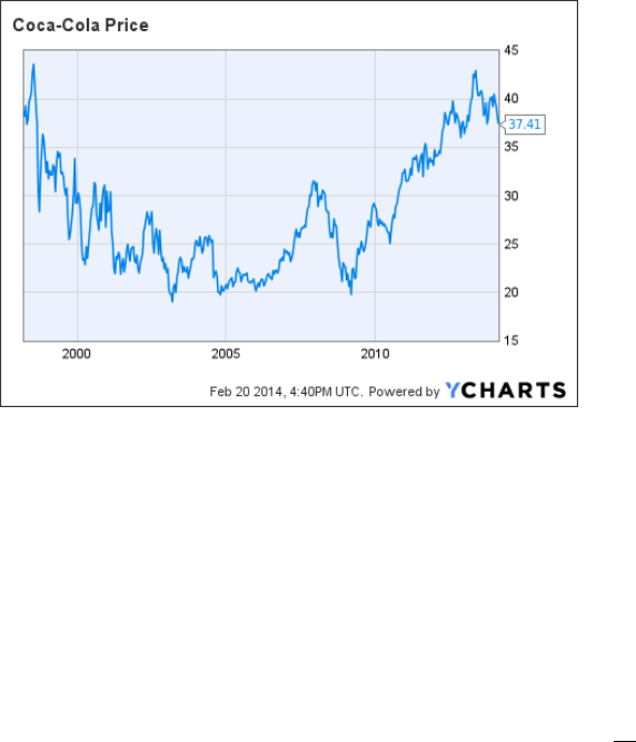
models so difficult. Financial mathematical models attempt to model the evolution
of an asset in order to forecast future values and identify important trends.
Figure 3.1: Plot of KO stock price with respect to time [5]
Consider an asset price S whose evolution we will try to model. In order to
look at this phenomenon we will associate a return, or the relative change in price.
Lets say at time t the value of the asset is S and on a subsequent time interval,
t + dt, we have S + dS. This represents a change in S by and infinitesimal amount
dS over an infinitesimal interval of time, dt. In modeling our return on the asset we
consider dS relative to S, as this scaling preserves proportion, giving
dS
S
. The most
basic financial models break down the return into two portions: the random portion
and the deterministic portion, where the latter is analogous to a risk free return on
investment. This portion we denote µdt and is typically a constant in basic financial
models, however µ can be a function in more complex models. The second portion
contains the randomness of the asset price denoted σdX. Here σ is the volatility
of the asset which is formally defined as a measure of the standard deviation of the
returns of the asset. More informally, the volatility of an asset can be thought of
as the amount of risk associated with the value of an asset. Asset prices are not
static and some fluctuate more so than others which creates an element of risk when
14

investing; σ accounts for this risk. The standard deviation, which defines volatility,
is defined as the dispersion of data points, which represent historical returns, from
the mean. In other words, given the historical returns of an asset over a period of
time and considering their distribution we can see the volatility. The volatility will
be expressed through the dispersion of data points from the mean. So the greater
the dispersion the higher the volatility. Asset volatility is an important and curious
topic for which we will devote more time later in the chapter. Note that σ is then
scaled by dX which is a random sample from a normal distribution. The choice of a
sample from a normal distribution results from the modeling of a random and volatile
phenomenon. It is obvious that seemingly random fluctuations exist in the market,
but the distributions cannot be predicted. However, it is known, by the Central Limit
Theorem, that given sufficiently many random variables the average will converge to
a normal distribution. It is for this reason that dX is defined as a random variable
from a normal distribution. Bringing the portions together to model our return we
have the stochastic differential equation,
dS
S
= σdX + µdt
This equation is an example of a random walk. A random walk is defined as a
sequence of discrete random steps. Random walks are used in many different fields,
but are omnipresent in Finance. Figure 3.1 is an example of a random walk as the
graph is composed of a connected series of discrete points. Random walks are useful
because they are strictly a mathematical construction that tracks real life phenomena.
This makes sense given the model above as we observe the relation between our
variables. Given S over a time interval dt, we consider dS as a step in the sequence.
A known fact it that prices in financial markets follow a random walk. However, it
is important to note precisely what this means. Random walks do not forecast asset
prices deterministically, but they are able to reveal interesting information about
15

Figure 3.2: A lognormal distribution [6]
asset behavior in a probabilistic sense. The fact that random walks are ”memoryless”
characterizes their importance in such models. Random walks are indeed a Markov
process which exhibit the necessary properties. We can now consider the random walk
of the stochastic differential equation discussed. If an asset S follows the random walk
given by this equation then the random variable’s probability density function is that
of a slightly skewed normal distribution called a lognormal distribution. A lognormal
distribution of a random variable is continuous distribution whose natural log is
normally distributed. A lognormal distribution is assumed in the case of the Black-
Scholes particularly because it does not allow for negative values. This is rather
intuitive for the reason that we cannot have a negative asset price.
3.3 Black-Scholes Derivation
In deriving and analyzing the Black- Scholes equation we will first look at the stochas-
tic differential equation from which it stems,
dS
S
= σdX
|{z}
Random
+ µdt
|{z}
Deterministic
(3.1)
Here, µdt is the average rate of growth of the asset price, which is predictable.
16

This portion of the equation is also known as ”the drift”. Conversely, σdX measures
the volatility of the underlying asset and is entirely random.
In order to better understand the mechanics of (3.1) we will take a function of S,
which represents the value of the underlying asset. We can take f(S) and expand the
function, df =
df
dS
dS +
1
2
d
2
f
dS
2
dS
2
+ ... . In doing this we see that varying S by a small
amount dS is the same as varying f(S). This concept is crucial in not only deriving,
but also understanding the derivation of the Black Scholes equation. Furthermore,
this idea captures the significance of Ito’s Lemma, which serves a an essential tool in
the derivation.
df =
df
dS
dS +
1
2
d
2
f
dS
2
dS
2
+ ... (3.2)
In addition to this expansion, we will introduce one more result that is key in
the derivation. We claim that dX
2
converges to dt as dt tends to 0.
In other words, for smaller dt, (as the time interval decreases), the more dX
2
behaves like dt. Now looking at 3.1:
dS
2
= (SσdX + Sµdt)
2
= σ
2
S
2
dX
2
+ 2µσS
2
dXdt + µ
2
S
2
dt
2
Given that dX =
√
dt,
= σ
2
S
2
dt + 2µ σS
2
dt
3
2
+ µ
2
σ
2
dt
2
as dX =
√
dt
We see that σ
2
S
2
dX
2
is the ”leading” term as we are interested in a small dt.
This results from the idea that analyzing the behavior of dS over the smallest time
interval will result in the most accurate evaluation of the asset. So,
17

dS
2
= σ
2
S
2
dX
2
+ ...
|{z}
Insignificant higher order terms
⇒ dS
2
= σ
2
S
2
dX
2
Here the dots indicate the higher order terms not considered given that the
leading term yields the smallest dt. Now substituting this into 3.2 we have,
df =
df
dS
(SσdX + Sµdt) +
1
2
d
2
f
dS
2
σ
2
S
2
dt
= σSdX
df
dS
+ µS
df
dS
dt +
1
2
d
2
f
dS
2
σ
2
S
2
dt
= σSdX
df
dS
+
µS
df
dS
+
1
2
d
2
f
dS
2
σ
2
S
2
!
dt
Again, in using Itˆo’s lemma what we have done is related a small change in a the
function of a variable to a small change in the variable itself. It is worth mentioning
that this exact process can be done with a function of two variables say f(S, t) for
example. Where the independent variables are S, the value of the underlying asset,
and t, time. The following is the above result for V (S, t), where V is the value of a
portfolio,
dV = σS
∂V
∂S
dX +
µS
∂V
∂S
+
1
2
σ
2
S
2
∂
2
V
∂S
2
+
∂V
∂t
!
dt
From here we will derive the Black-Scholes equation. To do this let us construct
a portfolio:
Π = V − ∆S
This portfolio consists of one option V and we assign to ∆ a number which scales
the underlying, S. This scaling value will consequently adjust the value of the option
18

and this the portfolio itself. We will discuss a value for ∆ later on, however a natural
choice will emerge which will play an important role in the final steps of the derivation.
Given our definition of the above portfolio we can say that the jump in the value of
this portfolio in one time step is:
dΠ = dV − ∆dS
Substituting dV and dS above yields,
dΠ = σS
∂V
∂S
dX + µS
∂V
∂S
dt +
1
2
σ
2
S
2
∂
2
V
∂S
2
dt +
∂V
∂t
dt − ∆SσdX − ∆Sµdt
= (σS
∂V
∂S
− ∆Sσ)dX +
µS
∂V
∂S
+
1
2
σ
2
S
2
∂
2
V
∂S
2
+
∂V
∂t
+ ∆Sµ
!
dt
= σS(
∂V
∂S
− ∆)dX
| {z }
random portion
+
µS
∂V
∂S
+
1
2
σ
2
S
2
∂
2
V
∂S
2
+
∂V
∂t
+ ∆Sµ
!
dt
We can now see how a natural choice for ∆ emerges which will eliminate the
random component present in the natural walk. Clearly, this leaves us will solely the
deterministic component allowing us to better forecast asset behavior.
∆ =
∂V
∂S
⇒ dΠ =
∂V
∂t
+
1
2
σ
2
S
2
∂
2
V
∂S
2
!
dt
Here we consider a more subtle concept of supply and demand called arbitrage.
Arbitrage is the process of continuously buying and selling assets in order to profit
from differences in price. Because arbitrage exists in the marketplace we can equate
the return of a portfolio Π with a riskless, return from an investment, denoted rΠdt.
19

⇒ rΠdt =
∂V
∂t
+
1
2
σ
2
S
2
∂
2
V
∂S
2
!
dt
Substituting our portfolio and our ∆ into the above equation yields,
r(V − ∆S)dt =
∂V
∂t
+
1
2
σ
2
S
2
∂
2
V
∂S
2
!
dt
⇔
∂V
∂t
+
1
2
σ
2
S
2
∂
2
V
∂S
2
+ rS
∂V
∂S
− rV = 0
Finally, we have derived the Black-Scholes equation presented above.
3.4 Implied Volatility and the ’Smile’
Apart from the Black-Schole’s new and innovative approach for valuation of options,
the equation has many other auxiliary effects. Many of these consequences are worth
noting, however here we will focus on the concept of implied volatility and an unusual
phenomenon known graphically as the ’smile’.
The Black-Scholes became such a powerful tool largely in part as a result of its
accessible and simple construction. To illustrate this we will look at the variables
present in the equation. The factors that are considered in the model of such an
option are the stock price, the exercise price, the interest rate, the time to expiration,
and the volatility. Most of these variables are self explanatory, however we require
one definition. The exercise price of an option, also known as the strike price, is the
value at which the owner of an option is entitled to buy or sell the asset. These are
all reasonable and relevant variables to utilize due particularly to their availability.
The stock price, exercise price, interest rate, and time to expiration are all current
quantities that are known, making them easily employable. However the volatility is
20
an important factor that is not so easily employed. A direct measurement of volatility
is inherently difficult to obtain given the nature of the factor. The volatility is not a
constant value. This highlights a major flaw in the Black-Scholes model because in
the equation σ is a constant. Regardless, the past volatility is of no use in considering
the present volatility over the life of the option. Yet, it is true that options are being
quoted and traded in the market on the basis of this volatility. This means that
even though we may not know the volatility the market does. In considering this
fact we can again employ the Black-Scholes equation only this time from a different
angle. We need the stock price, exercise price, interest rate, and time to expiration,
which are easy enough to locate as they are constantly quoted or prescribed in the
option contract. Next we find the option price that is quoted in the market, and
work backwards. Instead of solving for the option price, we are solving for the market
implied volatility. This is possible as there exists a one to one correspondence between
implied volatility and market price. This directly proportional relation between the
two factors serves as the ground from which we are able to draw the market implied
volatility. This result is powerful in that it allows us to quantify and analyze an
elusive, but essential variable in the valuation of options.
While this technique does shed light on the markets view of volatility, an in-
teresting phenomenon can be observed that highlights a flaw in the model. To best
see the discrepancy between the Black-Scholes model and the real world phenomenon
we introduce the ’smile’. The ’smile’ is the resulting curve when implied volatility
and and strike price are plotted accordingly. According to the Black-Scholes model,
given the same strike price and maturity date, volatility should be held constant.
In other words according to the model, implied volatility should be static across all
strike prices, all else held constant. This is not the case. In reality if we plot strike
price and volatility we see an upward sloping curve that looks like a smile, hence the
21


CHAPTER 4
THE HEAT EQUATION
The significance of partial differential equations in financial modeling is enormous
given that PDE’s function as the machinery which makes these models possible. The
importance of PDE’s is logical considering that most often there are many dynamic
factors which constitute the value of an continuously evolving asset. In order to
contextualize PDE’s in the light of Finance we begin by examining the well known
heat equation. A basic but enlightening example of a partial differential equation, the
heat equation is to PDE’s what the logistics equation is to ODE’s. The heat equation
is a partial differential equation that models heat flow through a medium over time.
∂u
∂t
= k
∂
2
u
∂x
2
Solutions to this equation, u(x, t), describe the temperature at a certain point of
the medium as a function of space and time.
Before we present a derivation we must first introduce several necessary assump-
tions and laws essential in the derivation. The assumption that is made in considering
the one dimensional heat equation is that we have long, thin uniform metal bar that
is perfectly insulated on its sides such that the only way for heat to escape is at the
ends. Furthermore, we assume that there is no heat source within the metal bar itself.
Given the nature of the equation we can see that the flow of heat through the metal
bar depends only on the distance x and the time t.
In figure 4.1; A metal bar of length l rests on the x-axis, denoting the spacial
component, with time t on the vertical axis. Given our assumption of perfect insu-
lation, heat can only be lost or gained at the boundaries 0 and l. In this instance
we will assume that heat flows from left to right. Furthermore, given non-uniform
temperature in the rod heat will flow from areas of higher temperature to areas of

Figure 4.1: Heat traveling along a rod. [8]
lower temperature. We are able to exploit these characteristics to derive the heat
equation.
First, we introduce the formula for the Transfer of Heat Energy.
dE = c m du
Where c is the specific heat of the substance. The specific heat is defined as the
amount of energy needed to raise the temperature by one unit. Here m is the mass of
the object and du is the change in temperature of the object. This formula relates the
heat energy lost or gained in an object to the temperature change and consequently
highlights the subtle but important distinction between heat energy and temperature.
Heat energy is a measure of total energy due to molecular motion in an object.
Temperature can be thought of as a measure of heat energy which is defined as the
measure of the average energy of molecular motion. Next, we will introduce Fourier’s
Law of Heat Transfer.
dE
dt
∝ k A
du
dx
This law states the fact the the change in energy with respect to time is proportional
to the change in temperature with respect to space. Furthermore, Fourier’s Law can
be expanded stating an equality.
dE = k A
du(x, t)
dx
dt
24

Here, we clearly see that now we have another expression for dE defined through the
change in temperature as a function of two variables.
Lastly we must define the Law of Conservation of Energy. Conservation
of Energy states that the total energy of an isolated system remains constant or is
conserved; that is, energy can neither be created nor destroyed in such a system, only
transferred. The law of conservation of energy combined with our initial assumptions
create the first step in deriving the heat equation.
Consider an arbitrary, thin cross-sectional slice of the metal rod with length dx.
We define the temperature at the left end of the slice, u(x, t), and the right end
u(x + dx, t). Through conservation of energy we are able to equate expressions for
the change in heat energy in the rod.
kA
du(x, t)
dx
− kA
du(x + dx, t)
dx
dt = c m du(x, t)
On the left, we now have the net heat in the rod for a time increment dt by Fourier’s
Law. On the right we will rewrite the formula for the transfer of heat energy given
that m = ρ V , where ρ is the density of the metal and V is the volume. A step
further, we can write V = A dx. This gives an equivalent expression m = ρ A dx.
Substituting into the above equation.
25

kA
du(x, t)
dx
− kA
du(x + dx, t)
dx
dt = c ρ A dx du(x, t)
d
dx
k
du(x, t) − du(x + dx, t)
dx
= c m
du(x, t)
dt
d
dx
du(x, t) − du(x + dx, t)
dx
=
c m
k
du(x, t)
dt
(Consolidating all constants as γ and taking the limit as dx → 0 we get by linearity:)
lim
dx→0
d
dx
du(x, t) − du(x + dx, t)
dx
= γ
du(x, t)
dt
d
dx
lim
dx→0
du(x, t) − du(x + dx, t)
dx
= γ
du(x, t)
dt
d
2
u(x, t)
dx
2
= γ
du(x, t)
dt
26

CHAPTER 5
CORRESPONDENCE
Given what we know about the Black-Scholes equation and the heat equation it is now
possible to analyze the correlation between the two equations. The well known heat
equation has many parallels with the Black-Scholes equation. This similarity is the
reason why such a profound correspondence exists. We are able to gain perspective
into the Black-Scholes equation by exploring it in the form of the heat equation and
ultimately deriving a solution. In order to do this we will first convert the Black-
Scholes equation into the heat equation.
∂V
∂t
+
1
2
σ
2
S
2
∂
2
V
∂S
2
+ rS
∂V
∂S
− rV = 0, 0 ≤ S, 0 ≤ t ≤ T
Given S as the value of the underlying, t representing time, and E as the strike
price of the call option, the equation has a terminal boundary condition giving the
price of the call option.
V (S, T ) = f (S) = max(S − E, 0)
Also, V (0, t) = 0 considering that the option becomes worthless if the value of
the underlying drops to 0. Without any manipulations we can compare the Black-
Scholes equation and the heat equation noticing the biggest similarity is that both
equations contain a first order derivative with respect to time and up to a second
order derivative with respect to space, considering S as the spacial equivalent. An
initial and well motivated transformation of variables will highlight the likeness.
S = e
x
, t = T −
τ
σ
2

V (S, t) = v(x, τ) = v
ln(S),
σ
2
2
(T − t)
Calculating the respective derivatives present in the original equation.
∂V
∂t
=
∂v
∂τ
∂τ
∂t
= −
σ
2
2
∂v
∂τ
∂V
∂S
=
∂v
∂x
∂x
∂S
=
1
S
∂v
∂x
∂
2
V
∂S
2
=
∂
∂s
∂v
∂S
=
∂
∂S
1
S
∂v
∂x
= −
1
S
2
∂v
∂x
+
1
S
∂
∂x
∂x
∂S
∂v
∂x
= −
1
S
2
∂v
∂x
+
1
S
2
∂
∂x
∂v
∂x
= −
1
S
2
∂v
∂x
+
1
S
2
∂
2
v
∂x
2
Substituting the new derivatives back into the Black-Scholes equation and group-
ing like terms.
∂v
∂τ
=
∂
2
v
∂x
2
+
2r
σ
2
− 1
∂v
∂x
−
2r
σ
2
v
Since we have combined parameters we can now let κ =
2r
σ
2
and replace τ with t.
Also, we redefine the boundary conditions and the domain of the new variables.
∂v
∂t
=
∂
2
v
∂x
2
+ (κ − 1)
∂v
∂x
− κv
We now have an equation with constant coeffecients that is defined on the interval
−∞ < x < ∞. Note that the old interval 0 < S < ∞ is still defined on the new
28

interval. The time interval is rescaled with a new upper bound 0 ≤ t ≤
σ
2
2
T . An added
consequence of the substitution is the transformation of the Black-Scholes terminal
boundary condition to an initial condition relevant to the heat equation. From our
substitution of S.
v(x, 0) = V (e
x
, T ) = f(e
x
) = max(e
x
− E, 0)
At this point it is noticeable that the new equation is quite similar to the heat
equation, the biggest exception being the two terms on the right hand side of the
equation. We eliminate these terms through one more substitution of variables.
v(x, t) = e
αx+βt
|
{z}
φ
(x, t)
|{z}
u
= φu
We will again compute the corresponding derivatives.
∂v
∂t
= βφu + φ
∂u
∂t
∂v
∂x
= αφu + φ
∂u
∂x
∂
2
v
∂x
2
=
∂
∂x
αφu + φ
∂u
∂t
= α
2
φu + 2αφ
∂u
∂x
+ φ
∂
2
u
∂x
2
Substituting the derivatives into the recently transformed PDE we gather like
terms and can cancel the common e
αx+βt
as it is an exponential function which is
always positive.
∂u
∂t
=
∂
2
u
∂x
2
+ [2α + (k − 1)]
∂u
∂x
+ [α
2
+ (k − 1)α − k − β]u
29

Since α and β are arbitrary constants we choose them appropriately in order to
eliminate the
∂u
∂x
and u terms.
α = −
k − 1
2
β = α
2
+ (k − 1)α − k = −
(k + 1)
2
4
Subsequently α and β create coeffecients of 0 which eliminate the
∂u
∂x
and u terms
respectively. The equation is then reduced to the one dimensional heat equation.
∂u
∂t
=
∂
2
u
∂x
2
, −∞ < x < ∞, 0 ≤ t ≤
σ
2
2
T
We now need to transform the initial condition.
u(x, 0) = e
−αx
v(x, 0) = e
−αx
f(e
x
)
For a call option with strike price E, f(x) = max(x − E, 0), so
u(x, 0) = e
−αx
f(e
x
) = e
−αx
max(e
x
− E, 0)
We can now employ the well known heat equation solution representation formula
for the Black-Scholes equation.
u(x, τ) =
1
2
√
πτ
Z
∞
−∞
u
0
(s)e
−
(x − s)
2
4τ
ds
In order to integrate we perform a change of variables. Let z =
(s−x)
√
2τ
⇒ dz =
−
1
√
2τ
dx
u(x, τ) =
1
2
√
π
Z
∞
−∞
u
0
(z
√
2τ + x)e
−
z
2
2
dz
30

Note that u
0
(s) is positive only if the argument s > 0, that is z
√
2τ +x > 0 or z >
−
x
√
2τ
. On this domain u
0
> 0. Given that u(x, 0) = e
−αx
max(e
x
− 1, 0).
u
0
= e
−
(k−1)
2
e
x
− 1
= e
(k+1)
2
(x+z
√
2τ )
− e
(k−1)
2
(x+z
√
2τ )
Given the new construction of u
0
we consider two separate integrals.
1
2
√
π
Z
∞
−
x
2τ
e
(k+1)
2
(x+z
√
2τ )
e
−
z
2
2
dz
| {z }
I
1
−
1
2
√
π
Z
∞
−
x
2τ
e
(k−1)
2
(x+z
√
2τ )
e
−
z
2
2
dz
| {z }
I
2
We now have two separate integrals I
1
and I
2
which we can evaluate. We will
evaluate I
1
first. Working in the exponent of I
1
we complete the square to simplify
the process.
(k+1)
2
(x + z
√
2τ) −
z
2
2
= −
z
2
2
+
(k + 1)
√
2τz
2
+
(k + 1)x
2
=
−
1
2
z
2
− (k + 1)
√
2τz
+
(k + 1)x
2
=
−
1
2
z
2
− (k + 1)
√
2τz +
(k + 1)
2
τ
2
+
(k + 1)
2
τ
4
+
(k + 1)x
2
=
−
1
2
z − (k + 1)
r
τ
2
2
+
(k + 1)
2
τ
4
+
Putting the exponent back into I
1
we can pull out the last two terms as they are
constants with respect to z.
e
(k+1)
2
τ
4
+ e
(k+1)x
2
√
2π
Z
∞
−
x
2τ
e
−
1
2
(z−(k+1)
√
τ
2
)
2
dz
31

One more change of variables is required to complete the integral.
y = z −
r
τ
2
(k + 1) =⇒ dy = dz
e
(k+1)
2
τ
4
+ e
(k+1)x
2
√
2π
Z
∞
−
x
2τ
−
√
τ
2
(k+1)
e
−
y
2
2
dz
Drawing from chapter 2, notice that the integrand is just the probability density
function of a normal distribution. The integral can be represented as the cumulative
distribution function of a normal random variable, d. The cumulative distribution
function, φ, of a normal random variable, d, is the probability that φ will take a
value less than or equal to d. For our particular instance we consider the cumulative
distribution function in a continuous case which is just the area under the probability
density function from −∞ to x.
φ(d) =
1
√
2π
Z
d
−∞
e
−
y
2
2
dy
Therefore,
I
1
= e
(k+1)
2
τ
4
+ e
(k+1)x
2
φ(d
1
), where d
1
=
x
2τ
+
r
τ
2
(k + 1φ(d
2
)
I
2
is computed the exact same way except that (k + 1) is replaced with (k − 1).
Therefore, the solution to this heat equation initial value problem.
u(x, τ) = e
(k+1)
2
τ
4
+ e
(k+1)x
2
φ(d
1
) − e
(k−1)
2
τ
4
+ e
(k−1)x
2
φ(d
2
)
We now must retrace our steps and undo each change of variables, starting with
v(x, τ ) = e
−
(k+1)
2
τ
4
−
(k+1)x
2
u(x, τ). Combined and simplifying the left hand side.
v(x, τ ) = e
x
φ(d
1
) − e
−τ k
φ(d
2
)
32

Replacing x = ln(S) and τ =
σ
2
2
(T − t) and V (S, t) = v(x, τ ). Also, note k =
2r
φ
2
V (S, t) = Sφ(d
1
) − e
−r(T −t)
φ(d
2
)
The last modification needed is the transformation of d
1
and d
2
back in terms of
initial variables. We do this the exact same was as their coefficients.
d
1
=
ln(S) + (r +
σ
2
2
)(T − t)
σ
√
T − t
d
2
=
ln(S) + (r −
σ
2
2
)(T − t)
σ
√
T − t
The end result is the Black-Scholes formula for the price of European call option
with strike price K at time T , if the current time, underlying price, interest rate, and
volatility are t, S, r, σ respectively. Most of the time the formula is not presented in
the full closed form solution, but rather piecemeal or:
V
c
(S, t) = S · φ(d
1
) − e
−r(T −t)
· φ(d
2
)
33
CHAPTER 6
CONCLUSION
To conclude, we have presented the powerful applications of such mathematical mod-
els as well as their tremendous implications in finance. Using mathematical tools the
substance behind such models can be deconstructed, reconstructed, and improved
allowing for a better understanding and utility. In deconstructing the Black-Scholes
equation we rebuild the structure with a new face and name which is that of the
familiar heat equation. This connection alone highlights intriguing properties shared
by the Black-Scholes equation and the heat equation, both as parabolic partial differ-
ential equations. Much more room is left for future exploration in the area motivated
by the relation between mathematical finance and natural phenomena.
REFERENCES & ICONOGRAPHY
[1] Retrieved from flickr on October 15, 2016. https://www.flickr.com/photos/
travel_aficionado/2396814840
[2] Retrieved from Financial Times on October 30, 2016. http://markets.ft.com/
data/indices/tearsheet/summary?s=DJI:DJI
[3] Wilmott, Paul, Sam Howison, and Jeff Dewynne. The Mathematics of Financial
Derivatives: A Student Introduction. Oxford: Cambridge UP, 1995. Print.
[4] From, By Changing the Mean. ”Normal Distribution.” Normal Distribution. N.p.,
n.d. Web. 31 Oct. 2016.
[5] Planes, Alex. ”Disney vs. Coca-Cola: Which Dow Stock’s Dividend Dominates?”
The Motley. N.p., 01 Jan. 1970. Web. 31 Oct. 2016.
[6] ”Lognormal Distribution.” - Definition, Function, Properties and Examples. N.p.,
n.d. Web. 31 Oct. 2016.
[7] Radcliffe, Brent. ”Volatility Smile.” Investopedia. N.p., 15 Apr. 2014. Web. 31
Oct. 2016.
[8] ”Heat Equation.” Wikipedia. Wikimedia Foundation, n.d. Web. 31 Oct. 2016.
35
