
315
13
Paired-
and Independent-
Samples
t
Tests
In this chapter, you can learn
• how to tell the difference between a paired-samples and an independent-samples t test,
• whether or not to reject a claim that the population means for two variables are identical,
• whether or not to reject a claim that the population mean for one variable is higher
than (or lower than) the population mean of another variable,
• whether or not to reject a claim that two populations have identical means on a variable,
• whether or not to reject a claim that one population’s mean is higher than (or lower
than) another population’s mean on the same variable,
• the two kinds of errors you risk when hypothesis testing,
• the difference between statistical significance and substantive importance, and
• why dispersion must not be ignored when comparing group means.
Controversial Persons,
Parental Schooling, and Hours Worked
This chapter will answer the following questions about 1980 GSS young adults:
• Were 1980 GSS young adults significantly more willing to let controversial persons give pub-
lic speeches than to let them teach in college?
• Were the fathers of 1980 GSS young adults significantly better educated than the mothers of
1980 GSS young adults?

316 PART III :: INFERENTIAL STATISTICS
• Was the number of hours worked per week by employed 1980 GSS young adults significantly
higher for males than for females?
• Was there a significant difference between the employed 1980 GSS young adults and the
employed 1980 GSS middle-age adults in the number of hours worked per week?
Overview
Two types of hypothesis tests are introduced in this chapter. Both check to see if a difference
between two means is significant. Paired-samples t tests compare scores on two different variables
but for the same group of cases; independent-samples t tests compare scores on the same variable
but for two different groups of cases.
The chapter also discusses three hypothesis-testing related topics: types of errors, substantive
importance, and significantly different but overlapping distributions.
Paired-Samples
t
Tests
Here are some research hypotheses that can be tested using paired-samples t tests:
• The average score of subjects on the posttest is different than the average of those same
subjects on the pretest. (
POSTTEST PRETEST≠
)
• People will listen longer to a female telephone marketer than the very same people will listen
to a male telephone marketer. (
FORAHER FORAHIM>
)
• Graduates had higher average salaries 10 years after graduation than they had 5 years after
graduation. (
SALARY SALARY10 5>
)
• On average, soldiers weighed less after they completed basic training than they weighed
before they started. (
AFTERBEFORE<
)
• In a comparison of universities, sociology departments averaged fewer faculty members than
did history departments. (
SOCDEPT HISTDEPT<
)
• First-born identical twins live longer, on average, than their second-born birth mates.
(
LIFE1STLIFE2ND>
)
• Husbands average more hours of sleep per night than their wives. (
HESLEEP SHESLEEP>
)
SPSS TIP
To Duplicate the Examples in This Chapter
To duplicate the examples in this chapter, use the fourGroups.sav data set. Before doing the
first three examples, set the select cases condition to GROUP = 1. For the final example, set
the select cases condition to “all cases.”

317Chapter 13 :: Paired- and Independent-Samples t Tests
What distinguishes these hypotheses from the one-sample t test hypotheses in the last chapter
is that each of these hypotheses is making a claim about two means. As always with hypothesis
testing, the claim is about the population, but it will be tested using sample data.
It might help to think of it this way: There are two groups of scores. The first is a group of scores
on the first variable. The second is a group of scores on the second variable. The mean for each
group of scores will be calculated, but first look more closely at the data groups themselves.
Each group is just a sample of the scores that would have been collected if every member of the
population had been questioned. But these two groups of sample data are not independent of one
another. In most cases, the sample data in the two groups came from the same people. In every case,
there is some kind of link between the individual cases that provided the data in the first group and
the cases that provided the data in the second group. This link is why the name of the procedure
refers to paired samples.
Look at the first four hypotheses listed above: subjects who took a pretest and a posttest, persons
listening to a female telemarketer and also a male telemarketer, graduates 5 years and then 10 years
after graduation, and soldiers weighed before and after basic training. The obvious link between the
two groups of scores is that they are both scores for the same group of people.
For the last three hypotheses, however, the two groups of scores are not for the same individuals.
Nevertheless, the scores are still linked. The fifth hypothesis compares sociology and history depart-
ments within the same universities. The sixth hypothesis compares first-born and second-born
children who are twins to one another. The seventh hypothesis compares husbands and wives who
are married to one another. For these hypotheses, the units of analysis (what each row in the data
set represents) are all things bigger than individual persons. They are universities, sets of twins, and
married couples. You can pair up history and sociology departments based on their university, first-
born children and second-born children based on what set of twins they represent, and husbands
and wives based on the married couples they form.
For each of these research hypotheses, you should be able to form the null hypothesis. For
example, the null hypothesis for the first research hypothesis is that the average score of subjects
on the posttest is the same as the average of those same subjects on the pretest
(
POSTTEST PRETEST=
), and the null hypothesis for the second is that the very same people
will listen for the same or shorter time to a female telephone marketer than they will listen to a
male telephone marketer (
FORAHER FORAHIM≤
).
As the seven hypotheses demonstrate, paired-samples t testing can be one- or two-tailed. Paired-
sample t testing proceeds through the same four steps as one-sample t tests.
A First Example
“Were 1980 GSS young adults significantly more willing to let controversial persons give public
speeches than to let them teach in college?”
Step 1: To answer this question, we form two hypotheses about the population. The research
hypothesis is “the average willingness of 1980 young adults to let controversial persons give public
speeches was greater than their willingness to let them teach college” (
OKSPEECHOKTEACH>
).

318 PART III :: INFERENTIAL STATISTICS
The corresponding null hypothesis is “the average willingness of 1980 young adults to let controver-
sial persons give public speeches was the same or less than their willingness to let them teach col-
lege” (
OKSPEECHOKTEACH≤
).
These hypotheses are claims about the means on two variables (OKSPEECH and OKTEACH) for
one population (1980 young adults). The sample of OKSPEECH scores and the sample of OKTEACH
scores are paired samples because the two samples consist of the same persons.
This is a one-tailed hypothesis test since the difference between the means must be sufficiently
large and in a particular direction (greater tolerance for speeches than for college teaching) to reject
the null hypothesis.
Step 2: The SPSS Paired-Samples T Test procedure provides both the sample means and, should
it be needed, the significance level. Pull down the Analyze menu, move the cursor over Compare
Means, and click on Paired-Samples T Test.
Analyze | Compare Means | Paired-Samples T Test
A dialog similar to Figure 13.1 appears.
Select the two variables whose means will be compared and move them into the “Paired
Variables” list. When you select your first variable, it becomes variable1 for pair 1. When you select
your second variable, it becomes variable2 for pair 1. Fields open up to specify a second pair, but
we will test just one pair at a time.
Pay attention to level of measurement! Since the mean for each variable will be calculated, both
variables must be interval/ratio. Once you have moved the pair of variables into the “Paired
Variables” list, click OK. Figure 13.2 shows the resulting output.
Figure 13.1 Dialog to Produce a Paired-Samples t Test
319Chapter 13 :: Paired- and Independent-Samples t Tests
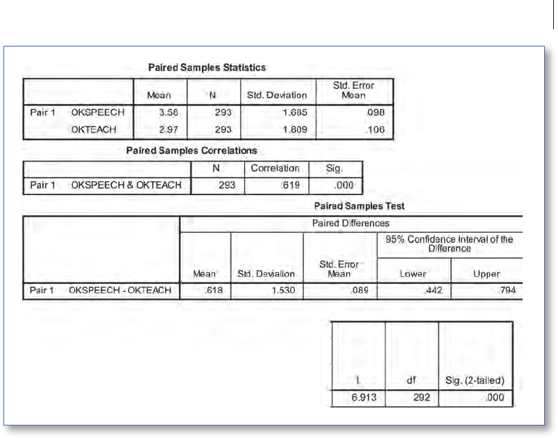
Figure 13.2 Paired-Samples T Test Output for OKSPEECH and OKTEACH for 1980 GSS Young Adults
The “Paired Samples Statistics” shows the mean for each variable. These means are based on the
293 persons in the data set with valid scores on both variables. Cases without valid scores on one
or both variables are dropped from the analysis.
In the sample, the average tolerance for giving a public speech is greater than for teaching col-
lege. This is consistent with the research hypothesis. So, we proceed to Step 3.
Step 3: Skip over the second box of output, the “Paired Samples Correlations” box. The informa-
tion in that box is not relevant for a hypothesis about means. The “Paired Samples Correlations” box
is testing a hypothesis about the correlation between the two variables. The significance level you
see in this second box is not the one we want.
The significance level we are looking for is in the “Paired Samples Test” box. This is a single long
box as it appears on a computer screen but has been divided into two parts for Figure 13.2. The
significance level appears at the extreme right of the box. It is a two-tailed significance. Since we are
testing a one-tailed hypothesis, the two-tailed significance must be divided in half, but, of course,
.000/2 still is .000.
Before going on to Step 4, however, a few words should be said about the other information
in the “Paired Samples Test” box. The degrees of freedom for the hypothesis test are to the left

320 PART III :: INFERENTIAL STATISTICS
of the significance level. Degrees of freedom for paired-sample t tests are calculated just like for
one-sample t tests:
paired-samples t test: df = N − 1
paired-samples t test: N = df + 1
The t statistic appears to the left of the degrees of freedom. The value of 6.913 for the t statistic
in Figure 13.2 indicates the sample difference in means is almost 7 standard errors to the right of
where the null hypothesis says the center of the sampling distribution is. How likely is a sample
result this far from the center of the sampling distribution? It is so unlikely that when rounded to
just three decimal places, the probability is .000.
Although it is not added to the data set, SPSS actually computes a new variable when it does
a paired-samples t test. This new variable is the value of the case’s score on the first variable
minus the value of the case’s score on the second variable. In this example, that would be
OKSPEECH minus OKTEACH. The null hypothesis is claiming the mean on this new variable
should be 0 or a negative number. The information in the “Paired Samples Test” under the
“Paired Differences” heading shows the mean, standard deviation, standard error, and confi-
dence interval for this new variable.
Step 4: The null hypothesis is rejected since the probability of getting the observed sample
results if the null hypothesis is true is .000. The results are statistically significant. By rejecting the
null hypothesis, support is given to the research hypothesis that 1980 young adults did have more
tolerance for controversial persons giving public speeches than for teaching college.
A Second Example
“Were the fathers of 1980 GSS young adults significantly better educated than the mothers of 1980
GSS young adults?”
This question leads directly to two competing hypotheses: “The average years of schooling of
the fathers of 1980 young adults was greater than the average years of schooling of the mothers of
1980 young adults” (
PAEDUC MAEDUC>
) is the research hypothesis; the null hypothesis is “the
average years of schooling of the fathers of 1980 young adults was the same or less than the average
years of schooling of the mothers of 1980 young adults” (
PAEDUC MAEDUC≤
).
The sample of fathers’ education scores and the sample of mothers’ education scores are paired
samples since any particular father’s education score can be matched to a particular mother’s edu-
cation score because they are the education scores for the parents of a person who took part in the
GSS. The hypothesis test is one-tailed since the difference between the two means must be suffi-
ciently large and in a particular direction to reject the null hypothesis.
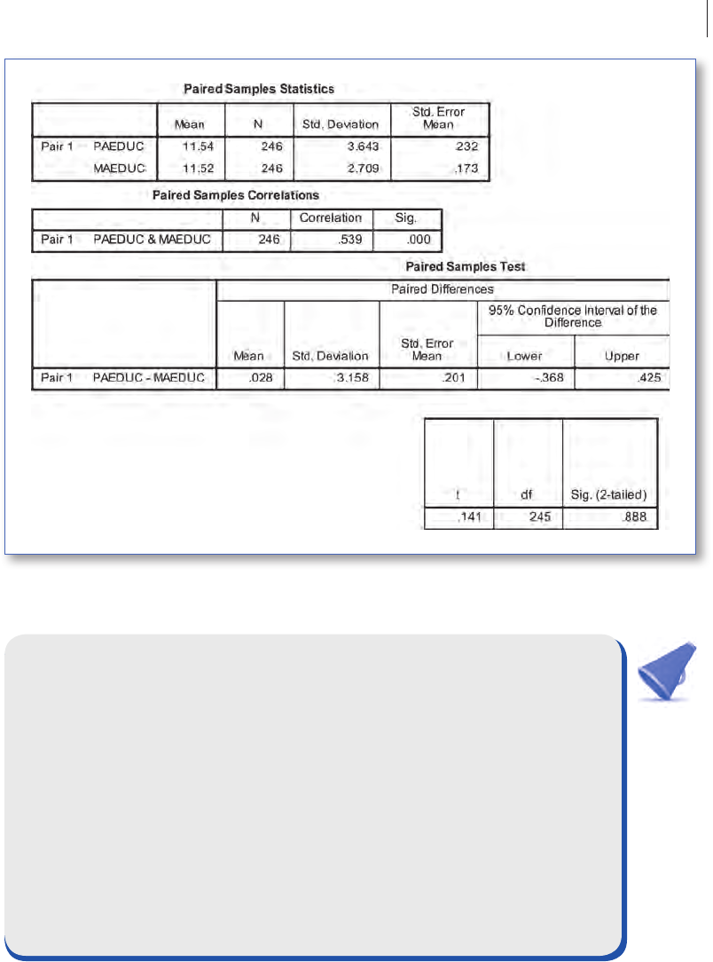
The Paired-Samples T Test output appears in Figure 13.3.
The fathers averaged 11.54 years of schooling; the mothers averaged 11.52 years. That makes the
sample results consistent with the research hypothesis. The means do not differ by much, but they
differ—and they differ in the direction predicted by the research hypothesis.
321Chapter 13 :: Paired- and Independent-Samples t Tests
Figure 13.3 Paired-Samples T Test Output for PAEDUC and MAEDUC for 1980 GSS Young Adults
SPSS TIP
These Are Not the Means We Saw Before!
Back in Chapter 4, the mean for MAEDUC was reported to be 11.41 years, and the mean for
PAEDUC was 11.59 years. These are not the means appearing in Figure 13.3. What is going on?
The difference results from how cases with missing data are handled. The Descriptives
procedure back in Chapter 4 by default used every valid case to calculate the statistics for
each variable. All 301 cases with valid data on MAEDUC were used to calculate its mean,
and all 256 cases with valid data on PAEDUC were used to calculate its mean.
The Paired-Samples T Test procedure, however, can only use cases that have valid values on
both of the variables being compared. Only 246 cases in the data set had valid information on
both MAEDUC and PAEDUC, and those are the cases being used for this procedure. Dropping
the cases with valid data on just one of the two variables accounts for the shift in means.

322 PART III :: INFERENTIAL STATISTICS
CONCEPT CHECK
Without looking back, can you answer the following questions:
• Why are paired samples called that?
• Paired-samples t tests compare means for how many variables for how many groups
of cases?
If not, go back and review before reading on.
The two-tailed significance level is .888. Since this is a one-tailed hypothesis, the one-tailed
significance level is .888/2, which is .444.
The null hypothesis, which claimed that, on average, the fathers of 1980 young adults had the
same or fewer years of schooling as the mothers of 1980 young adults, cannot be rejected. The
results are not statistically significant. Whether the fathers had more schooling than the mothers or
had equal or less schooling remains an open question.
RESEARCH TIP
One-Sample and Paired-Samples t Tests
With a little bit of extra work, every paired-samples t test can be reduced to a one-sample t test.
It was pointed out that SPSS actually computes a new variable, a difference score, whenever it
does a paired-samples t test. It then tests the null hypothesis using this new variable.
Well, we could do the same thing. Our first example of paired-samples t testing had as a
research hypothesis that the average willingness of 1980 young adults to let controversial per-
sons give public speeches was greater than their willingness to let them teach college. We
could have calculated a new variable using the Compute procedure. It might be named DIFF
and calculated as OKSPEECH minus OKTEACH. In terms of this new variable, our research
hypothesis would be
DIFF > 0
and our null hypothesis would be
DIFF ≤ 0
. Testing this with
a one-sample t test would produce values for the t statistic, degrees of freedom, and signifi-
cance level that are identical to the values produced with the paired-samples t test procedure.
Using the paired-samples t test procedure simply saves the effort of computing a new variable!
Independent-Samples
t
Tests
Like paired-samples t tests, independent-samples t tests also test hypotheses about differences
between two means; however, the means are for the same variable but for two different populations.
The following research hypotheses would use independent-samples t tests. (In the mathematical

323Chapter 13 :: Paired- and Independent-Samples t Tests
expressions of the hypotheses, the subscript following each variable name indicates the group for
which the mean would be calculated.)
• Catholic women average more children than Protestant women. (
CHILDREN CHILDREN
Cath wome
nP
rot women
>
)
• Biology graduates have a different average annual income than chemistry graduates.
(
INCOME INCOME
biograds chem grads
≠
)
• Homicide rates, on average, are higher in Western counties than in Southern counties of the
United States. (
HOMICIDE HOMICIDE
West counties Southcounties
>
)
• Length of life, on average, is shorter for never-married persons than for ever-married persons.
(
LIFE LIFE
never married ever married
<
)
• The mean years of schooling of Republicans are different than the mean years of schooling
of Democrats. (
EDUC EDUC
Republican
sD
emocrats
≠
)
• Husbands average more hours of sleep per night than wives. (
SLEEP SLEEP
husbands wives
>
)
As with paired-samples t tests, there are again two groups of scores. However, this time, the
scores in both groups are scores on the same variable. What distinguishes the groups is that they
represent different populations: for example, Catholic women and Protestant women, biology
graduates and chemistry graduates, and counties in the West and counties in the South.
Even though all the cases may have been selected in a single sample, it is as if the first group was the
result of a sample from the first population (e.g., a sample from the population of Republicans) and the
second group was the result of a separate sample from the second population (e.g., a sample from the
population of Democrats). There is no reason for pairing up individual cases in one group with individual
cases in the other group. In fact, the number of cases in each of the two groups will typically not be the
same. The groups (or samples) are independent of one another, thus the name independent samples.
The Independent-Samples T Test procedure is used to compare just two groups in the population.
It would not be used to test a hypothesis about differences in average number of children for
Catholic, Protestant, and Jewish women. Comparisons of three or more groups require a different
procedure, one presented in the next chapter.
Hypothesis tests using independent-samples t tests can be one-tailed or two-tailed. Independent-
samples t tests use the same four steps in hypothesis testing; however, Step 3 involves an additional
decision.
One more thing before starting the first example: At the start of the chapter, the research hypoth-
esis “husbands average more hours of sleep per night than their wives (
HESLEEP SHESLEEP>
)”
was said to require a paired-samples t test. Now, we have the research hypothesis “husbands average
more hours of sleep per night than wives (
SLEEP SLEEP
husbands wives
>
),” and it is said to require an
independent-samples t test. Why the difference in hypothesis testing techniques?
Although the hypotheses are similar, they are not identical. The first hypothesis talks about
husbands and their wives. That indicates the cases in the data set represent couples. One of the
variables in the data set records how much sleep the husband in the couple gets. A separate variable
in the data set records how much sleep the wife in the couple gets. Any HESLEEP score can be
paired up with a specific SHESLEEP score, and the basis for the pairing would be that the two scores
come from persons who are married to one another. The situation calls for paired-samples t testing.

324 PART III :: INFERENTIAL STATISTICS
The research hypothesis “husbands average more hours of sleep per night than wives,” however,
provides no evidence that the husbands and wives are necessarily married to one another. Someone
took a sample from the adult population. Everyone in the sample was asked how many hours per
day they typically sleep. Some of the persons in the sample were married men; some were married
women. The married men in the sample can be viewed as a random sample of all married men in
the population. The married women in the sample can be viewed as a random sample of all married
women in the population. There is no basis for linking up scores on SLEEP reported by individual
husbands with scores on SLEEP reported by individual wives. The situation calls for independent-
samples t testing. Unless there is clear evidence that there is a basis for pairing up individual scores,
assume you have independent samples.
By the way, there may have been others in the sample besides married men and married
women, for example, persons who have never married or persons who are divorced or widowed.
Since independent-samples t tests only permit comparisons of two groups, these other cases would
be excluded from the analysis.
A First Example
“Was the number of hours worked per week by employed 1980 GSS young adults significantly
higher for males than for females?”
Step 1: The research hypothesis for this question is “the average number of hours worked
per week by employed 1980 young adults was higher for males than for females”
(
HOURSHOURS
male
sf
emales
>
). The null hypothesis is “the average number of hours worked per
week by employed 1980 young adults was the same or lower for males than for females”
(
HOURSHOURS
male
sf
emales
≤
).
These hypotheses require an independent-samples t test. They are claims about the mean on
one variable (HOURS) for two populations (male 1980 young adults and female 1980 young adults).
No particular reason exists for pairing up particular male answers with particular female answers.
This is a one-tail hypothesis test since only sample results in which the male average is higher
than the female average could lead to the rejection of the null hypothesis.
Step 2: To do an Independent-Samples T Test procedure, pull down the Analyze menu, move the
cursor over Compare Means, and click on Independent-Samples T Test.
Analyze | Compare Means | Independent-Samples T Test
Figure 13.4 shows the dialog that appears.
Move the variable on whose mean the groups will be compared into the “Test Variable” list. Since
means will be calculated for this variable, it must be interval/ratio. Next, the two groups to be com-
pared must be identified. Select the variable whose attributes will define the two groups and move
that variable into the “Grouping Variable” field. The grouping variable can be any level of measure-
ment. As soon as a variable is moved into that field, a set of parentheses containing two question
marks appears after the name of the variable. SPSS wants to know which codes on this variable
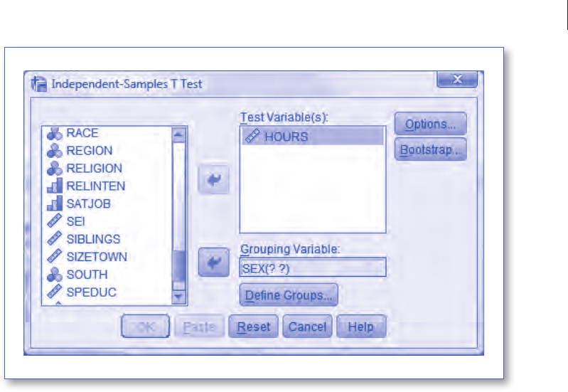
325Chapter 13 :: Paired- and Independent-Samples t Tests
identify the two groups to be compared. Even if the variable is a dichotomy and has just two codes,
those codes must be specified. Click on “Define Groups.” (The button only becomes active once a
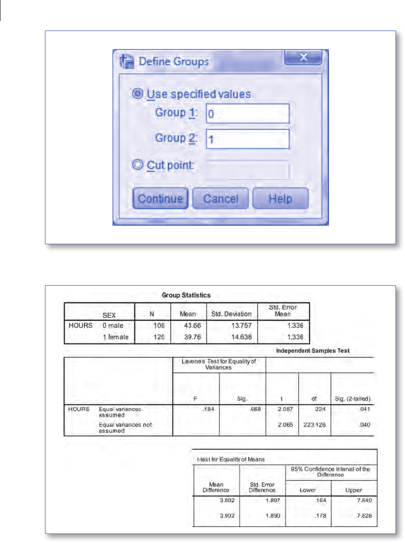
grouping variable has been specified.) The dialog in Figure 13.5 appears.
The two groups can be defined specifying exact values or by designating a cut point. When
specifying exact values, enter in the “Group 1” field the value that cases must have to be in the first
group, and enter in the “Group 2” field the value that cases must have to be in the second group.
For this example, 0 was entered for Group 1 since on the variable SEX, males are coded 0, and 1 was
entered for Group 2 since females are coded 1.
Designating a cut point will also define two groups to be compared. If the grouping variable was
years of schooling, for example, and 13 was entered as the cut point, the first group would include
all valid cases with less than 13 years of schooling, and the second group would include all valid
cases with 13 or more years of schooling.
After defining the groups, click “Continue” to return to the initial independent-samples t test
dialog. The question marks behind the grouping variable are now replaced by the codes that define
the groups. Click OK to produce output similar to Figure 13.6.
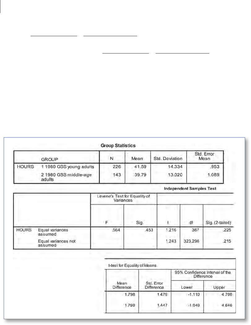
The first box of output, the “Group Statistics” box, shows the sample means. The mean number
of hours worked reported by employed males was 43.66, and the mean reported by employed
females was 39.76. The sample results are consistent with the research hypothesis that predicted
the mean for males would be higher than the mean for females. We proceed to Step 3.
Figure 13.4 Dialog to Produce an Independent-Samples t Test
326 PART III :: INFERENTIAL STATISTICS
Figure 13.5 Dialog to Identify Two Groups Being Compared
Figure 13.6 Independent-Samples T Test Output for HOURS by SEX (0, 1) for 1980 GSS Young Adults

327Chapter 13 :: Paired- and Independent-Samples t Tests
Step 3: This step uses the “Independent Samples Test” output box, which appears on a computer
screen as a single long box but has been broken in two parts to better fit in Figure 13.6. But this box
contains two lines of results for the independent-samples t test. There are two values for the t statis-
tic, for degrees of freedom, and for the significance level. Step 3 for the independent-samples t tests
includes an additional decision because you must decide which result line is the correct one to use.
The reason for two sets of results is that there are two ways of estimating the standard error of
the sampling distribution for independent-samples t tests. One method assumes that the variance
in the male population on number of hours worked is exactly equal to the variance in the female
population on number of hours worked. The other method does not assume the population vari-
ances are equal. Whether the variances in the two populations are the same or different affects the
calculation of the standard error, the value of the t statistic, the degrees of freedom, and the prob-
ability or significance level.
To reach a conclusion about whether the variances are or are not equal, an entirely separate
hypothesis test is done with the null hypothesis that the variances are equal. What appears in the
output under the heading “Levene’s Test for Equality of Variances” are the results of that separate
hypothesis test. If the significance level (“Sig.”) of Levene’s test is .05 or less, use the second line of
t test results, the “Equal variances not assumed” line. If the significance level of Levene’s test is
greater than .05, use the first line of t test results, the “Equal variances assumed” line.
Sometimes the two methods of estimating the standard error give you almost identical results
(as they do in Figure 13.6), and sometimes they do not. Always check the significance of Levene’s
test and then use the correct line of t test results.
In Figure 13.6, the significance level of Levene’s test is .668. Since this is greater than .05, the
first line of results is used. The two-tailed significance level for the t test for equality of means is
.041. Since this is a one-tailed hypothesis, we want the one-tailed significance level, which is .041/2
or .0205. (Make sure you leave Step 3 with the significance level for the t test for equality of means.
Do not leave Step 3 with the significance for Levene’s test. Once the significance of Levene’s test
tells you which row of output to use, you are done with it.)
How degrees of freedom are calculated for independent-samples t tests depends on whether
equal variances are or are not assumed. When equal variances are assumed, degrees of freedom are
simply N minus 2. A more complex formula is used when equal variances are not assumed.
The “Independent Samples Test” box also shows you the mean difference, the standard error of
the difference, and the 95% confidence interval of the difference. The mean difference is always
calculated by subtracting the sample mean for Group 2 from the sample mean for Group 1. If Group
1 has the higher mean, the mean difference will be positive; if Group 2 has the higher mean, the
mean difference will be negative. In the sample data, employed males report an average of 3.902
more hours of work per week than employed females.
Step 4: Since the probability is .0205, we reject the null hypothesis. Among the 1980 GSS young
adults, employed males did work significantly more hours per week than employed females.
A Second Example
“Was there a significant difference between the employed 1980 GSS young adults and the employed
1980 GSS middle-age adults in the number of hours worked per week?”
328 PART III :: INFERENTIAL STATISTICS
The null hypothesis is “the average number of hours worked per week by
employed 1980 young adults and by employed 1980 middle-age adults is the same”
(
HOURSHOURS
youngadult
sm
iddle-age adults1980 1980
=
). The research hypothesis is “the average
number of hours worked per week by employed 1980 young adults and by employed 1980
middle-age adults is different” (
HOURSHOURS
youngadult
sm
iddle-age adults1980 1980
≠
).
Hypotheses about a difference in means for one variable (HOURS) in two populations (1980
young adults and 1980 middle-age adults) call for an independent-samples t test. This is a two-
tailed hypothesis test because a sample difference in either direction could lead to rejecting the
null hypothesis.
For setting up the independent-samples t test, the test variable is HOURS and the grouping
variable is GROUP. Codes 1 (1980 GSS young adults) and 2 (1980 GSS middle-age adults) define the
comparison groups. Cases with codes other than 1 or 2 on GROUP are excluded from the analysis.
(Since GROUP is the variable used to identify the comparison groups, Select Cases was set to “All
cases.”) The output appears in Figure 13.7.
Figure 13.7 Independent-Samples T Test Output for HOURS by GROUP (1, 2)

329Chapter 13 :: Paired- and Independent-Samples t Tests
In the sample, the mean number of hours worked reported by employed 1980 GSS young adults
was 41.59, while the mean reported by 1980 GSS middle-age adults was 39.79. The research
hypothesis says the two groups will have different means, and in the sample they do. Therefore, we
proceed to Step 3.
The significance level of Levene’s test is .453. Since that is greater than .05, we again use the
equal variances assumed line of results. The two-tailed significance level of the t test for equality of
means is .225.
Because the probability of getting the observed sample results if the null hypothesis is true is
.225, the null hypothesis is not rejected. The results are not statistically significant. Although young
adults and middle-age adults had different average hours of work in our sample, the evidence is not
sufficiently strong to reject the possibility that the populations of 1980 young adults and 1980
middle-age adults had the same average number of hours worked. If the null hypothesis was
rejected, we would be taking a 22.5% risk that we rejected a null hypothesis that was actually true.
We will accept no more than a 5% risk of making such an error!
CONCEPT CHECK
Without looking back, can you answer the following questions:
• Why are independent samples called that?
• Independent-samples t tests compare means for how many variables for how many
groups of cases?
• If the significance of Levene’s test is greater than .05, are “equal variances assumed”
or “equal variances not assumed” for the independent-samples t test?
If not, go back and review before reading on.
More About Hypothesis Testing
Type I and Type II Errors
Figure 13.8 describes the consequences of rejecting or not rejecting the null hypothesis when the
null hypothesis is actually true for the population and when the null hypothesis is actually false for
the population.
When a researcher rejects a null hypothesis that is actually false, that is a good outcome.
Similarly, when a researcher does not reject a null hypothesis that is actually true, that is also a good
outcome. The errors occur when the researcher rejects a null hypothesis that is actually true (Type
I error) or does not reject a null hypothesis that is actually false (Type II error).
Of course, researchers do not intentionally commit either of these types of errors. Nor do they
know for certain if they have or have not committed an error. In Figure 13.8, you would have to

330 PART III :: INFERENTIAL STATISTICS
know what row and what column you are in before you could determine if you made an error or
not. But in reality, a researcher never knows what column she is in. To know if the research hypoth-
esis is actually true or actually false, you would have to do a census, which the researcher has not
done. She is working with a sample and, based on that sample, rejects or does not reject the null
hypothesis. In other words, she knows which row in Figure 13.8 she is in but not which column.
When she rejects the null hypothesis, she knows she is either making a correct decision or commit-
ting a Type I error. When she does not reject a null hypothesis, she knows she is either making a
correct decision or committing a Type II error.
While it is true that when you reject the null hypothesis, you do not know if you are making
a correct decision or committing a Type I error, you do know the risk you are taking of making a
Type I error. The probability of making a Type I error when rejecting the null hypothesis is equal
to the significance level that comes from Step 3 of hypothesis testing. The smaller the significance
level is, the less likely that you are rejecting a null hypothesis that is actually true, which also
means the less likely that you are committing a Type I error and the greater the likelihood you
are making a correct decision.
As noted earlier, science is particularly concerned about rejecting null hypotheses that are
actually true. In other words, it is very reluctant to commit Type I errors. That is why the greatest
risk we will take of committing a Type I error is .05. But here comes the dilemma! The greater the
evidence we require before rejecting a null hypothesis, the greater the risk we run of committing
a Type II error.
Both are errors, and both are to be avoided, but rejecting a true null hypothesis (Type I error) is
considered a graver problem than not rejecting a false null hypothesis (Type II error). Better to pro-
ceed slowly but correctly than rapidly but uncertainly. Null hypotheses not rejected now can always
be rejected later if the evidence becomes stronger, but null hypotheses rejected now rarely get fur-
ther examined.
Whatever decision you make at Step 4, you may be making a correct decision or an error. The
significance level indicates the risk of making a Type I error if the null hypothesis is rejected.
Usually, social scientists refuse to accept more than a 5% chance of making a Type I error.
Figure 13.8 Hypothesis-Testing Conclusions by Actual Population Conditions
Based on hypothesis testing
using sample results, the
researcher
If the researcher did a census, he or she
would find
The null hypothesis is
true
The null hypothesis
is false
Rejected the null hypothesis Type I error Correct decision
Did not reject the null hypothesis Correct decision Type II error

331Chapter 13 :: Paired- and Independent-Samples t Tests
RESEARCH TIP
More Parallels Between Science and the American Court System
Rules for the admissibility of evidence in American courts are stringent. Furthermore, jurors are
instructed to render a guilty verdict only if they are confident “beyond a reasonable doubt.” The
system is designed to safeguard against convicting innocent persons. That is the good news. But
those same stringent rules of evidence and the requirement that the evidence against a defen-
dant be overwhelming also mean that more guilty persons will get off. That is the bad news. Just
like in the system of justice, so also in inferential hypothesis testing, the greater the effort you
make to avoid one type of error, the greater the probability of making the other type of error.
In the American justice system, it is considered a more serious error to convict an inno-
cent person than to not convict a guilty one. That is why the rules for evidence are so strict
and the requirements for rejecting the assumption of innocence so high. Just like in the
justice system, the two types of error are not considered equally bad in inferential hypoth-
esis testing. The graver error is to reject a null hypothesis that is actually true, and to avoid
that error, analysts are willing to take on an increased risk of not rejecting a null hypothesis
that is actually false.
Significant Versus Important
When testing a hypothesis, data analysts can tell you if the results are statistically significant. When
an analyst says those results are statistically significant, he is saying that he rejects the null hypoth-
esis; he is saying the results support the research hypothesis. He is not saying the results are sub-
stantively important.
In the first example of independent-samples t testing, we found that the average number of
hours worked per week by employed 1980 GSS young adult males (43.66 hours) was significantly
higher than the average hours worked per week by employed 1980 GSS young adult females (39.76
hours)—a difference of 3.90 hours. The difference is statistically significant, but is the difference
important? Will a difference that size affect how important work is in a person’s definition of self?
Will a difference that size impact the allocation of responsibilities within the family? Does a differ-
ence that size represent prima facie evidence of workplace discrimination?
If all the analyst knows is that the difference is statistically significant, then the proper answer
to these questions is “I do not know.” When you ask about importance, you are asking a substantive
question, not a statistical question. The data analyst can tell you with a specified degree of confi-
dence what the difference is between men and women on hours worked per week, but the analyst
cannot tell you whether that difference matters.
So, is the data analyst unimportant? Hardly! Unless statistical significance is established, it
remains unclear whether the observed sample differences actually exist in the population. Before
someone starts talking about the consequences of gender differences in hours worked, he wants
to be very confident that those differences aren’t just sampling error. To find that out, he needs

332 PART III :: INFERENTIAL STATISTICS
inferential statistics. But if the results are found to be statistically significant, judgments about the
importance of the results are best made by the substantive expert.
Central Tendency Versus Dispersion
This is a good time to briefly restate something discussed several chapters back: In describing the
distribution of cases on some variable, central tendency is a useful summary technique, but so is
dispersion. Not every case falls right at the mean! Similarly, when comparing scores on two variables
within a population or comparing two populations on some variable, differences in means are inter-
esting and sometimes important, but so also are differences or similarities in dispersion.
It is particularly important to remember this when you are testing for significant differences
between group means. People sometimes talk about significant differences in means as if every
member of the group with the higher mean has a higher score than every member of the group with
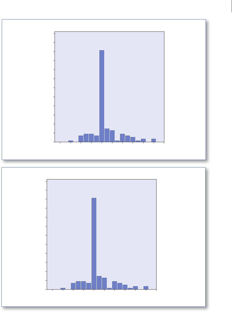
the lower mean. Such is rarely the case. Graphing the distribution of each group on the variable in
question often reveals substantial overlap.
The gender difference in hours worked per week by employed 1980 GSS young adults was
statistically significant, with males having a higher average. Because the difference was statisti-
cally significant, it is unlikely to have occurred simply by chance. We can be quite sure that the
means for the male population and the female population from which these samples came truly
did differ. But how did this difference come about? Did almost all employed 1980 young adult
males work more hours than almost all employed young adult females? That is hardly the case,
as Figure 13.9 shows.
There is considerable overlap in the hours worked by the two groups. For both, 40 was by far
the most commonly reported number of hours worked. Many women worked as many or more
hours as many men, and many men worked less than many women. Even so, women were a little
more likely to work shorter hours and men were a little more likely to work longer hours, and those
differences were enough to make the mean difference statistically significant. And that difference
in means may, in fact, be important.
The point of this section is not to dismiss differences in means but to also encourage you to
examine patterns of dispersion. Be careful (or better, be curious) when you hear about significant
gender, race, region, age, or whatever differences. You are probably being told about differences in
means. That is valuable information but, to get a fuller picture, also inquire about dispersion.
CONCEPT CHECK
Without looking back, can you answer the following questions:
• When does a researcher risk making a Type I error?
• Does statistical significance indicate substantive importance?
• Can two frequency distributions substantially overlap if their means are significantly
different?
If not, go back and review before reading on.
333Chapter 13 :: Paired- and Independent-Samples t Tests
0
0102030405060708090 100
5
10
15
20
25
30
35
40
45
50
55
60
Frequency Percent
Number of Hours Worked Last Week
Respondent’s Sex: male
0
0102030405060708090 100
5
10
15
20
25
30
35
40
45
50
55
60
Frequency Percent
Number of Hours Worked Last Week
Respondent’s Sex: male
Figure 13.9 Separate Male and Female Histograms for HOURS Worked by 1980 GSS Young Adults

334 PART III :: INFERENTIAL STATISTICS
1980 GSS Young Adults
The chapter began with some questions about 1980 GSS young adults. On the basis of our analyses,
what do we now know?
• 1980 GSS young adults were significantly more willing to let controversial persons give pub-
lic speeches than to let them teach in college (t = 6.913, df = 292, p = .000). Their average
tolerance for controversial persons giving public speeches was 3.58 on an index that could
range from 0 to 5, while their average tolerance for controversial persons teaching college
was just 2.97 on an index that also ranged from 0 to 5.
• The fathers of 1980 GSS young adults were not significantly better educated than the moth-
ers of 1980 GSS young adults (t = 0.141, df = 245, p = .444). In our samples, fathers averaged
11.54 years of schooling, and mothers averaged 11.52 years; this difference was too small to
reject the possibility that in the full population of 1980 young adults, their fathers averaged
the same or even less schooling than their mothers.
• Among employed 1980 GSS young adults, males worked significantly more hours per week
than females (t = 2.057, df = 224, p = .0205). In our samples, men worked an average of 43.66
hours per week, and women worked an average of 39.76 hours.
• The difference in hours worked per week between employed 1980 GSS young adults and
employed 1980 GSS middle-age adults was not statistically significant (t = 1.216, df = 367,
p = .225). Although employed 1980 GSS young adults averaged 41.59 hours of work com-
pared to 39.79 hours for employed 1980 GSS middle-age adults, this difference was too
small to reject the possibility that these two populations have the same average weekly
hours worked.
Important Concepts in the Chapter
central tendency
dispersion
independent samples
Independent Samples T Test procedure
paired samples
Paired-Samples T Test procedure
statistical significance
substantive importance
Type I error
Type II error

335Chapter 13 :: Paired- and Independent-Samples t Tests
Practice Problems
1. Which type of hypothesis test (one-sample t test, paired-samples t test, or independent-samples t test)
should be used for each of the following hypotheses?
a. On average, wives have more education than their husbands.
b. The average education of wives is 13.4 years.
c. The average age at first marriage for women is less than 25 years.
d. The average age at first marriage for women is less than the average age at first marriage for men.
e. On average, grooms are older than their brides.
f. The average age at first marriage of persons marrying for the first time in the 1970s was younger than
the average age at first marriage of persons marrying for the first time in the 2000s.
2. If you have 1,500 cases, how many degrees of freedom will your paired-samples t test have?
3. An author reports the following results of a paired-samples t test: t = 2.12, df = 76, p = .041.
a. How many standard errors from the middle of the hypothesized sampling distribution was the sample
result?
b. How many valid cases did the researcher have?
c. Did the author reject or not reject the null hypothesis?
d. Were the results statistically significant?
4. An author reports the following results of an independent-samples t test: t = −0.83, df = 215, p = .444.
a. How many standard errors from the middle of the hypothesized sampling distribution was the sample
result?
b. Did the author reject or not reject the null hypothesis?
c. Were the results statistically significant?
5. You are doing an independent-samples t test. Do you use the “equal variances assumed” or the “equal
variances not assumed” set of results for the independent samples t test if Levene’s test for equality of
variances
a. has a significance level of .05 or less?
b. has a significance level greater than .05?
6. Define each of the following:
a. Type I error
b. Type II error
7. “Significance level” is the same as the risk of making which type of error if you reject the null hypothesis?

336 PART III :: INFERENTIAL STATISTICS
8. What is the largest risk social scientists will usually take of making a Type I error?
9. Answer each of the following with an explanation:
a. If results are statistically significant, does that mean they are substantively important?
b.
If results are not statistically significant, does that mean they are not substantively important?
10.
If the mean for men on aggressiveness is significantly higher than the mean for women on aggressiveness,
can we assume that most men are more aggressive than most women? Explain your answer.
Problems Requiring SPSS and the
fourGroups.sav
Data Set
For each of the remaining problems, answer the following set of questions:
a.
State and label the research and the null hypothesis. Is this a one-tailed or two-tailed hypothesis test?
b.
What are the sample results? Are they consistent with the null hypothesis or with the research
hypothesis?
c.
What is the probability of getting the observed sample results if the null hypothesis is true? (If this step
is skipped, state that.)
d.
Do you reject or not reject the null hypothesis? Are your results statistically significant?
e.
Summarize in a few well-written sentences totaling 100 words or less what you found out.
11.
(2010 GSS young adults) Were 2010 GSS twentysomethings significantly more willing to let controversial
persons give public speeches than to let them teach in college? (Variables: OKSPEECH, OKTEACH; Select
Cases: GROUP = 3)
12.
(2010 GSS middle-age adults) Was there a significant difference in the willingness of 2010 GSS
fiftysomethings to let controversial persons give public speeches and in their willingness to leave the
books of controversial persons in libraries? (Variables: OKBOOK, OKSPEECH; Select Cases: GROUP = 4)
13.
(1980 middle-age adults) Test the hypothesis that the average years of schooling of the fathers and mothers
of the 1980 fiftysomethings were the same. (Variables: PAEDUC, MAEDUC; Select Cases: GROUP = 2)
14.
(2010 young adults) Test the hypothesis that the average years of schooling of the fathers and mothers of
2010 twentysomethings were the same. (Variables: PAEDUC, MAEDUC; Select Cases: GROUP = 3)
15.
(2010 GSS young adults) Was there a significant difference in the prestige of the occupations held by 2010
GSS young men and women? (Variables: SEI, SEX; Select Cases: GROUP = 3)
16.
(2010 GSS middle-age adults) Was there a significant difference in the prestige of the occupations held by
2010 GSS middle-age men and women? (Variables: SEI, SEX; Select Cases: GROUP = 4)
17.
(2010 GSS young adults and 2010 GSS middle-age adults) Was there a significant difference in the prestige
of the occupations held by 2010 GSS twentysomethings and fiftysomethings? (Variables: SEI, GROUP;
Select Cases: all cases)

337Chapter 13 :: Paired- and Independent-Samples t Tests
18. (1980 GSS middle-age adults and 2010 GSS middle-age adults) Did 2010 GSS fiftysomethings
have significantly fewer children than 1980 GSS fiftysomethings? (Variables: CHILDREN,
GROUP; Select Cases: all cases)
19.
(2010 young adults) Test the hypothesis that the average years of schooling of the 2010
twentysomethings and the average years of schooling of their spouses were identical.
(Variables: EDUC, SPEDUC; Select Cases: GROUP = 3)
20.
(2010 middle-age adults) Test the hypothesis that there was a difference in the average years of
schooling of 2010 fiftysomethings who were liberal and those who were conservative.
(Variables: EDUC, POLVIEWS; Select Cases: GROUP = 4)

338 ANSWERING QUESTIONS WITH STATISTICS
Questions and Tools for Answering Them
(Chapter 14)
Univariate Descriptive Univariate Inferential
Data Management
Multivariate Descriptive Multivariate Inferential
Questions:
• Is there a significant difference in the means of these
groups? If so, between which groups?
• Do these two variables significantly interact in their effect
on that variable?
• If they don’t significantly interact, do they have
significant individual net effects?
Statistics:
• F ratio
• degrees of freedom
• significance level
• post hoc multiple comparisons
SPSS Procedures:
• One-Way ANOVA
• Univariate General Linear Model
