Palette-based Photo Recoloring

Huiwen Chang

Ohad Fried

Yiming Liu

Stephen DiVerdi

Adam Finkelstein

Princeton University

Google

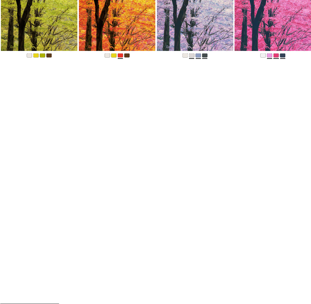
Figure 1: Palette-based photo recoloring. From left: original (computed palette below); user changes green palette entry to red (underlined),

and the system recolors photo to match; user changes multiple colors to make two other styles. Photo courtesy of the MIT-Adobe FiveK Dataset [2011].

Abstract

Image editing applications offer a wide array of tools for color

manipulation. Some of these tools are easy to understand but offer a

limited range of expressiveness. Other more powerful tools are time

consuming for experts and inscrutable to novices. Researchers have

described a variety of more sophisticated methods but these are

typically not interactive, which is crucial for creative exploration.

This paper introduces a simple, intuitive and interactive tool that

allows non-experts to recolor an image by editing a color palette.

This system is comprised of several components: a GUI that is easy

to learn and understand, an efﬁcient algorithm for creating a color

palette from an image, and a novel color transfer algorithm that

recolors the image based on a user-modiﬁed palette. We evaluate

our approach via a user study, showing that it is faster and easier

to use than two alternatives, and allows untrained users to achieve

results comparable to those of experts using professional software.

CR Categories: I.3.4 [Computer Graphics]: Graphics Utilities

Keywords: photo recoloring, color transformation, palette

1 Introduction

Research and commercial software offer a myriad of tools for

manipulating the colors in photographs. Unfortunately these tools

remain largely inscrutable to non-experts. Many features like the

“levels tool” in software like Photoshop and iPhoto require the user

to interpret histograms and to have a good mental model of how

color spaces like RGB work, so non-experts have weak intuition

about their behavior. There is a natural tradeoff between ease of

use and range of expressiveness, so for example a simple hue slider,

while easier to understand and manipulate than the levels tool,

offers substantially less control over the resulting image. This paper

introduces a tool that is easy for novices to learn while offering a

broad expressive range.

Methods like that of Reinhard et al. [2001] and Yoo et al. [2013]

allow a user to specify complex image modiﬁcations by simply

providing an example; however an example of the kind of change

the user would like to make is often unavailable. The method of

Liu et al. [2014] allows users to modify the global statistics of an

image by simply typing a text query like “vintage” or “new york.”

However, for many desired color modiﬁcations it is hard to predict

what text query would yield the desired effect. Another challenge

in color manipulation is to selectively apply modiﬁcations – either

locally within the image (e.g., this hat) or locally in color space

(e.g., this range of blue colors) instead of globally. Selection is

particularly challenging for non-experts, and a binary selection

mask often leads to visual artifacts at the selection boundaries.

Our approach speciﬁes both the colors to be manipulated and the

modiﬁcations to these colors via a color palette – a small set of

colors that digest the full range of colors in the image. Given an

image, we generate a suitable palette. The user can then modify the

image by modifying the colors in the palette (Figure 1). The image

is changed globally such that the chosen colors are interpolated

exactly with a smooth falloff in color space expressed through

radial basis functions. These operations are performed in LAB

color space to provide perceptual uniformity in the falloff. The

naive application of this paradigm would in general lead to several

kinds of artifacts. First, some pixels could go out of gamut.

Simply clamping to the gamut can cause a color gradient to be

lost. Therefore we formulate the radial falloff in color space

so as to squeeze colors towards the gamut boundary. Second,

many natural palette modiﬁcations would give rise to unpleasant

visual artifacts wherein the relative brightness of different pixels is

inverted. Thus, our color transfer function is tightly coupled with

a subtle GUI affordance that together ensure monotonicity in the

resulting changes in luminance.

This kind of color editing interface offers the best creative freedom

when the user has interactive feedback while they explore various

options. Therefore we show that our algorithm can easily be accel-

erated by a table-based approach that allows it to run at interactive

frame rates, even when implemented in javascript running in a web

browser. It is even fast enough to recolor video in the browser as it

is being streamed over the network.

We perform a study showing that with our tool untrained users can

produce similar results to those of expert Photoshop users. Finally,

we show that our palette-based color transfer framework also sup-

ports other interfaces including a stroke-based interface, localized

editing via a selection mask, fully-automatic palette improvement,

and editing a collection of images simultaneously.

2 Related work

Color Transfer (Example based Recoloring) Researchers have

proposed many recoloring methods requiring an example image

as input Reinhard et al. [2001] exploit the Lab color space and

apply a statistical transformation to map colors from another image.

When the reference is dissimilar, users need to manually point

out the region correspondence by swatches. Tai et al. [2005]

modify a Gaussian mixture model by adding spatial smoothness

and do parametric matching between source and reference images.

Chang et al. [2005] classify pixels into basic color categories

(experimentally derived), then match input pixels to reference

pixels within the same category. HaCohen et al. [2011] utilize dense

correspondences between images to enhance a collection. Their

results are compelling but the dependence on compatibility between

images is high. Yoo et al. [2013] ﬁnd local region correspondences

between two images by exploiting their dominant colors in order

to apply a statistical transfer. It is important to note that all these

methods require a reference image as input, which needs to be

provided by the user or produced by another algorithm.

Automatic Color Enhancement Bychkovsky et al. [2011] build a

large retouching dataset collected from professional photographers

to learn an automatic model for tone adjustment in the luminance

channel. Cohen-Or et al. [2006] propose to automatically enhance

image colors according to harmonization rules. However, the

user can only control the hue template type and rotation, which

is not ﬂexible enough for our needs. Hou and Zhang [2007]

provide several concepts for users to change the mood of an

image. The concepts are extracted by clustering hue histograms for

different topics. They only provide 8 concepts, which limits their

transformation and editing styles. More ﬂexibly, Wang et al. [2013]

and Csurka et al. [2010] use a semantic word to describe a desired

editing style or emotions. The semantic word is automatically

quantiﬁed by a color palette, however, people cannot set the target

palette directly. Shapira et al. [2009] enable users to explore editing

alternatives interactively using a Gaussian mixture models (GMM).

In Section 4 we compare against a GMM based algorithm.

Edit Propagation (Stroke Based Recoloring) Stroke-based meth-

ods [Levin et al. 2004; Qu et al. 2006; An and Pellacini 2008; Li

et al. 2008; Li and Chen 2009; Li et al. 2010] propose to recolor

images by drawing scribbles in a desired color on different re-

gions, automatically propagating these edits to similar pixels. Levin

et al. [2004] allow UV changes (in YUV). Qu et al. [2006] are

speciﬁc for manga recoloring. An and Pellacini [2008] propose to

approximate the all-pairs afﬁnity matrix for propagation, and Xu

et al. [2009] further accelerate it by using adaptive clustering based

on k-d trees. Chen et al. [2014] propose sparsity-based edit propa-

gation by computing only on a set of sparse, representative samples

instead of the whole image or video. This accelerates and saves

memory, especially for high-resolution inputs; we compare against

this approach in Section 4. Section 5.5 describes our uniﬁed frame-

work that uses both stroke-based and palette-based interactions.

Palette based Recoloring A recent work [Lin et al. 2013] proposes

a method for coloring vector art by palettes based on a probabilistic

model. They learn and predict the distribution of properties such

as saturation, lightness and contrast for individual regions and

adjacent regions, and use the predicted distributions and color

compatibility model by [O’Donovan et al. 2011] to score pattern

colorings. Wang et al. [2010] adapt the edit propagation method in

An and Pellacini [2008] to obtain a soft image segmentation and

recolor an image. While our method works for a pair of initial and

ﬁnal values for each palette entry, they only have the ﬁnal palette

colors. Thus the bulk of their method addresses how to associate

pixels in the image with the ﬁnal palette colors (which can be ill-

posed, and also leads to a complex and slow method).

Figure 2: Our GUI shows a representative color palette. The user

adjusts a selected palette color via an HSL controller, and the image

updates interactively. Photo courtesy of the MIT-Adobe FiveK Dataset [2011].

3 Approach

This section introduces a new, simple approach for palette-based

photo recoloring. Section 3.1 describes our user interface, as mo-

tivated by a set of explicit goals that support non-expert as well as

expert users. Second, Section 3.2 introduces a clustering approach

based on k-means suitable for creating an initial palette from a

photo. Section 3.3 describes the goals that motivate our color trans-

fer algorithm, which is introduced in the subsequent two sections.

Section 3.4 describes our approach for preserving monotonicity in

luminance, while Section 3.5 introduces our color transfer algo-

rithm. Finally, Section 3.6 shows a table-based acceleration that

allows the algorithm to run at interactive rates.

3.1 User interface

These criteria are important for a color manipulation user interface:

Simple. The GUI should be simple enough to learn and use, even

for non-expert users. For example it should not require a deep

understanding of color theory or various color spaces.

Expressive. The GUI should offer sufﬁcient degrees of freedom

that it is possible to achieve what the user wants.

Intuitive. Assuming there exist some settings that achieve what the

user wants (previous goal), the user should be able to ﬁnd them

quickly and easily.

Responsive. The GUI should produce results at interactive frame

rates so as to facilitate creative freedom in exploration and

experimentation.

While there are many existing tools that allow users to recolor

images, to our knowledge none of them simultaneously achieve

these goals (especially when coupled with the algorithmic goals

described in Section 3.3). Sliders like those in Photoshop that adjust

hue, saturation, and lightness (or similarly in iPhoto exposure,

contrast, saturation, temperature and tint) while they are simple,

responsive, and (to a lesser extent) intuitive, they are not sufﬁciently

expressive to achieve many of the effects shown in this paper. On

the other hand, histogram adjustment methods like the levels tool

in Photoshop provide huge expressive range at responsive rates, but

are neither simple nor intuitive. Methods that match the statistics of

a reference image (e.g. [Yoo et al. 2013; Liu et al. 2014]) address

all four goals above, but succeeds for expressiveness only when the

user already has an example of what they want.

We describe a palette-based GUI, shown in Figure 2. When a photo

is loaded into the application, a palette is automatically generated

(Section 3.2). The user needs only to click on a palette color (C)

and change it (to C

) via a HSL color picker. As the user inter-

actively adjusts C

in the color picker, the overall color statistics

of the photo are smoothly adjusted such that pixels colored C in

the original photo become C

. Our interface meets all four crite-

ria above. Section 4 shows that novice users are able to learn the

interface in a few minutes and then quickly produce edited images

that are qualitatively (and numerically) similar to those produced

by experts in Photoshop. This paper is not the ﬁrst to describe this

kind of palette-based recoloring. However, some existing palette

based approaches are not sufﬁciently responsive while others are

less expressive than ours, as discussed in Section 4.1.

3.2 Automatic Palette Selection

This section describes our automatic approach for creating a palette

based on an image, using a variant of the k-means algorithm. Our

goal is to select a set of k colors {C

} that distill the main color

groups in the image, to be used as “controls” during editing. The

choice of k matters, and often depends on the image as well as the

user’s desired modiﬁcations. If k is too small, then some colors

to be changed might not be well-represented among {C

}. On

the other hand if k is too large, the user may have to change a

large subset of {C

} to get a desired change. There are automatic

methods for choosing k (e.g., [Pelleg and Moore 2000]), but in

our application this choice depends heavily on the user’s intentions.

Thus we leave the choice of k up to the user. We ﬁnd that k ∈ [3, 7]

works well for typical operations, and use k = 5 by default.

The literature describes a number of methods for creating a palette

from an image. Based on a large dataset of user-rated “color

themes,” O’Donovan et al. [2011] build a measure of the compati-

bility of a set of colors as well as a method for extracting a theme

from an image. Because the dataset they use is targeted at graphic

design applications, we ﬁnd the method tends not to produce high-

quality palettes for natural photographs. Lin et al. [2013] describe a

method for creating color themes that works well for natural photos,

built on a study of how people do so. The study assumes a palette of

exactly ﬁve colors and thus their model intrinsically uses k = 5, as

does that of O’Donovan et al. [2011]. However, as discussed above,

we ﬁnd that for many editing goals a different k works better. While

the k = 5 assumption is not a fundamental limitation of these previ-

ous approaches, they rely on large datasets that do assume k = 5 so

to change k would require new datasets. Moreover, their methods

are slow to compute the palette. Therefore we propose a simpler

approach that produces comparably good palettes (at least for our

application), but works for any choice of k. Shapira et al. [2009]

describe a method for clustering image pixels based on a Gaussian

mixture model (GMM). The straightforward application of GMM

is too slow for interactive use with moderately large images. While

acceleration options are available for GMM, we describe a variant

of k-means that is already faster than GMM (by a factor of about

three for megapixel images, but still too slow in typical cases) and

then further improve its performance. In Section 4 we compare our

method to the GMM-based approach.

In a naive application of k-means to the colors in an image, each

iteration of the algorithm touches each pixel in the image, which

is costly for large images. Researchers have identiﬁed various

opportunities to accelerate k-means, for example by organizing the

data in K-D trees [Kanungo et al. 2002]. Exploiting the property

that our data are colors restricted to R, G, B ∈ [0, 1], we assign

them to bins in a b × b × b histogram (we use b = 16 in RGB).

For each bin we compute the mean color in Lab space, and these

colors c

(or less because some bins may be empty) are the

data we use for k-means – typically at least a couple orders of

magnitude smaller than the number of pixels in the image, and

now independent of image size. Because each data point c

now

(D)

(L)

Figure 3: Automatic palette methods: (D) O’Donovan et al. [2011]

build on a color theme dataset targeted at graphic design, which

is not ideal for natural photos. (L) Lin et al. [2013] acquire and

build on a dataset for natural imagery. Both of these methods take

more than one minute, and also assume a palette of size k = 5 (so

are omitted from the third column). (G) Gaussian mixture models

(GMMs) used by Shapira et al. [2009] are also slow to compute

(10 sec). (K) K-means is faster (2 sec) but is non-deterministic and

often yields too many dark colors. (O) Our method takes 60ms.

Photos courtesy of the MIT-Adobe FiveK Dataset [2011].

represents the n

pixels associated with that bin, we use a weighted

mean (weighted by n

) when ﬁnding each of the k means in

each iteration. The weighted k-means approach has been used in

other applications, for example the automatic stippling method of

Secord [2002].

For generating color palettes for our GUI, k-means suffers from

two related problems: the basic formulation uses randomly selected

data points to initialize the means, and the convergence of the

algorithm can be sensitive to this initialization (as discussed by

Pelleg and Moore [2000]). To present the most helpful GUI to the

user, we prefer that the algorithm be deterministic, and that palette

colors be far from one another. Thus, instead of randomizing, we

initialize the means as follows. We initialize the ﬁrst “mean” as

the color c

representing the bin with the largest weight n

. Next

we attenuate all other weights n

by a factor (1 − exp(−d

/σ

))

where d

is the distance in Lab space from c

to c

and σ

expresses a falloff (we use σ

= 80 which is 80% of the distance

from black to white, and have found the algorithm to be relatively

insensitive to this parameter). Next we choose bin with the highest

remaining weight n

, repeating until k initial “means” have been

chosen. This approach is deterministic and initializes the k-means

with large clusters that are far from each other.

Finally, we have observed that choosing a palette based on pixel

color clustering often leads to a very dark (near black) palette entry,

because typically a signiﬁcant number of image pixels are dark.

However, editing the dark palette entry is rarely fruitful for the

user, because dark colors are hard to distinguish (regardless of hue

and saturation). Essentially it offers the user a set of controls with

little or no effect. Therefore we discourage very dark palette entries

as follows. Rather than computing k-means, we actually compute

(k + 1)-means, where one of them is initialized and perpetually

locked to black. The darkest colors in the image will be assigned

to this mean, and will therefore not pull the other nearby means

towards black. After computing the (k + 1)-means, we discard the

black entry to leave k remaining palette colors. For a comparison of

our approach with the previously described methods, see Figure 3.

Original Result 1 Result 2 Result 3

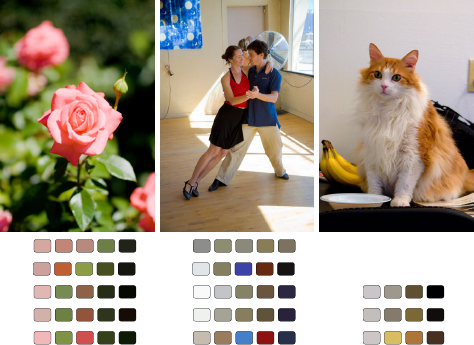
Figure 4: More recoloring examples. Originals on left, followed by various edits with our system including both local changes (e.g. make

the girl’s shirt turquoise) and global changes (e.g. change the image tone to orange). Photos courtesy of the MIT-Adobe FiveK Dataset [2011].

We ﬁnd that this algorithm produces useful palettes, and all of the

results shown in this paper and accompanying materials (including

the study described in Section 4) use this approach, except for

Figures 8 and 12 which require other methods. However, our GUI

also allows the user to select some or all of the palette entries

explicitly by a color picker or by clicking on the image. Any

remaining unspeciﬁed palette entries are then automatically chosen

via the algorithm described above.

3.3 Color Transfer Goals

Now we have a set of palette colors {C

}, and our GUI allows the

user to modify the palette colors to {C

} as a way of adjusting the

colors in the image. That is, the association ({C

}, {C

}) deﬁnes a

transfer function f that maps colors in the original image to colors

in the edited image. We assume that f acts on colors independently

of pixel location or context in the image. Some color mapping

approaches relax this assumption, for example the high-quality high

dynamic range compression approach of Fattal et al. [2002] which

operates in the gradient domain. Nevertheless, for our application

the assumption is reasonable and permits the acceleration method

described in Section 3.6.

Here we identify some key properties we would like in f that

address the GUI criteria described at the beginning of Section 3.1,

particularly the “expressive” and “intuitive” qualities:

Interpolation. Any pixel in the original image with the same color

as one of the original palette colors C

should be transformed

exactly as the user changed the palette color: f(C

) = C

In Gamut. The output should remain in gamut G : f(p ∈ G) ∈ G.

Pixel Continuity. The transfer function should be continuous with

respect to pixel color p: lim

q→p

f(q) = f(p).

Palette Continuity. The function should be continuous with re-

spect to changes in the palette: lim

C→C

(p) = f

(p).

One-to-One. The function should be one-to-one. Together with

the continuity requirement this prevents the function from fold-

ing over itself, which could lead to counter-intuitive behaviors.

Formally: f(p) = f (q) =⇒ p = q.

Monotonicity in L. The transformation in the luminance L should

be monotonic. In our early prototype applications we found

that transformation functions that allowed relative brightness of

different pixels to ﬂip often led to undesirable imagery. Thus

we require: L(p) < L(q) =⇒ L(f (p)) <= L(f(q)).

Dynamic Range A gradient in the input maps to a gradient in the

output (not a single value). For example an algorithm that shifts

all colors in some direction uniformly and then clamps to the

gamut is bad by this criterion.

The literature describes a variety of transformation models that

might be used for this application, for example Gaussian mixture

models (GMM) [McLachlan and Peel 2004], histogram methods

[Liu et al. 2014], or non-parametric approaches [HaCohen et al.

2013]. However, to our knowledge no existing approaches can be

easily adapted to meet the requirements listed above. For example,

GMM-based editing can easily send colors out of gamut. Of course

it is easy to clamp to the gamut boundary but this would violate the

one-to-one and dynamic range qualities.

(far case)

x’

C’

(near case)

x’

C’

(a) Lab slices (b) edit one color (c) RBF blending

Figure 5: Transfer in AB space: (a) constant-L slices of Lab space;

(b) when a single palette color C is changed to C

the resulting

editing effect at different locations x; (c) how the effects of changing

multiple palette colors C

are blended at location x using RBFs.

To make matters worse, the requirements themselves are inconsis-

tent. For example, it is not possible to simultaneously satisfy the in-

terpolation and monotonicity requirements. If the user changes the

relative brightness of two palette colors, interpolating those colors

in the resulting image would violate the monotonicity requirement.

However, we would like to satisfy these requirements insofar as

is possible, and the following section directly addresses the mono-

tonicity concern.

3.4 Monotonic Luminance Transfer

Our application preserves monotonicity in luminance via two mech-

anisms, one in the GUI and one in the transfer function.

First, the GUI constrains the relative ordering of luminance L

the edited palette colors C

. That is, suppose that L

i<j

< L

the input palette. Then the GUI constrains L

i<j

< L

in the edited

palette, as follows. Whenever the user modiﬁes C

, the GUI also

sets L

j>i

= max(

, L

j−1

), where

is the most recently user-

edited value for palette entry j (or the initial value, if never edited).

To change the luminance of a palette entry we simply modify the

L channel in Lab space. This operation is evaluated in increasing

order for all palette entries j > i; and the symmetric operation

(involving min and L

j+1

) is applied in decreasing order for entries

where j < i. This policy has the nice property that if the user

brightens L

in such a way that L

j>i

is also brightened, but then

the user reverts L

back to the original value, then L

also reverts

(avoiding hysteresis).

The second aspect of our treatment of luminance is that we design a

transfer function that has two orthogonal components – f

(which

modiﬁes pixel luminance based on the palette luminance) and f

(which modiﬁes the corresponding ab values, and is discussed in

the next section). The luminance transfer function simply takes

a weighted combination of the two nearest palette entries (or one

nearest entry and either black or white if the pixel is darker or

brighter than all the palette entries).

With regard to luminance, these two strategies together ensure that

both the interpolation and monotonicity requirements are satisﬁed

as well as some others – in-gamut and the two continuity require-

ments. However, this approach can violate the one-to-one and dy-

namic range requirements, because a range of shades of gray can be

collapsed into a single luminance value when one or more palette

colors are pushed to the same luminance. However, we have found

through experimentation that these concerns are less critical than

interpolation and monotonicity. While it might be possible to sat-

isfy all four requirements by disallowing changes in luminance in

the GUI, we ﬁnd this is an important feature for expressive control.

input naive transfer our transfer

Figure 6: A naive transfer function that copies the color offset from

the palette to every color in the image, even if clamped to remain in

gamut, reduces dynamic range in the image (middle). Our transfer

function (right) is able to make better use of the dynamic range.

Photo courtesy of the MIT-Adobe FiveK Dataset [2011].

3.5 Color Transfer (ab)

In the last section we devised a simple luminance transfer function

that adjusts the luminances of pixels based on those of the

palette. In this section we introduce a more complex transfer

function f

that plays an analogous role in the ab channels. The

design of this function is not guided by the monotonicity concern,

but it does target the other requirements.

First we devise the function f

for the simple case where the

original palette contains a single color C, and the user modiﬁes

it to be color C

(Figure 5b). For any color x we would like

to know x

= f

(x). In general we want to translate colors in

the same direction, and a naive strategy might simply add exactly

the same offset vector (C

− C) to every x. However, it would

be easy to go out of gamut, and simply clamping to the nearest

in-gamut value would violate the one-to-one and dynamic range

goals, as illustrated in Figure 6. Instead we devise a scheme that

translates colors that are far away from the boundary of the gamut,

but squeezes values nearer to the boundary towards the boundary

and towards the C

as follows. First we ﬁnd C

, the point where

the ray from C towards C

intersects the gamut boundary. Next, we

determine if x

= x + C

− C is in gamut. If so (the “far” case)

we ﬁnd x

the location where the parallel ray from x intersects

the gamut boundary. If not (the “near” case) we take x

to be the

point where the ray from C

towards x

intersects the boundary.

These intersections are found by binary search. Finally, we take

(x) = x

, the point on the ray from x to x

such that:

||x

− x||

||C

− C||

= min(1,

||x

− x||

||C

− C||

)

In the far case this policy squeezes f

(x) toward the boundary

in proportion to C

− C with a maximum ratio of 1, meaning

very far from the boundary we just translate colors parallel to the

palette change. Very close to the boundary, the offset vectors swivel

towards C

, which we found by experimentation helps to achieve a

desired palette change in those areas. Also note that this transfer

function enjoys several of the desired properties descried above.

Assuming C and C

are in gamut, so is f

(x). It interpolates:

. If the gamut were convex, then it would one-to-one

and continuous with respect to x and C

. Of course the gamut is

only close to convex, so these properties are almost satisﬁed. While

it is possible to devise cases where they are violated, we ﬁnd in

practice that it does not happen when performing reasonable color

palette edits.

Now that we have f

(x) we will generalize it to handle the case

of larger palettes containing k > 1 entries. Our strategy is to

deﬁne k transfer functions f

(x), each equivalent to the f

(x) map

described above as if it were the only palette entry, and then blend

them, weighted by proximity:

f(x) =

(x)f

(x) and

(x) = 1

For the weights we use radial basis functions (RBFs):

(x) =

φ(||x − C

||)

We tried various kernel functions and found that the Gaussian

kernel works well in our application:

φ(r) = exp(−r

/2σ

)

where the scalar parameter σ

is chosen to be the mean distance

between all pairs of colors in the original palette. The k

unknown

coefﬁcients λ

are found by solving a system of k

equations:

k of which require w

) = 1 and k

− k of which require

j6=i

) = 0.

This approach leads to smooth interpolation of the individual

transfer functions f

at C

. Unfortunately solving the system of

equations set up by the RBFs can lead to negative weights, with two

potential hazards. First, it will add some component of the opposite

behavior of some palette changes. Second, and more dangerously,

it can throw the result out of gamut. We therefore use a simple

ﬁx – we clamp any negative weights to zero and renormalize the

non-zero weights. We ﬁnd in practice this solution works well. The

ﬁnal weighted combination is illustrated in Figure 5c for a palette

size of k = 3.

3.6 Acceleration

The RBF interpolation scheme described in Section 3.5 is relatively

fast, but its naive application to the image would require making

this computation for every unique color in the image (often in the

millions). This section describes an acceleration scheme that allows

it to be usable in an interactive application. First, note that the

weights w

(x) are found based only on the color x and the initial

palette colors C

. Therefore, in principle the RBF computations

need only be performed when the initial palette is established (not

during color palette editing). We further accelerate the computation

by caching these weights w

only at a g × g × g grid of locations

g=4, t = 3ms, d = 5.3 g=12, t = 39ms, d = 1.0 g=64, t = 5615ms, d = 0

Grid size

Time (seconds)

0 1 2 3 4 5 6

Transformation (grid)

Interpolation (pixels)

Figure 7: Acceleration. Top: results of varying grid size g. Time

t is to update the grid values (averaged). d is CIEDE distance

from the g = 64 version. Small grid sizes give visual differences,

whereas g = 12 is indistinguishable from g = 64 (but roughly 140

times faster). Bottom: Update time vs. grid size. The time to update

the pixels of the image remains near constant (brown, about 50ms

for a 1 MP image). Photo courtesy of the MIT-Adobe FiveK Dataset [2011].

Original Theirs Ours

Figure 8: Comparison to the methods of (top to bottom)

Chen et al. [2014], Shapira et al. [2009], and Wang et al. [2010].

Left to right: original photo, their result, our result. We used

the same initial and ﬁnal palettes as in their paper, except for

Wang et al., who do not use an initial palette.

uniformly sampled in the RGB cube. Next, during color editing

when the C

are known, we can compute the output color f(x)

at these g

locations using the precomputed weights. Finally, to

recolor each pixel in the image use trilinear interpolation on eight

nearest grid values. This strategy not only gives our implementation

interactive performance (in javascript running in a web browser),

but also ameliorates any small discontinuities in f(x) due to the

non-convex gamut.

Figure 7 demonstrates the performance advantage. We see that

using larger grid sizes g has a diminishing return in image quality

such that g = 12 is almost indistinguishable from g = 64, while

running about 140 times faster. Without acceleration, our runtime

is T p where T is the time to transform one color and p is the

number of pixels. With acceleration, runtime is T g

+ Ip where

I is the time to perform trilinear interpolation of grid samples, and

I  T . Throughout this paper and in our demo we use g = 12,

because it performs well across a range of computers and images,

so g

 p. Moreover, while in principle for very large images

p could grow to overwhelm the runtime, in practice p is limited

by how many pixels we could reasonably “preview” on the screen.

Finally we note that splitting the calculation to a pre-processing step

followed by sampling and interpolation steps lends itself well to

shader programming. While we did not test this idea, implementing

the interpolation as an OpenGL shader would be trivial, and should

achieve substantially faster performance, even for huge images or

dense grids.

4 Evaluation

In this section we evaluate our method in two ways. Section 4.1

directly compares our approach to some existing methods in the

literature. Section 4.2 presents a user study in which we ask novice

users to use our method, using two alternate methods as a baseline.

4.1 Other Recoloring Methods

Figure 8 shows a comparison to three other palette based recoloring

methods, and in each case we believe our method responds more

faithfully to the speciﬁed palette. The method of Chen et al. [2014]

Original Target Hue-blend GMM Ours

3.240 (66s, 73s) 4.935 (40s, 77s) 2.707 (4s, 30s)

1.281 (47s, 76s) 1.259 (6s, 27s) 2.588 (4s, 20s)

8.319 (75s, 81s) 8.099 (50s, 90s) 7.607 (39s, 90s)

6.340 (86s, 90s) 6.126 (49s, 63s) 3.857 (38s, 64s)

8.124 (25s, 32s) 4.678 (44s, 90s) 3.686 (68s, 90s)

Figure 9: Examples from our user study. Left to right: original, target, results of hue-blend approach, GMM approach and our method.

Under each result is the distance to target (RMS of CIEDE2000), and for each method this ﬁgure shows the best result out of all subjects

according to this distance. Times in parentheses: number of seconds in which there was some user interaction, total number of seconds until

task completion. Photos courtesy of the MIT-Adobe FiveK Dataset [2011] (top three), Chen et al. [2012] (fourth), Wang et al. [2010] (bottom).

(top) offers a fast and space efﬁcient recoloring algorithm that also

works for video. Our method is faster, e.g., at least 10× for Big

Buck Bunny. The method of Shapira et al. [2009] (middle) focuses

an interface for exploration, in the spirit of the design galleries of

Marks et al. [1997]. Wang et al. [2010] (bottom) address the harder

problem of how to map the colors when no initial palette is present,

and thus their method is more complex and slower than ours.

4.2 User Study

Evaluating a task that has a component of personal taste is al-

ways challenging. Here we describe a user study showing that our

method is easily learned by non-experts, sufﬁciently fast, expressive

enough to produce a variety of imagery. In order to judge expres-

siveness, the task we give our users is a matching task: they are

given a target image (created from the original by manipulating its

colors) and the user is asked to manipulate the original to match

the target, using our method and two others. Thus we can judge

whether our method can achieve a spectrum of desired results, and

can use the other methods as baseline comparisons.

With the goal of capturing a broad spectrum of color editing

operations, we collected 32 original-target pairs as follows. Half

(16) were selected from eight papers in the literature that perform

color manipulation [An and Pellacini 2008; Chen et al. 2014; Hou

and Zhang 2007; Liu et al. 2014; Pitie et al. 2005; Shapira et al.

2009; wing Tai et al. 2005; Wang et al. 2010]. The other half were

created by two expert Photoshop users (having the entire Photoshop

tool-set at their disposal) according to a written task description

like “Change the color of the bridge to be a richer red color.” or

“Brighten everything to make it look more like daytime.”

Ours GMM Hue Blend Photoshop

Min 3 7 17 ∼ 60

Max 90

∗

∼ 720

Median 71 69 90 ∼ 210

∗

our user study task was capped at 90 seconds per image.

Table 1: Task completion times. The table shows time (seconds) to

recolor an image, for each of the methods in our user study. Last

column is approximate time for expert Photoshop user to recolor

the same images. Note that the user study task was capped at 90

seconds, and we observe that most of the hue blend mode users did

not complete the task within that time frame. Using our full method

and GMM takes roughly the same amount of time, while hue blend

is slower and using Photoshop was the slowest.

For the study we used Amazon’s Mechanical Turk framework. In

each task (called a “HIT”), the subject was asked to edit four images

(selected randomly without repetition per worker) from among the

32 original-target pairs. They were instructed to attempt to edit the

original to match the target as best as they could within 90 seconds.

Subjects who satisﬁed earlier were able to click a button to advance

to the next image. Before beginning the task they were given a brief

set of instructions that took a few minutes to complete.

Each worker was assigned randomly to one of three different

conditions: our method, GMM, and hue-blend (described below).

Most workers did just one task for us, but any workers that did

more than one were always assigned the same condition. Our

method was the approach described in Section 3, but with a ﬁxed

ﬁve-color palette automatically selected that could not be changed.

GMM used the same GUI and instructions as our method, but the

underlying color manipulation algorithm used a Gaussian mixture

model both to select the palette and to manipulate it. Hue-blend

was similar to a hue blend layer in Photoshop. In this interface

the user “paints” hue into the image, which replaces the hue in the

image but leaves saturation and luminance unchanged. Subjects

were given a choice of three brush sizes which were either circular

or a “smart brush” that reshapes according to gradients in the image.

(Speciﬁcally, we segment the image into superpixels [Mori 2005]

and paint any superpixel intersected by the circular brush.)

Via this study we collected 1820 images, of which 592, 608 and

620 were produced respectively by our method, GMM and hue-

blend. The number of results for each target in each condition

ranged from 15 to 25. Next we compare the three methods it terms

of expressibility (were the workers able to reach the target?) and

ease of use (were they able to do so within the 90 seconds?).

Figure 9 shows a few examples: the original image, the target image

(either from related papers or created using Photoshop) and the best

results for each method, measured by CIEDE2000 distance from

the target [Luo et al. 2001]. In the ﬁgure (and in the study) our

method produced the single best performing result by this measure

more often than the other methods. Figure 10 aggregates all

distance-from-target results. The median distance for our method

is smaller than that of GMM (p < 0.001) and that of hue-blend

(p < 0.0001). Statistical signiﬁcance was found via a randomized

permutation test with Bonferroni correction. Because the hue-blend

mode did not allow subjects to adjust luminance (which is required

for some of the targets) we also calculated the same distances but

ﬁrst using histogram equalization on the luminance channel of the

result. Of course this changed all individual distances but the

relative performances of the different methods (and the p-values)

were comparable.

Table 1 shows completion times over all subjects, for each of the

three methods. It also shows the time it took an expert Photoshop

0 2 4 6 8 10 12 14 16 18

Ours

GMM

Hue-blend

Figure 10: Distance comparison across methods. For all user study

results, we calculate the CIEDE2000 distance between result image

and target. The plot shows results for the 3 methods: hue-blend,

GMM and ours (lower is better). Thick line indicates range between

25th and 75th percentiles. Dotted circle on the thick line indicates

the median, which is lower (with statistical signiﬁcance) for our

method than for GMM and hue-blend.

user to produce the corresponding 16 target images. From the table

it is clear that our GUI is the fastest (using either our algorithm or

GMM) while using a brush to paint hues is slower. The Photoshop

experts took the longest to edit images, although we note that the

other three interfaces explicitly capped the amount of time available

whereas the Photoshop experts had no time pressure.

Moreover, inspection of the pool of results leads us to believe that

these distance measures were overly kind to the other methods.

Qualitatively we observe that: (1) GMM results often contain

highlights and halos that did not seem to hugely adverse effect their

distance scores. (2) Hue-blend results often exhibit visual artifacts,

as users had difﬁculty painting accurately. When these artifacts

are small (yet noticeable) they do not adversely effect the distance

commensurate with their visual impact. (3) Some of our results that

have high distances actually look very similar to the target. The L-

monotonicity constraint described in Section 3.4 allows the user to

make subtle changes in luminance overall that induce high distance

values even though they are not visually objectionable. While

researchers have investigated other distance measures that better

capture human perception (e.g., [Wang et al. 2004]) this remains

an open research problem.

Finally we note that inasmuch as the results of our method did

not exactly match those produced by the Photoshop experts (with

the entire suite of color manipulation tools in that software and

unlimited time to work on the images), it is not obvious that one

or the other is “better.”

5 Results

Figures 1 and 4 show examples of using our method with palettes

of size 3, 4 and 5. They demonstrate both local and global changes

(and a combination of the two).

Our method supports masks, constraining the edits to speciﬁc image

regions, as can be seen in Figure 11. Using a mask is necessary only

if similarly colored objects should be edited in a different manner.

Except for Figure 11, all results in this paper do not use masks.

Figure 11: Using a mask. Left-to-right: original, mask, result.

Photo courtesy of the MIT-Adobe FiveK Dataset [2011].

The remainder of this section describes various other applications

made possible by our palette based approach.

5.1 Video Recoloring

Our method is fast enough to be applied to a video, in real time. The

interaction uses the same interface as for photos, shown in Figure 2.

An example may be seen in the accompanying video. For this

application, we need to choose a source palette for each frame. Our

implementation selects a palette from one of the frames and uses

it throughout the sequence. This approach encourages temporal

coherence, but might not be suitable for long sequences. The

selection method could be extended to a sliding window scheme,

thus making is usable for longer, more heterogeneous sequences.

5.2 Duotone

Duotone reproduction is a traditional printing technique that typi-

cally involves two colors of ink applied via halftone patterns over

white paper. This style gives an overall sense of coloration and has

a nostalgic quality (but costs less than full-color printing involv-

ing three or four inks). Digital imaging software like Photoshop

provides a duotone function to produce this effect, while allowing

the user to choose the ink color(s). Our method can easily produce

a similar effect as follows. We start with a grayscale image (or

desaturate a color image). We select a 3-color palette and force one

of the colors to be white (paper), letting the automatic algorithm of

Section 3.2 choose the other two palette colors. Finally the user can

adjust the two darker (ink) palette colors to achieve various imagery

in the style of a duotone. Figure 12 shows an example.

Figure 12: Duotone. Starting from a grayscale image, we use a

three color palette (white and two other colors) to create this effect.

Photo courtesy of the MIT-Adobe FiveK Dataset [2011].

5.3 Automatic Color Manipulation

Our methods was constructed with controllability in mind, allowing

the user to select the resulting colors manually. While we believe

that to be the most common use case, some users might prefer a

fully automatic method. There are many on-line repositories of

“good” color palettes, such as the Adobe Color CC database used

by O’Donovan et al. [2011]. We can automatically pick a top rated

palette and apply it to an image.

For this application we need to enhance our method with an

automatic way to match source and target palette colors. Using

the annotation in Section 3.2, there we know that C

, C

...C

correspond to C

, C

, ..., C

(e.g. C

corresponds to C

). This

matching is given to us via our GUI (the user selects a palette

color, then changes it) but is not available for the fully automatic

method. Thus we augment our method with a palette matching step

Figure 13: Fully automatic pipeline. As an example, we use the

top rated palette from Adobe Color CC and apply it to an image.

The input and output palettes are matched in increasing luminance

order. Left: original, right: result of applying the “sandy stone

beach ocean diver” palette. Photo courtesy of the MIT-Adobe FiveK Dataset

[2011].

that decides on the correct permutation of colors. As discussed in

Section 3.4, we found that sorting colors according the luminance

value is a good matching strategy. Figure 13 shows automatic

image recoloring result using the top Adobe Color CC palettes.

5.4 Editing an Image Collection

HaCohen et al. [2013] describe a method of consistently editing

a whole collection of photos that share content. Inspired by their

approach, we show that our system can trivially operate on a

collection of images simultaneously. We calculate a single color

palette for the entire collection, thus editing operations will change

all images in a consistent manner. Figure 14 shows an example

of an edited photo collection. Notice that all photos (combined)

were edited with less than 20 seconds of user input, and this

number is constant regardless of the number of images we are

editing. Moreover, because of the acceleration scheme described

in Section 3.6, the resulting output can be rendered at interactive

frame rates even for collections containing many millions of pixels.

Figure 14: Image collection editing. Our system can be applied

to multiple images at once. The user manipulates the joint palette

of all input images, thus achieving a consistent result across the

collection. Left: original collection. Right: result. In this example

the user changed the sky to have a sunrise effect, made the greens

more saturated and changed the water to a deeper shade. The entire

editing session took less than 20 seconds. Photos

Jingwan Lu.

5.5 Stroke-Based Interface

Finally, our palette based editing method can easily be augmented

with a stroke-based interface that relies on the same algorithms

described in Section 3. Using a mouse (or tablet or multitouch

device) the user draws a stroke over the image as a way of indicating

a “selection” in color space. This operation essentially speciﬁes a

palette and a selected palette color as follows. We take the mean

color of the pixels under the stroke to be the selected palette color to

be edited. The remainder of the palette is ﬁlled using the approach

described in Section 3.2. Next as the user changes the color of

the selected palette entry, the corresponding colors in the image are

modiﬁed using the color transfer approach in Section 3.

As observed in Section 3.1, the size of the palette governs the

locality in color space of various edits. We set the palette size:

k = max(3, 7 − b

7σ

where σ

and σ

are the standard deviations of the pixel colors

under the stroke and of the whole image. This gives a palette

size between 3 and 7, depending on whether the colors under the

stroke have high or low variance relative to those of the image.

This approach offers the user a simple control of the locality, as

illustrated in Figure 15-top. A small brush stroke in the blue of

the sky (left) yields a palette size of 7 and thus the color edits

are localized to blue colors; in contrast a large stroke that crosses

the blue sky and gray clouds gives a palette of size 3 and thus

affects a broader swath of colors in the result (right). Comparing

this interface to that of Chen et al. [2012] which requires brushes

indicating both colors to be modiﬁed (red stroke in the lower-left)

and colors to be left untouched (black stroke) we ﬁnd that we are

able to produce similar effects with only the modifying strokes

(lower-right).

Note that our current implementation uses strokes to select color

ranges, regardless of location in the image. A more sophisticated

approach might select for both color and location (in 5D rather

than 3D). However, adding these dimensions to the lookup table

described in Section 3.6 would have a performance impact.

6 Conclusion

We introduce a new method for image color editing. Our method

includes a carefully considered GUI along with a new color transfer

mechanism. We show results for recoloring, image collection

editing and video editing, and validate via a user study.

The realm of possibilities for color transfer is far from explored.

In future works we would like to tackle some of the challenges we

encountered while creating the current system. First, in the current

work we do not take pixel location into consideration, which leads

to a fast algorithm that allows interactive exploration. However,

it would be interesting to incorporate spatial information into the

algorithm. Second, one of our main goals is to create an intuitive

user interface, that behaves “as the user expects.” We believe that

this goal could be enhanced by considering a computational model

of color names, for example that of Mojsilovic [2005]. Most people

think in terms of color names (e.g. change black to red) and we

believe incorporating such notion of colors into the system (forcing

the transformation to respect color boundaries) would enhance

its intuitiveness. Lastly, while we show a completely automatic

pipeline using user-rated palettes, we believe full automation can

be extended beyond the realm of human curation, to an algorithm

that combines automatic palette selection with recoloring.

Figure 15: Stroke-based editing. Top: Different brush marks

select local (left) or global (right) color ranges for editing. Input

images with red brush marks are left of diagonals while output is

to the right with automatic palettes below. Photo courtesy of the MIT-

Adobe FiveK Dataset [2011]. Bottom: Comparing to the approach of

Chen et al. [2012] (left), our method achieves similar effects with

fewer marks (right).

7 Acknowledgments

Most of the photos in this paper are courtesy of the MIT-Adobe

FiveK Dataset [2011] which was created, described, and shared by

Bychkovsky et al. [2011], for which we are grateful. This research

was supported in part by generous gifts from Adobe and Google as

well as a Google Graduate Fellowship.

References

AN, X., AND PELLACINI, F. 2008. Appprop: All-pairs

appearance-space edit propagation. In ACM SIGGRAPH 2008

Papers, ACM, SIGGRAPH ’08, 40:1–40:9.

BYCHKOVSKY, V., PARIS, S., CHAN, E., AND DURAND, F.

2011. Learning photographic global tonal adjustment with a

database of input / output image pairs. In The Twenty-Fourth

IEEE Conference on Computer Vision and Pattern Recognition.

CHANG, Y., SAITO, S., UCHIKAWA, K., AND NAKAJIMA, M.

2005. Example-based color stylization of images. ACM Trans-

actions on Applied Perception 2, 3 (July), 322345.

CHEN, X., ZOU, D., ZHAO, Q., AND TAN, P. 2012. Manifold

preserving edit propagation. ACM Trans. Graph. 31, 6 (Nov),

132:1–132:7.

CHEN, X., ZOU, D., LI, J., CAO, X., ZHAO, Q., AND ZHANG,

H., 2014. Sparse dictionary learning for edit propagation of high-

resolution images. Computer Vision and Pattern Recognition

(CVPR), June.

COHEN-OR, D., SORKINE, O., GAL, R., LEYVAND, T., AND

XU, Y.-Q. 2006. Color harmonization. Association for

Computing Machinery, Inc.

CSURKA, G., SKAFF, S., MARCHESOTTI, L., AND SAUNDERS,

C. 2010. Learning moods and emotions from color combi-

nations. In Proceedings of the Seventh Indian Conference on

Computer Vision, Graphics and Image Processing, ACM, 298–

305.

FATTAL, R., LISCHINSKI, D., AND WERMAN, M. 2002. Gradient

domain high dynamic range compression. In ACM Transactions

on Graphics (TOG), vol. 21, ACM, 249–256.

HACOHEN, Y., SHECHTMAN, E., GOLDMAN, D. B., AND

LISCHINSKI, D., 2011. Nrdc: Non-rigid dense correspondence

with applications for image enhancement. ACM SIGGRAPH

2011 papers, Article No. 70.

HACOHEN, Y., SHECHTMAN, E., GOLDMAN, D. B., AND

LISCHINSKI, D. 2013. Optimizing color consistency in photo

collections. ACM Trans. Graph. 32, 4 (July), 38:1–38:10.

HOU, X., AND ZHANG, L. 2007. Color conceptualization. In

Proceedings of the 15th International Conference on Multime-

dia, ACM, MULTIMEDIA ’07, 265–268.

KANUNGO, T., MOUNT, D., NETANYAHU, N., PIATKO, C.,

SILVERMAN, R., AND WU, A. 2002. An efﬁcient k-means

clustering algorithm: analysis and implementation. Pattern

Analysis and Machine Intelligence, IEEE Transactions on 24, 7

(Jul), 881–892.

LEVIN, A., LISCHINSKI, D., AND WEISS, Y. 2004. Colorization

using optimization. In ACM SIGGRAPH 2004 Papers, ACM,

SIGGRAPH ’04, 689–694.

LI, C., AND CHEN, T. 2009. Aesthetic visual quality assessment

of paintings. Selected Topics in Signal Processing, IEEE Journal

of 3, 2, 236–252.

LI, Y., ADELSON, E., AND AGARWALA, A. 2008. Scribbleboost:

Adding classiﬁcation to edge-aware interpolation of local image

and video adjustments. In Computer Graphics Forum, vol. 27,

Wiley Online Library, 1255–1264.

LI, Y., JU, T., AND HU, S.-M. 2010. Instant propagation of

sparse edits on images and videos. In Computer Graphics Forum,

vol. 29, Wiley Online Library, 2049–2054.

LIN, S., AND HANRAHAN, P. 2013. Modeling how people

extract color themes from images. In Proceedings of the SIGCHI

Conference on Human Factors in Computing Systems, CHI ’13.

LIN, S., RITCHIE, D., FISHER, M., AND HANRAHAN, P. 2013.

Probabilistic color-by-numbers: Suggesting pattern colorizations

using factor graphs. vol. 32, 37:1–37:12.

LIU, Y., COHEN, M., UYTTENDAELE, M., AND RUSINKIEWICZ,

S. 2014. Autostyle: Automatic style transfer from image

collections to users images. Computer Graphics Forum 33, 4,

21–31.

LUO, M. R., CUI, G., AND RIGG, B. 2001. The development

of the CIE 2000 colour-difference formula: CIEDE2000. Color

Research & Application 26, 5, 340–350.

MARKS, J., ANDALMAN, B., BEARDSLEY, P. A., FREEMAN, W.,

GIBSON, S., HODGINS, J., KANG, T., MIRTICH, B., PFISTER,

H., RUML, W., RYALL, K., SEIMS, J., AND SHIEBER, S.

1997. Design galleries: A general approach to setting parameters

for computer graphics and animation. In Proceedings of the

24th Annual Conference on Computer Graphics and Interactive

Techniques, SIGGRAPH ’97, 389–400.

MCLACHLAN, G., AND PEEL, D. 2004. Finite mixture models.

John Wiley & Sons.

MIT-ADOBE FIVEK DATASET, 2011. http://groups.

csail.mit.edu/graphics/fivek_dataset/.

MOJSILOVIC, A. 2005. A computational model for color naming

and describing color composition of images. Image Processing,

IEEE Transactions on 14, 5, 690–699.

MORI, G. 2005. Guiding model search using segmentation. In

Computer Vision, 2005. ICCV 2005. Tenth IEEE International

Conference on, vol. 2, 1417–1423 Vol. 2.

O’DONOVAN, P., AGARWALA, A., AND HERTZMANN, A. 2011.

Color Compatibility From Large Datasets. ACM Transactions on

Graphics 30, 4.

PELLEG, D., AND MOORE, A. 2000. X-means: Extending

k-means with efﬁcient estimation of the number of clusters.

In Proceedings of the Seventeenth International Conference on

Machine Learning, Morgan Kaufmann, San Francisco, 727–734.

PITIE, F., KOKARAM, A. C., AND DAHYOT, R. 2005. N-

dimensional probability density function transfer and its appli-

cation to color transfer. In Computer Vision, 2005. ICCV 2005.

Tenth IEEE International Conference on, vol. 2, IEEE, 1434–

1439.

QU, Y., WONG, T.-T., AND HENG, P.-A. 2006. Manga

colorization. ACM Transactions on Graphics (SIGGRAPH 2006

issue) 25, 3 (July), 1214–1220.

REINHARD, E., ASHIKHMIN, M., GOOCH, B., AND SHIRLEY, P.

2001. Color transfer between images. IEEE Computer Graphics

and Applications 21, 5 (September), 3441.

SECORD, A. 2002. Weighted voronoi stippling. In Proceedings of

the 2nd international symposium on Non-photorealistic anima-

tion and rendering, ACM, 37–43.

SHAPIRA, L., SHAMIR, A., AND COHEN-OR, D. 2009. Image

appearance exploration by model-based navigation. In Computer

Graphics Forum, vol. 28, 629–638.

WANG, Z., BOVIK, A. C., SHEIKH, H. R., AND SIMONCELLI,

E. P. 2004. Image quality assessment: from error visibility to

structural similarity. Image Processing, IEEE Transactions on

13, 4, 600–612.

WANG, B., YU, Y., WONG, T.-T., CHEN, C., AND XU, Y.-Q.

2010. Data-driven image color theme enhancement. In ACM

SIGGRAPH Asia 2010 Papers, ACM, SIGGRAPH ASIA ’10,

146:1–146:10.

WANG, X., JIA, J., AND CAI, L. 2013. Affective image

adjustment with a single word. Vis. Comput. 29, 11 (Nov.), 1121–

1133.

WING TAI, Y., JIA, J., AND KEUNG TANG, C. 2005. Lo-

cal color transfer via probabilistic segmentation by expectation-

maximization. In Proc. Computer Vision and Pattern Recogni-

tion, 747–754.

XU, K., LI, Y., JU, T., HU, S.-M., AND LIU, T.-Q. 2009.

Efﬁcient afﬁnity-based edit propagation using k-d tree. In ACM

SIGGRAPH Asia 2009 Papers, ACM, SIGGRAPH Asia ’09,

118:1–118:6.

YOO, J.-D., PARK, M.-K., CHO, J.-H., AND LEE, K. H. 2013.

Local color transfer between images using dominant colors. J.

Electron. Imaging 22, 3 (July).