
Mathematics and Economics: Connections for Life © National Council on Economic Education, New York, NY 1
Lesson
1
The Nature of Demand
Mathematics Focus:
Algebra 1
Mathematics Prerequisites:
Prior to this lesson, students should be able to:
➤
Make a graph using a table of values
➤
Find slope and vertical intercept
➤
Write the equation of a line given
a) a point and a slope
b) two points on the line
c) a slope and one intercept
➤
Define the dependent and independent variables
Lesson Objectives:
To apply prerequisite mathematics concepts and processes to:
➤
explain why a demand curve has a negative slope
➤
explain reasons why the law of demand exists
➤
explain why quantity demanded depends on price
Overview of Mathematics and Economics:
This lesson develops the economic tool of demand. Demand is deter-
mined by the value that people attach to a product (a good or a service).
A demand curve is a graph with a negative slope that lies in the first quad-
rant. It illustrates the inverse relationship between the quantity of a prod-
uct demanded and the price that people are willing and able to pay. A
demand curve is most accurately derived from a demand schedule, which
is a table of values relating prices to quantities demanded. To make this
lesson appropriate for algebra I students, it will be restricted to the study
of linear demand curves.
A change in the quantity demanded of a product is caused by a
change in the product’s price. The demand curve shows the extent to
which a change in price causes a change in quantity demanded. A
change in quantity demanded can be viewed graphically as a movement
along the demand curve. Other factors that influence peoples’ desire to
buy the product—such as changes in income, tastes, or the prices of
substitutes or complements—cause a change in demand as opposed to

a change in quantity demanded. A change in demand leads to a new
demand curve that is parallel to the original curve. This phenomenon is
referred to as a “shift in demand.” (See Lesson 4 for further discussion
of this concept.)
The demand curve is a graphical representation of the law of demand.
The law of demand states that holding everything else constant, there is an
inverse relationship between price and quantity demanded. As prices
increase, quantity demanded decreases. Some people buy less of an item,
thus decreasing the total quantity demanded. As prices decrease, quantity
demanded increases because people are willing and able to buy more of
the item.
Mathematics and Economics Terms
➤
Demand curve
➤
Demand schedule
➤
Dependent variable
➤
Independent variable
➤
Inverse relationship
➤
Law of demand
➤
Quantity demanded
Materials
➤
Straight edge
➤
Overhead transparencies of Visuals 1.1, 1.2, 1.3, and 1.4 and Activity 1.2
➤
One copy of Activity 1.2 and 1.3 for each student
➤
Make one copy of Activity 1.1 on colored paper. Cut the activity slips
on the solid lines and place one slip for each student in the class in a
paper bag. The following instruction is important:
To ensure that a linear function is produced, leave out the slips that rep-
resent the lower prices if you have fewer students than there are slips of
paper. In addition, be sure that you use an even number of students. This
paper bag will be used in step 3.
Estimated Time
80–100 Minutes
Procedures
1. Warm-Up Activity: Have the students answer the questions in Visual
1.1. Discuss the answers with the class.
■
COMMENT When discussing the answers to the problems, emphasize
the following points:
2 Mathematics and Economics: Connections for Life © National Council on Economic Education, New York, NY
Lesson 1 The Nature of Demand

➤
In mathematics, the horizontal axis is used for the independent
variable and the vertical axis is used for the dependent variable.
➤
Since the relationship is only valid for positive numbers of lunch
charges and a positive balance remaining, the line should be graphed
in the first quadrant only.
➤
Meaningful variables are used. The variables l (quantity of lunches
charged) and r (remaining balance) are substituted for x and y, respec-
tively, in the equation
y = mx + b.
Answers to the questions include:
a) r = –2l + 50
b) independent—quantity of lunches charged; dependent—remaining
balance.
c) See Visual 1.2.
d) m = –2 and b = 50
e) Nine lunches.
2. Tell the students that today they will be looking at the market for the
latest popular CD. Ask the students, “What CD would you most like to
buy?” In this activity, they should all imagine that they are studying the
market for this CD. They will be looking at the relationship between the
number of CDs that people are willing and able to purchase and CD prices.
3. Distribute a copy of Activity 1.2 to each student. Then have each stu-
dent take a slip of paper at random from the paper bag that you have pre-
pared in Activity 1.1. Tell the students that the number on each slip rep-
resents the maximum price that each student is willing and able to pay for
the CD. Tell the students, “The number of CDs [or other product] that buy-
ers are willing and able to buy at each and every price is known as the
quantity demanded.”
4. Tell the students that they will now complete a table of values called a
demand schedule. Have the students look at their slips of paper. Ask the
students to raise their hands if they are willing and able to pay $32 for the
CD. No one should raise his or her hand, so enter a 0 for quantity demand-
ed in your table of values on the projected overhead. Have the students
put a 0 in the column “Quantity Demanded of CD” on their copy of Activ-
ity 1.2. Ask the students, “In real life, why is no one willing and able to pay
$32 for this CD?” Answers will vary but be sure that the reason that the
“price is too high” is given. Then ask, “Who is willing and able to pay $30
for the CD?” Two people should raise their hands so write “2” under
quantity demanded to correspond with the price of $30. Next ask, “Who
is willing and able to pay $28 for the CD?” Four people should raise their
hands: the people with $28 on their slips as well as the students with $30
Mathematics and Economics: Connections for Life © National Council on Economic Education, New York, NY 3
Mathematics and Economics: Connections for Life
◆

on their slips. Ask the students, “Why would the individuals who would
pay $30 also be willing and able to buy the CD for $28?” For each price
level, two additional students should raise their hands. Continue this exer-
cise until the table of values is completed and all hands are raised. Work
together with the class to fill in the Quantity Demanded column in the
table of values in Activity 1.2. As the students fill in the table on their indi-
vidual sheets, you should complete the table of values on the overhead
projector.
Answers are given in Visual 1.3.
Tell the students, “In economics, this table of values is called a demand
schedule.” Have the students look at the table of values and explain why
the quantity demanded decreases as the price increases. Also ask why
the quantity demanded increases as the price decreases.
■
COMMENT As the price increases, fewer people are willing and able
to purchase the item. As the price decreases, more people are willing and
able to purchase the item. For example, more people buy items when
they are on sale than at a higher regular price.
5. Ask the students to identify the dependent and independent variable
in the price/quantity demanded relationship. Remind the students that in
mathematics, the independent variable is usually placed on the horizontal
axis and the dependent variable on the vertical axis. Economists do the
reverse, placing the independent variable (price) on the vertical axis and
the dependent variable (quantity demanded) on the horizontal axis. Thus
each ordered pair is in the form:
(dependent variable, independent variable) =
(quantity demanded, price).
Students should then complete the ordered pair column of the demand
schedule.
Answers are given in Visual 1.3.
6. In Part 2 of Activity 1.2 have the students graph the line from the table
of values in Part I. Remind them to label the axes with the appropriate
variable. Tell the students that in economics, the line that they have
graphed is called a demand curve. Economists and mathematicians often
call a linear graph a curve. Have the students label this curve, “Demand.”
Use Visual 1.4 to demonstrate how the graph should appear.
■
COMMENT Tell the students that all demand curves are not linear and
even though this curve is a straight line, it is referred to as a “curve.”
7. Ask the students to record the characteristics of the graph and the rea-
son why the graph has each characteristic. You may need to use leading
4 Mathematics and Economics: Connections for Life © National Council on Economic Education, New York, NY
Lesson 1 The Nature of Demand

questions to help your students identify all of these characteristics. Dis-
cuss the students’ answers as a class.
The answers should include:
a) The graph is linear because for each $1 increase in price, the quantity-
demanded decreases by one.
b) The line has a negative slope because as the price decreases, the
quantity demanded increases. Or as the price increases, the quantity
demanded decreases.
c) The vertical intercept is $32, or the line intersects the vertical axis at
P = $32. This is because no one is willing and able to buy the CD for a
price of $32.
d) The line should not intersect the horizontal axis because an infinite
number of people would want the CD for a price of zero dollars.
e) The graph lies entirely in the first quadrant because the quantity
demanded and the price are never negative.
8. Tell the students,
“In mathematics, the slope of the line is typically viewed as
change in dependent variable
change in independent variable.
Because economists put the independent variable on the vertical axis and
the dependent variable on the horizontal axis, we must refer to slope as
change in the variable on the vertical axis
change in the variable on the horizontal axis.
Therefore, in this example, the slope is
change in price
change in quantity demanded.
The students should now calculate the slope. Remind the students that
the negative slope means that there is an inverse relationship between
price and quantity demanded. The
law of demand says, holding every-
thing else constant, when price rises, the amount that people are willing
and able to buy falls, and when price falls, the amount that people are will-
ing and able to buy rises.
■
COMMENT The slope is
Mathematics and Economics: Connections for Life © National Council on Economic Education, New York, NY 5
Mathematics and Economics: Connections for Life
◆
”
$2
=
$1
________ _____
2 CDs 1 CD

9. For Part 3 of Activity 1.2, divide the students into three groups and
have each group find the equation of the demand curve using one of the
following methods (assign a different method to each group):
Group 1: Point and slope method
Group 2: Two points method
Group 3: Slope and vertical intercept method
■
COMMENT The equation of the demand curve is P = 32 – Q
d
. When
the students have found and compared their equations for the demand
curve, regroup the students so that in the new groupings each method is
represented. Students should share their methods with other members
of the group. Have the students record each method on their copy of
Activity 1.2. (This method is commonly called the “jigsaw method” in
cooperative learning.)
EXTENSIONS
1. Activity 1.3 can be used as an additional assignment.
■
COMMENT
Answers to Activity 1.3
1. Figure A
2. A demand schedule shows the quantity demanded of an item at dif-
ferent prices.
3. Price and quantity demanded
4. Quantity demanded is the dependent variable because it is affected by
price, which is the independent variable.
5. The
law of demand states that, holding everything else constant,
there is an inverse relationship between price and quantity demanded.
That is, as price increases, the quantity demanded decreases. As price
decreases, the quantity demanded increases.
6. P = 70
1
⁄6Q
d
or Q
d
= 6P + 420. Students might write the equation
either way. Economists usually write the equation as Q
d
= 6P + 420.
Economists refer to the equation, P = 70 –
1
⁄6 Q
d
, as the “inverse
demand curve.”
7. P = 69 –
2
⁄3Q
d
or Q
d
= 1.5P + 103.5. Students might write the equa-
tion either way. Economists usually write the equation as
Q
d
= -1.5P + 103.5
Economists refer to the equation, P = 69 –
2
⁄3Q
d
, as the “inverse
demand curve.”
8. Same answer as problem 7.
6 Mathematics and Economics: Connections for Life © National Council on Economic Education, New York, NY
Lesson 1 The Nature of Demand
◆

Mathematics and Economics: Connections for Life © National Council on Economic Education, New York, NY 7
Mathematics and Economics: Connections for Life
9. (a)
Price in cents Quantity Demanded
(Number of People)
75¢ 1
70¢ 3
65¢ 6
60¢ 21
55¢ 33
50¢ 33
45¢ 38
40¢ 38
35¢ 46
9. (b and c)
(d) By using the ordered pairs (1,75) and (46,35) to establish our straight
line, the slope of the demand curve is
8
⁄9. If we assume that no stu-
dent is willing to pay more than 75 cents for a can of soft drink, then
the vertical intercept is approximately 76 cents (75
8
⁄9).
(e) Since quantity demanded is the dependent variable, economists write
the equation of the line of best fit for the demand curve as Q
d
=
9
⁄8P
+ 85.5. Some students might write the equation for the “inverse
demand curve” which is P=
8
⁄9 Q
d
+ 76.
0 4 8 12162024283236404448
0
10
20
30
40
50
60
70
80
QUANTITY
PRICE (IN CENTS)
Straight line
approximation
8 Mathematics and Economics: Connections for Life © National Council on Economic Education, New York, NY
VISUAL 1.1 ▲ Warm-Up
A student opens a school lunch account with an opening balance of $50. Lunch
costs $2.00 a day, and the student can have the cost charged against the
account each day.
ANSWER THE FOLLOWING QUESTIONS:
a) Write the equation for the line representing the balance remaining in the school lunch
account in terms of the number of lunches charged.
b) What are your independent and dependent variables?
c) Sketch the graph for 0 to 25 lunches.
QUANTITY OF LUNCHES CHARGED
d) What is the slope of the line? (Remember: Slope is the rate of change.) What is the vertical
intercept of the line?
e) If the remaining balance is $32, how many lunches have been charged?
REMAINING BALANCE

Mathematics and Economics: Connections for Life © National Council on Economic Education, New York, NY 9
VISUAL 1.2 ▲ Schedule from Warm-Up
0 2 4 6 8 101214161820222426
0
5
10
15
20
25
30
35
40
45
50
QUANTITY OF LUNCHES CHARGED
REMAINING BALANCE

VISUAL 1.3 ▲ Demand Schedule
32 0 (0,32)
30 2 (2,30)
28 4 (4,28)
26 6 (6,26)
24 8 (8,24)
22 10 (10,22)
20 12 (12,20)
18 14 (14,18)
16 16 (16,16)
14 18 (18,14)
12 20 (20,12)
10 22 (22,10)
8 24 (24,8)
6 26 (26,6)
4 28 (28,4)
2 30 (30,2)
Price of CD in $
(Independent Variable)
Quantity Demanded of CD
(Dependent Variable)
(Dependent Independent
Variable, Variable)
10 Mathematics and Economics: Connections for Life © National Council on Economic Education, New York, NY

VISUAL 1.4 ▲ Demand Curve for CDs
Mathematics and Economics: Connections for Life © National Council on Economic Education, New York, NY 11
0 2 4 6 8 10 12 14 16 18 20 22 24 26 28 30 32
0
2
4
6
8
10
12
14
16
18
20
22
24
26
28
30
32
QUANTITY OF CDS DEMANDED
PRICE OF CD
Demand
ACTIVITY 1.1
Reproduce this page on colored paper, cut out the slips, and place them in a
paper bag. Students will randomly select slips for an activity to create a
simulated demand schedule.
12 Mathematics and Economics: Connections for Life © National Council on Economic Education, New York, NY
You are willing and able to buy the CD
for no more than $30
You are willing and able to buy the CD
for no more than $28
You are willing and able to buy the CD
for no more than $26
You are willing and able to buy the CD
for no more than $24
You are willing and able to buy the CD
for no more than $22
You are willing and able to buy the CD
for no more than $20
You are willing and able to buy the CD
for no more than $18
You are willing and able to buy the CD
for no more than $16
You are willing and able to buy the CD
for no more than $14
You are willing and able to buy the CD
for no more than $12
You are willing and able to buy the CD
for no more than $10
You are willing and able to buy the CD
for no more than $8
You are willing and able to buy the CD
for no more than $6
You are willing and able to buy the CD
for no more than $4
You are willing and able to buy the CD
for no more than $2
You are willing and able to buy the CD
for no more than $30
You are willing and able to buy the CD
for no more than $28
You are willing and able to buy the CD
for no more than $26
You are willing and able to buy the CD
for no more than $24
You are willing and able to buy the CD
for no more than $22
You are willing and able to buy the CD
for no more than $20
You are willing and able to buy the CD
for no more than $18
You are willing and able to buy the CD
for no more than $16
You are willing and able to buy the CD
for no more than $14
You are willing and able to buy the CD
for no more than $12
You are willing and able to buy the CD
for no more than $10
You are willing and able to buy the CD
for no more than $8
You are willing and able to buy the CD
for no more than $6
You are willing and able to buy the CD
for no more than $4
You are willing and able to buy the CD
for no more than $2

Price of CD in $
(Independent Variable)
Quantity Demanded of CD
(Dependent Variable)
(Dependent Independent
Variable, Variable)
ACTIVITY 1.2
Name_______________________________________________ Date_____________ Period______
A popular CD has recently been released. You will be collecting data on the
maximum price that you and your classmates are willing and able to pay for this
CD. These data will be collected and represented in three different ways.
Part 1 DEMAND SCHEDULE
32
30
28
26
24
22
20
18
16
14
12
10
8
6
4
2
Mathematics and Economics: Connections for Life © National Council on Economic Education, New York, NY 13

ACTIVITY 1.2 (continued)
Part 2 DEMAND CURVE
QUANTITY OF CDS DEMANDED
14 Mathematics and Economics: Connections for Life © National Council on Economic Education, New York, NY
PRICE OF CDS

ACTIVITY 1.2 (continued)
Part 3 EQUATION OF THE DEMAND CURVE
Point Slope
Method
Slope and Vertical
Intercept Method
Two Points
Method
Mathematics and Economics: Connections for Life © National Council on Economic Education, New York, NY 15

0 50 100 150 200 250 300 350
$0
$10
$20
$30
$40
$50
$60
$70
$80
QUANTITY OF DESIGNER JEANS
PRICE
Demand
16 Mathematics and Economics: Connections for Life © National Council on Economic Education, New York, NY
ACTIVITY 1.3
Name_______________________________________________ Date_____________ Period______
1. Circle the graph that could be a graph representing a demand curve
Figure A Figure B
2. What is a demand schedule?
3. A demand curve shows the relationship between _______________ and ____________.
4. Explain why quantity demanded is the dependent variable.
5. What is the law of demand?
6. Below is a demand curve for the price and the quantity demanded of designer jeans.
Write the equation of the demand curve using the slope intercept method.
Demand Curve for Designer Jeans
ACTIVITY 1.3 (continued)
7. Below is a demand schedule for bananas. Use this to write the equation of the demand
curve using the point slope method.
59¢ 15
49¢ 30
39¢ 45
29¢ 60
19¢ 75
8. Choose two points from the demand schedule for bananas in problem 7 and find the equa-
tion of the demand curve using these two points.
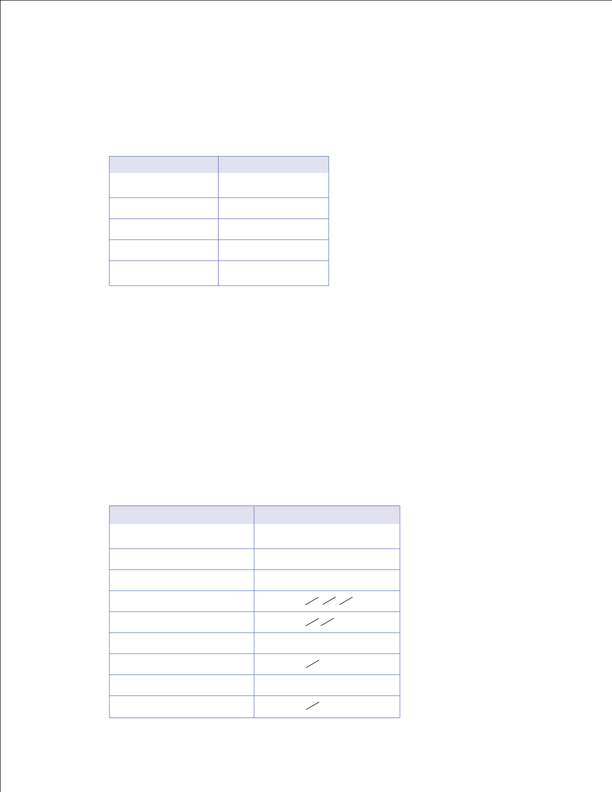
9. Before a soft drink machine is installed in your school, the student government surveyed a
sampling of students. The survey asked each student, “What is the most you would be willing
to pay for one can of soft drink?“ Use the data to complete the following tasks:
a) make a demand schedule
b) plot and connect the points from the demand schedule as an economist would
c) draw the linear demand curve that best represents the points plotted
d) write the slope and vertical intercept of the demand curve
e) write the equation of the demand curve
75¢ I
70¢ II
65¢ III
60¢ IIII IIII IIII
55¢ IIII IIII II
50¢
45¢ IIII
40¢
35¢ IIII III
Price/lb. in cents Quantity Demanded
Mathematics and Economics: Connections for Life © National Council on Economic Education, New York, NY 17
Maximum Price in cents Number of People
