Financial stability considerations in the conduct of monetary policy

Working Paper Series

Financial stability considerations in

the conduct of monetary policy

Paul Bochmann, Daniel Dieckelmann,

Stephan Fahr, Josef Ruzicka

Disclaimer: This paper should not be reported as representing the views of the European Central Bank

(ECB). The views expressed are those of the authors and do not necessarily reflect those of the ECB.

No 2870

Abstract

We empirically analyze the interaction of monetary policy with ﬁnancial stability and the

real economy in the euro area. For this, we apply a quantile vector autoregressive model

and two alternative estimation approaches: simulation and local projections. Our speciﬁ-

cations include monetary policy surprises, real GDP, inﬂation, ﬁnancial vulnerabilities and

systemic ﬁnancial stress. We disentangle conventional and unconventional monetary policy

by separating interest rate surprises into two factors that move the yield curve either at the

short end or at the long end. Our results show that a build-up of ﬁnancial vulnerabilities

tends to be accompanied initially by subdued ﬁnancial stress which resurges, however, over

a medium-term horizon, harming economic growth. Tighter conventional monetary policy

reduces inﬂationary pressures but increases the risk of ﬁnancial stress. We ﬁnd unconven-

tional monetary policy to be similarly eﬀective in reducing inﬂation, but with a lower adverse

eﬀect on growth and ﬁnancial stress. Tighter unconventional monetary policy is also found

to have a dampening eﬀect on the build-up of ﬁnancial vulnerabilities.

Keywords: monetary policy, ﬁnancial stability, macroprudential policy, quantile regres-

sions, monetary policy identiﬁcation.

JEL codes: E31, E52, G01, G10.

ECB Working Paper Series No 2870

Non-technical summary

The interplay of monetary policy, ﬁnancial conditions and the real economy has been part of

a long-standing macro-ﬁnancial debate. Monetary policy transmits to the real economy by

aﬀecting ﬁnancial conditions which themselves are taken into consideration in the conduct of

monetary policy to stabilize inﬂation and the real economy. In this transmission process, mon-

etary policy may enhance ﬁnancial stability during slowdowns by supporting the debt servicing

capacity of economic and ﬁnancial sectors, while tighter monetary policy during exuberant times

can attempt to mitigate ﬁnancial imbalances by implicitly leaning against the wind of frothy

market conditions.

By expanding the empirical quantile regression framework of Chavleishvili and Kremer (2021)

to include monetary policy shocks, inﬂation and ﬁnancial vulnerabilities we analyze the inter-

action of monetary policy with ﬁnancial stability conditions and the real economy. We estimate

impulse response functions of a quantile vector autoregressive model via two estimation tech-

niques. First, using a simulation approach, following Ruzicka (2021b), and, second, using local

projections as in Ruzicka (2021a). These quantile methods capture potential asymmetries in the

interactions between economic activity, ﬁnancial stability variables and monetary policy over

the full distribution of the variables. Our speciﬁcations contain a range of interest rate shocks

along the euro area yield curve as measure for monetary policy, euro area real GDP, euro area

HICP inﬂation, the Systemic Risk Indicator (SRI) of Lang et al. (2019) as a measure of ﬁnancial

vulnerabilities and the Composite Indicator of Systemic Stress (CISS) of Hollo et al. (2012) as

a measure of ﬁnancial stress. All models are estimated on monthly euro area data from 2002 to

2019.

Our results show that surging ﬁnancial stress has a strong short-term impact on economic

growth, especially on the lower tail of the GDP distribution, in line with Adrian et al. (2018). A

build-up of ﬁnancial vulnerabilities tends to initially be accompanied by subdued ﬁnancial stress,

but ﬁnancial stress surges over the medium term. Finally, tightening conventional monetary

policy reduces real GDP growth and inﬂationary pressures accompanied by increasing ﬁnancial

stress. Unconventional monetary policy, such as quantitative easing, identiﬁed as surprises

in longer-term interest rates are found to be similarly eﬀective in reducing inﬂation but have

a smaller ’sacriﬁce ratio’ for GDP growth and ﬁnancial stress. We also ﬁnd that ﬁnancial

vulnerabilities tend to mildly recede following tighter unconventional monetary policy.

ECB Working Paper Series No 2870

The empirical results lend themselves to counterfactual analysis on the trade-oﬀs that mon-

etary policy faces when pursuing price stability. The implemented exercises using 1-year ahead

forecasts reveal that monetary policy has faced a trade-oﬀ during the global ﬁnancial crisis:

either tighten to stabilize inﬂation forecasts at 2% or loosen to curb stress and prevent tail risks

to economic growth to increase.

ECB Working Paper Series No 2870

1 Introduction

The interplay of monetary policy, ﬁnancial conditions and the real economy has been part

of a long-standing macro-ﬁnancial debate. Monetary policy transmits to the real economy to a

large extent by aﬀecting ﬁnancial conditions. Equally, monetary policy takes ﬁnancial conditions

into account to stabilize inﬂation and the real economy (Mishkin, 2007; European Central Bank,

2021). During slowdowns monetary policy can enhance ﬁnancial stability by supporting the debt

servicing capacity of the non-ﬁnancial sector and by containing losses for the ﬁnancial sector.

In the extreme event of a ﬁnancial crisis, monetary policy – especially through liquidity support

– is crucial to contain ﬁnancial stress and to avoid the materialisation of adverse equilibria

(Mishkin, 2009; Bekaert et al., 2013). At the same time, however, the theoretical literature

suggests that accommodative monetary policy could create ﬁnancial vulnerabilities by raising

asset values, lowering risk premia, increasing leverage and increasing maturity and liquidity

mismatches (Ajello et al., 2022).

During ﬁnancial exuberant times tighter monetary policy can help mitigate ﬁnancial im-

balances by implicitly leaning against the wind of frothy market conditions. This would help

reduce the likelihood and severity of future ﬁnancial crises. However, the empirical evidence on

the general eﬀect of monetary policy on ﬁnancial vulnerabilities and its eﬀectiveness in leaning

against the wind is mixed and entails trade-oﬀs (Svensson, 2017; Kockerols and Kok, 2019; Schu-

larick et al., 2021; Boyarchenko et al., 2022). One monetary policy trade-oﬀ involves interactions

between macro variables such as inﬂation and GDP growth, and ﬁnancial stability, as measured

by ﬁnancial stress and vulnerabilities. A second trade-oﬀ in the conduct of monetary policy

relates to the management of tail risks for the real economy relative to tail risks for ﬁnancial

stability. Finally, an intertemporal trade-oﬀ relates the potential impact of monetary policy on

short-term ﬁnancial stress relative to adjustments to economic and ﬁnancial vulnerabilities in

the medium-term.

In this paper, we empirically analyze the interaction of monetary policy shocks, ﬁnancial

stability conditions and the real economy in the euro area. We do so by estimating impulse re-

sponse functions of a quantile vector autoregressive model via two estimation techniques, namely

through simulation, following Ruzicka (2021b), and local projections as in Ruzicka (2021a). The

speciﬁcations include ﬁve variables: a range of interest rates from the euro area yield curve

as measure for monetary policy, euro area real GDP, euro area HICP inﬂation, the Composite

ECB Working Paper Series No 2870

Indicator of Systemic Stress (CISS) of Hollo et al. (2012) as a measure of ﬁnancial stress, and

the Systemic Risk Indicator (SRI) of Lang et al. (2019) as a measure of ﬁnancial vulnerabilities.

Importantly, quantile methods capture potential asymmetries in the interactions between eco-

nomic activity (GDP and inﬂation), ﬁnancial stability conditions (SRI and CISS) and monetary

policy shocks over the full distribution of the variables, including for impulse response analysis.

While macroeconomic conditions are typically summarized by real GDP and inﬂation, ﬁ-

nancial stability conditions are less clearly deﬁned. The SRI is our vulnerability metric and

characterizes the general state of the ﬁnancial environment and serves as a ‘barometer’ for the

ﬁnancial system (Duprey and Roberts, 2017). In exuberant times with elevated vulnerabilities,

the propagation of small shocks may result in ampliﬁcations for the economy, absent in normal

times (Lang et al., 2019). While vulnerability indicators contain forward-looking information,

they provide only limited information for the materialisation of stress at a speciﬁc point in time

in the future, given the uncertainty surrounding the future materialisation of shocks. For this,

our stress metric, the CISS, captures the materialization of ﬁnancial instability and serves as

a ‘thermometer’ for the ﬁnancial system (Chavleishvili and Kremer, 2021). The distinction of

ﬁnancial vulnerability and stress is especially important to capture the intertemporal relation

between the initial build-up of vulnerabilities and subsequent downside tail risks to the ﬁnancial

system and real economy.

Similarly to ﬁnancial conditions, the monetary policy stance is only imperfectly summarized

by the short-term policy interest rate, given purchases of longer-term securities. Since the global

ﬁnancial crisis, central banks have made active use of their balance sheets and forward guid-

ance. Monetary policy rates predominantly impact short-term market rates, forward guidance

aﬀects interest rates further into the future, and purchases of medium- to long-term securities

aﬀect interest rates over longer maturities. To capture monetary policies and their eﬀects in an

empirical macro-ﬁnancial estimation framework, we use monetary policy surprises in risk-free in-

terest rates between one month and ten years over a narrow time window (covering press release

and subsequent press conference) around the communication of ECB monetary policy decisions

contained in the “Euro Area Monetary Policy Event-Study Database” developed and regularly

updated by Altavilla et al. (2019). From these surprises we estimate a short- and long-term

factor of interest rate surprises and identify monetary policy shocks following G¨urkaynak et al.

(2005), Jaroci´nski and Karadi (2020) and Giuzio et al. (2021). The approach separates surprises

related to conventional monetary policy (short-term rates) from those related to unconventional

ECB Working Paper Series No 2870

monetary policy (longer-term maturities).

Our results show that surging ﬁnancial stress has a strong short-term impact on economic

growth, especially on the lower tail of the GDP distribution, in line with earlier ﬁndings such

as Adrian et al. (2018). We also ﬁnd that while a build-up of ﬁnancial vulnerabilities tends

to initially be accompanied by subdued ﬁnancial stress – i.e. below-average ﬁnancial market

volatility, risk-pricing and excess returns – stress surges over the medium term. This provides

for evidence that ﬁnancial market tranquility during the initial phase of a ﬁnancial expansion

hits back with a vengeance down the road. Finally, the estimation indicates that tightening

conventional monetary policy reduces inﬂationary pressures at the cost of slower real GDP

growth and surging ﬁnancial stress. Tightening unconventional monetary policy, identiﬁed as

surprises in longer-term interest rates, is found to be similarly eﬀective in reducing inﬂation

as shorter-term rates, but has a smaller impact on growth and ﬁnancial stress, while ﬁnancial

vulnerabilities mildly recede. This indicates that conventional and unconventional monetary

policies may at times be complementary for stabilizing the economy and ﬁnancial system.

The empirical results allow for a quantitative assessment of monetary policy using coun-

terfactuals to shed light on monetary policy trade-oﬀs in its pursuit of price stability. A ﬁrst

counterfactual traces out the eﬀects of monetary policy on Growth-at-Risk (GaR; the 10th per-

centile of the forecasted GDP growth distribution one year ahead) when setting price stability

at the objective of 2% annual inﬂation. Especially during the global ﬁnancial crisis, monetary

policy faced a trade-oﬀ: either tightening to stabilizing inﬂation forecasts at 2% or loosening

to prevent Growth-at-Risk to deteriorate. This analysis indicates the potential beneﬁcial use of

alternative policy measures to oﬀer a complementary angle for stabilisation of the real economy.

Having established the relative eﬃciency of diﬀerent policy tools, we illustrate how the esti-

mation results could inform a monetary and macroprudential policy mix to enhance stabilisation

over the sample period. We assume policy objectives of a 2% median inﬂation forecast one year

ahead and stabilization of GaR at its sample average of -1.08%. Given the relative eﬃciencies

the policymaker uses a mix of monetary policy (long-end interest rate factor) and macropruden-

tial policy (SRI). The GaR objective is non-symmetric, implying that the policymaker avoids

that GaR falls below the value of -1.08% while focussing solely on the objective of inﬂation

otherwise. The policymakers thus provides a hedge against crisis outcomes. We compute the

needed counterfactual policies based on the cumulated impulse response functions and ﬁnd that

relatively large monetary policy shocks would have been needed to bring inﬂation forecasts back

ECB Working Paper Series No 2870

to their target over the period 2005 until the ﬁrst half of 2009. In contrast, over the earlier as

well as later parts of the sample period our results would have called for looser monetary policy.

Our results also indicate that looser macroprudential policy would have been needed starting

in September 2007 and throughout the global ﬁnancial crises until September 2009 and again

on a few occasions during the euro area debt crisis to maintain GaR above its historical value.

Forecasts implied by these policy counterfactuals show that they would have been eﬀective in

meeting combined inﬂation and growth targets, while limiting ﬁnancial stress.

The remainder of the paper is structured as follows. Section 2 reviews the core elements

of ﬁnancial stability conditions and monetary policy in the recent literature. In section 3 we

describe our data set, including the indicators used to measure ﬁnancial stability conditions

and the identiﬁcation of monetary policy shocks. Next, in section 4 we describe the econometric

speciﬁcations. Section 5 presents impulse responses from our quantile vector autoregressions and

uncovers the dynamic interactions of ﬁnancial vulnerabilities and stress with the real economy,

and the impact of monetary policy shocks. Section 6 covers counterfactual analysis and illus-

trates trade-oﬀs between price stability and ﬁnancial stability objectives for monetary policy.

It further assesses interactions between monetary policy and macroprudential policy. Finally,

section 7 concludes.

2 Monetary policy and ﬁnancial stability interactions

Monetary policy frameworks around the globe focus on price stability as their main objective,

often accompanied with additional objectives such as full employment or ﬁnancial stability.

Monetary policy’s role for ﬁnancial stability is often subsumed in the eﬀectiveness of monetary

policy transmission or delegated to other policy domains such as macroprudential policy. While

it is generally accepted that monetary policy takes ﬁnancial stability into account at least in

some form, quantitative trade-oﬀs are less prominent in the literature. Smets (2014) indicates

that the degree to which monetary policy should take ﬁnancial stability considerations into

account depends crucially on its eﬀectiveness in addressing risks to ﬁnancial stability, but also

to what degree the ﬁnancial stability considerations undermine the credibility of the central

bank’s price stability mandate.

Monetary policy faces several challenges when including ﬁnancial stability considerations.

First, narrow indicators of ﬁnancial conditions, stress and vulnerabilities (such as metrics of

ECB Working Paper Series No 2870

risk-taking, liquidity and leverage) oﬀer only partial measures of ﬁnancial stability, especially

when considered in isolation, but are not fully comprehensive of prevailing ﬁnancial stability

conditions. In turn, monetary policy instruments are multiple, and each one may interact diﬀer-

ently with ﬁnancial stability. Furthermore, at least theoretically, monetary policy may create an

inter-temporal trade-oﬀ for ﬁnancial stability whereby accommodative monetary policy improves

current ﬁnancial conditions in the short run at the cost of increasing future ﬁnancial vulnerabil-

ities Adrian and Liang (2018). Empirically, it appears unclear to date whether monetary policy

itself can inﬂuence ﬁnancial vulnerabilities, partly because ﬁnancial cycles are typically much

longer than the business cycles monetary policy reacts to (Boyarchenko et al., 2022). Ultimately,

monetary policy’s eﬃcacy as a tool for ﬁnancial stability will depend on the cost-beneﬁt trade-oﬀ

of tighter monetary policy for economic activity and inﬂation.

Our paper relates to diﬀerent strands of the literature. First, we contribute to the literature

that investigates the empirical relationship between monetary policy and ﬁnancial stability. The

primary focus of existing studies lies on ﬁnancial vulnerabilities. However, a (surprise) monetary

tightening could also lead to acute episodes of surging ﬁnancial stress and an abrupt tightening

of ﬁnancial conditions. Recent literature (Adrian et al., 2019; Figueres and Jaroci´nski, 2020)

points to the importance of associated indicators for short-term (up to one year ahead) downside

risks to economic growth. Boyarchenko et al. (2022) provide a recent and detailed review of the

empirical literature studying the relationship between monetary policy and ﬁnancial vulnerabil-

ities. Overall, the authors conclude that empirical evidence on the link between monetary policy

and ﬁnancial vulnerabilities is limited.

However, the current literature does not rule out causal eﬀects of monetary policy on ﬁnan-

cial vulnerabilities. Several research gaps emerge from this existing literature, some of which our

paper attempts to ﬁll: Existing studies focus primarily on the United States while analyses for

the euro area are scarce. Furthermore, existing studies diﬀer in their measurement of ﬁnancial

vulnerabilities and focus mostly on narrow concepts such as asset valuations in selected mar-

kets, risk-taking by banks or other intermediaries, leverage and liquidity-maturity mismatches

or leverage of ﬁnancial intermediaries, households and businesses. However, vulnerabilities that

have material impacts on the real economy appear to emerge from the interplay of asset prices

and credit (Jord`a et al., 2015) and we therefore employ a broad indicator of ﬁnancial vulnera-

bilities in this paper.

Second, we estimate the dynamic interactions of macroeconomic, ﬁnancial and monetary pol-

ECB Working Paper Series No 2870

icy variables using multivariate quantile regression techniques. Quantile regressions of Koenker

and Bassett Jr (1978) have been extended to multivariate dynamic frameworks in various

ways. One approach involves multiple equations and iteration or simulation (White et al.,

2015; Chavleishvili and Manganelli, 2019; Montes-Rojas, 2022; Ruzicka, 2021b). The other ap-

proach focuses on a single-equation setup and direct estimation through local projections of

Jord`a (2005) in combination with quantile regression – a prominent example is the work of

Adrian et al. (2019). Identiﬁcation, smooth estimation, and inference for quantile regression

local projections is studied by Ruzicka (2021a). A unique feature of our paper is that we employ

both estimation approaches by using the methods from Ruzicka (2021b) as well as from Ruzicka

(2021a). Doing so, we obtain two valid estimates, which trade oﬀ bias and variance of impulse

response functions diﬀerently. In a least squares regression setting, Plagborg-Møller and Wolf

(2021) show that at shorter forecast horizons local projections are comparable with structural

vector autoregressions (Sims, 1980, SVAR), whereas at longer forecast horizons the local pro-

jections have lower bias but higher variance. We expect that the same phenomenon arises in a

quantile regression setting, as well.

Third, our assessment of the impact of monetary policy on ﬁnancial stability focuses on an

assessment of the tails of the distribution of real economic and ﬁnancial variables. The estimation

provides impacts for the lower and upper quantiles of these distributions and oﬀers thereby risk

considerations beyond the impact on median or average eﬀects. This relates to other work on the

stance of monetary and macroprudential policy using quantile reqressions, such as in Cecchetti

(2006), Kilian and Manganelli (2008), Duprey and Ueberfeldt (2018), Aikman et al. (2019)

and Carney (2020). The common feature of these approaches resides in the use of the tail of

forecasted variables to infer assessment of risks to the economy or a policy stance. And ﬁnally,

we relate to the empirical literature that identiﬁes eﬀects of monetary policy on asset prices

and the macroeconomy using high-frequency ﬁnancial market surprises around central bank

monetary policy announcements going back to Kuttner (2001), as well as literature about the

identiﬁcation of monetary policy from such event-study data (G¨urkaynak et al., 2005; Altavilla

et al., 2019; Jaroci´nski and Karadi, 2020; Giuzio et al., 2021).

ECB Working Paper Series No 2870

3 Financial stability indicators and identiﬁcation of monetary

policy shocks

Our data consists of a set of aggregate euro area macro-ﬁnancial and monetary policy variables,

starting in the beginning of 2002 and running through the end of June 2019 at monthly frequency.

Our baseline model input consists of two macroeconomic variables, namely real GDP growth

and HICP inﬂation, the Composite Indicator of Systemic Stress (CISS) as a measure of ﬁnancial

stress (Hollo et al., 2012; Chavleishvili and Kremer, 2021), and the Systemic Risk Indicator

(Lang et al., 2019, SRI) as a measure of ﬁnancial vulnerabilities,monetary policy shocks built

from surprise rate changes over narrow time windows covering the communication of monetary

policy decisions through press release and the subsequent press conference on ECB Governing

Council monetary policy meeting dates using a data set developed and regularly updated by

Altavilla et al. (2019). The computation of these shocks is explained in detail further below in

Section 3.3.

Figure 1 plots the macro-ﬁnancial variables used in our estimation which are further sum-

marized in Table 1. We deliberately represent ﬁnancial stability aspects in our models with

two separate variables, distinguishing between short-term ﬁnancial stress which can trigger in-

stability and medium-term vulnerabilities which make the ﬁnancial system more susceptible to

destabilizing triggers. We approximate monthly GDP by interpolating a quarterly GDP series

with a monthly index of industrial production for the euro area.

3.1 Financial stress

The CISS serves as our measure of ﬁnancial stress and captures the severity of ﬁnancial crises,

serving as a ‘thermometer’ of ﬁnancial instability. It is a timely, frequent and publicly available

indicator based on 15 individual indicators grouped into ﬁve sub-indices: ﬁnancial intermediaries,

bond markets, equity markets, foreign exchange markets, and money markets. The contribution

from ﬁnancial intermediaries is around 30%, that of equity markets around 25%, and each of

the three remaining sub-indexes around 15%.

Importantly, the CISS takes into account the

The equity market sub-index comprises stock price volatility of non-ﬁnancial corporations (NFC), a measure

of maximum cumulated stock price losses and a measure of stock-bond correlation. The FX market sub-index

captures the volatility of EUR/USD, EUR/JPY and EUR/GBP exchange rates. The ﬁnancial intermediaries

sub-index reﬂects bank stock return volatility, ﬁnancial-nonﬁnancial bonds spread, and the cumulated loss of the

book-price ratio of banks. The bond market sub-index captures the volatility of German sovereign bonds (at

10-year maturity), the spread between A-rated NFC and sovereign bonds, and the 10Y interest rate swap spread.

ECB Working Paper Series No 2870

Figure 1: Macro-ﬁnancial variables, monthly

‐2

‐1.5

‐1

‐0.5

0.5

1.5

2002M1

2003M1

2004M1

2005M1

2006M1

2007M1

2008M1

2009M1

2010M1

2011M1

2012M1

2013M1

2014M1

2015M1

2016M1

2017M1

2018M1

2019M1

RealGDPgrowth

‐0.6

‐0.4

‐0.2

0.2

0.4

0.6

0.8

2002M1

2003M1

2004M1

2005M1

2006M1

2007M1

2008M1

2009M1

2010M1

2011M1

2012M1

2013M1

2014M1

2015M1

2016M1

2017M1

2018M1

2019M1

HICPinflation

0.1

0.2

0.3

0.4

0.5

0.6

0.7

0.8

0.9

2002M1

2003M1

2004M1

2005M1

2006M1

2007M1

2008M1

2009M1

2010M1

2011M1

2012M1

2013M1

2014M1

2015M1

2016M1

2017M1

2018M1

2019M1

CISS

‐0.6

‐0.4

‐0.2

0.2

0.4

0.6

2002M1

2003M1

2004M1

2005M1

2006M1

2007M1

2008M1

2009M1

2010M1

2011M1

2012M1

2013M1

2014M1

2015M1

2016M1

2017M1

2018M1

2019M1

SRI

Notes: Monthly data 2002M1-2019M6. Variables are displayed as they enter

our models: real GDP and HICP in ﬁrst diﬀerences of logs (in %), CISS and

SRI in levels.

correlation across sub-components, whereby higher correlation implies higher values of systemic

stress. The CISS leads GDP by up to one quarter (Chavleishvili and Kremer, 2021) and has

been shown to outperform narrower measures of ﬁnancial conditions in the prediction of one-year

ahead tail risks to euro area output growth (Figueres and Jaroci´nski, 2020).

3.2 Financial vulnerabilities

We capture medium-term ﬁnancial vulnerabilities with the Systemic Risk Indicator (SRI): a

broad-based cyclical indicator that captures risks stemming from potential overvaluation of

property prices, credit conditions, external imbalances, private sector debt burden and the po-

tential mispricing of risk that serves as a ‘barometer’ of ﬁnancial instability (Lang et al., 2019).

With the exception of the credit category, the authors use one variable for each of the aforemen-

The Money market sub-index comprises the 3M EURIBOR volatility, its spread to the 3M French T-bill spread,

and a measure of emergency lending of the Eurosystem.

ECB Working Paper Series No 2870

Table 1: Summary statistics

Statistic T Mean St. Dev. Min Max

Real GDP 210 0.100 0.359 −1.416 0.910

HICP 210 0.138 0.171 −0.413 0.644

CISS 210 0.177 0.201 0.002 0.913

SRI 210 −0.068 0.296 −0.436 0.542

Notes: Real GDP and HICP is in ﬁrst diﬀerences of monthly logs

(in %). CISS and SRI are in monthly levels.

tioned categories, selecting from a larger pool of potential variables and transformations those

with the best predictive ability for systemic ﬁnancial crises. In total, Lang et al. (2019) derive

six indicators which are normalized and aggregated as an optimally weighted average in terms

of overall predictive power of the composite indicator.

Measures of ﬁnancial vulnerabilities are typically used to inform macroprudential policies.

For example, the credit-to-GDP gap is instrumental in the calibration of countercyclical capital

buﬀers. The SRI increases on average several years before the onset of systemic ﬁnancial crises

with superior early-warning properties in comparison to the credit-to-GDP gap. In this capacity,

it also has signiﬁcant predictive power for large declines in real GDP growth three to four years

into the future and its level at the onset of systemic ﬁnancial crises is highly correlated with

measures of subsequent crisis severity. The SRI therefore provides useful information about

both the probability and the likely cost of systemic ﬁnancial crises which makes it our preferred

measure of the ﬁnancial cycle in comparison to other available indicators.

Financial vulnerabilities evolve more slowly and more gradually than the other variables in

our models, reﬂecting that ﬁnancial cycles tend to last longer than economic cycles. Indeed,

the within-month interactions between the SRI and the other variables, measured by quantile

impulse responses, are negligible and insigniﬁcant – except for ﬁnancial stress (CISS) at the

90th percentile. On the other hand, ﬁnancial vulnerabilities can be controlled by a range of

ﬁnancial stability instruments, microprudential and macroprudential. Due to the negligible

contemporaneous interactions, we can interpret SRI changes as exogenous shocks, and treat the

SRI as the third policy tool, in addition to conventional and unconventional monetary policy.

The six sub-indicators used are the two-year change in the bank credit-to-GDP ratio, the two-year growth rate

of real total credit, the two-year change in the debt-service-ratio, the three-year change in the RRE price-to-income

ratio, the three-year growth rate of real equity prices, and the current account-to-GDP ratio.

ECB Working Paper Series No 2870

3.3 Monetary policy shocks

A large empirical literature, going back to Kuttner (2001), identiﬁes eﬀects of monetary policy

on asset prices and the macroeconomy using high-frequency, intra-day, ﬁnancial market price

changes over short time windows covering central bank monetary policy announcements. Based

on such high-frequency event-study data, G¨urkaynak et al. (2005) ﬁnd that two independent

factors constructed from federal funds futures – the ﬁrst related to short rates and an independent

second factor related to rates of longer maturities – summarize the eﬀects of U.S. monetary policy

on bond prices and stock returns.

We use their approach to extract two factors from intra-day overnight index swap (OIS) rate

changes over narrow time windows covering the press release as well as the subsequent press

conference about monetary policy decisions on ECB Governing Council monetary policy meeting

dates using the “Euro Area Monetary Policy Event-Study Database”, developed and regularly

updated by Altavilla et al. (2019). These two factors capture surprises along the yield curve as

they are constructed by ﬁtting the time series of surprises in OIS rates of seven maturities (one,

three and six months as well as one, two, ﬁve and ten years). Surprises in OIS rates of maturities

longer than two years are only available from August 2011 onward and we proxy these series by

surprises in German government bond yields of the same maturity for the period from January

2002 to July 2011.

To provide a structural interpretation of the two factors, we rotate them as in G¨urkaynak

et al. (2005) such that the second factor is not impacted by surprises in the OIS rate of the

shortest maturity, i.e. its factor loading on the 1-month OIS surprises is set to zero, while im-

posing orthogonality between the two rotated factors. Finally, the rotated factors are rescaled

to match the standard deviations of 3-month OIS surprises for the ﬁrst factor and 10-year OIS

surprise for the second factor. In this way, the ﬁrst factor corresponds to shorter maturities –

reﬂecting surprises related to conventional monetary policy – and the second factor corresponds

to longer maturities, capturing surprises related to unconventional monetary policy. For conve-

nience we label these factors short- and long-end factors, in line with G¨urkaynak et al. (2005).

The corresponding factor loadings are shown in Figure 2.

The short- and long-end factors provide information about interest rate surprises along

the yield curve. Jaroci´nski and Karadi (2020) point out that such surprises reveal, addition-

ally to information about the monetary policy stance, also private central bank information

ECB Working Paper Series No 2870

Figure 2: Monetary policy surprise factors - loadings

1m 3m 6m 1Y 2Y 5Y 10Y

0.1

0.2

0.3

0.4

0.5

0.6

0.7

0.8

0.9

F1 - short

F2 - long

Notes: The ﬁgure shows the estimated factor loadings after rotation.

about the state of the economy. To separate monetary policy from central bank information

shocks, Jaroci´nski and Karadi (2020) use an identiﬁcation strategy with sign restrictions on high-

frequency stock price changes around monetary policy announcements. A positive co-movement

between intra-day interest rates and intra-day stock prices is interpreted as an information shock

as the central bank reveals new information about the state of the economy. In turn, a negative

co-movement reﬂects a monetary policy surprise whereby higher interest rates imply a decline

in stock prices, while a fall in interest rates implies higher stock prices. While intuitive, this

method yields implausible results for the euro area; in particular, the response of the monthly

stock index remains insigniﬁcant while a monthly BBB bond spread index used in their model

declines after a contractionary monetary policy shock. However, the analysis in our paper

builds on a consistent identiﬁcation between high-frequency monetary policy shocks and asset

price responses to assess the ﬁnancial stability implications of monetary policy.

As an alternative to stock prices, we therefore identify monetary policy and information

shocks based on daily changes of non-ﬁnancial corporate (NFC) bond spreads instead of intra-

day stock price changes, as suggested by Giuzio et al. (2021). More speciﬁcally, we identify

monetary policy shocks from positive co-movement of our interest rate factors with daily changes

in BBB-rated euro-denominated NFC bond spreads (at 5-year maturity). Thus, a contractionary

monetary policy shock occurs when interest rates rise and bond spreads widen simultaneously

whereas an expansionary monetary policy shock is characterized by falling interest rates and

narrowing bond spreads. Consequently, central bank information shocks are identiﬁed from

ECB Working Paper Series No 2870

negative co-movement between interest rate surprises and bond spreads. This identiﬁcation

strategy improves not only the response of monthly bond spreads but also the response of

monthly stock prices to monetary policy shocks. We use bond spreads from Bank of America

obtained through Bloomberg until March 2007, while from April 2007 we use bond spreads from

iBoxx, which we found to be more liquid compared to those from Bank of America but not

continuously available before April 2007. Summary statistics of the interest rate series, bond

spreads, and identiﬁed surprises can be found in Table 2.

Table 2: Summary statistics for monthly interest rate factors and monetary policy surprises

(January 2002 - June 2019), T = 210, in bps.

Mean St. Dev. Min Max

Short-end factor −0.09 2.87 −13.20 16.70

Short-end factor, MP shock 0.03 1.54 −6.34 16.70

Short-end factor, CB info shock −0.11 2.39 −13.20 10.27

Long-end factor 0.00 4.09 −25.77 13.22

Long-end factor, MP shock 0.06 1.97 10.09 −10.21

Long-end factor, CB info shock −0.12 3.52 −25.77 13.22

BBB-rated NFC bond spread changes 0.13 3.40 -8.94 23.52

The cumulated factors of surprises in OIS rates are displayed in Figure 3 together with their

information and monetary policy components, based on the identiﬁcation using BBB-rated NFC

bond spreads. Increasing values indicate tightening of interest rates relative to the prevailing

market expectations before monetary policy statements.

The short-end factor indicates a tightening of surprises in short rates during the early part

of our sample, followed by a period of loosening leading up to the Global Financial Crisis,

then a short period of tightening at the peak of Global Financial Crisis and ﬁnally an overall

loosening of rates over the remainder of our sample period. These dynamics were mainly driven

by surprises identiﬁed as central bank information shocks, while monetary policy shocks often

moved in opposite direction and indicate an overall tightening.

In turn, the cumulated long end factor falls strongly in July and August 2008, driven by

central bank information shocks, while gradually tightening for most of the remainder of the

sample period. This long tightening episode appears to be driven at least partially by monetary

policy shocks.

ECB Working Paper Series No 2870

Figure 3: Cumulated monetary policy factors 2002-2019

-50

-40

-30

-20

-10

2002

2003

2004

2005

2006

2007

2008

2009

2010

2011

2012

2013

2014

2015

2016

2017

2018

2019

long end factor

long end factor - CB info.

long end factor - MP

-40

-30

-20

-10

2002

2003

2004

2005

2006

2007

2008

2009

2010

2011

2012

2013

2014

2015

2016

2017

2018

2019

short end factor

short end factor - CB info.

short end factor - MP

Notes: The ﬁgure shows cumulated factors before and after identiﬁcation with

BBB-rated NFC bond spreads in basis points.

The factors are extracted in a ﬁrst step using maximum likelihood estimation to employ them

in a second step for estimating quantile treatment eﬀects of policy interventions by minimizing

asymmetric l

loss functions. As a result, the two steps of the empirical strategy employ diﬀerent

loss functions. While it may be possible to use the l

loss functions in factor extraction, such

an approach has not been used in the literature on monetary policy event study factors as far

as we know and is not considered in this work either.

4 Quantile modelling

4.1 Estimating quantile treatment eﬀects of structural shocks

The main goal of our estimations is to quantify the impact of exogenous shocks on vulner-

abilities in the real economy and the ﬁnancial sector. We do so by estimating the eﬀect of

structural shocks on diﬀerent parts of the distribution of the response variables, namely real

GDP growth, HICP inﬂation, ﬁnancial vulnerabilities and ﬁnancial stress. However, this task

is complex because we need to model the distributions of our endogenous variables, along with

their contemporaneous and dynamic interactions. Speciﬁcally, we estimate quantile treatment

eﬀects (see Koenker, 2005, pp. 26–32) of structural shocks. A quantile treatment eﬀect measures

how each quantile of a response variable is aﬀected by a treatment. In our case, the treatment

ECB Working Paper Series No 2870

is an exogenous impulse, also called a shock.

We estimate the quantile treatment eﬀects by two diﬀerent methods. The ﬁrst is a simulation-

based, two-step approach in form of a quantile vector autoregressive model, while the second

one relies on direct estimation and regularization in form of a quantile local projection approach.

Both methods identify the shocks by recursive short-run restrictions and provide valid estimates

of the quantile treatment eﬀect. However, the methods diﬀer in their ﬁnite sample performance

and in robustness to misspeciﬁcation, especially at longer forecast horizons. In the following, we

provide the general features of the two estimation methods together with basic technical notions

of their setup and refer the reader for additional details to the referenced papers.

The ﬁrst method – simulation-based – follows Ruzicka (2021b) and is based on the estimation

of the quantile regression process for a system of equations, with subsequent simulation using the

approach proposed by Koenker and Xiao (2006), described in detail in Koenker et al. (2018, pp.

328–329), and also used by Montes-Rojas (2022). It is similar to Chavleishvili and Manganelli

(2019) and Montes-Rojas (2022). However, unlike Chavleishvili and Manganelli (2019), we do

not set any sample paths to their median values and instead consider the full set of possible

sample paths. This increases the computational complexity, but gives a more complete and

agnostic picture of the eﬀects we estimate. Unlike Montes-Rojas (2022) and Chavleishvili and

Manganelli (2019), we do not discretize the model on an ex-ante chosen grid of quantile indices,

but instead estimate the entire quantile regression process, that is, we estimate each quantile

regression for all quantile indices in (0,1). The practical consequence is that our estimates

don’t suﬀer from unnecessary approximation errors due to discretization. In addition, unlike

Chavleishvili and Manganelli (2019) and Montes-Rojas (2022), we construct conﬁdence intervals

for the quantile treatment eﬀects as in Ruzicka (2021b).

The second method estimates the quantile treatment eﬀects directly by employing the lo-

cal projections of Jord`a (2005) in a quantile regression setting. Local projections estimated by

quantile regressions have become a popular way to capture heterogeneous eﬀects of macroeco-

nomic shocks. However, applied research based on plain quantile regression local projections is

challenging: The estimated impulse response functions tend to wiggle a lot, it is unclear what

the underlying identiﬁcation conditions are, and it is unclear how to construct closed-form conﬁ-

dence intervals. Ruzicka (2021a) overcomes these challenges by introducing roughness penalties

to smooth the impulse response functions, by establishing the identiﬁcation conditions, and by

providing closed-from as well as weighted bootstrap conﬁdence intervals.

ECB Working Paper Series No 2870

These features are essential for our results for the following reasons. First, if it were not

for the smoothing, the estimated impulse response functions would change abruptly from one

forecast horizon to the next, making them diﬃcult to interpret and less accurate. Second, the

theoretical result of Ruzicka (2021a) reveals which control variables must be included (and which

must not) in order to identify the quantile treatment eﬀect of interest. This is essential for causal

interpretation and to prevent simultaneity bias. Third, the weighted bootstrap doesn’t entail any

tuning parameters, unlike the stationary bootstrap proposed Han et al. (2022) which depends

on a parameter (average block length), whose appropriate choice is nontrivial in practice.

Next, we present the basic technical notions underlying both estimation methodologies: the

data generating process and the impulse response function that measures the quantile treat-

ment eﬀect of interest. For random variables X and Y we denote Q

(Y |X) the τ th conditional

quantile of Y given X. For a stochastic process {Y

}, let {F

} be its ﬁltration (the informa-

tion known up to time t). We assume the data follow an I-dimensional stochastic process

} = {[y

1,t

, y

2,t

, . . . , y

I,t

]} given by

1,t

t−1

) =

i=1

p=1

p1i

(τ

i,t−p

+ ε

(τ

)

2,t

1,t

, F

t−1

) = a

021

(τ

1,t

i=1

p=1

p2i

(τ

i,t−p

+ ε

(τ

)

I,t

1,t

, y

2,t

, . . . , y

I−1,t

, F

t−1

) =

I−1

i=1

0Ii

(τ

i,t

i=1

p=1

pIi

(τ

i,t−p

+ ε

(τ

)

(1)

This type of a stochastic process was studied by Chavleishvili and Manganelli (2019), Ruzicka (2021a,b) and

Montes-Rojas (2022). It is a special case of the VAR for VaR of White et al. (2015), who additionally allow

conditional quantiles to depend on the lags of conditional quantiles.

ECB Working Paper Series No 2870

This stochastic process can be expressed in a random coeﬃcient representation as

1,t

i=1

p=1

p1i

i,t−p

+ ε

)

2,t

= a

021

1,t

i=1

p=1

p2i

i,t−p

+ ε

)

I,t

I−1

i=1

0Ii

i,t

i=1

p=1

pIi

i,t−p

+ ε

)

(2)

where u

i,t

∼ U[0, 1], y

i,t

is non-decreasing in u

a.s. for all i and t, and {u

} are independent.

The disturbances {u

} in (2) change from one period to the next and represent the realized

values of τ

in each time period.

The model is identiﬁed by recursive short-run restrictions. For example, the second variable

is not allowed to contemporaneously aﬀect the distribution of the ﬁrst variable, but it may

aﬀect the distribution of the third variable. This recursive ordering is analogous to the one of

Sims (1980). However, note that the identiﬁcation restrictions are not equivalent to a Cholesky

decomposition of a covariance matrix – in fact, the quantile model above is well-deﬁned even if

the variance of Y

doesn’t exist.

In the ﬁrst, simulation-based approach, we estimate the quantile regression process of all

equations above over all quantile indices in (0,1) and subsequently recover the quantile treatment

eﬀects of shocks by simulation, as outlined earlier. In the second, direct estimation approach,

we rely on the result of Ruzicka (2021a) who shows that for all forecast horizons h ∈ N

and all

i, j ∈ {1, 2, . . . , I} in the representation

j,t+h

t−1

, y

1,t

, . . . , y

i,t

) = β

0,j,0,h

(τ) +

k=1

k,j,0,h

(τ)y

k,t

k=1

P −1

p=1

k,j,p,h

(τ)y

k,t−p

(3)

the slope coeﬃcient β

i,j,0,h

(τ) is the quantile treatment eﬀect of the ith shock on variable j after

h periods at quantile τ . The last equation could be estimated directly by quantile regression,

separately for each forecast horizon. However, such estimates are usually rather inaccurate

and diﬃcult to interpret as they diﬀer dramatically between neighboring forecast horizons. For

Koenker et al. (2018)[pp. 313-317, 328-329] discuss the conditional quantile and random coeﬃcient forms of

quantile autoregressive processes, their relations and role in forecasting.

ECB Working Paper Series No 2870

that reason we use the smooth quantile local projections estimator of Ruzicka (2021a), which

solves the problem by regularization, shrinking the impulse response functions towards cubic

polynomials via roughness penalties. In addition, we impose a long-run equilibrium constraint

which ensures the impulse response functions converge to a constant function at the ﬁnal forecast

horizon.

We set the optimal value of the roughness penalty by the Bayesian information

criterion (Schwarz, 1978), as adapted for this setup by Ruzicka (2021a). Following Ruzicka

(2021a), we construct the conﬁdence intervals by the weighted bootstrap with undersmoothing

(using standard exponential weights; the roughness penalty for conﬁdence intervals is one quarter

of its value for point estimates.)

We collect the quantile treatment eﬀects at diﬀerent horizons into a quantile impulse re-

sponse function, using the deﬁnition of Ruzicka (2021b). The quantile impulse response function

QIR(j, i, h, τ, s) is the response of the jth variable at quantile τ to the ith shock of size s after

h periods, formally

QIR(j, i, h, τ, s) = Q

j,t+h



) := ε

) + s

−Q

j,t+h

(4)

∂Q

j,t+h

]

∂ε

)

s (5)

where the notation ε

) := ε

) + s represents a modiﬁed version of the process, with ε

)

substituted by ε

)+s for all u

∈ [0, 1]. For some variables we are interested in the cumulative

eﬀect of a shock through cumulative quantile impulse response functions, given by

QIRC(j, i, h, τ, s) = Q

k=0

j,t+k



) := ε

) + s

−Q

k=0

j,t+k

(6)

∂Q

k=0

j,t+k



∂ε

)

s (7)

4.2 Counterfactual scenarios – linking forecasts and impulse responses

The quantile impulse response function as deﬁned above involves an intervention at a single

point in time. However, it is also possible to allow interventions in various consecutive time

periods. This is more complicated, but it is useful in order to isolate the eﬀects of sustained

policy interventions. To be speciﬁc, we work with monthly data, the interventions are introduced

For our two models, the forecast horizon is up to 72 months and 12 months, respectively.

ECB Working Paper Series No 2870

in 12 consecutive months, and the response variable is a monthly growth rate. Formally, the

intervention at time t + m is of size s

, where m ∈ {0, 1, . . . , 11}. We want to see the eﬀect of

the interventions on the τ th quantile of

k=0

j,t+k

, which represents the year-over-year growth

rate of the response variable. Using the same notation as in (4), the eﬀect of the sequence of

interventions is

k=0

j,t+k



∀m ∈ {0, 1, . . . , 11}: ε

i,t+m

) := ε

i,t+m

) + s

−Q

k=0

j,t+k

(8)

It can be shown

that (8) equals

l=0

QIRC(j, i, l, τ, s

11−l

) (9)

The sequence of external impulses can be combined with quantile forecasts into a counter-

factual scenario. Such a scenario shows how quantile forecasts would have responded to policy

interventions in the past. Recall that F

t−1

represents the information known at time t − 1. The

forecast of the year-over-year growth rate of the ith variable is represented by

k=0

j,t+k



t−1

(10)

Next, we introduce policy interventions over 12 consecutive months. The forecast changes to

k=0

j,t+k



t−1

, ∀m ∈ {0, 1, . . . , 11}: ε

i,t+m

) := ε

i,t+m

) + s

(11)

and represents our counterfactual scenario. It turns out that

(11) equals (12)

k=0

j,t+k



t−1

l=0

QIRC(j, i, l, τ, s

11−l

) (12)

which comprises the quantile forecast (the ﬁrst term) and the eﬀect of the sequence of interven-

tions (the second term).

This form of a counterfactual scenario does not set any speciﬁc sample path and so it is diﬀer-

ent from the one in Chavleishvili et al. (2021). Fixing a sample path ex ante as in Chavleishvili

Proof A.2 in the appendix.

Proof A.3 in the appendix.

ECB Working Paper Series No 2870

et al. (2021) obviates the need to run a large number of simulations. However, since our coun-

terfactual scenario is based on a sequence of exogenous interventions, we can calculate (9) just

by summing up the cumulative quantile impulse response functions. These must be estimated

beforehand, either by simulation or by direct estimation through local projections.

Finally, the counterfactual scenario gives us a way to quantify the contribution of interven-

tions (observed or estimated) on the in-sample quantile forecasts over a speciﬁc time horizon.

In our case, the interventions are monetary policy surprises. Formally, consider interventions to

variable i at time t + l of size s

t+l

, where 0 ≤ l ≤ 11. Then the term

l=0

QIRC(j, i, l, τ, s

t+11−l

) (13)

measures how the year-over-year growth rate of the jth variable would change if the interventions

, s

t+1

, . . . , s

t+11

were replaced by zero. We interpret (13) as the contribution of the interven-

tions to the year-over-year growth rate of variable j over the time horizon t, t + 1, . . . , t + 11.

4.3 The setup: real economy, ﬁnancial variables and monetary policy

Based on the general framework described in the previous section, we outline the speciﬁc model

setup for an economy with ﬁnancial interactions. In brief, we estimate three models. The ﬁrst

one encompasses economic activity, price level, ﬁnancial vulnerabilities, and ﬁnancial stress. We

obtain the second model by incorporating short-term rates. Finally, we replace the short-term

rates by long-term rates to arrive at our third model. These models are estimated separately

to ensure tractability, results from one combined model with both monetary policy series are

qualitatively similar but subject to wider conﬁdence bands.

We estimate each of the three models using the two alternative methods described earlier,

that is, with a simulation-based approach as well as with a local projection approach. Both

approaches rely on the same identiﬁcation assumptions. Theoretically, the estimates from both

methods converge to the same limit in large samples, provided our model is correctly speciﬁed.

All speciﬁcations include three lags of all the included variables.

The ﬁrst model combines real GDP growth and HICP inﬂation with variables of ﬁnancial

vulnerabilities and systemic stress into a four-variable model of their entire distribution. Fi-

nancial vulnerabilities are captured by the SRI and ﬁnancial stress is measured by the CISS.

Identiﬁcation is achieved through recursive short-run restrictions: Hereby real GDP growth is

ECB Working Paper Series No 2870

placed ﬁrst, HICP inﬂation second, the SRI third and CISS fourth. The identiﬁcation strategy

thus implies that the ﬁnancial stress variable (placed fourth) can react contemporaneously to

macroeconomic and SRI shocks, while the SRI (placed third) can only react contemporaneously

to shocks to output growth and HICP inﬂation. In turn, real output growth only reacts with

a lag to shocks of inﬂation, the SRI, and stress. This follows standard assumptions in the

empirical literature such as Kilian (2009) and Gilchrist and Zakrajˇsek (2012). The estimates

and the identiﬁcation strategy allow us to quantify ampliﬁcations of risks for future economic

activity caused by elevated levels of ﬁnancial imbalances as well as ﬁnancial stress. This is rel-

evant for modelling the variables over time and for the counterfactual policy scenarios. In this

four-variable model we consider impulse responses up to 72 months ahead.

The second and third model append the previous four-variable model by adding either the

short-end or the long-end monetary policy surprise factors (while results based on central bank

information shocks are shown in the appendix). The monetary policy series are ordered ﬁrst so

as to contemporaneously aﬀect all the other variables in the system. Given that we investigate

the monetary policy eﬀects on diﬀerent parts of the distribution of the response variables while

having a modest sample size, we focus on impulse responses over the short-run, up to 12 months

ahead. Even though we cannot comment on medium term monetary policy eﬀects, Doh and

Foerster (2022) show that monetary policy transmission lags have shortened after 2009, at least

in the United States.

5 Results

With model speciﬁcations and the monetary policy shock identiﬁcation fully established, this

section focuses on the estimation results and their interpretation. We discuss the quantile im-

pulse response functions in two blocks starting with those based on the model without monetary

policy surprises which we show up to 72 months ahead, followed by those from the two models

that include monetary policy surprises, for which we focus on short-term dynamics of up to 12

months ahead.

5.1 Impulse responses of macro-ﬁnancial variables

The impulse responses of macroeconomic variables in our quantile setting follow those known

from structural linear VARs in the literature. As Figure 4 shows, an impulse to real GDP leads to

ECB Working Paper Series No 2870

a persistent increase of GDP, accompanied by an increase in inﬂation – with a mild overshooting

– over two quarters. In turn, an impulse to inﬂation does not imply persistent eﬀects for future

inﬂation and does not aﬀect real GDP growth in a statistically signiﬁcant manner. The impulse

responses of the two variables do not indicate heterogeneous dynamics across quantiles.

Figure 4: Impulse Responses of GDP, inﬂation, ﬁnancial vulnerability, and stress

(estimated by simulation)

monthly GDP response (cumulative)

0.0

0.2

0.4

0.6

1 SD monthly GDP shock

HICP inf. response (cumulative)

−0.05

0.00

0.05

0.10

0.15

SRI response

−0.050

−0.025

0.000

0.025

0.050

CISS response

−0.02

−0.01

0.00

0.01

−0.1

0.0

0.1

1 SD HICP inf. shock

0.0

0.1

0.2

0.3

−0.050

−0.025

0.000

0.025

0.050

−0.01

0.00

0.01

−0.5

0.0

0.5

1.0

1 SD SRI shock

0.0

0.5

1.0

1.5

0.00

0.05

0.10

0.15

0.20

−0.03

0.00

0.03

0.06

−0.6

−0.4

−0.2

0.0

0 12 24 36 48 60 72

month

1 SD CISS shock

−0.2

−0.1

0.0

0.1

0 12 24 36 48 60 72

month

−0.050

−0.025

0.000

0.025

0.050

0 12 24 36 48 60 72

month

0.00

0.02

0.04

0.06

0.08

0 12 24 36 48 60 72

month

quantile

0.1 0.5 0.9

Notes: Four-variable speciﬁcation without monetary policy shock. Conﬁdence bands are at 90% and are excluded

for the median response.

In turn, the ﬁnancial variables provide additional information on the macroeconomic dy-

namics. An innovation of the SRI, reﬂecting an increase in ﬁnancial vulnerabilities, implies a

temporary upward deviation of output with a peak after 24 months, whereby the 10th percentile

of the distribution reverts more quickly while the 90th percentile has a larger persistence. The

eﬀects on inﬂation, on the other hand, appear more persistent, especially for the upper tail of

the distribution. These ﬁndings indicate that macroprudential policy targeting the SRI can be

eﬀective in boosting or slowing growth and inﬂation. As regards the materialisation of stress

ECB Working Paper Series No 2870

as captured by the CISS, it exerts a strong downward adjustment for the 10th percentile of the

GDP distribution, in line with the ﬁndings in the literature (Adrian et al., 2019; Chavleishvili

and Manganelli, 2019; Chavleishvili and Kremer, 2021). In turn, the inﬂation rate adjusts in

the short term but rebounds quickly, without statistically signiﬁcant longer-term eﬀects on the

price level.

As regards the impulse responses of ﬁnancial vulnerabilities and stress, we ﬁnd that shocks to

GDP and HICP inﬂation have only insigniﬁcant impacts on ﬁnancial variables, while the corre-

sponding impulse responses indicate that a positive SRI impulse initiates a persistent medium-

term episode of increasing vulnerabilities, whereby higher quantiles increase relatively more

strongly and cumulate after 24 months compared to the lower quantiles. Together with in-

creasing ﬁnancial vulnerabilities, ﬁnancial stress is being dampened in the short-term, especially

for higher quantiles of the CISS. However, as the vulnerabilities indicator recedes, the stress

indicator reverts with ﬁnancial market stress and losses. This interplay between ﬁnancial vul-

nerabilities and ﬁnancial stress reﬂects a key intertemporal trade-oﬀ for policymakers between

short-term gains from exuberant ﬁnancial conditions and higher risks of ﬁnancial stress in the

medium term. Shocks to the CISS have only a statistically insigniﬁcant impact on the SRI, and

appear to die out after about 24 months.

The impulse responses from the two estimation approaches are qualitatively comparable with

only few exceptions, such as the impact of CISS shocks on the upper part of the SRI distribution

or the eﬀect of the SRI shock on the upper part of the GDP growth distribution.

5.2 Impact of monetary policy shocks

Beyond the macro-ﬁnancial interactions discussed thus far, we next assess the impact of mone-

tary policy shocks on ﬁnancial stability conditions and the real economy. For this, we employ

the two monetary policy factors deﬁned in Section 3.3, the short-end factor capturing surprises

in short-term rates and linked to conventional monetary policy, and the long-end factor cap-

turing surprises in longer rates, unrelated to surprises in short-term rates, and thus linked to

unconventional monetary policy. The results for monetary policy shocks feature in this section,

while the impulse responses of the central bank information shocks are shown in the appendix.

As Figures 6 and 7 show, an identiﬁed conventional monetary policy tightening shock has

the expected contractionary eﬀect on real GDP growth and HICP inﬂation, in line with the

monetary policy literature (Bernanke and Mishkin, 1997; Clarida et al., 1999). Beyond the

ECB Working Paper Series No 2870

Figure 5: Impulse Responses of GDP, inﬂation, ﬁnancial vulnerability, and stress

(estimated by local projections)

monthly GDP response (cumulative)

−0.4

0.0

0.4

0.8

1 SD monthly GDP shock

HICP inf. response (cumulative)

−0.2

0.0

0.2

0.4

0.6

SRI response

−0.09

−0.06

−0.03

0.00

0.03

CISS response

−0.050

−0.025

0.000

0.025

0.050

−0.6

−0.4

−0.2

0.0

0.2

1 SD HICP inf. shock

−0.25

0.00

0.25

0.50

−0.05

0.00

0.05

−0.06

−0.03

0.00

0.03

0.06

0.0

0.5

1 SD SRI shock

−0.2

0.0

0.2

0.4

−0.05

0.00

0.05

0.10

−0.05

0.00

0.05

−1.00

−0.75

−0.50

−0.25

0.00

0 12 24 36 48 60 72

month

1 SD CISS shock

−0.75

−0.50

−0.25

0.00

0.25

0 12 24 36 48 60 72

month

−0.100

−0.075

−0.050

−0.025

0.000

0 12 24 36 48 60 72

month

−0.05

0.00

0.05

0 12 24 36 48 60 72

month

quantile

0.1 0.5 0.9

Notes: Four-variable speciﬁcation without monetary policy shock. Conﬁdence bands are at 90% and are excluded

for the median response.

macroeconomic eﬀects, a tightening shock also impacts ﬁnancial stability conditions. In the

short term, the shock raises ﬁnancial stress measured by the CISS across all quantiles, but

especially so for the upper part of the distribution. This implies that following a tightening

shock, the CISS does not only increase on average, but the distribution also becomes more

asymmetric with a larger right tail, permitting stronger surges in ﬁnancial stress.

In turn, the impact on systemic risk and medium-term ﬁnancial vulnerabilities is less clear

cut. It appears that over time, the impact on the SRI is negative, indicating ’taming-the-cycle’

dynamics, but the eﬀects are statistically insigniﬁcant.

Impulse responses to an unconventional monetary policy tightening shock diﬀer meaningfully

from those following a shock to the short-end factor. Figures 8 and 9 show that the impact of

a comparable one standard deviation shock on GDP growth is smaller, and statistically not

ECB Working Paper Series No 2870

Figure 6: Impulse Responses of monetary policy tightening shock on short-term rates

(estimated by simulation)

monthly GDP response (cumulative)

−0.4

−0.3

−0.2

−0.1

0.0

0.1

1 SD FShort − MP shock

HICP inf. response (cumulative)

−0.20

−0.15

−0.10

−0.05

0.00

SRI response

−0.01

0.00

0.01

CISS response

0.00

0.01

0.02

0.03

0.04

0.0

0.1

0.2

0.3

1 SD monthly GDP shock

−0.025

0.000

0.025

0.050

−0.010

−0.005

0.000

−0.01

0.00

0.01

−0.10

−0.05

0.00

0.05

1 SD HICP inf. shock

0.00

0.05

0.10

0.15

0.20

0.25

−0.010

−0.005

0.000

0.005

0.010

−0.010

−0.005

0.000

0.005

0.010

0.0

0.1

0.2

0.3

0.4

1 SD SRI shock

0.00

0.05

0.10

0.15

0.000

0.025

0.050

0.075

−0.05

−0.04

−0.03

−0.02

−0.01

0.00

−0.3

−0.2

−0.1

0.0

0 3 6 9 12

month

1 SD CISS shock

−0.05

0.00

0.05

0 3 6 9 12

month

−0.010

−0.005

0.000

0.005

0.010

0.015

0 3 6 9 12

month

0.00

0.02

0.04

0.06

0.08

0 3 6 9 12

month

quantile

0.1 0.5 0.9

Notes: Five-variable speciﬁcation with response of monetary policy shock variable excluded. Conﬁdence bands

are at 90% and are excluded for the median response.

signiﬁcant, while the impact on HICP inﬂation is comparable and statistically signiﬁcant. As

for short-end shocks we ﬁnd a dampening impact on ﬁnancial vulnerabilities, this time marginally

signiﬁcant at least for the 10th percentile. The impact of long-end shocks on ﬁnancial stress

is found to be insigniﬁcant, unlike short-end shocks. Finally, impulse responses to monetary

policy shocks generated from the two estimation approaches are generally comparable for both

monetary policy factors.

ECB Working Paper Series No 2870

Figure 7: Impulse Responses of monetary policy tightening shock on short-term rates

(estimated by local projections)

monthly GDP response (cumulative)

−0.4

−0.2

0.0

1 SD FShort − MP shock

HICP inf. response (cumulative)

−0.4

−0.3

−0.2

−0.1

0.0

SRI response

−0.02

−0.01

0.00

0.01

CISS response

−0.050

−0.025

0.000

0.025

0.050

0.075

0.0

0.2

0.4

0.6

1 SD monthly GDP shock

0.0

0.1

0.2

−0.02

−0.01

0.00

0.01

−0.025

0.000

0.025

0.050

−0.3

−0.2

−0.1

0.0

1 SD HICP inf. shock

0.0

0.1

0.2

0.3

−0.01

0.00

0.01

−0.02

0.00

0.02

0.0

0.1

0.2

0.3

1 SD SRI shock

−0.05

0.00

0.05

0.10

0.15

0.00

0.02

0.04

0.06

−0.06

−0.04

−0.02

0.00

−0.6

−0.4

−0.2

0.0

0 3 6 9 12

month

1 SD CISS shock

−0.3

−0.2

−0.1

0.0

0.1

0 3 6 9 12

month

0.00

0.01

0.02

0 3 6 9 12

month

0.00

0.02

0.04

0.06

0.08

0 3 6 9 12

month

quantile

0.1 0.5 0.9

Notes: Five-variable speciﬁcation with response of monetary policy shock variable excluded. Conﬁdence bands

are at 90% and are excluded for the median response.

6 Counterfactuals

6.1 Impact of monetary policy shocks on inﬂation and Growth-at-Risk

The empirical quantile models allow us to identify the role of monetary policy in the forecasts of

macro-ﬁnancial variables and to consider counterfactual analysis. Figure 10 shows the forecasts

for GaR and one year ahead median annual HICP inﬂation together with the contribution of

monetary policy shocks over time. The monetary policy contributions are constructed as the

12-month cumulative impact of the individual monetary policy surprises in each of these months

ECB Working Paper Series No 2870

Figure 8: Impulse Responses of monetary policy tightening shock on long-term rates

(estimated by simulation)

monthly GDP response (cumulative)

−0.2

−0.1

0.0

1 SD FLong − MP shock

HICP inf. response (cumulative)

−0.10

−0.05

0.00

SRI response

−0.015

−0.010

−0.005

0.000

0.005

CISS response

−0.01

0.00

0.01

0.0

0.1

0.2

0.3

0.4

0.5

1 SD monthly GDP shock

−0.04

0.00

0.04

0.08

−0.010

−0.005

0.000

0.005

−0.01

0.00

0.01

−0.10

−0.05

0.00

0.05

0.10

1 SD HICP inf. shock

0.00

0.05

0.10

0.15

0.20

0.25

−0.010

−0.005

0.000

0.005

0.010

−0.01

0.00

0.01

0.0

0.1

0.2

0.3

0.4

1 SD SRI shock

0.00

0.05

0.10

0.15

0.000

0.025

0.050

0.075

−0.05

−0.04

−0.03

−0.02

−0.01

0.00

−0.4

−0.3

−0.2

−0.1

0.0

0 3 6 9 12

month

1 SD CISS shock

−0.10

−0.05

0.00

0.05

0 3 6 9 12

month

−0.01

0.00

0 3 6 9 12

month

0.00

0.02

0.04

0.06

0.08

0 3 6 9 12

month

quantile

0.1 0.5 0.9

Notes: Five-variable speciﬁcation with response of monetary policy shock variable excluded. Conﬁdence bands

are at 90%.

multiplied with the estimated impulse response function of the relevant horizon. They are thus

conditional on the macro-ﬁnancial information up to a point t, but conditional on the monetary

policy surprises from t to t + 12.

The largest contributions of conventional monetary policy for GaR and the annual median

inﬂation forecast (left panels), can be observed over the period 2007–2008 when it exerted

large negative, i.e. tightening, contributions. When excluding these shocks, the Growth-at-Risk

measure would have been positive, instead of falling into negative territory. Our counterfactual

analysis indicates that the cumulative impact of conventional monetary policy shocks helped to

ECB Working Paper Series No 2870

Figure 9: Impulse Responses of monetary policy tightening shock on long-term rates

(estimated by local projections)

monthly GDP response (cumulative)

−0.2

−0.1

0.0

0.1

0.2

1 SD FLong − MP shock

HICP inf. response (cumulative)

−0.2

−0.1

0.0

0.1

SRI response

−0.02

−0.01

0.00

0.01

CISS response

−0.04

−0.02

0.00

0.02

0.0

0.1

0.2

0.3

0.4

0.5

0.6

1 SD monthly GDP shock

0.0

0.1

0.2

−0.01

0.00

−0.03

0.00

0.03

0.06

−0.2

−0.1

0.0

1 SD HICP inf. shock

0.0

0.1

0.2

0.3

−0.01

0.00

0.01

−0.03

−0.02

−0.01

0.00

0.01

0.02

0.0

0.1

0.2

0.3

1 SD SRI shock

0.0

0.1

0.00

0.02

0.04

0.06

−0.08

−0.06

−0.04

−0.02

0.00

−0.6

−0.4

−0.2

0.0

0 3 6 9 12

month

1 SD CISS shock

−0.3

−0.2

−0.1

0.0

0.1

0 3 6 9 12

month

0.00

0.01

0 3 6 9 12

month

0.000

0.025

0.050

0.075

0 3 6 9 12

month

quantile

0.1 0.5 0.9

Notes: Five-variable speciﬁcation with response of monetary policy shock variable excluded. Conﬁdence bands

are at 90% and are excluded for the median response.

stabilize inﬂation over that period – it would otherwise have increased above 4% – and then

bring down inﬂation forecasts in 2008.

The relatively large impact of monetary policy over this episode can be explained by tight-

ening shocks in the second half of 2008 (see also Figure 3), while markets may have expected

larger reductions earlier in the crisis. Beyond the Global Financial Crisis, sizable monetary pol-

icy impacts of the short-term interest rate factor appear during the aftermath of the euro area

debt crisis (2013–2014) when loosening policy helped to boost growth and to uphold inﬂation.

While the 12-month cumulated surprises in the short-rate factor played an important role

ECB Working Paper Series No 2870

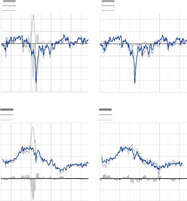
Figure 10: Monetary policy contributions to 1-year ahead GaR and inﬂation for short- and

long-end factor

‐8

‐6

‐4

‐2

2001M12 2005M12 2009M12 2013M12 2017M12

CumulatedshortMPcontribution

Growth‐at‐Risk(1yearahead)

GaRnetofmonetarypolicycontribution

‐2

‐1

2001M12 2005M12 2009M12 2013M12 2017M12

CumulatedshortMPcontribution

Medianannualinflationforecast(1‐yearahead)

InflationforecastnetofMPcontribution

‐2

‐1

2001M12 2005M12 2009M12 2013M12 2017M12

CumulatedlongMPcontribution

Medianannualinflationforecast(1‐yearahead)

InflationforecastnetofMPcontribution

‐8

‐6

‐4

‐2

2001M12 2005M12 2009M12 2013M12 2017M12

CumulatedlongMPcontribution

Growth‐at‐Risk(1yearahead)

GaRnetofmonetarypolicycontribution

Notes: This ﬁgure shows the forecasts for one year ahead GaR and median annual HICP inﬂation

together with the contribution of monetary policy shocks over time. The monetary policy contributions

are constructed as the 12-month cumulative impact of the individual monetary policy surprises in each

of these months multiplied with the estimated impulse response function of the relevant horizon. They

are thus conditional on the macro-ﬁnancial information up to a point t, but conditional on the monetary

policy surprises from t to t + 12.

during the Global Financial Crisis, the long-rate factor had more limited eﬀects on GaR and

median inﬂation forecasts, as can be seen from the right panels in Figure 10. The contributions

are not only smaller in comparison to those from the short-end factor, but alternate sign more

frequently. Up until 2014, eﬀects were in the range of up to one percentage point for GaR and

0.5 percentage points for median inﬂation, but became more muted since then.

ECB Working Paper Series No 2870

6.2 Monetary policy and stabilization trade-oﬀs

The contributions of monetary policy surprises to GDP Growth-at-Risk and HICP inﬂation serve

as a basis for assessing monetary policy trade-oﬀs while pursuing a price stability objective. We

illustrate how monetary policy could stabilize median inﬂation at the price stability objective

of 2% and how such a stabilization compares to a policy that would stabilize GaR at its long-

run mean. The sign and size of the required stabilizing policy will depend on the state of the

economy in deviations from the respective inﬂation and GaR objective and the eﬀectiveness

with which the policy instruments can achieve these objectives. A larger policy innovation is

needed if current forecasts strongly deviate from the objective or if the policy instrument is less

eﬀective in bringing the economy back to the objective.

Figure 11: Short-end monetary policy shocks needed to stabilise GaR and 1-year ahead

median inﬂation forecasts

-15

-10

-5

-15 -10 -5 0 5 10

Monetary policy shock to stabilize HICP

inflation

Monetary policy shock to stabilize GaR(10)

2002-2004 2005-2007 2008-2009 2010-2019

Notes: The monetary policy changes required to stabilize median HICP inﬂation and the 10th per-

centile of GDP growth are in standard deviations of the monetary policy innovations. Positive values

imply a required tightening and negative values a required loosening of short-term rates.

Figure 11 illustrates the necessary size of the short-term interest rate factor to stabilize 1-

year ahead forecasts of median inﬂation at 2% (vertical axis) and of GaR at its sample average

of -1.08% (horizontal axis). Observations in the upper right quadrant indicate that a tightening

of short-term rate would have helped to jointly stabilize price inﬂation and GaR objective. This

ECB Working Paper Series No 2870

concerns primarily the period leading up to the Global Financial Crisis (2005–2007). In turn,

observations in the lower left quadrant would have implied a loosening to bring the variables

towards their objectives, but there have been only few of such instances over the sample period.

For the observations in the upper left quadrant, instead, policy prescriptions would have implied

a monetary policy tightening to stabilize inﬂation, but a loosening to raise GaR towards its tar-

get, relevant during the height of the Global Financial Crisis (2008–2009). For the observations

in the bottom right quadrant, a loosening of monetary policy would have been needed to raise

inﬂation towards its 2% objective, but a tighter policy would have helped to stabilize GaR.

The numerous observations in this bottom right quadrant indicate that monetary policy faced

an inﬂation-GaR trade-oﬀ for most of the post-crisis period. In such a trade-oﬀ situation, an

additional policy instrument could complement and support monetary policy to stabilize the

macroeconomy. Such policies may be ﬁscal or structural policies for the economic dimension, or

macroprudential policy for the ﬁnancial dimension.

6.3 Relative eﬃciency of monetary and macroprudential policy

Our estimation framework can capture an important role for macroprudential policy in comple-

menting monetary policy in its eﬀorts to stabilize the macroeconomy. The use of macroprudential

policy would be most eﬀective if it was complementary to monetary policy in stabilizing median

inﬂation and GaR. To assess the relative eﬃciency of the two policies, we consider the policy

interventions that are necessary to bring one-year ahead median inﬂation to 2% or to stabilize

GaR at its historical average of -1.08%. In the empirical speciﬁcations, monetary policy is cap-

tured by the short- or the long-factor of risk-free interest rates, and macroprudential policy is

captured by the SRI.

In order to make the size of the two policies comparable, we divide both

measures by their historical standard deviation. The results on the relative eﬃciency hinge on

the standard deviation of historical surprises in the short- and long-factor and in the SRI.

The cumulated impulse responses of the policy variables reveal that, to stabilize 1-year

ahead GaR, a one-standard deviation of monetary policy achieves the same stabilization as

1.39 standard deviations of the SRI. When considering the long-term factor of interest rates, the

relative eﬃciency to stabilize GaR is 0.42 which implies that macroprudential policy is more than

twice as eﬀective relative to the long-rate factor. Taken together, the short-term interest rate

factor is more eﬃcient relative to macroprudential policy and macroprudential policy is more

This implicitly assumes that macroprudential policy makers can freely adjust the level of vulnerabilities.

ECB Working Paper Series No 2870

eﬀective than the long term factor in stabilising GaR. When assessing the relative eﬀectiveness

in stabilizing median inﬂation based on the cumulative impulse responses, we ﬁnd that the short

factor is 1.3 times more eﬀective than the SRI and the long-rate factor is as eﬀective as the SRI

(factor of 1.0).

The estimation indicates that the short factor is the most eﬃcient instrument not only to

stabilize GaR but also inﬂation. However the diﬀerences in eﬀectiveness are larger for GaR

than for inﬂation. When considering a potential assignment of policy instruments to policy

objectives, the relative eﬀectiveness in stabilizing one or the other variable becomes key (Fahr

and Fell, 2017). Using the eﬀectiveness of the SRI as a reference point, the short-term rate

is 1.07 (=1.39/1.30) times more eﬀective in stabilising GaR relative to inﬂation. In turn, the

long-rate factor is only 0.42 (=0.42/1.00) times as eﬀective to stabilize GaR relative to inﬂation,

which implies that in relative terms the long-rate stabilizes inﬂation with least impact on GaR.

The relative eﬃciency itself does not yet provide us with the indications on the speciﬁc timing

for using either of the two policies. The complementarity comes to the fore when monetary policy

is constrained by a trade-oﬀ between stabilizing inﬂation and GaR, as captured in the top-left

and bottom-right corner of Figure 11. In those situations, the adjustment of macroprudential

policy can help to reduce the trade-oﬀ for monetary policy.

6.4 Monetary and macroprudential policy for stabilizing inﬂation and Growth-

at-Risk

Having established the relative eﬃciency of diﬀerent policy tools, we illustrate how the estima-

tion results could inform monetary and macroprudential policy to enhance stabilization over the

sample period. We assume policy objectives of 2% median inﬂation one year ahead and stabi-

lization of GaR at its sample average of -1.08%. Given the relative eﬃciencies ,the policymaker

uses monetary policy (long-end interest rate factor) and macroprudential policy (SRI). The GaR

objective is non-symmetric, implying that the policymaker avoids GaR falling below the value

of -1.08% while focusing solely on the objective of inﬂation otherwise. The policymakers thus

provides a hedge against crisis outcomes.

Figure 12 displays results from this exercise. We ﬁnd that relatively large monetary policy

shocks would have been needed to bring inﬂation forecasts back to their target over the period

from 2005 until the ﬁrst half of 2009. In contrast, over the earlier as well as later parts of the

sample period our results would have called for looser monetary policy as inﬂation forecasts

ECB Working Paper Series No 2870

Figure 12: Monetary- and macroprudential policy mix for joint inﬂation and Growth-at-Risk

targets.

Left: policy shocks. Right: forecasts conditional on policy shocks

-20

-15

-10

-5

04/2002

04/2003

04/2004

04/2005

04/2006

04/2007

04/2008

04/2009

04/2010

04/2011

04/2012

04/2013

04/2014

04/2015

04/2016

04/2017

04/2018

04/2019

long-end shock

dSRI shock

0.0

0.1

0.2

0.3

0.4

0.5

0.6

-1.5

-1.0

-0.5

0.0

0.5

1.0

1.5

2.0

2.5

04/2002

04/2003

04/2004

04/2005

04/2006

04/2007

04/2008

04/2009

04/2010

04/2011

04/2012

04/2013

04/2014

04/2015

04/2016

04/2017

04/2018

04/2019

GaR(10)

HICP 0.5

dSRI 0.5

CISS 0.9 (rhs)

Notes: Left: This panel shows long-end and SRI shocks (in standard deviations) required to simul-

taneously achieve a 2% one-year ahead HICP inﬂation forecast while ensuring GaR above its sample

average of -1.08%. Positive shocks indicate tightening for monetary policy but loosening for macro-

prudential policy. Right: This panel shows one-year ahead forecasts conditional on the policy shocks

from the left panel. We show median forecasts for inﬂation and SRI, GaR and the 90th percentile

forecast for the CISS.

from our models were consistently below their 2% target. Looser macroprudential policy (SRI)

would have been needed starting in September 2007 and throughout the Global Financial Crisis

until September 2009 and again on a few occasions during the euro area debt crisis. Forecasts

implied by these policy counterfactuals show that they would have been eﬀective in meeting

their targets, while eﬀectively limiting ﬁnancial stress.

7 Conclusions

Our empirical analysis focused on the interaction of monetary policy shocks, ﬁnancial stability

conditions and the real economy in the euro area. The quantile vector autoregressive model,

using two estimation techniques and ﬁve variables, estimates the entire distribution of real and

ﬁnancial variables. The setup allows for quantitatively assessing monetary policy trade-oﬀs.

One such trade-oﬀ involves two diﬀerent policy goals and is captured by interactions between

macro variables, such as inﬂation and GDP growth, and ﬁnancial stability as measured by

ﬁnancial stress and vulnerabilities. A second trade-oﬀ is of intertemporal nature and diﬀerenti-

ates between the potential impact of monetary policy on short-term ﬁnancial stress relative to

ECB Working Paper Series No 2870

adjustments to ﬁnancial vulnerabilities in the medium term.

Our speciﬁcations consider not only the short-term interest rates as a policy tool, but also

changes in the longer term rates, so as to capture eﬀects from forward guidance and asset

purchases of medium- to long-term securities. To identify monetary policy shocks, our empirical

strategy considers surprises in risk-free interest rates in a narrow time window around the

communication of ECB monetary policy decisions and further separates between information

and monetary policy shocks.

We ﬁnd that surging ﬁnancial stress has a strong short-term impact on the lower tail of the

GDP distribution. In turn, a build-up of ﬁnancial vulnerabilities tends to be followed by sub-

dued ﬁnancial stress initially, but vulnerabilities rise again over the medium term. Furthermore,

tightening conventional monetary policy reduces inﬂationary pressures (and real GDP growth)

at the cost of increasing ﬁnancial stress. Changes in the long-term interest rates induced by

unconventional monetary policy, on the other hand, are equally eﬀective in bringing down inﬂa-

tion but have a relatively smaller adverse impact on growth and ﬁnancial stress while ﬁnancial

vulnerabilities mildly recede.

Our quantitative assessment of monetary policy using counterfactuals sheds light on mon-

etary policy trade-oﬀs. During the global ﬁnancial crisis, monetary policy would have had to

either tighten to stabilize inﬂation forecasts at 2% or loosen to prevent Growth-at-Risk to de-

teriorate. Our analysis thus indicates the potentially beneﬁcial use of an alternative policy and

we show how macroprudential tools - through their impact on ﬁnancial vulnerabilities - can

be deployed eﬀectively in a complementary way to stabilize the ﬁnancial system and macro

economy.

ECB Working Paper Series No 2870

References

Adrian, T., N. Boyarchenko, and D. Giannone (2019). Vulnerable growth. American Economic

Review 109, 1263–1289.

Adrian, T., F. Grinberg, N. Liang, and S. Malik (2018). The term structure of growth-at-risk.

IMF Working paper 18/180 . International Monetary Fund.

Adrian, T. and N. Liang (2018). Monetary policy, ﬁnancial conditions, and ﬁnancial stability.

International Journal of Central Banking 14(1), 73–131.

Aikman, D., J. Bridges, S. H. Hoke, C. O’Neill, and A. Raja (2019). Credit, capital and crises:

a gdp-at-risk approach. Bank of England Staﬀ Working Paper No. 824.

Ajello, A., N. Boyarchenko, F. Gourio, and A. Tambalotti (2022). Financial stability considera-

tions for monetary policy: Theoretical mechanisms. Federal Reserve Bank of New York Staﬀ

Reports No. 1002.

Altavilla, C., L. Brugnolini, R. S. G¨urkaynak, R. Motto, and G. Ragusa (2019). Measuring euro

area monetary policy. Journal of Monetary Economics 108, 162–179.

Bekaert, G., M. Hoerova, and M. L. Duca (2013). Risk, uncertainty and monetary policy. Journal

of Monetary Economics 60 (7), 771–788.

Bernanke, B. S. and F. S. Mishkin (1997). Inﬂation targeting: a new framework for monetary

policy? Journal of Economic perspectives 11 (2), 97–116.

Boyarchenko, N., G. Favara, and M. Schularick (2022). Financial stability considerations for

monetary policy: Empirical evidence and challenges. Federal Reserve Finance and Economics

Discussion Series No. 2022-006.

Carney, M. (2020). The grand unifying theory (and practice) of macroprudential policy. Speech

at University College London.

Cecchetti, S. G. (2006). The brave new world of central banking: Policy challenges posed by

asset price booms and busts. National Institute Economic Review 196, 107–119.

ECB Working Paper Series No 2870

Chavleishvili, S., R. F. Engle, S. Fahr, M. Kremer, S. Manganelli, and B. Schwaab (2021). The

risk management approach to macro-prudential policy. Working Paper Series 2565, European

Central Bank.

Chavleishvili, S. and M. Kremer (2021). Measuring Systemic Financial Stress and its Impact on

the Macroeconomy. SSRN Working Paper.

Chavleishvili, S. and S. Manganelli (2019). Forecasting and stress testing with quantile vector

autoregression. ECB Working paper No. 2223. European Central Bank.

Clarida, R., J. Gali, and M. Gertler (1999). The science of monetary policy: a new keynesian

perspective. Journal of economic literature 37 (4), 1661–1707.

Doh, T. and A. Foerster (2022, December). Have Lags in Monetary Policy Transmission Short-

ened? Economic Bulletin (December), 1–3.

Duprey, T. and T. Roberts (2017). A barometer of canadian ﬁnancial system vulnerabilities.

BoC Staﬀ Analytical Note No. 2017-24. Bank of Canada.

Duprey, T. and A. Ueberfeldt (2018). How to manage macroeconomic and ﬁnancial stability

risks: A new framework. Staﬀ Analytical Note No. 2018-11.

European Central Bank (2021). The role of ﬁnancial stability considerations in monetary policy

and the interaction with macroprudential policy in the euro area. ECB Occasional Paper No.

272.

Fahr, S. A. and J. P. Fell (2017). Macroprudential policy – closing the ﬁnancial stability gap.

Journal of Financial Regulation and Compliance 25, 334–359.

Figueres, J. M. and M. Jaroci´nski (2020). Vulnerable growth in the euro area: Measuring the

ﬁnancial conditions. Economics Letters 191, 109–126.

Gilchrist, S. and E. Zakrajˇsek (2012). Credit spreads and business cycle ﬂuctuations. American

Economic Review 102 (4), 1692–1720.

Giuzio, M., C. Kaufmann, E. Ryan, and L. Cappiello (2021). Investment funds, risk-taking, and

monetary policy in the euro area. ECB Working Paper No. 2605. European Central Bank.

ECB Working Paper Series No 2870

G¨urkaynak, R. S., B. Sack, and E. T. Swanson (2005). Do actions speak louder than words? the

response of asset prices to monetary policy actions and statements. International Journal of

Central Banking 1, 55–93.

Han, H., W. Jung, and J. H. Lee (2022). Estimation and Inference of Quantile Impulse Response

Functions by Local Projections: With Applications to VaR Dynamics. Journal of Financial

Econometrics 2022, 1–29.

Hollo, D., M. Kremer, and M. Lo Duca (2012). CISS – a composite indicator of systemic stress

in the ﬁnancial system. ECB Working paper No. 1426. European Central Bank.

Jaroci´nski, M. and P. Karadi (2020). Deconstructing Monetary Policy Surprises—The Role of

Information Shocks. American Economic Journal: Macroeconomics 12, 1–43.

Jord`a,

O. (2005). Estimation and inference of impulse responses by local projections. American

economic review 95 (1), 161–182.

Jord`a,

O., M. Schularick, and A. Taylor (2015). Leveraged bubbles. Journal of Monetary

Economics 76 (S), S1–S20.

Kilian, L. (2009). Not all oil price shocks are alike: Disentangling demand and supply shocks in

the crude oil market. American Economic Review 99 (3), 1053–1069.

Kilian, L. and S. Manganelli (2008). The central banker as a risk manager: Estimating the

federal reserve’s preferences under greenspan. Journal of Money, Credit and Banking 40 (6),

1103–1129.

Kockerols, T. and C. Kok (2019). Leaning against the wind: Macroprudential policy and the

ﬁnancial cycle. ECB Working paper No. 2223. European Central Bank.

Koenker, R. (2005). Quantile Regression. Cambridge University Press.

Koenker, R. and G. Bassett Jr (1978). Regression quantiles. Econometrica: Journal of the

Econometric Society, 33–50.

Koenker, R., V. Chernozhukov, X. He, and L. Peng (2018). Handbook of Quantile Regression.

Chapman & Hall/CRC Handbooks of Modern Statistical Methods. CRC Press.

ECB Working Paper Series No 2870

Koenker, R. and Z. Xiao (2006). Quantile autoregression. Journal of the American statistical

association 101 (475), 980–990.

Kuttner, K. N. (2001). Monetary policy surprises and interest rates: Evidence from the fed

funds futures market. Journal of Monetary Economics 47 (3), 523–544.

Lang, J. H., C. Izzo, S. Fahr, and J. Ruzicka (2019). Anticipating the bust: a new cyclical

systemic risk indicator to assess the likelihood and severity of ﬁnancial crises. ECB Occasional

Paper No. 219. European Central Bank.

Mishkin, F. S. (2007). Financial instability and monetary policy. Speech at the Risk USA 2007

Conference, New York City, NY.

Mishkin, F. S. (2009). Is monetary policy eﬀective during ﬁnancial crises? American Economic

Review 99 (2), 573–577.

Montes-Rojas, G. (2022). Estimating Impulse-Response Functions for Macroeconomic Models

using Directional Quantiles. Journal of Time Series Econometrics 14 (2), 199–225.

Plagborg-Møller, M. and C. K. Wolf (2021). Local Projections and VARs Estimate the Same

Impulse Responses. Econometrica 89 (2), 955–980.

Ruzicka, J. (2021a). Quantile local projections: Identiﬁcation, smooth estimation, and inference.

mimeo, Universidad Carlos III de Madrid.

Ruzicka, J. (2021b). Quantile structural vector autoregression. mimeo, Universidad Carlos III

de Madrid.

Schularick, M., L. Ter Steege, and F. Ward (2021). Leaning against the wind and crisis risk.

American Economic Review: Insights 3 (2), 199–214.

Schwarz, G. (1978). Estimating the Dimension of a Model. The Annals of Statistics 6 (2),

461–464.

Sims, C. A. (1980). Macroeconomics and reality. Econometrica 48 (1), 1–48.

Smets, F. (2014). Financial stability and monetary policy: How closely interlinked? Interna-

tional Journal of Central Banking 10 (2), 263–300.

ECB Working Paper Series No 2870

Svensson, L. E. O. (2017). Cost-beneﬁt analysis of leaning against the wind. Journal of Monetary

Economics 90, 193–213.

White, H., T.-H. Kim, and S. Manganelli (2015). VAR for VaR: Measuring tail dependence

using multivariate regression quantiles. Journal of Econometrics 187 (1), 169–188.

ECB Working Paper Series No 2870

A Appendix

A.1 Additional results

Figure A.1: Impulse Responses of information shock on short-term rates

(estimated by simulation)

monthly GDP response (cumulative)

0.0

0.1

0.2

1 SD FShort − INFO shock

HICP inf. response (cumulative)

−0.05

0.00

0.05

0.10

SRI response

−0.005

0.000

0.005

0.010

0.015

0.020

CISS response

−0.02

−0.01

0.00

0.01

0.02

0.0

0.1

0.2

0.3

0.4

0.5

1 SD monthly GDP shock

0.00

0.04

0.08

0.12

−0.005

0.000

0.005

−0.02

−0.01

0.00

0.01

−0.10

−0.05

0.00

0.05

0.10

1 SD HICP inf. shock

0.00

0.05

0.10

0.15

0.20

0.25

−0.015

−0.010

−0.005

0.000

0.005

0.010

−0.02

−0.01

0.00

0.01

0.0

0.1

0.2

0.3

0.4

1 SD SRI shock

0.00

0.05

0.10

0.15

0.000

0.025

0.050

0.075

−0.05

−0.04

−0.03

−0.02

−0.01

0.00

−0.4

−0.3

−0.2

−0.1

0.0

0 3 6 9 12

month

1 SD CISS shock

−0.10

−0.05

0.00

0.05

0 3 6 9 12

month

−0.015

−0.010

−0.005

0.000

0.005

0 3 6 9 12

month

0.00

0.02

0.04

0.06

0.08

0 3 6 9 12

month

quantile

0.1 0.5 0.9

Notes: Five-variable speciﬁcation with response of information shock variable excluded. Conﬁdence bands are at

90% and are excluded for the median response.

ECB Working Paper Series No 2870

Figure A.2: Impulse Responses of information shock on short-term rates

(estimated by local projections)

monthly GDP response (cumulative)

−0.2

0.0

0.2

1 SD FShort − INFO shock

HICP inf. response (cumulative)

−0.2

−0.1

0.0

0.1

0.2

SRI response

0.000

0.005

0.010

0.015

0.020

0.025

CISS response

−0.04

−0.02

0.00

0.02

0.04

0.0

0.2

0.4

0.6

1 SD monthly GDP shock

0.0

0.1

0.2

−0.01

0.00

−0.04

−0.02

0.00

0.02

0.04

0.06

−0.3

−0.2

−0.1

0.0

0.1

1 SD HICP inf. shock

0.0

0.1

0.2

0.3

−0.01

0.00

0.01

−0.02

0.00

0.02

0.0

0.1

0.2

0.3

1 SD SRI shock

0.0

0.1

0.00

0.02

0.04

0.06

−0.06

−0.04

−0.02

0.00

−0.6

−0.4

−0.2

0.0

0 3 6 9 12

month

1 SD CISS shock

−0.2

−0.1

0.0

0.1

0 3 6 9 12

month

0.00

0.01

0.02

0 3 6 9 12

month

0.00

0.02

0.04

0.06

0.08

0 3 6 9 12

month

quantile

0.1 0.5 0.9

Notes: Five-variable speciﬁcation with response of information shock variable excluded. Conﬁdence bands are at

90% and are excluded for the median response.

ECB Working Paper Series No 2870

Figure A.3: Impulse Responses of information shock on long-term rates

(estimated by simulation)

monthly GDP response (cumulative)

0.0

0.1

0.2

1 SD FLong − INFO shock

HICP inf. response (cumulative)

0.00

0.05

0.10

SRI response

−0.005

0.000

0.005

0.010

CISS response

−0.04

−0.03

−0.02

−0.01

0.00

0.01

0.0

0.2

0.4

0.6

1 SD monthly GDP shock

0.00

0.05

0.10

−0.010

−0.005

0.000

0.005

−0.01

0.00

0.01

−0.10

−0.05

0.00

0.05

0.10

1 SD HICP inf. shock

0.0

0.1

0.2

−0.010

−0.005

0.000

0.005

0.010

−0.01

0.00

0.01

0.0

0.1

0.2

0.3

0.4

1 SD SRI shock

0.00

0.05

0.10

0.15

0.000

0.025

0.050

0.075

−0.05

−0.04

−0.03

−0.02

−0.01

0.00

−0.3

−0.2

−0.1

0.0

0 3 6 9 12

month

1 SD CISS shock

−0.10

−0.05

0.00

0.05

0 3 6 9 12

month

−0.010

−0.005

0.000

0.005

0.010

0 3 6 9 12

month

0.00

0.02

0.04

0.06

0 3 6 9 12

month

quantile

0.1 0.5 0.9

Notes: Five-variable speciﬁcation with response of information shock variable excluded. Conﬁdence

bands are at 90% and are excluded for the median response.

ECB Working Paper Series No 2870

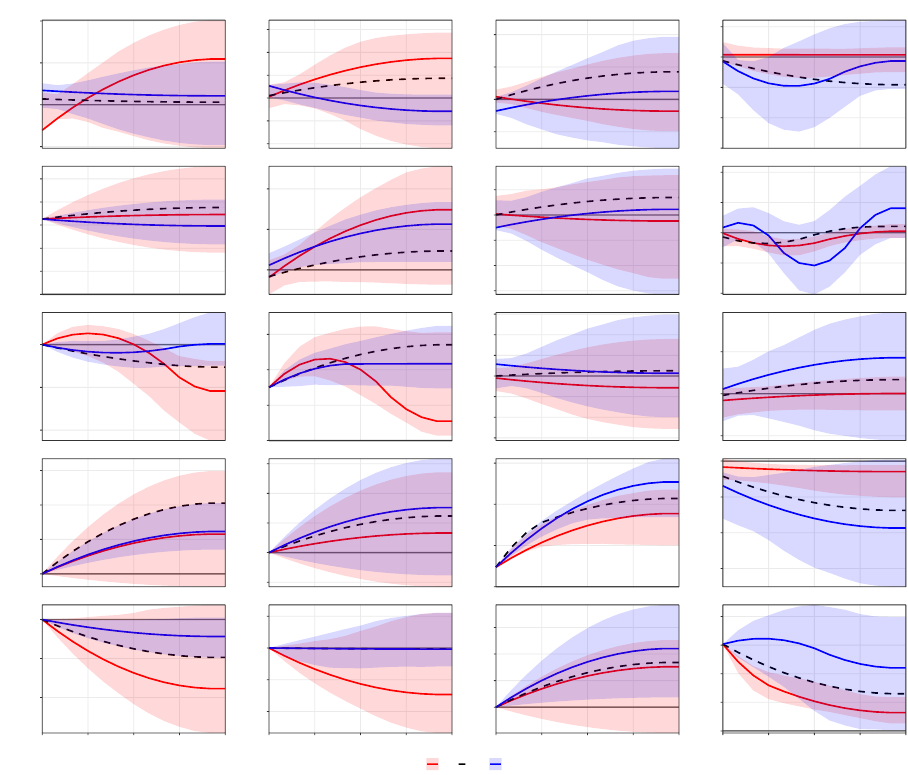
Figure A.4: Impulse Responses of information shock on long-term rates

(estimated by local projections)

monthly GDP response (cumulative)

−0.2

0.0

0.2

0.4

1 SD FLong − INFO shock

HICP inf. response (cumulative)

−0.2

−0.1

0.0

0.1

0.2

0.3

SRI response

−0.01

0.00

0.01

0.02

CISS response

−0.075

−0.050

−0.025

0.000

0.025

0.0

0.1

0.2

0.3

0.4

0.5

1 SD monthly GDP shock

0.0

0.1

0.2

−0.015

−0.010

−0.005

0.000

0.005

−0.06

−0.03

0.00

0.03

0.06

−0.4

−0.2

0.0

1 SD HICP inf. shock

0.0

0.1

0.2

0.3

−0.015

−0.010

−0.005

0.000

0.005

0.010

0.015

−0.02

0.00

0.02

0.0

0.1

0.2

0.3

1 SD SRI shock

−0.05

0.00

0.05

0.10

0.15

0.00

0.02

0.04

0.06

−0.06

−0.04

−0.02

0.00

−0.4

−0.2

0.0

0 3 6 9 12

month

1 SD CISS shock

−0.2

−0.1

0.0

0.1

0 3 6 9 12

month

0.000

0.005

0.010

0.015

0 3 6 9 12

month

0.00

0.02

0.04

0.06

0.08

0 3 6 9 12

month

quantile

0.1 0.5 0.9

Notes: Five-variable speciﬁcation with response of information shock variable excluded. Conﬁdence

bands are at 90% and are exluded for the median response.

A.2 Representing a sequence of external interventions – proof

We need to show

k=0

j,t+k



∀m ∈ {0, 1, . . . , 11}: ε

i,t+m

) := ε

i,t+m

) + s

−Q

k=0

j,t+k

l=0

QIRC(j, i, l, τ, s

11−l

)

ECB Working Paper Series No 2870

First, we rewrite the expression as a telescoping sum. Second, we use the history independence

property of quantile impulse response functions (4). Third, using the linearity of quantile impulse

response functions (4), we express the diﬀerence between the two quantiles as the derivative of

a conditional quantile. Finally, u

i,t+l

is independent of y

j,t+k

for k < l, so we can eliminate the

ﬁrst l − 1 terms from the sum.

k=0

j,t+k



∀m ∈ {0, 1, . . . , 11}: ε

i,t+m

) := ε

i,t+m

) + s

−Q

k=0

j,t+k

(14)

l=0

k=0

j,t+k



∀m ∈ {0, 1, . . . , l}: ε

i,t+m

) := ε

i,t+m

) + s

(15)

− Q

k=0

j,t+k



∀m ∈ {0, 1, . . . , l − 1}: ε

i,t+m

) := ε

i,t+m

) + s

(16)

l=0

k=0

j,t+k



∀u

i,t+l

∈ [0, 1]: ε

i,t+l

) := ε

i,t+l

) + s

−Q

k=0

j,t+k

(17)

l=0

∂Q

k=0

j,t+k



i,t+l

∂ε

i,t+l

)

l=0

∂Q

k=l

j,t+k



i,t+l

∂ε

i,t+l

)

(18)

l=0

QIRC(j, i, 11 − l, τ, s

) =

l=0

QIRC(j, i, l, τ, s

11−l

) (19)

ECB Working Paper Series No 2870

A.3 Representing a counterfactual scenario – proof

We need to show

k=0

j,t+k



t−1

, ∀m ∈ {0, 1, . . . , 11}: ε

i,t+m

) := ε

i,t+m

) + s

k=0

j,t+k



t−1

l=0

QIRC(j, i, l, τ, s

11−l

)

(20)

First, we subtract and add the quantile forecast. The second equality follows by the same

arguments as in the proof (A.2). The third equality is due to the history independence property

of quantile impulse response functions (4).

k=0

j,t+k



t−1

, ∀m ∈ {0, 1, . . . , 11}: ε

i,t+m

) := ε

i,t+m

) + s

= (21)

k=0

j,t+k



t−1

, ∀m ∈ {0, 1, . . . , 11}: ε

i,t+m

) := ε

i,t+m

) + s

(22)

− Q

k=0

j,t+k



t−1

k=0

j,t+k



t−1

= (23)

l=0

∂Q

k=l

j,t+k



t−1

, u

i,t+l

∂ε

i,t+l

)

+ Q

k=0

j,t+k



t−1

= (24)

l=0

∂Q

k=l

j,t+k



i,t+l

∂ε

i,t+l

)

+ Q

k=0

j,t+k



t−1

= (25)

k=0

j,t+k



t−1

l=0

QIRC(j, i, l, τ, s

11−l

) (26)

ECB Working Paper Series No 2870

Acknowledgements

The views expressed in this paper are those of the authors and do not necessarily reﬂect the views of the European Central Bank.

Paul Bochmann

European Central Bank, Frankfurt am Main, Germany; email: paul.bochmann@ecb.europa.eu

Daniel Dieckelmann

European Central Bank, Frankfurt am Main, Germany; email: daniel.[email protected]ropa.eu

Stephan Fahr

European Central Bank, Frankfurt am Main, Germany; email: stephan.fahr@ecb.europa.eu

Josef Ruzicka

Nazarbayev University, Astana, Kazakhstan; email: josef.ruzicka@nu.edu.kz

Postal address 60640 Frankfurt am Main, Germany

Telephone +49 69 1344 0

Website www.ecb.europa.eu

electronically, in whole or in part, is permitted only with the explicit written authorisation of the ECB or the authors.

This paper can be downloaded without charge from www.ecb.europa.eu, from the Social Science Research Network electronic library or

from RePEc: Research Papers in Economics. Information on all of the papers published in the ECB Working Paper Series can be found

on the ECB’s website.

PDF ISBN 978-92-899-6247-6 ISSN 1725-2806 doi:10.2866/271025 QB-AR-23-107-EN-N