Weathering Cash Flow Shocks

∗

James R. Brown

†

Matthew T. Gustafson

‡

Ivan T. Ivanov

9/7/2017

Abstract

We show that unexpectedly severe winter weather, which is arguably exogenous to

ﬁrm and bank fundamentals, represents a signiﬁcant cash ﬂow shock for the average

bank-borrowing ﬁrm. Firms respond to such shocks by increasing credit line use, but

do not signiﬁcantly adjust cash reserves, non-cash working capital, or real activities.

The increased credit line use occurs within one calendar quarter of the cash ﬂow shock

and is accompanied by an increase in credit line size, for all but the most distressed

borrowers. These results highlight the role of banks in mitigating transitory cash ﬂow

shocks to ﬁrms.

∗

The views stated herein are those of the authors and are not necessarily the views of the Federal

Reserve Board or the Federal Reserve System. We thank Heitor Almeida, Mitchell Berlin, Mark Carey,

Kristle Romero Cortes, Christopher James, Kathleen Johnson, Ralf Meisenzahl, Atanas Mihov, Joe Nichols,

Ben Ranish, Robert Sarama, Antoinette Schoar, Phillip Strahan, Nathan Swem, Bastian von Beschwitz,

James Wang and seminar participants at the 13th Annual Conference on Corporate Finance at Washington

University in St. Louis, the 2017 SFS Cavalcade, the Federal Reserve Board, the Federal Reserve Bank of

Philadelphia, the FDIC, Iowa State University, Penn State University, and the SEC for helpful comments.

†

Iowa State University, College of Business, 3331 Gerdin Business Building, Ames, IA 50011; 515-294-

4668; [email protected].

‡

Smeal College of Business, Penn State University, State College, PA 16801, USA; +1-814-867-4042;

m[email protected].

Federal Reserve Board, 20th Street and Constitution Avenue NW, Washington, DC, 20551; 202-452-

2987; ivan.t.iv[email protected]v.

1 Introduction

Despite the extensive literature emphasizing the unique advantages of banks as liquidity

providers (e.g., Kashyap, Rajan, and Stein (2002); Gatev and Strahan (2006)), there is little

empirical evidence on how bank-dependent ﬁrms manage idiosyncratic cash ﬂow shocks. One

challenge is the lack of data on the ﬁnancing activities of private ﬁrms, which leads most prior

research to study liquidity management in larger publicly-traded ﬁrms (e.g., Suﬁ (2009)).

Another challenge is that it is diﬃcult to isolate cash ﬂow variation that is exogenous to

ﬁrm-level investment opportunities and unrelated to the health of ﬁnancial intermediaries.

In this paper we introduce a new dataset and a unique empirical setting to overcome

these challenges and provide new evidence on the extent to which ﬁrms rely on bank ﬁnanc-

ing to mitigate the eﬀects of idiosyncratic cash ﬂow shocks. The dataset we employ, which

is only recently available and collected by the Federal Reserve, contains detailed information

on bank loan contracts, including credit line limits, credit line drawn amount, and a range

of borrower (ﬁrm) characteristics. Because the data collection covers the full set of ﬁrms

in a bank’s loan portfolio with outstanding loan commitments of at least $1 million, we

observe a much broader cross-section of borrowers than most other research on corporate

liquidity management. In particular, our sample is largely comprised of private ﬁrms, which

tend to be particularly dependent on bank ﬁnancing (e.g., Robb and Robinson (2014)). For

example, in our sample the average credit line is 24% of total assets, which is approximately

50% larger than the average for the publicly traded ﬁrms studied in Suﬁ (2009). Thus, this

sample oﬀers a unique opportunity to study the eﬀects of cash ﬂow volatility in a broad

sample of private ﬁrms, and to directly evaluate how the borrowers that are most reliant on

credit lines use them to manage liquidity.

To break the endogenous link between cash ﬂow and factors such as investment op-

portunities or the ﬁnancial health of intermediaries, we introduce abnormally severe local

winter weather as a shock to corporate cash ﬂows. We obtain data on winter weather at

the county level from the National Oceanic and Atmospheric Administration (NOAA). We

ﬁnd that abnormally-severe weather in the ﬁrst calendar quarter signiﬁcantly aﬀects total

annual ﬁrm-level cash ﬂows. For example, a two standard deviation increase in abnormal

winter snow cover in a given county reduces the annual cash ﬂow of ﬁrms headquartered

in that county by 0.36% of total assets. Partitioning by industry reveals that this negative

relation between snow cover and cash ﬂow exists in all 8 sectors that each comprise over 3%

of our sample, with the eﬀect being statistically signiﬁcant at the 10% level or better for the

transportation, manufacturing, wholesale and construction industries. This result provides

large scale support for anecdotal and sector-speciﬁc evidence that severe weather adversely

aﬀects ﬁrm performance (e.g., Tran (2016)).

We use the abnormal winter snow cover in the county of a ﬁrm’s headquarters as an

instrumental variable (IV) for cash ﬂow to investigate how ﬁrms manage cash ﬂow shocks.

The exclusion restriction is that severe weather aﬀects corporate liquidity management only

through its eﬀect on cash ﬂow. The temporary nature of severe winter weather makes this

assumption plausible. A typical winter storm is unlikely to aﬀect investment opportunities

or access to capital, except through its eﬀect on cash ﬂows. The most severe winter weather

events may aﬀect investment opportunities for reasons other than reduced cash ﬂows. Such

events do not drive our results as our ﬁndings are similar after trimming our measures of

abnormal snow cover.

Two-stage least squares (2SLS) regressions reveal an economically large and statistically

signiﬁcant negative relation between cash ﬂow and credit line drawdowns. The coeﬃcient

estimates suggest that annual credit line drawdowns increase by between 41 and 61 cents

for every $1 reduction in annual cash ﬂow. In addition, the IV estimates indicate a sig-

niﬁcant negative relation between cash ﬂow and changes in credit line limits. On average,

we estimate that the end of year credit limit increases by between 74 cents and $1 and 13

cents for every $1 reduction in ﬁrm cash ﬂow. Together, these results show that ﬁrms with

existing lending relationships rely extensively on credit lines to manage liquidity, and that

banks accommodate these ﬁrms by adjusting credit line limits.

These ﬁndings suggest that the average bank-reliant ﬁrm uses credit lines as their pri-

mary means of managing liquidity shocks. In contrast, survey evidence in Lins, Servaes,

and Tufano (2010) suggests that larger ﬁrms use cash to hedge against potential cash ﬂow

shortfalls, reserving credit line use primarily to pursue investment opportunities. To in-

vestigate whether ﬁrms in our sample also use cash to buﬀer weather induced cash ﬂow

shocks, we employ the same IV approach with the change in cash holdings as the second

stage dependent variable. We ﬁnd a positive but statistically insigniﬁcant relation between

exogenous cash ﬂow shocks and changes in cash, suggesting that cash balances decrease by

approximately 20 cents for every $1 decrease in annual cash ﬂow. We also ﬁnd a similarly

sized but insigniﬁcant relation between cash ﬂows and changes in non-cash working capital.

Importantly, we ﬁnd no evidence that cash ﬂow shocks signiﬁcantly aﬀect the accumulation

of either ﬁxed or total assets. Thus, the ﬁrms we study fully shield real investment from

cash ﬂow shocks, primarily via credit line adjustments.

In our ﬁnal set of tests, we estimate the direct relation between abnormal winter snow

cover and corporate outcomes. Consistent with our two-stage estimates, abnormal snow

cover is positively and signiﬁcantly related to changes in credit line draws and credit line

size, but not to other corporate outcomes. A two standard deviation increase in ﬁrst quarter

abnormal snow results in the average ﬁrm drawing 0.15% of assets more on their credit line

and increasing their credit line size by 0.27% of assets over the course of the year.

An important beneﬁt to this reduced form analysis is that we can examine the relation

between severe winter weather and credit line activity on a quarterly basis. Doing so, we

ﬁnd that ﬁrms respond to abnormal snow in the ﬁrst calendar quarter by drawing on and

expanding the size of credit lines in the second quarter (i.e., between April 1 and June 30).

Interestingly, abnormal snow cover is negatively related to credit line size during the ﬁrst

quarter.

Thus, there is some initial hesitance of banks to oﬀer ﬁnancing, but (on average)

this hesitance is short-lived, at least for the cash ﬂows shocks we examine, which are exoge-

There is no signiﬁcant relation between abnormal ﬁrst quarter snow cover and credit line activity in the

third or fourth calendar quarters.

nous to ﬁrm fundamentals.

This one-quarter delay in line expansion is consistent with Suﬁ

(2009) and Acharya et al. (2014), who argue that bank ﬁnancing may not be available to

ﬁrms experiencing low cash ﬂows or negative proﬁtability shocks. We ﬁnd further support

for this idea when partitioning the sample on the lender’s assessment of credit risk. As credit

risk increases, credit line size and drawdowns become less related to adverse weather. Thus,

bank ﬁnancing becomes a less viable liquidity source as borrower ﬁnancial health deterio-

rates.

Our study contributes most directly to the literature that considers the extent to which

ﬁrms rely on credit lines as a source of short-term liquidity. Our ﬁnding that credit lines are

actively used to manage cash ﬂow shocks is consistent with the large theoretical literature

arguing that credit lines are a valuable and eﬃcient liquidity management tool (e.g., Shock-

ley and Thakor (1997); Holmstrom and Tirole (1998)). Kashyap, Rajan, and Stein (2002)

and Gatev and Strahan (2006) argue that banks are ideal providers of this liquidity because

deposits and credit line drawdowns are imperfectly correlated. Our ﬁndings also support the

idea in Diamond (1991) that bank ﬁnancing may become less accessible for ﬁrms as their

ﬁnancial health deteriorates.

Despite the prominence of credit line use,

there is little evidence that ﬁrms rely on credit

lines to manage idiosyncratic cash ﬂow shocks. Rather, many empirical studies question the

extent to which credit lines are a viable source of liquidity when ﬁrms face cash ﬂow short-

falls (Suﬁ (2009); Lins, Servaes, and Tufano (2010)).

Our evidence shows that the average

bank-dependent ﬁrm is able to rely extensively on credit lines to manage unexpected cash

Data limitations prevent us from examining how ﬁrms manage their liquidity through sources such as

cash buﬀers and non-cash working capital within the ﬁrst quarter when credit limits fall.

Suﬁ (2009) documents that credit lines account for over 80% of bank ﬁnancing provided to U.S. public

ﬁrms, with the median credit line size being approximately 16% of a ﬁrm’s total assets. 65% of the private

ﬁrms sampled by Demiroglu, James, and Kizilaslan (2012) had a credit line in the year before they were

acquired or went public. Lins, Servaes, and Tufano (2010) conduct an international survey and conclude

that lines of credit are the dominant source of liquidity for companies around the world. See Demiroglu and

James (2011) for a survey of literature on credit line usage.

Other determinants of credit line usage include systemic risk (Acharya, Almeida, and Campello (2013)),

time since loan origination and borrower defaults (Jimenez, Lopez, and Saurina (2009)), governance quality

(Yun (2009)), and variation in bank lending standards (Demiroglu, James, and Kizilaslan (2012)).

ﬂow shocks that are exogenous to ﬁrm fundamentals. This evidence contributes to the large

literature on the value of lending relationships (e.g., James and Wier (1990); Petersen and

Rajan (1994)) by providing a speciﬁc channel through which bank relationships provide in-

creased access to capital.

These ﬁndings complement recent evidence on ﬁrm use of credit lines during the ﬁnancial

crisis. Campello et al. (2011) survey a large number of CFOs from around the world and ﬁnd

that credit lines helped ease the impact of the ﬁnancial crisis for ﬁrms with available credit.

In a related vein, Berospide and Meisenzahl (2016) show that public ﬁrms drew on credit

lines in late-2007 and used these drawdowns to sustain investment during the crisis, while

Ivashina and Scharfstein (2010) document a run on syndicated credit lines leading into the

crisis that was followed by some syndicated lenders cutting back available credit. Ivanov and

Pettit (2017) study how a number of large lenders managed their entire credit line portfolio

during the crisis and ﬁnd that once bilateral credit lines are taken into account, outstanding

credit line draws at these large institutions appear less consequential from a systemic risk

standpoint. Our setting is notably diﬀerent in that we focus on exogenous shocks to corpo-

rate cash ﬂow that are uncorrelated with lender ﬁnancial health. For these types of shocks

credit lines appear to be the primary way bank-dependent ﬁrms manage liquidity.

We also contribute to the broader liquidity management literature (e.g., Almeida, Campello,

and Weisbach (2004); Denis and Sibilkov (2010); Campello et al. (2011)). As Almeida et al.

(2014) discuss, this literature emphasizes the increasing importance of cash holdings as

a liquidity management tool, particularly for ﬁnancially constrained ﬁrms that face large

aggregate liquidity risks. We contribute to this literature by showing that the typical bank-

dependent ﬁrm manages liquidity very diﬀerently than large public ﬁrms, which are the focus

of this literature.

Our focus on exogenous cash ﬂow shocks also distinguishes our study from most prior

evidence on corporate liquidity management. Scholars have long recognized the inherent

challenges in identifying the eﬀects of cash ﬂow volatility, due in large part to diﬃculties

in adequately controlling for changes in the proﬁtability of future investment (e.g., Poterba

(1988); Erickson and Whited (2000); Alti (2004); Almeida, Campello, and Weisbach (2004);

Moyen (2004); Almeida and Campello (2007); Riddick and Whited (2009); Chang et al.

(2014)). The correlation between cash ﬂows and other economic factors makes it diﬃcult

to interpret any observed associations between cash ﬂow and other corporate outcomes.

Indeed, in sharp contrast with our 2SLS estimates, OLS regressions show a positive and sta-

tistically signiﬁcant association between cash ﬂow and bank credit line commitments. That

is, although banks almost fully accommodate ﬁrms experiencing cash ﬂow shocks that are

orthogonal to ﬁrm fundamentals, in general credit line commitments actually tend to fall

when ﬁrm cash ﬂows decline. These ﬁndings directly illustrate the importance of isolating

the component of cash ﬂow volatility that is free of information about future growth oppor-

tunities in order to draw causal inferences about cash ﬂow shocks and corporate liquidity

decisions.

Finally, our study contributes to a small but growing literature on the eﬀects of weather

and other natural events on ﬁrm decision-making and economic activity (e.g., Giroud et al.

(2012); Chen et al. (2017)). In particular, Tran (2016) links negative weather shocks with

signiﬁcant reductions in retail sales, and Bloesch and Gourio (2015) ﬁnd that the winter of

2013-2014 negatively aﬀected the broader U.S. economy. We provide broad evidence on the

implications of unanticipated weather shocks for ﬁrm-level cash ﬂows. Moreover, we identify

an important role of banks in helping small ﬁrms deal with these unanticipated weather

events. In so doing, our work complements recent evidence showing that local banks play

an important role in mitigating the negative eﬀects of natural disasters (Cortes and Strahan

(2016); Cortes (2014)).

2 Data construction and sample descriptive statistics

2.1 Federal Reserve’s Y-14Q collection

Our main data source is Schedule H.1 of the Federal Reserve’s Y-14Q data collection.

This data collection began in June of 2012 to support the Dodd-Frank Stress Tests and the

Comprehensive Capital Analysis and Review. The reporting panel includes bank holding

companies exceeding US $50 billion in total assets. The 35 institutions in the Y-14 collection

provide loan-level data on their corporate loan portfolio whenever a loan exceeds $1 million in

commitment exposure.

We restrict the sample to domestic borrowers, excluding government

entities, individual borrowers, foreign entities, and nonproﬁt organizations.

We build a ﬁrm-year-level panel from the loan characteristics and ﬁnancial statement

information in the bank lending portfolios. The majority of ﬁrms update their ﬁnancials

only once a year, however some ﬁrms report quarterly. To avoid duplicate observations we

keep the ﬁnancial statement information with ﬁnancial reporting date closest to the end of

each calendar year, which typically are the ﬁnancials as of Q4. We next match the ﬁnancial

statement information for each ﬁrm-quarter to the loan data based on the identity of the

borrower and the quarter of the loan and ﬁnancial reports. We aggregate all loan-level

variables to the ﬁrm-quarter level by summing up the committed/utilized exposure of a

given borrower across all lenders in a given quarter.

We exclude likely data errors by requiring that for each ﬁrm and ﬁnancial statement date:

1) EBITDA does not exceed net sales, 2) ﬁxed assets do exceed total assets, 3) cash and

As Bidder, Krainer, and Shapiro (2016) document, the commercial loans in the Y-14 data represent

approximately 70% of all commercial loans extended in the United States.

This aggregation does not aﬀect any of the variables constructed from the ﬁnancial statement information

as these pertain to all operating, ﬁnancing, and investment activities of a given borrower, however it may bias

the total bank borrowing of large ﬁrms downward to the extent that their loans are syndicated to non-Y14

and smaller banks. This bias is mitigated by the fact that syndicated credit lines are almost always held

by banks and Y-14 reporting banks participate in approximately 98% of all banks credit line exposure in

the Shared National Credit data between 2011 and 2015. Therefore, changes in the committed and utilized

shares of Y-14 banks are likely to mirror changes in overall credit lines. In the FR-Y14Q Schedule H1

between 2012 and 2016 syndicated credit line commitments typically taken by mid-size and large corporate

borrowers represented between 54% and 57% of total commercial and industrial credit commitments at the

30-35 largest US banks.

marketable securities do not exceed total assets, and 4) total liabilities do not exceed total

assets. In addition, we trim all variables at the 0.5% and 99.5% percentiles to mitigate the

eﬀect of outliers. See Appendix A for more detailed description of the data cleaning.

We require data on total assets, ﬁxed assets, cash and marketable securities, non-cash

working capital, total liabilities, total sales, total debt, and EBITDA, which we use as our

measure of cash ﬂow. For our main tests, we also require at least two consecutive years

of bank ﬁnancing information so that we can compute changes in credit line limits and

utilization. After imposing these restrictions, the ﬁnal sample consists of 97,619 ﬁrm-year

observations with available information on bank ﬁnancing and ﬁrm characteristics during

the period 2012 to 2015.

2.2 Descriptive statistics

Table 1 presents descriptive statistics. Small private ﬁrms dominate our sample. The

75th percentile of the book value of total assets is approximately $91 million, and the average

size of ﬁrms falling below this threshold is only $22 million. The ﬁrms we study are thus

substantially smaller than the majority of ﬁrms in studies using COMPUSTAT and survey

data. For example, Campello et al. (2011) consider ﬁrms “small” if their sales are less than

$1 billion, whereas the 75th percentile of sales in our sample is $5.5 million (unreported, the

sales measure in Table 1 is scaled by total assets).

On average, the ﬁrms in our sample are more levered than the typical COMPUSTAT

ﬁrm, with average leverage (i.e., total liabilities-to-assets) and total deb-to-assets ratios of

approximately 60% and 32%, respectively. This is likely due, in part, to the fact that our

sample only includes ﬁrms that have obtained a bank loan, though the extensive reliance

on bank debt is broadly consistent with the evidence on small ﬁrm borrowing in Robb and

Robinson (2014).

The average credit line size is approximately 24% of total assets, which is considerably

larger than the average ratio of credit line commitments to total assets among large publicly-

traded ﬁrms reported in recent studies (e.g., Suﬁ (2009)). There is also substantial variation

in line size. The 75th percentile of credit line size is approximately 35% of total assets,

while the 25th percentile is only 9%. By comparison, cash holdings are somewhat small as

a fraction of total assets – the mean is approximately 10% while the median is about 5% –

which also highlights an important diﬀerence between the bank-dependent ﬁrms we sample

and the typical public ﬁrm (e.g., Bates, Kahle, and Stulz (2009)).

3 Severe weather and cash ﬂow

There is no shortage of anecdotal evidence suggesting that abnormally bad weather has

a signiﬁcant negative impact on ﬁrm cash ﬂows, even at the annual level. Recently, this

idea has manifested itself during the abnormally cold winters in the Northeast United States

during 2014 and 2015. Colvin and Loten (2014) document this phenomenon, citing evidence

that bad winter weather in 2014 adversely aﬀected small business sales. A CNBC report

in February of 2014 on the manufacturing sector contains a long list of companies detailing

the impact of severe winter weather. For example, Fabricated Metal Products cited poor

weather impacting their outbound and inbound shipments, and Plastics & Rubber Products

said that they experienced many late deliveries due to truck lines being shut down.

There

is also no shortage of anecdotes in other industries. For example, Todd Smith, VP Sales, at

Leonard’s Express, a mid-sized trucking company summarizes the eﬀect that winter storms

can have in his industry, stating ”ultimately, the true cost of a winter weather storm can be

staggering. Multiple days of lost productivity, added miles, additional equipment, fuel, snow

removal, lost driver wages, and accident/incident costs are all very real results. A midsized

trucking company can easily see a ﬁnancial hit in the tens of thousands of dollars per day.”

There is also some academic literature supporting this idea. For example, Tran (2016)

See the February 5, 2014 article entitled ”Here’s how bad winter weather is hurting the economy”

by Kristen Scholer, which can be found online at http://www.cnbc.com/2014/02/05/heres-how-bad-winter-

weather-is-hurting-the-economy.html

see http://blog.chrwtrucks.com/carrier/winter-weather-a-trucking-company’s-perspective-2/

ﬁnds that the worst 5% of weather shocks decrease in-store sales by 20%, with no evidence

of substitution toward other forms of purchases. Bloesch and Gourio (2015) ﬁnd that the

unusually cold and snowy winter of 2013-2014 had a temporary but signiﬁcant eﬀect on the

U.S. economy. However, we are not aware of any broad empirical evidence on the extent to

which abnormally severe winter weather aﬀects ﬁrm cash ﬂows.

To the extent that severe winter weather has an impact on cash ﬂow, it provides a unique

opportunity to investigate how ﬁrms manage exogenous cash ﬂow shocks. The reason for this

is that unexpectedly bad winter weather is unlikely to impact long-run ﬁrm outcomes. This is

especially true if the severe weather is measured over a relatively short interval and extreme

severe weather incidents, which may destroy a jurisdiction’s infrastructure and aﬀect the

ﬁrm’s long-run growth prospects, are excluded from the measure. Below, we describe how we

develop a measure of unanticipated severe winter weather that has a negative impact on ﬁrms’

immediate cash ﬂows, but arguably does not aﬀect their long-run investment opportunities.

3.1 Measuring severe winter weather

There are a variety of ways to measure severe winter weather, and the extent to which

various aspects of weather aﬀect corporate cash ﬂow is an empirical question. We use nor-

malized measures of severe winter weather, such that they capture the component of winter

weather that ﬁrms are not already prepared for. Our two primary measures of abnormal

weather are the average daily snow cover during the ﬁrst quarter of each year and the 95th

percentile of daily snow cover during the ﬁrst quarter (i.e., the snow cover on the fourth

snowiest day of the quarter). The reason we choose snow cover as our main measure is

because it combines the intuitive negative eﬀects that snowfall and cold weather may have

on ﬁrm cash ﬂow.

We construct these measures using data on daily snow cover (in inches) from the NOAA’s

website. NOAA reports this measure (SNWD) for each weather station in the United States.

For each day and county, we ﬁrst compute the median value of snow cover across weather

stations. We use the median to mitigate the eﬀect of weather in high elevation geographic

areas that we do not expect to have as much of an eﬀect on corporate outcomes. We then

calculate the average and 95th percentile of daily snow cover in each county-quarter between

2000 and 2015. Finally, we compute the time series average of snow cover in the ﬁrst cal-

endar quarter for each county-year using the previous 10 years worth of data.

We then

deﬁne Abnormal Snow as the diﬀerence between the average daily snow cover in a given

county-quarter minus the county’s average daily snow cover in the same quarter during the

previous ten years. Abnormal Snow 95 is deﬁned similarly as the 95th percentile of daily

snow cover in a county-quarter, which can be interpreted as the snow cover on the fourth

most snow covered day during the quarter, minus the average 95th percentile of daily snow

cover in the county during the ten previous years.

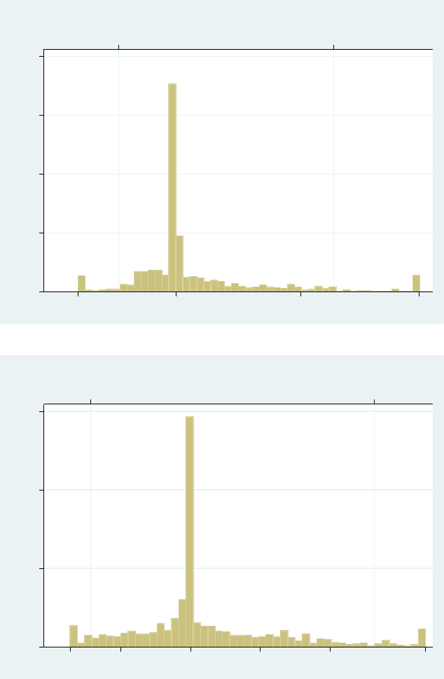
Panels A and B of Figure 1 present the distribution of these two measures of severe

winter weather over our sample period. For the sake of presentation, all of these metrics

are divided by 1,000. The ﬁgures show a large dispersion in abnormal weather during our

sample period, and show that there are a signiﬁcant number of observations with extreme

weather outcomes. However, it is also notable that abnormal snow cover is close to zero in

approximately 50% of ﬁrm-years. One reason for this concentration around zero is that some

counties do not get a lot of snow during our sample period or in the previous ten years.

Both Panels A and B reveal that the distribution of abnormal snow cover exhibits posi-

tive skew. In addition, both measures of snow cover contain extreme events. In unreported

tests we show that our results are not sensitive to trimming both measures at 2.5% and

97.5% percentiles (in Panel A that is −0.08 and 0.20, while in Panel B that is −0.17 and

0.34, respectively). Thus, it is not just the most severe winter weather events that drive our

results.

Results are robust to deﬁning benchmark weather conditions using a ﬁxed ten year period from 2001

through 2010.

3.2 Abnormal weather and cash ﬂow

To investigate if severe winter weather aﬀects corporate cash ﬂow, we regress annual cash

ﬂow on the abnormal weather measure of interest, ﬁrm-speciﬁc control variables, and a set

of industry, county, and year-quarter ﬁxed eﬀects. Therefore, we identify the eﬀect of severe

weather on cash ﬂows using only within-county severe weather variation over time, while the

year-quarter ﬁxed eﬀects control for macro-economic conditions aﬀecting all ﬁrms. Equation

1 details this speciﬁcation:

Cash F low

=α

+ α

Abnormal Snow

+ α

F ixed Assets

it−1

Log(Assets)

it−1

+ α

Leverage

t−1

+ α

Sales

t−1

Cash

t−1

+ α

Debt

t−1

+ α

W orkCap

t−1

+ γX + ε

, (1)

where Cash F low

denotes the cash ﬂow realization of ﬁrm i in year t, and Abnormal Snow

denotes the abnormal snow cover in Q1 for county j corresponding to the location of the

headquarters of ﬁrm i at time t. We include the following control variables, which we more

formally deﬁne in Appendix B: Fixed Assets

it−1

, which is the total ﬁxed assets for ﬁrm i

at time t − 1 scaled by ﬁrm total assets at time t − 1; the natural log of the book value of

total assets of ﬁrm i at time t − 1 (Log(Assets)

it−1

); Leverage

it−1

– total liabilities divided

by total assets of ﬁrm i both as of time t − 1; Sales

t−1

represents the net sales in time t − 1

divided by total assets of ﬁrm i at time t − 1; Cash

t−1

represents the balance of cash and

marketable securities at time t − 1 divided by total assets of ﬁrm i at time t − 1; Debt

t−1

deﬁned as the total borrowing of ﬁrm i at time t − 1 divided by total assets as of time t − 1;

W orkCap

t−1

is deﬁned as the non-cash working capital of ﬁrm i at time t − 1 divided by

total assets as of time t − 1. X is a vector of industry, county, and year-quarter ﬁxed eﬀects.

Notably, all of these controls are measured as of the beginning of the period over which cash

ﬂow is measured.

Table 2 reports estimates of Equation 1 for our sample of ﬁrms. Columns 1 through 4

present associations between cash ﬂow and our primary measures of severe winter weather,

Abnormal Snow and Abnormal Snow 95. Comparing Column 1 with Column 2 and Col-

umn 3 with Column 4 indicates that the inclusion of control variables has little eﬀect on the

relation between severe winter weather and corporate cash ﬂows. This evidence is consistent

with our measure of weather capturing a cash ﬂow shock that is exogenous to ﬁrm funda-

mentals.

Across all four columns there is a negative and statistically signiﬁcant relation between

abnormal snow cover and corporate cash ﬂows. Focusing on Columns 2 and 4, which in-

clude the full set of control variables, Abnormal Snow and Abnormal Snow 95 have t-

statistics of approximately −3.9 and −4.7, respectively. Given that the standard deviation

of Abnormal Snow is 0.0765, the coeﬃcient of −0.0236 in Column 2 suggests that a two

standard deviation increase in average snow cover results in an annual cash ﬂow decrease of

approximately 0.36% of total assets. The magnitude of this cash ﬂow shock is approximately

0.18 standard deviations of annual cash ﬂow (or 2.27% of average cash ﬂow), consistent with

abnormally severe weather having an important impact on corporate cash ﬂow.

Undoubtedly, there is signiﬁcant heterogeneity in the eﬀect of severe weather on cash

ﬂow. Small ﬁrms are more likely to be aﬀected by our measure of abnormal weather than

large ﬁrms because their operations are likely to be concentrated around the corporate head-

quarters, where abnormal weather is deﬁned. For example, we ﬁnd no consistent evidence

that abnormally severe winter weather in the headquarter county of Compustat ﬁrms sig-

niﬁcantly aﬀects annual cash ﬂows. Thus, our sample, which is tilted towards small and

middle-market private ﬁrms, within which over 75% of ﬁrms have total assets less than $100

million, is well suited for this analysis.

Although a negative relation between cash ﬂows and severe winter weather can be ra-

tionalized across a wide range of industries, the magnitude of these severe weather eﬀects

will likely vary. To examine this, Table 3 presents separate estimates of Equation 1 for 15

diﬀerent sectors. Of the ﬁfteen sectors, four industries each comprise between 9% and 24%

of our sample, four comprise between 4% and 7% of our sample, and the remaining seven

each comprise less than 2.31% of our sample. Of the eight sectors comprising more than

4% of our sample, all exhibit a negative relation between both of our measures of abnormal

snow cover and cash ﬂow. For each measure, the negative eﬀect is statistically signiﬁcant at

the 10% level or better in three of these eight sectors. The eﬀect is statistically signiﬁcant in

the transportation and manufacturing sectors using either measure and is signiﬁcant using

one of the two measures in the wholesale and construction industries. The magnitude of the

eﬀect is largest in the transportation industry, which is intuitive because transportation is

directly aﬀected by snow cover. It is somewhat surprising that the negative relation between

abnormal snow and retail cash ﬂows is not more statistically signiﬁcant, given evidence in

Tran (2016) showing that retail sales are adversely aﬀected by rain.

Since we are primarily interested in the eﬀect of abnormally severe weather as an exoge-

nous shock to cash ﬂow in the context of a 2SLS procedure, we leave additional discussion

of the heterogeneous eﬀect of weather on corporate cash ﬂow to future research. What is

important for the validity of our 2SLS procedure is that the F-statistics in the ﬁrst stage are

large enough to mitigate weak instrument concerns. The F-statistics in Columns 2 and 4

are approximately 15 and 22, respectively. This makes it unlikely that we encounter a weak

instruments problem. For example, Table 2 in Stock and Yogo (2005) shows that potential

bias of the IV estimate attributable to weak instruments could be at most 10% of the size of

the IV coeﬃcient whenever the ﬁrst-stage F-statistic is 16 or higher. The two-stage proce-

dure we employ in the following section will identify the eﬀect of exogenous cash ﬂow shocks

on liquidity outcomes for a given ﬁrm-year only to the extent that severe winter weather

meaningfully aﬀects cash ﬂow. Thus, our identiﬁcation is likely to come primarily from small

ﬁrms and industries with high sensitivities of cash ﬂow to winter weather.

4 Managing Exogenous Cash Flow Shocks

The results in Section 3 show that abnormal weather leads to reduced cash ﬂows. In this

section, we investigate how this aﬀects corporate outcomes. For empirical estimation, we use

a 2SLS procedure, where the second stage regresses corporate outcomes on the ﬁtted value

of cash ﬂows from the model reported in Column 2 or 4 of Table 2. Formally, we estimate

the following system of equations using 2SLS:

Cash F low

=α

+ α

Abnormal Snow

+ α

F ixed Assets

it−1

Log(Assets)

it−1

+ α

Leverage

t−1

+ α

Sales

t−1

Cash

t−1

+ α

Debt

t−1

+ α

W orkCap

t−1

+ γX + ε

, (2a)

=β

+ β

Cash F low

+ β

F ixed Assets

it−1

+ β

Log(Assets)

it−1

Leverage

t−1

+ β

Sales

t−1

+ β

Cash

t−1

Debt

t−1

+ β

W orkCap

t−1

+ δX + 

(2b)

where Cash F low

, Abn W eather Q1

, F ixed Assets

it−1

, Log(Assets)

it−1

, Leverage

t−1

Sales

t−1

, Cash

t−1

, Debt

t−1

; W orkCap

t−1

and X are deﬁned as in Section 2. Y

represents

the second-stage outcome of interest, such as credit line drawdowns, change in credit line

limit, change in cash, or real investment.

4.1 Liquidity Management

Despite extensive literature investigating corporate cash reserves and credit lines, there

is little direct evidence on how ﬁrms use credit lines to deal with unanticipated liquidity

shocks. The evidence on credit line use that does exist is mixed and comes primarily from

surveys or studies of large ﬁrms. Lins, Servaes, and Tufano (2010) provide survey evidence

that ﬁrms typically rely on cash buﬀers to manage liquidity shocks, while short-term debt

in the form of credit lines is used primarily to pursue investment opportunities. However,

managers surveyed in Campello et al. (2011) and Campello et al. (2012) indicated that credit

lines were an important source of liquidity during the ﬁnancial crisis. A goal of this paper

is to provide broad-based, direct evidence on how ﬁrms manage random ﬂuctuations in cash

ﬂow. Notably, our analysis occurs outside of the crisis period and centers on small U.S. ﬁrms

with access to bank lenders.

In Table 4 we investigate the extent to which ﬁrms use credit lines to manage exogenous

cash ﬂow shocks. Column 1 of Table 4 presents an OLS regression in which the dependent

variable is the year over year change in drawn credit line amount scaled by the beginning

of period total assets. The explanatory variable of interest is cash ﬂow. The OLS analysis

in column 1 reveals a negative and signiﬁcant relation between cash ﬂow and credit line

drawdowns, but the point estimate is small (−0.005). It is diﬃcult to pinpoint the driving

forces behind this estimate given the correlation between cash ﬂows and omitted variables,

such as investment opportunities (e.g., Riddick and Whited (2009)) and the availability of

credit (e.g.,Suﬁ (2009)).

In Columns 2 and 3 of Table 4 we present the IV results, which isolate the eﬀect of exoge-

nous cash ﬂow ﬂuctuations on changes in credit line draws. Column 2 uses Abnormal Snow,

which is the average daily abnormal snow cover in the ﬁrst calendar quarter, to instrument

for annual cash ﬂow, while Column 3 uses Abnormal Snow 95 – the snow cover during the

95th percentile of daily snow cover during the ﬁrst quarter. The coeﬃcients in Columns

2 and 3 of Table 4 are negative, statistically signiﬁcant, and range from −0.41 to −0.61,

suggesting that ﬁrms with access to bank debt cover the majority of a weather related cash

ﬂow shock with credit line draws.

These ﬁndings highlight the value of our two-stage procedure. By focusing on exogenous

shocks to cash ﬂow, we identify the eﬀect of cash ﬂow changes on credit line drawdowns in a

manner that is not confounded by the high correlations between cash ﬂows and other factors,

such as unobserved investment opportunities (e.g., Riddick and Whited (2009)). Our results

suggest that these correlations between cash ﬂow and other factors are suﬃciently strong to

camouﬂage the extent to which credit lines are used to buﬀer unanticipated shocks to cash

ﬂow.

In unreported results, we conduct two additional tests that oﬀer circumstantial support

for our identifying assumption that abnormally severe winter weather aﬀects ﬁrm outcomes

only through its eﬀect on corporate cash ﬂows. First, we replicate our analyses using trimmed

weather IVs, which drop the most extreme 2.5% of abnormal snow outcomes. We obtain very

similar coeﬃcient estimates of −0.3657 and −0.8162, which mitigates any concern that the

most severe weather events, which may impact investment opportunities, drive our ﬁndings.

Second, we replicate our ﬁndings excluding ﬁrm-level controls (i.e., using Columns 1 and 3

of Table 2 as the ﬁrst-stage regression). As would be expected if abnormally severe winter

weather represents a shock to corporate cash ﬂows that is unrelated to ﬁrm characteristics,

we ﬁnd qualitatively similar second-stage estimates for the eﬀect of cash ﬂows on credit line

use.

Next, we investigate how ﬁrms use alternative sources of liquidity such as cash balances

and non-cash working capital to manage cash ﬂow shocks. The OLS estimate in Column 1 of

Table 5 reveals a small but signiﬁcantly positive association between cash ﬂow and changes

in cash. These results are consistent with a large literature on the cash ﬂow sensitivity of

cash, such as Almeida, Campello, and Weisbach (2004) and Khurana, Martin, and Pereira

(2006), and suggest that ﬁrms draw on cash balances when cash ﬂow declines. As with the

OLS estimates in Table 4, however, it is diﬃcult to draw causal inferences from this positive

relation regarding the use of cash as a buﬀer for cash ﬂow shocks.

In Columns 2 and 3, we estimate the two stage regressions with changes in cash as the

dependent variable. The coeﬃcient on cash ﬂow increases to 0.17 in Column 2 and 0.16 in

Column 3, but the standard error also increases substantially and the point estimate is no

longer statistically signiﬁcant. Columns 4 through 6 yield similar estimates using non-cash

working capital as the dependent variable (point estimates of 0.16 and 0.24, respectively).

Overall, the point estimates in Tables 4 and 5 suggest that for every dollar an exogenous

cash ﬂow shock costs a ﬁrm, approximately 41 to 61 cents are reﬂected in increased credit

line drawn amount, and approximately 20 cents each are reﬂected in reduced cash and non-

cash working capital balances. Thus, credit lines are the primary way that ﬁrms with bank

lending relationships manage exogenous cash ﬂow shocks.

4.2 Credit Line Size Adjustments

Next, we investigate whether cash ﬂow shocks cause ﬁrms to adjust their credit line

size. Credit lines of public ﬁrms are frequently renegotiated – Roberts and Suﬁ (2009) and

Roberts (2015) ﬁnd that the average bank loan in their sample is renegotiated once every

6-9 months, and that most renegotiations are not due to impending covenant violations.

Within our sample, credit line sizes are adjusted in almost half of ﬁrm-years. This raises the

possibility that banks work with ﬁrms to adjust available credit in response to exogenous

cash ﬂow shocks.

Interestingly, the OLS evidence in Column 1 of Table 6 indicates the opposite relation.

When cash ﬂow is high, credit line size expands. This is consistent with proﬁtable ﬁrms

having greater demand for, or access to, bank credit. This is also consistent with Suﬁ

(2009), who ﬁnds that the availability of credit lines can be dependent on maintaining high

levels of cash ﬂow as lenders may reduce credit line availability following cash ﬂow shortfalls

by using ﬁnancial covenants to force loan renegotiation (also see Smith (1993) and Smith

and Warner (1979)).

Although this may be the predominant relation in the data, we expect the opposite

response if banks work with ﬁrms to manage exogenous liquidity shocks. Columns 2 and 3

examine this question using IV regressions with the change in credit line size (as a percentage

Once again, using the trimmed weather IVs provides similar evidence on ﬁrm use of cash and non-cash

working capital to respond to exogenous cash ﬂow shocks (coeﬃcients of 0.067 and 0.029 for cash, and 0.07

and 0.189 for non-cash working capital).

of beginning of period total assets) as the second stage dependent variable. In Columns 4

through 6 we replicate the OLS and IV speciﬁcations using an indicator equal to one if the

ﬁrm experiences a credit line increase over the previous year as the dependent variable.

Columns 2 and 3 indicate that there is a negative relation between exogenous cash ﬂow

shocks and credit line size. These results are consistent with banks accommodating random

cash ﬂow ﬂuctuations with credit line adjustments. The coeﬃcient of −0.74 in Column 2

and −1.13 in Column 3 indicate that in our sample of ﬁrms – all of which have established

bank lending relationships – a one dollar reduction in cash ﬂow due to the weather shock

is associated with approximately a one dollar increase in credit line size. The coeﬃcients

of −3.31 and −3.92 in Columns 5 and 6 indicate that increasing cash ﬂows by 1% of total

assets increases (decreases) the probability of a credit line increase (decrease) by between 3

and 4%. Again, these eﬀects are similar when using the trimmed weather variables as IVs.

We posit that the reason ﬁrms seek this additional credit is to maintain suﬃcient liquidity

as they draw down their existing credit line. Consistent with this, we cannot reject the null

hypothesis that the increased credit line drawdown (in Table 4) is the same size as the credit

line size increase. It is also possible that a portion of the credit line size increase we observe is

due to ﬁrms adjusting their beliefs regarding the probability of future cash ﬂow shocks. Such

behavior would be consistent with evidence in Dessaint and Matray (2017) who ﬁnd that

managers temporarily overestimate hurricane risk when there have been recent hurricanes

in nearby areas. In either case, our ﬁndings provide new evidence on how ﬁrms work with

banks to adjust their available credit in response to cash ﬂow shocks.

Overall, the results in Tables 4 and 6 indicate that bank-borrowing ﬁrms rely on their

credit lines as an important source of liquidity. Not only do ﬁrms use existing credit when

faced with exogenous cash ﬂow shocks, but they are also able to work with their lender to

expand available credit.

4.3 Investment and Cash Flow

An important question is whether the credit line adjustments documented in the previous

section are suﬃcient to prevent cash ﬂow shocks from aﬀecting other corporate outcomes.

To address this question, we use our 2SLS framework to investigate how exogenous cash ﬂow

shocks relate to changes in ﬁxed assets, total assets, and (in unreported tests with a smaller

sample) net capital expenditures.

We present evidence on the relation between cash ﬂow and the change in ﬁxed assets in

the ﬁrst three columns of Table 7. In the ﬁrst column, the OLS estimates show a positive

and signiﬁcant association between cash ﬂow and investment in ﬁxed assets. In the second

and third columns, we report IV estimates, using two measures of abnormal snow cover

to instrument for cash ﬂow. In both cases, the coeﬃcient on cash ﬂow is negative, small,

and statistically insigniﬁcant. This result is interesting because it suggests that small ﬁrms

with access to credit lines are able to buﬀer investment from exogenous cash ﬂow shocks.

This ﬁnding also underscores how misleading OLS estimates of the investment-cash ﬂow

sensitivity can be, particularly when, as in this case, controls for investment opportunities

are imperfect (e.g., Erickson and Whited (2000); Alti (2004); Moyen (2004); Almeida and

Campello (2007)).

In Columns 4 through 6 of Table 7, we investigate whether exogenous cash ﬂow shocks

aﬀect asset growth. Although there is a positive OLS relation between cash ﬂows and

asset growth, this eﬀect becomes statistically insigniﬁcant using our two-stage procedure.

Comparing the magnitude of the 2SLS estimate to the cash and working capital estimates

in Table 5, reveals that any change in assets that does exist appears to be attributable to

changes in cash and working capital. Analyses using net CAPEX are qualitatively similar to

those we report in Columns 1 through 3 (using the change in ﬁxed assets as the second stage

dependent variable). However, these results should be interpreted with caution since net

CAPEX is not always reported in our sample. Overall, the evidence in this section suggests

that the average bank-borrowing ﬁrm manages exogenous cash ﬂow shocks primarily via

credit line adjustments. The eﬀect of these cash ﬂow shocks does not spill over into other

corporate activities.

5 Reduced Form Analyses

In our ﬁnal set of analyses, we more directly investigate the eﬀect of abnormally severe

winter weather on corporate outcomes. We continue to maintain our identifying assumption

used in the 2SLS approach, which is that severe winter weather only aﬀects corporate out-

comes through its eﬀect on corporate cash ﬂow. If this instrument is indeed an important

determinant of random variation in cash ﬂow, then abnormally severe winter weather should

directly predict corporate outcomes when plugged into the second stage regressions.

5.1 Direct Eﬀect of Winter Weather

A beneﬁt to this analysis is that it allows us to directly examine the economic magnitude

of the eﬀect of severe winter weather on corporate activity. The results in the previous

section suggest that severe winter weather will be positively related to credit line use and

size, but not other corporate outcomes. The evidence in Table 8 supports this prediction.

Panels A and B show that both measures of abnormal snow are positively and signiﬁcantly

related to changes in credit line drawn amount and credit line size, but not other corporate

outcomes. The magnitude of the eﬀect of severe weather on credit line use is economically

meaningful. Given that the standard deviation of Abnormal Snow is 0.0765, the coeﬃcient

of 0.0098 in Column 1 of Table 8 Panel A suggests that a two standard deviation increase in

abnormal snow results in the average ﬁrm drawing 0.15% of assets more on their credit line

over the course of the year. The coeﬃcient in Column 2 suggests that severe winter weather

has almost double that eﬀect on the change in credit line size. Consistent with our earlier

ﬁndings, weather has no statistically or economically signiﬁcant eﬀect on cash balances, ﬁxed

assets, or total assets.

5.2 Quarterly Credit Line Adjustments

This reduced form analysis also allows us to examine the relation between severe ﬁrst

quarter weather and credit line activity on a quarterly basis. We cannot conduct such an

analysis using cash ﬂows or any of our other dependent variables because we only observe

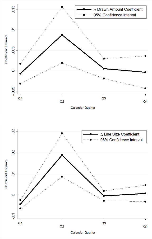
ﬁnancial data at an annual frequency. In Panel A of Figure 2 we decompose the annual eﬀect

of Abnormal Snow 95 on the change in credit line drawn amount, estimated in Column 1 of

Table 8 Panel B, into its quarterly components. Speciﬁcally, each point on the solid line in

the ﬁgure represents the estimated eﬀect of abnormal ﬁrst quarter snow cover on credit line

draw downs during the calendar quarter indicated on the x-axis. The dashed lines represent

the 95% conﬁdence interval for these estimates. Panel A of Figure 2 indicates that the ef-

fect of abnormal ﬁrst quarter snow on credit line use is concentrated in the second calendar

quarter, meaning that ﬁrms respond to bad weather between January 1 and March 31 by

drawing on their credit line at some point between April 1 and June 30th. Panel B of Figure

2 shows that, similar to the credit line drawdowns, the credit line size increases that occur in

response to severe winter weather happen during the second calendar quarter. Interestingly,

during the ﬁrst quarter we ﬁnd that line size decreases in response to severe winter weather.

Taken together, the evidence in Figure 2 is consistent with banks providing liquidity to

ﬁrms experiencing exogenous cash ﬂow shocks, but not immediately. It is possible that ﬁrms

manage exogenous cash ﬂow shocks by tapping cash or working capital reserves in the very

short-run. One reason for this might be that ﬁrms only meet with their banks sporadically,

however this is unlikely to be the entire story because it does not explain the credit line size

reduction in the ﬁrst quarter or the delay with which ﬁrms draw on their credit line.

Our ﬁndings seem more consistent with banks being cautious about extending additional

credit to ﬁrms whose cash ﬂows have declined, preferring to take “a wait and see” approach.

This explanation is consistent with Suﬁ (2009) and Acharya et al. (2014) who argue that

bank ﬁnancing may not be available to ﬁrms experiencing low cash ﬂows or negative prof-

itability shocks. However, our results suggest that the hesitance of banks to oﬀer ﬁnancing

in these situations is (on average) short-lived when the cash ﬂow shock is exogenous to ﬁrm

fundamentals, making credit lines an important way that ﬁrms manage their liquidity in

response to exogenous cash ﬂow shocks.

5.3 Partitioning on Borrower Financial Health

In our ﬁnal set of tests we delve deeper into the possibility that bank liquidity may not be

available for some ﬁrms when they need it. For example, Diamond (1991) shows theoretically

that low- and medium-credit risk borrowers can rely on bank ﬁnancing, while high credit risk

borrowers may not be able to obtain bank ﬁnancing when needed. We therefore partition

the sample based on the credit quality of the borrower as of the year-end immediately prior

to the weather shock, quarter 4 of year t − 1. Our measure of credit quality is the borrower’s

internal risk rating assigned by the lender converted to a ten-grade S&P ratings scale.

In Table 9 we partition the sample into two groups – BB and better and B and below.

Approximately 94% of the sample is contained within the B, BB, and BBB rating categories.

Speciﬁcally, the breakdown of the sample in terms of credit quality is as follows – B-rated

(14.54%), BB-rated (52.75%), BBB-rated (26.50%), below B (3.31%), above BBB (2.90%).

Panel A shows that cash ﬂow is adversely impacted by weather in both subsamples (compare

columns 1 and 2 to columns 3 and 4) and that these adverse eﬀects are somewhat stronger in

the poor-credit quality subsample. Columns 1 through 4 of Panel B show that more severe

abnormal weather is associated with larger annual increases in credit line draw and credit

line size for the borrowers with ratings of BB and better, while columns 5 through 8 indicate

the lack of an association between adverse weather and credit line use.

The absolute value of the coeﬃcients in the ﬁrst two columns of both Panels A and B

are all approximately 0.01. This suggests that a given increase in adverse weather leads to a

decrease in cash ﬂows and an increase credit line draws that are of similar magnitude. Thus,

Each bank is required to provide its internal risk rating together with a concordance mapping to a

10-grade S&P scale ranging from AAA to D. These internal ratings are available for almost all borrowers in

our sample – 96,251 borrower-years out of a total of 97,619 borrower-years. To the extent that a borrower

has ﬁnancing from multiple banks we use the most conservative among these ratings.

medium- and high-credit quality ﬁrms appear to buﬀer cash ﬂow shocks entirely with credit

line draw downs. In contrast, low-credit quality ﬁrms do not draw on their lines of credit

in response to more severe winter weather, even though such weather shocks signiﬁcantly

aﬀect cash ﬂows. These results illustrate that only medium- and high-credit quality ﬁrms

can rely on their credit lines to buﬀer adverse transitory cash ﬂow shocks. In unreported

tests, we ﬁnd no signiﬁcant relation between severe winter weather and either cash reserves

or working capital within either subsample. Rather, the inability of low credit quality ﬁrms

to buﬀer cash ﬂow shocks appears to result in reductions in total assets (with t-statistics

ranging between −1.4 and −1.6).

6 Concluding Remarks

This study uses a unique dataset on bank lending portfolios to study how ﬁrms manage

liquidity in the face of exogenous cash ﬂow shocks. Starting in 2012, the Federal Reserve

has collected comprehensive data on bank lending activities as part of the Dodd-Frank

Stress Tests and Comprehensive Capital Analysis and Review. The resulting data (the

Federal Reserve Y-14 collection) contains a rich set of information on bank lending terms

and borrower ﬁnancial information. Notably, the FR Y-14 collection has broad coverage

of lending and ﬁnancial activity of the small private ﬁrms that rely extensively on external

credit, but typically do not appear in publicly available databases.

We show that these ﬁrms rely extensively on credit lines as a source of ﬁnance. To identify

the causal connection between cash ﬂow shocks and corporate liquidity management, we

construct an instrument for cash ﬂow based on abnormal adverse weather conditions in the

county in which the company is located. Using this instrument to predict ﬁrm-level cash

ﬂows, we ﬁnd that ﬁrms manage negative cash ﬂow shocks by drawing on their credit lines

rather than tapping their cash reserves or adjusting their real activities. In addition, negative

cash ﬂow shocks are accompanied by signiﬁcant increases in the size of the ﬁrm’s overall

credit line, indicating that banks accommodate borrowers confronted with unexpected cash

ﬂow shortfalls. Taken together, these results show that, for ﬁrms with lending relationships,

credit lines are the primary means of corporate liquidity management.

References

Acharya, Viral, Heitor Almeida, and Murillo Campello. 2013. “Aggregate risk and the choice between cash

and lines of credit.” Journal of Finance 68:2059–2116.

Acharya, Viral, Heitor Almeida, Filippo Ippolito, and Ander Perez. 2014. “Credit lines as monitored liquidity

insurance: Theory and evidence.” Journal of Financial Economics 112 (3):287–319.

Almeida, Heitor and Murillo Campello. 2007. “Financial constraints, asset tangibility, and corporate invest-

ment.” Review of Financial Studies 20 (5):1429–1460.

Almeida, Heitor, Murillo Campello, Igor Cunha, and Michael Weisbach. 2014. “Corporate Liquidity Man-

agement: A Conceptual Framework and Survey.” Annual Review of Financial Economics 6:135–162.

Almeida, Heitor, Murillo Campello, and Michael Weisbach. 2004. “The Cash Flow Sensitivity of Cash.”

Journal of Finance 59 (4):1777–1804.

Alti, Aydogan. 2004. “How sensitive is investment to cash ﬂow when ﬁnancing is frictionless?” Journal of

Finance 58 (2):707–722.

Bates, Thomas W., Kathleen M. Kahle, and Renee M. Stulz. 2009. “Why Do U.S. Firms Hold So Much

More Cash than They Used To?” Journal of Finance 64 (5):1985–2021.

Berospide, Jose and Ralf Meisenzahl. 2016. “The Real Eﬀects of Credit Line Drawdowns.” Working Paper.

Bidder, Rhys M., John R. Krainer, and Adam H. Shapiro. 2016. “Drilling into Bank Balance Sheets:

Examining Portfolio Responses to an Oil Shock.” Working Paper.

Bloesch, Justin and Francois Gourio. 2015. “The eﬀect of winter weather on U.S. economic activity.”

Economic Perspectives, FRB Chicago.

Campello, Murillo, Erasmo Giambona, John Graham, and Campbell Harvey. 2011. “Liquidity management

and corporate investment during a ﬁnancial crisis.” Review of Financial Studies 24:19441979.

———. 2012. “Access to Liquidity and Corporate Investment in Europe during the Financial Crisis.” Review

of Finance 16 (2):323–346.

Chang, Xin, Sudipto Dasgupta, George Wong, and Jiaquan Yao. 2014. “Cash-ﬂow sensitivities and the

allocation of internal cash ﬂow.” Review of Financial Studies 27 (12):3628–3657.

Chen, Yangyang, Po-Hsuan Hsu, Edward J. Podolski, and Madhu Veeraraghavan. 2017. “In the Mood for

Creativity: Weather-Induced Mood, Inventor Productivity, and Firm Value.” Working Paper.

Colvin, R and A Loten. 2014. “Small-Business’ Sales Decline Amid Winter Weather.” Wall Street Journal,

February 19th.

Cortes, Kristle Romero. 2014. “Rebuilding after disaster strikes: How local lenders aid in the recovery.”

FRB of Cleveland Working Paper No. 14-28.

Cortes, Kristle Romero and Philip E. Strahan. 2016. “Tracing out capital ﬂows: How ﬁnancially integrated

banks respond to natural disasters.” Journal of Financial Economics forthcoming.

Demiroglu, Cem and Christopher James. 2011. “The use of bank lines of credit in corporate liquidity

management: A review of empirical evidence.” Journal of Banking and Finance 35 (4):775–782.

Demiroglu, Cem, Christopher James, and Atay Kizilaslan. 2012. “Bank lending standards and access to

lines of credit.” Journal of Money, Credit and Banking 44 (6):1063–1089.

Denis, David and Valeriy Sibilkov. 2010. “Financial constraints, investment, and the value of cash holdings.”

Review of Financial Studies 23 (1):247–269.

Dessaint, Olivier and Adrien Matray. 2017. “Do managers overreact to salient risks? Evidence from hurricane

strikes.” Journal of Financial Economics, Forthcoming.

Diamond, Douglas. 1991. “Monitoring and Reputation: The choice between bank loans and directly placed

debt.” Journal of Political Economy 99 (4):689–721.

Erickson, Timothy and Toni Whited. 2000. “Measurement error and the relationship between investment

and q.” Journal of political economy 108 (5):1027–1057.

Gatev, Evan and Phillip Strahan. 2006. “Banks’ Advantage in Hedging Liquidity Risk: Theory and Evidence

from the Commercial Paper Market.” Journal of Finance 61 (2):867–892.

Giroud, Xavier, Holger M. Mueller, Alex Stomper, and Arne Westerkamp. 2012. “Snow and Leverage.”

Review of Financial Studies 25 (3):680–710.

Holmstrom, Bengt and Jean Tirole. 1998. “Private and Public Supply of Liquidity.” Journal of Political

Economy 106 (1):1–40.

Ivanov, Ivan and Luke Pettit. 2017. “Credit Line Dynamics during the Great Recession.” Working Paper.

Ivashina, Victoria and David Scharfstein. 2010. “Bank lending during the ﬁnancial crisis of 2008.” Journal

of Financial Economics 97 (3):319–338.

James, Christopher and Peggy Wier. 1990. “Borrowing relationships, intermediation, and the cost of issuing

public securities.” Journal of Financial Economics 28 (1-2):149–171.

Jimenez, Gabriel, Jose Lopez, and Jesus Saurina. 2009. “Empirical Analysis of Corporate Credit Lines.”

The Review of Financial Studies 22 (12):5069–5098.

Kashyap, Anil, Raghuram Rajan, and Jeremy Stein. 2002. “Banks as Liquidity Providers: An Explanation

for the Co-Existence of Lending and Deposit-Taking.” Journal of Finance 57 (1):33–37.

Khurana, Inder K., Xiumin Martin, and Raynolde Pereira. 2006. “Financial Development and the Cash

Flow Sensitivity of Cash.” Journal of Financial and Quantitative Analysis 41 (4):787–807.

Lins, Karl, Henry Servaes, and Peter Tufano. 2010. “What drives corporate liquidity? An international

survey of cash holdings and lines of credit.” Journal of Financial Economics 98 (1):160–176.

Moyen, Nathalie. 2004. “Investmentcash ﬂow sensitivities: Constrained versus unconstrained ﬁrms.” Journal

of Finance 59 (5):2061–2092.

Petersen, Mitchell A. and Raghuram G. Rajan. 1994. “The Beneﬁts of Lending Relationships: Evidence

from Small Business Data.” Journal of Finance 49 (1):3–37.

Poterba, James M. 1988. “Comment on ’Financing constraints and corporate investment’.” Brookings Papers

on Economic Activity 1988 (1):200–204.

Riddick, Leigh and Toni Whited. 2009. “The corporate propensity to save.” Journal of Finance 64 (4):1729–

1766.

Robb, Alicia and David T. Robinson. 2014. “The capital structure decisions of new ﬁrms.” Review of

Financial Studies 27 (1):153–179.

Roberts, Michael R. 2015. “The role of dynamic renegotiation and asymmetric information in ﬁnancial

contracting.” Journal of Financial Economics 116 (1):61–81.

Roberts, Michael R. and Amir Suﬁ. 2009. “Renegotiation of nancial contracts: Evidence from private credit

agreements.” Journal of Financial Economics 93 (2):159–184.

Shockley, Richard and Anjan Thakor. 1997. “Bank Loan Commitment Contracts: Data, Theory and Tests.”

Journal of Money, Credit and Banking 29 (4):517–534.

Smith, Jr., Cliﬀord W. 1993. “A Perspective on Accounting-Based Debt Covenant Violations.” The Ac-

counting Review 68 (2):289–303.

Smith, Jr., Cliﬀord W. and Jerold B. Warner. 1979. “On Financial Contracting.” Journal of Financial

Economics 7 (1):117–161.

Stock, James and Motohiro Yogo. 2005. “Testing for Weak Instruments in Linear IV Regressions.” Identiﬁ-

cation and Inference for Econometric Models: Essays in Honor of Thomas Rothenberg.

Suﬁ, Amir. 2009. “Bank lines of credit in corporate ﬁnance: An empirical analysis.” Review of Financial

Studies 22 (3):1057–1088.

Tran, Brigitte Roth. 2016. “Blame it on the Rain Weather Shocks and Retail Sales.” Working Paper.

Yun, Hayong. 2009. “The choice of corporate liquidity and corporate governance.” Review of Financial

Studies 22 (4):1447–1475.

0 10 20 30 40

Percent of Observations

5th 95th

0 .1<-0.08 >0.20

Percentiles of Abnormal Snow Cover

(a) Abormal Snow Cover

0 10 20 30

Percent of Observations

5th 95th

-.1 0 .1 .2 >0.34<-0.17

Percentiles of Abnormal Snow Cover P95

(b) Abnormal Snow Cover P 95

Figure 1: Distribution of Abnormal Snow Cover. This ﬁgure presents the distribution of

abnormal snow cover during the ﬁrst calendar quarter for the 97,619 ﬁrm-years in our sample.

The distribution in Panel A is constructed based on the average daily snow cover during the ﬁrst

calendar quarter, while Panel B uses the 95th percentile of snow cover during the ﬁrst calendar

quarter. Abnormal snow cover is deﬁned relative to the the time-series average of ﬁrst calendar

quarter snow cover in each county over the previous 10 years.

(a) ∆Draw

(b) ∆Line Size

Figure 2: Credit Line Dynamics Following the Weather Shock This ﬁgure decomposes

the annual eﬀect of abnormal snow on change in credit line drawn amount (Panel A) or credit line

size (Panel B), estimated in Columns 1 and 4 of Table 8 Panel B, into its quarterly components.

Speciﬁcally, each point on the solid line in the ﬁgure represents the estimated eﬀect of abnormal

ﬁrst quarter snow cover on quarterly change in credit line drawn amounts or credit line size during

the calendar quarter indicated on the x-axis (for example, Q1 represents the change in credit line

drawn amount or line size between the end of Q4 of the previous year and the end of Q1 of the

current year). The dashed lines represent the 95% conﬁdence interval for these estimates.

Table 1: Descriptive Statistics. This table presents descriptive statistics for our sample of

97,619 observations with available borrower and loan characteristics. Columns 1 and 2 present

the mean and standard deviation, while Columns 3 through 5 present the 25th, 50th, and 75th

percentiles, respectively. All explanatory variables are deﬁned in Appendix B.

Mean SD P 25 P 50 P 75

T otal Assets ($ Millions) 726.9890 3668.5250 8.4290 22.0430 90.6961

Cash F low 0.1584 0.2011 0.0635 0.1177 0.1987

Leverage 0.6004 0.2042 0.4609 0.6209 0.7572

F ixed Assets 0.2933 0.2668 0.0680 0.2109 0.4562

Sales 2.2846 1.8593 1.0880 1.9588 3.0008

Cash 0.0975 0.1234 0.0124 0.0501 0.1348

Debt 0.3168 0.2337 0.1230 0.2908 0.4746

W orkCap 0.1015 0.2022 −0.0288 0.0787 0.2236

Line Size 0.2419 0.1913 0.0892 0.1974 0.3517

Draw 0.0866 0.1539 0.0000 0.0000 0.1163

∆Line Size 0.0267 0.1064 0.0000 0.0000 0.0101

∆Draw 0.0153 0.0803 0.0000 0.0000 0.0101

∆Cash 0.0084 0.0701 −0.0136 0.0006 0.0249

∆W orkCap 0.0075 0.0915 −0.0292 0.0045 0.0450

∆Liabilities 0.0422 0.1600 −0.0437 0.0119 0.0978

∆Debt 0.0214 0.1243 −0.0357 0.0000 0.0576

∆Assets 0.0752 0.1895 −0.0267 0.0433 0.1400

∆F ixed Assets 0.0188 0.0894 −0.0111 0.0008 0.0258

Table 2: Cash Flow and Abnormal Weather. This table contains estimated coeﬃcients from

an OLS regression of Cash F low

on Abnormal Snow (columns 1 and 2) and Abnormal Snow P 95

(columns 3 and 4). We include a number of control variables (deﬁned in Appendix B), as well as

three-digit NAICS 2012 industry indicators, county, and year-quarter ﬁxed eﬀects. The standard

errors are clustered at the three-digit NAICS 2012 industry level.

Cash F low

(1) (2) (3) (4)

Abnormal Snow −0.0217*** −0.0236***

(0.00593) (0.00603)

Abnormal Snow P 95 −0.0139*** −0.0148***

(0.00355) (0.00317)

Log(Assets

it−1

) −0.00484*** −0.00484***

(0.00182) (0.00182)

F ixed Assets

it−1

0.0930*** 0.0930***

(0.0200) (0.0200)

Leverage

it−1

−0.0521 −0.0521

(0.0324) (0.0324)

Sales

it−1

0.0250*** 0.0250***

(0.00853) (0.00853)

Cash

it−1

0.240*** 0.240***

(0.0570) (0.0570)

Debt

it−1

−0.0111 −0.0111

(0.0361) (0.0361)

W orkCap

it−1

0.0373*** 0.0373***

(0.0132) (0.0132)

Industry Fixed Eﬀects YES YES YES YES

County Fixed Eﬀects YES YES YES YES

Year-Quarter Fixed Eﬀects YES YES YES YES

Adjusted R-Squared 0.0183 0.152 0.0183 0.152

Observations 97,619 97,619 97,619 97,619

Standard errors in parentheses

*p < 0.10, **p < 0.05, ***p < 0.01

Table 3: Cash Flow and Abnormal Weather: Industry Partitions This table contains

estimated coeﬃcients from an OLS regression of Cash F low

on Abnormal Snow in a model with

identical controls to that in Speciﬁcations (2) and (4) of Table 2. Each row in the table restricts

the sample to one of ﬁfteen sectors, which are indicated in Column 1. Columns 2 and 3 present the

estimates (and standard errors below in parentheses) for the coeﬃcients on Abnormal Snow and

Abnormal Snow P 95, respectively. We include a number of control variables (deﬁned in Appendix

B), as well as three-digit NAICS 2012 industry indicators, county, and year-quarter ﬁxed eﬀects.

The standard errors are clustered at the three-digit NAICS 2012 industry level.

IV 1 Coef f IV 2 Coef f P ercent Obs Obs

(SE) (SE)

MANUF ACT URING −0.0267* −0.0189** 24.16% 23,583

(0.0148) (0.00756)

W HOLESALE −0.0206 −0.0128** 17.14% 16,729

(0.0126) (0.00628)

RET AIL −0.00251 −0.00494 14.16% 13,823

(0.0126) (0.00732)

BUSINESS SERV ICES −0.0591 −0.0300 9.32% 9,098

(0.0441) (0.0274)

CON ST RUCT ION −0.0498* −0.0134 7.12% 6,947

(0.0264) (0.0121)

REAL EST AT E −0.0291 −0.0103 7.43% 7,252

(0.0227) (0.0113)

EDUCAT ION & HEALT H −0.0166 −0.0149 4.44% 4,335

(0.0815) (0.0382)

T RANSP ORT AT ION −0.0554** −0.0257** 4.43% 4,325

(0.0264) (0.0130)

ACCOMODAT ION & F OOD −0.0464 −0.0117 2.31% 2,253

(0.0693) (0.0412)

AGRICULT URE −0.0234 −0.0242 1.94% 1,898

(0.0371) (0.0219)

INF ORMAT ION 0.0694 0.0108 1.92% 1,870

(0.0835) (0.0436)

MINING & EXT RACT ION 0.0655 0.0560 1.86% 1,819

(0.0764) (0.0367)

LEISU RE −0.0957 −0.0630 1.46% 1,429

(0.0780) (0.0427)

UT ILIT IES −0.0193 −0.0182 1.34% 1,314

(0.0288) (0.0163)

OT HER 0.113* 0.0578 0.97% 944

(0.0630) (0.0376)

Standard errors in parentheses

*p < 0.10, **p < 0.05, ***p < 0.01

Table 4: Credit Line Use and Cash Flow Column 1 present OLS estimates from regres-

sions of ∆Draw

on Cash F low

and controls. Columns 2 and 3 present 2SLS estimates of

IV regressions of ∆Draw

on instrumented Cash F low

and controls using Abnormal Snow

and Abnormal Snow P 95 as IVs, respectively. IV1 and IV2 correspond to Abnormal Snow and

Abnormal Snow P 95, respectively. We include a number of control variables (deﬁned in Appendix

B), as well as three-digit NAICS 2012 industry indicators, county, and year-quarter ﬁxed eﬀects.

The standard errors are clustered at the three-digit NAICS 2012 industry level.

∆Draw

OLS IV 1 IV 2

(1) (2) (3)

Cash F low

−0.0049*** −0.4140** −0.6050***

(0.0012) (0.1821) (0.2143)

Log(Assets)

it−1

−0.0019*** −0.0039*** −0.0048***

(0.0004) (0.0014) (0.0018)

F ixed Assets

it−1

−0.0131*** 0.0250 0.0427**

(0.0033) (0.0165) (0.0190)

Leverage

it−1

0.0027 −0.0186 −0.0286

(0.0027) (0.0140) (0.0216)

Sales

it−1

0.0014*** 0.0117** 0.0165***

(0.0005) (0.0047) (0.0061)

Cash

it−1

−0.0281*** 0.0701 0.1160*

(0.0056) (0.0460) (0.0600)

Debt

it−1

0.0096*** 0.0050 0.0028

(0.0034) (0.0126) (0.0189)

W orkCap

it−1

−0.0009 0.0144 0.0215**

(0.0023) (0.0090) (0.0107)

Industry FE YES YES YES

County FE YES YES YES

Year-Quarter FE YES YES YES

Adjusted R-Squared 0.0641 . .

Observations 97,619 97,619 97,619

Standard errors in parentheses

*p < 0.10, **p < 0.05, ***p < 0.01

Table 5: Other Liquidity Management and Cash Flow Columns 1 and 4 present OLS estimates from regressions of ∆Cash

and

∆W orkCap

on Cash F l ow

and controls. Columns 2 and 3 present 2SLS estimates of IV regressions of ∆Cash

on instrumented

Cash F low

and controls, while Columns 5 and 6 present 2SLS estimates of IV regressions of ∆W orkCap

on instrumented Cash F low

and controls. IV1 and IV2 correspond to Abnormal Snow and Abnormal Snow P 95, respectively. We include a number of control

variables (deﬁned in Appendix B), as well as three-digit NAICS 2012 industry indicators, county, and year-quarter ﬁxed eﬀects. The

standard errors are clustered at the three-digit NAICS 2012 industry level.

∆Cash

∆W orkCap

OLS IV 1 IV 2 OLS IV 1 IV 2

(1) (2) (3) (4) (5) (6)

Cash F low

0.0543*** 0.1748 0.1583 0.0488*** 0.1591 0.2392

(0.0073) (0.1268) (0.1119) (0.0095) (0.2610) (0.2482)

Log(Assets)

it−1

−0.0008*** −0.0002 −0.0003 −0.0014*** −0.0009 −0.0005

(0.0002) (0.0007) (0.0007) (0.0003) (0.0014) (0.0014)

F ixed Assets

it−1

−0.0030 −0.0142 −0.0126 −0.0221*** −0.0323 −0.0398*

(0.0027) (0.0120) (0.0104) (0.0019) (0.0232) (0.0218)

Leverage

it−1

−0.0106** −0.0043 −0.0052 0.0174*** 0.0232 0.0273

(0.0046) (0.0089) (0.0079) (0.0031) (0.0160) (0.0173)

Sales

it−1

0.0004 −0.0026 −0.0022 −0.0021*** −0.0049 −0.0069

(0.0004) (0.0029) (0.0025) (0.0004) (0.0066) (0.0067)

Cash

it−1

−0.0829*** −0.1118*** −0.1078*** 0.0134** −0.0131 −0.0323

(0.0050) (0.0293) (0.0247) (0.0061) (0.0619) (0.0615)

Debt

it−1

−0.0151** −0.0138 −0.0139 −0.0130*** −0.0118** −0.0109

(0.0072) (0.0109) (0.0103) (0.0037) (0.0060) (0.0080)

W orkCap

it−1

0.0065*** 0.0020 0.0026 −0.0287*** −0.0328*** −0.0358***

(0.0024) (0.0059) (0.0053) (0.0051) (0.0083) (0.0080)

Industry FE YES YES YES YES YES YES

County FE YES YES YES YES YES YES

Year-Quarter FE YES YES YES YES YES YES

Adjusted R-Squared 0.0354 . . 0.0196 . .

Observations 97,619 97,619 97,619 97,619 97,619 97,619

Standard errors in parentheses

*p < 0.10, **p < 0.05, ***p < 0.01

Table 6: Credit Line Adjustments and Cash Flow. Columns 1 and 4 present OLS estimates from regressions of ∆Line Size

(in

Column 1) and Line Increase

(in Column 4) on Cash F low

and controls. Columns 2 and 3 present 2SLS estimates of IV regressions

of ∆Line Size

, while columns 5 and 6 present estimates of IV regressions of Line Increase

on instrumented Cash F low

and controls.

IV1 and IV2 correspond to Abnormal Snow and Abnormal Snow P 95, respectively. We include a number of control variables (deﬁned

in Appendix B), as well as three-digit NAICS 2012 industry indicators, county, and year-quarter ﬁxed eﬀects. The standard errors are

clustered at the three-digit NAICS 2012 industry level.

∆Line Size

Line Increase

OLS IV 1 IV 2 OLS IV 1 IV 2

(1) (2) (3) (4) (5) (6)

Cash F low

0.0128*** −0.7407** −1.1320*** 0.0537*** −3.3060*** −3.9155***

(0.0040) (0.3041) (0.3823) (0.0145) (1.1841) (1.0810)

Log(Assets)

it−1

−0.0021*** −0.0058** −0.0077** 0.0397*** 0.0235** 0.0205*

(0.0004) (0.0023) (0.0032) (0.0026) (0.0099) (0.0107)

F ixed Assets

it−1

−0.0217*** 0.0484* 0.0848** −0.1370*** 0.1754 0.2320**

(0.0050) (0.0292) (0.0357) (0.0259) (0.1077) (0.0908)

Leverage

it−1

0.0114*** −0.0278 −0.0482 0.0426* −0.1322 −0.1639

(0.0037) (0.0285) (0.0430) (0.0241) (0.1062) (0.1343)

Sales

it−1

0.0028*** 0.0217** 0.0314*** 0.0059** 0.0900*** 0.1052***

(0.0007) (0.0085) (0.0112) (0.0023) (0.0297) (0.0306)

Cash

it−1

−0.0485*** 0.1324 0.2263* −0.3207*** 0.4856 0.6319**

(0.0055) (0.0925) (0.1241) (0.0350) (0.3119) (0.3224)

Debt

it−1

0.0072 −0.0012 −0.0056 0.0624*** 0.0248 0.0180

(0.0056) (0.0270) (0.0403) (0.0155) (0.1233) (0.1417)

W orkCap

it−1

−0.0032 0.0249 0.0396* −0.0524*** 0.0732 0.0960

(0.0030) (0.0160) (0.0210) (0.0186) (0.0809) (0.0784)

Industry FE YES YES YES YES YES YES

County FE YES YES YES YES YES YES

Year-Quarter FE YES YES YES YES YES YES

Adjusted R-Squared 0.1111 . . 0.1335 . .

Observations 97,619 97,619 97,619 97,619 97,619 97,619

Standard errors in parentheses

*p < 0.10, **p < 0.05, ***p < 0.01

Table 7: Investment and Cash Flow Columns 1 and 4 present OLS estimates from regressions of ∆F ixed Assets

(in Column 1) and

∆Assets

(in Column 4) on Cash F low

and controls. Columns 2 and 3 present 2SLS estimates of IV regressions of ∆F ixed Assets

while columns 5 and 6 present estimates of regressions of ∆Assets

on instrumented Cash F low

and controls. IV1 and IV2 correspond

to Abnormal Snow and Abnormal Snow P 95, respectively. We include a number of control variables (deﬁned in Appendix B), as well as

three-digit NAICS 2012 industry indicators, county, and year-quarter ﬁxed eﬀects. The standard errors are clustered at the three-digit

NAICS 2012 industry level.

∆F ixed Assets

∆Assets

OLS IV 1 IV 2 OLS IV 1 IV 2

(1) (2) (3) (4) (5) (6)

Cash F low

0.0391*** −0.0541 −0.1472 0.1781*** 0.3972 0.1833

(0.0107) (0.2526) (0.2321) (0.0373) (0.3634) (0.3141)

Log(Assets)

it−1

0.0018* 0.0014 0.0009 0.0009 0.0020 0.0009

(0.0010) (0.0009) (0.0009) (0.0011) (0.0022) (0.0018)

F ixed Assets

it−1

−0.0115 −0.0028 0.0058 −0.0232*** −0.0436 −0.0237

(0.0118) (0.0172) (0.0161) (0.0069) (0.0347) (0.0286)

Leverage

it−1

−0.0200** −0.0249 −0.0297 −0.0071 0.0043 −0.0068

(0.0087) (0.0207) (0.0201) (0.0115) (0.0278) (0.0220)

Sales

it−1

−0.0003 0.0020 0.0043 0.0045*** −0.0010 0.0043

(0.0006) (0.0062) (0.0059) (0.0016) (0.0096) (0.0083)

Cash

it−1

−0.0250** −0.0027 0.0197 −0.0685*** −0.1211 −0.0697

(0.0099) (0.0550) (0.0511) (0.0131) (0.0978) (0.0780)

Debt

it−1

0.0026 0.0015 0.0005 −0.0302** −0.0278 −0.0302**

(0.0066) (0.0050) (0.0070) (0.0145) (0.0202) (0.0141)

W orkCap

it−1

−0.0171** −0.0136* −0.0101 0.0175** 0.0093 0.0173

(0.0082) (0.0070) (0.0073) (0.0085) (0.0169) (0.0143)

Industry FE YES YES YES YES YES YES

County FE YES YES YES YES YES YES

Year-Quarter FE YES YES YES YES YES YES

Adjusted R-Squared 0.0370 . . 0.0577 . .

Observations 97,619 97,619 97,619 97,619 97,619 97,619

Standard errors in parentheses

*p < 0.10, **p < 0.05, ***p < 0.01

Table 8: Direct Weather Plugin and Corporate Outcomes This table presents the direct association between Abnormal Snow

(Panel A) or Abnormal Snow P 95 (Panel B) and corporate liquidity management, saving, and investment outcomes. The dependent

variables are ∆Draw

(in Column 1), ∆Cash

(in Column 2), ∆W orkCap

(in Column 3), ∆Line Size

(in Column 4), ∆F ixed Assets

(in Column 5), and ∆Assets

(in Column 6). Controls variables are deﬁned in Appendix B. All models include all ﬁrm-level variables

from Table 7 except Cash F low

in addition to three-digit NAICS 2012 industry indicators, county, and year-quarter ﬁxed eﬀects. The

standard errors are clustered at the three-digit NAICS 2012 industry level.

Panel A: Abnormal Snow Cover

∆Draw

∆Cash

∆W orkCap

∆Line Size

∆F ixed Assets

∆Assets

(1) (2) (3) (4) (5) (6)

Abnormal Snow Cover 0.00977** −0.00412 −0.00375 0.0175*** 0.00128 −0.00937

(0.00391) (0.00296) (0.00625) (0.00627) (0.00606) (0.00834)

Adjusted R-Squared 0.0640 0.0149 0.00986 0.111 0.0305 0.0274

Observations 97,619 97,619 97,619 97,619 97,619 97,619

Panel B: Abnormal Snow Cover P 95

∆Draw

∆Cash

∆W orkCap

∆Line Size

∆F ixed Assets

∆Assets

(1) (2) (3) (4) (5) (6)

Abnormal Snow Cover P 95 0.00893*** −0.00234 −0.00353 0.0167*** 0.00217 −0.00271

(0.00294) (0.00158) (0.00377) (0.00481) (0.00337) (0.00471)

Adjusted R-Squared 0.0642 0.0149 0.00987 0.111 0.0305 0.0274

Observations 97,619 97,619 97,619 97,619 97,619 97,619

Table 9: Credit Line Use, Weather Shocks, and Credit Quality This table presents the direct association between

Abnormal Snow or Abnormal Snow P 95 and cash ﬂow (in Panel A) or credit line use (Panel B) for low- and high-credit quality

ﬁrms, where high-credit ﬁrms are deﬁned as those with BB ratings or better. Controls variables are deﬁned in Appendix B. All models

include all ﬁrm-level variables from Table 7 except Cash F low

in addition to three-digit NAICS 2012 industry indicators, county, and

year-quarter ﬁxed eﬀects. The standard errors are clustered at the three-digit NAICS 2012 industry level.

Panel A: Weather Shocks and Cash Flow

Cash F low

BB and better B and worse

(1) (2) (3) (4)

Abnormal Snow −0.0109 −0.0575***

(0.00677) (0.0183)

Abnormal Snow P 95 −0.00925** −0.0250**

(0.00351) (0.00975)

Observations 79,124 79,124 17,127 17,127

Adjusted R-Squared 0.152 0.152 0.122 0.122

Panel B: Weather Shocks and Credit Lines Use

∆Draw

∆Line Size

∆Draw

∆Line Size

BB and better B and worse

(1) (2) (3) (4) (5) (6) (7) (8)

Abnormal Snow 0.0124** 0.0227*** −0.000134 0.00345

(0.00475) (0.00700) (0.00830) (0.0131)

Abnormal Snow P 95 0.0112*** 0.0205*** 0.00208 0.00810

(0.00343) (0.00549) (0.00528) (0.00647)

Observations 79,124 79,124 79,124 79,124 17,127 17,127 17,127 17,127

Adjusted R-Squared 0.0703 0.0705 0.128 0.129 0.0671 0.0671 0.0773 0.0774

Appendix A - Data Cleaning

We use the IRS tax identiﬁcation (TIN) number to identify borrowers in the Y-14 data.

While the TIN is likely to be the unique ﬁrm ID for small and mid-market ﬁrms, large ﬁrms

are likely to have multiple subsidiaries that may have diﬀerent TINs than the parent com-

pany.

If we were solely relying on the TIN from the Y-14 data, we would erroneously treat

some subsidiaries of large ﬁrms as separate companies. To address this issue, we supplement

the TIN from the Y-14 collection with additional borrower identifying information from the

quarterly reports from the Shared National Credit (SNC) spanning 2009 through present.

Speciﬁcally, the examiners at the Shared National Credit program create a unique borrower

identiﬁer of each borrowers participating in the syndicated loan market and link all TINs

associated with it including that of the parent company and any subsidiaries. Even though

the quarterly SNC data collection only tracks the syndicated participations of the 18 largest

banks in the United States, these banks participate in the vast majority of syndicated bank

loans and as a result this correction is likely to capture most subsidiaries that would be

otherwise identiﬁed as separate ﬁrms.

First, to minimize the eﬀect of errors we exclude ﬁnancial statement information if the

ﬁnancial statement date is missing or comes later than the data report date if: (1) there are

no other valid ﬁnancial statement date observations for the given borrower as of the data

report date (2) there are multiple other valid ﬁnancial statement dates for this borrower as

of the report date. We also exclude likely data errors by requiring that for each ﬁrm and

ﬁnancial statement date: 1) EBITDA does not exceed net sales, 2) ﬁxed assets do exceed

total assets, 3) cash and marketable securities do not exceed total assets, and 4) total liabil-

ities do not exceed total assets.

Next, we correct errors related to the dollar units of reporting. In some cases the ﬁ-

nancial statement information may be reported in thousands of US dollars instead of raw

dollar amounts as instructed. To address this potential reporting irregularity, we multiply

Please see https://www.irs.gov/businesses/small-businesses-self-employed/do-you-need-a-new-ein.

all ﬁnancial statement information by 1,000 if either the utilized loan exposure in a given

reporting quarter exceeds total liabilities by a factor of 100 or more, or if total assets are less

than $100,000. Given that the reporting criteria only includes loans larger than $1 million,

it is highly unlikely that the borrower has total assets below $100,000.

Last, to address the possibility that some large corporations are borrowing through their

subsidiaries, for each borrower and ﬁnancial statement date we only keep the ﬁnancial state-

ment information corresponding to the observation with the largest value of total assets.

Given that the ﬁnancials and physical location information we observe always correspond

to the entity that is directly responsible for loan repayment, in the case of large ﬁrms the

ﬁnancial statement information could be that of a subsidiary instead of the ultimate parent

company. For example, to the extent that for a given borrower-quarter one ﬁnancial insti-

tution reports the ﬁnancials of a corresponding subsidiary while another institution reports

ﬁnancials associated with the parent entity, then we will retain the ﬁnancials of the parent

entity. If, however, certain companies only borrow through their subsidiaries, we may un-

derstate the size of some ﬁrms in our sample.

Additionally, given that we rely on the time series aspect of the data, we require that

currently-reported borrower total assets for the prior year are within 2.5% of the 1-year

lagged value of currently-reported borrower total assets. This ﬁlter eliminates observations

in which the Y-14 reporters switch reporting of ﬁnancial statement information between

subsidiaries and the parent company of the borrower.

Appendix B - Variable Deﬁnitions

Below we present variable deﬁnitions, the item numbers of data ﬁelds refer to Schedule

H1 of the Y-14Q data on the Federal Reserve’s website:

https : //www.federalreserve.gov/reportforms/forms/F R Y − 14Q20160930 i.pdf

T otal Assets

it−1

– is deﬁned as the ﬁrst annual lag of the book value of total assets as

of the current ﬁnancial statement date, ‘Total Assets Current Year’ (item #70) data ﬁeld in

Y-14Q Schedule H1. To the extent that ‘Total Assets Current Year’ is missing, we replace

it with the book value of total assets as of exactly one year prior to the current ﬁnancial

statement date, ‘Total Assets Prior Year’ (item #71).

Cash F low

– we primarily rely on the sum of ‘Operating Income’ (item #56) and

‘Depreciation & Amortization’ (item #57) to arrive at a measure of EBITDA. To the extent

that the ‘Operating Income’ ﬁeld is not populated in our data, we ﬁll in missing values with

the ‘EBITDA’ ﬁeld that is overall available for a smaller fraction of the data. We then scale

the resulting variable by T otal Assets

it−1

to arrive at Cash F low.

Sales

it−1

is deﬁned as the net sales from time t − 2 to t − 1, ‘Net Sales Prior Year’ (item

#55) divided by total assets of ﬁrm i at time t − 1, T otal Assets

it−1

Leverage

it−1

is deﬁned as the ﬁrst annual lag of the value of total liabilities of ﬁrm

i, ‘Total Liabilities’ (item #80), divided by total assets of ﬁrm i also as of time t − 1,

T otal Assets

it−1

F ixed Assets

it−1

is deﬁned as the ﬁrst annual lag of the value of total ﬁxed assets

of ﬁrm i, ‘Fixed Assets’ (item #69), divided by total assets of ﬁrm i also as of time t − 1,

T otal Assets

it−1

W orkCap

it−1

is deﬁned as the ﬁrst annual lag of the value of current assets of ﬁrm

i, ‘Current Assets Current’ (item #66), minus the ﬁrst annual lag of the value of current

liabilities, ‘Current Liabilities Current’ (item #76)’, minus ﬁrst annual lag of the value of

cash and marketable securities of ﬁrm i, ‘Cash & Marketable Securities’ (item #61). Then

the resulting value is divided by total assets of ﬁrm i also as of time t − 1, T otal Assets

it−1

To the extent that ‘Current Assets Current’ and ‘Current Liabilities Current’ are missing, we

replace it with ‘Current Assets Prior Year’ (item #67) and ‘Current Liabilities Prior Year’

(item #77) which are the values current assets and current liabilities exactly one year prior

to the current ﬁnancial statement date.

Cash

it−1

is deﬁned as the ﬁrst annual lag of the value of cash and marketable securities

of ﬁrm i, ‘Cash & Marketable Securities’ (item #61), divided by total assets of ﬁrm i also

as of time t − 1, T otal Assets

it−1

Debt

it−1

is deﬁned as the ﬁrst annual lag of the value of total debt of ﬁrm i, ‘Short-Term

Debt’ (item #74) + ‘Long-Term Debt’ (item #78), divided by total assets of ﬁrm i also as

of time t − 1, T otal Assets

it−1

Lines

it−1

is deﬁned as the ﬁrst annual lag of the total value of credit line commitments

of ﬁrm i (‘Commitment Exposure Global’ (item #24) aggregated for each ﬁrm-quarter in

our sample), divided by total assets of ﬁrm i also as of time t − 1, T otal Assets

it−1

Draw

it−1

is deﬁned as the ﬁrst annual lag of the total value of drawn amount under

all credit line commitments of ﬁrm i (‘Utilized Exposure Global’ (item #25) aggregated for

each ﬁrm-quarter in our sample), divided by total assets of ﬁrm i also as of time t − 1,

T otal Assets

it−1

∆Line Size

is deﬁned as the annual change of the total value of credit line commit-

ments of ﬁrm i (‘Commitment Exposure Global’ (item #24) aggregated for each ﬁrm-quarter

in our sample), divided by total assets of ﬁrm i also as of time t − 1, T otal Assets

it−1

Line Increase

is an indicator variable that takes the value of one whenever the total

credit line commitments of ﬁrm i in year t exceed the total credit line commitments of ﬁrm

i in year t − 1.

∆Draw

is deﬁned as the annual change of the total value of drawn amount under

all credit line commitments of ﬁrm i (‘Utilized Exposure Global’ (item #25) aggregated for

each ﬁrm-quarter in our sample), divided by total assets of ﬁrm i also as of time t − 1,

T otal Assets

it−1

∆Cash

is deﬁned as the annual change of the value of cash and marketable securities

of ﬁrm i (‘Cash & Marketable Securities’ (item #61)), divided by total assets of ﬁrm i also

as of time t − 1, T otal Assets

it−1

∆Liabilities

is deﬁned as the annual change of the value of total liabilities of ﬁrm

i (‘Total Liabilities’ (item #80)), divided by total assets of ﬁrm i also as of time t − 1,

T otal Assets

it−1

∆Debt

is deﬁned as the annual change of of the value of total debt of ﬁrm i (‘Short-

Term Debt’ (item #74) + ‘Long-Term Debt’ (item #78)), divided by total assets of ﬁrm i

also as of time t − 1, T otal Assets

it−1

∆Assets

is deﬁned as the annual change of the value of total assets of ﬁrm i (we use

‘Total Assets Current Year’ (item #70) to build the current value of total assets), divided

by total assets of ﬁrm i also as of time t − 1, T otal Assets

it−1

∆F ixed Assets

is deﬁned as the annual change of the value of total ﬁxed assets of

ﬁrm i (‘Fixed Assets’ (item #69)), divided by total assets of ﬁrm i also as of time t − 1,

T otal Assets

it−1

∆W orkCap

is deﬁned as the annual change of the value of non-cash working capital

of ﬁrm i (W orkCap) between years t − 1 and t, divided by total assets of ﬁrm i also as of

time t − 1, T otal Assets

it−1