Stochastic Optimization

II.6Stochastic Optimization

James C. Spall

6.1 Introduction ....................................................................................... 170

General Background

............................................................................. 170

F ormal Problem Statement

.................................................................... 171

Contrast of Stochastic and Deterministic Optimization

............................ 172

Some Principles of Stochastic Optimization

............................................ 174

6.2 Random Search ................................................................................. 176

Some General Properties of Direct Random Search

................................. 176

Two Algorithms for Random Search

....................................................... 177

6.3 Stochastic Approximation ................................................................ 180

Introduction

......................................................................................... 180

Finite-Difference SA .............................................................................. 181

Simultaneous Perturbation SA

............................................................... 183

6.4 Genetic Algorithms............................................................................ 186

Introduction

......................................................................................... 186

Chromosome Coding and the Basic GA Operations

................................. 188

The Core Genetic Algorithm .................................................................. 191

Some Implementation Aspects

.............................................................. 191

Some Comments on the Theory for GAs

................................................. 192

6.5 Concluding Remarks ......................................................................... 194

On-screen viewing permitted. Printing not permitted.

Please buy this book at your bookshop. Order information see http://www.springeronline.com/3-540-40464-3

Handbook of Computational Statistics

(J. Gentle, W. Härdle, and Y. Mori, eds.)

170 James C. Spall

Stochastic optimization algorithms have been growing rapidly in popularity over

the last decade or two, with a number of methods now becoming “industry stan-

dard” approaches for solving challenging optimization problems. This paper pro-

vides a synopsis of some of the critical issues associated with stochastic optimiza-

tion and a gives a summary of several popular algorithms. Much more complete

discussions are available in the indicated references.

To help constrain the scope of this article, we restrict our attention to methods

using only measurements of the criterion (loss function). Hence, we do not cover

the many stochastic methods using information such as gradients of the loss

function. Section 6.1 discusses some general issues in stochastic optimization.

Section 6.2 discusses random search methods, which are simple and surprisingly

powerful in many applications. Section 6.3 discusses stochastic approximation,

which is a foundational approach in stochastic optimization. Section 6.4 discusses

a popular method that is based on connections to natural evolution – genetic

algorithms. Finally, Sect. 6.5 offers some concluding remarks.

Introduction6.1

General Background6.1.1

Stochastic optimization plays a signiﬁcant role in the analysis, design, and oper-

ation of modern systems. Methods for stochastic optimization provide a means

of coping with inherent system noise and coping with models or systems that are

highly nonlinear, high dimensional, or otherwise inappropriate for classical deter-

ministic methods of optimization. Stochastic optimization algorithms have broad

application to problems in statistics (e.g., design of experiments and response sur-

face modeling), science, engineering, and business. Algorithms that employ some

form of stochastic optimization have become widely available. For example, many

modern data mining packages include methods such as simulated annealing and

genetic algorithms as tools for extracting patterns in data.

Speciﬁcapplications includebusiness(making short- and long-term investment

decisions in order to increase proﬁt), aerospace engineering (running computer

simulations to reﬁne the design of a missile or aircraft), medicine (designing

laboratory experiments to extract the maximum information about the efﬁcacy of

a new drug), and trafﬁc engineering (setting the timing for the signals in a trafﬁc

network). There are, of course, many other applications.

Let us introduce some concepts and notation. Suppose

Θ is the domain of

allowable values for a vector

θ.Thefundamentalproblemofinterestistoﬁnd

the value(s) of a vector

θ ∈ Θ that minimize a scalar-valued loss function L(θ).

Other common names for L are performance measure, objective function,measure-

of-effectiveness (MOE), ﬁtness function (or negative ﬁtness function), or criterion.

While this problem refers to minimizing a loss function, a maximization problem

(e.g., maximizing proﬁt) can be trivially converted to a minimization problem by

On-screen viewing permitted. Printing not permitted.

Please buy this book at your bookshop. Order information see http://www.springeronline.com/3-540-40464-3

Handbook of Computational Statistics

(J. Gentle, W. Härdle, and Y. Mori, eds.)

Stochastic Optimization 171

changing the sign of the criterion. This paper focuses on the problem of mini-

mization. In some cases (i.e., differentiable L), the minimization problem can be

converted to a root-ﬁnding problem of ﬁnding θ such that g(θ) = ∂L(θ)|∂θ = 0.

Of course, this conversion must be done with care because such a root may not

correspond to a global minimum of L.

The three remaining subsections in this section deﬁne some basic quantities,

discuss some contrasts between (classical) deterministic optimizationandstochas-

tic optimization, and discuss some basic properties and fundamental limits. This

section provides the foundation for interpreting the algorithm presentations in

Sects. 6.2 to 6.4. There are many other references that give general reviews of vari-

ous aspects of stochastic optimization. Among these are Arsham (1998), Fouskakis

and Draper (2002), Fu (2002), Gosavi (2003), Michalewicz and Fogel (2000), and

Spall (2003).

Formal Problem Statement 6.1.2

The problem of minimizing a loss function L

= L(θ) can be formally represented

as ﬁnding the set:

∗

≡ arg min

θ∈Θ

L(θ) = {θ

∗

∈ Θ : L(θ

∗

) ≤ L(θ) for all θ ∈ Θ} , (6.1)

where

θ is the p-dimensional vector of parameters that are being adjusted and

Θ ⊆ R

.The“arg min

θ∈Θ

” statement in (6.1) should be read as: Θ

∗

is the set of

values

θ = θ

∗

(θ the “argument” in “arg min”) that minimize L(θ) subject to θ

∗

satisfying the constraints represented in the set Θ. The elements θ

∗

∈ Θ

∗

⊆ Θ

are equivalent solutions in the sense that they yield identical values of the loss

function. The solution set Θ

∗

in (6.1) may be a unique point, a countable (ﬁnite or

inﬁnite) collection of points, or a set containing an uncountable number of points.

For ease of exposition, this paper generally focuses on continuous optimization

problems,althoughsomeofthemethodsmayalsobeusedindiscreteproblems.In

the continuous case, it is often assumed that L is a “smooth” (perhaps several times

differentiable) function of

θ. Continuous problems arise frequently in applications

such as model ﬁtting (parameter estimation), adaptive control, neural network

training, signal processing, and experimental design. Discrete optimization (or

combinatorial optimization) is a large subject unto itself (resource allocation, net-

work routing, policy planning, etc.).

A major issue in optimization is distinguishing between global and local optima.

All other factors being equal, one would always want a globally optimal solution to

the optimization problem (i.e., at least one

∗

in the set of values Θ

∗

). In practice,

however, it may not be feasible to ﬁnd a global solution and one must be satisﬁed

with obtaining a local solution. For example, L may be shaped such that there is

a clearly deﬁned minimum point over a broad region of the domain

Θ, while there

is a very narrow spike at a distant point. If the trough of this spike is lower than any

point in the broad region, the local optimal solution is better than any nearby

θ,

butitisnotbethebestpossibleθ.

On-screen viewing permitted. Printing not permitted.

Please buy this book at your bookshop. Order information see http://www.springeronline.com/3-540-40464-3

Handbook of Computational Statistics

(J. Gentle, W. Härdle, and Y. Mori, eds.)

172 James C. Spall

It is usually only possible to ensure that an algorithm will approach a local

minimumwitha ﬁniteamountofresourcesbeingputintothe optimizationprocess.

Thatis,itiseasytoconstructfunctionsthatwill“fool”anyknownalgorithm,

unless the algorithm is given explicit prior information about the location of the

global solution – certainly not a case of practical interest! However, since the

local minimum may still yield a signiﬁcantly improved solution (relative to no

formal optimization process at all), the local minimum may be a fully acceptable

solution for the resources available (human time, money, computer time, etc.) to

be spent on the optimization. However, we discuss several algorithms (random

search, stochastic approximation, and genetic algorithms) that are sometimes able

to ﬁnd global solutions from among multiple local solutions.

Contrast of Stochastic and Deterministic Optimization6.1.3

As a paper on stochastic optimization,thealgorithms consideredhereapplywhere:

I. There is random noise in the measurements of L(

θ)

–and

|or –

II. There is a random (Monte Carlo) choice made in the search direction as the

algorithm iterates toward a solution.

In contrast, classical deterministic optimization assumes that perfect information

is available about the loss function (and derivatives, if relevant) and that this

information is used to determine the search direction in a deterministic manner

at every step of the algorithm. In many practical problems, such information is not

available. We discuss properties I and II below.

Let

be the generic notation for the estimate for θ at the kth iteration of

whatever algorithm is being considered, k

= 0, 1, 2, … . Throughout this paper, the

speciﬁc mathematical form of

will change as the algorithm being considered

changes. The following notation will be used to represent noisy measurements of L

at a speciﬁc

θ:

θ) ≡ L(θ)+ε(θ), (6.2)

where ε represents the noise term. Note that the noise terms showdependenceonθ.

This dependence is relevant for many applications. It indicates that the common

statistical assumption of independent, identically distributed (i.i.d.) noise does not

necessarily apply since

θ will be changing as the search process proceeds.

Relative to property I, noise fundamentally alters the search and optimiza-

tion process because the algorithm is getting potentially misleading information

throughout the search process. For example, as described in Example 1.4 of Spall

(2003), consider the following loss function with a scalar

θ: L(θ) = e

−0.1θ

sin(2θ).

If the domain for optimization is

Θ = [0, 7], the (unique) minimum occurs at

∗

= 3π|4 ≈ 2.36, as shown in Fig. 6.1. Suppose that the analyst carrying out the

optimization is not able to calculate L(

θ), obtaining instead only noisy measure-

ments y(θ) = L(θ)+ε,wherethenoisesε are i.i.d. with distribution N(0, 0.5

)

On-screen viewing permitted. Printing not permitted.

Please buy this book at your bookshop. Order information see http://www.springeronline.com/3-540-40464-3

Handbook of Computational Statistics

(J. Gentle, W. Härdle, and Y. Mori, eds.)

Stochastic Optimization 173

(a normal distribution with mean zero and variance 0.5

). The analyst uses the

θ) measurements in conjunction with an algorithm to attempt to ﬁnd θ

∗

Considerthe experimentdepicted in Fig. 6.1 (with datagenerated via MATLAB).

Based onthe simplemethod ofcollectingonemeasurement ateach incrementof0.1

over the interval deﬁned by

Θ (including the endpoints 0 and 7), the analyst would

falsely conclude that the minimum is at

θ = 5.9. As shown, this false minimum is

far from the actual

∗

Figure 6.1. Simple loss function L(θ) with indicated minimum θ

∗

.Notehownoisecausesthe

algorithm to be deceived into sensing that the minimum is at the indicated false minimum

(Reprinted from Introduction to Stochastic Search and Optimization with permission of John

Wiley & Sons, Inc.)

Noiseinthe loss functionmeasurementsarises inalmostanycasewherephysical

system measurements or computer simulations are used to approximate a steady-

state criterion. Some speciﬁc areas of relevance include real-time estimation and

control problems where data are collected “on the ﬂy” as a system is operating

and problems where large-scale simulations are run as estimates of actual system

behavior.

Let us summarize two distinct problems involving noise in the loss function

measurements: target tracking and simulation-based optimization. In the tracking

problem there is a mean-squared error (MSE) criterion of the form

θ) = E





actual output − desired output



The stochastic optimization algorithm uses the actual (observed) squared error

θ) =



, which is equivalent to an observation of L embedded in noise. In

the simulation problem, let L(θ) be the loss function representing some type of

On-screen viewing permitted. Printing not permitted.

Please buy this book at your bookshop. Order information see http://www.springeronline.com/3-540-40464-3

Handbook of Computational Statistics

(J. Gentle, W. Härdle, and Y. Mori, eds.)

174 James C. Spall

“average” performance for the system. A single run of a Monte Carlo simulation at

a speciﬁc value of θ provides a noisy measurement: y(θ) = L(θ)+ noise at θ.(Note

that it is rarely desirable to spend computational resources in averaging many

simulation runs at a given value of

θ; in optimization, it is typically necessary to

consider many values of

θ.) The above problems are described in more detail in

Examples 1.5 and 1.6 in Spall (2003).

Relative to the other deﬁning property of stochastic optimization, property II

(i.e., randomness in the search direction), it is sometimes beneﬁcial to deliberately

introduce randomness into the search process as a means of speeding convergence

and making the algorithm less sensitive to modeling errors. This injected (Monte

Carlo) randomness is usually created via computer-based pseudorandom number

generators. One of the roles of injected randomness in stochastic optimization is

to allow for “surprise” movements to unexplored areas of the search space that

may contain an unexpectedly good

θ value. This is especially relevant in seeking

out a global optimum among multiple local solutions. Some algorithms that use

injected randomness are random search (Sect. 6.2), simultaneous perturbation

stochastic approximation (Sect. 6.3), and genetic algorithms (Sect. 6.4).

Some Principles of Stochastic Optimization6.1.4

The discussion above is intended to motivate some of the issues and challenges

in stochastic optimization. Let us now summarize some important issues for the

implementation and interpretation of results in stochastic optimization.

The ﬁrst issue we mention is the fundamental limits in optimization with only

noisy information about the L function. Foremost, perhaps, is that the statistical

error of the information fed into the algorithm – and the resulting error of the

output of the algorithm – can only be reduced by incurring a signiﬁcant cost in

number of function evaluations. For the simple case of independent noise, the

error decreases at the rate 1

√

N,whereN represents the number of L measure-

ments fed into the algorithm. This is a classical result in statistics, indicating

that a 25-fold increase in function evaluations reduces the error by a factor of

ﬁve.

A further limit for multivariate (p>1) optimization is that the volume of the

search region generally grows rapidly with dimension. This implies that one must

usuallyexploitproblemstructuretohaveahopeofgettingareasonablesolution

in a high-dimensional problem.

All practical problems involve at least some restrictions on

θ,althoughinsome

applications it may be possible to effectively ignore the constraints. Constraints

can be encountered in many different ways, as motivated by the speciﬁc appli-

cation. Note that the constraint set

Θ does not necessarily correspond to the set

of allowable values for

θ in the search since some problems allow for the “tri-

al” values of the search to be outside the set of allowable ﬁnal estimates. Con-

straints are usually handled in practice on an ad hoc basis, especially tuned

to the problem at hand. There are few general, practical methods that apply

broadly in stochastic optimization. Michalewicz and Fogel (2000, Chap. 9), for

On-screen viewing permitted. Printing not permitted.

Please buy this book at your bookshop. Order information see http://www.springeronline.com/3-540-40464-3

Handbook of Computational Statistics

(J. Gentle, W. Härdle, and Y. Mori, eds.)

Stochastic Optimization 175

example, discuss some of the practical methods by which constraints are han-

dled in evolutionary computation. Similar methods apply in other stochastic

algorithms.

In general search and optimization, it is very difﬁcult (perhaps impossible) to

develop automated methods for indicating when the algorithm is close enough

to the solution that it can be stopped. Without prior knowledge, there is al-

ways the possibility that

∗

could lie in some unexplored region of the search

space. This applies even when the functions involved are relatively benign; see

Solis and Wets (1981) for mention of this in the context of twice-differentiable

convex L. Difﬁculties are compounded when the function measurements include

noise.

It is quitenormal forthe environment tochangeovertime. Hence,the solution to

a problem now may not be the best (or even a good) solution to the corresponding

problem in the future. In some search and optimization problems, the algorithm

will be explicitly designed to adapt to a changing environment and automatically

provide a new estimate at the optimal value (e.g., a control system). In other cases,

oneneedstorestarttheprocessandﬁndanewsolution.Ineithersense,the

problem solving may never stop!

In reading or contributing to the literature on stochastic optimization, it is

important to recognize the limits of numerical comparisons by Monte Carlo. Monte

Carlo studies can beasoundscientiﬁc method ofgaining insight and can be auseful

supplementtotheory,muchofwhichisbasedonasymptotic(inﬁnitesample)

analysis. In fact, it is especially popular in certain branches of optimization to

create “test suites” of problems, where various algorithms compete against each

other. A danger arises, however, in making broad claims about the performance

of individual algorithms based on the results of numerical studies. Performance

can vary tremendously under even small changes in the form of the functions

involved or the coefﬁcient settings within the algorithms themselves. One must be

careful about drawing conclusions beyond those directly supported by the speciﬁc

numerical studies performed.Forpurposes ofdrawing objective conclusionsabout

the relative performance of algorithms, it is preferable to use both theory and

numerical studies.

Some real systems have one (unique) globally “best” operating point (

∗

)inthe

domain

Θ while others have multiple global solutions (in either case, of course,

there could be many locally optimal solutions). To avoid excessively cumbersome

discussion of algorithms and supporting implementation issues and theory, we

will often refer to “the” solution

∗

(versus “a” solution θ

∗

). In practice, an analyst

may be quite satisﬁed to reach a solution at or close to any one

∗

∈ Θ

∗

The so-called no free lunch (NFL) theorems provide a formal basis for the

intuitively appealing idea that there is a fundamental tradeoff between algorithm

efﬁciency and algorithm robustness (reliability and stability in a broad range of

problems). In essence, algorithms that are very efﬁcient on one type of problem are

not automatically efﬁcient on problems of a different type. Hence, there can never

be a universally best search algorithm just as there is rarely (never?) a universally

best solution to any general problem of society. Wolpert and Macready (1997)

On-screen viewing permitted. Printing not permitted.

Please buy this book at your bookshop. Order information see http://www.springeronline.com/3-540-40464-3

Handbook of Computational Statistics

(J. Gentle, W. Härdle, and Y. Mori, eds.)

176 James C. Spall

provided a general formal structure for the NFL theorems, although the general

ideas had been around for a long time prior to their paper (Wolpert and Macready

were the ones to coin the expression “no free lunch” in this search and optimization

context). The NFL theorems are established for discrete optimization with a ﬁnite

(but arbitrarily large) number of options. However, their applicability includes

most practical continuous problems because virtually all optimization is carried

out on 32-or64-bit digital computers. The theorems apply to the cases of both

noise-free and noisy loss measurements. NFL states, in essence, that an algorithm

thatiseffectiveononeclassofproblemsisguaranteed to be ineffective on another

class. Spall (2003, Sects. 1.2.2 and 10.6) provides more-detailed discussion on the

basis and implications of NFL.

We are now in a position to discuss several popular stochastic optimization

methods. The summaries here are just that – summaries. Much more complete

discussions are available in the indicated references or in Spall (2003). We let

represent the estimate for θ at the kth iteration ofanalgorithm under consideration.

Section 6.2 discusses random search methods, which are simple and surprisingly

powerful in many applications. Section 6.3 discusses stochastic approximation and

Sect. 6.4 discusses the popular genetic algorithms. Because of the relative brevity

of this review, there are many methods of stochastic optimization not covered

here, including simulated annealing, stochastic programming, evolutionary com-

putation other than genetic algorithms, temporal difference methods, and so on.

Readers with an interest in one of those may consult the references listed at the

end of Sect. 6.1.1.

Random Search6.2

This section describes some simple methods based on the notion of randomly

searching over the domain of interest. Section 6.2.1 gives a short discussion of

general issues in direct random search methods. The algorithms discussed in

Sect. 6.2.2 represent two versions of random search.

Some General Properties of Direct Random Search6.2.1

Consider the problem of trying to ﬁnd the optimal θ ∈ Θ based on noise-free mea-

surements of L

= L(θ). Random search methods are perhaps the simplest methods

of stochastic optimization in such a setting and can be quite effective in many

problems. Their relative simplicity is an appealing feature to both practitioners

and theoreticians. These direct random search methods have a number of advan-

tages relative to most other search methods. The advantages include relative ease

of coding in software, the need to only obtain L measurements (versus gradients or

other ancillary information), reasonable computational efﬁciency (especially for

those direct search algorithms that make use of some local information in their

search), broad applicability to non-trivial loss functions and

|or to θ that may be

On-screen viewing permitted. Printing not permitted.

Please buy this book at your bookshop. Order information see http://www.springeronline.com/3-540-40464-3

Handbook of Computational Statistics

(J. Gentle, W. Härdle, and Y. Mori, eds.)

Stochastic Optimization 177

continuous, discrete, or some hybrid form, and a strong theoretical foundation.

Some of these attributes were mentioned in the forward-looking paper of Karnopp

(1963). A good recent survey of random search and related methods is Kolda et al.

(2003).

Two Algorithms for Random Search 6.2.2

This section describes two direct random search techniques. These two algorithms

represent only a tiny fraction of available methods. Solis and Wets (1981) and

Zhigljavsky (1991) are among many references discussing these and other random

search methods. The two algorithms here are intended to convey the essential

ﬂavor of most available direct random search algorithms. With the exception of

some discussion at the end of the subsection, the methods here assume perfect

(noise-free) values of L.

The ﬁrst method we discuss is “blind random search.” This is the simplest

random search method, where the current sampling for

θ does not take into

account the previous samples. That is, this blind search approach does not adapt

the current sampling strategy to information that has been garnered in the search

process. The approach can be implemented in batch (non-recursive) form simply

by laying down a number of points in

Θ and taking the value of θ yielding the

lowest L value as our estimate of the optimum. The approach can be conveniently

implemented in recursive form as we illustrate below.

Thesimplestsettingforconductingtherandomsamplingofnew(candidate)val-

ues of

θ is when Θ is a hypercube and we are using uniformly generated values of θ.

The uniform distribution is continuous or discrete for the elements of θ depending

onthe deﬁnitions forthese elements.In fact, the blind search form of the algorithm

is unique among all general stochastic optimization algorithms in that it is the

only one without any adjustable algorithm coefﬁcients that need to be “tuned” to

the problem at hand. (Of course, a de facto tuning decision has been made by

choosing the uniform distribution for sampling.)

For a domain

Θ that is not a hypercube or for other sampling distributions,

one may use transformations, rejection methods, or Markov chain Monte Carlo

to generate the sample

θ values (see, e.g., Gentle, 2003). For example, if Θ is an

irregular shape, one can generate a sample on a hypercube superset containing

and then reject the sample point if it lies outside of Θ.

The steps for a recursive implementation of blind random search are given

below. This method applies when

θ has continuous, discrete, or hybrid elements.

Blind Random Search

Step 0 (Initialization) Choose an initial value of θ,say

∈ Θ,eitherrandomlyor

deterministically. (If random, usually a uniform distribution on

Θ is used.)

Calculate L(

).Setk = 0.

Step 1 Generate a new independent value

new

(k +1)∈ Θ, according to the chosen

probability distribution. If L(

new

(k +1)) <L(

),set

k+1

= θ

new

(k +1).

Else, take

k+1

On-screen viewing permitted. Printing not permitted.

Please buy this book at your bookshop. Order information see http://www.springeronline.com/3-540-40464-3

Handbook of Computational Statistics

(J. Gentle, W. Härdle, and Y. Mori, eds.)

178 James C. Spall

Step 2 Stop if the maximum number of L evaluations has been reachedor the user is

otherwise satisﬁed with the current estimate for θ via appropriate stopping

criteria;else,returntoStep1withthenewk set to the former k +1.

The above algorithm converges almost surely (a.s.) to

∗

under very general

conditions (see, e.g., Spall, 2003, pp. 40–41). Of course, convergence alone is an

incomplete indication of the performance of the algorithm. It is also of interest

to examine the rate of convergence. The rate is intended to tell the analyst how

islikelytobetoθ

∗

for a given cost of search. While blind random search

is a reasonable algorithm when

θ is low dimensional, it can be shown that the

method is generally a very slowalgorithm for even moderatelydimensionedθ (see,

e.g., Spall, 2003, 42–43). This is a direct consequence of the exponential increase

in the size of the search space as p increases. As an illustration, Spall (2003,

Example 2.2) considers a case where

Θ = [0, 1]

(the p-dimensional hypercube

with minimum and maximum values of 0 and 1 for each component of θ)and

where one wishes to guarantee with probability 0.90 that each element of

θ is

within 0.04 units of the optimal value. As p increases from one to ten, there is

an approximate 10

-fold increase in the number of loss function evaluations

required.

Blind search is the simplest random search in that the sampling generating

the new

θ value does not take account of where the previous estimates of θ have

been. The random search algorithm below is slightly more sophisticated in that the

random sampling is a function of the position of the current best estimate for

θ.

In this way, the search is more localized in the neighborhood of that estimate,

allowing for a better exploitation of information that has previously been obtained

about the shape of the loss function.

The localized algorithm is presented below. This algorithm was described in

Matyas (1965). Note that the use of the term “localized” here pertains to the

sampling strategy and does not imply that the algorithm is only useful for local

(versusglobal)optimizationinthesensedescribed inSect.6.1.Infact,the algorithm

has global convergence properties as described below. As with blind search, the

algorithm may be used for continuous or discrete problems.

Localized Random Search

Step 0 (Initialization) Pick an initial guess

∈ Θ,eitherrandomlyorwithprior

information. Set k

= 0.

Step 1 Generate an independent random vector d

∈ R

and add it to the current

θ value,

. Check if

+ d

∈ Θ.If

+ d

|∈ Θ, generate a new d

and

repeat or, alternatively, move

+ d

to the nearest valid point within Θ.Let

new

(k+1)equal

∈ Θ or the aforementioned nearest valid point in Θ.

Step 2 If L(

new

(k +1))<L(

),set

k+1

= θ

new

(k +1);else,set

k+1

Step 3 Stop if the maximum number of L evaluations has been reachedor the user is

otherwise satisﬁed with the current estimate for

θ via appropriate stopping

criteria;else,returntoStep1withthenewk set to the former k +1.

On-screen viewing permitted. Printing not permitted.

Please buy this book at your bookshop. Order information see http://www.springeronline.com/3-540-40464-3

Handbook of Computational Statistics

(J. Gentle, W. Härdle, and Y. Mori, eds.)

Stochastic Optimization 179

For continuous problems, Matyas (1965) and others have used the (multivari-

ate) normal distribution for generating d

. However, the user is free to set the

distribution of the deviation vector d

. The distribution should have mean zero

and each component should have a variation (e.g., standard deviation) consistent

with the magnitudes of the corresponding

θ elements. This allows the algorithm

to assign roughly equal weight to each of the components of

θ as it moves through

the search space. Although not formally allowed in the convergence theory, it is

often advantageous in practice if the variability in d

is reduced as k increases. This

allows one to focus the search more tightly as evidence is accrued on the location

of the solution (as expressed by the location of our current estimate

The convergence theory for the localized algorithms tends to be more restrictive

than the theory for blind search. Solis and Wets (1981) provide a theorem for

global convergence of localized algorithms, but the theorem conditions may not be

veriﬁable in practice. An earlier theorem from Matyas (1965) (with proof corrected

in Baba et al., 1977) provides for global convergence of the localized search above

if L is a continuous function. The convergence is in the “in probability” sense. The

theorem allows for more than one global minimum to exist in

Θ. Therefore, in

general, the result provides no guarantee of

ever settling near any one value θ

∗

We present the theorem statement below.

Convergence Theorem for Localized Search. Let

∗

represent the set of global

minima for L (see Sect. 6.1). Suppose that L is continuous on a bounded domain

and that if

+ d

|∈ Θ at a given iteration, a new d

is randomly generated. For

any

η > 0,letR

∗

∈Θ

∗



θ : |L(θ)−L(θ

∗

)| < η



.Then,ford

having an i.i.d.

N(0, I

) distribution, lim

k→∞

∈ R

) = 1.

The above algorithm might be considered the most na¨ıve of the localized random

search algorithms. More sophisticated approaches are also easy to implement. For

instance, if a search in one direction increases L, then it is likely to be beneﬁcial

to move in the opposite direction. Further, successive iterations in a direction

that tend to consistently reduce L should encourage further iterations in the same

direction. Many algorithms exploiting these simple properties exist (e.g., Solis and

Wets, 1981, and Zhigljavsky, 1991).

In spite of its simplicity, the localized search algorithm is surprisingly effective

in a wide range of problems. Several demonstrations are givenin Sects. 2.2.3 and 2.3

in Spall (2003).

The random search algorithms above are usually based on perfect (noise-free)

measurements of the loss function. This is generally considered a critical part

of such algorithms (Pﬂug, 1996, p. 25). In contrast to the noise-free case, random

search methods with noisy loss evaluations of the form y(

θ) = L(θ)+ε(θ) generally

do not formally converge. However, there are means by which the random search

techniques can be modiﬁed to accommodate noisy measurements, at least on

a heuristic basis.

Some of the limited formal convergence theory for random search as applied

to the noisy measurement case includes Yakowitz and Fisher (1973, Sect. 4) and

On-screen viewing permitted. Printing not permitted.

Please buy this book at your bookshop. Order information see http://www.springeronline.com/3-540-40464-3

Handbook of Computational Statistics

(J. Gentle, W. Härdle, and Y. Mori, eds.)

180 James C. Spall

Zhigljavsky (1991, Chap. 3). Spall (2003, Sect. 2.3) discusses some practical methods

for coping with noise, including simple averaging of the noisy loss function eval-

uations y(θ) at each value of θ generated in the search process and a modiﬁcation

of the algorithm’s key decision criterion (step 1 of blind random search and step 2

of localized random search) to build in some robustness to the noise. However,

the averaging method can be costly since the error decreases only at the rate of

√

N when averaging N function evaluations with independent noise. Likewise,

the altered threshold may be costly by rejecting too many changes in

θ due to the

conservative nature of the modiﬁed criterion. The presence of noise in the loss

evaluations makes the optimization problem so much more challenging that there

is little choice but to accept these penalties if one wants to use a simple random

search. We will see in the next section that stochastic approximation tends to be

more adept at coping with noise at the price of a more restrictive problem setting

than the noise-free convergence theorem above.

Stochastic Approximation6.3

Introduction6.3.1

Stochastic approximation(SA) is a cornerstone ofstochastic optimization.Robbins

and Monro (1951) introduced SA as a general root-ﬁnding method when only noisy

measurements of the underlying function are available. Let us now discuss some

aspects of SA as applied to the more speciﬁc problem of root-ﬁnding in the context

of optimization. With a differentiable loss function L(

θ), recall the familiar set of

p equations and p unknowns for use in ﬁnding a minimum θ

∗

θ) =

∂L

∂θ

= 0 . (6.3)

(Of course, side conditions are required to guarantee that a root of (6.3) is a mini-

mum, not a maximum or saddlepoint.) Note that (6.3) is nominally only directed

at local optimization problems, although some extensions to global optimization

are possible, as brieﬂy discussed in Sect. 6.3.3. There are a number of approaches

for solving the problem represented by (6.3) when direct (usually noisy) measure-

ments of the gradient g are available. These typically go by the name of stochastic

gradient methods (e.g., Spall, 2003, Chap. 5). In contrast to the stochastic gradient

approach – but consistent with the emphasis in the random search and genetic

algorithms (Sects. 6.2 and 6.4 here) – let us focus on SA when only measurements

of L are available. However, unlike the emphasis in random search and genetic

algorithms, we consider noisy measurements of L.

To motivate the general SA approach, ﬁrst recall the familiar form for the

unconstrained deterministic steepest descent algorithm for solving (6.3):

k+1

− a

On-screen viewing permitted. Printing not permitted.

Please buy this book at your bookshop. Order information see http://www.springeronline.com/3-540-40464-3

Handbook of Computational Statistics

(J. Gentle, W. Härdle, and Y. Mori, eds.)

Stochastic Optimization 181

where the gain (or step size) satisﬁes a

> 0 (see, e.g., Bazaraa et al., 1993,

pp. 300–308 or any other book on mathematical programming; Spall, 2003,

Sect. 1.4). This algorithm requires exact knowledge of g. Steepest descent will

converge to

∗

under certain fairly general conditions. (A notable variation of

steepest descent is the Newton–Raphson algorithm [sometimes called Newton’s

method; e.g., Bazaraa et al., 1993, pp. 308–312], which has the form

k+1

−

)

−1

),whereH(·) is the Hessian (second derivative) matrix of L.Under

more restrictive conditions, the Newton–Raphson algorithm has a much faster

rate of convergence to

∗

than steepest descent. However, with its requirement for

a Hessian matrix, it is generally more challenging to implement. An SA version of

Newton–Raphson is discussed brieﬂy at the end of Sect. 6.3.3.)

Unlikewith steepestdescent,it isassumedhere thatwehaveno directknowledge

of g. The recursive procedure of interest is in the general SA form

k+1

− a

ˆg

(

), (6.4)

where ˆg

(

) is the estimate of g at the iterate

based on measurements of the

loss function. Hence, (6.4) is analogous to the steepest descent algorithm, with

the gradient estimate ˆg

(θ) replacing the direct gradient g at θ =

.Thegain

> 0 here also acts in a way similar to its role in the steepest descent form. Under

appropriate conditions, the iteration in (6.4) converges to

∗

in some stochastic

sense (usually almost surely, a.s.). (There are constrained forms of SA, but we do

not discuss those here; see, e.g., Spall, 2003, Chaps. 4–7).

Sections6.3.2 and6.3.3discusstwo SA methods forcarryingouttheoptimization

task using noisy measurements of the loss function. Section 6.3.2 discusses the

traditional ﬁnite-difference SA method and Sect. 6.3.3 discusses the more recent

simultaneous perturbation method.

Finite-Difference SA 6.3.2

The essential part of (6.4) is the gradient approximation ˆg

(

). The tradition-

al means of forming the approximation is the ﬁnite-difference method. Expres-

sion (6.4) with this approximation represents the ﬁnite-difference SA (FDSA)

algorithm. One-sided gradient approximations involve measurements y(

) and

+ perturbation), while two-sided approximations involve measurements of

the form y(

±perturbation). The two-sided FD approximation for use with (6.4)

ˆg

(

) =







+ c

)−y(

− c

)

+ c

)−y(

− c

)







, (6.5)

where

denotes a vector with a 1 in the ith place and 0’s elsewhere and c

> 0

deﬁnes the difference magnitude. The pair {a

, c

}are the gains (or gain sequences)

On-screen viewing permitted. Printing not permitted.

Please buy this book at your bookshop. Order information see http://www.springeronline.com/3-540-40464-3

Handbook of Computational Statistics

(J. Gentle, W. Härdle, and Y. Mori, eds.)

182 James C. Spall

for the FDSA algorithm. The two-sided form in (6.5) is the obvious multivariate

extension of the scalar two-sided form in Kiefer and Wolfowitz (1952). The initial

multivariate method in Blum (1954) used a one-sided approximation.

It is of fundamental importance to determine conditions such that

as shown

in (6.4) and (6.5) converges to

∗

in some appropriate stochastic sense. The conver-

gence theory for the FDSA algorithm is similar to “standard” convergence theory

for the root-ﬁndingSA algorithm of Robbins and Monro (1951). Additional difﬁcul-

ties, however, arise due to a bias in ˆg

(

) as an estimator of g(

). That is, standard

conditions for convergence of SA require unbiased estimates of g(·) at all k.Onthe

other hand, ˆg

(

), as shown in (6.5), is a biased estimator, with the bias having

a magnitude of order c

. We will not present the details of the convergence theory

here, as it is available in many other references (e.g., Fabian, 1971; Kushner and Yin,

1997, Sects. 5.3, 8.3, and 10.3; Ruppert, 1991; Spall, 2003, Chap. 6). However, let us

note that the standard conditions on the gain sequences are: a

> 0, c

> 0, a

→ 0,



∞

= ∞,and



∞

< ∞. The choice of these gain sequences is

critical to the performance of the method. Common forms for the sequences are:

(k +1+A)

and c

(k +1)

where the coefﬁcients a, c,

α,andγ are strictly positive and A ≥ 0. The user must

choose these coefﬁcients, a process usually based on a combination of the the-

oretical restrictions above, trial-and-error numerical experimentation, and basic

problem knowledge. In some cases, it is possible to partially automate the selection

of the gains (see, e.g., Spall, 2003, Sect. 6.6).

Let us summarize a numerical example based on the following p

= 10 loss

function:

θ) = θ

Bθ +0.1



i=1

(Bθ)

+ 0.01



i=1

(Bθ)

where (·)

represents the ith component of the argument vector Bθ,andB is such

that 10 B is an upper triangular matrix of 1’s. The minimum occurs at θ

∗

= 0 with

∗

) = 0; all runs are initialized at

= [1, 1, …,1]

(so L(

) = 4.178). Suppose

thatthe measurement noise ε is independent,identically distributed (i.i.d.) N(0, 1).

All iterates

are constrained to be in Θ = [−5, 5]

.IfaniteratefallsoutsideofΘ,

each individual component of the candidate

θ that violates the interval [−5, 5] is

mapped to it nearest endpoint ±5. The subsequent gradient estimate is formed

at the modiﬁed (valid)

θ value. (The perturbed values

± c

are allowed to go

outside of

Θ.)

Using n

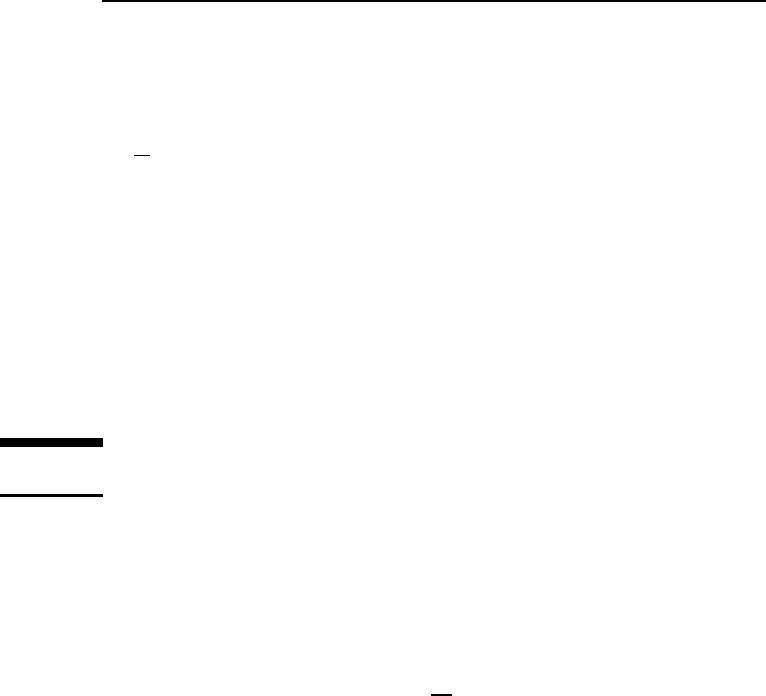
= 1000 loss measurements per run, we compareFDSA with the localized

random search method of Sect. 6.2. Based on principles for gain selection in Spall

(2003, Sect. 6.6) together with some limited trial-and-error experimentation, we

chose a

= 0.5, c = 1, A = 5, α = 0.602,andγ = 0.101 for FDSA and an average

of 20 loss measurements per iteration with normally distributed perturbations

having distribution N(0,0.5

) for the random search method.

On-screen viewing permitted. Printing not permitted.

Please buy this book at your bookshop. Order information see http://www.springeronline.com/3-540-40464-3

Handbook of Computational Statistics

(J. Gentle, W. Härdle, and Y. Mori, eds.)

Stochastic Optimization 183

Figure 6.2 summarizes the results. Each curve represents the sample mean of

50 independent replications. An individual replication of one of the two algo-

rithms has much more variation than the corresponding smoothed curve in the

ﬁgure.

Figure 6.2. Comparison of FDSA and localized random search. Each curve represents sample mean of

50 independent replications

Figure 6.2 shows that both algorithms produce an overall reduction in the

(true) loss function as the number of measurements approach 1000.Thecurves

illustrate that FDSA outperforms random search in this case. To make the com-

parison fair, attempts were made to tune each algorithm to provide approxi-

mately the best performance possible. Of course, one must be careful about

using this example to infer that such a result will hold in other problems as

well.

Simultaneous Perturbation SA 6.3.3

The FDSA algorithm of Sect. 6.3.2 is a standard SA method for carrying out opti-

mizationwith noisy measurement ofthe loss function. However,as the dimensionp

grows large, the number of loss measurements required may become prohibitive.

That is, each two-sided gradient approximation requires 2p loss measurements.

More recently, the simultaneous perturbation SA (SPSA) method was introduced,

requiring only two measurements per iteration to form a gradient approximation

independent of the dimension p. This provides the potential for a large savings in

the overall cost of optimization.

Beginning with the generic SA form in (6.4), we now present the SP form of the

gradient approximation. In this form, all elements of

are randomly perturbed

On-screen viewing permitted. Printing not permitted.

Please buy this book at your bookshop. Order information see http://www.springeronline.com/3-540-40464-3

Handbook of Computational Statistics

(J. Gentle, W. Härdle, and Y. Mori, eds.)

184 James C. Spall

together to obtain two loss measurements y(·). For the two-sided SP gradient

approximation, this leads to

ˆg

(

) =







+ c

∆

)−y(

− c

∆

)

∆

+ c

∆

)−y(

− c

∆

)

∆







+ c

∆

)−y(

− c

∆

)

∆

−1

, ∆

−1

, … , ∆

−1

, (6.6)

where the mean-zero p-dimensional random perturbation vector,

∆

= [∆

, ∆

… ,

∆

]

, has a user-speciﬁed distribution satisfying certain conditions and c

is a positive scalar (as with FDSA). Because the numerator is the same in all

p components of ˆg

(

), the number of loss measurements needed to estimate the

gradient in SPSA is two,regardlessofthedimensionp.

Relative to FDSA, the p-fold measurement savings per iteration, of course, pro-

vides only the potential for SPSA to achieve large savings in the total number of

measurementsrequired to estimate

θ when p is large. This potential is realizedif the

number of iterations required for effective convergence to an optimum θ

∗

does not

increase in a way to cancel the measurement savings per gradient approximation.

One can use asymptotic distribution theory to address this issue. In particular,

both FDSA and SPSA are known to be asymptotically normally distributed under

very similar conditions. One can use this asymptotic distribution result to charac-

terize the mean-squared error E





− θ

∗



for the two algorithms for large k.

Fortunately, under fairly broad conditions, the p-fold savings at each iteration is

preserved across iterations. In particular, based on asymptotic considerations:

Under reasonably general conditions (see Spall, 1992, or Spall, 2003, Chap. 7),

the SPSA and FDSA algorithms achieve the same level of statistical accuracy

for a given number of iterations even though SPSA uses only 1

|p times the

number of function evaluations of FDSA (since each gradient approximation

uses only 1

|p the number of function evaluations).

The SPSA Web site (www.jhuapl.edu|SPSA) includes many references on the

theory and application of SPSA. On this Web site, one can ﬁnd many accounts

of numerical studies that are consistent with the efﬁciency statement above. (Of

course, given that the statement is based on asymptotic arguments and associ-

ated regularity conditions, one should not assume that the result always holds.)

In addition, there are references describing many applications. These include

queuing systems, pattern recognition, industrial quality improvement, aircraft

design, simulation-based optimization, bioprocess control, neural network train-

On-screen viewing permitted. Printing not permitted.

Please buy this book at your bookshop. Order information see http://www.springeronline.com/3-540-40464-3

Handbook of Computational Statistics

(J. Gentle, W. Härdle, and Y. Mori, eds.)

Stochastic Optimization 185

ing, chemical process control, fault detection, human-machine interaction, sensor

placement and conﬁguration, and vehicle trafﬁc management.

We will not present the formal conditions for convergence and asymptotic

normalityof SPSA,as suchconditionsareavailablein manyreferences(e.g.,Dippon

and Renz, 1997; Gerencsér, 1999; Spall, 1992, 2003, Chap. 7). These conditions are

essentially identical to the standard conditions for convergence of SA algorithms,

with the exception of the additional conditions on the user-generated perturbation

vector

∆

The choice of the distribution for generating the

∆

is important to the perfor-

mance of the algorithm. The standard conditions for the elements

∆

of ∆

are

that the {∆

} are independent for all k, i, identically distributed for all i at each k,

symmetrically distributed about zero and uniformly bounded in magnitude for

all k. In addition, there is an important inverse moments condition:



∆

2+2τ



≤ C

for some

τ > 0 and C>0. The role of this condition is to control the variation

of the elements of ˆg

(

) (which have ∆

in the denominator). One simple and

popular distribution that satisﬁes the inverse moments condition is the symmetric

Bernoulli ±1 distribution. (In fact, as discussed in Spall, 2003, Sect. 7.7, this

distribution can be shown to be optimal under general conditions when using

asymptotic considerations.) Two common mean-zero distributions that do not

satisfy the inverse moments condition are symmetric uniform and normal with

mean zero. The failureofboth ofthese distributions is a consequence of the amount

of probability mass near zero. Exercise 7.3 in Spall (2003) illustrates the dramatic

performance degradation that can occur through using distributions that violate

the inverse moments condition.

As with any real-world implementation of stochastic optimization, there are

important practical considerations when using SPSA. One is to attempt to deﬁne

so that the magnitudes of the θ elements are similar to one another. This desire is

apparent bynoting thatthe magnitudes ofall components in the perturbations c

∆

are identical in the case where identical Bernoulli distributions are used. Although

it is not always possible to choose the deﬁnition of the elements in θ,inmost

cases an analyst will have the ﬂexibility to specify the units for

θ to ensure similar

magnitudes. Another important consideration is the choice of the gains a

, c

.The

principles described for FDSA above apply to SPSA as well. Section 7.5 of Spall

(2003) provides additional practical guidance.

There have been a number of important extensions of the basic SPSA method

represented by the combination of (6.4) and (6.6). Three such extensions are to

the problem of global (versus local) optimization, to discrete (versus continuous)

problems, and to include second-order-type information (Hessian matrix) with

the aim of creating a stochastic analogue to the deterministic Newton–Raphson

method.

On-screen viewing permitted. Printing not permitted.

Please buy this book at your bookshop. Order information see http://www.springeronline.com/3-540-40464-3

Handbook of Computational Statistics

(J. Gentle, W. Härdle, and Y. Mori, eds.)

186 James C. Spall

TheuseofSPSAforglobal minimization among multiple local minima is dis-

cussed in Maryak and Chin (2001). One of their approaches relies on injecting

Monte Carlo noise in the right-hand side of the basic SPSA updating step in (6.4).

This approach is a common way of converting SA algorithms to global optimiz-

ers through the additional “bounce” introduced into the algorithm (Yin, 1999).

Maryak and Chin (2001) also show that basic SPSA without injected noise (i.e.,

(6.4) and (6.6) without modiﬁcation) may, under certain conditions, be a global

optimizer. Formal justiﬁcation for this result follows because the random error in

the SP gradient approximation acts in a way that is statistically equivalent to the

injected noise mentioned above.

Discrete optimization problems (where

θ may take on discrete or combined

discrete

|continuous values) are discussed in Gerencsér et al. (1999). Discrete SPSA

relies on a ﬁxed-gain (constant a

and c

) version of the standard SPSA method.

The parameter estimates produced are constrained to lie on a discrete-valued

grid. Although gradients do not exist in this setting, the approximation in (6.6)

(appropriately modiﬁed) is still useful as an efﬁcient measure of slope information.

Finally, using the simultaneous perturbation idea, it is possible to construct

a simple method for estimating the Hessian (or Jacobian) matrix of L while, con-

currently, estimating the primary parameters of interest (

θ). This adaptive SPSA

(ASP) approach produces a stochastic analogue to the deterministic Newton–

Raphson algorithm (e.g., Bazaraa et al., 1993, pp. 308–312), leading to a recursion

that is optimal or near-optimal in its rate of convergence and asymptotic error. The

approach applies in both the gradient-free setting emphasized in this section and

in the root-ﬁnding

|stochastic gradient-based (Robbins–Monro) setting reviewed

in Spall (2003, Chaps. 4 and 5). Like the standard SPSA algorithm, the ASP al-

gorithm requires only a small number of loss function (or gradient, if relevant)

measurementsper iteration – independentoftheproblem dimension– to adaptive-

ly estimate the Hessian and parameters of primary interest. Further information

is available at Spall (2000) or Spall (2003, Sect. 7.8).

Genetic Algorithms6.4

Introduction6.4.1

Genetic algorithms (GAs)represent a popular approach to stochastic optimization,

especially as relates to the global optimization problem of ﬁnding the best solution

among multiple local mimima. (GAs may be used in general search problems that

are not directly represented as stochastic optimization problems, but we focus

here on their use in optimization.) GAs represent a special case of the more general

class of evolutionary computation algorithms (which also includes methods such

as evolutionary programming and evolution strategies). The GA applies when the

elements of

θ are real-, discrete-, or complex-valued. As suggested by the name, the

GA is based loosely on principles of natural evolution and survival of the ﬁttest.

On-screen viewing permitted. Printing not permitted.

Please buy this book at your bookshop. Order information see http://www.springeronline.com/3-540-40464-3

Handbook of Computational Statistics

(J. Gentle, W. Härdle, and Y. Mori, eds.)

Stochastic Optimization 187

Infact,inGAterminology,anequivalentmaximization criterion, such as −L(θ)

(or its analogue based on a bit-string form of θ),isoftenreferredtoastheﬁtness

function to emphasize the evolutionary concept of the ﬁttest of a species.

A fundamental difference between GAs and the random search and SA al-

gorithms considered in Sects. 6.2 and 6.3 is that GAs work with a population

of candidate solutions to the problem. The previous algorithms worked with one

solutionand moved toward the optimumby updating this one estimate. GAssimul-

taneously consider multiple candidate solutions to the problem of minimizing L

and iterate by moving this population of solutions toward a global optimum. The

terms generation and iteration are used interchangeably to describe the process

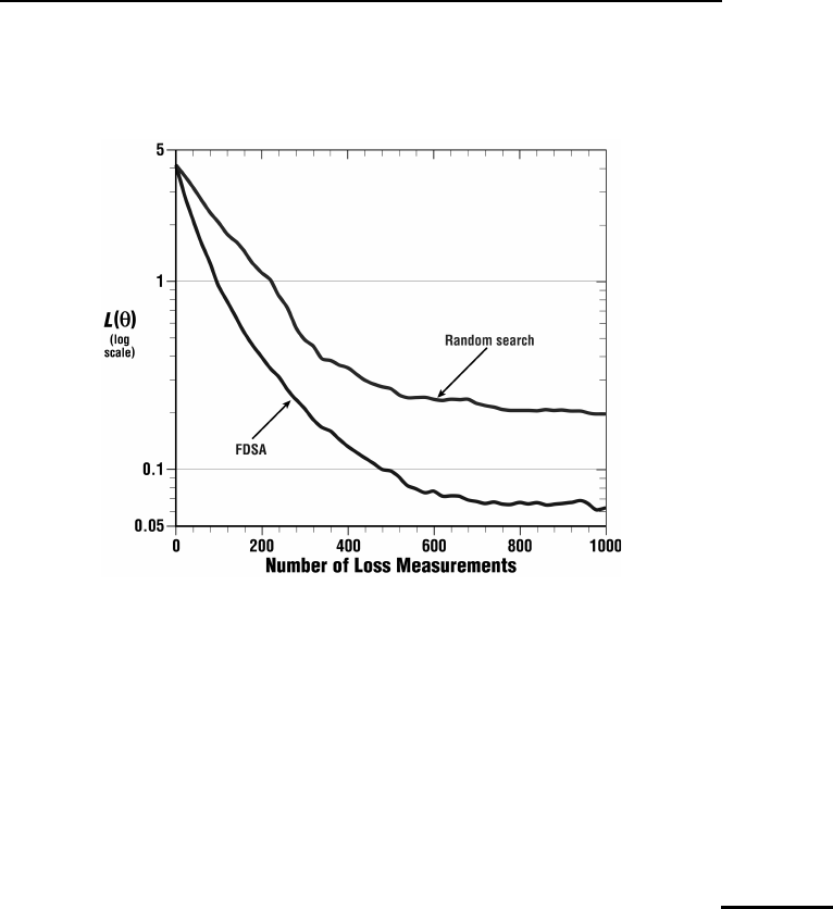
of transforming one population of solutions to another. Figure 6.3 illustrates the

successful operations of a GA for a population of size 12 with problem dimension

= 2. In this conceptual illustration, the population of solutions eventually come

together at the global optimum.

Figure 6.3. Minimization of multimodal loss function. Successful operations of a GA with

apopulationof12 candidate solutions clustering around the global minimum after some number of

iterations (generations) (Reprinted from Introduction to Stochastic Search and Optimization with

permission of John Wiley & Sons, Inc.)

The use of a population versus a single solution affects in a basic way the

range of practical problems that can be considered. In particular, GAs tend to be

best suited to problems where the loss function evaluations are computer-based

calculations such as complex function evaluations or simulations. This contrasts

with the single-solution approaches discussed earlier, where the loss function

evaluations may represent computer-based calculations or physical experiments.

Population-based approaches are not generally feasible when working with real-

time physical experiments. Implementing a GA with physical experimentsrequires

that either there be multiple identical experimental setups (parallel processing)

or that the single experimental apparatus be set to the same state prior to each

population member’s loss evaluation (serial processing). These situations do not

occur often in practice.

Speciﬁc values of

θ in the population are referred to as chromosomes.Thecen-

tral idea in a GA is to move a set (population) of chromosomes from an initial

collection of values to a point where the ﬁtness function is optimized. We let N

denote the population size (number of chromosomes in the population). Most

of the early work in the ﬁeld came from those in the ﬁelds of computer science

and artiﬁcial intelligence. More recently, interest has extended to essentially all

On-screen viewing permitted. Printing not permitted.

Please buy this book at your bookshop. Order information see http://www.springeronline.com/3-540-40464-3

Handbook of Computational Statistics

(J. Gentle, W. Härdle, and Y. Mori, eds.)

188 James C. Spall

branches of business, engineering, and science where search and optimization are

of interest. The widespread interest in GAs appears to be due to the success in

solving many difﬁcult optimization problems. Unfortunately, to an extent greater

than with other methods, some interest appears also to be due to a regrettable

amount of “salesmanship” and exaggerated claims. (For example, in a recent soft-

ware advertisement, the claim is made that the software “… uses GAs to solve

any optimization problem.” Such statements are provably false.) While GAs are

important tools within stochastic optimization, there is no formal evidence of con-

sistently superior performance – relative to other appropriate types of stochastic

algorithms – in any broad, identiﬁable class of problems.

Let us now give a very brief historical account.The reader is directed to Goldberg

(1989, Chap. 4), Mitchell (1996, Chap. 1), Michalewicz (1996, pp. 1–10), Fogel (2000,

Chap. 3), and Spall (2003, Sect. 9.2) for more complete historical discussions.

There had been some success in creating mathematical analogues of biological

evolution for purposes of search and optimization since at least the 1950 s (e.g.,

Box, 1957). The cornerstones of modern evolutionary computation – evolution

strategies, evolutionary programming, and GAs – were developed independently

of each other in the 1960 s and 1970 s. John Holland at the University of Michigan

published the seminal monograph Adaptation in Natural and Artiﬁcial Systems

(Holland, 1975). There was subsequently a sprinkle of publications, leading to the

ﬁrst full-ﬂedged textbook Goldberg (1989). Activity in GAs grew rapidly beginning

in the mid-1980 s, roughly coinciding with resurgent activity in other artiﬁcial

intelligence-type areas such as neural networks and fuzzy logic. There are now

many conferences and books in the area of evolutionary computation (especially

GAs), together with countless other publications.

Chromosome Coding and the Basic GA Operations6.4.2

This section summarizes some aspects of the encoding process for the popula-

tion chromosomes and discusses the selection, elitism, crossover,andmutation

operations. These operations are combined to produce the steps of the GA.

An essential aspect of GAs is the encoding of the N values of

θ appearing in

the population. This encoding is critical to the GA operations and the associated

decoding to return to the natural problem space in

θ. Standard binary (0, 1) bit

strings have traditionally been the most common encoding method, but other

methods include gray coding (which also uses (0, 1) strings, but differs in the way

the bits are arranged) and basic computer-based ﬂoating-point representation

of the real numbers in

θ.This10-character coding is often referred to as real-

number coding since it operates as if working with θ directly. Based largely on

successful numerical implementations, this natural representation of

θ has grown

more popular over time. Details and further references on the above and other

coding schemes are given in Michalewicz (1996, Chap. 5), Mitchell (1996, Sects. 5.2

and 5.3), Fogel (2000, Sects. 3.5 and 4.3), and Spall (2003, Sect. 9.3).

Let us now describe the basic operations mentioned above. For consistency

with standard GA terminology, let us assume that L(

θ) has been transformed

On-screen viewing permitted. Printing not permitted.

Please buy this book at your bookshop. Order information see http://www.springeronline.com/3-540-40464-3

Handbook of Computational Statistics

(J. Gentle, W. Härdle, and Y. Mori, eds.)

Stochastic Optimization 189

to a ﬁtness function with higher values being better. A common transformation

is to simply set the ﬁtness function to −L(θ)+C,whereC ≥ 0 is a constant

that ensures that the ﬁtness function is nonnegative on

Θ (nonnegativity is only

required in some GA implementations). Hence, the operations below are described

for a maximization problem. It is also assumed here that the ﬁtness evaluations are

noise-free. Unless otherwise noted, the operations below apply with any coding

scheme for the chromosomes.

selection and elitism steps occur after evaluating the ﬁtness function for the

current population of chromosomes. A subset of chromosomes is selected to use

as parents for the succeedinggeneration.This operation is where the survival of the

ﬁttest principle arises, as the parents are chosen according to their ﬁtness value.

While the aim is to emphasize the ﬁtter chromosomes in the selection process,

it is important that not too much priority is given to the chromosomes with the

highest ﬁtness values early in the optimization process. Too much emphasis of

the ﬁtter chromosomes may tend to reduce the diversity needed for an adequate

search of the domain of interest, possibly causing premature convergence in a local

optimum. Hence methods for selection allow with some nonzero probability the

selection of chromosomes that are suboptimal.

Associated with the selection step is the optional “elitism” strategy, where the

<Nbest chromosomes (as determined from their ﬁtness evaluations) are

placed directly into the next generation. This guarantees the preservation of the

best chromosomes at each generation. Note that the elitist chromosomes in the

original population are also eligible for selection and subsequent recombination.

As with the coding operation for

θ, many schemes have been proposed for the

selection process of choosing parents for subsequent recombination. One of the

most popular methods is roulette wheel selection (also called ﬁtness proportionate

selection). In this selection method, the ﬁtness functions must be nonnegative

Θ. An individual’s slice of a Monte Carlo-based roulette wheel is an area pro-

portional to its ﬁtness. The “wheel” is spun in a simulated fashion N − N

times

and the parents are chosen based on where the pointer stops. Another popu-

lar approach is called tournament selection. In this method, chromosomes are

compared in a “tournament,” with the better chromosome being more likely to

win. The tournament process is continued by sampling (with replacement) from

the original population until a full complement of parents has been chosen. The

most common tournament method is the binary approach, where one selects two

pairs of chromosomes and chooses as the two parents the chromosome in each

pair having the higher ﬁtness value. Empirical evidence suggests that the tour-

nament selection method often performs better than roulette selection. (Unlike

tournament selection, roulette selection is very sensitive to the scaling of the ﬁt-

ness function.) Mitchell (1996, Sect. 5.4) provides a good survey of several other

selection methods.

The crossover operation creates offspring of the pairs of parents from the

selection step. A crossover probability P

is used to determine if the offspring

will represent a blend of the chromosomes of the parents. If no crossover takes

place, then the two offspring are clones of the two parents. If crossover does take

On-screen viewing permitted. Printing not permitted.

Please buy this book at your bookshop. Order information see http://www.springeronline.com/3-540-40464-3

Handbook of Computational Statistics

(J. Gentle, W. Härdle, and Y. Mori, eds.)

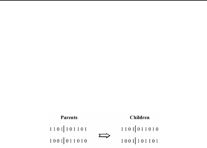
190 James C. Spall

place, then the two offspring are produced according to an interchange of parts

of the chromosome structure of the two parents. Figure 6.4 illustrates this for

the case of a ten-bit binary representation of the chromosomes. This example

shows one-point crossover, where the bits appearing after one randomly cho-

sen dividing (splice) point in the chromosome are interchanged. In general, one

can have a number of splice points up to the number of bits in the chromo-

somes minus one, but one-point crossover appears to be the most commonly

used.

Note that the crossover operator also applies directly with real-number cod-

ing since there is nothing directly connected to binary coding in crossover. All

that is required are two lists of compatible symbols. For example, one-point

crossover applied to the chromosomes (

θ values) [6.7, −7.4, 4.0, 3.9|6.2, −1.5] and

[−3.8, 5.3, 9.2, −0.6|8.4, −5.1] yields the two children: [6.7, −7.4, 4.0, 3.9, 8.4, −5.1]

and [−3.8, 5.3, 9.2, −0.6, 6.2, −1.5].

Figure 6.4. Example of crossover operator under binary coding with one splice point

The ﬁnal operation we discuss is mutation. Because the initial population may

not contain enough variability to ﬁnd the solution via crossover operations alone,

the GA also uses a mutation operator where the chromosomes are randomly

changed. For the binary coding, the mutation is usually done on a bit-by-bit basis

where a chosen bit is ﬂipped from 0 to 1, or vice versa. Mutation of a given bit

occurs with small probability P

. Real-number coding requires a different type

of mutation operator. That is, with a (0, 1)-based coding, an opposite is uniquely

deﬁned, but with a real number, there is no clearly deﬁned opposite (e.g., it does

not make sense to “ﬂip” the 2.74 element). Probably the most common type of

mutation operator is simply to add small independent normal (or other) random

vectors to each of the chromosomes (the

θ values) in the population.

As discussed in Sect. 6.1.4, there is no easy way to know when a stochastic

optimization algorithm has effectively converged to an optimum. this includes

gas. The one obvious means of stopping a GA is to end the search when a budget

of ﬁtness (equivalently, loss) function evaluations has been spent. Alternatively,

termination may be performed heuristically based on subjective and objective

impressions about convergence. In the case where noise-free ﬁtness measure-

ments are available, criteria based on ﬁtness evaluations may be most useful.

for example, a fairly natural criterion suggested in Schwefel (1995, p. 145) is to

stop when the maximum and minimum ﬁtness values over the N population

values within a generation are sufﬁciently close to one another. however, this

criterion provides no formal guarantee that the algorithm has found a global

solution.

On-screen viewing permitted. Printing not permitted.

Please buy this book at your bookshop. Order information see http://www.springeronline.com/3-540-40464-3

Handbook of Computational Statistics

(J. Gentle, W. Härdle, and Y. Mori, eds.)

Stochastic Optimization 191

The Core Genetic Algorithm 6.4.3

The steps of a basic form of the GA are given below. These steps are general enough

to govern many (perhaps most) modern implementations of GAs, including those

in modern commercial software. Of course, the performance of a GA typically

depends greatly on the implementation details, just as with other stochastic opti-

mization algorithms. Some of these practical implementation issues are taken up

in the next section.

Core GA Steps for Noise-Free Fitness Evaluations

Step 0 (Initialization) Randomly generate an initial population of N chromosomes

and evaluate the ﬁtness function (the conversion of L(

θ) to a function to be

maximized for the encoded version of

θ) for each of the chromosomes.

Step 1 (Parent Selection)SetN

= 0 if elitism strategy is not used; 0 <N

otherwise. Select with replacement N − N

parents from the full population

(including the N

elitist elements). The parents are selected according to

their ﬁtness, with those chromosomes having a higher ﬁtness value being

selected more often.

Step 2 (Crossover) For each pair of parents identiﬁed in Step 1, perform crossover

on the parents at a randomly (perhaps uniformly) chosen splice point (or

points if using multi-point crossover) with probability P

.Ifnocrossover

takes place (probability 1−P

), then form two offspring that are exact copies

(clones) of the two parents.

Step 3 (Replacement and Mutation) While retaining the N

best chromosomes

from the previous generation, replace the remaining N − N

chromosomes

with the current population of offspring from Step 2. For the bit-based

implementations, mutate the individual bits with probability P

; for real

coded implementations, use an alternative form of “small” modiﬁcation (in

either case, one has the option of choosing whether to make the N

elitist

chromosomes candidates for mutation).

Step 4 (Fitness and End Test) Compute the ﬁtness values for the new population

of N chromosomes. Terminate the algorithm if the stopping criterion is met

or if the budget of ﬁtness function evaluations is exhausted; else return to

Step 1.

Some Implementation Aspects 6.4.4

Whilethe above stepsprovidethebroad outlineformany modernimplementations

of GAs, there are some important implementation aspects that must be decided

before a practical implementation. This section outlines a few of those aspects.

More detailed discussions are given in Mitchell (1996, Chap. 5), Michalewicz (1996,

Chaps. 4–6), Fogel (2000, Chaps. 3 and 4), Goldberg (2002, Chap. 12), and other

references mentioned below. A countless number of numerical studies have been

reported in the literature; we do not add to that list here.

On-screen viewing permitted. Printing not permitted.

Please buy this book at your bookshop. Order information see http://www.springeronline.com/3-540-40464-3

Handbook of Computational Statistics

(J. Gentle, W. Härdle, and Y. Mori, eds.)

192 James C. Spall

As with other stochastic optimization methods, the choice of algorithm-speciﬁc

coefﬁcients has a signiﬁcant impact on performance. With GAs, there is a relatively

large number of user decisions required. The following must be set: the choice of

chromosome encoding, the population size (N), the probability distribution gen-

erating the initial population, the strategy for parent selection (roulette wheel or

otherwise), the number of splice points in the crossover, the crossover probabil-

ity (P

), the mutation probability (P

), the number of retained chromosomes in

elitism (N

), and some termination criterion. Some typical values for these quan-

tities are discussed, for example, in Mitchell (1996, pp. 175–177) and Spall (2003,

Sect. 9.6).

Constraints on L(

θ) (or the equivalent ﬁtness function) and|or θ are of major

importancein practice.Thebit-basedimplementationofGAsprovide a naturalway

of implementing component-wise lower and upper bounds on the elements of

(i.e., a hypercube constraint). More general approaches to handling constraints are

discussed in Michalewicz (1996, Chap. 7 and Sects. 4.5 and 15.3) and Michalewicz

and Fogel (2000, Chap. 9).

Until now, it has been assumed that the ﬁtness function is observed without

noise. One of the two possible deﬁning characteristics of stochastic optimization,

however, is optimization with noise in the function measurements (Property I

in Sect. 6.1.3). There appears to be relatively little formal analysis of GAs in the

presenceofnoise,althoughtheapplicationandtestingofGAsin suchcases hasbeen

carried out since at least the mid-1970 s (e.g., De Jong, 1975, p. 203). A large number

of numerical studies are in the literature (e.g., the references and studies in Spall,

2003, Sects. 9.6 and 9.7). As with other algorithms, there is a fundamental tradeoff

of more accurate information for each function input (typically, via an averaging

of the inputs) and fewer function inputs versus less accurate (“raw”) information

to the algorithm together with a greater number of inputs to the algorithm. There

appears to be no rigorous comparison of GAs with other algorithms regarding

relative robustness to noise. Regarding noise, Michalewicz and Fogel (2000, p. 325)

state: “There really are no effective heuristics to guide the choices to be made that

will work in general.”

Some Comments on the Theory for GAs6.4.5

One of the key innovations in Holland (1975) was the attempt to put GAs on

a stronger theoretical footing than the previous ad hoc treatments. He did this by

the introduction of schema theory. While many aspects and implications of schema

theory have subsequently been challenged (Reeves and Rowe, 2003, Chap. 3; Spall,

2003, Sect. 10.3), some aspects remain viable. In particular, schema theory itself is

generally correct (subject to a few modiﬁcations), although many of the assumed

implications have not been correct. With the appropriate caveats and restrictions,

schema theory provides some intuitive explanation for the good performance that

is frequently observed with GAs.

Morerecently,Markovchainshavebeenusedtoprovideaformalstructurefor

analyzing GAs. First, let us mention one negative result. Markov chains can be used

On-screen viewing permitted. Printing not permitted.

Please buy this book at your bookshop. Order information see http://www.springeronline.com/3-540-40464-3

Handbook of Computational Statistics

(J. Gentle, W. Härdle, and Y. Mori, eds.)

Stochastic Optimization 193

to show that a canonical GA without elitismis (in general) provably nonconvergent

(Rudolph, 1994). That is, with a GA that does not hold onto the best solution at

each generation, there is the possibility (through crossover and mutation) that

a chromosome corresponding to

∗

will be lost. (Note that the GA without elitism

corresponds to the form in Holland, 1975.)

Onthe otherhand,conditionsforthe formal convergenceofGAs toan optimal

∗

(or its coded equivalent) are presented in Vose (1999, Chaps. 13 and 14), Fogel

(2000, Chap. 4), Reeves and Rowe (2003, Chap. 6), and Spall (2003, Sect. 10.5),

among other references. Consider a binary bit-coded GA with a population size

of N and a string length of B bits per chromosome. Then the total number of

possible unique populations is:

≡



N +2

−1



(N +2

−1)!

−1)!N!

(Suzuki, 1995). It is possible to construct an N

×N

Markov transition matrix P,

where the ijth element is the probability of transitioning from the ith population

of N chromosomes to the jth population of the same size. These elements depend

in a nontrivial way on N, the crossover rate, and the mutation rate; the number of

elite chromosomes is assumed to be N

= 1 (Suzuki, 1995). Let p

be an N

× 1

vector having jth component p

(j) equal to the probability that the kth generation

will result in population j, j = 1, 2, … , N

. From basic Markov chain theory,

k+1

= p

P = p

k+1

where p

isaninitialprobabilitydistribution.Ifthechainisirreducibleandergodic

(see, e.g., Spall, 2003, Appendix E), the limiting distribution of the GA (i.e.,

lim

k→∞

= lim

k→∞

)existsand satisﬁes thestationarity equation

(Recall from basic Markov chain theory that irreducibility indicates that any state

may be reached from any other state after a ﬁnite number of steps.)

Suppose that

∗

is unique (i.e., Θ

∗

is the singleton θ

∗

). Let J ⊆{1, 2, … , N

}

be the set of indices corresponding to the populations that contain at least one

chromosome representing

∗

. So, for example, if J = {1, 6, N

−3},theneachofthe

three populations indexed by 1, 6 and N

−3contains at least one chromosome

that,whendecoded,isequalto

∗

. Under the above-mentioned assumptions of

irreducibility and ergodicity,



i∈J

= 1,where

is the ith element of

p. Hence,

aGAwithN

= 1 and a transition matrix that is irreducible and ergodic converges

in probability to θ

∗

Toestablishthe factofconvergencealone,it maynotbe necessary tocomputethe

P matrix. Rather, it sufﬁces to know that the chain is irreducible and ergodic. (For

example, Rudolph, 1997, p. 125, shows that the Markov chain approach yields con-

vergence when 0 <P

< 1.) However, P must be explicitly computed to get the rate

of convergence information that is available from p

.Thisisrarelypossibleinprac-

tice because the number of states in the Markov chain (and hence dimension of the

Markov transition matrix) grows very rapidly with increases in the population size

On-screen viewing permitted. Printing not permitted.

Please buy this book at your bookshop. Order information see http://www.springeronline.com/3-540-40464-3

Handbook of Computational Statistics

(J. Gentle, W. Härdle, and Y. Mori, eds.)

194 James C. Spall

and|or the number of bits used in coding for the population elements. For example,

in even a trivial problem of N = B = 6,thereare∼ 10

states and ∼ 10

elements

in the transition matrix; this problem is much smaller than any practical GA, which

can easily have 50 to 100 population elements and 15 to 40 bits per population el-

ement (leading to well over 10

100

states, with each element in the corresponding

row and column in the transition matrix requiring signiﬁcant computation).

Concluding Remarks6.5

Stochastic optimization is a major branch of computational statistics. This paper

has been a whirlwind tour through some important issues and methods in stochas-

tic optimization. Stochastic optimization applies when there are noisy measure-

ments of the criterion being optimized and|orthereisaninjectedMonteCarlo

randomness as part of the algorithm. Of necessity, we cover only a small fraction of

available methods in this relatively brief review, although the methods described

(random search, stochastic approximation, and genetic algorithms) are represen-

tative of a broad range of important and widely used algorithms. Further, the

treatment here on the speciﬁc algorithms is relatively brief. In particular, the sub-

jects covered in this paper of approximately 30 pages are treated in over 160 pages

in Spall (2003, Chaps. 1–2, 6–7, and 9–10) and are given an even more detailed

treatment in the many specialized books or other references.

There are many challenges to carrying out real-world optimization, including

the presence of noise in the function evaluations, the difﬁculties in distinguishing

a globally optimal solution from locally optimal solutions, the “curse of dimen-

sionality,” the difﬁculties associated with nontrivial constraints, and the lack of

stationarity in the solution as a result of the conditions of the problem changing

over time. Stochastic optimization methods are especially useful in treating some

of these challenges. In particular, by deﬁnition, they are designed for noisy func-

tion evaluations. Further, when considering injected (Monte Carlo) randomness

(property II in Sect. 6.1.3), certain stochastic optimization algorithms will (under

conditions, of course) serve as global optimizers. That is, the injected randomness

provides enough “bounce” to the algorithm to allow for escape from local minima

en route to achieving a global minimum.

In summary, while classical deterministic optimization methods (linear and

nonlinear programming) are effective for a range of problems, stochastic methods

are able to handle many of the problems for which deterministic methods are

inappropriate. It is hoped that this summary gives the reader a ﬂavor of the issues,

algorithms, and challenges in carrying out optimization in the face of stochastic

effects.

Acknowledgements. IappreciatethehelpfulcommentsofDr.StacyHillonadraft

version of this paper. Funding was provided by the U. S. Navy (contract N00024-

98-D-8124) and the JHU

|APL Independent Research and Development (IRAD)

On-screen viewing permitted. Printing not permitted.

Please buy this book at your bookshop. Order information see http://www.springeronline.com/3-540-40464-3

Handbook of Computational Statistics

(J. Gentle, W. Härdle, and Y. Mori, eds.)

Stochastic Optimization 195

Program. Selected parts of this article havebeenreprinted,bypermission,from J.C.

Spall, Introduction to Stochastic Search and Optimization,

2003 by John Wiley

and Sons, Inc.

References

Arsham, H. (1998), “Techniques for Monte Carlo Optimizing,” Monte Carlo Meth-

ods and Applications, vol. 4, pp. 181–229.

Baba, N., Shoman, T., and Sawaragi, Y. (1977), “A Modiﬁed Convergence Theorem

for a Random Optimization Method,” Information Sciences,vol.13,pp.159–166.

Bazaraa, M.S., Sherali, H.D., and Shetty, C.M. (1993), Nonlinear Programming:

Theory and Algorithms (2nd ed.), Wiley, New York.

Blum, J.R. (1954), “Multidimensional Stochastic Approximation Methods,” Annals

of Mathematical Statistics, vol. 25, pp. 737–744.

Box, G.E.P. (1957), “Evolutionary Operation: A Method for Increasing Industrial

Productivity,” Journal of the Royal Statistical Society, Ser. C., vol. 6, pp. 81–101.

De Jong, K.A. (1975), “An Analysis of the Behavior of a Class of Genetic Adaptive

Systems,” Ph.D. dissertation, University of Michigan, Ann Arbor, MI (Univer-

sity Microﬁlms no. 76–9381).

Dippon, J. and Renz, J. (1997), “Weighted Means in Stochastic Approximation of

Minima,” SIAM Journal of Control and Optimization, vol. 35, pp. 1811–1827.

Fabian, V. (1971), “Stochastic Approximation,” in Optimizing Methods in Statistics

(J.S. Rustigi, ed.), Academic Press, New York, pp. 439–470.

Fogel, D.B. (2000), Evolutionary Computation: Toward a New Philosophy of Ma-

chine Intelligence (2nd ed.), IEEE Press, Piscataway, NJ.

Fouskakis, D. and Draper, D. (2002), “Stochastic Optimization: A Review,” Inter-

national Statistical Review, vol. 70, pp. 315–349.

Fu, M.C. (2002), “Optimization for Simulation: Theory vs. Practice” (with discus-

sion by S. Andrad

ottir, P. Glynn, and J.P. Kelly), INFORMS Journal on Comput-

ing,vol.14,pp.192–227.

Gentle, J.E. (2003), Random Number Generation and Monte Carlo Methods (2nd

ed.), Springer-Verlag, New York.

Gerencsér, L. (1999), “Convergence Rate of Moments in Stochastic Approximation

with Simultaneous Perturbation Gradient Approximation and Resetting,” IEEE

Transactions on Automatic Control, vol. 44, pp. 894–905.

Gerencsér, L., Hill, S.D., and V

o, Z. (1999), “Fixed Gain SPSA for Discrete Op-

timization,” in Proceedings of the IEEE Conference on Decision and Control,

7–10 December 1999, Phoenix, AZ, pp. 1791–1795.

Goldberg, D.E. (1989), Genetic Algorithms in Search, Optimization, and Machine

Learning, Addison-Wesley, Reading, MA.

Gosavi, A. (2003), Simulation-Based Optimization: Parametric Optimization Tech-

niques and Reinforcement Learning, Kluwer Academic, Boston.

Holland, J.H. (1975), Adaptation in Natural and Artiﬁcial Systems,Universityof

Michigan Press, Ann Arbor, MI.

On-screen viewing permitted. Printing not permitted.

Please buy this book at your bookshop. Order information see http://www.springeronline.com/3-540-40464-3

Handbook of Computational Statistics

(J. Gentle, W. Härdle, and Y. Mori, eds.)

196 James C. Spall

Karnopp, D.C. (1963), “Random Search Techniques for Optimization Problems,”

Automatica, vol. 1, pp. 111–121.

Kiefer, J. and Wolfowitz, J. (1952), “Stochastic Estimation of a Regression Func-

tion,”Annals of Mathematical Statistics, vol. 23, pp. 462–466.

Kolda, T.G., Lewis, R.M., and Torczon, V. (2003), “Optimization by Direct Search:

New Perspectives on Some Classical and Modern Methods,” SIAM Review,

vol. 45, pp. 385–482.

Kushner, H.J. and Yin, G.G. (1997), Stochastic Approximation Algorithms and Ap-

plications, Springer-Verlag, New York.

Maryak, J.L. and Chin, D.C. (2001), “Global Random Optimization by Simultane-

ous Perturbation Stochastic Approximation,” in ProceedingsoftheAmerican

Control Conference, 25–27 June 2001, Arlington, VA, pp. 756–762.

Matyas, J. (1965), “Random Optimization,” Automation and Remote Control,

vol. 26, pp. 244–251.

Michalewicz, Z. (1996), Genetic Algorithms + Data Structures = Evolution Pro-

grams (3rd ed.), Springer-Verlag, New York.

Michalewicz, Z. and Fogel, D.B. (2000), HowtoSolveIt:ModernHeuristics,

Springer-Verlag, New York.

Mitchell, M. (1996), An Introduction to Genetic Algorithms, MIT Press,Cambridge,

MA.

Nelder, J.A. and Mead, R. (1965), “A Simplex Method for Function Minimization,”

The Computer Journal, vol. 7, pp. 308–313.

Pﬂug, G.Ch. (1996), Optimization of Stochastic Models: The Interface Between

Simulation and Optimization, Kluwer Academic, Boston.

Reeves, C.R. and Rowe, J.E. (2003), Genetic Algorithms – Principles and Perspec-

tives:AGuidetoGATheory, Kluwer Academic, Boston.

Robbins, H. and Monro, S. (1951), “A Stochastic Approximation Method,” Annals

of Mathematical Statistics, vol. 22, pp. 400–407.

Rudolph, G. (1994), “Convergence Analysis of Canonical Genetic Algorithms,”

IEEE Transactions on Neural Networks,vol.5,pp.96–101.

Rudolph, G. (1997), Convergence Properties of Evolutionary Algorithms,VerlagKo-

vac, Hamburg.

Ruppert, D. (1991), “Stochastic Approximation,” in Handbook of Sequential Anal-

ysis (B.K. Ghosh and P.K. Sen, eds.), Marcel Dekker, New York, pp. 503–529.

Schwefel, H.-P. (1995), Evolution and Optimum Seeking,Wiley,NewYork.

Solis, F.J. and Wets, J.B. (1981), “Minimization by Random Search Techniques,”

Mathematics of Operations Research,vol.6,pp.19–30.

Spall, J.C. (1992), “Multivariate Stochastic Approximation Using a Simultaneous

Perturbation Gradient Approximation,” IEEE Transactions on Automatic Con-

trol, vol. 37, pp. 332–341.

Spall, J.C. (2000), “Adaptive Stochastic Approximation by the Simultaneous Per-

turbation Method,”IEEE Transactions on Automatic Control, vol. 45, pp. 1839–

1853.

Spall, J.C. (2003), Introduction to Stochastic Search and Optimization: Estimation,

Simulation, and Control,Wiley,Hoboken,NJ.

On-screen viewing permitted. Printing not permitted.

Please buy this book at your bookshop. Order information see http://www.springeronline.com/3-540-40464-3

Handbook of Computational Statistics

(J. Gentle, W. Härdle, and Y. Mori, eds.)

Stochastic Optimization 197

Suzuki, J. (1995), “A Markov Chain Analysis on Simple Genetic Algorithms,” IEEE

Transactions on Systems, Man, and Cybernetics, vol. 25, pp. 655–659.

Wolpert, D.H. and Macready, W.G. (1997), “No Free Lunch Theorems for Optimiza-

tion,” IEEE Transactions on Evolutionary Computation, vol. 1, pp. 67–82.

Yin, G. (1999), “Rates of Convergence for a Class of Global Stochastic Optimization

Algorithms,” SIAM Journal on Optimization, vol. 10, pp. 99–120.

Zhigljavsky, A.A. (1991), Theory of Global Random Search, Kluwer Academic,

Boston.

On-screen viewing permitted. Printing not permitted.

Please buy this book at your bookshop. Order information see http://www.springeronline.com/3-540-40464-3

Handbook of Computational Statistics

(J. Gentle, W. Härdle, and Y. Mori, eds.)