Asia and Global Production Networks—Implications for Trade

EE_1439_Ferrarini_OL.indd 1 22/09/2014 08:06

Asia and Global

Production Networks

Implications for Trade, Incomes and

Economic Vulnerability

Edited by

Benno Ferrarini

Senior Economist, Economics and Research Department,

Asian Development Bank, Philippines

David Hummels

Professor of Economics, Department of Economics, Purdue

University and Research Associate, National Bureau of

Economic Research, USA

CO-PUBLICATION OF THE ASIAN DEVELOPMENT

BANK AND EDWARD ELGAR PUBLISHING

Edward Elgar

Cheltenham, UK • Northampton, MA, USA

retrieval system or transmitted in any form or by any means, electronic, mechanical

or photocopying, recording, or otherwise without the prior permission of the

publisher.

Published by

Edward Elgar Publishing Limited Edward Elgar Publishing, Inc.

The Lypiatts William Pratt House

15 Lansdown Road 9 Dewey Court

Cheltenham Northampton

Glos GL50 2JA Massachusetts 01060

UK USA

The views expressed in this book are those of the authors and do not necessarily

reflect the views and policies of the Asian Development Bank (ADB), its Board of

Governors or the governments they represent.

ADB does not guarantee the accuracy of the data included in this publication and

accepts no responsibility for any consequences of their use.

By making any designation of or reference to a particular territory or geographic

area, or by using the term “country” in this document, ADB does not intend to

make any judgments as to the legal or other status of any territory or area.

ADB encourages printing or copying information exclusively for personal and

noncommercial use with proper acknowledgment of ADB. Users are restricted

from reselling, redistributing, or creating derivative works for commercial purposes

without the express, written consent of ADB.

Asian Development Bank

6 ADB Avenue, Mandaluyong City

1550 Metro Manila, Philippines

Tel +63 2 632 4444

Fax +63 2 636 2444

www.adb.org

A catalogue record for this book

is available from the British Library

Library of Congress Control Number: 2014938802

This book is available electronically in the ElgarOnline.com

Economics Subject Collection

ISBN 978 1 78347 208 6 (cased)

ISBN 978 1 78347 209 3 (eBook)

Typeset by Servis Filmsetting Ltd, Stockport, Cheshire

Printed and bound in Great Britain by T.J. International Ltd, Padstow

Contents

List of contributors vii

Foreword by Changyong Rhee ix

List of abbreviations and acronyms xi

1 Asia and global production networks: implications for trade,

incomes and economic vulnerability 1

Benno Ferrarini and David Hummels

2 Developing a GTAP- based multi- region, input–output

framework for supply chain analysis 16

Terrie L. Walmsley, Thomas Hertel and David Hummels

3 The vulnerability of the Asian supply chain to localized

disasters 81

Thomas Hertel, David Hummels and Terrie L. Walmsley

4 Global supply chains and natural disasters: implications for

international trade 112

Laura Puzzello and Paul Raschky

5 Vertical specialization, tariff shirking and trade 148

Alyson C. Ma and Ari Van Assche

6 Changes in the production stage position of People’s Republic

of China trade 179

Deborah Swenson

7 External rebalancing, structural adjustment, and real exchange

rates in developing Asia 215

Andrei Levchenko and Jing Zhang

8 Global supply chains and macroeconomic relationships

in Asia 249

Menzie Chinn

9 Mapping global value chains and measuring trade in tasks 287

Hubert Escaith

vi Asia and global production networks

10 The development and future of Factory Asia 338

Richard Baldwin and Rikard Forslid

Index 369

vii

Contributors

Richard Baldwin is Professor of International Economics at the Graduate

Institute, Geneva, Switzerland; a visiting Research Professor at the

University of Oxford, UK; Director of the Center for Economic Policy

Research (CEPR), UK; and Editor- in- Chief of Vox.

Menzie Chinn is Professor of Public Affairs and Economics at the

RobertM. La Follette School of Public Affairs, University of Wisconsin,

USA.

Hubert Escaith is the Chief Statistician of the World Trade Organization,

Switzerland and Research Associate at the Centre de Recherche en

Développement Économique et Finance Internationale, GREQAM/

DEFI Aix- Marseille University, France.

Benno Ferrarini is Senior Economist in the Economics and Research

Department of the Asian Development Bank, Philippines.

Rikard Forslid is Professor, Department of Economics, Stockholm

University, Sweden.

Thomas Hertel is Distinguished Professor of Agricultural Economics

at Purdue University, USA and founder and Executive Director of the

Global Trade Analysis Project (GTAP).

David Hummels is Professor of Economics, Department of Economics,

Purdue University and a Research Associate of National Bureau of

Economic Research, USA.

Andrei Levchenko is Associate Professor, Department of Economics,

University of Michigan, USA; Faculty Research Fellow, National Bureau

of Economic Research, USA; and Research Fellow, Centre for Economic

Policy Research, UK.

Alyson C. Ma is Associate Professor of Economics, University of San

Diego, USA.

Laura Puzzello is Senior Lecturer in the Department of Economics at

Monash University, Australia.

viii Asia and global production networks

Deborah Swenson is Professor of Economics, University of California –

Davis, USA and a Research Associate of National Bureau of Economic

Research.

Paul Raschky is Senior Lecturer in the Department of Economics at

Monash University, Australia.

Ari Van Assche is Associate Professor of International Business at HEC

Montréal and Research Fellow at CIRANO, Canada.

Terrie L. Walmsley is an Honorary Associate Professor in the Department

of Economics at the University of Melbourne, Australia and Chief

Economist at ImpactECON LLC, USA.

Jing Zhang is Senior Economist at the Federal Reserve Bank of Chicago,

USA.

Foreword

The past few years have witnessed the emergence of a large and growing

body of research on global value chains (GVCs), that is the creation of

final goods and services through interlinked stages of production scattered

across international borders. Although GVCs are hardly a new phenom-

enon, the attention devoted to the topic largely is. After years of neglect,

policy makers, practitioners and scholars in the field of international

economics have come to agree that global value chains should figure more

prominently in policies, advice and research.

To be fair, there has been earlier work in the business and economics

literature, focused primarily on measurement of the extent, geographic

orientation, and growth in GVCs. But such work was sporadic, and only

during the past three years or so has GVCs as a topic been receiving the

full attention of the international policy community. Efforts have been

directed mainly to gathering necessary statistics and correctly measur-

ing the value- added trade associated with production fragmentation, as

opposed to gross trade statistics, which mask the true origin of the value

added embodied in goods and services traded internationally. Notably,

the World Trade Organization (WTO) Secretariat launched its ‘Made

in the World’ initiative in 2010, and has collaborated since with the

Organisation for Co- operation and Economic Development (OECD) and

other agencies to establish a statistical platform (OECD- WTO TIVA) that

quantifies GVCs and to increase the measurement capacity of the national

and international statistics agencies. Other notable efforts include the

United Nations Conference on Trade and Development UNCTAD- Eora

GVC database, as well as the World Input–Output Database (WIOD),

which was established by a consortium of universities, think tanks and

international bodies with funding by the European Commission and

launched in 2012.

Proper measurement is an important first step in understanding the

extent of GVCs, and a wealth of path breaking statistics and insights

have accrued from recent efforts in that direction. But what remains is

a far harder task: to understand how GVCs change the nature of global

economic interdependence, and how that in turn changes our under-

standing of policies appropriate in this new environment. This volume

x Asia and global production networks

attempts to take on some of this task, with particular focus on two broad

themes.

The first explores the impact of greater integration and interdependence

on economies’ exposure to adverse shocks elsewhere in the world, such as

natural disasters, political disputes, or recessions. Various chapters inves-

tigate to what extent do global value chains serve to transmit and even

magnify shocks across national borders and, when a national economy

absorbs the blow from an international shock, how firms respond. The

second theme looks at the evolution of global value chains at the firm level

and how this will affect competitiveness in Asia. Various chapters explore

theory and data at the firm level to understand the evolution of GVCs

within and across countries.

In this volume, authors bring to bear a wide variety of methodologi-

cal tools and data, and perspectives ranging from the firm-level micro

economy to the global macro economy to help understand how GVCs are

reshaping interdependence in Asia. With its emphasis on analysis, rather

than policy, this volume aims at providing scholars and stakeholders with

an analytical toolbox useful to conceptualizing and assessing the relevant

phenomena. Future work will have to complement these analytical aspects

with in- depth discussions about the policy and regulatory implications

stemming from the latest progress in this line of research, which largely

represents a joint effort and work in progress by a large community of

international and national policy makers, academia, and think- tanks.

I would like to thank Benno Ferrarini and David Hummels for their

outstanding leadership, coordination and management of the research

underlying this volume, and Cindy Castillejos- Petalcorin for invaluable

administrative support and editorial assistance. The volume benefitted

from excellent inputs from Richard Niebuhr as copy editor, and from

helpful advice by Anna Sherwood of the ADB Department for External

Relations on contractual matters concerning its publication. Joseph

Zveglich Jr provided strategic support and guidance throughout the study.

My special acknowledgement goes to the many scholars who contributed

their invaluable expertise to this study.

Changyong Rhee

Chief Economist, Asian Development Bank

Abbreviations and acronyms

ADB Asian Development Bank

AIO Asian input–output

APL average propagation length

ASEAN Association of Southeast Asian Nations

B2B business- to- business

BACI Base pour l’analyse du commerce internationale

BEC Broad Economic Classification

CAD computer- aided design

CDE constant difference of elasticity

CEPII Centre d’Etudes Prospectives et d’Informations

Internationales

CES constant elasticity of substitution

CGE computable general equilibrium

CIF cost, insurance and freight

CNY Chinese yuan

carbon dioxide

COMTRADE Commodity Trade Statistics Database

CPC Central Product Classification

CPI consumer price index

CRED Centre for Research on Epidemiology of Disasters

CT coordination technologies

DC developing countries

DGP data- generating process

EA East Asia

EBOPS Extended Balance of Payments Services Classification

ECLAC Economic Committee for Latin America and the

Caribbean

ELE electrical equipment

EM- DAT Emergency Events Database

Eora Eora multi- region input–output database

EU European Union

EUROSTAT European Commission statistics

EXIOBASE global, detailed multi- regional environmentally extended

supply and use/input–output database

xii Asia and global production networks

FAO Food and Agriculture Organization

FDI foreign direct investment

FOB free on board

G5 Group of five (France, Germany, Japan, the United

Kingdom, the United States)

G7 Group of Seven (Canada, France, Germany, Italy, Japan,

the United Kingdom, the United States)

G- 20 Group of Twenty (Argentina, Australia, Brazil, Canada,

the People’s Republic of China, France, Germany, India,

Indonesia, Italy, Japan, the Republic of Korea, Mexico,

the Russian Federation, Saudi Arabia, South Africa,

Turkey, the United Kingdom, the United States, and the

European Union)

GAD Global Antidumping Database

GATT General Agreement on Tariffs and Trade

GDP gross domestic product

GTAP Global Trade Analysis Project

GTAP- ICIO Global Trade Analysis Project- Inter- Country

Input–Output

GVCs global value chains

HHI Herfindahl–Hirschman Index

HP Hodrick–Prescott

HQ headquarters

HS Harmonized System

ICIO inter- country input–output

ICT information and communication technology

IDE- JETRO Institute of Developing Economies- Japan External Trade

Organization

IIO international input–output

IIT intra- industry trade

ILO International Labour Organization

IMF International Monetary Fund

IO input–output

IOT input–output table

IRF impulse response functions

ISIC International Standard Industrial Classification of All

Economic Activities

MNEs multinational enterprises

MRIO multi- region, input–output

NBER National Bureau of Economic Research

NICs newly industrialized countries

NSO national statistical office

Abbreviations and acronyms xiii

OECD Organisation for Economic Co- operation and

Development

OLS ordinary least squares

PPP purchasing power parity

PRC People’s Republic of China

RCA relative comparative advantage

RER real exchange rate

SC supply chain

SCT supply chain trade

SCV supply chain vulnerability

SDR Special Drawing Rights

SITC Standard International Trade Classification

SNA system of national accounts

SOE state owned enterprise

SUT supply and use table

TEC trade by enterprise characteristics

TFP total factor productivity

TiVA OECD- WTO trade in value added database

TOSP tasks, occupations, stages, products

ToT terms of trade

UK United Kingdom

UN United Nations

UNCTAD UN Conference on Trade and Development

UNIDO United Nations Industrial Development Organization

US United States

VA value added

VAR vector autoregressions

WDI World Development Indicators

WIOD World Input–Output Database

WTO World Trade Organization

WTW World Trade Web

ADB recognizes China by the name People’s Republic of China.

1. Asia and global production

networks: implications for trade,

incomes and economic vulnerability

Benno Ferrarini and David Hummels

1. INTRODUCTION

Global value chains (GVCs) involve the production of goods and services

through interlinked stages of production scattered across international

borders. The international exchange of intermediate inputs, as opposed to

final consumer goods, is a phenomenon as old as trade itself. What is new

in the global economy is rapid growth in the extent and the complexity of

global value chains. Nowhere in the world is production fragmented quite

as much, or GVCs quite as complex or as fast growing, as in Asia.

As a consequence, there has been a widespread recognition by policy

makers, practitioners and scholars in the field of international economics

that global value chains should figure more prominently in their policies,

advice and research. Early academic work focused primarily on measure-

ment of the extent, geographic orientation, and growth in GVCs (Arndt

and Kierzkowski 2001; Hummels, Ishii and Yi 2001; Grossman and Rossi-

Hansberg 2008; Kimura 2006; Johnson and Noguera 2012). Among inter-

national bodies, the World Trade Organization (WTO) Secretariat launched

its “Made in the World” initiative in 2010, and has collaborated since with

the Organisation for Co- operation and Economic Development (OECD)

to establish a statistical platform (OECD- WTO TiVA) to quantify GVCs

and to increase measurement capacity. Reports have thus proliferated by

international bodies, including the World Bank (Cattaneo et al. 2010),

IDE/JETRO and WTO (2011), OECD (2013), and UNCTAD (2013), and

various think tanks and other bodies, such as the World Economic Forum

(2012) and the Fung Global Institute (Park et al. 2013; Elms and Low 2013).

New measures have opened up insights into the extent and complexity

of global production networks. For example, Figure 1.1 shows a network

graph based on the OECD- WTO TIVA indicator of value added embodied

in 2009 gross exports by source country.

Three hubs – the United States

AUS

KOR

HKG

CHL

PHI

INO

VIE

NET

RUS

USA

GER

FRA

UKG

LTU

TUR

BEL

JPN

SWI

POR

POL

CZE

LUX

AUT

NOR

SVK

ITA

SPA

HUN

>40%

>60%

>80%

DEN

ISR

SWE

IRE

MEX

CAN

SIN

MAL

BRA

PRC

TAP

IND

FIN

THA

Relative size of countries’ total gross exports

Relative intensity and direction of value added transferred

Domestic value added as share of gross exports

Note: Based on OECD- WTO TiVA database, accessed 5 October 2013.

Source: Authors’ calculations.

Figure 1.1 Global value chains in 2009

Implications for trade, incomes and economic vulnerability 3

(US), Germany and the People’s Republic of China (PRC) – are seen at the

center of a tightly knit web of value added transfers mainly among regional

economies engaged in split production processes. The US is positioned at

the center of the global supply chains both as the largest gross exporter of

goods and services and as the main exporter of US value added embodied

in other countries’ exports. Germany and the PRC follow in the ranks in

terms of gross (direct) and value added (indirect) exports. Compared to the

US, these economies are positioned further downstream the value chains,

involving a substantial share of value added inflows and outflows.

In the

European regional network, horizontal integration prevails, with value

added flowing in both directions among country pairs. Asian production

networks are more hierarchical. At the top, countries such as Japan – and

the US from outside the region – inject value added through the provision

of key components and services to the PRC, the hub downstream, as well

as through Malaysia, Thailand and to a lesser extent the other Association

of Southeast Asian Nations economies as well as India. Other key players,

right at the center of the regional networks, are the Republic of Korea,

Taipei,China, as well as Singapore, each economy exporting high shares of

foreign value added in reflection of their strong GVC involvement.

Baldwin and Forslid (Chapter 10) in this volume provide a deeper

insight into the genesis and development of the Asian production net-

works, drawing on the latest data and insights that have become available

during the past two years, while Escaith (Chapter 9) delves into methodo-

logical issues concerning measuring and mapping of trade associated with

GVCs’ activities.

Proper measurement is an appropriate first step in understanding the

extent of GVCs, but it is only a beginning. What remains is a far harder

task: to understand how GVCs change the nature of global economic

interdependence, and how that in turn changes our understanding of poli-

cies appropriate in this new environment. The chapters in this volume are

focused on this harder task. The authors bring to bear a wide variety of

methodological tools and data, and perspectives ranging from the firm-

level micro economy to the global macro economy to help understand how

GVCs are reshaping interdependence in Asia.

2. ANALYTICAL TOOLS TO ASSESS THE

IMPLICATIONS OF GVCS FOR TRADE,

INCOMES AND ECONOMIC VULNERABILITY

We have two broad themes. We start with a topic of great concern to

scholars and policy makers. Greater integration and interdependence

4 Asia and global production networks

can lead to efficiency gains, but it can also expose national economies to

adverse shocks (natural disasters, political disputes, recessions) elsewhere

in the world. This suggests several important but underexplored questions.

One, to what extent do global value chains serve to transmit and even

magnify shocks across national borders? Two, when a national economy

absorbs the blow from an international shock, what are the most impor-

tant response margins? That is, do firms respond to the failure of a key

supplier or a drop off in foreign demand by shifting to new partners? If

not, do these trade shocks result in large changes in output and employ-

ment, or are they absorbed through changes in factor and product prices?

Of course, shocks need not be abrupt to have important effects at the mac-

roeconomic level. Rebalancing current account surpluses may take years

or decades, and the ways in which rebalancing is absorbed will depend

critically on how nations are linked through GVCs in both consumption

and production.

Our second theme is focused on the evolution of global value chains at

the firm level and how this will affect competitiveness in Asia. Global value

chains allow firms to specialize in stages of production in which they excel,

leaving remaining stages to other firms or other nations. Conceptually this

is a straightforward proposition – applying the principle of comparative

advantage to exchanging stages of production rather than final goods.

What remains unclear are the sources of advantage at the firm level.

Perhaps firm advantages are based on technological sophistication, the

realization of scale economies, arbitrage of policy differentials, or simply,

factor input costs. Also unclear is how firm advantages trade off against

the greater coordination costs of realizing these advantages in a far- flung

“global factory”. Various chapters explore theory and data at the firm

level to understand the evolution of GVCs within and across countries.

2.1 Disaster Impact Assessments with the GTAP Supply Chain Model

Walmsley, Hertel and Hummels (Chapter 2 in this volume) and Hertel,

Hummels and Walmsley (Chapter 3 in this volume) provide a set of tools

for analyzing global value chains in a full general equilibrium context.

Their approach can be thought of as a bridge between two important

literatures related to GVCs: multi- region input–output (MRIO) analysis

and computable general equilibrium (CGE) analysis. In a MRIO analysis

researchers link national input–output tables with trade data to construct

an international, multi- region IO table. Rather than examine total input

usage for each industry, as is the case in national tables, a MRIO provides

information on the source of these inputs. With this disaggregation a

researcher can calculate the share of foreign versus domestic value added

Implications for trade, incomes and economic vulnerability 5

in output and exports for a particular industry, or further break foreign

value added into specific source countries. That is, a MRIO distinguishes

the value of Korean and Chinese steel used in the Japanese automobile

industry, enabling researchers to examine how the Republic of Korea

and the PRC are differentially affected by a shock to Japan. Such tables

provide the basis of most trade in value added statistics and macro level

assessments of global value chains. Additional details on the strengths

and weaknesses of this approach can be found both in Walmsley et al.

(Chapter 2) and in Escaith (Chapter 9).

The challenge for a MRIO comes when a researcher wants to go beyond

a static look at the data and consider changes to the world economy.

That is, a MRIO describes a particular pattern of input–output use that

prevailed at a point in time, but is not well suited to analyzing what will

happen to that pattern should there be a significant shock to an economy.

To answer such questions requires a full computable general equilibrium

model that can track behavioral responses in production, consumption,

and trade.

Walmsley et al. (Chapter 2) provide a detailed discussion of how to

embed MRIO- like data on global value chains into GTAP, a widely used

CGE tool for world trade analysis. The resulting model is called GTAP-

SC (“Supply Chain”). This methodological piece includes a discussion of

the challenges and choices involved in reconciling disparate data sources

on GVCs. The chapter then provides a series of exercises meant to illus-

trate how MRIO and CGE approaches differ when analyzing changes

to global value chains. The authors show that standard MRIO analysis

is actually an extremely restrictive version of a CGE analysis in which

one assumes that output can instantaneously and costlessly adjust to any

shock to the system. The GTAP- SC model allows for much more general

responses, including evaluating how shocks lead to price changes, which

in turn induce substitution in production and consumption, both within

and across countries. The results here are illuminating in themselves,

but readers may find them even more useful as a kind of guidebook to

pursuing their own analysis of GVCs.

Hertel et al. (Chapter 3) employ the GTAP- SC model to evaluate two

major disasters that reduce output and productivity: the first in the elec-

tronics sector in Taipei,China and the second at the Port of Singapore.

The model traces through effects on goods and factor markets, focus-

ing on the distribution of effects as a function of GVC linkages to these

sectors. A clear distinction arises between sectors and countries that are

vertically linked to the disrupted area versus sectors and countries that are

substitutes. Vertically linked sectors suffer while substitutes enjoy tremen-

dous growth as they at least temporarily replace the disrupted production.

6 Asia and global production networks

A novel part of the analysis is the ability to evaluate changes that occur at

different time horizons. For example, at very short time horizons, output

quantities may be slow to respond to shocks, so all adjustment must

occur through prices. At medium horizons, some factors of production

(unskilled labor) may be mobile across firms, while others (capital to build

factories) are not, which allows for adjustment to occur through a mix of

price and quantity changes. Similarly, by varying substitution parameters

in the model, the authors can experiment with inputs as vitally necessary

(very difficult to replace), or commodities (easy to replace) to gauge the

resulting impact.

2.2 Natural Disasters Impact Assessment through Regression Analysis

We can think of Hertel et al. (Chapter 3) as a stylized simulation of

what might happen in some future disastrous event, tracing through the

effects on output, trade, employment, wages, and prices. Puzzello and

Raschky (Chapter 4) also examine natural disasters, but they focus on

disasters that have actually occurred and econometrically examine the

linkage between these disasters and trade flows. They draw on a com-

prehensive database of natural disasters (drought, earthquakes, floods,

wind storms) that provides data on the number of persons affected,

numbers killed, and estimated dollar damage for all countries worldwide

during the period 1995–2010. Using this data, they construct measures

of the vulnerability of global value chains to natural disasters. For each

country and industry, these measures capture the proportion of inputs

provided by suppliers struck by at least one large natural disaster in a

given year.

Next, they estimate a regression model that explains a country’s exports

at the industry level as a function of, among other factors, the vulner-

ability to natural disasters of that country- industry’s supply chain. The

causal channel here is straightforward. If an industry relies heavily on

inputs whose supply is disrupted by a disaster, it should raise costs or

lower production for that industry, and this will show up in reduced inter-

national competitiveness and exports. This is not inevitable, of course. It

may be that, while firms purchase inputs from abroad they are not truly

dependent on them. Rather, they may find it relatively easy to switch

away from a disaster- struck supplier to an alternative vendor, with costs,

competitiveness and exports unimpeded.

These authors reveal a set of interesting facts. They find that manu-

facturing products are highly exposed to large natural disasters abroad,

which is consistent with the high incidence of input trade in the manufac-

turing sector. Asia and North America are the regions most vulnerable to

Implications for trade, incomes and economic vulnerability 7

large natural disasters both at home and abroad, both because they are

more disaster prone and because production there is more globalized. The

regression estimates show that higher supply chain vulnerability to large

natural disasters significantly reduces exports, and that the effects are

larger when large disasters happen at home. More complex industries are

little affected by disasters at home, but are affected by disasters abroad.

This is consistent with the idea that firms find it relatively easy to substi-

tute away from affected inputs when they are domestically sourced inputs,

but find it difficult to do the same for imported inputs.

2.3 Impact Assessment of Current Account Rebalancing in Asia

While natural disasters are an excellent laboratory for examining abrupt

changes to GVCs and the world economy, not all shocks are abrupt or

unanticipated. Even slow moving changes can have profound effects if

they fundamentally reorder patterns of production and consumption.

Levchenko and Zhang (Chapter 7) examine one such shock, current

account rebalancing in Asia. A country running a trade surplus is spend-

ing less than the value of its output. Rebalancing – an elimination of the

trade surplus – then by construction increases the country’s total spend-

ing. Classical theory predicts that an elimination of a trade surplus in a

country: (i) increases both relative and real incomes; (ii) appreciates the

real exchange rate; (iii) increases the employment share in the non- traded

sector; and (iv) reduces exports. All of these effects are reversed in the

trade deficit countries as the trade imbalance is eliminated.

While useful starting points, classic theory on rebalancing is based on

stylized small- country or two- country models that are too simplistic to

reliably gauge the magnitudes involved. The real world features many het-

erogeneous countries with highly asymmetric trade relationships between

them. While this distinction is non- existent in two- country models, in the

real world the elimination of the PRC’s trade surplus will likely have a

very different global impact than the elimination of Japan’s trade surplus,

as those two countries occupy different positions in the world trading

system. Since there are differences in the nature and orientation of global

value chains feeding inputs into traded and nontraded sectors, rebalancing

will have differential effects on these suppliers.

Levchenko and Zhang base their analysis on a quantitative Ricardian-

Heckscher–Ohlin framework that features 75 countries (including 14

from developing Asia), 19 tradeable and 1 non- tradeable sector, multiple

factors of production, as well as the full set of cross- sectoral input–output

linkages forming a global supply chain. They begin with a baseline equilib-

rium that matches the observed levels of trade imbalances in each country

8 Asia and global production networks

in 2011, and then compare outcomes to a counterfactual scenario in which

each country is constrained to have balanced trade.

In their sample of 14 developing Asia countries, seven have trade sur-

pluses and seven trade deficits in 2011. Rebalancing leads to the following

effects. The surplus countries experience a large increase in wages relative

to the US, 17.5 percent on average. There is a modest (at the median, 4

percent) increase in the share of labor employed in the non- traded sector

as these countries stop transferring income abroad and instead use it to

purchase domestically produced goods and services. The trade- weighted

real exchange rate (RER) for the surplus countries in developing Asia

appreciates slightly, 1.47 percent on average. While one might expect

larger adjustments given the magnitude of the rebalancing involved, it is

important to keep in mind patterns of trade. Much of these countries’ trade

is with each other, and thus even as they are all appreciating relative to the

US, their trade- weighted appreciation is much smaller. The Republic of

Korea and Taipei,China even experience modest RER depreciations.

The impact of external rebalancing on welfare is much smaller than on

either relative wages or RERs. At the median, these countries experience a

rise in welfare of 0.4 percent, two orders of magnitude less than the average

increase in the relative wage. This is sensible: as these countries’ relative

wages rise dramatically, so do domestic prices. The net impact is positive

(with the sole exception of the Republic of Korea), but much smaller than

the gross changes in either wages or price levels. For countries running

deficits, the adjustments are the opposite of the surplus countries, and

of similar magnitudes, though welfare losses are much more substantial.

Finally, the authors track the changes due to rebalancing through global

value chains. A country’s welfare changes due to global rebalancing are

strongly positively correlated with whether it exports mostly to the deficit

or to surplus countries. Thus, multilateral trade relationships are crucial

for fully understanding the importance of rebalancing.

2.4 Monetary, Exchange Rate Policy and Business Cycle Analysis in

Light of GVCs

Continuing with a macroeconomic focus, Chinn (Chapter 8) offers a

broad look at how GVCs change the measurement and estimation of

key macroeconomic variables and relationships. In a world where all

trade is in final goods and all goods are traded, the real exchange rate

is easily defined and measured as the nominal exchange rate net of the

price level for final goods at home and abroad. In the presence of global

value chains, real exchange rates are conceptually difficult. Chinn reviews

two approaches in the literature, which turn on whether consumers have

Implications for trade, incomes and economic vulnerability 9

preferences over value- added (i.e. consumers care about each stage in

production and so real exchange rates must reflect where each stage took

place), or only over the final good, in which case global value chains only

matter to the extent that multi- stage production reduces the price of that

good. This literature shows that accounting for GVCs gives a picture

of the RER that differs significantly from conventional measures. For

example, using a GVC adjusted RER, the PRC’s effective exchange rate

appreciated 11.4 percentage points more than was implied using conven-

tional measures. These adjusted measures also significantly change our

measurement and interpretation of how the RER affects trade quantities

(i.e. the elasticity of trade with respect to movements in the RER) and

prices (the degree of pass- through).

Chinn next turns to business cycles. A number of researchers have

claimed that deeper integration via global value chains causes a greater

degree of business cycle synchronization. Chinn provides static and

dynamic exercises to examine whether there have been changes in theextent

of synchronization in Asia over time. First, he calculates thecorrelation of

quarterly GDP growth for Asian country pairs over the 1990–1996 and

1999–2012 periods, using a variety of techniques (HP filters, quadratic and

log detrending) to isolate business cycle components. Correlation coeffi-

cients among Asian country pairs rise significantly, especially those pairs

involving the PRC. As an accompanying exercise focused on dynamics,

Chinn estimates a non- structural VAR to evaluate the impulse response of

each country to output gaps in other countries.

Finally, Chinn analyzes whether global value chains alter the conduct

of monetary and exchange rate policy. The starting point is the idea that

policymakers will value a stable exchange rate when there is more produc-

tion sharing, and therefore more commercial transactions whose value will

be made uncertain by a fluctuating exchange rate. Further, if countries

desire to stabilize, do they stabilize against the US dollar or, owing to the

centrality of the PRC in Asian value chains, do they stabilize against the

Chinese yuan (CNY)? Previous work using daily currency movements has

shown that central banks now place more weight on the CNY than they

did prior to 2005. Chinn extends this work to longer horizons, monthly

and quarterly movements, and confirms the primary finding that the CNY

has risen in importance as a nominal anchor for the region’s currencies.

2.5 The Progression of People’s Republic of China’s Trade through GVC

Participation

We turn next to two chapters that are focused on the microeconomics

of global value chains at the firm level. Previous chapters in the volume

10 Asia and global production networks

have employed input–output tables to measure GVCs. This is a standard

approach, which is useful for comparability across countries and over

time, but it fails to capture significant heterogeneity across firms within

industries. An alternative approach is to rely on firm-level data that pro-

vides a highly detailed picture of which firms are deeply integrated into

GVCs, relying on foreign suppliers and selling to foreign customers, and

which are not. Chapters by Swenson (Chapter 6) and Ma and Van Assche

(Chapter 5), make use of Chinese customs data that provides a rich picture

of these transactions, including product and origin country information

for inputs and product and destination detail for exports. These data are

further broken out by “processing firms”, which import inputs free of

charge and sell their products outside the PRC, and “ordinary firms”,

which do not enjoy duty free imports, but can sell output domestically and

abroad.

One of the central questions of development relates to the progression

of countries through a rising level of production sophistication. At the

crudest level this can be characterized as a switch from agriculture to

“light” manufacturing to more complex manufacturing, and the literature

has provided a variety of ways to characterize technological sophistica-

tion. The rise of global value chains upends these traditional distinctions.

While a laptop computer may be a highly complex piece of machinery,

embodying advanced parts and technology, not all stages of its produc-

tion are complex or sophisticated. Some assembly stages may be labor

intensive, produced capably by workers with few skills or training. This

raises the question of whether the apparent rise in the sophistication of

Chinese exports (for example, a switch from textiles and apparel to elec-

tronics) simply captures Chinese participation in the simplest stages of

production.

Swenson (Chapter 6) uses the rich detail in Chinese customs data to

characterize changes in the production stage position of PRC firms. Key

to her analysis are measures of “upstreamness” and “stages” in production

developed by Fally (2012 a, 2012b). Suppose we have a production process

involving 10 sequential steps. A firm that produces the seventh step has six

previous “stages”, and is “upstream” from three subsequent steps. By using

very detailed IO tables to measure how far a production stage is from final

consumption, then matching this data to traded products, Fally is able

to characterize the “upstream” and “stage” measure of a given product.

Taking these measures, Swenson can then characterize where Chinese

firms sit in sequencing based on the inputs they purchase and the outputs

they produce. Over time, a firm can change its position in two ways. For a

given production process it can move closer to the point of final consump-

tion (increasing stages and decreasing upstreamness), or further away. Or

Implications for trade, incomes and economic vulnerability 11

it can switch to a more complex production process involving more steps

(conceivably increasing both stages and upstreamness).

In the aggregate, Swenson finds that Chinese firms have increased

both the stages and upstreamness, consistent with the view that they are

switching to production processes that involve increasingly long produc-

tion chains. Swenson next provides an alternative measure of complexity,

the number of distinct inputs used in production. Based only on a count

of distinct HS6 product lines imported, there is a decline in the number

of inputs. This could reveal falling complexity, or it could reveal a move

along the production chain further from final consumption. For example,

production of a microchip could involve relatively few parts, while

assembly of a laptop computer could involve many parts.

The initial work focuses on aggregate behavior of the Chinese economy

so Swenson next exploits firm-level data. She relates growth in imports and

exports to the position of these products in the value chain as measured by

Fally’s stages/upstreamness variables, while using fixed effects to control

for unobservables. There are striking differences between imports and

exports. Import growth is greater for products that exhibit higher stages

and upstreamness (products with longer chains), while export growth is

smaller for these products. Swenson also explores an alternative way to

see a similar relationship. She focuses on the probability of exit, that is,

identifying products that were imported (or exported) at some point by

a Chinese firm, but then cease to be, as a function of their position in

the value chain. Here the results are mixed and depend highly on goods

type. All in all, this chapter represents a wholly novel way to evaluate the

changing advantages of firms within multi- stage production processes.

2.6 Trade Policy Shocks and Production Relocation by Processing Firms

in the People’s Republic of China

Ma and Van Assche (Chapter 5) also employ the PRC customs data, but

in pursuit of a very different objective. They are interested in how global

value chains allow firms to circumvent trade policy barriers. The authors

begin with a model of heterogeneous firms similar to Melitz (2003), but

introduce two vertical stages of production: headquarters services pro-

duced at home, and manufacturing, which is footloose. The mobility of

manufacturing makes it profitable for some firms to circumvent tariffs and

produce abroad. A key insight is that global value chains increase the elas-

ticity of bilateral exports with respect to tariffs. The reason is that a tariff

hike has two effects. First it raises prices and lowers export sales for firms

who continue to produce at home. Second, it induces a subset of firms to

stop exporting and relocate production to avoid the tariff. Note that while

12 Asia and global production networks

global value chains amplify the effect of the tariff on manufacturing at

home, it dampens the effect on headquarters activities, which continue to

operate and provide services to manufacturing plants abroad. This result

is complementary to recent studies that find offshored assembly activities

are more vulnerable to business cycle shocks than corresponding domestic

activities.

Next, Ma and Van Assche investigate the prediction that vertically spe-

cialized trade is more sensitive to a country- specific tariff hike than exports

that are part of local value chains. They draw on both firm- level (2000–

2006) and provincial level (1997–2009) data from the PRC’s customs sta-

tistics, distinguishing Chinese firms based on customs regimes (processing

and ordinary trade). The processing trade regime is used primarily by

exporting firms in the PRC that are part of a global value chain, while the

ordinary trade regime is used by exporting firms that have more extensive

domestic value chains. Apart from legal treatment, this distinction is clear

in the data: processing exports embody less than half as much domestic

value added than ordinary exports, and foreign- owned firms play a much

more dominant role in the processing trade regime than in the ordinary

trade regime. To measure country- specific trade policy shocks, they use

antidumping cases against the PRC at the HS6 digit level as identified in

the World Bank’s Global Antidumping Database (GAD). Ma and Van

Assche find strong evidence that processing exports are more sensitive

to the imposition of antidumping measures than ordinary exports, and

consistent with the theoretical model, this is mostly due to the extensive

margin effect.

2.7 Measuring Global Value Chains

We conclude with two chapters that address broad conceptual issues high-

lighting the rise and future development of global value chains in Asia.

Escaith (Chapter 9) returns to the issue of measurement of global value

chains, setting in context the varied efforts by researchers and policy

institutes around the world. He strongly advocates for a process of theory

before measurement, or put another way, for researchers to understand

what questions they are trying to answer, and what measurement and data

organization tools are appropriate in that context. He reviews work on

input–output table based approaches, such as those used in the chapters

by Walmsley et al., Puzzello and Raschky, and to some extent in those by

Chinn and by Levchenko and Zhang. While these authors draw on exten-

sive work elsewhere and employ it in varied applications, readers may

find their explanations somewhat terse. Escaith’s chapter provides a more

detailed exegesis, including the economic assumptions implicit in these

Implications for trade, incomes and economic vulnerability 13

calculations. As an example, Chinn describes two methods for calculation

of the real exchange rate in the presence of GVCs, and these approaches

turn on whether consumers have preferences over value added or prefer-

ences over final goods. This is conceptually very close to the problem

described by Escaith in terms of using network theory to understand

GVCs. Can we think of consumers valuing electronic components from

Thailand independently of the way they are integrated into the network of

computer production throughout Asia?

When a methodology becomes dominant, as the MRIO approach has

in measuring GVCs, it can become easy to forget its limitations. Escaith

reminds us of these problems, and then highlights the different sorts of

conceptual questions and problems that can be answered with reference to

firm-level data. This points clearly to the strengths of the data approaches

employed by Swenson and by Ma and Van Assche.

As we noted at the outset of this chapter, the study of global value

chains has progressed beyond infancy but is at best an adolescent litera-

ture. There remain a host of interesting questions about GVCs that are

little understood. Indeed, Escaith’s simple enumeration of “what should

be counted” with respect to GVCs illustrates the fairly limited dimen-

sions of “what has been counted” in the literature extant. Ultimately

Escaith’s chapter provides a useful overview of the work to date, and

a rich outline of work to do for the ambitious researcher or concerned

policy maker.

2.8 The Development and Future of Production Networks in Asia

In a similar vein, Baldwin and Forslid’s Chapter 10 provides a useful over-

view of how global value chains arose in Asia, and where they are going.

They begin with the history, describing globalization as two unbundlings

driven first by lower trade costs (tariffs, transportation costs), and second

by improvements in information and communication technology (ICT).

The first unbundling allowed production and consumption to be sepa-

rated by great distances, but production stages remained bundled locally,

in factories and industrial districts. The ICT revolution unbundled the

factories themselves. They illustrate these facts with a series of data dis-

plays meant to illustrate the sharp changes in trade volumes and patterns

of trade in value added corresponding to the period of the ICT revolution.

These displays also provide a useful set of indicators going forward to

track the extent and growth of GVCs.

The second part of the chapter provides some simple conceptual theory

to help the reader understand driving forces between the second unbun-

dling. The first organizes production into a TOSP (tasks, occupations,

14 Asia and global production networks

stages, and products) hierarchy, where tasks, or the most granular activi-

ties, are bundled in groups to workers of particular occupations, who are

themselves bundled into stages, with these stages ultimately bundled into

products. For a product like a laptop computer, we could separate design,

parts production, assembly, and marketing into four distinct stages. The

design stage could involve occupations like electrical engineers or soft-

ware coders, each of whom has a large set of discrete tasks that must be

completed to design a microchip or the computer’s hardware BIOS.

With this setup in hand, the challenge is to think in terms of the optimal

aggregation of occupations and stages, that is, how many tasks should be

completed by each occupation, and how occupations should be bundled

into a given stage. The ICT revolution lowers the cost of communicating

between disparate stages (making it lower cost to disaggregate occupa-

tions), but it also lowers the marginal benefit of specialization as automa-

tion enables individual workers to master more tasks without the loss of

efficiency. This simple framework helps us to think through the extent of

unbundling, trading off efficiency and coordination costs. A key point

here is that relationships are not monotonic; in other words, the model

reveals tipping points at which offshoring can increase rapidly or even

decrease as costs fall. Further, these costs interact with traditional sources

of comparative advantage that may itself evolve. In short, it is not at

all obvious whether global value chains in Asia will continue to grow in

size and complexity, or whether we have hit a high water mark in their

importance.

NOTES

1. Figure 1.1 was drawn with the help of Cytoscape, an open- source platform for complex

network analysis and visualization (www.cytoscape.org). The network graph extends

across all country pairs, involving more than 3000 connections. To avoid clutter, only

the top 5 percent are shown on this map. Also omitted from the map are value added

transfers to and from the rest of the world aggregate, as well as self- looping arches in

relation to countries’ domestic value added. Shown are the top 5 percent of value added

flows among country pairs in 2009, connected by arches whose width is proportional

to source countries’ value added embodied in recipient countries’ exports. Individual

economies are shown as nodes whose size relates to the gross value of goods and services

exports. Darker shades denote economies with lower shares of domestic value added in

gross exports, compared to more brightly shaded nodes. The method is described further

in Ferrarini (2013).

2. In fact, exports by the US (89 percent) contain a considerably higher share of domestic

value added compared with that of Germany (73 percent) and the PRC (68 percent).

Implications for trade, incomes and economic vulnerability 15

REFERENCES

Arndt, S.W. and H. Kierzkowski (2001), Fragmentation: New Production Patterns

in the World Economy, Oxford University Press.

Cattaneo, O., G. Gereffi, and C. Staritz (eds) (2010), Global Value Chains in a

Postcrisis World – A Development Perspective, The World Bank, Washington,

DC.

Elms, D.K. and P. Low (eds) (2013), Global Value Chains in a Changing World,

Fung Global Institute, Nanyang Technological University, and World Trade

Organization.

Fally, T. (2012a), ‘Production staging: measurement and facts’, University of

Colorado, Boulder, Manuscript.

Fally, T. (2012b), ‘Data on the fragmentation of production in the U.S.’,

University of Colorado, Boulder, Manuscript.

Ferrarini, B. (2013), ‘Vertical trade maps’, Asian Economic Journal, 105–123.

Grossman, G.M. and R.- H. Esteban (2008), ‘Trading tasks: a simple theory of

offshoring’, American Economic Review, 98, 1978–1997.

Hummels, D., J. Ishii, and K.- M. Yi (2001), ‘The nature and growth of vertical

specialization in world trade’, Journal of International Economics, 54, 75–96.

IDE/JETRO (Institute of Developing Economies/Japan External Trade

Organization and World Trade Organization) (2011), Trade Patterns and Global

Value Chains in East Asia: From Trade in Goods to Trade in Tasks, Geneva:

World Trade Organization.

Johnson, R.C. and G. Noguera (2012), ‘Accounting for intermediates: produc-

tion sharing and trade in value added’, Journal of International Economics, 86,

224–236.

Kimura, F. (2006), ‘International production and distribution networks in East

Asia: eighteen facts, mechanics, and policy implications’, Asian Economic Policy

Review, 1, 326–344.

Melitz, M.J. (2003), ‘The impact of trade on intra-industry reallocations and

aggregate industry productivity’, Econometrica, 71, 1695–1725.

OECD (2013), Interconnected Economies – Benefitting from Global Value Chains,

OECD Publishing.

Park, A., G. Nayyar, and P. Low (eds) (2013), Supply Chain Perspectives and Issues

– A Literature Review, Fung Global Institute and World Trade Organization.

UNCTAD (2013), World Investment Report 2013 – Global Value Chains: Investment

and Trade for Development, Geneva: United Nations.

World Economic Forum (2012), The Shifting Geography of Global Value Chains:

Implications for Developing Countries and Trade Policy, Cologny/Geneva,

Switzerland.

2. Developing a GTAP- based multi-

region, input–output framework for

supply chain analysis

Terrie L. Walmsley, Thomas Hertel and

David Hummels*

1. INTRODUCTION

With the global economy increasingly inter- connected through interna-

tional trade in intermediate inputs as well as consumer goods, the demand

for analytical tools that trace out the implications of these linkages has

grown significantly. Examples include studies of international supply

chains and trade in value added (Koopman et al., forthcoming; and

Johnson and Noguera, 2012), virtual water trade (Konar et al., 2013), life

cycle assessment of environmental impacts (Hendrickson et al., 1998), and

greenhouse gas (GHG) emissions associated with global trade flows (Peters

et al., 2011). All of these studies require a global database that traces out

these trade flows between sectors and between producers and consumers

of final goods and services, that is, a multi- region, input–output (MRIO)

database. In response to these demands, several projects have been formed

with the goal of producing new MRIO databases, including EXIOBASE

(Tukker et al., 2009), WIOD (Timmer, 2012), OECD- TiVA (OECD,

2012) and Eora (Lenzen et al., 2013 and Lenzen et al., 2012).

An alternative source of global economic data suitable for MRIO-type

analysis is the Global Trade Analysis Project (GTAP) database

(Narayanan et al., 2012), first released in 1993, which has been updated

and encompasses eight releases covering the period 1990 to 2007; a 2011

update is being prepared. The GTAP database is most commonly used as

the foundation for global computable general equilibrium (CGE) models.

At its core, it is very similar to a MRIO database in that there is an input–

output structure for each country that is linked via trade flows to partner

countries. However, while it contains far more policy detail than a MRIO,

the existing GTAP data contains less import- sourcing detail than is found

in a typical MRIO database. Rather than tracing bilateral trade flows to

Developing a GTAP- based multi- region, input–output framework 17

individual agents (intermediate and final), the existing GTAP database

aggregates these flows at the border. In this chapter we adopt procedures

found in the MRIO literature to disaggregate these flows, thereby creating

a complete MRIO from the GTAP database. The benefit of adapting the

GTAP database is that it offers broad geographical coverage, and has long

term support from a community of researchers and policy makers who

employ and update the data on an ongoing basis.

A MRIO database is most useful if it is integrated with tools that can be

used to understand the evolution of supply chains in response to changes

in technology, final demands, policy and other shocks. That is, global

supply chains represent a complex set of general equilibrium interdepend-

encies between countries that reflect a combination of preferences, tech-

nology, endowments, and policy. Shocks to income or changes in trade

policy, for example, may result in subtle ripple effects throughout supply

chains that are difficult to understand by considering only retrospective

patterns of output and trade, or by fixing relative prices in prospective

analyses. By relaxing these restrictive assumptions, CGE analysis of global

supply chains can be considerably more flexible and powerful.

In its simplest form, MRIO- based supply chain analysis investigates

the strength of forward and backward linkages from a critical sector or

region to the rest of the global economy. If the Japanese automobile sector

expands by 10 percent, we can use MRIO tools to calculate the quantity of

Korean steel and Thai electronics embodied in a Japanese car, and assume

these sectors expand accordingly. This type of fixed- price, IO- multiplier

analysis relies on some very strong assumptions. In particular, it requires

that there is an infinitely elastic supply of factors available to the economy.

In contrast, CGE analysis would typically take supplies of factors as fixed

and allow prices to adjust and factors to be reallocated across sectors in

order to achieve a new, general equilibrium. That is, an expansion of the

Korean steel sector incurs an opportunity cost in terms of output fore-

gone elsewhere in the Korean economy and the adjustment mechanism is

through changes in factor and commodity prices that cascade throughout

the economy.

We can then think of MRIO supply chain analysis as a special case

of CGE analysis in which there is a perfectly elastic supply of primary

factors that can expand or contract at constant wage and rental rates.

By imposing these factor supply conditions as special restrictions on the

CGE model, we can alternately explore the implications of a given shock

in the presence of MRIO assumptions or in a more general environment in

which these assumptions are relaxed.

Having built a GTAP- based MRIO, this chapter illustrates its use-

fulness through two applications, which have been selected in order to

18 Asia and global production networks

highlight key features of MRIO analysis and extensions thereof. First,

we examine the global labor market implications of economic growth.

We start with a fixed- price IO multiplier model then sequentially relax

the model’s closure assumptions to demonstrate the flexibility of the full

CGE. This application also capitalizes on recent work to disaggregate

labor endowments in GTAP into five occupational categories to under-

stand how economic growth will affect direct and indirect labor market

demands in major Asian markets. We find that the linkages within Asia

and between Asia and the rest of the world make it a true engine for

growth in the world economy. However, sourcing splits are ultimately

endogenous – suggesting that more formal economic modeling is required

to understand how these are likely to evolve.

Our second application highlights both the importance of disaggre-

gating import sources in a MRIO database, and of analyzing them in a

CGE policy setting. Specifically, a key aspect of developing a full MRIO

is attributing import sources for both intermediate and final demands to

individual source countries. For example, it might be that both Thailand

and Japan export large volumes of electronics, but Thailand exports elec-

tronics inputs while Japan exports electronics final goods. To illustrate

this distinction we analyze the effect of eliminating tariffs on imported

intermediates, while leaving tariffs on final goods unchanged. We find

that the additional detail on sourcing can significantly improve our ability

to examine the impact of trade liberalization policies aimed specifically

at firms. Indeed we find that different sourcing shares can affect the size

of the tariff shock and the extent to which other countries gain from

increased exports.

2. BACKGROUND TO MRIO DATABASES

With the increased interest in life cycle and supply chain analyses at the

global or multi- regional level there has been a significant escalation in the

development of databases linking country input–output tables (IOT).

Since the motivation behind the development of these datasets is the exami-

nation of supply chains, these databases require information on the value of

imports of commodity

by agent (firms, government, households etc), from

source

by region

At this time, however, there is no global source for this

kind of detailed information and data on individual countries (databases

built by IDE- JETRO using industry surveys being the exception). Most of

the global datasets must therefore rely on the proportionality assumption

or the use of the UN Broad Economic Classification (or BEC concordance)

with HS6 COMTRADE data to split imports sources by agent.

Developing a GTAP- based multi- region, input–output framework 19

Table 2.1 can be used to better explain the challenge faced by those

undertaking global MRIO analyses. (The table follows GTAP notational

conventions, since they are widely used and well defined.) In an ideal

world data would be available on the commodity

(

)

source

(

)

destina-

tion

(

)

and agent (

VIFMS

i,j,s,r

intermediate firms (1 . . . j),

VIPMS

i,s,r

household private consumption,

VIGMS

i,s,r

Government consumption

(

)

and

VIEMS

i,s,r

Investment).

Country IO tables or supply and use tables provide the total purchases

of intermediate inputs by firm

(

VFM

i,j,r

)

and the total purchases of final

goods by households, government and for investment

(

VPM

i,r

VGM

i,r

and

VEM

i,r

)

as well as the value of domestic sales

(

VDM

i,r

)

and the

value of imports

(

VIM

i,r

)

Note that the latter are typically not broken

out by source. In some tables there may also be reasonable detail on

the split of intermediate and final purchases into domestically pro-

duced

(

VDFM

i,j,r

,VDPM

i,r

,VDGM

i,r

and

VDEM

i,r

)

and imported items

(

VIFM

i,j,s,r

,VIPM

i,s,r

,VIGM

i,s,r

and

VIEM

i,s,r

)

but again, none of these

imports are disaggregated by source country. Rather, imports are simply

aggregated into a single category.

From the United Nations’ COMTRADE database we can obtain

imports

(

VIMS

i,s,r

)

of commodity

(

)

by source

(

)

and destination

(

)

but these are not disaggregated by use within the importing country and,

once aggregated, they do not match the data reported in the IO tables.

Two approaches have therefore been used to estimate

VIFMS

i,j,s,r

and

VIPMS

i,s,r

,VIGMS

i,s,r

and

VIEMS

i,s,r

thereby constructing an MRIO

database.

Table 2.1 Creating a multi- region input–output database

Sources Intermediate Final Constraints

Sectors 1. . .j Investment Private

Consumption

Government

Consumption

Import

sources 1. . .s

VIFMS

i,j,s,r

VIFMS

i,s,r

VIPMS

i,s,r

VIGMS

i,s,r

VIMS

i,s,r

(COMTRADE)

Domestic r

(IO Data)

VDFM

i,r

VDEM

i,r

VDPM

i,r

VDGM

i,r

VDM

i,r

(IO data)

Constraints

(IO Data)

VFM

i,j,r

VEM

i,r

VPM

i,r

VGM

i,r

Note: COMTRADE = United Nations Commodity Trade Statistics Database; IO =

input–output.

Source: Authors’ calculations.

20 Asia and global production networks

2.1 The Proportionality Method

This is the simplest method, and has therefore been frequently used in the

MRIO literature. It assumes that all uses of a good are sourced in the same

way. That is, if 10 percent of all Chinese imports of electronics come from

Thailand, we assume that the same 10 percent share applies whether they

are used as intermediate inputs, investment, by the government sector or

household final demand, so that:

VIFMS

i,j,s,r

VIFMS

i,j,s,r

VIPMS

i,s,r

VIPMS

i,s,r

VIGMS

i,s,r

VIGMS

i,s,r

VIEMS

i,s,r

VIEMS

i,s,r

VIMS

i,s,r

VIMS

i,s,r

2.2 The BEC Concordance Method

This method uses the detailed BEC concordances to split commodities at

the HS6 level into intermediate goods, final goods or mixed. Within elec-

tronics, for example, a microchip would likely be classified as an interme-

diate input, while a laptop could be a final good. Using the COMTRADE

HS6 data with source countries disaggregated, in conjunction with these

BEC- derived splits into final, intermediate and mixed, then allows us

to determine the sourcing shares of both intermediate and final goods

independently. If in the trade data Thailand exports microchips and the

People’s Republic of China (PRC) exports laptops, we will obtain differ-

ent sourcing shares for the aggregated category of electronics, even though

we have no independent information on sourcing shares at the HS6 level.

These BEC- influenced sourcing shares for aggregated commodities

are then applied and the data are rebalanced to ensure the adding up

constraints given in Table 2.1. Given the limited information about sourc-

ing in the BEC concordance, this method only provides sourcing shares

for total intermediates (i.e.,

VINMS

i,s,r

5 S

VIFMS

i,j,s,r

) and total final

goods

(

VILMS

i,s,r

VIPMS

i,s,r

VIGMS

i,s,r

VIEMS

i,s,r

)

It does not

distinguish between the sources of, for example, imported steel used in the

motor vehicle industry as opposed to the coal industry for a given desti-

nation country. Nor does it distinguish between the sources of imported

leather for private consumption as opposed to investment or government

uses. To further split these data across intermediate or final uses the

proportionality assumption must be used. Hence:

Developing a GTAP- based multi- region, input–output framework 21

VIFMS

i,j,s,r

VIFMS

i,j,s,r

VINMS

i,s,r

VINMS

i,s,r

and

VIPMS

i,s,r

VIPMS

i,s,r

VIGMS

i,s,r

VIGMS

i,s,r

VIEMS

i,s,r

VIEMS

i,s,r

VLMS

i,s,r

VLMS

i,s,r

But

VINMS

i,s,r

VINMS

i,s,r

≠

VLMS

i,s,r

VLMS

i,s,r

A number of efforts are currently being undertaken to develop regional

and/or global MRIO datasets. Some of these tables do not yet include the

additional MRIO detail on sourcing by agent, while others have devel-

oped MRIO variants using the proportionality method – for example,

EXIOBASE (Tukker et al., 2009) and various GTAP- based MRIOs

(Andrew and Peters, 2013 and Johnson and Noguera, 2012). The World

Input–Output Database (WIOD) (Timmer, 2012), the TiVA database

(OECD, 2012) and the GTAP- Inter- Country Input–Output (GTAP-

ICIO) (Koopman et al., 2010) are examples of global databases where the

BEC concordance has been used to improve the sourcing splits. Table 2.2

lists some of these projects and the differences in their approaches to the

inclusion of the supply chain detail.

Since IO tables are not produced on an annual basis, all of the datasets

discussed above will have had to rely on external data to update the MRIO

to a consistent ‘base year’ and/or ‘fill in’ missing information in the IO

tables to ensure consistency in the data across countries. Another feature

of many of these datasets is the availability of time series. The underlying

idea/assumption behind the updating of these IO tables to a new base year

or the creation of time series data is that it is the IO shares that matter and

that these shares do not change significantly between releases of new IO

tables by statistical agencies. In some cases the producers of these datasets

have chosen to release only those years for which they have IO tables

(e.g., the OECD- WTO TiVA and JETRO databases), while in other cases

constrained optimization techniques have been used to fill in missing years

using the structure given in the IO table for another year as the starting

point and updating it with additional macroeconomic and/or production

data (e.g., WIOD and Eora). In the case of GTAP and EXIOBASE the

data are released for one year (or two in the case of the recent GTAP v.8

22 Asia and global production networks

Table 2.2 Summary of datasets

Database Reference Primary

approach used

to include

supplychain

detail

Balancing

IDE- JETRO

Asian

International

Input–

Output

Tables

Meng et al. (2013) Country foreign

trade data and

imported input

surveys

Manual

identification of

errors/reasons

fordifferences,

followed by

manual

adjustment

OECD- WTO

TiVA

database

OECD (2012) OECD tables

and BEC

concordances

approach

withHS6

tradedata

OECD IO Tables

were adjusted to

ensure balanced

bilateral trade

GTAP

Database

Narayanan et al.

(2012)

Does not include

MRIO detail

Trade data given

priority

GTAP- MRIO Andrew and

Peters (2013)

and Johnson and

Noguera (2012)

Proportional Re- balancing not

required

GTAP- ICIO Koopman et al.

(2010)

BEC

concordance

plus additional

detail on special

processing zones

in People’s

Republic of

China, and

Mexico.

Trade data given

priority

WIOD Timmer (2012) BEC

concordances

approach

withHS6 trade

data

IO/SUT data

given priority. No

balancing undertaken

EXIOBASE Tukker et al.

(2009)

Proportional IOT given priority

but RAS used

torebalance and

ensure non- negative

trade

Developing a GTAP- based multi- region, input–output framework 23

database),

however, not all IO tables derive from the base year and hence

they use similar optimization techniques to update the data to the relevant

year.

3. BUILDING A GTAP- BASED MRIO

In this section we describe in detail the process of converting the GTAP

database to a global MRIO by disaggregating imports of commodity

from source

by region

into distinct uses (intermediate versus final). By

going through this process in some detail, we gain better insight into the

alternative approaches currently employed in this literature.

Table 2.2 (continued)

Database Reference Primary

approach used

to include

supplychain

detail

Balancing

EORA Lenzen, Moran

et al. (2013)

and Lenzen,

Kanemoto et al.

(2012)

IO tables

where available

and BEC

concordances

approach with

HS6 trade data

Re- balanced:

preferences are

based on estimated

standard deviations.

In current version

national IO

tables(e.g., IDE/

JETRO) have

highest priority,

COMTRADE the

lowest

Notes:

BEC = Broad Economic Classification; EXIOBASE = global, detailed Multi- regional

Environmentally Extended Supply and Use/Input Output; GTAP = Global Trade

Analysis Project; IDE- JETRO = Institute of Development Economics- Japan External

Trade Organization; IO = input–output; MRIO = multi- region, input–output; OECD =

Organisation for Economic Co- operation and Development; SUT = supply and use table;

TiVA = trade in value added; WIOD = World Input–Output Database; WTO = World

Trade Organization.

Primary approach is the primary source of the additional MRIO sourcing detail. Where

the primary source is unavailable other methods, such as proportionality, are likely to have

been used.

Source: Sources of information listed in column 2.

24 Asia and global production networks

3.1 How to Build a GTAP- MRIO

The following sections provide an overview of the assumptions made and

procedures used in constructing our extended GTAP database.

Application of the BEC concordance

As described above, we use a concordance from the UN Broad Economic

Classification (BEC), applied at the HS6 level, to allocate commodi-

ties to intermediate, final or mixed demand. The commodities are then

aggregated from HS6 to the GTAP level using COMTRADE weights to

provide the allocation of bilateral GTAP imports

(

VIMS

i,s,r

)

across final

(

VILMS

i,s,r

)

and intermediate

(

VINMS

i,s,r

)

uses by source (Table 2.3).

allocate across intermediate sectors and final demand types (private and

government consumption, and investment) the proportionality assump-

tion is then used, as is customary in all those datasets using the BEC con-

cordance (WIOD and GTAP- ICIO). Like Koopman et al. (2010) we also

find significant variation between the sources of intermediate and final

use.

International trade data are available for 45 GTAP commodities, 159

importing regions and 231 exporting regions. Missing commodities include

water, construction, trade, other transport, water transport, air transport,

Table 2.3 Creating a GTAP- MRIO

Sources Intermediate Final Constraints

(GTAP data)

Imports 1. . .s VINMS

i,s,r

VILMS

i,s,r

VIMS

i,s,r

(5S

VIFM

i,j,r

) (5VIEM

i,r

1VIPM

i,r

1VIGM

i,r

)

Domestic r VDNM

i,r

VDLM

i,r

VDM

i,r

(5S

VDFM

i,j,r

) (VDEM

i,r

1VDPM

i,r

1VDGM

i,r

)

Constraints

(GTAP data)

VNM

i,r

VFM

i,j,r

VLM

i,r

5 VEM

i,r

VPM

i,r

1VGM

i,r

Notes:

GTAP = Global Trade Analysis Project; MRIO = multi- region, input–output.

For ‘Final’, we are using E for investment: VEM

i, j,r

[

cgds

,VFM

i,j,r

in GTAP notation.

Source: Authors’ calculations.

Developing a GTAP- based multi- region, input–output framework 25

communication services, other financial services, insurance, other business

services, recreational services, government services and dwellings. Since

the UN COMTRADE database does not cover services it is not surprising

that these data are unavailable. In these cases the proportionality assump-

tion is used to allocate bilateral GTAP imports

(

VIMS

i,s,r

)

across final

(

VILMS

i,s,r

)

and intermediate

(

VINMS

i,s,r

)

uses by source.

The 159 importers cover a substantial proportion of trade between the

244 countries underlying the GTAP database. However, there are five

primary

countries in GTAP that have no import data shares from the

application of BEC: Taipei,China, Egypt, Iran, Lao People’s Democratic

Republic (Lao PDR) and Nepal. Taipei,China is also not recorded as an

exporter, although Egypt, Iran, Lao PDR and Nepal are included in the

231 exporters. In these cases the proportionality rule is applied.

Rebalancing

The aim of this data construction exercise is to create a globally consistent,

bilaterally- sourced GTAP- MRIO database while minimizing changes to

the underlying economic flows recorded in the original GTAP database.

Table 2.3 illustrates the balancing problem. We need to find values for

intermediate

(

VINMS

i,s,r

)

and final

(

VILMS

i,s,r

)

demand by source that

add up to total imports by source

(

VIMS

i,s,r

)

and that, when combined

with domestic sales, add up to the total value of intermediate

(

VNM

i,r

)

and

final

(

VLM

i,r

)

demand.

Given the high priority which the GTAP database construction proce-

dures afford the trade data, the decision was first made to benchmark to

the underlying GTAP trade data

(

VIMS

i,s,r

)

thereby keeping the trade

data intact. The shares obtained from the BEC concordance are applied

to bilateral trade in GTAP

(

VIMS

i,s,r

)

to provide estimates of intermediate

(

)

imports,

VINMS

i,s,r

and final imports

(

)

VILMS

i,s,r

This is con-

sistent with what was done by Koopman et al. (2010), although it is not

consistent with what has been done in the WIOD database, where the IO

data are given the highest priority.

The first issue that results from this decision is that any changes in

VINMS

i,s,r

and

VILMS

i,s,r

resulting from application of the BEC shares will

likely cause a deviation from the original total in the standard GTAP data-

base (for instance, in the case of intermediates

VINMS

i,s,r

2 S

VIFM

i,j,r

Since this split between domestic and imported goods, is generally

thought to be the weakest part of the IO table construction, it would seem

to make sense to allow these splits to adjust to reflect the new informa-

tion contained in the BEC shares. Under this assumption, these changes

will need to be offset by corresponding changes in domestic intermediate

(

VDNM

i,r

)

and domestic final

(

VDLM

i,r

)

to retain a balanced IO table and

26 Asia and global production networks

retain total intermediate and final demand (i.e., the final row of Table2.3).

Moreover, if those changes were to cause either of these domestic values

(

VDNM

i,r

VDLM

i,r

) to fall below zero, then the sourcing implied by

BEC would have to adjust to restore balance. Under this approach,

the only constraints applied in the rebalancing procedure are those

represented by the shaded areas in Table 2.3.

The alternative is to assume that the domestic- import splits in the IO

table do indeed contain meritorious information, therefore suggesting

that the sourcing shares should adjust to retain the domestic/imports split

reported in the IO tables. Under this option the italicized and bolded items

in brackets in Table 2.3 are imposed as constraints on the new database,

along with the GTAP trade data

(

VIMS

i,s,r

)

Since each approach yields a different MRIO, which in turn may result

in different conclusions from a given study, we construct and compare

outcomes from three alternative datasets in the subsequent analyses:

1. GTAP prop:

GTAP sourcing shares (i.e., the proportionality

assumption is applied as in EXIOBASE; Peters et al., 2011; and

Johnson and Noguera, 2012).

2. GTAP- BEC: BEC sourcing shares are applied to intermediate and

final imports; however the splits between intermediate and final

imports, and hence domestic goods obtained from the GTAP data-

base, are also applied as constraints on the rebalancing. This is akin

to the alternative listed above wherein the italicized items in Table 2.3

are imposed as constraints on the new database.

3. BEC: the IO data are rebalanced, thereby allowing BEC to alter the

intermediate/nal import shares in the IOT, as well as the sourc-

ing shares. The balancing constraints are therefore those shaded in

Table2.3.

For the sake of illustration, Table 2.4 reports the shares of imports of

Japanese wearing apparel to help illustrate what has been held constant

under the three alternative dataset options. There is a considerable dif-

ference between the proportionality assumption (option 1) and using the

BEC concordance (options 2 and 3) in this simple example: Japan imports

much more ‘intermediate’ wearing apparel from the EU and more ‘final’

wearing apparel from the PRC and Viet Nam under the BEC concord-

ance than is suggested by the proportionality assumption. Since it is these

differences in bilateral flows that underlie supply chain analysis, there

appears to be an important role for the BEC concordance in this case.

The difference between GTAP- BEC and BEC is less obvious. Since Japan

imports significantly more wearing apparel overall from the PRC than it

Developing a GTAP- based multi- region, input–output framework 27

does from the EU, the share of intermediate goods in total imports goes

down from 3.6 percent to 2.8 percent because Japan purchases mostly final

wearing apparel from the PRC. Hence the share of imported intermediates

in the production of wearing apparel goes down and the share of domestic

increases (and vice versa for final wearing apparel). To keep those import

shares the same (GTAP- BEC), the sourcing shares must adjust back

toward the proportionality shares – in this case the required adjustment in

sourcing shares is relatively small.

Preferences for either the second or the third option will depend on

the extent to which one ‘believes’ that the import shares in the IO tables

(GTAP- BEC) are more realistic than those implied by the BEC shares

(BEC). Which approach is best ultimately depends on the quality of the

IO data relative to the BEC data. Since the split between imports and

domestically produced goods is the weakest part of many IO tables, focus-

ing on total intermediate and final demand as the balancing constraint

(BEC) is a reasonably sound choice. However if a national statistical

office (NSO) has made a serious attempt to estimate these, then it is dif-

ficult to believe that the BEC concordance – one that arbitrarily allocates

goods into mixed, final or intermediate goods at the HS6 level – would

produce better import shares by intermediate and final agents than the

NSO. In future work we would hope to utilize the information we collect

Table 2.4 Japanese imports of wearing apparel (%)

in total

imports

in total

demand

Share of imports from

PRC EU Viet Nam

Intermediate

imports

GTAP 3.6 4.3 77.8 9.8 4.2

GTAP- BEC 3.6 4.3 55.4 31.6 0.5

BEC 2.8 3.4 53.8 32.1 0.5

Final imports GTAP 96.4 44.7 77.8 9.8 4.2

GTAP- BEC 96.4 44.7 78.6 9.0 4.3

BEC 97.2 45.0 78.5 9.2 4.3

Notes:

BEC = Broad Economic Classification; EU = European Union; GTAP = Global Trade

Analysis Project; PRC = People’s Republic of China.

Share in total imports = Sum to 100.

Share in total demand = Share of imported intermediate in total intermediated and share of

imported final goods in total final goods. Domestic share = 1 – import share.

Share of imports from People’s Republic of China/European Union/Viet Nam = Sum to

100% across all sources.

Source: Authors’ calculations.

28 Asia and global production networks

from contributors to ascertain how reliable this aspect of each GTAP IO

table might be. Indeed, the best strategy may well be to employ a mixed

approach in which the choice between BEC and GTAP- BEC depends on

the country in question.

Koopman et al. (2010) bring another level of sophistication to the con-

struction of a MRIO database by taking into account the trade reporter

reliability indexes prepared in constructing the underlying GTAP trade

data as discussed in Gehlhar et al. (2008). This suggests that there may

be a preference for data reported by the exporter in some cases, thereby

overruling the importer- based data. It is hoped that once the MRIO con-

struction process is rolled into the GTAP database construction process,

the underlying BEC shares would come from the same source as the

trade data, namely the work of Mark Gehlhar, and hence the reliability

of reporters will have been taken into account. This would increase the

quality of the implied BEC shares and our belief in them.

One can also alter the objective function used in the constrained opti-

mization, rebalancing exercise. For example, Koopman et al. (2010) use

a quadratic optimization process, while we use an entropy- based objec-

tive function. The Koopman et al. (2010) approach targets total inter-

mediate and final demands in the GTAP IO table shares, and therefore

their data are more akin to option 3: BEC, although there are additional

differences in their procedures that would cause other differences in their

database.

Figure 2.1 offers a summary of the resulting demand for Asia’s exports

under the BEC database produced for this chapter. It clearly illustrates

that intra- regional trade within Asia is dominated by intermediate goods:

approximately 75 percent of Asian exports to inside Asia are intermediate,

while less than 50 percent of Asian exports to outside Asia are interme-

diate. This is consistent with the characterization of ‘Factory Asia’ by

Baldwin and Forslid elsewhere in this volume. (Comparable figures for the

GTAP- BEC and GTAP proportional methods can be found in Appendix

2A.2: at this aggregated level the differences between the datasets are not

significant.)

Other adjustments

Having determined the aggregated intermediate and final import source

splits, these are then applied within the broad categories of intermediate

and final demands, using the proportionality rule (i.e. across sectors in the

case of intermediates, and across private and government consumption

and investment for final demands). Adjustments are also made to separate

any taxes, import duties and transportation margins by agent, assuming

the same rate regardless of the agent purchasing the import.

Developing a GTAP- based multi- region, input–output framework 29

An aside on labor splits

Since the impact of supply chains on value added and employment is

an important consideration for this chapter, we also incorporate recent

work that splits labor into five categories within the GTAP- MRIO. These

five categories are based on International Labour Office (ILO) data and

include labor cost shares by sector for:

 Professionals

 Technicians and associate professionals

 Clerks

 Service workers, shop and sales workers

 Agricultural, machine operators, assemblers and unskilled workers

Details on how the ILO data were processed and incorporated into the

GTAP database can be obtained from Weingarden and Tsigas (2010) and

Walmsley and Carrico (2013).

Asia’s exports

100.0%

Inside Asia

43.8%

Final demand

10.2%

Final demand

exported to rest of

the world

70.7%

United States

27.4%

European Union

23.8%

Rest of the world

19.5%

Final demand

exported to Asia

29.3%

Intermediate

33.6%

Outside Asia

56.2%

Intermediate

26.5%

Final demand

29.7%

United States

27.4%

European Union

23.8%

Rest of the world

19.5%

Final demand

exported to rest

of the world

70.7%

United States

27.4%

European Union

23.8%

Rest of the world

19.5%

14.7

18.9

4.4

22.1

Source: Based on Asian Development Bank (2010), p. 33.

Figure 2.1 Final demand for Asia’s exports: broad economic classification

database

30 Asia and global production networks

3.2 Comparing the Alternative GTAP- MRIO Data Sets

For purposes of this chapter the final GTAP- MRIO database is then

aggregated into 20 commodities and 22 regions (Table 2.5). The choice of

aggregation reflects the fact that we are interested in examining the impact

of Asia- Pacific growth on the developing member countries of the Asian

Development Bank.

In comparing the three alternative datasets, there are two shares that

are of special interest. First, we look at the share of intermediate (or final)

imports to total imports under option 3 compared to the same GTAP

share.

VINMS

i,r,s

VINMS

i,r,s

VILMS

i,r,s

VIFM

i,j,s

VIFM

i,j,s

1VIPM

i,s

1VIGM

i,s

1VIEM

i,s

Table 2.5 Commodity and regional aggregation

Regions Commodities

Japan Cereals

Korea, Republic of Other crops

China, People’s Republic of Livestock and raw milk

Taipei,China Forestry and fishing

Other East Asia Resources

Singapore Meat and dairy

Philippines Processed rice

Thailand Other food

Indonesia Textiles

Malaysia Wearing apparel

Viet Nam Lumber and paper

Other Southeast Asia Resource products

India Chemicals, rubbers and plastics

Bangladesh Metals

Pakistan Metal products

Other South Asia Motor vehicles

Central Asia Electronic goods and other equipment

Pacific Islands Other manufactures

Australia and New Zealand Non- tradable services

European Union Services

North America

Other developing countries

Source: Authors’ calculations.

Developing a GTAP- based multi- region, input–output framework 31

The comparison shows that in all but two cases the main differences

between he original GTAP shares and the BEC shares (option 3) are

in the agricultural commodities. This could be due to a number of

factors.

First, certain countries (e.g., Australia) require that agricultural goods,

such as sugar or processed rice, be sold first to a domestic firm which then

checks and packages the product before selling it to final consumers. The

BEC concordance misses these types of country specific issues, while the

IO table is likely to capture these idiosyncrasies.

Second, many IOT/SUTs do not include individual agriculture com-

modities, reporting instead flows only for a single agricultural industry.

This single industry is then disaggregated/processed in- house at the GTAP

center using econometric estimates based on FAO data which means that

there is no country- specific inter- industry information brought to bear at

the sub- sector level.

In those countries that do break out agriculture in the IO tables we often

find that the distinction between raw and processed agricultural products

(such as rice and grains) is more complicated than the BEC concordance

would suggest. In some cases basic processing may take place on the

farm and/or unprocessed or semi- processed grains may be sold directly to

households, particularly in developing countries.

The countries appearing more than twice in the top 100 are listed in

the right hand column of Table 2.6. While 17 commodities continuously

appear in the top 100, many more countries (57) appeared in the top 100

differences, suggesting this is more of an issue with agriculture than with

specific countries. Not surprisingly, developing countries were more likely

than developed countries to be in the top 100. Of the Asian countries,

Mongolia, India, Sri Lanka, Kazakhstan and the Kyrgyz Republic appear

twice in this list. The top 25 commodity- country pairs, in terms of largest

differences between GTAP and BEC, for the aggregation presented in this

chapter, are listed in Appendix Table 2A.1.

The second key point of comparison in the databases is the sourcing

shares and the differences between sourcing of intermediate and final as

opposed to using the proportional assumption

VINMS

i,r,s

VINMS

i,r,s

VIMS

i,r,s

VIMS

i,r,s

VILMS

i,r,s

VILMS

i,r,s

VIMS

i,r,s

VIMS

i,r,s

In Appendix Table 2A.2, the top differences between these shares in the

aggregated data are listed. As in the case above, the differences are most

pronounced in agriculture, with processed rice featuring most prominently.

32 Asia and global production networks

Other goods include wearing apparel and non- tradable services, which is

related to electricity imports by Thailand from neighboring countries.

4. GTAP- SC ANALYSIS

In order to accommodate this MRIO database, we have also constructed

a new version of the GTAP model, complete with sourcing splits, and

designed to be used in analyzing supply chains. We call this new model

GTAP- SC and illustrate its use through several applications in this section.

In the first section, we use a special closure and parameters file to turn

the GTAP- SC model into a fixed- price IO multiplier model. We then use

this model to examine the impact of a 10 percent increase in net national

income in each country under a succession of three alternative datasets

Table 2.6 Largest changes in the share of intermediate imports to total

imports in disaggregated GTAP 8 Database

Commodities

appearing in

top 100

Number of times

commodity appears

in top 100

Countries

appearing more

than twice in

top 100

Number of

times country

appears in top

100

Grains 21 Morocco 6

Processed rice 19 Ethiopia 6

Other animal

products

10 Bolivia

Turkey

Kenya

Honduras

Ivory Coast

Ghana

Malawi

Cattle 9

Vegetables and fruit 9

Oil seeds 6

Paddy rice 5

Fish 4

Forestry 4

Sugar 3

Plant fibers 2

Vegetable oils 2

Wheat 2

Electricity 1

Other meat 1

Wool 1

Wearing apparel 1

Sum 100

Source: Authors’ calculations.

Developing a GTAP- based multi- region, input–output framework 33

(options 1–3 discussed above). The assumptions underlying the fixed- price,

IO multiplier model are then progressively relaxed. Overall, the results

show insignificant differences resulting from the incorporation of the

sourcing splits and the different balancing assumptions used – particularly

when contrasted with the very large changes which result from relaxing the

economic assumptions behind the fixed- price multiplier model.

To illustrate how the additional sourcing information can alter results,

we then use GTAP- SC as a policy- oriented CGE model to examine the

impact of removing tariffs on all intermediate imports. We compare the

results from the GTAP- SC model under the three alternative datasets with

those obtained from the GTAP model using the standard GTAP database.

Here, the differences are more significant, suggesting that the approach to

construction of MRIO databases is indeed an important topic for further

investigation.

4.1 The GTAP- SC Model

In the standard GTAP model for every region, each agent (firms, gov-

ernment, and private households) chooses quantities of domestic and

imported intermediate inputs (Figure 2.2, left hand side). The three

demands for imports are then aggregated, as indicated below the dashed

line in the left hand side of Figure 2.2 to obtain total demand for imports.

Finally, sourcing decisions for those imports are made at this aggregated

level. This was done because of the lack of data on sourcing by agents and

to keep the model tractable computationally as the number of regions in

the database proliferated.

In GTAP- SC (Figure 2.2, right hand side) for each region, individual

agents choose quantities of domestic and imported intermediates, as well

as determining where to source those imported intermediates (

QIFS

i,j,s,r

where

is used for quantity). This acknowledges the fact that firms may

source the same goods from different sources than private households or

government, as shown above. Agents therefore make their decision on the

price paid by them for the imported good, including any taxes and tariffs.

The Armington assumption is still in place, it is just now at the agent level.

Similar structures exist for private and government consumption.

Importantly, this treatment in GTAP- SC allows import prices to differ

by agent, as would be the case if there are differential import taxes or duties

applied to intermediate vs. final goods. Such differences are pervasive at the

GTAP commodity level, once the BEC concordance is used to aggregate

commodities from the HS6 level, since tariffs vary considerably across HS6

commodities within a given GTAP sector. Another instance in which such

differences in tariffs will arise is in those countries where duty drawbacks

34 Asia and global production networks

are offered on imports used to produce goods produced in export process-

ing zones. Without the additional detail on imports by agent, such differ-

ences in tariffs will not show up in the database. (Of course, a full treatment

of duty- drawbacks requires the disaggregation of sectors into those within

export- processing zones and those producing for the domestic market. For

a GTAP- based application of this approach, see Ianchovichina, 2003).

where:

j,r

quantity of output of industry

in region

QVA

j,r

quantity of value added purchased by industry

in region

i,j,r

quantity of intermediate good

purchased by industry

region

QFD

i,j,r

quantity of domestic intermediate good

purchased by indus-

try

in region

QIM

i,r

quantity of imported goods

purchased by ALL agents in

region

QFM

i,j,r

quantity of imported intermediate good

purchased by

industry

in region

GTAP = Global Trade Analysis Project; SC = supply chains

GTAP GTAP-SC

j,r

i,j,r

QVA

j,r

QFD

i,j,r

QFM

i,j,r



j,r

i,j,r

QVA

j,r

QFD

i,j,r

QFM

i,j,r



......QIFS

i,j,s,r

......



.....QXS

i,s,r

.....

QIM

i,r

= jQFM

i,j,r

QPM

i,r

+ QGM

i,r

Note: GTAP 5 Global Trade Analysis Project; SC 5 supply chains.

Source: Authors’ illustration.

Figure 2.2 Firm structure in GTAP and GTAP- SC

Developing a GTAP- based multi- region, input–output framework 35

QPM

i,r

quantity of imported good

purchased by private households

in region

QGM

i,r

quantity of imported good

purchased by government in

region

QXS

i,s,r

quantity of total imports of good

from region

in region

QIFS

i,j,s,r

quantity of imported intermediate good

from region

region

ESUBD

(in GTAP): constant elasticity of substitution (CES)

between domestic and imported good

(same for all agents)

ESUBM

(in GTAP): CES elasticity of substitution between

imports by source

(same for all agents)

We impose a balancing constraint that the quantity of imports demanded

from each source by each agent must equal the quantity exported.

QXS

i,s,r

QIFS

i,j,s,r

1 QIPS

i,s,r

1 QIGS

i,s,r

where:

QIPS

i,s,r

quantity of imported good

for private consumption from

region

in region

QIGS

i,s,r

quantity of imported good

for government consumption

from region

in region

Note:

QIFS

i,cgds,s,r

quantity of imported good

for investment from

region

in region

Finally, the model allows for the possibility that technological change,

taxes and import duties may be applied at different rates depending on the

agent purchasing the commodity, and hence these can be shocked inde-

pendently in GTAP- SC. On the other hand, international transportation

margins are not differentiated by agent.

4.2 GTAP- SC as a Fixed Multiplier Model

Supply chain analysis in its simplest form involves investigation of the

forward and backward linkages from a critical sector/region of the global

economy. This type of ‘multiplier analysis’ is a special case of CGE analy-

sis in which the aggregate supply of primary factors is perfectly elastic

and can therefore respond endogenously to a ‘shock’ in the economy.

In CGE analysis, the supply of factors is often (but not always) fixed,

and any increase in demand leads to a change in prices and reallocation

of factors across sectors. The closure of a CGE model must therefore be

36 Asia and global production networks

adjusted to convert the model into a fixed- price IO multiplier model as

follows:

1. By fixing real factor prices in all regions and endogenizing their aggre-

gate supplies. As aggregate income rises, demand rises and firms can

simply produce whatever is demanded without an increase in costs.

They are able to do this because their access to factors is limitless.

Output is therefore fully demand- driven.

2. The GTAP model has a non- homothetic demand system (constant

difference of elasticity or CDE) for private consumption that causes

budget shares to change as incomes rise. In order to neutralize these

changes in the budget shares, the non- homotheticity in the CDE func-

tion must be ‘turned off’ by appropriately changing the parameter

file.

3. Finally, in order to shock a variable, in this case regional income,

this variable must be fixed. However, in a CGE framework, regional

income is endogenously determined by changes in factor earnings and

net tax receipts. And since we have already artificially endogenized

endowments, it makes sense to fix regional incomes. Of course, fixing

a region’s income destroys the link between expenditure and income

and eliminates the general equilibrium characteristics of the model

and therefore further adjustments must be made. In particular, since

Walras’s Law no longer applies, we must impose equilibrium in the

(normally omitted) market for global savings and investment. In

adding another equation, we must also add another variable – in this

case the global index of primary factor prices, which is normally the

(fixed) numeraire. Since all prices are fixed in this closure anyway, the

issue of a numeraire does not come up.

Exploring the impacts of a 10 percent increase in income

In Table 2.7 we use the fixed price multiplier model to analyze how a 10

percent rise in income within one country results in changes in real GDP

within that country and throughout all other economies. Each column

refers to a separate experiment, with the matrix of results showing the

impact on every country of an increase in its own income (along the diago-

nal), and of an increase in the income of every other country (off diagonal

elements in the table). There are several items worthy of discussion.

First, countries tend to gain most from their own growth, rather than

that of others. However, countries that are more globally integrated (e.g.

Singapore, Malaysia, Thailand and Viet Nam) see a larger share of the

10 percent income shock absorbed by their trading partners. All of these

countries have high import and export shares relative to GDP (Figure 2.3

Developing a GTAP- based multi- region, input–output framework 37

and Table 2.8), leading to ‘leakage’ of the income shock into the rest of the

world and vice versa. The higher the import to GDP share the greater the

leakage.

Moreover, larger countries/regions (Japan, the PRC, the EU, North

America and DCs) tend to induce higher growth elsewhere simply because

even a small outward leakage in percentage change terms for them is a

large inward leakage for the smaller economies. Of course this is only part

of the story – while the EU and North America are of similar economic

size, the gains from EU growth are much larger due to the region being

more integrated into the world economy. Similarly the gains from the DCs

are closer to those of North America despite being half their size, simply

because they are more integrated with the rest of the world (Table 2.8).

Table 2.8 also shows the contribution of own and others’ growth in

the total percentage change in real imports and exports. Not surpris-

ingly the changes in imports from own and others’ growth tends to

follow the same pattern as the change in real GDP. Exports on the other

hand are not greatly affected by own growth, although they do rise con-

siderably as a result of others’ growth. This follows from the fact that

own growth increases imports, which in turn raises exports of the trade

partners (others). The exceptions are the EU, North America and DCs

0.0

0.2

0.4

0.6

0.8

1.0

1.2

1.4

0 2 4 6 8 10

Share of trade in GDP (%)

Own growth in real GDP (%)

Share of exports in GDP

Share of imports in GDP

Note: GDP = gross domestic product.

Source: Authors’ illustration.

Figure 2.3 Scatterplot of import and export to GDP shares against own

growth in real GDP

Table 2.7 Impact of a 10 percent increase (shock) in income on real GDP in own and other economies

Impacted

region

Region in which income is shocked

Japan Korea,

Rep. of

PRC Taipei,

China

OEA Singapore Philippines Thailand Indonesia Malaysia Viet

Nam

OSE

Japan 8.27 0.09 0.41 0.06 0.00 0.03 0.01 0.03 0.03 0.03 0.01 0.00

Korea, Rep. of 0.28 6.60 0.69 0.06 0.00 0.03 0.02 0.03 0.05 0.04 0.02 0.01

PRC 0.37 0.15 6.30 0.06 0.01 0.04 0.02 0.04 0.05 0.04 0.02 0.01

Taipei,China 0.36 0.14 1.06 5.48 0.01 0.03 0.03 0.05 0.05 0.05 0.04 0.01

Other East Asia 0.23 0.13 0.72 0.03 4.41 0.04 0.01 0.05 0.04 0.04 0.01 0.00

Singapore 0.51 0.24 0.93 0.08 0.01 3.07 0.05 0.11 0.27 0.16 0.05 0.02

Philippines 0.39 0.11 0.70 0.05 0.00 0.03 6.68 0.04 0.05 0.05 0.02 0.00

Thailand 0.52 0.13 0.68 0.07 0.01 0.05 0.05 4.72 0.13 0.10 0.06 0.08

Indonesia 0.53 0.17 0.38 0.08 0.00 0.04 0.03 0.05 7.00 0.07 0.02 0.01

Malaysia 0.64 0.21 0.86 0.13 0.01 0.12 0.06 0.12 0.16 3.40 0.05 0.03

Viet Nam 0.56 0.14 0.48 0.08 0.00 0.05 0.08 0.06 0.15 0.09 4.92 0.04

Other Southeast

Asia

0.71 0.21 0.31 0.03 0.00 0.03 0.01 0.42 0.25 0.04 0.05 5.67

India 0.08 0.04 0.25 0.02 0.00 0.02 0.01 0.02 0.02 0.02 0.01 0.00

Bangladesh 0.04 0.02 0.12 0.02 0.00 0.01 0.00 0.01 0.01 0.01 0.00 0.00

Pakistan 0.04 0.03 0.14 0.02 0.00 0.01 0.00 0.01 0.01 0.01 0.00 0.00

Other South

Asia

0.08 0.03 0.15 0.02 0.00 0.02 0.00 0.02 0.02 0.01 0.00 0.00

Central Asia 0.14 0.07 0.43 0.03 0.00 0.03 0.01 0.02 0.03 0.02 0.00 0.00

Pacific Islands 0.42 0.09 0.44 0.05 0.00 0.03 0.03 0.06 0.03 0.03 0.01 0.00

Australia and

New Zealand

0.31 0.11 0.38 0.05 0.00 0.04 0.01 0.03 0.04 0.03 0.01 0.00

European

Union

0.09 0.04 0.24 0.03 0.00 0.02 0.01 0.02 0.02 0.02 0.00 0.00

North America 0.07 0.04 0.16 0.02 0.00 0.01 0.00 0.01 0.01 0.01 0.00 0.00

Other DCs 0.21 0.09 0.31 0.04 0.00 0.02 0.01 0.03 0.03 0.02 0.01 0.00

Impacted

region

Region in which income is shocked

India Bangladesh Pakistan Other

South Asia

Central Asia Pacific

Islands

Australia

New

Zealand

European

Union

North

America

Other

DCs

Japan 0.02 0.00 0.00 0.00 0.01 0.00 0.05 0.36 0.25 0.33

Korea, Rep. of 0.06 0.00 0.00 0.00 0.03 0.00 0.06 0.77 0.56 0.68

PRC 0.08 0.01 0.01 0.00 0.03 0.00 0.09 1.05 0.94 0.69

Taipei,China 0.07 0.01 0.01 0.00 0.02 0.00 0.09 0.96 0.98 0.55

Other East Asia 0.10 0.00 0.01 0.00 0.02 0.00 0.11 2.14 0.95 0.95

Singapore 0.32 0.01 0.02 0.02 0.03 0.01 0.21 1.87 1.10 0.91

Philippines 0.04 0.00 0.00 0.00 0.01 0.01 0.06 0.74 0.66 0.35

Thailand 0.09 0.01 0.02 0.01 0.02 0.01 0.21 1.29 0.91 0.81

Table 2.7 (continued)

Impacted

region

Region in which income is shocked

India Bangladesh Pakistan Other

South Asia

Central Asia Pacific

Islands

Australia

New

Zealand

European

Union

North

America

Other

DCs

Indonesia 0.12 0.01 0.02 0.01 0.01 0.00 0.09 0.57 0.38 0.39

Malaysia 0.25 0.02 0.05 0.02 0.02 0.01 0.24 1.42 1.33 0.87

Viet Nam 0.05 0.00 0.01 0.00 0.01 0.01 0.39 1.27 1.08 0.53

Other Southeast Asia 0.28 0.02 0.01 0.00 0.01 0.00 0.21 0.72 0.69 0.31

India 7.96 0.02 0.01 0.03 0.01 0.00 0.03 0.63 0.31 0.50

Bangladesh 0.03 8.17 0.01 0.00 0.01 0.00 0.01 0.85 0.46 0.22

Pakistan 0.02 0.01 8.58 0.05 0.01 0.00 0.02 0.43 0.27 0.36

Other South Asia 0.20 0.01 0.02 7.82 0.01 0.00 0.03 0.78 0.37 0.38

Central Asia 0.05 0.01 0.01 0.01 5.10 0.00 0.03 1.96 0.47 1.57

Pacific Islands 0.09 0.00 0.00 0.00 0.02 6.39 0.40 1.00 0.43 0.46

Australia and

New Zealand

0.09 0.00 0.00 0.00 0.01 0.02 7.87 0.45 0.17 0.34

European Union 0.04 0.00 0.00 0.00 0.02 0.00 0.03 8.69 0.20 0.53

North America 0.02 0.00 0.00 0.00 0.01 0.00 0.02 0.27 9.13 0.22

Other DCs 0.10 0.00 0.01 0.00 0.03 0.00 0.03 1.03 0.47 7.53

Note: DCs = developing countries; OEA = Other East Asia; OSE = Other Southeast Asia; PRC = People’s Republic of China.

Source: Authors’ calculations.

Table 2.8 Impact of a 10 percent increase (shock) in income on real values of GDP, imports and exports from own and

other economies

GDP US$

million

Share of

exports in

GDP (%)

Share of

imports in

GDP (%)

% change in real

GDP

% change in

imports

% change in exports

From own

growth

From

others’

growth

From own

growth

From

others’

growth

From own

growth

From

others’

growth

Japan 4 377 945 18.1 16.2 8.29 1.71 7.53 2.47 0.31 9.69

Korea, Rep. of 1 049 236 42.3 38.9 6.61 3.39 5.37 4.63 0.14 9.86

PRC 3 701 129 38.3 30.3 6.31 3.69 5.71 4.29 0.79 9.21

Taipei,China 393 763 71.7 57.5 5.48 4.52 3.85 6.15 0.06 9.94

Other East Asia 36 902 56.8 42.9 4.40 5.60 4.87 5.13 0.01 9.99

Singapore 176 760 132.8 104.1 3.06 6.94 2.25 7.75 0.05 9.95

Philippines 144 071 51.1 46.2 6.69 3.31 4.89 5.11 0.03 9.97

Thailand 247 110 72.4 60.3 4.73 5.27 4.38 5.62 0.04 9.96

Indonesia 432 103 29.8 24.8 7.03 2.97 6.99 3.01 0.09 9.91

Malaysia 186 642 106.8 79.5 3.41 6.59 3.27 6.73 0.06 9.94

Viet Nam 68 435 78.4 93.2 4.94 5.06 4.73 5.27 0.07 9.93

Other Southeast Asia 41 246 48.9 38.8 5.67 4.33 6.57 3.43 0.15 9.85

India 1 232 816 18.8 23.5 7.98 2.02 7.49 2.51 0.09 9.91

Bangladesh 68 416 20.4 27.5 8.20 1.80 7.52 2.48 0.02 9.98

Table 2.8 (continued)

GDP US$

million

Share of

exports in

GDP (%)

Share of

imports in

GDP (%)

% change in real

GDP

% change in

imports

% change in exports

From own

growth

From

others’

growth

From own

growth

From

others’

growth

From own

growth

From

others’

growth

Pakistan 143 170 14.6 28.7 8.59 1.41 8.47 1.53 0.02 9.98

Other South Asia 54 651 23.9 39.6 7.83 2.17 7.78 2.22 0.10 9.90

Central Asia 199 769 50.6 39.6 5.12 4.88 6.44 3.56 0.37 9.63

Pacific Islands 31 830 40.8 41.9 6.39 3.61 6.83 3.17 0.11 9.89

Australia and

New Zealand

995 228 20.4 20.9 7.87 2.13 8.13 1.87 0.52 9.48

European Union 17 638 780 35.3 35.3 8.69 1.31 8.53 1.47 5.75 4.25

North America 16 519 626 12.7 17.5 9.13 0.87 8.83 1.17 3.95 6.05

Other DCs 8 091 719 31.6 28.6 7.53 2.47 7.97 2.03 2.20 7.80

Notes:

GDP = gross domestic product; DCs = developing countries; PRC = People’s Republic of China.

‘From own growth’ are the diagonal elements of the matrix in Table 2.6. It shows the gains to a country from its own growth. Others’ growth is the

sum of the off diagonal elements (across the row). It is the gains to a country from growth in all other countries, except itself.

Source: Authors’ calculations and GTAP database.

Developing a GTAP- based multi- region, input–output framework 43

that are aggregate regions that trade a lot with other countries in their

regions–hence imports from the EU to the EU also appear as EU exports.

Greater global integration means that a country has more to gain from

positive income shocks (and more to lose from negative shocks), and most

Asian countries have trade to GDP shares significantly greater than 30

percent. This suggests that Asia as a whole will be more affected by interna-

tional shocks. To investigate this, we calculate the average regional growth

for ‘Asia (developing and developed)’ and the rest of world in response to

the 10 percent increase in income in particular economies. We find that on

average ‘Asia (developing and developed)’ gains more than the rest of the

world from growth in income in any given country (Figure2.4). Although

not shown, breaking this down into growth in East vs Southeast vs South

Asia the pattern remains, with Southeast Asia gaining the most and South

Asia the least. In fact the lower integration of South Asia means that its

gains are more in line with the non- Asian regions.

Finally we explore the impacts of these income shocks on employment

of the five labor types (Table 2.9). In the fixed multiplier model, employ-

ment of all endowments rises, as there are no constraints on endowments.

In general, the results are consistent with the overall impact on real GDP

from own and others’ growth, although there are some notable differ-

ences. First, when compared to the other occupational categories, agricul-

tural/unskilled workers gain less from own growth and more from others’

growth in all countries. This is due to the fact that these laborers primarily

work in industries producing tradable commodities. In contrast, highly

skilled professional or technical workers are employed more intensively in

the non- tradable service sectors, which means they are more sensitive to

shocks at home rather than shocks abroad.

Recall that we constructed three alternative MRIO datasets, each dif-

fering in its import sourcing splits. When we applied the same 10 percent

increase in real income shock to each of the three MRIO datasets we found

no differences (at the second decimal point) relative to the results in Tables

2.7–2.9. This suggests that the additional detail on supply chains had no

impact on the results under this scenario.

Introducing economics into the multiplier model

In this section the assumptions underlying the fixed- price, input–output

multiplier model are gradually dismantled, ultimately returning us to a

full- fledged, CGE model. Three alternatives are considered:

1. Multiplier: Results from fixed multiplier model

2. Behavioral: In the fixed multiplier scenario final demand is assumed

to be homothetic, while under this scenario, the standard GTAP

0.1

0.2

0.3

0.4

0.5

0.6

0.7

0.8

Japan

Republic of Korea

People's Republic of China

Taipei,China

Other East Asia

Singapore

Philippines

Thailand

Indonesia

Malaysia

Viet Nam

Other Southeast Asia

India

Bangladesh

Pakistan

Other South Asia

Central Asia

The Pacific

Australia and New Zealand

European Union

North America

Other DCs

Growth in Asia (developing and developed) Growth in rest of world

Note: DCs = developing countries.

Source: Authors’ illustration.

Figure 2.4 Impact of a 10 percent increase in income in each country’s growth on real GDP of the Asia region and rest

of the world (excludes own growth)(%)

Table 2.9 Impact on employment by labor type of 10 percent shock to regional income

Professionals Technicians

and associate

professionals

Clerks Service workers,

shop and sales

workers

Agricultural, machine

operators, assemblers

and unskilled workers

Own

growth

Others’

growth

Own

growth

Others’

growth

Own

growth

Others’

growth

Own

growth

Others’

growth

Own

growth

Others’

growth

Japan 8.7 1.3 8.3 1.7 8.1 1.9 8.9 1.1 7.3 2.7

Korea, Rep. of 7.4 2.6 6.8 3.2 6.2 3.8 7.5 2.5 6.1 3.9

PRC 7.2 2.8 7.0 3.0 6.2 3.8 6.6 3.4 6.0 4.0

Taipei,China 6.7 3.3 5.8 4.2 5.2 4.8 6.3 3.7 3.8 6.2

Other East Asia 5.5 4.5 4.2 5.8 3.9 6.1 4.5 5.5 4.1 5.9

Singapore 2.7 7.3 3.9 6.1 3.0 7.0 3.6 6.4 2.2 7.8

Philippines 7.3 2.7 7.5 2.5 7.2 2.8 7.6 2.4 6.7 3.3

Thailand 6.2 3.8 4.8 5.2 5.8 4.2 7.2 2.9 4.1 5.9

Indonesia 8.5 1.5 7.6 2.4 7.4 2.6 8.3 1.7 6.7 3.3

Malaysia 3.6 6.4 3.7 6.3 4.2 5.8 4.1 5.9 2.9 7.1

Viet Nam 5.6 4.4 5.2 4.8 5.2 4.8 6.0 4.0 4.5 5.5

Other Southeast

Asia

6.2 3.8 5.7 4.3 6.7 3.3 6.5 3.5 5.8 4.2

India 8.4 1.6 8.4 1.6 7.8 2.2 8.0 2.1 8.0 2.1

Bangladesh 7.6 2.4 8.5 1.5 8.4 1.6 8.3 1.7 7.5 2.5

Table 2.9 (continued)

Professionals Technicians

and associate

professionals

Clerks Service workers,

shop and sales

workers

Agricultural, machine

operators, assemblers

and unskilled workers

Own

growth

Others’

growth

Own

growth

Others’

growth

Own

growth

Others’

growth

Own

growth

Others’

growth

Own

growth

Others’

growth

Pakistan 8.6 1.4 8.9 1.1 8.8 1.2 8.8 1.2 8.6 1.4

Other South Asia 8.2 1.8 8.1 1.9 7.8 2.2 8.0 2.0 7.8 2.2

Central Asia 6.2 3.8 6.3 3.7 5.7 4.3 6.3 3.7 5.6 4.4

Pacific Islands 6.8 3.2 6.6 3.4 6.5 3.5 7.1 2.9 5.3 4.7

Australia and

New Zealand

8.2 1.8 8.1 1.9 8.1 1.9 8.4 1.6 7.3 2.7

European Union 8.8 1.2 8.7 1.3 8.6 1.4 9.0 1.0 8.3 1.8

North America 9.2 0.8 9.2 0.8 9.2 0.8 9.1 0.9 8.7 1.3

Other DCs 8.2 1.9 8.4 1.6 8.1 1.9 8.3 1.7 7.8 2.2

Note: DCs = developing countries; PRC = People’s Republic of China.

Source: Authors’ calculations.

Developing a GTAP- based multi- region, input–output framework 47

non- homothetic CDE utility structure causes rising income to shift

consumption shares toward the service sector and away from food.

3. Factors: In the multiplier scenario, factor prices are xed and supplies

are perfectly elastic. In this scenario, total factor employment is xed

for each country, and factor prices adjust to maintain this equilibrium.

Because endowments cannot expand to increase output, factors will

reallocate across sectors and any increase in aggregate labor demand

will cause wages to rise.

The impacts on employment (Multiplier and Income) and on real factor

prices (Factors) of the 10 percent shock in income are shown in Table 2.10.

By introducing non- homothetic preferences, rising income causes consum-

ers to shift away from agricultural products toward services. The impact

of this on the budget shares are shown in Appendix Table 2A.3. They

cause the employment of low skilled agricultural workers to fall relative to

real GDP in both the own growth and others’ growth cases. The worsen-

ing position of agricultural/low skilled workers relative to other workers

becomes most apparent when factor employment is also fixed. In this last

scenario the real wages of these agricultural/low skilled workers actually

falls in some cases as a result of the shock to real income (Table 2.10).

Of course, the differences between analyzing supply chains using a fixed

price IO multiplier and a full CGE approach will depend on the particular

question and experiment at hand. The value of integrating a MRIO into

GTAP is the ability to more fully understand which kinds of adjustments

matter and the magnitudes of those adjustments. In this example we focus

on the distribution of impacts from an income shock. Allowing non-

homothetic preferences and price adjustments does little to change the

country distribution of effects. That is, an income shock in Japan mostly

stays at home while the same shock in Singapore is absorbed abroad.

However, we do see significant effects on both the distribution of activity

across broad sectors (agriculture as compared to services) and large effects

on relative wages for different worker types.

In our example, the way in which income shocks are distributed across

nations depends primarily on the degree of outward orientation and not

on the subtle differences in import sourcing splits between intermediate

inputs and final goods. We turn next to an experiment where these splits

are more central to the story.

4.3 The Elimination of Tariffs on Intermediate Imports

In this section we utilize GTAP- SC to examine the impact of reducing

all tariffs on intermediate imports across the entire world, as well as the

Table 2.10 Impact on employment or real factor prices of selected labor types of 10 percent shock to own regional

income (i.e., own growth only)

Technicians and associate

professionals

Service workers, shop and sales

workers

Agricultural, machine operators,

assemblers and unskilled workers

Growth in

employment

Change in

real wages

Growth in

employment

Change in

real wages

Growth in

employment

Change in

real wages

Multiplier Behavioral Factors Multiplier Behavioral Factors Multiplier Behavioral Factors

Japan 8.26 8.34 1.04 8.88 9.00 2.47 7.26 7.10 −1.77

Korea, Rep. of 6.84 7.00 1.57 7.48 7.66 2.89 6.11 5.66 −0.02

PRC 6.97 7.17 1.87 6.59 6.60 1.14 6.03 5.69 −0.32

Taipei,China 5.83 5.95 1.26 6.31 6.41 1.89 3.76 3.53 −2.00

Other East Asia 4.19 4.36 0.69 4.49 4.62 0.99 4.13 4.06 0.02

Singapore 3.91 3.95 1.74 3.59 3.63 1.59 2.17 2.15 0.03

Philippines 7.48 7.99 2.37 7.61 8.27 2.73 6.70 5.76 −0.56

Thailand 4.77 4.86 1.19 7.15 7.37 4.29 4.11 3.63 −0.24

Indonesia 7.56 8.06 2.10 8.34 8.94 3.54 6.73 6.27 −0.61

Malaysia 3.74 3.86 1.29 4.10 4.24 1.68 2.92 2.81 0.05

Viet Nam 5.21 5.78 3.04 5.96 6.59 3.88 4.51 4.50 1.29

Other Southeast

Asia

5.69 6.87 1.66 6.48 7.55 2.58 5.81 5.87 0.24

India 8.38 9.00 1.93 7.95 8.54 1.08 7.95 7.16 −0.45

Bangladesh 8.50 9.28 2.31 8.30 9.04 1.83 7.52 7.26 −0.94

Pakistan 8.90 9.52 2.55 8.77 9.35 2.15 8.58 8.00 0.64

Other South

Asia

8.13 9.13 3.30 8.02 9.00 3.05 7.83 6.90 0.77

Central Asia 6.27 6.68 3.06 6.28 6.58 2.98 5.63 5.15 0.84

Pacific Islands 6.62 6.84 2.05 7.13 7.43 2.94 5.34 5.37 −0.46

Australia and

New Zealand

8.10 8.18 1.59 8.41 8.52 2.31 7.32 7.33 −0.33

European Union 8.69 8.74 0.75 9.02 9.12 1.71 8.25 8.08 −0.54

North America 9.19 9.25 1.22 9.06 9.12 0.91 8.67 8.65 −0.94

Other DCs 8.39 8.69 2.21 8.31 8.66 2.24 7.77 6.99 0.07

Note: DCs = developing countries; PRC = People’s Republic of China.

Source: Authors’ calculations.

50 Asia and global production networks

impact of unilateral elimination of these tariffs on intermediates by each

country. The policy experiment is designed to illustrate some of the ben-

efits of using a supply chain model, rather than being a true reflection of

how such a policy might be implemented. Tariffs on all commodities pur-

chased by all firms, producing any commodity, are completely removed.

The fixed price multiplier model, outlined above, is not adequate for this

purpose, since we need a model that will allow for the tariffs’ impact on

price. In the GTAP- SC model the price at which firms in region

import

commodity

from region

(

pfms

i,f,s,r

) depends on the cif price

(

pcif

i,s,r

)

and

the ad valorem tariff

(

tfms

i,j,s,r

)

which are now sector and source specific.

This ad valorem tariff on intermediate imports can therefore be eliminated

while leaving all tariffs on final goods unchanged. Moreover the countries

from which intermediates and final goods are sourced differ and there-

fore we would expect the impact of this partial removal of tariffs to have

differential impacts on the source countries.

Three alternative models/data sources are used to examine the impact of

removing tariffs on intermediate goods:

1. BEC: Uses the BEC sourcing shares examined above with the GTAP-

SC model.

2. GTAP- BEC: Using the GTAP- BEC sourcing shares examined above

with the GTAP- SC model.

3. GTAP Proportional: Uses the GTAP based on proportional sourcing

shares examined above with the GTAP- SC model.

In addition to the three experiments above, we are also interested in how

these results compare to those obtained using the standard GTAP model.

The results of two additional experiments are therefore noted:

4. GTAP: Using the standard GTAP model and database.

5. GTAP- SC: Using the BEC sourcing shares but removing tariffs on

both intermediate and final goods.

Overview: impacts on real GDP

The impact of these five experiments on real GDP is shown in Table 2.11.

Taking each panel in the table in turn:

First, as expected the liberalization of trade in intermediate goods

(Columns I- III, Table 2.11) benefits most of the world’s economies, partic-

ularly in Asia where intra- regional trade tends to be primarily in interme-

diate goods (Figure 2.1). With the exception of Japan and Viet Nam, the

impact of the three alternative MRIO datasets is relatively insignificant.

As we dig down deeper into the trade results however, further differences

can be seen, and in this section we focus on the results for Viet Nam.

Developing a GTAP- based multi- region, input–output framework 51

Table 2.11 Percent changes in real GDP from the liberalization of tariffs

on intermediate inputs

From world liberalization

of intermediates

From world

liberalization of final

and intermediates

From own liberalization

of intermediates

BEC

GTAP-

BEC

III

GTAP

Prop

Standard

GTAP

GTAP- SC

(BEC)

BEC

VII

GTAP-

BEC

VIII

GTAP

Prop

Japan 0.09 0.18 0.18 0.32 0.31 0.04 0.14 0.14

Korea,

Republic of

0.42 0.48 0.45 0.81 0.95 0.50 0.56 0.51

PRC 2.06 2.06 2.08 2.53 2.55 2.01 2.00 2.01

Taipei,China −0.01 −0.02 −0.02 0.06 0.06 0.05 0.05 0.05

Other East

Asia

0.03 0.02 0.03 0.13 0.15 0.01 0.01 0.01

Singapore 0.03 0.02 0.03 0.04 0.04 0.03 0.02 0.03

Philippines 0.06 0.07 0.07 0.17 0.18 0.08 0.09 0.09

Thailand 0.69 0.68 0.67 1.44 1.50 0.72 0.70 0.71

Indonesia 0.07 0.06 0.06 0.14 0.15 0.06 0.06 0.06

Malaysia 0.43 0.45 0.46 0.58 0.83 0.47 0.48 0.48

Viet Nam 1.85 1.96 2.08 3.26 3.91 1.86 1.93 1.95

Other South-

east Asia

0.12 0.12 0.13 0.30 0.33 0.13 0.13 0.13

India 0.69 0.60 0.61 1.22 1.19 0.68 0.60 0.59

Bangladesh 0.29 0.29 0.29 0.53 0.48 0.24 0.25 0.24

Pakistan 0.24 0.21 0.26 0.42 0.44 0.21 0.19 0.20

Other South

Asia

0.26 0.27 0.24 0.49 0.54 0.20 0.20 0.18

Central Asia 0.04 0.04 0.04 0.10 0.09 0.05 0.06 0.05

Pacific Islands 1.98 1.94 1.92 2.25 2.39 1.89 1.86 1.88

Australia and

New Zealand

0.01 0.01 0.01 0.12 0.12 0.02 0.02 0.02

European

Union

0.01 0.02 0.03 0.08 0.09 0.01 0.01 0.02

North America 0.04 0.04 0.04 0.06 0.07 0.00 0.00 0.01

Other DCs 0.09 0.08 0.08 0.17 0.17 0.09 0.08 0.09

Note: BEC = Broad Economic Classification; DCs = developing countries; GTAP =

Global Trade Analysis Project; PRC = People’s Republic of China; Prop =proportionality.

Source: Authors’ calculations.

52 Asia and global production networks

Second, the differences between the three MRIO databases (Columns

I- III) and the standard GTAP model and database (Column IV) are much

more significant. The reason for this is simply that the standard GTAP

model cannot examine the impact of more complex trade policies that

liberalize tariffs on intermediate and final goods at different rates. Of

course when we compare the standard GTAP model with the GTAP-SC

model applying the same shocks (liberalization of both intermediate

and final imports) the differences between the two models are less stark

(Columns IV and V). However, there are some notable differences – in

those countries that are highly integrated into the global supply chain for

processing intermediates (Viet Nam, Thailand and Malaysia), the gains

under the GTAP- SC model are larger than for the standard GTAP model.

India on the other hand is not well integrated into the global supply chain,

and hence the gains are lower under the GTAP- SC model than under the

GTAP model. This is due to the fact that countries that import intermedi-

ates more intensely than final goods are more likely to see greater indirect

benefits from trade liberalization, due to lower costs of production, which

in turn flow on to further increase wages, capital rentals, incomes, final

consumption, investment and so forth.

Third, the benefits from liberalizing trade in intermediates are less than

if all trade was liberalized (see Columns IV and V, Table 2.11), however

for many economies (most notably the PRC,

Malaysia, Singapore and

North America) more than half of the benefits that could have been

obtained from liberalization accrue from the liberalization of intermediate

goods.

Columns VI–VIII illustrate the impact on the region of its own liberali-

zation of intermediate tariffs. They reveal that most of these gains from

liberalization of intermediates are due to each country’s own liberalization

(compare Columns I- III with VI- VIII in Table 2.11). In order to focus

in on some of the differences, it is advantageous to consider just one or

two countries. For this reason in the remainder of this section we focus

on Viet Nam and India to see the impact on each economy of its own

liberalizations and consider their sectoral effects.

Sectoral results

As expected, when the tariffs on intermediate goods fall, variable costs

fall, prices drop, and firms substitute toward imported intermediate inputs

(Tables 2.12 and 2.13) and away from domestic inputs. In the GTAP- SC

model where there is a separation of tariffs on imported intermediates and

final goods, final consumers will then substitute toward domestic goods as

the price of these domestically produced goods falls (Tables 2.12 and 2.13),

while the tariffs on their imports of final goods have not changed. This

Developing a GTAP- based multi- region, input–output framework 53

effect is somewhat muted by the fact that households will also have more

income as a result of higher returns to factors, and hence their demand for

imports may also rise: this is the case in Viet Nam (Table 2.12), but it is less

apparent in the case of India (Table 2.13).

Production in some sectors rises, while in others it falls as resources

are shifted toward those that benefit most from the liberalization. The

sectors that gain are those with high shares of imported intermediates,

high initial tariffs and price- responsive demand for their products (as

exports or consumer goods), since there is less demand for domestic

intermediates (Tables 2.12 and 2.13). For instance, a comparison of

the other food production and the wearing apparel sectors in Viet Nam

reveals that while both rely on intermediate imports, there are more

opportunities for the wearing apparel industry to switch to cheaper

inputs of textiles and wearing apparel following the liberalization. The

food industry, on the other hand, can purchase cheaper imported food,

but other important primary inputs, such as livestock and raw milk, do

not have high initial tariffs and do not benefit to the same degree as the

apparel industry. Moreover, domestically produced food for intermedi-

ate use is an important element of the demand for food production in

Viet Nam, and the switch to imports causes demand for food produc-

tion to fall significantly. Textiles and wearing apparel on the other

hand are generally produced for export, demand for which rises. As a

result resources move toward textiles and away from food production.

In general production becomes more import intensive and the share of

value added in output also rises as the returns to factors rise (Tables 2.12

and 2.13).

Differences in sourcing

While the differences in the macro results for the three different datasets

are quite small, there are sectoral differences owing to the differential

sourcing of the imports underlying the three different datasets. Tables 2.14

and 2.15 show two examples of how differences in shares lead to differ-

ences in the tariff shocks applied and hence differences in the results. Table

2.14 gives the example of the food industry in India. The average tariffs

on cereals and food imported into India are 99 percent and 89 percent

respectively in the BEC database (Table 2.13), and since cereals and food

are important intermediate inputs into the food industry this translates to

some large source specific shocks to the food industry in Table 2.14.

expected the tariff shock drives the price of food down and final demand

rises. Despite the fall in domestic prices output does not rise as intermedi-

ate demand for domestic food has fallen considerably. For those sources

where Indian tariffs on intermediate inputs into the food industry fall,

Table 2.12 Percent changes in Viet Nam’s output, value- added to output shares, intermediate and final demand

resulting from the liberalization of tariffs on intermediate inputs by Viet Nam (BEC)

Sector/Commodity Output by sector Share of value added/

Output by sector

Intermediate input

demand by sector

Private household

demand for commodity

Initial

average

tariff rate on

intermediate

commodity

Initial value

(US$ mn)

Initial After

simulation

Domestic Imports Domestic Imports

All % % % % % % % %

Cereals 4 027 −4.16 66 66 −4.3 5.4 −0.5 4.7 3.9

Other crops 5 520 −4.48 72 73 −4.7 29.1 0.3 3.3 10.1

Livestock and raw

milk

2 558 1.31 48 49 −1.0 −2.9 2.0 4.9 0.9

Forestry and fishing 4 939 −6.77 60 61 −11.0 −6.7 1.8 6.1 1.8

Resources 9 664 −6.02 60 60 −9.6 9.6 2.4 5.8 2.4

Meat and dairy 849 −10.55 21 25 −38.3 17.8 1.6 3.0 18.2

Processed rice 4 616 −3.05 10 12 −4.9 3.4 1.1 9.8 0.0

Other food 10 383 −6.95 23 26 −15.4 17.5 −0.4 5.2 15.5

Textiles 5 097 35.08 29 34 −7.1 86.6 23.3 −6.3 28.9

Wearing apparel 14 259 78.85 27 31 47.9 110.8 19.5 −15.6 16.4

Lumber and paper 5 215 −17.28 21 25 −20.7 12.8 −2.4 9.2 7.8

Resource products 5 603 −17.68 28 32 −19.4 14.3 −6.0 5.5 12.7

Chemicals, rubbers

and plastics

7 058 −8.70 20 24 −7.4 13.4 −1.9 7.1 4.5

Metals 1 373 −18.46 3 4 −1.1 0.7 −12.6 8.6 2.5

Metal products 928 −1.28 19 22 10.7 8.4 1.4 3.1 10.9

Motor vehicles 3 904 2.14 25 29 1.9 11.9 5.9 1.9 17.6

Electronic

goods and other

equipment

7 050 −9.94 18 21 −10.8 5.8 −2.1 3.2 4.7

Other manufactures 2 503 −9.04 18 21 −13.1 78.7 2.3 3.5 21.7

Non- tradable

services

18 665 −4.90 72 76 −6.4 20.8 −0.5 25.4 0.8

Services 35 087 4.61 44 50 10.1 15.0 −0.2 10.1 0.0

Notes:

BEC = Broad Economic Classification; mn = million.

The initial average tariff rate on intermediate commodity is the average tariff across all sectors applied on this commodity; it is not the average

tariff on all intermediates purchased by this sector.

Source: Authors’ calculations.

Table 2.13 Percent changes in India’s output, value- added to output shares, intermediate and final demand resulting

from the liberalization of tariffs on intermediate inputs by India (BEC)

Sector/Commodity Output by sector Share of value added/

Output by sector

Intermediate input

demand by sector

Private household

demand for

commodity

Initial average

tariff rate on

intermediate

commodity

Initial value

(US$ mn)

Initial After

simulation

Domestic Imports Domestic Imports

All % % % % % % % %

Cereals 43 424 −9.56 48 47 −13.6 514.1 0.8 −12.5 99.6

Other crops 141 160 0.07 71 72 −1.1 85.6 0.6 −3.8 27.6

Livestock and raw

milk

71 741 0.21 66 67 −1.0 23.1 0.6 −4.8 12.2

Forestry and fishing 21 248 −0.74 83 83 −3.5 8.1 0.1 0.4 6.5

Resources 40 645 −4.74 64 63 −25.1 11.6 2.1 −20.8 10.6

Meat and dairy 24 271 0.74 16 16 −1.9 160.1 0.5 −5.3 28.5

Processed rice 33 452 0.79 28 29 −0.4 146.8 0.4 −5.8 33.6

Other food 86 674 −1.97 19 20 −32.4 80.5 1.1 −7.9 89.8

Textiles 57 080 1.50 26 26 −4.1 60.2 0.7 −4.3 15.8

Wearing apparel 22 743 4.68 28 29 −3.8 42.0 0.7 −4.4 12.3

Lumber and paper 23 738 −4.90 30 31 −7.2 32.8 0.7 −2.2 13.5

Resource products 141 450 3.47 13 14 −1.6 14.0 1.8 −11.9 13.9

Chemicals, rubbers

and plastics

108 532 −0.66 20 22 −7.2 22.9 2.1 −10.0 13.8

Metals 77 819 −6.11 25 26 −11.3 27.1 4.0 −4.7 16.1

Metal products 45 385 0.97 28 29 −1.0 32.2 1.5 −9.7 14.9

Motor vehicles 51 110 2.17 24 25 0.7 5.2 1.2 −6.2 10.0

Electronic goods and

other equipment

122 836 3.71 20 21 1.2 5.6 5.1 −7.6 10.3

Other manufactures 51 287 2.93 35 36 −0.7 23.4 0.9 −4.9 14.9

Non- tradable services 290 364 −0.83 75 76 −1.3 2.0 0.0 1.6 0.0

Services 876 717 0.89 58 59 1.4 1.4 0.1 0.4 0.0

Notes:

BEC = Broad Economic Classification; mn = million.

Initial average tariff rate on intermediate commodity is the average tariff across all sectors applied on this commodity; it is not the average tariff on

all intermediates purchased by this sector.

Source: Authors’ calculations and GTAP database.

58 Asia and global production networks

Table 2.14 India’s intermediate imports used in the food industry and

production and price response to tariff liberalization of

intermediates

Value of intermediate

imports by source (in

millions of dollars)

BEC GTAP-

BEC

GTAP

Prop

BEC GTAP-

BEC

GTAP

Prop

Tariff shock

Price (% change) 4.84 −3.59 −3.51

Output (% change) 1.97 −0.95 −0.81

Tariff rate

Japan 120 103 94 13 12 12

Korea, Republic of 95 83 74 14 14 13

PRC 293 282 315 14 14 14

Taipei,China 30 30 44 12 13 13

Other East Asia 5 4 4 7 6 7

Singapore 163 154 155 9 8 8

Philippines 4 4 4 9 8 9

Thailand 65 37 49 44 20 27

Indonesia 2 546 1 048 778 97 93 92

Malaysia 98 58 127 31 16 50

Viet Nam 5 5 5 25 29 27

Other Southeast Asia 15 29 67 8 22 27

India 0 0 0 0 0 0

Bangladesh 5 6 6 8 13 9

Pakistan 30 25 29 76 54 64

Other South Asia 81 80 74 25 24 13

Central Asia 6 3 13 54 10 75

Pacific Islands 3 1 2 8 11 10

Australia and

New Zealand

49 63 62 13 18 18

European Union 747 714 693 11 11 12

North America 484 496 578 20 21 22

Other DCs 1 446 1 143 1 195 42 40 41

Total/Average 6 289 4 368 4 368 46 34 33

Note: BEC = Broad Economic Classification; DCs = developing countries; GTAP =

Global Trade Analysis Project; PRC = People’s Republic of China; Prop = proportionality.

Source: Authors’ calculations.

Developing a GTAP- based multi- region, input–output framework 59

Table 2.15 Viet Nam’s intermediate imports used in motor vehicle and

transportation production and production and price response

to tariff liberalization of intermediates

Value of intermediate imports

by source (in millions of US

dollars)

BEC GTAP-

BEC

GTAP

Prop

BEC GTAP-

BEC

GTAP

Prop

Tariff shock

Price (% change) −1.19 −0.77 −2.13

Output (% change) 2.14 −0.74 0.44

Tariff rate

Japan 205 182 231 10 9 14

Korea, Republic of 126 114 215 7 6 13

PRC 695 634 548 13 12 13

Taipei,China 28 25 132 12 12 8

Other East Asia 0 0 0 4 2 7

Singapore 30 27 32 7 7 11

Philippines 37 35 24 4 4 3

Thailand 195 193 124 5 5 5

Indonesia 87 86 48 9 9 7

Malaysia 100 99 82 2 2 2

Viet Nam 0 0 0 0 0 0

Other Southeast

Asia

15 13 13 0 0 2

India 18 16 16 2 2 3

Bangladesh 0 0 0 13 13 13

Pakistan 0 0 0 10 11 11

Other South Asia 0 0 0 6 6 5

Central Asia 2 2 2 4 4 3

Pacific Islands 0 0 0 1 1 8

Australia and

New Zealand

74 71 60 2 2 2

European Union 518 494 439 7 7 9

North America 42 39 116 4 3 28

Other DCs 195 193 143 15 15 12

Total 2 367 2 225 2 225 9 9 11

Notes: BEC = Broad Economic Classification; DCs = developing countries; GTAP =

Global Trade Analysis Project; PRC = People’s Republic of China; Prop = proportionality.

Source: Authors’ calculations.

60 Asia and global production networks

demand increases (Japan, Indonesia and Thailand), while those where

tariffs are small experience declines.

What is surprising, however, is the extent to which differences in tariffs

among the three different databases in turn alter the results. In the first

case (BEC), inputs used in food production are more intensively obtained

from Indonesia, where tariffs are initially substantially higher than else-

where. This higher share of Indonesian food in India’s food production in

the BEC database raises the average tariff faced by the food industry on

its imported intermediates to 46 percent (as opposed to about 34 percent in

the GTAP proportional and GTAP- BEC databases, see total row, Table

2.14). The reason for the lower tariff in the GTAP- BEC database is that,

while the sourcing data from BEC indicates that the share of imported

food for intermediate use from Indonesia should be higher than that speci-

fied in GTAP prop (40 percent as opposed to 18 percent), this raises the

share of imported intermediates in total imported and domestic use. In

order to adjust for this the GTAP- BEC database must lower the values

to match the original GTAP total intermediate imports (see totals row in

Table 2.14). In doing so the value of imports purchased from Indonesia

must fall in order to maintain balance and the share also falls back toward

the original GTAP share. However, the rebalancing causes the total

intermediate imports to fall, which has the effect of reducing the shares of

imports from Indonesia, thereby reducing the impact of the tariff shock on

the price of food in India.

In the second example, we examine the impact of tariff shocks on the

motor vehicle and transportation sector in Viet Nam. Unlike the previ-

ous example, in this case the BEC shares suggest that Viet Nam’s motor

vehicle and transportation industry purchase more of its intermediate

inputs (metal and motor vehicle parts) from Southeast Asia, where tariffs

are already low due to ASEAN trade preferences. As a result, the removal

of these smaller tariffs on intermediate inputs has a much smaller effect

(in absolute terms) on the price of motor vehicles than would have been

the case if the proportionality assumption had been used (–1.19 percent as

opposed to –2.13 percent).

Turning to GTAP- BEC, the increased use of imports from Southeast

Asia raises intermediate imports relative to final imports under BEC, which

means that the total value of intermediate imports must fall again to the

GTAP level under GTAP- BEC. As a result of the rebalancing, the value

of intermediate imports falls, but the share of Southeast Asian imports

remains high.

The result is that tariffs are still lower than in GTAP (see

totals row in Table 2.15) and intermediate imports are also lower. The

result is that the impact of the tariff shock on the price of motor vehicles is

even less pronounced (–0.77 percent as opposed to –1.19 percent).

Developing a GTAP- based multi- region, input–output framework 61

Given these changes in prices resulting from the three alternative data-

sets, the large positive change in production of motor vehicles under the

BEC database, as compared to the negative change in the GTAP- BEC, is

somewhat unexpected. The reason for the increase in production under

BEC is an increase in demand for domestic motor vehicles for invest-

ment purposes. Under BEC, motor vehicles are mainly imported for

intermediate use, rather than final use (or investment). Hence the share

of imported (domestic) motor vehicles in investment is lower (higher) in

the BEC database. Moreover, trade liberalization generally results in an

expansion in investment, due to the higher rates of return on capital in

Viet Nam following trade reforms. Thus the slightly larger domestic share

of motor vehicles in investment in the BEC database means that the rise

in investment will result in an additional source of demand for domestic

motor vehicles that, in turn, causes production to rise in the BEC case, as

opposed to falling in the other case.

5. CONCLUSIONS

With firms increasingly reliant on international trade to source their

intermediate inputs into production, the need to be able to undertake

supply- chain analyses has risen. This is particularly true in Asia, where the

inter- connectedness of trade and production has made the region a pow-

erful engine for growth. Our aim in this chapter has been to develop and

examine some of the tools that can be used to understand the evolution of

supply chains in response to policy and other shocks.

In order to do this, however, we first needed to construct a global MRIO

database suitable for supply chain analysis. We found that this could be

done using the GTAP database as our foundation. The benefits of starting

from the GTAP database are clear: the GTAP database offers a publicly

available and continuously updated source of globally reconciled trade

data covering 134 countries/regions and 57 sectors. As in other MRIO

datasets, the GTAP database can be augmented with shares obtained from

the trade data and application of the BEC concordance.

Like others (Koopman et al. 2010), we find that there are significant

differences in the sourcing of intermediate versus final goods, obtained

through the use of BEC concordances, and that these differences are

important for the analysis of supply chains. We find, however, that

there is still a great deal of work to be done on improving the quality of

these data and reconciling it with the underlying trade and IO tables in

GTAP. Most of the work done to date in this area has invoked extreme

assumptions aimed at simplifying the task of creating a MRIO. Future

62 Asia and global production networks

efforts must factor in more information on the provenance of source data

and how this should influence the relative priority given to conflicting

information.

With our database in hand, the task of developing tools for analysis of

supply chains was then considered. Using the GTAP model as our starting

point, we implemented the additional detail on supply chains (GTAP-SC)

and then used ‘closure’ swaps and parameter changes to turn the GTAP-SC

model into a fixed price multiplier model. From this we were able to see

very clearly the linkages between economies and how growth in aggregate

demand in one region could affect other regions through trade. We found

that the Asian region in particular, through its interconnectedness with

the rest of the world, was a powerful driver behind the spread of growth.

However, we also found that the addition of the sourcing information did

not significantly affect this result. Moreover, the assumption that prices

are fixed had a significant effect on the results and limited our ability to

analyze trade policy.

For this reason we then chose to use the GTAP- SC in its original CGE

form to show how CGE models can be used to analyze some of the key

issues in supply chain analysis. We then used this model to examine the

impact of removing all tariffs on imported intermediate goods, as the PRC

and others have done for export- oriented firms in the special economic

zones. We find that the additional detail on the sourcing of imports by

agent can have considerable effects on the impact of trade liberalization,

particularly in countries that are highly integrated in global supply chains,

such as Viet Nam, Malaysia and Thailand. We also find that a large pro-

portion of the gains from full trade liberalization can be achieved from the

removal of these tariffs on intermediate goods. There is a general increase

in intermediate imports as firms switch to foreign sources for their inter-

mediate inputs and away from domestic sources, resulting in growth in the

PRC and abroad. The source of these new imports depends on the current

sourcing of intermediate inputs and the tariffs imposed. We find that the

tariffs can differ significantly as a result of the additional information on

the supply chains.

The scope for future analysis in this area is considerable. Currently, the

differences in tariffs between intermediate and final goods reported here

are due only to differences in weights applied in aggregating up from the

GTAP level. There are other sources of differences that are not captured

here. First, these differential weights should be applied when aggregating

tariffs from the HS6 level up to the GTAP level. This is likely to have a

considerable impact on the tariffs applied on intermediate versus final

goods and hence for the results of this analysis. Moreover, countries may

have differential policies with regards to the treatment of intermediate and

Developing a GTAP- based multi- region, input–output framework 63

final imports, such as the duty drawbacks schemes in the PRC and other

countries. By factoring in these differences into a global MRIO database

and supply chain model, future analysis can better capture the impacts of

exogenous shocks as well as policy reforms on the global supply chain.

NOTES

* This chapter has been commissioned as part of the Asian Development Bank study on

Supply Chains in Asia, led by David Hummels and Benno Ferrarini. The authors would

like to thank Angel Aguiar for discussions comparing the various new MRIO datasets.

1. Supply and use tables may also be used where input–output tables are not available.

2. GTAP notation is being used where possible.

VIFMS

is Value of Imported Intermediate/

Firm goods at Market prices from Source s. In general, note

is value,

is imports,

domestic output,

market prices,

firms,

private consumption, and

government

consumption. Where a letter is missing it means that the variable is aggregated over that

set or type: for example, if

is missing then the variable is aggregated over domes-

tic output or imports; and if

is missing then the value is aggregated over all sources.

Instead of using the GTAP notation for invEstment (

VIFM

i.cgds,r

is used

(

VIEM

i.r

)

emphasize its place in final demand. Below

and

are also used to represent aggregate

iNtermediate demand (i.e., the sum of 1 to j in intermediate demand F) and aggregate

finaL demand (the sum of P – private consumption, G – government consumption and

E – Investment).

3. N and L are also used to represent aggregate iNtermediate demand (i.e., the sum of all

1. . . j

in intermediate demand

) and aggregate finaL demand (the sum of P private

consumption, G government consumption and E Investment). In Table 2.1 these are

shown by the double bordering around final and intermediate imports.

4. Appendix 2A.1 provides a summary of a number of initiatives in the area of Global

MRIO datasets. A full summary of the approaches can be found in Murray and Lenzen

(2013).

5. The GTAP 8 database was released with two base years, 2004 and 2007. It is expected

that GTAP will update all previous years and add (at least) one additional base year

with each new release in future. The decision to expand to multiple base years reflects

the fact that the GTAP data construction techniques and the data inputs have continu-

ously improved and expanded with each version, making comparison of GTAP data-

bases across versions difficult.

6. Table 2.3 is similar to Table 2.1, except that Table 2.3 simplifies the problem in terms of

aggregated intermediates and final demand.

7. Primary countries in GTAP are those countries that have an IO table and are therefore

separately identified in the GTAP database. Other countries may also be missing from

the BEC, however they are contained in regional aggregates in the GTAP database and

therefore their non- inclusion in BEC is less significant, since the sourcing shares can be

obtained from other countries in that aggregated region.

8. The decision of which data to prioritize depends on your beliefs about which data are

most reliable. In the case of GTAP there are many more countries included than in

other databases, and not all IO tables are of equal quality. Moreover, the ultimate aim

of this database is for use with a CGE trade model that requires that the IO table be

globally balanced. Country IOTs are not globally balanced and any attempt to keep

all the trade information in country IOTs results in negative trade with the rest of the

world (as in WIOD). Given the ultimate use of the GTAP database, negative trade is

not an option and hence the data are benchmarked against the trade data.

9. Note that the shaded items will also be maintained since the initial GTAP database is

already balanced.

64 Asia and global production networks

10. Where ‘prop’ stands for proportionality.

11. Note that there is no difference between the GTAP shares and the GTAP- BEC shares

(option 2) since these shares are benchmarked in option 2.

12. Note that investment is a sector and therefore part

QIFS

i,j,s,r

13. This is equivalent to using the ‘altertax’ closure in RunGTAP (Malcolm, 1998).

14. Note that we have not taken into account any pre- existing duty drawbacks. It was

assumed that at the GTAP sectoral level all tariffs on intermediate and final goods were

the same. Once the data are aggregated, however, these tariff rates on intermediate and

final goods will differ due to differences in the import shares of intermediate and final

demand goods.

15. Although this is very small, since the GTAP- SC assumes a Leontief structure at the top

level.

16. Note that we assumed that tariffs in the GTAP database applied equally to

intermediate and final goods. Hence all differences in tariffs across the three datasets

are the result of aggregating tariffs using different weights from GTAP to the aggrega-

tion provided in Table 2.4. Further differences in tariffs are likely to be considerable if

these alternate weights are applied to aggregate tariffs from the HS6 level to GTAP.

17. This is in stark contrast to the Indian food case where the share of Indonesian imports

falls in order to restore balance in intermediate imports.

REFERENCES

Andrew, R., and G. Peters (2013), ‘A multi- regional input–output table based

on the Global Trade Analysis Project Database (GTAP- MRIO)’, Economic

Systems Research, 25, 99–121.

Asian Development Bank (2010), Institutions for Regional Integration – Toward an

Asian Economic Community, Manila: Asian Development Bank.

Gehlhar, M., Z. Wang, and S. Yao (2008), ‘GTAP 7 Data Base documentation –

Chapter 9.A: Reconciling merchandise trade data’, in B. Narayanan and T.L.

Walmsley (eds), Global Trade, Assistance, and Production: The GTAP 7 Data

Base, Center for Global Trade Analysis, Purdue University.

GRAM (2012), Ein globales Modell zur Berechnung der Ökologischen Rucksäcke

des internationalen Handels, Sustainable Europe Research Institute (SERI),

Wien, Austria.

Hendrickson, C., A. Horvath, S. Joshi, and L. Lave (1998), ‘Economic input–

output models for environmental life- cycle assessment’, Environmental Science

and Technology Policy Analysis, 32, 184A–191.

Ianchovichina, E. (2003), ‘GTAP- DD: A model for analyzing trade reforms in the

presence of duty drawbacks’, GTAP Technical Papers 21, Center for Global

Trade Analysis, West Lafayette, IN, USA.

Inomata, S., and B. Meng (2013), ‘Transnational interregional input–output

tables: an alternative approach to MRIO?’, Chapter 4 in J. Murray and

M. Lenzen (eds), The Practitioners Guide to Multi- Regional Input–Output

Analysis, Champaign, IL: Common Ground.

Johnson, R.C., and G. Noguera (2012), ‘Accounting for intermediates: produc-

tion sharing and trade in value added’, Journal of International Economics, 86,

224–236.

Konar, M., Z. Hussein, N. Hanasaki, D.L. Mauzerall, and I. Rodriguez- Iturbe

(2013), ‘Virtual water trade flows and savings under climate change’, Hydrology

and Earth System Sciences, 10, 67–101, doi:10.5194/hessd- 10- 67- 2013.

Developing a GTAP- based multi- region, input–output framework 65

Koopman, R., W. Powers, Z. Wang, and S. Wei (2010), ‘Give credit where credit

is due: tracing the value- added in global production chains’, NBER Working

Paper No. 16426, available at http://www.nber.org/papers/w16426.

Koopman, R., Z. Wang, and S. Wei (forthcoming), ‘Tracing value- added and

double counting in gross exports’, The American Economic Review.

Lenzen, M., K. Kanemoto, D. Moran, and A. Geschke (2012), ‘Mapping the

structure of the world economy’, Environmental Science & Technology, 46,

8374–8381.

Lenzen, M., D. Moran, K. Kanemoto, and A. Geschke (2013), ‘Building Eora: a

global multi- region input–output database at high country and sectoral resolu-

tion’, Economic Systems Research, 25, 20–49.

Malcolm, G. (1998), ‘Adjusting tax rates in the GTAP data base’, GTAP Technical

Paper No. 12, Center for Global Trade Analysis, West Lafayette, IN, USA.

McDougall, R. (1999), ‘Entropy theory and RAS are friends’, GTAP Working

paper No. 6, Center for Global Trade Analysis, West Lafayette, IN, USA.

Meng, B., Y. Zhang, and S. Inomata (2013), ‘Compilation and application of

IDE- JETRO’s international input–output tables’, Economic Systems Research,

25, 122–142.

Murray, J., and M. Lenzen (2013), The Practitioners Guide to Multi- regional Input–

Output Analysis, Champaign, IL: Common Ground.

Narayanan, G.B., A. Aguiar, and R. McDougall (2012), Global Trade, Assistance,

and Production: The GTAP 8 Data Base, Center for Global Trade Analysis,

Purdue University.

OECD (Organisation for Economic Co- operation and Development) (2009),

OECD Input–Output Tables: 2002, 2006 and 2009 Editions, Paris, France:

OECD.

OECD (2012), Measuring Trade in Value- Added; An OECD- WTO Joint Initiative,

Paris, France: OECD.

Peters, G., R. Andrew, and J. Lennox (2011), ‘Constructing an environmentally

extended multi- regional input–output table using the GTAP Data Base’,

Economic Systems Research, 23, 131–152.

Reimer, J. (2010), ‘The domestic content of imports and the foreign content of

exports’, International Review of Economics and Finance, 20, 173–184.

Rutherford, T., J. Carbone, and C. Böhringer (2011), ‘Using embodied carbon

to control carbon leakage’, paper presented at the 14th Annual Conference on

Global Economic Analysis, Venice, Italy.

Timmer, M.P. (2012), ‘The World Input–Output Database (WIOD): contents,

sources and methods’, WIOD Working Paper No. 10.

Tukker, A., E. Poliakov, R. Heijungs, T. Hawkins, F. Neuwahl, J. Rueda- Cantuche,

S. Giljum, S. Moll, J. Oosterhaven, and M. Bouwmeester (2009), ‘Towards

a global multi- regional environmentally extended input–output database’,

Ecological Economics, 68, 1929–1937.

Walmsley, T.L., and C. Carrico (2013), ‘Disaggregating labor payments by skill

level in GTAP’, Unpublished manuscript, Center for Global Trade Analysis.

Weingarden, A., and M. Tsigas (2010), ‘Labor statistics for the GTAP Database’,

paper presented at 13th Annual Conference on Global Economic Analysis,

Malaysia, Penang.

66 Asia and global production networks

APPENDIX 2A.1 OVERVIEW OF DATASETS

IDE- JETRO Asian Input–Output Tables

The Institute of Developing Economies Japan External Trade

Organization (IDE- JETRO) is the longest standing producer of inter-

national input–output tables, with more than 30 years of experience in

producing input–output tables for the Asia- Pacific region (Inomata and

Meng, 2013). Recently the IDE- JETRO released its latest version of the

Asian International Input–Output tables covering 10 countries, 76 sectors

and value- added (compensation of employees, operating surplus, capital

depreciation, and net indirect taxes less subsidies). The base year for these

tables is 2005. The MRIO information is obtained from each country’s

trade statistics (concordances are used if required) and this is supple-

mented by imported input surveys. The rebalancing involves manually

identifying differences/errors in data sources, analyzing causes and then

making adjustments to remove the cause and the error (Meng et al., 2013).

The OECD Input–Output Tables and TiVA Database

The OECD tables (OECD, 2009) include 37 independent, harmonized,

industry by industry country IO tables covering 48 sectors, two of which

are in food and agriculture, and two endowments (capital and labor). In

2006 the OECD released version 3 with a base year of 2000, and they are

working on version 4. The OECD obtains input–output or supply and use

tables from the various national statistical offices and then process the

data to harmonize the structure and sectoral coverage in- house; no recon-

ciliation with other external data sources or to ensure any cross- country

balance constraints is undertaken.

These OECD tables have been used to produce trade in value added

measures (TiVA: OECD, 2012) in a joint initiative by the OECD and

WTO. The TiVA database includes indicators for 57 economies (includ-

ing all OECD countries, Brazil, the PRC, India, Indonesia, Russian

Federation and South Africa) and 18 industries. It also covers the years

1995, 2000, 2005, 2008 and 2009. The TiVA database reconciles bilateral

trade and uses BEC concordances and the proportionality assumption to

allocate trade when other data are not available. The IO table for the PRC

has also been revised to include export processing zones, as was done in

the GTAP- ICIO database below. Available indicators include: decompo-

sition of gross exports by industry into their domestic and foreign content;

the services content of gross exports by exporting industry (broken down

by foreign and domestic origin); bilateral trade balances based on flows

Developing a GTAP- based multi- region, input–output framework 67

of value added embodied in domestic final demand; and intermediate

imports embodied in exports.

The GTAP Database

The GTAP database (Narayanan et al., 2012) is the most longstanding

of all the global datasets, with version 8.1 released in 2013. The current

version has two base years (2004 and 2007) and covers 134 regions (includ-

ing approximately 20 rest of world

aggregates). The underlying country

data are based on contributed

input–output or supply and use tables.

The GTAP database covers 57 industries/commodities, including 8 food

and 12 agricultural products, and 5 endowments (land, capital, skilled

and unskilled labor

and natural resources). Satellite datasets also include

emissions, energy volumes, international migration and 18 agro-

ecological zones. Unlike the other global datasets, the GTAP database

was established by economists and policy makers interested in trade policy

analysis and hence special attention has been paid to the trade data and

to reconciling the country data to the trade and macro (GDP, private and

government consumption and investment). Trade is taken from the UN

COMTRADE database and reconciled depending on the reliability of the

reporter (importer versus exporter). Trade is therefore globally reconciled,

although trade balances do not match national statistical office data.

Estimates are also produced for international transportation margins and

protection on imports and exports; as well as for energy commodities.

A number of research papers (Peters et al., 2011; Andrew and Peters,

2013; Johnson and Noguera, 2012; Rutherford et al., 2011; Reimer,

2010; Ianchovichina, 2003) have taken the GTAP Database and used the

proportionality assumption to further split imports by agent by source,

thereby producing a basic MRIO.

GTAP- ICIO Database

Koopman et al. (2010) utilized additional information from the trade

data to construct a GTAP MRIO that more accurately depicts the dif-

ferences between agents’ sourcing of imports. They constructed a global

ICIO table from the GTAP 8 database using detailed trade data from UN

COMTRADE and processing export information from two additional IO

tables – Mexico and the PRC. Emphasis is placed on minimizing deviation

from the original GTAP data, and in particular in the sectoral bilateral

trade data. They also utilized the reliability indexes used to reconcile

the standard GTAP trade data to assist them in obtaining the sourcing

shares by agent, and hence produce more reliable estimates. The resulting

68 Asia and global production networks

database covers 63 countries/regions and 41 sectors for the two base years,

2004 and 2007.

WIOD

The World Input–Output Database (Timmer, 2012), released in 2012, was

funded under the European Commission 7th framework program. It is a

time series database (1995–2009) covering 41 countries (including Rest of

World), 35 industries and 59 commodities, two of which are in food and

agriculture, and four endowments (capital and three labor). The underly-

ing country data are based on publicly available input–output (IOT) or

supply and use (SUT) tables, usually from national statistical offices.

Two versions are produced, an industry by industry variant and a com-

modity by industry version. Special attention was paid to keeping with

UN SNA concepts, such as price definitions, the treatment of domestic

margins and changes in stocks; and to limiting the number of changes

made to the underlying country data from the national statistical offices.

Sectoral output and macro aggregates (private and public consumption

and investment) were reconciled over time to the national account statis-

tics. Trade was taken from the country IO or SUT data and hence trade

balances match the underlying country statistics. International trade data

were then used to obtain bilateral imports by use and adjustments were

made for international margins. Since trade is not globally reconciled

and differences were included as a residual in exports to rest of the world,

exports to the rest of the world could be negative. Detailed bilateral trade

data are also used to obtain estimates of imports by intermediate and final

demanders and hence it is a MRIO. The method used by WIOD is similar

to that undertaken in this chapter for the GTAP- MRIO database.

EXIOBASE

The EXIOBASE Database, first released in 2010, was funded under the

European Commission 6th framework program (Tukker et al., 2009).

The base year is 2000 and covers 44 countries (including Rest of World),

129 industries/commodities, with extensive coverage of food and agricul-

ture, and numerous endowments (capital, 3 types of labor, land, and 80

resources and water). The EXIOBASE database also includes around 30

emissions and 60 IEA energy carriers. The underlying country data are

based on input–output (IOT) or supply and use (SUT) tables, usually

from national statistical offices. Trade was taken from the country IOT

or SUT, and hence trade balances match underlying country statistics.

International trade data were then used to obtain bilateral imports by use,

Developing a GTAP- based multi- region, input–output framework 69

and adjustments were made for international margins. Unlike WIOD,

RAS

was used to reconcile the trade and ensure no negative residuals.

The proportionality assumption was used to produce a MRIO, as done by

Peters et al., 2011 and others with the GTAP database (discussed above).

The Eora MRIO

The Eora MRIO database (Lenzen et al., 2013) is a time series database

covering the period 1990–2011 and 187 countries. Each country has a

unique set of sectors (between 25 and 400) depending on the underlying

data from the original source. The database also includes around 35 envi-

ronmental indicators and estimates of the level of uncertainty or standard

deviations associated with each element of the global matrix. Behind the

Eora database is an optimization program that ensures that conflicting

data are reconciled and the global IO table is balanced.

Source: Authors’ calculations using GTAP-BEC database.

Figure 2A.1 Using final demand for Asia’s exports: GTAP-BEC database

Asia’s exports

100.0%

Inside Asia

43.8%

Final demand

11.1%

Final demand

exported to Asia

30.0%

Intermediate

32.7%

Outside Asia

56.2%

Intermediate

27.4%

Final demand

28.8%

Final demand

exported to rest

of the world

70.0%

United States

27.3%

European Union

23.4%

Rest of the world

19.3%

14.3 18.4

4.6

22.8

APPENDIX 2A.2 SUMMARY OF FINAL DEMAND FOR ASIA’S EXPORTS

Source: Based on Asian Development Bank (2010), p. 33.

Figure 2A.2 Using final demand for Asia’s exports: GTAP proportionality database

Asia’s exports

100.0%

Inside Asia

43.8%

Final demand

10.7%

Final demand

exported to Asia

29.4%

Intermediate

33.1%

Outside Asia

56.2%

Intermediate

24.8%

Final demand

31.4%

Final demand

exported to rest

of the world

70.7%

United States

27.8%

European Union

23.0%

Rest of the world

19.9%

14.5

18.6

4.2

20.7

Table 2A.1 Top 25 differences in the share of imported intermediates to total imports in 20 commodities by 22 region

aggregation

Values Shares %

1 Prop 2 GTAP- BEC 3 BEC 1 Prop 2 GTAP- BEC 3 BEC

1 Processed rice Malaysia 209.7 209.7 1.3 62 62 0

2 Processed rice Japan 1 301.5 1 301.5 24.0 67 67 1

3 Processed rice Australia and New Zealand 112.2 112.2 28.3 98 98 25

4 Processed rice Other East Asia 29.1 29.1 0.7 24 24 1

5 Livestock and raw milk Pakistan 6.8 6.8 38.0 10 10 57

6 Processed rice Korea, Republic of 23.2 23.2 5.2 65 65 14

7 Processed rice Philippines 122.4 122.4 0.4 12 12 0

8 Livestock and raw milk India 105.9 105.9 328.5 29 29 89

9 Processed rice PRC 323.5 323.5 68.5 54 54 12

10 Livestock and raw milk Viet Nam 38.2 38.2 131.0 21 21 70

11 Forestry and fishing India 482.7 482.7 1 240.2 38 38 98

12 Other food India 2 350.4 2 350.4 6 364.1 27 27 73

13 Forestry and fishing Bangladesh 30.3 30.3 64.5 47 47 99

14 Processed rice Thailand 2.4 2.4 0.8 47 47 16

15 Cereals PRC 185.1 185.1 348.5 50 50 95

16 Livestock and raw milk Malaysia 34.6 34.6 69.6 36 36 72

17 Cereals Central Asia 415.5 415.5 723.3 51 51 89

18 Livestock and raw milk Bangladesh 12.8 12.8 23.4 41 41 74

19 Processed rice North America 309.8 309.8 139.3 46 46 20

20 Other crops India 1 555.4 1 555.4 689.5 41 41 18

21 Processed rice Indonesia 35.7 35.7 1.0 5 5 0

22 Processed rice European Union 683.5 683.5 321.7 42 42 20

23 Processed rice Bangladesh 10.0 10.0 0.1 3 3 0

24 Processed rice Viet Nam 0.7 0.7 0.3 20 20 8

25 Wearing apparel Philippines 266.6 266.6 161.7 56 56 34

Notes: BEC = Broad Economic Classification; GTAP = Global Trade Analysis Project; Prop = proportionality.

Source: Authors’ calculations.

Table 2A.2 Top differences in sourcing share in 20 commodities by 22 region aggregation

Commodity Source Destination Values Shares %

1 Prop 2 GTAP- BEC 3 BEC 1 Prop 2 GTAP- BEC 3 BEC

Processed rice Viet Nam Indonesia 27 14 0 74.30 39.44 0.00

Processed rice India Bangladesh 10 5 0 97.97 47.69 0.10

Processed rice Viet Nam Philippines 93 61 0 76.19 50.05 0.01

Processed rice Thailand Viet Nam 0 0 0 45.55 5.47 0.00

Processed rice Thailand Malaysia 125 109 0 59.42 52.01 0.00

Processed rice North America Japan 675 517 0 51.85 39.75 0.02

Processed rice PRC Korea, Rep. of 11 7 0 47.94 31.83 0.03

Processed rice Other

Southeast Asia

Viet Nam 0 0 0 33.41 13.33 0.00

Processed rice Other DCs Indonesia 0 1 1 0.07 1.49 51.82

Processed rice Other DCs Philippines 0 0 0 0.02 0.14 41.06

Processed rice Viet Nam Malaysia 68 74 0 32.43 35.44 0.00

Processed rice Other DCs Bangladesh 0 0 0 0.01 0.23 33.77

Processed rice Pakistan Other South

Asia

7 8 0 24.91 28.07 0.00

Processed rice India Thailand 0 0 0 18.91 2.74 0.00

Processed rice Other DCs Malaysia 0 1 1 0.18 0.28 44.10

Processed rice Thailand Indonesia 9 12 0 24.23 33.56 0.00

Processed rice Pakistan Thailand 0 0 0 20.85 16.56 0.00

Processed rice Other DCs Japan 8 13 13 0.64 0.96 52.10

Processed rice Thailand India 0 0 0 17.27 0.00 0.00

Processed rice Thailand Japan 220 265 0 16.93 20.37 0.00

Processed rice Other DCs Other East Asia 0 0 0 0.22 0.92 39.11

Processed rice Thailand Philippines 28 51 0 22.62 41.31 0.01

Processed rice Thailand Other East Asia 21 9 0 72.93 30.46 7.31

Processed rice Taipei,China Bangladesh 0 0 0 0.00 0.11 16.31

Processed rice Indonesia Philippines 0 0 0 0.01 0.06 17.33

Wearing apparel Philippines Malaysia 30 0 0 8.49 0.00 0.00

Processed rice PRC Japan 217 262 0 16.64 20.11 0.01

Processed rice Thailand Pakistan 0 0 0 12.24 0.00 0.00

Processed rice North America Korea, Rep. of 5 5 0 20.82 20.41 0.07

Processed rice Indonesia Malaysia 0 0 0 0.08 0.12 18.87

Processed rice Thailand Pacific Islands 9 0 0 20.49 0.22 0.19

Processed rice Other

Southeast Asia

Indonesia 0 0 0 0.02 0.40 13.91

Processed rice Indonesia Bangladesh 0 0 0 0.00 0.07 10.49

Processed rice Taipei,China Japan 3 5 5 0.26 0.38 20.72

Processed rice Viet Nam Bangladesh 0 0 0 0.00 0.07 9.91

Processed rice Other

Southeast Asia

Philippines 0 0 0 0.00 0.04 11.07

Processed rice Philippines Indonesia 0 0 0 0.02 0.37 13.03

Processed rice Viet Nam Japan 89 119 0 6.84 9.12 0.00

Processed rice Australia and

New Zealand

Pacific Islands 8 0 0 17.76 0.26 0.23

Processed rice Other DCs Viet Nam 0 0 0 3.82 19.03 36.41

Non- tradable services Malaysia Thailand 6 18 92 6.27 19.42 43.74

Processed rice Thailand Korea, Rep. of 1 2 0 5.42 7.91 0.00

Wearing apparel PRC Bangladesh 12 1 2 37.81 3.68 5.19

Processed rice Other DCs Korea, Rep. of 1 2 2 6.01 9.28 40.08

Other crops Other

Southeast Asia

India 180 57 0 11.60 3.67 0.04

Table 2A.2 (continued)

Commodity Source Destination Values Shares %

1 Prop 2 GTAP- BEC 3 BEC 1 Prop 2 GTAP- BEC 3 BEC

Processed rice Australia and

New Zealand

Thailand 0 0 0 11.10 2.50 0.04

Processed rice Philippines Malaysia 0 0 0 0.05 0.07 11.39

Processed rice Pakistan Viet Nam 0 0 0 5.46 5.65 0.00

Other manufactures PRC Pakistan 5 1 1 36.32 4.16 5.09

Cereals Thailand Viet Nam 1 1 61 0.19 0.30 13.69

Other crops PRC Singapore 97 8 6 21.53 1.78 1.35

Processed rice Malaysia Bangladesh 0 0 0 0.00 0.04 6.41

Processed rice Philippines Bangladesh 0 0 0 0.00 0.04 6.34

Metals Taipei,China Viet Nam 555 0 1 8.97 0.00 0.02

Forestry and fishing Australia and

New Zealand

Australia and

New Zealand

29 13 4 32.65 14.70 5.07

Livestock and raw

milk

Taipei,China Viet Nam 4 0 0 9.96 0.00 0.06

Other food Pacific Islands Thailand 191 0 0 5.89 0.00 0.00

Processed rice Other DCs Thailand 0 0 0 10.68 18.62 44.79

Processed rice Korea, Rep. of Philippines 0 0 0 0.00 0.02 6.32

Other manufactures PRC North America 5 553 887 1 808 41.54 6.63 9.75

Wearing apparel PRC North America 4 256 1 557 973 52.83 19.32 15.84

Processed rice Taipei,China Indonesia 0 0 0 0.01 0.19 6.75

Processed rice European

Union

Indonesia 0 0 0 0.01 0.19 6.70

Processed rice Australia and

New Zealand

Japan 81 109 0 6.23 8.39 0.01

Resource products Taipei,China Viet Nam 1 351 42 121 18.97 0.59 1.67

Forestry and fishing Viet Nam Other Southeast

Asia

3 2 0 47.15 43.79 13.53

Processed rice Taipei,China Philippines 0 0 0 0.00 0.02 5.37

Metal products Taipei,China Viet Nam 72 2 2 11.16 0.24 0.25

Processed rice Indonesia Other East Asia 0 0 0 0.04 0.18 7.87

Other manufactures Other DCs North America 1 888 7 083 8 681 14.12 52.98 46.82

Note: BEC = Broad Economic Classification; DC= developing countries; GTAP = Global Trade Analysis Project; PRC = People’s Republic of

China; Prop = proportionality.

Source: Authors’ calculations.

Table 2A.3 Percent changes in private households’ budget shares of selected commodities resulting from non-

homothetic preferences due to a 10 percent increase in every region’s income

Cereals Other

crops

Livestock

and raw

milk

Forestry

and

fishing

Meat

and

dairy

Processed

rice

Wearing

apparel

Motor

vehicles

Electronic

goods

and other

equipment

Non-

tradable

services

Services

Japan −9.77 −9.57 −1.49 −0.84 −1.53 −9.75 −0.29 0.32 0.34 0.33 0.38

Korea, Rep. of −9.49 −9.65 −1.94 −1.79 −2.09 −9.49 −0.35 0.68 0.69 0.68 0.79

PRC −4.41 −4.58 −1.91 −2.33 −1.93 −4.55 −1.01 0.32 0.54 0.90 2.06

Taipei,China −9.30 −9.28 −2.40 −2.80 −2.47 −9.28 −0.58 0.53 0.62 0.61 0.75

Other East Asia −4.39 −4.30 −1.17 −1.25 −1.19 −4.26 −1.26 −0.43 −0.44 0.55 1.32

Singapore −9.47 −9.53 −2.02 −2.21 −2.09 −9.65 −0.60 0.19 0.20 0.18 0.32

Philippines −5.20 −5.11 −2.25 −2.49 −2.32 −5.20 −1.37 0.17 0.49 0.73 2.03

Thailand −6.17 −5.98 −3.01 −3.35 −3.10 −6.13 −1.53 0.36 0.56 0.58 1.64

Indonesia −4.90 −4.73 −1.93 −2.57 −2.09 −4.87 −1.04 0.40 0.91 1.21 2.20

Malaysia −7.40 −6.86 −3.34 −3.70 −3.43 −7.15 −1.39 0.65 0.71 0.64 1.09

Viet Nam −4.05 −3.30 −0.21 −0.71 −0.45 −4.06 −0.67 0.50 0.45 1.25 2.95

Other Southeast

Asia

−3.17 −3.94 0.54 −0.02 0.73 −3.76 −0.49 −0.29 −0.37 1.33 2.47

India −4.64 −4.59 −0.68 −0.45 −0.89 −4.53 −0.71 0.49 0.51 1.36 2.77

Bangladesh −3.89 −3.77 1.07 0.51 0.92 −3.86 −0.22 1.07 −0.03 1.79 2.94

Pakistan −3.89 −4.03 −0.84 −1.14 −0.94 −3.93 −0.51 0.82 0.88 1.43 2.12

Other South Asia −4.00 −4.36 1.06 −0.89 −0.51 −4.42 −0.41 0.71 0.35 1.79 2.54

Central Asia −6.13 −4.87 −1.83 −0.25 −2.26 −6.33 −0.26 1.95 1.44 1.79 2.35

Pacific Islands −6.23 −6.15 −3.39 −1.68 −3.45 −6.27 −1.82 −0.13 0.25 0.35 1.31

Australia and

New Zealand

−9.68 −9.68 −1.40 −1.37 −1.48 −9.78 −0.35 0.19 0.21 0.20 0.28

European Union −9.59 −9.58 −1.76 −1.02 −1.63 −9.71 −0.35 0.20 0.23 0.21 0.41

North America −9.10 −9.62 −1.66 −0.34 −1.31 −9.76 −0.30 0.10 0.13 0.12 0.22

Other DCs −5.49 −5.53 −2.30 −1.25 −2.81 −6.22 −0.76 0.81 0.96 1.00 1.61

Note: DC= developing countries; PRC = People’s Republic of China.

Source: Authors’ calculations.

80 Asia and global production networks

Notes

1. Another dataset not discussed here is GRAM (2012). The Global Resource Accounting

Model (GRAM) is a multi- regional input–output (MRIO) model, covering 53 countries

and 48 sectors and the years 1995 and 2005. It is based on an OECD IOT and trade data.

2. The reason for 20 ‘rest of’ regions is to facilitate the analysis of regional free trade agree-

ments, the main reason for the development of the GTAP database in the early 1990s.

3. The GTAP project relies on individuals from the network contributing their country

data. These country data may be based on data from the national statistical office or on

other data sources if national statistical office data do not exist. Contributions are then

checked and reviewed in- house.

4. In the database used in this chapter labor includes five categories, raising the number

of endowments to eight. This new feature is expected to be included in version 9 of the

GTAP database.

5. Not all of the countries in the WIOD database are based on official country data, a

limited number were engineered.

6. RAS is an iterative scaling method commonly used for balancing matrices (McDougall,

1999).

7. Figures are based on Asian Development Outlook, 2010, p. 33. Asia includes all 18 Asian

countries, country groups and Pacific Islands listed in Table 2.5.

3. The vulnerability of the Asian

supply chain to localized disasters*

Thomas Hertel, David Hummels and

Terrie L. Walmsley

1. INTRODUCTION

There are good reasons to believe that globalization of supply chains leads

to significant productivity gains for national economies. But heightened

interdependence comes with a down side: shocks to one economy may

create ripples, or in some cases, tidal waves which come crashing down on

the economies of its trade partners.

Economic shocks to global supply chains can take many forms. At the

micro scale, key input suppliers may fail to meet quality and scheduling

targets or simply go out of business. Shocks of this sort can be extraor-

dinarily harmful to agents with close vertical links to the failing firm, but

may have few discernible effects on the economy as a whole. In contrast,

macro scale shocks such as deep recessions, wars and terrorist attacks, and

large natural disasters may create widespread damage. Regrettably, there

is good reason to believe that the severity of these macro scale shocks is on

the rise. The Great Recession and subsequent trade collapse of 2008–2009

represents the largest downturn in international transactions on record.

Climate change is expected to increase the frequency and intensity of

natural disasters. And high profile terrorist attacks against vital infra-

structure, waged in person or online, may significantly impede movements

of goods, services and people.

In this chapter, we use the GTAP- SC (Supply Chain) CGE model to

explore the consequences of two major disruptions to Asian trade and

global production networks: a natural disaster that significantly damages

Taipei,China’s electronics equipment sector, and a severe disruption of

Singapore’s port and entrepot operations. By examining these two, very

different, types of supply chain disruptions, we seek to learn more about

the way in which disasters that are specific to a given industry or entrepot

spread around the world.

82 Asia and global production networks

The existing literature, detailed below, has focused on several dimen-

sions of response to natural disasters. We extend previous work in a

number of ways. First, we introduce a globally consistent multi- region

input–output (MRIO) framework (see Chapter 2 by Walmsley, Hertel and

Hummels for details) that provides an exhaustive framework for global

supply chain analysis. Notably, we can measure the effect of a well- defined

shock to final demand, outputs, and trade. Second, and in contrast to

input–output multiplier approaches, we model temporary scarcities and

market- mediated economic adjustments to the disaster. That is, rather

than assuming that all foreign market outputs adjust costlessly to absorb

the shock, we consider how market prices of goods and factors will adjust

to supply chain disruptions. Third, we address a common criticism of

computable general equilibrium (CGE) analysis, namely that it focuses

excessively on the post- shock, long run equilibrium. In the same spirit as

the analysis of regional impact of municipal water supply disruptions by

Rose and Liao (2005), we develop model variants that replicate short run

versus long run adjustments within the context of a global supply chain.

These include: allowing labor to be imperfectly mobile across sectors,

allowing for short run changes in aggregate employment levels, and allow-

ing for different degrees of substitutability across input sources in response

to price changes.

The existing literature has examined how natural disasters affect trade,

firm- level outcomes, and economy- wide growth. The focus on disasters

and global supply chains is especially relevant because important theo-

ries of offshoring have at their core the possibility of supply disruptions.

In these models (for example, Antras and Helpman, 2004), firms face a

choice between producing inputs internally and offshoring those inputs.

Internal production comes at higher cost but with no chance of supply dis-

ruption, while external production is lower cost but subject to the chance

that foreign suppliers will not deliver the input. In these models the disrup-

tion is often cast in terms of agency problems, often a deliberate defection

by the foreign supplier. But these models can also be understood in terms

of a disruption caused by a natural disaster or political unrest.

The empirical literature on disasters, output and trade employs two dis-

parate approaches. The first focuses on a particular outcome and relates

changes in that outcome to the event of natural disasters. For example,

Noy and Nualsri (2007) employ country- level, panel data to look at the

impact of disasters on economic growth in a dynamic context.

Leiter et al.

(2009) delve into firm-level data in order to analyze the impact of flooding

in Europe on firm-level productivity, employment, capital accumulation

and growth. Several papers use panel data on natural disasters and trade,

and estimate the decline in bilateral trade for countries afflicted by natural

The vulnerability of the Asian supply chain 83

disasters of varying severity. In Chapter 4 of this volume, Puzzello and

Raschky show that natural disasters have greater effects on trade volumes

when two countries have tightly linked supply chains.

These analyses excel at showing, retrospectively, the effects of observed

shocks on particular outcome variables. A limitation of these exercises is

that one cannot trace through broader impacts, nor can one definitively

identify the channels (income effects, supply disruption, and price changes

that induce substitution in sourcing, etc.) through which a shock affects

trade or output. To capture these ‘higher order’ effects, one needs a model-

based analysis (Okuyama, 2008). Input–output and general equilibrium

analyses allow for this more in- depth treatment and these approaches are

therefore highly complementary to the econometric studies.

There is a large literature that uses input–output (IO) analysis in order

to track the impact of a disaster all the way through the supply chain

(Lin and Polenske, 1998). This approach has been deployed in a number

of cases to analyze the impact of localized disasters that result in shocks

to output or demand (Okuyama, 2008), or a port shutdown in the case

of Rose and Wei (2013). MacKenzie et al. (2012) offer a recent MRIO

analysis of the 2011 earthquake and tsunami in Japan.

In his review of

modeling methods used to analyze the macro- economic consequences

of terrorist attacks, Rose (2013) highlights the many limitations of IO

analysis for accurately assessing these effects. Foremost among these is the

absence of any role for scarcity- driven, market adjustments.

In the companion Chapter 2 of this volume, we describe in detail how

IO multiplier analysis can be thought of as a special case of full CGE anal-

ysis that applies under a very particular set of (strong) assumptions. To

wit, factor supplies are treated as perfectly elastic so that sectoral output

can freely expand in response to the shocks. In contrast, in this chapter, we

explore how factor scarcity and varying degrees of factor mobility, in the

face of a shock, give rise to factor and goods price changes that mediate

the kinds of adjustments that can take place.

2. METHODS

Overview

A MRIO analysis is a common approach to providing economy- wide,

supply- chain analysis of shocks. An example of this methodology is

portrayed in Figure 3.1. With primary factors in perfectly elastic supply,

output prices are fixed and the product supply curve is horizontal.

Therefore, output is demand- driven. Now, suppose income in the foreign

84 Asia and global production networks

country declines due to an exogenous event. The quantity of exports

demanded falls in proportion to the foreign agents’ share of the market,

from D to D’, and output falls by an equal amount from Q to Q’ We can

mimic this behavior in the CGE model by fixing primary factor prices and

allowing their supply to adjust freely in the wake of the demand shock (see

Chapter 2). In this case the drop in foreign incomes will result in a con-

traction in labor demand and an increase in unemployment in the home

market.

There are several problems with this demand- driven input–output

analysis. First, any increase in domestic unemployment will translate into

lower domestic income and a further decrease in demand (from D’ to D”

in Figure 3.2). The CGE approach, which we employ here, captures this

inward shift in demand. Second, supply adjustment is likely to be costly,

especially in the short run, which can be captured with an upward sloping

supply curve in Figure 3.2. This could reflect capacity constraints among

input suppliers, or rival uses for primary factors in other sectors of the

economy, as we see below. Contrasting Figures 3.1 and 3.2, not only are

the quantity responses different, but other response margins (prices, factor

supplies) are accounted for, thereby lending considerable advantage to the

CGE approach.

The simplest way of introducing a supply chain disruption – and the one

most readily available in MRIO analysis – would be through an exogenous

shock to the quantity of output in the affected sector. However, in reality,

output is not an exogenous factor in the context of most disasters. A more

realistic way to handle disruptions is to assume that production capacity

Price

Quantity

Supply

Q' Q

Source: Authors’ construction.

Figure 3.1 Impact of a demand shock in a MRIO framework

The vulnerability of the Asian supply chain 85

is either destroyed, or firms in the industry experience reduced efficiency.

Depending on market prices and response horizons, plant operators may

respond to the shock by reducing output, laying off workers, or by altering

the input–output intensity of certain factors of production in an attempt

to come to grips with this loss in productivity. Following this approach,

output remains endogenous, with quantity and price adjustments explic-

itly modeled so that adjustments in both factor and commodity prices

become a key part of the story. The CGE approach employed here allows

us to overcome these limitations of partial equilibrium, MRIO analysis.

By enforcing a link from income to expenditure, we capture the depend-

ence of total demand on earnings in the economy. By shocking technology

instead of output, we allow for affected firms to respond to the disaster

by applying more capital, labor and materials, subject to availability and

relevant incentives. And by endogenizing firms’ output decisions, we are

able to allow affected industries to respond to the natural disaster in a

rational manner – a point which Rose and Wei describe as ‘resilience’

(Rose and Wei, 2013). However, and contrary to occasional critiques (e.g.,

Okuyama, 2008), we are not assuming long run equilibrium applies in our

CGE analysis. Rather, we can vary our assumptions to allow for adjust-

ments that may occur at different time horizons (see also Rose and Liao,

2005 on this same point).

In order to capture the short run nature of the supply chain disruptions,

we invoke a special set of factor market assumptions. While one might

initially think about fixing all factors of production, a bit of reflection

Q' Q

Price

Quantity

Supply

Source: Authors’ construction.

Figure 3.2 Impact of a demand shock in a CGE framework

86 Asia and global production networks

makes it clear that this is not a reasonable assumption. With all factors

of production fixed, and no short run substitution possibilities between

materials and value- added, output in the model is also fixed in all sectors.

With output fixed in all sectors, there can be no supply- side adjustment

and any production shortfall will be met with dramatic price increases,

while any reduction in demand will be accompanied by a collapse in prices.

So the absence of any supply adjustment seems unrealistic and the ques-

tion becomes: Where is the supply- side adjustment most likely to occur in

the short run?

In our base case, we choose to fix capital stock in each sector in the

short run closure. This seems reasonable, since opportunities for adjusting

manufacturing capital in the wake of a natural disaster appear to be quite

limited. On the other hand, we allow for the free movement of unskilled

labor across sectors in response to the shock. In addition, we fix real wages

for unskilled workers and allow for changes in the rate of employment.

While clerks and other low- skill workers must be given notice prior to

layoffs in many economies, we believe that some adjustment along these

lines is likely. As part of our robustness checks, we explore the implications

of restricting unskilled labor mobility in the presence of a supply shock.

The final primary factors of interest are the skilled labor categories.

Here, due to the sector- specific skills of workers, we assume that there is

less labor mobility. With imperfect labor mobility, skill premia are allowed

to emerge across sectors over the short run. In addition, we assume firms

that have invested in these workers are reluctant to lay them off, and

therefore there is no change in the aggregate employment rate for skilled

workers in this closure.

Experimental Design

A convenient way of thinking about the impact of different types of dis-

ruptions along the global supply chain is through the global inter- industry

matrix depicted in Figure 3.3. When these flows are converted to a per- unit

output basis, we refer to this as the ‘A’ matrix in deference to customary

notation in IO analysis. The columns in the A matrix portray the amount

of input required from every industry in every region of the world in order

to produce one unit of output in a given country, where each block of

rows/columns corresponds to a given country and each individual row

depicts the domestic sales of an industry within that country. Due to the

proclivity of industries to source products from domestic suppliers, this

matrix tends to be block diagonal. The density of the off- diagonal blocks

reflects the dependence of a given industry/country on foreign suppliers

and export sales.

JPN

Agriculture

… TAP

Agriculture

TAP

Apparel

TAP

ELE

… MAL

Services

MAL

Agriculture

SIN

Apparel

SIN

ELE

SIN

Machinery

SIN

…

… ROW

Services

JPN Agriculture

…

TAP Agriculture

TAP Apparel

TAP ELE

…

MAL Services

SIN Agriculture

SIN Apparel

SIN ELE

SIN Machinery

SIN …

…

ROW Services

Outputs

Inputs

Notes: JPN = Japan; TAP = Taipei,China; MAL = Malaysia; SIN = Singapore; ROW = rest of the world. The actual technology matrix has 22

× 21 (= 462) rows and 22 × 21 columns to fully represent the 22 sectors in each of the 21 regions, for a matrix with 462 × 462 (= 213,444) cells. The

diagonally shaded regions represent Taipei,China’s ELE sector as an input into potentially 462 distinct region x sectors, and a purchaser of inputs

from up to 462 distinct region x sectors.

Source: Authors’ construction.

Figure 3.3 Global inter-industry matrix

88 Asia and global production networks

In this chapter, we explore the impact of two different types of global

supply disruptions. In the first case, we consider the situation in which a

given industry (electrical equipment) in a given country (Taipei,China)

experiences a natural disaster. This is motivated by the 21 September 1999

earthquake in Taipei,China that temporarily disabled two plants produc-

ing the vast majority of highly specialized semiconductor chips used by

electronics manufacturers worldwide (Barry, 2005). This supply disrup-

tion resulted in global shortages in products for which these chips were

critical components. It laid in stark relief the vulnerability of the global

supply chain for manufactures, which has evolved into a highly integrated

system in recent decades.

When viewed in terms of Figure 3.3, the first round of this supply

chain disruption can be thought of as a shock to the purchasers of

Taipei,Chinese semiconductor chips – represented by the narrow shaded

row of the A matrix. Furthermore, any slow- down in chip manufacturing

in Taipei,China will also affect those industries supplying the semiconduc-

tor industry – a set of transactions reflected in the first shaded column

in Figure 3.3. And there will be second round and third round effects

beyond these direct effects. For example, in many cases the products in

which these chips are used are themselves intermediate inputs into other

products. Therefore, in order to deduce the combination of direct and

indirect effects implicit in this infinite chain of sales dependencies, we must

compute the elements of the matrix: (I − A)

−1

. Herein lies the heart of IO

analysis. In the CGE model, these same direct and indirect elements come

into play when the model is solved for a new equilibrium following an

exogenous shock. However, in addition to these inter- industry dependen-

cies, we have the income effects and factor market interactions described

in Figure 3.2.

The inter- industry flows matrix in Figure 3.3 can also be used to con-

ceptualize the second experiment to be considered in this chapter. Here, we

explore the case in which a natural or man- made disaster hits Singapore–

the key entrepot in Southeast Asia, through which a large share of the

region’s trade passes. In the case of this entrepot disruption, it is the

external transactions between Singapore and her trading partners that

are directly affected. These are represented by the larger shaded blocks of

off- diagonal columns and rows in Figure 3.3 (rows and columns beginning

with SIN). These blocks are quite dense when it comes to Singapore’s trade

with Southeast Asia. Therefore, anything that disrupts these flows can

have a significant impact in the region, and even in the global economy.

As with the Taipei,Chinese semiconductor disruption, any disruption to

these flows in the A matrix will have further knock- on effects, as these

traded intermediate inputs are used in other products further down the

The vulnerability of the Asian supply chain 89

supply chain. These effects can be captured by computing (I − A)

−1

– or

equivalently, by solving the CGE model.

In keeping with our desire to allow outputs to adjust endogenously in

the face of a supply chain disaster, both of these experiments are imple-

mented as shocks to the underlying technology variables. In the case of the

Taipei,Chinese electronic equipment sector, we postulate a 40 percent pro-

ductivity loss.

Thus, rather than eliminating production altogether, we

assume that, if no additional inputs are applied, production would drop

to 60 percent of initial levels. In fact, with this kind of adverse productiv-

ity shock, in the context of a competitive global economy, output may fall

more, or less, depending on demand and supply conditions. This point will

be illustrated in our robustness analysis later in the chapter.

In the case of the Singaporean trade disruption, we postulate an 80

percent reduction in productivity of international trade margin activi-

ties between Singapore and all her trading partners (both imports and

exports).

One way of thinking about this would be that Singapore’s

vaunted electronic customs clearance system is disrupted such that all of

these transactions must be handled by hand. Alternatively, a hurricane or

tsunami might destroy some of the port facilities. In any case, the upshot is

a sharp increase in the cost of trading with Singapore and hence of trading

within the Southeast Asia region. Therefore, some of the shipments that

had previously passed through Singapore must now be diverted along

other routes, thereby raising the cost of delivered products.

3. MODEL, DATA, PARAMETERS AND CLOSURE

CGE Model

The CGE model, which is used for this study, is a modified version of the

GTAP model of global trade (Hertel, 1997). GTAP is a relatively stand-

ard, global CGE model in which products are differentiated by region of

origin. For this chapter, we assume that all of the adjustment to scarcity

is at the intensive margin (higher prices for existing varieties). There are

other versions of the GTAP model that also feature an extensive margin

of adjustment (entry and exit of new varieties and product differentiation

by firm, for example by Francois, 1998 and by Hertel and Swaminathan,

1996); however, we do not believe that the extensive margin of adjustment

is relevant for the short run analyses undertaken here.

Another important feature of the standard model is the treatment of

international trade and transport activities. Rather than treat these activi-

ties as a pure trade barrier, akin to tariffs, bilateral merchandise trade

90 Asia and global production networks

is facilitated by the application of international transport services. The

GTAP database measures the associated transport and insurance serv-

ices obtained from national exports and provided to the global trade and

transport sectors of which there are three distinct modes in the database

(air, sea and land). Thus when entrepot trade is disrupted via productiv-

ity deterioration, trade must either contract, or transport services exports

must rise in order to cover the gap left by the drop in efficiency associated

with Singaporean trade flows.

Finally, and most important for the present study, we extend the

standard model to include bilateral sourcing of imports by agent. Thus the

global CGE model must embody the full ‘A’ matrix shown in Figure 3.3.

Therefore, for example, the intensity of Japanese imports of Taipei,Chinese

electronic equipment must be allowed to vary by sector and use (consump-

tion, government purchases, investment, and intermediate inputs).

Data

For the purposes of this study, we use the GTAP 8.1 database (Narayanan

et al., 2012). This was the latest available version of the GTAP database

at the time we undertook this research. It is benchmarked to the year

2007 and disaggregates global economic activity into 57 sectors and 129

countries/regions. This means that the dimensions of the ‘A’ matrix in

Figure 3.3 are (57x129) rows and (57x129) columns. While inverting a

matrix of this dimension no longer presents a computational challenge, it

does render analysis rather difficult. As a consequence, and given the focus

of this chapter on manufacturing supply chains in Asia, we have aggre-

gated the GTAP 8.1 database to 21 sectors (largely manufacturing) and

to 22 economies/regions. There are 19 Asia economies/regions separately

identified in this study, as well as three non- Asian regions: the European

Union (EU), North America and Other.

Since the GTAP database does not track imports to individual sectors,

some further adjustments were required in order to match the schematic

called for in Figure 3.3; the details are provided in Chapter 2. Essentially, the

procedure involves application of the UN Broad Economic Classification

(or BEC concordance) at the harmonized system (HS6) trade level in order

to identify which suppliers are sending products primarily to intermediate

uses and which are supplying imports for final demand. It should be noted

that this approach does not really employ product sourcing information.

Such data can only be obtained by conducting detailed industry surveys,

which are generally not available at present. The other important limita-

tion to note is that Taipei,China is not a reporter in the HS6 trade data

obtained from the United Nations. Therefore the sourcing of imports

The vulnerability of the Asian supply chain 91

by agent for Taipei,China is done in a strictly proportional fashion. (See

Chapter 2 for more details and for a comparison of BEC- based versus

proportional sourcing of imports.)

Given our interest in labor markets, we also take advantage of the

more refined disaggregation of labor categories, following the work of

Weingarden and Tsigas (2010), as implemented by Walmsley and Carrico

(2013). Rather than just two categories of labor (skilled and unskilled), we

have five categories, disaggregated by occupation using source data from

the International Labour Organization (ILO). These categories include:

office managers and professionals, technicians and associate profession-

als, clerks, service and shop workers, and finally, agricultural workers and

other low- skill employees. For ease of discussion below, when we refer

to skilled workers, this category will encompass the first two groups of

workers (office managers and professionals plus technicians and associate

professionals). Accordingly, unskilled workers will refer to the final three

categories (clerks; service and shop workers; and agricultural and other

low- skill workers).

Parameters and Model Closure

We begin with the standard GTAP parameter file and modify these

values as appropriate to this study. The constant difference of elasticities

(CDE) consumer demand system parameters are based on international

cross- section estimates following the approach of Reimer and Hertel

(2004). Trade elasticities are based on the international cross- section

estimates of Hertel et al. (2007) using bilateral imports, tariff and trans-

port cost data for six countries in the Americas, as well as New Zealand.

Production side parameters are specified in terms of elasticities of sub-

stitution among inputs in the nested constant elasticity of substitution

(CES) production functions, and are based on a review of the econometric

literature as reported in Hertel et al. (2009).

In addition, the GTAP model parameter file includes elasticities of

transformation governing the inter- sectoral mobility of land, labor and

capital. For example, in order to move labor from one sector to another, it

must be ‘transformed’, say from manufacturing capital to services capital.

These elasticities of transformation range from zero (sector- specificity,

which is what we assume for capital and land) to infinite (perfect mobil-

ity, which is what we assume for unskilled labor). In the case of skilled

labor, we allow for partial mobility. Specifically, we assume a value of

−1.0, which means that there is incomplete labor mobility such that wages

can diverge across sectors. Later, we will explore the implications of also

making unskilled labor imperfectly mobile.

92 Asia and global production networks

The final aspect of our model closure that is relevant for this study is our

treatment of unemployment. Given the short run nature of this study, we

allow for unemployment of unskilled labor. This is achieved in the model

by imposing real wage rigidity. With real wages for unskilled workers

fixed, equilibrium is restored after the shock by changing the overall

employment rate. In the case of skilled labor, we assume that the aggregate

employment rate is unaffected by the disaster.

4. RESULTS FROM THE INDUSTRY- SPECIFIC

SHOCK

We begin with an analysis of the adverse shock to the Taipei,Chinese elec-

trical equipment sector. The 1999 earthquake in Taipei,China notwith-

standing, it is unlikely that such an event will only affect one sector of the

economy. In practice, given the spatial distribution of industries, one would

expect multiple sectors to be affected. However, by focusing on a single

sector, we are able to draw out more sharply the implications of a shock

that is not economy- wide in nature. How will this affect other sectors in the

Taipei,Chinese economy? How will it affect competing sectors in other econ-

omies? In short, this targeted shock to productivity is a useful way to think

about supply disruptions that disproportionately affect a single industry.

The electrical equipment (ELE) sector in Taipei,China is dispropor-

tionate in size, accounting for roughly 10 percent of the country’s gross

domestic product (GDP), and more than 8 percent of global ELE exports

in the year 2007. (In contrast, Japan’s ELE sector accounts for less than

3 percent of GDP.) Taipei,China’s ELE sector is also heavily integrated

into the Asian supply chain, with two- thirds of its exports destined for

Asia. The majority of these flows (43 percent of total ELE exports) are

destined for the People’s Republic of China (PRC).

When the ELE sector experiences this adverse productivity shock, we

anticipate a variety of different impacts on the global economy. First

of all, consumers will face higher priced goods due to the ensuing short-

age. While this effect will likely be most sharply felt in the domestic

economy, consumers in other economies that are closely integrated with

Taipei,China (e.g., the PRC) will also be affected. In addition, ELE firms

in other regions will be affected by this supply disruption. In their case,

they stand to benefit from this event – both through higher prices for

existing sales, as well as through increased sales volume to export markets.

Other sectors will also be affected by this productivity shock –particu-

larly those, such as the automotive industry, which rely on the electrical

equipment sector for intermediate inputs.

The vulnerability of the Asian supply chain 93

Finally, we expect the rest of the Taipei,Chinese economy to be affected

by this disruption. Tradable sectors may benefit from the availability of

additional unskilled workers – that will hinge critically on the mobility of

the labor force, as discussed above. We also anticipate this shock being

accompanied by a real exchange rate depreciation. As Taipei,Chinese ELE

exports shrink, other exports must rise and/or imports must contract, in

order to restore balance of payments equilibrium, given a fixed capital

account. This will stimulate the other tradable sectors. On the other hand,

the ensuing reduction in spending due to income losses incurred in the

wake of this disaster will likely harm the non- tradable sectors, which rely

on consumer spending to drive sales.

Domestic Impacts

The 40 percent drop in Taipei,Chinese ELE productivity results in an

81 percent reduction in output of that sector in the short run (Table 3.1:

baseline – other columns will be discussed below), as the ELE sector loses

competitiveness and sheds workers (capital stock is fixed in the short

run). ELE exports drop even more sharply (–85 percent: Table 3.2). In

order to restore external balance, exports of other sectors must rise (Table

3.2), a development that is facilitated by a real depreciation, with the real

exchange rate in Taipei,China dropping by 19 percent in the baseline

case (Table 3.1). As a result, output in nearly all the other sectors of the

Taipei,Chinese economy rises. The only non- ELE sectors that experience

a decline in output are the two service sectors and the food industry. These

sectors rely heavily on sales to domestic consumers, who experience a

strong drop in real income following this disaster (–14 percent: Table 3.1,

baseline). Overall the contraction in domestic demand results in a fall in

short run employment of unskilled workers in the economy by 7 percent

(unskilled production workers), 11 percent (clerks) and 13 percent (service

workers).

As noted above, a critical piece of this analysis is the treatment of factor

markets. In our baseline model, we treat capital as sector- specific, and

therefore immobile in the short run. Skilled labor is partially mobile, and

unskilled labor is perfectly mobile. What if unskilled labor is also imper-

fectly mobile? This change in assumption means less supply- side flexibil-

ity in the economy and the associated outcomes are reported under the

heading ‘lowmobile’ in the tables of results. Comparing across the first two

columns in Tables 3.1 and 3.2, we see that further restricting factor mobil-

ity results in less contraction of the ELE sector, less expansion of output

and exports in the other heavily traded sectors of the economy, a stronger

real depreciation, a larger decline in employment and a greater fall in

94 Asia and global production networks

real income (two percentage points more decline). In short, the impact of

this disaster on the Taipei,Chinese economy is considerably worse when

unskilled workers cannot readily shift their sector of employment.

The foregoing analysis has focused on the supply- side. However, the

demand side characteristics are also critical to supply- chain adjustment

to an industry- specific disaster. Here, the most important parameters

are the trade elasticities governing the potential to substitute away from

Taipei,Chinese ELE products. If there is little potential to replace these

products with substitute goods in the short run, then the adverse impact

of the disruption will be much larger, and the beneficial effects for com-

petitor economies will be smaller. The trade elasticities employed in the

standard GTAP model were estimated by Hertel et al. (2007). These esti-

mates employed data at the HS6 level, but were pooled across disaggregate

commodities, with the estimated elasticities constrained to be equal within

GTAP commodity categories. As such these elasticities of substitution

between products sourced from different regions reflect longer run adjust-

ments. This contrasts with short run estimates of trade elasticities, such as

those by Gallaway et al. (2003) who report much smaller trade elasticities.

Therefore, it seems appropriate to evaluate the impact of sharply reducing

these parameter values in the context of a ‘demand- side’ sensitivity analy-

sis. For purposes of the current chapter, we adopt short run values which

are just one- third of the longer run values and we dub this experiment

‘lowelast’ for reporting purposes.

The third columns in Tables 3.1 and 3.2 report the change in selected

economic variables for the Taipei,Chinese economy following the ELE

Table 3.1 Impact of ELE disruption on Taipei,China economy

(percentage change)

Variable Baseline

scenario

Lowmobile

scenario

Lowelast

scenario

Low/low

scenario

Real income −14 −16 −18 −18

Real exchange rate −19 −22 −26 −27

ELE output −81 −74 −57 −52

Employment of:

Clerks −11 −14 −17 −18

Service workers −13 −16 −21 −22

Unskilled production workers −7 −9 −9 −6

Note: ELE 5 electronics equipment sector.

Source: Authors’ calculations.

The vulnerability of the Asian supply chain 95

productivity shock in the context of these smaller trade elasticities, while

retaining the baseline assumptions about the factor markets. Not surpris-

ingly, lower trade elasticities make it harder for other firms to shift away

from Taipei,Chinese ELE products and output now falls by less (–57

Table 3.2 Impact of ELE disruption on Taipei,China output and exports,

by sector (percentage change)

Sector Output Exports

Base-

line

scenario

Low-

mobile

scenario

Low-

elast

scenario

Low/

low

scenario

Base-

line

scenario

Low-

mobile

scenario

Low-

elast

scenario

Low/

low

scenario

Agriculture 1 0 −2 −2 36 36 33 32

Processed food −1 −2 −6 −6 47 52 31 33

Resources 4 2 5 2 3 5 15 11

Textiles 24 9 20 11 25 10 22 13

Apparel 12 4 4 0 53 40 33 29

Leather 19 8 11 7 26 14 18 14

Lumber 23 9 16 10 33 15 23 15

Paper products 6 2 0 0 57 47 32 31

Petro-

chemicals

3 −1 0 −2 3 4 2 3

Chemical,

rubber and

plastics

14 6 11 7 22 14 16 12

Mineral

products

5 2 2 2 44 36 26 23

Iron and steel 15 7 13 8 14 9 15 10

Nonferrous

metals

20 9 17 11 29 18 20 14

Fabricated

metals

19 7 14 8 42 24 30 20

Motor vehicles 6 2 −2 −2 36 33 25 25

Transport

equipment

22 8 14 7 40 21 31 21

Electrical

equipment

−81 −74 −57 −52 −85 −78 −61 −56

Machinery

equipment

19 7 14 8 29 16 22 15

Other

manufactures

15 5 8 4 28 16 21 16

Non- trade

services

−5 −5 −7 −6 144 198 57 63

Services −5 −5 −9 −8 60 75 32 36

Note: ELE 5 electronics equipment sector.

Source: Authors’ calculations.

96 Asia and global production networks

percent vs –81 percent in the baseline experiment). However, less intuitive

is the much stronger real exchange rate depreciation and the sharper rise

in unemployment. Aggregate employment of service workers now falls

by 21 percent. This stems from a more indirect mechanism – namely the

smaller trade elasticities in other sectors of the economy. In this ‘lowelast’

scenario, it is much harder for the non- ELE sectors to expand in the wake

of the ELE disaster. Their ability to displace imports in the Taipei,Chinese

market is greatly muted, as is their ability to penetrate foreign markets

with increased exports. As a consequence, the increase in non- ELE exports

is much smaller under the ‘lowelast’ scenario than under the baseline

scenario – despite the fact that unskilled workers are perfectly mobile

under this experiment. Therefore, in order to restore external balance, the

real exchange rate depreciation must be much larger, and the consequences

of real wage rigidity for unskilled employment are more significant when

there is greater demand side rigidity in the supply chain.

It is also interesting to explore how the inelastic supply and inelastic

demand scenarios interact. The final (fourth) columns in Tables 3.1

and 3.2 report results for selected Taipei,China variables when both the

supply- and demand- side rigidities are imposed simultaneously. In this

case, the real exchange rate depreciation is somewhat larger, as are the

employment decreases for clerks and services workers. However, the

employment reduction for production workers is now diminished – even

relative to baseline – due to the lesser decline in Taipei,China’s ELE

output, as both supply- and demand- side forces conspire to retain workers

in the ELE sector. In short, inelasticity on the demand and supply sides

is not always mutually reinforcing – that is, the combined impact on key

variables is not always as expected from a simple addition of the indi-

vidual effects.

Global Impacts

Table 3.3 reports the impact of the ELE productivity shock on other

regions in the global economy. The first block of columns reports

the impact on domestic firms’ prices for ELE products in these non-

Taipei,China regions. (All price changes are reported, relative to the

numeraire, which is a global index of primary factor prices.) We expect

upward pressure on ELE prices for several reasons. Firstly, Taipei,Chinese

ELE components represent an intermediate input to ELE manufacturing

in many of these regions. So higher priced components raise the cost of the

final product. Ceteris paribus, this will result in a decline in ELE output,

as consumers purchase less in the face of higher prices. However, there is

another important factor at work, which is the outward shift in demand

Table 3.3 Impact of ELE disruption on other regions’ ELE output, terms of trade and real income (percentage change)

Region ELE price ELE output

Baseline

scenario

Lowmobile

scenario

Lowelast

scenario

Low/low

scenario

Baseline

scenario

Lowmobile

scenario

Lowelast

scenario

Low/low

scenario

Japan 2.3 4.3 4.5 7.2 5.2 4.1 3.4 2.4

Korea, Republic of 2.8 4.7 4.2 6.3 3.8 3.2 4.3 3.4

China, People’s

Republic of

2.7 4.6 3.8 5.8 5.5 4.0 4.7 3.7

Other East Asia 1.8 3.8 1.4 3.3 6.2 4.9 4.9 4.2

Singapore 2.9 4.7 4.7 6.4 1.2 1.7 1.6 1.9

Philippines 3.4 5.3 6.6 8.4 1.2 1.1 0.5 0.2

Thailand 3.2 5.1 5.0 7.1 2.3 1.8 3.3 2.3

Indonesia 2.5 4.7 2.8 5.2 8.1 5.6 8.5 6.2

Malaysia 2.9 4.7 4.1 6.0 3.5 3.0 4.0 3.3

Viet Nam 2.3 4.3 2.6 4.7 10.3 7.8 9.1 7.6

Other Southeast Asia 1.6 3.3 1.4 2.6 2.2 2.1 1.5 1.6

India 1.1 2.9 0.8 2.0 4.5 4.6 2.8 3.1

Bangladesh 2.2 4.1 2.4 4.3 2.0 1.7 2.5 2.2

Pakistan 1.5 3.2 5.8 5.6 1.5 1.5 1.0 1.0

Other South Asia 1.5 3.2 0.6 0.8 3.1 3.0 1.5 1.6

Central Asia 1.0 2.9 0.3 1.7 2.8 2.4 1.5 1.5

Pacific Islands 1.2 2.8 0.6 1.5 3.6 4.0 2.4 2.8

Australia and

New Zealand

1.4 3.2 0.4 1.7 5.6 5.4 4.3 4.4

European Union 2.0 3.8 2.0 3.6 4.3 4.1 3.9 3.7

North America 1.7 3.5 1.4 2.8 5.6 5.3 4.6 4.6

Rest of world 1.7 3.4 1.1 2.4 3.2 3.2 2.6 2.6

Table 3.3 (continued)

Region Terms of trade Real income

Baseline

scenario

Lowmobile

scenario

Lowelast

scenario

Low/low

scenario

Baseline

scenario

Lowmobile

scenario

Lowelast

scenario

Low/low

scenario

Japan 0.3 0.5 2.5 3.3 0.1 0.2 0.8 1.1

Korea, Republic of 0.4 0.8 0.9 1.5 0.3 0.6 0.9 1.4

China, People’s Republic of −0.2 −0.2 −0.9 −0.9 −0.1 0.0 −0.4 −0.4

Other East Asia −0.1 −0.2 −0.4 −0.5 0.0 −0.1 −0.2 −0.3

Singapore 0.1 0.3 0.1 0.4 0.2 0.5 0.3 0.8

Philippines 1.3 2.0 3.6 4.7 0.9 1.4 2.3 3.0

Thailand 0.3 0.5 0.4 0.6 0.3 0.6 0.5 0.8

Indonesia 0.0 0.0 −0.2 −0.3 0.0 0.0 0.0 −0.1

Malaysia 0.4 0.5 0.5 0.6 0.8 1.1 0.9 1.2

Viet Nam 0.2 0.1 0.3 −0.1 0.6 0.3 0.8 0.1

Other Southeast Asia 0.0 −0.1 −0.2 −0.5 0.0 −0.1 −0.1 −0.3

India −0.1 −0.2 −0.2 −0.3 0.0 0.0 0.0 −0.1

Bangladesh 0.0 0.0 −0.2 −0.5 0.0 0.0 −0.1 −0.3

Pakistan −0.2 −0.2 3.4 2.0 0.0 0.0 1.7 1.2

Other South Asia 0.0 −0.1 −1.5 −3.0 0.0 0.0 −1.0 −2.2

Central Asia −0.2 −0.3 −0.5 −0.7 −0.1 −0.2 −0.3 −0.4

Pacific Islands −0.1 −0.2 −0.4 −0.6 0.0 −0.1 −0.2 −0.4

Australia and New Zealand −0.3 −0.5 −1.0 −1.3 −0.1 −0.1 −0.4 −0.5

European Union 0.0 −0.1 −0.1 −0.1 0.0 0.0 0.0 0.0

North America −0.1 −0.1 −0.5 −0.7 0.0 0.0 −0.1 −0.2

Rest of world −0.1 −0.3 −0.5 −0.6 −0.1 −0.1 −0.2 −0.3

Note: ELE = electronics equipment sector.

Source: Authors’ calculations.

The vulnerability of the Asian supply chain 99

for ELE products around the world in the face of the sharp reduction in

output (and accompanying price rise) in Taipei,China’s ELE sector. The

strongest price rises are for ELE products produced in the Southeast Asian

economies, led by the Philippines (3.4 percent), Thailand (3.2 percent) and

Malaysia and Singapore (2.9 percent). These are followed closely by the

Republic of Korea, the PRC and Indonesia.

The second panel of columns of Table 3.3 report the percentage changes

in ELE output, by region in response to the adverse productivity shock to

the Taipei,Chinese industry. Recall that there are two competing forces at

work here – one is the effect of higher costs, and one is the outward shift

in demand for the country’s ELE output. Both drive prices higher, but the

first does so by raising costs and the second does so by boosting demand.

In addition, the profile of ELE sales to intermediate and final demands,

as well as by region, varies greatly. Therefore, it is not surprising that the

pattern of output increases is somewhat different from the price changes.

The strongest output rises are for Viet Nam (10.3 percent) and Indonesia

(8.1 percent). Australia/New Zealand and North America also experi-

ence significant output rises as domestic producers replace Taipei,China

ELE products in their domestic markets. A more nuanced view of the

impact of the Taipei,Chinese ELE shock on her partner economies is

offered in Figure 3.4, which reports the percentage change in non- ELE

export volumes from Japan and the PRC. In the case of Japan, there

is a much stronger increase in ELE exports and a consistent reduction

in non- ELE exports as resources are drawn away from other sectors to

permit this expansion. From this perspective, Japan looks like a com-

petitor economy with Taipei,China. In contrast, the pattern of non- ELE

export impact is different in the case of the PRC where Figure 3.4 shows

that the trade effects are generally more muted, with ELE expanding much

more modestly, non- ELE exports changing less as well, and, in a number

of cases, non- ELE exports actually expanding. These are exports from

Chinese sectors (iron and steel, non- ferrous metals) that are tied into the

Taipei,Chinese economy and benefit when non- ELE tradable sectors in

that economy expand. In this sense, Taipei,China and the PRC appear to

be complementary economies.

The final two blocks of columns in Table 3.3 report two important

economy- wide indicators for these other economies: the terms of trade

(ToT) and real income. The ToT can be decomposed into three component

parts (McDougall, 1993): the world price effect, the export price effect and

the import price effect. Countries will benefit from the higher average

world prices for ELE products, provided they are net exporters of ELE

goods. Countries can additionally gain from the export price effect if their

differentiated product price rises relatively more than the world average

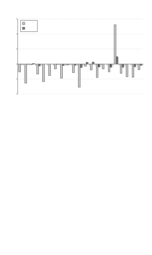
100 Asia and global production networks

(e.g., the Philippines). Finally, those regions that rely disproportionately

on Taipei,China for ELE imports are expected to lose from this disaster

scenario due to the import price effect, as Taipei,China’s ELE prices rise,

relatively more. In light of these considerations, it is not surprising that

the Philippines experiences a strong ToT gain, as do Thailand, Malaysia,

Japan and the Republic of Korea. The PRC shows a ToT loss – which

arises due to its heavy dependence on Taipei,China for component parts.

Other Asian regions that lose on the ToT front include India, Pakistan and

Central Asia.

In the absence of domestic distortions, we expect real income changes to

follow the ToT, being somewhat more muted, with the relative magnitude

being determined by the openness of the economy. However, the presence

of numerous taxes and subsidies in the global economy complicate this

story considerably. From the first column in the final panel of Table 3.3,

–10

–5

AGR

TEX

WAP

LEA

LUM

PPP

CRP

NMM

NFM

FMP

MVH

OTN

ELE

OME

OMF

NTS

SVC

% change

Japan

PRC

Note: AGR = agriculture; CRP = chemicals, rubber and plastics; ELE = electrical

equipment; FMP = fabricated metals; IS = iron and steel; LEA = leather; LUM = lumber;

MVH = motor vehicles; NFM = nonferrous metals; NMM = mineral products; NTS =

nontrade services; OME = machinery equipment; OMF = other manufactures; OTN =

transport equipment; PC = petro- chemicals; PF = processed food; PPP = paper products;

PRC = People’s Republic of China; RC = resource products; SVC = services; TEX =

textiles; WAP = wearing apparel.

Source: Authors’ simulation.

Figure 3.4 Impact of ELE productivity shock on non- ELE exports from

Japan and the PRC (percentage change)

The vulnerability of the Asian supply chain 101

we see that the largest gainers from the Taipei,China ELE disaster are

the Philippines (0.9 percent rise in real income), followed by Indonesia,

Malaysia, Thailand and the Republic of Korea. The only regions that

show a decline in real income under the base case are the PRC, Central

Asia, Australia/New Zealand and the rest of the world. The result that

unaffected regions are likely to gain from a single region’s disaster is

consistent with the findings of MacKenzie et al. (2012) who analyze the

impacts of the 2011 Japanese earthquake and tsunami.

The subsequent columns in Table 3.3 explore the changes in ELE prices,

outputs, ToT and real incomes for non- Taipei,China regions under the

low labor mobility, low substitutability in demand and combined sce-

narios. Here, it is clearly evident that more inelastic supply and demand

curves result in significantly higher price changes. Indeed, the price rises

under the combined scenario are more than twice as high as under the

baseline case. Of course, the associated ELE output changes are lower

under the combined low mobility and low elasticity scenarios, as it is more

difficult to move unskilled labor between sectors, and firms find it harder

to change their pattern of sourcing in response to the adverse productivity

shock in Taipei,China. However, if we focus solely on the impact of the

smaller trade elasticities, the results are somewhat more varied. The most

common result is for the inelastic demands to result in smaller output

expansions – since Taipei,Chinese ELE output contracts less under this

parameter specification, there is less room for others to expand. However,

this is not universally the case. In particular, a number of the Southeast

Asian economies experience stronger output expansions under the inelas-

tic demand cases. This suggests the presence of more complex, cross- sector

effects.

With larger price changes in the more inelastic supply and demand

scenarios, it is not surprising to see larger ToT effects. Indeed, under

the combined inelastic supply/demand scenario, the Philippines’ ToT

gain reaches 4.7 percent and Japan’s gain rises to 3.3 percent. There are

several cases where a negligible effect becomes significantly negative

under the inelastic scenario (Indonesia, Bangladesh, Other South Asia).

And there are even a few cases of sign reversals. In Pakistan, for example,

the ToT effect is negative in the first two cases, but turns positive in the

context of low elasticities of substitution in use. For the most part, the

larger (in absolute value) ToT effects translate into larger real income

effects, as would be expected.

The largest loss is felt by Other South

Asia (–2.2 percent), whereas the largest gain accrues to the Philippines

(3 percent).

102 Asia and global production networks

5. RESULTS FROM THE ENTREPOT SHOCK

Singapore is a key trading hub in Southeast Asia, with a very large share

of regional trade passing through its ports. Our experiment involves

sharply reducing the efficiency with which this trade occurs, as would

arise in the context of a natural disaster, which disrupted the port, or a

cyber- attack, which disabled the country’s customs clearance system. The

entrepot shock contrasts with the preceding experiment in that it affects

the productivity with which goods are traded, rather than the productivity

with which they are produced. This experiment affects all the incoming

and outgoing merchandise trade flows for Singapore. As with the previ-

ous experiment, we explore the impact of this shock in the context of a

baseline experiment in which capital is immobile, skilled labor is partially

mobile with fixed aggregate employment, and unskilled labor is perfectly

mobile, with rigid real wages and variable short run employment levels. As

before, these baseline impacts will be contrasted with scenarios in which,

alternately, supply, demand and then both supply and demand are ren-

dered more inelastic by either reducing unskilled labor mobility, reducing

substitution across import sources, or both.

In all of these entrepot experiments, the 80 percent drop in efficiency of

merchandise trading results in higher bilateral merchandise trading costs

with Singapore, which rise by 400 percent. The impact of this increase

on bilateral prices depends on the share of global trade and transport

services in the cost, insurance, and freight- inclusive (cif) price of imports.

For products such as natural resources and agricultural commodities, this

has a significant impact on prices, while the impact is more moderate for

low margin goods. In any case, the need to offset the reduced efficiency of

Singaporean trade requires additional global trade and transport services,

as does the re- routing of trade around the Singapore entrepot. Given

our treatment of the international trade and transport sector as a single

pool, from which the supply of shipping services are drawn to meet the

global demand for international transport margins, these services must

ultimately be supplied from the pool of national services exports. The

increase in global trade and transport services required to accommodate

this supply chain shock is reported at the bottom of Table 3.4 and ranges

from 4 percent in the baseline to 6 percent when the ability of firms and

households to alter their sourcing patterns is more restricted. (Note that

limiting labor mobility on the supply side does not substantially alter this

figure.)

The main two panels of Table 3.4 summarize the impact on the

Singapore economy of this disruption in trade facilitation. With ‘sand in

the gears’ of Singapore’s usually efficient trading system, the economy

The vulnerability of the Asian supply chain 103

experiences a sharp real exchange rate depreciation, large reductions in

unskilled employment, and a 21 percent decline in real income under the

baseline scenario. Since the shock cuts across the board in the Singaporean

economy, this outcome is little affected by the reduction in labor mobil-

ity (column two). All sectors are hurt by this entrepot disruption, and

unlike the Taipei,China ELE shock, adjustment is less reliant on shifting

labor between sectors. However, when trade elasticities are reduced, the

macro- economic outcome is far worse for Singapore. In this case, the real

exchange rate depreciation, and the reductions in employment and real

income approach 30 percent. The difficulty in changing the sourcing of

products affects not only her trading partners, but also Singaporean pro-

ducers and therefore there is little scope for avoiding the burden of higher

trade costs. This makes the economy much less competitive, thereby

requiring an even greater real depreciation. In short, this is an example

of a supply chain disruption for which the ability to alter the sourcing of

imports is paramount.

Table 3.5 reports the impact of this entrepot disruption on global

merchandise and services trade by commodity. It is hardly surprising

that services exports rise, as the reduction in Singapore’s trade efficiency

requires additional effort to move the same amount of goods. The largest

percentage reduction in global trade volume is for petro- chemicals (–1.12

percent). Singapore is an important refiner of petroleum and related

products and this industry suffers from the higher cost of importing

crude petroleum and exporting refined products. Transport equipment,

Table 3.4 Impact of entrepot disruption on Singapore economy

(percentage change)

Variable Baseline

scenario

Lowmobile

scenario

Lowelast

scenario

Low/low

scenario

Real income −21 −21 −28 −28

Real exchange rate −19 −19 −29 −29

Exports −11 −10 −0.1 −0.1

Employment of:

Clerks −21 −21 −29 −30

Service workers −15 −15 −27 −27

Unskilled production workers −25 −26 −30 −30

Global trade and transport services

4 4 6 6

Source: Authors’ calculations.

104 Asia and global production networks

machinery and equipment and fabricated metal products are also rela-

tively hard hit. As with the earlier results, restricting factor mobility does

not change the results significantly. And in the case of global commod-

ity exports, the smaller trade elasticities have less effect than might be

expected. While the smaller trade elasticities generally reduce the change

in trade volume, as expected, this is not always the case, as shown by the

other transport equipment sector, where the impact of lesser substitutabil-

ity across sources dominates and trade falls even more under the inelastic

demand scenarios.

Table 3.6 reports the impact of this entrepot disruption on the

non- Singaporean economies. In the first block of columns, under the base-

line parameter settings, exports for many of these economies rise, as trade

Table 3.5 Impact of entrepot disruption on global trade volume

(percentage change)

Commodity Global exports by commodity

Baseline

scenario

Lowmobile

scenario

Lowelast

scenario

Low/low

scenario

Agriculture −0.05 −0.05 0.04 0.04

Processed food −0.23 −0.23 −0.07 −0.06

Resources −0.27 −0.27 −0.11 −0.11

Textiles −0.07 −0.07 −0.04 −0.05

Apparel −0.08 −0.07 0.02 0.01

Leather −0.11 −0.11 −0.02 −0.02

Lumber −0.01 −0.03 0.00 −0.04

Paper products −0.33 −0.33 −0.15 −0.17

Petro- chemicals −1.12 −1.13 −0.54 −0.55

Chemical, rubber and plastics −0.28 −0.28 −0.17 −0.17

Mineral products −0.33 −0.33 −0.21 −0.24

Iron and steel −0.21 −0.21 −0.18 −0.18

Nonferrous metals −0.11 −0.10 −0.13 −0.13

Fabricated metals −0.46 −0.46 −0.31 −0.33

Motor vehicles −0.08 −0.08 −0.20 −0.22

Transport equipment −0.98 −0.96 −1.16 −1.14

Electrical equipment −0.29 −0.28 −0.22 −0.23

Machinery equipment −0.46 −0.45 −0.46 −0.45

Other manufactures −0.18 −0.18 −0.19 −0.21

Non- trade services 0.01 0.01 −0.03 0.00

Services 0.80 0.79 1.05 1.04

Source: Authors’ calculations.

105

Table 3.6 Global impact of entrepot disruption (percentage change)

Region Regional exports Real exchange rate

Baseline

scenario

Lowmobile

scenario

Lowelast

scenario

Low/low

scenario

Baseline

scenario

Lowmobile

scenario

Lowelast

scenario

Low/low

scenario

Japan −0.12 −0.14 −1.42 −1.62 0.24 0.30 1.49 1.96

Korea, Republic of 0.15 0.14 −0.36 −0.33 0.49 0.57 1.41 1.62

China, People’s Republic of 0.00 −0.01 0.05 0.04 0.06 0.06 0.01 0.02

Taipei,China 0.03 0.02 −0.02 −0.03 0.13 0.15 −0.01 0.02

Other East Asia 0.07 0.09 0.05 0.08 0.07 0.04 0.04 0.01

Philippines 0.23 0.21 0.54 0.46 −0.18 −0.18 −0.98 −0.97

Thailand 0.16 0.10 0.28 0.25 −0.15 −0.10 −0.71 −0.70

Indonesia −0.52 −0.48 0.78 0.73 −0.91 −1.00 −2.61 −2.87

Malaysia −0.84 −0.84 0.03 0.00 −0.93 −0.90 −1.97 −2.02

Viet Nam 0.46 0.54 1.45 1.68 −1.48 −1.76 −4.14 −5.31

Other Southeast Asia 0.02 0.10 0.43 0.46 −0.41 −0.54 −1.28 −1.49

India −0.02 −0.12 −0.20 −0.33 0.09 0.12 0.38 0.52

Bangladesh 0.07 0.07 0.69 0.66 −0.06 −0.09 −0.67 −0.87

Pakistan 0.11 0.10 −3.41 −1.86 0.03 0.02 3.65 2.22

Other South Asia 0.35 0.35 5.91 7.22 −0.2 −0.22 −6.45 −8.45

Central Asia 0.17 0.19 0.20 0.23 −0.08 −0.16 −0.23 −0.37

Pacific Islands −0.20 −0.18 0.97 1.04 −0.29 −0.36 −1.58 −1.83

Australia and New Zealand 0.19 0.21 1.05 1.12 −0.36 −0.42 −1.89 −2.13

European Union 0.01 0.01 −0.15 −0.19 0.14 0.16 0.53 0.66

North America 0.05 0.06 0.39 0.50 0.04 0.04 −0.32 −0.48

Rest of world 0.16 0.18 0.26 0.30 −0.02 −0.06 −0.22 −0.31

106

Table 3.6 (continued)

Region Terms of trade Real income

Baseline

scenario

Lowmobile

scenario

Lowelast

scenario

Low/low

scenario

Baseline

scenario

Lowmobile

scenario

Lowelast

scenario

Low/low

scenario

Japan 0.15 0.18 1.04 1.19 0.07 0.07 0.34 0.37

Korea, Republic of 0.24 0.27 0.68 0.71 0.26 0.28 0.65 0.68

China, People’s Republic of −0.06 −0.05 −0.10 −0.10 −0.01 0.00 −0.04 −0.03

Other East Asia 0.02 0.04 −0.09 −0.07 0.03 0.04 −0.08 −0.06

Singapore 0.01 −0.03 0.04 −0.01 −0.02 −0.03 0.03 0.01

Philippines −0.29 −0.28 −0.59 −0.54 −0.15 −0.15 −0.36 −0.32

Thailand −0.20 −0.17 −0.51 −0.50 −0.28 −0.25 −0.55 −0.52

Indonesia −1.61 −1.64 −2.72 −2.73 −0.80 −0.79 −1.27 −1.24

Malaysia −1.16 −1.14 −1.74 −1.74 −1.73 −1.68 −2.36 −2.29

Viet Nam −1.05 −1.12 −2.05 −2.25 −1.65 −1.75 −3.66 −4.14

Other Southeast Asia −0.91 −1.03 −1.31 −1.39 −0.67 −0.72 −0.88 −0.89

India 0.09 0.14 0.38 0.49 0.03 0.03 0.16 0.20

Bangladesh −0.17 −0.17 −0.47 −0.46 −0.08 −0.09 −0.26 −0.28

Pakistan −0.01 0.00 1.98 1.10 0.00 0.00 0.94 0.56

Other South Asia −0.30 −0.31 −3.92 −4.80 −0.23 −0.23 −2.96 −3.71

Central Asia −0.16 −0.23 −0.24 −0.34 −0.07 −0.12 −0.14 −0.20

Pacific Islands −0.81 −0.86 −1.46 −1.58 −0.15 −0.19 −0.96 −1.03

Australia and New Zealand −0.60 −0.64 −1.46 −1.55 −0.25 −0.27 −0.67 −0.70

European Union 0.06 0.07 0.22 0.26 0.05 0.06 0.17 0.19

North America 0.01 0.01 −0.21 −0.29 0.01 0.01 −0.06 −0.08

Rest of world −0.13 −0.17 −0.26 −0.33 −0.04 −0.06 −0.11 −0.14

Source: Authors’ calculations.

The vulnerability of the Asian supply chain 107

by- passes Singapore. Indeed the only significant regional export volume

declines are for the most closely related economies of Indonesia, Malaysia

and the Pacific Islands, as well as for Japan. This picture is little altered

by supply- side rigidity in the form of immobile labor (second column of

results). However, once import sourcing is more tightly constrained (final

two columns), there are some sharp differences, with exports from the

Republic of Korea, India, Pakistan and the EU all turning negative as it

becomes more difficult to change sourcing patterns.

The next blocks of columns in Table 3.6 report the impact of this supply

disruption on the real exchange rate, ToT and real incomes for each

economy across the baseline and alternate rigidity scenarios. These vari-

ables are closely related, and an improvement in any one of them reflects

increased export prices, relative to import costs as trade with the entrepot

becomes more costly and trade flows are diverted from Singapore. Not

surprisingly, the Southeast Asian economies – closely linked to Singapore

– are hardest hit by the entrepot shock, with ToT losses, real exchange

rate depreciations and real income losses. In contrast, Japan and the

Republic of Korea gain as their ToT improve. These welfare impacts of

Singapore’s entrepot shock are robust to changes in the supply side of the

economy – for the same reason noted above – namely the shock does not

give a strong incentive to reallocate factors of production across sectors.

However, the macro- economic outcome is extremely sensitive to the trade

elasticities. When sourcing of imports becomes more difficult to change

(inelastic demand), the inability to avoid this entrepot shock by readily

substituting imports from other sources significantly raises the costs for

many of the Southeast Asian economies. The ‘Other South Asia’ region

– dominated by Sri Lanka – is extremely hard hit under this parameter

setting. Meanwhile, the inelastic demand scenario significantly enhances

the gains of Japan and the Republic of Korea.

6. DISCUSSION AND CONCLUSIONS

In conclusion, we find that the GTAP- SC framework is a useful vehicle

for analyzing the impact of sector and entrepot disruptions on the global

supply chain, and indeed, on the global economy. Unlike the econometric

approaches employed elsewhere in this volume, we are able to fully inves-

tigate the general equilibrium determinants of changes in global trade and

production. And unlike the input–output approaches often used in supply

chain analyses, this CGE framework allows us to explore the implications

of rigidities on both the supply and demand sides for transmission of

localized disasters throughout the global economy.

108 Asia and global production networks

We find that the supply chain impacts of local disasters are rather

robust to labor market rigidities when the external shock affects the entire

economy, as is the case with the entrepot disruption. This is due to the fact

that all sectors are adversely affected, and there is less of an incentive to

dramatically change the employment of labor and capital across sectors.

However, this is not the case when the disaster hits a particular industry,

as is the case when Taipei,China’s ELE sector experiences a 40 percent

reduction in productivity. In this sector- focused, supply chain disruption,

the impact, both on the Taipei,Chinese economy, as well as on the global

economy, hinges critically on the mobility of labor out of the damaged

sector and into other sectors of the affected economy, as well as labor

mobility in the trading partners’ economies.

One of the potentially surprising results from the chapter is that even

a major disruption to a critical world supplier of inputs (Taipei,China’s

electronics industry) has modest effects on incomes elsewhere – especially

under our baseline parameter settings. How does this square with our

notion that disruptions to supply chains create havoc worldwide?

In contrast to supply- side rigidities, the impact of both types of disasters

discussed in this chapter is heavily dependent on individual firms’ abilities

to substitute away from products affected by the supply chain disruption.

When we reduce the associated import sourcing elasticities to one- third

of their baseline values, the consequences of the disaster for the affected

region are invariably much worse. And the scope for terms of trade

changes and the associated real income changes in other regions is magni-

fied. Still, it might seem that for some critical inputs there are no substi-

tutes, at least in the short run. If input supply is disrupted, downstream

firms will simply shut down.

To understand this case in light of our model it is important to think

about the role of aggregation. The use of industry data, rather than firm-

level data on inputs can mask two very different realities at the level of

individual firms. One is the case where firms in a given industry share the

same technology, and require all inputs (from all sources) used in that

industry. Disruptions to a particular input are important to the extent

that the input represents a large cost- share for the industry, and that close

substitutes are difficult to come by.

The other case is where individual firms within the industry are

extremely heterogeneous in their technologies and use of inputs. In

this case, it may be that only a small subset of firms needs any par-

ticular input, but these inputs are absolutely critical to their operation.

Disruption in input supply shuts these firms down entirely, but since

affected firms represent only a small percentage of all firms in the indus-

try, the impact on aggregate sector output is modest. To be clear, the

The vulnerability of the Asian supply chain 109

composition of output changes looks different in this second case. For

example, we might have 90 percent of firms unaffected by the disruption

and 10 percent of firms shutting down; as opposed to all firms reducing

output by 10 percent. But the aggregate effects at the sector level – and

indeed the consequences for labor markets and regional income – are the

same in both cases.

Of course, it could be that an input is both critical for every firm, and

that all these firms lack substitutes. Where this is the case, the input would

likely represent a very large share of input costs prior to the shock.

using the detailed information on input shares by source country in the

pre- shock equilibrium, we are taking into account whether an input is very

important to a lot of firms or not. Since it is rare to find inputs that have

both large cost shares and no substitutes, we believe that it will be unusual

for supply disruptions to have very large aggregate effects.

NOTES

* This chapter has been commissioned as part of the Asian Development Bank study

on Supply Chains in Asia, led by David Hummels and Benno Ferrarini. The authors

would like to thank Ari Van Assche, Anson Soderbery, and Laura Puzzello for valuable

comments on an earlier draft of this work.

1. For example, they find that adverse shocks to human capital result in a decreased growth

rate, with no eventual return to the previous growth trajectory, while loss of physical

capital seems to have no discernible long- term impact on growth.

2. MacKenzie et al. (2013) explore, alternatively, shocks based on output disruption and

shocks based on demand disruption. The former are an order of magnitude more dam-

aging, largely due to the mitigating role of foreign suppliers and inventory adjustment

in the latter. Overall, they conclude that foreigners likely gained from this disruption,

and that a similar disaster in other countries would be even more beneficial to the com-

petition, due to the relatively large share of intermediates sourced domestically in the

Japanese auto industry.

3. In GTAP notation, this is given by ao(ELE, TWN) 5 −40.

4. In GTAP notation, this is given by ats(“Singapore”) 5 −80, and atd(“Singapore”) 5

−80.

5. Of course, where there are significant efficiency gains and losses, these will likely be more

muted under the low mobility/low elasticity scenarios.

6. Imagine a firm that is a monopoly supplier of some input, without which every firm in

Asia shuts down, and for which no substitutes exist. You can be sure that key input is

supplied at very high prices.

REFERENCES

Antras, P. and E. Helpman (2004), ‘Global sourcing’, Journal of Political

Economy, 112, 552–580.

Barry, L. (2005), End of the Line, New York: Doubleday.

110 Asia and global production networks

Francois, J. (1998), ‘Scale economies and imperfect competition in the GTAP

model’, GTAP Technical Paper No. 14, Purdue University, available at: https://

www.gtap.agecon.purdue.edu/resources/res_display.asp?RecordID5317.

Gallaway, M.P., C.A. McDaniel and S.A. Rivera (2003), ‘Short- run and long- run

industry- level estimates of U.S. Armington elasticities’, The North American

Journal of Economics and Finance, 14, 49–68.

Hertel, T.W. (ed.) (1997), Global Trade Analysis: Modeling and Applications, New

York: Cambridge University Press.

Hertel, T.W. and P. Swaminathan (1996), ‘Introducing monopolistic competition

into the GTAP model’, GTAP Technical Paper No. 6, Purdue University, avail-

able at: https://www.gtap.agecon.purdue.edu/resources/res_display.asp?Record

ID5309.

Hertel, T.W., D. Hummels, M. Ivanic and R. Keeney (2007), ‘How confident can

we be in CGE- based analysis of free trade agreements?’, Economic Modelling,

24, 611–635.

Hertel, T.W., R. McDougall, B. Narayanan and A. Aguiar (2009), ‘Behavioral

parameters’, in B. Narayanan and T.L. Walmsley (eds), Global Trade Assistance

and Protection: The GTAP 7 Data Base, Center for Global Trade Analysis,

Purdue University, available at: https://www.gtap.agecon.purdue.edu/data-

bases/v7/v7_doco.asp.

Leiter, A.M., H. Oberhofer and P.A. Raschky (2009), ‘Creative disasters?

Flooding effects on capital, labour and productivity within European firms’,

Environmental and Resource Economics, 43, 333–350.

Lin, X. and K.R. Polenske (1998), ‘Input–output modeling of production proc-

esses for business management’, Structural Change and Economic Dynamics, 9,

205–226.

MacKenzie, C.A., J.R. Santos and K. Barker (2012), ‘Measuring changes in inter-

national production from a disruption: case study of the Japanese earthquake

and tsunami’, International Journal of Production Economics, 138, 293–302.

McDougall, R.A. (1993), ‘Two small extensions to SALTER’, SALTER Working

Paper Series, No. 12, Canberra: Industry Commission.

Narayanan, G., A.A. Badri and R. McDougall (eds) (2012), Global Trade,

Assistance, and Production: The GTAP 8 Data Base, Center for Global Trade

Analysis, Purdue University.

Noy, I. and A. Nualsri (2007), ‘What do exogenous shocks tell us about growth

theories’, SCCIE Working Paper Series, No. 07- 16, Santa Cruz Center for

International Economics, available at: http://sccie.ucsc.edu/.

Okuyama, Y. (2008), ‘Critical review of methodologies on disaster impact estima-

tion’, mimeo, Global Facility for Disaster Risk Reduction, available at: http://

gfdrr.org/sites/gfdrr.org/files/New%20Folder/Okuyama_Critical_Review.pdf.

Reimer, J.J. and T.W. Hertel (2004), ‘Estimation of international demand behavior

for use with input–output based data’, Economic Systems Research, 16, 347–366.

Rose, A. (2013), ‘Macroeconomic consequences of terrorist attacks: estimation for

the analysis of policies and rules’, in V.K. Smith and C. Mansfield (eds), Benefit

Transfer for the Analysis of DHS Rules and Regulations, Cheltenham, UK and

Northampton, MA, USA: Edward Elgar.

Rose, A. and S. Liao (2005), ‘Modeling resilience to disasters: computable general

equilibrium analysis of a water service disruption’, Journal of Regional Science,

45, 75–112.

Rose, A. and D. Wei (2013), ‘Estimating the economic consequences of a port

The vulnerability of the Asian supply chain 111

shutdown: the special role of resilience’, Economic Systems Research, 25,

212–232.

Walmsley, T.L. and C. Carrico (2013), ‘Disaggregating labor payments by skill

level in GTAP’, unpublished manuscript, Center for Global Trade Analysis.

Weingarden, A. and M. Tsigas (2010), ‘Labor statistics for the GTAP database’,

presented at 13th Annual Conference on Global Economic Analysis Papers,

Malaysia, Penang.

112

4. Global supply chains and natural

disasters: implications for

international trade*

Laura Puzzello and Paul Raschky

1. INTRODUCTION

Every once in a while news reports show the disastrous impact of natural

disasters on local communities. In some cases, the losses in terms of

property and lives are so big that economies struggle for months, some-

times years, before bouncing back. Local production is often affected

and so is the transport of local goods to other areas. There are plenty

of examples of such disasters in the 1990s and more recently: the Kobe

Earthquake (Japan, 1995), the 921 earthquake (Taipei,China, 1999),

Hurricanes Katrina and Rita (United States, 2004), the Japanese Great

Tohoku earthquake and tsunami and the Thai floods (2011).

Anecdotal

evidence suggests that the distinguishing feature of these recent disasters

is the global scope of their effects. It is not uncommon for firms abroad

to report production delays and profit losses because suppliers in source

countries struck by natural disasters fail to provide parts in time. For

example, the disruptions in the supply chain caused by the Great Tohoku

earthquake and tsunami events in March 2011, not only forced Japanese

car manufacturers to shut down their plants for a short period, but also

resulted in temporary closures of a General Motors truck plant in the

United States (US).

However, the question arises whether these global

supply chain effects are just limited to a small group of extreme cases

of disaster events, or are a more systematic feature of (large) natural

disasters.

In this chapter we provide insights into this matter by examining the

effect of disruptions to global supply chains due to natural disasters on

countries’ exports. Our focus is on natural disasters that have a “large”

impact on the local population or economy. These, in fact, are the disasters

whose extent is capable of delaying a country’s production and exports,

and, through supply linkages, of stretching across national borders.

Global supply chains and natural disasters 113

In order to test whether large disasters affect countries’ exports through

input trade, we first construct measures of supply chain vulnerability to

natural disasters. For each country and product, these measures capture

the proportion of inputs provided by suppliers located in countries struck

by at least one large natural disaster in a given year. We use input–output

(IO) structures from the GTAP database and import data from Base pour

l’analyse du commerce international (BACI) to calculate the total amount

of each input, by origin country, used in the production of each good. We

identify which inputs are produced in countries subject to large natural

disasters in any given year using data from the International Disaster

Database (EM- DAT).

Our measures of supply chain vulnerability capture interesting facts.

For instance, we find that manufacturing products tend to have large

shares of inputs exposed to natural disasters abroad, and small input

shares exposed to domestic disasters. This is exactly what one would

expect given the high incidence of input trade in the manufacturing sector.

We also find that Asia and North America are the regions most vulnerable

to large natural disasters both at home and abroad. That is consistent with

the higher incidence of disasters in these regions and the key role they play

in global production.

Our empirical results suggest that higher supply chain vulnerability to

large natural disasters significantly reduces exports. Intuitively, this is

because the production of goods with high supply chain vulnerability is

more likely to be disrupted by large natural disasters. We also find that

the negative effects on a country’s exports of supply chain disruptions are

bigger when large disasters happen at home. These results are robust to the

identification of large disasters and disappear if one focuses on all natural

disasters. We find that earthquakes, tsunamis and storms striking at home

and floods abroad pose the biggest threat to global supply chains and

trade. Our results further imply that more complex industries are relatively

more resilient if supply shocks are due to large disasters hitting home, but

not other supplier countries.

This chapter relates to a recent literature, which examines the effect of

natural disasters on trade. Gassebner et al. (2010) estimate a gravity model

to identify the causal effect on bilateral trade of disasters in either one of

the trading countries. Their findings suggest that large disasters, whether

natural or technological, decrease a country’s exports, but not necessarily

its imports. Countries’ size and level of democracy turn out to be key deter-

minants of the overall effect of disasters on trade. Andrade da Silva and

Cernat (2012), using a gravity approach, find that domestic natural disas-

ters affect most negatively the exports of small developing countries. Jones

and Olken (2010) examine the effect of a country’s weather on exports

114 Asia and global production networks

growth, and find that higher temperatures reduce substantially the growth

of exports for poor countries, but not for rich countries. We add to this

strand of the literature by focusing on the effects on a country’s exports of

large natural disasters occurring both at home and abroad, emphasizing

failures in supply chains as the potential transmission mechanism.

Our chapter also relates to a few studies that account for the interna-

tional transmission of natural disasters through input trade. MacKenzie

et al. (2012) use a multiregional IO model to show that, following the

earthquake and tsunami of 2011 in Japan, the unavailability of Japanese

inputs decreased substantially both domestic and international produc-

tion. Japanese output decreased the most in the transportation and office

equipment industries, which indirectly affected production in many service

and manufacturing sectors. Abroad, the People’s Republic of China (PRC)

suffered, indirectly, the largest output losses. Despite these findings, the

authors conclude that, overall, other economies might have benefitted

from the Japanese disasters, as their production increased to substitute for

Japanese products both in the domestic markets and in Japan. Martin et

al. (2011) analyze the effect on the United Kingdom (UK) manufacturing

firms’ productivity of extreme weather events at home and abroad. They

account for the fact that climate shocks abroad affect firms from both the

supply side, through input trade, and the demand side, through favorable

shifts in foreign consumer demand. They find evidence that importing

from countries experiencing exceptional heat decreases UK firms’ produc-

tivity, while exporting to these destinations increases it. In contrast to both

these studies, we take a global perspective; our focus is on exports and the

transmission of natural disasters’ effects through supply linkages.

The rest of the chapter is organized as follows. Section 2 presents some

facts on natural disasters, and discusses their potential to disrupt global

production and trade. Section 3 presents the estimating equation. Section

4 describes the data and provides details on our measures of supply chain

vulnerability. Section 5 discusses our estimates. Section 6 concludes.

2. NATURAL DISASTERS AND GLOBAL

PRODUCTION: A FIRST LOOK AT THE DATA

In this section we use data from the EM- DAT database, collected by the

Centre for Research on Epidemiology of Disasters (CRED), to describe

the incidence of different types of disasters, and uncover the geographic

distribution of natural disasters, in general, and large- scale natural dis-

asters, in particular. A disaster is recorded in the EM- DAT database if

at least one of the following occurs: (1) it kills at least ten people, (2) it

Global supply chains and natural disasters 115

affects at least 100 people, (3) a state of emergency is declared, or (4) a

call for international assistance is made. Natural disasters included in our

analysis are listed in Table 4.1.

For each disaster, the EM- DAT database

reports information on when the disaster happened, how long it lasted for,

the number of people killed, the total number of people affected,

and the

total amount of estimated damage in US dollars.

In this section we also verify whether key input suppliers in global pro-

duction tend to be more often subject to natural disasters. Owing to data

availability constraints, our analysis focuses on the period between 1995

and 2010.

2.1 On Natural Disasters

A natural disaster is an unforeseen natural phenomenon such as an earth-

quake, hurricane, or flood that causes extensive damage, destruction of

properties and loss of lives. Between 1995 and 2010 the world experi-

enced 5479 such disasters, which killed more than a million people and

affected the lives of about 3.6 billion people. In the same period, natural

disaster- related monetary losses tallied $1.5 trillion. Panel A in Table 4.1

reports detailed information on the number of people killed and affected,

and the estimated damages related to each of the disaster types included

in our sample. Panel B in Table 4.1 reports similar statistics for large

natural disasters only. In the spirit of Gassebner et al. (2010) we classify a

disaster as large if at least one of the following occurs: (1) it kills at least

1000 people, or (2) it affects at least 100 000 people in total, or (3) it causes

damages worth at least one billion (2005) dollars.

5, 6

A glance at the first column of Table 4.1 reveals that floods and wind-

storms are the most frequent types of disasters and those classified as large

disasters. They are also among the most costly and affect high numbers

of people. The deadliest disasters, not surprisingly, are earthquakes and

tsunamis. A very interesting implication of Table 4.1 is that, even though

large disasters account for only 20 percent of all natural disasters, they

are responsible for the vast majority of lives lost, people affected and eco-

nomic costs due to natural disasters. This reinforces our belief that one is

more likely to find any effect of disasters on a country’s trade by consider-

ing supply chain disruptions caused by large disasters. Hence, from this

point forward our discussion focuses on large natural disasters.

Table 4.2 reports statistics on the incidence and consequences of large

natural disasters by country or region

in our sample. The 15 regions most

often struck by large disasters are highlighted in grey. The country that

experienced the highest number of large disasters between 1995 and 2010

is the PRC, which also reports the highest number of people killed and

116 Asia and global production networks

Table 4.1 Incidence and consequences of natural disasters

Disaster type Number Number killed

(’000)

Number

affected

(millions)

Estimated

damages (2005

bn $)

Panel A All natural disasters, 1995–2010

Drought 261 2.17 894.12 38.29

Earthquake 411 493.60 105.67 384.57

Extreme temperature 298 154.64 87.40 50.51

Flood 2 325 129.91 1 980.36 369.98

Insect infestation 23 0.00 0.50 0.27

Mass movement (Dry) 4 0.16 0.00 0.00

Mass movement (Wet) 73 4.56 2.51 1.29

Slides 238 11.67 2.91 2.72

Storm 288 145.76 74.98 105.03

Volcano 88 0.61 1.69 0.21

Wave/Surge 27 230.01 2.53 10.38

Wild fires 211 1.31 1.77 35.69

Wind storm 1 232 74.34 435.43 520.14

Total 5 479 1 248.75 3 589.87 1 519.08

Panel B Large natural disasters, 1995–2010

Drought 154 2.04 892.78 31.53

Earthquake 80 488.98 102.62 373.89

Extreme temperature 33 134.98 86.93 48.92

Flood 431 96.71 1 959.39 321.23

Insect infestation 1 0.00 0.50 0.00

Mass movement (Dry) 0 0.00 0.00 0.00

Mass movement (Wet) 3 1.89 2.29 0.69

Slides 9 2.74 2.46 1.14

Storm 67 143.02 72.85 86.19

Volcano 5 0.53 0.92 0.16

Wave/Surge 6 228.32 2.39 8.15

Wild fires 15 0.57 1.51 30.13

Wind storm 235 60.02 429.49 462.20

Total 1 039 1 159.78 3 554.13 1 364.23

Note: A natural disaster is classified as large if at least one of the following occurs: (1) it

kills at least 1 000 people, or (2) it affects at least 100 000 people, or (3) it causes damages for

at least one billion (real) dollars.

Source: Authors’ calculation using EM- DAT data.

Global supply chains and natural disasters 117

Table 4.2 Regional incidence and consequences of large natural disasters

(1995–2010)

Number Killed

(’000)

Total affected

(millions)

Total damages

(2005 bn $)

Oceania

Australia 11 0.21 1.57 14.48

New Zealand 1 0.00 0.30 5.87

Rest of Oceania 3 2.24 0.77 0.00

Asia

People’s Republic of China 174 115.58 2 044.57 280.36

Hong Kong, China 0 na na na

Japan 15 5.62 1.91 205.00

Korea, Rep. of 3 0.60 0.50 6.59

Rest of East Asia 14 1.05 14.78 30.10

Taipei,China 5 3.02 3.47 18.68

Rest of Southeast Asia 24 139.16 16.74 4.07

Indonesia 21 175.85 11.85 22.06

Sri Lanka 18 35.75 6.71 1.40

Malaysia 2 0.02 0.20 0.05

Philippines 69 10.57 68.90 3.46

Singapore 0 na na na

Thailand 23 9.73 59.08 2.16

Viet Nam 33 8.03 37.30 6.32

Bangladesh 37 5.87 104.32 10.30

India 78 76.03 757.65 32.40

Rest of South Asia 34 90.20 52.33 16.55

North America

Canada 1 0.03 0.00 1.75

United States of America 69 3.40 23.59 397.78

Mexico 19 1.11 8.55 24.00

Rest of North America 0 na na na

South America

Colombia 11 2.22 7.51 3.04

Peru 9 1.87 6.28 0.35

Venezuela 1 30.00 0.48 3.64

Rest of Andean Pact 9 0.22 2.07 1.36

Argentina 4 0.11 1.65 3.20

Brazil 13 0.55 16.26 4.59

Chile 4 0.60 3.14 27.35

Uruguay 1 0.00 0.12 0.04

Rest of South America 6 0.04 1.53 0.53

118 Asia and global production networks

Table 4.2 (continued)

Number

Killed

(’000)

Total affected

(millions)

Total damages

(2005 bn $)

Rest of the Americas

Central America 21 21.40 11.32 10.54

Rest of Free Trade Area of

The Americas and

Caribbean

228.52

16.76

34.65

Europe

Austria 1 0.01 0.06 2.22

Belgium and Luxembourg 2 1.18 0.00 1.15

Denmark 2 0.01 0.00 4.30

Finland 0 na na na

France 10 21.10 4.03 29.46

Germany 6 9.41 0.43 19.16

United Kingdom 5 0.03 0.64 16.77

Greece 1 0.14 0.12 4.84

Ireland 0 na na na

Italy 4 20.42 0.14 21.33

Netherlands 2 1.00 0.25 1.45

Portugal 5 2.77 0.15 6.09

Spain 5 15.12 0.00 9.41

Sweden 1 0.01 0.00 2.80

Switzerland 3 1.06 0.00 4.12

Rest of EFTA 0 na na na

Rest of Europe 3 0.00 1.38 0.00

Albania 2 0.01 0.53 0.00

Bulgaria 0 na na na

Croatia 0 na na na

Cyprus 0 na na na

Czech Republic 2 0.05 0.30 2.19

Hungary 0 na na na

Malta 0 na na na

Poland 2 0.07 0.32 6.93

Romania 1 0.02 0.12 0.13

Slovakia 0 na na na

Slovenia 0 na na na

Estonia 0 na na na

Lithuania 0 na na na

Latvia 0 na na na

Russian Federation 11 58.00 2.68 5.35

Rest of Former Soviet Union 16 0.05 17.75 2.23

Global supply chains and natural disasters 119

affected by large natural disasters. Glancing over the table, other countries

highly vulnerable to large natural disasters are in Asia (India, Philippines,

Bangladesh, Viet Nam, Thailand, Indonesia, and Sri Lanka) and in North

America (the US and Mexico). The US records the largest amount of esti-

mated damages, followed by the PRC. In general, countries subject to a

higher number of large disasters report higher numbers of people affected

and estimated damages. The exception in this respect is Africa, where

regions more vulnerable to disasters report higher numbers of people

affected but not necessarily higher damages.

Interestingly, the countries we found most vulnerable to large disasters

are among the most active in the international trade of inputs (Baldwin

and Lopez- Gonzales, 2013). To verify whether this correlation holds

Table 4.2 (continued)

Number

Killed

(’000)

Total affected

(millions)

Total damages

(2005 bn $)

Middle East

Turkey 9 18.50 5.42 33.22

Rest of Middle East 14 30.62 41.27 10.12

Africa

Morocco 1 0.00 0.28 1.04

Tunisia 0 na na na

Rest of North Africa 1 2.27 0.21 5.31

South Africa (SA) 3 0.02 15.40 0.01

Malawi 7 0.57 9.75 0.01

Mozambique 17 1.03 10.72 0.55

Tanzania 3 0.00 5.15 0.00

Zambia 7 0.04 6.60 0.02

Zimbabwe 3 0.07 7.95 0.08

Rest of SA Development

Community and Sub-

Saharan Africa

104

5.15

126.51

0.63

Madagascar 13 1.07 5.97 0.38

Uganda 7 0.31 4.05 0.00

Botswana* 1 0.00 0.14 0.01

Rest of SA Custom Unions* 9 0.10 3.59 0.00

Total 1 039 1 160 3 554 1 364

Note: * 5 not included in the empirical analysis as unmatched in the trade data; na 5 not

available.

Source: Authors’ calculation using EM- DAT data.

120 Asia and global production networks

systematically in our data, we construct two measures of each supplier’s

importance in global production, using IO data from the GTAP database.

The first measure we consider is the quantity of each supplier’s inputs

directly used in the production of one unit of world gross output, which

we compute as follows:

World per unit use of j’s inputs 5

(

g, h

)

(4.1)

Where B

(g, h) is the amount of good g sourced by region j and used to

produce one unit of country i’s output of good h, and GO

is the world’s

gross output. This quantity takes on larger values the more a region sup-

plies to large producers in large sectors.

The second measure we construct

captures the extent of a supplier’s production network by counting the

average number of destinations using each of that supplier’s inputs.

Formally we compute:

Average number of destinations per input of j 5

(

)

. 0

)

(4.2)

where

(

)

takes on the value of 1 if region i uses input g from j

in at least one sector, and G is the total number of inputs g. Figures 4.1

and 4.2 plot the quantities in (4.1) and (4.2), against the number of large

natural disasters in the corresponding supplier region. For readability of

the graphs all the quantities are averaged over the period 1995–2010, but

results are similar if each year is considered separately. In both diagrams

the relationship is positive. In other words, international suppliers that are

large and that have more extended production networks tend to experi-

ence a larger number of large natural disasters. This implies that large

natural disasters might pose a real threat to global production and trade

through their disruptive effect on supply chains.

3. EMPIRICAL MODEL

Natural disasters can be thought of as a combination of natural events

and human activity. Worldwide, a large number of human settlements

and production facilities are subject to at least one type of natural hazard

exactly because the location chosen offers benefits to production and

economic activities. For example, the primary sector heavily depends on

access to freshwater for irrigation or direct access to the actual resource

that is harvested (e.g. fisheries). Manufacturing plants are often located in

Global supply chains and natural disasters 121

the proximity of rivers because freshwater is used as an input factor (i.e.,

cooling) and riverine systems are used as a means of inland transport.

Transport in general is a reason why the vast majority of today’s urban

agglomerations are either in coastal areas or next to riverine systems,

making them vulnerable to floods, hurricanes or other climatic hazards.

More specifically, if a large disaster happens domestically, the produc-

tion of exporting firms might be disrupted because of damage to physical

capital and production facilities, or injuries to workers. Even firms whose

production is not directly affected by the disaster might not be able to

export because of the damage to domestic transport infrastructure.

Indeed, the destruction of roads or the temporary closure of ports can

cause major export delays. If a large disaster happens abroad, the produc-

tion of domestic exporting firms might be boosted or depressed depending

on whether the foreign shock translates in higher or lower demand for

their own products.

The existing literature on natural disasters and trade has explored the

empirical relevance of these channels using information on the occurrence

ALB

ARG

AUS

AUT

BAN

BGR

BLX

BRA

CAN

CHE

CHL

PRC

COL

CYP

CZE

GER

DEN

SPA

EST

FIN

FRA

UKG

GRC

HKG

HRV

HUN

INO

IND

IRL

ITA

JPN

KOR

SRI

LTU

LVA

MAR

MDG

MEX

MLT MOZ

MWI

MAL

NLD

NZL

PER

PHI

POL

POR

ROU

RUS

SIN

SVK

SVN

SWE

THA

TUN

TUR

TAP

TZA

UGA

URY

USA

VEN

VIE

XAP

XCA

XCB

XEA

XEF

XER

XME

XNA

XNF

XOC

XSA

XSD

XSE

XSM

XSU

ZAF

ZMB

ZWE

0.01

0.02

0.03

0.04

0 2 4 6 8 10 12

World per unit use of supplier region's inputs

Number of large natural disasters in supplier region

Average 1995–2010

Source: Authors’ calculations based on EM- DAT and GTAP data.

Figure 4.1 Suppliers’ size and large natural disasters

122 Asia and global production networks

of disasters at home or in partner countries. In contrast, our focus in this

chapter is on determining the effect on exports of disruptions to supply

chains due to large natural disasters. Independent of whether a large dis-

aster happens at home or abroad, the production of a country’s exporting

firms might be disrupted because inputs from domestic or foreign sup-

pliers are received with delay, if at all. This might happen if domestic or

foreign suppliers are located in areas hit by the natural disaster, but also

if their suppliers or their suppliers’ suppliers fail to provide (on time) key

inputs to production due to the disaster.

In order to capture this additional transmission mechanism of disasters

on exports, we construct a measure of supply chain vulnerability, SCV,

which captures for each country, industry and year the share of inputs

directly and indirectly provided by suppliers located in countries hit by

large natural disasters. The intuition behind this measure is that exporters

that source a higher share of their inputs from suppliers located in areas hit

by disasters are more vulnerable and likely to experience production and

exports losses at any given point in time.

Formally, to test the effect of large natural disasters on region i’s

exports of good h, X

, we estimate the following equation:

ALB

ARG

AUS

AUT

BAN

BGR

BLX

BRA

CAN

CHE

CHL

PRC

COL

CYP

CZE

GER

DEN

SPA

EST

FIN

FRA

UKG

GRC

HKG

HRV

HUN

INO

IND

IRL

ITA

JPN

KOR

SRI

LTU

LVA

MAR

MDG

MEX

MLT

MOZ

MWI

MAL

NLD

NZL

PER

PHI

POL

POR

ROU

RUS

SIN

SVK

SVN

SWE

THA

TUN

TUR

TAP

TZA

UGA

URY

USA

VEN

VIE

XAP

XCA

XCB

XEA

XEF

XER

XME

XNA

XNF

XOC

XSA

XSD

XSE

XSM

XSU

ZAF

ZMB

ZWE

0 2 4 6 8 10 12

Average number of destinations per input of supplier region

Number of large natural disasters in supplier region

Average 1995–2010

Source: Authors’ calculations based on EM- DAT and GTAP data.

Figure 4.2 Extent of suppliers’ production network and large natural

disasters

Global supply chains and natural disasters 123

ln X

iht

5 b

SCV

iht

1 b

NLD

1 b

NLD*

iht

1 b

ln GDP

1 b

ln GDPpc

1 b

ln Remoteness

1 b

GATT

1 f

1 l

1 e

iht

(4.3)

where SCV

iht

is a measure of vulnerability to large natural disasters of the

supply chain of good h produced in region i; NLD

is the number of large

natural disasters occurred in i at time t;

NLD*

iht

is good h’s output weighted

number of large natural disasters occurred abroad;

GDP

and GDPpc

are i’s GDP and GDP per- capita; Remoteness

is the trade- weighted dis-

tance of exporter i to its importers at time t; GATT

is a continuous vari-

able that takes values between zero and one depending on the proportion

of countries within a region that are GATT/WTO members at time t;

and

denote industry fixed effects and time fixed effects.

We are mostly interested in the estimates of

A negative coefficient

indicates that countries with supply chains more vulnerable to large

natural disasters tend to export less. In equation (4.3) we control for the

number of large disasters that occurred at home and abroad to capture

any effect of these events on trade through channels different from supply

chain disruptions. Consistent with the literature, we expect

to be nega-

tive. The estimates for

might be positive if exporting firms benefit from

disasters abroad by becoming relatively more competitive in the world

market. But negative estimates for

are plausible too: if large produc-

ers of good h abroad are affected by natural disasters, their demand for

intra- industry inputs might decrease impacting negatively on country i’s

exports in that sector.

One should be cautious about the estimates of

from (4.3) as they

might be endogenous if variables correlated with SCV are omitted. For

instance, large exporters might have a lot of domestic and international

experience, which further strengthens their competitiveness. At the same

time, they might be less vulnerable to large disasters if their experience

allows them to better manage their supply chains. Omitting variables

related to the experience of exporters induces a downward bias on

In the same vein, large producers are often also large exporters. If large

producers source relatively more of their inputs domestically, their supply

chains might be systematically more vulnerable to large disasters because

of their higher exposure to domestic natural hazards. In this case, omitting

variables related to the size of exporters induces an upward bias on

our empirical analysis we carefully address this endogeneity issue. Reverse

causation does not seem to be a problem in equation (4.3), as large natural

disasters happen unexpectedly along the supply chain.

Our approach differs from that of previous studies on natural disasters

and trade. Gassebner et al. (2010), and Andrade da Silva and Cernat (2012)

124 Asia and global production networks

estimate gravity models to explain the effect on bilateral trade of disasters.

In addition to standard gravity controls, their specifications control for

the incidence of disasters in the exporting country and importing country

separately.

Jones and Olken (2010), instead, estimate the effect on the

growth of a country’s disaggregated exports of the temperature and pre-

cipitation in the exporting country. Even though the estimates from these

studies capture the effect on trade of failures in the exporting or import-

ing country’s supply chains once disasters hit the domestic economy, this

effect is not noted or modelled explicitly. More important, past studies

ignore the fact that disasters hitting countries outside a trading pair can

affect that pair’s bilateral trade, as failures anywhere along the supply

chain affect an exporter’s ability to produce.

Before presenting the estimation results, the next section discusses

the data, and provides details on the construction and features of our

measures of supply chain vulnerability.

4. THE DATA

In addition to the data on natural disasters we use trade data for the

period 1995 to 2010 from the BACI World trade database. These data

have been assembled by Gaulier and Zignano (2010) and made avail-

able online through the Centre d’Etudes Prospectives et d’Informations

Internationales (CEPII). The BACI database provides disaggregated

bilateral trade data for more than 200 countries. It increases the informa-

tion available in the COMTRADE database by combining information

reported by exporters and importers, and adjusting import values for

estimated cost, insurance and freight (cif) rates.

Countries’ domestic and import IO structures are taken from four dif-

ferent versions of the GTAP database: versions 5.4, 6, 7 and 8 with base

years 1997, 2001, 2004, and 2007, respectively. Even though these versions

of the database have the same sectoral disaggregation, the regional aggre-

gation differs. We use the regional representation of version 6 to concord

the data.

Regional IO coefficients between 1995 and 2000 are based on

GTAP 5.4 for all the regions that have a match in GTAP 6; for the remain-

ing regions we proxy the 1997 IO data with those available in GTAP 6. IO

coefficients for 2001–2003, 2004–2006 and 2007–2010 are based on GTAP

6, 7 and 8, respectively.

The concordance of the BACI data with the GTAP sectoral and

regional classifications leaves us with 44 sectors and 82 regions. A list

of regions and sectors included in our analysis is reported in Appendix

4A.1.

Global supply chains and natural disasters 125

Data for GDP and population are from the World Development

Indicators (WDI). Each region’s trade- weighted distance from its partners

is constructed using bilateral distance measures from the CEPII. GATT

membership data are from the CEPII gravity database.

4.1 Construction of a Measure of Supply Chain Vulnerability

The key variable in our analysis is an index of supply chain vulnerability

(SCV) to natural disasters that is country and industry specific. To con-

struct this index we first combine the GTAP IO tables with import data

from BACI to determine the total amount of each input, by origin region,

used in the production of each good. Using the EM- DAT data, we identify

which inputs are produced in regions subject to large natural disasters at

any given time.

In more detail, from the GTAP IO tables we obtain values for the

amount of each domestic or imported input g directly employed in the

production of one unit of each region i’s good h. Let us denote these

quantities by B

(g, h) if input g 5 1, . . . , G is sourced domestically, and by

(g, h) if input g is imported. We then use the proportionality assump-

tion, commonly adopted in the literature, to impute the distribution of

IO import coefficients by source region j 5 1, . . . , N, in any given year.

According to this assumption, if 10 percent of Chinese imports of steel

are from Japan, then 10 percent of any Chinese sector’s use of imported

steel originates from Japan.

Formally, the amount of good g sourced by

region j 5 1, . . . , N and used to produce one unit of country i’s output of

good h, B

(g, h), is imputed as follows:

(

g, h

)

(

)

(

)

*B*

(

g, h

)

with j 2 i and j 5 1, . . . , N (4.4)

where M

(g) denotes the amount of good g region i imports from j,

and M

(g) denotes region i’s total imports of g. Let the matrix B be the

(NG 3 NG) world input–output matrix collecting all the possible B

(g,

h).

The total amount of input region j’s input g used in i’s production

of h, A

(g, h), is obtained by taking the

ji 2 gh

element of the Leontief

inverse

(

)

where I is the (NG 3 NG) identity matrix.

Combining the elements in matrix A with the EM- DAT data, we con-

struct, for each industry- region pair, the proportion of inputs potentially

subject to large natural disasters at time t,

SCV

iht

as follows:

SCV

iht

j5 1

g5 1

jit

(

g, h

)

(

)

* I

(4.5)

126 Asia and global production networks

where

(

)

is the total per unit use of inputs in region

’s sector h at time

t, and I

is an indicator variable that takes on the value 1 if country j is

subject to at least one large natural disaster in t.

The index in equation (4.5) can be further decomposed to account, sepa-

rately, for a SCV to large natural disasters that happen at home or abroad.

We define the SCV index to domestic disasters as:

SCV

home

iht

g5 1

iit

(

g,h

)

(

)

* I

(4.5a)

and the SCV to disasters abroad as:

SCV*

iht

j2 i

g5 1

jit

(

g,h

)

(

)

* I

(4.5b)

Panel A and Panel B of Figure 4.3 plot the distribution for the SCV

indexes defined in (4.5), and (4.5a) and (4.5b), respectively. For legibility

of the graph, the plots of Panel B exclude values of

SCV

home

and

SCV*

equal to zero. Focusing on Panel A, there are two striking features of the

SCV distribution: first, it is bimodal; second, more of its density is concen-

trated at the lower end of the support. A glance at Panel B shows that the

bimodal nature of the SCV distribution is explained by the origin of the

shock to the supply chains. A large domestic natural disaster potentially

compromises the delivery of all domestic inputs used in the production of

any given good. Given that domestic inputs constitute the largest share of

total input purchases in any production process,

SCV

and

SCV

home

take

on large values if a big disaster strikes at home. When the shock is due

to natural disasters happening abroad a smaller share of total inputs is

affected, so

SCV

and

SCV*

take on small values. The higher concentra-

tion of the

SCV

distribution at the lower end of the support indicates that

most often the origin of (potential) shocks to supply chains is foreign. This

is further confirmed by the fact that

SCV

home

equals 0 in 67 percent of all

possible 57 728 (44 3 82 3 16) industry- region- year combinations.

In order to explore the vulnerability of different sectors to large natural

disasters, Figure 4.4 shows the

SCV

index distribution by aggregate

product categories, with the 44 original sectors included in one of the

following four categories: Food products, Manufacturing, Energy and

Raw agriculture.

The SCV distributions are bimodal in each product

category. Most interestingly, relative to the SCV distributions of other

sectors, the manufacturing one is shifted to the right at the lower end of

the support and to the left at the upper end of the support. This tells us

that in the manufacturing sector, regions have a larger share of inputs

that is exposed to natural disasters happening abroad. At the same time,

Global supply chains and natural disasters 127

Panel A) Distribution of the SCV index defined in equation (4.5).

Density

0.0 0.2 0.4 0.6 0.8 1.0

Value of supply chain vulnerability index

Large natural disasters

Panel B) Distribution of the SCV index defined in equation (4.5a, left panel) and equation (4.5b)

Density

0.2 0.4 0.6 0.8 1.0

Value of supply chain vulnerability index

Large domestic natural disasters

Density

0.0 0.2 0.4 0.6

Value of supply chain vulnerability index

Large natural disasters abroad

Note: In panel B, values of SCV

home

and SCV* equal to zero have been dropped for

legibility of the plots.

Source: Authors’ calculations based on EM- DAT and GTAP data.

Figure 4.3 Distribution of SCV indexes

128 Asia and global production networks

a lower percentage of their inputs is exposed to domestic disasters. Both

findings are consistent with the higher incidence of global supply chains in

manufacturing.

To explore the vulnerability of different regions to large natural dis-

asters, Figure 4.5 shows the SCV index distribution by aggregate geo-

graphic areas, with the 82 original regions included in one of the following

six areas: Oceania, Asia, North America, Other Americas, Africa and

Middle East, and Europe.

The SCV distributions are bimodal in each

geographic group. Europe stands out as having the most concentrated

SCV density at the lower end of the support and the least concentrated

at the upper end of the support. In other words, Europe is mostly vulner-

able to disasters happening abroad. This is consistent with our findings in

Table 4.2, which show countries in Europe were not struck by many large

disasters during the sample period. Asia and North America, instead, are

characterized by the highest values of the SCV density in the upper end

of the support. This is consistent with the fact that many regions in Asia

and North America received a high number of large disasters during the

sample period. Interestingly, at the lower end of the support, the prob-

ability of SCV taking on relatively high values, between 0.2 and 0.5, is the

Density supply chain vulnerability index

0.0 0.2 0.4 0.6 0.8 1.0

Value of supply chain vulnerability index

Food products Manufacturing

Energy Raw agriculture

Note: Each industry- region observation is weighted by the corresponding export share

in industry exports. The list of sectors included in each product category is reported in

Appendix 4A.1.

Source: Authors’ calculations based on EM- DAT and GTAP data.

Figure 4.4 Distribution of the SCV index by aggregate product categories

Global supply chains and natural disasters 129

highest in Asia and North America. Put another way, countries in Asia

and North America are quite vulnerable to large disasters abroad as well.

This is not surprising given that many of them are extensively involved in

global production networks.

5. ESTIMATION RESULTS

5.1 Supply Chain Vulnerability and Exports

Table 4.3 reports the estimation results for equation (4.3). We report

robust standard errors in parentheses, and standard errors clustered at the

region- industry level in square brackets. The significance of our estimates

is not affected by the residuals variance structure unless noted.

Focusing on Column (1) of Table 4.3, the estimates for the country-

specific control variables are as expected when significant. Economically

bigger and less remote regions tend to export more. However, a region’s

income per capita and its GATT membership status do not significantly

affect its exports. The estimates for the weighted average number of

disasters abroad,

NLD*,

imply that a region’s exports in a given sector

Density supply chain vulnerability index

0.0 0.2 0.4 0.6 0.8 1.0

Value of supply chain vulnerability index

Oceania Asia

North America Other Americas

Africa and Middle East Europe

Note: Each industry- region observation is weighted by the corresponding export share

in industry exports. The list of regions included in each geographical area is reported in

Appendix 4A.1.

Source: Authors’ calculations based on EM- DAT and GTAP data.

Figure 4.5 Distribution of the SCV index by aggregate geographic areas

130 Asia and global production networks

decrease with the average number of large natural disasters experienced

by other producers abroad. In other words, the benefits of weaker inter-

national competition are more than compensated by the loss of foreign

intra- industry demand for domestic inputs. In contrast to the literature,

the estimates for the number of large disasters at home, NLD, suggest that

thegreater the number of large natural disasters a country experiences, the

higher its exports are. Consistent with our intuition, instead, the estimated

coefficient for SCV is negative and significant, implying that the higher is

the vulnerability of a supply chain to large natural disasters, the lower the

corresponding exports.

To ensure that our estimates on SCV are not biased due to the omission

of variables related to the experience and size of exporters, in Column (2)

of Table 4.3 we add as control variables lagged values of the exporter’s

share in world trade and its size. Our estimate of the SCV coefficient is

only slightly affected. This is not surprising if one considers that large

exporters are big and potentially more experienced. While more experi-

ence allows exporters to improve their supply chain management, their

size makes them rely relatively more on domestic inputs increasing their

vulnerability to (domestic) natural disasters. These biasing effects almost

cancel each other out. Interestingly, controlling for the exporter’s share

and size changes substantially all the other coefficients. While the mag-

nitude of the GDP estimate shrinks, it turns out that richer regions and

members of the GATT do export significantly more. The puzzling posi-

tive coefficient on NLD shown in Column (1) decreases in magnitude and

becomes insignificant in Column (2). This finding put together with the

fact that the estimate on SCV is not affected by the additional controls

suggests that the main channel through which domestic disasters affect

trade is through failures of producers’ supply chains. The coefficient of

NLD*

switches sign in Column (2), implying that the benefits of weaker

foreign competition do, in fact, more than make up for the loss of foreign

intra- industry demand for domestic inputs.

In Column (3) of Table 4.3 we control for annual changes in the trade

weighted GDP of importers to ensure that the negative estimated effect

of SCV on exports is not driven by changes in the demand for domestic

goods from countries affected by large disasters. Our estimated effect of

SCV on exports is robust to this addition.

In order to make sure our estimated effect of SCV on exports is not

affected by any omitted region- time specific effect, we estimate a modified

specification of equation (4.3) where all the region- time specific variables

are replaced by region- time fixed effects. The last column of Table 4.3

shows our results. The size of the SCV coefficient increases in absolute

value, implying that one standard deviation increase in SCV decreases

Global supply chains and natural disasters 131

Table 4.3 Large natural disasters and exports

(1) (2) (3) (4)

Supply chain

vulnerability to large

disasters: SCV

iht

−0.1333***

(0.0326)

[0.0575]**

−0.1392***

(0.0277)

[0.0454]***

–0.1403***

(0.0278)

[0.0454]***

−0.6051***

(0.1731)

[0.2301]***

Number of large natural

disasters at origin o:

NLD

0.0329***

(0.0060)

[0.0159]**

0.0013

(0.0052)

[0.0128]

0.0014

(0.0052)

[0.0128]

Gross output weighted

average number of large

natural disasters abroad:

NLD*

iht

−0.1127***

(0.0177)

[0.0165]***

0.0773***

(0.0163)

[0.0192]***

0.0776***

(0.0163)

[0.0193]***

0.0358**

(0.0177)

[0.0168]**

Income:

GDP

0.9323***

(0.0074)

[0.0244]***

0.2676***

(0.0099)

[0.0295]***

0.2677***

(0.0099)

[0.0295]***

Income per capita:

GDPpc

0.0076

(0.0100)

[0.0334]

0.1504***

(0.0093)

[0.0283]

0.1509***

(0.0093)

[0.0282]***

Log trade

weighted distance:

(

Remoteness

)

−0.4473***

(0.0166)

[0.0567]***

−0.4017***

(0.0146)

[0.0457]***

−0.4015***

(0.0146)

[0.0457]***

GATT membership:

GATT

−0.0375

(0.0317)

[0.1029]

0.2144***

(0.0281)

[0.0838]**

0.2139***

(0.0281)

[0.0838]**

Lag export share: (

)

t21

19.6374***

(0.5439)

[1.7828]***

19.6330***

(0.5439)

[1.7827]***

19.6111***

(0.8409)

[1.9336]***

Lag gross output:

ih,t

0.4841***

(0.0074)

[0.0202]***

0.4844***

(0.0074)

[0.0202]***

0.4896***

(0.0100)

[0.0200]***

Change in weighted

income of importers: D

DWGDP

importers

−0.2249**

(0.0994)

[0.0715]***

Industry fixed effects Yes Yes Yes Yes

Year fixed effects Yes Yes Yes No

Exporter- year fixed

effects

No No No Yes

R- squared 0.6494 0.7558 0.7558 0.7100

N 54 663 51 288 51 288 51 288

Note: Dependent variable is the log of country i’s exports of good h at time t:

(

iht

)

Robust standard errors are in parentheses. Standard errors clustered by country- industry

are in square brackets. *** Significant at the 1% level; ** significant at the 5% level; *

significant at the 10% level.

Source: Authors’ calculations based on data from the following databases: BACI, EM-

DAT, GTAP, WDI and CEPII gravity.

132 Asia and global production networks

exports by 21 percent. This is our preferred specification, which we refer

to as baseline specification henceforth.

Table 4.4 reports the baseline results in Column (1). Column (2) of

Table 4.4 displays the estimation results for the baseline specification with

SCV split in SCV

home

and SCV*. This allows us to explore how sensitive

exports are to supply chain disruptions due to large natural disasters at

home and abroad, separately. We now find that, independent of the origin

of disasters, higher supply chain vulnerability lowers exports. Specifically,

we find that while a one standard deviation increase in SCV

home

decreases

exports by about 24 percent, a one standard deviation increase in SCV*

decreases exports by 4 percent. However, the latter estimate loses signifi-

cance once standard errors are clustered at the region- industry level.

In sum, disruptions to supply chains due to large natural disasters

decrease a country’s exports, more so if these disasters strike at home.

5.2 Impact of Natural Disasters, Supply Chain Vulnerability and Exports

Our focus so far has been on large natural disasters, as we believe not

all natural disasters affect a country’s production facilities or transport

infrastructures to an extent capable of delaying production and affecting

exports. To test this belief, we construct the SCV measures focusing on all

natural disasters instead of on large natural disasters only. Columns (3)

and (4) of Table 4.4 show how once we use these modified SCV measures

supply chain vulnerability does not matter for trade.

One can argue that we fail to find any effect of SCV to all natural disas-

ters, as we do not account for the impact of each disaster. We address this

concern by constructing an alternative measure of vulnerability, WSCI,

where we weight each input exposed to a natural disaster by a measure of

that disaster’s impact as follows:

WSCI

iht

j5 1

g5 1

jit

(

g,h

)

(

)

* Impact

with Impact

being the simple average of the economic loss in GDP terms

and the percentage of population affected associated to disasters hitting

supplier j at time t.

We refer to this measure as supply chain weighted

impact of all disasters, and we report results for our baseline specifications

where we replace SCV with WSCI in Columns (5) and (6) of Table 4.4. Our

estimates suggest that higher values for the supply chain weighted impact

of natural disasters correspond to lower exports. In particular, one stand-

ard deviation increase in the supply chain weighted impact of all disasters,

of all domestic disasters and of all disasters abroad decreases exports

133

Table 4.4 Impact of natural disasters and exports

Large

disasters

Large

disasters

All

disasters

All

disasters

Large

disasters

Large

disasters

(1) (2) (3) (4) (5) (6) (7) (8)

Supply chain

vulnerability to

disasters: SCV

iht

−0.6051***

(0.1731)

[0.2301]***

−0.0290

(0.2139)

[0.3018]

−0.5192***

(0.1823)

[0.2365]**

−0.5161***

(0.1826)

[0.2359]**

Supply chain

vulnerability to

domestic disasters:

SCV

home

iht

−0.7098***

(0.2023)

[0.2827]**

−0.0819

(0.2263)

[0.3077]

Supply chain

vulnerability to

disasters abroad:

SCV*

iht

−0.4587**

(0.1998)

[0.3424]

−0.2526

(0.2211)

[0.3590]

Supply chain weighted

impact of all

disasters: WSCI

iht

−9.0718**

(3.8231)

[3.5805]**

−4.8020

(4.0172)

[3.5028]

Supply chain weighted

impact of all

domestic disasters:

WSCI

home

iht

−8.2556*

(4.2753)

[4.5488]*

−4.2366

(4.4371)

[4.5073]

134

Table 4.4 (continued)

Large

disasters

Large

disasters

All

disasters

All

disasters

Large

disasters

Large

disasters

(1) (2) (3) (4) (5) (6) (7) (8)

Supply chain weighted

impact of all disasters

abroad:

WSCI*

iht

−11.7993*

(6.0889)

[8.6744]

−6.8017

(6.2599)

[8.5676]

Industry fixed effects Yes Yes Yes Yes Yes Yes Yes Yes

Exporter- year fixed

effects

Yes Yes Yes Yes Yes Yes Yes Yes

Other Controls Yes Yes Yes Yes Yes Yes Yes Yes

N 51 288 51 288 51 288 51 288 51 288 51 288 51 288 51 288

R- squared 0.7100 0.7098 0.7076 0.7081 0.7099 0.7099 0.7110 0.7109

Note: Dependent variable is the log of country i’s exports of good h at time t:

(

iht

)

The heading of each column refers to the disasters

considered in calculating SCV for the relevant specification. All specifications include the following ‘Other Controls’:

(

)

t2 1

,GO

ih,t2 1

and

NLD*

iht

Robust standard errors are in parentheses. Standard errors clustered by country- industry are in square brackets. *** Significant at the 1%

level; ** significant at the 5% level; * significant at the 10% level.

Source: Authors’ calculations based on data from the following databases: BACI, EM- DAT and GTAP.

Global supply chains and natural disasters 135

by 17.0 percent, 21.0 percent and 2.6 percent, respectively. However, as

shown in the last two columns of Table 4.4, these results lose significance

as soon as we control for our original SCV measure, where only large dis-

asters are considered. Put another way, not all natural disasters pose a real

threat to global production and trade, but the large ones do.

Our SCV measures critically depend on the identification of large dis-

asters. To this point we have identified large natural disasters based on

non- normalized measures of impact. We do so following Gassebner et

al. (2010), but recognize that the numbers of people affected or amount

of damages have different implications for small and large countries or

economies. So, in Table 4.5, we report estimates for our baseline specifica-

tions when the large disasters underlying our calculations are identified

based on normalized measures of impact.

In Columns (3)–(4) of Table 4.5, we classify a disaster as large if at least

one of the following occurs: (a) the number of people killed as a percentage

of the population falls in the top 1 percent of the relevant empirical distri-

bution; (b) the number of people affected as a percentage of the popula-

tion falls in the top 10 percent of the relevant empirical distribution; (c)

the economic damages as a percentage of GDP fall in the top decile of the

damage to GDP distribution. Because data on economic damage are only

available in a limited number of cases, in Columns (5)–(6) and (7)–(8) of

Table 4.5 we define a disaster as large if it meets any of the conditions in

(a) and (b), or if it generates economic damage as a percentage of GDP

that falls in the top quintile and the top 5 percent of the damage to GDP

distribution, respectively.

Our estimates on the effect of SCV on exports are robust to the alterna-

tive definitions even though they tend to become smaller and weaker.

Across Table 4.5, a one standard deviation increase in SCV is estimated

to decrease exports by between 13 percent and 17 percent. A one standard

deviation in the supply chain vulnerability to large domestic disasters and

to large disasters abroad decreases exports by between 15 and 24 percent,

and 0 and 4 percent, respectively. If one considers that when a large dis-

aster hits home, on average about 80 percent of all input purchases are

affected, our estimates imply decreases in exports by between 27 percent

and 43 percent.

In conclusion, large disasters, independent of how we define them, are

detrimental to a country’s trade, especially when they strike at home.

5.3 Supply Chain Vulnerability and Exports: Additional Results

The effect of a natural disaster on a country’s exports through supply link-

ages might vary depending on the number of inputs used in the production

136

Table 4.5 Large natural disasters and exports: robustness to alternative definitions of large disasters

Baseline Bin 1 Bin 2 Bin 3

(1) (2) (3) (4) (5) (6) (7) (8)

Supply chain vulnerability

to large disasters: SCV

iht

−0.6051***

(0.1731)

[0.2301]***

−0.3409*

(0.1743)

[0.1762]*

−0.3739**

(0.1671)

[0.1964]*

−0.4998***

(0.1875)

[0.2145]**

Supply chain vulnerability

to domestic large

disasters:

SCV

home

iht

−0.7098***

(0.2023)

[0.2827]**

−0.3929**

(0.1851)

[0.2151]*

−0.4993***

(0.1824)

[0.2174]**

−0.4769**

(0.1995)

[0.2542]*

Supply chain vulnerability

to large disasters abroad:

SCV*

iht

−0.4587**

(0.1998)

[0.3424]

−0.2146

(0.2246)

[0.3265]

−0.1866

(0.1897)

[0.3101]

−0.5781**

(0.2611)

[0.3866]

Industry fixed effects Yes Yes Yes Yes Yes Yes Yes Yes

Exporter- year fixed effects Yes Yes Yes Yes Yes Yes Yes Yes

Other Controls Yes Yes Yes Yes Yes Yes Yes Yes

N 51 288 51 288 51 288 51 288 51 288 51 288 51 288 51 288

R- squared 0.7100 0.7098 0.7092 0.7094 0.7066 0.7064 0.7108 0.7106

Note: Dependent variable is the log of country i’s exports of good h at time t:

(

iht

)

All specifications include the following ‘Other Controls’:

(

)

,GO

ih,t

and

NLD*

iht

In Bin 1, a natural disaster is classified as large if it causes damages as a percentage of GDP in the top decile of the

damage to GDP distribution, or the number of people killed as a percentage of the population falls in the top 1 percent of the relevant empirical

distribution, or the number of people affected as a percentage of the population falls in the top decile of the relevant empirical distribution. The

conditions for a disaster to be considered large in Bin 2 and 3 are the same as in Bin 1 except that it must cause damage as a percentage of GDP

in the top quintile and top 5 percent of the damage to GDP distribution, respectively. Robust standard errors are in parentheses. Standard errors

clustered by country- industry are in square brackets. *** Significant at the 1% level; ** significant at the 5% level; * significant at the 10% level.

Source: Authors’ calculations based on data from the following databases: BACI, EM- DAT and GTAP.

Global supply chains and natural disasters 137

of the goods being traded, i.e., on goods’ complexity. As the number of

inputs used in production goes up, the higher are the chances of at least

a supplier’s failure. However, depending on whether inputs are comple-

ments or substitutes the same supplier’s failure has, respectively, a large or

a small impact on production and trade.

To explore whether more complex goods are more or less vulnerable

to large disasters, we augment our baseline specifications with both a

measure of complexity that is region and industry specific, and its interac-

tion with our measures of supply chain vulnerability to large disasters. We

calculate complexity in two ways using the GTAP IO data. First, we count

the number of distinct inputs used in production of each good. Higher

numbers correspond to more complex goods. Second, we construct the

Herfindahl- Hirschman Index (HHI) of input purchases for each exported

good. In this case, higher numbers imply more concentrated input pur-

chases and lower complexity. Columns (1)–(2) and (3)–(4) in Table 4.6

display our estimates when the count of inputs and the HHI are used as a

measure of complexity, respectively.

The estimates on the interaction term in Columns (1) and (3) suggest

that exports of more complex goods are less vulnerable to large natural

disasters. This is consistent with recent literature, which supports that

more complex production chains cope better with shocks and their

production is less volatile (Koren and Tenreyro, 2013; Krishna and

Levchenko, forthcoming).

In Columns (2) and (4), we explore whether the effect of the interac-

tion between a good’s complexity and its vulnerability to large disasters

depends on whether a disaster happens at home or abroad. The estimates

in Column (4) are the most robust and imply that exports of more complex

goods are less vulnerable to large natural disasters at home, but more

vulnerable to natural disasters abroad. These findings imply that domesti-

cally sourced inputs are relatively easy to substitute but imported inputs

are not.

The last set of results, in Table 4.7, explores a supply chain’s vulnerabil-

ity to large disasters by the category of the disaster. We distinguish two

main categories of disasters: geological and climatic. The former includes:

earthquakes, mass movements (wet and dry), slides, volcano eruptions

and tsunamis. The latter consists of: floods, storms, droughts, wild fires

and extreme temperature.

The results in Column (1) of Table 4.7 suggest that large disasters of

climatic origin do threaten global production chains and trade. To explore

further the effect of climatic disasters on exports through supply linkages,

in Column (2) we analyze the effect of SCV to large floods and storms,

separately. According to our estimates a one standard deviation increase

138 Asia and global production networks

Table 4.6 Large natural disasters, exports and complexity

Count

distinct

inputs

Count

distinct

inputs

HHI of input

purchases

HHI of

input

purchases

(1) (2) (3) (4)

Supply chain

vulnerability to large

disasters: SCV

iht

−1.2491***

0.4352

[0.5192]**

−0.4880***

(0.1695)

[0.2429]**

Supply chain

vulnerability to

domestic large

disasters:

SCV

home

iht

−1.2776***

(0.4631)

[0.5844]**

−0.6233***

(0.1951)

[0.2853]**

Supply chain

vulnerability to large

disasters abroad:

SCV*

iht

−3.6057***

(1.3147)

[2.1726]*

−2.0745***

(0.3441)

[0.6454]***

Complexity: Compl

iht

−0.0137***

(0.0046)

[0.0169]*

−0.0210***

(0.0059)

[0.0094]**

0.2757***

(0.0712)

[0.1507]*

−0.0277

(0.0861)

[0.1839]

Interaction SCV

with Complexity:

SCV

iht

*Compl

iht

0.0153*

(0.0089)

[0.0105]

−0.4084***

(0.1223)

[0.2259]*

Interaction

SCV

home

with Complexity:

SCV

home

iht

*Compl

iht

0.0129

(0.0091)

[0.0112]

−0.4916***

(0.1255)

[0.2296]**

Interaction SCV*

with Complexity:

SCV*

iht

Compl

iht

0.0791**

(0.0318)

[0.0528]

2.8226***

(0.5233)

[1.0179]***

Industry fixed effects Yes Yes Yes Yes

Exporter- year fixed

effects

Yes Yes Yes Yes

Other controls Yes Yes Yes Yes

N 51 288 51 288 51 288 51 288

R- squared 0.7098 0.7096 0.7099 0.7094

Note: Dependent variable is the log of country i’s exports of good h at time t:

(

iht

)

The heading of each column refers to the measure of complexity considered in the relevant

specification. All specifications include the following ‘Other Controls’:

(

)

,GO

ih,t

and

NLD*

iht

Robust standard errors are in parentheses. Standard errors clustered by

country- industry are in square brackets. *** Significant at the 1% level; ** significant at the

5% level; * significant at the 10% level.

Source: Authors’ calculations based on data from the following databases: BACI, EM-

DAT and GTAP.

Global supply chains and natural disasters 139

in a SCV to floods and storms decreases exports by 12 percent and 20

percent, respectively.

Finally, the last two columns of Table 4.7 display the estimated effect on

exports of a supply chain’s vulnerability to large disasters striking at home

and abroad, separately, by disasters category. Higher supply chain vulner-

ability to both large geological disasters and storms hitting home leads to

lower exports, while only higher supply chain vulnerability to large floods

abroad lowers export.

Table 4.7 Types of large natural disasters and exports

(1) (2) (3) (4)

SCV to large geo

disasters:

SCVgeo

iht

−0.4513

(0.3149)

[0.3534]

−0.3155

(0.3231)

[0.3471]

SCV to large climatic

disasters: SCVclim

iht

−0.4861***

(0.1759)

[0.2258]**

SCV to large floods:

SCVflood

iht

−0.3942*

(0.2042)

[0.2611]

SCV to large storms:

SCVstorm

iht

−0.7456***

(0.2486)

[0.3215]**

SCV to domestic large

geo disasters:

SCVgeo

home

iht

−1.1129**

(0.4404)

[0.3976]***

−1.0028**

(0.4255)

[0.3952]**

SCV to large geo

disasters abroad:

SCVgeo*

iht

0.2257

(0.4121)

[0.4919]

0.1695

(0.4202)

[0.4653]

SCV to domestic large

climatic disasters:

SCVclim

home

iht

−0.5147**

(0.2101)

[0.2864]*

SCV to domestic large

floods:

SCVflood

home

iht

−0.1780

(0.2442)

[0.3320]

SCV to domestic large

storms:

SCVstorm

home

iht

−1.5375***

(0.3134)

[0.4230]***

SCV to large climatic

disasters abroad:

SCVclim*

iht

−0.4617**

(0.2106)

[0.3325]

SCV to large floods

abroad:

SCVflood*

iht

−1.0301***

(0.2995)

[0.4270]**

140 Asia and global production networks

6. CONCLUSIONS

This chapter estimates the effect of large natural disasters on countries’

exports, emphasizing failures in supply chains as the potential transmis-

sion mechanism. We construct supply chain vulnerability measures that

capture, for each country, industry and year, the share of inputs pro-

vided by suppliers located in countries hit by large natural disasters. We

find robust evidence that higher levels of SCV imply significantly lower

exports, especially so when large disasters happen at home. Domestic large

disasters that affect a country’s supply chains and its trade include earth-

quakes, tsunamis and storms. Foreign large disasters that pose the biggest

threat to global supply chains and trade include floods.

Our findings are problematic given that countries that are subject to

large disasters frequently include the PRC, the US, India and other Asian

countries, which are key players in global production networks. On a

brighter note, our results also suggest that not all natural disasters pose a

threat to international trade, but the large ones do.

We find evidence that more complex industries are more resilient

to supply chain shocks due to large disasters at home but not abroad.

Recent studies show that developing countries tend to specialize in low-

complexity, high- volatility goods. Thus, our results imply that large

Table 4.7 (continued)

(1) (2) (3) (4)

SCV to large storms

abroad:

SCVstorm*

iht

0.4472

(0.3199)

[0.4898]

Industry fixed effects Yes Yes Yes Yes

Exporter- year fixed

effects

Yes Yes Yes Yes

Other controls Yes Yes Yes Yes

N 51 288 51 288 51 288 51 288

R- squared 0.7094 0.7071 0.7058 0.6958

Note: Dependent variable is the log of country i’s exports of good h at time t:

(

iht

)

All specifications include the following ‘Other Controls’:

(

)

,GO

ih,t

and

NLD*

iht

Robust standard errors are in parentheses. Standard errors clustered by country- industry

are in square brackets. *** Significant at the 1% level; ** significant at the 5% level;

*significant at the 10% level.

Source: Authors’ calculations based on data from the following databases: BACI, EM-

DAT and GTAP.

Global supply chains and natural disasters 141

domestic natural disasters contribute to the higher volatility of production

in developing countries through disruptions of supply chains. Importing

inputs might increase volatility further if international suppliers are

located in regions vulnerable to disasters.

On the one hand, direct disaster damage to physical assets, infra-

structure and human lives could be reduced by increased investment in

appropriate protective measures (i.e., dikes). However, due to diminishing

returns to investment in protection against natural disasters, technological

constraints and limited public funds, it is very often not feasible to provide

protection against certain types of large- scale disasters for all exposed pro-

duction facilities, infrastructure and people. On the other hand, financial

risk- transfer (i.e., insurance) can compensate for the financial damages

to physical assets and infrastructure. While financial risk- transfer pro-

vides necessary liquidity for rebuilding and repairing damaged assets,

it cannot prevent the actual destruction of production facilities and the

resulting disruptions in the supply chain. At its best, it can speed up the

recovery period and decrease the length of the supply chain disruptions.

Considering the limited potential of traditional risk- management methods

to mitigate supply chain effects of natural disasters, an alternative could be

a greater geographical diversification of suppliers, multiple sourcing and

changes in stock- management.

NOTES

* We would like to thank David Hummels, Benno Ferrarini, Pedro Gomis- Porqueras,

and participants of the ADB Global Supply Chain Conference for helpful comments

and suggestions.

1. See Sherin and Bartoletti (2000) and Kumins and Bamberger (2005) for discussions

related to the disruptive effects of the Taipei,China 921 earthquake, and hurricanes

Katrina and Rita, respectively.

2. See ‘Lacking parts, G.M. will close plant’, New York Times, 17 March 2011.

3. The database records both natural and technological disasters. Technological disasters

include industrial, transport and miscellaneous accidents. Our data cover technological

disasters only between 1995 and 2007, so we exclude them from our analysis. We believe

this does not affect our results for two main reasons. First, the correlation between the

number of natural disasters and the number of technological disasters at the regional

level is very high (0.85). Second, even though between 1995 and 2007 there were 3716

technological disasters, only 12 of them were large. Following Gassebner et al. (2010)

we also exclude epidemics from our analysis. In contrast with the rest of the disasters

we consider, the extent of epidemics can be contained as people avoid contact.

4. The total number of affected people include those people injured in the disaster and

medically treated, people needing assistance for shelter/homeless, and people requiring

immediate assistance during the period of emergency (these include people displaced or

evacuated).

5. Because our definition of large natural disasters uses multiple criteria, we are able

to identify large- scale disasters happening both in developed countries (where the

142 Asia and global production networks

economic damage is high) and developing countries (where the economic damage is not

as high, if reported at all, but where many lives are affected or lost).

6. We choose this definition of large disasters following the related literature. In Section

5.2 we discuss alternative definitions of large disasters, which take into consideration

normalized measures of a disaster’s impact.

7. We use the term country and region interchangeably in the text, as our sample consists

of both single countries and aggregated regions. See Appendix 4A.1 for details on the

regional aggregation.

8. This is mostly explained by missing data for estimated damages in Africa.

9. This is evident if one notes that

(

g,h

)

(

)

(

)

(

)

(

)

(

)

where

(

)

is country i’s output in sector h. Calculating (4.1) using total instead of

direct input uses does not affect the results, which are available upon request to the

authors.

10. One could also compute the average number of distinct region- industry pairs using each

of a supplier’s inputs. However, because, as detailed in section 4, we use the proportion-

ality assumption to split import IO structures by source country, calculating that would

not provide additional insights.

11. Disentangling the impact of disasters on supply chains into the effect of destroyed

production capacity and destroyed transport infrastructure is difficult because of data

limitations. With the exception of a few well- studied cases, data collections of natural

disaster events, if at all, only contain estimates about the total damage, but do not dis-

tinguish between damage to plants and infrastructure.

12. Technically,

NLD*

iht

is given by:

(

)

(

)

(

NLD

)

, where

(

)

and

(

)

are

region j and the world gross output of good h, and

NLD

is the number of large disasters

occurred in j at time t.

13. At the country level GATT

can only take values zero and one.

14. Gassebner et al. (2010) use the number of disasters in the exporting and the importing

country, separately, as controls. In their preferred specifications both measures are

normalized by the relevant country’s land area. Andrade da Silva and Cernat (2012)

control for the occurrence of specific natural disasters in the exporting country only

using a dummy variable.

15. There are two reasons why we do not use the regional aggregation of version 5.4. First,

France and the US would be included in an aggregate ‘Rest of the World’ (ROW).

Second, Asia has a better country disaggregation in GTAP version 6. Given the impor-

tance of France and the US in world trade, and the incidence of disasters and produc-

tion networks in Asia we believe that the regional disaggregation in GTAP version 6

improves our identification.

16. See Winkler and Milberg (2009), Puzzello (2012), and Feenstra and Jensen (2012) for

assessments of the proportionality assumption.

17. The elements of the world matrix B are important for three interrelated strands of the

literature. The first calculates the factor content of trade in the presence of interna-

tional differences in production techniques and trade in inputs (Reimer, 2006; Trefler

and Zhu, 2010; Puzzello, 2012). The second aims to quantify the extent of global

production networks and their effect on an economy’s wage structure (Hummels et al.

2001; Feenstra and Hanson, 1996, 1999). The third examines the value added content

of trade, which depends on a country’s participation in global production chains, and

direct and indirect absorption of domestic output (Johnson and Noguera, 2012).

18. Appendix 4A.1 lists the sectors included in each of the four product categories.

19. Appendix 4A.1 lists the regions included in each of the six geographical areas.

20. Changes in the SCV index over time can occur because of changes in either the input use

or the incidence of large natural disasters across supplier regions. Empirically, changes

Global supply chains and natural disasters 143

in SCV turn out to be explained mostly by changes in the incidence of disasters across

supplier regions between years. If in two consecutive years a country is either hit or not

hit by a large disaster changes in SCV are explained almost completely by changes in

the incidence of disasters in foreign suppliers’ countries. In all other cases, big switches

in our SCV measure are observed and depend almost entirely on the change in the inci-

dence of disasters at home.

21. Any particular exporter or year does not drive these results. Estimates for the baseline

specifications when observations for either an exporter or a year are dropped are avail-

able upon request.

22. We do not measure impact only using the percentage of population affected because

doing so would understate the impact of disasters in wealthy countries where, typically,

the number of people affected is small but the reported economic damage is large and

more likely to be reported.

23. The conclusions drawn from Tables 4.1 and 4.2, and Figures 4.1–4.5 hold independent

of the definition of large disasters, with two main exceptions. First, as we increase the

cutoff for the damage to the GDP distribution, the number of large disasters in the

richer countries decreases. Second, the correlation in Figure 4.2 becomes flatter and

insignificant.

24. Given that the presence of rich countries varies across Bins, the findings imply our SCV

estimates are robust to the exclusion of large disasters in rich countries.

REFERENCES

Andrade da Silva, J., and L. Cernat (2012), ‘Coping with loss: the impact of

natural disasters on developing countries’ trade flows’, Trade Chief Economist

Note – European Commission, 1.

Baldwin, R., and J. Lopez- Gonzalez (2013), ‘Supply- chain trade: a portrait of

global patterns and several testable hypotheses’, NBER Working Paper Series,

No. 18957.

Feenstra, R.C., and G.H. Hanson (1996), ‘Globalization, outsourcing and wage

inequality’, American Economic Review, 86, 240–245.

Feenstra, R.C., and G.H. Hanson (1999), ‘The impact of outsourcing and high-

technology capital on wages: estimates from the United States, 1979–1990’,

Quarterly Journal of Economics, 114, 907–940.

Feenstra, R.C., and J.B. Jensen (2012), ‘Evaluating estimates of materials offshor-

ing from US manufacturing’, Economics Letters, 117, 170–173.

Gassebner, M., A. Keck, and R. Teh (2010), ‘Shaken, not stirred: the impact of dis-

asters on international trade’, Review of International Economics, 18, 351–368.

Gaulier, G., and S. Zignano (2010), ‘BACI: International trade database at the

product- level, the 1994–2007 version’, CEPII Working Paper Series, No. 23.

Hummels, D.L., J. Ishii, and K.- M. Yi (2001), ‘The nature and growth of vertical

specialization in world trade’, Journal of International Economics, 54, 75–96.

Johnson, R.C., and G. Noguera (2012), ‘Accounting for intermediates: produc-

tion sharing and trade in value added’, Journal of International Economics, 86,

224–236.

Jones, B., and B.A. Olken (2010), ‘Climate shocks and exports’, American

Economic Review: Papers and Proceedings, 100, 454–459.

Koren, M., and S. Tenreyro (2013), ‘Technological diversification’, American

Economic Review, 103, 378–414.

144 Asia and global production networks

Krishna, P., and A. Levchenko (forthcoming), ‘Complexity, comparative advan-

tage and volatility’, Journal of Economic Behavior and Organization.

Kumins, L., and R. Bamberger (2005), ‘Oil and gas disruptions from hurricanes

Katrina and Rita’, Congressional Research Report for Congress.

MacKenzie, C.A., J.R. Santos, and K. Barker (2012), ‘Measuring changes in inter-

national production from a disruption: case study of the Japanese earthquake

and tsunami’, International Journal of Production Economics, 138, 293–302.

Martin, R., M. Muûls, and A. Ward (2011), ‘The sensitivity of UK manufacturing

firms to extreme weather events’, mimeo.

Puzzello, L. (2012), ‘A proportionality assumption and measurement biases in the

factor content of trade’, Journal of International Economics, 87, 105–111.

Reimer, J.J. (2006), ‘Global production sharing and trade in the services of

factors’, Journal of International Economics, 68, 384–408.

Sherin, B., and S. Bartoletti (2000), ‘Taiwan’s 921 quake and what it means to

the semiconductor industry’, available at http://www.semiconductorsafety.org/

proceedings00/sherinbrian.pdf.

Trefler, D., and S.C. Zhu (2010), ‘The structure of factor content predictions’,

Journal of International Economics, 82, 195–207.

Winkler, D., and W. Milberg (2009), ‘Errors from the “proportionality assump-

tion” in the measurement of offshoring: application to German labor demand’,

SCEPA Working Paper Series, No. 2009–12.

Global supply chains and natural disasters 145

APPENDIX 4A.1 REGIONAL AND SECTORAL

AGGREGATION

The concordance of BACI data with the GTAP sectoral and regional clas-

sifications leaves us with 82 regions and 44 sectors. We list them below.

Region Aggregation

Oceania

AUS (Australia, Cocos Islands, Christmas Island, Heard Island and

McDonald Island), NZL (New Zealand), XOC (Rest of Oceania: American

Samoa, Cook Islands, Fiji, Micronesia Federated States of, Guam,

Kiribati, Marshall Islands, Northern Mariana Islands, New Caledonia,

Niue, Nauru, Palau, Papua New Guinea, French Polynesia, Solomon

Islands, Tokelau, Tonga, Tuvalu, Vanuatu, Wallis and Futuna, Samoa,

and United States Minor Outlying Islands);

Asia

PRC (People’s Republic of China), HKG (Hong Kong, China), JPN

(Japan), KOR (Republic of Korea), XEA (Rest of East Asia: Mongolia,

Korea, Democratic People’s Republic of, Macao), TAP (Taipei,China),

XSE (Rest of Southeast Asia: Brunei Darussalam, Cambodia, Lao

People’s Democratic Republic, Myanmar, Timor- Leste), INO (Indonesia),

MAL (Malaysia), PHI (Philippines), SIN (Singapore), THA (Thailand),

VIE (Viet Nam), BAN (Bangladesh), IND (India), SRI (Sri Lanka), XSA

(Rest of South Asia: Afghanistan, Bhutan, Maldives, Nepal, Pakistan);

North America

CAN (Canada), USA (United States of America), MEX (Mexico),

XNA (Rest of North America: Bermuda, Greenland, Saint Pierre and

Miquelon);

Other Americas

COL (Colombia), PER (Peru), VEN (Venezuela), XAP (Rest of Andean

Pact: Bolivia, Ecuador), ARG (Argentina), BRA (Brazil), CHL (Chile),

URY (Uruguay), XSM (Rest of South America: Falkland Islands, French

Guiana, Guyana, Paraguay, Suriname), XCA (Central America: Belize,

Costa Rica, El Salvador, Guatemala, Honduras, Nicaragua, Panama),

XCB (Rest of Free Trade Area of the Americas and Rest of the Caribbean:

Antigua and Barbuda, Bahamas, Barbados, Dominica, Dominican

Republic, Grenada, Haiti, Jamaica, Puerto Rico, Saint Kitts and Nevis,

Saint Lucia, Saint Vincent and the Grenadines, Trinidad and Tobago,

146 Asia and global production networks

Virgin Islands – US; Anguilla, Aruba, Cayman Islands, Cuba, Montserrat,

Netherlands Antilles, Turks and Caicos, Virgin Islands – British);

Europe

AUT (Austria), BLX (Belgium and Luxembourg), DEN (Denmark), FIN

(Finland), FRA (France), GER (Germany), UKG (United Kingdom),

GRC (Greece), IRE (Ireland), ITA (Italy), NET (Netherlands), POR

(Portugal), SPA (Spain), SWE (Sweden), SWI (Switzerland), XEF (Rest

of Efta: Iceland, Liechtenstein, Norway), XER (Rest of Europe: Andorra,

Bosnia and Herzegovina, Faroe Islands, Gibraltar, Macedonia, the former

Yugoslav Republic of, Monaco, San Marino, Serbia and Montenegro),

ALB (Albania), BGR (Bulgaria), HRV (Croatia), CYP (Cyprus), CZE

(Czech Republic), HUN (Hungary), MLT (Malta), POL (Poland), ROU

(Romania), SVK (Slovakia), SVN (Slovenia), EST (Estonia), LVA (Latvia),

LTU (Lithuania), RUS (Russian Federation), XSU (Rest of Former Soviet

Union: Armenia, Azerbaijan, Belarus, Georgia, Kazakhstan, Kyrgyz

Republic, Moldova, Republic of, Tajikistan, Turkmenistan, Ukraine,

Uzbekistan), TUR (Turkey);

Africa and Middle East

XME (Rest of Middle East: Bahrain, Iran, Iraq, Israel, Jordan,

Kuwait, Lebanon, Oman, Palestinian Territory, Occupied, Qatar, Saudi

Arabia, Syrian Arab Republic, United Arab Emirates, Yemen), MAR

(Morocco), TUN (Tunisia), XNF (Rest of North Africa: Algeria, Egypt,

Libyan Arab Jamahiriya), ZAF (South Africa), MWI (Malawi), MOZ

(Mozambique), TZA (Tanzania), ZMB (Zambia), ZWE (Zimbabwe),

XSD (Rest of Southern African Development Community and Rest of

Sub- Saharan Africa: Angola, Congo, the Democratic Republic of the,

Mauritius, Seychelles; Benin, Burkina Faso, Burundi, Cameroon, Cape

Verde, Central African Republic, Chad, Comoros, Congo, Cote d’Ivoire

Djibouti, Equatorial Guinea, Eritrea, Ethiopia, Gabon, Gambia, Ghana,

Guinea, Guinea- Bissau, Kenya, Liberia, Mali, Mauritania, Mayotte,

Niger, Nigeria, Rwanda, Saint Helena, Sao Tome and Principe, Senegal,

Sierra Leone, Somalia, Sudan, Togo), MDG (Madagascar), UGA

(Uganda), BWA (Botswana), XSC (Rest of South African Customs

Union: Lesotho, Namibia, Swaziland).

Sector Aggregation

Raw agriculture

PDR (Paddy rice), WHT (Wheat), GRO (Cereal grains not elsewhere clas-

sified (nec, henceforth)), V_F (Vegetables, fruit, nuts), OSD (Oil seeds),

Global supply chains and natural disasters 147

C_B (Sugar cane, sugar beet), PFB (Plant- based fibers), OCR (Crops

nec), CTL (Bovine cattle, sheep and goats, horses), OAP (Animal prod-

ucts nec), RMK (Raw milk), WOL (Wool, silk- worm cocoons), FOR

(Forestry), FSH (Fishing);

Food products

OMN (Minerals nec), CMT (Bovine meat products), OMT (Meat prod-

ucts nec), VOL (Vegetable oils and fats), MIL (Dairy products), PCR

(Processed rice), SGR (Sugar), OFD (Food products nec), B_T (Beverages

and tobacco products);

Manufacturing

TEX (Textiles), WAP (Wearing apparel), LEA (Leather products), LUM

(Wood products), PPP (Paper products, publishing), P_C (Petroleum,

coal products), CRP (Chemical, rubber, plastic products), NMM (Mineral

products nec), I_S (Ferrous metals), NFM (Metals nec), FMP (Metal

products), MVH (Motor vehicles and parts), OTN (Transport equipment

nec), ELE (Electronic equipment), OME (Machinery and equipment nec),

OMF (Manufactures nec);

Energy

COL (Coal), OIL (Oil), GAS (Gas), ELY (Electricity), GDT (Gas manu-

facture, distribution).

148

5. Vertical specialization, tariff

shirking and trade

Alyson C. Ma and Ari Van Assche

1. INTRODUCTION

The organization of production has changed in the past few decades.

Groundbreaking advances in transportation and communications tech-

nology have enabled firms to separate value chain tasks in space and time

(Grossman and Rossi- Hansberg, 2008). Recent studies have extensively

investigated how this added organizational flexibility allows firms to arbi-

trage factor cost and institutional differences across countries, leading to the

emergence of global value chains (see Van Assche, 2012 for an overview).

An additional benefit related to the slicing up of value chains, which

has received less attention, is that it allows firms to more easily circumvent

trade policy barriers. To avoid a country- specific trade barrier, a company

no longer has to relocate its entire value chain to another country, but

only a single value chain stage, often final assembly. Fung et al. (2007,

pp. 58–59), for example, describe how the trading company Li & Fung

scrambled to restructure its value chain in response to an unexpected trade

policy shock:

[O]n a Friday in early September 2006, the South African government

announced that it would be imposing strict quotas on Chinese imports in two

weeks. Li & Fung had orders already in production for South African retailers

that would be affected by these changes. Managers began to look at contin-

gency plans to move production to factories in different countries and even

to move the last stage of existing orders to different end countries to satisfy

non- China country- of- origin rules.

The trading company’s urge to restructure its value chain to circumvent

trade barriers implies that tariff shirking may be a powerful force affecting

trade patterns. A firm’s ability to circumvent trade policy, in turn, may

have important implications for the effectiveness of trade policy to protect

domestic firms and for the transmission of trade policy shocks along

different parts of the value chain.

Vertical specialization, tariff shirking and trade 149

In this chapter, we present an analytical framework that allows us to

investigate the effects of tariff shirking on trade. We build on the hetero-

geneous firm models by Melitz (2003) and by Chaney (2008), but allow

Northern firms to manufacture their goods either in their home country

(local value chain) or in the South (global value chain). We show that this

added organizational flexibility makes it profitable for some Northern

firms (at the margin) to circumvent country- specific tariff hikes by relo-

cating their manufacturing. For example, if tariffs increase on Southern

exports, some Northern firms will reshore their manufacturing to their

home country, leading to an extensive margin effect. Several strong results

emerge from the model. First, tariff shirking reduces the effectiveness

of trade policy to protect a domestic industry since it provides foreign

companies with an extra tool to circumvent country- specific tariffs.

Second, vertical specialization increases the elasticity of bilateral exports

to country- specific tariff hikes. Third, Southern exports that are part of

global value chains are more sensitive to a country- specific tariff hike than

Southern exports that are part of local value chains. Fourth, the effect

of trade policy is distributed unevenly along the value chain. While tariff

shirking dampens the vulnerability of headquarters services to trade policy

shocks, it amplifies the vulnerability of manufacturing to trade policy

shocks.

Guided by the theory, we empirically investigate the prediction that

Southern exports that are part of global value chains are more sensitive to

a country- specific tariff hike than Southern exports that are part of local

value chains. For this purpose, we draw on both firm- level and provincial

level data from the customs statistics of the People’s Republic of China

(PRC). We do so by making a distinction between Chinese exports under

two separate customs regimes: processing trade and ordinary trade. As

both Kee and Tang (2013) and Koopman et al. (2012) have illustrated,

processing exports are predominantly part of global value chains, while

ordinary exports more extensively use domestic value chains. In line

with our theoretical predictions, we find strong evidence that processing

exports are more sensitive to the imposition of antidumping measures

than ordinary exports. This is mostly due to the extensive margin effect

identified in the theoretical model.

The rest of the chapter is organized as follows. In Section 2, we survey

the related literature on trade policy and global value chains. In Section

3, we present the theoretical model and discuss our central predictions.

Section 4 then presents the data and methods used for our empirical analy-

sis, and the results. Section 5 talks about the implications for policy and

we finally conclude.

150 Asia and global production networks

2. VERTICAL SPECIALIZATION AND TRADE

POLICY

The growing ability of companies to separate value chain tasks in space

and time is intrinsically related to the modularization of product archi-

tectures. Ulrich (1995) defines a product as a combination of components

– or modules – that interact with one another according to the design

rules of its product architecture. Products’ architectures can vary on a

continuum from integral to modular depending on the number of inter-

dependencies between modules (Schilling, 2000). If the product architec-

ture is integral, modules are highly interdependent and require constant

monitoring and tacit interactions. In that case, geographically separating

value chain activities is hard to do since it requires significant coordi-

nation efforts (Fort, 2011). In contrast, if the product architecture is

modular, then the modules interact through codified (and often digitized)

interfaces, which make them relatively independent from one another.

In that case, modules can be geographically separated at a relatively low

coordination cost.

The emergence of e- mail, the Internet and common communications

protocols, as well as the increased availability of high- capacity computing

power, has made it easier for firms to modularize their product architec-

ture. Currently, many companies rely on sophisticated computer- aided

design (CAD) technologies and business- to- business (B2B) systems to

share codified information between geographically separated locations.

These technologies allow them to perform tasks in geographically dis-

persed locations with limited risk of miscommunication and with a

relatively modest cost of monitoring (Blinder, 2006; Leamer and Storper,

2001; Levy and Murnane, 2003). Indeed, Fort (2011) estimates that US

companies that use CAD technology to coordinate shipments have frag-

mented their international production processes more extensively than

have companies without CAD technology.

A now vast literature in international trade has investigated how the

added organizational flexibility related to the modularization of product

architectures allows firms to arbitrage cost differences across countries.

Beyond the traditional sources of comparative advantage such as tech-

nological differences and relative endowments, scholars have pinpointed

new sources of comparative advantage for task trade. Focusing on the fact

that global value chains often involve multiple companies that sign con-

tracts with each other, one stream of literature has identified the quality

of a country’s judiciary system as a source of comparative advantage

(Acemoglu et al., 2007; Costinot, 2009; Levchenko, 2007; Nunn, 2007).

Other studies have focused on the quality of a country’s transportation

Vertical specialization, tariff shirking and trade 151

infrastructure (Gamberoni et al., 2010) and labor markets (Helpman and

Itskhoki, 2010) as a source of comparative advantage.

Less attention has been paid to trade policy barriers as a cost factor that

can be arbitraged through the restructuring of the value chain.

The litera-

ture has largely considered trade policy barriers as a factor that reduces a

firm’s incentive to slice up its value chains. Focusing on worldwide tariffs,

Yi (2003) shows that they have a higher impact on the cost of trade within

global value chains as compared with regular trade (i.e. trade of final

goods fully produced in a single country), since the same component needs

to cross borders multiple times. As a result, he predicts that a relatively

small rise in worldwide tariffs or other trade barriers will deter many firms

from fragmenting production internationally, therefore leading to a large

drop in trade.

In Yi’s (2003) model, the ability to fragment production internationally

does not provide firms with added flexibility to circumvent tariffs, since

tariffs world- wide are assumed to uniformly move up or down. The litera-

ture on tariff jumping, then again, provides insights into the effect of tariff

changes on the spatial structure of production. Belderbos and Sleuwaegen

(1998) and Blonigen (2002) provide evidence that many firms react to a

country- specific tariff increase or antidumping measure by moving their

production to the destination country, thereby avoiding the trade barrier.

Blonigen et al. (2004) show that such tariff jumping foreign direct invest-

ment (FDI) reduces the effectiveness of trade policy to protect domestic

firms.

Surprisingly, the international trade literature has paid limited attention

to tariff shirking as a strategy to avoid country- specific changes in trade

policy. Distinct from tariff jumping, where the firm moves production to

the destination country or region, a firm under tariff shirking would try

to circumvent the trade policy barrier by moving manufacturing to a third

country that does not face the trade policy barrier.

Arguably, vertical

specialization has made tariff shirking easier since firms only need to move

a part of their value chain instead of their entire value chain. In the next

section we move to set up a theoretical model that allows us to analyze the

mechanism of tariff shirking and the effect on trade.

3. MODEL

Our model builds on the firm heterogeneity models of Melitz (2003) and

Chaney (2008), but allows firms to manufacture their final goods either in

their home country (local value chain) or in a Southern country (global

value chain). Consider a world with many small Northern countries and

152 Asia and global production networks

a small Southern country. In each country j, households spend the fixed

amount

. 0

on a specific differentiated goods sector. The demand

function for a variety

in this sector produced in country i and sold in

country j equals:

(

)

(

)

(5.1)

where e 5

1 2 a

is the elasticity of substitution between any pair of

differentiated goods and the demand level A

is exogenous from the point

of view of the individual firm and the individual country (due to the small

country assumption).

Exports from country i to country j are subject to an ad valorem tariff

where

5 1 1 t

Tariffs are country- specific and vary across countries.

The tariff implies that the consumer price in country j is higher than the

domestically charged price (i.e. in country i):

(

)

(

) (

)

(

)

(5.2)

where

(

)

is the domestic price.

In each country, a continuum of firms has the know- how to produce

a single variety. We assume that each firm draws a productivity

from

a cumulative Pareto distribution

(

)

with shape parameter

z . e 2 1

(Helpman et al., 2004):

(

)

2 f

(5.3)

An inverse measure of the heterogeneity in a sector is given by z. If z is

high, firms are more homogeneous, in the sense that more output is con-

centrated among the smallest and least productive firms. We assume that

all countries face an identical Pareto distribution function.

The value chain of a product consists of three stages: knowledge-

intensive headquarters service production, labor- intensive manufacturing

and final sale. A firm is required to produce its headquarters services in

its home country. Manufacturing, in contrast, is footloose and can be

conducted either in a Northern country at a fixed unit labor cost of

or in the South at a fixed unit labor cost of

. If manufacturing is not

co- located with headquarters services, the firm faces a fixed cost g of coor-

dinating its global value chain activities across borders. Finally, to sell its

product variety to consumers in the destination country j, a firm faces a

fixed cost f.

In our model, we assume that wages are fixed and are lower in the South

Vertical specialization, tariff shirking and trade 153

than in the Northern countries,

, w

Furthermore, we assume that

the following condition holds:

. 1. (5.4)

Under this condition, any firm has a marginal cost advantage of manufac-

turing its products in the South compared to the North. In other words,

the wage advantage of manufacturing in the South is sufficiently large to

outweigh a potential tariff advantage of exporting the final good from the

North.

Without loss of generality, we will focus on the strategies of firms from

a single Northern country l 5 N and from the South l 5 S that sell their

products to a specific Northern destination country j. For notational

clarity, we will drop the subscript j that identifies the destination country.

We solve the model in two steps. In Section 3.1, we analyze the

benchmark scenario of “no vertical specialization” where Northern and

Southern firms are required to spatially co- locate headquarters services

and manufacturing. In Section 3.2, we then study the scenario of “verti-

cal specialization” where it becomes optimal for some Northern firms to

slice up their value chain and offshore their manufacturing to a Southern

country. By comparing the equilibrium outcomes of both scenarios we

can investigate how the extra organizational ability of slicing up the value

chain affects the elasticity of exports to country- specific tariff changes.

3.1 No Vertical Specialization

Consider the benchmark case where g approaches infinity so that all firms

are better off co- locating manufacturing with headquarters services.

This is in line with the scenario where the product architecture is integral

so that it is difficult to spatially disperse value chain activities. From

equations (5.1) and (5.2), firms from l[{N, S} choose y to maximize

(

)

2 f. It is straightforward to check that this program yields

the optimal price, p

, the optimal firm- specific exports:

2 a

, (5.5)

and the optimal firm- specific profit:

B 2 f, (5.6)

154 Asia and global production networks

where

(

2 a

)

Intuitively, equations (5.5) and (5.6) suggest

that a firm’s exports and profits decline with the rise of its home country

l’s wages

and the country- specific tariffs it faces

Not all firms are able to generate enough profits to cover the fixed cost

f of exporting to the destination country. Define

as the threshold pro-

ductivity at which

5 0.

Using equation (5.6), the cut- off productivity

coefficient for firms in country l equals:

5 w

e2 1

(5.7)

From equation (5.6), it is clear that less productive firms with

f , f

not export to the destination country, while firms with

f . f

become

exporters.

Country l’s aggregate exports to the destination country equal the sum

of exports by firms with

f . f

Using the firm- level export equation (5.5),

the aggregate export equation equals:

(

)

(

)

1 2 a

2 e

e2 1

(

)

. (5.8)

We can use equation (5.8) to investigate the elasticity of aggregate exports

with respect to a country- specific tariff change

As illustrated by

Chaney (2008) the effect can be decomposed into two different margins:

5 2

(

)

(

)

(

)

(

)

, (5.9)

where the first term is the intensive margin and the second is the exten-

sive margin. The intensive margin determines by which amount existing

exporters (or incumbents) change the size of their exports. The extensive

margin defines the amount that aggregate exports change due to firm

entry and exit. In Appendix 5A.1, we solve equation (5.9) to obtain the

elasticity of a country’s exports to a country- specific tariff change:

5 e 1

(

z 2

(

e 2 1

))

e 2 1

. (5.10)

There are two important aspects to note about this elasticity. First, the

elasticity differs from Chaney (2008) because we model trade barriers as ad

valorem tariffs and not as iceberg transport costs. As Cole and Davies (2011)

show, the use of ad valorem tariffs implies that, unlike in Chaney (2008), the

Vertical specialization, tariff shirking and trade 155

elasticity of trade with respect to trade barriers is a function of the elastic-

ity of substitution between product varieties. It is important to emphasize,

however, that the central predictions of our model would be unaffected if

we had used iceberg transport costs. Second, due to our assumption that the

productivity dispersion is identical across countries, the elasticity of aggre-

gate exports with respect to a country- specific tariff change is the same for

both Northern countries and South. In the remainder of the chapter, we will

use equation (5.10) as a benchmark to investigate how vertical specializa-

tion alters the impact of country- specific trade policy shocks on trade.

3.2 Vertical Specialization

Consider next the scenario where the fixed coordination costs g are within

the parameter range.

[ (

)

(

)

e2 1

]

,1`

In that case, it is only

optimal for the most productive Northern firms to locate their manufac-

turing in the South.

As Figure 5.1 illustrates, three organizational forms

coexist in the industry under this condition: (1) Southern firms with local

Northern firm with

global value chain

Headquarter

service

Manufacturing

Sales

Headquarter

service

Manufacturing

Sales

Southern firm with

local value chain

DESTINATION

SOUTH

NORTH

Northern firm with

local value chain

Sales

Manufacturing

Headquarter

service

Source: Authors’ depiction.

Figure 5.1 Types of organizational forms exporting to the destination

country

156 Asia and global production networks

value chains, (2) Northern firms with local value chains, and (3) Northern

firms with global value chains. In the remainder of this section, we esti-

mate the elasticity of exports with respect to country- specific tariffs for

these three organizational forms.

3.2.1 Southern firms

Due to the marginal cost advantage of manufacturing in the South, there

is no benefit for Southern firms to manufacture their goods in the North.

As a result, all Southern firms co- locate manufacturing with headquarters

services in the South and the analysis is identical to Section 3.1. The elas-

ticity of Southern firms’ exports with respect to a country- specific tariff

change thus equals:

5 e 1

(

z 2

(

e 2 1

))

e 2 1

. (5.11)

3.2.2 Northern firms

As is illustrated in Figures 5.1 and 5.2, two types of Northern firms

sell their products to the destination country: less productive firms

(

, f , f

) which manufacture in the North, and more productive

Non-exporters Northern firms with

domestic value

chain

Northern firms with

global value

chain

–(f + g)

–f

(

)

–1

(

)

–1



(

)

–1

Source: Authors’ calculations.

Figure 5.2 Productivity and Northern firms’ organizational form

Vertical specialization, tariff shirking and trade 157

firms (

f . f

) which manufacture in the South. We consider their

optimization problems in turn.

For Northern firms with a domestic value chain (

, f , f

), the

profit maximization problem is identical to section 3.1. Firm- specific

profits amount to p

(

)

which imply that firms with a

productivity below f

5 w

(

)

e 2 1

do not export to the destination

country. Firm- specific exports amount to

1 2 a

(

)

e2 1

Northern firms with a global value chain (

f . f

) perform their manu-

facturing in the South and choose y to maximize p

(

p 2

)

y 2 f 2 g

For these firms, their optimal price equals p

, their firm- specific

exports equal:

2 a

, (5.12)

and their firm- specific profits equal:

B 2 f 2 g. (5.13)

Using equations (5.5) and (5.13), the threshold at which p

(

)

(

)

equals:

(

1 2 e

2 w

1 2 e

)

e2 1

. (5.14)

The Northern firms with a productivity

f . f

manufacture in the

South, while firms with a productivity

, f , f

manufacture in the

North.

3.3 Aggregate Exports by Firm Type

Aggregate exports from the North by firms with domestic value chains,

equals the integral of firm- level exports

for firms with a productiv-

ity

, f , f

Using equation (5.5):

(

)

(

)

. (5.15)

Aggregate exports from the South by Northern firms with global value

chains,

equals the integral of firm- level exports

for Northern

firms with a productivity

f . f

Using equation (5.12):

158 Asia and global production networks

(

)

(

)

. (5.16)

We can use these aggregate export equations to investigate if vertical spe-

cialization affects the elasticity of exports with respect to country- specific

tariffs.

3.3.1 Impact of an increase in t

We first investigate the impact of an ad valorem bilateral tariff increase

In Appendix 5A.2, we use equation (5.16) to calculate that the

elasticity of

with respect to

equals:

/dt

5 e 1

(

z 2

(

e 2 1

))

e 2 1

c, (5.17)

where

c 5

e2 1

2 1

. 1.

Due to our assumption in equation (5.4) that there is a marginal cost

advantage of manufacturing in the South compared to the North, the fol-

lowing inequality holds:

c . 1.

As a result, if we compare to the equation

(5.10), Northern firms’ exports from South,

are more elastic with

respect to an increase in

than their exports were under no vertical spe-

cialization. This result is driven by an extra extensive margin effect related

to tariff shirking. If

increases, it induces an extra number of firms to

stop exporting from country S since they move assembly back to N to cir-

cumvent the tariff hike. Note that the extra elasticity denoted by

is larger

if the marginal cost advantage of manufacturing in the South is smaller. In

other words, the smaller is the marginal cost advantage of manufacturing

in the South, the more

would be affected by tariff shirking.

Compared to equation (5.11), Northern firms’ exports from South,

are also more elastic than Southern firms’ exports from South,

with

respect to an increase in

This is once again because some Northern

firms (at the margin) have the extra flexibility to circumvent the tariff

increase by reshoring manufacturing back to the North. An implication

of the difference in elasticities between Southern exports conducted by

Northern and Southern firms is that an increase in

will reduce the share

Vertical specialization, tariff shirking and trade 159

of Southern exports conducted by Northern firms. Define

as the share

of Southern exports conducted by Northern firms:

1 X

. (5.18)

By taking the derivate of equation (5.18) and using the elasticities in equa-

tions (5.11) and (5.17), it is straightforward to show that the share

negatively affected by a rise in

5 2

(

1 2 s

) (

z 2

(

e 2 1

))

e 2 1

(

c 2 1

)

, 0

(5.19)

In our empirical analysis, we will further investigate this specific predic-

tion of the model.

3.3.2 Impact of an increase in

We next investigate the effect of an ad valorem bilateral tariff increase

In Appendix 5A.2, we use equation (5.15) to calculate that the

elasticity equals:

/dt

5 e1

(

e 21

))

e21

e2 1

. (5.20)

If we compare with the scenario of no vertical specialization in equation

(5.10), it is clear that

is more elastic with respect to

under vertical

specialization than under no vertical specialization since

e2 1

2 1

. 0.

This result is once again due to an extra extensive margin effect. The logic

is the following. Compared to no vertical specialization, a tariff hike not

only induces a number of Northern firms to become non- exporters, but

also causes a number of firms to divert their exports through the South in

order to circumvent the tariff increase. This extra tariff shirking effect at

the extensive margin, which is driven by the ability to fragment assembly

from input production, increases the elasticity of

with respect to

The extra elasticity once again depends on the size of the marginal cost

160 Asia and global production networks

advantage of manufacturing in the South. The smaller this marginal cost

advantage is, the more sensitive is

to a country- specific tariff hike.

3.3.3 Sensitivity of production stages to trade policy shocks

Finally, we investigate whether vertical specialization affects the impact

of a tariff increase differentially along the two vertical stages of the

value chain: (non- footloose) headquarters services and (footloose)

manufacturing.

It is straightforward to show that vertical specialization reduces the

vulnerability of sector- wide headquarters services in the North to a

country- specific tariff increase

The intuition is the following.

Since a number of companies (at the margin) are able to dampen the

effect of the tariff hike by relocating their manufacturing, the demand

for products sold by firms from N is less affected by the tariff hike than

under the no- vertical- specialization scenario. As a result, non- footloose

headquarters service production in country N is also less vulnerable to

the tariff hike.

In contrast, vertical specialization increases the vulnerability of manu-

facturing activities in both country

and S to a country- specific tariff

increase

As Northern companies (at the margin) relocate their

manufacturing to circumvent tariffs, footloose manufacturing activities

become particularly vulnerable to trade policy shocks. Manufacturing in

country N, for example, is extra vulnerable to an increase in

since it

induces a number of firms to cease manufacturing in N and offshore it to

S. Similarly, manufacturing in country S is extra vulnerable to an increase

since it induces a number of Northern firms to cease production in

and reshore it to country N.

4. EMPIRICAL ANALYSIS

A key prediction from the model is that Southern exports that are part

of global value chains are more elastic with respect to a country- specific

tariff hike than Southern exports that are part of local value chains. As a

result, a country- specific tariff hike should reduce the share of exports that

are part of global value chains. In this section, we draw on both province-

level (1997–2009) and firm- level (2000–2006) data from Chinese customs

statistics to investigate this claim.

To classify Chinese exports that are part of global versus local value

chains, we distinguish between two customs regimes: processing trade and

ordinary trade. These two trade forms differ in terms of tariff treatment

and the ability of firms to sell on the domestic market:

Vertical specialization, tariff shirking and trade 161

 Under the processing trade regime, firms enjoy the right of duty- free

imports of intermediate goods and capital equipment that are used

in their export processing activity, but face restrictions in selling to

the domestic market.

 Under the ordinary trade regime, firms pay import duties on

imported inputs but can sell their output locally.

Due to these distinct characteristics the processing trade regime is used

primarily by exporting firms that are part of a global value chain, while

the ordinary trade regime is used by exporting firms that have more

extensive domestic value chains. Two stylized facts back this up. First,

recent estimates suggest that processing exports embody less than half as

much domestic value added than ordinary exports (Kee and Tang, 2013;

Koopman et al., 2012). Second, as is shown in Figure 5.3, foreign- owned

firms play a much more dominant role in the processing trade regime than

in the ordinary trade regime. Between 1997 and 2009, the share of process-

ing exports conducted by foreign- owned enterprises increased from 64

percent to 85 percent. In comparison, this share throughout the sample

period remained under 30 percent in the ordinary trade regime. We use

100

1997 1998 1999 2000 2001 2002 2003 2004 2005 2006 2007 2008 2009

Ordinary trade Processing trade

Source: Authors’ calculations using data from the People’s Republic of China’s Customs

Statistics.

Figure 5.3 Share of the People’s Republic of China’s exports conducted

by foreign- owned enterprises, by customs regime, 1997–2009

(%)

162 Asia and global production networks

this distinction to evaluate the theoretical prediction that exports are more

sensitive to country- specific trade policy shocks under the processing trade

regime than under the ordinary trade regime.

As our measure of country- specific trade policy shocks, we use anti-

dumping cases against the PRC as identified in the Global Antidumping

Database (GAD) published by the World Bank (Bown, 2009). The benefit

of using antidumping as a measure for a country- specific trade policy

shock is that it is generally imposed by a country on firms of a specific

country, and not across the board. The GAD has detailed information on

each antidumping case, such as product information (6- digit HS codes),

the investigating country, the target country, the preliminary determi-

nation date and the year it was revoked. For our analysis, we collect

information on all antidumping cases against the PRC during the period

1997–2009. We match the GAD data with the Chinese customs data at the

HS6 digit level, the most disaggregated level at which the two datasets are

comparable.

From 1997 to 2009 there were a total of 1042 cases of which 1011 were

in the manufacturing sector. We focus our study on the manufacturing

sector, which is more in line with the theory presented on vertical spe-

cialization. Over the 12- year period in the data set, the average number of

cases was 78 per year with a median of 61 cases. The antidumping charges

were imposed on $131 billion of Chinese exports, which represented 1.75

percent of total Chinese exports in manufacturing. Table 5.1 shows that

the number of cases increased by 162 percent from 55 to 144 between 2000

and 2001. The number of cases also spiked in 2006 with 127 cases (up by 22

percent) and again in 2008 and 2009 with 110 and 158 cases, respectively.

The table also shows that the United States (US) held the most antidump-

ing charges against the PRC with about a quarter of the total number of

cases. The next three largest initiators are India, the European Union, and

Canada with 15 percent, 12 percent, and 10 percent, respectively.

4.1 Province- level Analysis

In a first step, we use aggregate province- level data for the time period

1997–2009 to investigate if antidumping disproportionately affects

processing exports compared to ordinary exports. In our analysis, our

dependent variable is the share in value of bilateral exports that is organ-

ized through processing trade in a specific HS 6- digit industry and year:

ijkt

1 OX

ijkt

, (5.21)

163

Table 5.1 Summary statistics of preliminary antidumping decisions imposed against the People’s Republic of China, by

year and country

Year of preliminary antidumping decision

1997 1998 1999 2000 2001 2002 2003 2004 2005 2006 2007 2008 2009 Total

India 1 8 3 9 21 8 24 2 9 11 6 11 36 149

Indonesia 8 3 0 0 0 0 0 0 0 0 0 0 0 11

Israel 0 0 2 0 0 0 0 0 1 3 4 0 0 10

Malaysia 0 0 0 0 0 1 0 0 0 0 0 0 0 1

Pakistan 0 0 0 0 0 0 0 0 1 4 0 0 4 9

Philippines 0 0 0 1 0 0 0 0 0 0 0 0 0 1

Republic of Korea 3 2 0 1 0 0 9 2 2 3 4 7 0 33

Turkey 0 0 0 0 0 2 0 0 0 0 0 0 0 2

Taipei,China 0 0 0 0 0 0 0 0 0 14 0 0 0 14

South Africa 13 4 0 1 2 1 0 1 3 4 2 3 1 35

European Union 11 20 2 6 3 1 3 2 20 20 5 7 21 121

Argentina 8 0 2 0 11 6 1 4 1 5 2 17 38 95

Brazil 0 2 0 0 0 0 0 0 0 5 3 2 16 28

Colombia 0 0 0 0 0 0 0 2 1 47 2 7 3 62

Mexico 1 1 1 0 5 1 3 1 2 2 2 3 0 22

Peru 0 1 6 0 11 4 1 1 0 0 0 0 0 24

Trinidad and

Tobago

0 0 0 1 0 0 0 6 0 0 0 0 0 7

Venezuela 0 0 13 0 0 0 0 0 0 0 0 0 0 13

Canada 2 0 0 11 43 2 3 8 1 2 1 10 17 100

United States 13 0 2 25 46 50 5 42 3 5 5 42 15 253

Australia 1 0 0 0 2 3 0 3 1 2 0 1 7 20

New Zealand 0 0 0 0 0 0 0 1 0 0 0 0 0 1

Total 61 41 31 55 144 79 49 75 45 127 36 110 158 1011

Source: Authors’ calculations using the Global Antidumping Database.

164 Asia and global production networks

where

ijkt

is the value of Chinese processing exports from province i

to country j in industry k and year t, and

ijkt

is the value of Chinese

ordinary exports from province i to country j in industry k and year t.

To test the prediction of the theoretical model, we estimate the following

regression equation:

ijkt

5 a

1 a

1 b

jkt

1 e

ijkt

(5.22)

where

and

are province, industry and year fixed effects;

jkt

a dummy variable that takes on a value of 1 when a HS 6- digit export

industry k faces an antidumping measure imposed by country j in a year

t and 0 otherwise; and

ijkt

is an error term. There will be evidence that an

antidumping measure disproportionately affects processing trade if the

OLS estimate b

is negative and significant.

The results of the benchmark analysis are presented in Column 1 of

Table 5.2. The negative and significant coefficient on the antidumping

indicator suggests that the share of processing exports declines after the

imposition of antidumping duties. Specifically, an antidumping imposi-

tion reduces the share of processing exports by 7.6 percent. We can infer

Table 5.2 Province- level estimation results

Dependent variable: Share

ijkt

Benchmark Foreign PT/

Domestic OT

Foreign PT/Domestic

OT/only AD sectors

(1) (2) (3)

AD −7.590***

(0.606)

−8.371***

(0.720)

−11.118***

(0.736)

Year FE Yes Yes Yes

Sector FE Yes Yes Yes

Province FE Yes Yes Yes

Observations 931 293 713 761 410 630

0.16 0.19 0.18

Notes:

AD 5 antidumping; FE 5 fixed effects; OT 5ordinary trade regime; PT 5 processing trade

regime.

Coefficients are reported with robust standard errors that are clustered at the province

level. Standard errors are given in parentheses. The individual coefficient is statistically

significant at the *10%, **5% or ***1% level.

Source: Authors’ calculations using the Global Antidumping Database and data from the

People’s Republic of China’s Customs Statistics.

Vertical specialization, tariff shirking and trade 165

from this that processing exports are considerably more sensitive to the

imposition of antidumping duties than ordinary exports.

In Column 2 of Table 5.2, we test whether the results are sensitive to

excluding Chinese firms that conduct processing exports and foreign firms

that conduct ordinary exports. This restriction aligns the empirical estima-

tion better to the theory that Southern exports within global value chains

are conducted by Northern firms, while Southern exports within local

value chains are conducted by Southern firms. The results are similar to

the benchmark analysis, with a slightly larger reduction of 8.4 percent in

the share of processing exports.

In Column 3 of Table 5.2, as an additional robustness test, we exclude

all industries from our data sample in which no antidumping was imposed

during the entire sample period (1997–2009). The results are once again

similar to the benchmark analysis, with a larger reduction of 11.1 percent.

4.2 Firm- level Analysis

The province- level data do not allow us to examine the impact of anti-

dumping impositions on the intensive and extensive margin separately.

To distinguish these two effects, we therefore utilize more disaggregated

firm-level data from Chinese customs statistics that are only available for

the subsample 2000 to 2006.

We define intensive margin as exports by incumbent firms. To be con-

sidered as an incumbent, a firm must have at least one year of positive

exports in an industry affected by antidumping prior to the imposition

of the antidumping charges and at least one year of positive exports

after the imposition. For example, a firm exporting a girl’s 16- inch bike

to the US in years 2001 to 2004 would be considered an incumbent if

the US imposed an antidumping charge on the PRC for the item in year

2002.

We define extensive margin as exports by non- incumbent firms (Morrow

and Brandt, 2013). In other words, the extensive margin captures exports

by firms that did not export in a year prior to the imposition of antidump-

ing charges or did not export in a year after the imposition of antidumping

charges.

To investigate if antidumping disproportionately affects processing

exports compared to ordinary exports at the intensive margin, we use the

following dependent variable:

Share_Int

jkt

PX_Int

jkt

PX_Int

jkt

1 OX_Int

jkt

, (5.23)

166 Asia and global production networks

where

PX_Int

jkt

is the value of processing exports to country j by incum-

bents in industry k and year t, and

OX_Int

jkt

is the value of ordinary exports

to country j by incumbents in industry k and year t. Similar to above, we

test our central prediction by estimating the following regression equation:

Share_Int

jkt

5 a

1 a

1 b

jkt

1 e

jkt

(5.24)

where

and

are industry and year fixed effects;

jkt

is a dummy varia-

ble that takes on a value of 1 when an HS 6- digit export industry k faces an

antidumping measure imposed by country j in a year t and 0 otherwise; and

jkt

is an error term. There will be evidence that an anti- dumping measure

disproportionately affects processing trade at the intensive margin if the

OLS estimate b

is negative and significant.

To investigate if antidumping disproportionately affects processing

trade compared to ordinary trade at the extensive margin, we use the

following dependent variable:

Share_Ext

jkt

PX_Ext

jkt

PX_Ext

jkt

1 OX_Ext

jkt

, (5.25)

where

PX_Ext

jkt

is the value of processing exports to country j by non-

incumbents in industry k and year t, and

OX_Ext

jkt

is the value of ordinary

exports to country j by non- incumbents in industry k and year t. Similar to

above, we estimate the following regression equation:

Share_Ext

jkt

5 a

1 a

1 b

jkt

1 e

jkt

(5.26)

There will be evidence that an antidumping measure disproportionately

affects processing exports at the extensive margin if the OLS estimate

negative and significant.

In Columns 1–3 of Table 5.3, we present the benchmark results for the

share of processing exports in total Chinese exports. The results for the

pooled estimation, intensive margin, and extensive margin are provided

in Columns 1, 2, and 3, respectively. All three specifications include year

and sector fixed effects. We find that antidumping has a negative impact

on the share of processing exports across all three specifications, although

it is only significant at the 10 percent level for the intensive margin. When

incumbent and non- incumbent firms are pooled together, antidumping

reduces the share of processing exports by 3.1 percent. When only incum-

bents are considered (intensive margin), antidumping reduces the share of

processing exports by 2.1 percent. For non- incumbents (extensive margin),

antidumping reduces the share of processing exports by 2.4 percent.

167

Table 5.3 Firm- level estimation results and decomposition using value of exports

Dependent: Share of processing exports in total value of export

Benchmark Domestic OT/

Foreign PT

Domestic OT/Foreign

PT/Import Cut off

Domestic OT/Foreign

PT/Import Cut off/AD

Pooled Intensive Extensive Intensive Extensive Intensive Extensive Intensive Extensive

(1) (2) (3) (4) (5) (6) (7) (8) (9)

AD −3.13***

(0.834)

−2.07*

(1.147)

−2.41**

(1.176)

−3.247**

(1.402)

−3.271**

(1.361)

−4.021**

(1.420)

−3.569**

(1.373)

−2.451*

(1.468)

−4.449***

(1.401)

Year FE Yes Yes Yes Yes Yes Yes Yes Yes Yes

Sector FE Yes Yes Yes Yes Yes Yes Yes Yes Yes

Observations 370 871 91 692 279 179 76 637 217 223 76 250 216 889 28 029 124 457

0.28 0.44 0.32 0.44 0.33 0.44 0.33 0.46 0.34

Notes:

AD 5 antidumping; FE 5 fixed effects; OT 5ordinary trade regime; PT 5 processing trade regime.

Coefficients are reported with robust standard errors that are clustered at the firm level. Standard errors are given in parentheses. The individual

coefficient is statistically significant at the *10%, **5% or ***1% level.

Source: Authors’ calculations using the Global Antidumping Database and data from the People’s Republic of China’s Customs Statistics.

168 Asia and global production networks

Similar to the provincial- level estimation, we also conducted a number

of robustness tests of our firm- level results. First, in Columns 4–5

of Table 5.3, we solely considered processing exports conducted by

foreign- owned firms and ordinary exports by Chinese- owned firms. The

results are similar to the benchmark findings, but with larger negative

magnitudes of 3.2 percent and 3.3 percent at the intensive and extensive

margin, respectively.

The decision to impose antidumping could be considered endogenous

since the foreign firms that originate from the imposing country may

actively lobby for or against their imposition. To address this possible

endogeneity, we have therefore as a robustness test eliminated from our

data sample any firm that imports more than 5 percent of its imports from

a country that imposes antidumping.

The findings in Columns 6–7 of

Table 5.3 suggest that it leads to slightly larger decreases in exports.

Finally, in Columns 8–9, we exclude all industries from our data sample

in which no antidumping was imposed during the entire sample period. In

this case, we find that the coefficient on the antidumping indicator for the

intensive margin is negative as in the benchmark but at only the 10 percent

significance level. The result predicts that the share of processing exports

in total exports by incumbents decreases by 2.5 percent in the presence of

an antidumping measure. The coefficient on the antidumping indicator

for the extensive margin is highly significant and with a larger magnitude

than the benchmark. Specifically, the share of processing exports at the

extensive margin is reduced by 4.5 percent in reaction to antidumping.

In Table 5.4, we estimate our empirical specification using quantities

instead of values. In other words, we use as our dependent variable the

share of processing exports in the total quantity exported for years 2001

to 2005. The results confirm the previous results that antidumping charges

negatively affect the share of processing exports in total exports, at both

the intensive and the extensive margin.

5. CONCLUDING REMARKS

The core idea behind the chapter is that trade policy matters for the organ-

ization of global value chains, a notion that seems to have been neglected

by trade economists, but has major implications for our understanding of

trade and the international transmission of trade policy shocks. To gain

new insights into this research area, we have developed a theoretical model

in which a firm’s ability to spatially separate manufacturing from head-

quarters services gives it the flexibility to circumvent a country- specific

tariff increase by relocating its manufacturing elsewhere, a phenomenon

169

Table 5.4 Firm- level estimation results and decomposition using quantity of export

Dependent: Share of processing exports in total quantity of exports

Benchmark Domestic OT/

Foreign PT

Domestic OT/Foreign

PT/Import Cut off

Domestic OT/Foreign

PT/Import Cut off/AD

Pooled Intensive Extensive Intensive Extensive Intensive Extensive Intensive Extensive

(1) (2) (3) (4) (5) (6) (7) (8) (9)

AD −2.83***

(0.819)

−2.00*

(1.146)

−2.36**

(1.186)

−3.072**

(1.393)

−2.746**

(1.365)

−3.651**

(1.415)

−2.459*

(1.366)

−3.217**

(1.484)

−3.724**

(1.391)

Year FE Yes Yes Yes Yes Yes Yes Yes Yes Yes

Sector FE Yes Yes Yes Yes Yes Yes Yes Yes Yes

Observations 370 224 91 571 278 653 76 537 216 691 76 156 216 358 27 994 124 167

0.28 0.45 0.32 0.45 0.33 0.45 0.33 0.47 0.34

Notes:

AD 5 antidumping; FE 5 fixed effects; OT 5ordinary trade regime; PT 5 processing trade regime.

Coefficients are reported with robust standard errors that are clustered at the firm level. Standard errors are given in parentheses. The individual

coefficient is statistically significant at the *10%, **5% or ***1% level.

Source: Authors’ calculations using the Global Antidumping Database and data from the People’s Republic of China’s Customs Statistics.

170 Asia and global production networks

that we have termed tariff shirking. We have illustrated a number of

general equilibrium implications of tariff shirking. First, we have shown

that it increases the elasticity of exports within global value chains

to country- specific trade policy shocks by creating an extra extensive

margin effect. Second, we have illustrated that tariff shirking differentially

affects the vulnerability of headquarters services and manufacturing to

country- specific trade policy shocks. Whereas tariff shirking dampens the

vulnerability of headquarters services to trade policy shocks, it amplifies

the vulnerability of manufacturing to trade policy shocks. This last result

is complementary to Bergin et al.’s (2011) finding that offshored assembly

activities in Mexico are more vulnerable to US business cycle shocks than

corresponding US industries.

We used firm- level and province- level export data from the PRC to see

if there is evidence that Chinese exports that are part of global value chains

are more sensitive to antidumping measures than Chinese exports that rely

on domestic value chains. The answer is yes: processing exports that rely

heavily on imported inputs are consistently more sensitive to antidumping

duties than ordinary exports. This result is found to be primarily driven by

an extensive margin effect.

While our empirical results apply only to the PRC, the economic logic is

broader and suggests that tariff shirking may be an important driver of trade

and the international organization of production, and an important deter-

minant of the effectiveness of trade policy. The policy implications of our

analysis are complex. Policymakers may be inclined to try to prevent tariff

shirking and restore the effectiveness of country- specific trade policy barri-

ers by linking them to rules of origin. Such a move, however, would further

increase the administrative complexity of trade and may even end up being

detrimental for a country. As Deardorff (2013) shows, rules of origin can

reduce or even eliminate completely the gains from trade. A policy reaction

that would be more in line with the spirit of the World Trade Organization

would be to step away from discriminatory trade policy barriers, which

are less effective due to tariff shirking, and to focus on non- discriminatory

trade policy barriers that limit the potential of tariff shirking.

NOTES

1. Konings and Vandenbussche (2013) provide evidence that antidumping measures on

imported inputs negatively affect firms’ exports. However, they do not analyze whether

firms react to this through tariff shirking.

2. Escaith and Diakantoni (2012) and Miroudot and Rouzet (2013) use international

input–output matrices to estimate the effective protection rates when components cross

borders multiple times.

Vertical specialization, tariff shirking and trade 171

3. There is a recent literature on export platform FDI that investigates the drivers of a

firm’s decision to conduct FDI in a third country (Ekholm et al., 2007; Grossman et

al., 2006; Ito, 2013; Mrázová and Neary, 2013). However, these studies have mainly

focused on the effect of uniform changes in trade costs across countries, and not on

the effect of country- specific changes in trade costs, therefore ruling out tariff shirking.

Furthermore, they have not considered the implications for the effectiveness of trade

policy.

4. As is well known from previous studies, A

5 Y

[

(

)

12 e

]

, where n

is the measure

of varieties available in country i and p

(v) is the price of variety v in country i. Firms

treat A

as fixed since they are too small to individually affect A

5. Under this condition, the marginal profit of manufacturing a unit in the South exceeds

the marginal profit of manufacturing a unit in the North. One can obtain this condition

by using equation (5.6).

6. Alternatively, we could cut off the productivity at a maximum value.

7. If,

[ (

)

(

)

e2 1

]

it is optimal for all Northern firms to manufacture in the

South. In this unrealistic case, there will be no extra extensive margin effect and the elas-

ticity of bilateral exports with respect to a country- specific tariff change reverts to that of

the case of no vertical specialization.

8. Given our definition of an incumbent, firms would not be considered in this category for

years 2000 and 2006. As such, we dropped these years in our estimation.

9. We would like to thank Laura Puzzello for suggesting this robustness test. The results are

similar for other cut off levels.

REFERENCES

Acemoglu, D., P. Antràs, and E. Helpman (2007), ‘Contracts and technology

adoption’, The American Economic Review, 97, 916–943.

Belderbos, R. and L. Sleuwaegen (1998), ‘Tariff jumping DFI and export substitu-

tion: Japanese electronics firms in Europe’, International Journal of Industrial

Organization, 16, 601–638.

Bergin, P.R., R.C. Feenstra, and G.H. Hanson (2011), ‘Volatility due to offshor-

ing: theory and evidence’, Journal of International Economics, 85, 163–173.

Blinder, Alan S. (2006), ‘Offshoring: the next industrial revolution’, Foreign

Affairs, 85, 113.

Blonigen, Bruce A. (2002), ‘Tariff- jumping antidumping duties’, Journal of Inter-

national Economics, 57, 31–49.

Blonigen, B.A., K. Tomlin, and W.W. Wilson (2004), ‘Tariff- jumping FDI and

domestic firms’ profits’, Canadian Journal of Economics/Revue Canadienne

d’Économique, 37, 656–677.

Bown, C.P. (2009), ‘Global antidumping database (Current Version 5.0)’, Brandeis

University working paper, available online at www.brandeis.edu/~cbown/

global_ad.

Chaney, T. (2008), ‘Distorted gravity: the intensive and extensive margins of

international trade’, The American Economic Review, 98, 1707–1721.

Cole, M.T. and R.B. Davies (2011), ‘Strategic tariffs, tariff jumping, and heteroge-

neous firms’, European Economic Review, 55, 480–496.

Costinot, A. (2009), ‘On the origins of comparative advantage’, Journal of

Inter national Economics, 77, 255–264.

Deardorff, A.V. (2013), ‘Rue the ROOs: Rules of Origin and the gains (or losses)

from trade agreements’, University of Michigan mimeo.

172 Asia and global production networks

Ekholm, K., R. Forslid, and J.R. Markusen (2007), ‘Export- platform foreign

direct investment’, Journal of the European Economic Association, 5, 776–795.

Escaith, Hubert, and A. Diakantoni (2012), ‘Reassessing effective protection rates

in a trade in tasks perspective: evolution of trade policy in ‘Factory Asia’, World

Trade Organization Economic Research and Statistics Division, Staff Working

Paper ERSD- 2012–13.

Fort, T. (2011), ‘Breaking up is hard to do: Why firms fragment production across

locations’, University of Maryland mimeo.

Fung, V.K., W.K. Fung, and Y.R. Wind (2007), Competing in a Flat World:

Building Enterprises for a Borderless World, Pearson Prentice Hall.

Gamberoni, E., R. Lanz, and R. Piermartini (2010), ‘Timeliness and contract

enforceability in intermediate goods trade’, World Bank Policy Research

Working Paper Series 5482.

Grossman, G.M., E. Helpman, and A. Szeidl (2006), ‘Optimal integration

strategies for the multinational firm’, Journal of International Economics, 70,

216–238.

Grossman, G.M., and E. Rossi- Hansberg (2008), ‘Trading tasks: A simple theory

of offshoring’, American Economic Review, 98, 1978.

Helpman, E., and O. Itskhoki (2010), ‘Labour market rigidities, trade and unem-

ployment’, The Review of Economic Studies, 77, 1100–1137.

Helpman, E., M.J. Melitz, and S.R. Yeaple (2004), ‘Export versus FDI with het-

erogeneous firms’, The American Economic Review, 94, 300–316.

Ito, T. (2013), ‘Export- platform foreign direct investment: theory and evidence’,

The World Economy, 36, 563–581.

Kee, H.L., and H. Tang (2013), ‘Domestic value added in Chinese exports: firm-

level evidence’, mimeo, Johns Hopkins University.

Konings, J. and H. Vandenbussche (2013), ‘Anti- dumping protection hurts export-

ers: firm- level evidence’, Review of World Economics, 149, 295–320.

Koopman, R., Z. Wang, and S.- J. Wei (2012), ‘Estimating domestic content in

exports when processing trade is pervasive’, Journal of Development Economics,

99, 178–189.

Leamer, E.E., and M. Storper (2001), ‘The economic geography of the internet

age’, National Bureau of Economic Research Working Paper No. 8450.

Levchenko, A.A. (2007), ‘Institutional quality and international trade’, The Review

of Economic Studies, 74, 791–819.

Levy, F., and R.J. Murnane (2003), ‘The skill content of recent technological

change: an empirical exploration’, The Quarterly Journal of Economics, 118,

1279–1333.

Melitz, M.J. (2003), ‘The impact of trade on intra- industry reallocations and

aggregate industry productivity’, Econometrica, 71, 1695–1725.

Miroudot, S., and D. Rouzet (2013), ‘The cumulative impact of trade barriers

along the value chain: an empirical assessment using the OECD inter- country

input–output model’, mimeo, OECD.

Morrow, P., and L. Brandt (2013), ‘Tariffs and the organization of trade in China’,

mimeo, University of Toronto.

Mrázová, M., and J. Neary (2013), ‘Selection effects with heterogeneous firms’,

mimeo, University of Oxford.

Nunn, N. (2007), ‘Relationship- specificity, incomplete contracts, and the pattern

of trade’, The Quarterly Journal of Economics, 122, 569–600.

Schilling, M.A. (2000), ‘Toward a general modular systems theory and its

Vertical specialization, tariff shirking and trade 173

application to interfirm product modularity’, Academy of Management Review,

25, 312–334.

Ulrich, K. (1995), ‘The role of product architecture in the manufacturing firm’,

Research Policy, 24, 419–440.

Van Assche, A. (2012), ‘The rise of global value chains: implications for Canadian

trade and competition policies’, Institute for Research on Public Policy No. 31.

Yi, K.- M. (2003), ‘Can vertical specialization explain the growth of world trade?’,

Journal of Political Economy, 111, 52–102.

174 Asia and global production networks

APPENDIX 5A.1 NO VERTICAL SPECIALIZATION

The elasticity of aggregate exports

with respect to country- specific tariff

under no vertical specialization can be separated into an intensive and

an extensive margin effect:

5 2

(

)

(

)

(

)

(

)

. (5A.1.1)

Using the definition of equilibrium individual exports from equation (5.5)

and using the assumption that country l is small enough so that a change

does not affect B, we get:

(

)

5 2 e

Inserting this into (5A.1.1) and rearranging, we obtain:

5 e 1

(

)

(

)

(5A.1.2)

Using the definition of the distribution of productivity shocks

(

)

from equation (5.3) and the definition of firm- level exports

from equation (5.5), we can rewrite aggregate exports in the following

way:

(

)

(

)

1 2 a

e2 1

2 e

2 z2 1

(

e 2

)

(

)

(

)

Inserting this into (5A.1.2), we obtain:

5 e 1

(

z 2

(

e 2 1

))

. (5A.1.3)

From equation (5.7), we can derive that

e 2

so that:

Vertical specialization, tariff shirking and trade 175

5 e 1

(

z 2

(

e 2 1

))

e 2 1

. (5A.1.4)

APPENDIX 5A.2 VERTICAL SPECIALIZATION

Elasticity of Aggregate Exports

with Respect to Tariff

We first calculate the elasticity of aggregate exports by Northern firms

that manufacture in the South,

with respect to tariff

. The elastic-

ity can once again be separated into an intensive and an extensive margin

effect:

5 2

(

)

(

)

(

)

(

)

(5A.2.1)

Using equation (5.12) and using the assumption that country l is small

enough so that a change in

does not affect B, we get:

(

)

5 2 e

Inserting this into (5A.2.1) and rearranging, we obtain:

5 e 1

(

)

(

)

(5A.2.2)

We can use the definition of firm- level exports from equation (5.12) and

the definition of the distribution of productivity shocks in equation (5.3)

to rewrite aggregate exports in the following way:

(

)

(

)

(

e21

)

(

)

(

)

. (5A.2.3)

Inserting (5A.2.3) into (5A.2.2), we obtain:

5 e 1

(

z 2

(

e 2 1

))

(5A.2.4)

176 Asia and global production networks

We can use equation (5.14) to derive the elasticity of the cut-off condition

with respect to tariffs:

e 2

where

c 5

e2 1

2 1

Inserting this elasticity into (5A.2.4) gives:

/dt

5 e 1

(

z 2

(

e 2 1

))

e 2 1

c. (5A.2.5)

Elasticity of Aggregate Exports

with Respect to Tariff

We can next calculate the elasticity of aggregate exports

with respect

to tariff

under vertical specialization. The elasticity can once again be

separated into an intensive and an extensive margin effect:

5 2

(

)

(

)

(

)

(

)

2 x

(

)

(

)

Using the definition of equilibrium individual exports from equation (5.4)

and using the assumption that country l is small enough so that a change

does not affect B, we get:

(

)

5 2 e

Inserting this into the above equation and rearranging, we obtain:

5 e1

(

)

(

)

(

)

(

)

(5A.2.6)

Vertical specialization, tariff shirking and trade 177

We have shown above that

e 2

Furthermore, it is straight-

forward to derive from equation (5.14) that:

5 2

e 2

(

c 2 1

)

, 0,

where

c 5

e2 1

2 1

. 1.

Inserting these cut- off elasticities into (5A.2.6) and rearranging:

5 e 1

e 2

(

)

(

)

(

)

(

)

(

)

(

)

(

)

(

)

1 c*

(

)

(

)

(5A.2.7)

Using the definition of firm- level exports from equation (5.5) and the defi-

nition of the distribution of productivity shocks in equation (5.3), we can

rewrite aggregate exports in the following way:

(

)

(

)

(

e21

)

[

(

)

(

)

(

)

(

)

]

Inserting this equation into (5A.2.7) and rearranging, we obtain:

/dt

5 e 1

(

z 2

(

e 2 1

))

e 2 1

1 1 c*

(

)

(

)

(

)

(

)

(

)

(

)

(

)

(

)

. (5A.2.8)

178 Asia and global production networks

Inserting equations (5.5), (5.12), (5A.2.3) and the definition of

into

(5A.2.8), we can rearrange the equation to:

/dt

5 e1

(

e21

))

e21

e2 1

. (5A.2.9)

179

6. Changes in the production stage

position of People’s Republic of

China trade

Deborah Swenson

1. INTRODUCTION

In the discussion of developments in global value chains, the People’s

Republic of China (PRC) has featured front and center due to the effects

of its market reforms, and the country’s 2001 World Trade Organization

(WTO) entry. The PRC’s participation in global value chains has also

attracted note due to the sheer scale of its involvement in international

trade. This attention is certainly warranted due to the heavy involvement

of the country’s imports and exports in the relocation and reorganization

of production through global value chains. However, while the nature of

the PRC’s contributions and connections has been recorded in great detail

in a small number of cases, such as for the Apple iPod, detailed knowledge

of its production structures and the related trade connections for most

products at the same level is rarely available.

In the absence of detailed data on the production of all products, econo-

mists have managed to use other methods for drawing inferences about

shifts in global production by tracking trade in parts and components, or

through the use of input–output tables.

Due to the operation of special

processing export policies, PRC trade has yielded further insights into the

developments of global value chains.

However, an ongoing assessment

of changes in its production activity is warranted due to major changes in

the country’s economic environment, which include increases in the cost

of labor and changes in technology, as well as changes in production chain

opportunities following its 2001 WTO entry.

Further, since Johnson and

Noguera (2012b) and Baldwin and Lopez- Gonzalez (2013) document

large declines in the value added content of trade in recent years, it is

important to evaluate how the trends have been manifested in the PRC’s

engagement in production.

To provide complementary insights about shifts in the trade

180 Asia and global production networks

connections between the PRC and Asia, as well as the rest of the world,

this chapter applies new product- level measures describing the position

of products in the production process to PRC trade. The idea that pro-

duction is conducted through a sequence of steps is easy to visualize,

and has long been embedded as a feature in economic models of interna-

tional production.

More recently, the idea of sequential production has

been taken to the data, in the work of Antras and Chor (forthcoming),

Fally (2012a), and Antras et al. (2012). In this work, data on United

States (US) production is used to develop measures that characterize an

industry or product’s place in the production sequence. With this data in

hand, I am able to use this production metric to observe how the char-

acteristics of PRC trade, and trade in intermediates in particular, have

changed in recent years.

Analysis of PRC trade growth at the product level between 2001 and

2011 indicates that the stages (number of plant- level steps) embedded in

imports have increased, while the number of stages implicitly contained

in exports have declined. However, this aggregate change reflects both

changes in the composition of trade, as well as changes in sourcing within

industries or within trade- partner relationships. In general, the overall

shift appears to relate tightly to shifts in the industry composition of

Chinese trade.

Naturally, while product level trade grew in the majority of cases, not

all of the country’s trade relationships observed at the product- province-

country- ownership level survived over the decade of observation. For

this reason, I also analyze how the probability of transaction exit was

related to the stages implicitly contained in PRC imports of intermedi-

ates. Here, I find the probability that an import transaction exit is related

to slower levels of export growth. Further, as with expansion of existing

transactions, industry plays a large role in the change in stages. Between

2001 and 2011, the exit of trade transactions was heavily concentrated in

high- stage products for some industries. Similarly, the degree of exit was

heavily concentrated in low- stage products for other industries. Thus,

while we have notions of how technology, income, distance and other

factors contribute to the relocation of production chains, this suggests

that the influences of these factors on sequential stage characteristics or

PRC participation in production chains are anything but uniform across

industries.

The remainder of the chapter is organized as follows. First, to provide

some background the next section introduces the data set and discusses

recent developments in PRC trade. Next, I describe recent measures of

production position – Upstreamness and Stages – and provide a summary

of changes in these measures for PRC trade. The fourth section describes

Changes in the production stage position of PRC trade 181

product trade variety, across countries and industries. The analysis in

sections 5 and 6 is in two parts: the first analysis tests how trade growth

was related to measures of production position, while the second set of

regressions tests how the measures of production position were related to

transaction exit.

2. DEVELOPMENTS IN PRC TRADE

The core data in this project are Chinese import and export transac-

tions for the years 1997 to 2011, which are collected by the General

Administration of Customs. A key strength of these data is the fact that

they include a number of identifiers that enable researchers to observe the

agents, and forms of activity that underpin the trade activities conducted

by firms in the PRC. Further, since the government offers trade policies

that facilitate processing trade, each trade transaction reports the customs

regime under which products enter or exit. While there are a handful of

custom regimes reported in the data, the two forms of organization that

account for the majority of Chinese trade activity are ordinary trade and

processing trade. The latter is especially interesting, since firms engaged in

processing trade by definition procure some of their inputs from abroad

and export all of their output. While the activities of global value chains

are not limited to the use of the processing trade regime, rules governing

the use of the processing trade benefit firms through a number of chan-

nels, including the exemption from tariffs on imported inputs used in

the production of export goods. The operation of the processing trade

regime provides a data trail for research, since the administration of

processing trade requires processing firms to provide separate reports on

their imports of inputs and subsequent export. Thus data from process-

ing firms shed light on the operation of global value chains.

Firms that

are not exclusively engaged in export may nonetheless provide or use

inputs or assembly services that are integrated with global value chains.

However, this activity does not qualify firms for tariff reductions on

imported inputs, and at least in the earliest years of this analysis, may

have left firms with less autonomy in their choice and use of imported

inputs.

A second important identifier in the Chinese trade data is the marker

for ownership, which allows researchers to distinguish whether the trade

was conducted by foreign owned enterprises, state owned enterprises, or

private firms. As has been shown by Koopman et al. (2008), as well as by

others, throughout the 2000s the overwhelming majority of processing

trade volume was handled by foreign owned firms, while private firms

182 Asia and global production networks

and state owned enterprises (SOEs) were responsible for the majority of

ordinary trade.

The last noteworthy identifier in the trade data is the information on

the location of the entity that produces the export, or the location that

was responsible for import purchases. While these data are recorded

at a fine geographic level – not just city, but zone within the city – this

chapter aggregates the data and studies geographic differences in import

or export at the provincial level. As with many national customs collection

systems, the PRC chooses to report transactions at a level of detail that

goes beyond the 6- digit harmonized system (HS) set of codes. However,

since the PRC modified its 8- digit identifiers over the sample period, the

product level component of this project aggregates the transactions data

to the 6- digit level for analysis.

Changes in the Composition of PRC Exports

One notable development has been the shift in industry composition of

exports since the late 1990s. To illustrate the changing industrial compo-

sition, the HS6 product transactions in the data set were assigned to 13

industries based on their 2- digit HS code, and the data were aggregated

to the industry- year level.

As the upper panel of Table 6.1 shows, in

both 1997 and 2011 the textile and electronic machinery sectors were the

two sectors that were responsible for the highest shares in total exports.

However, their relative representation flipped during the time interval:

while textiles exports in 1997 were substantially larger than electronics

exports in 1997, the relative importance of the two industries reversed,

with electronics taking a substantial and ongoing lead for the latter years

of the sample period. Since processing exports are known participants

in global value chains, the lower panel of Table 6.1 displays the industry

sector export shares only for processing exports. Similar to the upper

panel for all exports, processing exports also recorded a dramatic reversal

in the relative importance of textiles and electronics. While the textile and

electronics industries were almost at parity, each responsible for roughly

20 percent of processing exports in 1997, by 2011 the share of textiles in

processing exports declined below 5 percent, while the share of process-

ing exports comprised of electrical machinery products rose to almost 35

percent.

The contrast between the importance of textiles and electronics in

overall export as compared with processing export raises an important

issue in the use of processing trade as a lens for observing Chinese

participation in global value chains. The fact that the PRC still had

substantial textile exports while processing exports of textiles declined

Changes in the production stage position of PRC trade 183

precipitously may be attributed to at least two factors. First, since later

in the period textile exports were increasingly provided by the new entry

of private firms in the textile industry, the decline in processing exports

of textiles can be partially explained by the fact that private firms are less

frequently engaged in processing trade than were foreign invested firms.

The other factor that explains the trends in processing trade participa-

tion is the general decline in usage of processing trade. When studying

Table 6.1 Industry shares of Chinese exports and processing exports

1997 2001 2007 2011

Export shares (%)

Textiles 23.7 18.8 13.6 12.7

Electrical machinery 13.5 19.3 24.7 23.5

Non- manufacturing 12.6 9.5 4.9 5.0

Miscellaneous manufacturing 10.5 10.1 9.0 9.0

Non- electrical machinery 7.5 12.6 18.8 9.0

Metals 7.4 6.1 9.5 7.6

Footwear and headgear 5.6 4.6 2.5 2.8

Chemicals and allied industries 5.2 4.8 4.2 5.1

Raw hides, leather and fur 3.4 3.2 1.3 1.6

Plastics and rubber 3.2 3.1 3.0 1.8

Transportation 2.8 3.6 4.5 5.8

Stone, clay and glass 2.8 2.5 2.2 3.2

Wood and wood products 1.9 1.8 1.7 1.6

Total 100.0 100.0 100.0 100.0

Processing export shares (%)

Electrical machinery 21.2 29.0 37.5 34.6

Textiles 20.0 13.7 5.9 4.8

Miscellaneous manufacturing 13.7 12.1 9.6 8.9

Non- electrical machinery 10.3 17.6 27.3 27.6

Footwear and headgear 7.2 4.8 1.8 1.6

Metals 6.8 3.9 2.8 2.3

Plastics and rubber 4.2 4.0 3.6 4.0

Raw hides, leather and fur 4.1 3.1 0.9 0.6

Transportation 3.9 4.0 4.5 7.6

Non- manufacturing 3.7 2.5 2.2 2.1

Stone, clay and glass 2.0 2.0 1.2 3.1

Chemicals and allied industries 1.5 1.8 1.5 1.5

Wood and wood products 1.4 1.3 1.1 1.1

Total 100.0 100.0 100.0 100.0

Source: Author’s calculation.

184 Asia and global production networks

the decline in the share of processing trade in PRC exports, Brandt

and Morrow (2013) document the role of input tariff reductions that

reduced a cost advantage that differentially benefited processing export-

ers relative to ordinary exporters, and the growth in domestic markets.

Alternatively, as the variety of domestic inputs increased, and as local

demand expanded, processing trade could have shrunk in importance as

local demand was met by local firm entry rather than processing trade

expansion by foreign owned firms. Thus, while earlier processing trade

data may have provided a relatively comprehensive view of PRC par-

ticipation in global value chains, it is likely that an increasing share of

production sharing activities was moving outside of the processing trade

regime in the later years.

More generally, Table 6.1 shows that the majority of manufacturing

industries had fairly stable export shares over the sample period. However,

the one industry that draws attention for its buoyancy is the transpor-

tation sector, which moved from 2.8 percent to 5.8 percent of overall

exports, and from 3.9 percent to 7.6 percent of processing exports between

1997 and 2011.

For another view of changes in trade composition, the data can be

aggregated by product type, rather than industry composition. Thus to

gain insight into developments in the PRC’s activities within global value

chains, UN Broad Economic Classification (BEC) codes that provide a

mapping between HS6 product codes and good type were used to distin-

guish trade in final goods from trade in intermediate inputs and primary

goods. Further, while parts of the analysis track changes in trade in

intermediate goods, the UN BEC codes can be used further to distinguish

between product trade in parts and components and product trades in

semi- finished goods.

By aggregating processing trade imports and exports by product

type, we can examine the types of products flow into and out of Chinese

processing trade operations to describe how the composition of processing

trade has changed over time. Figure 6.1a, which shows the developments

in processing imports and exports for the five goods categories (capital

goods, consumer goods, parts and components, semi- finished goods and

primary goods), reveals that aside from the downturn during the global

recession, the PRC has managed a sustained growth in its exports of

final goods – growth that is particularly pronounced in the case of capital

goods as compared with the growth in the export of consumer final goods.

Through the entire period, the country was both an importer and an

exporter of intermediate goods; however it was a net importer of both

parts and components and semi- finished goods.

For comparison Figure 6.1b displays the developments in the PRC’s

Changes in the production stage position of PRC trade 185

overall imports and exports of the five goods groups. On the export side,

the growth in overall consumer products exports is more pronounced

than was the growth in consumer products exports by processing trade

firms. One factor for this change, noted by Brandt and Morrow (2013),

was a decline in importance of the processing trade in industry sectors

where input tariffs declined. More important, the data show that the PRC

involvement with intermediate inputs trade extended outside of processing

trade. As with processing trade, import and export of parts and compo-

nents and of semi- finished goods all increased, though the country transi-

tioned from a net importer to a modest net exporter in the semi- finished

goods category, while it retained its status as a net importer in the parts

and components sector. Thus, because the activities of global value chain

type production were not limited to the activities of firms engaged in

processing trade, it appears important when describing the developments

in the country’s participation in global value chains to analyze changes in

both processing and ordinary trade.

100

150

200

1997

1999

2001

2003

2005

2007

2009

2011

US$

billion

Consumer goods

100

150

200

250

1997

1999

2001

2003

2005

2007

2009

2011

US$

billion

Parts and components

1997

1999

2001

2003

2005

2007

2009

2011

US$

billion

Primary goods

Processing exports

Processing imports

1999

1997

100

200

300

400

500

2001

2003

2005

2007

2009

2011

Capital goods

US$

billion

Source: Author’s calculation.

Figure 6.1a People’s Republic of China processing trade, 1997–2011

186 Asia and global production networks

3. PRODUCTION STAGES – UPSTREAMNESS AND

STAGES

To search for evidence of shifts in the country’s position in global supply

chains, I turn to new measures of product position developed by Fally

(2012a, 2012b). Conceptually, we can visualize production as involving a

number of steps, as final goods are created through the completion of a

number of tasks. Within this sequential process, a good can be character-

ized by the number of stages or steps that precede or follow the handling

of a particular product. Based on this idea, Fally generates measures of

Upstreamness and Stages. For example, each input handled in a pro-

duction chain will ultimately be handled in a number of steps prior to

completion and sale as a final good. The count of future stages is deemed

upstreamness. Similarly, the creation of each input implies that the input

has already passed through a number of prior steps. When weighted by

the value- added of each step, Fally terms the count of prior steps, stages.

Through the use of the US Bureau of Economic Analysis concordances,

Fally links his measures of upstreamness and stages to HS6 products.

In this project, I use HS6 product identifiers to match Fally’s measures

100

200

300

400

500

600

1997

1999

2001

2003

2005

2007

2009

2011

US$

billion

Capital goods

100

200

300

400

500

600

1997

1999

2001

2003

2005

2007

2009

2011

US$

billion

Consumer goods

100

200

300

400

500

1997

1999

2001

2003

2005

2007

2009

2011

US$

billion

Parts and components

100

200

300

400

500

600

1997

1999

2001

2003

2005

2007

2009

2011

US$

billion

Primary goods

Overall exports

Overall imports

Source: Author’s calculation.

Figure 6.1b People’s Republic of China overall trade, 1997–2011

Changes in the production stage position of PRC trade 187

of stages and upstreamness with Chinese customs data on imports and

exports. While production techniques may not be identical in the US and

the PRC, the connection is used to answer two questions. First, how does

the production chain position of the products traded by the PRC – traded

intermediate products in particular – compare with the production chain

position of US- based activities? Second, when the measures are applied to

Chinese trade across the 2000s, is there evidence that the production chain

position of the country’s trade has shifted over time – overall, by indus-

try or across countries? Both of these questions are descriptive empiri-

cal inquiries. In particular, while Antras and Chor (forthcoming) test a

property rights model of the firm by examining the connection between

their related measure of downstreamness to ownership and the elasticity of

demand, the connection between product position and trade outcomes is

still a new research endeavor. Further, since Nunn (2007) has shown how

lock- in due to relationship specific investments is especially important in

intermediate inputs, it is not clear whether one would expect to see notice-

able changes in the production position of PRC trade.

Thus, this work

will provide some initial evidence on this question.

In contrast with Fally’s observation that US production data in recent

decades has been characterized by a decline in the number of stages, the

PRC’s intermediate imports are characterized by increases in both stages

and upstreamness between 2001 and 2011. For example, if I calculate PRC

stage measures by weighting each HS6 intermediate input import transac-

tion by its dutiable value, the PRC’s measure of stages rose from 2.49 to

2.61 in the decade running from 2001 and 2011. This trend is interesting,

since it suggests that the PRC, in contrast with the US, is participating

in industries that are increasing in stages, rather than declining in stages.

This change could arise from one of two sources. First, changes in relative

production capability could cause Chinese firms to move away from the

processing of low stage items to the processing of higher stage items that

are characterized by handling by a larger number of prior plants. This

would imply that the upstreamness measure should have declined over

the period, since the later receipt of the inputs along the production chain

implies that the completion of the production will require fewer subse-

quent steps to arrive at the end of the production sequence. However, if I

take the same approach, and calculate the weighted average of upstream-

ness for PRC intermediate imports using transaction dutiable values as

weights, these too rose, beginning at a value of 2.84 and ending at 3.18

during the period. Taken together, this evidence suggests that the PRC

was moving into production processes that involved production chains of

increasing length.

Next, to better understand the trends in PRC values of the stages and

188 Asia and global production networks

upstreamness measures, I provide more systematic disaggregation of

Chinese imports, noting differential trends across different groups of

trade. I apply Fally’s measures to import data, and examine how they

differ by type of importer (processing firms versus ordinary firms), and

by industry. In Table 6.2, I begin by presenting information on aggregate

shifts in the measures for processing and ordinary imports between 1997

and 2011. As the first two rows show, the average stages of all processing

imports declined between 1997 and 2011, whether the average is computed

as the average across all transactions, or the average across all transac-

tions weighted by the dutiable values of import. In a similar evaluation of

average upstreamness, the evidence is mixed. However, when the process-

ing trade observations are weighted by dutiable transaction value, the data

show that the number of stages subsequent to the receipt of the import

declined between 1997 and 2011.

However, one problem with upstreamness or stages measures based on

the universe of imports is the fact that they combine both intermediate

inputs and raw materials. Alternatively, the measures may also change

over time due to the inclusion of capital goods imports. Thus, to isolate

changes related to the use of intermediates, the bottom rows of Table 6.2

recalculate average upstreamness and stages, using data only on imported

intermediates. Under this new metric, the data now suggest that imported

Table 6.2 Import upstreamness and stages by trade type

 Upstreamness Stages

1997 2001 2007 2011 1997 2001 2007 2011

All Imports

Processing trade 2.52 2.58 2.55 2.53 2.45 2.45 2.42 2.39

Processing trade (weighted) 2.69 2.73 2.55 2.52 2.48 2.41 2.35 2.31

Ordinary trade 2.26 2.42 2.42 2.39 2.37 2.32 2.30 2.29

Ordinary trade (weighted) 2.69 2.79 3.11 3.21 2.39 2.34 2.26 2.42

Intermediate input imports

Processing trade 2.66 2.59 2.78 2.58 2.47 2.34 2.44 2.42

Processing trade (weighted) 2.81 2.84 3.12 2.83 2.51 2.35 2.45 2.41

Ordinary trade 2.59 2.59 3.09 2.57 2.34 2.47 2.31 2.31

Ordinary trade (weighted) 2.78 3.30 3.44 3.42 2.41 2.35 2.26 2.23

Note: For each product group, the first row represented the unweighted average, while

the second row denoted (weighted) is the mean value for Upstreamness or Stages, when

dutiable import transaction values are used as weights.

Source: Author’s calculation.

Changes in the production stage position of PRC trade 189

intermediates have gone through more stages prior to their import for

Chinese processing. It also suggests that the products imported by PRC

processors are closer to final demand than before, since the number of

stages characterizing processing trade imported inputs declined between

1997 and 2011.

For a different view on upstreamness and stages, Table 6.3 presents

measures based on imported intermediate inputs that were sourced from

different regions. In the case of processing imports of intermediates,

Table 6.3 Upstreamness and stages for intermediates trade by source

region



All intermediate imports

Upstreamness Stages

2000 2011 2000 2011

Japan 2.73 2.74 2.45 2.42

ASEAN 5 2.95 3.10 2.51 2.68

Republic of Korea and Taipei,China 2.96 3.00 2.62 2.59

NAFTA 2.87 2.89 2.48 2.50

European Union 28 2.47 2.61 2.36 2.39

Australia and New Zealand 2.94 3.20 2.41 2.46

Processing intermediate imports

Japan 2.59 2.66 2.41 2.37

ASEAN 5 2.81 2.82 2.38 2.54

Republic of Korea and Taipei,China 2.74 2.77 2.56 2.49

NAFTA 2.77 2.92 2.31 2.49

EU28 2.53 2.74 2.36 2.47

Australia and New Zealand 3.05 3.23 2.46 2.44

Ordinary intermediate imports

Japan 2.97 2.80 2.55 2.42

ASEAN 5 3.08 3.27 2.67 2.78

Republic of Korea and Taipei,China 3.33 3.00 2.75 2.59

NAFTA 2.92 2.91 2.55 2.52

European Union 28 2.49 3.20 2.37 2.46

Australia and New Zealand 2.90 3.05 2.38 2.45

Notes:

ASEAN 5 5 Indonesia, Malaysia, the Philippines, Singapore and Thailand.

Regional values are weighted averages that use trade transaction values as weights. Values

in 2011 columns are listed in bold if the value increased between 2000 and 2011.

Source: Author’s calculation.

190 Asia and global production networks

upstreamness increased for all regional groups, without exception. In

contrast, stages increased between 1997 and 2011 in three of the six cases.

Notably, the regional dimension for ordinary trade is somewhat different,

as the increase in upstreamness and stages was present in only three of

the six sources. Nonetheless, since processing and ordinary firms special-

ized in somewhat different industries, the differences might reflect such

composition differences, rather than differences in sourcing preferences.

To determine whether processing versus ordinary firm sourcing choices

differed by industry, Table 6.4 presents information on the stages charac-

terizing import of intermediates for processing and by ordinary importers

disaggregated by industry. The striking result here is the tight correspond-

ence between the values recorded for processing and ordinary trade by

industry. While the relative importance of stages for processing and ordi-

nary exports varies by industry, this suggests that the profit maximizing

organization of production chain input use did not differ significantly for

processing versus ordinary firms.

Table 6.4 Industry input import stages, by trade type

Stages

All

intermediates

import

Processing

intermediates

import

Ordinary

intermediates

import

2000 2011 2000 2011 2000 2011

Non- manufacturing 2.02 2.01 2.04 1.91 2.01 2.01

Chemicals and allied industries 2.70 2.80 2.56 2.72 2.76 2.81

Plastics and rubber 2.86 2.76 2.85 2.77 2.89 2.80

Raw hides, leather and fur 3.25 3.21 3.25 3.19 3.23 3.25

Wood and wood products 2.42 2.48 2.40 2.43 2.43 2.50

Textiles 2.67 2.65 2.67 2.68 2.64 2.66

Footwear and headgear 2.14 2.13 2.14 2.13 2.15 2.14

Stone, clay and glass 2.20 2.28 2.26 2.28 2.04 2.28

Metals 2.46 2.51 2.46 2.49 2.47 2.49

Non- electrical machinery 2.32 2.29 2.23 2.41 2.25 2.22

Electrical machinery 2.18 2.16 2.20 2.17 2.16 2.15

Transportation 2.41 2.44 2.37 2.38 2.45 2.47

Miscellaneous manufacturing 2.13 2.17 2.10 2.18 2.19 2.21

Overall 2.41 2.28 2.48 2.41 2.34 2.22

Note: Industry values are weighted averages that use trade transaction values as weights.

Values in 2011 column are listed in bold if the value increased between 2000 and 2011.

Source: Author’s calculation.

Changes in the production stage position of PRC trade 191

If changes in upstreamness or stages were driven solely by macro or

country factors, such as increases in assembly costs or changes in transpor-

tation charges, we would expect the changes in stages to be similar across

industries. However, comparison of trends in Table 6.4 reveals that stages

rose in six of the thirteen industries, while they declined in the remaining

industries. If the trends are evaluated using only processing or ordinary

trade, the industries that had rising stage imports in the case of processing

intermediate input imports were the same industries that also had ordinary

imports of intermediates that were characterized by rising stages. Thus, it

appears that fundamental changes in technology or organizational form

were more important in determining the trend in stages than general

macroeconomic factors.

For a last comparison, it is worth asking how trends in upstreamness

and stages for export of intermediate inputs compared with the values

observed in their imports. Notably, among intermediate inputs both

stages and upstreamness were declining. When weighted by the export

value of each HS6 intermediate input, the number of stages fell from 2.49

in 2000 to 2.40 in 2011, while the value of upstreamness declined from 2.83

to 2.60.

4. IMPORTED INPUT PRODUCT VARIETY

To provide another view on sourcing changes over time, I examine

changes in input diversity and input sourcing. A simple way to measure

input diversity is to count the number of unique HS6 products imported

by firms in the PRC. While the trade transactions are initially recorded at

the 8- digit level, the use of 8- digit PRC trade data is complicated by the

fact that the HS8 code lexicon was increased over the period of study. To

avoid the appearance of product introductions that were actually created

by innovations or modifications in the trade classification system, it is

safer to remain instead with counts based on HS6 codes.

On the import side, Table 6.5 demonstrates that between 1997 and

2011, both PRC processing and ordinary firms reduced the diversity of

their imports based on HS6 codes. However, since we are interested in the

operation of global value chains, it makes sense to track developments in

the import of intermediates and capital goods. Again, the data in Table 6.5

show that import diversity measured by unique product counts declined

between 1997 and 2011 for both processing and ordinary trade. However,

one possibility is that firms reduced the range of imported intermediates

and capital goods, as they moved out of unprofitable or unsuccessful

export product lines. Consistent with this conjecture, counts of unique

192 Asia and global production networks

HS6 export product lines contracted for both processing and ordinary

exporters.

Naturally, the use of HS6 counts at the national level is overly coarse

given the scale of the PRC’s economic activity. As an alternative, Table 6.5

also shows how unique counts of HS6- Province activities changed over the

time period. When geographic detail is added, the spread of ordinary trade

across provinces is evidenced by the 50 percent increase over the period in

the number of HS6- province ordinary transactions. In the case of process-

ing, the concentration of producers in a more limited number of provinces

is evidenced in the smaller counts. Most notable is the decrease in distinct

processing trade transactions, whether recorded for imports, imported

intermediates and capital goods, or exports.

The earlier data characteristics presented in Table 6.1 show that the indus-

try composition of processing trade has changed over the sample period.

Since the predominance of textile exports over non- electrical machinery

and electrical machinery activities was overturned by 2011, I check to see

whether the change in input sourcing diversity was related to industry

composition. To illustrate industry trends in the sourcing of intermediates

and capital goods, Table 6.6 presents the counts of HS6 products for these

Table 6.5 Unique transactions — processing and ordinary trade



Unique HS6 products Unique HS6 province

Processing Ordinary Processing Ordinary

Imports

1997 4 445 4 824 30 819 41 882

2001 4 309 4 865 28 787 51 478

2007 4 042 4 800 28 787 57 997

2011 3 891 4 801 27 267 61 277

Imported intermediate and capital goods

1997 3 441 3 634 26 643 33 751

2001 3 342 3 678 24 653 41 654

2007 3 157 3 632 25 189 47 030

2011 2 950 3 471 22 921 46 767

Exports

1997 3 996 4 835 19 278 56 191

2001 3 705 4 882 16 309 65 629

2007 3 693 4 795 18 427 77 698

2011 3 366 4 719 16 524 77 119

Source: Author’s calculation.

Changes in the production stage position of PRC trade 193

major industries. What is notable about the table is that there is no evidence

of a shrinking range of inputs purchased by the textile industry, while the

reduction in input range observed in the non- electrical machinery industry

is small and the reductions for the electrical machinery industry are moder-

ate. For this reason, the reduction in the range of HS6 products cannot be

blamed on the decline in the importance of textile production. Further, to

the extent that there were industry trends in the diversity of inputs sourced,

the trends were similar for both ordinary and processing traders. One likely

cause of the similarity is that developments in Chinese production of inputs

allowed the country’s firms to increase domestic content in production as

documented by Kee and Tang (2012). Thus, as new parts became available

domestically, it would have enabled both processing and ordinary export-

ing firms to replace imported varieties with local varieties.

Finally, for an alternative geographic approach, it is also possible to

track unique HS6- source region counts for processing and ordinary trade

in intermediates and capital goods. The counts, which are reported in

Table 6.7, reveal some modest shifts in the location of sourcing. First,

while the count of distinct intermediate inputs imported from Japan,

Hong Kong, China, the Republic of Korea and Taipei,China decreased

between 1997 and 2011, the counts for most other regions remained stable

or decreased. In the case of capital goods imports, the diversity of capital

goods declined across all regions. Here too, the fact that export of capital

goods expanded rapidly during this time period suggests that PRC firms

had the option of replacing imported capital goods with newly developed

local varieties.

Table 6.6 Imported intermediate and capital goods by industry –

processing and ordinary trade

 1997 2001 2007 2011

Textiles

Processing HS6 500 497 496 481

Ordinary HS6 464 484 500 499

Non- electrical machinery

Processing HS6 336 314 333 319

Ordinary HS6 244 248 224 197

Electrical machinery

Processing HS6 238 232 218 188

Ordinary HS6 244 248 224 197

Source: Author’s calculation.

194 Asia and global production networks

5. ANALYSIS OF PRODUCT LEVEL TRADE DATA–

PRODUCTION POSITION AND PRC TRADE

GROWTH

To determine whether PRC imports and exports involve products that are

characterized by changing positions, as determined by Fally’s stages or

upstreamness measures, I implement a few simple estimating frameworks.

This begins with equations (6.1A) and (6.1B).

Dln

(

Import

)

pcho

5 b

Stages

Upstreamness

1 b

(

Import, 2000

)

pcho

1 y

pcho

(6.1A)

Table 6.7 Imported intermediate inputs and capital goods by source

region, HS6 counts

 1997 2001 2007 2011

Intermediate inputs imports

Hong Kong, China 3 014 2 962 1 938 1 546

Japan 2 728 2 741 2 718 2 556

ASEAN 5 2 123 2 265 2 284 2 135

Republic of Korea and

Taipei,China

2 687 2 714 2 662 2 504

NAFTA 2 503 2 550 2 703 2 622

European Union 28 2 639 2 748 2 808 2 704

Australia and New Zealand 1 205 1 365 1 731 1 596

Rest of the world 2 346 2 422 2 776 2 684

Capital goods imports

Hong Kong, China 648 642 395 314

Japan 629 620 598 542

ASEAN 5 507 530 459 396

Republic of Korea and

Taipei,China

600 596 574 519

NAFTA 607 626 603 551

European Union 28 618 637 627 571

Australia and New Zealand 342 369 401 342

Rest of the world 543 550 546 530

Notes:

ASEAN 5 5 Indonesia, Malaysia, the Philippines, Singapore and Thailand; HS 5

harmonized system; NAFTA 5 North American Free Trade Agreement.

Number of unique HS6 codes of intermediates or capital goods.

Source: Author’s calculation.

Changes in the production stage position of PRC trade 195

Dln

(

Import

)

pcho

1 b

Stages

Upstreamness

1 b

(

Import, 2000

)

pcho

1 y

pcho

(6.1B)

The dependent variable, D

(

Import

)

which measures the change in

import value between 2000 and 2011, has subscripts,

pcho,

referring to

the province (p), country (c), hs6 good (h), and ownership type (o) of

each trade transaction.

To determine whether import growth differed

by product position in the value chain, each regression includes Fally’s

measure of either stages or upstreamness. For scaling, each observation

of changes in import value is also related to the import value in the initial

year, D

(

Import, 2000

)

Due to unmeasured features that may have influenced changes in import,

the specifications beginning with (6.1B) also include a large set of fixed

effects, the first of which,

is province. This control is intended to capture

differences in provincial participation in international trade that arose

from factors such as differences in provincial endowments, geography,

and policy. For example, Defever and Riaño (2012) note the importance

of policy interventions, such as free trade zones at the subnational level in

the PRC, as factors that contributed to the unusually strong presence of

pure exporters – firms whose exports comprised 90 percent or more of sales.

Others, including Lu et al. (2012), have suggested that the PRC is a lumpy

country. If so, the failure of factor price equalization within the country due

to dramatic differences in local endowments will influence regional speciali-

zation patterns. Further, as noted by Head et al. (2011), there is evidence

of provincial differences in sourcing choices, which suggests that provincial

differences in foreign direct investment (FDI) connections may establish

differential choices in the sourcing of intermediates. Thus, fixed effects for

provinces are meant to account for these factors and other elements that

may have caused unevenness in the growth of trade across the country.

The regression specifications also include fixed effects for firm owner-

ship type,

This set of fixed effects distinguishes between firms that

had foreign involvement (foreign owned firms and joint ventures), as

compared with the other main ownership types: state- owned enterprises

and private firms. The use of these indicators is justified by the differential

capabilities and opportunities that were available to firms in each of these

three ownership groups.

Country fixed effects

are added to capture differences in country trade

opportunities over time that were related to changes in income, exchange

rates, policy and other factors over the analysis period 2001–2011. Finally,

to capture differences in industry trends and opportunities, the fixed

196 Asia and global production networks

effects regressions include controls for industry,

When classifying each

transaction as a member of an industry, the transactions HS6 codes were

assigned to the industry categories, as described in Appendix Table 6A.1.

Table 6.8a illustrates how during 2001–2011 changes in PRC imports

of intermediates and overall imports were related to Fally’s stages and

upstreamness measures. In the case of imports, the results show that

imports of HS6 products that were characterized by higher values of stages

or upstreamness grew more rapidly than did HS6 product imports that

were lower on either of these scales. In the case of the stages measure, the

strength of this correlation was stronger for intermediate input imports

than it was for overall imports.

Next, to evaluate whether HS6 product export growth was systemati-

cally related to Fally’s (2012b) measures of upstreamness or stages, analo-

gous regression specifications were applied to changes in Chinese exports

of intermediate products and overall exports.

Dln

(

Export

)

pcho

5 b

Stages

Upstreamness

(

Export, 2000

)

pcho

1 y

pcho

(6.2A)

Dln

(

Export

)

pcho

(6.2B)

1 b

Stages

Upstreamness

1 b

(

Export, 2000

)

pcho

1 y

pcho

When these specifications are used to examine the country’s export

growth, the results in Table 6.8b show that exports grew less rapidly in

sectors that were characterized by higher values of stages or upstreamness.

Thus the relationship between upstreamness or stages and export growth

was directly opposite to the correlations describing import growth.

While the initial results provide an overview of general trade trends based

on the full sample with ownership firm type fixed effects to control for

general differences in firm trade by firm ownership, it is possible that firm

ownership may have affected firm propensity to expand the import or export

of higher stage items. Thus, in the first three columns of Tables6.9a and

6.9b, the imports and exports of intermediate inputs are analyzed separately

for each of the three major firm ownership types: foreign owned, SOEs and

private firms.

Similar to the overall results in Tables6.8a and 6.8b, the new

regressions show that stages were positively related to import growth and

negatively related to export growth, regardless of firm ownership. However,

the correlation between stages and intermediates trade growth was stronger

for both exports and imports in the case of private firms than the correlation

for trade transactions that were handled by foreign firms.

Since differential trade growth could also be manifested along

197

Table 6.8a Stages/upstreamness and changes in Chinese imports, 2000–2011

 All imports Imported intermediates

(1) (2) (3) (4) (5) (6) (7) (8)

Stages 0.148*** 0.357*** 0.255*** 0.401***

−0.027 −0.032 −0.031 −0.039

Upstreamness 0.183*** 0.308*** 0.267*** 0.242***

−0.01 −0.012 −0.015 −0.016

ln (Import_2000) −0.556*** −0.559*** −0.544*** −0.549*** −0.597*** −0.599*** −0.576*** −0.576***

−0.003 −0.003 −0.003 −0.003 −0.003 −0.003 −0.003 −0.003

Controls Industry Industry Industry Industry

Country Country Country Country

Province Province Province Province

Firm Type Firm Type Firm Type Firm Type

N 128 571 128 571 128 571 128 571 85 156 85 156 85 156 85 156

Adjusted R

0.262 0.264 0.364 0.366 0.283 0.285 0.385 0.386

Note: Standard errors in parentheses. * p < 0.10, ** p < 0.05, *** p < 0.01.

Source: Author’s calculation.

198

Table 6.8b Stages/upstreamness and changes in Chinese exports, 2000–2011

 All exports Exported intermediates

(1) (2) (3) (4) (5) (6) (7) (8)

Stages −0.280*** −0.408*** −0.486*** −0.358***

−0.033 −0.038 −0.038 −0.046

Upstreamness −0.503*** −0.389*** −0.344*** −0.240***

−0.012 −0.014 −0.017 −0.019

ln (Exports_2000) −0.865*** −0.852*** −0.865*** −0.857*** −0.826*** −0.827*** −0.820*** −0.819***

−0.003 −0.003 −0.003 −0.003 −0.004 −0.004 −0.004 −0.004

Controls Industry Industry Industry Industry

Country Country Country Country

Province Province Province Province

Firm Type Firm Type Firm Type Firm Type

N 110 489 110 489 110 489 110 489 70 049 70 049 70 049 70 049

Adjusted R

0.451 0.459 0.521 0.524 0.425 0.426 0.495 0.496

Note: Standard errors in parentheses. * p < 0.10, ** p < 0.05, *** p < 0.01.

Source: Author’s calculation.

Changes in the production stage position of PRC trade 199

geographic lines, Tables 6.9a and 6.9b also test whether the correlation

between growth in intermediates imports and exports and the measure

of stages differed for different country regions. For this examination,

I report the regressions for three country groups: (1) the Republic of

Korea and Taipei,China, (2) Association of Southeast Asian Nations

(ASEAN) and (3) rich countries (Japan, the US, Canada, European

Union 28, Australia, and New Zealand). In the case of imported inputs,

import growth for all three country groups was most rapid for HS6

products that were characterized by higher levels of stages. However,

since the correlation is especially strong for the first two groups located

in Asia, as compared with the rich country aggregate, it appears that

nearby Asian locations were increasing their supply share of higher stage

intermediates.

In the case of intermediate exports, Table 6.8b indicates there was a

negative correlation between stages and export growth in the full sample.

However, in Table 6.9b the separate regressions for each of the geographic

regions provide no single response. Similar to the full sample, the data show

that the export growth to rich countries was much slower in high stage inter-

mediate products than it was in HS6 products that had lower values of the

Table 6.9a Stages and changes in Chinese imports of intermediates:

differences by firm ownership and source region, 2000–2011

By firm ownership By source region

(1)

Foreign

invested

enterprise

(2)

State-

owned

enterprise

(3)

Private

enterprise

(4)

Republic of

Korea and

Taipei,China

(5)

ASEAN

(6)

Rich

countries

Stages 0.116** 0.857*** 0.705*** 0.722*** 0.953*** 0.125***

−0.049 −0.072 −0.119 −0.075 −0.136 −0.048

ln (Imports_2000) −0.571*** −0.563*** −0.697*** −0.604*** −0.597*** −0.576***

−0.005 −0.006 −0.010 −0.006 −0.013 −0.004

Controls Industry Industry Industry Industry Industry Industry

Country Country Country Country Country Country

Province Province Province Province Province Province

Firm Type Firm Type Firm Type

N 50 170 24 774 10 212 25 397 7 116 51 410

Adjusted R

0.359 0.347 0.496 0.429 0.324 0.357

Note: Standard errors in parentheses. * p < 0.10, ** p < 0.05, *** p < 0.01.

Source: Author’s calculation.

200 Asia and global production networks

stage measure. In contrast, there is no apparent correlation in the case of

exported intermediates destined for ASEAN countries, while the correlation

with exports to Taipei,China and the Republic of Korea group was positive.

The demand for imported intermediates is linked, in part, to the demand

for those inputs in the production of exports. Thus, the estimating equa-

tion is further changed to include the contemporaneous, 2000 to 2011,

change in export demand according to regression equation (6.3).

(

Export

)

pcho

1 b

Stages

1 b

(

Import, 2000

)

pcho

1 b

(

Export

)

1 y

pcho

(6.3)

Table 6.10 first demonstrates the results of estimating this new equa-

tion with different measures of the change in export, beginning with

industry- province (ip) export changes, followed by industry- province-

ownership (ipo) changes in export. As expected, either export measure

is positively related to changes in intermediates export, and the esti-

mated coefficient on stages is similar regardless of the export measure.

Table 6.9b Stages and changes in Chinese exports of intermediates:

differences by firm ownership and destination region,

2000–2011

By firm ownership By destination region

(1) (2) (3) (4) (5) (6)

Foreign

invested

enterprise

State-

owned

enterprise

Private

enterprise

Republic of

Korea and

Taipei,China

ASEAN Rich

countries

Stages −0.369*** −0.008 −1.009*** 0.184** −0.041 −0.716***

−0.066 −0.077 −0.11 −0.083 −0.129 −0.063

ln (Exports_2000) −0.778*** −0.852*** −0.923*** −0.756*** −0.833*** −0.855***

−0.006 −0.007 −0.009 −0.007 −0.010 −0.005

Controls Industry Industry Industry Industry Industry Industry

Country Country Country Country Country Country

Province Province Province Province Province Province

Firm Type Firm Type Firm Type

N 37 291 22 433 10 325 22 098 7 979 38 504

Adjusted R

0.419 0.527 0.596 0.422 0.51 0.502

Note: Standard errors in parentheses. * p < 0.10, ** p < 0.05, *** p < 0.01.

Source: Author’s calculation.

Changes in the production stage position of PRC trade 201

Table 6.10 Stages and changes in Chinese intermediate imports:

controlling for export demand, 2000–2011

 (1) (2) (3) (4) (5)

ln (Imports_2000) −0.576*** −0.576*** −0.576*** −0.577*** −0.580***

−0.003 −0.003 −0.003 −0.003 −0.003

∆ln (Exports_All_ip) 0.096*** 0.015

−0.026 −0.029

∆ln (Exports_All_ipo) 0.105*** 0.101***

−0.015 −0.017

∆ln (Exports_Fin_ipo) −0.027*** −0.027***

−0.006 −0.006

∆ln (Exports_Int_ipo) −0.011* −0.003

−0.006 −0.006

∆ln (Exports_Cap_ipo) 0.017*** 0.011**

−0.006 −0.006

Stages 0.400*** 0.403*** 0.403*** 0.397*** 0.377

−0.039 −0.039 −0.039 −0.039 −0.263

*Chemicals −0.351

−0.273

*Plastics 1.081***

−0.274

*Furs 0.403

−0.558

*Wood 0.926***

−0.297

*Textile −0.611**

−0.297

*Footwear −1.153

−1.503

*Stoneware

and glass

0.541

−0.387

*Metals −0.318

−0.282

*Machinery −1.604***

−0.317

*Electrical

machinery

−0.912***

−0.297

*Transport

equipment

0.870

−0.664

*Miscellaneous 2.741***

manufacturing     −0.394

N 85 142 85 142 85 142 85 142 85 142

Adjusted R

0.385 0.386 0.386 0.386 0.389

Notes: Standard errors in parentheses. * p < 0.10, ** p < 0.05, *** p < 0.01. Regressions

include fixed effects for country, ownership, industry, and province.

Source: Author’s calculation.

202 Asia and global production networks

Nonetheless, the fact that the regression fit is somewhat better when

the industry- province- ownership (ipo) measures of export changes are

included suggests that trade decisions which link imports to exports are

tied to firm ownership type.

To further explore the connection between intermediates import and

provincial export, I generate three industry- province export measures.

The first measures changes in exports of final consumption goods

(∆

Exports

Fin

ipo

), the second measures changes in exports of inter-

mediate goods (∆

Exports

Int

ipo

), and the last measures changes in the

export of capital goods (∆

Exports

Cap

ipo

When the export data are

delineated along these usage lines, the association between intermediates

import and industry- province- ownership export reveals some interesting

differences. First, the strong positive association between intermediates

import and export is only apparent in the case of capital goods export.

In contrast, there is a negative association in the case of final consumer

goods and intermediates export. Nonetheless, while the coefficients on

each form of export demand differ dramatically, the estimated coef-

ficient on stages is almost identical to the value of stages coefficients in

the earlier regressions. Thus, even when controlling for different meas-

ures of export demand, the general finding remains: Chinese imports of

intermediate inputs have indeed been more rapid in higher- stage HS6

products.

The final column in Table 6.10 modifies regression equation (6.3) to

allow the coefficient on stages to differ across industries. This improves

the regression fit, and reveals considerable cross- industry differences in

the correlation between intermediates import and the measure of stages.

First, the correlations are strongly negative, and highly significant for

the textiles, non- electrical machinery and electrical machinery sectors.

Since these sectors were among the largest export sectors of the country,

it suggests that the negative correlation might be related to industry scale.

In contrast, large positive and significant correlations between interme-

diates import growth and stages are observed in the wood, plastics and

miscellaneous manufacturing sectors.

6. ANALYSIS OF PRODUCT LEVEL TRADE DATA –

TRANSACTION EXIT

While the initial regressions show how the stages characteristics of PRC

imports and exports, and imports of intermediates in particular, changed

between 2000 and 2011, the initial analysis is focused on trade relation-

ships that continued over the sample period. For this reason, the initial

Changes in the production stage position of PRC trade 203

regressions provide insight into the changing composition of trade for

products that were traded in all years. However, many trade transactions

observed in 2000 were not present in 2011. Thus, we can gain further

information on the changing composition of Chinese intermediate imports

by evaluating the characteristics that predisposed some of the original

transactions to end, while others continued 11 years later.

An overview of the product data suggests that PRC imports of inter-

mediates and capital goods were moving from lower stage to higher stage

HS6 products. For example, of the 3442 distinct HS6 intermediates and

capital goods imports recorded in 1997, the average value of stages for

the 563 HS6 products that were not imported in 2011 was 2.40, while the

average value of stages for the 2879 products that were imported in both

years was 2.45. Further, between 1997 and 2011 the PRC started to import

202 HS6 intermediate and capital goods products that it did not import in

1997. The average value of stages for this group was higher yet, at 2.56.

Thus, it appears that the product composition of the country’s import of

intermediates and capital goods was moving toward higher stage products.

To determine whether production stage helped to predict whether a

trade relationship would end, specification (6.4) examines the probability

that a particular trade transaction was terminated. The dependent variable

for this exercise is the dichotomous variable EXIT.

Prob

(

EXIT

)

pcho

(6.4)

1 b

Stages

1 b

(

Import, 2000

)

pcho

(

Export

)

ipo

pcho

Beginning with the universe of intermediate input import transactions

observed in 2000 at the province- industry- firmownership- hs6 (p- i- o- hs6)

level the indicator variable EXIT is set to 0 for p- i- o- hs6 transactions that

were also observed in 2011, and 1 for all cases where the p- i- o- hs6 trans-

action was not observed in 2011. However, since HS6 codes were refined

over the sample period, some ongoing trade transactions were recorded

under different HS6 headings in different years. Thus, to avoid the poten-

tial of classifying an ongoing transaction as an exit, HS6 codes were first

converted to a single HS6 classification using the World Bank concord-

ance for HS6 codes.

The variable stages is included in the regression to

learn whether the risk of exit was higher for some production stages than

others. The remaining regressors and fixed effects in specification (6.4) are

similar to those used to describe changes in import or export value.

The basic results are in Table 6.11. First, in columns 1–4, the basic

regression is run first for all Chinese imports, followed by individual

regressions run for import of intermediate inputs, capital goods and final

204

Table 6.11 Stages and the probability of exit from import

(1) (2) (3) (4) (5) (6) (7)

All Intermed Capgood Final Intermed Intermed Intermed

Stages 0.443*** 0.581*** - 0.074* 0.234*** 0.633*** 0.633*** −0.102*

−0.010 −0.013 −0.041 −0.027 −0.016 −0.016 −0.058

*ASEAN −0.112***

−0.021

*Rich 0.106***

−0.021

*Chemicals 0.418***

−0.062

*Plastics 0.689***

−0.067

*Furs −0.018

−0.222

*Wood 1.169***

−0.078

*Textile 1.109***

−0.077

*Footwear 0.394

−0.489

*Stoneware

& glass

−0.355***

−0.115

*Metals 1.642***

−0.068

*Machinery 1.668***

−0.091

205

*Electrical 0.207***

Machinery −0.075

*Transport −0.587***

Equipment −0.217

*Miscellaneous −1.169***

manufacturing −0.121

ln (Imports_2000) −0.078*** −0.076*** −0.069*** −0.088*** −0.076*** −0.076*** −0.081***

−0.001 −0.001 −0.002 −0.003 −0.001 −0.001 −0.001

∆ln (Exports_All_ipo) −0.052*** −0.050*** −0.033*** −0.036*** −0.050*** −0.050*** −0.052***

 −0.004 −0.005 −0.008 −0.010 −0.005 −0.005 −0.005

N 261 233 165 795 48 809 39 140 165 795 165 795 165 795

Log likelihood −143 000 −89 200 −26 800 −20 300 −89 200 −89 200 −88 200

Notes:

Capgood 5 capital goods; Intermed 5 intermediate goods.

Standard errors in parentheses. * p , 0.10, ** p , 0.05, *** p , 0.01. Each regression has fixed effects that control for industry, country, province,

and firm ownership type.

Source: Author’s calculation.

206

Table 6.12 Industry exit from import of intermediates, by industry, 2000–2011

(1)

Machinery

(2)

Electronics

(3)

Transport

(4)

Miscellaneous

manufacturing

(5)

Textiles

(6)

Footwear

Stages

*Hong Kong,

China

1.136*** 0.493*** 0.661 −0.835*** 1.885*** 1.136***

−0.205 −0.128 −0.682 −0.259 −0.130 −0.205

*ASEAN5 0.839*** −0.428** −1.508* −0.073 −1.158*** 0.839***

−0.270 −0.17 −0.859 −0.367 −0.171 −0.270

*Japan 0.120 −0.158 −1.722* −0.558 −0.892*** 0.120

−0.287 −0.186 −0.984 −0.442 −0.269 −0.287

*Republic of

Korea and

Taipei,China

*NAFTA

0.500* −0.348** −1.622 −0.203 −0.616*** 0.500*

−0.266 −0.166 −1.010 −0.351 −0.160 −0.266

0.352 −0.763*** −2.002** −0.651* −0.001 0.352

−0.276 −0.179 −0.833 −0.384 −0.271 −0.276

*European Union 28 0.720*** −0.704*** −1.593* −1.040*** −0.593*** 0.720***

−0.270 −0.176 −0.872 −0.391 −0.194 −0.270

207

*Australia and 0.385 −0.175 −1.504 −2.237** 1.650** 0.385

New Zealand −0.427 −0.348 −1.399 −0.915 −0.668 −0.427

*Rest of the world 0.454 −0.196 −0.672 −0.779 −1.372*** 0.454

−0.337 −0.209 −1.075 −0.476 −0.229 −0.337

ln (Imports_2000) −0.095*** −0.051*** −0.119*** −0.090*** −0.129*** −0.095***

−0.005 −0.003 −0.012 −0.006 −0.003 −0.005

∆ln (Exports_All_ipo) −0.030** −0.023 −0.001 −0.056** −0.233*** −0.030**

−0.014 −0.017 −0.041 −0.026 −0.027 −0.014

N 14 447 15 808 1 941 8 274 27 139 338

Log likelihood −7 052 −9 139 −937 −4 292 −14 000 −165

Notes:

ASEAN 5 = Indonesia, Malaysia, the Philippines, Singapore and Thailand; NAFTA = North American Free Trade Agreement.

Standard errors in parentheses. * p < 0.10, ** p < 0.05, *** p < 0.01. Each regression has fixed effects that control for country, province, and firm

ownership type.

Source: Author’s calculation.

208 Asia and global production networks

consumption goods. In each regression, the results show that import trade

relationships at the province- HS6 product- country- ownership type level

were less likely to end in the case of transactions that were larger in value

in the initial year, 2000. In the full sample, import transactions in higher

HS6 stage products were more likely to end than were transactions involv-

ing lower HS6 stage products. However, the stage characteristics of exiting

products differed across good type. Notably, while there was a higher exit

rate for high stage imports of intermediate goods or consumer goods,

lower stage capital goods were at a greater threat of exit. To examine the

geographic dimensions of these correlations, columns 5 and 6 add inter-

actions between the variable stages and indicator variables for ASEAN

countries and rich countries. In the case of intermediate imports, the inter-

action terms reveal that the higher stage intermediate input imports were

at slightly lower risk of termination in the case of import from rich source

countries, while higher stage intermediate input imports were at slightly

higher risk of termination in the cases where they were imported from

ASEAN country sources. However, these apparent changes are driven by

changes in the industrial composition of PRC trade changes. In particular,

if the estimating framework adds interactions between stages and indus-

try indicator variables, the data reveal highly different exit risks across

industries based on stages. For example, higher stage products were at

particularly high exit risk in the wood, textile and machinery sectors, while

high sector products faced much lower exit risk in the cases of the trans-

portation and miscellaneous manufacturing sectors. When the industry

interactions are included, the country interaction terms that were shown

in columns 5 and 6 no longer have any statistically significant relationship.

Due to the large differences in the correlation of stages with exit across

industries, Table 6.12 runs separate exit regressions for a number of

the industries in the sample. The regression specification tests how exit

from transactions is related to the import source, controlling for general

country, province and ownership fixed effects. On an industry dimension,

one main distinction is between industries that are characterized by exit

from high stage imported inputs, regardless of source: namely machinery

and footwear. In contrast, in other industries the exit is similar across all

sources, with the exit concentrated in lower stage imported intermediates:

namely electronics, transportation equipment, and miscellaneous manu-

facturing. Alone, this evidence would suggest that changes in technology

have dictated the changing patterns in intermediates import. However, the

fact that other industries have differential stage correlations depending

on source (textiles), while the strength of the correlations differ markedly

across countries, suggest that there is no uniform technological develop-

ment behind the unbundling of production that governs the organization

Changes in the production stage position of PRC trade 209

of all industries. Further, although it is hard to characterize industry level

incentives for co- location, these results might also be affected by industry

needs to move groups of items/activities at the same time in the relocation

of modules of activity.

Since processing exports and ordinary exports were qualitatively similar

at the industry level, and because firms have shifted increasingly from

processing to ordinary exports, the analysis has focused primarily on the

trade in intermediate inputs, regardless of the customs regime. However,

to test for robustness, I experimented with some alternative samples.

First, processing trade, though a large component of the country’s overall

trade, is not ubiquitous, as the large majority of provinces are only

lightly involved in processing trade. Further, although the government

sought to change this pattern with its new “Go West” policies that were

introduced in 2006, examination of trade at the provincial level does not

suggest that the pattern has shifted. For this reason, as a first test for

robustness, I estimate the specification shown in Table 6.10, column 4 on

the subset of provinces that were the most heavily involved in processing

trade: Guandong, Jiangsu, Shandong, Shanghai, and Zhejian. When the

estimation is limited to the smaller subsample, the coefficient on stages in

Table6.10, column 4 drops almost imperceptibly from 0.397 to 0.396.

To provide further insight into changes in industry structure, I posed

the following question. If we look at the types of inputs that were intro-

duced into PRC processing trade, can we see anything systematic about

the handling of those items in later years? Implementation of this idea

required the identification of products that were common to supply

chains. Thus, the first step was to take processing trade data to form a

list of HS6 products that were processing intermediates or capital goods

between the years 1997 and 2001. To do so, BEC codes were applied to

assign goods to product groups, and all goods that were categorized as

final goods or primary goods were dropped from the sample. This left

3521 distinct HS6 codes that were either intermediate or capital goods.

Next, the sample was limited only to transactions that were known to

involve processing trade, due to their presence in the processing trade

regime. This restriction reduced the number of unique HS6 codes to 3300.

Notably, there is a strong overlap between intermediates and capital

goods trade conducted by processing and ordinary firms, as ordinary

firms handled 3448 distinct HS6 product categories during this same

period. For a final screen in creating a list of supply chain trade, the

list of distinct products was limited to those transactions that involved

foreign invested firms. This screen reduces the scope of HS6 items to

3200, of which 2691 were intermediate inputs, while 501 involved capital

goods imports. Since the data cross HS6 code groups that were classified

210 Asia and global production networks

according to the changing definitions from 1997, 2002, and 2007, the

World Bank concordance, as described by Cebeci (2012), was used to

form a single set of codes. Due to changes in definitions over time, this

consolidates groups of HS6 codes that were later regrouped. Adopting

this consolidation leaves 2405 unique consolidated groups of HS6 inter-

mediate product imports, and 449 groups of HS6 capital goods imports.

After identifying this subset of products, I ran the specification of Table

6.10, column 4 only on those goods. In this setting, the coefficient on

stages rises much more dramatically to a statistically significant value

of 0.87, which suggests that processing imports of intermediates were

growing most rapidly for high- stage products.

7. CONCLUSIONS

To assess changes in the position of the PRC in production this chapter

studies how the production position, or stages, of the country’s trade

changed during the 2000s. The data show that imported intermediates

grew more rapidly in high stage items – items that embodied a greater

number of stages of handling prior to their import. Production position

was also related to the likelihood of transaction exit, as higher stage

intermediate imports were more likely to cease between 2000 and 2011

than were imports of lower stage intermediates. The data reveal shifts

in composition of intermediates trade along geographic, firm ownership

and industry lines. However, the strong heterogeneity in compositional

changes across industries suggests that the recent reconfiguration of indus-

try may be shaped not only by aggregate factors (such as changes in wages

or export demand) that would move all industries in a similar fashion, but

also by industry- level factors that allow for the unbundling of industry

production, and influence the locations at which activities cluster.

NOTES

1. Hummels et al. (2001) pioneered this approach in international data. Its refinement and

application to PRC trade is demonstrated in Johnson and Noguera (2012a).

2. Koopman et al. (2008); Ma et al. (2009); and Ma and Van Assche (2010) use this

approach to assess the contribution of PRC value- added in production, and to demon-

strate how economic factors influence the organization of global production networks.

More generally, Gaulier et al. (2007) provide insights into changes in country connec-

tions and product composition of PRC trade.

3. For example, Johnson and Noguera (2012b) finding that country bilateral value added

to export ratios decline when countries join regional trade agreements suggests that the

organization of production sharing activities responds to trade reforms.

Changes in the production stage position of PRC trade 211

4. Use of sequential production can be seen in Findlay (1978), Dixit and Grossman (1982),

Sanyal (1983), Yi (2003) and Baldwin and Venables (2010).

5. When Amiti and Freund (2010) apply US measures of industry skill- intensity to PRC

trade, they find that the distribution of imported inputs – both processing and ordinary

– shifted between 1992 and 2005 from less- skilled to more skilled sectors.

6. Koopman et al. (2008); Ma et al. (2009); and Ma and Van Assche (2010) exploit infor-

mation from Chinese processing trade activities.

7. The industry groups are: Textiles, Electrical machinery, Non- manufacturing, non-

electrical machinery, Metals, Footwear and headgear, Chemicals and allied industries,

Raw hides, Leather and fur, Plastics and rubber, Transportation, Stone clay and glass,

Wood and wood products, and miscellaneous manufacturing. The mapping between

HS codes and industries is listed in Appendix Table 6A.2.

8. At the firm level, Wang and Yu (2012) show that some firms specialized in processing

exports, while others engaged in both processing and ordinary exports. Notably, they

show that the productivity of pure processing firms is inferior to firms that are engaged

in both processing and ordinary trade.

9. Further, when Gangnes et al. (2012) study the effects of trade shocks on PRC trade,

they do not uncover any systematic evidence that processing exports had different

responses to OECD income changes than did nonprocessing exports, though they do

observe distinct responses for durable versus nondurable goods.

10. While the concept of upstreamness or stages is based on the idea of tasks, the creation of

the measures are based on US Bureau of Economic Analysis input–output tables from

2002. Thus, the measures are more closely related to the number of plants involved in

the production process than they are related to the number of tasks.

11. This can explain Levchenko’s (2007) finding that trade is enhanced by institutions that

support the formation of contractual arrangements.

12. This cannot be interpreted as a move into more sophisticated sectors, as Fally does not

uncover a positive correlation between the length of his production sequence measures

and sector technological levels. Recent declines in US measures of stages are in part due

to the rising importance of the service sector as a share of output.

13. The numbers in this example were calculated by applying Fally’s production measures

to the universe of data on Chinese export transactions, and calculating the raw average

outcome as well as the outcome when weighted by export transaction values.

14. This may be due to local provision of intermediates, consistent with Kee and Tang’s

(2012) evidence.

15. Due to revisions in HS6 codes over time, I use a World Bank consolidated HS6 codes,

documented by Cebeci (2012), to link transaction codes that changed during the

sample period. In the case where codes were changed, the data are aggregated accord-

ing to the linked/consolidated HS6 code. The concordance was downloaded from:

http://econ.worldbank.org/WBSITE/EXTERNAL/EXTDEC/EXTRESEARCH/EXT

PROGRAMS/EXTTRADERESEARCH/0,,contentMDK:23192741~pagePK:641681

82~piPK:64168060~theSitePK:544849,00.html.

16. For an overview on the relevance of firm- ownership type differences for firm opera-

tions, Hale and Long (2012) provide firm- level operational details and an overview of

the PRC policies.

17. In this project, foreign owned and joint venture firms are included in the category

foreign invested enterprises (FIE), while the category Private includes both private and

collective firms.

18. Each form of demand is created by applying the UN BEC codes to the HS6 trade data.

The intermediates group includes both parts and components and the semi- finished

categories. Final consumption and capital goods categories are defined according to

Appendix Table 6A.2.

19. http://documents.worldbank.org/curated/en/2012/11/17122599/ concordance- among-

harmonized- system- 1996- 2002- 2007- classifications.

212 Asia and global production networks

REFERENCES

Amiti, M. and C. Freund (2010), ‘The anatomy of China’s export growth’, in R.C.

Feenstra and S.- J. Wei (eds), China’s Growing Role in World Trade, University

of Chicago Press, pp. 35–56.

Antras, P. and D. Chor (forthcoming), ‘Organizing the global value chain’,

Econometrica.

Antras, P., D. Chor, T. Fally, and R. Hillberry (2012), ‘Measuring upstreamness

of production and trade’, American Economic Review Papers & Proceedings.

Baldwin, R. and J. Lopez- Gonzalez (2013), ‘Supply- chain trade: a portrait

of global patterns and several testable hypotheses’, NBER Working Paper

18957.

Baldwin, R. and A. Venables (2010), ‘Relocating the value chain: offshoring and

agglomeration in the global economy’, NBER Working Papers 16611.

Brandt, L. and P.M. Morrow (2013), ‘Tariffs and the organization of trade in

China’, University of Toronto Working Paper–491.

Cebeci, T. (2012), A Concordance Among Harmonized System 1996, 2002 and

2007 Classifications, Washington, DC: World Bank, http://documents.

worldbank.org/curated/en/2012/11/17122599/concordance- among- harmonized-

system- 1996- 2002- 2007- classifications.

Defever, F. and A. Riaño (2012), ‘China’s pure exporter subsidies’, Centre for

Economic Performance Discussion Paper No. 1182.

Dixit, A. and G. Grossman (1982), ‘Trade and protection with multistage produc-

tion’, Review of Economic Studies, 49, 583–594.

Fally, T. (2012a), ‘Production staging: measurement and facts’, University of

Colorado, Boulder, Manuscript.

Fally, T. (2012b), ‘Data on the fragmentation of production in the U.S.’,

University of Colorado, Boulder, Manuscript.

Findlay, R. (1978), ‘An “Austrian” model of international trade and interest rate

equalization’, Journal of Political Economy, 86, 989–1007.

Gangnes, B., A.C. Ma, and A. Van Assche (2012), ‘Global value chains and the

transmission of business cycle shocks’, ADB Economics Working Paper Series,

No. 329.

Gaulier, G., F. Lemoine, and D. Unal- Kesenci (2007), ‘China’s emergence and

the reorganization of trade flows in Asia’, China Economic Review, 18, 209–243.

Hale, G. and C. Long (2012), Foreign Direct Investment in China: Winners and

Losers, Singapore: World Scientific.

Head, K., R. Jing, and J. Ries (2011), ‘Import sourcing of Chinese cities: order

versus randomness’, University of British Columbia, Manuscript.

Hummels, D., J. Ishii, and K.- M. Yi (2001), ‘The nature and growth of vertical

specialization in world trade’, Journal of International Economics, 54, 75–96.

Johnson, R. and G. Noguera (2012a), ‘Accounting for intermediates: produc-

tion sharing and trade in value added’, Journal of International Economics, 86,

224–236.

Johnson, R. and G. Noguera (2012b), ‘Fragmentation and trade in value added

over four decades’, NBER Working Paper 18186.

Kee, H.L. and H. Tang (2012), ‘Domestic value added in Chinese exports: firm-

level evidence’, Johns Hopkins School of Advanced International Studies,

Manuscript.

Changes in the production stage position of PRC trade 213

Koopman, R., Z. Wang, and S.- J. Wei (2008), ‘How much of Chinese exports is

really made in China? Assessing domestic value- added when processing trade is

pervasive’, NBER Working Paper 14109.

Levchenko, A. (2007), ‘Institutional quality and international trade’, Review of

Economic Studies, 74, 791–819.

Lu, D. (2010), ‘Exceptional exporter performance? Evidence from Chinese manu-

facturing firms’, University of Chicago, Manuscript.

Lu, M., C. Milner, and Z. Yu (2012), ‘Regional heterogeneity and China’s trade:

sufficient lumpiness or not?’, Review of International Economics, 20, 415–429.

Ma, A. and A. Van Assche (2010), ‘The role of trade costs in global production

networks: evidence from China’s processing trade regime’, World Bank Policy

Research Working Paper 5490.

Ma, A., A. Van Assche, and C. Hong (2009), ‘Global production networks and

China’s processing trade’, Asian Development Bank Institute Working Paper

Series Number 175.

Nunn, N. (2007), ‘Relationship- specificity, incomplete contracts and the pattern of

trade’, Quarterly Journal of Economics, 122, 569–600.

Sanyal, K.K. (1983), ‘Vertical specialization in a Ricardian model with a con-

tinuum of stages of production’, Economica, 50, 71–78.

Wang, Z. and Z. Yu (2012), ‘Trading partners, traded products and firm perform-

ances of China’s exporter- importers: does processing trade make a difference?’,

The World Economy, 35, 1795–1824.

Yi, K.- M. (2003), ‘Can vertical specialization explain the growth of world trade?’,

Journal of Political Economy, 111b, 52–102.

214 Asia and global production networks

APPENDIX 6A.1 DATA CLASSIFICATIONS

Industry categories are in Table 6A.1. Traded products are assigned to

five goods categories (Primary, Semi- finished, Parts and components,

Capital, and Consumption). The assignments are based on the UN BEC

(Broad Economic Categories) classifications of production stages that

provide a link between products at the 6- digit Harmonized System and the

production stage code (Table 6A.2).

Table 6A.1 Industry classifications

Name HS 2- digit codes

Non- manufacturing 01–27

Chemicals and allied industries 28–38

Plastics and rubber 39–40

Raw hides, leather and fur 41–43

Wood and wood products 44–49

Textiles 50–63

Footwear and headgear 64–67

Stone, clay and glass 68–71

Metals 72–83

Machinery 84

Electrical machinery 85

Transportation 86–89

Miscellaneous manufacturing 90–97

Table 6A.2 Goods classifications

Goods category BEC code

Primary goods 111, 21, 31

Intermediate goods

Semi- finished goods 121, 22, 322

Parts and components 42, 53

Final goods

Capital goods 41, 521

Consumption goods 112, 122, 51, 522, 61, 62, 63

215

7. External rebalancing, structural

adjustment, and real exchange rates

in developing Asia*

Andrei Levchenko and Jing Zhang

1. INTRODUCTION

The developing Asia region has been the fastest- growing in the world in

recent decades. As is common for fast- growing countries, the region’s

growth has been export- led, and many of the countries in it have been

running trade surpluses. As these countries develop, sustained economic

growth will require a rebalancing from reliance on exports and toward

greater domestic demand.

What will be the consequences of that rebalancing process, for the devel-

oping Asia countries themselves and for the rest of the world? A country

running a trade surplus is spending less than the value of its output.

Rebalancing – an elimination of the trade surplus – then by construction

increases the country’s total spending. If the country is small (i.e., does

not affect the world goods prices) and all goods are freely traded, rebal-

ancing directly increases nominal spending, but has no effect on the real

exchange rate, factor prices, or the sectoral allocation of employment.

A small country model with non- tradeable goods, sometimes called the

“dependent economy” or the Salter–Swan model (Salter 1959; Swan 1960)

predicts that a rise in domestic spending due to the elimination of the trade

surplus will increase demand for non- tradeables and their prices, thereby

moving factors of production into non- tradeables and appreciating the

country’s real exchange rate. The dependent economy model assumes a

small country and a single exportable good, and thus it makes no pre-

diction on how the patterns of international specialization or relative

factor prices will change in response to rebalancing. In the two- country

Ricardian model with a continuum of goods, Dornbusch et al. (1977)

show that an elimination of the trade surplus in a country will raise both

its relative and real wage, and reduce the set of goods that it exports. In

summary, classical theory predicts that an elimination of a trade surplus in

216 Asia and global production networks

a country: (i)increases both relative and real incomes; (ii) appreciates the

real exchange rate; (iii) increases the employment share in the non- traded

sector; and (iv) reduces exports. All of these effects are reversed in the

trade deficit countries as the trade imbalance is eliminated.

As insightful as these predictions are, classical theory leaves many unan-

swered questions. First and foremost, while the directions of the effects

outlined above are well- established, stylized small- country or two- country

models are too simplistic to reliably gauge the magnitudes involved.

Second, the world is a great deal more complex than the simple models.

The real world features many heterogeneous countries with highly asym-

metric trade relationships between them. While this distinction is non-

existent in two- country models, in the real world the elimination of the

People’s Republic of China’s (PRC) trade surplus will likely have a very

different global impact than the elimination of Japan’s trade surplus, since

those two countries occupy different positions in the world trading system.

In addition, the world is increasingly engaged in intermediate input trade

(“the global supply chains”), and thus a rebalancing in, say, the PRC will

have knock- on effects on countries supplying inputs to its traded and non-

traded sectors. Finally, the world has many surplus and many deficit coun-

tries at the same time. An elimination of the trade imbalance in several

surplus countries simultaneously may yield heterogeneous effects in the

different surplus countries. While the complexity of the real- world global

economy may not overturn the basic predictions of the classical theory, in

order to develop a set of quantitative results about the impact of rebalanc-

ing, we must develop a framework that goes some way toward reflecting

the rich heterogeneity of countries and trading relationships observed in

the world today.

This chapter uses a large- scale quantitative model of production

and trade to simulate the global impact of rebalancing. The analysis

is based on a Ricardian-Heckscher–Ohlin framework that features 75

countries (including 14 from developing Asia), 19 tradeable and 1 non-

tradeable sector, multiple factors of production, as well as the full set of

cross- sectoral input–output linkages forming a global supply chain. The

model is implemented on sectoral trade and production data in such a

way that it matches the sector- level bilateral trade shares in our sample

of countries, as well as the countries’ relative incomes. In the baseline

equilibrium, we solve the model under the observed levels of trade imbal-

ances in each country. We then compare outcomes to the counterfactual

scenario in which “external rebalancing” took place, and each country

is constrained to have balanced trade. This exercise thus follows the

approach of Obstfeld and Rogoff (2005) and Dekle et al. (2007, 2008).

We examine the impact of rebalancing on a range of outcomes, including

External rebalancing, structural adjustment, and real exchange rates 217

relative wages, real exchange rates, the size of the non- tradeable sector,

and finally welfare.

Our model quantifies these impacts for both developing Asia and the

rest of the world. In the surplus countries in the region (the PRC, the

Republic of Korea, Malaysia, among others) relative wages with respect

to the United States (US) rise by double digits, 17.5 percent at the median,

and the real exchange rate with respect to the US dollar appreciates by a

similar, slightly smaller, amount. Interestingly, the trade- weighted real

exchange rate in these countries appreciates by much less (1.5 percent at

the median), with the Republic of Korea and Taipei,China actually experi-

encing modest real depreciations in trade- weighted terms. This difference

is due to the fact that these countries trade a great deal among themselves,

and thus as they are all appreciating against the US dollar, their real

appreciation against one another is much more modest.

As expected, a rebalancing toward greater domestic demand in the

surplus countries is accompanied by an increase in the size of the

non- tradeable sector. At the median, the share of labor in the non-

tradeable sector rises by 4 percentage points. This is a modest change in

proportional terms: the average share of labor in the non- tradeable sector

is two- thirds in this group of countries. Finally, the impact on welfare of

the rebalancing is a fraction of 1 percent among the surplus countries (0.4

percent at the median). Welfare corresponds to the real income in this

model. A rebalancing leads to a rise in factor prices, and an increase in

the price level. The net effect on welfare is more subdued than either the

change in nominal factor prices or the change in the price level.

The impact is roughly opposite for the deficit countries in developing

Asia (India, Sri Lanka, Viet Nam, among others). While for four out

of seven developing Asia deficit countries wages relative to the US rise,

the average increase, at about 5.1 percent, is much more subdued than

for the surplus countries. While the real exchange with respect to the US

appreciates in most of these countries, the trade- weighted real exchange

depreciates in all of them, on average by 6 percent. As rebalancing requires

a reduction in domestic spending, the share of labor in the non- tradeable

sector shrinks by 3 percentage points. All in all, these countries experience

a significant reduction in welfare of about 2.6 percent on average.

It is intuitive that countries running surpluses tend to benefit from the

reductions in their own trade surplus, and vice versa. However, the multi-

lateral trade patterns are also important for understanding the impact of

rebalancing on these economies. Countries that currently export mostly

to the deficit countries (chiefly the US) tend to experience reductions in

welfare due to the rebalancing. By contrast, countries exporting to the

major surplus countries (chiefly the PRC) tend to benefit.

218 Asia and global production networks

In addition to the classical contributions discussed above, our chapter is

related to the more recent literature on the impact of external rebalancing.

Obstfeld and Rogoff (2005) simulate rebalancing in a three- country (the

US, Europe, Asia) Armington model. Dekle et al. (2007, 2008) perform

a similar exercise in a Ricardian model with 42 countries and two sectors

(tradeable and non- tradeable). Our chapter is the first to evaluate global

rebalancing in a multi- sector framework with a full- fledged within- and

cross- sectoral set of input–output linkages. This allows for a much greater

degree of precision regarding each country’s impact on its trading part-

ners. In addition, our chapter is the first, to our knowledge, to apply this

quantitative approach with particular emphasis on developing Asia.

The rest of the chapter is organized as follows. Section 2 lays out

the quantitative framework and discusses the details of calibration and

estimation. Section 3 discusses the main results, and Section 4 concludes.

2. QUANTITATIVE FRAMEWORK

Motivated by the discussion in the Introduction, our goal is to assess the

impact of global rebalancing in an appropriately rich quantitative model.

Classical theory emphasizes that in order to model rebalancing, it is essen-

tial for the framework to feature: (i) both traded and non- traded sectors

(Salter 1959; Swan 1960); and (ii) endogenous specialization (Dornbusch

et al. 1977). We also argued that a reliable assessment will require: (iii) a

large number of countries; and (iv) a sufficiently rich production structure

that features multiple sectors and a fully articulated set of input–output

linkages between them, forming a global supply chain. It turns out that

a multi- sector version of the Eaton and Kortum (2002) Ricardian model

(henceforth the EK approach) provides the necessary tractability to build

a quantitative framework of this scale.

2.1 The Environment

The world is comprised of

N 5 75

countries, indexed by n and i. There are

J 5 19

tradeable sectors, plus one non- tradeable sector

J 1 1.

Utility over

these sectors in country n is given by

(

)

h2 1

(

J1 1

)

12 x

, (7.1)

where

J1 1

is the non- tradeable- sector composite good, and

is the com-

posite good in the tradeable sector j. That is, utility is Cobb–Douglas in

External rebalancing, structural adjustment, and real exchange rates 219

tradeables and non- tradeables, implying that consumers have a constant

expenditure share devoted to tradeable goods, equal to

in country n. In

turn, the bundle of tradeables is a constant elasticity of substitution (CES)

aggregate of the J tradeable sectors, with

the elasticity of substitution

between the tradeable sectors, and

the taste parameter for tradeable

sector

The assumption that utility is Cobb–Douglas in tradeables and

non- tradeables will have quantitative implications for the extent of

labor reallocation following external rebalancing. Generally, a higher

elasticity of substitution would imply greater factor reallocation, as

demand will respond more to relative price changes. It is well known

that Cobb–Douglas utility implies an elasticity of substitution between

tradeables and the non- tradeables equal to 1. This assumption is not too

far from the available estimates. Herrendorf et al. (2013) estimate the elas-

ticity of substitution between services (which in our model is interpreted

as non- tradeables) and manufacturing of 0.9. Other estimates show even

smaller substitution possibilities. For instance, Świe¸cki (2013) estimates

the elasticity to be 0.2, implying very few substitution possibilities between

manufacturing and services. Under that elasticity, the labor reallocation

towards non- tradeables in surplus countries will be even smaller.

A related issue is the role of non-homothetic preferences. For instance,

a surplus country like the PRC will experience an income increase when

external rebalancing takes place. Non- homothetic preferences such that

higher incomes imply greater demand for non- tradeables would translate

into even greater reallocation of labor to the non- tradeable sector fol-

lowing rebalancing. As will become clear below, however, the change in

real income due to rebalancing is rather modest – a fraction of 1 percent

for the surplus developing Asia countries. Thus, we would not expect a

large change in the relative demand for non- tradeables acting through a

non- homotheticity channel following rebalancing.

All goods and factor markets are competitive, and all production fea-

tures constant returns to scale, implying that all profits are zero. There are

two factors of production, labor (with country

endowed with

units)

and capital (

). Production uses labor, capital, and intermediate inputs

from other sectors. The cost of an input bundle in country

and sector

is:

(

12 a

)

k5 1

(

)

k,j

2 b

where

is the wage of workers,

is the return to capital, and

is the

price of intermediate input from sector k in country

That is, the produc-

tion function is Cobb–Douglas in the two primary factors

and

220 Asia and global production networks

the intermediate inputs. The intermediate inputs can come from any other

sector.

The share of payments to labor in value added (also known as “labor

intensity”) is given by

It varies by sector: some sectors will be very

labor- intensive, others less so. The share of value added in the value of

total output is given

It varies across sectors as well: some sectors will

spend a lot on intermediate inputs relative to the value of gross output,

others less so. Finally,

k, j

captures the usage in sector

of intermediate

inputs coming from sector

Precisely,

k,j

is the share of spending on

sector

inputs in total input spending in sector

These shares will vary

by output industry

as well as input industry

That is, we allow for the

apparel sector, say, to use a great deal of textile inputs, but much fewer

basic metals inputs.

Each sector

j 5 1, . . . , J 1 1

is composed of a continuum of varie-

ties

q [

[

0,1

]

unique to each sector. Perfectly competitive producers can

produce each variety q in each sector j in every country n. However, pro-

ductivities will differ across countries in each q and j. Producing one unit

of good q in sector j in country n requires

(

)

input bundles. Following

the EK approach, productivity

(

)

for each

q [

[

0,1

]

in each sector

j is random, and drawn from the Fréchet distribution with cumulative

distribution function:

(

)

In this distribution,

is a central tendency parameter. It varies by both

country and sector, with higher values of

implying higher average

productivity draws in sector j in country n. The parameter

captures

dispersion, with larger values of

implying smaller dispersion in draws.

The intuition for this physical environment is as follows. Each j should

be thought of as a very large sector, say textiles, apparel, or electrical

machinery. Within each sector, there is a large number of varieties

If j is

apparel, then blue cotton T- shirts, green cotton T- shirts, black socks, etc,

are different varieties q within apparel. Each country can produce each

but productivities will vary across countries: Japan may happen to be

better at blue cotton T- shirts than Viet Nam, but Pakistan may be better

than Japan at producing black socks. While we may not be able to say with

confidence whether Japan or Pakistan is better at making black socks, we

will be able to make statements about the average productivity of each

country in the apparel sector, captured by

Since there is a continuum

of varieties

and the Fréchet distribution has infinite support, even

countries with a very low

relative to their trading partners will have a

few q’s in which they got an unusually high draw, and thus they would be

External rebalancing, structural adjustment, and real exchange rates 221

able to produce individual varieties even in its (on average) comparative

disadvantage sectors.

Why impose the assumptions that there is a continuum of varieties in

each sector, and that productivity draws come from a Fréchet distribu-

tion? The reasons are realism and tractability. Real- world trade flows

within broad sectors are characterized by substantial two- way trade: pairs

of countries often ship similar products to each other. This setup allows

us to model that phenomenon and thus successfully match global bilateral

trade flows within each sector. The Fréchet distributional assumption

helps because it yields especially simple analytical expressions for bilateral

trade shares, thus making model estimation and calibration easy even for

a very large number of countries.

The production cost of one unit of good q in sector j and country n is

thus equal to

(

)

International trade is subject to “iceberg” costs:

. 1

units of good q produced in sector j in country i must be shipped

to country n in order for one unit to be available for consumption there.

The trade costs need not be symmetric –

need not equal

– and will

vary by sector. We normalize

5 1

for any n and j. The price at which

country i supplies tradeable good q in sector j to country n is:

(

)

(

)

Buyers of each good q in tradeable sector j in country n will shop glo-

bally, and will only buy from the cheapest source country. Thus the price

actually paid for this good in country n will be:

(

)

min

i5 1,. . .,N

{

(

) }

International trade happens whenever the cheapest provider of some

variety q to some market n is foreign. Note that there are several ways to

be the cheapest supplier of good q in sector j in country n. A country may

become the cheapest source of a good because it is productive (high

(

)

it has cheap inputs (low

), or it has low trade costs.

Output in sector j is produced from varieties

q [

[

0,1

]

using a CES

production function:

(

)

e2 1

where

denotes the elasticity of substitution across varieties

is the

total output of sector j in country

and

(

)

is the amount of variety q

222 Asia and global production networks

that is used in production in sector j and country n. Note that some of the

(

)

’s will be imported, except in the non- tradeable sector.

Trade is not balanced. We incorporate trade imbalances following the

approach of Dekle et al. (2007, 2008) and assume that at a point in time,

a trade imbalance represents a transfer from the surplus to the deficit

country. Specifically, the budget constraint (or the resource constraint) of

the consumer is

J1 1

5 w

1 r

2 D

, (7.2)

where

are prices of sector j output in country

and

is the trade

surplus of country n. When

is negative, countries are running a deficit

and consume more than their factor income. The deficits add up to

zero globally,

5 0, and are thus transfers of resources between

countries.

2.2 Characterization of Equilibrium

Given the preferences and technology described above and the exog-

enous parameters of the model, we can find the global equilibrium in this

economy. Factors of production (

and

) are perfectly mobile across

sectors within a country, but immobile across countries. Intuitively, the

global equilibrium is a set of resource allocations and prices such that

all markets clear, both domestically and internationally. What follows

is the formal definition of equilibrium and the detailed statement of the

equilibrium conditions in this economy.

The competitive equilibrium of this model of the world economy with

exogenous trade deficits consists of a set of prices, allocation rules, and

trade shares such that: (i) given the prices, all firms’ inputs satisfy the

first- order conditions, and their output is given by the production func-

tion; (ii) given the prices, the consumers’ demand satisfies the first- order

conditions; (iii) the prices ensure the market clearing conditions for labor,

capital, tradeable goods and non- tradeable goods; and (iv) trade shares

ensure exogenous trade deficit for each country.

The set of prices includes the wage rate

the rental rate

the sectoral

prices

{

}

and the aggregate price

in each country n. The allocation

rules include the capital and labor allocation across sectors

{

, L

}

final consumption demand

{

}

and total demand

{

}

(both

final and intermediate goods) for each sector. The trade shares include

the expenditure share

in country n on goods coming from country i in

sector j.

External rebalancing, structural adjustment, and real exchange rates 223

2.2.1 Demand and prices

It can be easily shown that the price of sector j’s output will be given by:

(

)

12 e

Following the standard EK approach, it is helpful to define

i5 1

(

)

This value summarizes, for country

the access to production technolo-

gies in sector j. Its value will be higher if in sector

country n’s trading

partners have high productivity (

) or low cost (

). It will also be higher

if the trade costs that country n faces in this sector are low. Standard steps

lead to the familiar result that the price of good j in country n is simply

5 G

(

)

(7.3)

where G 5

[

(

) ]

1 2 e

with

the Gamma function. The consump-

tion price index in country n is then:

5 B

(

)

12 h

(

J1 1

)

12 x

, (7.4)

where

5 x

(

2 x

)

(

2 x

)

Given the set of prices

{

, r

, P

{

}

we first characterize the

optimal allocations from final demand. Consumers maximize utility (7.1)

subject to the budget constraint (7.2). The first order conditions associated

with this optimization problem imply the following final demand:

5 x

(

1 r

2 D

)

(

)

2 h

k5 1

(

)

12 h

, for all j 5

{

1, . . ,J

}

(7.5)

and

(

2 x

) (

)

2.2.2 Production allocation and market clearing

The EK structure in each sector j delivers the standard result that the

probability of importing good q from country i,

is equal to the share

of total spending on goods coming from country i,

and is given by

224 Asia and global production networks

5 p

(

)

Let

denote the total sectoral demand in country n and sector j.

used for both final consumption and intermediate inputs in domestic

production of all sectors. That is,

5 p

k5 1

(

1 2 b

)

j,k

i5 1

(

1 2 b

J1 1

)

j,J1 1

J1 1

Total expenditure in sector

j 5 1, . . . , J 1 1

of country n,

is the

sum of (i) domestic final consumption expenditure

;

(ii) expendi-

ture on sector j goods as intermediate inputs in all the traded sectors

k5 1

(

2 b

)

j,k

(

i5 1

)

and (iii) expenditure on the j’s sector inter-

mediate inputs in the domestic non- traded sector

(

J1 1

)

j,J1 1

These market clearing conditions summarize the two important features

of the world economy captured by our model: complex international

production linkages, as much of world trade is in intermediate inputs, and

a good crosses borders multiple times before being consumed (Hummels

et al., 2001); and two- way input linkages between the tradeable and the

non- tradeable sectors.

In each tradeable sector

some goods q are imported from abroad and

some goods q are exported to the rest of the world. Country n’s exports in

sector j are given by

i5 1

i2 n

and its imports in sector j are

given by

i5 1

i2 n

where

i2 n

is the indicator function. The

total exports of country n are then EX

j5 1

and total imports are

j5 1

Exogenous trade deficit requires that for any country

2 IM

5 D

Given the total production revenue in tradeable sector j in country n,

the optimal sectoral factor allocations must satisfy

i5 1

(

1 2 a

)

For the non- tradeable sector

J 1 1,

the optimal factor allocations in

country n are simply given by

J1 1

(

2 a

J1 1

)

J1 1

Finally, for any n the feasibility conditions for factors are given by

External rebalancing, structural adjustment, and real exchange rates 225

5 L

and

5 K

2.3 Welfare

Welfare in this framework corresponds to the indirect utility function.

Straightforward steps using the CES functional form can be used to show

that the indirect utility in each country n is equal to total income divided

by the price level. Since both goods and factor markets are competitive,

total income equals the total returns to factors of production. Thus total

welfare in a country is given by

(

)

where the consumption

price level P

comes from equation (7.4). Expressed in per- capita terms it

becomes

1 r

, (7.6)

where

5 K

is capital per worker. This expression is the metric of

welfare in all counterfactual exercises below. Importantly, we do not

include the direct effect of consuming (or transferring away) D

when

calculating the welfare levels of countries. Rather, we focus on real factor

incomes.

2.4 Calibration

The equations above define the equilibrium in this economy. Analytical

solutions of this model are not available. However, the equilibrium can be

found numerically. Essentially, the equilibrium conditions are simply a set

of non- linear equations in the prices and resource allocations. Solving the

model amounts to finding a solution to this set of equations.

Any numerical implementation, of course, requires us to take a stand

on the values of every parameter in the model. Specifically, we must take

a stand on the following sets of parameters: (i) moments of the produc-

tivity distributions

and

(ii) trade costs

;

(iii) production function

parameters

k, j

and

(iv) country factor endowments L

and K

;

and (v) preference parameters

and

What follows is a detailed dis-

cussion of how each parameter is picked. As there are many parameters to

be chosen, we follow three broad approaches in choosing them. First, in

some cases we use data and model- implied relationships to estimate sets of

parameters structurally. This is the most sophisticated approach. Second,

some parameters can be easily computed with basic data, without the need

to rely on the model structure explicitly. Finally, in a very limited set of

226 Asia and global production networks

cases, we simply adopt parameter values estimated elsewhere in the litera-

ture and commonly used. This approach is followed only in cases where

the model does not provide enough guidance on how to compute these

parameters based on data.

The structure of the model is used to estimate the sector- level

technology parameters

for a large set of countries. The estimation

procedure relies on fitting a structural gravity equation implied by the

model, and using the resulting estimates along with data on input costs

to back out the underlying technology. Intuitively, if controlling for the

typical gravity determinants of trade, a country spends relatively more

on domestically produced goods in a particular sector, it is revealed to

have either a high relative productivity or a low relative unit cost in that

sector. The procedure then uses data on factor and intermediate input

prices to net out the role of factor costs, yielding an estimate of relative

productivity. This step also produces estimates of bilateral sector- level

trade costs

The parametric model for iceberg trade costs includes

the common geographic variables such as distance and common border,

as well as policy variables, such as regional trade agreements and cur-

rency unions. The detailed procedures for all three steps are described in

Levchenko and Zhang (2011) and reproduced in Appendix 7A.1.

Estimation of sectoral productivity parameters

and trade costs

requires data on total output by sector, as well as sectoral data on bilateral

trade. For 52 countries in the sample, information on output comes from

the 2009 UNIDO Industrial Statistics Database. For the European Union

countries, the EUROSTAT database contains data of superior quality,

and thus for those countries we use EUROSTAT production data. The

two output data sources are merged at the roughly 2- digit International

Standard Industrial Classification of All Economic Activities (ISIC)

Revision 3 level of disaggregation, yielding 19 manufacturing sectors.

Bilateral trade data were collected from the UN COMTRADE database,

and concorded to the same sectoral classification. We assume that the

dispersion parameter

does not vary across sectors. There are no reli-

able estimates of how it varies across sectors, and thus we do not model

this variation. We pick the value of

q 5 8.28,

which is the preferred esti-

mate of EK.

It is important to assess how the results below are affected

by the value of this parameter. One may be especially concerned about

how the results change under lower values of

Lower

implies greater

within- sector heterogeneity in the random productivity draws. Thus,

trade flows become less sensitive to the costs of the input bundles (

and the gains from intra- sectoral trade become larger relative to the gains

from inter- sectoral trade. Elsewhere (Levchenko and Zhang 2011) we

re- estimated all the technology parameters using instead a value of

q 5 4,

External rebalancing, structural adjustment, and real exchange rates 227

which has been advocated by Simonovska and Waugh (2011) and is at or

near the bottom of the range that has been used in the literature. Overall,

the outcome was remarkably similar. The correlation between estimated

’s under

q 5 4

and the baseline is above 0.95, and there is actually

somewhat greater variability in

’s under

q 5 4.

The production function parameters

and

are estimated using the

UNIDO and EUROSTAT production data, which contain information

on output, value added, employment, and wage bills. To compute

for

each sector, we calculate the share of the total wage bill in value added,

and take a simple median across countries (taking the mean yields essen-

tially the same results). To compute

we take the median of value added

divided by total output.

The intermediate input coefficients

k, j

are obtained from the direct

requirements table for the United States. We use the 1997 Benchmark

Detailed Make and Use Tables (covering approximately 500 distinct

sectors), as well as a concordance to the ISIC Revision 3 classification

to build a direct requirements table at the 2- digit ISIC level. The direct

requirements table gives the value of the intermediate input in row k

required to produce one dollar of final output in column j. Thus, it is the

direct counterpart to the input coefficients

k, j

Note that we assume these

to be the same in all countries.

In addition, we use the US IO matrix

to obtain

J1 1

and

J1 1

in the non- tradeable sector, which cannot be

obtained from UNIDO.

The elasticity of substitution between varieties

within each tradeable sector,

is set to 4 (as is well known, in the EK

model this elasticity plays no role, entering only the constant

The total labor force in each country,

and the total capital stock,

, are obtained from the Penn World Tables 6.3. Following the standard

approach in the literature (see, e.g., Hall and Jones 1999, Bernanke and

Gürkaynak 2001, and Caselli 2005), the total labor force is calculated

from the data on the total GDP per capita and per worker.

The total

capital is calculated using the perpetual inventory method that assumes a

depreciation rate of 6 percent:

n,t

(

0.06

)

n,t

where I

n,t

total investment in country n in period t. For most countries, investment

data start in 1950, and the initial value of

is set equal to

n,0

(

g 1

0.06

)

where

is the average growth rate of investment in the first 10 years for

which data are available.

The share of expenditure on traded goods,

in each country is sourced

from Uy et al. (2013), who compile this information for 36 developed and

developing countries. For countries unavailable in their data, values of

are imputed based on their level of development. We fit a simple linear

relationship between

and log PPP- adjusted per capita GDP from the

Penn World Tables on the countries in the Uy et al. (2013) dataset. The

228 Asia and global production networks

fit of this simple bivariate linear relationship is quite good, with an R

0.55. For the remaining countries, we then set

to the value predicted

by this bivariate regression at their level of income. The taste parameters

for tradeable sectors

were estimated by combining the model struc-

ture above with data on final consumption expenditure shares in the US

sourced from the US IO matrix, as described in Appendix 7A.1. The elas-

ticity of substitution between broad sectors within the tradeable bundle,

is set to 2. Since these are very large product categories, it is sensible

that this elasticity would be relatively low. It is higher, however, than the

elasticity of substitution between tradeable and non- tradeable goods that

is set to 1 by the Cobb–Douglas assumption.

2.5 Basic Patterns

All of the variables that vary over time are averaged over the period

2005–2007 (the latest available year on which we can implement the quan-

titative model). To assess the impact of rebalancing we use values of

for

2011, which is the latest available year total trade data are available for a

large sample of countries. The trade balance

is defined as goods exports

minus goods imports, and the data to compute trade balances are sourced

from the World Bank’s World Development Indicators. Appendix Table

7A.1 lists the 20 sectors along with the key parameter values for each

sector:

the share of non- tradeable inputs in total inputs

1, j

and

the taste parameter

Table 7.1 reports the sample of developing Asian countries and their

trade balances, both in absolute terms and as a share of each coun-

try’s GDP. In absolute terms, the largest trade surplus ($224 billion)

belongs to the PRC, and the largest trade deficit ($110 billion) to India.

Of course, those are the largest countries in absolute terms, and thus

their trade balances as a share of GDP (3 percent of GDP for PRC,

–6 percentof GDP for India) are actually some of the lowest in this

group of countries. Relative to GDP, Kazakhstan and Malaysia have

the largest trade surplus (22 percent and 16 percent, respectively),

and Fiji and Sri Lanka the largest deficits (23 percent and 11 percent,

respectively).

Table 7.2 reports the same data for the rest of the sample, broken down

by country group/region. As is well known, the US has the largest trade

deficit in absolute terms ($711 billion), and Germany, the largest trade

surplus ($199 billion).

External rebalancing, structural adjustment, and real exchange rates 229

3. COUNTERFACTUAL: IMPACT OF EXTERNAL

REBALANCING

This section traces out the impact of external rebalancing on outcomes

in developing Asia and the rest of the world. We proceed by first solving

the model under the baseline values of all the estimated parameters and

observed trade imbalances, and present a number of checks on the model

fit with respect to observed data. Then, we compute counterfactual

welfare and sectoral factor allocations under the assumption that all trade

imbalances disappear (D

5 0 for all n). We present the impact of external

rebalancing on relative wages, real exchange rates, welfare, as well as the

sectoral structure of these countries.

Note that in our framework trade deficits take the form of transfers and

thus external rebalancing amounts to simply removing those transfers.

The exercise follows the treatments of external rebalancing in Obstfeld and

Rogoff (2005) and Dekle et al. (2007, 2008).

The model is static, and thus does not allow us to think about

Table 7.1 Developing Asia: country sample and deficits

Country 3- letter code Trade balance

US$ billion Percent of GDP

Bangladesh BAN −7.31 −6.89

Fiji FIJ −0.79 −22.54

India IND −110.54 −6.17

Indonesia INO 31.07 4.00

Kazakhstan KAZ 37.25 22.17

Malaysia MAL 42.49 15.89

Pakistan PAK −12.35 −6.39

People’s Republic of China PRC 223.70 3.38

Philippines PHI −15.03 −7.08

Republic of Korea KOR 29.35 2.75

Sri Lanka SRI −5.75 −10.57

Taipei,China TAP 21.26 4.74

Thailand THA 20.74 6.24

Viet Nam VIE −3.94 −3.43

Note: This table reports, for countries in the developing Asia region, the trade balances

in US$ billion and as percent of GDP, as well as the 3- letter codes used to denote the

countries.

Source: World Development Indicators.

230 Asia and global production networks

Table 7.2 Rest of the world: country sample and deficits

Country 3- letter code Trade balance

US$ billion Percent of GDP

Organisation for Economic Co- operation and Development

Australia AUS 20.31 1.61

Austria AUT −4.89 −1.23

Belgium- Luxembourg BLX −12.23 −2.49

Canada CAN −10.56 −0.64

Denmark DEN 8.61 2.66

Finland FIN 5.75 2.31

France FRA −82.75 −3.11

Germany GER 198.81 5.77

Greece GRC −38.31 −13.17

Iceland ISL 0.85 6.39

Ireland IRE 56.88 26.92

Italy ITA −29.5 −1.39

Japan JPN 42.20 0.74

Netherlands NET 53.60 6.66

New Zealand NZL 2.12 1.41

Norway NOR 60.58 13.41

Portugal POR −23.35 −10.05

Spain SPA −63.57 −4.45

Sweden SWE 12.05 2.40

Switzerland SWI 24.33 4.02

United Kingdom UKG −163.53 −6.96

United States USA −711.41 −4.84

Central and Eastern Europe

Bulgaria BGR −3.67 −7.25

Czech Republic CZE 1.71 0.82

Hungary HUN 2.95 2.19

Poland POL −15.41 −3.13

Romania ROM −12.96 −7.32

Russian Federation RUS 167.14 9.99

Slovak Republic SVK 0.79 0.87

Slovenia SVN −1.51 −3.13

Ukraine UKR −14.64 −9.71

Latin America and Caribbean

Argentina ARG 12.79 3.14

Bolivia BOL 1.00 4.58

Brazil BRA 22.09 0.96

Chile CHL 12.13 5.22

Colombia COL 3.21 1.04

External rebalancing, structural adjustment, and real exchange rates 231

Table 7.2 (continued)

Country 3- letter code Trade balance

US$ billion Percent of GDP

Latin America and Caribbean

Costa Rica CRI −6.25 −16.22

Ecuador ECU −1.10 −1.77

El Salvador SLV −4.48 −20.13

Guatemala GTM −4.78 −10.82

Honduras HND −4.13 −25.19

Mexico MEX −6.37 −0.58

Peru PER 8.10 4.90

Trinidad and Tobago TTO 4.62 −21.28

Uruguay URY −1.08 −2.50

Venezuela RB VEN 35.82 10.09

Middle East and North Africa

Egypt Arab Rep. EGY −20.24 −9.03

Iran Islamic Rep. IRN 48.03 –

Israel ISR −5.61 −2.44

Jordan JOR −7.96 −28.80

Kuwait KWT 64.24 42.69

Saudi Arabia SAU 196.47 38.24

Turkey TUR −74.93 −9.95

Sub- Saharan Africa

Ethiopia ETH −5.16 −18.17

Ghana GHA −3.17 −8.88

Kenya KEN −7.42 −22.56

Mauritius MUS −2.13 −20.36

Nigeria NGA 29.68 12.56

Senegal SEN −1.97 −14.52

South Africa ZAF 1.93 0.50

Tanzania TZA −3.87 −16.56

Notes:

– 5 data not available; RB 5 República Bolivariana.

This table reports the country sample outside of the developing Asia region, trade balances

in US$ billion and as percent of GDP as well as the 3- letter codes used to denote the

countries.

Source: World Development Indicators.

232 Asia and global production networks

what the surplus countries are getting in return for running a surplus.

Presumably, in the real world they are accumulating foreign assets that

they can draw on to raise consumption at some future date. Thus, our

welfare comparisons should not be thought of as capturing the full

present discounted value of eliminating trade imbalances. Rather, they

should be seen as capturing utility from current period consumption,

relative to the counterfactual current period consumption in the world

without imbalances. Note that while our welfare results are subject to

this caveat, predictions about real exchange rates and factor alloca-

tions are more straightforward to understand, since both refer to static

prices and resource allocations, and thus for those it is not crucial what

happens in future periods.

Since the model is static and there is no capital accumulation, our exer-

cise also does not feature the impact of rebalancing on the capital stock.

At the extreme, if all trade imbalances were turned into capital stock, then

a deficit country would experience not just a static loss of income but also

a dynamic loss of capital per worker. It would not be feasible to model

this channel in our model, because it cannot be identified empirically how

much of the trade deficit in each country is consumed or invested, much

less what consumption and investment would have been in the rebalancing

counterfactual.

3.1 Model Fit

Table 7.3 compares the wages, returns to capital, and trade shares in

the baseline model and in the data. The top panel shows that mean and

median wages implied by the model are very close to the data. The cor-

relation coefficient between model- implied wages and those in the data is

0.99. The second panel performs the same comparison for the return to

capital. Since it is difficult to observe the return to capital in the data, we

follow the approach adopted in the estimation of

’s and impute

from

an aggregate factor market clearing condition:

(

2 a

)

(

)

where

is the aggregate share of labor in GDP, assumed to be two- thirds.

Once again, the average levels of

are very similar in the model and the

data, and the correlation between the two is about 0.97.

Next, we compare the trade shares implied by the model to those in the

data. The third panel of Table 7.3 reports the spending on domestically

produced goods as a share of overall spending,

These values reflect the

overall trade openness, with lower values implying higher international

trade as a share of absorption. The averages are quite similar, and the

correlation between the model and data values is 0.84. Finally, the bottom

panel compares the international trade flows in the model and the data.

External rebalancing, structural adjustment, and real exchange rates 233

The averages are very close, and the correlation between model and data

is nearly 0.75.

We conclude from this exercise that our model matches quite closely

the relative incomes of countries, as well as bilateral and overall trade

flows observed in the data. We now use the model to carry out a number

of counterfactual scenarios to assess the impact of external rebalancing.

3.2 Main Results

Table 7.4 presents the impact of rebalancing in developing Asia. To ease

interpretation, we split that group of countries into those with surpluses

and deficits. Conveniently, there are seven in each group. The table

reports the change in the wage (relative to the US wage), the change in

the real exchange rate (RER) with respect to the US, the change in the

trade- weighted real exchange rate, the absolute change in the share of

labor employed in the non- tradeable sector, and the percentage change

Table 7.3 The fit of the baseline model with the data

Model Data

Wages:

mean 0.407 0.413

median 0.147 0.154

corr(model, data) 0.990

Return to capital:

mean 0.966 1.074

median 0.757 0.758

corr(model, data) 0.947

mean 0.586 0.565

median 0.631 0.607

corr(model, data) 0.839

, i 2 n

mean 0.006 0.006

median 0.0002 0.0002

corr(model, data) 0.747

Notes: This table reports the means and medians of wages relative to the US (top panel);

return to capital relative to the US (second panel), share of domestically produced goods

in overall spending (third panel), and share of goods from country i in overall spending

(bottom panel) in the model and in the data. Wages and return to capital in the data are

calculated as described in Appendix 7A.1.

Source: Authors’ calculations.

234 Asia and global production networks

in welfare. The units are in percentage points, with the exception of the

change in the labor share, which is expressed in absolute terms.

The RERs are defined as follows. The RER with respect to the United

States is the ratio of the price levels:

Table 7.4 Developing Asia: impact of external rebalancing

(1)

∆w

(2)

∆RER

(with respect

to US)

(3)

∆RER

(trade-

weighted)

(4)

∆ Share of

in NT

(5)

∆

Welfare

Surplus countries

Indonesia 17.47 13.33 1.48 0.04 0.07

Kazakhstan 71.36 36.45 25.25 0.36 1.36

Malaysia 25.57 15.69 4.67 0.14 1.88

People’s

Republic of

China

16.67 12.87 1.39 0.03 0.34

Republic of

Korea

14.11 11.57 −2.24 0.01 −0.03

Taipei,China 16.22 12.25 −0.14 0.03 0.46

Thailand 18.72 13.78 1.47 0.05 0.41

Mean 25.73 16.56 4.56 0.10 0.64

Median 17.47 13.33 1.47 0.04 0.41

Deficit countries

Bangladesh 6.80 8.34 −1.65 −0.03 −2.57

Fiji −1.84 4.27 −5.55 −0.08 −4.58

India −0.25 1.17 −12.63 −0.04 −1.78

Pakistan 6.31 8.26 −8.29 −0.03 −2.86

Philippines 5.09 5.80 −5.97 −0.03 −1.34

Sri Lanka −12.13 −1.99 −10.46 −0.16 −8.14

Viet Nam 7.18 8.02 −2.25 −0.02 −1.98

Mean 1.59 4.84 −6.68 −0.06 −3.32

Median 5.09 5.80 −5.97 −0.03 −2.57

Notes:

NT 5 non- tradeable; RER 5 real exchange rate; US 5 United States of America.

Units are in percentage points, with the exception of column (2), which is the absolute

change in the share of labor in the non- tradeable sector. This table reports the changes in

wages relative to the US, the real exchange rate (both relative to the US price level and

trade- weighted), the absolute change in the share of labor in the non- tradeable sector, and

the change in welfare, due to the closing of trade imbalances world- wide.

Source: Authors’ calculations.

External rebalancing, structural adjustment, and real exchange rates 235

RER

n,US

Thus, by convention, an increase in RER

n,US

represents a real apprecia-

tion for country n. The trade- weighted RER is defined similarly, except

that in the denominator is the trade- weighted geometric average of all the

countries with which n trades:

RER

n,tw

where

is the share of trade with country i (imports plus exports) in

total country n’s trade (imports plus exports).

A number of results stand out. The surplus countries experience a large

increase in wages relative to the US, about 20 percent on average. The

magnitude of the shift in the RER relative to the US is of similar, but

somewhat smaller, magnitude. This is to be expected, given that the US

is the largest deficit country in the world. As the US is forced to consume

less, its labor demand falls, and so do wages.

Interestingly, the appreciation in the trade- weighted RER for the

surplus countries in developing Asia is much more subdued, 1.47 percent

at the median compared to 13.3 percent for the US- based RER. This is to

be expected: much of these countries’ trade is with each other, and thus

even as they are all appreciating relative to the US, their trade- weighted

appreciation is much smaller. The Republic of Korea and Taipei,China

even experience modest RER depreciations.

In all of the surplus countries, external rebalancing leads to an increase

in the share of labor employed in the non- tradeable sector, as expected.

Now that these countries are not transferring income abroad, domestic

demand rises, and with it demand for non- tradeables. The change is

modest on average: at the median there is a 4 percentage point increase

in the share of labor in the non- tradeable sector. On average in this group

of countries, the share of labor in the non- tradeable sector is two- thirds.

For the PRC, for instance, the labor share in non- tradeables increases by

3 percentage points.

Finally, the impact of external rebalancing on welfare is much smaller

than on either relative wages or RERs. At the median, these countries

experience a rise in welfare of 0.41 percent, 2 orders of magnitude less

than the average increase in the relative wage. This is sensible: as these

countries’ relative wages rise dramatically, so do domestic prices. The net

impact is positive (with the sole exception of the Republic of Korea), but

236 Asia and global production networks

much smaller than the gross changes in either wages or price levels. Note

that our metric for welfare is real factor income (7.6). Thus, we ignore any

direct impact of changes in D

on consumption.

The bottom half of Table 7.4 presents the results for the deficit countries

in developing Asia. Starting with the relative wage, for four out of seven

countries in this sample the relative wage (compared to the US) actually

rises. This is because while these countries do have deficits, the deficit of

the US is still larger. By the same token, six out of seven of these countries

actually experience a real appreciation relative to the US, even though

they also have to close their deficits. The picture becomes much clearer

when we move to the trade- weighted exchange rates. By this metric, every

single one of these countries experiences a real depreciation, with an

average of 6–7 percent.

Predictably, the share of labor devoted to the non- tradeable sector

falls in these countries due to the rebalancing. The absolute magnitudes

are similar to the surplus countries, but with the opposite sign. Finally,

all of the countries in this sample experience a fall in welfare, of about 3

percent on average. This is a much more sizeable welfare change than for

the surplus countries.

Table 7.5 presents the outcomes of the rebalancing for the rest of the

world. For the US, welfare falls by 0.85 percent. Looking at the summary

statistics across regions, we see that by and large welfare falls due to the

rebalancing, which reflects the net trade surplus Asia runs with the rest of

the world.

3.2.1 Interpretation

As expected, countries that currently run deficits spend less after the

rebalancing, and their welfare falls. Countries with observed surpluses

spend more, and their welfare rises. The relationship between welfare

changes and the initial trade balance is thus positive, and is depicted in

Figure 7.1. The initial trade balance explains quite well the subsequent

welfare change. The correlation between these two for developing Asia

is 0.81. Note that our welfare numbers do not include the direct effect of

consuming the trade surplus (see Section 2.3). The positive welfare impact

of rebalancing comes from the general equilibrium effect of changes in

domestic spending on the demand for factors of production, and thus on

real wages and the return to capital.

While changes in domestic spending have an impact on countries, in

a world integrated through trade we would also expect changes in the

trade balances of one’s trading partner to affect welfare. Intuitively, an

increase in spending in one’s trading partner is expected to stimulate a

country’s exports and therefore increase the demand for that country’s

External rebalancing, structural adjustment, and real exchange rates 237

Table 7.5 Rest of the world: impact of external rebalancing

(1)

∆w

(2)

∆RER

(with respect

to US)

(3)

∆RER

(trade-

weighted)

(4)

∆ Share of

in NT

(5)

∆

Welfare

Organisation for Economic Co- operation and Development

Australia 16.88 12.92 2.15 0.02 0.41

Austria 10.71 8.96 −1.88 −0.01 −0.23

Belgium-

Luxembourg

9.36 8.17 −1.65 −0.01 −0.43

Canada 5.89 4.26 0.27 0.00 −0.27

Denmark 14.82 11.69 1.03 0.01 0.12

Finland 14.29 11.54 −1.26 0.01 0.04

France 7.48 6.34 −3.63 −0.01 −0.38

Germany 16.00 12.25 2.20 0.02 0.36

Greece −11.14 −6.64 −17.30 −0.07 −3.40

Iceland 17.63 13.52 2.13 0.02 0.40

Ireland 33.55 20.29 12.82 0.15 1.71

Italy 9.41 7.82 −2.36 −0.01 −0.28

Japan 13.41 11.03 −1.81 0.00 −0.04

Netherlands 18.37 13.40 2.49 0.03 0.59

New Zealand 13.75 10.87 −0.79 0.01 −0.02

Norway 26.27 18.36 8.61 0.07 1.22

Portugal −3.11 −1.13 −9.36 −0.05 −1.84

Spain 4.17 3.96 −5.79 −0.02 −0.79

Sweden 14.43 11.61 0.23 0.01 0.05

Switzerland 16.08 12.39 2.56 0.03 0.25

United

Kingdom

4.61 4.66 −5.07 −0.02 −0.99

United States 0.00 0.00 −9.54 −0.03 −0.85

Mean 11.49 8.92 −1.18 0.01 −0.20

Median 13.58 10.95 −1.02 0.01 −0.03

Central and Eastern Europe

Bulgaria −2.32 1.87 −6.97 −0.09 −3.12

Czech

Republic

12.86 10.26 −0.44 0.01 0.04

Hungary 13.71 10.64 0.08 0.01 0.20

Poland 7.97 7.54 −3.41 −0.02 −0.73

Romania 4.40 5.18 −4.31 −0.04 −1.31

Russian

Federation

48.2 30.07 18.58 0.15 1.24

238 Asia and global production networks

Table 7.5 (continued)

(1)

∆w

(2)

∆RER

(with respect

to US)

(3)

∆RER

(trade-

weighted)

(4)

∆ Share of

in NT

(5)

∆

Welfare

Central and Eastern Europe

Slovak

Republic

12.91 10.27 −0.56 0.01 0.07

Slovenia 9.08 7.92 −1.79 −0.02 −0.41

Ukraine −3.84 3.44 −11.86 −0.10 −5.08

Mean 11.44 9.69 −1.19 −0.01 −1.01

Median 9.08 7.92 −1.79 −0.02 −0.41

Latin America and Caribbean

Argentina 16.43 11.78 1.33 0.02 0.67

Bolivia 13.03 10.70 0.20 0.01 0.41

Brazil 14.20 11.32 0.11 0.01 0.13

Chile 17.15 12.25 2.98 0.03 0.80

Colombia 12.71 9.84 3.30 0.01 0.09

Costa Rica −17.65 −9.17 −12.48 −0.12 −6.78

Ecuador 8.91 7.75 0.43 −0.01 −0.60

El Salvador −4.84 −1.20 −2.23 −0.09 −3.41

Guatemala −21.90 −11.24 −14.43 −0.14 −8.75

Honduras −13.93 −3.87 −5.57 −0.16 −7.98

Mexico 5.93 4.44 0.96 0.00 −0.49

Peru 22.83 15.40 6.43 0.07 1.20

Trinidad and

Tobago

42.53 22.05 15.67 0.14 1.63

Uruguay 6.83 7.02 −4.02 −0.03 −1.06

Venezuela,

51.46 25.05 19.67 0.20 1.91

Mean 10.25 7.48 0.82 0.00 −1.48

Median 12.71 9.84 0.43 0.01 0.09

Middle East and North Africa

Egypt, Arab

Rep.

−4.06 3.54 −8.03 −0.08 −5.55

Iran, Islamic

Rep.

52.80 37.61 25.26 0.16 0.82

Israel 6.10 5.34 −1.42 −0.02 −0.68

Jordan −27.74 −5.33 −23.57 −0.21 −18.50

Kuwait 62.02 34.61 22.50 0.37 2.27

Saudi Arabia 475.00 94.41 79.80 4.60 −34.55

External rebalancing, structural adjustment, and real exchange rates 239

factors of production. It turns out that a country’s welfare changes due

to global rebalancing are strongly positively correlated with whether it

exports mostly to the deficit or to surplus countries. Figure 7.2 presents

a scatterplot of welfare changes on the y- axis against the export- share-

weighted deficit of a country’s trading partners. That is, if a country

exports disproportionately to countries currently running deficits, it will

have negative values on the x- axis, and vice versa. There is a pronounced

positive relationship: countries exporting mostly to deficit countries tend

to experience a fall in welfare, while countries exporting more to surplus

countries tend to increase their welfare. The correlation between the

two variables is 0.82. This scatterplot demonstrates the importance of

Table 7.5 (continued)

(1)

∆w

(2)

∆RER

(with respect

to US)

(3)

∆RER

(trade-

weighted)

(4)

∆ Share of

in NT

(5)

∆

Welfare

Middle East and North Africa

Turkey −2.90 1.69 −9.61 −0.09 −3.68

Mean 80.17 24.55 12.13 0.68 −8.55

Median 6.10 5.34 −1.42 −0.02 −3.68

Sub- Saharan Africa

Ethiopia 7.59 10.73 −5.77 −0.03 −3.90

Ghana 6.73 7.51 −4.06 −0.03 −1.60

Kenya 1.21 2.02 −9.71 −0.03 −1.68

Mauritius −12.99 −5.25 −11.59 −0.13 −6.33

Nigeria 76.01 52.98 43.97 0.26 0.39

Senegal 6.62 7.08 −4.18 −0.02 −1.62

South Africa 12.40 10.11 −2.05 0.00 −0.04

Tanzania −9.77 −2.06 −10.63 −0.07 −6.67

Mean 10.98 10.39 −0.50 0.00 −2.68

Median 6.68 7.29 - 4.98 - 0.03 −1.65

Notes:

NT 5 non- tradeable; RB 5 República Bolivariana; RER 5 real exchange rate; US 5

United States of America.

Units are in percentage points, with the exception of column (2), which is the absolute

change in the share of labor in the non- tradeable sector. This table reports the changes in

wages relative to the US, the real exchange rate (both relative to the US price level and

trade- weighted), the absolute change in the share of labor in the non- tradeable sector, and

the change in welfare, due to the closing of trade imbalances world- wide.

Source: Authors’ calculations.

240 Asia and global production networks

multilateral trade relationships for fully understanding the importance of

rebalancing.

To be more concrete, we can compare the major export destinations

of Sri Lanka and Bangladesh to those of Kazakhstan and Taipei,China.

Thirty- seven percent of Sri Lanka’s and 30 percent of Bangladesh’s

exports go to the US and the UK, the major deficit countries in the world.

Thus, a rebalancing hurts the demand for their exports, and leads to

reductions in their welfare. By contrast, 21 percent of Kazakhstan’s and 35

percent of Taipei,China’s exports go to the PRC, the major trade surplus

country. This difference in the identity of the major export destination

corresponds well to the difference in the welfare impact of rebalancing in

these four countries.

4. CONCLUSION

Fast- growing countries often run sustained trade surpluses. A natural

question going forward is what would be the long- run impact of external

rebalancing – narrowing or elimination of trade imbalances – on the

BAN

FIJ

IND

INO

KAZ

MAL

PAK

PRC

PHI

KOR

SRI

TAP

THA

VIE

–10

–5

–0.3 –0.2 –0.1 0 0.1 0.2 0.3

Percent change in welfare (%)

Trade balance/GDP

Note: This figure displays the welfare gains to developing Asian countries from external

rebalancing against their trade balance as a share of GDP, along with the least- squares fit.

Source: Authors’ calculations.

Figure 7.1 Developing Asia: initial trade balances and change in welfare

External rebalancing, structural adjustment, and real exchange rates 241

economies of developing Asia and the rest of the world. In this chapter,

we evaluate this question using a quantitative multi- country, multi-

sector model of world production and trade that includes 14 economies

of developing Asia as well as 61 other major economies from the rest of

the world.

In our developing Asia sample, there are seven surplus countries and

seven deficit ones. For the surplus countries (the PRC, Malaysia, and

others), the global external rebalancing brings about a significant rise in

relative wages, a real appreciation, an increase in the size of the non- traded

sector, and an increase in welfare of a fraction of 1 percent on average.

For the deficit countries, the impacts are the opposite: a real deprecia-

tion, a shrinking of the non- traded sector, and a 2–3 percent reduction in

welfare. We show that multilateral trade relationships are important for

developing the full account of the impact of global rebalancing: countries

currently exporting mostly to deficit countries tend to lose from rebalanc-

ing, whereas countries exporting to the surplus countries tend to gain in

welfare.

BAN

FIJ

IND

INO

KAZ

MAL

PAK

PRC

PHI

KOR

SRI

TAP

THA

VIE

–10

–8

–6

–4

–2

–200 –150 –100 –50 0 50

Percent change in welfare (%)

Trade-weighted deficit of export destinations ($ billion)

Note: This figure displays the welfare gains to developing Asian countries from external

rebalancing against the export- share weighted trade imbalances of their trading partners,

along with the least- squares fit. The units on the x- axis are US$ billions.

Source: Authors’ calculations.

Figure 7.2 Developing Asia: trade balances in export destinations and

change in welfare

242 Asia and global production networks

NOTES

* We are grateful to the participants of the ADB Global Supply Chain Conference for

helpful suggestions.

1. Shikher (2005, 2011, 2012), Burstein and Vogel (2012), and Eaton et al. (2011), among

others, follow the same approach of assuming the same

across sectors. Caliendo and

Parro (2010) use tariff data and triple differencing to estimate sector- level

However,

their approach may suffer from significant measurement error: at times the values of

they estimate are negative. In addition, in each sector the restriction that

q . e 2 1

must

be satisfied, and it is not clear whether Caliendo and Parro (2010) estimated sectoral

’s

meet this restriction in every case. Our approach is thus conservative by being agnostic

on this variation across sectors.

2. Di Giovanni and Levchenko (2010) provide suggestive evidence that at such a coarse

level of aggregation, input–output matrices are indeed similar across countries. To check

robustness of the results, we collected country- specific I–O matrices from the GTAP

database. Productivities computed based on country- specific IO matrices were very

similar to the baseline values. In our sample of countries, the median correlation was

0.98, with all but 3 out of 75 countries having a correlation of 0.93 or above, and the

minimum correlation of 0.65.

3. The US IO matrix provides an alternative way of computing

and

These parameters

calculated based on the US IO table are very similar to those obtained from UNIDO,

with the correlation coefficients between them above 0.85 in each case. The US IO table

implies greater variability in

’s and

’s across sectors than does UNIDO.

4. Using the variable name conventions in the Penn World Tables,

1000* pop*rgdpch/

rgdpwok.

5. Note that this is not a necessary outcome. Rebalancing in the US requires a shift of

domestic factors of production from the non- tradeable to the tradeable sectors. If the

tradeable sectors were more labor- intensive than the non- tradeable sectors, this may

actually raise labor demand in the US, since in that case factors would be reallocating

from capital- to labor- intensive sectors. In practice, it is if anything the opposite: trade-

able sectors are on average less labor intensive than non- tradeable ones, though the dif-

ference is not drastic (Table 7A.1).

REFERENCES

Bartelsman, E.J. and W. Gray (1996), ‘The NBER manufacturing productivity

database’, NBER Technical Working Paper 205.

Bernanke, B. and R. Gürkaynak (2001), ‘Is growth exogenous? Taking Mankiw,

Romer, and Weil seriously’, NBER Macroeconomics Annual, 16, 11–57.

Berthelon, M. and C. Freund (2008), ‘On the conservation of distance in interna-

tional trade’, Journal of International Economics, 75, 310–320.

Burstein, A. and J. Vogel (2012), ‘International trade, technology, and the skill

premium’, Mimeo, UCLA and Columbia University.

Caliendo, L. and F. Parro (2010), ‘Estimates of the trade and welfare effects of

NAFTA’, Mimeo, University of Chicago.

Caselli, F. (2005), ‘Accounting for cross- country income differences’, in S. Durlauf

and P. Aghion (eds), Handbook of Economic Growth, 1, Elsevier- North Holland,

679–741.

Dekle, R., J. Eaton, and S. Kortum (2007), ‘Unbalanced trade’, American Economic

Review: Papers and Proceedings, 97, 351–355.

External rebalancing, structural adjustment, and real exchange rates 243

Dekle, R., J. Eaton, and S. Kortum (2008), ‘Global rebalancing with gravity:

measuring the burden of adjustment’, IMF Staff Papers, 55, 511–540.

di Giovanni, J. and A.A. Levchenko (2010), ‘Putting the parts together: trade,

vertical linkages, and business cycle comovement’, American Economic Journal:

Macroeconomics, 2, 95–124.

Do, Q.- T. and A.A. Levchenko (2007), ‘Comparative advantage, demand for

external finance, and financial development’, Journal of Financial Economics,

86 (3).

Dornbusch, R., S. Fischer, and P. Samuelson (1977), ‘Comparative advantage,

trade, and payments in a Ricardian model with a continuum of goods’, American

Economic Review, 67, 823–39.

Eaton, J. and S. Kortum (2002), ‘Technology, geography, and trade’, Econometrica,

70, 1741–1779.

Eaton, J., S. Kortum, B. Neiman, and J. Romalis (2011), ‘Trade and the global

recession’, NBER Working Paper No. 16666.

Finicelli, A., P. Pagano, and M. Sbracia (2013), ‘Ricardian selection’, Journal of

International Economics, 89, 96–106.

Hall, R. and C. Jones (1999), ‘Why do some countries produce so much more

output per worker than others?’, Quarterly Journal of Economics, 114, 83–116.

Herrendorf, B., R. Rogerson, and A. Valentinyi (2013), ‘Two perspectives on

preferences and structural transformation’, American Economic Review, 103,

2752–2789.

Hummels, D., J. Ishii, and K.- M. Yi (2001), ‘The nature and growth of vertical

specialization in world trade’, Journal of International Economics, 54, 75–96.

Levchenko, A.A. and J. Zhang (2011), ‘The evolution of comparative advantage:

measurement and welfare implications’, NBER Working Paper No. 16806.

Obstfeld, M. and K.S. Rogoff (2005), ‘Global current account imbalances and

exchange rate adjustments’, Brookings Papers on Economic Activity, 36, 67–146.

Salter, W.E.G. (1959), ‘Internal and external balance: the role of price and expend-

iture effects’, Economic Record, 35, 226–238.

Shikher, S. (2005), ‘Accounting for international trade’, Mimeo, Suffolk University.

Shikher, S. (2011), ‘Capital, technology, and specialization in the neoclassical

model’, Journal of International Economics, 83, 229–242.

Shikher, S. (2012), ‘Putting industries into the Eaton- Kortum model’, Journal of

International Trade and Economic Development, 21, 807–837.

Simonovska, I. and M.E. Waugh (2011), ‘The elasticity of trade: estimates and

evidence’, University of California Davis Working Paper No. 11- 2.

Swan, T.W. (1960), ‘Economic control in a dependent economy’, Economic Record,

36, 51–66.

Świe¸cki, T. (2013), ‘Intersectoral distortions, structural change and the welfare

gains from trade’, Mimeo, Princeton University.

Uy, T., K.- M. Yi, and J. Zhang (2013), ‘Structural change in an open economy’,

Journal of Monetary Economics, 60, 667–682.

Waugh, M. (2010), ‘International trade and income differences’, American Economic

Review, 100, 2093–2124.

244 Asia and global production networks

APPENDIX 7A.1 PROCEDURE FOR ESTIMATING

AND

This appendix reproduces from Levchenko and Zhang (2011) the details

of the procedure for estimating technology, trade costs, and taste param-

eters required to implement the model. Interested readers should consult

that paper for further details on estimation steps and data sources.

7A.1 Tradeable Sector Relative Technology

We now focus on the tradeable sectors. Following the standard EK

approach, first divide trade shares by their domestic counterpart:

(

)

(

)

which in logs becomes:

Let the (log) iceberg costs be given by the following expression:

ln d

5 d

1 b

1 CU

1 RTA

1 ex

1 v

where

is an indicator variable for a distance interval. Following EK, we

set the distance intervals, in miles, to [0, 350], [350, 750], [750, 1500], [1500,

3000], [3000, 6000], [6000, maximum). Additional variables are whether

the two countries share a common border (

), belong to a currency union

(

), or to a regional trade agreement (

RTA

). Following the arguments

in Waugh (2010), we include an exporter fixed effect

Finally, there is

an error term

Note that all the variables have a sector superscript j: we

allow all the trade cost proxy variables to affect true iceberg trade costs

differentially across sectors. There is a range of evidence that trade

volumes at sector level vary in their sensitivity to distance or common

border (see, among many others, Do and Levchenko 2007, Berthelon and

Freund 2008).

This leads to the following final estimating equation:

5 ln

(

)

2 qex

2ln

(

)

Exporter Fixed Eect

Importer Fixed Eect

2qd

2 qb

2 qCU

2 qRTA

2 qv

Bilateral Observables Error Term

External rebalancing, structural adjustment, and real exchange rates 245

This equation is estimated for each tradeable sector j 5 1,. . .J. Estimating

this relationship will thus yield, for each country, an estimate of its

technology- cum- unit- cost term in each sector j,

(

)

which is obtained

by exponentiating the importer fixed effect. The available degrees of

freedom imply that these estimates are of each country’s

(

)

relative

to a reference country, which in our estimation is the United States. We

denote this estimated value by

where the subscript us denotes the United States. It is immediate from this

expression that estimation delivers a convolution of technology parameters

and cost parameters

Both will of course affect trade volumes, but we

would like to extract technology

from these estimates. In order to do that,

we follow the approach of Shikher (2012). In particular, for each country n,

the share of total spending going to home- produced goods is given by

5 T

Dividing by its US counterpart yields:

us,us

5 S

and thus the ratio of price levels in sector j relative to the US becomes:

us,us

. (7A.1)

The entire right- hand side of this expression is either observable or esti-

mated. Thus, we can impute the price levels relative to the US in each

country and each tradeable sector.

The cost of the input bundles relative to the US can be written as:

(

2 a

)

k5 1

k,j

2 b

J1 1

J 1 1,j

(

2 b

)

Using information on relative wages, returns to capital, price in each

tradeable sector from (7A.1), and the non- tradeable sector price relative

to the US, we can thus impute the costs of the input bundles relative to

246 Asia and global production networks

the US in each country and each sector. Armed with those values, it is

straightforward to back out the relative technology parameters:

5 S

7A.2 Trade Costs

The bilateral, directional, sector- level trade costs of shipping from country

i to country n in sector j are then computed based on the estimated

coefficients as:

ln d

5 q

1 q

RTA

1 q

for an assumed value of

Note that the estimate of the trade costs includes

the residual from the gravity regression

Thus, the trade costs computed

as above will fit bilateral sectoral trade flows exactly, given the estimated

fixed effects. Note also that the exporter component of the trade costs

qex

is part of the exporter fixed effect. Since each country in the sample appears

as both an exporter and an importer, the exporter and importer estimated

fixed effects are combined to extract an estimate of

qex

7A.3 Complete Estimation

So far we have estimated the levels of technology of the tradeable sectors rel-

ative to the United States. To complete our estimation, we still need to find

(i) the levels of T for the tradeable sectors in the United States; (ii) the taste

parameters

and (iii) the non- tradeable technology levels for all countries.

To obtain (i), we use the NBER- CES Manufacturing Industry Database

for the US (Bartelsman and Gray 1996). We start by measuring the

observed total factor productivity (TFP) levels for the tradeable sectors in

the US. The form of the production function gives

ln Z

lnL

1 b

(

2 a

)

ln K

(

1 2 b

)

J1 1

k5 1

k,j

lnM

k,j

(7A.2)

where

denotes the measured TFP in sector j,

denotes the output,

denotes the labor input,

denotes the capital input, and

k, j

denotes

the intermediate input from sector k. The NBER- CES Manufacturing

Industry Database offers information on output, and inputs of labor,

capital, and intermediates, along with deflators for each. Thus, we can

External rebalancing, structural adjustment, and real exchange rates 247

estimate the observed TFP level for each manufacturing tradeable sector

using the above equation.

If the United States were a closed economy, the observed TFP level for

sector j would be given by L

(

)

. In the open economies, the goods

with inefficient domestic productivity draws will not be produced and will

be imported instead. Thus, international trade and competition introduce

selection in the observed TFP level, as demonstrated by Finicelli et al.

(2013). We thus use the model to back out the true level of

of each

tradeable sector in the United States. Here we follow Finicelli et al. (2013)

and use the following relationship:

(

)

5 T

i2 us

us,i

Thus, we have

(

)

5 T

1 1

i2 us

us,i

5 T

1 1

i2 us

(

us,i

)

. (7A.3)

This equation can be solved for underlying technology parameters

in the US, given estimated observed TFP

and all the

’s and

us,i

’s

estimated in the previous subsection.

To estimate the taste parameters

{

}

we use information on final

consumption shares in the tradeable sectors in the US. We start with

a guess of

{

}

and find sectoral prices

as follows. For an initial

guess of sectoral prices, we compute the tradeable sector aggregate price

and the non- tradeable sector price using the data on the relative prices of

non- tradeables to tradeables. Using these prices, we calculate sectoral unit

costs and

’s, and update prices according to equation (7.3), iterating

until the prices converge. We then update the taste parameters according

to equation (7.5), using the data on final sectoral expenditure shares in the

US. We normalize the vector of

’s to have a sum of one, and repeat the

above procedure until the values for the taste parameters converge.

Finally, we estimate the non- tradeable sector TFP using the relative

prices. In the model, the non- tradeable sector price is given by

J1 1

5 G

(

J1 1

)

J1 1

Since we know the aggregate price level in the tradeable sector

J1 1

and the relative price of non- tradeables (which we take from the data), we

can back out

J1 1

from the equation above for all countries.

248 Asia and global production networks

Table 7A.1 Sectors

ISIC code Sector Name

1, j

15 Food and beverages 0.290 0.290 0.303 0.169

16 Tobacco products 0.272 0.490 0.527 0.014

17 Textiles 0.444 0.368 0.295 0.019

18 Wearing apparel, fur 0.468 0.369 0.320 0.109

19 Leather, leather products,

Footwear

0.469 0.350 0.330 0.015

20 Wood products (excl.

furniture)

0.455 0.368 0.288 0.008

21 Paper and paper products 0.351 0.341 0.407 0.012

22 Printing and publishing 0.484 0.453 0.407 0.005

23 Coke, refined petroleum

products, nuclear fuel

0.248 0.246 0.246 0.141

24 Chemical and chemical

products

0.297 0.368 0.479 0.009

25 Rubber and plastics products 0.366 0.375 0.350 0.014

26 Non- metallic mineral products 0.350 0.448 0.499 0.073

27 Basic metals 0.345 0.298 0.451 0.002

28 Fabricated metal products 0.424 0.387 0.364 0.013

29C Office, accounting, computing,

and other machinery

0.481 0.381 0.388 0.051

31A Electrical machinery,

communication equipment

0.369 0.368 0.416 0.022

33 Medical, precision, and optical

instruments

0.451 0.428 0.441 0.038

34A Transport equipment 0.437 0.329 0.286 0.220

36 Furniture and other

manufacturing

0.447 0.396 0.397 0.065

4A Non- tradeables 0.561 0.651 0.788 –

Mean 0.400 0.385 0.399 0.053

Min. 0.248 0.246 0.246 0.002

Max. 0.561 0.651 0.788 0.220

Notes:

– 5 data not available; ISIC 5 International Standard Industrial Classification of All

Economic Activities.

This table reports the sectors used in the analysis. The classification corresponds to the

ISICRevision 3, 2- digit, aggregated further due to data availability.

is the value- added

based labor intensity;

is the share of value added in total output;

1,j

is the share of

non- tradeable inputs in total intermediate inputs;

is the taste parameter for tradeable

sector j, estimated using the procedure described in Section A7.3.

Variable definitions and sources are described in detail in the text.

249

8. Global supply chains and

macroeconomic relationships in

Asia

Menzie Chinn*

1. INTRODUCTION

One of the key challenges to the analysis of open economy macroeconomic

interactions involves the understanding of how flows in goods and serv-

ices, capital and asset prices respond in a world where trade is not limited

to final goods, but includes (potentially many) stages of intermediate

production. That is particularly true in parts of the world deeply involved

in trade in global supply chains – the phenomenon wherein a final good

is produced in separate countries. Nowhere has this process of produc-

tion fragmentation extended as far as in East Asia: hence, the need for an

examination of the macroeconomic implications for the region.

In this chapter, I survey the various channels by which economic inter-

actions might evolve with increasing integration. First, I assess the impli-

cations for the measurement of macroeconomic variables; in particular the

real exchange rate – the relative price of traded goods and services – will

become more difficult to measure. One can no longer merely apply the

final good prices to deflate the nominal exchange rate; rather one would

need to keep track of the value added at each stage of production – and

where it took place.

Second, I assess the ramifications for the measurement of the relation-

ship between exchange rates and trade flows, when relative prices and

trade flows are properly measured.

Third, the impact of greater vertical specialization on exchange rate

pass- through into traded goods prices is examined.

Fourth, I assess the evidence on business cycle synchronization. With

production fragmented across economies, in principle an additional

channel has been added to the other means by which shocks are propa-

gated across economies.

Finally, I investigate the conjecture that increasing integration by

250 Asia and global production networks

way of global supply chains will lead to increasing motivation for poli-

cymakers to stabilize nominal exchange rates, insofar as exchange rate

volatility complicates planning and production in integrated production

chains.

The following conclusions stem from the survey.

First, the conventional means of measuring international competitive-

ness are going to be less and less adequate, as production becomes more

fragmented. Relatedly, it will become less and less tenable to estimate

the traditional partial equilibrium trade equations in order to obtain

macro- level trade elasticities, as mis- measurement of trade flows becomes

more pronounced, and appropriate deflators for real exchange rates

diverge further from the typically used deflators.

Second, the increasing role of intermediate inputs will likely drive

down exchange rate pass- through. This is true even if the increase is

due to increasing arms- length transactions. However, to the extent that

pass- through is less pronounced the greater the amount of intra- firm

trade, a further decrease in exchange rate pass- through is likely to occur.

Third, business cycle correlations are rising throughout the region. The

more prominent increases are often associated with the People’s Republic

of China (PRC), a finding consistent with the country’s growing role in the

global supply chain. Furthermore, the propagation of shocks throughout

the East Asia system is consistent with the PRC driving movements in

output, at least in the Republic of Korea and Taipei,China.

Finally, there is evidence that the central banks of the region are paying

more heed to the Chinese currency’s value, at the high frequency (daily)

and at lower frequency (monthly), with respect to rates of depreciation,

as well as levels of exchange rates. Since these relationships are not struc-

tural, there is no guarantee that they will remain in place. At the same

time, continued integration by way of production fragmentation should

make central bankers pay extra attention to stabilizing currency values

against each other.

2. THE MEASUREMENT OF THE REAL EFFECTIVE

EXCHANGE RATE

The real exchange rate occupies a central role in international finance as

the key relative price between home and foreign goods. In a world where

trade is in final goods, and all goods are traded, the real exchange rate

definition is relatively clear:

; s

2 p

1 p*

(8.1)

Global supply chains and macroeconomic relationships in Asia 251

where s is the log nominal exchange rate expressed in home currency units

per foreign, and p is the log price level for home final goods, and p

for

foreign final goods. Then q denotes the number of home units of final

goods necessary to obtain one unit of foreign.

This simple expression can be complicated in a number of ways, depend-

ing upon whether there are nontraded goods, or whether final goods are

the only goods traded.

The fact that there are multiple countries should

not complicate the expression terribly. Then the real exchange rate is a

weighted average of the exchange rates and price levels corresponding

to the various trade partners. The complication involves what weights to

attribute to each bilateral real exchange rate.

The correct definition of the real exchange rate is altered when there is

trade in intermediate goods. Then one can ask either of two questions. The

first is whether agents have preferences over the value added originating

in different countries, or preferences over final goods. This distinction is

sometimes characterized as the difference between trade in tasks versus

trade in goods.

Let’s consider the first approach. Then, the appropriate definition of

the relative price of traded output is the relative price of value added

expressed in common currency terms. In practical terms, this greatly com-

plicates the calculation of the relative price. Now one has to keep track of

where inputs come from, and measure the appropriate price deflators for

the amount of value added actually incorporated into the good in a given

country.

Bems and Johnson (2012) argue that the conventional real effective

exchange rates incorporating prices of gross sales do not conform to any

theoretically justified measure – not even one in which goods are produced

without imported intermediates. In addition, the popular expedient of

using consumer price indices instead of price indices of the goods traded

introduces another possible difference. Of course the relevant question is

whether in practice the conventional measures deviate substantially from

the theoretically more correct measures.

In practice, Bems and Johnson find that in many cases the appropri-

ate effective exchange rates do differ from the conventionally used ones.

However, the differences are most pronounced for exactly those instances

wherein one would expect the biggest differences – the PRC, Germany,

other East Asian economies. Figures 8.1a–c depict the conventional (IMF)

real effective exchange rates and the Bems–Johnson value added counter-

parts for the PRC, Japan and Republic of Korea (all graphed so that a rise

denotes an appreciation).

Interestingly, the big differences in the real exchange rate values are not

driven by the adjustment in trade weights. Rather the main factor is in the

252 Asia and global production networks

Value added deflator IMF price deflator

–0.2

0.0

0.2

0.4

0.6

0.8

1.0

1.2

1.4

1980

(a) People’s Republic of China

IndexIndexIndex

(b) Japan

1982

1984

1986

1988

1990

1992

1994

1996

1998

2000

2002

2004

2006

2008

Value added deflator IMF price deflator

–0.8

–0.7

–0.6

–0.5

–0.4

–0.3

–0.2

–0.1

0.0

1980

1982

1984

1986

1988

1990

1992

1994

1996

1998

2000

2002

2004

2006

2008

Value added deflator IMF price deflator

–0.6

–0.5

–0.4

–0.3

–0.2

–0.1

0.0

0.1

0.2

1980

1982

1984

1986

1988

1990

1992

1994

1996

1998

2000

2002

2004

2006

2008

Note: IMF – International Monetary Fund.

Source: Bems and Johnson (2012) and IMF.

Figure 8.1 Real effective exchange rates (1995 = 100)

Global supply chains and macroeconomic relationships in Asia 253

use of a value- added deflator, rather than the consumer price index (CPI).

It has always been known that the use of the CPI is likely to lead to mis-

taken inferences regarding relative prices due to the heavy weight adduced

to services and other nontraded goods in CPIs.

For instance, over the 1995–2009 period, the Chinese effective exchange

rate appreciated 11.4 percentage points more than was implied using the

conventional (CPI, trade weighted) measured using log changes (Figure

8.1a).

Relative to 2000, the differential is 8.8 percentage points. Had

this result been known in 2005–2006, the controversy over yuan (CNY)

exchange rate misalignment might have been less heated. Most of the dif-

ference is attributable not to the difference in trade weights, but rather to

the difference in use of the deflator.

Japan is another case of a country deeply involved in the East Asian

global supply chain. In this instance, as of 2009, the cumulative gap

between the conventional and value added series, both based on year

1995, amounted to 21.7 percentage points more after taking into account

intermediate goods and the correct deflator than was indicated using the

conventional measure (Figure 8.1b). This result casts in a different light

the increase in the trade balance in the years leading up to the global

financial crisis; apparently the improvement was driven by a greater than

measured yen depreciation. The Korean value added measure also shows

a less pronounced appreciation than the conventional measure (Figure

8.1c).

Notice the correct deflator is not the deflator for all of gross domestic

product (GDP), but for the value added component imbedded in traded

goods. The two might move together, but there are no guarantees. CPIs

are likely to deviate even further from the ideal deflator.

The Bems–Johnson approach focuses on value added. An alternative

approach is to view trade as driven by preferences over final goods – that

is, the price of the final good, but taking into account the price savings

due to outsourcing of production is key. This approach is taken up by

Bayoumi et al. (2013).

In this approach, one wants to take into account the costs along the

entire production chain, i.e., taking into account outsourcing of produc-

tion. As mentioned before, this approach makes more sense if preferences

are expressed over goods, rather than value- added. Bayoumi et al. imple-

ment this alternative approach and show that the impact vis- à- vis the

Bems–Johnson formulation is in several cases minor. On the other hand,

in the case of the PRC, use of outsourcing means that the appreciation

in the value of final goods is less than the appreciation in terms of tasks.

This approach is consistent with the Thorbecke (2011) measurement of

the integrated exchange rate measure for the PRC, which incorporates

254 Asia and global production networks

information on inputs from other East Asian countries in the production

of Chinese exports.

On the other hand, for the United States (US), the difference is neg-

ligible. Finally there are intermediate cases such as Germany, where the

trade- in- tasks and trade- in- goods measure deviates sometimes, and at

other times, does not.

To the extent that competitiveness is appropriately defined over the

value added component of exports and imports, this issue of measurement

is quantitatively important in the East Asian region.

3. ASSESSING THE IMPLICATIONS FOR TRADE

FLOWS

3.1 Background

One of the reasons that one would want to measure correctly exchange

rates is so that one could obtain accurate measures of competitiveness, and

hence of the responsiveness of trade flows to price changes.

The typical macroeconomist’s approach is to assume that one can esti-

mate trade elasticities in a partial equilibrium framework following the

“imperfect substitutes” methodology outlined in, for instance, Goldstein

and Khan (1985). That is, one can write out export and import equations

(assuming log- linear functional forms, where lowercase letters denote log

values of upper case):

5 d

1 d

RoW

1 d

1 e

(8.2)

5 b

1 b

RoW

1 e

(8.3)

where y is income, z is a supply (shift) variable, and

, 0,

. 0,

. 0

and,

. 0,

. 0

and

. 0.

Notice that exports are the residual of production over domestic con-

sumption of exportables; similarly imports are the residual of foreign

production over foreign consumption of tradables. The difference between

this specification and the standard is the inclusion of the exportables supply

shift variable, z. In standard import and export regressions, this term is

omitted, implicitly holding the export supply curve fixed; in other words, it

constrains the relationship between domestic consumption of exportables

and production of exportables to be constant. A bout of consumption at

home that reduces the supply available for exports would induce an appar-

ent structural break in equation (8.2) if the z term is omitted. Similarly,

Global supply chains and macroeconomic relationships in Asia 255

omission of the rest- of- world export supply term from the import equation

makes the estimated relationships susceptible to structural breaks.

The preceding estimation procedure assumes that the export and import

equations can be estimated separately. This would be most appropriate if

trade was in final goods, but clearly this is a less and less tenable propo-

sition over time. Johnson (2014) summarizes the prevailing estimates:

exports of value added are equal to about 70 percent–75 percent of gross

exports, down from about 85 percent in the 1970s–1980s.

The foregoing is a reduced form approach. As documented in Hillberry

and Hummels (2012), estimation of such reduced form equations is typi-

cally plagued by endogeneity issues (as well as measurement error). To

the extent that the relative price variable is the real exchange rate, which

incorporates the nominal exchange rate, the problem is mitigated. In the

typical econometric exercise, the real exchange rate is weakly exogenous

for trade flows.

In the macroeconomic literature, most attempts to deal with the issue of

vertical specialization have been ad hoc in nature. In addressing US trade

for instance, Chinn (2010) takes an indirect approach. He adduces the high

income elasticities to production fragmentation, which in turn is increas-

ing as tariffs are reduced, following Hummels et al. (2001), Yi (2003) and

Chen et al. (2005). At this juncture it is useful to recognize that services

exhibit less of this fragmentation.

Chinn (2010) finds that the tariff factor and the square both enter with

statistical significance, indicating that lower tariffs increase trade flows.

However, as expected, higher energy costs, as proxied by the relative price

of oil, also enter in. These findings are indirectly supportive of the view

that vertical specialization is important. So too is the fact that income

elasticities differ substantially for durables and nondurables, particularly

on the US export side.

Clearly, the results pertaining to the US, with relatively low levels of

vertical specialization in trade flows, are of some, but limited, relevance.

Perhaps the most important instance would be the Chinese case. In their

study of Chinese imports and exports, Cheung et al. (2010, 2012) follow

previous studies by incorporating an ad hoc correction. This involves

adding processing imports into the export equation, and exports into the

processing imports equation.

Cheung et al. (2012) consider Chinese trade flows with respect to the

rest- of- the- world using the Chinese version of equations (8.2) and (8.3).

Then q is the real value of the RMB, and

RoW

replaced with w in the import

equation. The variable w is a shift variable accounting for other factors

that might increase import demand. Because of the PRC’s role in the

global supply chain, it is assumed that a fraction of imports is intermediate

256 Asia and global production networks

goods and its demand is driven by export activity; hence w could include

exports.

Also, to account for the PRC’s role in the global supply chain,

they include exports as an independent variable.

Exports enter in with

the expected sign (and a near unit elasticity). However, the real exchange

rate retains a negative and significant coefficient.

Another way Cheung et al. (2012) address the supply chain effect is

to disaggregate the trade flows. The Chinese customs agency categorizes

exports and imports into those goods that are to be used for process-

ing purposes, and those to be used as ordinary exports or imports.

For instance, processing imports are usually for manufacturing finished

products in the country for (re- ) exporting, and these imports are usually

subjected to more favorable tariff rates. In contrast, processing exports

are exports that are used by the importing country for processing and

assembly.

For both ordinary and processing exports, the typical result is that

the value of the yuan (CNY) enters in with the right sign and statistical

significance. One large difference is the fact that ordinary exports do not

exhibit a statistically significant sensitivity to rest- of- world GDP (unless a

post- World Trade Organization trend is included). In contrast, processing

exports always exhibit income elasticities in excess of unity.

Next, they investigate whether the corresponding disaggregation yields

more promising results for imports. For ordinary imports, the income

elasticity is positive but not statistically significant, while the exchange rate

has the wrong effect. If one includes exports (which is not well motivated

for ordinary imports), the results are largely negative as well, since no

economic variable enters with significance.

For processing imports, both income and the real exchange rate

enter significantly, but the latter enters with the wrong sign. Including

exports results in properly signed coefficients for the exchange rate and

export variables. Income now enters with a negative, and significant,

sign. These results demonstrate that obtaining a correctly signed price

elasticity depends on accounting, however imperfectly, for imported

inputs.

3.2 Using the “Correct” Real Exchange Rate Measure

An ideal approach would estimate a relationship between the trade flows

and the real exchange rate, measured in consistent terms. As Johnson

(2014) observes, there are two ways to proceed. The first is to work with a

model couched in terms of value added. Another is to remain in the final

goods framework, and work backward to calculate the amount of value

added at various stages of production. In the absence of that data, one can

Global supply chains and macroeconomic relationships in Asia 257

return to the ad hoc procedure used by Cheung et al. (2010). If one esti-

mates a relationship with imports as a function of income, real exchange

rate, exports and a time trend over the 2000Q1–2009Q4 period using the

conventional real exchange rate measure, one obtains an estimated (and

statistically significant) import elasticity of 1.5; that is, an appreciation

of the CNY induces a decrease in imports, even after controlling (imper-

fectly) for the export motivation. Using the Bems–Johnson real exchange

rate measure the point estimate drops to 0.6, and is no longer statistically

significant.

In the case of the PRC, the use of a value added real exchange rate

helps to eliminate a strongly perverse finding. This suggests that, contrary

to some findings (including Cheung et al., 2010, 2012), trade flows (even

mismeasured) do respond to real exchange rate changes.

Whether in fact the true underlying trade elasticities have changed

is a separate matter that cannot be determined from these data. With

exchange rate changes operating only on value added, rather than on

gross sales, it is tempting to conclude that the measured impact on trade

flows will be less. The canonical example is the case wherein imported

inputs are used to produce an exported good. In that case, an exchange

rate depreciation raises the price of export (for simplicity one- for-one),

but also increases the price of the imported input (for simplicity,

one- for- one again). Then the exchange rate depreciation only affects

the relative price of the value added. The true impact (on value added)

should be unchanged, but will appear to be smaller over time as verti-

cal specialization proceeds, holding all else constant. Thorbecke and

Smith (2010) and Thorbecke (2011) estimate the impact of exchange rate

changes on gross trade flows, taking into account intermediate trade

flows.

What about evaluating bilateral trade elasticities? Here, the analysis

becomes more complicated, as one cannot simply examine the bilateral

trade, activity and price variables.

The response of one country’s exports

to a change in the nominal exchange rate will have different effects if, for

instance, three countries are involved in production sharing. If the CNY

appreciates against a currency of a country from which it imports inter-

mediate goods to be used in exports to the US, the gross price of Chinese

goods exported to the US will likely fall even if the bilateral dollar–yuan

rate has not changed. This will then have an impact on demand for

Chinese value added, even if the original shock did not involve a change in

Chinese value added.

258 Asia and global production networks

4. EXCHANGE RATE PASS- THROUGH

4.1 Background

Exchange rate pass- through is the relationship between trade prices (or

consumer prices) and exchange rates. Increased vertical specialization is

likely to reduce pass- through, according to various models, although the

effect is likely to be difficult to detect in the welter of other effects.

The standard approach to explaining exchange rate pass- through (e.g.,

Hooper and Mann, 1989) appeals to imperfect competition, but without

explicit micro- foundations. Let

be the price of exports from the foreign

(*) country, denominated in foreign currency; and

be the marginal cost

of production (also in foreign currency terms).

5 mC*

(8.4)

where

is the cost- markup. The US import price (

) is obtained

by multiplying through by the exchange rate (

in currency i/foreign

currency unit, e.g., Korean won/US$):

(

PX*

)

(8.5)

Where the markup,

µ,

depends on the degree of substitutability between US

and imported goods, and capacity utilization in the foreign country, as in:

m 5

C*E

(

CU*

)

(8.6)

where

is the average local price level in local currency of the good in

question. Solving, and taking logs yields:

(

2 a

)

1 a

(

2 a

)

1 b

cu*

(8.7)

Note that

0pm

/0e ;

(

2 a

)

;

exchange rate pass- through (where

denotes partial derivative).

Further observe that the expression has implications for foreign firms’

(log) markup:

5 a

(

)

1 b

cu*

(8.8)

so that the log markup or profit margin on sales to the US is a function

of gap between the US price and foreign cost. When

is near unity (or

Global supply chains and macroeconomic relationships in Asia 259

pass- through is low) then a rise in e causes a decline in foreign profit

margins.

Note three limitations. First, the exposition above relies upon all

value added originating in a given country. Second, most of the studies

of exchange rate pass- through have focused on industrialized countries.

Third, these studies focused on macroeconomic determinants (most

importantly, inflation). Within this literature, the evidence in the years

before the financial crisis documented a decline in industrial country

exchange rate pass- through. These studies included a comprehensive

analysis by the Federal Reserve of US import prices (Marazzi et al., 2005),

and industrial countries generally (Sekine, 2006). Bailliu and Fujii (2004)

attribute the drop to the decline in trend inflation.

The development of open economy, New Keynesian models has focused

attention on the relationship between exchange rate pass- through and

whether pricing is undertaken in producer currency or local currency.

Local currency pricing is consistent with incomplete pass- through into

import prices. The fact that export price pass- through is also less than

complete suggests to Choudhri and Hakura (2012) that there is a mixture

of producer currency and local currency pricing occurring for both exports

and imports.

There is, of course, an endogeneity issue. Gopinath et al. (2010) show

that the selection of pricing currency depends upon the desired level of

exchange rate pass- through. This is the topic of some recent analyses,

which have focused on the microeconomic aspects of exchange rate

pass- through. In particular, increasing vertical specialization should on

average reduce exchange rate pass- through. That’s because, with imported

inputs, an exchange rate change will change marginal costs, as illustrated

in the example in the previous section. Hellerstein and Villas- Boas (2010)

and Neiman (2010) document the fact that exchange rate pass- through

varies inversely with the intensity of vertical specialization for US imports.

Of the $16 trillion of gross world trade in 2010, roughly $6.3 trillion is

intra- firm in nature, so presumably this phenomenon extends to other

currencies and trade flows (UNCTAD, 2013).

4.2 Application to East Asia

Ghosh and Rajan (2007) survey the literature on exchange rate

pass- through in Asia, and find a wide dispersion of estimates, ranging

from relatively high for developing Asian economies such as Thailand and

Indonesia, and substantially lower for industrial Japan. The dispersion

of estimates is not unexpected given the wide diversity of exchange rate

regimes (and relatedly, inflation outcomes).

260 Asia and global production networks

Choudhri and Hakura (2012) provide some recent estimates of import

and export exchange rate pass- through, obtained using vector autore-

gressions (VARs) over the 1979–2010 period. Estimates for selected East

Asian economies are presented in Figures 8.2a–b, for import and export

pass- through, respectively.

While the estimates for Hong Kong, China

and Singapore indicate very low import pass- through coefficients, in accord

with the predictions, those for Thailand and Singapore exceed the average

for emerging market economies. This suggests that, for now at least, mac-

roeconomic factors (inflation, exchange rate regime) trump micro factors.

Amiti et al. (2012) provide a microeconomic- based explanation for

exchange rate pass- through to be particularly muted. They note that large

exporters are often large importers. In such instances, in the presence

of strategic complementarities and high market shares, exchange rate

pass- through will tend to be small. To the extent that this characteriza-

tion applies to East Asian firms, then one would expect the relatively low

exchange rate pass- through coefficients to make sense, holding all else

constant. However, with the exceptions of both Hong Kong, China and

Singapore, pass- through coefficients appear fairly high, which suggests

that other macroeconomic factors that have been determined to be impor-

tant (inflation, exchange rate regime) trump micro factors. Nonetheless,

to the extent that the process of vertical specialization continues, then

pass- through coefficients should decline over time.

5. SYNCHRONIZATION OF BUSINESS CYCLES

5.1 Business Cycles

During the Great Recession, output in East Asia was hit particularly hard

as trade flows dropped precipitously. Several hypotheses were put forward

for why trade fell so much more than output, including the drying up of

trade financing, a composition effect (hard hit durables are much more

procyclical than nondurables), and the importance of vertical specializa-

tion.

On this point there is no complete agreement, but it at least seems

to be a plausible argument that high degrees of vertical specialization will

induce greater business cycle comovement.

Kose and Yi (2001) are an early expositor of the view that greater

vertical specialization leads to greater business cycle synchronization.

More recently Burstein et al. (2008) have argued that vertical spe-

cialization is an important determinant of synchronization. Arkolakis

and Ramanarayanan (2009) show that GDP growth will become more

synchronized if imperfect competition prevails.

Global supply chains and macroeconomic relationships in Asia 261

–0.4

–0.2

0.0

0.2

0.4

0.6

0.8

1.0

SIN

MEX

HKG

ZAF

POL

JOR

PAK

COL

HUN

PER

BRA

CHL

KOR

THA

ARG

TUR

% change in import price for a one percentage point

change in the exchange rate

(a) Import pass-through

Sample average

–0.8

–0.4

0.0

0.4

0.8

1.2

1.6

SIN

MEX

JOR

HKG

ZAF

PAK

POL

CHL

HUN

THA

KOR

COL

ARG

TUR

BRA

PER

% change in export price for a one percentage point

change in the exchange rate

(b) Export pass-through

Sample average

Note: ARG = Argentina, BRA = Brazil; CHL = Chile; COL = Colombia; HKG =

Hong Kong, China; HUN = Hungary; JOR = Jordan; KOR = Republic of Korea; MEX

= Mexico; PAK = Pakistan; PER = Peru; POL = Poland; SIN = Singapore; THA =

Thailand; TUR = Turkey; ZAF = South Africa.

Source: Choudhri and Hakura (2012).

Figure 8.2 One quarter exchange rate pass- through for (a) emerging

market imports; (b) emerging market exports

262 Asia and global production networks

Carare and Mody (2012) have recently undertaken an empirical

analysis of this hypothesis. In it, they relate volatility spillovers and the

extentof vertical specialization, for a sample of 18 countries, over the

1977–2007 period. First, they estimate a factor structural VAR (Stock

and Watson, 2005). The FSVAR allows for a decomposition of the

variance of the shocks into domestic shocks and common international

shocks that affect all countries in the same quarter. Spillovers have a spe-

cific interpretation –country- specific shocks that affect other countries

after one quarter.

The degree of vertical specialization is taken from the OECD’s Measuring

Globalization publication, and is the share of imported inputs in exports.

They document a clear positive association between the change in growth

spillovers and the change in vertical specialization over the 1995–2000

period; when the change in vertical specialization between 1995 and 2000

rises by 1 percent, the change in the share of spillovers in volatility rises by

0.92 units. The bivariate relationship between vertical specialization and

spillovers is stronger than that between trade intensity and spillovers (the

partial effect is not discernable due to multicollinearity).

One drawback of this approach is that the link is between vertical spe-

cialization in the form of imports used for overall exports, and overall

sensitivity to spillovers from the rest of the world. That is, there is no direct

relationship between bilateral vertical specialization and the spillover

from a particular trading partner.

Ng (2010) examines a sample of 30 OECD countries over the 1970–2004

period, but investigates the relationship between bilateral correlation

and bilateral trade linkages. He regresses bilateral GDP correlation

coefficients, derived from HP- filtered GDP, on two measures of verti-

cal specialization – the imported input share of gross output (weighted

using either exports or output). Ng controls for intra- industry trade,

trade intensity, similarity in industrial structure, and financial integration

(all bilateral). While the standard variables, such as trade intensity and

intra- industry trade, matter, the latter loses significance when the vertical

specialization measures are included; in addition, trade intensity takes on

the wrong sign.

Di Giovanni and Levchenko (2012) examine a larger, more detailed

dataset that encompasses 55 countries and 28 manufacturing sectors, over

the 1970–1999 period. They use a decomposition of the correlation of

output growth correlation into correlations between sector growth cor-

relations. They find that for this sample, vertical linkages account for 32

percent of the impact of bilateral trade on aggregate comovement of GDP

growth, a share that is consistent with previous studies such as Burstein et

al. (2008).

Global supply chains and macroeconomic relationships in Asia 263

In interpreting these results in the context of East Asia, several caveats

are necessary. Ng’s sample only includes four East Asian countries: Japan,

the Republic of Korea, the PRC, and Taipei,China – plus Indonesia. The

di Giovanni and Levchenko study added Hong Kong, China in East Asia,

and they also include Malaysia and Singapore; however they omit the

PRC. Perhaps more importantly, the vertical integration statistics apply

to either before 2000, or up to 2000. In other words, most of the relation-

ship between vertical specialization and business cycle correlation that is

documented pertains to the extent of linkages in place over a decade ago.

This suggests that it might be useful to examine more recent trends

in business cycle dynamics, under the presumption that the links have

become stronger over time.

5.2 Recent Trends in East Asian Business Cycle Dynamics

In this section, I document the changes in business cycle dynamics over the

past thirty years. In the absence of recent data on the extent of bilateral

vertical specialization for all the relevant countries in the region, I limit

myself to documenting the business cycle dynamics.

To this end, I examine the time series properties of real GDP in the

region, utilizing quarterly data over the 1980Q1–2012Q4 period. The

use of quarterly data allows for a more detailed view of business cycle

dynamics. I focus on the four newly industrialized countries (NICs), of

Hong Kong, China, the Republic of Korea, Singapore and Taipei,China;

and the emerging Asian economies of the PRC, Indonesia, Malaysia,

Philippines and Thailand. I check the correlations with Japan, the US,

and, for comparison’s sake, Mexico.

In order to isolate the business cycle components, I employ several sta-

tistical techniques: a Hodrick–Prescott (HP) filter, quadratic detrending

and log- differencing.

The resulting bilateral correlations of HP- filtered

deviations of log GDP are then calculated for the 1990Q1–1997Q4

and 1999Q1–2012Q4 periods. The change in the correlation coefficients

between the two sub periods is reported in Table 8.1.

The results indicate that correlation coefficients among the East Asian

countries rise, sometimes significantly. In particular, the PRC’s correla-

tion rises with most of the East Asian countries rise, and substantially so

with Singapore and Japan – the latter is important to the extent that it

matches the narrative of increasing linkages between the two economies.

Note the exception is Indonesia, but in this case the result is probably an

artifact of the sharp and permanent drop in the trend in Indonesian GDP

in 1997. This event distorts the estimated business cycle obtained using

the HP filter (as well as linear detrending). In fact, once one takes out the

264

Table 8.1 Change in business cycle correlations, using Hodrick–Prescott detrending

Correlation PRC JPN KOR TAP HKG INO MAL PHI SIN THA USA MEX

PRC 0.000

JPN 0.821 0.000

KOR 0.088 0.262 0.000

TAP 0.409 0.734 0.046 0.000

HKG −0.003 0.919 0.048 0.131 0.000

INO −0.250 0.086 −0.263 −0.418 −0.131 0.000

MAL 0.457 0.393 0.136 0.456 0.474 −0.251 0.000

PHI 0.838 0.287 −0.126 0.112 0.118 −0.035 0.002 0.000

SIN 0.510 0.613 0.074 0.721 0.455 −0.421 −0.042 −0.047 0.000

THA 0.143 0.265 −0.165 0.268 0.298 −0.051 −0.077 −0.069 −0.157 0.000

USA 0.123 0.564 0.288 0.490 0.533 −0.313 0.526 0.650 0.724 0.227 0.000

MEX 0.779 0.443 0.807 0.726 0.767 0.054 0.515 0.545 0.777 0.366 0.711 0.000

Notes:

PRC 5 People’s Republic of China; HKG 5 Hong Kong, China; INO 5 Indonesia; JPN 5 Japan; KOR 5 Republic of Korea; MEX 5 Mexico;

MAL 5 Malaysia; PHI 5 Philippines; SIN 5 Singapore; TAP 5 Taipei,China; THA 5 Thailand; USA 5 United States.

Dark- shaded cell values are greater than 0.30, light- shaded cell values are smaller than −0.15.

Source: Author’s calculations.

Global supply chains and macroeconomic relationships in Asia 265

Indonesian entries, the dominant impression one obtains is that business

cycle correlations have risen, often substantially.

24, 25

The HP filter is but one way of identifying business cycles; it tends to

identify smaller cyclical deviations than those obtained using quadratic

detrending. If one uses quadratic detrending, once again one obtains

broadly similar results (as long as one ignores the Indonesian results). The

intra- East Asia correlations typically rise in the more recent period. This

characterization holds regardless of whether the sample ends in 2006 or

2012.

Using non- overlapping four quarter growth rates as a measure of busi-

ness cycles, one obtains results similar to those obtained using the HP filter

to define business cycles. Business cycle correlations have tended to rise,

as summarized in Table 8.2. The exceptions involve Indonesia, or involve

very modest declines. If the later subsample is extended to 2012, then the

pattern is more pronounced.

It is notable that the PRC’s correlation rises in a noticeable fashion

with Japan and Republic of Korea, using this definition of the business

cycle. So too do correlations between Japan and Taipei,China, as well as

Singapore and Taipei,China.

Typically, researchers have examined the static correlations as a way

of explaining the strength of economic interactions. An alternative is

to use an econometric methodology that allows for dynamics. I use a

simple non- structural VAR to characterize the dynamics relating key

variables to individual economies. Ideally, one would want to model all

the economies simultaneously; however, there are not enough observa-

tions to undertake such an analysis using this approach. Hence, I use a

more ad hoc approach, examining each East Asian country’s dynamics

separately.

In each case I estimate a two lag VAR including the US, Japan, the

PRC and each respective East Asian country, using the indicated ordering.

This means that I assume that all economic activity variables – in this case

the HP filter defined output gaps – are endogenous, but the US business

cycle is more exogenous than Japan’s, Japan’s is more exogenous than the

PRC’s, and the PRC’s is more exogenous than the cycle of the individual

small East Asian economy.

In order to conserve space, I present the detailed results for two of the

larger economies of interest (Republic of Korea and Taipei,China), and

discuss the other economies’ results in general terms. Republic of Korea

and Taipei,China are two countries that account for large shares of global

imports used for exports.

The resulting impulse response functions

(IRFs) show the response of a variable to a one standard deviation shock

to a particular variable. Plus/minus one standard error bands are included

266

Table 8.2 Change in business cycle correlations, using non- overlapping four- quarter growth rates

Correlation PRC JPN KOR TAP HKG INO MAL PHI SIN THA USA MEX

PRC 0.000

JPN 0.514 0.000

KOR 0.465 −0.103 0.000

TAP 0.201 0.338 0.264 0.000

HKG 0.721 0.222 −0.431 0.356 0.000

INO −0.046 0.579 −0.036 −0.462 0.289 0.000

MAL 0.260 −0.074 0.347 0.276 0.163 −0.478 0.000

PHI 0.129 −0.094 −0.279 0.082 0.019 0.480 −0.567 0.000

SIN 0.215 0.060 −0.071 1.073 0.542 −0.138 0.302 0.139 0.000

THA 0.199 −0.003 −0.525 0.318 0.149 −0.121 −0.378 0.048 0.229 0.000

USA −0.531 −0.019 0.324 0.775 0.426 −0.095 0.091 0.132 −0.007 0.011 0.000

MEX −0.455 0.433 0.444 −0.008 0.177 −0.729 −0.281 −0.271 0.153 −0.008 0.008 0.000

Notes:

PRC 5 People’s Republic of China; HKG 5 Hong Kong, China; INO 5 Indonesia; JPN 5 Japan; KOR 5 Republic of Korea; MEX 5 Mexico;

MAL 5 Malaysia; PHI 5 Philippines; SIN 5 Singapore; TAP 5 Taipei,China; THA 5 Thailand; USA 5 United States.

Dark- shaded cell values are greater than 0.30, light- shaded cell values are smaller than −0.15.

Source: Author’s calculations.

Global supply chains and macroeconomic relationships in Asia 267

to illustrate the degree of statistical precision – or lack of – in each set of

estimates.

In Figure 8.3a, the graph in the first row of the first column denotes

the response of the US GDP output gap to a shock to the US output

gap, over time, during the 1981Q1–1997Q4 period. The hump shaped

pattern indicates that after an initial positive impact, the response

increases before decaying toward zero. The impulse response is sta-

tistically significant. The second figure in the first column shows the

response of the Japanese output gap to the US output gap shock. As in

the third and fourth figures (the Chinese and Korean output gaps), the

output gap does not respond with statistical significance to US output

shocks.

The second column shows the impulse response functions for shocks to

the Japanese output gap, while the third and fourth show the correspond-

ing functions for Chinese and Korean output gaps. One general charac-

teristic of these figures is that only the impulse response functions in the

diagonal elements display much statistical significance.

These results can be interpreted as indicating that whatever macroeco-

nomic business cycle links there are between the US, Japan, the PRC and

the Republic of Korea they are not typically easy to detect in the pre- 1997

sample.

For the 1999Q1–2007Q4 period (Figure 8.3b), the IRFs provide a

substantially different story. The Japanese output gap responds to the

US output gap, as does the Korean. Now, Japanese and Korean output

gaps respond to the Chinese output gap (borderline significance). In other

words, the PRC’s business cycle has a noticeable impact on two other

economies with which the vertical specialization links are particularly

strong.

Given the strongly synchronized downturn in trade flows and eco-

nomic activity in 2008–2009, attributed by some to increasing vertical

specialization, my prior was that extending the sample to incorporate the

global recession would have strengthened these results. Surprisingly, the

aforementioned effects largely disappear when the sample is extended up

to 2012Q4 (results not shown). One interpretation of this phenomenon is

that the effect of the vertical specialization linkages have been obscured

by the divergence in macro policies, with Chinese GDP delinking from

the rest of the global supply chain. The alternative view would allow that

the measurement of the business cycle (i.e., output gap) has become much

more problematic at the end of the sample period.

Next I consider Taipei,China. In the early period (Figure 8.4a), there

are rarely any significant effects detected – most economies’ output gaps

appear to be affected by their own lagged output gaps. In this respect, the

268

–0.004

0.000

0.004

0.008

0.012

1 2 3 4 5 6 7 8 9 10

Response of YDEVUS to YDEVUS

–0.004

0.000

0.004

0.008

0.012

1 2 3 4 5 6 7 8 9 10

Response of YDEVUS to YDEVJP

–0.004

0.000

0.004

0.008

0.012

1 2 3 4 5 6 7 8 9 10

Response of YDEVUS to YDEVCH2

–0.004

0.000

0.004

0.008

0.012

1 2 3 4 5 6 7 8 9 10

Response of YDEVUS to YDEVKO

–0.004

0.000

0.004

0.008

0.012

1 2 3 4 5 6 7 8 9 10

Response of YDEVJP to YDEVUS

–0.004

0.000

0.004

0.008

0.012

1 2 3 4 5 6 7 8 9 10

Response of YDEVJP to YDEVJP

–0.004

0.000

0.004

0.008

0.012

1 2 3 4 5 6 7 8 9 10

Response of YDEVJP to YDEVCH2

–0.004

0.000

0.004

0.008

0.012

1 2 3 4 5 6 7 8 9 10

Response of YDEVJP to YDEVKO

–0.010

–0.005

0.000

0.005

0.010

0.015

1 2 3 4 5 6 7 8 9 10

Response of YDEVCH2 to YDEVUS

–0.010

–0.005

0.000

0.005

0.010

0.015

1 2 3 4 5 6 7 8 9 10

Response of YDEVCH2 to YDEVJP

–0.010

–0.005

0.000

0.005

0.010

0.015

1 2 3 4 5 6 7 8 9 10

Response of YDEVCH2 to YDEVCH2

–0.010

–0.005

0.000

0.005

0.010

0.015

1 2 3 4 5 6 7 8 9 10

Response of YDEVCH2 to YDEVKO

–0.010

–0.005

0.000

0.005

0.010

0.015

1 2 3 4 5 6 7 8 9 10

Response of YDEVKO to YDEVUS

–0.010

–0.005

0.000

0.005

0.010

0.015

1 2 3 4 5 6 7 8 9 10

Response of YDEVKO to YDEVJP

–0.010

–0.005

0.000

0.005

0.010

0.015

1 2 3 4 5 6 7 8 9 10

Response of YDEVKO to YDEVCH2

–0.010

–0.005

0.000

0.005

0.010

0.015

1 2 3 4 5 6 7 8 9 10

Response of YDEVKO to YDEVKO

Response to Chole sky One S.D. Innovations ± 2S.E.

Note: VAR = vector autoregression.

Source: Author’s calculations.

Figure 8.3a Impulse response functions for Republic of Korea VAR, 1981Q1–1997Q4

269

–0.005

0.000

0.005

0.010

0.015

0.020

1 2 3 4 5 6 7 8 9 10

–0.005

0.000

0.005

0.010

0.015

0.020

1 2 3 4 5 6 7 8 9 10

–0.005

0.000

0.005

0.010

0.015

0.020

1 2 3 4 5 6 7 8 9 10

–0.005

0.000

0.005

0.010

0.015

0.020

1 2 3 4 5 6 7 8 9 10

–0.005

0.000

0.005

0.010

0.015

0.020

1 2 3 4 5 6 7 8 9 10

–0.005

0.000

0.005

0.010

0.015

0.020

1 2 3 4 5 6 7 8 9 10

–0.005

0.000

0.005

0.010

0.015

0.020

1 2 3 4 5 6 7 8 9 10

–0.005

0.000

0.005

0.010

0.015

0.020

1 2 3 4 5 6 7 8 9 10

–0.01

0.00

0.01

0.02

1 2 3 4 5 6 7 8 9 10

–0.01

0.00

0.01

0.02

1 2 3 4 5 6 7 8 9 10

–0.01

0.00

0.01

0.02

1 2 3 4 5 6 7 8 9 10

–0.01

0.00

0.01

0.02

1 2 3 4 5 6 7 8 9 10

–0.010

–0.005

0.000

0.005

0.010

0.015

1 2 3 4 5 6 7 8 9 10

–0.010

–0.005

0.000

0.005

0.010

0.015

1 2 3 4 5 6 7 8 9 10

–0.010

–0.005

0.000

0.005

0.010

0.015

1 2 3 4 5 6 7 8 9 10

–0.010

–0.005

0.000

0.005

0.010

0.015

1 2 3 4 5 6 7 8 9 10

Response of YDEVUS to YDEVUS Response of YDEVUS to YDEVJP Response of YDEVUS to YDEVCH2 Response of YDEVUS to YDEVKO

Response of YDEVJP to YDEVUS Response of YDEVJP to YDEVJP Response of YDEVJP to YDEVCH2 Response of YDEVJP to YDEVKO

Response of YDEVCH2 to YDEVUS Response of YDEVCH2 to YDEVJP Response of YDEVCH2 to YDEVCH2 Response of YDEVCH2 to YDEVKO

Response of YDEVKO to YDEVUS Response of YDEVKO to YDEVJP Response of YDEVKO to YDEVCH2 Response of YDEVKO to YDEVKO

Response to Chole sky One S.D. Innovations ± 2S.E.

Note: VAR = vector autoregression.

Source: Author’s calculations.

Figure 8.3b Impulse response functions for Republic of Korea VAR, 1999Q1–2007Q4

270

–0.004

0.000

0.004

0.008

0.012

1 2 3 4 5 6 7 8 9 10

–0.004

0.000

0.004

0.008

0.012

1 2 3 4 5 6 7 8 9 10

–0.004

0.000

0.004

0.008

0.012

1 2 3 4 5 6 7 8 9 10

–0.004

0.000

0.004

0.008

0.012

1 2 3 4 5 6 7 8 9 10

–0.004

0.000

0.004

0.008

0.012

1 2 3 4 5 6 7 8 9 10

–0.004

0.000

0.004

0.008

0.012

1 2 3 4 5 6 7 8 9 10

–0.004

0.000

0.004

0.008

0.012

1 2 3 4 5 6 7 8 9 10

–0.004

0.000

0.004

0.008

0.012

1 2 3 4 5 6 7 8 9 10

–0.010

–0.005

0.000

0.005

0.010

0.015

1 2 3 4 5 6 7 8 9 10

–0.010

–0.005

0.000

0.005

0.010

0.015

1 2 3 4 5 6 7 8 9 10

–0.010

–0.005

0.000

0.005

0.010

0.015

1 2 3 4 5 6 7 8 9 10

–0.010

–0.005

0.000

0.005

0.010

0.015

1 2 3 4 5 6 7 8 9 10

–0.010

–0.005

0.000

0.005

0.010

0.015

1 2 3 4 5 6 7 8 9 10

–0.010

–0.005

0.000

0.005

0.010

0.015

1 2 3 4 5 6 7 8 9 10

–0.010

–0.005

0.000

0.005

0.010

0.015

1 2 3 4 5 6 7 8 9 10

–0.010

–0.005

0.000

0.005

0.010

0.015

1 2 3 4 5 6 7 8 9 10

Response to Chole sky One S.D. Innovations ± 2S.E.

Response of YDEVUS to YDEVUS Response of YDEVUS to YDEVJP Response of YDEVUS to YDEVCH2 Response of YDEVUS to YDEVKO

Response of YDEVJP to YDEVUS Response of YDEVJP to YDEVJP Response of YDEVJP to YDEVCH2 Response of YDEVJP to YDEVKO

Response of YDEVCH2 to YDEVUS Response of YDEVCH2 to YDEVJP Response of YDEVCH2 to YDEVCH2 Response of YDEVCH2 to YDEVKO

Response of YDEVKO to YDEVUS Response of YDEVKO to YDEVJP Response of YDEVKO to YDEVCH2 Response of YDEVKO to YDEVKO

Note: VAR = vector autoregression.

Source: Author’s calculations.

Figure 8.4a Impulse response functions for Taipei,China VAR, 1981Q1–1997Q4

271

–0.005

0.000

0.005

0.010

0.015

0.020

1 2 3 4 5 6 7 8 9 10

–0.005

0.000

0.005

0.010

0.015

0.020

1 2 3 4 5 6 7 8 9 10

–0.005

0.000

0.005

0.010

0.015

0.020

1 2 3 4 5 6 7 8 9 10

–0.005

0.000

0.005

0.010

0.015

0.020

1 2 3 4 5 6 7 8 9 10

–0.005

0.000

0.005

0.010

0.015

0.020

1 2 3 4 5 6 7 8 9 10

–0.005

0.000

0.005

0.010

0.015

0.020

1 2 3 4 5 6 7 8 9 10

–0.005

0.000

0.005

0.010

0.015

0.020

1 2 3 4 5 6 7 8 9 10

–0.005

0.000

0.005

0.010

0.015

0.020

1 2 3 4 5 6 7 8 9 10

–0.005

0.000

0.005

0.010

0.015

0.020

1 2 3 4 5 6 7 8 9 10

–0.005

0.000

0.005

0.010

0.015

0.020

1 2 3 4 5 6 7 8 9 10

–0.005

0.000

0.005

0.010

0.015

0.020

1 2 3 4 5 6 7 8 9 10

–0.005

0.000

0.005

0.010

0.015

0.020

1 2 3 4 5 6 7 8 9 10

–0.01

0.00

0.01

0.02

0.03

1 2 3 4 5 6 7 8 9 10

–0.01

0.00

0.01

0.02

0.03

1 2 3 4 5 6 7 8 9 10

–0.01

0.00

0.01

0.02

0.03

1 2 3 4 5 6 7 8 9 10

–0.01

0.00

0.01

0.02

0.03

1 2 3 4 5 6 7 8 9 10

Response of YDEVUS to YDEVUS Response of YDEVUS to YDEVJP Response of YDEVUS to YDEVCH2 Response of YDEVUS to YDEVKO

Response of YDEVJP to YDEVUS Response of YDEVJP to YDEVJP Response of YDEVJP to YDEVCH2 Response of YDEVJP to YDEVKO

Response of YDEVCH2 to YDEVUS Response of YDEVCH2 to YDEVJP Response of YDEVCH2 to YDEVCH2 Response of YDEVCH2 to YDEVKO

Response of YDEVKO to YDEVUS Response of YDEVKO to YDEVJP Response of YDEVKO to YDEVCH2 Response of YDEVKO to YDEVKO

Response to Chole sky One S.D. Innovations ± 2S.E.

Note: VAR = vector autoregression.

Source: Author’s calculations.

Figure 8.4b Impulse response functions for Taipei,China VAR, 1999Q1–2007Q4

272 Asia and global production networks

findings are similar to those obtained for Republic of Korea. In the more

recent 1999Q1–2007Q4 period, both Japanese and Taipei,China output

gaps respond to the US output gap shock.

In contrast to the results for the earlier period, in the latter period

(Figure8.4b), Taipei,China output responds positively to Chinese output,

and with statistical significance at the 3–4 quarter horizon. The US

appears to respond to the PRC, even though it is treated as more exog-

enous than the PRC; however the results are borderline significant.

Once

again, these results largely disappear once one extends the latter sample to

2012Q4.

A similar pattern of contrasting results holds for Singapore, Thailand

and Malaysia. In the early period, most output gaps are largely explained

by lagged own- economy output gaps. In the latter period, the output gaps

respond to the PRC’s output gap, with borderline statistical significance

(after accounting for US and Japan effects). The enhanced sensitivity of

these countries’ business cycles to the PRC’s is also detected in alternative

global models (Bussiere et al., 2012).

On the other hand, Indonesia and the Philippines do not exhibit any

substantial change in IRFs, particularly of own output gap to the Chinese

output gap, moving from the early period to the later. It is conceivable

that other factors obscure the relationship. For instance, Indonesia’s

intermediate exports to PRC are substantial, but involve mostly energy

exports. The Philippines experienced numerous political shocks during the

1980s and 1990s.

In sum, during this period when arguably global supply chains have

become increasingly important, business cycle correlations have risen,

and risen in a fashion mostly consistent with the pattern of linkages.

Moreover, using an HP- filtered measure of the business cycle, it appears

that in the period up to the onset of the global financial crisis, the PRC’s

role in determining business cycles in East Asia grew.

However, that

evidence is less visible in the period spanning the global recession and the

subsequent recovery.

6. EXCHANGE RATE STABILIZATION AND THE

CHINESE DOMINANCE THESIS

6.1 Previous Assessments

As vertical integration proceeds, it is likely that government reaction

functions – in particular those of central banks – will evolve. One con-

jecture is that to the extent that exchange rate movements complicate

Global supply chains and macroeconomic relationships in Asia 273

decision making within the global supply chain, one would anticipate that

policymakers experience pressure to stabilize exchange rates.

On the other hand, it is unclear whether policymakers will want to stifle

one key avenue of macroeconomic adjustment. For instance, Bems (2012)

shows that increasing vertical specialization does not have unambiguous

effects on the amount of exchange rate adjustment necessary to effect a

given change in trade inflows. That’s because accounting for intermediates

means that countries are more closed than conventionally understood;

but accounting for domestic intermediates means that economies are

more open as services (which are typically thought of as untraded) are

incorporated in exports.

Nonetheless, the conventional wisdom holds that policymakers will

welcome more stable exchange rates when there is much production

sharing. If they are to stabilize against each other, which currency will they

stabilize against? There are several candidates –historically, the US dollar

is the obvious candidate, due to its use as a financing and invoicing cur-

rency. But with the PRC’s outsize role in trade transactions (and supply

chains), it seems reasonable to ask whether the regional central banks

will coordinate to an ever greater extent on the Chinese yuan, much as

European countries anchored their currencies to the Deutsche mark some

thirty years ago.

This hypothesis gains even more plausibility as Chinese authorities

embark on a project to internationalize the renminbi (RMB). The meas-

ures include allowing for RMB swaps, and encouraging invoicing in

CNY.

Figures 8.5 and 8.6 show the evolution of the regional currencies, includ-

ing the Chinese yuan (CNY), expressed in terms of IMF Special Drawing

Rights (SDRs), in the wake of the reform of the Chinese exchange rate

regime in July 2005, and after the financial crisis starting in July 2010.

Notice that the currencies of the region appear to follow the Chinese yuan,

suggesting that central banks in the region pay close attention to Chinese

currency interventions.

One way of making this assessment is to examine how daily currency

movements are related to movements in the major currencies – the United

States dollar (USD), the euro (EUR), the Japanese yen (JPY) and the

CNY (all expressed against the SDR). The regression coefficients are

then interpretable as the weight ascribed to each currency in the currency

basket targeted by the central bank.

SDR

5 a

1 a

USD

SDR

1 a

CNY

SDR

1 a

EUR

SDR

1 b

JPY/SDR

1 a

GBP/SDR

1 u

(8.9)

274 Asia and global production networks

Where

i/SDR

is the number of currency units per SDR, in logs, the i super-

script denotes the specific East Asian currency of interest, and

is the first

difference operator.

For instance, if

5 1

for i 5 KRW (Korean won), then the interpreta-

tion would be that the Bank of Korea targeted the US dollar.

Huang et al. (2013) examine daily data from January 1999 to July 2005,

and July 2005 to June 2013, for the Hong Kong dollar (HKD), Indian

rupee (INR), Indonesian rupiah (IDR), Korean won (KRW), Malaysian

ringgit (MYR), Singapore dollar (SGD), and Thai baht (THB), using

equation (8.8). In all cases, the weight ascribed to the USD declines going

from the first sample to the second, save the SGD and THB. Moreover,

the estimated weight on the CNY becomes statistically significant. Those

results confirm that at high frequencies (daily), the central banks have paid

much more attention to movements in the CNY than they did before July

2005.

Fratzscher and Mehl (2011) use a variant of this approach. In their

study, they assess the tripolar thesis – the idea that the USD, EUR and

CNY are becoming the anchors for currency management – using daily

–0.20

–0.15

–0.10

–0.05

0.00

0.05

0.10

0.15

Jun-05

Aug-05

Oct-05

Dec-05

Feb-06

Apr-06

Jun-06

Aug-06

Oct-06

Dec-06

Feb-07

Apr-07

Jun-07

Aug-07

Oct-07

Dec-07

Feb-08

Apr-08

Jun-08

Aug-08

Index

PRC Malaysia Singapore

Taipei,China Thailand Indonesia

Note: PRC = People’s Republic of China.

Source: Author’s calculations.

Figure 8.5 Log exchange rates against special drawing rights, 2005M06 = 0

Global supply chains and macroeconomic relationships in Asia 275

data on nearly fifty exchange rates over the 1996 to 2011 period. They

undertake two types of analyses; the first is an unconditional factor

analysis, and the second, an extension of the first, augmented with policy

announcements.

In the unconditional analysis, the authors regress changes in the

exchange rates against the SDR on a US, euro area and regional factor,

and other conditioning variables. The US factor (the US dollar–SDR

exchange rate) is taken as exogenous, the euro factor is the residual from

the regression of the euro exchange rate on the dollar rate, and the regional

factor is a GDP- weighted average of the regional currencies (excluding the

CNY), orthogonalized by taking the residuals from a regression on the

dollar and euro rates.

Fratzscher and Mehl find that the regional factor is increasing in impor-

tance over time. The US factor is dominant both pre- and post- reform

(July 2005). The results for emerging Asia are reported in Figure 8.7. For

the currencies of that region, the coefficient on the US factor is 0.74 and

0.60, respectively. This means that after July 2005, a depreciation of 10

percent in the US dollar induces a depreciation of 6 percent in a currency.

The Asian regional factor coefficient increases from 0.19 to 0.25.

–0.15

–0.10

–0.05

0.00

0.05

0.10

0.15

Jun-10

Aug-10

Oct-10

Dec-10

Feb-11

Apr-11

Jun-11

Aug-11

Oct-11

Dec-11

Feb-12

Apr-12

Jun-12

Aug-12

Oct-12

Dec-12

Feb-13

Apr-13

Index

PRC Malaysia Singapore

Taipei,China Thailand Indonesia

Note: PRC = People’s Republic of China.

Source: Author’s calculations.

Figure 8.6 Log exchange rates against special drawing rights, 2010M06 = 0

276 Asia and global production networks

The interesting question is whether the CNY drives the regional factor.

Using Granger causality tests, the authors find that pre- 2005, one typically

cannot reject the hypothesis that the CNY does not Granger- cause the

regional factor; post- 2005, one rejects the null. In addition, replacing the

regional factor with the CNY rate yields similar results.

Fratzscher and Mehl then extend the analysis to include dummy

variables for Chinese statements regarding increased flexibility or reserve

diversification. The general pattern of factor loading estimates remains

intact, while Chinese official announcements have a greater impact in the

latter period.

6.2 Longer Term Trends and Exchange Rate Adjustment

The preceding section outlined approaches that examined the behavior of

exchange rates at high (daily) frequency. However, for macroeconomic

interactions, one needs to know how the exchange rates behave over the

longer term – monthly and quarterly. Not only are changes of interest, so

too are levels.

In this section I attempt to redress this deficiency by examining how

East Asian exchange rates have been managed in response to major

currencies.

0.1

0.2

0.3

0.4

0.5

0.6

0.7

0.8

Before 2005 After 2005

Factor value

US factor

Euro factor

Regional factor

Source: Fratzscher and Mehl (2011), Table 6.

Figure 8.7 Determinants of East Asian currency movements, 1997–2011

Global supply chains and macroeconomic relationships in Asia 277

SDR

5 b

SDR

t2 1

1 b

USD

SDR

t2 1

1 b

CNY

SDR

t2 1

1 b

JPY

SDR

t2 1

1 b

t2 1

1 b

SDR

t2 1

1 b

USD

SDR

t2 1

CNY/SDR

t2 1

JPY/SDR

t2 1

(8.10)

where F is the financial stress index for the US.

This specification is an error correction model, which allows for a long

run cointegrating relationship between the log levels of the six exchange

rates against the SDR. The long run cointegrating relationship is given

by the expression

while

is an estimate of the rate of reversion

to long run equilibrium. Note the inclusion of the contemporaneous first

difference of the financial stress index is consistent with weak exogeneity

of US financial stress.

I estimate the specification in equation (8.10) over two samples,

1999M01 to 2005M06, and 2005M07 to 2013M04, and examine the evolu-

tion of weights attached to the USD and the CNY going between the two

subsamples.

This break matches with the reform in the Chinese exchange

rate regime. I do not include the HK$ (since at this frequency it is collinear

with the USD), but add in the currency for Taipei,China (NT$).

Note that the estimation of the error correction specifications is

appropriate if the series are cointegrated. While the series do not appear

to be cointegrated over the entire 1999M01–2013M04 period, they do

appear cointegrated over the subsamples, thus validating the estimation

procedure implemented.

Table 8.3 reports the results of estimating equation (8.10); the top half

presents results pertaining to the early subsample, before the reform of

the Chinese exchange rate regime. The bottom half applies to the later

subsample.

Because the CNY is effectively pegged to the USD during the early

period, it is not possible to identify a separate CNY effect. Hence, the

only currencies included in the estimation in the early period are the USD

and JPY. Nonetheless, it is still surprisingly difficult to identify a long run

relationship between the currency values in the early sub- period. By and

large the proportion of variation explained is nil, while there is some slight

evidence of mean reversion, as evidenced by negative estimated

coef-

ficients. Because the fit is so poor, there is only weak evidence of a long

run relationship between the various currencies and the USD and JPY

(denoted by the US(LR) and JP(LR) entries).

In the bottom half of Table 8.3, the results suggest a much better fit. In

all cases, there is evidence of reversion to long run relationships between

278 Asia and global production networks

the individual currencies and the CNY, USD and JPY. For instance, the

estimated

ranges between 0.16 and 0.21. This means the half- life of a

deviation of the exchange rate from the long run relationship ranges from

3 to 4 months, ignoring short run dynamics.

For the cases where the coefficients are statistically significant, the

CNY has taken on a more important role. For the SGD, the MYR and

Table 8.3 Coefficients from error correction model

KRW SGD NTD IDR MYR THB

Period: 1999M01–2005M06

−0.117† −0.110 0.141† −0.105† −9.593 −0.054

(0.075) (0.095) (0.075) (0.069) (9.703) (0.064)

US −0.055 0.036 −0.173** 0.129† 9.557 0.006

(0.039) (0.052) (0.069) (0.082) (9.705) (0.035)

JP 0.045 0.040 −0.038 −0.112 0.052** −0.005

(0.073) (0.031) (0.064) (0.132) (0.024) (0.065)

Adj R

0.03 0.02 0.14 0.02 0.01 −0.05

US(LR) −0.47 na na 1.23 na na

JP(LR) 0.38 na na −1.07 na na

Period: 2005M07–2013M04

−0.160*** −0.167** −0.156** −0.212*** −0.204** −0.151***

(0.063) (0.074) (0.064) (0.064) (0.081) (0.053)

CN −0.019 0.176* 0.029 −0.099 0.144* 0.171**

(0.086) (0.091) (0.048) (0.099) (0.082) (0.083)

US 0.247** −0.092** 0.016 −0.018 −0.025 −0.046

(0.108) (0.045) (0.058) (0.109) (0.043) (0.057)

JP −0.051 −0.005 0.032† 0.025 −0.009 −0.023

(0.051) (0.029) (0.024) (0.046) (0.027) (0.029)

Adj R

0.55 0.15 0.3 0.32 0.07 0.04

CN(LR) −1.19 1.05 0.19 −0.47 0.71 1.13

US(LR) 1.54 −0.55 0.10 −0.08 0.12 −0.30

JP(LR) −0.32 0.03 0.21 −0.12 −0.04 −0.15

Notes:

IDR 5 Indonesian rupiah; KRW 5 Korean won; MYR 5 Malaysian ringgit; NTD 5 New

Taiwan dollars; SGD 5 Singapore dollar; THB 5 Thai baht.

na 5not available; significant at † 20%; * 10%; ** 5%; *** 1%.

Coefficient estimates from equation (8.9). B

is coefficient on lagged level of dependent

variable. CN, US, JP are coefficients on respective currency values. CN(LR), US(LR), and

JP(LR) are implied long run elasticities. Bold face entries indicate that both the long run

and reversion coefficient used to calculate the long run elasticities are statistically significant

at the 10% marginal significance level.

Source: Author’s calculations.

Global supply chains and macroeconomic relationships in Asia 279

the THB, the Chinese currency is the dominant factor, as measured by

the long run coefficient. In the case of the NTD, no currency seems to

have an important impact; however, a slight variation in the specification

(assuming US financial stress is not weakly exogenous with respect to the

Taipei,China currency) leads to a significant role for the Chinese currency.

One interesting counterexample is the KRW; in this case, the USD

remains the most important factor. This is somewhat surprising, given the

strong economic links to Japan and the PRC. However, this outcome is

consistent with results for daily data given in Huang et al. (2013).

Bringing together the results from other studies and the preceding

empirical exercise, it appears fairly clear that more currencies are becom-

ing anchored to the CNY, particularly since the reform of the Chinese

exchange rate regime in 2005. Why this phenomenon is occurring cannot

be determined within the context of these empirical studies, but one of the

reasons is likely because in the context of an integrated supply chain, large

exchange rate movements are unwelcome. With a lot of production costs

located in the PRC, it makes sense that the Chinese currency would serve

as one of the nominal anchors for the region’s currencies.

7. CONCLUSION

The increasing importance of global supply chains in East Asia has

sparked substantial research tracing out the microeconomic and trade

implications. The macroeconomics profession has been a relative late-

comer to examining the implications for the transmission of price and

output effects. Moreover, the ramifications for how policy reaction func-

tions will evolve in response to the changing nature of trade linkages have

only been touched upon. This survey suggests several conclusions.

First, the conventional means of measuring international competitive-

ness are going to be less and less adequate, as production becomes more

fragmented. Relatedly, it will become less and less tenable to estimate

the traditional partial equilibrium trade equations in order to obtain

macro- level trade elasticities, as mis- measurement of trade flows becomes

more pronounced, and appropriate deflators for real exchange rates

diverge further from the typically used deflators.

Second, the increasing role of vertical specialization will likely drive

down exchange rate pass- through. This is true even if the increase is

due to increasing arms- length transactions. However, to the extent that

pass- through is less pronounced the greater the amount of intra- firm

trade, a decrease in exchange rate pass- through is likely to occur.

Third, business cycle correlations are rising throughout the region. The

280 Asia and global production networks

more prominent increases are often associated with the PRC, a finding

consistent with the country’s growing role in the global supply chain.

Furthermore, the propagation of shocks throughout the East Asia system

is consistent with the PRC driving movements in output, at least in the

Republic of Korea and Taipei,China.

Finally, there is evidence that the central banks of the region are paying

more heed to the Chinese currency’s value. This is true at the high fre-

quency (daily) and at lower frequency (monthly); it is true with respect

to rates of depreciation, as well as levels of currency values. Since these

relationships are not structural, there is no guarantee that they will remain

in place. At the same time, continued integration by way of production

fragmentation should make central bankers pay extra heed to stabilizing

currency values against each other.

NOTES

* Paper prepared for the ADB Conference on Global Supply Chains and Trade in Value

Added. I thank David Hummels for very helpful comments. All remaining errors

remain solely my responsibility.

1. Data sources for each section are listed in Appendix 8A.1.

2. See Chinn (2006) for a discussion of the various different concepts of the real exchange

rate. In general, intermediates are not directly accounted for.

3. The conventional approach uses trade weights for traded goods, assuming goods are

differentiated by location.

4. There is a tradeoff between the use of the theoretically correct measures and the con-

ventional ones. The former requires detailed data on trade flows and from input–output

tables. Substantial measurement error is likely to be introduced as a consequence of

using conventional measures that use prices of final goods.

5. The sharp move in 1994 should be treated with caution, as the series is calculated using

official rates. Fernald et al. (1999) document the fact that pre- 1994, many transactions

were taking place at a different “swap” rate.

6. This leads to the question of whether simply using GDP deflators would mitigate the

problem substantially.

7. Koopman et al. (2012) approach the issue of measuring vertical specialization, defined

in various ways, in a manner that nests some of the other approaches. Their approach

incorporates measurement of domestic value added that is incorporated in imports used

in exports.

8. The problem, of course, is obtaining good proxies for these supply terms. In some previ-

ous studies, a measure of the US capital stock has been used. Obvious candidates, such

as US industrial production for US exports, exhibit too much collinearity with rest- of-

world GDP to identify the supply effect precisely. That is why this supply factor has

typically been identified in panel cross section analyses (Gagnon, 2003).

9. For instance, as in Chinn (2005).

10. Barrell and Dées (2005) and Camarero and Tamarit (2003) address the issue of very

high income elasticities by incorporating FDI into the specifications. IMF (2007) incor-

porates exports of intermediates in the import equation, and imports of intermediates

in the export equation, to account for vertical specialization. This procedure reduces the

estimated income elasticities.

11. Although even for the United States, the impact of vertical specialization is measurable;

Global supply chains and macroeconomic relationships in Asia 281

the conventional and value added measures deviate by about 10 percent from 1995 to

2009.

12. One particularly difficult issue involves price deflators to use to convert nominal mag-

nitudes into real. Until 2005, the Chinese did not report price indices for imports and

exports; this limits the sample to one far too short to use in the analysis. Hence, we rely

upon a variety of proxy measures, each with some drawbacks. Since the trade flows are

reported in US dollars, the price measures we consider include the US producer price

index for finished goods, price indices from the World Bank, and Hong Kong, China

re- export unit value indices. We only report results based upon the last deflator; the

remaining results are qualitatively similar to those reported, and are available upon

request.

13. It could be argued that we should use processing exports instead of total exports.

Substituting one for the other does not lead to any consequential changes in the results.

We conjecture that this is the case because the two series share the same trajectory. See

Figure 3 in Cheung et al. (2012).

14. See Thorbecke (2006) for an examination of the impact of a yuan appreciation on the

US- PRC trade balance, taking into account imported intermediate goods.

15. Obviously, at a minimum, this approach would require correct measurement of bilat-

eral trade flows. Koopman et al. (2012) show that in many instances, particularly

involving East Asia, gross and value added trade balances can differ substantially.

16. This example is a modification of an example in Johnson (2014).

17. Estimates of exchange rate pass- through for industrial countries are around 0.5,

according to Campa and Goldberg (2005). Long run pass- through of 50 percent implies

that long- run profit margins for foreign exporting firms sustain extremely large shifts if

wages are sticky in the local currency.

18. Regression- based estimates are of similar magnitudes.

19. Ito and Chinn (2013) document the rapid rise in CNY invoicing in Chinese trade. To

the extent this is a largely exogenously driven process, exchange rate pass- through

should be expected to decline over time, holding all else constant.

20. See Baldwin (2009) for a summary of competing views.

21. In addition, most of the sample involves OECD countries, and includes only two East

Asian countries (Japan and the Republic of Korea).

22. An end- point problem arises in the context of the HP- filter, which is a two sided filter.

I have implemented the standard procedure, which is to extend the sample (in this case

by seven quarters) using an ARIMA (1,1,1) so the two- sided filter can be implemented

up to 2012Q4. A more economically substantive problem is that the recent observations

are likely to be based upon preliminary data, while data earlier in the sample are likely

to have undergone repeated benchmarking revisions.

23. If one expands the latter subsample to 2012, the business cycle correlations are typically

higher, attributable to the common shock associated with the global recession.

24. The fairly large change in the PRC- Philippines correlation probably reflects the end of

shocks to the Philippine economy arising from political events. The PRC- Philippines

correlation is actually negative in the earlier sample period.

25. Tempering the results, it is of note that the correlations also rise for Mexico and all

other countries in the sample. On the other hand, most of the Mexico pre- crisis correla-

tions were negative, or slightly positive (with Japan and United States), so that in the

latter sub- period, the Mexico correlations are still modest.

26. An alternative approach would be to use a VAR incorporating more macro variables,

such as interest or exchange rates, or employ a structural VAR. Given the brevity of the

available subsamples, and the large number of parameters that would have to be esti-

mated, I have opted for more parsimonious specifications. For an alternative approach,

see Bussiere et al. (2012).

27. This means a standard Cholesky decomposition is used, rather than the restriction

imposed by theory involving zero constraints.

28. Baldwin and Lopez- Gonzalez (2013), Table 23. This characterization applies to 2009.

282 Asia and global production networks

29. The results regarding US- PRC interactions differ because the impulse response func-

tions depend upon all the estimated parameters in the system of equations. In any case,

the quantitative impacts are very similar.

30. For an assessment based upon imports for production, see Ahuja and Nabar (2012).

31. For a practitioner’s view on how exchange rate movements complicate the management

of production chains, see Mahidhar (2006).

32. See Chinn (2012) for a discussion of what prerequisites need to hold for internation-

alization of a currency, with special reference to emerging market currencies. Ito and

Chinn (2013) examine the determinants of the use of the yuan as an invoicing currency.

33. The other conditioning factors are the three- month USD Libor- US Treasury (TED)

spread and the equity volatility index (VIX). These variables control for credit and

liquidity risk.

34. Spencer (2013) takes issue with the yuan bloc thesis. He undertakes a more limited

analysis, regressing exchange rates on four anchor currencies (US dollar, euro, yen,

and Chinese yuan), and finds that post- 2005, the dollar retains a high factor loading.

There is a problem of interpretation, since the yuan is managed against the dollar,

so movements adduced to the yuan might be more properly adduced to the dollar.

Nonetheless, the importance of the dollar persists even after the yuan is orthogo-

nalized against the other major currencies (although for the Korean won and the

Malaysian ringgit, the yuan coefficient is larger than the corresponding dollar coef-

ficient, so there does appear to be some evidence of a more prominent yuan bloc, even

in this analysis).

35. The financial stress index is suppressed in the early subsample.

36. I suppress inclusion of the US financial stress index in the early subsample, since it does

not vary much.

REFERENCES

Ahuja, A., and M. Nabar (2012), ‘Investment- led growth in China: global spillo-

vers’, IMF Working Paper No. 12/267.

Amiti, M., O. Itskhoki, and J. Konings (2012), ‘Importers, exporters, and exchange

rate disconnect’, mimeo.

Arkolakis, C., and A. Ramanarayanan (2009), ‘Vertical specialization and interna-

tional business cycle synchronization’, The Scandinavian Journal of Economics,

111, 655–680.

Bailliu, J., and E. Fujii (2004), ‘Exchange rate pass- through and the inflation

environment in industrialized countries: an empirical investigation’, Bank of

Canada Working Paper No. 2004–21.

Baldwin, R. (ed.) (2009), The Great Trade Collapse: Causes, Consequences and

Prospects, London: CEPR.

Baldwin, R. and J. Lopez- Gonzalez (2013), ‘Supply- chain trade: a portrait of

global patterns and several testable hypotheses’, NBER Working Paper No.

18957, Cambridge, MA: National Bureau of Economic Research.

Barrell, R. and S. Dées (2005), ‘World trade and global integration in production

processes: a re- assessment of import demand equations’, ECB Working Paper

No. 503, Frankfurt: European Central Bank.

Bayoumi, T., M. Saito, and J. Turunen (2013), ‘Measuring competitiveness: trade

in goods or tasks?’, IMF Working Paper No. 13/100, Washington, DC: IMF.

Bems, R. (2012), ‘Intermediate inputs, external rebalancing and relative price

adjustment’, mimeo.

Global supply chains and macroeconomic relationships in Asia 283

Bems, R., and R.C. Johnson (2012), ‘Value- added exchange rates’, NBER Working

Paper No. 18498, Cambridge, MA: National Bureau of Economic Research.

Burstein, A., C. Kurz, and L. Tesar (2008), ‘Trade, production sharing, and the

international transmission of business cycles’, Journal of Monetary Economics,

55, 775–795.

Bussiere, M., A. Chudik, and G. Sestieri (2012), ‘Modelling global trade flows:

results from a GVAR model’, Globalization and Monetary Policy Institute

Working Paper No. 119, Dallas: Federal Reserve Bank of Dallas.

Camarero, M. and C. Tamarit (2003), ‘Estimating the export and import demand

for manufactured goods: the role of FDI’, Leverhulme Center Research Paper

Series No. 2003/34, Nottingham: University of Nottingham.

Campa, J.M., and L.S. Goldberg (2005), ‘Exchange rate pass- through to import

prices’, Review of Economics and Statistics, 87, 679–690.

Carare, A., and A. Mody (2012), ‘Spillovers of domestic shocks: will they counter-

act the “Great Moderation”?’, International Finance, 15, 69–97.

Chen, H., M. Kondratowicz, and K.- M. Yi (2005), ‘Vertical specialization

and three facts about U.S. international trade’, North American Journal of

Economics and Finance, 16, 35–59.

Cheung, Y.- W., M. Chinn, and E. Fujii (2010), ‘China’s current account and

exchange rate’, in R. Feenstra and S.- J. Wei (eds), China’s Growing Role in

World Trade, University of Chicago Press for NBER.

Cheung, Y.- W., M. Chinn, and X.W. Qian (2012), ‘Are Chinese trade flows differ-

ent?’, Journal of International Money and Finance, 31, 2127–2146.

Chinn, M. (2005), ‘Doomed to deficits? Aggregate U.S. trade flows revisited’,

Review of World Economics, 141, 460–485.

Chinn, M. (2006), ‘A primer on real effective exchange rates: determinants, over-

valuation, trade flows and competitive devaluations’, Open Economies Review,

17, 115–143.

Chinn, M. (2010), ‘Supply capacity, vertical specialization and trade costs: the

implications for aggregate U.S. trade flow equations’, mimeo.

Chinn, M. (2012), ‘A note on reserve currencies with special reference to the G- 20

countries’, paper written for the International Growth Centre (IGC), India

Central Programme.

Choudhri, E. and D. Hakura (2012), ‘The exchange rate pass- through to import

and export prices: the role of nominal rigidities and currency choice’, IMF

Working Paper No. 12226, Washington, DC: IMF.

Di Giovanni, J., and A. Levchenko (2012), ‘Putting the parts together: trade,

vertical linkages, and business cycle comovement’, American Economic Journal:

Macroeconomics, 2, 95–124.

Fernald, J., H. Edison, and P. Loungani (1999), ‘Was China the first domino?

Assessing links between China and other Asian economies’, Journal of Inter-

national Money and Finance, 18, 515–535.

Fratzscher, M., and A. Mehl (2011), ‘China’s dominance hypothesis and the

emergence of a tri- polar global currency system’, ECB Working Paper No.

1392.

Gagnon, J.E. (2003), ‘Long- run supply effects and the elasticities approach to

trade’, FRB International Finance Discussion Paper 754.

Ghosh, A., and R.S. Rajan (2007), ‘A survey of exchange rate pass- through in

Asia’, Asian- Pacific Economic Literature, 21, 13–28.

Goldstein, M., and M. Khan (1985), ‘Income and price effects in foreign trade’,

284 Asia and global production networks

in R. Jones and P. Kenen (eds), Handbook of International Economics, Vol. 2,

Amsterdam: Elsevier.

Gopinath, G., O. Itskhoki, and R. Rigobon (2010), ‘Currency choice and exchange

rate pass- through’, American Economic Review, 100, 304–336.

Hellerstein, R., and S.B. Villas- Boas (2010), ‘Outsourcing and pass- through’,

Journal of International Economics, 81, 170–183.

Hillberry, R. and D. Hummels (2012), ‘Trade elasticity parameters for a CGE

model’, in P.B. Dixon and D.W. Jorgenson (eds), Handbook of Computable

General Equilibrium Modeling, Elsevier.

Hooper, P., and C. Mann (1989), ‘Exchange rate pass- through in the 1980s: the

case of US imports of manufactures’, Brookings Papers in Economic Activity,

1, 297–337.

Huang, Y., D.L. Wang, and G. Fan (2013), ‘Paths to a reserve currency: interna-

tionalization of RMB and its implications’, paper prepared for ADBI workshop

Currency Internationalization: Lessons for the RMB, Tokyo.

Hummels, D., J. Ishii, and K.- M. Yi (2001), ‘The nature and growth of vertical

specialization in world trade’, Journal of International Economics, 54, 75–96.

International Monetary Fund (2007), ‘Chapter 3: Exchange rates and the adjust-

ment of external imbalances’, World Economic Outlook, Washington, DC:

IMF.

Ito, H. and M. Chinn (2013), ‘The rise of the “Redback” and China’s capital

account liberalization: an empirical analysis on the determinants of invoicing

currencies’, paper prepared for Asian Development Bank Institute workshop on

Currency Internationalization: Lessons for the RMB, Tokyo.

Johnson, R.C. (2014), ‘Five facts about value-added exports and implications for

macroeconomics and trade research’, Journal of Economic Perspectives, 28 (2),

119–142.

Koopman, R., Z. Wang, and S.- J. Wei (2012), ‘Tracing value- added and double

counting in gross exports’, NBER Working Paper No. 18579, Cambridge, MA:

National Bureau of Economic Research.

Kose, M.A., and K.- M. Yi (2001), ‘International trade and business cycles: is

vertical specialization the missing link?’, The American Economic Review, 91,

371–375.

Mahidhar, V. (2006), ‘Managing in the face of exchange- rate uncertainty: a case

for operational hedging’, A Deloitte Research Study.

Marazzi, M., N. Sheets, R.J. Vigfusson, J. Faust, J.E. Gagnon, J. Marquez, R.F.

Martin, T.A. Reeve, and J.H. Rogers (2005), ‘Exchange rate pass- through to

U.S. import prices: some new evidence’, International Finance and Discussion

Papers No. 833.

Neiman, B. (2010), ‘Stickiness, synchronization, and pass through in intrafirm

trade prices’, Journal of Monetary Economics, 57, 295–308.

Ng, E.C.Y. (2010), ‘Production fragmentation and business- cycle comovement’,

Journal of International Economics, 82, 1–14.

Sekine, T. (2006), ‘Time- varying exchange rate pass- through: experiences of some

industrial countries’, BIS Working Paper No. 202.

Spencer, M. (2013), ‘A “yuan bloc” in Asia? Not yet’, Global Economic Perspectives,

New York: Deutsche Bank.

Stock, J., and M.W. Watson (2005), ‘Implications of dynamic factor models for

VAR analysis’, NBER Working Paper No. 11467, Cambridge, MA: National

Bureau of Economic Research.

Global supply chains and macroeconomic relationships in Asia 285

Thorbecke, W. (2006), ‘How would an appreciation of the renminbi affect the US

trade deficit with China?’, BE Journal of Macroeconomics, 6, 1–17.

Thorbecke, W. (2011), ‘The effect of exchange rate changes on trade in East Asia’,

Asian Development Bank Institute Working Paper No. 263.

Thorbecke, W. and G. Smith (2010), ‘How would an appreciation of the RMB

and other East Asian currencies affect China’s exports?’, Review of International

Economics, 18, 95–108.

United Nations Conference on Trade and Development (2013), World Investment

Report, UN: New York and Geneva.

Yi, K.- M. (2003), ‘Can vertical specialization explain the growth of world trade?’,

Journal of Political Economy, 111, 53–102.

286 Asia and global production networks

APPENDIX 8A.1

Section 2

Exchange rates: VAREER and REER_INS from Bems and Johnson

(2012).

Section 3

Data on exchange rates, GDP, trade flows, from Cheung et al. (2012).

Section 4

Quarterly real GDP in local currency, from IMF, International Financial

Statistics, except Euro area GDP from European Central Bank, and

Korean GDP from Organisation for Economic Co- operation and

Development via FRED, and Chinese GDP pre- 2000 from Cheung et al.

(2010).

Malaysian GDP starts in 1988, Thai GDP in 1993, Singapore GDP

begins in 1983Q2, Indonesian GDP starts in 1997, Taipei,China GDP data

in 1981. Annual data from IMF, World Economic Outlook (April 2013)

spliced to all series except Taipei,China using regressions in logs, where

annual data is interpolated via quadratic match average. All GDP series

except US, Japan, Republic of Korea, Euro area, and United Kingdom,

seasonally adjusted using ARIMA X- 12 applied to logged values.

HP detrending uses default l51600 for quarterly data; end point

problem addressed by using ARIMA(1,1,1) to project out seven quarters,

before HP filter is applied. For Indonesia, the ARIMA is applied only to

the 1997–2013Q1 sample.

Section 5

Exchange rates: Bilateral SDR exchange rates from the IMF, International

Financial Statistics (end of period). Euro/dollar exchange rates are from

the ECB. Data on the Taipei,China currency (NT$) is from the Bank of

China.

Financial stress indices are from the IMF (personal communication).

287

9. Mapping global value chains and

measuring trade in tasks

Hubert Escaith*

1. INTRODUCTION

Adequately measuring international trade taking place in global value

chains (GVCs) and its impact on national economies is still a work in

progress. Mapping GVCs, identifying where value- added is created,

how much and by whom, are the challenges that trade statisticians face.

Within supply chains, many production steps are carried out across dif-

ferent countries, with semi- finished products travelling along the produc-

tion chain between these countries. Each time these products criss- cross

national borders, international transactions are recorded at the full or

gross value of the product, which leads to multiple counts. At the end of

the supply chain, the parts are assembled for final use and then either con-

sumed domestically or exported. Ordinary concepts of country of origin

or country of destination do not fully apply anymore: if we look at the

national origin of the value- added incorporated in the final product, we

realize that significant shares of the value may come from other countries

than from the country of origin as ascribed by customs records.

Rising to this statistical challenge and producing the right numbers is

important for decision making in today’s world: not only business models

and strategies are changing, but also the way public policy makers should

understand their “home” country and their defensive and offensive inter-

ests in trade policy. The old division of labor between industrialized and

developing nations is losing its relevance, even if we are still far from

living in the same village. Meeting at the Los Cabos Summit in June

2012, G20 Leaders noted “. . . the relevance of regional and global value

chains to world trade, recognizing their role in fostering economic growth,

employment and development and emphasizing the need to enhance the

participation of developing countries in such value chains.”

GVCs may also change the way we understand trade theory. Some

researchers suggest they changed the old Ricardian law of comparative

advantages, as we shall see later. Even if this remains an open question, the

288 Asia and global production networks

fact is that GVCs alter many of the stylized facts on which trade or eco-

nomic development models are based. Even if for many dimensions, the

changes are of degree and of speed, on balance this is not old wine in a new

bottle: because of GVCs, something original and new is happening in the

international economy, with profound economic and social implications

at home. Theory and statistics go hand in hand; it is important to develop

the right empirical tools to back academic research and, in turn, highlight

new dimensions and identify gaps that require further attention.

The purpose of this chapter is to build on this compact between theory

and statistics in order to provide a road map for empirical work. It ana-

lyzes the challenge posed to trade statisticians by looking in the first place

for guidance from some relevant theoretical frameworks suggested by

trade and development models or business practices. The subsequent

sections enter into more detail on what kind of information needs to be

collected, and how. The review covers basically three lines of work, start-

ing from traditional trade statistics, then input–output accounting, then

finally reviewing recent developments in collecting micro- data on trade

by enterprise characteristics. At each step, examples involving the Asia-

Pacific region will be introduced; those examples are provided for didactic

purpose and do not pretend to offer an analysis, nor exhaust all the pos-

sibilities that a fully- fledged statistical exploration of trade in value- added

data would provide. The conclusion summarizes the main results and

looks for an integrating framework.

2. WHY AND WHAT? (THOU SHOULDST NOT

MEASURE WITHOUT A THEORETICAL

FRAMEWORK)

While slicing up the production process through international outsourc-

ing is not new, it is only recently that it became the dominant model in

industrial organization. Technical advances in transportation and com-

munications technology, as well as a series of institutional reforms, have

“flattened the world” and enabled the fragmentation of the production

process in different production stages, located in different countries.

This phenomenon has variously been called fragmentation, unbundling,

offshoring, vertical specialization, slicing- up of the value- added chain or

trade in tasks (WTO, 2008). Grossman and Rossi- Hansberg (2006) advo-

cate that the theory of trade in tasks is a new paradigm that differs from

the Ricardian law of comparative advantages.

Examples of processing trade existed since the 1970s; isolated cases

can even be traced in the early years of the 20th century. More recently,

Mapping global value chains and measuring trade in tasks 289

fostering regional value chains was one of the driving factors behind

the signature of the North American Free Trade Agreement in the early

1990s. Yet the accession of the People’s Republic of China (PRC) to

the WTO in 2001 led to a quantum leap. In less than 10 years, trade in

intermediate products supplanted the old “Ricardian” trade in finished

goods in explaining emerging trade patterns, creating en passant a series of

accounting issues as goods in process of finalization criss- crossed several

international borders and inflated traditional statistics based on customs

values. While anecdotic data were available through case studies, aggre-

gate level analyses were more limited. An off- shoring index for the United

States (US) was calculated by Feenstra and Hanson in 1996, but it was

not before the 2000s that more systemic efforts were put in place. The first

worldwide estimates of trade in value- added were produced by scholars

(e.g., Daudin et al., 2006, building on Hummels et al., 2001); professional

statisticians joined efforts more recently and released in 2012 (WIOD) and

2013 (TiVA), the first “official” databases.

Before revising the different approaches that the statistical community

has adopted, the present chapter starts by taking the time to look at the

underlying models that have guided the work of the statisticians. Data

compiled by statisticians are the observed occurrences of a data- generating

process (DGP), and have only a meaning when put in relation to relevant

theoretical frameworks. Understanding the theoretical properties of this

DGP guides the work of the statisticians when looking at relevant indi-

cators, and provides the organizing principles that determine on which

aspects of the observed variables their attention should be concentrated.

Understanding that DGPs lie beyond the data is also important for the

user of statistics. As Koopmans (1947) once commented, without a model,

no practical inference for decision making is possible: “the rejection of

the help that economic theorizing might give leaves a void. . . . Without

resort to theory, in the sense indicated, conclusions relevant to the guid-

ance of economic policies cannot be drawn.” Oxley et al. (2008) go as far

as describing most attempts to measure complex socio- economic develop-

ments without some proper understanding or a theoretical definition, as

movies where “Mr Bean (counter) Measures the Economy”.

2.1 Looking for Relevant Models

The nature of trade along global production networks is multifaceted and

crosses several academic topics. The new trends in trade theory put much

emphasis on the micro- economic dimension of firm heterogeneity. The

management of international supply chains is now a profession and is

taught as a subject matter in engineering and business schools. Park et al.

290 Asia and global production networks

(2013) offer a commented review of the literature covering most, if not all,

its relevant strands. We propose here to look selectively for theoretical

guidelines in different places and then try to develop an integrating frame-

work. Pursuing a general to specific approach, our first model of reference

is network economics.

2.1.1 Network economics

The neoclassical approach to trade economics tends to focus on the bilat-

eral commerce between two parties and ignores much of the interactions

with other partners (for many years, the workhorse of the profession was

the two countries- two goods model). Global production networks (or

social networks, as the two share many points in common) are interested

in describing what kind of other third party connections two participants

have in common. A production network is, at its core, the nexus of inter-

connected functions, operations and transactions through which a specific

product or service is produced, distributed and consumed (Coe et al.,

2008).

In this framework, trade between two parties consists not only of the

characteristics proper of each partner (what they produce at what cost),

but also of their business environment (who they are in business with).

A neoclassical market could be seen as a collection of independent buy

and sell decisions, characterized by high entropy from a probabilistic per-

spective. In a trade and production network, what happens is the result

of a series of business decisions, some of them of long- term nature, such

as investment decisions. They will also involve a series of other partners

downstream, or can take place only after another upstream partner has

done its part of the contract and delivered the parts. The entropy of such

a system is much lower: trade takes place among pre- determined partners

glued together by arm’s length contracts or intra- firm relationship and

trade patterns that tend to reproduce themselves identically through time.

GVCs result from lead firms arbitraging between “make or buy” deci-

sions. The chemically pure example of the new model of globalized manu-

factures is perhaps the so- called “factoryless” firm, which creates networks

of workshops and manages its production lines in the cyberspace. Who

you are connected with is important: those networks determine and organ-

ize the production, distribution and use of knowledge and information.

The first tool associated with network economics is graph theory, as

this is the most intuitive way of representing the intricate relationships

between various firms and how they interact in order to conceive, produce

and deliver a product to its final market (Box 9.1). The graph model

introduces three crucial concepts: nodes or vertices (firms, consumers),

edges (connections) and orientation (upstream to downstream, loops).

Mapping global value chains and measuring trade in tasks 291

BOX 9.1 WORLD TRADE NETWORK AS A GRAPH

Graph theory is particularly useful for analyzing international trade,

if only for its (apparent) simplicity. Graphs, understood as math-

ematical constructs (Figure 9.1) are simplified maps composed

exclusively of vertices (nodes) and edges (connections). Actual

trade networks are best described as directed graphs, or digraphs,

because they are made of directed edges (imports from, exports

to). A digraph G

n,k

consists of a set of vertices and a set of directed

edges (arcs), each linking a source vertex v

to a target vertex v

Source: Elaborated by the author.

Figure 9.1 Simple representation of trade as a graph

Despite their simplicity, graphs can be developed as relatively

complex mathematical models, providing important insights on

the way the actors (nodes) interact. From an historical per-

spective, the best- known example of graph analytics is the

Königsberg Bridge Problem solved by the Swiss mathematician

Euler (1707–1783). Its modern version is the Traveling Salesman

Problem, one of the cornerstones of operation research. The

increasing importance of social networks and improved computer

software has recently revived the interest in this subject, fostering

the development of new indicators.

292 Asia and global production networks

Graph theory, the mathematical approach to networks, may

rapidly become cumbersome when graphs are densely popu-

lated (many nodes) and complex (many links between nodes).

The World Trade Web (WTW), where countries are referred to

as nodes and the flows between them as arcs, is an example of

such a complex network (Tang and Wagner, 2010). Graphs that

contain too many nodes and arcs to be effectively illustrated using

standard graphs have to be analyzed in terms of their statistical

properties.

The most common statistical approach to trade and production

networks is through an input–output matrix. The graph can be

reproduced as a table where the line shows for a given industry

i the probability of intermediate product transiting from i to j while

in process of production (the probability of industry i selling its

output to industry j), or being absorbed in final demand as a fin-

ished product. This provides a forward view of the graph, where

the product will go industry by industry to receive a series of

transformations before reaching the stage of final product where

it is consumed or invested domestically, or exported to a third

country where it will be absorbed.

But the graph can also be read

backward as a process where industry j purchases intermediate

inputs from node i. Those inputs can be goods or services, and

the suppliers may be located in different countries.

Table 9.1 Matrix representation of Figure 9.1

IO(G) A B C D

A – 10 8 –

B 15 – – –

C – 9 – 2

D – – 3 –

Source: Author’s illustration.

Our previous example can be represented in a tabular form, as

in Table 9.1. The backward and forward process is represented

by the matrix form IO(G), describing in a line the sales of outputs

to the different nodes of the network, and in columns the pur-

chase of inputs to these nodes. If we consider only the transac-

tions in intermediate inputs (excluding sales for final demand, or

Mapping global value chains and measuring trade in tasks 293

Those building blocks are the essential constituting elements identifying a

network, thus are primary candidates on “what to measure”. Using these

simple building blocks, graph theory develops sophisticated indicators of

connectedness.

The graph approach tends to emphasize connectivity, and the related

field of network economics has developed several tools to qualify and

measure connectedness. As mentioned in Box 9.1, production networks

can also be analyzed using well- known input–output matrix algebra. The

representation of the network graph through an input–output matrix

extended to cover international transactions in intermediate goods cap-

tures directly or indirectly all the features of the graph, including the

notion of connectedness strength and the average distance between

connected nodes.

Value- added, finance and corporate ownership In a GVC network, the

connections between the nodes (industries) go beyond the trade dimen-

sion. The difference between the total value of the sales of industry j (the

sum of the weight of outgoing arcs) and the total value of inputs entering

into node j (the total value of incoming arcs) gives the value that the indus-

try created during the transformation of inputs into output. This value,

called value- added by the national accountants, plays a significant role

in the economic analysis of production networks: it serves to remunerate

the primary inputs (labor and capital) as well as paying indirect taxes on

production.

This value- added belongs also to another circuit – income flows – that

runs parallel to the product circuit. Income flows are made, for example,

of dividends, royalties and interest payments. Monetary income is created

in one industry but can be transferred to households or firms that are resi-

dent in other countries. This secondary circuit makes possible the financial

absorbing state in the Markov chain terminology), then we obtain

a square matrix listing all industries in all countries participating to

the network. The diagonal (sales of an industrial sector to itself)

does not need to be zero; as in our example, a sector/country is

made of several firms, which may specialize in different varieties

of the same product; obviously, the more aggregated the sector,

the higher the frequency of inter- industry transactions.

Note:

Exports of intermediate products to an industry located abroad were

already considered as part of the inter- industry network.

294 Asia and global production networks

viability of the product circuit (its reproduction) when the final products

are eventually purchased, consumed or invested thanks to the income

generated. It is possible (Escaith and Gonguet, 2011) to superpose a mon-

etary circuit to the product space defined by intra- industry international

trade. Eventually, the trade and production network also relates to the

corporate networks, as in a globalized world international trade is domi-

nated by a subset of large multinational enterprises (MNEs) and many

transactions take place within related firms and establishments. According

to the UN Conference on Trade and Development (UNCTAD, 2013),

MNE- coordinated GVCs account for some 80 percent of global trade.

For the same network, physical flows may differ from financial ones

for a series of reasons, ranging from supply- chain governance (intra- firm

trade may not entail change of ownership and actual payments for inputs

purchased, or the banks issuing and receiving payments may be located in

countries that differ from those involved in the physical flows) to tax plan-

ning.

Moreover, as we shall see later, physical flows between two partners

may not provide anymore an adequate picture of the trade relationship

between those countries. It is, in particular, the case when trade flows are

intermediated by a third country that plays the role of a “hub”. As Maurer

and Degain (2010) highlight, what you see (through traditional trade sta-

tistics) is not what you get.

Besides their theoretical and statistical implications, the coexistence of

three interconnected spaces – product, income and finance circuits – has

important consequences for understanding the dynamics of globalized

economies, the micro- macro interaction of national economies and the

accumulation of imbalances. All those aspects, obviously, shall call the

attention of the statistician when defining the new measures and indicators

required for representing the economic implications of global production

networks. Production is only one side of the GVC coin, as the rationales

behind those chains are also closely related to international economics,

which responds to its proper set of theoretical models.

2.1.2 Trade theory and development policy implications

The natural theoretical framework of reference for identifying the rel-

evant dimensions to be measured when analyzing global value chains is

trade theory, in particular its most recent avatars: new and “new” new

trade theories. The new trade theory is strongly associated with, inter alia,

Wilfred Ethier (1979) and Paul Krugman (1979) who, in the late 1970s,

incorporated increasing returns to scale into previous models. Increasing

returns are a deviation from the neo- classical hypothesis and tend to gen-

erate specialized and localized patterns. In particular, external benefits

such as agglomeration effects facilitate the creation of localized industrial

Mapping global value chains and measuring trade in tasks 295

networks, as those discussed in the previous section. Those clusters are

self- reinforcing, thanks to the benefits provided by the size of the cluster

and the scope of specialization of participating firms. Thus, connectedness

within networks is, once again, an important dimension to measure.

Reductions in trade costs are also even more important in the new trade

theories. Not only do transaction costs explain the agglomeration of pro-

duction in a specific location, but their reduction was a necessary factor

in facilitating the international fragmentation of the production process

(WTO, 2008). More generally, gravity models that use some measure of

distance between trade partners as explanatory variables are standard

features of the trade- economist’s tool- box; a current topic of research

is measuring the effect of distance on trade in intermediate products

(typical of GVCs) and trade in final goods. Therefore, measuring those

trade costs should be an important item on the trade statistician’s agenda.

Transaction costs include border aspects (tariff and non- tariff measures),

as well as logistics and freight costs by mode of transport. Those transport

modes are also relevant for the environmental implication of international

trade.

The “new” new trade theory, by putting the emphasis on firm heteroge-

neity (Melitz, 2003) is another source of guidance on the relevant dimen-

sions to take into account in our attempt at measuring global value chains.

This new school, which has a clear empirical foundation, thrived on the

increasing availability of firm-level data-tracking trade operations by firm

characteristics.

Firms typically differ in terms of their productivity; some

of them find it profitable to sell only on the domestic market, while the

most productive export. Further empirical investigation shows that firm

heterogeneity is closely related to ownership and governance structures,

including global supply chain linkages. What the statistician should retain

here are two things. First, that the “representative firm” approach adopted

in input–output models is not sufficient for providing an adequate repre-

sentation of modern trade. Second, foreign direct investment flows have

to be part of the picture because foreign ownership is often a key factor

explaining GVC trade patterns.

As part of the larger trend of “new” new trade theory, a growing

strand is dedicated to analyzing trade within global value chains as “trade

in tasks”. Through GVCs, technology proper to lead firms (typically

installed in developed countries) can be used effectively by first- tier pro-

viders and affiliates located in developing countries. This is analytically

similar to a virtual migration of workers from cheap labor location to

high productivity locations, without actually paying the full increase in

labor cost. In more technical terms, trade in tasks is assimilated to a tech-

nological shock that changes a country’s labor endowments measured in

296 Asia and global production networks

productivity- equivalent units. This shock may allow firms in high labor

cost countries to remain competitive vis- à- vis the increasing competition

from emerging countries; on the other hand, it may also help firms in

developing countries to close their technological gap. Trade in tasks is

also trade in skills, as differences in wages across countries is determined

not only by the average wage level, but also by the relative abundance of

skilled labor. In practical terms, this has important effects on wages and

income distribution in both developed and developing countries. This

theoretical branch of trade policy signals, therefore, that any attempt to

“map” international trade in its new dimensions should include a measure

of labor by skills and industries.

GVCs offer new options to developing countries. Gereffi and Sturgeon

(2013) review the situation and policy options of emerging countries, but

the potential is also high for small developing countries that did not find

a niche in the older international division of labor. What Grossman and

Rossi- Hansberg (2006) and Baldwin (2006) tell us is that globalization

today differs from the old approach in that the opportunities for jobs and

value creation is occurring at a much finer level of disaggregation. GVCs

enable a finer degree of specialization, allowing the production process

to be fragmented into narrowly defined segments or “tasks”. Recently,

development theory has borrowed from network sciences to define the

concept of “product space”. This is a network approach to trade by

product grouping, similar to the idea of revealed comparative advantages

(Hidalgo et al., 2007). Countries export products for which they have

comparative advantages, but not all products have the same potential for

export diversification at the extensive margin. Being able to diversify into

new products depends not only on the relative situation of the developing

country from the production frontier, but also the easiness of moving to

other products (connectedness). Some areas of the product space may be

denser than others and transition easier. Environmental impacts of natural

resources based GVCs and international modes of transport are relevant

issues for sustainable development analysis. Finally, the macro- economics

of open economies – be they developing or developed – is also interested

in the outcome of the statistical research agenda on trade in value- added,

as signalled in Box 9.2.

2.1.3 International supply chain management

The last strand of literature to be called in the service of defining a

theoretical framework for “measuring trade in global value chains” is

the business school approach to international supply chain management.

Actually, the term GVC originated in the management literature and is

closely associated with international supply chains. Geoffrion and Powers

Mapping global value chains and measuring trade in tasks 297

BOX 9.2 WHY IS TRADE IN VALUE- ADDED

IMPORTANT? A MACRO- POLICY

PERSPECTIVE

Rifflart and Schweisguth (2013) mention several areas where

measuring trade in value- added brings a new perspective and is

likely to impact policy choices:

1. Using accurate value- added trade data would improve

exchange rate assessments. Real effective exchange rates

based on value- added trade weights would reveal more

accurate measures of competitiveness of a country than

those based on gross trade weights.

2. Real effective exchange rates based on value- added trade

would improve estimates of the impact of changes in

relative prices, including that on global rebalancing. This

reflects the higher foreign content in the downstream coun-

try’s exports, which mitigates the impact of exchange rate

changes.

3. Decomposing foreign value- added in exports by source

country would help understand how disruptions to supply

chains can have spillover effects. Disruptions of trade flows

could be either policy induced, such as preferential/regional

trade agreements, or naturally caused, such as the 2011

earthquake in Japan.

4. Bilateral balances, if discussed for political economy con-

siderations, are better measured with value- added, rather

than gross, trade data. Accounting for trade in intermedi-

ate parts and components, and taking into account “trade

in tasks”, does not change the overall trade balance of a

country with the rest of the world, but it redistributes the

surpluses and deficits across partner countries.

5. Measuring trade in value- added sheds new light on today’s

trade reality, where competition is not between nations,

but between firms. Competitiveness in a world of global

value chains means access to competitive inputs and tech-

nology. Optimum tariff structure in such a situation is flat

(little or no escalation) and reliable (contractual arrange-

ments within supply chains, especially between affiliated

establishments, tend to be long term). As a consequence,

298 Asia and global production networks

(1995) provide a comprehensive review of the early literature and how

the corporate status of logistics has changed dramatically since the late

1970s. The main object of the business approach is value creation, and

most of the present- day literature refers formally or informally to earlier

work by Michael Porter on cluster and competitive advantages (Porter,

1985). Another important contribution, if only to be able to understand

the variations in the value- added per unit of output, is attributed to Stan

Shih, the founder of IT Acer Company, in the early 1990s. Shih realized

that value- added ratios define a “smiley curve” through the product cycle.

Manufacturing lies at the bottom of the value- added curve, while higher

value- added content is found in services, either at the upstream part of

the chain (R&D) or closer to the customer, at the down- stream segment

(branding, distribution, after- sale services).

This analysis has important implications on the trade and development

perspective, as most developing countries enter GVCs through cheap

labor at assembly level. More directly relevant for our present purpose, the

smiley curve tends to indicate that what is important when analyzing trade

in tasks are the business functions, rather than the tasks themselves. Lanz

et al. (2011) highlight the importance of “working with others” and look

at the “task intensity” by clusters of tasks.

Analyzing trade through business practices may also help in identifying

potential issues in data collection. Trade practices show that not all export-

ing firms trade directly, but many go through trade agents, or wholesal-

ers. Some estimates put at about 20 percent the value of international

trade done by agents. In practice, this means that customs registers will

not reflect the true industrial origin of the exported goods. The business

perspective shows the limits of the value- added dimension when looking

tariffs, non- tariff barriers and trade measures such as

anti- dumping rights are likely to impact domestic producers

in addition to foreign producers.

6. The impact of macro- economic shocks would be better

assessed. The 2008–2009 financial crisis was character-

ized by a synchronized trade collapse in all economies.

What role did global supply chains play in the transmis-

sion of a demand shock in markets affected by a credit

shortage? A better understanding of value- added trade

flows would provide tools for policymakers to anticipate

the impact of macro- economic shocks and adopt the right

policy responses.

Mapping global value chains and measuring trade in tasks 299

at profitability and investment decisions from a micro- economic perspec-

tive. Value- added includes many elements that are actually costs for the

firms (wages, taxes, even part of the capital income, which corresponds

to the cost of capital). Similarly, high value- added per unit of output may

not correspond to high technology or to high quality jobs: the rate of

value- added in traditional agriculture is close to 100 percent, because the

monetary cost of inputs is nil. Conversely, high technology means high

volumes with good quality standards, but higher input consumption (i.e.,

lower value- added per unit of output).

2.2 What Should Be Counted?

The review of underlying theories and their main topics of interest should

help us advance more rapidly with the next question: what? We saw that

global production networks operate in many dimensions: trade in inter-

mediate goods, trade in factors of production, trade in tasks, financial and

income transfers, etc. Some of these dimensions may be more difficult to

measure as they are hidden below several layers of superficial informa-

tion. Moreover, trade in tasks itself (or the value- added content of trade)

can only be measured indirectly: strictly speaking, therefore, we cannot

measure it, but only provide an estimate.

A proper mapping of global value chains requires collecting informa-

tion on operational, financial and corporate governance aspects. Those

are fruits that hang at different heights of the tree, operational aspects

being low- hanging, while governance ones stay unseen at the top. It is also

important to compile the information, keeping the systemic dimension

that relates all those bounties within a comprehensive and analytically

relevant statistical model.

Our review of the relevant analytical approaches identified the follow-

ing points of interest, which are either flows (visible or invisible; physical

or financial) or actors (firms, households, markets):

 Trade in intermediate inputs, including goods and services. This is

the glue connecting the firms participating in international supply

chains and, at the same time, the belt that keeps them moving

together. Trade flows are classified (according to the relevant

classification for goods and services) and divided as incoming

(inputs) or outgoing (output) for each relevant actor (firm or

sector).

 Transaction costs: freight and insurance by modes of transport,

border and “behind the border” costs (tariff duties and cost of

complying with non- tariff measures).

300 Asia and global production networks

 Balance between incoming and outgoing trade flows. This provides

the measure of the value- added created by each firm in the value

chain. Value- added should be disaggregated into its main compo-

nents (wages, profit and taxes, to use common language).



Jobs and skills, if possible related within broader business functions.

 Capital and its ownership (tangible, intangible, technological content

and intellectual property, as it relates to trade in income through

royalties and fees).

 Non- reproducible capital or inputs (natural resources, land, water)

used and consumed, as well as other environmental variables (trade

and production related carbon dioxide (CO

) emissions, etc.).

3. HOW TO MAP AND MEASURE?

This section will review some of the approaches that have been used by

trade statisticians to map the various dimensions of trade taking place

within global value chains and estimate its value.

3.1 Mapping the Flow of Goods and Services

The obvious starting point for mapping value chains is to look at the

intermediate inputs, which are used for the production of final (finished)

products.

Unlike final products, intermediate goods or services produced

by a given firm will be further processed by other downstream productive

establishments before being sold, either to another firm further down the

value chain, or as final products. Trade in intermediate inputs, includ-

ing goods and services, is the glue connecting the firms participating in

international supply chains and, at the same time, the belt that keeps them

moving together. Mapping those flows, using available trade statistics,

is therefore an intuitive way of describing the network. As mentioned by

Sturgeon and Memedovic (2010), revisiting existing trade data sets with a

new angle leads to considerable benefits, rapidly available and at relatively

little cost. One early example in the specialized literature is Yeats (2001).

Moreover, recent advances in the analysis of social networks provide a

series of quantitative indicators (and dedicated software) that go beyond

the simple mapping of trade patterns to compute synthetic indicators.

Trade flows are classified according to the relevant classification for

goods and services and divided as incoming (inputs) or outgoing (output)

for each relevant actor (firm or sector). Trade in goods is relatively well

mapped, and detailed information by products and partners is available

at dedicated databases like COMTRADE, maintained by the United

Mapping global value chains and measuring trade in tasks 301

Nations Statistical Division. Differentiating between intermediate and

final goods can be solved relatively easily by doing a secondary classifi-

cation on the UN Broad Economic Categories (BEC) classification that

splits the Standard International Trade Classification (SITC) or, alter-

natively, the Harmonized System (HS) of merchandise, into their final

use (intermediate, capital or consumer goods). Crossing BEC and SITC

has the advantage of classifying each good by stage of production and by

industry (OECD, 2005).

The case of services is much more complex. Most existing statistics are

compiled for balance of payments purposes (the IMF BOP or the UN

Extended Balance of Payments Services Classification or EBOPS clas-

sifications) rather than analytical purpose (as in the UN Central Product

Classification or CPC). Moreover, only the most advanced countries

publish bilateral flows of services. When only the most aggregate values

are available (total imports and total exports of transport, travel and

“other services”), imputing bilateral flows remains a matter of guesswork

(Miroudot et al., 2009; and Timmer, 2012). The good news is that the task

may become easier in the future, as work is under way to develop a cor-

respondence table between EBOPS 2010 and CPC Version 2.0, which may

help in the future.

Trade in intermediate goods and services within GVCs is sometimes

seen as a statistical nuisance because it creates double counting. The value

of parts and components that compose goods in process of elaboration are

counted each time they (or the product in which they are embedded) cross

a border. This double counting tends to artificially inflate the importance

of trade and was probably one of the factors that led to a gradual increase

in the world trade to GDP ratio up to 1995 (WTO, 2013a and b). Yet, far

from being a double counting nuisance, trade in intermediate products

can, to the contrary, provide invaluable information on the topology of

value chains. Because the information on trade in intermediate inputs, at

least in the domain of merchandise, is very detailed (the HS classification

at its 6 digit level distinguishes some 5000 different categories of goods),

the mapping can be very precise and provides information on the pattern

of specialization of each country within regional or international produc-

tive clusters (Goyal, 2007; Flores and Vaillant, 2011). As we shall see later,

this is a clear advantage over more holistic accounting approaches such as

input–output models, because the mapping of trade in intermediate goods

allows one to understand very detailed inter- industrial interactions.

According to Ferrarini (2011), Ng and Yeats (1999) were the first to

compile detailed lists of the parts and components trade to assess the mag-

nitude of processing trade in East Asia.

IDE- JETRO in the late 1970s

was already compiling inter- industry trade flows of intermediate products

302 Asia and global production networks

in order to build its Asian input–output matrices, one of the first of such

attempts. Indeed, compiling and allocating trade flows of intermediate

products by country and sector of origin and destination is a critical step

in building international input–output matrices. Ferrarini (2011) provides

a very good example of the practical steps that statisticians must undertake

in order to have a good database on intermediate flows.

The first practical issue a researcher has to solve is that trade partners

usually have different perceptions of their mutual trade flows – something

called asymmetry in data. One important source of discrepancy is that an

export from A to B will usually be recorded ‘free on board’ (FOB), while

imports of B from A will be recorded on their higher ‘cost, insurance and

freight’ (CIF) basis.

Other sources of discrepancies are due to different

ways of recording merchandise in the export and import countries, or the

difficulty in tracing the actual country of origin or destination when goods

are transiting through international hubs such as Rotterdam, Singapore or

Hong Kong, China. As done by many other researchers, Ferrarini (2011)

uses BACI, a data set compiled by the Centre d’Etudes Prospectives et

d’Information Internationales (CEPII), which reconciles trade partners’

import and export data to obtain a symmetric matrix of trade flows.

Instead of using only one year, he averages two observation points (say

2006 and 2007), in order to reduce the incidence of outliers.

The next step is to differentiate between final and intermediate goods,

based on the correspondence between the HS at 6 digits and the BEC. In

practice, this can be quite a tricky issue because some items have mixed

use. The Ferrarini paper gives the example of “Internal combustion engine

spark plugs” (HS 851110), which can be mounted on an engine in a factory

(intermediate consumption of manufacture), purchased by a garage (inter-

mediate consumption of a service sector) or sold to car owners (adminis-

tration and household final consumption). Besides the conceptual issues

mentioned in Note 7, one of the biggest classification issues, at least in

terms of value, is the treatment of fuels. When a taxi driver fills up the

tank of her car, it is an intermediate consumption by the service sector;

the same purchase done to fill a private or a government car will be final

consumption. As it is very difficult to impute the imports of fuel according

to their use (unless one uses supply- utilization tables, but this technique is

proper to the IO approach and does not belong to the simpler trade flow

approach), fuels are therefore usually excluded from the computation (it is

at least the practice at WTO).

Once the dissociation between intermediate and final use is done, the

next step is to assign the goods to their sector of production in order to

have an economic perspective (this step is not compulsory if one needs

only to map trade without looking into the sectoral implications). Here,

Mapping global value chains and measuring trade in tasks 303

it is often easier to use SITC rather than HS, as SITC has a clearer sec-

toral relationship. Fortunately, correspondence tables are maintained by

the UN Statistical Division, even if some fine tuning may be required in

specific cases.

To provide an example, Figure 9.2 shows the purchase of inputs by

selected Asia- Pacific sectors using trade in intermediate goods data esti-

mated for 2008 by IDE- JETRO for the Asia- Pacific region (Inomata,

2011). Note that a sector in one country can also be a provider for the

same sector in another country. After filtering out the intermediate trade

flows that represent less than 20 percent of the purchases of each importer,

a visual analysis of the graph provides a few interesting indications. The

main provider of inputs is the manufacturing sector (coded 3 in the graph).

The People’s Republic of China (C) and Japan (J) appear as the main

source of manufacturing inputs. Note also the role of Singapore (S), espe-

cially as provider of manufacturing inputs to Malaysia (M).

Besides the actual mapping of trade in intermediate products, some

quantitative indicators can be derived from this approach.

In- degree in

such a directed graph (digraph) is the number of international suppliers

(upstream connections) from which the sector sources its inputs (domestic

inputs are excluded from the graph). “Betweenness centrality” can be best

defined intuitively by the damage the removal of a vertex would do to the

network if it was removed: some nodes work as “hubs” and have a sys-

temic importance. Weighting this centrality criteria by the degree of con-

nections each of the connected vertices have will lead to the “Eigenvector

Centrality” indicator.

The list of indicators that can be constructed from a graph is long (and

increasing thanks to the new interest graph theory has been receiving in

the past decade).

Table 9.2 presents, for illustration purpose only, some

of the network statistics calculated on the graph in Figure 9.2. Individual

data show the first 15 vertices (country/sector) and the average for all

other 55 vertices.

A diachronic approach of graphs is also a source of interesting results.

Using the same set of countries that is used in Figure 9.2, Escaith and

Inomata (2013) describe the evolution of industrial networks in Asia-

Pacific through time, and the rise of the PRC as a hub. As shown in

Figure9.3, in 1985 there were only four key players in the region: Japan (J)

as hub, Indonesia (I), Malaysia (M) and Singapore (S). With time, Japan

also extended supply chain relationships to other East Asian economies,

especially to the group known as the newly industrialized economies

(NIEs). This is the phase when the relocation of Japanese production

bases to neighboring countries was accelerating, triggered by the Plaza

Accord in 1985. It saw the building of strong linkages between core parts

304 Asia and global production networks

suppliers in Japan and their foreign subsidiaries. The United States (U)

came into the picture in the late 1990s while the PRC began to emerge as

the third regional giant. By 2005, the center of the network had completely

shifted to the PRC, pushing the United States and Japan to the periphery.

The PRC became the supply chain hub, where final consumption goods

were produced for export to the US and European markets.

GVCs are primarily about making money (value- added, using the

national accounts jargon). The graph approach is the first step toward

analyzing the value- added that is generated at each step of the value

chain. The difference between the value of out- going flows (sales) and

incoming ones (purchases) provides a measure of the value- added gen-

erated in the process. Considering only imported inputs and exported

output flows, Figure 9.4 shows, for example, that the countries which

registered highest growth in their manufactured exports between 1995

and 2008 were those countries that had increased more rapidly their use

of imported inputs.

Using traditional trade statistics for analyzing global value chains is

particularly effective when the researcher is interested in a certain type

of product. Different from the value- added approach – which will be

Notes:

Letters denote the reporting economy (C: People’s Republic of China; I: Indonesia; J:

Japan; K: Korea; M: Malaysia; N: Taipei,China; P: Philippines; S: Singapore; T: Thailand;

U: USA) and numbers the sectors (1: Agriculture; 2: Mining; 3: Manufacturing; 4:

Electricity, gas and water; 5: Construction; 6: Trade and transport; 7: Other services).

To simplify the graph, flows lower than 20% of sectoral imported inputs were excluded.

Source: Digraph generated by NodeXL based on IDE- JETRO Asia Input–Output data.

Figure 9.2

Graph of intermediate inputs trade by industries in selected

Asia- Pacific reporters, 2008

Mapping global value chains and measuring trade in tasks 305

reviewed in the next section and provides information at aggregated sec-

toral level –merchandise trade statistics can be disaggregated into more

than 5000 product categories in the Harmonized System. For example,

many researchers interested in the trade- development nexus and the issue

of value- chain upgrading want to analyze trade patterns according to the

technological sophistication of the products. Lall et al. (2005) provide a

detailed example of the calculation of sophistication scores for 237 exports

at the 3- digit SITC level and 766 exports at the 4- digit level. This classifica-

tion, while not pretending to be a world standard, has inspired analytical

work in UN agencies such as Economic Committee for Latin America

and the Caribbean (ECLAC) and UNCTAD. OECD and EUROSTAT

also have defined a classification of high- technology sectors and products

(Hatzichronoglou, 1997). The classification is based both on direct R&D

intensity and R&D embodied in intermediate and investment goods.

Table 9.2 Selected network indicators for the Asian input–output 2008

graph

Vertices

In- degree Betweenness

centrality

Eigenvector

centrality

S3 19 93.7 0.021

N3 25 95.6 0.021

K3 30 95.0 0.021

J3 31 94.1 0.021

J6 20 94.1 0.021

M3 25 97.0 0.021

U3 25 96.9 0.021

U6 18 96.9 0.021

I3 31 97.8 0.021

I6 18 97.8 0.021

T3 29 98.7 0.021

K6 20 87.7 0.021

C3 26 99.6 0.021

C6 22 99.6 0.021

S6 18 80.6 0.021

Other sectors

(simple average) 24 13.3 0.013

Notes:

a. First character denotes the trade partners, the number refers to the industrial sector

(seeFigure 9.2).

b. Simple average of all non- negative trade flows, including those inferior to 20% of total

inputs.

Source: See Figure 9.2.

306 Asia and global production networks

Interestingly, the latest revision of the classification includes services

(OECD, 2011).

Nevertheless, it remains important to keep in mind that such classifications

– based on imported and exported goods – can be greatly misleading when

trade takes place in GVCs where what is actually traded are the tasks and

not the products. Relatively simple tasks (e.g., assembly) can be incorpo-

rated into very sophisticated electronic equipment. This does not imply

that the sector/country’s production frontier has moved toward high-

technology. Therefore, popular indicators such as revealed comparative

advantages have to be treated carefully when trade in tasks is prevalent.

Another aspect of interest for the researchers following the new “new”

trade theory is product differentiation. Applying statistical filters to

the raw data (e.g., splitting HS categories by quality, using unit values)

should help to provide a better understanding of the industrial clusters

participating in GVCs.

2005

1985

Note: See Figure 9.2.

Source: Escaith and Inomata (2013).

Figure 9.3 Evolution of Asia- Pacific intra- industry network, 1985–2005

Mapping global value chains and measuring trade in tasks 307

Using OECD data, Figure 9.5 gives an example of trade indicators

crossing technological content and quality differentiation for a selection.

Industries are classified by technological content and, for each HS6 product

they export, high, medium and low quality ranks are determined by looking

at the relative position of their unit value compared to world trade in

similar products (OECD, 2013). Within each of the industries, the graph

nicely illustrates the specialization of high- income countries (Japan, the

US) in high quality/high price products, while developing countries export

low or medium quality varieties. The graph shows also that the US is still an

exporter of medium and low priced products in the low technology sectors.

This specialization on different quality segments allows countries with

different comparative advantage to trade in the same type of products, in

apparent breach of the traditional trade theory that predicted a clear spe-

cialization by type of activity. This type of information is also relevant for

development economists, as it shows that lesser developed economies are

not condemned to compete head- to- head with emerging and developed

countries, but may find an entry niche in low quality segments, before

upgrading by climbing up the quality ladder.

AUS

BGR

BRA

CAN

PRC

DEN

CZE

GER

SPA

EST

FRA

UKG

GRC

HUN

INO

IND

IRE

ITA

JPN

KOR

LVA

MEX

NET

POL

POR

ROM

RUS

TUR

TAP

USA

ROW

–5 0 5 10 15 20 25

Manufacturing exports increase

Foreign content of exports (VS)

increase

Note: VS stands for Vertical Specialization (see text).

Source: Adapted from WTR (2013) on the basis of OECD- WTO TiVA database.

Figure 9.4 Export performance and reliance on imported inputs (1995–

2007, % annual growth)

308 Asia and global production networks

Medium–low technology

Low prices (%)

Low technology

JPN

PRC

INO

IND

USA

High prices (%)

Medium prices (%)

High technology Medium–high technology

JPN

PRCINO

INO

IND

PRC

USA

Note: The position of a point in the triangular graph represents the relative share of low- ,

medium- and high- priced products for each technological category.

Source: Based on an interpretation of data displayed in Figure 5.12 of OECD (2013).

Figure 9.5 Exports by technology content and price level, selected Asia-

Pacific countries (2010)

Mapping global value chains and measuring trade in tasks 309

Rauch (1999) looks into the issue from a different angle and offers a

classification of merchandise into three categories (homogeneous, ref-

erence priced, and differentiated). Products traded on an organized

exchange (Chicago Board of Trade, New York Mercantile Exchange,

etc.) are considered homogeneous goods. When manufactured goods are

not sold on mercantile exchanges but are sufficiently standardized to be

benchmarked for price and quality (chemicals, special types of steel), they

are classified as reference priced; all other products were deemed differen-

tiated. The latter category includes the inputs specifically tailored to the

end- user’s needs (e.g., automobile parts).

3.2 Measuring Trade in Value- Added

While mapping trade in intermediate inputs is important to under-

stand the topology of the production process, a value- added approach

enables one to assess the net economic contribution of each contribut-

ing sector/country and further disaggregate it into its main components

(wages, profits and taxes).

Estimates of the value- added content of

trade rely typically on Leontief inverse matrices based on international

input–output (IIO) tables, which integrate national accounts and bilat-

eral trade statistics. IIO tables present the advantage of capturing in a

cost- effective manner not only direct linkages and exchanges between

countries and sectors, but also after applying the standard Leontief

transformation, the indirect sectoral linkages. The IDE- JETRO’s Asian

Input–Output Tables are the earliest examples of systematic compila-

tion of IIO with a clear statistical objective (most academic researchers

have instead used non- official or ad- hoc data, such as GTAP or Eora

databases).

The most recent advances in compiling IIO rely principally on the

increasing availability of country supply- use tables, which – for each

sector – provide a detailed picture of the supply of goods and services

inputs by origin (domestic production and imports) and the use of output

for intermediate, consumption and final use (consumption, gross capital

formation, exports). The supply- use table also provides information on

the value- added components (compensation of employees, other net

taxes on production, consumption of fixed capital, net operating surplus).

From 2010 to 2012, best practices in compiling such data were greatly

enhanced by the experience gained through an EU- funded project, the

World Input–Output Data Base (WIOD). The WIOD project also devel-

oped socio- economic satellite accounts that allow deriving employment or

environmental impact from the models (Box 9.3).

Once the IIO table is available, a series of trade indicators can be

310 Asia and global production networks

produced, each one capturing a specific aspect of trade in value- added.

Most, if not all, start from a simple accounting framework. The basic rela-

tionship, from a single country perspective, can be described as follows:

g 5 A*g 1 y

where:

BOX 9.3 DERIVING SOCIO- ECONOMIC IMPACT

FROM TRADE IN VALUE- ADDED

Since the 2008–2009 crisis, the trade- and- labor issue is par-

ticularly high on the research agenda. In a GVC framework,

the demand for labor is affected by those industries that have

to compete against imports of final goods and in industries that

provide intermediate inputs. Foreign competition may induce a

change in the absolute number of workers or in the skills required.

For example, firms in developed countries may specialize in higher

quality – high technology and high skills – processes. Conversely,

off- shoring and international outsourcing are additional sources of

jobs for firms that are able to qualify as GVC suppliers.

WTO and IDE- JETRO (2011) show that in the Asia- Pacific

region, each country tends to specialize in exporting value- added

that is generated by job skills that represent their comparative

advantage (for example, Japan and the US are specializing

in high- skill and high cost type of labor) while importing goods

and services where they do not have such advantages from

other developing Asian countries, especially the PRC. Foster et

al. (2012), using WIOD data and a more formal methodology,

examine the GVC- linked evolution of the skill- structure of labor

demand for a sample of 18 countries.

The trade and environment nexus is another high- priority item

in the research agenda. The Eora MRIO Database project has

been developed with the objective of tracking the environmental

“footprint” of consumption across countries. As we shall see,

the “demand- side” approach to measuring trade in value- added

builds largely on methodologies developed to track back to

developing countries the source of CO

emissions of products

consumed in developed countries.

Mapping global value chains and measuring trade in tasks 311

g: is an n*1 vector of the output of n industries within an economy.

A: is an n*n technical coefficients matrix; where

is the ratio of inputs

from domestic industry i used in the output of industry j.

y: is an n*1 vector of nal demand for domestically produced goods

and services (nal demand includes consumption, investment and

exports).

A country’s total value- added can be split in two parts: one is the VA

embodied in goods and services absorbed domestically (consumption

and investment), the other is the VA embodied in its exports. Assuming

the homogeneity of products made for the domestic market and products

made for exports, total imports embodied directly and indirectly within

exports are given by:

Import content of exports 5

(

)

*e,

where:

m: is a 1*n vector with components m

(the ratio of imports to output in

industry j)

e: is a n*1 vector of exports by industry to the rest of the world.

In the same way, one can estimate the total indirect and direct contribution

of exports to value- added by replacing the import vector m above with an

equivalent vector that shows the ratio of value- added to output (v). So, the

contribution of exports to total economy value- added is equal to:

VAE:v*

(

)

*e;

(1 – A)

–1

being the Leontief inverse matrix (L)

Before revising in the following sections some of the main indicators

that are derived from this basic relationship, it is important to highlight

some of the limitations that are related to the definition of the technical

coefficients matrix A. Those technical coefficients are derived by normal-

izing the intermediate coefficients Z

by the value of total production

= Z

); where Z

is the intermediate consumption of products from

sector i by j (i and j being possibly in different countries) and Q

is the total

production of sector j.

These I–O coefficients present the direct requirements of inputs from “i”

for producing one unit of output of industry “j”. For example, to produce

one unit of output, sector 2 will require a

units from sector 1. The techni-

cal coefficients tell only part of the story of the productive chain. In order

to be able to produce the a

units demanded by sector 2, the productive

sector 1 will need inputs from other sectors. To satisfy this endogenous

demand created by one additional unit of output in sector 2, individual

firms in each other connected sector will also require inputs produced

312 Asia and global production networks

by suppliers operating from other sectors. And so on and so forth, as

the indirect demands generated at each step create in turn additional

requirements.

The feedback sequence resulting from the initial demand injection can

be obtained by the series

I 1 A 1 A

1 A

1 . . . 1 A

where I is an identity matrix representing the initial demand injection and

is the progressive impact of initial demands at the n

stage of the pro-

duction chain. When n tends to infinity, the series has a limit equal to L.

The coefficients of the Leontief Inverse measure the depth (intensity) of the

backward linkages between sectors. They describe entirely the direct and

indirect flows of intermediate products involved by the productive chains.

But the elegance of the algebraic formulation hides some messy statisti-

cal issues. Q

results from aggregating the production of all establishments

surveyed when establishing the supply and use tables, mixing large and

small firms. These firms may use different technologies and may therefore

require different types and/or quantity of inputs. The higher the produc-

tive heterogeneity (as happens in developing countries), the less represent-

ative the average a

= Z

will be. Additionally, Q

aggregates sales to

the domestic sectors (firms, households and administration) and exports.

It is well documented by the new “new” trade literature that, within each

industrial sector, exporting firms are usually the largest and the most tech-

nically advanced ones. Therefore, one unit of additional export is unlikely

to foster the same type of endogenous demand for intermediate inputs as

one unit of additional domestic consumption. Typically, in least advanced

countries, the multiplier effect through endogenous demand is low because

traditional producers use little intermediate inputs (labor intensive pro-

duction technologies) while most of the intermediate inputs required for

non- traditional exports will be satisfied by imports. This aggregation bias

has important implications when measuring trade in value- added and will

be discussed more in detail.

3.2.1 Vertical specialization

Hummels et al. (2001) define vertical- specialization trade as “the value

of imported intermediates embodied in a country’s exports”, or import

content of exports. VS measures the value of imports that is required to

produce one unit of exports. Intuitively (as we shall see, the issue is a bit

more complex), the domestic value- added embodied in exports (VAE)

is the difference between gross exports and VS. An additional defini-

tion is VS1, the value of exports that are embodied in a second country’s

Mapping global value chains and measuring trade in tasks 313

export goods: “This occurs when the country exports goods that are

used as inputs into another country’s production of export goods.” The

first attempt at measuring vertical specialization was based on national

input– output matrices and was not subject to the above- mentioned

endogeneity issue. Daudin et al. (2006, 2011) and Johnson and Noguera

(2012) develop further those concepts to an international IO framework.

A subset of VS1 can actually return to the country in which the intermedi-

ate has been originally produced, that is, this country re- imports domestic

value- added in final goods (VS1*). Johnson and Noguera (2012) follow

similar lines and describe shipments from country i to j of final and inter-

mediate goods (embodied in country j in consumption) as “absorbed” (the

absorption state of the Markov chain described earlier in this chapter).

Shipments of country A to B which return back to country A are called

“reflected”. Shipments from A to B that are processed in country B and

afterwards sent to a third country C are called “re- directed”.

At this stage, and discounting the reflected part of exports, we can

define two types of domestic VA exports: for final demand ( fd) and for

intermediate (imd):

VAE

(

)

:v*

(

)

and

VAE

(

imd

)

:v*

(

)

imd

with

1 e

imd

5 e

As we shall see,

VAE

(

imd

)

should be further refined in order to avoid

double counting and have a complete mapping of trade in value- added.

3.2.2 Full decomposition of gross exports

Koopman et al. (2012) develop a full decomposition of exports along

these concepts, and build a consistent accounting framework that allows

them to measure a country’s gross exports according to its various value-

added components. The net domestic value added content of exports is

composed of the following four elements (Figure 9.6):

(i) and (ii) The domestic value- added embodied either in final or inter-

mediate goods/services and directly absorbed and consumed

by the importing country. Those represent a strict bilateral

trade pattern, as in the traditional Ricardian model.

(iii) The domestic value- added contained in intermediates exported

to a country and re- exported to a third country as part of

a sale of goods or services. This represents a one- to- many

314 Asia and global production networks

country transfer of value- added, when the embodied content of

exported goods/services crosses borders more than once. This

component would not have existed in the absence of global

manufacturing, and is the source of trade creation from a trade

in tasks perspective (Baldwin and Robert- Nicoud, 2010).

(iv) The domestic value- added of exported goods/services which is

sent back to the country of value- added origin. Such a value-

added round- trip corresponds to the reected case in Johnson

and Noguera (2012).

The foreign value- added content of exports is similar to the VS index

and corresponds to the value- added of inputs that was imported in order to

produce intermediate or final goods/services to be exported. To avoid double

counting and maintain the identity in trade balance measured in gross or in

VA term, the domestic value- added sent back to its country of origin, or

reflected, should not be included in the estimate of value- added exports.

The identification of “double counting” is a complex “accounting

cum modelling” issue. From an accounting perspective, it has to do with

trade in intermediates that are embodied in other intermediate or final

goods/services, but not absorbed abroad. The issue is also conceptual.

When moving from a national to an international IO matrix, the part

Gross exports

Domestic value added content

(DC)

Foreign value added content

(FC)

Exported in final

goods and

services

(1)

Exported in

intermediates

to a first partner

country which

re-exports it to third

countries

(3)

Exported in

intermediates and

returned back to the

country of VA origin

(4)

Exported in

intermediates

(goods

and services)

(2)

Domestic value

added

in direct exports

(1) + (2)

Domestic value

added in

redirected exports

(3)

(5) FC embodied in

exported intermediates

(6) FC embodied in

exported final goods

and services

Double counting. VA

imported back by the

country of origin:

(a) in final goods and

services

(b) embodied in

intermediates

(5b) Double counting in

intermediates flows

Source: Adapted from Koopman et al. (2012).

Figure 9.6 Decomposition of gross exports into their value added

components

Mapping global value chains and measuring trade in tasks 315

of exports corresponding to intermediate inputs sent to industries in

other countries for further processing are not included in final demand

anymore. They are now endogenous to the global production process.

The proper treatment of the endogenous portion of exports has been

the source of some intense discussion in the expert community, as the

limitations mentioned in Oosterhaven and Stelder (2002) apply in some

cases (forecasting and simulation based on IIO models). Koopman et

al. (2012) solve the accounting issue by distinguishing two occurrences:

imported inputs used by a country to produce goods/services for export

but already counted as domestic value- added amount by another country;

domestic value- added content that returns home as imports but already

included in the value- added of the country itself. The duplicated elements

must be excluded from value- added exports to exclude double counting.

Double counting may, nevertheless, provide useful information on vertical

specialization (Box 9.4).

Table 9.3 presents a selection of results showing the decomposition of

gross exports for Asia- Pacific countries based on the OECD- WTO Trade

in Value Added Database (TiVA).

The average of the sampled countries

indicates the foreign content of gross exports (similar to the VS criteria)

increased from 24 percent to 32 percent between 1995 and 2008, showing

a greater integration of the countries in GVC trade. Ranked on the VS

criteria, Singapore is the most reliant on imported inputs for producing

her exports, Australia –with a rich natural resources endowment – being

at the other extreme of the sample. Interestingly, the PRC, far from being

the downstream final assembly point for consumer goods, is exporting a

high proportion of intermediate goods (see the column VA exported to

third country). VA returning home is quantitatively marginal, but it is a

good qualitative indicator of the back- and- forth trade typical of GVCs.

The PRC ranked first on this indicator for 2008, showing a huge increase

from 1995. The US is second (those indicators are computed on the basis

of all reporters, and the US value is clearly influenced by the close trade

relationship with Canada and Mexico).

3.2.3 The demand- side absorption approach

The previous approach entails complex calculation in order to avoid

double counting. The WIOD project turned the tables and looked at trade

flows from the final demand perspective. Reflecting a methodology previ-

ously used in environment economics to measure the CO

content imbed-

ded in consumption and track its domestic and foreign origin, Stehrer

(2012) measures the value- added of one country directly and indirectly

contained in final demand of another country. The final demand approach

has the advantage of looking at the issue from the exogenous side of the

316 Asia and global production networks

BOX 9.4 DOUBLE COUNTING: ISSUE OR

BLESSING?

One of the first motivations for measuring trade in value- added

was to eliminate double counting. Because the value of interme-

diate inputs is double- counted each time the product into which

the parts are embodied crosses a border, the sum of all customs

registers will over- estimate the actual economic content of physi-

cal trade flows. This bias is eliminated by accounting only the net

value aggregated at each step of the international value chain,

exactly in the same way national accountants discard the value of

intermediate transactions in the computation of the gross domes-

tic product. The new IMF Balance of Payments Manual (BPM6)

and the last revision of the UN System of National Accounts

(SNA, 2008) goes further and recommends that one ignore trade

in intermediates when no change of ownership takes place, as

it is often the case in GVCs, and record only the manufacturing

fees.

Yet, information on intermediate trade remains crucial for

understanding how supply chains actually work. With the excep-

tion of the last step of the production network, all GVC trade is in

intermediates. WTO (2013a) estimates that intermediates repre-

sent about 54 percent of global merchandise trade, excluding oil;

in the OECD countries, they represent 56 percent and 73 percent

of trade flows in goods and services, respectively (Miroudot et

al., 2009). Knowing the composition, origin and destination of the

flows of intermediate goods and services is key for understanding

the architecture and topological properties of regional and inter-

national value chains.

Koopman et al. (2012) provide a detailed structural analysis of

the trade in intermediate flows, identifying six categories of transac-

tions, two of them being “pure” double- counting. Their estimates of

double counting are particularly high for countries closely involved

in value chains. The PRC normal exports (products exported by

national firms) have a 3 percent incidence of such double counting

while processing trade exports (firms operating in export process-

ing zones) have a 10 percent incidence. The largest double count-

ing in their paper is found for Singapore with 22 percent. Malaysia

trade records 14 percent double counting while Indonesia, a

natural resources- based economy, has only 7 percent.

Mapping global value chains and measuring trade in tasks 317

trade in value- added equation, avoiding endogeneity issues. The author

goes further and proposes that this should be the proper measure of trade

in value- added;

in an earlier paper of WIOD (Los et al., 2012), the two

concepts were called the “direct trade flow (DTF)” perspective (cor-

responding to the decomposition of exports and value- added in trade)

and the “global value chain (GVC)” perspective (for the foreign content

in a unit of consumption). This battle of denominations was closed by

Koopman et al. (2012) and Meng et al. (2012) who show that, properly

measured, the two approaches (gross exports decomposition and final

demand) lead to similar aggregated results.

Contrary to the previous approaches, which are supply- based and

focus on exports (irrespective of their use by the importing country), the

absorption approach relates to the demand side and estimates a country’s

value- added induced by its partners’ final demand. When analyzing trade

in value- added from the final demand side, the main building block is the

measure of value- added used by an economy to satisfy its final demand

but created in foreign countries. Foreign value- added can either come

directly from one partner country or may have been indirectly transferred

through several partner countries belonging to a same production chain.

Symmetrically (a trade statistician would say, using mirror statistics), the

exports of a country are defined as the domestic value- added exported

to satisfy the final demand from other countries (this corresponds to the

VAX definition of Johnson and Noguera, 2012).

3.2.4 Complementarity of the two approaches

At global level, the total trade measured from the supply side (exports)

and the (final) demand side give the same results. Meng et al. (2012) show

in a two country accounting framework that the demand- side approach

can be expressed through two types of exports of value- added: the first

component represents country value- added embodied in exports of final

goods and the second one is composed from VA embodied in trade in

Thus, double counting is well correlated with the “vertical spe-

cialization” index (VS). We see in Figure 9.8 that the incidence

of double counting may also help in identifying linear GVCs

(“snakes”) from hub- and- spoke ones (“spiders”). In other words,

far from being a nuisance because of double counting, trade in

intermediates provides very valuable information on the industrial

logic behind global production networks.

318

Table 9.3 Decomposition of gross exports of goods and services into their value- added components, 1995 and 2008 (%

of total gross exports)

Foreign value added

content (vertical

specialization)

Domestic value added (VA) content of gross exports

VA directly absorbed by

importer

VA exported to

third countries

VA sent back to country

of origin

Total

1995 2008 1995 2008 1995 2008 1995 2008 1995 2008

Singapore 46.7 53.1 39.2 25.5 13.8 21.1 0.3 0.3 53.3 46.9

Taipei,China 35.8 47.8 50.4 23.1 13.6 28.6 0.2 0.5 64.2 52.2

Republic of Korea 23.7 43.4 62.0 31.1 14.2 25.0 0.1 0.5 76.3 56.6

Philippines 30.9 41.7 52.4 27.0 16.6 31.1 0.0 0.2 69.1 58.3

Viet Nam 24.4 39.8 62.9 43.6 12.6 16.5 0.0 0.1 75.6 60.2

Malaysia 40.3 38.1 44.3 31.9 15.2 29.6 0.3 0.4 59.7 61.9

Thailand 29.8 37.8 58.1 43.4 12.0 18.7 0.1 0.2 70.2 62.2

Cambodia 26.0 36.1 56.3 59.1 17.8 4.8 0.0 0.0 74.0 63.9

People’s Republic of China 11.9 33.3 74.1 51.2 13.9 14.4 0.1 1.1 88.1 66.7

Hong Kong, China 40.6 29.1 48.0 41.8 11.3 29.1 0.1 0.1 59.4 70.9

India 9.6 23.7 76.1 53.8 14.2 22.3 0.0 0.1 90.4 76.3

New Zealand 17.4 21.4 69.3 59.0 13.3 19.5 0.0 0.0 82.6 78.6

Japan 6.8 19.4 70.5 49.5 22.4 30.7 0.2 0.4 93.2 80.6

Indonesia 14.7 17.4 66.4 50.7 18.8 31.8 0.1 0.1 85.3 82.6

United States 8.4 14.6 66.6 55.0 24.5 29.7 0.5 0.7 91.6 85.4

Australia 11.8 13.9 66.3 50.8 21.8 35.1 0.1 0.2 88.2 86.1

Notes:

PRC 5 People’s Republic of China.

a. One border crossing only.

b. Multiple border crossings.

Source: Based on OECD- WTO TiVA database.

Mapping global value chains and measuring trade in tasks 319

intermediate goods and services. Degain et al. (2012) verify the result

applying both methods to the WIOD table 2007.

From a practitioner’s perspective, the actual “GVC”, or “trade in tasks”

perspective is perhaps better captured by the supply- side approach of export

decomposition. This opinion stems from the network approach presented

earlier in this chapter. Consider a simple example of a system of four coun-

tries (Figure 9.7). In the situation without fragmentation of production, all

value- added is produced in the same country of origin. Here, for example

(panel a), Japan (J) exports $100 of computers to US (U). In a distributed

production network (panel b), J retains the production of key components

(value of $50), outsources to Thailand (T) the production of hard disks

($20) and creates an affiliate in the PRC (C) that manufactures non- key

components and does the assembly (value- added of $30). The final product

is then shipped to U where it is consumed. The demand- side approach will

decompose U’s final demand according to C, J and T respective contribu-

tions, even when no trade took place between U and J or between U and T.

This has the advantage of showing how J and T’s productive activities

are influenced by U’s demand; something a traditional macroeconomic

model based on gross trade would have difficulties to track. From a trade

100

b) Value chaina) No fragmentation

100

Flow and value

of physical trade

Flow and value

of VA trade (demand-side)

Source: Elaborated by the author.

Figure 9.7 Imputed versus observed trade flows in value- added

320 Asia and global production networks

perspective, nevertheless, this creates two issues. One is that trade flows

between J and C and between T and C disappear from the measure though

they actually took place, while virtual ones are created (U and J, U and T)

that did not occur in reality. In other words, the demand approach creates

virtual bilateral flows that may not possibly exist in reality (due to physical

or political impediments, for example).

The other argument is analytical. Focusing on demand- side only may

blur our understanding of comparative advantages in trade in tasks and

bias the results of some classical indicators such as gravity models. Losing

the role of C as an intermediate step between T and U has implications

when it comes to understanding comparative advantages in a trade in

tasks environment. In a GVC T’s specialization is complementary with C

and both T and C are competitive with respect to J and U (from a compar-

ative advantage point of view) in their respective specializations. But there

is no certainty that T individually would have a comparative advantage in

the absence of C. For example, if Japan decides that computers sold to the

US will be assembled in Mexico instead of the PRC, the hard disks used

may come from Mexico or other places closer than Thailand. In other

words, it is possible that for T, international competitiveness is conditional

to supplying assembly lines in C.

From the topological perspective presented previously, this means

that not all connections in the network are possible or have independent

probabilities. Instead, the path trees of connections in GVC networks are

usually Bayesian: connection probabilities at each node are path depend-

ent and influenced by origin or ultimate destination. Translating probabil-

ities into “distances” or “trade resistances”, as in a gravity model where

the probability of observing a high value of trade between two countries

is inversely proportional to the distance separating them, we can say that

the resistance to trade between T and U is higher for direct flows than

triangular ones through C.

(

T,U

)

(

T,C

)

(

C,U

)

Thus, “distances” in trade in tasks do not define a metric from a topologi-

cal point of view.

From a gravity model perspective, it means that some direct connec-

tions from suppliers to customers are “longer” (costlier) than indirect

ones. Taking the US perspective in Figure 9.7, it may be cheaper to

import a hard- disk drive made in Thailand and imbedded in a computer

assembled in the PRC than importing it directly from nearby Mexico. But

as soon as the assembly point is not the PRC, Mexico’s hard disks may

become competitive. The choice of sourcing components is not determined

Mapping global value chains and measuring trade in tasks 321

by the location of the final consumer, but depends on the cost of doing

business with each of the intermediate nodes.

As trade analysts are interested in understanding these costs and their

determinants (comparative advantage, competitiveness, trade policy, etc.),

they are more attentive to tracking the exports side, and its successive

steps, rather than simply identifying the foreign origin of domestic final

demand. It is therefore important to be able to keep track of all inter-

mediate steps and assign correctly the gross and net flows in the global

production network, even if it results in additional data compilation and

processing costs. Obviously, this is particularly relevant when supply

chains are of the “linear” or “snake” type (various successive intermedi-

ate suppliers aggregating value- added to a good) rather than the “star”

or “spider” type (a GVC organized as a hub and spikes, with various

suppliers sending separately their inputs for final assembly).

Comparing the bilateral flows of trade in value- added obtained from

the export side and the demand side, as well as physical flows, may provide

additional information on the topological structure of the GVC. The

amount of double counting is higher in a snake configuration, as shown

in Figure 9.8. In panel (a), C plays the role of a hub, a “spider” type, and

the amount of double counting (the difference between the sum of physical

flows and their VA content) is $70 ($170 of physical exports minus $100

of value- added). In panel (b), J exports first to T and the resulting good in

process is re- exported to C for further processing before its sale to U (in a

“snake” configuration, all operations are successive), then the amount of

double counting is $120 ($220 minus $100).

A series of other indicators can be calculated from the IIO trade in

value- added methodology. To cite a few:

 Bilateral balance of trade: comparison of value- added versus gross

terms- based bilateral trade balances.

 Sectoral contributions to value- added exports, showing the direct

and indirect contribution of each sector of the economy to the

exports of one given sector. This is particularly important in the case

of services, as they contribute to some 50 percent of “manufacture

exports” in industrialized countries.

 Global value chain participation index; length of GVCs as measured

by APL (see Box 9.5).

 Global value chain position index (relative length of upstream

versus the downstream part of the chain), as in De Backer and

Miroudot (2012).

 Relative comparative advantage (RCA) based on gross and value-

added exports (incorporated in the OECD- WTO TiVA database).

322 Asia and global production networks

The list of possible indicators is much larger: on the basis of the interna-

tional input–output matrices such as WIOD or OECD- WTO’s TiVA that

form today’s backbone of trade in value- added indicators, it is possible to

adapt most traditional input–output connectedness indicators. The 2013

version of the OECD- WTO TiVA database displays up to 39 indicators

provided for 34 OECD countries and 23 non- OECD economies. Carlos-

Lopes et al. (2008) offer a list of 12 of such indicators, some of them dating

from the earliest years of input–output analysis. Miller and Blair (2009)

is an example of a classic textbook on input–output analysis that can be

revisited with a “trade in value- added mind”.

To provide an example of how TiVA revisits traditional indicators and

provides new insights, Figure 9.9 shows revealed comparative advantage

(RCA), comparing on a 45° diagram gross and value- added indicators for

machinery and transport equipment, one of the sectors most influenced

by GVCs. Countries very active in the downstream part of the value chain

(closest to final demand) have much higher RCA in gross values than in

value- added, and fall below the 45° line. This is the case of the PRC and

India in Asia, or Mexico in the Americas. On the contrary, countries will

100

b. Snake value chaina. Spider value chain

100

Flow and value

of physical trade

Flow and value

of VA trade (demand-side)

Source: Elaborated by the author.

Figure 9.8 Global value chains: snake and spider configurations

Mapping global value chains and measuring trade in tasks 323

rank higher on the value- added indicator when firms are more upstream

(R&D, production of components). This is the case of Japan, Republic of

Korea and Taipei,China in Asia, or the US in the Americas. Indonesia’s

relative situation in gross or value- added terms does not change much,

which may be explained, either by a relatively low degree of GVC par-

ticipation and/or a balanced mix of upstream and downstream exporting

firms.

3.2.5 Limitations of the trade in value- added approach

The statistical limitations can be defined in two broad categories: data

gaps and aggregation bias. The value- added approach suffers from all

the shortcomings that afflict compiling intermediate trade flow statistics.

Those flows are critical in “gluing” together the various industries and

countries that are modelled in the IIO, but their estimation remains too

often a guesswork exercise where statisticians have to ponder the relative

merits of diverging sources and impute missing data. This is particularly

true for trade in intermediate services. An additional challenge is the

attribution of flows by sector of origin and sectors of destination (a “one

to many” relationship). Identifying the sector of origin is a relatively

easy task for good producing sectors, using the International Standard

Industrial Classification (ISIC) and the SITC correspondence tables, but

more of an issue for trade in services.

Sectors of destinations are allocated

Taipei,China

Republic of Korea

Mexico

Japan

People's Republic of

China

United States

Germany

Poland

France

Sweden

India

United Kingdom

Canada

Romania

Turkey

Italy

Denmark

Brazil

Netherlands

Indonesia

0.2

0.4

0.6

0.8

1.2

1.4

1.6

1.8

0 0.2 0.4 0.6 0.8 1 1.2 1.4 1.6 1.8

RCA indicator value added statistics

RCA indicator, gross trade statistics

Source: Based on OECD- WTO TiVA database.

Figure 9.9 Revealed comparative advantage in machinery and transport

equipment (gross versus value added, 2007)

324 Asia and global production networks

BOX 9.5 LENGTH, STRENGTH OF SUPPLY

CHAINS AND RELATIVE POSITIONS OF

TRADE PARTNERS

The conventional input–output approach to supply chains focuses

principally on measuring the strength of interconnectedness,

based on the traditional demand- pull impact derived from techni-

cal coefficients. For trade analysts, the “length” of linkages also

becomes important for mapping the geometry of supply chains.

Length is most often estimated using the concept of average

propagation length (APL) developed in Dietzenbacher et al.

(2005).

It is defined as:

APL

j2 i

5 1*

(

2 d

)

1 2*

[

]

(

2 d

)

1 3*

[

]

(

2 d

)

where l

is Leontief inverse coefficients,[I−A]

−1

, d

is a Kronecker

delta product which is d

51 if i5j and d

50 otherwise.

APL is the weighted average of the number of production

stages, where an impact from industry j goes through until it ulti-

mately reaches industry i, using the strength of an impact at each

stage as a weight. APL was applied at the international level in

Dietzenbacher and Romero (2007) for major European countries

and by Inomata (2008) for Asia. Building on the APL methodol-

ogy, Escaith and Inomata (2013) develop a graph showing the

evolution of the length and upstreamness of regional supply

chains in Asia- Pacific between 1985 and 2005.

Most economies have moved towards the northeast corner of

the graph, indicating that the length of their supply chains link-

ages increased between 1985 and 2005. The PRC, in particular,

shows a large increase in the length of the supply chains in which

it participates (considering both its domestic supply chains and

the overseas production networks). The exceptions to the trend

are the US and Taipei,China, while Japan did not change much.

The northwest- southeast diagonal distinguishes the relative posi-

tion of each economy within the regional supply chains, as deter-

mined by the ratio of forward and backward APL. The US and

Japan, the most advanced economies in the Asia- Pacific region,

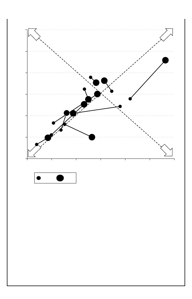
Mapping global value chains and measuring trade in tasks 325

are located in the upstream position. The USA moved down-

ward during the period and swapped its position with Republic of

Korea. The PRC stays in the downstream segment of the regional

supply chains, which reflects the country’s position as a “final

assembler” of the regional products.

Note:

Using a different method developed by Fally (2011), De Backer and

Miroudot (2012) develop an index of “distance to final demand” for OECD.

People’s Rep. of

China

1985

PRC 2005

Indonesia

Japan

Rep. of

Korea

Malaysia

Taipei,China

Philippines

Singapore

Thailand

United States

2.7

2.9

3.1

3.3

3.5

3.7

3.9

2.7 2.9 3.1 3.3 3.5 3.7 3.9

Forward APL

Backward APL

Upstreamness

Downstreamness

Longer supply chains

Shorter supply chains

20051985

Source: Escaith and Inomata (2013).

Figure 9.10 Change of relative positions in the regional supply

chains, 1985–2005

326 Asia and global production networks

on the basis of the import coefficients of SUT tables and some proportion-

ality assumption with respect to the countries of origin. In other words, if

the agricultural sector’s consumption of imported chemicals represents 10

percent of the country’s imports for this particular input, then 10 percent

of all bilateral import flows of chemical inputs will be allocated to the

agricultural sector. This “proportionality” assumption may not reflect the

actual origin when the quality of intermediate products required is very

different across the importing sectors, and that countries of origin special-

ize in particular qualities. Moreover, additional proportional imputations

may be required when the SUT are not detailed enough by products, or

simply not available.

Once flows of intermediates are allocated by sectors, the resulting IIO

needs to be balanced, which raises complex issues of compatibilities. Some

data conflicts can be solved using a priori inferences. For example, the

multi- regional Eora tables, based on a mix of hard data and algorithmic

imputations, are built by giving prominence to national input- output

tables, followed by the UN Statistical Division series of national accounts

and COMTRADE data.

Giving priority to national accounts (as is

usually the case in order to satisfy balancing conditions) means that there

are many occurrences where trade data are misrepresented. Even if prec-

edence rules are established, many imputations rely ultimately on some

value judgment. Timmer (2012) provides a detailed review of the numer-

ous steps that eventually lead to the construction of the IIO table produced

by the WIOD project. OECD (2013) discusses how the national input–

output tables behind the TiVA database have been harmonized and linked

together TiVA; Degain et al. (2013) compare three of the main databases

used so far in the literature (GTAP, OECD- WTO’s TiVA and WIOD).

Diachronic comparison of time series of IIO indicators also confronts

the issue of price variations, in particular the impact of exchange rate.

This complicates the chronological analysis of trade in VA indicators.

WIOD provides chained time- series of its IIO tables that allow computing

indicators in last- year’s prices. For long term comparison Diakantoni and

Escaith (2012) delineate a heuristic method to identify where exchange

rate adjustments are taking place.

Most analytical issues are related to aggregation. I mentioned two of

them: firm heterogeneity and product differentiation. An aggregation bias

is created when very different firms (and very different underlying GVCs)

are aggregated together into a single sector. In developing countries’ pro-

duction technologies the use of imported inputs may differ widely between

firms producing for exports and firms producing only for the domestic

market. This is well documented in the case of the PRC and Mexico, as we

shall see in the next section.

Mapping global value chains and measuring trade in tasks 327

BOX 9.6 TOPOLOGICAL LIMITATIONS OF

INTERNATIONAL INPUT–OUTPUT

MATRICES

Despite their analytical advantages, international input–output

matrices have topological limitations from a GVC perspective,

most – if not all – of them due to aggregation biases and short-

comings in the underlying formal statistical properties (i.e., from

a probabilistic point of view). For example, APL computes the

average length using [a

] as probabilities for transiting from i to

j Input–output matrices define a Markovian process where the

transaction probabilities depend only on the current position of

the node [i] (a sector in a given country), but not on the manner

a node gathered its inputs from other markets. We saw that in

a GVC, suppliers are not undifferentiated as assumed, and the

choice of suppliers may itself be conditioned by the market of final

destination. High quality suppliers will be preferred if the market of

final destination is of high income. From a statistical perspective,

transition probabilities along the supply chain are not independ-

ent (Markovian), but conditioned by the market of final destination

(Bayesian). A Markovian representation of the global network is

only the expected value of the realization of a large number of

mutually independent Bayesian trees. This is perfectly acceptable

when APL is used for descriptive (ex post) reasons, but may be

subject to serious aggregation bias if it is used to forecast or simu-

late the strength and length of a country/sector specific (supply or

demand) shock. The “cascading” effect of a Markovian process

will spread and dilute the shock, while a Bayesian approach

would have called for a more concentrated effect.

The issue is better described through a simple example. A

textile factory in Morocco imports cotton to produce fabric that

is then cut and sown according to the specification of a Spanish

fashion designer and exported. The shirts exported to the Italian

market use long fiber cotton imported from Egypt, and T- shirts for

the Portuguese tourism market use cotton imported from Mali.

Due to the Spanish designer’s price and quality constraints, the

two types of cotton are not substitutable. If a supply shock affects

agriculture in Egypt, only the shirt production will be affected; sim-

ilarly, if demand for T- shirts increases only Malian producers will

benefit from the surge in fabric production. Yet an input–output

328 Asia and global production networks

Product differentiation (quality, specifications) is a more complex issue

and may actually reduce the possibility of sourcing inputs from all pos-

sible trade partners. This is particularly true when intermediate products

are GVC specific. To take an example, sand is processed into silicon chips,

which are assembled according to specific references. While sand and chips

are both intermediate inputs, they respond to different market logics. Sand

is a commodity: as long as it satisfies some physical specifications, its

origin is not really important. Computer chips are much more specific

and a chip made by a company according to very precise specifications

required by the customer (e.g., a computer firm) may not be substitutable

by other apparently similar products. The market powers associated with

those two intermediate goods are very different.

Implications, either in terms of the topological properties of the under-

lying network (Bayesian versus Markovian approaches) or in terms of

economic analysis and market power, are very different when inputs

are commodities or process- specific (see Box 9.6). While international

matrix will not be able to differentiate between those two differ-

entiated value- chains and will aggregate them into a single set

of coefficients. If the sales of the Moroccan factory split equally

between Italy and Portugal, a 100 percent increase in demand

for T- shirts exported to Portugal will translate, equivocally, to a

50 percent increase in Egyptian cotton (upward bias in measuring

the strength of the demand shock) and a 50 percent increase in

Malian cotton (downward bias, respectively).

Similarly, in an input–output perspective, the strength of back-

wards dependence at different stages (nodes) tends to decline

as the “distance”, as measured by the number of production

steps (nodes), increases. Yet, this property is not consistent with

the micro- economic and supply chain management views of the

trade. In our previous example, the trade path is strictly deter-

mined by the market destination: if the final node of the graph is

Italy (alt. Portugal), then the initial node is Egypt (alt. Mali). The

path between nodes is not independent of initial or final states.

From a topological perspective, the GVC network is closer to a

Bayesian process than the Markovian setting that is implied by a

usual input–output matrix. The local probability distribution asso-

ciated with a given node is not independent of the final node (if the

GVC is demand- driven), or of some particular intermediate node

in the network (if the GVC is producer driven).

Mapping global value chains and measuring trade in tasks 329

input–output matrices can be differentiated to capture firm heterogeneity

within a same industry (using a business register, as in the next section),

they are not well equipped to deal with the heterogeneity in intermedi-

ate goods in a same product classification. As we saw previously in the

chapter on mapping intermediate trade, these aspects have to be analyzed

using the graph and network analysis tools on traditional trade statistics,

after applying ad- hoc filters to discriminate products according to their

specificity.

3.3 Linking Trade and Business Statistics

Input–output data, despite their great systemic value, are too aggregated to

capture the business reality behind trade in global value chains. Sturgeon

(2013) presents a state- of- the- art discussion on firm- level data require-

ments and data compilation strategies based on EUROSTAT experience.

Some developing countries involved in GVCs have also developed appro-

priate statistical tools, be they large emerging economies such as the PRC

or Mexico, or smaller countries such as Costa Rica. Obtaining firm- level

data on global value chains requires dedicated surveys, something official

statisticians look at with caution, considering the implementation cost,

as well as the statistical fatigue of responding firms. Fortunately, there

are cost- effective approaches at gathering relevant information without

increasing the statistical burden on responding firms.

Data already collected by national administrations are able to provide a

detailed view of the trade activity generated by each firm. Administrative

registers gather a lot of information on firms’ activities, their corporate

structure, their labor force and productive characteristics. By linking those

administrative data with customs statistics, it is therefore possible to cross-

check several existing databases and build very detailed maps of trade

activity by firm characteristics. EUROSTAT has spearheaded a project

called “Trade by Enterprise Characteristics” to understand the specific

profiles of firms that actively engage into trade. This institutional initiative

mirrors other initiatives from academia that burgeoned in response to the

new “new” trade theory, which had a clear focus on empirical issues and

micro- data. For example, Bernard et al. (2005) look at US data to provide

an ID card of firms according to their trading activity. More recently, the

Chinese Academy of Sciences (2013) has released detailed information on

export activity by type of firms.

These “trade by enterprise characteristics” (TEC) are so far restricted

to national or custom union areas, because one needs to use a single iden-

tification for the firm across all administrative registers. In addition, con-

fidentiality aspects constrain their dissemination. A second best solution

330 Asia and global production networks

is provided by disaggregating sectorial IIO by firm characteristics. De la

Cruz et al. (2011) undertake such an exercise on Mexico; Tang et al. (2013)

combine IO tables and firm census data to disaggregate Chinese GVC

trade by firm size and type of ownership.

4. CONCLUSION: SEARCHING FOR AN

INTEGRATING FRAMEWORK

Up to very recently, trade statistics were considered as a mature field by

the profession; this sleeping beauty has recently awakened to transform

herself into a vibrant teenager, curious to explore new areas, but yet

unsure of the best avenues. While global production networks have been

prevalent since the mid- 1980s, the interest in this new form of globaliza-

tion had remained largely circumscribed to the academic circle. The finan-

cial crisis of 2008–2009 and the resulting great trade collapse determined

a new demand from policy makers for adequate statistical information

regarding this phenomenon. The interest comes from various corners of

policy making; from trade policy with the “Made in the World Initiative”

launched by the WTO to the global governance and development objec-

tives expressed by the G- 20, the United Nations and regional institutions

such as the ADB.

The objective of the present chapter was to tentatively map what we

needed to know, while recognizing that there remain plenty of known

unknowns and unknown unknowns. The starting point was to address

the measurement issues by looking at the analytical and policy questions.

Transactions between firms operating from different countries create

new interdependencies between the national economies, with economic,

financial, social and environmental dimensions. Statisticians have risen

to the measurement challenge by making the best use of existing data.

Using traditional trade statistics in innovative ways allows mapping more

finely the World Trade Network, highlighting the specificities of trade in

intermediate goods and the inter- industry linkages connecting produc-

tion networks. Linking intermediary trade flows with national accounts

data to construct international input–output tables and measuring the

value- added content of trade were part of this effort.

We have so far only scraped the surface of the issue. The available sta-

tistics that the global trade in value- added databases provide today are

estimates at macro- sectoral level. Having this information is already a

great step in the right direction and helped in demonstrating that under-

standing the economic relevance of trade in today’s globalized economy

required new instruments and new methodologies. The results so far help

Mapping global value chains and measuring trade in tasks 331

in understanding the big picture, resizing the relative weight of services

and manufactures and the real size of bilateral trade imbalances. Trade in

value- added also helps understanding the complex relationships between

trade in tasks and job creation.

The existing databases on trade in value- added still suffer from serious

shortcomings. While they bring very valuable information on the relation-

ship between international trade and economic development, existing

databases developed on official data (AIO, OECD- WTO, WIOD) still

need to cover many more developing and least developed countries, an

effort hampered by data restrictions. So far, the incorporation of most

developing countries in international IO tables results from the use of

non- official estimates (GTAP) or algorithmic imputations (Eora) that

may ignore the actual specificities of these countries. Extending the cover-

age of developing and least developed countries using official data should

therefore be a priority.

From an analytical perspective, the indicators obtained so far suffer

from sizable aggregation biases. These impair their use if one wishes to

go beyond descriptive and exploratory statistics and look into causality

factors and confirmatory analysis, using the sophisticated econometric

models favored by the modern (new “new”) trade theory. The new statisti-

cal frontier lies in the development of micro- databases to fully capture the

heterogeneity of firms that are active in these global value chains and com-

plements the trade data with information on firm characteristics, includ-

ing the financial and corporate dimensions. The compilation of business

data for international trade analysis calls for a revision of the existing

classifications, in particular a better understanding of what are the “tasks”

or “business functions” that are subject to outsourcing and eventually

determine “trade in value- added”.

The momentum created by this renewed interest was strong enough

for calling the attention of the highest supra- national governing body,

the United Nations Statistical Conference, which is in charge of setting

international standards that are then applied by official statisticians.

Without prejudging of the future developments in this field of statistics,

trends point toward integrating micro- economic data, including business

registers, labor and financial information, using the national accounts as

the organizing and integrating framework. The relevant data would be

interrelated into a “satellite account” of the external sector, linked to the

national accounts as far as residents are concerned, but also interlinked

with other trading partners. A good example of such a statistical frame-

work is provided by the satellite accounts for tourism, a branch of trade in

services with complex interactions between many different economic and

social actors.

332 Asia and global production networks

Installing such accounts in the routine of national statistical institutes

will be challenging for most developing countries, as it is very demand-

ing in terms of the quality of administrative data and dedicated business

surveys. It is nevertheless in these countries that the need for developing

such an information system is the greatest, considering the relevance

between global value chains, trade and development. On the other hand,

the difficulty of the task should not be overstated, because most trade

activity in developing countries is concentrated in a few firms, greatly

simplifying the data compilation.

NOTES

* I thank G. Daudin, B. Ferrarini, D. Hummels and anonymous editors for their com-

ments on preliminary drafts. I also recognize the contribution of my colleagues at

WTO, IDE- JETRO, OECD, UN, USITC, WIOD and the other researchers with whom

I worked on “trade in value- added” in the past few years. I learned a lot from them,

but most probably not enough to avoid errors and omissions in this chapter. Those, as

well as any opinions expressed here, remain mine and do not reflect any position of the

WTO or its members.

1. Other economists contest the claim for paradigm shift and show that comparative

advantages in trade in tasks can be analyzed through available mainstream models

(Baldwin and Robert- Nicoud, 2010).

2. TiVA, launched by OECD and WTO in January 2013, builds on a series of works by

IDE- JETRO, US- ITC and the WIOD project.

3. Vitali et al. (2011) present an analysis of intra- firm transaction within a large corpo-

ration, illustrating how graph and network theories can help in mapping a hierarchy

across these relationships.

4. As pointed out by Feenstra (2004), recent work in trade economics has been more

empirical than theoretical, and about accounting for global trade flows rather than

about testing hypotheses related to trade.

5. National accounts would prefer to say compensation of employees and operating

surplus (or labor and capital compensations) and net indirect taxes, after subsidies.

6. Final goods are purchased for consumption or investment purposes. In practice, the

boundaries are not clear. Gross investment includes changes in inventories, while final

demand in national accounts covers total exports (of final and intermediate goods).

International IO accountants separate exports of intermediate products from final

demand, but the treatment of inventories remains an empirical issue.

7. See, for a relatively nontechnical example, Hansen et al. (2011); Goyal (2007) develops

a more formal approach of the economic theory of networks.

8. V. Leontief, as early as 1950s, had already identified the potential of IO models for

trade analysis. In 1953, Leontief published ‘Domestic production and foreign trade;

the American capital position re- examined,’ resulting in the famed Leontief paradox.

Later, he promoted the construction of international IO matrices to model economic

interdependencies.

9. Some countries, such as the US, record imports free alongside board (FAB) or free on

board (FOB), but this remains exceptional and most countries favor a cost, insurance

and freight (cif) recording for customs purposes, as it increases the statistical basis on

which tax duties are levied.

10. It is usual, in the social network literature, to call these indicators “metrics” albeit, from

a strict mathematical perspective, they seldom define a true metrical space.

Mapping global value chains and measuring trade in tasks 333

11. See, for example, Hansen et al. (2011) for a non- technical presentation of the main

indicators used in this section.

12. The present section draws heavily on work done at OECD and WTO in co- operation

with IDE- JETRO and USITC; see OECD- WTO (2012) and Degain et al. (2012) for the

main technical conclusions of this research program.

13. Compensation of employees and operating surplus are primary factor income, and net

indirect taxes after subsidies affect market pricing.

14. An introduction on international input–output can be found in the ‘Explanatory Notes’

of Inomata and Uchida (2009).

15. OECD- WTO (2012).

16. For more detailed review of TiVA indicators, see Ahmad (2013) and OECD (2013).

17. At more or less the same time, and independently of this debate, Sancho (2012) also

criticized the use of input–output multipliers on gross output. Yet this criticism is not

relevant when looking at ex- post data, as is usually done when measuring trade in

value- added, because all endogenous effects have taken place.

18. Many researchers refer to trade in VA as a “new metric”. Actually, trade in VA does not

fulfill any of the necessary conditions for defining a metric space. Not even d (U, U) =0

is verified, as we may have reflexive trade (exported VA returning home, as in Table 9.3).

19. See Goyal (2007) for a review of the network economics implications, and Baldwin and

Venables (2010) for a trade perspective.

20. OECD has been developing a Bilateral Trade Database by industry and end- use cat-

egory, where values and quantities of imports and exports are compiled according to

product classifications and by partner countries. A similar Bilateral Trade in Services

database, using detailed EBOPS data and the total services bilateral trade data is in

prospect.

21. Eora is a project to estimate international input–output tables in order to assist envi-

ronmental research, in particular footprint assessments of international trade; differing

from WIOD or OECD- WTO TiVA, which use only official data, the aim of Eora is

to cover as many countries as possible, relying on a mix of hard data and algorithmic

procedures (Kanemoto et al., 2011).

22. Based on economic assumptions (the law of one- price and long- term adjustment of

exchange rates to their purchasing parity), the heuristic is only indicative. Applied on

Asian IIOs, the authors show that exchange rate corrections induced by the Asian crisis

of 1997 had strong medium- term impact for the calculation of the indicators.

23. The aggregation bias relates not only to heterogeneity of quality within alternative

sources, but may also reflect the monopolistic nature of GVCs: the sourcing inputs may

be predetermined in an actual GVC, privileging intra- firm transactions (see Milberg

and Winkler, 2013).

24. A report of the Statistical Commission (UNSC, 2013) provides a comprehensive review

of the work undertaken so far at international level, and it proposes the development of

an overreaching framework for ensuring consistency in methodology, data compilation

and data dissemination.

REFERENCES

Ahmad, N. (2013),‘Estimating trade in value- added: why and how?’, in D. Elms

and P. Low (eds), Global Value Chains in a Changing World, Fung Global

Institute, Nanyang Technological University, and World Trade Organization.

Baldwin, R. (2006), ‘Globalisation: the great unbundling (s)’, paper contribution

to the project Globalisation Challenges for Europe and Finland, Economic

Council of Finland.

Baldwin, R. and F. Robert- Nicoud (2010), ‘Trade- in- goods and trade- in- tasks: an

334 Asia and global production networks

integrating framework’, NBER Working Paper No. 15882, Cambridge, MA:

National Bureau of Economic Research.

Baldwin, R. and A. Venables (2010), ‘Relocating the value chain: offshoring

and agglomeration in the global economy’, NBER Working Paper No. 16611,

Cambridge, MA: National Bureau of Economic Research.

Bernard, A.B., J.B. Jensen and P.K. Schott (2005),‘Importers, exporters,

and multinationals: a portrait of firms in the US that trade goods’, NBER

Working Paper No. 11404, Cambridge, MA: National Bureau of Economic

Research.

Carlos- Lopes, J., J. Dias and J. Ferreira do Amaral (2008), ‘Assessing economic

complexity in some OECD countries with input–output based measures’,

International Conference on Policy Modelling, Berlin.

Chinese Academy of Sciences (2013), ‘Interim report on global value chains and

the value- added estimates in China’s trade’, June.

Coe, N., P. Dicken and M. Hess (2008), ‘Global production networks: realizing the

potential’, Journal of Economic Geography, 8, 271–295.

Daudin, G., P. Monperrus- Veroni, Ch. Rifflart and D. Schweisguth (2006), ‘Le

commerce extérieur en valeur ajoutée’, Revue de l’OFCE 98, 129–165.

Daudin, G., Ch. Rifflart and D. Schweisguth (2011), ‘Who produces for whom in

the world economy?’, Canadian Journal of Economics, 44, 1403–1437.

De Backer, K. and S. Miroudot (2012), ‘Mapping global value chains’, WIOD

Conference “Causes and Consequences of Globalization”, Groningen, The

Netherlands, 24–26 April.

De La Cruz, J., R. Koopman, Z. Wang and S.- J. Wei (2011), ‘Estimating foreign

value- added in Mexico’s manufacturing exports’, U.S. International Trade

Commission, Office of Economics Working Paper No. 2011–04A.

Degain, Ch., H. Escaith and A. Maurer (2012), ‘Comparison of methodolo-

gies to estimate trade in value- added terms’, WTO- MIWI, draft note, mimeo,

September.

Degain, Ch., L. Jones, Z. Wang and L. Xin (2013), ‘The similarities and differences

among the three major global inter- country input–output databases and their

implications for trade in value- added estimates’, 16th GTAP Conference on

Global Economic Analysis, June.

Diakantoni, A. and H. Escaith (2012), ‘Reassessing effective protection rates in

a trade in tasks perspective: evolution of trade policy in factory Asia’, WTO

Working Paper ERSD 2012–11.

Dietzenbacher, E. and I. Romero (2007), ‘Production chains in an interre-

gional framework: identification by means of average propagation lengths’,

International Regional Science Review, 30, 362.

Dietzenbacher, E., I. Romero and N.S. Bosma (2005), ‘Using average propagation

lengths to identify production chains in the Andalusian economy’, Estudios de

Economia Aplicada, 23, 405–422.

Elms, D. and P. Low (eds) (2013), Global Value Chains in a Changing World,

Fung Global Institute, Nanyang Technological University, and World Trade

Organization.

Escaith, H. and F. Gonguet (2011), ‘International supply chains as real transmis-

sion channels of financial shocks’, Journal of Financial Transformation, 31,

83–97.

Escaith, H. and S. Inomata (2013),‘Geometry of global value chains in East Asia:

the role of industrial networks and trade policies’, in D. Elms and P. Low (eds),

Mapping global value chains and measuring trade in tasks 335

Global Value Chains in a Changing World, Fung Global Institute, Nanyang

Technological University, and World Trade Organization.

Ethier, W.J (1979), ‘Internationally decreasing costs and world trade’, Journal of

International Economics, 9, 1–24.

Fally, T. (2011), ‘On the fragmentation of production in the US’, presentation,

University of Colorado- Boulder, July.

Feenstra, R. (2004), Advanced International Trade: Theory and Evidence, Princeton:

Princeton University Press.

Feenstra R.C. and G.H. Hanson (1996), ‘Globalisation, outsourcing and wage

inequality’, American Economic Review, 86, 240–245.

Ferrarini, B. (2011), ‘Mapping vertical trade’, ADB Working Paper Series 263,

Manila: Asian Development Bank.

Flores, M. and M. Vaillant (2011), ‘Global value chains and export sophistication

in Latin America’, Inter- American Development Bank- Integration and Trade

Journal, 32, 15–35.

Foster, N., R. Stehrer, M. Timmer and G. de Vries (2012), ‘Offshoring and the

skill structure of labour demand’, World Input–Output Database Working

Paper Nr. 6.

Geoffrion A. and R. Powers (1995), ’20 Years of strategic distribution system

design: an evolutionary perspective’, Interfaces, 25, 105–127.

Gereffi, G. and T. Sturgeon (2013),‘Global value chain- oriented industrial policy:

the role of emerging economies’, in D. Elms and P. Low (eds), Global Value

Chains in a Changing World, Fung Global Institute, Nanyang Technological

University, and World Trade Organization.

Goyal, S. (2007), Connections: An Introduction to the Economics of Networks,

Princeton University Press.

Grossman, G.M. and E. Rossi- Hansberg (2006), ‘Trading tasks: A simple theory

of offshoring’, NBER Working Paper No. 12721, Cambridge, MA: National

Bureau of Economic Research.

Hansen, D., B. Shneiderman and M. Smith (2011), Analyzing Social Media Networks

with NodeXL: Insights from a Connected World, Elsevier.

Hatzichronoglou, T. (1997), ‘Revision of the high- technology sector and product

classification’, OECD Science, Technology and Industry Working Papers, No.

1997/02.

Hidalgo, C., B. Klinger, R. Hausmann and A. László Barabási (2007), ‘The

product space conditions the development of nations’, Science, 317, 482–487.

Hummels, D., Jun Ishii and Kei- Mu Yi (2001), ‘The nature and growth of

vertical specialization in world trade’, Journal of International Economics, 54,

75–96.

Inomata, S. (2008), ‘Average propagation lengths: a new concept of the “distance”

between industries, with an application to the Asia- Pacific region’, Sangyo-

Renkan, 16–1 (in Japanese), Japan: Pan- Pacific Association of Input–Output

Studies.

Inomata, S. (2011), ‘Explanatory notes’, in S. Inomata (ed.), Asia Beyond the

Global Economic Crisis: The Transmission Mechanism of Financial Shocks,

Cheltenham, UK and Northampton, MA, USA: Edward Elgar, in association

with IDE- JETRO.

Inomata, S. and Y. Uchida (2009), ‘Asia beyond the crisis: visions from interna-

tional input–output analyses’, IDE Spot Survey No. 31.

Johnson, R.C. and G. Noguera (2012), ‘Accounting for intermediates: production

336 Asia and global production networks

sharing and trade in value added’, Journal of International Economics, 86,

224–236.

Kanemoto, K., M. Lenzen, A. Geschke and D. Moran (2011), ‘Building Eora:

a global multi- region input output model at high country and sector’, 19th

International Input- Output Conference.

Koopman, R., W. Powers, Z. Wang and S.- J. Wei (2012), ‘Tracing value- added

and double counting in gross exports’, NBER Working Paper No. 18579,

Cambridge, MA: National Bureau of Economic Research.

Koopmans, T.C. (1947), ‘Measurement without theory’, Review of Economics and

Statistics, 29, 161–172.

Krugman, P.R. (1979), ‘Increasing returns, monopolistic competition, and inter-

national trade’, Journal of International Economics, 9, 469–479.

Lall, S., J. Weiss and J. Zhang (2005), ‘The “sophistication” of exports: a new

measure of product characteristics’, Queen Elizabeth House Working Paper

Series 123, Oxford University.

Lanz, R., S. Miroudot and H.K. Nordås (2011), ‘Trade in tasks’, OECD Trade

Policy Working Papers, No. 117.Leontief, W. (1953), ‘Domestic production and

foreign trade; the American capital position re- examined’, Proceedings of the

American Philosophical Society, 97 (4), 28 September, 332–349.

Los, B., E. Dietzenbacher, R. Stehrer, M.P. Timmer and G. de Vries (2012), ‘Trade

performance in internationally fragmented production networks: concepts and

measures”, World Input–Output Database Working Paper Nr. 11.

Maurer, A. and Ch. Degain (2010), ‘Globalization and trade flows: what you see is

not what you get!’, WTO Staff Working Paper No. 2010–12.

Melitz, M. (2003), ‘The impact of trade on intra- industry reallocations and aggre-

gate industry productivity’, Econometrica, 71, 1695–1725.

Meng, B., Y. Fang and N. Yamano (2012), ‘Measuring global value chains and

regional economic integration: an international input–output approach’, IDE

Discussion Paper 362.

Milberg, W. and D. Winkler (2013), Outsourcing Economics: Global Value Chains

in Capitalist Development, Cambridge University Press.

Miller, R. and P. Blair (2009), Input–Output Analysis: Foundations and Extensions

(second edition), Cambridge University Press.

Miroudot, S., R. Lanz and A. Ragoussis (2009), ‘Trade in intermediate goods and

services’, OECD Trade Policy Papers 93.

Ng, F., and A. Yeats (1999), ‘Production sharing in East Asia: who does what for

whom, and why?’, Policy Research Working Paper Series 2197, Washington,

DC: The World Bank.

OECD (Organisation for Economic Co- operation and Development) (2005),

Handbook on Economic Globalization Indicators, Paris.

OECD (2011), ISIC REV. 3 Technology Intensity Definition: Classification of

Manufacturing Industries into Categories Based on R&D Intensities, Paris.

OECD (2013), Interconnected Economies: Benefitting from Global Value Chains,

Paris.

OECD- World Trade Organization (WTO) (2012), ‘Note on measuring trade in

value added’, e- document (WTO- MIWI website).

Oosterhaven, J. and D. Stelder (2002), ‘Net multipliers avoid exaggerating

impacts: with a biregional illustration for the Dutch transportation sector’,

Journal of Regional Science, 42, 533–543.

Oxley, L., P. Walker, D. Thorns and H. Wang (2008). ‘The knowledge economy/

Mapping global value chains and measuring trade in tasks 337

society: the latest example of “measurement without theory”?’, The Journal of

Philosophical Economics, 2, 20–54.

Park, A., G. Nayyar and P. Low (2013), ‘Supply chains perspective and issues: a

literature review’, Fung Global Institute and World Trade Organization.

Porter, M.E. (1985), Competitive Advantage: Creating and Sustaining Superior

Performance, The Free Press: New York.

Rauch, J.E. (1999), ‘Networks versus markets in international trade’, Journal of

International Economics, 48, 7–35.

Rifflart, Ch. and D. Schweisguth (2013), ‘Draft report on new measures of interna-

tional trade’, in European Framework for Measuring Progress, e- Frame.

Sancho, F. (2012), ‘Some conceptual difficulties regarding net multipliers’, Depart-

ment of Economics Universitat Autònoma de Barcelona, mimeo.

Stehrer, R. (2012), ‘Trade in value added and the value added of trade’, World

Input–Output Working Paper No 8.

Sturgeon, T. (2013), ‘Global value chains and economic globalization: towards a

new measurement framework’, EUROSTAT.

Sturgeon, T. and O. Memedovic (2010), ‘Mapping global value chains: intermedi-

ate goods trade and structural change in the world economy’, UNIDO Working

Paper 05, Vienna: UNIDO.

Tang, K.K. and A. Wagner (2010), ‘Measuring globalization using weighted network

indexes’, paper presented at the 31st General Conference of the International

Association for Research in Income and Wealth, St. Gallen, Switzerland, August.

Tang, H., F. Wang and Z. Wang (2013), ‘The domestic segment of global supply

chain in China under state capitalism’, paper presented at the International

Conference on Global Value Chains and Structural Adjustments, Tsinghua

University, Beijing, June.

Timmer, M. (2012), ‘The World Input–Output Database: contents, sources and

methods’, World Input–Output Database Working Paper Number 10.

UNCTAD (2013), World Investment Report 2013: Global Value Chains: Investment

and Trade for Development, Geneva.

UNSC (2013), International Trade Statistics: Report to the Secretary General,

United Nations Statistical Commission, 44th session.

Vitali, S., J.B. Glattfelder and S. Battiston (2011), ‘The network of global corpo-

rate control’, PLoS ONE 6(10).

World Trade Organization (WTO) (2013a), World Trade Report 2013: Factors

Shaping the Future of World Trade, Geneva.

WTO (2013b), International Trade Statistics, annual statistical yearbook, Geneva.

WTO (2008), World Trade Report 2008: Trade in a Globalizing World, Geneva.

WTO and IDE- JETRO (2011), Trade Patterns and Global Value Chains in East

Asia: From Trade in Goods to Trade in Tasks, Geneva and Tokyo.

WTR (World Trade Report) (2013), Factors Shaping The World Trade, Geneva:

World Trade Organization.

Yeats, A. (2001), ‘Just how big is global production sharing?’, in S. Arndt and

H. Kierzkowski (eds), Fragmentation: New Production Patterns in the World

Economy, New York: Oxford University Press.

338

10. The development and future of

Factory Asia*

Richard Baldwin and Rikard Forslid

1. INTRODUCTION

Like a gigantic, impossibly complex but wonderfully efficient factory,

East Asia churns out a vast array of manufactured goods with

world- beating price- quality ratios. But this is not a series of national

efforts. Manufacturing processes that used to be performed in single fac-

tories (mostly in Japan and Republic of Korea) have been fractionalized

and dispersed across the region – creating what Baldwin (2006) called

‘Factory Asia’.

This chapter looks at the underlying interconnected processes that

have led to the development of Factory Asia – namely the fractionali-

zation of the manufacturing process into stages and the dispersion of

these stages around Asia. It does so by developing the TOSP (tasks,

occupations, stages, products) framework that was informally intro-

duced in Baldwin (2012). The TOSP framework views the production

of goods as the performance of a range of tasks that are organized into

occupations (collection of tasks) and stages (collections of occupations).

Typically offshoring occurs at the level of stages rather than tasks or

occupation.

This framework is then used to examine the likely effects of improv-

ing information and communication technology (ICT) on the future

of Factory Asia. Two dimensions are distinguished: fractionalization

of the production process (slicing up the value chain), and their spatial

dispersion (offshoring stages).

A key premise of this chapter is that it is a trap to think of Factory Asia

from the perspective of traditional trade theory. It is tempting to think of

the fractionalization as simply a further step in the century’s long march

from autarky to free trade. After all, the fast lane of Factory Asia involves

the offshoring of low- skill intensive stage to nations that are abundant

in low- skill labor while knowledge- intensive stages remain in nations

that are well endowed with knowledge workers. A natural, but incorrect,

The development and future of Factory Asia 339

way to think of this is as nations’ shifting resources to their comparative

advantage sectors.

As this misthinking is pervasive, the rest of the introduction is devoted

to contrast the old globalization paradigm – which views the process as

driven by the steady lowering of trade costs – with an alternative narrative

that views globalization as two processes rather than one.

1.1 Globalization as Two Unbundlings

Globalization is often viewed as linear – a progressive integration of

national economies driven by lower technical and manmade trade costs. In

trade economists’ jargon, globalization is basically the move from autarky

to free trade done slowly. The sharp trends in Figure 10.1 suggest that this

is a mistake.

Globalization was associated with an agglomeration of economic activ-

ity in what used to be called the industrialized nations. From 1820 to 1988,

the G7’s share of global output rose from 22 percent to 67 percent. Since

then, the share has plummeted and is now back to the level it first attained

in 1900. About the same time, the world saw a massive shift in manufac-

turing activity from G7 nations to a handful of developing nations that

1820,

22%

1988,

67%

2010,

50%

10%

20%

30%

40%

50%

60%

70%

80%

1820

1839

1858

1877

1896

1915

1934

1953

1972

1991

2010

G7 nations' share of global GDP,

1820–2010

1990,

65%

G7,

47%

PRC,

19%

6 risers,

RoW

10%

20%

30%

40%

50%

60%

70%

80%

1970

1974

1978

1982

1986

1990

1994

1998

2002

2006

2010

G7 nations' share of global

manufacturing, 1970–2010

Note: 6 risers = Republic of Korea, India, Indonesia, Thailand, Turkey, and Poland; G7

= Canada, France, Germany, Italy, Japan, United Kingdom and United States of America;

PRC = People’s Republic of China; RoW = rest of the world.

Source: Authors’ elaboration of data from unstats.un.org and Maddison’s database.

Figure 10.1 Globalization: one process or two?

340 Asia and global production networks

have come to be called Emerging Economies. In the two decades from

1970 to 1990, the G7’s manufacturing share dropped from 71 percent to

65 percent. The subsequent two decades saw it plummet to 50 percent. The

share shifts, however, were not generalized. Only seven nations saw their

share of manufacturing rise by more than one- half of one percentage point

(the People’s Republic of China (PRC), the Republic of Korea, India,

Indonesia, Thailand, Turkey and Poland). Plainly we are in a new phase of

globalization – a phase that is distinct from earlier phases. There are many

names for this new globalization paradigm – the global value chain (GVC)

revolution, fragmentation, trade in tasks, etc.

On the back of this prima facie evidence, it would seem we need two

processes to explain globalization’s main outlines, not one. Falling trade

cost will not cover it. In a 2006 paper for the Finnish Prime Minister’s

office, Baldwin (2006) characterizes this as globalization’s two great

unbundlings. The first unbundling – up to the mid or late 1980s is the tra-

ditional, linear process driven by lower trade costs. The second unbundling

was driven by better information and communication technology. The

first unbundling allowed consumption and production to be separated by

great distances but production stages remained bundled in factories and

industrial districts. The ICT revolution sparked the second unbundling by

unbundling the factories. Improved ICT made it economical for stages of

production formerly performed in a rich- nation factory to be unbundled

and dispersed to low- wage nations.

The development of Factory Asia was one of the first manifestations of

the second unbundling, although a similar development occurred in North

America and Europe.

2. FACTS: THE DEVELOPMENT OF FACTORY ASIA

We use here the Trade in Value- Added (TiVA) database, which contains

the value- added in goods and services of a county’s export (and import).

The joint OECD–WTO Trade in Value- Added (TiVA) project traces the

value- added by each industry and country in the production chain, and

allocates the value- added to these source industries and countries.

One of the most striking features of Factory Asia is the very rapid

growth of exports from emerging East Asian economies – measured in

either gross or value- added (VA) terms. By ‘gross exports’ we mean the

standard, customs- based numbers. By value- added exports, we mean the

domestic value- added contained in a nation’s gross exports. The difference

is that the value- added figures net out the foreign value- added embedded

in gross exports. For example, if Mexico exports a car that contains a US

The development and future of Factory Asia 341

engine, the gross export is the value of the whole car; the value- added

export is just the value that was added in Mexico.

As Figure 10.2 shows, the growth has been quite uneven. In general,

emerging markets have seen higher growth with the PRC, Cambodia, and

Viet Nam showing spectacular growth (although from very low bases in

the latter two cases).

For comparison, we include the export growth figures for the G7 and a

handful of emerging markets that are known to be active in outsourcing and

GVCs. A point we will explore more below is that there seems to be a con-

nection between the magnitude of the growth and the size of the gap between

gross and value- added exports (a rough measure of supply- chain trade).

The commonality of emerging markets’ rapid export growth hides an

important distinction. Some of these nations – like Brazil and the Russian

Federation – achieve high export growth on the back of the booming

demand for commodities. Others are doing it via manufactured goods.

0% 500% 1000%

East Asians

JPN

TAP

HKG

PHI

KOR

MAL

INO

THA

SIN

BRU

CAM

PRC

VIE

G7 nations

FRA

ITA

CAN

USA

UKG

GER

0% 500% 1000%

Other EMs in GVCs

POR

SVN

MEX

TUR

CZE

HUN

POL

SVK

ROU

Primary exporters

ZAF

AUS

CHL

NOR

BRU

RUS

BRA

Gross export growth

VA export growth

Gross export growth

VA export growth

Notes:

EM = emerging market; G7 = Canada, France, Germany, Italy, Japan, United Kingdom

and United States of America; GVC = global value chain.

Country codes are listed in Appendix Table 10A.1.

Source: TiVA database with authors’ calculations.

Figure 10.2 Total export growth, 1995–2009, various nations, gross and

value- added

342 Asia and global production networks

To provide hints as to the sources of the growth, Figure 10.3 shows the

growth decomposition by broad sector – focusing on primary exports,

light manufactured exports, heavy manufactured exports, and service

exports. The left panel shows a wide diversity among East Southeast Asian

(EA) nations. Some nations – such as Brunei Darussalam, Viet Nam, and

Cambodia have seen their natural resource based exports account for sub-

stantial fractions of their total export growth. For most, however, the key

driver was manufactured exports. Only in three economies (Hong Kong,

China; Singapore and Japan) have service exports played a large role in

VA export growth.

The role of commodity exports has been smaller in the emerging

markets involved in Factory North America (Mexico), and Factory

Europe (Poland, Turkey, etc.). The commonality is that manufacturing

exports account for the lion’s share of the growth – often two- thirds or

more.

–40%

–20%

20%

40%

60%

80%

100%

PHI

TAP

HKG

KOR

SIN

JPN

PRC

THA

INO

MAL

CAM

VIE

BRU

Value-added export growth

composition, East Asia

Primary

Light manufacturing

Heavy manufacturing

Services

Primary

Light manufacturing

Heavy manufacturing

Services

–40%

–20%

20%

40%

60%

80%

100%

CZE

POL

SVN

HUN

SVK

POL

TUR

ROU

MEX

Value-added export growth

composition, other emerging

markets in global value chains

Note: Country codes are listed in Appendix Table 10A.1.

Source: TiVA database with authors’ calculations.

Figure 10.3 Decomposition of value- added export growth by broad sector,

1995–2009

The development and future of Factory Asia 343

2.1 Connection to Supply- chain Trade

A property of fast growers that rely on manufacturers is that they seem to

be linking- up to global supply chains to a much larger extent. This section

presents prima facie evidence that this link is indeed important for many

of the East Asian nations.

The measure of supply- chain trade involvement we use is the share of

re- exported intermediates (REI), that is, imported intermediates that are

re- exported either as parts and components, or embedded in final goods.

Our aim is to explore the connection between increases in this measure

of supply chain trade (SCT) and increases in the domestic value- added

contained in exports. In both cases, we look at the percentage increase

from 1995 to 2009 (which is the full span of the TiVA database). The first

look at the raw data is not encouraging. Figure 10.4 shows the scatter plot

of the change in 57 nations’ SCT measure in 18 different sectors against

the same nations’ growth of domestic value- added in exports in the same

sectors. The overall correlation is unclear.

The second unbundling logic, however, suggests that the correlation

should differ greatly for ‘headquarters (HQ) economies’ and ‘factories

economies’ – as well as across sectors (since production unbundling has

–500%

500%

1000%

1500%

2000%

2500%

–100% 0% 100% 200% 300%

Growth in domestic value added in exports

Re-exported intermediates as a % of total intermediate imports

Re-exported intermediates as a % of total intermediate

imports versus growth in domestic value-added in exports

Source: TiVA database with authors’ calculations.

Figure 10.4 Growth in supply- chain participation and domestic value-

added in exports

344 Asia and global production networks

not happened equally in all sectors). Once we separate the East Asia

nations from the others, a positive relationship looks much more plausi-

ble. Indeed, Figure 10.5 shows that a positive link seems to hold for other

nations involved in supply- chain trade (those in Factory North America

and Factory Europe). The link is completely missing for G5 nations, the

headquarters economies, and is driven by outliers in the large economies

outside of Asia for other emerging markets.

When we look at sectors – pooling across of nations – the positive asso-

ciation is clear in some sectors but not in others (Figure 10.6). It is par-

ticularly clear in the machinery sectors, electrical and optical equipment,

transportation equipment, and machinery and equipment not elsewhere

classified (nec).

The last cut of the data highlights the growth correlation between

supply- chain participation and VA export growth by country group and by

sector (Figure 10.7). Here a couple of points stand out. First, the PRC and

Viet Nam are frequently outliers – with big positive growth in both meas-

ures. Second, East Asian nations seem to systematically have more positive

links between the two measures than the other nations. This, however, is

less true in the classic outsourcing sectors such as textiles and machinery of

various sorts. Indeed in transportation, the correlation of the East Asian

nations and other factory economies (Other SCTers) is not at all clear.

2.2 Evolution of Factory Asia

Data for the early days of Factory Asia are difficult to come by. One

rough indicator that does reach back to the 1960s is a simple intra- industry

trade index (IIT) (Brülhart 2009). The idea here is that two- way trade in

similar products that is either North- South, or South- South is likely to be

largely supply- chain trade, i.e. two- way trade in parts and components.

Plainly this is a crude measure, but it is transparent, widely understood

and available for most nations going back to the early 1960s.

Figure 10.8 shows the paths of Japan’s and the Republic of Korea’s

IIT with each of seven Association of Southeast Asian Nation (ASEAN)

economies. The first salient point is that Japan’s exchange with the other

Asian nations has been growing since the 1960s. In the early days, much

of this was in microelectronics (Grunwald and Flamm, 1985). Japan’s IIT

with three of the big ASEAN economies – Malaysia, Thailand and the

Philippines – took off at about the same time, i.e. mid- to late- 1980s. The

sharp rise in IIT with Indonesia and Viet Nam came a decade later. For

Indonesia (which is still a big commodity exporter), the rise was much

less marked than for the others. Lao People’s Democratic Republic and

Cambodia have not really joined the Japanese supply chains according

The development and future of Factory Asia 345

–500%

500%

1000%

1500%

2000%

2500%

–100% 0% 100% 200% 300%

Value added export growth

Re-exported intermediates as a

% of total intermediate imports

East Asian nations

–500%

500%

1000%

1500%

2000%

2500%

–100% 0% 100% 200% 300%

Value added export growth

Re-exported intermediates as a

% of total intermediate imports

Other emerging markets

–500%

500%

1000%

1500%

2000%

2500%

–100% 0% 100% 200% 300%

Value added export growth

Re-exported intermediates as a

% of total intermediate imports

Group of 5

–500%

500%

1000%

1500%

2000%

2500%

–100% 0% 100% 200% 300%

Value added export growth

Re-exported intermediates as a

% of total intermediate imports

Other factory economies

Note: East Asian nations = China, People’s Rep. of, Indonesia, Korea, Rep. of, Malaysia,

Philippines, Taipei,China, Thailand and Viet Nam; Group of 5 = France, Germany, Japan,

United Kingdom and United States of America; other factory economies = Hungary,

Mexico, Poland, Slovakia and Turkey; other emerging markets = Brazil, Canada, India,

South Africa and Russian Federation.

Source: TiVA database with authors’calculations.

Figure 10.5 Supply chain participation and value- added exports, by

nation groups

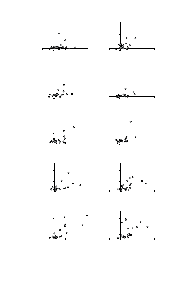
346 Asia and global production networks

VIE

PHI

PRC

INO

KOR

THA

MAL

TAP

USA

GER

FRA

UKG

JPN

TUR

SVK

POL

HUN

MEX

IND

BRA

ZAF

RUS

CAN

–200%

800%

1800%

–100% 0% 100% 200% 300%

REI growth

VA export growth

01T05: Agriculture, hunting, forestry

and fishing

VIE

PHI

PRC

INO

KOR

THA

MAL

TAP

USA

GER

FRA

UKG

JPN

TUR

SVK

POL

HUN

MEX

IND

BRA

ZAF

RUS

CAN

–200%

300%

800%

1300%

1800%

2300%

–100% 0% 100% 200% 300%

REI growth

VA export growth

10T14: Mining and quarrying

VIE

PHI PRC

INO

KOR

THA

MAL

TAP

USA

GER

UKG

JPN

TUR

SVK

POL

HUN

MEX

IND

BRA

ZAF

RUS

CAN

–200%

800%

1800%

–100% 0% 100% 200% 300%

REI growth

VA export growth

15T16: Food products, beverages

and tobacco

VIE

PHI

PRC

INO

KOR

THA

MALTAP

USA

GER

FRA

UKG

JPN

TUR

SVK

POL

HUN

MEX

IND

BRA

ZAF

RUS

CAN

–200%

800%

1800%

–100% 0% 100% 200% 300%

REI growth

VA export growth

17T19: Textiles, textile products,

leather and footwear

VIE

PHI

PRC

INO

KOR

THA

MAL

TAP

USA

GER

FRA

UKG

JPN

TUR

SVK

POL

HUN

MEX

IND

BRA

ZAF

RUS

CAN

–200%

800%

1800%

–100% 0% 100% 200% 300%

REI growth

VA export growth

20T22: Wood, paper, paper

products, printing and publishing

VIE

PHI

PRC

INO

KOR

THA

MAL

TAP

USA

GERFRA

UKG

JPN

TUR

SVK

POL

HUN

MEX

IND

BRA

ZAF

RUS

CAN

–200%

800%

1800%

–100% 0% 100% 200% 300%

REI growth

VA export growth

23T26: Chemicals and non–metallic

mineral products

VIE

PHI

PRC

INO

KOR

THA

MAL

TAP

USA

GER

FRA

UKG

JPN

TUR

SVK

POL

HUN

MEX

IND

BRA

ZAF

RUS

CAN

–200%

800%

1800%

–100% 0% 100% 200% 300%

REI growth

VA export growth

27T28: Basic metals and fabricated

metal products

VIE

PHI

PRC

INO

KOR

THA

MAL

TAP

USA

GER

FRA

UKG

JPN

TUR

SVK

POL

HUN

MEX

IND

BRA

ZAF

RUS

CAN

–200%

300%

800%

1300%

1800%

2300%

–100% 0% 100% 200% 300%

REI growth

VA export growth

29: Machinery and equipment, nec

VIE

PHI

PRC

INO

KOR

THA

MAL

TAP

USA

GER

FRA

UKG

JPN

TUR

SVK

POL

HUN

MEX

IND

BRA

ZAF

RUS

CAN

–200%

800%

1800%

–100% 0% 100% 200% 300%

REI growth

VA export growth

30T33: Electrical and optical

equipment

VIE

PHI

PRC

INO

KOR

THA

MAL

TAP

USA

GER

FRA

UKG

JPN

TUR

SVK

POL

HUN

MEX

IND

BRA

ZAF

RUS

CAN

–200%

300%

800%

1300%

1800%

2300%

–100% 0% 100% 200% 300%

REI growth

VA export growth

34T35: Transport equipment

Notes:

Country codes are listed in Appendix Table 10A.1.

nec = not elsewhere classified; REI = re- exported intermediates; VA = value- added.

Source: TiVA database with authors’ calculations.

Figure 10.6 Supply chain participation and value- added exports, by all

nation groups by sectors

The development and future of Factory Asia 347

VIE

PRC

INO

THA

MAL

KOR

TAP

PHI

–200%

300%

800%

1300%

1800%

2300%

–100% 0% 100% 200% 300%

REI growth

VA export growth

34T35: Transport equipment

VIE

PRC

INO

THA

MAL

KOR

TAPPHI

–200%

300%

800%

1300%

1800%

2300%

–50% 0% 50% 100% 150%

REI growth

VA export growth

17T19: Textiles, leather and footwear

VIE

PRC INO

THA

MAL

KOR

TAP

PHI

–200%

300%

800%

1300%

1800%

2300%

–100% 0% 100% 200% 300% 400% 500%

REI growth

VA export growth

15T16: Food products, beverages and

tobacco

VIE

PRC

INO

THA

MAL

KOR

TAP

PHI

–200%

300%

800%

1300%

1800%

2300%

–50% 0% 50% 100% 150% 200%

REI growth

VA export growth

20T22: Wood, paper, printing and publishing

VIE

PRC

INO

THA

MAL

KOR

TAP

PHI

–200%

300%

800%

1300%

1800%

2300%

–50% 0% 50% 100% 150%

REI growth

VA export growth

23T26: Chemicals and non–metallic

mineral products

VIE

PRC

INO

THA

MAL

KOR

TAP

PHI

–200%

300%

800%

1300%

1800%

2300%

–100% 0% 100% 200% 300%

REI growth

VA export growth

27T28: Basic metals and fabricated

metal products

VIE

PRC

INO

THA

MAL

KOR

TAP

PHI

–200%

300%

800%

1300%

1800%

2300%

–100% 0% 100% 200% 300%

REI growth

VA export growth

29: Machinery and equipment, nec

VIE

PRC

INO

THA

MAL

KOR

TAP

PHI

–200%

300%

800%

1300%

1800%

2300%

–100% 0% 100% 200% 300% 400%

REI growth

VA export growth

30T33: Electrical and optical equipment

East Asia Other factory economies

Group of 5 Other emerging markets

Notes:

nec = not elsewhere classified; REI = re- exported intermediates; VA = value- added.

Follows country codes list in Appendix Table 10A.1.

Source: TiVA database with authors’ calculations.

Figure 10.7 Supply chain participation and value- added export growth, by

sector and country group

348 Asia and global production networks

10%

15%

20%

25%

30%

35%

40%

45%

50%

1962

1966

1970

1974

1978

1982

1986

1990

1994

1998

2002

2006

2010

Japan’s bilateral intra-industry

trade with ASEAN

10%

15%

20%

25%

30%

35%

40%

45%

50%

1962

1966

1970

1974

1978

1982

1986

1990

1994

1998

2002

2006

2010

Republic of Korea’s bilateral

intra-industry trade with ASEAN

INO

CAM

LAO

MAL

PHI

THA

VIE

INO

CAM

LAO

MAL

PHI

THA

VIE

Note: Country codes are listed in Appendix Table 10A.1.

Source: Author’s calculations on COMTRADE data.

Figure 10.8 Japan’s and the Republic of Korea’s bilateral intra- industry

trade with ASEAN, 1962–2012

10%

15%

20%

25%

30%

35%

40%

45%

50%

PRC's bilateral intra-industry

trade with ASEAN

INO

CAM

LAO

MAL

PHI

THA

VIE

10%

20%

30%

40%

50%

ASEAN's bilateral intra-

industry trade with ASEAN

INO

CAM

LAO

MAL

PHI

THA

VIE

1962

1966

1970

1974

1978

1982

1986

1990

1994

1998

2002

2006

2010

1962

1966

1970

1974

1978

1982

1986

1990

1994

1998

2002

2006

2010

Note: Country codes are listed in Appendix Table 10A.1.

Source: Author’s calculations on COMTRADE data.

Figure 10.9 PRC’s and each ASEAN’s bilateral intra- industry trade with

ASEAN, 1962–2012

The development and future of Factory Asia 349

to this indicator. For the Republic of Korea, the timing is similar but the

engagement with ASEAN economies is muted compared to Japan.

Figure 10.9 shows the IIT proxy for Factory Asia participation for

the PRC with each of seven ASEAN economies and for each ASEAN

with the others. What we see is that PRC’s bilateral IIT with Thailand

and Malaysia jumped in the mid- 1980s, but it did not start until the early

1990s with Indonesia and the Philippines. The IIT measure slopes up from

the later 1990s for Viet Nam but does not really take off until the early

2000s. Cambodia’s IIT with PRC has taken off only in the 2010s. As for

the ASEANs among themselves, we see a similar timing. The ‘big four’

ASEANs, Thailand, Malaysia, Indonesia and the Philippines, see their

IIT scores jump in the mid- 1980s. Viet Nam’s jump is delayed till the late

1990s with a significant acceleration in the 2000s.

More direct evidence comes from the IDE- JETRO international input–

output table. This shows the country of origin of imported manufactured

goods purchased by the manufacturing sector of each East Asian economy.

Table 10.1 has three panels corresponding to the shape of Factory Asia in

1985, 1990 and 2000.

The top panel shows the situation in 1985 when Factory Asia was very

simple. With the exception of Singapore, East Asian nations sourced their

imported manufactured inputs from Japan and the rest of the world – all

the rows are dominated by zeros except those of Japan and the rest of the

world (mainly the US and Europe). By 1990 (second panel), it was more

complex: ‘Triangle trade’ still dominated the picture with the low- wage

nations (first five columns) buying inputs from Japan and the rest of the

world but providing no inputs in return. Now, however, Japan is not the

only headquarters economy. Taipei,China, the Republic of Korea, and

Hong Kong, China experienced their own hollowing- out phases and new

triangle trade appears. This new triangle trade involves the shipment of

parts from the new HQ economies to the ‘factory economies’ (the PRC

and the advanced ASEANs, Indonesia, Malaysia, the Philippines and

Thailand). This can be seen from the emergence of new non- zero entries in

the rows for Taipei,China, the Republic of Korea and Singapore.

By 2000, Factory Asia was really complex. Firms based in the ‘factory

economies’ began to source parts from other factory economies rather

than from the HQ economy alone. In particular, Thailand, Malaysia and

the PRC became important suppliers of parts to other ‘factory econo-

mies’ including each other. In short, the input–output matrix went from

simple triangle trade to a much more complex situation where the ‘factory

economies’ were both makers and buyers of parts and components.

This rise of the PRC position in the Matrix between 1990 and 2000 is

especially noteworthy. At the beginning of the decade, it neither bought

350

Table 10.1 Widening and deepening of the Asian manufacturing matrix, 1985, 1990, 2000 (%)

PRC Indonesia Malaysia Philippines Thailand Singapore Taipei,China Republic of

Korea

Japan

1985

Indonesia 8

Malaysia 16

Philippines 0

Thailand 0

PRC 2 14

Taipei,China 3

Republic of Korea

Singapore 3 7

Japan 3 12 14 4 9 12 7 8

Rest of the world 15 19 19 14 11 10 16 8

1990

Indonesia

Malaysia 5

Philippines

Thailand

PRC 3

Taipei,China 3 4 3 3

Republic of Korea 2 2

Singapore 7 2 3

Japan 8 10 8 14 18 10 8

Rest of the world 8 23 20 21 22 44 17 13 5

351

2000

Indonesia 2

Malaysia 3 4 12 2

Philippines

Thailand 4 3 3

PRC 2 3 4 5 2

Taipei,China 5 5 3 3

Republic of Korea 2 3 4 8 3 4 4

Singapore 13 6 4

Japan 2 7 15 20 16 19 14 7

Rest of the world 4 16 20 20 17 38 15 11 4

Notes:

PRC 5 People’s Republic of China.

Percentage share of manufactured inputs bought by column nation’s manufacturing sector from the row nation; numbers less than 2% are zeroed

out; own- nation purchases are also zeroed out.

The columns would sum to 100% if we had included each nation’s supply of inputs to its own manufactured sector (a number that is often greater

than 50%) and if we had not zeroed out the low numbers (less than 2%).

Source: IDE- JETRO, Asian input–output matrix (7 sectors) for 1985, 1990 and 2000; see, for example, www.ide.go.jp/English/Publish /Books/

Sds/082.html.

352 Asia and global production networks

nor sold much manufactured inputs in East Asia. By the end of the decade,

we see many entries for the Chinese column (which shows its purchase

pattern) and the Chinese row (which shows which nations depend a lot on

inputs from the PRC). The flourishing of intra- ASEAN trade is also clear

from the comparison of 1990 and 2000.

The message of Table 10.1 is clear. By 2000, the competitiveness of

manufacturing firms in East Asia depended in a serious way on the

smooth functioning of regional trade. A disruption of trade between, say,

Malaysia and the PRC, could cause serious problems for Japanese and

Korean firms trying to sell in the US.

3. ECONOMICS OF SUPPLY- CHAIN UNBUNDLING

Globalization’s second unbundling shifted the locus of globalization from

sectors to stages of production. This requires an analytic focus on supply

chains. The economics of this change is best looked at by decomposing it

into two phenomena: fractionalization and dispersion.

 Fractionalization concerns the unbundling of supply chains into

finer stages of production.

 Dispersion concerns the geographic unbundling of stages.

The two are linked in so far as the organization of stages may be crafted

with dispersion, i.e. offshoring, in mind. This section considers them in

turn and their interlinks.

3.1 Supply Chain Unbundling: The Functional Dimension

A prime assumption behind our conceptualization of Factory Asia is that

the ICT revolution triggered the second unbundling and this resulted in

Factory Asia. The main avenue of investigation is thus to understand how

ICT improvements fostered production unbundling. Here we start with

fractionalization, putting off issues of dispersion (offshoring) temporarily.

To this end, it is useful to view a firm’s supply chain at four levels of

aggregation (Figure 10.10):

1. Tasks: This is the list of everything that must get done to produce

value for the corporation; the list includes all pre- fabrication and

post- fabrication services.

2. Occupations: One natural intermediate aggregation of tasks is an

‘occupation’ – the group of tasks performed by an individual worker.

The development and future of Factory Asia 353

3. Stages: Stages are defined as a collection of occupations that are

performed in close proximity due to the need for face- to- face interac-

tion, fragility of the partially processed goods, etc. This is a critical

level of aggregation since supply chain internationalization typically

involves the offshoring of stages rather than individual occupations or

individual tasks.

4. Products: The product is the supply chain’s output broadly viewed.

3.1.1 Optimal tasks per occupation and occupations per stage

With this aggregation scheme in mind, consider the economics of the

optimal:

1. Tasks per occupation; and

2. Occupations per stage.

Adam Smith illustrated the first issue with an example – an 18th- century

pin factory where making a pin involved twelve distinct ‘tasks’, or what

Smith called ‘operations’. The full list of tasks/operations was: drawing

out the wire, straightening the wire, cutting the wire, sharpening the pointy

end, grinding the top end, making the pinhead (which itself involves three

distinct tasks/operations), attaching the pinhead, whitening the completed

pin, and putting the pins into the packaging.

Smith reported that pin factory managers had workers specialize in

particular tasks. Workers did not make pins; they performed particular

The TOSP Framework

Tasks:

Stages:

Product:

Occupations:

Occupation

Product

Stage

B C D E F G H I J K L

Occupation Occupation Occupation Occupation

Source: Authors’ illustration.

Figure 10.10 Tasks, occupations, stages and products – the TOSP

framework

354 Asia and global production networks

sets of tasks. This allowed each worker to get really good at his or her

assigned task. The downside of splitting up tasks is the difficulty of coor-

dinating the whole process. This is the fundamental trade- off we focus

on – the benefit of specialization versus the cost of coordination. Our key

trade- off differs fundamentally from Costinot (2009) and Bloom et al.

(2009); see Box 10.1.

BOX 10.1 RELATED THEORETICAL

FRAMEWORKS IN THE LITERATURE

The Costinot (2009) model looks at optimal ‘team size’ (akin to

our stages) that turns on a very different trade- off, namely spe-

cialization versus risk. Big teams allow workers to specialize in

particular tasks and this lowers average time cost. Big teams,

however, are assumed to be riskier.

Specifically, the model assumes an exogenous probability that

each worker will fail to complete the assigned task. To avoid risk

pooling – which would obviate all the analysis and results – the

paper adopts a series of strong assumptions. First no worker can

help any other; a failure in any task is a failure in all tasks, so more

workers mean more failure. Second, there can be no inventory that

would smooth over task- level failures. Third, the firm cannot reduce

the probability of failure with managers a la Garicano (2000).

While specialization- versus- risk is the fundamental trade- off

in the model, the paper discusses this trade- off as if it were a

specialization- versus- transaction- costs trade- off.

That is, the

discussion simply asserts that the failure- risk is due to contracting

problems, and then it simply asserts that contracting problems are

transaction costs.

Bloom et al. (2009) also model the team size choice based on a

trade- off that is quite different to ours. Drawing on the seminal work

by Garicano (2000), they focus on firm hierarchy, where production

requires problems to be solved and hierarchy is a way of econo-

mizing on workers’ problem- solving- training. Their core trade- off

is between spending more to train workers to solve problems by

themselves, and spending more on managers who are not directly

productive but who have the knowledge to solve all problems.

Note:

The independent and identically distributed nature of the risk is adopted

for technical reasons, namely to convexify outcomes in a way that allows the

authors to work in a general setting.

The development and future of Factory Asia 355

Fractionalization and improved communication technology versus informa-

tion technology Since we are addressing the history and future of Factory

Asia, we focus on how ICT developments alter fractionalization. Here the

important point is that ICT affects the optimal division of labor via two

channels, as Bloom et al. (2009) have stressed.

 First, communication and organizational technologies – call them

coordination technologies (CT) for short – lower the marginal cost

of coordination. Intuitively, better CT will make it easier to slice up

production processes into more stages, and will make it easier to dis-

perse stages internationally. Thus CT will tend to foster the current

trends in Asia toward more vertical specialization, more offshoring,

more foreign direct investment and more intra- industry trade.

 Second, information technology (IT) lowers the marginal benefit

to specialization; think of how robots make it easier for individual

workers to master more tasks without loss of efficiency.

 3D printing is the extreme where IT allows a single worker to

perform all tasks simply by operating one machine. For example

Japanese industry is a leading user of industrial robots. Without

these machines far more stages of production would have been

offshored to low- skill abundant neighbors.

Plainly, CT and IT cut in opposite directions. Better CT favors greater

fractionalization by making it cheaper; better IT discourages it by making

it less necessary.

To explain and explore these effects in greater detail and

with greater precision of thought, we present a one- line sketch model of

optimal fractionalization.

3.1.2 Functional unbundling: a basic model

To crystalize thinking about our specialization- versus- coordination

trade-off, this subsection provides a simple model that allows us to be

more precise about the basic trade- off between specialization gains versus

coordination costs, as well as the very different effects that better CT and

IT have on supply chain fractionalization. We work in a partial equilib-

rium setting since when firms make these choices, they are likely to ignore

the impact of their decisions on labor and product markets. Likewise, we

initially work in a closed economy to separate the organization issues from

the offshoring issues. Even though they are ultimately linked, intuition is

served by first dealing with them separately.

One factor, one- tier organization Consider a firm with a constant-

returns- to- scale process whereby producing a good requires performance

356 Asia and global production networks

of a given list of tasks. To be concrete, view this as a continuum of tasks

that we arbitrarily list along the range from zero to unity. The tasks are

performed using homogenous labor and there is, in the simplest model,

only one organizational choice – the number of occupations into which the

tasks are organized. Stages are left out of the analysis for the time being.

The problem is to assign tasks to occupations optimally. In principle

this assignment would involve a matching of task- types to worker- types.

Even with homogenous workers the assignment problem could be complex

if the degree of task- level efficiency depended upon the group of tasks

assigned per worker. For example, it would be reasonable to assume that

a worker would gain more efficiency by specializing in related tasks – say,

painting tasks or welding tasks. In such a case, it would be natural to

define the occupation by the nature of tasks assigned to it (e.g. painters,

welders, etc.). While this degree of resolution is desirable, making progress

would require seemingly arbitrary specificity concerning the efficiency

effects of task specialization.

To keep the analysis streamlined and transparent, we assume that

the tasks, as well as the workers, are homogenous. With this simplifica-

tion, all occupations are symmetric and the only choice is the range of

tasks assigned to a typical worker. That is, each worker’s ‘occupation’

is defined by his/her range of assigned tasks and all occupations will be

identical.

The gains from specialization are modeled as a link between the amount

of labor per task and the range of tasks per occupation. Specifically, the

labor input coefficient increases with the range of tasks performed by a

single worker. There are many ways of micro- founding such an outcome

but to keep things focused on essentials we simply assume the hours per

tasks rises with the range of tasks per worker. What we have in mind is

some sort of learning curve.

From the production- cost perspective, the least efficient arrangement is

to have each worker doing every task. The most efficient is to have each

worker specialized in only one task. The least cost for an organization with

a given number of occupations will be to assign an equal range of tasks to

each occupation; occupations are symmetric in equilibrium. Specifically, if

there are n

occupations, a range of

1/n

tasks is assigned to each occupation.

Greater specialization, however, engenders greater coordination costs

among occupations. A worker specializing in a range of tasks that is

one- n

of all tasks must coordinate with (n

– 1) other occupations. For

simplicity, the between- occupation coordination costs are all identical

and given by the parameter as

(chi is a mnemonic for coordination).

Ignoring within- occupation coordination, the number of coordination-

pairs is

(

)

/2.

The development and future of Factory Asia 357

More formally, the organizational cost- minimization problem is:

min

{

}

[

]

2 1

; ar

[

]

, 0 (10.1)

Here w is the wage; the function

[

]

captures the efficiency- inducing

effect of specialization. That is, the per- task labor input coefficient ‘a’

falls as the number of occupations goes up (the range of tasks per work

1/n

with no symmetric occupations, so a higher n

is associated with

greater specialization of workers). Here ‘a’ – a mnemonic for automation

– parameterizes the impact of IT on the efficiency- specialization effect;

; a

]

indicates the first derivative with respect to n

as usual.

The first- order condition is:

0 5 ar

[

]

1 c

(10.2)

The second order condition holds if

[

]

is decreasing (i.e. the second

derivative is positive) which is true if there are diminishing returns to

specialization – an assumption we maintain throughout.

a'[n;]

Number of

stages/occupations

euros



(n – 1/2)

a'[n;"]



"(n – 1/2)

Source: Authors’ illustration.

Figure 10.11 Functional unbundling: stages and occupations in symmetric

case

358 Asia and global production networks

The solution is illustrated in Figure 10.11. The marginal benefit of

increased specialization (i.e. more occupations) is shown

a’

[

]

while

the marginal coordination cost is rising with the number of occupations

as shown. The optimal specialization is n

as shown. This illustrates the

specialization- coordination trade- off that is central to our thinking on

functional fragmentation.

With this framework, it is straightforward to illustrate the distinct

impact of IT and CT. Improved IT makes it easier for one worker to

master many tasks without loss of efficiency – this is why

[

]

downward sloped. Improved IT, which is parameterized as a rise in a

(automation) to a”, shifts down the marginal benefit of specialization.

In other words, the marginal benefit of additional specialization is lower,

when a is higher. With the higher a”, the optimal number of occupations

is n

rather than n

Improved CT (communications), by contrast, makes it easier to coordi-

nate occupations; this shows up as a reduction

cs .

The result is a lower

marginal cost of increasing the number of occupations; graphically this

shows up as a shift down in c

(

1/2

)

The resulting optimal number of

occupations is therefore n

rather than n

One factor, two- tier organization It is straightforward to introduce addi-

tional levels of organizational hierarchy. We do this by assuming that

occupations can be organized into ‘stages’ as a means of economizing on

coordination costs. The occupation- level coordination costs remain as

before, but we assume that workers only face this for an occupation inside

their own stage. The new element is the cost of coordinating among stages.

For simplicity, we assume that all stages are symmetric from this perspec-

tive. Specifically, if all occupations are broken up into n

stages, each stage

will have to coordinate with n

− 1) /2 other stages. The modified cost

minimization problem then becomes:

min

{

}

[

]

1 w

2 1

1 c

(10.3)

Note that the range of tasks per symmetric occupation is now 1/n

, so

the argument of

[

]

is n

, and the coordination cost parameter for

stage- coordination is denoted as

The first- order conditions are:

0 5 ar

[

]

1 c

, 0 5 ar

[

]

1 c

(10.4)

The development and future of Factory Asia 359

The simplest solution occurs when the

’s are equal so the solution involves

an equal number of stages and occupations. In this case, Figure 10.11

continues to characterize the basic trade- off between coordination and

specialization – as well as the role of CT and IT. More complex combina-

tions of parameters would yield a different number of occupations and

stages.

With a basic framework in place for the fractionalization of production

processes, we turn to the issue of spatial dispersion.

3.2 Geographical Unbundling: Balancing Dispersion and Agglomeration

Forces

If it were not for offshoring, fractionalization would be purely a matter of

industrial organization. To put it in an international dimension we now

turn to location decisions. The touchstone principle is that firms seek to

put each stage in the lowest cost location.

In reality, places differ along many dimensions that matter for the loca-

tion. The World Economic Forum’s competitiveness index, for example,

has 110 different measures. Our goal here, however, is to illustrate the

first order trade- off that has influenced the development of Factory Asia.

What we focus on is factor costs – for example, low versus high wage – as

the gain from offshoring. The cost of offshoring is the downside.

The cost calculation involves a trade- off between direct factor costs and

‘separation’ costs.

 The direct costs include wages, capital costs and implicit or explicit

subsidies.

 The separation costs should be broadly interpreted to include both

transmission and transportation costs, increased risk and increased

face- to- face managerial time.

The location decision may also be influenced by local spillovers of various

types. In some sectors and stages, say fashion clothing, proximity between

designers and consumers may be critical. In others, product development

stages may be made cheaper, faster and more effective by co- location

with certain fabrication stages. Yet other stages and sectors are marked

by strong technological spillovers that make clustering of producers the

natural outcome.

360 Asia and global production networks

3.2.1 Production efficiency versus coordination costs

The first aspect of spatial unbundling turns on a trade- off that is closely

aligned with the functional unbundling discussed above. Offshoring a

particular stage can save on production costs but raise coordination costs.

To crystalize the fundamental economic logic, we adopt a simple setting

with two nations – high- tech North and low- wage South – and stages

that vary continuously in their technology intensity. We work with a

‘spider- like’ production process (Baldwin and Venables 2013) whereby the

engineering of the production process implies no particular sequencing of

stages. Each stage produces a ‘part’ and the parts get assembled into the

good in the final stage called ‘assembly’. This permits us to order the stages

in analytically convenient ways.

Specifically, the stages – exogenously defined in this section – are

arranged in order of increasing tech- intensity, i.e. in order of increasing

North comparative advantage. This means that the high- tech North tends

to have a comparative advantage in ‘high’ stages (those with indices near

unity) while low- wage South has a comparative advantage in ‘low’ stages.

More specifically, the per- stage production cost is w

in North and

is w

in South, where a

and a

are the North and South unit labor

input coefficient for stage i and the w’s are the national wages. Since there

are only two locations, relative cost is all that matters, so we normalize

North’s w

to unity for all stages.

Recalling that we have arranged

stages such that North’s comparative advantage is greatest in stages with

high indices, South’s cost per stage starts below North’s (i.e. below unity)

and rises steadily to a number above unity.

A particularly simple case is illustrated in Figure 10.12 where w

rises

linearly with the sophistication of the stage; b is the slope of this relation-

ship, i.e. w

5 b9i where ‘i’ indexes the stages and i ranges from 0 to

1. Plainly South is the low cost producer in stages from zero to 1/b9 and

North is the low cost producer in the rest. It is convenient to think of as b

the strength of North’s comparative advantage in stages, since as b rises

more stages are most cheaply produced in the North.

To study the offshoring solution, the first anchor point is the cost-

minimizing outcome when coordination costs are zero. As mentioned, the

answer is that the lower tech stages are placed in South – namely, stages

from 0 to 1/b – with the rest in North. Separating stages, however, has impli-

cations for coordination costs. The nature of these costs matters greatly.

Products with complex coordination demands We begin with a case where

coordination demands are complex, in the sense that every stage needs

to coordinate with every other stage. An illustration of this is given in

Table10.2, which is drawn for the six- stage case where stages 1 to 2 are

The development and future of Factory Asia 361

undertaken in South and the rest in North. The table allows for different

coordination costs for coordination of stages within North,

within

South,

and ‘international’,

To keep the expressions simple and to sharpen the intuition, we start

with the simple example where within- nation coordination costs are zero,

i.e.

5 0 but

. 0, so total coordination costs are:

(1 − n

)

euros

Stages

0 11/2

·n

·(1 – n

)

euros

1/2

= 1

= 2·i

'·i

"·i

1/' 1/"

Stages

Note: Here North is offshoring stages to South.

Source: Authors’ illustration.

Figure 10.12 Comparative advantage, coordinate cost and optimal

unbundling

362 Asia and global production networks

where w

, n

, and n

are the North wage and number of stages in South

and North respectively. We assume that international coordination costs

involve North labor, and have assumed that the mass of stages equals

unity. Here coordination cost varies with the range of stages offshored to

South according to a parabola.

It is important to note that this convexity means that coordination

costs act as an agglomeration force. That is to say, the coordinate- cost-

minimizing solution is to keep all stages bundled together. Coordination

costs are maximized when stages are split evenly between North and South.

Production cost considerations, by contrast, act as a dispersion force. The

optimal unbundling and offshoring of stages from North to South involves

the usual balancing of dispersion and agglomeration forces.

More formally, taking coordination and production costs together

(assuming the linear example, i.e. w

5 b

where 0 , b , 1), total costs

as a function of the range of stages in South, (0, n

), are:

{

}

{

(

) }

This is a quadratic function whose second derivative is negative if and only

if coordination costs are not too high relative to the strength of North’s

comparative advantage, specifically

c , b/2.

We assume this regularity

condition so that the first order conditions indicate cost minimizing rather

than cost maximizing solutions.

The first order condition with respect to the range of stages placed in

South, n

, is:

{

}

{

(

) }

Solving the first order condition with respect to the range of stages placed

in South, we have:

Table 10.2 Coordination- cost matrix: complex good case

Stage 1 Stage 2 Stage 3 Stage 4 Stage 5 Stage 6

Stage 1

Stage 2

Stage 3

Stage 4

Stage 5

Stage 6

Note: This table discretizes the continuum of parts for the sake of illustration.

The development and future of Factory Asia 363

n 5

b 2

This spatial unbundling setting presents some unusual features.

First, it is subject to threshold behavior, with the threshold at

. b/2.

The reason for this is simple. The solution is the cost- maximizing solution

for

. b/2

but the cost- minimizing solution for

, b/2.

Thus:

If coordination costs are high relative to North’s comparative advan-

tage (as measured by b), then we have a corner solution, i.e. all stages are

clustered in one nation.

Which nation it is depends upon North’s comparative advantage.

Production is cheaper in the North if and only if b . 2; otherwise the

cluster is in South.

For coordination costs lower than the clustering threshold (i.e.

, b/2

stages will be dispersed internationally according to 0.

Thus a continuous reduction in coordination costs starting from a

very high level would have a discontinuous effect on offshoring at the

threshold.

A second unusual feature is that cheaper coordination may lead to

more or less production in South. The sign of the impact of

on n

switches at b 5 2. If South has a strong comparative advantage, in the

sense that more than half the stages would be produced there based solely

on production cost considerations (e.g. b” as in Figure 10.12), then con-

siderations of communication costs will lead to ‘too much’ production in

the South. The point is that even though Southern production costs are

higher, the fact that more than half the stages are there already means

that sending more stages lowers coordination costs. In this case, lower

communication costs will lead to less offshoring to South. By contrast, if

b is high, say b’ in Figure 10.12, then lower

will increase the offshoring

to South.

One particularly intuitive case is when North has a strong comparative

advantage in parts, e.g. b’ in the diagram, so more than half the parts are

produced in North. In this case, coordination cost considerations tend

to reduce the amount of offshoring from the North to the South. As

coordination costs fall, the range of stages placed in the South rises.

To summarize, even in the simplest framework that allows a trade- off

between efficiency and coordination costs, the relationship between easier

communication and offshoring is far from monotonic. The convex nature

of coordination costs tends to create tipping points and comparative static

results that can flip signs according to parameters that may be hard for the

econometrician to observe.

364 Asia and global production networks

4. CONCLUDING REMARKS

This chapter looks at the underlying interconnected processes that drove

Factory Asia’s development from the mid- 1980s. We focused on two

complementary trends: fractionalization of the manufacturing process

into stages, and the dispersion of these stages around Asia. The chapter

organized the thinking by providing a formal model for the TOSP (tasks,

occupations, stages, products) framework that was informally introduced

in Baldwin (2012). The TOSP framework views the production of goods

as the performance of a range of tasks that are organized into occupations

(collection of tasks) and stages (collections of occupations). Typically

offshoring occurs at the level of stages rather than tasks or occupation.

4.1 Policy Issues

While no formal evidence- based policy recommendations can be made

based on our chapter’s contribution, a number of important themes emerge.

First, geography is an important determinant of the ease of participat-

ing in Factory Asia. Just as it is easier to set up a supply plant in or near

an industrial district, joining Factory Asia is much easier for nations that

are proximate to the headquarters economies in East Asia – Japan, the

Republic of Korea, Taipei,China, Singapore, and Hong Kong, China. As

Factory Asia is not so developed, proximity to other factory economies is

also important – especially proximity to the PRC, which is a massive and

highly competitive producer of industry inputs (parts and components).

This is nothing more than an assertion that forward and backward link-

ages matter at the regional level as well as at the national or industrial

district level.

The intuition is similarly straightforward. In the main production

unbundling sectors – electrical and mechanical machinery – fractionalized

production processes involve time- sensitive and shipping- cost sensitive

elements. Being near other supply- chain traders – both headquarters

and factory economies – makes it easier to join Factory Asia. Another

way to put this is that ‘regional comparative advantage’ matters as

well as ‘national comparative advantage’ when it comes to joining an

international production network.

Second, size matters. Nations that have over a billion consumers (the

PRC and India) can pursue policies that smaller nations cannot. In essence

the two giants can leverage their local market as a powerful attraction

force for supply chain segments.

Third, providing assurances to tangible and intangible property rights

is likely to be an important element in attracting supply chain production.

The development and future of Factory Asia 365

As such production is necessarily networked, some firms or networks of

firms must be coordinating the process. Such firms are naturally reluctant

to expose their managerial, technical and marketing knowhow to tacit

or explicit expropriation, which would facilitate the emergence of new

competitors.

4.2 Future Research

The charts in the chapter suggest many correlations and relationships

that can and should be tested more formally using the newly devel-

oped TiVA database. Such empirical work will be critical in developing

evidence- based policy recommendations. How important are intellectual

property rights protection versus quick port clearance? How damaging is

distance to participation in international supply chains (controlling for

other factors)? How important are formal free trade agreements overall,

and particular provisions specifically (e.g. investment provisions, versus

capital mobility provisions).

A wide range of institutional measures exist in databases such as the

World Bank’s Doing Business and the World Economic Forum’s Global

Competitiveness Report, and the detailed work from the trade facilitation

literature. These are essentially right- hand side variables that have been

used to explain macro growth trends. It would be important to sort out

how these various ‘institutional or policy’ measures interact with more

fundamental determinants such as distance from headquarters economies,

distance from final goods markets, wages, etc. The key contribution of the

new value- added databases is that we now have left- hand side measures of

supply- chain participation. Moreover, the network nature of the new data

should allow us to go beyond simple nation- by- nation approaches where

a nation’s own right- hand side features are all that is allowed to affect

outcomes. This would allow us to look at regional as well as national

comparative advantage and perhaps better identify which sectors are more

likely to be successful in which nations.

Factory Asia has been deepening and widening at a historically unprec-

edented rate since the 1980s. Despite the Global Crisis, the Great Trade

Collapse and the rise of anti- globalization elements in rich nations,

Factory Asia does not seem to be leveling off. New nations like Viet Nam

seem to be joining with success. In short, the future of Factory Asia seems

bright. The key questions are: How can developing nations join, and how

can they make sure that joining leads to an ever- denser participation

in value networks? Those are questions that economists would be well

advised to tackle.

366 Asia and global production networks

NOTES

* This chapter was written for the ADB’s project ‘The Future of Factory Asia’. Our con-

tribution draws heavily on the authors’ earlier works; it is intended to inform policy and

help direct future research.

1. This insight – which is due to Bloom et al. (2009) – has recently received some empirical

support from Lanz et al. (2011). They find that offshoring of business services comple-

ments manufacturing activities, in the sense that increased import penetration in business

services is associated with a shift in local task content from information and communica-

tion related tasks toward tasks related to handling machinery and equipment. Offshoring

of other services complements local information- intensive tasks in that it shifts local task

composition towards ICT- related tasks.

2. As wages are exogenous here, we could do this by choosing North labor as numeraire

and choosing units for all stages since that a

5 1 for all i.

3. Note that b measures North’s comparative advantage in the sense that the range of stages

where North is the low cost producer ranges from

1/b

to unity, so this expands as b rises.

4. Total cost with all stages in the South and North, respectively, will be

b /2

and 1.

5. It is a quirk of language, but remarkable that one can get from ‘supply chain’ to ‘supply

China’ by moving just one letter!

REFERENCES

Baldwin, R. (2006),‘Globalisation: the great unbundling (s)’, paper contribution

to the project Globalisation Challenges for Europe and Finland, Economic

Council of Finland.

Baldwin, R. –(2012),‘Global supply chains: why they emerged, why they matter,

and where they are going’, Centre for Economic Policy Research Discussion

Papers No. 9103.

Baldwin, R., and A.J. Venables (2013), ‘Spiders and snakes: offshoring and

agglomeration in the global economy’, Journal of International Economics, 90,

245–254.

Bloom, N., L. Garicano, R. Sadun, and J. Van Reenen (2009),‘The distinct effects

of information technology and communication technology on firm organiza-

tion’, NBER Working Papers No. 14975, Cambridge, MA: National Bureau of

Economic Research.

Brülhart, M. (2009), ‘An account of global intra- industry trade, 1962–2006’, The

World Economy, 32, 401–459.

Costinot, A. (2009),‘On the origins of comparative advantage’, Journal of

International Economics, 77, 255–264.

Costinot, A., L. Oldenski, and J. Rauch (2011),‘Adaptation and the boundary of

multinational firms’, The Review of Economics and Statistics, 93, 298–308.

Garicano, L. (2000),‘Hierarchies and the organization of knowledge in produc-

tion’, Journal of Political Economy, 108, 874–904.

Grunwald, J., and K. Flamm (1985), The Global Factory: Foreign Assembly in

International Trade, Brookings Institution Press.

Lanz, R., S. Miroudot, and H.K. Nordås (2011), ‘Trade in tasks’, OECD

Trade Policy Papers No 117, OECD Publishing, available at: http://dx.doi.

org/10.1787/5kg6v2hkvmmw- en.

The development and future of Factory Asia 367

APPENDIX 10A.1

Table 10A.1 Country codes

Country name Country code

Australia AUS

Brazil BRA

Brunei Darussalam BRU

Cambodia CAM

Canada CAN

Chile CHL

Czech Republic CZE

France FRA

Germany GER

Hong Kong, China HKG

Hungary HUN

Indonesia INO

Italy ITA

Japan JPN

Korea, Republic of KOR

Malaysia MAL

Mexico MEX

Norway NOR

People’s Republic of China PRC

Philippines PHI

Poland POL

Portugal POR

Romania ROU

Russia RUS

Saudi Arabia SAU

Singapore SIN

Slovakia SVK

Slovenia SVN

South Africa ZAF

Taipei,China TAP

Thailand THA

Turkey TUR

United Kingdom UKG

United States USA

Viet Nam VIE

Source: Authors’ listing.

369

aggregation bias 326, 331

Amiti, M. 211, 260

Andrade da Silva, J. 113, 123–4

antidumping, effect on exports 162–8

Antras, P. 82, 180, 187

Arkolakis, C. 260

Asian Input–Output tables

(IDE-JETRO) 66, 309

BACI database 124, 302

Baldwin, R. 179, 296, 333, 338, 340

Barrell, R. 280

Bayoumi, T. 253

BEC concordances and constructing a

GTAP-MRIO 20–23, 24–5

Belderbos, R. 151

Bems, R. 251, 273

Bergin, P.R. 170

Bernard, A.B. 329

betweenness centrality 303

bilateral trade

and real exchange rate 257

and vertical specialization 262

Blair, P. 322

Blonigen, B.A. 151

Bloom, N. 354, 355

Brandt, L. 184, 185

Burstein, A. 242, 260

business approach to international

supply chain management 296–9

business cycle synchronization 260–71

business statistics and trade data

329–30

Caliendo, L. 242

Camarero, M. 280

Campa, J.M. 281

Carare, A. 262

Carlos-Lopes, J. 322

Carrico, C. 29, 91

Cebeci, T. 210

Cernat, L. 113, 123–4

CGE model and impact of demand

shocks 84–5, 89–90

Chaney, T. 149, 151, 154

Chen, H. 255

Cheung, Y.-W. 255, 257

China

antidumping cases 162

and exchange rate stabilization

272–9

exports composition 182–5

gross exports decomposition 315

imported input diversity 191–3

intra-ASEAN trade 349

processing trade and ordinary trade

160–62

production stages 186–91

production stages and trade growth

194–202

production stages and transaction

exit 202–10

real exchange rate 253

trade developments 181–5

trade flows and real exchange rate

255–6

trade policy shocks, impact on

exports 160–68

Chinese yuan and regional currency

movements 273–6

Chinn, M. 255, 280, 281, 282

Chor, D. 180, 187

Choudri, E. 259, 260

Cole, M.T. 154

COMTRADE database 19

Costinot, A. 354

currency movements 273–6

current account rebalancing, see

rebalancing

Daudin, G. 313

Davies, R.B. 154

Index

370 Asia and global production networks

De la Cruz, J. 330

Deardorff, A.V. 170

Dées, S. 280

Defever, F. 195

deficit countries, impact of rebalancing

217, 236–40

Degain, C. 294, 319, 326

Dekle, R. 216, 218, 222, 229

demand and prices, model of world

economy 223

demand-side absorption approach to

measuring trade flows 315–17

compared with supply-side

measurement 317–23

dependent economy 215

developing countries and global value

chains 296

development policy and trade theory

294

di Giovanni, J. 242, 262, 263

Diakantoni, A. 170, 326

Dietzenbacher, E. 324

disaster data, EM-DAT database

114–15

disasters and supply chain

vulnerability 81–109

CGE model 89–90

GTAP supply chain model 4–6,

89–92

MRIO analysis 4–5, 83–4

natural disasters, see natural

disasters and global supply

chains

Singapore entrepot disruption 88–9,

102–7

dispersion 359–63

domestic value added content of

exports 312–14

Dornbusch, R. 215

double counting 301, 314–15, 316–17,

321

earthquakes

Great Tohoku, impact on Japanese

car manufacture 112

Taipei,China, impact on electrical

equipment sector 88, 92–101

Eaton, J. 218, 242

“Eigenvector Centrality” indicator

303

electrical equipment sector,

Taipei,China, impact of

earthquake 88, 92–101

electronics exports, China 182–3

EM-DAT database 114–15

entrepot disruption, Singapore, impact

on supply chain 88–9, 102–7

Eora MRIO database 69, 310, 326

equilibrium in model of world

economy 222–5

Escaith, H. 170, 294, 324, 326

Ethier, W.J. 294

Euler, Leonhard 291

EUROSTAT “Trade by Enterprise

Characteristics” project 329

exchange rate pass-through 258–60

exchange rate stabilization and

Chinese dominance 272–9

EXIOBASE database 68–9

exports

composition, China 182–5

decomposition into value-added

components 313–15, 317–23

emerging East Asian economies

340–42

impact of growth 37

impact of natural disasters 93,

112–14, 129–39

impact of Singapore entrepot

disruption 103–7

impact of tariff increase 158–68

upstreamness and stages, China 196

extensive margin, impact of

antidumping 165–8

external rebalancing, see rebalancing

Factory Asia 338–65

development of 340–52

functional supply chain unbundling

352–9

geographical supply chain

unbundling 359–63

Fally, T. 10, 180

Feenstra, R. 289, 332

Fernald, J. 280

Ferrarini, B. 301, 302

final and intermediate goods 302

financial flows 294

financial risk-transfer and natural

disaster compensation 140–41

Index 371

Finicelli, A. 247

food industry, India, impact of tariff

reduction 53, 60

foreign ownership and trade, China

181–2

Fort, T. 150

Foster, N. 310

fractionalization of supply chains

352–9

fragmentation of production process

288; see also trade in tasks;

unbundling of supply chains;

vertical specialization

Fratzscher, M. 274–6

Freund, C. 211

functional unbundling 352–9

Fung, V.K. 148

Gallaway, M.P. 94

Gangnes, B. 211

Garicano, L. 354

Gassebner, M. 113, 115, 123–4

Gaulier, G. 124, 210

GDP

GDP correlation and trade linkages

262

impact of income shocks 36–43

impact of tariff reduction on

intermediate imports 50–52

Gehlhar, M. 28

Geoffrion, A. 296–8

geographical unbundling 359–63

Gereffi, G. 296

Ghosh, A. 259

global inter-industry matrix 86–9

Global Trade Analysis Project, see

GTAP

global value chains 1–3

impact of disasters 81–109,

112–41

measuring 12–13, 287–332

models 289–99

unbundling 352–63