Insurance data

Generalized linear modeling is a methodology for modeling relationships

between variables. It generalizes the classical normal linear model, by relax-

ing some of its restrictive assumptions, and provides methods for the analysis

of non-normal data. The tools date back to the original article by Nelder and

Wedderburn (1972) and have since become part of mainstream statistics, used

in many diverse areas of application.

This text presents the generalized linear model (GLM) methodology, with

applications oriented to data that actuarial analysts are likely to encounter, and

the analyses that they are likely required to perform.

With the GLM, the variability in one variable is explained by the changes in

one or more other variables. The variable being explained is called the “depen-

dent” or “response” variable, while the variables that are doing the explaining

are the “explanatory” variables. In some contexts these are called “risk factors”

or “drivers of risk.” The model explains the connection between the response

and the explanatory variables.

Statistical modeling in general and generalized linear modeling in particular

is the art or science of designing, ﬁtting and interpreting a model. A statistical

model helps in answering the following types of questions:

• Which explanatory variables are predictive of the response, and what is the

appropriate scale for their inclusion in the model?

• Is the variability in the response well explained by the variability in the

explanatory variables?

• What is the prediction of the response for given values of the explanatory

variables, and what is the precision associated with this prediction?

A statistical model is only as good as the data underlying it. Consequently

a good understanding of the data is an essential starting point for model-

ing. A signiﬁcant amount of time is spent on cleaning and exploring the

data. This chapter discusses different types of insurance data. Methods for

Cambridge University Press

978-0-521-87914-9 - Generalized Linear Models for Insurance Data

Piet de Jong and Gillian Z. Heller

Excerpt

More information

2 Insurance data

the display, exploration and transformation of the data are demonstrated and

biases typically encountered are highlighted.

1.1 Introduction

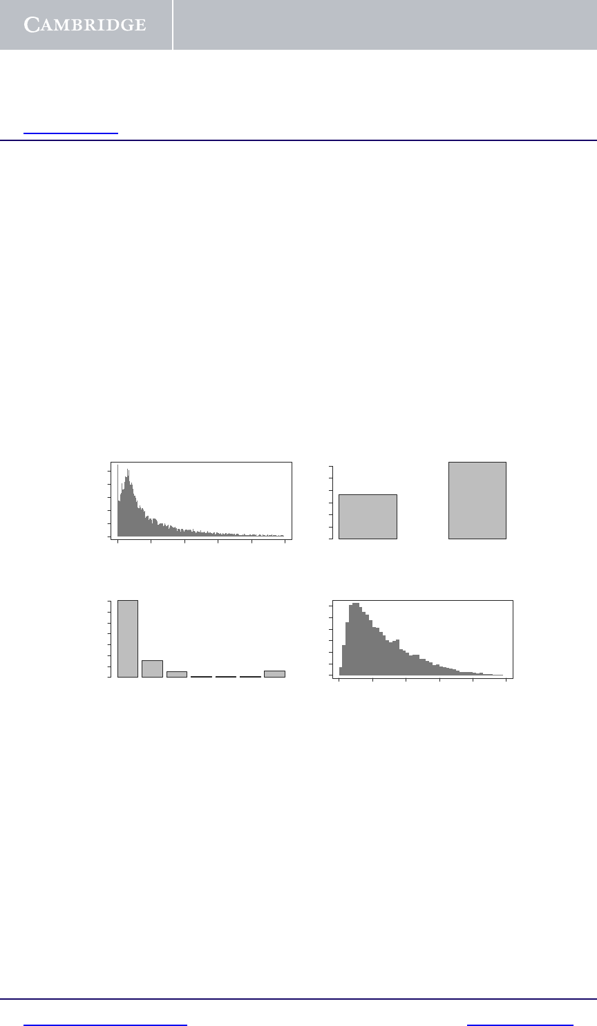
Figure 1.1 displays summaries of insurance data relating to n = 22 036 settled

personal injury insurance claims, described on page 14. These claims were

reported during the period from July 1989 through to the end of 1999. Claims

settled with zero payment are excluded.

The top left panel of Figure 1.1 displays a histogram of the dollar values of

the claims. The top right indicates the proportion of cases which are legally

represented. The bottom left indicates the proportion of various injury codes

as discussed in Section 1.2 below. The bottom right panel is a histogram of

settlement delay.

0 20406080100

0.00 0.02 0.04

Claim size ($1000s)

Frequency

No Yes

Legal representation

Frequency

0.0 0.2 0.4 0.6

1234569

Injury code

Frequency

0.0 0.2 0.4 0.6

0 20406080100

0.000 0.015 0.030

Settlement delay (months)

Frequency

Fig. 1.1. Graphical representation of personal injury insurance data

This data set is typical of those amenable to generalized linear modeling.

The aim of statistical modeling is usually to address questions of the following

nature:

• What is the relationship between settlement delay and the ﬁnalized claim

amount?

• Does legal representation have any effect on the dollar value of the claim?

• What is the impact on the dollar value of claims of the level of injury?

• Given a claim has already dragged on for some time and given the level of

injury and the fact that it is legally represented, what is the likely outcome

of the claim?

Cambridge University Press

978-0-521-87914-9 - Generalized Linear Models for Insurance Data

Piet de Jong and Gillian Z. Heller

Excerpt

More information

1.2 Types of variables 3

Answering such questions is subject to pitfalls and problems. This book aims

to point these out and outline useful tools that have been developed to aid in

providing answers.

Modeling is not an end in itself, rather the aim is to provide a framework for

answering questions of interest. Different models can, and often are, applied

to the same data depending on the question of interest. This stresses that

modeling is a pragmatic activity and there is no such thing as the “true” model.

Models connect variables, and the art of connecting variables requires an

understanding of the nature of the variables. Variables come in different forms:

discrete or continuous, nominal, ordinal, categorical, and so on. It is impor-

tant to distinguish between different types of variables, as the way that they

can reasonably enter a model depends on their type. Variables can, and often

are, transformed. Part of modeling requires one to consider the appropriate

transformations of variables.

1.2 Types of variables

Insurance data is usually organized in a two-way array according to cases and

variables. Cases can be policies, claims, individuals or accidents. Variables

can be level of injury, sex, dollar cost, whether there is legal representation,

and so on. Cases and variables are ﬂexible constructs: a variable in one study

forms the cases in another. Variables can be quantitative or qualitative. The

data displayed in Figure 1.1 provide an illustration of types of variables often

encountered in insurance:

• Claim amount is an example of what is commonly regarded as continuous

variable even though, practically speaking, it is conﬁned to an integer num-

ber of dollars. In this case the variable is skewed to the right. Not indicated

on the graphs are a small number of very large claims in excess of $100 000.

The largest claim is around $4.5 million dollars. Continuous variables are

also called “interval” variables to indicate they can take on values anywhere

in an interval of the real line.

• Legal representation is a categorical variable with two levels “no” or “yes.”

Variables taking on just two possible values are often coded “0” and “1” and

are also called binary, indicator or Bernoulli variables. Binary variables indi-

cate the presence or absence of an attribute, or occurrence or non-occurrence

of an event of interest such as a claim or fatality.

• Injury code is a categorical variable, also called qualitative. The variable

has seven values corresponding to different levels of physical injury: 1–6

and 9. Level 1 indicates the lowest level of injury, 2 the next level and so on

up to level 5 which is a catastrophic level of injury, while level 6 indicates

death. Level 9 corresponds to an “unknown” or unrecorded level of injury

Cambridge University Press

978-0-521-87914-9 - Generalized Linear Models for Insurance Data

Piet de Jong and Gillian Z. Heller

Excerpt

More information

4 Insurance data

and hence probably indicates no physical injury. The injury code variable

is thus partially ordered, although there are no levels 7 and 8 and level 9

does not conform to the ordering. Categorical variables generally take on

one of a discrete set of values which are nominal in nature and need not be

ordered. Other types of categorical variables are the type of crash: (non-

injury, injury, fatality); or claim type on household insurance: (burglary,

storm, other types). When there is a natural ordering in the categories, such

as (none, mild, moderate, severe), then the variable is called ordinal.

• The distribution of settlement delay is in the ﬁnal panel. This is another

example of a continuous variable, which in practical terms is conﬁned to an

integer number of months or days.

Data are often converted to counts or frequencies. Examples of count vari-

ables are: number of claims on a class of policy in a year, number of trafﬁc

accidents at an intersection in a week, number of children in a family, num-

ber of deaths in a population. Count variables are by their nature non-negative

integers. They are sometimes expressed as relative frequencies or proportions.

1.3 Data transformations

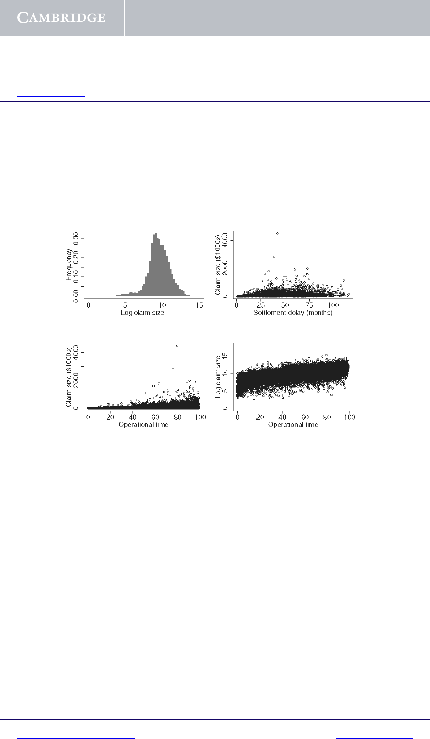
The panels in Figure 1.2 indicate alternative transformations and displays of

the personal injury data:

• Histogram of log claim size. The top left panel displays the histogram of

log claim size. Compared to the histogram in Figure 1.1 of actual claim size,

the logarithm is roughly symmetric and indeed almost normal. Historically

normal variables have been easier to model. However generalized linear

modeling has been at least partially developed to deal with data that are not

normally distributed.

• Claim size versus settlement delay. The top right panel does not reveal a

clear picture of the relationship between claim sizes and settlement delay. It

is expected that larger claims are associated with longer delays since larger

claims are often more contentious and difﬁcult to quantify. Whatever the

relationship, it is masked by noise.

• Claim size versus operational time. The bottom left panel displays claim

size versus the percentile rank of the settlement delay. The percentile rank

is the percentage of cases that settle faster than the given case. In insurance

data analysis the settlement delay percentile rank is called operational time.

Thus a claim with operational time 23% means that 23% of claims in the

group are settled faster than the given case. Note that both the mean and

variability of claim size appear to increase with operational time.

• Log claim size versus operational time. The bottom right panel of

Figure 1.2 plots log claim size versus operational time. The relationship

Cambridge University Press

978-0-521-87914-9 - Generalized Linear Models for Insurance Data

Piet de Jong and Gillian Z. Heller

Excerpt

More information

1.3 Data transformations 5

between claim and settlement delay is now apparent: log claim size

increases virtually linearly with operational time. The log transform has

“stabilized the variance.” Thus whereas in the bottom left panel the vari-

ance appears to increase with the mean and operational time, in the bottom

right panel the variance is approximately constant. Variance-stabilizing

transformations are further discussed in Section 4.9.

Fig. 1.2. Relationships between variables in personal injury insurance data set

The above examples illustrate ways of transforming a variable. The aim

of transformations is to make variables more easily amenable to statistical

analysis, and to tease out trends and effects. Commonly used transformations

include:

• Logarithms. The log transform applies to positive variables. Logs are usu-

ally “natural” logs (to the base e ≈ 2.718 and denoted ln y). If x = log

(y)

then x =ln(y)/ ln(b) and hence logs to different bases are multiples of each

other.

• Powers. The power transform of a variable y is y

. For mathematical conve-

nience this is rewritten as y

1−p/2

for p =2and interpreted as ln y if p =2.

This is known as the “Box–Cox” transform. The case p =0corresponds to

the identity transform, p =1the square root and p =4the reciprocal. The

transform is often used to stabilize the variance – see Section 4.9.

• Percentile ranks and quantiles. The percentile rank of a case is the per-

centage of cases having a value less than the given case. Thus the percentile

Cambridge University Press

978-0-521-87914-9 - Generalized Linear Models for Insurance Data

Piet de Jong and Gillian Z. Heller

Excerpt

More information

6 Insurance data

rank depends on the value of the given case as well as all other case values.

Percentile ranks are uniformly distributed from 0 to 100. The quantile of a

case is the value associated with a given percentile rank. For example the

75% quantile is the value of the case which has percentile rank 75. Quantiles

are often called percentiles.

• z-score. Given a variable y, the z-score of a case is the number of standard

deviations the value of y for the given case is away from the mean. Both the

mean and standard deviation are computed from all cases and hence, similar

to percentile ranks, z-scores depend on all cases.

• Logits. If y is between 0 and 1 then the logit of y is ln{y/(1 − y)}. Logits

lie between minus and plus inﬁnity, and are used to transform a variable in

the (0,1) interval to one over the whole real line.

1.4 Data exploration

Data exploration using appropriate graphical displays and tabulations is a ﬁrst

step in model building. It makes for an overall understanding of relationships

between variables, and it permits basic checks of the validity and appropri-

ateness of individual data values, the likely direction of relationships and the

likely size of model parameters. Data exploration is also used to examine:

(i) relationships between the response and potential explanatory variables;

and

(ii) relationships between potential explanatory variables.

The ﬁndings of (i) suggest variables or risk factors for the model, and their

likely effects on the response. The second point highlights which explanatory

variables are associated. This understanding is essential for sensible model

building. Strongly related explanatory variables are included in a model with

care.

Data displays differ fundamentally, depending on whether the variables are

continuous or categorical.

Continuous by continuous. The relationship between two continuous vari-

ables is explored with a scatterplot. A scatterplot is sometimes enhanced with

the inclusion of a third, categorical, variable using color and/or different sym-

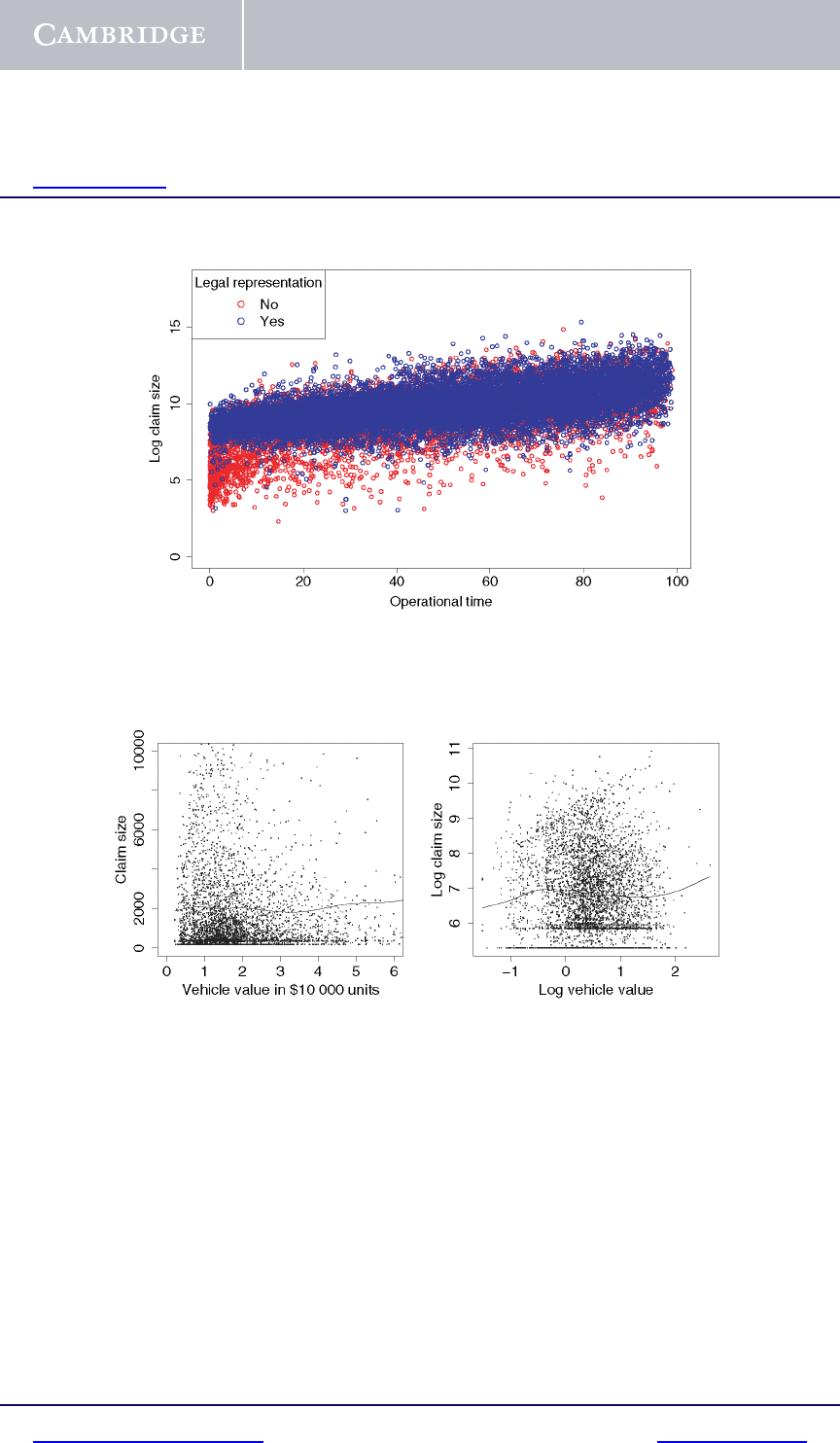
bols. This is illustrated in Figure 1.3, an enhanced version of the bottom right

panel of Figure 1.2. Here legal representation is indicated by the color of the

plotted points. It is clear that the lower claim sizes tend to be the faster-settled

claims without legal representation.

Scatterplot smoothers are useful for uncovering relationships between vari-

ables. These are similar in spirit to weighted moving average curves, albeit

more sophisticated. Splines are commonly used scatterplot smoothers. They

Cambridge University Press

978-0-521-87914-9 - Generalized Linear Models for Insurance Data

Piet de Jong and Gillian Z. Heller

Excerpt

More information

1.4 Data exploration 7

Fig. 1.3. Scatterplot for personal injury data

Fig. 1.4. Scatterplots with splines for vehicle insurance data

have a tuning parameter controlling the smoothness of the curve. The point of a

scatterplot smoother is to reveal the shape of a possibly nonlinear relationship.

The left panel of Figure 1.4 displays claim size plotted against vehicle value,

in the vehicle insurance data (described on page 15), with a spline curve super-

imposed. The right panel shows the scatterplot and spline with both variables

log-transformed. Both plots suggest that the relationship between claim size

and value is nonlinear. These displays do not indicate the strength or statistical

signiﬁcance of the relationships.

Cambridge University Press

978-0-521-87914-9 - Generalized Linear Models for Insurance Data

Piet de Jong and Gillian Z. Heller

Excerpt

More information

8 Insurance data

Table 1.1. Claim by driver’s age in vehicle insurance

Driver’s age category

Claim 1 2 3 4 5 6 Total

Yes 496 932 1 113 1 104 614 365 4 624

8.6% 7.2% 7.1% 6.8% 5.7% 5.6% 6.8%

No 5 246 11 943 14 654 15 085 10 122 6 182 63 232

91.4% 92.8% 92.9% 93.2% 94.3% 94.4% 93.2%

Total 5 742 12 875 15 767 16 189 10 736 6 547 67 856

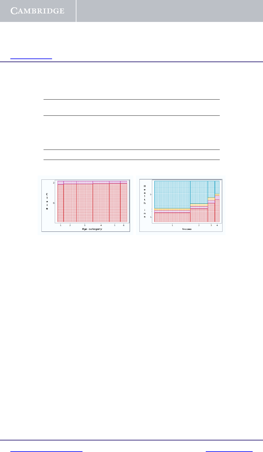
Vehicle insurance Private health insurance

Fig. 1.5. Mosaic plots

Categorical by categorical. A frequency table is the usual means of display

when examining the relationship between two categorical variables. Mosaic

plots are also useful. A simple example is given in Table 1.1, displaying

the occurrence of a claim in the vehicle insurance data tabulated by driver’s

age category. Column percentages are also shown. The overall percentage

of no claims is 93.2%. This percentage increases monotonically from 91.4%

for the youngest drivers to 94.4% for the oldest drivers. The effect is shown

graphically in the mosaic plot in the left panel of Figure 1.5. The areas of the

rectangles are proportional to the frequencies in the corresponding cells in the

table, and the column widths are proportional to the square roots of the column

frequencies. The relationship of claim occurrence with age is clearly visible.

A more substantial example is the relationship of type of private health insur-

ance with personal income, in the National Health Survey data, described on

page 17. The tabulation and mosaic plot are shown in Table 1.2 and the right

panel of Figure 1.5, respectively. “Hospital and ancillary” insurance is coded

as 1, and is indicated as the red cells on the mosaic plot. The trend for increas-

ing uptake of hospital and ancillary insurance with increasing income level is

apparent in the plot.

Cambridge University Press

978-0-521-87914-9 - Generalized Linear Models for Insurance Data

Piet de Jong and Gillian Z. Heller

Excerpt

More information

1.4 Data exploration 9

Table 1.2. Private health insurance type by income

Income

<$20 000 $20 000 $35 000 >$50 000 Total

Private health –$35 000 –$50 000

insurance type 123 4

Hospital and 1 2 178 1 534 875 693 5 280

ancillary 22.6% 32.3% 45.9% 54.8% 30.1%

Hospital only 2 611 269 132 120 1 132

6.3% 5.7% 6.9% 9.5% 6.5%

Ancillary only 3 397 306 119 46 868

4.1% 6.5% 6.2% 3.6% 4.9%

None 5 6 458 2 638 780 405 10 281

67.0% 55.6% 40.9% 32.0% 58.5%

Total 9 644 4 747 1 906 1 264 17 561

Mosaic plots are less effective when the number of categories is large. In

this case, judicious collapsing of categories is helpful. A reference for mosaic

plots and other visual displays is Friendly (2000).

Continuous by categorical. Boxplots are appropriate for examining a contin-

uous variable against a categorical variable. The boxplots in Figure 1.6 display

claim size against injury code and legal representation for the personal injury

data. The left plots are of raw claim sizes: the extreme skewness blurs the

relationships. The right plots are of log claim size: the log transform clariﬁes

the effect of injury code. The effect of legal representation is not as obvi-

ous, but there is a suggestion that larger claim sizes are associated with legal

representation.

Scatterplot smoothers are useful when a binary variable is plotted against a

continuous variable. Consider the occurrence of a claim versus vehicle value,

in the vehicle insurance data. In Figure 1.7, boxplots of vehicle value (top) and

log vehicle value (bottom), by claim occurrence, are on the left. On the right,

occurrence of a claim (1=yes, 0=no) is plotted on the vertical axis, against

vehicle value on the horizontal axis, with a scatterplot smoother. Raw vehi-

cle values are used in the top plot and log-transformed values in the bottom

plot. In the boxplots, the only discernible difference between vehicle values of

those policies which had a claim and those which did not, is that policies with

a claim have a smaller variation in vehicle value. The plots on the right are

more informative. They show that the probability of a claim is nonlinear, pos-

sibly quadratic, with the maximum probability occurring for vehicles valued

Cambridge University Press

978-0-521-87914-9 - Generalized Linear Models for Insurance Data

Piet de Jong and Gillian Z. Heller

Excerpt

More information

10 Insurance data

1234569

0e+00 2e+06 4e+06

Injury code

Claim size

1234569

246810 14

Injury code

Log claim size

No Yes

0e+00 2e+06 4e+06

Legal representation

Claim size

No Yes

246810 14

Legal representation

Log claim size

Fig. 1.6. Personal injury claim sizes by injury code and legal representation

around $40 000. This information is important for formulating a model for the

probability of a claim. This is discussed in Section 7.3.

1.5 Grouping and runoff triangles

Cases are often grouped according to one or more categorical variables. For

example, the personal injury insurance data may be grouped according to

injury code and whether or not there is legal representation. Table 1.3 displays

the average log claim sizes for such different groups.

An important form of grouping occurs when claims data is classiﬁed accord-

ing to year of accident and settlement delay. Years are often replaced by

months or quarters and the variable of interest is the total number of claims

or total amount for each combination. If i denotes the accident year and j the

settlement delay, then the matrix with (i, j) entry equal to the total number

or amount is called a runoff triangle. Table 1.4 displays the runoff triangle

corresponding to the personal injury data. Runoff triangles have a triangu-

lar structure since i + j>nis not yet observed, where n is current time.

Cambridge University Press

978-0-521-87914-9 - Generalized Linear Models for Insurance Data

Piet de Jong and Gillian Z. Heller

Excerpt

More information