NBER WORKING PAPER SERIES
UNDERSTANDING TRENDS IN CHINESE SKILL PREMIUMS, 2007-2018
Eric A. Hanushek
Yuan Wang
Lei Zhang
Working Paper 31367
http://www.nber.org/papers/w31367
NATIONAL BUREAU OF ECONOMIC RESEARCH
1050 Massachusetts Avenue
Cambridge, MA 02138
June 2023
Lei Zhang acknowledges financial support from the National Natural Science Foundation of
China (grant number 71973095). Gang Xie provides valuable research assistance. The views
expressed herein are those of the authors and do not necessarily reflect the views of the National
Bureau of Economic Research.
NBER working papers are circulated for discussion and comment purposes. They have not been
peer-reviewed or been subject to the review by the NBER Board of Directors that accompanies
official NBER publications.
© 2023 by Eric A. Hanushek, Yuan Wang, and Lei Zhang. All rights reserved. Short sections of
text, not to exceed two paragraphs, may be quoted without explicit permission provided that full
credit, including © notice, is given to the source.

Understanding Trends in Chinese Skill Premiums, 2007-2018
Eric A. Hanushek, Yuan Wang, and Lei Zhang
NBER Working Paper No. 31367
June 2023
JEL No. I26,J01,O10
ABSTRACT
The dramatic expansion of the education system and the transformation of the economy in China
provide an opportunity to investigate how the labor market rewards skills. Between 2007 and
2018, the overall return to cognitive skills is virtually constant at 10%, whereas the college
premium drops steeply by more than 20 percentage points. But, the regional differences in returns
are significant and highlight the importance of differential demand factors. College returns are
higher in more developed regions, but the declining trend is more pronounced. Returns to
cognitive skills increase in more developed regions and decrease in less developed regions.
Eric A. Hanushek
Hoover Institution
Stanford University
Stanford, CA 94305-6010
and NBER
Yuan Wang
National School of Development
Peking University
Beijing 100871
China
Lei Zhang
Antai College of Economics and Management
Shanghai Jiao Tong University
1954 Huashan Road
Shanghai, 200030
P. R. China

2
1. Introduction
The simplest economic model suggests that rapidly expanding educational attainment would
force relative wages of college workers down as they become more plentiful. But this ceteris
paribus statement must obviously be balanced by changes in demand. Understanding this
balance has been the subject of a variety of investigations in the United States, but the rather
smooth transitions of both education and technology have made reconciliation of these
influences difficult.
1
In contrast, the dramatic policy-driven changes in college availability and
in industrial structure in 21
st
century China offer a clearer view of how the supply and demand
factors play out in the labor market. Importantly, the full interplay can still be obscured by the
regional complexity of Chinese labor markets.
China experienced fast growth in both supply of and demand for skills over the past two
decades. The expansion of the higher education sector led to a sharp increase in college
graduates and hence the supply of skilled labor since the early 2000s. But, the economy also
experienced unprecedented growth, particularly among the high-skilled sectors. The overall
effect on the labor market returns to skills has yet to be fully analyzed, in part because of various
measurement issues.
In spite of the central importance of skills in such an investigation, measures of skills have
not been readily available. While school attainment is widely available in survey data, skill
measures are not. Using school attainment to gauge returns to skills can, however, be quite
misleading in economies experiencing large-scale school expansions. Expansion may be
accompanied by concurrent changes in the ability distribution of students across education
groups and in the resources allocated to different educational sectors. Therefore, a more direct
measure of skills is essential.
In this paper we construct a longitudinal database that allows us to estimate the time path of
returns to both cognitive skills and educational attainment in contemporary China. We use two
complementary datasets. The Chinese Household Income Project (CHIP) for 2007, 2013, and
2018 contain data on college entrance exam (Gaokao) scores for high-school and college
graduates. With these data, we estimate trends in the returns to a college degree and to cognitive
1
In the U.S., the early suggestion of falling relative wages of more educated workers (Freeman 1976) was
reconciled with the subsequent rise in college wages by notions of skill-biased technology change (Goldin and Katz
2007).
3
skills over a period of more than a decade during which the Chinese economy experienced
tremendous transformations, both in overall economic growth and in the structure of the
economy. The China Family Panel Studies (CFPS) for 2014 provides measures of basic cognitive
skills for individuals of all education levels that allow us to compare labor market returns to
skills in China with those in other countries.
On a nationwide basis, estimates of the return to cognitive skills controlling for college
degree remain quite stable at 10% for full-time workers with at least a high school degree from
2007 to 2018. But, over the same time period, the college premium relative to high school
graduation declines sharply by over 20 percentage points. For all three waves of the CHIP data,
the return to cognitive skills is weakly higher for female and younger workers, while the return
to a college degree is significantly higher for older workers. For all demographic groups, the
decline in the return to a college degree from 2007 to later years is salient.
Turning to regional data, however, brings the overall picture into sharper focus. Continued
increases in the supply of college-educated workers combined with the growth of the high-
skilled sector in the economy and hence increases in the demand for high-skilled workers can
explain the trend in the returns to a college degree and cognitive skills. The college premium
declines from 2007 to 2018 in both more and less developed regions, but only in the most
developed region (Beijing, Shanghai, Zhejiang, Guangdong) is the decline monotonic. This is
likely due to disproportionate increases in the supply of college-educated workers in this region
that offset the upward pressure on wages from the increases in the demand for more educated
workers following the growth of the high-skilled sector.
The trend in skill premium estimated on national data masks a strong regional disparity. The
return to cognitive skills increases from 2007 to later years in the more developed region, but
weakly decreases in the less developed region, consistent with the growth pattern of the high-
skilled sector and the corresponding demand for skills in the two regions.
We can also directly compare these returns to what is observed more broadly in developed
countries. The return to cognitive skills we estimate from the CHIP survey of 2013 and CFPS
survey of 2014 are both comparable to estimates from surveys data collected between 2011 and
2012 for a large number of OECD countries. In all three cases, the return to cognitive skills is
around 20 percent without controlling for schooling and drops to about 10 percent once
schooling is controlled for; this holds for both the sample of individuals of all education levels

4
(CFPS 2014 in the Chinese case) and that of individuals with at least a high school education.
2
This comparability across different data sets for a particular time period is reassuring, and the
comparability to estimates for OECD countries also sheds light on the progression of the market-
oriented reforms of the Chinese labor market in general.
2. Related Research
This paper is related and contributes primarily to two strands of the literature.
2.1 Trends in returns to schooling
The dynamic pattern of returns to skills has received much research attention as it reflects
important aspects of changes in the labor market. The bulk of the literature on this subject uses
years of schooling or education degrees as measures of skills (Katz and Murphy 1992; Zhang,
Zhao, Park, Song 2005; Goldin and Katz 2007 to name just a few). Yet years of schooling only
captures a part of the determinants of cognitive skills, and other sources of skill formation have
been left out including individual ability, family input, and school quality itself. Focusing only
on the quantity of schooling can be particularly troublesome in a dynamic context due to the
varying quality of education as well as the changing skill distribution within each educational
group.
Some research recognizes and attempts to deal with this measurement issue via
decomposition analyses. Decomposition analyses explain the variance in earnings with changes
in the distribution of observed skills, such as education and experience, and their prices, and with
the residual variance including changes in the distribution of unobserved skills and their prices.
Essentially, skills formed through channels other than schooling are included in the unobserved
component. The unobserved component of skills is found to be crucial in explaining earnings
inequality, both within education groups (Juhn, Murphy, and Pierce 1993; Meng, Shen, Xue
2013) and between education groups (Carneiro and Lee 2011). For instance, Carneiro and Lee
(2011) find that college premium in the United States over the period of 1960-2000 would be 6
percentage points higher (compared to an increase of 40 percentage points) if decreases in the
quality of college graduates are taken into account.
The consensus of these studies is that we need variations in both the supply and demand
sides to explain the observed trend in returns to observed skills (schooling) and unobserved
2
Guido Schwerdt kindly provided us with estimates for the sample of individuals with at least a high school education
for OECD countries using the PIAAC data.
5
skills. A surge in the supply may put a direct downward pressure on the return to a college
degree, but the gradual rise in demand help maintain or even increase the price of unobserved
skills. Therefore, the college premium and the return to cognitive skills may not move in parallel,
and comparing their movements will provide a better understanding of changes in the labor
market.
Nevertheless, investigating returns to unobserved skills still poses a challenge in these
studies since it is difficult to disentangle the price and the distribution of unobserved skills in the
residual component. Our strategy is to isolate some components from the unobserved skills with
a direct measure of cognitive skills. We use repeated cross-sectional data that contain information
on both education attainment and cognitive skill measures for high school and college graduates.
This provides a very rare opportunity to study the trend in returns to skills.
2.2 Returns to cognitive skills
Studies on returns to cognitive skills usually use cross-sectional data for a particular point of
time and focus on OECD countries due to data availability (Hanushek, Schwerdt, Wiederhold,
and Woessmann 2015; Lindqvist and Ronie 2011). Hanushek and Woessmann (2008) review
early studies for a few developing countries, but evidence on developing economies continues to
be scarce. A few recent studies estimate returns to cognitive skills in China, but they either use
coarse measures of skills or data with limited population coverage. Knight, Deng, and Li (2017)
draw on the urban sample of CHIP 2002 and 2007 and use self-reported quintiles of high school
performance in both waves and Gaokao score (unadjusted) in 2007 to measure quality of
education, essentially, actual skills of individuals. They find positive and significant returns to
both measures. Glewwe, Huang, and Park (2017) use longitudinal survey data of rural children in
Gansu Province, one of China’s least developed provinces, and find no significant explanatory
power of childhood cognitive skills for wages at the very early stage of the labor market once
years of schooling is controlled for. Using a new wave of data from the same survey, however,
Glewwe, Song, and Zou (2022) find a positive return to cognitive skills for adults in their late
20s even after conditioning on years of schooling. Employer learning and frictions in job search
are proposed as possible explanations for the discrepancy between these two studies, but the
limited sample size does not allow for a formal test of these hypotheses.
This paper employs recent data for representative samples of the Chinese population
working in the waged sector, which allows us to estimate the return to cognitive skills in China at

6
large. The sample size is sufficiently large to allow us to explore the heterogeneity in the return
from various perspectives. Additionally, our data cover the time period comparable to studies of
OECD countries (Hanushek et al. 2015, 2017), which may serve as a benchmark for our results.
Juxtaposing these results provides new insights regarding the development of China’s labor
market in comparison to that of the more developed countries.
While there is a growing number of studies on the return to cognitive skills, research on
trends in this returns is still rare. Murnane, Willett, and Levy (1995) study returns to cognitive
skills for two cohorts of U.S. high school graduates by age 24 and find greater importance of
skills in the 1980s than the 1970s, where skills are measured by test scores on elementary
mathematical concepts conducted in the high school senior year. Using NLSY 1979 and 1997
data, Castex and Dechter (2014) find that returns to cognitive skills measured by the AFQT score
decline by 30%-50% between 1980s and 2000s for the 18-28 year olds, which they attribute to
differences in the growth rate of technology between the two periods. Both papers focus on
workers in the early stage of their careers in the US. Edin, Fredriksson, Nybom, and Ӧckert
(2022) document that the return to non-cognitive skills roughly doubles while the return to
cognitive skills remains relatively stable between 1992 and 2013 for Swedish male workers aged
38-42. This paper adds to the literature by documenting trends in the skill premium in one of the
largest developing economies over a ten-year period and for workers in a wide range of career
stages.
3. Changing Chinese Labor market
The labor market in China has undergone substantial changes entering the new millennium. In
this section, we describe major changes in the supply and demand sides that are likely to have
lasting impacts on the returns to a college degree and to cognitive skills.
3
The most important development on the supply side is the higher education expansion
started in 1999. Nationwide, college admissions increased by over 40 percent in both 1999 and
2000, and continued to grow at more than 10 percent per year through 2005.
4
Because the vast
majority of college students finish their study on time, the number of college graduates grows
dramatically, from one million in 2000 to 8.1 million in 2018 (Figure 1). The growth rate of
3
Major reforms that transformed the labor market from one of centrally-planned to one of market-oriented occurred
in the 1990s, and the institutional changes virtually completed by the early 2000s. See, for example, Meng et al. (2013)
and Ge et al. (2021).
4
See Che and Zhang (2018) for a more detailed description of the reform of the higher education system.

7
college completion is the highest in 2003 (40.2 percent), when the first cohort of students
admitted to college under the expansion regime graduated, and it stabilized at around 3 percent in
recent years. Overall, the supply of college-educated and skilled workers has grown continuously
in the past decade.
The most prominent changes on the demand side are the slowdown of the economic growth
and the transition of the economic structure, in particular, post of the 2008 global economic
recession. As can be seen from Figure 2, while per capita GDP has grown steadily and more than
quadrupled over the past two decades,
5
the annual growth rate plunged in 2008 from an all-time
high of close to 14 percent in large part due to the recession. It recovered moderately by 2010
thanks to the quick implementation of the Four-Trillion Yuan stimulus package, but the annual
growth rate started a downward trend afterwards and stayed at slightly above 6 percent in recent
years.
The recession and the ensuing slowdown of the economic growth prompted the central
government to intensify the effort to push the transition of the economic growth from relying on
heavy usage of natural resources and raw labor to being driven by innovation and adoption of
frontier, more skill-biased technologies. In 2008 and subsequent years the State Council issued a
series of guiding opinions regarding the upgrade of the industrial structure and measures to
promote the transition such as project approval, bank loans, and tax subsidies.
6
Particularly
emphasized is the upgrade of the producer service sectors including logistics, information
technology, financing and leasing, research and development, business consulting, and so forth.
The shift in the economic structure in the 2010s is salient. While the share of national GDP
accounted for by the industrial sector was around 46 percent in the 2000s, it declined steeply
after 2011. Mirroring these changes, while the size of the service sector lagged behind the
industrial sector in the entire 2000s, it started to grow faster after 2008 and accelerated further in
2012. By 2019, the service sector accounted for a dominant 54% of the national GDP, compared
to 39% by the industrial sector (Figure 3).
5
Per capita GDP measured in constant 2000 Yuan is 7,912 Yuan and 35,006 Yuan in 2000 and 2018 respectively.
6
Examples of the State Council policy documents include Opinions of the General Office of the State Council on
Implementation of Several Policies and Measures for Accelerating the Development of the Service Industry (2008),
Guiding Opinions of the General Office of the State Council on Financial Support to Economic Structure Adjustment,
Transformation and Upgrading (2013), Guiding Opinions of the State Council on Accelerating the Development of
Producer Services and Promoting the Adjustment and Upgrading of Industrial Structure (2014), Made in China 2025
(2015). All documents can be accessed at the State Council website.

8
The expansion of the service sector in general tends to raise the demand for skilled labor, but
clearly industries within the service sector vary substantially in the high-skilled share, ranging
from 8.2 percent to 69.8 percent. The service sector includes both industries intensive in the
employment of high-skilled workers such as finance and information and communication
technology (ICT) and industries employing primarily low-skilled labors such as wholesale and
retail and food services. To draw a more precise picture of the industrial structure and relative
demand for skilled workers, we directly classify industries by the share of high-skilled
employees, i.e., those with at least a 3-year college degree. Table 1 reports the share of high-
skilled workers for each industry in 2017.
7
We define high-skilled (HS) sector as industries whose nationwide share of high-skilled
workers is above 30% in 2017, and low-skilled (LS) sector as industries employing less than
30% of high-skilled workers in 2017. Figure 4 depicts the per capita value-added and share in
GDP of the HS and LS sectors.
8
Between 2000 and 2018, the per capita value-added of the HS
sector experience a five-fold increase, from 1,808 Yuan to 9,392 Yuan measured in constant 2000
Yuan, whereas that of the LS sector grows much slower, from 6,050 Yuan to 20,670 Yuan. With
the exception between 2009 and 2011, the growth rate of per capita value-added of the HS sector
is quite stable at around 8 percent annually, but that of the LS sector decelerates to 5.8 percent
after 2013, from 8.8 percent previously. Similar to Figure 3, HS sector’s value-added share in
GDP increases substantially from 23% in 2000 to 37% in 2018, with a corresponding decline of
the LS sector.
As a result of both the increase in college graduates and the structural changes of the
Chinese economy, the share of employed workers with at least a 3-year college education rises
from 5.6 percent in 2001 to 19.1 percent in 2018 (Figure 5). Note that this share began to
increase rapidly only after 2009, perhaps because although the growth rate of college graduates
is high at the start of the expansion, the stock of college-educated workers in the labor force is
still too small to substantially change the composition of the labor force.
9
7
Data come from the China Population and Employment Statistics Yearbook.
8
Since the National Bureau of Statistics of China does not separately report the value-added of Production and Supply
of Electricity, Heat, Gas, and Water industry (in the industrial sector), it is included in the low-skilled sector, even
though it has 40.1% of high-skilled employees. For the same reason, Management of Water Conservancy, Environment
and Public Infrastructure industry (24.9% of high-skilled employees) and Residential and Household Services industry
(12.2% of high-skilled employees, both in the service sector) are included in the high-skilled sector.
9
China’s mandatory retirement age of formal sector employees varies with occupation; in general, occupations that
tend to be filled by less-educated workers (for example, physically strenuous occupations) have an earlier retirement

9
China is a large country of tremendous regional heterogeneity, manifested also in the
development of the HS sector. Figure 6 illustrates the evolution of the value-added of the HS
sector by province from 2007 to 2017 (see Appendix Table A1 for the exact values).
10
Not only
has the HS sector expanded over time nationwide, but the regional disparity has also grown
considerably. Eastern regions have already shown advantages in the development of the HS
sector in 2007, and the advantage has enlarged over time. Meanwhile, some provinces in the
western and central parts of China, including Sichuan, Hunan, Hubei, Henan, and Hebei, also
catch up rapidly. Nevertheless, the majority of the western and central regions experiences a
much slower transition to a skill-intensive economy. For example, the value-added of the HS
sector in Jiangxi Province (in the central region) increases from 85 billion Yuan in 2007 to 271
billion Yuan in 2017; meanwhile that of its neighboring Zhejiang Province (on the coast) has
grown from 363 billion Yuan to 1,008 billion Yuan. Holding the relative labor supply equal,
skilled workers in regions with a larger HS sector will likely enjoy a higher skill premium due to
a greater relative demand for skills. At the same time, regions with a higher price for skills will
likely attract more skilled workers, attenuating to some extent the skill premium. Which force
dominates is intrinsically an empirical question.
4. Data and Empirical Framework
We employ two complementary data sets for the empirical analysis: The Chinese Household
Income Project (CHIP) data and the China Family Panel Studies (CFPS) data. Both data are
high-quality, nationally representative and have been widely used by researchers to study
China’s social and economic issues.
11
They both contain rich information on individual
characteristics including age, gender, educational attainment, and family background, and current
labor market activities such as annual salary, working hours, industry, and occupation.
One unique feature of these two data sets that is particularly valuable for our study is that
they both contain cognitive skill measures for individuals. The CHIP data contain the college
entrance exam (Gaokao) scores for high school and college graduates since the 2007 wave; they
age. Appendix Figure A1 shows that the share of older workers (aged 45-60) with a college degree or above have
increased steadily since 2007, partially contributing to the pattern observed in Figure 5.
10
We choose three time points (2007, 2013, and 2017) to match the years of data for the empirical analysis. Using
2018 would be preferable, but data on value-added of HS sector in 2018 is not yet available.
11
Examples that use CHIP data include Wei and Zhang (2011), Nakamura, Steinsson, and Liu (2016), and Sun and
Zhang (2020); examples that use CFPS data are Bai and Wu (2020), Ong, Yang, and Zhang (2020), and Fan, Yi, and
Zhang (2021). Zhou (2014) uses both data sets.

10
are repeated cross-sections, enabling us to use the 2007, 2013, and 2018 waves to estimate the
trends of returns to a college degree and cognitive skills. The CFPS data are longitudinal,
collected initially in 2010 and biennially thereafter; it contains scores on basic literacy tests
(math and word) administered to all individuals aged 10 and above regardless of their education
level. We use the adult sample of the 2014 wave, which allows us to compare estimates with both
those from the 2013 CHIP data and those of recent international studies (Hanushek et al. 2015).
4.1 Cognitive skill measures in CHIP 2007, 2013, 2018 and CFPS 2014
The 2007, 2013 and 2018 waves of the CHIP survey elicit self-reported information on
individuals’ college entrance exam (Gaokao) scores. Gaokao is one of the most important
educational institutions in China. It is administered nationwide in the early summer each year to
high school graduates in the academic track, whose eligibility for college admissions is virtually
entirely determined by their Gaokao score. Students with Gaokao scores above a threshold are
eligible for 4-year universities, and those with scores above a lower threshold may be admitted to
a 3-year college. The raw Gaokao scores differ by year-province-subject track (sciences v.
humanities) and are not directly comparable.
12
Following Démurger, Hanushek, and Zhang
(2019), we normalize them in two steps. First, because the maximum possible score varies with
the specific test, we divide individual scores by the maximum possible score of each specific
test.
13
Assuming that the population distributions of Gaokao scores are comparable over time
and across provinces and subjects, we then convert this percentage score into a z-score with a
mean of zero and a standard deviation of one. The normalization is performed for the entire
sample of individuals reporting the Gaokao score regardless of their current work status. While
the assumption of a common distribution across provinces is strong and untested, it is unlikely to
affect our empirical results. All of our estimates below include province fixed effects so that the
comparisons are restricted to within-province comparisons.
14
In the regression analyses we use
12
The college entrance exams are based on a national education curriculum. With the approval of the Ministry of
Education, a province may choose to write its own tests, which may have different maximum possible scores from the
national tests and from tests of other provinces.
13
For example, the maximum possible score was 640 for the humanity-oriented test and 710 for the science-oriented
test in 1989 for all provinces. It changed to 750 in 1994 for both tests nationwide. Starting in 1999, several provinces,
such as Fujian, Guangdong, Shaanxi, and Hainan adopted different tests with a maximum possible score of 900 for
both tests. There are larger cross-province variations in more recent years as more provinces started to experiment
different test regimes. The maximum possible score is obtained from various Gaokao-related websites such as
http://edu.sina.com.cn/Gaokao/. It is missing for a small number of years and provinces, and individual observations
are therefore dropped for these years and provinces.
14
For a small number of individuals, the current province of residence may not be the same province where they

11
the Gaokao z-score as a measure of individual cognitive skills; we however do not presume that
they fully capture productivity differences among individuals.
One important advantage of using Gaokao score as the skill measure is that it is assessed
before individuals enter the labor market. Thus it does not suffer from the reverse causality issue
that may confound estimates using skill measures concurrent with wages. Meanwhile, Gaokao
score has special features that may limit the comparability of our analyses to existing studies.
First, Gaokao score is only available for college graduates and high school graduates in the
academic track, limiting the population under study. Second, Gaokao is a high-stake test, on
which students may exert more efforts to perform well; hence it may better reflect student
capability and be more closely related to future labor market outcomes. Third, Gaokao is highly
academic and abstract, and the extent to which this type of skill is valued in the labor market
may be different from basic and more practical skills. We therefore employ the CFPS data for
complementary analyses.
The 2014 CFPS survey administered math and word tests to all individuals aged 10 or above
to assess their cognitive ability. Test questions are based on the national curriculum of the basic
education (Grades 1-12). Math problems include addition, subtraction, multiplication, division,
logarithms, trigonometric functions, sequence, permutation and combination, etc. In the word
test, individuals are asked to read aloud Chinese characteristics presented to them. For both tests,
questions are ordered from the easiest to the hardest, and the test score is assigned as the question
number of the most difficult problem an individual has correctly answered. Since curriculums
have changed over time, and what individuals learned in school tend to diminish with age, we
normalize test scores by age to obtain z-scores with a mean of zero and a standard deviation of
one within each year of age. We use the math score for the main analyses.
15
We regard results from the 2014 CFPS data as a bridge between our analyses using the CHIP
data and recent international studies for two reasons. First, estimates from the entire CFPS
sample and the subsample of high school and college graduates can be compared with those from
the CHIP 2013 data. This comparison allows us to infer whether returns to cognitive skills in
China are robust to the use of different skill measures and estimation samples. Second, the math
went to high school and took the Gaokao test. In regressions controlling additionally for Gaokao province fixed
effects and Gaokao province by Gaokao year fixed effects, estimation results are virtually unchanged.
15
Estimation results using the word score and the average of math and word scores are available upon request.

12
test in CFPS evaluates basic skills, plausibly comparable to the assessment in the Programme for
the International Assessment of Adult Competencies (PIAAC) data developed by OECD and
collected between August 2011 and March 2012. Thus, we are able to compare returns to skills in
China with those in OECD countries for the same time period estimated in Hanushek et al.
(2015), allowing us to gain an understanding of the progression of China’s labor market against a
broader backdrop.
4.2 Sample creation and summary statistics
For the empirical analysis, we focus on the subsample of full-time employees, with full-time
defined as working at least 30 hours a week.
16
We construct hourly wage by dividing the annual
salary (inclusive of monetary bonuses and subsidies) by hours worked in a year.
17
All monetary
values are adjusted by national CPI to constant 2007 Yuan. To mitigate the influence of outliers,
we exclude individuals with hourly earnings less than 1 Yuan or greater than 100 Yuan in real
terms. We also exclude observations missing information on cognitive test scores, gender, age,
and province of residence. We do not impose restrictions on age, but the vast majority of the
sample is between 16 and 60, and restricting the sample to this age group does not change the
results.
Panel A of Table 2 reports the summary statistics of individual characteristics for the
analysis sample. The average age of the three waves of the CHIP sample is between 33 and 35,
slightly younger but comparable to the CFPS sample of individuals with a high school education
or above. In all four samples, individuals are younger than the full CFPS sample including those
with less than a high school education (column 5) due to continued improvement in the
educational attainment of the population such that younger people are on average more educated.
The gender composition of samples from the two data sets are also comparable, with males
accounting for about 60%, likely due to the more flexible labor market participation of females.
For both the Gaokao z-score in CHIP and the math z-score in CFPS, college graduates have
significantly higher scores than high school graduates. The high average math z-score in CFPS
(column 4) relative to the CHIP samples is because we normalize it by age regardless of the
16
Studies of returns to education in China generally use a sample of urban residents with local urban Hukou,
excluding a large number of migrants and residents without an urban Hukou in waged jobs. Our sample includes all
full-time employees regardless of their Hukou or migration status, consistent with the recent development of the
Chinese labor market.
17
Very few individuals report receiving in-kind subsidies, and the reported values are small. Results are virtually
the same when we also include the monetary value of in-kind subsidies

13
education attainment of each age group, and those with less than a high school education account
for 57% of the analysis sample in 2014 and have on average much lower math z-score (-0.13, see
column 5),
18
whereas Gaokao scores are normalized for high school and college graduates.
From 2007 to 2013, the Gaokao z-score declines drastically for both high school and college
graduates, from -0.46 to -0.63 and from 0.3 to 0.2 respectively, reflecting the fact that with the
rapid expansion of college admissions, the ability distributions of both groups have shifted
leftward. Between 2013 and 2018, the decline continues but to a much lesser extent. The average
real hourly wage overall almost doubled between 2007 and 2018, and it grew substantially for
both high school and college graduates.
In the CHIP data, as expected, college graduates account for an increasingly larger share of
the sample, but at 70%, 79%, and 83% in 2007, 2013, and 2018, these are much larger than that
in the CFPS high school and above sample (52%), which helps explain the higher average hourly
wage in CHIP 2013 (16.33 Yuan) relative to that in CFPS 2014 (12.83 Yuan). This discrepancy in
the distribution of education attainment between the two data sets is because a large number of
individuals, in particular high school graduates, are missing the Gaokao z-score in CHIP while
most have math test score in CFPS.
19
Indeed, college graduates account for 50% of the high
school and above sample in CHIP 2013 (Panel B of Table 2) if we do not restrict the sample to
those not missing Gaokao scores, comparable to the CFPS 2014 sample.
To inspect whether the sample size reduction due to missing Gaokao z-scores pose a severe
problem of sample selection, we provide in Panel B of Table 2 summary statistics of individual
characteristics for the otherwise identical sample as our analysis sample but without requiring
non-missing Gaokao z-scores. Individuals are slightly older due to the now larger proportion of
high school graduates, and the gender distribution is similar. Most importantly, while the average
hourly wage of the unrestricted sample is lower in each year due to the inclusion of more high
18
57% of the full-time employed adults in the CFPS 2014 data have less than a high school education. It is 77% for
the entire adult population.
19
Missing Gaokao z-score is due to either missing individual Gaokao score or missing information on the
maximum possible Goakao score, which is collected from the internet and is needed for the normalization and
comparison of scores. In the sample of full-time employed individuals with hourly wage between 1 and 100 Yuan,
47% and 86% of college and high school graduates miss Gaokao z-score respectively, of which 12 and 5 percentage
points are due to missing information on the maximum possible Gaokao score. Slightly fewer individuals miss
Gaokao z-scores over time. Proportionately more high school graduates miss the Gaokao score because they may
not have taken Gaokao in the first place, including the vast majority in the vocational-technical track and some in
the academic track, as well as not reporting it to the interviewer. Since dropouts are included in the high school
category in Chinese surveys, this group also contributes to the missing values.
14
school graduates, it is similar to that of the analysis sample for each education level in each year.
Kernel densities of the hourly wage of the two samples are almost identical for each education
level in each year (Appendix Figure A2). T-tests of equality of the mean fail to reject the null
hypothesis for all but the college graduates in 2018 at 1% significance level, and Kolmogorov-
Smirnov equality-of-distribution tests fail to reject the null hypothesis for all but the high school
graduates in 2007 at 1% significance level. In sum, the similarities of major individual
characteristics suggest that the analysis sample is a random subsample of the full-time
employees.
As supplementary tests, we compare the Gaokao z-score of the analysis sample with that of
the sample of all adults with non-missing Gaokao z-score regardless of their working status.
Kernel densities of the Gaokao z-score of the two samples are again almost identical for each
education level in each year (Appendix Figure A3); t-tests of equality of the mean fail to reject
the null hypothesis for all but the high school students in 2018 (at 5% significance level), while
Kolmogorov-Smirnov equality-of-distribution tests fail to reject the null hypothesis for all year-
degree combinations. Thus, the analysis sample is likely a random subsample of all those
reporting a Gaokao score.
While none of the above tests can definitively rule out the bias in our analysis sample due
to missing Gaokao z-scores, the similarities in both the wage distribution and the Gaokao z-score
distribution between the analysis sample and unrestricted samples help alleviate this concern. We
provide robustness regression analyses in the next section to further address this issue.
4.3 Empirical model
Our goal is to estimate how returns to a college degree and to cognitive skills evolve over time
using repeated cross-sectional data. We start with estimating a generalized Mincer equation for
each cross section:
2
0 12 3
ln
i i i i ii
HP Ewage EP X
βγ β β β ε
=++ + + +
(1)
In Equation (1), ln
is the natural logarithm of hourly wage of individual ,
is
potential experience (=age-years of schooling-6),
is a vector of control variables including
gender and province of residence, and
is the error term. The coefficient of interest is , the
earnings gradient associated with measures of human capital
, which is measured by cognitive
skills (Gaokao z-score) or the attainment of a college degree or both. When both cognitive skills
measure and the college degree indicator are included in the regression, the estimate on college

15
degree reflects returns to factors that are not captured by the measure of cognitive skills such as
broad subject-matter knowledge as well as noncognitive skills and the signaling value generated
by a college degree.
20
Equation (1) can be further written as:
2
01 2 1 2 3
ln ,
i i i i i ii
Cog Col PE PE Xwage
βγ γ β β β ε
=+ + + + ++
(2)
where
denote cognitive skills and
is an indicator for graduating from at least a 3-
year college. To more conveniently compare returns over time, we estimate Equation (2) with all
three waves of CHIP data and add interaction terms of the cognitive skills measure and college
degree indicator with year dummies for 2013 and 2018, taking the returns in 2007 as the
benchmark. In this specification, year dummies are also separately included.
Our data allow us to address several common concerns in identifying the impacts of
cognitive skills on earnings. First is the reverse causality. When cognitive skills are measured
concurrently with wage, estimates on cognitive skills may be upwardly biased. For example,
individuals may have higher skill levels because they have better jobs on which they can
constantly practice and hence sustain their skills. In the CHIP data, Gaokao score is measured at
the end of high school, before individuals start their career; therefore, the estimate on Gaokao z-
score is unlikely confounded by this bias. Second is the omitted variable bias. For example,
family background may affect both skill formation and employment opportunities and wages.
With both CHIP and CFPS data, we use mother’s education to partially control for the influence
of family background. Third is the measurement error in cognitive skills, which may lead to
biased (generally attenuated) estimate. Since the CFPS data include measures of cognitive skills
in both math and word, we use the word test score as an instrument for the math test to deal with
the measurement error problem.
21
In summary, while we are not able to use exogenous variations in measures of cognitive
skills to achieve a convincing causal identification, the variety of approaches we take to deal
with specific issues strengthen the interpretation of our estimates. The consistency of our
estimated impacts of cognitive skills across different models and different data and comparability
with that from international studies provide support for the substantial role played by cognitive
20
A college degree as a more easily observable individual characteristic has generally a strong signaling value at the
career entry when employers can only partially observe individual productivity (Altonji and Pierret 2001). It
continues to have substantial impacts on wage determination later in one’s career due to asymmetric learning
between the current employer and the labor market in general (DeVaro and Waldman 2012; Waldman 2016).
21
Hanushek et al. (2023) indicate that the different dimensions of cognitive skills may influence occupational
choices.
16
skills in individual labor market outcomes in China.
5. Returns to Skills for China
In this section, we first report estimated returns to a college degree and to cognitive skills for
China over the decade of 2007-2018 from the CHIP data. We then compare these estimates with
those from complementary analyses using the CFPS 2014 data followed by heterogeneity
estimates by gender and age. In the next section, we show the heterogeneity of returns by region,
linking these returns to the differential demands for and supply of skills.
5.1 Estimates of returns to skills 2007-2018
We first estimate the wage equation for each cross section of the CHIP data. All models control
for gender, potential experience and its square, and province fixed effects. Robust standard errors
are reported in brackets.
We start with a traditional Mincer equation of log hourly wage using college degree as the
human capital measure. Results are reported in columns 1, 4, and 7 of Table 3 for 2007, 2013,
and 2018 respectively. The college wage premium decreases from 68% in 2007 to 41% in 2013,
a sharp decline of 40 per cent; it recovers somewhat to 49% by 2018, but the difference between
2013 and 2018 is not statistically significant. This suggests the dominant influence of the surge
in the supply of college-educated workers over the entire decade, while the restructuring of the
economy may to some extent raise the demand for skilled workers and prevent a continued
decline in the college premium in the second half of this period.
In columns 2, 5, and 8, we estimate the wage equation using Gaokao score as the measure of
human capital for each of the three years. Ceteris paribus, a one standard deviation increase in
Gaokao score raises hourly wage by 21% in 2007, and the return to skills drops by more than a
third to 14% in 2007 and comes back slightly to 16% in 2018. This similarity in the pattern
between the two sets of estimates is not surprising, as Gaokao score is closely related to college
attendance, and the estimate on Gaokao score partially captures the premium to a college degree.
This conjecture is born out by estimation results in columns 3, 6, and 9, where we include the
indicator for a college degree and Gaokao score simultaneously. The estimated college wage
premium exhibits virtually the same trend as those in columns 1, 4, and 7, whereas the estimated
gradient of cognitive skills displays much muted changes over time and stays at around 10%.
Estimates on both the college degree indicator and Gaokao score are smaller than when they are
included individually due to the close correlation between the two measures, yet all estimates are

17
significant at the 1% level, suggesting that they each have an independent impact on wages.
Since Gaokao score, albeit imperfect, may proxy some more direct measures of cognitive skills
that employers may observe,
22
when it is controlled for, the estimate on the college degree
indicator is likely to reflect the impact of college education through other channels such as non-
cognitive skills, networks, or its signaling values, which appear to be more affected by relative
increases in the supply of college graduates.
As discussed in the previous section, our analysis sample is a relatively small subsample of
all full-time employees in the CHIP data due to missing Gaokao z-scores. An alternative is to
estimate the models with the full CHIP samples based on imputed Gaokao scores using either
year means of all observations or means by education-year groups. These expanded models
(shown in Appendix Table A2) provide very similar estimates of the human capital terms,
indicating that sample selection is not important for our results.
23
Table 4 reports estimation results using three-year pooled data, and the models include
interactions of college indicator and Gaokao score with dummies for 2013 and 2018. Column 1
uses the same model as column 3 of Table 3 with added interactions and year dummies. The
estimation results confirm findings in Table 3. The return to a college degree diminishes from
2007 to 2013 and ticks up slightly in 2018, but the difference between the two years is only
marginally significant, whereas the return to cognitive skills is stable at around 10%. Column 2
controls for mother’s education to address the concern that family background may affect both
Gaokao score and employment opportunities, and returns to human capital measures may be
22
College graduates do not list their Gaokao score in the resume when applying for a job, but Gaokao score is
highly correlated with items that are usually listed. Based on surveys of a nationally representative sample of college
graduates in 2003 conducted by researchers of Peking University (the data are courtesy of Professor Changjun Yue
of Peking University), we find that Gaokao score is positively associated with a variety of traits valued by
employers. Students with a higher Gaokao score are significantly more likely to pass a higher level of national
English test (Level 6 vs. Level 4), have taken a second major and have received merit-based college scholarships
based on performance during college, and are more likely to have had any internship experience. Gaokao score
alone explains about 16% of the variation in the probability of passing the higher level English test, and the
combination of these correlates jointly explains 64% of the variation in the standardized Gaokao score.
23
To alleviate concerns that trends of returns estimated in Table 3 are due to sample selection, we perform
additional regression analyses and present results in Appendix Table A2. We first estimate the traditional Mincer
equation of log hourly wage on college degree. As can be seen from columns 1, 4, and 7 of Appendix Table A2, the
point estimates for all three years are smaller, but their magnitude is close to those in Table 3. More importantly, the
trend in the return to a college degree is identical to that reported in Table 3. In the remaining columns, we
extrapolate the missing Gaokao z-scores by the mean score of either the entire sample in each year (columns 2, 5,
and 8) or the mean score of the respective education level in each year (columns 3, 6, and 9) and include an indicator
for individuals with missing scores. In both cases, the returns to a college degree are again smaller, of comparable
magnitude, and show the same trend as those in Table 3; furthermore, the return to Gaokao score is within a narrow
range around 10% for all years.

18
confounded if this factor is neglected. Yet, the estimated returns to a college degree and to
cognitive skills are virtually unchanged. In columns 3 and 4, we control respectively for a full set
of industry and occupation indicators to address the concern that estimates of returns reflect
primarily selection of individuals of higher human capital levels into more lucrative jobs.
24
Returns to a college degree and cognitive skills reduce slightly once industry dummies are
controlled for (column 3), and the reduction is much larger with occupation controls (column 4);
however, within-industry and within-occupation returns continue to be economically significant.
Thus sorting of individuals into jobs based on skills is not driving our results. Finally, in column
5 we control for mother’s education along with occupation and industry dummies, and the results
are qualitatively similar to that in column 1 and of comparable magnitude. For the remainder of
the analysis, we adopt primarily the model in column 1 of Table 4.
In all columns, estimates on the year dummies are positive and significant both statistically
and economically. On average hourly wage increases by 50% between 2007 and 2013 and by
about 25% additionally from 2013 to 2018, indicating a general improvement of labor
productivity. The magnitude of the increase in each period is also in line with the growth rate of
per capita GDP in the respective period.
5.2 Comparability to International Estimates for Developed Countries
The Gaokao scores are a specialized skill measure developed for college admissions, leaving
open the question of how this measure relates to other commonly employed measures. In this
section, we report estimated returns to cognitive skills from the 2014 CFPS data and compare
them with both estimates using the 2013 CHIP data and international studies using the PIAAC
data collected in 2011-12. These comparisons allow us to both establish commonalities across
different skill measures, data, and countries and detect and understand any differences.
Panel A of Table 5 presents estimates using the high school and above sample of the 2014
CFPS. To facilitate comparison, we also report estimates from the 2013 CHIP data. As in Table
4, we start with the baseline model controlling only for gender, a quadratic function of potential
experience, and province fixed effects. We add controls of mother’s education, occupation,
24
Occupation and industry are identified essentially at the one-digit level. Industries include: Agriculture and
mining; Electricity, gas & water; Manufacturing; Construction; Transport, storage, post and telecom & IT;
Wholesale and retail trade and catering services; Finance and insurance; Real estate; Social services; Health,
education, culture & research; and Party and Government organs and social organizations. Occupations include:
Leading cadres; Professional and technical staff; Office workers; Service workers; and Production workers.

19
industry, and sector in columns 2-5 separately and jointly in column 6, and an indicator for
college degree in column 7.
25
The estimates on cognitive skills from the CFPS sample (0.153) is
slightly higher than that from the CHIP sample (0.137) but comparable. When additional controls
are included, estimates all become smaller but continue to be of similar magnitude and
significant both economically and statistically. Thus, while skill measures are different in the two
data sets, the similarity in the estimated returns suggests that they both capture common factors
of cognitive abilities valued in the labor market. In column 8, we report IV estimation results on
the CFPS sample, using word test score as instrument for math score to deal with the problem of
subject-specific measurement error; the first stage estimate on the word test score is 0.78 and
significant, and the second stage estimate on the math test score increases from 0.153 in the OLS
model (column 1) to 0.199, suggesting that measurement error may indeed be an issue and we
are likely to underestimate the returns to skills.
In panel B of Table 5, we report estimates using the CFPS sample of individuals of all
education levels, along with estimates of comparable models for the pooled sample of 23 OECD
countries reproduced from various tables in Hanushek et al. (2015). The baseline OLS estimate is
0.17 from the CFPS data, almost identical to the OECD average (0.178), and the IV estimates in
the last column are also almost identical (0.20) and both are of larger magnitude than the OLS
estimates.
26
Controlling for mother’s education, occupation, industry, and individual education
level reduces the estimated return to skills; the reduction is more pronounced when education
level and occupation are controlled for, due perhaps to the high correlation between education
level and test scores and sorting into occupations based on individual skills. Additionally,
estimates presented in Panel B using the entire sample of the CFPS data are quantitatively close
to those reported in Panel A for the high school and above sample.
27
In summary, the comparability of returns to skills estimates from all three data (CHIP, CFPS,
and PIAAC) lends credibility to estimates using Gaokao score as the cognitive skill measure, and
the trend of returns to skills estimated from the CHIP data is plausibly not restricted to the high
25
Sectors include government agencies, public institutions, state-owned enterprises (SOEs), and firms and small
business of all other ownerships. Sector fixed effects are not controlled for in Table 4 because this information is not
available for a subset of individuals (rural residents) in the 2007 CHIP data.
26
The first stage estimate on the word test score is 0.72 with a standard error of 0.016.
27
Guido Schwerdt kindly provided us the estimates of returns to skills using the high school and above sample of
the PIAAC data. The estimates for the pooled OECD countries are 0.175 without controlling for schooling and
0.107 controlling for schooling, which are virtually identical to those for the entire sample. Estimates for individual
countries are also similar.
20
school and above sample, but also a good indicator of returns to skills for China’s overall
working population.
Returns to cognitive skills in the Chinese labor market in the mid 2010s are on average
closer in magnitude to those estimated for Italy, Belgium, and the Nordic countries, and much
smaller than those of the U.S., U.K, Germany, Japan, and Korea, countries that have a more
dynamic economy. Meanwhile, the flatness of the returns to Gaokao score from 2007 to 2018
suggests that in spite of the growing importance of the high-skilled sector in the Chinese
economy in the past decade, this growth has not translated meaningfully into higher demand for
skills and hence higher returns to skills. This is in contrast to findings of Murnane, Willett, and
Levy (1995) for the U.S., where the returns to cognitive skills was larger for individuals in their
mid 20s in 1986 than in 1978, with a particularly substantial increase for women. They attribute
this increase to higher demand for skills associated with an occupational shift. Both cross-
country and over-time comparisons point to frictions existing in the Chinese economy and labor
market. In the remainder of the paper, we conduct heterogeneity analyses to better understand the
driving forces, first by demographics in the next subsection and then by regional development
level in Section 6. We focus on results from the CHIP data that allow investigation of the time
patterns of returns.
5.3 Heterogeneity by age and gender
This section reports estimated trends of returns to a college degree and cognitive skills for
younger and older workers and for males and females separately. Heterogeneity analyses for
important subgroups of the population facilitate understanding of the driving forces of the pattern
of returns to skills estimated for the entire population in section 5.1.
Columns 1-2 of Table 6 report estimates for young and older workers separately, where
young workers are those aged below 35 and older workers are those aged 35 or above. Within
each group, the trend is similar to that estimated for the entire population; i.e., the return to a
college degree drops sharply from 2007 to 2013 and recovers somewhat in 2018, and the return
to cognitive skills does not change significantly over the decade. Meanwhile, there are important
differences between the two groups. First, the return to a college degree is significantly higher (at
1 percent level) for the older workers in all three years, and the gap remains the same statistically
between 2007 and later years; thus the younger cohorts of college graduates bear the brunt of the
changing relative supply. Second, the return to cognitive skills is somewhat higher for the

21
younger workers in 2007 and weakly increases over time, and the return to cognitive skills for
the older workers weakly decreases over time. Consequently, while the skill premium is not
significantly higher for younger workers in 2007, it become significantly higher in 2013 (at 10
percent level) and 2018 (at 1 percent level).
28
One reason for the higher returns to a college degree for older workers is that in China’s
fast-evolving labor market, older incumbent college-educated workers are in more stable jobs
and less exposed to competition. An alternative explanation is that, if college-educated workers
in different age and hence experience groups are imperfect substitutes – for example, older
college-educated workers are more likely in management positions, then large increases in the
supply of young college graduates will dampen the return to college education for the young
cohorts but improve that for the older cohorts. Since we control for a measure of cognitive skills,
the higher college premium for the older cohorts perhaps reflects a higher return to non-cognitive
skills, which are likely in more use by older college-educated workers in management positions.
Card and Lemieux (2001) interpret increases in college wage premium for young cohorts
between 1970s and 2000 in the U.S. along the same line; i.e., it is due to a slowdown in the rate
of education attainment beginning with the cohorts born in the early 1950s, a situation opposite
to what China has experienced. The lower returns to cognitive skills for the older workers, in
particular in more recent years, may be because their skills become quickly obsolete, given
China’s rapid adoption of new production technologies and expansion of new industries, along
with continuous changes in curriculums that accommodate the changing economic environment.
This is similar to the findings of Hanushek et al. (2015) for the transition economies but opposite
to those for other OECD countries, where higher levels of cognitive skills may help older
workers to adapt and stay ahead in the labor market.
29
Columns 3-4 of Table 6 report results for males and females respectively. Here again, the
estimated trends of returns to a college degree and to cognitive skills within each group are
similar to that for the entire population, but between-group disparities exit. The return to a
28
Knight, Deng, and Li (2017), using CHIP 2002 and 2007 data, find that wage premium of self-reported high-
school performance is larger for entrant cohorts than incumbents; they also find higher unemployment rate for the
entry cohorts of college graduates in 2007 than in 2002.
29
The cohort difference is more pronounced when we restrict the older group to those older than 45. The estimate
of skill premium is 0.051 (significant at 10% level) in 2007 and not significantly different in 2013 and 2018. The
estimate of college premium is a significant 0.77 in 2007, and drops by 34 and 20 percentage points in 2013 and
2018 respectively.

22
college degree, while identical in 2007 for males and females, decreases to a much smaller extent
for females than for males over time, resulting in a larger return for females in 2013 (marginally
significantly) and a still larger one in 2018 (significant at 1 percent level). The returns to
cognitive skills is slightly larger for females in 2007 and remains stable for both gender groups
over time, and the gender differences are insignificant. One explanation for the higher returns to
a college degree for females in 2013 and 2018 is the continued decreases of labor force
participation by women. Calculated with data from Chinese Population Censuses, full-time
workers account for 83%, 81%, and 77% of all non-student female working-age population with
a college degree in 2005, 2010, and 2015 respectively, whereas the ratio is almost a constant of
87% for males.
30
This leads to an increasingly stronger positive selection of female workers, and
part of this positive selection is manifested in the higher returns to a college degree, which, with
cognitive skills controlled for by Gaokao score, signals higher levels of other aspects of the
human capital of the working women, such as non-cognitive skills (aspiration, competitiveness,
perseverance, etc.) and cognitive skills unmeasured by Gaokao score.
6. Regional Heterogeneity
China is a large country, and as depicted in Figure 6, is vastly heterogeneous in regional
industrial structure and hence the demand for skills; accordingly, the return to skills may also
vary substantially across regions. By looking at how the returns to skills have evolved across
varying subregions, we can gain further insights into the interplay of the supply and demand for
skills. This analysis highlights the perhaps-obvious fact that labor markets differ sharply across
China, implying that the aggregate results mask very different underlying markets.
We approach this by estimating the base model of column 1 of Table 4 for different regions
defined by alternative measures of local economic development. We report the results of
estimates of skill returns for alternate definitions of economic aggregates in Table 7.
We first compare returns to skills in the coastal and inland regions, where the coastal region
is traditionally considered as more developed.
31
As can be seen from columns 1 and 2, the return
to a college degree is significantly higher in the coastal region than the inland region in 2007,
30
Feng, Hu, and Moffitt (2017) document the decreasing labor force participation trend for female college
graduates up to 2009, and Ge, Sun, and Zhao (2021) for the overall female working-age population from 1990 to
2015.
31
We use the classification of the National Bureau of Statistics of China. In the CHIP data, coastal regions include
Beijing, Hebei, Shanghai, Jiangsu, Zhejiang, Shandong, and Guangdong. Inland regions include Shanxi, Inner
Mongolia, Liaoning, Anhui, Henan, Hubei, Hunan, Chongqing, Sichuan, Yunnan, and Gansu.

23
and the return in the coastal region declines sharply in 2013 and remains at the same level in
2018; in the inland region the return experiences an even larger decline in 2013, but slightly
recovers in 2018, which explains the trend observed for the entire CHIP sample. As a result, the
gap in the return to a college degree between these two broadly-defined regions narrows over
time. Controlling for college degree, the return to cognitive skills is not statistically significantly
different between coastal and inland regions in each year and between years within each region,
echoing the trend found for the entire sample.
32
Grouping provinces by geographical location is intuitive but rough. We next consider
subsamples based on more province-specific measures of development that are intended to
capture differences in the demand for high-skilled workers across regions. Specifically, we
compare provinces with above- and below-median measures of economic development based on
the contribution of the high-skilled sector to regional GDP. If the value-added share of the high-
skilled sector of a province is above the national median for all three waves of the survey, then
the province is included in the region of above-median high-skilled sector, and vice versa.
33
In
this way, we are comparing consistently well-performing provinces with consistently poorly-
performing provinces in terms of the value-added share of the high-skilled sector.
34
The
estimation results are reported in columns 3-4 of Table 7. The point estimate of college premium
is higher in the above-median HS-sector region in all three years, but the differences are not
statistically significant. In both regions, the college premium experiences significant declines
between 2007 and later years, consistent with findings for the national sample. The return to
cognitive skills, however, demonstrate quite different dynamics. While the point estimates are
not statistically significantly different between the two regions in 2007, between 2007 and 2013,
the return to cognitive skills increases substantially (significant at 5% level) in the above-median
HS-sector region and decreases substantially (marginally significant) in the below-median
region. As a result, the skill premium is significantly (at 1% level) higher in the former in 2013.
The estimates on the interaction between Gaokao z-score and 2018 dummy for both regions are
32
All test statistics here and below are available upon request from the authors.
33
Since wages may not respond to local demand conditions immediately, we choose a time window for each survey
year (2002-2006 for the 2007 survey, 2008-2012 for the 2013 survey, and 2014-2017 for the 2018 survey) and
calculate the average share of GDP that comes from the service or high-skilled sector during each of the three time
windows for each province. We use this average share for classification.
34
Provinces with above median high-skilled sector GDP share are Beijing, Shanghai, Zhejiang, Hunan, Guangdong,
Yunnan, and Gansu, and those with below median share are Hebei, Inner Mongolia, Liaoning, Shandong, and
Henan.
24
small and insignificant; therefore the skill premium is not significantly higher in the above-
median HS-sector region.
The high-skilled sector includes the Residential and Household Services industry, whose
share of college-educated workers is very small; it also includes all the public sectors, where
wages are generally not set according to market conditions. This imprecise way of classification
may explain why three relatively less-developed provinces – Gansu, Hunan, and Yunnan – are
included in the above-median HS-sector category, which may confound the returns to a college
degree and to cognitive skills determined in competitive labor markets with a high demand for
high-skilled workers. To alleviate this problem, we report in column 5 estimates for the
subsample of Beijing, Shanghai, Zhejiang, and Guangdong (BSZG), all of which belong to the
above-median HS-sector category and are economically the most dynamic provinces in China.
For these provinces, the return to a college degree declines monotonically over time, and the
differences between consecutive years are statistically significant. The return to cognitive skills
follows a similar trend as in column 3 but of larger magnitudes; it more than doubles from 2007
to 2013 (significant at 1% level) and is also moderately higher in 2018 than in 2007 (marginally
significant).
In summary, the college premium is higher in more developed regions (coastal, regions with
above-median high-skilled sector, and BSZG) than in other regions, but in all regions, the college
premium declines over time. This pattern may be explained by both the demand- and supply-side
forces. More developed regions have a larger HS sector, and the HS sector also grows faster in
these regions, as can be seen in Figure 6 and Appendix Table A1. This leads to a continued
higher demand for skilled labor and help maintain a higher college premium. Meanwhile,
increasingly more college-educated working-age population resides in more developed regions,
many of whom are likely attracted by better job opportunities and higher wages in these regions.
Table 8 reports the education distribution of working-age population (aged 16-65) in different
regions calculated from the 2005, 2010, and 2015 population censuses. Due to the higher
education expansion, the share of college-educated workers continues to increase in all regions
(columns 2, 4, 6), but the increase is larger in the coastal region and still larger in BSZG, the four
most developed provinces on the coast than the inland region. For example, relative to the inland
region, in 2005, the coastal region and BSZG have 3.5 and 5 percentage points more college-
educated full-time workers respectively, and the differences rise to 5.2 and 8.5 percentage points
25
respectively in 2015. This relative increase in the supply of college-educated workers likely
slows down the wage growth in the more developed regions and reduces the gap in the college
premium relative to the less developed regions. This countervailing force from the supply side
appears to be stronger in BSZG than in the coastal region in general, reflected in the monotonic
decline of the college premium (column 5 of Table 7).
Controlling for college degree, the return to cognitive skills shows the largest increases from
2007 to 2013 and 2018 in BSZG; this is likely due to the strongest growth of the high-skilled
sector in these four provinces. However, the return for more developed regions does not increase
monotonically over time; if anything, it is weakly lower in 2018 than in 2013. This echoes the
occupational dynamics documented by Ge, Sun, and Zhao (2021). Using census data, they find
that from 1990 to 2015, routine cognitive jobs increased significantly from 8% to 19%, whereas
the share of non-routine cognitive jobs is flat – indeed, the share decreases from 13% to 11%. If
skills are particularly more valuable in non-routine cognitive occupations, this stagnation may
explain the lack of continued improvement in returns to skills. This also points to potential
problems of China’s high-skilled sectors: their value-added may derive more from jobs using
basic skills, whereas creative jobs that demand more advanced problem-solving skills are still
lacking. On balance, this reflects increases in relative demand lagging supply.
The return to skills is 0.173 in BSZG in 2013, comparable to the highest of estimates for the
OECD countries, such as Germany, US, and UK. In less developed regions, the return to skills in
2013 is in a much lower range of 0.02 to 0.08. Thus, the constant average return to cognitive
skills from 2007 to 2018 reported in Table 4 masks the large regional variation. This indicates the
huge disparity in industrial development within China and great potential for future
improvement.
7. Conclusions
The Chinese labor market has undergone tremendous shifts in the supply of and demand for
skilled labor over the past decades. However, we know very little about the evolution of the
returns to skills during this unprecedented period. Using data of three waves of representative
samples of Chinese workers, we examine the labor market returns to a college degree and to
cognitive skills from 2007 to 2018.
A decade is not a very long time to definitively define a trend, especially when we only have
three data points during the decade. Some robust patterns however emerge that may provide a
26
broad picture of the role skills play in the Chinese economy. From 2007 to 2018, the return to
cognitive skills remain quite stable at 10% for full-time workers with at least a high school
degree, while the college premium relative to high school graduation declines sharply by over 20
percentage points. The skill premium is larger for female and younger workers, whereas the
college premium is larger for older workers. The declining trend in college premium holds for all
demographic groups.
These national results, however, hide considerable heterogeneity that has accompanied the
uneven geographic development of the Chinese economy. While the differential development
across geographical components of China is well known, the implications of these differences for
the returns to human capital have not been previously detailed.
The college premium is lower in 2013 and 2018 than in 2007 in both more and less
developed regions, but only in the most developed region do we observe a monotonic decline.
This is likely due to disproportionate increases in the supply of college-educated workers in this
region, which to some extent reduces the upward pressure on wages of college-educated workers
due to increases in demand for more educated workers following the growth of the high-skilled
sector. Meanwhile, the return to cognitive skills increases from 2007 to later years in the more
developed region, but weakly declines in the less developed region, consistent with the pattern of
development of the high-skilled sector in these two broad regions.
We also use a supplementary dataset to link our findings with international studies. The skill
premium in China in the mid 2010s is on average of comparable magnitude to those estimated
for OECD countries in general and specifically to Italy, Belgium, and the Nordic countries. In the
mean time, the skill premium in the most developed region in China (Beijing, Shanghai,
Zhejiang, and Guangdong) is comparable to the highest estimates of OECD countries, i.e., those
of U.S., U.K., and Germany, which have a more dynamic economy, whereas the estimated return
for the less developed region in China is much smaller. The cross-country comparison
demonstrates China’s past success in transitioning towards a market-oriented and skill-based
economy. The regional disparity within China raises concerns about the unbalanced regional
development of the Chinese industries, while at the same time it points to the direction of future
improvement.
27
References
Altonji, Joseph G. and Charles R. Perret, 2001. “Employer learning and statistical
discrimination.” Quarterly Journal of Economics, 116(1): 313-350.
Bai, Liang and Lingwei Wu, 2020. “Political movement and trust formation: Evidence from the
Cultural Revolution (1966-1976).” European Economic Review, 122: 1-18.
Card, David and Thomas Lemieux, 2001. “Can falling supply explain the rising return to college
for younger men? A cohort-based analysis.” Quarterly Journal of Economics, 116(2): 705-
746.
Carneiro, Pedro and Sokbae Lee, 2011. “Trends in quality-adjusted skill premia in the United
States, 1960-2000.” American Economic Review, 101(6): 23-9-2349.
Castex, Gonzalo and Evgenia Kogan Dechter, 2014. “The changing roles of education and ability
in wage determination.” Journal of Labor Economics, 32(4): 685-710.
Che, Yi and Lei Zhang, 2018. “Human capital, technology adoption and firm performance:
Impacts of China’s higher education Expansion in the late 1990s.” Economic Journal,
128(614): 2282-2320.
Démurger, Sylvie, Eric A Hanushek, and Lei Zhang, 2019. “Employer learning and the dynamics
of returns to universities: Evidence from Chinese elite education during university
expansion.” NBER Working Paper No. 25955.
DeVaro, Jed and Michael Waldman, 2012. “The signaling role of promotions: Further theory and
empirical evidence.” Journal of Labor Economics, 30(1): 91-147.
Edin, Per-Anders, Peter Fredriksson, Martin Nybom, and Bjӧrn Ӧckert, 2022. “The Rising return
to noncognitive skills.” American Economic Journal: Applied Economics, 14(2): 78-100.
Fan, Yi, Junjian Yi, and Junsen Zhang, 2021. “Rising intergenerational income persistence in
China.” American Economic Journal: Applied Economics, 13(1): 202-230.
Feng, Shuaizhang, Yingyao Hu, and Robert Moffitt, 2017. “Long run trends in unemployment
and labor force participation in urban China.” Journal of Comparative Economics, 45: 304-
324.
Freeman, Richard B, 1976. The over-educated American. New York: Academic Press.
Ge, Peng, Wenkai Sun, and Zhong Zhao, 2021. “Employment structure in China from 1990 to
2015.” Journal of Economic Behavior and Organization, 185: 168-190.
Glewwe, Paul, Qiuqiong Huang, and Albert Park, 2017. “Cognitive skills, noncognitive skills,
and school-to-work transitions in rural China.” Journal Economic Behavior and
Organization, 134: 141-167.
Glewwe, Paul, Yang Song, and Xianqiang Zou, 2022. “Labor Market Outcomes, cognitive skills,
and noncognitive skills in rural China.” Journal of Economic Behavior and Organization,
193: 294-311.
Goldin, Claudia, and Lawrence F. Katz, 2007. “The Race between Education and Technology:
The Evolution of U.S. Educational Wage Differentials, 1890 to 2005.” NBER Working
Paper No. 12984. Cambridge, MA: National Bureau of Economic Research.
Hanushek, Eric A., Babs Jacobs, Guido Schwerdt, Rolf van der Velden, Stan Vermeulen, and
Simon Wiederhold, 2023. “Where Do STEM Graduates Stem From? The Intergenerational
Transmission of Comparative Skill Advantages.” NBER Working Paper No. 31186.
Cambridge, MA: National Bureau of Economic Research.
Hanushek, Eric A., Guido Schwerdt, Simon Wiederhold, and Ludger Woessmann, 2015.
“Returns to skills around the world: Evidence from PIAAC.” European Economic Review,
73: 103–30.
28
Hanushek, Eric A., Guido Schwerdt, Simon Wiederhold, and Ludger Woessmann, 2017.
“Coping with change: International differences in the returns to skills.” Economics Letters,
153: 15–19.
Hanushek, Eric A. and Ludger Woessmann, 2008. “The role of cognitive skills in economic
development.” Journal of Economic Literature, 46(3): 607-668.
Juhn, Chinhui, Kevin M. Murphy, and Brooks Pierce, 1993. “Wage inequality and the rise in
returns to skills.” Journal of Political Economy, 101(3): 410-442.
Katz, Lawrence F. and Kevin M. Murphy, 1992. “Changes in relative wages, 1963-1987.”
Quarterly Journal of Economics, 107(1): 35-78.
Knight, John, Quheng Deng, and Shi Li, 2017. “China’s expansion of higher education: The
labour market consequences of a supply shock.” China Economic Review, 43: 127-141.
Lindqvist, Erik and Ronie Vestman, 2011. “The labor market returns to cognitive and
noncognitive ability: Evidence from the Swedish Enlistment.” American Economic Journal:
Applied Economics, 3(1): 101-128.
Meng, Xin, Kailing Shen, and Sen Xue, 2013. “Economic reform, education expansion, and
earnings inequality for urban males in China, 1988-2009.” Journal of Comparative
Economics, 41: 227-244.
Murnane, Richard J., John B. Willett, and Frank Levy, 1995. “The growing importance of
cognitive skills in wage determination.” The Review of Economics and Statistics, 77(2): 252-
266.
Nakamura, Emi, Jón Steinsson, and Miao Liu, 2016. “Are Chinese growth and inflation too
smooth? Evidence from Engel Curves.” American Economic Journal: Macroeconomics,
8(3): 113-144.
Ong, David, Yu (Alan) Yang, and Junsen Zhang, 2020. “Hard to get: The scarcity of women and
competition for high-income men in urban China.” Journal of Development Economics, 144:
1-19.
Sun, Ang and Qinghua Zhang, 2020. “Who marries whom in a surging housing market?” Journal
of Development Economics, 146: 1-23.
Waldman, Michael, 2016. “The dual avenues of labor market signaling.” Labour Economics, 41:
120-134.
Wei, Shangjin and Xiaobo Zhang, 2011. “The competitive saving motive: Evidence from rising
sex ratios and savings rates in China.” Journal of Political Economy, 119(3): 511-564.
Zhao, Yaohui, Albert Park, and Xiaoqing Song, 2005. “Economic returns to schooling in Urban
China, 1988 to 2001.” Journal of Comparative Economics, 33(4): 730-752.
Zhou, Weina, 2014. “Brothers, household financial markets and savings rate in China.” Journal
of Development Economics, 111: 34-47.
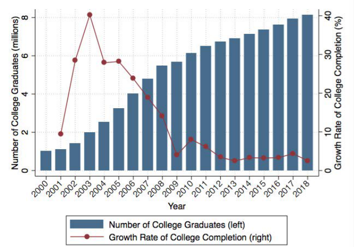
29
Figure 1: Number and Growth rate of College Graduates
Note: The figure depicts the number of graduates from 3- or 4-year colleges or above (the left vertical axis) and
the annual growth rate of college graduates (the right vertical axis) each year from 2000 to 2018. Data comes
from the China Statistics Yearbook.
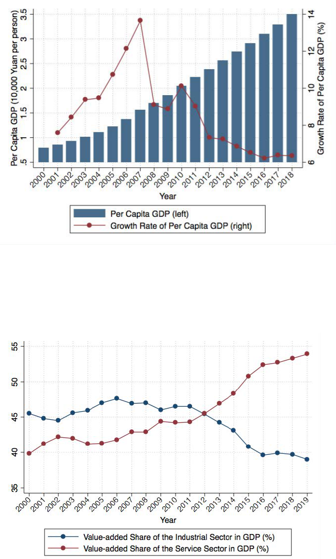
30
Figure 2: Per Capita GDP and Growth Rate of Per Capita GDP
Note: The figure depicts the evolution of per capita GDP (the left vertical axis) and growth rate of per capita GDP
(the right vertical axis) from 2000 to 2018. Per capita GDP is calculated by dividing GDP by the total population.
All monetary values are adjusted to the 2000 price level. Data comes from the National Bureau of Statistics.
Figure 3: Value-added Shares of the Industrial and Service Sectors
Note: The figure depicts the evolution of shares of value-added of the industrial sector and the service sector in
national GDP from 2000 to 2019. Data comes from the National Bureau of Statistics.
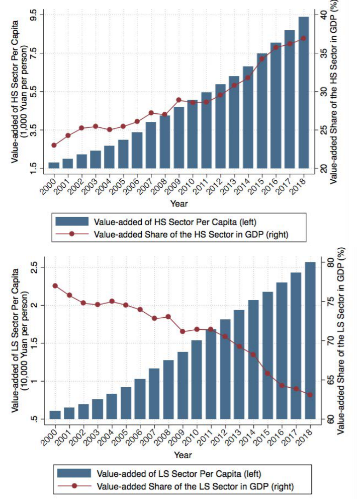
31
Figure 4: Value-added of HS Sector Per Capita and Share of HS Sector
Note: The figures depict the evolution of the value-added of HS (LS) sector per capita (the left vertical
axis) and the share of HS (LS) sector value-added in national GDP (the right vertical axis) from 2000 to
2018. The value-added of HS (LS) sector per capita is calculated by dividing the value-added of HS (LS)
sector by the total population. All monetary values are adjusted to the 2000 price level. Data come from the
National Bureau of Statistics.
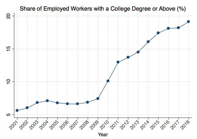
32
Figure 5: Share of Workers with a College Degree or Above
Note: The figure depicts the share of employed workers with a 3- or 4-year college degree or above each year
from 2001 to 2018. Data comes from the China Labor Statistics Yearbook and China Population and
Employment Statistics Yearbook. The definition of employed workers in the yearbook includes restrictions on
age and working hours after 2012, but it seems to be just an elaboration of the previous definition.
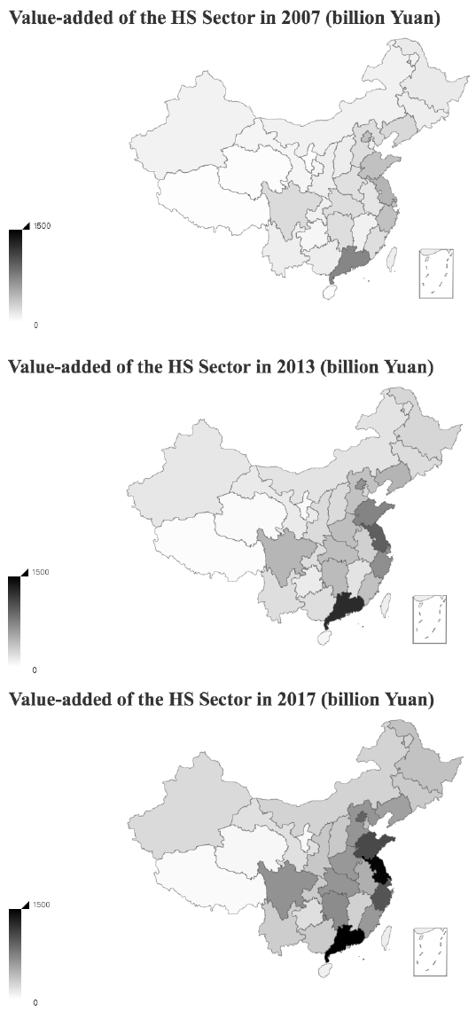
33
Figure 6: Regional Distribution of the Value-added of HS Sector
Note: The figure depicts the value-added of HS sector (in billion Yuan) by province in 2007, 2013 and 2017.
Darker color indicates a higher value-added of the HS sector. The actual maximum of the value-added of the HS
sector is about 1930 billion Yuan (Guangdong in 2017), but the range in the figure is censored at 1500 billion
Yuan for better visual effect. No other observation exceeds 1500 billion Yuan. All monetary values are adjusted
to the 2000 price level. Data comes from the National Bureau of Statistics.

34
Table 1: Share of Employees with a College Degree or Above in 2017
Sector Industry
Share of
Employees
with a College
Degree or
Above (%)
The Agricultural Sector Farming, Forestry, Animal Husbandry and Fishery 0.7
The Industrial Sector Mining and Quarrying 21.6
Manufacturing 15.2
Production and Supply of Electricity, Heat, Gas and Water 40.1
Construction 8.6
The Service Sector Wholesale and Retail Trade 18.3
Transport, Storage and Post 15.7
Accommodation and Food Services 8.2
Information and Communication Technology, Software 67.1
Finance and Insurance 67
Real Estate 36.4
Leasing and Business Services 42.9
Scientific Research and Technical Services 68.1
Management of Water Conservancy, Environment and
Public Infrastructure
24.9
Residential and Household Services
12.2
Education
69.8
Health and Social Services
59.9
Culture, Sports and Entertainment
41.2
Public Administration, Social Security and Social
Organizations
62.3
Note: The table reports the share of employed workers with a 3- or 4-year college degree or above by industry in 2017. The
classification follows the 2017 industrial classification for national economic activities. The international organization
industry is excluded since it is not relevant to this study. Data comes from the China Labor Statistics Yearbook.

35
Table 2: Summary Statistics
CHIP Survey year
CFPS HS+
CFPS all
2007
2013
2018
2014
2014
Panel A. Analysis Sample
Age
32.93
34.56
35.00
35.56
37.99
Male (%)
60.38
56.66
57.96
58.33
61.86
Gaokao Z-score / Math Z-score
Less than HS
.
.
.
.
-0.13
HS
-0.47
-0.63
-0.65
0.52
0.52
College
0.29
0.20
0.19
1.12
1.12
Hourly Wage
12.61
16.33
22.89
12.82
9.92
HS
7.67
11.91
15.20
10.03
10.03
College
14.75
17.48
24.49
15.43
15.43
HS (%)
30.32
20.61
17.16
48.40
20.71
College (%)
69.68
79.39
82.84
51.60
22.08
Observations
2,259
2,882
4,569
2,719
6,353
Panel B. Analysis Sample Inclusive of Observations Missing Gaokao Z-score or Math Z-score
Age
34.85
37.23
37.00
34.84
37.29
Male (%)
60.36
57.99
57.93
58.60
62.40
Hourly Wage
10.67
14.52
19.87
13.07
10.00
HS
8.06
11.74
14.86
10.16
10.16
College
14.77
17.25
23.62
15.73
15.73
HS (%)
61.04
49.62
42.79
47.66
20.04
College (%)
38.96
50.38
57.21
52.34
22.01
Observations
8,239
8,863
11,600
3,053
7,261
Note: The five columns correspond to CHIP 2007, 2013 and 2018, the high school and above sample and the
full sample of CFPS 2014, respectively. The analysis sample includes all full-time employees with hourly
wages between 1 and 100 Yuan per hour (CPI-adjusted to constant 2007 Yuan), and non-missing information
about the Gaokao score or math score, gender, age, years of schooling, province of residence, and sampling
weights. High school includes ordinary high school, technical school and specialized secondary school
(Zhong Zhuan). College includes 4-year college, 3-year college and graduate degrees. Panel B does not
impose restrictions on the availability of Gaokao score or math score.

36
Table 3: Returns to Cognitive Skills and College Degrees by Year
1 2 3 4 5 6 7 8 9
Year 2007 2007 2007 2013 2013 2013 2018 2018 2018
College 0.679
0.602 0.406
0.328 0.491
0.400
(0.026)
(0.028) (0.028)
(0.030) (0.024)
(0.025)
Gaokao z-score 0.207 0.104
0.137 0.094
0.161 0.111
(0.015) (0.014)
(0.012) (0.013)
(0.011) (0.011)
PE 0.054 0.052 0.051 0.045 0.042 0.043 0.043 0.041 0.040
(0.005) (0.006) (0.005) (0.005) (0.005) (0.005) (0.003) (0.003) (0.003)
PE Squared -0.001 -0.001 -0.001 -0.001 -0.001 -0.001 -0.001 -0.001 -0.001
(0.000) (0.000) (0.000) (0.000) (0.000) (0.000) (0.000) (0.000) (0.000)
Male 0.149 0.126 0.145 0.170 0.168 0.168 0.146 0.156 0.150
(0.024) (0.026) (0.024) (0.021) (0.022) (0.021) (0.019) (0.019) (0.018)
Constant 0.910 1.389 1.001 2.229 2.622 2.296 2.424 2.877 2.495
(0.177) (0.161) (0.172) (0.053) (0.043) (0.052) (0.046) (0.039) (0.046)
Observations 2,259 2,259 2,259 2,882 2,882 2,882 4,569 4,569 4,569
Adjusted R2 0.348 0.232 0.365 0.227 0.211 0.245 0.195 0.176 0.214
Note: The sample includes all full-time employees with hourly wages between 1 and 100 Yuan per hour and at least a high school degree in CHIP 2007, 2013 and 2018.
The dependent variable is log hourly wage. College is a dummy that takes 1 if the individual has a 3- or 4-year college degree or above, 0 if otherwise. PE is potential
experience measured by age minus six minus years of schooling. All regressions control for province fixed effects. Robust standard errors in parentheses.

37
Table 4: Trends in Returns to Cognitive Skills and College Degrees
1 2 3 4 5
College 0.608 0.583 0.574 0.501 0.485
(0.028) (0.029) (0.028) (0.028) (0.029)
College x Year2013
-0.279
-0.285
-0.277
-0.247
-0.248
(0.040) (0.042) (0.039) (0.039) (0.041)
College x Year2018 -0.214 -0.280 -0.219 -0.173 -0.243
(0.037) (0.051) (0.037) (0.036) (0.050)
Gaokao z-score 0.111 0.103 0.100 0.093 0.084
(0.014)
(0.015)
(0.014)
(0.014)
(0.014)
Gaokao x Year2013 -0.013 -0.016 -0.013 -0.017 -0.019
(0.019) (0.020) (0.018) (0.018) (0.019)
Gaokao x Year2018 -0.003 0.009 -0.003 -0.001 0.008
(0.018) (0.024) (0.017) (0.017) (0.023)
Year2013
0.510
0.523
0.501
0.498
0.501
(0.034) (0.037) (0.034) (0.034) (0.036)
Year2018 0.760 0.761 0.759 0.731 0.733
(0.033) (0.046) (0.032) (0.032) (0.045)
Male 0.156 0.138 0.147 0.149 0.127
(0.012) (0.015) (0.012) (0.012) (0.015)
Maternal Education No Yes No No Yes
Industry No No Yes No Yes
Occupation No No No Yes Yes
Province FEs Yes Yes Yes Yes Yes
Observations
9,710
6,261
9,697
9,650
6,202
Adjusted R2 0.344 0.315 0.361 0.367 0.349
Note: The sample includes all full-time employees with hourly wages between 1 and 100 Yuan per hour and
at least a high school degree in CHIP 2007, 2013 and 2018. The dependent variable is log hourly wages. All
regressions control for a quadratic function of potential experience. The omitted year category is 2007.
Maternal education are dummy variables corresponding to below middle school education, middle school
education, high school education and above higher education, respectively. Occupation and industry are
identified essentially at the one-digit level. Industries include: Agriculture and mining; Electricity, gas &
water; Manufacturing; Construction; Transport, storage, post and telecom & IT; Wholesale and retail trade
and catering services; Finance and insurance; Real estate; Social services; Health, education, culture &
research; and Party and Government organs and social organizations. Occupations include: Leading cadres;
Professional and technical staff; Office workers; Service workers; and Production workers. Robust standard
errors in parentheses.

38
Table 5: Comparison of Returns to Cognitive Skills Estimates from Different Data
Panel A. High School and Above Sample without Controls for College
1 2 3 4 5 6 7 8
OLS
OLS+Mother
Edu
OLS+Occu OLS+Indu OLS+Sector
OLS+Occu, Indu,
Sector, Mother edu
Col
Degree
IV
Math z-Score (CFPS14) 0.153 0.140 0.084 0.133 0.133 0.071 0.086 0.199
(0.017) (0.017) (0.018) (0.018) (0.018) (0.019) (0.018) (0.036)
Observations 2719 2578 2715 2677 2719 2537 2719 2719
Adjusted R2 0.187 0.195 0.291 0.207 0.221 0.312 0.239 0.087
Gaokao z-score (CHIP13) 0.137 0.124 0.105 0.121 0.113 0.083 0.094
(0.012) (0.013) (0.012) (0.012) (0.012) (0.012) (0.013)
Observations 2882 2535 2834 2879 2878 2491 2882
Adjusted R2 0.211 0.213 0.242 0.236 0.246 0.267 0.245
Panel B. Full Sample Without Controls for Schooling
OLS
OLS+Mother
Edu
OLS+Occu OLS+Indu OLS+Sector
OLS+Occu, Indu,
Sector, Mother edu
Edu Level IV
Math z-Score (CFPS14) 0.170 0.163 0.086 0.147 0.132 0.079 0.062 0.200
(0.011) (0.012) (0.013) (0.012) (0.012) (0.013) (0.013) (0.019)
Observations 6353 5890 6347 5914 6347 5483 6353 6353
Adjusted R2 0.195 0.205 0.289 0.213 0.228 0.307 0.251 0.114
Numeracy (PIAAC) 0.178 0.162 0.097 0.150
0.103 0.201
(0.003) (0.003) (0.003) (0.003)
(0.003) (0.003)
Note: The sample includes full-time employees with hourly wages between 1 and 100 Yuan per hour in CFPS 2014 and CHIP 2013. Panel A restricts to the high
school and above sample, and panel B uses the full sample. The bottom section of panel A report estimates from CHIP 2013; the bottom section of Panel B reproduces
estimates of Hanushek et al. (2015). Column 1 reports the baseline OLS estimate controlling for gender, a quadratic function of potential experience, and province
fixed effects. We add controls of maternal education, occupation, industry, and sector in columns 2-5 separately and jointly in column 6, and an indicator for college
degree in column 7. Sectors include government agencies, public institutions, state-owned enterprises (SOEs), and firms and small business of all other ownerships.
Column 8 reports the IV estimate using word test score as instrument for math score. Robust standard errors in parentheses.

39
Table 6: Heterogeneity By Gender and By Age
1
2
3
4
Young Workers
(age<35)
Older Workers
(age>=35)
Male
Workers
Female
Workers
College
0.543
0.686
0.610
0.610
(0.034)
(0.047)
(0.036)
(0.044)
College x Year2013
-0.330
-0.249
-0.318
-0.229
(0.052)
(0.062)
(0.052)
(0.061)
College x Year2018
-0.249
-0.161
-0.275
-0.129
(0.046)
(0.061)
(0.049)
(0.057)
Gaokao z-score
0.127
0.090
0.099
0.129
(0.020) (0.019) (0.018) (0.022)
Gaokao x Year2013
0.003
-0.018
0.000
-0.033
(0.026)
(0.026)
(0.024)
(0.029)
Gaokao x Year2018
0.012
-0.016
-0.004
-0.001
(0.024)
(0.025)
(0.023)
(0.027)
Year2013
0.546
0.491
0.552
0.448
(0.046)
(0.052)
(0.045)
(0.054)
Year2018
0.786
0.706
0.816
0.678
(0.041)
(0.053)
(0.043)
(0.049)
Male 0.156 0.147
(0.015)
(0.020)
Observations
5,616
4,094
5,645
4,065
Adjusted R2 0.346 0.324 0.327 0.356
Note: The sample includes all full-time employees with hourly wages between 1 and 100 Yuan per hour and
at least a high school degree in CHIP 2007, 2013 and 2018. The dependent variable is log hourly wages. The
four columns report estimates for young workers, senior workers, males and females, respectively. Young
workers are those aged below 35 and older workers are those aged above or equal to 35. The omitted year
category is 2007. All regressions control for province fixed effects, as well as a quadratic function of
potential experience. Robust standard errors in parentheses.

40
Table 7: Trends in Returns to Cognitive Skills and College Degrees By Region
1 2 3 4 5
Coastal Inland
≥Median
HS Share
<Median
HS Share
BJ, SH,
ZJ, GD
College 0.690 0.542 0.710 0.618
0.715
(0.039) (0.039) (0.047) (0.088)
(0.047)
College x Year2013 -0.238 -0.264 -0.307 -0.328
-0.141
(0.061) (0.053) (0.066) (0.109)
(0.081)
College x Year2018 -0.236 -0.172 -0.291 -0.310
-0.286
(0.059) (0.049) (0.062) (0.110)
(0.076)
Gaokao z-score 0.083 0.127 0.083 0.102
0.081
(0.020) (0.019) (0.023) (0.038)
(0.023)
Gaokao x Year2013 0.039 -0.048 0.070 -0.079
0.092
(0.027) (0.025) (0.030) (0.051)
(0.034)
Gaokao x Year2018 0.026 -0.013 0.021 -0.012
0.048
(0.026) (0.024) (0.029) (0.046)
(0.032)
Year2013 0.425 0.519 0.394 0.592
0.276
(0.053) (0.046) (0.062) (0.094)
(0.072)
Year2018 0.687 0.778 0.662 0.813
0.636
(0.052) (0.043) (0.059) (0.100)
(0.069)
Male 0.150 0.158 0.146 0.177
0.159
(0.019) (0.015) (0.020) (0.028)
(0.025)
Observations 3,729 5,981 3,559 1,978
2,320
Adjusted R2 0.371 0.301 0.334 0.261
0.375
Note: The sample includes all full-time employees with hourly wages between 1 and 100 Yuan per hour and
at least a high school degree in CHIP 2007, 2013 and 2018. The dependent variable is log hourly wage. All
regressions control for province fixed effects, as well as a quadratic function of potential experience. The
omitted year category is 2007. Columns 1 and 2 use samples of coastal and inland provinces respectively.
Coastal provinces in the estimation sample include Beijing, Shanghai, Hebei, Jiangsu, Zhejiang, Shandong
and Guangdong. Inland provinces include Anhui, Henan, Hubei, Chongqing, Sichuan, Shanxi, Liaoning,
Hunan, Yunnan, Gansu and Inner Mongolia. Columns 3-4 use samples of provinces with above- or below-
median measures of economic development in the high-skilled sector in regional GDP, respectively. Column
5 use the sample of Beijing, Shanghai, Zhejiang and Guangdong. Robust standard errors in parentheses.

41
Table 8: Education attainment of adults (aged 16-65) in different regions
inland coastal
Beijing, Shanghai,
Guangdong, Zhejiang
all non-
full time
student
residents
full-time
working
residents
all non-
full time
student
residents
full-time
working
residents
all non-full
time
student
residents
full-time
working
residents
Panel A: 2005 census
<= primary school
0.416
0.420
0.274
0.254
0.259
0.236
middle school
0.409
0.408
0.463
0.478
0.447
0.462
high school 0.116 0.108 0.174 0.169 0.192 0.187
>= 3 year college
0.058
0.064
0.089
0.099
0.102
0.114
Panel B: 2010 census
<= primary school
0.305
0.297
0.214
0.192
0.198
0.174
middle school 0.475 0.483 0.497 0.512 0.456 0.471
high school
0.136
0.129
0.170
0.166
0.194
0.188
>= 3 year college
0.084
0.091
0.120
0.130
0.153
0.167
Panel C: 2015 census
<= primary school
0.265
0.247
0.194
0.165
0.189
0.154
middle school
0.465
0.472
0.467
0.477
0.425
0.434
high school 0.165 0.161 0.188 0.186 0.210 0.207
>= 3 year college
0.105
0.120
0.150
0.172
0.177
0.205
Notes: This table reports the education attainment of adults (aged 16-65) residing in different regions of China
calculated from the 2005, 2010, and 2015 censuses. Numbers in each column in each panel add up to 1. Coastal
provinces are Liaoning, Hebei, Beijing, Tianjin, Shandong, Jiangsu, Shanghai, Zhejiang, Fujian, Guangdong,
Hainan; all other provinces are inland provinces.
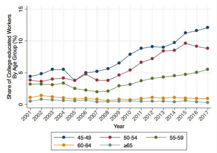
42
Appendix
Figure A1: Share of Workers with a College Degree or Above By Age
Note: The figure depicts the share of employed workers with a college degree or above for age groups 45-49,
50-54, 55-59, 60-64, and 65 and above from 2001 to 2017. Data comes from the China Labor Statistics
Yearbook.
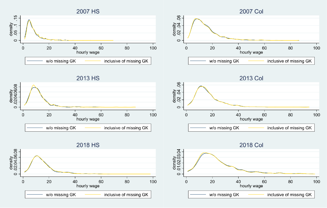
43
Figure A2: Wage Distribution of Analysis Sample and Full-Time Working Sample Missing Gaokao Z-Score by Education Level
Note:
The figure presents kernel densities of the hourly wage of the analysis sample and the full-time working sample in CHIP for each education level in each year. The
analysis sample includes all full-time employees with hourly wages between 1 and 100 Yuan per hour (CPI-adjusted to constant 2007 Yuan), and non-missing information
about the Gaokao score, gender, age, and province of residence. The full-time working sample are otherwise identical to the analysis sample except for no requirements on
non-missing gaokao z-score.
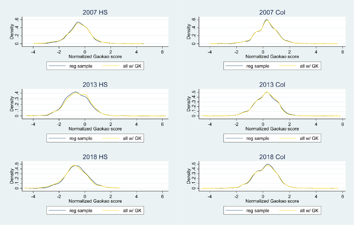
44
Figure A3: Gaokao Z-score Distribution of Analysis Sample and Overall Sample with Non-Missing Gaokao Z-Score by Education Level
Note:
The figure presents kernel densities of Gaokao z-score of the analysis sample and the sample of all adults with non-missing Gaokao z-score regardless of their working
status in CHIP for each education level in each year. The analysis sample includes all full-time employees with hourly wages between 1 and 100 Yuan per hour (CPI-adjusted
to constant 2007 Yuan), and non-missing information about the Gaokao score, gender, age, and province of residence.

45
Table A1: Value-added of HS Sector By Providence in 2007, 2013, and 2017
Province
Year
2007
2013
2017
Beijing
368.3
641.4
917.3
Tianjin
95.7
233.5
370.8
Hebei
199.2
356.3
621.8
Shanxi
103.4
210.1
316.3
Inner Mongolia
82.3
164.6
258.7
Liaoning
226.6
443.9
559.4
Jilin
99.6
207.2
310.8
Heilongjiang
124.0
241.9
360.2
Shanghai
367.9
651.1
1003.6
Jiangsu
442.4
941.7
1478.8
Zhejiang
363.0
656.8
1008.1
Anhui
152.7
278.7
471.0
Fujian
193.0
364.6
597.8
Jiangxi
84.6
162.2
270.8
Shandong
366.6
725.1
1072.5
Henan
180.8
384.4
603.9
Hubei
201.9
384.7
622.6
Hunan
194.8
397.4
674.1
Guangdong
709.1
1245.2
1930.8
Guangxi
104.3
196.2
303.4
Hainan
25.7
61.3
90.1
Chongqing
91.0
195.8
309.6
Sichuan
209.6
427.3
640.1
Guizhou
53.8
114.7
187.8
Yunnan
101.9
194.8
295.1
Tibet
9.9
19.2
29.3
Shaanxi
99.6
210.9
329.7
Gansu
56.7
122.2
184.2
Qinghai
16.1
30.1
45.2
Ningxia
15.3
27.7
42.9
Xinjiang
77.1
143.1
215.0
Note: The table reports the value-added of HS sector (in billion Yuan) by province in 2007,
2013 and 2017. All monetary values are adjusted to the 2000 price level. Data comes from
the National Bureau of Statistics.

46
Table A2: Returns to Cognitive Skills and College Degrees by Year, No Sample Restrictions on the Availability of Gaokao Z-score
1
2
3
4
5
6
7
8
9
Year 2007 2007 2007 2013 2013 2013 2018 2018 2018
College
0.609 0.567 0.511 0.388 0.343 0.285 0.481 0.414 0.342
(0.013) (0.014) (0.017) (0.013) (0.014) (0.017) (0.012) (0.014) (0.016)
Gaokao z-score
0.116 0.109
0.096 0.098
0.109 0.110
(0.013) (0.014)
(0.012) (0.013)
(0.010) (0.011)
1(missing GK z-score)
-0.050 -0.045
-0.075 -0.071
-0.114 -0.104
(0.015) (0.016)
(0.014) (0.014)
(0.013) (0.013)
PE
0.036 0.036 0.036 0.034 0.035 0.035 0.040 0.041 0.041
(0.003) (0.003) (0.003) (0.002) (0.002) (0.002) (0.002) (0.002) (0.002)
PE Squared
-0.001 -0.001 -0.001 -0.001 -0.001 -0.001 -0.001 -0.001 -0.001
(0.000) (0.000) (0.000) (0.000) (0.000) (0.000) (0.000) (0.000) (0.000)
Male
0.142 0.139 0.139 0.195 0.193 0.193 0.175 0.171 0.172
(0.012) (0.012) (0.012) (0.012) (0.012) (0.012) (0.012) (0.012) (0.012)
Constant
1.314 1.374 1.415 2.150 2.211 2.262 2.307 2.398 2.461
(0.027) (0.030) (0.031) (0.029) (0.030) (0.031) (0.029) (0.030) (0.032)
Observations
8,239 8,239 8,239 8,863 8,863 8,863 11,600 11,600 11,600
Adjusted R2
0.333 0.341 0.339 0.200 0.209 0.209 0.197 0.210 0.209
Note: The sample includes all full-time employees with hourly wages between 1 and 100 Yuan per hour in CHIP 2007, 2013 and 2018. The dependent variable is log
hourly wage. College is a dummy that takes 1 if the individual has a 3- or 4-year college degree or above, 0 if otherwise. PE is potential experience measured by age minus
six minus years of schooling. 1(missing GK z-score) is a dummy variable indicating missing Gaokao z-score. Columns 2, 5, and 8 impute missing gaokao z-score as the
average gaokao z-score by year group in full sample (basically 0). Columns 3, 6, and 9 impute missing gaokao z-score as the average gaokao z-score by education-year
group. All regressions control for province fixed effects. Robust standard errors in parentheses.
