Polynomial-Time Algorithms for Prime Factorization and Discrete

arXiv:quant-ph/9508027v2 25 Jan 1996

Polynomial-Time Algorithms for Prime Factorization

and Discrete Logarithms on a Quantum Computer

∗

Peter W. Shor

†

Abstract

A digital computer is generally believed to be an eﬃcient universal computing

device; that is, it is believed able to simulate any physical computing device with

an increase in computation time by at most a polynomial factor. This may not be

true when quantum mechanics is taken into consideration. This paper considers

factoring integers and ﬁnding discrete logarithms, two problems which are generally

thought to be hard on a classical computer and which have been used as the b asis

of several proposed cryptosystems. Eﬃcient randomized algorithms are given for

these two problems on a hypothetical quantum computer. These algorithms take

a number of steps polynomial in the input size, e.g., the number of digits of the

integer to be factored.

Keywords: algorithmic number theory, prime factorization, discrete logarithms ,

Church’s thesis, quantum computers, foundations of quantum mechanics, spin systems,

Fourier transforms

AMS subject classiﬁcations: 81P10, 11Y05, 68Q10, 03D10

∗

A preliminary version of this paper app eared in the Proceedings of the 35th Annual Symposium

on Foundations of Computer Science, Santa Fe, NM, Nov. 20–22, 1994, IEEE Computer Society Pr ess,

pp. 124–134.

†

AT&T Research, Room 2D-149, 600 Mountain Ave., Murray Hill, NJ 07974.

2 P. W. SHOR

1 Introduction

One o f the ﬁr st results in the mathematics of computation, which underlies the subse-

quent development of much of theoretical c omputer science, was the distinction between

computable and non-computable functions shown in papers of Chur ch [1936], Turing

[1936], and Post [1936]. Central to this result is Church’s thesis, which says that all

computing devic e s can be simulated by a Turing machine. This thesis g reatly simpli-

ﬁes the study of computation, s ince it reduces the potential ﬁeld of study from any of

an inﬁnite number of potential computing devices to Turing machines. Church’s thesis

is no t a mathematical theorem; to make it one would require a precise mathematical

description of a computing device. Such a description, however, would leave open the

possibility of some practical computing device which did no t satisfy this pre c ise math-

ematical description, and thus would make the resulting mathematical theorem weaker

than Church’s original thesis.

With the development of practical computers, it has become apparent that the dis-

tinction between c omputable and non-computable functions is much too coarse; com-

puter scientists are now interested in the exact eﬃciency with which speciﬁc functions

can be computed. This exact eﬃciency, on the other hand, is too precise a quantity to

work with easily. The generally accepted compromise between coarseness and precision

distinguishes eﬃciently and ineﬃciently computable functions by whether the length of

the computation scales polynomially or superpolynomially with the input s ize. The class

of problems which can be solved by algorithms having a number of steps polynomial in

the input size is known as P.

For this class iﬁcation to ma ke sense, we need it to be machine-independent. That is,

we need to know that whether a function is computable in polynomial time is indepe n-

dent of the kind of computing device used. This corresponds to the following quantitative

version of Church’s thesis, which Vergis et al. [1986] have called the “Strong Church’s

Thesis” and which makes up ha lf of the “Invariance Thesis” of van Emde Boas [1990].

Thesis (Quantitative Church’s thesis). Any physical computing device can be simu-

lated by a Turing machine in a number of steps polynomial in the resources used by the

computing device.

In sta tements of this thesis, the Turing machine is sometimes augmented with a ran-

dom number generator, as it has not yet been determined whether there are pseudoran-

dom number generators which can eﬃciently simulate truly random number generators

for all purposes. Readers who are not comfortable with Turing machines may think

instead of digital computers having an amount of memory that grows linearly with the

length of the computation, as these two classes of computing machines can eﬃciently

simulate each other.

There are two escape clauses in the above thesis. One of these is the word “physical.”

Researchers have pr oduced machine models that violate the above quantitative Church’s

thesis, but most of these have been ruled out by some reaso n for why they are not “phys-

ical,” that is, why they could not be built and made to work. T he other escape clause in

the above thesis is the word “resources,” the meaning of which is not completely sp e ci-

ﬁed above. There are generally two resources which limit the ability of digital co mputers

to solve large problems: time (computation steps) and space (memory). There are more

resources pertinent to analog computation; so me proposed analog machines that seem

able to solve NP-complete problems in polynomial time have required the machining of

FACTORING WITH A QUANTUM COMPUTER 3

exp onentially precise pa rts, or an e xponential amount of energy. (See Ve rgis et al. [1 986]

and Steiglitz [1988]; this issue is also implicit in the pap ers of Canny and Reif [1987]

and Choi et al. [1995] on three-dimensional shortest paths.)

For quantum computation, in addition to space and time, there is also a third poten-

tially important resource, precision. For a quantum computer to work, at lea st in any

currently envisioned implementation, it must be able to make changes in the quantum

states of o bjects (e.g., atoms, photons, or nuclear spins). These changes can clearly

not be perfectly accurate, but must contain some small amount of inherent impreci-

sion. If this imprec ision is constant (i.e., it does not depend on the size of the input),

then it is not known how to compute a ny functions in polynomial time o n a quantum

computer that cannot also be computed in polynomial time on a classical computer

with a random number generator. Howe ver, if we let the precision g row polynomially

in the input size (that is, we let the number of bits of precision grow logarithmically

in the input size), we appear to obtain a more powerful type of computer. Allowing

the same polynomial growth in precision does not appear to confer extra computing

power to c lassical mechanics, although allowing exponential growth in precis ion does

[Hartmanis and Simon 1974, Vergis et al. 1 986].

As far as we know, what precision is possible in quantum state ma nipulation is dic-

tated not by fundamental physical laws but by the properties of the materials and the

architecture with which a quantum computer is built. It is currently not clea r which

architectures, if any, will give high precision, and what this pr ecision will be . If the pre-

cision of a q uantum computer is large enough to make it more p owerful than a classical

computer, then in order to understand its potential it is important to think o f precision

as a resource that can vary. Treating the precision as a larg e constant (even though it is

almost ce rtain to be co nstant for any given machine) would be comparable to treating

a classical dig ita l computer as a ﬁnite automaton — since any given computer has a

ﬁxed amount of memory, this view is technically correct; however, it is not particularly

useful.

Because of the remarkable eﬀectiveness of our ma thematical models of computation,

computer scientists have tended to forget that computation is dependent on the laws of

physics. This can b e seen in the statement of the quantitative Church’s thesis in van

Emde Boas [1990], where the word “physical” in the above phrasing is replaced with

the word “reasonable.” It is diﬃcult to imagine any deﬁnition of “reasonable” in this

context which does not mean “physically realizable,” i.e., that this computing machine

could actually be built and would work.

Computer scientists have become convinced of the truth of the quantitative Church’s

thesis through the failure of all proposed counter- examples. Mo st of these proposed

counter-examples have been based on the laws of classical mechanics; however, the uni-

verse is in reality quantum mechanical. Quantum mechanical objects o ften behave quite

diﬀerently from how our intuition, based on classical mechanics, tells us they should.

It thus s e e ms plausible that the natural computing power of classical mechanics corre-

sp onds to Turing machines,

while the natural computing power of quantum mechanics

might be gr e ater.

I b elieve that this question has not yet been settled and is worthy of further investigation. See

Vergis et al. [1986], Steiglitz [1988], and Rubel [1989]. In particular, turbulence seems a good candidate

for a counterexample to the quanti tative Church’s thesis because the non-tri vial dynamics on many

length scales may make it diﬃcult to simulate on a classical computer.

4 P. W. SHOR

The ﬁrst person to look at the interaction between computation and quantum me-

chanics appears to have been Benioﬀ [1980, 1982a, 1982b]. Although he did not ask

whether quantum mechanics conferred extra power to computation, he showed that re-

versible unitary evolution was suﬃcient to realize the computational power of a Turing

machine, thus showing that quantum mechanics is at least as powerful computationally

as a c lassical computer. This work was fundamental in making later investigation of

quantum computers possible.

Feynman [1982,1986] seems to have been the ﬁrst to suggest that qua ntum mechanics

might be more powerful computationally than a Turing machine. He gave arguments as

to why quantum mecha nics might be intrinsically expensive co mputationally to simulate

on a classical computer. He also raised the possibility of using a computer based on

quantum mechanical principles to avo id this problem, thus implicitly asking the convers e

question: by using quantum mechanics in a computer can you compute more eﬃciently

than on a classical computer? Deutsch [1985, 1989] was the ﬁrst to ask this ques tio n

explicitly. In order to study this question, he deﬁned both quantum Turing machines

and quantum circuits and inves tig ated some of their properties.

The ques tion of whether using quantum mechanics in a computer allows one to

obtain more computational power was more recently addressed by Deutsch and Jozsa

[1992] and Berthiaume and Brassard [1992a, 1992b]. These papers showed that there

are pro blems which quantum computers ca n quickly solve exactly, but that classical

computers can only solve quickly with high probability and the aid of a random number

generator. However, these papers did not show how to solve a ny problem in quantum

polynomial time that was not already known to be solvable in polynomial time with

the aid of a random number gener ator, allowing a small probability of error; this is

the characterization of the complexity class BPP, which is widely viewed as the class of

eﬃciently solvable problems.

Further work on this problem was stimulated by Berns tein and Vazirani [1993]. One

of the results contained in their paper was an oracle problem (that is, a problem involving

a “ black box” subroutine that the computer is allowed to pe rform, but for which no code

is accessible) which can be done in polynomial time on a quantum Tur ing machine but

which requires super-polynomial time on a classical computer. This result was improved

by Simon [1994], who gave a much simpler construction of a n oracle problem which takes

polynomial time on a quantum computer but requires exponential time on a classical

computer. Indeed, while B e rnstein and Va z iarni’s problem appears c ontrived, Simon’s

problem looks quite natural. Simon’s algorithm inspired the work pr esented in this

paper.

Two number theory problems which have been studied extensively but for which no

polynomial-time algorithms have yet been discovered are ﬁnding discrete logarithms and

factoring integers [Pomerance 198 7, Gor don 1993, Lenstra and Lenstra 1993, Adleman

and McCurley 1995]. These problems are so widely believed to be hard that several

cryptosystems based on their diﬃculty have been proposed, including the widely used

RSA public key cryptosystem developed by Rivest, Shamir , and Adleman [1978]. We

show that these problems can be solved in polynomial time on a quantum computer

with a s mall probability of error.

Currently, nobody k nows how to build a qua ntum computer, although it seems as

though it might be possible within the laws of quantum mechanics. Some suggestions

have been made as to possible designs for such compute rs [Teich et al. 1988, Lloyd 1993,

FACTORING WITH A QUANTUM COMPUTER 5

1994, Cirac and Zoller 1995, DiVincenzo 1995, Sleator and Weinfurter 1995, Barenco et

al. 1995 b, Chuang and Yamo moto 1995], but there will be substantia l diﬃculty in build-

ing any of these [Landauer 1995a, Landauer 199 5b, Unruh 1995, Chuang et al. 1995,

Palma e t al. 1995]. The most diﬃcult obstacles appear to involve the decoherence of

quantum superpositions through the interaction of the computer with the environment,

and the implementation o f quantum state transformations with enough precision to give

accurate results after many computation steps. Both of these obstacles become more

diﬃcult as the size of the computer grows, so it may turn out to be possible to build

small quantum computers, while scaling up to machines large enough to do interesting

computations may present fundamental diﬃculties.

Even if no useful quantum computer is ever built, this research does illuminate

the problem of simulating quantum mechanics on a class ical computer. Any method of

doing this for an arbitrary Hamiltonian would necessarily be able to simulate a quantum

computer. Thus, any general method for simulating quantum mechanics with at most

a polynomial slowdown would lead to a polynomial-time algorithm for factoring.

The res t of this paper is organized as follows. In § 2, we introduce the mo del of

quantum co mputation, the quantum gate array, that we use in the re st of the paper.

In §§3 and 4, we explain two s ubroutines that are used in our algorithms: reversible

modular exponentiation in §3 and quantum Fourier transforms in §4. In §5, we give

our algorithm fo r prime factorization, and in §6, we give our algorithm for extracting

discrete logarithms. In §7, we give a br ie f discussion of the practicality of quantum

computation and suggest possible directions for further work.

2 Quantum computation

In this section we give a brief introduction to quantum co mputation, empha sizing the

properties tha t we will use. We will describe only quantum gate arrays, or quantum

acyclic circuits, which are a nalogous to acyclic c ircuits in classical computer science.

For other models of quantum computers, see references on quantum Turing machines

[Deutsch 1989, Bernstein and Vazirani 1993, Yao 1993] and quantum cellular automata

[Feynman 1986, Margolus 1986, 1990, Lloyd 1993, Biafore 1994]. If they are allowed

a small pr obability of error, quantum Turing machines and quantum gate arrays can

compute the same functions in polynomial time [Yao 1993]. This may also be true for

the various models of quantum cellular automata, but it has not yet been proved. This

gives evidence that the class of functions computable in quantum polynomial time with

a small pro bability of error is robust, in tha t it does not dep end on the exact a rchitecture

of a quantum computer. By analogy with the classical class BPP, this class is called

BQP.

Consider a system with n components, each of which can have two states. Whereas

in clas sical physics, a complete description of the state of this system requires only n

bits, in quantum physics, a complete description of the state of this system requires

− 1 complex numbers. To be more precise, the state of the quantum system is a

point in a 2

-dimensional vector spac e. For each of the 2

possible classical positions

of the components, there is a basis state of this vector space which we represent, for

example, by |011 ···0i mea ning that the ﬁrst bit is 0, the second bit is 1, and so on.

Here, the ket no tation |xi means that x is a (pure) q uantum state. (Mixed states will

6 P. W. SHOR

not be discusse d in this paper, and thus we do not deﬁne them; see a q uantum theory

book such as Peres [1993] for this deﬁnition.) The Hilbert space ass ociated with this

quantum sys tem is the complex vector space with these 2

states as basis vectors, and

the state of the sys tem at any time is represented by a unit-leng th vector in this Hilbert

space. As multiplying this s tate vector by a unit-length c omplex phase does not change

any behavior o f the state, we need only 2

−1 c omplex numbers to completely describe

the state. We represent this superposition of states as

−1

i=0

i, (2.1)

where the amplitudes a

are complex numbers s uch that

= 1 and each |S

is a basis vector of the Hilbert space. If the machine is mea sured (with respect to

this bas is) at any particular step, the probability of see ing basis state |S

i is |a

;

however, measur ing the state of the machine projects this state to the o bs erved basis

vector |S

i. Thus, looking at the machine during the computation will inva lidate the

rest of the computation. In this paper, we o nly consider measurements with respect

to the canonical basis. This doe s not greatly restrict our model of computation, since

measurements in other reasonable bases could be simulated by ﬁrst using q uantum

computation to perform a change of basis and then performing a measur e ment in the

canonical basis.

In order to use a physical system for computation, we must be able to change the

state of the system. The laws of quantum mechanics permit only unitary transfor ma-

tions of state vectors. A unitar y matrix is one whose conjugate transpose is equal to

its inverse, and requiring state transformations to be represented by unitary matrices

ensures that summing the probabilities of obtaining every possible outcome will result

in 1. The deﬁnition of quantum circuits (and quantum Turing machine s) only allows

local unitary transformations; that is, unitary transformations on a ﬁxed number of

bits. This is physically justiﬁed because, given a general unitary transformation on n

bits, it is not at all clear how one would eﬃciently implement it phy sically, whereas

two-bit tr ansformations can at least in theory be implemented by relatively simple

physical systems [Cirac and Zoller 1995, DiVincenzo 1995, Sleator and Weinfurter 1995,

Chuang and Yamomoto 1995]. While general n-bit transformations can always be

built out of two-bit transfor mations [DiVincenzo 1995, Sleator and Weinfurter 1995,

Lloyd 1995 , Deutsch et al. 1995], the number required will often be exponential in n

[Barenco et al. 1995a]. Thus, the set of two-bit transformations form a set of building

blocks for quantum circuits in a manner analogous to the way a universal set of classical

gates (such as the AND, OR and NOT gates) form a s et of building blocks for clas sical

circuits. I n fact, for a universal set of quantum gates, it is s uﬃcient to take all one-bit

gates and a single type of two-bit gate, the controlled NOT, which negates the second

bit if and only if the ﬁrst bit is 1.

Perhaps an example will be informative at this point. A quantum gate can be

expressed as a truth table: for each input basis vector we need to give the output of the

gate. One such gate is:

FACTORING WITH A QUANTUM COMPUTER 7

|00i → |00i

|01i → |01i (2.2)

|10i →

√

(|10i + |11i)

|11i →

√

(|10i − |11i).

Not all truth tables correspond to physically feasible quantum gates, as many truth

tables will not give rise to unitary transformations.

The same ga te ca n also be represented as a matrix. The rows correspond to input

basis vectors. The columns correspond to output basis vectors. The (i, j) entry gives,

when the ith basis vector is input to the gate, the coeﬃcient of the jth basis vector in

the corresponding output of the gate. The truth table above would then correspond to

the following matrix:

|00i |01i |10i |11i

|00i

1 0 0 0

|01i 0 1 0 0

|10i 0 0

√

|11i 0 0

√

−

√

(2.3)

A quantum gate is feasible if and only if the corresponding matrix is unitary, i.e., its

inverse is its conjugate transpose.

Suppose our machine is in the superposition of states

√

|10i −

√

|11i (2.4)

and we a pply the unitary transformation represented by (2.2) and (2.3) to this state.

The resulting output will be the result of multiplying the vector (2.4) by the matrix

(2.3). The machine will thus go to the superposition of states

(|10i + |11i) −

(|10i − |11i) = |11i. (2.5)

This example shows the potential eﬀects of inter ference on quantum computation. Had

we started with either the state |10i or the state |11i, there would have been a chance of

observing the state |10i after the application of the gate (2.3). However, when we start

with a superposition of these two states, the pro bability amplitudes for the sta te |10i

cancel, and we have no possibility of observing |10 i after the application of the gate.

Notice that the output of the gate would have be e n |10i instead of |11i had we started

with the superposition of states

√

|10i +

√

|11i (2.6)

which has the same probabilities of being in any particular conﬁguration if it is observed

as does the superposition (2 .4).

If we apply a gate to only two bits of a longer basis ve c tor (now our circuit must have

more than two wires), we multiply the gate matrix by the two bits to which the gate is

8 P. W. SHOR

applied, and leave the other bits alone. This correspo nds to multiplying the whole state

by the tensor product of the gate matrix on those two bits with the identity matrix on

the remaining bits.

A q uantum gate array is a set of quantum gates with logical “wires” connecting their

inputs and outputs. The input to the gate array, possibly along with e xtra work bits

that are initially set to 0, is fed through a sequence of quantum gates. The values of

the bits are observed after the last quantum ga te, and these values are the output. To

compare gate arrays with quantum Turing machines, we need to add conditions that

make gate arrays a uniform complexity class. In other words, be c ause there is a diﬀerent

gate array for each size of input, we need to keep the designer of the gate arrays from

hiding non-computable (or hard to compute) information in the arrangement of the

gates. To make quantum gate arrays uniform, we must add two things to the deﬁnition

of gate arrays. The ﬁrs t is the standard requirement that the design of the gate array

be produced by a polynomial-time (classical) computation. The se c ond requirement

should be a standard part of the deﬁnition of analog complexity clas ses, although since

analog co mplexity classes have not been widely studied, this re quirement is much less

widely known. This requirement is that the entries in the unitary matrices describing

the gates must be computable numbers. Speciﬁcally, the ﬁr st log n bits of each entry

should be classically computable in time p olynomial in n [Solovay 1995]. This keeps

non-computable (or hard to compute) information from being hidden in the bits of the

amplitudes of the quantum gates.

3 Reversible logic and modular exponentiation

The deﬁnition o f quantum gate arrays gives rise to completely reversible computation.

That is, knowing the quantum state on the wires leading out of a gate tells uniquely

what the quantum state must have been on the wires leading into that gate. This is a

reﬂection of the fact that, despite the mac roscopic ar row of time, the laws of physics ap-

pear to be completely reversible. This would seem to imply that anything built with the

laws of physics must be completely reversible; however, classical computers get around

this fact by dissipa ting energy and thus making their computatio ns thermodynamically

irreversible. This appears impossible to do for quantum computers becaus e superpo-

sitions of quantum states need to be maintained throughout the computation. Thus,

quantum computers necessarily have to use reversible computation. This imposes ex-

tra costs when doing clas sical computations on a quantum computer, as is sometimes

necessary in subroutines of quantum computations.

Because of the reversibility of quantum co mputation, a deter ministic computation

is performable on a quantum co mputer only if it is reversible. Luckily, it has already

been shown that any deterministic computation can be made reversible [Lecerf 1963,

Bennett 1973]. In fact, reversible classical gate arrays have been s tudied. Much like

the result that any classical co mputation can be done using NAND gates, there are also

unive rsal gates for reversible computation. Two of these are Toﬀoli ga tes [Toﬀoli 1980]

and Fredkin gates [Fredkin and Toﬀoli 1982]; these are illustrated in Table 3.1.

The Toﬀoli gate is just a controlled controlled NOT, i.e., the last bit is negated if

and only if the ﬁrst two bits are 1. In a Toﬀoli g ate, if the third input bit is set to 1,

then the third output bit is the NAND of the ﬁrst two input bits. Since NAND is a

FACTORING WITH A QUANTUM COMPUTER 9

Table 3.1: Truth tables for Toﬀoli and Fredkin gates.

Toﬀoli Gate

INPUT OUTPUT

0 0 0 0 0 0

0 0 1 0 0 1

0 1 0 0 1 0

0 1 1 0 1 1

1 0 0 1 0 0

1 0 1 1 0 1

1 1 0 1 1 1

1 1 1 1 1 0

Fredkin Gate

INPUT OUTPUT

0 0 0 0 0 0

0 0 1 0 1 0

0 1 0 0 0 1

0 1 1 0 1 1

1 0 0 1 0 0

1 0 1 1 0 1

1 1 0 1 1 0

1 1 1 1 1 1

unive rsal gate for classical gate arrays, this shows that the Toﬀoli gate is universal. In

a Fredkin gate, the last two bits are swapped if the ﬁrst bit is 0, and left untouched if

the ﬁrst bit is 1. For a Fredkin g ate, if the third input bit is set to 0, the second output

bit is the AND of the ﬁrst two input bits; and if the last two input bits are s et to 0

and 1 respectively, the second output bit is the NO T of the ﬁrst input bit. Thus, both

AND and NOT gates are realizable using Fredkin gates, showing that the Fredkin gate

is universal.

From results on reversible computation [Lecerf 1963, Bennett 1973], we can compute

any polynomial time function F (x) as long as we keep the input x in the computer. We do

this by adapting the method for co mputing the function F non-reversibly. T hese results

can easily be extended to work for gate arrays [Toﬀoli 1980, Fredkin and Toﬀoli 1982].

When AND, OR or NOT gates are changed to Fredkin or To ﬀo li gates, o ne obtains

both additional input bits, which must be preset to speciﬁed values, and additional

output bits, which contain the information needed to reverse the computation. While

the additional input bits do not present diﬃculties in designing quantum computers,

the additional output bits do, because unless they are all reset to 0, they will aﬀect the

interference patterns in quantum computation. Bennett’s method fo r r e setting these bits

to 0 is shown in the top half of Table 3.2. A non-reversible gate array may thus be turned

into a re versible gate ar ray as follows. First, duplicate the input bits as many times as

necessary (since each input bit could be used more than once by the gate array). Next,

keeping one copy of the input around, use To ﬀo li and Fredkin gates to simulate non-

reversible gates , putting the extra output bits into the RECORD register . These extra

output bits preserve enough of a rec ord of the o perations to enable the computation of

the gate array to be re versed. Once the output F (x) has been computed, copy it into a

ﬁrst OUTPUT register and the RE CORD register.

To erase x and replace it with F (x), in addition to a polynomial-time algorithm for F ,

we also need a polynomial-time algorithm for computing x from F (x); i.e., we need that

F is one-to-one and that both F and F

−1

are p olynomial-time computable. The method

for this computation is given in the whole of Table 3.2. There are two stages to this

computation. The ﬁrst is the same as befo re, taking x to (x, F(x)). For the second

stage, shown in the bottom half of Table 3.2 , note that if we have a method to compute

−1

non-reversibly in polynomial time, we can use the same technique to reversibly map

F (x) to (F (x), F

−1

(F (x))) = (F (x), x). However, since this is a reversible computation,

10 P. W. SHOR

Table 3.2: Bennett’s method for making a computation r eversible.

INPUT - - - - - - - - - - - - - - - - - -

INPUT OUTPUT RECORD(F ) - - - - - -

INPUT OUTPUT RECORD(F ) OUTPUT

INPUT - - - - - - - - - - - - OUTPUT

INPUT INPUT RECORD(F

−1

) OUTPUT

- - - - - - INPUT RECORD(F

−1

) OUTPUT

- - - - - - - - - - - - - - - - - - OUTPUT

we can reverse it to go from (x, F (x)) to F (x). Put together, these two pieces take x to

F (x).

The above discussion shows that co mputations can be made reversible for only a

constant factor cost in time, but the a bove method uses as much s pace as it does time.

If the classical computation requires much less space than time, then making it reversible

in this manner will result in a large increase in the space required. There are methods

that do not use as much space, but use more time, to make computations reversible

[Bennett 1989, Levine and Sherman 1990]. While there is no g eneral method that does

not cause an increase in either space or time, speciﬁc algorithms can sometimes be

made reversible without paying a large penalty in either space or time; a t the e nd of this

section we will show how to do this for modular exponentiation, which is a subroutine

necessary for quantum factoring.

The bottleneck in the qua ntum factoring algorithm; i.e ., the piece of the fac-

toring algorithm that co nsumes the most time and space, is modular exponentia-

tion. The modular exponentiation problem is, given n, x, and r, ﬁnd x

(mod n).

The best classical method for doing this is to repe atedly square of x (mod n) to

get x

(mod n) for i ≤ log

r, and then multiply a subset of these powers (mod n)

to get x

(mod n). If we are working with l-bit numbers, this requires O(l) squar-

ings and multiplications of l-bit numbers (mod n ). Asymptotically, the best clas-

sical result for gate arrays for multiplication is the Sch¨onhage–Strassen algorithm

[Sch¨onhage and Strassen 1971, Knuth 1981, Sch¨onhage 1982]. This gives a gate array

for intege r multiplication that uses O(l log l log log l) gates to multiply two l-bit numbers.

Thus, asymptotica lly, modular exponentiation requires O(l

log l log lo g l) time. Mak ing

this re versible would na¨ıvely cost the same amount in space; however, one can reuse the

space used in the repeated squaring part of the algorithm, and thus reduce the amount

of space needed to essentially that required for multiplying two l-bit numbers; o ne simple

method for reducing this space (although no t the most versatile one) will be given later

in this section. Thus, modular exponentiation can be done in O(l

log l log lo g l) time

and O(l log l log log l) space.

While the Sch¨onhage–Strassen algorithm is the best multiplication algorithm discov-

ered to date for large l, it does not scale well for small l. For small numbers, the best

gate arrays for multiplication essentially use elementary-school longhand multiplication

in binary. This method r e quires O(l

) time to multiply two l-bit numbers, and thus

modular exponentiation requires O(l

) time with this method. These g ate arrays can

be made re versible, howe ver, using only O(l) space.

We will now give the method for constructing a reversible g ate array that takes o nly

FACTORING WITH A QUANTUM COMPUTER 11

O(l) space and O(l

) time to compute (a, x

(mod n)) from a, where a, x, and n are

l-bit numbers. The basic building block use d is a gate array that takes b as input and

outputs b + c (mod n). Note that here b is the gate arr ay’s input but c a nd n are built

into the structure o f the gate array. Since addition (mod n) is computable in O(log n)

time classically, this reversible gate arr ay can be made with only O(log n) gates and

O(log n) work bits using the techniques explained earlier in this section.

The technique we use for c omputing x

(mod n) is essentially the same a s the clas si-

cal metho d. First, by repeated squaring we compute x

(mod n) for all i < l. Then, to

obtain x

(mod n) we multiply the powers x

(mod n) where 2

appears in the binary

expansion of a. In our algorithm for factoring n, we only need to co mpute x

(mod n)

where a is in a superposition of states, but x is some ﬁxed integer. This makes things

much easier, because we can use a reversible gate array where a is treated as input,

but where x and n are built into the structure of the ga te array. Thus, we can use the

algorithm described by the following pseudocode; here, a

represents the ith bit o f a in

binary, where the bits are indexed from right to left and the rightmost bit of a is a

power := 1

for i = 0 to l −1

if ( a

== 1 ) then

power := power ∗ x

(mod n)

endif

endfor

The variable a is left unchanged by the code and x

(mod n) is output as the variable

power. Thus, this code takes the pair of values (a, 1) to (a, x

(mod n)).

This pseudocode can easily be turned into a gate ar ray; the only hard part o f this

is the fourth line, where we multiply the variable power by x

(mod n); to do this we

need to use a fairly complicated gate array as a subroutine. Recall that x

(mod n)

can be computed classically and then built into the structure of the gate array. Thus,

to implement this line, we need a reversible gate array that takes b as input and gives

bc (mod n) as output, where the structure of the gate array can depend on c and n.

Of course, this step can only be reversible if gcd(c, n) = 1, i.e., if c and n have no

common factors, as otherwise two distinct values of b will be mapped to the same value

of bc (mod n); this case is fortunately all we need for the factoring algorithm. We will

show how to build this gate array in two stages. The ﬁrst stage is directly analogous

to expo nentiation by repeated multiplication; we obtain multiplication from repeated

addition (mod n). Pseudocode for this stage is as follows.

result := 0

for i = 0 to l −1

if ( b

== 1 ) then

result := result + 2

c (mod n)

endif

endfor

Again, 2

c (mod n) can be precomputed and built into the structure of the gate array.

12 P. W. SHOR

The above pseudocode takes b as input, and gives (b, bc (mod n)) as output. To

get the desired result, we now need to erase b. Recall that gcd(c, n) = 1, so there is

a c

−1

(mod n) with c c

−1

≡ 1 (mod n). Multiplication by this c

−1

could be used to

reversibly take bc (mod n) to (bc (mod n), bcc

−1

(mod n)) = (bc (mod n), b). This is

just the reverse of the operation we want, and since we are working with reversible

computing, we can turn this operation around to erase b. The pseudocode for this

follows.

for i = 0 to l −1

if ( result

== 1 ) then

b := b − 2

−1

(mod n)

endif

endfor

As before, result

is the ith bit of result.

Note that at this stage of the computation, b should b e 0. However, we did not set b

directly to ze ro, as this would not have been a re versible operation and thus impos sible on

a quantum computer, but instead we did a relatively complicated sequence of operations

which ended with b = 0 and which in fact depended on multiplication being a group

(mod n). At this point, then, we could do something somewhat sneaky: we co uld

measure b to see if it actually is 0. If it is not, we know tha t there has been an error

somewhere in the quantum computation, i.e., that the res ults are worthless and we

should stop the computer and start over again. However, if we do ﬁnd that b is 0,

then we know (because we just observed it) that it is now exactly 0. This measurement

thus may bring the q uantum computation back o n track in that any amplitude that b

had for being non-zero has been eliminated. Further, because the probability that we

observe a state is proportional to the square of the amplitude of that state, depending

on the error model, doing the modular exponentiation and measuring b every time that

we know that it should be 0 may have a higher probability of overall success than the

same computation done without the re peated measurements of b; this is the quantum

watchdog (or quantum Zeno) eﬀect [Peres 1993]. The argument above does not actually

show that repeated measurement of b is indeed beneﬁcial, because there is a cost (in time,

if no thing else) of measuring b. Before this is implemented, then, it should be checked

with ana lysis or experiment that the beneﬁt of such measurements exce e ds their cost.

However, I believe that partial measurements such as this one are a promising way of

trying to sta bilize quantum computations.

Currently, Sch¨onhage–Str assen is the algorithm of choice for multiplying very la rge

number s, and longhand multiplication is the algorithm of choice for small numbers.

There are also multiplication algorithms which have eﬃciencies between these two al-

gorithms, and which a re the best algorithms to use fo r intermediate length numbers

[Karatsuba a nd Ofman 1962, Knuth 1 981, Sch¨onhage et al. 1994]. It is not clear which

algorithms are best for which size numbers. While this may be known to some extent

for classical computation [Sch¨onhage e t al. 1994], using data on which algorithms work

better on classical computers could be misleading for two reasons: First, classica l com-

puters need not be reversible, and the cost of making an algorithm reversible depends

on the algorithm. Second, existing computers generally have multiplication for 32- or

64-bit numbers built into their hardware, and this will increase the optimal changeover

FACTORING WITH A QUANTUM COMPUTER 13

points to asymptotically faster algorithms; further, some multiplication algorithms can

take b e tter advantage of this har dwired multiplication than others. Thus, in order to

program quantum computers most eﬃciently, work needs to be done on the best way of

implementing elementary arithmetic op erations on quantum computers. One tantalizing

fact is that the Sch¨onhage–Strassen fast multiplication algorithm uses the fast Fourier

transform, which is als o the basis for all the fast algorithms on quantum computers

discovered to date; it is tempting to speculate that integer multiplica tion itself might be

sp e e ded up by a quantum algorithm; if possible, this would result in a somewhat faster

asymptotic bound for factoring on a quantum computer, a nd indeed could even make

breaking RSA on a quantum computer asymptotically faster than encrypting with RSA

on a classical computer.

4 Quantum Fourier transforms

Since quantum computation deals with unitary tr ansformations, it is helpful to be able

to build certain useful unitary tr ansformations. In this section we give a technique for

constructing in polynomial time on quantum computers one particular unitary trans fo r-

mation, which is essentially a discrete Fourier transform. This transformation will be

given as a matrix , with both rows and columns indexed by states. These states corre-

sp ond to binary representations o f integers on the computer; in particular, the rows and

columns will be indexed beginning with 0 unless otherwise speciﬁed.

This trans formations is as follows. Consider a number a with 0 ≤ a < q for some q

where the number o f bits of q is polynomial. We will perform the transformation that

takes the state |ai to the state

1/2

q−1

c=0

|ciexp(2πiac/q). (4.1)

That is, we apply the unitary matrix whose (a, c) entry is

1/2

exp(2πiac/q). This Fourier

transform is at the heart of our algorithms , and we call this matrix A

Since we will use A

for q of exponential size, we must show how this transforma tion

can be done in polynomial time. In this paper, we will give a simple c onstruction for A

when q is a power of 2 that was discovered independently by Coppersmith [1994] and

Deutsch [see Ekert and J ozsa 1995]. This construction is essentially the standar d fast

Fourier transform (FFT) algorithm [Knuth 1981] adapted for a quantum computer; the

following description of it follows that of Ekert and Jozsa [1995]. In the earlier version

of this paper [Shor 1994 ], we gave a construction for A

when q was in the s pecial class

of smooth numbe rs with small prime power factors. In fact, Cleve [1994] has shown how

to construct A

for all smooth numbers q whose prime fac tors are at most O(log n).

Take q = 2

, and let us represent an integer a in binar y as |a

l−1

l−2

. . . a

i. For the

quantum Fourier transform A

, we only need to use two types of quantum g ates. These

gates are R

, which operates on the jth bit of the quantum computer:

|0i |1i

|0i

√

|1i

√

−

√

(4.2)

14 P. W. SHOR

and S

j,k

, which operates on the bits in positions j and k with j < k:

j,k

|00i |01i |10i |11i

|00i

1 0 0 0

|01i 0 1 0 0

|10i 0 0 1 0

|11i 0 0 0 e

iθ

k−j

(4.3)

where θ

k−j

= π/2

k−j

. To perform a quantum Fourier tr ansform, we apply the matrices

in the order (from left to right)

l−1

l−2,l−1

l−2

l−3,l−1

l−3,l−2

l−3

. . . R

0,l−1

0,l−2

. . . S

0,2

0,1

; (4.4)

that is, we apply the gates R

in reverse order from R

l−1

to R

, and between R

j+1

and

we apply all the gates S

j,k

where k > j. For example, on 3 bits, the matrices would

be applied in the order R

1,2

0,2

0,1

. To take the Fourier transform A

when

q = 2

, we thus need to use l(l − 1)/2 quantum gates.

Applying this sequence of transformations will result in a quantum state

1/2

exp(2πiac/q) |bi, where b is the bit-reversal of c, i.e., the binary number ob-

tained by reading the bits of c from right to left. Thus, to obtain the actual quantum

Fourier transform, we need eithe r to do further computation to r e verse the bits of |bi

to obtain |ci, or to leave these bits in place and read them in re verse order; either

alternative is easy to implement.

To show that this operation actually performs a quantum Fourier transform, consider

the amplitude o f going from |ai = |a

l−1

. . . a

i to |bi = |b

l−1

. . . b

i. First, the factors

of 1/

√

2 in the R matrices multiply to produce a factor of 1/ q

1/2

overall; thus we need

only worry about the ex p(2πiac/q) phase facto r in the express ion (4.1). The matrices

j,k

do not change the values of any bits, but merely change their phases. There is thus

only o ne way to switch the jth bit from a

to b

, and that is to use the appropriate entry

in the matrix R

. This entry adds π to the phase if the bits a

and b

are both 1, and

leaves it unchanged otherw ise. Further, the matrix S

j,k

adds π/2

k−j

to the phase if a

and b

are both 1 a nd leaves it unchanged otherwise. Thus, the phase on the path from

|ai to |bi is

0≤j<l

πa

0≤j<k<l

k−j

. (4.5)

This expression can be rewritten as

0≤j≤k<l

k−j

. (4.6)

Since c is the bit-reversal of b, this expression c an be further rewritten as

0≤j≤k<l

k−j

l−1−k

. (4.7)

Making the substitution l − k − 1 for k in this sum, we get

0≤j+k<l

2π

(4.8)

FACTORING WITH A QUANTUM COMPUTER 15

Now, since adding multiples of 2π do not aﬀect the pha se, we obtain the same phase if

we sum over all j and k less than l, obtaining

l−1

j,k=0

2π

l−1

j=0

l−1

k=0

, (4.9)

where the last equality follows from the distributive law of multiplica tion. Now, q = 2

a =

l−1

j=0

, and similarly for c, so the above expression is equal to 2πac/q, which is

the phase for the amplitude of |ai → |ci in the transformation (4.1).

When k − j is large in the gate S

j,k

in (4.3), we are multiplying by a very small

phase factor. This would be very diﬃcult to do accurately physically, and thus it would

be somewhat disturbing if this were necessary for quantum computation. Luckily, Cop-

persmith [1994] has shown that one can deﬁne an approximate Fourier transform that

ignores these tiny phase factors, but which approximates the Fourier transfo rm closely

enough that it can also be used for factoring. In fact, this technique reduces the number

of quantum gates needed for the (approximate) Fourier transform considerably, as it

leaves out most of the gates S

j,k

5 Prime factorization

It has be e n known since before Euclid that every integer n is uniquely decomposable

into a product of primes. Mathematicians have been interested in the question of how

to factor a number into this product of primes for near ly as long. It was only in the

1970’s , however, that resea rchers applied the paradigms of theoretical computer science

to number theory, and lo oked at the asymptotic running times of factoring algorithms

[Adleman 1994]. This has resulted in a great improvement in the eﬃciency of factoring

algorithms. The best factoring algorithm asymptotically is currently the number ﬁeld

sieve [Lenstra et al. 1990, Lenstra and Lenstra 1993], which in order to factor an inte-

ger n takes asymptotic running time exp(c(log n)

1/3

(log log n)

2/3

) for some constant c.

Since the input, n, is only log n bits in length, this algorithm is an exponential-time

algorithm. Our quantum factoring algorithm takes asymptotically O((log n)

(log log n)

(log log log n)) steps on a quantum computer, along with a po ly nomial (in log n) amount

of post-processing time on a class ic al computer that is used to c onvert the output of

the quantum co mputer to fac tors of n. While this post-processing could in principle be

done on a quantum computer, there is no reason not to use a classical computer if they

are more eﬃcient in practice.

Instead of giving a quantum computer algorithm for fac toring n directly, we give a

quantum computer algorithm for ﬁnding the order of an element x in the multiplicative

group (mod n ); that is, the least integer r such that x

≡ 1 (mod n). It is known that

using randomization, factorization can be reduced to ﬁnding the or der of an element

[Miller 1976]; we now brieﬂy give this reduction.

To ﬁnd a factor of an odd number n , g iven a metho d for computing the order r

of x, choose a random x (mod n), ﬁnd its order r, and compute gcd(x

r/2

−1, n). Here,

gcd(a, b) is the greatest c ommon divisor of a and b, i.e., the largest intege r that divides

both a and b. The Euclidean algorithm [Knuth 1981] can be used to compute gcd(a, b)

in polynomial time. Since (x

r/2

−1)(x

r/2

+1) = x

−1 ≡ 0 (mo d n), the gcd(x

r/2

−1, n)

16 P. W. SHOR

fails to be a non-trivial divisor of n only if r is odd or if x

r/2

≡ −1 (mod n). Using this

criterion, it can be shown that this procedure, when applied to a random x (mod n),

yields a factor of n with probability at least 1−1/2

k−1

, where k is the number of distinct

odd prime fa c tors of n. A brief sketch of the proof of this result follows. Suppose that

n =

i=1

. Let r

be the order of x (mod p

). Then r is the least common multiple

of all the r

. Consider the largest power of 2 dividing each r

. The algorithm only fails

if all of these powers of 2 agree: if they are all 1, then r is odd and r/2 does not exist; if

they are all equal and larger than 1, then x

r/2

≡ −1 (mod n) since x

r/2

≡ −1 (mod p

)

for every i. By the Chinese remainder theorem [Knuth 1981, Hardy and Wright 1979,

Theorem 1 21], choosing an x (mod n) at random is the same as choosing for each i a

number x

(mod p

) at random, where p

is the ith prime powe r factor of n. The

multiplicative group (mod p

) for any odd prime power p

is cyclic [Knuth 1981], so for

any odd prime power p

, the probability is at most 1/2 of choos ing an x

having any

particular power of two as the largest divisor of its order r

. Thus each of these powers

of 2 has at most a 50% probability o f agreeing with the previous ones, so all k of them

agree with probability at most 1/2

k−1

, a nd there is at least a 1 − 1/2

k−1

chance that

the x we choose is goo d. This scheme will thus work as long as n is odd and not a prime

power; ﬁnding factors of prime p owers can be done eﬃciently with classical methods.

We now describe the algorithm for ﬁnding the order of x (mod n) on a quantum

computer. This algor ithm will use two quantum regis ters which hold integers represented

in binary. There w ill also be s ome amount o f workspace. This workspace gets reset to

0 after each subroutine of our algo rithm, so we will not include it when we write down

the state of our machine.

Given x and n, to ﬁnd the order of x, i.e., the least r such that x

≡ 1 (mod n ), we

do the fo llowing. First, we ﬁnd q, the power of 2 with n

≤ q < 2n

. We will not include

n, x, or q when we write down the state of our machine, because we never change these

values. In a quantum gate array we need not even keep these values in memory, as they

can be built into the structure of the gate array.

Next, we put the ﬁrst regis ter in the unifor m superposition of states representing

number s a (mod q). This leaves o ur machine in state

1/2

q−1

a=0

|ai|0i. (5.1)

This step is relatively ea sy, since all it entails is putting each bit in the ﬁrs t register into

the superposition

√

(|0i + |1i).

Next, we compute x

(mod n) in the second register as described in §3. Since we

keep a in the ﬁrst register this can be done reversibly. This leaves our machine in the

state

1/2

q−1

a=0

|ai|x

(mod n)i. (5.2)

We then perform our Fourier transform A

on the ﬁrst register, as described in §4,

mapping |ai to

1/2

q−1

c=0

exp(2πiac/q) |ci. (5.3)

FACTORING WITH A QUANTUM COMPUTER 17

That is, we apply the unitary matrix with the (a, c) entry equal to

1/2

exp(2πiac/q).

This leaves our machine in state

q−1

a=0

q−1

c=0

exp(2πiac/q) |ci|x

(mod n)i. (5.4)

Finally, we observe the machine. It would be suﬃcient to observe solely the value

of |ci in the ﬁrst re gister, but for clarity we will a ssume that we observe both |ci and

(mod n)i. We now compute the probability that our machine ends in a particular

state



c, x

(mod n)



, where we may assume 0 ≤ k < r. Summing over all possible ways

to reach the state



c, x

(mod n)



, we ﬁnd that this probability is



a: x

≡x

exp(2πiac/q)



. (5.5)

where the sum is over all a, 0 ≤ a < q, such that x

≡ x

(mod n). Because the order

of x is r, this sum is over all a satisfying a ≡ k (mod r). Writing a = br + k, we ﬁnd

that the above probability is



⌊(q−k− 1)/r⌋

b=0

exp(2πi(br + k)c/q)



. (5.6)

We can ignore the term of exp(2πikc/q), as it can be factored out of the sum and has

magnitude 1. We can also replace rc with {rc}

, where {rc}

is the residue which is

congruent to rc (mod q) and is in the range −q/2 < {rc}

≤ q/2 . This leaves us with

the expression



⌊(q−k− 1)/r⌋

b=0

exp(2πib{rc}

/q)



. (5.7)

We will now show that if {rc}

is small enough, all the amplitudes in this sum will be

in nearly the same dire c tion (i.e., have close to the same phase), and thus make the sum

large. Turning the sum into a n integral, we obtain

⌊

q−k−1

⌋

exp(2πib{rc}

/q)db + O



⌊(q−k− 1)/r⌋

(exp(2πi{rc}

/q) −1)



. (5.8)

If |{rc}

| ≤ r/2, the error term in the above expression is easily seen to be bounded by

O(1/q). We now show that if |{r c}

| ≤ r/2, the above integral is large, so the probability

of obtaining a state



c, x

(mod n)



is large. Note that this condition depends only on

c and is independent of k. Substituting u = rb/q in the above integral, we get

⌊

q−k−1

⌋

exp



2πi

{rc}



du. (5.9)

Since k < r , approximating the upper limit of integration by 1 results in only a O(1/q)

error in the above expression. If we do this, we obtain the integral

exp



2πi

{rc}



du. (5.10)

18 P. W. SHOR

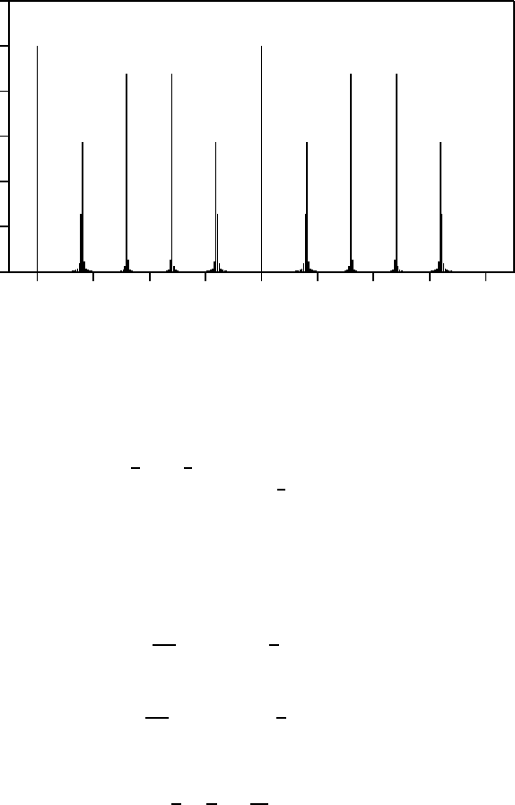
0.00

0.02

0.04

0.06

0.08

0.10

0.12

0 32 64 96 128 160 192 224 256

Figure 5.1: The probability P o f observing values of c between 0 and 255, given q = 256

and r = 10.

Letting {rc}

/r vary between −

and

, the absolute magnitude of the integral (5.10)

is easily seen to be minimized when {rc}

/r = ±

, in which case the absolute value

of expre ssion (5.10) is 2/(πr). The square of this quantity is a lower bound on the

probability tha t we see any particular state



c, x

(mod n)



with {rc}

≤ r/2; this

probability is thus asymptotically bo unded below by 4/(π

), and s o is a t least 1/3r

for suﬃciently large n.

The probability of seeing a given state



c, x

(mod n)



will thus be at least 1/3r

−r

≤ {rc}

≤

, (5.11)

i.e., if there is a d such that

−r

≤ rc − dq ≤

. (5.12)

Dividing by rq and rearr anging the terms gives



−



≤

. (5.13)

We know c and q. Because q > n

, there is at most one fraction d/r with r < n that

satisﬁes the above inequality. Thus, we can obtain the fraction d/r in lowes t terms by

rounding c/q to the nearest fraction having a denominator smaller than n. This fraction

can be found in polynomial time by using a continued fraction expans ion of c/q, which

FACTORING WITH A QUANTUM COMPUTER 19

ﬁnds all the best appr oximations of c/ q by fractions [Hardy and Wright 1979, Chapter

X, Knuth 1981].

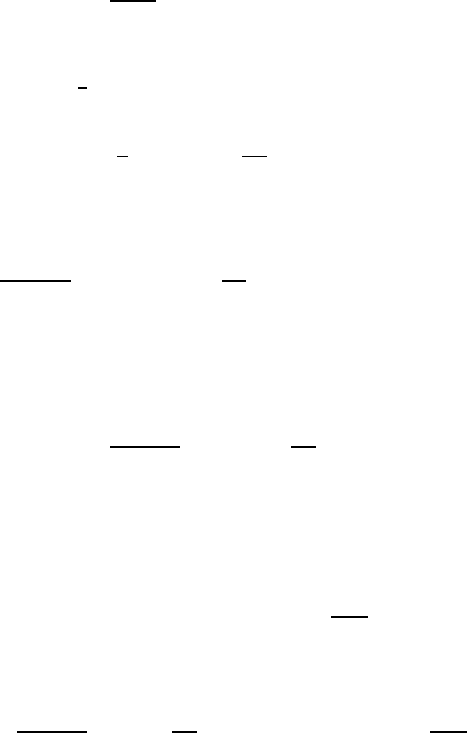
The exact probabilities as given by equation (5.7) for an example case with r = 10

and q = 256 are plotted in Figure 5.1. The value r = 10 could occur when factoring 33

if x were chosen to be 5, for exa mple. Here q is taken smaller than 33

so as to make the

values of c in the plot distinguis hable; this does not change the functional structure of

P(c). Note that with high probability the observed value of c is near an integral multiple

of q/r = 256/10.

If we have the fraction d/r in lowest terms, and if d happens to be relatively prime

to r, this will give us r. We will now c ount the number of states



c, x

(mod n)



which

enable us to compute r in this way. There are φ(r) possible values of d relatively prime

to r, where φ is Euler’s totient function [Knuth 1981, Hardy and Wright 1979, §5.5].

Each of these fractions d/r is close to o ne fraction c/q with |c/q − d/ r| ≤ 1/2q. There

are also r possible values for x

, since r is the or der of x. Thus, there ar e rφ(r) states



c, x

(mod n)



which would enable us to obtain r. Since each of these states occurs

with probability at least 1/3r

, we obtain r with probability at least φ(r)/3r. Using

the theorem that φ(r)/r > δ/ log lo g r for some constant δ [Hardy and Wr ight 1979,

Theorem 328], this shows that we ﬁnd r at least a δ/ log log r fraction of the time, so by

repeating this experiment only O(log log r) times, we are assured of a high proba bility

of success.

In practice, assuming that quantum computation is more expensive than classical

computation, it would be worthwhile to alter the above algorithm s o as to perform less

quantum computation and mo re postprocessing. First, if the observed state is |ci, it

would be wise to also try numbers close to c such as c ± 1, c ± 2, . . ., since these also

have a re asonable chance of being close to a frac tio n qd/r. Second, if c/q ≈ d/r , and

d and r have a common factor, it is likely to be small. Thus, if the observed value of

c/q is rounded oﬀ to d

′

in lowest terms, for a candidate r one should consider not

only r

′

but also its small multiples 2r

′

, 3r

′

, . . . , to see if these are the actual order of x.

Although the ﬁrst technique will only reduce the expected number of trials required to

ﬁnd r by a constant factor, the second technique will reduce the expected number of

trials for the hardest n from O(log log n) to O(1) if the ﬁrst (log n)

1+ǫ

multiples of r

′

are

considered [Odylzko 1995]. A third technique is, if two candidate r’s have been found,

say r

and r

, to test the least common multiple of r

and r

as a candidate r. This third

technique is also able to reduce the expected number of trials to a constant [Knill 1995],

and will also work in s ome cases where the ﬁrst two techniques fail.

Note that in this algor ithm for determining the order of an element, we did not use

many of the properties of multiplica tio n (mod n). In fact, if we have a permutation

f mapping the set {0, 1, 2, . . ., n − 1} into itself such that its kth iterate, f

(k)

(a), is

computable in time polynomial in log n and log k, the same algorithm will be able to

ﬁnd the order of an element a under f , i.e., the minimum r such that f

(r)

(a) = a.

6 Discrete logarithms

For every prime p, the multiplicative group (mod p) is cyclic, that is, there are generators

g such that 1, g, g

, . . . , g

p−2

comprise all the non-zero residues (mod p) [Hardy and

Wright 1979, Theorem 111, Knuth 1981]. Suppose we are given a prime p and such

20 P. W. SHOR

a generator g. The discrete logarithm of a number x with respect to p and g is the

integer r with 0 ≤ r < p −1 such that g

≡ x (mod p). The fastest algorithm known for

ﬁnding discrete logarithms modulo arbitrary primes p is Gordon’s [1993] adaptation of

the number ﬁeld sieve, which runs in time exp(O(log p)

1/3

(log log p)

2/3

)). We show how

to ﬁnd discrete logarithms on a quantum computer with two modular exponentiations

and two quantum Fourier transforms.

This algorithm will use three quantum registers. We ﬁr st ﬁnd q a power of 2 such

that q is close to p, i.e., with p < q < 2p. Next, we put the ﬁrst two registers in our

quantum computer in the uniform superposition of all |ai and |bi (mod p − 1), and

compute g

−b

(mod p) in the third register. This leaves our machine in the state

p − 1

p−2

a=0

p−2

b=0



a, b, g

−b

(mod p)



. (6.1)

As before, we use the Fourier transform A

to send |ai → |ci and |bi → |di with

probability amplitude

exp(2πi(ac+bd)/q). This is, we take the state |a, bi to the state

q−1

c=0

q−1

d=0

exp



2π i

(ac + bd)



|c, di. (6.2)

This leaves our qua ntum computer in the state

(p − 1)q

p−2

a,b=0

q−1

c,d=0

exp



2π i

(ac + bd)





c, d, g

−b

(mod p)



. (6.3)

Finally, we observe the state of the quantum c omputer.

The probability of observing a state |c, d, yi with y ≡ g

(mod p) is



(p − 1)q

a,b

a−rb≡k

exp



2π i

(ac + bd)





(6.4)

where the sum is over all (a, b) such that a − rb ≡ k (mod p − 1). Note that we now

have two moduli to deal with, p − 1 and q. While this makes keeping track of things

more confusing, it does not pose serious pro blems. We now us e the relation

a = br + k − (p − 1)

br+k

p−1

(6.5)

and substitute (6.5) in the expression (6.4) to obtain the amplitude on



c, d, g

(mod p)



which is

(p − 1)q

p−2

b=0

exp



2π i



brc + kc + bd −c(p − 1)

br+k

p−1





. (6.6)

The absolute value of the square of this amplitude is the probability of observing the

state



c, d, g

(mod p)



. We will now analyze the expression (6.6). First, a factor of

FACTORING WITH A QUANTUM COMPUTER 21

exp(2πikc/q) can be taken out of all the terms and ignored, because it does not change

the probability. Next, we split the exponent into two parts and fac tor out b to obtain

(p − 1)q

p−2

b=0

exp



2π i



exp



2π i



, (6.7)

where

T = rc + d −

p−1

{c(p − 1)}

, (6.8)

and

V =



p−1

−

br+k

p−1

k

{c(p −1)}

. (6.9)

Here by {z}

we mean the residue of z (mo d q) with −q/2 < {z}

≤ q/2, as in equation

(5.7).

We next classify possible outputs (observed states) of the quantum computer into

“goo d” and “bad.” We will show that if we g e t enough “good” outputs, then we will

likely be able to deduce r, and that furthermore, the chance of getting a “good” output

is constant. The idea is that if



{T }



rc + d −

p−1

{c(p − 1)}

− jq



≤

, (6.10)

where j is the closest integer to T /q, then as b varies between 0 and p − 2, the phase

of the ﬁr st exponential term in equation (6.7) only varies over at most half of the unit

circle. Further, if

|{c(p − 1)}

| ≤ q/12, (6.11)

then |V | is always at most q/12, so the phase of the second exponential term in equation

(6.7) never is farther than exp(πi/6 ) from 1. If conditions (6.1 0) and (6.11) both hold,

we will say that an output is “good.” We will show that if both conditions hold, then the

contribution to the probability from the corresponding term is signiﬁcant. Furthermore,

both conditions will hold with constant probability, and a reasonable sample of c’s for

which condition (6.10) holds will allow us to deduce r.

We now give a lower bound on the probability of each good output, i.e., an output

that satisﬁes conditions (6.10) and (6.11). We know that as b ranges from 0 to p − 2,

the phase of exp(2πibT/q) ranges from 0 to 2πiW where

W =

p − 2



rc + d −

p − 1

{c(p − 1)}

− jq



(6.12)

and j is as in equation (6.10). Thus, the component of the amplitude of the ﬁrst

exp onential in the summand of (6.7) in the direction

exp (πiW) (6.13)

is at least cos(2π |W/2 − W b/(p − 2)|). By condition (6.11), the phase ca n vary by at

most πi/6 due to the second exponential exp(2πiV/q). Applying this variation in the

manner that minimizes the component in the direction (6.13), we get that the component

in this direction is at least

cos(2π |W/2 − W b/(p −2)|+

). (6.14)

22 P. W. SHOR

Thus we get that the abs olute value of the amplitude (6.7) is at least

(p − 1)q

p−2

b=0

cos



2π |W/2 − W b/(p − 2)| +



. (6.15)

Replacing this sum with an integral, we get that the absolute value o f this amplitude is

at least

1/2

cos(

+ 2π|W |u)du + O





. (6.16)

From c ondition (6.10), |W | ≤

, so the erro r term is O(

). As W varies between −

and

, the integral (6.16) is minimized when |W | =

. Thus, the probability of arriving

at a state |c, d, yi that satisﬁes both conditions (6.10) and (6.11) is at least

2π /3

π/6

cos u du

, (6.17)

or at least .054/ q

> 1/(20q

We will now count the numb e r of pairs (c, d) satisfying conditions (6.10) and (6.11).

The number of pairs (c, d) such that (6.10) holds is exactly the number of po ssible c’s ,

since for every c there is exactly one d such tha t (6 .10) holds. Unless gcd(p−1, q) is large,

the number of c’s for which (6.11) holds is approximately q/6, and even if it is large,

this number is at least q/12. Thus, there are at least q/12 pairs (c, d) satisfying both

conditions. Multiplying by p−1, which is the number of possible y’s, gives approximately

pq/12 good states |c, d, yi. Combining this calculation with the lower bound 1/(20q

) on

the probability of observing each good state gives us that the probability of observing

some good state is at least p/(240q), or at least 1/480 (since q < 2p). Note that each

good c has a proba bility of at least (p − 1)/(20q

) ≥ 1/(40q) of being observed, since

there p − 1 values o f y and one value of d with which c can ma ke a good state |c, d, yi.

We now want to recover r from a pair c, d such that

−

≤

+ r



c(p − 1) − {c(p − 1)}

(p − 1)q



≤

(mod 1), (6.18)

where this equation was obtained from condition (6.10) by dividing by q. The ﬁrst thing

to notice is that the multiplier on r is a fraction with denominator p −1, since q evenly

divides c(p −1) −{c(p − 1)}

. Thus, we need only round d/q oﬀ to the nearest multiple

of 1 /(p −1) and divide (mod p − 1) by the integer

′

c(p − 1) − {c(p − 1)}

(6.19)

to ﬁnd a candidate r. To show that the quantum calculation need only be repeated a

polynomial number of times to ﬁnd the correct r requires only a few more details. The

problem is that we cannot divide by a number c

′

which is not r e latively prime to p −1.

For the discrete log algorithm, we do not know that all possible va lues of c

′

are

generated with reasonable likelihood; we only know this about one-twelfth of them.

This additional diﬃculty makes the next step harder than the c orresponding step in the

FACTORING WITH A QUANTUM COMPUTER 23

algorithm for factoring. If we knew the remainder of r modulo all prime powers dividing

p −1, we could use the Chinese remainder theorem to recover r in polynomial time. We

will o nly be able to prove that we can ﬁnd this remainder for primes larg e r than 18, but

with a little extra work we will still be able to recover r.

Recall that each good (c, d) pair is generated with probability at least 1/(20q

), and

that at least a twelfth of the p ossible c’s are in a good (c, d) pair. From equation (6.19),

it follows that these c’s are mapped from c/q to c

′

/(p − 1) by rounding to the nearest

integral multiple of 1/(p − 1). Further, the good c’s are exactly those in which c/q is

close to c

′

/(p − 1). Thus , each good c corresponds with exactly one c

′

. We would like

to show that for any prime power p

dividing p − 1, a random good c

′

is unlikely to

contain p

. If we are willing to accept a large cons tant for our algorithm, we can just

ignore the prime powers under 18; if we know r modulo all prime powers over 18, we can

try all possible residues for primes under 18 with only a (large) constant factor increase

in running time. Because at leas t one twelfth of the c’s were in a good (c, d) pair, at

least one twelfth of the c

′

’s are good. Thus, for a prime power p

, a random good c

′

divisible by p

with probability at most 12/p

. If we have t good c

′

’s, the probability

of having a prime power over 18 that divides all of them is therefore at most

18 < p



(p−1)





, (6.20)

where a|b means that a evenly divides b, so the sum is over all prime powers grea ter

than 18 tha t divide p − 1. This sum (over all integers > 18) converges for t = 2, and

goes down by at least a factor of 2/3 for each further increase of t by 1; thus for some

constant t it is less than 1/2.

Recall that each good c

′

is obtained with probability at least 1/(40q) from any

exp eriment. Since there are q/12 good c

′

’s, after 480t experiments, we are likely to

obtain a sample of t goo d c

′

’s chosen e qually likely from all good c

′

’s. Thus, we will be

able to ﬁnd a set of c

′

’s such that all prime powers p

> 20 dividing p −1 are relatively

prime to at lea st one of these c

′

’s. To obtain a polynomial time algorithm, all one need

do is try all possible sets of c

′

’s of size t; in practice, one would use an algorithm to

ﬁnd sets of c

′

’s with large common factors. This set gives the residue of r for all primes

larger than 18. For each prime p

less than 18, we have at most 18 possibilities for the

residue modulo p

, where α

is the exponent on prime p

in the prime factorization of

p−1. We can thus try all possibilities for residues modulo powers of primes less than 18:

for each possibility we can calculate the corresponding r using the Chines e r emainder

theorem and then check to see whether it is the desired discrete logarithm.

If one were to actually program this algorithm there are many ways in which the

eﬃciency could be increased over the eﬃciency shown in this paper. For exa mple, the

estimate for the number of good c

′

’s is likely too low, especially since weaker conditions

than (6.10) and (6.11) should suﬃce. This means that the number of times the exper-

iment need be run could be reduced. It also seems improbable that the distribution of

bad values of c

′

would have any relationship to primes under 18; if this is true, we need

not treat small prime powers separately.

This algorithm does not use very many properties of Z

, so we can use the same

algorithm to ﬁnd discrete logarithms over other ﬁelds such as Z

, as long as the ﬁeld

24 P. W. SHOR

has a cyclic multiplicative group. All we need is that we know the order of the generator,

and that we can multiply and take inverses of elements in polynomial time. The order

of the generator could in fact be computed using the quantum order-ﬁnding algorithm

given in §5 of this paper. Boneh a nd Lipton [1995] have generalized the algorithm so as

to be able to ﬁnd discrete logarithms when the group is abelian but not cyclic.

7 Comments and open problems

It is currently believed that the most diﬃcult aspect of building an actual quantum

computer will b e dealing with the problems o f imprecision and decoherence. It was

shown by Bennett et al. [1994] that the quantum gates need only have precision O(1/t)

in order to have a re asonable probability of completing t steps of quantum computation;

that is, there is a c such that if the amplitudes in the unitary matric e s representing the

quantum gates are all perturbed by at most c/t, the quantum computer will still have a

reasonable chance of producing the desired output. Similarly, the decoherence needs to

be only polynomially small in t in o rder to have a reasonable probability of completing t

steps of computation successfully. This holds not only for the simple model of decoher-

ence where each bit has a ﬁxed probability of dec ohering at e ach time step, but als o for

more complicated models of decoherence which are derived from fundamental quantum

mechanical considerations [Unruh 1995, Palma et al. 1995, Chuang et al. 1995]. How-

ever, building quantum computers with high enough precision a nd low enough deco-

herence to a c c urately perform long computations may present formidable diﬃculties to

exp erimental physicists. In classical computers, error probabilities c an be reduced not

only though har dware but also through software, by the use of redundancy and error-

correcting codes. T he most obvious method of using redundancy in quantum computers

is ruled out by the theorem that quantum bits cannot be cloned [Peres 1993, §9-4],

but this arg ument does not rule out more complicated ways of reducing inaccuracy or

decoherence using software. In fact, some progress in the direction of reducing inaccu-

racy [B erthiaume et al. 1994] and decoherence [Shor 1995] has already been made. The

result of Bennett et al. [1995] that quantum bits can be faithfully transmitted over a

noisy quantum channel gives further hope that qua ntum computations can similarly be

faithfully carried out using noisy quantum bits and noisy quantum ga tes .

Discrete logarithms and factoring a re not in themselves widely useful problems. They

have only become useful because they have been found to be crucial for public-key cr yp-

tography, and this application is in turn p ossible only because they have been presumed

to be diﬃcult. This is also true of the generalizations of Boneh and Lipton [1995 ] of

these algorithms. If the only uses of quantum computation remain discrete logarithms

and fa c toring, it will likely become a special-purpose technique whose only raison d’ˆetre

is to thwart public key cryptosystems. However, there may be other hard problems

which could be solved asymptotically faster with quantum computers. In particular,

of interesting problems not known to be NP-complete, the problem of ﬁnding a short

vector in a lattice [Adleman 199 4, Adleman and McCurley 1995] seems as if it might

potentially be amenable to solution by a quantum computer.

In the history of computer science, howe ver, most important problems have turned

out to be either polynomial-time or NP-complete. Thus quantum computers will likely

not become widely use ful unless they can solve NP-complete problems. Solving NP-

FACTORING WITH A QUANTUM COMPUTER 25

complete problems eﬃciently is a Holy Grail of theoretical computer science which very

few people expect to be possible on a classica l computer. Finding poly nomial-time

algorithms for solving these problems on a quantum computer would be a momentous

discovery. There ar e s ome weak indications that quantum computers are not powerful

enough to solve NP-complete problems [Bennett et al. 1994], but I do not believe that

this potentiality should be ruled out as yet.

Acknowledgements

I would like to thank Jeﬀ Lagarias for ﬁnding and ﬁxing a critical error in the ﬁrst version

of the discrete log algorithm. I would also like to thank him, David Applegate, Charles

Bennett, Gilles Br assard, Andrew Odlyz ko, Dan Simon, Bob Solovay, Umesh Vazirani,

and correspondents too numerous to list, for productive discussions, for corrections to

and improvements of e arly drafts of this paper, and for pointers to the literature.

REFERENCES

L. M. Adleman (1994), Algorithmic number theory—The complexity contribution, in Proceedings of

the 35th Annual Symposium on Foundations of Computer Science, IEEE Computer Society Press,

Los Alamitos, CA, pp. 88–113.

L. M. Adleman and K. S. McCurley (1995), Open problems in number-t heoret ic complexity II, in

Proceedings of the 1994 Algorithmic Number Theory Symposium, Ithaca, NY, May 6–9, Lecture

Notes in Computer Science, L. M . Adleman and M.-D . Huang, eds., Springer, to appear.

A. Barenco, C. H. Bennett, R. Cleve, D. P. DiVincenzo, N. Margolus, P. Shor, T. Sleator,

J. A. Smolin, and H. Weinfurter (1995a), Elementary gates for quantum computation, Phys.

Rev. A, 52, pp. 3457–3467.

A. Barenco, D. Deutsch, A. Ekert, and R. Jozsa (1995b), Conditional quantum dynamics and logic

gates, Phys. Rev. Lett., 74, pp. 4083–4086.

P. Benioff (1980), The computer as a physical system: A microscopic quantum mechanical Hamilto-

nian model of computers as represent ed by Turing machines, J. Statist. Phys., 22, pp. 563–591.

(1982a), Quantum mechanical Hamiltonian models of Turing machines, J. Statist. Phys., 29,

pp. 515–546.

(1982b), Quantum mechanical Hamiltonian models of Turing machines that dissipate no energy,

Phys. Rev. Lett., 48, pp. 1581–1585.

C. H. Bennett (1973), Logical reversibility of computation, IBM J. Res. Develop., 17, pp. 525–532.

(1989), Time/space trade-oﬀs for reversible computation, SIAM J. Comput., 18, pp. 766–776.

C. H. Bennett, E. Bernstein, G. Brassard, and U. Vazirani (1994), Strengths and weaknesses of

quantum computing, preprint.

C. H. Bennett, G. Brassard, S. Popescu, B. Schumacher, J. A. Smolin, and W. K. Wooters

(1995), Puriﬁcation of noisy entanglement, and faithful teleportation via noisy channels, Phys.

Rev. Lett., to appear.

E. Bernstein and U. Vazirani (1993), Quantum complexity theory, in Pro ceedings of the 25th Annual

ACM Symposium on Theory of Computing, ACM, New York, pp. 11–20.

26 P. W. SHOR

A. Berthiaume and G. Brassard (1992a), The quantum challenge to structural complexity t heory, in

Proceedings of the Seventh Annual Structure in Complexity Theory Conference, IEEE Computer

Society Press, Los Alamitos, CA, pp. 132–137.

(1992b), Oracle quantum computing, in Proceedings of the Workshop on Physics of Computation:

PhysComp ’92, IEEE Computer Society Press, Los A lamitos, CA, pp. 195–199.

A. Berthiaume, D. Deutsch, and R. Jozsa (1994), The stabilisation of quantum computations, in

Proceedings of the Workshop on Physics of Computation: PhysComp ’94, IEEE Computer Society

Press, Los Alamitos, CA, pp. 60–62.

M. Biafore (1994), Can quantum computers have simple Hamiltonians, in Proceedings of the Workshop

on Physics of Computation: PhysComp ’94, IEEE Computer Society Press, Los Alamitos, CA,

pp. 63–68.

D. Boneh and R. J. Lipton (1995), Quantum cryptanalysis of hidden linear functions, Advances in

Cryptology—CRYPTO ’ 95, Proceedi ngs of the 15th Annual International Cryptology Conference,

Santa Barbara, CA, Aug. 27–31, D. Coppersmith, ed. Springer, pp. 424–437.

J. F. Canny and J. Reif (1987), New lower bound techniques for robot motion planning problems, in

Proceedings of the 28th Annual Symposium on Foundations of Computer Science, IEEE Computer

Society Press, Los Alamitos, CA, pp. 49–60.

J. Choi, J. Sellen, and C.-K. Yap (1995), Precision-sensitive Euclidean shortest path in 3-space,

in Proceedings of the 11th Annual Symposium on Computational Geometry, ACM, New York,

pp. 350–359.

I. L. Chuang, R. Laflamme, P. W. Shor, and W. H. Zurek (1995), Quantum computers, factoring

and decoherence , Science, 270, pp. 1635–1637.

I. L. Chuang and Y. Yamamoto (1995), A simple quantum computer, Phys. Rev. A, 52, pp. 3489–3496.

A. Church (1936), An unsolvable problem of elementary number theory, Am er. J. Math., 58, pp. 345–

363.

J. I. Cirac and P. Zoller (1995), Quantum computations with cold trapped ions, Phys. Rev. Lett.,

74, pp. 4091–4094.

R. Cleve (1994), A note on computing Fourier transforms by quantum programs, preprint.

D. Coppersmith (1994), An approximate Fourier transform useful in quantum factoring, IBM Research

Report RC 19642.

D. Deutsch (1985), Quantum theory, the Church–Turing principle and the universal quantum com-

puter, Proc. Roy. Soc. London Ser. A, 400, pp. 96–117.

(1989), Quantum computational networks, Proc. Roy. Soc. London Ser. A, 425, pp. 73–90.

D. Deutsch, A. Barenco, and A. Ekert (1995), Universality of quantum computation, Proc. Roy.

Soc. London Ser. A, 449, pp. 669-677.

D. Deutsch and R. Jozsa (1992), Rapid solution of problems by quantum computation, Proc. Roy.

Soc. London Ser. A, 439, pp. 553–558.

D. P. DiVincenzo (1995), Two-bit gates are universal for quantum computation, Phys. Rev. A, 51,

pp. 1015–1022.

A. Ekert and R. Jozsa (1995), Shor’s quantum algorithm for factorising numbers, Rev. Mod. Phys.,

to appear.

R. Feynman (1982), Simulating physics with computers, Internat. J. Theoret. Phys., 21, pp. 467–488.

FACTORING WITH A QUANTUM COMPUTER 27

(1986), Quantum mechanical computers, Found. Phys., 16, pp. 507–531. Originally appeared in

Optics News (February 1985), pp. 11–20.

E. Fredkin and T. Toffoli (1982), Conservative logic, Internat. J. Theoret. Phys., 21, pp. 219–253.

D. M. Gordon (1993), Discrete logarithms in GF(p) using the number ﬁeld sieve, SIAM J. Discrete

Math., 6, pp. 124–139.

G. H. Hardy and E. M. Wright (1979), An Introduction to the Theory of Numbers, Fifth ed., Oxford

University Press, New York.

J. Hartmanis and J. Simon (1974), On the power of multiplication in random access machines, in

Proceedings of the 15th Annual Symposium on Switching and Automata Theory, IEEE Computer

Society, Long Beach, CA, pp. 13–23.

A. Karatsuba and Yu. Ofman (1962), Multiplication of multidigit numbers on automata, Dokl. Akad.

Nauk SSSR, 145, pp. 293–294 (in Russian). English translation i n Sov. Phys. Dokl., 7 (1963),

pp. 595–596.

D. E. Knuth (1981), The Art of Computer Programming, Vol. 2: Seminumerical Algorithms, Second

ed., Addison-Wesley.

E. Knill (1995), personal communication.

R. Landauer (1995a), Is quantum mechanics useful? Philos. Trans. Roy. Soc. London Ser. A, to

appear.

(1995b), Is quant um mechanically coherent computation useful? in Proceedings of the Drexel-4

Symposium on Quantum Nonintegrability—Quantum Classical Correspondence, D . H. Feng and

B-L. Hu, eds., International Press, to appear.

Y. Lecerf (1963), Machines de Turing r´eversibles. R´ecursive insolubilit´e en n ∈ N de l’´equation

u = θ

u, o`u θ est un isomorphisme de codes, C. R. Acad. Fran¸caise Sci., 257, pp. 2597–2600.

A. K. Lenstra and H. W. Lenstra, Jr., eds. (1993), The Development of the Number Field Sieve,

Lecture Notes in Mathematics, Vol. 1554, Springer.

A. K. Lenstra, H. W. Lenstra, Jr., M. S. Manasse, and J. M. Pollard (1990), The number ﬁe ld

sieve, in Proceedings of the 22nd Annual ACM Symposium on Theory of Computing, ACM, New

York, pp. 564–572. An expanded version appeared in Lenstra and Lenstra [1993], pp. 11–42.

R. Y. Levine and A. T. Sherman (1990), A note on Bennett’s time-space tradeoﬀ for reversible

computation, SIAM J. Comput., 19, pp. 673–677.

S. Lloyd (1993), A potentially realizable quantum computer, Science, 261, pp. 1569–1571.

(1994), Envisioning a quantum supercomputer, Science, 263, p. 695.

(1995), Almost any quantum logic gate is universal, Phys. Rev. Lett., 75, pp. 346–349.

N. Margolus (1986), Quantum computation, Ann. New York Acad. Sci., 480, pp. 487–497.

(1990), Parallel quantum computation, in Complexity, Entropy and the Physics of Information,

Santa Fe Institute Studies in the Sciences of Complexity, Vol. VIII, W. H. Zurek, ed., Addison-

Wesley, pp. 273–287.

G. L. Miller (1976), Rie mann’s hypothesis and tests for primality, J. Comput. System Sci., 13, pp. 300–

317.

A. M. Odlyzko (1995), personal communication.

G. M. Palma, K.-A. Suominen, and A. K. Ekert (1995), Quantum computers and dissipation, Proc.

Roy. Soc. London Ser. A, submitted.

28 P. W. SHOR

A. Peres (1993), Quantum Theory: Concepts and Methods, Kluwer Academic Publishers.

C. Pomerance (1987), Fast, rigorous factorization and discrete logarithm algorithms, in Discrete Algo-

rithms and Complexity, Proceedings of the Japan–US Joint Seminar, June 4–6, 1986, Kyoto, D. S.

Johnson, T. Nishizeki, A. Nozaki, and H. S. Wil f, eds., Academic Press, pp. 119–143.

E. Post (1936), Finite combinatory processes. Formulation I., J. Symbolic Logic, 1, pp. 103–105.

R. L. Rivest, A. Shamir, and L. Adleman (1978), A method of obtaining digital signatures and

public-key cryptosystems, Comm. Assoc. Comput. Mach., 21, pp. 120–126.

L. A. Rubel (1989), Digital simulation of analog computation and Church’s thesis, J. Symbolic Logic,

54, pp. 1011–1017.

A. Sch

onhage (1982), Asymptotically fast algorithms for the numerical multiplication and division

of polynomials with complex coeﬃcients, in Computer Algebra EUROCAM ’82, Lecture Notes in

Computer Science, Vol . 144, J. Calmet, ed., Springer, pp. 3–15.

A. Sch

onhage, A. F. W. Grotefeld, and E. Vetter (1994), Fast Algorithms: A Multitape Turing

Machine Implementation, B. I. Wissenschaf tsverlag, Mannheim, Germany.

A. Sch

onhage and V. Strassen (1971), Schnelle Multiplikation grosser Zahlen, Computing, 7,

pp. 281–292.

P. W. Shor (1994), Algorithms for quantum computation: Discrete logarithms and factoring, in Pro-

ceedings of the 35th Annual Symposium on Foundations of Computer Science, IEEE Computer

Society Press, Los Alamitos, CA, pp. 124–134.

(1995), Scheme for reducing decoherence in quantum memory, Phys. Rev. A, 52, pp. 2493–2496.

D. Simon (1994), On the power of quantum computation, in Proceedings of the 35th Annual Symposium

on Foundations of Computer Science, IEEE Computer Society Press, Los Alamitos, CA, pp. 116–

123.

T. Sleator and H. Weinfurter (1995), Realizable universal quantum logic gates, Phys . Rev. Lett.,

74, pp. 4087–4090.

R. Solovay (1995), personal communication.

K. Steiglitz (1988), Two non-standard paradigms for computation: Analog machines and cellular

automata, in Performance Limits in Communication Theory and Practice, Proceedings of the NATO

Advanced Study Institute, Il Ciocco, Castelvecchio Pascoli, Tuscany, Italy, July 7–19, 1986, J. K.

Skwirzynski, ed., Kluwer Academic Publishers, pp. 173–192.

W. G. Teich, K. Obermayer, and G. Mahler (1988), Structural basis of multistationary quantum

systems II: Eﬀective few-particle dynamics, Phys. Rev. B, 37, pp. 8111–8121.

T. Toffoli (1980), Reversible computing, in Automata, Languages and Programming, Seventh Collo-

quium, Lecture Notes in Computer Science, Vol. 84, J. W. de Bakker and J. van Leeuwen, eds.,

Springer, pp. 632–644.

A. M. Turing (1936), On computable numbers, with an application to the Entscheidungsproblem, Proc.

London Math. Soc. (2), 42, pp. 230–265. Corrections in Proc. London Math. Soc. (2), 43 (1937),

pp. 544–546.

W. G. Unruh (1995), Maintaining coherence in quantum computers, Phys. Rev. A, 51, pp. 992–997.

P. van Emde Boas (1990), Machine models and simulations, in Handbook of Theoretical Computer

Science, Vol. A, J. van Leeuwen, ed., Elsevier, Amsterdam, pp. 1–66.

A. Vergis, K. Steiglitz, and B. Dickinson (1986), The complexity of analog computation, Math.

Comput. Simulation, 28, pp. 91–113.

A. Yao (1993), Quantum circuit complexity, in Proceedings of the 34th Annual Symposium on Foun-

dations of Computer Science, IEEE Computer Society Press, Los Alamitos, CA, pp. 352–361.