

Transfer Function Limitations
ZIC
Modern control theory
is applicable to:
– MIMO systems.
– linear or nonlinear
Systems.
– time invariant or time
varying.
Conventional control
theory is applicable to:
– SISO systems.
– Linear.
– time invariant.
2

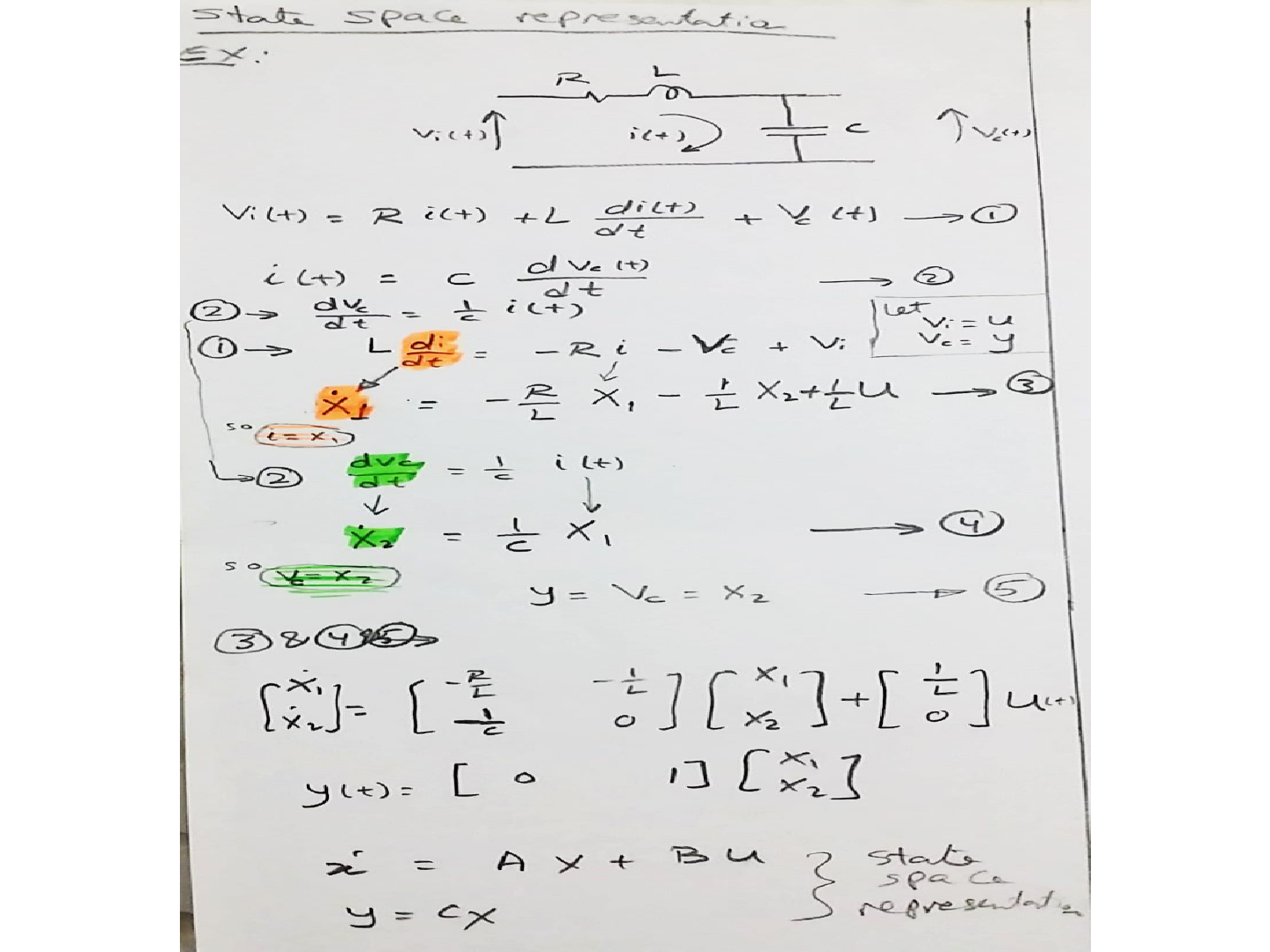
State Space Representation
3
Example
Consider the mechanical system shown in figure. We assume that the
system is linear. The external force u(t) is the input to the system, and
the displacement y(t) of the mass is the output. The displacement y(t)
is measured from the equilibrium position in the absence of the
external force. This system is a single-input, single-output system.
From the diagram, the system equation is
This system is of second order. This means that
the system involves two integrators. Let us define
state variables
and
as
Example
Then we obtain
Or
The output equation is
Example
)(
1
0
)(
)(
10
)(
)(
2
1
2
1
tu
m
tx
tx
m
b
m
k
tx
tx
)(
)(
01)(
2
1
tx
tx
ty
• In a vector-matrix form,
)()()( tButAxtx
)()( tCxty
Example(summary)
• The system equati on is
• Let
• Then
• Or
)(
1
0
)(
)(
10
)(
)(
2
1
2
1
tu
m
tx
tx
m
b
m
k
tx
tx
)(
)(
01)(
2
1
tx
tx
ty
8

State Space Modeling
• State space equations can be simplified as
State Equation
Output Equation
)()()( tButAxtx
)()()( tDutCxty
Where,
x(t) ------------ State Vector
A(nxn) ------ System Matrix
B(nxp) ------- Input Matrix
u(t) ----------- Input Vector
y(t) ----------- Output Vector
C(qxn) ------ Output Matrix
D -------------- Feed forward Matrix

Canonical Forms
Canonical forms are the standard forms of state space models.
Each of these canonical form has specific advantages which
makes it convenient for use in particular design technique.
There are several canonical forms of state space models
– Phase variable canonical form
– Controllable Canonical form
– Observable Canonical form
– Diagonal Canonical form
• Jordan Canonical Form
It is interesting to note that the dynamics properties of system
remain unchanged whichever the type of representation is
used.

• Obtain the state equation in phase variable form for the
following differential equation, where u(t) is input and y(t) is
output.
• The differential equation is third order, thus there are three
state variables:
• And their derivatives are (i.e state equations)
Phase Variable Canonical form

Phase Variable Canonical form
• In vector matrix form
3
2
1
3
2
1
3
2
1
001)(
)(
5
0
0
234
100
010
x
x
x
ty
tu
x
x
x
x
x
x

state-space representations
• Consider a system defined by
• where
u
is the input and
y
is the output.
• This equation can also be written as
• We will present state-space representations of the system
defined by above equations in controllable canonical form
and observable canonical form.
ububububyayayay
nn
nn
onn
nn
1
1
11
1
1
Controllable Canonical Form
u
x
x
x
x
aaaax
x
x
x
n
n
nnnn
n
1
0
0
0
1000
0100
0010
1
2
1
121
1
2
1
ub
x
x
x
x
bbbby
o
n
n
nn
1
2
1
121
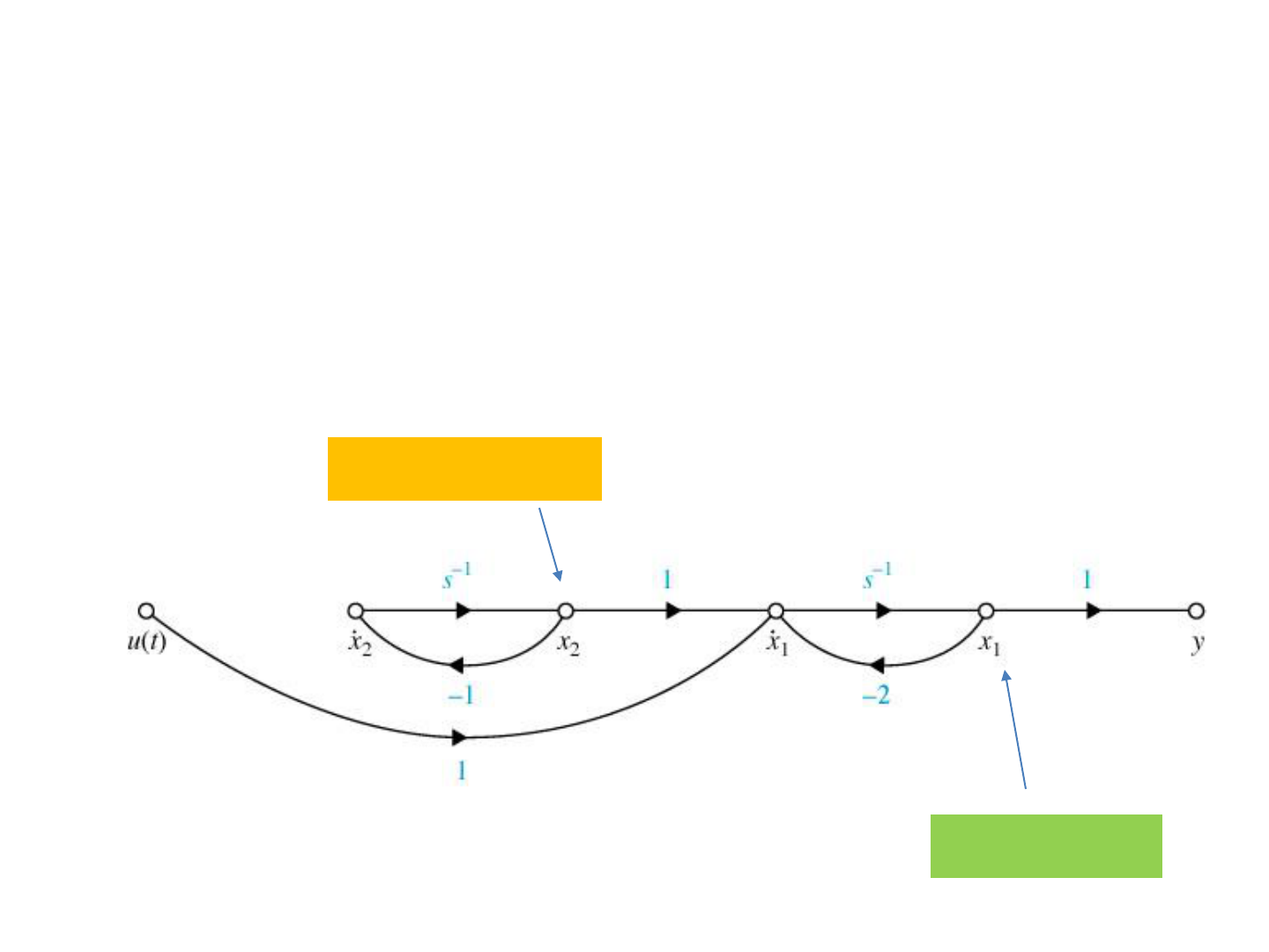
Controllable Canonical Form (Example)
u
x
x
x
x
1
0
32
10
2
1
2
1
2
1
13
x
x
y
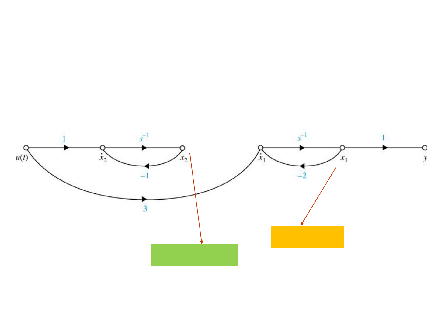
Observable Canonical Form
u
b
b
b
b
x
x
x
x
a
a
a
a
x
x
x
x
n
n
n
n
n
n
n
n
1
2
1
1
2
1
1
2
1
1
2
1
100
000
001
000
ub
x
x
x
x
y
o
n
n
1
2
1
1000
Controllable form:
17
Observable form:
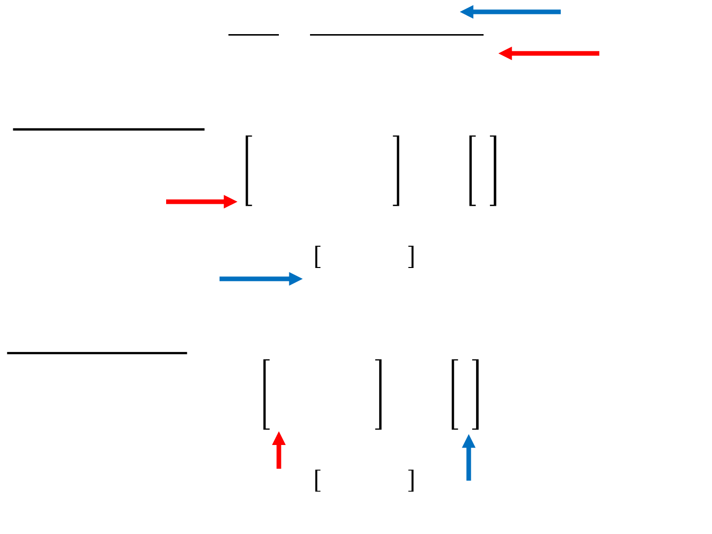
Diagonal Canonical Form
u
x
x
x
p
p
p
x
x
x
n
n
n
1
1
1
0
.
.
0
2
1
2
1
2
1
ub
x
x
x
cccy
o
n
n
2
1
21

Example
u
x
x
x
x
1
1
20
01
2
1
2
1
2
1
12
x
x
y
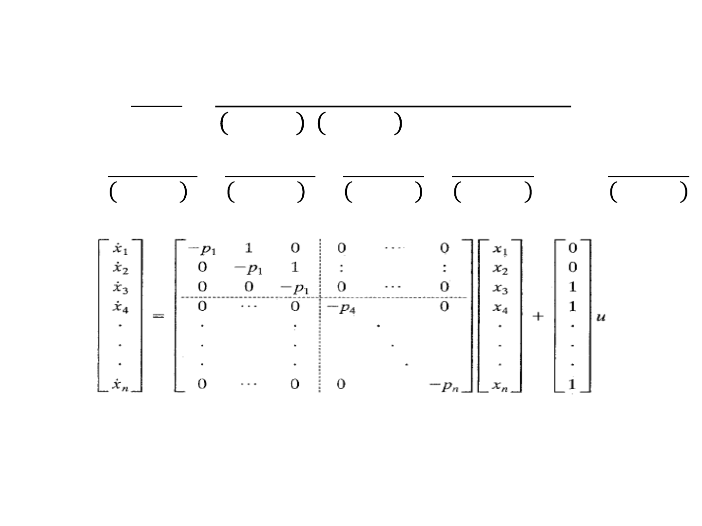
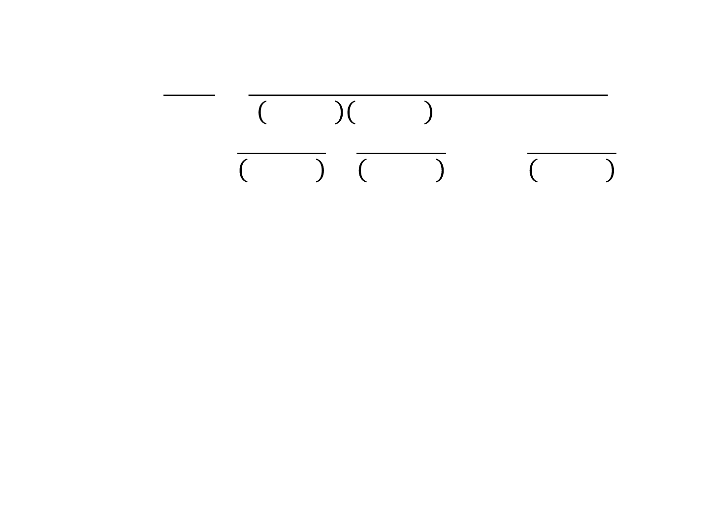
Jordan Canonical Form
ub
x
x
x
cccy
o
n
n
2
1
21

21

State Space to T.F
• Now Let us convert a space model to a transfer function model.
• Taking Laplace transform of equation (1) and (2) considering
initial conditions to zero.
• From equation (3)
)()()( tButAxtx
(1)
)()()( tDutCxty
(2)
)()()( sBUsAXssX
(3)
)()()( sDUsCXsY
(4)
)()()( sBUsXAsI
)()()(
1
sBUAsIsX
(5)

Transfer Matrix (State Space to T.F)
• Substituting equation (5) into equation (4) yields
)()()()(
1
sDUsBUAsICsY
)()()(
1
sUDBAsICsY
DBAsIC
sU
sY
1
)(
)(
)(

Example 3
Convert the following State Space Model to
Transfer Function Model if K=3, B=1 and
M=10;
)(tf
M
v
x
M
B
M
K
v
x
1
010
v
x
ty 10)(

Example 3
Substitute the given values and obtain A, B,
C and D matrices.
)(
10
1
0
10
1
10
3
10
tf
v
x
v
x
v
x
ty 10)(

Example 3
10
1
10
3
10
A
10C
10
1
0
B
0D
DBAsIC
sU
sY
1
)(
)(
)(

Example 3
10
1
10
3
10
A
10C
10
1
0
B
0D
10
1
0
10
1
10
3
10
0
0
10
)(
)(
1
s
s
sU
sY

Example 3
10
1
0
10
1
10
3
10
0
0
10
)(
)(
1
s
s
sU
sY
10
1
0
10
1
10
3
1
10
)(
)(
1
s
s
sU
sY
10
1
0
10
3
1
10
1
10
3
)
10
1
(
1
10
)(
)(
s
s
ss
sU
sY

Example 3
10
1
0
10
3
1
10
1
10
3
)
10
1
(
1
10
)(
)(
s
s
ss
sU
sY
10
1
0
10
3
10
3
)
10
1
(
1
)(
)(
s
ss
sU
sY
10
10
3
)
10
1
(
1
)(
)( s
ss
sU
sY

Example 3
10
10
3
)
10
1
(
1
)(
)( s
ss
sU
sY
3)110()(
)(
ss
s
sU
sY
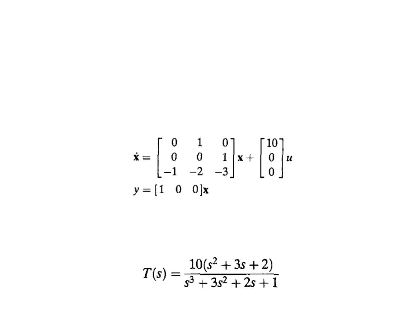
Example
Obtain the transfer function T(s) from
following state space representation.
Answer
State Controllability
A system is completely controllable if there exists an
unconstrained control u(t) that can transfer any initial
state x(t
o
) to any other desired location x(t) in a finite
time, t
o
≤ t ≤ T.
controllable
uncontrollable

State Controllability
Controllability Matrix C
T
System is said to be state controllable if
BABAABBC
n
T
12
)( nCrank T

State Controllability (Example)
Consider the system given below
xy
uxx
21
0
1
30
01

State Controllability (Example)
• Controllability matrix C
T
is obtained as
• Thus
• Since therefore system is not completely
state controllable.
ABBCT
00
11
TC
0
1
B
0
1
A B
State Observability
A system is completely observable if and only if there exists a
finite time T such that the initial state x(0) can be determined
from the observation history y(t) given the control u(t), 0≤ t ≤ T.
observable
unobservable

State Observability
Observable Matrix (O
T
)
The system is said to be completely state observable if
1
2
Matrix ity Observabil
n
CA
CA
CA
C
OT
nOrank T )(

Example
Consider the system given below
O
T
is obtained as
Where
xy
uxx
40
1
0
20
10
CA
C
OT
40C
120
20
10
40
CA

State Observability (Example)
• Therefore O
T
is given as
• Since
therefore system is not completely state
observable.
120
40
TO

Example
Check the state controllability, state
observability of the following system
10,
1
0
,
01
10
CBA

45
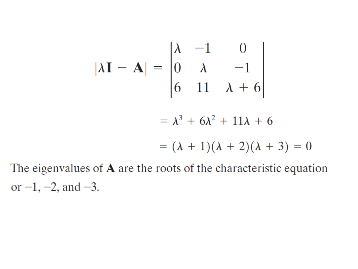
Eigenvalues & Eigen Vectors
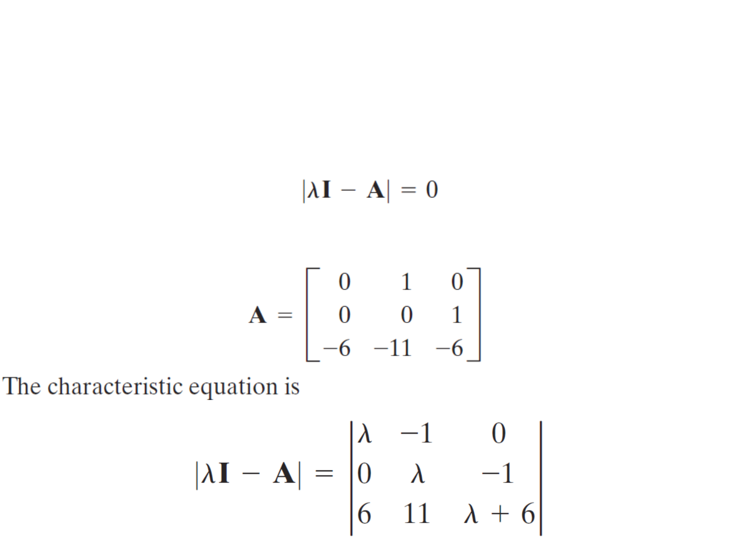
Eigenvalues & Eigen Vectors
• The eigenvalues of an
nxn
matrix A are the roots of the
characteristic equation.
• Consider, for example, the following matrix A:
46
Eigen Values & Eigen Vectors
47

Example#4
• Find the eigenvalues if
– K = 2
– M=10
– B=3
)(tf
M
v
x
M
B
M
K
v
x
1
010
48

Similarity Transformations
• It is desirable to have a means of transforming one state-space
representation into another.
• This is achieved using so-called similarity transformations.
• Consider state space model
• Along with this, consider another state space model of the
same plant
• Here the state vector , say, represents the physical state
relative to some other reference, or even a mathematical
coordinate vector.
)()()( tButAxtx
)()()( tDutCxty
)()()( tuBtxAtx
)()()( tuDtxCty

Similarity Transformations
• When one set of coordinates are transformed into another
set of coordinates of the same dimension using an algebraic
coordinate transformation, such transformation is known as
similarity transformation.
• In mathematical form the change of variables is written as,
• Where T is a nonsingular
nxn
transformation matrix.
• The transformed state is written as
)( )( txTtx
)( )(
1
txTtx

Similarity Transformations
• The transformed state is written as
• Taking time derivative of above equation
)( )(
1
txTtx
(t) )(
1
xTtx
)()( )(
1
tButAxTtx
)( )( txTtx
)()()( tButAxtx
)()( )(
1
tButxATTtx
)()()(
11
tBuTtxATTtx
)()()( tuBtxAtx
ATTA
1
BTB
1
Similarity Transformations
• Consider transformed output equation
• Substituting
in above equation
• Since output of the system remain unchanged [i.e.
] therefore above equation is compared with
that yields
)()()( tuDtxCty
)()()(
1
tuDtxTCty
CTC
DD

Similarity Transformations
• Following relations are used to preform transformation of
coordinates algebraically
CTC
DD
ATTA
1
BTB
1

Transformation to DCF
• In linear algebra, a square matrix
A
is called diagonalizable, if
there exists an invertible matrix
P
such that
P
-1
AP
is a
diagonal matrix.
•
n
-by-
n
square matrix A is called invertible (also nonsingular)
if there exists an
n
-by-
n
square matrix B such that
AB=BA=I
• Diagonalizable matrices are
o easy to handle
o their eigenvalues and eigenvectors are known
o can raise a diagonal matrix to a power by simply raising the
diagonal entries to that same power
o the determinant of a diagonal matrix is simply the product of all
diagonal entries.
Example
Find Eigen values, Eigen vectors, and diagonal form of
this system
=
68

Eigen vectors
,
Or Dependent
Let
, so
,
,
69

Eigen vectors
Or Dependent
Let
, so
,
,
70

71

72

83

89
