Dynamic Processes Permitting Stable Coexistence of Antimicrobial

ScienceAsia 33 (2007): 197-206

Dynamic Processes Permitting Stable Coexistence of

Antimicrobial Resistant and Non-Resistant Organisms in

a Gastrointestinal Tract Model

Tippawan Puttasontiphot

a

, Yongwimon Lenbury

a*

, Chontita Rattanakul

a

, Sahattaya

Rattanamongkonkul

b

, John R. Hotchkiss

c

and Philip S. Crooke

d

a

Department of Mathematics, Faculty of Science, Mahidol University,Bangkok, 10400, Thailand.

b

Department of Mathematics, Faculty of Science, Burapha University,Chonburi, 20131, Thailand.

c

Department of Critical Care Medicine, University of Pittsburgh,Pittsburgh, PA 15261, USA.

d

Biomathematics Study Group, Department of Mathematics,Vanderbilt University, Nashville, TN 37240, USA.

* Corresponding author, E-mail: [email protected]

Received 7 Jun 2006

Accepted 22 Dec 2006

ABSTRACT: In this paper, bacteria-antibiotic dynamics in a gastrointestinal tract exposed to antimicrobial

selection pressure is modeled as occurring in a continuous chemostat. Two populations of microorganisms,

one sensitive and the other resistant to an inhibitor, namely an antibiotic, compete for a single limiting

resource. It is shown that conditions exist whereby the two types of bacteria can persist. Application of the

singular perturbation analysis also yields delineating conditions on the “effective” antibiotic level that encode

information on the minimum inhibitory concentration (MIC) and the minimum antibiotic concentration

(MAC), which are extremely important parameters commonly used to quantify the activity of antibiotics

against a given bacterium.

K

EYWORDS: gastrointestinal tract model, antimicrobial resistance, continuous chemostat, singular perturbation.

doi: 10.2306/scienceasia1513-1874.2007.33.197

INTRODUCTION

As has been noted by Nolting and Derendorf

1

, “the

outcome of treating bacterial infections with antibiotics

is a function of multiple variables.” Therapeutic efficacy

depends on bacterial susceptibility to the antibiotics,

specific properties of the infected site, metabolism in

antibiotic elimination, dosing regimen, and several other

factors. Up to date, many questions about dosing

regimen remain unanswered

1

. Risk of infection may

not be reduced even though the antibiotic dose is

titrated to produce serum concentrations within the

recommended range.

Parameters traditionally used to quantify the activity

of antibiotic against bacterial infection are the minimum

inhibitory concentration (MIC), the minimum

bactericidal concentration (MBC) and the minimum

antibiotic concentration (MAC). These parameters are

determined under standardized conditions as

discussed in

Nolting and Derendorf’s report

1

. There

are several disadvantages to this approach, however.

The in vitro models do not necessarily reflect the in vivo

situation where the drug undergoes metabolism and

elimination. The inoculum size can be variable and the

infected size might pose severe restrictions on antibiotic

diffusion into the tissue

1

. Most importantly, prolonged

treatment can give rise to resistant strains. Such

concerns have prompted researchers to devise in vitro

systems or models to simulate in vivo conditions and to

investigate the killing effects of antibiotics against

bacteria as a function of time.

The mammalian digestive tract becomes colonized

with bacteria acquired, since birth, from the mother

and the immediate environment. Numerous bacterial

species populate the digestive tract and constitute the

indigeneous gastrointestinal flora of a mammal

contributing to a gastrointestinal ecosystem that is

necessary for an animal to digest and absorb nutrients

efficiently from the alimentary

2

. It is well known that

the gastrointestinal (GI) microflora that inhabit the

digestive tract of mammals have a great influence on

the host’s physiology, intestinal anatomy and resistance

to infectious diseases

3

.

Several studies

4,5

have demonstrated that

overgrowth of intestinal bacteria promotes their

translocation from the GI tract to other organs. Such

translocation of viable bacteria from the GI tract to the

mesenteric lymph nodes and other organs is

undoubtedly an initial step in the pathogenesis of many

bacterial diseases

4

. It was also reported by Steffenand

and Berg

5

that the extent of translocation of certain

indigenous bacteria is directly related to their

population levels in the GI tract.

Apparently, there is a great variety in the

198

ScienceAsia ScienceAsia

ScienceAsia

33 (2007)33 (2007)

33 (2007)

composition of gastrointestinal microflora among

animals, as well as varying degrees of sensitivity among

the microbials to the various antibiotics that might be

used to inhibit their growth. However, the emergence

of resistant microorganisms is always a potential risk

when antibiotics are administered.

Moreover, a recent report

6

indicated that there is

huge potential for genetic exchange to occur within the

dense, diverse anaerobic microbial population

inhabiting the GI tract of humans and animals.

Specifically, Scott

6

reported on recent evidence that

anaerobic bacteria native to the rumen or hindgut

harbour both novel antibiotic resistance genes and

novel conjugative transposons (CTns). These CTns,

and previously characterized CTns, can be transferred

to a wide range of commensal bacteria under laboratory

and in vivo conditions.

In their investigation of the impact of various

antibiotics on the fecal flora of newborn infants, Bennet

et al.

7

found that sequential development of the neonatal

intestinal flora can be dramatically altered upon

administration of broad-spectrum antimicrobial agents.

It takes possibly several weeks for the intestinal flora

to return to normal even when administration of the

antimicrobial agents was discontinued.

Additional evidence that demonstrates the

importance of intestinal flora in the control of GI

overgrowth was given in

the work of Burr and Sugiyama

8

, where it was shown that adult mice with normal

microbial flora but treated with large oral doses of two

broad spectrum antimicrobial agents are at least 50-

fold more susceptible to C. botulinum intestinal

colonization than untreated mice. The increased

susceptibility of antimicrobial treated mice to C.

botulinum intestinal colonization is terminated when

the antibiotics are stopped and the mice are housed

with untreated control mice.

A body of evidence

9

suggests that multiple

mechanisms are employed by the flora to exclude non-

indigeneous organisms from the intestinal tract and to

maintain the status quo. Only the most extreme stress

situations, such as antibiotic administration, have major

effects on the stability of the initial flora. Experiments

of Freter et al.

10

provided data on possible E. coli

population control mechanisms. Anaerobic continuous

flow cultures of homogenates of intestinal contents

from conventional mice mixed with E. coli in veal infusion

broth suppressed E. coli population growth, compared

with pure continuous flow cultures of E. coli. The

inhibition of E. coli multiplication was reversed,

however, by addition of glucose. These results suggested

that competition for nutrients is the overriding activity

of importance in the control of E. coli population growth

in continuous flow cultures that reflect the intestinal

conditions

10

.

Thus, in this paper, the effects of antimicrobial

selection pressure on bacterial population dynamics

and competition in the gastrointestinal tract is modeled

as occurring within a continuous chemostat. Two

populations of microorganisms in the culture compete

for a single limiting resource in the presence of a drug,

or antibiotic, as the inhibitor to which one population

is sensitive and the other resistant. Clinical data are

utilized to support the choice of terms that appear in

the model. We then investigate the conditions under

which different dynamic behavior is possible. Through

our analysis, different dosing and kill curves may be

examined. The analytical results are discussed in terms

of their clinical implications, in the hope that deeper

insights may be gained which are important for the

understanding of the stability of the microflora

composition in the GI tract, as well as the possible

factors that may disrupt such stability.

Model ConstructionModel Construction

Model Construction

We visualize the gastrointestinal tract as a

continuous flow chemostat in which C is the

concentration of the resource, S the number of sensitive

microbial population, R that of the resistant population,

and A is the drug concentration at any moment in time.

Resource enters the habitat at concentration C

1

, while

A

1

is the asymptotic antibiotic concentration. Sensitive

and resistant populations are removed at the rates

ω

1

and

ω

2

while the resource and antibiotics are removed

at the rates

ω

3

and

ω

4

, respectively.

Experimental data have been collected from a culture

of Enterococcus faecalis ATCC 29212 and Serratia

marcescens ATCC 43861 growing in 1% Mueller-Hinton

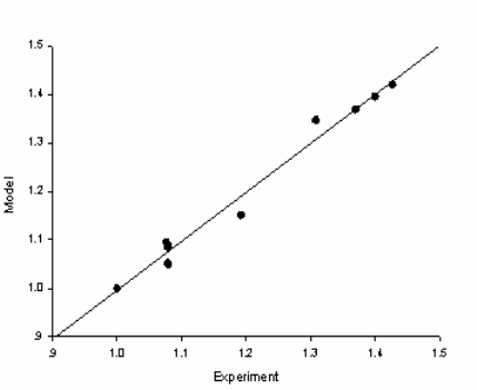
Broth II in the absence of antibiotics. The experimentally

measured values of the microbial counts are then

plotted, in Figure 1, against those obtained from the

simulation of the following logistic model for the

microbial population X(t):

Fig 1. Plot of experimental data against model simulations.

ScienceAsia ScienceAsia

ScienceAsia

33 (2007)33 (2007)

33 (2007)

199

0

()1 (0)

max

dX X

CXXX

dt X

μ

⎛⎞

=−,=

⎜⎟

⎝⎠

(1)

where

()

max

S

C

KC

μ

=.

+

( 2 )

We observe in Figure 1 that the data points are

aligned along the straight line

y

x=

. Experimenting

with other sets of data yields the same result which

assures us that the equation (1) gives a reasonable fit

to the real data, with appropriately chosen values of the

parameters.

Next, we incorporated antibiotic effect with the

following model equation:

(3)

where A(t) = A

1

+ A

2

e

-

ω

t

( 4 )

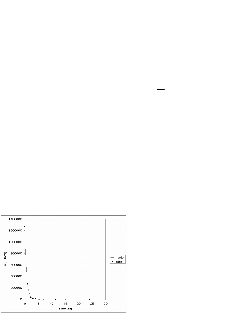
Figure 2 shows a comparison of the simulation of

equation (3) with a set of experimental data collected

from a culture of Bacteroides Fragilis (BF) with BMS-

284756, an experimental drug, for the antibiotic, in

Mueller-Hinton Broth II. The colony counts were done

at t = 0, 2, 4, 6, 8, 24 and 48 hours by serial dilution in

normal sterile saline. The parametric values, given in

the figure caption, have been determined to obtain the

best least square fit of the kill curve. A very close fit of

this set of experimental data was obtained when the

values of the parameters were suitably chosen.

Guided by the above observations and the

discussion in the previous section, we will therefore

consider the following model system of 4 ordinary

differential equations.

Fig 2. Comparison of numerical simulation. Data generated

from equation (3), where

μ

max

=

0.02, X

max

= 2.6×10

6

,

ε

k

=

1.5945848, K

K

= 0.3911216, A

1

= 18.87638 and A

2

=

0.1,

ω

= 0.9, X

0

= 1.27×10

6

, was composed with a set of

experimental data collected from a culture of

Bacteroides Fragilis ATCC 25285 with BMS-284756 as

the antibiotic in Mueller-Hinton Broth II grown on

Tryptic-Soy agar plate.

20

2

(0)

R

SR

RC

dR

RR R

dt K C K S

γ

ε

ψ

ω

=+−,=

++

(6)

13 0

3

() (0)

(1 )( ) ( )

SS RR

aS R

SC

RC

dC

CC C C

dt A K C K C

εψ

ω

γ

=− − − , =

++ +

(7)

14 0

1

()(0)

dA

AA A A

dt

ω

=− , =

(8)

where the first term in equation (5) is the growth

rate of the susceptible population level S, taking after

equation (2) previously mentioned. The second term

accounts for the reduction in the number of susceptible

population level as its member is converted into a

resistant strain due to the acquisition of an extra

chromosomal element, or plasmid, from members of

the resistant strain. Resistance can also be due to

chromosomal mutation that renders the strain

insensitive to the antibiotics

11

. The third term in

equation (5) is the rate at which the susceptible bacteria

is killed off by the antibiotic, taking the form suggested

by equation (3). The last term is then the rate of removal

of S by natural means. The response functions used in

equations (5) and (6) are of the Holling’s type generally

assumed in many previous population models

1,12-17

.

This means that the consumption rate increases as the

level of nutrient increases but reaches a saturation

point, beyond which rate of consumption cannot

increase even if there were more nutrient available.

Here, we do not take into account the detoxification of

the antibiotic (viz chloramphenicol by enzymatic

acetylation), assuming that this effect is negligently

small. Thus, in equation (8), the antibiotic is removed

naturally at the rate that is proportional to its amount

A at any time t.

Equation (6) describes the rate of change of the

resistant population level R growing at the rate given

by the first term which assumes a Holling type saturating

function of the substrate concentration C. To give it a

different dynamics from that of the susceptible strain,

since R is the resistant strain and thus not limited by its

environment, the growth rate of R is allowed to increase

with its number, not limited by its surrounding

conditions as in the logistic growth rate. The second

term in equation (6) accounts for the increase in R due

to the development of resistance in the susceptible

strain. It is then naturally removed at the rate

ω

2

R.

1

10

()

(1 )( )

(0)

S

aS

K

C

dS

SS

dt A K C

SR

AS

SS S

KSK A

γ

ψ

γ

ε

ω

′

=−

++

−− −,=

++

(5)

0

1(0)

k

max

max K

AX

dX X

XXX

dt X K A

ε

μ

⎛⎞

=− − ,=

⎜⎟

+

⎝⎠

200

ScienceAsia ScienceAsia

ScienceAsia

33 (2007)33 (2007)

33 (2007)

The levels of S, R and C are assumed here to vary

with different time scales t

1

,

t

2

and t

3

, respectively, as

shall be explained in the next section. Equation (7)

describes the rate of change of the resource or substrate

C. The second term accounts for its consumption by

the susceptible bacteria S, while the last term accounts

for that by the resistant bacteria R. Since S is sensitive

to the presence of antibiotic A, the consumption rate

by S is reduced as A increases, and thus the factor 1+

γ

a

A

in the denominator of this term.

Since equation (8) is autonomous and depends only

on A, it can be easily solved for A(t) which is found to

eventually tend to A

1

as time progresses. We may

therefore consider the above model in the event that

A has reached the level A

1

. We are thus reduced to only

the 3 equations (5)-(7) for t ≥ t

0

, with A replaced by A

0

such that S(t

0

) = S

0

, R(t

0

) = R

0

and C(t

0

) = C

0

.

Model AnalysisModel Analysis

Model Analysis

In order to analyze the model equations (5)-(8) by

the singular perturbation method, we further make the

following assumptions.

As S represents the sensitive bacterial population,

it is reasonable that S should have the fastest dynamics,

while the resistant strain should be more adaptable to

the environment and less susceptible to destruction

and hence more stable, changing at a slower rate, or has

intermediate dynamics. The resource C may be kept

abundant at more or less constant level and thus

assumed to have the slowest dynamics. We therefore

utilize two small scaling parameters

ε

and

δ

, and

dimensionless variables and parameters defined as

follows.

Letting

1

0

()

102 03 0

()

St

S

tttt ttt ttxt

εεδ

=+ , = + , = + , = ,

3

2

00

()

() () ,

Ct

Rt

SS

yt zt=,=

1

0

1

C

S

z =,

0000

SR

K

KK

SR

SSSS

KKK

γ

′

=, =, =,=,

and

1

S

a

A

a

ψ

γ

+

=,

1

2

K

A

KA

a

ε

+

=

1

3

1

SS

a

A

a

εψ

γ

+

,=

,

4 RR

a

εψ

= , ( 9 )

one is led to the following system.

0

()(0)

dx

fxyz x x

dt

=,,, =

(10)

0

()(0)

dy

gxyz y y

dt

ε

=,,,=

(11)

0

()(0)

dz

hxyz z z

dt

εδ

=,,,=

(12)

where

1

21

()

S

xy

axz x

fxyz ax x

Kz Kx

γ

ε

γ

ω

−

,, = − − −

++

(13)

2

()

R

xy

yz

gxyz y

KzKx

γ

ε

ψ

ω

,, = + −

++

(14)

34

13

()()

SR

axz ayz

hxyz z z

KzKz

ω

,, = − − −

++

(15)

Thus, for fixed x, y and z, the rate of change

dz

dt

is

O(

εδ

),

dy

dt

is O(

ε

), while

(1)

dx

dt

O=

. This means that x

has the fastest dynamics, y the intermediate, and z the

slowest dynamics. We can then carry out a singular

perturbation analysis on the model system (10)-(12)

with (13)-(15) that involves purely geometric

arguments. Such method of analysis has been developed

by Muratori and Rinaldi

12

, extended to 3-dimensional

systems by Muratori

13

. Examples of its use may be

found in the works of Muratori and Rinaldi

14

, Lenbury

and Likasiri

15

and Rattanakul et al.

16

. Through the

identification of the shapes and locations in the phase

space of the equilibrium manifolds where f(x,y,z) = 0,

g(x,y,z) = 0 and h(x,y,z) = 0, conditions can be determined

under which as time passes, the three state variables

x(t), y(t) and z(t) tend to the corresponding steady state

values x

S

, y

S

and z

S

, respectively, at which point f(x

S

,

y

S

,z

S

) = g(x

S

,y

S

,z

S

)= h(x

S

,y

S

,z

S

) = 0. The direction of the

trajectories in the phase space is determined by

considering the signs of

xy,



and in different regions

in the (x,y,z) - space delineated by the equilibrium

manifolds. We are particularly interested in the case

where the wash-out steady state (0,0,z

1

) is stable and

the bacteria populations are eradicated.

Since experimental data invariably show oscillatory

behavior in the time series, as can be seen in Figure 3,

we are also interested in the possibility that our model

allows such behavior. The conditions under which this

occurs are important for control purposes and yield

insightful interpretations.

Fig 3.

Colony counts of Serratia marcescens ATCC 43861 in

varying concentration of 0.1% MHB with ceftazidime

(0.125 ng/ml) on Trypticase-Soy agar plate. The colony

counts were done at t = 0, 1, 3, 5, 7 hours by serial

dilution in normal sterile saline. Experimental data are

shown as dots, while the solid curve corresponds to the

model simulation.

z



ScienceAsia ScienceAsia

ScienceAsia

33 (2007)33 (2007)

33 (2007)

201

The shapes and relative positions of the manifolds

{f = 0}, {g = 0}, and {h = 0} determine the directions,

speeds, and shapes of the resulting solution trajectories.

Therefore, we need to analyze each of the equilibrium

manifolds in detail. The delineating conditions for

occurrence of different dynamic behavior as well as

the existence of limit cycles are arrived at from the

close inspection of those manifolds.

The manifold The manifold

The manifold

{{

{

ff

f

= 0} = 0}

= 0}

This manifold consists of two submanifolds. One is

the trivial manifold x = 0, while the other is the nontrivial

manifold given by the equation

y =

112 12

()()

()

S

aK aK z aKK

Kz

γγ γ

γ

γω ω

ε

⎡⎤

⎢⎥

⎣⎦

−+ −+

+

2

112121

[( )( )] ( )

()

S

aK az aKxazx

Kz

γ

γω ω

ε

⎡⎤

⎢⎥

⎣⎦

−−+ −+ −

+

(16)

The surface intersects the z-axis at the point where

12

2

112

()

S

aK

zz

aa

ω

γω

+

=≡

−+

(17)

In order that z

2

> 0, we need to require

112

()aa

γω

>+

(18)

Moreover, the curve where the surface intersects

the (y, z)-plane is asymptotic to the line

112

1

()aK aK

yy

γγ

γ

γω

ε

−+

=≡

(19)

for which y

1

> 0 provided (18) holds. Also the curve

where the surface intersects the (x, z)-plane is

asymptotic to the line

112

1

()aa

xx

a

γ

ω

−+

=≡

(20)

for which x

1

> 0 provided (18) holds.

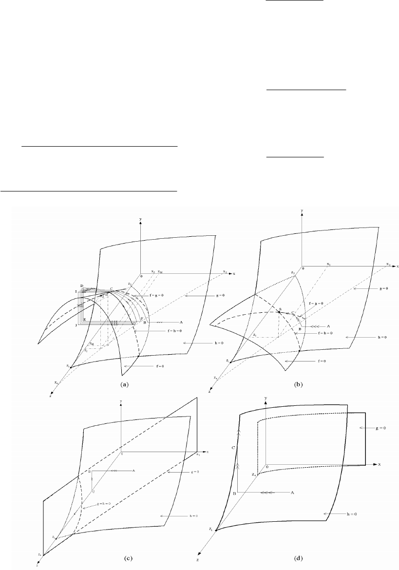
Fig 4.

Trajectories of the model system (10)-(12) with (13)-(15). The trajectory tends to a limit cycle in a), a positive equilibrium

point in b), a wash-out equilibrium point in c), and becomes unbounded in d).

202

ScienceAsia ScienceAsia

ScienceAsia

33 (2007)33 (2007)

33 (2007)

We now consider

y

x

∂

, the slope of y given by (16)

as a function of x, for a fixed z, as follows.

112121

()( )( )2

()

S

aK az aKaxz

y

xKz

γ

γω ω

ε

⎡⎤

−−+ −+ −

∂

⎣⎦

=

∂+

(21)

We see that

y

x

∂

= 0 along the curve where

11212

1

()( )( )

()

2

S

max

aK az aK

xz x

az

γ

γω ω

⎡⎤

−−+ −+

⎣⎦

==

(22)

In order that x

max

> 0, we need

12

3

112

()

()( )

S

aK

zz

aK a

γ

ω

γω

+

>≡

−−+

(23)

We observe that z

3

> 0 if

112

()aK a

γ

γω

−>+

(24)

in which case the manifold {f = 0} is shaped and

located in the phase space shown in Figure 4a.

The manifold The manifold

The manifold

{{

{

gg

g

= 0} = 0}

= 0}

This manifold consists of two submanifolds. One is

the trivial manifold y = 0, while the other is the nontrivial

manifold given by the equation

22

()

()()

RR

Kz KK

x

zK

γγ

ψω ω

ωψ ε ωε

−−

=

−− + −

(25)

This nontrivial manifold is independent of the

intermediate variable y, and thus it is parallel to the y -

axis. It intersects the z- axis at the point where

2

4

2

R

K

zz

ω

ψω

=≡

−

(26)

which will be positive if

2R

ψ

ω

> (27)

Moreover, it intersects the x-axis at the point where

2

K

xx

γ

ω

εω

=≡

−

(28)

which will be positive if

2

γ

ωε

<

(29)

The manifold The manifold

The manifold

{{

{

hh

h

= 0} = 0}

= 0}

This manifold is given by the equation

133

4

()()() ()

()

SR R

S

zzK zK z axzK z

y

azK z

ω

−++− +

=

+

(30)

which intersects the

z

-axis (x = y = 0) at the point

where

(31)

We see that we need to require that

41

zz> (32)

and

21

xx> (33)

for the surfaces to be located as shown in Figures

4a-d.

We now let (x

S

,y

S

,z

S

) be the intersection point of {f

= 0}, {g = 0} and{h = 0}, with x

S

> 0, y

S

> 0, z

S

> 0, and let

(x

M

,y

M

,z

M

) be the maximum point of the curve f = h = 0.

Four cases of different dynamic behavior can be

identified as follows.

Case 1Case 1

Case 1

..

. This case is identified by the inequalities

(18), (24), (27), (29), (32), (33), and 0 < x

S

< x

M

.

Under these conditions, the shapes and relative

positions of the equilibrium manifolds {f = 0}, {g = 0} and

{h = 0} are as depicted in Figure 4a, where three arrows

indicate fast transitions, two arrows indicate

intermediate ones, while single arrows indicate slow

ones.

Thus, a system initially at a generic point, say point

A of Figure 4a, will make a quick transition to the

surface given by equation (16) of the fast manifold {f =

0} (point B in Figure 4a), since the signs of f assure us

that this part of the manifold {f = 0} is stable. As the

surface where {f = 0} is approached, y has slowly become

active. A transition at an intermediate speed is made

along {f = 0} in the direction of increasing y, since g > 0

here.

Once the point C is reached, the stability of the

manifold is lost, a catastrophic transition brings the

system to point D on the (x,z)-plane. Consequently, the

system will slowly develop along this plane in the

direction of decreasing y, since g is now negative.

At a point E on the (y,z)-plane, the stability will again

be lost and a quick transition will bring the system back

to the point F which almost closes a cycle. However,

since this part of the transition is in the region

where

0z >



, z slowly increases giving rise to a high

frequency oscillation which densely covers a surface,

until the point H on the curve {f = h = 0} is reached. A

quick jump brings the trajectory to point I which is on

the (y,z)-plane, and an intermediate transition will bring

the system to the point J, followed by a quick transition

which will bring the system back to the point G which

lies on the stable part of the curve{f = h = 0}, thereby

forming a closed cycle GHIJG. Thus, the existence of a

limit cycle in the system for

ε

and

δ

sufficiently small

is assured.

Case 2Case 2

Case 2. This case is identified by inequalities (18),

(27), (29), (31), (32) and (33) while (24) is violated (see

Figure 4b).

Under these conditions, the system initially at a

generic point A will make a quick transition to the fast

manifold {f = 0} (point B), then an intermediate transition

is made along this surface in the direction of increasing

1

0zz=>

ScienceAsia ScienceAsia

ScienceAsia

33 (2007)33 (2007)

33 (2007)

203

y until the curve {f = g = 0} is reached. The trajectory will

follow this curve until the stable equilibrium point

(x

S

,y

S

,z

S

) where {f = g = h = 0} is reached at which point

the transition ceases. This is, therefore, the case where

all three populations persist at constant stable levels.

Case 3Case 3

Case 3

..

. This case is identified by inequalities (27),

(29), (32), and (33) while (18), and thus (24), are

violated. In Figure 4c, we see that the nontrivial fast

manifold does not appear in the first octant since (18)

does not hold. The intermediate manifold and the slow

manifold are as shown in Figure 4c. A system initially

at a point A, where the level of substrate C

0

is not too

high, will make a quick transition to the trivial manifold

x = 0, namely the (y,z)-plane (point B). Then, since g <

0 here, a transition at an intermediate speed in the

direction of decreasing y is made to the point C on the

z-axis. Then the slow variable z has become active, and

a transition at a slow speed is made along the z-axis to

end at the stable equilibrium point(0, 0, z

1

). This is thus

the case in which both susceptible and resistant bacterial

populations are washed out.

Case 4Case 4

Case 4

..

. This case is identified by inequalities (27),

(29), and (33), while (18), (24), and (32) are violated.

Also, this is the case where z

1

>> z

4

(high feed substrate

or efficient substrate consumption by the resistant

population). The system initially at a point A (in Figure

4d) will make a quick transition in the direction of

decreasing x until a point B on the manifold {h = 0} is

reached (as shown in Figure 4d). At this point, the

intermediate variable y has become active and a

transition at intermediate speed is then made along {h

= 0} in the direction of increasing y, since g > 0 here in

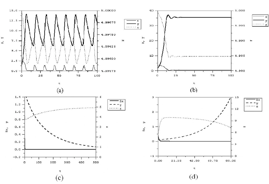
Fig 5.

Time courses of x, y and

z

corresponding to the 4 cases of Figure 4.

(a)

ε

= 1.0,

δ

= 1.0, z

1

= 5.0,

ε

γ

= 0.9,

ψ

R

= 1.2,

γ

= 3.0,

ω

1

= 0.7,

ω

2

= 0.7,

ω

3

= 0.7, K

S

= 0.7, K

γ

= 1.5, K

R

= 5.0, a

1

= 2.45283,

a

2

= 0.023077, a

3

= 0.00196, a

4

= 0.0006, x

0

= 0.5, y

0

= 1.5, and z

0

= 5.0. The solution in Case 1 exhibits sustained

oscillation.

(b)

ε

= 1.0,

δ

= 1.0, z

1

= 5.0,

ε

γ

= 0.9,

ψ

R

= 1.2,

γ

= 4.0,

ω

1

= 0.7,

ω

2

= 0.7,

ω

3

= 0.7, K

S

= 0.7, K

γ

= 4.3, K

R

= 5.0, a

1

= 2.407407,

a

2

= 0.023077, a

3

= 0.00196, a

4

= 0.0006, x

0

= 0.5, y

0

= 1.5, and z

0

= 5.0. The solution in Case 2 is seen here to tend towards

a stable non-washout steady state values.

(c)

ε

= 1.0,

δ

= 1.0, z

1

= 5.0,

ε

γ

= 0.1,

ψ

R

= 0.09291,

γ

= 2.0,

ω

1

= 0.5,

ω

2

= 0.09,

ω

3

= 0.5, K

S

= 2.0, K

γ

= 2.0, K

R

= 0.5, a

1

= 0.1, a

2

= 0.8, a

3

= 0.5, a

4

= 0.5, x

0

= 0.5, y

0

= 1.5, and z

0

= 5.0. The solution in Case 3 is seen here to tend towards a stable

wash-out steady state values.

(d)

ε

= 1.0,

δ

= 1.0, z

1

= 10.0,

ε

γ

= 0.06,

ψ

R

= 0.1,

γ

= 2.0,

ω

1

= 0.5,

ω

2

= 0.06,

ω

3

= 0.5, K

S

= 2.0, K

γ

= 2.0, K

R

= 0.00001,

a

1

= 0.1, a

2

= 0.8, a

3

= 0.5, a

4

= 0.5, x

0

= 0.1, y

0

= 0.1, and z

0

= 5.0. The solution in Case 4 is seen here to exhibit a steady

increase in the resistant population y.

204

ScienceAsia ScienceAsia

ScienceAsia

33 (2007)33 (2007)

33 (2007)

front of the manifold {g = 0}, until the point C on the

curve {h = 0} on the plane {x = 0} is reached. The

transition will continue along this curve so that the

resistant population can become too high leading to a

bacteria overgrowth in the GI tract. The results of the

above analysis may be stated as in the following theorem.

TheorTheor

Theor

emem

em For the model system (10)-(12), with (13)-

(15), and a suitable starting point(x

0

,y

0

,z

0

) , suppose

inequalities (27), (29) and (33) hold.

1. If inequalities (18), (24) and (32) are satisfied and

0 < x

S

< x

M

, then there exists a periodic solution to the

model system which is locally asymptotically stable.

The solution trajectory starting close enough to the

unstable non-washout steady state (x

S

,y

S

,z

S

) in this case

will tend, as time progresses, towards a limit cycle

which surrounds that steady state.

2. If the inequality (24) is violated, while (18) and

(32) still hold, then the non-washout steady state will

be stable. In this case, we have coexistence of the two

microbial species at steady state levels.

3. If, moreover, (18) is violated (in which case (24)

also is), while (32) still holds, then the washout steady

state (x,y,z) = (0, 0, z

1

) is locally stable. In this case, there

is an

ε

0

> 0 such that if C

0

<

ε

0

, then bacteria are eventually

eradicated.

4. On the other hand, when the environment is too

conductive to bacteria growth, there exists a such

that if C

0

>

ˆ

C

and (18), (24), and (32) are violated, with

z

1

>> z

4

, the mechanism to control the resistant strain

through nutrient competition is no longer viable. The

antibiotic dose of A

0

which settles down eventually to

the level A

1

in this case is high enough to violate (24).

The susceptible population is therefore quickly

eliminated, allowing the overgrowth of the resistant

population.

Numerical Simulation and InterpretationNumerical Simulation and Interpretation

Numerical Simulation and Interpretation

Figure 5 shows the time series of the numerical

simulations of model equations (10)-(12), with (13)-

(15). The parameters are chosen to satisfy (18), (24),

(27), (29), (32) and (33) in Figure 5a yielding a limit

cycle solution as theoretically predicted. The solution

trajectory in Figure 5b tends to the non-washout

equilibrium point, while in Figure 5c it tends to the

washout steady state (0, 0, z

1

) if it starts with a low C

0

.

However, if C

0

is too high bacteria overgrowth may be

expected as shown in Figure 5d. We observe here that

although our analysis was done on the assumption of

ε

and

δ

being small in order to carry out the singular

perturbation arguments, our conclusions are in fact

still valid even without

ε

or

δ

being very small. Both are

set equal to 1 in the simulations shown in Figure 5.

In order to understand the clinical implications of

the conditions given in the different cases of the above

theorem, we consider the delineating conditions (18)

and (24). We define

2

a

as the value of a

2

that satisfies

(18) when inequality is replaced by equality, namely,

1

2

a

γω

≡− (34)

and

2

a

as the value of a

2

that satisfies (24) when

inequality is replaced by equality, namely,

1

2

aK

a

γ

γω

≡−−

(35)

The above analytical conclusions may be

understood to say that if the antibiotic dose can be kept

at the sustaining level A

1

, low enough so that the

“inhibition factor” a

2

remains below the level

2

a

, but

kept high enough so that a

2

exceeds the critical level

2

a

,

then we shall be in Case 2 of the above theorem. That

is, if

2

22

a

<<

(36)

then the two bacterial populations can persist at

controllable stable steady state levels (Case 2). However,

if the antibiotic level asymptotically settles toward the

level A

1

that is high enough so that the inhibition factor

a

2

exceeds both

2

a

and

2

a

, given in (34) and (35), then

the inequalities (18) and (24) are both violated. We may

then expect an eventual eradication of both the sensitive

and the resistant populations (Case 3), provided that

the initial condition (substrate level C

0

) is not too highly

conductive to bacteria growth.

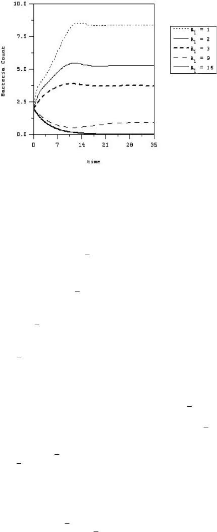
Figure 6 shows different “kill curves” from our

model simulations for different “effective” antibiotic

levels A

1

. The oscillatory behavior exhibited by our

model in these kill curves closely resembles that

Fig 6.

Kill curves for different “effective” antibiotic levels.

ε

=

1.0,

δ

= 1.0, z

1

= 5.0,

ε

γ

= 0.9,

ψ

R

= 0.5,

γ

′′

′

= 2.5,

γ

a

= 1.0,

ω

1

= 0.5,

ω

2

= 0.7,

ω

3

= 0.5, K

S

= 2.0, K

γ

= 2.0, K

R

= 0.5,

K

= 1.0,

ε

S

= 0.000814,

ε

R

= 0.0006,

ε

K

= 0.046154,

ψ

S

= 4.814814, x

0

= 0.5, y

0

= 1.5, z

0

= 5.0 and S

0

= 1.0, A

1

= antibiotic level.

1

ScienceAsia ScienceAsia

ScienceAsia

33 (2007)33 (2007)

33 (2007)

205

observed in clinical data, an example of which is shown

in Figure 3 where a simulation of our model is shown

fitted with the experimental data, taking into account

the measurement errors. Solving (34) for A

1

gives us an

indication of the MAC (minimum antibiotic

concentration), while solving (35) for A

1

provides a

lower bound for the MIC (minimum inhibitory

concentration). According to Sharma et al

18

the amount

of time during which the antibacterial concentration

remains above the MIC or MAC is an important

determinant of deciding the dose regimens of an

antibacterial agent.

However, the “effective” antibiotic level A

1

for each

patient cannot be measured, but may by obtained by

interpolating the pharmaco-kinetic data collected from

controlled clinical trials. Considering equation (8), if

the antibiotic rate of change of A

is plotted against the

antibiotic level A at each moment in time, then the slope

of the fitted line that best fits the data shall give the value

of

ω

4

, and the y-intersect of the line gives the value of

A

1

ω

4

, thus yielding the effective antibiotic level A

1

characteristic to each patient. In this way, it is possible

to design the dosing regimen to obtain the desired

outcome in the control range given by (36).

Finally, in terms of maintenance of the community

stability in the GI tract, we can offer the following

interpretation. The transition from a stable situation of

Case 2 seen in Figure 5b to the unstable situation of

Case 1 seen in Figure 5a occurs with the realization of

condition (24). Considering this condition, we see that

it may be satisfied with low enough antibiotic level A

1

,

or sufficiently low removal rate of susceptible

population

ω

1

, or high enough carrying capacity

γ

of

the environment for the susceptible population, or

faster conversion of susceptible to resistant strain (low

K

γ

), or high enough initial nutrient level C

0

.

Also, transition from the stable situation of Case 3

seen in Figure 6c to that seen in Figure 5d again is

facilitated by the abundance of nutrients (large z

1

) or

efficient consumption of nutrients by the resistant

population (high

ψ

R

or low K

R

) so that z

1

>> z

4

even with

a high level of antimicrobial agents A

1

. Our model thus

bears support to the experimental observation of Freter

et al.

10

, already mentioned in the Introduction, that

suggested that competition for nutrients is of an

overriding importance in the activity that maintains the

stability of the microflora community. From such

analysis, we can suggest a possible control strategy that

combines appropriate drug protocol and strict diet

regimen.

CONCLUSION

We have discussed a model of bacteria responses

and resistance to antibiotics, which accounts for the

mechanisms involved in the bacteria-antibiotic

interactions in vivo. For a specific patient, it is possible

to determine the values of the parameters by

interpolating the data collected from controlled clinical

trials, as has been described above. The model can then

be used to simulate different dynamic behavior due to

different dosing regimes. Since routine application of

antibiotics inevitably leads to the emergence of drug

resistance, it is vital that strategies are divised to reduce

the speed with which this occurs.

Clinically, it is difficult to assess pharmaco-dynamic

effects of antibiotics due to the complexity in repeatedly

determining the bacterial load at the site of infection

and antibiotic concentrations during the dosing

interval

18

. Using dynamic models of bacteria-antibiotic

interactions can overcome these difficulties. Through

the model development and analysis, we gain an

understanding of the pharmaco-dynamic factors that

are involved in the process, while our model tries to

simulate human infection mechanisms and can suggest

how best the microbiological activity and antibacterial

pharmacokinetic data in vivo can be used to select an

antimicrobial agent and its dosage regimen that

minimizes GI tract overgrowth by resistant species.

The model might also be used to provide information

regarding the kinetics of elimination of resistant strains

once antimicrobial selection pressure has been relieved.

Such information could prove useful in designing,

monitoring, and control of empiric therapy stragies.

ACKNOWLEDGEMENTS

Appreciations are extended towards the Thailand

Research Fund and National Center for Genetic

Engineering and Biotechnology, National Science and

Technology Development Agency (contract no. 3-

2548) for financial support.

REFERENCES

1. Nolting and Derendorf H (1995) Pharmacokinetic/

Pharmacodynamic Modeling of Antibiotics. CRC Press.

2. Johnson SA, Nicolson SW and Jackson S (2004) The effect

of different oral antibiotics on the gastrointestinal microflora

of a wild rodent (Aethomys namaquensis). Comparative

Biochemistry and Physiology,

A138A138

A138, pp 475-83.

3. Tannock GW (1999) Medical importance of the normal

microflora. Kluwer Academic Publ., Dordrecht, the

Netherlands,.

4. Van der Waaij D, Berghuis-deVries JM and Lekkerkerk-van

der Wees JEC (1972) Colonization resistance of the digestive

tract and the spread of bacteria to the lymphatic organs in

mice. J. Hyg.

70,70,

70, pp 335-42.

5. Steffenand EK and Berg RD (1983) Relationship between

cecal population levels of indigenous bacteria and

translocation to the mesenteric lymph nodes. Infection and

Immunity

39(3)39(3)

39(3), pp 1252-9.

6. Scott KP (2002) The role of conjugative transposons in

206

ScienceAsia ScienceAsia

ScienceAsia

33 (2007)33 (2007)

33 (2007)

spreading antibiotic resistance between bacteria that inhabit

the gastrointestinal tract. Cell. Mol. Life Sci.

5959

59

,,

, pp 2071-82.

7. Bennet R, Erickssen M, Nord CE and Zetterstrom R (1984)

Impact of various antibiotics on the fecal flora of newborn

infants. Microecol. Ther.

1414

14, pp 251.

8. Burr DH and Sugiyama H (1982) Susceptibility to enteric

botulinum colonization of antibiotic-treated adult mice.

Infect. Immun.

3636

36

, ,

, pp103-6.

9. Van der Waaij D, Heidt PJ, Rusch VC and Gebbers JO (1990)

Microbial ecology of the human digestive tract. In: Old Herborn

University seminar monograph, pp 1-83. Institute for

Microecology, Germany.

10. Freter R, Abrams GD and Aranki A (1973) Patterns of

interaction in gnotobiotic mice among bacteria of a synthetic

“normal” intestinal flora. In: Germfree Research: Biological effect

of gnotobiotic environments (Ed.: Heneghan, J.B.). pp 429-

434. Academic Press, New York, London.

11. Peacock SJ, Mandal S and ICJW (2002) Bowler, Preventing

Staphylococcus aureus infection in the renal unit. Q J Med

9595

95, pp 405-10.

12. Muratori S and Rinaldi S (2002) A separation condition for

the existence of limit cycles in slow-fast systems. International

report, Elettronica

3,3,

3, pp 90.

13. Muratori S (1991) An application of the saparation principle

for detecting slow – fact limit cycle in three – dimensional

system. Appl. Math. Comput.

4343

43, pp 1-18.

14. Muratori S and Rinaldi S (1992) Low – and high – frequency

oscillations in three – dimensional food chain systems. SIAM

Journal on Applied Mathematics.

52,52,

52, pp 1688-706.

15. Lenbury Y and Likasiri C (1994) Low-and high-frequency

oscillations in a food chain where one of the competing

species feeds on the other. Math. Comp. Modelling.

20,20,

20, pp

71-89.

16. Rattanakul C, Lenbury Y, Krishnamara N and Wollkind DJ

(2003)Modeling of bone formation and resorption mediated

by parathyroid hormone: response to estrogen/PTH therapy.

BioSystems

70,70,

70, pp 55-72.

17. Leah EK (1988) Mathematical models in biology. Random

House, New York.

18. Sharma KK, Sangraula H and Mediratta PK (2002) Some

New Concepts in Antibacterial Drug Therapy. Indian Journal

of Pharmacology

3434

34, pp 390-6.