ACCEPTED FOR PRESENTATION IN 11
TH
BULK POWER SYSTEMS DYNAMICS AND CONTROL SYMPOSIUM (IREP 2022),
JULY 25-30, 2022, BANFF, CANADA 1
Neural Networks for Encoding
Dynamic Security-Constrained Optimal Power Flow
Ilgiz Murzakhanov, Andreas Venzke, George S. Misyris, Spyros Chatzivasileiadis
Department of Wind and Energy Systems
Technical University of Denmark
Kgs. Lyngby, Denmark
{ilgmu, andven, gmisy, spchatz}@dtu.dk
Abstract—This paper introduces a framework to capture pre-
viously intractable optimization constraints and transform them
to a mixed-integer linear program, through the use of neural
networks. We encode the feasible space of optimization problems
characterized by both tractable and intractable constraints, e.g.
differential equations, to a neural network. Leveraging an exact
mixed-integer reformulation of neural networks, we solve mixed-
integer linear programs that accurately approximate solutions
to the originally intractable non-linear optimization problem.
We apply our methods to the AC optimal power flow problem
(AC-OPF), where directly including dynamic security constraints
renders the AC-OPF intractable. Our proposed approach has
the potential to be significantly more scalable than traditional
approaches. We demonstrate our approach for power system
operation considering N-1 security and small-signal stability,
showing how it can efficiently obtain cost-optimal solutions
which at the same time satisfy both static and dynamic security
constraints.
Index Terms—Neural networks, mixed-integer linear program-
ming, optimal power flow, power system security
I. INTRODUCTION
A. Motivation
In a wide range of optimization problems, especially related
to physical systems, the feasible space is characterized by
differential equations and other intractable constraints [1].
Inspired by power system operation, this paper uses the AC
optimal power flow (AC-OPF) problem with dynamic security
constraints as a guiding example to introduce a framework
that efficiently captures previously intractable constraints and
transforms them to a mixed-integer linear program, through
the use of neural networks. More specifically, we use neural
networks to encode the previously intractable feasible space,
and through an exact transformation we convert them to
a set of linear constraints with binary variables that can
be integrated to an equivalent mixed-integer linear problem
(MILP).
Power system security assessment is among the most fun-
damental functions of power system operators. With growing
uncertainty both in generation and demand, the complexity of
This work is supported by the ID-EDGe project, funded by Innovation
Fund Denmark, Grant Agreement No. 8127-00017B, by the FLEXGRID
project, funded by the European Commission Horizon 2020 program, Grant
Agreement No. 863876, and by the ERC Starting Grant VeriPhIED, Grant
Agreement No. 949899.
this task further increases, necessitating the development of
new approaches [2]. In power systems, the AC optimal power
flow (AC-OPF) is an essential tool for cost-optimal and secure
power system operation [3]. The non-convex AC-OPF problem
minimizes an objective function (e.g. generation cost) subject
to steady-state operational constraints (e.g. voltage magnitudes
and transmission line flows). While the obtained generation
dispatch from the AC-OPF solution ensures compliance with
static security criteria such as N-1 security, the dispatch
additionally needs to comply with dynamic security criteria
such as small-signal or transient stability. However, directly
including dynamic security constraints renders the AC-OPF
problem intractable [4]. To obtain solutions which satisfy
both static and dynamic security criteria, we propose a novel
framework using neural networks to encode dynamic security
constrained AC-OPF to MILPs.
B. Literature Review
In literature, a range of works [5]–[8] have proposed iter-
ative approaches and approximations to account for dynamic
security constraints in AC-OPF problems. For a comprehen-
sive review please refer to [4]. The work in [5] considers
transient stability by discretizing a simplified formulation of
the power system dynamics and proposes an iterative solution
scheme. Alternatively, to include transient stability constraints,
the work in [6] proposes a hybrid solution approach using
evolutionary algorithms. The work in [7] addresses voltage
stability and proposes a three-level hierarchical scheme to
identify suitable preventive and corrective control actions. To
approximate the small-signal stability criterion, the work in [8]
linearizes the system state around a given operating point and
includes the eigenvalue sensitivities in the AC-OPF problem.
While the majority of these approaches are tailored to a
specific dynamic stability criterion and require to iteratively
solve non-linear programs (NLPs), in this paper we propose
a general framework which allows us to encode any security
criterion.
A range of machine learning approaches have been proposed
to learn optimal solutions to the AC-OPF problem [9], [10]
and approximations thereof such as the DC-OPF problem [11],
[12], without considering dynamic security constraints. The
work in [9] compares different machine learning approaches
arXiv:2003.07939v5 [eess.SY] 14 Jul 2022
ACCEPTED FOR PRESENTATION IN 11
TH
BULK POWER SYSTEMS DYNAMICS AND CONTROL SYMPOSIUM (IREP 2022),
JULY 25-30, 2022, BANFF, CANADA 2
and finds that neural networks achieve the best performance.
To predict optimal solutions to AC-OPF problems, the work in
[10] trains deep neural networks and penalizes constraints vio-
lations. For the DC-OPF approximation, the work in [11] trains
deep neural networks as well, achieving a speed-up of two
orders of magnitude compared to conventional methods and
accounting for static security constraints. Instead of directly
learning the optimal solutions, the work in [12] predicts the set
of active constraints for the DC-OPF approximation. Note that
the DC-OPF approximation neglects reactive power, voltage
magnitudes and losses and can lead to substantial errors [13].
Ref. [14] is among the few that employ a multi-input multi-
output random forest model to solve a security-constrained
AC-OPF. The model first solves voltage magnitudes and angles
and then calculates other parameters, such as power generation
settings; still, this work does not include any dynamic security
constraints. While these approaches demonstrate substantial
computational speed-up compared to conventional solvers,
they do not account for dynamic security criteria, and most
of them rely on a large training dataset of computed optimal
solutions to the AC-OPF problem. Obtaining such a dataset is
computationally prohibitive for dynamic security-constrained
AC-OPF.
Using machine learning techniques for static and dynamic
security assessment has been explored in literature, for a
comprehensive survey please refer to [15]. The main area
of application has been the screening of a large number of
operating points with respect to different security criteria.
Several works have shown that the proposed machine learning
methods including neural networks require only a fraction
of the computational time needed for conventional methods.
Fewer works [16]–[18] explored using machine learning tech-
niques to directly include dynamic security constraints in AC-
OPF problems. The work in [16] proposed ensemble decision
trees to identify corrective actions to satisfy security crite-
ria. Embedding the decision trees in an AC-OPF framework
requires to solve computationally highly expensive mixed-
integer non-linear problems (MINLPs). To address computa-
tional tractability, the work in [17] proposed a second-order
cone relaxation of the AC-OPF to relax the MINLP to a
mixed-integer second-order cone program (MISOCP). This,
however, does not guarantee feasibility of the obtained solution
in case the relaxation is inexact. Approaching mixed-integer
programming (MIP) problem with the use of a convolutional
neural network (CNN) is presented in [19]. The proposed
solution targets scenario-based security-constrained unit com-
mitment (SCUC) with a battery energy storage system (BESS)
and has two stages. In the first stage, CNN-SCUC trains a
CNN to obtain solutions to the binary variables correspond-
ing to unit commitment decisions. In the second stage, the
continuous variables corresponding to unit power outputs are
solved by a small-scale convex optimization problem. The
proposed model-free CNN-SCUC algorithm greatly reduces
the computational complexity and obtains close-to-optimal
solutions. The work in [18] uses a non-linear representation of
neural networks with one single hidden layer to represent the
stability boundary in the AC-OPF problem. Instead of solving
computationally expensive NLPs or MINLPs, we propose a
novel framework using neural networks to encode the dynamic
security constrained AC-OPF to MILPs.
C. Main Contributions
The main contributions of our work are:
1) Using classification neural networks we encode the
feasible space of AC-OPF problems including any type
of static and dynamic security criteria.
2) Leveraging a mixed-integer linear reformulation of the
trained neural network and a systematic iterative pro-
cedure to include non-linear equality constraints, we
accurately approximate cost-optimal solutions to the
original intractable AC-OPF problems.
3) We introduce a method to trade-off conservativeness
of the neural network prediction with cost-optimality,
ensuring feasibility of the obtained solutions.
4) Considering both N-1 security and small-signal stability,
and using an IEEE 14 bus system, we demonstrate how
the proposed approach allows to obtain cost-optimal
solutions which at the same time satisfy both static and
dynamic security constraints.
D. Outline
The structure of this paper is as follows: In Section II, we
formulate optimization problems with intractable dynamic se-
curity constraints including the dynamic security-constrained
AC optimal power flow. In Section III, we encode the feasible
space using neural networks, state the mixed-integer linear
reformulation of the trained neural network, and introduce
efficient methods to include equality constraints and to ensure
feasibility. In Section IV, we demonstrate our methods using
an IEEE 14 bus system and considering both N-1 security and
small-signal stability. Section V concludes.
II. NON-LINEAR OPTIMIZATION PROBLEMS WITH
DYNAMIC SECURITY CONSTRAINTS
A. General Formulation
We consider the following class of non-linear optimization
problems with intractable dynamic constraints:
min
x∈X ,u∈U
f(u) (1)
s.t. g
i
(x, u) ≤ 0 ∀i = 1, ..., m (2)
h
i
(x, u) = 0 ∀i = 1, ..., n (3)
φ
i
(x, u) ∈ S
i
∀i = 1, ..., l (4)
The variables are split into state variables x and control
variables u which are constrained to the sets X and U,
respectively. The objective function is denoted with f in (1).
There is a number of m and n non-linear inequality and
equality constraints g and h, respectively. The l number of
constraints φ in (4) encode dynamic security constraints (e.g.
based on differential equations) and are intractable. While the
non-linear optimization problem (1)–(3) can be solved using a
non-linear solver, the addition of the constraints in (4) renders

ACCEPTED FOR PRESENTATION IN 11
TH
BULK POWER SYSTEMS DYNAMICS AND CONTROL SYMPOSIUM (IREP 2022),
JULY 25-30, 2022, BANFF, CANADA 3
the optimization problem intractable. Note that for given
fixed system state (x, u) we can determine computationally
efficiently whether it belongs to set S satisfying dynamic
constraints, i.e. is feasible or infeasible. One possible solution
strategy is to follow an iterative approach where the optimiza-
tion problem (1)–(3) is solved first, and then if constraint (4)
is violated a nearby solution is identified which satisfies (4).
This has several drawbacks including that this procedure does
not guarantee the recovery of a solution that is feasible to the
original problem, and the feasibility recovery procedure does
not consider optimality of the solution. In the following, using
power system operation as a guiding example, we will present
an approach that allows to directly approximate a high-quality
solution to (1)–(4) by solving mixed-integer linear programs
instead.
B. Application to AC Optimal Power Flow (AC-OPF)
In the following, we consider the AC-OPF problem with
combined N-1 security and small-signal stability criteria as
guiding example. Note that our proposed methodology is
general and can include any static or dynamic security criteria.
The AC-OPF problem optimizes the operation of a power
grid consisting of a set of N buses connected by a set of
L lines. A subset of the set of N buses has a generator
connected and is denoted with G. The variables are the vectors
of active and reactive power injections p and q, the voltage
magnitudes v and voltage angles θ. Each of these vectors have
the size n ×1, where n is the number of buses in the set N.
The control variables u are the active power injections and
voltage set-points of generators p
g
and v
g
, i.e. the entries
in p and v that correspond to the buses in the set G. If
the control variables are fixed, the remaining state variables
can be identified by solving an AC power flow, i.e. solving
a system of non-linear equations [20]. To satisfy the N-1
security criterion, the identified control variables u must lead
to a power system state which complies with the operational
constraints for a set of line outages. We denote this set with
C, with the first element C
1
= {0} corresponding to the intact
system state. The dimension of set C is defined by the number
of considered contingencies plus the intact system state. As
for its structure, the set C contains the IDs of the outaged
lines, while for the intact system state the corresponding ID is
’0’. The superscript ’c’ in (6)–(13) denotes the corresponding
outaged system state and the superscript ’0’ the intact system
state. To ensure small-signal stability, we analyze the stability
of the linearization of the power system dynamics around the
current operating point [21]. The system matrix A describes
the linearized system dynamics as function of the current oper-
ating point defined by (p, q, v, θ). To satisfy the small-signal
stability criterion, the minimum damping ratio associated with
the eigenvalues λ of A has to be larger than γ
min
; where
γ
min
≤ min
λ
−<{λ}
√
={λ}
2
+<{λ}
2
. Finally, we formulate the N-1
security and small-signal stability constrained AC-OPF:
min
p
c
,q
c
,v
c
,θ
c
,λ
c
,ν
c
f(p
0
g
) (5)
s.t. p
min
≤ p
c
≤ p
max
∀c ∈ C (6)
q
min
≤ q
c
≤ q
max
∀c ∈ C (7)
v
min
≤ v
c
≤ v
max
∀c ∈ C (8)
|s
line
(p
c
, q
c
, v
c
, θ
c
)| ≤ s
max
line
∀c ∈ C (9)
s
balance
(p
c
, q
c
, v
c
, θ
c
) = 0 ∀c ∈ C (10)
p
0
g
= p
c
g
, v
0
g
= v
c
g
∀c ∈ C (11)
A(p
c
, q
c
, v
c
, θ
c
)ν
c
= λ
c
ν
c
∀c ∈ C (12)
γ
min
≤ min
λ
c
−<{λ
c
}
√
={λ
c
}
2
+<{λ
c
}
2
∀c ∈ C (13)
The objective function in (5) minimizes the cost of the system
generation for the intact system state. All inequality and
equality constraints (6)–(13) have to hold for the intact system
state and each contingency in C. The inequality constraints
in (6)–(8) define minimum and maximum limits on active
and reactive power injections and voltage magnitudes. The
inequality constraint in (9) bounds the absolute apparent
branch flow s
line
for each line in L. The equality constraint in
(10) enforces the AC power flow balance s
balance
at each bus
N in the system. For a detailed mathematical description of
the apparent branch flow and the AC power flow balance, for
brevity, please refer to [3]. We consider preventive control for
N-1 security defined in (11), i.e. the generator active power
set-points and voltage set-points remain fixed if a line outage
occurs. The inequality constraint (12) ensures a minimum
damping ratio of critical modes in the system. The term ν
denotes the right hand eigenvectors of the system matrix A.
Note that the small-signal stability constraints (12)–(13) have
to hold for each considered line outage in set C. For more
details related to small-signal stability, we refer the interested
reader to [22]. Adding the small-signal stability constraints in
(12)–(13) increases the non-linearity and computational com-
plexity of the optimization problem substantially, rendering
it intractable and requiring iterative solution approaches [8].
In the following, we introduce a framework which allows to
directly approximate cost-optimal solutions to (5)–(13).
III. METHODOLOGY TO ACCURATELY APPROXIMATE
COST-OPTIMAL AND FEASIBLE SOLUTIONS
A. Encoding Feasible Space using Neural Networks
We denote the feasible space F of the optimization problem
(1)–(4) as: F := {x ∈ X and u ∈ U satisfy (2)–(4)}. As first
step, we train a classification neural network which takes the
control variables u ∈ U as input and predicts whether there
exists state variables x ∈ X such that the resulting operating
point is in the feasible space (x, u) ∈ F or is infeasible
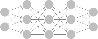
(x, u) /∈ F. The general architecture of the classification
neural network is illustrated in Fig. 1. The neural network is
defined by a number K of fully-connected hidden layers, that
each consist of N
k
number of neurons with k = 1, ..., K. The
neural network input vector u has dimension N
0
× 1 and the
output vector z has dimension N
K+1
×1. Here, the dimension
ACCEPTED FOR PRESENTATION IN 11
TH
BULK POWER SYSTEMS DYNAMICS AND CONTROL SYMPOSIUM (IREP 2022),
JULY 25-30, 2022, BANFF, CANADA 4
u
1
u
2
y
1
1
y
2
1
y
3
1
y
1
2
y
2
2
y
3
2
y
1
3
y
2
3
y
3
3
z
1
z
2
Hidden
layer 1
W
1
, b
1
Hidden
layer 2
W
2
, b
2
Hidden
layer 3
W
3
, b
3
Input
layer
Output
layer
W
4
, b
4
Fig. 1. Classification neural network with input, hidden and output layers.
The input layer takes the vector u as input. A weight matrix W and bias
b is applied between each layer. At the neurons of each hidden layer the
non-linear ReLU activation function is applied. For the binary classification
the magnitude of the two outputs are compared, i.e. z
1
≥ z
2
or z
1
< z
2
.
of z is 2 × 1, as we consider binary classification. The input
to each layer ˆy
k
is defined as:
ˆy
k+1
= W
k+1
y
k
+ b
k+1
∀k = 0, 1, ..., K − 1 (14)
where y
0
= u is the input to the neural network. The weight
matrices W
k
have dimensions N
k+1
×N
k
and the bias vector
b has dimension N
k+1
× 1. Each neuron in the hidden layer
applies a non-linear activation function to the input. Here, we
assume the ReLU activation function:
y
k
= max(ˆy
k
, 0) ∀k = 1, ..., K (15)
The ReLU activation function in (15) outputs 0 if the input
ˆy is negative, otherwise it propagates the input ˆy. Note that
the max operator is applied element-wise to the vector ˆy
k
.
The majority of recent neural network applications uses the
ReLU function as activation function as it has been found to
accelerate neural network training [23]. The main challenge of
implementing other activation functions is their mixed-integer
reformulation. While it is straightforward for (15) of ReLU,
for other activation functions a direct reformulation might not
be possible. However, one could approximate other activation
functions (e.g. SiLU) with piecewise linear functions. The
output of the neural network is:
z = W
K+1
y
K
+ b
K+1
(16)
For binary classification, based on a comparison of the mag-
nitude of the neural network output, we can either classify the
input as belonging to the first class z
1
≥ z
2
or the second
class z
2
> z
1
. Here, the first class z
1
≥ z
2
corresponds to the
prediction that the input is in the feasible space u ∈ F, and
the second class z
2
> z
1
to the prediction that the input is not
in the feasible space u /∈ F.
To train the neural network a dataset of labeled samples is
required. The performance of the neural network highly de-
pends on the quality of the dataset used.To encode the feasible
space F of a general optimization problem (1)–(4), we sample
u from the set U and determine whether the sample is feasible
or not. For the application to the N-1 security and small-
signal stability constrained AC-OPF in (5)–(13) this requires
to sample u = [p
0
g
v
0
g
]
T
from within the limits defined in
(6)–(8), and then test feasibility with respect to all constraints
(6)–(13). If available, historical data of secure operating points
can be used by the transmission system operator in conjunction
with dataset creation methods. To achieve satisfactory neural
network performance, the goal of the dataset creation is to
create a balanced dataset of feasible and infeasible operating
points which at the same time describe the feasibility boundary
in detail. This is particularly important in AC-OPF applications
as large parts of the possible sampling space lead to infeasible
operating points [24]. While the dataset creation is not the
scope of this work, several approaches [24], [25] focus on
efficient methods to create datasets.
Before training of the neural network, the dataset is split into
a training and test data set. During training of classification
networks, the cross-entropy loss function is minimized using
stochastic gradient descent [26]. This penalizes the deviation
between the predicted and true label of the training dataset.
The weight matrices W and biases b are updated at each
iteration of the training to minimize the loss function. After
training, the generalization capability of the neural network
is evaluated by calculating the accuracy and other relevant
metrics on the unseen test data set.
B. Exact Mixed-Integer Reformulation of Trained Neural Net-
work
With the goal of using the trained neural network in an
optimization framework, following the work in [27], we first
need to reformulate the maximum operator in (15) using binary
variables b
k
∈ 0, 1
N
k
for all k = 1, ..., K:
y
k
= max(
ˆ
y
k
, 0) ⇒
y
k
≤
ˆ
y
k
−
ˆ
y
min
k
(1 − b
k
) (17a)
y
k
≥
ˆ
y
k
(17b)
y
k
≤
ˆ
y
max
k
b
k
(17c)
y
k
≥ 0 (17d)
b
k
∈ {0, 1}
N
k
(17e)
We introduce one binary variable for each neuron in the hidden
layers of the neural network. In case the input to the neuron
is ˆy ≤ 0 then the corresponding binary variable is 0 and (17c)
and (17d) constrain the neuron output y
k
to 0. Conversely,
if the input to the neuron is ˆy ≥ 0, then the binary variable
is 1 and (17a) and (17b) constrain the neuron output y
k
to
the input
ˆ
y
k
. Note that the minimum and maximum bounds
on the neuron output
ˆ
y
min
and
ˆ
y
max
have to be chosen large
enough to not be binding and as small as possible to facilitate
tight bounds for the mixed-integer solver. We compute suitable
bounds using interval arithmetic [27]. To maintain scalability
of the resulting MILP, several approaches have been proposed
in literature including weight and ReLU pruning [28]. Here,
we follow [28] and prune weight matrices W during training,
i.e. we gradually enforce a defined share of entries to be zero.
C. Mixed-Integer Non-Linear Approximation
Based on the exact mixed-integer reformulation of the
trained neural network with (14), (16) and (17a)–(17e), we
can approximate solutions to the intractable problem (5)–(13)
ACCEPTED FOR PRESENTATION IN 11
TH
BULK POWER SYSTEMS DYNAMICS AND CONTROL SYMPOSIUM (IREP 2022),
JULY 25-30, 2022, BANFF, CANADA 5
by solving the following tractable mixed-integer non-linear
optimization problem instead:
min
p
0
,q
0
,v
0
,θ
0
ˆ
y,y,z
f(p
0
g
) (18)
s.t. p
min
g
≤ p
0
g
≤ p
max
g
(19)
v
min
g
≤ v
0
g
≤ v
max
g
(20)
s
balance
(p
0
, q
0
, v
0
, θ
0
) = 0 (21)
ˆy
1
= W
1
[p
0
g
v
0
g
]
T
+ b
1
(22)
ˆy
k
= W
k
y
k−1
+ b
k
∀k = 2, ..., K (23)
(17a) − (17e) ∀k = 1, ..., K (24)
z = W
K+1
y
K
+ b
K+1
(25)
z
1
≥ z
2
(26)
The inequality constraints (19)–(20) provide upper and lower
bounds on the control variables u = [p
0
g
v
0
g
]
T
. For the intact
system state, (21) ensures the non-linear AC power balance for
each bus. The exact mixed-integer reformulation of the neural
network is given in (22)–(25). The constraint on the neural
network output z in (26) ensures that the neural network pre-
dicts that the input [p
0
g
v
0
g
] belongs to the feasible space F of
the original problem in (5)–(13). Note that the neural network
(22)–(26) encodes all constraints related to N-1 security and
small-signal stability, and eliminates all related optimization
variables. The remaining non-linear constraint in (21) enforces
the non-linear AC power flow balance for the intact system
state and requires to maintain the state variables for the intact
system state only. While the number of optimization variables
in (18)–(26) has been substantially reduced compared to (5)–
(13), the resulting optimization problem is a mixed-integer
non-linear problem, which are in general hard to solve. In the
following, we will propose a systematic procedure to handle
the non-linear equality constraint in (21).
D. Mixed-Integer Linear Approximation
The non-linear AC power flow equations described by the
nodal power balance in (21) can be summed over all buses.
Then, we take the real part and write the summed active power
balance as:
X
G
p
0
g
+
X
N
p
0
d
+ p
losses
(p
0
, q
0
, v
0
, θ
0
) = 0 (27)
The first term
P
G
p
0
g
is the sum of active power generation
and the second term
P
N
p
0
d
the sum of the active power
loading of the system where the parameter p
0
d
represent the
active power load at each bus in N. The third term p
losses
encapsulates the non-linearity and represents the active power
losses. We propose to use an iterative linear approximation of
the third non-linear term with a first-order Taylor expansion.
At iteration i + 1, we approximate (27) as:
X
G
p
0
g
+
X
N
p
0
d
+ p
losses
|
i
+
δp
losses
δp
0
g
|
i
(p
0
g
− p
0
g
|
i
) +
δp
losses
δv
0
g
|
i
(v
0
g
− v
0
g
|
i
) = 0 (28)
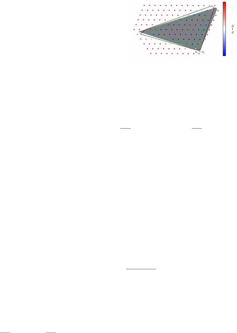
Fig. 2. Illustrative reduction of predicted feasible space: Red dots are pre-
dicted infeasible, blue dots are predicted feasible. The grey area represents the
true feasible space. The black dotted line represents the predicted feasibility
boundary. The green dotted line is the predicted feasibility boundary after
introducing a suitable in the classification decision z
1
≥ z
2
+ .
The notation |
i
is shorthand for evaluated at the operating point
of the i-th iteration, i.e. at (p
0
, q
0
, v
0
, θ
0
)|
i
. At the current
operating point, we evaluate the value of the losses p
losses
|
i
and the gradients with respect to the active generator dispatch
δp
losses
δp
0
g
|
i
and the generator voltages
δp
losses
δv
0
g
|
i
, respectively. Then,
we approximate the value of the losses as a function of both
the active generator dispatch and the generator voltages using
the first-order Taylor expansion.
The iterative scheme has the following steps. To initialize
for iteration i = 0, we linearize around a known operating
point (p
0
, q
0
, v
0
, θ
0
)|
i=0
, e.g. the solution to the AC-OPF or
N-1 security-constrained AC-OPF problem. Then, we solve
the following mixed-integer linear program for iteration i:
min
p
0
g
,v
0
g
,
ˆ
y,y,z
f(p
0
g
) (29)
s.t. (19), (20), (22) − (26), (28) (30)
By iteratively linearizing the non-linear equation in (21), we
solve MILPs instead of MINLPs. MILPs can be solved at a
fraction of the time required for MINLPs as the convexity of
the problem without integer variables allows for a significantly
improved pruning of the branch-and-bound procedure. Based
on the result of this optimization problem, we subsequently
run an AC power flow for the intact system state to recover
the full power system state and the losses. The iterative scheme
converges if the change between the active power losses
between iteration i and i − 1 is below a defined threshold
ρ:
p
losses
|
i
−p
losses
|
i−1
p
losses
|
i
≤ ρ. Otherwise, we resolve (29)–(30) with
the loss parameters in (28) updated. In Section IV-B, we
demonstrate fast convergence of this method.
E. Ensuring Feasibility of Solutions
The classification neural network is trained on a finite
number of data samples and with a finite number of neurons.
As a result, there might be a mismatch between the prediction
of the feasibility boundary and the actual true feasibility
boundary. This could lead to falsely identifying an operating
point as feasible while it is in fact not feasible. Note that
feasibility refers to satisfication of both static and dynamic

ACCEPTED FOR PRESENTATION IN 11
TH
BULK POWER SYSTEMS DYNAMICS AND CONTROL SYMPOSIUM (IREP 2022),
JULY 25-30, 2022, BANFF, CANADA 6
security criteria. To control the conservativeness of the neural
network prediction we introduce an additional constant factor
in the classification and replace (26) in the MILP formulation
(29)–(30) with:
z
1
≥ z
2
+ (31)
Adding the term to the right hand side in (31) effectively
shrinks the size of the predicted feasible space. This reduces
the risk that operating points close to the feasibility boundary
are falsely classified as feasible. But this can lead to an in-
crease of the cost of operation, i.e. there is a trade-off between
ensuring feasibility and optimality. In Fig. 2 we illustrate the
reduction of the predicted feasible space by introducing .
In Section IV-B, we quantify the trade-off between ensuring
feasibility and obtaining a cost-optimal solution.
IV. SIMULATION AND RESULTS
In the following, we demonstrate our proposed methodology
using an IEEE 14-bus system and considering combined N-1
security and small-signal stability as security criteria.
A. Simulation Setup
As test case, we use the IEEE 14-bus system from [29]
consisting of 5 generators, 11 loads and 20 lines with the
following modifications: For the N-1 security criterion, we
consider all possible line outages except of the lines connect-
ing buses 7 to 8 and 6 to 13, similar to previous works [24], as
including these outages would render the problem infeasible.
Furthermore, we enlarge the apparent branch flow limits in (9)
by 30% and the reactive power generator limits in (7) by 25%
to be able to obtain feasible solutions. To build the system
matrix A of the small signal stability model in (12), we use a
tenth-order synchronous machine model and follow standard
modeling procedures outlined in [21]. We use Mathematica to
derive the small signal model, MATPOWER AC power flows
to initialize the system matrix [29], and Matlab to compute
its eigenvalues and damping ratio, and assess the small-signal
stability for each operating point and contingency. Note that
we require a minimum damping ratio γ
min
of 3%.
To create the dataset of labeled operating points, we dis-
cretize the set U within the minimum and maximum generator
limits in (19). For each sample, we compute the feasibility
w.r.t. combined N-1 security and small-signal stability. As
large parts of this set lead to infeasible solutions, we resample
around identified feasible solutions. As a result, we obtain a
dataset of 45’000 datapoints with 50.0% feasible and 50.0%
infeasible samples. We split the dataset into 80% training and
20% test set and train a neural network with 3 hidden layers
and 50 neurons in each hidden layer using TensorFlow [26].
During training, we gradually increase the enforced sparsity
of the weight matrices to 50%, i.e. 50% of the entries of W
have to be zero. This increases the tractability of the resulting
MILPs significantly [28]. Finally, we obtain a trained neural
network with a predictive accuracy of 99% on the test dataset,
showing good generalization capability of the neural network.
We formulate the mixed-integer linear programs (29)–(30)
in YALMIP [30] and solve it using Gurobi. We evaluate the
performance of our methodology for 125 random objective
functions. For these we draw random linear cost coefficients
for each of the five generators between 5
$
MW
and 20
$
MW
using
Latin hypercube sampling. We initialize the loss approxima-
tion in (28) with the solution to the AC-OPF for each random
cost function. The computational experiments are run on a
laptop with an Intel Core i7 CPU @ 2.70 GHz, 8 GB RAM,
and 64-bit operating system.
B. Simulation Results
In Table I, we compare the solutions to the conventional AC-
OPF and N-1 security constrained AC-OPF (both solved using
MATPOWER and IPOPT [31]) with our proposed approach
encoding the feasible space to MILPs in terms of problem
formulation and type, generation cost, solver time and share
of feasible instances for 125 instances with random cost
functions. Note that random cost functions allow us to explore
the feasible region better, as they result to different optimal
points. At the same time, random cost functions do not affect
the feasible space. Both the conventional AC-OPF and N-1
security constrained AC-OPF do not return a feasible solution
for 64.8% of the 125 random test instances, requiring compu-
tationally expensive post-processing. Following our proposed
approach, where we include the dynamic constraints in the
optimization problem encoded as a MILP, for a value of = 0,
we decrease this share to 47.2%. Introducing a value of = 8
in the classification decision of the neural network in (31)
allows us to obtain feasible solutions for all test instances, i.e.
all obtained solutions satisfy N-1 security and small-signal
stability criteria. Note that we select the value of = 8
based on a sensitivity analysis that we explain in detail in
the following paragraphs. The iterative loss approximation
in section III-D with ρ = 1% converges rapidly within 7
iterations on average. This shows good performance of the
proposed approach to handle the equality constraint.
In Table I, the average cost increase of including N-1
security evaluates to 5.7%, and including small-signal stability
leads to an additional increase of 15.6% which is expected.
Notably, the additional cost increase by introducing a value of
= 8, i.e. increasing the conservativeness of the neural net-
work prediction, evaluates only to 0.033%, while it increases
the share of feasible instances from 84.0% to 100%. Note
that in terms of scalability, our proposed approach requires
only to include the control variables of the intact system
state, and depends mainly on the tractability of the MILP
reformulation of the neural network. In contrast to that, the
complexity of the conventional N-1 security constrained AC-
OPF increases exponentially for large scale instances requiring
iterative solution schemes [4]. The scalability of the proposed
approach is not affected by the power system size and number
of contingencies, assuming a given fixed neural network size.
To explore the trade-off between conservativeness of the
neural network boundary prediction (through increasing ) and
the resulting generation cost increase, Fig. 3 shows the share of
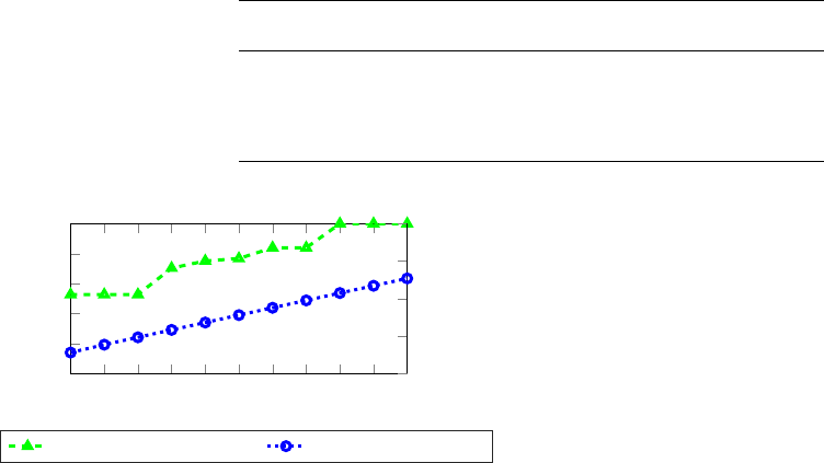
ACCEPTED FOR PRESENTATION IN 11
TH
BULK POWER SYSTEMS DYNAMICS AND CONTROL SYMPOSIUM (IREP 2022),
JULY 25-30, 2022, BANFF, CANADA 7
TABLE I
COMPARISON OF PROBLEM FORMULATION AND TYPE, GENERATION COST, AND SHARE OF FEASIBLE INSTANCES FOR 125 INSTANCES WITH RANDOM
COST FUNCTIONS
Problem Problem Generation Share of feasible
formulation type cost ($) instances (%)
AC-OPF NLP 2425.94 35.2
+ N-1 security NLP 2565.13 35.2
+ small-signal stability ( = 0) MILP 2942.83 52.8
+ small-signal stability ( = 7) MILP 2949.78 84.0
+ small-signal stability ( = 8) MILP 2950.76 100.0
0 1 2 3 4 5 6 7 8 9 10
0
20
40
60
80
100
Share (%)
2,940
2,945
2,950
2,955
2,960
Cost ($)
Share of feasible instances Average objective value
Fig. 3. For 125 random cost functions, we show the share of feasible instances
and average cost function as function of parameter .
feasible instances and the average objective value for ranging
from 0 to 10. The share of feasible instances increases in two
jumps from = 3 to = 4 (from 52.8 % to 70.4%) and from
= 7 to = 8, from 84.0% to 100%. As an alternative to the
proposed heuristic of identifying , our future work is directed
towards robust retraining of neural networks [32].
Our proposed approach has the following limitations. First,
the approach may incur optimality loss, due to the approxi-
mation errors. However, considering that the constraints about
small-signal stability are intractable for any conventional op-
timization method, all methods are bound to use some sort of
approximation. So far, no method exists in the literature that
introduces approximations for dynamic security and guaran-
tees no optimality loss. At the same time, a tractable, efficient
and suboptimal solution can still provide useful information
to the grid operator, compared to a solution that would not
consider dynamic security at all. Second, if we apply this
approach to different power grids, we will need to train
different NNs, as, at the moment, it is difficult to train NNs that
can generically apply to any power system. First approaches
to train more general neural networks have already been
proposed using e.g. Graph Neural Networks [33], [34]. Further
developing such approaches will be the object of future work.
V. CONCLUSION
We introduce a framework that can efficiently capture
previously intractable optimization constraints and transform
them to a mixed-integer linear program, through the use of
neural networks. First, we encode the feasible space which
is characterized by both tractable and intractable constraints,
e.g. constraints based on differential equations, to a neural
network. Leveraging an exact mixed-integer reformulation
of the trained neural network, and an efficient method to
include non-linear equality constraints, we solve mixed-integer
linear programs that can efficiently approximate non-linear
optimization programs with previously intractable constraints.
We apply our methods to the AC optimal power flow problem
with dynamic security constraints. For an IEEE 14-bus system,
and considering a combination of N-1 security and small-
signal stability, we demonstrate how the proposed approach
allows to obtain cost-optimal solutions which at the same
time satisfy both static and dynamic security constraints. To
the best of our knowledge, this is the first work that utilizes
an exact transformation to convert the information encoded
in neural networks to set of mixed integer-linear constraints
and use it in an optimal power flow problem. Future work
is directed towards utilizing efficient dataset creation methods
[25], increasing robustness of classification neural networks
to boost the applicability of this approach [32], determining
critical system indices using physics-informed neural networks
[35], and learning worst-case guarantees for neural networks
[36], [37].
REFERENCES
[1] S. K. Agrawal and B. C. Fabien, Optimization of dynamic systems.
Springer Science & Business Media, 2013, vol. 70.
[2] P. Panciatici, G. Bareux, and L. Wehenkel, “Operating in the fog:
Security management under uncertainty,” IEEE Power and Energy
Magazine, vol. 10, no. 5, pp. 40–49, 2012.
[3] M. B. Cain, R. P. O’neill, and A. Castillo, “History of optimal power
flow and formulations,” Federal Energy Regulatory Commission, vol. 1,
pp. 1–36, 2012.
[4] F. Capitanescu, J. M. Ramos, P. Panciatici, D. Kirschen, A. M. Mar-
colini, L. Platbrood, and L. Wehenkel, “State-of-the-art, challenges, and
future trends in security constrained optimal power flow,” Electric Power
Systems Research, vol. 81, no. 8, pp. 1731–1741, 2011.
[5] R. Z
´
arate-Mi
˜
nano, T. Van Cutsem, F. Milano, and A. J. Conejo,
“Securing transient stability using time-domain simulations within an
optimal power flow,” IEEE Trans. on Power Systems, vol. 25, no. 1, pp.
243–253, 2009.
[6] Y. Xu, Z. Y. Dong, K. Meng, J. H. Zhao, and K. P. Wong, “A
hybrid method for transient stability-constrained optimal power flow
computation,” IEEE Trans. on Power Systems, vol. 27, no. 4, pp. 1769–
1777, 2012.
[7] E. Vaahedi, Y. Mansour, C. Fuchs, S. Granville, M. D. L. Latore,
and H. Hamadanizadeh, “Dynamic security constrained optimal power
flow/var planning,” IEEE Trans. on Power Systems, vol. 16, no. 1, pp.
38–43, 2001.
[8] J. Condren and T. W. Gedra, “Expected-security-cost optimal power flow
with small-signal stability constraints,” IEEE Trans. on Power Systems,
vol. 21, no. 4, pp. 1736–1743, 2006.
ACCEPTED FOR PRESENTATION IN 11
TH
BULK POWER SYSTEMS DYNAMICS AND CONTROL SYMPOSIUM (IREP 2022),
JULY 25-30, 2022, BANFF, CANADA 8
[9] R. Canyasse, G. Dalal, and S. Mannor, “Supervised learning for optimal
power flow as a real-time proxy,” in 2017 IEEE Power Energy Society
Innovative Smart Grid Technologies Conference, no. 1, 2017, pp. 1–5.
[10] F. Fioretto, T. W. Mak, and P. Van Hentenryck, “Predicting ac optimal
power flows: Combining deep learning and lagrangian dual methods,”
Proceedings of the AAAI Conference on Artificial Intelligence, vol. 34,
no. 01, pp. 630–637, Apr. 2020.
[11] X. Pan, T. Zhao, M. Chen, and S. Zhang, “Deepopf: A deep neural
network approach for security-constrained dc optimal power flow,” IEEE
Trans. on Power Systems, vol. 36, no. 3, pp. 1725–1735, 2021.
[12] Y. Chen and B. Zhang, “Learning to solve network flow problems via
neural decoding,” arXiv preprint:2002.04091, 2020.
[13] K. Dvijotham and D. K. Molzahn, “Error bounds on the dc power
flow approximation: A convex relaxation approach,” in 2016 IEEE 55th
Conference on Decision and Control. IEEE, 2016, pp. 2411–2418.
[14] J. Rahman, C. Feng, and J. Zhang, “Machine learning-aided security
constrained optimal power flow,” in 2020 IEEE Power Energy Society
General Meeting (PESGM), 2020, pp. 1–5.
[15] L. A. Wehenkel, Automatic learning techniques in power systems.
Springer Science & Business Media, 2012.
[16] J. L. Cremer, I. Konstantelos, S. H. Tindemans, and G. Strbac, “Data-
driven power system operation: Exploring the balance between cost and
risk,” IEEE Trans. on Power Systems, vol. 34, no. 1, pp. 791–801, 2018.
[17] L. Halilba
ˇ
si
´
c, F. Thams, A. Venzke, S. Chatzivasileiadis, and P. Pinson,
“Data-driven security-constrained ac-opf for operations and markets,” in
2018 Power Systems Computation Conference (PSCC), 2018, pp. 1–7.
[18] V. J. Gutierrez-Martinez, C. A. Ca
˜
nizares, C. R. Fuerte-Esquivel,
A. Pizano-Martinez, and X. Gu, “Neural-network security-boundary
constrained optimal power flow,” IEEE Trans. on Power Systems, vol. 26,
no. 1, pp. 63–72, 2010.
[19] T. Wu, Y.-J. Angela Zhang, and S. Wang, “Deep learning to optimize:
Security-constrained unit commitment with uncertain wind power gen-
eration and besss,” IEEE Transactions on Sustainable Energy, vol. 13,
no. 1, pp. 231–240, 2022.
[20] W. F. Tinney and C. E. Hart, “Power flow solution by newton’s method,”
IEEE Trans. on Power Apparatus and Systems, vol. PAS-86, no. 11, pp.
1449–1460, 1967.
[21] F. Milano, Power system modelling and scripting. Springer Science &
Business Media, 2010.
[22] P. W. Sauer, M. A. Pai, and J. H. Chow, Small-Signal Stability, 2017,
pp. 183–231.
[23] X. Glorot, A. Bordes, and Y. Bengio, “Deep sparse rectifier neural
networks,” in Proceedings of the fourteenth international conference on
artificial intelligence and statistics, 2011, pp. 315–323.
[24] F. Thams, A. Venzke, R. Eriksson, and S. Chatzivasileiadis, “Efficient
database generation for data-driven security assessment of power sys-
tems,” IEEE Trans. on Power Systems, vol. 35, no. 1, pp. 30–41, 2020.
[25] A. Venzke, D. K. Molzahn, and S. Chatzivasileiadis, “Efficient creation
of datasets for data-driven power system applications,” Electric Power
Systems Research, vol. 190, p. 106614, 2021.
[26] M. Abadi, A. Agarwal, P. Barham, E. Brevdo, Z. Chen, C. Citro, G. S.
Corrado, A. Davis, J. Dean, M. Devin et al., “Tensorflow: Large-scale
machine learning on heterogeneous distributed systems,” 2016.
[27] V. Tjeng, K. Y. Xiao, and R. Tedrake, “Evaluating robustness of
neural networks with mixed integer programming,” in 7th International
Conference on Learning Representations, New Orleans, LA, USA, 2019.
[28] K. Y. Xiao, V. Tjeng, N. M. Shafiullah, and A. Madry, “Training for
faster adversarial robustness verification via inducing relu stability,”
International Conference on Learning Representations, 2019.
[29] R. D. Zimmerman, C. E. Murillo-S
´
anchez, and R. J. Thomas, “Mat-
power: Steady-state operations, planning, and analysis tools for power
systems research and education,” IEEE Trans. on power systems, vol. 26,
no. 1, pp. 12–19, 2010.
[30] J. Lofberg, “Yalmip: A toolbox for modeling and optimization in mat-
lab,” in 2004 IEEE international conference on robotics and automation
(IEEE Cat. No. 04CH37508). IEEE, 2004, pp. 284–289.
[31] A. W
¨
achter and L. T. Biegler, “On the implementation of an interior-
point filter line-search algorithm for large-scale nonlinear programming,”
Mathematical programming, vol. 106, no. 1, pp. 25–57, 2006.
[32] A. Venzke and S. Chatzivasileiadis, “Verification of neural network
behaviour: Formal guarantees for power system applications,” IEEE
Trans. on Smart Grid, vol. 12, no. 1, pp. 383–397, 2021.
[33] B. Donon, B. Donnot, I. Guyon, and A. Marot, “Graph neural solver
for power systems,” in 2019 International Joint Conference on Neural
Networks (IJCNN), 2019, pp. 1–8.
[34] B. Donon, R. Cl
´
ement, B. Donnot, A. Marot, I. Guyon, and
M. Schoenauer, “Neural networks for power flow: Graph neural
solver,” Electric Power Systems Research, vol. 189, p. 106547, 2020.
[Online]. Available: https://www.sciencedirect.com/science/article/pii/
S0378779620303515
[35] G. S. Misyris, J. Stiasny, and S. Chatzivasileiadis, “Capturing power sys-
tem dynamics by physics-informed neural networks and optimization,”
arXiv preprint:2103.17004, 2021.
[36] S. L. Andreas Venzke, Guannan Qu and S. Chatzivasileiadis, “Learning
optimal power flow: Worst-case guarantees for neural networks,” in
2020 IEEE International Conference on Communications, Control, and
Computing Technologies for Smart Grids (SmartGridComm), 2020.
[37] R. Nellikkath and S. Chatzivasileiadis, “Physics-informed neural net-
works for minimising worst-case violations in dc optimal power flow,”
arXiv preprint:2107.00465, 2021.
