Graver Bases via Quantum Annealing with application to non-linear

Graver Bases via Quantum Annealing

with application to non-linear integer programs

Hedayat Alghassi

∗

, Raouf Dridi

†

, Sridhar Tayur

‡

CMU Quantum Computing Group

Tepper School of Business, Carnegie Mellon University, Pittsburgh, PA 15213

February 13, 2019

Abstract

We propose a novel hybrid quantum-classical approach to calculate Graver bases,

which have the potential to solve a variety of hard linear and non-linear integer pro-

grams, as they form a test set (optimality certiﬁcate) with very appealing properties.

The calculation of Graver bases is exponentially hard (in general) on classical com-

puters, so they not used for solving practical problems on commercial solvers. With

a quantum annealer, however, it may be a viable approach to use them. We test two

hybrid quantum-classical algorithms (on D-Wave)–one for computing Graver basis and

a second for optimizing non-linear integer programs that utilize Graver bases–to under-

stand the strengths and limitations of the practical quantum annealers available today.

Our experiments suggest that with a modest increase in coupler precision–along with

near-term improvements in the number of qubits and connectivity (density of hardware

graph) that are expected–the ability to outperform classical best-in-class algorithms is

within reach, with respect to non-linear integer optimization.

Keywords: Graver bases, quantum annealing, test sets, non-linear integer optimization,

computational testing.

∗

halghassi@cmu.edu

†

[email protected]u.edu

‡

stayur@cmu.edu

arXiv:1902.04215v1 [quant-ph] 12 Feb 2019

Contents

1 Introduction 4

1.1 Illustrative Example . . . . . . . . . . . . . . . . . . . . . . . . . . . . . . . 4

1.2 Features and Contributions of our Approach . . . . . . . . . . . . . . . . . . 5

1.2.1 Features . . . . . . . . . . . . . . . . . . . . . . . . . . . . . . . . . . 6

1.2.2 Contributions . . . . . . . . . . . . . . . . . . . . . . . . . . . . . . . 6

1.3 Outline . . . . . . . . . . . . . . . . . . . . . . . . . . . . . . . . . . . . . . . 7

2 Background: Graver Bases and its Use in Non-linear Integer Optimization 7

2.1 Mathematics of Graver Bases . . . . . . . . . . . . . . . . . . . . . . . . . . 8

2.2 Wide Applicability of Graver Bases as Optimality Certiﬁcates . . . . . . . . 9

3 Graver Basis via Quantum Annealing 10

3.1 QUBOs for Kernels . . . . . . . . . . . . . . . . . . . . . . . . . . . . . . . . 11

3.1.1 Integer to binary encoding . . . . . . . . . . . . . . . . . . . . . . . . 11

3.1.2 Sampling the kernel . . . . . . . . . . . . . . . . . . . . . . . . . . . . 12

3.2 Post-Processing . . . . . . . . . . . . . . . . . . . . . . . . . . . . . . . . . . 13

3.2.1 Systematic post-processing of near-optimal solutions into optimal . . 13

3.2.2 Distribution of optimal and near-optimal solutions: Experimental results 14

3.2.3 Combining near-optimal solutions . . . . . . . . . . . . . . . . . . . . 14

3.3 Using Residual Kernel to Obtain More Graver Bases Elements . . . . . . . . 16

3.4 Adaptive Centering and Encoding . . . . . . . . . . . . . . . . . . . . . . . . 16

3.5 Numerical Results . . . . . . . . . . . . . . . . . . . . . . . . . . . . . . . . . 17

3.5.1 Example 1: Four coin problem . . . . . . . . . . . . . . . . . . . . . . 17

3.5.2 Example 2: Variation problem . . . . . . . . . . . . . . . . . . . . . . 18

3.5.3 Example 3: Snake-wise prime number . . . . . . . . . . . . . . . . . . 18

3.5.4 Example 4: Some random matrices of size (2 × 5) . . . . . . . . . . . 19

3.5.5 Example 5: Four cycle binary model . . . . . . . . . . . . . . . . . . 19

3.5.6 Example 6: Random low span integer matrices of size (4×8) . . . . . 20

3.6 Discussion . . . . . . . . . . . . . . . . . . . . . . . . . . . . . . . . . . . . . 21

3.6.1 Chainbreak . . . . . . . . . . . . . . . . . . . . . . . . . . . . . . . . 21

3.6.2 Communication delays . . . . . . . . . . . . . . . . . . . . . . . . . . 21

4 Hybrid Quantum Classical Algorithm for Non-Linear Integer Optimiza-

tion 22

4.1 Algorithm Structure . . . . . . . . . . . . . . . . . . . . . . . . . . . . . . . 22

4.2 QUBO for Obtaining Feasible Solutions . . . . . . . . . . . . . . . . . . . . . 23

4.3 Parallel Augmentations with Limited Elements of the Graver Bases . . . . . 23

4.4 Numerical Results . . . . . . . . . . . . . . . . . . . . . . . . . . . . . . . . . 23

4.4.1 Case 1: Nonlinear 0-1 program with 50 binary variables . . . . . . . . 24

4.4.2 Comparison with a best-in-class classical method . . . . . . . . . . . 27

4.4.3 Case 2: Nonlinear low span integer program with 25 integer variables 28

4.4.4 Augmenting with partial Graver basis . . . . . . . . . . . . . . . . . . 30

5 Conclusions 32

Acknowledgements 32

Bibliography 32

A Graver Basis via Classical Methods 36

B Quantum Annealing and D-Wave Processors 37

B.1 Quantum Annealing . . . . . . . . . . . . . . . . . . . . . . . . . . . . . . . 37

B.2 Quantum Annealer from D-Wave . . . . . . . . . . . . . . . . . . . . . . . . 37

B.2.1 D-Wave SAPI . . . . . . . . . . . . . . . . . . . . . . . . . . . . . . . 37

B.2.2 Chainbreak strategy . . . . . . . . . . . . . . . . . . . . . . . . . . . 38

B.2.3 Annealing time . . . . . . . . . . . . . . . . . . . . . . . . . . . . . . 39

1 Introduction

This paper explores the capability of an available quantum annealer for solving non-linear

integer optimization problems (that arise in engineering and business applications) using test

sets. Of course, we do not expect current quantum annealers (D-Wave 2000Q, in our setting)

to be competitive against classical computing algorithms that have decades of innovations

and implementation improvements. Our motivation in this work is more of a proof-of-

concept: to check how viable a hybrid quantum-classical approach is and understand what

it would take to surpass classical methods.

The D-Wave quantum annealer solves Quadratic Unconstrained Binary Optimization (QUBO)

problems of the form [Ber18]:

min x

Qx such that x ∈ {0, 1}

(1)

In this paper, we develop a hybrid quantum-classical algorithm that calculates a test set

called Graver bases, on such a quantum annealer, and then we use it to optimize nonlinear

integer programming problems. Because Graver bases [Gra75] have applications in areas

other than optimization, studying how our algorithm acquires Graver bases of integer ma-

trices of various kinds is of interest in itself. We test our approach on D-Wave and report

our ﬁndings.

1.1 Illustrative Example

The following example walks through some of the key steps of our algorithms (and reviews

the deﬁnition of Graver bases). Those steps will be described in detail in later sections.

Consider the following integer optimization problem with a non-linear objective function:











min f(x) =

i=1

− 5|

, x

> 0 , x

∈ Z



1 1 1 1

1 5 10 25

















156



Let A denote the 2× 4 integer matrix above; so we write the above constraint as Ax = b. By

deﬁnition, the Graver basis G(A) of the matrix A is a minimal set of elements of the kernel

ker

A with respect to the partial ordering

x v y when x

> 0 (the two vectors x and y lie on the same orthant) and |x

| 6 |y

| .

The steps of our hybrid quantum-classical algorithm for computing Graver bases are:

• We map the problem of ﬁnding the kernel of A into a QUBO of the form (1). This is

the quantum part of the hybrid approach.

• The elements of G(A) can be obtained from the degenerate solutions of the given

QUBO. The way such elements are obtained (ﬁltered from kernel elements, followed

by some post-processing) constitutes the classical part of our hybrid approach.

In our example, the Graver basis elements are the column vectors of the matrix:

G(A) =







0 5 5 5 5

3 −9 −6 −3 0

−4 4 0 −4 −8

1 0 1 2 3











This was obtained using only one call to the D-Wave quantum annealer (details in 3.5.1) and

some classical post-processing. (Typically, more than one call is required. We detail this in

a later section.) Once the Graver basis is computed, the optimal solution can be obtained

by augmenting, beginning from any feasible solution. To solve the optimization problem,

our second hybrid quantum-classical algorithm is as follows:

• We use the quantum annealer (once more) to solve the constraint Ax = b (using

QUBO in Equation (11)) and obtain a feasible solution. (Actually, a call of D-Wave

usually gives many solutions, up to 10000. We discuss how many of these are unique,

sometimes more than 6000, and which one(s)to use, in later subsections).

• With the Graver basis and a feasible solution at hand, we can start the augmentation

procedure (which is classical portion of our second algorithm).

Let us illustrate the augmentation step. An initial feasible solution obtained is x



1 15 3 2



with f(x

) = 19. Adding the vector −g



0 −3 4 −1



to the

previous value gives x



1 12 7 1



, which has a lower cost value of f(x

) = 17.

Similarly, adding g



5 −9 4 0



to the previous value yields x



6 3 11 1



which has a lower cost value of f(x

) = 13. Similar calculations are done consecutively with

the vectors g

, −g

and −g

again, which ﬁnally results in x



6 6 7 2



, which has

the cost value f(x

) = 7. Adding any of the Graver basis elements again to x

results in vec-

tors that all have a cost higher than the current minimum 7 (inside the feasible region x > 0);

therefore, the augmentation procedure stops with the optimal solution x

∗

= x

While the objective function can be linearized, it would require increasing the number of

variables, an important consideration when we have limited number of qubits and connec-

tivity. Furthermore, other non-linear objective functions that may not be easily linearizable

can also be handled with the same Graver basis and feasible solutions, making our procedure

more general purpose.

1.2 Features and Contributions of our Approach

We list below some key features followed by key contributions of our approach.

1.2.1 Features

• Graver basis is an optimality certiﬁcate, and the calculation of elements depends only

on the constraints. Thus, the objective function can even be a comparison oracle. The

objective function appears only in the augmentation step where it is called (queried).

Several diﬀerent objective functions (for the same constraints) can be studied classically

once the Graver basis has been computed.

• In the special case of a quadratic objective function, a naive approach of combining the

objective function and the constraints through a Lagrangian multiplier into a single

QUBO may appear attractive. However, searching for the right Lagrangian multiplier

is non-trivial. We avoid this complexity in our approach as we have decoupled the

objective function from the constraints.

• In the case of an objective function that is a polynomial function, there is no need for

any reduction to QUBO and adding extra variables, diﬀerent from other methods that

utilize a quantum annealer.

• At each anneal (read), the algorithm starts out fresh from the uniform superposition

(superposition of the states of the computational basis of C

⊗n

). A single call can have

up to 10000 reads. Thus, it can reach diﬀerent ground states with good probabilities

(i.e., be able to extract diﬀerent kernel elements, ker

(A) ⊂ Z

,), and so within a few

calls, we can expect to ﬁnd all of them.

1.2.2 Contributions

• We provide two hybrid quantum classical algorithms: (1) to calculate the Graver basis

of any general integer matrix, and (2) to solve a non-linear integer programming prob-

lem using the Graver basis. By separating the objective function and the constraints

equation’s (Ax = b) right hand side (b) from the calculation of the test set (Graver

basis), our approach can tackle many non-linear objectives, cost functions, only via

an oracle call, and also help in solving deterministic and stochastic programs (with

varying right hand sides b or objective function parameters) in a systematic manner.

• For the Graver calculation algorithm, we develop a (classical) systematic post-processing

strategy that transforms the quantum annealer’s near-optimal solutions into optimal

solutions, which might be an useful technique in other situations.

• For iterative integer to binary transformation in these algorithms, we develop an adap-

tive strategy that moves (a) the middle point and (b) the encoding length of integer

variables based on the suboptimal solutions obtained in the previous iteration. This

strategy, which optimizes resources (qubits), can be used in any integer to binary

encoding that is solved iteratively by a quantum annealer.

• We test both Graver and non-linear optimization algorithms, on the D-Wave 2000Q

quantum annealing processor and discuss the implementation details, strengths, and

shortcomings.

• Unlike the typical application of a quantum annealer that uses the many reads to

increase the conﬁdence of a desired solution, we use the many reads to sample the

many unique solutions. This re-purposing makes our approach particularly suitable to

tackle hard integer optimization problems.

• Our experiments were designed to elucidate what is preventing the quantum annealer

from being competitive today, and what enhancements are needed (and why) to sur-

pass classical methods. What we ﬁnd is that even if we have a processor with the

same number of qubits and connectivity structure, with a higher coupler precision,

some classes of nonlinear integer problems can be solved comparably to best-in-class

classical solvers, e.g., Gurobi Optimizer (latest version, 8.0). Alternatively, with a new

processor with a higher number of qubits and better connectivity that has already

been announced, even without an increase in coupler precision, certain instances can

be solved better than classical methods. Indeed, doubling the coupler precision (on

top of the announced increases in qubits and connectivity) would lead to surpassing

classical methods for many problems of practical importance.

1.3 Outline

We are bringing together (a) the calculation of Graver bases using quantum annealing

and (b) solving integer optimization through Graver bases with feasible solutions obtained

via quantum annealing. Section 2 introduces nonlinear integer programs and Graver bases.

A pre-requisite to acquiring the Graver basis is to ﬁnd the kernel of a matrix. Section 3

develops a hybrid quantum classical algorithm for calculation of Graver basis of an inte-

ger matrix and presents computational results. Section 4 develops the quantum classical

algorithm for non-linear integer programs and presents numerical results. Section 5 summa-

rizes our ﬁndings. To make this document self-contained, our appendices brieﬂy review (A)

computing Graver bases classically and (B) quantum annealing with D-Wave processors.

2 Background: Graver Bases and its Use in Non-linear

Integer Optimization

Let f : R

→ R be a real-valued function. We want to solve the general non-linear integer

optimization problem:

(IP)

A,b,l,u,f







min f(x),

Ax = b, l 6 x 6 u, x, l, u ∈ Z

A ∈ Z

m×n

, b ∈ Z

(2)

One approach to solving such problem is to use an augmentation procedure: start from an

initial feasible solution (which itself can be hard to ﬁnd) and take an improvement step–

augmentation - until one reaches the optimal solution. Augmentation procedures such as

these need test sets or optimality certiﬁcates: so it either declares the optimality of the

current feasible solution or provides direction(s) towards better solution(s). Note that it

does not matter from which feasible solution one begins, nor the sequence of improving steps

taken: the ﬁnal stop is an optimal solution. (It is not hard to see that computing a test

set can be very expensive classically. We want to study whether quantum annealing can be

competitive.)

Deﬁnition 1. A set S ∈ Z

is called a test set or optimality certiﬁcate if for every non-

optimal but feasible solution x

there exists t ∈ S and λ ∈ Z

such that x

+ λt is feasible

and f (x

+ λt) < f (x

). The vector t (or λt) is called the improving or augmenting direction.

If the optimality certiﬁcate is given, any initial feasible solution x

can be augmented to

the optimal solution. If S is ﬁnite, one can enumerate over all t ∈ S and check if it is aug-

menting (improving). If S is not practically ﬁnite, or if all elements t ∈ S are not available

in advance, it is still practically enough to ﬁnd a subset of S that is feasible and augmenting.

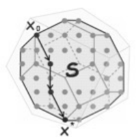
Figure 1: Augmenting from initial to optimal solution [Onn10].

In the next section, we discuss the Graver basis of an integer matrix A ∈ Z

m×n

which is

known to be an optimality certiﬁcate.

2.1 Mathematics of Graver Bases

First, on the set R

, we deﬁne the following partial order:

Deﬁnition 2. Let x, y ∈ R

. We say x is conformal to y, written x v y, when x

> 0 (x

and y lie on the same orthant) and |x

| 6 |y

| for i = 1, ..., n. Additionally, a sum u =

is called conformal, if v

v u for all i (u majorizes all v

Suppose A is a matrix in Z

m×n

. Deﬁne :

∗

(A) =





Ax = 0, x ∈ Z

, A ∈ Z

m×n



\ {0} . (3)

The notion of Graver basis was ﬁrst introduced in [Gra75] for integer linear programs (ILP):

Deﬁnition 3. The Graver basis of integer matrix A is deﬁned to be the ﬁnite set of v

minimal elements (indecomposable elements) in the lattice L

∗

(A). We denote by G(A) ⊂ Z

the Graver basis of A.

The following proposition summarizes the properties of Graver bases that are relevant to our

setting.

Proposition 1. The following statements are true:

(i) Every vector x in the lattice L

∗

(A) is a conformal sum of the Graver basis elements.

(ii) Every vector x in the lattice L

∗

(A) can be written as x =

i=1

for some λ

∈ Z

and

∈ G(A). The upper bound on number of Graver basis elements required (t) (called

integer Caratheodory number) is (2n − 2).

(iii) A Graver basis is a test set (optimality certiﬁcate) for ILP. That is a point x

∗

is optimal

for the optimization problem (IP )

A,b,l,u,f

, if and only if there are no g

∈ G(A) such

that x

∗

+ g

is better than x

∗

(iv) For any g ∈ G(A), an upper bound on the norm of Graver basis elements is given by

kgk

∞

6 (n − r) ∆ (A) and kgk

6 (n − r) (r + 1) ∆ (A) (4)

where r = rank(A) 6 m and ∆ (A) is the maximum absolute value of the determinant

of a square submatrix of A.

2.2 Wide Applicability of Graver Bases as Optimality Certiﬁcates

Beyond integer linear programs (ILP) with a ﬁxed integer matrix, Graver bases as optimality

certiﬁcates have now been generalized to include several nonlinear objective functions:

• Separable convex minimization [MSW04]:

min

with f

is convex.

• Convex integer maximization (weighted) [DLHO

09]:

max f(Wx) , W ∈ Z

d×n

with f convex on Z

• Norm p (nearest to x

) minimization [HOW11]:

min kx − x

• Quadratic minimization [MSW04, LORW12]:

min x

V x

where V lies in dual of

quadratic Graver cone of A

• Polynomial minimization [LORW12]:

min P (x)

where P is a polynomial of degree

d, that lies on cone K

(A), dual of d

degree Graver cone of A.

It has been shown that only polynomially many augmentation steps are needed to solve

such minimization problems [HOW11] [DLHO

09]. Graver did not provide an algorithm for

computing Graver bases; Pottier [Pot96] and Sturmfels [ST97] provided such algorithms (see

Appendix A).

The use of test sets to study integer programs is a vibrant area of research. Another collection

of test sets is based on Groebner bases. See [CT91, TTN95, BLSR99, HS95] and [BPT00]

for several diﬀerent examples of the use of Groebner bases for integer programs.

3 Graver Basis via Quantum Annealing

Here we present our ﬁrst hybrid quantum classical algorithm, for Graver basis, constructed

from a subset of inﬁnite set of kernels of matrix A (obtained using the quantum annealer by

solving a QUBO) and reﬁning them classically:

• Quantum kernel: Calculate a subset of the kernel as discussed below.

• Classical ﬁltering: Reﬁne the Graver basis using v-minimal ﬁltration on the kernel

subset.

This two step procedure is repeated in a loop until all required Graver basis elements are

acquired. In each iteration i within this loop, we extract the Graver basis of the given integer

matrix A for a given bound [L

, U

]. These bounds are updated adaptively [L

, U

] from one

iteration to another.

Each call of a hybrid quantum classical algorithm to extract Graver basis, inside such a

bounded region, is as follows:

Algorithm 1 Graver Extraction

1: inputs: Integer matrix A, Graver basis lower (L

) and upper (U

) bound vectors

2: output: Graver basis G(A), inside the bounded region [L

, U

]

3: Initialize: Graver set G(A), Kernel set K(A), Midpoint vector M

, Encoding length vector K

4: while (iteration i) ∆



(A)



6 δ do

5: Reshuﬄe columns of A, using random permutation P

6: Construct QUBO matrix Q

, using equation (8), (see 3.1)

7: Find optimal and suboptimal solutions [x

, x

] = Quantum Solve(Q

), (see B)

8: Revert variable orders (using P

)

9: Post-process suboptimals x

into new optimals x

, (see 3.2.3)

10: Create unique kernel set K

(A) = x

11: G(A) = G(A)

(A) and K(A) = K(A)

(A)

12: # Kernel to Graver, v minimal post-processing:

13: for v

, v

in G(A) do

14: if v

v v

then G(A) = G(A)\v

15: end for

16: G(A) = Residual P rocedure(G(A), K

(A)); (see 3.3)

17: [M

i+1

, K

i+1

] = Adaptive Adjustments P rocedure(M

, K

, x

); (see 3.4)

18: end while

19: return G(A)

3.1 QUBOs for Kernels

The mapping of the kernel problem into a QUBO is the essential quantum step in our hybrid

approach. Each call of a quantum-annealing based QUBO solver can– through multiple

reads– extract several (unique) degenerate ground states. We expect to be able to compute

a large sampling of the kernel of A in one or more calls (of 10000 reads each).

We need to solve

Ax = 0, x ∈ Z

, A ∈ Z

m×n

which is computationally hard, in a

bounded region [Pap81]. Instead, we look to ﬁnd a large sampling of the non-zero elements

of the kernel. To do this, we use quadratic unconstrained integer optimization (QUIO):

min x

x , Q

= A

A , x ∈ Z



. . . x



, x

∈ Z

(5)

3.1.1 Integer to binary encoding

Because the quantum annealer solves quadratic unconstrained binary problems, we need to

encode the integer variables into binary variables through an integer to binary mapping.

Due to the limited number of qubits available, we need to be eﬃcient in our encoding. We

do so by adaptively allocating the qubits to the variables, so that the variables may have a

diﬀerent number allocated to them in any given iteration. In subsequent iterations, based

on which variable appears to be in need, we readjust the allocation. We also re-center our

variables adaptively to further increase the eﬃciency of encoding. We discuss this in a later

subsection (see 3.4).

To map an integer variable to a binary, while keeping the problem quadratic, we use a linear

mapping: x

= e

where e



· · · e



∈ Z

is the linear encoding vector and



i,1

i,2

· · · X

i,k



∈ {0, 1}

is the encoded binary vector that encodes integer

value x

. The k

is the length (number of bits) of encoding vector e

, and depends on the

linear encoding scheme that is in use. For a speciﬁc integer length, the diﬀerence between

the upper bound of x

to the lower bound of x

is ∆

= Ux

− Lx

; thus, the minimum

is dlog

∆

e for binary encoding with the encoder vector e



· · · 2



, and

the maximum k

is ∆

for unary encoding with the encoder vector e

z }| {



1 1 · · · 1



Therefore,

x = L + EX =



















· · · 0

· · · e



















(6)

where E is a (n ×

i=1

) matrix that encodes the integer vector x into binary vector

X ∈ {0, 1}

and L is a (n×1) vector containing the integer variable’s lower bounds. (If one

chooses the same encoding size for all integer variables

e = e

, k = k

, ∀i = 1, . . . , n,

then the (n × nk) encoding matrix simpliﬁes to E = e ⊗ I

, where ⊗ is the Kronecker

product and I

is the identity matrix of size n.) Inserting (6) into (5):

x = (L + EX)

(L + EX) = X

EX +



L + L



+ L

(7)

The last term in equation (7) is constant. Because x

= x

for binary variables, the middle

linear terms can be rewritten as X

diag





X. Therefore the quadratic unconstrained

binary optimization formulation simpliﬁes to,

min X

, Q

= E

E + diag





X ∈ {0, 1}

, Q

= A

(8)

3.1.2 Sampling the kernel

The QUBO in equation (8) has inherent symmetry in Q

for each of the variables. For

a randomly chosen integer matrix A, the valleys for all degenerate solutions should have

similar spreads. This gives us optimism that with certain variable perturbations and some

post-processing of near-optimal solutions, we should be able to sample well. Additionally,

because we solve (8) in a sequence of adaptive D-Wave calls, ﬁne-tuning the bit sizes for

each variable and targeting our kernel search, we expect that although the D-Wave annealer

is not an uniform sampler (in the theoretical sense, see [MZK17]), we should nevertheless be

quite successful.

We should mention that applying any modiﬁcation that changes Q

requires a new embed-

ding of the modiﬁed problem graph into the sparse hardware graph of the D-Wave processor,

which is a downside. Using D-Wave SAPI in-house embedder program, the embedder starts

from scratch each time, which creates an unknown delay in each iteration of the main loop.

We have designed a new approach that transforms the embedding of any problem graph

into any hardware graph into an equational system of quadratic integer equations and solves

them by powerful tools of algebraic geometry and Groebner bases [DAT18b]. This approach

has the property that minor changes in Q

result in only minor change in equations, thus

the Groebner bases solver still utilizes the majority of simpliﬁed equations from the previous

pool of equations that leads to shorter embedding time for minor changes in Q

. We have

not used this new embedding approach in this paper, however, as our goal was to see what

the available hardware and SAPI could do.

3.2 Post-Processing

We have developed two post-processing steps to be done classically.

3.2.1 Systematic post-processing of near-optimal solutions into optimal

Implementation of the model in equation (7) on the D-Wave quantum annealing solver

(DW2000Q, solver id: C16-VFYC) shows promising results in extracting degenerate kernel

solutions, especially when using minimize energy chainbreak strategy (see Appendix B). For

a random selection of integer matrices with various sizes, one run of the processor with

approximately 10000 reads (annealing time 290 msec) returns ≈ 100 − 150 unique (non-

similar) optimal and suboptimal solutions. Among these, ≈ 10 − 20 are optimal degenerate

solutions and the rest are suboptimal solutions.

Analysis of these suboptimal solutions shows that, remarkably, the majority (over 87%) of

them have very small errors, and so are near-optimal. This motivated us to design a post-

processing procedure to extract more degenerate solutions from the existing suboptimal

solutions. Because this post-processing is based on our known problem (Ax = 0), the

operations required to reach the optimal solutions are systematic and with known predictable

polynomial overhead.

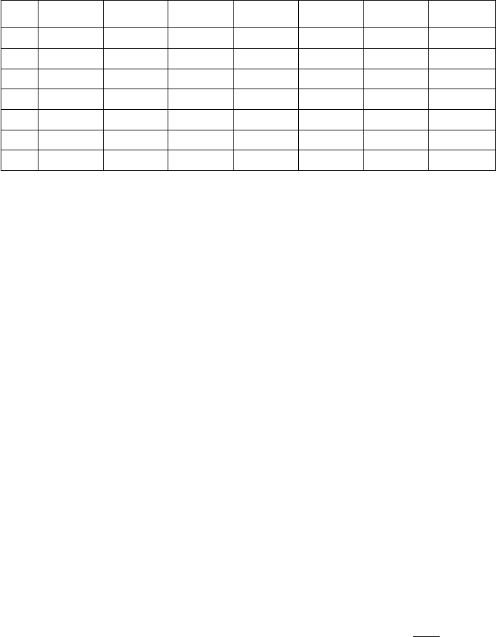
3.2.2 Distribution of optimal and near-optimal solutions: Experimental results

We chose a selection of random integer matrices A ∈ Z

m×n

, −10 6 a

6 10

; ten matrices

from each size (m × n) ∈ {(2 × 5) , (3 × 5) , (3 × 6) , (3 × 7) , (4 × 8) , (5 × 8)}. Having

a ﬁxed embedding for each size category, we acquired the unique solutions of each call (10000

reads per call, annealing time of 290nsec), and evaluated the percentage of unique solutions,

which fall into any of the seven solution categories: zero error (optimal solutions), 1 to 5

total sum errors, and greater than or equal to 6 total sum errors.

(2 × 5) (3 × 5) (3 × 6) (3 × 7) (4 × 8) (5 × 8) Overall

0 15 12 10 13 12 9 11.8

1 24 28 26 31 30 33 28.7

2 31 28 27 24 21 25 26.0

3 20 21 25 19 20 17 20.3

4 7 8 10 9 9 8 8.5

5 2 1 0 3 4 5 2.5

>6 1 2 2 1 4 3 2.2

Table 1: Optimal and suboptimal solution percentages for various size matrices.

As seen in Table 1, over 75% of unique solutions, fall into the categories with total sum

errors 1 to 3. Overall, 87% of unique solutions are either optimal solutions or near-optimal.

3.2.3 Combining near-optimal solutions

Assume x

∈ Z

n×N

is the unique solution matrix (each column is a unique read), acquired

by ﬁltering out the repeated solutions out of all reads from the quantum annealer.

The matrix Ax

= E

contains the b values in each of N columns. We expect that b = 0

for optimal solutions, and b 6= 0 but 1

|b| small for nonoptimal solutions. We sorted and

separated the columns of x

based on their corresponding sum of absolute value error in

. Because the majority of reads have no maximum error greater than 3, we categorized

solutions into four groups of 0, 1, 2, and 3 total sum errors. The solutions with a total sum

of 0 obviously do not need post-processing.

Post-processing for the solutions with a total sum error = 1 For each row r

, 1 ≤ i ≤ m

all columns with +1 error and all columns with -1 error consist two sub-groups. For each row,

thus, we have three sets of operations: Subtracting all +1 columns pairwise, subtracting all

-1 columns pairwise, and adding any of columns from +1 to any of columns from -1 pairwise.

The above-mentioned operations, on average for all m rows, cost O





pairwise column

additions, where N

is the number of unique solutions with a total sum error of 1.

Post-processing for the solutions with total sum error = 2 The absolute sum error

=2 situation has two cases. The ﬁrst one is similar to the previous case; for each of the

m rows, we have either +2 or -2 (and of course 0), which we will resolve similarly. In the

second case, for each pair of rows,

, r

, i, j = 1, . . . , m

, among m(m − 1)/2 possible

pairs, we have four sub-groups of errors (r

, r

) that are (+1, +1), (+1, -1), (-1, +1), and (-1,

-1). For each sub-group any pairwise subtraction results to zero. Additionally, we have two

sub-groups of (+1, +1), (-1, -1) and (+1, -1), (-1, +1) that can have pairwise subtraction

to result in zero. The above-mentioned operations, for all m rows, on average roughly cost





column pairwise additions to resolve +2, -2 errors and O





pairwise additions

to resolve the eight remaining categories of various +1, -1 errors, where N

is the number

of unique solutions with a total sum error of 2.

Post-processing for the solutions with total sum error = 3 This situation has three

general categories of errors. As before, if for each of m rows, in each column we have either

+3 or -3, this case is similar to the ﬁrst case (and the ﬁrst case in the second situation) and

is resolved similarly. The second case here has similarities with the second category of the

second case. It consists of 4 subgroups on m(m − 1)/2 pairs of rows, that have (-2, -1), (-2,

+1), (+2, -1), (+2, +1). Likewise, it needs in-group subtraction for each of the four groups

and two pairwise additions between the subgroups (-2, -1), (+2, +1) and (-2, +1), (+2, -1).

The third category consists of columns, which have one of the eight groups of (-1, -1, -1), (-1,

-1, +1), (-1, +1, -1), (-1, +1, +1), (+1, -1, -1), (+1, -1, +1), (+1, +1, -1), (+1, +1, +1). For

every triple row among





possible row combinations, we have eight in-group pairwise

column subtractions, plus four out-group pairwise additions between (-1, -1, -1), (+1, +1,

+1), (-1, -1, +1), (+1, +1, -1), (-1, +1, -1), (+1, -1, +1), (-1, +1, +1), (+1, -1, -1). These

operations, for all m rows, on average roughly cost O





column pairwise additions to

resolve +3, -3 errors and O





pairwise additions to resolve the eight category of +/-2,

+/-1 errors, and maximum O





for resolving 12 cases with three +/-1 error in a

column, which N

is the number of unique solutions with total sum error equal to 3.

Notes:

(a) The routine used in case sum error =1 is reused (with diﬀerent values) in the ﬁrst cases

of sum error=2 and sum error=3. Similarly, the routine used in the second category of sum

error =2 is used in the second case of sum error =3.

(b) This systematic post-processing procedure can go to higher levels of errors, but detailed

analysis of all unique solutions using the D-Wave processor shows that the majority of sub-

optimal solutions have sum errors up to 3 (with low chainbreak rate, also while using the

minimize energy chain break strategy), so we did not implement the post-processing for the

higher error values.

span of values set by encoding size, because there are additions of columns, thus it acts like

adding one extra bit to each variable.

3.3 Using Residual Kernel to Obtain More Graver Bases Elements

After acquiring the kernel set K

in call iteration i, by sifting the v minimal elements of

the kernel into Graver bases elements G

, many of the kernel elements that are not part of

the Graver bases (or any multiple of them) are left unused (K

∗

: K

= G

∪ K

∗

). They

are either: (1) a linear combination of the Graver bases elements already found, or (2) a

linear combination of found and not yet found Graver bases elements. The second case is of

interest. Inspired by Pottier’s algorithm, the post-processing procedure to acquire the not

yet found Graver bases elements, from these extra kernel elements, is as follows:

Algorithm 2 Residual Kernel

1: input (iteration i) Partial Graver basis set G

and existing kernel set K

∗

2: output Graver basis set G

⊆ L\ {0}

3: Initialize symmetric set: K ← K

∗

∪ (−K

∗

)

4: Generate (in orthant θ

) the vector set: C

←

∈K,g

∈G



+ g



5: Collecting residues from all existing orthants: C

6: Extracting the v conformal minimal elements: G

=v (G

∪ C

)

7: return G

This simple post-processing procedure is implemented inside the Graver extraction algo-

rithm.

3.4 Adaptive Centering and Encoding

We formulated instances of the problem QUBO in such a way that one can change each

integer variable’s number of encoding bits k

allocated to variable x

. We also formulated

the QUBO such that the encoding’s base value, either the lower point L

or the central

point (see equations 6 to 8) can be adjusted.

In each iteration, we check the previous iteration solution’s possible border (corner) values

among suboptimal unique solutions. A solution has a border value if its value is either the

upper or the lower value of the encoding range. For example, if a variable has 4 bits encoding,

the solution range (considering a zero encoding center) is between −8 to +7; thus, if the

suboptimal solution is either −8 or +7, it is on the border. If a solution in iteration i is on

the border, we expect that a better solution lies beyond this border. So, we can adapt either

(or both) the center and size of this variable in the next iteration. In the previous example

having a value of +7 is an indication that in iteration i + 1, the center could be moved

toward +7. Instead of just moving the center, we can also increase the encoding length of

that variable by one, and decrease the encoding length of another variable (which has small

enough values).

We initially use the same encoding length and zero center for all variables. To prevent sudden

changes in encoding length and base, we employed a moving average-based ﬁltering method.

A simpliﬁed version of the adaptive adjustment is as follows:

Algorithm 3 Adaptive Adjustments

1: input (iteration i) Middle points vector M

, Encoding lengths vector K

, suboptimals vector x

2: output Middle points vector M

i+1

, Encoding lengths vector K

i+1

3: Calculate saturated borders: right border and lef t border based on M

and K

4: # Adaptive adjustment of middle points

5: if (x

== right border(M

, K

)) then

6: M

i+1

= M

+ 1

7: else if (x

== lef t border(M

, K

)) then

8: M

i+1

= M

− 1

9: end if

10: # Adaptive adjustment of encoding lengths

11: if |x

− M

| 6 2

−1

then

12: K

i+1

= K

− 1

13: end if

14: return M

i+1

and K

i+1

3.5 Numerical Results

We provide several examples illustrating the calculation of Graver bases using the D-Wave

quantum annealer. We used the chain break post-processing minimize energy ﬁrst, and then

redid the calculations using majority vote (see B.2.2 for deﬁnitions).

3.5.1 Example 1: Four coin problem

Consider the problem of four coins discussed in [Stu03], which asks for replacing a speciﬁc

amount of money with the correct combination of pennies (1 cent), nickels (5 cents), dimes

(10 cents), and quarters (25 cents) and a ﬁxed total sum of coins.

A =



1 1 1 1

1 5 10 25



Allocating k = 4 bits for each of the variables, hence limiting the integer variable span to

[−8, +7] using binary encoding, one call obtained four out of ﬁve Graver basis without any

post-processing. Obviously, because one of the basis elements is out of encoding range, it

could not be found. However, because we post-process near optimal solutions, using only

sumerror = 1, post-processing extracted the other basis element. The Graver basis, also

used in our illustrative example (1.1), is

G(A) =







0 5 5 5 5

3 −9 −6 −3 0

−4 4 0 −4 −8

1 0 1 2 3







Changing the chain break to majority vote, we still extract all the Graver basis using two

D-Wave calls (average 52% chainbreak).

3.5.2 Example 2: Variation problem

The following (3 × 6) matrix in an example given in [ST97]:

A =





2 1 1 0 0 0

0 1 0 2 1 0

0 0 1 0 1 2





Here n = 6, r = 3 and ∆(A) = 2. Based on Proposition 1-iv (equation 4), kgk

∞

6 6,

we start by allocating k = 3 bits for each of the six variables, hence limiting the integer

variable span to [−4, +3] using binary encoding. One D-Wave call extracted 10 Graver basis

elements. Increasing k to 4, still gives us the same 10 Graver basis elements.

G(A) =







0 0 0 0 1 1 1 1 1 1

0 1 1 2 −2 −2 −1 −1 0 0

0 −1 −1 −2 0 0 −1 −1 −2 −2

1 −1 0 −1 0 1 0 1 −1 0

−2 1 −1 0 2 0 1 −1 2 0

1 0 1 1 −1 0 0 1 0 1







Changing the chain break to majority vote, we extract all the Graver basis in one D-Wave

calls (average only 8% chainbreak, due to the small size of the problem, thus small length of

chains).

3.5.3 Example 3: Snake-wise prime number

Consider the problem of ﬁlling a matrix snake-wise with prime numbers from Ref. [Stu03],

but with smaller matrix size of (2 × 5):

A =



1 2 3 5

15 13 11 7



This matrix has 22 Graver basis elements that were extracted in 3 calls using 6 bits of binary

encoding and utilizing all three post-processings.

G(A) =







0 17 17 17 17 17 17 17 17 17 17 17 17 17 17 17 17 17 17 17 17 17

2 −40 −38 −36 −34 −32 −30 −28 −26 −24 −22 −20 −18 −16 −14 −12 −10 −8 −6 −4 −2 0

−3 21 18 15 12 9 6 3 0 −3 −6 −9 −12 −15 −18 −21 −24 −27 −30 −33 −36 −39

1 0 1 2 3 4 5 6 7 8 9 10 11 12 13 14 15 16 17 19 19 20







Choosing the higher sizes for the snake-wise prime number matrix increases the Graver basis

element range, which needs a higher number of binary encoding bits, thus makes the problem

unembeddable in the current processor. Changing the chain break to majority vote, we could

extract all the Graver basis in 8 D-Wave calls (average 61% chainbreak).

3.5.4 Example 4: Some random matrices of size (2 × 5)

The following matrix from Ref. [Onn10]:

A =



−8 −9 1 0 4

4 1 8 −2 5



This matrix has 107 Graver basis elements. Using 6 binary encoding followed by three level

post-processing and adaptive encoding of the center, in ﬁve D-Wave calls, 98 of the Graver

basis were acquired.

Choosing a random integer matrix of the same size, with integer values spanning between

-10 and 10, roughly 90 percent of the Graver basis elements were acquired in less than 10

D-Wave calls. Changing the chain break to majority vote, we could extract only 12% of the

Graver basis in 10 D-Wave calls (average 72% chainbreak).

3.5.5 Example 5: Four cycle binary model

The four-cycle binary model matrix size (16 × 16) in [Stu03]:

A =







1 1 1 1 0 0 0 0 0 0 0 0 0 0 0 0

0 0 0 0 1 1 1 1 0 0 0 0 0 0 0 0

0 0 0 0 0 0 0 0 1 1 1 1 0 0 0 0

0 0 0 0 0 0 0 0 0 0 0 0 1 1 1 1

1 1 0 0 0 0 0 0 1 1 0 0 0 0 0 0

0 0 1 1 0 0 0 0 0 0 1 1 0 0 0 0

0 0 0 0 1 1 0 0 0 0 0 0 1 1 0 0

0 0 0 0 0 0 1 1 0 0 0 0 0 0 1 1

1 0 0 0 1 0 0 0 1 0 0 0 1 0 0 0

0 1 0 0 0 1 0 0 0 1 0 0 0 1 0 0

0 0 1 0 0 0 1 0 0 0 1 0 0 0 1 0

0 0 0 1 0 0 0 1 0 0 0 1 0 0 0 1

1 0 1 0 1 0 1 0 1 0 1 0 1 0 1 0

0 1 0 1 0 1 0 1 0 0 0 0 0 0 0 0

0 0 0 0 0 0 0 0 1 0 1 0 1 0 1 0

0 0 0 0 0 0 0 0 0 1 0 1 0 1 0 1







The rank of this matrix is 9, and the maximum of all sub-determinants is 1, thus based on

the upper bound evaluation, Proposition 1-iv, equation (4) in section (2), the Graver basis

has no element greater than 7. It has 106 elements, and all of them were acquired with three

D-Wave calls by setting annealing time to the maximum value of 280µsec (while having

10000 reads). Interestingly, only one D-Wave call was needed when using the annealing time

of 1µsec.

By creating and storing the ﬁxed size embedding of a complete graphs of size 64, we can

eliminate the embedding time. This ultimately reduces the total computation time of Graver

basis of this matrix with current D-Wave processors to only 4.38sec. The majority of this

time is due to the quantum processing unit access time. The total time derived by the

classical program 4ti2 for this problem is about 3.0 seconds. This gives us optimism that

ﬁrst generation quantum annealers (with a ﬁrst attempt at hybrid algorithms) are not that

far behind best-in-class classical algorithms. Changing the chain break to majority vote, we

could extract only 9% of the Graver basis in 10 D-Wave calls (annealing time 280µsec) with

the average 80% chainbreak.

3.5.6 Example 6: Random low span integer matrices of size (4×8)

Using random integer matrices of size (4×8), with a low integer value span of (-4 , +4), and

using 6 binary encoding, we could calculate almost all of the Graver basis elements in less

than 5 D-Wave calls (10000 reads, annealing time 280µsec). Reducing the annealing time to

a minimum of (1 − 10)µsec increased the number of unique solutions per call, but with the

price of increased percentage of chainbreaks. Changing the chain break strategy to majority

vote, and returning the annealing time back to 280µsec and speciﬁc embeddings, we could

extract 15% of the Graver basis with 10 D-Wave calls, while the average chainbreak was

65%.

3.6 Discussion

In general, we did not expect the current version of the quantum annealer (D-Wave 2000Q)

to be competitive against classical computing that has decades of innovations and imple-

mentation improvements. Our motivation in this work was to demonstrate the possibility of

calculating the Graver bases and subsequently optimization of nonlinear convex costs, using

a quantum-classical approach.

3.6.1 Chainbreak

As we observe from the examples, the percentage of Graver basis acquired using D-Wave

processor is mainly dependent on chainbreak strategy (see B.2.2). The reality is that with

the current sparse Chimera structure, the majority of problems embedded end up becoming

very dense, and thus have long chains, which are prone to be broken. For such problems when

using minimize energy, we obtained many unique solutions (1000+), as many as just one

order of magnitude less than number of reads (10000), which makes our hybrid approach

competitive with classical methods. While using majority vote, however, the number of

unique solutions drops signiﬁcantly, sometimes by two or three orders of magnitude from

10000, making it diﬃcult be competitive to classical algorithms.

3.6.2 Communication delays

The communication delay from our local computer to the D-Wave machine, in addition

the unknown job queuing delay before quantum processing, is an unknown idle time. This

happens between classical and quantum computations in each iteration. These prevent us

from carrying out an exact time comparison between our hybrid algorithm and classical

Graver basis software packages, such as 4ti2 [noa]. The lower bound for the computation

time is the quantum processor total annealing time, which is low, and the upper bound is

the overall time, which contains all extra idle times. One way of keeping score is to track

the number of quantum calls, each with a maximum of under 3 seconds (10000 reads with a

maximum anneal time of 290 µsec.)

Detailed tests of the 4ti2 package (and other classical solvers) shows that when the problem

size approaches 120 variables (for random binary matrices), the classical method takes a

long time to ﬁnd the Graver basis elements. In other words, it reaches its exponential crunch

point. We believe that for such problems, the majority of Graver basis elements can be found

with 4-5 bits of encoding for each variable. Thus, if we had a quantum annealer with a higher

graph density, or higher number of qubits and the same density, which could embed problems

of size 200, we could surpass the current classical approaches. (We also see this in our next

section with respect to optimization.) This is not unrealistic with the next generation of

D-wave processors being developed [Boo18].

4 Hybrid Quantum Classical Algorithm for Non-Linear

Integer Optimization

4.1 Algorithm Structure

For solving problem types given in equation (2), we do not necessarily need all Graver basis

elements at the beginning of the algorithm. Therefore, we propose the following:

• Truncated Graver basis: Calculate the Graver basis, just for the bound set by

diﬀerence of the upper and lower bound.

• Initial feasible point(s): Using a call to the quantum annealer, ﬁnd the set of feasible

solutions and select one with minimum cost, or many, to increase redundancy.

• Augmentation: Successively augmenting to better solutions, as discussed in Propo-

sition 1-(iii).

Our hybrid quantum classical algorithm to ﬁnd the optimum value of a nonlinear integer

program is as follows (simpliﬁed). This algorithm uses Algorithm 1 to extract Graver basis.

Algorithm 4 Graver Optimization

1: inputs: Matrix A, vector b, cost function f(x), bounds [l, u], as in Equation (2)

2: output: Augmentation evaluation of the objective function f(x) and reaching to global

solution x

∗

3: Using Algorithm 1 inputs: A, L

= −(u − l), U

= +(u − l), extract truncated G(A)

4: Finding a set of feasible solutions using Equation (11), while maintaining l 6 x 6 u using

middle point vector M and encoding length vector K.

5: Sort the feasible solutions from low to high according to evaluated objective functions.

6: Select the feasible solution x

corresponding to the low objective value (x = x

7: while g ∈ G(A) do

8: if l 6 (x + g) 6 u and f(x + g) < f(x) then

9: x = x + g

10: end if

11: end while

12: return x

∗

= x

4.2 QUBO for Obtaining Feasible Solutions

We ﬁrst obtain a feasible solution for Ax = b as follows. Note:

(Ax − b)

(Ax − b) = x

Ax −



b + b



+ b

b (9)

The last term is constant, and the two middle terms are equal; hence to solve Ax = b one

needs to solve the quadratic unconstrained integer optimization (QUIO):

min x

x − 2b

Ax , Q

= A

x ∈ Z

(10)

After applying the integer to the binary encoding of equation (6), the quadratic uncon-

strained binary optimization (QUBO) simpliﬁes to.

min X

, Q

= E

E + 2diag



− b





X ∈ {0, 1}

, Q

= A

(11)

4.3 Parallel Augmentations with Limited Elements of the Graver

Bases

From a feasible solution, we augment using the Graver basis. Depending on where the initial

feasible solution is and where the unknown optimal solution falls, the path between these

two points is a vector that falls into a speciﬁc orthant. The sooner the algorithm derives the

Graver basis inside this unknown orthant, the quicker it reaches the optimal solution. Thus,

it is better if one starts with several feasible solutions and perform augmentation on several

of them, in parallel. Thus, during the iterative course of building Graver basis, there would

be a higher likelihood of reaching the optimum value faster. The integer solution can be

recovered from the binary solution after each run using the integer to binary transformation

given in equation (6).

4.4 Numerical Results

We explore two diﬀerent nonlinear integer programs. In the ﬁrst case (motivated by a

problem in Finance), the integer variables are binary. Therefore, l = 0 and u = 1, so the

required Graver basis is a truncated (boxed) Graver basis G(A), g

∈ {−1, 0, 1}

. The second

example is an integer optimization problem with a low integer span x ∈ {−2, ..., 2}

In both examples, we have used Algorithm 1 to generate a truncated Graver basis and

Algorithm 4 to optimize the given cost function.

4.4.1 Case 1: Nonlinear 0-1 program with 50 binary variables

The risk-averse capital budgeting problem with integer (or binary) variables is of the form [AN08]:

(

min −

i=1

1−ε

i=1

Ax = b , x ∈ {0, 1}

(12)

where µ

s are expected return values, σ

s are variances, and ε > 0 represents the level of

risk an investor is willing to take. The linear constraints are the risk-averse limits on the

capital budget. The solution(s) to this problem are eﬃcient portfolios, which matches the

budget constraints. The objective function is a sum of a linear and a convex nonlinear term.

We randomly generated many (5 × 50) binary matrices A. Similar to [AN08], we set b as

close as half of row-sum of A. Also, µ

is chosen from the uniform distribution [0, 1] and σ

is chosen from the uniform distribution [0, µ

]. The risk factor is set at ε = 0.01 to make the

problem realistic as well as among the hardest to solve for classical MIP solvers.

For n = 50, we needed at least k

= 2 bits to cover {−1, 0, 1} span needed for a trun-

cated Graver basis. This makes the problem size equal to 100, which is not embeddable on

the current D-Wave chip. But if we choose k

= 1 bit, by beneﬁting from suboptimal post

processing, the span of results doubles (as we discussed in 3.2.3). All embeddings in this

problem are a complete graph embedding of size 50, which is very convenient. For k

= 1,

which is the combinatorial case, the 2

exponential binary encoding terms do not exist (ex-

cept 2

= 1); therefore, q

or J

coupler values stay more uniform. Also, having only 0 and

1 in integer matrix A results in fewer number of (unique) coupler values. These factors cause

fewer chain breaks; therefore, chainbreak strategy majority vote works as well as minimize

energy, in this speciﬁc conﬁguration. Both yield many unique kernels, which help to extract

Graver basis elements eﬃciently.

Here is an example that typiﬁes several of our ﬁndings. The matrix is:

A =







0 0 0 0 0 1 0 0 1 0 1 0 1 0 1 1 1 0 0 1 0 0 0 0 0 1 1 0 0 1 1 1 1 0 1 0 0 0 1 0 0 1 0 0 0 1 1 1 0 0

0 0 0 0 1 0 0 0 1 0 0 1 0 1 1 0 1 0 0 1 0 0 0 1 1 1 0 1 0 1 1 1 1 1 1 0 0 0 0 1 1 0 0 0 1 0 0 1 0 0

0 0 0 0 0 1 0 1 0 1 1 0 0 1 1 1 0 1 1 1 0 0 0 0 1 0 1 1 0 0 0 0 1 0 0 1 0 1 0 0 0 0 1 1 0 1 0 0 1 0

1 1 1 1 1 0 0 1 0 0 1 1 1 0 0 1 0 1 1 1 0 1 0 1 0 0 1 1 0 1 1 0 1 0 0 0 1 0 0 1 1 0 0 1 0 1 0 0 1 0

0 1 0 0 0 1 0 1 1 0 1 0 0 1 0 1 0 1 1 0 0 0 0 0 1 0 0 0 0 0 1 0 0 1 0 1 1 1 1 0 1 1 1 0 0 0 1 0 0 1







The expected return vector is also created as a uniform real random variable in [0, 1] range:

µ =



0.4718 0.7759 0.8211 0.2811 0.6575 ... 0.5669 0.1867 0.406 0.3712 0.09876



The variance for each term σ

is a real random variable between 0 and µ

σ =



0.4383 0.5841 0.07405 0.09704 0.1738 ... 0.337 0.1412 0.05004 0.3668 0.00677



We chose the budget values equal to half of the sum of each row of A: b =



10 11 10 13 11



based on [AN08]. Readers can use this code

in Matlab to regenerate the exact problem val-

ues (A, µ, σ, b). Also, ε = 0.01 to make the problem harder to solve, according to [AN08].

The Graver basis of matrix A inside the box {−1, .., 1} has 304 (608 including symmetric

elements) basis elements. The ﬁrst and last 10 vectors of the Graver basis are shown in

Figure 3. This Graver basis is calculated using one call of D-Wave (10000 reads, annealing

time = 1µsec.) using minimize energy chainbreak strategy (or three calls using majority vote

chainbreak strategy).

We solved the Ax = b using one call to the D-Wave quantum annealer, with 10000 reads,

annealing time = 1µsec.. Over 6000 unique solutions were obtained using minimize energy

chainbreak (and over 3000 unique solutions using majority vote chainbreak strategy).

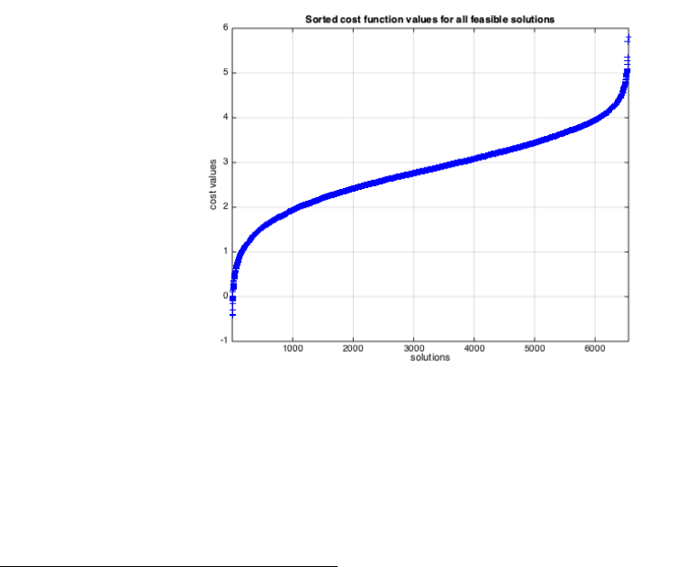
Evaluating the optimization cost function over the set of all obtained feasible solutions gives

us a range of cost values and is shown in Figure 2. What is interesting – as we see after

augmentation – is that the optimal solution is quite far way from these 6000+ solutions.

Figure 2: The sorted cost values of all feasible solutions

As it can be seen, for various solutions the cost values changes from a maximum of 5.7999

rng = 1; m = 5; n = 50; A = randi([0 1],m,n); mu = rand(n,1); sigma = rand(n,1); sigma = sigma .* mu; b

= round(sum(A’)/2)’;

G(A) =







0 0 0 0 0 0 0 0 0 0 ... 1 1 1 1 1 1 1 1 1 1

0 0 0 0 0 0 0 0 0 0 ... 0 0 0 0 0 0 0 0 0 0

0 0 0 0 0 0 0 0 0 0 ... 0 0 0 0 0 1 1 1 1 1

0 0 0 0 0 0 0 0 0 0 ... 0 0 0 0 0 0 0 0 0 0

0 0 0 0 0 0 0 0 0 0 ... 0 0 0 0 0 −1 0 0 0 0

0 0 0 0 0 0 0 0 0 0 ... 0 0 0 0 0 0 −1 0 0 0

0 0 0 0 0 0 0 0 0 0 ... 0 0 0 0 0 0 0 0 0 0

0 0 0 0 0 0 0 0 0 0 ... 0 0 0 0 1 0 0 0 0 0

0 0 0 0 0 0 0 0 0 0 ... 0 0 0 0 0 0 0 0 0 0

0 0 0 0 0 0 0 0 0 0 ... 0 0 0 0 0 0 0 −1 0 0

0 0 0 0 0 0 0 0 0 0 ... 0 0 0 0 0 0 0 0 0 0

0 0 0 0 0 0 0 0 0 0 ... 0 0 0 0 −1 0 0 0 0 0

0 0 0 0 0 0 0 0 0 0 ... 0 0 0 0 0 0 0 0 0 0

0 0 0 0 0 0 0 0 0 0 ... 0 0 1 1 0 0 0 0 0 0

0 0 0 0 0 0 0 0 0 0 ... 0 0 0 0 0 0 0 0 0 0

0 0 0 0 0 0 0 0 1 1 ... 1 1 0 0 0 0 0 0 0 0

0 0 0 0 0 0 0 0 0 0 ... 0 0 0 0 0 0 0 0 0 0

0 0 0 0 0 0 0 1 −1 0 ... 0 0 0 0 0 0 0 0 0 0

0 0 0 0 1 1 1 0 0 0 ... 0 0 0 0 0 0 0 0 0 0

0 0 0 1 0 0 0 0 0 0 ... 0 0 −1 0 0 0 0 0 0 0

0 0 0 −1 0 0 0 0 0 0 ... 0 0 0 −1 0 0 0 0 0 0

0 1 1 0 −1 0 0 0 0 0 ... 0 0 0 0 0 0 0 0 0 0

0 0 0 0 0 0 0 −1 0 −1 ... 0 0 0 0 0 0 0 0 0 0

1 0 0 0 0 0 0 0 0 0 ... −1 0 0 0 0 0 0 0 −1 0

0 0 1 0 0 0 1 0 0 0 ... 0 0 0 0 0 0 0 1 0 0

0 0 0 0 0 0 0 0 0 0 ... 0 0 0 0 0 0 0 0 0 0

0 −1 0 0 0 −1 0 0 0 0 ... 0 0 0 0 0 0 0 0 0 0

0 0 −1 0 0 0 −1 0 0 0 ... 0 0 0 0 0 0 0 0 0 0

−1 0 0 0 0 0 0 0 0 0 ... 0 −1 0 0 0 0 0 0 0 −1

0 0 −1 1 0 0 −1 0 0 0 ... −1 −1 −1 0 0 1 1 0 0 0







Figure 3: The ﬁrst and last 10 elements of the Graver basis of the matrix A of Example 1

to a minimum of −0.4154. Clearly, a wise choice of initial feasible solution is to choose the

minimum solution corresponding to the minimum cost value, which is,



0 0 1 1 1 1 1 0 0 0 0 0 1 0 0 1 0 1 1 1 1 0 1 0 1 0 0 1 1 0 0 1 1 1 1 0 0 1 0 1 1 1 0 0 0 0 1 1 1 1



If we start the augmentation procedure from the minimum x

, using 24 augmenting (im-

proving) steps, we reach the global solution of the problem, which has a value of −3.6947.

A global solution for this problem is,

∗



0 0 1 1 1 1 1 0 1 0 0 0 1 0 0 1 0 1 1 1 1 0 1 1 0 0 1 1 1 0 0 0 1 1 1 0 0 1 1 0 1 0 1 0 1 0 0 1 0 1



If we instead start the augmentation from the farthest feasible point among all feasible

points, which is the solution corresponding to the cost value 5.7999:



1 1 0 0 1 0 1 1 1 1 1 1 0 1 1 1 1 0 0 0 1 0 1 1 1 1 0 0 1 1 1 0 0 0 0 1 1 0 0 0 0 1 0 0 0 1 0 0 1 0



using 30 augmenting (improving) steps we reach the same global solution.

As we can observe, although we initially had over 6000 feasible points, the minimum cost

value among these was −0.4154 which is not optimal. From the cost value of −0.4154 to

the optimum cost (−3.6947), we needed 24 augmentations. This does not mean that we

only did 24 comparisons. In fact, we tested all of the 2 × 304 Graver basis elements, three

times. Many of the choices of the form x + g resulted in values outside {0, 1} and could be

immediately ignored before calculating their cost.

4.4.2 Comparison with a best-in-class classical method

For a quick comparison with a leading edge classical solver, the same problem was passed to

the Gurobi Optimizer (latest version, 8.0)

. Gurobi solved the above problem in less than

0.2sec, which is much faster than our algorithm on D-Wave Processor. If we increase the

span of random integer terms (a

’s) in matrix A, from {0, 1} to {0, ..., t}, by increasing t, the

problem becomes harder and harder for Gurobi. At t = 10, Gurobi needs 16sec, at t = 20

over 3min, at t = 30 over 5min, at t = 40 over 21min, at t = 50 over 75min, ... , and at

t = 100, even after 8 hours Gurobi could not solve the problem. Note that for our quantum

annealing algorithm, the size and number of calls to D-Wave and the embedding for all of

those t stays exactly the same. The only diﬀerence is that with increasing t, the number of

unique terms in the QUBO q

’s that maps to the Ising model J

’s (i.e. the cardinality of

set of J

values) increases.

For t = 1, there are 6 unique terms, for t = 10: ' 230, for t = 20: ' 620, for t = 30: ' 860,

for t = 40: ' 1030, for t = 50: ' 1070, and for t = 100: ' 1190 unique terms required

Installed on MacBookPro15,1: 6 Core 2.6 GHz Intel Core i7 processor, 32 GB 2400 MHz DDR4 RAM

to be mapped into a coupler. The current hardware has a limited precision (4bits = 16

steps) to address coupler instances. This matches the case of t = 1. Therefore, if the next

generation of quantum annealers invests in improving only the coupler precision (without

increasing the number of qubits or improving connectivity between them), we can match, or

even surpass, the current classical solvers, using our quantum algorithm, in a wide range of

nonlinear integer programming problems.

Now if we ﬁx the matrix parameters (e.g. t = 1) and increase problem size (n), solving the

problem still becomes harder for Gurobi solver, whilst the number of unique coupler terms

roughly stays the same. For random problems with A

20×80

(size 80, 12 unique terms), Gurobi

needs ∼ 135sec, for A

25×100

(size 100, 16 terms), about ∼ 2hours and for A

30×120

(size 120,

16 terms), even after 3hours Gurobi did not converge to an optimal solution.

D-Wave’s technical report [Boo18] about their next generation chip - due to newly designed

denser connectivity structure called Pegasus- indicates it can embed complete graph problems

of size up to 180, and do so with lower chain lengths than the current D-Wave 2000Q

processor. We estimate, even if the new processor’s coupler precision is increased by only

one bit, due to embedding size expansion, our quantum classical algorithm can surpass

the speed of best-in-class classical solvers (e.g. Gurobi), in similar nonlinear combinatorial

programming problems with sizes greater that 100, up until 180.

Our approach is a ﬁrst that beneﬁts from many anneals (thus reads) of quantum annealer in

each call, not to increase the conﬁdence of an optimal solution, but instead to sample many

optimal and near-optimal solutions of highly degenerate problems. Many unique feasible

solutions can be found very quickly. If the next generation of quantum annealing processors

can increase the maximum number of anneals per each call (from 10000 to say 100000), it

will signiﬁcantly enhance the performance of our approach as the number of quantum calls

needed can be just one for Graver, and another for obtaining many good starting points for

optimization.

4.4.3 Case 2: Nonlinear low span integer program with 25 integer variables

Consider again the nonlinear programming problem shown in Equation (12), but now in

bounded integer form x ∈ {−2, −1, 0, 1, 2}

. To be able to embed the problem into the

current processor, we generate a 5 × 25 problem and use k = 2 bits for each integer variable.

Consider a typical example, where the matrix is:

A =







1 1 1 1 1 1 1 1 1 1 0 1 0 1 0 1 0 1 1 1 0 1 0 1 0

1 1 1 1 0 1 0 1 0 0 1 0 0 0 1 0 0 1 0 1 1 1 1 1 1

0 1 0 0 0 1 0 1 0 1 1 0 1 1 0 1 1 0 0 1 0 0 1 1 1

0 0 0 0 0 0 0 1 0 1 1 1 0 1 1 1 1 0 0 1 0 0 0 0 0

0 1 1 1 1 1 0 0 0 1 0 0 0 1 0 0 0 0 0 1 0 1 0 1 0







The expected return vector is a uniform real random variable of size 25 in [0, 1] range:

µ =



0.9277 0.06858 0.2994 0.5916 0.2033 ... 0.5098 0.9742 0.1973 0.1112 0.2974



The variance for each term σ

is a real random variable between 0 and µ

σ =



0.3677 0.02886 0.09326 0.4105 0.01868 ... 0.4081 0.8942 0.02709 0.05612 0.1204



We chose the budget values equal to half of sum of each row of A: b =



9 8 7 5 5



based on [AN08].

The lower and upper bounds for the problem variables are l = −21 and u = +21. Therefore,

the truncated Graver basis bound is [L

, U

] = [−41, +41]. Spanning the variables in this

range needs a little more than the average 3 bits encoding. We calculated all of the Graver

basis elements in this range using only 2 bits encoding length, in two D-Wave calls with a

center adjustment and beneﬁting from the range doubling obtained from suboptimal post-

processings (see 3.2.3). Matrix A in this band contains 2 × 616 Graver elements.

Separately, we solved Ax = b using one call to the D-Wave quantum annealer, having only

two bits of encoding (10000 reads, annealing time = 1µsec.). We chose the center of the two

bit encoding at 0. Therefore, it covers {−2, −1, 0, 1}, which is enough for ﬁnding an initial

point. The number of unique optimal solutions was 773 using minimize energy chainbreak

and 238 using majority vote chainbreak.

Evaluating the optimization cost function over the set of all solutions gives us a range of

cost values, as shown below.

The cost values range from maximum of 20.7211 for the initial feasible solution:

max



1 1 1 1 −1 1 1 1 1 1 1 1 −2 1 0 −1 0 1 −1 1 −2 −2 1 1 1



to minimum of 2.3622 for the initial feasible solution:

min



0 1 0 1 1 1 1 0 1 1 1 0 0 1 1 0 1 1 1 0 1 0 1 −1 1



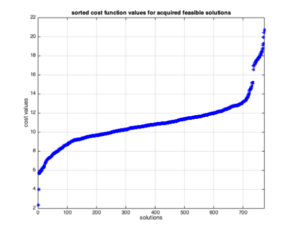
Figure 4: The sorted cost values of acquired feasible solutions for low span example

Starting from x

max

using 22 augmenting (improving) steps, the global solution is achieved,

while starting from x

min

using only 8 augmenting steps, the same global solution is achieved:

∗



0 1 1 0 2 0 0 0 2 0 2 1 −2 0 0 0 2 0 1 0 0 0 2 1 1



which has a minimum cost of −2.4603.

4.4.4 Augmenting with partial Graver basis

In the above, we assumed that all of the truncated Graver basis is acquired, thus starting

from any of the many available initial solutions, we reach the global solution. In fact,

the starting point aﬀects only the number of augmentations required to reach the ﬁnal

solution. Theoretically, if we have only one feasible solution and all of the Graver basis

elements in the required region, we certainly reach the global solution in polynomial number

of augmentations, for the proved class of nonlinear costs (see 2.2). Looking from the other

side of spectrum, if we have all feasible solutions and none of the Graver basis elements, just

by checking each feasible solution’s cost and ﬁnding the minimum among them, we reach

the global solution.

Our quantum annealing-based algorithm provides a third opportunity. If we have many

feasible solutions distributed in the solution space (let us say, uniformly), then we most

likely may reach the global solution even with a subset of Graver basis elements (which we

refer to as partial Graver basis). The point is, if we can not reach from a particular feasible

solution to a global one, due to lack of speciﬁc Graver basis elements in the available set,

other feasible solutions provide many other paths (to the global solution) that may not need

these speciﬁc Graver basis elements that are missing.

This interesting opportunity has borne out in our experiments. In the previous example, if we

call D-Wave only once for the Graver basis, we acquire almost 2 ×418 Graver basis elements,

which is 68% of the Graver basis elements previously found. Now, we start augmenting the

problem from all of 773 initial feasible points. Interestingly, using this partial Graver basis,

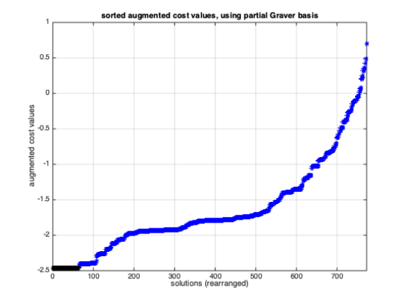
we could reach the global solution from 64 (out of 773) of the initial solutions; see Figure

(5) The other paths also terminate to very good near-optimal solutions (compare average

values in Figure 4, 10.9013, versus average values in Figure 5, −1.6546).

Furthermore, in case there is degeneracy in the global solution (that is, there are alternate

optimal solutions), this multi augmentation strategy can also result in several unique degen-

erate solutions. In the above example, the problem does not have a degenerate solution, and

so all 64 paths resulted in the same solution x

∗

, the only one.

Using many or all of the feasible solutions clearly adds linear computational cost to aug-

mentation, but the augmentation cost is low (polynomial) compared with the Graver cost.

Finding a good balance between the number of feasible solutions and the amount and vari-

ability of Graver basis elements would be an interesting experimental study.

Figure 5: The sorted augmented cost values for all feasible solutions, using partially acquired

Graver basis

5 Conclusions

In this paper, we demonstrate that calculation of Graver bases using quantum annealing,

and its subsequent use for nonlinear integer optimization, is a viable approach in available

hardware. To accomplish this, we developed several post-processing procedures, and an

adaptive approach that adjusts the encoding length as well as the center of the variables to

be eﬃcient in the use of the limited number of qubits.

We did not expect to outperform best-in-class classical solvers, and indeed that was not our

motivation. If anything, we began as skeptics about the practical capabilities of the available

hardware. We are pleasantly surprised that we are able to solve many problems of medium

size in decent time, not too far behind the classical best, if we select problem instances that

are hard for classical approaches. Our tests suggest that with improvements in the number

of qubits and their connectivity, which have already been announced and are expected in

the near term, an improvement in the coupler precision will bring our hybrid quantum-

classical approach within reach of, or even surpass, the best-in-class classical algorithms for

an important class of non-linear integer optimization problems.

Acknowledgements

The authors thank Davide Venturelli, Eleanor G. Rieﬀel, Bryan O’Gorman, and other NASA

QuAIL team members for their comments and feedback.

Bibliography

[AN08] Alper Atamtürk and Vishnu Narayanan, Polymatroids and mean-risk minimiza-

tion in discrete optimization, Operations Research Letters 36 (2008), no. 5,

618–622. 24, 25, 29

[Bar82] F. Barahona, On the computational complexity of Ising spin glass models, Jour-

nal of Physics A: Mathematical and General 15 (1982), no. 10, 3241 (en). 37

[Ber18] Jesse J. Berwald, The Mathematics of Quantum-Enabled Applications on

the D-Wave Quantum Computer, arXiv:1812.00062 [quant-ph] (2018), arXiv:

1812.00062. 4

[BHJ

14] P. I. Bunyk, E. M. Hoskinson, M. W. Johnson, E. Tolkacheva, F. Altomare, A. J.

Berkley, R. Harris, J. P. Hilton, T. Lanting, A. J. Przybysz, and J. Whittaker,

Architectural Considerations in the Design of a Superconducting Quantum An-

nealing Processor, IEEE Transactions on Applied Superconductivity 24 (2014),

no. 4, 1–10. 37

[BLSR99] A. M. Bigatti, R. La Scala, and L. Robbiano, Computing Toric Ideals, Journal

of Symbolic Computation 27 (1999), no. 4, 351–365. 10

[Boo18] Kelly Boothby, Next-Generation Topology of D-Wave Quantum Processors, D-

Wave Technical Report (2018). 22, 28

[BPT00] Dimitris Bertsimas, Georgia Perakis, and Sridhar Tayur, A New Algebraic Ge-

ometry Algorithm for Integer Programming, Management Science 46 (2000),

no. 7, 999–1008. 10

[Cho08] Vicky Choi, Minor-embedding in Adiabatic Quantum Computation: I. The Pa-

rameter Setting Problem, Quantum Information Processing 7 (2008), no. 5,

193–209. 37

[CT91] Pasqualina Conti and Carlo Traverso, Buchberger Algorithm and Integer Pro-

gramming, Proceedings of the 9th International Symposium, on Applied Al-

gebra, Algebraic Algorithms and Error-Correcting Codes (London, UK, UK),

AAECC-9, Springer-Verlag, 1991, pp. 130–139. 10

[CUWW97] G. Cornuejols, R. Urbaniak, R. Weismantel, and L. Wolsey, Decomposition of

integer programs and of generating sets, Algorithms — ESA ’97 (Rainer Burkard

and Gerhard Woeginger, eds.), Lecture Notes in Computer Science, Springer

Berlin Heidelberg, 1997, pp. 92–103 (en). 37

[DAT18a] Raouf Dridi, Hedayat Alghassi, and Sridhar Tayur, Homological description

of the quantum adiabatic evolution with a view toward quantum computations,

arXiv:1811.00675 (2018). 37

[DAT18b] , A novel algebraic geometry compiling framework for adiabatic quantum

computations, arXiv:1810.01440 (2018). 13, 37

[DLHK12] J. De Loera, R. Hemmecke, and M. Köppe, Algebraic and Geometric Ideas in the

Theory of Discrete Optimization, MOS-SIAM Series on Optimization, Society

for Industrial and Applied Mathematics, December 2012. 36

[DLHO

09] J. A. De Loera, R. Hemmecke, S. Onn, U. G. Rothblum, and R. Weismantel,

Convex integer maximization via Graver bases, Journal of Pure and Applied

Algebra 213 (2009), no. 8, 1569–1577. 9, 10

[FGGS00] Edward Farhi, Jeﬀrey Goldstone, Sam Gutmann, and Michael Sipser, Quantum

Computation by Adiabatic Evolution, arXiv:quant-ph/0001106 (2000), arXiv:

quant-ph/0001106. 37

[Gra75] Jack E. Graver, On the foundations of linear and integer linear programming I,

Mathematical Programming 9 (1975), no. 1, 207–226 (en). 4, 9

[Hem02] Raymond Hemmecke, On the computation of hilbert bases of cones, Mathemat-

ical Software, World Scientiﬁc, July 2002, pp. 307–317. 37

[HJL

10] R. Harris, M. W. Johnson, T. Lanting, A. J. Berkley, J. Johansson, P. Bunyk,

E. Tolkacheva, E. Ladizinsky, N. Ladizinsky, T. Oh, F. Cioata, I. Perminov,

P. Spear, C. Enderud, C. Rich, S. Uchaikin, M. C. Thom, E. M. Chapple,

J. Wang, B. Wilson, M. H. S. Amin, N. Dickson, K. Karimi, B. Macready,

C. J. S. Truncik, and G. Rose, Experimental investigation of an eight-qubit unit

cell in a superconducting optimization processor, Physical Review B 82 (2010),

no. 2, 024511. 37

[HOW11] Raymond Hemmecke, Shmuel Onn, and Robert Weismantel, A polynomial

oracle-time algorithm for convex integer minimization, Mathematical Program-

ming 126 (2011), no. 1, 97–117 (en). 9, 10

[HS95] Serkan Hoşten and Bernd Sturmfels, GRIN: An implementation of Gröbner

bases for integer programming, Integer Programming and Combinatorial Op-

timization, Lecture Notes in Computer Science, Springer, Berlin, Heidelberg,

May 1995, pp. 267–276 (en). 10

[JAG

11] M. W. Johnson, M. H. S. Amin, S. Gildert, T. Lanting, F. Hamze, N. Dickson,

R. Harris, A. J. Berkley, J. Johansson, P. Bunyk, E. M. Chapple, C. Enderud,

J. P. Hilton, K. Karimi, E. Ladizinsky, N. Ladizinsky, T. Oh, I. Perminov,

C. Rich, M. C. Thom, E. Tolkacheva, C. J. S. Truncik, S. Uchaikin, J. Wang,

B. Wilson, and G. Rose, Quantum annealing with manufactured spins, Nature

473 (2011), no. 7346, 194–198 (en). 37

[Kat50] Tosio Kato, On the Adiabatic Theorem of Quantum Mechanics, Journal of the

Physical Society of Japan 5 (1950), no. 6, 435–439. 37

[LORW12] Jon Lee, Shmuel Onn, Lyubov Romanchuk, and Robert Weismantel, The

quadratic Graver cone, quadratic integer minimization, and extensions, Mathe-

matical Programming 136 (2012), no. 2, 301–323 (en). 10

[McG14] Catherine C. McGeoch, Adiabatic Quantum Computation and Quantum An-

nealing: Theory and Practice, Synthesis Lectures on Quantum Computing 5

(2014), no. 2, 1–93. 37

[MSW04] Kazuo Murota, Hiroo Saito, and Robert Weismantel, Optimality criterion for

a class of nonlinear integer programs, Operations Research Letters 32 (2004),

no. 5, 468–472. 9, 10

[MZK17] Salvatore Mandrà, Zheng Zhu, and Helmut G. Katzgraber, Exponentially Biased

Ground-State Sampling of Quantum Annealing Machines with Transverse-Field

Driving Hamiltonians, Physical Review Letters 118 (2017), no. 7, 070502. 13

[noa] 4ti2–A software package for algebraic, geometric and combinatorial problems on

linear spaces. 21

[Onn10] Shmuel Onn, Nonlinear Discrete Optimization: An Algorithmic Theory, Euro-

pean Mathematical Soc., 2010 (en), Google-Books-ID: kcD5DAEACAAJ. 8,

[Pap81] Christos H. Papadimitriou, On the Complexity of Integer Programming, J. ACM

28 (1981), no. 4, 765–768. 11

[Pot96] Loïc Pottier, The Euclidean Algorithm in Dimension N, Proceedings of the 1996

International Symposium on Symbolic and Algebraic Computation (New York,

NY, USA), ISSAC ’96, ACM, 1996, pp. 40–42. 10, 36

[ST97] Bernd Sturmfels and Rekha R. Thomas, Variation of cost functions in integer

programming, Mathematical Programming 77 (1997), no. 2, 357–387 (en). 10,

[Stu95] Bernd Sturmfels, Gröbner Bases and Convex Polytopes, University Lecture Se-

ries, vol. 8, American Mathematical Society, December 1995 (en-US). 37

[Stu03] , Algebraic Recipes for Integer Programming, arXiv:math/0310194

(2003), arXiv: math/0310194. 17, 18, 19

[TTN95] Sridhar R. Tayur, Rekha R. Thomas, and N. R. Natraj, An algebraic geometry

algorithm for scheduling in presence of setups and correlated demands, Mathe-

matical Programming 69 (1995), no. 1-3, 369–401 (en). 10

[VK18] Davide Venturelli and Alexei Kondratyev, Reverse Quantum Annealing Ap-

proach to Portfolio Optimization Problems, arXiv:1810.08584 [quant-ph, q-ﬁn]

(2018), arXiv: 1810.08584. 38

A Graver Basis via Classical Methods

Classically any algorithm that can calculate all inclusion-minimal elements of any sublattice

L ⊆ Z

can be used to calculate Graver basis.All such algorithms have a computational

complexity that is exponential.

Pottier’s algorithm [Pot96] – also called completion procedure - starts with any lattice basis

G of L, and iteratively adds new vectors to G until any vector z ∈ L can be written as a

positive linear sign-compatible (same orthant) representation:

z =

∈ Z

∈ G g

v z

(13)

If G reaches the representation property, then it contains all v-minimal elements. The vector

version is shown in Algorithm 5.

Algorithm 5 Normal Form

1: input vector s ∈ L, set G ⊂ L

2: output vector r = normalF orm(s, G) ∈ L s.t. s =

+ r, α

∈ Z

, g

, r v s

3: Initialize: r ← s

4: while

∃g ∈ G s.t. g v r

5: r ← r − g

6: end while

7: return r

When r becomes zero, s is integer linear combination of g

’s in the same orthant. If r

does not reach zero, the last r has to be added to G thus in future iterations r becomes zero.

This is shown in Algorithm 6.

Algorithm 6 Pottier

1: input Generating initial set F ⊆ L = ker N(A)

2: output Graver basis set G ⊆ L\ {0}

3: Initialize symmetric set: G ← F ∪ (−F )

4: Generate S vector set: C ←

f,g∈G

{f + g}

5: while C 6= ∅ do

∀s ∈ C : r ← normalF orm(s, G) and C ← C\ {s}

7: if r 6= 0 then

8: Update:

G ← G ∪ {r} and C ← C ∪ {r + g

} g

∈ G

9: end if

10: end while

11: return G

It can be shown [DLHK12] that the above algorithm terminates with all inclusion mini-

mal elements of L. (There remain non inclusion minimal terms that should be ﬁltered out

based on the inclusion minimal concept.) Other algorithms for computing Graver bases exist

such as project and lift [CUWW97, Hem02] and using Lawrence lifting [Stu95].

B Quantum Annealing and D-Wave Processors

B.1 Quantum Annealing

Quantum annealing [FGGS00, McG14] uses the quantum adiabatic evolution [Kat50] to

solve optimization problems (QUBOs). (See [DAT18a] for a Morse theoretical description

for the quantum adiabatic evolution.) This is done by slowly evolving the ground state of

some known system into the sought ground state of the problem Hamiltonian. For instance,

D-Wave 2000Q [HJL

10, JAG

11, BHJ

14] implements quantum annealing using the time

dependent Hamiltonian

H(s) = A(s)H

+ B(s)H

(14)

where A(s) is monotonically decreasing while B(s) is monotonically increasing with respect to

normalized (slow) time s =

∈ [0, 1]. τ is the total annealing time. The initial Hamiltonian

(with known ground state) is a transverse magnetic ﬁeld H

= −

where σ

is the i

Pauli x-matrix. The problem Hamiltonian H

is [Bar82]:

i∈V

(i,j)∈E

, (15)

where the parameters h

and J

encode the particular problem instance. The σ

are Pauli

z-matrices. A measurement of the ﬁnal state (i.e.,end of the adiabatic evolution at s = 1)

will yield a solution of the problem.

B.2 Quantum Annealer from D-Wave

We had access to a D-Wave Quantum Annealer 2000Q

(C16-VFYC solver) administered

by NASA Quantum Artiﬁcial Intelligence Laboratory (QuAIL). This processor operates at

20(±5)milliKelvin and designed with 2048 qubits with a 95.5 qubits yield in its 16 by 16

block Chimera conﬁguration. The Chimera structure has a limited connectivity as shown

in Figure 6. Therefore, the graph of a speciﬁc QUBO problem needs to be embedded into

the graph of hardware (Figure 6). Embedding an input graph into the hardware graph is a

speciﬁc instance of a graph homomorphism and its associated decision problem is in general

NP-complete [Cho08, DAT18b].

B.2.1 D-Wave SAPI

D-Wave’s software application programming interface (SAPI) is an application layer built

to provide resource discovery, permissions, and scheduling for quantum annealing. The

Figure 6: Schematic representation of a 3 by 3 block Chimera

codes for this project are implemented using Matlab SAPI (version 3.0). For embedding the

problem graph into hardware graph and also for parameter settings, the sapiFindEmbedding

(default parameters) and sapiEmbedProblem (adaptive problem per chain strength) software

modules are used. To solve, sapiSolveIsing and sapiUnembedAnswer modules (with two

distinct chainbreak strategies discussed in 4.3.1) are used. The maximum number of reads

available (10000) is used to increase the eﬃciency of each call (the number of unique optimal

and nonoptimal solutions).

B.2.2 Chainbreak strategy

Embedding a problem graph into the hardware graph has two parts: topological and problem

value mapping. The second aspect deals with setting of the parameters. All qubit values

in a chain are expected to remain at the same value (+1 or -1) at the end of quantum

annealing process. Due to situations in which the chain couplers (J

, identiﬁed couplers)

are not strong enough in comparison with problem couplers, chains frequently break. To

recover from these breaks, D-Wave has provided two post-processing strategies:

• Minimize energy, which is the default choice. This approach walks each broken solution

down to a local minimum by repeatedly ﬂipping random bits to reduce solution cost,

somewhat like a zero-temperature simulated annealing, but without moves that do not

change the energy ([VK18]).

• Majority vote, on the other hand, is computationally less expensive: it sets the chain

value according to a majority vote of qubits in the chain, and a random value in case

of ties.

In structured and dense problems, where the embedding is close to a complete graph em-

bedding, all variables end up having long chains thus the probability of chain break in them

increases. In such situations, the eﬀect of chainbreak post processing might exceed the eﬀect

of quantum annealing itself. Therefore, in the results, we report the chain-break strategy

used as well as the percentage of chains broken. This indicates how much of the problem

has been impacted by chainbreak post-processing.

B.2.3 Annealing time

Annealing time (τ) is the (a) forward (or reverse) dynamic time from the start of annealing

to the end, or (b) from the start to the pause, or (c) from end of pause to end of annealing.

Our experimental tests show that when we select a large annealing time(i.e. 290µsec), we

have fewer chain breaks, but also fewer unique solutions. When we chose a small annealing

time (i.e. 1 − 10µsec) we have more chain breaks, but higher number of unique solutions

(using minimize energy chain-break strategy).

Pause is the static stopping time (usually in the middle of forward or reverse annealing)

that allows local exploration through thermal hopping and enhances the analog of classical

gradient descent. The pause time (ρ) is usually larger than forward (or reverse) annealing

time (τ ). In reverse annealing, the system is initialized with B(1) = 1 and A(0) = 0,

with all used qubits preset to a classically known solution. The annealing then turns back

to somewhere in the middle of the schedule, where the initial (transverse ﬁeld) Hamiltonian

and problem Hamiltonian have roughly the same strength, and then pauses. After the pause,

there is a third phase, which is the ﬁnal forward annealing. The reasoning behind reverse

annealing is that by starting from a known local minimum of the problem, the reciprocation

of quantum and thermal ﬂuctuations might help the quantum state to tunnel through the

energy barriers (in reverse phase), while the pause and the (ﬁnal) forward annealing allows

the system to relax and thermalize in vicinity of a better minimum. In our results, we report

the annealing schedule, because it is an important factor in the quality and quantity of the

results.