title: A Guide to Econometrics
author: Kennedy, Peter.
publisher: MIT Press
isbn10 | asin: 0262112353
print isbn13: 9780262112352
ebook isbn13: 9780585202037
language: English
subject Econometrics.
publication date: 1998
lcc: HB139.K45 1998eb
ddc: 330/.01/5195
subject: Econometrics.
cover
Page iii
A Guide to Econometrics
Fourth Edition

Peter Kennedy
Simon Fraser University
The MIT Press
Cambridge, Massachusetts
page_iii
Page iv
© 1998 Peter Kennedy
All rights reserved. No part of this book may be reproduced in any form
or by any electronic or mechanical means (including photocopying,
recording, or information storage and retrieval), without permission in
writing from the publisher.
Printed and bound in The United Kingdom by TJ International.
ISBN 0-262 11235-3 (hardcover), 0-262-61140-6 (paperback)
Library of Congress Catalog Card Number: 98-65110
page_iv
Contents
Preface
I
Introduction
1.1
What is Econometrics?
1.2
The Disturbance Term

1.3
Estimates and Estimators
1.4
Good and Preferred Estimators
General Notes
Technical Notes
2
Criteria for Estimators
2.1
Introduction
2.2
Computational Cost
2.3
Least Squares
2.4
Highest R2
2.5
Unbiasedness
2.6
Efficiency
2.7
Mean Square Error (MSE)
2.8
Asymptotic Properties
2.9
Maximum Likelihood
2.10
Monte Carlo Studies

2.11
Adding Up
General Notes
Technical Notes
3
The Classical Linear Regression Model
3.1
Textbooks as Catalogs
3.2
The Five Assumptions
3.3
The OLS Estimator in the CLR Model
General Notes
Technical Notes
page_v
4
Interval Estimation and Hypothesis Testing
4.1
Introduction
4.2
Testing a Single Hypothesis: the t Test
4.3
Testing a Joint Hypothesis: the F Test
4.4
Interval Estimation for a Parameter Vector

4.5
LR, W, and LM Statistics
4.6
Bootstrapping
General Notes
Technical Notes
5
Specification
5.1
Introduction
5.2
Three Methodologies
5.3
General Principles for Specification
5.4
Misspecification Tests/Diagnostics
5.5
R2 Again
General Notes
Technical Notes
6
Violating Assumption One: Wrong Regressors, Nonlinearities, and Parameter
Inconstancy
6.1
Introduction
6.2
Incorrect Set of Independent Variables
6.3
Nonlinearity

6.4
Changing Parameter Values
General Notes
Technical Notes
7
Violating Assumption Two: Nonzero Expected Disturbance
General Notes
8
Violating Assumption Three: Nonspherical Disturbances
8.1
Introduction
8.2
Consequences of Violation
8.3
Heteroskedasticity
8.4
Autocorrelated Disturbances
General Notes
Technical Notes
page_vi
9
Violating Assumption Four: Measurement Errors and Autoregression
9.1
Introduction
9.2
Instrumental Variable Estimation

9.3
Errors in Variables
9.4
Autoregression
General Notes
Technical Notes
10
Violating Assumption Four: Simultaneous Equations
10.1
Introduction
10.2
Identification
10.3
Single-equation Methods
10.4
Systems Methods
10.5
VARs
General Notes
Technical Notes
11
Violating Assumption Five: Multicollinearity
11.1
Introduction
11.2
Consequences
11.3
Detecting Multicollinearity

11.4
What to Do
General Notes
Technical Notes
12
Incorporating Extraneous Information
12.1
Introduction
12.2
Exact Restrictions
12.3
Stochastic Restrictions
12.4
Pre-test Estimators
12.5
Extraneous Information and MSE
General Notes
Technical Notes
13
The Bayesian Approach
13.1
Introduction
13.2
What is a Bayesian Analysis?
13.3
Advantages of the Bayesian Approach
page_vii

13.4
Overcoming Practitioners' Complaints
General Notes
Technical Notes
14
Dummy Variables
14.1
Introduction
14.2
Interpretation
14.3
Adding Another Qualitative Variable
14.4
Interacting with Quantitative Variables
14.5
Observation-specific Dummies
14.6
Fixed and Random Effects Models
General Notes
Technical Notes
15
Qualitative Dependent Variables
15.1
Dichotomous Dependent Variables
15.2
Polychotomous Dependent Variables
15.3
Ordered Logit/Probit

15.4
Count Data
General Notes
Technical Notes
16
Limited Dependent Variables
16.1
Introduction
16.2
The Tobit Model
16.3
Sample Selection
16.4
Duration Models
General Notes
Technical Notes
17
Time Series Econometrics
17.1
Introduction
17.2
ARIMA Models
17.3
SEMTSA
17.4
Error-correction Models
17.5
Testing for Unit Roots

17.6
Cointegration
General Notes
Technical Notes
page_viii
18
Forecasting
18.1
Introduction
18.2
Causal Forecasting/Econometric Models
18.3
Time Series Analysis
18.4
Forecasting Accuracy
General Notes
Technical Notes
19
Robust Estimation
19.1
Introduction
19.2
Outliers and Influential Observations
19.3
Robust Estimators

19.4
Non-parametric Estimation
General Notes
Technical Notes
Appendix A: Sampling Distributions, the Foundation of Statistics
Appendix B: All About Variance
Appendix C: A Primer on Asymptotics
Appendix D: Exercises
Appendix E: Answers to Even-numbered Questions
Glossary
Bibliography
Author Index
Subject Index
page_ix
Page xi
Preface
In the preface to the third edition of this book I noted that upper-level
undergraduate and beginning graduate econometrics students are as
likely to learn about this book from their instructor as by word-of-
mouth, the phenomenon that made the first edition of this book so
successful. Sales of the third edition indicate that this trend has
continued - more and more instructors are realizing that students find
this book to be of immense value to their understanding of
econometrics.

What is it about this book that students have found to be of such value?
This book supplements econometrics texts, at all levels, by providing an
overview of the subject and an intuitive feel for its concepts and
techniques, without the usual clutter of notation and technical detail
that necessarily characterize an econometrics textbook. It is often said
of econometrics textbooks that their readers miss the forest for the
trees. This is inevitable - the terminology and techniques that must be
taught do not allow the text to convey a proper intuitive sense of
"What's it all about?" and "How does it all fit together?" All
econometrics textbooks fail to provide this overview. This is not from
lack of trying - most textbooks have excellent passages containing the
relevant insights and interpretations. They make good sense to
instructors, but they do not make the expected impact on the students.
Why? Because these insights and interpretations are broken up,
appearing throughout the book, mixed with the technical details. In their
struggle to keep up with notation and to learn these technical details,
students miss the overview so essential to a real understanding of those
details. This book provides students with a perspective from which it is
possible to assimilate more easily the details of these textbooks.
Although the changes from the third edition are numerous, the basic
structure and flavor of the book remain unchanged. Following an
introductory chapter, the second chapter discusses at some length the
criteria for choosing estimators, and in doing so develops many of the
basic concepts used throughout the book. The third chapter provides an
overview of the subject matter, presenting the five assumptions of the
classical linear regression model and explaining how most problems
encountered in econometrics can be interpreted as a violation of one of
these assumptions. The fourth chapter exposits some concepts of
inference to
page_xi
Page xii
provide a foundation for later chapters. Chapter 5 discusses general
approaches to the specification of an econometric model, setting the
stage for the next six chapters, each of which deals with violations of an
assumption of the classical linear regression model, describes their
implications, discusses relevant tests, and suggests means of resolving
resulting estimation problems. The remaining eight chapters and
Appendices A, B and C address selected topics. Appendix D provides
some student exercises and Appendix E offers suggested answers to the

even-numbered exercises. A set of suggested answers to odd-numbered
questions is available from the publisher upon request to instructors
adopting this book for classroom use.
There are several major changes in this edition. The chapter on
qualitative and limited dependent variables was split into a chapter on
qualitative dependent variables (adding a section on count data) and a
chapter on limited dependent variables (adding a section on duration
models). The time series chapter has been extensively revised to
incorporate the huge amount of work done in this area since the third
edition. A new appendix on the sampling distribution concept has been
added, to deal with what I believe is students' biggest stumbling block to
understanding econometrics. In the exercises, a new type of question
has been added, in which a Monte Carlo study is described and students
are asked to explain the expected results. New material has been added
to a wide variety of topics such as bootstrapping, generalized method of
moments, neural nets, linear structural relations, VARs, and
instrumental variable estimation. Minor changes have been made
throughout to update results and references, and to improve exposition.
To minimize readers' distractions, there are no footnotes. All references,
peripheral points and details worthy of comment are relegated to a
section at the end of each chapter entitled "General Notes". The
technical material that appears in the book is placed in end-of-chapter
sections entitled "Technical Notes". This technical material continues to
be presented in a way that supplements rather than duplicates the
contents of traditional textbooks. Students should find that this material
provides a useful introductory bridge to the more sophisticated
presentations found in the main text. Students are advised to wait until a
second or third reading of the body of a chapter before addressing the
material in the General or Technical Notes. A glossary explains
common econometric terms not found in the body of this book.
Errors in or shortcomings of this book are my responsibility, but for
improvements I owe many debts, mainly to scores of students, both
graduate and undergraduate, whose comments and reactions have
played a prominent role in shaping this fourth edition. Jan Kmenta and
Terry Seaks have made major contributions in their role as
"anonymous" referees, even though I have not always followed their
advice. I continue to be grateful to students throughout the world who
have expressed thanks to me for writing this book; I hope this fourth
edition continues to be of value to students both during and after their
formal course-work.

page_xii
Dedication
To ANNA and RED
who, until they discovered what an econometrician was, were
very impressed that their son might become one. With apologies to
K. A. C. Manderville, I draw their attention to the following, adapted from
Undoing of Lamia Gurdleneck.
''You haven't told me yet," said Lady Nuttal, "what it is your fiancé does for a
living."
"He's an econometrician." replied Lamia, with an annoying sense of being on
the defensive.
Lady Nuttal was obviously taken aback. It had not occurred to her that econo-
metricians entered into normal social relationships. The species, she would have
surmised, was perpetuated in some collateral manner, like mules.
"But Aunt Sara, it's a very interesting profession," said Lamia warmly.
"I don't doubt it," said her aunt, who obviously doubted it very much. "To
express anything important in mere figures is so plainly impossible that there
must be endless scope for well-paid advice on how to do it. But don't you think
that life with an econometrician would be rather, shall we say, humdrum?"
Lamia was silent. She felt reluctant to discuss the surprising depth of emo-
tional possibility which she had discovered below Edward's numerical veneer.
"It's not the figures themselves," she said finally, "it's what you do with them
that matters."
page_xiii
Page 1

1
Introduction
1.1 What is Econometrics?
Strange as it may seem, there does not exist a generally accepted
answer to this question. Responses vary from the silly "Econometrics is
what econometricians do" to the staid "Econometrics is the study of the
application of statistical methods to the analysis of economic
phenomena," with sufficient disagreements to warrant an entire journal
article devoted to this question (Tintner, 1953).
This confusion stems from the fact that econometricians wear many
different hats. First, and foremost, they are economists, capable of
utilizing economic theory to improve their empirical analyses of the
problems they address. At times they are mathematicians, formulating
economic theory in ways that make it appropriate for statistical testing.
At times they are accountants, concerned with the problem of finding
and collecting economic data and relating theoretical economic
variables to observable ones. At times they are applied statisticians,
spending hours with the computer trying to estimate economic
relationships or predict economic events. And at times they are
theoretical statisticians, applying their skills to the development of
statistical techniques appropriate to the empirical problems
characterizing the science of economics. It is to the last of these roles
that the term "econometric theory" applies, and it is on this aspect of
econometrics that most textbooks on the subject focus. This guide is
accordingly devoted to this "econometric theory" dimension of
econometrics, discussing the empirical problems typical of economics
and the statistical techniques used to overcome these problems.
What distinguishes an econometrician from a statistician is the former's
pre-occupation with problems caused by violations of statisticians'
standard assumptions; owing to the nature of economic relationships
and the lack of controlled experimentation, these assumptions are
seldom met. Patching up statistical methods to deal with situations
frequently encountered in empirical work in economics has created a
large battery of extremely sophisticated statistical techniques. In fact,
econometricians are often accused of using sledgehammers to crack
open peanuts while turning a blind eye to data deficiencies and the
many
page_1

Page 2
questionable assumptions required for the successful application of
these techniques. Valavanis has expressed this feeling forcefully:
Econometric theory is like an exquisitely balanced French
recipe, spelling out precisely with how many turns to mix the
sauce, how many carats of spice to add, and for how many
milliseconds to bake the mixture at exactly 474 degrees of
temperature. But when the statistical cook turns to raw
materials, he finds that hearts of cactus fruit are unavailable, so
he substitutes chunks of cantaloupe; where the recipe calls for
vermicelli he used shredded wheat; and he substitutes green
garment die for curry, ping-pong balls for turtle's eggs, and, for
Chalifougnac vintage 1883, a can of turpentine. (Valavanis,
1959, p. 83)
How has this state of affairs come about? One reason is that prestige in
the econometrics profession hinges on technical expertise rather than on
hard work required to collect good data:
It is the preparation skill of the econometric chef that catches
the professional eye, not the quality of the raw materials in the
meal, or the effort that went into procuring them. (Griliches,
1994, p. 14)
Criticisms of econometrics along these lines are not uncommon.
Rebuttals cite improvements in data collection, extol the fruits of the
computer revolution and provide examples of improvements in
estimation due to advanced techniques. It remains a fact, though, that in
practice good results depend as much on the input of sound and
imaginative economic theory as on the application of correct statistical
methods. The skill of the econometrician lies in judiciously mixing these
two essential ingredients; in the words of Malinvaud:
The art of the econometrician consists in finding the set of
assumptions which are both sufficiently specific and sufficiently
realistic to allow him to take the best possible advantage of the
data available to him. (Malinvaud, 1966, p. 514)
Modern econometrics texts try to infuse this art into students by
providing a large number of detailed examples of empirical application.
This important dimension of econometrics texts lies beyond the scope of
this book. Readers should keep this in mind as they use this guide to

improve their understanding of the purely statistical methods of
econometrics.
1.2 The Disturbance Term
A major distinction between economists and econometricians is the
latter's concern with disturbance terms. An economist will specify, for
example, that consumption is a function of income, and write C = (Y)
where C is consumption and Y is income. An econometrician will claim
that this relationship must also include a disturbance (or error) term,
and may alter the equation to read
page_2
Page 3
C = (Y) +e where e (epsilon) is a disturbance term. Without the
disturbance term the relationship is said to be exact or deterministic;
with the disturbance term it is said to be stochastic.
The word "stochastic" comes from the Greek "stokhos," meaning a
target or bull's eye. A stochastic relationship is not always right on
target in the sense that it predicts the precise value of the variable being
explained, just as a dart thrown at a target seldom hits the bull's eye.
The disturbance term is used to capture explicitly the size of these
''misses" or "errors." The existence of the disturbance term is justified in
three main ways. (Note: these are not mutually exclusive.)
(1) Omission of the influence of innumerable chance events Although
income might be the major determinant of the level of consumption, it is
not the only determinant. Other variables, such as the interest rate or
liquid asset holdings, may have a systematic influence on consumption.
Their omission constitutes one type of specification error:
the nature of
the economic relationship is not correctly specified. In addition to these
systematic influences, however, are innumerable less systematic
influences, such as weather variations, taste changes, earthquakes,
epidemics and postal strikes. Although some of these variables may
have a significant impact on consumption, and thus should definitely be
included in the specified relationship, many have only a very slight,
irregular influence; the disturbance is often viewed as representing the
net influence of a large number of such small and independent causes.
(2)
Measurement error
It may be the case that the variable being
explained cannot be measured accurately, either because of data
collection difficulties or because it is inherently unmeasurable and a
proxy variable must be used in its stead. The disturbance term can in
these circumstances be thought of as representing this measurement
error. Errors in measuring the explaining variable(s) (as opposed to the
variable being explained) create a serious econometric problem,
discussed in chapter 9. The terminology errors in variables is also used
to refer to measurement errors.
(3) Human indeterminacy Some people believe that human behavior is
such that actions taken under identical circumstances will differ in a
random way. The disturbance term can be thought of as representing
this inherent randomness in human behavior.
Associated with any explanatory relationship are unknown constants,
called parameters, which tie the relevant variables into an equation. For
example, the relationship between consumption and income could be
specified as
where b1 and b2 are the parameters characterizing this consumption
function. Economists are often keenly interested in learning the values
of these unknown parameters.
page_3
Page 4
The existence of the disturbance term, coupled with the fact that its
magnitude is unknown, makes calculation of these parameter values
impossible. Instead, they must be estimated. It is on this task, the
estimation of parameter values, that the bulk of econometric theory
focuses. The success of econometricians' methods of estimating
parameter values depends in large part on the nature of the disturbance
term; statistical assumptions concerning the characteristics of the
disturbance term, and means of testing these assumptions, therefore
play a prominent role in econometric theory.
1.3 Estimates and Estimators
In their mathematical notation, econometricians usually employ Greek
letters to represent the true, unknown values of parameters. The Greek
letter most often used in this context is beta (b). Thus, throughout this
book, b is used as the parameter value that the econometrician is
seeking to learn. Of course, no one ever actually learns the value of b,
but it can be estimated: via statistical techniques, empirical data can be
used to take an educated guess at b. In any particular application, an
estimate of b is simply a number. For example, b might be estimated as
16.2. But, in general, econometricians are seldom interested in
estimating a single parameter; economic relationships are usually
sufficiently complex to require more than one parameter, and because
these parameters occur in the same relationship, better estimates of
these parameters can be obtained if they are estimated together (i.e., the
influence of one explaining variable is more accurately captured if the
influence of the other explaining variables is simultaneously accounted
for). As a result, b seldom refers to a single parameter value; it almost
always refers to a set of parameter values, individually called b1, b2, . .
., bk where k is the number of different parameters in the set. b is then
referred to as a vector and is written as
In any particular application, an estimate of b will be a set of numbers.
For example, if three parameters are being estimated (i.e., if the
dimension of b is three), b might be estimated as
In general, econometric theory focuses not on the estimate itself, but on
the estimator - the formula or "recipe" by which the data are
transformed into an actual estimate. The reason for this is that the
justification of an estimate computed
page_4

Page 5
from a particular sample rests on a justification of the estimation
method (the estimator). The econometrician has no way of knowing the
actual values of the disturbances inherent in a sample of data;
depending on these disturbances, an estimate calculated from that
sample could be quite inaccurate. It is therefore impossible to justify the
estimate itself. However, it may be the case that the econometrician can
justify the estimator by showing, for example, that the estimator
"usually" produces an estimate that is "quite close" to the true
parameter value regardless of the particular sample chosen. (The
meaning of this sentence, in particular the meaning of ''usually" and of
"quite close," is discussed at length in the next chapter.) Thus an
estimate of b from a particular sample is defended by justifying the
estimator.
Because attention is focused on estimators of b, a convenient way of
denoting those estimators is required. An easy way of doing this is to
place a mark over the b or a superscript on it. Thus (beta-hat) and b*
(beta-star) are often used to denote estimators of beta. One estimator,
the ordinary least squares (OLS) estimator, is very popular in
econometrics; the notation bOLS is used throughout this book to
represent it. Alternative estimators are denoted by , b*, or something
similar. Many textbooks use the letter b to denote the OLS estimator.
1.4 Good and Preferred Estimators
Any fool can produce an estimator of b, since literally an infinite
number of them exists, i.e., there exists an infinite number of different
ways in which a sample of data can be used to produce an estimate of b,
all but a few of these ways producing "bad" estimates. What
distinguishes an econometrician is the ability to produce "good"
estimators, which in turn produce "good" estimates. One of these
"good" estimators could be chosen as the "best" or "preferred"
estimator and be used to generate the "preferred" estimate of b. What
further distinguishes an econometrician is the ability to provide "good"
estimators in a variety of different estimating contexts. The set of
"good" estimators (and the choice of "preferred" estimator) is not the
same in all estimating problems. In fact, a "good" estimator in one
estimating situation could be a "bad" estimator in another situation.

The study of econometrics revolves around how to generate a "good" or
the "preferred" estimator in a given estimating situation. But before the
"how to" can be explained, the meaning of "good" and "preferred" must
be made clear. This takes the discussion into the subjective realm: the
meaning of "good" or "preferred" estimator depends upon the subjective
values of the person doing the estimating. The best the econometrician
can do under these circumstances is to recognize the more popular
criteria used in this regard and generate estimators that meet one or
more of these criteria. Estimators meeting certain of these criteria could
be called "good" estimators. The ultimate choice of the "preferred"
estimator, however, lies in the hands of the person doing the estimating,
for it is
page_5
Page 6
his or her value judgements that determine which of these criteria is the
most important. This value judgement may well be influenced by the
purpose for which the estimate is sought, in addition to the subjective
prejudices of the individual.
Clearly, our investigation of the subject of econometrics can go no
further until the possible criteria for a "good" estimator are discussed.
This is the purpose of the next chapter.
General Notes
1.1 What is Econometrics?
The term "econometrics" first came into prominence with the formation
in the early 1930s of the Econometric Society and the founding of the
journal
Econometrica. The introduction of Dowling and Glahe (1970)
surveys briefly the landmark publications in econometrics. Pesaran
(1987) is a concise history and overview of econometrics. Hendry and
Morgan (1995) is a collection of papers of historical importance in the
development of econometrics. Epstein (1987), Morgan (1990a) and Qin
(1993) are extended histories; see also Morgan (1990b). Hendry (1980)
notes that the word econometrics should not be confused with
"economystics," ''economic-tricks," or "icon-ometrics."
The discipline of econometrics has grown so rapidly, and in so many
different directions, that disagreement regarding the definition of
econometrics has grown rather than diminished over the past decade.

Reflecting this, at least one prominent econometrician, Goldberger
(1989, p. 151), has concluded that "nowadays my definition would be
that econometrics is what econometricians do." One thing that
econometricians do that is not discussed in this book is serve as expert
witnesses in court cases. Fisher (1986) has an interesting account of this
dimension of econometric work. Judge et al. (1988, p. 81) remind
readers that "econometrics is fun!"
A distinguishing feature of econometrics is that it focuses on ways of
dealing with data that are awkward/dirty because they were not
produced by controlled experiments. In recent years, however,
controlled experimentation in economics has become more common.
Burtless (1995) summarizes the nature of such experimentation and
argues for its continued use. Heckman and Smith (1995) is a strong
defense of using traditional data sources. Much of this argument is
associated with the selection bias phenomenon (discussed in chapter 16)
- people in an experimental program inevitably are not a random
selection of all people, particularly with respect to their unmeasured
attributes, and so results from the experiment are compromised.
Friedman and Sunder (1994) is a primer on conducting economic
experiments. Meyer (1995) discusses the attributes of "natural"
experiments in economics.
Mayer (1933, chapter 10), Summers (1991), Brunner (1973), Rubner
(1970) and Streissler (1970) are good sources of cynical views of
econometrics, summed up dramatically by McCloskey (1994, p. 359) ".
. .most allegedly empirical research in economics is unbelievable,
uninteresting or both." More comments appear in this book in section
9.2 on errors in variables and chapter 18 on prediction. Fair (1973) and
From and Schink (1973) are examples of studies defending the use of
sophisticated econometric techniques. The use of econometrics in the
policy context has been hampered
page_6
Page 7
by the (inexplicable?) operation of "Goodhart's Law" (1978), namely
that all econometric models break down when used for policy. The
finding of Dewald et al. (1986), that there is a remarkably high
incidence of inability to replicate empirical studies in economics, does
not promote a favorable view of econometricians.

What has been the contribution of econometrics to the development of
economic science? Some would argue that empirical work frequently
uncovers empirical regularities which inspire theoretical advances. For
example, the difference between time-series and cross-sectional
estimates of the MPC prompted development of the relative, permanent
and life-cycle consumption theories. But many others view
econometrics with scorn, as evidenced by the following quotes:
We don't genuinely take empirical work seriously in economics.
It's not the source by which economists accumulate their
opinions, by and large. (Leamer in Hendry et al., 1990, p. 182);
Very little of what economists will tell you they know, and
almost none of the content of the elementary text, has been
discovered by running regressions. Regressions on government-
collected data have been used mainly to bolster one theoretical
argument over another. But the bolstering they provide is weak,
inconclusive, and easily countered by someone else's
regressions. (Bergmann, 1987, p. 192);
No economic theory was ever abandoned because it was
rejected by some empirical econometric test, nor was a clear cut
decision between competing theories made in light of the
evidence of such a test. (Spanos, 1986, p. 660); and
I invite the reader to try . . . to identify a meaningful hypothesis
about economic behavior that has fallen into disrepute because
of a formal statistical test. (Summers, 1991, p. 130)
This reflects the belief that economic data are not powerful enough to
test and choose among theories, and that as a result econometrics has
shifted from being a tool for testing theories to being a tool for
exhibiting/displaying theories. Because economics is a
non-experimental science, often the data are weak, and because of this
empirical evidence provided by econometrics is frequently
inconclusive; in such cases it should be qualified as such. Griliches
(1986) comments at length on the role of data in econometrics, and
notes that they are improving; Aigner (1988) stresses the potential role
of improved data.
Critics might choose to paraphrase the Malinvaud quote as "The art of
drawing a crooked line from an unproved assumption to a foregone
conclusion." The importance of a proper understanding of econometric
techniques in the face of a potential inferiority of econometrics to

inspired economic theorizing is captured nicely by Samuelson (1965, p.
9): "Even if a scientific regularity were less accurate than the intuitive
hunches of a virtuoso, the fact that it can be put into operation by
thousands of people who are not virtuosos gives it a transcendental
importance." This guide is designed for those of us who are not
virtuosos!
Feminist economists have complained that traditional econometrics
contains a male bias. They urge econometricians to broaden their
teaching and research methodology to encompass the collection of
primary data of different types, such as survey or interview data, and
the use of qualitative studies which are not based on the exclusive use
of "objective" data. See MacDonald (1995) and Nelson (1995). King,
Keohane and
page_7
Page 8
Verba (1994) discuss how research using qualitative studies can meet
traditional scientific standards.
Several books focus on the empirical applications dimension of
econometrics. Some recent examples are Thomas (1993), Berndt (1991)
and Lott and Ray (1992). Manski (1991, p. 49) notes that "in the past,
advances in econometrics were usually motivated by a desire to answer
specific empirical questions. This symbiosis of theory and practice is
less common today." He laments that "the distancing of methodological
research from its applied roots is unhealthy."
1.2 The Disturbance Term
The error term associated with a relationship need not necessarily be
additive, as it is in the example cited. For some nonlinear functions it is
often convenient to specify the error term in a multiplicative form. In
other instances it may be appropriate to build the stochastic element
into the relationship by specifying the parameters to be random
variables rather than constants. (This is called the random-coefficients
model.)
Some econometricians prefer to define the relationship between C and
Y
discussed earlier as "the mean of C conditional on Y is (Y)," written as
E(C\Y). = (Y).
This spells out more explicitly what econometricians
have in mind when using this specification.

In terms of the throwing-darts-at-a-target analogy, characterizing
disturbance terms refers to describing the nature of the misses: are the
darts distributed uniformly around the bull's eye? Is the average miss
large or small? Does the average miss depend on who is throwing the
darts? Is a miss to the right likely to be followed by another miss to the
right? In later chapters the statistical specification of these
characteristics and the related terminology (such as "homoskedasticity"
and "autocorrelated errors") are explained in considerable detail.
1.3 Estimates and Estimators
An estimator is simply an algebraic function of a potential sample of
data; once the sample is drawn, this function creates and actual
numerical estimate.
Chapter 2 discusses in detail the means whereby an estimator is
"justified" and compared with alternative estimators.
1.4 Good and Preferred Estimators
The terminology "preferred" estimator is used instead of the term "best"
estimator because the latter has a specific meaning in econometrics.
This is explained in chapter 2.
Estimation of parameter values is not the only purpose of econometrics.
Two other major themes can be identified: testing of hypotheses and
economic forecasting. Because both these problems are intimately
related to the estimation of parameter values, it is not misleading to
characterize econometrics as being primarily concerned with parameter
estimation.
page_8
Page 9
Technical Notes
1.1 What is Econometrics?
In the macroeconomic context, in particular in research on real business
cycles, a computational simulation procedure called calibration is often
employed as an alternative to traditional econometric analysis. In this
procedure economic theory plays a much more prominent role than
usual, supplying ingredients to a general equilibrium model designed to

address a specific economic question. This model is then "calibrated" by
setting parameter values equal to average values of economic ratios
known not to have changed much over time or equal to empirical
estimates from microeconomic studies. A computer simulation produces
output from the model, with adjustments to model and parameters made
until the output from these simulations has qualitative characteristics
(such as correlations between variables of interest) matching those of
the real world. Once this qualitative matching is achieved the model is
simulated to address the primary question of interest. Kydland and
Prescott (1996) is a good exposition of this approach.
Econometricians have not viewed this technique with favor, primarily
because there is so little emphasis on evaluating the quality of the
output using traditional testing/assessment procedures. Hansen and
Heckman (1996), a cogent critique, note (p. 90) that "Such models are
often elegant, and the discussions produced from using them are
frequently stimulating and provocative, but their empirical foundations
are not secure. What credibility should we attach to numbers produced
from their 'computational experiments,' and why should we use their
'calibrated models' as a basis for serious quantitative policy evaluation?"
King (1995) is a good comparison of econometrics and calibration.
page_9
Page 10
2
Criteria for Estimators
2.1 Introduction
Chapter 1 posed the question, What is a "good" estimator? The aim of
this chapter is to answer that question by describing a number of criteria
that econometricians feel are measures of "goodness." These criteria are
discussed under the following headings:
(1) Computational cost
(2) Least squares
(3) Highest R2

(4) Unbiasedness
(5) Efficiency
(6) Mean square error
(7) Asymptotic properties
(8) Maximum likelihood
Since econometrics can be characterized as a search for estimators
satisfying one or more of these criteria, care is taken in the discussion of
the criteria to ensure that the reader understands fully the meaning of
the different criteria and the terminology associated with them. Many
fundamental ideas of econometrics, critical to the question, What's
econometrics all about?, are presented in this chapter.
2.2 Computational Cost
To anyone, but particularly to economists, the extra benefit associated
with choosing one estimator over another must be compared with its
extra cost, where cost refers to expenditure of both money and effort.
Thus, the computational ease and cost of using one estimator rather
than another must be taken into account whenever selecting an
estimator. Fortunately, the existence and ready availability of
high-speed computers, along with standard packaged routines for most
of the popular estimators, has made computational cost very low. As a
page_10
Page 11
result, this criterion does not play as strong a role as it once did. Its
influence is now felt only when dealing with two kinds of estimators.
One is the case of an atypical estimation procedure for which there does
not exist a readily available packaged computer program and for which
the cost of programming is high. The second is an estimation method for
which the cost of running a packaged program is high because it needs
large quantities of computer time; this could occur, for example, when
using an iterative routine to find parameter estimates for a problem
involving several nonlinearities.
2.3 Least Squares
For any set of values of the parameters characterizing a relationship,
estimated values of the dependent variable (the variable being
explained) can be calculated using the values of the independent
variables (the explaining variables) in the data set. These estimated
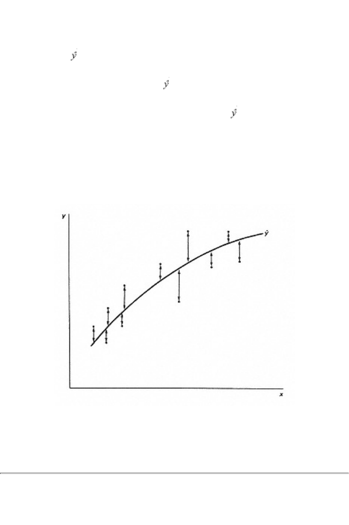
values (called ) of the dependent variable can be subtracted from the
actual values (y) of the dependent variable in the data set to produce
what are called the residuals (y - ). These residuals could be thought
of as estimates of the unknown disturbances inherent in the data set.
This is illustrated in figure 2.1. The line labeled is the estimated
relationship corresponding to a specific set of values of the unknown
parameters. The dots represent actual observations on the dependent
variable y and the independent variable x. Each observation is a certain
vertical distance away from the estimated line, as pictured by the
double-ended arrows. The lengths of these double-ended arrows
measure the residuals. A different set of specific values of the
Figure 2.1
Minimizing the sum of squared residuals
page_11
Page 12

parameters would create a different estimating line and thus a different
set of residuals.
It seems natural to ask that a "good" estimator be one that generates a
set of estimates of the parameters that makes these residuals "small."
Controversy arises, however, over the appropriate definition of "small."
Although it is agreed that the estimator should be chosen to minimize a
weighted sum of all these residuals, full agreement as to what the
weights should be does not exist. For example, those feeling that all
residuals should be weighted equally advocate choosing the estimator
that minimizes the sum of the absolute values of these residuals. Those
feeling that large residuals should be avoided advocate weighting large
residuals more heavily by choosing the estimator that minimizes the sum
of the squared values of these residuals. Those worried about misplaced
decimals and other data errors advocate placing a constant (sometimes
zero) weight on the squared values of particularly large residuals. Those
concerned only with whether or not a residual is bigger than some
specified value suggest placing a zero weight on residuals smaller than
this critical value and a weight equal to the inverse of the residual on
residuals larger than this value. Clearly a large number of alternative
definitions could be proposed, each with appealing features.
By far the most popular of these definitions of "small" is the
minimization of the sum of squared residuals. The estimator generating
the set of values of the parameters that minimizes the sum of squared
residuals is called the ordinary least squares estimator. It is referred to
as the OLS estimator and is denoted by bOLS in this book. This
estimator is probably the most popular estimator among researchers
doing empirical work. The reason for this popularity, however, does not
stem from the fact that it makes the residuals "small" by minimizing the
sum of squared residuals. Many econometricians are leery of this
criterion because minimizing the sum of squared residuals does not say
anything specific about the relationship of the estimator to the true
parameter value b that it is estimating. In fact, it is possible to be too
successful in minimizing the sum of squared residuals, accounting for so
many unique features of that particular sample that the estimator loses
its general validity, in the sense that, were that estimator applied to a
new sample, poor estimates would result. The great popularity of the
OLS estimator comes from the fact that in some estimating problems
(but not all!) it scores well on some of the other criteria, described
below, that are thought to be of greater importance. A secondary reason
for its popularity is its computational ease; all computer packages
include the OLS estimator for linear relationships, and many have

routines for nonlinear cases.
Because the OLS estimator is used so much in econometrics, the
characteristics of this estimator in different estimating problems are
explored very thoroughly by all econometrics texts. The OLS estimator
always minimizes the sum of squared residuals; but it does not always
meet other criteria that econometricians feel are more important. As will
become clear in the next chapter, the subject of econometrics can be
characterized as an attempt to find alternative estimators to the OLS
estimator for situations in which the OLS estimator does
page_12
Page 13
not meet the estimating criterion considered to be of greatest
importance in the problem at hand.
2.4 Highest R2
A statistic that appears frequently in econometrics is the coefficient of
determination, R2. It is supposed to represent the proportion of the
variation in the dependent variable "explained" by variation in the
independent variables. It does this in a meaningful sense in the case of a
linear relationship estimated by OLS. In this case it happens that the
sum of the squared deviations of the dependent variable about its mean
(the "total" variation in the dependent variable) can be broken into two
parts, called the "explained" variation (the sum of squared deviations of
the estimated values of the dependent variable around their mean) and
the ''unexplained" variation (the sum of squared residuals). R2 is
measured either as the ratio of the "explained" variation to the "total"
variation or, equivalently, as 1 minus the ratio of the "unexplained"
variation to the "total" variation, and thus represents the percentage of
variation in the dependent variable "explained" by variation in the
independent variables.
Because the OLS estimator minimizes the sum of squared residuals (the
"unexplained" variation), it automatically maximizes R2. Thus
maximization of R2, as a criterion for an estimator, is formally identical
to the least squares criterion, and as such it really does not deserve a
separate section in this chapter. It is given a separate section for two
reasons. The first is that the formal identity between the highest R2
criterion and the least squares criterion is worthy of emphasis. And the

second is to distinguish clearly the difference between applying R2 as a
criterion in the context of searching for a "good" estimator when the
functional form and included independent variables are known, as is the
case in the present discussion, and using R2 to help determine the
proper functional form and the appropriate independent variables to be
included. This later use of R2, and its misuse, are discussed later in the
book (in sections 5.5 and 6.2).
2.5 Unbiasedness
Suppose we perform the conceptual experiment of taking what is called
a repeated sample: keeping the values of the independent variables
unchanged, we obtain new observations for the dependent variable by
drawing a new set of disturbances. This could be repeated, say, 2,000
times, obtaining 2,000 of these repeated samples. For each of these
repeated samples we could use an estimator b* to calculate an estimate
of b. Because the samples differ, these 2,000 estimates will not be the
same. The manner in which these estimates are distributed is called the
sampling distribution of b*. This is illustrated for the one-dimensional
case in figure 2.2, where the sampling distribution of the estimator is
labeled (b*). It is simply the probability density function of b*,
approximated
page_13
Page 14
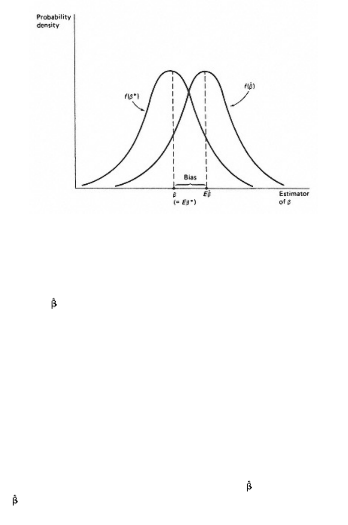
Figure 2.2
Using the sampling distribution to illustrate bias
by using the 2,000 estimates of b to construct a histogram, which in turn
is used to approximate the relative frequencies of different estimates of
b from the estimator b*. The sampling distribution of an alternative
estimator, , is also shown in figure 2.2.
This concept of a sampling distribution, the distribution of estimates
produced by an estimator in repeated sampling, is crucial to an
understanding of econometrics. Appendix A at the end of this book
discusses sampling distributions at greater length. Most estimators are
adopted because their sampling distributions have "good" properties;
the criteria discussed in this and the following three sections are directly
concerned with the nature of an estimator's sampling distribution.
The first of these properties is unbiasedness. An estimator b* is said to
be an unbiased estimator of b if the mean of its sampling distribution is
equal to b, i.e., if the average value of b* in repeated sampling is b. The
mean of the sampling distribution of b* is called the expected value of
b* and is written Eb* the bias of b* is the difference between Eb* and
b. In figure 2.2, b* is seen to be unbiased, whereas
has a bias of size
(E - b). The property of unbiasedness does not mean that b* = b; it
says only that, if we could undertake repeated sampling an infinite

number of times, we would get the correct estimate "on the average."
The OLS criterion can be applied with no information concerning how
the data were generated. This is not the case for the unbiasedness
criterion (and all other criteria related to the sampling distribution),
since this knowledge is required to construct the sampling distribution.
Econometricians have therefore
page_14
Page 15
developed a standard set of assumptions (discussed in chapter 3)
concerning the way in which observations are generated. The general,
but not the specific, way in which the disturbances are distributed is an
important component of this. These assumptions are sufficient to allow
the basic nature of the sampling distribution of many estimators to be
calculated, either by mathematical means (part of the technical skill of
an econometrician) or, failing that, by an empirical means called a
Monte Carlo study, discussed in section 2.10.
Although the mean of a distribution is not necessarily the ideal measure
of its location (the median or mode in some circumstances might be
considered superior), most econometricians consider unbiasedness a
desirable property for an estimator to have. This preference for an
unbiased estimator stems from the hope that a particular estimate (i.e.,
from the sample at hand) will be close to the mean of the estimator's
sampling distribution. Having to justify a particular estimate on a "hope"
is not especially satisfactory, however. As a result, econometricians
have recognized that being centered over the parameter to be estimated
is only one good property that the sampling distribution of an estimator
can have. The variance of the sampling distribution, discussed next, is
also of great importance.
2.6 Efficiency
In some econometric problems it is impossible to find an unbiased
estimator. But whenever one unbiased estimator can be found, it is
usually the case that a large number of other unbiased estimators can
also be found. In this circumstance the unbiased estimator whose
sampling distribution has the smallest variance is considered the most
desirable of these unbiased estimators; it is called the best unbiased
estimator, or the efficient estimator among all unbiased estimators. Why
it is considered the most desirable of all unbiased estimators is easy to

visualize. In figure 2.3 the sampling distributions of two unbiased
estimators are drawn. The sampling distribution of the estimator
denoted f( ), is drawn "flatter" or "wider" than the sampling
distribution of b*, reflecting the larger variance of . Although both
estimators would produce estimates in repeated samples whose average
would be b, the estimates from would range more widely and thus
would be less desirable. A researcher using would be less certain that
his or her estimate was close to b than would a researcher using b*.
Sometimes reference is made to a criterion called "minimum variance."
This criterion, by itself, is meaningless. Consider the estimator b* = 5.2
(i.e., whenever a sample is taken, estimate b by 5.2 ignoring the
sample). This estimator has a variance of zero, the smallest possible
variance, but no one would use this estimator because it performs so
poorly on other criteria such as unbiasedness. (It is interesting to note,
however, that it performs exceptionally well on the computational cost
criterion!) Thus, whenever the minimum variance, or "efficiency,"
criterion is mentioned, there must exist, at least implicitly, some
additional constraint, such as unbiasedness, accompanying that
criterion. When the
page_15
Page 16
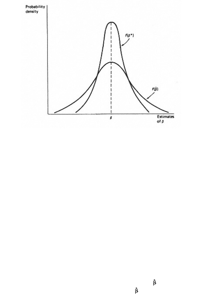
Figure 2.3
Using the sampling distribution to illustrate
efficiency
additional constraint accompanying the minimum variance criterion is
that the estimators under consideration be unbiased, the estimator is
referred to as the best unbiased estimator.
Unfortunately, in many cases it is impossible to determine
mathematically which estimator, of all unbiased estimators, has the
smallest variance. Because of this problem, econometricians frequently
add the further restriction that the estimator be a linear function of the
observations on the dependent variable. This reduces the task of finding
the efficient estimator to mathematically manageable proportions. An
estimator that is linear and unbiased and that has minimum variance
among all linear unbiased estimators is called the best linear unbiased
estimator (BLUE). The BLUE is very popular among econometricians.
This discussion of minimum variance or efficiency has been implicitly
undertaken in the context of a undimensional estimator, i.e., the case in
which b is a single number rather than a vector containing several
numbers. In the multidimensional case the variance of
becomes a
matrix called the variance-covariance matrix of . This creates special
problems in determining which estimator has the smallest variance. The
technical notes to this section discuss this further.
2.7 Mean Square Error (MSE)
Using the best unbiased criterion allows unbiasedness to play an
extremely strong role in determining the choice of an estimator, since
only unbiased esti-
page_16
Page 17
Figure 2.4
MSE trades off bias and variance
mators are considered. It may well be the case that, by restricting
attention to only unbiased estimators, we are ignoring estimators that
are only slightly biased but have considerably lower variances. This
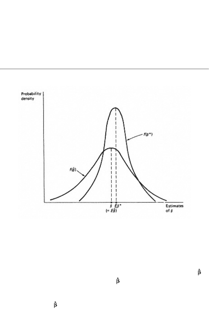
phenomenon is illustrated in figure 2.4. The sampling distribution of
the best unbiased estimator, is labeled f( ). b* is a biased estimator
with sampling distribution (b*). It is apparent from figure 2.4 that,
although (b*) is not centered over b reflecting the bias of b*, it is
"narrower" than f( ), indicating a smaller variance. It should be clear

from the diagram that most researchers would probably choose the
biased estimator b* in preference to the best unbiased estimator .
This trade-off between low bias and low variance is formalized by using
as a criterion the minimization of a weighted average of the bias and the
variance (i.e., choosing the estimator that minimizes this weighted
average). This is not a variable formalization, however, because the bias
could be negative. One way to correct for this is to use the absolute
value of the bias; a more popular way is to use its square. When the
estimator is chosen so as to minimize a weighted average of the
variance and the square of the bias, the estimator is said to be chosen on
the weighted square error criterion. When the weights are equal, the
criterion is the popular mean square error (MSE) criterion. The
popularity of the mean square error criterion comes from an alternative
derivation of this criterion: it happens that the expected value of a loss
function consisting of the square of the difference between b and its
estimate (i.e., the square of the estimation error) is the same as the sum
of the variance and the squared bias. Minimization of the expected
value of this loss function makes good intuitive sense as a criterion for
choosing an estimator.
page_17
Page 18
In practice, the MSE criterion is not usually adopted unless the best
unbiased criterion is unable to produce estimates with small variances.
The problem of multicollinearity, discussed in chapter 11, is an example
of such a situation.
2.8 Asymptotic Properties
The estimator properties discussed in sections 2.5, 2.6 and 2.7 above
relate to the nature of an estimator's sampling distribution. An unbiased
estimator, for example, is one whose sampling distribution is centered
over the true value of the parameter being estimated. These properties
do not depend on the size of the sample of data at hand: an unbiased
estimator, for example, is unbiased in both small and large samples. In
many econometric problems, however, it is impossible to find estimators
possessing these desirable sampling distribution properties in small
samples. When this happens, as it frequently does, econometricians may
justify an estimator on the basis of its
asymptotic properties - the nature
of the estimator's sampling distribution in extremely large samples.
The sampling distribution of most estimators changes as the sample size
changes. The sample mean statistic, for example, has a sampling
distribution that is centered over the population mean but whose
variance becomes smaller as the sample size becomes larger. In many
cases it happens that a biased estimator becomes less and less biased as
the sample size becomes larger and larger - as the sample size becomes
larger its sampling distribution changes, such that the mean of its
sampling distribution shifts closer to the true value of the parameter
being estimated. Econometricians have formalized their study of these
phenomena by structuring the concept of an asymptotic distribution
and defining desirable asymptotic or "large-sample properties" of an
estimator in terms of the character of its asymptotic distribution. The
discussion below of this concept and how it is used is heuristic (and not
technically correct); a more formal exposition appears in appendix C at
the end of this book.
Consider the sequence of sampling distributions of an estimator
formed by calculating the sampling distribution of for successively
larger sample sizes. If the distributions in this sequence become more
and more similar in form to some specific distribution (such as a normal
distribution) as the sample size becomes extremely large, this specific
distribution is called the asymptotic distribution of . Two basic
estimator properties are defined in terms of the asymptotic distribution.
(1) If the asymptotic distribution of becomes concentrated on a
particular value k as the sample size approaches infinity, k is said to be
the probability limit of and is written plim = k if plim = b, then
is said to be consistent.
(2) The variance of the asymptotic distribution of is called the
asymptotic variance of if
is consistent and its asymptotic variance is
smaller than
page_18
Page 19
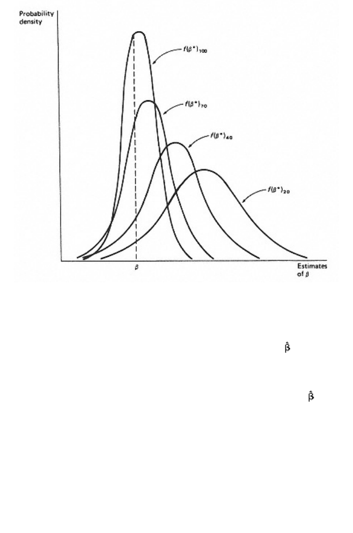
Figure 2.5
How sampling distribution can change as the sample size
grows
the asymptotic variance of all other consistent estimators, is said to be
asymptotically efficient.
At considerable risk of oversimplification, the plim can be thought of as
the large-sample equivalent of the expected value, and so plim = b is
the large-sample equivalent of unbiasedness. Consistency can be
crudely conceptualized as the large-sample equivalent of the minimum
mean square error property, since a consistent estimator can be (loosely
speaking) though of as having, in the limit, zero bias and a zero
variance. Asymptotic efficiency is the large-sample equivalent of best
unbiasedness: the variance of an asymptotically efficient estimator goes
to zero faster than the variance of any other consistent estimator.
Figure 2.5 illustrates the basic appeal of asymptotic properties. For
sample size 20, the sampling distribution of b* is shown as (b*)20. Since

this sampling distribution is not centered over
b
, the estimator
b
* is
biased. As shown in figure 2.5, however, as the sample size increases to
40, then 70 and then 100, the sampling distribution of b* shifts so as to
be more closely centered over b (i.e., it becomes less biased), and it
becomes less spread out (i.e., its variance becomes smaller). If b* were
consistent, as the sample size increased to infinity
page_19
Page 20
the sampling distribution would shrink in width to a single vertical line,
of infinite height, placed exactly at the point b.
It must be emphasized that these asymptotic criteria are only employed
in situations in which estimators with the traditional desirable small-
sample properties, such as unbiasedness, best unbiasedness and
minimum mean square error, cannot be found. Since econometricians
quite often must work with small samples, defending estimators on the
basis of their asymptotic properties is legitimate only if it is the case that
estimators with desirable asymptotic properties have more desirable
small-sample properties than do estimators without desirable asymptotic
properties. Monte Carlo studies (see section 2.10) have shown that in
general this supposition is warranted.
The message of the discussion above is that when estimators with
attractive small-sample properties cannot be found one may wish to
choose an estimator on the basis of its large-sample properties. There is
an additional reason for interest in asymptotic properties, however, of
equal importance. Often the derivation of small-sample properties of an
estimator is algebraically intractable, whereas derivation of large-sample
properties is not. This is because, as explained in the technical notes, the
expected value of a nonlinear function of a statistic is not the nonlinear
function of the expected value of that statistic, whereas the plim of a
nonlinear function of a statistic is equal to the nonlinear function of the
plim of that statistic.
These two features of asymptotics give rise to the following four
reasons for why asymptotic theory has come to play such a prominent
role in econometrics.
(1) When no estimator with desirable small-sample properties can be
found, as is often the case, econometricians are forced to choose
estimators on the basis of their asymptotic properties. As example is the
choice of the OLS estimator when a lagged value of the dependent
variable serves as a regressor. See chapter 9.
(2) Small-sample properties of some estimators are extraordinarily
difficult to calculate, in which case using asymptotic algebra can
provide an indication of what the small-sample properties of this
estimator are likely to be. An example is the plim of the OLS estimator
in the simultaneous equations context. See chapter 10.
(3) Formulas based on asymptotic derivations are useful approximations
to formulas that otherwise would be very difficult to derive and
estimate. An example is the formula in the technical notes used to
estimate the variance of a nonlinear function of an estimator.
(4) Many useful estimators and test statistics may never have been
found had it not been for algebraic simplifications made possible by
asymptotic algebra. An example is the development of LR, W and LM
test statistics for testing nonlinear restrictions. See chapter 4.
page_20
Page 21
Figure 2.6
Maximum likelihood estimation
2.9 Maximum Likelihood
The maximum likelihood principle of estimation is based on the idea
that the sample of data at hand is more likely to have come from a "real
world" characterized by one particular set of parameter values than

from a "real world" characterized by any other set of parameter values.
The maximum likelihood estimate (MLE) of a vector of parameter
values b is simply the particular vector bMLE that gives the greatest
probability of obtaining the observed data.
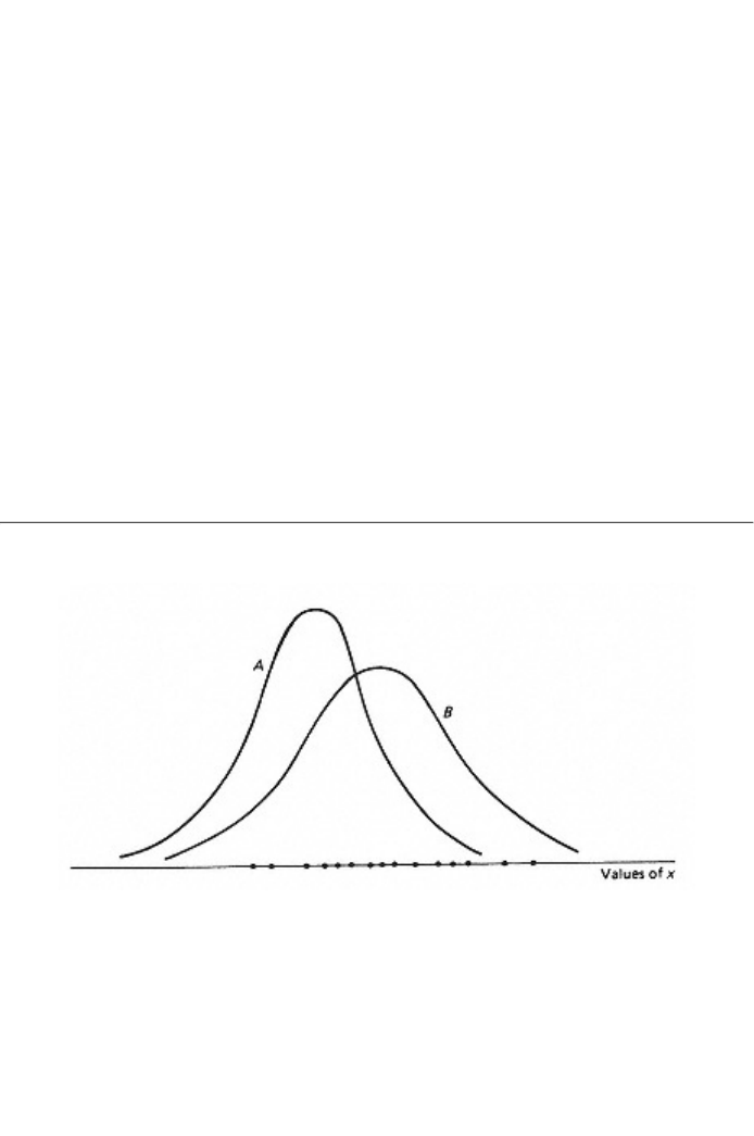
This idea is illustrated in figure 2.6. Each of the dots represents an
observation on x drawn at random from a population with mean m and
variance s2. Pair A of parameter values, mA and (s2)A, gives rise in
figure 2.6 to the probability density function A for x while the pair B,
mB and (s2)B, gives rise to probability density function B. Inspection of
the diagram should reveal that the probability of having obtained the
sample in question if the parameter values were mA and (s2)A is very
low compared with the probability of having obtained the sample if the
parameter values were mB and (s2)B. On the maximum likelihood
principle, pair B is preferred to pair A as an estimate of m and s2. The
maximum likelihood estimate is the particular pair of values mMLE and
(s2)MLE that creates the greatest probability of having obtained the
sample in question; i.e., no other pair of values would be preferred to
this maximum likelihood pair, in the sense that pair B is preferred to
pair A. The means by which the econometrician finds this maximum
likelihood estimates is discussed briefly in the technical notes to this
section.
In addition to its intuitive appeal, the maximum likelihood estimator has
several desirable asymptotic properties. It is asymptotically unbiased, it
is consistent, it is asymptotically efficient, it is distributed
asymptotically normally, and its asymptotic variance can be found via a
standard formula (the Cramer-Rao lower bound - see the technical
notes to this section). Its only major theoretical drawback is that in
order to calculate the MLE the econometrician must assume
page_21
Page 22
a specific (e.g., normal) distribution for the error term. Most
econometricians seem willing to do this.
These properties make maximum likelihood estimation very appealing
for situations in which it is impossible to find estimators with desirable
small-sample properties, a situation that arises all too often in practice.
In spite of this, however, until recently maximum likelihood estimation

has not been popular, mainly because of high computational cost.
Considerable algebraic manipulation is required before estimation, and
most types of MLE problems require substantial input preparation for
available computer packages. But econometricians' attitudes to MLEs
have changed recently, for several reasons. Advances in computers and
related software have dramatically reduced the computational burden.
Many interesting estimation problems have been solved through the use
of MLE techniques, rendering this approach more useful (and in the
process advertising its properties more widely). And instructors have
been teaching students the theoretical aspects of MLE techniques,
enabling them to be more comfortable with the algebraic manipulations
it requires.
2.10 Monte Carlo Studies
A Monte Carlo study is a simulation exercise designed to shed light on
the small-sample properties of competing estimators for a given
estimating problem. They are called upon whenever, for that particular
problem, there exist potentially attractive estimators whose small-
sample properties cannot be derived theoretically. Estimators with
unknown small-sample properties are continually being proposed in the
econometric literature, so Monte Carlo studies have become quite
common, especially now that computer technology has made their
undertaking quite cheap. This is one good reason for having a good
understanding of this technique. A more important reason is that a
thorough understanding of Monte Carlo studies guarantees an
understanding of the repeated sample and sampling distribution
concepts, which are crucial to an understanding of econometrics.
Appendix A at the end of this book has more on sampling distributions
and their relation to Monte Carlo studies.
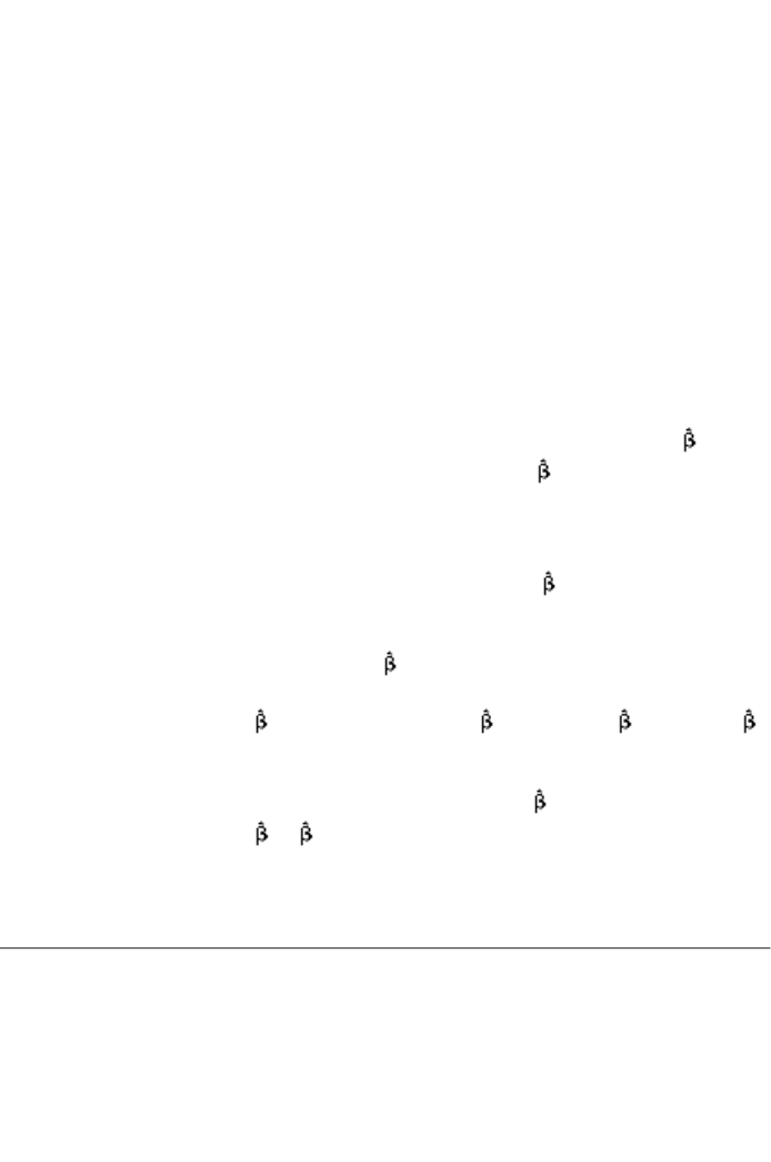
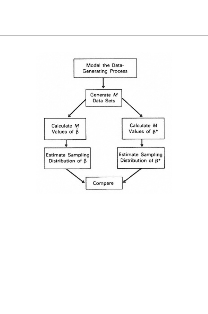
The general idea behind a Monte Carlo study is to (1) model the
data-generating process, (2) generate several sets of artificial data, (3)
employ these data and an estimator to create several estimates, and (4)
use these estimates to gauge the sampling distribution properties of that
estimator. This is illustrated in figure 2.7. These four steps are described
below.
(1) Model the data-generating process Simulation of the process
thought to be generating the real-world data for the problem at hand
requires building a model for the computer to mimic the data-generating
process, including its stochastic component(s). For example, it could be
specified that N (the sample size) values of X, Z and an error term
generate N values of Y according to Y = b1 + b2X + b3Z + e, where the
bi are specific, known numbers, the N val-
page_22
Page 23
Figure 2.7
Structure of a Monte Carlo study
use of X and Z are given, exogenous, observations on explanatory
variables, and the N values of e are drawn randomly from a normal
distribution with mean zero and known variance s2. (Computers are
capable of generating such random error terms.) Any special features
thought to characterize the problem at hand must be built into this
model. For example, if b2 = b3-1 then the values of b2 and b3 must be
chosen such that this is the case. Or if the variance s2 varies from
observation to observation, depending on the value of Z, then the error
terms must be adjusted accordingly. An important feature of the study is
that all of the (usually unknown) parameter values are known to the
person conducting the study (because this person chooses these values).
(2)
Create sets of data
With a model of the data-generating process
built into the computer, artificial data can be created. The key to doing
this is the stochastic element of the data-generating process. A sample
of size N is created by obtaining N values of the stochastic variable e
and then using these values, in conjunction with the rest of the model, to
generate N, values of Y. This yields one complete sample of size N,
namely N observations on each of Y, X and Z, corresponding to the
particular set of N error terms drawn. Note that this artificially
generated set of sample data could be viewed as an example of
real-world data that a researcher would be faced with when dealing with
the kind of estimation problem this model represents. Note especially
that the set of data obtained depends crucially on the particular set of
error terms drawn. A different set of
page_23
Page 24
error terms would create a different data set for the same problem.
Several of these examples of data sets could be created by drawing
different sets of N error terms. Suppose this is done, say, 2,000 times,
generating 2,000 set of sample data, each of sample size N. These are
called repeated samples.
(3) Calculate estimates Each of the 2,000 repeated samples can be used
as data for an estimator 3 say, creating 2,000 estimated 3i (i = 1,2,. .
., 2,000) of the parameter b3. These 2,000 estimates can be viewed as
random ''drawings" from the sampling distribution of 3
(4) Estimate sampling distribution properties These 2,000 drawings
from the sampling distribution of 3 can be used as data to estimate the
properties of this sampling distribution. The properties of most interest
are its expected value and variance, estimates of which can be used to
estimate bias and mean square error.
(a) The expected value of the sampling distribution of 3 is
estimated by the average of the 2,000 estimates:
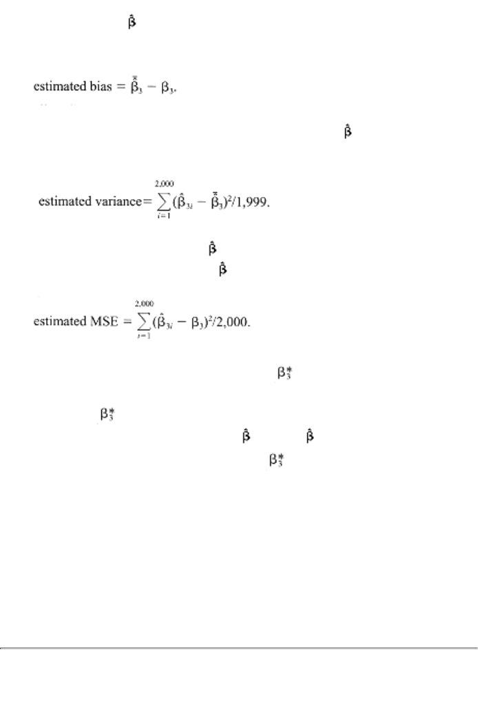
(b) The bias of 3 is estimated by subtracting the known true value
of b3 from the average:
(c) The variance of the sampling distribution of 3 is estimated by
using the traditional formula for estimating variance:
(d) The mean square error 3 is estimated by the average of the
squared differences between 3 and the true value of b3:
At stage 3 above an alternative estimator could also have been used
to calculate 2,000 estimates. If so, the properties of the sampling
distribution of could also be estimated and then compared with
those of the sampling distribution of 3 (Here 3 could be, for example,
the ordinary least squares estimator and any competing estimator
such as an instrumental variable estimator, the least absolute error
estimator or a generalized least squares estimator. These estimators are
discussed in later chapters.) On the basis of this comparison, the person
conducting the Monte Carlo study may be in a position to recommend
one estimator in preference to another for the sample size N. By
repeating such a study for progressively greater values of N, it is
possible to investigate how quickly an estimator attains its asymptotic
properties.
page_24
Page 25
2.11 Adding Up

Because in most estimating situations there does not exist a "super-
estimator" that is better than all other estimators on all or even most of
these (or other) criteria, the ultimate choice of estimator is made by
forming an "overall judgement" of the desirableness of each available
estimator by combining the degree to which an estimator meets each of
these criteria with a subjective (on the part of the econometrician)
evaluation of the importance of each of these criteria. Sometimes an
econometrician will hold a particular criterion in very high esteem and
this will determine the estimator chosen (if an estimator meeting this
criterion can be found). More typically, other criteria also play a role on
the econometrician's choice of estimator, so that, for example, only
estimators with reasonable computational cost are considered. Among
these major criteria, most attention seems to be paid to the best
unbiased criterion, with occasional deference to the mean square error
criterion in estimating situations in which all unbiased estimators have
variances that are considered too large. If estimators meeting these
criteria cannot be found, as is often the case, asymptotic criteria are
adopted.
A major skill of econometricians is the ability to determine estimator
properties with regard to the criteria discussed in this chapter. This is
done either through theoretical derivations using mathematics, part of
the technical expertise of the econometrician, or through Monte Carlo
studies. To derive estimator properties by either of these means, the
mechanism generating the observations must be known; changing the
way in which the observations are generated creates a new estimating
problem, in which old estimators may have new properties and for
which new estimators may have to be developed.
The OLS estimator has a special place in all this. When faced with any
estimating problem, the econometric theorist usually checks the OLS
estimator first, determining whether or not it has desirable properties.
As seen in the next chapter, in some circumstances it does have
desirable properties and is chosen as the "preferred" estimator, but in
many other circumstances it does not have desirable properties and a
replacement must be found. The econometrician must investigate
whether the circumstances under which the OLS estimator is desirable
are met, and, if not, suggest appropriate alternative estimators.
(Unfortunately, in practice this is too often not done, with the OLS
estimator being adopted without justification.) The next chapter
explains how the econometrician orders this investigation.
General Notes

2.2 Computational Cost
Computational cost has been reduced significantly by the development
of extensive computer software for econometricians. The more
prominent of these are ET,
page_25
Page 26
GAUSS, LIMDEP, Micro-FIT, PC-GIVE, RATS, SAS, SHAZAM,
SORITEC, SPSS, and TSP. The Journal of Applied Econometrics and
the Journal of Economic Surveys both publish software reviews
regularly. All these packages are very comprehensive, encompassing
most of the econometric techniques discussed in textbooks. For
applications they do not cover, in most cases specialized programs exist.
These packages should only be used by those well versed in
econometric theory, however. Misleading or even erroneous results can
easily be produced if these packages are used without a full
understanding of the circumstances in which they are applicable, their
inherent assumptions and the nature of their output; sound research
cannot be produced merely by feeding data to a computer and saying
SHAZAM.
Problems with the accuracy of computer calculations are ignored in
practice, but can be considerable. See Aigner (1971, pp. 99101) and
Rhodes (1975). Quandt (1983) is a survey of computational problems
and methods in econometrics.
2.3 Least Squares
Experiments have shown that OLS estimates tend to correspond to the
average of laymen's "freehand" attempts to fit a line to a scatter of data.
See Mosteller et al. (1981).
In figure 2.1 the residuals were measured as the vertical distances from
the observations to the estimated line. A natural alternative to this
vertical measure is the orthogonal measure - the distance from the
observation to the estimating line along a line perpendicular to the
estimating line. This infrequently seen alternative is discussed in
Malinvaud (1966, pp. 711); it is sometimes used when measurement
errors plague the data, as discussed in section 9.2
2.4 Highest R2
R2 is called the coefficient of determination. It is the square of the
correlation coefficient between y and its OLS estimate
The total variation of the dependent variable y about its mean, s(y - y)2,
is called SST (the total sum of squares); the "explained" variation, the
sum of squared deviations of the estimated values of the dependent
variable about their mean, is called SSR (the regression sum of
squares); and the "unexplained" variation, the sum of squared residuals,
is called SSE (the error sum of squares). R2 is then given by SSR/SST or
by 1 - (SSE/SST).
What is a high R2? There is no generally accepted answer to this
question. In dealing with time series data, very high R2s are not
unusual, because of common trends. Ames and Reiter (1961) found, for
example, that on average the R2 of a relationship between a randomly
chosen variable and its own value lagged one period is about 0.7, and
that an R2 in excess of 0.5 could be obtained by selecting an economic
time series and regressing it against two to six other randomly selected
economic time series. For cross-sectional data, typical R2s are not
nearly so high.
The OLS estimator maximizes R2. Since the R2 measure is used as an
index of how well an estimator "fits" the sample data, the OLS
estimator is often called the "best-fitting" estimator. A high R2 is often
called a ''good fit."
Because the R2 and OLS criteria are formally identical, objections to
the latter apply
page_26
Page 27
to the former. The most frequently voiced of these is that searching for
a good fit is likely to generate parameter estimates tailored to the
particular sample at hand rather than to the underlying "real world."
Further, a high R2 is not necessary for "good" estimates; R2 could be
low because of a high variance of the disturbance terms, and our
estimate of b could be ''good" on other criteria, such as those discussed
later in this chapter.

The neat breakdown of the total variation into the "explained" and
"unexplained" variations that allows meaningful interpretation of the R2
statistic is valid only under three conditions. First, the estimator in
question must be the OLS estimator. Second, the relationship being
estimated must be linear. Thus the R2 statistic only gives the percentage
of the variation in the dependent variable explained linearly by
variation in the independent variables. And third, the linear relationship
being estimated must include a constant, or intercept, term. The
formulas for R2 can still be used to calculate an R2 for estimators other
than the OLS estimator, for nonlinear cases and for cases in which the
intercept term is omitted; it can no longer have the same meaning,
however, and could possibly lie outside the 01 interval. The zero
intercept case is discussed at length in Aigner (1971, pp. 8590). An
alternative R2 measure, in which the variations in y and are measured
as deviations from zero rather than their means, is suggested.
Running a regression without an intercept is the most common way of
obtaining an R2 outside the 01 range. To see how this could happen,
draw a scatter of points in (x,y) space with an estimated OLS line such
that there is a substantial intercept. Now draw in the OLS line that
would be estimated if it were forced to go through the origin. In both
cases SST is identical (because the same observations are used). But in
the second case the SSE and the SSR could be gigantic, because the
and the ( -y)could be huge. Thus if R2 is calculated as 1 - SSR/SST, a
negative number could result; if it is calculated as SSR/SST, a number
greater than one could result.
R2 is sensitive to the range of variation of the dependent variable, so
that comparisons of R2s must be undertaken with care. The favorite
example used to illustrate this is the case of the consumption function
versus the savings function. If savings is defined as income less
consumption, income will do exactly as well in explaining variations in
consumption as in explaining variations in savings, in the sense that the
sum of squared residuals, the unexplained variation, will be exactly the
same for each case. But in percentage terms, the unexplained variation
will be a higher percentage of the variation in savings than of the
variation in consumption because the latter are larger numbers. Thus the
R2 in the savings function case will be lower than in the consumption
function case. This reflects the result that the expected value of R2 is
approximately equal to b2V/(b2V + s2) where V is E(x-x)2.

In general, econometricians are interested in obtaining "good"
parameter estimates where "good" is not defined in terms of R2.
Consequently the measure R2 is not of much importance in
econometrics. Unfortunately, however, many practitioners act as though
it is important, for reasons that are not entirely clear, as noted by
Cramer (1987, p. 253):
These measures of goodness of fit have a fatal attraction.
Although it is generally conceded among insiders that they do
not mean a thing, high values are still a source of pride and
satisfaction to their authors, however hard they may try to
conceal these feelings.
page_27
Page 28
Because of this, the meaning and role of R2 are discussed at some
length throughout this book. Section 5.5 and its general notes extend the
discussion of this section. Comments are offered in the general notes of
other sections when appropriate. For example, one should be aware that
R2 from two equations with different dependent variables should not be
compared, and that adding dummy variables (to capture seasonal
influences, for example) can inflate R2 and that regressing on group
means overstates R2 because the error terms have been averaged.
2.5 Unbiasedness
In contrast to the OLS and R2 criteria, the unbiasedness criterion (and
the other criteria related to the sampling distribution) says something
specific about the relationship of the estimator to b, the parameter being
estimated.
Many econometricians are not impressed with the unbiasedness
criterion, as our later discussion of the mean square error criterion will
attest. Savage (1954, p. 244) goes so far as to say: "A serious reason to
prefer unbiased estimates seems never to have been proposed." This
feeling probably stems from the fact that it is possible to have an
"unlucky" sample and thus a bad estimate, with only cold comfort from
the knowledge that, had all possible samples of that size been taken, the
correct estimate would have been hit on average. This is especially the
case whenever a crucial outcome, such as in the case of a matter of life
or death, or a decision to undertake a huge capital expenditure, hinges

on a single correct estimate. None the less, unbiasedness has enjoyed
remarkable popularity among practitioners. Part of the reason for this
may be due to the emotive content of the terminology: who can stand
up in public and state that they prefer biased estimators?
The main objection to the unbiasedness criterion is summarized nicely
by the story of the three econometricians who go duck hunting. The first
shoots about a foot in front of the duck, the second about a foot behind;
the third yells, "We got him!"
2.6 Efficiency
Often econometricians forget that although the BLUE property is
attractive, its requirement that the estimator be linear can sometimes be
restrictive. If the errors have been generated from a "fat-tailed"
distribution, for example, so that relatively high errors occur frequently,
linear unbiased estimators are inferior to several popular nonlinear
unbiased estimators, called robust estimators. See chapter 19.
Linear estimators are not suitable for all estimating problems. For
example, in estimating the variance s2 of the disturbance term,
quadratic estimators are more appropriate. The traditional formula
SSE/(T - K), where T is the number of observations and K is the number
of explanatory variables (including a constant), is under general
conditions the best quadratic unbiased estimator of s2. When K
does not
include the constant (intercept) term, this formula is written as SSE(T -
K -
1).
Although in many instances it is mathematically impossible to determine
the best unbiased estimator (as opposed to the best linear unbiased
estimator), this is not the case if the specific distribution of the error is
known. In this instance a lower bound, called the Cramer-Rao lower
bound, for the variance (or variance-covariance matrix)
page_28
Page 29
of unbiased estimators can be calculated. Furthermore, if this lower
bound is attained (which is not always the case), it is attained by a
transformation of the maximum likelihood estimator (see section 2.9)
creating an unbiased estimator. As an example, consider the sample
mean statistic X. Its variance, s2/T, is equal to the Cramer-Rao lower
bound if the parent population is normal. Thus X is the best unbiased
estimator (whether linear or not) of the mean of a normal population.
2.7 Mean Square Error (MSE)
Preference for the mean square error criterion over the unbiasedness
criterion often hinges on the use to which the estimate is put. As an
example of this, consider a man betting on horse races. If he is buying
"win" tickets, he will want an unbiased estimate of the winning horse,
but if he is buying "show" tickets it is not important that his horse wins
the race (only that his horse finishes among the first three), so he will be
willing to use a slightly biased estimator of the winning horse if it has a
smaller variance.
The difference between the variance of an estimator and its MSE is that
the variance measures the dispersion of the estimator around its mean
whereas the MSE measures its dispersion around the true value of the
parameter being estimated. For unbiased estimators they are identical.
Biased estimators with smaller variances than unbiased estimators are
easy to find. For example, if is an unbiased estimator with variance V
, then 0.9 is a biased estimator with variance 0.81V( ). As a more
relevant example, consider the fact that, although (SSE/(T - K) is the
best quadratic unbiased estimator of s2, as noted in section 2.6, it can be
shown that among quadratic estimators the MSE estimator of s2 is
SSE/(T - K + 2).
The MSE estimator has not been as popular as the best unbiased
estimator because of the mathematical difficulties in its derivation.
Furthermore, when it can be derived its formula often involves
unknown coefficients (the value of b), making its application
impossible. Monte Carlo studies have shown that approximating the
estimator by using OLS estimates of the unknown parameters can
sometimes circumvent this problem.
2.8 Asymptotic Properties
How large does the sample size have to be for estimators to display their
asymptotic properties? The answer to this crucial question depends on
the characteristics of the problem at hand. Goldfeld and Quandt (1972,
p. 277) report an example in which a sample size of 30 is sufficiently
large and an example in which a sample of 200 is required. They also
note that large sample sizes are needed if interest focuses on estimation
of estimator variances rather than on estimation of coefficients.
An observant reader of the discussion in the body of this chapter might
wonder why the large-sample equivalent of the expected value is
defined as the plim rather than being called the "asymptotic
expectation." In practice most people use the two terms synonymously,
but technically the latter refers to the limit of the expected value, which
is usually, but not always, the same as the plim. For discussion see the
technical notes to appendix C.
page_29
Page 30
2.9 Maximum Likelihood
Note that
bMLE is not, as is sometimes carelessly stated, the most
probable value of b; the most probable value of b is b itself. (Only in a
Bayesian interpretation, discussed later in this book, would the former
statement be meaningful.) bMLE is simply the value of b that
maximizes the probability of drawing the sample actually obtained.
The asymptotic variance of the MLE is usually equal to the Cramer-Rao
lower bound, the lowest asymptotic variance that a consistent estimator
can have. This is why the MLE is asymptotically efficient.
Consequently, the variance (not just the asymptotic variance) of the
MLE is estimated by an estimate of the Cramer-Rao lower bound. The
formula for the Cramer-Rao lower bound is given in the technical notes
to this section.
Despite the fact that bMLE is sometimes a biased estimator of b
(although asymptotically unbiased), often a simple adjustment can be
found that creates an unbiased estimator, and this unbiased estimator
can be shown to be best unbiased (with no linearity requirement)
through the relationship between the maximum likelihood estimator and
the Cramer-Rao lower bound. For example, the maximum likelihood
estimator of the variance of a random variable x is given by the formula
which is a biased (but asymptotically unbiased) estimator of the true
variance. By multiplying this expression by T/(T - 1), this estimator can
be transformed into a best unbiased estimator.

Maximum likelihood estimators have an invariance property similar to
that of consistent estimators. The maximum likelihood estimator of a
nonlinear function of a parameter is the nonlinear function of the
maximum likelihood estimator of that parameter: [g(b)]MLE =
g
(bMLE) where g is a nonlinear function. This greatly simplifies the
algebraic derivations of maximum likelihood estimators, making
adoption of this criterion more attractive.
Goldfeld and Quandt (1972) conclude that the maximum likelihood
technique performs well in a wide variety of applications and for
relatively small sample sizes. It is particularly evident, from reading
their book, that the maximum likelihood technique is well-suited to
estimation involving nonlinearities and unusual estimation problems.
Even in 1972 they did not feel that the computational costs of MLE
were prohibitive.
Application of the maximum likelihood estimation technique requires
that a specific distribution for the error term be chosen. In the context
of regression, the normal distribution is invariably chosen for this
purpose, usually on the grounds that the error term consists of the sum
of a large number of random shocks and thus, by the Central Limit
Theorem, can be considered to be approximately normally distributed.
(See Bartels, 1977, for a warning on the use of this argument.) A more
compelling reason is that the normal distribution is relatively easy to
work with. See the general notes to chapter 4 for further discussion. In
later chapters we encounter situations (such as count data and logit
models) in which a distribution other than the normal is employed.
Maximum likelihood estimates that are formed on the incorrect
assumption that the errors are distributed normally are called quasi-
maximum likelihood estimators. In
page_30
Page 31
many circumstances they have the same asymptotic distribution as that
predicted by assuming normality, and often related test statistics retain
their validity (asymptotically, of course). See Godfrey (1988, p. 402) for
discussion.
Kmenta (1986, pp. 17583) has a clear discussion of maximum likelihood
estimation. A good brief exposition is in Kane (1968, pp. 17780).
Valavanis (1959, pp. 236), an econometrics text subtitled "An

Introduction to Maximum Likelihood Methods," has an interesting
account of the meaning of the maximum likelihood technique.
2.10 Monte Carlo Studies
In this author's opinion, understanding Monte Carlo studies is one of the
most important elements of studying econometrics, not because a
student may need actually to do a Monte Carlo study, but because an
understanding of Monte Carlo studies guarantees an understanding of
the concept of a sampling distribution and the uses to which it is put.
For examples and advice on Monte Carlo methods see Smith (1973) and
Kmenta (1986, chapter 2). Hendry (1984) is a more advanced
reference. Appendix A at the end of this book provides further
discussion of sampling distributions and Monte Carlo studies. Several
exercises in appendix D illustrate Monte Carlo studies.
If a researcher is worried that the specific parameter values used in the
Monte Carlo study may influence the results, it is wise to choose the
parameter values equal to the estimated parameter values using the data
at hand, so that these parameter values are reasonably close to the true
parameter values. Furthermore, the Monte Carlo study should be
repeated using nearby parameter values to check for sensitivity of the
results. Bootstrapping is a special Monte Carlo method designed to
reduce the influence of assumptions made about the parameter values
and the error distribution. Section 4.6 of chapter 4 has an extended
discussion.
The Monte Carlo technique can be used to examine test statistic as well
as parameter estimators. For example, a test statistic could be examined
to see how closely its sampling distribution matches, say, a chi-square.
In this context interest would undoubtedly focus on determining its size
(type I error for a given critical value) and power, particularly as
compared with alternative test statistics.
By repeating a Monte Carlo study for several different values of the
factors that affect the outcome of the study, such as sample size or
nuisance parameters, one obtains several estimates of, say, the bias of
an estimator. These estimated biases can be used as observations with
which to estimate a functional relationship between the bias and the
factors affecting the bias. This relationship is called a response surface.
Davidson and MacKinnon (1993, pp. 75563) has a good exposition.
It is common to hold the values of the explanatory variables fixed
during repeated sampling when conducting a Monte Carlo study.

Whenever the values of the explanatory variables are affected by the
error term, such as in the cases of simultaneous equations, measurement
error, or the lagged value of a dependent variable serving as a regressor,
this is illegitimate and must not be done - the process generating the
data must be properly mimicked. But in other cases it is not obvious if
the explanatory variables should be fixed. If the sample exhausts the
population, such as would be the case for observations on all cities in
Washington state with population greater than 30,000, it would not
make sense to allow the explanatory variable values to change during
repeated sampling. On the other hand, if a sample of wage-earners is
drawn
page_31
Page 32
from a very large potential sample of wage-earners, one could visualize
the repeated sample as encompassing the selection of wage-earners as
well as the error term, and so one could allow the values of the
explanatory variables to vary in some representative way during
repeated samples. Doing this allows the Monte Carlo study to produce
an estimated sampling distribution which is not sensitive to the
characteristics of the particular wage-earners in the sample; fixing the
wage-earners in repeated samples produces an estimated sampling
distribution conditional on the observed sample of wage-earners, which
may be what one wants if decisions are to be based on that sample.
2.11 Adding Up
Other, less prominent, criteria exist for selecting point estimates, some
examples of which follow.
(a) Admissibility An estimator is said to be admissible (with respect
to some criterion) if, for at least one value of the unknown b, it
cannot be beaten on that criterion by any other estimator.
(b) Minimax A minimax estimator is one that minimizes the
maximum expected loss, usually measured as MSE, generated by
competing estimators as the unknown b varies through its possible
values.
(c) Robustness An estimator is said to be robust if its desirable
properties are not sensitive to violations of the conditions under
which it is optimal. In general, a robust estimator is applicable to a
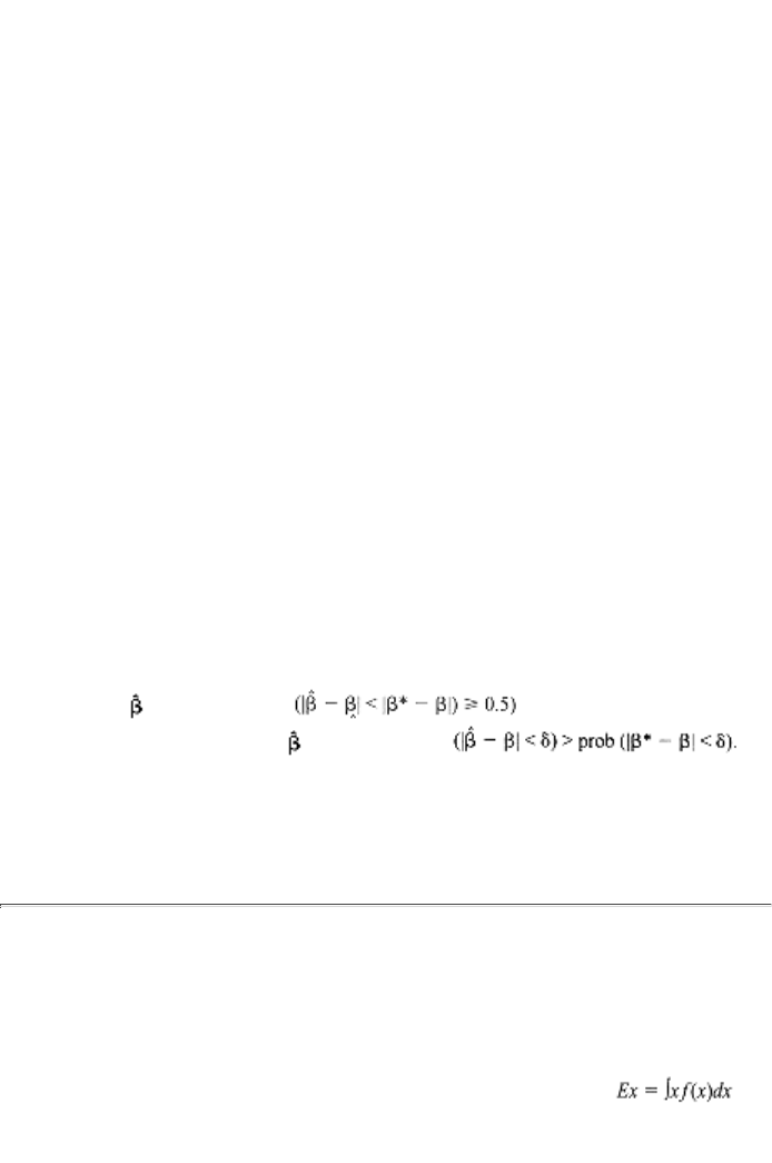
wide variety of situations, and is relatively unaffected by a small
number of bad data values. See chapter 19.
(d) MELO In the Bayesian approach to statistics (see chapter 13), a
decision-theoretic approach is taken to estimation; an estimate is
chosen such that it minimizes an expected loss function and is
called the MELO (minimum expected loss) estimator. Under
general conditions, if a quadratic loss function is adopted the mean
of the posterior distribution of b is chosen as the point estimate of b
and this has been interpreted in the non-Bayesian approach as
corresponding to minimization of average risk. (Risk is the sum of
the MSEs of the individual elements of the estimator of the vector
b.) See Zellner (1978).
(e) Analogy principle Parameters are estimated by sample statistics
that have the same property in the sample as the parameters do in
the population. See chapter 2 of Goldberger (1968b) for an
interpretation of the OLS estimator in these terms. Manski (1988)
gives a more complete treatment. This approach is sometimes
called the method of moments because it implies that a moment of
the population distribution should be estimated by the
corresponding moment of the sample. See the technical notes.
(f) Nearness/concentration Some estimators have infinite variances
and for that reason are often dismissed. With this in mind, Fiebig
(1985) suggests using as a criterion the probability of nearness
(prefer to b* if prob or the probability of
concentration (prefer to b* if prob
Two good introductory references for the material of this chapter are
Kmenta (1986, pp. 916, 97108, 15672) and Kane (1968, chapter 8).
page_32
Page 33
Technical Notes
2.5 Unbiasedness
The expected value of a variable x is defined formally as
where f is the probability density function (sampling distribution) of x.

Thus
E(x)
could be viewed as a weighted average of all possible values
of x where the weights are proportional to the heights of the density
function (sampling distribution) of x.
2.6 Efficiency
In this author's experience, student assessment of sampling distributions
is hindered, more than anything else, by confusion about how to
calculate an estimator's variance. This confusion arises for several
reasons.
(1) There is a crucial difference between a variance and an estimate
of that variance, something that often is not well understood.
(2) Many instructors assume that some variance formulas are
"common knowledge," retained from previous courses.
(3) It is frequently not apparent that the derivations of variance
formulas all follow a generic form.
(4) Students are expected to recognize that some formulas are
special cases of more general formulas.
(5) Discussions of variance, and appropriate formulas, are seldom
gathered together in one place for easy reference.
Appendix B has been included at the end of this book to alleviate this
confusion, supplementing the material in these technical notes.
In our discussion of unbiasedness, no confusion could arise from b
being
multidimensional: an estimator's expected value is either equal to b (in
every dimension) or it is not. But in the case of the variance of an
estimator confusion could arise. An estimator b* that is k-dimensional
really consists of k different estimators, one for each dimension of b.
These k different estimators all have their own variances. If all k of the
variances associated with the estimator b* are smaller than their
respective counterparts of the estimator then it is clear that the
variance of b* can be considered smaller than the variance of . For
example, if b is two-dimensional, consisting of two separate parameters
b1 and b2
an estimator b* would consist of two estimators and . If b* were
an unbiased estimator of b, would be an unbiased estimator of ,
and would be an unbiased estimator of b2. The estimators and
would each have variances. Suppose their variances were 3.1 and 7.4,
respectively. Now suppose , consisting of 1 2, is another unbiased
estimator, where 1 and 2 have variances 5.6 and 8.3, respectively. In
this example, since the variance of is less than the variance of 1
and the
page_33
Page 34
variance of is less than the variance of 2, it is clear that the
"variance" of b* is less than the variance of . But what if the variance
of 2 were 6.3 instead of 8.3? Then it is not clear which "variance" is
smallest.
An additional complication exists in comparing the variances of
estimators of a multi-dimensional b. There may exist a nonzero
covariance between the estimators of the separate components of b. For
example, a positive covariance between 1 and 2 implies that,
whenever 1 overestimates b1, there is a tendency for 2 to
overestimate b2, making the complete estimate of b worse than would
be the case were this covariance zero. Comparison of the "variances" of
multidimensional estimators should therefore somehow account for this
covariance phenomenon.
The "variance" of a multidimensional estimator is called a variance-
covariance matrix. If b* is an estimator of k-dimensional b, then the
variance-covariance matrix of b*, denoted by V(b*), is defined as a k ×
k matrix (a table with k entries in each direction) containing the
variances of the k elements of b* along the diagonal and the covariance
in the off-diagonal positions. Thus,
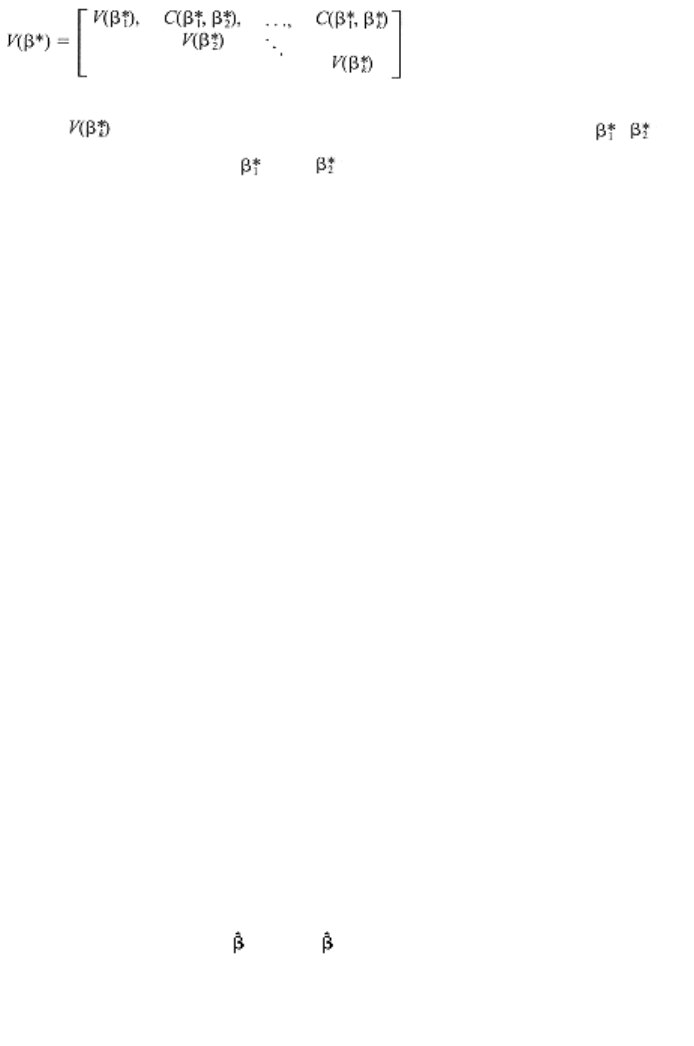
where is the variance of the k the element of b* and C( , ) is
the covariance between and . All this variance-covariance
matrix does is array the relevant variances and covariances in a table.
One this is done, the econometrician can draw on mathematicians'
knowledge of matrix algebra to suggest ways in which the variance-
covariance matrix of one unbiased estimator could be considered
"smaller" than the variance-covariance matrix of another unbiased
estimator.
Consider four alternative ways of measuring smallness among variance-
covariance matrices, all accomplished by transforming the matrices into
single numbers and then comparing those numbers:
(1) Choose the unbiased estimator whose variance-covariance
matrix has the smallest trace (sum of diagonal elements);
(2) choose the unbiased estimator whose variance-covariance
matrix has the smallest determinant;
(3) choose the unbiased estimator for which any given linear
combination of its elements has the smallest variance;
(4) choose the unbiased estimator whose variance-covariance
matrix minimizes a risk function consisting of a weighted sum of
the individual variances and covariances. (A risk function is the
expected value of a traditional loss function, such as the square of
the difference between an estimate and what it is estimating.)
This last criterion seems sensible: a researcher can weight the variances
and covariances according to the importance he or she subjectively
feels their minimization should be given in choosing an estimator. It
happens that in the context of an unbiased estimator this risk function
can be expressed in an alternative form, as the expected value of a
quadratic function of the difference between the estimate and the true
parameter value; i.e.,E (
- b)'Q ( - b) This alternative interpretation
also makes good intuitive sense as a choice criterion for use in the
estimating context.

If the weights in the risk function described above, the elements of
Q,
are chosen so as to make it impossible for this risk function to be
negative (a reasonable request,
page_34
Page 35
since if it were negative it would be a gain, not a loss), then a very
fortunate thing occurs. Under these circumstances all four of these
criteria lead to the same choice of estimator. What is more, this result
does not depend on the particular weights used in the risk function.
Although these four ways of defining a smallest matrix are reasonably
straightforward, econometricians have chosen, for mathematical
reasons, to use as their definition an equivalent but conceptually more
difficult idea. This fifth rule says, choose the unbiased estimator whose
variance-covariance matrix, when subtracted from the variance-
covariance matrix of any other unbiased estimator, leaves a
non-negative definite matrix. (A matrix A is non-negative definite if the
quadratic function formed by using the elements of A as parameters
(x'Ax) takes on only non-negative values. Thus to ensure a non-negative
risk function as described above, the weighting matrix Q must be
non-negative definite.)
Proofs of the equivalence of these five selection rules can be
constructed by consulting Rothenberg (1973, p. 8), Theil (1971, p. 121),
and Goldberger (1964, p. 38).
A special case of the risk function is revealing. Suppose we choose the
weighting such that the variance of any one element of the estimator
has a very heavy weight, with all other weights negligible. This implies
that each of the elements of the estimator with the "smallest" variance-
covariance matrix has individual minimum variance. (Thus, the example
given earlier of one estimator with individual variances 3.1 and 7.4 and
another with variances 5.6 and 6.3 is unfair; these two estimators could
be combined into a new estimator with variances 3.1 and 6.3.) This
special case also indicates that in general covariances play no role in
determining the best estimator.
2.7 Mean Square Error (MSE)
In the multivariate context the MSE criterion can be interpreted in
terms of the "smallest" (as defined in the technical notes to section 2.6)

MSE matrix. This matrix, given by the formula E( - b)( - b)', is a
natural matrix generalization of the MSE criterion. In practice, however,
this generalization is shunned in favor of the sum of the MSEs of all the
individual components of , a definition of risk that has come to be the
usual meaning of the term.
2.8 Asymptotic Properties
The econometric literature has become full of asymptotics, so much so
that at least one prominent econometrician, Leamer (1988), has
complained that there is too much of it. Appendix C of this book
provides an introduction to the technical dimension of this important
area of econometrics, supplementing the items that follow.
The reason for the important result that Eg g(Ex) for g nonlinear is
illustrated in figure 2.8. On the horizontal axis are measured values of
, the sampling distribution of which is portrayed by pdf( ), with values
ofg( ) measured on the vertical axis. Values A and B of , equidistant
from E , are traced to give g(A) and g(B). Note that g(B) is much
farther from g( ) than is g(A): high values of lead to values of g( )
considerably above g(E ), but low values of lead to values of g( )
only slightly below g(E ) Consequently the sampling distribution of g(
) is asymmetric, as shown by pdf[g( )], and in this example the
expected value of g( ) lies above g(E )
page_35
Page 36
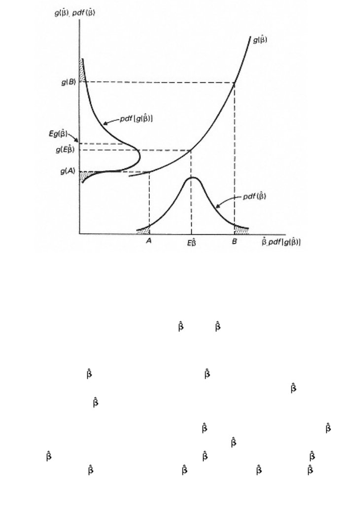
Figure 2.8
Why the expected value of a nonlinear function is
not the nonlinear function of the expected value
If g were a linear function, the asymmetry portrayed in figure 2.8 would
not arise and thus we would have Eg( )=g(E )For g nonlinear,
however, this result does not hold.
Suppose now that we allow the sample size to become very large, and
suppose that plim exists and is equal to E in figure 2.8. As the
sample size becomes very large, the sampling distributionpdf( ) begins
to collapse on plim i.e., its variance becomes very, very small. The
points A and B are no longer relevant since values near them now occur
with negligible probability. Only values of very, very close to plim
are relevant; such values when traced through g( ) are very, very close
to g(plim
). Clearly, the distribution of g( ) collapses on g(plim ) as
the distribution of collapses on plim . Thus plim g( )=g(plim ), for
g
a continuous function.
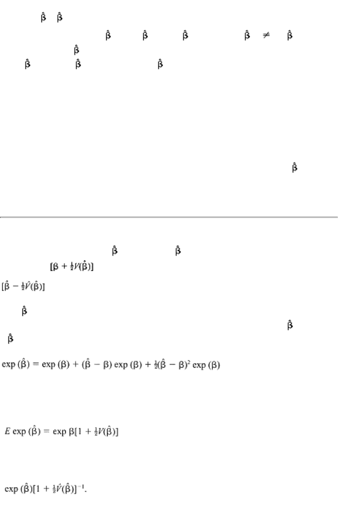
For a simple example of this phenomenon, let
g
be the square function,
so that g = .2. From the well-known result that V(x) = E(x)2-E(x)2,
we can deduce that E( 2)=(E )2+V ( )Clearly,E( 2) (E 2), but if
the variance of goes to zero as the sample size goes to infinity then
plim( 2)=(plim )2. The case of equal to the sample mean statistic
provides an easy example of this.
Note that in figure 2.8 the modes, as well as the expected values, of the
two densities do not correspond. An explanation of this can be
constructed with the help of the "change of variable" theorem discussed
in the technical notes to section 2.9.
An approximate correction factor can be estimated to reduce the small-
sample bias discussed here. For example, suppose an estimate of b is
distributed normally with
page_36
Page 37
mean b and variance V( .) Then exp is distributed log-normally with
mean exp suggesting that exp (b) could be estimated by exp
which, although biased, should have less bias than exp (b). If
in this same example the original error were not distributed normally, so
that was not distributed normally, a Taylor series expansion could be
used to deduce an appropriate correction factor. Expand exp around
E
=b
plus higher-order terms which are neglected. Taking the expected value
of both sides produces
suggesting that exp b could be estimated by

For discussion and examples of these kinds of adjustments, see Miller
(1984), Kennedy (1981a, 1983) and Goldberger (1968a). An alternative
way of producing an estimate of a nonlinear function g(b) is to calculate
many values of g(b* + e), where e is an error with mean zero and
variance equal to the estimated variance of b*, and average them. For
more on this ''smearing" estimate see Duan (1983).
When g is a linear function, the variance of g( ) is given by the square
of the slope of g times the variance of i.e., V(ax) = a2V(x). When g is
a continuous nonlinear function its variance is more difficult to
calculate. As noted above in the context of figure 2.8, when the sample
size becomes very large only values of very, very close to plim are
relevant, and in this range a linear approximation to is adequate. The
slope of such a linear approximation is given by the first derivative of g
with respect to . Thus the asymptotic variance of g( ) is often
calculated as the square of this first derivative times the asymptotic
variance of , with this derivative evaluated at = plim for the
theoretical variance, and evaluated at for the estimated variance.
2.9 Maximum Likelihood
The likelihood of a sample is often identified with the "probability" of
obtaining that sample, something which is, strictly speaking, not correct.
The use of this terminology is accepted, however, because of an implicit
understanding, articulated by Press et al. (1986, p. 500): "If the yi's take
on continuous values, the probability will always be zero unless we add
the phrase, '. . . plus or minus some fixed dy on each data point.' So let's
always take this phrase as understood."
The likelihood function is identical to the joint probability density
function of the given sample. It is given a different name (i.e., the name
"likelihood") to denote the fact that in this context it is to be
interpreted
as a function of the parameter values (since it is to be maximized with
respect to those parameter values) rather than, as is usually the case,
being interpreted as a function of the sample data.
The mechanics of finding a maximum likelihood estimator are explained
in most econometrics texts. Because of the importance of maximum
likelihood estimation in
page_37
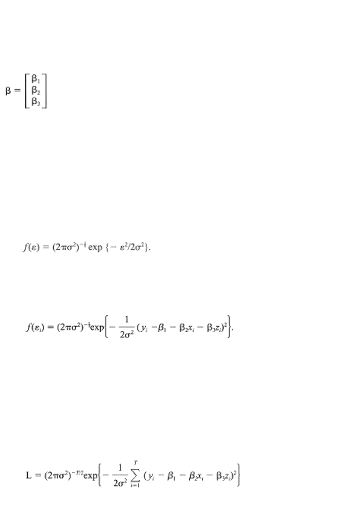
Page 38
the econometric literature, an example is presented here. Consider a
typical econometric problem of trying to find the maximum likelihood
estimator of the vector
in the relationship y = b1 + b2x + b3z + e where T observations on y, x
and z are available.
(1) The first step is to specify the nature of the distribution of the
disturbance term e. Suppose the disturbances are identically and
independently distributed with probability density function (e). For
example, it could be postulated that e is distributed normally with
mean zero and variance s2 so that
(2) The second step is to rewrite the given relationship as e = y - b1
- b2x - b3z so that for the ithe value of e we have
(3) The third step is to form the likelihood function, the formula for
the joint probability distribution of the sample, i.e., a formula
proportional to the probability of drawing the particular error terms
inherent in this sample. If the error terms are independent of each
other, this is given by the product of all the (e)s, one for each of the
T sample observations. For the example at hand, this creates the
likelihood function
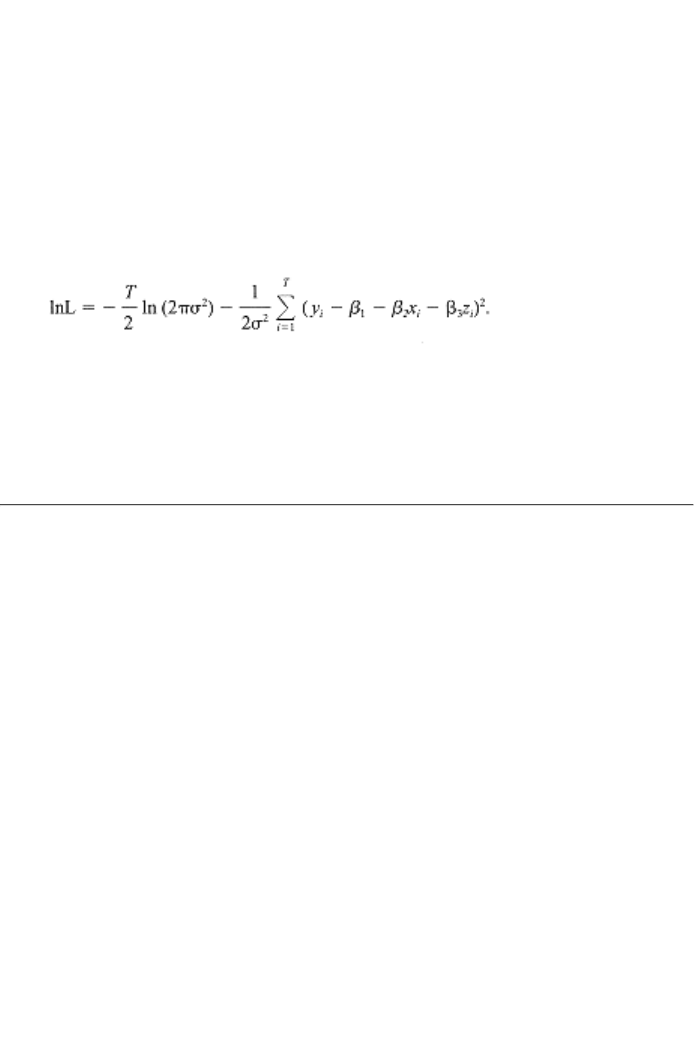
a complicated function of the sample data and the unknown
parameters b1, b2 and b3, plus any unknown parameters inherent in
the probability density function - in this case s2.
(4) The fourth step is to find the set of values of the unknown
parameters (b1, b2, b3 and s2), as functions of the sample data, that
maximize this likelihood function. Since the parameter values that
maximize L also maximize lnL, and the latter task is easier, attention
usually focuses on the log-likelihood function. In this example,
In some simple cases, such as this one, the maximizing values of this
function (i.e., the MLEs) can be found using standard algebraic
maximizing techniques. In
page_38
Page 39
most cases, however, a numerical search technique (described in
section 6.3) must be employed to find the MLE.
There are two circumstances in which the technique presented above
must be modified.
(1) Density of y not equal to density of e We have observations on
y, not e. Thus, the likelihood function should be structured from the
density of y, not the density of e. The technique described above
implicitly assumes that the density of y, (y), is identical to (e), the
density of e with e replaced in this formula by y - Xb, but this is not
necessarily the case. The probability of obtaining a value of e in the
small range de is given by (e) de; this implies an equivalent
probability for y of (y)|dy| where (y) is the density function of y and
|dy| is the absolute value of the range of y values corresponding to
de. Thus, because of (e) de = (y)|dy|, we can calculate (y) as
(e)|de/dy|.
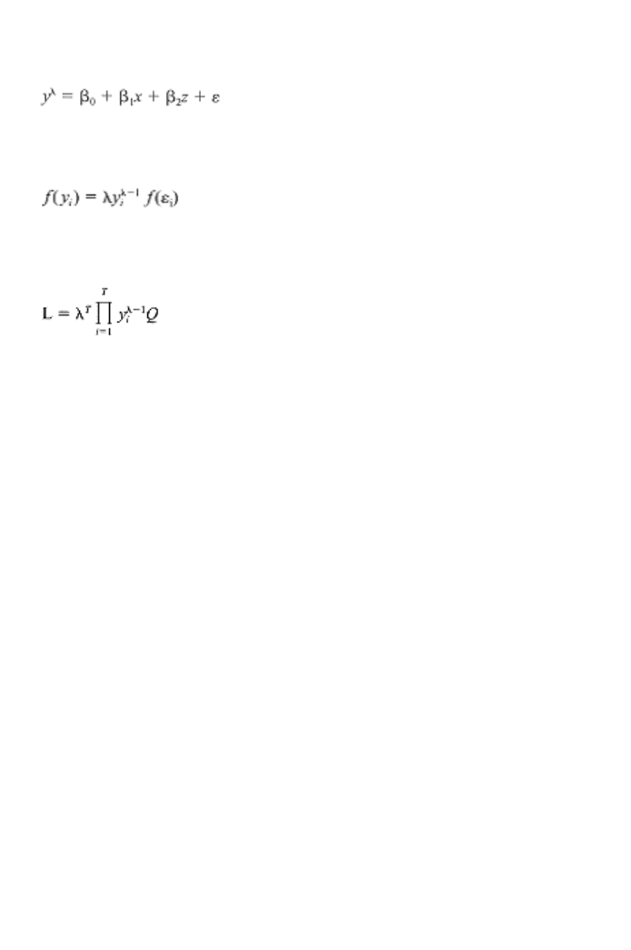
In the example given above (y) and (e) are identical since |de/dy| is
one. But suppose our example were such that we had
where l is some (known or unknown) parameter. In this case,
and the likelihood function would become
where Q
is the likelihood function of the original example, with each
yi raised to the power l.
This method of finding the density of y when y is a function of
another variable e whose density is known, is referred to as the
change-of-variable technique. The multivariate analogue of |de/dy|
is the absolute value of the Jacobian of the transformation - the
determinant of the matrix of first derivatives of the vector e with
respect to the vector y. Judge et al. (1988, pp. 30-6) have a good
exposition.
(2) Observations not independent In the examples above, the
observations were independent of one another so that the density
values for each observation could simply be multiplied together to
obtain the likelihood function. When the observations are not
independent, for example if a lagged value of the regress and
appears as a regressor, or if the errors are autocorrelated, an
alternative means of finding the likelihood function must be
employed. There are two ways of handling this problem.
(a) Using a multivariate density A multivariate density function
gives the density of an entire vector of e rather than of just one
element of that vector (i.e., it gives the "probability" of obtaining
the entire set of ei). For example, the multivariate normal
density function for the vector e is given (in matrix terminology)
by the formula
page_39
Page 40
where s2W is the variance-covariance matrix of the vector e.
This formula itself can serve as the likelihood function (i.e.,
there is no need to multiply a set of densities together since this
formula has implicity already done that, as well as taking
account of interdependencies among the data). Note that this
formula gives the density of the vector e, not the vector y. Since
what is required is the density of y, a multivariate adjustment
factor equivalent to the univariate |de/dy| used earlier is
necessary. This adjustment factor is |det de/dy| where de/dy is a
matrix containing in its ijth position the derivative of the ith
observation of e with respect to the jth observation of y. It is
called the Jacobian of the transformation from e to y. Watts
(1973) has a good explanation of the Jacobian.
(b) Using a transformation It may be possible to transform the
variables of the problem so as to be able to work with errors that
are independent. For example, suppose we have
but e is such that et = ret-1 + ut where ut is a normally
distributed error with mean zero and variance $sigmatwou The
es are not independent of one another, so the density for the
vector e cannot be formed by multiplying together all the
individual densities; the multivariate density formula given
earlier must be used, where W is a function of r and s2 is a
function of r and $sigmatwou. But the u errors are distributed
independently, so the density of the u vector can be formed by
multiplying together all the individual ut densities. Some
algebraic manipulation allows ut to be expressed as
(There is a special transformation for u1; see the technical notes
to section 8.3 where autocorrelated errors are discussed.) The
density of the y vector, and thus the required likelihood
function, is then calculated as the density of the u vector times
the Jacobian of the transformation from u to y. In the example at
hand, this second method turns out to be easier, since the first
method (using a multivariate density function) requires that the
determinant of W be calculated, a difficult task.
Working through examples in the literature of the application of these
techniques is the best way to become comfortable with them and to
become aware of the uses to which MLEs can be put. To this end see
Beach and MacKinnon (1978a), Savin and White (1978), Lahiri and
Egy (1981), Spitzer (1982), Seaks and Layson (1983), and Layson and
Seaks (1984).
The Cramer-Rao lower bound is a matrix given by the formula
where q is the vector of unknown parameters (including s2) for the
MLE estimates of which the Cramer-Rao lower bound is the asymptotic
variance-covariance matrix. Its estimation is accomplished by inserting
the MLE estimates of the unknown parameters. The inverse of the
Cramer-Rao lower bound is called the information matrix.
page_40
Page 41
If the disturbances were distributed normally, the MLE estimator of s2
is SSE/T. Drawing on similar examples reported in preceding sections,
we see that estimation of the variance of a normally distributed
population can be computed as SSE/(T - 1), SSE/T or SSE/(T + 1),
which are, respectively, the best unbiased estimator, the MLE, and the
minimum MSE estimator. Here SSE is s(x - x)2.
2.11 Adding Up

The analogy principle of estimation is often called the method of
moments because typically moment conditions (such as that EX'e = 0,
the covariance between the explanatory variables and the error is zero)
are utilized to derive estimators using this technique. For example,
consider a variable x with unknown mean m. The mean m of x is the
first moment, so we estimate m by the first moment (the average) of the
data, x. This procedure is not always so easy. Suppose, for example,
that the density of x is given by f(x)=lxl-1 for 0 < × < 1 and zero
elsewhere. The expected value of x is l/(l + 1) so the method of
moments estimator l* of l is found by setting x = l*/(l* + 1) and solving
to obtain l
* = x/(1 - x). In general we are usually interested in estimating
several parameters and so will require as many of these moment
conditions as there are parameters to be estimated, in which case
finding estimates involves solving these equations simultaneously.
Consider, for example, estimating a and b in y = a + bx + e. Because
e is specified to be an independent error, the expected value of the
product of x and e is zero, an "orthogonality" or "moment"
condition. This suggests that estimation could be based on setting
the product of x and the residual e* = y - a* - b*x equal to zero,
where a* and b* are the desired estimates of a and b. Similarly, the
expected value of e (its first moment) is specified to be zero,
suggesting that estimation could be based on setting the average of
the e* equal to zero. This gives rise to two equations in two
unknowns:
which a reader might recognize as the normal equations of the
ordinary least squares estimator. It is not unusual for a method of
moments estimator to turn out to be a familiar estimator, a result
which gives it some appeal. Greene (1997, pp. 14553) has a good
textbook exposition.
This approach to estimation is straightforward so long as the number
of moment conditions is equal to the number of parameters to be
estimated. But what if there are more moment conditions than
parameters? In this case there will be more equations than
unknowns and it is not obvious how to proceed. The generalized
method of moments (GMM) procedure, described in the technical

notes of section 8.1, deals with this case.
page_41
Page 42
3
The Classical Linear Regression Model
3.1 Textbooks as Catalogs
In chapter 2 we learned that many of the estimating criteria held in high
regard by econometricians (such as best unbiasedness and minimum
mean square error) are characteristics of an estimator's sampling
distribution. These characteristics cannot be determined unless a set of
repeated samples can be taken or hypothesized; to take or hypothesize
these repeated samples, knowledge of the way in which the
observations are generated is necessary. Unfortunately, an estimator
does not have the same characteristics for all ways in which the
observations can be generated. This means that in some estimating
situations a particular estimator has desirable properties but in other
estimating situations it does not have desirable properties. Because
there is no "superestimator" having desirable properties in all situations,
for each estimating problem (i.e., for each different way in which the
observations can be generated) the econometrician must determine
anew which estimator is preferred. An econometrics textbook can be
characterized as a catalog of which estimators are most desirable in
what estimating situations. Thus, a researcher facing a particular
estimating problem simply turns to the catalog to determine which
estimator is most appropriate for him or her to employ in that situation.
The purpose of this chapter is to explain how this catalog is structured.
The cataloging process described above is centered around a standard
estimating situation referred to as the classical linear regression model
(CLR model). It happens that in this standard situation the OLS
estimator is considered the optimal estimator. This model consists of
five assumptions concerning the way in which the data are generated.
By changing these assumptions in one way or another, different
estimating situations are created, in many of which the OLS estimator is
no longer considered to be the optimal estimator. Most econometric
problems can be characterized as situations in which one (or more) of
