
title: Strategies and Games : Theory and Practice
author: Dutta, Prajit K.
publisher: MIT Press
isbn10 | asin: 0262041693
print isbn13: 9780262041690
ebook isbn13: 9780585070223
language: English
subject Game theory, Equilibrium (Economics)
publication date: 1999
lcc: HB144.D88 1999eb
ddc: 330/.01/5193
subject: Game theory, Equilibrium (Economics)
cover
Page III
Strategies and Games
Theory and Practice
Prajit K. Dutta
THE MIT PRESS CAMBRIDGE, MASSACHUSETTS LONDON, ENGLAND
page_iii
Page IV
© 1999 Massachusetts Institute of Technology
All rights reserved. No part of this book may be reproduced in any form by any electronic or mechanical
means (including photocopying, recording, or information storage and retrieval) without permission in
writing from the publisher.
This book was set in Melior and MetaPlus by Windfall Software using ZzTEX and was printed and bound in
the United States of America.
Library of Congress Cataloging-in-Publication Data
Dutta, Prajit K.
Strategies and games: theory and practice / Prajit K.
Dutta.
p. cm.
Includes bibliographical references and index.
ISBN 0-262-04169-3
1. Game theory. 2. Equilibrium (Economics). I. Title.
HB144.D88 1999
330'.01'15193dc21 98-42937

CIP
page_iv
Page V
MA AAR
BABA KE
page_v
Page VII
BRIEF CONTENTS
Preface XXI
A Reader's Guide XXIX
Part One Introduction 1
Chapter 1 A First Look at the Applications 3
2 A First Look at the Theory 17
Two Strategic Form Games: Theory and Practice 33
3 Strategic Form Games and Dominant Strategies 35
4 Dominance Solvability 49
5 Nash Equilibrium 63
6 An Application" Cournot Duopoly 75
7 An Application: The Commons Problem 91
8 Mixed Strategies 103
9 Two Applications: Natural Monopoly and Bankruptcy Law 121
10 Zero-Sum Games 139
Three Extensive Form Games: Theory and Applications 155
11 Extensive Form Games and Backward Induction 157
12 An Application: Research and Development 179
13 Subgame Perfect Equilibrium 193
14 Finitely Repeated Games 209
15 Infinitely Repeated Games 227
16 An Application: Competition and Collusion in the NASDAQ Stock Market 243
17 An Application: OPEC 257
18 Dynamic Games with an Application to the Commmons Problem 275
Four Asymmetric Information Games: Theory and Applications 291
19 Moral Hazard and Incentives Theory 293

20 Games with Incomplete Information 309
page_vii
Page VIII
21 An Application: Incomplete Information in a Cournot Duopoly 331
22 Mechanism Design, the Revelation Principle, and Sales to an Unknown Buyer 349
23 An Application: Auctions 367
24 Signaling Games and the Lemons Problem 383
Five Foundations 401
25 Calculus and Optimization 403
26 Probability and Expectation 421
27 Utility and Expected Utility 433
28 Existence of Nash Equilibria 451
Index 465
page_viii
Page IX
CONTENTS
Preface XXI
A Reader's Guide XXIX
Part One Indroduction 1
Chapter 1 A First Look at the Applications 3
1.1 Gabes That We Play 3
1.2 Background 7
1.3 Examples 8
Summary 12
Exercises 12
Chapter 2 A First Look at the Theory 17
2.1 Rules of the Game: Background 17
2.2 Who, What, When: The Extensive Form 18
2.2.1 Information Sets and Strategies 20
2.3 Who What, When: The Normal (or Strategic) Form 21
2.4 How Much: Von Neumann-Morgenstern Utility Function 23
2.5 Representation of the Examples 25

Summary 27
Exercises 28
Part Two Strategic Form Games: Theory and Practice 33
Chapter 3 Strategic Form Games and Dominant Strategies 35
3.1 Strategic Form Games 35
3.1.1 Examples 36
3.1.2 Equivalence with the Extensive Form 39
3.2 Case Study The Strategic Form of Art Auctions 40
3.2.1 Art Auctions: A Description 40
3.2.2 Art Auctions: The Strategic Form 40
3.3 Dominant Strategy Solution 41
page_ix
Page X
3.4 Cae Study Again A Dominant Strategy at the Auction 43
Summary 44
Exercises 45
Chapter 4 Dominance Solvability 49
4.1 The Idea 49
4.1.1 Dominated and Undominated Strategies 49
4.1.2 Iterated Elimination of Dominated Strategies 51
4.1.3 More Examples 51
4.2 Case Study Electing the United Nations Secretary General 54
4.3 A More Formal Definition 55
4.4 A Discussion 57
Summary 59
Exercises 59
Chapter 5 Nash Equilibrium 63
5.1 The Concept 63
5.1.1 Intuition and Definition 63
5.1.2 Nash Parables 64
5.2 Examples 66
5.3 Case Study Nash Equilibrium in the Animal Kingdom 68
5.4 Relation Between the Solution Concepts
69

Summary 71
Exercises 71
Chapter 6 An Application: Cournot Duopoly 75
6.1 Background 75
6.2 The Basic Model 76
6.3 Cournot Nash Equilibrium 77
6.4 Cartel Solution 79
6.5 Case Study Today's OPEC 81
page_x
Page XI
6.6 Variants on the Main Theme I: A Graphical Analysis 82
6.6.1 The IEDS Solution to the Cournot Model 84
6.7 Variants on the Main Theme II: Stackelberg Model 85
6.8 Variants on the Main Theme III: Generalization 86
Summary 87
Exercises 88
Chapter 7 An Application: The Commons Problem 91
7.1 Background: What is the Commons? 91
7.2 A Simple Model 93
7.3 Social Optimality 95
7.4 The Problem Worsens in a Large Population 96
7.5 Case Studies Buffalo, Global Warming, and the Internet 97
7.6 Averting a Tragedy 98
Summary 99
Exercises 100
Chapter 8 Mixed Strategies 103
8.1 Definition and Examples 103
8.1.1 What Is a Mixed Strategy? 103
8.1.2 Yet More Examples 106
8.2 An Implication 107
8.3 Mixed Strategies Can Dominate Some Pure Strategies 108
8.3.1 Implications for Dominant Strategy Solution and IEDS 109
8.4 Mixed Strategies are Good for Bluffing 110
8.5 Mixed Strategies and Nash Equilibrium 111
8.5.1 Mixed-Strategy Nash Equilibria in an Example 113
8.6 Case Study Random Drug Testing 114
Summary 115
Exercises 116
page_xi
Page XII
Chapter 9 Tow Applications: Naturla Monopoly and Bankruptcy Law 121
9.1 Chicken, Symmetric Games, and Symmetric Equilibria 121
9.1.1 Chicken 121
9.1.2 Symmetric Games and Symmetric Equilibria 122
9.2 Natural Monopoly 123
9.2.1 The Economic Background 123
9.2.2 A Simple Example 124
9.2.3 War of Attrition and a General Analysis 125
9.3 Bankruptcy Law 128
9.3.1 The Legal Background 128
9.3.2 A Numerical Example 128
9.3.3 A General Analysis 130
Summary 132
Exercises 133
Chapter 10 Zero-Sum Games 139
10.1 Definition and Examples 139
10.2 Playing Safe: Maxmin 141
10.2.1 The Concept 141
10.2.2 Examples 142
10.3 Playing Sound: Minmax 144
10.3.1 The Concept and Examples 144
10.3.2 Two Results 146
10.4 Playing Nash: Playing Both Safe and Sound 147
Summary 149
Exercises 149
Part Three Extensive Form Games: Theory and Applications 155
Chapter 11 Extensive Form Games and Backward Induction 157
11.1 The Extensive Form 157
11.1.1 A More Formal Treatment 158
page_xii
Page XIII
11.1.2 Strategies, Mixed Strategies, and Chance Nodes 160
11.2 Perfect Information Games: Definition and Examples 162
11.3 Backward Induction: Examples 165
11.3.1 The Power of Commitment 167
11.4 Backward Induction: A General Result 168
11.5 Connection With IEDS in the Strategic Form 170
11.6 Case Study Poison Pills and Other Takeover Deterrents 172
Summary 174
Exercises 175
Chapter 12 An Application: Research and Development 179
12.1 Background: R&D, Patents, and Ologopolies 179
12.1.1 A Patent Race in Progress: High-Definition Television 180
12.2 A Model of R&D 181
12.3 Backward Induction: Analysis of the Model 183
12.4 Some Remarks 188
Summary 189
Exercises 190
Chapter 13 Subgame Perfect Equilibrium 193
13.1 A Motivating Example 193
13.2 Subgames and Strategies Within Subgames 196
13.3 Subgame Perfect Equilibrium 197
13.4 Two More Examples 199
13.5 Some Remarks 202
13.6 Case Study Peace in the World War I Trenches 203
Summary 205
Exercises 205
Chapter 14 Finitely Repeated Games 209
14.1 Examples and Economic Applications 209
page_xiii
Page XIV
14.1.1 Three Repeated Games and a Definition 209
14.1.2 Four Economic Applications 212
14.2 Finitely Repeated Games 214
14.2.1 Some General Conclusions 218
14.3 Case Study Treasury Bill Auctions 219
Summary 222
Exercises 222
Chapter 15 Infinitely Repeated Games 227
15.1 Detour Through Discounting 227
15.2 Analysis of Example 3: Trigger Strategies and Good Behavior 229
15.3 The Folk Theorem 232
15.4 Repeated Games With Imperfect Detection 234
Summary 237
Exercises 238
Chapter 16 An Application: Competition and Collusion in the NASDAQ Stock Market243
16.1 The Background 243
16.2 The Analysis 245
16.2.1 A Model of the NASDAQ Market 245
16.2.2 Collusion 246
16.2.3 More on Collusion 248
16.3 The Broker-Dealer Relationship 249
16.3.1 Order Preferencing 249
16.3.2 Dealers Big and Small 250
16.4 The Epilogue 251
Summary 252
Exercises 252
Chapter 17 An Application: OPEC 257
17.1 Oil: A Historical Review 257
page_xiv
Page XV
17.1.1 Production and Price History 258
17.2 A Simple Model of the Oil Market 259
17.3 Oil Prices and the Role of OPEC 260
17.4 Repteated Games With Demand Uncertainty 262
17.5 Unobserved Quota Violations 266
17.6 Some Further Comments 269
Summary 270
Exercises 271
Chapter 18 Dynamic Games With An Application to the Commons Problem 275
18.1 Dynamic Games: A Prologue 275
18.2 The Commons Problem: A Model 276
18.3 Sustainable Development and Social Optimum 278
18.3.1 A Computation of the Social Optimum 278
18.3.2 An Explanation of the Social Optimum 281
18.4 Achievable Development and Game Equilibrium 282
18.4.1 A Computation of the Game Equilibrium 282
18.4.2 An Explanation of the Equilibrium 284
18.4.3 A Comparison of the Socially Optimal and the Equilibrium Outcomes 285
18.5 Dynamic Games: An Epilogue 286
Summary 287
Exercises 288
Part Four Asymmetric Information Games: Theory and Applications 291
Chapter 19 Moral Hazard and Incentives Theory 293
19.1 Moral Hazard: Examples and a Definition 293
29.2 A Principal-Agent Model 295
19.2.1 Some Examples of Incentive Schemes 297
19.3 The Optimal Incentive Scheme 299
19.3.1 No Moral Hazard 299
page_xv
Page XVI
19.3.2 Moral Hazard 299
19.4 Some General Conclusions 301
19.4.1 Extensions and Generalizations 303
19.5 Case Study Compensating Primary Care Physicians in an HMO 304
Summary 305
Exercises 306
Chapter 20 Games with Incomplete Information 309
20.1 Some Examples 309
20.1.1 Some Analysis of the Examples 312
20.2 A Complete Analysis of Example 4 313
20.2.1 Bayes-Nash Equilibrium 313
20.2.2 Pure-Strategy Bayes-Nash Equilibria 315
20.2.3 Mixed-Strategy Bayes-Nash Equilibria 316
20.3 More General Considerations 318
20.3.1 A Modified Example 318
20.3.2 A General Framework 320
20.4 Dominance-Based Solution Concepts 321
20.5 Case Study Final Jeopardy 323
Summary 326
Exercises 326
Chapter 21 An Application: Incomplete Information in a Cournot Duopoly 331
21.1 A Model and its Equilibrium 331
21.1.1 The Basic Model 331
21.1.2 Bayes-Nash Equilibrium 332
21.2 The Complete Information Solution 336
21.3 Revealing Costs to a Rival 338
21.4 Two-Sided Incompleteness of Information 340
21.5 Generalizations and Extensions 341
21.5.1 Oligopoly 341
page_xvi
Page XVII
21.5.2 Demand Uncertainty 342
Summary 343
Exercises 343
Chapter 22 Mechanism Design, The Revelation Priciple, and Sales to an Unknown
Buyer
349
22.1 Mechanism Design: The Economic Context 349
22.2 A Simple Example: Selling to a Buyer With an Unknown Valuation 351
22.2.1 Known Passion 351
22.2.2 Unknown Passion 352
22.3 Mechanism Design and the Revelation Principle 356
22.3.1 Single Player 356
22.3.2 Many Players 357
22.4 A More General Example: Selling Variable Amounts 358
22.4.1 Known Type 359
22.4.2 Unknown Type 359
Summary 362
Exercises 362
Chapter 23 An Application: Auctions 367
23.1 Background and Examples 367
23.1.1 Basic Model 369
23.2 Second-Price Auctions 369
23.3 First-Price Auctions 371
23.4 Optimal Auctions 373
23.4.1 How Well Do the First- and Second-Price Auctions Do? 375
23.5 Final Remarks 376
Summary 377
Exercises 378
Chapter 24 Signaling Games and the Lemons Problem 383
24.1 Motivation and Two Examples 383
24.1.1 A First Analysis of the Examples 385
page_xvii
Page XVIII
24.2 A Definition, an Equilibrium Concept, and Examples 387
24.2.1 Definition 387
24.2.2 Perfect Bayesian Equilibrium 387
24.2.3 A Further Analysis of the Examples 389
24.3 Signaling Product Quality 391
24.3.1 The Bad Can Drive Out the Good 391
24.3.2 Good Can Signal Quality? 392
24.4 Case Study Used CarsA Market for Lemons? 394

24.5 Concluding Remarks 395
Summary 396
Exercises 396
Part Five Foundations 401
Chapter 25 Calculus and Optimization 403
25.1 A Calculus Primer 403
25.1.1 Functions 404
25.1.2 Slopes 405
25.1.3 Some Formulas 407
25.1.4 Concave Functions 408
25.2 An Optimization Theory Primer 409
25.2.1 Necessary Conditions 409
25.2.2 Sufficient Conditions 410
25.2.3 Feasibility Constraints 411
25.2.4 Quadratic and Log Functions 413
Summary 414
Exercises 415
Chapter 26 Probability and Expectation 421
26.1 Probability 421
26.1.1 Independence and Conditional Probability 425
26.2 Random Variables and Expectation 426
26.2.1 Conditional Expectation 427
page_xviii
Page XIX
Summary 428
Exercises 428
Chapter 27 Utility and Expected Utility 433
27.1 Decision Making Under Certainty 433
27.2 Decision Making Under Uncertainty 436
27.2.1 The Expected Utility Theorem and the Expected Return Puzzle 437
27.2.2 Details on the Von Neumann-Morgenstern Theorem
439
27.2.3 Payoffs in a Game 441
27.3 Risk Aversion 441

Summary 444
Exercises 444
Chapter 28 Existence of Nash Equilibria 452
28.1 Definition and Examples 451
28.2 Mathematical Background: Fixed Points 453
28.3 Existence of Nash Equilibria: Results and Intuition 458
Summary 460
Exercises 461
Index 465
page_xix
Page XXI
PREFACE
This book evolved out of lecture notes for an undergraduate course in game theory that I have taught at
Columbia University for the past six years. On the first two occasions I took the straight road, teaching out
of available texts. But the road turned out to be somewhat bumpy; for a variety of reasons I was not satisfied
with the many texts that I considered. So the third time around I built myself a small bypass; I wrote a set of
sketchy lecture notes from which I taught while I assigned a more complete text to the students. Although
this compromise involved minimal costs to me, it turned out to be even worse for my students, since we were
now traveling on different roads. And then I (foolishly) decided to build my own highway; buoyed by a
number of favorable referee reports, I decided to turn my notes into a book. I say foolishly because I had no
idea how much hard work is involved in building a road. I only hope I built a smooth one.
The Book's Purpose And Its Intended Audience
The objective of this book is to provide a rigorous yet accessible introduction to game theory and its
applications, primarily in economics and business, but also in political science, the law, and everyday life.
The material is intended principally for two audiences: first, an undergraduate audience that would take this
course as an elective for an economics major. (My experience has been, however, that my classes are also
heavily attended by undergraduate majors in engineering and the sciences who take this course to fulfill their
economics requirement.) The many applications and case studies in the book should make it attractive to its
second audience, MBA students in business schools. In addition, I have tried to make the material useful to
graduate students in economics and related disciplinesPh.D. students in political science, Ph.D. students in
economics not specializing in economic theory, etc.who would like to have a source from which they can get
a self-contained, albeit basic, treatment of game theory.
Pedagogically I have had one overriding objective: to write a textbook that would take the middle road
between the anecdotal and the theorem-driven treatments of the subject. On the one hand is the approach
that teaches purely by examples and anecdotes. In my experience that leaves the students, especially the
brighter ones, hungering for more. On the other hand, there is the more advanced approach emphasizing a
rigorous treatment, but again, in my experience, if there are too few examples and applications it is difficult
to keep even the brighter students interested.
I have tried to combine the best elements of both approaches. Every result is precisely stated (albeit with
minimal notation), all assumptions are detailed, and at least a sketch of a proof is provided. The text also
contains nine chapter-length applications and twelve fairly detailed case studies.
page_xxi
Page XXII
Distinctive Features Of The Book
I believe this book improves on available undergraduate texts in the following ways.
Content a full description of utility theory and a detailed analysis of dynamic game theory
The book provides a thorough discussion of the single-agent decision theory that forms the underpinning of
game theory. (That exercise takes up three chapters in Part Five.) More importantly perhaps, this is the first
text that provides a detailed analysis of dynamic strategic interaction (in Part Three). The theory of repeated
games is studied over two and a half chapters, including discussions of finitely and infinitely repeated games
as well as games with varying stage payoffs. I follow the theory with two chapter-length applications:
market-making on the NASDAQ financial market and the price history of OPEC. A discussion of dynamic
games (in which the game environment evolves according to players' previous choices) follows along with an
application to the dynamic commons problem. I believe many of the interesting applications of game theory
are dynamicstudent interest seems always to heighten when I get to this part of the courseand I have found
that every other text pays only cursory attention to many dynamic issues.
Style emphasis on a parallel development of theory and examples
Almost every chapter that introduces a new concept opens with numerical examples, some of which are well
known and many of which are not. Sometimes I have a leading example and at other times a set of (small)
examples. After explaining the exam-pies, I go to the concept and discuss it with reasonable rigor. At this
point I return to the examples and analyze the just introduced concept within the context of the examples. At
the end of a sectiona set of chapters on related ideasI devote a whole chapter, and sometimes two, to
economic applications of those ideas.
Length and Organization bite-sized chapters and a static to dynamic progression
I decided to organize the material within each chapter in such a fashion that the essential elements of a
whole chapter can be taught in one class (or a class and a half, depending on level). In my experience it has
been a lot easier to keep the students engaged with this structure than with texts that have individual
chapters that are, for example, over fifty pages long. The topics evolve in a natural sequence: static complete
information to dynamic complete information to static incomplete information. I decided to skip much of
dynamic incomplete information (other than signaling) because the questions in this part of the subject are a
lot easier than the answers (and my students seemed to have little stomach for equilibrium refinements, for
example). There are a few advanced topics as well; different instructors will have the freedom to decide
which subset of the advanced topics they would like to teach in their course. Sections that are more difficult
are marked with the symbol . Depending on level, some instructors will want to skip
page_xxii
Page XXIII
these sections at first presentation, while others may wish to take extra time in discussing the material.
Exercises
At the end of each chapter there are about twenty-five to thirty problems (in the Exercises section). In
addition, within the text itself, each chapter has a number of questions (or concept checks) in which the
student is asked to complete a part of an argument, to compute a remaining case in an example, to check the
computation for an assertion, and so on. The point of these questions is to make sure that the reader is really
following the chapter's argument; I strongly encourage my students to answer these questions and often
include some of them in the problem sets.
Case Studies and Applications
At the end of virtually every theoretical chapter there is a case study drawn from real life to illustrate the
concept just discussed. For example, after the chapter on Nash equilibrium, there is a discussion of its usage
in understanding animal conflicts. After a chapter on backward induction (and the power of commitment),
there is a discussion of poison pills and other take-over deterrents. Similarly, at the end of each cluster of
similar topics there is a whole chapter-length application. These range from the tragedy of the commons to
bankruptcy law to incomplete information Cournot competition.

An Overview And Two Possible Syllabi
The book is divided into five parts. The two chapters of Part One constitute an Introduction. Part Two
(Chapters 3 through 10) covers Strategic Form Games: Theory and Practice, while Part Three (Chapters 11
through 18) concentrates on Extensive Form Games: Theory and Practice. In Part Four (Chapters 19
through 24) I discuss Asymmetric Information Games: Theory and Practice. Finally, Part Five (Chapters 25
through 28) consists of chapters on Foundations.
I can suggest two possible syllabi for a one-semester course in game theory and applications. The first
stresses the applications end while the second covers all the theoretical topics. In terms of mathematical
requirements, the second is, naturally, more demanding and presumes that the students are at a higher level.
I have consequently included twenty chapters in the second syllabus and only eighteen in the first. (Note
that the numbers are chapter numbers.)
Syllabus 1 (Applications Emphasis)
1. A First Look at the Applications
3. Strategic Form Games and Dominant Strategies
page_xxiii
Page XXIV
4. Dominance Solvability
5. Nash Equilibrium
6. An Application: Cournot Duopoly
8. Mixed Strategies
9.Two Applications: Natural Monopoly and Bankruptcy Law
11. Extensive Form Games and Backward Induction
12. An Application: Research and Development
13. Subgame Perfect Equilibrium
15. Infinitely Repeated Games
16. An Application: Competition and Collusion in the NASDAQ Stock Market
17. An Application: OPEC
19. Moral Hazard and Incentives Theory
20. Games with Incomplete Information
22. Mechanism Design, the Revelation Principle, and Sales to an Unknown Buyer
23. An Application: Auctions
24.Signaling Games and the Lemons Problem
Syllabus 2 (Theory Emphasis)
2. A First Look at the Theory
27. Utility and Expected Utility
3. Strategic Form Games and Dominant Strategies
4. Dominance Solvability

5. Nash Equilibrium
page_xxiv
Page XXV
6. An Application: Cournot Duopoly
7. An Application: The Commons Problem
8. Mixed Strategies
10. Zero-Sum Games
28. Existence of Nash Equilibria
11. Extensive Form Games and Backward Induction
13. Subgame Perfect Equilibrium
14. Finitely Repeated Games
15. Infinitely Repeated Games
17. An Application: OPEC
18. Dynamic Games with an Application to the Commons Problem
20. Games with Incomplete Information
21. An Application: Incomplete Information in a Cournot Duopoly
22. Mechanism Design, the Revelation Principle, and Sales to an Unknown Buyer
23. An Application: Auctions
Prerequisites
I have tried to write the book in a manner such that very little is presumed of a reader's mathematics or
economics background. This is not to say that one semester each of calculus and statistics and a semester of
intermediate microeconomics will not help. However, students who do not already have this background but
are willing to put in extra work should be able to educate themselves sufficiently.
Toward that end, I have included a chapter on calculus and optimization, and one on probability and
expectation. Readers can afford not to read the two chapters if they already have the following knowledge.
In calculus, I presume knowledge of the slope of a function and a familiarity with slopes of the linear,
quadratic, log, and the square-root functions. In optimization theory, I use the first-order characterization of
an interior
page_xxv
Page XXVI
optimum, that the slope of a maximand is zero at a maximum. As for probability, it helps to know how to
take an expectation. As for economic knowledge, I have attempted to explain all relevant terms and have
not presumed, for example, any knowledge of Pareto optimality, perfect competition, and monopoly.
Acknowledgments
This book has benefited from the comments and criticisms of many colleagues and friends. Tom Gresik at
Penn State, Giorgidi Giorgio at La Sapienza in Rome, Sanjeev Goyal at Erasmus, Matt Kahn at Columbia,
Amanda Bayer at Swarthmore, Rob Porter at Northwestern, and Charles Wilson at NYU were foolhardy

enough to have taught from preliminary versions of the text, and I thank them for the
ir courage and
comments. In addition, the following reviewers provided very helpful comments:
Amanda Bayer, Swarthmore College
James Dearden, Lehigh University
Tom Gresik, Penn State
Ehud Kalai, Northwestern University
David Levine, UCLA
Michael Meurer, SUNY Buffalo
Yaw Nyarko, NYU
Robert Rosenthal, Boston University
Roberto Serrano, Brown University
Rangarajan Sundaram, NYU
A second group of ten referees provided extremely useful, but anonymous, comments.
My graduate students Satyajit Bose, Tack-Seung Jun, and Tsz-Cheong Lai very carefully read the entire
manuscript. Without their hawk-eyed intervention, the book would have many more errors. They are also
responsible for the Solutions Manual, which accompanies this text. My colleagues in the community, Venky
Bala, Terri Devine, Ananth
page_xxvi
Page XXVII
Madhavan, Mukul Majumdar, Alon Orlitsky, Roy Radner, John Rust, Paulo Siconolfi, and Raghu Sundaram,
provided support, sometimes simply by questioning my sanity in undertaking this project. My brother, Prajjal
Dutta, often provided a noneconomist's reality check. Finally, I cannot sufficiently thank my wife, Susan
Sobelewski, who provided critical intellectual and emotional support during the writing of this book.
page_xxvii
Page XXIX
A READER'S GUIDE
Game theory studies strategic situations. Suppose that you are a contestant on the quiz show "Jeopardy!" At
the end of the half hour contest (during Final Jeopardy) you have to make a wager on being able to answer
correctly a final question (that you have not yet been asked). If you answer correctly, your wager will be
added to your winnings up to that point; otherwise, the wager will be subtracted from your total. The two
other contestants also make wagers and their final totals are computed in an identical fashion. The catch is
that there will be only one winner: the contestant with the maximum amount at the very end will take home
his or her winnings while the other two will get (essentially) nothing.
Question: How much should you wager? The easy part of the answer is that the more confident you are in
your knowledge, the more you should bet. The difficult part is, how much is enough to beat out your rivals?
That clearly depends on how much they wager, that is, what their strategies are. It also depends on how
knowledgeable you think they are (after all, like you, they will bet more if they are more knowledgeable, and
they are also more likely to add to their total in that case). The right wager may also depend on how much
money you have already wonand how much they have won.
For instance, suppose you currently have $10,000 and they have $7,500 each. Then a $5,001 wagerand a
correct answerguarantees you victory. But that wager also guarantees you a lossif you answer
incorrectlyagainst an opponent who wagers only $2,500. You could have bet nothing and guaranteed victory
against the $2,500 opponent (since the rules of "Jeopardy!" allow all contestants to keep their winnings in

the event of a tie). Of course, the zero bet would have been out of luck against an o
pponent who bet
everything and answered correctly. And then there is a third possibility for you: betting everything . . .
As you can see the problem appears to be quite complicated. (And keep in mind that I did not even mention
additional relevant factors: estimates that you have about answering correctly or about the other contestants
answering correctly, that the others may have less than $5,000, that you may have more than $15,000, and
so forth.) However, game theory has the answer to this seemingly complicated problem! (And you will read
about it in Chapter 20.) The theory provides us with a systematic way to analyze questions such as: What are
the options available for each contestant? What are the consequences of various choices? How can we
model a contestant's estimate of the others' knowledge? What is a rational wager for a contestant?
In Chapter I you will encounter a variety of other examplesfrom real life, from economics, from politics,
from law, and from businesswhere game theory gives us the tools and the techniques to analyze the strategic
issues.
In terms of prerequisites for this book, I have attempted to write a self-contained text. If you have taken one
semester each of calculus, statistics, and intermediate microeconomics, you will find life easier. If you do not
have the mathematics background,
page_xxix
Page XXX
it is essential that you acquire it. You should start with the two chapters in Part Five, one on calculus and
optimization, the other on probability and expectation. Read them carefully and do as many of the exercises
as possible. If the chapter on utility theory, also in Part Five, is not going to be covered in class, you should
read that carefully as well. As for economic knowledge, if you have not taken an intermediate
microeconomics class, it would help for you to pick up one of the many textbooks for that course and read
the chapters on perfect competition and monopoly.
I have tried to write each chapterand each part of the bookin a way that the level of difficulty rises as you
read through it. This approach facilitates jumping from topic to topic. If you are reading this book on your
ownand not as part of a classthen a good way to proceed is to read the foundational chapters (25 through 27)
first and then to read sequentially through each part. At a first reading you may wish to skip the last two
chapters within each part, which present more difficult material. Likewise you may wish to skip the last
conceptual section or so within each chapter (but don't skip the case studies!). Sections that are more
difficult are marked with the symbol ; you may wish to skip those sections as well at first reading (or to
read them at a more deliberate pace).
page_xxx
Page 1
PART ONE
INTRODUCTION
page_1
Page 3
Chapter 1
A First Look At The Applications
This chapter is organized in three sections. Section 1.1 will introduce you to some applications of game
theory while section 1.2 will provide a background to its history and principal subject matter. Finally, in
section 1.3, we will discuss in detail three specific games.
1.1 Games That We Play

If game theory were a company, its corporate slogan would be
No man is an island
. This is because the
focus of game theory is interdependence, situations in which an entire group of people is affected by the
choices made by every individual within that group. In such an interlinked situation, the interesting questions
include
What will each individual guess about the others' choices?
What action will each person take? (This question is especially intriguing when the best action depends on
what the others do.)
What is the outcome of these actions? Is this outcome good for the group as a whole? Does it make any
difference if the group interacts more than once?
How do the answers change if each individual is unsure about the characteristics of others in the group?
page_3
Page 4
The content of game theory is a study of these and related questions. A more formal definition of game
theory follows; but consider first some examples of interdependence drawn from economics, politics,
finance, law, and even our daily lives.
Art auctions
(such as the ones at Christie's or Sotheby's where works of art from Braque to Veronese are
sold) and Treasury auctions (at which the United States Treasury Department sells U.S. government bonds
to finance federal budget expenditures): Chapters 3, 14, and 23, respectively
Voting at the United Nations (for instance, to select a new Secretary General for the organization): Chapter
4
Animal conflicts
(over a prized breeding ground, scarce fertile females of the species, etc.): Chapter 5
Sustainable use of natural resources (the pattern of extraction of an exhaustible resource such as oil or a
renewable resource such as forestry): Chapters 7 and 18
Random drug testing at sports meets and the workplace
(the practice of selecting a few athletes or workers
to take a test that identifies the use of banned substances): Chapter 8
Bankruptcy law
(which specifies when and how much creditors can collect from a company that has gone
bankrupt): Chapter 9
Poison pill provisions
(that give management certain latitude in fending off unwelcome suitors looking to
take over or merge with their company): Chapter 11
R&D expenditures
(for example, by pharmaceutical firms): Chapter 12
Trench warfare in World War I (when armies faced each other for months on end, dug into rival
trench-lines on the borders between Germany and France): Chapter 13
OPEC (the oil cartel that controls half of the world's oil production and, hence, has an important say in
determining the price that you pay at the pump): Chapter 17
A group project
(such as preparing a case study for your game theory class)
Game theory
A formal way to analyze interaction among a group of rational agents who
behave strategically.
Game theory is a formal way to consider each of the following items:
group In any game there is more than one decision-maker; each decision-maker is referred to as a
"player."
page_4

Page 5
interaction What any one individual player does directly affects at least one other player in the
group.
strategic An individual player accounts for this interdependence in deciding what action to take.
rational While accounting for this interdependence, each player chooses her best action.
Let me now illustrate these four conceptsgroup, interaction, strategic, and rationalby discussing in detail
some of the examples given above.
Examples from Everyday Life
Working on a group project, a case study for the game theory class: The group comprises the students jointly
working on the case. Their interaction arises from the fact that a certain amount of work needs to get done
in order to write a paper; hence, if one student slacks off, somebody else has to put in extra hours the night
before the paper is due. Strategic play involves estimating the likelihood of freeloaders in the group, and
rational play requires a careful comparison of the benefits to a better grade against the costs of the extra
work.
Random drug testing (at the Olympics): The group is made up of competitive athletes and the International
Olympic Committee (IOC). The interaction is both between the athleteswho make decisions on training
regimens as well as on whether or not to use drugsand with the IOC, which needs to preserve the reputation
of the sport. Rational strategic play requires the athletes to make decisions based on their chances of
winning and, if they dope, their chances of getting caught. Similarly, it requires the IOC to determine drug
testing procedures and punishments on the basis of testing costs and the value of a clean-whistle reputation.
Examples from Economics and Finance
R&D efforts by pharmaceutical companies: Some estimates suggest that research and development (R&D)
expenditures constitute as much as 20% of annual sales of U.S. pharmaceutical companies and that, on
average, the development cost of a new drug is about $350 million dollars. Companies are naturally
concerned about issues such as which product lines to invest research dollars in, how high to price a new
drug, how to reduce the risk associated with a new drug's development, and the like. In this example, the
group
is the set of drug companies. The interaction arises because the first developer of a drug makes the
most profits (thanks to the associated patent). R&D expenditures are strategic and rational if they are
chosen to maximize the profits from developing a new drug, given inferences about the competition's
commitment to this line of drugs.
page_5
Page 6
Treasury auctions: On a regular basis, the United States Treasury auctions off U.S. government securities.1
The principal bidders are investment banks such as Lehman Brothers or Merrill Lynch (who in turn sell the
securities off to their clients). The group is therefore the set of investment banks. (The bidders, in fact, rarely
change from auction to auction.) They interact because the other bids determine whether a bidder is
allocated any securities and possibly also the price that the bidder pays. Bidding is rational and strategic if
bids are based on the likely competition and achieve the right balance between paying too much and the risk
of not getting any securities.
Examples from Biology and Law
Animal behavior: One of the more fascinating applications of game theory in the last twenty-five years has
been to biology and, in particular, to the analyses of animal conflicts and competition. Animals in the wild
typically have to compete for scarce resources (such as fertile females or the carcasses of dead animals); it
pays, therefore, to discover such a resourceor to snatch it away from the discoverer. The problem is that
doing so can lead to a costly fight. Here the group of "players" is all the animals that have an eye on the
same prize(s). They interact because resources are limited. Their choices are strategic if they account for
the behavior of competitors, and are rational if they satisfy short-term goals such as satisfying hunger or
long-term goals such as the perpetuation of the species.

Bankruptcy law: In the United States once a company declares bankruptcy its assets ca
n no longer be
attached by individual creditors but instead are held in safekeeping until such time as the company and its
creditors reach some understanding. However, creditors can move the courts to collect payments before the
bankruptcy declaration (although by doing so a creditor may force the company into bankruptcy). Here the
interaction among the group of creditors arises from the fact that any money that an individual creditor can
successfully seize is money that becomes unavailable to everyone else. Strategic play requires an estimation
of how patient other creditors are going to be and a rational choice involves a trade-off between collecting
early and forcing an unnecessary bankruptcy.
At this point, you may well ask what, then, is not a game? A situation can fail to be a game in either of two
casesthe one or the infinity case. By the one case, I mean contexts where your decisions affect no one but
yourself. Examples include your choice about whether or not to go jogging, how many movies to see this
week, and where to eat dinner. By the infinity case, I mean situations where your decisions do affect others,
but there are so many people involved that it is neither feasible nor sensible to keep track of what each one
does. For example, if you were to buy some stock in AT&T it is best to imagine that your purchase has left
the large body of shareholders in AT&T entirely unaffected. Likewise, if you are the owner of Columbia
Bagels in New York City, your decision on the price of onion bagels is unlikely to affect the citywidenot to
speak of the nationwideonion bagel price.
1These securities are Treasury Bonds and Bills, financial instruments that are held by the public
(or its representatives, such as mutual funds or pension funds). These securities promise to pay a
sum of money after a fixed period of time, say three months, a year, or five years. Additionally,
they may also promise to pay a fixed sum of money periodically over the lifetime of the security.
page_6
Page 7
Although many situations can be formalized as a game, this book will not provide you with a menu of
answers. It will introduce you to the methodology of games and illustrate that methodology with a variety of
examples. However, when faced with a particular strategic setting, you will have to incorporate its unique
(informational and other) features in order to come up with the right answer. What this book will teach you
is a systematic way to incorporate those features and it will give you a coherent way to analyze the
consequent game. Everyone of us acts strategically, whether we know it or not. This book is designed to help
you become a better strategist.
1.2 Background
The earliest predecessors of game theory are economic analyses of imperfectly competitive markets. The
pioneering analyses were those of the French economist Augustin Cournot (in the year 1838)2 and the
English economist Francis Edgeworth (1881)3 (with subsequent advances due to Bertrand and Stackelberg).
Cournot analyzed an oligopoly problemwhich now goes by the name of the Cournot modeland employed a
method of analysis which is a special case of the most widely used solution concept found in modern game
theory. We will study the Cournot model in some detail in Chapter 6.
An early breakthrough in more modern times was the study of the game of chess by E. Zermelo in 1913.
Zermelo showed that the game of chess always has a solution, in the sense that from any position on the
board one of the two players has a winning strategy.4 More importantly, he pioneered a technique for
solving a certain class of games that is today called backwards induction. We will study this procedure in
detail in Chapters 11 and 12.
The seminal works in modern times is a paper by John von Neumann that was published in 1928 and, more
importantly, the subsequent book by him and Oskar Morgenstern titled Theory of Games & Economic
Behavior
(1944). Von Neumann was a multi-faceted man who made seminal contributions to a number of
subjects including computer science, statistics, abstract topology, and linear programming. His 1928 paper
resolved a long-standing puzzle in game theory.5 Von Neumann got interested in economic problems in part
because of the economist Oskar Morgenstern. Their collaboration dates to 1938 when Morgenstern came to
Princeton University, where Von Neumann had been a professor at the Institute of Advanced Study since
1933. Von Neumann and Morgenstern started by working on a paper about the connection between
economics and game theory and ended with the crown jewelthe Theory of Games & Economic Behavior.

In their book Yon Neumann and Morgenstern made three major contributions, in addition
to formalizing the
concept of a game. First, they gave an axiom-based foundation to utility theory, a theory that explains just
what it is that players get from playing a game. (We will discuss this work in Chapter 27.) Second, they
thoroughly characterized the optimal solutions to what are called zero-sum games, two-player games in
which
2See Cournot's Researches Into the Mathematical Principles of the Theory of Wealth (especially
Chapter 7).
3See Mathematical Psychics: An Essay on the Application of Mathematics to the Moral Sciences.
4That, of course, is not the same thing as saying that the player can easily figure what this winning
strategy is!(It is also possible that neither player has a winning strategy but rather that the game will
end in a stalemate.)
5The puzzle was whether or not a class of games called zerosum gameswhich are defined in the next
paragraphalways have a solution. A famous French mathematician, Emile Borel, had conjectured in
1913 that they need not; Von Neumann proved that they must always have a solution.
page_7
Page 8
one player wins if and only if the other loses. Third, they introduced a version of game theory called
cooperative games. Although neither of these constructions are used very much in modem game theory,
they both played an important role in the development of game theory that followed the publication of their
book.6
The next great advance is due to John Nash who, in 1950, introduced the equilibrium (or solution) concept
which is the one most widely used in modern game theory. This solution conceptcalled, of course, Nash
equilibriumhas been extremely influential; in this book we will meet it for the first time in Chapter 5. Nash's
approach advanced game theory from zero-sum to nonzero-sum games (i.e., situations in which both players
could win or lose). As mentioned above, Nash's solution concept built on the earlier work of Cournot on
oligopolistic markets.7 For all this he was awarded the Nobel Prize for Economics in 1994.
Which brings us to John Harsanyi and Reinhard Selten who shared the Nobel Prize with John Nash. In two
papers dating back to 1965 and 1975, Reinhard Selten generalized the idea of Nash equilibrium to dynamic
games
, settings where play unfolds sequentially through time.8 In such contexts it is extremely important to
consider the future consequences of one's present actions. Of course there can be many possible future
consequences and Selten offered a methodology to select among them a ''reasonable" forecast for future
play. We will study Selten's fundamental idea in Chapter 13 and its applications in Chapters 14 through 18.9
In 1967-1968, Harsanyi generalized Nash's ideas to settings in which players have incomplete information
about each others' choices or preferences. Since many economic problems are in fact characterized by such
incompleteness of information, Harsanyi's generalization was an important step to take. Incomplete
information games will be discussed in Chapter 20 and their applications can be found in Chapters 21
through 24.10
At this point you might be wondering why this subjectwhich promises to study such weighty matters as the
arms race, oligopoly markets, and natural resource usagegoes by the name of something quite as fun-loving
as game theory. Part of the reason for this is historical: Game theory is called game theory because parlor
gamespoker, bridge, chess, backgammon, and so onwere a convenient starting point to think about the
deeper conceptual issues regarding interaction, strategy, and rationality, which form the core of the subject.
Even as the terminology is not meant to suggest that the issues addressed are light or trivial in any way, it is
also hoped that the terminology will turn out to be somewhat appropriate and that you will have fun learning
the subject.11
1.3 Examples
To fix ideas, let us now work though three games in some detail.
1. Nim and Marienbad.

These are two parlor games that work as follows. There are two piles of matches and t
wo players. The game
starts with player 1 and thereafter the
6In this book we will study zerosum games in some detail in Chapter 10. We will not, however, look
at cooperative game theory.
7John Nash wrote four papers on game theory, two on Nash equilibrium and two more on bargaining
theory (and he co-authored three others). Each of the four papers has greatly influenced the further
development of the discipline. (If you wish, perhaps at a later point in the course, to read the paper on
Nash equilibrium, look for "Equilibrium Points of N-person Games, 1950, Proceedings of the National
Academy of Sciences.) Unfortunately, health problems cut short what would have been a longer and
even more spectacular research career.
8The Selten papers are "Spieltheoretische Behandlung eines Oligopolmodells mit Nachfrage-tragheit"
(1965), Zietschrift für die gesamte Statswissenschaft, and Reexamination of the Perfectness Concept
for Equilibrium Points in Extensive Games (1975), International Journal of Game Theory.
9Many interesting applications of game theory have a sequential, or dynamic, character to them. Put
differently, there are few game situations where you are sure that you are never going to encounter
any of the other players ever again; as the good game theorist James Bond would say, "Never say
never again." We will discuss, in Chapters 15 and 16, games where you think (there is some chance)
that you will encounter the same players again, and in an identical context. In Chapters 17 and 18, we
will discuss games where you think you will encounter the same players again but possibly in a
differerent context.
page_8
Page 9
players take turns. When it is a player's turn, he can remove any number of matches from either pile. Each
player is required to remove some number of matches if either pile has matches remaining, and he can only
remove matches from one pile at a time.
In Nim, whichever player removes the last match wins the game. In Marienbad, the player who removes the
last match loses the game.
The interesting question for either of these games is whether or not there is a winning strategy, that is, is
there a strategy such that if you used it whenever it is your turn to move, you can guarantee that you will
win regardless of how play unfolds from that point on?
Analysis of Nim.
Call the two piles balanced if there is an equal number of matches in each pile; and call them unbalanced
otherwise. It turns out that if the piles are balanced, player 2 has a winning strategy. Conversely, if the piles
are unbalanced, player 1 has a winning strategy.
Let us consider the case where there is exactly one match in each pile; denote this (1,1). It is easy to see that
player 2 wins this game. It is not difficult either to see that player 2 also wins if we start with (2,2). For
example, if player 1 removes two matches from the first pile, thus moving the game to (0,2), then all player 2
has to do is remove the remaining two matches. On the other hand, if player I removes only one match and
moves the game, say, to (1,2), then player 2 can counter that by removing a match from the other pile. At
that point the game will be at (1,1) and now we know player 2 is going to win.
More generally, suppose that we start with n matches in each pile, n > 2. Notice that player I will never want
to remove the last match from either pile, that is, he would want to make sure that both piles have matches
in them.12 However, in that case, player 2 can ensure that after every one of his plays, there is an equal
number of matches in each pile. (How?)13 This means that sooner or later there will ultimately be one match
in each pile.
If we start with unbalanced piles, player I can balance the piles on his first play. Hence, by the above logic,
he has a winning strategy. The reason for that is clear: once the piles are balanced, it is as if we are starting
afresh with balanced piles but with player 2 going first. However, we know that the first to play loses when
the piles are balanced.
CONCEPT CHECK
Are there any other winning strategies in this game? What do you think might
happen if there are more than two piles? Do all such games, in which players
take turns making plays, have winning strategies? (Think of tic-tac-toe.)14
Similar logic can be applied to the analysis of Nim's cousin, Marienbad. Remember, though, in working
through the claims below that in Marienbad the last player to remove matches loses the game.
10The original I967-1968 Harsanyi papers are "Games with Incomplete Information Played by
Bayesian Players," Management Science. Do notas David Letterman would say after a Stupid
Human Tricks segmenttry them at home, just yet!
11There are several books that I hope you will graduate to once you are finished reading this one. Two
that I have found very useful for their theoretical treatments are Game Theory by Drew Fudenberg
and Jean Tirole (MIT Press) and An Introduction to Game Theory by Martin Osborne and Ariel
Rubinstein (MIT Press). If you want a more advanced treatment of any topic in this book, you could do
worse than pick up either of these two texts. A hook that is more applications oriented is Thinking
Strategically by Barry Nalebuff and Avinash Dixit (W. W. Norton).
12Else, player 2 can force a win by removing all the matches from the pile which has matches
remaining.
13Think of what happens if player 2 simply mimics everything that player 1 does, except with the other
pile.
14These three questions have been broken down into further bite-sized pieces in the Exercises section.
page_9
Page 10
CONCEPT CHECK
ANALYSIS OF MARIENBAD
We claim that: If the two piles are balanced with one match in each pile,
player 1 has a winning strategy. On the other hand, if the two piles are
balanced, with at least two matches in each pile, player 2 has a winning
strategy. Finally, if the two piles are unbalanced, player I has a winning
strategy. Try proving these claims.15
Note, incidentally, that in both of these games the first player to move (referred to
in my discussion as player
1) has an advantage if the piles are unbalanced, but not otherwise.
2. Voting.
This example is an idealized version of committee voting. It is meant to illustrate the advantages of strategic
voting, in other words, a manner of voting in which a voter thinks through what the other voters are likely to
do rather than voting simply according to his preferences.16
Suppose that there are two competing bills, designated here as A and B, and three legislators, voters 1, 2 and
3, who vote on the passage of these bills. Either of two outcomes are possible: either A or B gets passed, or
the legislators choose to pass neither bill (and stay with the status quo law instead). The voting proceeds as
follows: first, bill A is pitted against bill B; the winner of that contest is then pitted against the status quo
which, for simplicity, we will call "neither"(or N). In each of the two rounds of voting, the bill that the
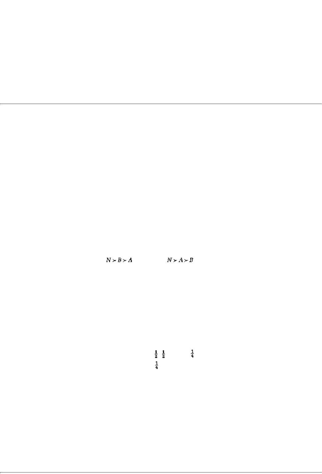
majority of voters cast their vote for, wins. The three legislators have the following preferences among the
available options.
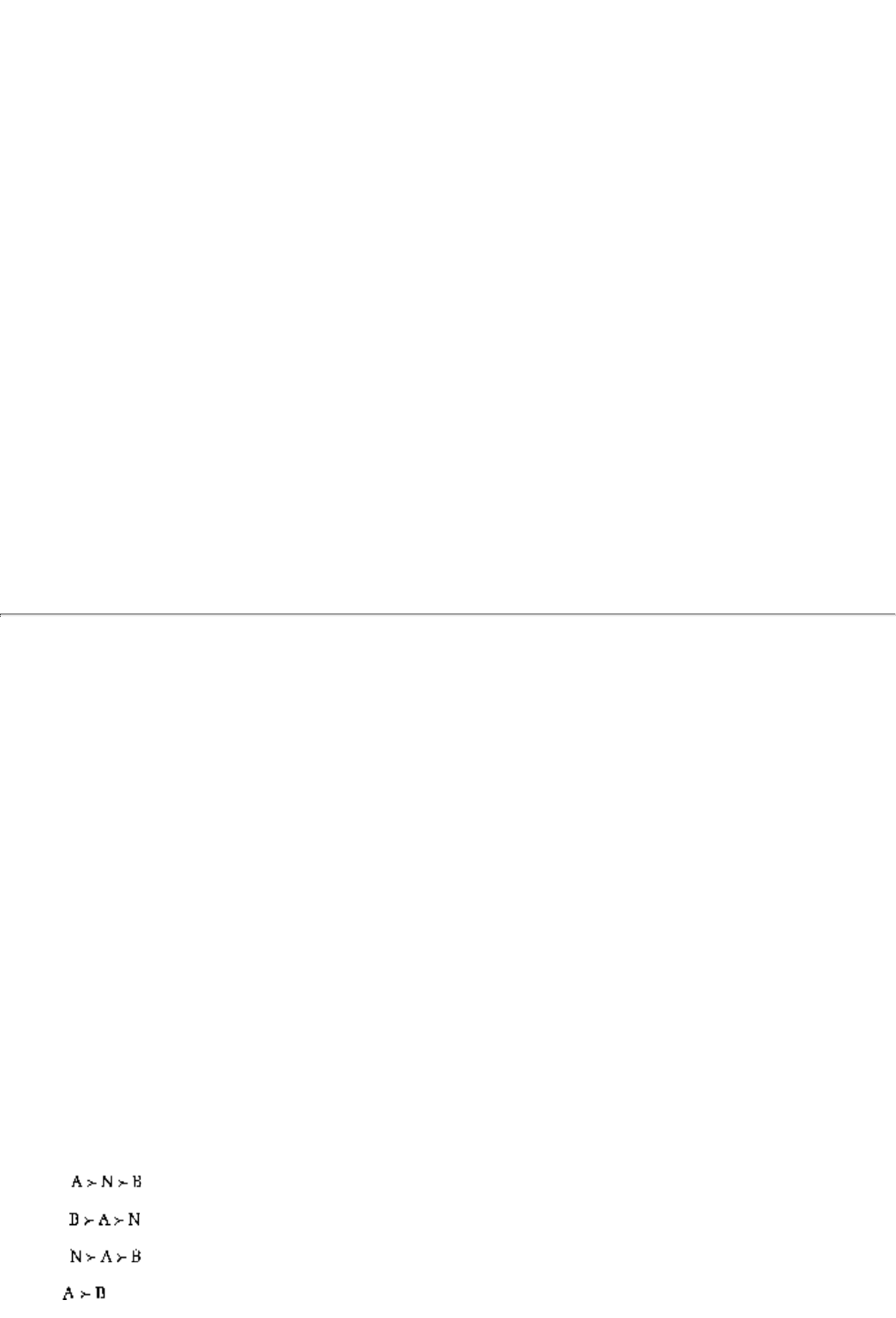
voter 1:
voter 2:
voter 3:
(where should be read as, "Bill A is preferred to bill B.")

Analysis.
Note that if the voters voted according to their preferences (i.e., truthfully) then
A would win against B and
then, in round two, would also win against N. However, voter 3 would be very unhappy with this state of
affairs; she most prefers N and can in fact enforce that outcome by simply switching her first round vote to
B, which would then lose to N. Is that the outcome? Well, since we got started we might wish to then note
that, acknowledging this possibility, voter 2 can also switch her vote and get A elected (which is preferable
to N for this voter).
There is a way to proceed more systematically with the strategic analysis. To begin with, notice that in the
second round each voter might as well vote truthfully. This is because by voting for a less preferred option, a
legislator might get that passed. That would be clearly worse than blocking its passage. Therefore, if A wins
in the first round, the eventual outcome will be A, whereas if B wins, the eventual outcome will be N. Every
15Again you may prefer to work step by step through these questions in the Exercises section.
16This example may also be found in Fun and Games by Ken Binmore (D.C. Heath).
page_10
Page 11
rational legislator realizes this. So, in voting between A and B in the first round, they are actually voting
between A and N. Hence, voters I and 2 will vote for A in the first round and A will get elected.
CONCEPT CHECK
TRUTHFUL VOTING
In what way is the analysis of strategic voting different from that of truthful
voting? Is the conclusion different? Are the votes different?
3. Prisoners' Dilemma.
This is the granddaddy of simple games. It was first analyzed in 1953 at the Rand Corporationa fertile
ground for much of the early work in game theoryby Melvin Dresher and A1 Tucker.
The story underlying the Prisoners' Dilemma goes as follows. Two prisoners, Calvin and Klein, are hauled in
for a suspected crime. The DA speaks to each prisoner separately, and tells them that she more or less has
the evidence to convict them but they could make her work a little easier (and help themselves) if they
confess to the crime. She offers each of them the following deal: Confess to the crime, turn a witness for the
State, and implicate the other guyyou will do no time. Of course, your confession will be worth a lot less if
the other guy confesses as well. In that case, you both go in for five years. If you do not confess, however,
be aware that we will nail you with the other guy's confession, and then you will do fifteen years. In the
event that I cannot get a confession from either of you, I have enough evidence to put you both away for a
year."
Here is a representation of this situation:
Calvin \ Klein
Confess Not Confess
Confess 5, 5 0, 15
Not Confess
15, 0 1, 1
Notice that the entries in the above table are the prison terms. Thus, the entry that
corresponds to (Confess,
Not Confess)the entry in the first row, second columnis the length of sentence to Cal
vin (0) and Klein (15),
respectively, when Calvin confesses but Klein does not. Note that since these are prison terms, a smaller
number (of years) is preferred to a bigger number.
Analysis.
From the pair's point of view, the best outcome is (Not Confess, Not Confess). The problem is that if Calvin
thinks that Klein is not going to confess, he can walk free by ratting on Klein. Indeed, even if he thinks that
Klein is going to confessthe ratCalvin had better confess to save his skin. Surely the same logic runs through
Klein's mind. Consequently, they both end up confessing.

Two remarks on the Prisoners' Dilemma are worth making. First, this game is not zero-
sum. There are
outcomes in which both players can gain, such as (Not Confess, Not
page_11
Page 12
Confess). Second, this game has been used in many applications. Here are two: (a) Two countries are in an
arms race. They would both rather spend little money on arms buildup (and more on education), but realize
that if they outspend the other country they will have a tactical superiority. If they spend the same (large)
amount, though, they will be deadlockedmuch the same way that they would be deadlocked if they both
spent the same, but smaller, amount. (b) Two parties to a dispute (a divorce, labor settlement, etc.) each
have the option of either bringing in a lawyer or not. If they settle (50-50) without lawyers, none of their
money goes to lawyers. If, however, only one party hires a lawyer, then that party gets better counsel and
can get more than 50% of the joint property (sufficiently more to compensate for the lawyer's fees). If they
both hire lawyers, they are back to equal shares, but now equal shares of a smaller estate.
Summary
1. Game theory is a study of interdependence. It studies interaction among a group of players who make
rational choices based on a strategic analysis of what others in the group might do.
2. Game theory can be used to study problems as widely varying as the use of natural resources, the election
of a United Nations Secretary General, animal behavior, and production strategies of OPEC.
3. The foundations of game theory go back 150 years. The main development of the subject is more recent,
however, spanning approximately the last fifty years, making game theory one of the youngest disciplines
within economics and mathematics.
4. Strategic analysis of games such as Nim and the Prisoners' Dilemma can expose the outcomes that will be
reached by rational players. These outcomes are not always desirable for the whole group of players.
Exercises
Section 1.1
1.1
Give three examples of game-like situations from your everyday life. Be sure in each
page_12
Page 13
case to identify the players, the nature of the interaction, the strategies available, and the objectives that
each player is trying to achieve.
1.2
Give three examples of economic problems that are not games. Explain why they are not.
1.3
Now give three examples of economic problems that are games. Explain why these situat
ions qualify as
games.
1.4
Consider the purchase of a house. By carefully examining each of the four components of a game
situationgroup, interaction, rationality, and strategydiscuss whether this qualifies as a game.
1.5
Repeat the last question for a trial by jury. Be sure to outline carefully what each player's objectives might
be.

Consider the following scenario: The market for bagels in the Morningside Heights nei
ghborhood of New
York City. In this example, the dramatis personae are the two bagel stores in the Columbia University
neighborhood, Columbia Bagels (CB) and University Food Market (UFM); and the interaction among them
arises from the fact that Columbia Bagels' sales depend on the price posted by University Food Market.
1.6
By considering a few sample prices, say, 40, 45, and 50 centsand likely bagel sales at these pricescan you
quantify how CB's sales revenue might depend on UFM's price? And vice versa?
1.7
For your numbers what would be a rational strategic price for CB if, say, UFM's bagels were priced at 45
cents? What if UFM raised its price to 50 cents?
Consider yet another scenario: Presidential primaries. The principal group of players are the candidates
themselves. Only one of them is going to win his party's nomination; hence, the interaction among them.
1.8
What are the strategic choices available to a candidate? (Hint: Think of political issues that a candidate can
highlight, how much time he can spend in any given state, etc.)
1.9
What is the objective against which we can measure the rationality of a candidate's choice? Should the
objective only be the likelihood of winning?17
17Bear in mind the hope once articulated by a young politician from Massachusetts, John E
Kennedy, that his margin of victory would be narrow; Kennedy explained that his father "hated to
overspend!
page_13
Page 14
Section 1.3
1.10
Show in detail that player 2 has a winning strategy in Nim if the two piles of matches are balanced. [Your
answer should follow the formalism introduced in the text; in particular, every configuration of matches
should be written as (m, n) and removing matches should be represented as a reduction in either m or n.]
1.11
Show that player 2 has exactly one winning strategy. In other words, show that if the winning strategy of
question 1.10 is not followed, then player I can at some point in the game turn the tables on player 2.
1.12
Verbally analyze the game of tic-tac-toe. Show that there is not a winning strategy in this game.
The next four questions have to do with a three pile version of Nim. The rules of the game are identical to
the case when there are two piles. In particular, each player can only choose from a single pile at a time and
can remove any number of the matches remaining in a pile. The last player to remove matches wins.
1.13
Show that if the piles have an equal number of matches, then player 1 has a winning strategy. [You may
wish to try out the configurations (1, 1,1) and (2, 2, 2) to get a feeling for this argument.]
1.14
Show that the same result is true if two of the piles have an equal number of matches; that is, show that
player I has a winning strategy in this case. [This time you might first try out the configurations (1, 1, p) and
(2, 2, p) where p is a number different from 1 and 2, respectively.]
1.15
Show that if the initial configuration of matches is (3, 2, 1)or any permutation of that configurationthen
player 2 has a winning strategy. As in the previous questions, carefully demonstrate what this winning
strategy is.
1.16
Use your answer in the previous questions to show that if the initial configuration is (3, 2, p)or (3,1, p) or (1,
2, p)where p is any number greater than 3, then player I has a winning strategy.
The next three questions have to do with the game of Marienbad played by two players.
page_14
Page 15
1.17
Show that if the configuration is (1, 1) then player 1 has a winning strategy.
1.18
On the other hand, if the two piles are balanced, with at least two matches in each pile, player 2 has a
winning strategy. Prove in detail that this must be the case.
1.19
Finally, show that if the two piles are unbalanced, player I has a winning strategy.
1.20
Consider the voting model of the second example of section 1.3 (pg. 10). Prove that in the second round,
each voter can do no better than vote truthfully according to her preferences.
1.21
Suppose voter 3's preferences were (instead of as in the text). What would be the
outcome of truthful voting in this case? What about strategic voting?
1.22
Write down a payoff matrix that corresponds to the legal scenario discussed at the end of the chapter (p. 12).
Give two alternative specifications of payoffs, the first in which this does correspond to a Prisoners'
Dilemma and the second in which it does not.
Suppose the Prisoners' Dilemma were modified by allowing a third choice for each playerPartly Confess.
Suppose further that the prison sentences (in years) in this modified game are as follows.
Calvin \ Klein Confess Not Partly
Confess 2, 2 0, 5 1, 3
Not
5, 0 , 4,
Partly
3,1 , 4 1,1
(As always, keep in mind that shorter prison terms are preferred by each player to longer prison terms.)
1.23
Is it true that Calvin is better off confessing to the crime no matter what Klein does? Explain.
1.24
Is there any other outcome in this gameother than both players confessingwhich is sensible? Your answer
should informally explain why you find any other outcome sensible (if you do).
page_15

Page 17
Chapter 2
A First Look At The Theory
This chapter will provide an introduction to game theory's toolkit; the formal structures within which we can
study strategic interdependence. Section 2.1 gives some necessary background. Sections 2.2 and 2.3 detail
the two principal ways in which a game can be written, the Extensive Form and the Strategic Form of a
game. Section 2.4 contains a discussion of utilityor payofffunctions, and Section 2.5 concludes with a revisit
to some of the examples discussed in the previous chapter.
2.1 Rules Of The Game: Background
Every game is played by a set of rules which have to specify four things.
1. who is playingthe group of players that strategically interacts
2. what they are playing withthe alternative actions or choices, the strategies, that each player has available
3. when each player gets to play (in what order)
4. how much they stand to gain (or lose) from the choices made in the game
In each of the examples discussed in Chapter 1, these four components were described verbally. A verbal
description can be very imprecise and tedious and so it is desirable to find a more compact description of the
rules. The two principal representations of (the rules off a game are called, respectively, the normal (or
strategic) form of a game and the extensive form; these terms will be discussed later in this chapter.
page_17
Page 18
Common knowledge about the rules
Every player knows the rules of a game and that fact is commonly known.
There is, however, a preliminary question to ask before we get to the rules: what is the rule about knowing
the rules? Put differently, how much are the players in a game supposed to know about the rules? In game
theory it is standard to assume common knowledge about the rules.
That everybody has knowledge about the rules means that if you asked any two players in the game a
question about who, what, when, or how much, they would give you the same answer. This does not mean
that all players are equally well informed or equally influential; it simply means that they know the same
rules. To understand this better, think of the rules of the game as being like a constitution (of a country or a
clubor, for that matter, a country club.) The constitution spells out the rules for admitting new members,
electing a President, acquiring new property, and so forth. Every member of this club is supposed to have a
copy of the constitution; in that sense they all have knowledge of the rules. This does not mean that they all
get to make the same choices or that they all have the same information when they make their choices. For
instance, perhaps it is only the Executive Committee members who decide whether the club should build a
new tennis court. In making this decision, they may furthermore have access to reports about the financial
health of the club that are not made available to all members. The point is that both of these rulesthe
Executive Committee's decision-making power and access to confidential reportsare in the club's
constitution and hence are known to everyone.
This established, the next question is: does everyone know that everyone knows? Common knowledge of the
rules goes even a few steps further: first, it says yes, everybody knows that the constitution is available to all.
Second, it says that everybody knows that everybody knows that the constitution is widely available. And
third, that everybody knows that everybody knows that everybody knows, ad infinitum.1 In a two-player
game, common knowledge of the rules says not only that player I knows the rules, but that she also knows
that player 2 knows the rules, knows that 2 knows that I knows the rules, knows that 2 knows that I knows
that 2 knows the rules, and so on.
In the next two sections we will discuss the two alternative representations of the three rules who, what, and
when
. The final rule, how much, will be discussed in section 2.4.
2.2 Who, What, When: The Extensive FOrm
Extensive form
A pictorial representation of the rules. The main pictorial form is called the
game tree, which is made up of a root and branches arranged in order.
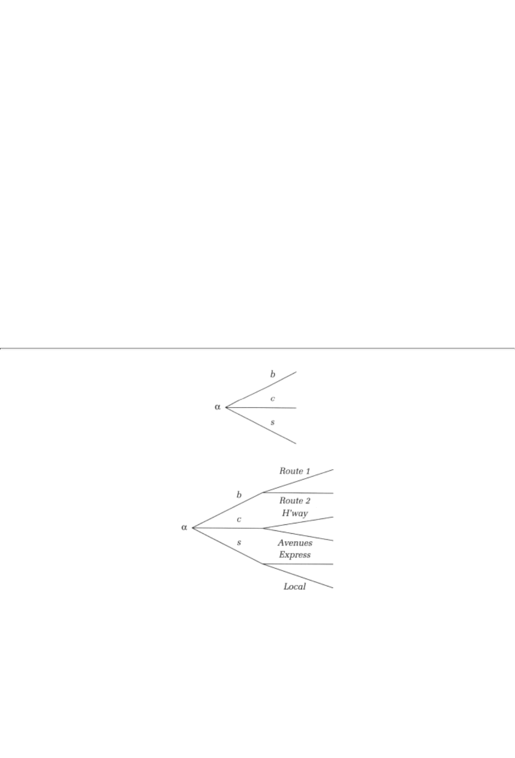
The extensive form is a pictorial representation of the rules. Its main pictorial form is called the game tree.
Much like an ordinary tree, a game tree starts from a root; at this starting point, or root, one of the players
has to make a choice. The various choices available to this player are represented as branches emanating
from the root. For example, in the game tree given by Figure 2.1, below, the root is denoted a; there are
three branches emerging from the root which correspond to the three choices b(us), c(ab), and s(ubway).2
At the end of each one of the branches that emerge from the root, either of two things can happen. The tree
might itself end with that branch; this signifies an end to the
1It may seem completely mysterious to you why we cannot simply stop with the assertion
"everybody knows the rules." The reason is that, knowing the rules, there might be certain
behaviors that a player will normally not undertake. However, if a player is unsure about whether
or not the others know that he knows the rules, he will consequently be unsure about whether the
others realize that he will not undertake those behaviors. This sort of doubt in players' minds can
have a dramaticand unreasonableimpact on what they end up doing, hence the need to assume
every level of knowledge.
2This tree could represent, for example, transportation choices in New York City; a player can either
take the bus, a cab, or the subway to his destination. Note that driving one's own car is not one of the
optionsthese are choices in New York City after all!
page_18
Page 19
FIGURE 2.1
FIGURE 2.2
game. Alternatively, it might split into further branches. In Figure 2.1, for instance, the tree ends after each
of the three branches b, c, and s. On the other hand, in Figure 2.2 each branch further divides in two. The
branch splits into E(xpress) and L(ocal); the implication is that after the initial choice s is made, the player
gets to choose again between the two options E and L (whether to stay on the Local train or to switch to an
Express
). The end of branch s, where the subsequent decision between E and L is made, is called a decision
node of the tree. Figure 2.2 is therefore a two-stage decision problem with a single player.
Of greater interest is a situation where a different player gets to make the second choice. For instance
suppose that two players are on their way to see a Broadway musical that is in great demand, such as Rent.
The demand is so great that there is exactly one ticket left; whoever arrives first will get that ticket. Hence,
we have a game. The first player (player 1) leaves home a little earlier than player 2; in that sense he makes
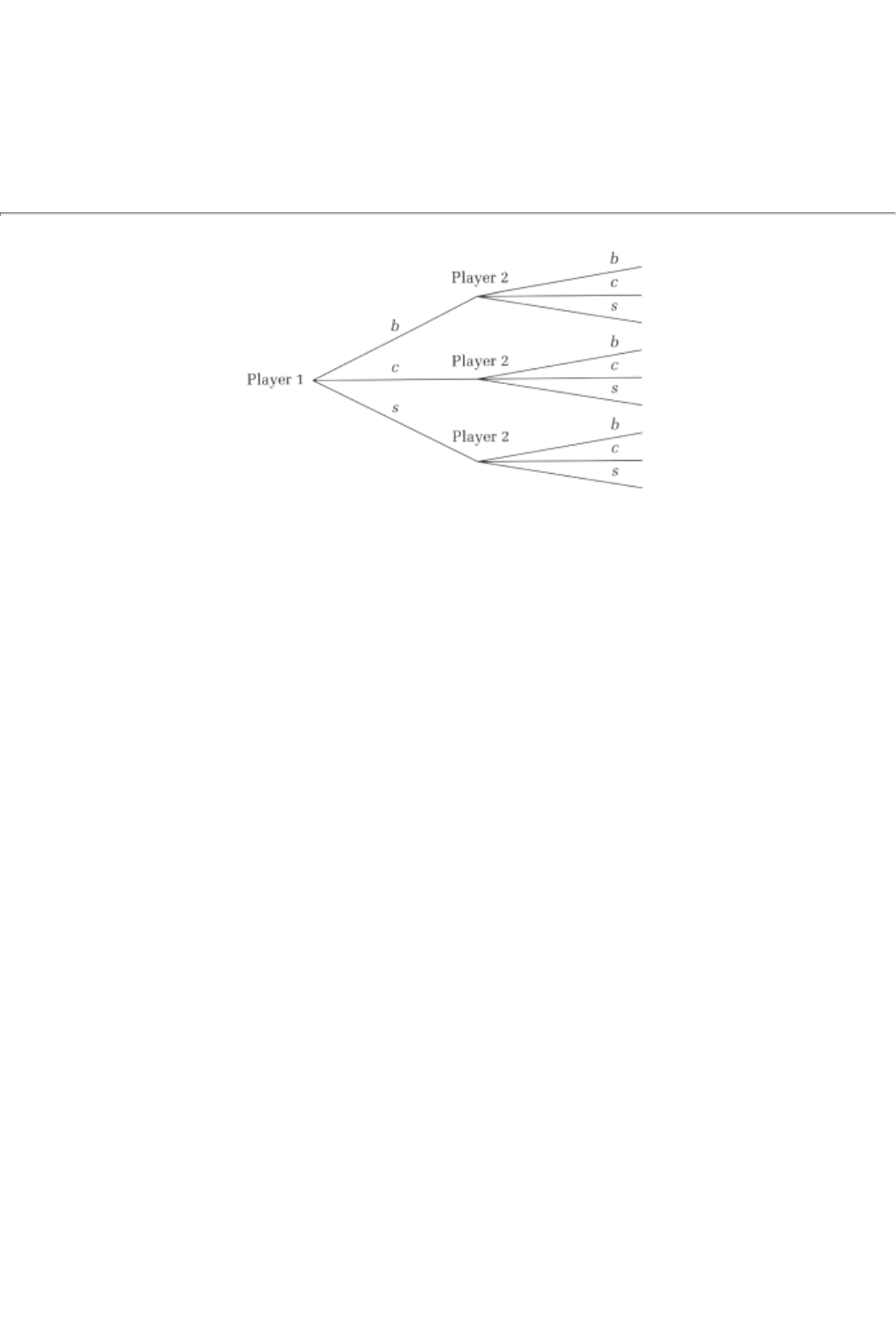
his choice at the root of the game tree and subsequently the other player makes her t
ransportation choice.
The extensive form of this game is represented in Figure 2.3.
From these building blocks we can draw more complicated game trees, trees that allow more than two
players to interact, allow many choices at each decision node, and allow each player to choose any number
of times. The extensive form answers the question whoany individual who has a decision node in the game
tree is a player in the game. It also answers the question what; the branches that come out of a decision node
represent the different choices available at that point. Finally, it answers the question
page_19
Page 20
FIGURE 2.3
when
; for example, a node that is four branches removed from the root is reached only after these first four
choices have been made.
2.2.1 Information Sets and Strategies
The extensive forms discussed above permit only one player to move at a time; the next question is how to
represent simultaneous moves within the extensive form. The key idea here is that a player will act in the
same way in either of two circumstances; first, if he literally chooses at the same time as his opponent and
second, if he actually chooses after his opponent but is unaware of his opponent's choice. Consequently, a
simultaneous move in the Prisoners' Dilemma can be represented by Figure 2.4. In this figure, the ''first"
choice is player 1's while the "second" choice is that of player 2. Notice that there is an oval that encircles
the two (second-stage) decision nodes of player 2. By collecting the two decision nodes into one oval we are
signifying that player 2 is unable to distinguish between the two nodes, that is, he cannot tell whether the
first decision of player I was c or n.
Information set
A collection of decision nodes that a player cannot distinguish between.
The oval here is called an information set.3
Strategy
A strategy for a player specifies what to do at every information set at which
the player has to make a choice.
Finally, every player needs a strategy to play a game! A strategy is a blueprint for action; for every decision
node it tells the player how to choose. More precisely, since a player cannot distinguish between the nodes
within any one information set, a strategy specifies what to do at each set.
For example, in the theater game above (Figure 2.3), player I has a single decision node, the root. Thus, he
has three possible strategies to choose from: b, c, or s. Player 2 has three decision nodes; what to do if player
I took the bus, what to do if he took a cab instead, and, finally, what choice to make if player I hopped on
the subway. Hence every strategy of player 2 must have three components, one for each of her decision
nodes. A possible strategy for player 2 is (s, s, b); the first entry specifies her choice if player 1 takes the bus
(and this choice is s); the second component specifies player 2's choice if 1 takes a cab (and this choice is
also s); and the third entry is player 2's choice conditional
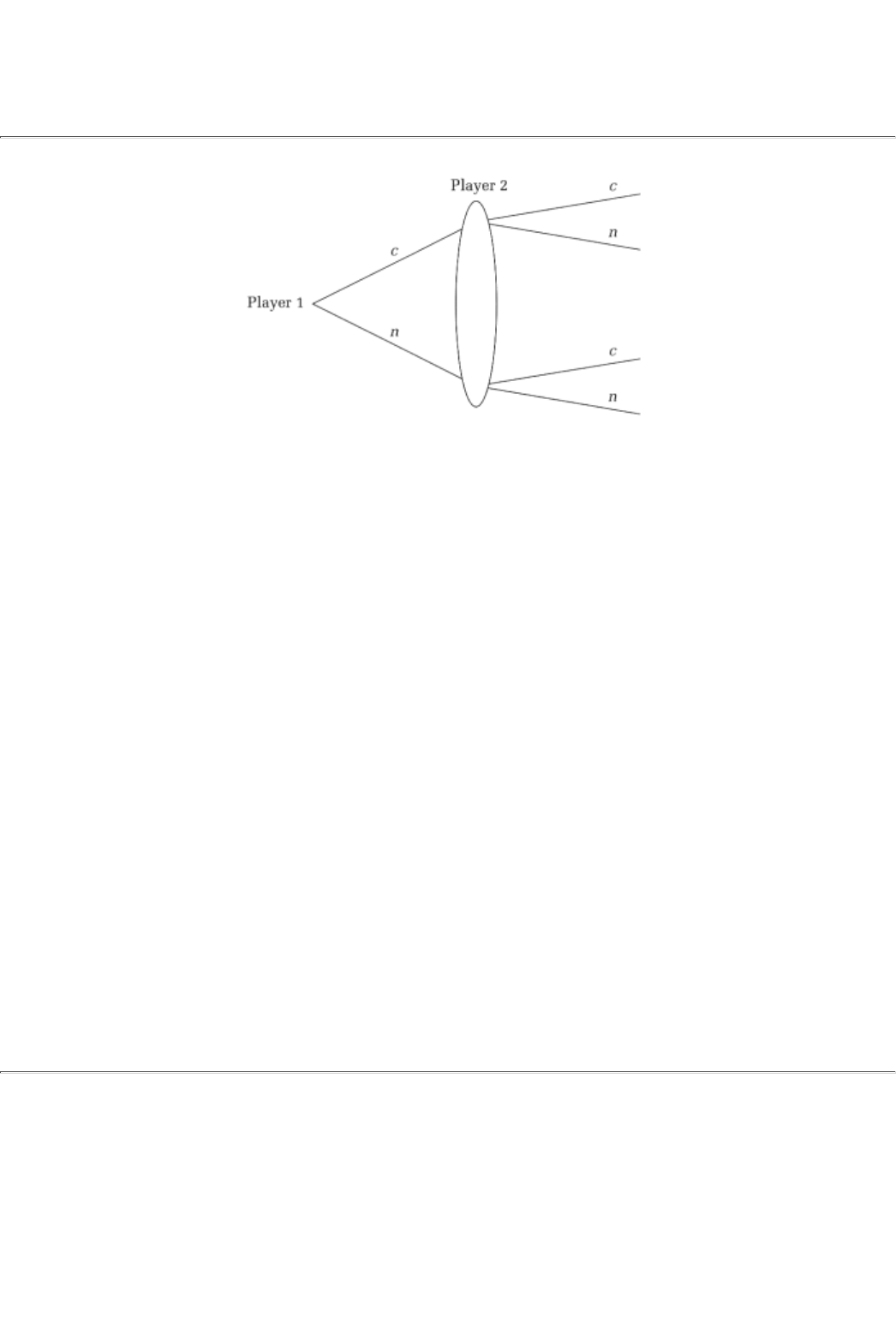
3Information sets will play an important role in a class of games called games of asymmetric
information that we will study in Chapters 19 through 24. At that point we will discuss, in greater
detail, properties that information sets must satisfy.
page_20
Page 21
FIGURE 2.4
on having seen player 1 take the subway (and in this strategy that conditional choice is b).
CONCEPT CHECK
HOW MANY STRATEGIES ARE THERE?
Can you show that player 2 has 33, that is, 27 strategies? Can you enumerate
some of
them?
A pair of strategies, one for player 1 and the other for player 2, determines the way in which the game
actually gets played. For example, suppose that player 1 chooses the strategy c while player 2 chooses (s, s,
b). Since the strategy for player 2, conditional on player 1 taking a cab, is to pick s, the pair of strategies
yields as outcome: 1 takes a cab and 2 follows by subway. In any game, a collection of strategies, one for
each player, will determine which branch of the game tree will actually get played out.
2.3 Who, What, When: The Normal (Or Strategic) Form
Strategic form
A complete list of who the players are, what strategies are available to each of
them, and how much each gets.
An alternative way to represent the rules of a game is called the normal or strategic form.
For example, the strategic form of the theater game can be represented in a table in which the three rows
correspond to the strategies of player 1 and the 33 columns correspond to the strategies of player 2. In each
cell of the table we write the how much rule, in other words, the payoffs associated with that pair of
strategies. Since we have yet
page_21
Page 22
TABLE 2.1
Player 1 \ Player 2 sss ssb ssc bbs . . . ccb ccs ccc
b N,T N,T N,T T,N N,T N,T N,T
c T,N T,N T,N T,N T,N T,N T,N
s T,N T,N N,T T,N T,N T,N N,T
to discuss payoff functions, for now we will simply write the outcomerather than the payoffsin each cell.
Suppose that player 1the first person to start for the theatergets the ticket regardless of player 2's mode of
transport as long as he takes a cab. He also gets the ticket if he travels by subway provided that 2 has not

taken a
cab
, and likewise gets the ticket after catching the
bus
if 2 catches a
bus
as well. Writing
T
for
Ticket
and N for Nuttin' the outcomes are presented in Table 2.1. (Note that in each cell the outcome for player 1 is
the first of the listed pair of outcomes.)
Whenever we have a two-player game, we can represent the strategic form as a table. The rows will stand
for the strategies of player 1, the columns for the strategies of player 2, and the entry in a cell for the payoffs
of the two players from the associated pair of strategies.
You might be wondering about the when question: in a strategic form, who moves when? The simplest
context for the strategic form is a one-time simultaneous move game such as the Prisoners' Dilemma. In this
case, each player makes only one choice and, hence, every strategy has a single element. But we can also
study sequential move games in strategic form; strategies then are more complicated, and they answer the
question of who moves when. A useful interpretation of the strategic form in such cases is that the players
choose their strategies simultaneously although the game itself is played sequentially.
For instance, in the theater game, suppose player 1 chooses s while simultaneously player 2 chooses (c, s, c)c
if player 1 picks b, s if he picks c, and c if he travels by s. These strategies are chosen simultaneously in that
neither player knows the opponent's strategy at the time of their choice. However, the actual play of the
game is sequential. By the choice of strategies player 1 leaves first by subway; player 2 observes that and
then follows by cab.
In summary, the extensive and strategic forms are two ways to represent a game.4 For the purpose of clarity,
this text uses the strategic form to study games that are played simultaneously. This is the content of Part II
(Chapters 3 through 10). Conversely, we will employ the extensive form to study sequential game situations;
these will be studied in Part III (Chapters 11 through 18). At the beginning of each part there will be a more
detailed description of the two game forms; Chapter 3 does this for the strategic form while Chapter 11
details the extensive form. Part IV, Chapters 19 through 24, will use both representations.
4Later in this book you will see that the two representations are interchangeable; every extensive
form game can be written in strategic form and, likewise, every game in strategic form can be
represented in extensive form.
page_22
Page 23
2.4 How Much: Von Neumann-Morgenstern Utility Function
The last rule specifies how much: how much does each player stand to gain or lose by playing the game (in
the way that she does)? Put differently, what is the payoffor utilityfunction of a player, a function that
would specify the payoff to a player for every possible strategy combination that sheand the othersmight
pick? When the outcome of a game is monetary, each player pays out or receives money; the amount of the
winnings is a candidate for the payoff. But what of games in which the outcome is not monetarygames such
as the theater game, the Prisoners' Dilemma, Nim, or the voting game?
To start with, note that a player will typically have opinions about which strategy combinations are
preferable. For instance, in the Prisoners' Dilemma each prisoner is able to rank the four possible strategy
outcomes: Most preferred is the lenient sentence of a canary (who implicates the nonconfessing partner).
Next in preference is the outcome in which neither confesses. Further down is the out
come of both
confessing, and the worst outcome is to be done in by the other guy. This suggests that we could simply
attach numbers that correspond to the rankssay, 4, 3, 2, and 1and call those numbers the payoffs. A higher
payoff would signify a preferred alternative.
This argument can be made more generally. The various outcomes in a game can be thought of as different
options from among which a player has to choose. If the player's preferences between these options satisfy
certain consistency requirements, then she can systematically rank the various outcomes. Any numbering
that corresponds to the rankinga higher number for a higher rankcan then be viewed as a payoff or utility
function.5
In the extensive form these utility numbers would get written at each one of the nodes where the game
terminates. For instance, in the theater game there are two possible outcomes: either player 1 gets the ticket
or player 2 does. Presumably, each player would rather have the ticket than not; hence, any pair of numbers,
p
(T) and p(N), with p(T) > p(N), would serve as a payoff function in this game for player 1. (Likewise for
player 2, any two numbers f(T) and f(N), with f(T) > f(N), would serve as a payoff function.) Filling in the
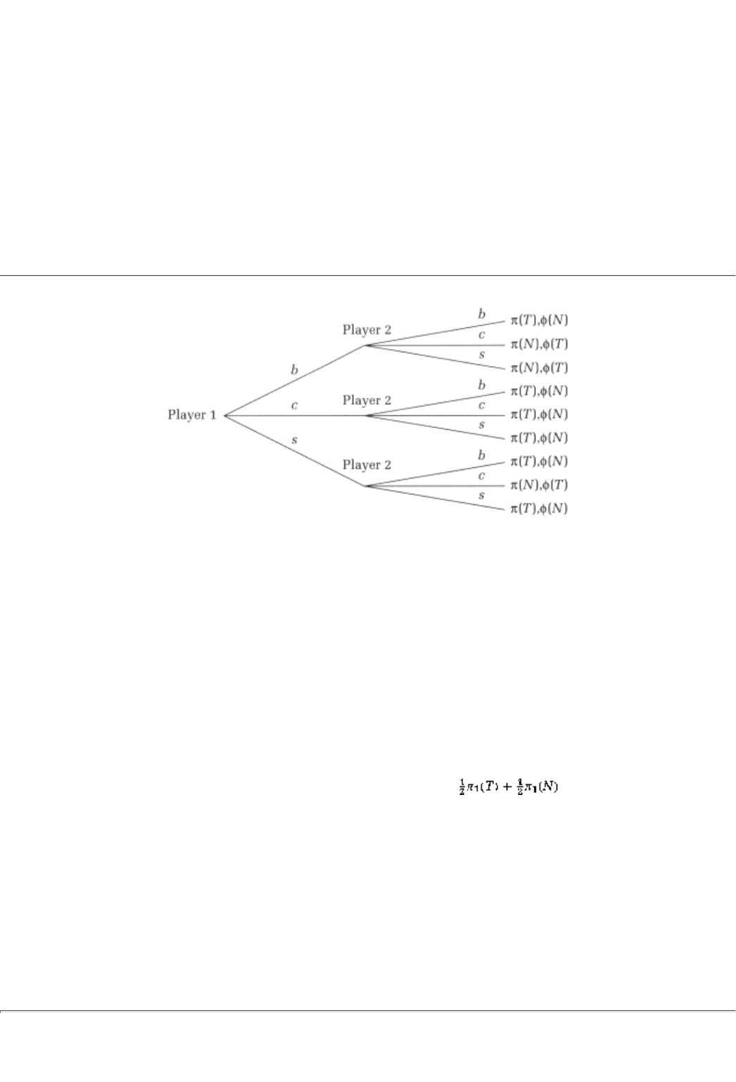
payoffs, the extensive form of this game is depicted in Figure 2.5.
In the strategic form, the payoff numbers would get written in the cells of the strategic matrix. The theater
game's strategic form would therefore look like Table 2.2. (Only some of the cells have been filled in; by
referring to Table 2.1 you should fill in some of the remaining ones.)
Matters are a little more complicated if the game's outcome is not known for sure. This can happen for a
variety of reasons. A player may choose her strategy in a probabilistic fashion by, for example, letting a coin
toss determine which of two possible strategies she will go with. It is also possible that there may be some
inherent uncertainty in the play of the game; for instance, if several firms are competing for the market share
of a new product, then nobody knows for sure how the market will view that product.
5A more detailed discussion of this subject can be found in Chapter 27. You should especially read
the section titled Decision-Making Under Certainty.
page_23
Page 24
FIGURE 2.5
TABLE 2.2
1 \ 2 sss ssb ssc bbs . . . ccb ccs ccc
b p(N),f(T)
c p(T), f(N)
s p(T), f(N)
When there is uncertainty a simple ranking of the outcomes will no longer suffice. In their book Von
Neumann and Morgenstern asked the following question: Under what conditions can we tr
eat the payoff to
an uncertain outcome as the average of the payoffs to the underlying certain outcomes? More concretely,
suppose that player 2 picks the strategy sss (she always travels by subway) while player 1 tosses a cointaking
a bus if the coin comes up heads or a cab if it comes up tails. In this case, there is a 50% chance that player 1
will get the remaining ticket and a 50% chance that he will not. Under what properties of player 1's
preferences is this uncertain outcome worth a payoff halfway between the certain outcomes, p1(T) and
p
1(N)? In other words, under what conditions is it worth the payoff ?
Expected utility
Preferences satisfy expected utility when the payoff to an uncertain outcome
is precisely the average payoff of the underlying certain outcomes.
You canand should!read more about Von Neumann and Morgenstern's answer in Chapter 27; they offer
conditions under which preferences satisfy the expected utility hypothesis. In this book, we will presume
that each player's preferences do satisfy these required conditions. When there is no uncertainty in the
underlying game, or in the way players choose to play the game, you may continue to think of the payoffs as
simply a ranking.
page_24
Page 25
2.5 Representation Of The Examples
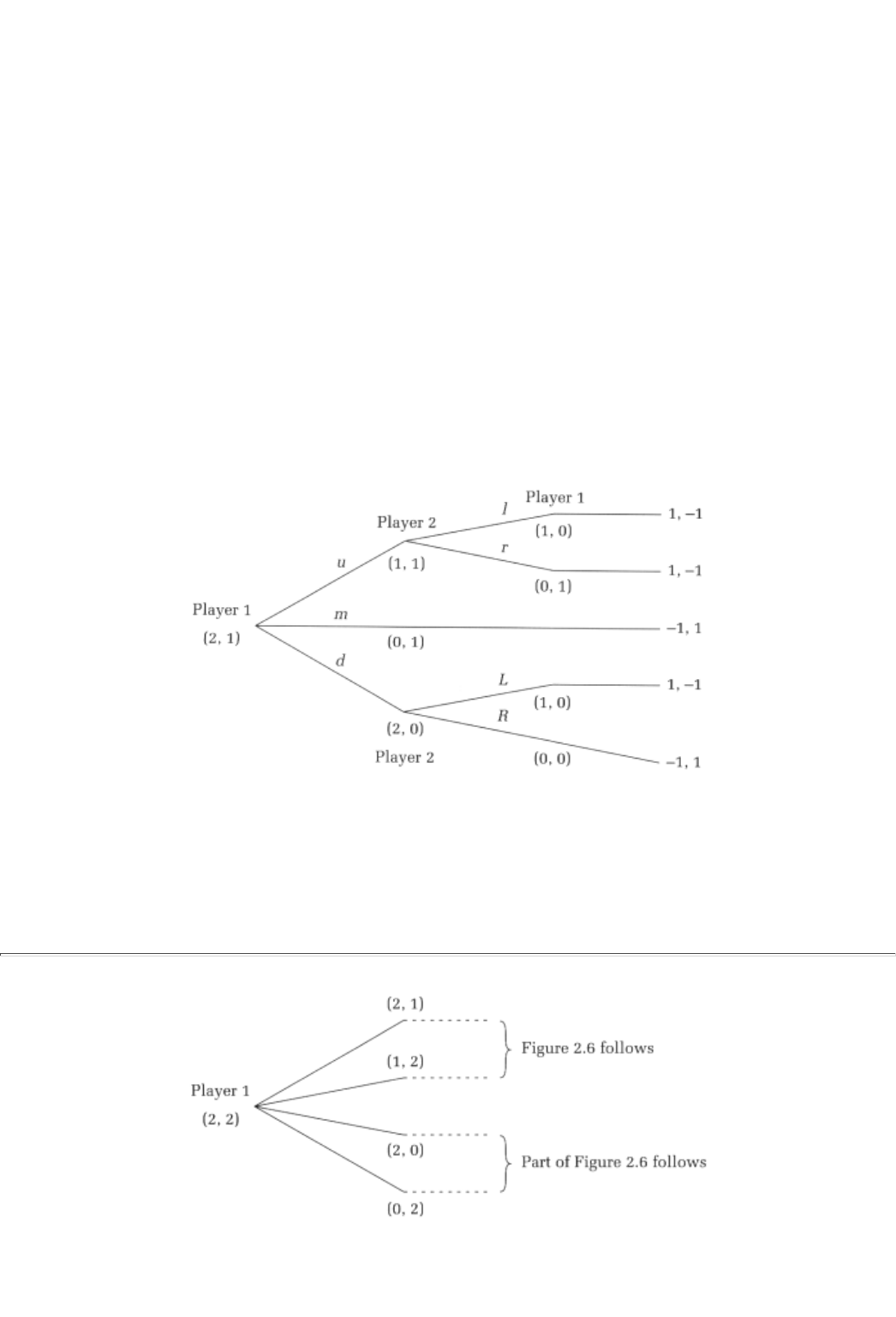
In this section we will examine the extensive and strategic forms of the three examples that were discussed
in detail at the end of Chapter 1.
Example 1: Nim
Suppose, to begin with, there are two matches in one pile and a single match in the other pile. Let us write
this configuration as (2,1). Winning is preferred to losing and, hence, the payoff number associated with
winning must be higher than the one that corresponds to losing; suppose that these numbers are,
respectively, 1 and -1. Figure 2.6 represents the extensive form of this game.6
The strategic form representation is as follows:
1 \ 2 1L lR rL rR
u 1,-1 1,-1 1,-1 1,-1
m -1,1 -1,1 -1,1 -1,1
d 1,-1 -1,1 1,-1 -1,1
If there are more matches in either pile at the beginning of the game, then the game tree would simply be
bigger. For instance, if the configuration is (2,2), then branches that come out of the root would lead to any
one of the following configurations: (2,1), (1,2), (2,0), and (0,2). From (2,1) onwards, the game tree would
look exactly like the tree in Figure 2.6; similarly, from (1,2) onwards, except in this case everything would
be switched around since it is the first pile, rather than the second, that has the single match. From (2,0) and
(0,2) onwards the tree would look like the part of the tree in Figure 2.6 starting from those configurations.
The full extensive form of this scenario is depicted in Figure 2.7.
FIGURE 2.6
6For compactness, I have written u, m, and d to be the three actions of player I that take the game
to (1,1), (0,1), and (2,0), respectively. Similarly, 1 and r correspond to player 2 taking the game
from (1,1) to (1,0) and (0,1), respectively, while L and R have him take the game from (2,0) to (1,0)
and (0,0).
page_25
Page 26
FIGURE 2.7

FIGURE 2.8
Example 2: Voting Game
Suppose that a voter gets a utility payoff of 1 if her favorite bill is passed, 0 if her second choice is passed,
and -1 if her least favorite choice is passed. The extensive form representation of this game with two
representative payoffs is shown in Figure 2.8.
The strategic form of the voting game is somewhat complicated to represent and so we will suspend that
discussion until the next chapter.
page_26
Page 27
FIGURE 2.9
Example 3: Prisoners' Dilemma
Suppose we write a prison term of 5 years as a utility payoff of -5, and so on. The extensive form of this
game is shown in Figure 2.9.
(Note that simultaneous moves have been represented using an information set.) The strategic form is as
follows:
l \ 2
c n
c -5,-5 0,-15
n -15,0 -1,-1
Summary
1. The rules of a game have to specify who the players are, what choices are available to each player, and
how much each player gets from a set of choices made by the group of players.
2. There are two principal representations of the rules of a game, the extensive form and the strategic form.

3. The extensive form is a pictorial representation of the game. It specifies the ord
er in which players make
choices, how many times each player gets to choose (and what choices are available to her each time), and
the eventual payoffs to each player for any sequence of choices.
page_27
Page 28
4. The strategic form is a representation in which the each player's choices (strategies) and the payoffs for a
set of choices are specified. You can think of this as the right game form when players make once for all
choices.
5. The payoffs in a game should be thought of as Von Neumann-Morgenstern utilities. For an uncertain
situation, payoffs should be computed by taking an expectation over the possible resolutions of the
uncertainty.
Exercises
Section 2.2
2.1
Consider the following decision situation. You have a choice to make about which two courses to take and
you have available four courses, A, B, C and D. Depict this problem in a tree form.
2.2
Suppose that after deciding which two courses to take you have a further decision to make: which course
you will concentrate your efforts on. To keep matters simple, suppose thatif you take courses B and C, for
instanceyou can either choose to Work Hard for B or Work Hard for C. Depict this full decision problem.
2.3
Draw the game tree for Nim with initial configuration (3, 2). Assume that the payoff for winning is 1 while
that for losing is 0.
2.4
Do the same for Marienbad with initial configuration (3, 3).
2.5
Consider the following game of "divide the dollar." There is a dollar to be split between two players. Player
1 can make any offer to player 2 in increments of 25 cents; that is, player 1 can make offers of 0 cents, 25
cents, 50 cents, 75 cents, and $1. An offer is the amount of the original dollar that player 1 would like player
2 to have. After player 2 gets an offer, she has the option of either accepting or rejecting the offer. If she
accepts, she gets the offered amount and player 1 keeps the remainder. If she rejects, neither player gets
anything. Draw the game tree.
page_28
Page 29
2.6
`Write down the modified version of the "divide the dollar" game in which player 2 can make a counteroffer
if she does not accept player l's offer. After player 2 makes her counterofferif she doesplayer 1 can accept or
reject the counteroffer. As before, if there is no agreement after the two rounds of offers, neither player gets
anything. If there is an agreement in either round then each player gets the amount agreed to.
2.7
Consider the following variant of the "divide the dollar" game. Players 1 and 2 move simultaneously; 1
makes an offer to 2 and 2 specifies what would be an acceptable offer. For instance, player 1 might make an
offer of 50 cents and player 2 might simultaneously set 25 cents as an acceptable offer. If player 1's offer is
at least as large as what is acceptable to player 2, then we will say that there is an agreement and player 1

will pay player 2 the amount of his offer. Alternatively, if player l's offer is smal
ler than what player 2
specifies as acceptable, there is no agreement, in which case neither player gets anything. Draw the game
tree for this game.
Section 2.3
2.8
Write down the strategies of player 1 in the "divide the dollar" game of question 2.5. Then do the same for
player 2.
2.9
Use your answer to the previous question to write down the strategic form of the "divide the dollar" game.
(You do not have to list every strategy for player 2.)
2.10
Write down the strategic form of the simultaneous move "divide the dollar" game of question 2.7.
2.11
Write down the strategic form of Nim when the initial configuration is (2,1). (You do not have to fill in the
payoffs of all the cells, but do fill in some.)
2.12
Consider the Morningside Heights Bagel Market example that is described in the previous chapter. Assume
that prices are simultaneously chosen by University Food Market and Columbia Bagels and that they can be
40, 45, or 50 cents. Assume that the cost of production is 25 cents a bagel. Assume further that the market is
of fixed size; 1000 bagels sell every day in this neighborhood and whichever store has the cheaper price gets
all of the business. If the prices are the same, then the market is shared equally. Write down the strategic
form of this game, with payoffs being each store's profits.
page_29
Page 30
2.13
Redo the previous question with the total number of bagels sold being, respectively, 1500, 1000, and 500
bagels at the three possible prices of 40, 45, and 50 cents. (Assume that all other factors remain unchanged.)
2.14
Redo question 2.12 such that the store with the cheaper price gets 75% of the business. (Assume that
everything else remains unchanged.)
2.15
Redo question 2.12 yet again, presuming that Columbia Bagels has, inherently, the tastier bagel and,
therefore, when the prices are the same Columbia Bagels gets 75% of the business. (Assume that everything
else remains unchanged.)
Section 2.4
2.16
Let us return to the course-work problem (question 2.2). Suppose that working hard produces a grade of A
while not working hard produces a grade of B. Fill in the payoffs to that decision problem.
2.17
Redo the extensive form of the theater game from this chapter to allow for the possibility that the first
person to get to the theater has a further choice to make between a good seat costing $60 and a not-so-good
(but, nevertheless, expensive) seat costing $40. (The later arrival then gets the remaining ticket.)
2.18

Discuss briefly how you might redo the original extensive form of the theater game if there is a 50% chance
that the show's star might be replaced by an understudy for that evening's performance.
2.19
How would you compute the payoffs to the game of question 2.18?
Consider the following group project example. Three studentsAndrew, Dice, and Claysimultaneously work
together on a problem set for their game theory class. The instructor has asked them, in fact, to submit a joint
problem set. Each student can choose to work hard (H) or goof off (G). If all three students work hard, their
assignment will get an A; if at least two students work hard, the assignment will get a B; if only one student
works hard, the assignment will get a C; and, finally, if nobody works hard the assignment will get an F.
Denote the payoff function p; this payoff depends on the grade and the amount of work. For example, the
payoff to H and a grade of B is denoted p(H, B).7
7A natural assumption is that a better grade is preferred to a worse grade, but goofing off is
preferred to working hard. For instance, p(G, B) > p(H, B) > p(H, C).
page_30
Page 31
2.20
Write out the extensive form.
2.21
The strategic form is easiest to read if it is written in two parts. First, consider the case where Clay is
expected to be a hard worker. Andrew and Dice can choose either H or G. Write down the strategic form.
2.22
There is also a second possibility, namely that Clay chooses to goof off. Show that in this case, the strategic
matrix becomes
Andrew \ Dice H G
H
p(H, B), p(H, B)p(G, B) p(H, C), p(G, C), p(G, C)
G p(G, C), p(H, C), p(G, C) p(G, F), p(G, F), p(G, F)
page_31
Page 33
PART TWO
STRATEGIC FORM GAMES: THEORY AND PRACTICE
page_33
Page 35
Chapter 3
Strategic Form Games and Dominant Strategies
In this chapter we will discuss two concepts: in section 3.1, we will examine in greater detail the strategic
form
representation of a game. Then, in section 3.3, we will look at the first of several solution concepts that
are applied to strategic form games, the dominant strategy solution. Sections 3.2 and 3.4 will serve as
practical illustrations for the two concepts. While section 3.2 will discuss the strategic form of an art auction,
section 3.4 will hunt for the dominant strategy solution in such an auction.
3.1 Strategic Form Games
The strategic form of a game is specified by three objects.
1. the list of players in the game
2. the set of strategies available to each player
3. the payoffs associated with any strategy combination (one strategy per player)
The payoffs should be thought of as Von Neumann-Morgenstern utilities. The simplest kind of game is one in
which there are two playerslabel them player 1 and player 2and each player has exactly two strategies. As
an illustration, consider a game in which player 1's two strategies are labelled High and Low and player 2's
strategies are called North and South. The four possible strategy combinations in this game are (High,
North
), (High, South), (Low, North), and (Low, South). The payoffs are specified for each player for every
one of the four strategy combinations. A more compact representation of this strategic form is by way of a 2
× 2 matrix.
page_35
Page 36
Player 1 \ Player 2 North South
High
p1(H, N), p2(H, N) p1(H, S), p2(H, S)
Low
p1(L, N), p2(L, N) p1(L, S), p2(L, S)
Here, for example, pl(H, N), p2(H, N) are the payoffs to the two players if the strategy combination (High,
North
) is played.
When there are more than two players, and each player has more than two strategies, it helps to have a
symbolic representation because the matrix representation can become very cumbersome very quickly.
Throughout the book, we will use the following symbols for the three components of the strategic form:
players will be labelled 1, 2, . . . N. A representative player will be denoted the i-th player, that is, the index i
will run from 1 through N. Player i's strategies will be denoted in general as si and sometimes a specific
strategy will be marked or and so on. A strategy choice of all players other than player i will be
denoted s-i. Finally, pi will denote player i's payoff (or Van Neumann-Morgenstern utility) function. For a
combination of strategies, , , . . . , one strategy for each player, player i's payoff will be denoted
.
3.1.1 Examples
Let us develop intuition for the strategic form through a series of examples. We start with two player-two
strategy games.
Example 1: Prisoners' Dilemma (c = confess, nc = not confess)
This is the first example that we met in Chapter 1the tale of Calvin and Klein.1
Calvin \ Klein c nc
c 0,0 7,-2
nc -2,7 5,5
Example 2: Battle of the Sexes (F = football, 0 = opera)
The (somewhat sexist) story for the Battle of the Sexes game goes as follows. A husband and wife are trying
to determine whether to go to the opera or to a football game. They each, respectively, prefer the football
game and the opera. At the same time, each of them would rather go with the spouse than go alone.
Husband \ Wife F O
F
3,1 0,0
O 0,0 1,3
1The entries in each cell are now in utility units, unlike in Chapter 1 where they represented
lengths of prison terms. Hence, a bigger number here is better than a smaller one.

page_36
Page 37
Example 3: Matching Pennies (h = heads, t = tails)
Two players write down either heads or tails on a piece of paper. If they have written down the same thing,
player 2 gives player 1 a dollaror, strictly speaking, 1 utility unit. If they have written down different things
then player 1 pays 2 instead.
Player 1 \ Player 2 h t
h 1,-1 -1,1
t -1,1 1,-1
Example 4: Hawk-Dove (or Chicken) (t = tough, c = concede)
Two (young) players are engaged in a conflict situation. For instance, they may be racing their cars towards
each other on Main Street, while being egged on by their many friends. If player 1 hangs tough and stays in
the center of the road while the other player concedeschickens outby moving out of the way, then all glory is
his and the other player eats humble pie. If they both hang tough they end up with broken bones, while if
they both concede they have their bodiesbut not their prideintact.
Player 1 \ Player 2 t c
t -1,-1 10,0
c 0, 10 5, 5
The matrix form can be used to compactly represent the strategic form when there are two players even if
each player has more than two strategies to choose from.
Example 5: Colonel Blotto (individual locations are 1, 2, 3, 4; pairs of locations are 1, 2; 1, 3; 1, 4; 2, 3; 2, 4;
3, 4)
In this war game, Colonel Blotto has two infantry units that he can send to any pair of locations (1, 4, for
example, means the units go to locations 1 and 4), while Colonel Tlobbo has one unit that he can send to any
one of four locations. A unit wins a location if it arrives uncontested, and a unit fights to a standstill if an
enemy unit also comes to the same location. A win counts as one unit of utility; a standstill yields zero
utility.
Tlobbo \ Blotto 1,2 1,3 1,4 2,3 2,4 3,4
10, 1 0, 1 0, 1 1, 2 1, 2 1, 2
20, 1 1, 2 1, 2 0, 1 0, 1 1, 2
31, 2 0, 1 1, 2 0, 1 1, 2 0, 1
41, 2 1, 2 0, 1 1, 2 0, 1 0,1
We can also generalize in the other direction, that is, we can depict with matrices a strategic form game with
more than two players.
page_37
Page 38
Example 6: Coordination Game
Three players are trying to coordinate at some ideal locationfor example, they would like to be together at a
New York Knicks game at game time,
7:30 P.M. It does them no good if twoor all threeof them show up at
10:30 P.M. nor does it do them any good if two of them show up at game time and the other shows up at
10:30.
Player 1 \ Player 2 7:30 10:30 Player 1 \ Player 2 7:30 10:30
7:301, 1, 1 0, 0, 0 7:300, 0, 0 0, 0, 0
10:300, 0, 0 0, 0, 0 10:300, 0, 0 0, 0, 0
Player 3 plays 7:30 Player 3 plays 10:30

Note that the first matrix represents the payoffs if players 1 and 2 choose any one o
f the four possible
strategy combinations7:30,7:30; 7:30,10:30; 10:30,7:30; and 10:30,10:30while player 3 arrives at 7:30.
The second matrix represents the payoffs if players 1 and 2 choose any one of those four strategy
combinations and player 3 chooses to arrive at 10:30. In every cell, the first payoff is that of player 1, the
second is that of player 2, and the third is that of player 3. If each player had three strategies, there would be
three 3 × 3 matrices representing the strategic form, and so on.
Here is an example of a non-matrix representation of the strategic form.
Example 7: Voting
Consider the following variant to the voting game that we studied in Chapter 1. The three voters who vote in
round I are only told what the outcome of the election at that stage was. They then have to decide what to
vote for in round II. No voter is told, in particular, the exact votes of the other voters in round I. So for every
voter a strategy in this game has three parts: how to vote in the first round and the second-round vote, which
itself has two components. The first component is how a voter would vote in round II if bill A passed the first
stage, and the second component is how she would vote if, instead, bill B passed. In particular, each voter
has the following eight strategies to choose from.2
AAN
; AAB; ANB; ANN
BAN
; BAB; BNB; BNN
For example, BAB is a first round vote for B; in the second round, vote for A if A passes the first round;
otherwise vote for B. By contrast, ANB is a strategy in which the first round vote is A. In the second round,
this strategy votes for N if A were the first stage winner but votes for B if B was the first stage winner
instead.
Given any triple of strategies, one for each of the voters, we can then figure out what the outcome to voting
will be. For instance, suppose that voter l's strategy choice is AAN, voter 2's is BAN, and voter 3's is ANB. In
this case, in the first round, A is passed (by virtue of the votes cast by voters 1 and 3) and then gets passed
again at round II (by
2A voter does, of course, know how she herself voted in round L In principle, her strategy could be
based on this information as well. We will ignore this complication for the moment, since all it
would do is increase the number of parts in every strategy to fiveinstead of three. (Why?)
page_38
Page 39
virtue of the votes cast by voters 1 and 2). In this fashion, we can specify the outcomes to every one of the
83 strategy triples that are possible in this game.
3.1.2 Equivalence with the Extensive Form
In Chapter 2 we had also looked at an alternative representation for a game, the extensive form. These two
ways of representing a game are equivalent in the sense that every extensive form game can be written in
strategic form and vice versa. That every extensive form game can be written in strategic form is easy
enough to see. All we need to do is write down the set of strategies for each playerin the extensive formand
then write down the associated outcomes and payoffs for every vector of strategies. We have then the
strategic form.3
In order to do the converse, that is, to write in the extensive form a game that is already in the strategic form,
all we have to remember is that a strategy is best thought of as a conditional plan of action. Any strategy
specifies what is to be clone in every contingency. Consequently, once a particular strategy is decided upon,
its actual implementation can be left to a machine. Given this interpretation, a strategy vectorone strategy
for each playercan be viewed as a simultaneous and one-time choice by the group of pl
ayers. For example, if
there are three players, and each player has available two strategiessay, a, b, for player 1; A, B for 2; and ab
for player 3the extensive form of this game can be written as in Figure 3.l(a).
Of course, there are at least as many extensive form representations of a strategic form game as the number
of players. (Why?) For instance, an alternative extensive form representation for the same game is given in
Figure 3.l(b).
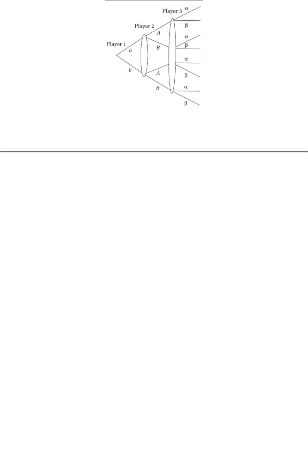
FIGURE 3.1
3This was, after all, exactly what we did with the voting game in the previous paragraph.
page_39
Page 40
3.2 Case Study: The Strategic Form Of Art Auctions
In this section we will look at a real-world situation that can beand indeed should be!modelled as a game.
3.2.1 Art Auctions: A Description
Suppose that we are transported into one of the large auction rooms of Sotheby's Parke-Bernet at
Rockefeller Center in New York City. The auctioneer stands on a podium in the front of the room. At her
side are a couple of attendants who hold up on the viewing stand the object that is being auctioned. Let us
imagine that the objects being auctioned are a set of drawings by Renoir; you would love to own the lovely
cafe scene that has been labelled ''Lot #264." Here is how you need to proceed.4
Registration
: If you intend to bid, you have to register at the entrance to the salesroom, at which point you
are handed a numbered bidding paddle. (In order to register, you will, I am afraid, need a major credit card.)
Bidding procedure:
Once lot #264 comes up, "all you have to do to bid is to raise your paddle and wait for
the auctioneer to acknowledge you. You don't have to call out the amount of your bidhigher bids are
automatically set by the auctioneer, generally in increments of 10%. Don't feel you have to sit on your
hands; scratching your nose or pulling on your ear will not be counted as a bid (unless you have made a prior
arrangement with the auctioneer). If nobody tops your bid, that is, there are no other paddles up, then the
auctioneer brings the hammer down to close the sale."5
Let us now translate this auction into a strategic form game.
3.2.2 Art Auctions: The Strategic Form
Players
: Those who registerand only those individualscan "play." Thus, the list of players is the list of
individuals who carry paddles.6
Strategies: An easy way to think of a player's strategy is to think of the maximum amount to which a player
will raise his paddle. In other words, a player's strategy can be thought of as the highest bid he is willing to
make.7 So player i's strategy si is simply a dollar figure.
Outcomes: The bidder with the last remaining standing paddle wins the Renoir (and the nose-scratchers and
ear-pullers do not). It should be easy to see that another way of saying the same thing is, the bidder who sets
up the highest bid (in his own mind) will take home the drawing.
4This information is drawn from Sotheby's Information catalog on the World Wide Web (at
sothebys.com). The quotations are from the section "Auctions: FAQ (Frequently Asked Questions)."
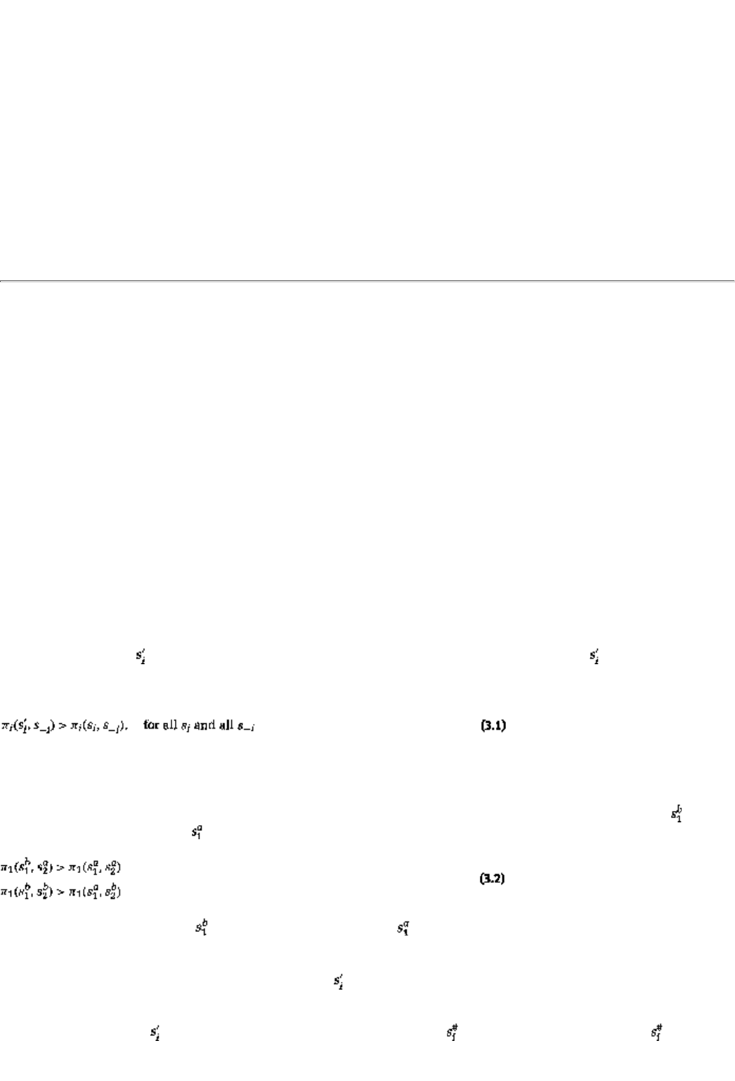
5In practice, the highest bid also has to be higher than the so-called reserve price, the minimum price
set by the seller and Sotheby's below which they would rather withdraw the item than sell it.
6Sotheby's also allows something called an absentee bid. A bidder may register ahead of time and not
attend the auction itself but simply leave with the auctioneer a maximum bid amount. They will be
counted as a bidder until such time as the going bid exceeds this maximum amount. If the bidding stops
before the maximum amount, the absentee bidder will be given the object at the last announced bid.
7In this sense, a bidder who is present at the auction is very much like the absentee bidder referred to
in the previous footnote. Note that, in principle, you could bid in more complicated ways. For instance,
you could decide that you don't want the drawing if you get it for less than $1,000 or you could decide
on your maximum bid after you see how many other people are bidding. For expositional ease, we will
ignore these complicated strategies for now.
page_40
Page 41
Payoffs
: How much will the winner pay? Suppose, for example, that you win the Renoir for which you were
willing to pay up to $2,000. Would you end up paying $2,000? Typically not. After all, the fact that you are
the last remaining bidder means that the auctioneer brought down her gavel when your last competitor
dropped outat some amount less than $2,000. Indeed, the winning bid is the amount that your last
competitor was willing to pay.
How much is the Renoir worth to you? Well, hopefully more than what you pay for it! For example, suppose
its dollar-equivalent utility is $3,000 and you get it at $1,800; you have come out ahead by $1,200. On the
other hand, if you do not win the bidding war your payoff is the utility of the status quo$0.
3.3 Dominant Strategy Solution
Consider the Prisoners' Dilemma (p. 36). The strategy confess has the property that it gives Calvin a higher
payoff than not confess7 rather than 5if Klein does not confess. It also gives him a higher payoff0 rather
than -2if Klein does confess. Hence, no matter what Klein does, Calvin is always better off confessing.
Similar logic applies for Klein. In this game it is therefore reasonable to predict that both players will end up
confessing.
These ideas can be made more precise.
Definition. Strategy strongly dominates all other strategies of player i if the payoff to is strictly greater
than the payoff to any other strategy, regardless of which strategy is chosen by the other player(s). In other
words,
where s-i is a strategy vector choice of players other than i.
To interpret equation 3.1 in words, let us see what the condition tells us for the two-player (1 and 2),
two-strategy (a and b) case. Let us consider player 1. We say that strategy b for this playerdenoted
dominates the other strategy if it does better against both strategies of player 2; thus,
The first inequality says that yields a higher payoff than if player 2 plays her first strategy; the second
says that the same is true even if 2 plays her second strategy.8
A slightly weaker domination concept emerges if is found to be better than every other strategy but not
always strictly better:
Definition. A strategy
(weakly) dominates another strategy, say , if it does at least as well as against
every strategy of the other players, and against some it does strictly
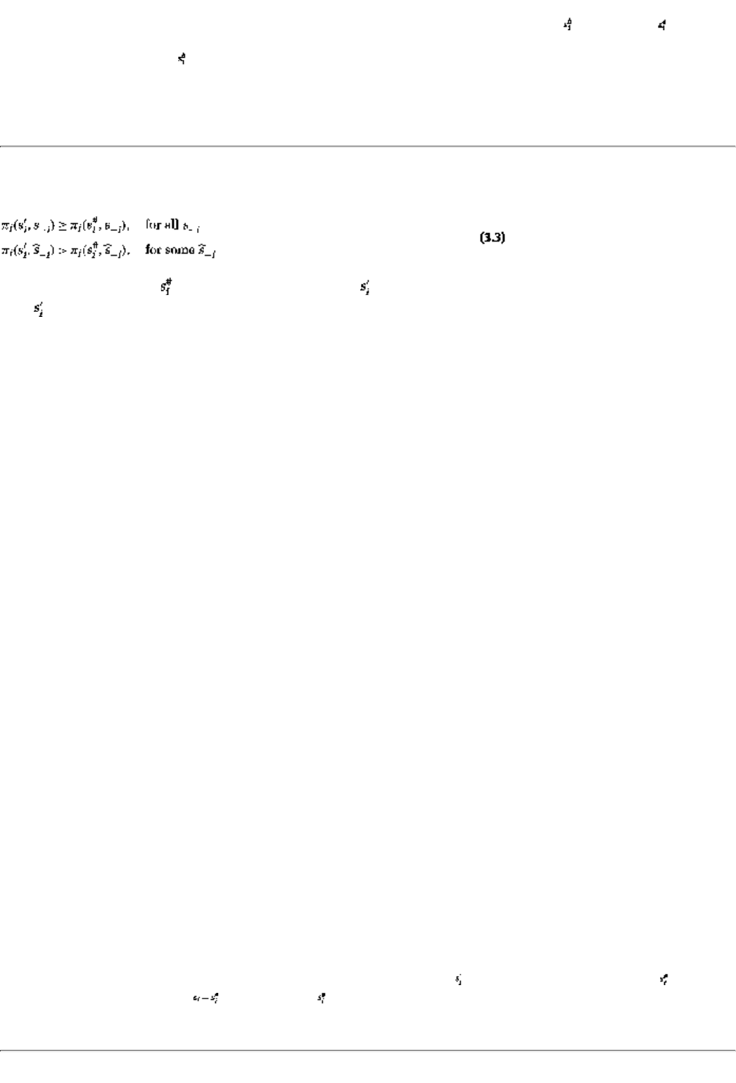
8If player 2 had ten strategies there would be ten such conditions in order for to dominate .
Furthermore, if the player herself had ten strategies, there would be 90 such inequalities; there
would be ten each for to dominate each one of the remaining nine strategies. Finally, if there are
three players, each with ten strategies, we would have 900 such inequalities! All of this is compactly
denoted by equation 3.1.
page_41
Page 42
better, i.e.,
In this case we say that is a dominated strategy. If weakly dominates every other candidate strategy si
then is said to be a weakly dominant strategy.9
Let us build intuition by determining which strategies are not dominant. Every strategy that is dominated is
clearly not a dominant strategy. So n in the Prisoners' Dilemma is not a dominant strategy. In the Battle of
the Sexes, f (football) is not a dominant strategy because it does not always yield a higher payoff than o
(opera)it does better if the other player chooses f as well but does worse if the other player's choice is o.
CONCEPT CHECK
Show that there are no dominant strategies in the games of matching pennies
and Colonel Blotto.
CHECK AGAIN
Each player can only have a single dominant strategy. Can you show that fact
for strong domination? What if a strategy is weakly dominant? Can there be
another one?
Let us see an example of a strategy that is weakly but not strongly dominant. Consider a two player-two
strategy game in which the payoffs of player 1 alone are as follows.
Left Right
Top7 5
Bottom7 3
In this case the first strategy, Top, weaklybut not stronglydominates the second strategy, Bottom. From now
on, in order to avoid confusion, any strategy termed a dominant strategy will refer to a weakly dominant
strategy.
Dominant strategy solution
A combination of strategies is said to be a dominant strategy solution if each
player's strategy is a dominant strategy.
When every player has a dominant strategy, the game has a dominant strategy solution.
For example, in the Prisoners' Dilemma (confess, confess) constitutes a dominant strategy solution. As a
second example, consider the following game.
Left Right
Top7, 3 5, 3
Bottom7, 0 3, -1
9The same definitions apply for strong domination. A strategy strongly dominates strategy , if
equation 3.1 applies for
. The strategy is then said to be strongly dominated.
page_42

Page 43
In this case, (Top,Left) is the dominant strategy solution. The argument for predicting that players will play
dominant strategies, when such strategies exist, is quite persuasive. After all, such a strategy is better than
the alternatives regardless of what other players do. So a player can ignore strategic complications brought
on by thoughts such as "What will the others do?" and "How will that affect my payoffs?"
The problem with the dominant strategy solution concept is that in many games it does not yield a solution.
In particular, even if a single player is without a dominant strategy, there will be no dominant strategy
solution to a game. Consider, for example, the Battle of the Sexes, the matching pennies, or the Colonel
Blotto games. In each of these games, players do not have a dominant strategy, so the solution concept fails
to give a prediction about play. In the next chapter we will see that there is a slightly weaker concept that
also uses the idea of domination and which may yet work for some of these games.
3.4 Case Study Again: A Dominant Strategy At The Auction
In this section we will see that the following startling statement is true: in the art auction game of section 3.2,
the strategy in which a bidder sets the maximum bid at her true valuation for the Renoir is a dominant
strategy. To see why this is startling consider what it says: no matter how the other bidders bid you cannot
do any better than bid what the drawing is worth to you. Put differently again, if the drawing is worth $3,000
to you, you can do no better than shut your eyes and keep your paddle up until such time as you hear the
auctioneer announce a bid above $3,000 (or when you hear the auctioneer say, "Going, going, gonethe lady
to my right has the Renoir" while pointing in your direction).
To see why this is a dominant strategy let us compare it with a couple of alternatives. Suppose you decide to
"shave your bid" and set your paddle down at $2,500. Well, there are two possible scenarios. First,
somebody else has a maximum bid above $3,000 anyway, so it makes no difference whether your maximum
bid is $2,500 or $3,000. Second, the highest bidthe bid that wins the Renoiris $2,700. Now you feel like a
fool! You let a drawing that you valued at $3,000 slip by, a drawing you could have purchased for (a little
above) $2,700. Hence, a maximum bid of $3,000 never does worseand sometimes does strictly betterthan a
maximum bid of $2,500.
CONCEPT CHECK
OTHER LOWBALL BIDS
Check that the same argument works for any maximum bid below $3,000, in
other words, that a bid of $3,000 dominates every bid less than $3,000.
page_43
Page 44
What if you overextended yourself and (carried away by the giddy excitement of the auction) bid all the
way up to $3,500? Again, there are two possible scenarios. First, somebody else rescues you by bidding
above $3,500. In that case it makes no difference whether you bid $3,000 or $3,500. However, what if the
next highest bidder drops out at $3,200? You feel like a fool again, this time because you are carrying home
a drawing which (although nice) you paid more for than what you think it is worth.
CONCEPT CHECK
OTHER HIGHBALL BIDS
Show that a bid of $3,000 dominates any bid higher than $3,000.
One thing that is especially nice about the above argument is that it is valid irrespective of whether you
know how much the Renoir is worth to the other bidders or (as is more likely) you do not have a clue. Either
way you can do no better than "bid the truth."
Summary
1. A strategic form game is described by the list of players, the strategies available to each player, and the
payoffs to any strategy combination, one strategy for each player.
2. The strategic form can be conveniently represented as a matrix of payoffs whenever there are two players
in a game. With more players, a symbolic representation is more convenient.
3. Every extensive form game can be represented in strategic form. Every strategic form game has at least
one extensive form representation.

4. A dominant strategy gives higher payoffs than every other strategy regardless of what the other players
do.
5. A dominant strategy solution to a game exists when every player has a dominant strategy.
6. An art auction can be modelled as a strategic form game. Bidding truthfully is a dominant strategy solution
in that game.
page_44
Page 45
Exercises
Section 3.1
3.1
Consider the game of Battle of the Sexes. How would you modify the payoffs to (f,o) and (o,f) to reflect the
following: the husband is unhappiest when he is at the opera by himself, he is a little happier if he is at the
football game by himself, he is happier still if he is with his wife at the opera, and he is the happiest if they
are both at the football game? (Likewise, the wife is unhappiest when she is at the football game by herself,
she is a little happier if she is alone at the opera, happier still if she is with her husband at the football game,
and the happiest if they are both at the opera.)
3.2
Provide yet another set of payoffs such that both players would rather be alone at their favorite activitythe
husband at the game and the wife at the operathan be with their spouse at the undesirable activity.
3.3
Consider the game of Colonel Blotto. Suppose that Blotto is allowed to send both of his units to the same
location, such that (3,3) is a feasible deployment [as are (1,1), (2,2), and (4,4)]. In addition, he can send units
to different locations. Clearly outline the consequent strategic form. Detail additional assumptions that you
need to make.
3.4
How would the strategic form change if locations 1 and 2 are more valuable than locations 3 and 4 (for
instance, if winning the first two locations gives twice as much utility as winning the last two)?
3.5
Consider the voting game. Suppose that each voter conditioned her second stage vote on how he voted the
first time around. Explain why every strategy has five components in this case.
3.6
Suppose that at the end of the first round, the votes are publicly announced, i.e., each voter is told how the
others voted. Write down the nature of the strategies that are now available to voter 1.
3.7
Explain why there are at least as many extensive form representations of a strategic form as the number of
players.
page_45
Page 46
Section 3.2
3.8
Consider an art auction with two bidders in which the auction procedure is that descr
ibed in the text.
Suppose that the auctioneer raises bids by multiples of one thousand dollars starting at the buyer's
reservation price of $2,000 and stopping when there is only one bidder left. The Renoir is worth $6,000 to
bidder 1 and $7,000 to bidder 2. Each bidder's strategy specifies the maximum that he is willing to bid for the
drawing. List all of the strategies available to the two bidders.
Suppose that, if the two bidders bid an equal amount, bidder 1 is given the drawing.10 If the bids are
unequal, the higher bidder pays the lower bid. Furthermore, the payoffs are as follows: if bidder 1 wins the
drawing and pays p dollars for it, then his utility is 6,000 - p, while if bidder 2 wins, his utility is 7,000 - p.
Utility to a bidder is zero if he does not win the object.
3.9
Write down the strategic form of this auction.
3.10
What would be the strategic form if a coin toss decides the winner when the bids are equal (and a 50%
chance of winning implies an expected utility equal to utility of winning)?
Section 3.3
Consider the following model of price competition. Two firms set prices in a market whose demand curve is
given by the equation
where p is the lower of the two prices. If firm 1 is the lower priced firm, then it is firm 1 that meets all of the
demand; conversely, the same applies to firm 2 if it is the lower priced outfit. For example, if firms 1 and 2
post prices equal to 2 and 4 dollars, respectively, then firm 1as the lower priced firmmeets all of the market
demand and, hence, sells 4 units. If the two firms post the same price p, then they each get half the market,
that is, they each get . Suppose that prices can only be quoted in dollar units, such as 0, 1, 2, 3, 4, 5, or 6
dollars. Suppose, furthermore, that costs of production are zero for both firms.
3.11
Write down the strategic form of this game assuming that each firm cares only about its own profits.
10Specifically, if the auctioneer finds both bidders are in the auction at a bid of $3,000, but neither
bids at $4,000, then she awards the Renoir to bidder 1 at a price of $3,000.
page_46
Page 47
3.12
Show that the strategy of posting a price of $5 (weakly) dominates the strategy of posting a price of $6. Does
it strongly dominate as well?
3.13
Are there any other (weakly) dominated strategies for firm 1? Explain.
3.14
Is there a dominant strategy for firm 1? Explain.
3.15
Rework questions 3.11 through 3.14 above, under the following alternative assumption: if the two firms post
the same price, then firm 1 sells the market demand (and firm 2 does not sell any quantity).
3.16
Give an example of a three player game in which two of the players have dominant stra
tegies but not the
third. Modify the example so that only one of the players has a dominant strategy.
In this game, each of two players can volunteer some of their spare time planting and cleaning up the
community garden. They both like a nicer garden and the garden is nicer if they volunteer more time to work
on it. However, each would rather that the other person do the volunteering. Suppose that each player can
volunteer 0, 1, 2, 3, or 4 hours. If player 1 volunteers x hours and 2 volunteers y hours, then the resultant
garden gives each of them a utility payoff equal to . Each player also gets disutility from the work
involved in gardening. Suppose that player 1 gets a disutility equal to x (and player 2 likewise gets a disutility
equal to y). Hence, the total utility of player 1 is , and that of player 2 is .
3.17
Write down the strategic form of this game.
3.18
Show that the strategy of volunteering for 1 hour (weakly) dominates the strategy of volunteering for 2
hours. Does it strongly dominate as well?
3.19
Are there any other (weakly) dominated strategies for player 1? Explain.
3.20
Is there a dominant strategy for player 1? Explain.
page_47
Page 48
3.21
Rework questions 3.17 through 3.20 above, under the following alternative assumption: player 1's utility
function is .
Section 3.4
Consider again the art auction problem that you saw in questions 3.8 and 3.9.
3.22
Show that for player 1 the strategy with a maximum bid of $6,000 dominates a strategy with a maximum bid
of $5,000. Repeat with an alternative maximum bid of $7,000. Do all this under the first tie-breaking rule in
which player 1 gets the drawing when the maximum bids are identical.
3.23
Repeat the previous question, using a tie-breaking rule in which a coin toss decides the winner.
3.24
Explain why your arguments in the previous two questions would still be valid even if player 1 had no idea
about how much the drawing is worth to player 2.
page_48
Page 49
Chapter 4
Dominance Solvability
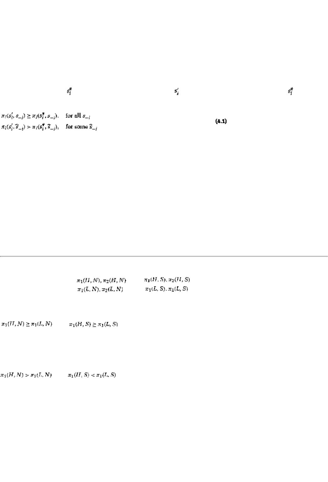
In this chapter we look at a second solution concept for strategic form games,
dominance solvability
or
iterated elimination of dominated strategies. The concept is informally introduced and discussed using
examples in section 4.1. Section 4.2 contains a Case Study: Electing the United Nations Secretary General,
while section 4.3 contains a more formal definition. Section 4.4 concludes with a discussion of this concept's
strengths and weaknesses.
4.1 The Idea
4.1.1 Dominated and Undominated Strategies
Here is a rewording of the dominance definition from the previous chapter.
Definition. A strategy is dominated by another strategy , if the latter does at least as well as against
every strategy of the other players, and against some it does strictly better, such that1
Undominated strategy
A strategy that is not dominated by any other strategy.
If a strategy is not dominated by any other, it is called an undominated strategy. It is useful to think of a
dominated strategy as a "bad" strategy and an undominated strategy as a "good" one. Of course, a dominant
strategy is a special kind of undominated strategy, namely one that itself dominates every other strategy. Put
differently, it is the "best" strategy.
Consider the High-Low, North-South (HLNS) game from Chapter 3.
1Note that throughout we will use the concept of weak, rather than strong, domination. Do see
section 4.4, however, where some disadvantages (and advantages) to using weak domination in the
definition of dominance solvability are discussed.
page_49
Page 50
Player 1 \ Player 2 North South
High
Low
In this strategic form Low is dominated by High if
and
with at least one of those inequalities being strict.
Low
is not dominated by High (and vice versa) if it does better against, say, South, but does worse against
North
.2
but
Let us consider the situation a little more generally. Consider a game in which player i has many strategies.
Either of two things have to be true. First, there may be a dominant strategy. All of the remaining strategies
are then dominated. Alternatively, there may not be a dominant strategy, in other words, there may not be
any best strategy. There has to be, however, at least one undominatedor goodstrategy. (Why?)
CONCEPT CHECK
Consider the HLNS game. Show that each player has at least one undominated
strategy. Under what conditions are both strategies undominated? Can you
generalize your argument to any game?
Consider the examples that we have seen so far.
CHECK AGAIN
Show that in the Battle of the Sexes, as well as in matching pennies and
Colonel Blotto, all strategies are undominated but that in the voting game, of
the four possible ways to vote in round II, three are dominated by truthful
voting.
The problem with the dominant strategy solutionas the examples showis that in many games a player need
not have a dominant or best strategy. What we will now pursue is a more modest objective: instead of
searching for the best strategy why not at least eliminate any dominatedor badstrategies?
2Or, Low is undominated if it does better against North but worse against South. For completeness,
we will also say that High does not dominate Low if they are just as good as each other all the time,
i.e., if
page_50
Page 51
4.1.2 Iterated Elimination of Dominated Strategies
Consider the following game.
Player 1 \ Player 2 Left Right
Up1, 1 0, 1
Middle0, 2 1, 0
Down0, -1 0, 0
For Player 1the row playerneither of the first two strategies dominate each other, but they both dominate
Down
. For the same reason that it is irrational for a player to play anything but a dominant strategy (should
there be any), it is also irrational to play a dominated strategy. The reason is that by playing any strategy that
dominates (this dominated strategy) she can guarantee herself payoff which is at least as high, no matter
what the other players do. Hence, the row player should never play Down but should rather play either Up or
Middle
.
What is interesting is that this logic could then set in motion a chain reaction. In any game once it is known
that player 1 will not play her bad strategies, the other players might find that certain of their strategies are in
fact dominated. This is because player 2, for instance, no longer has to worry about how his strategies would
perform against player 1's dominated strategies. So some of player 2's strategies, which are only good against
player 1's dominated strategies, might in fact turn out to be bad strategies themselves. Hence, player 2 will
not play these strategies. This might lead to a third round of discovery of bad strategies by some of the other
players, and so on.
To illustrate these ideas, note that if it was known to player 2the column playerthat 1 will never play Down,
then Right looks dominated to him. (Why?) Therefore, a rational column player would never play Right. But
then, the row player should not worry about player 2 playing Right. Hence she would choose the very first
of her strategies, Up.
The strategy choice (Up, Left) is said to be reached by iterated elimination of dominated strategies (IEDS);
the game itself is said to be dominance solvable. Indeed, in any game, if we are able to reach a unique
strategy vector by following this procedure, we call the outcome the solution to IEDS and call the game
dominance solvable.
4.1.3 More Examples
Example 1: Bertrand (Price) Competition
Suppose that either of two firms in a duopoly market can charge any one of three priceshigh, medium, or
low.3 Suppose further that whichever firm charges the lower price gets the entire market. If the two firms
charge the same price, they share the market equally.4 These assumptionsand any pair of pricestranslate into
profit levels for the two firms. For example, firm 1 only makes a profit if its price is no higher than that of

firm 2. Suppose that the profits are given by the following payoff matrix.
3Price competition in duopoly markets was first studied by the French economist Bertrand in 1883.
He presented his analysis as an alternative to the Cournot model (in which firms decide how much
to produce); we will study Cournot's model in Chapter 6.
4The analysis is easy to extend to the case where a firm can charge more than three prices. The other
two assumptions make sense if you imagine that this is a market with no brand loyalty (because the
products are identical) and all customers go to the vendor who charges the lower price. Think of two
grocery stores or two discount electronic outlets.
page_51
Page 52
Firm 1 \ Firm 2 high medium low Bertrand game
high6, 6 0, 10 0, 8
medium10, 0 5, 5 0, 8
low8, 0 8, 0 4, 4
Let us now apply the concept of dominance solvability to this game. Notice first that the strategy high
(price) is dominated by the strategy medium (and indeed this is true for both the firms). Hence, we can
eliminate high as an irrational strategy for both firms (it either leads to no sales or a 50% share of a small
market). Having eliminated high we are left with the following payoff matrix.
Firm 1 \ Firm 2 medium low
medium5, 5 0, 8
low8, 0 4, 4
We can now see that low dominates the medium price. Hence, the outcome to IEDS is (low, low). Notice
that medium is a useful strategy only if you believe that your opponent is going to price high; hence, once
you are convinced that he will never do so, you have no reason to price medium either.
Example 2: The Odd Couple
Felix and Oscar share an apartment. They have decidedly different views on cleanliness and, hence, on
whether or not they would be willing to put in the hours of work necessary to clean the apartment.5 Suppose
that it takes at least twelve hours of work (per week) to keep the apartment clean, nine hours to make it
livable, and anything less than nine hours leaves the apartment filthy. Suppose that each person can devote
either three, six, or nine hours to cleaning.
Felix and Oscar agree that a livable apartment is worth 2 on the utility index. They disagree on the value of a
clean apartmentFelix thinks it is worth 10 utility units, while Oscar thinks it is only worth 5. They also
disagree on the unpleasantness of a filthy apartmentFelix thinks it is worth -10 utility units, while Oscar
thinks it is only worth -5. Each person's payoff is the utility from the apartment minus the number of hours
worked; for example, a clean apartment on which he has worked six hours gives Felix a payoff of 4, while it
gives Oscar a payoff of -1. Hence, the strategic form is as follows.
Felix \ Oscar 3 hours 6 hours 9 hours
3 hours-13, -8 -1, -4 7, -4
6 hours-4, -1 4, -1 4, -4
9 hours1, 2 1, -1 1, -4
5Any similarity to situations that you may have seen on the TV sitcom The Odd Couple is entirely
intentional. On the other hand, I am sure that you have also personally encountered the roommate
who you think is a slobor, perhaps the one that you think is a fusssy neatnik!
page_52
Page 53
Note first that Oscarthe slobviews
9 hours as crazy; this strategy is dominated by 6 hours. But that implies
that the relevant game is
Felix \ Oscar 3 hours 6 hours
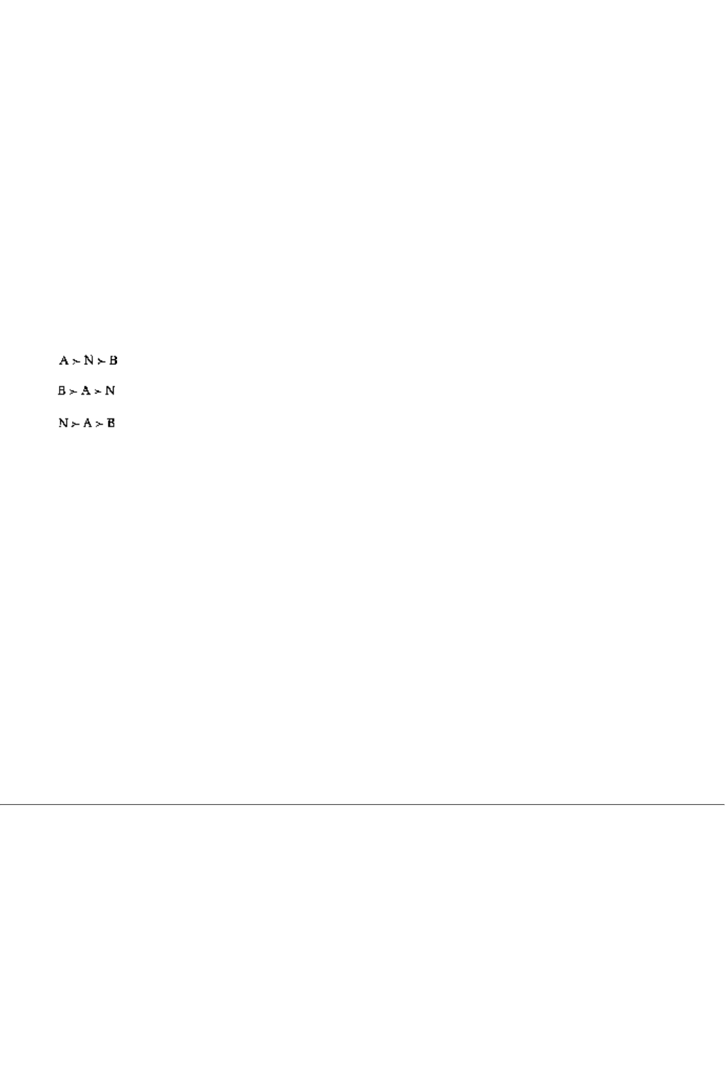
3 hours
-13, -8
-1, -4
6 hours-4, -1 4, -1
9 hours1, 2 1, -1
However, 3 hours is now a dominated strategy for Felix, the neatnik; he so values cleanliness that he would
rather work at least 6 hours. Hence, the relevant game is
Felix \ Oscar 3 hours 6 hours
6 hours-4, -1 4, -1
9 hours1, 2 1, -1
In turn, that implies 6 hours is dominated for Oscar (because Felix is going to work hard enough anyway),
which in turn implies that 6 hours is also dominated for Felix. Therefore, the outcome to IEDS is that Felix
works the maximum 9 hours and Oscar works the minimum 3 hours.6
Example 3: Voting Game
Recall the voting game of Chapter 1: by majority rule, three voters select either of two bills, A or B. The bill
that passes the first round then faces a runoff against the status quo N (''Neither"). The true preferences of
the three voters are as follows.
voter 1:
voter 2:
voter 3:
Every strategy has three components. The strategy A (followed by) AN says, "Vote for A against B, and then
in the second round vote for A (against N), but vote for N (against B)." For payoffs, let us use the convention
that a voter gets payoff 1 if his most preferred bill is passed, 0 for the second best, and -1 if the third best
(i.e., least preferred) option passes. For example, voter 1's payoffs are 1 if A is eventually passed, 0 if N
passes, and -1 if B passes.
Now recall from the previous section that voting truthfully in the second round domin
ates voting
untruthfully; thus, for voter 1, AAN dominates ANN, ANB, and AAB. Similarly, BAN dominates BNN, BNB,
and BAB. By the same logic, for voter 2, AB as the second round voting strategy dominates NB, NN, and AN;
for voter 3, a second round voting strategy of NN dominates the alternatives. Note that if the voters vote
truthfully in round II, then at that stage A defeats N but B loses to N.
After eliminating the (second round untruthful) dominated strategies, the remainder of the strategic form can
be written as shown below.7
6In the sitcom this outcome corresponded to Felix keeping the entire apartment clean, except for
Oscar's room; Oscar had the responsibility of keeping his room cleanand did so after a fashion.
7Note that the first payoff in every cell is player 1's, the second is player 2's and the third player 3's.
page_53
Page 54
Voter 1 \ Voter 2 AAB BAB Voter 1 \ Voter 2 AAB BAB
AAN1, 0, 0 1, 0, 0 AAN1, 0, 0 0, -1, 1
BAN1, 0, 0 0, -1, 1 BAN0, -1, 1 0, -1, 1
Voter 3 plays ANN Voter 3 plays BNN
Now note that
AAN dominates BAN for voter 1, AAB dominates BAB for voter 2, and BNN dominates ANN
for voter 3. Hence, we are left with the IEDS outcome AAN for voter 1, AAB for voter 2, and BNN for voter
3; A wins the first round (with two votes) and goes on to defeat N in the runoff.
4.2 Case Study: Electing The United Nations Secretary General
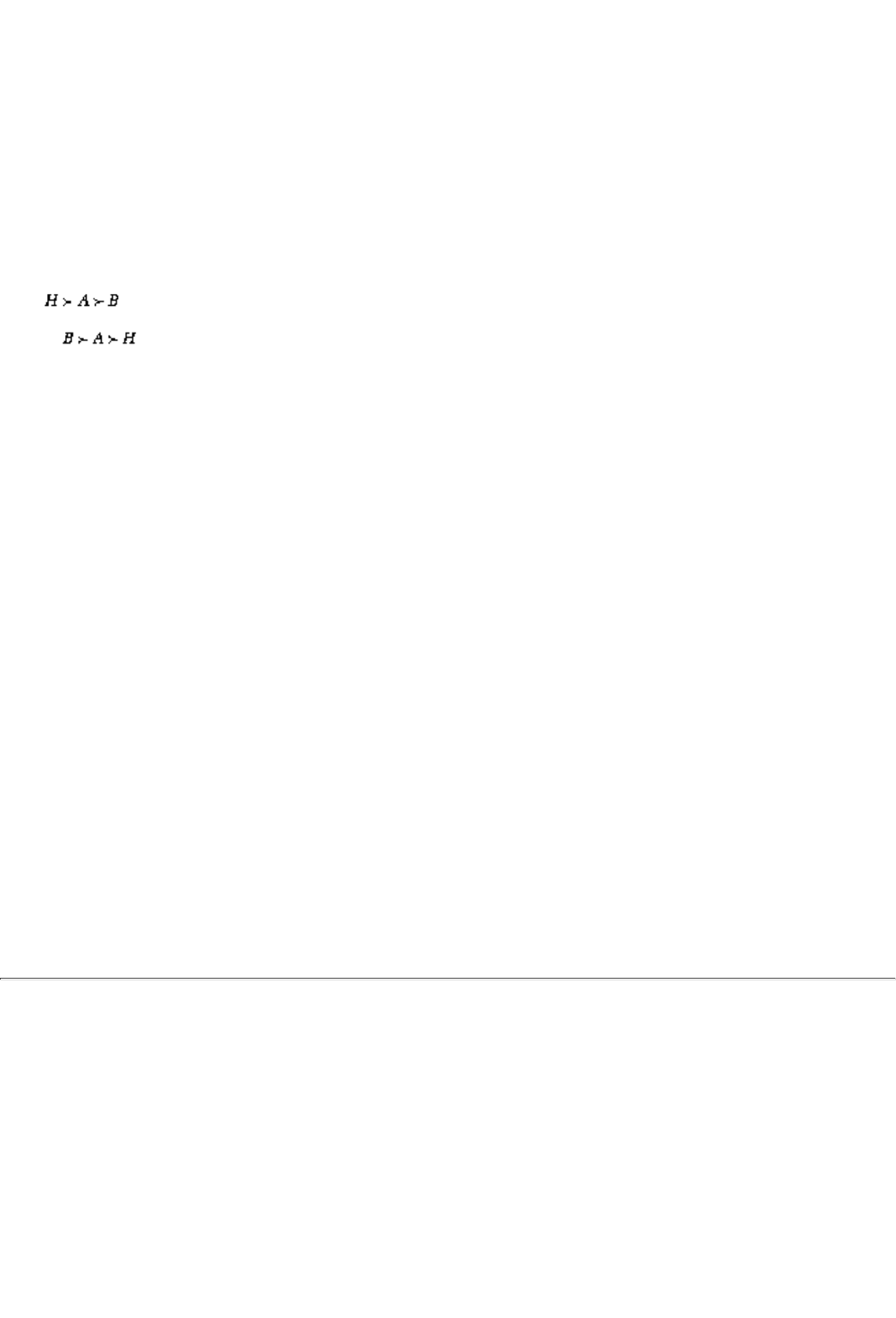
The United Nations elected a Secretary General for the 1997-2001 five-year term in De
cember 1996. One of
the candidates was Boutros Boutros-Ghali, from Egypt, who had been the Secretary General from 1992 to
1996. He was seeking re-election but faced the daunting prospect of early and strong opposition from the
United States government.8
Rumor had it that the U.S. was in favor of a woman as Secretary General; one of
the women mentioned as a possibility was Glo Harlem Brundtland, the Norwegian Prime Minister.9
However, the African member countries of the UN wanted to have a second term from an African Secretary
General.10 The name of another Africanand a United Nations veteranKafi Annan, of Ghana, surfaced late in
the campaign.
Let us use a simple game model to analyze this election. Consider an election with two voterssay, the United
States and Africa. Voter 1U.S.votes first and gets to veto one of three candidates A(nnan), B(outros-Ghali),
or H(arlem Brundtland). Then voter 2Africavetoes one of the two remaining candidates. Suppose the United
States' and Africa's preferences over the three candidates are as follows.
U.S.:
Africa:
In other words, the U.S. most prefers H(arlem Brundtland) but, failing that, prefers A(nnan) over B(outros-
Ghali). Africa, on the other hand, is perfectly happy with B(outros-Ghali) but would rather have a second
African than H(arlem Brundtland). Suppose the payoff is 1 if the voter's best candidate is elected, 0 if the
second best is elected, and -1 if only the third best is elected.11
The United States has exactly three strategies to choose from: A or B or H; that is, the U.S. can veto Annan
or Boutros-Ghali or Harlem Brundtland. Africa has three components in its strategy; whom to veto if,
respectively, A, B, or H has already been vetoed. There are clearly two choices that Africa has for each of its
three components; hence, it has eight strategies in all to choose from. A representative strategy for Africa is
8In the late summer of 1996, the U.S. administration announced that it was going to oppose
Boutros-Ghali who (they said) had not done enough to eliminate waste and mismanagement within
the U.N. Some political observers speculated that the decision had as much to do with U.S.
Presidential politics; President Clinton wanted to take the wind out of his Republican opponents
who viewed Boutros-Ghali with disfavor and the Presidential elections were coming up in
November 1996.
9She even resigned her position as Prime Minister in early November, supposedly in order to
campaign more effectively for the Secretary Generalship.
10Traditionally, each Secretary General has served two terms in office and so the point was that if
Boutros-Ghali, an African, could not serve a second term his replacement, at least, should he another
African.
11In Example 3 above, and in this case study the exact numbers in the payoffs are unimportant. What
matters is that the election of the most preferred candidate gives a voter the highest payoff and the
election of the least preferred candidate gives him the lowest payoff.
page_54
Page 55
BAA
; in this case, it follows a veto of A by the U.S. by vetoing B, while it follows a veto of either B or H by
vetoing candidate A. The strategic form of the game is shown here.
U.S. \ Africa HAA HHA HAB HHB BAA BHA BAB BHB
A-1, 1 -1, 1 -1, 1 -1, 1 1, -1 1, -1 1, -1 1, -1
B1, -1 0, 0 1, -1 0, 0 1, -1 0, 0 1, -1 0, 0
H-1, 1 -1, 1 0, 0 0, 0 -1, 1 -1, 1 0, 0 0, 0
Start with Africa. Note that between B and H, it prefers B; between A and H, it prefers A; and between A and
B
, it prefers B. Hence, the strategy HHA dominates every other strategy. Put differently, if Boutros-Ghali
were available Africa would veto the alternative and get him elected; in the event that he had already been
vetoed Africa would veto H. Hence, after this one round of elimination, the effective game becomes:
U.S. \ Africa HHA
A-1, 1
B
0, 0
H-1, 1
It follows that A and H are dominated; the best thing that the U.S. can do is veto B. (Put differently, by
vetoing either Annan or Harlem Brundtland, the United States opens the door for Boutros-Ghali; hence it is
best to veto Boutros-Ghali instead.) The IEDS outcome therefore is the U.S. starts off by vetoing Boutros-
Ghali, and Africa follows by vetoing Harlem Brundtland; the compromise candidate Annan is elected
Secretary General.12
The symbol signifies more challenging material.
4.3 A More Formal Definition
Let us look at a somewhat more formal treatment of dominance solvability. Consider a strategic form game
with N players; player i's strategies are denoted si; let the set of strategies of player i be denoted Si. At round
I, denote the set of dominated strategies of player i, Di(I). In other words,
Rational players will not play strategies that are dominated, that is, strategies that lie in Di(I). And this is true
for i = 1, 2, . . . N.
Now in round II, player
i can do a further determination among the strategies that are left over for him, Si -
D
i(I), to see if any of them have now become dominated. A strategy has now become dominated if there
is an alternative strategy in Si - Di(I) which does at least as well all the time and sometimes does strictly
better, provided every
12The United States stuck to its announced intention of opposing Boutros-Ghali even after the
November presidential elections. The Africans insisted on n second African term thereupon. On
December 17, 1996, Kofi Annan, United Nations Under Secretary General for Peacekeeping
Operations, was ejected Secretary General for 1997-2001.
page_55
Page 56
other player also eliminates strategies that are dominated in round I. Thus,
where S-i_D-i(I) is the set of undominated strategy combinations of all players other than i.13 Denote the
sum total of all strategies of player i that are dominated, either in round I or round II, Di(II). Repeat the
procedure to weed out any further strategies that are now dominated, once it is known that no player will
play a strategy that belongs to Di(II). By doing this, construct the set of strategies that have been dominated
in the first three rounds; call this set Di(III). And so on.
Suppose we arrive finally at a situation in which there is a single strategy left over for each player, i.e.,
suppose that after T rounds of elimination, the left over set, Si - Di(T), contains exactly one strategy and this
is true for i = 1, 2, . . . N. In that case, this vector of strategies is said to be the outcome to iterated
elimination of dominated strategies (IEDS) and the game is said to be dominance solvable. If this does not
happenif at some round, and for some player, there are no more strategies that can be eliminated although
there are multiple strategies still outstandingthe game is said to have no IEDS solution.
In the Bertrand Price Competition example, there were two rounds of elimination. In the first, high price is
eliminated as dominated, and in the second round, medium price is then found to be dominated and
eliminated. The IEDS outcome is low price for each firm.

In the Odd Couple example, there were four rounds of elimination. In the first Oscar
eliminates
9 hours
,
which leads Felix to eliminate 3 hours. In the third round, Oscar eliminates 6 hours, whereupon Felix
eliminates 6 hours as well. The IEDS outcome has Felix work 9 hours while Oscar only works for 3.
Finally, in the voting game of example 3 there were two rounds of elimination. In the first, each voter
eliminates all the strategies that involve untruthful stage two voting and in the second, each voter eliminates
one of the remaining two strategies.
Notice the chain of logic that was employed in the definition (and in each of the exa
mples).
Player 1 is rational in that she never plays a dominated strategy, and this is known to player 2.
Hence, in round II, player 2 has a dominated strategy and will never play it, and player 1 knows that.
Player 1 only considers payoffs in the event that 2 plays a remaining undominated strategy.Consequently,
she has a dominated strategy which she never plays.14 And so on. . . .
13Specifically, S-i - D-i(I) contains strategy vectors(s1, . . . si+1, . . . sN) in which every strategy sj
is undominated.
14There is a symmetric and simultaneous chain of logic starting with player 2: player 2 will never play
a dominated strategy; 1 knows that and hence will not play a now dominated strategy; 2 knows that and
may further eliminate a strategy. This logic is similar to common knowledge about the rules (recall
Chapter 3).
page_56
Page 57
4.4 A Discussion
The solution conceptIterated Elimination of Dominated Strategiesis widely used in game theory and its
applications. The advantage of this solution concept is inherent in the simplicity of the dominance concept.
If a player is convinced that one of his strategies always does worse than some alternative strategy, then he
will never use it. It is also clear that other players should realize this and take this into account in
determining what they should do. (Later in this book you will see that dominance solvability has a link with a
solution concept used in the extensive form called backwards induction.)
The disadvantages of this solution concept are the following.
Layers of rationality. That no player will play a dominated strategy is a reasonable assumption. That no
player will play a strategy that is dominated once the others' dominated strategies are eliminated also appears
reasonable. That no player will play a strategy that becomes dominated only after fifteen rounds of
elimination of dominated strategies seems less reasonable. This is because it presumes that everybody agrees
that every body else is reasonable in this form over succeeding (fourteen) higher orders. This is especially
problematic if a "mistake" about the other player's rationality can be costly. Consider the following game.
1 \ 2 Left Center Right
Top4, 5 1, 6 5, 6
Middle3, 5 2, 5 5, 4
Bottom2, 5 2, 0 7, 0
CONCEPT CHECK
Show that the outcome to IEDS is (Middle, Center) with payoffs of (2,5).
However, player 2 could have guaranteed a payoff of 5 by playing Left. Indeed by playing Center, she runs
the risk of getting 0 should player 1 not be as rational as she thinks he is and instead plays Bottom. Left
ceases to be a good strategy only if she is sure that player 1 will never play Bottom, but she can be sure of
that only if she is, in turn, sure that he is convinced that she will never play Right herself. As you can see,
the logic begins to look a little shaky even with as little as four rounds of elimination and would only look
worse after 30 or 300 rounds of such elimination.
Order of elimination matters (and non unique outcomes). When strategies are dominated but not strongly,
the order of elimination matters. Consider the game below.
page_57

Page 58
1 \ 2 Left Right
Top0, 0 0, 1
Bottom1, 0 0, 0
If we eliminate dominated strategies for both players simultaneously, as we are asked to do in the definition
of IEDS, then we have a unique outcome (Bottom,Right). We may ask, however, if the elimination
procedure could have been defined sequentially, eliminating dominated strategies for one player at a time. In
other words, we eliminate all dominated strategies for player 1, then eliminate dominated strategies for
player 2, return to eliminate newly dominated strategies for player 1, and so forth.
In the game above, if we start with player 1, we can eliminate Top. Then we can go no further since player 2
is indifferent between Left and Right. If we start with player 2, we can eliminate Left. Again we can go no
further, since player 1 is indifferent between Top and Bottom. Iterated elimination of dominated
strategiesfollowing this sequential elimination proceduredoes not lead us to a unique outcome. This makes us
wary about the robustness of the solution concept because it gives us different answers when we follow,
seemingly, similar procedures.
It turns out that this problem is not a problem if we use strong domination in our definition of IEDS. I will
discuss this a bit more after the next point.
Nonexistence. Not all games are dominance solvable. For example, in the Battle of the
Sexes as well as in
matching pennies and Colonel Blotto there are no dominated strategies and, hence, there is no outcome to
IEDS. In the game below, each player has one dominated strategyBadbut after eliminating that strategy we
are left with a 2 × 2 game with undominated strategies.
1 \ 2 Left Middle Bad
Top1, -1 -1, 1 0, -2
Middle-1, 1 1, -1 0, -2
Bad-2, 0 -2, 0 -2, -2
There is an alternative definition for IEDS in which the concept of domination that is used throughout is that
of strong domination. This concept is identical in every way to the one that I have discussed except that a
strategy is eliminated if and only if it is strongly dominated by some other strategy. We can call this concept
strong IEDS.
For example, in the Pricing game, high is strongly dominated by low; once, that strategy is eliminated,
medium becomes strongly dominated by low. In other words, the strong IEDS outcome is also (low, low). In
the voting games of example 3 and the Case Study, however, the strategies that are eliminated are weakly
(but not strongly) dominated. Hence, if we used the strong dominance criterion, there would be no strong
IEDS solution, although, as we have seen, there is an IEDS solution in each case.15
15There is a more general point behind these two examples. Games whose strategic forms are
derived from an extensive form game tree will have dominated but not strongly dominated
strategies. When we get to the extensive formand the related solution concept called backwards
induction in the extensive formthis point will become clearer.
page_58
Page 59
The strong IEDS solution has the attractive feature that the order of elimination does not matter; if
simultaneous elimination of strongly dominated strategies yields a solution so does sequential elimination
(and the solutions coincide). The disadvantage of the concept is that there are many games that are
dominance solvable where strong IEDS yields no solution.
Summary
1. No rational player will play a dominated strategy but would rather play one of his undominated strategies.
A rational player would not expect his opponents to play a dominated strategy either.
2. Elimination of dominated strategies can lead to a chain reaction that successively narrows down how a
group of rational players will act. If there is eventually a unique prediction, it is called the IEDS solution.
3. When there are many rounds of elimination involved in an IEDS solution, there is r
eason to be concerned
about the reasonableness of its prediction.
Exercises
Section 4.1
4.1
Explain why we can determine whether or not strategy dominates strategy based solely on player i's
payoffs.
4.2
Prove that in every game and for every player there must be at least one undominated strategy, as long as
each player has a finite number of strategies.
4.3
Can you give a simple example of a game with an infinite number of strategies in which a player has no
undominated strategies?
4.4
In the voting game, explain carefully why the strategy of honest voting in the second round dominates every
other way of voting in that stage.
page_59
Page 60
4.5
Consider voter 1. There are two strategies that involve voting truthfully in the second round: AAN and BAN.
Does AAN dominate BAN, or vice versa?
4.6
Return to the game in section 4.1.2 and carefully work through every step of the IEDS procedure. Be sure to
show all of the comparisons that make a strategy dominated.
Bertrand price competition
: Suppose that we have two (duopoly) firms that set prices in a market whose
demand curve is given by
where p is the lower of the two prices. If there is a lower priced firm, then it meets all of the demand. If the
two firms post the same price p, then they each get half the market, that is, they each get . Suppose that
prices can only be quoted in dollar units (0, 1, 2, 3, 4, 5, or 6 dollars) and that costs of production are zero.
4.7
Show that posting a price of 0 dollars and posting a price of 6 dollars are both dominated strategies. What
about the strategy of posting a price of $4? $5?
4.8
Suppose for a moment that this market had only one firm. Show that the price at which this monopoly firm
maximizes profits is $3.
4.9
Based on your answer to the previous two questions, can you give a reason whyin any price competition
modela duopoly firm would never want to price above the monopoly price? (Hint: When can a duopoly firm
that prices above the monopoly price make positive profits? What would happen to those profits if the firm
charged a monopoly price instead?)
4.10
Show that when we restrict attention to the prices 1, 2, and 3 dollars, the (monopoly) price of 3 dollars is a
dominated strategy.
4.11
Argue that the unique outcome to IEDS in this model is for both firms to price at 1 dollar.
There is a more general result about price competition that we have established in the course of the previous
five questions.
page_60
Page 61
In any model of duopoly price competition with zero costs the IEDS outcome is the lowest price at
which each firm makes a positive profit, that is, a price equal to a dollar.
Let us investigate why price competition appears to be so beneficial for the customer! Suppose that our
earlier model is modified so that the demand curve is written more generally as
where D(p) is a downward sloping function, i.e., the quantity demanded at price (p - 1), D(p - 1), is larger
than the quantity demanded at price p, D(p). Denote the monopoly price pm and suppose, without loss of
generality, that it is 2 dollars or greater.
4.12
Show, by using similar logic to that of question 4.9, that charging a price above the monopoly price pm is a
dominated strategy.
4.13
Now show that, as a consequence, charging price
pm - 1 dominates the monopoly price. [Hint: You need to
show that . What can you assert about versus pm - 1? What about the
quantities D(pm) versus D(pm - 1)?]
4.14
Generalize the above argument to show the following: if it is known that no price greater than p will be
charged by either firm, then p is dominated by the strategy of undercutting to a price of p - 1, provided p ³ 2.
4.15
Conclude from the above arguments that the IEDS price must be, again, 1 dollar for each firm.
4.16
Suppose, finally, that costs are not zero. Can you sketch an argument to show that all of the previous results
hold as long as undercutting to price p - 1 (and serving the entire market as a consequence) are higher than
the profits from sharing the market at price p?
Section 4.2
4.17
Consider the veto game of section 4.2. Show that Africa has a dominant strategy. What is it?
page_61
Page 62
4.18
Prove the following general proposition.
Whenever N - 1 players in a game have dominant strategies, there must be an IEDS solution to the
game.
4.19
Suppose now that the preferences of the U.S. and Africa are slightly different than those in the text.
U.S.:
Africa:
What is the dominant strategy for Africa? What is the IEDS solution?
Section 4.4
4.20
Show that if strategies were eliminated only if they are strongly dominated, then the outcome to IEDS is
independent of the order in which we eliminate strategies. It suffices to answer the question for a two-player,
three-strategy game.
4.21
Give another example (in addition to the one in the text) to show that the order of elimination matters if we
eliminate strategies that are dominated but not strongly.
4.22
Give an example of a game that has an outcome to IEDS although no player has a dominant strategy. Do this
for strong as well as weak domination.
4.23
Give an example of a game that has an outcome to IEDS although the strategies picked out by this procedure
did not, initially, dominate any other strategy. Again, do this for strong as well as weak domination.
page_62
Page 63
Chapter 5
Nash Equilibrium
In this chapter we will look at the thirdand by far the most popularsolution concept for strategic form games:
Nash equilibrium
. Section 5.1 will present the intuition of Nash equilibrium and give a precise definition.
Section 5.2 will work through a cluster of examples, and section 5.3 will be a case study of Nash equilibrium
among animals. By that point you will have seen three different solutions to a game: dominant strategy
solution, IEDS, and Nash equilibrium. In order to keep you from being fully confused, section 5.4 will
outline the relation between these concepts.
5.1 The Concept
5.1.1 Intuition and Definition
Suppose that you have a strategy b that is dominated by another strategy, say a. We have seen that it is
never a good idea to play b because no matter what the other player does, you can always do better with a.
Now suppose you actually have some idea about the other player's intentions. In that
case, you would
choose a provided it does better than b given what the other player is going to do. You don't, in other
words, need to know that a performs better than b against all strategies of the other player; you simply need
to know that it performs better against the specific strategy of your opponent. Indeed, a is called a best
response against the other player's known strategy if it does better than any of your other strategies against
this known strategy.
Typically you will not know exactly what the other player intends to do; at best you
will have a guess about
his strategy choice. The same logic applies, however; what you really care about is how a performs vis-à-vis
bor any other strategy for that matterwhen played against your guess about your opponent's strategy. It only
pays to play a best response against that strategy which you believe your opponent is about to play.
page_63
Page 64
Of course, your guess might be wrong! And then you would be unhappyand you would want to change what
you did. But suppose you and your opponent guessed correctly, and you each played best responses to your
guesses. In that case, you would have no reason to do anything else if you had to do it all over again. In that
case, you would be in a Nash equilibrium!
Definition. A strategy is a best response to a strategy vector of the other players if1
, for all si
In other words, is a ''dominant strategy" in the very weak sense that it is a best strategy to play provided
the other players do in fact play the strategy combination . We need a condition to ensure that player i is
correct in his conjecture that the other players are going to play . And, likewise, the other players are
correct in their conjectures. This analysis gives us the following definition:
Definition. The strategy vector , , is a Nash equilibrium if
Equation 5.1 says that each player i, in playing , is playing a best response to the others' strategy choice.
This one condition includes the two requirements of Nash equilibrium that were intuitively discussed earlier:
Each player must be playing a best response against a conjecture.
The conjectures must be correct.
It includes the first requirement because is a best response against the conjecture for every player i. It
includes the second because no player has an incentive to change his strategy (from ). Hence, is
stableand each player's conjecture is correct.
Consider the case of two players, 1 and 2, each with two strategies, a1 and a2 for player 1, b1 and b2 for
player 2. Here (a2, b1), for example, is a Nash equilibrium if and only if
5.1.2 Nash Parables
There are various other ways in which the Nash equilibrium concept has been motivated within game theory.
These motivations are parables in the sense that we will only offer a verbal description of each one. Some of
these motivations have been precisely worked out in mathematical models; some others have turned out to
be simple and intuitive verbally but virtually impossible to analyze formally. In either case, the parables are
1As always, refers to a strategy choice by all players other than player i, while is a strategy of
player i. In other words, is a list of strategy choices; , , , where, for example,
is a strategy choice of player 2.
page_64
Page 65

worth telling because Nash equilibrium will be the most widely used solution concept
in this (and every
other) game theory text. Hopefully, these parables will convince you even more about the reasonableness of
this solution concept.
Play Prescription
One can think of a Nash Equilibrium s* as a prescription for play. If this strategy vector is proposed to the
players, then it is a stable prescription in the sense that no one has an incentive to play otherwise. By playing
an alternative strategy, a player would simply lower her payoffs, if she thinks the others are going to follow
their part of the prescription.
Preplay Communication
How would the players in a game find their way to a Nash equilibrium? One answer that has been proposed
is that they could coordinate on a Nash equilibrium by way of preplay communication; that is, they could
coordinate by meeting before the game is actually played and discussing their options. It is not credible for
the players to agree on anything that is not a Nash equilibrium because at least one player would cheat
against such an agreement.2
Rational Introspection
A related motivation is rational introspection: each player could ask himself what he expects will be the
outcome to a game. Some candidate outcomes will appear unreasonable in that there are players who could
do better than they are doing; that is, there will be players not playing a best response. The only time no
player appears to be making a mistake is when each is playing a best response, that is, when we are at a
Nash equilibrium.
Focal Point
Another motivation is the idea that a Nash equilibrium forms a focal point for the players in a game. The
intuitive idea of a focal point was first advanced by Thomas Schelling in 1960 in his book The Strategy of
Conflict. It refers to a strategy vector that stands out from the other strategy vectors because of some
distinguishing characteristics.3 A Nash equilibrium strategy vector is a focal point because it has the
distinguishing characteristic that each player plays a best response under that strategy vector.
Trial and Error
If players started by playing a strategy vector that is not a Nash equilibrium, somebody would discover that
she could do better. If she changes her strategy choice, and we are still not in a Nash equilibrium, somebody
else might want to change his strategy. This process of trial and error would go on till such time as we reach
a Nash equilibriumand then nobody has the incentive to change her strategy choice. This reasoning is
persuasive but not entirely correct because there is no guarantee that this process would ever lead to a stable
situation. Moreover, it is easy to construct examples in which this process could
2The problem with this story, though, is that for it to be internally consistent, the preplay
communication stage should itself be modeled as part of the game.
3As an example, consider the following coordination games: (a) two players have to write down either
heads or tails. They are paid only if their choices match. (b) Two players have to meet in New York City
and have to choose a time for their meeting. Again they are paid only if their chosen times coincide.
(c) Same as game b except that the players also have to choose a place to meet. In experiments that he
conducted with his students, Schelling found that in a disproportionate number of cases, students chose
heads in a, twelve noon in b, and twelve noon, Grand Central Station in c.
page_65
Page 66
leave us trapped in cycles in which players keep changing their strategies in search of higher payoffs but
nowhere is everyone satisfied simultaneously.
Two questions about Nash equilibrium arise:
Existence. (When) Do we know that every game has a Nash equilibrium?
Recall that one problem with the dominance-based solution concepts, such as Dominant
Strategy solution or
Iterated Elimination of Dominated Strategies, was that these concepts yield no solution in many games. In
Chapter 28 we discuss conditions under which Nash equilibria are known always to exist.
Uniqueness. (When) Do we know that a given game will have exactly one Nash equilibrium?
The answer to this question is a lot less satisfactory; in many games we have an embarrassment of riches in
that there are many Nash equilibria. And then the (third) question becomes, Which one of them is the most
reasonable?
5.2 Examples
Let us now examine the Nash equilibrium concept in several examples.
Example 1: Battle of the Sexes
Husband \ Wife Football (F) Opera (O)
Football (F)3, 1 0, 0
Opera (O)0, 0 1, 3
Here a best response of player 1 (the husband), to a play of F by 2 (the wife) is to play F; denote this choice
as b1(F) = F. Likewise, b1(O) = O. For player 2, the best response can be written as b2(F) = F and b2(O) =
O. Note that an alternative definition of a Nash equilibrium in a two-player game is that it is a pair of
strategies in which each strategy is a best response to the other one in that pair. In the Battle of the Sexes,
(F, F) is a Nash equilibrium because
CONCEPT CHECK
ANOTHER NASH
Show that there is another Nash equilibrium, (O, O).
page_66
Page 67
Example 2: Prisoners' Dilemma
1 \ 2 Confess Not Confess
Confess0, 0 7, -2
Not Confess-2, 7 5, 5
In the Prisoners' Dilemma, we know that confess is a dominant strategy. In the notation being used here that
is the same thing as saying that the best response to either strategy of the other player is confess. Hence, the
only Nash equilibrium of the Prisoners' Dilemma game is (confess, confess). This is, of course, also the
dominant strategy solution.
Example 3: Bertrand Pricing
Firm 1 \ Firm 2 High (H) Medium (M) Low (L)
High (H)6, 6 0, 10 0, 8
Medium (M)10, 0 5, 5 0, 8
Low (L)8, 0 8, 0 4, 4
In this game, b1(H) = M, b1(M) = L, and b1(L) = L. Likewise for firm 2 one can derive the best response
functionand note that it is identical to that for firm 1. The only Nash equilibrium in this game is therefore
(L,L). This is also the IEDS solution, as you may recall from the previous chapter.
Example 4: The Odd Couple
Felix \ Oscar 3 hours 6 hours 9 hours
3 hours-13, -8 -1, -4 7, -4
6 hours-4, -1 4, -1 4, -4

9 hours
1, 2
1, -1
1, -4
CONCEPT CHECK
NASH EQUILIBRIA
Show that there are three equilibria: (1) Felix works 9 hours and Oscar works
3. (2) They both work 6 hours. (3) Felix works 3 hours and Oscar works 9.
The first Nash equilibrium is also the IEDS solutionas you may recall from the previous chapter.
page_67
Page 68
Example 5: Two-Player Coordination Game
1 \ 2 7:30 10:30
7:301, 1 0, 0
10:300, 0 0, 0
CONCEPT CHECK
BEST RESPONSES
Show that b1(7:30) = 7:30, b1(10:30) = 7:30 or 10:30 (symmetrically for the
other player). What are the Nash equilibria in this game?
5.3 Case Study: Nash Equilibrium In The Animal Kingdom
One of the more fascinating applications of game theory in the last 25 years has been to biology, in
particular, to the analysis of animal conflicts and competition and, consequently, to the evolution of whole
species. The seminal work in this area was done by the English biologist John Maynard Smith in 1973 (along
with G. R. Price).4
Animals in the wild typically have to compete for such scarce resources as fertile females, safe places for
females to lay eggs, or carcasses of dead animals. Having a mate, a safe haven, or more food will likely
lengthen an animal's lifetime or perpetuate the species. Given the scarcity of resources, it pays to discover
such a resourceor snatch it away from a competitor. The problem is that the competitor is unlikely to give up
without a fight, and fighting is costly. An animal may lose an arm and a legor even worse.
Consider the story of the desert spider Agelenopsis aperta, found in New Mexico. The female lays its eggs
within a web. Webs are scarce because they are difficult to build. Biologists have noticed that female spiders
often fightor almost fightover an existing web; two females line up in front of a web and make threatening
gestures such as violently shaking the web (although they rarely have actual physical contact). The conflict
is settled when one spider retreats leaving the other in sole possession of the web.5
Biologists have tried to explain two stylized facts about animal competition:
1. Most conflicts are settled without fighting. Furthermore, the winner of the conflict is often "differently
endowed" from the loser in certain vital characteristics.
2. When the stakes are higher, fighting is more likely.
4The Maynard Smith and Price paper was "The Logic of Animal Conflict," Nature, 246, pp. 15-18.
For a good survey of subsequent work, see "Game Theory and Evolutionary Biology" by Peter
Hammerstein and Reinhard Selten in Handbook of Game Theory, vol. 2, ed. R. J. Aumann and S.
Hart (North-Holland). Most of that chapter will be too technical for you, but see section 8 for the
many fascinating stories it contains about strategic animal behavior.
5Here is another storythis time about the common toad. The male-to-female ratio is really high (and
you men were complaining about your school!), making it very difficult for a male toad to find a fertile
female. During mating season, the females come to one area (to be mated) and the males strike
preemptively. If a male toad sees a female headed for the mating area, he climbs onto her back in
order to assert property rights. For another male to wrest control he has to also get onto the back of
this female toad and try to push the incumbent off. When a fight breaks out, biologists report seeing as
many as five to six male toads on the back of one poor female. (Budweiser should make a commercial
based on
this!)
page_68
Page 69
Let us see if we can explain these facts with the game theory that you have learned so far. Recall the
Hawk-Dove game from Chapter 3:6
Spider 1 \ Spider 2 Concede (c) Fight (f)
Concede (c)5, 5 0, 10
Fight (f)10, 0 x, x
Suppose the valueor utilityof having the web is 10.7 If one spider fights, and the other concedes, she has the
web. If neither fights there is a 50-50 chance that either of them will have the web. Finally, if they both fight,
then, again, there is a 50-50 chance that either of them will have the web, but there is also a likelihood that
they will be physically harmed by the fighting. If the physical costs are higher than the expected value of the
web, then the payoff x will be less than 0; otherwise, it will be bigger than 0.
What is the Nash equilibrium of this game? Suppose, to begin with, that x << 0; that is, the physical harm is
large or, put differently, the stakes to winning the web are not high enough. It should be easy to see that
there are two Nash equilibriaspider 1 fights and the other concedes, and vice versa. On the other hand, if x >
0, then the only Nash equilibrium is for both spiders to fight; higher stakes engender more fights.
How are we to predict which of the two spiders will win the web in the case when there is no fighting? The
authors of the study found that two things matteredincumbency and weight. If the spiders were more or less
equal in weight, then the incumbent kept the web. If, however, the challenger was considerably heavier, she
would win.8 To see this last fact explained, suppose that the payoffs to (f, f) are (x, y) with x << 0 << y; the
second spiderbecause she is heaviersuffers less from a fight than the first one. Now the only Nash
equilibrium is for the first spider to concede because the second one is going to fight. The two stylized facts
have been explained in terms of our simple Hawk-Dove game.9
5.4 Relation Between The Solution Concepts
The general relation between the two solution conceptsIEDS and Nash equilibriumcan be summarized by
the following result:
Proposition. Consider any game in which there is an outcome to IEDS. It must be the case that this outcome
is a Nash equilibrium. However, not every Nash equilibrium can be obtained as the outcome to IEDS.
We have seen this proposition illustrated in examples 3 though 5. For example, in the Bertrand pricing game,
the IEDS solution (low, low) is the only Nash equilibrium of the game. In the Odd Couple game, the IEDS
solution (9 hours, 3 hours) is a Nash
6We have written the payoff to both spiders fighting as x, x rather than -1, -1, as earlier.
7You may wonder what it means to assign payoffs or utilities to spiders. The authors of the spider
study, P. Hammerstein and S. Riechert, have a very precise answer. They measured the value of having
a web by calculating how many more eggs survive inside a web than outside it. They calculated the
costs of fightingbroken limbsby how many fewer eggs the female could lay or shepherd to birth as a
consequence of injuries suffered while fighting.
8You may wonder how the spiders know which of them is heavier. Well, that, apparently, is the point of
shaking the web violently (before engaging in any combat). From the intensity of the shaking the
spiders are able to figure out which of them is heavier.
9Apparently the toads fight more. Indeed so many of them sometimes clamber onto the female's back
that she drownsand there goes any chance of mating. One explanation is that the physical harm in this
case is more likely to fall on the female rather than the male combatants; that is, that the payoff to
fighting, x, is likely to be bigger than the payoff to conceding, 0.
page_69

Page 70
equilibrium. There are also two other Nash equilibria (that were eliminated in the IEDS procedure).
We will not prove the proposition in full generality. What we will do is give you the idea of proof in a simple
special casea two-player three-strategy game. The players' strategies are a1, a2, a3 for player 1 and b1, b2,
b3 for player 2. Suppose that the pair of strategies (a2, b3) is the IEDS solution. In order to establish that this
pair is also a Nash equilibrium we need to show that a2 has a higher payoff than a1 or a3 when played
against b3. Likewise, b3 has a higher payoff than b2 or b1 against player 1's strategy a2.
Suppose that a1 is the strategy of player 1 that is eliminated in the last round of elimination, and likewise b1
is a last-round elimination. We can then proceed by way of the following three-step proof (and be sure to fill
out the details):
Step 1. Regardless of whether player 2 plays b3 or b1, a2 has a payoff as high as a1. In particular, against
b3, a2 is at least as good a response as a1.
Step 2. Similarly, b3 is as good a response for player 2 as b1 against a2.
How do a2's payoffs compare with those of a3? Since a3 got eliminated in the very first round, it must have
been dominated by either a2 or a2. If it is dominated by a2 we are done. (Why?) If it is dominated by a1,
then we know that it does worse than a1 against player 2's strategy of b3. But in turn, a1 has no higher a
payoff than a2 against that same strategy, b3. We have therefore concluded:
Step 3. For player 1, a2 is a best response against b3. Likewise, b3 is a best response for player 2 against a2.
The reverse implication is not necessarily true; there may be Nash equilibria that are not the solution to
IEDS. This point is easy to see in any game, such as Battle of the Sexes, in which there is a Nash equilibrium
but the game is not dominance solvable. Another situation where Nash does not imply IEDS can arise when
there are multiple Nash equilibria; some of these Nash equilibria would be eliminated by iterated elimination
of dominated strategies. We saw this illustrated in examples 4 and 5.
As regards the relation between dominant strategy solution and Nash equilibrium, exactly the same result
holds. First, note that every dominant strategy solution is an IEDS outcome; if there is a dominant strategy
every other strategy is immediately eliminated. But we have just learned that every IEDS outcome is a Nash
equilibrium. It follows therefore that every dominant strategy solution is a Nash equilibrium. The converse
(again) need not hold. The coordination game had a dominant strategy solution (7:30, 7:30). However,
(10:30, 10:30) is also a Nash equilibrium.
page_70
Page 71
Summary
1. A strategy choice of player i is a best response to his opponents' strategy choice if it yields him the highest
payoff possible against that choice.
2. A strategy combination is a Nash equilibrium if each player's strategy choice is a best response against her
opponents' choices in that combination.
3. Nash equilibrium is the most popular solution concept in all of game theory. It can be motivated in a
variety of ways.
4. Nash equilibrium has been used to explain observable behavior patterns among animals living in the wild.
5. Any IEDS solution has to be a Nash equilibrium. However, there may be Nash equilibria that are not
IEDS solutions.
6. The same thing is true of a dominant strategy solution; it must be a Nash equilibrium, but the reverse
implication need not hold.
Exercises
Section 5.1
5.1
Give examples of games with (a) one Nash equilibrium, (b) two Nash equilibria, and (c) three Nash
equilibria.
5.2
Find Nash equilibria in the game of Colonel Blotto [example 5 in Chapter 3).
5.3
Do likewise for the voting game (example 7 in Chapter 3).
Recall the voluntarism question from Chapter 3. Each of two players can volunteer 0, 1, 2, 3, or 4 hours. If
player 1 volunteers x hours and player 2 volunteers y hours, then the resultant garden gives each of them a
utility payoff equal to . Each player also
page_71
Page 72
gets disutility equal to the number of hours spent working in the garden. Hence, the total utility of player 1 is
(and that of player 2 is ).
5.4
Write down the best response of a player to every strategy of the other player.
5.5
Determine the Nash equilibria of the game.
5.6
Suppose that an outside observer asked the following question: How much total time should be volunteered
in order to make the sum of their utilities the highest? How would you answer this observer?
Section 5.2
And now, yet again (!) we return to the duopoly price competition game. Recall that the demand curve is
given by
where p is the lower of the two prices (and prices are quoted in dollar amounts). The lower-priced firm
meets all of the market's demand. If the two firms post the same price p, then each gets half the market; that
is, each gets . Suppose that costs of production are zero.
5.7
Show that the best response to your rival posting a price of 6 dollars is to post the monopoly price of 3
dollars. What is the best response against a rival's price of 5 dollars? 4 dollars?
5.8
Can you show that the best response to 3 dollars is to price at 2 dollars instead?
5.9
Show that the Nash equilibrium of this price competition model is for each firm to price at 1 dollar.
There is a more general result about price competition that can be established. The result is the following:
In any model of duopoly price competition with zero costs there is a single Nash equilibrium; each
firm charges the lowest price at which it makes a positive profit, that is, one dollar.
page_72
Page 73
Suppose that the demand curve is written as
where D(p) is a downward-sloping function. Denote the monopoly price pm and suppose that it is 2 dollars
or greater.
5.10
Show that if the rival firm charges a price above the monopoly price Pro, then the best response is to charge
the monopoly price.
5.11
Show further that if the rival firm charges a price p (> 1) at or below the monopoly price, then the best
response is to charge a price below p. (Hint: Can you show that charging a price p - 1, for example, is more
profitable than charging p or above?)
5.12
Conclude from the preceding arguments that the unique Nash equilibrium price must be, again, 1 dollar for
each firm.
5.13
How would your answers to exercises 5.7-5.9 change if there were 3 firms in this market? More generally, if
there were N firms? Explain.
Suppose in the same three questions we assume instead that firm 1 has unit costs of production; that is, for
every output level Q, its costs are Q dollars.
5.14
What is firm 1's best response to a price of 1 dollar (posted by firm 2)? Can you show that firm 1 posting a
price of 2 dollars and firm 2 posting a price of 1 dollar is a Nash equilibrium?
5.15
Are the following prices a Nash equilibriumfirm 1 posts a price of 3 dollars, while firm 2 prices at 1 dollar?
What about 3 and 2, respectively? Can you demonstrate that there cannot be a Nash equilibrium in which
the firms post different prices unless it happens to be 2 and 1 dollars, respectively (for firms 1 and 2)?
5.16
Argue that there cannot be a Nash equilibrium in which each firm posts a price of 2 dollars? Indeed show
that there cannot be a Nash equilibrium in which the firms post the same prices and these are above the
minimum price of a dollar?
5.17
Show that there is a Nash equilibrium in which each firm posts a price of a dollar.
page_73
Page 74
Section 5.3
Consider again the Hawk-Dove game.
5.18

Suppose that the payoff to winning the web is higher (than 10). Clearly explain how t
he payoff to (
f, f
) might
change as well. What difference, if any, would that make to the analysis?
5.19
Show that what determines whether or not the spiders fight is the difference between the payoffs to fighting
and conceding when the other spider chooses to fight.
5.20
Argue that both spiders conceding can never be a Nash equilibrium of this game. For what payoffs would
this be the socially desirable outcome?
Section 5.4
5.21
Argue that if we arrive at an IEDS outcome by eliminating strongly dominated strategies alone, then (a) the
strong IEDS outcome is a Nash equilibrium, and (b) there cannot be any other Nash equilibria.
5.22
Give an exampleother than the coordination gamewhere there is a dominant strategy solution and multiple
Nash equilibria.
5.23
Prove that the situation in the previous question can arise only if the dominant strategies are weakly
dominant. In other words, show that if there is a dominant strategy solution in which the strategies are
strongly dominant, then there cannot be any other Nash equilibrium.
page_74
Page 75
Chapter 6
An Application: Cournot Duopoly
In this chapter an application of the Nash equilibrium concept to a model of a duopolistic market, the
Cournot model, will be discussed.1 Section 6.1 offers appropriate background for the problem, and section
6.2 outlines the basic model. (Cournot) Nash equilibrium is computed in section 6.3, and then in section 6.4
we study the cartel solution. Section 6.5 is devoted to a case study of today's OPEC. Finally, sections 6.6
through 6.8 explore various extensions of the basic model.
6.1 Background
Historically, economists have expended the greatest amount of time and energy studying two extreme forms
of markets: a monopoly, where there is a single firm, and a perfectly competitive market, where there are
(infinitely) many firms. A reason for this focus is that one does not have to worry about strategic interaction
in either of these cases; in a monopoly by definition, and in perfect competition because it is unreasonable
for one firm to track the actions of all of its very many competitors. However, in real-world markets, the
most prevalent scenario is one where there are a few firms in any given market.
For instance, in automobile manufacturing there are three domestic and, roughly, ten major foreign
manufacturers in the United States. In the aircraft manufacturing industry, there is only one domestic
manufacturer of large passenger aircraft and one foreign manufacturer.2 In the world oil market, about ten
manufacturing nations account for more than 80 percent of production, and one group, the Organization of
Petroleum Exporting Countries (OPEC), accounts for three-quarters of that output. On a smaller scale, the
two large grocery stores in your town, or the two bagel stores in your neighborhood, are examples of ''local
duopolies"duopolies in your town or in your neighborhood.
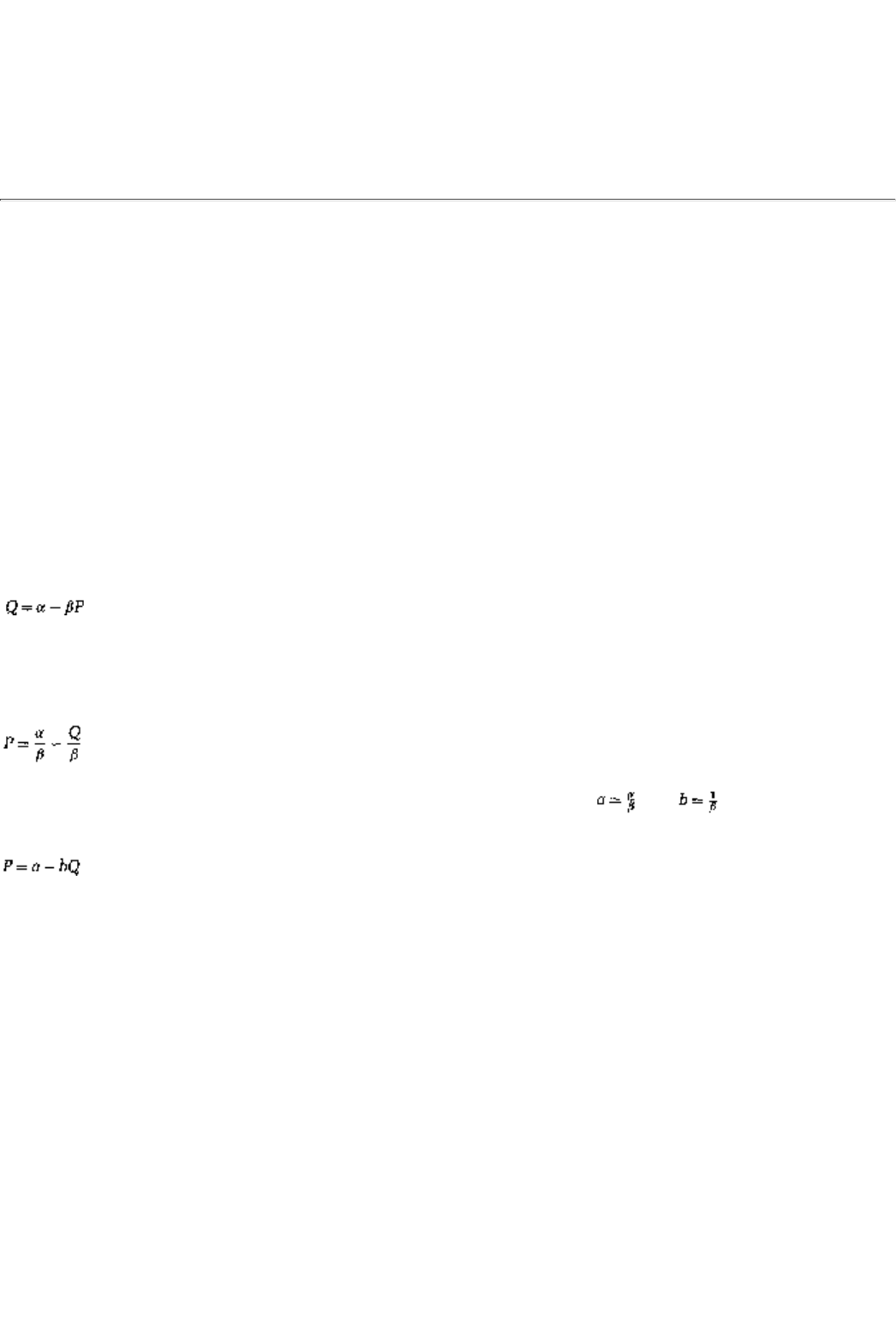
1It is entirely appropriate that we discuss the Cournot model as our first application of Nash
equilibrium. This model, first published in 1838 by Antoine Augustin Cournot, is the earliest
predecessor of modern game theory. Cournot also proposed a solution for the model that has many
features similar to a Nash equilibrium.
2These are, respectively, Boeing and the Airbus consortium of Europe.
page_75
Page 76
When there are only a few firms in its market, a firm will analyze the likely effect of its actions on its
competitors, and it will try to anticipate what the competition might do. For example, senior management in
a major airline is very likely to ponder the following questions before a price increase: Will the competition
match the change? Will they raise prices too, or will we lose customers? Will the competition offer
discounts? If they do, what will we do then? And so on.3 In a similar fashion, when OPEC's oil ministers
meet to consider future production plans, they clearly worry about the response from non-OPEC
oil-producing nations. Will their attempt to maintain a high world crude oil price be frustrated by increased
production from those nations?
Game theory, of course, is precisely the tool designed to formalize these questions.
6.2 The Basic Model
In the model proposed by Cournot, two firms compete in a market for a homogeneous product. In other
words, the two firms' products are virtually indistinguishable from the consumers' standpoint.4 Therefore, the
two firms are faced with a single demand curve in the market; suppose that the demand curve is given by
where a > 0, b > 0, and Q = Q1 + Q2, is the aggregate quantity produced by firms 1 and 2. An alternative
way of reading the demand curve is that if Q = Q1 + Q2 is the amount that the duopolists produce between
themselves, then the price that results is
Let us simplify the expression for this (inverse) demand curve by writing and ; that is, the inverse
demand curve that we will use from this point on is
Indeed, as illustration, we will refer occasionally to the special case where a = 10 and b = 1, that is, to the
inverse demand curve P = 10 - Q. Of course the picture for this demand curve is given by Figure 6.1.
Suppose now that the cost function is the same for each firm and that the cost per unit does not vary with the
number of units produced. More formally, each firm has a constant marginal cost function; the cost of
producing quantity Qi is cQi, where c > 0 is the constant marginal cost and i = 1, 2.
How much would each firm produce? To make that decision, each firm has to take two steps:
3Indeed, the dangers of not doing this analysis carefully or getting the answers wrong can be quite
serious. Recall, for example, the summer of 1992 when American Airlines decided to make pricing,
"rational." They raised business fares, eliminated multiple fares, reduced the number of discount
price categories, and so on. The competition responded by cutting prices and left the fare structure
in terms of categories virtually unchanged. American had to backtrack, a fare war of sorts started,
and, some insiders claim, the airline industry suffered huge losses consequently.
4The particular product that Cournot used as an example was mineral spring water. Of course, this
was in the old days when there weren't supposedly distinctive mineral waters such as Perrier and
Evian (which, somebody pointed out to me, is naive spelled backward).
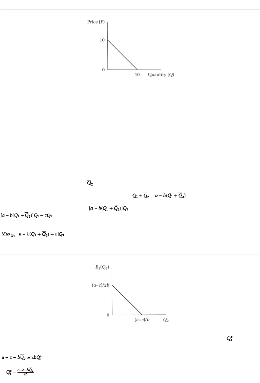
page_76
Page 77
FIGURE 6.1
1. Make a conjecture about the other firm's production. This step will give the firm an idea about the likely
market price; for instance, if it thinks the rival is going to produce a lot, then the price will be low no matter
how much it produces.
2. Determine the quantity to produce. To make this determination the firm has to weigh the benefits from
increasing productionthat is, that it will sell more unitsagainst the costs of doing sothat is, that these extra
units will sell at a lower price (and will need to be produced at a higher total cost). An industry-wideor
Nashequilibrium will obtain when both firms satisfactorily resolve these two issues.
6.3 Cournot Nash Equilibrium
Let us first analyze the two questions from the perspective of firm 1. If it was the only firm in the market,
firm 1's production decision would determine the market price. It could then compute the profits from selling
different quantity levels and pick the quantity that maximizes profits. This is no longer true; the market price
will depend on both its own production Q1 and the other firm's production. As a start, what firm 1 can do is
ask, if firm 2 were going to produce , what quantity should I produce in order to maximize profits?
Note that the market price when the total production is
is .
The revenues of firm 1 are therefore . Since costs are cQ1, the total profits are given by
. Hence, the quantity that maximizes profits can be determined from the following
exercise:
page_77
Page 78
FIGURE 6.2
The expression for profits is a quadratic function. There is a maximum profit quantity, denoted , which we
can compute by the first-order condition to the problem5
or .6 What we have just computed is the best response of firm 1 to a quantity
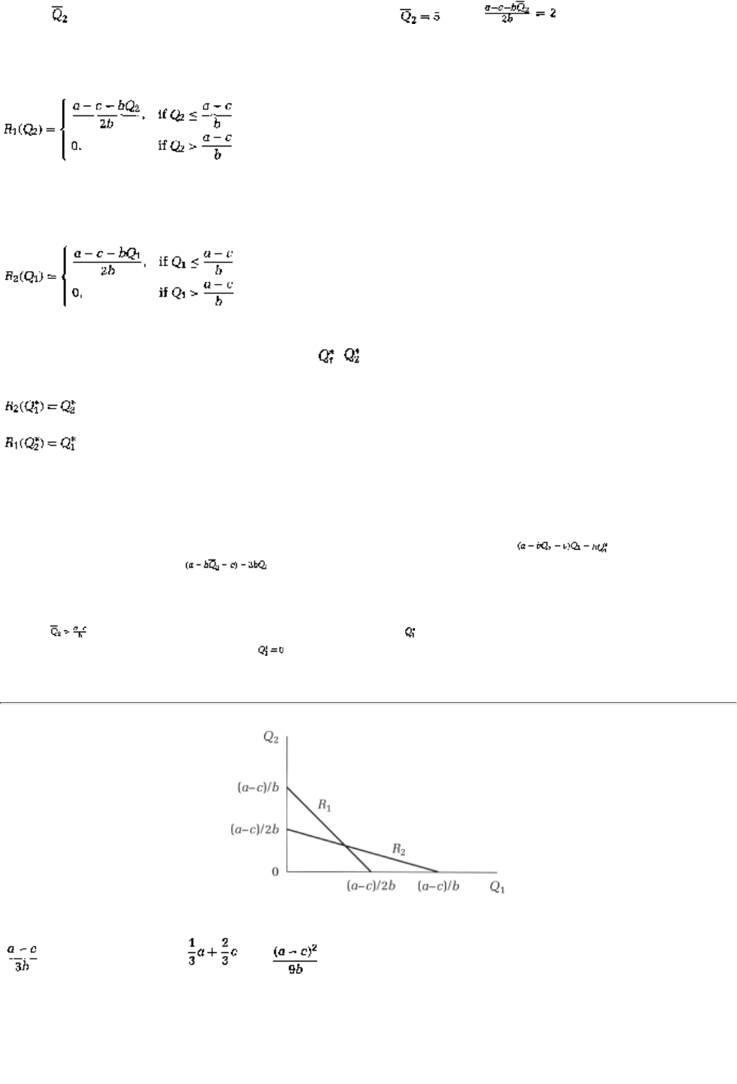
choice of firm 2. For example, if P = 10 - Q, c = 1, and , then that is, the optimal
quantity for firm 1 to produce is 2. Indeed, this formula gives us the best response of firm 1 for any quantity
that it conjectures firm 2 might produce. Let us denote this best response function R1. So we have shown
that
Let us observe the graph that goes along with this best response function, Figure 6.2.
By symmetric reasoning the best response function of firm 2 is given by
Figure 6.3 incorporates both best-response functionsalso called reaction functions in the Cournot model.
Notice that there is a unique pair of quantities,
, , at which the reaction functions cross. Hence this is a
pair of quantities for which
In other words, this pair is a Cournot Nash equilibrium of this game. Explicit computation now yields the
following equilibrium quantities, price, and profits:
5By the first-order condition we refer to the fact that at the profit-maximizing quantity, the slope,
or derivative, of the profit function must be zero. The profit function is ; its
derivative is therefore . Also note that the profit maximization is done subject to the
constraint that the quantity chosen has to be zero or positive. For a further discussion of
first-order conditions, see Chapter 25.
6If , then this formula yields a negative value for ; put differently, the quantity that maximizes
firm 1's profits in that instance is .
page_78
Page 79
FIGURE 6.3
Per-Firm Quantity Price Per-Firm Profit
Example
Consider the case where P = 10 - Q and c = 1. Show that we reach the following conclusions in the example:
Per-Firm Quantity Price Per-Firm Profit
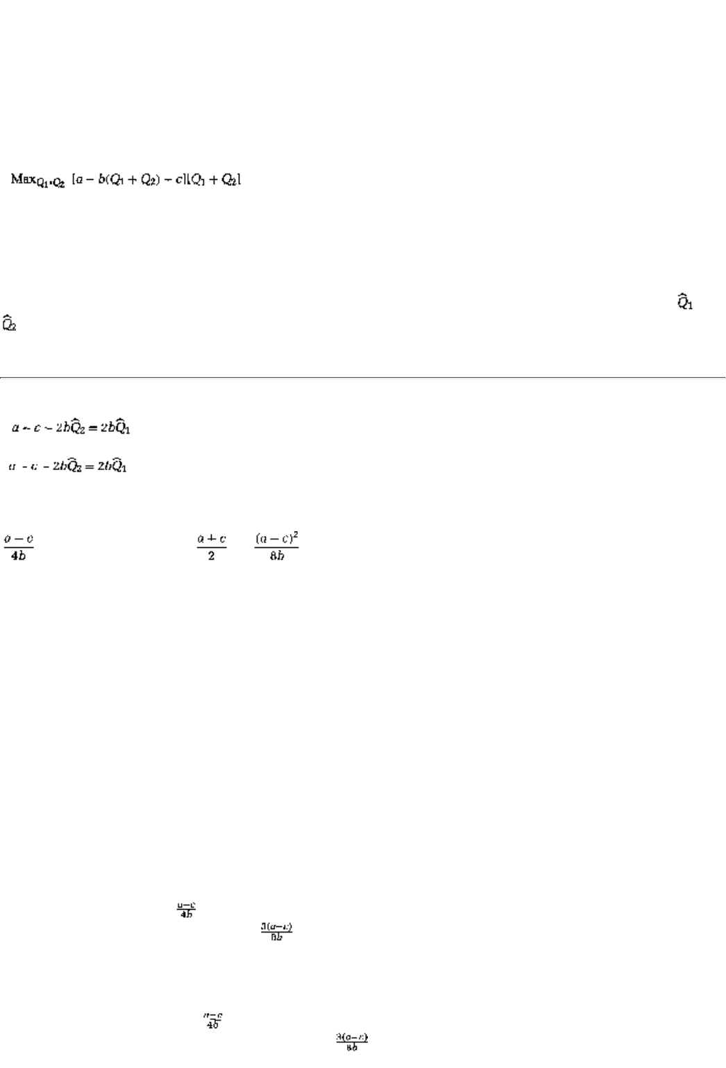
3
4
9
6.4 Cartel Solution
As a contrast let us compute the quantities that would be produced if the two firms operate as a cartel, that
is, if they coordinate their production decisions. If firms operate as a cartel, it is reasonable to suppose that
they set production targets in such a way as to maximize their jointor totalprofits. Call the production
"quotas" Q1 and Q2; these are selected so as to maximize the total profits:
The difference between the cartel problem and the best response problem is that here the two firms
acknowledge explicitly that their profits are determined by their total production. In the best response
problem, however, each firm computes profits on the basis of its own output alone (and assumes that the
other firm would hold rigidly to some quantity level).
Again, the profit-maximizing aggregate quantity is characterized by the first-order conditions; writing and
for the cartel-mandated quantities, the first-order condition can be written as
page_79
Page 80
The two equations are easily seen to solve for the cartel quantities, price, and profits:7
Per-Firm Quantity Price Per-Firm Profit
Notice that if the firms operate as a cartel they produce a smaller quantity than in
the Nash equilibrium; the
cartel output is 75 percent of the Cournot Nash equilibrium output level. Both firms make lower profits in
Nash equilibrium than if they operate as a cartel (because in equilibrium they overpr
oduce).
Example
Again consider the case in which P = 10 - Q and c = 1. Ascertain the following values:
Per-Firm Quantity Price Per-Firm Profit
2.25 5.5 10.125
(whereas, they are, respectively, 3, 4, and 9 in Cournot Nash equilibrium).8
A natural question to ask is, Given that there are higher profits to be made in this market, why don't the two
firms increase profits (by cutting back production)? The answer to this seeming puzzle, as with the Prisoners'
Dilemma, is that what is good for the group is not necessarily good for the individual. If the firms tried to
produce as a cartel, there would be incentives for each firm to cheat and increase its own profit at the
expense of the other firm.9
Indeed if firm 2 produced , the cartel quantity, it follows from firm 1's reaction function that its profit-
maximizing production level would be ; firm 1 would increase its own profits by producing more than
the cartel output level. When Q1 increases but Q2 does not, firm 2 is unambiguously worse off. After all, the
market price goes down, but firm 2 sells exactly the same amount.
The cartel weighs the profit loss of firm 2 against the profit gain of firm 1 and chooses not to recommend a
higher production quota than .
Firm 1, in deciding whether or not to cheat against this quota, simply notes
that it can increase profits by expanding output to . In particular, it ignores the effects of its cheating on

firm 2's profit levels.10
CONCEPT CHECK
Show that, by cheating on the cartel, a firm increases its own profits, but it
necessarily lowers its rival's profits by an even larger amount.
7We looked for a solution in which In general, the two equations can be solved only for .
8These differences in profits may seem small to you, but note that the quantity unit could be 200
million (as in the case of barrels of crude oil produced daily by OPEC); then, the profit difference
needs to be multiplied by 200 million.
9The duopoly problem is different from the Prisoners' Dilemma in one important respectthere is no
dominant strategy. An easy way to see this point is to note that the reaction function is a downward-
Moping line; that is, the more the other firm produces, the less a firm should produce in best response.
(What would the reaction functions look like if there were a dominant strategy?)
10In the real world, firms do not completely ignore the effect of their production on the profits of their
competitors. For instance, they worry about possible retaliation by competitors in the future. These
future considerations will be analyzed in Part III when we turn to dynamic games.
page_80
Page 81
6.5 Case Study: Today's OPEC
The Organization of Petroleum Exporting Countries (OPEC) is a consortium of major oil-producing
countries.11 OPEC was formed in 1961 and has tried since then to keep world oil prices high by restricting
production levels (through production quotas on its members). It has had varying degrees of success with
this policy; the early 1970s was a period of spectacular success, but the recent history has been mixed.12
Here are some facts about recent performance. First, by keeping prices high, OPEC quotas have made it
worthwhile for non-OPEC oil-producing nations to invest in new oil fields and increase production levels.13
Second, this response has put pressure on OPEC itself. Some members have leftsuch as Ecuador in 1992.
Others have been known to cheat on their quotas. Yet the core of OPEC is holding steady; the larger
producers show no signs of dissolving OPEC anytime in the near future.
Let us analyze the first two facts by way of a simple Cournot model. I simplify the number of real-world
players down to two: OPEC and the non-OPEC producing nations. We will assume that the costs of
production are $5 a barrel for OPEC and $10 a barrel for the non-OPEC producers.14 Finally, We will
assume the following demand curve for the world oil market:
where QO is OPEC's production and QN is non-OPEC production (in each case, in million units of barrels
per day, mbd).15
CONCEPT CHECK
BEST RESPONSES
Show that the reaction functions for OPEC and non-OPEC producers are16
Direct computation yields oil market equilibrium, as follows:
OPEC Quantity Price OPEC Profit
65
Non-OPEC Quantity
Price Non-OPEC Profit
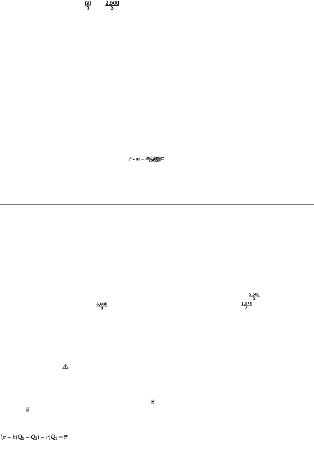
50
11. OPEC includes most of the Middle Eastern producers, such as Saudi Arabia, Kuwait, Iran, Iraq,
and the United Arab Emirates; most of the African producers, such as Libya, Nigeria, and Gabon;
and many of the Latin American producers, such as Venezuela. It does not include the European
producers, such as Norway, the Netherlands, Britain, and the former Soviet Union, nor does it
include the United States.
12. For a detailed history of OPEC and world oil prices, see Chapter 17.
13. For example, more than 60 percent of the total increase in production since 1990 has come from
non-OPEC producers. Non-OPEC oil production has grown from 27.2 million barrels per day (mbd)
in 1974 to 39.7 mbd in 1994. (Scenarios for Non OPEC Oil Production through the Year 2010, by
Herman T. Franssen, International Energy Association, mimeo, October 28, 1995).
14. The Franssen mimeo cited in note 12 reports the costs of production of OPEC oil to be $4 a barrel;
we round this off to $5 to simplify the computations. The same report quotes a variety of cost estimates
for various non-OPEC producers ranging from $7 for U.S. producers to $18 for North Sea oil from
Britain.
15. Put differently, the demand curve is if total quantity is expressed as barrels per day.
16. Note that the costs of production are different for the two "firms" in this example. Hence, the two
reaction functions are a little different from each other.
page_81
Page 82
What would happen if non-OPEC producers joined OPEC? We can compute quantities and profits from the
cartel formula obtained in the previous section. Note though that costs of production are lower in OPEC's
fields ($5 versus $10 in non-OPEC fields). Hence, if this giant cartel wants to hold down costs, all
production should come out of OPEC fields. (Why?) Applying the general formula we can now infer the
following global oil cartel solution:
Total Quantity Price OPEC Profit
90 35 2,700
Again, total profits are higher than in Nash equilibrium (because production is lower). Even if OPEC paid
the non-OPEC producers their profits in the Nash equilibriumthat is, even if they paid to the non-OPEC
producersOPEC would still have left over. In other words, OPEC would make or approximately
$458 million more per day in this arrangement. The problem for OPEC is that there is no obvious
arrangement whereby it can pay cost-inefficient non-OPEC producers not to produce. And what is worse is
that ex-OPEC members like Ecuador have found that it is more profitable to benefit from OPEC quotas by
being outside OPEC; they are no longer subject to the quotas and yet they benefit from the consequent
higher prices.17
6.6 Variants On The Main Theme I:
A Graphical Analysis
Let us look briefly at a graphical analysis of the Cournot model. (As a side benefit, we will also be able to
infer its IEDS solution.) The starting point is the concept of an isoprofit curve:
Definition. Firm 1's isoprofit curve, at a profit level , is given by all combinations of Q1 and Q2 that yield a
profit of .
These combinations of Q1 and Q2 can be expressed as
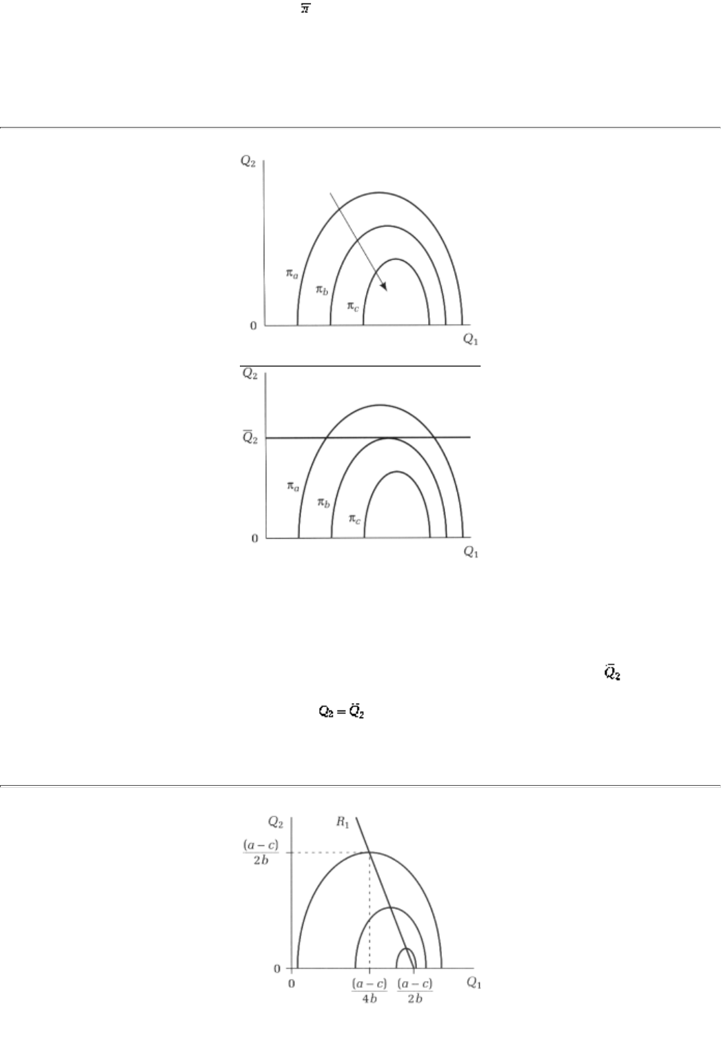
For different profit levelsthat is, for different
, there are different isoprofit curves. The family of such
curves is shown in Figure 6.4.
17. The third fact about OPECits surprising longevitywill be examined in great detail from a
dynamic game theoretic perspective in Chapter 17.
page_82
Page 83
FIGURE 6.4
FIGURE 6.5
CONCEPT CHECK
In Figure 6.4, show that profit levels increase in the direction of the arrow, that
is, that pc > pb > pa.
We can use the isoprofit curves to graph the best response of firm 1 to an output level, say . In the figure,
that response corresponds to the following problem: Get to the highest isoprofit curve for firm 1, while
remaining on the horizontal line that represents . The solution to this problem, shown in Figure 6.5, is
profit level pb.
page_83
Page 84
FIGURE 6.6
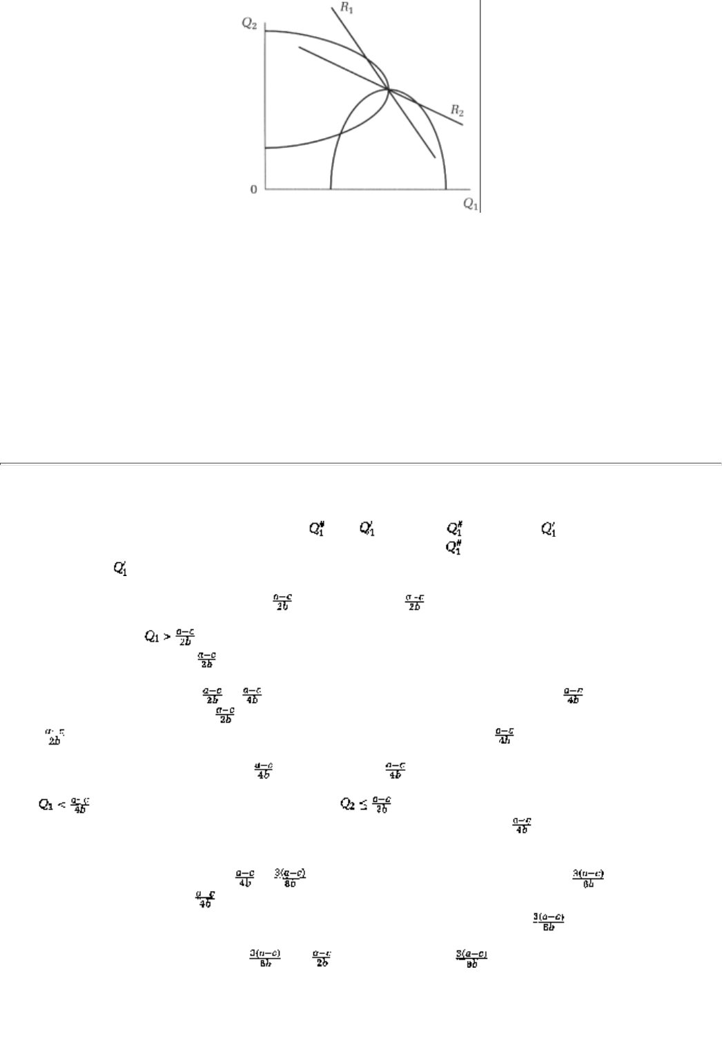
FIGURE 6.7
As we vary firm 2's quantity, we map firm 1's reaction function, as in Figure 6.6. We can do a similar
exercisecomplete with isoprofit curvesfor firm 2 as well. The two representative isoprofit curves and the
reaction functions are pictured in Figure 6.7. The intersection of the two reaction functions is the Nash
equilibrium (Q*, Q*).
6.6.1 The Ieds Solution to the Cournot Model
The isoprofit curves and the reaction functions can be used to prove the following result:
Proposition. There is an IEDS solution in the Cournot model, and it is precisely the Cournot Nash
equilibrium.
page_84
Page 85
We will sketch a proof of the proposition by analyzing firm 1. Symmetric arguments apply for firm 2.
Suppose we compare two quantity levels, say, and . Quantity dominates if for every possible
production level of firm 2, Q2, the isoprofit curve passing through ( , Q2) lies below the isoprofit curve
passing through ( , Q2).
Step 1. Every quantity level in excess of is dominated by
Take a quantity level . For any Q2, Figure 6.6 shows that the isoprofit curve passing through Q1, Q2
is below that passing through , Q2. Hence, Q1 is dominated.
Note that the best response to
is and that firm 1 produces quantities less than only if firm 2
produces quantities in excess of . Since, by step 1, it is known that firm 2 will actually never produce
above , it turns out that firm I has no reason to produce amounts below either.
Step 2. Every quantity level less than is dominated by
Take . By step 1, we only have to consider ; it should not be difficult to see from Figure 6.6
that the isoprofit curve passing through Q1, Q2 is below that passing through , Q2. Hence, Q1 is
dominated.
Now note that the best response to
is ; firm I produces quantities in excess of only if firm 2
produces quantities less than . Since, by step 2, it is known that firm 2 will never produce such small
quantities, it turns out that firm I has no reason to produce amounts greater than either.
Step 3. Show that quantities between and are dominated by
This procedure of iteratively eliminating dominated strategies is essentially eliminating portions of the two
reaction functions. Some thought (and exercises at the end of the chapter) should convince you that this
process of elimination can only stop at the intersection of the reaction functions, that is, at the Nash
equilibrium.

6.7 Variants on the Main Theme II:
Stackelberg Model
In the Cournot analysis discussed up to this point, we presumed that the two firms would pick quantities
simultaneously. In his 1934 criticism of Cournot, the German economist Heinrich von Stackelberg pointed
out that the conclusions would be quite different if the two firms chose quantities sequentially.
Suppose that firm I decides on its quantity choice before firm 2. How much should each of the two profit-
maximizing firms produce? Note that firm 2's decision is made when it already knows how much firm I is
committed to producing. It follows from our reaction function analysis that, if firm I is producing , then
firm 2 can do no better than produce its best response quantity . Hence, in turn, firm I should choose
the
page_85
Page 86
value realizing that is going to be firm 2's subsequent production choice. In other words, firm I
should solve the following problem:
Substituting for , we get
It follows from the first-order condition that the optimal choice is . We can therefore conclude, from
firm 2's reaction function that
CONCEPT CHECK
STACKELBERG PROFITS
Check that firm 1's profits are higher in the Stackelberg solution than in the
Nash equilibrium but firm 2's are smaller.
The reason why firm I is able to make a higher profit is straightforward. By committing to produce more than
it would in the Nash equilibrium, firm I forces firm 2 to cut back on its own production. This commitment
keeps the price relatively highalthough lower than in the cartel solutionbut more importantly yields firm 1
two-thirds of the marketas opposed to the market share of half that it gets in the Nash equilibrium.
6.8 Variants on the Main Theme III:
Generalization
The Cournot model can be generalized in two directions. First, it is easy to generalize the analysis to an
oligopolistic market. If there are N firms in the market producing identical products, the inverse demand
function can be written, as before, as P = a - bQ, the only difference being that the aggregate quantity Q =
Q1 + Q2 +. . . + QN If firm 1 conjectures that each of the other firms is going to produce an amount ,then
its profit-maximizing quantity can be shown to be
Why? In a Cournot-Nash equilibrium, the best responses have to be to correct conjectures, so it must be the
case that (Why?) This equation, therefore, yields the
page_86
Page 87
following Nash equilibrium quantity:18
Total quantity produced in the market is therefore , and hence the price is . Note that as the
number of firms becomes very largethat is, as N approachesinfinitythe price approaches the (marginal) cost
of production c.19 In other words, an oligopoly with many firms looks a lot like a perfectly competitive
industry (in which competition drives price to marginal cost).
We could also work out the cartel and Stackelberg solutions by following exactly the same reasoning as in a
duopoly.
A second generalization involves examining demand functions that are non-linear and cost functions for
which marginal cost rises with output. Under appropriate restrictions on the demand and cost function, we
can show that there is a Nash equilibrium, that production is higher in this equilibrium than in a cartel
solution, and that the leading firm in a Stackelberg solution does better than in the Nash equilibrium.20
Summary
1. Many real-world markets are oligopolistic. In the analysis of such markets, the study of strategic
interaction is of utmost importance.
2. The Cournot model studies quantity competition among duopolistic firms facing linear demand and with
constant marginal cost. It predicts play of a Nash equilibrium in quantities.
3. In the Cournot Nash equilibrium, each firm produces a greater quantity than it would produce as part of a
cartel. This result occurs because each firm ignores the adverse effect its overproduction has on the other
firm's profits.
4. OPEC's role in the world oil market can be analyzed by use of a Cournot model. Such a model explains
how non-OPEC oil producers can be the biggest beneficiaries of OPEC's policies.
5. There is an IEDS solution to the Cournot model, and it coincides with the Cournot Nash equilibrium.
6. If firm 1 can make an early commitment to a production level, it can make more profits (in this
Stackelberg solution) than in the Cournot Nash equilibrium.
18. In the preceding analysis, we restricted ourselves to Nash equilibria in which all firms produce
the same quantities. Could there be any other equilibria, that is, equilibria in which each firm
might produce a different quantity? How would you go about finding these asymmetric equilibria?
19. This is because approaches 0 and approaches 1 as N approaches infinity.
20. The restrictions include the following: the demand function is decreasing and concave, and the
cost function is increasing and convex. (See Chapter 25 for greater detail on these concepts.)
page_87
Page 88
Exercises
Section 6.3
In the next few questions, we will walk you through the Cournot version of the Bertrand (price) competition
model that you have previously analyzed. Recall that we have a duopoly with inverse market demand:21
Assume that each firm can only choose one of the quantity levels 0, 1, 2, 3, . . . ,6 and that costs of
production are zero.
6.1
Write down the strategic form of this game.
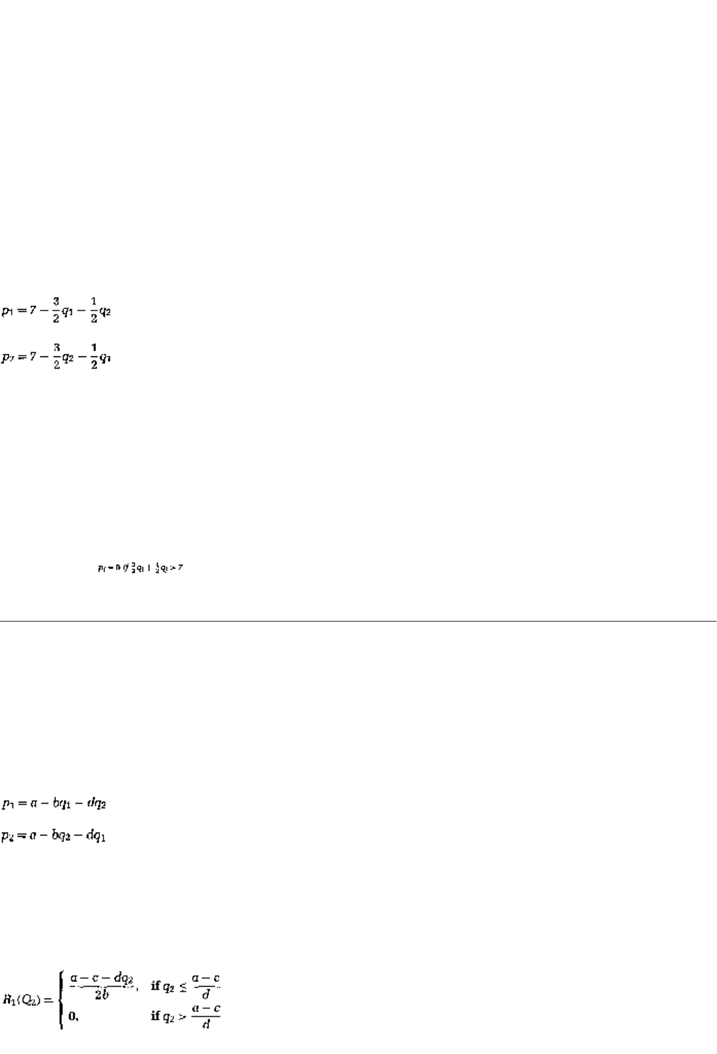
6.2
What is the best response for firm I if it thinks that firm 2 will produce 4 units of output? What if it thinks
firm 2 will produce 2 units of output?
6.3
Show that the market price in Nash equilibrium is 2 dollars. Contrast your answer with that under Bertrand
competition.
6.4
What is the Stackelberg solution to this model? Detail any additional assumption that you need to make to
answer this question.
Suppose now that the two firms produce slightly different products; suppose, as a consequence, the first
firm's price is more sensitive to its own product than that of firm 2. In particular, letting the outputs be
denoted by q1 and q2, (qi = 0, 1, . . . .,7), suppose the two demand curves are22
6.5
Write down the strategic form of this game. Argue that neither firm will produce an output greater than 4
units.
6.6
What is firm 1's best response if it thinks that firm 2 is going to produce 2 units?
21. Whenever Q > 6, p = 0.
22. Again, .
page_88
Page 89
6.7
Find a Cournot Nash equilibrium for this duopoly model.
Section 6.4
(Calculus problem) The model analyzed in exercises 6.5 through 6.7 is called a differentiated goods duopoly
model. Let us now derive some general properties of this model. Suppose the demand curves are
where b > 0 and d > 0 (and any quantity, including fractions, can be produced). Suppose also that the costs
of producing a unit of output is the same for both firms and is equal to c dollars where a > c.
6.8
Set up the best response problem for firm 1. Show that the best response function is given by
6.9
Compute the Cournot Nash equilibrium of this model.
6.10
Compute the cartel quantities.
6.11
Show that even in this model, the cartel produces less than what gets produced in the Cournot Nash
equilibrium. Explain this answer.
6.12
Show that the ratio of cartel output to Nash equilibrium output is greater than the corresponding ratio in the
homogeneous-good case ( ) if and only if b > d. Explain this answer as well.
6.13
Suppose instead that the effect of the other firm's production is positively felt; that is, d << 0. What does this
tell you about the nature of the two goods?
6.14
Redo your computations in questions 6.9 and 6.10 for this specification.23
23. You will need to make the further assumption that b + d > 0.
page_89
Page 90
6.15
How does the Nash equilibrium output compare with the cartel output? Explain your answer.
Section 6.6
The next few questions will work through the details of the IEDS analysis of the Cournot model.
6.16
Show, using isoprofit curves, that every quantity level in excess of is dominated by the quantity level
6.17
Show that amounts below are dominated by the amount . Argue that this is equivalent to removing
quantities between 0 and from the reaction function. Use isoprofit curves again.
6.18
What is the best response to ? Call this q'. Argue that quantities in between and q' are dominated.
Carefully mark the corresponding elimination on the reaction functions.
6.19
Explain in detail why this procedure of eliminating dominated strategies will eventually lead to the Cournot
Nash equilibrium.
Section 6.8
6.20
(Calculus problem) Solve the Cournot modelthat is, find the Cournot Nash equilibriumwhen the demand
curve is given by
and there are N firms. For this problem continue to assume that costs of production are zero and, for ease of
calculus-based computation, that any quantity, including fractions, can be produced.
6.21
Compute the cartel solution in this problem. Contrast your answer to that in the previous question.
page_90
Page 91
Chapter 7
An Application: The Commons Problem
In this chapter we will discuss yet another application of Nash equilibrium, the usage of a commonly owned
resource (such as deep-sea fisheries or the environment). One conclusion that we will draw from our study is
that such resources are often overused. On account of this overuse, the phenomenon goes by the name of
the tragedy of the commons.
Section 7.1 will provide a background to the commons problem. In section 7.2 we will introduce a simple
model and characterize its Nash equilibrium. Section 7.3 will contrast the equilibrium overuse with the
socially desirable outcome, and the subsequent section will show that this contrast is even more stark in a
large population. Section 7.5 will discuss several case studies: buffalo, global warming, and the Internet.
Possible resolutions to the tragedy will be the topic of section 7.6.
7.1 Background: What is the Commons?
The terminologyand backgroundto this problem can be traced to 16th-century England. Villages were
designed in such a fashion that in the center of a village there would be a piece of green land that everybody
could use. In addition to its serving as a site for village celebrations, this landthe commonswas also used by
villagers as pastureland for their cattle.1 There was, of course, pastureland that was privately ownedand in
those cases only the owner had access to that land. However, everybody had access to the commons.
Indeed a common property resource is more than just a historical curiosity. In today's world, international
waters (and the fish in them) form a common. The waters on the high seas, outside national boundaries, are
commonly owned by all nations of the world, and so each one of these nationsor strictly speaking, fishing
companies in
1. Indeed, even towns in the United States that were settled earlyand presumably by
Englishmenhave village commons. For instance, Morristown, New Jersey, has one. Only these days
it is surrounded by Macy's and Wendy's with no cable in sight!
page_91
Page 92
these nationscan fish freely in these waters. Perhaps the most important example of a common natural
resource is the environment. Every one of us ''owns" the environment (jointly) with everyone else. Usage of
this common resource, by individuals or firms, adds pollution and greenhouse gases. For example, the
burning of fossil fuels such as coal, oil, and natural gas adds carbon dioxide to the earth's atmosphere.
There are other examples that are not as immediate but that have the feature that everybody has access to
the resource or commodity in question. Library books are commonly owned by all the students at any one
college. Another (New York City) example is fire hydrants. Although these are meant to be used only by the
fire department and only in an emergency, anybody who has spent a summer afternoon in the city knows
that such an image is merely a myth perpetuated by the fire department. In actual fact, anybody can use the
hydrants for some impromptu cooling off!
As the preceding discussion suggests, there are two critical characteristics of a commons:
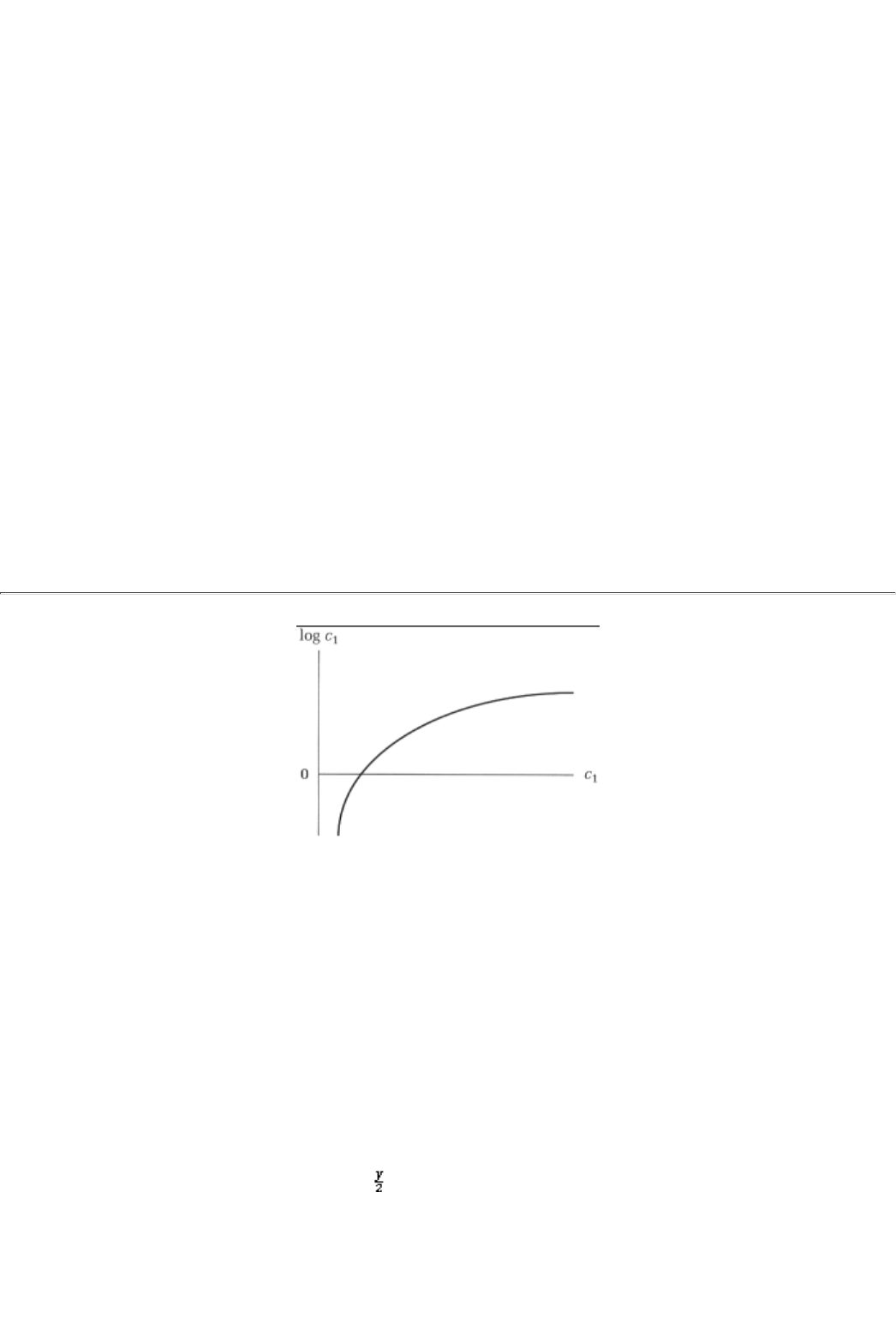
Access to (nearly) everyone. It is infeasible (think of the environment) or undesirab
le (think of National
Parks) to restrict access.
Resource depletability. The more people use the resourceor the more intensively each person uses the
resourcethe less there is of the resource in the future.
The second characteristic is worth a comment. The reason why we worry about commonly owned resources
is precisely because they can be used over a long, long period of timeand by generations of our
descendentsprovided they are used in such a manner that they regenerate from time to time. The more fish
are in the waters today, the more there will be a year from now. Conversely, the smaller is the buildup of
carbon dioxide in the earth's atmosphere today, the less there will be 50 years from now. In other words, the
result of our usage today bears a stamp well into the future. Of course this is not to say that the resource
should not be used today at all; rather, the question is how much constitutes the "best" usage. And that
brings us to the tragic part.
On account of the commonality of access, there are two sources of externality in the usage of such a
common property resource or commodity: (1) a current externalityone person's usage may decrease the
benefits to usage for other peopleif you borrow a library book then I cannot use it today; and (2) a future
externalitythe condition in which you return the book determines how long the library will be able to keep it
in circulation. Indeed, in many interesting problemssuch as the environmental onesthe important externality
is really the future externality. In this sense, this problem is different from the duopoly application of the
previous chapter. In that application, overproduction by one firm generates an immediate externality for the
other because it reduces the market price. However, this externality does not carry over into future market
interactions.
The consequence of the fact that the resource is commonly owned is that it might get overused. This
conjectureor phenomenon, if indeed it is a correct conjectureis
page_92
Page 93
FIGURE 7.1
called the tragedy of the commons. The intuition for this conjecture is straightforward. Consider pollution. If
your firm produces a chemical pollutant that it releases into the local river rather than treating it to remove
the pollutant, you save yourself the costs of treatment. Youand everybody else in townpay a cost for the
polluted river, but this cost is shared among everyone. Hence, unless checked by regulation or your
exemplary conscience, you have every incentive to dump that pollutant into the river waters. What is worse
is that every other firm in town has exactly the same incentive to pollute. If you all ended up dumping your
wastes in the river, the townspeople would have a very polluted river. They would have a tragedy of the
commons.
7.2 A Simple Model
Suppose that we have a common property resource of size y > 0. Each of two players can withdraw a
nonnegative amountc1 or c2for consumption, provided of course that c1+ c2 £ y. In the event that they
attempt to consume in excess of what is available, suppose that the total amount is simply split between
them; that is, each player ends up consuming . When total consumption is less than y, then the leftover
amount, y -(c1 + c2), forms the future resource base, out of which comes future consumption. To keep
matters simple, let us collapse the future into just one more period of consumption; that is, there are two time
periods in this model.
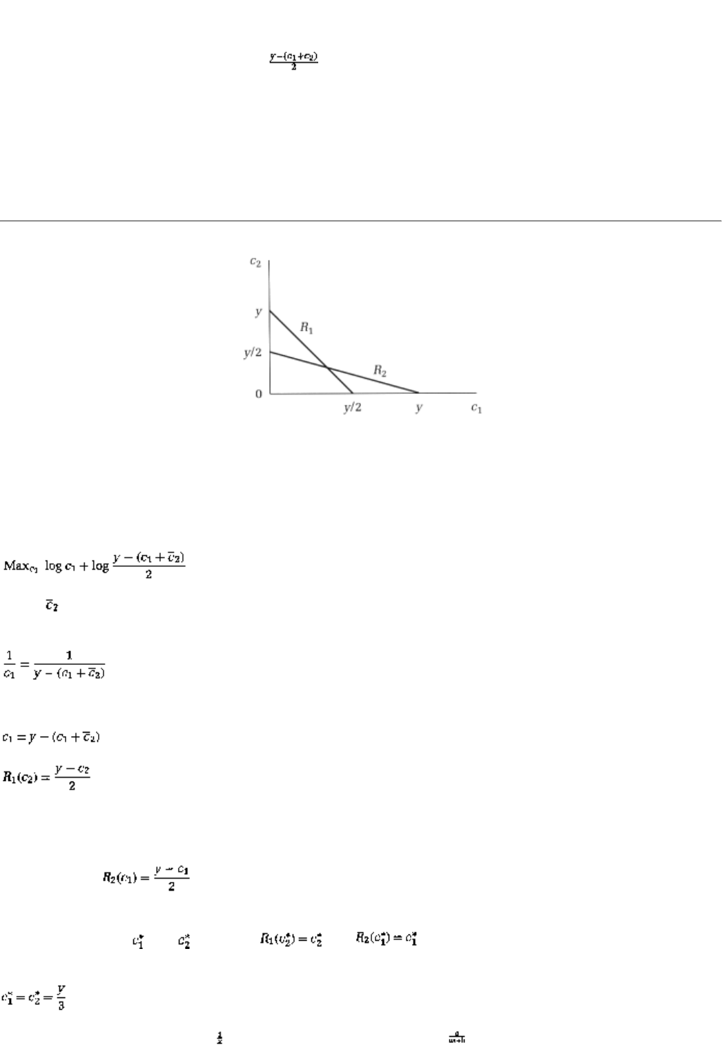
In period 2, each player has to decide how much to consume out of the available quantity y - (c1 + c2).
Since there are no more periods left, there is no reason to save any fraction of the amount that is available in
period 2. Each player would therefore like to consume as much as possible. Hence, in period 2, the total
amount is divided among themeach gets
Now let us turn to period one. If player I were to consume an amount
c1, his utility from doing so will be
taken to be log c1; that is, his utility of consumption looks like Figure 7.1.2
2. We assume that the Von Neumann-Morgenstern utility function is of this logarithmic form for
computational simplicity alone. Much of what follows is true for any concave utility function.
page_93
Page 94
FIGURE 7.2
Player I has to determine how much he would like to consume out of the available stock of the resource. His
utility depends on the amount that player 2 chooses to consume because the latter (partly) determines the
size of the resource base that will be left over. As always, player 1 has a conjecture about player 2's
consumption and determines his consumption level on that basis. In other words, Player 1's best response
problem is
where is the amount that player I conjectures player 2 is going to consume in the first period. From the
first-order conditions, player 1's best response consumption is3
or
CONCEPT CHECK
By similar logic, carefully derive the best response function of player 2 and
show it to be
The two reaction functions are pictured in Figure 7.2. The Nash equilibrium is therefore given by
consumption levels and such that and . Substituting into the reaction functions, we
can compute the Nash equilibrium to be
3. The derivative of log x is . The derivative of log (ax + b) is (See Chapter 25.)
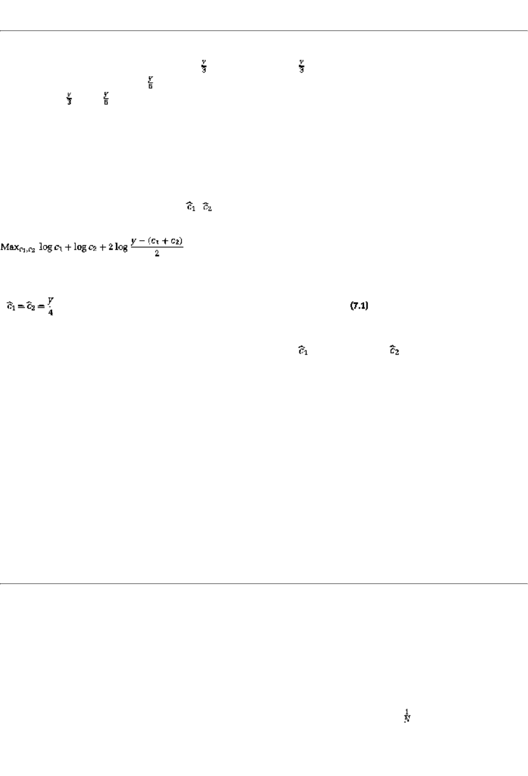
page_94
Page 95
In the first period, each player consumes , leaving a total of for the second period, which is then split in
half to yield a consumption of each in the second period. Each player's utility from this consumption
pattern is log + log .
7.3 Social Optimality
In order to determine whether or not this equilibrium pattern constitutes a tragedy, let us see what pattern of
resource use would constitute socially optimal usage. Let us define social optimality as follows: suppose that
these two players constituted society and got together to decide how much they should each consume for the
"common good." The common good is equivalent to making sure that the aggregate utility is maximized:
Definition. A pattern of consumption, , , is socially optimal if it maximizes the sum of the two players'
utility, that is, if it solves the following problem:
This procedure leads to a socially optimal solution of
CONCEPT CHECK
Write down the first-order conditions, one for and another for , of the
social optimality problem. Solve those conditions to derive the socially optimal
levels of consumption, equation 7.1.
Note that in this case, exactly half of the resource is used in the first periodin co
ntrast to the Nash
equilibrium where as much as two-thirds of the resource is used up in the first period.4 In this sense we have
an overextraction of the resource in the Nash equilibrium; that is, we have a tragedy of the commons.
The reason for this overextraction is precisely the externalities discussed previously. Notice that if player I
were to cut back his consumption in the first period by one unit, he makes this one unit available for
consumption by both players in the second period. He is, however, able to recover only half of this unit as
additional consumption in the second period, because the other half accrues to player 2. Consequently,
player 1and by extension both playerstends to overconsume. This phenomenon does not arise in the socially
optimal solution, however, because in that solution we
4. It should be clear that in the socially optimal solution, each player then consumes a quarter of
the resource in the second period as well.
page_95
Page 96
care about the utilities of both players. A unit of consumption set aside for tomorrowby either
playercontinues to be a unit of consumption for society as a whole in the second period. Hence, there is no
externality that distorts first-period consumption.
7.4 The Problem Worsens in a Large Population
To fix these ideas even more firmly, let us see what happens in this example as the number of players
increases. The intuition would be that this increase makes the tragedy even more acute. The reason is that if
player I forgoes a unit of consumption in the first period, he is able to retrieve only
of that unit as
consumption in the next period (where N is the number of players). That should make player I even less
willing to set aside any resource for the future.
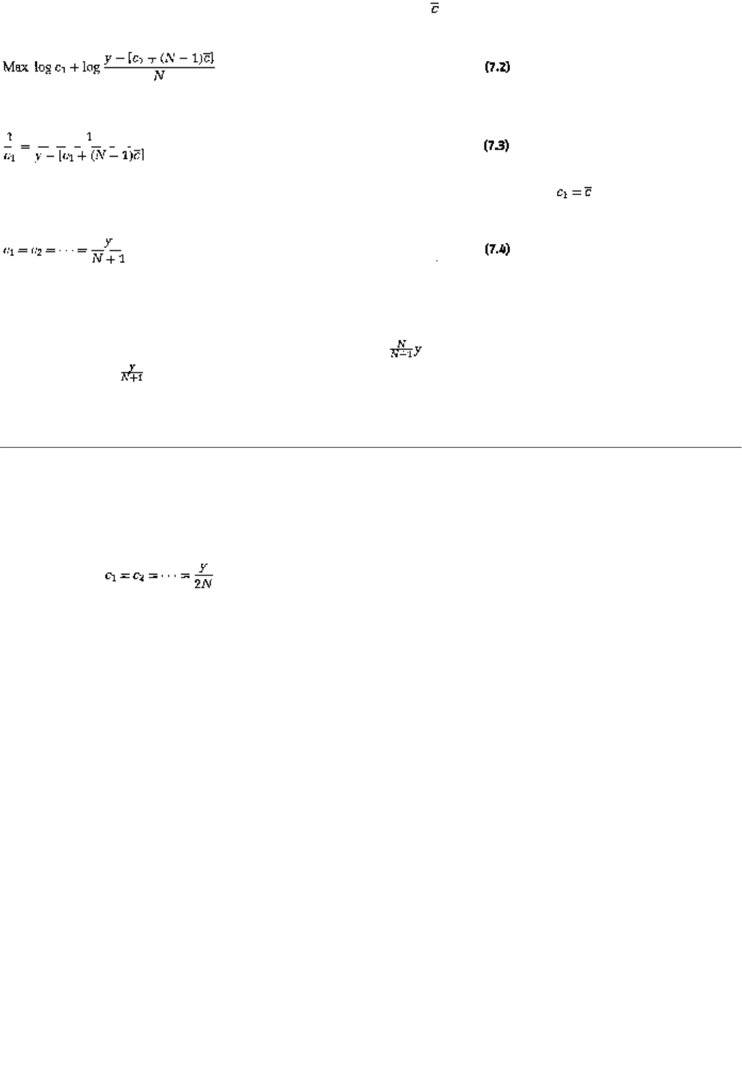
If player 1 conjectures that the others will consume an amount
in the first period, then his utility-
maximizing consumption is determined from the following optimization problem:
From the first-order conditions, player 1's best response consumption is
In the Nash equilibrium in which each player consumes the same amount, that is, , it follows from
equation 7.3 that the equilibrium consumption level is
CONCEPT CHECK
Derive equations 7.2, 7.3, and 7.4.
The total consumption in a Nash equilibrium is therefore . Consequently, the amount that remains after
the first period is . As N becomes large, a vanishingly small amount of the resource reaches the second
period. The tragedy of the commons is exacerbated in large populations.
page_96
Page 97
CONCEPT CHECK
SOCIAL OPTIMALITY
Show that in order to maximize the total utility of all players, consumption
should be
In other words, society would always like half the resource to be saved for the future, no matter how many
members there are in society. This result should also be intuitive. A unit of consumption withheld from social
consumption today is always available as a unit of consumption in the future, regardless of how many
members there are in society. So the conclusion that half of the total resource should be withheld for social
consumption in the future is a result that is independent of the number of players.
7.5 Case Studies: Buffalo, Global Warming, and the Internet
A very popular historical example of the tragedy of the commons is that of the buffalo in the American
West. Till the middle of the 19th century great herds of American buffalo roamed the Great Plains. They
were a commons in that any hunter could hunt them down if he so desired. Starting in the middle of the
century, the hunting grew increasingly widespread and effective, and the buffalo herds had a more and more
difficult time regenerating. By the end of the century many of these sprawling herds had disappeared. Here
is a commentary on their usage:
The Plains Indians very eagerly accepted modern technology in the form of horses, guns and steel
tools. . . . By I840 the Indian had driven the buffalo from portions of the Great Plains area and
there is evidence of concern about this problem. . . . Given multiple tribes and the fact of no real
cooperation, the Indians were incapable of managing the buffalo as a common pool resource. . . .
The benefits from harvesting one more buffalo accrue to the individual hunter, while the costs of
depletion of the herd are spread among all hunters. The true costs of hunting are not borne by the
hunter and overuse is predictable. (American Indians: A Test of the Conservation Ethic, by John
Baden, Rick Stroup and Walter Thurman).5
Here is a more recent example, global warming. Much of the energy that is produced to heat our homes,
drive our cars, or produce our economy's goods and services

5. As quoted in Costs of Innovation in the Commons, September I996, by Douglas Noonan, mimeo,
Foundation for Research on the Economics and the Environment.
page_97
Page 98
comes from carbon sources. It comes from burning coal, oil, or natural gas. This combustion releases carbon
dioxide into the earth's atmosphere and (although some of it is broken down by plant photosynthesis) much
of it remains in the atmosphere. Carbon dioxide (and certain other "greenhouse gases") traps heat, in much
the same way that a greenhouse does. Imagine then the total amount of carbon dioxide in the atmosphere as
a common pool, since it is this total that determines temperatures all over the world. Each individual or
firmor simply, each nationadds to this stock of carbon dioxide by its energy consumption. Whereas the
benefits to this energy consumptiona higher national output, or a better standard of livingare entirely
experienced by the energy user, the costshotter temperatures and consequent climatic and economic
dislocationare shared by everyone. Scientists say that average surface temperatures have risen between 1
and 2°F in the last 200 years and, more alarmingly, can arise another 4 to 8°F in the next 100 years if present
trends of carbon dioxide buildup continue.6
Here is another recent example; let us call it the Internet jam. Starting in the summer of 1996, a number of
online companies started offering a fixed-monthly-rate service; you pay a fixed rate, say $19.99, for the
month, and you can gain access to the Internet as many times and for as long as you want that month. Under
the pricing practice that existed before, consumers were charged an hourly rate for Internet access.7Note
that since customers use phone lines to access the Internet, the resources of the phone systemthe switches,
the lines, and so oncan be thought of as a commons for all Internet users.8 Once the monthly fee has been
paid, it is a sunk cost; that is, it is as if Internet access is a free good. It is not of course free for society, since
there is a fixed capacity for the phone lines. Unsurprisingly, phone systems were completely overloaded,
systems broke down several times, and some customers complained of having to wait up to an hour before
they could get through to the Internet.9
7.6 Averting a Tragedy
The question that many economists and other social scientists grapple with is how to balance the private
desire for utility or profits against the social imperative of sustainable resource use. Many (incomplete)
solutions have been proposed to deal with the tragedy of the commons. Some economists favor a
privatization of the resource ownership. Privatization is clearly a solution that has been employed, up to a
point, for land. There is no longer a common pasture in villages, nor are there common town centers in
suburban developments.10 Privatization would certainly remove the externality inherent in the common
ownership of the resource. (Why?) The problem with privatization is that it simultaneously takes away the
common access to usage that may be desirable for a variety of other reasons. Furthermore, for some
resourcessuch as the environmentit is not even a practical solution.
Other economists have proposed a tax or fee for usage. This is the solution that is most widely used when
dealing with pollution. It is also the solution that is used in
6. More details on global warming can be found in an authoritative report of the Inter-
Governmental Panel on Climate Change, Climate Change 95: The IPCC Scientific Assessment New
York: Cambridge University Press, 1995.
7. The most significant switch came when the biggest access provider, America Online, started offering
the new service in October 1996. Details on this story can be found in the New York Times, December
17, 1996.
8. In the United States, some estimates put the number of people accessing the Internet at 50
millionand growing.
9. In a development that only makes the tragedy of the commons worse, there is now software that will
keep redialing for you and, once you get access, will keep you logged on while you sleep, go to class,
or attend to the other duties of your daily life! (See the Times article referenced in note 7 for further
details.)
10There is, of course, the ubiquitous shopping mall.

page_98
Page 99
National Parks. The problem here is that assessing fees is an inefficient solution wh
enever the marginal cost
of production is near zero. In other words, if the cost of allowing one more person into the park is virtually
zero, then that person should not be charged a high fee. Put differently, a fee of $5 would simply discourage
from coming to the park a person who is only able to pay $2 (or who only derives a utility of $2 from using
the park). This approach would be inefficient if the actual extra cost of cleanup is 10 cents. A desirable fee
would be one that varies with the number of users, charging more as the park becomes more and more
crowded. A proxy to this scheme is one that charges different fees for different times of the year (or even
different times of day). The problem with these schemes is that they are more complicated to implement.
A third solution that has been proposed is to simply put a ceiling on the number of users of the resource. The
size of the ceiling could be designed in such a manner that the resource is able to regenerate itself. For
instance, park rangers close off Yosemite National Park in the middle of the afternoon if they determine that
too many people have already entered the park that day. The same inefficiency problem discussed in the
previous paragraph also plagues this solution. Yet from a long-term standpoint either of these last two
solutions can be better than an unregulated tragedy of the commons.
It should be noted that the model analyzed in this chapter can be generalized in a variety of ways without
changing the qualitative flavor of the result. First, we only analyzed an exhaustible resource problem; the
amount of the resource that remains at the end of the first period, say, x, is precisely the amount available
for consumption in the second period. However, the analysis carries over to a renewable resource model,
that is, a model in which the amount x becomes something larger, say, f(x) > x, by the start of the second
period. It is still true that there is a future externality because sacrificing a unit of consumption yields a
player only half of the consequent increase in second-period resource stock. Hence, she overconsumes in the
first period.
A second direction in which the model can be generalized is to allow several future periods or more general
utility functions. Again the basic externality is unchanged and so therefore is the tragedy. Indeed in Chapter
18 you will see just such a generalization.
Summary
1. A common (resource or commodity) has two characteristics: it is accessible to everyone, and its amount
depletes upon usage.
2. In the Nash equilibrium of a commons game, each player overuses the resource because he gets all of the
immediate benefits from usage and bears only a fraction of the future costs of depletion.
3. In a socially optimal solution, there is enough of the resource set aside for desirable regeneration.
page_99
Page 100
4. The tragedy of the commons is exacerbated in large populations.
5. There are many real-world illustrations of the tragedy of the commons; the historical extinction of the
American buffalo and the current possibility of global warming are two such examples.
6. Various solutions have been proposed to avert a tragedy. They include privatization, taxes or user fees,
and limits to accessibility.
Exercises
Section 7.1
7.1
Give an example of a resource, natural or otherwise, to which there is not common access, that is, a resource
that only selected people can use.
7.2
Give an example of a resource, natural or otherwise, that is not depletable, that is, a resource that does not
deplete in quantity (for all practical purposes) when more people use the resource.
7.3
Is there a tragedy of the commons in either of your examples? Does a resource have to be commonly
accessible and depletable for it to be overused?
7.4
Are the resources devoted to public education an example of a common property resource? Explain.
7.5
From your daily life can you think of a tragedy of the commons phenomenon? Explain your answer.
Section 7.2
(Calculus problem) The resource that we analyzed in the text is an exhaustible resource. To see that the
phenomenon of the tragedy of the commons can also arise if the resource
page_100
Page 101
is renewable, consider the following variant of the model in the text. Each player extracts an amount ci in
the first period, i = 1, 2. Whatever is not extracted, that is, the amount y - c1 - c2, regenerates and becomes
an amount equal to in period 2.11 The rest of the model will be identical to that in the text; in
particular, the utility function will be log c, and the allocation rule (if the total desired is more than what is
available) will be to give half to each player.
7.6
Write down the best response problem for player 1.
7.7
Show that the best response function is given by12
7.8
Compute the Nash equilibrium.
(Calculus problem) In the next few questions, we will walk you through a private property version of the
common property model that is analyzed in the chapter. Suppose that we have two (duopoly) firms and they
each own a homogeneous resource, such as a forest or a fishing pool, of size 25. Each of them can withdraw
any nonnegative amount, c or d, in the first period, provided of course that c £ 25, d £ 25. There are two
periods, and whatever is not extracted in the first period is extracted in the second. Finally, the extracted
amounts are sold in a (common) market whose demand curve is given by
where Q is the total amount extracted in any period. Assume that each firm is a profit maximizer and that
costs of production are zero.
7.9
Write down the strategic form of this game.
7.10
What is the best response for firm I if it thinks that firm 2 will produce 7.5 units
of output? What is the best
response function of firm 1? (In answering this question, you will need to use the facts that profits are
maximized when the slope of the profit function is zero and that the slope of a quadratic function a + bx -
cx2 is b - 2cx).
7.11
What is the Nash equilibrium extraction levels in period 1? period 2? What about market price?
11In order that the resource is soon to grow, that is, in order for to be greater than y - c1 -
c2, we will make the assumption that y £ 1. This is simply an accounting convention; if the actual
maximum amount is 100 we would simply consider a regeneration function like .
12Use the fact that log is the same as log x.
page_101
Page 102
Section 7.3
7.12
Set up and solve the social optimality problem in the renewable resource problem. Show that the socially
optimal extraction is for each player.
7.13
Explain why exercise 7.12 differs from the exhaustible resource model in which the socially optimal
extraction is for each player.
7.14
In the private property model, how would your answers change if the firms operated as a cartel? Explain
your answer carefully.
Section 7.4
7.15
Analyze the renewable resource problem for N players. Is it true that all of the resource is extracted in the
first period if N approaches infinity?
7.16
Analyze the private property resource problem for N players. Is it true that the price of the resource is driven
to zero as the number of firms increases without bound? Explain very carefully any assumptions that you
make in order to do your analysis.
Section 7.6
7.17
Explain why privatizing the common resource would solve the overextraction problem.
7.18
Consider the Internet jam problem. Suggest a solution that would avert a tragedy in that case. Is the solution
you propose in the interests of the online companies to implement? If so, speculate on why they have not
done something similar already.
page_102

Page 103
Chapter 8
Mixed Strategies
This chapter will present a more general class of strategies, called mixed strategies, that players can
profitably employ. We will define these strategies precisely in section 8.1.1 and present a few examples in
section 8.1.2. In section 8.2 we will discuss an important implication of using mixed strategies. Sections 8.3,
8.4, and 8.5 will give three different answers to the question, Why would players in a game ever want to use
mixed strategies? Finally, in section 8.6, we will see a case study of random drug testing that involves mixed
strategies.
8.1 Definition and Examples
8.1.1 What Is a Mixed Strategy?
Suppose that you are playing the game Battle of the Sexes. Seemingly, you have only one of two choices to
makego to the football game or the opera. Actually, those are not the only choices you have. For instance,
you can toss a coin. If it comes up heads you can go to the football game, whereas if it comes up tails you
can go to the opera instead. Hence, you have at least three strategies to choose from: (a) football, (b) opera,
and (c) a coin toss, that is, a strategy with an equal likelihood of going to football or opera.
Notice that
after the coin has been tossed, you will end up doing one or the otherfootball or opera. In that
sense, the coin toss has not enlarged the set of eventual actions available to you. However, it has clearly
enlarged the set of initial choices; strategy c is evidently distinct from a or b. Before the coin lands, you are
not sureand neither is your spousewhether you will be at the game or at the opera house.
Strategies a and bas well as every other strategy that we have discussed so farare called pure strategies. A
strategy such as c is called a mixed strategy. Indeed, strategy c is just one of many mixed strategies. For
every distinct likelihood of football versus opera,
page_103
Page 104
there is a corresponding mixed strategy. For instance, there is a mixed strategy in which football is twice as
likely an eventual choice as the opera; this corresponds to a strategy in which the probability of playing the
pure strategy football is while the probability of playing opera is .1
Definition. Suppose a player has M pure strategies, s1, s2, . . . , sM. A mixed strategy for this player is a
probability distribution over his pure strategies; that is, it is a probability vector (p1, p2, . . . , pM), with pk³ 0,
k = 1, . . . , M, and .
A particularly simple mixed strategy is one in which each pure strategy is equally likely, that is, . This
would correspond to writing down the numbers 1, . . . , M on separate (equal-sized!) pieces of paper, folding
up the pieces, and getting your roommate to pick one for you. It is not necessary that each pure strategy
have a positive probability in a mixed strategy. For example, you can write down the numbers 1, . . . , M - 1
and repeat the procedure. The corresponding mixed strategy is, , k = 1, . . . , M - 1 and pM = 0.
Similarly it is not necessary that the pure strategies that are assigned positive probabilities are all picked with
equal probability. For instance, you could have written the number I on two of the original M scraps and
omitted, say, the number 2. Then you would have constructed a mixed strategy for which , p2 = 0, and
, k=3, . . . , M.
Every pure strategy isin a trivial sensealso a mixed strategy. For instance, the pure strategy s1 is equivalent
to the mixed strategy in which p1 = 1 and pk = 0 for all other pure strategies.
The next question is, How should a mixed strategy's payoffs be evaluated? Recall that the payoffs in a game
are Yon Neumann-Morgenstern utilities. Hence, from the expected utility theorem of Chapter 27 it follows
that the right way to evaluate the uncertainty inherent in a mixed strategy is to take its expected payoff.
Expected payoffs are computed in two steps:
Step 1. Weight the payoff to each pure strategy by the probability with which that strategy is played.
Step 2. Add up the weighted payoffs.
Consider the following strategy pair in the Battle of the Sexes: the husband goes to the opera with
probability , while his wife plays the pure strategy football. The payoff matrix of the game is
Husband \ Wife F O
F3,1 0,0
O0,0 1,3
1For a discussion of probabilities and expectation, see Chapter 26. Before reading any further.
you should make sure that you have a good understanding of that chapter.
page_104
Page 105
For this pair of strategies, the likelihood that both spouses go to the football game is , while the probability
of the husband going by himself to the opera is . These two probabilities should be multiplied by the
corresponding payoffs, respectively, 3 and 0, and then added. Hence, the husband's expected payoff is
On the other hand, if the wife plays the pure strategy opera, then the husband's expected payoff is
Note that the expected payoff is different for the husband in the second case; this c
omputation illustrates the
somewhat obvious point that a mixed strategy's payoff depends on the strategies chosen by the other players.
Finally, suppose the wife also plays a mixed strategy; she is equally likely to go to the football game or the
opera. Since the probability of any pair of pure strategies being chosen is the product of the probability of
each strategy, the probability that husband and wife both end up at the football game is . The expected
payoff to the husband is therefore
Definition. Suppose that player i plays a mixed strategy (p1, p2, . . . , pM). Suppose that the other players
play the pure strategy . Then the expected payoff to player i is equal to
Definition. Now suppose that the other players play a mixed strategy themselves; say, the strategy is
played with probability q while is played with probability 1 - q. Then the expected payoff to player i is
equal to
In equation 8.1 we have used the fact that the likelihood that the pair of pure strategies (s1, ) gets played
is given by p1q and likewise the probability that the pair (sM, ) gets played is given by pMq, and so on. By
collecting the common terms, equation 8.1 can be written more compactly as
page_105
Page 106
8.1.2 Yet More Examples
In each example we will focus on player 1 and write out in detail his mixed strategies and their expected
payoffs. Symmetric computations can be done for the other player(s), and you should be sure to do them as
practice.
Example 1: Matching Pennies (h = heads, t = tails)
Player 1 \ Player 2 h t
h1, -1 1, 1
t-1, 1 , -1
Consider the mixed strategy in which player 1 plays h with probability while player 2 plays t for sure.
Then, player 1's expected payoff is . More generally, suppose that player 1 plays h with
probability p while player 2 plays t for sure. Then, player 1's expected payoff is p × (-1) + (1 - p) × 1 = 1 -
2p.
COMPUTATION CHECK
Show that if player 1 plays h with probability p while 2 plays h for sure, then
player 1's expected payoff is 2p - 1. What are player 2's expected payoffs?
Example 2: Hawk-Dove (or Chicken) (t = tough, c = concede)
Player 1 \ Player 2 t c
t-1, -1 10, 0
c0, 10 5, 5
Consider the mixed strategy in which player 1 plays t with probability while player 2 plays t for sure.
Then, player 1's expected payoff is . On the other hand, suppose that player 1
continues to play t with probability but player 2 plays c for sure. Then, player 1's expected payoff is
.
ANOTHER COMPUTATION CHECK
Show that if player 1 plays t with probability while player 2 plays t with
probability , then player 1's expected payoff is . What are player 2's
expected payoffs in this case?
page_106
Page 107
Example 3: No-Name
Player 1 \ Player 2 L M1 M2 R
U1,0 4,2 2,4 3,1
M2,4 2,0 2,2 2,1
D4,2 1,4 2,0 3,1
THIRD COMPUTATION CHECK
Suppose that player 1 plays U, M, D with probabilities .2, .3, and .5,
respectively, while player 2 plays L and M2 with probabilities .4 and .6. Show
that player 1's expected payoffs equal 2.32. What about player 2's expected
payoffs?
Finally, suppose that player 1 plays U, M, D with probabilities p1, p2, and p3, respectively,2 while player 2
plays L and M2 with probabilities q and 1 - q. Player 1's expected payoffs are then given as
8.2 An Implication
In this section, we will discuss an implication of using mixed rather than pure strategies. In order to do so, we
will need one more definition.
Definition. Consider a mixed strategy given by the probability vector (pl, p2, . . . , pM). The support of this
mixed strategy is given by all those pure strategies that have a positive probability of getting played (in this
strategy).
For example, if p1 > 0 and p3 > 0 but pk = 0 for all other k, then the support of this mixed strategy is made
up of the pure strategies 1 and 3.
The expected payoff to a mixed strategy is simply an average of the component pure-strategy payoffs in the
support of this mixed strategy. If the payoffs to each of the pure strategies in the support are not the same,
then deleting all but the pure strategies that have the maximum payoff must increase the average, that is,
must increase the expected payoff. In other words, if strategies s1 and s3 yield the highest payoff against,
say, , then a mixed strategy that only involves these two pure strategies will yield a higher expected
payoff than one that also involves strategies s2, s4, . . . , sM.
2Of course, p3must equal 1 - p1 - p2. (Why?)
page_107
Page 108
Implication. (a) A mixed strategy (pl, p2, . . . , pM) is a best response to if and only if each of the pure
strategies in its support is itself a best response to . (b) In that case, any mixed strategy over this support
will be a best response.
Regarding part b of the implication, note that if each of the remaining strategies in the support is a best
response, then each yields the same payoff. Hence any average of these strategies will also yield exactly the
same payoff; that is, any mixture of these strategies must also be a best response.
Consider the No-Name game of example 3:
Player 1 \ Player 2 L M1 M2 R
U1,0 4,2 2,4 3,1
M2,4 2,0 2,2 2,1
D4,2 1,4 2,0 3,1
Take the column player's strategy to be R. The implication simply says that a mixed strategy involving U and
M
is worse than U alone. It further says that any mixed strategy that has U and D as its support is a best
response.
Why would a player in any game use a mixed strategy? In the next three sections we will give three related
reasons. The common observation in all three situations is that by doing so, a player may ''do better" than she
would do by playing some of the pure strategies that she has available to her, and sometimes she may even
"do better" than all of her pure strategies.
8.3 Mixed Strategies Can Dominate Some Pure Strategies
Let us start with the most unambiguous notion of doing bettera strategy does better than an alternative if it
dominates the latter. We will now see an example in which there is a mixed strategy that dominates a pure
strategy, say
, even though no other pure strategy is able to dominate . The example is in fact the
No-Name game.
It is clear that no pure strategy dominates any other pure strategy in the No-Name ga
me. Consider now the
mixed strategy in which player I plays U and D with equal probabilities of . By playing this strategy, player
I can guarantee herself an expected payoff of at least 2 and possibly more. Note that if player 2 plays either
L
or M1, then the mixed strategy yields an expected payoff of 2.5, whereas if 2 plays R then the mixed
strategy's payoff is 3. The only time that the mixed strategy yields an expected payoff exactly equal to 2 is
when player 2 plays M2. On the other hand, by playing the pure strategy M, player 1 always gets a payoff
equal to 2. We can conclude, therefore, that the mixed strategy dominates the pure strategy M.3
3Since we are considering mixed strategies, the definition of dominance needs to be carefully
specified. We say that a mixed strategy p dominates another mixed strategy p' if , for
all s-i, and , for some , where denotes the expected payoff
[with a similar definition for .
page_108
Page 109
CONCEPT CHECK
OTHERS?
Are there any other mixed strategies for player 1 that also dominate M? Make
sure you detail them!
The intuition for the preceding conclusion is quite straightforward. Notice that player 1 does very well by
playing U whenever player 2 plays M1 but does rather poorly if player 2 plays L. Strategy D is exactly the
opposite: it does very well against L but poorly against M1. Playing U and D with equal probabilities allows
player 1 to "insure" herself: no matter what player 2 does, player 1 is equally likely to do well or poorly; that
is, she guarantees herself a superior outcome to that under M.
CONCEPT CHECK
OTHER PLAYER
Show that for player 2, the mixed strategy L, M1, M2 with equal probabilities
dominates the pure strategy R.
So this is the first of our three reasons for playing a mixed strategy rather than some of the available pure
strategies:
Reason 1. A mixed strategy may dominate some pure strategies (that are themselves undominated by other
pure strategies).
8.3.1 Implications for dominant Strategy Solution and IEDS
Adding mixed strategies changes absolutely nothing with regard to the dominant strategy solution. If there is
a pure strategy that dominates every other pure strategy, then it must also dominate every other mixed
strategy. (Why?) However, if there is no dominant strategy in pure strategies, there cannot be one in mixed
strategies either. (Why?)
Mixed strategies do make a difference, however, for the IEDS solution concept. They do make a difference
in the sense that a game that ostensibly has no IEDS solution when only pure strategies are considered can
have an IEDS solution in mixed strategies. Consider the No-Name game. We have already seen that the
strategies M for player 1 and B for player 2 are dominated (by mixed strategies). Ruling them out, we are
left with the following payoff matrix:
page_109
Page 110
Player 1 \ Player 2 L M1 M2
U1,0 4,2 2,4
D4,2 1,4 2,0
In turn L is now dominated (by M1), and removing L leads to D becoming dominated for player 1. That in
turn leads player 2 to eliminate M1; the IEDS solution is therefore (U, M2). Had we not examined mixed
strategies we would not have found this IEDS solution.4
However, whenever a game has an IEDS solution in pure strategies, that solution will also be the mixed
strategy IEDS.
8.4 Mixed Strategies Are Good for Bluffing
We turn now to a second reason why a player may want to use a mixed strategy. The idea can be explained
quite simply by employing a sports analogy: an unpredictable player is better able to keep his opponent off
balance.
Imagine that you are playing the effete East Coast game of squash. In the middle of a rally you have to
decide whether to position your next shot (softly) in the front of the court or hit it (hard) to the back. Your
opponent likewise has to move in anticipation of your shot; he could start moving forward or backward. Of
course, if he does move forward, he is likely to finish off the rally if you dropped your shot in front, but you
are likely to win if you did in fact hit the hard shot behind him. If he moves backward, converse reasoning
applies. In the following table are displayed your chances of winning the rally in the four possible cases:
Forward (F) Backward (B)
Front (f).2 .8
Back (b).7 .3
Suppose that you picked the strategy front (hereafter f). If your opponent correctly guessed that you were
going to make this choicealternatively, if in every rally you play fthen he will move forward (F) and he will
win 80 percent of the rallies. By the same logic, if you always picked b, or if this choice was correctly
guessed, you would only win 30 percent of the rallies. What happens, though, if you occasionally bluffhalf
the time you go f (and the other half b)? If your opponent goes forward, you win 45 percent (the average of
20% and 70%) of the rallies, while if he goes backward, you win 55 percent of the rallies. In other words,
even though your opponent is correctly guessing (that you go f with probability ), you nevertheless win at
least 45 percent of your rallies. This outcome is in contrast with either of the pure strategies where your
opponent could hold you down to either 20 percent or 30 percent wins.
4You might wonder why it is that we only eliminated pureand not mixedstrategies while finding the
IEDS outcome. Actually we did implicitly eliminate mixed strategies as well. For example consider
step 2; we eliminated the pure strategy L because it is dominated at that point by M1. However, any
mixed strategy containing L and M1 is also dominated by M1. Hence those mixed strategies can
also be eliminated. By similar reasoning one can show that all mixed strategies are eliminated in
the process of reaching the IEDS outcome (U, M2).
page_110
Page 111
The intuition is also straightforward; if you are predictable, your opponent can pick the move that will kill
you (and win the game). If you are unpredictablethat is, if you use a mixed strategyhe has no one move that
is a sure winner. If he goes F, he gives up on your shots to the back, and if he goes B he conversely loses
when you hit to the front. You could conceivably do even better than a 50-50 mix. In Chapter 10 we will
examine the following question: In what proportions should you mix between f and b so that you have the
highest guaranteed probability of winning?
That mixed strategies are good for bluffing is true more generally. Consider the No-Name game again (and
from the perspective of player 2). If she plays the pure strategy L, then her lowest possible payoff is 0
(which happens when player 1 picks U against her). Similarly, the lowest payoff from the pure strategies M1
and M2 is also 0, while that from playing R is 1. Now consider instead the mixed strategy that places
probabilities each on L, M1, and M2. In the previous section, we saw that the expected payoff of this
mixed strategy is 2, regardless of what player 1 does. In other words, mixing guarantees a higher payoff than
not mixing; its worst-case outcome is better than the worst-case outcome of any of the pure strategies.
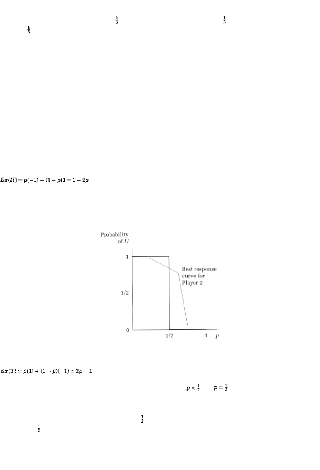
Again the intuition is that if player 2 plays a pure strategyno matter whether it is L or M1 or M2 or Rthere is
something that player I can do that would be terrible for player 2's payoffs. By mixing, player 2 can avoid a
disaster; no matter what player 1 does, of the time player 2 is very happy, of the time she is fairly happy,
and only of the time is she faced with a disastrous payoff of 0.
So this is the second of our three reasons.
Reason 2. The worst-case payoff of a mixed strategy may be better than the worst-case payoff of every pure
strategy.
8.5 Mixed Strategies and Nash Equilibrium
Without mixed strategies, Nash equilibria need not always exist. Recall the game of matching pennies:
H T
H1,-1 -1,1
T-1,1 1, -1
Note that
b1(H) = H and b1(T) = T, but b2(H) = T and b2(T) = H. So in this game (it appears as if) there is
no Nash equilibrium.
Suppose now that player I plays a mixed strategy: (H, p); that is, with probability p he plays H (and with
remaining probability 1 - p he plays T). Player 2's expected payoff from playing a pure strategy H is5
5Note that Ep(H) denotes the expected payoff to the strategy H.
page_111
Page 112
FIGURE 8.1
Likewise the payoff to playing T is
Evidently, H has a higher expected payoff than T if and only if . At both pure strategies yield the
same expected payoff, and hence by the implication of section 8.2, the best response of player 2 is any
mixed strategy. The best response can therefore be represented in Figure 8.1.
Hence, if player 2 were to play the strategy (H, ) herself, she would be playing a best response to the
strategy (H,
). In other words, this pair of mixed strategies constitute a Nash equilibrium.
The intuition for the preceding analysis is straightforward as well. In matching pennies no matter what pure
strategy combination we examine, one of the players always has an incentive to change his strategy; player 1
is always trying to match, while player 2 is always trying to mismatch. However, a mixed strategy can help.
If player 1 mixes between heads and tails (with equal probabilities), then player 2 can do no better by
switching from
H
to
T
(or vice versa). Half the time she inevitably matches in either case. A similar logi
c
applies to player 1's choices if player 2 mixes between H and T with equal probabilities.
This reasoning brings us to the final imperative for considering mixed strategies.
Reason 3. If we restrict ourselves to pure strategies, we may not be able to find a Nash equilibrium to a
game.
In Chapter 28, "Existence of Nash Equilibria" we will see a general result that says that in strategic form
games there is always a Nash equilibrium in mixed strategies.
page_112
Page 113
Despite all these arguments in favor of the use of mixed strategies, I should point out that many economists
and game theorists remain skeptical about their usefulness. Part of the skepticism stems from a belief that
people do not actually toss coins or use other forms of randomization in their day-to-day lives to make
decisions. (Do you?) Another reason to view Nash equilibria in mixed strategies with some skepticism is that
although individual players may in fact use mixed strategies, it seems heroic to assume that their opponents
are able to correctly conjecture the exact probabilities that are being used by those players. The Nash
equilibrium logic requires opponents to do just that.
There is an alternative interpretation of a mixed-strategy Nash equilibrium that was first pointed out by the
Nobel laureate John Harsanyi in 1973.
6 Imagine the following scenario: Each player is unsure about exactly
whom he is playing against. For instance, in a two-player game, player I may be unsure about player 2's
payoffs; these payoffs might be either p2 - b or p2 + b. Suppose a high-payoff player 2 is expected to play a
(pure) strategy s that is different from the (pure) strategy that a low-payoff player 2 is expected to playsay s'.
If high and low payoffs are equally likely, it is as if player 1 is facing a mixed strategy with equal
probabilities on s and s'. Although each player actually plays a pure strategy, to the opponentsand an outside
observerit appears as if mixed strategies are being played.
8.5.1 Mixed-Strategy Nash Equilibria in an Example
Consider the Battle of the Sexes. We have already seen that there are two asymmetric pure strategy Nash
equilibria in this game: (F, O) and (O, F) yielding payoffs of, respectively, (3, 1) and (1, 3). There is also a
symmetric Nash equilibrium in which both players play the same mixed strategy.
Suppose the wife plays F with probability q (and O with probability 1 - q).
COMPUTATION CHECK
Show that the husband's expected payoffs from playing F is 3q + 0(1 - q) = 3q.
And the expected payoff from playing O is 1(1 - q) + 0q = 1 - q.
These two payoffs are equal if 3q = 1 - q, that is, . By the implication of section 8.2, the husband will
mix only if , and at that point it is a best response for him to play any mix of F and O.
CHECK AGAIN
Similarly show that the wife is only willing to mix if her husband plays O with
probability .
6Harsanyi's article, "Games with Randomly Disturbed Payoffs: A New Rationale for Mixed
Strategy Equilibrium Points," appeared in the International Journal of Game Theory, vol. 2, pp.
1-23.
page_113
Page 114
In other words, a mixed-strategy Nash equilibrium is one in which each spouse plays his or her undesirable
actionO for the husband and F for the wifewith probability .
8.6 Case Study: Random Drug Testing
Random drug testing is a fact of corporate and sports life in many places. For example, in the United States,
81 percent of firms in 1996 had workplace drug testing. Among manufacturing firms, about 89 percent test
their employees, although less than 25 percent are required by law to do so.7 These tests seek to identify
employees who have been using illegal drugs and whose on-the-job performance could therefore be affected.
Sports organizations such as the NCAA, the U.S. Olympic Committee (USOC), and the International
Olympic Committee (IOC) also routinely test athletes. Typically athletes are selected at random at their
meets and subjected to a test that looks for the usage of performance-enhancing drugs, especially steroids.8
In this case, the objective is to weed out athletes who give themselves an unfair advantage and hurt the
credibility of the sport and its organizing body.
The outstanding feature of all these testing procedures is that they are random; a worker or athlete does not
know whether she is going to be tested, or when; the testing protocol is designed to maintain randomness and
an element of surprise.9 In other words, the firm or the sports body uses a mixed strategynot every athlete is
selected, and the ones who are, are notified only at the time of testing. The question is, Why a mixed
strategy?
To answer that question let us look at a very simple example of testing at a sports meet. Two
swimmersEvans and Smithare to participate in a runoff. Each athlete has the option of using a performance-
enhancing steroid (s) or not using it (n) before the meet. The two swimmers are equally good, and each has a
50 percent chance of winning, everything else being equal, that is, if neither uses steroids or they both do. If
only one swimmer uses steroids, then she will win. Without any IOC intervention, therefore, the payoff
matrix is as follows (we denote the payoff to winning as I and the payoff to losing as -1):
Evans \ Smith s n
s0,0 1,-1
n-1,1 0,0
where the expected payoff when the swimmers both do the same thing is computed as .
Note that s is a dominant strategy, and hence, without IOC intervention, both swimmer
s would use steroids.
Neither swimmer will be better off, and the IOC will acquire a disreputable stench on
ce word comes out
about the rampant drug use among its athletes. So the IOC needs to intervene.
7These numbers are from a survey of 961 companies conducted by the American Management
Association. For further details, consult Workplace Drug Testing and Drug Abuse Policies, AMA
Research mimeo, accessible at their website: amanet. org/ama/survey.
8For details on drug testing within the NCAA and the USOC consult ADR: Athletic Drug Reference, an
instructional report issued by a company called Helix and available at their web site, helix. corn.
Sports bodies typically use a combination of random testing and testing by position of finish. For
example, in the 1996 Summer Olympics swimming events, two of the top four finishers were tested as
well as some of the also-rans.
9The ADR guideline relates that upon (random) selection, an athlete has 60 minutes within which he or
she has to report to the drug-testing station. Throughout this time, an official stays with the athlete.
The test is conducted on a urine specimen, and dehydration is no excuse for delaying the test; the rules
require that the athlete remain at the testing station and be pumped full of fluids till the job is done!
page_114
Page 115
To begin with, suppose that the IOC can test only one swimmer. So the choices are (a) test Evans, (b) test
Smith, or (c) use a mixed strategy and test Evans with probability p (and Smith with probability 1 - p). In
fact, let us keep the third option simple and symmetric: take . Let us keep the IOC's payoffs simple as
well; if the tests uncover drug use, the IOC looks vigilant (and improves its reputation), and if the tests turn
up negative, then the IOC's reputation remains unchanged. The former will be given a payoff of I and the
latter a payoff of 0. Finally, if a swimmer tests positive she faces a penalty, and this penalty is typically
worse than simply losing; let this payoff be denoted -(1 + b), where b > 0. Also the race is awarded to the
other swimmer. All of this gives us the following payoff matrices for the three playersEvans, Smith, and the
IOC:
Evans \ Smith s n Evans \ Smith s n
s-1 - b, 1, 1 -1 - b, 1, 1 s1, -1 - b, 1 1, -1, 0
n
-1, 1, 0
0, 0, 0
n
1, -1 -
b
, 1
0, 0, 0
IOC Tests Evans IOC Tests Smith
Let us start with the two (pure) strategies of the IOC. If they test Evans for sure, then we are in the first
matrix. It is easy to see that Evans has a dominant strategynand so does Smiths. Exactly the opposite is true
if Smith is tested for sure. So the outcome is that the swimmer who knows she will be tested stays away from
drugs, but the other swimmer uses steroids. Over time the IOC's reputation suffers.
Consider instead the mixed strategy. We claim that now n is a dominant strategy for both players.
CONCEPT CHECK
TO DOPE OR NOT TO DOPE
(a) Show that Evans' expected payoffs from playing n are 0, regardless of
whether Smith plays s or n. (b) On the other hand, Evans' expected payoffs
from playing s are , regardless of what Smith plays.
So (n, n) for the two swimmers and random testing for the IOC is a Nash equilibrium.10 This outcome is
better for the IOC than testing both swimmers because it achieves the same desired objective (no doping)
and costs less.
Summary
1. A mixed strategy is a probability distribution over a player's pure strategies; not every pure strategy need
be included in every mixed strategy.
10Make sure you understand why random testing is a best response for the IOC.
page_115
Page 116
2. The payoff to a mixed strategy is computed as the expected payoff to its component pure strategies.
3. A mixed strategy is a best response if and only if every one of the pure strategies in its support is itself a
best response.
4. A mixed strategy can dominate a pure strategy even if the latter is undominated by every other pure
strategy.
5. The worst-case payoff to a mixed strategy can be better than the worst-case payoff to every pure strategy.
6. There are games with no Nash equilibrium in pure strategies, but there will always be such an equilibrium
in mixed strategies.
7. Random drug testing is a cost-effective way to ensure a desirable no-doping outcome on the part of
employees and athletes.
Exercises
Section 8.1
8.1
Consider a game in which player I has three pure strategies s', s#, and s*.
a. Write down the three mixed strategies that correspond to these pure strategies.
b. Write down the mixed strategy that corresponds to the case in which s' is twice as likely as either s# or s*.
c. Write down the mixed strategy that corresponds to the case in which s' is three times as likely as s#, which
in turn is twice as likely to be played as s*.
Consider the following game:
1 \ 2 L R
s
'
-1, 3
6, 2
s#5, 0 -2,5
s*0, 9 4,9
page_116
Page 117
8.2
Suppose that player 2 plays L for sure.
a. Compute the expected payoff of player I from the mixed strategy in part b of exercise 8.1.
b. Repeat the exercise for part c of exercise 8.1.
8.3
Suppose that player 2 is equally likely to play L as she is to play R.
a. Repeat parts a and b of exercise 8.2.
b. In exactly the same circumstances, compute the expected payoffs of player 2.
8.4
Suppose instead that player 2 plays L with probability p and B with probability I - p.
a. Repeat exercise 8.3 for this case.
b. Can you give the general formula for the expected payoffs of the two players when, additionally, player 1
plays s', s#, and s* with probabilities q, r, and 1 - q - r respectively?
And now, yet again (!) we return to the price competition game, this time from the standpoint of mixed
strategies. Recall that we have two (duopoly) firms that set prices in a market whose demand curve is
where p is the lower of the two prices. If firm 1 is the lower priced firm, then it meets all of the demand; the
converse applies if firm 2 is the one that posts the lower price. If the two firms post the same price p, they
each get half the market . Suppose that prices can only be quoted in dollar units and that costs of
production are zero for both firms.
8.5
Write down the mixed strategies that correspond to the following randomizing procedures for firm 1:
a. Roll a die and post as price the number that shows up on the die roll.
b. Roll a die twice and post the average of the two numbers provided it is a round dollar figure; otherwise,
post the nearest round dollar figure above the average.
c. Roll a die twice and post the higher of the two numbers that show up on the two rolls.
page_117
Page 118
8.6
a. What is firm 1's expected profit in the three preceding mixed strategies if firm 2's price equals 3?
b. What is firm 2's expected profit in the three cases?
8.7
What are the two firms' expected profits if

a. Firm I plays the mixed strategy of exercise 8.5a, while firm 2 plays the mixed str
ategy given by exercise
8.5b?
b. Firm I plays the mixed strategy of exercise 8.5c, while firm 2 plays the mixed strategy given by exercise
8.5b?
Section 8.2
8.8
Illustrate the implication from section 8.2 by using exercises 8.2 and 8.6. In each case, what is player 1's best
response strategy?
8.9
Give a complete proof of the implication.
Section 8.3
Let us return to the pricing game. Suppose that we want to iteratively eliminate dominated strategies in this
game but we look at mixed as well as pure strategies.
8.10
Show that if a mixed strategy q yields an expected payoff that is at least as high as that from another mixed
strategy p, against every pure strategy of the other player, then it must also yield as high a payoff against
every mixed strategy of the other player. Conclude that we only need to check how each strategy does
against the pure strategy prices 0 through 6.
8.11
Use exercise 8.10 to show that any mixed strategy that places positive probability on a price of six
dollarsthat is, a mixed strategy p in which the probability p6 > 0is dominated. Explain carefully the strategy
that dominates p.
8.12
Can you show that, as a consequence, any mixed strategy that places positive probability on a price of five
dollarsthat is, a mixed strategy p in which p5 > 0is dominated as well.
page_118
Page 119
8.13
What is the outcome to IEDS in this game? Explain your answer carefully.
8.14
Show that if there is a pure strategy that dominates every other pure strategy, then it must also dominate
every other mixed strategy.
8.15
Show that if there is no dominant pure strategy, then there cannot be a dominant mixed strategy either. (You
may want to use some game examples to illustrate your answer to this question.)
Section 8.4
Consider the game of squash:
Forward (F) Backward (B)
Front (f).2 .8
Back (b).7 .3
8.16

a. What percentage of the rallies do you expect to win if you are twice as likely to
pick
f
as you are to pick
b
and your opponent goes forward?
b. What if he goes backward?
c. What is the minimum percentage that you will win from playing this mixed strategy?
8.17
Repeat exercise 8.16 for the case that in four out of ten rallies you pick f.
Section 8.5
8.18
Find mixed-strategy Nash equilibria in the game of Chicken (example 2, p. 106).
8.19
Are there any mixed-strategy Nash equilibria in the No-Name game of Example 3? Explain.
page_119
Page 120
Consider the following three-player game:
1 \ 2 s n 1 \ 2 s n
s1, 1, 1 -1, -2, -1 s-1, -1, -2 1, -1, 0
n-2, -1, -1 1, 1, -1 n1, -1, 1 0, 0, 0
3 Plays s 3 Plays n
8.20
a. Is there an equilibrium in which only one of the three players plays a mixed strategy (and the other two
play pure strategies)? Explain your answer.
b. Repeat part a for the case in which exactly two of the three players play mixed strategies.
8.21
Compute a Nash equilibrium in which no player plays a pure strategy and they all play identical strategies.
page_120
Page 121
Chapter 9
Two Applications: Natural Monopoly and Bankruptcy Law
This chapter will present two applications of mixed-strategy Nash equilibrium. Both have at their core the
game of Chicken (aka Hawk-Dove) that you have seen in previous chapters. In section 9.1, we will review
that game and find a ''plausible" symmetric equilibrium that requires mixed strategies. In section 9.2 we will
provide economic background for the problem of a natural monopoly and then use two extensions of
Chicken to analyze that problem. In section 9.3 we turn to bankruptcy law and give legal background for
something called voidable preference law. Then we will present a game-theoretic analysis of this law, first
by way of a numerical example and then via a general model.
9.1 Chicken, Symmetric Games, And Symmetric Equilibria
9.1.1 Chicken
Recall the game of Chicken, introduced in Chapter 3 with an example of two daredevil drivers and retold in
Chapter 5 with the two fighting spiders. Let us now write the payoffs using symbols rather than actual
numbers.
Chicken (t=tough, c=concede)1
Player 1 \ Player 2 t c
ta, a d, 0
c0, d b, b
1This chapter will refer to this game as Chicken rather than Hawk-Dove.
page_121
Page 122
where d > b > 0 > a. In other words, as a group, the players are better off if both concede rather than if both
act tough (b > a). However, if the other player is going to concede, then a player has an incentive to be
tough (d > b)and, conversely, against a tough opponent conceding is better than fighting (0 > a).2 The
numerical version used in previous chapters was d = 10 > b = 5 > 0 > -1 = a.
This discussion should convince you that there are exactly two pure-strategy equilibria in this game; one of
the players concedes, while the other acts tough.3 Their payoffs are respectively 0 and d.
There is also a mixed-strategy equilibrium in this game, and let us now compute it. Suppose that player 2
plays t with probability p (and c with probability 1 - p). Then the expected payoffs of player 1 from playing t
are ap + d(1 - p) and from playing c are b(1 - p). By the implication of Chapter 8, it follows that in a mixed-
strategy best response of player 1, the two pure strategies must give him the same expected payoffs. Hence,
the probability p must satisfy
After collecting terms, we get and hence . Furthermore, by the same implication, if player
2 plays t with probability , then any mixed strategy is a best response for player 1; in particular, the
mixed strategy in which player 1 plays t with exactly the same probability is a best response. Hence, we
have the following:
Mixed-Strategy Nash Equilibrium. There is a mixed-strategy equilibrium in which the two players play
identical strategies; each plays t with probability .
The expected payoffs are the same for the two players and equal , a number between the two
pure-strategy payoffs of 0 and d.
In the numerical version, each plays t with probability and c with probability , and the expected payoff is
for each player (while in the pure-strategy equilibria, the tough player gets 10 and the weakling gets 0).
9.1.2 Symmetric Games and Symmetric Equilibria
Symmetric game
A game is symmetric if each player has exactly the same strategy set and the
payoff functions are identical.
A game such as Chicken is called a symmetric game. Roughly speaking, a symmetric game is one in which
each player is equal to every other player: each has the same opportunities, and the same actions yield the
same payoffs. Equivalently, you can think of a symmetric game as one in which the players' names are
irrelevant and only their actions are relevant.
By identical payoff functions we mean that, if player i plays while the others play , then i's payoff
does not depend on who she is that is, does not depend on whether i = 1 or 3 or N. The definition is
a bit abstract. To better understand it, let us try it for two players.
2Strictly speaking, therefore, the relationships that need to be satisfied are d b and both b and 0
are bigger than a. For simplicity, we also assume that b > 0.

3These are the equilibria that were discussed for the fighting spiders in Chapter 5.
page_122
Page 123
Definition. A two-player game is symmetric if the strategy set is the same for each player, say (a, b, . . ., m).
Furthermore, if player 1 picks b and player 2 picks ethat is, if the strategy pair (b, e) is pickedthen player 1's
payoff is the same as player 2's would be under the pair (e, b).
An implication of the definition is that if they pick the same strategy, say, (m, m), then their payoffs are
identical. (Why?) As you can readily verify, Chicken is a symmetric game and so is the Prisoners' Dilemma.
On the other hand, the Battle of the Sexes is not a symmetric game, nor is Colonel Blotto.4
CONCEPT CHECK
SYMMETRY AND NO SYMMETRY
(a) Show that the Coordination game and the Bertrand game are symmetric.
(b) Show that neither the Odd Couple game nor the Veto Voting game of
Chapter 4 are symmetric.
Symmetric equilibrium
A Nash equilibrium in a symmetric game, whether pure or mixed, is said to be
symmetric if identical strategies are chosen by the players. Payoffs are
identical for all players in such an equilibrium.
The fact that each player in a symmetric game is identical to every other player motivates the definition of a
symmetric equilibrium, a Nash equilibrium in which every player has the same strategy.
Some game theorists argue that in a symmetric game, a symmetric Nash equilibrium is more compelling than
an asymmetric one. After all, if players are identical in every respect, why would they play in different
ways? Think of some of the motivating parables for Nash equilibrium. If there is preplay communication
between the players, it is likely that the player(s) who have low payoffs in an asymmetric equilibrium will
push instead for the symmetric mixed-strategy equilibrium that equalizes payoffs. If Nash equilibrium play
arises from rational introspection, then again it is likely that a player will expect his opponentthe twinto play
as he plans to play. And, finally, a symmetric equilibrium is more likely to be a focal point of a game.5
It should be clear that the mixed-strategy equilibrium in Chicken is a symmetric equilibrium but the
pure-strategy equilibria are not. And that difference makes the mixed-strategy equilibrium more plausible.
9.2 Natural Monopoly
9.2.1 The Economic Background
A natural monopoly is an industry in which technological or demand conditions are such that it is "natural"
that there be only one firm in the market. One technological reason for a natural monopoly to arise is seen
when the costs per unit of production decline with the size of output. This phenomenon might occur if there
are increasing returns to scale in production6 or if there are large unavoidable costs7 of doing business.8 A
4Colonel Blotto has different strategy sets for the two players. Battle of the Sexes has the same
strategy sets, but the payoff functions are not symmetric.
5After all, if there is one asymmetric equilibrium in a symmetric game, then there are at least as many
qualitatively identical asymmetric equilibria as there are players. (Why?) Consequently no single one
of these equilibria can be the focal point in players' minds.
6Increasing returns means that twice as much output can be produced with less than twice as much
input. Consequently, total costs do not double when total output is doubled.
7For instance, there may be a minimum size at which some inputs can be purchased; it may not be
possible to rent production space of size less than 10,000 square feet. Again, output can be doubled
without doubling input costs.
8The aircraft manufacturing industry is a technological natural monopoly because of the large
unavoidable costs associated with manufacturing planes (and possibly, because of increasing returns
as well). Perhaps unsurprisingly, there is now a single domestic manufacturer of large airplanes in the
United States (Boeing having taken over McDonnell Douglas).
page_123
Page 124
natural monopoly can also arise when demand is low (and consequently the only way to make any money is
to keep the price relatively high). Recall that duopoly competitionwhether Cournot or Bertranddrives down
the price.
The question that economists are most interested in is, How will a natural monopoly become an actual
monopoly? If we start off in an industry with two or more firms, which firms will drop out? In many cases
there are obvious candidates; firms with higher costs will be the first ones to leave. If a firm has "deep
pockets," then a rival will throw in the towel earlier. If the products are differentiated, then the firm with
greater demand is more likely to remain. And so on.
The question that remains is, How will a natural monopoly become an actual monopoly when, to begin with,
there are two (or more) essentially identical firms in the market?9
9.2.2 A Simple Example
Consider a duopoly that will last two more years, in which each firm is currently suffering losses of c dollars
per period. If one of the firms were to drop out, then the remaining firm would make a monopoly profit of p
dollars per period for the remainder of the two years. Each firm can choose when to drop out: today (date 0)
or a year from now (date 1), or it can stay till the end (date 2). Furthermore, each firm only cares about
profits.10 The payoff matrix is therefore
Firm 1 \ Firm 2 date 0 date 1 date 2
date 00, 0 0, p 0, 2p
date 1p, 0 -c, -c -c, p -c
date 22p, 0 p -c, -c -2c, -2c
Let us first look for pure-strategy Nash equilibria of this game. Note that b1 (date 0) = date 2, b1(date 1) =
date 2, and b1(date 2) = date 0.11 Firm 2 has an identical best response function.12 Consequently, there are
two asymmetric pure-strategy Nash equilibria in this game: one of the two firms drops out (i.e., concedes) at
date 0, and the other then remains in the market for the two years.
The problem is that there is no reason that firm I should think that firm 2an identical firmis going to concede,
especially since by conceding firm 2 would lose out on 2p dollars worth of profits.13
What of a symmetric mixed equilibrium? Let us turn now to that computation. Suppose that firm 2 plays
date 0 with probability p, date 1 with probability q, and date 2 with probability 1 - p - q. Firm 1's expected
profits from its three pure strategies are
Expected profits (date 0) = 0
Expected profits
Expected profits
9An industry where this question is immediately relevant is defense production. With the demise of
the cold war and the consequent decrease in military expenditures, there has been a substantial
reduction in demand. Will there be, for example, a single aircraft manufacturer to come out of a
current lineup that includes Martin Marietta, Lockheed, and Grumman? (After this chapter was
written, Martin Marietta and Lockheed did in fact merge to form Lockheed Martin.)
10These assumptions will all be relaxed in the more general analysis of the next subsection.
11We assume that p > c; that is, one monopoly period makes up for (the losses suffered in) a duopoly
period. If this were not the case, then b1 (date 1) = date 0. This change in the best response function
would not, however, affect the equilibria. (Why?)
12The game is in fact a version of Chicken. Think of date 0 as concede, date 2 as tough, and the
intermediate date 1 as medium. Now note that both conceding is better than both playing tough (or
medium). However, if the other player concedes then it is better to play mediumand better still to play
toughwhile concede is the best option against a medium or tough opponent.
13As always, if you are thereby more convinced of the magnitude of the loss, think of all the payoffs as
being in millions of dollars.
page_124
Page 125
If there is to be a mixed-strategy best response for firm I that involves all three dates, it must be the case that
each strategy yields the same expected payoff. This fact leads to the following exercise:
CONCEPT CHECK
EQUAL PROFITS
Show that firm I is indifferent about its date of exit only if (a) and (b) q
= 0
Hence, in particular, playing date 0 with probability and date 2 with remaining probability is a best
response for firm I as well. This then is the symmetric mixed-strategy Nash equilibrium: , q = 0, and
.
CONCEPT CHECK
OTHER EQUILIBRIA?
Convince yourselfby doing the necessary computations!that there are no other
mixed-strategy Nash equilibria; for example, none involving only dates 0 and
1.
Consider a numerical example; suppose p = 10 and c = 2. Then in the symmetric equilibrium, each firm
drops out with probability at date 0 itself. If a firm does not drop out at date 0, it remains till date 2.
Hence, with probability or both firms exit the market at date 0, with probability they both stay
the course, and with the remaining probability one or the other leaves at date 0.
Note that the first two outcomesboth leaving and both stayingare collectively unprofi
table; in the first case a
market that would be profitable for a monopoly is abandoned, while in the second case a market that is only
profitable for a monopoly remains a duopoly.14
9.2.3 War of Attrition and a General Analysis
In this subsection we show that the previous conclusiona firm will only consider the extreme options of
leaving immediately and leaving at the endcontinues to hold in a more general version of Chicken called the
War of Attrition.15 Suppose that instead of three dates, there are N + 1 dates; a generic date will be denoted
t. As before, a monopolist makes profits of p dollars per period, while a duopolist suffers losses of c dollars
per period. The payoff matrix is
14One interpretation of a mixed strategy is that it is based on events outside a firm's control. For
instance, a firm might believe that its rival will leave the market immediately if the Fed's projection
for GDP growth is less than 2 percent. If the firm further believes that there is a likelihood p of
such a projection, then it is as if it plays against a mixed strategy with probability p on date 0.
Alternatively, a firm may not know some relevant characteristic about its rival, such as costs. If it
believes that high-cost rivals will exit at date 0 but not low-cost ones and that the likelihood of high
costs is p, then again it is as if it faces a mixed strategy with probability p on date 0.
15War of Attrition was introduced by the biologist Maynard Smith, who used it to analyze the length of
animal conflicts.
page_125
Page 126
1 \ 2 date 0 date 1 . . . date t . . . date N
date 0 0, 0 0, p 0, tp 0, Np
date 1 p, 0 -c, -c -c, (t - 1)p - c -c, (N - 1)p -c
date t tp, 0 (t - 1)p - c, -c -tc, -tc -tc, (N - t)p - tc
date N Np, 0 (N - 1)p - c, -c (N - t)p - tc, -tc -Nc, -Nc
Notice that the War of Attrition retains the essential features of Chicken; both play
ers conceding
immediately is better collectively than both conceding simultaneously but later. If the rival concedes at date
t, and a firm is still in the market at that date, then it is best to go all the way to date N.
Let us first look at the pure-strategy Nash equilibria. Start with the best response function of firm 1. Suppose
that firm 2 is going to drop out at date t.
CONCEPT CHECK
BEST RESPONSE: STEP 1
Show that the best response to date t must be either date 0 or date N. The
former strategy yields a payoff of 0, while the latter yields a payoff of (N - t)p
- tc. Hence,
BEST RESPONSE: STEP 2
Show that the best response function of firm 1 is
The two best-response functions are pictured in Figure 9.1, where . It follows that even in this more
general game there are exactly the same two pure-strategy equilibria; one of the two firms drops out at date
0, but the other stays till date N.
What of symmetric mixed-strategy equilibria? In principle, a firm can exit the market at any date between 0
and N with positive probability. We will show, however, that a firm will never choose an intermediate date
at which to exit; either it will leave at date 0, or it will stay till date N. This conclusion will seem intuitive
given what we just saw about the best response functions. We have to be a little careful, however; the rival
can now play a mixed strategy, and the best response function that we have so far analyzed was only
computed against a pure strategy of the rival.
We will now prove the following:
page_126
Page 127
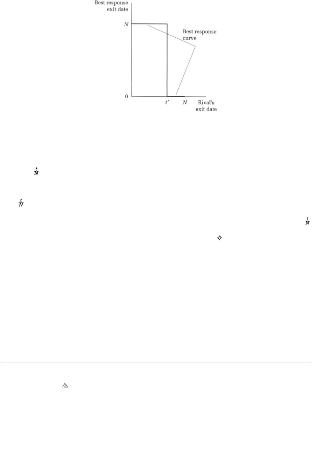
FIGURE 9.1
Dominance Proposition. very pure strategy other than date 0 and date N is dominated by some mixed
strategy that has date 0 and date N in its support.
Proof
Consider the pure strategy date t and compare it to the mixed strategy in which a firm plays date N with
probability and date 0 with the remaining probability. Suppose that its rival plays the pure strategy date t.
There are two cases to consider:
Case 1 t < t: In this case the pure strategy date t yields a payoff equal to (t - t)p - tc, while the mixed strategy
yields [(N - t)p - tc]. The mixed-strategy payoff is greater if t(N - t)p - ttc³ N(t - t)p - Ntc. Collecting and
eliminating common terms, that is equivalent to t(p + c) ³ 0, which is true.
Case 2 t³ t: Here the pure strategy date t yields a payoff equal to -tc, while the mixed strategy again yields .
[(N - t)p - tc]. The mixed-strategy payoff is greater if t(N - t)p - ttc ³ -Ntc. Collecting common terms, that is
equivalent to (N - t)(p + c), which is clearly true.16 The proof is complete.
Since the mixed strategy dominates the pure strategy, the latter will never be used in a best response even if
the rival firm plays a mixed strategy. (Why?) Hence, in order to compute the mixed-strategy equilibrium we
can concentrate on date 0 and date N alone. Put differently, qualitatively the same symmetric mixed-
strategy equilibrium that we computed in the previous subsection is the symmetric mixed-strategy
equilibrium of this general model as well.17
16Note the inequalities are strict of N > t > 0.
17We have assumed so far that a firm makes a once-for-all decision about its exit date. In practice, if
a firm finds itself as a monopoly, it should abandon any earlier commitment to drop out by date t and
instead should stay till date N. We can generalize the analysis to incorporate this possibility (see
Exercises). In this general analysis it is possible that a firm might stay till intermediate dates such as 1,
2, . . ., N - 1.
page_127
Page 128
9.3 Bankruptcy Law
9.3.1 The Legal Background
In the United States, once a company declares bankruptcy18 its assets can no longer be attached by
individual creditors. Instead they are held in safekeeping till such time as the company and the group of
creditors reach some understanding; the assets might get liquidated and creditors paid out of the proceeds, or
the creditors might refinance the failing company. The reason for this protection is to prevent creditors from
going into a reclamation frenzy that might dismember the remaining assets.19

Bankruptcy law actually goes even further. After all, if assets were only safeguarded
after
a company
declares bankruptcy, then individual creditors might have an incentive to attach assets just prior to that
declaration. Hence, in many instances, a firm is allowed to recapture any transfers it makes to creditors
within a 90-day period prior to bankruptcy (as long as it can show that it was insolvent during that period).
These recapturable transfers are called voidable preferences. The traditional legal view of voidable
preferences is that they strengthen bankruptcy law's protection of creditor assets.
As you might have begun to see already, this issue has elements of the tragedy of the commons problem.
Voidable preference law appears to be an attractive way to avert a tragedy, that is, the dismemberment of
the company's assets (which are jointly the property of all of its creditors). In this section, we will analyze
the question, Is it really?
9.3.2 A Numerical Example
Suppose that a company has assets valued at 15 (million) dollars. There are three creditors; for simplicity
suppose that each creditor has lent 10 dollars to the company. The company's assets are therefore less than
its liabilities. If the company declares bankruptcy, then its assets are liquidated (and each creditor gets 5
dollars back). Since recovery of loans from this bankrupt company is partial, each creditor has an incentive
to try to recover his own loan. He can do so by conducting a fire sale that will yield 12 dollars (i.e., 3 dollars
worth of assets will be dismembered).
Suppose that each creditor has to decide today whether or not to try to recover his loan. If two (or three)
creditors make such an attempt, then the company goes into immediate bankruptcy, voidable preference law
kicks in, and the proceeds of the fire sale are split between the three creditors; each receives 4 dollars. If
only one creditor tries to preemptively attach the company's assets, she is successful; in this case, the
company declares bankruptcy at some later date and distributes the proceeds of the remaining assets, 2
dollars, among the other two creditors. Similarly if no creditor preempts, then again the insolvent company is
sold at a later date and the proceeds distributed among the creditors, except now each creditor gets a third of
the original assets; that is, each gets 5 dollars.
18A company declares bankruptcy (becomes insolvent) if its assets are less than its liabilities (to its
creditors).
19The discussion in this section is based on "A Reexamination of Near-Bankruptcy Investment
Incentives" by Barry Adler, 1995, University of Chicago Law Review, vol. 62, pp. 575-606. I thank my
colleague Chris Sanchirico for drawing my attention to this paper.
page_128
Page 129
The payoffs to an individual creditor can therefore be written as
Number of other creditors grabbing
0 1 2
grab10 4 4
refrain5 1 4
It is easy to see that refrain, which is collectively the best thing to do, is dominated by grab. Hence there
will be a mad dash by creditors to collect their share of the company's assets, the assets will be dismembered,
and each creditor will end up with only 4 dollars. Voidable preference law in this case has no deterrent effect
whatsoever. (After all, there are no rewards to refraining; either it leaves a creditor with a stripped company
[if one other creditor grabs], or it yields only a third rather than two-thirds of the company [if nobody else
grabs].)
You might think that there must be some benefits to being the nice guy if recovering assets is costly. (After
all, creditors have to pursue the company to pay them back; they may have to move the courts to get
payment; etc.) It would appear that in this case refrain may sometimes be a smart strategy.
Suppose that it costs a creditor I dollar to institute recovery proceedings, regardless of whether recovery is
successful or not. The payoff matrix is now
Number of other creditors grabbing
0 1 2
grab9 3 3
refrain5 1 4
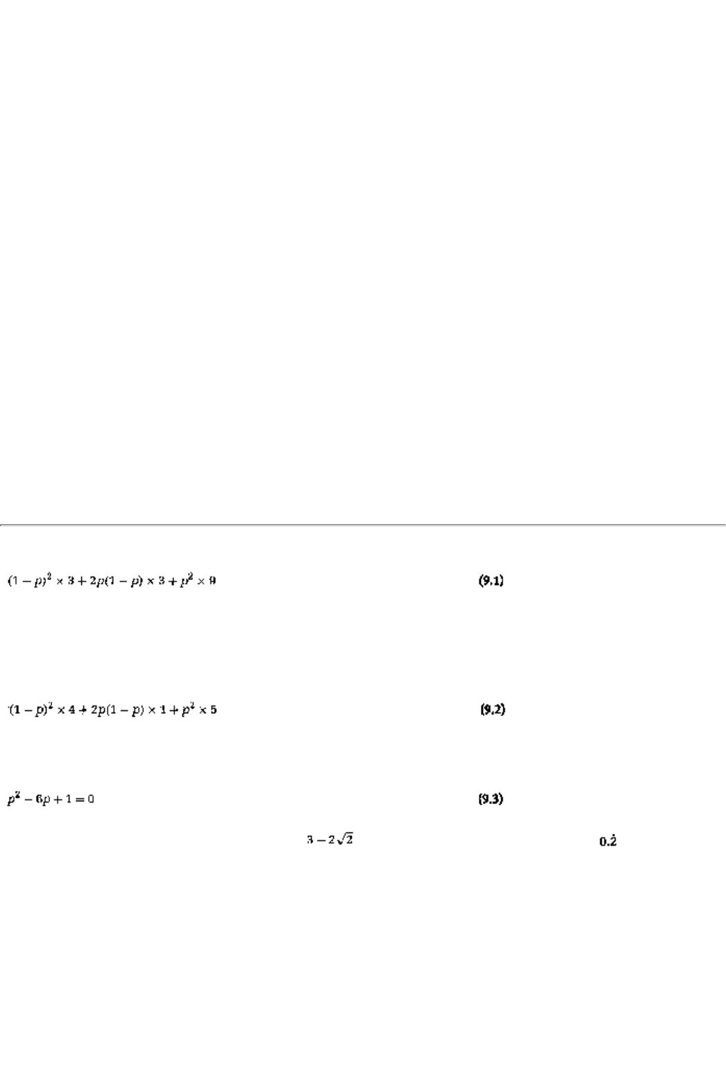
Note that the payoff to
grab
has been reduced by 1 dollar across the board. Now
grab
is no longer a
dominant strategy. In fact we now have a generalized version of Chicken.20 Everybody grabbing (i.e.,
acting tough) is worse than everybody refraining (i.e., conceding), since the former yields a payoff of 3 each
while the latter yields 5 each. However, if at least one of the other players concedes, then it is better to be
tough than to concede; conversely, if the other two creditors are tough it is better to concede.
Pure-Strategy Equilibria
There are three Chicken-like pure-strategy equilibria; exactly two creditors grab and dismember the
company's assets, voidable preference kicks in, and they have to return the seized assets. Each creditor ends
up with a third of the reduced asset base. Interestingly, the creditor who sits out the fight ends up with a
higher net payoff because he avoids the costly recovery process.21
Mixed-Strategy Equilibrium
As always, in this symmetric game a more plausible equilibrium is the symmetric mixed-strategy equilibrium.
Suppose that each of the other creditors refrains with a probability p (and grabs with probability 1 - p).22
Then the expected payoff to grab is
20Note that in the natural monopoly problem we looked at a generalization of Chicken in which
each player has more than two strategies. Now we are looking at a generalization in which there
are more than two players.
21Another way of saying the same thing is that the asymmetric equilibria in Chicken can have the
weakling do better than the tough players when there are more than two players. This outcome can
occur because the tough guys fight each other and expend resources in doing so.
22Since we are looking for a symmetric equilibrium, we can restrict attention to the case in which the
other two creditors use the same mixed strategy.
page_129
Page 130
In equation 9.1 we have used the fact that the probability that neither of the other two creditors refrains is
(1 - p)2, the probability that exactly one of the other two creditors refrains is 2p(1 - p), and, finally, the
probability that they both refrain is p2. Equation 9.1 can be rewritten as 3 + 6p2. On the other hand, the
expected payoff to refrain is
Equation 9.2 can be simplified to 4 - 6p + 7p2. Equating the two expected payoffs, we can see that p is the
solution to the following quadratic equation:
By standard techniques23 p is found to equal ; that is, p is approximately equal to . Put another
way, there is an 80 percent chance that each creditor will grab and hence only a 0.23 (or less than 1%)
chance that everybody will refrain. Voidable preference law is therefore spectacularly unsuccessful in
achieving its stated purposes, since 99 percent of the time the company's assets are dismembered.
9.3.3 A General Analysis
In this subsection we will present a general analysis of voidable preference law. To keep the game symmetric
we will retain the assumption that there are three creditors who have identical debts outstanding and
identical costs of collecting. We will also retain the assumption that an attempt by two or more creditors to
collect sends the company into immediate bankruptcy.
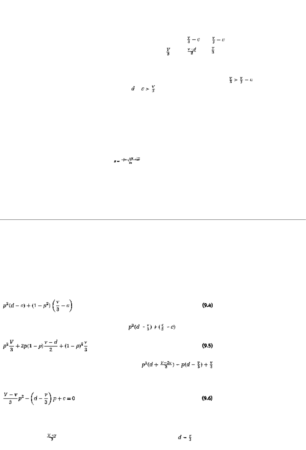
Suppose that each creditor is owed d dollars, and the value of the firm's assets is
V
dollars. The firm is
insolvent in that 3d > V. If one or more creditors attempt to collect, they reduce the firm's assets to v dollars;
that is, the size of the dismemberment is V - v. Finally, the costs of collection are c dollars. The payoff matrix
is therefore
Number of other creditors grabbing
0 1 2
grabd - c
refrain
Again this is a Chicken game; it is collectively better for all three creditors to refrain than for all three to
grab
(V > v - 3c). If two other creditors are going to grab, then it is better not to ( ). Finally, assume
that it is better to grab if nobody else does24 ( ).
Pure-Strategy Equilibria
There are two possibilities for pure-strategy equilibria. If the best response to one other creditor grabbing is
to grab as well, then the equilibria are exactly two creditors grab. If, however, the best response is to
refrain, then the equilibria are exactly one creditor grabs. Notice that in either case the company's assets are
dismembered.
23For the quadratic function ax2 + bx + c the two values at which the quadratic function equals
zero can be found from the formula .
24If the opposite is true, that is, if the costs of collection c are so high that it is better to refrain even if
the others are refraining, then a pure-strategy Nash equilibrium is for everyone to refrain. In this case
the firm does not need the protection of bankruptcy law because its creditors have no incentive to strip
the company's assets.
page_130
Page 131
CONCEPT CHECK
PURE EXERCISE
Show that these are indeed the only two possibilities and, in particular, that
there is no symmetric pure strategy equilibrium.
Mixed-Strategy Equilibrium
Suppose that each of the other two creditors refrains with probability p. The expected payoff to grab is then
Equation 9.4 can be simplified and written as . The expected payoff to refrain is
Equation 9.5 can also be simplified and written as . An individual creditor will play
a mixed-strategy best response if grab and refrain are equally profitable, that is, if the expressions in
equations 9.4 and 9.5 match. Equating them and simplifying we get a quadratic equation in p:
Equation 9.6 is worth spending a few moments on.
Relevant Parameters. Three intuitive parameter combinations decide the size of p: (1)
the per-creditor size of
dismemberment (denote this D), (2) the size of insolvency (call this I),25 and (3) the collection
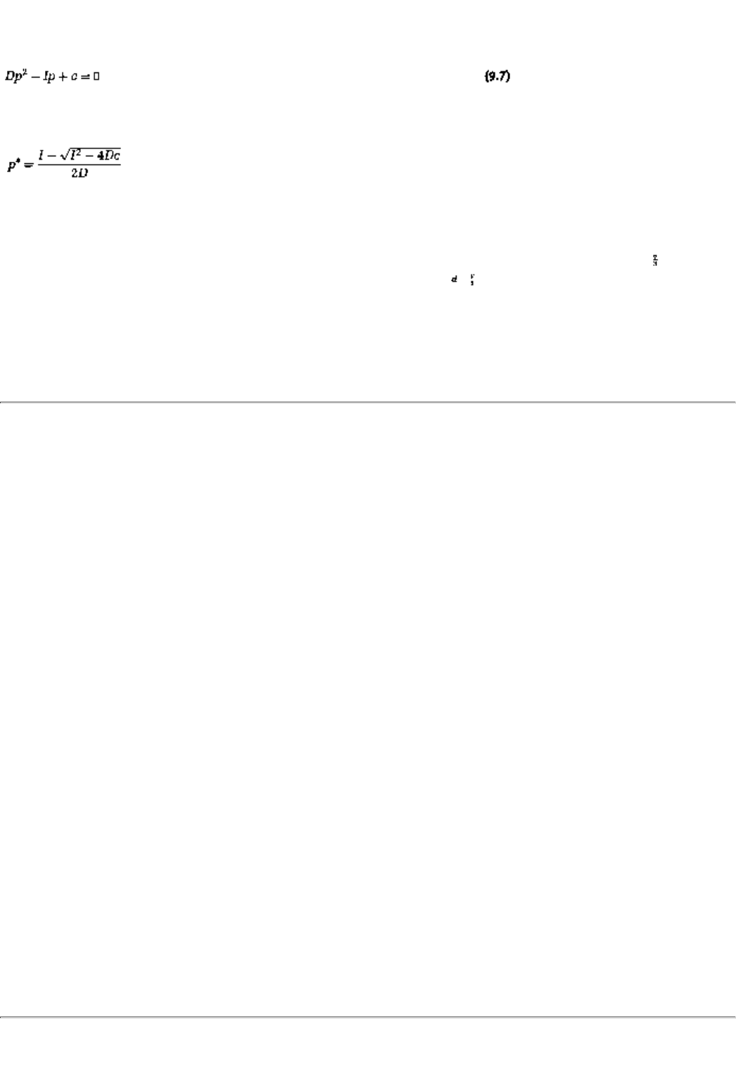
costs c
.
In terms of our new and simpler notation, equation 9.6 can be rewritten as26
This quadratic equation can be solved to yield the equilibrium probability p*:
It is straightforward now to figure out how p* might change if any one of the three
determinantsdismemberment D, insolvency I, or collection costs cchanges.
25Recall that the firm's liability toward each creditor is d. A dismembered firm will return dollars
to each creditor. Hence, the per-creditor size of insolvency is
26Be sure to check the general formula of equation 9.5 against the numerical version of the previous
subsection. In that case, what was the value of D? I? c? (How) Does equation 9.6 generalize equation
9.3?
page_131
Page 132
CONCEPT CHECK
MIXED EXERCISE (CALCULUS)
Show that if the size of dismemberment D or collection costs c are higher,
then refraining is more likely; that is, p*is larger. Similarly, if the size of
insolvency I is smaller, then again refraining is more likely.
The result should be intuitive. If a creditor figures that her costs are small, or that she will not destroy too
much of the assets, or that her loans are very large relative to the firm's assets, she will be more aggressive in
trying to recover her loans. Note that bankruptcy (and voidable preference) law becomes more successful as
a deterrent as the value of p* becomes larger. Put differently, the law only works if collection or
dismemberment costs are very high and the size of insolvency is very small.
Summary
1 A symmetric game is one in which all players are identical in their choices and payoff functions. A
symmetric equilibrium is one in which all players take identical actions.
2. The game of Chicken is a symmetric game. Its symmetric equilibrium is in mixed strategies.
3. Natural monopoly is a market in which economic reasons suggest that there should be only one firm. For
instance, it may be unprofitable for two or more firms to operate at the same time.
4. A generalized version of Chicken can be used to analyze the behavior of firms in a natural monopoly. In a
symmetric equilibrium, a firm will choose probabilistically between its extreme optionsleave immediately or
never.
5. Bankruptcy law, via voidable preferences, seeks to protect an insolvent company's assets against
predatory creditors.
6. A generalized version of Chicken can be used to analyze the behavior of creditors in the presence of such
a law. The law is successful only if the cost of collection or asset dismemberment is high and less successful
if insolvency costs are high instead.
page_132

Page 133
Exercises
Section 9.1
9.1
Consider the following symmetric game:
Player 1 \ Player 2 t c
t-5, -5 d, 0
c0, d 10, 10
Find the symmetric equilibrium of this game. Be careful to spell out any assumptions that you make about
the value of d.
9.2
Consider the payoff matrix of any 2 × 2 game, that is, any game with two players and two pure strategies:
Player 1 \ Player 2 t c
ta, a d, e
ce, d b, b
a. Write down parameter restrictions so that (t, t) is a symmetric Nash equilibrium.
b. Under what restrictions, can (c, c) be a symmetric Nash equilibrium? Are the restrictions in parts a and b
compatible with each other; that is, can such a game have multiple pure-strategy symmetric Nash equilibria?
9.3
Keep the parameters d and e fixed; that is, consider the same payoff matrix with two free parameters a and b
that can take on any values.
a. Suppose that a > e and d > b. What is the symmetric Nash equilibrium in this case?
b. Repeat the question when a > e but d > b. Be sure to check for more than one symmetric Nash
equilibirum in this case.
c. In this fashion map out the entire set of symmetric equilibria in this game. Can you draw a figure, with the
parameters a and b on the two axes, that shows the symmetric equilibria for each parameter combination?
9.4
Write down modifications of Battle of the Sexes, Colonel Blotto, and the Odd Couple games that would turn
them into symmetric games. Be careful to spell out in detail all the changes that you make.
page_133
Page 134
9.5
Consider the definition of a two-player symmetric game. Using the definition, prove the following statement
in a semirigorous fashion: If the two players play identical actions, they get exactly the same payoff.
9.6
Consider a symmetric game. Prove the following statement in a semirigorous fashion: If there are any
asymmetric equilibria in the game, then there have to be at least as many asymmetric equilibria as the
number of players.
Section 9.2
9.7
Consider the following numerical version of the natural monopoly problem:

Firm 1 \ Firm 2
date 0
date 1
date 2
date 00, 0 0, 15 0, 30
date 115, 0 -5, -5 -5, 10
date 230, 0 10, -5 -10, -10
a. Compute the symmetric equilibrium.
b. What is the expected payoff of each firm in equilibrium?
c. What is the probability that exactly one of the firms will drop out of the market at date 0 in the symmetric
equilibrium?
9.8
a. Redo parts a and b of exercise 9.7 but with an increase in the costs of staying from 5 dollars to 10 dollars,
so that the payoff matrix becomes
Firm 1 \ Firm 2 date 0 date 1 date 2
date 00, 0 0, 15 0, 30
date 115, 0 -10, -10 -10, 5
date 230, 0 5, -10 -20, -20
b. How does this cost increase affect the probability that exactly one firm exists on the market at date 0?
Explain.
9.9
Consider instead the general model studied in the text:
page_134
Page 135
Firm 1 \ Firm 2 date 0 date 1 date 2
date 00, 0 0, p 0, 2p
date 1p, 0 -c, -c -c, p -c
date 22p ,0 p -c, -c -2c, -2c
a. In the symmetric mixed-strategy equilibrium of this game, can you tell whether dropping out at date 0 is
more likely if costs c increase? Explain your answer.
b. How is the probability that exactly one firm drops out at date 0 affected if c increases? What about the
probability that at least one firm drops out?
c. Does an increase in c make a monopoly more likely? Explain.
9.10
a. Redo exercise 9.9 for the case where c is unchanged but the profits p increase.
b. Is there a sense in which an increase in costs and a decrease in profits have exactly the same effect on
market outcomes, that is, exactly the same effect on the symmetric equilibria of the game? Explain your
answer.
The next few questions will explore the interpretation that date t really is the following strategy: ''If my
opponent has not dropped out by date t - 1, then I will drop out at t; otherwise I will continue till the end."
9.11
a. Argue that the consequent payoff matrix when there are three exit dates becomes
Firm 1 \ Firm 2 date 0 date 1 date 2
date 00, 0 0, 2p 0, 2p
date 12p, 0 -c, -c -c, p -c
date 22p, 0 p -c, -c -2c, -2c
b. What are the pure-strategy Nash equilibria of the game?
9.12
Compute the symmetric mixed-strategy equilibrium of this game.
9.13
a. How do the expected payoffs in this symmetric equilibrium compare with the one that follows from
exercise 9.9?
b. What about the probability that at least one of the firms drops out at date 0?
page_135
Page 136
Section 9.3
9.14
Consider the bankruptcy model. Show that grab always dominates refrain as long as collection is costless;
this statement is true no matter what size the outstanding debt is, what the company's assets are, and how
much is dismembered in the attachment process.
9.15
(How) Would your answer change if the company's assets are so low that the attempt by even one creditor
to attach his loan drives the company into immediate bankruptcy? What if up to two creditors can recover
their loans before the company has to file for bankruptcy? Explain your answers carefully.
9.16
Consider the following bankruptcy model (with collection costs of two dollars):
Number of other creditors grabbing
0 1 2
grab8 2 2
refrain5 1 4
a. Compute the symmetric mixed-strategy equilibrium.
b. Compare the probability that each creditor refrains with the probability that was derived in the text.
Explain your answer.
c. How successful is voidable preference law as a deterrent in this case?
9.17
a. Redo exercise 9.16 for collection costs of four dollars.
b. How high would the costs need to be for all three creditors to refrain from stripping the insolvent
company's assets?
Now consider the general bankruptcy model:
Number of other creditors grabbing
0 1 2
grabd - c
refrain
9.18
a. Write down a parameter configuration in which all creditors refraining is a symmetric Nash equilibrium.
b. Similarly find parameter restrictions so that only one creditor grabbing is a Nash equilibrium.
page_136

Page 137
c. Are the restrictions in parts a and b compatible; that is, can there be a model in which there are two
symmetric Nash equilibria?
9.19
Can you think of any changes in the law that would make creditors less likely to strip the assets of an
insolvent company? Explain.
page_137
Page 139
Chapter 10
Zero-Sum Games
In this chapter we will discuss two-person zero-sum or strictly competitive games. Section 10.1 will formally
define this category of games and present several examples. Section 10.2 will discuss a conservative
approach to playing such a game and define a related concept called a security strategy. Section 10.3 will
revert to the by now more familiar best-response approach and show that a player can do better with this
approach than the conservative one. Finally, in section 10.4, you will see that when both players play a best
responsethat is, when we are in a Nash equilibriumthen, surprisingly, the two approaches to playing a
zero-sum game turn out to be equivalent.
10.1 Definition And Examples
Zero-sum game
A zero-sum game is one in which the payoffs of the two players always add up
to zero, no matter what strategy vector is played; that is, for all strategies s1
and s2, p1(s1, s2) + p2(s1, s2) = 0
In a (two-player) zero-sum game the payoffs of player 2 are just the negative of the payoffs of player 1.1
Consequently, the incentives of the two players are diametrically opposedone player wins if and only if the
other player loses. Most games that are actual sporting contestssuch as card games, chess, one-on-one
basketballare, therefore, zero-sum games. Two economic applications that are zero-sum games are (1) the
transaction between a buyer and a seller, say, on a house or a used car, and (2) the battle for market share by
two firms in a market of fixed size.2
Many economic applications are, on the other hand, not zero-sum games; the Cournot duopoly model, the
commons problem, and the natural monopoly problem, for instance, are not zero-sum games. In the Cournot
problem, collective profits are highest if total production is at monopoly level, but these profits are a lot
lower if each firm overproduces. In the natural monopoly problem, if both firms remain in the market, they
lose money, but it is profitable for only one of them to remain.
1Zero-sum games are studied only in the case where there are two players. Hence, we will say
"zero-sum game" rather than "two-player zero-sum game" whenever we refer to this category of
games.
2Assume for the first example that the payoff to a buyer is his valuation of the car minus the price
while the payoff to the seller is the price minus the seller's valuation. For the second example, assume
that, since the market is of fixed size, so also is the total profit (of the two firms). Under these
assumptions, the payoffs of the two players always add up to a constant number. We will see in a short
while that such a situation can be effectively reduced to a zero-sum game.
page_139
Page 140
Zero-sum games are more important, perhaps, because of the historical role they have
played in the
development of the subject; that, by itself, is a reason to discuss them. A second reason is that several
concepts that were first introduced for zero-sum games have turned out to be very useful for non-zero-sum
games as well. In the course of this chapter (and the exercises that follow) we will try to point out which of
the results and concepts of zero-sum game theory are valid even outside its confines.
Here are two examples of zero-sum games, one that you have already seen and another that you have not:
Example 1: Matching Pennies
1 \ 2 H T
H1, -1 -1, 1
T-1, 1 1, -1
Example 2
1 \ 2 L C R
U5, -5 8, -8 4, -4
M-7, 7 9, -9 0, 0
D9, -9 1, -1 -2, 2
One example that we will use extensively is the squash game of Chapter 8:3
Example 3: Squash
1 \ 2 Forward (F) Backward (B)
Front (f)20, 80 70, 30
Back (b)90, 10 30, 70
Constant-sum game
A constant-sum game is one in which the payoffs of the two players always
add up to a constant, say b, no matter what strategy vector is played; that is,
for all strategies s1 and s2, p1(s1, s2) + p2(s1, s2) = b
where in each cell, the entries are, respectively, the winning percentages of players I and 2. Example 3 is an
example of a related class of games that look, smell, and talk much like zero-sum games. These are called
constant-sum games. In these games, the two payoffs always add to a constant.
In the game of squash, that constant is 100. Note that if we subtract the constant out of the payoffs, the
game would become zero-sum. Furthermore, the players would play this zero-sum transformation exactly the
same way that they would play the original constant-sum game.
To see all this, subtract the constant b from every payoff of player 1. In other words, suppose the new
payoffs are for all pairs (s1, s2). Evidently this new game is zero-sum because
.
Would player 1 behave any differently if her payoffs are instead of p1? The answer is no because and
p
1 represent exactly the same set of preferences: if a strategy s is preferred to s' under p1, then it is also
preferred under . Indeed that statement is
3For variety's sake we have changed the payoffs just a little bit.
page_140
Page 141
true for mixed strategies as well. Consider a pair (p1, p2), p1 being a mixed strategy of player 1 and p2 that
of player 2:
CONCEPT CHECK
JUST SUBTRACT A CONSTANT
Show that the expected payoffs under
are nothing but the expected payoffs
under p1 less the constant b, that is,
Hence, if p1 is preferred to p1' under , then so must it be preferred under p1. (Why?) Another way of
thinking about it is to interpret the payoff as p1 with an additional penalty -b; this is a penalty that player I
pays regardless of what she does. Such an indiscriminate penalty therefore does not influence her decision
making in any way.
From this point on the discussion will apply to zero-sum and constant-sum games; to avoid clutter we will
refer to both as zero-sum games. Furthermore, we will only write player 1's payoff, since player 2's payoff is
simply the negative of player 1's. Accordingly we will drop the player subscript in the payoff function; for
any strategy pair (s1, s2) we will write player 1's payoff as p(s1, s2).
Hence the squash game's payoffs will be written:
Example 3: Squash (again)
1 \ 2 Forward (F) Backward (B)
Front (f)20 70
Back (b)90 30
10.2 Playing Safe: Maxmin
10.2.1 The Concept
In a zero-sum game player 2 does well if and only if player I does badly. For any strategy s1, there is a
strategy b(s1) that player 2 can select that makes his payoff the highest possible and simultaneously makes
player 1's the lowest. The strategy b(s1) is formally defined as
page_141
Page 142
In the conservative approach, player I presumes that no matter which strategy she plays, player 2 will
correctly anticipate it and play the worst-case or payoff-minimizing strategy b(s1). Hence, in order to play it
safe, player I should play that strategy s1 whose worst-case payoff is better than the worst-case payoff to
every other strategy.4
It is important that, in choosing her best worst payoff, player I consider mixed strategies as well. After all,
recall that when we studied the game of squash we found that a player is better off bluffing a little bit; the
percentage of times she wins is higher if she mixes her shots between front and back.
We now come to the formal definition of the guaranteed payoff (or best worst-case payoff). This payoff is
called the maxmin payoff and denoted m1:
where p(p, s2) is player 1's expected payoff when she plays a mixed strategy p and player 2 plays a pure
strategy s25
Security Strategy
The strategy that guarantees player 1 her maxmin payoff is called her security
strategy.
A strategy p* is a security strategy for player 1 if
. Two remarks about the safeor
maxminapproach are worth making.
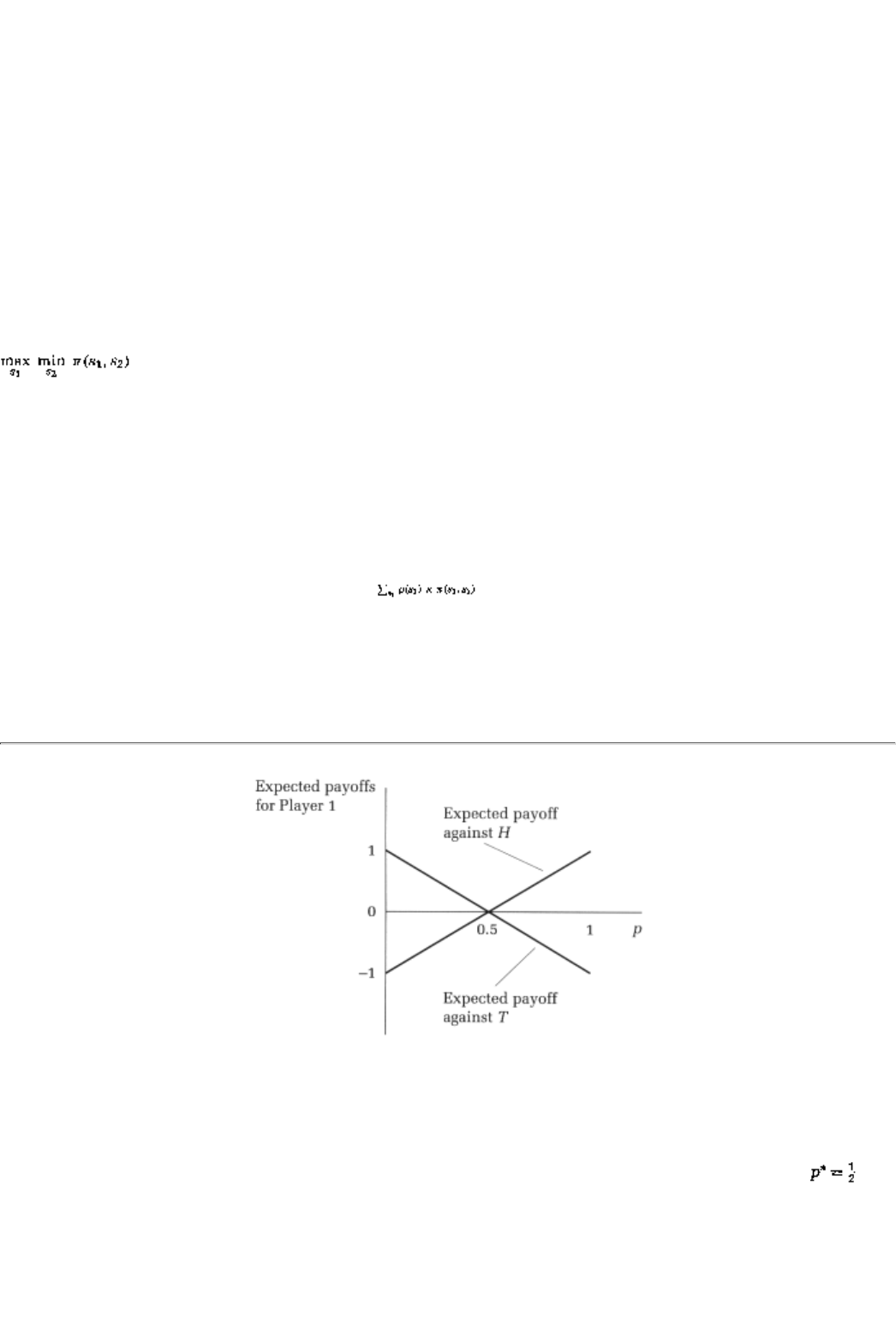
Remark 1
: Since the strategy
b
(
p
) minimizes player 1's payoff, it is a
best-response
for player 2 against p
(and hence the notation). Consequently, the safe approach is one in which a player expects her opponent to
play a best-response strategy and wants to guard against any consequent adverse outcomes.
Remark 2
: The safe approach gives player I a unilateral way to play the game. She knows that she can do no
worse than m1 if she plays her security strategy p*. If her opponent in fact does not play a best response,
then her payoffs can only be higher. This is unlike best-response behavior, which requires player I to think
through the question: what is it that I am best responding to? Of course such unilateralism may come at a
price; safe play may not be as profitable as best response play. That possibility will be the subject of Section
10.3.
10.2.2 Examples
Example 1: Matching Pennies
To begin with, let us compute the maxmin payoff if player I only uses pure strategies. This pure strategy
maxmin payoff is defined as
In matching pennies, regardless of whether player I plays H or T, her payoffs are at a minimum if player 2
mismatches; in each case player 1's payoff is -1, and so her pure-strategy maxmin payoff is -1.
However, suppose that player 1 does use mixed strategies. Let p denote the probability with which she plays
H
. If player 2 plays H for sure, player 1's expected payoffs
4This is exactly the same concept that was called the Stackelberg solution when we discussed the
Cournot model.
5The expected payoff p(P, s2) is equal to , where s1 is a pure strategy for player 1. Note
that in the definition of a maxmin payoff, we only consider pure strategies for player 2 (while
considering mixed strategies for player 1). the reason is that player 2 gets no higher a payoff from
playing mixed strategies; that is, mins2 p(p,s2) = minq p (p,q), where q is a mixed strategy for 2. (Hint:
think of the implication of Chapter 8.)
page_142
Page 143
FIGURE 10.1
are 2p - 1, while if player 2 plays T for sure, then player 1's expected payoffs are 1 - 2p. (Why?)
The two sets of expected payoffs are graphed in Figure 10.1. The minimum payoff for any player F is the
smaller of the two payoffs; that is, it is the lower envelope of the two expected payoff lines in the figure. It is
clear that the highest minimum payoff is realized where the two expected payoff lines intersect, at .
Furthermore, the maxmin payoff is O. Note that this mixed-strategy maxmin payoff is higher than the
pure-strategy maxmin payoff computed earlier. This is another instance where a mixed strategy guarantees a
player a higher worst-case payoff than the pure strategies.
Example 3: Squash
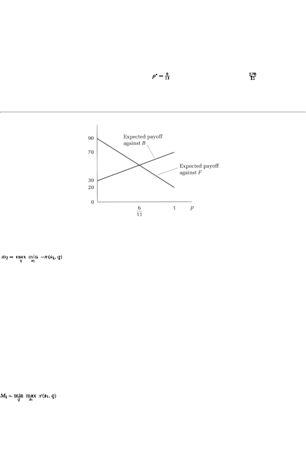
Pure-Strategy Maxmin. Show that the pure-strategy maxmin payoff is 30.
On the other hand, suppose that player 1 plays f with probability p.
Mixed Strategy's Payoffs. Show that the expected payoffs for player I when player 2 plays F and B for sure
are, respectively, 20p + 90(1 - p) and 70p + 30(1 - p).
Figure 10.2 displays these two expected payoff lines. As before, the lower envelope represents the minimum
expected payoff for each p
. It is clear that the highest such minimum payoff is achieved at the intersection of
the two expected payoff lines:
Maxmin. Show that the maxmin payoff is achieved at (with associated payoffs of
(Notice that, yet again, the mixed-strategy maxmin payoff is higher than the pure-strategy maxmin payoff.)
page_143
Page 144
FIGURE 10.2
So far we have concentrated on maxmin payoffsand the security strategyof player 1. Analogous arguments
however hold for player 2. Player 2's maxmin payoff is denoted m2 and is defined as
Notice that we have used the fact that player 2's payoffs are given by -
p. Let q* denote the security strategy
of player 2; m2 is the highest payoff that player 2 can guarantee himself (and he can do that by playing q*).
10.3 Playing Sound: Minmax
In the previous section we reached the following conclusion: player l's payoffs must be at least as high as
her maxmin payoffs, m1, and she can guarantee these payoffs by playing safely, that is, by playing her
security strategy p*. In this section we will see that there is an alternative (sound!) way for player I to play
the game.
10.3.1 The Concept and Examples
Instead of playing to guard against worst-case outcomes, player I could play "more aggressively" by playing
best responses against player 2's strategies. One could think of this as the more optimistic approach; try to
predict the opponent's play and do the best against it. The associated concept is called the minmax payoff; it
is the worst of the best (response) payoffs for player 1 (and is denoted M1):
where, again, p(s1, q) is the expected payoff to player I when she plays the pure strategy s1 and her
opponent plays the mixed strategy q.6
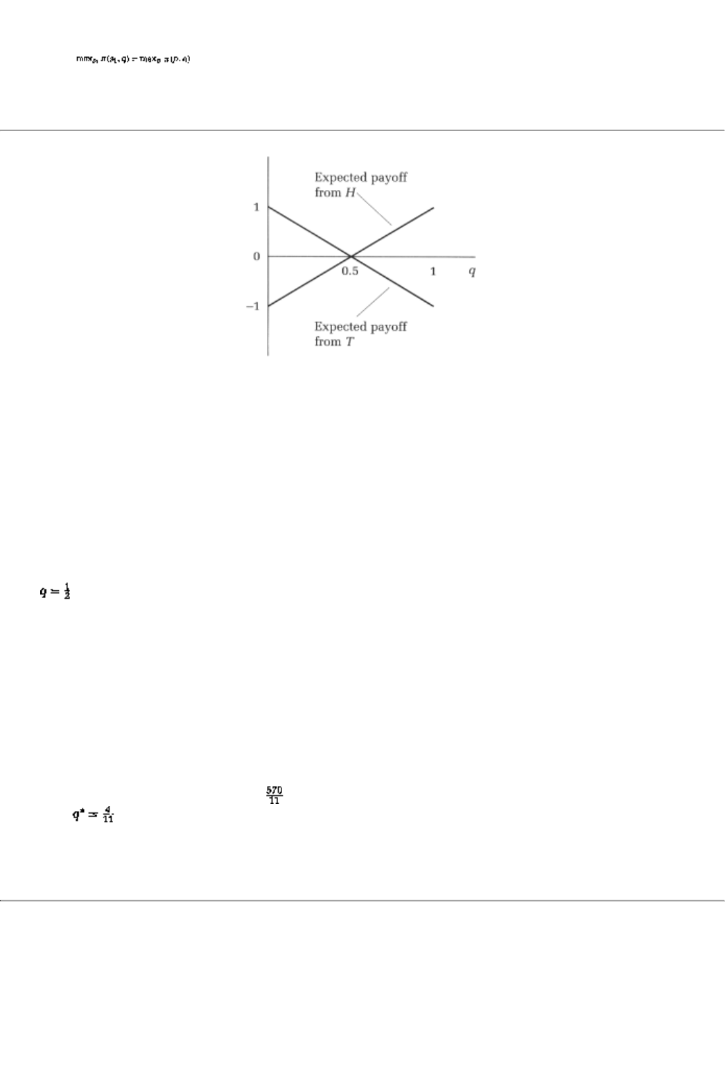
6In the minmax definition we restrict attention to pure strategies for player 1 (while considering
mixed strategies for player 2). This is because player 1 can do no better by using mixed strategies,
that is, (Why?) If player 2 is also restricted to pure strategies, then the
purestrategy minmax payoff of player 1 is defined as mins1 maxmax1p(s1, s2)
page_144
Page 145
FIGURE 10.3
Let us examine the minmax payoff in examples I and 3.
Example 1: Matching Pennies
Pure-Strategy MinMax. Show that the pure-strategy minmax payoff of player 1 is 1.
If, instead, player 2 plays a mixed strategy, say, plays H with probability q, then player 1's payoffs from
playing H and T are, respectively, 2q - 1 and 1 - 2q.
As before, these expected payoffs can be graphed as in Figure 10.3. The maximum of these expected
payoffs is the upper envelope of these two lines. The minmax payoff is then the lowest value of these
maximum expected payoffs; that is, the mixed-strategy minmax is 0. Note that these payoffs are realized
when ; that is, they are realized when player 2 plays his security strategy.
Example 3: Squash
Pure Strategy Minmax. Show that the pure strategy minmax payoff is 70.
Now suppose player 2 plays a mixed strategy, putting probability q on the strategy
F.
Mixed MinMax.
Step 1. Show that the two pure strategies for player 1, f and b, give player I expected payoffs of,
respectively, 20q + 70(1 - q) and 90q + 30(1 - q). See Figure 10.4.
Step 2. Show that the minmax payoff is and that the strategy of player 2 against which this payoff is
realized is . Verify that this is the security strategy of player 2.
Let us collect the computations:
page_145
Page 146
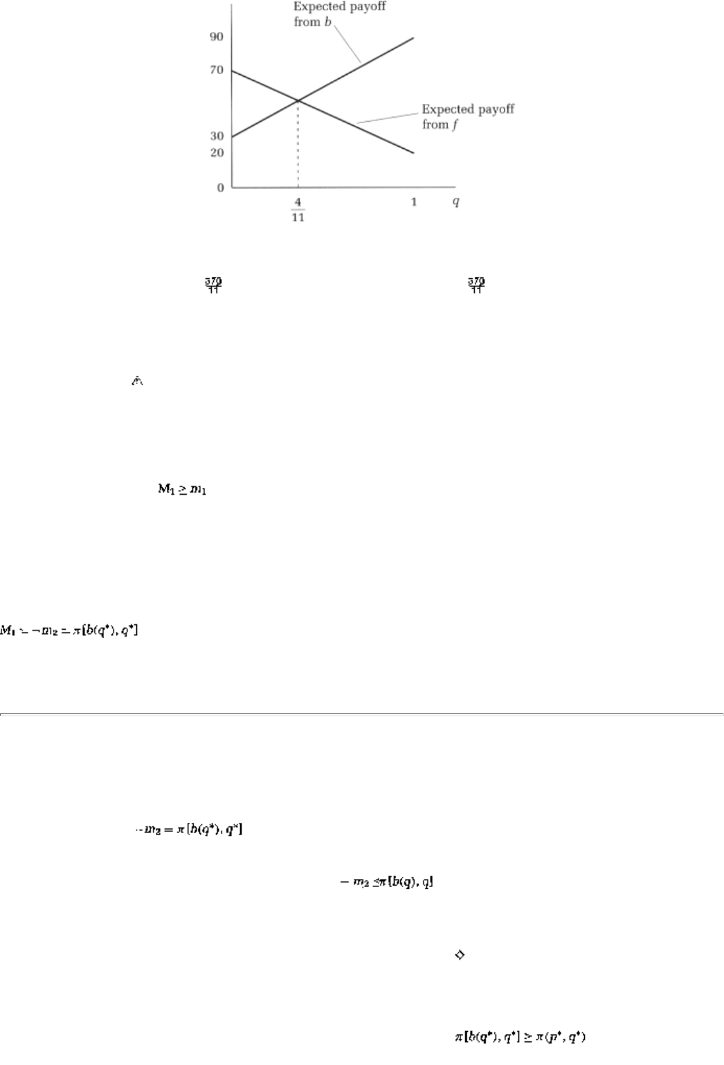
FIGURE 10.4
Example Pure Maxmin Mixed Maxmin Pure Minmax Mixed Minmax
1 -1 0 1 0
3 30 70
Player 1 realizes her maxmin payoff by playing her security strategy; she gets her minmax payoff when her
opponent, player 2, plays his security strategy.
10.3.2 Two Results
The examples illustrate two very general results. The first is that by playing the best-response approach, a
player can do no worse than by playing safely. The second is that one person's safe approach is another
player's best-response approach. After stating the two results, we will prove them in reverse order.
Proposition 1 (Minmax Is Better Than Maxmin). The minmax payoff of player I is at least as high as her
maxmin payoff, that is, . This statement is true regardless of whether we consider pure or mixed
strategies.
Note that the same result also holds for player 2's minmax and maxmin payoffs; that i
s, his minmax payoff is
at least as much as his maxmin payoff. The second result is as follows:
Proposition 2 (One's Minmax Is the Other's Maxmin). The minmax payoff of player 1 is precisely (the
negative of) the maxmin payoff of player 2, that is,
(Conversely, the minmax payoff of player 2 is the negative of the maxmin of player 1.)
page_146
Page 147
Proof of Proposition 2
When player 2 plays his security strategy q*, his payoffs are at least m2. Put differently, when 2 plays q*,
player 1's payoff is at most -m2. (Why?) In fact it is her best response b(q*) that gets player 1 a payoff of
exactly -m2, that is, .
If player 2 plays any other strategy q, his worst-case payoffs are less than m2 by definition; hence, player 1's
best payoffs are more than -m2 in this case, that is, . (Why?)
The inequality and the equality taken together say that -m2 is in fact player 1's minmax payoff M1. (Why?)
Put differently, player 2's safe approachplaying q*when coincident with player 1's sound approachplaying
b(q*)generates the latter's minmax and the former's maxmin payoff.
Proof of Proposition 1
Suppose that player 2 plays his security strategy q*; by definition, it is better for player I to play her best
response b(q*) than to play her security strategy p*. In other words, .
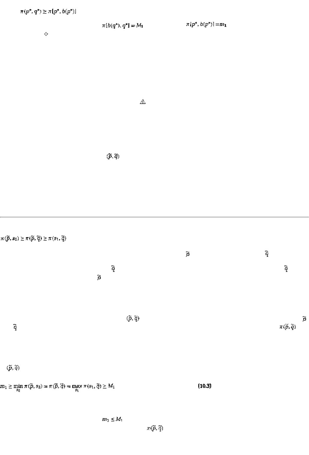
In turn, p(p*, q* is a payoff higher than what player I would get if 2 switched to his best response against p*,
that is, . (Why?)
In the preceding proof, we saw that . Furthermore, . Hence, Proposition I has
been proved.7
Here is a summary:
Safe Strategy. Player 1 can guarantee herself a payoff of at least m1 by playing her security strategy p*; she
gets exactly m1 when her opponent plays his best response to p*.
Sound Strategy. Player I cannot get payoffs any higher than her minmax payoff M1 if player 2, in turn, plays
his security strategy q*. She gets exactly M1 by playing a best response to q*.
10.4 Playing Nash: Playing Both Safe and Sound
What if both players played best responses; that is, what if we have a Nash equilibrium? Well, somewhat
remarkably, that situation turns out to be the same thing as both players playing safe! That conclusion is the
main result of this section.
First, note that Nash equilibria in zero-sum games have an interesting characterization:
Definition. A pair of mixed strategies constitute a Nash Equilibrium of a zero-sum game if for all pure
strategies s1 and s2,
7The result that a player's minmax payoff is at least as high as his maxmin payoff holds in all
games, whether they be zero-sum or nonzero-sum and whether they be two-player or many-player
games.
page_147
Page 148
Note that the second inequality in equation 10.2 simply says that
is a best response against . On the other
hand, the first inequality in equation 10.2 says that player 1's payoffs are minimized, among all possible
strategies of player 2, by the choice of . That statement, of course, is the same thing as saying that is a
best response for player 2 against .
We will now show that any pair of strategies that constitute a Nash equilibrium of a zero-sum game also
constitutes a pair of security strategies for the two playersand vice versa; that is, the security strategies form
a Nash equilibrium, provided the maxmin and minmax payoffs are equal to each other.
Proposition 3 (Playing Safe and Sound). Let constitute a Nash equilibrium of a zero-sum game. Then
and are security strategies and the maxmin (and minmax) payoffs are equal to each other and to .
Conversely, suppose that the minmax and maxmin payoffs are equal. Then the security strategies constitute
a Nash equilibrium of the game.
Proof
If constitutes a Nash equilibrium of the game, then
The outer inequalities in equation 10.3 follow from the definition of maxmin and minmax payoffs, and the
inner ones follow from the definition of a Nash equilibrium, equation 10.2. However, by virtue of
Proposition I we already know that
. Hence, it must be the case that m1=M1, that is, that the maxmin
and minmax payoffs are equal to each other and to .
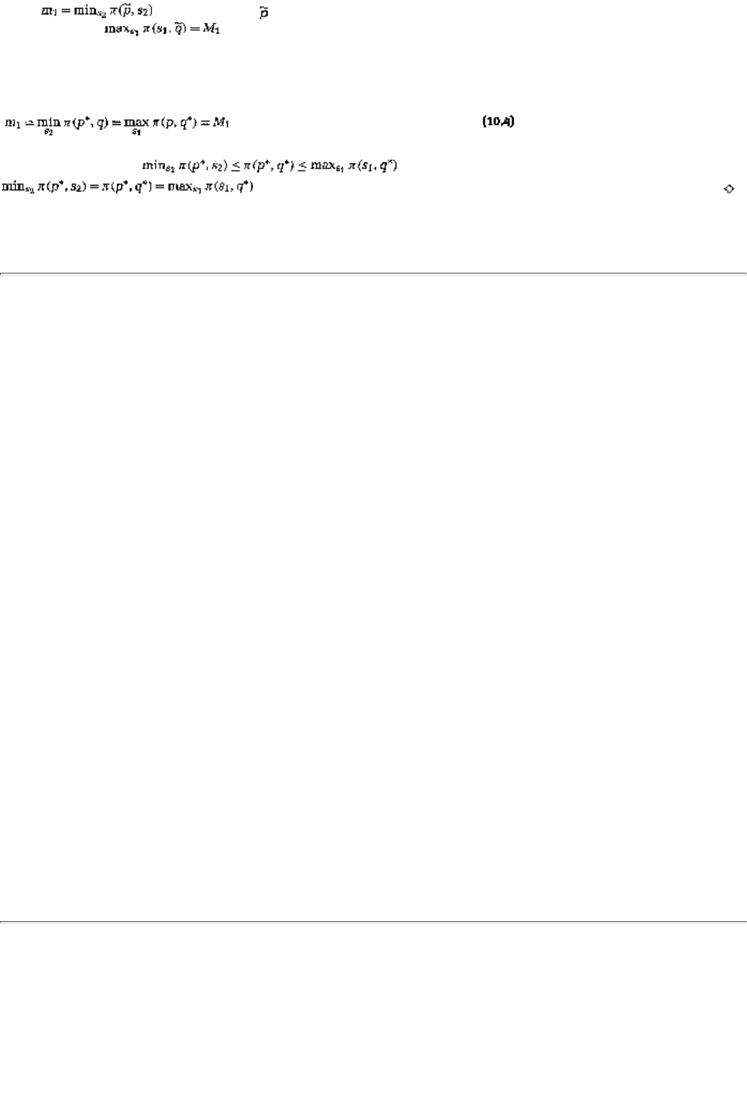
Since it follows that is a security strategy for player 1. (Why?) Proposition 2 and the fact
that imply that is a security strategy of player 2. (Why?)
In order to see the reverse implication, suppose that the maxmin and minmax payoffs are equal. In
particular, then, for the security strategies p* and q* we have
Since, by definition, it follows that it actually must be the case that
. Equation 10.2 then tells us that p*, q* must be a Nash equilibrium.
An implication of the above result is seen in the following problem.
page_148
Page 149
COCEPT CHECK
ALL EQUILIBRIUM PAYOFFS ARE EQUAL
Show that if there are many Nash equilibria in a zero-sum game, then they
must all have exactly the same payoffs for both players.
Summary
1. A zero-sum game is one in which the payoff of player 2 is the negative of player l's payoff; hence player
1's worst possibility is also player 2's best.
2. A safe approach for player I is to play a strategy whose worst-case payoff is better than the worst-case
payoff of any other strategy. Such a strategy is called a security strategy, and its worst-case payoff is called
the maxmin payoff.
3. The maxmin payoff is typically greater when player 1 plays a mixed rather than a pure strategy.
4. A ''sound" approach for player I is to play a best response against her opponent's conjectured strategy. The
lowest best-response payoff is called the maxmin payoff.
5. Player 1's minmax payoff is at least as high as her maxmin payoff. Player l's minmax payoff is exactly the
negative of player 2's maxmin payoff.
6. In a Nash equilibrium, both players play security strategies; that is, the safe and sound approaches
coincide. Conversely, when the maxmin and minmax payoffs are equal, the pair of security strategies
constitute a Nash equilibrium.
Exercises
Section 10.1
10.1
Give two real-world examples of game situations between two players in which player 1 gains if and only if
player 2 loses. Are your examples zero-sum (or constant-sum) games? Explain.
page_149
Page 150
10.2
Take the duopoly pricing game that we have studied extensively so far.
a. Show that it becomes a constant-sum game if the two firms care only about market share (rather than
profits).
b. Write down the zero-sum version of the same game.
c. Would we have a zero-sum game if the two firms were interested in sales (rather than profits)? Explain.
10.3
Consider the two economic examples of constant-sum games that were discussed at the beginning of this
chapter: a buyer-seller transaction and two firms competing in a market of fixed size.
a. Write down the strategic form of each of these examples. (Be sure to carefully spell out any assumptions
that you need to make in order for these examples to be constant-sum games.)
b. Now write down the zero-sum version of each example.
10.4
Consider a zero-sum game. Suppose that the players play mixed strategies, p and q, respectively. Show that
the expected payoffs of the two playersfrom the strategy pair p, qadd up to zero.
Section 10.2
In the questions that follow we will sometimes ask you to compute the pure-strategy maxmin or minmax
payoff. When there is no such qualification mentioned it means that we have in mind the usual mixed-
strategy maxmin or minmax.
10.5
Consider example 2 from the text:
1 \ 2 L C R
U5 8 4
M-7 9 0
D9 1 -2
a. Compute the pure-strategy maxmin payoff of player 1.
b. What is the minimum expected payoff if she mixes between the strategies U and M playing the former
with probability and the latter with probability as well?
page_150
Page 151
c. What is the minimum expected payoff if she mixes between all three strategies playing U, M, and D with
equal probabilities of each?
d. Show that no matter what mixed strategy p player I employs, player 2 can hold her expected payoffs from
p at or below 4.
e. What can you conclude about the maxmin payoff of player I in this example?
10.6
a. Repeat parts a-c of exercise 10.5 for the following variant of the payoff matrix:
1 \ 2 L C B
U5 8 -4
M-7 9 0
D9 1 -2
b. Compute the maxmin payoff and the security strategy.
10.7
Consider the following two-firm pricing game in which the two firmsColumbia Bagels and H&H Bagelscan
choose either of two priceshigh and lowand care only about their market share:
Columbia \ H&H High Low
High60, 40 30, 70

Low
80, 20
50, 50
a. Turn this into a zero-sum game.
b. Compute the security strategy for each firm as well as the maxmin payoff.
10.8
a. Based on your answer to the previous question, what can you conclude about the security strategy and the
maxmin payoff if each of the two players has a dominant strategy in the game?
b. What if only one of them has a dominant strategy? (Use game examples if you need to in order to make
your point.)
c. What can you conclude about the minmax payoff in either of the two preceding situations?
10.9
Consider the following two-firm advertising game in which the two firmsColumbia Bagels and H&H
Bagelscan choose either of two levels of advertising expenditureshigh and lowand each firm only cares
about long-run market share.
page_151
Page 152
Columbia \ H&H High Low
High0, 100 70, 30
Low40, 60 30, 70
a. Turn this into a zero-sum game.
b. Compute the maxmin payoffs and the security strategy for Columbia Bagels. Do this computation first for
pure strategies alone and then for mixed strategies.
c. What are the maxmin payoffs for H&H Bagels?
10.10
Consider the following variant of the advertising game in which H&H Bagels has a third strategy of spending
modest amounts on advertising. The payoffsfor Columbia Bagelsin this case are represented as follows:
Columbia \ H&H High Modest Low
High0 10 70
Low40 36 30
a. Compute the pure-strategy maxmin payoffs and the security strategy for Columbia Bagels. Then repeat
the exercise for mixed strategies.
b. What are the maxmin payoffs for H&H Bagels?
Section 10.3
10.11
Consider the zero-sum game of exercise 10.5.
a. Compute the minmax payoff of player I if player 2 only uses pure strategies.
b. Redo the exercise for mixed strategies; that is, compute the minmax payoff of player 1.
10.12
Consider instead the zero-sum game of exercise 10.6.
a. Compute the minmax payoff of player I if player 2 only uses pure strategies.

b. Redo the exercise for mixed strategies; that is, compute the minmax payoff of play
er 1.
c. Is the pure-strategy minmax equal to the pure-strategy maxmin? What about for mixed strategies?
10.13
Write down the minmax payoff of player I in each of the three exercises, 10.7, 10.9, and 10.10. Do the same
for the minmax payoff of player 2.
page_152
Page 153
10.14
Give a complete argument for two results that we keep seeing in each of the examples:
a. The pure-strategy maxmin payoff is less than or equal to the maxmin payoff.
b. The pure-strategy minmax payoff is greater than or equal to the minmax payoff.
10.15
Write out fully a proof of the statement: the minmax payoff for player 2 is precisely the negative of the
maxmin payoff for player 1.
10.16
Sketch an argument to show that Proposition 1 holds for non-zero-sum games as well, that is, that the
minmax payoff is at least as high as the maxmin.
Section 10.4
10.17
Verify that the security strategies in examples I and 3 of the text do in fact constitute Nash equilibria.
10.18
Do a similar verification for the zero-sum games of exercises 10.5 and 10.6.
10.19
Give an example of a zero-sum game that has more than one Nash equilibrium. Be sure to compute all Nash
equilibria including those in mixed strategies.
10.20
Consider a further modification of the bagel store model. Suppose that Columbia Bagels can spend modestly
on advertising (as well as H&H Bagels). In fact, suppose the payoff matrix is as follows:
Columbia \ H&H High Modest Low
High0 10 70
Modest15 50 60
Low40 36 30
a. Compute the pure-strategy maxmin payoff and minmax payoff for Columbia Bagels.
b. Now compute the (regular) maxmin and minmax payoffs.
c. What are the Nash equilibria of this game?
page_153
Page 155

PART THREE
EXTENSIVE FORM GAMES; THEORY AND APPLICATIONS
page_155
Page 157
Chapter 11
Extensive Form Games and Backward Induction
This chapter is the first stop in the extensive form magical mystery tour. In section 11.1 we will formally
discuss the extensive form of a game, a representation informally introduced in Chapter 2. In section 11.2
we will discuss a special class of extensive form games called games of perfect information. Within this
class, we will discuss a solution concept called backward induction and illustrate it with several examples in
section 11.3. In section 11.4 we will show that backward induction is the same thing as Iterated Elimination
of Dominated Strategies in the associated strategic form of the same game. Finally, in section 11.5, we will
turn to a case study of poison pills and other takeover deterrents.
11.1 The Extensive Form
Let us recall the basic concepts and terminology of the extensive form. This form is pictured by way of a
game tree
that starts from a unique node called the root. Out of the root come several branches and at the
end of each branch is a decision node. In turn, branches emanate from each of these decision nodes and end
in yet another set of nodes. A decision node is a point in the game where one playerand only one playerhas
to make a decision. Each branch of the tree emanating from that node corresponds to one of his choices. If a
node has no branches emerging from it then it is called a terminal node (and the game ends at that point).
A representative extensive form is the theater game that was first discussed in Chapter 2.1 For convenience,
we reproduce the extensive form of that game in Figure 11.1. By following a sequence of branches we get a
play of the game. In the theater game, if player 1 picks c while player 2, upon seeing this choice, chooses b,
then the play of the game takes us along the middle branch (c) emerging from the root followed by the top
1Two theater-goers have to decide which form of transportationb(us), c(ab), or s(ubway)they
should take to the Nederlander Theater to see the hit musical Rent. There is exactly one ticket left,
and whoever gets to the Nederlander first will get it. Player 1 leaves before player 2. A cab is
faster than the subway, which, in turn, is faster than the bus. Player 2 gets a ticket under three
circumstances: she takes a cab and player 1 takes a bus or the subway, and she takes the subway
while player I takes a bus.
page_157
Page 158
FIGURE 11.1
branch (b) thereafter. For each play of the game, there is a payoff to every player. For the play just
described, player I gets the last ticket. Hence, player 1's payoff is p1(T, c), while that of player 2 is p2(N,
b).2
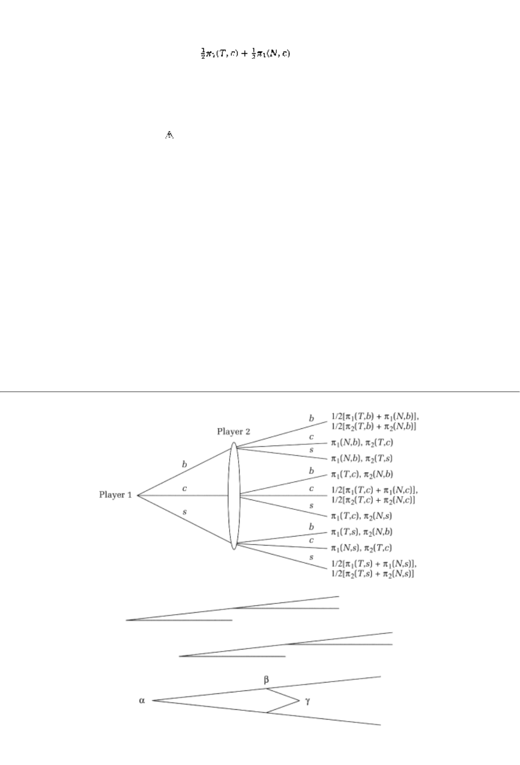
We also introduced
information sets
in Chapter 2 to represent simultaneous moves. An information set is
made up of nodes that are indistinguishable from the decision maker's standpoint. Suppose for instance that
our two theater-goers actually leave simultaneously. Each makes a transportation choice, and if they happen
to be the same choice, then there is a 50 percent chance that player I will get the ticket (and a 50% chance
that 2 will instead).3 Hence, for example, is the expected payoff to player I if both
players choose a cab.
The extensive form can be written as in Figure 11.2. Note that the difference between Figure 11.1 and
Figure 11.2 is that in the latter case player 2 cannot make her transportation choice conditional on player 1's
choice. This is signified by the fact that all three of her decision nodes belong to one information set.
11.1.1 A More Formal Treatment
In order for a tree to represent a game, the nodes and the branches need to satisfy three consistency
requirements:
1. Single Starting Point. It is important to know where a game starts, and so there must be one, and only
one, starting point. Hence, a situation as in Figure 11.3 is inadmissible.
2. No Cycles. It is important that we not hit an impasse while playing the game; it must not be possible for
the branches of a tree to double back and create a cycle.
3. One Way to Proceed. It is important that there be no ambiguity about how a game proceeds, and so there
must not be two or more branches leading to a node. Figure 11.4 is inadmissible.
2We have now made the payoffs dependent on ticket availability as well as the mode of
transportation. After all, getting a ticket and spending $10 on a cab ride is not quite the same thing
as getting it after a $1.50 subway ride.
3If they make different transportation choices, then suppose, as before, that a cab arrives before the
subway and a subway in turn arrives before a bus.
page_158
Page 159
FIGURE 11.2
FIGURE 11.3
FIGURE 11.4

Predecessor
The predecessors of a node, say a, are those nodes from which you can go
(through a sequence of branches) to a.
In order to state the three consistency requirements more precisely, let us introduce one more concept, the
predecessor of the node. For instance, in the theater game of Figure 11.1, for every one of player 2's decision
nodes there is a single (common) predecessor: the root node. Each terminal node, on the other hand, has two
predecessor nodes; the root and a decision node of player 2. The root of a tree is the only node that has no
predecessors.
To guarantee the three consistency requirements, the following restrictions are imposed on predecessor
nodes:
page_159
Page 160
1. A node cannot be a predecessor of itself.
2. A predecessor's predecessor is also a predecessor: if a node b is a predecessor of a, and a node g is, in
turn, a predecessor of b, then g is a predecessor of a as well.
3. Predecessors can be ranked: if b and g are both predecessors of a, it must be the case that either b is a
predecessor of y or vice versa.
4. There must be a common predecessor: Consider any two nodes, a and b, neither of which precedes the
other. Then there must be a node g that is a predecessor of both a and b.
Restriction 4, by itself, implies that there cannot be two or more roots in a tree. If there are two roots, then
there are two nodes neither of which precedes the other. But then there must be yet a third node that
precedes them both, and that is a logical contradiction.
Restrictions 1 and 2 together imply that there cannot be a cycle. Suppose it were the case that b is a
predecessor of a, g is a predecessor of b, and so on until we reach a node l. for which a is a predecessor.
(This, after all, is what we mean by a cycle.) But then, by restriction 2, a is a predecessor of a. And that
result violates the first restriction.
Finally, restriction 3 implies that there cannot be two or more branches leading to a. If there were, then there
would be two associated nodes, say, b and g, that are predecessors of a. However, it must then be the case
that either b is a predecessor of y or vice versa. Put differently, the road from, say, g, has to come through b.
CONCEPT CHECK
SINGLE PLAY
Show that an implication of restrictions 1-3 is that starting from any node we
can find a wayand only one wayback to the root of the tree.
11.1.2 Strategies, Mixed Strategies, and Chance Nodes
In our discussion of the extensive form thus far there has been no role for uncertainty. You might wonder
how mixed strategies fit into the extensive form. Let us now turn to that and other uncertainties.
Strategies
Recall from Chapter 2 that a player's strategy is a complete, conditional plan of action. It is conditional in
that it tells a player which branch to follow out of a decision node if the game arrives at that node. It is
complete in that it tells him what to choose at every relevant decision node.
page_160
Page 161

In the sequential theater game of Figure 11.1, for example, player 1 makes only one c
hoiceat the root. Hence
he has three strategies to pick fromtake b, take c, or take s. Player 2 is faced with three possible
conditionalities: what to do if player I takes the bus, what if he took a cab, and, finally, what if player I
hopped the subway. Hence, each strategy of player 2 has three components, one component for every
conditionality. A representative strategy is cbs; take a cab if player I takes the bus, bus if player I takes a
cab, and subway if player I hops a subway as well. Since there are three possible ways to choose in every
conditionality, player 2 has 3 × 3 × 3, that is, 33 such strategies.
CONCEPT CHECK
SIMULTANEOUS THEATER GAME (OF FIGURE 11.2).
Show that the strategy sets of the two players are identical and contain the
three strategies, b, c, and s.
Once the strategies have been determined, we can write down the strategic form of an extensive form game
by enumerating the list of players, their respective strategies, and the payoff associated with every strategy
vector. In the sequential theater game, for example, the strategic form is as follows:
1 \ 2 bbb cbb . . . ssb sss
bp1(T, b), p2(N, b) p1(N, b), p2(T, c) p1(N, b), p2(T, s) p1(N, b), p2(T, s)
cp1(T, c), p2(N, b) p1(T, c), p2(N, b) p1(T, c), p2(N, s) p1(T, c), p2(N, s)
sp1(T, s), p2(N, b) p1(T, s), p2(N, b) p1(T, s), p2(N, b) p1(T, s), p2(N, s)
(There are 33 columns, one for each one of player 2's strategies.)
Mixed Strategies
A mixed strategy is defined in exactly the same way as in the strategic form; it is simply a probability
distribution over the pure strategies. So in the sequential theater game a mixed strategy for player I is given
by two numbers p and q, which are, respectively, the probabilities with which b and c are chosen (and 1 - p -
q is the probability with which s is picked). A mixed strategy for player 2 is given by 33 I numbers, one for
the probability attached to every pure strategy.
Chance Nodes
We can also build uncertainty that is inherent to the game (as opposed to uncertainty that the players
introduce via mixed strategies) into the extensive form. For instance, the amount of time it takes on the
subway might depend on whether or not there is a rush-hour delay in the subway system. One way to model
that possibility is to allow for a
page_161
Page 162
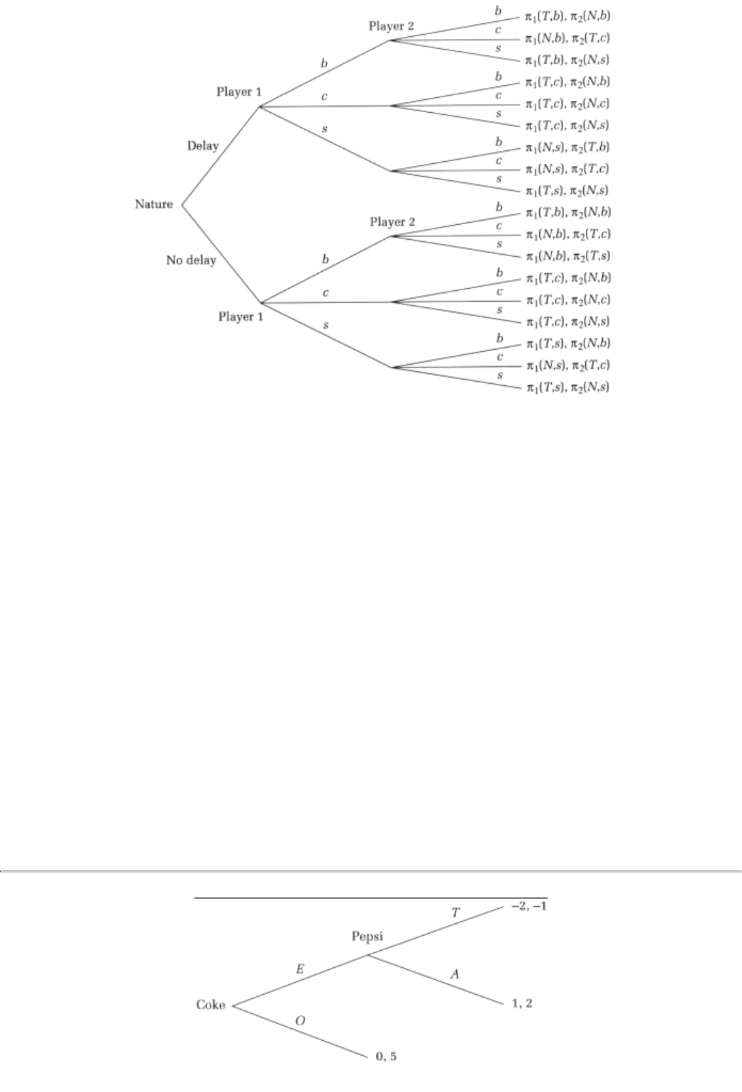
FIGURE 11.5
third kind of node, called a chance node; this is a node whose branches represent several random
possibilities.
For example, suppose that there are two possible subway outcomesdelay or no delay. This uncertainty needs
to be incorporated into the extensive form. Exactly how it will be incorporated will depend on when this
uncertainty is resolved: do the players know whether or not there is a delay before they make their choices,
and so on. For the simplest possibility, suppose that when our theater-goers make their transportation choice
they do know whether there is a delay or not (perhaps because it is reported on the radio).4 In that case, the
extensive form of the sequential theater game becomes Figure 11.5, where the chance node is the root of the
tree.
11.2 Perfect Information Games: Definition And Examples
Game of perfect information
An extensive form game with the property that there is exactly one node in
every information set.
A game of perfect information is one in which there is no information set (with multiple nodes). If an
information set has three nodes, then a player cannot tell which of the three immediately preceding nodes is
the one that was actually played, although she knows
4Note that the payoffs are specified to reflect the fact that if there is a delay, then even the bus is
faster than the subway.
page_162
Page 163
FIGURE 11.6

that one of them must have been played. If, on the other hand, an information set has a single node then
there is no such ambiguity; any time a player has to move she knows exactly the entire history of choices
that were made by all previous players. (Why?)5
CONCEPT CHECK
NO SIMULTANEOUS MOVES
Show that a game of perfect information cannot have any simultaneous moves.
Example 1: Entry I
Consider the following economic model. A firmsay, Cokeis debating whether or not to enter a new
marketsay, the Former Soviet Union (FSU)where the market is dominated by its rival, Pepsi. Coke's decision
is guided by the potential profitability of this new market, and that depends principally on how Pepsi is going
to react to Coke coming into its market. If Pepsi mounts a big advertising campaign, spends a lot of money
upgrading facilities, ties up retailers with exclusive contractsin other words, acts ''tough"then Coke will lose
money. On the other hand, if Pepsi were not to mount such a tough counterattackwhich after all is
costlyCoke would make money.6 in Figure 11.6, E (for enter) and O (for stay out) stand for Coke's
alternatives, whereas T (for tough) and A (for accommodate) refer to Pepsi's two choices on how to counter
Coke's entry. Note that the first entry in each pair of payoffs is Coke's payoff.
Example 2: Entry II
For a (slightly) more complex setting let us consider the following variant. Suppose that after Pepsi's
decision, Coke has a further decision to make; it has to decide whether or not it will itself mount an
aggressive advertising campaign and spend a lot of money on facilities, and the like. In other words, suppose
that after observing Pepsi's response, Coke will itself have to act "tough" or "accommodate" (Figure 11.7).
5The very first time the concept of the extensive form appeared was in John Von Neumann's 1928
article "Zur Theorie der Gesselschaftsspiele," Mathematische Annalen, vol. 100, pp. 295-320. In
this article, Von Neumann only considered the two extreme assumptions: (1) when a player knows
everything, that is, a game of perfect information, and (2) when a player knows nothing, that is, a
game of simultaneous moves.
6Under Communist rule the only American soft-drink manufacturer with a presence in the Soviet
Union was Pepsi. Indeed this was true of all the countries in the Soviet bloc. After the demise of
communism, Coke had to make a decision about whether or not to enter these markets. Stay tuned till
the next section to find out what happened!
page_163
Page 164
FIGURE 11.7
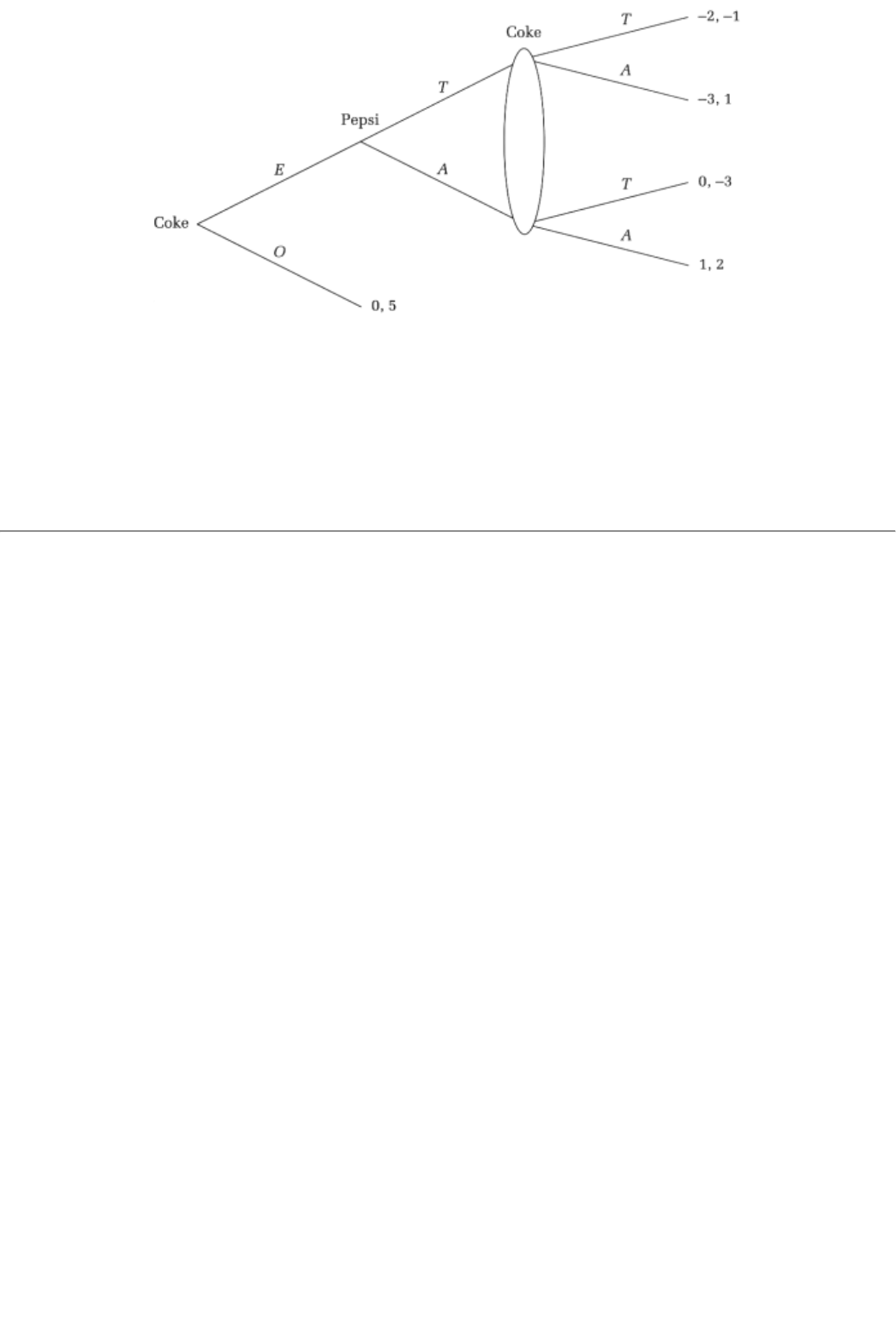
FIGURE 11.8
Example 3 (Not): Entry III
Suppose that, should Coke enter the FSU market, both Coke and Pepsi will make a decision about how much
to invest in this market, that is, whether to act tough or accommodate. However, unlike Example 2, suppose
these decisions are taken simultaneously (and that fact makes this not a game of perfect information) (Figure
11.8).
page_164
Page 165
11.3 Backward Induction: Examples
The question we are interested in is, What is a reasonable prediction about play in examples I and 2? It will
turn out that this is really a question about sequential rationality. It will involve rationality because a player
will pick the best action available to him at a decision node, given what he thinks is going to be the future
play of the game. It will involve sequentiality because a player will infer what this future is going to be
knowing that, in the future, players will reason in the same way. In particular, the decision maker at a
subsequent node will pick the best available action given what he, in turn, believes about the remaining
future of the game.
Example 1
To illustrate these ideas, let us start with example 1. A first natural step to take in order to predict play is to
find the Nash equilibria. Those are actually easier to see in the strategic form of the game.
Coke \ Pepsi Tough Accommodate
Enter-2, -1 1,2
Out0, 5 0, 5
Note that there are two Nash equilibria of this game: (
enter, accommodate) and (out, tough). The Nash
equilibrium (out, tough) is, however, unreasonable: Pepsi undertakes to fight Coke if Coke were to enter the
market. But if Coke were to enter the market, Pepsi would be better off accommodating. Indeed Pepsi's
strategy, tough, is a best responseto outonly because that strategy is actually never used, since, anticipating a
tough response, Coke chooses to stay out of the market. However, Coke might not find a tough stand by
Pepsi credible precisely for this reason; if its bluff were called, Pepsi would accommodate. By this line of
logic, the only reasonable equilibrium behavior is for Pepsi to accommodate; hence, (enter, accommodate) is
the only reasonable Nash equilibrium.7
Example 2
The logic employed can be further understood in the more complicated example 2. Again let us start with the
strategic form of this game. Note that every strategy of Coke's must have three components. The first
component tells Coke whether or not to enter the market, the second tells it whether or not to act "tough" if
Pepsi acts "tough," and the third specifies behavior if Pepsi accommodates. For example, EAT means (1)
enter, (2) against a tough Pepsi, accommodate, and (3) against an accommodating Pepsi, act tough. Pepsi,
however, has exactly two strategieseither to act tough or to accommodate Coke.

7Are there any mixed-strategy Nosh equilibria in this game? Explain.
page_165
Page 166
Coke \ Pepsi T A
ETT-2, -1 0,-3
ETA-2, -1 1, 2
EAT-3,1 0,-3
EAA-3, 1 1, 2
OTT0, 5 0, 5
OTA0, 5 0, 5
OAT0, 5 0, 5
OAA0, 5 0, 5
where the outcome to the strategy pair EAT and T is: Coke enters, Pepsi acts tough, and consequently, Coke
accommodates.
There are essentially three pure-strategy Nash equilibria of the strategic form:
1. Nash equilibria in which Pepsi plays T and Coke plays any one of the (four) strategies in which it stays
outOTT, OTA, OAT, or OAA.
2. (ETA, A)with outcome that Coke enters and both firms accommodate.
3. (EAA, A)with the same outcome as in the second equilibrium.
Consider Pepsi's decision. What should Pepsi's action be? The answer will depend on whether Coke will
subsequently act tough or accommodate. For example, it is more profitable for Pepsi to accommodate if it
thinks Coke will accommodate as well, but it is better for Pepsi to fight if it thinks Coke will act tough. In
order to determine which of these options will be chosen by Cokeand therefore what Pepsi should dowe can
apply the logic of sequential rationality twice.
Suppose that Pepsi accommodates. At this point it is more profitable for Coke to accommodate than to fight.
Hence, the only credible choice for Coke is to accommodate. On the other hand, if Pepsi acts tough, Coke
will find it more profitable to fight (and so this is the only credible thing for Coke to do). Knowing Coke's
responses, Pepsi now has to compare the profits from (T, T) against (A, A), that is, the two profit levels of -1
and 2. Pepsi will therefore accommodate.
One can, finally, back this logic out to Coke's initial decision. Coke can either enterand then it expects Pepsi
to accommodate and expects to do the same thing itself. Or it can stay out. The profit level in the first case is
1, while it is 0 for the second option; Coke enters.
In conclusion, the only sequentially rational strategy for Coke is ETA, while for Pepsi it is to play A; the only
one of the three types of Nash equilibria in the strategic form that is sequentially rational is the second one.8
8After the demise of communism, "Things have gone better with Coke"; Coke is now the market
leader in all of the former Soviet bloc countries, except Rumania and Bulgaria. For an interesting
economic account that underlies the model studied in this chapter, see the New York Times, March
15, 1995.
page_166
Page 167
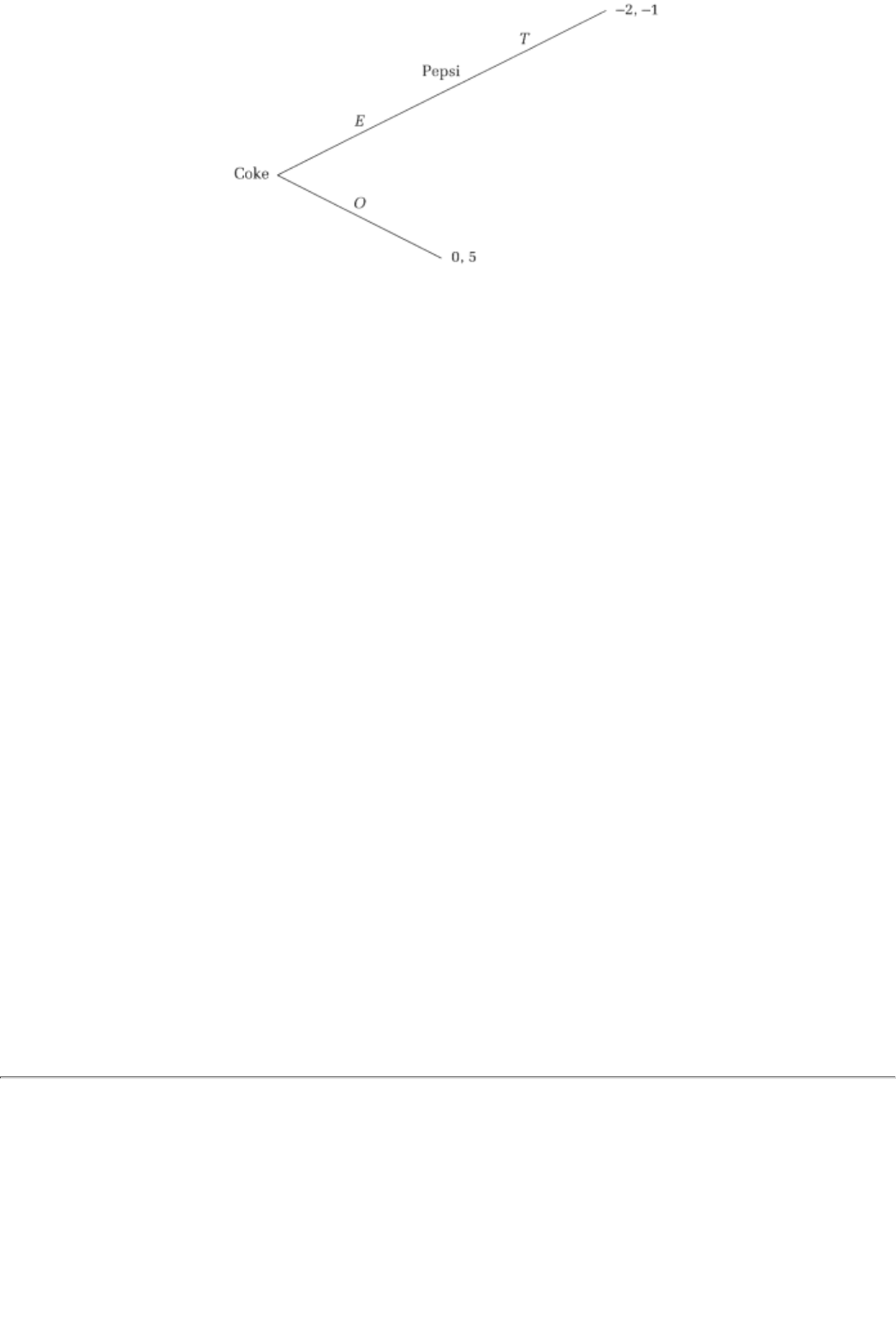
FIGURE 11.9
11.3.1 The Power Of Commitment
In life, having fewer choices is typically worse than having more choices. You might think that this should be
true for games as well. However extensive form games, and in particular games of perfect information,
provide examples where less (choices) can mean more (equilibrium payoffs). This statement may sound
paradoxical at first, but the intuition is actually straightforward. If a player has more options later, she may
behave very differently in the future than she would if she had fewer options. In turn, this behavior will
affect current play by her as well as by the other players. This change can, in principle, be beneficial or
harmful to the player with enlarged options.
Let us make matters more concrete by going to our two examples but with a twist.
Example 1': Only Tough Pepsi
Consider example 1. Suppose that we simplify this (already simple!) example in the following way: after
Coke enters the FSU market, Pepsi has no choice but to play tough (i.e., let us reduce Pepsi's options by
eliminating the choice accommodate).9
The extensive form is therefore as seen in Figure 11.9. Since Pepsi has only one option, it will necessarily
exercise that option and fight Coke's entry. So Coke suffers a loss if it enters this market. Hence, Coke will
prefer to stay out. By having fewer optionsor, alternatively, by committing to one option in the futurePepsi is
able to increase its (backward induction) equilibrium payoffs.
Example 2': Only Tough Coke
Consider example 2. Suppose that we modify the example in the following way: after Coke enters the FSU
market, Coke has no choice but to play tough (i.e., suppose Coke has one option less; it cannot
accommodate).
The extensive form is therefore as seen in Figure 11.10. Let us apply sequential rationality to this tree. At
Coke's second stage "decision nodes" there is only one choice
9This may happen if Pepsi's local management is told by headquarters that they will lose their jobs
if Coke gets a toehold in the market, Or management may have already signed contracts with
advertising agencies, newspapers, and such to trigger an advertising blitz if Coke comes into the
market.
page_167
Page 168
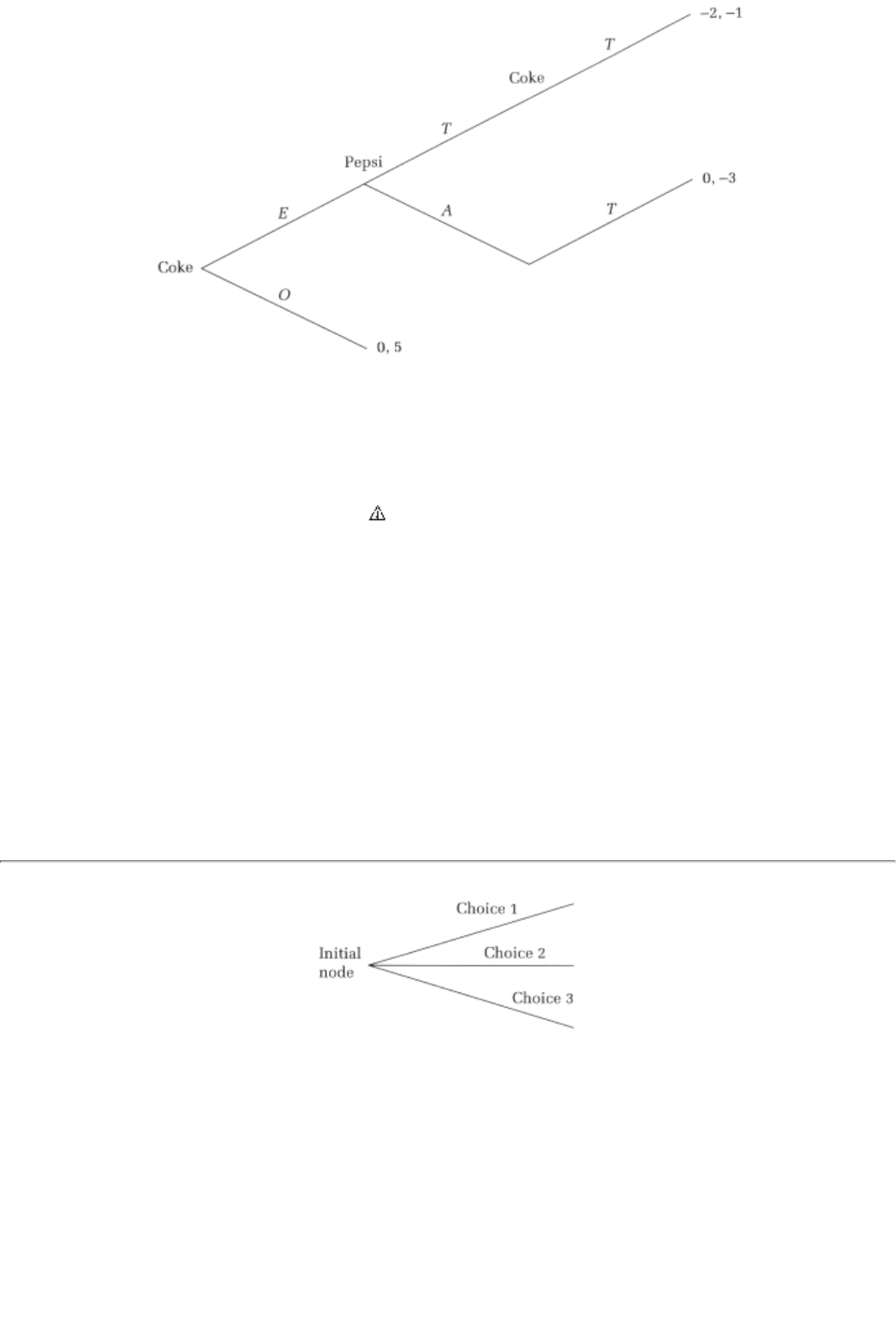
FIGURE 11.10
availabletough. This fact implies that while making its choice Pepsi knows that it will surely face a tough
opponent in the future. Pepsi's best response is therefore also to play tough. Consequently, at the entry stage
Coke is better off deciding to stay out, since coming in will entail a loss of 2. Here fewer options for Coke
benefits Pepsi because it renders Pepsi's threat to be tough credible.
11.4. Backward Induction: A General Result
The solution concept employed in the two examples can be generalized; the generalization goes by the name
backward induction. The logic is the following: suppose the game is at a final decision node; any decision
by the player who chooses at that node terminates the game. The only reasonable prediction for play is that
this player will pick that action which maximizes her payoffs. For instance, in example 2, Coke as the final
decision maker gets a higher profit from playing tough if Pepsi is being tough; hence, a rational Coke must
pick tough. In the other final decision node, that which follows Pepsi accommodating, Coke must pick
accommodate because it gets a higher profit by doing so.
Consider now a penultimate decision nodefor instance, Pepsi's decision node in example 2. At any such
node, the decision maker knows the exact consequence of each of his choices because he knows the
subsequent decision that will be taken at the final decision node. For example, Pepsi's tough stance will be
reciprocated; so will an accommodating stance. Hence a decision maker at the penultimate decision node
can compute the exact payoff to each of his choices, and he must make the best available choice.
page_168
Page 169
FIGURE 11.11
Maximum lenth n = 1
By similar logic, at decision nodes three steps removed from a terminal node, the decision maker knows the
exact consequence of her choices. This is the case because she knows the choice that will be made by any
player in a penultimate decision node as well as the choice that will be made at the consequent final decision
node. Hence such a three-step removed decision maker has a best choice. And so on.10
In other words, we fold the game tree back one step at a time till we reach the beginning. The fact that we
start at the end of the tree is the backward part of the terminology. The fact that we work one step at a time
in doing the tree folding is why it is called an induction procedure. Note that this procedure works as long as
there is a last node to start from.
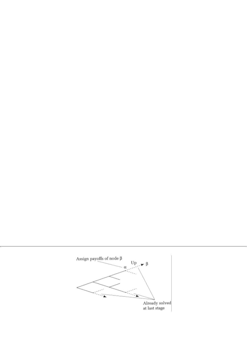
The above arguments yield the result called
Kuhn's theorem
. A special case of this result was proved in 1913
by E. Zermelo, who showed that the game of chess must always have a winning strategy.11
Kuhn's (and Zermelo's) Theorem. Every game of perfect information with a finite number of nodes has a
solution to backward induction. Indeed, if for every player it is the case that no two payoffs are the same,
then there is a unique solution to backward induction.
Sketch of the Proof
The logical structure of the proof goes by the name of proof by induction. The idea is the following: consider
any problem that comes in n steps, where n is some positive number. In order to show that an n-step problem
is solvable, no matter what the value of n is, it suffices to show that (a) the problem has a solution whenever
n equals 1 and (b) if a problem in n - 1 steps has a solution, then so must a problem in n steps.12
Consider any game of perfect information. Let n refer to the maximum number of steps you need to take in
starting from a terminal node and working your way back to the root.13 Since there are only a finite number
of nodes, the maximum number of steps is in turn finite.
For example if n = 1, we have a picture like the one seen in Figure 11.11. Clearly there is an outcome to
backward induction in this case; pick that action which yields the highest payoff. So we know the theorem is
true for n = 1. What about a game with n > 1 steps? Suppose that any game with n - 1 as the maximum
number of Fsteps has a backward induction solution.
10In the preceding discussion we implicitly assumed that every choice at a decision node is the
same number of steps removed from a terminal node. In general this need not be the case, but the
procedure works anyway. If the maximum number of steps to a terminal node is n, then we can
solve the decision problem at that node after n steps of backward induction.
11But try finding it! This argument suggests, however, the reason why an IBM computer (Big Blue) was
able to match up well against the world champion Gary Kasparov in their six-game encounter in
Philadelphia in February 1996. By brute forcealso called parallel processing!the computer can do
backward induction better than any human being. The computer cannot do backward induction
perfectly, since the problem is too big, that is, there are too many branches in the game tree of chess.
But one day it will. The world champion then will be a computer!
12Suppose we know that we can solve the problem whenever n equals 1. By b, we then also know that a
problem with n = 2 is solvable, But then, again by b, we know that a problem with n = 3 is solvable.
And so on for any finite n.
13For instance, in example 1, the maximum number is 2, whereas in example 2 it is 3terminal node to
Coke's accommodate/tough decision to Pepsi's accommodate/tough decision to Coke's initial node.
page_169
Page 170
FIGURE 11.12
Take the game with n steps and turn this into an artificial game with n - 1 steps by folding the tree once; at
every final decision node, find the payoff-maximizingor best-responseaction for the player at that node. (For
example, suppose that at node a, player I has to move and his best move is Up.) Now imagine that the
original game "ends" at each of its final decision nodes with payoffs equal to the payoffs that would be
realized had the original game proceeded along the best-response branches emanating from these nodes. (For
instance, the payoff assigned to "terminal" node a is precisely the payoffs that correspond to the terminal
node that comes after playing Up at the node a.) This procedure is illustrated in Figure 11.12.

The modified game has, by construction, a maximum number of steps equal to n - 1. Hence, by the induction
hypothesis, it has a solution to backward induction. Attach this solution to the best response choices at each
final decision node of the original game. It is not difficult to show that now we have a backward induction
solution to the complete original game.
If no two payoffs are equalthat is, if there are no ties in the payoffsthen the best response is unique at each
one of the final decision nodes. But this logic is also true at the first n - 1 decisions. Put differently, there is a
unique solution to backward induction.à
11.5 Connection With Leds In The Strategic Form
Backward induction in the extensive form of a game turns out to be exactly the same as solving the game by
iterated elimination of dominated strategies (IEDS) in the strategic form. To see this point, let us return to
the two examples that were discussed previously.
In example 1 the backward induction outcome was for Coke to enter and for Pepsi to accommodate. For
ease of discussion, we reproduce the strategic form of the game here:
Coke \ Pepsi Tough Accommodate
Enter-2, -1 1, 2
Out0, 5 0, 5
page_170
Page 171
Note that
tough is a dominated strategy for Pepsi. Hence, the IEDS outcome is indeed (enter,
accommodate).
Consider instead example 2. Again for ease of discussion let us reproduce the strategic form of this game:
Coke \ Pepsi T A
ETT-2, -1 0,-3
ETA-2, -1 1,2
EAT-3,1 0,-3
EAA-3, 1 1, 2
OTT0, 5 0, 5
OTA0, 5 0, 5
OAT0, 5 0, 5
OAA0, 5 0, 5
Note that the first, third, and fourth strategies of Coke are dominated by
ETA. Eliminating those strategies,
we have the following payoff matrix:
Coke \ Pepsi T A
ETA-2, -1 1,2
OTT0, 5 0, 5
OTA0, 5 0, 5
OATO, 5 0, 5
OAA0, 5 0, 5
For Pepsi, T is now dominated by A. Hence the IEDS outcome is in fact (ETA, A) exactly as we saw by way
of backward induction in the extensive form.
From the two examples you may begin to see why backward induction in the extensive form is equivalent to
IEDS in the strategic form. Take a final decision node in the extensive form with, say, two choices at that
node. Consider the two strategies that are identical everywhere else except at this decision node:
CONCEPT CHECK
DOMINANCE
Show that, in the strategic form, the strategy that contains the better decision
at this node dominates the alternative strategy.
page_171

Page 172
By extension, the strategy that contains the rightor bestdecision at each final decision node dominates all
other strategies. Hence all other such strategies will be eliminated in the very first stage of the IEDS
procedure. In Example 2, the strategy in which Coke reciprocates at both of its final decision nodesT against
T but A against A dominates the three other ways of deciding at this pair of decision nodes; ETA dominates
EAA, EAT
, and ETT.
But now take a penultimate decision node in the extensive form. There is a best decision at this node, given
what we know is going to be the choice at the subsequent, final, decision nodes. Consider any two strategies
that are identical everywhere except at this penultimate node.
CONCEPT CHECK
DOMINANCE, STEP 2
Show that, in the strategic form, the strategy that contains the better decision
at this penultimate node must dominate the other strategy.
Indeed all strategies, except those that take the best action at the penultimate node, are thereby eliminated.
This procedure, of course, is analogous to folding the tree a second step. (In example 2, A is therefore a
better response for Pepsi than T.)
And then we can go to decision nodes three steps from the end. And so on.
11.6 Case Study: Poison Pills And Other Takeover Deterrents
A fact of corporate life is the merger of two companies or the takeover of one company by another.14
Sometimes the merger is friendly in that the boards of the two companies agree to the terms and necessity of
the merger. At other times, the attempted takeover is decidedly unfriendly; the management and board of
the target company "fight" the takeover, and the aggressor firm too may take steps to force the
transaction.15
A target company can fight potential aggressors by building in various legal or economic defenses that make
it an unattractive prize. These defenses include, (a) requiring a company that takes over to make costly
buyout payments to the management; (b) allowing the board to dilute the company's shares by issuing new
shares in the event of an offer by a rival; (c) prohibiting the board from considering any offer that is "not in
the long-term interest of shareholders"; and (d) prohibiting management from entertaining certain
competitors' offers. These various statutes are sometimes given the common moniker of a "poison pill."16
14In any given month between 1980 and 1991, the proportion of companies listed on the New York
Stock Exchange that received merger or takeover offers varied between 0.25 percent and 2.5
percent. During the height of the takeover mania, between the middle of 1987 and 1988, there was
just one month when less than I percent of the companies received such offers. (See the article by
Robert Comment and G. William Schwert, "Poison or Placebo: Evidence on the Deterrence and
Wealth Effects of Modern Antitakeover Measures," 1995, Journal of Financial Economics, vol. 39,
pp. 3-43.)
15A recent friendly acquisition was Boeing's takeover of McDonnell Douglas. An unfriendly takeover
war was the one recently fought over Conrail, the freight carrier with a virtual monopoly in the
northeastern United States; Conrail and CSX Corporation together fought Norfolk Southern.
16The Comment and Schwert article referred to above reports that 87 percent of all exchange-listed
firms now have some form of poison pill statutes built in.
page_172
Page 173
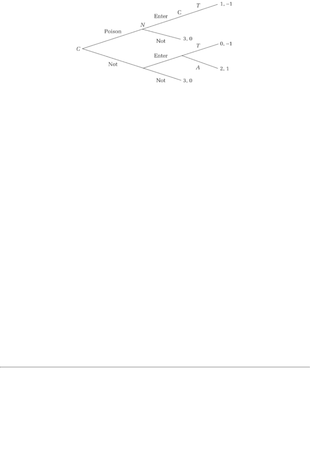
FIGURE 11.13
C = CSX/Conrail
N = Norfolk Southern
In this section we will analyze the working of poison pills. The game-theoretic idea that will be relevant is
the power of commitment, the idea that poison pills act as commitment devices.17
Let us consider two different ways in which a poison pill may work: they may either discourage aggressors
from trying or they may change the terms of the eventual takeover agreements. The first game is a variant on
examples 1 and 1'.
Legal Poison Pill 1
Suppose that without a poison pill provision the game is that of example 1Norfolk Southern has to decide
whether or not to fight the CSX-Conrail combine. On one hand, if they do decide to fight (and make a share
offer), CSX-Conrail can either play tough by refusing to negotiate, by upping their own terms, and the like,
or they may accommodate and reach some trilateral settlement. On the other hand, suppose that with a
poison pill provision the game is that of Example 1': CSX-Conrail is committed to fight.
Additionally, now suppose that there is an initial choice that CSX-Conrail has to make, and that is to decide
whether or not to arm themselves with the poison pill. The extensive form is therefore as seen in Figure
11.13 (note that the first entry in the pair of payoffs is that of the first mover, i.e., CSX-Conrail).
Without the poison pill, CSX-Conrail will accommodate and hence Norfolk Southern will enter; the former's
profits are therefore 2. With the poison pill, Norfolk Southern will choose to stay away from the takeover,
and hence CSX-Conrail will make profits of 3. Clearly, CSX-Conrail prefers to adopt the poison pill, and this
commitment nets them an extra dollar (billion dollars) of profits.
17A story to keep in mind for illustrative purposes is the freight-rail flap. On October 15, 1996,
CSX Corporation and Conrail announced a $8.6 billion dollar friendly merger that would make the
merged company the largest freight railroad on the East Coast and give it a monopoly in much of
the Northeast. CSX's main rival on the Atlantic Coast, Norfolk Southern, announced on October 22
an unfriendly takeover bid for Conrail that topped the CSX terms. In the meantime, Conrail's board
adopted a provision that prohibited it from discussing a merger agreement with any other company
until 1999 without CSX's approval. They also invoked certain Pennsylvania statutes that allow
management of a company to ignore offers that it considers not to be in a company's long-term
interest. Subsequently, the National Transportation Safety Board (NTSB) got involved, the offers
were revised upward, and so on. At the end of the section, you will see the denoument to this plot.
page_173
Page 174
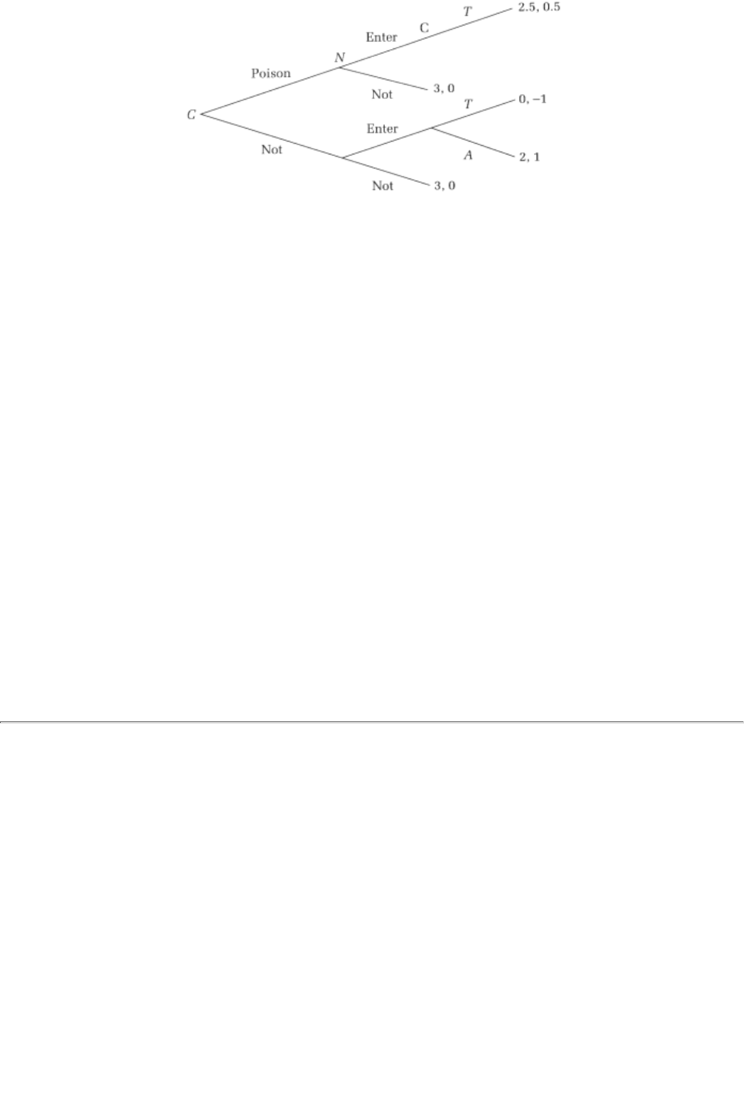
FIGURE 11.14
C = CSX/Conrail
N = Norfolk Southern
Legal Poison Pill 2
All this is fine you think, but didn't Norfolk Southern actually make a takeover offer? Well, perhaps then the
payoffsin the extensive formare slightly different. Consider Figure 11.14. As before, without the poison pill,
CSX-Conrails's payoff is 2. Now, though, despite the poison pill, Norfolk Southern finds it profitable to enter
(since they make profits of 0.5). However, CSX-Conrail makes a profit of 2.5, which is still better than the 2
they would make by not adopting the poison pill.
So the backward induction outcome is that CSX-Conrail prefers to adopt the poison pill provisions, Norfolk
Southern prefers to make a share offer (mount a takeover of Conrail), and CSX-Conrail fights that offer.
This example mirrors what actually happened in the freight-rail flap.18
Summary
1. The extensive form representation specifies who moves at different points in a game, what their choices
are at such moves, and what the eventual consequences are for all players.
2. Restrictions are placed on the precedence between decision nodes to ensure that there is a well-defined
play for every choice of strategies.
3. A game of perfect information is one in which every information set has a single element.
18The freight-rail flap was settled eventually after the intervention of the NTSB. Conrails's tracks
in the northeast were divided between CSX and Norfolk Southern. The division was made in such a
manner that Conrail-CSX did not in fact gain a monopoly in much of the northeast.
page_174
Page 175
4. Backward induction is a general solution concept for games of perfect information. Every finite game of
perfect information has a backward induction solution.
5. Backward induction in the extensive form of a game of perfect information is identical to Iterated
Elimination of Dominated Strategies in the associated strategic form.
6. In a perfect information game, being able to commit to having fewer choices in the future may be
beneficial for a player.
7. Poison pills are commitment devices that restrict management's options in the event of an unfriendly
takeover. Consequently, hey may increase the payoffs of a target firm.
Exercises
Section 11.1
11.1
Draw an extensive form game with two players and three decision nodes. Is there more than one game tree
for this description of players and decision nodes? Explain.

11.2
Redo the theater game of Figure 11.1 to allow for the possibility that a cab can get caught in a traffic jam
(and in that case is slower than the subway, although it is faster than the bus). Suppose that traffic conditions
are known to both players before they make their transportation choices. Be sure to explain carefully the
payoffs that you assign.
11.3
Redo exercise 11.2 to allow for the possibility that traffic conditions become known only after the
theater-goers make their choices. Suppose also that there is a 25 percent chance that a cab can get caught in
a traffic jam. Be sure to explain the payoffs carefully.
Section 11.2
11.4
Represent the game of Marienbad (see Chapter 1)with a starting configuration of 3 matches in each pile, that
is, (3, 3)in extensive form. Is this a game of perfect information? Explain.
page_175
Page 176
11.5
Use backward induction to solve the game from a configuration of (1, 0). What about (2, 0) and (3, 0)?
11.6
Similarly, use backward induction to solve the game from a configuration of (1, 1). What about (2, 1) and (3,
1)?
11.7
Now use backward induction to solve the game from a configuration of (2, 2). What abo
ut (3, 2)? Finally,
what about the starting configuration (3, 3)?
11.8
How does the solution that you uncovered in exercises 11.5-11.7 compare with what we called the ''winning
strategy" in our discussion of Marienbad in Chapter 1? Explain your answer.
11.9
Repeat the analysis of exercises 11.5-11.7 for Nim; that is, uncover the backward induction solution to Nim
if the initial configuration of matches in the two piles is (3, 3).
11.10
Consider example 2. Recall that there are four strategiesOTT, OTA, OAT, and OAAin all of which Coke
makes an initial decision not to enter the FSU market.
a. Explain carefully how, from each of these four strategies, we can find answers to the counterfactual
question "What would Coke do if it entered the market?"
b. Explain carefully why, in order to check for sequential rationality, we need to be able to find answers to
the same counterfactual question.
11.11
Consider example 2 again. Show that there are no (fully) mixed-strategy Nash equilibria in that game of
entry, that is, there are no Nash equilibria in which both players play mixed strategies. (Hint: Show that if
Pepsi mixes between T and A, then Coke will never play any of the strategies ETT, EAT, and EAAsince these
are all dominated by ETA.)
11.12

Based upon your answer to exercise 11.11, what can you say about the existence of mix
ed-strategy Nash
equilibria in games of perfect information? In particular, is it true that the backward induction procedure
picks out the only sequentially rational solution among the full set of pure as well as mixed strategies?
Explain.
page_176
Page 177
11.13
Suppose that Coke's decision on the FSU market is reversible in the following sense: after it has entered and
after Pepsi has chosen T or A, Coke has any one of three options to choose from: T, A, and O(ut). Suppose
that exiting at that point nets Coke a payoff of -1 and Pepsi a payoff of 3 if it had been Tough and 4 had it
accommodated. Write down the extensive form of this game.
11.14
Solve the game of exercise 11.13 by backward induction. Explain any connection to the power of
commitment that you unearth in your solution.
Section 11.4
11.15
Show an example of a game of perfect information in which the maximum number of steps you need to take,
n, starting from a terminal node and working back to the initial node, is 3. Give an example where n = 6.
11.16
In the game tree of Marienbad that you drew in exercise 11.4, do a one-step induction. In other words, solve
the game at every one of the final decision points, and create a game with n - I maximum number of steps.
11.17
Show that if we attach a backward induction solution to the n - 1 step problem to the best choices at the final
decision nodes, we get a backward induction solution to the n step problem.
Section 11.5
11.18
Write down the strategic form of the game of exercise 11.13.
11.19
Solve the game by IEDS.
11.20
Explain carefully how each of your steps of iterated elimination corresponds to steps in which you fold the
game tree while doing backward induction.
page_177
Page 179
Chapter 12
An Application: Research and Development
This chapter will present an application of the backward induction solution proposed in the previous chapter.
The economic problem is that of research and development (R&D), and the setting for this particular
application is that of a patent race. The R&D problem will be discussed in section 12.1, and a model of a
patent race will be presented in section 12.2. In section 12.3 we will derive the backward induction solution
of that model. Section 12.4 will conclude with a discussion of possible generalizations of the model.

12.1 Background: R&D, Patents, And Oligopolies
The engine of growth for modern economies is technological progress; indeed, this has been the engine for
some 250 years, ever since the early years of the Industrial Revolution.1 Some economists have estimated
that by far the majority of the growth that has taken place in the United States economy in the 20th century
has been driven by technological advancement.2 Even today, many of the sectors that are experiencing the
highest rates of growthsuch as computers, telecommunications, pharmaceuticals, and biotechnologyare, in
fact, the sectors where the growth rates of technology are the highest. It is therefore extremely important to
answer such questions as, What drives the growth of new technologies, and how can government R&D
policy further stimulate this growth?
A central aspect of an innovation is that it is a public good; a new idea can be exploited by whoever has
access to itand the next person who gets access to it will not have any less of the idea to work with. For
example, if a new gene is sequenced, and the result is announced in a scientific journal, then the same code
will be available to
1A spate of technological break-throughs launched the Industrial Revolution in England in the
middle of the 18th century. Important innovations of the 18th and 19th centuries included the steam
engine and the spinning jenny in the textile industry, and the Bessemer process in the iron and steel
industry.
2For instance, in a famous study published in 1957, Robert Solow of MIT estimated that 87.5 percent
of the growth in United States GNP between 1909 and 1949 could be attributed to technological
growth (see Technical Change and the Aggregate Production Function, Review of Economics and
Statistics, vol. 3: pp. 312-320).
page_179
Page 180
every person who reads the scientific paper. Furthermore, using this information, a new drug could be
developed by any pharmaceutical company that has the requisite drug development infrastructure.
This brings up the question, If the original gene sequencing was a costly enterprise, why would any drug
company do this spadework? They would all rather have some other company's laboratory do the initial
sequencing, acquire the information from the scientific journal, and then only spend money to actually
develop the consequent drug.3 However, if all drug companies thought along these lines, nobody would do
the initial, but critical, work.
That is precisely where patents come in; they are a way of rewarding the company that did the original
sequencing. A patent on a sequence gives a company the exclusive right to develop any drugs that emerge
from that initial research breakthrough. Patents can be awarded with different degrees of
comprehensiveness: some cover all developments that emerge from the first innovation, whereas others only
cover developments that arise directly from it. The important point is that patents give private companies an
incentive to do R&D4 and they have a "winner-take-all" element to them.5
In most major modern economies, R&D is conducted by private firms in oligopolistic industries. For
instance, the U.S. pharmaceutical industry, which spends $15.8 billion annually on R&D, is an industry with
a few major firms and another cluster of smaller players. Hence there is intense competition among these
companies in the development of new drugs.
In an oligopoly, since there are only a few rivals and doing R&D is a costly business, its conduct is a
strategic variable. In choosing how much R&D to do, how many new projects to fund, when to fund them,
when to pull the plug on an R&D project that is not proceeding satisfactorily, and the like, an oligopolistic
firm takes into account decisions on similar matters that its rivals make. That factor brings game theory into
this important issue and brings us to the analysis of this chapter.
12.1.1 A Patent Race In Progress: High-Definition Television
High-definition television (HDTV) is thought by many to be the next frontier in home entertainment. HDTV,
by using a digital technology, will provide a much higher picture quality than conventional (analog)
television images. In particular, picture quality will not depreciate even on very large screens, and the color
quality will be several times better. On Christmas Eve, 1996, the Federal Communications Commission
finally approved the industry-wide standard for this technology. The FCC is also enco
uraging broadcasters to

switch to the new technology by granting them the necessary increase in the broadcasting spectrum.6
The history of HDTV is interesting especially for the insights it gives about the R&D process. The first steps
toward its development were taken in Japan, where at the urging of the Japanese Broadcasting Corporation a
consortium of Japanese television manufacturers started research on digital television technology in 1964.7
In the early 1980s they carried out the first experimental transmission of HDTV signals, and at an
3This statement is especially true given the costs of developing a new drug from start to finish. One
study estimated that the average cost of doing so is about $359 million (see "Pharmaceutical R&D:
Costs, Risks, and Rewards," 1993, U.S. Congress, Office of Technology Assessment). This study is
based on drags that were developed in the 1980s, and it may actually underestimate the costs of
developing new drugs today, because the length of time that drugs undergo clinical trials has now
increased to an average of 15 years.
4Edward Mansfield of the University of Pennsylvania estimated the percentage of commercially
introduced innovations that would not have been developed without patent protection (see Intellectual
Property Rights and Capital Formation in the Next Decades, University Press of America, 1988). The
numbers range from 60 percent for pharmaceuticals and 38 percent for chemicals through 17 percent
for machinery and 1 percent for primary metals.
5A company that holds a patent can license the technology to other companies or can enter into joint
development agreements with others. The point remains, though, that a patent is a way of melting a
research breakthrough less freely available to those who did not make the breakthrough.
6Since HDTV signals carry more information, they need wider bandwidths for transmission than does
conventional television technology. Incidentally, much of the information in this subsection comes
from the article "The Next Generation of Television" by Dale Cripps, featured in the HDTV Newsletter
and available at the web site teletron.com/hdtv/
page_180
Page 181
international meeting in Algiers in 1981, they presented the first set of standards for the new technology.
About this time, the American Electronics Association decided that HDTV was indeed going to be the
technology of the future and urged the American administration to take steps to help catch up with the
Japanese. A consortium of largely American companies that goes by the (sinister sounding) name of the
Grand Alliance8 was formed. The American consortium has made rapid progress since its inception and is
now acknowledged to be the technological leader. But the race is still on. . . .
12.2 A Model of R&D
The setting for our model is a duopolistic industrysay, consumer electronicsin which each firm is working
toward a technological breakthroughsay, HDTV. To the winner go the spoils; the winner gets a patent for the
new innovation. The questions of interest are these: How much should each firm spend on R&D, and how
often? When should it get into a race, and at what point should it opt out of such a race? What factors
determine the likely winner: is it an advantage to be in a related manufacturing area, is it more important to
have a superior R&D department, and so on?9
Suppose there are two firms in an industry, RCA and Sonyhereafter firm R and firm Seach of which is
conducting R&D to produce HDTV.10 There are several stages that need to be completed successfully
before HDTV can be brought to the market. To make the analysis tractable, we will make several simplifying
assumptions:
1. The distance from the eventual goal can be measured; we can say, for example, that firm S is n steps from
completing the project.
2. Either firm can move 1, 2, or 3 steps closer to the end in any one period.
3. It costs $2 (million) to move one step forward, $7 to move two steps forward, and $15 to move three steps
forward.11
4. Whichever firm completes all the steps first gets the patent; the patent is worth $20.

Discussion of the Assumptions
The first assumption says, in essence, that there is a one-dimensional index by which the technology can be
measured. For instance, the number of technological problems that need to be resolved before a company
can apply for a patent may be the number of steps from completion of the project.
The second assumption asserts that infinite progress cannot be made in one period. You can think of a period
in this game to be, say, anything from one to three months. The assumption says that if the project is at an
early stage, we cannot expect to complete it
7The consortium included such household names in consumer electronics as Sony, Panasonic,
Toshiba, Hitachi, Mitsubishi, and JVC.
8The Grand Alliance is made up of David Sarnoff Research Laboratories (David Sarnoff as head of
RCA was the pioneer in color television), General Instrument, Zenith, AT&T, Philips, MIT, and
Thomson.
9The model in this chapter is drawn from Christopher Harris and John Vickers' "Patent Competition
in a Model of Race," Review of Economic Studies, 1986, vol. 52, pp. 193-209. They do not, however,
suggest the application to HDTV and should not therefore be held responsible for any awkwardness in
the fit between their model and the facts of the HDTV world.
10Alternatively, there are two consortia conducting R&D. We use the terminology "two firms" rather
than "two consortia" simply because the latter term is a little unwieldy.
11A firm can also decide not to make any progress at all, that is, move 0 steps. The cost is $0.
page_181
Page 182
over the next three-month period. As the project nears completionthat is, when it is already within three
steps of completionit can indeed be finished in one period.12
The third assumption says there is no free lunch. If the project is to move faster, its managers have to hire
more personnel or invest in greater infrastructure, and so on, all of which costs more money. The actual
numbers have been chosen to reflect an underlying decreasing returns to scale in R&D; costs go up faster
when a firm tries to complete 3 rather than 2 steps than they do in going from I to 2 steps.
Finally, the fourth assumption is the definition of a patent; it gives the winner a positive reward (whereas the
loser gets zero). This reward can be thought of as the increased profits from selling a product with an
exclusive technology, a technology that no other competitor possesses. Hence, the total profit to the patent
winner is the value of the patent less the cost incurred in winning it. For the other firm, the total loss is the
R&D cost.
The numbers that we use are for illustrative purposes. In the Exercises section you will redo the analysis
with other sets of numbers. Also, at the end of this chapter we will suggest some further generalizations of
the assumptions.
Before getting to the game-theoretic analysis, however, let us first ask what would happen in this simple
model if the two firms were able to coordinate their R&D activities and operate as a cartel (and hence pick
the R&D expenditures to maximize joint profits).
CONCEPT CHECK
CARTEL, STEP 1
Verify the following statement: Since only one of the two firms is going to get
the patent, it only pays to have one of them do R&D.
CARTEL, STEP 2
Verify the following statement: Whichever firm does R&D does so by
spending the smallest possible amount and moving forward a step at a time.
Furthermore, the firm chosen will be the one that is closer to finishing.
(Hint: For the first part of the statement remember that there are decreasing
returns to doing R&D.)
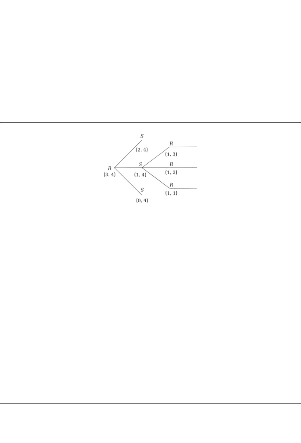
The two steps would be true in a modified form if there is uncertainty and impatience.13
To summarize, a cartel would minimize R&D competition. It would let the technologically more advanced
member firm advance toward the patent in minimal cost increments.
12This assumption can be a consequence of technological constraints as well. If, for example, five
technological problems need resolution and the project team can start on the fourth problem only
after the first three have been satisfactorily resolved, then it is very likely that they will not get to it
within the next period.
13The argument of step 1 would be less true if there were uncertainty in the R&D process. In that case,
the cartel might wish to have both firms do R&D because there is a greater probability that at least
one of the two will finish the project quickly. The second step would need to be modified if the cartel
had reason to want to bring the new product to the market as quickly as possible. We will discuss these
generalizations in the last section.
page_182
Page 183
FIGURE 12.1
12.3 Backward Induction: Analysis of the Model
What would be the duopoly outcome (with the two firms competing in their pursuit of the patent)?
Somewhat surprisingly, it turns out that we get a sharp answer to that question if we make one last
assumption:
5. The two firms take turns deciding how much to spend on R&D; if RCA makes an R&D decision this
period, it waits to make any further decisions till it learns of Sony's next R&D commitment. Furthermore,
Sony makes its announcement in the period following RCA's announcement.
One way to think about this assumption is that each firm's management makes periodic reviews of the
project. These reviews are conducted every few months, and at each such review a decision is taken about
R&D spending until the next review. The decision might be to step up spending levels, to hold them at the
current level, or to cut back. Firms alternate in their decisions if the review dates are different, although the
length of the review period is the same for the two firms.
Assumption 5 turns the patent race into a game of perfect information; let us look at its extensive form. In
Figure 12.1, RCA has the first R&D decision, and RCA and Sony are, respectively, 3 and 4 steps from
completing the project.
A somewhat more transparent depiction of this same situation can be given in a location space picture. By
that we mean a picture in which the "coordinates" of the two firmsthat is, how far they are from finishingare
graphed. In this location space picture, the northeast point refers to the joint finish line for both firms; that is,
successful completion of R&D by both firms. The finish line for S is the vertical terminal line, whereas the
finish line for R is the horizontal terminal line; see Figure 12.2.
page_183
Page 184
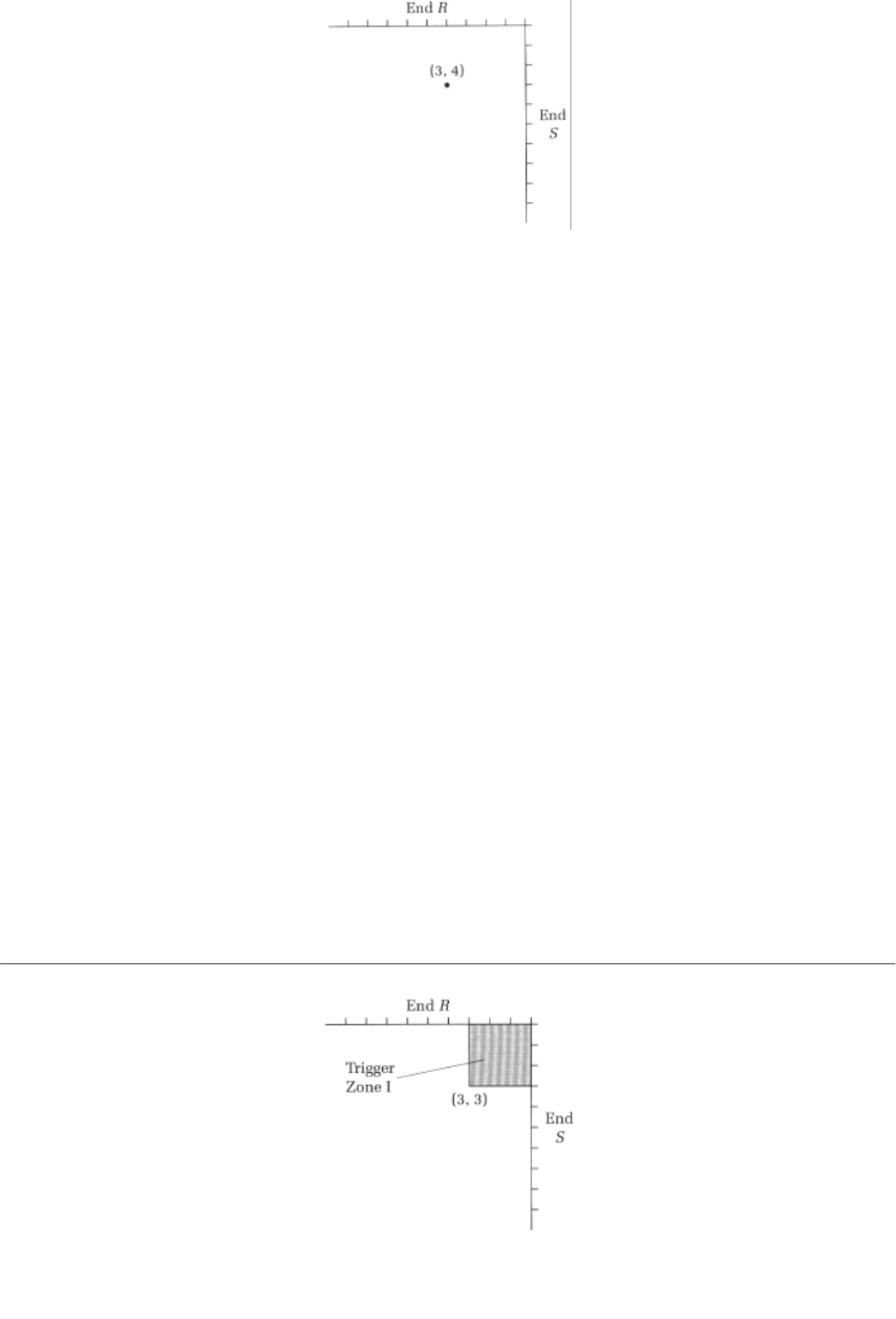
FIGURE 12.2
The following notation will be useful for the location space. If R is r steps from completion while S is s steps
away, we will denote their location as (r, s). The game will be solved by backward induction on the location
space. In other words, we will show that when either firm is near completion there is a best way for them to
make their R&D choice. In turn, these eventual decisions will affect the choices the firms make at more
formative stages of R&D.
To illustrate these ideas, we will proceed in a stepwise fashion:
Step 1. Suppose that the game is at (1,s), and it is firm R's turn to move. Its optimal decision evidently is to
finish the game in one move. That will yield a patent of value $20 (million) and will cost $2 (million).
Similarly, if the location is (r, 1) and it is firm S's turn to move, S will complete the project in one step.14
Step 2. Now suppose that the two firms are at either (2, 1) or at (3, 1), and it is firm R's turn to move. It can
complete in one move, and if it does R makes a positive profit at both locations: $20 - $7 in the first case and
$20 - $15 if it is 3 steps from finishing. Indeed, if R does not finish the game in one move, it knows that S
will do so at the very next opportunity (why?), and hence R will either make nothing from that point on or
suffer a loss. For example, if R chooses to make no progress, which is costless, it will find that S will win the
patent in the next period. If it makes incomplete progress1 step starting from (2, 1) or 2 steps or less from (3,
1)it will incur a cost but will not win the patent.
Hence, it is best for R to complete in one step if it has a move at (2, 1) or at (3, 1). Of course, the same result
holds if the firms are at (1, 2) or at (1, 3) and it is firm S's turn to move; S will complete in one step.
In turn this result has the following implication:
Step 3. (a) Use the previous analysis to show that if the game is at (2, 2), whichever firm has the first move
should invest for two steps and finish the game. (b) Can you then
14Note that we made no mention of how much either firm may already have spent. Regardless of
how much has already been spent, a firm one step from finishing stands to make a net profit of $18
by completing the project. We will come back to this ideathe irrelevance of sunk costsat the end of
this chapter.
page_184
Page 185
FIGURE 12.3
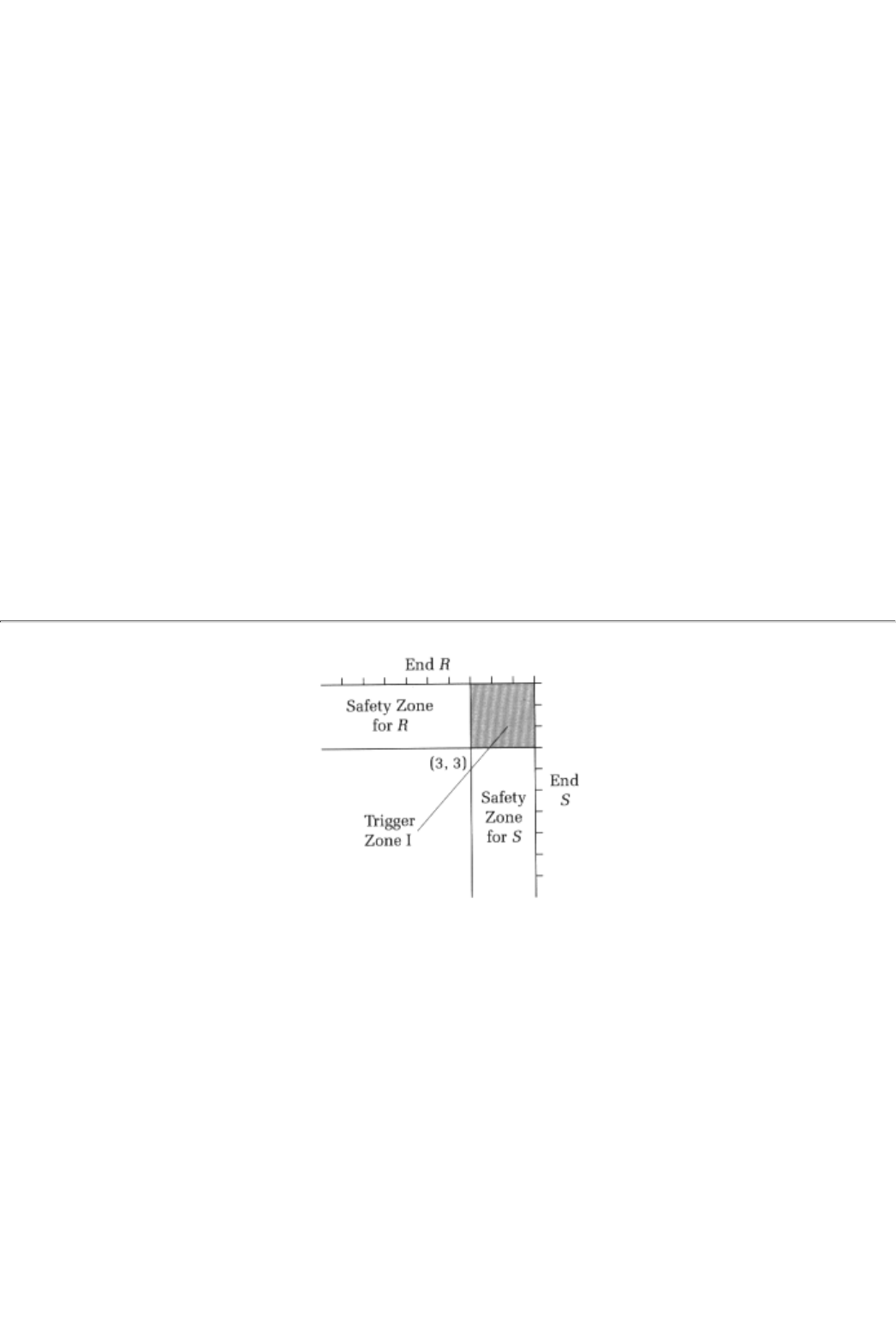
show that if the game is at (3, 2) and it is firm
R
's turn to move, it should finish in one step. What if the game
is at (2, 3) and S has the first move?15
In fact what we have shown via steps I through 3 is the following:
Proposition (TI). If the game is at any location (r, s), r £ 3 and s £ 3, whichever firm has the first move at
that point will trigger a completion, that is, will end the project in one step.
Call this set of locations Trigger Zone I, as seen in Figure 12.3. Let us use the information about Trigger
Zone I to analyze what happens at other locations. What we are really going to do is fold the location space
back; that is, we will do backward induction on it. Since we know what is going to happen at the "end" of
the space, we can now ask what will happen at a penultimate zone of that same space.
Step 4. For instance, what can we conclude about a location such as (4, 3) when it is firm R's turn to move?
Note that
R cannot finish the game in one step. The most that it can do is move its project forward by three
steps to (1, 3). Or it can move two steps to (2, 3) or one step to (3, 3). Or it can remain where it is by
stopping R&D. In the first three of these cases, R knows that S will, in fact, finish the game at the next step.
(Why?) So the best response for R is to pick the fourth option, make no progress. This is equivalent to
dropping out of the race.
If firm R finds it in its best interest to drop out of the patent race at (4, 3), what should firm S do
subsequently? Well, firm S, as the sole survivor, will get the patent eventually. Since rapid R&D is more
costly than slow R&D, the best approach for S is to move in the least costly fashion, one step at a time,
toward the patent.
Step 5. Show that the same conclusion, R should drop out of the race and S should then advance slowly, is
true also for locations (4, 2) and (4, 1). What about locations (5, 3), (5, 2), and (5, 1)?
15In all of these cases, ask yourself what would happen if the first mover did not complete the
project in one step. What, in particular, would its rival do in the next period?
page_185
Page 186
FIGURE 12.4
Iterating, we can, in fact, conclude the following:
Proposition 2. For all locations (r, s), whenever r > 3 and s £ 3, the best thing that firm R as a first mover can
do is drop out. After this, firm S can take a step forward at a time.
This set of locations is therefore called Safety Zone I for S; in these locations, S can coast and R will drop
out. Since the game is symmetric, we can also conclude that all locations (r, s), r £ 3 and s > 3, is Safety
Zone I for firm R. The two safety zones are pictured in Figure 12.4.
Let us continue with the backward induction argument. We know that in Trigger Zone I there will be a
preemptive move while in Safety Zone I, the "war" is over. The next question to ask is, Is there an incentive
for either firm to try and get into its own safety zone even if doing so means doing rapid R&D?
Step 6. Consider a location such as (4,4). Suppose it is firm R's turn to move. Firm R can, in fact, take the
game into its Safety Zone I in one stepat a cost of 2. Thereafter it knows that S will drop out, and hence it
can move a step at a time toward eventual completion; those three steps will cost a further $6. The total
costs then will be $8, and that is less than the value of the patent.
More is true; as long as R has a way to get into its safety zone-and thereafter move a step at a timewhile
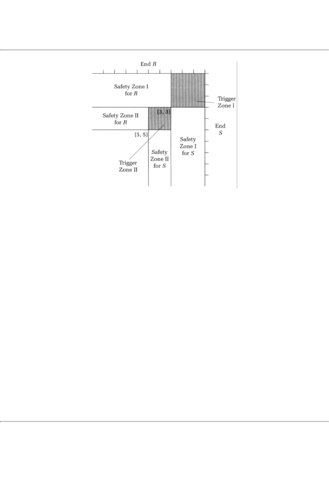
incurring costs that are no more than $20, the value of the patent, it is worth
R
's while to do so. The
argument applies symmetrically, of course, to firm S.
Step 7. Show that from locations (r, s), if r, s = 4, 5, the first mover will find it profitable to take the game in
to its Safety Zone I. Show that if R has to move at (5, 4), its consequent net profit is $7.
page_186
Page 187
FIGURE 12.5
However, it is not worth firm R's while to move into its safety zone if it is at (6, 5). That would cost $21 in
total (why?), which exceeds the value of the patent. Of course, this result implies that, from that location, the
best response for R, if it is the first mover, is to drop out of the race. (Why?)
These arguments give us the following:
Proposition 3. There is a second Trigger Zone between (3, 3) and (5, 5); the first mover in this zone should
move the game into its own Safety Zone I. There is also a second set of safety zones. The one for R is 3 £ r £
5 and s > 5 (and symmetrically for S). In Finn R's Safety Zone II, S should immediately drop out. See Figure
12.5.
Continuing in this fashion, we get the picture shown in Figure 12.6 for the solution in location space.
To summarize, the associated strategies are the following: If S is in R's safety zone whatever the zone
numberthe best thing it can do is drop out of the race. Finn S in its own safety zone spends the minimum
amount on R&D, moves a step at a time, and coasts to win the patent. In Trigger Zone n, each firm spends
what it needs to-profitablyto get an invincible advantage for itself and move the game into safety zone n -
1.16
For these numbers on costs and patent value, there are six trigger zones and five corresponding safety zones.
Different numbers on the cost and patent value variables will change the size and number of these zones, but
will not change the qualitative feature of the solution. Indeed, you will establish the truth of this assertion in
the Exercises.
16Note that except for the trigger zones, the outcome looks a lot like the cartel solution. In other
words, the duopolists fightor spend moneyto establish initial advantage, but once that advantage
has been established there is only a single firm that continues to do R&D.
page_187
Page 188
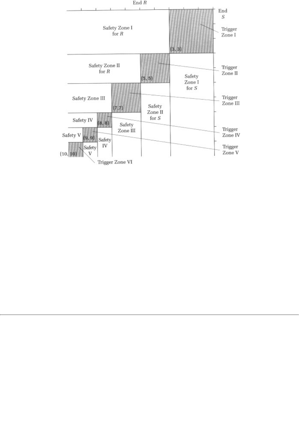
FIGURE 12.6
12.4 Some Remarks
First, our solution teaches us the importance of ''sunk costs." Even if firm S has already spent a large sum up
until some point, it will be ready to spend up to $20 additionally in order to secure the patent. It will be
willing to do so because its net profit from that point on is the patent value minus additional costs, and this
net profit is positive as long as the additional costs are less than $20. Hence the way that the game gets
played from any location (r, s) is completely independent of how the game got to that point, that is, is
independent of the investments that have been sunk by the two firms in getting to that location.
Second, the symmetry assumptions that we madeeach firm's costs of doing R&D are identical, and so is the
value of the patentare completely inessential. The entire analysis can be repeated for the case of dissimilar
costs or patent valuations. All that changes is that the sizes of the trigger and safety zones become
firm-specific. If a firm has lower costs, its zones are going to be bigger, for example. It still remains true,
however, that from any location we will see a one-step movement to a safety zone or an immediate dropout
by the first mover.17
17Again, you will work through some exercises to better understand this point.
page_188
Page 189
Third, the larger the value of the patent, the larger are the trigger zones. For instance, if the value of the
patent is $30, then the size of Trigger Zone II would be the "square" between (3,3) and (6,6), and that of
Trigger Zone III would be between (7,7) and (9,9). Put differently, the patent race would be much more of a
race; a firm would drop out only if it was more than three steps behind its rival but would remain in the race
if it was any closer. The higher the value of the patentor the lower the costs of doing R&Dthe more likely it
is that we have a horse race.
Fourth, if there is uncertainty about the outcome to R&D, then that might induce a firm to stay in the race
longer, because there is some chance that would looks like an insurmountable lead now will not remain so
forever.
Fifth, if a firm has a preference for quick profitsrather than profits that accrue further off in the futureit may
choose to do R&D more rapidly even when there is no competitive threat. For example, consider the cartel
doing R&D. If a cartel member is three steps from finishing the cartel, how much should the cartel spend in
the current period? If the patent is only useful when acquired immediately, the cartel will clearly choose to
complete all three steps in the current period (and pay the higher cost of $15). More generally, if the future

is discounted, the analysis applies except the size of the trigger and safety zones a
nd the behavior within a
safety zone depend on how heavily the future is discounted.18
Sixth, public policy toward R&D is extremely important in this setting because it pays to be ahead even if it
is by a small amount. In the case where the other firm is a foreign competitor, for example, it will pay the
domestic government to subsidize the R&D efforts of the domestic firm so as to give the latter the necessary
small advantage. Furthermore, since all that is required is a small advantage, public policy is also very
cost-effective in this context.19
Finally, what have we learned about HDTV from our model? We know that neither consortium has dropped
out. This fact suggests that profits are expected to be high (or R&D costs are low). Both these inferences
sound reasonable; clearly both consortia (and their administration backers) view HDTV as the technology of
the futureand hence expect large eventual profits. (Further, each government has defense or other
motivations that make the nonmonetary payoffs also loom large.) Doing R&D through the consortia has
lowered the riskiness as well as the capital costs of doing R&D. Finally, if the firms are in their (large) trigger
zones, they should be doing R&D as rapidly as possible. There is certainly evidence to suggest that they are.
Summary
1. A technological breakthrough can be profitably utilized by more than one company, and hence each
company has an incentive to let somebody else make a costly breakthrough. Patents are a way of solving this
incentive problem.
18See Chapter 15 for a discussion of discounting.
19Of course, if both governments are subsidizing their respective R&D efforts, public policy may not
be quite as effective. In particular, relative positions may be completely unchanged if the two
governments spend the sameor similaramounts on subsidizing R&D. This may be a better description
of Japanese and U.S. public policy toward R&D in HDTV. Both governments are activethe Japanese
through the Japanese Broadcasting Corporation's Science and Technology Center and the Americans
through the Advanced Television Center; their efforts might therefore be a wash.
page_189
Page 190
2. In many industries, firms battle furiously to win patents on new technologies; high-definition television
(HDTV) is an example of an ongoing patent race.
3. A two-firm patent race in which the competitors take turns making R&D investments can be modeled as a
game of perfect information. Furthermore, this game can be solved using backward induction on location
space.
4. The backward induction solution has the feature that two firms that are similar distances from project
completion invest heavily to get an R&D advantage. A firm that falls sufficiently behind is better off
dropping out of the patent race.
5. Dropping out is less likely the higher the value of the patent and the lower the costs of doing R&D. These
characteristics describe the current HDTV race.
Exercises
Section 12.1
12.1
Give an example of a research breakthrough that was patented by the company that made the breakthrough
(you might wish to explore the pharmaceutical industry for this example).
12.2
Give an example of a research breakthrough that was privately developed but not patented. Explain whether
it was nevertheless profitable for the company in question to make the breakthrough.
12.3

Give an example of a research breakthrough that was achieved in the public domain either at a university or
at a government research laboratory.
Section 12.3
Let us redo the analysis of the chapter with somewhat different patent values and costs to doing R&D.
page_190
Page 191
12.4
Suppose that the patent is worth $25. Everything else is unchanged. Solve the R&D game by backward
induction.
12.5
What is the difference between your conclusion and that reached in the text? Explain your answer. What
general conclusion can you draw about the effect of patent valuation? Explain carefully.
12.6
Suppose instead that the costs of moving 1, 2, and 3 steps are $4, $10, and $15, respectively (but the patent
value remains at $20). Solve the R&D game by backward induction.
12.7
What is the difference between the conclusion that you arrived at in exercise 12.6 and that reached in the
text? Explain your answer. What general conclusions can you draw about the effect of costs? Explain
carefully.
The next few questions explore a game in which two firmsfirms A and Bhave different costs and benefits
from doing R&D. Let us start with different benefits. Suppose that all of the data of the chapter remain
unchanged except for the fact that the patent is worth only $12 to firm B (whereas it is worth $20 to firm A).
Let a (respectively, b) denote the distance that firm A (respectively, firm B) is from completing its R&D
project.
12.8
Show that Trigger Zone I is made up of all locations in which firm A is within 3 steps and firm B is within 2
steps, that is, is made up of all locations (a, b) such that a £ 3 and b £ 2.
12.9
Show then that Safety Zone I, for firm A, is made up of all locations in which firm A is within 3 steps and
firm B is more than 2 steps from finishing, that is, is made up of all locations (a, b) such that a £ 3 and b > 2.
Similarly, show that Safety Zone I, for B, is made up of all locations in which firm B is within 2 steps and
firm A is more than 3 steps from finishing, that is, is made up of all locations (a, b) such that a > 3 and b £ 2.
12.10
Show that Trigger Zone II is made up of all locations in which firm A is between 3 and 5 steps from finishing
and firm B is between 2 and 4 steps, that is, is made up of all locations (a, b) such that 3 << a £ 5 and 2 << b
£ 4.
12.11
Based upon your answer to the previous question, what do you conclude about Safety Zone II. Explain.
page_191
Page 192
12.12

Explain how you would go about finding the next level of a trigger zone and how that
procedure would pin
down the next level of safety zones. What is the size of Trigger Zone III and Safety Zone III? Explain.
12.13
Find the backward induction solution to this game.
12.14
How would your answers to exercises 12.8-12.13 differ if the firms had different costsin particular, if firm B
is only able to take 1 or 2 steps at a time? Explain in detail.
Section 12.4
12.15
Explain how the principle of sunk costs plays a role in all of your arguments. Briefly describe how these
arguments change if one of the firms is operating with a budget for the entire R&D project.
12.16
Suppose that public policy toward R&D gives one of the two firmssay, firm A, the "domestic" firman initial
advantage. Does it necessarily mean that firm A will win the patent? Under what conditions will this
outcome be predicted? Explain.
12.17
Redo the analysis of the chapter when public policy subsidizes firm R's R&D by 50 percent; that is, it costs
Firm A, 1, 3.5, and 7.5 dollars to make, respectively, 1, 2, and 3 steps of progress.
page_192
Page 193
Chapter 13
Subgame Perfect Equilibrium
This chapter will present a generalization of backward induction called subgame perfect (Nash) equilibrium
that applies to any game in extensive form (and not just to games of perfect information). We will first
motivate the equilibrium concept by way of an example, in section 13.1. Then, in section 13.2, we will
informally define something called a subgame (of a larger game). In section 13.3 we will discuss the
equilibrium concept itself and apply it to the example with which we began the chapter. To illustrate the idea
further, in section 13.4, we will then discuss subgame perfect equilibria in two more examples. Some
remarks about this equilibrium concept follow in section 13.5. Finally, in section 13.6, we will analyze a case
study: Peace in the World War I Trenches.
13.1 A Motivating Example
A game in extensive form that is not a game of perfect information is called a game of imperfect
informationand those are the games that we will study in this chapter. The question that motivates subgame
perfection in imperfect information games is the same as the one that motivated backward induction in
perfect information games: What future behaviors are "credible"? When should a player believe an
opponent's threat to "do x in the future unless you do y today"? What promises, likewise, are "credible"?
Consequently, which equilibrium is "reasonable''?
To motivate the concept of subgame perfect equilibrium, consider the second variation of the entry game
that was unveiled as example 3 in Chapter 11:
Expample 1: Entry Ill
Recall that Coke is debating whether or not to enter a previously untapped East European
market, this time in Transylvania. Pepsi is the current provider in that market and will
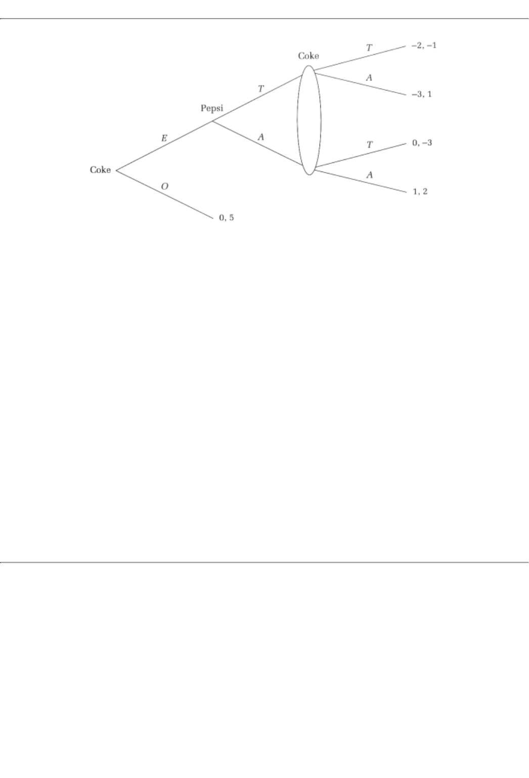
page_193
Page 194
FIGURE 13.1
certainly respond to Coke's entry either by being tough (T) or by accommodating (A). Coke can make a
similar set of choicesT or A. Suppose, finally, that these postentry choices by Coke and Pepsi are made
simultaneously. (Hence this is a game of imperfect information.) The payoffs to the postentry competition
phase are as follows:
Coke \ Pepsi T A
T-2,-1 0,-3
A-3,1 1,2
If Coke stays out of this market, Pepsi continues to make profits of 5. Hence, the full extensive form is as
seen in Figure 13.1.
What would we predict about the play of this game? For starters, let us ask, What are the Nash equilibria of
the game? Those are easier to spot in the strategic form of the game:
Coke \ Pepsi T A
ET-2,-1 0,-3
EA-3,1 1,2
OT0,5 0,5
OA0,5 0,5
There are exactly three pure-strategy Nash equilibria in this game:
1. Coke plays (enter, accommodate)that is, EAwhile Pepsi plays A.
page_194
Page 195
2. Coke plays (out, accommodate)that is, OAwhile Pepsi plays T.
3. Coke plays OT while Pepsi plays T.
The question is, are all these equilibria "reasonable"; that is, is each player's future action "credible"? In this
simple example there is only one future date, namely, the postentry competition phase, and so the question
can be rephrased as, Is each firm's anticipated behavior in the postentry market "credible?"
At this point we have to be precise about what we mean by "reasonable" and "credible." The idea motivating
credibility is very similar to that underlying backward induction; an anticipated choice in the postentry phase
is credible if, after Coke has entered the market, a player would have the payoff incentives to follow through
and make precisely that choice. In particular, it has to be the case that she cannot do any better by reneging
and playing some other action; that is, her anticipated choice must be a best response. For the pair of players
therefore, the two choices must be a Nash equilibrium in the postentry market.

Let us examine the three Nash equilibria of the whole game. Consider the second one;
the pair of strategies,
OA and T. This equilibrium requires Coke to play A in the postentry game against Pepsi's strategywhich is to
play T. However, if Coke does enter the Transylvanian market, then A is not a best response for Coke (nor
indeed is T a best response for Pepsi). Against a tough Pepsi, Coke would stanch its losses by being tough as
well, while Pepsi would make greater profits by reciprocating against an accommodating Coke (rather than
by being tough). Put differently, the pair (A, T) is not a Nash equilibrium within the postentry game.
Another way of thinking about credibility is that the postentry game is a game in and of itself; once Coke has
entered the Transylvanian market, both firms have to take that entry as a fact of their (corporate) life and
maximize whatever profits they can make at that point. Equivalently, at that point it should be irrelevant
what Coke's prioror preentrybeliefs might have been about Pepsi's intentionsand vice versa. To summarize,
however the two firms plan on playing the entire game, it must be the case that once they find themselves in
the postentry part of the game, their actions must constitute a Nash equilibrium of the postentry game.
Otherwise, at this stage, one or both firms would not stick to their strategy (or strategies).
CONCEPT CHECK
CREDIBLE POSTENTRY BEHAVIOR
Show, using the preceding logic, that the postentry behavior of the first and
third Nash equilibriarespectively, (A, A) and (T, T)are, in fact, credible. Is there
any other credible behavior within the postentry phase? (Hint: think mixed-
strategy Nash equilibrium.)
page_195
Page 196
Anticipating, (A, A), entry is a best-response choice for Coke preentry, and so the pair of strategies (entry, A)
and A is a reasonable Nash equilibrium for the entire game. Likewise, since staying out is better if there is
going to be a drag-down all-out fight upon entry, (out, T) and T is also a reasonable Nash equilibrium for the
whole game.1
An implication of this approach is worth pointing out: whether or not Coke actually enters the Transylvanian
market is irrelevant to the credibility argument. The reasonableness of a Nash equilibrium in the whole game
is to be judged by the counterfactual: if Coke chose to enteror, even, by mistake ended up enteringis its
subsequent behaviorand that of Pepsicredible?2
This ideathat reasonableness of an equilibrium can be judged by the reasonableness of what may not get
playedis similar to what we saw under backward induction. in that case, only one branch of the tree is
actually played, but in order to determine which branch it is, we folded back the entire tree; that is, we
checked credibility everywhere. There is one key difference between a game of imperfect information and
one of perfect information. In the latter, at any node, only one player is called upon to make a decision.
Credibility of a strategy can therefore be judged by simply asking if that player would find it in her best
interest to make that decision at that particular node.3 In a game of imperfect information, two or more
players make simultaneous decisions. So it is the credibility of the group's decisions that we have to judge,
and one way to do so is to check whether or not the group plays a Nash equilibrium in that component of the
larger game.
The credibility arguments of example I can be generalized. To do so, however, we need a few more
concepts.
13.2 Subgames And Strategies Within Subgames
Some parts of a game look very much like a game by themselves. For example, the postentry phase in the
entry game is a game by itself. When we have such a feature we call that part of the original game a
subgame.
Definition. A subgame is a part of the extensive form; it is a collection of nodes and branches that satisfies
three properties: (1) It starts at a single decision node. (2) It contains every successor to this node. (A
successor to node x is all of those nodes that can be reached by following some sequence of branches
originating from x.) (3) If it contains any part of an information set, then it contains all the nodes in that
information set.
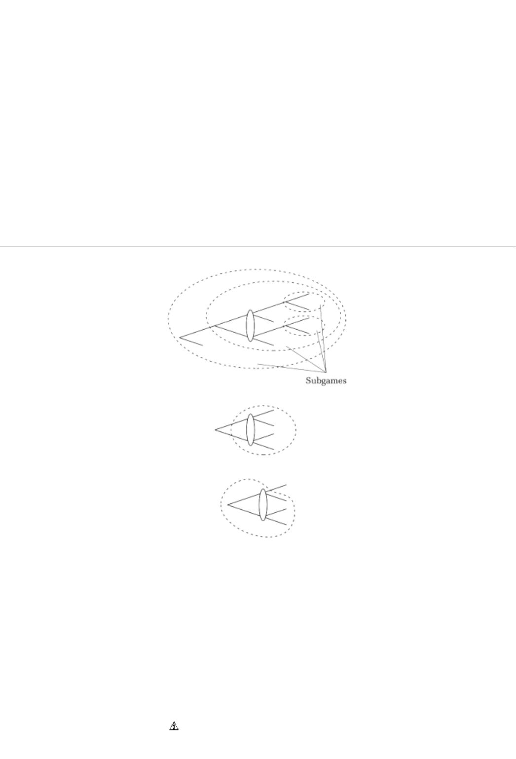
The idea of a subgame is internal containment. So the second and third restrictions s
imply say that you
cannot stray out of the subgame once you are in it and that you will have, within the subgame, all the
information that you need to make decisions. The first restriction is similar to the requirement that the root
of a tree be well defined; it says that we have a unique starting point for the subgame. It is also customary to
call the entire game a subgame (of itself).
1The mixed-strategy Nash equilibrium of the postentry part of the game also begets a reasonable
equilibrium; out coupled with that mixed-strategy equilibrium pair. If Coke anticipates this mixed-
strategy play, with its associated losses of 1, then it is better off staying out.
2For example, in the pair of strategies (O, T) for Coke and T for Pepsi, the postentry game is never
actually played. Yet (T, T) would get played if somehow the players found themselves in the postentry
game. Knowing that (T, T) is a credible continuation, it makes sense for Coke to stay out of the market
(and away from that part of the game).
3For instance, in example 2 in Chapter 11, Coke makes its T or A decision after it knows whether Pepsi
is going to play T or A. Hence, reasonableness can be judged by asking, If Pepsi plays T, what is the
best response for Coke? If Pepsi plays A, what is the best response for Coke?
page_196
Page 197
FIGURE 13.2
FIGURE 13.3
FIGURE 23.4
Examples of subgames are those parts of the extensive formsin the graph shown in Figure 13.2that have
been enclosed in a dot-dash-dot surrounding.
However, the parts of the extensive form shown in Figures 13.3 and 13.4 are not subgames. The first is not a
subgame because it does not start from a single node. The second is not a subgame because it does not
contain all successor nodes.
Finally, since a strategy specifies what a player should do in all contingencies, it tells, in particular, what to
do in any subgame. For example, in the subgame that starts after Coke enters the Transylvanian market, its
strategy tells Coke whether or not to play T. Likewise, Pepsi's strategy tells it whether or not to play T in that
subgame. If player i's strategy for the entire game is denoted si then it will be useful to denote the strategy in
a subgame, say g, as si(g).
13.3 Subgame Perfect Equilibrium
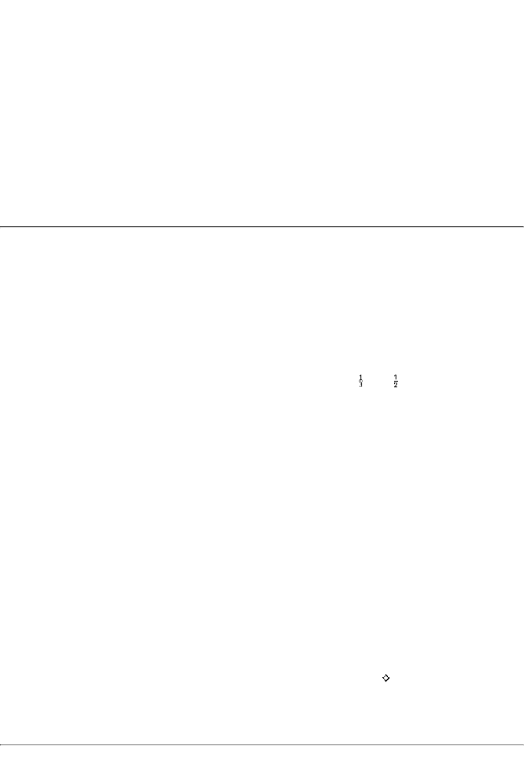
Subgame perfect (Nash) equilibrium
A pair of strategies is a sub-game perfect (Nash) equilibrium if the strategies,
when confined to any subgame of the original game, have the players playing a
Nash equilibrium within that subgame.
To paraphrase the definition, s1 and s2 constitute a subgame perfect (Nash) equilibrium if for every subgame
g, s
1(g) and s2(g) constitute a Nash equilibrium within the subgame.4
We will determine subgame perfect equilibria in games of imperfect information (that have an end) by a
backward induction procedure. We will start with a final
4For N-player games, the definition extends in the natural way; s1, s2, . . ., sN constitute a
sub-game perfect (Nash) equilibrium if the vector of subgame strategies, s1(g), s2(g), . . ., sN(g),
form a Nash equilibrium in every subgame g. This equilibrium concept was introduced by Reinhard
Selten (and it got him the Nobel Prize in 1993).
page_197
Page 198
subgamethat is, with a subgame that ends only in terminal nodesand determine Nash equilibria within that
subgame. We will do the same with all final subgames. We will then back out to a subgame that precedes
final subgames and restrict attention to Nash equilibria within this penultimate subgame that only involve the
play of Nash equilibria in final subgames. And so on.
Let us briefly revisit the game of entry.
CONCEPT CHECK
EQUILIBRIA
Show that there are three subgame perfect (Nash) equilibria to the whole
game: (1) (enter, A) and A, (2) (out, T) and T, and (3) (out, ) and (where
the numbers are the probabilities with which T is selected by the two players).
It is not too difficult to see that subgame perfect Nash equilibrium is, in fact, a generalization of the
backward induction solution, that, in other words, we have the following proposition:
Proposition. In a game of perfect information, the subgame perfect equilibria are precisely the backward
induction solutions. Hence, whenever the backward induction solution is unique, there is a single subgame
perfect equilibrium.
Sketch of a Proof
In a game of perfect information, a subgame starts at every node.5 Consider, therefore, any node that is a
final decision node. For a subgame perfect equilibrium, the decision maker at that node must pick the action
that gives him the highest payoff, that is, must pick a best response. For backward induction, that constitutes
a stage-one folding of the game tree.
At a penultimate decision node starts a game with two players: the penultimate and ultimate decision
makers. A Nash equilibrium of this subgame is, by definition, both players playing best responses. We know
what the best response of the ultimate decision maker is. A best response for the penultimate player is to find
the best choice against the (already inferred) ultimate decision. And that is exactly the same thing as a
stage-two folding of the tree in the backward induction procedure.
It should not be too difficult to see that finding Nash equilibria within every subgame is therefore equivalent
to folding the tree within that subgame. It should, likewise, not be too difficult to see that if there is a unique
way to fold the tree, there is also a unique Nash equilibrium in every subgame.
5The subgame that starts at a node, say a, is made up of all the nodes that follow a.
page_198
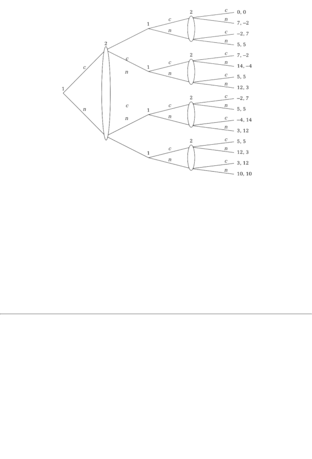
Page 199
FIGURE 13.5
13.4 Two More Examples
To further develop these ideas we will analyze two more examples.
Example 2: Once-Repeated Prisoners' Dilemma
Suppose that the game of Prisoners' Dilemma is played twice. The first time around, the two players have a
choice of (confess [c], not confess [n]). Then these choices are revealed and the two players again get to
choose between c and n. The payoff to these two rounds of interaction is the sum of the payoffs in each
round. The extensive form of the game is presented in Figure 13.5. Note, first of all, that there are five
subgames; four of these are round-two interactions that follow the respective play of (c, c), (c, n), (n, c), and
(n, n) in round one. The fifth is the whole game.
Let us start with the (final) subgame that follows (c, c) in round one. Subgame perfect equilibrium strategies
must specify a pair of actions that form a Nash equilibrium
page_199
Page 200
within this subgame. That statement implies that each player's strategy must specify the play of c at this
second round. (Why?) Indeed, more is true:
CONCEPT CHECK
CONTINUATIONS
Show that regardless of whether round-one play was (c, c), (c, n), (n, c), or (n,
n), in a subgame perfect equilibrium round-two play has to be (c, c).
Hence, regardless of what the players do in round one, their round-two payoff is going to be the payoff to
(c, c), that is, 0. Hence, the only two strategies to check in round one are the two that play, respectively, c or
n in that round (and follow with c no matter what, in round two). In comparing the two strategies we clearly
need only compare their first-round payoffs. An equivalent way of stating this point is that, in choosing
between the two strategies, a player may as well treat his choice as if he is playing the Prisoners' Dilemma
once. In that game, of course, the only Nash equilibrium is (c, c).
To summarize, the unique subgame perfect equilibrium is as follows: Each player confesses no matter what;
each confesses the very first time and again in the second round (even if his opponent had not confessed in
round one and even if he, mistakenly, did not confess the first time around).
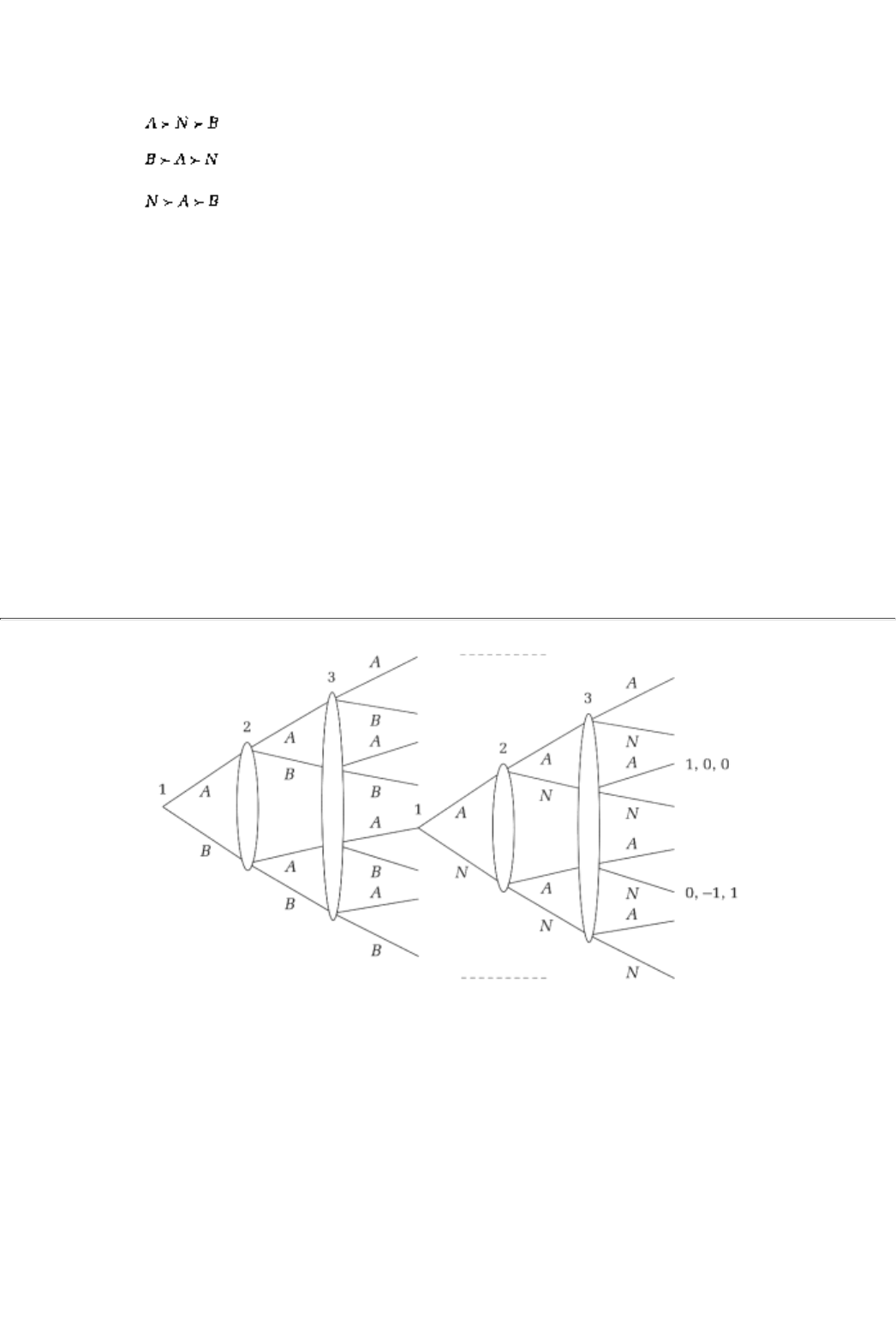
In the next example, we return to the voting game of Chapter 1.
Example 3: Voting
Three legislators have the following preferences among three bills: A, B, and the status quoor neither (N):
Voter l:
Voter 2:
Voter 3:
Voting proceeds in two rounds, and in each round voting is simultaneous. Bills A and B face off in the first
round; the winner then goes up against the status quo (see Figure 13.6).6
From the extensive form it is clear that there are nine subgames: eight second-roundor finalsubgames and the
whole game itself. One set of final subgames is the second round of voting if A is the first-round victor,7 and
the other set of four subgames is the second round of voting if B wins the first round.
Evidently, the four subgames in which A is the first-round victor have identical second-round equilibrium
possibilities. In fact, there are three Nash equilib-
6Figure 13.6 is only part of the extensive form, since it shows the round 2 contamination only after
a B, B, A vote in round 1.
7And A can be the first-round victor in four possible ways: all three voters voted for that bill, only 1
and 2 did, only 1 and 3 did, or, finally, only 2 and 3 did.
page_200
Page 201
FIGURE 13.6
ria in each of those subgames, and one of those is a (weakly) dominant strategy solution:
CONCEPT CHECK
DOMINANT STRATEGY
Show that voting truthfully is a dominant strategy in the second round for
every voter.
In the truthful-voting Nash equilibrium, A wins over N. There are, however, two other (trivial) Nash
equilibria in this subgame: everybody votes for A or everybody votes for N. (Why are these Nash equilibria
of the subgame?).8 Since these last two equilibria involve the play of dominated strategies, I will exclude
them in what follows (but see footnote 9). Likewise, in the round-two B-versus-N vote, there are three Nash
equilibria: (1) everybody votes truthfully and N gets elected; (2) everybody votes N; and (3) everybody
votes B (we will ignore the last two).

Let us now consider the penultimate subgamethe whole game. Since
A
will defeat
N
in the second round but
B
will not, in the first round each legislator really chooses between candidates A and N. Again, voting one's
true preferences between A and N is a dominant strategy for each player. (Why?) Hence, there is one Nash
equilibrium in which voters 1 and 2 vote for A while 3 votes for B; A gets elected. Put differently, the
8This is a more general, and annoying, phenomenon about voting games. It is worth voting one's
preference only if there is (some) chance that the vote will make a difference. If I am convinced
that my vote will make no difference to the outcome, I may as well vote any which way. This
phenomenon can also affect real-world voting; voters who think that they will have no effect on the
outcome simply stay away from the polling booth.
page_201
Page 202
only subgame perfect (Nash) equilibrium in which no player ever plays a dominated strategy is the following
set of strategies:
Voter 1: AAN
Voter 2: AAB
Voter 3: BNN
where AAN, for example, is the strategy in which the first-round vote is for A, the second-round vote is also
for A (against N) but is N (against B). There are two other Nash equilibria that involve the play of dominated
strategies in the first round:
CONCEPT CHECK
FIRST ROUND WITH DOMINATED STRATEGIES
Show that everybody voting for A (followed by truthful voting in the second
round) is a subgame perfect equilibrium. What about everybody voting for B
in the first round?
To summarize, there is a single subgame perfect equilibrium in which no player plays a dominated strategy in
either round: voter i votes for A in the first round if A is preferred to N (and in the second round votes
truthfully). There are two other subgame perfect equilibria in which no dominated strategies are played in
round two (where everyone votes truthfully), but they are in round one. In the first of these equilibria,
everyone votes for A in the first round, whereas in the second, everyone votes for B.9
13.5 Some Remarks
The first thing to note about the concept of subgame perfect equilibrium is that it enshrines the notion that
"bygones are bygones." It requires that no matter which subgame we start from, players must play a Nash
equilibrium from that point on. This choice is required even if we got to that subgame by the play of
something other than a Nash equilibrium strategy. On the one hand, the argument is really a rationality
argument; rational players will recognize a profit opportunity when they see it. Hence, if they are asked not
to play a best response, they will profitably deviate from such a prescription for play.
On the other hand, this is a very strong rationality postulate; no matter how irrational other players may have
been in the past, a player still believes that they will be rational in the future. In other words, they will play
Nash in the future although, for some reason that the player cannot explain, they hav
e not played Nash in
the past. Some people find this strong a dose of rationality disquieting!
9There are also equilibria in which dominated strategies are played in both rounds. For example,
everybody votes for A in each round. (Why is this a subgame perfect equilibrium? Are there others
like it?)
page_202
Page 203
Second, to repeat a point made earlier, the way we solve for subgame perfect equilibria in a game that has an
endthat is, a game with a finite number of nodesis by backward induction. We look for Nash equilibria in the
last subgame, then use them to solve for play in the penultimate subgame, and so on. In games that have an
infinite number of decision nodesthat is, in infinite gamesthe subgame perfect equilibrium concept is still
valid. We cannot, however, use backward induction anymore because there are no last s
ubgames. In the
next few chapters you will see how we can nevertheless proceed in this case.
13.6 Case Study: Peace In The World War I Trenches
World War I was one of the bloodiest wars in human history.10 Part of the reason was that this was the first
war when new technologies, such as machine guns, with much greater destructive capabilities were available
but the generals were still fighting a 19th-century war heavily dependent on infantry movements. It was also
one of the slowest wars; for a couple of years the two sides were dug into trenches constantly fighting but
gaining little territory.11 The same regiments faced each other across the barbed wire month after dreary
month. In a sense, the troops on either side got to know each other better through the months of stalemate
than their respective high commands knew them or their ground conditions.12
One of the most unusual phenomena reported from the trenches was the implicit peace that broke out
spontaneously among the soldiers doing the actual fighting. Observers reported that every day for a few
hours the guns would fall silent in the trenches of Verdun, Somme, and Massines. These pauses would give
the tired men a chance to rest and recuperate and cleanse themselves. What is more interesting is that the
hours of peace were very regular; one report says that every day like clockwork the Germans would fire a
lone shell into the same spot in no-man's-land, and that shot would signal the beginning of the temporary
peace.
Here is a simple extensive form rendering of this phenomenon. Suppose that there can be two levels of
preparedness: high (H) and Low (L).13 Regardless of the level of preparedness each side has available two
options on what it can do, fight (f) or accommodate (a). For example, if the level of preparedness is high
then the strategic form (sub)game is as follows:
Central \ Allied f a
f 1, -1
a-1, 1 0, 0
10On the Allied Powers side ranged Britain, France, the United States, and Russia, while on the
Central Powers side there was Germany, Austria-Hungary, and the Ottoman Empire.
11One of the bloodiest and slowest locales was along the French-German border, the so-called
Western Front. In perhaps the most infamous battle in those trenches, the Battle of the Somme in 1916,
in over four months of fighting the Allies gained only 125 square miles of ground along the Somme
River. In order to do so they sacrificed 600,000 lives (400,000 British and 200,000 French) while the
Germans lost 450,000 lives. For much fascinating information about this war you can visit a World
Wide Web site called Trenches on the Web at worldwar1.com.
12One reason why casualties were as heavy as they were in the Battle of the Somme is that on the first
day the British commander, Sir Henry Rawlinson, ordered his troops to march in formation toward the
German machine guns.
13Think of high as having some of the soldiers always on alert while low is having them all ''at ease."
page_203
Page 204
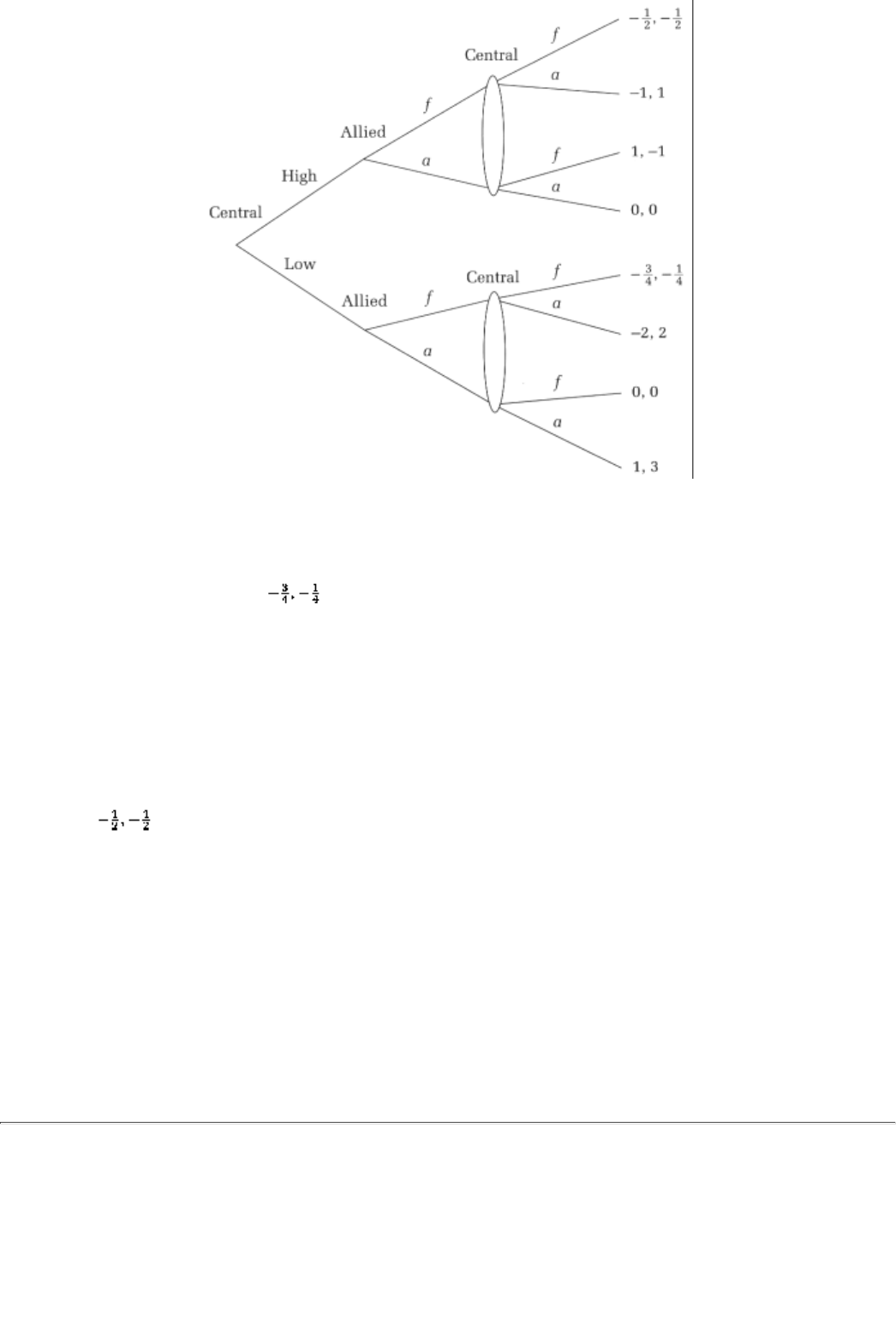
Figure 13.7
However, if the level of preparedness is low for the Germans, but remains high for the British-French, then
the strategic form (sub)game looks like this:
Central \ Allied f a
f 0, 0
a-2, 2 1, 3
Finally, suppose that the German (Central Powers) forces can determine unilaterally their level of
preparedness (and that is what they signal to the Allied forces by the early evening lone shell; firing it
indicates that they are descaling from high to low, while not firing indicates that they are maintaining the
level of escalation at high).14
The extensive form game is displayed in Figure 13.7. Note that when the level of preparedness is high, f is a
dominant strategy for both sides. So the only Nash equilibrium in that subgame is (f, f) with associated
payoffs of ( ). If the Germans choose to deescalate, then that subgame has a unique pure-strategy
Nash equilibrium (
a, a)and the payoff for that is (1, 3). Backing to the root of the tree, the German forces
will choose to fire that signaling shell; that is, they will choose low.15
14In this analysis we are assuming that the Germans cannot lie about the implication of their
signal; put differently, they can commit to deescalate. In Chapter 24 we will analyze conditions
under which this signal will in fact be truthful.
15Needless to add, this is a very simple analysis of a complex situation. In particular, we would have to
add further elements to the game to explain why the two forces ever go back to fighting (later in the
night). A practical reason during WWI was that the generals, far from the killing fields, were upset at
reports that their men were making peace with the enemy.
page_204
Page 205
This case also illustrates the power of commitment, a topic we first encountered with games of perfect
information. Since the Central Powers are able to commit to lowand they suffer disproportionately if there is
fighting at that level of preparedness(a, a) is a credible future play for the two adversaries. Consequently, in
this example, both players are better off.
Summary

1. A subgame is a part of the whole game that is a game in and of itself; it contains
all the future
consequences, and it includes all the information that is necessary to play this part of the game.
2. A strategy vector within a subgame is credible if it forms a Nash equilibrium within the subgame; no
player has an incentive then to renege.
3. A strategy vector for the whole game is a subgame perfect (Nash) equilibrium if every containment within
every subgame is a Nash equilibrium (of that subgame).
4. Subgame perfection can be used to select reasonable equilibria among the entire set of Nash equilibria in a
game. For example, in the game of entry it says that the only circumstance in which Coke will enter is if it
expects Pepsi (and itself) to accommodate entry.
Exercises
Section 13.1
Let us modify the timing structure of the game of entry. Suppose that Coke's entry decision is made at the
same time that Pepsi decides between tough and accommodate. Then, if Coke chooses to enter, it has a
further decision between tough and accommodate. Suppose that the payoffs at every terminal node that
follow enter are exactly as before. If Coke stays out, then the payoffs are (0, -1) if Pepsi plays T and (0, 0) if
it plays A.
13.1
Write down the extensive form of this game. How many subgames are there in this game?
13.2
Solve the game by backward induction. Be sure to detail every step.
page_205
Page 206
13.3
Suppose the payoffs when Coke stays out are (0, 1) and (0, 0) instead when, respectively, Pepsi plays T and
A
. Solve this game by backward induction.
Let us yet again modify the game of entry. Supposeas beforethat Coke's entry decision and Pepsi's T/A
decisions are simultaneous. Suppose, furthermore, that when Coke makes its subsequent choice between T
and A it is unaware of Pepsi's choice.
13.4
Write down the extensive form. How many subgames are there in this game? How many strategies does
Coke have? (Use the payoffs of exercise 13.1.)
13.5
Explain why this timing structure is equivalent to Coke and Pepsi making a single simultaneous decision.
What are the strategies involved?
13.6
Find the Nash equilibria of the game.
Section 13.2
Consider the extensive form of exercises 13.1 through 13.3.
13.7
Identify a part of the game tree that is not a subgame because it does not start at a single decision node.
13.8
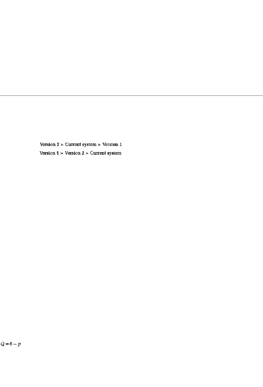
Identify a part of the tree that is not a subgame because it does not contain every s
uccessor to the node that
starts this part of the tree.
13.9
Finally, identify a part of the tree that is not a subgame because it does not contain all the nodes in some
information set although it contains some.
Section 13.4
Consider the following (idealized) model of voting in a Senate committee. The committee is made up of
three members: A1 (A), Bob (B), and Christopher (C), two Republicans and a Democrat, respectively. They
are confronted with two versions of a bill (to end welfare as we know it). Version I proposes a radical
restructuring of the current system,
page_206
Page 207
while Version 2 proposes a more modest overhaul. The committee members vote simultaneously, and they
recommend the version that gets a majority of votes. At that point, the full Senate votes simultaneously and
along party lines between that version and the current system. If a majority of the Senate votes in favor of
the bill it passes; otherwise, it fails and the welfare system remains unchanged. Democrat and Republican
preferences on the two versions and the current system are as follows:
Democrat:
Republican:
13.10
Represent this setup as an extensive form game. (Within the committee distinguish between the members,
but at the Senate level distinguish only between the two parties.)
13.11
Identify the subgames in the game.
13.12
Write down the strategies for each player in the game. Define a subgame perfect equilibrium.
13.13
What must be the votes cast in the Senate by (a) a Democrat and (b) a Republican if neither plays a
dominated strategy?
13.14
Suppose that there is a Republican majority in the Senate. What is the subgame perfect equilibrium of this
voting game (with no dominated strategies played)? Explain your answer in detail.
13.15
Suppose, however, that there is a Democratic majority in the Senate. What is the subgame perfect
equilibrium of this voting game (with no dominated strategies played)? Again, explain your answer in detail.
The next few questions return to the model of price competition. To recall, we have two firms that set prices
in a market with this demand curve:
where p is the lower of the two prices. If the prices are different, the lower priced firm sells all the output. If
the two firms post the same price, then each gets half the market. Suppose that prices can only be quoted in
dollar units and costs of production are zero for both firms. Suppose, unlike in past versions of this problem,
that prior to this price
page_207
Page 208
competition phase firm 2 has to make an entry decision. If firm 2 stays out, firm I remains a monopoly (and
gets the maximum profits that can be generated with the given demand curve). If firm 2 enters, price
competition ensues.
13.16
Write down the extensive form of the game. Identify the subgames.
13.17
Write down the strategies for each firm in the game. Define a subgame perfect equilibrium.
13.18
In a subgame perfect equilibrium, what must be the market price if firm 2 enters the market?
13.19
What is the subgame perfect equilibrium of this model? Does firm 2 enter the market?
13.20
Suppose that there is an entry cost of size c for entering this market (for example, the cost of advertising or
promotional discounts). At what value of c does it not make sense for firm 2 to enter this market? Explain
your answer. What is the subgame perfect equilibrium above this cost level?
Section 13.6
Consider the case study. Suppose that the payoff matrix, if the Germans have deescalated, is given by
Central \ Allied f a
f 0, 0
a-2, 2 1, 1
13.21
Compute the Nash equilibrium within this subgame.
13.22
Draw the extensive form of the entire game. Be careful in filling in the payoffs to each of the terminal nodes.
13.23
Find the subgame perfect equilibrium of this game. Does peace break out in this example?
page_208
Page 209
Chapter 14
Finitely Repeated Games
In the next two chapters we will discuss a special class of extensive form games, called repeated games,
whose principal feature is that players interact not just once but many times. These games have helped
explain why ongoing economic phenomena produce behavior very different from those observed in a
one-time interaction.
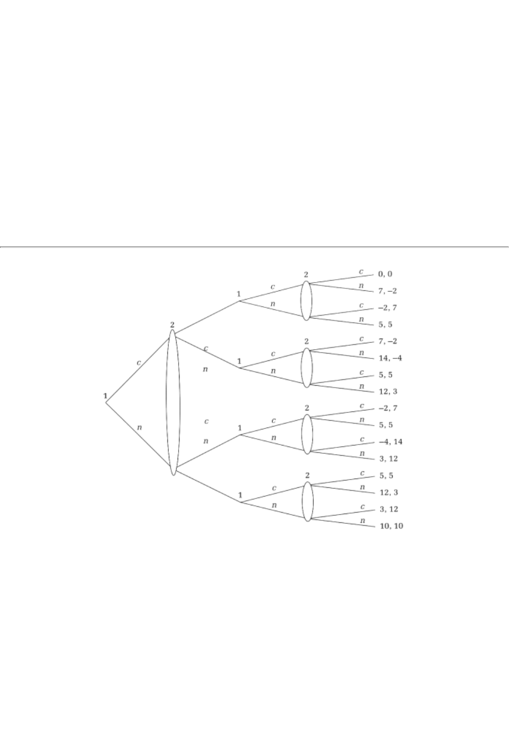
The basic intuition for this difference is straightforward. If players believe that f
uture behavior will be
affected by the nature of current interaction, then they may behave in ways that they would not otherwise.
In particular, if a player believes that "no good deed today will go unrewarded tomorrow," she will have a
greater reason to do a good deed today. Equivalently, if she believes that "no bad deed today will go
unpunished tomorrow," she may be less inclined to do a bad deed today. The prospect of reciprocity then,
either by way of rewards or punishments, is what separates a repeated game from a one-time interaction. Of
course these punishments and rewards have to be credible in the precise sense of the previous chapter; that
is, players will only believe them if they are part of a subgame perfect equilibrium.
In section 14.1 we will give a definition of repeated games and then discuss several examples, including
some real-world examples. In section 14.2 we will turn to a particular subclass of repeated games called
finitely repeated games
, analyze several examples of such games, and from them draw some general
conclusions. Finally, in section 14.3 we will discuss a case study of Treasury bill auctions.
14.1 Examples And Economic Applications
14.1.1 Three Repeated Games And A Definition
In every repeated game there is a component gamesometimes called a stage gamethat is played many times.
page_209
Page 210
Figure 14.1
Example 1: Once-Repeated Prisoners' Dilemma
This is a repeat of example 2 from the previous chapter: the game of Prisoners' Dilemma once repeated. Two
prisoners make a simultaneous choice between confess (c) and not confess (n). Their choices are revealed to
them, and then they are allowed to make the same choices, that is, play the same game again. The payoffs in
the game are the sum of the payoffs in each stage. The extensive form of this game is displayed in Figure
14.1.
Example 2: Finitely Repeated Modified Prisoners' Dilemma
The second example has a stage game that is a slight modification of the Prisoners' Dilemmaand we will
therefore call it the Modified Prisoners' Dilemma. We add one strategy to the standard Prisoners' Dilemma;
in addition to c and n, each player has a third strategy, say, p for "partly confess." Consider the following as
a stage game:
1 \ 2 c n p
c0, 0 7, -2 3, -1
n-2, 7 5, 5 0, 6
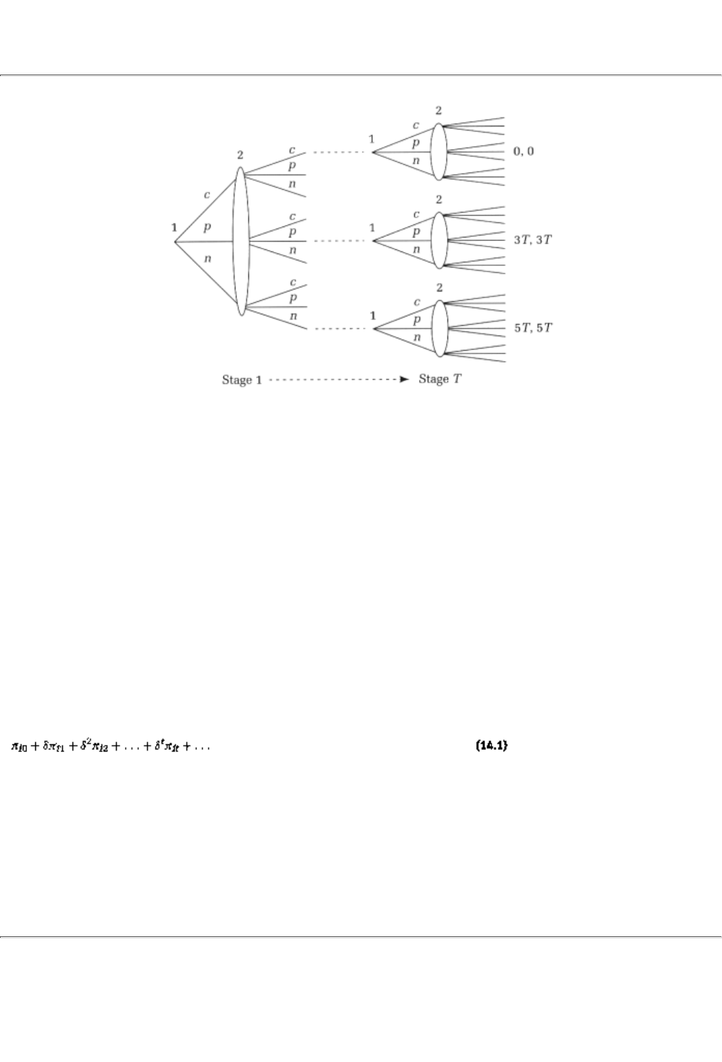
p
-1, 3
6, 0
3, 3
page_210
Page 211
Figure 14.2
Suppose now that this stage game is played T times. At each of these stages, the two players get to choose
from the three strategies, n, c, and p. At the end of each stage, they are told the choices made by both
players, and then they get to make the same choices again. Again, the total payoffs in the repeated game are
simply the sum of payoffs to the T stage games. The extensive form for this game is shown in Figure 14.2.
Example 3: Infinitely Repeated Prisoners' Dilemma
This example is again a modification of example 1. Suppose, as before, that at every stage the two players
play the Prisoners' Dilemma. However, there is no fixed number of repetitions. Every time that they play the
stage game, there is a probability d that the same players will play the stage game again. Conversely, there is
a probability 1 - d that the current interaction is the last one.1 The extensive form of this game is therefore as
presented in Figure 14.3.
This game is called the Infinitely Repeated Prisoners' Dilemma; the terminology refers to the fact that the
game has no fixed end. The payoffs to the Infinitely Repeated Prisoners' Dilemma are computed as follows.
Suppose that at the tth stage, player i gets a payoff of pit. The likelihood that the tth stage will even get
played is dt. Hence the expected payoff to the tth stage is dtpit. The total expected payoff is the sum of
these stage-game expected payoffs; that is, it equals
From these examples it is possible to see the general structure of a repeated game.
1There is an alternative interpretation of d. A player may prefer to get a payoff in stage t rather
than wait to get exactly the same payoff in stage t + 1; (a unit of utility in) stage t + 1 may be only
worth a fraction d in stage t. This bias toward earlier payments is called time preference, and the
associated fraction d is called the discount factor (for a more extensive treatment of tills issue, see
section 15.1).
page_211
Page 212
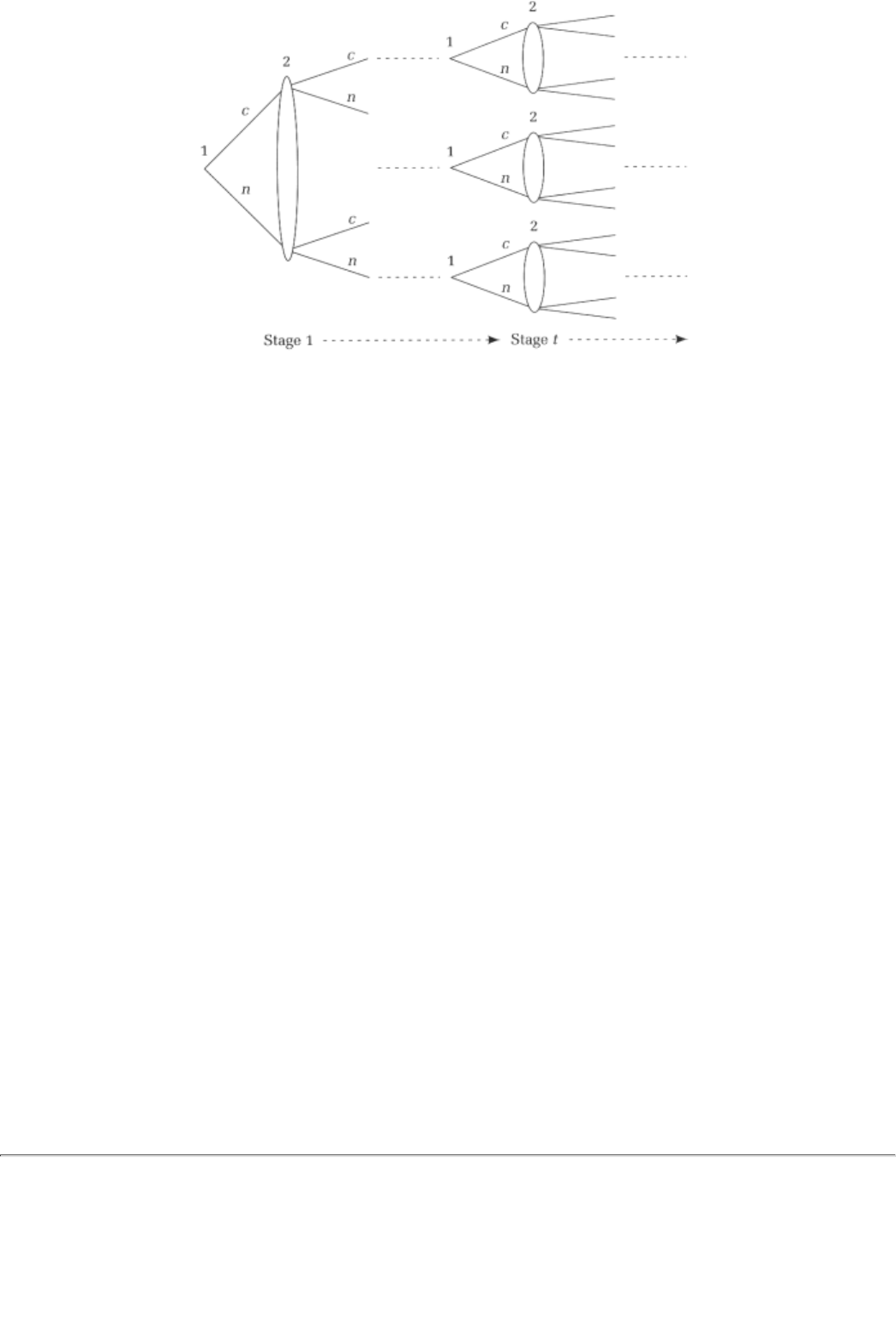
Figure 14.3
Definition. A repeated game is defined by a stage game G and the number of its repetitions, say T. The stage
game G is a game in strategic form: G = {Si,pi; i = 1, . . ., N} where Si is player i's set of strategies and pi is
his payoff function [and it depends on (S1, S2, . . ., SN)]
If T is finite, we call the game a finitely repeated game, whereas if the repeated game has no fixed end we
call it an infinitely repeated game. It is customary to compute the payoffs of a finitely repeated game as the
sum of the payoffs in each stage. For the infinitely repeated game, a common way to compute payoffs is to
add the (discounted) expected payoffs in the manner shown in equation 14.1. In the remainder of this
chapter we will discuss finitely repeated games, and in the next one we will turn to infinitely repeated games.
14.1.2 Four Economic Applications
Finitely Repeated Games
1. Treasury Bill Auction. The U.S. Treasury Department periodically sells securities to raise the cash needed
to finance the federal government's expenditures and to repay maturing debt.2 These securities are sold by
auction, and the principal buyers at these auctions are the government bond departments of large financial
institutions such as Salomon Brothers, Merrill Lynch, and Morgan Stanley.3 The auctions are held on a very
regular basis; on certain kinds of securities the auctions are weekly, and some others are monthly.4
The auctions work as follows: The Department of Treasury issues a press release about one week before
each auction announcing the auction date, the amount, and the type of securities that are to be sold. A
prospective buyer submits a "tender" that specifies
2The securities that are sold vary by maturitywhen a lump-sum payment will be madeand
couponhow much interest will be paid in the interim. The maturities vary from 13-week Treasury
bills to 30-year Treasury bonds.
3In turn, the investment banks sell these securities to institutional investors such as pension funds as
well as to individual investors.
4Thirteen- and 26-week Treasury bills are offered each week, and two- and five-year Treasury notes
are issued once a month. For details about Treasury auctions, visit the Department of Treasury's web
site at ustreas.gov.
page_212
Page 213
the price and amount that he would like. After all the tenders have arrived, the Treasury Department
determines either a fixed price that they will charge on that lot of securities or a range for the price. The
former system is called a single-price auction (since every buyer gets the same rate); this single price is the
one at which the quantity demanded is equal to the amount being sold. The latter is called a multiprice
auction; those willing to pay the highest price are allocated their demand first, then the next highest, and so

on.5
This is clearly a repeated game. The players are the major financial institutions, and they remain unchanged
from auction to auction. The stage game is the auction (for a particular kind of security, say, 26-week
Treasury bills); it is a game with simultaneous moves because the tenders are submitted simultaneously. The
payoffs are the subsequent profits that each institution makes from selling the securities to individual
investors and pension funds. It becomes a finitely repeated game if we consider the 52 such auctions in a
calender year as a group (and separate them from the auctions in previous and following years).6 Treasury
auctions will be studied in greater detail in section 14.3.
2. Competition in a Patented Drug's Market. When a new drug is successfully patented, no competing drug
can be introduced that violates the parent's coverage as long as the patent is in force. Competing drugs
therefore have to use a different chemical composition than the patented drug.7 The competition among the
patented drug and any follower drug during the patent period is an example of a finitely repeated game. It is
clearly a game because there are only a few drug companies involved (and their payoffs are the profits that
they make). It is a finitely repeated game because the patent period is finite.8
Infinitely Repeated Games
1. NASDAQ Market Making. The NASDAQ market is the second-largest stock market in the United States,
after the New York Stock Exchange (NYSE). On this market, there are, on average, about ten dealers who
''make the market" for every stock; each of these ten dealers quotes a buy and a sell pricethe bid and the ask
priceand stands ready to transact at those prices when orders come in. Orders are filled at the lowest ask
price and at the highest bid price. Market makers make profits from the difference between the ask and the
bid price, that is, from the difference between the price at which they sell to customers and the price at
which they buy from (other) customers.
The stage game G is therefore a price competition modellike the Bertrand model that you have seen in
previous chapters. The market makers strategically interact; each one knows that he can capture order flow
by undercutting the rival market makers. This is a marketor gamein which there is no end date to the ongoing
interaction; every time that dealers make a market they believe that there is a (high) probability that the
same group of dealers will make the market again the next hour, or the next day. In other words, this is an
infinitely repeated game. There is, of course, always the possibility that some dealer may leave or a new
dealer may join the market; this is captured by the idea that the probability d of continuing as an unchanged
group is less than one. Market making in NASDAQ is the subject of Chapter 16.
5Thirteen- and 26-week Treasury bills as well as three- and 10-year Treasury notes are sold in
multiprice auctions, whereas two- and five-year Treasury notes are sold by way of single-price
auctions.
6One reason for this approach is that the managers who oversee the financial institutions' strategies
are typically paid on the basis of yearly performance.
7And competing drugs are getting introduced very rapidly these days. The drug AZT, which was
introduced in 1987, had a competitor in Pravachol by 1991. The same length of time separated Prozac,
introduced in 1988, from Zoloft. Also note that after the patent runs out, the field is wide open because
the original drug's chemistry can be utilized by any competing drug.
8After the patent runs out, competition drives down profits for each firm. Since the bulk of the profits
are made during the patent period, we can concentrate on that period for analytical purposes.
page_213
Page 214
2. The International Oil Marketor OPEC. The Organization of Petroleum Exporting Countries is a group of
oil producers who coordinate on the price at which they sell their output. You have seen some discussion of
OPEC already in Chapter 6, and it will be discussed in even greater detail in Chapter 17, and so we will give
only a brief overview here.
The stage game for this application is the international oil market. Producing countries or companies sell to
various customers, who might themselves be companies or countries. The competition is over quantity; each
producer determines how much crude it is going to pump over, say, the next month. The total mount
producedand the world demand for oilthen determines the price. Producers make profits on the basis of how
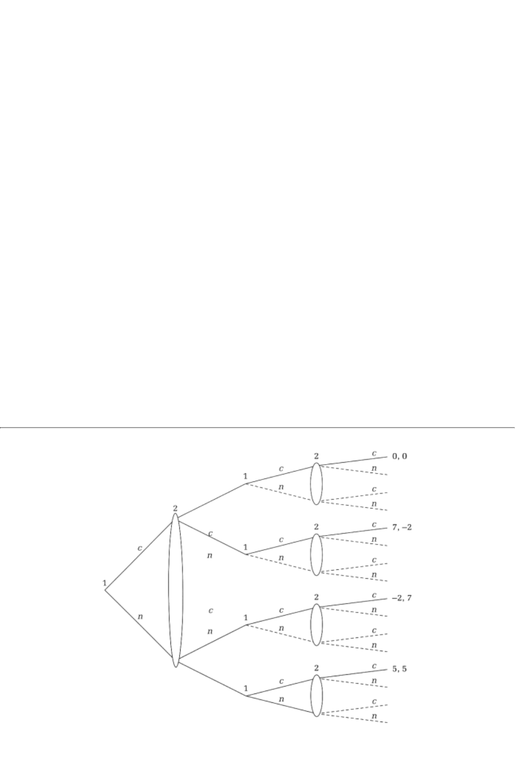
much they sell and what the difference is between the (average) price at which they s
ell and their (average)
cost of production.
The interaction is ongoing; Saudi Arabia and Venezuela fully expect to compete in the oil market a month, a
year, a decade, and possibly even a century from now.9 Indeed the issue for OPEC is precisely whether,
given this ongoing nature of their competition, the producers can refrain from undercutting each other.
14.2 Finitely Repeated Games
The analysis of subgame perfect equilibria in finitely repeated games proceeds by way of backward
induction. Recall, from the previous chapter, that this corresponds to folding the repeated game, one
subgame at a time, from the end.
Analysis of Example 1
In example 1 the last subgames are those in the second stage (see Figure 14.1). As we saw in the previous
chapter, no matter what gets played in the first stage, subgame perfect equilibrium second-stage play must be
(c, c). Folding back to the first round, we see that the players face the game shown in Figure 14.4. Evidently,
the only Nash equilibrium of this game is, again, (c, c). Hence, the players play each of the two stages as if
they were playing each stage by itself. And they play the stage game Nash equilibrium regardless.
Indeed this observation can be confirmed more generally. Suppose the Prisoners' Dilemma is played T + 1
times, where T is any positive integer.
CONCEPT CHECK
STEP 1
Argue that in the last two rounds of the T-times repeated Prisoners' Dilemma,
the preceding analysis applies; each player plays c in each of those two stages.
9Of course, this game is not strictly infinitely repeated, since there is a zero probability that it will
last, say, a million years or more. However, there is no certainty either about when the oil reserves
will actually run out. Therefore, we can study this application, at first pass, as a game with no fixed
endthat is, as an infinitely repeated gamepossibly with a lot of discounting of the very distant
future.
page_214
Page 215
Figure 14.4

What happens when there are three rounds left? It is not too difficult to see that th
e effective game that
remains after the first round is the same as Figure 14.4. Hence, we have the following:
CONCEPT CHECK
STEP 2
Show that, since play in the last two rounds will be independent of what
happens in the current stage, players must treat the game as if there is exactly
one stage left. Hence both players will confess.
So the three-round Prisoners' Dilemma, again, has only one subgame perfect equilibriumand both players
always confess in every subgame. But then we can use the observation for the three-stage Prisoners'
Dilemma game to show that the thrice-repeated Prisoners' Dilemma also has a unique equilibrium, (confess,
confess), all the
page_215
Page 216
time. And indeed we can extend the argument all the way back to the initial node of the T-times-repeated
Prisoners' Dilemma:
CONCEPT CHECK
ALWAYS CONFESS
Show that the unique subgame perfect equilibrium of the T-times-repeated
Prisoners' Dilemma is for each player to confess in every contingency.
Analysis of Example 2
Let us develop the argument for example 2 in steps. Consider, first, the case where the Modified Prisoners'
Dilemma is played just once. You should be able to convince yourself from looking at the structure of
payoffs that there are two Nash equilibria of this stage game(c, c) and (p, p).
If the Modified Prisoners' Dilemma is repeated once, then in the second stage one of these two Nash
equilibria has to be played. Since there are two Nash equilibria to choose from, ther
e is now the possibility of
reciprocal behavior; which of the two equilibria gets played may depend on what behavior is observed in the
first stage. In particular, "good" behavior in the first stage may be rewarded by the better Nash equilibrium
(p, p), whereas "bad" behavior may be punished by (c, c). Put differently, good behavior in the first stage
may generate a belief among the players that there will be continuation of such cooperative behavior in the
second stage, but if the first-stage behavior is itself bad, there is little reason to believe that the second stage
will see cooperative behavior.
Consider the following strategy: At Stage 1, each player plays n, the "good" strategy. If they both do so, in
the second stage each plays p. On the other hand, if either of them plays c or p in the first stage, then in the
second stage they both play c. Put differently, the strategy specifies that in every second-stage subgame,
except that which follows (n, n), the players play (c, c); only in the subgame that follows (n, n) do they
reward themselves by playing (p, p).
CONCEPT CHECK
Argue that the preceding strategy is a subgame perfect equilibrium if player 1's
payoff to (n, n) followed by (p, p) is greater than his payoff under (c, n)
followed by (c, c). Show that it is.
page_216
Page 217
Note that by playing
n, neither player gets the highest payoff that he could achieve in that stage. By playing
c a player would get himself a payoff of 7 rather than 5 in the first stage. [However, by doing so he would
also jeopardize a future play of (p, p) and hence a future payoff of 3.] In other words, players do not
necessarily play the first round according to stage-game Nash equilibrium strategies. This is precisely the
lesson of repeated games; a player will be willing to sacrifice short-term gains from "doing bad" if he is
convinced that by doing so he will get a reciprocal reward in the future.
Suppose the Modified Prisoners' Dilemma is played
T
times. Consider the following strategy pair: start with
(n, n) and continue in that way at all stages except the last one [and at that stage, play (p, p)]. Follow this
procedure provided neither player deviates from it (and plays something other than n at any of the first T
stages). In the event of a deviation, play (c, c) from the subsequent stage onward.
CONCEPT CHECK
EQUILIBRIA
Show that the preceding strategy is a subgame perfect equilibrium.
Notice that we have not asserted that this strategy is the
only subgame perfect equilibrium of this game.
Indeed it is not. For instance, here is another one (in the once-repeated game): Start with (n, c). If that is in
fact played, then play (p, p) in the second stage. Otherwise, play (c, c).
CONCEPT CHECK
ANOTHER EQUILIBRIUM
Show that the preceding strategy is a subgame perfect equilibrium.
Consider the following two strategies as yet other equilibria: (1) play (p, p) in the first round and in every
one of the second round subgames or (2) play (c, c) in the first round and in every one of the subgames in
the second round. These strategies are simply repeats of one-stage Nash equilibria. It should be clear that
these continue to be subgame perfect equilibria of the finitely repeated Modified Prisoners' Dilemma. More
generally, the following is true:
page_217
Page 218
CONCEPT CHECK
REPEATING OUR MISTAKES
Consider any finitely repeated game. Show that one subgame perfect
equilibrium of the repeated game is for players to play (myopically) a
one-stage Nash equilibrium over and over again.
14.2.1 Some General Conclusions
The two examples that we have analyzed contain some general conclusions. There is a fundamental
difference between the finite repetition of stage games in which there is a unique Nash equilibrium and those
in which there is more than one Nash equilibrium. When there is a single Nash equilibriumas in the Prisoners'
Dilemmano matter how many times the game is repeated, there is still only one subgame perfect equilibrium.
That equilibrium is to play the stage game Nash equilibrium repeatedly. In other words, the prospect of
future interaction does not change players' behavior in any way; we can assert the following proposition:
Proposition. Consider a finitely repeated game (G, T) with G={Si,pi; i = 1,. . . , N} Suppose the stage game
G has exactly one Nash equilibrium, say ( ). Then the repeated game has a unique subgame
perfect equilibrium. In this equilibrium, player i plays at every one of the T stages, regardless of what
might have been played, by him or any of the others, in any previous stage.
Sketch of Proof
The proof of this proposition is exactly the same as that which we have already seen for the T-repeated
Prisoners' Dilemma. In the very last stage, every subgame perfect equilibrium must specify the play of the
unique stage-game Nash equilibrium, (). Consequently, play in the penultimate stage cannot be conditioned
on future rewards because ( ) will be played in the last stage no matter what is played in the
penultimate stage. Hence, the penultimate stage will be treated as if it is a stage game by itselfand within that
game the only possible equilibrium is, of course, ( ).
Hence no matter how play proceeds in the first T - 1 stages, in the last two stages it must necessarily involve
the play of the stage-game Nash equilibrium in each of those stages. This fact then implies that in the
third-last stage no future rewards are expected by the players. Hence they treat this stage as a one-time
interaction; its only outcome is therefore (
). And so on. à

However, if there is more than one Nash equilibrium, there is always the possibility
of sustaining good
behavior in early stages of repeated interaction. This good behavior is sustained by the prospect of better
future play than that which follows short-term opportunistic behavior. Again, the general argument is the
same as the one that we saw in the context of the repeated Modified Prisoners' Dilemma. Good behavior in
early
page_218
Page 219
interactions can be rewarded by the play of better Nash equilibria in future subgames, while any deviations
from this behavior can be punished by the play of bad Nash equilibria in future subgames.10
14.3 Case Study: Treasury Bill Auctions
The institutional structure of Treasury bill auctions was explained earlier in this chapter. We will therefore
focus on one key aspect of these auctions, the pricing issue. Recall that for some securities, there is a
single-price auction in which all buyers pay the same price. For some others, there is a multiprice auction in
which different buyers pay different prices. The question that we will now investigate is the following: If the
Treasury wants to maximize the amount that it collects, which of the two auction forms should it use?
In order to keep the analysis tractable, we will make several simplifying assumptions. First, we will assume
that there are two financial institutions, or players, at this auction. Second, the quantity that the Treasury
sells remains fixed from auction to auction; let this amount be 100.11 Third, we will assume that there are
two prices and two quantities that each buyer can offer; call the prices high (h) and low (l) and the amounts
50 and 75. Fourth, buyers care only about profits; denote the profit per security if the price is h as ph and
likewise the profit if the price is l as pl. Suppose that both profit levels are positive (and, of course, pl > ph).
If each buyer wants to buy at a high price, then the total demand at that price is at least 100 and all of the
Treasuries sell at that price. Likewise, if both buyers want to buy at the low price, then the market price is
low. If, however, one of the buyers wants to buy at h while the other wants to buy at l, then the price
outcome depends on the type of auction. In a single-price auction, the market price will be low, while in a
multiprice auction one buyer will pay h and the other will pay l. In either case, the high bidder gets all of the
quantity he asks for and the remaining quantity is allocated to the low bidder. Finally, if the price bids are
the same, then the quantity is allocated in proportion to the quantity demands. For example, if one buyer
wants 75 units and the other wants 50, then the former gets 60 of the available 100 units.12
With these assumptions, the strategic form of a single-price auction is as follows:
Buyer 1 \ Buyer 2 50, h 75, h 50, l 75, l
50, h50ph, 50ph 40ph, 60ph 50pl, 50pl 50pl, 50pl
75, h60ph, 40ph 50ph, 50ph 75pl, 25pl 75pl, 25pl
50, l50pl, 50pl 25pl, 75pl 50pl, 50pl 40pl, 60pl
75, l50pl, 50pl 25pl, 75pl 60pl, 40pl 50pl, 50pl
For example, if buyer 1 bids a high price against 50, l, then he gets all of his quantity at a low price; the price
is low because there is no demand for all 100 units at price h. If he bids 75, l (against 50, l), then he gets 60
units allocated at the low price. Note furthermore
10In the Modified Prisoners' Dilemma there are two Nash equilibria in the stage game, one of
which is preferred by both players to the other equilibrium. In general there may not exist such
unanimity in opinion; that is, there may be two Nash equilibria in the stage game, the first of which
is preferred by player I while the second is preferred by player 2. Nevertheless it is still possible to
sustain good behavior in early stages by an appropriate modification of the arguments discussed in
the text. For details, consult Drew Fudenberg and Jean Tirole, Game Theory (Cambridge, MA:
MIT Press, 1991).
11Note that we are looking at the repeated auction of any one kind of security, say, 26-week Treasury
bills. The assumption that the same number of such bills are sold every week makes it a repeated game.
If the quantity were to vary from week to week, each week's stage game would be a little different from
every other week's. The current analysis can be generalized in that direction. In Chapter 17 we will
look at repeated games with random variations in the stage game (for instance, because the federal
government's financing needs vary randomly from time to time).
12The assumed quantity allocation rules are essentially the same as the Treasury Department's actual
rules.
page_219
Page 220
that, at any price, it is always better to ask for a larger quantity75, l dominates 50, 1, and 75, h dominates 50,
h. The reason is simple: 75, l dominates 50, l because at the consequent low price a higher quantity demand
means a higher (and more profitable) allocation. Also, 75, h dominates 50, h; it has the same effect on price,
and its quantity allocation is at least as high.
Similarly, the strategic form of a multiprice auction looks like this:
Buyer 1 \ Buyer 2 50, h 75, h 50, l 75, l
50, h50ph, 50ph 40ph, 60ph 50ph, 50pl 50ph, 50pl
75, h60ph, 40ph 50ph, 50ph 75ph, 25pl 75ph, 25pl
50, l50pl, 50ph 25pl, 75ph 50pl, 50pl 40pl, 60pl
75, l50pl, 50ph 25pl, 75ph 60pl, 40pl 50pl, 50pl
For precisely the same reason as before, again 75, l dominates 50, l, and 75, h dominates 50, h. From the
point of view of stage-game Nash equilibrium analysis we can therefore look at the reduced single-price
auction:
Buyer 1 \ Buyer 2 75, h 75, l
75, h50ph, 50ph 75pl, 25pl
75, l25pl, 75pl 50pl, 50pl
And this is the reduced multiprice auction:
Buyer 1 \ Buyer 2 75, h 75, l
75, h50ph, 50ph 75ph, 25pl
75, l25pl, 75ph 50pl, 50pl
(Note that the profits are different in the two cases when one bidder bids h and the other bids l.) On one
hand, the Treasury would like the price to be high because a high price produces a larger revenue. On the
other hand, the financial institutions would like the price to be low because a low price enables them to
make a larger profit. Which is it going to be? And does it make a difference whether the auction is single
price or multiprice? There are two cases to consider.
Case I: The Competitive Case
Suppose that it is less profitable to buy half the quantity even if it is at a low price; that is, suppose that 50ph
> 25pl. Then h is a dominant strategy in the reduced single-price auction. Hence the unique Nash
equilibrium in the stage game is (h, h). The Treasury is especially happy because (h, h) in every stage is then
the unique subgame perfect equilibrium as well. (Why?) Repeating the auction, as the Treasury does, makes
page_220
Page 221
no difference to the intensity of competition in the market and does not allow the participants to make
credible deals to keep prices low.
Consider now the reduced multiprice auction. Now there might be a second Nash equilibrium if the best
response to a low price is to also to bid low, that is, if .13 In that case, (l, l) is also a Nash
equilibrium; that is, the buyers have the incentive to implicitly collude and keep the price low. Hence one
subgame perfect equilibrium is for both buyers to bid l all the time.14
Case II: The Collusive Case
Suppose instead that
. It is straightforward to see the following:
CONCEPT CHECK
LOWBALLING
Show that in the multiprice auction, l is a dominant strategy (and hence, the
buyers stiff the Treasury by offering low bids).
In the single-price auction there is still a unique Nash equilibrium, but it is now a mixed-strategy
equilibrium.
CONCEPT CHECK
MIXED STRATEGY
Show that in the single-price auction, there is a unique mixed-strategy Nash
equilibrium in the stage game. Compute this equilibrium (as a function of the
parameters ph and pl).
By the proposition of section 14.2.1, the unique stage game play is also the unique subgame perfect
equilibrium play. Hence, in multiprice auctions, (l, l) is played repeatedly, while in the single-price auction,
the same (Nash equilibrium) mixture of l and h is played repeatedly. Since in the latter equilibrium the
Treasury sees high prices at least some of the time, it clearly prefers it.
To summarize, the single-price auction is always preferred by the Treasury. In the competitive case, it
guarantees high prices all the time, while in the collusive case it guarantees high prices some of the time.
With the multi-price auction, the Treasury is either guaranteed a low price (in the collusive case) or can see
any number of behaviors including periodic shifts in prices (in the competitive case).
At first sight this result seems counterintuitive; after all, when there is one high and one low bidder, in a
multiprice auction the Treasury collects a high price from the high bidder, but in a single-price auction it gets
a low price from both. The point, though, is that
13If , however, then h is again a dominant strategy in this reduced form and hence (h, h) is
the unique stage game Nash equilibrium.
14There are other equilibria as well. For instance, an alternating sequence of high and low prices is
also a subgame perfect equilibrium. In the Exercises we will develop this point in greater detail.
page_221
Page 222
precisely because of that fact, no one wants to be a high bidder in the multiprice auction! Put differently, in
a single-price auction, (l, l) is difficult to sustain as an equilibrium because each buyer has an incentive to
raise his bid (after all, he does not pay a higher price by raising his bid but does get a larger quantity). In a
multiprice auction, in contrast, a buyer may be gun-shy about raising his low bidif the other bidder bids
lowsince he gets a larger quantity but at a higher price.
Summary
1. A repeated game is a special kind of extensive form game in which the same component ("stage") game is
played over and over again.
2. If the stage game is played a fixed number of times, it is called a finitely repeated game and the payoffs to
this repeated game are taken to be the sum of payoffs to each of the stage games.
3. If the stage game has a unique Nash equilibrium, then there is a unique subgame perfect equilibrium of the
finitely repeated game as well. This equilibrium involves simply repeating the stage game equilibrium over
and over again.
4. If the stage game has multiple Nash equilibria, then there are many subgame perfect equilibria of the
finitely repeated game. Some of them involve the play of strategies that are collectively more profitable for
the players than the stage game Nash equilibria.
5. Such nonmyopic behavior is sustained by the expectation of reciprocity; a player may be willing to
sacrifice short-term gains within any particular stage game if she anticipates that she will be rewarded in the
future for having made such a sacrifice.
6. Treasury Bill auctions can be analyzed as finitely repeated games. Single-price au
ctions net the Treasury a
higher revenue than multiprice auctions.
Exercises
Section 14.1
14.1
Provide one real-world example each of a finitely repeated game and an infinitely repeated game.
page_222
Page 223
14.2
a. Write down the extensive form of the once-repeated Battle of the Sexes.
b. Sketch the extensive form of the infinitely repeated Battle of the Sexes.
14.3
a. Repeat exercise 14.2a for the Odd Couple stage game (of Chapter 4).
b. Sketch the T-times-repeated game for the Odd Couple stage game.
Section 14.2
14.4
Verify, with complete details, that a subgame perfect equilibrium in the once-repeated modified Prisoners'
Dilemma is as follows: play (n, c) in the first stage followed by (p, p) [provided (n, c) is played in the first
stage], but otherwise play (c, c) in the second stage.
14.5
Verify, with complete details, that a subgame perfect equilibrium in the once-repeated Modified Prisoners'
Dilemma is as follows: play (c, c) in the first stage followed by (p, p). What can you conclude about the
reverseplay (p, p) in the first stage followed by (c, c)? Explain your answer.
14.6
a. Show that in the T-times-repeated Battle of the Sexes game, a subgame perfect equilibrium is to play
(football, opera) in every stageregardless of what got played in the previous stages.
b. Show that in the T-times-repeated Battle of the Sexes game, a subgame perfect equilibrium is to play
(opera, football) in every stageregardless of what got played in the previous stages.
14.7
a. Based on your answers to the previous questions, can you show that one subgame perfect equilibrium, in
every finitely repeated game, is to play a stage-game Nash equilibrium repeatedly.
b. Andif there is more than one stage-game Nash equilibriumto alternate between these equilibria. Provide
full details of the arguments in each part.
The next few questions return to the analysis of the model of (Bertrand) price competition. We have two
(duopoly) stores that set prices in a market whose demand curve is given by
page_223

Page 224
where p is the lower of the two prices (and the lower priced store meets all the demand).
If the two stores post the same price p, then each gets half the market; that is, each gets Suppose that
prices can only be quoted in dollars and that costs of production are zero. Suppose, finally, that the two
stores compete repeatedly, say, every week over a period of two years.
14.8
Sketch the extensive form of this game.
14.9
Write down the strategies for each store in the game. Define a subgame perfect equilibrium.
14.10
What is the subgame perfect equilibrium of this model? Explain your answer.
Consider the following three-player stage game:
1 \ 2 Left Right 1 \ 2 Left Right
Up1, 1, 1 2, 0, 2 Up0, 0, -1 -1, 0, 0
Down0, 2, 2 0, 0, 0 Down0, -1, 0, 0, 0, 0
Player 3 East Player 3 West
14.11
Find the (pure-strategy) Nash equilibria of this stage game.
Suppose that the game is repeated once. Consider the following strategy: play (up, left, west) followed by
(up, left, east); but if anything other than (up, left, west) is played in the first stage, then follow with (down,
right, west).
14.12
Is the preceding strategy a subgame perfect equilibrium? Explain.
14.13
What are the pure-strategy subgame perfect equilibria of the game?
14.14
Explain, in detail, which of the equilibria that you found in the previous question involve reciprocal promises
(or threats).
Section 14.3
Let us turn to multiprice Treasury auctions.
page_224
Page 225
14.15
Show that in the competitive case, any time pattern of high and low pricessuch as l for two auctions followed
by h for the next threeis also a subgame perfect equilibrium.15 Be careful to spell out the arguments for
every subgame.
Actually even more is true. Within the same auction, one bidder might bid l and the other might bid h
(thereby completely throwing the Treasury off!). Let us study that phenomenon in the next few questions.
Consider the following strategies: for the last T* auctions (T* to be specified later) each bidder bids low.
Earlier, in even-numbered auctions the bids are (l, h), and in odd-numbered auctions the bids are (h, l),
provided this behavior has been seen in the past. If notthat is, if a buyer bids h when it is his turn to bid l or
vice versathen the bids are (
h, h
) from that point on.
14.16
Show that in the last T* auctions neither buyer has an incentive to bid other than l.
14.17
Show that in the auction phase prior to the last T*, each buyer makes an average profit of per
auction. (Bear in mind that they alternate their bids.)
14.18
Show that after departing from this strategy, each gets a profit of 50ph per auction.
14.19
Prove that alternating is more profitable, that is, . In other words, show that by departing from
the bidding behavior in the current auction, a buyer expects a future loss of
if there are T auctions remaining (T > T*).
14.20
What about the present gain? Show that a buyer makes an additional profit of by switching his
bid from h to l, and by switching from l to h he makes an additional .
14.21
Finally, show that the future loss outweighs the present gain if T* is large enough. Hence no buyer deviates
from the strategy.
14.22
Finally establish that what the Treasury sees is pairs of high and low bids all year except toward the end
when the bids are all low.
15Provided that the best response to a low price is also to bid low, that is, if .
page_225
Page 227
Chapter 15
Infinitely Repeated Games
In this chapter we continue the discussion of ongoing strategic interaction by talking about infinitely
repeated games, and especially the infinitely repeated Prisoners' Dilemma. In section 15.1, we make a
technical detour to discuss how one can add up stage-game payoffs when there are an infinite number of
stages. Section 15.2 then talks about the infinitely repeated Prisoners' Dilemma and answers the question,
Can the players stop each other from always confessing (the finitely repeated Prisoners' Dilemma's unique
outcome)? Section 15.3 shows that the idea of reciprocal threats and promises, introduced in section 15.2, is
valid much more generally, and it finds expression in an influential result called the folk theorem. Finally, in
section 15.4, we present an analysis of the Prisoners' Dilemma when one player's action choices are not
observable to the other player.
15.1 Detour Through Discounting
When a game has no identifiable endthat is, when T is infinitewe cannot simply add up payoffs because we
run into problems if we do. First, the payoff numbers may add to infinity. Consider the play ''(n, n) at every
stage." Its total payoff after (a finite number of) T stages is 5T. Similarly, the play "alternate between (c, n)
and (n, c)" has a total payoff that is (essentially)
.1 It seems intuitive that the first play is better than the
second, but how can we compare two infinities (when
T
is infinite)?
A second problem is that the numbers may not add up the same way (for every T). Consider the following
play: a repeated cycle comprising (n, c) five times followed by (n, n) twice. For player 1, the total payoff
over any one cycle is ; hence every seven stages the total payoff comes back to 0.
However, the total payoff after 8, or 15, or 22 . . . stages is always -2.
1Recall the strategic form of the Prisoners' Dilemma (page 36) and the convention that play starts
at stage 0. For T even, the total payoff for player 1 is therefore when play starts with I playing
c (against n), and it is if it starts with 1 playing n (against c). (As an exercise, compute player
2's payoffs for any T.)
page_227
Page 228
One way to resolve this seeming impasse is to treat future periods a little differently from the presentand it
may be sensible to do so anyway. Suppose for a moment that payoffs are monetary. In that case, should we
treat $100 today the same way that we treat $100 a month from now? The answer is no. After all, we can
place today's $100 in the stock market and it would yield some return, say 1 percent. Hence in a month's
time, we would have not $100 but rather $101 in hand. Another way of saying the same thing is that a future
payment of $100 is worth less than $100 today. It is worth the amount of money today that would grow into
$100 by next month. Since every dollar grows into 1.01 dollars, a payment of $100 next month is only worth
today.
The multiplying factor which is approximately 0.99is called a discount factor; it is the amount by which
future payments are discounted to get their present-day equivalent. In our example, $1 a month from now is
equivalent to 99 cents today. The discount factor is often denoted by the symbol d.
A player may discount a future payoff even when payoffs are nonmonetary. For example, he may be
impatient and simply prefer to have a utility payoff in hand rather than wait for it.2 Or a player may be
uncertain about the future.3 He may believe that there is some positive probability 1 - d that the current
interaction is the very last one. For example, if this is market interaction and the player is a firm's manager,
then there is some probability that he may get fired, or a new product may be introduced by a rival, or the
government may introduce new regulations, and so on. Hence the payoff a month from now should be
assessed in expected terms by multiplying it by its probability d.
For any of these explanations, the amount by which a payoff two stages from today is discounted is d2, three
stages in the future is discounted by d3, and so on. Consequently, the total discounted payoffs for player i
are
where pit is the tth-stage payoff. This total cannot run off to infinity (or negative infinity).4 Furthermore, it
always adds up; that is, after we have added a sufficient number of stages, the total remains virtually the
same no matter how many more stages get added on subsequently.
One fact about the discounted total is very useful to know:
Fact 1. When the stage-game payoffs are 1 in every stage, the total is equal to .
Hence, when the stage-game payoffs are a constant, say p, then the total is equal to .
This formula is actually easy to derive.5 Applying the formula we see that when d equals 0.8, the discounted
total over the infinite horizon is or 5. The total is 2.5 when d = 0.5. Finally, when d equals 0.8 and p
equals 10, then the discounted total is 50.
2This justification for discounting the future is called pure time preference.
3This is the explanation we gave in our brief discussion of this issue in the previous chapter.
4We assume that the stage payoffs, pit, cannot be arbitrarily large.
5Denote the total by the symbol S. In particular, the total from the second term onward,
that is, , is nothing but dS. The difference between the two totals is 1; that is, S(1 - d) = 1. It
follows that .
page_228
Page 229
FIGURE 15.1
15.2 Analysis Of Example 3: Trigger Strategies And Good Behavior
Let us start with example 3 from Chapter 14. The Prisoners' Dilemma stage game is played period after
period with no clearly defined last stage. The payoff to player i in the infinitely repeated game is the total
discounted payoff given by equation 15.1.
Consider the following pair of strategies, one for each player: start by playing (n, n). Continue playing (n, n)
if neither player confesses at any stage. However, if either player confesses at some stage, then play (c, c)
from the subsequent stage onward. A strategy such as this is called a grim trigger strategy: a deviation from
the desired behavior, (n, n), triggers a switch to a "punishment phase," (c, c). The trigger is grim in the sense
that once the punishment phase is initiated, it is never revoked.
Let us check whether this pair of grim trigger strategies constitute a subgame perfect equilibrium. Note that
in the infinitely repeated Prisoners' Dilemma there are an infinite number of subgames; indeed after every t
stages of play, no matter how those stages were played, a new subgame starts. In principle, therefore, in
order to check whether the exhibited strategies are subgame perfect equilibria, we have to check every one
of these subgames. Of course we cannot and will not do that!
For the grim trigger strategy, there are really only two kinds of subgames(1) the subgame that follows the
repeated play of (n, n) in the first t stages and (2) every other subgame. This is pictured in Figure 15.1. Along
the bottom (dashed) branch start subgames of type 1; everywhere else are subgames of the second type.
page_229
Page 230
For type 2, the strategy specifies the play of (c, c) forever thereafter. Within this subgame, this is indeed a
Nash equilibrium. No player can increase his payoff in any stage by playing
n against c; furthermore, he does
not change the expected pattern of play thereafter.
For subgames of type 1, let us check whether a player has an incentive to confess at any stagewhile the other
player plays n in that stage. Doing so would give the player who confesses an immediate payoff of 7 but
would result in a payoff of 0 in every subsequent stage. (Why?) Staying with the strategy would yield this
player a payoff of 5 in the current stage and a stream of 5 in every future period. Hence the total payoff to
staying with the strategy is
It is clear that staying with the proposed grim trigger strategy is better, provided , that is, provided d is
greater than . In particular, the "nice guy" behaviorboth players always play (n, n), and neither ever
succumbs to the temptation of confessingturns out to be equilibrium play provided there is not too much
discounting, that is, provided . Note that this is exactly the opposite of the "nasty guy" behaviorboth
players always play (c, c)that was found to be the only possible outcome in the finitely repeated Prisoners'
Dilemma.
The intuition for this stark difference in conclusion is worth emphasizing. Niceness is sustainable in the
infinitely repeated game because at every stage it is possible to make a conditional nice guy promiseif you
are nice today, I will be nice tomorrow as well. (The accompanying threat is that if you are nasty today, I
will be nasty forever after.) The promise guarantees a continuation of the payoff 5; the threat darkly suggests
a drop down to 0 forever. Between them, they constitute a future loss of worth of payoffs if a player
unilaterally decides to be nasty today. This "stick-carrot" is a sufficient deterrent if the future matters, that
is, if d is large.6
To summarize, a grim trigger strategy has two components: first, there is the grim punishment, (c, c) forever.
Second, there is the desired nice guy behavior, (n, n) forever. Any departure from the desired behavior
triggers the punishment. We have seen that if d is high enough, then the grim punishment is a sufficient
deterrent and the nice guy behavior is achievable.
Let us now demonstrate two other things:
The threat of the grim punishment might help achieve other behaviors as well.
The nice guy behavior might be achievable with a different (and less severe) punishment.
There are, in fact, many achievable behaviors in the infinitely repeated Prisoners' Dilemma. Here is one:
start with (n, c) and alternate between that pair and (c, n) provided both players stick to this plan (and
otherwise, play [c, c] forever).
6This analysis also explains why niceness is lost in the finitely repeated game. Close to the end
there is no future to promise; hence niceness unravels. But since the players know that it will
unravel, there is no real future even in the middle. And so on.
page_230
Page 231
CONCEPT CHECK
GRIM EQUILIBRIUM
Show that if anything other than (n, c) is played at an even-numbered stage, or
anything other than (c, n) at an odd-numbered stage, then playing (c, c)
forever after is a Nash equilibrium.
What remains to check is whether either player will initiate the punishment phase, that is, whether or not the
grim trigger is a sufficient deterrent. Suppose we are in an even-numbered stage. If player 1 deviates and
plays c instead of n, she gets 0 in that period rather than -2. However, from the next stage onward, she will
get 0 forever. By staying with n she gets, from the next stage onward, an infinite stream of alternating (c, n)
and (n, c) payoffs; that is, she gets the infinite payoff stream
CONCEPT CHECK
DETERRENCE
Show that player I will not deviate in an even-numbered stage if . Also
show that she will not deviate in an odd-numbered stage either. Finally, show
that the grim trigger is a sufficient deterrent for player 2 as well if
.7
Now let us turn to
other punishments. Consider the following: Start by playing (n, n) and continue playing
(n, n) if neither player confesses; however, if either player confesses at some stage, then play (c, c) for the
next T stages. Thereafter, revert to (n, n), bearing in mind, though, that every subsequent departure from (n,
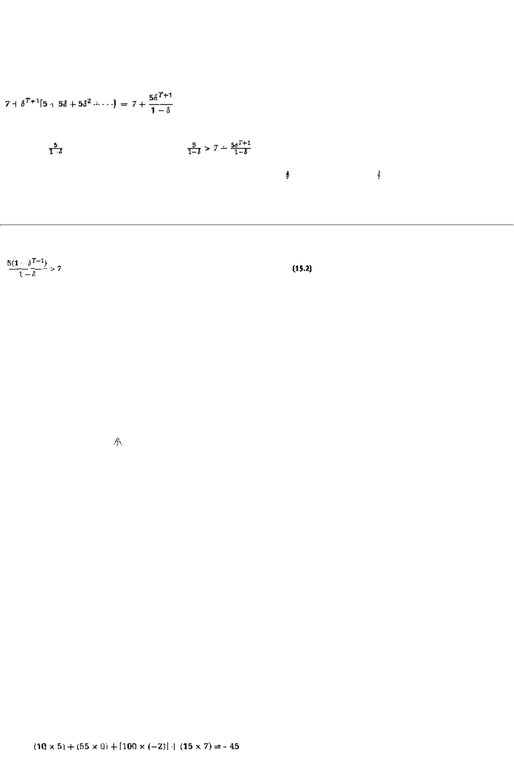
n
) will also be met by the
T
stages of (
c, c
). A strategy such as this is called a
forgiving trigger
: a deviation
from the desired behavior, (n, n), triggers a switch to a punishment phase, (c, c), but all is forgiven after T
stages of punishment.
Is the forgiving trigger a sufficient deterrent? By playing c when he is supposed to play n, a player gets a
payoff of 7. Then T stages of 0 follow, and thenonce play reverts to (n, n)an infinite stream of 5. So the total
payoff from this "deviant" behavior is
However, staying with the proposed not confess behavior yields an infinite stream of 5, that is, a lifetime
payoff of . The trigger is credible if , or equivalently
7It is purely a coincidence that the cutoff value for d is in both examples; is not a magical
"repeated game constant"!
page_231
Page 232
When the discount factor d is close to 1, the left-hand side of equation 15.2 is approximately 5(T + 1).8
Hence, when the future mattersthat is, when d is close to 1even one period of punishmentthat is, even T =
1is sufficient.
In conclusion, it is worth reemphasizing that the unifying theme in each of the three equilibria is the power
of future reciprocity. Threats and promises, if made in a subgame perfect credible way, are believable. If the
stick is stern enough or the carrot sweet enough, then they can discourage opportunistic behavior today and
get the players to play in a collectively optimal way. Actually they can do more; if the future punishments
and rewards are sufficiently large, then they can induce the players to play today in a variety of ways that
they would not otherwise. Both good behavior(n, n) alwaysand more whimsical behavioralternating between
(n, c) and (c, n)can be sustained by a significant future.
15.3 The Folk Theorem
There is a more general result that we can derive about subgame perfect equilibria in the infinitely repeated
Prisoners' Dilemma; this result is called the folk theorem of repeated games.9
The general result answers the question, What are all possible behaviors that can arise in equilibrium? The
answer, it will turn out, is virtually anything! While this is not entirely satisfactory from the point of view of
predictions, the result does highlight the absolute power of reciprocity. After you have seen the result, we
will discuss its implications, richness, and shortcomings in greater detail.
Before we can present the result we need to define something called a behavior cycle.
Definition. A behavior cycle is a repeated cycle of actions; play (n, n) for T1 stages, then (c, c) for T2 stages,
followed by (n, c) for T3 stages, and then (c, n) for T4 stages. At the end of these T1 + T2 + T3 + T4 stages,
start the cycle again, then yet again, and so on.
Some of the subcomponents of the cycle can be zero; that is, T1 or T2. or T3 or T4 can be zero. Indeed the
nice guy behavior, (n, n) always, is one where T2 = T3 = T4 = 0, whereas in the nasty guy behavior, (c, c)
always, T1 = T3 = T4 = 0. The alternating behavior(n, c) in even periods and (c, n) in odd periodsis a
behavior cycle where T1 = T2 = 0 and T3 = T4 = 1.
Let us call a behavior cycle individually rational if each player gets strictly positive payoffs within a cycle;
that is, for each player the sum of stage payoffs over the T1 + T2 + T3 + T4 stages is positive. So the nice
guy behavior cycle is individually rational, as is the alternating behavior. If the behavior cycle is T1 = 10, T2
= 55, T3 = 100, and T4 = 15, then it is not individually rational because player 1's payoff over the cycle
equals
.
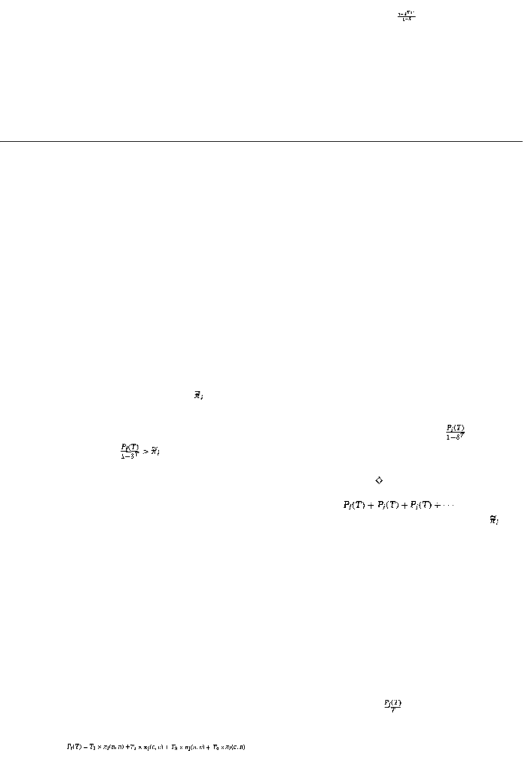
8We are using a result from calculus called L'Hospital's rule, which says that is approximately
equal to T + 1 when d is close to 1.
9This more general result is called the folio theorem because a simple version of it has been known for
a long time and known to many "folks" in game theory, A modern, less simple, version of the result was
proved in 1986 by Drew Fudenberg and Eric Maskin. You can find their result in the journal
Econometrica, vol. 54, pp. 533-554, under the title "The Folk Theorem in Repeated Games under
Discounting and with Incomplete Information."
page_232
Page 233
Denote the total length of a cycle Tthat is, T = T1 + T2 + T3 + T4and denote the total payoff of player i over
the T stages, Pi(T).10
The next two results constitute the folk theorem for the infinitely repeated Prisoners' Dilemma.
Folk Theorem
Equilibrium Behavior. Consider any individually rational behavior cycle. Then this cycle is achievable as the
play of a subgame perfect equilibrium whenever the discount factor d is close to 1.
Equilibrium Strategy. One strategy that constitutes an equilibrium is the grim trigger; start with the desired
behavior cycle and continue with it if the two players do nothing else. If either player deviates to do
something else, then play (c, c) forever after.
Sketch of a Proof
As before, if the grim trigger punishment is ever initiated, it gets carried out. So the only issue is, Would it
ever get initiated? That is, is it a sufficient deterrent so that no player would want to have it initiated? A
player initiates the punishment by failing, at some stage, to play the appropriate action in the behavior cycle.
That play gives him a stage payoffcall it in the current stage and thereafter a payoff of zero, on account of
the grim trigger punishment.
Staying with the behavior cycle, however, yields a lifetime payoff that is essentially equal to .11 Staying
is better than initiating if . Notice that the denominator of the left-hand side of the inequality
vanishes as d gets close to 1; in other words, the left-hand side becomes infinitely large. The right-hand side
is a fixed constant. Eventually, for d close to 1, not deviating has to be better.
The proof is intuitive. It says that by deviating a player will lose out on for an
infinite number of cycles. Clearly, that consideration has to be stronger than any immediate payoff of no
matter how large it is, as long as the future matters sufficiently.
Some general remarks follow:
All Potential Behaviors Are Equilibrium Behaviors
In any equilibrium, every player's payoff over a cycle must be at least zero. This statement is true because
each player can guarantee himself a payoff that high by simply confessing at every stage. The folk theorem
result says that not only are positive payoffs necessary for equilibrium but they are sufficient as well; every
behavior cycle with positive payoffs is an equilibrium for high values of d.
All Payoffs Are Accounted For
You might think that by looking only at cycles we are excluding certain kinds of behaviors. Although that is
true, the restriction involves no loss because we are not excluding any possible payoffs. To explain, one way
to think about the payoff to a behavior cycle is in terms of its per-stage payoff,
. As we look at different
behavior cycles we get
10Hence, An individually rational behavior cycle is therefore
a cycle for which P1(T) > 0and likewise P2(T) > 0.

11We say "essentially" because the exact payoffs in every cycle are actually
When d is close to 1, that sum is
essentially , that is, Pi(T). Since every T periods this payoff is
received, by Fact 1, the lifetime payoff is equal to
page_233
Page 234
different payoffs per stage. Suppose we look at a behavior that is not cyclical. This pattern will have a
per-stage payoff as well.12 It turns out that no matter what this per-stage payoff is, there is a behavior cycle
that has exactly the same payoff per stage.
Future Needs to Matter
The result only works for high values of d because that is exactly what is needed to make promises and
threats have deterrent value. As we have seen before, a high d means that future payoffs matter. In turn, that
fact means future promisesor threatscan affect current behavior.
Infinitely Many Equilibria
An implication of the result is that there are an infinite number of subgame perfect equilibria in the infinitely
repeated Prisoners' Dilemma. This is discouraging from the point of view of predictions. All that we can
conclude is that the prospect of threats and rewards is so potent that players may be willing to do virtually
anything.
A More General Conclusion
There is a more general result, called the folk theorem for infinitely repeated games, which asserts that by
repeating any stage gamenot just the Prisoners' Dilemmawe can get all individually rational behavior cycles
as part of a subgame perfect equilibrium.13
Observable Actions
One shortcoming of the analysis so far is that it requires deviations to be perfectly observableand hence
immediately punishable. In many contexts this assumption is unrealistic because other players may not have
precise information on what a rival has done in the past. In the next section you will see a generalization of
the trigger strategy idea that takes account of this complication.
15.4 Repeated Games With Imperfect Detection
Up until now we have assumed that each player sees the other player's action perfectly. In some contexts
this is not a good assumption. For instance we can interpret the stage game of the Prisoners' Dilemma as a
price competition model (with confess representing low price and not confess representing high price). In
that case, actions may not be perfectly observable; for example, each firm might offer special discounts to
certain customers or for bulk orders, and these discounts will typically not be observed by the competing
firm.
It is quite likely, however, that a firm's profits will be observable. For the Prisoners' Dilemma that statement
is equivalent to saying that, although the action chosen is not observable, the payoff is. You might wonder
whether observable payoffs are equivalent to the actions themselves being observable. After all, if a payoff
of 7 can only arise from
12In general, for any behavior pattern, a per-stage payoff is defined as whenever the
number of stages T is large.
13This is subject to one further assumption when a game has more than two players.
page_234
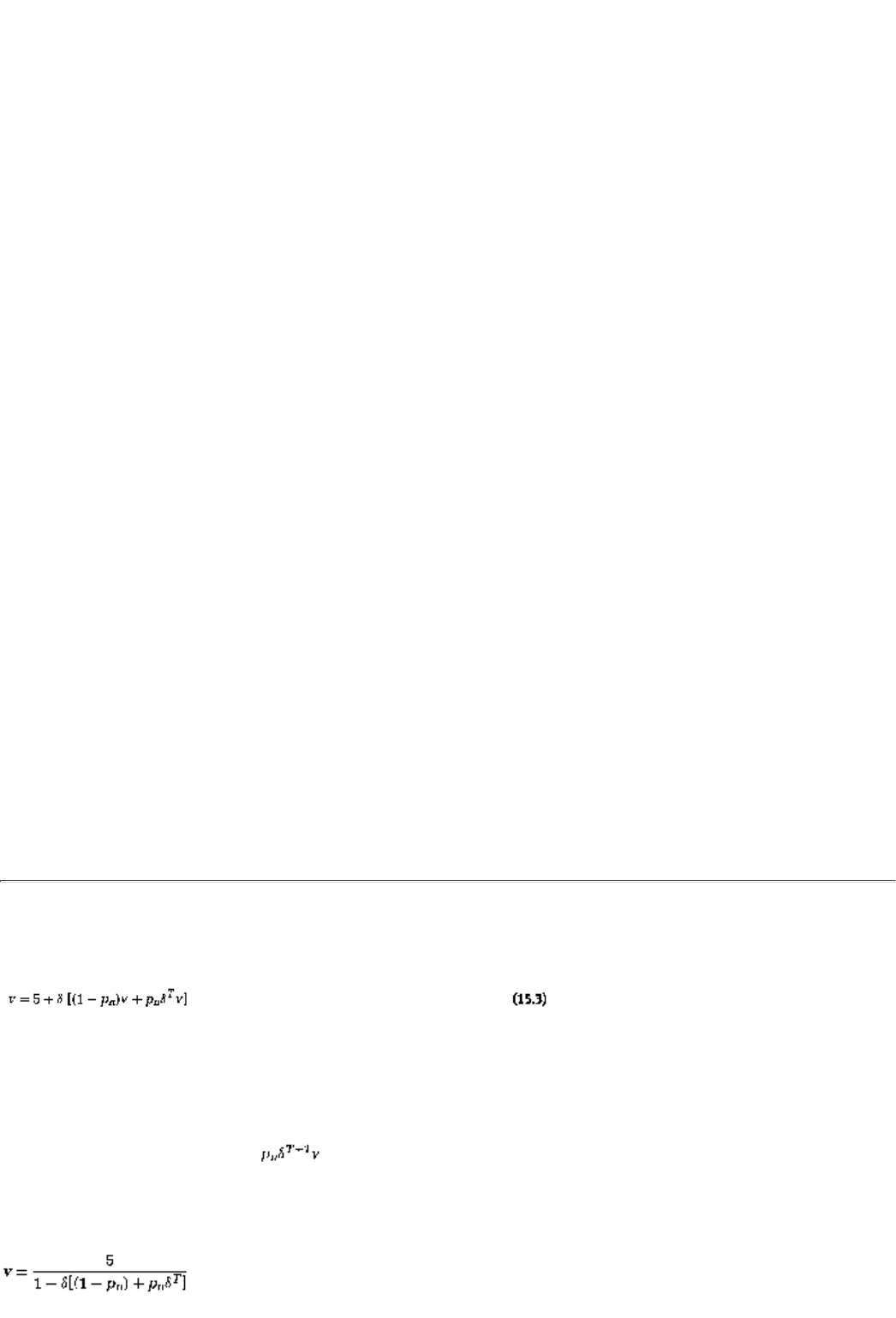
Page 235
confessing (against not confessing), then can't we infer actions from payoffs? In general we can. To make
the analysis meaningful, we therefore need to be a little careful with the interpretation of payoffs. Consider
again the Prisoners' Dilemma stage game:
Calvin \ Klein c n
c0, 0 7, -2
n-2, 7 5, 5
Suppose that we interpret the payoffs in the matrix as expected, or average, payoffs. In other words, if (c, c)
actually gets played, then the payoffs to the two players are uncertain and can take on any value (x, y).
However, the average value of x is 0, as is the average value of y. Suppose also that any particular value of
(x, y), say (2, -1), can arise from the play of (c, c) but can also arise from the play of (c, n) or (n, c) or (n, n).
Put differently, if (x, y) is the observed payoff, then neither player can be sure about what the opponent
played. Of course, the likelihood that (x, y) will arise if (c, c) is actually played is different from the
likelihood if (c, n) is played, and so on. Hence, having observed the payoffs, a player will typically assign
different probabilities to the possibility that (c, c) was played versus the possibility that (c, n) was played.
If deviations cannot be perfectly detected, are we back to perpetual confessions? The answer, thankfully, is
no. In order for players to not confess, however, it must be the case that their opponents view very low
payoffs as evidence of confession. If that is not the case, then a player would have the incentive to drive his
(nice guy) opponent's payment down by continually confessing against the other player's nonconfessions.
This observation motivates the following definition:
Definition. A threshold trigger strategy is defined by a number, say m. Players start by playing (n, n) and
continue to do so if both players' payoffs remain above m in every stage. The first time either payoff drops
below m players play (c, c) for T stages; and then restart the strategy.
Hence a threshold strategy is defined by two parameters, the quickness of the trigger m and the severity of
the trigger T. Let us now investigate when a threshold trigger strategy is an equilibrium and how good an
equilibrium it is.
There will be two general conclusions:
The more severe is the trigger, that is, the higher is T, the more likely it is that the strategy will be an
equilibrium.
The more severe or more quick (higher m) is the trigger, the less profitable is the strategy.
Put differently, there will be a tension: the more severe the trigger, the greater its deterrence value but, from
excessive usage, the smaller its profits.
page_235
Page 236
Suppose that a threshold trigger strategy is being played. Let us first compute its payoffs. Denote this payoff
v. The payoff is given by
where pn is the probability that one of the two stage payoffs is less than mthat is, the trigger gets
activatedeven though the actions chosen were (n, n) as suggested. The first term, 5, in the right-hand side of
equation 15.3 is the current stage's expected profit if both players play (n, n). The second term, d(1 - pn)v
refers to the following: with probability (1 - Pn) the trigger is not activated, and in that case we are back in
the current situation with lifetime expected payoffs of v. Since all this happens one stage hence, it is
discounted by d. The last term, , refers to the fact that with probability pn the trigger is activated, T
stages of zero profits follow, and then we return to the current situation with lifetime expected payoffs of v.
That return will start T + 1 stages from the current one and hence is discounted by dT+1. Collecting terms,
equation 15.3 yields
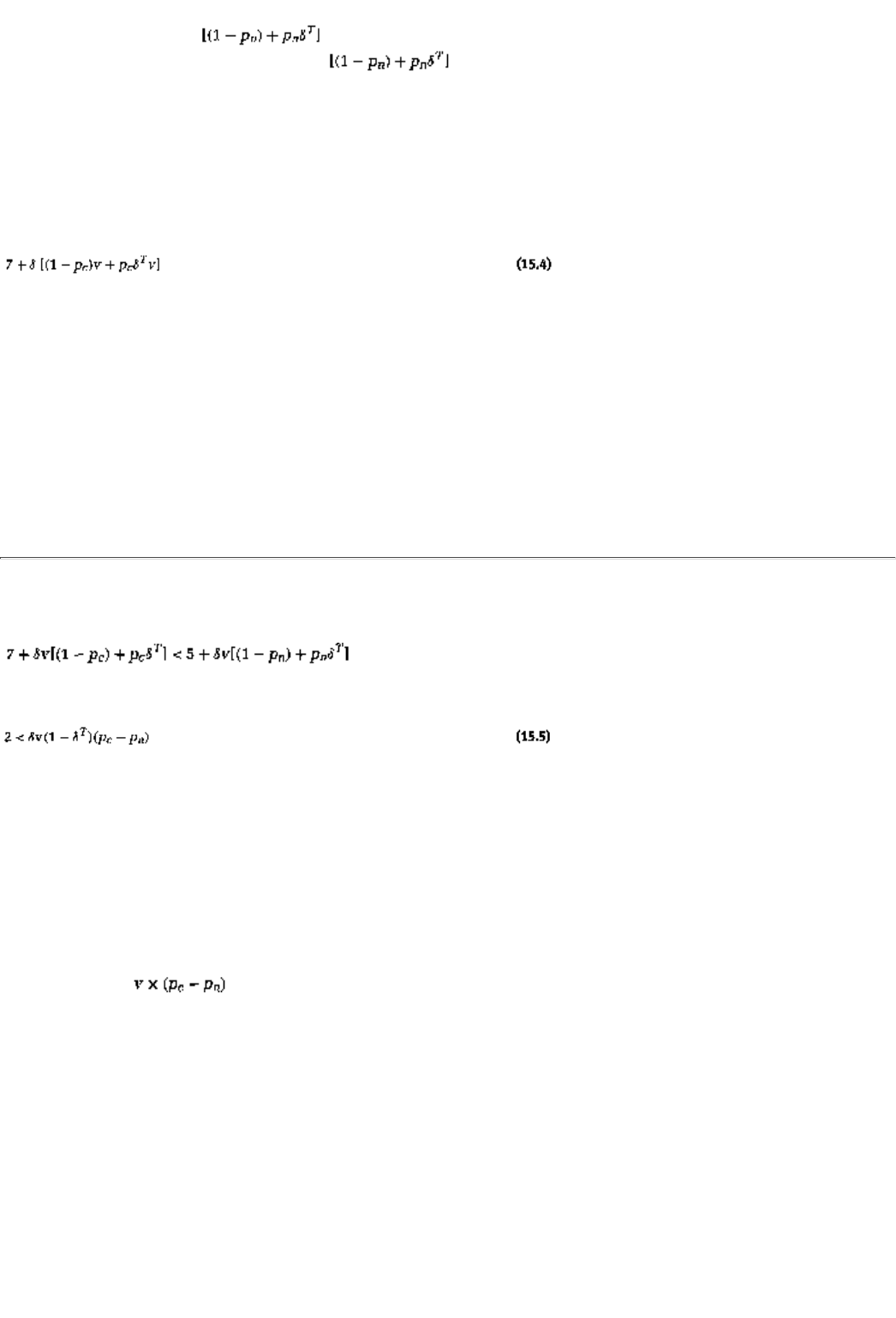
The quicker is the trigger (i.e., the higher is m), the higher is its likely use (the higher is Pn). In turn, that
implies a lower value of and therefore a lower value of v. Similarly, the more severe is the
triggerthat is, the longer is Tthe lower is and hence the lower is v. To summarize, higher
values of m or T make a trigger strategy, if followed, less attractive. Hence, the players would like to make
the trigger milder by lowering the values of m and T. Therein lies the rub; that might simultaneously destroy
a trigger's efficacy.
The trigger strategy is an equilibrium in the T stage punishment phase. A player cannot make positive
average profits by choosing not confess in this phase, nor does he change the future profile of actions. So
consider instead a stage when the players are supposed to be playing (n, n). By deviating, a player would get
a discounted total payoff of
where pc is the probability that the trigger will be activated by the play of (c, n); presumably, Pc > pn.
CONCEPT CHECK
PAYOFF
Show that the lifetime payoff, after a deviation, is in fact given by equation
15.4.
Comparing equations 15.3 and 15.4 makes the incentives clear. On one hand, confession is immediately
more gratifying because its payoff of 7 is higher than the 5 from not confessing. On the other hand, the
future benefits are lower because there is a
page_236
Page 237
greater chance of triggering the punishment phase. The play (n, n) is sustainable provided
that is, provided
From the definition of v it is straightforward to show that the more severe is the triggerthat is, the longer is
Tthe greater is its deterrent value. Put differently, long punishment phases get players to behave well.
CONCEPT CHECK
INCENTIVE (CALCULUS QUESTION)
Show that the higher is T, the more likely it is that equation 15.5 will be
satisfied.
The deterrent effect of m is a little ambiguous. A higher value of m lowers v as we have seen. It may,
however, increase Pc - Pn; that is, it may make confession comparatively easier to detect. The net effect will
then depend on .
To summarize, a cousin of the trigger strategies that we encountered in the previous sections, called a
threshold trigger strategy, can work to enforce (n, n) even when actions are unobservable. One key
difference, though, is that every so often the punishment phase will be triggered whenever actions are
unobservable; that is, along the equilibrium play path there will be periods of (c, c) interspersed among the
(n, n)'s. These phases are wasteful in that they lower total payoffs. They are, however, necessary because
without them each player would confess all the time. Hence, how long to spend in the punishment phase,
and how frequently, needs to be carefully chosen in order to balance the two conflicting forces of waste and
deterrence.
Summary
1. In an infinitely repeated game, lifetime payoffs are computed by adding up the discounted payoffs at
every stage of the game.

2. The grim trigger strategy comprises two parts: a desired behavior on the part of t
he players and a
punishment regime-always confessthat is triggered whenever either player violates the desired behavior.
page_237
Page 238
3. The grim trigger punishment can sustain the nice guy behaviornever confessas the desired behavior
provided players have a high discount factor.
4. The same punishment can sustain any behavior cycle that gives each player a strictly positive payoff over
each cycle. This result is called the folk theorem for the infinitely repeated Prisoners' Dilemma.
5. Reciprocity (in threats and punishments) can sustain periodic bouts of nice guy behavior even if the
actions chosen by a player are not observable to his opponent.
Exercises
Section 15.1
15.1
a. What is the discounted lifetime payoff of the following stage payoff sequence:
1, 3, 1, 3, 1, 3, . . .
b. What of
1, 1, . . ., 1, 3, 3, . . ., 3, 1, 1, 1, . . .
where each sequence of 1s and 3s lasts 10 stages? (You need only give the formula.)
15.2
a. What if the sequence of 1s lasts 10 stages but the 3s last 20?
b. What if the sequence of 1s lasts T1 stages but the 3s last T2?
15.3
a. Compute the payoff over the cycle P(T) for exercise 15.1.
b. Repeat for exercise 15.2.
15.4
Consider the sum of discounted payoffs over the cycle. What is it equal to for the scenarios in exercises 15.1
and 15.2 when d = 0.8?
15.5
What if d = 0.95? Which one is closer to P(T)?
page_238
Page 239
Section 15.2
15.6
Consider the infinitely repeated Prisoners' Dilemma. Show that the strategy that plays (c, c) in every
subgameregardless of past behavioris a subgame perfect equilibrium
15.7
Suppose that a pair of strategies, say
,
, form a subgame perfect equilibrium of the infinitely repeated
Prisoners' Dilemma. Suppose, furthermore, that these strategies prescribe play at every stage t that is
independent of past behavior. Show that , must be the same as the pair of strategies that play (c, c) in
every subgame.
15.8
Explain briefly why a high value of d is conducive to sustaining good behavior in the play of the infinitely
repeated Prisoners' Dilemma.
15.9
Consider the forgiving trigger punishment. How high does the value of d need to be in order for the nice guy
behavior(n, n) foreverto be achievable (as part of a subgame perfect equilibrium)? (Your answer will depend
on the length of the punishment phase T.) How does your answer compare with what we found about the
grim trigger punishment?
15.10
Can you show that the grim trigger is always a more efficient punishment in the sense that, no matter what
behavior cycle we are trying to achieve, if the forgiving trigger is a sufficient deterrent, then so is the grim
trigger?
15.11
Construct an example of a behavior cycle that is achievable by using the grim trigger punishment if d = 0.9?
(Do not use any of the patterns that were discussed within the chapter.)
15.12
Is the behavior cycle of the previous question also achievable by using a forgiving trigger with trigger length
10? Explain your answer. If the answer is no, at what discount factor does the forgiving trigger become a
sufficient deterrent?
Section 15.3
The next few questions return to the analysis of the model of price competition with a market whose
demand curve is
page_239
Page 240
where p is the lower of the two prices. The lower priced firm gets the entire market, and if the two firms post
the same price, then each gets half the market. Suppose that prices can only be quoted in dollar units and
costs of production are zero. Suppose, finally, that price competition continues indefinitely; that is, every
time the two firms compete they think that there is a probability d that they will compete again.
15.13
Write down the extensive form of the game. Identify the subgames.
15.14
Write down the strategies for each firm in the game. Define a subgame perfect equilibrium.
15.15
Consider the following strategy: Price at 2 dollars each and continue with that price if it has been maintained
by both firms in the past. Otherwise, switch to a price of a dollar. For what values of d is this strategy a
subgame perfect equilibrium? Explain.
15.16
Show that there is also a subgame perfect equilibrium in which the price is always 2
dollars but which is
sustained by a forgiving trigger. Be explicit about the nature of the forgiving trigger.
15.17
Suppose that d = 0.9. What is the maximum price that can arise in a subgame perfect equilibrium of this
model? Explain.
15.18
State a version of the folk theorem that is applicable for this price competition model.
15.19
Provide an argument in support of your stated result in exercise 15.18.
Section 15.5
Let us return to the infinitely repeated Prisoners' Dilemma but with unobservable actions. Suppose that there
is a 50 percent chance that at least one player's stage payoff is less than 0 if the action that is played is (c,
n)or (n, c)but there is only a 10 percent chance of that outcome if (n, n) is played. Suppose that the threshold
trigger gets activated whenever a payoff less than 0 is observed.
15.20
Is a forgiving trigger of length 10 a sufficient deterrent if d = 0.9? What is the minimum value of d at which
it becomes a sufficient deterrent?
page_240
Page 241
15.21
Compute the lifetime payoff to this strategy at the cutoff value of the discount factor that you computed in
exercise 15.20.
15.22
Consider a punishment of length 20 instead. Show that this too is a sufficient deterrent. Show furthermore
that its lifetime payoff is actually worse.
15.23
What can you infer about the length of the punishment phase from your previous answers? Explain.
15.24
Suppose that at both of the following triggers are sufficient deterrents: (a) cutoff = 0 and length of
punishment = 10 and (b) cutoff = -1 and length of punishment = 5. Suppose furthermore that there is a 5
percent chance that either player's payoff will be less than -1 if (n, n) is played. Which strategy will the
players prefer?
15.25
Would your answer be any different if there were a 8 percent chance that either player's payoff will be less
than -1 if (n, n) is played? Explain.
page_241
Page 243
Chapter 16
An Application: Competition and Collusion in the NASDAQ Stock Market
In this chapter we will discuss an application of infinitely repeated games to a rece
nt controversy: have
investors been systematically overcharged on the NASDAQ stock market? Section 16.1 will explain the
background to the question, section 16.2 will present a simple model to analyze it, and section 16.3 will
discuss some further variations of that model. Finally, section 16.4 will contain the denouement to the plot
line: were they or weren't they overcharged?
16.1 The Background
The NASDAQ stock market is the second-largest stock market in the United States after the New York
Stock Exchange, the NYSE (and ahead of the American Stock Exchange, the AMEX, and all of the regional
exchanges such as the stock markets in Philadelphia, Chicago, and San Francisco).1 Furthermore, it is the
fastest growing exchange. Its slogan is ''The Stock Market for the Next 100 Years."
The NASDAQ market is unlike the NYSE2 in at least a couple of ways. First, it has no physical location;
rather, it trades online.3 Second, unlike the NYSE, where there is a single "market maker" per stock, the
NASDAQ has multiple market makers. (The average number ranges between 10 and 20 with
up to 50 for
more popular stocks such as Microsoft, MCI, Intel, and Amgen.)4
The roles of the market makers are also quite different at the two exchanges. At the NYSE, the market
maker acts like a clearinghouse or auctioneer; he collects buy and sell orders and tries to find a price at
which the quantity being bought matches the quantity being sold. In a sense, therefore, each potential buyer
competes against every other buyer because he can be outbid by the latter; likewise sellers compete against
each other.
1Strictly speaking, the NASDAQ market is the largest in terms of share volumethe number of shares
that get traded on a typical day. Its 1997 average of 647.8 million shares per day was 132 percent
of the corresponding figure for the NYSE. It is second, after the NYSE, in terms of the dollar value
of traded shares.
2The stock market for the last 100 years, if NASDAQ's publicists are to be believed.
3The NYSE, on the other hand, is located at the comer of Wall and Broad streets in downtown New
York.
4Dealers is another name for market makers.
page_243
Page 244
At the NASDAQ, each market maker posts two quotesan "ask" price at which he will sell the stock and a
"bid" price at which he will buy. These quotes can only be in increments of an eighth of a dollar, and,
typically, the ask price is higher than the bid. The lowest ask and the highest bid constitute the market prices
(and are called the inside prices or inside quotes). On this market, dealers compete among themselves, and
because there are multiple dealers per stock, the NASDAQ market has been claimed by its supporters to be
more competitive than the NYSE. The key difference, though, and this will be crucial for our subsequent
story, is that on the NASDAQ market, dealers do not compete against buyers and sellers because the
relevant quotes are their own asks and bids. In particular, the asks or bids of non-market makers cannot set
the market price.
At least this is the way things worked on NASDAQ till 1996. Why, you may ask, have things changed?
Therein lies our tale!
In December 1994, two academics, William Christie and Paul Schultz, published a study that showed that an
unusually high percentage of asks and bids on the NASDAQ were clustered around the "even eighths" of a
dollar, that is, were clustered around, say, $10, , , and .5 Very few prices were at , ,
, and . Consequently, the difference between the ask and the bidalso called the spreadfor all of
these stocks was at least 25 cents and in many instances was as much as 50 cents.6 This finding seemed
puzzling because there could potentially be many investors who would be willing to buy or sell inside the
spread, that is, pay more than the bid and sell at less than the ask. Such competition should, in principle,
narrow the spread, especially on stocks that are heavily traded and hence have many interested buyers and
sellers.7
All of this matters because larger spreads hurt potential investors and help market m
akers make greater
profits than they would otherwise. On 10,000 shares, an extra spread of I translates to an extra payment of
$1,250 by investors (and a similar-sized extra profit for market makers). It is instructive to recall that the
daily volume on NASDAQ is about 650 million shares; an extra spread of translates for that volume to an
extra payment by investors of about $80 million dollars daily. There is also a further cost; in the long run
investors could stay away from a market if they perceived that they were being overcharged.
Christie and Schultz offered no ironclad explanation for the missing-odd-eighth phenomenon. Instead they
made the following conjecture: "Market makers interact frequently and over long periods of time with the
same population of other market makers. Thus, in setting quotes, NASDAQ dealers are essentially engaged
in an infinitely repeated game. Furthermore current and historical quotes of all market makers are available
to all dealers. . .. The well-known folk theorem states that . . . collusion is a possible equilibrium" (p. 1834).
Put more succinctly, they claimed that market makers are ripping off the public and that they are able to do
so because they are in a repeated game.
Christie and Schultz go on to point out that the screen-based NASDAQ trading system allows immediate
detection of dealers who undercut the "accepted" spread. Finally, the authors emphasize the importance in
all this of a NASDAQ practice called order preferencing; this is a practice by which brokersthe middlemen
who direct
5See "Why do NASDAQ Market Makers Avoid Odd-Eighth Quotes?" in the Journal of Finance,
1994, vol. 49, pp. 1813-1840. After their findings became public, the two authors noticed another
phenomenon, which was the subject of a companion piece, "Why Did NASDAQ Market Makers Stop
Avoiding Odd-Eighth Quotes?" This was coauthored with Jeffrey Harris, and it also appeared in
the Journal of Finance, 1994, vol. 49, pp. 1841-1860.
6Based on 1991 quotes, Christie and Schultz found only 10 percent of the stocks had a spread of , 39
percent had a spread of , 5 percent had a spread of , and 33 percent had a spread of . The
corresponding figures for the NYSE and AMEX were 25, 46, 22, and 5 percent. Hence, an investor
would pay a spread of 50 cents on a third of NASDAQ stocks but only on 5 percent of NYSE stocks. To
keep the comparisons meaningful, the authors tried to compare apples with apples; that is, they tried
to compare companies with similar capitalizations.
7About half the time spreads were 50 cents for each of the following three heavily traded stocks:
Apple, MCI, and Lotus. (Remember that in 1991 Apple was still in its glory days and Lotus had not yet
been bought out by IBM.)
page_244
Page 245
customer orders to the dealerscan choose to send an order to a dealer who does not have the best quote
provided he matches that quote.
The Christie-Schultz findingand their conjectureunleashed a veritable fire-storm. NASDAQ reacted with
understandable outrage. They lined up an impressive collection of academics who argued that collusion was
impossible because (a) there were too many market makers, and (b) even if there were not, there would be.
In other words, they argued that with 10 or more dealers competing per stock, somebody would always have
the incentive to undercut a collusive price and lure customers away. Furthermore, it is relatively easy to set
up as a dealer in the NASDAQ market.8 Hence, if there were collusive profits being made, many more
people would want to become dealers. The fact that there is not such a clamor is evidence that dealers do
not make large profits.
Everybody agrees, of course, that dealers need to make some profits in order to stay in business; they carry
the risk of making losses on shares that they buy, they have costs of doing business, and so on. The question
is, Are they making too much profit? Let us now turn to a repeated-game analysis of the Christie-Schultz
argument and that of their detractors.9
16.2 The Analysis
16.2.1 A Model of the NASDAQ Market
The stage game of this model is the simultaneous submission of an ask and a bid quote
by each market
maker; in the course of a single trading day, there may be six such trading stages.10 Suppose that there are N
dealers for the stock in question. Let dealer i's ask be denoted ai and his bid bi. The best ask is the lowest;
that is, it is the quote of the dealer who is asking for the smallest amount of money in order to sell the stock
to a customer. Let a denote the best or inside ask, that is,a = mini ai. Similarly, let b denote the inside bid,
that is, b = maxi bi, the highest that any dealer is willing to pay for a share. The inside spread therefore is a -
b.
In the current period, when these quotes are binding, all buy orders are executed at a price equal to a. The
profit to a dealer from participating in this transaction depends on what the real value of this share is. If that
value is v, then the dealer makes a - v dollars worth of profit from each share.11 Similarly a dealer who buys
at the inside bid, stands to make v - b dollars worth of profits from every share. Hence, if a total volume of
D
(a) shares is demanded by the public at the price of a dollars, then market makers stand to make (a -
v)D(a) dollars worth of profits from selling the share. Likewise, if S(b) is the volume of shares sold by the
public at a bid price of b, market makers as a group make (v - b)S(b) profit from that transaction. The profit
that each dealer makes depends on the fraction of the aggregate order flow that he receives. If he does not
post the best price, he makes nothing. To keep matters simple, let us suppose, to begin with, that every
dealer with the inside quote gets an equal fraction of the orders.
8For example, there is only a modest $10,000 fee that needs to be paid to become a market maker.
By contrast the right to become a market maker on the NYSE trades for amounts between $250,000
and $300,000. The waiting period, before a dealer can start posting quotes on NASDAQ, is only a
day.
9The analysis that follows is a simplified version of "Competition and Collusion in Dealer Markets" by
Prajit K. Dutta and Ananth Madhavan, Journal of Finance, 1997, vol. 52, pp. 245-276. We should also
mention that based on the Christie-Schultz paper and independent evidence, the Justice Department
and the Securities and Exchange Commision (SEC) started separate investigations of the NASDAQ
market. We will report their findings in section 16.4.
10This number is based on hourly quote revisions. A dealer may, of course, choose not to change his
bid every hour.
11The real value of a share can be thought of as the discounted total of all payments that a
shareholder will receive. These payments can include dividend payments as well as the proceeds from
selling the share in the future.
page_245
Page 246
Let us also make matters simple by considering specific demand and supply functions for the stock. Suppose
that these functions are given by
where the prices are in eighths of a dollar and the quantities are in units of 10,000 shares. By setting demand
equal to supply, you can check that this is a stock whose market clears at a price of 20, or 2.5 dollars; at this
price both demand and supply equal 200,000 shares.
Furthermore, it makes sense to assume that 20 is also the value of the stock, that is, v = 20. The reason why
this is a sensible assumption is that, as the real value of the share, v can be interpreted as the average
forecast among potential investors about the payback from this stock. If optimistic forecasts are just as likely
as pessimistic forecasts, then the average is also the cutoff above which there are exactly as many optimists
as there are pessimists below it; that is, it is the market-clearing price.12
Let us now turn to Nash equilibrium. It is straightforward to see that ai = bi = v
= 20 is a Nash equilibrium of
the stage game. If every other dealer is posting a competitive quote, a single dealer can do no better than go
along with it. Of course every dealer makes zero profits from this equilibrium; consequently, this will
constitute the benchmark punishment regime when we get to repeated trading.

16.2.2 Collusion
Before doing the repeated game analysis let us look at purely collusive pricing in the stage game. If the
dealers set prices in order to maximize their collective profits, they would set an ask and a bid to solve the
following maximization problem:
Consider the profit-maximizing ask. The slope of the profit function is 220 - 10a, and at a maximum-profit
ask that slope must be equal to zero.13 Hence, the collusive ask a* = 22; that is, it equals 2.75 dollars. A
similar exercise for the bid gives us the profit function's slope to be 180 - 10b and hence the collusive bid b*
= 18, or 2.25 dollars. Note that the collusive spread is therefore 50 cents (whereas the competitive spread is
0). The quantity that is sold by dealers at a price of 22, is 10, that is, 100,000 shares; that is also the quantity
that is bought by them at a price of 18. Hence, at the end of the trading round, dealers have cleared all
inventory off their books, and they take home a collective profit of (22 - 18) × 10, or 40.14
If the stage game is played only once, that is, if dealers post quotes once and never again, then they will in
fact find it impossible to sustain the collusive spread. To see this point, note that each dealer's profit from
posting the collusive quote is . On the other hand, by dropping the ask down to 21 and raising the bid to
19, any one dealer can draw away all the potential volume. At these quotes, the buy orders from the public
will equal 120 - (5 × 21), or 15 (× 10,000), shares, and the sell orders will also be 15 shares at a bid of 19.
Hence, this one dealer will clear his books and make a profit equal to (15 × 1)
12The median of a distribution (of potential investors, say) is that value above which there is 50
percent of the (investor) population. The market clears at the median value because then there are
just as many buyers as sellers. The dealers are interested in the average value of the share because
they care about profits they make on average. When optimists and pessimists are equally likely in a
distribution, its median and average coincide; that is, v is both the market-clearing price and the
real value of the share.
13Recall that the slope of ax - bx2(with respect to a variable x) is a - 2bx, where a and b are constants.
Also consult Chapter 25, where we discuss maximization problems such as this one, if any of this seems
mysterious to you. Finally, in the maximization exercise we pretend that any number a can be chosen
as an ask. In actuality, only integers can be chosen because prices have to be in units of eighths of a
dollar. This pretense is harmless, since the profit-maximizing ask turns out to be an integer.
14Since prices are in eighths of a dollar and quantity is in units of 10,000 shares, a profit of 40 is
equivalent to a dollar profit of , or 50,000 dollars.
page_246
Page 247
+ (15 × 1) = 30. As you can see, this profit of 30 is always greater than the shared profit of (since N > 1).
CONCEPT CHECK
ANOTHER STAGE GAME NASH EQUILIBRIUM
Show that asks and bids of 21 and 19, respectively, also constitute a Nash
equilibrium of the stage game (with a spread of 25 cents).
We are now ready for the repeated game analysis. Consider the following grim trigger strategy: Each dealer
begins with the collusive quotes and maintains them as long as the others have done so in the past. If any
dealer undercuts, from the next trading round onward all dealers go to pricing at value v forever thereafter.
As always, once the punishment regime has been initiated, no dealer can do any better by pricing at any
price other than v = 20. Hence, in any subgame that has already seen a noncollusive price, pricing always at
value is a Nash equilibrium.
Consider instead a situation where up until now the asks and bids have been collusive. By sticking with the
strategy, a market maker expects a continued payoff of
, that is, a discounted total profit of where d,
as always, denotes the discount factor. By undercutting the other dealers, a single market maker makes a
profit of 30 in the current round but thereafter looks down the barrel of the threat of 0 profits. Sustaining
collusion is the better option if
Clearly, the last condition translates to . Note two immediate implications: First, the greater is the
number of dealers, that is, the larger is N, the more difficult it is to meet the condition (and sustain collusion).
In that sense, NASDAQ's backers were quite right in saying that the existence of many dealers on NASDAQ
makes collusion harder. Second, the higher is the discount factor, that is, the larger is d, the easier it is to
meet the condition (and sustain collusion). This second implication we have already encountered (in the
previous chapter).
The interesting question in the current context is, What is a realistic value for d Consider two of the
interpretations of d that you have seen. If it represents the probability that the dealers will interact with each
other at least one more time, then d is virtually 1. After all, between now and an hour from now (or even a
day from now) how high can the likelihood be that someone in Merrill Lynch who makes the market for
Apple will have quit his job or be fired or that Merrill Lynch would have decided to discontinue making the
market in Apple's stock? If d represents a preference for earlier payments because a current dollar can grow
into more than a dollar in the future, again d has to be
page_247
Page 248
virtually 1. How much interest, after all, can you collect between now and an hour from now (or even a day
from today)?
To put that discussion into perspective, let us look at some numbers. If N = 11,15 then collusion is
sustainable provided that , that is, provided that a dollar an hour from now is worth at least 88
cents. If N = 50, then collusion is sustainable provided that , that is, provided that a dollar an
hour from now is worth at least 97 cents. It seems quite likely that the discount factor will be this high for
trading rounds that are hourly. Put differently, it seems likely that collusion is sustainable even in heavily
traded NASDAQ stocks as conjectured by Christie and Schultze.
This conclusion still leaves open the question, Why don't more dealer (or member firms) set up in this
market? After all, each market maker (or each member firm) makes a discounted total profit of . When
N
= 20 and , this translates to yearly profits of almost $2.5 million.16 In the next section we will turn
to the question, Why aren't there more dealers?
16.2.3 More on Collusion
There are two more-benignand more-plausiblepunishment possibilities that might also sustain collusive
pricing. One punishment, in the event of a departure from collusive pricing by some market maker, is to
price forever thereafter at the alternative stage game Nash equilibrium:
CONCEPT CHECK
BENIGN PUNISHMENT 1
Show that repeatedly pricing at an ask equal to 21 and bid equal to 19
constitutes an equilibrium in the repeated game.
The next question is, Is this punishment a sufficient deterrent? That is, would the threat of such a punishment
prevent undercutting from the collusive asks and bids? Recall that the collective profit for this stage game
Nash pricing structure is 30. Hence, by deviating against the collusive price, a mark
et maker can grab all the
customer orders
and single-handedly make the collective profit. However, he then faces the threat of thereafter.
CONCEPT CHECK
A SUFFICIENT DETERRENT
Show that collusion is sustainable if
15The NASDAQ web site (at nasd.com) cites that, on average, there are 11 market makers for every
NASDAQ stock.
16Recall from the earlier discussion that 40 translates to $50,000 worth of profits. The discounted
total is million (and with 1,500 hourly trading rounds a year, that is also effectively the annual
total). In this context, remember that it costs $10,000 to become a market maker on NASDAQ.
page_248
Page 249
A little algebra rearranges that condition to be . A sufficient condition is therefore
. Clearly, collusion is now harder to sustain;17 put differently, the number of traders has to
be smaller or the discount factor higher than was the case with the more severe zero-profit threat. That result
should not be surprising; if the punishment is milder, there is a greater temptation to cheat! Again, for
illustrative purposes, if N = 11, d needs to be at least or 0.97, for the sufficient condition to be met.
A second benign punishment is a forgiving trigger in which spreads narrow for some number of trading
rounds to punish deviation but then go back to the collusive spread. We will leave it to you to work out the
details of this case in the Exercises.
Two things about the analysis are worth pointing out. First, when some market maker undercuts, everybody
suffers in the subsequent punishment regime, the sinner as well as the good guys. This result might appear
unrealisticand it is. It is also inessential. If the punishment can be targeted, then we can achieve the same
end by singling out the dealer who undercut and subjecting him to punishment. For instance, if a deviant
market maker can be subsequently shut out of the market (while the others continue to price collusively),
then it is as if he alone faces a grim trigger punishment. Hence all of our conclusions about the grim trigger
apply here without any change. In the next section, we will discuss some institutional arrangements of the
NASDAQ market that make it easier to shut out individual dealers.
Second, collusion is either sustainable or it is not; there is no possibility in the analysis that collusion may be
sustainable in some marketsor on some daysbut not in others. Furthermore, since the demand and supply
functions remain the same from trading round to trading round, the size of the collusive spread also remains
unchanged. In particular, if collusion is sustainable, then the observed spread is always 50 cents. In reality,
the spread on the same stock changes from day to dayand often hour to hour. One can, however, do a more
general analysis of collusion on the NASDAQ market that allows demand and supply functions to change.
One conclusion that emerges from such an analysis is that collusion may be sustainable only some of the
time. Another consequence is that the size of the collusive spread itself can vary from day to day or hour to
hour.18
16.3 The Broker-Dealer Relationship
Brokers are the ones who direct customer orders to dealers. Some of these brokers have been in the business
for a long time as well. Consequently, over time, brokers typically build up relationships with particular
dealers. These relationshipsalong with an associated institutional feature of the NASDAQ markethave a
direct relevance to the collusive pricing question.
16.3.1 Order Preferencing
NASDAQ permits a broker to direct an order to a dealer even if that dealer's quote is
not the best available
quote. This practice is called order preferencing; a broker "preferences"
17Recall that collusion is sustainable of under the stronger punishment of the previous
section.
18 The Dutta and Madhavan paper cited in footnote 9 does just such an analysis. Something similar in
spirit will also be done in Chapter 17 when we study the oil cartel, OPEC.
page_249
Page 250
an order to a market maker who has agreed in advance to meet the inside price. In other words, if the inside
ask is, say, $10 and dealer i has posted an ask equal to , a broker could nevertheless send the order to i
for execution. Of course dealer i would have to sell the stock at $10, but as long as she is willing to do so,
nothing improper would occur.
This practice has a simple consequence: a broker is indifferent about which dealers he directs orders to and
does not have an incentive to seek out the best price. Put differently, a dealer who posts the best price will
not necessarily attract all the volume at that price. Indeed if each broker has his own favorite market maker
that he goes to all the time, then a dealer who undercuts gets no extra volume by undercutting; each broker
will simply have his order filled at the undercut price by his favorite dealer.19
The implication of all this should be clear. Consider the following simple strategy: in every trading round, no
matter what, each dealer prices collusively and arranges with her brokers to match the best price if it is
better than the collusive ask and bid. By pricing collusively at 22 and 18, each market maker makes profits
of . By undercutting that price, to 21 and 19, each market maker lowers the collective profits down to 30.
She does not, however, get any larger a fraction of that total; her profits from deviation are Clearly, no
dealer has an incentive to undercut the collusive price.20
With order preferencing one does not even need trigger strategiesor any repeated game analysisto sustain
collusion. Actually that statement is not quite true. The relationship between a broker and his preferred
dealer only makes sense from a repeated game viewpoint. We will not pursue that point here.
16.3.2 Dealers Big and Small
In this subsection we will answer two questions. The second one will be, Why don't more people set up
business as (profitable) NASDAQ market makers? The key again is the broker-dealer relationship. On
account of that relationship, not all dealers are created equal. Some market makers handle a larger fraction
of the aggregate transactions than other market makers. So, the preliminary question will be, Is the market
more or less competitive when there are dealers both big and small?
To simplify matters, suppose that there are two categories of market makers: big and small. Suppose that a
big dealer handles twice as much volume as a small dealer (provided they both have the inside quote).
Nevertheless, if a dealer is the only one with the inside quote, then he gets all the
volume regardless of
whether he started off big or small.21 In other words if there are N big dealers and M small ones and they all
have the inside quote, then each big dealer gets of the aggregate volume and a small dealer gets .
Consider the following grim trigger strategy: price collusively until somebody undercuts and thereafter price
at value. Let us consider the incentives of big and small dealers separately. Clearly in the punishment phase
every dealer is making zero profits, and nobody can do much about it. So suppose instead that we are in a
situation where the collusive arrangement has held up so far. A big dealer by deviating gets an immediate
profit of 30and thereafter nothing. By staying with the current arrangement he expects to get in
every trading round. So a big dealer will hold the line if
19One reason for a broker to stick with a single dealer is that she gets a better price by doing so.
During the course of a trading day, the price of a stock moves around, and a dealer has some
discretion about when she executes an order. By going back repeatedly to the same dealer, a
broker gives that dealer an incentive to execute buys at low ebbs and sells at high tides.
20 "Match the best price" is a practice that is widely prevalent in other industries as well. In the New
York metropolitan area, the largest discount electronics store is called Nobody Beats the Wiz; their
boast is that their prices are so good, and they are so confident about those prices, that they will give a
10 percent discount on any published competitors' prices. Customers do not shop around because they
think no one else can beat the Wiz's low price. What they don't realize is that actually no one else has
any reason to beat the Wiz's high price!
21In this subsection we are therefore ignoring the order preferencing arrangements that we discussed
earlier.
page_250
Page 251
By the same argument a small dealer will price collusively if
Clearly the small dealer is the weak link! Compared to a big market maker he has less at stake in collusive
pricing and just as much to gain by abandoning it.
Which brings us to new market makers. Consider a market with N big dealers
who are able to price collusively, that is, . Consequently, they make profits, far in excess of
the costs of setting up in business as a market maker. In comes a new entrant (who receives, say, half as
much business as long-standing market makers with well-established broker relationships). Does he expect to
make similar profits? The answer is no for two reasons.
First, collusion may no longer be sustainable; the entrant may be precisely what breaks collusion. This result
would occur if . Second, in any case, whether or not collusion is sustainable, the entrant is
going to make half as much profit as the existing dealers. For instance, if collusion breaks down and instead
the second-best Nash equilibrium with a spread of 25 cents is played, then the entrant makes . Put
differently, what tempts him to enter this business is the existing profit levels of ; what discourages him
from coming in is the realization that he will only make , that is, about of that amount.22
16.4 The Epilogue
Here is what has happened since the NASDAQ controversy started: The Justice Department wound up its
investigation by concluding that they had indeed found evidence of collusive pricing by NASDAQ dealers.
Indeed, they made their case not on the basis of implicit collusion of the sort that we have discussed in this
chapterin which no dealer need actually talk to another dealerbut rather on the basis of explicit collusion. In
particular, they had tapes of phone conversations between market makers in which they arranged collusive
pricing!
The SEC pushed NASDAQ to take steps that would make collusion in the future more difficult to sustain. In
response NASDAQ has implemented a set of changes that have been approved by the SEC. The most
important change in order-handling protocol is something that NASDAQ calls the limit order display rule.
Put simply, this rule allows investors to compete with dealers in making the market (as they are able to do on
the NYSE). A limit order is an order that specifies a quantity as well as a price; for example, buy 1,000
shares of Apple at $15. The limit order display rule requires market makers to display all customer limit
orders that are priced better than the dealers' inside quotes. For instance, if the inside quotes are currently an
ask of and a bid of , and the
22The ratio of to is equal to . When N is large that last number is approximately .
page_251
Page 252
limit order described comes in, then the dealers have to immediately revise their inside quotes to a bid of
$15.23
All this has to make everyone but the dealers happy.
Summary
1. The NASDAQ market is the largest stock market in the United States in terms of the number of shares
traded and the second-largest in terms of the dollar value of those shares.
2. The NASDAQ market was rocked, in the early 1990s, by allegations of price fixing by market makers.
The evidence that was offered was that many actively traded stocks had spreads of 25 and 50 cents.
3. A simple repeated game analysis shows that collusive pricing is possible even when there are multiple
dealers for every stock. Collusion is more likely with fewer dealers and higher discount factors.
4. The possibility of collusion was increased by NASDAQ institutional features such as order preferencing
and by long-standing broker-dealer relationships.
5. NASDAQ has recently instituted a number of rule changes that will make it harder for dealers to maintain
collusive prices in the future.
Exercises
Section 16.1
16.1
Locate some information on the relative size of the NYSE, the NASDAQ market, and the AMEX. What
measures of size do you think are relevantnumber of shares that were traded, the dollar value of those
shares, or something else? Explain your answer.
16.2
Do the same for the relative size of the three American exchanges vis-à-vis international stock markets such
as the Tokyo Stock Exchange, the London Stock Exchange, and the Frankfurt Stock market.
23This new rule was introduced for 50 stocks on January 20, 1997, and subsequently expanded to
cover all NASDAQ stocks.
page_252
Page 253
Section 16.2
(Calculus Problem) Consider the following specification of demand and supply functions:
16.3
a. Compute the market-clearing price.
b. What is the quantity that is transacted at that price?
c. If prices are in eighths of a dollar and quantities are in 10,000 shares, what is the dollar price and quantity
traded in this equilibrium?
16.4
For the specification of demand and supply given by the previous question, what is the collusive ask price?
What about the collusive bid price? Hence, what is the collusive spread? Do collusive market makers sell as
much as they buy? (Continue to assume that the market-clearing price is the value of the share.)
16.5
What are the profit levelsin dollarsassociated with the collusive prices?
16.6
Suppose that there are six trading rounds in a day. What is the total profit that market makers make daily?
And yearly, assuming that there are 250 trading days in the year? What is the yearly profit per dealer if there
are 20 dealers for this stock?
16.7
Could you compute the discounted total annual profits, if the discount factor is 0.99
? For your computations,
use the following formula:
Note that exercises 16.8-16.19 refer to the same data as in exercises 16.3-16.7.
Section 16.3
16.8
Show that an ask and a bid of 20 is a stage game Nash equilibrium.
16.9
Consider the following grim trigger strategy: trade at the collusive quote unless some
page_253
Page 254
dealer undercuts; thereafter trade at the market-clearing price of 20. When is this an equilibrium? (Assume
unless otherwise noted that the dealers with the inside quotes share the market equally.)
16.10
Show that an ask of 21 and a bid of 19 is also a stage game Nash equilibrium. What are the profits in that
equilibrium?
16.11
Consider the following benign trigger strategy: trade at the collusive quote unless some dealer undercuts;
thereafter trade at the Nash equilibrium. When is this strategy an equilibrium?
16.12
Consider, finally, the following forgiving trigger strategy: trade at the collusive quote unless some dealer
undercuts; thereafter trade at the market-clearing price for T stages; then revert to the collusive quotes.
When is this strategy an equilibrium?
16.13
Compare and explain the answers that you got in the previous three questions.
Section 16.4
16.14
Suppose there is perfect order preferencingeach broker has a favorite dealer to whom he directs order flow.
Show that regardless ofd, collusive quotes are a subgame perfect equilibrium.
16.15
Can you show that the same conclusion is true regardless of what demand and supply function we consider?
Suppose that half of the twenty dealers are big dealers and get twice as much order flow as the remaining ten
dealers.
16.16
Write down the condition that determines whether or not big dealers will undercut the collusive quotes (in a
grim trigger strategy)? Do the same for the smaller dealers. At what d will collusion be a sustainable
strategy?
16.17

Suppose that the actual
d
is less than the cutoff that you computed in exercise 16.16. Can you find an ask
and a bid price, respectively, greater than 21 and smaller than 19 that can be sustained as an equilibrium?
What are the profits in such an equilibrium?
page_254
Page 255
16.18
Suppose that the big dealers shared some of their order flow with the small dealers. Explain why this practice
might make collusion easier to sustain.
16.19
By sharing order flow, however, big dealers give up some of their own volume and hence potential profits
associated with that volume. In your computations can you figure out whether it is ever worth the while of
the big dealers to direct some order flow to the small dealers? Explain.
page_255
Page 257
Chapter 17
An Application: OPEC
In this chapter we will examine the oil-producing cartel, the Organization of Petroleum Exporting Countries
(OPEC), and argue that a repeated-game perspective is useful to understand the working of this
organization. We will start in section 17.1 with a brief review of OPEC and, in the course of that discussion,
identify four key phases in the recent history of the oil industry. In section 17.2 we will outline a very simple
model of the industry. In sections 17.3 and 17.4 we will employ the ideas of repeated-game theory to
understand the four historical phases; in order to do so we will have to make a digression and discuss
repeated games with demand uncertainty. Finally, section 17.5 will offer some further remarks on OPEC and
the model used in this chapter.
17.1 Oil: A Historical Review
OPEC is an organization of oil producers; it was formed in September 1960 at the primary urging of the
bigger producersSaudi Arabia, Iran, and Venezuela. OPEC has 13 member states; it does not include the
Western producers and the former Soviet Union, but it does include virtually all the othersthe Gulf States of
Kuwait, Qatar, and the United Arab Emirates; the African nations of Libya and Nigeria; and Asian nations
such as Indonesia. OPEC was the culmination of roughly a decade's worth of negotiations and the writing of
bilateral agreements among member nations. To understand how OPEC came to be at the time that it did, we
have to understand both the economics and the politics of oil.1
Oil production involves at least three key stages: drilling, refining, and shipping. Historically, oil companies
from Europe and the United States have been the major players in all three areas of the industry. The
influence of at least some of these companies goes back to ''national concessions" that were granted by host
governments in the first
1Producer organizations existor have existedfor many other commodities as well. International
organizations exist for coffee and diamonds. In the United States such producer groups were very
popular in the 19th century. In sugar, railroads, steel, cement, and the like, groups or "trusts"
controlled an overwhelming percentage of production. Public outrage over price-fixing by these
trusts led to sweeping legislation in the 1880s that goes by the general name of "antitrust"
legislation. The most famous of these laws is the Sherman Antitrust Act, which was passed in 1890
and continues to be a major tool for government industrial policy today.
page_257

Page 258
half of the 20th century. The archetype of these concessionsand indeed the very first onewas a concession
that the shah of Persia (now Iran) granted to an Englishman called William Knox D'Arcy in 1901. This
concession allowed D'Arcy's company, the Anglo-Persian Oil Company, formed for this express purpose, the
right to prospect and drill for oil anywhere in Iran. In return, the shah was to be given a fraction of the
profits.2
Similar agreements followed between the governments of Indonesia, Iraq, Saudi Arabia,3 and Libya and
companies such as Royal Dutch, Standard Oil, and Compagnie Française. These concessions lasted until
about the 1940s and 1950s when one after the other the governments of these countriessome of them newly
independentterminated these arrangements.4
17.1.1 Production and Price History
In the first half of the 20th century the primary producers and exporters of oil were not in the Middle East;
rather they were in the United States and Venezuelaand in later years in the Soviet Union.5 Indeed oil was
not discovered in Kuwait and Qatar until the 1950s. This overwhelming presence of Western oil lessened
somewhat in the years between the two world wars, but even in 1945 almost half of the world's oil came
from Western sources.
Two dramatic changes occurred during and after World War II. First, new sources of oil were discovered in
the Middle East, and production capacity was greatly increased in Iran and Iraq (for the Allied war effort).
Second, the postwar industrial boom in the United States increased demand severalfold. Indeed the United
States went from being a net exporter to an importer of oil (by 1970, 60% of U.S. oil demand was being met
by imports). By the mid-1960s, then, the Middle East had in fact emerged as the dominant oil-producing
region in a world in which demand was increasing rapidly.
The price history of oil can be broken down roughly into four phases (these numbers are rounded off):6
Phase 1, Before 1960
: Prices were both low and stable. For example, the price of a barrel of oil only rose
from $1.25 in 1950 to $1.75 in 1960.
Phase 2, 1960 to October 1973
: Prices remained low but began to creep up. Through the 1960s they
remained in a one-dollar bandbetween $1.50 and $2.50and by the middle of 1973 they were up to $5.
Phase 3, October 1973 to 1979
: Prices were both high and stable. The most dramatic phase was
undoubtedly the mid-1970s; the price of a barrel of oil went from $5 to $17 in the last two months of 1973.
It remained in the twenties throughout the decade.7
Phase 4, 1980 Onwards
: Prices have been lower and unstable; that is, there has been a lot of volatility. For
example, prices were as high as $30 a barrel around 1982 and as low as $10 a barrel in the early 1990s.
Through the first six months of 1996 prices
2It is interesting to note that although the shah was given a fraction of the profits, he was expressly
prohibited from inspecting Anglo-Persian's books.
3The agreements got a little less lopsided with time. For example, in 1933 when the Saudi King Abdul
granted Standard Oil of California the right to prospect for oil in his kingdom, he retained part
ownership. Indeed by 1944 a whole new company, Arabian American Oil Company (Aramco), was in
operation with greater participation by the Saudis.
4In many cases, the producing nations also added refining and shipping capability. For example, up
until the early 1960s, Saudi Arabia used to send all its crude oil to foreign refineries and import
refined products for its own use. Subsequently they have constructed nine domestic refineries.
5For example, in the years leading up to World War I, a full two-thirds of the world's oil production
came from the United States, Venezuela, and Mexico; one-fifth of the total world consumption was
accounted for by U.S. exports.
6For a detailed institutional and price history of OPEC, see Models of the Oil Market: A Study of
OPEC by Jacques Cremer and Djavad Salehi-Isfahani (New York: Harwood, 1989).

7There was another rapid escalation in 1979-80 with an all-time high barrel price of $36; this was an
imediate consequence of the start of the seven-year war between Iran and Iraq. These high prices
came back down as the cut in Iranian production was made up by a compensating increase by other
OPEC members, especially Saudi Arabia.
page_258
Page 259
were in the range of $15-$17 a barrel, and they had climbed up to $23 a barrel by the end of the year.8
In the next two sections we will try to understand these four phases in terms of a simple model of repeated
games that emphasizes the role of demand conditions in the market for oil.
17.2 A Simple Model of the Oil Market
Oil-producing nations, whether they are members of OPEC or not, compete with each other as Cournot-style
competitors in the world oil market. Producers make decisions about the quantity that each of them is going
to pump over, say, the next month. They have some flexibility in making this decision because they can
choose to run their wells at less than full capacity.
The aggregate supply of world oil together with current demand determines the price for a barrel of crude
oil. There is a very active worldwide spot market as well as a market in oil futures.9 The main markets are
the International Petroleum Exchange (IPE) based in London and the New York Mercantile Exchange
(NYME). Oil producers such as Saudi Arabia also quote prices for their products, but these prices have to
fall in line with prices on the IPE or NYME (or else some traders can make arbitrage profits by buying on
the cheaper market and selling on the expensive market).
OPEC tries to ensure that this competition nevertheless generates high profits for the producers. It does so
by specifying production quotas for its members. These quotas are set in such a way as to generate a target
price for oilwith an associated desirable profit level for OPEC's members. Periodically, the oil ministers of
the OPEC member countries meet to discuss the efficacy of the current quotas and whether or not to set
fresh quota levels.
Let us reduce these observations to the following simple stage game. There are two oil producerssay, Saudi
Arabia (SA) and Venezuela (VA).10 Each of these producers can produce either a high output or a low
output. SA and VA are different-sized producers; let us suppose, therefore, that the two output levels for SA
are QH = 10 mbd and QL = 8 mbd; for VA these output levels are qH = 7 mbd and qL = 5 mbd. Aggregate
output can therefore be any one of three levels; when both producers withhold output the total is 13 mbd,
when only one withholds it is 15 mbd and when both overproduce it is 17 mbd.
On the demand side, let us suppose that demand conditions can be either good or bad. When conditions are
good
that is, when demand is robustsuppose that a total output of 13 mbd fetches a price of $25 per barrel,
whereas the price is only $22 per barrel for an aggregate output of 15 mbd and $19 for the highest output
level. Finally, suppose that the marginal cost of production is $5 a barrel.11 All this leads to the profit matrix
for good demand periods shown in Table 17.1.
8Note that none of these prices are adjusted for inflation. In other words, a $30 price in 1982 is
much higher in real terms than a $23 price in late 1996.
9A spot market is a market in which a buyer can buy (different grades of) crude oil for immediate
delivery. Oil futures are contracts that promise the buyer delivery at a specified date in the future, for
example, the delivery of a hundred thousand barrels two months from the contract date.
10The two biggest producers of OPEC are Saudi Arabia, which accounts for a third of OPEC's total
output of about 25 million barrels per day (mbd), and Iran, which accounts for about a sixth.
Venezuela accounts for about a ninth. Venezuela, however, is the leading dissident within OPEC on
what price the organization should aim for. That is the reason we have included them as the second
player along with Saudi Arabia.

11These numbers have a rough congruence with actual production and price numbers in the current
market. It will also become clear from the analysis that many of these assumptions on market structure
and costs can be generalized without doing too much violence to either the arguments or the
conclusions.
page_259
Page 260
TABLE.17.1
SA \ VA. qL qH
QL160, 100 136, 119
QH170, 85 140, 98
TABLE 17.2
SA \ VA qL qH
QL88, 55 80, 70
QH100, 50 90, 63
CONCEPT CHECK
Derive each of the profit numbers in Table 17.1 from the information given to
you about quantities and prices.
In contrast, when times are badthat is, when demand is weak12suppose the three prices are respectively $16,
$15, and $14 per barrel for high, medium, and low total output. Suppose also that the costs of production are
no different. This leads to the payoff matrix for low demand periods shown in Table 17.2. With these
numbers we are finally ready to turn to our main plot line.
17.3 Oil Prices And The Role Of OPEC
Phase 1, Before 1960
: The 1950s was the first decade of significant growth in oil demand. Yet the rates of
growth were still far below what was to come in the 1960s and 1970s. The 1950s was also a period of low
prices.
One explanation of the 1950s, then, is that demand at that time can be characterized as a bad or weak
demand situation with associated profits like those in Table 17.2. In the stage game of Table 17.2 there is
exactly one (dominant strategy) equilibrium; that is, each producer produces a high output. Saudi Arabia
produces 10 mbd, Venezuela produces 7 mbd, and consequently the price is the low price of $14 per barrel.
The associated profits are (90, 63).
12A natural way to think about demand conditions for oil is that they depend quite critically on
world economic performance. In years that Western economies are growing robustly, demand for
oil is robust as well, while periods of worldwide recession are accompanied by an anemic demand
for oil. The other determinant is weather conditions; harsh winters produce an increase in the
demand for (heating) oil. Given all this, it is natural to think about the actual demand condition as
being uncertain and subject to change.
page_260
Page 261
Notice that when demand is weak, the dominant strategy equilibrium of overproduction
and low prices also
generates the highest collective profits for OPEC. The total profit of 153 cannot be improved upon by any
other combination of production levels. Hence, it is individually as well as collectively rational for the group
to produce at capacity and keep prices low.13
Things change, however, when demand increases.
Phase 2, 1960-October 1973
: The 1960s witnessed a continuing increase in demand; demand was
significantly higher in this decade than in the 1950s, although per capita consumption was still below the
levels that would be witnessed in the 1970s.
We will model these two observations in the following way: Suppose that in each perio
d there is a chance
that demand is robust, with payoffs given by Table 17.1. The probability that demand is robust in any given
period will be denoted p; with the remaining probability, (1 - p), profits are given by Table 17.2.14
When demand is robust we are in a true Prisoners' Dilemma situation. Although joint profits are maximized
at (QL, qL), the dominant strategy in the stage game is
(QH, qH). The stepped-up pace of deliberations among the producers who comprise OPEC can be seen as
testament to their realizing that with increased demand they would really stand to benefit from higher prices.
The question is, Can OPEC maintain high prices in good years while continuing to target a low price in bad
demand years? Well, the facts are that they were not able to hold up prices even in good years during the
1960s. We will see an explanation in the next section, but here is the punchline: there need to be enough
good demand yearsthe probability p needs to be sufficiently highfor OPEC members not to undercut each
other by overproducing in good years. And p was arguably not high enough in the 1960s.
Phase 3, October 1973-1979
: Things change in the early 1970s. Demand peaks around this time. A
shorthand modeling of this condition is to imagine that demand is almost never anemic during this phase, that
is, that p is (virtually) equal to 1.
The implication of this heightened demand for OPEC's pricing policies is familiar from Chapter 15. Let us
analyze cartel sustainability using the familiar grim trigger strategy: production is low to begin with and
remains low provided that honoring the quota remains the observed pumping pattern; if either producer
starts to exceed its quota, this cooperation breaks down and each starts producing at capacity forever
thereafter.
With the profit numbers given earlier, cooperating on withholding output yields Saudi Arabia a profit stream
of
(where d represents the discount factor), whereas overproduction in any period yields an immediate increase
of profits to 170 but is followed thereafter by the punishment of
13Notice that the Saudis would do better if Venezuela withheld production while they continued to
produce QH. In that case their profits would rise to 100 (from 90). The problem is that VA's profits
would dip down to 50 (from 63) and SA has no way to compensate Venezuela for this loss.
14 Notice that the 1950s were a period when demand was never robust, that is, a period when p was
always equal to 0.
page_261
Page 262
a grim trigger, which yields a profit stream of
Evidently it pays not to cheat against OPEC's high-price policy, provided that , that is,
provided that the discount factor . In contrast, cooperation yields Venezuela a profit stream of
while overproduction in any one period yields
Venezuela will refrain from overproducing only if , that is, if .
Notice that the smaller producer, VA, is the more fragile member of the coalition. Th
ey have more to gain
from cheating against the cartel [an extra immediate boost of 19rather than 10 for SA) and less to lose in the
future (a drop of profits per stage by 2 rather than the 20 for SA). Hence they need to care more about the
futurethat is, their discount factor needs to be higherin order for them to refrain from stabbing the cartel in

the back.15
Phase 4, 1980 Onward
: This has been a period of unstable prices driven by demand uncertainty. Demand
fluctuates in part because of conservation efforts in industrialized countries and increasing reliance on
alternative energy sources. There have also been discoveries of non-OPEC oil supplies, such as from the
North Sea. In other words, the probability of robust demand,
p, is again less than 1.
This probability is, however, not as low as it was in the 1960s. Consequently, OPEC has been successful in
maintaining high prices in good demand years. There is price volatility, though, on account of the fact that
there were a number of bad years and in those years prices were lower.
In order to understand phases 2 and 4 in greater detail, however, we have to take a short detour through the
theory of repeated games with varying stage games.
17.4 Repeated Games with Demand Uncertainty
In Chapters 14 and 15 we studied repeated games, that is, interactions in which exactly the same game is
played time and time again. In many economic applications, such as competition within OPEC, the game
that is played in any one year is typically a little different from the one played in the previous year. For
instance, demand conditions in
15Note that we did not explicitly check subgames after one of the producers has already defected.
It should be clear that in such a subgame "overproduction always" is a Nash equilibrium, for the
same reason that "confessing always" was an equilibrium in the corresponding subgame of the
infinitely repeated Prisoners' Dilemma.
page_262
Page 263
TABLE 17.3
SA \ VA qL, qL qL, qH
QL, Q.L160p + 88(1 - p), 100p + 55(1 - p) 160p + 80(1 - p), 100p + 70(1 - p)
QL, QH160p + 100(1 - p), 100p + 50(1 - p) 160p + 90(1 - p), 100p + 63(1 - p)
QH, QL170p + 88(1 - p), 85p + 55(1 - p) 170p + 80(1 - p), 85p + 70(1 - p)
QH, QH170p + 100(1 - p), 85p + 50(1 - p) 170p + 90(1 - p), 85p + 63(1 - p)
the oil market may change from year to year. The question that we will discuss now is how to modify the
analysis to take account of such variations in market conditions.16
Let us first modify the stage-game payoff matrix in an appropriate way. In any stage, each producer can now
make any one of four decisions: withhold production regardless of demand conditions, withhold production
only if demand conditions are good, withhold only if they are bad, and, finally, overproduce no matter what.
In other words, SA has four strategies within a stage game: (QL, QL), (QL, QH), (QH, QL), and (QH, QH).
In each case, interpret the first component as SA's choice if demand is good, while the second component is
the choice if demand is bad. Likewise, VA has four analogous strategies within a stage game.
Denoting by p the probability that demand is going to be robust, and restricting attention to the two cases
where VA chooses either (qL, qL) or (qL, qH), the expected profit to each producer in any given period is
given by the payoff matrix of Table 17.3.
CONCEPT CHECK
Write down the analogue of Table 17.3 if VA chooses either (qH, qL) or (qH,
qH).
Consider any pair of stage-game strategies; say, QL, QL for SA and qL, qH for VA, that is, the top-right
combination. The total expected profits then are 160p + 80(1 - p) + 100p + 70(1 - p), that is, 260p + 150(1 -
p
). We can similarly compute the total expected profits for every pair of strategies.
CONCEPT CHECK
PROFIT MAXIMIZATION
Show that the total expected profits are maximized if the two producers both
produce low in good demand periods and high in bad demand periods.
16The discussion in this section is related to an analysis of price competition with demand
uncertainty by Julio Rotemberg and Garth Saloner; see "A Supergame Theoretic Model of Price
Wars during Booms," American Economic Review, 1985, vol. 76, pp. 390-407.
page_263
Page 264
The question of interest then is, Can OPEC sustain this profit maximizing production policy? Again suppose
that the "punishment" for cheating on OPEC is the following grim trigger: overproduction no matter what the
market demand conditions are like, forever after. Note that by following the cartel's best policyL output in
good years, H in badSA gets a future profit stream, starting a period from today, of
where, again, d is the discount factor. Suppose that we are in a year when demand is good and SA has to
decide whether or not to withhold production. By doing so it will get an immediate profit of 160 plus the
expected profit from next period onward given by equation 17.1. On the other hand, SA could overproduce
in that good year. Consequently, it would generate a profit of 170 in the current period. However, it would
anticipate too that its future profits are going to be lower from retaliatory overproduction in the future.
Hence, by producing an amount QH in the current period, SA gets lifetime expected profits of
It is not profitable to overproduce if
Since is a common term on both sides, this expression simplifies. We can conclude that it does not
pay for SA to undercut OPEC if
from which emerges the following simple condition:
Note that when
p = 1, that is, when demand is always good, this equation corresponds precisely to the
previous section's condition: SA will not undercut OPEC if . In general, the lower is p, that is, the less
likely it is that world demand for oil will be good, the harder it is for OPEC to deter SA from cheating.
Let us do a parallel analysis of Venezuela's incentives.
CONCEPT CHECK
VENEZUELA'S PROFITS
Show that if current conditions are good, by producing at qL, VA would get a
lifetime expected profit equal to
page_264
Page 265
By producing qH, VA can increase its immediate profits to 119, but thereafter it would get the lower
expected profit stream of 98p + 63(1 - p) every period. Hence we have the following:
CONCEPT CHECK
VENEZUELA'S INCENTIVES
Show that VA will not cheat against OPEC quotas if
If demand is always good, that is, p = 1, then again we have the last section's condition. Again, cooperation
is harder to sustain when p is lower. Equations 17.2 and 17.3 also prove the general point that the smaller
producer VA is the weak link in OPEC.
If the current demand conditions are bad, OPEC desires a higher output from its two members. Clearly
neither member has an incentive to act otherwise and withhold production. If they did so, they would simply
lower immediate profits, and the grim trigger would also lower profits in the future.
An illustrative table is the following; the term "critical d for SA" refers to the value of the discount factor
above which the country will not cheat on the OPEC quota; that is, it is the solution of equation 17.2.
Similarly, for VA it refers to the solution of equation 17.3.
Value of p Critical d for SA Critical d for VA
0.667 0.974
0.5 0.95
0.4 0.927
1 0.333 0.905
Note the two patterns: First, the
higher is p, the more effective is OPEC (the bigger is the range of d over
which neither producer cheats). This conclusion should be intuitive; when demand conditions are bad,
OPEC quotas are completely unnecessary, and ineffective anyway, because withholding output actually
lowers total profits. It is only when demand is good that it is more attractive for each producer to cheat on
his quota and increase his own profits at the expense of the cartel. Hence, cheating needs to be deterred by
the threat of "flooding the market" in the future. If the future holds very
page_265
Page 266
few good demand periods, this is almost an empty threat because high production is a desirable outcome
anyway in bad demand years.
Second, VA, the smaller producer, is more likely to cheat on OPEC (the critical d is always higher for VA).
This conclusion is also intuitive; the smaller producer has more to gain today by overproducing. After all,
the only thing to worry about is that overproduction will depress the price in the current market, and that is
less of a worry if current production is small.17 They also have less to lose; after all if y dollars over all is
what OPEC loses in the future from overproducing, VA cares less about this loss if it collects a smaller
fraction of y than does SA.
The role of the discount factor is much as it was in the analysis of the previous chapter. A high d denotes
producers who care about future profitsand hence about future retaliatory production. A high d therefore
lowers the incentives to cheat against the cartel. Put differently, the higher the discount factor, the lower the
critical probability p above which the cartel is sustainable.
The thesis of phases 2 and 4 can now be stated. In the 1960s, phase 2, demand was growing but not
sufficiently quickly; that is, p was low. In particular, not all members of OPEC had an incentive to sustain a
cartel.18 Hence, OPEC was unable to maintain high prices even in good demand years. However, starting in
the early 1980s, although demand dropped off from the early 1970s peak, it nevertheless has been
sufficiently high. What we see, therefore, is high prices in good demand years and low prices in bad demand
years.19
17.5 Unobserved Quota Violations

In the analysis thus far we have assumed that any quota violation is observable to th
e cartel partners. For
example, if Venezuela pumps 2 million more barrels a day than they are supposed to, then the Saudis know
itand can take appropriate action. You might wonder how realistic this assumption is; cannot VA cheat on its
quota without being found out? Cannot Petroleos de Venezuela load an extra few hundred thousand barrels
on every tanker that sails away from its ports without OPEC noticing?
The answer, basically, is no. A lot of information about world oil production, refining, and transit is widely
available. For example, weekly updates are available on the amount of oil in transit from all areas, from the
Middle East to all areas, from the Middle East to the West, from the Middle East to the East, and so on.20
Similarly, monthly updates are available on production; you can acquire information on total output, total
OPEC output, output from individual producers, non-OPEC output, and the like. You can also get
information on the quantities that have already been committed to; weekly updates are available on how
much crude or gasoline or heating oil has been sold but not delivered yet by traders on the main markets of
the NYME and IPE. And, of course, information is available on the recent prices of every conceivable grade
of oil.
17This argument can be formalized; the extra 2 mbd depresses the market price by three dollars,
from P dollars a barrel to P - 3 dollars a barrel. The benefit to overproduction is therefore the
additional profit, 2(P - 8) dollars (remember the costs of production are 5 dollars a barrel)and this
benefit is the same for all producers. The cost to overproduction is that all units are now sold at the
lower price; if x mbd is the quota amount, then at a lower price there is a reduction of x × 3 of
profits. Clearly that cost is higher if x is higher; SA will therefore be less likely to bust the quota. It
should be clear that the argument works regardless of how much price falls on account of
overproduction.
18This statement is historically true; the bigger producers such as Saudi Arabia and Iran were more
eager than the smaller producers to reach an agreement on production quotas.
19That fact by itself can explain some price movements. Note too that a corollary of these arguments
is that in phase 1 (p = 0) OPEC is not sustainable, and in phase 3 (p = 1) OPEC is sustainable (as long
as VA is sufficiently patient).
20These figures, as well as the ones referred to in the next few sentences, can be readily accessed on
the World Wide Web; for instance, you can find them on the home pages of the oil broker Norwegian
Energy (UK), Ltd., at noenergy.com.
page_266
Page 267
However, partly to show that the conclusions of our previous analysis apply even when secret quota busting
is possible, let us apply the lessons of section 15.4, ''Repeated Games with Imperfect Detection," to OPEC.
So the question is, Is OPEC sustainable if its members can cheat on quotas without getting directly caught?
The hope for OPEC is indirect apprehension: overproduction will lower average oil prices (although here
again, we will assume that it is never completely obvious from seeing a low price that in fact somebody
overproduced).
So suppose that VA and SA can overproduce without getting directly caught. Overproduction does increase
the likelihood of a low price. The distribution of prices, in good demand years, from a total output of 13 mbd
and 15 mbd, respectively, is21
Output \ Probability Price = $25 Price = $22 Price = $19
13 mbd70% 20% 10%
15 mbd20% 60% 20%
If nobody cheated and production was 13 mbd, then the most likely price would be $25. Note that even
when the price is $19 we cannot tell for sure that there has been overproduction; a $19 price, however, is
twice as likely if there was overproduction than if there was not. OPEC's hope then is to use some cutoff
price from which to conclude that somebody overproduced. There are two possible cutoffs:
The Stern Trigger. Any price other than $25 is taken as a signal of overproduction. In that case, cartel
arrangements are abandoned, and (QH, qH) is produced for T periods, after which the cartel is given a
"second shot."
The Lenient Trigger. Only a price of
$19
is seen as evidence of cheating. In that case, cartel arrangements
are abandoned, and (QH, qH) is produced for T periods, followed by a resumption of cartel arrangements.
The questions are, Which trigger strategy is more profitable, stern or lenient, and can either of them deter
cheating? And the answers are . . .
Profitability. If both strategies have sufficient deterrence, then it is more profitable to be lenient than to be
stern.
By sufficient deterrence we mean that no matter which of the two strategies is played, neither SA nor VA
will overproduce and total production will be 13 mbd. The intuition for the profitability conclusion is then
straightforward. Any observed price other than $25 is a "mistake" in the sense that it happened because of
price uncertainty and not because of overproduction. Triggering retaliatory overproduction because of a
mistake unnecessarily reduces profits, and so the less stern the trigger, the smaller the potential profits
forgone.
21There is a 20 percent chance that the price will be the next closest to the price that should have
resulted and a 10 percent chance that the price will be two levels removed, We will also assume, in
order to keep the discussion simple, that OPEC faces good demand conditions all the time. Those,
after all, are the times when a member state would want to cheat in any case.
page_267
Page 268
Let us make all this precise. Suppose the stern trigger strategy is being played. Denote its lifetime expected
profits to Venezuela by S.22 This payoff can be computed as follows:
where P is the profits realized during the punishment phase, that is, . Equation 17.4 is derived as
follows: the immediate profit is 100. In the next period, there is a 70 percent chance that punishment will be
avoided, and in that case we are back to the current situation
(with a lifetime payoff of S). There is also a 30 percent chance that retaliatory production will commence
and last for T periods, and thereafter we will be back to the current situation. The expression can be
simplified by collecting terms:
CONCEPT CHECK
LIFETIME LENIENT PAYOFFS
By logic similar to that of equation 17.4, show that the payoffs from the
lenient trigger are
LENIENT IS MORE PROFITABLE
Show that L > S.
Looking at the two expressions for profits, L and S, it should also be clear that the longer the punishment
period T, the lower the expected profits. Again this observation is intuitive; the deterrent is working, and
hence every period of punishment is a period of lost profits. The fewer such periods the better.
At this point, you might be wondering, Why would one ever use the stern trigger? Similarly, why ever drag
out the punishment phase? The common answer to these questions is that they may be better deterrents.
Here is a result on deterrence:
Deterrence. A stern trigger may be a better deterrent than a lenient trigger. It is a better deterrent if
The relative deterrence condition, equation 17.5, has a natural interpretation. The two trigger strategies are
possible deterrents because overproduction makes it more likely
22As in the last section, the critical partner will be VA, and so we will carry out all the
computations for VA alone; in the Exercises you will verify that the parallel computations work for
SA as well.
page_268
Page 269
that the punishment phase will commence. Consider the stem trigger; since there is an 80 percent chance
that punishment will be triggered if there is overproduction and only a 30 percent chance if the quota is
adhered to, there is consequently a 50 percent greater likelihood of punishment if VA cheats. When the
punishment phase commences, each period the profit forgone is S(1 - d) - 98. This explains the left-hand side
of equation 17.5. With the lenient trigger, however, there is a 10 percent increased likelihood of punishment
if there is cheating, and each period the profit loss is L(1 - d) - 98, thus explaining the right-hand side.23
On one hand, since a lenient trigger is more profitable, a stem trigger will never be employed if the lenient
trigger also has a bigger deterrent. On the other hand, if the stem trigger is a bigger deterrent, that is, if
equation 17.5 holds, then we have the following conclusion:
Choice. If the lenient trigger is a sufficient deterrent, it is always chosen. If the lenient trigger is not
sufficient to deter cheating, but the stern trigger is, then the latter is chosen.
From the formulas it is not difficult to show that at least one of the triggers becomes a sufficient deterrent
provided d is high enough. To summarize, OPEC needs to initiate occasional periods of overproduction after
having observed low prices in order to deter cheating against its quotas. However, it may be the case that
these retaliatory phases are only instigated by extremely low prices and not by moderately low prices.
17.6 Some Further Comments
The model of OPEC that we studied in this chapter is deliberately simplified on several dimensions. Some of
these simplifications can be dispensed with only at the further cost of additional notation. For example, it
should be easy enough to see that it is not essential that here be only two members of OPEC, nor is it
essential that there be only two possible production levels. Likewise, the costs of production need not be the
same.
One simplification that this story ignoresand which is somewhat importantis that OPEC's oil reserves are
shrinking over time. This shrinkage will eventually have an impact on the profitability of any production
policy.24 It is unclear, however, how important an issue this is. New oil fields are constantly being
discovered, expanding the size of available reserves.25 Furthermore, known reserves are expected to last
another 50 to 100 years at current levels of demand, and that horizon may be long enough for practical
purposes.
A simplification that is very important (and that we ignored altogether) is the role of non-OPEC production.
Production has been rapidly expanding in the North Sea oil fields, and this increased supply is putting
pressure on oil pricesand consequently on the future of OPEC. OPEC has responded to this threat by trying
to draw the non-OPEC producers into an implicit cartel and has urged them to restrain output expansion.26
23Equation 17.5 can be derived as follows. The lifetime payoff to overproduction by VA is
; denote this sum D. From equation 17.4 the size of the deterrence, S - D, is seen to
be . A similar computation reveals the size of the deterrence for the lenient
trigger to be . The stern trigger is therefore a better deterrent if
.
24Issues such as these are addressed in a model that generalizes the repeated game structure; such
games, called dynamic games, are studied in Chapter 18.
25The most extensive recent discovery is offshore oil reserves in the North Sea; Great Britain and
Norway have been the main beneficiaries of this discovery. Even Saudi Arabia, in the early 1990s,
discovered major deposits in a hitherto untapped region (central Saudi Arabia).

26After the June 1996 meeting of OPEC oil ministers, a press release issued by the OPEC News
Agency said, "The conference also served notice on non-OPEC producers that it is in the common
interest of both sides to work towards improving the price. . .. The ministers urged non-OPEC
producers to exercise production restraint. "A threat was also sounded: "Once again OPEC has
reminded these countries of its willingness to cooperate while there is still room for dialogue."
page_269
Page 270
It remains to be seen whether non-OPEC producers will fall in line. As we have seen, the smaller producers
have the least to gain from cartelization; hence the non-OPEC producers might need to expand substantially
more before they find it in their interest to cooperate with OPEC.
Finally, in practice, OPEC does put up with some amount of overproduction (unlike the equilibria we studied
where there is no overproduction). For instance, it is widely believed that Venezuela is producing a half
million barrels a day more than its allotted quota. One way to rationalize such behavior is that our game is a
little too simple, that pulling a trigger on retaliatory production has political costs that we have not modeled.
Modeling these costs could lead to a conclusion that somebut not allcheating is an acceptable part of
equilibrium behavior.
Summary
1. The oil cartel OPEC seeks to maintain high prices by restraining its members' production levels through
explicit quotas. In recent years it has had mixed success.
2. The recent price history of world oil can be broken into four phases: pre-1960 when prices were low and
stable, 1960s-1973 when prices were low but creeping up, 1973-1979 when prices were high and stable, and
subsequent years when prices have been high and unstable.
3. This price history can be rationalized by way of two critical ideasdemand uncertainty and a
repeated-game perspective. OPEC exists because its members realize that they are in a repeated game;
OPEC can unravel if there is not sufficient persistence in high demand for oil.
4. The second phase in OPEC's price history can be understood as a period when there were not enough
good demand years, and the fourth phase is one in which there were. OPEC was also sustainable in its
second phase because of high demand (and in that phase demand was both high and stable).
5. In any market it is the smaller producers who have the most to gain from cheating on OPEC. Hence they
are the most likely quota violators.
6. A similar analysis can be carried out even if quota violations are unobservable. In that case there will be
strategic price uncertainty (in addition to that caused by demand uncertainty) as OPEC triggers occasional
price wars on account of low prices.
page_270
Page 271
Exercises
Section 17.2
Suppose that the production capabilities of Saudi Arabia and Venezuela and production costs are as in the
text, but suppose that the price consequences are different. In particular, suppose that when the aggregate
production is 13 mbd, 15 mbd, and 17 mbd, and demand is good, the respective prices are $24, $21, and $18
per barrel.
17.1
Write down the payoff matrix for good demand periods.
17.2
Identify the output combination that maximizes OPEC's joint profits. What is the stag
e-game Nash
equilibrium?
17.3
Suppose that good demand is expected to persist forever. For what values of discount factors does a low
production level become an equilibrium?
17.4
What conclusions, if any, can you draw from your answer about the link between higher prices and cartel
sustainability? Explain your answer.
17.5
Suppose that, in addition to setting production quotas, OPEC can also redistribute profits. For example, SA
can pay VA if the latter agrees to withhold production. If for both SA and VA, how much would SA
have to pay VA for the latter not to overproduce? Explain any assumptions that you make in computing your
answer.
Suppose now that VA not only has lower production capacity but also has higher costs of production.
Suppose its costs of production are $6 per barrel.
17.6
Redo the payoff matrix. What is OPEC's profit-maximizing production target?
17.7
Redo exercise 17.3 for this new cost configuration.
17.8
What conclusions can you draw from your previous question about sustainability of OPEC when its
members have different production costs?
page_271
Page 272
Section 17.3
Let us revert to the setting of exercises 17.1 through 17.4. Suppose that OPEC is subject to demand
uncertainty, and let p denote the probability of good demand.
17.9
Establish the two discount factor conditions that need to be satisfied in order for OPEC to be able to sustain
the profit-maximizing output pattern of low output in good demand periods but high output in bad demand
periods when the punishment used is the grim trigger punishment.
17.10
How would your answer be any different if OPEC used the forgiving trigger insteadand chose to
overproduce for T periods only? Explain.
17.11
If the punishment used is the forgiving trigger, is there any reason to punish SA's transgressions any
differently than VA'sfor example, by having punishment lengths be different in the two cases? Explain your
answer carefully and be sure to do some computations.
17.12
Establish the exact requirements for collusion sustainability if
.
17.13
In the last case and if for both SA and VA, how much would SA have to pay VA for the latter not to
overproduce? Explain any assumptions that you make in computing your answer.
17.14
Based upon a comparison of your answers to exercises 17.5 and 17.13, what general conclusions can you
draw about the effect of p on the "bribes" that SA would need to pay VA in order for the latter not to bust
the cartel? Explain your answer carefully.
Section 17.4
In the next few questions we will consider SA's incentives to cheat on the cartel if cheating cannot be
directly seen. In other words, we will complete the analysis begun in the chapter (where VA's incentives
alone were considered).
17.15
Redo the computations of equation 17.4 to derive the lifetime payoffs for SA associated with the stern and
the lenient triggers.
page_272
Page 273
17.16
From the previous answer show that the lenient trigger is the more profitable strategy. Explain the answer.
17.17
Redo the computations of equation 17.5 to derive the relative deterrence capabilities of the stern and the
lenient triggers.
17.18
Under what conditions will OPEC be forced to use the stern trigger (even if the lenient trigger works for one
of its members)? Give a precise condition, and explain your answer.
page_273
Page 275
Chapter 18
Dynamic Games with an Application to the Commons Problem
In this chapter we turn to a more general class of games, called dynamic games, in order to analyze ongoing
interaction. Dynamic games are informally explained and motivated in section 18.1. Sections 18.2 through
18.4 will focus on a particular dynamic game, a dynamic version of the tragedy of the commons (first
discussed in Chapter 7). Section 18.2 will lay out the basic model, and section 18.3 will discuss the socially
desirable pattern of sustainable resource use. In section 18.4 we will examine the game equilibrium and
contrast it with the socially desirable solution. Finally, in section 18.5, we will discuss which of the commons
conclusions apply more generally to the whole class of dynamic games.
18.1 Dynamic Games: A Prologue
Repeated games have proved to be real workhorses in the analysis of strategic situations that are ongoing
and dynamic. Our analyses of Treasury auctions, pricing on the NASDAQ market, and oil production by
OPEC have hopefully convinced you of that fact. One drawback of the repeated-game framework is that it
presumes that literally the same stage game is played in every interaction. In other words, it assumes that the
underlying problem is static (and unchanging) although players' strategies could be dynamic (and ever
changing).

Dynamic games address this shortcoming: this is a class of games in which
both
the underlying problem
and
players' strategies are dynamic. A simple way to make a repeated game dynamic is to presume that there is
something called a game environment. This environment can change from period to period, and it affects the
payoffs within the stage game of any period. The environment can change for reasons beyond the players'
control, or it may change because of what the players do.
page_275
Page 276
To better explain dynamic games, let us discuss the three repeated game applicationsOPEC, Treasury
auctions, and NASDAQand demonstrate that in each case there are interesting generalizations of the
problem that require us to step outside the purely repeated model. The generalizations can, however, be
modeled as dynamic games, and we will point out the relevant game environment in each case.
Consider OPEC. In order to explain demand-driven world oil prices, in Chapter 17 we already had to step
outside the pure repeated-game framework and allow stage games in good years to be different from those in
bad years. In that example, the environment was the state of world oil demandgood or badand it was beyond
OPEC's control. Additionally, production costs may depend on the size of remaining reserves.1 In that case,
the sizes of remaining deposits will also be part of the game environment (and they will determine current as
well as future profitability). This part of the environment will be controlled by the players.
Consider Treasury auctions instead. To retain a repeated-game framework, we assumed in Chapter 14 that
the Treasury sells the same amount of securities at every auction, and that assumption is clearly untrue. The
Treasury decides on the amount based on the federal government's financial needs, and hence that amount
varies from auction to auction. Potential profits to bidders are clearly higher when bigger lots are sold. Put
differently, the environment for a stage game is the volume of T-bills on the auction blockand it is not
controlled by the players.
Consider NASDAQ now. In order to apply a repeated game model we assumed that exactly the same
number of buyers and sellers are in the market all the time. That assumption is again untrue. Demand
depends on profit announcements by the company whose shares are being traded, on information about
potential mergers and takeovers, on the likelihood of an economy-wide recession, on existing inventory with
the market makers, and so on. These factors constitute the game environment in this case. Some of these
factors are within the control of the dealers, but others are not.
Consider, finally, the commons problem of Chapter 7. (Recall that in this problem a resource is jointly
utilized by a number of players who all have access to it; one example is fishing on the high seas, and
another is surfing the Internet.) In the earlier discussion we had restricted attention to a one-time interaction.
However, the heart of the commons problem (will open access lead to persistent overuse of the resource?)
involves ongoing interaction. Here the game environment is the size of the resource, which evolves through
time according to the pattern of past usage and affects payoffs in every stage game.
18.2 The Commons Problem: A Model
The game environment at period t is the size of the resource stock in that period, yt; yt³ 0. The resource can
be accessed by any player, and let us continue to assume that there are two players. Denote player i's
consumptionor extractionof the resource in
1If reserves are plentiful, then it might be possible to extract oil from deposits that are closer to the
surface or that contain a lower percentage of impurities.
page_276
Page 277
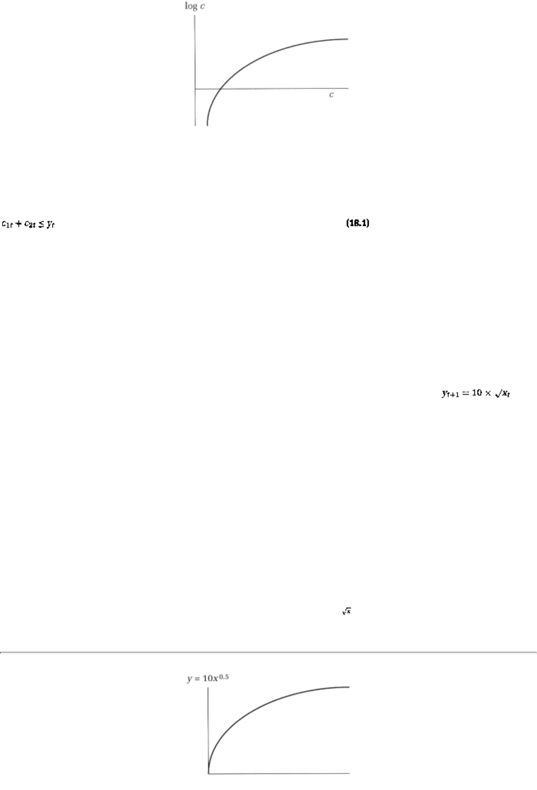
FIGURE 18.1
period t by cit. Again, it will be natural to only consider cit³ 0. Consumption gives player i a payoff or utility.
The exact value of yt constrains the total amount that can be consumed; that is, at every period t it must be
the case that
The amount of the resource not extracted, therefore, is yt - (c1t + c2t). This is the investment that can
generate future growth; call it xt. From the preceding equation it follows that xt³ 0. Investment produces next
period's stock yt+l through a production function. In Chapter 7 we examined the case of an exhaustible
resource (with no growth possibility); that is, we assumed yt+1 = xt. By way of contrast, let us now consider
a renewable resource, that is, a resource for which yt+1 > xt (at least for some investment levels).
In fact, in order to do some actual computations, we will specify particular forms for the utility and
production functions.2 Suppose that player i's utility from consuming amount ci is given by log ci; utility
increases with the amount consumed, although the utility increase is smaller, the larger is the base from
which consumption is further increased. The utility function is pictured in Figure 18.1.
We are also going to assume that investment xt results in a period t + 1 stock yt+1 of size .
Again higher investments produce higher stocks, although additional investment becomes less and less
productive, as the base investment grows larger. The production function is pictured in Figure 18.2.3
Note that if investment
xt is equal to 0 in any period, then so is the stock yt+1 in the next period. This fact
suggests a natural horizon for the gameit continues as long as there is a positive resource level and hence can
potentially go on forever.
The questions of interest are these: How does the resource stock yt evolve over time, and is there an
eventual size that can be sustained? What is the socially optimal sustainable resource stock? Does strategic
interaction lead to overextraction of the resource? In the next two sections we turn to these questions.
2The specific example that we will discuss was first worked out by David Levhari and Leonard
Mirman; see "The Great Fish War: A Solution Using Cournot-Nash Equilibrium," Bell Journal of
Economics, vol. 11, pp. 322-334, 1980.
3Note that tomorrow's stock is larger than today's investment provided xt << 100 but not otherwise.
Also for future reference, recall that an alternative notation for is x0.5.
page_277
Page 278
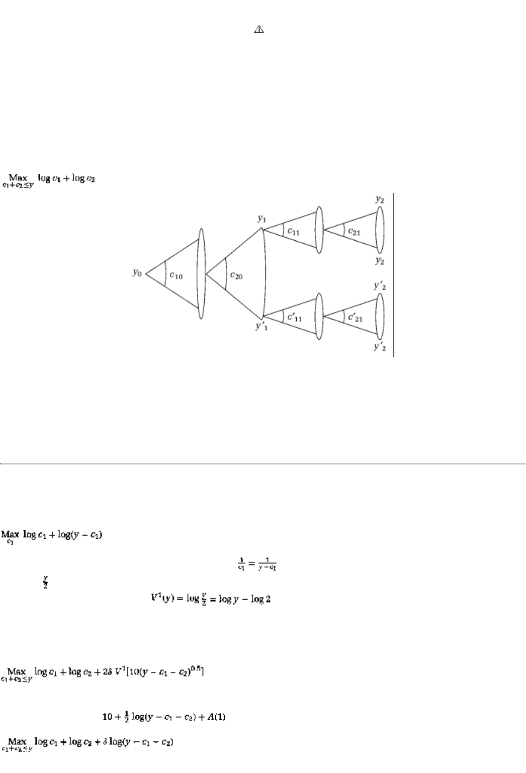
FIGURE 18.2
18.3 Sustainable Development And Social Optimum
Let us start with social optimality: if one wants to make this society of two individuals as happy as they can
be, how should one extract the resource?
18.3.1 A Computation of the Social Optimum
To derive the socially optimal solution we need to consider the sum of the two players' utilitiesand maximize
it. We will proceed by way of backward induction. Suppose, to begin with, that there are exactly two
periods. The extensive form can then be pictured as in Figure 18.3.4
If we are in the last period, with stock y, then we need to solve
FIGURE 18.3
4Note that an arc connecting two branches means that all intermediate choices, between the two
branches, are also available. For instance if consumption c leads to a future stock of y (and c'
leads to y') then the arc signifies that all consumptions between c and c' are also possibleand will
lead to a stock between y and y'.
page_278
Page 279
Since utility increases with consumption, there should never be any unused stock; that is, it must be that c1 +
c2 = y. Hence the maximization problem can be rewritten as5
The first-order condition for this maximization is ; that is, consumption should be equal, cl = c2 (and
equal to ).6 Consequently, each player's socially optimal utility when there is one stage left and the
available stock is y is given by .7 It will be useful to write this socially optimal
utility as log y + A(1), where A(1) is a shorthand for the constant, - log 2.
Let us now fold the tree of Figure 18.3 back. When there are two periods left, the socially optimal extraction
is found from solving the following problem:
where d is the discount factor and cl + c2£ y. Since V1[10(y - cl - c2)0.5] = 10g[10(y -cl - c2)0.5] + A(1),
which is equal to log
, we can rewrite the problem a little more simply as
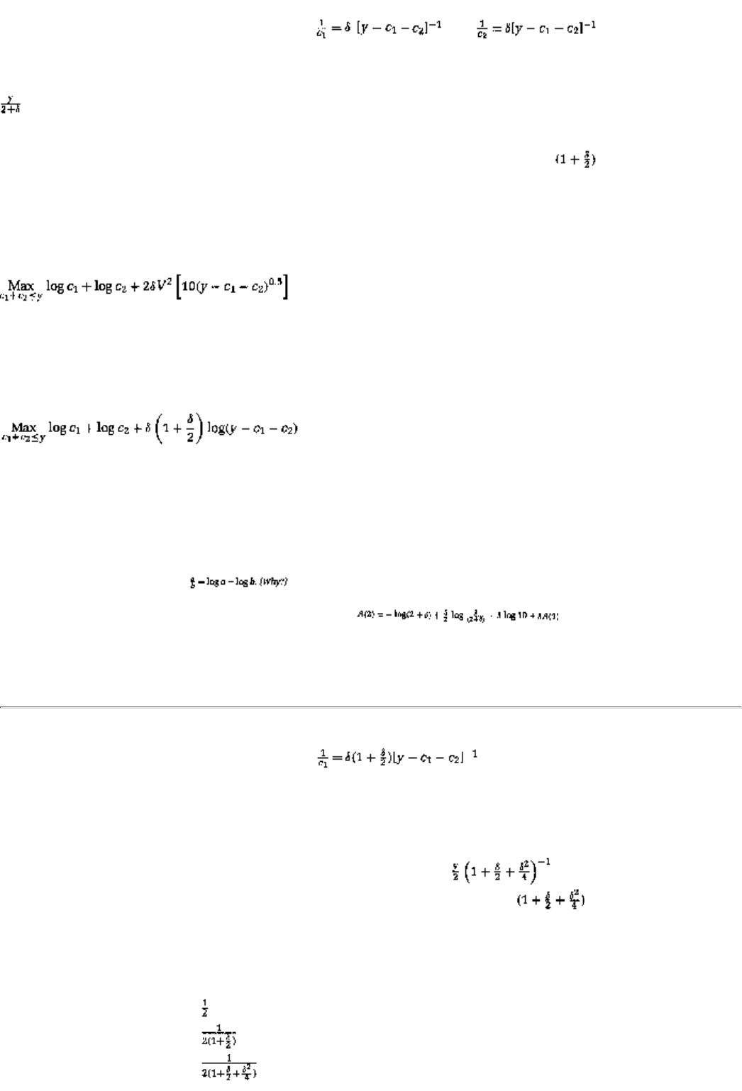
where we have suppressed the additive constants log 10 and
A
(1) because they do not affect the optimal
choice. (Why?) The first-order conditions are and . Since the
expressions are identical, it follows that the and two consumptions must be equal, that is, c1 = c2. It further
follows that this common consumption equals
. Notice that consumption is less than it is when there is only one period left; in particular, some
investment is made toward period 2's stock.
After collecting terms, the socially optimal per capita utility V2 can be written as log y + A(2), where
A
(2) is a compilation of constants.8
What if there are more than two extraction periods? Instead of solving the general case right away, let us do
just one more step of induction in order to spot a solution pattern. Suppose that the
re are three periods of
resource usage. In the first period we have the following problem to solve:
CONCEPT CHECK
MAXIMAND
Show that, after substituting for V2 and suppressing all irrelevant constants, we
can rewrite the last expression as
5Throughout, we continue to assume cit³ 0.
6As always, for a more detailed discussion of first-order conditions see Chapter 25.
7We will repeatedly use two facts about the log function: (1) for any two positive numbers a and b, log
ab = log a + log b; (2) for any two numbers a and b, with a positive, log ab = b log a. A third fact
follows from these two: . (Why?)
8And, if you must know and verify for yourself, . This expression is
derived by substituting the optimal consumption policy into the preceding equation and adding back
the suppressed constants log 10 and A(1).
page_279
Page 280
The first-order conditions for this problem are and an
identical expression for c2; since the expressions are identical, it follows that cl = c2.
CONCEPT CHECK
OPTIMAL SOLUTION
Show that the socially optimal consumption equals . Show also
that the socially optimal utility for each player is of the form log y +
A(3), where A(3) is a compilation of constants.
At this stage we can see a pattern. We have the following results (and a conjecture):
Number of Periods Remaining Consumption (Fraction of
y)
1
2
3
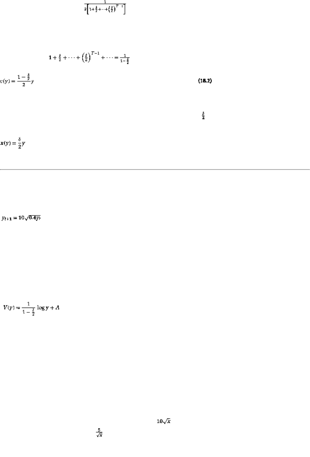
T (conjecture)
In fact, we can take the conjecture a step further; in the infinite-period model every periods's consumption
fraction will be identical, since there are exactly the same number of periods remaining in each case. This
identical consumption function, call it c(y), will be given by the limit of the optimal consumption as T tends
to infinity. Since we can in turn assert that
CONCEPT CHECK
INVESTMENT
Show that the associated optimal investment fraction is ; that is, the
investment function is
page_280
Page 281
Some Numbers
If d = 0.8, then each player consumes 30 percent of the available stock in every period while the remaining
40 percent forms the investment base. Hence, next period's resource stock is given by the formula
.
CONCEPT CHECK
RESOURCE DYNAMICS
Show that if yt = 90, then yt+1 shrinks further down to 60. What is yt+1 if yt =
10? Finally, show that if period t's stock is 40, then it neither shrinks nor
grows.
In other words, the socially optimal sustainable resource stock is equal to 40.
Returning to the general case socially optimal lifetime utility, by extrapolation, is given by
where A is a constant.9
18.3.2 An Explanation of the Social Optimum
The determination of the social optimum requires a balance between society's desire for immediate versus
future consumption. Increasing immediate consumption lowers the resource stock in the next period, and it
lowers consumption then (and possibly also in subsequent periods). Suppose an additional unit of investment
grows to 1 + k units of additional resource stock. An extraction policy achieves the right balance if society
would neither want to cut current consumption by a unit (and have 1 + k additional consumption units in the
next period) nor want to cut tomorrow's consumption by 1 + k units (and have an additional unit of
consumption today).
Consider the second option, increasing today's consumptionequivalently, decreasing today's investmentby a
unit. In our commons model, with production equal to
, a unit decline of investment produces a
decrease in future stock equal to .10
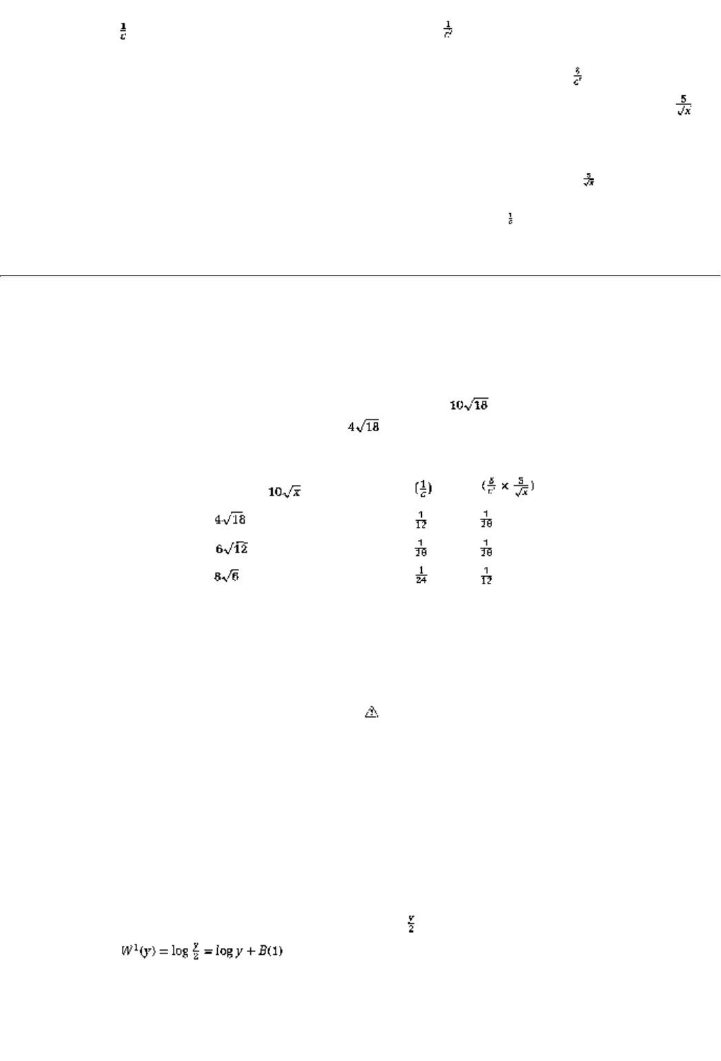
Since the utility function is equal to log
c
, a unit increase in per capita consumption today adds utility equal
to approximately .11 A unit decrease in consumption in the next units, where c' period similarly
decreases that utility by c' is next period's per capita consumption. Since next period's consumption is
discounted, next period's utility loss for every unit of consumption is actually equal to . This per-unit utility
loss next period should then be multiplied by the number of lost units, that is, should be multiplied by .
9And using this formula, verify that the consumption function is indeed given by equation 18.2.
10In other words, the slope of the production function, or marginal productivity, is .
11In other words, the slope of the utility function, or marginal utility, is .
page_281
Page 282
Some Numbers
Consider three possible extraction rates, 40 percent, 60 percent, and 80 percent. In doing the comparisons
below, we will consider values of d = 0.8 and current size of resource equal to 30. Note that current
consumption (C) at a 40 percent extraction rate is 0.4 × 30, that is, 12, while current investment (x) is 0.6 ×
30, that is, 18. This investment produces a stock tomorrow equal to and hence, at a 40 percent
extraction rate, consumption tomorrow (c') equal to . The consumption and investment numbers for
extraction rates of 60 percent and 80 percent are computed similarly.
Extraction c x c' Gain Loss
Rate (Rate × )
40% 12 18
60% 18 12
80% 24 6
As you can see from the table, there is nothing to be gained from increasing current consumption if 60
percent of the resource is consumed every period. Consumption should be increased if only 40 percent is
being currently extracted, and it should be curtailed if 80 percent is currently being consumed. Of course, 60
percent is the socially optimal extraction that we computed a few paragraphs back.
18.4 Achievable Development And Game Equilibrium
Let us now turn to the parallel analysis in a strategic, rather than social, setting. Suppose that the two players
are extracting the resource unilaterally. Each player will then only consider her own utility and seek to pick
extraction rates that maximize this utility.
18.4.1 A Computation of the Game Equilibrium
Like the social optimum, the game equilibrium can also be solved by backward induction. Suppose, to begin
with, that there are exactly two periods. The extensive form is that of Figure 18.3.12
Suppose we are in the last period with stock y. Since utility increases in the amount of consumption and
there are no more periods afterward, each player will attempt to consume everything. Hence, the stage-game
equilibrium is one where each player's actual consumption is . Consequently, each player's equilibrium
utility is given by , where B(1) equals the constant, - log 2.
Let us now fold the tree of Figure 18.3 back. When there are two periods left, player 1 faces the following
best-response problem:

12For the game we also have to specify what happens when the desired consumptions add up to an
amount greater than the available stock. We will assume, as in Chapter 7, that in this case the stack
is divided equally between the two players.
page_282
Page 283
where q is the fraction of the resource that player 2 is expected to consume in the first period.13 Since
we can rewrite the problem as
where we have suppressed the constants log 10 and B(1). The first-order condition is . Hence,
the best-response consumption is given by . If we write consumption as a fraction of
resource stockthat is, if we write it as b(q) ythen it follows that
Since the game is symmetric, it is natural to first look for a symmetric equilibrium. In a symmetric
equilibrium, each player chooses the same extraction rate, and the rate is such that it is a best response (to
itself), that is, b(q) = q. Put differently, the extraction rate is a symmetric equilibrium. After collecting
terms, the equilibrium utility when there are two remaining periods, W2, can be written as
, where, as always, B(2) denotes a constant.
Now suppose that there are three periods of resource usage.
CONCEPT CHECK
BEST-RESPONSE PROBLEM
After substituting for the formula for W2, show that the first-period
best-response problem of player 1 is
The first-order condition for this problem is .
EQUILIBRIUM
Show that a symmetric equilibrium is for each player to extract a fraction equal to (in the first
period).
13Note that we have assumed that player I will consume within his means, that is, that .
Otherwise, we know that there will be no consumption for either player in the lost period. When
utility is specified by the log function, a player will always avoid zero consumption in any period;
that is, he will in fact consume within his means in the first period.
page_283
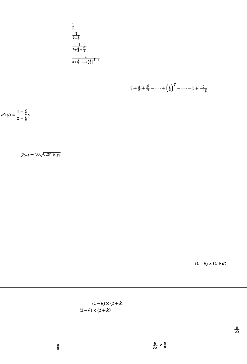
Page 284
As with the social optimality problem, we can now see a pattern.
Number of Periods
Consumption (Fraction of y)
1
2
3
T (conjecture)
In the infinite-period model, the equilibrium consumption function, call it c*(y), will be given by the limit of
the equilibrium consumption as T tends to infinity. Since we can in turn
assert that
Some Numbers
If d = 0.8, in equilibrium, each player consumes 37.5 percent of the available stock in every period while the
remaining 25 percent forms the investment base. In this case, next period's resource stock is given by the
formula, .
CONCEPT CHECK
RESOURCE DYNAMICS
Show that if yt = 100, then yt+1 shrinks down to 50. Show that the stock
grows if yt = 20, and that if period t's stock is 25, then it neither shrinks nor
grows.
In other words, the equilibrium achievable resource stock is equal to 25.
18.4.2 An Explanation of the Equilibrium
The determination of a game equilibrium, like the determination of the social optimum, requires a balance
between immediate and future consumption. There is, however, one key difference between the two
situations; in the game a player reaps only a part of the future consequences of his actions. Let us explain.
Suppose an additional unit of investment grows to 1 + k units of additional resource stock. A part of this
increase is appropriated as future consumption by the other player; suppose this fraction is q. In that case,
from the perspective of the player who makes the common investment higher by withholding his own
immediate consumption, the effective increase in the stock is not 1 + k but rather it is . An
extraction policy for a player achieves the right balance if he would want neither to cut current
page_284
Page 285
consumption by a unit [and instead have additional consumption units in the next period] nor
to cut tomorrow's consumption by units (and have an additional unit of consumption today).
Suppose, therefore, that a player increases today's consumptionequivalently, de creases today's investmentby
a unit. As we have seen, a unit decline of investment produces a decrease in tomorrow's stock equal to
,
where x is the current investment. Suppose further that the other player's extraction rate is (the equilibrium
rate of) 37.5 percent, or . Then the effective decrease in stock is .
Exactly as in the social optimality case, a unit increase in consumption today adds u
tility equal to
approximately and a unit decrease in consumption in the next period decreases utility by units, where c'
is next periods's consumption. Since next period's consumption is discounted, next period's utility loss is
actually . This per unit utility loss should then be multiplied by the number of lost units, .
Let us see which of the twocurrent gain or future lossis higher, for three possible extraction rates for player
1, 30 percent, 37.5 percent, and 50 percent.14 We will consider values of q = 0.8 and current size of
resource equal to 40 and presume that the other player extracts at the equilibrium rate equal to 37.5 percent.
Note that current consumption at a 30 percent extraction rate is 0.3 × 40, that is, 1
2. Together with the other
player's consumptionequal to 15 at an extraction rate of 37.5 percentthat yields a current consumption total
(c1 + c2) of 12 + 15, or 27. Hence, current investment (x) is 13. This investment produces a stock tomorrow
equal to and hence, at the 30 percent extraction rate, consumption equal to . The
consumption and investment numbers for extraction rates of 37.5 and 50 percent are similarly computed.
Extraction c1 + c2 x Gain Loss
Rate
30% 27 13
37.5% 30 10
50% 35 5
As you can see from the table, there is nothing to be gained from increasing current consumption if 37.5
percent of the resource is being consumed every period. Consumption should be increased if player 1 is only
consuming 30 percent currently, and it should be curtailed if she is consuming 50 percent instead.
18.4.3 A Comparison of the Socially Optimal and the Equilibrium Outcomes
The general lesson is that unilateral extraction leads to overextraction; consumption in the equilibrium
solution is higher than in the socially optimal solution. Compare the two consumption functions: the
socially optimal function c(y) and the equilibrium function c*(y). Note the following:
14Recall that 30 percent is the socially optimal rate and 37.5 percent is the equilibrium rate.
page_285
Page 286
The equation holds simply because is smaller than 2. The intuition for this conclusion is precisely that
in the equilibrium solution a player only collects a part of his action's consequences. Hence, he is more likely
to overextract because part of the burden of that overconsumption is borne by a lowering of the other
player's future consumption.
Consider two different societies, one in which consumption is socially managed and another in which it is
unilaterally determined. Imagine that both societies start with the same resource stock. By period 2, the first
society would have a larger resource stock because it invested more in the first period. This incease implies
in turn that this society would again have a larger investment level in period 2. This result would occur for
two reasons; first, society 1 in any case invests a larger fraction of any resource stock. Second, it has a larger
resource stock available. Now, hopefully, the continuation of this logic is also clear. In each period the
socially managed society would have a larger resource stock, would invest more, and hence would continue
to have a larger resource stock in the future. If yt denotes the resource stock in the socially managed
situation and
denotes the equilibrium stock, then for all periods t > 1 even though .
Another consequence of this argument is that the sustainable socially optimal stock i
s higher than the
achievable equilibrium stock. We have already seen this outcome with some numbers, but here is the general
argument: A sustainable stock is one that keeps getting regenerated; that is, it is a level at which yt = yt+1 in
all periods. Put differently, at the sustainable socially optimal stock, call it , socially optimal investment
exactly regenerates that stock, that is, . This stock is not achievable in equilibrium because
the equilibrium investment at is less than . In fact, the achievable equilibrium stock must be lower.
18.5 Dynamic Games: An Epilogue
Two natural questions arise at this point: First, how general are the conclusions of the commons model; that
is, do broadly similar conclusions arise in any dynamic game? Second, what have we learned that is different
from the conclusion of the simpler repeated-games structure?
There are three conclusions that we have seen in the commons model. First, there is an equilibrium in which
each player looks only at the size of the current resource stock, or game environment, to decide how much
to consume.15 Such strategies have a technical name; they are called Markovian strategies, and an
equilibrium in these strategies is called a Markov perfect equilibrium (MPE). Markovian strategies are
attractive because of their simplicity; they do not require a player to keep track of either what his opponent
did in the past or how the resource has evolved in previous periods.
For general dynamic games, MPE always exists if the number of game environments is finite. When the
environment can be any one of an infinite number, tricky mathematical
15In the finite-horizon game, each player also looks at how many periods of extraction remain in
order to make this choice.
page_286
Page 287
issues arise, and we do not know whether there is always an MPE.16 In a repeated game, there is only one
environment; hence a Markovian strategy is the same thing as choosing the same action over and over again.
An MPE, therefore, is the same thing as playing a stage-game Nash equilibrium repeatedly. (Why?) Unlike a
dynamic game, therefore, MPEs in repeated games do not lead to any interesting time patterns of behavior.
The second conclusion of our model is that there is a unique equilibrium (that looks similar to the socially
optimal solution). This conclusion is not at all robust. In general dynamic games, there are many MPEs.
When we additionally consider strategies that look like the trigger strategies of repeated games, we generate
yet more equilibria.
The final conclusion was that equilibrium is socially suboptimal; too much of the resource is extracted and
hence equilibrium utilities are lower than socially optimal utilities. This conclusion is very robust and shows
up in a variety of dynamic games. And, of course, it also shows up with repeated gamesunless the threat of
punishment is imposed, equilibria are suboptimal. Using logic similar to that of repeated games, it is also
possible to show that triggerlike strategies can sometimes remedy this problem in a dynamic game. If players
believe that good behavior will be rewarded and bad behavior punished in the future, they might be inclined
to behave themselves.
Summary
1. Dynamic games generalize the framework of repeated games by allowing the game environment to change
from period to period. They are needed to study problems that are fundamentally dynamic.
2. An example of a dynamic game is the commons problem in which players have access to a common
property resource. The size of the resource constitutes the game's environment, and it evolves over time
depending on the pattern of resource usage.
3. A socially optimal resource usage balances the competing social desires for immediate and future
consumption. The optimal balance typically lies between the two extremes of no usage and complete
exhaustion of the resource.

4. If the resource is used in a decentralized fashion, then each player's usage balan
ces the competing desires
for immediate individual consumption and future consumption. However, each player realizes that he will
only get a fraction of any additional (common) future resource stock.
5. Typically, equilibrium usage leads to overextraction, relative to the social optimum. This phenomenon is
called the tragedy of the commons.
16Of course some games, such as our commons model, do have MPE even when there are an
infinite number of possible environments.
page_287
Page 288
Exercises
Section 18.1
18.1
Give two examples of dynamic strategic interaction that should be studied as a dynamic game. Be sure to
describe carefully what the game environment is, how it affects payoffs, and how it evolves.
18.2
Write down a simple dynamic game model of the Treasury auctions (section 14.3) when the quantity sold
can vary from auction to auction. State explicitly any assumptions that you make.
18.3
Can you write down a simple dynamic game model for OPEC in which the costs of extraction depend on
existing reserves in every period? For the purposes of this example you can utilize the numbers on extraction
levels that we discussed in Chapter 17.
Section 18.2
18.4
For the production function used in the chapter, what is the stock that arises from investment level 50? What
of investment level 20? level 90?
18.5
If the current size of the resource is 60, how much investment would there need to be to regenerate this
stock level? What if the current resource stock is 90?
18.6
From the picture of the production function (Figure 18.2), and your answer to exercise 18.5, what can you
conclude about sustainability of higher and higher stocks? Explain your answer.
18.7
The marginal productivity of investment is the additional stock that would result from a small increase in
investment (for example, a unit increase). Graph the marginal productivity function , where x is the
investment level. Can you explain its shape?
18.8
Explain the answers that you got in exercise 18.6 in light of what you concluded in
page_288
Page 289
exercise 18.7. Is it correct to say, ''It becomes increasingly difficult to sustain larger resource levels"?
18.9
The marginal utility of consumption is the additional utility that would result from a small increase in
consumption (for example, a unit increase). Graph the marginal utility function , where c is the
consumption level. Can you explain its shape?
Section 18.3
(Calculus problem) Suppose that the production function is given by but the utility functions are the
same as those in the text; that is, player i's utility is log ci. The next several questions will compute the social
optimum and the game equilibrium for this case.
18.10
Formulate the social optimality problem when there is just one more period of extraction left. What is the
socially optimal utility level?
18.11
Formulate the social optimality problem when there are two more periods of extraction left. What is the
socially optimal consumption rule? What is the socially optimal utility level? (You do not have to write down
all of the constants in the optimal utility.)
18.12
Repeat the previous question for three remaining periods of extraction.
18.13
What can you infer about the general case of T remaining extraction periods? What if there are an infinite
number of periods? Explain your answers carefully.
18.14
How do your answers compare with those found in the chapter? Explain your finding.
18.15
For the special case of d = 0.8, compute the consumption and investment functions. What is the socially
optimal sustainable resource level? How does your answer compare with that in the text?
Section 18.4
18.16
Now formulate the equilibrium problem when there is just one more period of extractio
n left. What is the
equilibrium utility level?
page_289
Page 290
18.17
Formulate the best-response problem of player 1 when there are two more periods of extraction left and
player 2 is expected to consume a fraction q of the current stock level. What is the best-response
consumption fraction?
18.18
What is the symmetric equilibrium to this game? What is the equilibrium utility level? (You do not have to
write down all of the constants in the equilibrium utility.)
18.19
Repeat exercises 18.17 and 18.18 for the case in which there are three remaining periods of extraction.

18.20
What can you infer about the general case of T remaining extraction periods? What if there are an infinite
number of periods? Explain your answers carefully. How do your answers compare with those found in the
chapter? Explain your finding.
18.21
For the special case of d = 0.8, compute the consumption and investment functions. What is the socially
optimal sustainable resource level? How does your answer compare with that in the text?
page_290
Page 291
PART FOUR
ASYMMETRIC INFORMATION GAMES; THEORY AND APPLICATIONS
page_291
Page 293
Chapter 19
Moral Hazard and Incentives Theory
This chapter is the first in a series that brings players' informationwhat they know, and equally importantly,
what they do not knowto center stage. It discusses a phenomenon called moral hazard that is important for
the theory of incentives. In section 19.1 we give a definition and present several real-world examples of
moral hazard. Section 19.2 presents a simple model and discusses a number of alternative incentive schemes.
Section 19.3 analyzes the model and derives the optimal incentive scheme, and section 19.4 contains some
general conclusions. Finally, in section 19.5, we discuss a case study on compensating primary care
physicians in an HMO.
19.1 Moral Hazard: Examples And A Definition
Moral hazard
A principal-agent problem arises when one economic agentthe agenttakes an
action that affects another economic agentthe principal. A principal-agent
problem has a moral-hazard component when the principal is unable to simply
force the agent to act according to his interests.
The term moral hazard arises in insurance and refers to the fact that a person who has insurance coverage
will have less incentive to take proper care of an insured object than a person who does not. For instance, if
your expensive stereo equipment is fully insured against theft, you might be less careful about locking your
door every time you step out of your dorm room; after all, even if the amplifier was stolen you would be able
to replace it at no additional cost. Conversely, if you do not have comprehensive insurance on your car you
may think twice about parking right in front of the rowdiest downtown bar on a Friday night.
In each of these cases there is something that you as the insured agent prefer to do that the insurance
company would rather you not do. In the first case, it is more convenient for you not to have to carry around
a heavy set of keys. In the second, you prefer to get to your destination sooner rather than drive around for
another 15 minutes looking for a safer parking spot. However, your actions expose the insurance company
page_293
Page 294
in legalese, the principalto unnecessary risk. In each of these cases it is also true that it is difficult for the
insurance company to prove that you did not take adequate precaution.

This then is the heart of the moral-hazard problem: what is good for the agent is not
(necessarily) good for
the principal, and the principal cannot always be on hand to monitor what the agent does.
There are at least two reasons why a principal may be unable to enforce his will by simply asking the agent
to act according to his (the principal's) interests. First, the agent's actions might not be observed by the
principal. Second, the principal might be able to observe the agent's action all right but might be unable to
prove breach of contract in a court of law. For instance, leaving your dorm room door unlocked is an action
that is unobservable to the insurance company. Parking in front of the rowdiest bar is an observable action,
but it might be impossible to prove to a court that you were fully aware of the risks of that action.
Whenever there is moral hazard, the principal has to devise schemes that will induce the agent to act in ways
that the principal prefers. For example, insurance policies routinely have a deductible; this is a dollar amount
on your claim that the insurance company will not pay. If your automobile insurance policy has a $500
deductible, then the first $500 worth of damage has to be paid out of pocket by you. In this case, you might
think twice about parking in front of a rowdy bar! This chapter will study various schemes that a principal
might come up with to give his agent appropriate incentives.
Let us turn now to some further examples of moral hazard from outside the insurance business. In each
example, the first character in a pair is the principal, and the second, the agent.
Owner-Manager
The managers of a company take a number of actions that affect profitability but are largely unobserved by
the owners (or shareholders, if it is a publicly held company); these include how hard the managers work,
whether or not they make every effort to contain costs, whether they account for all possibilities before
deciding on a new project, and so on. The preferences of owners and managers are in conflict if owners care
only about the firm's profits whereas managers care additionally about such things as the number of hours
that they work and the number of people under their direct control.
Client-Service Provider (For Example, Client-Lawyer, Patient-Doctor, Car Owner-Car Mechanic)
A doctor runs tests, makes diagnoses, and prescribes care for her patient. The appropriateness and quality of
these actions are essentially unobservable to the patient, who does not have the expertise to judge these
issues. And that statement is also true of the other examples. In each case, the preferences of the principal
and agent are different; the doctor, for example, cares about her fees, the likelihood of being sued, and the
like in addition to treating the patient. The patient is primarily interested in getting better.
page_294
Page 295
Firm-Salesman
A salesman collects orders for her firm. Sometimes she may do so on the phone, and, more traditionally, she
may do so by calling on her clients. Typically, the firm would like salesmen to maximize sales, but doing so
may require the salesman to work incredibly long hours, travel miles away from home, be away from home
days on end, and so on. You can see the divergence in preferences now; what is good for the principal may
be too onerous for the agent. Furthermore, the firm typically cannot ensure that the salesman puts in hours
that the latter might not want to.
There will be two essential questions in the principal-agent moral hazard problem:
What kind of incentives should the principal give his agent to make her choose a prespecified action?
What action should the principal specify? Should it be the action the principal most desires, the one that the
agent prefers, or something in between?
19.2 A Principal-Agent Model
In this section we will present a simple model of moral hazard involving a principal and an agent and discuss
some examples of incentive schemes that the principal might use to combat moral hazard.
The principal-agent game can be represented by the game tree of Figure 19.1. In drawing the tree we restrict
attention to a simple case in which the agent can only choose among two actions and there are three
consequences for each action of the agent.
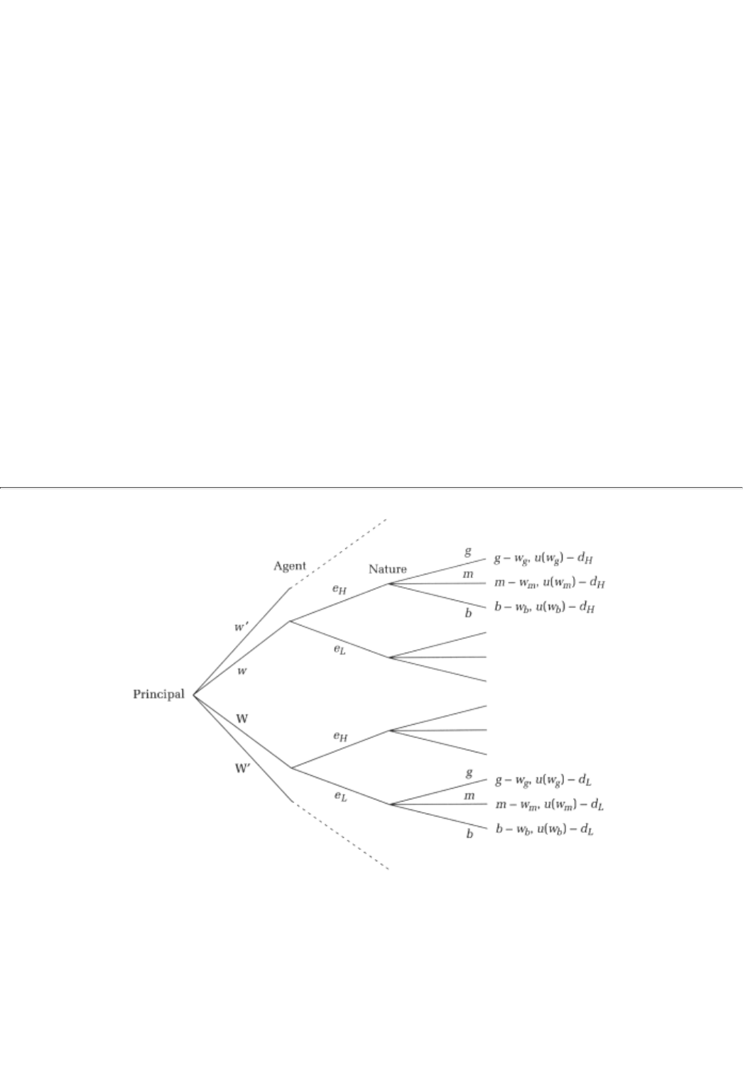
At the root of the tree, the principal makes a decision about the kinds of incentives
to offer his agent. For
instance, the owner of a firm has to decide on the compensation package he will offer his manager.1 After
seeing the incentive scheme, the agent chooses her action among the two choices eH and eL, and these
denote high and low effort respectively; the term effort includes decisions on how hard to work, what
projects to select for the company (and, possibly, whether or not to look for another job).2 The agent's action
is unobservable to the principal. Since the agent chooses after the principal, the agent's decision nodes form
the second stage of the tree.
The agent's action determines the firm's profitability; the three possible profit levels are denoted good,
medium, and bad, and g > m > b. The profit determination is uncertain; that is, every action of the agent
leads to a probability distribution over profits.3 It is important that there not be a one-to-one relationship
between the agent's action and the firm's profits; otherwise, the action would be exactly inferred from the
1In the discussion that follows we will often refer to the principal as owner and to the agent as
manager. The owner-manager story will provide a concrete context for the analysis although the
conclusions will apply more generally to any principal-agent problem.
2In some of the examples the terminologyeffortneeds to be interpreted in a very broad sense. For
instance, an insured agent exerts care, a doctor chooses appropriate treatment, and a car mechanic
fixes a car.
3As in earlier chapters, uncertainty is modeled via a fictional player"nature." For instance, when the
agent chooses action eH, nature "chooses" among profit levels g, m, and b with probabilities 0.6, 0.3,
and 0.1, respectively. Similarly, when the agent chooses eL, nature assigns probabilities 0.1, 0.3, and
0.6 to the three profit levels.
page_295
Page 296
FIGURE 19.1
resultant profit. Uncertainty allows for such incompleteness in inference; upon seeing a profit level g, the
principal is not sure whether the agent took action eH or eL.
Consider now the principal's payoffs. The principal pays the agent wg if he observes profits of size g, wm for
profits equal to m, and wb if profits are only equal to b. The principal can only reward on the basis of what
he sees, that is, profits.4 Consequently, the net profit for the principal is g - wg whenever gross profits are g,
m - wm in the medium case, and b - wb in the bad profit scenario. We will assume that the principal only
cares about net profits.
The agent gets a payoff, or utility, from her compensation as well as from the effort
that she exerts. For
example, if she is paid wm and she has taken action eH, then her total payoff is u(wm) - dH, where u(wm) is
the utility from compensation wm and dH is the disutility of eH. We will assume that the utility of
compensation, u(.), is an increasing, concave function, that is, that the agent prefers more money to less and
is risk averse.5 Finally, eH stands for high effort in the sense that its disutility is greater, that is, dH > dL.
At various points in the discussion we will want to compute solutions to various incentive schemes explicitly.
At those points, we will make the following special assumption:
4It will also be natural to presume that the principal cannot charge the agent for (the pleasure of)
working for him; that is, we will only consider wg³ 0, wm³ 0, and wm³ 0.
5Risk aversion means that the agent prefers to avoid risky situations; in particular, she prefers to have
a dollar for sure to a gamble in which she has an equal chance of losing that dollar and of winning an
additional dollar. See Chapter 27 for further elaboration. For expositional ease, we shall also assume
that u(.) also has a slope.
page_296
Page 297
Special Assumption (SA). ; dH = 10; dL = 0; and profit levels are g = 200, m = 100, and b = 50.
19.2.1 Some Examples of Incentive Schemes
A Pure Wage Scheme
One possible compensation scheme is to treat the agent as a salaried employee who gets a fixed salary
regardless of the firm's profits. Hence, wg = wm = wb = w, for some salary level w.
In this case the agent's payoff, if she takes action eH, is u(w) - dH (no matter what the profit level is) while
the payoff from eL is u(w) - dL. Since the disutility dH is higher, the agent would prefer to take action eL,
that is, would prefer not to exert high effort. This result should not cause any surprise; if her compensation
does not depend on results, then the agent would prefer to take the action that she most prefers rather than
that which is good for the principal (and the firm).6
A Pure Franchise Scheme
The opposite extreme is a pure franchise scheme in which the agent pays the principal a fixed sum of
moneythe franchise feeregardless of profits. In this case, the agent bears all the risks and is like a "residual"
owner.7 Denote the franchise fee f. Therefore wg is equal to g - f, wm is the same thing as m - f, and wb is
equal to b - f.
If the agent takes the action eH, her payoff is uncertain; with probability 0.6 it is u(g - f) - dH, with
probability 0.3 it is u(m - f) - dH, and with probability 0.1 it is u(b - f) - dH. Her expected payoff is therefore
By similar reasoning her expected payoff from taking action eL is
It is no longer immediately obvious which of her two actions the agent prefers. Although eH is more
onerous, it has a higher probability that the agent's take will be g - f rather than b - f. To fix some ideas,
consider the numbers given in the special assumption (SA).
CONCEPT CHECK
FRANCHISE (SA)
Show that the agent will take action eH if and only if
6Even at this preliminary stage of our discussion on incentives we seem to have gained some
understanding of why there are never more than two counters open at the local post office, why so
many postal workers feel the need to talk endlessly to each other, and why the only thing that is
prompt at that office is the closing of the doors at the stroke of 5 P.M.
7Your local McDonald's is most likely a franchise.
page_297
Page 298
The highest fee that the principal can possibly charge is 50. (Why?) For that fee, the agent would take action
eH because .
An Intermediate Scheme: Wage Plus Bonus
In the first two schemes, either the principal or the agent bears all the risks. In a pure wage scheme, the
agent gets the same salary regardless of profit, while in a pure franchise scheme, the principal gets the same
franchise fee (again regardless of profit level). In an intermediate scheme, the risks are shared; the agent is
given a base wage wb regardless of profit level. A bonus is paid to her only if a higher profit level m or g is
observed; in the first case, the size of the bonus is wm - wb, while in the second case it is wg - wb. The agent
bears some risk because at least one of the two bonuses is positive (and not zero), while the principal bears
some risk because the bonus is less than the increase in profit.
If the agent takes the action eH, her payoff is uncertain: with probability 0.6 it is u(wg) - dH; with probability
0.3 it is u(wm) - dH; and with probability 0.1 it is u(wb) - dH. Her expected payoff is therefore
By the same reasoning, the agent's expected payoff from taking action eL is
It follows that the agent will take action eH if and only if
An Infeasible Scheme: Effort-Based Wage
If moral hazard were not present, that is, if the principal could observe the agent's effort, he could pay the
agent directly on that basis. As a benchmark comparison, let us see what happens in that instance. Denote
the two wage levels wH and wL.
The agent will take action eH if and only if
CONCEPT CHECK
BONUSES IN THE SA CASE
Consider the intermediate incentives case. Use equation 19.2 to write down
the bonus that would induce the agent to pick eH. Knowing that the lowest
base wage wb is 0, can you show that the bonus is 100? Repeat, using equation
19.3, for the infeasible case. Is the bonus in this case, wH - wL, bigger or
smaller than 100?
page_298
Page 299
19.3 The Optimal Incentive Scheme
In this section we will answer the question, Which incentive scheme should the principal offer his agent?
Although we are particularly interested in the answer when there is moral hazard, it will be useful to first
answer the question when there is not.
19.3.1 No Moral Hazard
Just for this subsection let us imagine that the principal observes the agent's action and can therefore reward
that effort directly. As we saw in the previous effort-based wage segment, the agent will choose eH only if
she is given an appropriate bonus wH - wL. If the agent chooses eH, the principal's net expected profit equals
whereas if she chooses eL, those profits equal
A straightforward calculation shows that the principal would rather offer the bonusand have the agent work
eHif and only if
The last condition has an easy interpretation: there is a 50 percent greater likelihood of the profit level g,
rather than b, if effort eH is exerted by the agent. In other words, there are increased expected profits of size
0.5 × (g - b) if eH is chosen, and the question is, Do those profits exceed the wage bonus wH - wL?
For SA, the increased expected profits equal 75 and the wage bonus required (as we hope you showed) is 25.
So in this case the principal would indeed offer an incentive scheme wH = 25, wL = 0, and the agent would
pick eH.8 Consequently, the principal's net expected profits would be 130 and the agent's payoff would be 0.
To summarize, the principal has one of two options: pay the wage bonus required to get the agent to pick eH
or, alternatively, pay no bonus and set wH = wL (= 0), and count on the agent to pick eL.9 Two
considerations determine the principal's choice: First, how large is the required bonus? That depends on how
averse the agent is to hard work; that is, it depends on dH - dL. Second, how large is the consequent increase
in profits; that is, how large is g - b? As equation 19.4 makes clear, the smaller the required bonus and the
larger the increased profits, the more likely that the optimal is a wage-plus-bonus scheme.
19.3.2 Moral Hazard
Let us revert to the case of moral hazard (in which the agent's compensation can only depend on the
observed profit level). Again, one option for the principal is to offer a pure wage scheme. Since the agent is
definitely going to respond by picking eL, the principal
8Note that at these wages, the agent is exactly indifferent between eH and eL. The principal could
make her strictly prefer eH by setting wH equal to 25.01.
9From the pure wage scheme discussion of the previous section we know that the agent will always
pick eL if she is a salaried employee.
page_299
Page 300
might as well offer a salary of 0. The principal's expected profits in that case will be (0.1 × g) + (0.3 × m) +
(0.6 × b). For the SA case, the expected profit equals 80.
A second option is to offer a pure franchise scheme. In this case, the principal's net profit is exactly the
franchise fee. In the SA case, as we saw earlier, the highest franchise fee that he can collect is 50. Hence, a
pure wage scheme is better for the principal than a pure franchise scheme. The question is, Is an
intermediate scheme even better than these two extremes?
If the agent picks action eH, the principal's net expected profit equals
whereas if the agent chooses eL those profits equal
CONCEPT CHECK
BONUS?
Use equations 19.5 and 19.6 to show that the principal would be willing to pay
the appropriate wage bonus, wg - wb, if and only if
This last equation has the following interpretation: If the agent picks eH there is a 50 percent greater
likelihood that the profits will be g rather than b. Consequently, there is also a 50 percent greater likelihood
that the principal will have to pay the bonus wg - wb. The principal finds the bonus worth paying if the
increase in profits is larger than the required bonus. From the wage plus bonus segment of the previous
section, and in particular equation 19.2, we know that this bonus is given implicitly by the requirement,
.
Hence, we have a qualitatively similar conclusion to the no-moral-hazard case: the principal will more likely
pay the bonus if the work aversion dH - dL is small or the increase in profits g - b is large.10 When he does
pay the bonus, that is, when the pure wage scheme is inoptimal, he pays exactly that amount at which the
agent is indifferent between actions eH and eL. The pure franchise scheme is inoptimal because the
franchise bonuses, m - b and g - b, are too large.
10You might wonder why the medium profit level m and its associated compensation wm have not
played any role in the discussion so far. The reason is that m has the same probability, 0.3, for both
actions. Its occurrence, therefore, does not give the principal any information about the agent's
effort, nor does it affect the agent's incentives. Hence, wm = wb. (Why?) In the next subsection we
will drop the equal-probability restriction, and we will see then that the medium outcome does play
a role in determining the optimal incentive scheme.
page_300
Page 301
CONCEPT CHECK
OPTIMAL SCHEME IN THE SA CASE
First, show that it is worth the principal's while to pay the bonus, that is,
equation 19.7 is satisfied. Then compute the optimal incentive scheme and
show that the principal's expected profit is 95. What is the agent's expected
payoff?
In comparing the SA numbers for the no-moral-hazard and the moral-hazard cases, note that the principal is
worse off in the latter (expected net profits of 95 versus 130). The reason is that he has to pay the agent a
larger bonus (100 versus 25) to get the agent to pick eH.
19.4 Some General Conclusions

There are two conclusions from the previous section that hold more generally:
Result 1: To elicit hard work, you need to give bonuses for good results.
Result 2: The higher the profits, the larger the bonus.
Result I follows straightforwardly from the discussion of the pure wage scheme in section 19.2. Suppose that
no bonuses are offered; that is, we have a pure wage scheme. No matter how complex the model, we
immediately know that the agent will always pick her most preferred action in that case, that is, will avoid
hard work.11
Result 1 has an interesting and not so obvious consequence:
Corollary 1: The principal is always strictly worse off if there is moral hazard versus when there is not,
unless he wants the agent to pick eL.
When there is no moral hazard, the principal can condition the agent's payment directly on the effort level.
So no matter what the profit outcome, the agent gets the same wage; that is, she faces a pure wage scheme.
For the principal to be no worse off with moral hazard, he has to be able to offer a pure wage scheme and
get the agent to pick the desired action. But we know that when there is moral hazard the only action that
the agent will find it in her self-interest to pick is eL.12
Result 2 holds in the model studied so far.13 It seems a natural conjecture that it will always hold, that is,
that we should always have wg³ wm³ wb. Somewhat surprisingly
11And Result I is pervasive. At the time a draft of this chapter was being written, the ''story of the
week" in New York tabloids was the Donald TrumpMaria Maples divorce. Perhaps the most
interesting part of the divorce was its timing. Apparently, it took place in 1997 rather than a year
later because the prenuptial agreement had a bonus scheme for Marla. It specified that if the
marriage broke down within five years, she would get a payment between $1 million and $5 million
(her baseline wage), but if it lasted more than five years then she would get a share of Trump's net
worth (valued between $450 million and $2.5 billion). The Donald got out of the bonus payment by
divorcing early! In a similar vein, Yankee third baseman Charlie Hayes got a bonus for keeping his
weight under a cutoff, and Miami Heat point guard Tim Hardaway, brilliant but prone to
inconsistency, got a bonus if his assists-to-turnovers ratio during the season was over 4.
12Note that it does not pay the principal to condition compensation on both effort and profits when
there is no moral hazard. The reason is that the agent is risk averse and so does not like any
unnecessary result-dependent uncertainty in her compensation. Since effort is observable, the
principal cannot apply any additional incentive pressure by having the wage depend on results. So it is
mutually beneficial not to make wages contingent on profit level.
13Note that in order to have the agent pick eH the principal offers a positive bonus, that is, wg > wb.
There is, however no such bonus offered for the medium outcome; that is, wm = wb.
page_301
Page 302
it turns out that such monotonicity only holds under an additional condition called monotone likelihood
ratios.
To get some feeling for what follows, let us modify the model a little bit. Suppose that eL implies that there is
(as before) a 0.1 probability of profit g, but now there is a probability p that the profit will be m (so far p =
0.3), and a remaining probability 0.9 -p that the profit level will be b. When effort eH is exerted, the
probabilities are (as before) 0.6, 0.3, and 0.1 for profits g, m, and b, respectively.
Whenever the probability p is less than 0.3, we are in a situation in which both m and g are more likely with
hard work. When the principal sees m or g, he should therefore reward the agent in either case. The question
is, which reward should be higher? The answer will be, whichever profit level is relatively more likely with
eH than with eL.
Definition. The likelihood ration for profit level g is The likelihood ratio for profit
level m is similarly defined.
Since the likelihoods of the profit level g are 0.6 and 0.1 (for eH and eL, respectively) the likelihood ratio is
6. In contrast, for profit level m, the likelihood ratio is
Result 2: The wage bonus for profit level g is higher than the bonus for m if and only if its likelihood ratio is
greater than that for m, that is, if
The intuition for the condition is this: Whenever a particular profit level is observed, the principal estimates
the chance that this profit was realized because the agent exerted effort eH and not eL. The higher his
estimate, the more he would like to reward the agent. The likelihood ratio is precisely that estimate. To
further see why this conclusion makes sense, imagine that p = 0; that is, if the principal saw m he would be
sure that the agent had in fact picked eH. In that case the principal would want to induce the agent to do the
right thing by offering a large sum of money if m were observed, but not very much if g were observed
instead, since in the latter scenario the principal is still unsure of what the agent actually did.
Sketch of Proof
To formalize the intuition, consider the following thought exercise. Suppose that the agent does pick action
eH. In that case the principal's expected wage bill is
(since he will always pay base wage wb = 0 to minimize on costs). From equation 19.8 it follows that starting
from any pair of wages wg and wm, if the principal cuts wm by $2 while increasing wg by $1, his costs will
remain unchanged. (Why?)14 More generally, the principal's costs remain unchanged if he cuts wm and
increases wg as long as the amount of the cut is twice the amount of the increase.
14The reason is that the profit level g is twice as likely as m, so that there is twice as much chance
that the principal will have to make good on any promise about wg.
page_302
Page 303
Suppose now that we start with equal-sized bonuses, that is, wg = wm = w say, but at a level that prompts
the agent to pick eH. In other words,15
How would these incentives change if the principal in fact increased wg by a small amount q (while
decreasing wm by 2q). The first term in the left-hand side of equation 19.9 would consequently increase by
0.5u(w) × q, and the second term would decrease by (0.3 - p)u(w) × 2q [where u(w) is the slope of the utility
function at wage w].16 The net effect on the agent's expected utility would therefore be
where we have used the fact that and . Clearly the expression is
positive if and only if , that is, if the likelihood ratio for g is higher than that for m. But if the
expression is positive, then the agent prefers that her principal offer her this wage adjustment, that is, offer
her a bigger bonus for g. In turn, the principal can therefore offer a q increase in wg, cut wm by more than
2q, yet be sure that the agent would continue to pick the high effort level eH (why?) and save himself some
money. So we have (almost) proved Result 2'.17
19.4.1 Extensions and Generalizations
So far the agent's action has had three possible consequences. In general, there may be several more
possibilities associated with every action. One can easily extend the model to allow for these; all it adds is
notation. If there are n possible outcomes, there will be one base wage and n - 1 bonuses in an optimal
scheme. The main conclusionsabout the need for a bonus and the conditions under which the bonus should
increase with profit levelwill remain unchanged.
A second generalization would be to allow for any number of actions by the agent. Again for any action
other than the one the agent most prefers, the principal will have to pay appropriate bonuses. It is not always
true that the principal will want the agent to take the action that involves the most effort because that might
require very sizable bonuses. He might settle for an intermediate action that has less expected profit but also
a lower expected wage bill. Monotonicity in the bonuseswhen such an intermediate action is being
implementedrequires one more condition, in addition to increasing likelihood ratios.
We also assumed that the principal is risk neutral and the agent is risk averse. In general for the results to go
through all one needs is for the principal to be more risk averse than the agent.
15Check that equation 19.9 ensures that the agent prefers to take action eH
16We have used here the fact that is approximately equal to u'(w) x q whenever q is a small
number. Also note that, in deriving equation 19.9, we have set u(0) = 0, and we can do this without loss
of generality<.
17Strictly speaking we have shown that a higher bonus for g is better than an equal-sized bonus. We
need to further show that it is also better than a lower bonus; the argument is very similar for that
case.
page_303
Page 304
19.5 Case Study: Compensating Primary Care Physicians In An Hmo
Managed care, through the institution of health maintenance organizations (HMOs), has transformed the
health-care landscape in the United States. In an economy that has seen health-care costs rise
precipitously18 under more traditional health insurance arrangements, HMOs are viewed as the best hope
for cost containment. In this section we will briefly discuss the institution of HMOs and the financial
arrangements that they have with doctors on their panels.19 At their core, these arrangements address
moral-hazard problems and are structured in ways that have more than a passing resemblance to our
salary-bonus incentive schemes.
Traditionally, doctors and hospitals billed insurance companies (and patients) for services provided. Since
the patients paid only a small fraction of the fee, they had little incentive to shop around for the cheapest
provider, nor did they have any incentive to buy a less complex procedure if that was available. Not
surprisingly doctors and hospitals, who were paid only for procedures performed and hence had every
incentive to do so, ended up overmedicating (and in some cases, overbilling) the patients.20 Insurance
companies, though aware of the problem, were unable to address it partly because of its moral-hazard
aspect. After all, whether or not a procedure is truly necessary is known only to the physician.
Enter HMOsthe principals in this story. The first thing an HMO does is contract with a list of physicians; the
physicians have their income risk reduced by having a regular customer base, and the HMO is able to write
incentive schemes to directly address moral hazard issues and contain costs.
An HMO's costs arise from treating sick members, that is, from the fees that it has to pay the physicians (and
hospitals) to cure the sick. Costs arise from two sourcesfirst, routine visits (and routine procedures),
including lab tests and immunizations, and second, specialty referrals and hospitalizations. Primary care
physicians handle routine visitsand we will restrict ourselves to a discussion of their incentives (although
parallel arguments apply to specialists and hospitals). The HMO's costs are minimized if members who fall ill
are cured at least expense.21 Meeting this goal means not providing two tests when one will suffice and yet
making sure that an illness is treated before it flares up and has to be cured at much greater expense.

The agentsthe primary care physiciansare the ones who make the actual calls on treatm
ent and decide how
many tests are necessary to make a diagnosis or determine what procedure is necessary to cure an illness.
There is an obvious moral hazard in that "necessity of treatment" is unobservable; furthermore, there is
always some uncertainty, so that it is not always possible to conclude from the fact that the patient got well
that the doctor's procedure was unnecessary. (Conversely, the patient taking a turn for the worse does not
necessarily imply that the doctor did not perform the necessary procedures.) Finally, the doctor is also
concerned about additional factors, such as peer esteem,
18The health-care sector accounts today for 15 percent of the U.S. GNP, a figure that is much
higher than the corresponding figures (8 to 12%) for the rest of the industrialized world.
19For more detailed discussions see The Managed Care Handbook, edited by Peter Kongstvedt
(Rockville, MD: Aspen, 1989) and HMORate Setting and Financial Strategy, by Charles Wrightson (Ann
Arbor, MI: Health Administration Press, 1990).
20Legal considerationsthe threat of being sued if procedures were not performedclearly added to
these incentives.
21Additionally, costs are lowered if few members fall ill. This explains why HMOsunlike traditional
insurance companiesgive their members positive incentives to stay healthy.
page_304
Page 305
malpractice, and the physician-patient relationship, that the HMO is less concerned with; these are the
factors that determine her "disutility of effort."
In short we have a principal-agent relationship that looks a lot like our previous model. So what kind of
incentive contracts do we see between HMOs and primary care physicians?
The most popular contracts have two elementscapitation and withholds/bonus. Capitation refers to a fixed
(monthly) fee that an HMO pays to a physician for every member. This fee is paid regardless of any
treatment during that period and is meant to cover the costs of any office visit and routine procedures such
as immunizations. Obviously, a healthy member who never shows up to the doctor's offices is the doctor's
best friend, and the worst is a very sick patient who requires many visitations. In summary, the capitation is
much like a salary, or base wage, for the physician in that it is independent of performance indices.22
The withholds/bonus works as follows. For every member in a physician's care, the HMO sets aside a sum of
moneywithholdsfor specialist expenses (specialist capitation fund) and hospital expenses (hospital capitation
fund). The expenses incurred on specialists or hospitals on account of referrals from the primary care
physician23 are charged to the respective funds. If the total expenses are in excess of the withholds in the
two funds, the primary care physician has the overflow subtracted from his capitation payment. Conversely,
if the expenses are less than the withholds, the doctor gets a bonus based on the difference. The withholds
discourage primary care physicians from making too many referrals and yet encourage them to treat an
illness before it blows up and requires hospitalization and specialist attention. And this part of the incentive
scheme looks a lot like a bonus!
Summary
1. A principal-agent problem arises when one economic agentthe agenttakes an action that affects another
economic agentthe principal. The problem involves moral hazard when the principal is not able to stipulate
the agent's action.
2. Moral-hazard problems originally arose in insurance contexts, but they are actually quite pervasive.
3. To combat moral hazard, a principal can offer a variety of incentive schemeswage-based, franchise-based,
and wage-plus-bonus schemes.
4. Typically the principal will need to offer a bonus to get the agent to take any action other than the one
that gives the latter least disutility. This statement also implies that a principal is strictly worse off with moral
hazard (than without it).

22The only way that capitation is different from a salary is that it is payment per memberand hence
varies with the number of members who sign up with the physician. Some HMOs actually pay base
salves that are independent of the number of members in the physician's practice.
23Each member of an HMO has to have a referral from his primary care physician before he can see
a specialist or be admitted to a hospital. This so-called gatekeeper role of a doctor allows the HMO to
monitor the expenses associated with that doctor's patients.
page_305
Page 306
5. The size of the bonus will increase with the profit level provided a condition called monotone likelihood
ratio is satisfied.
6. HMOs offer a capitation-withholds scheme to primary care physicians on their contracted list that looks a
lot like a wage-bonus scheme.
Exercises
Section 19.2
19.1
Give two examples from the real world of moral-hazard problems (other than the examples given in the
text). Clearly identify the principal, the agent, and the actions available to each player.
19.2
Consider the firm and salesperson problem. Lay out in detail the options available to each party as well as
their likely objectives. Identify explicitly the source of moral hazard.
19.3
It has been argued that monitoring can solve the moral hazard problem. Discuss this statement. Be sure to
give examples of moral-hazard contexts where monitoring is used.
19.4
Can you cite any moral hazard situation that you have been personally involved in either as a principal or as
an agent? Explain.
Section 19.2
19.5
Draw the game tree for the special assumptions (SA) case. Be sure to fill in the exact payoffs at the terminal
nodes.
Consider the SA case with the following modification: when the effort level eL is taken, the probability of
the three outcomes is respectively, 0.1, p, and 0.9 -p.
19.6
Suppose the principal offers a pure wage scheme. Discuss the agent's incentives. What are the principal's
expected payoffs from such a scheme?
page_306
Page 307
19.7
Suppose instead that the principal offers a pure franchise scheme with fee f. For what values of the fee (and
probability p) would the agent take action eH?
19.8
What is the principal's highest expected payoff from a franchise scheme? (Your answer will depend on the
probability p.)
19.9
Consider finally an intermediate wage-plus-bonus scheme. Give a condition on the two bonuses that would
induce the agent to take action eH. Interpret the condition.
Section 19.3
19.10
(Calculus problem) What is the principal's highest expected payoff from a wage-plus-bonus scheme?
(Compute your answer for the probability p = 0.2.) Is the worker's compensation increasing in the size of
profits? Explain.
For the next two questions we are going to continue with the probabilities used in exercises 19.6 through
19.10. However, we will now use general notation (as in the text): utility function u, profit levels g, m, and b,
and effort disutilities dL, and dH.
19.11
Give a condition on the two bonuses that would induce the agent to take action eH. Interpret the condition.
19.12
(Calculus problem) For p = 0.2, give a condition for the least costly compensation schemefrom the
principal's point of viewthat gets the agent to pick effort level eH. Does you answer conform to Result 2'?
Explain.
Consider a generalization of the model in which there are many possible effort levels. Let the minimum
disutility of effort be normalized to zero.
19.13
"A bonus needs to be paid whenever we want the agent to pick an action that has a positive disutility."
Prove the statement. (Recall dL = 0.)
19.14
"That is also the only time that a bonus needs to be paid." Prove this statement as well.
page_307
Page 308
Section 19.4
(Calculus problem) In the next few questions we turn to worker monitoring in the presence of moral hazard.
Work effort is measured by an index, e, that ranges between 0 and 1: 0 indicates complete idleness, and a
value of I indicates fully effective work. The worker's utility function takes the form where w is
wage. On one hand, if the employee is checked by the supervisor, then the amount of effort, e, is revealed
and the employee is paid ew. On the other hand, if the employee is not checked, then she is paid the full
wage w. The probability of being checked is p, and this probability is independent of the worker's own
behavior.
19.15
Set up the worker's maximization problem and determine the optimal effort level. (Hint: The slope of
is .)
19.16
Show that the worker either works the full amount possible (e = 1) or not at all (e =
0) depending on whether
p is greater than or less than
(Calculus problem) Suppose now that an effort level e produces an expected (gross) profit of p(e) for the
firm. Suppose further that installing a monitoring technology involves a cost of q(p); q(.) increases in p, and
it is costless if there is no monitoring, that is, .
19.17
Set up the firm's choice problem. Give a condition under which it is better for the firm to install the
technology. Interpret the condition.
19.18
Redo exercise 19.15 for the case in which and (Hint: the slope of is
19.19
Redo exercise 19.17 for the case in which the only two options for the firm are p = 0 and
19.20
In the previous exercises the firm chooses p prior to the worker choosing e. How would your answers change
if instead the firm chose p after the worker decided on her effort level? Explain.
page_308
Page 309
Chapter 20
Games with Incomplete Information
This is the first in a series of chapters in which we will discuss incomplete information games. In Parts II and
III, and again in Chapter 19, we analyzed imperfect information games in which a player is unaware of
actions taken by other players, either in the past or contemporaneously. However, a player always knows the
answers to such questions as, Who are the other players? What are their strategies? What are their
preferences? And so on. Incomplete information games include situations where a player is unsure about the
answer to some or all of those questions.
In section 20.1 we will discuss several games whose complete information versions were introduced in
earlier chapters. In section 20.2 we will analyze one of those examples at length and introduce the concept
of Bayes-Nash equilibrium. Section 20.3 will generalize the example and also present a structure, first
proposed by John Harsanyi, for studying the whole class of incomplete information games. Section 20.4 will
discuss dominance-based solution concepts, and section 20.5 will be devoted to a case study of final
jeopardy.
20.1 Some Examples
Example 1: Prisoners' Dilemma I
Suppose that player I has the usual preferences of the Prisoners' Dilemma game: he always prefers to confess
regardless of whether player 2 confesses or not. Player 2's preferences are, however, unknown (to player 1);
he can be either a tough or an accommodating player. A tough player has the Prisoners' Dilemma
preferences, but an accommodating player prefers not confessing (to confessing). Hence the game can be
represented by two payoff matrices, one for each type of player 2 (Tables 20.1a and 20.1b); player I does
not know which is the relevant matrix, but player 2 does.
page_309
Page 310
TABLE 20.1
1 \ 2 c n 1 \ 2 c n

c
0, 0
7, -2
c
0, -2
7, 0
n-2,7 5, 5 n-2,5 5,7
(a) Tough (b) Accommodating
TABLE 20.2
1 \ 2 c n 1 \ 2 c n
c0, 0 7, -2 c-2, -2 5, 0
n-2, 7 5, 5 n0, 5 7, 7
(a) Tough (b) Accommodating
You can think of this as a stylized model of trade negotiations between two countries ("confess" = "no
concessions" and ''not confess" = "make concessions"). One country, say China, prefers never to concede to
the other;1 the second country, say the United States, could be represented by a tough negotiator as wellwith
Prisoners' Dilemma preferencesor she might be a more accommodating negotiator who most prefers mutual
concessions and least prefers no concessions by either party. Another scenario that the game of Table 20.1
represents is negotiations between a labor union (such as the United Auto Workers, or UAW) and a firm
(such as General Motors, or GM); the incompleteness of information may arise from not knowing how long
GM can afford to keep its factories closed in the event of a strike.
Example 2: Prisoners' Dilemma II
One variant to the game arises if player 1's preferences themselves depend on whether he plays a tough or an
accommodating player 2. For example, suppose that China has Prisoners' Dilemma preferences when
confronted with a tough United States but has the oppositeaccommodating preferencesif the United States
happens to have those preferences as well. This is also the relevant scenario in a union-firm negotiation if an
accommodating firm not only prefers to settle but also gives the union a better deal when it settles. Again,
the real game is given by one of the matrices presented in Tables 20.2a and 20.2b; player 1 does not know
which one it is, although player 2 does.
Example 3: Bertrand (Price) Competition
Recall the Bertrand price competition example. There are two competing firms producing identical goods;
the lower priced firm gets the entire market, and if prices are equal the
1Perhaps the Chinese negotiator believes that conceding would be politically very costly.
page_310
Page 311
TABLE 20.3
Firm 1 \ Firm 2 High Medium Low Firm 1 \ Firm 2 High Medium Low
High5, 5 0, 8 0, 6 High5, 5 6, 3 10, 1
Medium8, 0 4, 4 0, 6 Medium3, 6 4, 4 5, 2
Low6, 0 6, 3 3, 3 Low1, 10 2, 5 3, 3
(a) Substitutes (b) Complements
TABLE 20.4
H \ W F O H \ W F O
F3, 1 0, 0 F3, 0 0, 1
O0, 0 1, 3 O0, 3 1, 0
(a) Loving (b) Leaving
firms share the market equally. Finally, collective profits are highest for high prices and lowest for low
prices.
Imagine now that there is a chance that firm 2's good, instead of being a substitute for 1's product, is actually
a complement; that is, if firm 2 lowers its price, then firm 1's sales increase as well (at any given price for
firm l's good). Furthermore, suppose that, for any given rival's price, a firm's profit increases in its own price.
All this leads to the payoff matrices of Tables 20.3a and 20.3b.
Again, the firm that has incomplete informationin this case firm 1does not know which is the correct payoff
matrix, but the other firm does. Note too that this is another instance where both players' payoffs depend on
the incompleteness of information, that is, on whether the goods are substitutes or complements.

Example 4: Battle of the Sexes
Recall the Battle of the Sexes game. Husband (H) and wife (W)have to decide whether to go to a football
game (F) or to the opera (O). They would rather be together than apart, but the husband prefers that they go
to F together while his wife prefers they go to O together.
Suppose now that the husband is not sure of his wife's preferences. In particular, he does not know if his
wife likes to be with him (loving) or if she prefers to go to either event by herself (leaving). In other words,
he is unaware whether her preferences are the standard preferences, given by Table 20.4a, or whether they
are given by Table 20.4b.
page_311
Page 312
TABLE 20.5
1 \ 2 c n 1 \ 2 c n
c-2, 0 5, -2 c-2, -2 5, 0
n0, 7 7, 5 n0, 5 7, 7
(a) Player 1 Accommodating, Player 2 Tough (b) Both Accommodating
As a real-world scenario, consider voting in committees (such as a Senate subcommittee); two committee
members' votes determine the fate of two rival bills, F and O. The rules require unanimity; if both members
vote for a bill, it passesand player H would really rather have bill F pass. If the votes are split, then neither
bill makes it past the committee. The first type of player W prefers that one of the bills pass rather than
neither, but the second type prefers that neither passes. In addition, she gets greatest pleasure in a vote split
where she votes for H's preferred issue (since it makes her look accommodating).
In each of these examples, the incompleteness has been about player 2's preferences, and there were just
two possible preferences in each case. In general, there may be incompleteness about player 1's preferences
as well, and there may be many possible preferences. As you might suspect, all that happens is that the
number of payoff matrices increases with the types of incompleteness. To give you an idea, let us present a
version of example I in which either player can be tough or accommodating. The whole game is then
described by Tables 20.1a and 20.1b (for both "tough and 1 tough, 2 accommodating, respectively) plus
Tables 20.5a and 20.5b.
Game of incomplete information
A game in which players lack some relevant information about their
opponents.
These examples suggest a definition: a game of incomplete information is one in which players do not know
some relevant characteristics of their opponents, which may include their payoffs, their available options,
and even their beliefs.
20.1.1 Some Analysis of the Examples
As the song goes, let us start at the very beginning (with example 1). Player I has Prisoners' Dilemma
preferences quite independently of whether player 2 is tough or accommodating; put differently, for player
1, in either case c dominates n. It should not be a surprise then that player I will definitely play c. A tough
player 2 has a dominant strategy as wellcwhile an accommodating player 2 has a dominant strategy n. So the
incomplete information game's dominant strategy solution is: c for player 1, c for tough player 2, and n for
accommodating player 2.2
In Example 2 matters are a little more complicated. Player 2's behavior is unchanged: a tough player 2 has c
as a dominant strategy, while an accommodating player 2 has n as a dominant strategy. The complication is
player 1. She does not know whether she is playing Table 20.2a or 20.2b, that is, whether she is going to
confront c or n. If she is relatively confident that it is the former, she would like to play c, but if she thinks it
is much more likely that it is the latter, then she would do better with n.
2Be careful to note that the dominance criterion means slightly different things for the two players:
for player 1, c dominates n in the sense that no matter whether the payoff matrix is Table 20.1a or
20.1b and no matter what either incarnation of player 2 does, the payoff to c is higher than the
payoff to n. For player 2, the criterion is applied more modestly: On one hand, c dominates n for a
tough player 2 in that it has a higher payoff no matter what player 1 does within the payoff matrix
Table 20.1a. On the other hand, n dominates c for an accommodating player 2 in that i
t has a
higher payoff irrespective of what player 1 does within payoff matrix 20.1b.
page_312
Page 313
Suppose that she thinks there is a 0.9 probability that she is up against a tough player 2, that is, there is a 0.9
probability that she will confront c and a 0.1 probability that she will confront n. Playing c would therefore
yield an expected payoff of , and playing n would yield ;
evidently it is better to play c in this case.
CONCEPT CHECK
LIKELY ACCOMMODATING
Check that if the probability of tough is 0.3, then n is a better choice for player
1. Can you show that if p denotes the probability that player I faces a tough
player 2, then n is the preferred option for her if and only if ?
Example 3 is even a little more complicated! Let us start with player 2 because he knows whether the goods
are substitutes or complements. In the latter case, he will definitely price high, since that is a dominant
strategy for him. In the former case, he will definitely not price high, since that is a dominated strategy.
Unlike example 2, however, player 2 does not have a dominant strategy in one of the possible cases, that is,
that of substitutes. Consequently, even if player I has an assessment of how likely is it that the goods are
substitutes, he cannot compute his expected payoffs from that fact alone. He will also have to make a guess
about how likely is it that player 2 will play medium or low in the substitutes case. But in turn that likelihood
will depend on player 2's guess about player 1's price choice . . .3
Finally, example 4 is the most complicated of the lot. Here player 2the informed playerdoes not have a
dominant strategy in either incarnation. So the uninformed player has a harder time predicting what player 2
will do, in part because that depends on what player I himself does. The next section will discuss this
example in gory detail.
20.2 A Complete Analysis of Example 4
20.2.1 Bayes-Nash Equilibrium
Three assumptions underlie Example 4:
Assumption 1
: The wife knows her preferences; that is, she knows whether the "right" game is given by
Table 20.4a or 20.4b.
Assumption 2
: The husband does not know his wife's real preferences; he attaches a probability p to the fact
that her true preferences are given by Table 20.4a (and therefore a probability 1 - r to Table 20.4b).
3Example 3 will reappear in section 20.4 when we illustrate dominance solvability (and also in the
Exercises to illustrate the concept of Bayes-Nash equilibrium).
page_313
Page 314
Assumption 3
: The wife knows her husband's estimate of her preferences; that is, she knows the value of r.
Of the three assumptions surely the most controversial is the last one. It goes by the name of the assumption
of a common prior. What this means precisely is that there is a common estimate that both players have
about what is known to be unknown. One interpretation is that in the larger population of playerswho could
be cast in the role of a "wife"a fraction r like to be with their husbands, and this fact is commonly known.
The further information that any specific wife has is knowing which part of the population she herself
belongs to.
Let us turn to equilibrium analysis. In three papers written in 1967 and 1968,4 John Harsanyi proposed a
generalization of Nash equilibrium that is appropriate for an incomplete information game. Harsanyi's
proposal
was in two parts.

First, turn the game of
incomplete information
into a game of
imperfect information
.
To do so, reinterpret the game as follows: an artificial player"nature"picks from the two possible player
preferencesor "types"the true preference or type of player 2 (and informs the wife but not the husband of
this choice). The corresponding extensive form is therefore as displayed in Figure 20.1.5
Now all players have the same
ex ante knowledge, that is, that it is a game of complete information; ex post,
the husband does not know nature's move although the wife does. In any game of imperfect information, an
appropriate equilibrium concept is Nash equilibrium. So,
Second, use Nash equilibrium (of this imperfect information version) as the solution concept.
In incomplete information games, Nash equilibrium is given a special name; it is called a Bayes-Nash
equilibrium. We will now compute Bayes-Nash equilibria in example 4. Note that a pure strategy for the
husband is a choice of F or O; a mixed strategy is the choice of a probability on F (and denote this
probability l). A strategy for the wife is a pair; its first component is the choice that a wife with the first set
of preferencescall her a type 1 wifewill make and the second component is a type 2 wife's choice. Hence a
pure strategy for the wife is one of the four pairs (F, F), (F, O), (O, F), and (O, O), and a mixed strategy is a
pair (m1, m2), where mi is the probability that the type i wife will play F.
Definition. A Bayes-Nash equilibrium of the game is a triple (l, m1, m2) in which each player (and each type
of player) plays a best response, as follows: (1) The probability mi maximizes a type i wife's payoffs if the
husband selects F with probability l. This holds for both i = 1 and 2. (2) The probability l maximizes the
husband's expected payoffs if
4The papers have a common title, "Games with Incomplete Information Played by Bayesian
Players," and they appeared over three issues in the journal Management Science, vol. 14, pp.
159-182, 320-334, and 486-502.
5Two stories can be told to explain this interpretation. In the first, the player is known, but his
preferences are not. For instance, in the trade negotiation example the identity of the United States'
chief negotiator may be known (to China) but not her toughness. Hence it is as if nature whispers her
type in the ear of the (known)player. A second interpretation is that nature selects from a "population"
of potential players; each player's preferences are known, but what is not known is nature's player
choice. What is unknown to the Chinese trade representative, for example, is who is going to be chief
U.S. negotiator. Also note that the first payoff in any pair is the wife's payoff.
page_314
Page 315
FIGURE 20.1
he believes that with probability r he will encounter a type 1 wife who will play F with probability m1 (while
with probability 1 - r he will encounter a type 2 wife who will play F with probability m2).
20.2.2 Pure-Strategy Bayes-Nash Equilibria
Suppose that the husband plays F for sure, that is, that l = 1. In a best response, a type 1 wife must play F,
and conversely, a type 2 wife must play O (i.e., m1 = 1, m2 = 0). The only remaining question is whether or
not the husband maximizes his expected payoffs by playing F [against (F, O)]. By playing F, he gets an
expected payoff of 3r (since he gets 3 by playing against the type I wife and 0 against the type 2 wife and
the former has probability r). By the same logic, by playing O, the husband gets an expected payoff of 1 - r.
Evidently, F is a best response if 3r³ 1 - r, or equivalently if . Hence, if the likelihood of the wife being
of type I is at least 25 percent, then it is a Bayes-Nash equilibrium for the husband to play F while the wives
play (F, O).
The only other candidate for a pure-strategy equilibrium is the one in which the husband picks O instead. In
a best response to this strategy a type 1 wife must also pick O, while a type 2 wife must pick F.
page_315
Page 316
CONCEPT CHECK
BEST RESPONSE FOR HUSBAND
Show that O is a best response for the husband against (O, F) if 3(1 - ³) £³, that
is, if
To summarize, we have the following proposition:
Proposition 1. There are two pure-strategy Bayes-Nash equilibria whenever . In the first, the husband
plays F while the wives play (F, O), and in the second, the husband plays O and the wives play (O, F). If
, there is only one pure-strategy Bayes-Nash equilibrium, namely, the first. Finally, if
, there is no pure-strategy Bayes-Nash equilibrium.
20.2.3 Mixed-Strategy Bayes-Nash Equilibria
The proposition leaves us with the following two (related) questions. First, what are the mixed-strategy
Bayes-Nash equilibria of this game? Second, what happens for ? To develop some intuition, consider the
limit case r = 0 (this is equivalent to saying that the husband knows for sure that his wife is of type 2, i.e.,
that we are in the complete information game of Table 20.4b).
In that game there is no pure-strategy Nash equilibrium. Notice that this is essentially the matching pennies
gamethe husband wants to match and go to the same event, but his wife wants to mismatch and go to
different events. Clearly they cannot both be satisfied in their desires. There is, however, a mixed-strategy
Nash equilibrium.
CONCEPT CHECK
MIXED EQUILIBRIUM (r = 0)
Show that if , then the wife is indifferent between F and O; likewise, when
,the husband is indifferent. Hence the (unique) mixed-strategy Nash
equilibrium is ,
One guess, then, about what happens in the incomplete information game with lowbut positiver is that the
Bayes-Nash equilibrium must also be a mixed-strategy equilibrium. Let us now verify this. Suppose that the
husband plays F with probability l. A type 1 wife's expected payoff from playing F is therefore l (why?),
while that from playing O is 3(1 - l). The wife would play a mixed strategy only if she were indifferent
between F and O, that is, if or
page_316
Page 317
Note that a type 2 wife gets the same payoffs from playing
F as a type 1 wife gets from playing O, and,
conversely, she gets the same payoffs from playing O as a type 1 wife gets from playing F. That result
proves the following claim:
CONCEPT CHECK
TYPE 2 IS THE OPPOSITE OF TYPE 1
Show that a type 2 wife will also be indifferent between playing F and O at
.
Now consider the husband's best response. If the wives play (
m1, m2), then the husband's expected payoff
from playing F is given by
With probability r, the husband will meet a type I wife who plays F with probability mlin which case, the
husband's payoff is 3and plays O with probability 1 - m1and then the husband's payoff is 0. Add to this
payoff the fact that, with probability I - r, the husband will meet a type 2 wife who plays F with probability
m2yielding the husband a payoff of 3and plays O with probability 1 - m2yielding the husband a payoff of 0.
By the same logic, the husband's expected payoff from playing O is given by
If the expression in equation 20.1 exceeds the expression in equation 20.2, the husband strictly prefers F to
O (and vice versa if equation 20.1 is less than equation 20.2). The husband is indifferent only if the two
expressions are equal; in this case, both F and O are best responses and any mixture between themin
particular, is a best response. After collecting terms, the two expected payoffs are seen to be equal if
Provided the mixed strategies (m1, m2) satisfy equation 20.3, the husband has a mixed-strategy best
responseand in particular a best response . When the husband plays , in turn, any mixed strategy
pair (m1, m2) is a best response for the wivesin particular, the (m1, m2) given by equation 20.3.
Summarizing all this, we have proved the following proposition:
Proposition 2. Regardless of the value of r, there is always a mixed-strategy Bayes-Nash equilibrium; in
particular, . There may be additional mixed-strategy Bayes-Nash equilibria, and these are
characterized by , and (ml, m2) that satisfy equation 20.3.
page_317
Page 318
What we learned in this section is that in a Bayes-Nash equilibrium, the informed player chooses a strategy
based on her information, and consequently this choice can be different for different types of this player.
The uninformed player realizes that different types will play different strategies; that is, he realizes that he is
in effect facing a mixed strategy with the probability weights in the mixture given by the odds on the
different types. He therefore has to choose the best response to this mixed strategy. An equilibrium occurs
when no type of informed playeror the uninformed playerwishes to alter her strategy choice.
20.3 More General Considerations
The first thing that we will do in this section is generalize example 4 to show you that the Harsanyi
approachreducing incompleteness to imperfection of informationworks for sources of incompleteness more
general than payoff ignorance. Then we will introduce a very general framework that will accommodate
example 4, and every other example, as special cases.
20.3.1 A Modified Example
As before, the wife can have preferences of type 1 or 2. Additionally, the husband is one of two types: he is
either a "pessimist" (type 1) who thinks that there is only a low probability that his wife would like to be
with him. Or he is an "optimist" (type 2) who thinks that there is a high probability that his wife is of Type
1; . Finally, and here is the common prior assumption again, husband and wife believe that there is a
probability q that the husband is a pessimist.
The analysis proceeds in a manner similar to that of the earlier example. Note first that this incomplete
information game can be reduced to the imperfect information game displayed in Figure 20.2.
A strategy for the type i wife is the choice of mi, the probability with which she picks F. The "pair" of wives
is characterized, as before, by the strategy pair (m1, m2). By the same logic, the strategy for the husband of
type i is lithe probability with which he picks Fand the pair of husbands is characterized by the strategy pair
(ll, l2).

Definition. A Bayes-Nash equilibrium of the modified example is a quadruple (l1, l2) and (m1, m2) such that
each type of each player plays a best response: (1) For each type of wife, mi maximizes expected payoffs if
a type j husband selects F with probability lj, j = 1, 2, and there is a probability q of encountering a type I
husband.6 (2) For each type of husband, the choice lj maximizes expected payoffs if a type i wife selects F
with probability mi, i = 1, 2. The type 1 husband believes that with probability he will encounter a type 1
wife, while a type 2 husband believes that probability is actually .
8The probability qi is defined in section 20.3.2.
page_318
Page 319
FIGURE 20.2
We will not try to look for all the Bayes-Nash equilibria but will only look for some of the pure-strategy
ones. In fact, let us check for equilibria in which both types of husbands play the same strategy, say F. Since
a type 1 wife wants to be with her husband, she has a unique best response (and she selects F as well). By
the same logic, the type 2 wife selects O.
The question then is, Is it a best response for husbands of either type to play F against (F, O)? In the
previous section we have seen that the answer is yes provided . (Why?)
This is not the only pure-strategy Bayes-Nash equilibrium of this game. It can be easily shown that there is
another.
page_319
Page 320
CONCEPT CHECK
ANOTHER EQUILIBRIUM
Show that if , then a pure-strategy Bayes-Nash equilibrium, regardless of
the value of q, is for the husbands to play O while the wives play (O, F).
20.3.2 A General Framework
The general framework that Harsanyi proposed for studying games of incomplete information follows up on
the ideas of the previous examples. Take a game with, say, two players. Suppose that player I does not have
some relevant information about player 2, such as player 2's preferences. Let the possible values of this
unknown variable be denoted q1, q2, . . ., qL. (In each of the examples, there have been two possible values
to this variable.) Player 2 may not, similarly, have some relevant information about player 1, and let the
possible values of this unknown variable be denoted y1, y2, . . ., yM.
This game of incomplete information is now reduced to a game of imperfect information by imagining that
nature moves first and ''chooses" a pair yj, qi. Player 2 is made aware of qi; then this player picks a strategy
to maximize her expected payoffs given what she believes is the distribution over player 1's types.
Symmetrically, player 1 is made aware of yj and as type j picks a strategy to maximize his expected payoffs
given what he believes is the distribution over player 2's types. If we can find strategies, for every type of
each player, that are best responses to each other, then we have a Bayes-Nash equilibrium.
The only thing that remains to specify is what distributions the two players use in computing their expected
payoffs. And this is where we make the common prior assumption: before knowing anything else, the players
share a common prior estimation of how likely is any pair yj, qi. For instance, in examples I through 4, the
only incompleteness was about player 2's information, and that information could be of two possible types,
q1and q2. The common prior was that probability of type q1 equals r.
In the modified Battle of the Sexes example, there is incompleteness about both players' information
described by the pairs q1, q2 (respectively, loving and leaving wives) and y1, y2 (respectively, pessimistic
and optimistic husbands). The prior distribution is given by the following table:
H \ W
Loving (Type 1) Leaving (Type 2)
Pessimist (Type 1)
Optimist (Type 2)
Note that the (common) prior distribution can be used to determine the conditional pr
obability of the other
player's types.7 For example, a loving wife assigns a conditional
7For a discussion of conditional probability, see section 26.1.1.
page_320
Page 321
probability to the possibility that her husband is a pessimist. Call that conditional probability q1>.
Similarly, the conditional probability of drawing a pessimist is for a leaving wife. Call that q2.
20.4 Dominance-Based Solution Concepts
In the previous two sections we discussed a generalization of Nash equilibrium to incomplete information
games. In this section we will discuss solution concepts based on the idea of dominance. The general
motivation is exactly the same as in complete information games; if there is a dominant strategy, then it is
the only rational strategy to play, and if a strategy is dominated, then no rational player should use it. And so
on.
The definition of "domination" is a little subtle. In a complete information game a strategy a is dominated by
an alternative strategy b if it yields a lower payoff than b for every strategy that a rival player can choose. In
an incomplete information game, a player does not know the rival's type. So a strategy a is dominated by b if
it yields a lower expected payoff than b for every list of strategies; a list contains one strategy for every type
of the rival, and expectations are computed according to the prior distribution.
Let us start with dominant strategy solution. A game has a dominant strategy solution if each player has a
dominant strategy. It is easy to see that Prisoners' Dilemma I (Table 20.1) is a game with a dominant strategy
solutionthe dominant strategies are c for player 1 and (c, n) for player 2. It is a little less easy to see that
Prisoners' Dilemma II (Table 20.2) is also a game with a dominant strategy solution provided . Consider
player 1; c dominates n if it has a higher expected payoff against every strategy pair for the (informed)
player 2. Against (c, n) for example, the expected payoffs of c are
while the expected payoffs of n are
The first payoff is higher if . And that is true even if we consider any of the other strategy pairs. Indeed
we can show that a dominant strategy solution always exists.
CCONCEPT CHECK
EXAMPLE 2
Show that a dominant strategy solution always exists. If , the dominant
strategies are c for player 1 and (c, n) for 2. If , player 1's dominant
strategy changes to n.
page_321
Page 322
Even if the game does not have a dominant strategy solution, it may be dominance-solvable; that is, there
may be an outcome to iterated elimination of dominated strategies (IEDS). As with complete information
games, this will involve eliminating strategies that successively become dominated, once players rule out
strategic options for themselves and their rivals. To illustrate we will use the Bertrand price competition
example, example 3 (with a prior probability
that player 2 is type 1). For easy reference we reproduce it:
Type 1 Type 2

1 \ 2
High
Medium
Low
1 \ 2
High
Medium
Low
High5, 5 0, 8 0, 6
High
5, 5 6, 3 10, 1
Medium8, 0 4, 4 0, 6
Medium
3, 6 4, 4 5, 2
Low6, 0 6, 3 3, 3
Low
1, 10 2, 5 3, 3
Firm 2 is the informed firm and so for this player the dominance criterion is the same as in any complete
information game. For a type 1 player high is dominated by both medium and low (and those two strategies
are noncomparable). For a type 2 player, high dominates both medium and low.
Firm 1 can face either type of player 2 and hence confronts a pair (or list) of possibilitiessuch as high,
medium. A price choice such as highagainst high, mediumyields an expected payoff of 5.5. For high to be
dominated by, say, low, it would have to yield a lower expected payoff against every one of the possible
pairs of player 2 strategies. It is straightforward to show that high neither dominates low nor is dominated by
it.8 In fact you should check for yourself that there is no dominated strategy for player 1.
Eliminating the only dominated strategieshigh for type 1 of player 2 and both medium and low for type 2we
have the following part of the payoff matrices remaining:
Type 1 Type 2
Firm 1 \ Firm 2 Medium Low Firm 1 \ Firm 2 High
High0,8 0,6 High5,5
Medium4, 4 0, 6 Medium3, 6
Low6, 3 3, 3 Low1, 10
Now we can ask, Can there be a second round of elimination of strategies? The answer
is yes.
8Against high, medium, a choice of low only yields an expected payoff of 4. However, against
medium, medium, a choice of high yields an expected payoff of 3, whereas low yields 4.
page_322
Page 323
CONCEPT CHECK
DOMINATION ROUND II
Show that for player 1 the strategy medium is now dominated by low.
Eliminating medium we have the following payoff matrices:
Type 1 Type 2
Firm 1 \ Firm 2 Medium Low Firm 1 \ Firm 2 High
High0,8 0,6 High5,5
Low6, 3 3, 3 Low1, 10
CONCEPT CHECK
DOMINATION ROUND III
Show that low is now a dominated strategy for type 1 player 2.
Eliminating that strategy we have
Type 1 Type 2
Firm 1 \ Firm 2 Medium Firm 1 \ Firm 2 High
High0,8 High5,5
Low6, 3 Low1, 10
Against medium, high player 1 gets an expected payoff of 2.5 by playing high and 3.5 by playing low. Hence
high is eliminated; the outcome to IEDS in this incomplete information game is low for player 1 and medium,
high for player 2.

The procedure can be generalized in a natural way to games with more than two players
and more than two
types for each player. At each stage we check for dominated strategies for every player, and we do so by
considering lists of strategies for all rival players. Every list has to contain a strategy choice for each type of
that player.
20.5 Case Study: Final Jeopardy
Suppose that you are a contestant on the popular quiz show "Jeopardy!" The last segment of the half-hour
contest is called Final Jeopardy and consists of just one question. Before
page_323
Page 324
you know what the question is, but after you know the category that the question comes from, you have to
make a wager (and you are allowed to bet any amount up to your winnings till that point). If subsequently
you answer the final question correctly, your wager gets added to your winnings but otherwise it is
subtracted from that total. The other two contestants also make wagers, and their final totals are computed in
an identical fashion. The contestant with the maximum amount at the very end takes home her winnings
while the other two get (essentially) nothing.
The question is, how much should you wager? Suppose the category is "American Civil War." Presumably
your wager will depend on your knowledge of this category. Let us denote the probability that you will
correctly answer a question in this category q.9 It is likely that the more confident you are in your
knowledge, that is, the higher is q, the more you should bet. The difficult part is deciding how much is
enough to beat out your rivals? That clearly depends on how much they wager. That is, what is their
strategy? It also depends on how knowledgable you think they are (after all, like you, they will bet more if
they are more knowledgable, and they are also more likely to add to their total in that case). The right wager
may also depend on how much money you have already wonand how much they have.
For instance, suppose you currently have $10,000 and they have $7,500 each. Then a medium-sized wager
of $5,001and a correct answerguarantees you victory. But that wager also guarantees you a lossif you
answer incorrectlyagainst an opponent who only wagers small, say, $2,500. You could have bet nothing and
guaranteed victory against the $2,500 opponent (since the rules of "Jeopardy!" allow all contestants to keep
their winnings in the event of a tie). On the other hand, the zero bet might be too little against an opponent
who bets everythingand answers correctly. And then there is a third possibility for youbetting everything.
Note that this is a game of incomplete information. Each player is knowledgable about
certain categories,
and only he know what these categories are. After the category is announced, a player knows the likelihood
that he will answer correctly; that is, he knows his type. At the same time, he does not know the others'
types. (And, of course, he does not know their strategies.)
To help you see the benefits and costs of different-sized wagers we provide an illustrative table. In each cell
is a list of the circumstances under which you will win with those bets and (in parentheses) how much you
will take home if you do win. Note that we continue to assume that you currently have $10,000 and the
others have $7,500 each.10
1's Wager \ 2's Wager Small (= 2,500) Large (= 7,500)
Small (= 0)Always (10,000) Opponents incorrect (10,000)
Medium (= 5,001)You correct (15,001) You correct (15,001);
everybody incorrect (4,999)
Large (= 10,000)You correct (20,000) You correct (20,000)
9This probability q could be an objective probability. For example, after answering hundreds of
practice questions in this category you know exactly the likelihood of being correct on the
American Civil War. Or it can be a subjective probability; that is, it can simply be a "gut reaction"
that you have about your chances of answering correctly.
10Recall the rule that in case of a tie each player gets to keep his winnings.
page_324

Page 325
Note that which of your wagers is best seems to depend on
q, your opponents' strategies, their qs, and so on;
for instance, against small bettors, 10,000 definitely does better than 5,001. Similarly 5,001 does worse than
0 against a small bettor if the likelihood q that you will be correct is low. Against large bettors, whether or
not 5,001 does better than 0 depends on the others' q; the more likely it is that at least one of them will
answer correctly, the less attractive is a bet of 0. And if 0 is better against a small-bettor opponent but worse
against a large-bettor opponent, then there is the further question, What strategies are the opponents going to
play? And then there are the additional complications if the wealth levels are 10,000 and 5,000or 10,000 and
15,000 . . . !
Despite this seeming complexity, the winning strategy is surprisingly simple if a player believes that he has at
least a 50 percent chance of answering correctly, that is, q³ 0.5 (and if he is interested in maximizing his
expected winnings):
Proposition 3. Suppose that q³ 0.5 and that the objective is to maximize expected winnings. Then the
dominant strategy in Final Jeopardy is to bet everything.
Sketch of a Proof11
Suppose that you do in fact bet everything. Then your expected winning is
where P(20,000) is the probability that 20,000 is enough to win; that is, it is the maximum among all three
totals. This probability will typically depend on the others' wagers, their likelihood of answering correctly,
and the three wealth levels heading into Final Jeopardy.12
Suppose instead that you bet an amount equal to b. Then your expected winning
is
A moment's reflection produces the following observation:
CONCEPT CHECK
MORE IS MORE LIKELY THE MAXIMUM
Show that P(20, 000) is bigger than P(10, 000 + b) and P(10, 000 - b) (no
matter what the others' strategies, types, and wealth levels).
In that case, equation 20.4 says that the expected winning from betting b is smaller than
11For a more complete description, see my paper "Final Jeopardy," 1998, mimeo, Columbia
University.
12For example, if the other two wealth levels are 7,500 each, then P(20,000) = 1. (Why?) But if they
are 12,500 eachand the other players' wagers are 10,000then 20.000 is enough only if both your
opponents answer incorrectly, Or if one of them wagers 10,000 and the other wagers 5,000, then
20,000 suffices if the high bettor answers incorrectly.
page_325
Page 326
and that is equal to
Since q³ 0.5, the last expression is clearly maximized at b = 10, 000; that is, the best option is to bet
everything!13à

Summary
1. A game of incomplete information is one in which players do not know some relevant characteristics of
their opponents. This may include the others' payoffs, heir available options, and even their beliefs.
2. A way to represent such a situation is to imagine that a player can be one of several types, and each type
has a different payoff function. Furthermore, every player knows his own type but not that of the others. All
players share a common probability distribution, called a prior, over the possible types.
3. A Bayes-Nash equilibrium is one in which each type of player plays a best response against a
type-dependent strategy vector of his opponent.
4. For a given prior, a strategy s dominates another strategy s' if the former yields a higher expected payoff
than the latter against all possible type-dependent strategy vectors of the opponents. A dominant strategy
solution and dominance solvability are defined in the same way as in complete information games.
5. In Final Jeopardy a player has a dominant strategy if he thinks that his likelihood of answering a question
correctly is at least 50 percent.
Exercises
Section 20.1
20.1
Give an example of a real-world problem in which the players do not know each other's payoffs.
13In the discussion above we kept things simple by ignoring a "Jeopardy!" rule: the player who
wins not only gets to keep his winning total, but also gets to come back the next day. Hence a player
should not only maximize current expected winnings but also future expected winnings. For a full
treatment, see the paper cited in footnote 11.
page_326
Page 327
20.2
Give yet another example of a real-world problem in which the players do not know something else about
each othersomething other than payoffs.
20.3
Show that, regardless of the value of r, the likelihood of a tough player 2, there is only one best response for
each player in example 1.
20.4
In the modification of example 1 that is presented at the end of the section, does either player have a
dominant strategy? Do both players have dominant strategies? Explain your answer.
We now turn to a variant of example 2. In this variant, only a tough player 2 has a dominant strategy:
1 \ 2 c n 1 \ 2 c n
c0,0 7,-2 c-2,0 5,-2
n-2,7 5,5 n0,5 7,7
20.5
Argue that a tough player 2 will always play c but an accommodating player 2 might play either c or n.
20.6
Suppose that player 1 is expected to play c. What is an accommodating player 2's best response?
20.7
For what values of
r
will player 1 want to play
c
, in response to
c
by both kinds of player 2? Explain.
20.8
Discuss what might happen for values of r other than the ones you computed in exercise 20.7.
Section 20.2
Let us analyze Bayes-Nash equilibria in the Bertrand pricing problem. The payoff matrices are given in
Tables 20.3a and 20.3b.
page_327
Page 328
20.9
Argue that firm 2 will always price high in the complements case but never price high in the substitutes case.
20.10
Suppose that firm 2 prices medium in the substitutes case. What is the best response of firm 1? (You can
make any assumptions that seem fit for the prior probability, but be careful to detail the assumptions
explicitly.)
20.11
Find a Bayes-Nash equilibrium in which firm 2 plays medium and high in the two cases of substitutes and
complements.
20.12
Fully characterize all Bayes-Nash equilibria in which firm 2 plays medium and high.
20.13
Consider instead Bayes-Nash equilibria in which firm 2 plays low and high. Can you give a complete
characterization of all such equilibria?
20.14
Find at least one mixed-strategy Bayes-Nash equilibrium in the Bertrand pricing game.
20.15
Is there a general condition, like equation 20.3, that needs to be satisfied by all mixed-strategy Bayes-Nash
equilibria of this game? Explain your answer.
20.16
Give a complete argument to establish the Bayes-Nash equilibria in the Battle of the Sexes game in which
the husband plays O.
20.17
Prove that there are no pure strategy Bayes-Nash equilibria if
20.18
Prove that a type 2 wife gets the same payoffs from playing F as a type 1 wife gets from playing O (and vice
versa).
We now turn to the Battle of the Sexes game.
20.19
Verify the following claims for the case r = 0:
page_328
Page 329
a. If , then the wife is indifferent between F and O.
b. Likewise, when , the husband is indifferent between F and O.
20.20
For any r, verify the following claim:
A type 2 wife will be indifferent between playing F and O at . So will a type 1 wife.
20.21
Compute the mixed-strategy Nash equilibrium when r = 1, that is, for the standard Battle of the Sexes game.
What relation does this equilibrium have to the mixed-strategy Bayes-Nash equilibrium for all r, ,
that is computed in the text? Can you give an intuition as to why this equilibrium works for all r?
Section 20.3
We now turn to the modified Battle of the Sexes example.
20.22
Show that if , then a pure-strategy Bayes-Nash equilibrium, regardless of the value of q, is for the
husbands to play O while the wives of type 1 and 2 play, respectively, O and F.
20.23
Show that if , , and , then there is a pure-strategy equilibrium in which the two types of
husband play F and O, respectively, and conversely the two types of wives play O and F. (Be sure to use the
conditional probability priors ql and q2.)
20.24
Are there any other pure-strategy Bayes-Nash equilibria that exist in this game? Explain.
20.25
Take a game in which there are M types of player 1 and L types of player 2. Draw the extensive-form
imperfect-information game tree that corresponds to this game.
Section 20.4
The next two questions concern the Bertrand pricing game.
20.26
Check that there is no dominated strategy for player 1 in step 1 of the IEDS procedure.
page_329
Page 330
20.27
Show that neither low nor high is dominated for player 1 in step 2 of the procedure.
Consider the following incomplete information game in which only player 2 knows the
correct payoff matrix and
:
1 \ 2 c n 1 \ 2 c n
c0, 0 5,-2 c-2,0 5,-2

n
-2,7
7,5
n
0,5
7,7
20.28
Solve the game by the IEDS criterion.
20.29
Provide one modification to the game after which it no longer has an IEDS solution.
Section 20.5
20.30
Argue in detail why Final Jeopardy is a game of incomplete information.
For questions 20.31 and 20.32 use the data in Section 20.5
20.31
Compute P(15,000) if the others bet small. Repeat when the others bet large.
20.32
Show that P(10,000) is smaller than P(20,000) no matter whether the others bet small or large.
20.33
Prove proposition 3 when wealth levels are, respectively, 10,000, 9,000, and 13,000. Be careful to detail
your arguments.
page_330
Page 331
Chapter 21
An Application: Incomplete Information in a Cournot Duopoly
In this chapter we return to the Cournot model (of quantity competition) in an oligopolistic market. In
Chapter 6 we analyzed the model under a complete information assumption; each firm was assumed to know
all payoff-relevant characteristics about its competitor (and itself) including data on production costs, market
demand, and so on. In this chapter, we will drop that patently unrealistic assumption and ask, How do
production, prices, and profits change if there is incomplete information?
In section 21.1 we will outline the basic Cournot model with one-sided incompleteness and determine the
Bayes-Nash equilibrium of that model. In section 21.2, we will see how the outcome differs from the
complete information solution, and in section 21.3 we will analyze the types of informed firms that have an
incentive to share their information. In section 21.4 we will turn to two-sided incompleteness of information.
Finally, section 21.5 will be devoted to generalizations and extensions.
21.1 A Model And Its Equilibrium
21.1.1 The Basic Model
In the Cournot model, two firms compete in the market for a homogeneous product, that is, a market in
which consumers have no brand loyalty. The firms are hence faced with a common (inverse) demand curve
given, say, by
where a > 0, b > 0, Q = Q1 + Q2 is the aggregate quantity produced by firms 1 and 2, and P is the price. As
illustration, we will refer occasionally to a special case:
Special Case (SC). a = 10 and b = 1; that is, the inverse demand curve is P = 10 - Q.
page_331
Page 332
So far everything is as in Chapter 6. Now comes the difference. Suppose that firm 2's costs are unknown to
firm 1, although the latter's costs are known to both parties.1 In fact, suppose that firm 1 has a constant
marginal cost function; the cost of producing quantity Q1 is, say, cQ1 (where c > 0 is the constant marginal
cost).
Firm 2 also has constant marginal costs except the actual value of the marginal cost is known only to firm 2's
owners (or managers). Specifically, the marginal cost is c + Î, where Î is a random variable that ranges
between, say, - X and X with mean zero (and distribution function F).2 Hence, on average, firm 2's marginal
costs are the same as firm 1's, that is, c, but more technologically adept firm 2s have a marginal cost less than
c (and this outcome occurs when Î << 0). Conversely, inefficient firm 2s have a marginal cost greater than c
(that is, have Î > 0). The deviation from the cost norm, Î, is known to firm 2 but not to firm 1. The
distribution F is known to both firms; that is, there is a common prior.
The question that we are interested in is, How much quantity would each firm produce (in a Bayes-Nash
equilibrium)? For firm 1 the answer will be given by a single number Q1. For firm 2 the answer will be given
by a whole list of numbers, Q2(Î), one number for each possible cost level c + Î. The reason that different
cost producers will want to produce different amounts is intuitive; after all, if marginal revenue is $15, it will
be profitable to produce another unit if marginal costs are $10 but not if they are $20.
In computing a Bayes-Nash equilibrium, each firm first has to conjecture how much the other firm (or every
type of the other firm) might produce; these conjectures will give the firm an idea about market price.
Second, the firm has to determine how much to produce after weighing the benefits from increasing
productionthat is, that it will sell more unitsagainst the costs of doing sothat is, that these extra units will sell
at a lower price (and will need to be produced at a higher cost). An incomplete-information Bayes-Nash
equilibrium will obtain when every type of each firm satisfactorily resolves these two issues.
21.1.2 Bayes-Nash Equilibrium
Let us start with firm 2, the informed firm. Suppose its costs are c + Î and its conjecture is that firm 1 will
produce ; it has to decide how much to produce. The market price will be and hence
revenues will be . Since total costs are (c + Î)Q2, the profit-maximizing quantity can be
determined from the following exercise:
The maximum-profit quantity can be computed from the first-order condition to the problem:3
or the maximum profit quantity is .4 What we have computed is the best response of firm 2 to a
quantity choice of firm 1. Note that this best response depends
1For instance, imagine that firm 1 is a long-established firm and firm 2 is a more recent entrant in
the market.
2And the marginal cost is always nonnegative, that is, c - X³ 0.
3As always, by the first-order condition we refer to the fact that at the profit-maximizing quantity the
slope, or derivative, of the profit function must be zero. The derivative is . Also note that
profit maximization is done subject to the constraint that the quantity chosen be zero or positive. See
also Chapter 25.
4If
, then the formula yields a negative value for the profit-maximizing quantity; put differently,
firm 1's profits are then maximized at quantity 0.
page_332
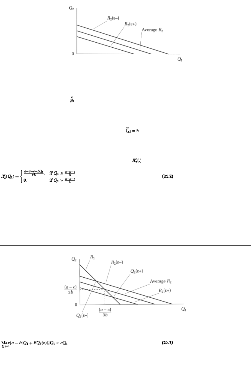
Page 333
FIGURE 22.1
on the cost parameter Î much as we had thought it would; the higher it is, that is, the higher firm 2's costs are,
the less it produces in a best response.
Indeed it is useful to earmark as a baseline the production of the average firm 2 type (whose Î = 0). A
(nonaverage) Î type produces less than the baseline if Î > 0, whereas if it has lower costs than the average,
that is, if Î << 0, then it produces more than the average.
CONCEPT CHECK
SC CASE
Show that in the SC case, with c = 1, if , then the baseline is to produce 2
units, but if Î = -2, then firm 2 should produce 3 units. What is the best
response if Î = 1?
The preceding formula gives us the best response of any type of firm 2 for any quantity that it conjectures
firm 1 might produce. Denote this best response function . We have shown that
Let us graph the best-response functions (Figure 21.1). Note that as the cost parameter Î decreases we move
toward the right to find the corresponding best-response function.
Let us now turn to firm 1, the uninformed firm. It realizes that different types of firm 2 will produce different
amounts. Hence, it conjectures a type-dependent quantity function Q2(Î). Since it does not know what firm
2's actual costs areand hence what quantity level it will producethe uninformed firm necessarily faces
uncertainty in
page_333
Page 334
FIGURE 21.2
profits. The maximization of this firm's expected profit is given by the following exercise:
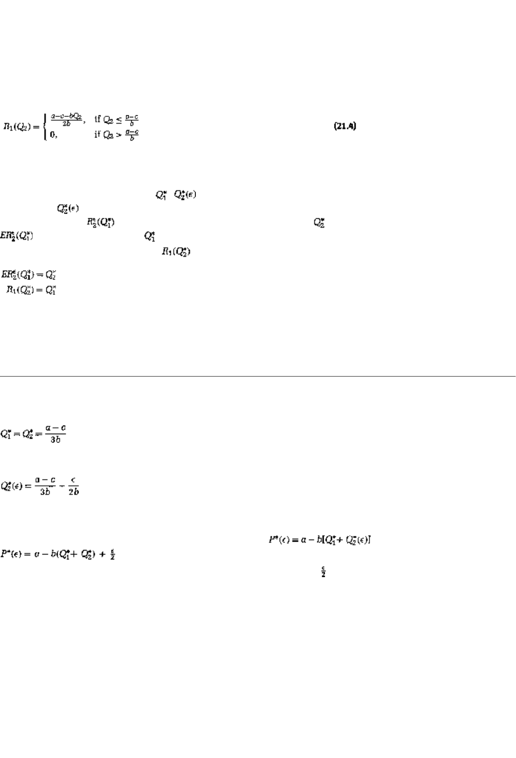
where EQ2(Î) is the expected quantity that firm 2 might produceand the expectation is taken with respect to
the distribution function F over the cost parameter Î. Somewhat more compactly, let us refer to this expected
quantity as simply Q2.
CONCEPT CHECK
BEST RESPONSE FOR FIRM 1
By a reasoning similar to the one for firm 2, show that firm 1's best response
function is
A figure that incorporates the best-response function of firm 1 as well as the family of best-response
functions for firm 2 can now be given, in Figure 21.2.5
At any Bayes-Nash equilibrium, , , the conjectures coincide with the best responses. In other words,
the amount that firm 1 conjectures an Î-type of firm 2 will produce is equal to that types's production,
that is, is equal to in particular, firm l's average conjecture, , equals the average firm 2 production
. Likewise, the amount that the different types conjecture about firm 1's production also turns out
to be correct; that is, it is equal to :
5Be a little careful in reading Figure 21.2. On the vertical axis are plotted both the actual
quantities that the different types of firm 2 produce in best response and the average firm 2
quantity that firm 1 best responds to.
page_334
Page 335
Explicit computation now yields the equilibrium quantities (actual for firm 1, average for firm 2):
It then follows from our earlier discussion that the quantity produced by an Î type is given by
Note that in equilibrium the low-cost producers produce more than the high-cost ones.
6
The distribution of prices can be easily computed. Since we can write
. The first component can be interpreted as an average price; denote it P*. Hence
the actual price is the average price P* plus an adjustment equal to On one hand, whenever firm 2 is a
low-cost producer, it produces more than average and hence drives down the price. On the other hand,
whenever the actual costs are higher than averagethat is, Î is bigger than zerofirm 2 produces less than the
average and therefore the price increases.
What about profits? Again they will depend on firm 2's costs. Intuitively you would expect that firm 1 would
prefer an inefficient rival (who would not drive down the price as much). On the other hand, firm 2's profits
should be negatively related to its costs. After all, a more efficient firm can always produce the same amount
as a less efficient type and generate greater profit. We leave you to formalize these intuitions with a bit of
algebra:
CONCEPT CHECK
EQUILIBRIUM PROFITS
Show that the equilibrium profit functions are

Note that the equilibrium profit for firm 1 is highest when firm 2's costs are highes
t. Similarly, profits are
highest for firm 2s with the least costs, that is, for firms with Î = - X, and they decrease all the way to the
highest costs, that is, to Î = X. Hence a more efficient firm 2 implies lower profits for firm 1 and higher
profits for firm 2.
To have a concrete handle available, you should plug the formulas for quantities, price, and profits into the
illustrative example:
6From this point on we will reserve the notation and for the (average) quantity level .
page_335
Page 336
CONCEPT CHECK
SC CASE
Show that and while Finally, the equilibrium
profit for firm 1 is (highest when firm 2's costs are highest), and the
profit level for firm 2 is given by .
21.2 The Complete Information Solution
In this section we will analyze the complete information Cournot-Nash solution when firm 2's costs are
known to be c + Î. The motivation for studying this issue is the following question: Which type of firm 2 has
the most to gain from its cost information being made public? Answering that question will, in turn, allow us
to look at ways in which such firms can make their information public.
Let us start with the best-response problem of firm 2 (for any conjectured production level of firm 1). A little
thought makes it clear that this is identical to the same problem under incomplete information; that is, it is
precisely the maximization of equation 21.1. After all, firm 2 knows exactly what it knew before, its costs,
and is trying to achieve the same goal, to maximize profits! Hence, firm 2's best response function is given
by equation 21.2.
The difference is that firm 1 now knows the type of firm 2. This fact has two implications. First, firm 1's
conjecture will be about one quantity levelrather than a type-dependent quantity function. Second, and
consequently, its profits are no longer uncertain. The profit maximization problem is therefore
Because this problem is qualitatively similar, you should be able to show the following:
CONCEPT CHECK
BEST RESPONSE OF FIRM 1
Show that the best-response function is
page_336
Page 337
The intersection of the two best-response functions7 gives us the Cournot-Nash equilibrium of this game.
This equilibrium, denoted
, , is easily computed to be
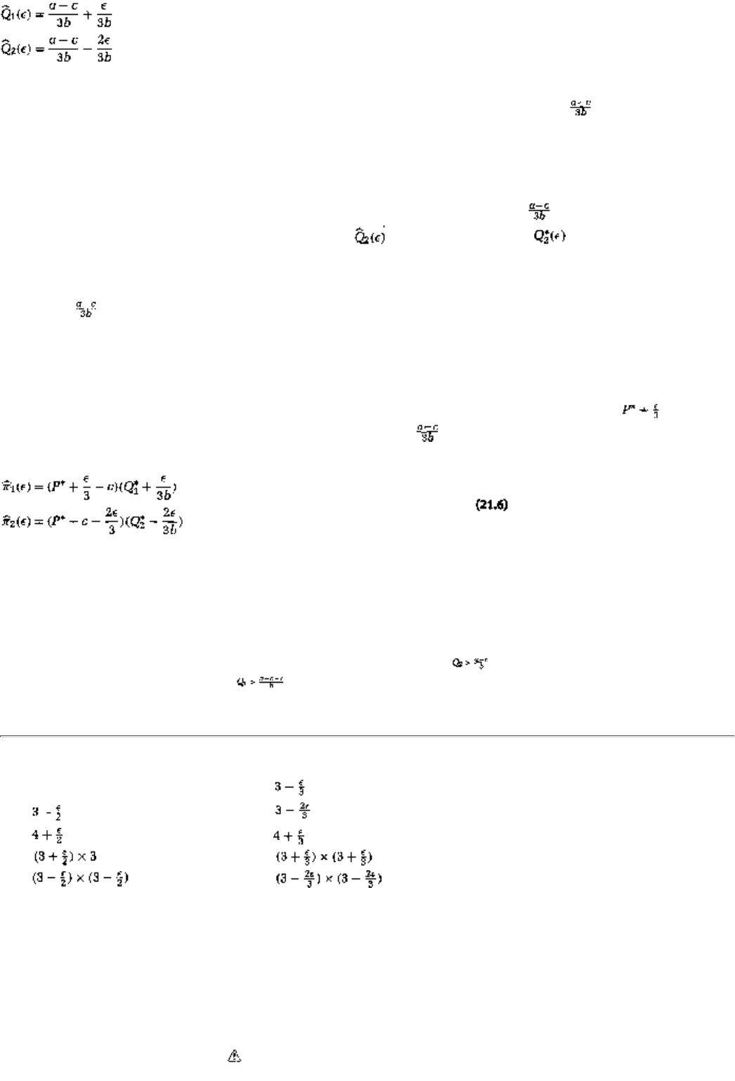
Note two key
differences with the incomplete information solution. First, firm 1 takes firm 2's costs into
account in deciding how much to produce. It lowers output below the baseline level for an efficient rival
and increases output against an inefficient rival. This difference is purely driven by strategic considerations;
after all, firm 1's costs are no different than in the previous section, but the mere fact of knowing that a
low-cost rival will find it profitable to expand production beyond the baseline level induces firm 1 to cut
back its own output (in an attempt to hold up the price).
The second difference is that firm 2 itself adjusts output around the base level more aggressively than in
the incomplete information case. More specifically, is strictly larger than if Î << 0 and strictly
smaller if Î > 0. The reason is straightforward: knowing that firm 1 will hold its output, a low-cost firm 2 will
find it profitable to push past the point where it would have stopped otherwise. Conversely, a high-cost firm
2 will have to withhold more output below the base level because it knows that firm 1 is going to produce
more than
This discussion suggests that all efficient types of firm 2, that is, those with Î << 0, would like to have their
costs publicly revealed, while inefficient types with Î > 0 would like to hide in the crowd of unknowns. Let
us confirm that conjecture by looking at equilibrium profits.
Substituting the equilibrium quantities into the demand function yields the equilibrium price (where P*
is again the price corresponding to the baseline production of by each firm). Consequently, the profits
are given by
A comparison of equations 21.5 and 21.6 confirms the conjecture: a low-cost firm 2 benefits from having its
costs made public because the consequent price is higher and it produces more in equilibrium. Conversely, a
high-cost firm 2 suffers because it sells a smaller quantity at a lower price.
Let us put together these observations for the special case:
7Note that the best response of firm 1 is to produce nothing if . Likewise, the best response of
firm 2 is to produce nothing if
page_337
Page 338
Incomplete Information Complete Information
Q1 3
Q2
P
p
1
p
2
CONCEPT CHECK
COMPARISONS
Verify that in the SC case low-cost firm 2s produce more, sell at a higher price,
andconsequentlymake higher profits in the complete (versus the incomplete)
information solution. Verify also that exactly the opposite is true for high-cost
firm 2s. What can you say about firm 1?
21.3 Revealing Costs To A Rival
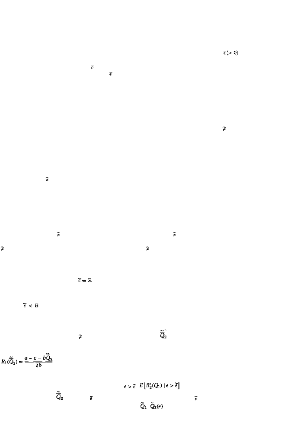
The next question therefore is, Will an efficient firm 2 make the information about i
ts low costs public? This
section will treat the simplest case in which a firm is able to reveal its costs to its rival credibly and costlessly
if it desires to do so.8 The punch line of this section is going to be that in fact every type of firm 2and not
just the more efficient oneswill find it in its best interests to reveal information
about its costs.
The reasoning is as follows: Suppose that only firms with Î << 0 revealed their costs. In that case,
nonrevelation is also informative; it tells firm 1 that it is definitely facing an inefficient rival with a cost
parameter Î > 0. Since firm 1 now presumes that its average rival has a cost, say , this presumption
creates incentives for those rivals who are relatively more efficient than this averagethat is, those who have
a cost parameter between 0 and to reveal that information. However, in that case nonrevelation indicates
that costs must actually be higher than . And so on.
Let us make all of this precise. Suppose that after learning its costs and before producing, firm 2 can reveal
this cost figure to firm 1or it can choose not to do so. Assume that revelation is credible in the sense that firm
2 cannot lie (and it is costless). After revelationor lack thereofthe two firms compete on quantities. Hence a
strategy for firm 2 is a type-dependent choice of whether or not to reveal and how much to produce
thereafter. A strategy for firm 1 is how much to produce depending on what it has learned in the revelation
phase (and it learns even if nothing is revealed). We will restrict attention to strategies in which firm 1
concludes from nonrevelation that firm 2's costs must be higher than some level .9
8For instance, a firm might include cost figures in its annual report (and be able to get an
independent auditor to certify the authenticity of the figures relatively inexpensively).
9Some more sophisticated arguments can be used to show that those are the only kind of beliefs that
''make sense"; that is, it is not sensible for firm 1 to conclude from nonrevelation that costs must be
higher than or lower than Î' or . . .
page_338
Page 339
The post-revelation-phase solution is the complete-information Cournot-Nash equilibrium if costs have been
revealedor the incomplete-information Bayes-Nash equilibrium if they have not. A full equilibrium of the
game is given by an such that firm 2s with costs at or below will reveal those costsand prefer the
corresponding Cournot-Nash profits to the Bayes-Nash profits of a game with costs presumed to lie between
and X. At the same time, firm 2s with costs above will prefer the Bayes-Nash profits to the
Cournot-Nash profits (once they reveal costs).
The result that we will demonstrate is as follows:
Proposition. In equilibrium, . Put differently, every type of firm 2 will reveal its costs.
Sketch of a Proof
Fix any . Consider any firm 2. Equation 21.2 gives us this firm's best-response function (regardless of
whether it made its cost information public).10
If costs have not been revealed, firm 1 picks a best response to the average quantity it expects will be
produced by types between and X; denote this average . From the discussion in section 21.1 the best
response is
In equilibrium, the average quantity produced in best response by firm 2, keeping in mind that the only ones
who do not reveal costs are those firms with , , must equal the average quantity
conjectured, that is, . Writing for the average parameter between and X, and invoking equation 21.2,
all this implies Bayes-Nash equilibrium quantities,
, , equal to
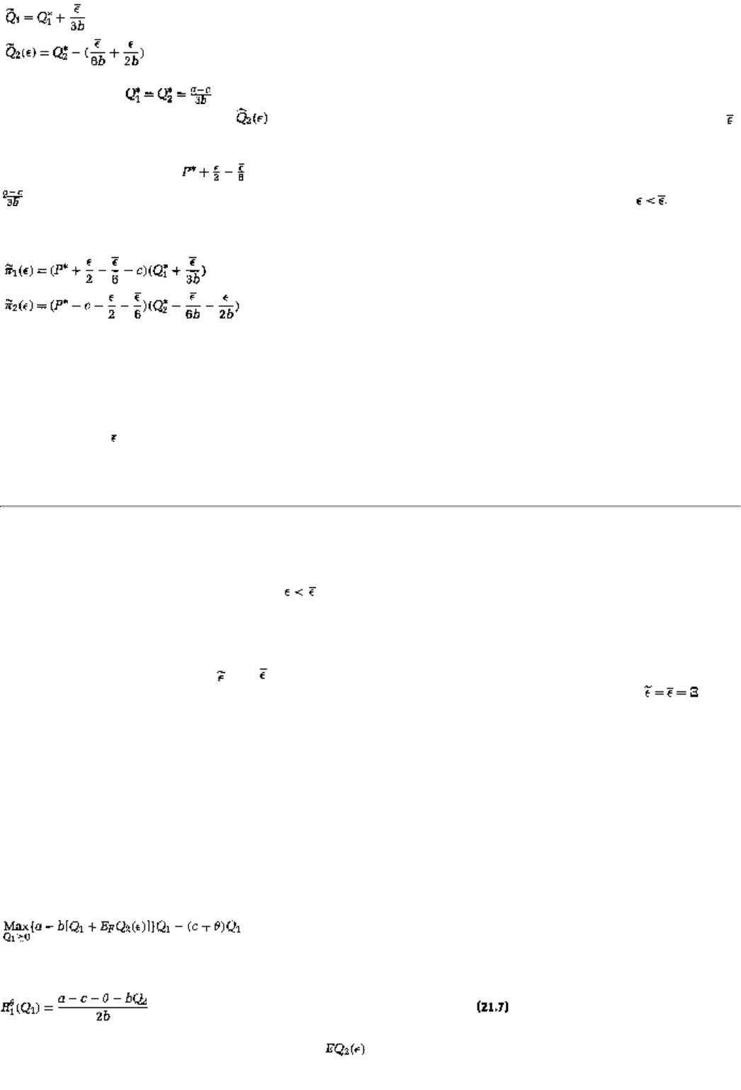
where, as always, the baseline production level. Compare the quantity produced by firm 2 with
the complete information quantity . Notice that all types that are more efficient than the average type
produce a smaller amount in this Bayes-Nash equilibrium.11
The price in equilibrium is (where P*
is again the price corresponding to the baseline production of
by each firm). Again notice that this price is lower than the complete information price if .
The consequent profits are given by
10Again note that whether or not it makes its information public, firm 2 itself has exactly the same
information and seeks to achieve the same goal in either case; hence its best-response function is
identical after revelation and nonrevelation.
11The reasoning is exactly the same as in the previous section. Firm 1 will pretend that it is facing a
firm of type and will choose output accordingly. Those types of firm 2 that are lower cost than this
average will therefore have to withhold some of the output that they would have liked to produce.
page_339
Page 340
CONCEPT CHECK
COMPARISON (AGAIN)
Verify that for a firm with , quantity and price are lower than in the
complete-information Cournot-Nash equilibrium, equation 21.6. Hence it
generates lower profits.
Put differently, all of these firms would prefer to reveal their costs in the first stage. In particular, firms that
have a cost parameter between and prefer to reveal their costs rather than not reveal (as they are
supposed to in this candidate equilibrium). Put still differently, the only possible equilibrium is ; that
is, all types reveal their costs. (Why?)12à
21.4 Two-Sided Incompleteness Of Information
So far we have restricted attention to one-sided incompleteness of information in which only firm 2's costs
are unknown to its rival. The techniques of analysis extend straight-forwardly, however, to the case where
neither firm knows its rival's costs (but does, of course, know its own). Suppose then that firm 1's costs are c
+ q where q is a parameter that is only known to firm 1's owners (or managers). Furthermore, the random
variable q has mean zero.
Each firm makes a conjecture about the type-dependent quantity choice of the other firm. The maximization
of expected profits by firm 1 is given by the following problem:
That expression yields as a best-response function the following:
where Q2 is shorthand for the average quantity .13 Analogous expressions hold for firm 2. Collecting
all of the preceding, we can derive the Bayes-Nash equilibria to be
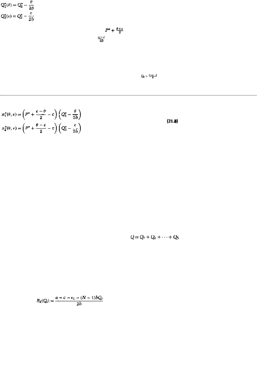
The corresponding price can be found to be , where P* is, of course, the price that corresponds to
each firm producing the baseline amount . Consequently, the profits in equilibrium are
12In Chapter 24 we will examine a class of games called signaling games. At that point you should
return to this section. You will see that what we have just discussed is a signaling game with a
"separating equilibrium" in which each firm truthfully reveals its type.
13As before, the best response is to produce nothing if
page_340
Page 341
To summarize our conclusions, whenever there is incompleteness of information, the firm that has
information acts on its information by adjusting up or down on an average type's behavior (producing more
than the average if costs are low and less than the average if costs are high). The firm that does not have
information behaves as if it is confronted with the average type of its rival.14 Consequently, low-cost firms
lose out when information is incomplete, but inefficient firms do better by hiding in the crowd.
The expressions in equation 21.8 for profits (and the associated price and quantity) are the most general for
this model; the price, quantity, and profits for the complete information model of Chapter 6 follow by setting
q = Î = 0, and the expressions for one-sided incompleteness follow from setting either q = 0 or Î = 0.
21.5 Generalizations And Extensions
21.5.1 Oligopoly
It is straightforward to allow for more than two firms, that is, to consider an oligopolistic market. If there are
N firms producing identical products, the inverse demand function can be written as b
efore as P = a - bQ,
the only difference being that the aggregate quantity is . Suppose that each of these
firms has a marginal cost known only to itself. Let us write the ith firm's marginal cost as c + Îi where Îi is a
random variable with mean zero (and the cost parameter is independently drawn for each firm).15
Reasoning identical to the two-firm case yields the following:
CONCEPT CHECK
BEST RESPONSE
Show that if firm 1 conjectures that each of the other firms will produce an
average amount Qi, then its profit-maximizing quantity is
In a Bayes-Nash equilibrium, the average best response has to be equal to the conjectured average, so it
must be the case that ER1(Qi) = Qi. (Why?) That equation yields the following:
14This last statement is a special property of the Cournot model. In general games, the uninformed
player reacts to the entire list of type-dependent choices of its rival and not just to the average.
15Put differently, knowing its own cost does not give firm i a sharper prediction about firm j's costs
(than not knowing its own cost). This is a reasonable assumption if the sources for cost variability are
different for different firms. The case where firm j's costs are related to firm j's costs can be analyzed
in a similar way; the formulas will look a little different.
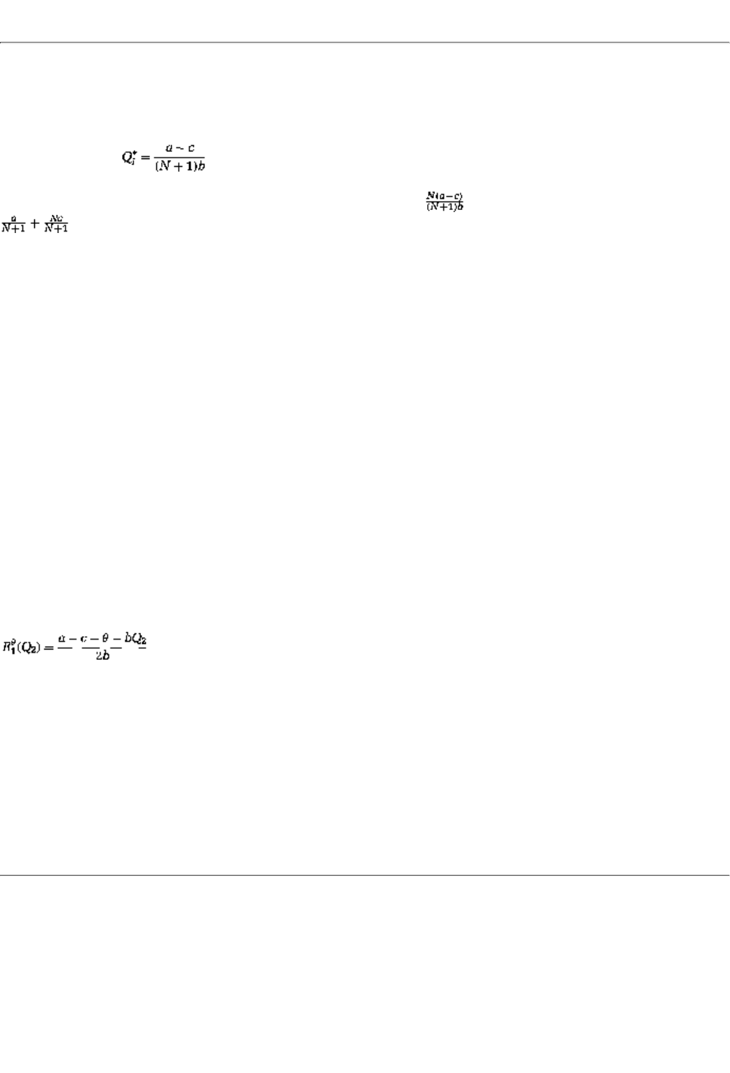
page_341
Page 342
CONCEPT CHECK
BAYES-NASH EQUILIBRIUM
Show that the average quantity in an oligopolistic market is16
Total quantity produced in the market, on average, is therefore and hence the average price is
. As the number of firms becomes very large, that is, as N approaches infinity, the average price
approaches the (marginal) cost c. In other words, an oligopoly with many firms looks, on average, a lot like a
perfectly competitive industry (in which competition drives price down to marginal cost).
We could further work out the complete information solution under oligopoly by following the same
reasoning as in a duopoly. Again it is the case that low-cost firms stand to gain from having information
about their costs revealed, whereas high-cost firms lose.
21.5.2 Demand Uncertainty
So far we have only discussed uncertainty about costs. The other likely source of uncertainty in this market
is demand, and a very similar analysis can be carried out for that case.
Suppose that the actual inverse demand function is P = (a - q - Î) - b(Q1 + Q2), where q and Î are random
variables (with, need we say, mean zero). The value of q is known to firm 1 but not to firm 2 (and vice versa
for Î).17 A strategy for firm 1 is a type(or q-) dependent quantity choice, Q1(q). Likewise a strategy for firm
2 is a list of choices Q2(q), a choice for every E. Each firm maximizes expected profits given a conjecture
about the other firm's strategy choice.
Arguments identical to the preceding will yield the following:
CONCEPT CHECK
UNKNOWN DEMAND
Show that the best-response function for firm 1 is
and an identical best-response function for firm 2 (and Q2 is the conjectured average production of firm 2).
Note that this is exactly the same as the reaction function, given by equation 21.7,
when there is cost
uncertainty. Put differently, from firm 1's point of view, knowing that
16In the preceding analysis, we have restricted ourselves to symmetric Bayes-Nash equilibria.
17You could imagine that both firms do market research that gives them some idea about demand. If
only they were able to pool their survey findings, they would learn the real state of demand.
page_342
Page 343
its costs are q away from the norm c induces exactly the same behavior as knowing that market demand is q
away from its norm of a. This relationship is intuitive; in either case every extra unit of production changes
profits per unit of production by q; for cost uncertainty, marginal costs change by q dollars, and for demand
uncertainty, marginal revenues change by the same q dollars. Hence, the equilibrium quantities, and profits
are exactly the same as in section 21.4.
Summary
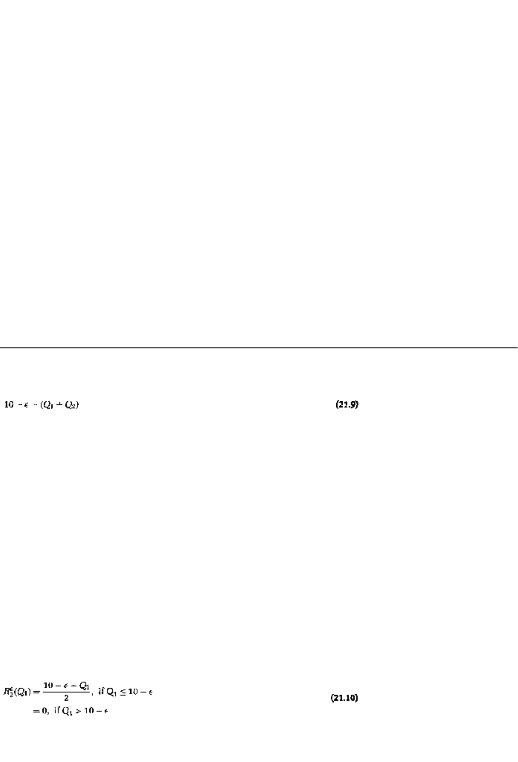
1. In real-world oligopolistic markets there is likely to be a lot of incompleteness
of information, a firm is
unlikely to know its rivals' costs, aspects of market demand, and so on.
2. In a Cournot duopoly with one-sided incompleteness, the informed firm chooses quantity based on its
actual costs, while the uninformed firm chooses it on the basis of its conjecture about the cost of the average
informed firm.
3. In a Bayes-Nash equilibrium, profits of firm 2 decrease with the level of its marginal costthe lower the
cost, the higher the equilibrium profit. Profits of firm 1 increase with firm 2's cost.
4. If firm 2's costs were made public, then the resultant Cournot-Nash equilibrium would be more profitable
than the Bayes-Nash equilibrium for firm 2s with costs lower than the averageand vice versa for those firms
with costs higher than the average.
5. Hence, lower cost firm 2s have an incentive to make that information public. That leads to a result that
actually all types of firm 2s make their cost information public.
6. With two-sided incompleteness, the analysis and conclusions are very similar to the one-sided case.
Similarly the analysis can be extended to oligopolies, and to demand uncertainty.
Exercises
Section 21.1
21.1
Give two examples of markets in which firms compete over quantities and two where they compete over
prices.
page_343
Page 344
Suppose that market demand in a duopoly is subject to uncertainty so that the actual demand is
where Î is a random variable.
21.2
Give an interpretation of Î; that is, discuss possible sources of demand uncertainty. Which ones can lead to
one-sided incompleteness of information (with firm 2 aware of the value of Î, but not firm 1)? Explain.
Suppose that there is one-sided incompleteness, Î is a random variable with mean zero, costs of production
are zero, and the firms are Cournot competitors.
21.3
Write down the expected profit function of the uninformed firm (firm 1) as well as the profit functions of the
different types of the informed firm (firm 2).
21.4
Formulate and solve the best-response problem for a firm 2 that knows the demand parameter e to be 2.
21.5
In general show that the best response is given by
21.6

Give an interpretation for why the best-response production level is decreasing in
Î
and in the other firm's
(conjectured) quantity.
21.7
Derive the general form of the best-response function for firm 1 if the conjectured average production by
firm 2 is Q2.
21.8
Solve for the Bayes-Nash equilibrium quantities of this model. Determine the distribution of prices and
profits in equilibrium. Interpret the effect of Î on each of these objects, quantities, prices, and profits.
21.9
Comment on any similarities that you may have uncovered between this analysis of demand uncertainty and
the analysis in the text of cost uncertainty. Explain your answer.
page_344
Page 345
Section 21.2
Let us turn to complete information; that is, for the next few questions assume that Î is known to both firms.
21.10
Formulate the best-response problem for firm 2 when it knows the value of Î to be 1. Find the best response.
21.11
Repeat exerise 21.10 for firm 1.
21.12
What is the general form of the best-response function for firm 2 for any value of Î? What about firm 1?
Explain your answers.
21.13
What is the Cournot-Nash equilibrium of this complete information game? Compute quantities, price, and
profits.
21.14
How do the complete-information quantities and profits compare with those in the incomplete-information
Bayes-Nash equilibrium? (Compare these objects at a fixed value for Î.)
Section 21.3
Let us revert to one-sided incompleteness, but now suppose that the informed firm could make its
information public to the uninformed firm.
21.15
Based on your answers to the previous exercises, can you tell which types of firm 2 would like to have their
information revealed?
21.16
If firm 2 had the option to reveal its information before quantities were chosen, conduct an analysis similar
to that in the text to determine what information would be revealed in the equilibrium of this game.
21.17
How does your answer compare with that obtained in the text for the cost uncertainty case? Provide
intuition for any differences that you may notice.
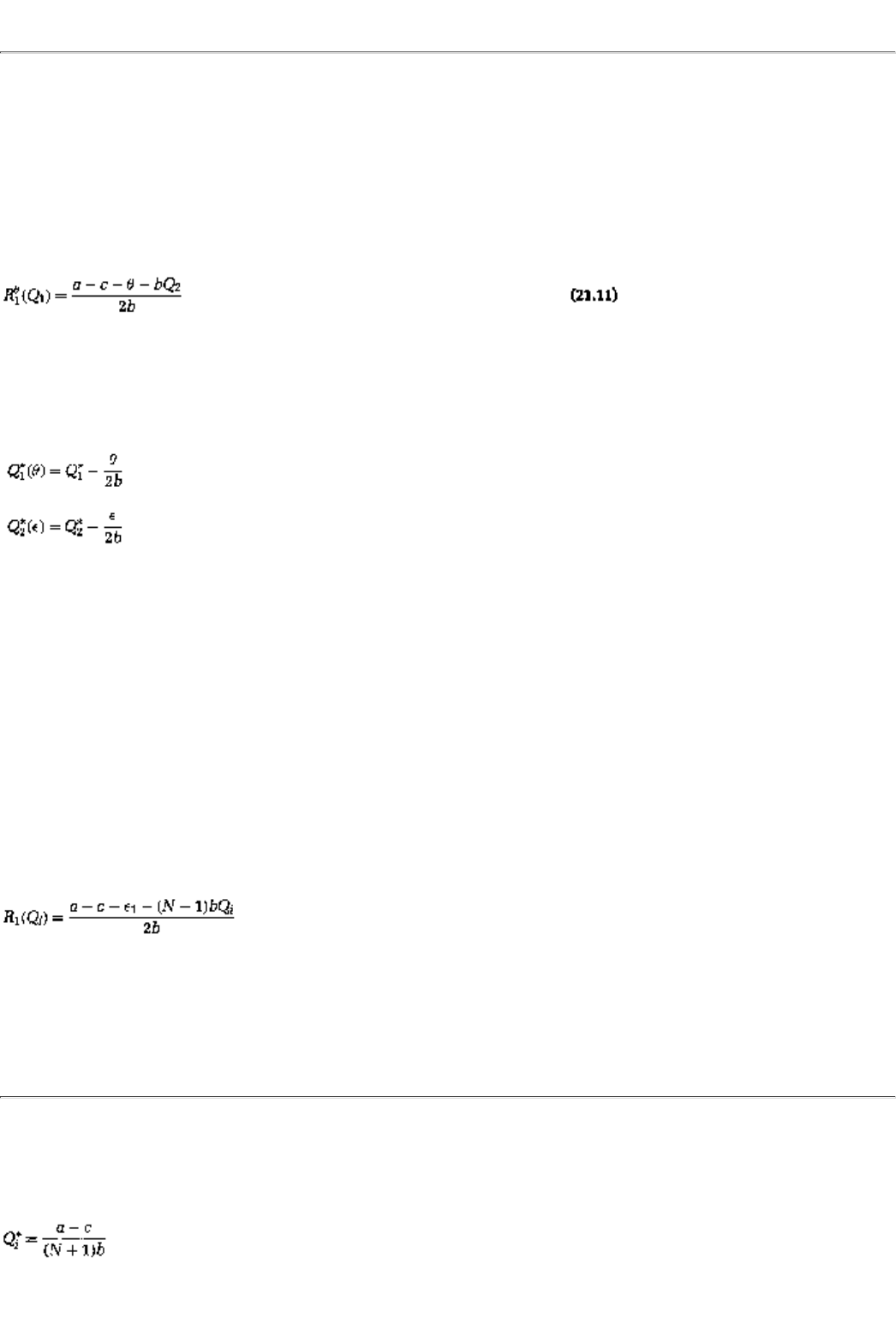
page_345
Page 346
Section 21.4
Let us now proceed to cost uncertainty. Consider the two-sided incompleteness case in which firm l's cost
parameter is q and firm 2's is Î, and both random variables have mean zero.
21.18
Verify in detail that the best-response function of firm 1 is given by
where Q2 is shorthand for the average quantity EQ2(Î).
21.19
Verify in detail again that the Bayes-Nash equilibrium of this game is
21.20
Consider instead the complete information version of this problem in which q and Î are known. Find the
Cournot-Nash equilibrium. Compute quantities, prices, and profits as functions of the parameters q and Î.
21.21
How does the complete information solution compare with the Bayes-Nash equilibrium? Which firms have
higher profits in the former case? Provide an interpretation for your results.
Section 21.5
21.22
Show that if firm 1 conjectures that each of the other firms is going to produce an average amount Qi, then
the profit-maximizing quantity that firm 1 should produce is
21.23
Argue in details that in a Bayes-Nash equilibrium, the average best response has to be equal to the
conjectured average, so it must be the case that ER1(Qi) = Qi.
page_346
Page 347
21.24
Prove consequently that the following is the average quantity in a Bayes-Nash equilibrium
page_347

Page 349
Chapter 22
Mechanism Design, the Revelation Principle, and Sales to an Unknown Buyer
This chapter and the next will study an entirely new topic called mechanism design (and its applications).
We will informally motivate the topic by providing economic contexts in section 22.1. In section 22.2 we
will study an example with a single player with an unknown valuation for the good being sold. Section 22.3
will discuss the general framework of mechanism design and state a fundamental result called the revelation
principle
. Finally, in section 22.4, we will discuss a more extended version of the example studied two
sections earlier.
22.1 Mechanism Design: the Economic Context
So far in this text we have taken the game played to be a given (and simply tried to infer what the players in
the given game might do). Mechanism design goes back a step and asks, What would happen if the rules of a
game (or ''mechanism") are "designed" so as to achieve some desirable objective? In doing the mechanism
design, of course, one has to bear in mind that the players who will eventually play the game will act in their
self-interest (and find their way to an equilibrium). Yet some gamesor mechanismsmay have more desirable
equilibria than others; the point of mechanism design is therefore to find the game that has the "best"
equilibrium.1
What is taken as given in a typical mechanism-design problem is the group of players. What the mechanism
designer is free to choose is the game; she can specify what choices are available to the players and what the
consequences of their actions are. There are two constraints on the designer. First, there cannot be any
coercion; she cannot design a mechanism that the players will refuse to play. Second, she has to have
reasonable expectations; she can only expect that players will play an equilibrium within the game that she
designs. The designer herself is typically an economic agent whose
1All terms in quotation marks will be defined more precisely later on in this chapter.
page_349
Page 350
fortunes are tied to the actions of the players; an optimal design is a mechanism whose equilibrium has the
best outcome from the designer's point of view.2
To make all this more transparent, let us discuss some examples and applications of mechanism design.
Example 1: The Commons Problem
Consider the following two mechanisms or games involving the commons.
Game 1: The governmentthe mechanism designer in this caseauctions off the rights to the common resource
to the highest bidder every year. The bids are made after the government decides how much the winning
bidder will be allowed to extract that year.
Game 2: The government auctions off the rights to extract from the common once and for all. The winning
bidder is then allowed to extract over time in any manner that he prefers.
The second mechanism is typically called privatization! The first mechanism is akin to restricted
privatization, with periodically reviewed limits on the amount of extraction. In a similar fashion you can
probably think of some other mechanisms. For example, yet another one is not to control the potential
extraction amount but to impose a tax on the actual extraction. Each one of these mechanisms will have a
different equilibrium extraction pattern and government revenues, and the optimal one is that combination
most preferred by the government.
Example 2: Selling the da Vinci Diaries (Selling to a Single Buyer with Unknown Valuation)

Suppose that Sotheby's Parke-Bernet Galleries has been entrusted with the sale of the
diaries of Leonardo da
Vinci and its most promising buyer is Bill Gates, the chairman of Microsoft. Sotheby's would like to get the
highest price for the diaries, but the problem is that it does not know how much they are worth to Mr.
Gatesand therefore how much he is willing to pay to have them. For the purposes of simplicity let us imagine
that Gates may either be a real aficionado, or he may be a less passionate fan (who derives a lower level of
utility from possessing the diaries).
Here are two different ways that Sotheby's might proceed:
Game 1: Post a really high price that will only be acceptable to an aficionado (and risk losing a less
passionate fan in order to make a very profitable sale).
Game 2: Post two prices. A buyer willing to pay the higher price is told that he will get the diaries for sure,
while a buyer only willing to pay the lower price is told that there is some chance that the sellers (on whose
behalf Sotheby's acts) may withdraw the diaries.
2In a sense, mechanism design is therefore a marriage of the principal-agent framework of
Chapter I9 and the concept of Bayes-Nash equilibrium that was discussed in Chapter 20. The
mechanism designer is the principal, the players are the agents, and the equilibrium concept is
Bayes-Nash.
page_350
Page 351
There may be yet other mechanisms even better than these two; an optimal mechanism (for Sotheby's and
the sellers) is the one for which the expected sale price is the highest.
Example 3: Auctions (Selling to One of Many Buyers with Unknown Valuations)
Suppose instead that Sotheby's puts the da Vinci diaries up for auction, thereby making them available to any
bidder (who registers ahead of time with Sotheby'srecall the discussion of Chapter 3) and let us suppose that
the diaries will be granted to the highest bidder. Since now there are multiple bidders, it is even more likely
that Sotheby's does not know the exact valuation that each of the bidders attaches to the diaries.
What Sotheby's would ideally like to do is identify which of the bidders has the highest valuation and then
sell the diaries to him (at the valuation). But therein lies the rub. A bidder with a high valuation has no
reason to let Sotheby's know that fact for fear of having to pay a high price. How should Sotheby's conduct
the auction so as to extract the highest expected price? Can Sotheby's get the bidder with the highest
valuation to acknowledge that fact if it promises not to charge him a price as high as his valuation?
There are many different ways in which Sotheby's can proceed. Here are two:
Game 1: The highest bidder gets the diaries and pays the amount of his bid ("first-price auction").
Game 2: The highest bidder gets the diaries but only has to pay the amount of the next highest bid
("second-price auction")
22.2 A Simple Example: Selling to a Buyer With an Unknown Valuation
We will now analyze example 2 in some detail. Suppose that, as an aficionado, Mr. Gates receives utility q
from having the diaries but as a mere fan he only gets utility equal to m (and q > m > 0). In particular, an
aficionado who pays a price p gets a net utilityor surplusequal to q - p from the transaction (while a fan gets
a surplus equal to m - p). Suppose further that while Bill Gates knows whether or not he is an aficionado,
Sotheby's does not; it attaches a probability r to that possibility.
To answer the question, "How should Sotheby's sell to Bill Gates," we will first step outside the current setup
and imagine that Sotheby's somehow finds out what Mr. Gates' real passion is. Then we will revert to the
current (incomplete information) setup in which Sotheby's does not know.
22.2.1 Known Passion
A buyer with valuation q is willing to pay up to q for the diaries. Similarly, a mere fan is willing to pay up to
m. Given that information, Sotheby's price policy is clear: it sets two
page_351
Page 352
prices, q and m On one hand, if Mr. Gates is known to be an aficionado, then Sotheby's makes a take-it-
or-leave-it offer to sell the diaries to him at a price equal to q. On the other hand, if he is known to be a mere
fan, then they make a take-it-or-leave-it offer at price m. In each case, the buyer is indifferent between
taking the offer and rejecting it. (Or Sotheby's could sweeten the deal by making the offer a dollaror a
hundred thousand dollarsbelow q and m, respectively, thereby making Bill Gates strictly prefer the deal to
passing up on it.)3
Before it is known whether Mr. Gates is an aficionado or not, Sotheby's anticipates an expected sale price
equal to rq + (1- r)m. A special case that we will return to periodically is this:
Special Numbers Case (SN). q = $40 million, m = $10 million, and .
Hence the expected sale priceor expected revenuefor Sotheby's is $25 million. (And Bill Gates' expected
surplus is zero.) This is the benchmark against which Sotheby's success will be measured in the real model in
which Sotheby's does not know the true passion of its buyer.
Let us turn now to that model.
22.2.2 Unknown Passion
Option 1: Ask the buyerand then charge a price based on the buyer's report; say p(q) if the buyer says he is
an aficionado and p(m) otherwise.
As long as p(q) > p(m), no buyer will ever own up to being an aficionado. Hence, all transactions will be
made at the price p(m). However, if p(q) = p(m), then a buyer will truthfully report his valuation, but again
all transactions are made at a flat fee (which applies to buyers of both passions). So this option is equivalent
to the following:
Option 2: Set a fiat price p (that either kind of buyer has to pay).
For either of these two options, the highest flat price that Sotheby's can charge is m, the mere fan's
valuation.4 At that price, buyers of both passions will buy and the aficionado will retain part of his utility, (q
- m), from possessing the da Vinci diaries. In the SN case, either of these options nets Sotheby's $10 million
dollars and the aficionado a surplus of $30 million.
The question is, Can Sotheby's do any better than a flat price offer? Note that the best flat price that attracts
both kinds of buyers is equal to m. If Sotheby's is going to get the aficionado to pay a price higher than m, it
can only do so by making the lower price alternative a little less attractive; one way of doing so is to make
the purchase at that price not a sure thing:
3For the da Vinci diaries we are talking about a price of $30 millionand so a hundred thousand is
mere change!
4We are making an implicit assumption that the low-valuation buyer must be offered a price that he
will find acceptable, Otherwise, if a fan anticipates a price offer in excess of m, he will not bother
dealing with Sotheby's. This is called the individual-rationality assumption; we will make it explicit and
discuss it in detail shortly.
page_352
Page 353
Option 3: Guarantee purchase at a higher price. A buyer can guarantee purchase at a higher price of, say,
. At the lower price of m there is a 50 percent probability that Sotheby's will withdraw the diaries from sale.5
Note that an aficionado gets a surplus of
from picking the guaranteed higher price purchase. If he chooses
the uncertain lower price alternative, then there is a 50 percent chance that his surplus will be q - m but an
equal likelihood that it will be 0; hence the expected surplus is . The aficionado clearly prefers the
guarantee.
CONCEPT CHECK
MERE FAN'S CHOICE
Show that a mere fan gets 0 surplus from the lower price option and
from the guaranteed higher price. As long as , the mere fan prefers the
uncertain alternative.
With probability r Sotheby's will sell (to the aficionado) at a price equal to ; with probability they will
sell (to the mere fan) at a price equal to m; (and with remaining probability they will not make a sale.
Hence their expected sales revenues are , and this is greater than m (the revenue from the flat
fee) provided .
CONCEPT CHECK
SN CASE
Show that the expected sales revenues are $12.5 million. How does this
amount compare with the flat fee?
In turn, the guaranteed fee that we have used as illustration is a special case of a more general class of
guaranteed fees:
Option 4: Guarantee sale at a higher price and offer a probabilistic sale at a lower price. At a price p a
buyer can have the diaries for sure, but at a price q (<< p) there is a probability 1 - Q that Sotheby's will take
the diaries off the market.6
An aficionado will prefer the sure sale if
that is, if . Conversely, a fan will prefer the uncertain lower priced sale if
5This pricing scheme is actually used in practice. In New York City there are telephone reservation
systems for cinema tickets that will guarantee you a ticket at a $2 premium over the standard sale
price. By not reserving early you run the risk that, by the time you show up at the theater, the film
will have sold out. Ticketing agencies for plays, musicals, and concerts also work on this principle.
6In option 3 we looked at the special case in which , q = m, and .
page_353
Page 354
that is, if . Collecting all this together, the aficionado will prefer the sure sale and the fan will prefer
uncertainty if
Equation 22.1 is called the incentive-compatibility constraint; it is in each buyer's interests to pick the price
intended for him. Note that if Sotheby's sets the price pthat which is intended for the aficionadotoo close to
his valuation q, it would simply encourage him to take a chance on the lower priced offer. It will also not do
to set the probability 1 - Q, the uncertainty intended for the mere fan, too low because again the aficionado
might then be encouraged to take a chance on the lower price.
There is one more constraint on Sotheby's behavior: there cannot be any coercion; that is, the prices cannot
be any higher than the corresponding utilities to the buyers:7
The no-coercion constraint is also called the
individual-rationality constraint
. Sotheby's
expected sales
revenues from this mechanism are equal to
as long as equation 22.1 holds. (Why?) The full problem can now be stated: Find p, q, and Q so as to
maximize the expected sales revenues subject to the individual-rationality and the incentive-compatibility
constraints.
The incentive-compatibility constraint for the aficionado, implies that the sure price p must be less
than q. (Why?) Hence the individual-rationality constraint for this buyer will be automatically met. As a
consequence, the incentive-compatibility constraint must be met with no room to spare, that is, . The
reason is that if , Sotheby's can raise the price p, continue to satisfy all the constraints, and make
more money.
An immediate consequence of the preceding argument is that the incentive-compatibility constraint for the
mere fan must have room to spare, that is, that . (Why?) Finally, that conclusion in turn implies that
m = q; again, if m > q, the price q can be raised without violating the incentive-compatibility constraints
(why?) and Sotheby's would make more money.
Collecting all these conclusions together we have,
After substitution that implies
7A price higher than a buyer's utility is a wasted price because the buyer will surely refuse that
offer.
page_354
Page 355
This expression implies, by substituting into equation 22.3, that Sotheby's expected revenues are
Since all the constraints are satisfied, what remains is to choose the probability of sale Q to maximize the
expected revenues (given by equation 22.4). There are two cases to consider:
Case 1: m << rq. Only sell to the aficionado
The optimal choice in this case is Q = 0; that is, Sotheby's refuses to sell to the mere fan (and p = q). So
Sotheby's passes up on sales to low-valuation buyers just so as to extract all of the surplus from the
aficionado.
Case 2: m > rq. Maximize sales
The optimal choice in this case is Q = 1, and hence p = m. So in this case the best Sotheby's can do is in fact
to use a flat fee system, sell to both kinds of buyers, and give up part of the aficionado's surplus.
CONCEPT CHECK
SN CASE
Check that the optimal scheme is to restrict participation to the aficionado.
What is Sotheby's expected revenue?
There is an alternative way in which this guaranteed sale mechanism can be specified. Paradoxically, this
way will look a little bit like the very first option we examined (and rejected as being not sensible!).
Option 5:
Tell me who you are
. Mr. Gates is asked by Sotheby's how strongly he feels about the diaries. If he
says q, he is guaranteed a sale at price p. If he says m, he can, with probability Q, have the diaries at price q.
Clearly this last option produces exactly the same effect as the previous two options. It gives an aficionado
the incentive to own up to being one and convinces a fan that he too should reveal himself truthfully. Since it
involves the buyer revealing his true passion, this mechanism is called a direct-revelation mechanism.8.
8It is called direct because it involves a buyer reporting his passion directly, rather than having it
inferred from something else that he might do.
page_355
Page 356
22.3 Mechanism Design and the Revelation Principle
The procedure used in the previous section is more general than the example might suggest, and so is the
result. In this section we will outline the general procedure and present a fundamental result called the
revelation principle.
22.3.1 Single Player
Suppose we have a single player who can be one of two types, q and m. As in Chapters 20 and 21, we can
think of a player's type as a characteristic that affects his payoff; for the same action, a type q player will
typically get a different payoff than a type m player. In the da Vinci diaries problem, a type is the maximum
amount a buyer is willing to pay. In the Cournot model of Chapter 21, a type is a description of a firm's
costs.
Mechanism
A game, or set of rules, that specifies the strategies a player can choose from,
and the outcome for every choice.
A mechanism is a game (or a set of rules) that specifies the strategies that the player can choose from and
the outcome for every choice. Denote a representative strategy, as always, by s, and the outcome by t. What
is a given is the payoff function (and that depends on the strategy chosen, the outcome, and the type);
denote the payoff of a type q player, p(s, t, q) (and similarly for a type m player). Put differently, the player
types q and m, as well as the payoff function p, are outside the designer's control, but the specification of
available (s,t) pairs is not.
For instance in the guaranteed sale mechanism of option 3, the strategies made available to a buyer are
"accept the high-priced sure offer" or "accept the lower priced uncertain offer." If the former strategy is
chosen, then the outcome is that the buyer pays and gets the diaries. If the latter is chosen, then the
outcome is that the buyer has a 50 percent chance of getting the diaries at a price m and a 50% chance of
coming up empty-handed.9 The payoff is the type-dependent value of the diaries minus the price.
Within any mechanism, consider a possible assignment s*, t* for the type q player and s', t' for the type m
player. This assignment is said to be incentive compatible if each type prefers its own assignment to any
other strategy (and its consequent outcome), that is, if
(and, in particular, the q type prefers s*, t* to s', t' while the m type prefers the reverse). No player can be
coerced into playing a mechanism. This constraint is captured by the idea that there is always an outside
option, with payoff denoted p0, and each player type has to be offered an assignment that guarantees that
payoff:
9Note that in this mechanism the outcomes are random. Whenever that is the case we will interpret
the payoff p(s, t, q) as an expected payoff.
page_356
Page 357
These last two inequalities are called individual-rationality constraints because no rational player would
willingly participate in a mechanism that yields a payoff worse than his outside option.
The mechanism-design problem is for the designeralso known as the principalto find a mechanism and an
associated incentive-compatible, individually rational assignment that gives her the highest payoff. The
principal's payoff typically depends on the strategy chosen by the player and its outcome.
Direct-revelation mechanism
A direct-revelation mechanism is one in which the strategy set of the player is
simply a report about his type. Every report leads to an assignment.
In general there are many mechanisms available to the principal, and some of them can be quite complex. It
turns out, however, that we can restrict attention to a simple class of mechanisms called direct-revelation
mechanisms. These are mechanisms in which the strategy set of a player is simply a report of his type.
Each type of player is free to lie about his real type. A q type can claim that he is really really a m type, and
a m type can always pretend to be a q type. Suppose, however, that the direct-revelation mechanism is one
in which a report of q leads to an assignment equal to (s*, t*) while a report of m leads to (s', t'). In that case,
the incentive-compatibility constraints, equation 22.5, imply that each type will tell the truth. The individual
rationality constraints, equation 22.6, imply that each type will agree to play this mechanism. In short, this
direct-revelation mechanism [with assignments (s*, t*) and (s', t')] will induce truth telling and voluntary
participation by the player with unknown type.
Hence we have shown that direct-revelation mechanismsand truth-inducing assignmentssuffice:
Proposition 1 (Revelation Principle I). For any mechanism and an incentive-compatible, individually rational
assignment, there is a direct-revelation mechanism in which truth telling is incentive compatible, individually
rational, and which produces an identical assignment. Hence a principal can restrict attention to direct-
revelation mechanisms and truth-telling assignments within those mechanisms.
22.3.2 Many Players
Suppose instead that there are many players. Since the argument is the same whether the number is two or
20, we will only discuss the two-player case. Player 1 can be one of two types, q or m, and so can player 2.
There is a common prior probability that type q has a likelihood equal to r.
Consider any mechanism with assignment and for the two types of player 1 and assignment
and for the two types of player 2. Each player derives a payoff from both his assignment and
that of the other player. As in the single-player case, the payoff function is integral to a player but not the
available strategies and their outcomes.
Let denote the expected payoff of player i, i = 1 or 2. For instance, when i = 1,
page_357
Page 358
since there is a probability r that player 1 will be confronted with a type q player 2, who is expected to play
and a probability 1 - r that he will play a type m player, who is expected to play In a similar
fashion we can define the expected payoff of a type of player 1 who plans on playing himself; call this
. Analogous concepts can be defined also for player 2 of either type. Within the mechanism, a
player is free to choose whatever strategies he wants; Ep1(s, t, m) will denote the expected payoff of a type
m player 1, for instance, who picks some arbitrary strategy s with an associated outcome t.
These assignments form a Bayes-Nash equilibrium if they are best responses for each type of each player,
that is, for i = 1, 2:
Now consider the following direct-revelation mechanism in which each player directly
reports his type. If
the reports are both q, then each player gets the star (*) assignment; that is, player i gets . Similarly, if
the reports are both m, then each player gets the prime (') assignment. If player 1 reports q while player 2
reports m, then player 1 gets the star assignment while player 2 gets the prime assignment and
vice versa if player 2 reports q while 1 reports m.
It is not difficult to see that in this direct-revelation mechanism, truth telling is a Bayes-Nash equilibrium.
After all, an implication of equation 22.7 is that a type q player prefers the star assignment to the prime and
a m player prefers the converse. This analysis leads to the following version of the revelation principle for
many-player games:
Proposition 2 (Revelation Principle II). For any mechanism and any Bayes-Nash equilibrium of that
mechanism, there is a direct-revelation mechanism with truth telling as a Bayes-Nash equilibrium that has an
identical assignment. Hence a principal can restrict attention to direct-revelation mechanisms and truth-
telling equilibria within those mechanisms.
We are going to illustrate this many-player version of the revelation principle when we turn to auctions in
the next chapter.
22.4 A more General Example: Selling Variable Amounts
We will now analyze a more general version of the example studied in section 22.2. The setting will be more
general in that the seller can sell any positive quantity of the good to the potential buyer, and higher
production levels are costlier for the seller. Suppose that a quantity Q produces utility equal to qU(Q) for the
8 type buyer but only mU(Q) for the
page_358
Page 359
m type buyer, q > m. If the q buyer has to pay b(Q) dollars, his net surplus is qU(Q) - b(Q) (and similarly for
the m type).
To keep the exposition simple we will assume that costs of production are 2Q, q = 2, and m = 1; the utility
function U is equal to 10Q - Q2; and the outside option has zero utility.
22.4.1 Known Type
If the seller can uncover the type of the buyer, then she should charge an amount equal to the buyer's utility.
For instance, a q type should be charged 2(10Q - Q2) for quantity Q. The only decision then for the seller is
how much to sell. That is solved from the following problem:
Setting marginal profit equal to zero implies 18 - 4Q = 0; in other words, 4.5 units should be sold to the q
type buyer and he should be charged 2[(10 × 4.5) - 4.52], that is, $49.50.
Similar arguments apply to the m type buyer:
CONCEPT CHECK
THE m TYPE
Show that the type m buyer should be sold 4 units and charged $24 dollars.
These transactions will be the benchmark against which we will judge the seller's per
formance when she
does not know the buyer's type.
22.4.2 Unknown Type
By virtue of the revelation principle we know that we can restrict ourselves to direct-revelation mechanisms
in which the buyer is asked to report his type. If he reports himself to be a q type, he gets a quantity equal to
Q and has to pay M dollars, but if he says that he is a m type, he is asked to pay m dollars for q units of the
good. The seller gets to choose the two quantities Q and q and the two payments M and m.10 The question
of interest is, What choice would yield the seller the highest expected profits?
Note first that if the two quantities are the same, that is, if
Q = q, then the two payments have to be the same
as well. Otherwise, both types of buyers will report themselves as the type that has the lower payment. For
example, if the quantity 4 units is offered for both reports, then the equal payment must be 24 dollars (given
individual-rationality considerations for the m type buyer). Since the cost of production is 8 dollars, the seller
will net a 16-dollar profit from this option. Can she do better?
10In principle we can also allow for random outcomes. Based on his report, the buyer gets a
distribution over price-payment pairs. In this problem we can restrict attention to nonrandom
outcomes without any loss of generally.
page_359
Page 360
A second option is to sell only to the aficionado. For example, sell 4.5 units to the q reporter and nothing to a
buyer who says his type is m, and charge the former $49.50.
CONCEPT CHECK
SELLING ONLY TO THE AFICIONADO
Show that the preceding scheme will induce each type of buyer to report his
type truthfully and will net the seller an expected profit of r × 40.5 dollars.
Is there a middle option that does even better than the two extremes? To answer the question let us now be a
little more precise. The incentive-compatibility constraints
are
The individual rationality constraints are
The seller's expected profits are
It is clear that the seller would like to make the two payments M and m as high as possible without violating
either the incentive-compatibility or the individual-rationality constraint. In turn, we can conclude that in an
optimal solution at least one of the two constraints in equation 22.9 has to hold with an equality. Otherwise,
the seller can increase both M and m by appropriate equal amounts (thereby leaving the incentive constraints
of equation 22.8 unchanged), continue to satisfy the individual rationality constraints, and increase revenues.
In fact, it is the m type's utility that must be exactly equal to zero, that is,
This relation holds because the
q
type can always report himself to be a
m
type and thereby get a utility
equal to 2(10q - q2) - m, and of course this is greater than (10q - q2) - m. Put differently, the utility to the
truthful report, 2(10Q - Q2) - M, must be even larger, and hence greater than zero.
It can be shown, however, that the incentive-compatibility constraint must exactly hold for the q type, that
is, that in the profit-maximizing solution
page_360
Page 361
If this were not the case, that is, if the q type strictly prefers his assignment to that of the m type, then the
seller could increase his payment M a little bit. The q type would still prefer his own assignment and would
still get a net utility above zero, the m type would have even greater reason to prefer his own assignment,
and the seller would have increased her expected revenues.
Substituting these last two conclusions into the seller's expected profits and collecting terms we get
In fact, as you can see from this above expression, the choice of Q can be made independently from the
choice of q and vice versa, since there are no terms that involve both the quantities simultaneously.11 Put
differently, we can pick Q by simply maximizing 18Q - 2Q2. Amazingly enough, the optimal choice is Q =
4.5, exactly the same answer as we obtained in the previous subsection! However, the payment is lower than
the $49.50 that was determined in the previous subsection; the aficionado gets a positive surplus from his
transaction. (Why?)
Similarly we can pick q by maximizing . The marginal profit for that expression is
equal to zero if , that is, if . This is the profit-maximizing quantity. For example, if
, then q = 3.5. Note that this quantity is less than the seller would have chosen to sell had she known the
buyers' types. It is possible to show, in fact, that the quantity q is always less than the 4 units the seller would
have sold if she could infer the buyer's real passion to be m. Indeed for , q = 0; that is, the buyer
concentrates on selling only to the aficionado.
Collecting all this together we have the following:
Proposition 3. In the optimal mechanism there are two cases:
Case 1 . Sell only to the aficionado, and charge him a price equal to his utility, that is, $49.50.
Case 2 . Sell to both types of buyers. To the m type she sells an amount , (less than she would have
sold had she known that buyer's type for sure). However, she charges him a payment equal to his utility for
that quantity. To the q type she sells 4.5 units (exactly the same amount that she would have sold him if she
knew his type). However, she charges an amount less than his utility.
Remark
The intuition for the result is straightforward. If the q buyer is to be sold 4.5 units, he has to be charged a
payment less than $49.50 because that price gives him zero net surplus and he always has the option of
buying the quantity meant for the m type. The only time he can be charged that amount is when nothing is
being sold to the m type. In addition, in order to further discourage the q buyer from lying, there has to be a
cutback in the quantity
11Strictly speaking, this last statement is true subject to one subtle qualification. It must always be
true that the m type prefer his own assignment to that of the q type. That statement, combined with
the fact that theq type is indifferent between the two assignments, implies that it must always be the
case that the quantity Q is at least as large as the quantity q.
page_361

Page 362
sold to the m buyer. The smaller is q, the closer is the payment to $49.50. Finally, it is optimal to sell the q
buyer a quantity equal to 4.5 units because the m player never covets the q player's quantity and a value of
4.5 units for that latter quantity maximizes the seller's revenues.
Summary
1. Mechanism design by a principal involves the choice of a gameor mechanismwhose equilibrium has
properties desirable to the principal. In designing a mechanism, the principal takes the players and their
payoffs as given, but not the available strategies and outcomes.
2. Although any mechanism can be specified by a principal, she canwithout any loss of her payoffsrestrict
attention to direct-revelation mechanisms and truth-inducing equilibria of those mechanisms. This result is
called the revelation principle.
3. In selling an object to a buyer with two possible payoff types, a seller will pick one of two options: either
set a price that is just acceptable to the low-payoff type (which gives the high-payoff type a positive surplus)
or shut out the former by setting a price that is just acceptable to the high-payoff type.
4. In selling multiple units to a buyer with two possible payoff types, a seller will again pick one of two
options: either specify a quantity and payment that is just acceptable to the low-payoff type (which gives the
high-payoff type a positive surplus) or shut out the former by selling a quantity (at high payment) that is just
acceptable to the high-payoff type.
Exercises
Section 22.1
22.1
''The single player mechanism design setup can be used when there are many players but they do not interact
in any fashion." Explain why this statement is true.
22.2
Give two examples of a mechanism-design problem from the real world in which there is a single player and
two in which there are many noninteracting players.
page_362
Page 363
22.3
Consider the NASDAQ market-making problem that was studied in Chapter 16. Argue that the NASDAQ
market's governing body, the group that decides the rules according to which investors buy and sell in that
market, is really a principal solving a mechanism-design problem. Can you identify the players and their
payoffs (including those of the governing body)?
22.4
Describe the current NASDAQ mechanism carefully and suggest one set of rule changes that can make the
market even more competitive.
22.5
It has been argued by some people that mechanism design is only relevant for domestic problems and that it
is inapplicable for international problems (such as global warming) because there is no well-defined principal
for the latter problem. Comment on this position.
Section 22.2
22.6
In addition to the options listed in the text, can you think of any other ways by which Sotheby's can sell the
da Vinci diaries? Explain.
22.7
How would you describe a mechanism in which Bill Gates makes a take-it-or-leave-it offer to Sotheby's?
Are mechanisms like these allowable in the current setup in which Sotheby's comes up with the rules of the
game? Explain.
22.8
Show that the incentive-compatibility constraint for the aficionado, , implies that the sure price p
must be strictly less than q (as long as Q > 0).
22.9
Show also that the incentive compatibility constraint will consequently be met with no room to spare, that is,
that .
22.10
Can you prove that then the incentive compatibility constraint for the mere fan must have room to spare,
that is, that ?
22.11
Finally, prove that m = q.
22.12
Demonstrate that Sotheby's expected revenues can be rewritten as
page_363
Page 364
Suppose that Sotheby's is interested in not only the expected sales revenue but also the buyer's surplus.
However, they are more interested in the revenues than the surplus (and they put twice as much weight on
the former).
22.13
Write out Sotheby's payoff function.
22.14
Write out the incentive-compatibility and individual-rationality constraints for the buyer. Argue that exactly
the same constraints hold with equality as in the text.
22.15
Characterize the optimal solution for Sotheby's. Is it still the case that there are no probabilistic sales in the
optimal mechanism? Explain your answer.
Section 22.3
22.16
Formally outline the steps involved in proving the revelation principle for the single-player case.
22.17
When the principal is the government, the individual rationality constraints are irrelevant (since a nation's
citizens cannot disobey the laws of the land). Show that this fact would allow a government agency to do
even better in its mechanism-design problem than if it also had to worry about individual rationality
constraints.
22.18
Consider a single-player problem in which the number of types of the player is L. Formally prove that the
revelation principle holds in this case as well.
22.19
Prove the revelation principle for the many-player case when there are N players, although each player can
be of two types.
22.20
Repeat exercise 22.19 for the case in which each player can be one of L types.
The next few exercises will explore a mechanism-design problem for a firmcalled the principal
contractorthat can either build a good in-house or can subcontract to another firm. The costs of production
are either q or m, q << m. Suppose too that the principal knows that its own costs are m but does not know
the other firm's costs.
page_364
Page 365
22.21
Formulate the mechanism-design problem facing the principal contractor, assume that it seeks to minimize
expected costs.
22.22
Identify the optimal direct-revelation mechanism. Can this optimal mechanism be implemented with a simple
pricing scheme? Explain.
22.23
Suppose that there is a third possible cost level l > m. Redo the analysis of the previous two questions taking
account of this additional cost level.
Section 22.4
(Calculus problem) The next few questions concern the variable quantity model. Suppose that U(Q) is given
by . The other data are those given in the text.
22.24
Solve the problem when player types are known to the mechanism designer.
22.25
Rewrite the incentive-compatibility and individual-rationality constraints for the case in which player types
are unknown.
22.26
Argue that even with this utility function it is the q type's incentive-compatibility constraint and the m type's
individual-rationality constraint that will be met with equality.
22.27
Can you make a general argument for that last conclusion? What conditions would need to be satisfied by
the utility function? Explain your answer.
22.28
Solve the mechanism-design problem for the given utility function.
page_365

Page 367
Chapter 23
An Application: Auctions
This chapter will discuss a market mechanism that is used to sell all manner of goods, the mechanism of
auctions. In section 23.1 we will discuss the kinds of goods sold by auction and the rules of the most
commonly used auctions. Sections 23.2 and 23.3 will contain analyses of two of these auctions, second- and
first-price auctions. In section 23.4 we will apply the revelation principle to characterize the optimalor
revenue-maximizingauction and compare the performance of the second- and first-price auctions against this
yardstick. Section 23.5 will conclude.
23.1 Background And Examples
Auctions are used to sell all kinds of things. If you are interested in buying a Rembrandt drawing, you could
bid for one at an auction run by Sotheby's Parke-Bernet Galleries or Christie's. Or you could bid for a used
Chevrolet Caprice at a General Services Administration (GSA) auction of government equipment. If you are
buying a house in a new development, you could bid for it at the developer's auction. Or again, you could bid
for the rights to be one of two providers of wireless service in New York City at an auction run by the
Federal Communication Commission (FCC). If you are interested in a round-trip plane ticket between
Baltimore and Paris you could bid for it online at the web site of Travel.Com.1 Or maybe you want to have
the exclusive rights to develop oil in Kazakhstan. If you are lucky enough to be a majority owner of a major
league ball club, you could bid for a free-agent player at an auction run by the player's agent. And, if you are
in charge of the Treasuries desk for Salomon Brothers, you could bid for federal government bonds at U.S.
Treasury auctions.
A typical auction is characterized by one seller and a number of potential buyers. Often the seller is unsure
about how much each buyer is willing to pay to have each
1Indeed you can bid for an astonishing variety of things online. A simple search of the topic
"Auctions Online" brought up over 200,000 entries. Included were auctions for sports cards (Allen
Iverson GoldTop anyone?), automobiles (how about a 1927 Bentley with gold fixtures?), computer
equipment, travel packages, stereo equipment, coins, stamps, land for development, vacation
homes, . . .
page_367
Page 368
good. Indeed if he had that information, he would not need to auction the merchandise; instead he could
simply negotiate to sell each item to the buyer with the highest valuation. The seller might be selling just one
unit of a good, such as a one-of-a-kind Rembrandt drawing or exclusive oil development rights or a
free-agent player; or he might be selling multiple units, such as a fleet of government cars or wireless rights
to various cities in the United States or a number of round-trip tickets; or maybe he is selling a number of
different goods all at once, such as government cars and office equipment or Rembrandt and Dürer
drawings.
There are many different kinds of auctions. In virtually every auction the highest bidder gets the good. What
varies between different types of auctions is two things: first, how the highest bidder is determined and,
second, how much the highest bidder has to pay.
A common auction is the ascending-bid auction: it starts at some low bid, each bidder can raise the bid at
any time,2 and bidding continues till such time as there is exactly one bidder left. The increments by which
the bids are raised are typically small percentages of the bids.3 Art auctions at Sotheby's, real estate
auctions, the FCC auction, the free-agent auction, and the Travel.Com auctions are all run as ascending-bid
auctions. Ascending-bid auctions are also called English auctions.
A second kind of auction, called a descending-bid auction, starts at a high price, and the auctioneer keeps
lowering the price till the point at which somebody is willing to buy the good. This mechanism is used to sell
flowers in the world's largest wholesale flower market in Amsterdam. Accordingly, such auctions are also
called Dutch auctions.4

In these two kinds of auctions there are multiple chances for each player to bid. An
alternative is an auction
in which the seller solicits a (single) sealed bid from each potential buyer. The highest bidder is given the
object, but the amount that he has to pay can vary. In a first-price auction he has to pay his bid, but in a
second-price auction he only has to pay the amount bid by the next highest bidder. The GSA auction, the
Treasury auction, and the oil rights auction are examples of sealed-bid first-price auctions.
There is a certain similarity between ascending-bid and sealed-bid second-price auctions. In the former,
bidding stops when there is exactly one bidder left. Imagine that bidding at that point has reached $100, and
that the previous bidat which there was at least one more bidder aroundwas $99. Then, the winner pays
$100, and the last bidder to drop out bid $99 (and was not willing to bid $100). In an analogous bidding
situation in a sealed-bid second-price auction the price that the winner would pay would be exactly the
second-highest bid, that is, $99. In other words, when the increments in an ascending-bid auction are small,
the winner pays an amount very close to the second-highest bid.
Similarly, there is a close relationship between descending-bid and first-price auctions. Suppose that $100 is
the price at which there is a first bidder in a descending-bid auction. She pays $100, and there is no other
bidder willing to bid that amount (for example, the next bidder might only have come in at $90). If this were
a sealed-bid first-price auction, the results would have been identical; the good would have gone to the
2Or there is an auctioneer who raises the bid and ascertains that there are in fact bidders who are
willing to go with the higher bid.
3The increments are sometimes specified in percentages; for instance, a bidder has to raise a bid by 5
percent or more. At other times, the bidder or auctioneer is left the discretion to choose increments of
any size.
4An alternative theory is that the name is a pejorative (for this "kookier" auction)in much the same
way that the English language has unflattering phrases such as Dutch courage and Dutch treat (for
drink-induced bravado and a supposed treat at which the guests end up paying their share)!
page_368
Page 369
$100 bidder at that price.5 You should keep these similarities in mind as we work our way through second-
and first-price auctions.
23.1.1 Basic model
In each of the three sections that follow we will use the same basic assumptions for buyers and the seller (the
assumptions are discussed in detail in section 23.5):
1. There is a single unit of a good that has to be sold.
2. There are two buyers, I and 2. Each buyer values the good at either q or m, q > m, both types are equally
likely, and the valuations are independent.6 A type q buyer's payoff is q - price if he gets the object, and 0
otherwise. (Similarly a type m buyer's payoff is either m - price or 0.)
3. The seller is interested in maximizing the (expected) sale price.
23.2 Second-Price Auctions
To briefly recall the rules, the higher bidder gets the object and pays the lower bid as price. If the bids are
identical, then there is an equal chance that either bidder gets the object. Depending on his type, the winner
gets a payoff equal to the difference between q (or m) and the lower bid, and the loser gets a payoff equal to
0.
A remarkable result about the second-price auction states that it is a dominant strategy for each
bidderregardless of typeto bid exactly the value of the object. In other words, it is a dominant strategy for a
8 type to bid exactly q dollars and for a m type to bid m dollars. In particular, it does not pay either type to
"save a little" and "shave" their bids by bidding, say, 90 percent of what the object is really worth (nor is it
worth overbidding to have a ''better chance" of winning). Moreover, bidding in this fashion gives a player the
highest expected payoff regardless of his opponent's bidding strategy, whether that is to bid truthfully or to
do something completely different.7
Proposition 1. In a second-price auction, it is a dominant strategy for (each type of
) each player to bid
exactly his valuation of the object.
Proof
Since the two players are identical, it suffices to consider any one of them, say, player 1. Suppose that his
valuation is q. Let us compare a truthful bid of q against an alternative bid, say, p.
If p is greater than q, there are some bids of player 2 against which player 1 gets the object having bid p (but
would not have got it by bidding truthfully; these are bids
5Of course, the set of strategies open to a bidder in an English or Dutch auction is much richer
than those available in a sealed-bid auction. For instance, in the latter case there is no possibility
of watching the other bids as the auction proceeds to form conjectures about the other bidders'
types.
6Meaning that buyer I cannot infer anything about buyer 2's valuation from knowing his own.
7Second-price auctions were first promoted in 1963 by the Columbia University economist William
Vickrey on the basis of precisely this amazing result (which he proved). The result is all the more
amazing because Vickrey proved it at a time when the study of incomplete-information games was still
in its infancy, indeed, was barely out of its crib. (Harsanyi had yet to propose the very concept of
Bayes-Nash equilibrium, for example.) For this and other work, Vickrey was awarded the Nobel Prize
in 1996. Unfortunately, Bill died of a heart attack a mere two days after hearing of his award and
hence was deprived of a wider audience for his many new and unorthodox ideas.
page_369
Page 370
greater than q but less than p). However, in all of these cases, player 1's payoff from winning is negative
because he pays a price (equal to player 2's bid) that is greater than his valuation. On the other hand, if
player I wins because player 2's bid is less than q, then he would have also won with a truthful bid, and he
would have paid the same price regardless.
If p is less than q then there are some bids of player 2 against which player 1 gets the object having bid q
(but would not have got it by bidding p; these are bids of player 2 smaller than q but greater than p). In all of
these cases, player 1's payoffif he winsis positive, since he pays a price that is smaller than his valuation. Of
course, he loses this opportunity to win if he shaves his bid down to p. On the other hand, if player 2's bid is
greater than q, then player I would not get the object regardless of whether his own bid is q or p. Finally, if
player 2's bid is less than p, then player 1 wins in either case and pays the same price regardless.
Combining all these arguments, we have shown that it is a dominant strategy for the q type to bid exactly
that amount and no more nor no less. A very similar set of arguments shows that it is a dominant strategy for
the m type to bid truthfully as well.
Remark
It should be easy to see that the proof does not depend on the fact that there are only two bidders or that
there are only two types to each bidder. Nor indeed that each type of buyer has a prior probability of .
Indeed the result is true no matter how many bidders there are, how many types each bidder might have, and
how likely the different types are.
For easy reference, let us compute equilibrium price and payoff in this auction. Suppose that a player is of
type q. He gets the object under two circumstances; the other player is of type m (and in that case he is the
sole winner) or the other player is of type q as well (and in that case he has a 50% chance of being the
winner). Since the two types of the opponent are equally likely, a q type player's probability of winning,
denoted P(q), equals .
The m type buyer gets the object only if his opponent is also a m type buyer, and then he has a 50 percent
chance of winning. Hence he has a probability of winning, denoted P(m), that equals
.
A type
q
buyer gets the object at price
m
(if the other player is of type
m
) and at price
q
(when the other
player is of type q as well, and he has a 50% chance of being the eventual winner in that case). Since the two
types of the opponent are equally likely, his expected payment, denoted M(q), is given by
Put differently, his expected surplus, is equal to . For instance, if q = $50 (million) and m =
$10 (million), then the expected surplus is $20 million.
page_370
Page 371
CONCEPT CHECK
THE m TYPE BUYER
Show that his expected payment is and his expected surplus,
, is zero.
23.3 First-Price Auctions
Let us now turn to first-price auctions. The difference in rules is that now the higher bidder (who is still the
winner of the auction) has to pay his own bid.
Unlike the second-price auction, there is no dominant strategy.8 Hence, the solution concept that we will
need to use is Bayes-Nash equilibrium. Since this is a symmetric game, let us restrict attention to symmetric
equilibria, that is, equilibria in which each buyer plays the same overall strategy and the only determinant of
the actual bid is a buyer's type. So we will look for one bid for the q type bidder, call it p, and another one
for the m type, call it q, such that p is a best response for the q type against (p, q) (and likewise, q is a best
response for the m type).
The first thing to verify is that truthful bidding, p = q and q = m, is not a Bayes-Nash equilibrium. In
particular, the q type has zero net surplus from bidding this way, whereas he can get positive net surplus by
bidding, say, a dollar less than q. In that instance, he would get a surplus of one dollar whenever he
confronts a m type bidder.9 In other words, in equilibrium, p << q.
The second thing to note is that, in equilibrium, the q type buyer has to play a continuous mixed strategy.10
To see why this statement must be true, note that if his opponent bids p for certain, and since p << q, a q
type buyer can always bid a cent more, get the object for sure, andsince his price is only marginally more
than penjoy greater net surplus than he would have got from a 50 percent share at a bid of p.
In contrast, the m type buyer must bid nonrandomly and, in fact, must pay full price, that is, q = m. We will
show you later why this statement is true. For now, note that if it is not, and if the opponent's bid q << m,
then by bidding a cent more than q, a mtype buyer can guarantee himself a win against another m type buyer
(and be virtually unchanged in his prospects versus a q type opponent). Again, this tactic is preferable to
having only a 50 percent chance of winning by bidding q (like the opponent).
All this can be collected together in the following proposition:
Proposition 2. There is a symmetric Bayes-Nash equilibrium of the first-price auction in which the m type
buyer bids his valuation while the q type buyer plays a mixed strategy that assigns probability to all bids
between m and . For any bid b between those extremes the probability that the bid will be less than b is
given by .
8After all, in comparing any two bids, the higher one is better if the opponent bids high, because it
could win the object (whereas the lower bid might lose). The higher bid is worse if the opponent
bids low, because now a lower bid might have won the object as well and the higher bid is simply
wasteful of money.
9We are presuming here that is more than a dollar below q. In general, the argument works for any
bid strictly between m and q.
10By a continuous mixed strategy over an interval of bids, say between $0 and $10, we mean a strategy
with the following properties: the probability that the bid will be less than $0 is 0, that it will be less
than $10 is 1, that it will be less than any number between $0 and $10 is positive (and increasing with
the number), and, finally, that it will be any one number, such as $5.71, is zero. An example is a mixed
strategy in which the probability that the bid will be less than b is (whenever b is between 0 and 10). A
mixed strategy that is not continuous is one that places probability each on the two bids $0 and $10.
page_371
Page 372
Proof
The m type buyer will never bid above his valuation, and any bid less than m will lose for sure. (Why?)
Hence, a bid of m is a best response to the proposed type-dependent strategy.
Now consider a
q type buyer. If he bids b, between the two extremes of m and he has a probability equal
to that he will beat out a q opponent's bid and a probability 1 that he will win against a m opponent. In
either case he will pay the amount of his bid. In other words, his net surplus will be
Note that this net surplus is independent of the bid
b! Put differently, regardless of what bid between m and
he makes, he gets the same (positive) amount of expected payoff. It is pointless to bid less than mand get
zero payoffor above , since a bid exactly at also wins the object for sure and minimizes on the price
paid. Combining all this, the mixed strategy given is a best response for the type q buyer. The proposition is
proved.
Remark
In fact, it can be shown that there is no other Bayes-Nash equilibrium in this game. The arguments
preceding the proposition essentially establish the following: for either type of buyer, an equilibrium strategy
has to be either a nonrandom bid (equal to that type's valuation), or it has to be a continuous mixed strategy.
For example, a m type's strategy can be either to bid m or to bid continuously between, say, a low bid of
and a high bid of .
In the Exercises you will show that a mixed strategy cannot be a best response for the m type buyer. The
basic argument is in two steps: For a mixed strategy to be a best response, each bid in its support has to be a
best response itselfincluding the lowest possible bid . But the net expected surplus from this bid has to be
zero (since it has a zero probability of winning). That result can only mean that . (Hint: If can
you show that bids in between have a positive expected surplus?)
Let us now turn to the q type buyer. Since he will never bid his valuation, the only possibility for him is a
mixed strategy with support, say, between a low bid of and a high bid of . In fact it can be shown that
. The expected surplus for that bid is . Since every bid that is a best response has to have this same
surplus, it must be the case that for every such bid b
It follows from simple algebra that . And so we have shown not only that the exhibited
strategy was a Bayes-Nash equilibrium but also that it is the only possible equilibrium!
page_372
Page 373
In conclusion, we note that the net surplus for the m type buyer is zero, and for the q type it is . These are
exactly the same surpluses that we computed for the second-price auction! So although the q type buyers bid
very differently in the two auctionstruthfully in one and shaving their bid in the otherthey end up with the
same surplus. Note too that the probabilities of winning are also the same: the
m
type only wins against
another m type and then he has a 50 percent chance of winning. Hence P(m) is again and P(q) is .
Note that the expected revenue from a
q type is the same in both auctions. After all, the net surplus to the
buyer, qP(q) - M(q), is the same in the two auctions (= ) and so is the win probability P(q). It follows that
the expected revenue, M(q), must also be the same.
CONCEPT CHECK
THE m TYPE BUYER
Show that his expected payment equals , as in the second-price auction.
This resultthat the seller's expected revenue is the same for first- and second-price auctionsis sometimes
referred to as revenue equivalence between the two auctions.
23.4 Optimal Auctions
We turn now to optimal auctions, that is, auctions that maximize the seller's expected revenues. We have so
far seen two kinds of auctions in gory detailsecond- and first-price auctions (and discussed how English and
Dutch auctions are their close cousins). Somewhat surprisingly we saw that the seller has the same expected
revenue in these two auctions. The optimality question is, If there are no limits placed on the auction
rulesexcept that buyers cannot be forced to participate and that they will act in their self-interestcan the
seller do any better than in a first- or second-price auction?
We will now answer that question by using the revelation principle. Thanks to that result we can restrict
attention to direct-revelation mechanisms (in which each buyer is asked to report his type, and based on the
two reports, the seller decides whether or not to sell the object, and if he does, the probability that he sells it
to buyer 1). The reports also determine the payment that the buyers have to make to the seller. The object
will be to find the probabilities of sale and the payments in such a way as to maximize the expected revenue
of the seller.11
Unfortunately, in order to proceed further, we have to introduce some more notation. Let P(q, m) denote the
probability that buyer I is given the object if he reports his
11We will also restrict attention to symmetric mechanisms in which the two reports (rather than the
identities of the two players) are the sole determinants of the payments and sale probabilities.
page_373
Page 374
type to be q while buyer 2 claims to be of type m. Hence, the probability that buyer 2 gets the object is
; by symmetry, this is also the probability that buyer 1 will get the object if the reports are reversed,
that is, if buyer 1 reports m and buyer 2 reports q. If both buyers report q, then each has a probability of
getting the object, while if they both report m, each has a probability P(m, m). Note that the seller may
choose not to sell the object if he gets a report of m from both buyers; that is, it is possible that .12
If buyer 1 reports his type to be q, and expects his opponents to report his type truthfully, then buyer 1
expects to win with probability (if the other buyer is of q type) and with probability P(q, m) (if buyer 2 is a
m type buyer). In other words, his expected win probability from that report, call it P(q), is
For a m type report, the expected win probability P(m) is
Denote the expected payment from reporting a q type as M(q) and that from reporting a m type as M(m).
Therefore, a q type buyer will report his own type truthfully if
Similarly, the incentive-compatibility constraint of the m type buyer is given by
Finally, the two individual rationality constraints are
The expected revenue of the seller is given by , since each type of buyer is equally likely. If you go
back and compare the incentive-compatibility and individual-rationality constraints for this problem with
those for the single-buyer problem discussed in Chapter 22, you will find that they are identical. Indeed,
identical arguments also establish that in an optimal solution, the incentive constraint for the q type and the
individual-rationality constraint for the m type must hold with equality:13
Substituting these conclusions into the seller's expected revenues and collecting terms gives us the following
expression for expected revenues:
12We have implicitly assumed that the seller will sell the object if at least one of the reports is q. In
general, he can choose not to sell in these good circumstances (even though all he needs is one
high-valuation buyer). Allowing for this counterintuitive "no-sale" possibility only adds more
notation. Since it will be the case that the seller will always sell under these circumstances, we
avoid introducing unnecessary notation.
13This rule is proved in detail in the Exercises.
page_374
Page 375
Substituting from equations 23.2 and 23.3 and collecting terms one more time gives us the following
expected seller revenue:
where c is a constant equal to . It is clear that the seller's expected revenues are maximized if ,
that is, if he sells to the buyer who reports the higher valuation. Furthermore, P(m, m) is either 0 or (the
most it can be) depending on which of two cases prevails:
Proposition 3, Case 1 . In this case, : the optimal auction is to sell to the higher report if there
are two distinct reports, and, if the reports are identical, to sell to either buyer with 50 percent probability
each.
Proposition 3, Case 2 . In this case P(m, m) - 0 [and hence P(m) = 0]: the optimal auction is never to
sell to a m report (and to sell with 50 percent probability each to either buyer if both reports are q).
In Case I the probabilities of sale are
From equation 23.2 it follows that the expected sale price in Case 1 is
and
Since the two types are equally likely, the per buyer expected revenue for the seller is therefore .
In Case 2, since P(m) = 0, therefore M(m) is also 0. It is easy to check that, as a consequence, .
Since there is a 50 percent chance that any buyer is of q type, the overall per buyer expected revenue for the
seller is .
23.4.1 How Well Do the First- and Second-Price Auctions Do?
First- and second-price auctions are pervasive.14 How well do they match up against the optimal auction?
For each of these auctions, we have derived the formula for the seller's expected revenue (and shown them
to be equal). Recall that from a q type buyer the expected collection is and from a m type
buyer it is . Since the two types are equally likely, the per buyer overall expected revenue for the
seller is
Recall now the two cases for the optimal auction:
14Actually, the sealed-bid second-price auction is rare, but its close cousin, the English auction, is
pensive.
page_375
Page 376
Case 1 . In this case, the probabilities of sale are and , exactly the same probabilities as
in both first- and second-price auctions (check!). So at least those two auctions are getting the good into the
right hands. But are they charging the right amounts?
The expected revenue for the optimal auction is . It is easy to see that this is higher than the first- and
second-price auctions' revenue (by an amount equal to ). By way of explanation, note first that the
expected payment of the m type is exactly the same in all three auctions (= ). Hence, the first- and
second-price auctions must be collecting less from the high-valuation buyer. Indeed M(q) is in the
optimal auction but only for the standard ones.
The reason that the standard auctions do not bring the seller as much revenue as they could is that they do
not sufficiently charge the type q buyer when he is the sole effective competitor, that is, when the other
buyer's type is m. For example, the second-price auction charges him only m when that is the lower bidand
lets him enjoy the surplus q - m. In the same auction, a way to correct for this shortfall is for the buyer to
charge the winner an additional amount (above the lower bid) whenever the two bids are different. It
can be shown that truthful reporting continues to be a Bayes-Nash equilibrium15 (although it is no longer a
dominant strategy). The seller gets this additional revenue from each buyer with probability (the
probability that he is a q type and the other buyer is a m type). Hence the seller's additional expected
revenue is . Put differently, this modified second-price auction is optimal.
Case 2 In this case, the optimal auction sells to the q type buyer alone; that is, there is no sale when
both buyers report their type to be m. In both first- and second-price auctions, there is always a sale; hence
they are inoptimal. Put differently, the optimal auction forces a high price out of the high-valuation buyer by
not selling to low-valuation buyers. The standard auctions are "too democratic."
CONCEPT CHECK
SPECIAL CASE
When q = 50 (million) and m = 10 (million), show that the relevant case is
Case 2. What is the expected revenue for the optimal auction? The first- and
second-price auctions? How would your answers change if q = 15?
23.5 Final Remarks
Some of the results of the previous auctions can be derived much more generally (howe
ver, some other more
slightly general auctions cannot be analyzed at all with the current techniques).
15The details for the argument are in the Exercises.
page_376
Page 377
Let us start with Assumption 1that a single unit of a single good is being auctioned. This assumption is fairly
critical. Without it, the analysis is much more complicated and the conclusions are incomplete. For example,
if multiple units of a single good are auctioned, then a bid can no longer be a number but rather has to be a
whole schedule that indicates the bid for different quantity levels. In that case, it is unclear what one means
by a high bidder and how much that bidder should pay in either the first- or second-price auction. A similar
problem arises when single units of a whole package of goods are auctioned.16
Part of Assumption 2that there are two equally likely types, and each type derives utility equal to the net
surpluscan be generalized in various ways. For example, in the Exercises, we will walk you through the
details of the case where the two types are not equally likely. A summary of the result there is that nothing
changes. The assumption that there are two players and two types can also be generalized quite easily. Again
the results do not change very much.17 What is more difficult to generalize is the assumption that the two
players are identical (and independent) in terms of information and preferences.
Summary
1. Auctions are used to sell a wide variety of goods and services. Two popular types of auctions are the first-
and second-price sealed-bid auctions (and their close cousins, descending- and ascending-bid auctions,
respectively).
2. Quite a lot is known about auctioning a single unit of a good to players who have independent private
valuations (and maximize their expected surplus in the auction).
3. In a second-price auction it is a dominant strategy for a player to truthfully bid her valuation. This is the
best strategy for her regardless of her beliefs about the others' valuations and their bidding strategies.
4. In a first-price auctionwith two types q and mthere is a symmetric Bayes-Nash equilibrium in which the
lower valuation type bids truthfully and the higher one's bidding strategy is random and continuous.
5. In order to determine the auction that maximizes his expected revenue, the seller can use a direct-
revelation mechanism. He can have each buyer report her valuation and charge them on the basis of the
reports.
6. There are two cases for the optimal auction: if , then the seller should never sell to a low (m) report
(and he should charge q if there is a high report). In the alternative case, the seller should sell to the high
report if there is only one such report (and sell with 50% probability to either buyer if the reports are
identical).
16For some research on these kinds of generalizations, see Lawrence Ausubel's 1997 article "An
Efficient Ascending Bid Auction for Multiple Objects," mimeo, University of Maryland, College
Park.
17Should you decide to read about these generalizations, consult Chapter 7 of Fudenberg and Tirole's
Game Theory (MIT Press, 1991).
page_377
Page 378
Exercises
Section 23.1
23.1
Give an example of an ascending-bid auction and a descending-bid auction (not from th
e text). In each case
be careful to detail the buyers and sellers, their likely preferences, and the incompleteness of information.
23.2
Repeat exercise 23.1 with sealed-bid first- and second-price auctions.
23.3
Give two examples of auctions not discussed in the text (these can include variants on the auctions that are
discussed).
Section 23.2
The next few questions consider a general second-price auction with an arbitrary number of bidders and
bidder types.
23.4
Suppose that there are N bidders; each bidder is one of two types, q and m, and each type is equally likely.
Show that truthful bidding is a dominant strategy for the q type. Repeat for the m type. Be sure to detail your
arguments.
23.5
What is the probability of winning for a q type bidder? (You do not have to solve the formula fully, but you
have to have the correct formula!) What is the formula for the expected payoff?.
23.6
Repeat question 23.5 for a m type bidder.
23.7
Suppose instead that although there are only two bidders, each bidder can be any one of L types, q1, q2 . . . ,
qL. Show that for any one of these types it is a dominant strategy to bid truthfully.
page_378
Page 379
Section 23.3
23.8
Show formally that no matter how many bidders there are and how many bidder types, there is no dominant
strategy for a representative bidder type in a first-price auction.
In the next few questions we will formally prove that there can be no other Bayes-Nash equilibrium in the
first-price auction other than the one studied in the text.
23.9
Show the following: for either type of buyer, an equilibrium strategy has to be one of two sorts; it has to be
either a nonrandom bid equal to that type's valuation, or it has to be a continuous mixed strategy.
23.10
Hence a m type buyer's strategy can be either to bid m or to bid continuously between, say, a low bid of
and a high bid of . Show that the net surplus from a bid of must be zero.
23.11
Show that this fact in turn implies that
. (Hint: What happens if the opponent's low bid is less than
m?)
Let us now turn to the q type buyer.

23.12
Prove formally that he will never bid his valuation and so the only possibility for him is a mixed strategy,
with support, say, between a low bid of and a high bid of .
23.13
Show that will never be greater than m. (Hint: Note that the lowest bidder wins only against a m type
opponent.)
23.14
In fact, show that . Show that the net surplus of such a bidder is
23.15
Show that it then follows that Prob. .
Section 23.4
In the next few questions you will formally show that the incentive constraint for the q type and the
rationality constraint for the m type must hold with equality in the optimal auction.
page_379
Page 380
23.16
Show that at least one of the individual rationality constraints has to holdor else the seller can increase his
expected revenues.
23.17
Show that if the individual rationality constraint holds for the m type then it also has to hold for the q type.
Conclude that the individual rationality constraint of the m type always has to hold with equality.
23.18
Prove that if the individual-rationality constraint of the q type is an inequality, then the incentive constraint
for the same type must hold with equality (or else the seller would increase revenues).
23.19
Formally derive the expression for expected seller revenue, equation 23.5.
In the next few questions we consider a modification of the second-price auction that raises the same
revenue as the optimal auction. Recall that this modification charges the winner an amount equal to (in
addition to the lower bid) whenever the two bids are different.
23.20
Suppose that a player anticipates that his opponent will bid truthfully, that is, that the bids will equal q and m
from the two types of his opponent. Show that a q buyer will only get a positive surplus if he bids at or above
m (and competes against a low-valuation opponent).
23.21
Prove that a bid of q is therefore a best response for the high-valuation buyer.
23.22
Show that it continues to be a best response for the low-valuation buyer to bid her valuation. What have you
concluded about the Bayes-Nash equilibria of this auction?
Section 23.5
The next set of exercises work through the analyses when the prior probability of the type can be any
number between 0 and 1 (and is not necessarily ). Suppose in fact that the prior probability of a type q is r
(and hence there is a probability 1 - r that a player can be a type m). Let us start with the second-price
auction.
page_380
Page 381
23.23
Show that truthful bidding continues to be a dominant strategy in the second-price auction.
23.24
Show that the consequent probabilities of winning become
23.25
Show similarly that the expected payments become
23.26
Establish that the q type buyer's expected surplus is (1 - r) × (q - m) and the m type has zero surplus.
Let us now turn to the first-price auction.
23.27
Show that the following strategies constitute a Bayes-Nash equilibrium. The m type buyer bids her valuation.
The q type buyer uses a continuous mixed strategy on the interval of bids m to rq + (1 - r)m. The probability
that the bid is less than b is given by .
23.28
Show that the q type buyer now has an expected surplus of (1 - r)(q - m).
23.29
Establish that the probabilities of winning, P(q) and P(m), are the same as in the second-price auction.
23.30
a. Argue that the expected payment of the m type buyer is unchanged at .
b. Using the same argument as for the case , show that the expected payment of the q type bidder is
also the same as in the second-price auction; that is, revenue equivalence holds.
Finally, let us consider optimal auctions with arbitrary priors. The probabilities of winning, P(q) and P(m),
are now given by
page_381
Page 382
23.31
Show that the individual-rationality constraints and the incentive-compatibility constraints are unchanged.
Argue that the individual-rationality constraint for the m type buyer and the incentive-compatibility
constraint for type q buyer must still hold with equality (for exactly the same reasons as before).
23.32
Consequently, derive the seller's expected revenues to be rqP(q) + (m - rq)P(m).
23.33
After substituting from equation 23.6, show that in any optimal auction P(q, m) = 1.
23.34
Show that whether or not the object is sold when there are two low-valuation reports depends on m - rq.
State and prove a result, with two cases, relating to this fact.
page_382
Page 383
Chapter 24
Signaling Games and the Lemons Problem
In this chapter we turn to a class of incomplete information games called signaling games. Section 24.1
contains a motivation for these games and two examples. In section 24.2 we formally define a signaling
game as well as an appropriate solution concept called perfect Bayesian equilibrium (which will turn out to
be a refinement of Bayes-Nash equilibrium). Signaling games have been used quite extensively in
applications; their economic motivation was provided by George Akerlof in a seminal analysis of markets
where buyers are uncertain about product quality.1 Hence, in section 24.3 we turn to precisely that
application. Section 24.4 contains a case study, Used CarsA Market Full of Lemons? Section 24.5 concludes.
24.1 Motivation and Two Examples
Suppose, as in Chapters 20 through 22, that we have a game with two players and that one of them knows
something that affects both payoffs. For example, in Chapter 20's Battle of the Sexes, the wife knows
whether or not she is a loving spouse; in the Cournot model of Chapter 21, a firm knows its production costs;
and, in Chapter 22, Bill Gates knows his willingness to pay for the da Vinci diaries. In each case, the
informed player will want to reveal certain kinds of information. For instance, in the Cournot model a
low-cost firm would like to make its costs public (and thereby discourage its rival from producing very
much). Bill Gates, if he is a mere fan (with a low valuation), would like to let Sotheby's know it (and thereby
draw a lower priced offer). In other words, these types of players will want to signal their type to the
uninformed player.
Of course, the remaining typea higher cost duopolist in the Cournot model, or a real aficionado of the da
Vinci diarieshas precisely the opposite incentives; they would like it if the uninformed player did not find out
their information. Put differently, if the
1We would very much recommend that you read the 1970 Akerlof paper, ''The Market for Lemons:
Quality Uncertainty and the Market Mechanism," Quarterly Journal of Economics, vol. 89, pp.
488-500. It contains important ideas but no difficult mathematics.
page_383
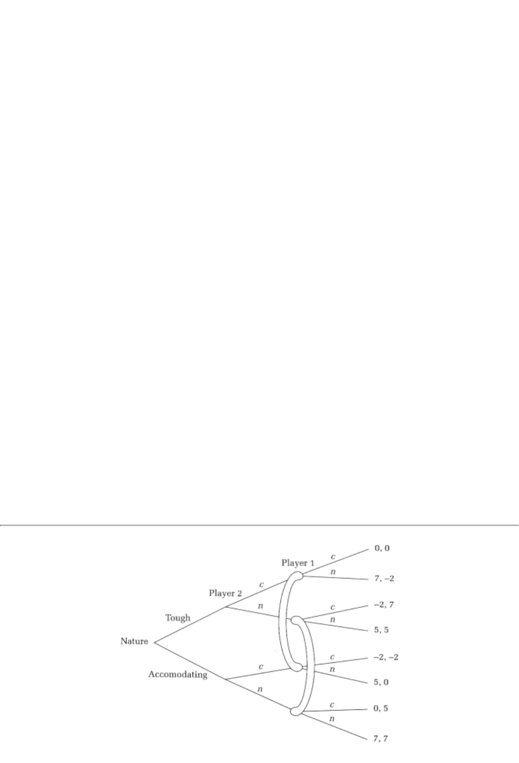
Page 384
TABLE 24.1
1 \ 2 c n 1 \ 2 c n
c0, 0 7, -2 c-2, -2 5, 0
n-2, 7 5, 5 n0, 5 7, 7
(a) Tough (b) Accommodating
signal were merely talk, then these types too would claim to be a lower cost firm and a mere fan,
respectively. And the uninformed player would typically be smart enough to realize this fact and discount his
opponent's talk.
He will believe certain signals; for example, he will believe a signal that is profitable for a particular type of
sender but unprofitable for an alternative type. For instance, in the Cournot duopoly, if he finds his rival
investing in a factory that would break even only if the rival's costs are low, then he is likely to believe the
signal conveyed by the building of the factory.
Two points ought to stand out from this discussion:
1. It is in the self-interest of certain types of informed players to signal their information. The uninformed
player should always process the signal to learn something she did not know about her opponent.
2. The signal has to be credible in the sense that it must not be in the self-interest of other types to send the
very same signal (or if it is, then the uninformed player will account for that fact).
Signaling games and their equilibria incorporate these two features. Before going to the general analysis,
however, let us discuss two examples.
Example 1: Prisoners' Dilemma
This is an incomplete information variant of the Prisoners' Dilemma (introduced as example 2 in Chapter
20). Both players' payoffs depend on whether player 2 is tough or accommodating; player 1 does not know
which one it is although player 2 does; see Tables 24.1a and 24.1b.
Note that whether or not the uninformed player (player 1) should play
confess or not confess depends
critically on which type his opponent happens to be. Hence, player I would greatly benefit from getting a
signal about player 2's type. A number of different things can serve as signals. For starters, let us suppose
that player 2 can "make his actions speak louder than words"; that is, he can pick his actionc or nahead of
player 1, and that choice is a signal of his type. The extensive form for this signaling game is therefore as
displayed in Figure 24.1.2
2Note that because player 2 appears before player 1 in the extensive form, we have written player
2's payoff as the first component of each part of payoffs.
page_384
Page 385
FIGURE 24.1

Example 2: The da Vinci Diaries
A whole class of signaling games is given by the direct-revelation games of Chapter 22. For example,
consider the da Vinci diary direct-revelation game between Sotheby's and Bill Gates. Mr. Gates files a report
about his type (he may choose to lie), and this report is the signal. After receiving the signal, Sotheby's has to
implement a preannounced price and likelihood of sale. Suppose that Sotheby's has only two options
available: sell for sure at price or sell with probability 50 percent at a price of m3 Suppose as before, that
the buyer cannot be coerced into buying at a price above his valuation for the object.
The signaling game is therefore as shown in Figure 24.2.
24.1.1 A First Analysis of the Examples
In everything that follows keep in mind the two main questions: First, does an informed player have a reason
to signal his type? Second, can he do so credibly? That is, can he choose a signal that the other type will not
also choose?
Example 1
Both types of the informed player, player 2, would like to get a high payoff. For a type 1 player, the payoffs
are higher if his opponent plays n (rather than c). Hence he would like to send a signal that would cause
player 1 to play n. Consider a type 2 player instead. Her payoffs are also higher if player 1 plays n. So each
type has a reason to signal; can they do so credibly?
Suppose that after receiving the two signals, player 1 is able to tell whether he is playing a type 1 or a type 2
player. (This can only happen if the two signals are different.)4
3And suppose that .
4For instance, type 1 might signal by picking c and type 2 by picking n. In that case, when player 1
sees c, he knows that the correct payoff matrix is Table 24.1a. However, if he sees n he infers that it is
Table 24.1b. The two types can also be distinguished if they pick n and c, respectively.
page_385
Page 386
FIGURE 24.2
Note that now player 1 is fully informed; that is, we have either a game of complete
information given by
Table 24.1a or one given by Table 24.1b. Consequently, player 1 will either pick c (his dominant strategy in
Table 24.1a) or n (his dominant strategy in Table 24.1b) depending on what he learns from the signal.
But now we have a credibility problem; type 1who would like to have the initially uninformed player 1 pick
nwill want to send the same signal as his type 2 counterpart just so he can fool player 1 into picking n.
Knowing this, player 1no fool himself!will look at the signal that he receives and infer that he should infer
nothing.
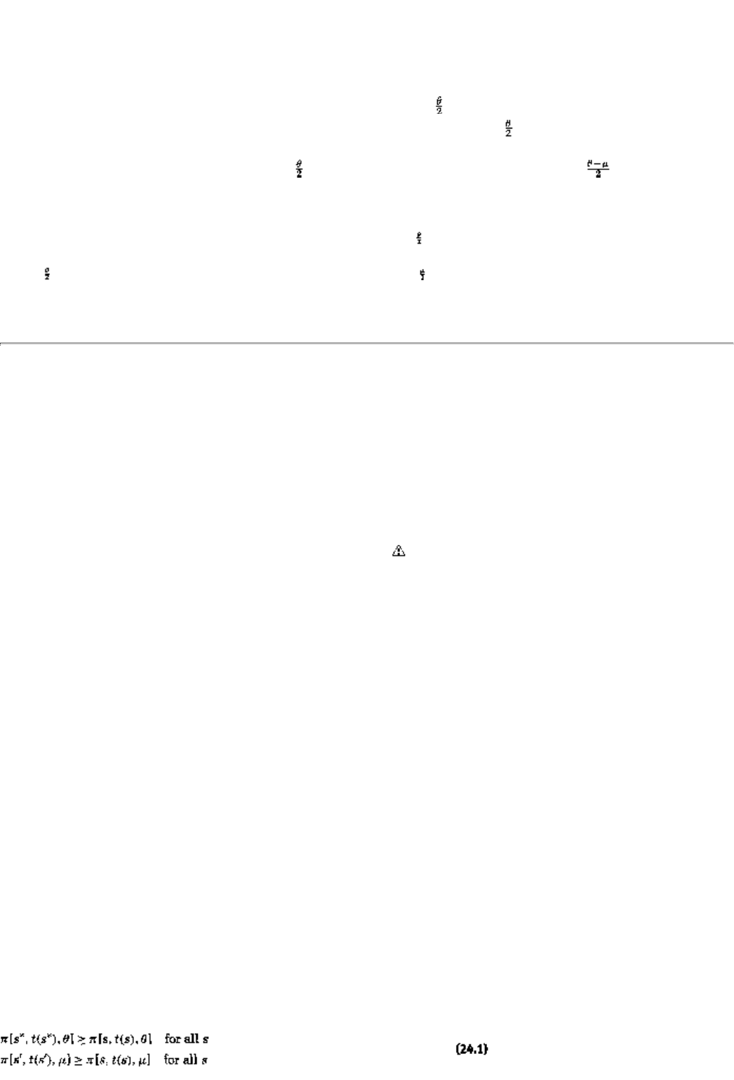
Example 2
Unlike the previous example, here it is possible for the two types to credibly signal their valuations. We will
show you why.
Note that if the types can be distinguished by the seller, then she would charge the
m type buyer the lower
priced uncertain outcome and charge the higher valuation buyer .5 Knowing this, a high-valuation buyer
has two choices: confirm that he is a high-valuation buyer and get charged or lie about his valuation and
get charged m with a 50 percent likelihood (and be unable to buy with a remaining probability of 50%). The
former option nets a utility surplus equal to , whereas the latter yields a net surplus of . Clearly, the
high-valuation buyer will truthfully report his type. The low-valuation buyer gains a zero surplus from either
price, and so a truthful signal is a best choice for him as well.
5The low-valuation buyer will refuse to buy at a price of , so it makes little sense to offer him that
option. The high-valuation buyer trill accept both prices; the higher price yields the seller a profit
of , whereas the lower price yields an expected profit of . Hence the seller prefers the higher
price.
page_386
Page 387
To summarize here are the two conclusions from the examples:
1. If the uninformed player can tell the types apart, then he will play a best response in the consequent
complete-information game.
2. Each informed type understands conclusion 1. This fact determines whether some type will want to hide
behind the veil of another type (by sending the same signal).
In the next section, we will do a more complete analysis of both examples.
24.2 A Definition, an Equilibrium Concept, and examples
24.2.1 Definition
In a signaling game there are two players. Player 2 has some private information that affects the payoff of
both players. As always, we will describe this information as being part of a player's type, and to keep things
simple, we will assume that there are two typesq and m (with a prior probability r that the type is q).
The informed player sends a signal, denoted s, to player 1 and after receiving the signal, the latter takes an
action, denoted t. Player 2's type, her signal, and the action of player 1 together determine each player's
payoff. Denote player 2's payoff as p(s, t, q), if she is a q type, and as p(s, t, m) if she is a m type player.
Denote player 1's payoff similarly as P(s, t, q) and P(s, t, m).
The extensive form of the signaling game is therefore given by the diagram in Figure 24.3.
In example 1, the signal is player 2's choice of n or c (similarly player 1's action is a choice of n or c). In
example 2, the signal is the buyer's report on his type, and the principal's (or seller's) action is the choice of a
price and a sale probability.6
24.2.2 Perfect Bayesian Equilibrium
A type-dependent strategy for the informed player 2 is a pair of signals, say, s* for type q and s' for type m.
A strategy for player 1 is a signal-dependent choice; let us denote the action chosen after receiving a
representative signal s as t(s). Since this action is chosen after seeing player 2's signal, player 1 at that point
may have a revised estimate of the prior probability r on the two types; call this estimate r(s).
A perfect Bayesian equilibrium (PBE) is given by
Best response of each type of player 2
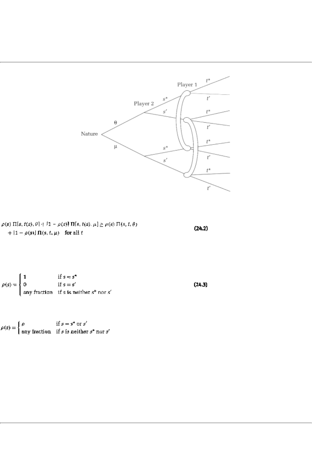
6There is a more general point that example 2 illustrates. Any direct-revelation game can be
thought of as a signaling game; the informed agent's report about his type is his signal. The
outcome to every report is the principal's action. Put differently, one of the mechanisms that a
principal can choose in a mechanism-design problem is a signaling game to be played by the agent
and himself. For more on this issue, see section 24.5.
page_387
Page 388
FIGURE 24.3
Best response of player 1
, for every s,
Correct estimate revision, in either of two cases:
Case 1: s*¹ s'
Case 2: s* = s'
Let us work our way backward through the three equations. In words, equation 24.3 says the following: if
player 1 expects to receive different signals, that is, if s*¹ s', then upon receipt of s* he knows he is facing a
type 1 player; that is, r(s) = 1 [and conversely upon receiving a signal of s' he knows he is faced with a type
2 player, that is, r(s) = 0]. If he expects to receive the same signal, that is, if s* = s', then he concludes
nothing from getting that signal; that is, r(s) = r. What is he to do when he receives a signal that he did not
expect, that is, if the signal is neither s* nor s'? Well, he might think it was a mistake (and that player 2
really meant to send either s* or s'). Or he might think that player 2 changed her mind. Since there are
multiple explanations, we can be agnostic
page_388
Page 389
the last part of equation 24.3 says any rationalization is acceptable; that is, any revision is correct.
Equation 24.2 says thatbased on the correct estimate of the two typesplayer I must pi
ck each one of his
actions t(s) in order to maximize his expected payoffs. In particular it requires that he play best responses
within the consequent complete-information games if he learns his opponent's type. Notice that the
arbitrariness in specifying the estimate, when player 1 receives an unexpected signal, spills over to equation
24.2 because different specifications of r(s) will engender quite different best responses.
Finally, equation 24.1 is a standard best-response condition for the informed player of every type. Note that
although player 1's choices t(s), for signals other than s* or s', are essentially arbitrary, the exact assignment
does matter to player 2; after all, if a q type were to switch the signal from s* to s, how the payoffs change
would depend on t(s).7
A perfect Bayesian equilibrium adds one further restriction to a plain old Bayes-Nash equilibrium and that is
equation 24.3that is, that the uninformed player is now allowed to (correctly) process information that
becomes available to him in the course of the game. On one hand, a PBE in which the two types send
distinct signals, and therefore can be distinguished from each other, is called a separating equilibrium. On
the other hand, an equilibrium in which the two types send identical signals, and therefore cannot be
distinguished from each other, is called a pooling equilibrium.8
24.2.3 A Further Analysis of the Examples
Example 1
We have already shown that there is no separating equilibrium. The only candidate therefore is a pooling
equilibrium, that is, one in which the two types both pick n or c.
Suppose, for the purposes of this discussion, that the prior probability on type q is less than 50 percent, that
is, . (In the Exercises you will analyze the case where .)
CONCEPT CHECK
PLAYER 1
If both types pick c, show that it is better for player 1 to play n.
What remains to check is player 2's best responses. Note that a type 1 player gets a payoff of 7 in this
candidate equilibrium while a type 2 gets 5. Clearly the first type can do no better. (Why?) Whether or not
the second type can do better depends on how player 1 treats an unexpected signal of n. If he stays with an
action choice of n, then player 2 would do betterand get a payoff of 7. Hence in this case type 2 would not
signal by playing c but rather would signal by playing n. But if upon receipt of signal n, player 1 in
7There are furtherand more complicatedgeneralizations of the equilibrium concept in which this
arbitrariness is somewhat reduced. One such concept is called sequential equilibrium.
8The definition that we have given is for pure-strategy PBE. The definition can be extended to mixed-
strategy PBE in the usual way.
page_389
Page 390
fact switches to c, then player 2's payoff would drop down to 0. In turn, player 1 would want to play c upon
receiving a signal of n if he believes that the likelihood of type 1 is at least , that is, .
To summarize, one perfect Bayesian pooling equilibrium is for both types of the agent to signal c, that is, s*
= s' = c, thereby eliciting a play of n by the principal, that is, t(c) = n. Neither type of player 2 wants to
change his signal if t(n) = c. The pair of actions t(c) = n and t(n) = c is a best response for player 1 if .
CONCEPT CHECK
ANOTHER EQUILIBRIUM
Show that s* = s' = n leads to a play of t(n) = n (recall that ) and that
neither type wants to switch his signal if t(c) = c. In turn, show that this choice
of action is a best response for player 1 if the signal c leads to
.
Example 2
We have already shown you one separating PBE in this game. Let us now look at pooling
equilibria instead.
Suppose that the two types of buyers send the same signal; either they both report q, or they both report m.
Since the signal does not convey any information, the seller still presumes that there is a probability r that
the buyer is of type q. By charging the higher price he can expect a sale only to the higher valuation buyer,
and hence the expected profit from this strategy is . If he charges the probabilistic lower price, however,
then both types of buyers will buy, although there will be an actual transaction only 50 percent of the time.
Consequently, the expected profit from this strategy is . The higher price is the better choice if and only if
rq³m.
Will either buyer want to switch his signal? The m type buyer receives zero net surplus regardless of the
price and hence has no reason to want to switch. The q type buyer gets a net surplus equal to from the
higher priced alternative and a net surplus of if he is charged the probabilistic lower price. Hence he
does not want to switch either.
CONCEPT CHECK
ANOTHER CASE (rq << m)
Show that there are two pooling equilibria (with signals q, q and m, m). Upon
receiving the expected signal, the seller charges m (with a 50% sale
probability). Upon receiving an unexpected signal, the seller presumes that the
buyer is of the m type and (again) charges the lower probabilistic price.9
9Indeed any belief in which the seller thinks the prior probability of the q type is less than would
lead him to charge the lower probabilistic price.
page_390
Page 391
24.3 Signaling Product Quality
The initial motivation for analyzing signaling gamesand indeed a major motivation for an entire subject
called information economicscame from Akerlof's discussion of markets with uncertain product quality (see
note 1). Akerlof modeled the following scenario: buyers in a market are uncertain about the exact quality of
the good they are buying, but sellers, who have greater experience with it are more certain about quality. He
asked, How are market price and availability affected by buyer uncertainty? Would buyers only be willing to
pay for average quality? Would that fact prompt sellers with goods of better than average quality to withhold
their merchandise? Would such decisions lead to a situation in which bad-quality goods drive out better
quality ones?
Akerlof showed that the answer to each of these questions can be a resounding yes. We will first
demonstrate the logic behind such a breakdown of the market, and then we will analyze the role of signaling
in ameliorating the problem.
24.3.1 The Bad Can Drive Out the Good
Imagine that there are only two product possibilities-good-quality merchandise and lemons (or bad-quality
merchandise). Suppose that a buyer cannot tell one from the other but a seller can. Suppose also that what
distinguishes bad from good is that they have different costs of upkeep and repairs. For example, suppose
that expected repair costs are $200 on a good-quality product and $1,700 on a lemon.
Suppose that a potential buyer values the objectbefore accounting for repair costsat $3,200; hence his net
valuation is $3,000 for a good product and $1,500 for a lemon. Suppose also that a seller has an intrinsic
valuation of $2,700; that is, a seller of good quality if he held on to the product would have a valuation of
$2,500 while a seller of a lemon would have a valuation of $1,000.
To help you remember all the numbers here is a table of the relevant ones:
Good Quality Lemon
Net valuation of buyer
3,000 1,500
Net valuation of seller
2,500 1,000
If a lemon is known to be a lemon, then its owner would negotiate solely with buyers
looking for lemons.
Consequently, the price of a lemon would be somewhere between the $1,000 that sellers are willing to take
and the $1,500 that buyers are willing to pay. Likewise, the buyers of good quality would negotiate with
similarly endowed sellers and settle on a price somewhere between $2,500 and $3,000. And both qualities of
goods would get sold in this market.
Now suppose that a buyer cannot tell a lemon from good quality. The maximum that he w
ould be willing to
bid would depend on how likely it is that he is buying a lemon. Suppose, for illustration's sake, that there are
an equal number of lemons and good-quality items in the market. In that case the average valuation for a
buyer is , or $2,250.
page_391
Page 392
The buyer in any transaction will not want to go beyond $2,250, and the seller of a lemon will accept such
an offer (since he values the good at $1,000), but the seller of good-quality merchandise will refuse (and
keep his good valued at $2,500). Consequently, the only goods that will get sold will be lemonsthe bad will
have driven the good out of this market. Note too that the buyer who recognizes this fact will only make
offers between $1,000 and $1,500, since he will clearly be overpaying if he pays $2,250 for a lemon that is
only worth $1,500 to him.10
Notice that there is no quick fix for this problem. For instance, it does not do for
a buyer, if he sees his first
offer refused, to say to himself, "Ah, I have found a good product," and raise his offer to $2,500. If the seller
of a lemon anticipated such behavior, he too would refuse the first offer! Nor does it do for the seller to give
a verbal guarantee, because lemon owners will have every incentive to give the most sincere guarantees.
The problem does not go away, either, if there are more than two quality levels. Indeed in many ways it can
get worse. Suppose that there is a third quality levelintermediate quality. A buyer who is unable to
distinguish between the three levels will pay for average quality, thereby losing the good-quality sellers. If
the buyer is cognizant of that fact, he will only be willing to pay for average quality after taking an average
over only lemons and intermediates. In turn intermediates' sellers, whose merchandise is now better than the
average, will sit out the market. Their withdrawal will lead buyers essentially to bid for lemons, and those
will be the only goods sold.
And you can extend this logic to four or five (or more) quality levels. To the extent that lemons constitute a
smaller and smaller fraction of available goods when there are more and more quality levels, the market
breakdown becomes even more stark.
24.3.2 Good Can Signal Quality?
Sellers of good-quality merchandise might want to signal the superior quality of their product. As we have
seen, it does not suffice merely to offer verbal assurances, since lemon owners are just as capable of
providing those very same assurances. One way to put one's money where one's mouth is, so to speak, is for
sellers to offer a warranty (against possible repairs after purchase). Warranties can be offered for any
fraction of repair costs between 0 and 100 percent; we will keep matters simple by considering only the two
extreme casescomplete warranty (100% coverage) and no warranty (0% coverage). Sellers decide whether
or not to include a warranty before buyers decide how much to offer for the merchandise.
Payoffs under Warranty
When a seller offers a complete warranty on a good, he will accept a price p for the good only if that price is
at least his intrinsic valuation 2,700. After all, if the price were any lower, the seller might as well hold onto
his good. (Why?) If p ³ 2,700, then the payoff to a lemon seller is p - 1,700, and that to a good-quality seller
is p - 200. The buyer's
10For alternative parameter values it is possible that quality levels other than lemons may get sold
as well. Although a buyer will only pay for average quality, this payment may still be enough to
compensate the better-than-average-quality sellers because their intrinsic valuation is less than
that of buyers. For instance, when lemons have a probability of
, the maximum that a buyer will
pay is , and good-quality sellers would be willing to sell their merchandise.
page_392
Page 393
TABLE 24.2
Price Warranty No Warranty Price Warranty No Warranty
1,000 0, 1,000 500, 1,000 1,000 0, 2,500 0, 2,500
1,500 0, 1,000 0, 1,500 1,500 0, 2,500 0, 2,500
2,500 0, 1,000 -1,000, 2,500 2,500 0, 2,500 500, 2,500
2,700 500, 1,000 -1,200, 2,700 2,700 500, 2,500 300, 2,700
2,900 300, 1,200 -1,400, 2,900 2,900 300, 2,700 100, 2,900
(a) Lemon (b) Good Quality
payoff in either case is 3,200 - p. If p << 2,700, since there is no sale, a buyer gets zero payoff while the two
types of sellers get payoffs of 1,000 and 2,500, respectively.
Payoffs with No Warranty
A lemon seller will accept any price p that is at least 1,000; the buyer's payoff will be 1,500 - p and the
seller's p. However, a good quality seller will only accept p ³ 2,500; the buyer's payoff will be 3,000 - p and
the seller's p.
This analysis gives us the payoff matrices of Tables 24.2a and 24.2b (in each pair, the first payoff is the
buyer's and the second is the seller's).
Consider the following strategies: A lemon seller offers no warranty, but a good quality seller does. The
buyer bids $2,700 if there is a warranty and $1,000 if there is not.
PBE Analysis
Since the signals are distinct, a buyer can tell whether or not he is bidding on a lemon, and given the seller's
strategies, the absence of a warranty implies a lemon. The buyer's best response is to bid the lowest
acceptable price; hence, once he spots a lemon (and knows that he is in Table 24.2a), he should bid $1,000,
and otherwise he should bid $2,700exactly as in the candidate strategies.
What about the two types of sellers? If a lemon owner offers a warranty, he would get an offer of $2,700,
but he would expect to pay $1,700 in warranty costs; so he would be no better off by switching his signal. A
good-quality owner could switch to not offering a warranty and get a $1,000 offer. This possibility is strictly
worse than getting a $2,700 offer with a $200 warranty cost tag attached. So he never wants to switch. Put
differently, we have a separating perfect Bayesian equilibrium.
page_393
Page 394
24.4 Case Study: Used CarsA Market For Lemons?
A market with uncertain product quality is that for used carsand Akerlof borrowed from that market the
terminology of ''lemons."11 In this section we ask, Are there signs of breakdown in this market? And is there
evidence of signaling by sellers? Here are some facts about this market:
1. The average 1994 car depreciated 37 percent in its first year. By the end of the second year it had
depreciated 50 percent (if you tried to sell your 1994 car in 1996, you would get only half the price that you
had paid for it a mere two years before.)
2. Of all used cars purchased, 20 percent are sold through new car dealerships, and another 15 percent are
sold through independent used car dealerships. Dealerships typically offer warranties on the used cars that
they sell.
3. The average price of a used car in 1994 was about $11,500. The average private-party sale price on a used
car was about $2,000 less than the average sale price at dealers.12
The first fact is a striking illustration of the lemons problem. There are some people who sell their cars within
the first couple of years because their circumstances changethey move out of town, they cannot afford to
make car payments, they get married and the spouse already has a car, and so on. These are people whose
cars are good-quality cars. If you as a buyer were convinced of their reason for selling, you would be willing

to pay 80 to 90 percent of the purchase price (for a car that has been driven only ab
out a year or so).
Then there are people who sell because their cars are lemonsthe car developed serious mechanical problems,
it is at the mechanic's all the time, and the like. These are cars that you as a buyer are willing to pay a lot less
than the purchase price for.
Among new cars, the fraction of lemons is very very small, maybe 1 percent. So in principle most of the
people selling a new used car are those whose circumstances have changed. Hence, if you are willing to pay
them 80 to 90 percent of their purchase price, you should be willing to purchase an "average" new used car
for, say, 75 percent of its original price. Right? Well, not quite because now the lemon logic kicks in. Sellers
who value their car at more than 75 percent don't sell, you as a buyer know that, and hence your average is
between lemons and cars worth less than 75 percent. You offer 65 percent. Now even more people with
changed circumstances decide to hold onto their cars. (Maybe the kids need a car, or they take the old car to
their new home, or . . . .) So now you figure that very likely the cars remaining in the market are lemons and
you only offer 55%. And so on.
11The principles of game theory and economics are largely context-free; you do need to know
details about an economy to judge whether or not a certain principle is true. Unfortunately, the
same cannot be said for the jargon of economics. I remember reading Akerlof's paper as a student
in India and being totally mystified as to what certain citric fruits and used cars have in common!
12These and other facts, along with much helpful advice about how to go about buying a used car, can
be found at the web site of a company called Edmunds (at edmunds.com).
page_394
Page 395
The second and third facts are good illustrations of the role of signaling in this market. The only reason to
pay more to a dealer is that the dealer offers a warranty. You say to yourself, "No seller of a lemon can offer
a warranty, and so I should be willing to pay more to the dealer." Indeed if there were not this signaling
element, then there would really be no good reason for dealers to be involved in this market. After all,
whatever profits a dealer makes could have been split between the original seller and the eventual buyer.13
Indeed there is yet another "fact" about this market, and that is that private sellers often provide other kinds
of quality signals. For example, some sellers have the car inspected by a mechanic of the buyer's choice,
some turn over past service records, some make relatively expensive repairs before selling, and so on.
24.5 Concluding Remarks
In this section we will comment on the link between signaling games and mechanism design. The difference
between these two topics is in who gets to go first: the informed (agent) or the uninformed (principal).
In a mechanism-design problem, the principal moves first and offers a set of options to the agent. Different
types of agents might choose among the options differently. Note two things: (a) agents select after knowing
the full consequences of each choice, and (b) after the fact the principal knows her agent's type, but because
she moves first she cannot use that information in taking her own action.
In a signaling game the agent moves first by signaling. Different types of agents might pick different
signalsor strategiesin anticipation of what the principal is going to do after she sees the signal. In this setup,
however, (a) the agent can only guess as to how the principal is going to react to an out-of-equilibrium
signal. Furthermore, (b) the principal can use information about her agent that she has learned from the
signal before taking her own action.
The general setting, in which some players have better information, is known as the problem of adverse
selection. Both approaches, mechanism design and signaling, have been employed for this problem. When a
health or life insurance company offers a whole menu of policies and lets its clients decide what they want,
the company is solving a mechanism-design problem. Similarly, an airline or a phone company may offer a
variety of price options. In each of these cases it is the uninformed party that offers the options to the
informed party.
In contrast, when used car sellers offer warranties or manufacturers offer money-back guarantees if
customers are not fully satisfied, then they are offering a signal.14 In these cases it is the informed party that
creates options for the uninformed party. One of the first applications of signaling models in economics was

to education.15 The thought here is that by going to school an individual can signal superior intellect and
greater competencequalities that an employer would value highly.
13There is the further question, Why don't private sellers offer warranties? They could then
convince buyers to buy from them directly and avoid paying the dealers' markup. Part of the
answer clearly is that it is inconvenient and costly for private individuals to do so.
14One of the more interesting offers recently was made by British Airways. They guaranteed that if
you traveled business class between New York and London and were not fully satisfied with the service
(you would simply have to say so) they would give you a free round-trip coach-class ticket anywhere in
the United States. Unfortunately, it is then a dominant strategy for every passenger to claim that the
service was terrible! I am not sure what results it produced for British Airways, but the program was
shut down after a little while.
15See "Market Signaling" by A. M. Spence. Cambridge, MA: Harvard University Press, 1973.
page_395
Page 396
Summary
1. In a game of one-sided incomplete information, the informed player will have an incentive to convey his
information to the uninformed player if doing so will change the latter's action to the former's advantage.
2. A signaling game is one in which an informed player can take actions that can convey such information.
The signal will, however, be noninformative if multiple types of informed players have incentives to send
identical signals.
3. A perfect Bayesian equilibrium (PBE) is a signal choice by every informed type and an action choice by
the uninformed player in which (a) the signals are correctly processed, (b) the uninformed player maximizes
her expected payoff after correctly processing the signal, and (c) informed types send the most profitable
signals.
4. A separating PBE is one in which different types send different signals and hence the initially uninformed
player is fully informed by the time she takes her action. A pooling PBE is one in which the signals are
noninformative.
5. In a market with uncertain product quality, bad-quality merchandise can drive out better quality goods.
This phenomenon is called the lemons problem. By offering warrantiesthat is, by sending signalsgood-quality
sellers might be able to ameliorate the problem.
Exercises
Section 24.1
24.1
Give two examples, other than the ones discussed in the text, of market signaling. Identify clearly what each
player's actions are.
24.2
Informally describe the market outcome in your two examples. What factors are important in determining
whether the outcome is a separating or a pooling one?
Section 24.2
The first few questions concern example 1 in the chapter.
page_396
Page 397
24.3
Explain why the argument that there are no perfect Bayesian separating equilibria is valid no matter what
the value of the prior probability r.
Suppose that r is actually greater than 50 percent. Given exercise 24.3, we need only look for pooling
equilibria.
24.4
Consider a signal of c by each of the informed agent types. Show that the best response for player 1 is to
play c. Show that the payoff is 0 for the q type and -2 for the m type of player 2.
24.5
Argue that the m type player can always do better by sending n as signal. Can you conclude that there is no
pure-strategy pooling equilibrium in which the two types send the signal c?
24.6
Consider a signal of n by each of the informed agent types. Show that the best response for player 1 is to
play c. Argue that the q type can then do better by sending c as signal. What can you conclude about
pure-strategy pooling equilibria in this game?
In the next few questions, therefore, we will look for a mixed-strategy PBE.
24.7
Consider the following strategy for player 1: t(c) = c and t(n) = c with probability (and with remaining
probability , she picks n after signal n). Show that the q type is consequently indifferent between his two
signals while the m type strictly prefers to send the signal n.
24.8
Consider therefore the following signal strategy for player 2: the q type sends the signal c with probability p
while the m type sends the signal n. If the principal receives a signal c, what can he conclude about the types
of player 2? What is his best-response action t(c)?
24.9
For what value of p is the principal indifferent between picking actions c and n? Is a strategy of picking t(n)
= c with probability a best response? Explain. Summarize your findings about a PBE for this case .
The next few questions are about the incomplete information Bertrand (price) competition example of
Chapter 20; firm 2 knows which is the correct payoff matrix (Table 24.3a
page_397
Page 398
TABLE 24.3
1 \ 2 High Medium Low 1 \ 2 High Medium Low
High5, 5 0, 8 0, 6 High5, 5 6, 3 10, 1
Medium8, 0 4, 4 0, 6 Medium3, 6 4, 4 5, 2
Low6, 0 6, 3 3, 3 Low1, 10 2, 5 3, 3
(a) (b)
or 24.3b), but firm 1 does not. Suppose that the informed player can make his price choice before the
uninformed player.
24.10
We will first investigate separating equilibria; suppose that player 1 can figure out
player 2's type. Show
from Table 24.3a that he will never play h. Show that a type 1 player 2's payoffif his signal is correctly
inferred and best responded tocan never be more than 3.
24.11
However, if player 1 recognizes that he is really playing Table 24.3b, show that it is a dominant strategy for
him to play h. What are the possible payoffs for player 2 in this case?
24.12
Demonstrate that a type 1 player will want to send the same signal that a type 2 player is supposed to send.
What can you conclude about separating equilibria in this game?
24.13
Suppose that . Show that there is a pooling equilibrium in which both types signal by picking h. (Be
careful to lay out every detail on the strategies.)
Section 24.3
In the next few questions we will explore the lemons problem with a third quality level, intermediate, whose
repair costs are $500. Hence a buyer values this quality at $2,700 and a seller at $2,200.
24.14
If each quality level is just as prevalent in the population, show that a buyer will not be willing to pay any
more than $2,400 for the merchandise. What kind of goods get sold at that price?
page_398
Page 399
24.15
If only intermediates and lemons are sold in the market, how much will a buyer be willing to pay for a good?
Would both of these kinds of buyers sell at this price? What is the market outcome?
24.16
Redo the exercises 24.14 and 24.15 for the case where the probabilities of lemons, intermediates, and good
quality are , , and , respectively.
24.17
Redo exercises 24.14 and 24.15 again for the case where lemons are only half as likely as either
intermediates or good-quality merchandise. What have you learned about market breakdown from this
exercise and the previous one?
24.18
If the probabilities of the three quality levels are, respectively, p, q, and 1 - p - q, can you give general
conditions for each of the following outcomes?
a. Only lemons are sold.
b. Lemons and intermediate-quality goods are sold but not good-quality merchandise.
c. All three quality levels are sold.
24.19
If the repair costs of the three quality levels are, respectively, p, q, and r and each quality is just as likely,
can you give general conditions for each of the following outcomes?
a. Only lemons are sold.
b. Lemons and intermediate-quality goods are sold but not good-quality merchandise.

c. All three quality levels are sold.
The next few questions are concerned with the signaling game version of the lemons problem.
24.20
Show that there is no separating equilibrium other than the one analyzed in the text.
24.21
Consider a candidate pooling equilibrium in which both types offer warranties. What would the buyer bid for
the good? Specify a belief that the buyer has when he gets an unexpected "no warranty" signal such that the
buyer's bid and warranties by both sellers constitute a PBE.
24.22
Repeat exercise 24.21 for a pooling equilibrium in which neither seller offers a warranty.
page_399
Page 400
Section 24.4
24.23
Some people have argued that the lemons problem can be ameliorated by way of government regulation.
Suppose that the government passes a law that states that the owner of a lemon is entitled to trade in his car
for another new car ("lemon laws" exist in many states, such as New Jersey). Argue in some detail that if the
only kinds of cars were lemons and good cars (which are being sold because their owners' circumstances
changed), the problem would indeed be solved.
24.24
How would your analysis change if there are more than two quality levelslemons, intermediates, and
good-quality cars? Explain your answer in detail.
24.25
What kind of regulation would be required to solve the problem that you uncovered in the previous
question? Comment on the feasibility of such regulation.
page_400
Page 401
PART FIVE
FOUNDATIONS
page_401
Page 403
Chapter 25
Calculus and Optimization
This is the first of three chapters that will develop the mathematics used in the text. In this chapter we will
discuss calculus and optimization theory. The next chapter will discuss probability and expectation, and in
Chapter 27 we will turn to decision theory. Each chapter will be a quick romp through a vast subject that can
easily constitute a semester-long course by itself. Hence the chapters are meant only as refreshers and
appetizers: refreshers that recall concepts and results that you have already seen or appetizers that send you
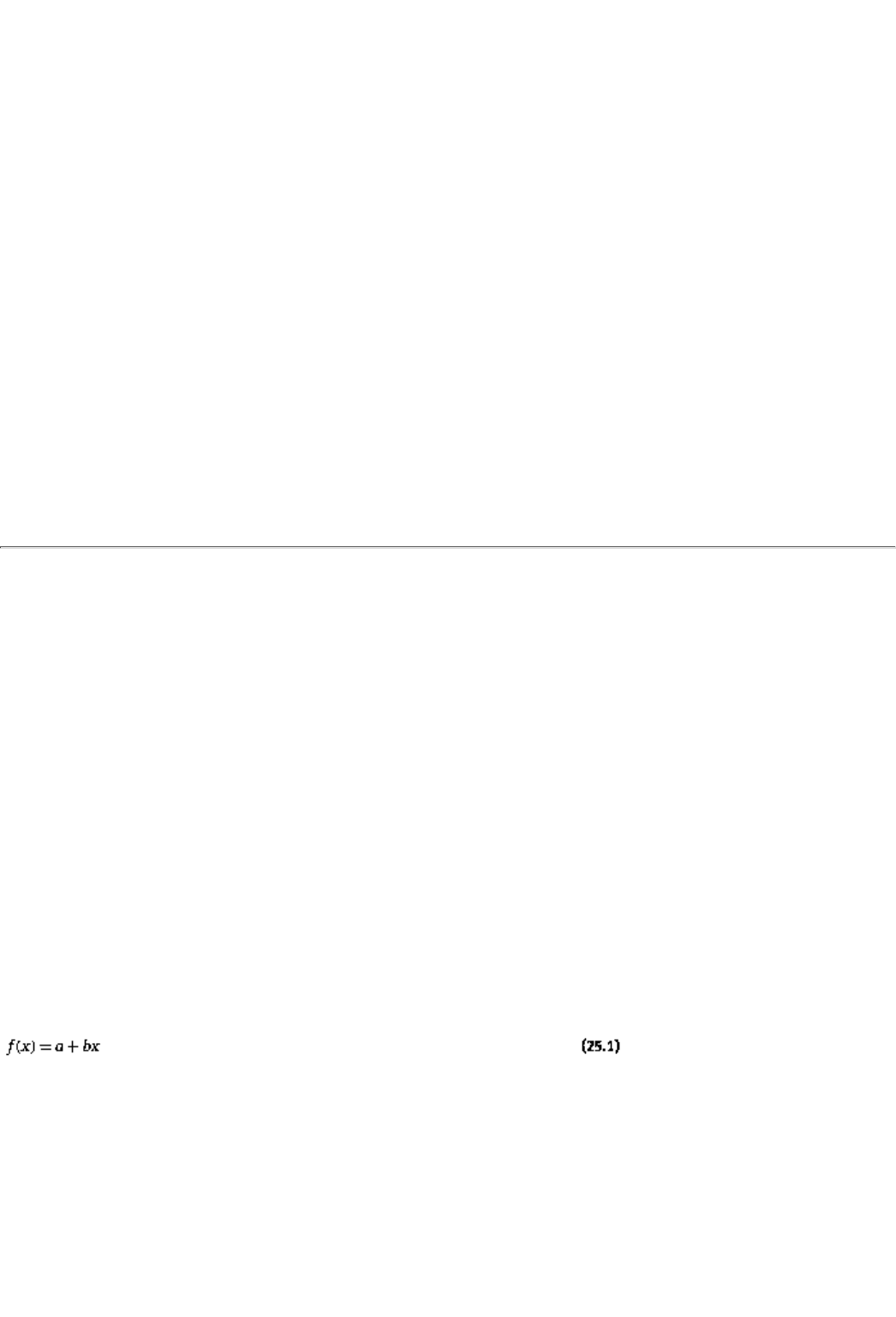
to the main course.1
In section 25.1 we will discuss three subtopics: variables, functions, and slopes of functions. In this section
we will also define a special category of functions called concave functions. Finally, in section 25.2, we will
discuss necessary and sufficient conditions for optimization and give several examples to illustrate the
results.
25.1 A Calculus Primer
The most basic entity in mathematics is called a variable. A variable is an object that can take on any
number of possible values. For instance, the number of stars that are visible to the naked eye is a variable.
This number can change with locationnorthern versus southern hemisphere, other light sources, Times
Square versus rural Georgiaor with time of year. Likewise, the value of the Dew-Jones index is a variable.
This number can change as factors affecting firm profitability changeinterest rates, unemployment levels, or
the trade deficit. Yet other variables include market price, the world's forest cover, the percentage of firms
that declare bankruptcy, the size of the world's oil reserves, bids made in Final Jeopardy, and the
depreciation of new cars within a year of purchase.
1For calculus and optimization the main course can be found, for example, in A. C. Chiang's
Fundamental Methods of Mathematical Economics, 2nd ed. (New York: McGraw-Hill, 1984). If you
wish to consult a book for a further treatment of probability and expectation, look at P. Newbold's
Statistics for Business and Economics, 4th ed. (Englewood Cliffs, NJ: Prentice Hall, 1995). Finally,
a somewhat advanced treatment of decision theory can be found in Mathematics for Economists by
L. Blume and C. Simon (New York: W. W. Norton, 1994).
page_403
Page 404
What is not a variable is an entity that cannot change in value; such an entity is called a constant. Physical
constants such as the speed of light or p are not variables. Neither is the location of Central Park or the face
value of a one-dollar bill.2
There are two kinds of variables: independent and dependent variables. Dependent variables take their value
from the values of independent variables. For example, the price of bagels is an independent variable that
determines the number of bagels bought at Columbia Bagels (on any weekday morning). That number also
depends on the price of muffins at nearby University Food Market, the number of people who live in the
Morningside Heights neighborhood (where the store is located), their income level, the price of cream
cheese, and so on. Similarly, the amount of fuel consumption in the world depends on the price of oil, the
price of substitute energy sources, time of year, available technologies, world GNPs, and other factors.3
It is standard to denote an independent variable by the symbol x and a dependent one by the symbol y.
25.1.1 Functions
A function is a mathematical description that tells us the value of the dependent variable y
for every value of
the independent variable x. The notation for a function is f; that is, we write y = f(x), and interpret the
notation as "f takes every value of x and transforms it into a value f(x)."
The simplest example of a function is
where a and b are constants. For instance, when a = 10 and b = -1, then this is the function f(x) = 10 - x.
Hence, when x = 5, y = f(x) = 10 - 5 = 5. Likewise, when x = 37, y = -27. Indeed a compact way of
representing this particular function is by means of a graph, as seen in Figure 25.1. Note that the relationship
between x and y is given by a straight line. Indeed this is true for the more general equation, equation 25.1.
Its graph is pictured in Figure 25.2.4 On account of the linear relationship, equations such as the ones given
by equation 25.1 are called linear functions.
By way of contrast, consider a graph such as the one given by Figure 25.3. Evidently the relationship
between x and y is not linear; a function that generates such a graph is called a nonlinear function. In this
particular instance, the function whose graph has been represented by Figure 25.3 is given by the general
form
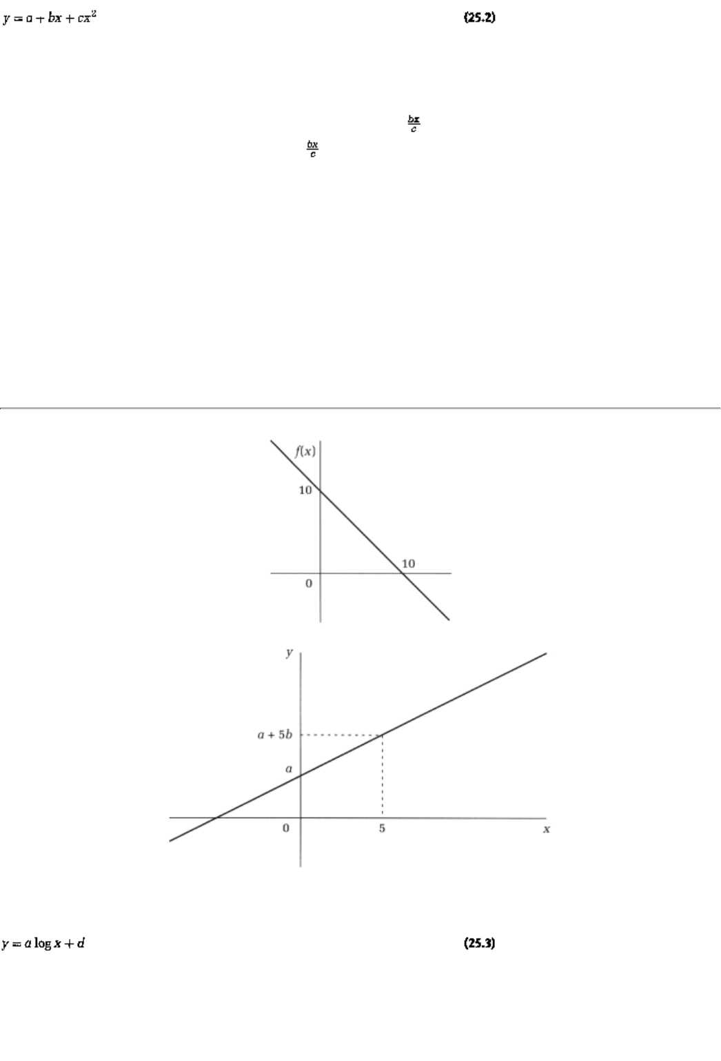
where a, b, and c are constants. The class of functions that are given by equation 25.2 are called quadratic
functions
. Once we specify values for the constants a, b, and c we get a specific quadratic function. For
instance, the figure has been drawn for y = 10 + x - 2x2, that is, for a = 10, b = 1, and c = -2.
Another category of nonlinear functions is given by y = a log , where, again, a, b, and c are constants.5
This class is called the log function. Since log is equal
2The face value is a constantat one dollaralthough what that dollar buys is a variable that changes
with the price index.
3As you might guess, what is independent and what is dependent will depend on the context. For
instance, if we analyze equilibrium conditions in the world oil market, then the price of oil is a
dependent variable that is determined by the quantities demanded and supplied.
4In the graph we have taken the value of b to be a positive number, and so there is a positive relation
between the independent and dependent variables; y is seen to increase as x increases.
5For this function, b and c are positive constants and the variable x only takes on positive values.
page_404
Page 405
FIGURE 25.1
FIGURE 25.2
to log bx - log c and, in turn, log bx is equal to log b + log x, we can rewrite the log function as
where d = a(log b - log c), a constant. For values of a = 1 and d = 2, we have drawn the graph of the log
function in Figure 25.4.
25.1.2 Slopes
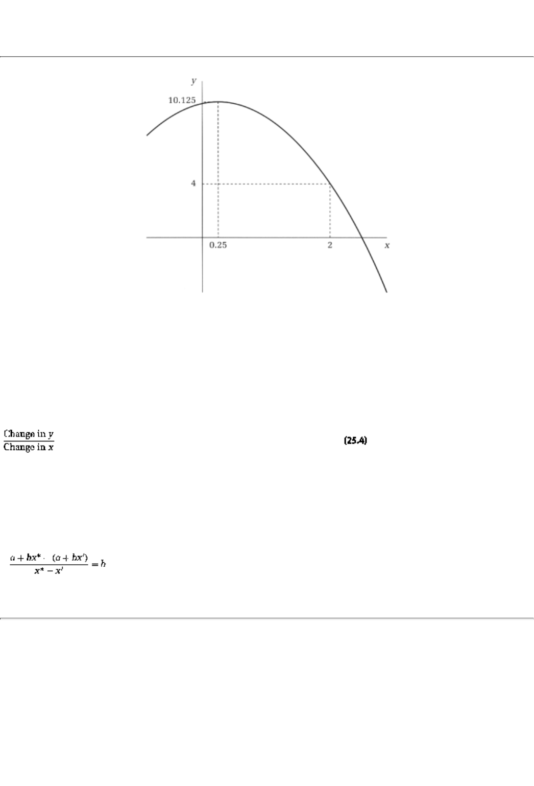
For our purposes the most important concept related to a function is the
slope
of the function; it is a measure
of the change in the dependent variable y when the independent variable x changes.
page_405
Page 406
FIGURE 25.3
Consider the linear function, y = 10 - x graphed in Figure 25.1. If x increases by one unit, say, from x = 5 to
x
= 6, y decreases from 5 to 4. Indeed, whenever x increases to x + 1 the change in y is [10 - (x + 1)] - [10 -
x
], that is, -1. Hence, for every unit increase in x there is always a unit decrease in y, and this statement is
true no matter what value of x we start from.
Indeed something more is true. If we consider an increase of x by 13 units, it is easy to verify that it leads to
a decrease of y by 13 units. Or if we consider a change of x by D units, then y changes by -D units; this
statement is true whether D equals 1, or 13, or -245. Put differently, the ratio
is always equal to -1, and this is true no matter what size change in x we consider, and no matter which
initial value of x we consider the change from. Equation 25.4 gives the rate of change (in y as x changes)and
it is the precise definition of slope for a linear function.
For the general linear function, y = a + bx, the rate of changeor slopewhen x changes from x' to x* is
page_406
Page 407
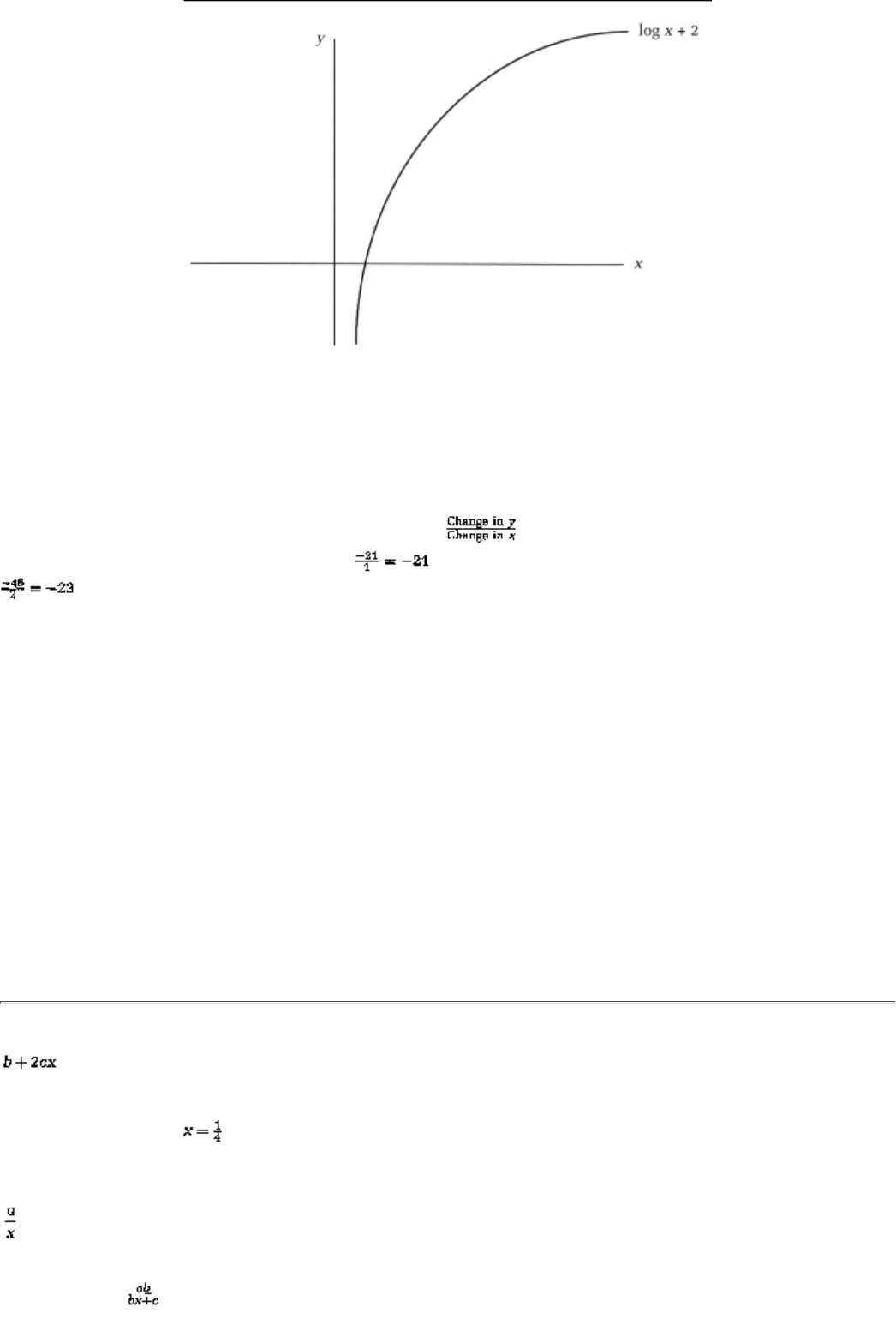
FIGURE 25.4
In other words, for any linear function, the slope is given by the constant b. When b is positive, the linear
function slopes upward; when it is negative, the function slopes downward.
Let us turn now to nonlinear functions. Here matters are a little more complicated. Consider y = 10 + x -
2x2. When x increases from 5 to 6, the dependent variable changes from -35 to -56. And when x further
increases from 6 to 7, then y changes to -81. Notice, therefore, that the size of the effect of a unit change in
x
depends on the initial value of x. Similarly, the ratio depends on how big the change in x is; a unit
change from x = 5 leads to a ratio equal to , and a two-unit change leads to a ratio value equal to
.
So we cannot always use equation 25.4 as the definition of slope for a nonlinear function. It turns out,
however, that if we consider changes in x that are very close to 0 in sizesuch as a change by 0.0001 units or
a change of 0.0002 unitsthen the ratio is essentially the same. Furthermore, for such small changes the ratio
is essentially the same as the slope of the straight line that forms the tangent to the function.
And this is the definition: The slope of a nonlinear function at some value of x, say at x = 5, is the slope of
the (linear) tangent to the function at x = 5.6 It is clear from looking at the graph that the slope therefore
varies with x (unlike in the case of a linear function).
25.1.3 Some Formulas
There are well-known formulas for the slope of the quadratic and the log function. The slope of the
quadratic function, y = a + bx + cx2 is given by
6A function need not have a well-defined tangent at every x, that is, it need not hove a slope
everywhere.
page_407
Page 408
If we consider the function y = 10 + x - 2x2, then its slope is 1 - 4x. As you can verify from Figure 25.3, the
slope is positive up to and negative thereafter.
On the other hand, the log function, y = a log x + d, has slope equal to
Hence for the function y = log x + 2, the slope is I Another log function is y = a log (bx + c). The slope of
this function is .
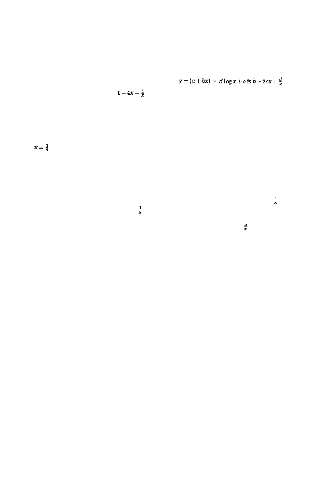
Two other formulas about slopes are very useful to know. First, the slope of the function a × f(x) where a is
a constant, is nothing but a times the slope of f. Second, if we have a sum of two functions, f and g, that is, y
= f(x) + g(x), then the slope of the sum function is nothing but the sum of the slopes of the two functions.
Sum of Two Linear Functions: The slope of the sum function y = a + bx + c + dx = a + c + (b + d)x is b + d.
Hence, the slope of y = (10 - x) + 227 + 6x is -1 + 6, or 5.
Sum of a Linear and a Quadratic Function: Similarly, the slope of y = (a + bx) + (c + dx + ex2) is b + d +
2ex. So the slope of y = 10 - x + 10 + x - 2x2 is -1 + 1 - 4x = -4x.
Sum of a Quadratic and a Log Function: And the slope of . Hence, the
slope of 10 + x - 2x2 - log x is equal to .
25.1.4 Concave Functions
If a function has the property that the higher the value of x the lower its slope, then the function is said to be
concave. For instance, consider the function y = 10 + x - 2x2. We just showed that its slope is 1 - 4x. Hence
the slope decreases with x; that is, the function is concave. You can also see that fact by looking at Figure
25.3; up to , where the function is rising, it rises more and more slowly; that is, it becomes flatter and
flatter. Beyond that value the function falls, and as you can see it falls faster and faster as x increases.
Since the slope of a general quadratic function is b + 2cx, the slope decreases with x if and only if the
constant c is negative. Hence all quadratic functions for which c is negative are concave, and those with c
positive are not concave.
As another example, consider the log function, log x + 2. We have told you that its slope is (the function is
only defined for x > 0). Again, as x increases, decreases, and hence the function is concave. You can also
see that relationship by looking at the graph of the function, Figure 25.4; the function becomes flatter and
flatter as x increases. For a general log function, a log x + d, the slope is equal to ; as long as a is positive,
the slope decreases with x. Hence such a function is concave.
For a linear function, the slope is unchanged (and equal to b) no matter what value of x we consider. In other
words, although the slope does not actually decrease with x, it does not increase either. Hence we can think
of this as a borderline case and also call it a concave function. Sometimes to distinguish functions such as 10
+ x - 2x2 or the log
page_408
Page 409
function log x + 2, whose slope actually decreases in x, we call those functions strictly concave functions.
From the previous subsection you know that the slope of the sum of two functions is the sum of the slopes.
Hence if each of the functions is concave, and therefore each has a slope that decreases with x, then so must
the sum of the slopes decrease with x. Put differently, the sum of two concave functions is also concave. By
exactly the same reasoning, af(x) is also a concave function whenever f is a concave function and a is a
positive constant.
In Chapter 27 you will see that there is a surprising connection between concave functions and risk attitudes
in the presence of uncertainty.
25.2 An Optimization Theory Primer
In this book, the function that we are interested in is the payoff (or utility) function of a player. The
independent variable in such a function is the player's strategy. Often we look for the best such strategy; that
is, we look for the strategy choice that makes the value of the payoff function greatest. To equip us to carry
out that optimization exercise we need to know how to find, for any function f, that value of x at which the
function attains its greatest value.
Here is a more precise statement of our quest: find conditions that characterize any x* such that f(x*) ³ f(x)
for all x. The last statement leaves open the possibility that there may be more than one such x*. We will
therefore additionally give conditions that characterize a unique maximum, that is, an x* for which f(x*) >
f
(x) for all x ¹ x*.7
25.2.1 Necessary Conditions
Suppose, to begin with, that the independent variable x can take on any real-numbered value. For
illustration's sake refer to Figure 25.3, the graph of the function y = 10 + x -2x2.
Consider any x at which the slope of the function is positive, that is, . Since the slope is positivey
increases as we increase xwe are able to increase y further; we must, therefore, not have yet hit the optimum
value x*.
Consider instead any x at which the slope is negative, that is, . Now things are exactly the opposite.
Since the slope is negative, y can be increased by decreasing the value of xand so we must not yet be at x*.
And that step brings us to our last candidate for x*, . As you can see from the graph, the function does
in fact attain its highest value at , that is, at an x where the slope is 0.
There is a more general finding from this analysis:
Proposition 1 (Necessary Condition for a Maximum). If a function f attains its maximum at x*, then the
slope of the function at x* must be zero.
7We will consider only functions that have a slope at all values of x.
page_409
Page 410
Put differently, you can immediately discard as inoptimal all x at which the slope is not equal to zero. This
necessary condition also has a physical analogy. Imagine that you are climbing up a hill. As long as the hill
slopes upward, you are yet to get to the summit. Conversely, if the hill slopes downward at your feet, then
you have already been to the summit.
Proposition 1's conclusionat the optimum the slope must be zerois sometimes called the first-order condition
for an optimum
. The reason for that terminology is that the slope is sometimes referred to as a first-order
concept and the condition that it has to obey at a maximum is that it must be equal to zero.
The function y = 10 - x (Figure 25.1) always slopes downward; hence it has no maximum. On the other
hand, the function y = log x + 2 (Figure 25.4) always slopes upward; again it has no maximum because the
further along with x that you go, the higher is the value of y that you generate. These two examples illustrate
one reason why Proposition I is called a necessary conditionif x* is a maximum, then its slope must be zero.
In particular, the condition does not guarantee that a maximum will always exist.
25.2.2 Sufficient Conditions
There is also no guarantee that merely because the slope is zero, the function must be at a peak. If you think
about it, when you reach the lowest point in the Grand Canyon, then too the slope is zero. Put differently,
the minimum of a function is also characterized by zero slope. Let us illustrate this case with a different
quadratic function, y = 10 - x + 2x2, Figure 25.5. For this function, the slope is zero at , but now that value
corresponds to a minimum rather than a maximum of the function.
So how can we distinguish a maximum from a minimum? When do we know that if the slope is zero it is so
because we have reached a maximum? When do we have sufficient cause for celebration? It turns out that
this will be the case if the function is concave. Recall that a function is strictly concave if its slope decreases
with x. Well, if the slope is 0 at x*, then it must be positive prior to x*; that is, the function must still be
climbing at those points and hence must be below f(x*). Likewise the slope must be negative beyond x*; that
is, the function must be decreasing in that region and at those points must be below f(x*).
Things are pretty much the same if the function is concave but not necessarily strictly concave. The
additional possibility here is that the slope may be zero at x*and also at points close to x*. In that case, these
other points are also points of maximum for the function. Collecting all this together we can state:
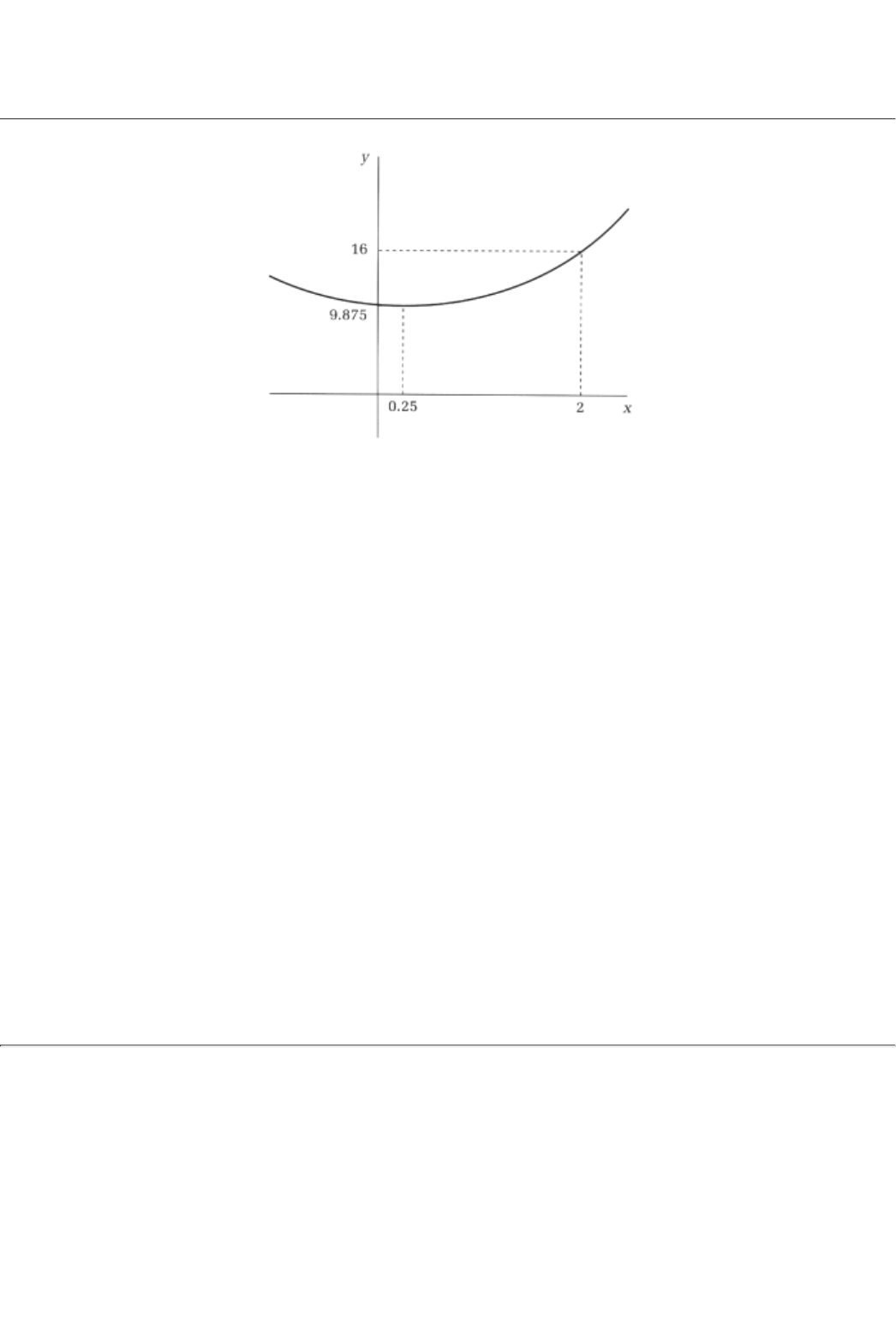
Proposition 2 (Sufficient Condition for a Maximum). If the slope of a concave function is zero at x*, then the
function attains a maximum at that point. If the function is strictly concave then there can be at most one
such point at which the slope is zero; that is, there is a unique maximum.
page_410
Page 411
FIGURE 25.5
25.2.3 Feasibility Constraints
In many economic contexts, there are constraints that have to be satisfied by the independent variable x. A
common one is that it cannot take on negative values. For instance, neither price nor quantity can be
negative. Another common constraint is that we can only pick those values of x for which yet another
function, say g, takes on nonnegative values. For example, in an investment problem we can only consider
strategies that generate a rate of return that is at least as high as the market rate.
Consider nonnegativity constraints first. When there are such constraints, the necessary condition for an
optimum needs to be modified somewhat. To see why this must be the case, consider the quadratic function,
y
= 10 - x - 2x2, Figure 25.6.
Note that we have drawn the graph only for nonnegative values of
x, that is, for x ³ 0. (The negative values
of x are graphed by a broken line.) As you can see, the highest value of the function (in nonnegative
territory) is achieved at x = 0, and at this point the slope of the function is not zero but rather it is negative.
What that observation tells us is that if we could, we would want to reduce the value of x even further [and
doing so would increase f(x)]. But of course we cannot. Put differently, the necessary condition for an
optimum now divides into two cases: If x* = 0, then the slope of the function at the optimum has to be less
than or equal to zero. All that we can say for sure is that if we increase x we will lower y. On the other hand,
if x* > 0, then the slope at that point has to be zero because if it is positive we will want to go forward and if
it is negative we will want to decrease x.
Indeed this idea can be generalized. Consider any set of feasibility constraints that puts limits on the values
of the independent variable; for example, suppose that 30 ³ x ³ 0. It should be clear that if the optimum x* is
strictly between 0 and 30, then
page_411
Page 412
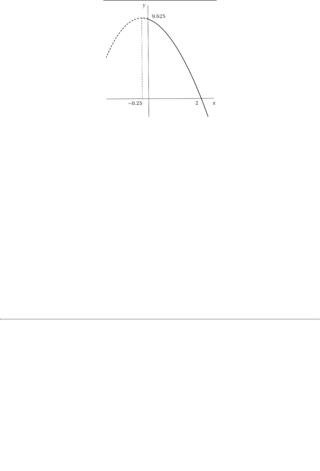
FIGURE 25.6
the slope of the function f has to be zero at that point. After all, we do have the room to either increase or
decrease x, and if the slope were not zero we would want to do one or the other in order to increase the
value of f. However, if the optimum is reached at either of the two corners, then the slope could be negative
(if x* = 0) or positive (if x* = 30). We call any x that is strictly in between the two corners, where neither
constraint is binding, an interior value of the variable.
And this statement is true even more generally: Suppose that x needs to satisfy another constraint such as
g
(x) ³ 0. Call a value of x interior if there is room to spare under this constraint as well, that is, if g(x) > 0.
We have the following condition:
Proposition 3 (Necessary Condition for a Maximum Subject to Feasibility Constraints). Suppose that x* is an
optimum that is interior relative to the constraints g(x) ³ 0 and a ³ x ³ 0, where a is some constant. Then the
slope at x* must be zero.
What about sufficient conditions? Suppose that f and g are both concave functions. Then one sufficient
condition is identical to that of the last subsection: if there is an x* that is feasible and at which the slope of f
is zero, then that x* is a maximum. Actually, for this problem there is even a slightly weaker requirement
that signals an optimum:
Proposition 4 (Sufficient Condition for a Maximum Subject to Feasibility Constraints). Suppose that f and g
are concave functions. Suppose too that we can find a feasible x* and a nonnegative constant l for which
two conditions are satisfied: lg(x*) = 0 and the
page_412
Page 413
slope of the sum function f(x) + lg(x) is zero. Then x* is a maximum. In particular, if the slope of f is zero at
x
*, then we have a maximum.
The special case in the last sentence follows because we can always set l = 0 if we already have the slope of
f
to be zero at some x*; thereby we will have satisfied the sufficient condition for a maximum.
25.2.4 Quadratic and Log Functions
Example 1
The quadratic function y = 10 + 8x - x2 has a slope function equal to 8 - 2x. Since the slope decreases in x,
this is a strictly concave function. There is a unique value of x*(= 4) at which the function has slope zero
(and this then is the unique maximum).
Example 2
Consider a sum function such as y = (10 + x - 2x2) + (7x - 17).
CONCEPT CHECK
CONCAVITY AND OPTIMUM
Show that each component of the sum is concave and hence so is the sum
function. Show that the slope equals 8 - 4x. Show finally that x* = 2. Why is
this a unique maximum for the function?
Example 3
Consider instead a sum function such as y = (10 + x - 2x2) - (7x - 17). Suppose we want to maximize this
function subject to the constraint that x ³ 0.
CONCEPT CHECK
CONSTRAINED OPTIMUM
Show that the slope of this function equals -4x - 6. Show that its unique
maximum is attained at x = 0? Is the slope 0 at that point?
Example 4: General Quadratic Example
Consider y = a + bx + cx2 (and c << 0).
page_413
Page 414
CONCEPT CHECK
OPTIMUM
Show that the first-order condition is b + 2cx* = 0. How would your answer
change if x is required to be nonnegative?
Example 5
Consider the function 2 log x - 8x.
CONCEPT CHECK
CONCAVITY AND OPTIMUM
Show that the function is strictly concave and the slope equals . Show
finally that . Why is this a unique maximum for the function?
Example 6
Consider y = log(30 - x).8 The slope of the function, applying the formula from the previous section, is
. As x increases, the denominator becomes smaller and hence the slope becomes more and more negative.
Put differently, the function is also concave. It attains a maximum at x = 0.
Summary
1. A dependent variable y takes its value from the values of an independent variable x. A function is a
mathematical representation of the relationship between an independent and a dependent variable.
2. A common example of a function is a linear function, y = a + bx, where a and b are constants. Examples
of nonlinear functions include quadratic and log functions.
3. The slope of a linear function is the ratio ; it equals the constant b. The slope of a nonlinear
function at x is the slope of the linear tangent to the function at that point.
4. A concave function is one whose slope decreases with the value of x.
8As we have said before, the log function is only defined for positive values of the independent
variable. In particular 30 - x therefore needs to be positive; that is, for this example we need to
restrict attention to x between 0 and 30.
page_414
Page 415
5. When there are no restrictions on x, if a function attains a maximum at x*, its slope must be zero at that
point. Conversely, if a concave function has slope zero at a point x*, then it must attain a maximum at that
point.
6. When x is constrained to be nonnegative, at a maximum x* > 0, the slope of the function must be zero.
Again if a concave function has slope zero at a point x*, then it must attain a maximum at that point.
Exercises
Section 25.1
25.1
Give three examples of variables. Indicate in each case why the value of the object is not constant.
25.2
Give three examples of constants. Indicate in each case why the value of the object is constant.
25.3
Give three examples of pairs of an independent and a dependent variable.
25.4
Graph the following linear functions:
a.
b.
c.
25.5
Graph the following quadratic functions:
a.
b.
c.
For the exercises that follow, whenever you see the function log x, assume that x > 0.
page_415
Page 416
25.6
Graph the following log functions:
a.
b.
c.
25.7
Compute the slope of the functions in the three examples of exercise 25.4. (Do not ap
ply the formula;
instead use the definition of the slope of a linear function, .)
25.8
Compute the slope of the functions in the three examples of exercise 25.5 at x = -3, x = 0, and x = 10. (In
these cases, do apply the formula for the slope of a quadratic function.)
25.9
For the three examples of exercise 25.5, graph the general formula for the slope as a function of x.
25.10
Compute the slope of the functions in the three examples of exercise 25.6 at x = 1, x = 5, and x = 100.
(Apply the formula for the slope of a log function.)
25.11
Compute the general formula for the slope for each of the following sum functions:
a.
b.
In each case also compute the specific value for the slope at x = 6 and x = 15.
25.12
Repeat exercise 25.11 for the following sum functions. (In each case, a through d refer to constants.)
a.
b.
25.13
Consider the following functions:
a.
b.
Find the slopes for the specific values x = 1, x = 5, and x = 100.
page_416
Page 417
25.14
Find the general formula of the slope of these functions:
a. 2 log x + log(100 - x), for x between 0 and 100
b. 2 log 5x + log(100 - x), again for x between 0 and 100
c. log x + log(2 + 3x - x2), for x between 0 and 3
In each case, also compute the specific values of the slope at x = 2.
25.15
Show that af(x) is also a concave function whenever f is a concave function and a is a positive constant.
25.16
Show that
af
(
x
) +
bg
(
x
) is also a concave function whenever
f
and
g
are concave functions and
a
and
b
are
positive constants.
25.17
Verify that the following functions are concave:
a.
b. log(100 - x), with x defined between 0 and 100
c.
25.18
Verify that the following functions are concave:
a.
b. log(80 - 16x) for x between 0 and 5
c. 51 log x
Section 25.2
25.19
By examining the general formula of the slope of the following functions, determine which values of x are
not points at which the function is at a maximum:
a. 2 log x + log(100 - x), for x between 0 and 100
b. 2 log 5x + log(100 - x), again for x between 0 and 100
c. log x + log(2 + 3x - x2), for x between 0 and 3
25.20
Find x at which the slope is equal to zero, for the following:
page_417
Page 418
a.
b.
25.21
Has your search in exercise 25.19 generated points of maxima? (Hint: Check for the concavity of the
functions concerned.)
25.22
Repeat exercise 25.21 for the functions in exercise 25.20.
25.23
Find the point(s) of maximum value for the following functions:
a.
b. log(80 - 16x) for x between 0 and 5
c.
25.24
Find the point(s) of maximum value for the following functions:
a. 2x + log(100 - x), for x between 0 and 100
b. -5x2 + log(100 - x), again for x between 0 and 100
c. 3x + log(2 + 3x - x2), for x between 0 and 3
25.25
Find the point(s) of maximum value for the following functions:
a.
b. log(100 - x), with x defined between 0 and 100
c.
25.26
Find the general formulas for the point(s) of maximum value for the following functions:
a.
b.
State precisely any restrictions that you need to place on the value of the constants.
25.27
In exercise 25.19, did you identify points of maxima that are interior? Explain.
25.28
Repeat exercise 25.27 for the functions in exercise 25.24.
page_418
Page 419
25.29
Find the points of maxima off subject to the constraints that x ³ 0 and g(x) ³ 0.
a. f = 2 + 3 log x and g = 2 + 3x - x2
b. f = 20 - 3x and g = 2 + 3x - x2
25.30
Repeat exercise 25.29 for the following functions:
a. f = 10 + log x + log(10 - x) and g = 10x - x2
b. f = 1 + x - x2 and g = 1 - x2
page_419
Page 421
Chapter 26
Probability and Expectation
Uncertainty plays a role in game theory for several reasons: players may be uncertain about whom they are
playing against or how the game is going to proceed, or they may be uncertain about what their opponents
are going to do, or they may wish to be uncertain about the exact action that they themselves might take (so
as to keep their opponents guessing).
In section 26.1 we will discuss the principal way in which uncertainty can be mathematically described.
Within this section we will also discuss a subtopic called independence and conditional probability. In
section 26.2 we will turn to a discussion of averages over uncertain events.
26.1 Probability
There is a common framework within which we can represent any uncertain situation, be it a lottery, a coin
toss, a course grade, the performance of a stock, the strategy of a rival, the outcome of a game, and so on.
There are three components to this common description: a sample space, an event space, and a probability
function.
A sample space contains a list of all possible outcomes to the uncertainty. For example in a coin toss the
sample space is {heads (H), tails (T)}; in a roll of a die, it is {1, 2, . . ., 6}; in a lottery, the sample space is
{win (W), lose (L)}; in the price of a stock when the price can only move by a sixteenth of a dollar-it is {
; n = 0, 1, 2 . . .} and so on. The sample space may have a finite or an infinite number of elements.
The event space is the set of subsets of the sample space; that is, each element of the event space is a set of
outcomes. In other words, an outcome is one possible way, and an event is one of several possible ways, in
which uncertainty may get resolved.
page_421
Page 422
To fix ideas, consider the four sample spaces described previously. For the coin toss, the associated event
space is (H, T, {H, T}, F.1 In the die roll, it is (1, . . ., 6, {1, 2}, {1, 3}, . . ., {5, 6}, {1, 2, 3}, (1, 2, 4}, . . .,
{4, 5, 6}, {1, 2, 3, 4}, . . ., F); the event {1, 2, 4}, for instance, should be interpreted as ''either 1 or 2 or 4
will come up when the die is rolled." Similarly, {4, 5, 6} describes the event that the outcome of the die roll
is at least as high as 4. For the lottery, the event space is (W, L, {W, L}, F). In each of these examples, the
event space is finite.
In contrast, the event space is infinite in the stock price example; it is, in fact, equal to an infinite number of
categories of possible outcomesall possible prices, all possible pairs of prices, all possible price triples, and so
on.2
Finally, a probability function, p(.), is an assignment of a fractional number to each event. This fraction
should be interpreted as the likelihood that the event in question will actually happen. This likelihood could
be an objective assignment, arising out of a description of the physical phenomenon; or it could be a
subjective likelihood, arising out of a player's beliefs about the way in which uncertainty might resolve itself.
For instance, in the first two examples, we could use the physical description of a coin toss or a die roll to
assign the appropriate probabilities.3 In the first example, for a fair coin, we will assign
, p(H
or T) = 1, p(F) = 0. Exactly the same objective approach would give us the following probability function for
the second example; p(any one number) = , p(either of any two numbers) = , . . ., p(any number at all) =
1,
p
(no number) = 0.
The assignment of probabilities in the third example would depend on the nature of the lottery. In a lottery in
which exactly one of, say, 1 million ticket holders wins, the probability probability of winning for the holder
of a single ticket is would have to be subjectively assigned if you did not know how many
other people also bought tickets to the lottery. In a slot machine, however, the chances of winning depend
only on the configuration of the machine and not on how many other people have played that machine.
Hence, the probability of winning is an objective probability.
The daily New York State lotto is an example of a lottery in which the likelihood of winning depends both
on objective factors and on how many other people are playing the lottery. The way this lottery works is the
following: In sequence, six balls are drawn from an urn full of numbered balls. The numbers associated with
these six balls constitutes the winning combination for the day. Each holder of a lottery ticket chooses six
numbers at the time he purchases his ticket. The winner of the lottery is the individual (if any)
1F is notation for the empty set, that is, a set that has no elements. By convention, all event spaces
include the empty set. Think of this as the possibility that "nothing will happen," in a coin toss, that
"neither H nor T will happen."
2You may have noticed that the event space is finite whenever the sample space is finite. Indeed the
converse is true as well; the event space is finite only if the sample space is finite.
3Another popular way to assign probabilitiesand this works for events that have been going on for a
long time like a series of coin tossesis to assign to each event the relative frequency of the observed
occurrence. In that case, the probability of getting a head on the next toss of the coin is taken to be the
fraction of the previous coin tosses that resulted in a head.
page_422
Page 423
whose picks match the numbers drawn later that day. If there are multiple matches, then the prize is shared.4
Subjective beliefs would be the appropriate way of assigning probabilities in the stock price example.
The probability function is required to satisfy two properties:5
1. The probability of the sample space is 1.
2. For any two disjoint sets E and F in the event space,
The first requirement is really a consistency condition. It says that all of the possible outcomes must be
included in the sample space. Since two events are disjoint if and only if they are mutually exclusive, the
second requirement says that the likelihood of one of two mutually exclusive events happening is the sum of
the likelihoods of each one individually happening.
To see these two properties at work, consider an event, say E, and its complement, say F (i.e., consider the
set F made up of all possible outcomes that are not in E). By definition, these two sets, E and F, are disjoint
and therefore, by property 2, p(E or F) = p(E) + p(F). However, it is also the case that between them, E and
F
cover all possible outcomes; that is, they cover the sample space. (Why?) Hence, by property 1, p(E) +
p
(F) = 1. Therefore, the probability of the complement of an event Ethat is, the probability of "not E"is 1 -
p
(E).
As another application, consider two events E and F that are not disjoint. What should be the probability
that either of these events will happen; that is, what should p(E or F) be? This probability is not p(E) + p(F)
because that would double-count the outcomes that are in both the events E and F. The natural thing to do
would be to count these outcomes once; either within E or F. To that end, denote F/E as the set of outcomes
in F that do not belong to E as well. Evidently, E and F/E are disjoint sets. Hence, by property 2, p(E or
F/E
) = p(E) + p(F/E). Note, furthermore, that the event E or F/E is really the same event as E or F. (Why?)
Collecting all this together, we have p(E or F) = p(E) + p(F/E).
Finally, let us apply all of the ideas of this section to a game. Consider the following simultaneous-move
game:
1 \ 2
L
C
R
U0,0 0,1 1,2
M1,0 1,1 1,1
D2,0 2,2 2,2
Suppose that there is uncertainty about exactly which strategies will be played by the two players. Consider
player 1. The sample space of his strategic uncertainty is,
4The drawing of numbers for the state lotto is conducted on television. For those of you in the New
York metropolitan area who wish to tune in, it is conducted every night during the 11 P.M. news
broadcast on the ABC affiliate, Channel 7. Prizes can range up to 14 million dollars.
5Two sets are said to be disjoint if they have no intersection. Two sets in the event space are disjoint if
there is no shared outcome between them. For instance the events (1,2,3) and (4,5) are disjoint.
page_423
Page 424
therefore, {U, M, D}; the event space is (U, M, D; {U, M}, (U, D}, {M, D}; {U, M, D}). The event D
means "D will get played," whereas the event {U, D} means "either U or D will get played," and the event
{U, M, D} means "any one of the three strategies will get played."
The probability function is an assignment of likelihoods to each of the seven possible events. Given property
2, one way to accomplish this purpose is to assign probabilities to the three outcomes and then "build up" the
probability of an event as the sum of the probabilities of all the outcomes contained in that event. For
instance, say player 1 is half as likely to play U as either M or D. In that case, , ;
, , and p({U, M, D}) = 1.
CONCEPT CHECK
PLAYER 2
Write down player 2's sample and event spaces. If player 2 is equally likely to
play her three strategies, write down the probability function.
Note that these two assignments satisfy the two requirements on the probability funct
ion. If we take the two
disjoint sets {U, M} and {D} for example, the probability that either of these events will happen{U, M} or
{D}, that is, {U, M, D}is exactly the sum of p({U, M}) and p(D).6
So far almost all of the examples that we have considered are those with a finite number of outcomes. It is
instructive sometimes to look instead at examples that involves an infinite number of outcomes.
To motivate such an example imagine that you draw a line 10 inches long on a piece of paper. Then you
close your eyes and place a pin at some random point on the line.7 Now the pin could be anywhere on that
line-at an inch from the beginning, 3.5 inches, 2.789 inches, or, as your measuring scale becomes more and
more accurate, at 7.9998 inches, 5.006748904 inches, and so on. In other words, any point on that lineand
there are an infinite number of themis a possibility. Furthermore, any point is just as likely as any other, or, if
you wish, any half-inch segment is just as likely to contain your pinpoint as any other half-inch segment.
This discussion can be formalized by the following probability assignment: Consider any segment between
the beginning and x inches from the beginning. It gets a probability assignment of . Hence the half line
between 0 and 5 inches has a probability assignment of , or 50 percent. The segment between 0 and 7.6
inches has an assignment of , or 76 percent; again this is exactly the fraction that it represents of the entire
line, and hence this is a natural assignment if you choose to place the pin with your eyes closed.
This probability assignment is called a uniform distribution; "uniform" refers to the fact that the uncertainty
is uniformly spread over all possible outcomes. More formally,
6The method by which we picked a probability function for the players' strategies can be applied to
any uncertain situation with a finite number of outcomes. To illustrate, suppose the sample space is
{sl, s2, . . ., sM} Pick an assignment of probabilities to the M outcomes, say, p1, p2, . . . ., pM. Then
given any event, say {s3, s8, s27}, the probability to be assigned to this event is p3 + p8 + p27.
7Okay, so it might take you a few tries before you actually land the pin on the line!
page_424
Page 425
if the outcomes to an uncertain occurrence can be given numerical values, and if these values lie between
two constants a and b, the assignment is said to be uniform if for any x between a and b, the probability of
the segment between aa and x is
26.1.1 Independence and Conditional Probability
Often we are asked to evaluate the likelihood that two specific events will occur in two resolutions of
uncertainty. For example, we may evaluate the likelihood that on two throws of a coin we will get an H
followed by a T, or that on two rolls of a die an even and then an odd number will turn up, or the stock price
will go up and then come down by . Let the two events be denoted E and F. The events are said to be
independent if and only if
If two events are not independent, they are said to be dependent. The first two examples in the preceding
paragraph are independent events. The third example may or may not be, and whether it is or is not will
depend on the underlying reason why the stock went up in the first place. If it went up because of a good
earnings report, then the events may not be independent; the likelihood that the stock will then go down is
not the same as the likelihood would have been without the earnings report.
In the game of the previous subsection, if the two players choose their strategies unilaterally, then the pair of
strategies are independent choices. For instance, suppose that player I chooses U, M, and D according to the
probabilities , , and and player 2 chooses between L, C, and R according to the probabilities , , and
(and they choose unilaterally). In that case the probability that the pair U and C gets chosen is , while
the probability that M and R get chosen is .
An example of dependent events comes from the nightly drawing for the New York State lottery. Recall that
from an urn full of balls, each of which carries an identifying number, balls are drawn in sequence and
without replacement. Suppose that there are a hundred balls in the urn. The likelihood that any one of them
will be drawn is therefore However, the likelihood that any pair of them will be drawn is not but
rather . (Why? See the discussion that follows if you are in doubt.) Another example is the likelihood
of reinjuring an already twisted ankle.
To deal with dependent events, we use the notion of a conditional probability. The conditional probability
that an event F will happen given that we know an event E has already happened is denoted . For
example, if the urn has six differently numbered balls in it, the conditional probability of drawing ball
number 6 if some other ball has already been drawn is , whereas if number 6 has already been drawn, the
conditional probability is 0. The likelihood that two dependent events E and F will both happen is then
page_425
Page 426
CONCEPT CHECK
COORDINATED DECISIONS
Suppose that in the simultaneous-move game of the preceding subsection the
two players coordinate their decisions: they toss a coin and if the coin comes
out heads, player 1 picks U and player 2 chooses C. If the coin comes out tails,
they respectively choose M and R. Compute
, , and . Also
compute , , and .
26.2 Random Variables And Expectation
In many instances it is convenient to think of the outcomes to uncertainty in a quantitative form. If we take
the outcomes and assign to each outcome a real number, we get what is called a random variable. For
example, outcomes to the roll of a die or the stock's price are (already numbered and therefore are) random
variables; they take on the values {1, 2, . . ., 6} and { ; n = 0, 1, 2, . . .}, respectively. In some instances,
a random variable may be the monetary reward associated with the uncertain outcomes. For example, if the
lottery costs a dollar to enter and the winnings total $14 million, then the monetary random variable that
describes the uncertainty of the lottery is +14 million and -1.
The expectation of a random variable is its average value. The formula for the average of a set of n numbers
is Notice that if a particular number, say 51, shows up twice in the set of numbers, then it gets added
twice in the total; that is, the average is Alternatively, the average equals
We can follow this procedure for every number that shows up in the total,
that is, weight it by the number of times it is included in the set of n numbers. Put another way, the
expectationor average-is a weighted sum of the (numbered) realizations, the weights being the associated
probabilities.
For instance, the expected value of the die roll is If
the probability of winning the lottery is then the expected value of the lottery is
.
Let us denote, in general, an outcome by the symbol to and the associated random variable by X(w). The
expectation of the random variable can then be formally written as8
To fix ideas, examine the game-theory example that was discussed earlier. Consider the two strategies: for
player 1, , , and for player 2, . Let us compute the expected
payoffs for player 1. Note first that,
8The notation means add up p(w) × (w) over all possible w.
page_426
Page 427
since the two players are choosing their strategies unilaterally, pairs of strategies are in fact independent
events. It follows, therefore, that p(U and C) = p(U) × p(C). Hence, . By extension, we have
Expected payoff of player
CONCEPT CHECK
PLAYER 2
Compute the expected payoff of player 2 (for the same pair of strategies).
26.2.1 Conditional Expectation
When two random variables are independent, knowing how one has occurred does not tell us much about
the likelihood of occurrence of the other. In particular, therefore, knowing what value the first random
variable took does not tell us anything about the expectation of the second random variable.
To illustrate this point consider two tosses of a coin. If we know that the first toss produced a head, we
would still expect that there is a 50 percent chance of a head on the second toss. And similarly, if we are told
instead that the first toss produced a tail. In other words, assigning, say, a numerical value of -1 to heads and
1 to tails, the expectation of the second toss is
and this expectation is the same regardless
of
whether the first toss produced heads or tails.
In contrast, consider drawing two balls, without replacement, from an urn containing five balls marked with
the numbers 1, 2, 3, 4, and 5. If the first ball that is drawn is marked 4, then the expected number from the
second drawing is
However, if the first ball drawn is 2, then the expectation of the second draw is
The reason why the two expectations were different is the fact that the two drawings are not independent
events but rather are dependent. Put differently, the conditional probabilities of the second draw are
different depending on whether the first draw yielded number 2 or 4.
Consider two random variables X(w) and Y(w) that are dependent, and denote the conditional probability of
Y given a particular value as ). Then the conditional expectation of the random variable Y is
denoted as
page_427
Page 428
Reark
To suggest the broadness of the framework described in this chapterand also to shorten verbal
descriptionswe often refer to any uncertain situation as a lottery. In other words, we refer to coin tosses, die
rolls, stock price movements, and strategy choices in a game by the common moniker lottery.
Summary
1. Any uncertainty can be represented by a triplea sample space, an event space, and a probability function.
2. The sample space is the set of all possible outcomes, whereas the event space is the set of all possible
groups of outcomes. The probability function assigns a likelihoodor probabilityto each event.
3. Two realizations of uncertainty are independent if the probability of the pair of events is the product of
their individual probabilities.
4. The expectation of a random variableor its averageis the weighted sum of the numbered outcomes, the
weights being the probabilities attached to each outcome.
Exercises
Section 26.1
26.1
Give three examples of uncertain situations with a finite number of outcomes.
26.2
Give two examples of uncertain situations with an infinite number of outcomes.
26.3
For exercise 26.1, in each case carefully list the outcomes and the consequent possible events.
page_428
Page 429
26.4
Repeat exercise 26.3 for exercise 26.2 (although you will obviously not be able to list all the possible
outcomes and events!).
26.5
For exercise 26.1, assign a probability function to each example. Explain whether the assignment is being
made objectively or subjectively.
26.6
Repeat exercise 26.5 for the examples in exercise 26.2.
26.7
Suppose that the set F is the complement of E. Why must it be true that between them, E and F cover all
possible outcomes, that is, they cover the sample space?
26.8
Explain why the event E or F/E is really the same event as E or F. Does your answer depend on the fact of
E
and F being nondisjoint? Explain.
26.9
Detail the arguments that establish the following property:
In the following exercises consider the game that was considered in the chapter.
26.10
Find the probability assignment in which player I is just as likely to play each of his three strategies. (Be sure
to assign probabilities to every event.)
26.11
Find the probability assignment in which player I is three times as likely to play U as each of his other two
strategies. (Be sure to assign probabilities to every event.)
26.12
Find the probability assignment in which player 2 is three times as likely to play C as each of his other two
strategies. (Be sure to assign probabilities to every event.)
26.13
Consider the uncertainty associated with the hair color that the basketball player Dennis Rodman will exhibit
on any given night. List the sample and event spaces (okay, color combinations are also allowed). How
would you assign a probability function to this uncertainty? How would Dennis Rodman?
page_429
Page 430
26.14
Consider the uncertainty associated with drawing a card from a deck of cards. List the sample and event
spaces (you do not have to list all possibilities but list the categories). How would you assign a probability
function to this uncertainty?
26.15
Consider a uniform distribution between the two values 0 and 1. What is the probabili
ty that
x
lies between 0
and ? What then is the probability that x lies between and 1? What is the probability that x lies between
any two fractions, a and b?
26.16
Draw a graph with the value of x on the horizontal axis and the probability assignment to numbers between 0
and x, under the uniform distribution of exercise 26.15, on the vertical axis.
26.17
Repeat exercise 26.16 for a uniform distribution between the two values 0 and 10.
26.18
Explain why the likelihood that any pair of balls will be drawn out of an urn full of 100 balls is not
but rather is .
26.19
Suppose the balls are drawn with replacement; that is, after a ball has been drawn it is thrown back into the
urn before the next number is drawn. Explain why the likelihood that any pair of balls will be drawn out of
an urn full of 100 balls is now .
26.20
Give an example of a pair of events that is independent. And one of a pair that is not.
Consider again the game in the chapter. Let us write its table with probabilities instead of payoffs; that is, the
probability in the cell (U, C) represents the probability that player 1 will play U and player 2 will play C:
1 \ 2 L C R
U0
M 0
D
26.21
What is the probability that U will get played? (Hint: What are the possible combinations of strategies that
include U?)
page_430
Page 431
26.22
Find the conditional probability of L given U. Repeat with the conditional probability of C given U.
26.23
Find the conditional probability of U given C. Repeat with the conditional probability of M given C.
Section 26.2
Consider the game yet again, but now with the payoffs restored to the matrix:
1 \ 2 L C R
U0,0 0,1 1,2
M1,0 1,1 2,1
D2,0 1,2 2,2
26.24
Consider the two strategies: for player 1, , , and for player 2, .
Compute the expected payoff of player 2.
26.25
Consider instead the following two strategies: for player 2, , , and for player 1,
. Compute the expected payoffs of both players.
26.26
Suppose that player I plays U while 2 plays L, C, and R with probabilities p, q, and 1 - p - q. Compute player
1's expected payoff (your answer will involve the two variables p and q).
26.27
What is player 2's expected payoff from the strategies of the previous question? At what values of p and q
does player 2 derive the greatest expected payoff?. Explain.
26.28
Repeat exercises 26.6 and 26.27 for the case in which player 1 plays M instead.
26.29
Suppose that a random variable can take on one of three values, 0, , and 1, and suppose that all three
values are just as likely. What is the expectation of this random variable?
26.30
Repeat exercise 26.29 for the case in which the random variable can take on any one of seven values, 0, ,
, . . ., 1.
page_431
Page 432
26.31
Can you use your answer in exercises 26.29 and 26.30 to conjecture the expected value of a random
variable that is uniformly distributed between 0 and 1? Explain your answer.
26.32
What about the expectation of a random variable that is uniformly distributed between 10 and 20?
26.33
Consider drawing two balls, without replacement, from an urn containing five balls marked with the numbers
1, 2, 3, 4, and 5. If the first ball drawn is marked 3, compute the expected number from the second drawing.
26.34
Repeat exercise 26.33 for a first draw that produces the number 5 ball.
26.35
Consider drawing two balls, without replacement, from an urn containing five balls marked with the numbers
2, 2, 3, 4, and 4. If the first ball drawn is marked 3, compute the expected number from the second drawing.
26.36
Repeat exercise 26.35 for a first draw that produces a number 2 ball.
page_432
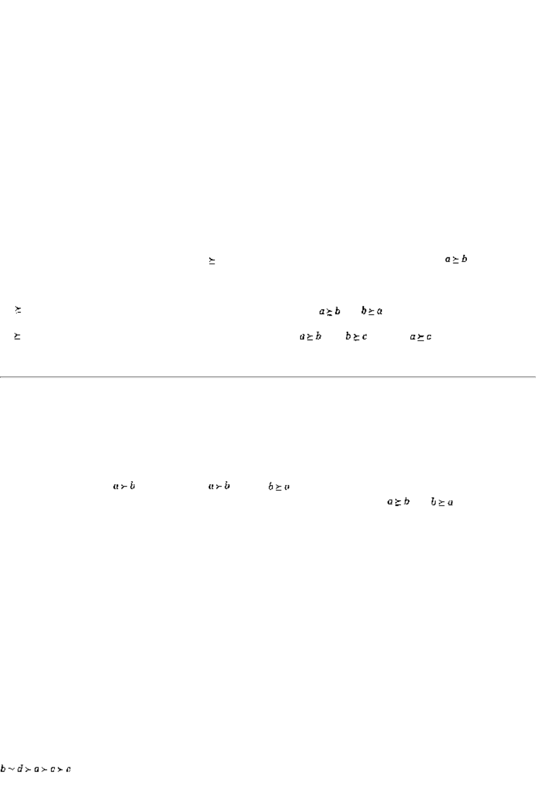
Page 433
Chapter 27
Utility and Expected Utility
In this chapter we will discuss how a player faced with a multiplicity of choices might go about assigning
payoff or utility numbers to each choice. The task of finding the best choice can then be reduced to the task
of locating the highest utility number. We will proceed in three steps: first, in section 27.1, we will review
the theory of utility assignments under certainly. Then, in section 27.2, we will use the conclusions of the
certainty model to build a theory of utility assignments under uncertainty, that is, a theory of decision
making over lotteries. In section 27.3 we will demonstrate how to apply the conclusions of the uncertainty
model to analyze a player's attitudes toward risk.
27.1 Decision Making Under Certainty
In this section we will ask, If there are a number of possible optionsor outcomesand they are exactly known,
how should a player choose between them?
Let the outcomes be denoted a, b, c, and so on. The starting point is the idea of a preference relation over
outcomes. A preference relation, denoted , is a comparison between any two outcomes: '' " should be
read as "the outcome a is at least as good as the outcome b." We impose the following rationality postulates
on the preference relation:
1. satisfies completeness; for all outcome pairs a and b, either , or , or both.
2. satisfies transitivity; for all outcome triples, a, b, and c, and implies .
page_433
Page 434
Completeness says we cannot reply "I do not know" when confronted with a comparison between two
outcomes. Transitivity is a little more demanding because it rules out cycles of the form: "I like doctor a
because of his politeness (over doctor b); I like b more than c because she is more knowledgeable; and
actually between a and c, I prefer c since his clinic is closer to my home."1
From the at-least-as-good-as relation we can derive the "strictly better than" relation: outcome a is strictly
better than b (denoted ) if and only if but not . One can also define an "indifference" relation:
the decision maker is indifferent between outcomes a and b (denoted a ~ b) if and .
When there are an infinite number of possible outcomes, some of the alternatives may be very close to each
other. In such a case preferences need to satisfy one other requirement, called continuity:2
3. If all of the outcomes al, a2, a3, . . . are at least as good as b and the chain collapses onto a, then a must
be as good as b.
How then can we make decisions? Let us start with the choice between a finite number of outcomes. One
procedure is simply to work through pairs of choices: compare a and b, then compare the winner to
alternative c, then compare the winner of the second contest against alternative d, and so on. Since
preferences are complete, each of these comparisons yields a winner.3 Since preferences are transitive, we
will never be caught in a cycle, and eventually we will have an overall winner. This is a somewhat
cumbersome procedure, especially when the number of outcomes is large. What we would like to do more
simply is assign a number (called utility) to each possible outcome and choose the outcome that has the
largest number.
Under the three restrictions there is, in fact, a way to assign utility numbers and (when there are an infinite
number of outcomes) to do so in a continuous fashion. It is easy enough to see why this must be the case,
under restrictions I and 2 by themselves, when there are only a finite number of outcomes. Suppose there are
five outcomes, (a, b, c, d, e), and let us suppose that
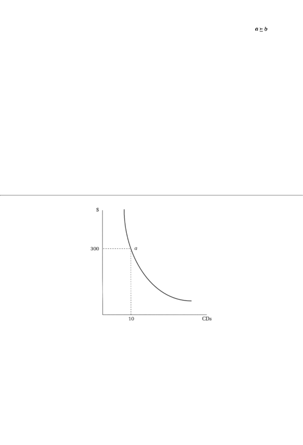
One way to assign utilities is to decide on an origin and a scale of assignment, for example, u(e) = 1, and
each strictly better outcome gets one point more (whereas indifferent outcomes get the same number). So
one possible assignment is (3, 4, 2, 4, 1).
A utility assignment u(.) is consistent with the preferences if for any two outcomes a and b, if and only
if u(a) ³ u(b). It is clear that there are multiple consistent utility assignments to the same preferences. For the
preceding preferences, for example, we could change the origin to 10 and the scale to 5 and get another
consistent assignment: (20, 25, 15, 25, 10). Actually even more is true: we need not even have the same
scale; another consistent assignment is (30, 55, 2, 55, 1). In other words any monotone function of the
original assignment is also a consistent utility assignment.4
1Put another way, all of these factorspoliteness, knowledge-ability, distance, and so onare already
incorporated in the preference relation. They play a role in determining whether or not a is at least
as good as b, but they cannot lead to ranking reversals. Also note that preferences can change over
time; a may be preferred to b today but may not have been a year ago. Completeness and
transitivity are only required of preferences at any one point in time.
2Note that a chain a1, a2, a3, . . . is said to collapse onto a if for large values of n the outcomes an are
very close to a. More precisely, the difference between an and a approaches zero as n approaches
infinity.
3In the case of a tieor indifferencepick either alternative.
4A function f is said to be monotone if f assigns a higher value f(xj), greater than f(xi), if and only if xj
itself is bigger than xi.
page_434
Page 435
FIGURE 27.1
When there are an infinite number of outcomes, the approach to utility assignment is qualitatively similar. As
a first step we can bracket with alternative a all choices that are just as good as a. Such a set of alternatives
is called an indifference set or indifference curve. Consider Figure 27.1. On the horizontal axis is the
quantity of some object, say, the number of CDs. On the vertical axis is the money left over to buy other
things. For instance, the alternative a corresponds to monthly purchases of 10 CDs with a remaining budget
of $300 (to spend on clothes, and movies, and . . .). The indifference curve through a includes all options
that are just as good as a.
Then we can rank various indifference curves. Since there are an infinite number of alternatives, each
indifference curvelike the one in Figure 27.1may have an infinite number of choices within it. Furthermore,
there may be an infinite number of indifference curves. For instance, the whole picture for the CDs-money
indifference curves might look something like Figure 27.2.
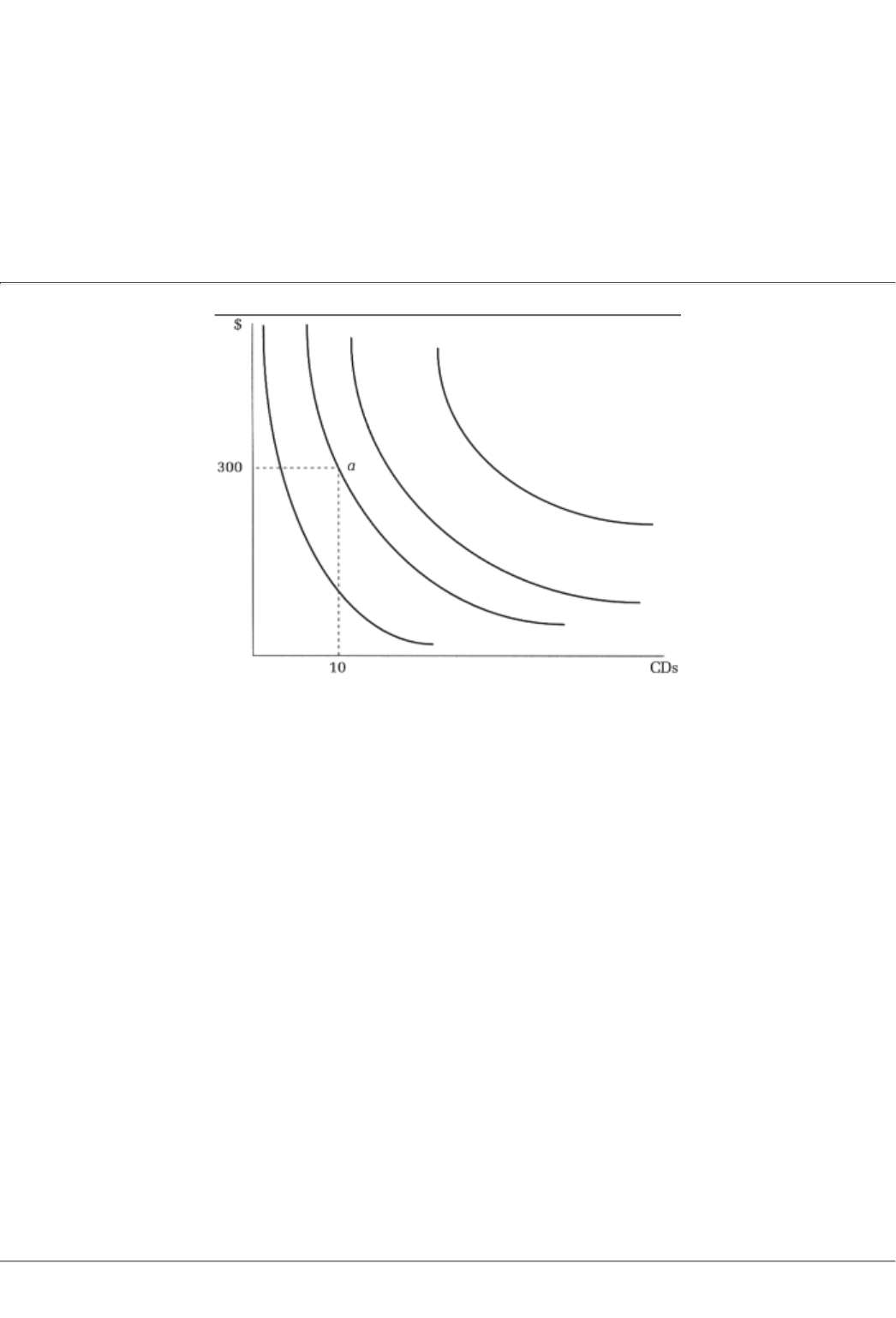
Each level of indifference curve gets a utility number; higher indifference curves ge
t higher numbers. Hence
the utility assignment will be a function (like the ones we saw in Chapter 25). Given the continuity
restriction, 3, we will in fact be able to assign nearby indifference curves utility numbers that are themselves
close to each other.
Hence the decision-making problem can be restated as, For any consistent assignment of utilities, find the
outcome that has the largest utility number; that is, solve the following optimization problem:5
maxw u(w)
5Recall that we introduced the notation w in the previous chapter to denote outcomes.
page_435
Page 436
FIGURE 27.2
When the set of outcomes is finite we can search by hand r use some algorithmto find the outcome that
corresponds to the highest utility. When the number of outcomes is infinite, then we can use the techniques
of optimization theory that we outlined in Chapter 25 to isolate the best choice.
27.2 Decision Making Under Uncertainty
We now turn to decision making under uncertainty. The alternatives are now uncertain; that is, they are
lotteries. Here is an example:
Lottery A: Buying (scalper's) tickets for a New York Knicks game that could cost 20, 25, 30, or 35
dollars with equal probabilities
Lottery B: Staying in and studying for the game theory midterm exam, which could raise your score
by 5, 10, or 15 points with probabilities .5, .4, and .1
Lottery C: Going to the West End Gate bar, watching the Knicks on television, and drinking beer
(which is going to cost you a sum of $10).6
The question for this section is, How should a decision maker analyze the relevant uncertainty and choose
between the various lotteries? In the next subsection we will state
6Notice that there is no uncertainty in this third alternative. However, we can think of it as a
lottery that assigns probability 1 to the outcome going to the bar, and assigns probability 0 to all
other outcomes.
page_436
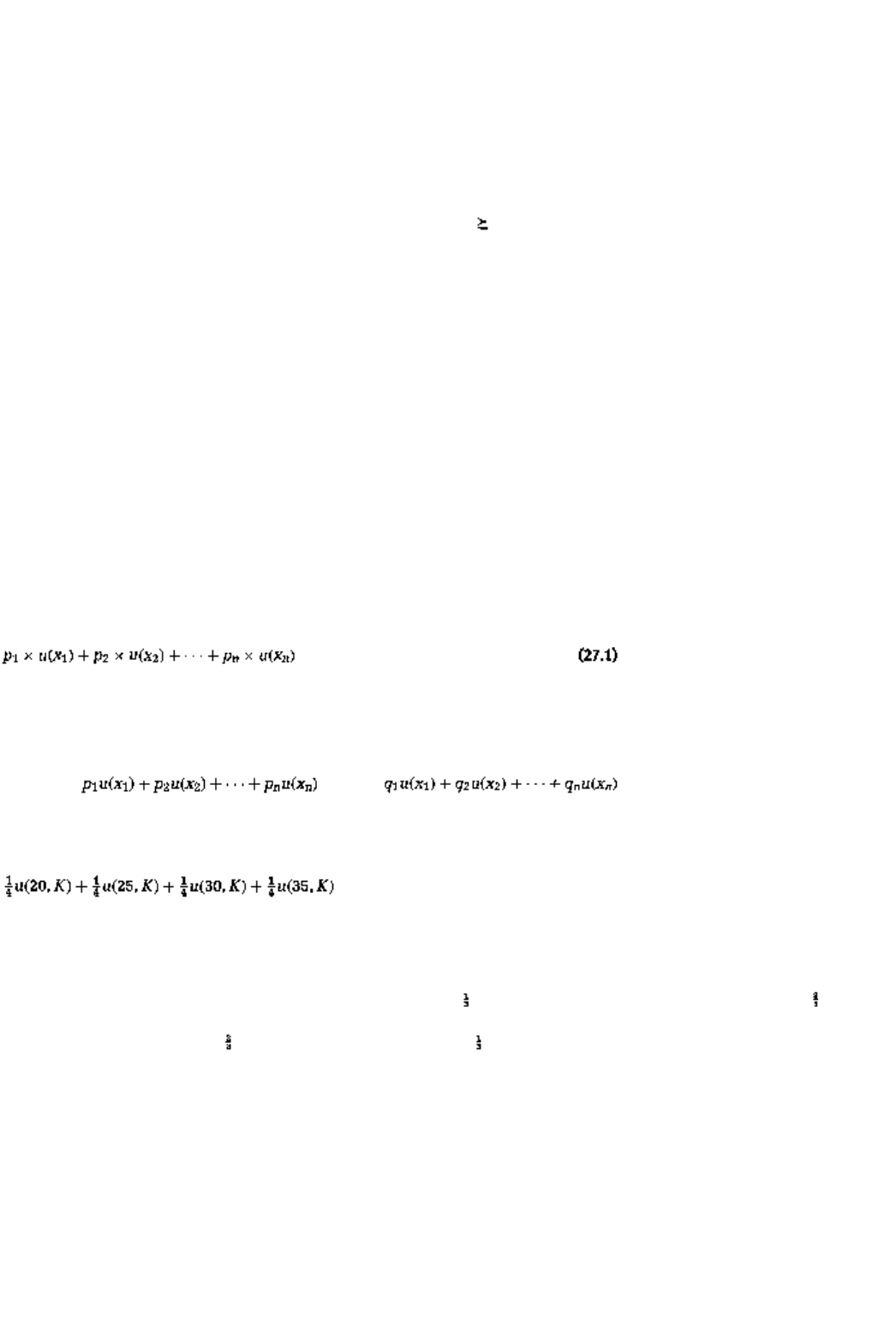
Page 437
a first version of the answer, called the expected utility theorem, and in the following subsection we will
sketch a proof of that result.
27.2.1 The Expected Utility Theorem and the Expected Return Puzzle
One possible way to proceed is to assume that the decision maker has a preference relation directly over
lotteries so that she is able to assert something like "I prefer lottery A to lottery C, but between lotteries A
and B, I am indifferent." If that relation is complete, transitive, and continuous, then we know from the
previous section that there is a continuous utility representation for it. In other words, there is a utility
function, say U, defined over lotteries such that lottery A lottery C if and only if U(A) ³ U(C). We could
then simply pick the lottery with the highest utility number.
A utility function over lotteries is conceptually cumbersome, and many people have trouble articulating such
preferences in a consistent way. For example, the way alternatives are framed can become very important
for such an articulation.7 Furthermore, a lottery does have a special structureit is a probability distribution
over possible outcomes. So the question is, Can the utility function over lotteries be deduced from a utility
function over the outcomes (under some additional restrictions)? In the present example, there is a utility
function, say u, that attaches a utility number to the outcome "seeing the Knicks game at $25 a ticket" as
also to the outcome "5 more points in the midterm exam."8 The question is, Can preferences over the
different lotteries be deduced from u?
Von Neumann and Morgenstern proved the following remarkable result:
Expected Utility Theorem I. A utility function over any lottery can be written as the expected utility of the
outcomes that make up this lottery (under some reasonable additional restrictions).
Suppose we have a lottery with n possible outcomes x1, x2, . . . , xn, and an associated list of probabilities for
each outcome. Denote this list pl, p2, . . . , pn. The theorem says that the utility of this lottery is equal to the
expected utility9
This is a remarkable result because it greatly simplifies the comparison of different lotteries. Although each
lottery is characterized by the whole list of probability numbers, the utility of this long list can be reduced to
just one number, namely, the expected utility. For instance, suppose we want to compa
re the lottery pl, p2, .
. ., pn with another one that has probabilities q1, q2, . . ., qn, then all we really need to compare are the two
numbers, versus .
For instance, the expected utility assignment to lottery Atickets for a Knicks game that could cost 20, 25, 30,
or 35 dollars with equal probabilitiescan be written as
7Two psychologists, Daniel Kahneman and Amos Tversky, have made this point in many contexts.
An example is the following two pairs of lotteries:
Pair 1: 600 people are struck with a disease that could kill. Vaccine I will save 400 for sure, while
the second will either save no one (with probability ) or will save everyone (with probability ).
Pair 2: Again 600 people are struck with a disease that could kill. Vaccine 1 will kill 200 people for
sure, while 2 implies a chance no one will die and a chance that everyone will.
Note that the two pairs of alternatives are identical decision situations (since "save" is equivalent
to "not kill"). In experiments most people chose vaccine 1 in the first pair but vaccine 2 in the
second!
8 For future use, denote the utility number to seeing the Knicks at ticket prices 20, 25, 30, and 35
dollars, respectively, u(20, K), u(25, K), u(30, K), and u(35, K). Denote the utility numbers to staying
in, studying for the midterm, and increasing the score by 5, 10, and 15 points, respectively, u(5, S),
u(10, S), and u(15, S). Finally, denote the utility number to watching the Knicks at West End Bar for 10
dollars by u(10, W).
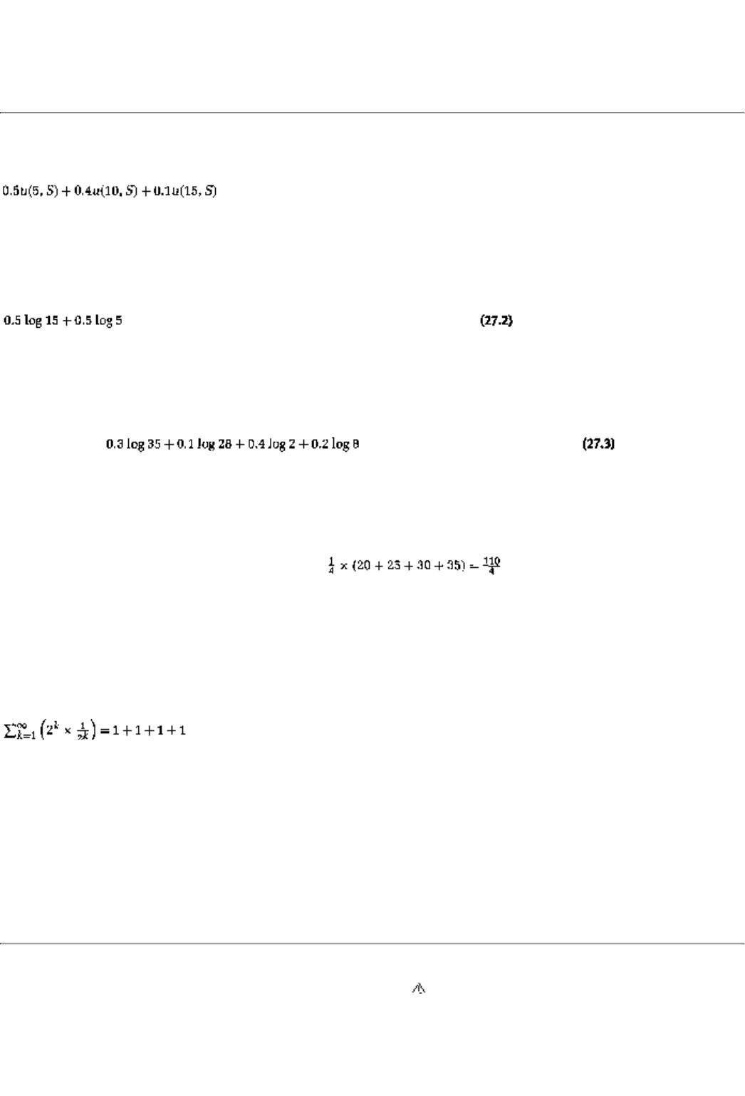
9Strictly speaking, the result says that there exists a utility function u, defined over the possible
outcomes, such that equation 27.1 holds. This more correct version is stated as Expected Utility
Theorem II on page 440.
page_437
Page 438
Similarly, the expected utility assignment to lottery Bstay in and study for the game theory examis
Finally, the utility assignment to the lottery Cgo to the West End Gate baris simply u(10, W).
Let us illustrate with yet another example. Suppose that the outcomes are monetary; so x is a dollar figure.
Suppose furthermore that the utility function over outcomes is given by u(x) = log(10 + x). Then a lottery
such as "Win $5 if heads, lose $5 if tails" has expected utility equal to
CONCEPT CHECK
EXPECTED UTILITY
Show that the lottery "Win $25 with probability 0.3, win $18 with probability
0.1, lose $8 with probability 0.4, and lose $2 with probability 0.2" has
expected utility equal to
The utility function u is called the Von Neumann-Morgenstern utility function.
Before getting to a detailed discussion of the Von Neumann-Morgenstern theorem, let us discuss why we
cannot simply define the utility of a lottery as the expectation of the random variable associated with the
lottery For instance, for lottery A, why does it not suffice to set u(20, K) = 20, u(25, K) = 25, and so on, and
hence compute the utility of the lottery itself as ? Similarly in the case of monetary
lotteries, why not simply compute the expected monetary return?
The reason is that if we only evaluated lotteries according to their expected returns, we would run into some
apparent inconsistencies in behavior. Perhaps the most famous instance of such an inconsistency is the St.
Petersburg paradox
(due to Nicholas Bernoulli).10 Consider the following lottery: a coin is tossed
repeatedly The first time H comes up, a payment is made; if the first H is at the kth toss, the payment is 2k
dollars. How much would you be willing to pay for this lottery? The same question, put differently, is, What
is the utility value of this lottery? Note that the expected monetary return of this lottery can be written as
. . . So the expectation is infinite. Does that fact mean we would pay an infinite
sum to play this lottery? Most people would not do so. Put another way, expected return is not a good utility
representation for many preferences. (More on this topic in the next section.)
10There is some controversy about who exactly was the first one to propose the St. Petersburg
paradox. It might have been the brother of Nicholas Bernoulli, the equally brilliant Daniel
Bernoulli, or it could have been the mathematician Leonhard Euler. The reason for the place name
in the paradox is that around 1725 these three Swiss scientists were all invited to work at Catherine
the Great's newly established St. Petersburg Academy of the Sciences. Daniel Bernoulli was the
first one to propose a solution to the paradox; we will see this solution in the next section.
page_438
Page 439
27.2.2 Details on the Von Neumann-Morgenstern Theorem
To explain what follows,11 it is important to distinguish between simple and compound lotteries. A simple
lottery is what we have so far called a lottery: uncertainty over a set of outcomes. A compound lottery is
one whose outcomes are lotteries themselves. For example, a coin is tossed, and if it comes out H you get
the simple lottery A whereas if it comes out T you get the lottery B; this compound lottery is denoted
. More generally, a compound lottery (denoted aA + (1 - a)B) has probability a that the outcome will
be a simple lottery A and probability 1 - a that it will be B instead.
An example of a compound lottery is the following: You go to a Knicks game, and the ticket will cost you
either 20, 25, or 30 dollars (with equal probabilities) if you arrive early, whereas if you arrive late, the ticket
will cost you 25, 30, or 35 dollars with probabilities , , and . There is a probability that the number I
or number 9 subway that you take to Madison Square Garden will be late.
Every compound lottery can be reduced to a simple lottery. In this example, the "real" probability
distribution is over the outcomes, ticket prices of 20, 25, 30, and 35 dollars. In particular, the probability that
you will in fact pay $25 can be decomposed into two events: you get to the game early, and then there is a
probability that you pay $25 for your ticket, or you get to the game late, and then there is probability that
this is the ticket price. Furthermore, there is a probability that you will get to the game early. Hence, the
probability of buying your ticket at $25 is
CONCEPT CHECK
PROBABILITIES
Show that the probabilities of buying the ticket for 20, 30, and 35 dollars are,
respectively, , ,and .
One restriction on preferences that we will soon discuss is that a decision maker is always indifferent
between a compound lottery and the associated simple lottery. That is, the basketball fan in the example is
indifferent between the compound lottery and a simple lottery with probabilities , , , and of buying
the ticket for 20, 25, 30, and 35 dollars, respectively.
For simplicity, we will also make the following assumption: there is a best and worst outcome, denoted
respectively b and w; it is preferable to have b for sure rather than any lottery. Likewise, any lottery is
preferable to having w for sure; that is, b any lottery w. As we saw earlier in this chapter, a sure
eventthe outcome x will happen with probability 1an be thought of as a lottery as well: denote it w (x).
Finally, a simple lottery with outcomes x and y, with probabilities a and I - a, respectively, will be written as
aw(x) + (1 - a)w(y).
11This subsection is a little complicated, and hence you may wish to skip it on first reading. Make
sure, though, to understand the conclusionthe Von Neumann-Morgenstern expected utility
theoremand be sure to read the section itself sometime during the semester.
page_439
Page 440
Von Neumann-Morgenstern Restrictions
Von Neumann and Morgenstern require preferences over lotteries to satisfy the following restrictions (in
addition to completeness and transitivity):
3. Monotonicity: Consider lotteries with outcomes b and w only. The preference between them is based
solely on the likelihood of b:
4. Archimedean: For any intermediate outcome a there must be a lottery over b and w that is just as good as
a; there is a such that
5. Substitution: If two lotteries are equally good A ~ B, then for all lotteries C,
6. Compound lotteries are equivalent to a simple lottery with the same distribution over final outcomes.
The complete statement of the theorem is as follows:
Expected Utility Theorem II. Under these restrictions there is a utility representati
on u over sure outcomes
such that lottery A is at least as good as lottery B if and only if the expected utility to lottery A is at least as
high as the expected utility to lottery B.
Sketch of the Proof
Consider any outcome x. By virtue of the Archimedean axiom there is a lottery over the best and worst
outcomes, u(x)n(b) + [1 - u(x)]n(w) that is just as good as the sure outcome (u(x) is therefore a probability).
We can repeat this exercise for an alternative outcome, say y, and find the corresponding number u(y) (such
that y is just as good as the lottery u(y)n(b) + [1 - u(y)]n(w)].
By virtue of the monotonicity axiom, the two lotteries u(x)n(b) + [1 - u(x)]n (w) and u(y)n(b) + [1 -
u(y)]n(w) can be compared by looking at the two numbers u(x) and u(y) alone. Indeed the first is better than
the second if and only if u(x) > u(y). In turn, this fact says that the outcome x is better than y if and only if
u(x) > u(y). (Why?) Put differently, the numbers u(x), u(y), and so on are exactly like utilities over the sure
outcomes x and y. (Why?)
Now take a lottery A and suppose for simplicity that it is made up of the two outcome
s x and y (with
probabilities p and I - p, respectively). By virtue of the substitution axiom, A is just as good as the compound
lottery that yields the simple lottery u(x)n(b) + [1 - u(x)]n(w) with probability p and u(y)n(b) + [1 - u(y)]n(w)
with remaining probability 1 - p. (Why?) By the compound lottery restriction, this compound
page_440
Page 441
lotteryand hence the original lottery Ais equivalent to the simple lottery
Notice that the weight attached to the outcome b is the "expected utility"
pu(x) + (1 - p)u(y). Consider an
alternative lottery B and suppose that it is also made up of the two outcomes x and y (with probabilities q
and 1 - q, respectively). A repetition of all these steps will yield that B is equivalent to the simple lottery
Equations 27.4 and 27.5 essentially prove the theorem. These are two simple lotteries over the best and
worst outcomes. By virtue of monotonicity they can be ranked by looking at the weight attached to the
outcome b, that is, by comparing pu(x) + (1 - p)u(y) and qu(x) + (1 - q)u(y). But that is the same thing as
saying that lottery A is better than B if and only if pu(x) + (1 - p)u(y) > qu(x) + (1 - q)u(y). (Why?)
27.2.3 Payoffs in a Game
In any game that we study in this text, the payoffs are Von Neumann-Morgenstern utilities. The payoff to a
game that has uncertain outcomes, then, is the Von Neumann-Morgenstern expected utility. The Von
Neumann-Morgenstern utilities are the entries in the matrix representation of a two-p
erson game in strategic
form or the entries at the terminal nodes of a tree in the extensive form.
27.3 Risk Aversion
Whenever there is uncertainty, a decision maker is exposed to risk. A natural question to ask is, (When)
Does the decision maker prefer not to be so exposed? It will turn out that whenever the Von Neumann-
Morgenstern utility function u is concave the decision maker will be averse to risk. Hence, risk attitudes will
be seen to be already embedded in the utility function u.
In this section we will only consider lotteries whose outcomes are dollar figures. Consider the following pair
of lotteries:
Lottery A: Win $1 if heads, lose $1 if tails
Lottery B: Win $5 if heads, lose $5 if tails
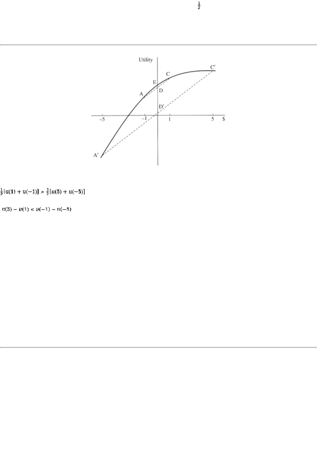
The two lotteries have the same win (and loss) probabilities, that is, . What distinguishes them is that the
amount that can be won (or lost) is smaller for lottery A than B. This is a special case of more general
conditions under which we can say that lottery A is less risky than lottery B.
page_441
Page 442
FIGURE 27.3
The first lottery will be preferred to the second if and only if its expected utility is greater, that is, if
. In turn this inequality can be written as
Whether or not that inequality is valid depends on the slope of the utility function u; the inequality holds if
the rate of change in utility between -5 and -1, u(-1) - u(-5), is greater than the rate of change between 1 and
5, u(5) - u(1). Hence if the decision maker's preferences are such that an additional $4 is worth lessin utility
termsif he already has $1, than an additional $4 is worth when he only has -$5, then he should go with the
first, less risky, lottery. Put differently still, if additional money yields less and less utility as he grows richer,
then he would prefer the less risky alternative. This is equivalent to saying, If u is concave, go with less risk.
Another way of seeing the same thing is by means of a graph. We will first demonstrate how to represent
expected utility graphically. Consider Figure 27.3. Point A corresponds to the utility level u(-1), that is,
corresponds to losing $1. Similarly, point C corresponds to the utility level u(1), that is, corresponds to
winning $1. After the uncertainty of the first lottery has resolved itself, the decision maker will find himself
either at A or at C. Before the uncertainty is resolved, however, he does not know which of these points he
might end up at. He does believe, though, that he is just as likely to be at A as at C; hence his expected, or
average, utility should be halfway between A and C, namely, halfway on the line segment between A and C,
that is, at D.
page_442
Page 443
By the same logic the expected utility of the second lottery is given by D'. The graph now tells you that D is
higher than D'; that is, the first lottery is the preferred one. The reason is precisely that the amount of utility
loss, A down to A', is bigger than the amount of utility gain, C up to C', exactly as we saw algebraically
before.
Indeed we can go further and ask how the lotteries compare to a situation in which there is no uncertainty.
Note that for both of these lotteries the decision maker expects to break even. After
all, he wins the same
amount that he loses, and winning and losing are equally likely. So the certainty situation is that in which he
gets $0 for sure, that is, does not gamble. It should be straightforward to see from Figure 27.3 that this option
(point E) is even better (than either lottery).
This example can be generalized. Recall that for a lottery A in which the outcomes are x1, x2, . . ., xn with
probabilities, respectively, of p1, p2, . . ., pn the expected return of this lottery, denoted EA, is
Suppose that this decision maker's Von Neumann-Morgenstern utility function u is strictly concave. A
consequence is that no matter how complicated a lottery you consider, having the expected return EA for
sure is always strictly preferred to the lottery A. In fact, one can show that the converse is true as well. If
the expected return EA for sure is strictly preferred to the lottery Aand this is true for all lotteriesthen the
underlying function u must be strictly concave.
Risk aversion
A preference for the sure outcomethe expected return of a lotteryover the
lottery itself.
Hence here is a definition of risk avoidanceor risk aversion: if a decision maker prefers the expected return
of every lottery to the lottery, he is said to be risk averse. Equivalently, he is said to be risk averse if his Von
Neumann-Morgenstern utility function is concave.
One example of a concave utility function, is u(x) = log x. With these preferences, the St. Petersburg
paradox can be resolved. Notice that in this case the expected utility is given by
It can be shown that this sum is finite. In particular, therefore, a person with these preferences would not be
willing to pay an infinite sum of money to participate in the St. Petersburg gamble. The intuition for this
result is straightforward. A risk-averse person gets less and less utility from additional winnings at high
wealth levels. In particular, the expected utility of the kth payout, , becomes smaller as k increases.12
Hence, the cumulative prospect of large winnings does not add up to infinite utility.13
We should note that there are two other alternatives to risk aversion. A player is risk neutral if the expected
utility of a lottery is nothing but its expected return. Alternatively, such a decision maker must have a utility
function u(x) = x.
12In fact the sum is finite because the ratio of the (k + 1)th term to the kth is roughly , that is,
when k is large. Hence the sum behaves much like the geometric series, (which is
known to be finite).
13Daniel Bernoulli was the first person to offer a resolution to his brother's paradox; he suggested
that a better representation of preferences toward large sums of money is the log utility function.
page_443
Page 444
If an additional $1 gives a greater increase in utility as the current level of wealth increases, then we have
risk-loving preferences. Whereas risk aversion implies that a lottery whose expected return is zero is never
accepted (over the alternative of not playing the lottery), the converse is true for risk-loving preferences. In
particular, a risk-loving decision maker would pick lottery B in the choice scenario.
Summary
1. The basic building block of decision making is a preference relation ; if outcome a is at least as good as
outcome b, we write .
2. If the preference relation is complete, transitive, and continuous, then it can represented by a continuous
utility function u that has the property that if and only if u(a) ³ u(b).
3. An uncertain situationor lotteryis a probability distribution over a set of out-comes. In making choices
between lotteries, a decision maker in principle has to take account of the entire distribution as well as the
outcomes themselves.
4. Under some reasonable restrictions, Von Neumann and Morgenstern showed that the utility of a lottery
can be written as the expected utility to the outcomes that make up the lottery.

5. A risk-averse decision maker always prefers to have the expected return (of a monetary lottery) to the
lottery itself. Risk aversion is equivalent to having a concave utility function over the lottery's outcomes.
Exercises
Section 27.1
27.1
Give two examples of a decision problem under certainty.
27.2
Transform the same examples into problems under uncertainty. In each case carefully detail the space of
outcomesand the lotteries over these outcomes.
page_444
Page 445
27.3
Take the sample space of this chapter's various evening entertainmentsKnicks at alternative prices, staying in
and studying, and drinking at the West End Barand write your preference relation over that space. Are your
preferences complete and transitive?
27.4
Repeat the previous question for one of the two examples that you gave in exercise 27.1.
27.5
Explain carefully why any monotone function of a utility assignment is also a utility assignment (which is
consistent with the underlying preferences). Consequently, provide two utility assignments for your
preferences over the entertainment outcomes.
27.6
Repeat exercise 27.5 for the examples you gave in exercise 27.10.
27.7
Suppose sports teams in a league like the NBA are ranked by their winning percentage (i.e., the fraction of
games that each team has played that it actually won). Is this ranking complete and transitive? Explain.
27.8
Suppose instead that team a is ranked above team b if and only if a has won more than half of its games
against b (and they are said to be indifferent if they have split their games). Is this ranking complete and
transitive? Explain.
We now move to infinite numbers of choices. Suppose the choices are to be made over pairs of CDs and
sums of money.
27.9
Let alternative a correspond to 10 CDs and $300. Draw the indifference curve that includes a if this person
is always willing to trade a CD for $10.
27.10
Draw the whole set of indifference curves for these preferences, assuming the same willingness to trade.
27.11
Denote CDs by the symbol c and money by the symbol m. Show that one possible utility function for these
preferences is

page_445
Page 446
27.12
Find a monotone function of the preceding utility assignment that is consistent with the preferences.
27.13
Suppose instead that the utility function is given by
Draw a representative indifference curve.
27.14
Suppose that the decision maker has $500 to spend and CDs cost $12. Show that the available CD-money
options can be written in terms of the following budget equation:
27.15
Use the previous equation to substitute into the utility function of equation 27.6. Consequently derive a
utility function that depends on c alone.
27.16
Solve for the utility-maximizing choice of CDs.
27.17
Repeat exercises 27.15 and 27.16 for the utility function given by equation 27.7.
27.18
Repeat exercises 27.16 and 27.17 for a price of CDs equal to $8.
Section 27.3
Consider a utility function over dollars x defined as u(x) = log(10 + x).
27.19
Compute the exact value of the expected utility of the two lotteries, lottery A and lottery B, discussed in the
text.
27.20
Suppose that we compare the two lotteries with a third lotterywin either $13 or $16 with probability each
and lose $4 with the remaining probability. How do the three lotteries rank?
page_446
Page 447
27.21
What is the sure outcome that is just as good as the lottery introduced in exercise 27.20?
27.22
Repeat exercises 27.20 and 27.21 for the case in which the utility over outcomes is instead given by 10 + x.

Consider the following simultaneous-move game (where the payoffs in each cell are the
Von Neumann-
Morgenstern utilities for that pair of strategies):
1 \ 2 L C R
U0, 0 0, 1 1, 2
M1, 0 1, 1 2, 1
D2, 0 1, 2 2, 2
27.23
Suppose that player 2 plays the strategy L. Compute player 1's expected payoff from playing a strategy that
picks each of her strategies with equal probability.
27.24
Repeat exercise 27.23 for player 2 playing R instead.
27.25
Repeat exercises 27.23 and 27.24 with player 1 playing U or M with equal probabilities and D with half that
probability.
27.26
Find player 2's expected payoffs in exercises 27.24 and 27.25.
27.27
Suppose that each player is equally likely to play each one of her strategies. Compute their expected
payoffs.
The next few questions fill in the details of the proof of the expected utility theorem.
27.28
Explain why the two lotteries u(x)d(b) + [1 - u(x)]d(w) and u(y)d(b) + [1 - u(y)]d(w) can be compared by
looking at the two numbers u(x) and u(y) alone [and furthermore that the first lottery is better than the
second if and only if u(x) > u(y)].
27.29
Show that the outcome x is better than y if and only if u(x) > u(y). Establish that the numbers u(x), u(y), and
so on are exactly like utilities over the certain outcomes.
page_447
Page 448
Now take a lottery
A made up of the two outcomes x and y (with probabilities p and 1 - p, respectively).
27.30
Show that A is just as good as the compound lottery that yields the simple lottery u(x)d(b) + [1 - u(x)]d(w)
with probability p and u(y)d(b) + [1 - u(y)]d(w) with remaining probability 1 - p.
27.31
Show that two lotteries can be ranked by looking at the weight attached to the outcome b, that is, by
comparing pu(x) + (1 - p)u(y) and qu(x) + (1 - q)u(y).
Section 27.4
Consider the pair of lotteries analyzed in section 27.3.
27.32
Redo Figure 27.3. Carefully show why the expected utility of the second lottery is at D'.

27.33
Show that the expected return to both lotteries is $0.
27.34
What is the utility of the sure option $0 on your figure? Can you explain algebraically why this sure option is
better than the first lottery?
27.35
Graph the expected utility of the lottery ''Win $10 and lose $10 with equal probabilities."
27.36
Repeat exercise 27.35 for the lottery "Win $10 with probability and lose $30 with probability ." Can you
tell from your graph which of these two lotteries, this one or the one in exercise 27.35, would be preferred?
Explain.
Consider the following pair of lotteries:
Lottery A: $1,000 if die rolls 6 or 1, $0 otherwise
Lottery B: $0 if die rolls 6, $400 otherwise
27.37
Compute the expected monetary return for each lottery. Show that they are equal.
page_448
Page 449
27.38
Under what conditions is the expected utility to the second lottery higher (than that to the first)?
27.39
Can you show that a risk-neutral decision maker must have a utility function u(x) = x?
page_449
Page 451
Chapter 28
Existence of Nash Equilibria
The most widely used solution concept in game theory (and this book) is Nash equilibrium. We used it
extensively in Part II when we analyzed strategic form games and their applications. A refinement of Nash
equilibrium, subgame perfect (Nash) equilibrium, was the main solution concept in Part III's extensive form
game analysis. Another refinement, Bayes-Nash equilibrium, was the principal solution tool for the games of
incomplete information in Part IV. Since Nash equilibrium turns out to be such an important idea, it is worth
asking whether we always know that one exists. The answer to that question is the content of this chapter.
Section 28.1 reviews definitions and examples and emphasizes the role of mixed strategies for the existence
question. We will introduce a relevant piece of mathematics called fixed-point theorems in section 28.2 and
apply it to Nash equilibrium existence in section 28.3. Throughout this chapter we will try to convey
mathematical ideas and results in a comprehensible way even at the risk of occasionally being somewhat
imprecise.
28.1 Definition And Examples
Let us recall the definition of a Nash equilibrium (NE), and allow explicitly for mix
ed strategies; as usual, a
pure strategy is thought of as a special case of a mixed strategy.
Consider a game with N players, i = 1, . . ., N. A mixed strategy for player i is a probability distribution Pi on
his pure strategies, and a representative pure strategy is si. In principle, the number of pure strategies could
be infinite.1
1An example of a game where there are an infinite number of pure strategies is the Cournot
duopoly game, Similarly, there are an infinite number of pure strategies in the commons problem.
page_451
Page 452
Definition. A vector of mixed strategies constitutes a Nash equilibrium if each player's
strategy is a best response to the array of other players' strategies; that is, if for all players i,
where is the notation for the expected payoff to the mixed strategy vector .2
Before proceeding any further, let us recall two games and directly compute the Nash equilibria in each.
Example 1: Squash
Player 1 \ Player 2 Forward (F) Backward (B)
Front (f)20, 80 70, 30
Back (b)90, 10 30, 70
The first conclusion is about pure-strategy equilibria:
CONCEPT CHECK
NO PURE NE
Verify that there are no pure-strategy Nash equilibria in the game of squash.
A mixed-strategy equilibrium is given by player 1 playing f with probability while player 2 plays F with
probability . When player 2 plays this mixed strategy, the expected payoff to player 1 from either of her
pure strategies is . Hence playing f with probability is a best response for player 1.
CONCEPT CHECK
MIXED NE
Verify that the exhibited strategy is a best response for player 2. Also show
that this is the unique mixed-strategy Nash equilibrium of the game.
A second example is the following modification to Battle of the Sexes:
2Hence, .
page_452
Page 453
Example 2: Modified Battle of the Sexes
Husband \ Wife Football Opera Home
Football3, 1 0, 0 0, 0
Opera0, 0 1, 3 0, 0
Home0, 0 0, 0 2, 2
In this game there are three pure-strategy Nash equilibria: (
F, F
), (
O, O
), (
H, H
). There are also four mixed-
strategy Nash equilibria; three of these involve each player mixing over pairs of pure strategies, and a fourth
involves mixing over all three pure strategies. In this example, therefore, there is an embarrassment of riches
in that there are many Nash equilibria to choose from.
To summarize, the two examples tell us that there is always at least one Nash equilibrium in a gamepossibly
only in mixed strategies. There may, however, be more than one such equilibrium. In the next two sections
we will see that the conclusions of these examples are actually very general.
28.2 Mathematical Background: Fixed Points
In this section two ideas are discussed: first, it is shown that Nash equilibria are mathematically equivalent to
something called fixed points of the best-response functions, and second, it is argued that fixed points exist
for certain kinds of functions.
In order to understand the first idea, we need some notation. Let Ri(p1, P2, . . ., PN) denote player i's best
response to the strategy choice of the other players, p-i = p1, p2, . . ., pi-1, pi+1, . . ., pN.3 An alternative
definition of a Nash equilibrium is the following: is a Nash equilibrum if for every player i=1, . .
., N,
Equation 28.2 simply says that a Nash equilibrium is an array of strategies that no player would like to
change. (The converse is also true; if no player wants to change his strategy then we have a Nash
equilibrium.) Take any candidate for a Nash equilibrium, say , apply to it the best-response
function
, and produce the strategy array . As equation 28.2 makes clear, a Nash
equilibrium is a fixed point of the best-response function; if we start with a Nash equilibrium strategy array
and apply the best-response mapping, then we remain fixed at that point.
The search for a Nash equilibrium can therefore be reformulated as the search for a fixed point of the
best-response functions. This formulation is useful because there is a very well developed theory in
mathematics that deals with the question "When does a function, say f, that maps a set X into X, have a fixed
point?" In other words, under what conditions on the function f and the set X, is there always an x* such that
x
* = f(x*)?
3If there is more than one best response for player i, then Ri should be thought of as a set of
strategies, each of which is a best response. We will first discuss the case where them is a unique
best response [and Ri(p1 p2, . . . pN) is that best-response strategy].
page_453
Page 454
We will not discuss the most general version of these fixed-point results because they involve mathematics
beyond the scope of this book. However, what we will do is very informally discuss two results for the
special case where the set X is a subset of the real line. In order to have a fixed point, two conditions need to
be satisfied:
1. The set X has to be compact and convex.
2. The function f has to be continuous.
A set is compact if (a) it is not unboundedly large and (b) there is no element outside the set that is arbitrarily
close to elements within it.4 Let us see, by way of some examples, what these conditions mean. A set that
has unboundedly large elements is the set of all real numbers at least as large as 0; this set is denoted [0, ¥).
Conversely, a set that has no unbounded element is the set of all real numbers that are at least as large as 0
but no larger than 1; this set is denoted [0,1].
An example that has an element outside the set arbitrarily close to elements within it is the set of all real
numbers between 0 and 1 not including either of the end points; this set is denoted (0, 1). Neither of the end
points is in the set, and yet each of them is arbitrarily close to elements of the set; 0, for example, is
arbitrarily close to
(for sufficiently large values of the integer n). In contrast, [0, 1] is a set where condition
b holds. No matter which element outside this set we pick, say 1.1, there is nothing
in the set that is less than
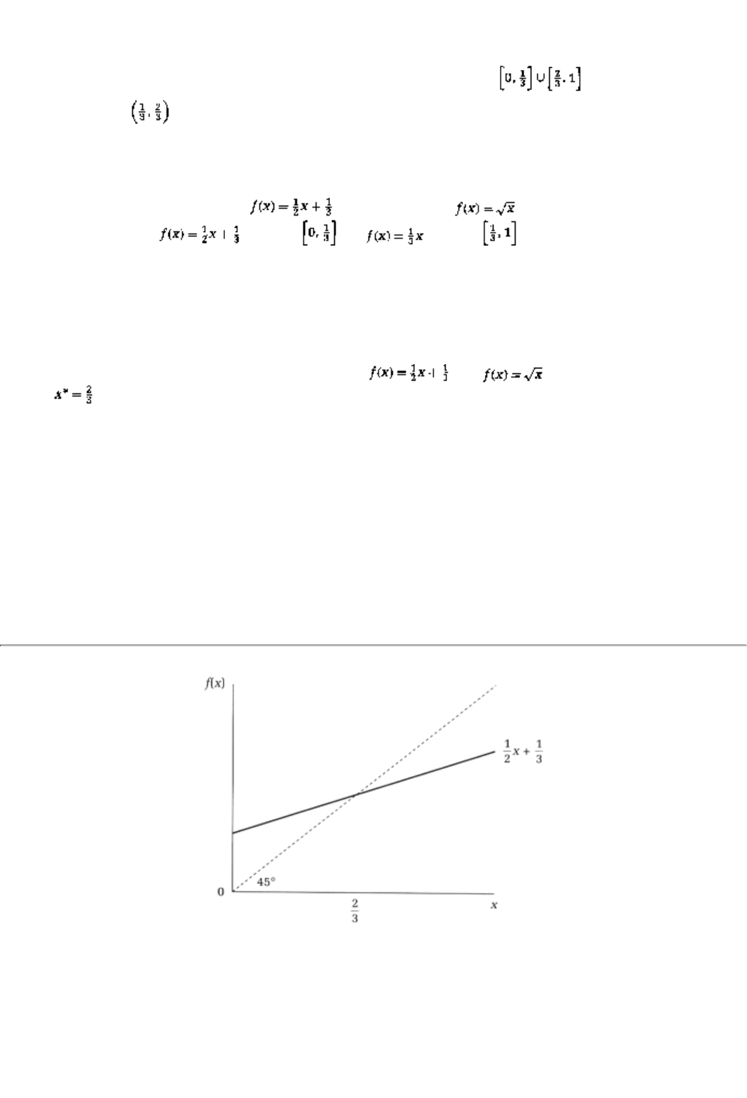
a distance of 0.1 from this point.
So, [0,1] is a compact set while neither [0, ¥) nor (0, 1) is compact.
A set X is convex if it does not have any holes in it. For example, the set is not convex because
it does not contain which is therefore a hole in the set. On the other hand, the set [0,1] is a convex
set.5 In fact, the only sets in the real line that are convex are sets of the form [a, b], that is, sets that contain
all numbers between a and b.6
A function f is said to be continuous if it has no jumps in it; you can draw the function without taking your
pencil off the page. So the function, and the function are continuous functions.
However, the function for x in but for x in is not continuous.
A fixed-point result that is widely used is the following:
Theorem (Brouwer). Suppose that X is a compact, convex subset of the real line. Suppose further that f takes
values in X and is a continuous function. Then there is a fixed point of f; that is, there is x* such that x* =
f
(x*).
Consider X = [0, 1] and the two continuous functions and . In the first case, the fixed
point is , whereas in the second case there are two fixed points, x* = 0 and x* = 1. (Show these results
algebraically, and also see Figures 28.1 and 28.2.)
4For those with some background in real analysis, all we are saying is that a set is compact if it is
bounded and closed. For those who do not have this background but are frustrated by the (lack of)
detail that we can provide here, hunt down a real-analysis or advanced-calculus text such as W.
Rudin's Principles of Mathematical Analysis (New York: McGraw-Hill, 1983).
5Again, for further discussion look at a real-analysis or a convex-analysis text.
6It is not important whether the end points are in the set or not. In other words, the set (a, b) which
does not include either end pointis also a convex set.
page_454
Page 455
FIGURE 28.1
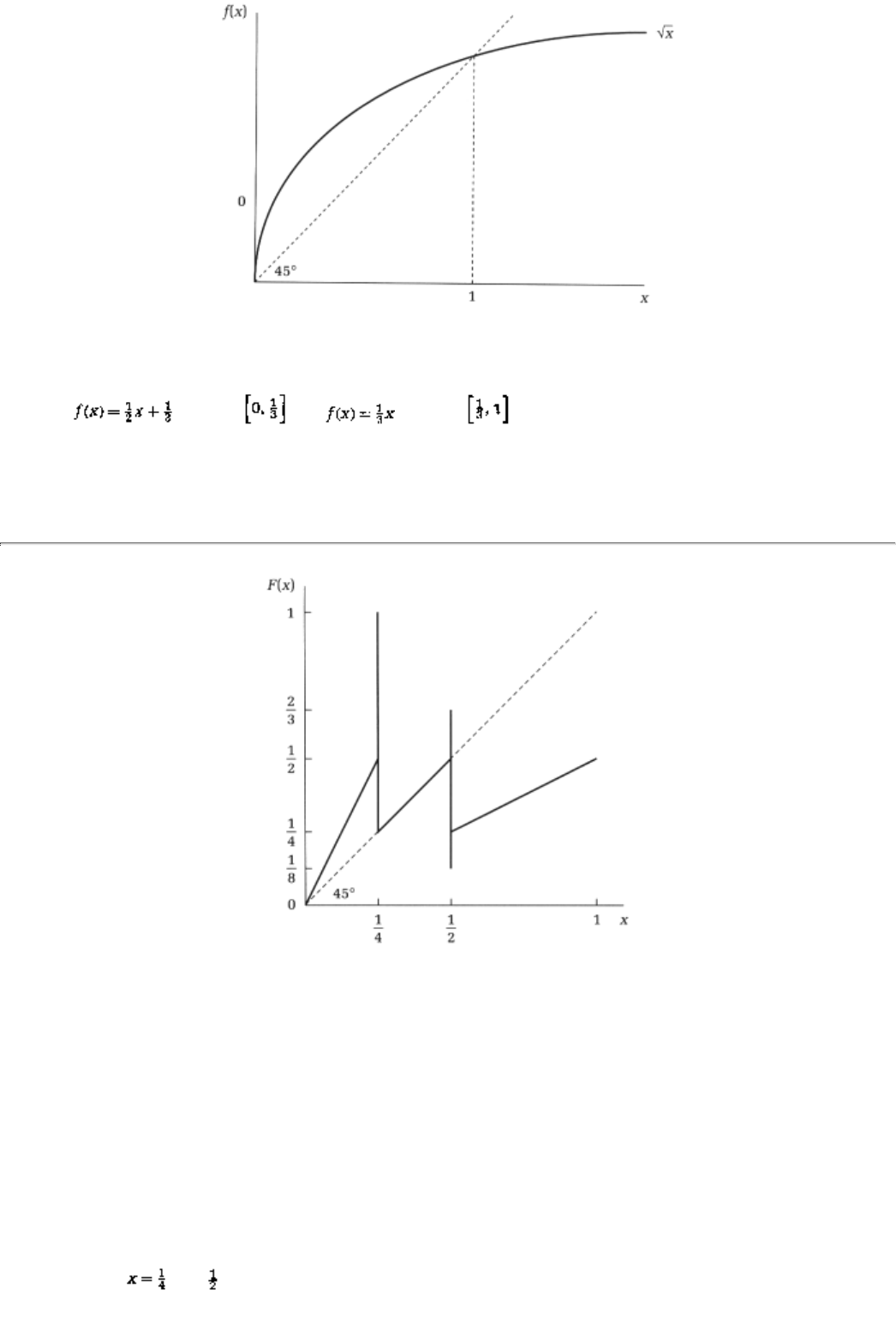
FIGURE 28.2
The reason why these conditions play an important role in the theorem can be seen by asking why there
might not be a fixed point if any of the conditions are violated. For example, consider the discontinuous
function for x in but for x in . This function does not have a fixed point.
Similarly, we can find examples of noncompact and nonconvex sets, including the ones given here, on which
continuous functions do not have fixed points. (In the Exercises you will be producing a number of these
examples.)
page_455
Page 456
FIGURE 28.3
In most games, there are certain strategies of the other players against which player i has not one but
multiple best responses. When that is the case the best-response function will no longer be a (single-valued)
function but rather will be multivalued. Hence we will need a fixed-point result that applies to multivalued
functions. There is a very close cousin of the Brouwer fixed-point theorem that then becomes relevant. This
result is called the Kakutani fixed-point theorem. We present this result next.
In order to explain the result, we have to formally define a multi-convex-valued function. Thankfully this
object is exactly what it says it is: F is a multi-convex-valued function if at every x we get as the dependent
variable not a single number but rather a convex set of numbers F(x). The fact that an independent variable
produces a set of dependent values is the multivalued part of the terminology. The fact that this set is convex
is the convex-valued part. Since a single point is also trivially a convex set, it means that at many values of x,
F
(x) can be akin to an ordinary function, that is, may be single-valued.
As an example of a multi-convex-valued function, consider Figure 28.3. F is defined on [0, 1]. At all values
of x other than and , F(x) is a single point:
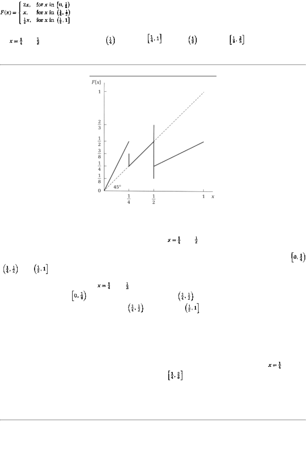
At and , F(x) is multivalued; F is equal to , while F is equal to
page_456
Page 457
FIGURE 28.4
Although F is no longer single-valued, it is still possible to define a notion of continuity. Before we do so
formally, though, let us motivate the idea by discussing Figure 28.3. Notice that as long as we stay away
from the two values of x where the function is multivalued, and , we can just use the notion of
continuity that applies to an ordinary function; can we draw the graph without taking a pencil off the page?
Since the answer is yes, we know that there are three continuous segments corresponding to x values in
, , and .
The potential complications are at and . However, we can ask, Is it possible to get from the
continuous segment over to the continuous segment over without the pencil leaving the page?
{And likewise can we move from x values in to x values in without jumps?} If the answer to
both questions is yes, then the multi-convex-valued function is (upper semi-) continuous. And of course our
example is,
The same idea can be applied to any multi-convex-valued function. If the single-valued segments are
continuous and if it is possible to travel the multivalued segments without taking a pencil off the page, then
we say that a multi-convex-valued function is (upper semi-) continuous.
The modification of F in Figure 28.4 is not upper semicontinuous. Note that when you arrive at you
need to leave the function because it jumps down to the set .
We will say that F takes values in the set X if F(x) is a subset of X for all x. The fixed-point theorem is as
follows:
page_457
Page 458

Theorem (Kakutani). Suppose that
X
is a compact, convex subset of the real line and that
F
is a multi-
convex-valued function that takes values in X. Suppose further that F is an upper semicontinuous function.
Then there is a fixed point of F; that is, there is x* such that x* is in the set F (x*).
28.3 Existence Of Nash Equilibria: Results And Intuition
The existence theorem that John Nash proved in the early 1950s is the following:
Theorem (Nash). Suppose that a game has a finite number of strategies for each player. Then there is at least
one Nash equilibrium (possibly in mixed strategies).
As with Brouwer's and Kakutani's theorems, we will not attempt to prove Nash's theorem. However, the
logic is straightforward enough to convey, especially in light of our discussion in the previous section. The
set of mixed strategies turns out to be both compact and convex. Note that when a player has only two pure
strategies, his mixed strategies are completely described by the probability with which he plays the first of
his pure strategies. Hence the set of mixed strategies is given by the set [0, 1]. And this set is, as we saw,
compact and convex. The same logic carries over even when a player has more than two pure strategies.
The best-response function is a multi-convex-valued function. This is the case because either of two things
must be true for a player's best response. Either there is a unique best response; that is, we have a single-
valued function (and that is trivially also a multi-convex-valued function). Or, if a player has two best
responses, then, as we saw in Chapter 8, any average of these best responses is also a best response; that is,
any convex set that includes the two as the end points is also a best response. Finally, the best-response
function also turns out to be an upper semicontinuous function. Hence, by Kakutani's fixed-point theorem,
the best-response function has a fixed point; put differently, there is a Nash equilibrium.7
Recall that games such as matching pennies and squash have no Nash equilibria in pure strategies; they only
have Nash equilibria in mixed strategies. The reason that we cannot assert that there is always a Nash
equilibrium in pure strategies is that the set of pure strategies is not convex; hence, the fixed-point result
does not guarantee an equilibrium in pure strategies.
Let us now turn to infinite number of strategies. We will give you some additional conditions under which a
game with an infinite number of strategies will not only have an equilibrium but will have one in pure
strategies.
7The careful reader will have noted that the set of mixed strategies X (in our earlier notation) is
not a subset of the real line. However, Kakutani's and Brouwer's fixed-point theorems can still be
used, since they do in fact apply to sets more general than just those in the real line.
page_458
Page 459
Theorem. Suppose that each player's pure strategy set is [a, b], where a and b are two constants, and that
each player's payoff function is continuous and strictly concave in his own pure strategy. Then there is at
least one pure-strategy Nash equilibrium of the game.
The fixed-point theorem that applies here is Brouwer's theorem. We restrict attention only to pure strategies
now. The set of such strategies is convex and compact because they are of the form [a, b]. The
best-response function turns out to be single-valued because the payoff function is strictly concave.8 This
function is also continuous. Hence there is a fixed point of the best response function; that is, there is a Nash
equilibrium.
This last result is applicable to the Cournot model and the commons problem.
What we will do now is give you some further feel for Nash's theorem by working out in detail the
best-response function and hence the Nash equilibrium in the following game:
1 \ 2 L R
U1,0 2,3
D0,2 4,0
CONCEPT CHECK
NO PURE NE
Check that there is no Nash equilibrium in pure strategies in this game.
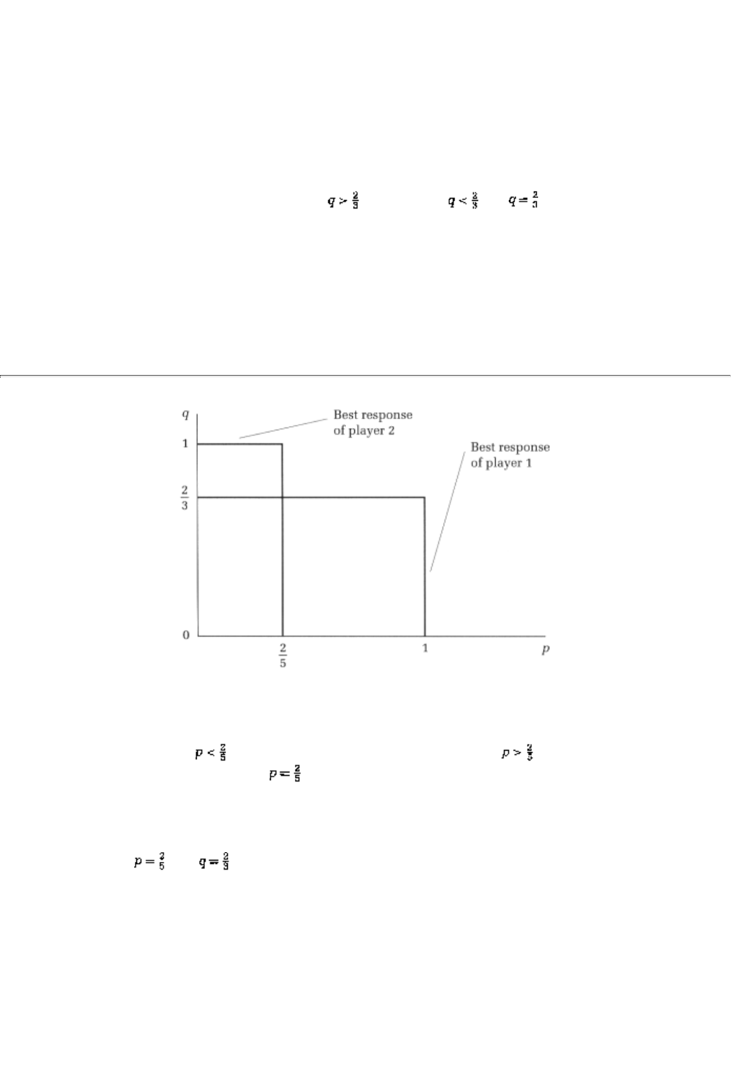
Now let us consider mixed strategies; for player 1, all mixed strategies can be descr
ibed by the probability
with which the strategy U is played; call this probability p. Likewise, for player 2, all mixed strategies can be
described by the probability with which L is played; call that q.
Best Response Mappings
Since a player will play one of her pure strategies if either of them is a best response by itself (and will play a
mixed strategy only if both of her pure strategies yield her the same payoff), it suffices to first check
pure-strategy best responses.
Against q, U yields a payoff of q + 2(1 - q) while D yields 4(1 - q). Evidently, U is a best response by
itselfrespectively, D is a best response by itselfif respectively, . At , player 1 is indifferent
between her two pure strategies; any mixture, that is, any p in [0, 1], is then a best response.
8The argument for this result is identical to the reason why a risk-averse individual prefers a (for
sure) average to a lottery over two outcomes. If we have two best responses, then the pure strategy
that is an average of the two is strictly preferred to a mixed-strategy lottery over them. In turn, this
fact means that the average is strictly preferred to each of the (purported) best responses because
the mixed strategy is as good as each pure strategy.
page_459
Page 460
FIGURE 28.5
CONCEPT CHECK
BEST RESPONSE OF PLAYER 2
Show that for , L is the unique best response, while for , R is the
unique best response. At , any q in [0, 1] is a best response.
The best-response functions are graphed in Figure 28.5. Note that the strategy spaces[0, 1] for each
playerare compact and convex. From the graph it is clear that the best-response mapping is continuous. The
theorem applies therefore. Of course, we can also see that conclusion by noting that the intersection of the
two best responses, and , is a Nash equilibrium.
In this chapter we have only discussed the existence of Nash equilibria. The discussion applies, however, to
subgame perfect Nash and Bayes-Nash equilibria as well. The results carry over to those two cases in the
sense that we can show the existence of those equilibria by appealing to the two results of this section. The
formal details will have to wait for your next course in game theory!
Summary
1. A Nash equilibrium is a fixed point of the best-response functions because no player has an incentive to
change his strategy at such an equilibrium.
page_460
Page 461
2. Brouwer's and Kakutani's fixed-point theorems give conditions under which a function (and a multi-
convex-valued function, respectively) has at least one fixed point.
3. Kakutani's fixed-point theorem can be applied to prove Nash's existence result: every finite game has a
Nash equilibrium (possibly in mixed strategies).
4. Brouwer's fixed-point theorem can be used to prove an existence theorem when there are an infinite
number of pure strategies: under the convexity conditions of this result, there is always a Nash equilibrium in
pure strategies.
Exercises
Section 28.2
28.1
Check that in matching pennies there are no pure-strategy Nash equilibria.
28.2
Check that a mixed-strategy equilibrium of the game is given by both players playing H with probability .
28.3
Show that there are no other mixed-strategy Nash equilibria in this game.
28.4
Verify that the following game has no pure-strategy Nash equilibrium:
1 \ 2 L R
U2,0 2,6
D0,7 5,0
28.5
Compute the mixed-strategy Nash equilibrium of the game.
28.6
Consider the modified Battle of the Sexes example. Show that, in addition to the pure-strategy equilibria,
there are also four mixed-strategy Nash equilibria. Compute these equilibria.
page_461
Page 462
Section 28.2
28.7
Show that the set [0, ¥) contains arbitrarily large numbers.
28.8
Can you give two other examples of sets that have arbitrarily large numbers?
28.9
Show that the set (0, 1) has numbers arbitrarily close to 1.
28.10
Can you give another example of a set that has elements in it that are arbitrarily close to a point outside the
set?
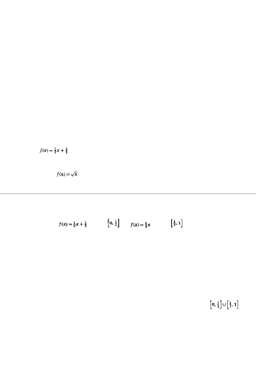
Take any subset A of the real line, and let us say that it has a hole if we can find a number x that is not in A
between two numbers y and z that are in A.
28.11
Show that [0,1] has no holes. Show likewise that (0,1) has no holes either.
28.12
Repeat exercise 28.11 for [a, b] and (a, b) where a and b are constants.
28.13
How about [a, b) and (a, b] where the first set does not contain b (but does contain a), and vice versa for the
second set? Are these sets convex? Explain.
28.14
Can you show that the sets of the previous two questions are the only convex sets in the real line, that is, the
only possible sets that have no holes?
28.15
Give two examples of sets that are not convex.
28.16
Draw a graph of .
28.17
Repeat for the function . Do your drawings show any jumps in the two functions? Explain.
page_462
Page 463
28.18
What about the function for x in but for x in ? Show graphically that this
function is not continuous.
28.19
Show that the function of exercise 28.18 does not have a fixed point [in [0,1]).
28.20
Find a continuous function that is defined on [0, ¥)and takes nonnegative valuesthat does not have a fixed
point.
28.21
Repeat exercise 28.20 for the case in which the function is defined on the nonconvex set .
[Make sure that f(x)always takes values in the same nonconvex set.]
28.22
Using the definition of a convex set, can you show that a single point is itself a convex set?
28.23
Can you formally show that a function that is single-valued for every x is also a multi-convex-valued
function?
28.24
Draw the following multi-convex-valued function: F is defined on [0,1]. At all values of x other than ,
F
(x)is a single point. Indeed on , F(x)is equal to 2x. On it is equal to . At , F(x)is
multivalued; F is equal to [ , 1]. Is the function upper semicontinuous?
28.25
Give an example of a multi-convex-valued function that is (upper semi-) continuous and one that is not.
Section 28.3
28.26
Show that when a player has only two strategies, the set of mixed strategies is given by the set [0, 1].
28.27
Show formally that any best-response function is a multi-convex-valued function. (You can restrict the
formal argument to the case where there are only two pure strategies.)
page_463
Page 464
28.28
For the infinite strategies case, show why we cannot have two pure-strategy best responses when payoffs are
strictly concave.
28.29
Verify with detail that the conditions of the second theorem are satisfied by the Cournot model of Chapter 6.
28.30
Repeat exercise 28.29 for the commons problem of Chapter 7.
page_464
Page 465
INDEX
A
Absentee bids, 40(n6)
Adler, Barry, 128(n19)
Advanced Television Center, 189(n19)
Adverse selection, 395
Aircraft industry
competition and, 76(n3)
as a natural monopoly, 123(n8)
Akerlof, George, 383, 391
American Airlines, 76(n3)

American buffalo, commons problem and, 97
America Online, 98(n7)
Animal behavior, 6, 68-69
Annan, Kofi, 54, 55(n12)
Antitrust legislation, 257(n1)
Art auctions. See also Auctions
as strategic form games, 40-41, 43-44
Ascending-bid auctions, 368
Asymmetric equilibrium, 123, 129(n21)
Athletic Drug Reference, 114(n8)
Auctions
basic model of, 369
first-price, analysis of, 371-373, 375-376
mechanism design and, 351
optimal, 373-376, 377
overview of, 367-368
second-price, analysis of, 369-371, 375-376, 377
signaling games applied to, 385, 386, 387, 390
simplifying assumptions and, 377
as strategic form games, 40-41, 43-44
types of, 368-369, 377
B
Backward induction, 7
in analysis of finitely repeated games, 214-218
applied to research and development models, 183-188, 190
case study in, takeover deterrents and, 174
in computation of social optimum, 278-281
examples of, 165-168
iterated elimination of dominated strategies and, 170-172, 175
overview of, 168-169, 175
power of commitment and, 167-168, 175
proof of, 169-170
subgame perfect equilibria and, 198, 203
Bankruptcy law

game theory and, 6
legal background, 128, 132
symmetric games applied to, 128-132
Battle of the Sexes game
incomplete information games applied to, 311, 313-320
mixed strategies and, 103-106, 113-114
Nash equilibria and, 66, 453
strategic form, 36
Bayesian equilibrium, perfect, 387-389, 390, 393, 396
Bayes-Nash equilibrium
in Cournot models with incomplete information, 332-336, 339, 340-341, 343
defined, 314-315, 326
in direct-revelation mechanisms, 358
in first-price auctions, 371-373, 377
generalizations of, 318-320
mixed-strategy, 316-318
overview of, 313-314
pure-strategy, 315-316, 319
Behavior. See also Rational play; Reciprocal behavior
animal, Nash equilibrium applied to, 68-69
grim trigger strategies and, 229-232, 237
Behavior cycle, 232-234
Bernoulli, Daniel, 438(n10), 443(n14)
Bernoulli, Nicholas, 438
Bertrand competition. See also Price competition
incomplete information games applied to, 310-311, 313
iterated elimination of dominated strategies and, 51-52, 56
Nash equilibrium and, 67
Best-response functions
fixed-point theorems and, 453-458
Nash equilibrium and, 459-460
Bluffing, mixed strategies and, 110-111
Bonus-based incentive schemes, 298, 300-303, 306
Borel, Emile, 7(n5)

Boutros-Ghali, Boutros, 54, 55(n12)
Branches, in game trees, 157
British Airways, 395(n14)
Broker-dealer relationships, 244-245, 249-251, 252
Brouwer fixed-point theorem, 454-455, 456, 459, 461
Brundtland, Glo Harlem, 54
Buffalo. See American buffalo
Buyers
in auctions, 367-368, 371-376, 377
direct-revelation mechanisms and, 355, 359-362
page_465
Page 466
Buyers (continued)
incentive-compatibility constraints and, 354
individual-rationality constraints and, 354
selling variable amounts to, 358-362
signals of product quality and, 391-393
single, selling to with an unknown valuation, 351-355, 362
used car markets and, 394-395
C
Calculus, basic concepts in, 403-409
Capitation, 305, 306
Cartels
Cournot model and, 79-80, 81-82
OPEC's pricing policies and, 261-262
in research and development modeling, 182, 189
Chance nodes, 161-162
Chess
computers and, 169(n11)
Zermelo's study of, 7
Chicken game. See also Hawk-Dove game
applied to bankruptcy law and voidable preferences, 128-132
generalized and applied to natural monopolies, 124-127

as a symmetric game, 122-123, 132
Christie, William, 244
Collection costs, 131-132
Collusion
in NASDAQ, 244-245
repeated games applied to, 246-249, 250-251, 252
Colonel Blotto game, 37
Commitment. See Power of commitment
Common prior concept, 314, 318, 320
Commons, history of, 91
Commons problem
American buffalo and, 97
background of, 91-93
global warming and, 97-98
Internet and, 98
large populations and, 96-97
limiting users and, 99
mechanism design and, 350
Nash equilibrium solution, 93-95, 99
privatization and, 98
pure strategies in, 451(n1)
renewable resources and, 99
socially optimal solution, 95-96, 99
usage fees and, 98-99
Commons problem, dynamic, 276-287
game equilibrium solution (unilateral usage) in, 282-286
Markovian strategies and, 286-287
socially optimal solution in, 278-282, 285-286
socially suboptimal results and, 287
Compact sets, 454
Competition. See also Market competition
animal, Nash equilibrium applied to, 68-69
economic, game theory and, 76
Completeness, preference relations and, 433, 434

Compound lotteries, 439
Computers, chess and, 169(n11)
Concave functions
optimization theory and, 412-414, 415
overview of, 408-409, 414
Von Neumann-Morgenstern utility function as, 441, 442-443
Conditional expectation of random variables, 427-428
Conditional probability, 425
Conrail, 172(n15), 173(n17), 174(n18)
Constants, 404
Constant-sum games, 140-141.
See also Zero-sum games
Consumption
in dynamic commons problems, 276-277, 279-282, 283-286
in static commons problems, 93-95
Continuity, preference relations and, 434
Continuous functions, 454
Continuous mixed strategy, in first-price auctions, 371-373
Convex sets, 454
Cooperative games, 8
Coordination game, 37, 67
Corporate takeovers. See Takeover deterrents
Costs
marginal, Cournot models and, 332, 343
revealing, Cournot models and, 338-340
Cournot, Antoine-Augustin, 7, 75(n1)
Cournot model
analysis of, 336-338
cartel solution for, 79-80
case study, OPEC and, 81-82
Cournot-Nash equilibrium in, 77-79, 337, 339, 343
generalization of, 86-87
isoprofit curves and, 82-85
iterated elimination of dominated strategies solution, 84-85

origin of, 75(n1)
overview of, 76-77, 87
pure strategies in, 451(n1)
revealing costs to a rival, 338-340
signaling and, 384
page_466
Page 467
Stackelberg solution for, 85-86
Cournot model, with incomplete information
Bayes-Nash equilibrium in, 332-336, 339, 340-341, 343
compared to complete information solutions, 337-338
demand uncertainty and, 342-343
generalizations and extensions of, 341-343
overview of, 331-332, 343
revealing costs to a rival, 338-340
two-sided, 340-341
Cournot-Nash equilibrium, 77-79, 84-85, 86, 87, 337, 339, 343
Credibility concept, subgame perfect equilibria and, 195-196
CSX Corporation, 172(n15), 173(n17), 174(n18)
Current externalities, 92
D
D'Arcy, William Knox, 258
da Vinci Diaries game. See Auctions
Decision making
under certainty, 433-436
preference relations and, 433-434, 444
risk aversion and, 441-444
under uncertainty, 436-441
Decision nodes
in game trees, 157
information sets and, 20
overview of, 19-20
precedence and, 159-160, 174

Defense industry, 124(n9)
Demand uncertainty, 342-343
Dependent events, 425, 428
Dependent variables, 404, 414
Depreciation, 394
Descending-bid auctions, 368-369
Direct-revelation mechanisms, 355, 357, 358, 359-362
applied to auctions, 373-375, 377
signaling and, 386, 387(n6)
Discount factors, 211(n1)
OPEC's pricing policies and, 262
payoffs and, 228
in repeated games modeling of collusion, 247-248
in repeated games with demand uncertainty, 264-266
Discount stores, ''match the best price" practice and, 250(n20)
Disjoint sets, 423(n5), 424
Dismemberment, 131-132
Dixit, Avinash, 9(n11)
Dominance
definition of, 108(n3)
strong, 58-59
in War of Attrition game, 127
Dominance solvable games
case study in, 54-55
examples of, 51-54
incomplete information games as, 321-323, 326
overview of, 51, 55-56
Dominant strategies, 41-43
at art auctions, 43-44
in second-price auctions, 369-371, 377
Dominant strategy solutions, 41-43, 44
in incomplete information games, 312-313, 321, 326
mixed strategies and, 109
Nash equilibrium and, 70, 71

Dominated strategies, 49-50
subgame perfect equilibria and, 202
Dresher, Melvin, 11
Drug industry. See Patented drug market; Pharmaceutical industry
Drug testing. See Random drug testing
Duopoly markets, 75.
See also Cournot model
iterated elimination of dominated strategies and, 51-52
Dutch auctions, 368, 369(n5).
See also Descending-bid auctions
Dutta, Prajit K., 245(n9)
Dynamic games, 8
applied to commons problem, 276-287
overview of, 275-276, 287
E
Economics, 394(n11)
history of game theory and, 7
Edgeworth, Francis, 7
Empty sets, 422(n1)
English auctions, 368, 369(n5), 375(n14).
See also Ascending-bid auctions
Entry game. See Market entry game
Equilibrium. See also Bayes-Nash equilibrium; Cournot-Nash equilibrium; Mixed-strategy equilibrium; Nash
equilibrium; Perfect Bayesian equilibrium; Subgame perfect equilibrium; Symmetric equilibrium
asymmetric, symmetric games and, 123, 129(n21)
in dynamic commons problem, 282-287
mechanism design and, 349, 350
pooling, 389, 390, 396
separating, 340(n12), 389, 393, 396
sequential, 389(n7)
Euler, Leonhard, 438(n10)
Events, 421
Event space, 421, 422, 423, 424, 428
Expectation of random variables, 426, 428

Expected returns puzzle, 438
page_467
Page 468
Expected utility theorem I, 437-438
Expected utility theorem II, 440-441
Extensive form/Extensive form games
backward induction and, 165-170
case study in, takeover deterrents and, 172-174
chance nodes in, 161-162
consistency requirements and, 158-160
examples of, 25, 26, 27, 157-158
game trees and, 18-21, 157-160
iterated elimination of dominated strategies and, 170-172
mixed strategies in, 161
origin of concept, Neumann and, 163(n5)
overview of, 18-21, 28, 157-158, 174
perfect information games and, 162-164
predecessors and, 159-160
repeated games as, 209, 222
strategic form and, 39, 44
strategies in, 160-161
subgames and, 196-197
F
Feasibility constraints, optimization theory and, 411-413
Final Jeopardy, 323-326
Finitely repeated games
analysis of subgame perfect equilibria in, 214-219
case study in, Treasury Bill auctions, 219-222
concept of reciprocal behavior and, 216-217, 222
economic applications, 212-213
example of, 210-211
general structure of, 211-212
First-price auctions, 368-369, 371-373, 375-376, 377

Fixed-point theorems, 453-458, 459, 460, 461
Focal point, 65
symmetric equilibrium and, 123
Folk theorem, 232-234, 238
Forgiving trigger strategy, 231-232, 249
Franchise incentive schemes, 297-298, 300
Fudenberg, Drew, 9(n11)
Functions
concave, 408-409
continuous, 454
multi-convex-valued, 456-458
overview of, 404-405
slopes of, 405-408, 414
Future externalities, 92
G
Game environments, in dynamic games, 275-276
Game rules. See also Mechanism design
assumption of common knowledge about, 18
fundamental role of, 17
Games
applying probability to, 423-424
assumption of common knowledge of rules, 18
basic components of, 17
extensive form, 18-21, 25, 26, 27
(See also Extensive form/Extensive form games)
payoffs and, 23-24, 28, 411
strategic form, 21-22, 25, 27, 28
(See also Strategic form/Strategic form games)
Games of imperfect information. See Imperfect information games
Games of incomplete information. See Incomplete information games
Games of perfect information. See Perfect information games
Game theory, 394(n11)
applications of, 5-6
definition of, 4-5, 12

history of, 7-8, 12
interdependence and, 3-4, 12
meaning of term, 8
the one case and the infinity case in, 6
outcomes and, 12
uncertainty and, 421
Game Theory (Fudenberg and Tirole), 9(n11)
Game trees. See also Extensive form/Extensive form games
consistency requirements and, 158-160
example of, 157-158
overview of, 18-21, 157
predecessors and, 159-160
Global warming, commons problem and, 97-98
Good behavior, grim trigger strategies and, 229-232, 237
Government securities, 6.
See also Treasury Bill auctions
Grand Alliance, 181
Grim trigger strategy
in finitely repeated games, overview of, 229-231, 233, 237
in models of collusion, 247, 249, 250-251
OPEC's pricing policies and, 261-262
in repeated games with demand uncertainty, 264-266
Group projects, game theory applied to, 5
Groups, defined, 4
H
Hardaway, Tim, 301(n11)
Harsanyi, John, 8, 113, 309, 314
Hawk-Dove game, 37.
See also Chicken game
mixed strategies and, 106
Hayes, Charlie, 301(n11)
HDTV. See High-definition television
page_468

Page 469
Health maintenance organizations (HMOs), moral hazard and incentive schemes in, 304-305, 306
Helix, 114(n8)
High-definition television (HDTV)
modeling of research and development in, 181-189
patent races and, 180-181, 190
HMOs. See Health maintenance organizations
I
IEDS. See Iterated elimination of dominated strategies
Imperfect information games, 193.
See also Subgame perfect equilibrium
incomplete information games reduced to, 314, 318, 320
perfect information games and, differences between, 196
Incentive-compatibility constraints, 354, 356, 360, 374
Incentive schemes
examples of, 297-299
HMOs and, 304-305
monotone likelihood ratios and, 302
optimal, 299-301
overview of, 295-297, 305
wage plus bonus, 298, 300-303, 305
Incomplete information games, 8.
See also Cournot model, with incomplete information
Bayes-Nash equilibrium and, 313-318
case study in, Final Jeopardy, 323-326
common prior concept, 314, 318, 320
dominance solvability in, 321-323
dominant strategy solutions in, 312-313, 321, 326
examples of, 309-313
overview of, 309, 326
signaling and, 383-384, 396
(See also Signaling games)
Independent events, 425, 428
Independent variables, 404, 414

Indifference curves, 435
Indifference relations, 434
Individual rationality constraints, 353(n4), 354, 360, 374
Industrial Revolution, 179(n1)
Infinitely repeated games
economic applications, 213-214
example of, 211
folk theorem and, 232-234, 238
imperfect detection of action and, 234-237
payoffs in, 211, 212, 227-228, 237
reciprocal behavior and, 232
subgame perfect equilibria and, 203
trigger strategies in, 229-232, 234-237
Information economics, 391
Information sets
defined, 20
game trees and, 158
perfect information games and, 162-163
Insolvency, 131-132
Insurance companies
incentive schemes and, 305, 306
moral hazard and, 293-294, 304-305
Interactions, in game theory, 5
Interdependence, in game theory, 3-4
Interior values, 412
International oil market. See Oil market
International Olympic Committee (IOC), random drug testing and, 5, 114-115
International Petroleum Exchange, 259
Internet, commons problem and, 98
Introduction to Game Theory, An
(Osborne and Rubinstein), 9(n11)
Investment, in renewable resources, 277, 281, 284-285
Investment banks, 6.
See also Treasury Bill auctions
Isoprofit curves, 82-85

Iterated elimination of dominated strategies (IEDS)
advantages of, 57
backward induction and, 170-172, 175
case study in, 54-55
Cournot model and, 84-85
examples of, 51-54
in incomplete information games, 321-323
mixed strategies and, 109-110
Nash equilibrium and, 69-70, 71
order of elimination and, 57-58
overview of, 51, 55-56
rationality of players and, 57
strong domination and, 58-59
J
Japan, high-definition television and, 180-181, 189(n19)
"Jeopardy!," 323-326
K
Kahneman, Daniel, 437(n7)
Kakutani fixed-point theorem, 456-458
Kasparov, Gary, 169(n11)
Kuhn's theorem, 169
L
Lemons problem, 394-395, 396
L'Hospital's rule, 232(n7)
Likelihoods, 422.
See also Probability
Limit order display rule, 251-252
Linear functions, 404, 414
slope of, 406-407, 414
Location space, 183-188
Log functions, 404-405
page_469

Page 470
Log functions (continued)
optimization theory and, 413-414
slope of, 408
Lotteries, 428
in decision making under uncertainty, 436
dependent events and, 425
expected utility theorem and, 437-438
operation of, 422-423
risk aversion and, 441-444
simple and compound, 439
Von Neumann-Morgenstern theorem and, 439-441
M
Madhavan, Ananth, 245(n9)
Managed care, moral hazard and incentive schemes in, 304-305, 306
Mansfield, Edward, 180(n4)
Maples, Maria, 301(n11)
Marginal costs, in Cournot models with incomplete information, 332, 343
Marginal utility, 281(n11)
Marienbad game, 8-10
Market competition, finitely repeated games applied to, 213
Market entry game
perfect information games and, 163-168, 170-172
subgame perfect equilibria and, 193-196, 198
Market makers, 250-251
in NASDAQ, 244
in New York Stock Exchange, 243
Markets. See also Oil market
Cournot model, 76-77
forms of, 75
game theory and, 76
patented drug, as a finitely repeated game, 213
signaling product quality and, 391-393
for used cars, signaling games applied to, 394-395

Markovian strategies, 286-287
Markov perfect equilibrium, 286-287
Matching Pennies game, 37
maxmin payoffs and, 142
minmax payoffs, 145
mixed strategies and, 106
as a zero-sum game, 140
"Match the best price" practice, 250(n20)
Maxima, optimization theory and, 409-410, 412, 413, 415
Maxmin payoffs
examples of, 142-144
Nash equilibrium and, 148
overview of, 141-142, 149
related to minmax payoffs, 146-147
security strategy and, 142
Mechanism design
direct-revelation and, 355, 357, 359-362
examples and applications of, 350-351
incentive-compatibility constraint and, 354, 356
individual-rationality assumption and, 353(n4), 354
overview of, 349-350, 362
revelation principle and, 356-358, 362
signaling games and, 387(n6), 395
when selling to a single buyer with unknown valuation, 350-355
when selling variable amounts, 358-362
Mechanisms, defined, 356
Minima, optimization theory and, 410
Minmax payoffs
examples of, 145-147
Nash equilibrium and, 148
overview of, 144, 149
related to maxmin payoffs, 146-147
Mixed strategies
best response implication, 107-108

bluffing and, 110-111
case study in, random drug testing, 114-115, 116
definition and overview of,
103-107, 115-116
dominant strategy solution and, 109
domination of pure strategies and, 108-110
examples of, 106-107
in extensive form games, 161
in first-price auctions, 371-373
iterated elimination of dominated strategies and, 109-110
Nash equilibrium and, 111-114, 451-452, 459, 461
natural monopolies and, 124-125
rationales for, 109, 111, 112
skeptics of, 113
worst-case payoffs and, 111, 116
in zero-sum games, 142-143, 145-146, 147-149
Mixed-strategy equilibrium
examples of, 452-453
in symmetric games, 122, 124-125, 126-127, 129-130, 131-132
Mixed-strategy Nash equilibrium. See Mixed-strategy equilibrium
Monopolies, 75
Monotone functions, 434
Monotone likelihood ratios, 302, 306
Monotonicity, Von Neumann-Morgenstern restrictions and, 440, 441
Moral hazard
page_470
Page 471
defined, 293
examples of, 294-295
HMOs and, 304-305
incentive schemes and, 295-303, 305
insurance companies and, 293-294, 304-305
principal-agent model of, 295-299
Morgenstern, Oskar, 7-8, 24, 437, 444

Multi-convex-valued functions, 456-458
Multiprice securities auctions, 213, 219-222
N
Nalebuff, Barry, 9(n11)
NASDAQ market making, infinitely repeated games applied to, 213
NASDAQ stock market
broker-dealer relationship in, 244-245, 249-251, 252
collusion in, 244-245, 252
dynamic game environment and, 276
limit order display rule and, 251-252
market makers in, 213, 244, 250-251
median values and, 246(n12)
order preferencing in, 244-245, 249-250, 252
overview of, 243, 252
repeated games applied to, 245-249, 250-251, 252
Nash, John, 8, 458
Nash equilibrium, 8.
See also Cournot-Nash equilibrium; Symmetric equilibrium
backward induction and, 165-166
case study in, 68-69
commons problem and, 93-95, 99
defined, 63-64, 71, 451-452
dominant strategy solution and, 70, 71
examples of, 66-68, 452-453
existence theorems in, 458-459
in finitely repeated games, 214-219, 222
fixed-point theorems and, 453-458, 459, 460
in incomplete information games (See Bayes-Nash equilibrium)
iterated elimination of dominated strategies and, 69-70, 71
mixed strategies and, 111-114
(See also Mixed-strategy equilibrium)
motivations for, 64-66
pure-strategy, in symmetric games, 122, 124, 126, 129, 130-131
questions of existence and uniqueness in, 66

in repeated game modeling of the NASDAQ stock market, 246
in subgames (See Subgame perfect equilibrium)
in zero-sum games, 147-149
Nash theorem, 458
Natural monopolies
economic background, 123-124, 132
symmetric games applied to, 124-127, 132
Negotiations, incomplete information games applied to, 310
Neumann, John yon, 7-8, 24, 163(n5), 437, 444
New York Mercantile Exchange, 259
New York State Lottery, 422-423, 425
New York Stock Exchange, 243
Nim game, 8-10, 25
Nobody Beats the Wiz, 250(n20)
Nodes.
See also Decision nodes
in game trees, 157
Nonlinear functions, 404, 414
slope of, 407, 414
Nonzero-sum games, 8
Norfolk Southern, 172(n15), 173(n17), 174(n18)
Normal form games.
See Strategic form/Strategic form games
O
Odd Couple game
iterated elimination of dominated strategies and, 52-53, 56
Nash equilibrium and, 67
Oil futures, 259
Oil industry
history of, 257-259
production, OPEC and non-OPEC, 81(n13)
Oil market. See also Organization of Petroleum Exporting Countries
infinitely repeated games applied to, 214
simple model of, 259-262
Oligopolistic markets
analysis of, history of game theory and, 7

Cournot model and, 86-87
incomplete information games applied to, 341-342, 343
research and development in, 180
OPEC. See Organization of Petroleum Exporting Countries
Optimization theory, 409-414, 415
applied to decision making under certainty, 435-436
examples in, 413-414
feasibility constraints and, 411-413
necessary conditions and, 409-410
sufficient conditions and, 410
page_471
Page 472
Order preferencing, 244-245, 249-250, 252
Organization of Petroleum Exporting Countries (OPEC)
Cournot model applied to, 81-82
dynamic game environment and, 276
future oil reserves and, 269
infinitely repeated games and, 214
non-OPEC production and, 269-270
oil prices and, 258-259, 260-262, 270
overview of, 257, 270
political costs of overproduction and, 270
repeated games with demand uncertainty applied to, 262-266
simple model of, 259-260
unobserved quota violations and, 266-269, 270
Osborne, Martin, 9(n11)
Outcomes, 12
event space and, 421
payoffs and, 23-24
preference relations and, 433-434
utility assignment and, 434-436
P
Parallel processing, 169(n11)

Patented drug market, finitely repeated games applied to, 213
Patent races
high-definition television and, 180-181, 190
perfect information games applied to, 181-189
Patents, economic role of, 180, 189
Payoffs/Payoff functions, 23-24, 441.
See also Maxmin payoffs; Minmax payoffs; Utility functions; Von Neumann-Morgenstern utilities
behavior cycle and, 232, 233-234
in constant-sum games, 140-141
discount factors and, 228
expected, in mixed strategies, 104-107, 116
in extensive form games, 158
in infinitely repeated games, 211, 212, 227-228, 234-237
mechanism design and, 356, 362
optimization theory and, 409
in strategic form games, 35-36
in symmetric games, 122-123
threshold trigger strategy and, 235-237
time preferences and, 211(n1), 228(n2)
warranties and, 392-393
worst-case, mixed strategies and, 111, 116
in zero-sum games (See Maxmin payoffs; Minmax payoffs)
Perfect Bayesian equilibrium, 387-389, 390, 393, 396
Perfect information games
applied to research and development, 183-188, 190
backward induction and, 165-170, 175
case study in, takeover deterrents and, 172-174
defined, 162-163, 174
examples of, 163-164
imperfect information games and, difference between, 196
iterated elimination of dominated strategies and, 170-172
Kuhn's theorem and, 169
power of commitment and, 167-168
simultaneous moves and, 163, 164

subgame perfect equilibria in, 198
Pharmaceutical industry. See also Patented drug market
research and development in, 5, 180
Physicians. See Health maintenance organizations
Player(s). See also Buyers; Sellers
defined, 4
in mechanism design, 349, 356-358, 362
revelation principle and, 356-358
Poison pills. See Takeover deterrents
Pollution, tragedy of the commons concept and, 93
Pooling equilibrium, 389, 390, 396.
See also Perfect Bayesian equilibrium
Power of commitment, 167-168, 173, 175
subgame perfect equilibria and, 204
Predecessors
defined, 159
restrictions on, 160, 174
Preference relations, 433-434, 444
Preferences, defined, 24
Preplay communication, 65
Price competition. See also Bertrand competition; Collusion
applied to Prisoners' Dilemma, 234
in infinitely repeated games, 213
iterated elimination of dominated strategies and, 51-52, 56
"match the best price" practice and, 250(n20)
Nash equilibrium and, 67
Price fixing. See Collusion
Prices
page_472
Page 473
in Cournot models, 334, 335, 337-338, 340-341
in selling to a single buyer with unknown valuation, 351-355
Principal-agent moral hazard problem, 305
examples of, 294-295

incentive schemes and, 295-303
modeling, 295-299
Prior concept. See Common prior concept
Prisoners' Dilemma game, 11-12
dominant strategy solution, 42
extensive form, 27
incomplete information games applied to, 309, 310, 312-313, 321
modified and finitely repeated, 210-211, 214-218, 219(n10)
Nash equilibrium and, 67
once-repeated, 210
payoffs and, 23
signaling games applied to, 384, 385-386, 387, 389-390
strategic form, 22, 27, 36
subgame perfect equilibria and, 199-200
Prisoners' Dilemma game, infinitely repeated, 211
folk theorem and, 233-234, 238
price competition model applied to, 234
trigger strategies in, 229-232, 234-237
Private sellers, warranties and, 395(n13)
Privatization, 98, 350
Probability
conditional, 425
dependent and independent events in, 425, 428
in Final Jeopardy model, 324-326
overview of, 421-426
random variables and, 426-428
Probability distributions. See also Common prior concept
mixed strategies and, 104, 115
Probability functions, overview of, 422, 423, 424, 428
Producer organizations, 257(n1).
See also Organization of Petroleum Exporting Countries
Product quality, signaling, 391-393
Profits. See also Isoprofit curves
in Cournot models with complete information, 77-80, 336, 337-338

in Cournot models with incomplete information, 334, 335, 340-341, 343
in sales of variable amounts, 359-362
Proof by induction, 169-170
Public good, technology growth and, 179-180
Public policy, effects on research and development, 189
Punishment
in repeated games modeling of collusion, 248-249
in repeated games with demand uncertainty, 264-266
in trigger strategies of infinitely repeated games, 230, 231, 233, 236-237, 239
Pure strategies, 451(n1)
mixed strategies and, 103-104, 108-110, 115, 116
Nash equilibrium and, 458, 461
Pure-strategy equilibria, 458, 461.
See also Nash equilibrium
in symmetric games, 122, 124, 126, 129, 130-131
Pure time preference, 228(n2)
Q
Quadratic functions, 404
optimization theory and, 413-414
slope of, 407-408
Quality, of products, signaling, 391-393
R
Rand Corporation, 11
Random drug testing, 5, 114-115, 116
Random variables
conditional expectation of, 427-428
defined, 426
expectation of, 426, 428
Rational introspection, 65
Rational play
defined, 5
subgame perfect equilibria and, 202
R&D. See Research and development

Reaction functions, 77, 84
Reciprocal behavior
finitely repeated games and, 209, 216-217, 222
infinitely repeated games and, 232, 238
Renewable resources. See Resources, renewable
Repeated games. See also Finitely repeated games; Infinitely repeated games
applied to NASDAQ collusion, 245-249, 250-251
concept of reciprocal behavior in, 209
definition of, 212, 222
with demand uncertainty, 262-266
dynamic (See Dynamic games)
economic applications, 212-214
examples of, 209-214
folk theorem of, 232-234
general structure of, 211-212
with imperfect detection of actions, 234-237, 267-269
overview of, 209
stage games and, 209
static basis of, 275
Research and development, role of patents in, 180
Research and development modeling, 5
page_473
Page 474
Research and development modeling (continued)
assumptions about, 181-182, 188
background for, 179-181
behavior of cartels and, 182, 189
patent value and, 189
perfect information games and backward induction applied to, 183-188, 190
public policy and, 189
sunk costs concept and, 184(n14), 188
uncertainty and, 189
Resources
as common property, 91-92

commons problem and, 92-99, 276-287
Resources, renewable, 99
investment rates and, 277
socially optimal usage, 278-282, 285-286
unilateral usage, 282-286
Revelation principle, 356-358, 362, 373-373.
See also Direct-revelation mechanisms
Revenue equivalence, 373
Risk aversion, 296(n5), 441-444
Risk-loving preferences, 444
Risk neutrality, 443
Roots, in game trees, 157
Rubinstein, Ariel, 9(n11)
S
Safety Zones, 186-187, 188, 189
Sales. See also Auctions
direct-revelation mechanisms and, 355, 359-362
incentive-compatibility constraint and, 354
individual-rationality assumption and, 353(n4), 354
to a single buyer with unknown valuation, 350-355, 362
of variable amounts, 358-362
Sample space, 421, 422, 423-424, 428
Sanchirico, Chris, 128(n19)
Saudi Arabia, oil production and, 257, 258, 259(n10)
Schelling, Thomas, 65
Schultz, Paul, 244
Second-price auctions, 368, 369-371, 375-376
dominant strategy in, 369-371, 377
revenue equivalence and, 373
Securities auctions. See Treasury Bill auctions
Security strategy, 142, 147, 148, 149
Sellers
in auctions, 367-368, 371-376, 377
signaling product quality, 391-393

used car markets and, 394-395
warranties and, 392-393, 395(n13)
Selten, Reinhard, 8
Separating equilibrium, 340(n12), 389, 393, 396.
See also Perfect Bayesian equilibrium
Sequential equilibrium, 389(n7)
Sherman Antitrust Act, 257(n1)
Signaling games, 340(n12)
adverse selection and, 395
analysis of, 385-387, 389-390
case study in, used car markets, 394-395
defined, 387, 396
examples of, 384-385
mechanism design and, 395
overview of, 383-384
perfect Bayesian equilibrium and, 387-389, 390, 393
signaling product quality and, 391-393
Simple lotteries, 439
Single-price securities auctions, 213, 219-222
Slopes, 405-408, 414
Smith, John Maynard, 68, 125(n15)
Socially optimal resource usage
compared to unilateral usage outcomes, 285-286
computation of, 278-281
explanation of, 281-282
in static commons problems, 95-96, 97, 99
Solow, Robert, 179(n2)
Solution concepts. See Dominant strategy solutions; Iterated elimination of dominated strategies; Nash
equilibrium
Sotheby's, 40(nn4,5,6)
Spiders, modeling competition in, 68-69
Spot markets, 259
Squash game
maxmin payoffs and, 143-144

minmax payoffs, 145-146
mixed strategies and, 110-111
Nash equilibrium in, 452
as a zero-sum game, 140-141
St. Petersburg paradox, 438, 443
Stackelberg, Heinrich von, 85
Stackelberg model, 85-86, 142(n4)
Stage games. See also Finitely repeated games; Infinitely repeated games
applied to oil market modeling, 259-262
in repeated game modeling of the NASDAQ stock market, 245-248
in repeated games, 209, 212, 222
Stock markets. See also NASDAQ stock market
broker-dealer relationships in, 244-245, 249-251, 252
market makers in, 243, 244, 250-251
Strategic form/Strategic form games
applied to art auctions, 40-41, 43-44
examples of, 25, 27, 36-39
page_474
Page 475
extensive form and, 39, 44
matrices and, 37
overview of, 21-22, 28, 35-36
Strategic play, defined, 5
Strategies
defined, 20-21
in definition of mechanism, 356
dominant and weakly dominant, 41-43, 44
dominated and undominated, 49-50
in extensive form games, 160-161
Nash equilibrium and, 63-64, 458-459
pure and mixed, 103-104
(See also Mixed strategies)
Strategy of Conflict, The (Schelling), 65
Strong domination, 58-59

Strong iterated elimination of dominated strategies, 58-59
Subgame perfect equilibrium
case study in, World War I trench warfare and, 203-204
characteristics of, 202-203
defined, 197-198, 204
examples of, 193-196, 199-202
in finitely repeated games, 214-219, 222
folk theorem and, 232-234
in infinitely repeated games, 229-232
in perfect information games, 198
Subgame perfect Nash equilibrium. See Subgame perfect equilibrium
Subgames. See also Subgame perfect equilibrium
defined, 196-197, 204
in infinitely repeated games, 229-230
Sunk costs concept, 184(n14), 188
Sustainable resources. See Resources, renewable
Symmetric equilibrium
Bayes-Nash, in first-price auctions, 371-373, 377
defined, 123, 132
in dynamic commons problems, 283
mixed-strategy, 122, 124-125, 126-127, 129-130, 131-132
motivations for, 123
Symmetric games
applied to bankruptcy law and voidable preferences, 128-132
applied to natural monopoly, 123-127
Chicken game as, 121-122
defined, 122-123, 132
first-price auctions as, 371
Symmetric mixed-strategy equilibrium, 124-125, 126-127, 129-130, 131-132
T
Takeover deterrents, perfect information games applied to, 172-174, 175
Tangents, 407(n6)
Taxes, commons problem and, 98
Technology growth

economic importance of, 179
patents and, 180
public good and, 179-180
research and development in, 180
"Tenders," 212-213
Terminal nodes, 157, 159
Theory of Games and Economic Behavior (Neumann and Morgenstern), 7-8
Thinking Strategically (Nalebuff and Dixit), 9(n11)
Ticketing agencies, 353(n5)
Time preferences, 211(n1), 228(n2)
Tirole, Jean, 9(n11)
Toads, behavior in, 68(n5), 69(n9)
Tragedy of the commons, 93, 100, 287.
See also Commons problem; Commons problem, dynamic
American buffalo and, 97
global warming and, 97-98
Internet and, 98
large populations and, 96-97
model of, 93-95
possible responses to, 98-99
Transitivity, preference relations and, 433, 434
Treasury Bill auctions, 6
dynamic game environment and, 276
finitely repeated games applied to, 212-213, 219-222
Trench warfare, modeling of, 203-204
Trial and error, Nash equilibrium and, 65-66
Trigger strategies. See also Grim trigger strategy
folk theorem and, 233
forgiving, 231-232, 249
in infinitely repeated games, 229-232, 237
in repeated games with imperfect detection, 267-269
threshold, 234-237
Trigger Zones, 185-187, 188, 189
Trump, Donald, 301(n11)

Tucker, A1, 11
Tversky, Amos, 437(n7)
U
Uncertainty. See also Probability
decision making and, 436-441
in extensive form games, 161-162
game theory and, 421
representation of, 428
risk aversion and, 441-444
Undominated strategies, 49-50
Uniform distributions, 424-425
United Nations elections, modeling of, 54-55
United States Treasury. See Treasury Bill auctions
Usage fees, commons problem and, 98
page_475
