
Intro to Excel spreadsheets
What are the objectives of this document?
The objectives of document are:
1. Familiarize you with what a spreadsheet is, how it works, and what its capabilities are;
2. Using the concepts introduced earlier in the course, apply certain mathematical manipulations to
data;
3. Provide you with the tools to make decisions that are more informed and present reports to
interested stakeholders in your respective offices.
Before we start…
Throughout the following pages, we will reference several menu options and how you can get to them. In
order to do this, we will use the following convention: when you see the following, ViewZoom, the
first word (View) refers to a menu option usually found in the top left, under the title bar. The word that
follows (Zoom) is a menu choice found under the first option you made.
What is a spreadsheet?
A . It has taken the place of the pencil,
paper, and calculator. Spreadsheet programs were first developed for accountants but have now been
adopted by anyone wanting to prepare a budget, forecast sales data, create profit and loss statements,
compare financial alternatives and any other mathematical applications requiring calculations.
spreadsheet is the computerized equivalent of a general ledger
The electronic spreadsheet is laid out similar to the paper ledger sheet in that it is divided into columns
and rows. Any task that can be done on paper can be performed on an electronic spreadsheet faster and
more accurately.
The problem with manual sheets is that if any error is found within the data, all answers must be erased
and recalculated manually. With the computerized spreadsheet, formulas can be written that are
automatically updated whenever the data are changed.
What can a spreadsheet do?
In contrast to a word processor, which manipulates text, a spreadsheet manipulates numerical data and
text. Using a spreadsheet, one can create budgets, analyze data, produce financial plans, and perform
various other simple and complex numerical applications.
By having formulas that automatically recalculate, either built by you, the user, or the built-in math
functions, you can play with the numbers to see how the result is affected. Using this “what-if?” analysis,
you can see what affect changing a data value or calculation can have on your monitoring program.
Spreadsheets can also be used for graphing data point
s, reporting data analyses, and organizing and
storing data.
1
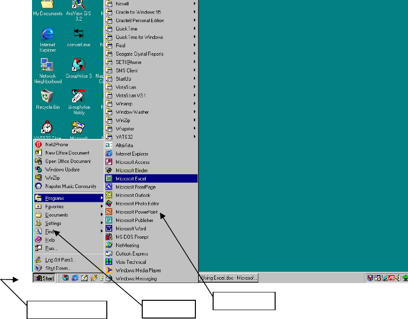
Starting Excel
You are encouraged to start using MS Excel as you read through the following materials to familiarize
yourself with the topics and procedures.
1. Click the Start button on the Windows taskbar.
a. The Start menu opens
2. Point to Programs
a. The Programs menu opens
3. Click Microsoft Excel
a. Excel opens a new workbook
Note: an icon for MS Excel may be located either on the desktop or on the Office toolbar.
Figure 1
3. MS Excel
1. The Start button
2. Programs
2
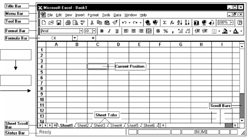
The Excel Screen
The screen in Excel looks different than those used in other types of applications.
Columns
Rows
Figure 2
The large window, labeled "Microsoft Excel" may take up the entire screen. This is referred to as the
Application Window. The top line is called the Title Bar and has three buttons (Minimize, Restore, and
Close) to the right. These buttons are used to size the window and close it. This title bar is standard in all
Windows programs.
The second line is called the Menu Bar. Notice that one character of each selection is highlighted or
underlined. This menu bar is also standard in all Windows programs.
The next two lines contain buttons with text or images and are referred to as the Standard and
Formatting Toolbars. If you have a mouse, these toolbars allow you to enhance your worksheet without
accessing the menu. Keep in mind that these may not be in the exact same place as on the illustration
above. All toolbars can be customized to display any buttons you desire.
The next line is the Formula Bar and displays the current cell address (see below) and contents. As you
move from cell to cell, Excel will keep track of the current cell address for you. The Formula Bar can
also be used to edit the text (contents) or formulas contained in the cell.
Columns and Cells and Rows…oh my!
The horizontal bar across the top of the worksheet area is filled with letters, beginning with A. Each letter
represents a column while the vertical bar on the left side of the worksheet filled with numbers refers to
rows.
3

The intersection between a column and a row is referred to as a cell. A cell is similar to a box that can be
used to store pieces of information. Each piece of information could be a word or group of words, a
number or a mathematical formula.
Each cell has its own address. This address is used in formulas for referencing different parts of the
worksheet. The address of a cell is defined by the letter of the column in which it is located and the
number of the row. For example, the address of a cell in column B, row 5 would be referred to as B5. The
column is always listed first followed by the row without any spaces between the two.
The outlined cell (the one with the dark borders) within the worksheet is referred to as the active cell.
Each cell may contain text, numbers, or dates. You can enter up to 32,000 characters in each cell
(Equivalent to a 44 page report!).
These cell addresses are useful when entering formulas. Instead of typing actual values in your equations,
you simply type the cell address where the value is stored. Then, if you need to go back and change one
of the values the spreadsheet automatically updates the result of the formula based on the new data.
For example, instead of typing 67*5.4 you could enter C5*D5. The number 67 is stored in cell C5 and the
number 5.4 is stored in cell D5. If these numbers change next month or next year, the formula remains
correct because it references the cells - not the actual values. With the second formula, you can change the
numbers stored in cells C5 and D5 as often as required and see the result recalculated immediately.
The next section of the screen lists the columns and rows within the current worksheet. As mentioned,
columns are lettered and rows are numbered. The first 26 columns are lettered A through Z. Excel then
begins lettering the 27th column with AA and so on. In a single Excel worksheet there are 256 columns
(lettered A-IV) and 65,536 rows (numbered 1-65,536), totaling 16,777,216 individual cells.
Sheets and Workbooks
Towards the bottom of the worksheet is a set of small Tabs that identify each sheet in the workbook
(file). If there are multiple sheets, you can use the tabs to easily identify what data is stored on each sheet.
For example, the top sheet could be "Expenses" and the second sheet could be called "Income". When
you begin a new workbook, the tabs default to being labeled Sheet1, Sheet2, etc.
At the bottom of the screen is another bar called the Status Bar. This bar is used to display various
information about the system and current workbook.
The left-hand corner of this line lists the Mode Indicator, which tells you what mode you are currently
working in.
The Zoom button
(located on the toolbar at the top of the screen) allows you to change the
size of the viewing area. This does not affect the actual printing of the file. Click on the down arrow
located to the right side of the current zoom factor. Scroll through the available zoom choices. When you
select a zoom factor, Excel will zoom in or out of the worksheet area - as specified in the Zoom. You can
also access the View Zoom menu. In addition, you can hide everything except the worksheet and the
menu (which will increase your working area) by accessing the View Full Screen menu.
4
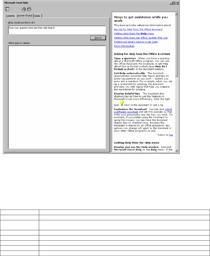
Using “Help”
Excel, along with many of the Microsoft applications, has its own online help menu. There are several
ways to access help. Either press F1 on the keyboard or choose Help Microsoft Excel Help from the
Menu bar. A window will appear as shown in figure 3.
Figure 3
Moving around in Excel
When Excel starts, a new worksheet opens. What is currently visible is only a small portion of what is available for
you to use. In order to move to areas that you cannot see, you can:
• Use the scroll bars
• Use the keys described in table 1
Keystroke Result
Arrow key Move one cell in the direction of the arrow
Ctrl + arrow key Move in the direction of the arrow to the last cell before a blank cell, or to the edge of the
worksheet if all cells are blank
Page Up Moves up one screen
Page Down Moves down one screen
Home Moves to the beginning of the row
Ctrl + Home Moves to cell A1
Ctrl + End Moves to the last cell containing data (in the bottom right of the worksheet
Table 1
5
Data Entry
In the following section, you will learn how to enter sample data, edit that sample data, and delete &
undelete that data. You should create a sample spreadsheet so you can practice the following procedures.
Entering data is as simple as beginning to type.
1. Click once on the cell you want to use for data entry and begin typing
2. The following keys can be used to update the contents of the cell: Enter, Tab, or any of the
directional arrows
Editing data is simple as well. There are several options for doing this:
1. Highlight the cell, type in a completely new amount (caution: this will overwrite any data already
in the cell)
2.
Double-click the cell and a flashing insertion point (cursor) appears in the cell
3.
Use the formula bar
4.
Highlight the cell to edit and press F2 on your keyboard
Deletion of data can be relatively straightforward. You can:
1. Select a cell or range of cells (click and hold your mouse or use the shift-click method) and press
delete
2. Select a cell or range of cells and Edit Clear then choose from All, Contents, or
Formatting from the menu bar
3. To actually remove the cells instead of just clearing the data, select a cell or range of cells and
Edit Delete…; you are given the option of shifting the remaining cells a direction or deleting
the entire row or column.
Undoing an action can save both time and headache. In the toolbar, you will find two arrows. Using these
arrows,
you can either undo (arrow pointing left) the last action or series of actions you
just completed, or Redo (arrow pointing right) an action such as formatting or
deleting; you can even Redo an action that was undone.
Let Excel enter data for you
Excel can help you enter series of numbers, dates or times. For instance, if you want to fill a column with
a list of consecutive or patterned dates or numbers, instead of typing dates or numbers in each cell of the
column you can use the “Series” command or you can click and drag the “fill handle” on a cell. Both of
these methods are described below. You can use a pre-determined series using the series command that
you can customize (for instance, date fills can be weekly instead of daily), or you can enter several logical
pieces of the series by hand and when selecting cells, include your custom series. Excel will fill the cells
with a series based on the cells in the original series selection
6
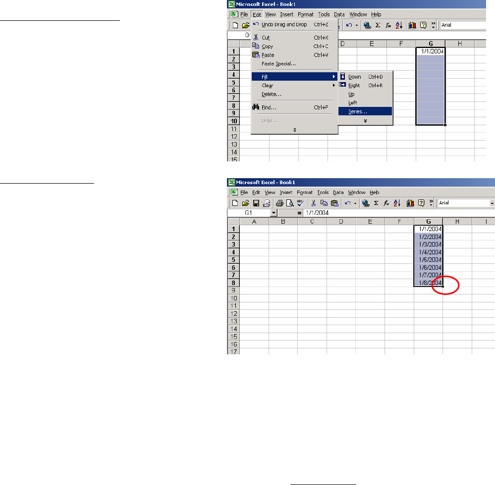
Using the Series command.
Select the cell that contains the first date or
number. Use your mouse to drag the selection
box down the number of rows that you wish to
fill. Go to the Edit menu, and select Fill, then
Series. The Series window will appear. For this
example, chose “Date” on the Type list and
“Day” on the Date Unit list. Click on OK and the
selected cells will be filled with consecutive
dates.
Fi
g
ure 4
Using the Fill Handle
When you select a cell, a small black square
appears in one corner of the selection. When you
point to the fill handle, the pointer changes to a
black cross. Left click with the black cross and
hold it down while you drag the selection box
over the cells that you want to fill. When you
release the mouse button, the boxes will fill
automatically.
Fi
g
ure 5
Formatting
Once you have created your worksheet, you will want to format it to make it as clear as possible.
Formatting is the structure and layout of a worksheet and its individual parts. Using some of the tools
available, you can change the alignment, font size and weight, the way numbers display, even add borders
and shading to your finished product.
Column Wid
th
Sometimes the data you enter does not fit the default cell width of 8.43 characters. When this happens,
you will see either ##### or see a number expressed in scientific notation (2.34E+08). To fix this, you
will have to adjust the cell width. There are two options available to do th
is:
1. Make sure the highlighted cell is in the column that you want adjusted. Choose Format
Column Width from the menu bar. Then type in a new width and press enter.
2. Using the mouse, position the pointer at the right-most end of the column you wish to re-size (in
the column header area where the letters are). Your pointer will turn into a vertical bar with two
small arrows on either side. You can then drag and drop to the desired column width.
3. Double-click on the right-most edge of the column header.
Row Height
In the same
respect, some of the data you enter will not fit the height of the cell and/or row it is in. In
order to change the row height, follow the following steps:
7
1. Point to the bottom edge of the row number boundary to get the two-headed arrow
2. Drag upward or downward to desired height
3. You can also highlight the row and use the Format Row Height menu options
If you have only certain cells that are too wide or too tall, you can select the “wrap text” option. Select
the row or column to be adjusted, use the FormatRow(or column) and select the Alignment tab for the
option of “wrap text.”
Inserting & Deleting
If you
decide that you need another column in between your existing values, or that you want to insert a
row or rows between existing values, you should use the following methods:
•
Inserting a single colum
n: click on the column to the right of where you want the new column,
then choose Insert
Columns
•
Inserting a single row: click a cell in the row below where you want the new row and choose
Insert
Rows
•
Deleting a row or column: select a cell in each row or column to be deleted and choose Edit
Delete
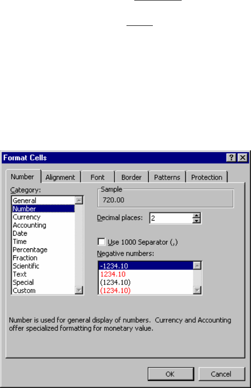
Numbers
To format the way
your cells display
numbers, select the cells you
would like to
format. Choose Format
Cells
Number
Tab from the menu bar. The format cells dialog box appears, looking similar to
figure 6
Figure 6
Using this dialog box, you can choose the way that your numbers look, from the number of decimal
places (rounding) to scientific notation, currency, and percentages. The Sample section of the dialog box
will show you what your data might look like after you format it. Use caution when formatting your data
to a different type than General or Number—for instance, if you have the value “10” in your cell and you
want to change the formatting to percentage, your resulting value will be 1000%; you would have to enter
0.10 for it to equal 10%! You can always revert your
formatting and the original values will be restored.
8

Formula Creation & Math Functions
Excel provides several built-in math functions, as well as provides you the opportunity to create your own
custom formulas. To use a built-in function:
1. Click in the cell where you want the results to appear.
2. Click the paste function on the standard toolbar
3. The Paste Function dialog box appears. Select a category in the Function category list. All of the
associated functions are listed in the Function name, with a description listed below.
4. Click OK to close the dialog box and open the Formula Palette.
5. After defining your arguments, click ok and the formula palette will close.
You can also create your own formula by either typing it or selecting cells to use in performing a
calculation. There are a few tips you need to keep in mind when creating your own formulas:
• Order of operations: Parenthesis, Exponentials, Multiplication & Division first, Addition
and Subtraction second, from left to right (aka PEMDAS)
• All formulas must start with an equals sign
• Use a blank cell as your active cell to avoid errors
Arithmetic operators To perform basic mathematical operations such as addition, subtraction, or
multiplication, combine numbers or produce numeric results, use the following arithmetic operators.
Arithmetic
operator Meaning Example
+ (plus sign) Addition 3+3
– (minus sign) Subtraction 3–1
Negation -6
* (asterisk) Multiplication 3*3
/ (forward slash) Division 3/3
% (percent sign) Percent 20%
^ (caret) Exponentiation 3^2 (the same as 3*3)
Reference operators Combine ranges of cells for calculations with the following operators.
Reference
operator Meaning Example
: (colon) Range operator, which produces one
reference to all the cells between two
references, including the two references
=AVG(B5:B15)
, (comma) Union operator, which combines
multiple references into one reference
(used when referencing cells that are
not consecutive)
=SUM(B5:B15,D5:D15)
9
The Difference Between Relative and Absolute References
Relative references When you create a formula, references to cells or ranges are usually based on their
position relative to the cell that contains the formula. In the following example, cell B6 contains the
formula =A5; Microsoft Excel finds the value one cell above and one cell to the left of B6. This is known
as a relative reference.
A B
5
100
6
200 =A5
7
When you copy a formula that uses relative references, Excel automatically adjusts the references in the
pasted formula to refer to different cells relative to the position of the formula. In the following example,
the formula in cell B6, =A5, which is one cell above and to the left of B6, has been copied to cell B7.
Excel has adjusted the formula in cell B7 to =A6, which refers to the cell that is one cell above and to the
left of cell B7.
A B
5
100
6
200 =A5
7
=A6
Absolute references If you don't want Excel to adjust references when you copy a formula to a different
cell, use an absolute reference. For example, if your formula multiplies cell A5 with cell C1 (=A5*C1)
and you copy the formula to another cell, Excel will adjust both references. You can create an absolute
reference to cell C1 by placing a dollar sign ($) before the parts of the reference that do not change. To
create an absolute reference to cell C1, for example, add dollar signs to the formula as follows:
=A5*$C$1
Switching between relative and absolute references If you created a formula and want to change
relative references to absolute (and vice versa), select the cell that contains the formula. In the formula
bar, select the reference you want to change and then press
F4. Each time you press F4, Excel toggles
through the combinations: absolute column and absolute row (for example, $C$1); relative column and
absolute row (C$1); absolute column and relative row ($C1); and relative column and relative row (C1).
For example, if you select the address $A$1 in a formula and press F4, the reference becomes A$1. Press
F4 again and the reference becomes $A1, and so on.
10
Creating charts
Charts can emphasize important points or trends in your data and make them easier to understand. Using charts, you
are able to get your point across efficiently and quickly, embedding them in reports or presenting them to interested
audiences.
What do different graphs represent?
Th
e following table illustrates what some of the different graphs illustrate.
Name Description of Use
Column Compares values across categories
Bar Compares values across categories
Line Displays a trend over time
Pie Displays parts of the whole
XY (Scatter) Compares pairs of values
Area Shows the trends of value over time
Table 2
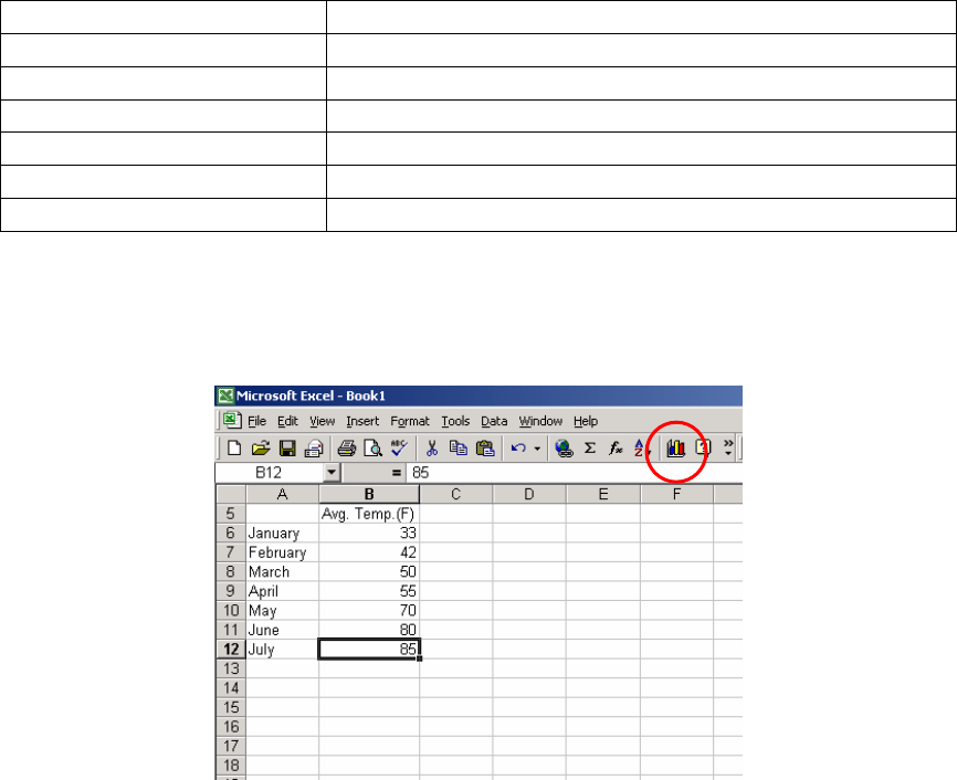
To create a chart, you must first have data in your worksheet. Included with this data, it is helpful to have
labels in the column to the left of the data to indicate categories, labels across the row above the data that
indicate the type of data or the time over which the data will be analyzed, data all formatted the same
way, and data in cells that are next to each other.
Fi
g
ure 7
First, determine the type of chart that will display the data most effectively. Second, select the cells that
contain the data that you want charted – this is the data range.
Chart Wizard
Click the Chart Wizard but
ton (circled in Figure 7) from the standard toolbar. The wizard will then open
up and prompt you for choosing chart types, data ranges, plotting methods, titles, legend placement, and
chart placement.
1. Choose the type of chart you would like to create; Click Next
2. Make sure the chart looks like you expect it to; if not, you may need to tell Excel to analyze the
data in rows instead of columns or vice-versa; Click Next
3. The third step has a series of tabs with options for adjusting how your chart looks; Click Next
after you have adjusted options on all desired tabs
11

a. Titles: type a meaningful heading in any desired area (for instance, a chart title may not
be sufficient, but the axes may need to be labeled as well)
b. Axes: select or deselect showing the axis values
c. Gridlines: select or deselect the gridlines on the chart to make it easier to read
d. Legend: choose whether or not to show the chart legend and where to place it
e. Data Labels: choose whether to include data labels, values, percents, etc.
f. Data Table: choose whether or not to include the table of values from your worksheet
4. The final step is to select where to place the chart; select As a New Sheet [Chart 1] for the chart
to be placed on a new worksheet in your workbook or select As Object In [Sheet1] for the chart to
be placed within a spreadsheet. Selecting As a New Sheet will yield a chart that is easier to
export to other applications such as MS Word or PowerPoint
Formatting the Chart
Once your chart is created, you may decide there are some things you need to change about how it looks
or how the data are displayed.
Scale: To adjust the scale of the chart for bar or line graphs, highlight the axis to adjust and go to
Format→Selected Axis (or double-click on the selected axis). Depending on which axis you select,
you’ll get different options. Typically the x-axis (vertical) is the one you’ll want to adjust. You can
uncheck the “Auto” boxes and set the values at your own levels. Minimum is the lowest value displayed
on the x-axis. Typically, this is zero, but it may at times be negative or you may want to start it at 1000,
depending on how your data are distributed. Maximum is the highest value displayed, and is usually set
at the most logical value based on your highest data point. You may want to adjust this value in order to
change the distribution of the points on the graph. Major and minor unit refer to how the gridlines are
displayed on the chart and how the numbers are displayed on the x-axis. If the major unit is 10, then the
values on the axis will be something like: 10, 20, 30, 40, 50; unless you have minor gridlines shown (an
option in the chart wizard), then the minor unit value will not affect the chart appearance.
Colors, Patterns and Fonts
To make your chart even more stunning visually, you can adjust the colors of the background,
foreground, borders, fonts, axes, bars, lines, pie slices, etc., etc. Just double-click on the object you want
to format and the color palette will open for you to express your artistic creativity. Patterns come in
useful when you are relying on black-and-white displays of multiple parameters because you can more
easily distinguish one bar or one line from another.
When working with Pie Charts, be careful to select the piece of the pie you to which you want to apply a
color or pattern (the first click will select the pie itself, the second click will select a piece of the pie) and
then double-click on it. Otherwise you will change the color or pattern for the entire pie instead of each
piece.
You can also adjust the size and style of the font for different pieces of your chart by double-clicking on
the desired text or section. (Note: if you change the font for a value on the x-axis, for instance, all values
on the x-axis will change formatting).
3-D Charts: If you have created a chart using a 3-D chart type, you can modify the angles at which the
chart is portrayed. Click once on the Chart so the black handles are selecting the entire chart. Go to
Chart→3-D View to change the depth or angle.
12

Once a chart has been created, you can also go and change the style of chart or other options that were set
in the Chart Wizard. Go to the Chart menu for a list of options.
Text Import Wizard
Some types of air monitors supply data in a text format. These files are often identified by the .txt suffix
(example: february00.txt). Text files contain lines of characters, including both numbers and letters. To
divide these lines of text into columns of data, characters such as commas or tabs are inserted to separate
each field or column of data. Text data can also be in a fixed width format, where the fields are aligned in
columns with spaces between each field. Excel’s Text Import Wizard can import both of these text file
data formats. The Text Import Wizard takes the lines of characters and converts them into data contained
within the columns and rows of an Excel file.
Chose Data
Get
Ext
ernal Data
Import Text File from the menu bar. The import text dialog box
appears. Choose the text file that you would like to
import from
Excel and double click on it or single
click the file name, then click the Import button. Follow the instructions given by the Text Import
Wizard dialog boxes that follow.
Printing
Previewing
Before you print a worksheet, click Print Preview to see how the sheet will look when you print it. The
way pages appear in the preview window depends on the available fonts, the resolution of the printer, and
the available colors.
Page setup
Change the p
age orientation
1. Click the worksheet.
2. On the File menu, click Page Setup, and then click the Page tab.
3. Under Orientation, click Portrait or Landscape.
Print a worksheet on a specified number of pages
1. Click the worksheet.
2. On the File menu, click Page Setup, and then click the Page tab.
3. Click Fit to.
4. Enter the number of pages on which you want to print the work.
Notes
• Excel ignores manual page breaks when you fit the worksheets on a specified number of pages.
• When you change the values for Fit to, Excel shrinks the printed image or expands it up to 100
percent, as necessary. To see the how much the image will be adjusted for your new values, click
OK, and then click Page Setup on the File menu. The Adjust to box on the Page tab shows the
percentage that the printed size will be adjusted.
13

Print row and column labels on every page
1. Click the worksheet.
2. On the File menu, click Page Setup
, and then click the Sheet tab.
3. To repeat column labels on every page, click Rows to repeat at top, and then enter the rows that
contain the column labels.
To repeat row labels on every page, click Columns to repeat at left, and then enter the columns
that contain the row labels.
Note Microsoft Excel prints repeating row and column labels only on the pages that include the labeled
rows or columns. Pages for rows below the labeled rows or columns to the right of the labeled columns
are printed without the repeating labels.
14
