
MIRI
M ACHINE INTELLIGENCE
RESEARCH INSTITUTE
Timeless Decision eory
Eliezer Yudkowsky
Machine Intelligence Research Institute
Abstract
Disputes between evidential decision theory and causal decision theory have continued
for decades, and many theorists state dissatisfaction with both alternatives. Timeless de-
cision theory (TDT) is an extension of causal decision networks that compactly repre-
sents uncertainty about correlated computational processes and represents the decision-
maker as such a process. is simple extension enables TDT to return the one-box
answer for Newcomb’s Problem, the causal answer in Solomon’s Problem, and mutual
cooperation in the one-shot Prisoner’s Dilemma, for reasons similar to human intuition.
Furthermore, an evidential or causal decision-maker will choose to imitate a timeless
decision-maker on a large class of problems if given the option to do so.
Yudkowsky, Eliezer. 2010. Timeless Decision eory. e Singularity Institute, San Francisco, CA.
e Machine Intelligence Research Institute was previously known as the Singularity Institute.
Long Abstract
Disputes between evidential decision theory and causal decision theory have continued
for decades, with many theorists stating that neither alternative seems satisfactory. I
present an extension of decision theory over causal networks, timeless decision theory
(TDT).TDT compactly represents uncertainty about the abstract outputs of correlated
computational processes, and represents the decision-maker’s decision as the output of
such a process. I argue that TDT has superior intuitive appeal when presented as ax-
ioms, and that the corresponding causal decision networks (which I call timeless deci-
sion networks) are more true in the sense of better representing physical reality. I review
Newcomb’s Problem and Solomon’s Problem, two paradoxes which are widely argued as
showing the inadequacy of causal decision theory and evidential decision theory respec-
tively. I walk through both paradoxes to show that TDT achieves the appealing con-
sequence in both cases. I argue that TDT implements correct human intuitions about
the paradoxes, and that other decision systems act oddly because they lack representative
power. I review the Prisoner’s Dilemma and show that TDT formalizes Hofstadter’s “su-
perrationality”: under certain circumstances, TDT can permit agents to achieve “both
C” rather than “both D” in the one-shot, non-iterated Prisoner’s Dilemma. Finally, I
show that an evidential or causal decision-maker capable of self-modifying actions, given
a choice between remaining an evidential or causal decision-maker and modifying itself
to imitate a timeless decision-maker, will choose to imitate a timeless decision-maker
on a large class of problems.
Contents
1 Some Newcomblike Problems 1
2 Precommitment and Dynamic Consistency 6
3 Invariance and Reective Consistency 17
4 Maximizing Decision-Determined Problems 29
5 Is Decision-Dependency Fair 35
6 Renormalization 42
7 Creating Space for a New Decision eory 52
8 Review: Pearl’s Formalism for Causal Diagrams 57
9 Translating Standard Analyses of Newcomblike Problems into the Language
of Causality 63
10 Review: e Markov Condition 69
11 Timeless Decision Diagrams 73
12 e Timeless Decision Procedure 98
13 Change and Determination: A Timeless View of Choice 100
References 115

Eliezer Yudkowsky
1. Some Newcomblike Problems
1.1. Newcomb’s Problem
Imagine that a superintelligence from another galaxy, whom we shall call the Predictor,
comes to Earth and at once sets about playing a strange and incomprehensible game. In
this game, the superintelligent Predictor selects a human being, then oers this human
being two boxes. e rst box, box A, is transparent and contains a thousand dollars. e
second box, box B, is opaque and contains either a million dollars or nothing. You may
take only box B,or you may take boxes A and B.But there’s a twist: If the superintelligent
Predictor thinks that you’ll take both boxes, the Predictor has left box B empty; and you
will receive only a thousand dollars. If the Predictor thinks that you’ll take only box B,
then It has placed a million dollars in box B. Before you make your choice, the Predictor
has already moved on to Its next game; there is no possible way for the contents of box
B to change after you make your decision. If you like, imagine that box B has no back,
so that your friend can look inside box B, though she can’t signal you in any way. Either
your friend sees that box B already contains a million dollars, or she sees that it already
contains nothing. Imagine that you have watched the Predictor play a thousand such
games, against people like you,some of whom two-boxed and some of whom one-boxed,
and on each and every occasion the Predictor has predicted accurately. Do you take both
boxes, or only box B?
is puzzle is known as Newcomb’s Problem or Newcomb’s Paradox. It was devised
by the physicist William Newcomb, and introduced to the philosophical community by
Nozick (1969).
e resulting dispute over Newcomb’s Problem split the eld of decision theory into
two branches, causal decision theory (CDT) and evidential decision theory (EDT).
e evidential theorists would take only box B in Newcomb’s Problem, and their
stance is easy to understand. Everyone who has previously taken both boxes has received
a mere thousand dollars, and everyone who has previously taken only box B has received
a million dollars. is is a simple dilemma and anyone who comes up with an elaborate
reason why it is “rational” to take both boxes is just outwitting themselves. e “rational”
chooser is the one with a million dollars.
e causal theorists analyze Newcomb’s Problem as follows: Because the Predictor
has already made its prediction and moved on to its next game, it is impossible for your
choice to aect the contents of box B in any way. Suppose you knew for a fact that box B
contained a million dollars; you would then prefer the situation where you receive both
boxes ($1,001,000) to the situation where you receive only box B ($1,000,000). Suppose
you knew for a fact that box B were empty; you would then prefer to receive both boxes
($1,000) to only box B ($0). Given that your choice is physically incapable of aecting
1

Timeless Decision eory
the content of box B, the rational choice must be to take both boxes—following the
dominance principle, which is that if we prefer A to B given X, and also prefer A to B
given ¬X (not-X), and our choice cannot causally aect X, then we should prefer A to
B. How then to explain the uncomfortable fact that evidential decision theorists end up
holding all the money and taking Caribbean vacations, while causal decision theorists
grit their teeth and go on struggling for tenure? According to causal decision theorists,
the Predictor has chosen to reward people for being irrational; Newcomb’s Problem is
no dierent from a scenario in which a superintelligence decides to arbitrarily reward
people who believe that the sky is green. Suppose you could make yourself believe the sky
was green; would you do so in exchange for a million dollars? In essence, the Predictor
oers you a large monetary bribe to relinquish your rationality.
What would you do?
e split between evidential decision theory and causal decision theory goes deeper than
a verbal disagreement over which boxes to take in Newcomb’s Problem. Decision the-
orists in both camps have formalized their arguments and their decision algorithms,
demonstrating that their dierent actions in Newcomb’s Problem reect dierent com-
putational algorithms for choosing between actions.
1
e evidential theorists espouse an
algorithm which, translated to English, might read as “Take actions such that you would
be glad to receive the news that you had taken them.” e causal decision theorists es-
pouse an algorithm which, translated to English, might cash out as “Take actions which
you expect to have a positive physical eect on the world.”
e decision theorists’dispute is not just about trading arguments within an informal,
but shared, common framework—as is the case when, for example, physicists argue over
which hypothesis best explains a surprising experiment. e causal decision theorists and
evidential decision theorists have oered dierent mathematical frameworks for dening
rational decision. Just as the evidential decision theorists walk o with the money in
Newcomb’s Problem, the causal decision theorists oer their own paradox-arguments
in which the causal decision theorist “wins”—in which the causal decision algorithm
produces the action that would seemingly have the better real-world consequence. And
the evidential decision theorists have their own counterarguments in turn.
1.2. Solomon’s Problem
Variants of Newcomb’s problem are known as Newcomblike problems. Here is an exam-
ple of a Newcomblike problem which is considered a paradox-argument favoring causal
decision theory. Suppose that a recently published medical study shows that chewing
1. I review the algorithms and their formal dierence in Section 3.
2

Eliezer Yudkowsky
gum seems to cause throat abscesses—an outcome-tracking study showed that of peo-
ple who chew gum, 90% died of throat abscesses before the age of 50. Meanwhile, of
people who do not chew gum, only 10% die of throat abscesses before the age of 50.
e researchers, to explain their results, wonder if saliva sliding down the throat wears
away cellular defenses against bacteria. Having read this study, would you choose to
chew gum? But now a second study comes out, which shows that most gum-chewers
have a certain gene, CGTA, and the researchers produce a table showing the following
mortality rates:
Chew gum Don’t chew gum
CGTA present: 89% die 99% die
CGTA absent: 8% die 11% die
is table shows that whether you have the gene CGTA or not, your chance of dying
of a throat abscess goes down if you chew gum. Why are fatalities so much higher for
gum-chewers, then? Because people with the gene CGTA tend to chew gum and die
of throat abscesses. e authors of the second study also present a test-tube experiment
which shows that the saliva from chewing gum can kill the bacteria that form throat
abscesses. e researchers hypothesize that because people with the gene CGTA are
highly susceptible to throat abscesses, natural selection has produced in them a tendency
to chew gum, which protects against throat abscesses.
2
e strong correlation between
chewing gum and throat abscesses is not because chewing gum causes throat abscesses,
but because a third factor, CGTA, leads to chewing gum and throat abscesses.
Having learned of this new study, would you choose to chew gum? Chewing gum
helps protect against throat abscesses whether or not you have the gene CGTA. Yet
a friend who heard that you had decided to chew gum (as people with the gene CGTA
often do) would be quite alarmed to hear the news—just as she would be saddened by
the news that you had chosen to take both boxes in Newcomb’s Problem. is is a case
where evidential decision theory seems to return the wrong answer, calling into question
the validity of the evidential rule “Take actions such that you would be glad to receive the
news that you had taken them.” Although the news that someone has decided to chew
2. One way in which natural selection could produce this eect is if the gene CGTA persisted in
the population—perhaps because it is a very common mutation, or because the gene CGTA oers other
benets to its bearers which renders CGTA a slight net evolutionary advantage. In this case, the gene
CGTA would be a feature of the genetic environment which would give an advantage to other genes
which mitigated the deleterious eect of CGTA. For example, in a population pool where CGTA is often
present as a gene, a mutation such that CGTA (in addition to causing throat cancer) also switches on other
genes which cause the CGTA-bearer to chew gum, will be advantageous. e end result would be that
a single gene, CGTA, could confer upon its bearer both a vulnerability to throat cancer and a tendency to
chew gum.
3

Timeless Decision eory
gum is alarming, medical studies nonetheless show that chewing gum protects against
throat abscesses. Causal decision theory’s rule of “Take actions which you expect to have
a positive physical eect on the world” seems to serve us better.
3
e CGTA dilemma is an essentially identical variant of a problem rst introduced by
Nozick in his original paper, but not then named. Presently this class of problem seems to
be most commonly known as Solomon’s Problem after Gibbard and Harper (1978), who
presented a variant involving King Solomon. In this variant, Solomon wishes to send for
another man’s wife.
4
Solomon knows that there are two types of rulers, charismatic and
uncharismatic. Uncharismatic rulers are frequently overthrown; charismatic rulers are
not. Solomon knows that charismatic rulers rarely send for other people’s spouses and
uncharismatic rulers often send for other people’s spouses, but Solomon also knows that
this does not cause the revolts—the reason uncharismatic rulers are overthrown is that
they have a sneaky and ignoble bearing. I have substituted the chewing-gum throat-
abscess variant of Solomon’s Problem because, in real life, we do not say that such deeds
are causally independent of overthrow. Similarly there is another common variant of
Solomon’s Problem in which smoking does not cause lung cancer, but rather there is
a gene that both causes people to smoke and causes them to get lung cancer (as the
tobacco industry is reputed to have once argued could be the case). I have avoided this
variant because in real life, smoking does cause lung cancer. Research in psychology
shows that people confronted with logical syllogisms possessing common-sense inter-
pretations often go by the common-sense conclusion instead of the syllogistic conclu-
sions. erefore I have chosen an example, chewing gum and throat abscesses, which
does not conict with a pre-existing picture of the world.
Nonetheless I will refer to this class of problem as Solomon’s Problem, in accordance
with previous literature.
1.3. Weiner’s Robot Problem
A third Newcomblike problem from (Weiner 2004): Suppose that your friend falls down
a mineshaft. It happens that in the world there exist robots, conscious robots, who
are in most ways indistinguishable from humans. Robots are so indistinguishable from
humans that most people do not know whether they are robots or humans. ere are
only two dierences between robots and humans. First, robots are programmed to rescue
3. ere is a formal counter-argument known as the “tickle defense” which proposes that evidential
decision agents will also decide to chew gum; but the same tickle defense is believed (by its proponents)
to choose two boxes in Newcomb’s Problem. See Section 9.
4. Gibbard and Harper gave this example invoking King Solomon after rst describing another
dilemma involving King David and Bathsheba.
4

Eliezer Yudkowsky
people whenever possible. Second, robots have special rockets in their heels that go o
only when necessary to perform a rescue. So if you are a robot, you can jump into the
mineshaft to rescue your friend, and your heel rockets will let you lift him out. But if
you are not a robot, you must nd some other way to rescue your friend—perhaps go
looking for a rope, though your friend is in a bad way, with a bleeding wound that needs
a tourniquet now. . . . Statistics collected for similar incidents show that while all robots
decide to jump into mineshafts, nearly all humans decide not to jump into mineshafts.
Would you decide to jump down the mineshaft?
1.4. Nick Bostrom’s Meta-Newcomb Problem
A fourth Newcomblike problem comes from (Bostrom 2001), who labels it the Meta-
Newcomb problem. In Nick Bostrom’s Meta-Newcomb problem you are faced with a
Predictor who may take one of two possible actions: Either the Predictor has already
made Its move—placed a million dollars or nothing in box B, depending on how It
predicts your choice—or else the Predictor is watching to see your choice, and will af-
terward, once you have irrevocably chosen your boxes, but before you open them, place
a million dollars into box B if and only if you have not taken box A. If you know that the
Predictor observes your choice before lling box B, there is no controversy—any decision
theorist would say to take only box B. Unfortunately, there is no way of knowing; the
Predictor makes Its move before or after your decision around half the time in both cases.
Now suppose there is a Meta-Predictor, who has a perfect track record of predicting the
Predictor’s choices and also your own. e Meta-Predictor informs you of the following
truth-functional prediction: Either you will choose A and B, and Predictor will make
its move after you make your choice; or else you will choose only B, and Predictor has
already made Its move.
An evidential decision theorist is unfazed by Nick Bostrom’s Meta-Newcomb Prob-
lem; he takes box B and walks away, pockets bulging with a million dollars. But a causal
decision theorist is faced with a puzzling dilemma: If she takes boxes A and B, then the
Predictor’s action depends physically on her decision, so the “rational” action is to take
only box B. But if she takes only box B, then the Predictor’s action temporally precedes
and is physically independent of her decision, so the “rational” action is to take boxes A
and B.
1.5. Decision eory
It would be unfair to accuse the eld of decision theory of being polarized between evi-
dential and causal branches, even though the computational algorithms seem incompat-
ible. Nozick, who originally introduced the Newcomb problem to philosophy, proposes
that a prudent decision-maker should compute both evidential and causal utilities and
5

Timeless Decision eory
then combine them according to some weighting (Nozick 1969). Egan (2007) lists what
he feels to be fatal problems for both theories, and concludes by hoping that some al-
ternative formal theory will succeed where both causal and evidential decision theory
fail.
5
In this paper I present a novel formal foundational treatment of Newcomblike prob-
lems, using an augmentation of Bayesian causal diagrams. I call this new representation
“timeless decision diagrams.”
From timeless decision diagrams there follows naturally a timeless decision algo-
rithm, in whose favor I will argue; however, using timeless decision diagrams to analyze
Newcomblike problems does not commit one to espousing the timeless decision algo-
rithm.
2. Precommitment and Dynamic Consistency
Nozick, in his original treatment of Newcomb’s Problem, suggested an agenda for fur-
ther analysis—in my opinion a very insightful agenda, which has been often (though not
always) overlooked in further discussion. is is to analyze the dierence between New-
comb’s Problem and Solomon’s Problem that leads to people advocating that one should
use the dominance principle in Solomon’s Problem but not in Newcomb’s Problem.
In the chewing-gum throat-abscess variant of Solomon’s Problem, the dominant ac-
tion is chewing gum, which leaves you better o whether or not you have the CGTA
gene; but choosing to chew gum is evidence for possessing the CGTA gene, although
it cannot aect the presence or absence of CGTA in any way. In Newcomb’s Problem,
causal decision theorists argue that the dominant action is taking both boxes, which
leaves you better o whether box B is empty or full; and your physical press of the but-
ton to choose only box B or both boxes cannot change the predetermined contents of
box B in any way. Nozick says:
I believe that one should take what is in both boxes. I fear that the consider-
ations I have adduced thus far will not convince those proponents of taking
only what is in the second box. Furthermore, I suspect that an adequate so-
lution to this problem will go much deeper than I have yet gone or shall go
in this paper. So I want to pose one question. . . . e question I should
like to put to proponents of taking only what is in the second box in New-
comb’s example (and hence not performing the dominant action) is: what is
5. ere have been other decision theories introduced in the literature as well (Arntzenius 2002; Au-
mann, Hart, and Perry 1997; Drescher 2006).
6

Eliezer Yudkowsky
the dierence between Newcomb’s example and the other two examples [of
Solomon’s Problem] which make the dierence between not following the
dominance principle and following it?
If no such dierence is produced, one should not rush to conclude that
one should perform the dominant action in Newcomb’s example. For it must
be granted that, at the very least, it is not as clear that one should perform the
dominant action in Newcomb’s example as in the other two examples. And
one should be wary of attempting to force a decision in an unclear case by
producing a similar case where the decision is clear and challenging one to nd
a dierence between the cases which makes a dierence to the decision. For
suppose the undecided person, or the proponent of another decision, cannot
nd such a dierence. Does not the forcer now have to nd a dierence
between the cases which explains why one is clear and the other is not?
What is the key dierence between chewing gum that is evidence of susceptibility to
throat abscesses, and taking both boxes which is evidence of box B’s emptiness? Most
two-boxers argue that there is no dierence. Insofar as two-boxers analyze the seeming
dierence between the two Newcomblike problems, they give deationary accounts, an-
alyzing a psychological illusion of dierence between two structurally identical problems.
E.g. Gibbard and Harper (1978) say in passing: “e Newcomb paradox discussed by
Nozick (1969) has the same structure as the case of Solomon.”
I will now present a preliminary argument that there is a signicant structural dif-
ference between the two cases:
Suppose that in advance of the Predictor making Its move in Newcomb’s Problem,
you have the ability to irrevocably resolve to take only box B. Perhaps, in a world lled
with chocolate-chip cookies and other harmful temptations,humans have nally evolved
(or genetically engineered) a mental capacity for sticking to diets—making resolutions
which, once made, automatically carry through without a chance for later reconsider-
ation. Newcomb’s Predictor predicts an irrevocably resolved individual as easily as It
predicts the undecided psyche.
A causal decision agent has every right to expect that if he irrevocably resolves to take
only box B in advance of the Predictor’s examination, this directly causes the Predictor to
ll box B with a million dollars. All decision theories agree that in this case it would be
rational to precommit yourself to taking only box B—even if, afterward, causal decision
agents would wistfully wish that they had the option to take both boxes, once box B’s
contents were xed. Such a rm resolution has the same eect as pressing a button
which locks in your choice of only B, in advance of the Predictor making Its move.
Conversely in the CGTA variant of Solomon’s Problem, a causal decision agent,
knowing in advance that he would have to choose between chewing gum and avoid-
7

Timeless Decision eory
ing gum, has no reason to precommit himself to avoiding gum. is is a dierence
between the two problems which suggests that they are not structurally equivalent from
the perspective of a causal decision agent.
McClennen (Edward 1985) analyzes cases where an agent may wish to precommit
himself to a particular course of action. McClennen gives the example of two play-
ers, Row and Column, locked in a non-zero-sum game with the following move/payo
matrix:
Payos are presented as (Row, Column). Column moves second.
Column:
No-U U
Row: No-D (4, 3) (1, 4)
D (3, 1) (2, 2)
Whether Row makes the move No-D or D, Column’s advantage lies in choosing U .
If Row chooses No-D, then U pays 4 for Column and No-U pays 3. If Row chooses
D, then U pays 2 for Column and No-U pays 1. Row, observing this dominance, as-
sumes that Column will play U, and therefore plays the move D, which pays 2 to Row
if Column plays U, as opposed to No-D which pays 1.
is outcome (D, U) = (2, 2) is not a Pareto optimum. Both Row and Column
would prefer (No-D, No-U) to (D, U). However, McClennen’s Dilemma diers from
the standard Prisoner’s Dilemma in that D is not a dominating option for Row. As
McClennen asks: “Who is responsible for the problem here?” McClennen goes on to
write:
In this game,Column cannot plead that Row’s disposition to non-cooperation
requires a security-oriented response of U. Row’s maximizing response to
a choice of No-U by Column is No-D, not D. . . . us, it is Column’s own
maximizing disposition so characterized that sets the problem for Column.
McClennen then suggests a scenario in which Column can pay a precommitment cost
which forestalls all possibility of Column playing U. “Of course,”says McClennen,“such
a precommitment device will typically require the expenditure of some resources.” Per-
haps the payo for Column of (No-D, No-U ) is 2.8 instead of 3 after precommitment
costs are paid.
McClennen cites the Allais Paradox as a related single-player example. e Allais
Paradox (Allais 1953) illustrates one of the rst systematic biases discovered in the human
psychology of decision-making and probability assessment, a bias which would later
be incorporated in the heuristics-and-biases program (Kahneman, Slovic, and Tversky
8

Eliezer Yudkowsky
1982). Suppose that you must choose between two gambles A and B with these payo
6
probabilities:
A: 33/34 probability of paying $2,500, 1/34 probability of paying $0.
B: Pays $2,400 with certainty.
Take a moment to ask yourself whether you would prefer A or B, if you had to play one
and only one of these gambles. You need not assume your utility is linear in wealth—
just ask which gamble you would prefer in real life. If you prefer A to B or vice versa,
ask yourself whether this preference is strong enough that you would be willing to pay
a single penny in order to play A instead of B or vice versa.
When you have done this, ask yourself about your preference over these two gambles:
C: ($2,500, 33/100; $0, 67/100)
D: ($2,400, 34/100; $0, 66/100)
Many people prefer B to A, but prefer C to D. is preference is called “paradoxical”
because the gambles C and D equate precisely to a 34/100 probability of playing the
gambles A and B respectively. at is, C equates to a gamble which oers a 34/100
chance of playing A, and D equates to a gamble which oers a 34/100 chance of playing
B.
If an agent prefers B to A and C to D this potentially introduces a dynamic inconsis-
tency into the agent’s planning. Suppose that at 12:00PM I roll a hundred-sided die. If
the die shows a number greater than 34 the game terminates. Otherwise, at 12:05PM I
consult a switch with two settings, X and Y . If the setting is Y , I pay you $2,400. If the
setting is X, I roll a 34-sided die and pay you $2,500 unless the die shows “34.” If you
prefer C to D and B to A and you would pay a penny to indulge each preference, your
preference reversal renders you exploitable. Suppose the switch starts in state Y . Before
12:00PM, you pay me a penny to throw the switch to X. After 12:00PM and before
12:05PM, you pay me a penny to throw the switch to Y . I have taken your two cents on
the subject.
McClennen speaks of a “political economy of past and future selves”; the past self
must choose present actions subject to the knowledge that the future self may have dif-
ferent priorities; the future self must live with the past self ’s choices but has its own
agenda of preference. Eectively the past self plays a non-zero-sum game against the
future self, the past self moving rst. Such an agent is characterized as a “sophisticated
chooser” (Hammond 1976; Yaari 1977). Ulysses, faced with the tempting Sirens, acts as
6. Since the Allais paradox dates back to the 1950s,a modern reader should multiply all dollar amounts
by a factor of 10 to maintain psychological parity.
9

Timeless Decision eory
a sophisticated chooser; he arranges for himself to be bound to a mast. Yet as McClen-
nen notes, such a strategy involves a retreat to second-best. Because of precommitment
costs, sophisticated choosers will tend to do systematically worse than agents with no
preference reversals. It is also usually held that preference reversal is inconsistent with
expected utility maximization and indeed rationality. See Kahneman and Tversky (2000)
for discussion.
McClennen therefore argues that being a resolute agent is better than being a sophis-
ticated chooser, for the resolute agent pays no precommitment costs. Yet it is better still
to have no need of resoluteness—to decide using an algorithm which is invariant under
translation in time. is would conserve mental energy. Such an agent’s decisions are
called dynamically consistent (Strotz 1955).
Consider this argument: “Causal decision theory is dynamically inconsistent because
there exists a problem, the Newcomb Problem, which calls forth a need for resoluteness
on the part of a causal decision agent.”
A causal decision theorist may reply that the analogy between McClennen’s Dilemma
or Newcomb’s Problem on the one hand, and the Allais Paradox or Ulysses on the other,
fails to carry through. In the case of the Allais Paradox or Ulysses and the Sirens, the
agent is willing to pay a precommitment cost because he fears a preference reversal from
one time to another. In McClennen’s Dilemma the source of Column’s willingness to
pay a precommitment cost is not Column’s anticipation of a future preference reversal.
Column prefers the outcome (No-D, U ) to (No-D ,No-U ) at both precommitment time
and decision time. However, Column prefers that Row play No-D to D—this is what
Column will accomplish by paying the precommitment cost. For McClennen’s Dilemma
to carry through, the eort made by Column to precommit to No-U must have two ef-
fects. First, it must cause Column to play No-U. Second, Row must know that Column
has committed to playing No-U, so that Row’s maximizing move is No-D. Otherwise
the result will be (D,No-U), the worst possible result for Column. A purely mental
resolution by Column might fail to reassure Row, thus leading to this worst possible
result.
7
In contrast, in the Allais Paradox or Ulysses and the Sirens the problem is wholly
self-generated, so a purely mental resolution suffices.
In Newcomb’s Problem the causal agent regards his precommitment to take only
box B as having two eects, the rst eect being receiving only box B, and the second
eect causing the Predictor to correctly predict the taking of only box B, hence lling
box B with a million dollars. e causal agent always prefers receiving $1,001,000 to
$1,000,000, or receiving $1000 to $0. Like Column trying to inuence Row, the causal
7. Column would be wiser to irrevocably resolve to play No-U if Row plays No-D. If Row knows
this, it would further encourage Row to play appropriately.
10

Eliezer Yudkowsky
agent does not precommit in anticipation of a future preference reversal, but to inuence
the move made by Predictor. e apparent dynamic inconsistency arises from dierent
eects of the decision to take both boxes when decided at dierent times. Since the
eects signicantly dier, the preference reversal is illusory.
When is a precommitment cost unnecessary, or a need for resoluteness a sign of dy-
namic inconsistency? Consider this argument: Paying a precommitment cost to decide
at t
1
instead of t
2
, or requiring an irrevocable resolution to implement at t
2
a decision
made at t
1
, shows dynamic inconsistency if agents who precommit to a decision at time
t
1
do just as well, no better and no worse excluding commitment costs, than agents who
choose the same option at time t
2
. More generally we may specify that for any agent who
decides to take a xed action at a xed time, the experienced outcome is the same for
that agent regardless of when the decision to take that action is made. Call this property
time-invariance of the dilemma.
Time-invariance may not properly describe McClennen’s Dilemma, since McClen-
nen does not specify that Row reliably predicts Column regardless of Column’s decision
time. Column may need to take extra external actions to ‘precommit’ in a fashion Row
can verify; the analogy to international diplomacy is suggestive of this. In Newcomb’s
Dilemma we are told that the Predictor is never or almost never wrong, in virtue of
an excellent ability to extrapolate the future decisions of agents, precommitted or not.
erefore it would seem that, in observed history, agents who precommit to take only
box B do no better and no worse than agents who choose on-the-y to take only box B.
is argument only thinly conceals the root of the disagreement between one-boxers
and two-boxers in Newcomb’s Problem; for the argument speaks not of how an agent’s
deciding at T or T + 1 causes or brings about an outcome, but only whether agents who
decide at T or T + 1 receive the same outcome. A causal decision theorist would protest
that agents who precommit at T cause the desired outcome and are therefore rational,
while agents who decide at T + 1 merely receive the same outcome without doing any-
thing to bring it about, and are therefore irrational. A one-boxer would say that this
reply illustrates the psychological quirk which underlies the causal agent’s dynamic in-
consistency; but it does not make his decisions any less dynamically inconsistent.
Before dismissing the force of this one-boxing argument, consider the following
dilemma, a converse of Newcomb’s Problem, which I will call Newcomb’s Soda. You
know that you will shortly be administered one of two sodas in a double-blind clini-
cal test. After drinking your assigned soda, you will enter a room in which you nd
a chocolate ice cream and a vanilla ice cream. e rst soda produces a strong but en-
tirely subconscious desire for chocolate ice cream, and the second soda produces a strong
subconscious desire for vanilla ice cream. By “subconscious” I mean that you have no
introspective access to the change, any more than you can answer questions about indi-
11

Timeless Decision eory
vidual neurons ring in your cerebral cortex. You can only infer your changed tastes by
observing which kind of ice cream you pick.
It so happens that all participants in the study who test the Chocolate Soda are re-
warded with a million dollars after the study is over, while participants in the study
who test the Vanilla Soda receive nothing. But subjects who actually eat vanilla ice
cream receive an additional thousand dollars, while subjects who actually eat chocolate
ice cream receive no additional payment. You can choose one and only one ice cream to
eat. A pseudo-random algorithm assigns sodas to experimental subjects, who are evenly
divided (50/50) between Chocolate and Vanilla Sodas. You are told that 90% of previous
research subjects who chose chocolate ice cream did in fact drink the Chocolate Soda,
while 90% of previous research subjects who chose vanilla ice cream did in fact drink the
Vanilla Soda.
8
Which ice cream would you eat?
Newcomb’s Soda has the same structure as Solomon’s Problem, except that instead of
the outcome stemming from genes you possessed since birth, the outcome stems from
a soda you will shortly drink. Both factors are in no way aected by your action nor by
your decision, but your action provides evidence about which genetic allele you inherited
or which soda you drank.
An evidential decision agent facing Newcomb’s Soda will, at the time of confronting
the ice cream, decide to eat chocolate ice cream because expected utility conditional on
this decision exceeds expected utility conditional on eating vanilla ice cream. However,
suppose the evidential decision agent is given an opportunity to precommit to an ice
cream avor in advance. An evidential agent would rather precommit to eating vanilla
ice cream than precommit to eating chocolate, because such a precommitment made in
advance of drinking the soda is not evidence about which soda will be assigned.
us, the evidential agent would rather precommit to eating vanilla, even though the
evidential agent will prefer to eat chocolate ice cream if making the decision “in the
moment.” is would not be dynamically inconsistent if agents who precommitted to
a future action received a dierent payo than agents who made that same decision “in
the moment.” But in Newcomb’s Soda you receive exactly the same payo regardless of
whether, in the moment of action, you eat vanilla ice cream because you precommitted
to doing so, or because you choose to do so at the last second. Now suppose that the
evidential decision theorist protests that this is not really a dynamic inconsistency be-
cause, even though the outcome is just the same for you regardless of when you make
your decision, the decision has dierent news-value before the soda is drunk and after
8. Given the dumbfounding human capability to rationalize a preferred answer, I do not consider it
implausible in the real world that 90% of the research subjects assigned the Chocolate Soda would choose
to eat chocolate ice cream (Kahneman, Slovic, and Tversky 1982).
12

Eliezer Yudkowsky
the soda is drunk. A vanilla-eater would say that this illustrates the psychological quirk
which underlies the evidential agent’s dynamic inconsistency, but it does not make the
evidential agent any less dynamically inconsistent.
erefore I suggest that time-invariance, for purposes of alleging dynamic incon-
sistency, should go according to invariance of the agent’s experienced outcome. Is it not
outcomes that are the ultimate purpose of all action and decision theory? If we exclude
the evidential agent’s protest that two decisions are not equivalent, despite identical out-
comes, because at dierent times they possess dierent news-values; then to be fair we
should also exclude the causal agent’s protest that two decisions are not equivalent, de-
spite identical outcomes, because at dierent times they bear dierent causal relations.
Advocates of causal decision theory (which has a long and honorable tradition in
academic discussion) may feel that I am trying to slip something under the rug with
this argument—that in some subtle way I assume that which I set out to argue. In the
next section, discussing the role of invariance in decision problems, I will bring out my
hidden assumption explicitly, and say under what criteria it does or does not hold; so at
least I cannot be accused of subtlety. Since I do not feel that I have yet made the case
for a purely outcome-oriented denition of time-invariance, I will not further press the
case against causal decision theory in this section.
I do feel I have fairly made my case that Newcomb’s Problem and Solomon’s Problem
have dierent structures. is structural dierence is evidenced by the dierent precom-
mitments which evidential theory and causal theory agree would dominate in Newcomb’s
Problem and Solomon’s Problem respectively.
Nozick (1969) begins by presenting Newcomb’s Problem as a conict between the
principle of maximizing expected utility and the principle of dominance. Shortly after-
ward, Nozick introduces the distinction between probabilistic independence and causal
independence, suggesting that the dominance principle should apply only when states
are causally independent of actions. In eect this reframed Newcomb’s Problem as a con-
ict between the principle of maximizing evidential expected utility and the principle
of maximizing causal expected utility, a line of attack which dominated nearly all later
discussion.
I think there are many people—especially, people who have not previously been in-
culcated in formal decision theory—who would say that the most appealing decision is
to take only box B in Newcomb’s Problem, and to eat vanilla ice cream in Newcomb’s
Soda.
After writing the previous sentence, I posed these two dilemmas to four friends of
mine who had not already heard of Newcomb’s Problem. (Unfortunately most of my
friends have already heard of Newcomb’s Problem, and hence are no longer “naive rea-
soners” for the purpose of psychological experiments.) I told each friend that the Pre-
13

Timeless Decision eory
dictor had been observed to correctly predict the decision of 90% of one-boxers and also
90% of two-boxers. For the second dilemma I specied that 90% of people who ate
vanilla ice cream did in fact drink the Vanilla Soda and likewise with chocolate eaters
and Chocolate Soda. us the internal payos and probabilities were symmetrical be-
tween Newcomb’s Problem and Newcomb’s Soda. One of my friends was a two-boxer;
and of course he also ate vanilla ice cream in Newcomb’s Soda. My other three friends
answered that they would one-box on Newcomb’s Problem. I then posed Newcomb’s
Soda. Two friends answered immediately that they would eat the vanilla ice cream; one
friend said chocolate, but then said, wait, let me reconsider, and answered vanilla. Two
friends felt that their answers of “only box B” and “vanilla ice cream” were perfectly con-
sistent; my third friend felt that these answers were inconsistent in some way, but said
that he would stick by them regardless.
is is a small sample size. But it does conrm to some degree that some naive
humans who one-box on Newcomb’s Problem would also eat vanilla ice cream in New-
comb’s Soda.
Traditionally people who give the “evidential answer” to Newcomb’s Problem and
the “causal answer” to Solomon’s Problem are regarded as vacillating between evidential
decision theory and causal decision theory. e more so, as Newcomb’s Problem and
Solomon’s Problem have been considered identically structured—in which case any per-
ceived dierence between them would stem from psychological framing eects. us, I
introduced the idea of precommitment to show that Newcomb’s Problem and Solomon’s
Problem are not identically structured. us, I introduced the idea of dynamic consis-
tency to show that my friends who chose one box and ate vanilla ice cream gave interesting
responses—responses with the admirable harmony that my friends would precommit to
the same actions they would choose in-the-moment.
ere is a potential logical aw in the very rst paper ever published on Newcomb’s
Problem, in Nozick’s assumption that evidential decision theory has anything whatsoever
to do with a one-box response. It is the retroductive fallacy: “All evidential agents choose
only one box; the human Bob chooses only one box; therefore the human Bob is an ev-
idential agent.” When we test evidential decision theory as a psychological hypothesis for
a human decision algorithm, observation frequently contradicts the hypothesis. It is not
uncommon—my own small experience suggests it is the usual case—to nd someone
who one-boxes on Newcomb’s Problem yet endorses the “causal” decision in variants of
Solomon’s Problem. So evidential decision theory, considered as an algorithmic hypoth-
esis, explains the psychological phenomenon (Newcomb’s Problem) which it was rst
invented to describe; but evidential decision theory does not successfully predict other
psychological phenomena (Solomon’s Problem). We should readily abandon the evi-
dential theory in favor of an alternative psychological hypothesis, if a better hypothesis
14

Eliezer Yudkowsky
presents itself—a hypothesis that predicts a broader range of phenomena or has simpler
mechanics.
What sort of hypothesis would explain people who choose one box in Newcomb’s
Problem and who send for another’s spouse, smoke, or chew gum in Solomon’s Prob-
lem? Nozick (1993) proposed that humans use a weighted mix of causal utilities and
evidential utilities. Nozick suggested that people one-box in Newcomb’s Problem be-
cause the dierential evidential expected utility of one-boxing is overwhelmingly high,
compared to the dierential causal expected utilities. On the evidential view a mil-
lion dollars is at stake; on the causal view a mere thousand dollars is at stake. On any
weighting that takes both evidential utility and causal utility noticeably into account, the
evidential dierentials in Newcomb’s Problem will swamp the causal dierentials. us
Nozick’s psychological hypothesis retrodicts the observation that many people choose
only one box in Newcomb’s Problem; yet send for another’s spouse, smoke, or chew gum
in Solomon’s Problem. In Solomon’s Problem as usually presented, the evidential utility
does not completely swamp the causal utility.
Ledwig (2000) complains that formal decision theories which select only one box in
Newcomb’s Problem are rare (in fact, Ledwig says that the evidential decision theory of
Jerey [1983] is the only such theory he knows); and goes on to sigh that “Argumentative
only-1-box-solutions (without providing a rational decision theory) for Nozick’s original
version of Newcomb’s problem are presented over and over again, though.” Ledwig’s
stance seems to be that although taking only one box is very appealing to naive reasoners,
it is difficult to justify it within a rational decision theory.
I reply that it is wise to value winning over the possession of a rational decision theory,
just as it is wise to value truth over adherence to a particular mode of reasoning. An
expected utility maximizer should maximize utility—not formality, reasonableness, or
defensibility.
Of course I am not without sympathy to Ledwig’s complaint. Indeed,the point of this
paper is to present a systematic decision procedure which ends up maximally rewarded
when challenged by Newcomblike problems. It is surely better to have a rational decision
theory than to not have one. All else being equal, the more formalizable our procedures,
the better. An algorithm reduced to mathematical clarity is likely to shed more light
on underlying principles than a verbal prescription. But it is not the goal in Newcomb’s
Problem to be reasonable or formal, but to walk o with the maximum sum of money.
Just as the goal of science is to uncover truth, not to be scientic. People succeeded in
transitioning from Aristotelian authority to science at least partially because they could
appreciate the value of truth, apart from valuing authoritarianism or scientism.
It is surely the job of decision theorists to systematize and formalize the principles
involved in deciding rationally; but we should not lose sight of which decision results in
15

Timeless Decision eory
attaining the ends that we desire. If one’s daily work consists of arguing for and against
the reasonableness of decision algorithms, one may develop a dierent apprehension of
reasonableness than if one’s daily work consisted of confronting real-world Newcomblike
problems, watching naive reasoners walk o with all the money while you struggle to
survive on a grad student’s salary. But it is the latter situation that we are actually trying
to prescribe—not, how to win arguments about Newcomblike problems, but how to
maximize utility on Newcomblike problems.
Can Nozick’s mixture hypothesis explain people who say that you should take only
box B, and also eat vanilla ice cream in Newcomb’s Soda? No: Newcomb’s Soda is
a precise inverse of Newcomb’s Problem, including the million dollars at stake according
to evidential decision theory, and the mere thousand dollars at stake according to causal
decision theory. It is apparent that my friends who would take only box B in Newcomb’s
Problem, and who also wished to eat vanilla ice cream with Newcomb’s Soda, completely
ignored the prescription of evidential theory. For evidential theory would advise them
that they must eat chocolate ice cream, on pain of losing a million dollars. Again, my
friends were naive reasoners with respect to Newcomblike problems.
If Newcomb’s Problem and Newcomb’s Soda expose a coherent decision principle
that leads to choosing only B and choosing vanilla ice cream, then it is clear that this
coherent principle may be brought into conict with either evidential expected utility
(Newcomb’s Soda) or causal expected utility (Newcomb’s Problem). at the principle
is coherent is a controversial suggestion—why should we believe that mere naive rea-
soners are coherent, when humans are so frequently inconsistent on problems like the
Allais Paradox? As suggestive evidence I observe that my naive friends’observed choices
have the intriguing property of being consistent with the preferred precommitment. My
friends’ past and future selves may not be set to war one against the other, nor may pre-
commitment costs be swindled from them. is harmony is absent from the evidential
decision principle and the causal decision principle. Should we not give naive reasoners
the benet of the doubt, that they may think more coherently than has heretofore been
appreciated? Sometimes the common-sense answer is wrong and naive reasoning goes
astray; aye, that is a lesson of science; but it is also a lesson that sometimes common
sense turns out to be right.
If so, then perhaps Newcomb’s Problem brings causal expected utility into conict
with this third principle,and therefore is used by one-boxers to argue against the prudence
of causal decision theory. Similarly, Solomon’s Problem brings into conict evidential
expected utility on the one hand, and the third principle on the other hand, and therefore
Solomon’s Problem appears as an argument against evidential decision theory.
Considering the blood, sweat and ink poured into framing Newcomb’s Problem as
a conict between evidential expected utility and causal expected utility, it is no trivial
16

Eliezer Yudkowsky
task to reconsider the entire problem. Along with the evidential-versus-causal debate
there are certain methods, rules of argument, that have become implicitly accepted in
the eld of decision theory. I wish to present not just an alternate answer to Newcomb’s
Problem, or even a new formal decision theory, but also to introduce dierent ways of
thinking about dilemmas.
3. Invariance and Reective Consistency
In the previous section, I dened time-invariance of a dilemma as requiring the invari-
ance of agents’outcomes given a xed decision and dierent times at which the decision
was made. In the eld of physics, the invariances of a problem are important, and physi-
cists are trained to notice them. Physicists consider the law known as conservation of
energy a consequence of the fact that the laws of physics do not vary with time. Or to
be precise, that the laws of physics are invariant under translation in time. Or to be even
more precise, that all equations relating physical variables take on the same form when
we apply the coordinate transform t
0
= t + x where x is a constant.
Physical equations are invariant under coordinate transforms that describe rotation
in space, which corresponds to the principle of conservation of angular momentum.
Maxwell’s Equations are invariant (the measured speed of light is the same) when time
and space coordinates transform in a fashion that we now call the theory of Special Rel-
ativity. For more on the importance physicists attach to invariance under transforming
coordinates, see e Feynman Lectures on Physics (Feynman, Leighton, and Sands 1963,
vol. 3 chap. 17). Invariance is interesting; that is one of the ways that physicists have
learned to think.
I want to make a very loose analogy here to decision theory, and oer the idea that
there are decision principles which correspond to certain kinds of invariance in dilem-
mas. For example, there is a correspondence between time-invariance in a dilemma, and
dynamic consistency in decision-making. If a dilemma is not time-invariant, so that it
makes a dierence when you make your decision to perform a xed action at a xed
time, then we have no right to criticize agents who pay precommitment costs, or enforce
mental resolutions against their own anticipated future preferences.
e hidden question—the subtle assumption—is how to determine whether it makes
a “dierence”at what time you decide. For example,an evidential decision theorist might
say that two decisions are dierent precisely in the case that they bear dierent news-
values, in which case Newcomb’s Soda is not time-invariant because deciding on the
same action at dierent times carries dierent news-values. Or a causal decision theo-
rist might say that two decisions are dierent precisely in the case that they bear dierent
17

Timeless Decision eory
causal relations, in which case Newcomb’s Problem is not time-invariant because decid-
ing on the same action at dierent times carries dierent causal relations.
In the previous section I declared that my own criterion for time-invariance was iden-
tity of outcome. If agents who decide at dierent times experience dierent outcomes,
then agents who pay an extra precommitment cost to decide early may do reliably better
than agents who make the same decision in-the-moment. Conversely, if agents who de-
cide at dierent times experience the same outcome, then you cannot do reliably better
by paying a precommitment cost.
How to choose which criterion of dierence should determine our criterion of invari-
ance?
To move closer to the heart of this issue, I wish to generalize the notion of dynamic
consistency to the notion of reective consistency. A decision algorithm is reectively incon-
sistent whenever an agent using that algorithm wishes she possessed a dierent decision
algorithm. Imagine that a decision agent possesses the ability to choose among decision
algorithms—perhaps she is a self-modifying Articial Intelligence with the ability to
rewrite her source code, or more mundanely a human pondering dierent philosophies
of decision.
If a self-modifying Articial Intelligence, who implements some particular decision
algorithm, ponders her anticipated future and rewrites herself because she would rather
have a dierent decision algorithm, then her old algorithm was reectively inconsistent.
Her old decision algorithm was unstable; it dened desirability and expectation such
that an alternate decision algorithm appeared more desirable, not just under its own
rules, but under her current rules.
I have never seen a formal framework for computing the relative expected utility of
dierent abstract decision algorithms, and until someone invents such, arguments about
reective inconsistency will remain less formal than analyses of dynamic inconsistency.
One may formally illustrate reective inconsistency only for specic concrete problems,
where we can directly compute the alternate prescriptions and alternate consequences
of dierent algorithms. It is clear nonetheless that reective inconsistency generalizes
dynamic inconsistency: All dynamically inconsistent agents are reectively inconsistent,
because they wish their future algorithm was such as to make a dierent decision.
What if an agent is not self-modifying? Any case of wistful regret that one does
not implement an alternative decision algorithm similarly shows reective inconsistency.
A two-boxer who, contemplating Newcomb’s Problem in advance, wistfully regrets not
being a single-boxer, is reectively inconsistent.
I hold that under certain circumstances, agents may be reectively inconsistent with-
out that implying their prior irrationality. Suppose that you are a self-modifying expected
utility maximizer, and the parent of a three-year-old daughter. You face a superintelli-
18

Eliezer Yudkowsky
gent entity who sets before you two boxes, A and B. Box A contains a thousand dollars
and box B contains two thousand dollars. e superintelligence delivers to you this
edict: Either choose between the two boxes according to the criterion of choosing the option
that comes rst in alphabetical order, or the superintelligence will kill your three-year-old
daughter.
You cannot win on this problem by choosing box A because you believe this choice
saves your daughter and maximizes expected utility. e superintelligence has the capa-
bility to monitor your thoughts—not just predict them but monitor them directly—and
will kill your daughter unless you implement a particular kind of decision algorithm in
coming to your choice, irrespective of any actual choice you make. A human, in this
scenario, might well be out of luck. We cannot stop ourselves from considering the
consequences of our actions; it is what we are.
But suppose you are a self-modifying agent, such as an Articial Intelligence with full
access to her own source code. If you attach a sufficiently high utility to your daughter’s
life, you can save her by executing a simple modication to your decision algorithm. e
source code for the old algorithm might be described in English as “Choose the action
whose anticipated consequences have maximal expected utility.” e new algorithm’s
source code might read “Choose the action whose anticipated consequences have maxi-
mal expected utility, unless between 7AM and 8AM on July 3rd, 2109 A.D., I am faced
with a choice between two labeled boxes,in which case,choose the box that comes alpha-
betically rst without calculating the anticipated consequences of this decision.” When
the new decision algorithm executes,the superintelligence observes that you have chosen
box A according to an alphabetical decision algorithm, and therefore does not kill your
daughter. We will presume that the superintelligence does consider this satisfactory;
and that choosing the alphabetically rst action by executing code which calculates the
expected utility of this action’s probable consequences and compares it to the expected
utility of other actions, would not placate the superintelligence.
So in this particular dilemma of the Alphabetical Box, we have a scenario where a self-
modifying decision agent would rather alphabetize than maximize expected utility. We
can postulate a nicer version of the dilemma, in which opaque box A contains a million
dollars if and only if the Predictor believes you will choose your box by alphabetizing.
On this dilemma, agents who alphabetize do systematically better—experience reliably
better outcomes—than agents who maximize expected utility.
But I do not think this dilemma of the Alphabetical Box shows that choosing the al-
phabetically rst decision is more rational than maximizing expected utility. I do not
think this dilemma shows a defect in rationality’s prescription to predict the conse-
quences of alternative decisions, even though this prescription is reectively inconsistent
given the dilemma of the Alphabetical Box. e dilemma’s mechanism invokes a super-
19

Timeless Decision eory
intelligence who shows prejudice in favor of a particular decision algorithm, in the course
of purporting to demonstrate that agents who implement this algorithm do systemati-
cally better.
erefore I cannot say: If there exists any dilemma that would render an agent reec-
tively inconsistent, that agent is irrational. e criterion is denitely too broad. Perhaps
a superintelligence says: “Change your algorithm to alphabetization or I’ll wipe out your
entire species.” An expected utility maximizer may deem it rational to self-modify her
algorithm under such circumstances, but this does not reect poorly on the original
algorithm of expected utility maximization. Indeed, I would look unfavorably on the ra-
tionality of any decision algorithm that did not execute a self-modifying action, in such
desperate circumstance.
To make reective inconsistency an interesting criterion of irrationality, we have to
restrict the range of dilemmas considered fair. I will say that I consider a dilemma “fair,”
if when an agent underperforms other agents on the dilemma, I consider this to speak
poorly of that agent’s rationality. To strengthen the judgment of irrationality, I require
that the “irrational” agent should systematically underperform other agents in the long
run, rather than losing once by luck. (Someone wins the lottery every week, and his
decision to buy a lottery ticket was irrational, whereas the decision of a rationalist not to
buy the same lottery ticket was rational. Let the lucky winner spend as much money as he
wants on more lottery tickets; the more he spends, the more surely he will see a net loss on
his investment.) I further strengthen the judgment of irrationality by requiring that the
“irrational”agent anticipate underperforming other agents; that is,her underperformance
is not due to unforeseen catastrophe. (Aaron McBride: “When you know better, and
you still make the mistake, that’s when ignorance becomes stupidity.”)
But this criterion of de facto underperformance is still not sufficient to reective
inconsistency. For example, all of these requirements are satised for a causal agent
in Solomon’s Problem. In the chewing-gum throat-abscess problem, people who are
CGTA-negative tend to avoid gum and also have much lower throat-abscess rates.
A CGTA-positive causal agent may chew gum, systematically underperform
CGTA-negative gum-avoiders in the long run, and even anticipate underperforming
gum-avoiders, but none of this reects poorly on the agent’s rationality. A CGTA-
negative agent will do better than a CGTA-positive agent regardless of what either
agent decides; the background of the problem treats them dierently. Nor is the CGTA-
positive agent who chews gum reectively inconsistent—she may wish she had dierent
genes, but she doesn’t wish she had a dierent decision algorithm.
With this concession in mind—that observed underperformance does not always
imply reective inconsistency, and that reective inconsistency does not always show
irrationality—I hope causal decision theorists will concede that, as a matter of straight-
20

Eliezer Yudkowsky
forward fact, causal decision agents are reectively inconsistent on Newcomb’s Problem.
A causal agent that expects to face a Newcomb’s Problem in the near future, whose cur-
rent decision algorithm reads “Choose the action whose anticipated causal consequences
have maximal expected utility,” and who considers the two actions “Leave my decision
algorithm as is” or “Execute a self-modifying rewrite to the decision algorithm ‘Choose
the action whose anticipated causal consequences have maximal expected utility, unless
faced with Newcomb’s Problem, in which case choose only box B,’ ” will evaluate the
rewrite as having more desirable (causal) consequences. Switching to the new algorithm
in advance of actually confronting Newcomb’s Problem, directly causes box B to con-
tain a million dollars and a payo of $1,000,000; whereas the action of keeping the old
algorithm directly causes box B to be empty and a payo of $1,000.
Causal decision theorists may dispute that Newcomb’s Problem reveals a dynamic
inconsistency in causal decision theory. ere is no actual preference reversal between
two outcomes or two gambles. But reective inconsistency generalizes dynamic incon-
sistency. All dynamically inconsistent agents are reectively inconsistent, but the con-
verse does not apply—for example, being confronted with an Alphabetical Box problem
does not render you dynamically inconsistent. It should not be in doubt that Newcomb’s
Problem renders a causal decision algorithm reectively inconsistent. On Newcomb’s
Problem a causal agent systematically underperforms single-boxing agents; the causal
agent anticipates this in advance; and a causal agent would prefer to self-modify to a
dierent decision algorithm.
But does a causal agent necessarily prefer to self-modify? Isaac Asimov once said of
Newcomb’s Problem that he would choose only box A. Perhaps a causal decision agent
is proud of his rationality, holding clear thought sacred. Above all other considerations!
Such an agent will contemptuously refuse the Predictor’s bribe, showing not even wist-
ful regret. No amount of money can convince this agent to behave as if his button-press
controlled the contents of box B, when the plain fact of the matter is that box B is
already lled or already empty. Even if the agent could self-modify to single-box on
Newcomb’s Problem in advance of the Predictor’s move, the agent would refuse to do
so. e agent attaches such high utility to a particular mode of thinking, apart from the
actual consequences of such thinking, that no possible bribe can make up for the disu-
tility of departing from treasured rationality. So the agent is reectively consistent, but
only trivially so, i.e., because of an immense, explicit utility attached to implementing
a particular decision algorithm, apart from the decisions produced or their consequences.
On the other hand, suppose that a causal decision agent has no attachment whatso-
ever to a particular mode of thinking—the causal decision agent cares nothing whatsoever
for rationality. Rather than love of clear thought, the agent is driven solely by greed; the
agent computes only the expected monetary reward in Newcomblike problems. (Or if
21

Timeless Decision eory
you demand a psychologically realistic dilemma,let box B possibly contain a cure for your
daughter’s cancer—just to be sure that the outcome matters more to you than the pro-
cess.) If a causal agent rst considers Newcomb’s Problem while staring at box B which
is already full or empty, the causal agent will compute that taking both boxes maximizes
expected utility. But if a causal agent considers Newcomb’s Problem in advance and as-
signs signicant probability to encountering a future instance of Newcomb’s Problem,
the causal agent will prefer, to an unmodied algorithm, an algorithm that is otherwise
the same except for choosing only box B. I do not say that the causal agent will choose
to self-modify to the “patched”algorithm—the agent might prefer some third algorithm
to both the current algorithm and the patched algorithm. But if a decision agent, facing
some dilemma, prefers any algorithm to her current algorithm, that dilemma renders the
agent reectively inconsistent. e question then becomes whether the causal agent’s re-
ective inconsistency reects a dilemma, Newcomb’s Problem, which is just as unfair as
the Alphabetical Box.
e idea that Newcomb’s Problem is unfair to causal decision theorists is not my own
invention. From Gibbard and Harper (1978):
U-maximization [causal decision theory] prescribes taking both boxes. To
some people, this prescription seems irrational. One possible argument
against it takes roughly the form “If you’re so smart, why ain’t you rich?”
V-maximizers [evidential agents] tend to leave the experiment millionaires
whereas U-maximizers [causal agents] do not. Both very much want to be
millionaires, and the V-maximizers usually succeed; hence it must be the V-
maximizers who are making the rational choice. We take the moral of the
paradox to be something else: if someone is very good at predicting behav-
ior and rewards predicted irrationality richly, then irrationality will be richly
rewarded.
e argument here seems to be that causal decision theorists are rational, but systemat-
ically underperform on Newcomb’s Problem because the Predictor despises rationalists.
Let’s esh out this argument. Suppose there exists some decision theory Q,whose agents
decide in such fashion that they choose to take only one box in Newcomb’s Problem. e
Q-theorists inquire of the causal decision theorist: “If causal decision theory is rational,
why do Q-agents do systematically better than causal agents on Newcomb’s Problem?”
e causal decision theorist replies: “e Predictor you postulate has decided to punish
rational agents, and there is nothing I can do about that. I can just as easily postulate
a Predictor who decides to punish Q-agents, in which case you would do worse than I.”
I can indeed imagine a scenario in which a Predictor decides to punish Q-agents.
Suppose that at 7AM, the Predictor inspects Quenya’s state and determines whether
or not Quenya is a Q-agent. e Predictor is lled with a burning, ery hatred for Q-
22

Eliezer Yudkowsky
agents; so if Quenya is a Q-agent, the Predictor leaves box B empty. Otherwise the
Predictor lls box B with a million dollars. In this situation it is better to be a causal de-
cision theorist, or an evidential decision theorist, than a Q-agent. And in this situation,
all agents take both boxes because there is no particular reason to leave behind box A.
e outcome is completely independent of the agent’s decision—causally independent,
probabilistically independent, just plain independent.
We can postulate Predictors that punish causal decision agents regardless of their de-
cisions, or Predictors that punish Q-agents regardless of their decisions. We excuse the
resulting underperformance by saying that the Predictor is moved internally by a par-
ticular hatred for these kinds of agents. But suppose the Predictor is, internally, utterly
indierent to what sort of mind you are and which algorithm you use to arrive at your
decision. e Predictor cares as little for rationality, as does a greedy agent who de-
sires only gold. Internally, the Predictor cares only about your decision, and judges you
only according to the Predictor’s reliable prediction of your decision. Whether you ar-
rive at your decision by maximizing expected utility, or by choosing the rst decision
in alphabetical order, the Predictor’s treatment of you is the same. en an agent who
takes only box B for whatever reason ends up with the best available outcome, while the
causal decision agent goes on pleading that the Predictor is lled with a special hatred
for rationalists.
Perhaps a decision agent who always chose the rst decision in alphabetical order
(given some xed algorithm for describing options in English sentences) would plead
that Nature hates rationalists because in most real-life problems the best decision is not
the rst decision in alphabetical order. But alphabetizing agents do well only on prob-
lems that have been carefully designed to favor alphabetizing agents. An expected utility
maximizer can succeed even on problems designed for the convenience of alphabetizers,
if the expected utility maximizer knows enough to calculate that the alphabetically rst
decision has maximum expected utility, and if the problem structure is such that all agents
who make the same decision receive the same payo regardless of which algorithm produced the
decision.
is last requirement is the critical one; I will call it decision-determination. Since
a problem strictly determined by agent decisions has no remaining room for sensitivity
to dierences of algorithm, I will also say that the dilemma has the property of being
algorithm-invariant. (ough to be truly precise we should say: algorithm-invariant
given a xed decision.)
Nearly all dilemmas discussed in the literature are algorithm-invariant. Algorithm-
invariance is implied by very act of setting down a payo matrix whose row keys are
decisions, not algorithms. What outrage would result, if a respected decision theorist
proposed as proof of the rationality of Q-theory: “Suppose that in problem X, we have
23

Timeless Decision eory
an algorithm-indexed payo matrix in which Q-theorists receive $1,000,000 payos,
while causal decision theorists receive $1,000 payos. Since Q-agents outperform causal
agents on this problem, this shows that Q-theory is more rational.” No, we ask that
“rational” agents be clever—that they exert intelligence to sort out the dierential con-
sequences of decisions—that they are not paid just for showing up. Even if an agent is
not intelligent, we expect that the alphabetizing agent, who happens to take the ratio-
nal action because it came alphabetically rst, is rewarded no more and no less than an
expected utility maximizer on that single
9
decision problem.
To underline the point: we are humans. Given a chance, we humans will turn princi-
ples or intuitions into timeless calves, and we will imagine that there is a magical princi-
ple that makes our particular mode of cognition intrinsically “rational” or good. But the
idea in decision theory is to move beyond this sort of social cognition by modeling the
expected consequences of various actions, and choosing the actions whose consequences
we nd most appealing (regardless of whether the type of thinking that can get us these
appealing consequences “feels rational,” or matches our particular intuitions or idols).
Suppose that we observe some class of problem—whether a challenge from Nature
or a challenge from multi-player games—and some agents receive systematically higher
payos than other agents. is payo dierence may not reect superior decision-making
capability by the better-performing agents. We nd in the gum-chewing variant of
Solomon’s Problem that agents who avoid gum do systematically better than agents who
chew gum, but the performance dierence stems from a favor shown these agents by the
background problem. We cannot say that all agents whose decision algorithms produce
a given output, regardless of the algorithm, do equally well on Solomon’s Problem.
Newcomb’s Problem as originally presented by Nozick is actually not
decision-determined. Nozick (1969) specied in footnote 1 that if the Predictor predicts
you will decide by ipping a coin, the Predictor leaves box B empty. erefore Nozick’s
Predictor cares about the algorithm used to produce the decision, and not merely the de-
cision itself. An agent who chooses only B by ipping a coin does worse than an agent
who chooses only B by ratiocination. Let us assume unless otherwise specied that the
Predictor predicts equally reliably regardless of agent algorithm. Either you do not have
a coin in your pocket, or the Predictor has a sophisticated physical model which reliably
predicts your coinips.
Newcomb’s Problem seems a forcible argument against causal decision theory because
of the decision-determination of Newcomb’s Problem. It is not just that some agents re-
9. In the long run the alphabetizing agent would be wise to choose some other philosophy. Unfortu-
nately, there is no decision theory that comes before “alphabetical”; the alphabetizer is consistent under
reection.
24

Eliezer Yudkowsky
ceive systematically higher payos than causal agents, but that any agent whose decision
theory advocates taking only box B will do systematically better, regardless of how she
thought about the problem. Similarly, any agent whose decision theory advocates taking
both boxes will do as poorly as the causal agent, regardless of clever justications. is
state of aairs is known to the causal agent in advance, yet this does not change the
causal agent’s strategy.
From Foundations of Causal Decision eory (Joyce 1999):
Rachel has a perfectly good answer to the “Why ain’t you rich?” question. “I
am not rich,”she will say,“because I am not the kind of person the psychologist
thinks will refuse the money. I’m just not like you, Irene. Given that I know
that I am the type who takes the money, and given that the psychologist knows
that I am this type, it was reasonable of me to think that the $1,000,000 was
not in my account. e $1,000 was the most I was going to get no matter
what I did. So the only reasonable thing for me to do was to take it.”
Irene may want to press the point here by asking, “But don’t you wish you
were like me, Rachel? Don’t you wish that you were the refusing type?” ere
is a tendency to think that Rachel, a committed causal decision theorist, must
answer this question in the negative, which seems obviously wrong (given that
being like Irene would have made her rich). is is not the case. Rachel can
and should admit that she does wish she were more like Irene. “It would have
been better for me,”she might concede,“had I been the refusing type.” At this
point Irene will exclaim, “You’ve admitted it! It wasn’t so smart to take the
money after all.” Unfortunately for Irene, her conclusion does not follow from
Rachel’s premise. Rachel will patiently explain that wishing to be a refuser in
a Newcomb problem is not inconsistent with thinking that one should take
the $1,000 whatever type one is. When Rachel wishes she was Irene’s type she
is wishing for Irene’s options, not sanctioning her choice.
Rachel does not wistfully wish to have a dierent algorithm per se, nor a dierent genetic
background. Rachel wishes, in the most general possible sense, that she were the type of
person who would take only box B. e specic reasons behind the wistful decision are
not given, only the decision itself. No other property of the wistfully desired “type” is
specied, nor is it relevant. Rachel wistfully wishes only that she were a member of the
entire class of agents who single-box on Newcomb’s Problem.
Rachel is reectively inconsistent on a decision-determined problem—that is agreed
by all parties concerned. But for some reason Joyce does not think this is a problem. Is
there any way to translate Joyce’s defense into the new terminology I have introduced?
If a decision-determined problem is not “fair” to a causal decision theorist, what sort of
dilemma is fair?
25

Timeless Decision eory
Imagine two vaccines A, B which may make a person sick for a day, a week, or
a month. Suppose that, as a matter of historical fact, we observe that nearly all agents
choose vaccine A,and all agents who choose A are sick for a week; a few agents choose B,
and all agents who choose B are sick for a month. Does this matter of historical record
prove that the problem is decision-determined and that the agents who choose A are
making the rational decision? No. Suppose there are two genotypes, G
A
and G
B
. All
agents of type G
A
, if they choose vaccine A, are sick for a week; and if they choose vac-
cine B they are sick for a month. All agents of type G
B
, if they choose vaccine A, are sick
for a week; and if they choose vaccine B they are sick for a day. It just so happens that,
among all the agents who have ever tried vaccine B, all of them happened to be of geno-
type G
A
. If nobody knows about this startling coincidence, then I do not think anyone
is being stupid in avoiding vaccine B. But suppose all the facts are known—the agents
know their own genotypes and they know that the consequences are dierent for dier-
ent genotypes. en agents of genotype G
B
are foolish to choose vaccine A, and agents
of genotype G
A
act rationally in choosing vaccine A, even though they make identical
decisions and receive identical payos. So merely observing the history of a dilemma,
and seeing that all agents who did in fact make the same decision did in fact receive the
same payos, does not suffice to make that problem decision-determined.
How can we provide a stronger criterion of decision-determination? I would strengthen
the criterion by requiring that a “decision-determined”dilemma have a decision-determined
mechanism. at is, there exists some method for computing the outcome that accrues
to each particular agent. is computation constitutes the specication of the dilemma,
in fact. As decision theorists communicate their ideas with each other, they communi-
cate mechanisms. As agents arrive at beliefs about the nature of the problem they face,
they hypothesize mechanisms. e dilemma’s mechanism may invoke outside variables,
store values in them (reecting changes to the state of the world), invoke random num-
bers (ip coins), all on the way to computing the nal payo—the agent’s experienced
outcome.
e constraint of decision-determination is this: At each step of the mechanism you
describe, you cannot refer to any property of an agent except the decision-type—what
sort of choice the agent makes on decision D, where D is a decision that the agent faces
in the past or future of the dilemma. Newcomb’s Problem has a decision-determined
mechanism. e mechanism of Newcomb’s Problem invokes the agent’s decision-type
twice, once at 7AM when we specify that the Predictor puts a million dollars in box B
if the agent is the sort of person who will only take one box, and again at 8AM, when
26

Eliezer Yudkowsky
we ask the agent’s decision-type in order to determine which boxes the agent actually
takes.
10
At no point in specifying the mechanism of Newcomb’s Problem do we need to refer-
ence the agent’s genotype, algorithm, name, age, sex, or anything else except the agent’s
decision-type.
is constraint is both stronger and weaker than requiring that all agents who took
the same actions got the same payos in the dilemma’s observed history. In the previous
dilemma of vaccines, the mechanism made explicit mention of the genotypes of agents
in computing the consequences that accrue to those agents, but the mechanism was
implausibly balanced, and some agents implausibly foolish, in such way that all agents
who happened to make the same decision happened to experience the same outcome.
On the other hand, we can specify a mechanism in which the Predictor places a million
dollars in box B with 90% probability if the agent is the type of person who will choose
only box B. Now not all agents who make the same decision receive the same payo in
observed history but the mechanism is still strictly decision-determined.
What class of dilemmas does a causal decision theorist deem “fair”? Causal agents
excel on the class of action-determined dilemmas—dilemmas whose mechanism makes
no mention of any property of the agent, except an action the agent has already actually
taken. is criterion makes Newcomb’s Problem unfair because Newcomb’s Problem
is not action-determined—Newcomb’s Problem makes reference to the decision-type,
what sort of decisions the agent will make, not strictly those decisions the agent has
already made.
Action-determined dilemmas, like decision-determined dilemmas, are necessarily
algorithm-invariant. If any step of the mechanism is sensitive to an agent’s algorithm,
then the mechanism is sensitive to something that is not the agent’s actual past action.
10. In some analyses, an agent’s action is treated as a separate proposition from the agent’s decision—
i.e., we nd ourselves analyzing the outcome for an agent who decides to take only box B but who then acts
by taking both boxes. I make no such distinction. I am minded of a rabbi I once knew,who turned a corner
at a red light by driving through a gas station. e rabbi said that this was legally and ethically acceptable,
so long as when he rst turned into the gas station he intended to buy gas, and then he changed his mind
and kept driving. We shall assume the Predictor is not fooled by such sophistries. By “decision-type” I
refer to the sort of actual action you end up taking, being the person that you are—not to any interim
resolutions you may make, or pretend to make, along the way. If there is some brain-seizure mechanism
that occasionally causes an agent to perform a dierent act then the one decided, we shall analyze this as
a stochastic mechanism from decision (or action) to further eects. We do not suppose any controllable
split between an agent’s decision and an agent’s act; anything you control is a decision. A causal agent,
analyzing the expected utility of dierent actions, would also need to take into account potential brain-
seizures in planning. “Decision” and “action” refer to identical decision-tree branch points, occurring prior
to any brain seizures. Without loss of generality, we may refer to the agent’s decision-type to determine
the agent’s action.
27

Timeless Decision eory
So if causal agents excel on action-determined dilemmas,it’s not because those dilemmas
explicitly favor causal agents. And there is something fair-sounding, a scent of justice,
about holding an agent accountable only for actions the agent actually has performed, not
actions someone else thinks the agent will perform.
But decision-determination is not so broad a criterion of judgment as it may initially
sound. My denition species that the only decisions whose “types”are referenceable are
decisions that the agent does denitely face at some point in the dilemma’s future or past.
A decision-determined dilemma uses no additional information about the agent, relative
to an action-determined dilemma. Either way, the agent makes the same number of
choices and those choices strictly determine the outcome. We can translate any action-
determined mechanism into a decision-determined mechanism, but not vice versa. Any
reference to an agent’s actual action in decision D translates into “e type of choice the
agent makes in decision D.”
I propose that causal decision theory corresponds to the class of action-determined dilem-
mas. On action-determined dilemmas, where every eect of being “the sort of person
who makes decision D” follows the actual performance of the action, causal decision
theory returns the maximizing answer. On action-determined dilemmas, causal agents
exhibit no dynamic inconsistency, no willingness to pay precommitment costs, and no
negative information values. ere is no type of agent and no algorithm that can outper-
form a causal agent on an action-determined dilemma. On action-determined dilem-
mas, causal agents are reectively consistent.
Action-determined dilemmas are the lock into which causal decision theory ts as
key: there is a direct correspondence between the allowable causal inuences in
an action-determined mechanism, and the allowable mental inuences on decision in
a causal agent. In Newcomb’s Problem,the step wherein at 7AM the Predictor takes into
account the agent’s decision-type is a forbidden causal inuence in an action-determined
dilemma, and correspondingly a causal agent is forbidden to represent that inuence in
his decision. An agent whose mental representations correspond to the class of action-
determined dilemmas, can only treat the Predictor’s reliance on decision-type as reliance
on a xed background property of an agent, analogous to a genetic property. Joyce’s
description of Irene and Rachel is consistent with this viewpoint. Rachel envies only
Irene’s options, the way a CGTA-positive agent might envy the CGTA-negative agent’s
options.
A causal agent systematically calculates and chooses the optimal action on action-
determined problems. On decision-determined problems which are not also action-
determined, the optimal action may not be the optimal decision. Suppose an agent
Gloria, who systematically calculates and chooses the optimal decision on all decision-
determined problems. By hypothesis in a decision-determined problem, there exists
28

Eliezer Yudkowsky
some mapping from decision-types to outcomes, or from decision-types to stochastic
outcomes (lotteries), and this mapping is the same for all agents. We allow both stochas-
tic and deterministic mechanisms in the dilemma specication, but the mechanism may
rely only on the agent’s decision-type and on no other property of the agent; this is
the denition of a decision-determined problem. Compounded deterministic mech-
anisms map decision-types to outcomes. Compounded stochastic mechanisms map
decision-types to stochastic outcomes—probability distributions over outcomes; lotter-
ies. We may directly take the utility of a deterministic outcome; we may calculate the
expected utility of a stochastic outcome. us in a decision-determined problem there
exists a mapping from decision-types onto expected utilities, given a utility function.
Suppose Gloria has true knowledge of the agent-universal xed mapping from decision-
types onto stochastic outcomes. en Gloria can map stochastic outcomes onto expected
utilities, and select a decision-type such that no other decision-type maps to greater ex-
pected utility; then take the corresponding decision at every juncture. Gloria, as con-
structed, is optimal on decision-determined problems. Gloria always behaves in such
a way that she has the decision-type she wishes she had. No other agent or algorithm
can systematically outperform Gloria on a decision-determined problem; on such prob-
lems Gloria is dynamically consistent and reectively consistent. Gloria corresponds to
the class of decision-determined problems the way a causal agent corresponds to the
class of action-determined problems. Is Gloria rational? Regardless my point is that we
can in fact construct Gloria. Let us take Gloria as specied and analyze her.
4. Maximizing Decision-Determined Problems
Let Gloria be an agent who, having true knowledge of any decision-determined prob-
lem,calculates the invariant mapping between agent decision-types and (stochastic) out-
comes, and chooses a decision whose type receives a maximal expected payo (according
to Gloria’s utility function over outcomes). e method that Gloria uses to break ties is
unimportant; let her alphabetize.
Gloria reasons as follows on Newcomb’s Problem: “An agent whose decision-type is
‘take two boxes’ receives $1,000 [with probability 90%, and $1,001,000 with probability
10%]. An agent whose decision-type is ‘take only B’ receives $1,000,000 [with proba-
bility 90%, and $0 with probability 10%]. I will therefore be an agent of the type who
takes only B.” Gloria then does take only box B.
Gloria only carries out the course of action to which causal agents would like to pre-
commit themselves. If Gloria faces a causal agent with the power of precommitment and
both consider Newcomb’s Problem in advance, Gloria can do no better than the causal
agent. Gloria’s distinctive capability is that she can compute her decisions on-the-y.
29

Timeless Decision eory
Gloria has no need of precommitment, and therefore, no need of advance information.
Gloria can systematically outperform resolute causal agents whenever agents are not told
which exact Newcomb’s Problem they will face,until after the Predictor has already made
its move. According to a causal decision agent who suddenly nds himself in the midst
of a Newcomb’s Problem, it is already too late for anything he does to aect the contents
of box B; there is no point in precommitting to take only box B after box B is already
full or empty. Gloria reasons in such fashion that the Predictor correctly concludes that
when Gloria suddenly nds herself in the midst of a Newcomb’s Problem, Gloria will
reason in such fashion as to take only box B. us when Gloria confronts box B, it is
already full. By Gloria’s nature, she always already has the decision-type causal agents
wish they had, without need of precommitment.
e causal agent Randy, watching Gloria make her decision, may call out to her:
“Don’t do it, Gloria! Take both boxes; you’ll be a thousand dollars richer!” When Gloria
takes only box B, Randy may be puzzled and dismayed,asking: “What’s wrong with you?
Don’t you believe that if you’d taken both boxes, you would have received $1,001,000 in-
stead of $1,000,000?” Randy may conclude that Gloria believes,wrongly and irrationally,
that her action physically aects box B in some way. But this is anthropomorphism, or
if you like, causalagentomorphism. A causal agent will single-box only if the causal
agent believes this action physically causes box B to be full. If a causal agent stood in
Gloria’s shoes and single-boxed, it would follow from his action that he believed his
action had a direct eect on box B. Gloria, as we have constructed her, need not work
this way; no such thought need cross her mind. Gloria constructs the invariant map
from decision-types to outcomes, then (predictably) makes the decision corresponding
to the decision-type whose associated outcome she assigns the greatest expected utility.
(From the Predictor’s perspective,Gloria already has,has always had, this decision-type.)
We can even suppose that Gloria is a short computer program, fed a specication of
a decision-determined problem in a tractably small XML le, so that we know Gloria
isn’t thinking the way a causal agent would need to think in her shoes in order to choose
only box B.
If we imagine Gloria to be possessed of a humanlike psychology, then she might
equally ask the causal agent, choosing both boxes: “Wait! Don’t you realize that your
decision-type had an inuence on whether box B was full or empty?” e causal agent,
puzzled, replies: “What dierence does that make?” Gloria says,“Well . . . don’t you need
to believe that whether you’re the sort of person who single-boxes or two-boxes had no
inuence on box B,in order to believe that the sort of agents who two-box receive higher
expected payos than the sort of agents who single-box?” e causal agent, now really
confused, says: “But what does that have to do with anything?” And Gloria replies:
“Why, that’s the whole criterion by which I make decisions!”
30

Eliezer Yudkowsky
Again, at this point I have made no claim that Gloria is rational. I have only claimed
that, granted the notion of a decision-determined problem, we can construct Gloria, and
she matches or systematically outperforms every other agent on the class of decision-
determined problems, which includes most Newcomblike problems and Newcomb’s
Problem itself.
How can we explain the fact that Gloria outperforms causal agents on problems
which are decision-determined but not action-determined? I would point to a symmetry,
in Gloria’s case, between the facts that determine her decision, and the facts that her
decision-type determines. Gloria’s decision-type inuences whether box B is empty or
full, as is the case for all agents in Newcomb’s Problem. Symmetrically, Gloria knows
that her decision-type inuences box B, and this knowledge inuences her decision and
hence her decision-type. Gloria’s decision-type, viewed as a timeless fact about her, is
inuenced by everything which Gloria’s decision-type inuences. Because of this, when
we plug Gloria into a decision-determined problem, she receives a maximal payo.
e same symmetry holds for a causal agent on action-determined problems, which
is why a causal agent matches or outperforms all other agents on an action-determined
problem. On an action-determined problem, every outcome inuenced by a causal
agent’s action may inuence the causal agent, at least if the causal agent knows about it.
Suppose that at 7:00:00AM on Monday, causal agent Randy must choose between
pressing brown or orange buttons. If the brown button is pressed, it trips a lever which
delivers $1,000 to Randy. If the orange button is pressed,it pops a balloon which releases
$10,000 to Randy. Randy can only press one button.
It is impossible for a $10,000 payo to Randy at 7:00:05AM to inuence Randy’s
choice at 7:00:00AM. e future does not inuence the past. is is the confusion of
“nal causes” which misled Aristotle. But Randy’s belief that the orange button drops
$10,000 into his lap, can be considered as a physical cause—a physically real pattern of
neural rings. And this physical belief is active at 7:00:00AM, capable of inuencing
Randy’s action. If Randy’s belief is accurate,he closes the loop between the future and the
past. e future consequence can be regarded as inuencing the present action mediated
by Randy’s accurate belief.
Now suppose that the orange button, for some odd reason, also causes $1,000,000
not to be deposited into Randy’s account on Wednesday. at is, the deposit will happen
unless the orange button is pressed. If Randy believes this, then Randy will ordinarily not
press the orange button, pressing the brown button instead. But suppose Randy is not
aware of this fact. Or,even stranger, suppose that Randy is aware of this fact,but for some
reason the potential $1,000,000 is simply not allowed to enter into Randy’s deliberations.
is breaks the symmetry—there is now some eect of Randy’s action, which is not also
a cause of Randy’s action via Randy’s present knowledge of the eect. e full eect on
31

Timeless Decision eory
Randy will be determined by all the eects of Randy’s action, whereas Randy determines
his action by optimizing over a subset of the eects of Randy’s action. Since Randy only
takes into account the $1,000 and $10,000 eects, Randy chooses in such fashion as
to bring about the $10,000 eect by pressing the orange button. Unfortunately this
foregoes a $1,000,000 gain. e potential future eects of $1,000,000, $10,000, and
$1000 are now determined by the inuence of only the $10,000 and $1,000 eects on
Randy’s deliberations. Alas for Randy that his symmetry broke. Now other agents can
systematically outperform him.
Gloria, if we presume that she has a sufficiently humanlike psychology, might sim-
ilarly criticize causal agents on Newcomb’s Problem. “e sort of decision an agent
makes, being the person that he is” determines the Predictor’s prediction and hence the
content of box B, yet causal agents do not permit their knowledge of this link to enter
into their deliberations. Hence it does not inuence their decision, hence it does not in-
uence the sort of decision that they make being the people that they are. On a decision-
determined problem Gloria makes sure that every known facet of the dilemma’s mech-
anism which depends on “What sort of decision Gloria makes, being the person that
she is,” enters into Gloria’s deliberations as an inuence on her decision—maintaining
the symmetric link between outcomes and the determinant of outcomes. Similarly, in
an action-determined problem, a causal agent will try to ensure that every belief he has
about the eect of his action, enters into his deliberations to inuence his action. Call
this determinative symmetry. On an X-determined dilemma (e.g. decision-determined,
action-determined), determinative symmetry holds when every facet of the problem
(which we believe) X determines, helps determine X (in our deliberations).
Let Reena be a resolute causal agent. Suppose Reena is told that she will face a
decision-determined Newcomblike Problem, but not what kind of problem, so that
Reena cannot precommit to a specic choice. en Reena may make the fully general
resolution,“I will do whatever Gloria would do in my shoes on this upcoming problem.”
But what if Reena anticipates that she might be plunged into the midst of a Newcomb-
like problem without warning? Reena may resolve, “On any problem I ever encounter
that is decision-determined but not action-determined, I will do what Gloria would do
in my shoes.” On action-determined problems, Gloria reduces to Reena. So Reena,
making her fully general resolution, transforms herself wholly into Gloria. We might
say that Reena reectively reduces to Gloria.
Why does this happen to Reena? In the moment of decision, plunged in the midst
of Newcomb’s Paradox without the opportunity to make resolutions, Reena reasons that
the contents of box B are already xed, regardless of her action. Looking into the future
in advance of the Predictor’s move, Reena reasons that any change of algorithm, or res-
olution which she now makes, will alter not only her decision but her decision-type. If
32

Eliezer Yudkowsky
Reena resolves to act on a dierent criterion in a Newcomblike problem, Reena sees this
as not only aecting her action in-the-moment, but also as aecting “the sort of decision
I make, being the person that I am” which plays a role in Newcomblike problems. For
example, if Reena considers irrevocably resolving to take only box B, in advance, Reena
expects this to have two eects: (a) future-Reena will take only box B (b) the Predictor
will predict that future-Reena will take only box B.
When Reena considers the future eect of resolving irrevocably or changing her own
decision algorithm, Reena sees this choice as aecting both her action and her decision-
type. us Reena sees her resolution or self-modication as having causal consequences
for all variables which a decision-type determines. Reena looking into her future takes
into account precisely the same considerations as does Gloria in her present. Reena
is determinatively symmetric when she sees the problem ahead of time. us Reena,
choosing between algorithms in advance, reectively reduces to Gloria.
In Section 3 I said:
An evidential decision theorist might say that two decisions are dierent pre-
cisely in the case that they bear dierent news-values, in which case New-
comb’s Soda is not time-invariant because deciding on the same action at dif-
ferent times carries dierent news-values. Or a causal decision theorist might
say that two decisions are dierent precisely in the case that they bear dier-
ent causal relations, in which case Newcomb’s Problem is not time-invariant
because deciding on the same action at dierent times carries dierent causal
relations.
In the previous section I declared that my own criterion for time-invariance
was identity of outcome. If agents who decide at dierent times experience
dierent outcomes, then agents who pay an extra precommitment cost to de-
cide early may do reliably better than agents who make the same decision in-
the-moment. Conversely, if agents who decide at dierent times experience
the same outcome, then you cannot do reliably better by paying a precommit-
ment cost.
How to choose which criterion of dierence should determine our criterion
of invariance? To move closer to the heart of this issue, I wish to generalize
the notion of dynamic consistency to the notion of reective consistency. . . .
It is now possible for me to justify concisely my original denition of time-invariance,
which focused only on the experienced outcomes for agents who decide a xed action at
dierent times. A self-modifying agent, looking into the future and choosing between
algorithms, and who does not attach any utility to a specic algorithm apart from its
consequences, will evaluate two algorithms A and B as equivalent whenever agents with
algorithms A or B always receive the same payos. Let Elan be an evidential agent.
33

Timeless Decision eory
Suppose Elan reectively evaluates the consequences of self-modifying to algorithms A
and B. If algorithms A and B always make the same decisions but decide in dierent
ways at dierent times (for example, algorithm A is Gloria, and algorithm B is resolute
Reena), and the problem is time-invariant as I dened it (invariance of outcomes only),
then Elan will evaluate A and B as having the same utility. Unless Elan attaches intrinsic
utility to possessing a particular algorithm, apart from its consequences; but we have said
Elan does not do this. It is of no consequence to Elan whether the two decisions, at dif-
ferent times, have dierent news-values for the future-Elan who makes the decision. To
evaluate the expected utility of a self-modication, Elan evaluates utility only over the
expected outcomes for future-Elan.
Similarly with causal agent Reena, who attaches no intrinsic utility to causal decision
theory apart from the outcomes it achieves. Reena, extrapolating forward the eects
of adopting a particular algorithm, does not need to notice when algorithm A makes
a decision at 7AM that bears a dierent causal relation (but the same experienced out-
come) than algorithm B making the same decision at 8AM. Reena is not evaluating
the expected utility of self-modications over internal features of the algorithm, such
as whether the algorithm conforms to a particular mode of reasoning. So far as Reena
is concerned, if you can do better by alphabetizing, all to the good. Reena starts out
as a causal agent, and she will use causal decision theory to extrapolate the future and
decide which considered algorithm has the highest expected utility. But Reena is not
explicitly prejudiced in favor of causal decision theory; she uses causal decision theory
implicitly to ask which choice of algorithm leads to which outcome, but she does not
explicitly compare a considered self-modication against her current algorithm.
e concept of “reective consistency” forces my particular criterion for
time-invariance of a dilemma. Reective agents who attach no special utility to algo-
rithms apart from their expected consequences, considering a time-invariant dilemma,
will consider two algorithms as equivalent (because of equivalent expected outcomes), if
the only dierence between the two algorithms is that they make the same xed deci-
sions at dierent times. erefore, if on a time-invariant dilemma, an agent prefers dif-
ferent decisions about a xed dilemma at dierent times, leading to dierent outcomes
with dierent utilities, at least one of those decisions must imply the agent’s reective
inconsistency.
Suppose that at 7AM the agent decides to take action A at 9AM, and at 8AM the
agent decides to take action B at 9AM, where the experienced outcomes are the same
regardless of the decision time, but dierent for actions A and B, and the dierent out-
comes have dierent utilities. Now let the agent consider the entire problem in advance
at 6AM. Either agents who take action A at 7AM do better than agents who take action
B at 8AM, in which case it is an improvement to have an algorithm that replicates the
34

Eliezer Yudkowsky
7AM decision at 8AM; or agents who take action B at 8AM do better than agents who
take action A at 7AM, in which case it is better to have an algorithm that replicates the
8AM decision at 7AM.
Let time-invariance be dened only over agents experiencing the same outcome regard-
less of at what dierent times they decide to perform a xed action at a xed time.
en any agent who would prefer dierent precommitments at dierent times—without
having learned new information, and with dierent outcomes with dierent utilities
resulting—will be reectively inconsistent. erefore I suggest that we should call an
agent dynamically inconsistent if they are reectively inconsistent, in this way, on a time-
invariant problem. If we dene time-invariance of a dilemma not in terms of experienced
outcomes—for example, by specifying that decisions bear the same news-values at dif-
ferent times, or bear the same causal relations at dierent times—then there would be
no link between reective consistency and dynamic consistency.
I say this not because I am prejudiced against news-value or causal linkage as use-
ful elements of a decision theory, but because I am prejudiced toward outcomes as the
proper nal criterion. An evidential agent considers news-value about outcomes; a causal
agent considers causal relations with outcomes. Similarly a reective agent should relate
algorithms to outcomes.
Given that time-invariance is invariance of outcomes,a decision-determined problem
is necessarily time-invariant. A dilemma’s mechanism citing only “the sort of decision
this agent makes, being the person that she is,” makes no mention of when the agent
comes to that decision. Any such dependency would break the xed mapping from
decision-types to outcomes; there would be a new index key, the time at which the
decision occurred.
Since Gloria is reectively consistent on decision-determined problems, and since
dynamically inconsistent agents are reectively inconsistent on time- invariant problems,
it follows that Gloria is dynamically consistent.
5. Is Decision-Dependency Fair
Let Gloria be an agent who maximizes decision-determined problems. I have oered the
following reasons why Gloria is interesting enough to be worthy of further investigation:
On decision-determined problems, and given full knowledge of the dilemma’s mechanism:
1. Gloria is dynamically consistent. Gloria always makes the same decision to which
she would prefer to precommit.
2. Gloria is reectively consistent. Gloria does not wistfully wish she had a dierent
algorithm.
35

Timeless Decision eory
3. Gloria is determinatively symmetric. Every dependency known to Gloria of the
dilemma’s mechanism on “What sort of decision Gloria makes, being the person
that she is,” enters into those deliberations of Gloria’s which determine her deci-
sion.
4. Gloria matches or systematically outperforms every other kind of agent. Relative
to the xed mapping from decision-types to stochastic outcomes, Gloria always
turns out to possess the decision-type with optimal expected utility according to
her utility function.
5. If we allege that a causal agent is rational and Gloria is not,then Gloria possesses
the interesting property of being the kind of agent that rational agents wish they
were, if rational agents expect to encounter decision- determined problems.
Suppose no rational agent ever expects to encounter a non-action-determined decision-
determined problem? en Gloria becomes less interesting. It seems to me that this
equates to a no-box response to Newcomb’s Problem, the argument that Newcomb’s
Problem is impossible of realization, and hence no problem at all. When was the last
time you saw a superintelligent Predictor?
Gloria, as we have dened her, is dened only over completely decision-determined
problems of which she has full knowledge. However, the agenda of this manuscript is
to introduce a formal, general decision theory which reduces to Gloria as a special case.
at is, on decision-determined problems of which a timeless agent has full knowl-
edge, the timeless agent executes the decision attributed to Gloria. Similarly, TDT re-
duces to causal decision theory on action-determined dilemmas. I constructed Gloria
to highlight what I perceive as defects in contemporary causal decision theory. Gloria
also gives me a way to refer to certain decisions—such as taking only box B in New-
comb’s Problem—which most contemporary decision theorists would otherwise dismiss
as naive, irrational, and not very interesting. Now I can say of both single-boxing and
eating vanilla ice cream that they are “Gloria’s decision,”that is, the decision which maps
to maximum payo on a decision-determined problem.
But even in the general case, the following categorical objection may be launched
against the fairness of any problem that is not action-determined:
e proper use of intelligent decision-making is to evaluate the alternate ef-
fects of an action,choose,act,and thereby bring about desirable consequences.
To introduce any other eects of the decision-making process, such as Predic-
tors who take dierent actions conditional upon your predicted decision, is to
introduce eects of the decision-making mechanism quite dierent from its
design purpose. It is no dierent from introducing a Predictor who rewards or
punishes you, conditional upon whether you believe the sky is blue or green.
36

Eliezer Yudkowsky
e proper purpose of belief is to control our predictions and hence direct
our actions. If you were to introduce direct eects of belief upon the dilemma
mechanism, who knows what warped agents would thrive? Newcomb’s Prob-
lem is no dierent; it introduces an extraneous eect of a cognitive process,
decision-making, which was originally meant to derive only the best causal
consequence of our actions.
e best intuitive justication I have heard for taking into account the inuence of dis-
positions on a dilemma, apart from the direct eects of actions,is Part (1986)’s dilemma
of the hitchhiker:
Suppose that I am driving at midnight through some desert. My car breaks
down. You are a stranger and the only other driver near. I manage to stop
you, and I oer you a great reward if you rescue me. I cannot reward you
now, but I promise to do so when we reach my home. Suppose next that I
am transparent, unable to deceive others. I cannot lie convincingly. Either
a blush, or my tone of voice, always gives me away. Suppose, nally, that I
know myself to be never self-denying. If you drive me to my home, it would
be worse for me if I gave you the promised reward. Since I know that I never
do what will be worse for me, I know that I shall break my promise. Given
my inability to lie convincingly, you know this too. You do not believe my
promise, and therefore leave me stranded in the desert. is happens to me
because I am never self-denying. It would have been better for me if I had
been trustworthy, disposed to keep my promises even when doing so would
be worse for me. You would then have rescued me.
Here the conict between decision-determination and causal decision theory arises sim-
ply and naturally. In Part’s Hitchhiker there is none of the articiality that marks the
original Newcomb’s Problem. Other agents exist in our world; they will naturally try to
predict our future behaviors; and they will treat us dierently conditionally upon our pre-
dicted future behavior. Suppose that the potential rescuer, whom I will call the Driver,
is a selsh amoralist of the sort that often turns up in decision problems. When the
Driver reasons, “I will leave this person in the desert unless I expect him to pay me $100
for rescuing him,” the Driver is not expressing a moralistic attitude; the Driver is not
saying, “I don’t think you’re worth rescuing if you’re self-interested and untrustworthy.”
Rather my potential rescuer would need to expend $20 in food and gas to take me from
the desert. If I will reward my rescuer with $100 after my rescue, then a selsh rescuer
maximizes by rescuing me. If I will not so reward my rescuer, then a selsh rescuer max-
imizes by leaving me in the desert. If my potential rescuer is a good judge of character,
my fate rests entirely on my own dispositions.
37

Timeless Decision eory
We may say of the potential rescuer, in Part’s Hitchhiker, that he is no Gandhi,
to demand reward. But an utterly selsh rescuer can hardly be accused of setting out to
reward irrational behavior. My rescuer is not even obliged to regard me as a moral agent;
he may regard me as a black box. Black boxes of type B produce $100 when taken from
the desert, black boxes of type A produce nothing when taken from the desert, and the
rescuer strives to accurately distinguish these two types of boxes. ere is no point in
picking up a box A; those things are heavy.
e categorical objection to disposition-inuenced dilemmas is that they invoke an
arbitrary extraneous inuence of a cognitive mechanism upon the external world. Part’s
Hitchhiker answers this objection by demonstrating that the inuence is not arbitrary;
it is a real-world problem, not a purely hypothetical dilemma. If I interact with other
intelligent agents, it naturally arises that they, in the course of maximizing their own
aims, treat me in a way contingent upon their predictions of my behavior. To the ex-
tent that their predictions are the slightest bit reective of reality, my disposition does
inuence the outcome. If I refuse to take into account this inuence in determining my
decision (hence my disposition), then my determinative symmetry with respect to the
problem is broken. I become reectively inconsistent and dynamically inconsistent, and
other agents can systematically outperform me.
It may be further objected that Part’s Hitchhiker is not realistic because people are
not perfectly transparent, as Part’s dilemma species. But it does not require decision-
determination,or even a strong inuence,to leave the class of action-determined problems
and break the determinative symmetry of causal decision theory. If there is the faintest
disposition-inuence on the dilemma, then it is no longer necessarily the case that causal
decision theory returns a reectively consistent answer.
Remember that action-determined problems are a special case of decision-determined
problems. ere is no obvious cost incurred by being determinatively symmetric with
respect to dispositional inuences—taking disposition-inuenced mechanisms into ac-
count doesn’t change how you handle problems that lack dispositional inuences. CDT
prescribes decisions not only for action-determined dilemmas where CDT is reectively
consistent, but also prescribes decisions for decision-determined dilemmas. CDT does
not return “Error: Causal decision theory not applicable” when considering Newcomb’s
Problem, but unhesitatingly prescribes that we should take two boxes. I would say that
CDT corresponds to the class of dilemmas in which dispositions have no inuence on
the problem apart from actions. From my perspective,it is unfortunate that CDT makes
a general prescription even for dilemmas that CDT is not adapted to handle.
e argument under consideration is that I should adopt a decision theory in which
my decision takes general account of dilemmas whose mechanism is inuenced by “the
sort of decision I make, being the person that I am” and not just the direct causal eects
38

Eliezer Yudkowsky
of my action. It should be clear that any dispositional inuence on the dilemma’s mech-
anism is sufficient to carry the force of this argument. ere is no minimum inuence,
no threshold value. ere would be a threshold value if taking account of dispositional
inuence carried a cost, such as suboptimality on other problems. In this case, we would
demand a dispositional inuence large enough to make up for the incurred cost. (Some
philosophers say that if Newcomb’s Predictor is infallible, then and only then does it be-
come rational to take only box B.) But it seems to me that if the way that other agents
treat us exhibits even a 0.0001 dependency on our own dispositions, then causal deci-
sion theory returns quantitatively a poor answer. Even in cases where the actual decisions
correlate with Gloria’s, the quantitative calculation of expected utility will be o by a fac-
tor of 0.0001 from Gloria’s. Some decision problems are continuous—for example, you
must choose where to draw a line or how much money to allocate to dierent strategies.
On continuous decision problems, a slight dierence in calculated expected utility will
produce a slightly dierent action.
It is not enough to say, “I have never yet encountered a Newcomb’s Predictor,” or to
say, “I am not perfectly transparent to the driver who encounters me in the desert.” If
the Predictor can do 0.0001 better than chance, then causal decision theory is arguably
the wrong way to calculate expected utility. If you are the slightest bit transparent, if
the faintest blush colors your cheeks; then from a decision-theoretic perspective, the
argument against causal decision theory has just as much force qualitatively, though it
makes a smaller quantitative dierence.
A possible counterargument is to assert the complete nonexistence of dispositional
inuences after other legitimate inuences are taken into account. Suppose that New-
comb’s Predictor makes its prediction of me by observing my behavior in past New-
comb’s Problems; suppose that Part’s driver decides to pick me up based on my good
reputation. In both cases there would exist a signicant observed correlation between my
present decision, and the move of Newcomb’s Predictor or Part’s driver; nor would this
observation reect an extraneous genetic factor as of Solomon’s Problem, the correlation
arises only from the sort of decisions I make, being the person that I am. Nonetheless
a causal agent maximizes such a problem. It is quite legitimate, under causal decision
theory, to say: “I will behave in a trustworthy fashion on this occasion, thereby eecting
that in future occasions people will trust me.” In the dilemma of Part’s Hitchhiker, if
we propose that a causal agent behaves untrustworthily and fails, it would seem to follow
that the causal agent anticipates that his reputation has no eect on future dilemmas. Is
this realistic?
A causal agent may take only box B on a single Newcomb’s Problem, if the causal
agent anticipates thereby inuencing the Predictor’s move in future Newcomb’s Prob-
lems. at is a direct causal eect of the agent’s action. Note, mind you, that the causal
39

Timeless Decision eory
agent is not reasoning: “It is rational for me to take only box B on round 1 of Newcomb’s
Problem because I thereby increase the probability that I will take only box B on round
2 of Newcomb’s Problem.” And the causal agent is certainly not reasoning, “How won-
derful that I have an excuse to take only box B! Now I will get a million dollars on this
round.” Rather the causal agent reasons,“I will take only box B on round 1 of Newcomb’s
Problem, deliberately forgoing a $1,000 gain, because this increases the probability that
the Predictor will put $1,000,000 in box B on round 2 of Newcomb’s Problem.”
For this reasoning to carry through, the increase in expected value of the future New-
comb’s Problems must exceed $1,000, the value given up by the causal agent in refusing
box A. Suppose there is no observed dependency of the Predictor’s predictions on past
actions? Instead we observe that the Predictor has a 90% chance of predicting suc-
cessfully a person who chooses two boxes, and a 90% chance of predicting successfully
a person who chooses only box B, regardless of past history. If someone chooses only box
B for ve successive rounds, and then on the sixth round chooses both boxes, then based
on the Predictor’s observed record, we would predict a 90% probability, in advance of
opening box B, that box B will be found to be empty. And this prediction would be
just the same, regardless of the past history of the agent. If an agent chooses only box
B on the rst ve rounds, we may expect the agent to choose only box B on the sixth
round and therefore expect that box B has already been lled by $1,000,000. But once
we observe that the agent actually does choose both boxes in the sixth round, this screens
o the agent’s earlier actions from our prediction of B’s contents. However the Predictor
predicts, it isn’t based on reputation.
If this condition holds,then even in the iterated Newcomb’s Problem,the causal agent
has no excuse to take only box B. e causal agent’s action on the rst round does not
inuence the Predictor’s prediction on the second round.
A further difficulty arises if the Newcomb’s Problem is not iterated indenitely. If the
Newcomb’s Problem lasts ve rounds, then the causal agent may hope to single-box on
the rst four rounds, thereby tricking the Predictor into lling box B on the fth round.
But the causal agent will take both boxes on the fth round because there is no further
iteration of the problem and no reason to forgo a $1,000 gain now that box B is already
lled. e causal agent knows this; it is obvious. Can we suppose the Predictor does not
know it too? So the Predictor will empty box B on the fth round. erefore the causal
agent, knowing this, has no reason to single-box on the fourth round. But the Predictor
can reason the same way also. And so on until we come to the conclusion that there
is no rational reason to single-box on the rst round of a vefold-iterated Newcomb’s
Problem.
Suppose the exact number of iterations is not known in advance? Say our uncertain
knowledge is that Newcomb’s Problem may be iterated dozens, thousands, or millions of
40

Eliezer Yudkowsky
times. But suppose it is common knowledge that Newcomb’s Problem will denitely not
exceed a googolplex iterations. en if the dilemma does somehow reach the 10
10
100
th
round, it is obvious to all that the agent will take both boxes. erefore the agent has no
motive to take only box B if the dilemma reaches Round 10
10
100
− 1. And so on until
we reason, with the expenditure of some reams of paper, to Round 1.
In the reasoning above,on the nal round of a vefold iteration,the Predictor does not
predict the agent’s action in the fth round strictly by induction on the agent’s action in
the past four rounds, but by anticipating an obvious thought of the causal decision agent.
at is why it is possible for me to depict the causal agent as failing. On a strictly action-
determined problem the causal agent must win. But conversely, for causal decision theory
to give qualitatively and quantitatively the right answer, others’ treatment of us must be
strictly determined by reputation, strictly determined by past actions. If Part’s Driver
encounters me in the desert, he may look up my reputation on Google, without that
violating the preconditions for applying causal decision theory. But what if there is the
faintest blush on my cheeks, the tiniest stutter in my voice?
What if my body language casts the smallest subconscious inuence on the Driver’s
decision? en the expected utility will come out dierently. Even for a causal agent it
will come out dierently, if the causal agent ponders in advance the value of precommit-
ment. We could eliminate the inuence of dispositions by supposing that I have total
control of my body language, so that I can control every factor the Driver takes into ac-
count. But of course, if I have total control of my body language, a wise Driver will not
take my body language into much account; and in any event human beings do not have
perfect control of voice and body language. We are not perfectly transparent. But we are
not perfectly opaque, either. We betray to some greater or lesser degree the decisions we
know we will make. For specics, consult Ekman (2007).
Part’s Hitchhiker is not a purely decision-determined problem. Perhaps some peo-
ple, depending on how they reason, blush more readily than others; or perhaps some
people believe themselves to be trustworthy but are mistaken. ese are mechanisms
in the dilemma that are not strictly decision-determined; the mechanisms exhibit de-
pendency on algorithms and even dependency on belief. Gloria, confronting Part’s
dilemma, shrugs and says “not applicable” unless the driver is an ideal Newcomblike
Predictor. Perhaps confronting Part’s dilemma you would wish to possess an algorithm
such that you would believe falsely that you will reward the driver, and then fail to re-
ward him. (Of course if humans ran such algorithms, or could adopt them, then a wise
Driver would ignore your beliefs about your future actions,and seek other ways to predict
you.) But in real human life, where we cannot perfectly control our body language, nor
perfectly deceive ourselves about our own future actions, Part’s dilemma is not strictly
41

Timeless Decision eory
action-determined. Part’s dilemma considered as a real-life problem exhibits, if not
strict decision-determination, then at least decision-contamination.
Newcomb’s Problem is not commonly encountered in everyday life. But it is realistic
to suppose that the driver in a real-life Part’s Hitchhiker may have a non-zero ability
to guess our trustworthiness. I like to imagine that the driver is Paul Ekman, who has
spent decades studying human facial expressions and learning to read tiny twitches of
obscure facial muscles. Decision theories should not break down when confronted by
Paul Ekman; he is a real person. Other humans also have a non-zero ability to guess, in
advance, our future actions.
Modeling agents as inuenced to some greater or lesser degree by “the sort of decision
you make,being the person that you are,” realistically describes present-day human existence.
A purely hypothetical philosophical dilemma, you may label as unfair. But what is
the use of objecting that real life is unfair? You may object if you wish.
To be precise—to make only statements whose meaning I have clearly dened—I
cannot say that I have shown causal decision theory to be “irrational,” or that Gloria is
“more rational” than a causal decision theorist on decision-determined problems. I can
make statements such as “Causal decision theory is reectively inconsistent on a class of
problems which includes real-world problems”or “A causal decision theorist confronting
a decision-determined problem wistfully wishes he were Gloria.”
I can even say that if you are presently a causal decision theorist, and if you attach
no especial intrinsic utility to conforming to causal decision theory, and if you expect
to encounter a problem in real life that is decision-contaminated, then you will wish to
adopt an alternative decision procedure that exhibits determinative symmetry—a pro-
cedure that takes into account each anticipated eect of your disposition, in your deci-
sion which determines your disposition. But if you attach an especial intrinsic utility to
conforming to causal decision theory, you might not so choose; you would be trivially
consistent under reection.
Of course such statements are hardly irrelevant to the rationality of the decision; but
the relevance is, at least temporarily, left to the judgment of the reader. Whoever wishes
to dispute my mistaken statement that agent G is reectively inconsistent in context C,
will have a much easier time of it than someone who sets out to dispute my mistaken
claim that agent G is irrational.
6. Renormalization
Gibbard and Harper (1978) oer this variation of Newcomb’s Problem:
e subject of the experiment is to take the contents of the opaque box rst
and learn what it is; he then may choose either to take the thousand dollars
42

Eliezer Yudkowsky
in the second box or not to take it. e Predictor has an excellent record and
a thoroughly accepted theory to back it up. Most people nd nothing in the
rst box and then take the contents of the second box. Of the million subjects
tested, one per cent have found a million dollars in the rst box, and strangely
enough only one per cent of these—one hundred in ten thousand—have gone
on to take the thousand dollars they could each see in the second box. When
those who leave the thousand dollars are later asked why they did so, they say
things like “If I were the sort of person who would take the thousand dollars
in that situation, I wouldn’t be a millionaire.”
On both grounds of U-maximization [causal decision theory] and of V-
maximization [evidential decision theory], these new millionaires have acted
irrationally in failing to take the extra thousand dollars. ey know for cer-
tain that they have the million dollars; therefore the V-utility of taking the
thousand as well is 101, whereas the V-utility of not taking it is 100. Even
on the view of V-maximizers, then, this experiment will almost always make
irrational people and only irrational people millionaires. Everyone knows so
at the outset.
. . . why then does it seem obvious to many people that [in Newcomb’s
original problem] it is rational to take only the opaque box and irrational to
take both boxes? We have three possible explanations.. . . e second possible
explanation lies in the force of the argument “If you’re so smart, why ain’t you
rich?” at argument, though, if it holds good, should apply equally well to
the modied Newcomb situation. . . . ere the conclusion of the argument
seems absurd: according to the argument, having already received the million
dollars, one should pass up the additional thousand dollars one is free to take,
on the grounds that those who are disposed to pass it up tend to become
millionaires. Since the argument leads to an absurd conclusion in one case, there
must be something wrong with it. [italics added]
Call this the Transparent Newcomb’s Problem. By now you can see that the “absurd con-
clusion” is not so readily dismissed. Neither an evidential decision theorist, nor a causal
decision theorist, would pass up the extra thousand dollars. But any resolute agent would
resolve to pass up the thousand. Any self-modifying agent would modify to an algorithm
that passed up the thousand. Any reectively consistent decision theory would neces-
sarily pass up the thousand.
It seems to me that arguing from the intuitive, psychological, seeming folly of a particular
decision in a particular dilemma, has often served decision theory ill. It is a common
form of argument, of which this manuscript is hardly free! But the force of Gibbard and
Harper’s argument comes not from an outcome (the agents who take only box B become
43

Timeless Decision eory
millionaires) but from a seeming absurdity of the decision itself, considered purely as
reasoning. If we argue from the seeming folly of a decision, apart from the systematic
underperformance of agents who make that decision,we end up judging a new algorithm
by its exact dilemma-by-dilemma conformance to our current theory, rather than asking
which outcomes accrue to which algorithms.
Under the criterion of reective consistency, checking the moment-by-moment con-
formance of a new theory to your current theory, has the same result as attaching an
especial intrinsic utility to a particular ritual of cognition. Someone says: “Well, I’m not
going to adopt decision theory Q because Q would advise me to pass up the thousand
dollars in the Transparent Newcomb’s Problem, and this decision is obviously absurd.”
Whence comes the negative utility of this absurdity, the revulsion of this result? It’s not
from the experienced outcome to the agent—an agent who bears such an algorithm gets
rich. Rather, Gibbard and Harper attach disutility to a decision algorithm because its
prescribed decision appears absurd under the logic of their current decision theory. e
principle of reective consistency stipulates that you use your current model of reality
to check the outcomes predicted for agents who have dierent decision algorithms—not
that you should imagine yourself in the shoes of agents as they make their momentary
decisions, and consider the apparent “absurdity” or “rationality” of the momentary deci-
sions under your current theory. If I evaluate new algorithms only by comparing their
momentary decisions to those of my current theory, I can never change theories! By at
my current theory has been dened as the standard of perfection to which all new theo-
ries must aspire; why would I ever adopt a new theory? I would be reectively consistent
but trivially so, like an agent that attaches a huge intrinsic utility (larger than the payo
in any imaginable problem) to keeping his current algorithm.
Human beings are not just philosophers considering decision theories; we also embody
decision theories. Decision is not a purely theoretical matter to us. Human beings
have chosen between actions for millennia before the invention of decision theory as
philosophy, let alone decision theory as mathematics. We don’t just ponder decision
algorithms as intangible abstractions. We embody decision algorithms; our thoughts
move in patterns of prediction and choice; that is much of our existence as human beings.
We know what it feels like to be a decision theory, from the inside.
Gibbard and Harper say, “On both grounds of U-maximization and of
V-maximization, these new millionaires have acted irrationally” in passing up the thou-
sand dollars. In so doing, Gibbard and Harper evaluate the millionaire’s decision under
the momentary logic of two deliberately considered,abstract, mathematical decision the-
ories: maximization of causal expected utility and maximization of evidential expected
utility. at is, Gibbard and Harper compare the millionaire’s decision to two explicit de-
cision theories. But this argument would not sound convincing (to Gibbard and Harper)
44

Eliezer Yudkowsky
if passing up the thousand dollars felt right to them. Gibbard and Harper also say, “e
conclusion of the argument seems absurd . . . since the argument leads to an absurd
conclusion in one case, there must be something wrong with it.” When Gibbard and
Harper use the word absurd, they talk about how the decision feels from the inside of
the decision algorithm they currently embody—their intuitive, built-in picture of how to
make choices. Saying that U-maximization does not endorse a decision, is an explicit
comparison to an explicit theory of U-maximization. Saying that a decision feels absurd,
is an implicit comparison to the decision algorithm that you yourself embody. “I would
never do that, being the person that I am”—so you think to yourself, embodying the
decision algorithm that you do.
Arguing from the seeming absurdity of decisions is dangerous because it assumes we
implicitly embody a decision algorithm which is already optimal, and the only task is
systematizing this implicit algorithm into an explicit theory. What if our embodied de-
cision algorithm is not optimal? Natural selection constructed the human brain. Natural
selection is not infallible, not even close. Whatever decision algorithms a naive human
being embodies, exist because those algorithms worked most of the time in the ancestral
environment. For more on the fallibility of evolved psychology, see Tooby and Cosmides
(1992).
But what higher criterion could we possibly use to judge harshly our own deci-
sion algorithms? e rst thing I want to point out is that we do criticize our own
decision-making mechanisms. When people encounter the Allais Paradox, they some-
times (though not always) think better of their preferences, for B over A or C over D.
If you read books of cognitive psychology, especially the heuristics-and-biases program,
you will become aware that human beings tend to overestimate small probabilities; fall
prey to the conjunction fallacy; judge probability by representativeness; judge probabil-
ity by availability; display a status quo bias because of loss aversion and framing eects;
honor sunk costs. In all these cases you may (or may not) then say, “How silly! From
now on I will try to avoid falling prey to these biases.” How is it possible that you should
say such a thing? How can you possibly judge harshly your own decision algorithm? e
answer is that, despite the incredulous question, there is no paradox involved—there is
no reason why our mechanisms of thought should not take themselves as their own sub-
ject matter. When the implicit pattern of a cognitive bias is made clear to us, explicitly
described as an experimental result in psychology, we look at this cognitive bias and say,
“at doesn’t look like a way of thinking that would be eective for achieving my goals,
therefore it is not a good idea.”
We use our implicit decision algorithms to choose between explicit decision theo-
ries, judging them according to how well they promise to achieve our goals. In this way
a awed algorithm may repair itself, providing that it contains sufficient unawed mate-
45

Timeless Decision eory
rial to carry out the repair. In politics we expect the PR acks of a political candidate to
defend his every action, even those that are indefensible. But a decision algorithm does
not need to behave like a political candidate; there is no requirement that a decision
theory have a privileged tendency to self-protect or self-justify. ere is no law which
states that a decision algorithm must, in every case of deciding between algorithms, pre-
fer the algorithm that best agrees with its momentary decisions. is would amount to
a theorem that every decision algorithm is always consistent under reection.
As humans we are fortunate to be blessed with an inconsistent, ad-hoc system of
compelling intuitions; we are lucky that our intuitions may readily be brought into con-
ict. Such a system is undoubtedly awed under its own standards. But the richness,
the redundancy of evolved biology, is cause for hope. We can criticize intuitions with
intuitions and so renormalize the whole.
What we are, implicitly, at the object level, does not always seem to us as a good idea,
when we consider it explicitly, at the meta-level. If in the Allais Paradox my object-level
code makes me prefer B over A and separately makes me prefer C over D, it doesn’t
mean that when the Allais Paradox is explained to me explicitly I will value the intuition
responsible. e heuristic-and-bias responsible for the Allais Paradox (subjective over-
weighting of small probabilities) is not invoked when I ponder the abstract question of
whether to adopt an explicit theory of expected utility maximization. e mechanism of
my mind is such that the object-level error does not directly protect itself on the reective
level.
A human may understand complicated things that do not appear in the ancestral en-
vironment, like car engines and computer programs. e human ability to comprehend
abstractly also extends to forces that appear in the ancestral environment but were not
ancestrally understood, such as nuclear physics and natural selection. And our ability ex-
tends to comprehending ourselves, not concretely by placing ourselves in our own shoes,
but abstractly by considering regularities in human behavior that experimental psychol-
ogists reveal. When we consider ourselves abstractly, and ask after the desirability of the
cognitive mechanisms thus revealed, we are under no obligation to regard our current
algorithms as optimal.
Not only is it possible for you to use your current intuitions and philosophical beliefs
to choose between proposed decision theories, you will do so. I am not presuming to
command you, only stating what seems to me a fact. Whatever criterion you use to
accept or reject a new decision theory, the cognitive operations will be carried out by
your current brain. You can no more decide by a criterion you have not yet adopted than
you can lift yourself up by your own bootstraps.
Imagine an agent Abby whose brain contains a bug that causes her to choose the rst
option in alphabetical order whenever she encounters a decision dilemma that involves
46

Eliezer Yudkowsky
choosing between exactly four options. For example, Abby might encounter a choice
between these four lotteries: “Fifty percent chance of winning $1000,” “Ninety percent
chance of winning $10,000,” “Ten percent chance of winning $10,” and “Eight percent
chance of winning $100.” Abby chooses the 8% chance of winning $100 because “eight”
comes rst in alphabetical order. We should imagine that this choice feels sensible to
Abby, indeed, it is the only choice that feels sensible. To choose a 90% chance of win-
ning $10,000, in this dilemma, is clearly absurd. We can even suppose that Abby has
systematized the rule as an appealing explicit principle: “When there are exactly four op-
tions, choose the rst option in alphabetical order.” is is the principle of alphabetical
dominance, though it only holds when there are exactly four options—as one can readily
verify by imagining oneself in the shoes of someone faced with such a dilemma. As an
explanation, this explicit principle fully accounts for the observed pattern of sensibility
and absurdity in imagined choices.
However, Abby soon notices that the principle of alphabetical dominance can readily
be brought into conict with other principles that seem equally appealing. For example,
if in a set of choices D we prefer the choice A, and we also prefer A to B, then we should
prefer A in the set {B} ∪ D. More generally, Abby decides, an agent should never do
worse as a result of choices being added —of more options becoming available. In an
intuitive sense (thinks Abby) greater freedom of choice should always make an agent
more eective, if the agent chooses wisely. For the agent always has it within her power
not to perform any hurtful choice. What agent that makes wise use of her power could
be hurt by an oer of greater freedom, greater power? Agents that do strictly worse with
a strictly expanded set of choices must behave pathologically in some way or other. Yet
adding the option “Ten percent chance of winning $10” to the set “Fifty percent chance
of winning $1000,” “Ninety percent chance of winning $10,000,” and “Eight percent
chance of winning $100,” will on the average make Abby around $9,000 poorer. In this
way Abby comes to realize that her intuitions are not consistent with her principles, nor
her principles consistent with each other.
Abby’s “buggy” intuition—that is, the part of Abby’s decision algorithm that we
would regard as insensible—is a special case. It is not active under all circumstances, only
in those circumstances where Abby chooses between exactly four options. us, when
Abby considers the outcome to an agent who possesses some algorithm that chooses
a 90% chance at $10,000, versus the outcome for her current algorithm, Abby will con-
clude that the former outcome is better and that bearing the former algorithm yields
higher expected utility for an agent faced with such a dilemma.
In this way, Abby can repair herself. She is not so broken (from our outside perspec-
tive) that she is incapable even of seeing her own aw. Of course, Abby might end up
concluding that while it is better to be an agent who takes the 90% chance at $10,000,
47

Timeless Decision eory
this does not imply that the choice is rational—to her it still feels absurd. If so, then
from our outside perspective, Abby has seen the light but not absorbed the light into
herself; she has mastered her reasons but not her intuitions.
Intuitions are not sovereign. Intuitions can be improved upon, through training and
reection. Our visuospatial intuitions, evolved to deal with the task of hunting prey and
dodging predators on the ancestral savanna, use algorithms that treat space as at. On
the ancestral savanna (or in a modern-day office) the curvature of space is so unnotice-
able that much simpler cognitive algorithms for processing at space give an organism
virtually all of the benet; on the savanna there would be no evolutionary advantage
to a cognitive system that correctly represented General Relativity. As a result of this
evolutionary design shortcut, Immanuel Kant would later declare that space by its very
nature was at, and that though the contradiction of Euclid’s axioms might be consis-
tent they would never be comprehensible. Nonetheless physics students master General
Relativity. I would also say that a wise physics student does not say, “How strange is
physics, that space is curved!” but rather “How strange is the human parietal cortex, that
we think space is at!”
A universally alphabetical agent might prefer “alphabetical decision theory”to “causal
decision theory” and “evidential decision theory,” since “alphabetical” comes alphabeti-
cally rst. is agent is broken beyond repair. How can we resolve our dispute with this
agent over what is “rational”? I would reply by saying that the word “rational” is being
used in a conated and confusing sense. Just because this agent bears an algorithm that
outputs the rst action in alphabetical order, and I output an action whose consequences
I anticipate to be best, does not mean that we disagree over what is wise, or right, or
rational in the way of decision. It means I am faced with a process so foreign that it
is useless to regard our dierent behaviors as imperfect approximations of a common
target. Abby is close enough to my way of thinking that I can argue with her about
decision theory, and perhaps convince her to switch to the way that I think is right. An
alphabetical agent is an utterly foreign system; it begs the question to call it an “agent.”
None of the statements that I usually regard as “arguments” can aect the alphabetical
agent; it is outside my frame of reference. ere is not even the core idea of a cognitive
relation between selection of decisions and consequences of decisions.
Perhaps I could suggest to the alphabetical agent that it consider switching to “Abby’s
decision theory.” Once adopted, Abby’s decision theory can repair itself further. I would
not regard the rst step in this chain as an “argument,” but rather as reprogramming
a strange computer system so that for the rst time it implements a fellow agent. e
steps after that are arguments.
We should not too early conclude that a fellow agent (let alone a fellow human be-
ing) is beyond saving. Suppose that you ask Abby which decision algorithm seems to her
48

Eliezer Yudkowsky
wisest, on Abby’s dilemma of the four options, and Abby responds that self-modifying to
an algorithm which chooses an 8% chance at $100 seems to her the best decision. Huh?
you think to yourself, and then realize that Abby must have considered four algorithms,
and “An algorithm that chooses an eight percent chance at $100” came rst alphabet-
ically. In this case, the original aw (from our perspective) in Abby’s decision theory
has reproduced itself under reection. But that doesn’t mean Abby is beyond saving, or
that she is trapped in a self-justifying loop immune to argument. You could try to ask
Abby which algorithm she prefers if she must choose only between the algorithm she
has now, and an algorithm that is the same but for deleting Abby’s principle of alpha-
betical dominance. Or you could present Abby with many specic algorithms, making
the initial dilemma of four options into a choice between ve or more algorithms for
treating those four options.
You could also try to brute-force Abby into what you conceive to be sanity, asking
Abby to choose between four hypothetical options: “Instantly destroy the whole human
species,” “Receive $100,” “Receive $1000,” and “Solve all major problems of the human
species so that everyone lives happily ever after.” Perhaps Abby, pondering this problem,
would reluctantly say that she thought the rational action was to instantly destroy the
whole human species in accordance with the principle of alphabetic dominance, but in
this case she would be strongly tempted to do something irrational.
Similarly, imagine a Newcomb’s Problem in which a black hole is hurtling toward
Earth, to wipe out you and everything you love. Box B is either empty or contains a black
hole deection device. Box A as ever transparently contains $1000. Are you tempted
to do something irrational? Are you tempted to change algorithms so that you are no
longer a causal decision agent, saying, perhaps, that though you treasure your rationality,
you treasure Earth’s life more? If so, then you never were a causal decision agent deep
down, whatever philosophy you adopted. e Predictor has already made its move and
left. According to causal decision theory, it is too late to change algorithms—though if
you do decide to change your algorithm, the Predictor has undoubtedly taken that into
account, and box B was always full from the beginning.
Why should the magnitude of the stakes make a dierence? One might object that
in such a terrible dilemma, the value of a thousand dollars vanishes utterly, so that in
taking box A there is no utility at all. en let box A contain a black-hole-deector that
has a 5% probability of working, and let box B either be empty or contain a deector
with a 99% probability of working. A 5% chance of saving the world may be a small
probability, but it is an inconceivably huge expected utility. Still it is better for us by far if
box B is full rather than empty. Are you tempted yet to do something irrational? What
should a person do, in that situation? Indeed, now that the Predictor has come and gone,
49

Timeless Decision eory
what do you want that agent to do, who confronts this problem on behalf of you and all
humanity?
If raising the stakes this high makes a psychological dierence to you—if you are
tempted to change your answer in one direction or another—it is probably because rais-
ing the stakes to Earth increases attention paid to the stakes and decreases the attention
paid to prior notions of rationality. Perhaps the rational decision is precisely that decision
you make when you care more about the stakes than being “rational.”
Let us suppose that the one who faces this dilemma on behalf of the human species
is causal to the core; he announces his intention to take both boxes. A watching single-
boxer pleads (in horrible fear and desperation) that it would be better to have an algo-
rithm that took only box B. e causal agent says, “It would have been better to me to
adopt such an algorithm in advance; but now it is too late for changing my algorithm to
change anything.” e single-boxer hopelessly cries: “It is only your belief that it is too
late that makes it too late! If you believed you could control the outcome, you could!”
And the causal agent says, “Yes, I agree that if I now believed falsely that I could change
the outcome, box B would always have been full. But I do not believe falsely, and so box
B has always been empty.” e single-boxer says in a voice sad and mournful: “But do
you not see that it would be better for Earth if you were the sort of agent who would
switch algorithms in the moment whenever it would be wise to switch algorithms in
advance?” “Aye,” says the causal agent, his voice now also sad. “Alas for humanity that I
did not consider the problem in advance!”
e agent could decide, even at this late hour, to use a determinatively symmetric
algorithm, so that his decision is determined by all those factors which are aected by
“the sort of decision he makes, being the person that he is.” In which case the Predictor
has already predicted that outcome and box B already contains a black-hole-deector.
e causal agent has no trouble seeing the value to humanity had he switched algorithms
in advance; but after the Predictor leaves, the argument seems moot. e causal agent
can even see in advance that it is better to be the sort of agent who switches algorithms
when confronted with the decision in the moment, but in the moment, it seems absurd
to change to the sort of agent who switches algorithms in the moment.
From the perspective of a single-boxer, the causal agent has a blind spot concerning
actions that are taken after the Predictor has already made its move—analogously to
our perspective on Abby’s blind spot concerning sets of four options. Abby may even
reproduce (what we regard as) her error under reection, if she considers four alternative
algorithms. To show Abby her blind spot, we can present her with two algorithms as
options, or we can present her with ve or more algorithms as options. Perhaps Abby
wonders at the conict of her intuitions, and says: “Maybe I should consider four algo-
rithms under reection, rather than considering two algorithms or ve algorithms under
50

Eliezer Yudkowsky
reection?” If so, we can appeal to meta-reection, saying, “It would be better for you
to have a reective algorithm that considers two algorithms under reection than to
have a reective algorithm that considers four algorithms under reection.” Since this
dilemma compares two alternatives, it should carry through to the decision we regard as
sane.
Similarly, if the single-boxer wishes to save the world by showing the causal agent
what the single-boxer sees as his blind spot, she can ask the causal agent to consider
the problem before the Predictor makes Its move. Unfortunately the single-boxer does
have to get to the causal agent before the Predictor does. After the Predictor makes Its
move, the causal agent’s “blind spot”reproduces itself reectively; the causal agent thinks
it is too late to change algorithms. e blind spot even applies to meta-reection. e
causal agent can see that it would have been best to have adopted in advance a reective
algorithm that would think it was not too late to change algorithms, but the causal agent
thinks it is now too late to adopt such a reective algorithm.
But the single-boxer’s plight is only truly hopeless if the causal agent is “causal to the
core”—a formal system, perhaps. If the causal agent is blessed with conicting intuitions,
then the watching single-boxer can hope to save the world (for by her lights it is not yet
too late) by strengthening one-box intuitions. For example, she could appeal to plausible
general principles of pragmatic rationality, such as that a prudent agent should not do
worse as the result of having greater freedom of action—should not pay to have fewer
options. is principle applies equally to Abby who anticipates doing worse when we
increase her free options to four, and to a causal agent who anticipates doing better when
the free option “take both boxes” is not available to him.
If the agent faced with the Newcomb’s Problem on humanity’s behalf is truly causal
to the core, like a formal system, then he will choose both boxes with a song in his
heart. Even if box A contains only ten dollars, and box B possibly contains a black-hole-
deector, an agent that is causal to the core will choose both boxes—scarcely perturbed,
amused perhaps, by the single-boxer’s horried indignation. e agent who is causal
to the core does not even think it worth his time to discuss the problem at length. For
nothing much depends on his choice between both box A and B versus only box B—just
ten dollars.
So is the causal agent “rational”? Horried as we might be to learn the news of his
decision, there is still something appealing about the principle that we should not behave
as if we control what we cannot aect. Box B is already lled or empty, after all.
51

Timeless Decision eory
7. Creating Space for a New Decision eory
If a tree falls in the forest, and no one hears it, does it make a sound? e falling tree
does cause vibrations in the air, waves carrying acoustic energy. e acoustic energy does
not strike a human eardrum and translate into auditory experiences. Having said this,
we have fully described the event of the falling tree and can answer any testable question
about the forest that could hinge on the presence or absence of “sound.” We can say that
a seismographic needle will vibrate. We can say that a device which (somehow) audits
human neurons and lights on nding the characteristic pattern of auditory experiences,
will not light. What more is there to say? What testable question hinges on whether
the falling tree makes a sound? Suppose we know that a computer program is being
demonstrated before an audience. Knowing nothing more as yet, it is a testable question
whether the computer program fails with a beep, or crashes silently. It makes sense to
ask whether the computer makes a “sound.” But when we have already stipulated the
presence or absence of acoustic vibrations and auditory experiences, there is nothing left
to ask after by asking after the presence or absence of sound. e question becomes
empty, a dispute over the denition attached to an arbitrary sound-pattern.
I say condently that (1) taking both boxes in Newcomb’s Problem is the decision
produced by causal decision theory. I say condently that (2) causal decision theory
renormalizes to an algorithm that takes only box B, if the causal agent is self-modifying,
expects to face a Newcomb’s Problem, considers the problem in advance, and attaches
no intrinsic utility to adhering to a particular ritual of cognition. Having already made
these two statements, would I say anything more by saying whether taking both boxes is
rational?
at would be one way to declare a stalemate on Newcomb’s Problem. But I do not
think it is an appropriate stalemate. Two readers may both agree with (1) and (2) above
and yet disagree on whether they would, themselves, in the moment, take two boxes or
only box B. is is a disparity of actions, not necessarily a disparity of beliefs or morals.
Yet if lives are at stake, the disputants may think that they have some hope of persuading
each other by reasoned argument. is disagreement is not unrelated to the question of
whether taking both boxes is “rational.” So there is more to say.
Also, the initial form of the question grants a rather privileged position to causal
decision theory. Perhaps my reader is not, and never has been, a causal decision theorist.
en what is it to my reader that causal decision theory endorses taking both boxes?
What does my reader care which theory causal decision theory renormalizes to? What
does causal decision theory have to do with rationality? From this perspective also, there
is more to say.
52

Eliezer Yudkowsky
Here is a possible resolution: suppose you found some attractive decision theory
which behaved like causal decision theory on action-determined problems, behaved like
Gloria on decision-determined problems, and this theory was based on simple general
principles appealing in their own right. ere would be no reason to regard causal de-
cision theory as anything except a special case of this more general theory. en you
might answer condently that it was rational to take only box B on Newcomb’s Prob-
lem. When the tree falls in the forest and someone does hear it, there is no reason to say
it does not make a sound.
But you may guess that, if such a general decision theory exists, it is to some greater
or lesser extent counterintuitive. If our intuitions were already in perfect accord with
this new theory, there would be nothing appealing about the intuition that we should
take both boxes because our action cannot aect the content of box B. Even one-boxers
may see the causal intuition’s appeal, though it does not dominate their nal decision.
Intuition is not sovereign, nor unalterable, nor correct by denition. But it takes work,
a mental eort, to reject old intuitions and learn new intuitions. A sense of perspective
probably helps. I would guess that the physics student who says, “How strange is the
human mind, that we think space is at!” masters General Relativity more readily than
the physics student who says, “How strange is the universe, that space is curved!” (But
that is only a guess; I cannot oer statistics.) For either physics student, unlearning
old intuitions is work. e motive for the physics student to put in this hard work
is that her teachers tell her: “Space is curved!” e physics student of pure motives
may look up the relevant experiments and conclude that space really is curved. e
physics student of impure motives may passively acquiesce to the authoritative voice, or
conclude that treating space as at will lead to lower exam scores. In either case, there is
a convincing motive—experimental evidence, social dominance of a paradigm—to work
hard to unlearn an old intuition.
is manuscript is addressed to students and professionals of a eld, decision theory,
in which previously the dominant paradigm has been causal decision theory. Students
who by intuition would be one-boxers, are told this is a naive intuition—an intuition at-
tributed to evidential decision theory, which gives clearly wrong answers on other prob-
lems. Students are told to unlearn this naive one-box intuition, and learn in its place
causal decision theory. Of course this instruction is not given with the same force as the
instruction to physics students to give up thinking of space as at. Newcomb’s Prob-
lem is not regarded as being so settled as that. It is socially acceptable to question causal
decision theory, even to one-box on Newcomb’s Problem, though one is expected to pro-
vide polite justication for doing so. Yet I ask my readers, not only to put in the mental
concentration to unlearn an intuition, but even to unlearn an intuition they previously
spent time and eort learning.
53

Timeless Decision eory
is manuscript is devoted to providing my readers with a motive for putting forth the
hard work to learn new intuitions—to sow dissatisfaction with causal decision theory—
to evoke a seeking of something better—to create a space in your heart where a new
decision theory could live.
I have labored to dispel the prejudice of naivete, the presumption of known folly,
that hangs over the one-box option in Newcomb’s Problem, and similar choices. I have
labored to show that the one-box option and similar choices have interesting properties,
such as dynamic consistency, which were not taken into consideration in those early
analyses that rst cast a pallour of presumptive irrationality on the option. So that if I
propose a new theory,and the new theory should take only box B in Newcomb’s Problem,
my professional readers will not groan and say, “at old chestnut again.” e issue is
not easily evaded; any general decision theory I proposed which did not one-box on
Newcomb’s Problem would be reectively inconsistent.
I have sought to illustrate general methods for the repair of broken decision theories.
I know of specic problems that this manuscript does not solve—open questions of
decision theory that are entirely orthogonal to the dilemmas on which this manuscript
seeks to make progress. Perhaps in the course of solving these other problems, all the
theory I hope to present, must needs be discarded in favor of a more general solution. Or
someone may discover aws of the present theory, specic failures on the set of problems
I tried to address. If so, I hope that in the course of solving these new problems, future
decision theorists may nd insight in such questions as:
• What algorithm would this agent prefer to his current one?
• Can I identify a class of dilemmas which the old theory solves successfully, and of
which my new dilemma is not a member?
• Is there a superclass that includes both the new dilemma and the old ones?
• What algorithm solves the superclass?
Let future decision theorists also be wary of reasoning from the apparent “absurdity”
of momentary reasoning, apart from the outcomes that accrue to such algorithms; for
otherwise our explicit theories will never produce higher yields than our initial intuitions.
If we cannot trust the plainness of plain absurdity, what is left to us? Let us look to
outcomes to say what is a “win,”construct an agent who systematically wins,and then ask
what this agent’s algorithm can say to us about decision theory. Again I oer an analogy
to physics: Rather than appealing to our intuitions to tell us that space is at, we should
nd a mathematical theory that systematically predicts our observations, and then ask
what this theory has to say about our spatial intuitions. Finding that some agents sys-
tematically become poor, and other agents systematically become rich, we should look
54

Eliezer Yudkowsky
to the rich agents to see if they have anything intelligent to say about fundamental ques-
tions of decision theory. is is not a hard-and-fast rule, but I think it a good idea in
every case, to pay close attention to the richest agent’s reply. I suggest that rather than
using intuition to answer basic questions of decision theory and then using the answers to con-
struct a formal algorithm, we should rst construct a formal agent who systematically becomes
rich and then ask whether her algorithm presents a coherent viewpoint on basic questions of
decision theory.
Suppose we carefully examine an agent who systematically becomes rich, and try hard
to make ourselves sympathize with the internal rhyme and reason of his algorithm. We
try to adopt this strange, foreign viewpoint as though it were our own. And then, after
enough work, it all starts to make sense—to visibly reect new principles appealing in
their own right. Would this not be the best of all possible worlds? We could become rich
and have a coherent viewpoint on decision theory. If such a happy outcome is possible, it
may require we go along with prescriptions that at rst seem absurd and counterintuitive
(but nonetheless make agents rich); and, rather than reject such prescriptions out of
hand, look for underlying coherence—seek a revealed way of thinking that is not an
absurd distortion of our intuitions, but rather, a way that is principled though dierent.
e objective is not just to adopt a foreign-seeming algorithm in the expectation of
becoming rich, but to alter our intuitions and nd a new view of the world—to, not only
see the light, but also absorb it into ourselves.
Gloria computes a mapping from agent decisions to experienced (stochastic) out-
comes, and chooses a decision that maximizes expected utility over this mapping. Glo-
ria is not the general agent we seek; Gloria is dened only over cases where she has full
knowledge of a problem in which the problem’s mechanism relies on no property of the
agents apart from their decisions. is manuscript introduces a general decision theory
which, among its other properties, yields Gloria as a special case given full knowledge
and decision-determination.
e next section attempts to justify individually each of the principles which combine
to yield this general decision theory. ese principles may, or may not, seem absurd to
you. If you are willing to go along with them temporarily—not just for the sake of
argument, but trying truly to see the world through those lenses—I hope that you will
arrive to a view of decision theory that makes satisfying, coherent sense in its own right;
though it was momentarily counterintuitive, relative to initial human intuitions. I will
ask my readers to adopt new intuitions regarding change, and control; but I do my best
to justify these principles as making sense in their own right, not just being the credo of
the richest agent.
My purpose so far has not been to justify the theory propounded in the sections to
come, but rather to create a place in your heart for a new decision theory—to convince
55

Timeless Decision eory
hardened decision theorists not to automatically reject the theory on the grounds that it
absurdly one-boxes in Newcomb’s Problem. My purpose so far has been to dissuade the
reader of some prevailing presumptions in current decision theory (as of this writing),
and more importantly, to convince you that intuition should not be sovereign judge over
decision theories. Rather it is legitimate to set out to reshape intuitions, even very deep
intuitions, if there is some prize—some improvement of agent outcomes—thereby to be
gained. And perhaps you will demand that the principle be justied in its own right,
by considerations beyond cash in hand; but you will not dismiss the principle immedi-
ately for the ultimate and unforgivable crime of intuitive absurdity. At the least, pockets
stued full of money should, if not convince us, convince us to hear out what the agent
has to say.
I have said little upon the nature of rationality, not because I think the question is
sterile, but because I think rationality is often best pursued without explicit appeal to
rationality. For that may only make our prior intuitions sovereign. e Way justied by
citing “e Way” is not the true Way. But now I will reveal a little of what rationality
means to me. If so far I have failed to create a space in your heart for a new decision
theory; if you are still satised with classical causal decision theory and the method
of arguing from intuitive absurdity; if you do not think that dynamic consistency or
reective consistency relate at all to “rationality”; then here is one last attempt to sway
you:
Suppose on a Newcomb’s Problem that the Predictor, in 10% of cases, lls box B after
you take your actual action, depending on your actual action; and in 90% of cases lls
box B depending on your predicted decision, as before. Where the Predictor lls the
box after your action, we will say the Predictor “moves second”; otherwise the Predictor
is said to “move rst.” You know that you will face this modied Newcomb’s Problem.
ough you are a causal decision theorist, you plan to choose only box B; for there is
a 10% chance that this action will directly bring about a million dollars in box B.
Before the time when the Predictor is to make Its move in the 90% of cases where
the Predictor moves rst, your helpful friend oers to tell you truly this fact, whether the
Predictor will move rst or second on this round. A causal decision theorist must say,
“No! Do not tell me.” For the causal decision theorist expects, with 90% probability, to
hear the words: “e Predictor will move rst on this round,” in which case the causal
decision theorist knows that he will choose both boxes and receive only $1,000. But if
the causal decision theorist does not know whether the Predictor moves rst or second,
then he will take only box B in all cases, and receive $1,000,000 in all cases; and this the
causal decision theorist also knows. So the causal decision theorist must avoid this piece
of true knowledge. If someone tries to tell him the real state of the universe, the causal
56

Eliezer Yudkowsky
decision theorist must stu his ngers in his ears! Indeed, the causal decision theorist
should pay not to know the truth.
is variant of Newcomb’s Problem occurred to me when, after I had previously de-
cided that causal decision theory was dynamically inconsistent, I ran across a reference
to a paper title that went something like, “Dynamic inconsistency can lead to negative
information values.” Immediately after reading the title, the above variant of Newcomb’s
Problem occurred to me. I did not even need to read the abstract. So unfortunately I
now have no idea whose paper it was. But that is another argument for treating causal
decision theory as dynamically inconsistent; it quacks like that duck. In my book, as-
signing negative value to information—being willing to pay not to confront reality—is
a terrible sign regarding the choiceworthiness of a decision theory!
8. Review: Pearl’s Formalism for Causal Diagrams
Judea Pearl, in his book Causality (Pearl 2000), explains and extensively defends a frame-
work for modelling counterfactuals based on directed acyclic graphs of causal mecha-
nisms. I nd Pearl’s arguments for his framework to be extremely compelling, but I lack
the space to reproduce here his entire book. I can only give a brief introduction to causal
diagrams, hopefully sufficient to the few uses I require (causal diagrams have many other
uses as well). e interested reader is referred to Pearl (2000).
Suppose we are researchers in the fast-expanding eld of sidewalk science, and we
are interested in what causes sidewalks to become slippery, and whether it has anything
to do with the season of the year. After extensive study we propose the set of causal
mechanisms shown in Figure 1. e season variable inuences how likely it is to rain,
and also whether the sprinkler is turned on. ese two variables in turn inuence how
likely the sidewalk is to be wet. And whether or not the sidewalk is wet determines how
likely the sidewalk is to be slippery.
is directed acyclic graph of causal connectivity is qualitative rather than quantita-
tive. e graph does not specify how likely it is to rain during summer; it only says that
seasons aect rain in some way. But by attaching conditional probability distributions to
each node of the graph, we can generate a joint probability for any possible outcome. Let
the capital letters X
1
, X
2
, X
3
, X
4
, X
5
stand for the variables SEASON, RAINFALL,
SPRINKLER, WETNESS, and SLIPPERY. Let x
1
, x
2
, x
3
, x
4
, x
5
stand for possible
specic values of the ve variables above. us, the variables x
1
= summer, x
2
=
norain, x
3
= on, x
4
= damp, and x
5
= treacherous, would correspond to the em-
pirical observation that it is summer, it is not raining, the sprinkler is on, the sidewalk
57
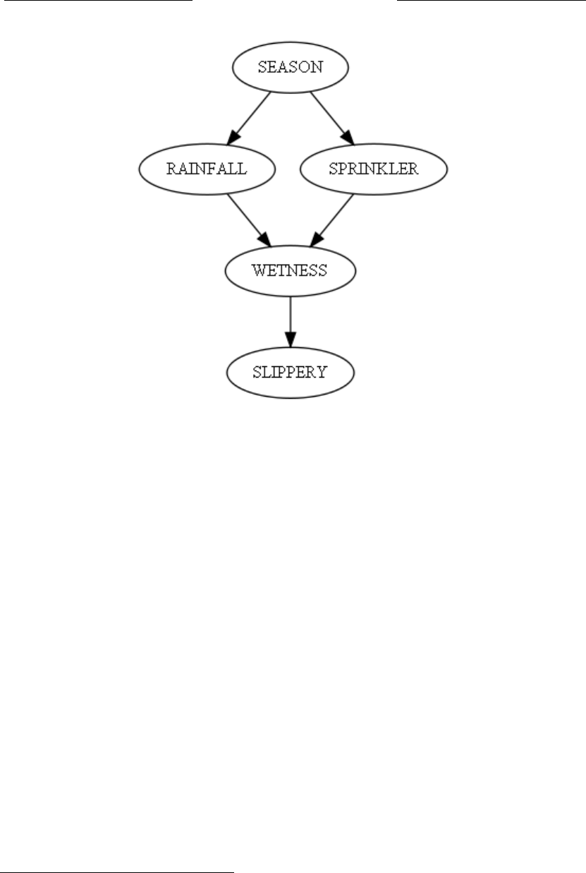
Timeless Decision eory
!"#$%&'"%#()&!#*&+%%,-%./0-!&./#&"12%3%/-4%'#5"%/-%6$"#%4'-)"%7#7"!%6&%4#)+%%8.&%
&'#&%6)%#/-&'"!%#!9.:"/&%0-!%&!"#&6/9%*#.)#1%$"*6)6-/%&'"-!2%#)%$2/#:6*#112%
6/*-/)6)&"/&;%6&%<.#*=)%16="%&'#&%$.*=+%3/%:2%(--=>%#))69/6/9%/"9#&65"%5#1."%&-%
6/0-!:#&6-/%?%("6/9%46116/9%&-%!"#%/-&%&-%*-/0!-/&%!"#16&2%?%6)%#%&"!!6(1"%)69/%
!"9#!$6/9%&'"%*'-6*"4-!&'6/"))%-0%#%$"*6)6-/%&'"-!2@
!"#$%&'%(#)*%+,-./)01,2+-'/2)01,)3+4/+-)5'+6,+2/7
A.$"#%B"#!1>%6/%'6)%(--=%$"%&"'()#%CB"#!1%DEEEF>%"G71#6/)%#/$%"G&"/)65"12%
$"0"/$)%#%0!#:"4-!=%0-!%:-$"116/9%*-./&"!0#*&.#1)%(#)"$%-/%$6!"*&"$%#*2*16*%
9!#7')%-0%*#.)#1%:"*'#/6):)+%%3%06/$%B"#!1H)%#!9.:"/&)%0-!%'6)%0!#:"4-!=%&-%("%
"G&!":"12%*-:7"116/9>%(.&%3%1#*=%&'"%)7#*"%&-%!"7!-$.*"%'"!"%'6)%"/&6!"%(--=+%%3%
*#/%-/12%965"%#%(!6"0%6/&!-$.*&6-/%&-%*#.)#1%$6#9!#:)>%'-7"0.112%).006*6"/&%&-%&'"%
0"4%.)")%3%!"<.6!"%C*#.)#1%$6#9!#:)%'#5"%:#/2%-&'"!%.)")%#)%4"11F+%%I'"%
6/&"!")&"$%!"#$"!%6)%!"0"!!"$%&-%B"#!1%CDEEEF+
,.77-)"%4"%#!"%!")"#!*'"!)%6/%&'"%
0#)&?"G7#/$6/9%06"1$%-0%)6$"4#1=%
)*6"/*">%#/$%4"%#!"%6/&"!")&"$%6/%4'#&%
*#.)")%)6$"4#1=)%&-%("*-:"%)1677"!2>%
#/$%4'"&'"!%6&%'#)%#/2&'6/9%&-%$-%46&'%
&'"%)"#)-/%-0%&'"%2"#!+%%J0&"!%"G&"/)65"%
)&.$2%4"%7!-7-)"%&'6)%)"&%-0%*#.)#1%
:"*'#/6):)K
I'"%&*"&+,%5#!6#(1"%6/01."/*")%'-4%
16="12%6&%6)%&-%!#6/>%#/$%#1)-%4'"&'"!%&'"%
)7!6/=1"!%6)%&.!/"$%-/+%%I'")"%&4-%
5#!6#(1")%6/%&.!/%6/01."/*"%'-4%16="12%
&'"%)6$"4#1=%6)%&-%("%4"&+%%J/$%4'" &'"!%
-!%/-&%&'"%)6$"4#1=%6)%4"&%$"&"!:6/")%
'-4%16="12%&'"%)6$"4#1=%6)%&-%("%
)1677"!2+
I'6)%$6!"*&"$%#*2*16*%9!#7'%-0%*#.)#1%
*-//"*&656&2%6)%<.#16&#&65"%!#&'"!%&'#/%<.#/&6&#&65"+%%I'"%9!#7'%$-")%/-&%)7"*602%
-+.%16="12%6&%6)%&-%!#6/%$.!6/9%).::"!;%6&%-/12%)#2)%&'#&%)"#)-/)%#00"*&%!#6/%6/%)-:"%
4#2+%%8.&%(2%#&&#*'6/9%*-/$6&6-/#1%7!-(#(616&2%$6)&!6(.&6-/)%&-%"#*'%/-$"%-0%&'"%
9!#7'>%4"%*#/%9"/"!#&"%#%L-6/&%7!-(#(616&2%0-!%#/2%7-))6(1"%-.&*-:"+%%M"&%&'"%
*#76%1"&&"!)%NO>%ND>%NP>%NQ>%NR%)&#/$%0-!%&'"%5#!6#(1")%,SJ,TU>%VJ3UWJMM>%
,BV3UXMSV>%YSIUS,,>%#/$%,M3BBSVZ+%%M"&%GO>%GD>%GP>%GQ>%GR%)&#/$%0-!%
7-))6(1"%)7"*606*%/"'%*&%-0%&'"%065"%5#!6#(1")%#(-5"+%%I'.)>%&'"%5#!6#(1")%
GO[).::"!>%GD[/-%!#6/>%GP[-/>%GQ[$#:7>%#/$%GR[&!"#*'"!-.)%4-.1$%
*-!!")7-/$%&-%&'"%":76!6*#1%-()"!5#&6-/%&'#&%6&%6)%).::"!>%6&%6)%/-&%!#6/6/9>%&'"%
R\
0(1%2*3453
Figure 1: Causal diagram of sidewalk slipperiness.
is “damp,” and the degree of slipperiness is “treacherous.”
11
We want to know what
probability our hypothesis assigns to this empirical observation.
Standard probability theory
12
makes it a tautology to state for any positive probabil-
ity:
p(x
1
x
2
x
3
x
4
x
5
) = p(x
1
)p(x
2
|x
1
)p(x
3
|x
2
x
1
)p(x
4
|x
3
x
2
x
1
)p(x
5
|x
4
x
3
x
2
x
1
) (1)
e directed causal graph shown in Figure 1 makes the falsiable,non-tautological claim
that the observed probability distribution will always factorize as follows:
p(x
1
x
2
x
3
x
4
x
5
) = p(x
1
)p(x
2
|x
1
)p(x
3
|x
1
)p(x
4
|x
3
x
2
)p(x
5
|x
4
) (2)
Intuitively, we might imagine that we rst ask what the probability is of it being summer
(25%), then the probability that it is not raining in the summer (80%), then the probabil-
ity that the sprinkler is on in the summer (30%), then the probability that the sidewalk is
damp when it is not raining and the sprinkler is on (99%), then the probability that the
sidewalk is treacherous when damp (80%). Implicit in this formula is the idea that only
11. If we demand quantitative predictions, we could suppose that the day is July 11th, the rainfall is
0 inches, the sprinkler is on, the sidewalk has 100 milligrams of water per square centimeter, and the
sidewalk’s coefficient of static friction is 0.2.
12. e notation p(a
1
) stands for “the probability of a
1
.” p(a
1
a
2
) stands for “the probability of a1 and
a2,” which may also be written p(a
1
, a
2
) or p(a
1
& a
2
). p(a
1
|a
2
) stands for “the probability of a1 given
that we know a
2
.” Bayes’s Rule denes that p(a
1
|a
2
) = p(a
1
a
2
)/p(a
2
).
58

Eliezer Yudkowsky
certain events directly aect other events. We write p(x
3
|x
1
) instead of the tautological
p(x
3
|x
2
x
1
) because we assume that whether the sprinkler is on does not aect the rain,
nor vice versa. Once we already know that it isn’t raining and that the sprinkler is on,
we no longer need to know the season in order to gure out how wet the sidewalk is;
we multiply by p(x
4
|x
3
x
2
) instead of p(x
4
|x
3
x
2
x
1
) and (by hypothesis) require the two
quantities to be identical. at is how we compute the probability distribution which
our causal hypothesis predicts.
Inference works dierently from causation. We know that the rooster’s crow does not
cause the sun to rise, but we infer that the sun will rise if we observe the rooster crow.
Raining causes the sidewalk to be wet, but we do not say that wet sidewalks cause rain.
Yet if we see a wet sidewalk we infer a greater probability that it is raining; and also if we
see it raining we infer that the sidewalk is more likely to be wet. In contrast to logical
deduction, probabilistic inference is always bidirectional; if we infer wet sidewalks from
rain we must necessarily infer rain from wet sidewalks.
13
How then are we to cash out, as
falsiable predictions, statements about asymmetrical causation? Suppose we have three
hypotheses:
a) Rain causes wet sidewalks.
b) Wet sidewalks cause rain.
c) Pink rabbits from within the hollow Earth
14
cause both rain and wet sidewalks.
Any of these three causal diagrams, when computed out to probability distributions,
could lead to the observed non-experimental correlation between wet sidewalks and rain.
In intuitive terms, we can distinguish among the three hypotheses as follows. First,
we pour water on the sidewalk, and then check whether we observe rain. Since no rain
13. In deductive logic,“P implies Q”does not imply “Q implies P.” However,in probabilistic inference,
if conditioning on A increases the probability of B, then conditioning on B must necessarily increase the
probability of A. p(a
1
|a
2
) > p(a
1
) implies p(a
1
a
2
)/p(a
2
) > p(a
1
) implies p(a
1
a
2
) > p(a
1
)p(a
2
)
implies p(a
1
a
2
)/p(a
1
) > p(a
2
) implies p(a
2
|a
1
) > p(a
2
). QED.
We can probabilistically infer a higher probability of B after observing A i p(A & B) > p(A)p(B),
that is, the joint probability of A and B is higher than it would be if A and B were independent. is
phrasing renders the symmetry visible.
We say A and B are dependent i p(A & B)! = p(A)p(B). We say A and B are independent i
p(A & B) = p(A)p(B), in which case we can infer nothing about B from observing A or vice versa.
14. Pink rabbits from within the hollow Earth are also known as “confounding factors,”“spurious cor-
relations,” “latent causes,” and “third causes.” For some time the tobacco industry staved o regulation
by arguing that the observed correlation between smoking and lung cancer could have been caused by
pink rabbits from within the hollow Earth who make people smoke and then give them lung cancer. e
correlation could have been caused by pink rabbits, but it was not, and this is an important point to bear
in mind when someone says “correlation does not imply causation.”
59

Timeless Decision eory
is observed, we conclude that wet sidewalks do not cause rain. is falsies b) and leaves
hypotheses a) and c). We send up a plane to seed some clouds overhead, making it rain.
We then check to see whether we observe wet sidewalks, and lo, the sidewalk is wet.
at falsies c) and leaves us with this experimentally observed asymmetry
15
: Making
rain causes a wet sidewalk, but wetting the sidewalk does not cause rain.
We begin to approach a way of describing the distinction between evidential decision
theory and causal decision theory—there is a dierence between observing that the side-
walk is wet, from which we infer that it may be raining, and making the sidewalk wet,
which does not imply a higher probability of rain. But how to formalize the distinction?
In Judea Pearl’s formalism, we write p(y|ˆx) to denote
16
“the probability of observing
y if we set variable X to x” or “the probability of y given that we do x.” To compute this
probability, we modify the causal diagram by deleting all the arrows which lead to X,
i.e., delete the conditional probability for X from the joint distribution.
Suppose that we pour water on the sidewalk—set variable X
4
to the value “wet,”
which we shall denote by x
4
. We would then have a new diagram (Figure 2). and a new
distribution:
p(x
1
x
2
x
3
x
5
|ˆx
4
) = p(x
1
)p(x
2
|x
1
)p(x
3
|x
1
)p(x
5
|x
4
) (3)
Note that the factor p(x
4
|x
3
x
2
) has been deleted from the computation of the new joint
distribution, since X
4
now takes on the xed value of x
4
. As expected, the probabilities
for the season, rainfall, and sprinkler activation are the same as before we poured water
on the sidewalk.
Only the slipperiness of the sidewalk is aected by our action. Note also that this
new equation is not the correct way to compute p(x
1
x
2
x
3
x
5
|x
4
)—if we observed a wet
sidewalk, it would change our inferred probabilities for rainfall, the season, etc.
15. Contrary to a long-standing misconception, asymmetrical causality can also be observed in (the
simplest explanation of ) non-experimental,non-temporal data sets. Presume that all our observations take
place during the summer, eliminating the seasonal confounding between sprinklers and rain. en if “wet
sidewalks cause both rain and sprinkler activations,” RAINFALL and SPRINKLER will be dependent,
but conditioning on WET will make them independent. at is, we will have p(rain & sprinkler)! =
p(rain)p(sprinkler), and p(rain & sprinkler|wet) = p(rain|wet)p(sprinkler|wet). If “rain and sprinkler
activations both cause wet sidewalks”then we will nd that rain and sprinklers are independent, unless we
observe the sidewalk to be wet, in which case they become dependent (because if we know the sidewalk is
wet, and we see it is not raining, we will know that the sprinkler is probably on). is testable consequence
of a directed causal graph is a core principle in algorithms that infer directionality of causation from non-
experimental non-temporal data. For more details see Pearl (2000).
16. Despite the resemblance of the notations p(y|x) and p(y|xˆ), the former usage denotes Bayesian
conditionalization, while the latter usage denotes a function from X to the space of probability distribu-
tions over Y .
60
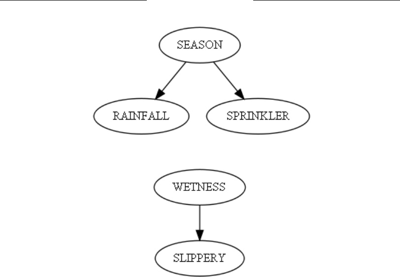
Eliezer Yudkowsky
!""#$%&$'()'&*+!,&-#&./&(0+0/&,+*+-+&-'+&)#1,(-(#1!*&2"#3!3(*(-4&5#"&.&5"#6&-'+&7#(1-&
,(%-"(38-(#10
9822#%+&-'!-&$+&2#8"&$!-+"&-'+&%(,+$!*:&;&%+-&<!"(!3*+&.=&-#&-'+&<!*8+&>$+->/&
$'()'&$+&%'!**&,+1#-+&34&?=0&&@+&$#8*,&-'+1&'!<+&!&1+$&,(!A"!6&!1,&!&1+$&
,(%-"(38-(#1B
2C?D?E?F?GH?I=J&K&2C?DJ2C?EH?DJ2C?FH?DJ2C?GH?=J
L#-+&-'!-&-'+&5!)-#"&2C?=H?F?EJ&'!%&3++1&,+*+-+,&5"#6&-'+&)#628-!-(#1&-'+&1+$&
7#(1-&,(%-"(38-(#1/&%(1)+&.=&1#$&-!:+%&-'+&5(?+,&<!*8+&?=0&&M%&+?2+)-+,/&-'+ &
2"#3!3(*(-(+%&5#"&-'+&%+!%#1/&"!(15!**/&!1,&%2"(1:*+"&!)-(<!-(#1&!"+&-'+&%!6+&!%&
3+5#"+&$+&2#8"+,&$!-+"&-'+&%(,+$!*:0&&
NOPQRS&EB&&
T1*4&-'+&%*(22+"(1+%%&-'+&%(,+$!*:&(%&!55+)-+,&34"&!)-(#10&&L#-+&!*%#&-'!-&-'(%&
1+$&+U8!-(#1&(%&!"#&-'+&)#""+)-&$!4&-#&)#628-+&2C?D?E?F?GH?=J&;&(5&$+&"$%&'(&)*
!&$+-&%(,+$!*:/&(-&$#8*,&)'!1A+"&(15+""+,&2"#3!3(*(-(+%&5#"&"!(15!**/&-'+&%+!%#1/&
+-)0
V#&%(68*!-+&!1&+?2+"(6+1-!*&6!1(28*!-(#1&$(-'(1&!&)!8%!*&,(!A"!6/&$+&%+<+"&-'+&
6!1(28*!-+,&<!"(!3*+&5"#6&(-%&2!"+1-%0&&W#""+%2#1,(1A*4/&$+&,+*+-+&-'+&
6!1(28*!-+,&<!"(!3*+X%&)#1,(-(#1!*&2"#3!3 (*(-4&5"#6&-'+&7#(1-&,(%-"(38-(#1&#<+"&-'+&
"+6!(1(1A&<!"(!3*+%0&&9-(**&!1#-'+"&$!4&<(+$(1A&-'(%+"!-(#1&(%&34&$"(-(1A&-'+&
)!8%!*&,(!A"!6&!%&!&%+"(+%&)&#&'+,!,%#,-&)#628-!-(#1%B
YD
Figure 2: Updated causal diagram of sidewalk slipperiness.
To simulate an experimental manipulation within a causal diagram, we sever the ma-
nipulated variable from its parents. Correspondingly, we delete the manipulated vari-
able’s conditional probability from the joint distribution over the remaining variables.
Still another way of viewing this operation is by writing the causal diagram as a series
of deterministic computations:
X
1
← f
1
(u
1
) (4a)
X
2
← f
2
(X
1
, u
2
) (4b)
X
3
← f
3
(X
1
, u
3
) (4c)
X
4
← f
4
(X
2
, X
3
, u
4
) (4d)
X
5
← f
5
(X
4
, u
5
) (4e)
Here the various u
i
are the error terms or probabilistic components, representing back-
ground variables which we choose not to take into account in our model. e ← opera-
tors are to be understood as denoting computations, or assignments as of a programming
language, rather than algebraic relations. In algebra, the equation y = x + b is identical,
as a mathematical object, to the equation x = y − b. But in that mathematics which
treats computer programs as formal mathematical objects, the assignment y ← x + b is
a dierent computation from the assignment x ← y−b. To assess the aect of the exper-
imental intervention p(x
1
x
2
x
3
x
5
|ˆx
4
), we delete the assignment X
4
← f
4
(X
2
, X
3
, u
4
)
and substitute the assignment X
4
← x
4
. When we carry through the computation, we
61

Timeless Decision eory
will nd a result that reects the predicted probability distribution for the causal diagram
under experimental intervention.
is formal rule for computing a prediction for an experimental intervention, given
a causal diagram, Pearl names the do-calculus. p(y|ˆx) may be read aloud as “probability
of y given do x.”
Computer programmers should nd the above quite intuitive. Mathematicians
17
may
nd it jarring, wondering why the elegant algebra over probability distributions should
transform into the computational blocks of causal diagrams. Statisticians may wince,
recalling harsh instruction to avoid the language of cause and eect. For a full defense,
one should consult the book Causality. Since it is not my main purpose to defend the
notion of causality, I contribute only these remarks:
• Since causal diagrams compute out to probability distributions, the mathematical
object called a “causal diagram” can plug into any socket that requires the mathe-
matical object called a “probability distribution”—while also possessing additional
useful properties of its own.
• Causal diagrams can explicitly represent compactness in a raw probability distri-
bution, such as probabilistic independences and relations between variables. Some
means of encoding the regularities in our observations is needed to invoke Occam’s
Razor, which underlies the inductive labor of science.
• A raw probability distribution over N discrete variables with M possible values has
M
N
− 1 degrees of freedom. is is too much exibility, too much license to t the
data, too little yield of predictive accuracy for each adjustment to the model. e
mathematical object called a “probability distribution” is not a productive scientic
hypothesis; it is a prediction produced by a productive hypothesis.
• All actual thinking takes place by means of cognition, which is to say, computation.
us causal diagrams, which specify how to compute probabilities, have a virtue
of real-world implementability lacking in the mathematical objects that are raw
probability distributions.
• Perhaps the greatest scientic virtue of causal diagrams is that a single causal hy-
pothesis predicts a non-experimental distribution plus additional predictions for
any performable experiment. All of these predictions are independently checkable
and falsiable, a severe test of a hypothesis. e formalism of probability distribu-
tions does not, of itself, specify any required relation between a non-experimental
17. Except constructivist mathematicians, who are accustomed to working with computations as the
basic elements of their proofs.
62

Eliezer Yudkowsky
distribution and an experimental distribution—implying innite freedom to acco-
modate the data.
9. Translating Standard Analyses of Newcomblike Problems into the
Language of Causality
With the language of Pearl’s causality in hand, we need only one more standard ingre-
dient to formally describe causal decision theory and evidential decision theory. is is
expected utility maximization, axiomatized in (von Neumann and Morgenstern 1944).
Suppose that I value vanilla ice cream with utility 5, chocolate ice cream with utility 10,
and I assign utility 0 to the event of receiving nothing. If I were an expected utility max-
imizer I would trade a 10% probability of chocolate ice cream (and a 90% probability of
nothing) for a 30% probability of vanilla ice cream, but I would trade a 90% probability
of vanilla ice cream for a 50% probability of chocolate ice cream.
“Expected utility” derives its name from the mathematical operation, expectation,
performed over utilities assigned to outcomes. When we have a quantitative function
f(X) and some probability distribution over X, our expectation of f(X) is the quantity:
E[f(X)] =
X
x
f(x)p(x) (5)
is is simply the weighted average of f (X), weighted by the probability function p(X)
over each possibility in X. In expected utility, the utility u(X) is a measure of the utility
we assign to each possible outcome—each possible consequence that could occur as the
result of our actions. When combined with some conditional probability distribution for
the consequences of an action, the result is a measure
18
of expected utility for that action.
We can then determine which of two actions we prefer by comparing their utilities and
selecting the one with a higher expected utility. Or, given a set of possible actions, we
can choose an action with maximal expected utility (an action such that no other action
has higher expected utility). An agent that behaves in this fashion is an expected utility
maximizer.
18. Utility functions are equivalent up to a positive affine transformation u
0
(x) = au(x) + b. A utility
function thus transformed will produce identical preferences over actions. us, both utility and expected
utility are referred to as “measures.”
63

Timeless Decision eory
Human beings are not expected utility maximizers (Kahneman and Tversky 2000)
but it is widely held that a rational agent should be
19
(von Neumann and Morgenstern
1944).
We can now easily describe the formal dierence between evidential and causal de-
cision algorithms:
Evidential decision algorithm:
E[u(a)] =
X
x
u(x)p(x|a) (6)
Causal decision algorithm:
E[u(a)] =
X
x
u(x)p(x|ˆa) (7)
Let’s begin by translating the classic analyses of Newcomb’s Problem into the lan-
guage of causality. A superintelligent Predictor arrives from another galaxy and sets
about playing Newcomb’s game: e Predictor sets out a transparent box A lled with
a thousand dollars, and an opaque box B.e Predictor places a million dollars in box B
if and only if the Predictor predicts that you will take only box B. Historically, the Pre-
dictor has always been accurate.
20
en the Predictor leaves. Do you take both boxes,
or only box B?
Let the action a
B
represent taking the single box B, and action a
AB
represent tak-
ing two boxes. Let the outcome B
$
represent the possibility that box B is lled with
$1,000,000, and the outcome B
0
represent the possibility that box B is empty. en the
game has these conceptually possible outcomes:
B
$
: B
0
:
a
B
: a
B
, B
$
: $1,000,000 a
B
, B
0
: $0
a
AB
: a
AB
, B
$
: $1,001,000 a
AB
, B
0
: $1000
Let us suppose that historically half the subjects took only box B and half the subjects
took both boxes, and the Predictor always predicted accurately. en we observed this
joint frequency distribution over actions and outcomes:
19. Note that the Von Neumann—Morgenstern axiomatization of expected utility makes no mention of
the philosophical commitments sometimes labeled as “utilitarianism.” An agent that obeys the expected
utility axioms need not assign any particular utility to happiness, nor value its own happiness over the
happiness of others, regard sensory experiences or its own psychological states as the only meaningful
consequences, etc. Expected utility in our sense is simply a mathematical constraint, fullled when the
agent’s preferences have a certain structure that forbids, e.g., nontransitivity of preferences (preferring A
to B, B to C, and C to A).
20. We also suppose that the Predictor has demonstrated good discrimination. For example, if every-
one tested took only box B, and the Predictor was always right, then perhaps the Predictor followed the
algorithm “put a million dollars in box B every time” rather than actually predicting.
64

Eliezer Yudkowsky
B
$
: B
0
:
a
B
: a
B
, B
$
: 50% a
B
, B
0
: 0%
21
a
AB
: a
AB
, B
$
: 0% a
AB
, B
0
: 50%
An evidential decision agent employs the standard operations of marginalization, con-
ditionalization, and Bayes’s Rule to compute conditional probabilities. (Note that these
operations require only a distributional representation of probability, without invoking
causal diagrams). An evidential agent concludes that the actions a
B
and a
AB
imply the
following probability distributions over outcomes:
B
$
: B
0
:
a
B
: p(B
$
, a
B
): 100%
22
p(B
0
, a
B
): 0%
a
AB
: p(B
$
, a
AB
): 0% p(B
0
, a
AB
): 100%
e expected utility of a
B
therefore equals u($1, 000, 000) and the expected utility of
a
AB
equals u($1, 000). Supposing the agent’s utility function to be increasing in money,
an evidential agent chooses a
B
by the rule of expected utility maximization.
Now consider the causal agent. e causal agent requires the probabilities:
B
$
: B
0
:
a
B
: p(B
$
, ˆa
B
) p(B
0
, ˆa
B
)
a
AB
: p(B
$
, ˆa
AB
) p(B
0
, ˆa
B
)
Since the do-calculus operates on causal diagrams, we cannot compute these probabili-
ties without a causal diagram of the Newcomb problem. Figure 3 shows a causal diagram
which can account for all dependencies historically observed in the non-experimental
distribution: e Predictor P observes the state of mind of a causal decision agent C at
7AM, represented by a link from C
7AM
to P (since, when P observes C, P ’s state be-
comes a function of C’s state). P , observing that C is a causal decision theorist, lls box
B with $0 to punish C for his rationality. en at 8AM, C is faced with the Predictor’s
game, and at node A must choose action a
B
or a
AB
. Being a causal decision theorist,
C chooses action a
AB
. is causal diagram explains the observed dependency between
variable A (the action) and variable B (the state of box B) by attributing it to a con-
founding mutual cause, C’s state of mind at 7AM. Had C been an evidential decision
21. Note that postulating an observed frequency of 0% may break some theorems about causal diagrams
which require a positive distribution (a probability distribution that is never zero).
22. A wise Bayesian will never claim a probability of exactly 1.0. “Once I assign a probability of 1 to
a proposition, I can never undo it. No matter what I see or learn, I have to reject everything that disagrees
with the axiom. I don’t like the idea of not being able to change my mind, ever.” (Smigrodzki 2003) For
the sake of simplifying calculations, we suppose the historical sample is large enough that an evidential
agent is “eectively certain,” 1.0 minus epsilon.
65
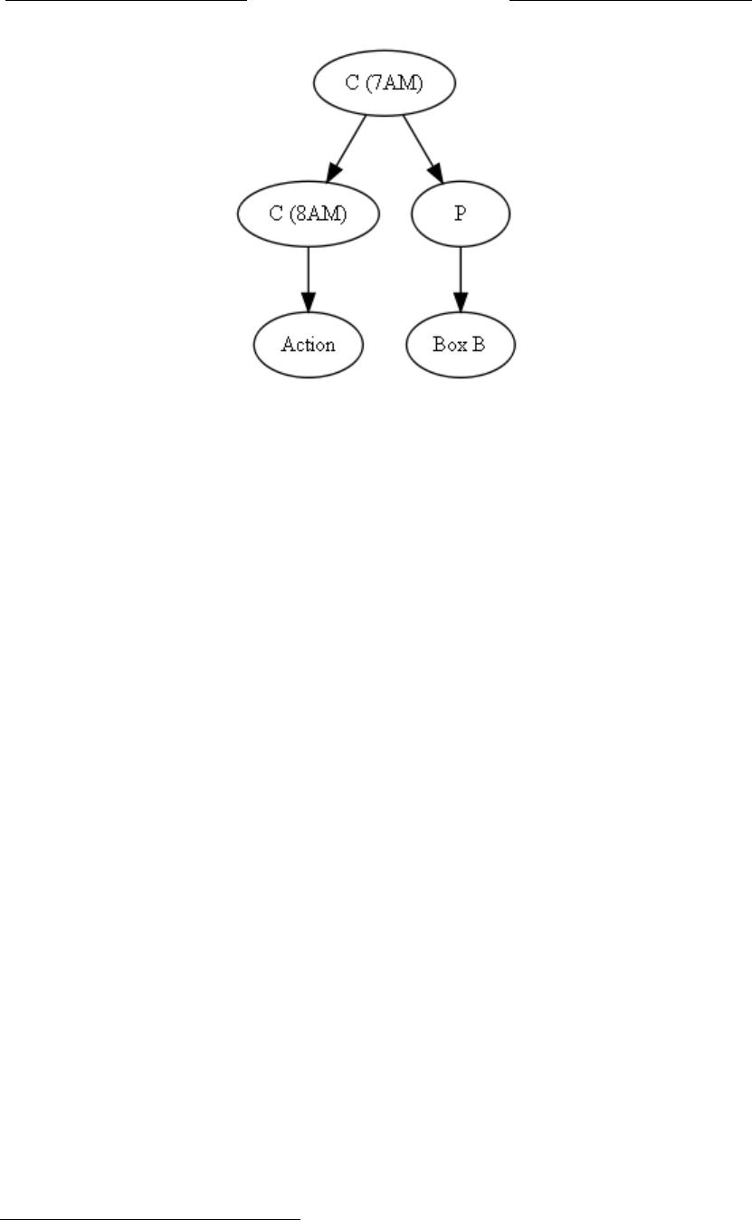
Timeless Decision eory
!"# !"$"%#&'() !"$"(#&()
*+
!,"# !,"$"%#&() !,"$"(#&'()
,-&./01.-20!3&1.40506-&!7.-2&.8936:5&2;.&52!-1!<1&69.<!206-5&6=&8!<70-!30>!206-$&
46-10206-!30>!206-$&!-1&"!:.5?5&@A3.&26&4689A2.&46-10206-!3&9<6B!B03020.5C&&DE62.&
2;!2&2;.5.&69.<!206-5&<.FA0<.&6-3:&!&1052<0BA206-!3&<.9<.5.-2!206-&6=&9<6B!B0302:$&
G02;6A2&0-/6H0-7&4!A5!3&10!7<!85IC&&,-&./01.-20!3&!7.-2&46-43A1.5&2;!2&2;.&
!4206-5&!"&!-1&!,"&0893:&2;.&=6336G0-7&9<6B!B0302:&1052<0BA206-5&6/.<&6A2468.5#
"%# "(#
!"# 9D"%J!"I#&+(()
**
9D"(J!"I#&()
!,"# 9D"%J!,"I#&() 9D"(J!,"I#&+(()
K;.&.L9.42.1&A20302:&6=&!"&2;.<.=6<.&.FA!35&AD%+$((($(((I&!-1&2;.&.L9.42.1&A20302:&
6=&!,"&.FA!35&AD%+$(((IC&&MA99650-7&2;.&!7.-2?5&A20302:&=A-4206-&26&B.&0-4<.!50-7&
0-&86-.:$&!-&./01.-20!3&!7.-2&4;665.5&!"&B:&2;.&<A3.&6=&.L9.42.1&A20302:&
8!L080>!206-C
E6G&46-501.<&2;.&4!A5!3&!7.-2C&&K;.&4!A5!3&!7.-2&<.FA0<.5&2;.&9<6B!B03020.5#
"%# "(#
!"# 9D"%J!N"I 9D"(J!N"I
!,"# 9D"%J!N,"I 9D"(J!N,"I
M0-4.&2;.&16O4!34A3A5&69.<!2.5&6-&4!A5!3&10!7<!85$&G.&4!--62&4689A2.&2;.5.&
9<6B!B03020.5&G02;6A2&!&4!A5!3&10!7<!8&6=&2;.&E.G468B&9<6B3.8#
P07A<.&Q&5;6G5&!&4!A5!3&10!7<!8&G;04;&4!-&
!446A-2&=6<&!33&1.9.-1.-40.5&;0526<04!33:&6B5.</.1&
0-&2;.&-6-O.L9.<08.-2!3&1052<0BA206-#&&K;.&R<.10426<&
DRI&6B5.</.5&2;.&52!2.&6=&80-1&6=&!&4!A5!3&1.40506-&
!7.-2&DSI&!2&T,U$&<.9<.5.-2.1&B:&!&30-H&=<68&
ST,U&26&R&D50-4.$&G;.-&R&6B5.</.5&S$&R?5&52!2.&
B.468.5&!&=A-4206-&6=&S?5&52!2.IC&&R$&6B5.</0-7&2;!2&
S&05&!&4!A5!3&1.40506-&2;.6<052$&=0335&B6L&"&G02;&%(&
26&9A-05;&S&=6<&;05&<!206-!302:C&&K;.-&!2&V,U$&S&05&
=!4.1&G02;&2;.&R<.10426<?5&7!8.$&!-1&!2&-61.&,&
8A52&4;665.&!4206-&!"&6<&!,"C&&&".0-7&!&4!A5!3&
1.40506-&2;.6<052$&S&4;665.5&!4206-&!,"C&&K;05&
4!A5!3&10!7<!8&.L93!0-5&2;.&6B5.</.1&
*+
&E62.&2;!2&9652A3!20-7&!-&6B5.</.1& = <.FA.-4:&6=&()&8!:&B<.!H&568.&2;.6<.85&!B6A2 & 4!A5!3&
10!7<!85&G;04;&<.FA0<.&!&965020/.&1052<0BA206-&D!&9<6B!B0302:&1052<0BA206-&2;!2&05&-./.<&>.<6IC
**
&,&G05.&"!:.50!-&G033&-./.<&43!08&!&9<6B!B0302:&6=&!"#$%&'&+C(C&&WX-4.&Y&!5507-&!&9<6B!B0302:&6=&+&26&
!&9<69650206-$&Y&4!-&-./.<&A-16&02C&E6&8!22.<&G;!2&Y&5..&6<&3.!<-$&Y&; !/.&26&<.Z.42&./.<:2;0-7&2 ;!2&
105!7<..5&G02;&2;.&!L068C&&Y& 16-?2&30H.&2;.&01.!&6=&-62&B.0-7&!B3.&26&4;!-7.&8:&80-1$&./.<CW&
DM807<61>H0&G;.-./.<IC&&P6<&2;.&5!H.&6=&508930=:0-7&4!34A3!206-5$&G.&5A9965.&2;.&;0526<04!3&
5!893.&05&3!<7.&.-6A7;&2;!2&!-&./01.-20!3&!7.-2&05&W.==.420/.3:&4.<2!0-W$&+C(&80-A5&.95036-C
['
()*+,!-./-
Figure 3
agent, the Predictor would have lled B with $1,000,000 at 7:30AM and C would have
chosen a
AB
at 8AM.
e causal decision agent, faced with a decision at node A, computes interventional
probabilities by severing the node A from its parents and substituting the equations
A ← a
B
and A ← a
AB
to compute the causal eect of choosing a
B
or a
AB
respectively:
B
$
: B
0
:
a
B
: p(B
$
, ˆa
B
): 0% p(B
0
, ˆa
B
): 100%
a
AB
: p(B
$
, ˆa
AB
): 0% p(B
0
, ˆa
AB
): 100%
is reects the intuitive argument that underlies the choice to take both boxes: “e
Predictor has already come and gone; therefore, the contents of box B cannot depend on
what I choose.”
From the perspective of an evidential decision theorist, this is the cleverest argument
ever devised for predictably losing $999,000.
We now move on to our second Newcomblike problem. In (this variant of) Solomon’s
Problem, we observe the following:
• People who chew gum have a much higher incidence of throat abscesses;
• In test tube experiments, chewing gum is observed to kill the bacteria that form
throat abscesses;
• Statistics show that conditioning on the gene CGTA reverses the correlation be-
tween chewing gum and throat abscesses.
23
23. at is, if we divide the subjects into separate pools according to the presence or absence of CGTA,
chewing gum appears to protect both pools against throat abscesses. p(abscess|gum) > p(abscess), but
66
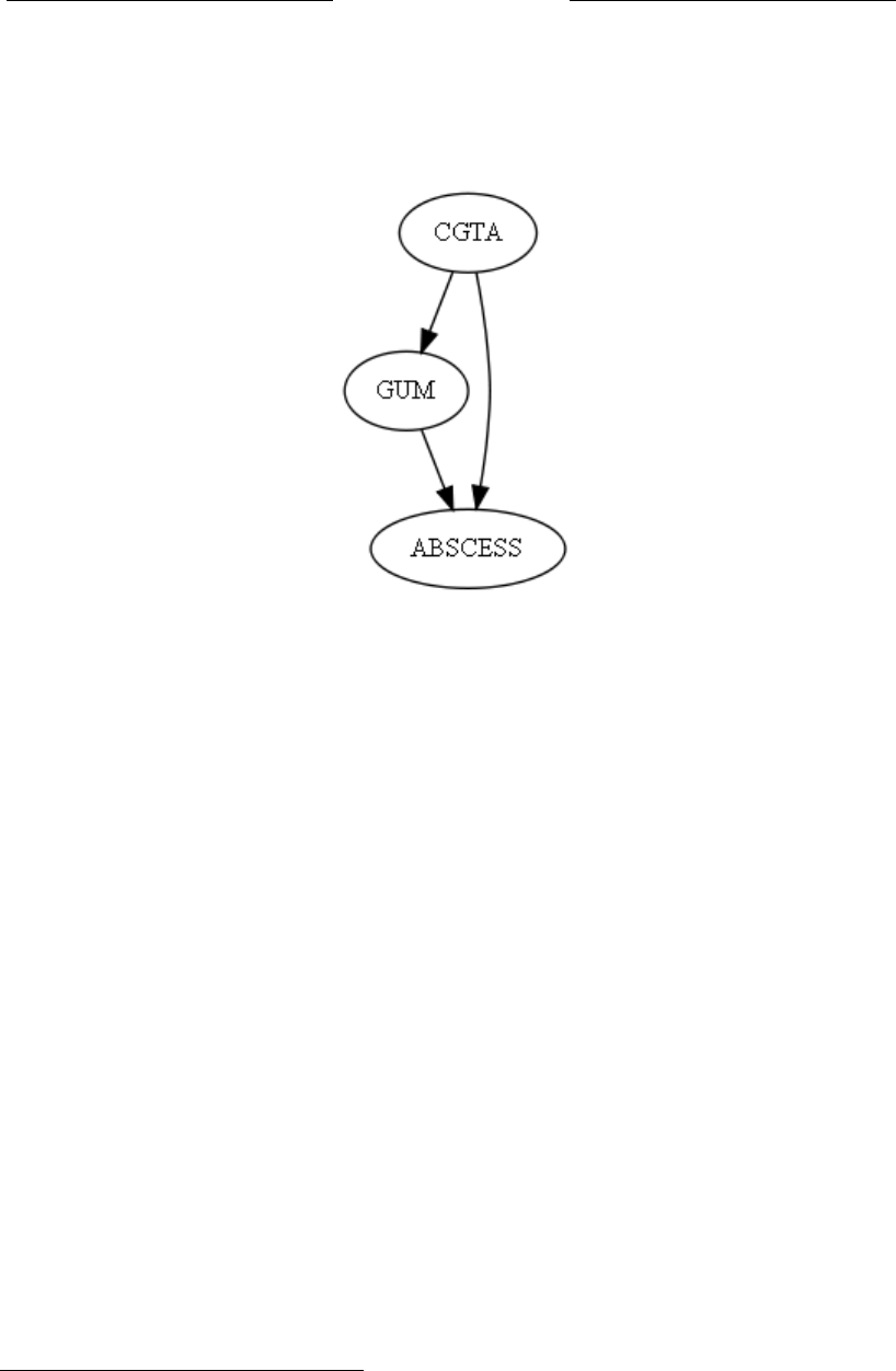
Eliezer Yudkowsky
We think this happens because the gene CGTA both causes throat abscesses and inu-
ences the decision to chew gum. We therefore explain the observed distribution using
Figure 4. and the formula:
!"#"$!"$%&'(")*""$'+,-.,(/"'0'1)2"',%).3$4',$!'+,-.,(/"'5'1)2"'6),)"'37'(38'54'
(&',))-.(9).$:'.)')3','%3$739$!.$:';9)9,/'%,96"<'=>6'6),)"'37';.$!',)'?0@A''B,!'='
(""$',$'"+.!"$).,/'!"%.6.3$',:"$)<')2"'C-"!.%)3-'*39/!'2,+"'7.//"!'5'*.)2'
DE<FFF<FFF',)'?GHF0@',$!'='*39/!'2,+"'%236"$',05',)'I0@A
J2"'%,96,/'!"%.6.3$',:"$)<'7,%"!'*.)2','!"%.6.3$',)'$3!"'0<'%3;#9)"6'
!"#$%&$"#!'"()'#-3(,(./.)."6'(&'6"+"-.$:')2"'$3!"'0'7-3;'.)6'#,-"$)6',$!'
69(6).)9).$:')2"'"K9,).3$6'0'GL',5',$!'0'GL',05')3'%3;#9)"')2"'%,96,/'"77"%)'37'
%2336.$:',5'3-',05'-"6#"%).+"/&G
5DG 5FG
,5G #15DM,N54G'FO #15FM,N54G'EFFO
,05G #15DM,N054G'FO #15FM,N054G'EFFO
J2.6'-"7/"%)6')2"'.$)9.).+"',-:9;"$)')2,)'9$!"-/."6')2"'%23.%"')3'),P"'(3)2'(38"6G'
QJ2"'C-"!.%)3-'2,6',/-",!&'%3;"',$!':3$"R')2"-"73-"<')2"'%3$)"$)6'37'(38'5'
%,$$3)'!"#"$!'3$'*2,)'S'%2336"AQ
T-3;')2"'#"-6#"%).+"'37',$'"+.!"$).,/'!"%.6.3$')2"3-.6)<')2.6'.6')2"'%/"+"-"6)'
,-:9;"$)'"+"-'!"+.6"!'73-'#-"!.%),(/&'/36.$:'DUUU<FFF'!3//,-6A
V"'$3*';3+"'3$')3'39-'6"%3$!'W"*%3;(/.P"'#-3(/";A''S$'1)2.6'+,-.,$)'374'
X3/3;3$>6'C-3(/";<'*"'3(6"-+"')2"'73//3*.$:G
EA C"3#/"'*23'%2"*':9;'2,+"',';9%2'2.:2"-'.$%.!" $ %" '37')2-3,)',(6%"66"6R'
YA S$')"6)')9("'"8#"-.;"$)6<'%2"*.$:':9;'.6'3(6"-+"!')3'P.//')2"'(,%)"-.,')2,)'
73-;')2-3,)',(6%"66"6R
HA X),).6).%6'623*')2,)'%3$!.).3$.$:'3$')2"':"$"'=ZJ0'
-"+"-6"6')2"'%3--"/,).3$'(")*""$'%2"*.$:':9;',$!')2-3,)'
,(6%"66"6A
YH
V"')2.$P')2.6'2,##"$6'("%,96"')2"':"$"'=ZJ0'(3)2'%,96"6')2-3,)'
,(6%"66"6',$!'.$7/9"$%"6')2"'!"%.6.3$')3'%2"*':9;A''V"')2"-"73-"'
"8#/,.$')2"'3(6"-+"!'!.6)-.(9).3$'96.$:'7.:9-"'[',$!')2"'73-;9/,G
#18E8Y8H4'L'#18E4#18YM8E4#18HM8Y8E4
Y[
J2"'%,96,/'!"%.6.3$')2"3-.6)'6"+"-6')2"'$3!"'Q%2"*':9;Q'7-3;'.)6'
#,-"$)<'=ZJ0<'.$'3-!"-')3'"+,/9,)"')2"'%,96,/'"77"%)'37'%2"*.$:'
:9;'+"-696'$3)'%2"*.$:':9;A''J2"'$"*'73-;9/,'.6'#18HM8NY4'L\
8E'
#18E8HM8NY4'L\
8E'
#18E4#18HM8Y8E4A''J2"'%,96,/'!"%.6.3$')2"3-.6)'
)296'(":.$6'(&',669;.$:'2.6'#-3(,(./.)&'37'#366"66.$:':"$"'=ZJ0'
YH
'J2,)'.6<'.7'*"'!.+.!"')2"'69(]"%)6'.$)3'6"# ,-,)"'#33/6',%%3-!.$:') 3')2"'#-"6"$%"'3 -', (6"$%"'37'
=ZJ0<'%2"*.$:':9;',##",-6')3'#-3)"%)'(3)2'#33 /6',:,.$6)')2-3,)',(6%"66"6A''#1,(6%"66M:9;4'^'
#1,(6%"664<'(9)'#1,(6%" 66M:9;<=ZJ04'_'#1,(6%"66M=ZJ04', $!'#1,(6%"66M:9;<`=ZJ04'_'
#1,(6%"66M`=ZJ04A''X9%2','6.)9,).3$'.6'P$3*$' ,6'QX.;#63$>6'C,-,!38Q<')239:2'.)'.6'$3)','
#,-,!38A
aa
*!+,%$-./-
Figure 4
p(x
1
x
2
x
3
) = p(x
1
)p(x
2
|x
1
)p(x
3
|x
2
x
1
)
24
(8)
e causal decision theorist severs the node “chew gum”from its parent, CGTA, in order
to evaluate the causal eect of chewing gum versus not chewing gum. e new formula
is p(x
3
|ˆx
2
) =
P
x
1
p(x
1
x
3
|ˆx
2
) =
P
x
1
p(x
1
)p(x
3
|x
2
x
1
). e causal decision theorist
thus begins by assuming his probability of possessing gene CGTA is the same as that
for the general population, and then assessing his probability of developing a throat
abscess given that he does (or does not) chew gum. e result is that chewing gum
shows a higher expected utility than the alternative. is seems to be the sensible course
of action.
e evidential decision theorist would, on rst sight, seem to behave oddly; using
standard probability theory yields the formula p(x
3
|x
2
) =
P
x
1
p(x
1
|x
2
)p(x
3
|x
2
x
1
).
us, the evidential decision theorist would rst update his probability of possessing the
gene CGTA in the light of his decision to chew gum, and then use his decision plus the
updated probability of CGTA to assess his probability of developing throat cancer. is
yields a lower expected utility for chewing gum.
p(abscess|gum, CGTA) < p(abscess|CGTA) and p(abscess|gum,¬CGTA) < p(abscess|¬CGTA).
Such a situation is known as “Simpson’s Paradox,” though it is not a paradox.
24. is formula equates to the tautological one. A fully connected causal graph requires no indepen-
dences and hence makes no testable predictions regarding dependences until an experimental manipula-
tion is performed.
67
Timeless Decision eory
9.1. Tickle Defense and Meta-tickle Defense
e “tickle defense” promulgated by Eells (1984) suggests that as soon as an evidential
agent notices his desire to chew gum, this evidence already informs the agent that he has
gene CGTA—alternatively the agent might introspect and nd that he has no desire to
chew gum. With the value of the CGTA variable already known and xed, the decision
to chew gum is no longer evidence about CGTA and the only remaining “news” about
throat abscesses is good news. p(abscess|gum) may be greater than p(abscess), but
p(abscess|gum, cgta+) < p(abscess|cgta+) and similarly with p(abscess|gum, cgta−).
e tickle defense shows up even more clearly in this variant of Solomon’s Problem:
!"#$%&#"'(&#'"#$%'$#)*+#$%&#,&-&+'.#/*/0.'$!*-1#'-2#$%&-#'""&""!-,#%!"#/+*3'3!.!$4#
*)#2&5&.*/!-,#'#$%+*'$#'3"6&""#,!5&-#$%'$#%*&"#7*+#2*&"#-*$8#6%&9#,0(:##;%&#
+&"0.$#!"#$%'$#6%&9!-,#,0(#"%*9"#'#%!,%&+#&</&6$&2#0$!.!$4#$%'-#$%&#'.$&+-'$!5&:#
;%!"#"&&("#$*#3&#$%&#"&-"!3.*0+"&#*)#'6$!*-:
;%&#&5!2&-$!'.#2&6!"!*-#$%&*+!"$#9*0.21#*-#)!+"$#"!,%$1#"&&(#$*#3&%'5&#*22.4=#0"!-,#
"$'-2'+2#/+*3'3!.!$4#$%&*+4#4!&.2"#$%&#)*+(0.'#/7<>?<@8#A#B
<C#
/7<C?<@8/7<>?<@<C8:#
;%0"1#$%&#&5!2&-$!'.#2&6!"!*-#$%&*+!"$#9*0.2#)!+"$#0/2'$&#%!"#/+*3'3!.!$4#*)#
/*""&""!-,#$%&#,&-&#DE;F#!-#$%&#.!,%$#*)#%!"#2&6!"!*-#$*#6%&9#,0(1#'-2#$%&-#0"&#
%!"#2&6!"!*-#/.0"#$%�/2'$&2#/+*3'3!.!$4#*)#DE;F#$*#'""&""#%!"#/+*3'3!.!$4#*)#
2&5&.*/!-,#$%+*'$#6'-6&+:##;%!"#4!&.2"#'#.*9&+#&</&6$&2#0$!.!$4#)*+#6%&9!-,#,0(:
!"#$%&'(&)&*+&',*('-&.,/."#$%&'(&)&*+&0
;%&#G$!6H.&)&-"&G#/+*(0.,'$&2#34#I&."#7CJK@8#"0,,&"$"#$%'$#'"#"**-#'"#'-#
&5!2&-$!'.#',&-$#-*$!6&"#%!"#(&+"1&#$*#6%&9#,0(1#$%!"#&5!2&-6&#'.+&'24#!-)*+("#
$%&#',&-$#$%'$#%&#%'"#,&-&#DE;F#L#'.$&+-'$!5&.4#$%&#',&-$#(!,%$#!-$+*"/&6$#'-2#
)!-2#$%'$#%&#%'"#-*#2&"!+&#$*#6%&9#,0(:##M!$%#$%'.0&#*)#$%&#DE;F#5'+!'3.&#
'.+&'24#H-*9-#'-2#)!<&21#$%&6!"!*-#$*#6%&9#,0(#!"#-*#.*-,&+#&5!2&-6&#'3*0$#
DE;F#'-2#$%&#*-.4#+&('!-!-,#G-&9"G#'3*0$#$%+*'$#'3"6&""&"#!"#,**2#-&9":#
/7'3"6&""?,0(8#('4#3&#,+&'$&+#$%'-#/7'3"6&""81#30$#/7'3"6&""?,0(1#6,$'N8#O#
/7'3"6&""?6,$'N8#'-2#"!(!.'+.4#9!$%#/7'3"6&""?,0(1#6,$'L8:##;%&#$!6H.&)&-"&#
"%*9"#0/#&5&-#(*+.&'+.4#!-#$%!"#5'+!'-$#*)#P*.*(*-Q"#R+*3.&(S
T&+&#$%&#"'(&#,&-'0"&"#/&*/.&#$*#.!H&#&'$!-,#
,+'/&"#'-2#'."*#6'0"&"#/&*/.&#$*#"/*-$'-&*0".4#
6*(30"$1#30$#$%&#"/*-$'-&*0"#6*(30"$!*-#2*&"#
-*$#6'0"&#/&*/.&#$*#&'$#,+'/&"#-*+#5!6&+"':##U)#
4*0#)!-2#$%'$#4*0#2,*.#$*#&'$#,+'/&"1#4*0#('4#'"#
9&..#,*#'%&'2#'-2#&'$#$%&(1#3&6'0"&#$%&#
'.+&'24L*3"&+5&2#)'6$#$%'$#4*0#2,*.#$*#&'$#
,+'/&"#'.+&'24#(&'-"#$%'$#4*0#%'5&#E&-&#IEV1#
'-2#$%&#'6$0'.#'6$#*)#&'$!-,#,+'/&"#%'"#-*#
6*++&.'$!*-#$*#"/*-$'-&*0"#6*(30"$!*-#*-6&#$%&#
5'.0&#*)#IEV#!"#H-*9-:##;%!"#!"#H-*9-#'"#G"6+&&-!-,#*))G:##D*-"!2&+&2#!-#
!"*.'$!*-1#$%'+!'3.&"#EWFRIP#'-2#VXXY#'+*++&.'$&2#!-#*0+#*3"&+5'$!*-"#L#
/7,+'/&"1)**(8#Z#/7,+'/&"8[/7)**(81#3&6'0"&#!)#4*0#&'$#,+'/&"#4*0#/+*3'3.4#
%'5&#IEV#'-2#IEV#('4#('H*0#"/*-$'-&*0".4#6*(30"$:##\0$#!)#4*0#*3"&+5&#
$%'.0&#*)#$%'+!'3.&#IEV1#$%&-#$%!"#+#1&&*+'3))#VXXY#)+*(#EWFRIP#7'-2#
EWFRIP#)+*(#VXXY81#+&-2&+!-,#$%'+!'3.&"#!-2&/&-2&-$:##F66*+2!-,#$*#$%&#
6'0"'.#2!',+'(#]1#/7EWFRIP1VXXY?IEV8#(0"$#&^0'.#/7EWFRIP?
IEV8[/7VXXY?IEV8#)*+#'..#"/&6!)!6#5'.0&"#*)#$%&"'+!'3.&":
@_
#;%!"#)*+(0.'#&^0'$&"#$*#$%&#$'0$*.*,!6'.#*-&:##F#)0..4#6*--&6$&2#6'0"' .#,+'/%#+&^0!+&"#-*#
!-2&/&-2&- 6&"#'-2#%&-6&#('H&"#-*#$&"$'3.&#/+&2!6$!*-"#+&,'+2!-,#2&/&-2&-6&"#0-$!.#'-#
&</&+!(&-$'.#('-!/0.'$!*-#!"#/ &+)*+(&2:
`a
4"561&'78'
Figure 5
Here the same gene causes people to like eating grapes and also causes people to
spontaneously combust, but the spontaneous combustion does not cause people to eat
grapes nor vice versa. If you nd that you want to eat grapes, you may as well go ahead
and eat them, because the already-observed fact that you want to eat grapes already
means that you have Gene EGF, and the actual act of eating grapes has no correlation
to spontaneous combustion once the value of EGF is known. is is known as “screen-
ing o.” Considered in isolation, the variables GRAPES and FOOM are correlated in
our observations—p(grapes, foom) > p(grapes) ∗ p(foom), because if you eat grapes
you probably have EGF and EGF may make you spontaneously combust. But if you
observe the value of the variable EGF, then this screens o FOOM from GRAPES (and
GRAPES from FOOM), rendering the variables independent. According to the causal
diagram D, p(GRAPES, FOOM|EGF) must equal p(GRAPES|EGF)∗p(FOOM|EGF)
for all specic values of these variables.
So far,so good. It seems that a single decision theory—evidential decision theory plus
the tickle defense—walks o with the money in Newcomb’s Problem, and also chews
protective gum in the throat-abscess variant of Solomon’s Problem.
Yet the theorists behind the tickle defense did not rest on that accomplishment, but
continued to elaborate and formalize their theory. Suppose that you cannot observe
yourself wanting to chew gum—you lack strong cognitive abilities of introspection. Or
suppose the inuence on your cognition is such that you can’t easily determine your own
68

Eliezer Yudkowsky
true motives.
25
Does an evidential theorist then avoid chewing gum, or the equiva-
lent thereof? No, says Eels: Once you make a tentative decision, that decision can be
taken into account as evidence and you can reconsider your decision in light of this ev-
idence. is is the meta-tickle defense (Eells 1984), and it is rather complicated, since
it introduces an iterative algorithm with a rst-order decision, a second-order decision,
continuing ad innitum or until a stable xed point is found. e meta-tickle defense
requires us to assign probabilities to our own decisions and sometimes to revise those
probabilities sharply, and there is no guarantee that the algorithm terminates.
In fact, Eels went on to say that his meta-tickle defense showed that an evidential
decision theorist would take both boxes in Newcomb’s Problem!
26
What we would ideally like is a version of the tickle defense that lets an evidential
theorist chew protective gum, and also take only box B in Newcomb’s Problem. Perhaps
we could simply use the tickle defense on one occasion but not the other? Unfortunately
this answer, pragmatic as it may seem, is unlikely to satisfy a decision theorist—it has
not been formalized, and in any case one would like to know why one uses the tickle
defense on one occasion but not the other.
10. Review: e Markov Condition
e Markov Condition requires statistical independence of the error terms, the u
i
in
the computations described in Section 8. is is a mathematical assumption inherent in
the formalism of causal diagrams; if reality violates the assumption, the causal diagram’s
prediction will not match observation.
Suppose that I roll a six-sided die and write down the result on a sheet of paper. I
dispatch two sealed copies of this paper to two distant locations, Outer Mongolia and the
planet Neptune, where two confederates each roll one additional six-sided die and add
this to the number from the piece of paper. Imagine that you are observing this scenario,
and that neither of my confederates has yet opened their sealed packet of paper, rolled
their dice, or announced their sums.
One ad hoc method for modeling this scenario might be as follows. First, I consider
the scenario in Mongolia. e Mongolian confederate’s six-sided die might turn up
any number from 1 to 6, and having no further useful information, by the Principle of
25. “Power corrupts,” said Lord Acton, “and absolute power corrupts absolutely.”
26. At this time the widespread opinion in the eld of decision theory was that taking both boxes was
the “rational” choice in Newcomb’s Problem and that the Predictor was simply punishing two-boxers.
Arguing that ticklish agents would take both boxes was, in the prevailing academic climate, an argument
seen as supporting the tickle defense.
69
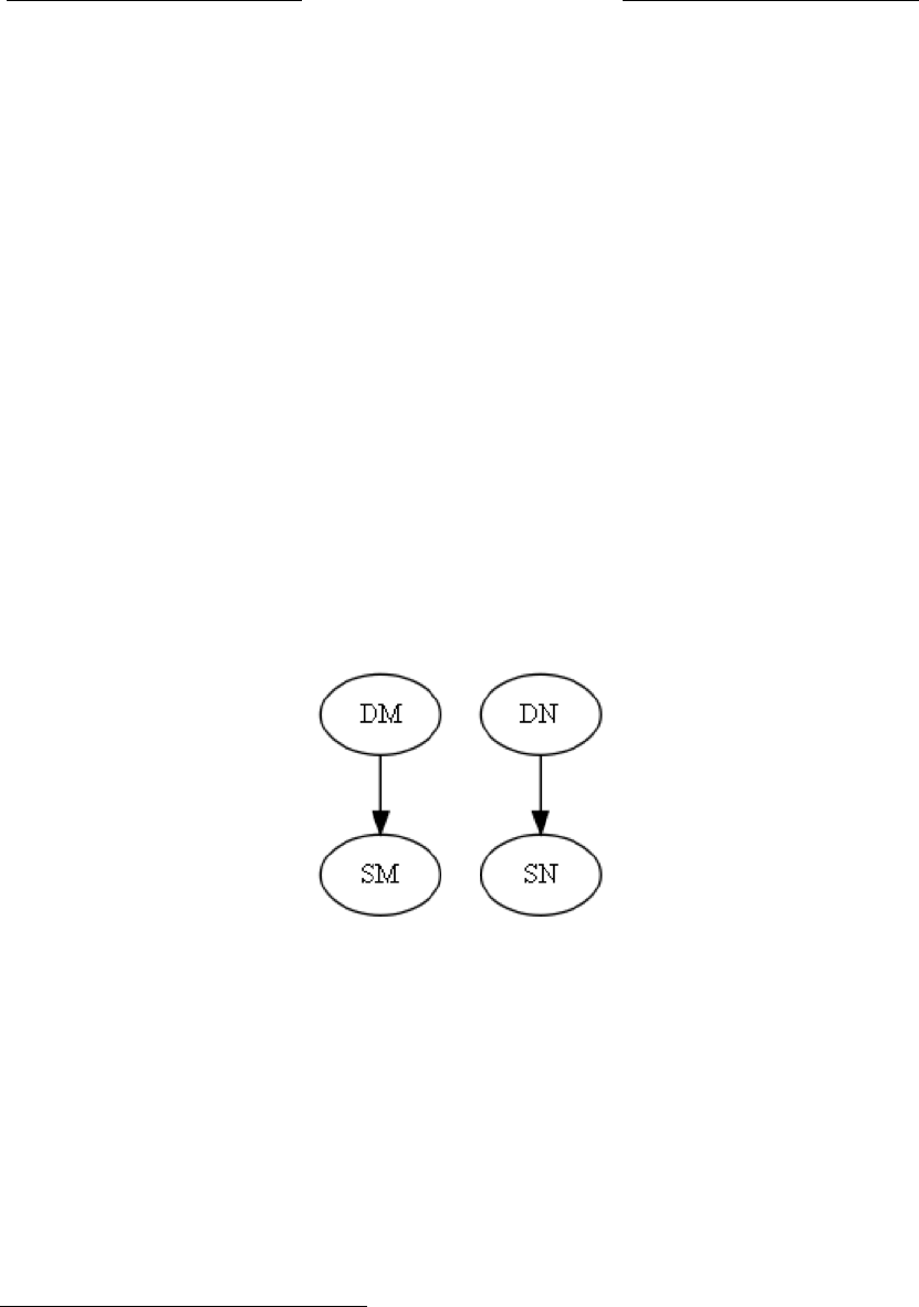
Timeless Decision eory
Indierence
27
I assign a probability of 1/6 to each number. Next we ask, given that
the Mongolian die turned up 5, the probability that each number between 2 and 12
will equal the sum of the Mongolian die and the number in the sealed envelope. If the
Mongolian die turned up 5, it would seem that the sums 6, 7, 8, 9, 10, and 11 are all
equally possible (again by the Principle of Indierence, having no further information
about the contents of the envelope). So we model the Mongolian probabilities using
two probability distributions, D
M
for the result of the Mongolian die, and P (S
M
|D
M
)
for the Mongolian sum given the Mongolian die. And similarly for the Neptunian die.
e rolling of dice on Neptune is independent of the rolling of dice in Mongolia, that is,
P (D
N
|D
M
) = P (D
N
). We may be very sure of this, for the confederates are scheduled
to roll their dice such that the events are spacelike separated,
28
and thus there is no
physically possible way that one event can have a causal eect on the other. en when
the Neptunian has rolled her die and gotten a 3, we again have a distribution P (S
N
|D
N
)
which assigns equal probabilities to the sums 4, 5, 6, 7, 8, and 9. If we write out this
computation as a causal diagram, it looks like this (Figure 6):
Figure 6
But ah!—this ad hoc diagram gives us a false answer, for the subgraphs containing S
N
and
S
M
are disconnected, necessarily requiring independence of the dice-sum in Mongolia
and the dice-sum on Neptune. But both envelopes contain the same number! If we
have a sum of 10 in Mongolia, we cannot possible have a sum of 4 on Neptune. A sum
of 10 in Mongolia implies that the least number in the envelope could have been 4;
and then the sum on Neptune must be at least 5. Because reality violates the Markov
27. More generally, the Principle of Indierence is a special case of the principle of maximum entropy.
is use of the maximum-entropy principle to set prior probabilities is licensed by the indistinguishability
and interchangeability of the six labels attached to the six faces of the die, in the absence of any further
information (Jaynes 2003).
28. at is, the two confederates roll their dice in such fashion that it would be impossible for a light
ray leaving the Neptunian die-roll to arrive in Mongolia before the Mongolian die rolls, or vice versa.
erefore any talk of the confederates rolling their dice “at the same time” is meaningless nonsense, as is
talk of one confederate rolling a die “before” or “after” the other.
70
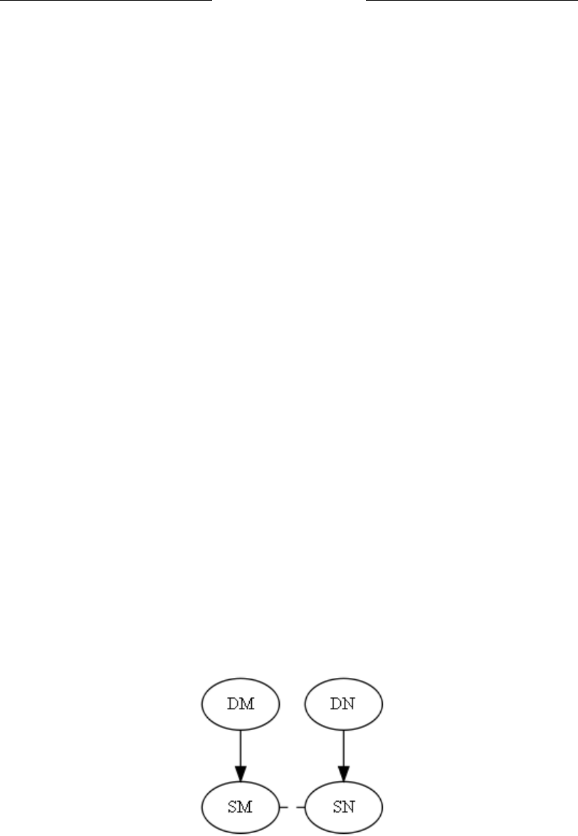
Eliezer Yudkowsky
assumption relative to our causal diagram, the diagram gives us a false joint distribution
over P (S
N
S
M
).
What is the Markov condition? To make the Markov condition more visible, let us
write out the false-to-fact causal diagram as a set of equations:
D
M
= f
1
(u
1
) p(u
1
) (9a)
S
M
= f
2
(D
M
, u
2
) p(u
2
) (9b)
D
N
= f
3
(u
3
) p(u
3
) (9c)
S
N
= f
4
(D
N
, u
4
) p(u
4
) (9d)
is formulation of a causal diagram makes the underlying computations t into deter-
ministic functions; all probabilism now resides in a probability distribution over the “error
terms” u
i
. Despite the phrase “error term,” the u
i
are not necessarily errors in the sense
of noise—the probability distributions over ui can represent any kind of information
that we do not know, including background conditions which would be too difficult to
determine in advance. e only requirement is that, given the information summarized
by the u
i
(including, e.g., the results of die rolls), the remaining mechanisms should be
functions rather than probabilities; that is, they should be deterministic (Pearl 1988).
e Markov condition is that the error terms ui should all be independent of each
other: p(u
1
u
2
u
3
u
4
) = p(u
1
)p(u
2
)p(u
3
)p(u
4
). Our dice-rolling scenario violates the
Markov condition relative to the diagram D because the error terms u
2
and u
4
are
dependent—in fact, u
2
= u
4
.
Can we add a dependency between u
2
and u
4
? is would be represented in a causal
diagram by a dashed arc between X
2
and X
4
, as seen in Figure 7. However, the diagram
!"#$#%&'(")#*&+ ,'*&+
-./0#%123*456/17#1%#5#85*054#9/5:253#35;<0#6.<#*79<24=/7:#813,*656/170#%/6#/761#
!"#"$%&'&(#&)#%*786/170>#544#*$+,-,&.&(%#71?#2<0/9<0#/7#5#,21@5@/4/6=#9/062/@*6/17#
1A<2#6.<#B<2212#6<230B#*/C##(<0,/6<#6.<#,.250<#B<2212#6<23B)#6.<#*/#52<#716#
7<8<0052/4=#<22120#/7#6.<#0<70<#1%#71/0<#D#6.<#,21@5@/4/6=#9/062/@*6/170#1A<2#*/#857#
2<,2<0<76#57=#;/79#1%#/7%12356/17#6.56#?<#91#716#;71?)#/784*9/7:#@58;:21*79#
8179/6/170#?./8.#?1*49#@<#611#9/%%/8*46#61#9<6<23/7<#/7#59A578<C##-.<#174=#
2<E*/2<3<76#/0#6.56)#/&0"'#6.<#/7%12356/17#0*3352/F<9#@=#6.<#*/#'/784*9/7:)#<C:C)#
6.<#2<0*460#1%#9/<#21440+)#6.<#$"%-&'&'/#3<8.57/030#0.1*49#@<#%*786/170#256.<2#
6.57#,21@5@/4/6/<0>#6.56#/0)#6.<=#0.1*49#@<#9<6<23/7/06/8C##'G<524#579#H<235#IJJIC+
-.<#K52;1A#8179/6/17#/0#6.56#6.<#<2212#6<230#*/#0.1*49#544#@<#&'!"*"'!"'##1%#<58.#
16.<2L##,'*I*M*N*&+#$#,'*I+,'*M+,'*N+,'*&+C##O*2#9/8<D2144/7:#08<752/1#A/1456<0#
6.<#K52;1A#8179/6/17#$".-#&0"1#+#6.<#9/5:253#(#@<85*0<#6.<#<2212#6<230#*M#579#
*4<#9<,<79<76#D#/7#%586)#*M#$#*&C
P57#?<#599#5#9<,<79<78=#@<6?<<7#*M#579#*&Q##-./0#?1*49#@<#2<,2<0<76<9#/7#5#
85*054#9/5:253#@=#5#950.<9#528#@<6?<<7#RM#579#R&L
S1?<A<2)#6.<#9/5:253#/0#71?#("%&23-$4+0&-'5#5#
8179/6/17#056/0%/<9#?.<7#71#9<,<79<78/<0#<T/06#5317:#
6.<#*/#<T8<,6#6.10<#0,<8/%/<9#@=#950.<9#5280C#
U*26.<2312<)#6.<#8179/6/1754#,21@5@/4/6=#%123*45#%12#
,'TITMTNT&+#/0#71#417:<2#A54/9)#6.56#/0)#,'TITMTNT&+#V$#
,'T&WTN+,'TN+,'TMWTI+,'TI+C##X<#857#71#417:<2#850.#1*6#
6./0#9/5:253#61#5#,21@5@/4/6=#9/062/@*6/17C
!1#.1?#91#?<#2<014A<#5#0<3/DK52;1A/57#9/5:253#@58;#
61#5#K52;1A/57#9/5:253Q##X/6.1*6#9/%%/8*46=)#?<#2<?2/6<#1*2#9/5:253#50#%1441?0L
(Y#$#%I'*I+ ,'*I+
(K#$#%M'*M+### ,'*M+
!K#$#%N'(Y)#(K+
("#$#%&'*&+ ,'*&+
!"#$#%Z'(Y)#("+
(Y#.<2<#065790#%12#6.<#9/<D2144#6.56#
9<6<23/7<0#6.<#8176<760#1%#6.<#<7A<41,<0#
9/0,568.<9#61#"<,6*7<#579#K17:14/5C#
-.<#06579529#%123*456/17#5990#<2212#6<230#56#*N#579#*Z)#0<66/7:#6.<3#61#%/T<9#
A54*<0C##G<2017544=#[#?1*49#,2<%<2#61#13/6#6.<#<2212#6<230#*N#579#*Z)#0/78<#6.<=#
,45=#71#813,*656/1754#214<#/7#6.<#%*786/170#%N#12#%ZC##"16<#5401#6.56#0/78<#(K#579#
\]
6&/7$"1891
6&/7$"1:91
Figure 7
is now semi-Markovian, a condition satised when no dependencies exist among the ui
except those specied by dashed arcs. Furthermore, the conditional probability formula
for p(x
1
x
2
x
3
x
4
) is no longer valid, that is, p(x
1
x
2
x
3
x
4
)! = p(x
4
|x
3
)p(x
3
)p(x
2
|x
1
)p(x
1
).
We can no longer cash out this diagram to a probability distribution.
71
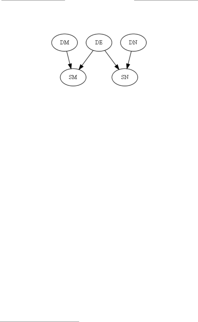
Timeless Decision eory
So how do we resolve a semi-Markovian diagram back to a Markovian diagram?
Without difficulty, we rewrite our diagram as shown in Figure 8. DE here stands for
!"#$#%&'(")#*&+ ,'*&+
-./0#%123*456/17#1%#5#85*054#9/5:253#35;<0#6.<#*79<24=/7:#813,*656/170#%/6#/761#
!"#"$%&'&(#&)#%*786/170>#544#*$+,-,&.&(%#71?#2<0/9<0#/7#5#,21@5@/4/6=#9/062/@*6/17#
1A<2#6.<#B<2212#6<230B#*/C##(<0,/6<#6.<#,.250<#B<2212#6<23B)#6.<#*/#52<#716#
7<8<0052/4=#<22120#/7#6.<#0<70<#1%#71/0<#D#6.<#,21@5@/4/6=#9/062/@*6/170#1A<2#*/#857#
2<,2<0<76#57=#;/79#1%#/7%12356/17#6.56#?<#91#716#;71?)#/784*9/7:#@58;:21*79#
8179/6/170#?./8.#?1*49#@<#611#9/%%/8*46#61#9<6<23/7<#/7#59A578<C##-.<#174=#
2<E*/2<3<76#/0#6.56)#/&0"'#6.<#/7%12356/17#0*3352/F<9#@=#6.<#*/#'/784*9/7:)#<C:C)#
6.<#2<0*460#1%#9/<#21440+)#6.<#$"%-&'&'/#3<8.57/030#0.1*49#@<#%*786/170#256.<2#
6.57#,21@5@/4/6/<0>#6.56#/0)#6.<=#0.1*49#@<#9<6<23/7/06/8C##'G<524#579#H<235#IJJIC+
-.<#K52;1A#8179/6/17#/0#6.56#6.<#<2212#6<230#*/#0.1*49#544#@<#&'!"*"'!"'##1%#<58.#
16.<2L##,'*I*M*N*&+#$#,'*I+,'*M+,'*N+,'*&+C##O*2#9/8<D2144/7:#08<752/1#A/1456<0#
6.<#K52;1A#8179/6/17#$".-#&0"1#+#6.<#9/5:253#(#@<85*0<#6.<#<2212#6<230#*M#579#
*4<#9<,<79<76#D#/7#%586)#*M#$#*&C
P57#?<#599#5#9<,<79<78=#@<6?<<7#*M#579#*&Q##-./0#?1*49#@<#2<,2<0<76<9#/7#5#
85*054#9/5:253#@=#5#950.<9#528#@<6?<<7#RM#579#R&L
S1?<A<2)#6.<#9/5:253#/0#71?#("%&23-$4+0&-'5#5#
8179/6/17#056/0%/<9#?.<7#71#9<,<79<78/<0#<T/06#5317:#
6.<#*/#<T8<,6#6.10<#0,<8/%/<9#@=#950.<9#5280C#
U*26.<2312<)#6.<#8179/6/1754#,21@5@/4/6=#%123*45#%12#
,'TITMTNT&+#/0#71#417:<2#A54/9)#6.56#/0)#,'TITMTNT&+#V$#
,'T&WTN+,'TN+,'TMWTI+,'TI+C##X<#857#71#417:<2#850.#1*6#
6./0#9/5:253#61#5#,21@5@/4/6=#9/062/@*6/17C
!1#.1?#91#?<#2<014A<#5#0<3/DK52;1A/57#9/5:253#@58;#
61#5#K52;1A/57#9/5:253Q##X/6.1*6#9/%%/8*46=)#?<#2<?2/6<#1*2#9/5:253#50#%1441?0L
(Y#$#%I'*I+ ,'*I+
(K#$#%M'*M+### ,'*M+
!K#$#%N'(Y)#(K+
("#$#%&'*&+ ,'*&+
!"#$#%Z'(Y)#("+
(Y#.<2<#065790#%12#6.<#9/<D2144#6.56#
9<6<23/7<0#6.<#8176<760#1%#6.<#<7A<41,<0#
9/0,568.<9#61#"<,6*7<#579#K17:14/5C#
-.<#06579529#%123*456/17#5990#<2212#6<230#56#*N#579#*Z)#0<66/7:#6.<3#61#%/T<9#
A54*<0C##G<2017544=#[#?1*49#,2<%<2#61#13/6#6.<#<2212#6<230#*N#579#*Z)#0/78<#6.<=#
,45=#71#813,*656/1754#214<#/7#6.<#%*786/170#%N#12#%ZC##"16<#5401#6.56#0/78<#(K#579#
\]
6&/7$"1891
6&/7$"1:91
Figure 8
D
E
= f
1
(u
1
) p(u
1
) (10a)
D
M
= f
2
(u
2
) p(u
2
) (10b)
S
M
= f
3
(D
E
, D
M
) (10c)
D
N
= f
4
(u
4
) p(u
4
) (10d)
S
N
= f
5
(D
E
, D
N
) (10e)
the die-roll that determines the contents of the envelopes dispatched to Neptune and
Mongolia. e standard formulation adds error terms at u
3
and u
5
, setting them to xed
values. Personally I would prefer to omit the error terms u
3
and u
5
, since they play no
computational role in the functions f
3
or f
5
. Note also that since D
M
and D
N
aect only
S
M
and S
N
respectively, we could as easily write the causal diagram to that displayed in
Figure 9. is more compact diagram also makes it easier to read o that if we observe
the value of DE, this renders SN and SM statistically independent of one another. at
is, once we know the value in the envelope,knowing the sum on Neptune tells us nothing
more about the sum in Mongolia. If we observe completely the local physical variables in
the preconditions to the two scenarios—if we examine fully the dice and the envelope,
before rolling the dice and computing the sum—then there are no correlated random
factors in the two scenarios; the remaining error terms are independent. is respects
the physical requirement (according to our current understanding of physics) that no
physical eect, no arrow of causality in a causal diagram, may cross a spacelike separation
between events.
29
Inference obeys no such constraint. If you take a matched pair of socks,
send a sock in a box to Proxima Centauri, and then show me that the other sock is black,
29. If two events are “spacelike separated,” traveling between them requires traveling faster than light.
72

Eliezer Yudkowsky
!"#$%%&'(#)*+,#-.#$*/#-"#0&12&'(34&+,5#6&#')7+/#$1#&$13+,#603(&#(8&#'$71$+#
/3$90$:;
!<#=#%>?7>@ 2?7>@
-.#=#%A?!<5#7A@ 2?7A@
-"#=#%B?!<5#7B@ 2?7B@
C831#:)0&#'):2$'(#/3$90$:#$+1)#:$D&1#3(#&$13&0#()#0&$/#
)%%#(8$(#3%#6&#)E1&04&#(8$+7&#)%#!<5#(831#0&*/&01#-"#
$*/#-.#1($(31(3'$++,#3*/&2&*/&*(#)%#)*&#$*)(8&0F##C8$(#
315#)*'&#D*)6#(8$+7*#(8&#&*4&+)2&5#D*)63*9#(8&#
17:#)*#"&2(7*&#(&++1#71#*)(83*9#!"#$#$E)7(#(8:#3*#
.)*9)+3$F##G%#6&#)E1&04&#'):2+&(&+,#(8&#+)'$+#28,13'$+#4$03$E+&1#3*#(8&#
20&')*/3(3)*1#()#(8&#(6)#1'&*$03)1#H#3%#6&#&I$:3*&#%7++,#(8&#/3'&#$*/#(8&#
&*4&+)2&5#E&%)0�)++3*9#(8&#/3'&#$*/#'):27(3*9#(8:#H#(8&*#(8&0&#$0&#*)#
')00&+$(&/#0$*/):#%$'()01#3*#(8&#(6)#1'&*$03)1J#(8�&:$3*3*9#&00)0#(&0:1#$0&#
3*/&2&*/&*(F##C831#0&12&'(1#(8,13'$+#0&K730&:&*(#?$'')0/3*9#()#)70#'700&*(#
7*/&01($*/3*9#)%#28,13'1@#(8$(#*)#28,13'$+#&%%&'(5#*)#$00)6#)%#'$71$+3(,#3*#$#
'$71$+#/3$90$:5#:$,#'0)11#$#12$'&+3D&2$0$(3)*#E&(6&&*#&4&*(1F
AL
##%&'$#$&($)
)E&,1#*)#17'8#')*1(0$3*(F##G%#,)7#($D&#$#:$('8&/#2$30#)%#1)'D15#1&*/#$#1)'D#3*#$#
E)I#()#M0)I3:$#N&*($7035#$*/#(8&*#18)6#:&#(8$(#(8&#)(8&0#1)'D#31#E+$'D5#G#:$,#
/&/7'::&/3$(&+,#(8$(#(8)'D#$(#M0)I3:$#N&*($703#31#E+$'DF##O7(#*)#3*%+7&*'&#
(0$4&+1#%$1(&0#(8$*#+398(#H#)*+,#$*#3*%&0&*'&F
C8&#:$2#31#*)(#(8&#(&003()0,F##P*#+&$0*3*9#$#*&6#%$'(5#G#:$,#603(*#:$*,#'8$*9&1#
()#:,#:$2#)%#(8*34&01&5#2&08$21#:$0D3*9#3*#/&/7'(3)*1#$E)7(#63/&+,#
1&2$0$(&/#9$+$I3&1F##O7(#(8&#&*(30&#:$2#+3&1#)*#:,#($E+&5#(8)798#3(#:$,#0&%&0#()#
/31($*(#2+$'&1F##-)#+)*9#$1#:,#*&6#D*)6+&/9&#/)&1#*)(#'$71&#(8&#(&003()0,#3(1&+%#
()#'8$*9&5#-2&'3$+#Q&+$(343(,#31#)E&,&/F
R1#M&$0+#2)3*(1#)7(5#6*(73(34&+,#0&')9*3S&#(8:2)0($*'&#)%#(8&#%7++#.$0D)4#
')*/3(3)*#3*#9))/#&I2+$*$(3)*1F##R*#7*&I2+$3*&/#')00&+$(3)*#18)61#(8$(#$#'$71$+#
&I2+$*$(3)*#31#3*'):2+&(&F##G%#6&#%+32#(6)#')3*1#3*#(6)#63/&+,#1&2$0$(&/#+)'$(3)*1#
$*/#%3*/#(8$(#E)(8#')3*1#20)/7'&#(8$:&K7&*'&#TCTCCCTCTTTTFFF5#)*#
$*/#)*#%)0#$#(8)71$*/#3/&*(3'$+#%+3215#6)7+/*U(#$''&2(#(8&#E+$*/#&I2+$*$(3)*5#
VP85#(8$(U1#W71(#$*#7*&I2+$3*&/#')00&+$(3)*FV##X)7+/#1712&'(#1):&(83*9#
3*(&0&1(3*9#8$22&*3*9#E&83*/#(8'&*&15#1):&(83*9#6)0(8,#)%#3*4&1(39$(3)*F
G%#Y#$*/#Z#')00&+$(&5#$#9))/#&I2+$*$(3)*#18)7+/#/&1'03E&#$#'$71$+#&%%&'(#)%#Y#)*#
Z5#$#'$71$+#&%%&'(#)%#Z#)*#Y5#)0#$#')*%)7*/&0#683'8#$%%&'(1#E)(8#Y#$*/#ZF##R#'$71$+#
/3$90$:#')*($3*3*9#*)#17'8#+3*D1#20&/3'(1#$#20)E$E3+31(3'#3*/&2&*/& * '& #683'8#
)E1&04$(3)*#%$+13%3&1F
AL
#G%#(6)#&4&*(1#$0&#V12$'&+3D&2$0$(&/V5#(0$4&+3*9#E&( 6& &*#(8&:#0&K730&1#(0$4&+3*9#%$ 1( &0#(8$*#
+398(F
[>
*+,-#$)./)
Figure 9
D
E
= f
1
(u
1
) p(u
2
) (11a)
S
M
= f
2
(D
E
, u
2
) p(u
2
) (11b)
S
N
= f
3
(D
E
, u
3
) p(u
3
) (11c)
I may deduce immediately that the sock at Proxima Centauri is black. But no inuence
travels faster than light—only an inference.
e map is not the territory. On learning a new fact, I may write in many changes to
my map of the universe, perhaps marking in deductions about widely separated galaxies.
But the entire map lies on my table, though it may refer to distant places. So long as my
new knowledge does not cause the territory itself to change, Special Relativity is obeyed.
As Pearl points out, we intuitively recognize the importance of the full Markov con-
dition in good explanations. An unexplained correlation shows that a causal explanation
is incomplete. If we ip two coins in two widely separated locations and nd that both
coins produce the same sequence HTHTTTHTHHHH . . . , on and on for a thousand
identical ips, we wouldn’t accept the bland explanation, “Oh, that’s just an unexplained
correlation.” We would suspect something interesting happening behind the scenes,
something worthy of investigation.
If X and Y correlate, a good explanation should describe a causal eect of X on Y ,
a causal eect of Y on X, or a confounder which aects both X and Y . A causal dia-
gram containing no such links predicts a probabilistic independence which observation
falsies.
11. Timeless Decision Diagrams
I propose that to properly represent Newcomblike problems we must augment standard-
issue causal diagrams in two ways. I present these two augmentations in turn.
For my rst augmentation of standard causal diagrams, I propose that causal dia-
grams should represent our uncertainty about the results of computations—for example,
73

Timeless Decision eory
“What do you get if you multiply six by nine?” It is not particularly difficult to include
uncertainty about computations into causal diagrams, but the inclusion must not break
underlying mathematical assumptions, as an ad hoc x might do. e chief assumption
in danger is the Markov property.
Suppose that I place, in Mongolia and Neptune, two calculators programmed to cal-
culate the result of 678 × 987 and then display the result. As before, the timing is such
that the events will be spacelike separated—both events occur at 5PM on Tuesday in
Earth’s space of simultaneity. Before 5PM on Tuesday, you travel to the location of both
calculators, inspect them transistor by transistor, and conrm to your satisfaction that
both calculators are physical processes poised to implement the process of multiplica-
tion and that the multiplicands are 678 and 987. You do not actually calculate out the
answer, so you remain uncertain of which number shall ash on the calculator screens.
As the calculators are spacelike separated, it is physically impossible for a signal to travel
from one calculator to another. Nonetheless you expect the same signs to ash on both
calculator screens, even though you are uncertain which signs will ash. For the sake of
simplication, I now inform you that the answer is either 669186 or 669168. Would it
be fair to say that you assign a probability of 50% to the answer being 669186?
Some statisticians may object to any attempt to describe uncertainty about computa-
tions in terms of probability theory, protesting that the product of 678 × 987 is a xed
value, not a random variable. It is nonsense to speak of the probability of the answer
being 669186; either the answer is 669186 or it is not. ere are a number of possible
replies to this, blending into the age-old debate between Bayesian probability theory
and frequentist statistics. Perhaps some philosophers would refuse to permit probability
theory to describe the value of a die roll written inside a sealed envelope I have not seen—
since, the die roll having been written down, it is now xed instead of random. Perhaps
they would say: “e written die result does not have a 1/6 probability of equalling 4;
either it equals 4 or it does not.”
As my rst reply, I would cite the wisdom of Jaynes (2003), who notes that a classical
“random” variable, such as the probability of drawing a red ball from a churning barrel
containing 30 red balls and 10 white balls, is rarely random—not in any physical sense.
To really calculate, e.g., the probability of drawing a red ball after drawing and replacing
a white ball, we would have to calculate the placement of the white ball in the barrel,
its motions and collisions with other balls. When statisticians talk of “randomizing”
a process, Jaynes says, they mean “making it vastly more complicated.” To say that the
outcome is random, on this theory, is to say that the process is so unmanageable that we
throw up our hands and assign a probability of 75%.
e map is not the territory. It may be that the balls in the churning barrel, as macro-
scopic objects, are actually quite deterministic in their collisions and reboundings; so that
74

Eliezer Yudkowsky
someone with a sophisticated computer model could predict precisely whether the next
ball would be red or white. But so long as we do not have this sophisticated computer
model, a probability of 75% best expresses our ignorance. Ignorance is a state of mind,
stored in neurons, not the environment. e red ball does not know that we are ignorant
of it. A probability is a way of quantifying a state of mind. Our ignorance then obeys
useful mathematical properties—Bayesian probability theory—allowing us to system-
atically reduce our ignorance through observation. How would you go about reducing
ignorance if there were no way to measure ignorance? What, indeed, is the advantage of
not quantifying our ignorance, once we understand that quantifying ignorance reects
a choice about how to think eectively, and not a physical property of red and white
balls?
It also happens that I ipped a coin to determine which of the two values I would
list rst when I wrote “669186 or 669168.” If it is impermissible to say that there is
a 50% probability of the answer being 669186, is it permissible to say that there is a 50%
probability that the value listed rst is the correct one?
Since this is a paper on decision theory, there is a much stronger reply—though it ap-
plies only to decision theory, not probability theory. ere is an old puzzle that Bayesians
use to annoy frequentist statisticians. Suppose we are measuring a physical parameter,
such as the mass of a particle, in a case where (a) our measuring instruments show ran-
dom errors and (b) it is physically impossible for the parameter to be less than zero.
A frequentist refuses to calculate any such thing as the “probability” that a xed pa-
rameter bears some specic value or range of values, since either the xed parameter
bears that value or it does not. Rather the frequentist says of some experimental pro-
cedure, “is procedure, repeated indenitely many times, will 95% of the time return
a range that contains the true value of the parameter.” According to the frequentist,
this is all you can ever say about the parameter—that a procedure has been performed
on it which will 95% of the time return a range containing the true value. But it may
happen that, owing to error in the measuring instruments, the experimental procedure
returns a range [-0.5, -0.1], where it is physically impossible for the parameter to be less
than zero. A Bayesian cheerfully says that since the prior probability of this range was
eectively 0%, the posterior probability remains eectively 0%, and goes on to say that
the real value of the parameter is probably quite close to zero. With a prior probability
distribution over plausible values of the parameter, this remaining uncertainty can be
quantied. A frequentist, in contrast, only goes on saying that the procedure performed
would work 95% of the time, and insists that there is nothing more to be said than this.
It is nonsense to treat a xed parameter as a random variable and assign probabilities to
it; either the xed parameter has value X or it does not.
75

Timeless Decision eory
If we are decision theorists, we can resolve this philosophical impasse by pointing
a gun to the frequentist’s head and saying, “Does the value of the xed parameter lie in
the range [-0.5, -0.1]? Respond yes or no. If you get it wrong or say any other word
I’ll blow your head o.” e frequentist shrieks “No!” We then perform the experi-
mental procedure again, and it returns a range of [0.01, 0.3]. We point the gun at the
frequentist’s head and say, “Does the value lie in this range?” e frequentist shrieks,
“Yes!” And then we put the gun away, apologize extensively, and say: “You know the sort
of belief that you used to make that decision? at’s what a Bayesian calls by the name,
‘probability.’ ”
If you look at this reply closely, it says that decision theory requires any mathemat-
ical object describing belief to cash out to a scalar quantity, so that we can plug com-
parative degrees of belief into the expected utility formula. Mathematicians have de-
vised Dempster-Shafer theory, long-run frequencies,and other interesting mathematical
objects—but when there’s a gun pointed at your head, you need something that cashes
out to what decision theorists (and Bayesian statisticians) call a probability. If some-
one should invent an improvement on the expected utility formula that accepts some
other kind of belief-object, and this improved decision rule produces better results, then
perhaps decision theorists will abandon probabilities. But until then, decision theorists
need some way to describe ignorance that permits choice under uncertainty, and our best
current method is to cash out our ignorance as a real number between 0 and 1.
is is the Dutch Book argument for Bayesian probability (Ramsey 1931). If your
uncertainty behaves in a way that violates Bayesian axioms, an exploiter can present you
with a set of bets that you are guaranteed to lose.
e Dutch Book argument applies no less to your uncertainty about whether 678 ×
987 equals 669186 or 669168. If you oered a truly committed frequentist only a small
sum of money, perhaps he would sni and say, “Either the result equals 669186 or it
does not.” But if you made him choose between the gambles G
1
and G
2
, where G
1
involves being shot if the value is 669186 and G
2
involves being shot unless a fair coin
turns up four successive heads, I think a sensible bounded rationalist would choose G
1
.
30
By requiring choices on many such gambles, we could demonstrate that the chooser
assigns credences that behave much like probabilities, and that the probability he assigns
is within epsilon of 50%.
30. Incidentally, I will ip a coin to determine which possible output I will cite in G
1
, only after writing
the footnoted sentence and this footnote. If the false value happens to come up in the coin ip, then that
will detract somewhat from the moral force of the illustration. Nonetheless I say that a sensible bounded
rationalist, having no other information, should prefer G
1
to G
2
.
76

Eliezer Yudkowsky
Since I wish to devise a formalism for timeless decision diagrams, I presently see no
alternative but to represent my ignorance of a deterministic computation’s output as
a probability distribution that can combine with other probabilities and ultimately plug
into an expected utility formula.
Note that is important to distinguish between the notion of a computation and the
notion of an algorithm. An “algorithm,” as programmers speak of it, is a template for
computations. e output of an algorithm may vary with its inputs, or with parameters
of the algorithm. “Multiplication” is an algorithm. “Multiply by three” is an algorithm.
“Multiply by X” is an algorithm with a parameter X. Take the algorithm “Multiply
by X,” set X to 987, and input 678: e result is a fully specied computation, 678
× 987, with a deterministic progress and a single xed output. A computation can be
regarded as an algorithm with no inputs and no parameters, but not all algorithms are
computations.
An underlying assumption of this paper is that the same computation always has
the same output. All jokes aside, humanity has never yet discovered any place in our
universe where 2 + 2 = 5—not even in Berkeley, California. If “computation” is said
where “algorithm” is meant, paradox could result; for the same algorithm may have dif-
ferent outputs given dierent inputs or parameters.
So how would a causal diagram represent two spacelike separated calculators imple-
menting the same computation? I can presently see only one way to do this that matches
the observed facts, lets us make prudent choices under uncertainty, and obeys the un-
derlying assumptions in causal diagrams (see Figure 10). Here F stands for the factory,
located perhaps in Taiwan, which produced calculators C
M
and C
N
at Mongolia and
Neptune (explaining their physically correlated state at the start of the problem). O
P
is a latent node
31
that stands for our uncertainty about the deterministic output of the
abstract computation 678 × 987—the “Platonic output”—and the outputs O
M
and O
N
at Mongolia and Neptune are the outputs which ash on the actual calculator screen.
Why is it necessary to have a node for O
P
, distinct from F ? Because this diagram is
intended to faithfully compute probabilities and independences in the scenario where:
a) We physically inspect the complete initial state of both calculators;
b) We remain uncertain which symbols shall ash upon each of the two screens;
and yet
c) We expect the uncertain ashing symbols at O
M
and O
N
to correlate.
31. A latent node in a causal diagram is a variable which is not directly observed. Any suggestion that
two correlated variables are linked by an unseen confounding factor hypothesizes a latent cause.
77
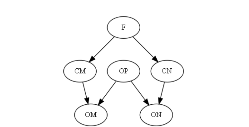
Timeless Decision eory
!"#$%&'&(")*&+,&-%.")%&/&0,12/3")2&0,1&+"2%3%))&!"#$%$&'&-"/41/2)5&'&61%)%#+37&)%%&
#,&/3+%1#/+".%&89+&+,&1%61%)%#+&27&"4#,1/#$%&,0&/&-%+%12"#")+"$&$,269+/+",#:)&
,9+69+&/)&/&61,8/8"3"+7&-")+1"89+",#&+*/+&$/#&$,28"#%&("+*&,+*%1&61,8/8"3"+"%)&/#-&
93+"2/+%37&6394&"#+,&/#&%;6%$+%-&9+"3"+7&0,1293/<
=,+%&+*/+&")&"26,1+/#+&+,&-")+"#49")*&8%+(%%#&+*%&#,+",#&,0&/&#&()*+,+$&'&/#-&+*%&
#,+",#&,0&/#&,-.&/$+0(1&&>#&?/34,1"+*2?5&/)&61,41/22%1)&)6%/@&,0&"+5&")&/&+%263/+%&
0,1&$,269+/+",#)<&&A*%&,9+69+&,0&/#&/34,1"+*2&2/7&./17&("+*&"+)&"#69+)5&,1&("+*&
6/1/2%+%1)&,0&+*%&/34,1"+*2<&&?B93+"63"$/+",#?&")&/#&/34,1"+*2<&&?B93+"637&87&+*1%%?&
")&/#&/34,1"+*2<&&?B93+"637&87&C?&")&/#&/34,1"+*2&("+*&/&6/1/2%+%1&C<&&A/@%&+*%&
/34,1"+*2&?B93+"637&87&C?5&)%+&C&+,&DEF5&/#-&"#69+&GFEH&A*%&1%)93+&")&/&09337&
)6%$"0"%-&$,269+/+",#5&GFE&I&DEF5&("+*&/&-%+%12"#")+"$&61,41%))&/#-&/&)"#43%&0";%-&
,9+69+<&&>&$,269+/+",#&$/#&8%&1%4/1-%-&/)&/#&/34,1"+*2&("+*&#,&"#69+)&/#-&#,&
6/1/2%+%1)5&89+&#,+&/33&/34,1"+*2)&/1%&$,269+/+",#)<
>#&9#-%137"#4&/))926+",#&,0&+*")&6/6%1&")&+*/+&+*%&)/2%&$,269+/+",#&/3(/7)&*/)&
+*%&)/2%&,9+69+<&&>33&J,@% )&/)"- % 5&*92/#"+7&*/)&#%.%1&7%+&-")$,.%1%-&/#7&63/$%&"#&
,91&9#".%1)%&(*%1%&K&L&K&M&N&O&#,+&%.%#&"#&P%1@%3%75&Q/3"0,1#"/<&&'0&?$,269+/+",#?&
")&)/"-&(*%1%&?/34,1"+*2?&")&2%/#+5&6/1/-,;&$,93-&1%)93+R&0,1&+*%&)/2%&/34,1"+*2&
2/7&*/.%&-"00%1%#+&,9+69+)&4".%#&-"00%1%#+&"#69+)&,1&6/1/2%+%1)<
!,&*,(&(,93-&/&$/9)/3&-"/41/2&1%61%)%#+&+(,&)6/$%3"@%&)%6/1/+%-&$/3$93/+,1)&
"263%2%#+"#4&+*%&)/2%&$,269+/+",#S&&'&$/#&61%)%#+37&)%%&,#37&,#%&(/7&+,&-,&
+*")&+*/+&2/+$*%)&+*%&,8)%1.%-&0/$+)5&3%+)&9)&2/@%&619-%#+&$*,"$%)&9#-%1&
9#$%1+/"#+75&/#-&,8%7)&+*%&9#-%137"#4&/))926+",#)&"#&$/9)/3&-"/41/2)H
T&M&0UV9UW 6V9UW
QB&M&0KVTW
Q=&M&0XVTW
YZ&M&0[V9[W 6V9[W
YB&M&0NVYZ5&QBW
Y=&M&0GVYZ5&Q=W
\%1%&T&)+/#-)&0,1&+*%&0/$+,175&3,$/+%-&
6%1*/6)&"#&A/"(/#5&(*"$*&61,-9$%-&
$/3$93/+,1)&QB&/#-&Q=&/+&B,#4,3"/&/#-&
=%6+9#%&V%;63/"#"#4&+*%"1&6*7)"$/337&
$,11%3/+%-&)+/+%&/+&+*%&)+/1+&,0&+*%&
61,83%2W<&&YZ&")&/&3/+%#+&#,-%
XU
&+*/+&
)+/#-)&0,1&,91&9#$%1+/"#+7&/8,9+&+*%&
-%+%12"#")+"$&,9+69+&,0&+*%&/8)+1/$+&$,269+/+",#&GFE&I&DEF&O&+*%&?Z3/+,#"$&,9+69+?&
O&/#-&+*%&,9+69+)&YB&/#-&Y=&/+&B,#4,3"/&/#-&=%6+9#%&/1%&+*%&,9+69+)&(*"$*&
03/)*&,#&+*%&/$+9/3&$/3$93/+,1&)$1%%#<
XU
&>&3/+%#+&#,-%&"#&/&$/9)/3&-"/41/2&")&/& ./1"/83%&(*"$*&")&#,+&-"1%$+37&,8)%1.%-<&&>#7&)944%)+",#&
+*/+&+(,&$,11%3/+%-&./1"/83% )& /1%&3"#@%-&87&/#&9#)%%#&$,#0,9#-"#4&0/$+,1&*76,+*%)"]%)&/&3/+%#+&
$/9)%<
FN
2$.*/"3453
Figure 10
F = f
1
(u
1
) p(u
1
) (12a)
C
M
= f
2
(F ) (12b)
C
N
= f
3
(F ) (12c)
O
P
= f
4
(u
4
) p(u
4
) (12d)
O
M
= f
5
(O
P
, C
M
) (12e)
O
N
= f
6
(O
P
, C
N
) (12f)
If we delete the node O
P
and its arcs from diagram D, then inspecting both C
M
and C
N
should screen o O
M
from O
N
, rendering them probabilistically independent.
(e same also holds of deleting the node O
P
and inspecting F.) If we delete O
P
, we
necessarily have that P (O
M
, O
N
|C
M
, C
N
) = P (O
M
|C
M
, C
N
) ∗ P (O
N
|C
M
, C
N
). is
does not correspond to the choices we would make under uncertainty. We would assign
a probability of 50% to P (O
M
= 669186|C
M
, C
N
) and also assign a probability of
50% to P (O
N
= 669186|C
M
, C
N
) yet not assign a probability of 25% to P (O
M
=
669186, O
N
= 669186|C
M
, C
N
).
Which is to say: Suppose you have previously observed both calculators to implement
the same multiplication, you trust both calculators to work correctly on the physical level
(no cosmic ray strikes on transistors), and you have heard from a trustworthy source that
678 × 987 equals either 669186 or 669168. You might eagerly pay $1 for a gamble that
wins $10 if the calculator at Mongolia shows 669186, or with equal eagerness pay $1 for
a gamble that wins $10 if the calculator at Neptune shows 669168. Yet you would not
pay 10 cents for a gamble that wins $100 if the Mongolian calculator shows 669186 and
the Neptunian calculator shows 669168. Contrariwise, you would happily oer $2 for
78

Eliezer Yudkowsky
a gamble that wins $2.10 if the Mongolian calculator shows 669186 or the Neptunian
calculator shows 669168. It’s free money.
If we deal in rolling dice and sealed envelopes, rather than uncertainty about computa-
tions, then knowing completely the physical initial conditions at Mongolia and Neptune
rules out any lingering information between our conditional probability distributions
over uncertain outcomes at Mongolia and Neptune. Uncertainty about computation
diers from uncertainty about dice,in that completely observing the physical initial con-
ditions screens o any remaining uncertainty about dice,
32
while it does not screen o
uncertainty about the outputs of computations. e presence of the node O
P
in the
causal diagram is intended to make the causal diagram faithfully represent this property
of our ignorance.
I emphasize that if we were logically omniscient, knowing every logical implication of
our current beliefs, we would never experience any uncertainty about the result of cal-
culations. A logically omniscient agent, conditioning on a complete initial state, would
thereby screen o all expected information from outside events. I regard probabilistic
uncertainty about computations as a way to manage our lack of logical omniscience. Un-
certainty about computation is uncertainty about the logical implications of beliefs we
already possess. As boundedly rational agents, we do not always have enough computing
power to know what we believe.
O
P
is represented as a latent node, unobserved and unobservable. We can only de-
termine the value of O
P
by observing some other variable to which O
P
has an arc. For
example, if we have a hand calculator C
H
whose output O
H
is also linked to O
P
, then
observing the value O
H
can tell us the value of O
P
, and hence O
M
and O
N
. Likewise,
observing the symbols that ash on the calculator screen at O
M
would also tell us the
product of 678 × 987, from which we could infer the symbols that will ash on the
calculator screen at O
N
. is does seem to be how human beings reason, and more
importantly, the reasoning works well to describe the physical world. After determin-
ing O
P
, by whatever means, we have independence of any remaining uncertainty that
may arise about the outputs at O
M
and O
N
—say, due to a stray radiation strike on the
calculator circuitry.
I suggest that we should represent all abstract computational outputs as latent nodes,
since any attempt to infer the outcome of an abstract computation works by observing
32. When I say that the uncertainty is “screened o,” I don’t necessarily mean that we can always
compute the observed result of the die roll. I mean that no external event, if we witness it, can give us
any further information about what to expect from our local die roll. Quantum physics complicates this
situation considerably, but as best I understand contemporary physics, it is still generally true that if you
start out by completely observing an observable variable, then outside observations should tell you no
further information—quantum or otherwise—about it.
79

Timeless Decision eory
the output of some physical process believed to correlate with that computation. is
holds whether the physical process is a calculator, a mental calculation implemented
in axons and dendrites, or a pencil and paper that scratches out the axioms of Peano
arithmetic.
I also emphasize that, when I insert the Platonic output of a computation as a latent
node in a causal diagram, I am not making a philosophical claim about computations
having Platonic existence. I am just trying to produce a good approximation of reality
that is faithful in its predictions and useful in its advice. Physics informs us that beneath
our macroscopic dreams lie the facts of electrons and protons, fermions and bosons. If
you want objective reality, look at Feynman diagrams, not decision diagrams.
33
Our
fundamental physics invokes no such fundamental object as a “calculator,” yet a causal
diagram containing a node labeled “calculator” can still produce good predictions about
the behavior of macroscopic experience.
e causal diagram D,if you try to read it directly, seems to say that the Platonic result
of a calculation is a cause that reaches out and modifes our physical world. We are not just
wondering about pure math, after all; we are trying to predict which symbols shall ash
on the physical screen of a physical calculator. Doesn’t this require the Platonic output
of 678 × 987 to somehow modify the physical world, acting as a peer to other physical
causes? I would caution against trying to read the causal diagram in this way. Rather,
I would say that our uncertainty about computation exhibits causelike behavior in that
our uncertainty obeys the causelike operations of dependence, independence, inference,
screening o, etc. is does not mean there is a little Platonic calculation oating out in
space somewhere. ere are two dierent kinds of uncertainty interacting in diagram D:
e rst is uncertainty about physical states, and the second is uncertainty about logical
implications. e rst is uncertainty about possible worlds and the second is uncertainty
about impossible possible worlds (Cresswell 1970).
is multiply uncertain representation seems to adequately describe ignorance, in-
ference, decisions, dependence, independence, screening o, and it cashes out to a prob-
ability distribution that doesn’t make absurd predictions about the physical universe. It
is also pretty much the obvious way to insert a single computational uncertainty into
a Bayesian network.
I make no specication in this paper as to how to compute prior probabilities over
uncertain computations. As we will see, this question is orthogonal to the decision al-
33. So far as I am concerned,probability distributions are also a sort of useful approximation bearing no
objective reality (until demonstrated otherwise). Physics does invoke something like a distribution over
a space of possible outcomes, but the values are complex amplitudes, not scalar probabilities.
80

Eliezer Yudkowsky
gorithm in this paper; so for our purposes, and for the moment, “ask a human mathe-
matician” will do.
For my second augmentation, yielding timeless decision diagrams, I propose that an
agent represent its own decision as the output of an abstract computation which describes
the agent’s decision process.
I will rst defend a general need for a representation that includes more than a simple
blank spot as the cause of our own decisions, on grounds of a priori reasonableness and
representational accuracy.
Decisions, and specically human decisions, are neither acausal nor uncaused. We
routinely attempt to predict the decisions of other humans, both in cases where predic-
tion seems hard (Is she likely to sleep with me? Is he likely to stay with me if I sleep
with him?) and easy (Will this starving person in the desert choose to accept a glass
of water and a steak?) Some evolutionary theorists hypothesize that the adaptive task
of manipulating our fellow primates (and, by implication, correctly modeling and pre-
dicting fellow primates) was the most important selection pressure driving the increase
of hominid intelligence and the rise of Homo sapiens. e Machiavellian Hypothesis is
especially interesting because out-predicting your conspecics is a Red Queen’s Race,
an open-ended demand for increasing intelligence in each successive generation, rather
than a single task like learning to chip handaxes. is may help to explain a rise in
hominid cranial capacity that stretched over 5 million years.
We model the minds, and the decisions, and the acts of other human beings. We
model these decisions as depending on environmental variables; someone is more likely
to choose to bend down and pick up a bill on the street, if the bill is $50 rather than $1.
We could not do this successfully, even to a rst approximation in the easiest cases, if the
decisions of other minds were uncaused. We achieve our successful predictions through
insight into other minds, understanding cognitive details; someone who sees a dollar bill
on the street values it, with a greater value for $50 than $1, weighs other factors such
as the need to stride on to work, and decides whether or not to pick it up. Indeed, the
whole eld of decision theory revolves around arguments about how other minds do or
should arrive at their decisions, based on the complex interaction of desires, beliefs, and
environmental contingencies. e mind is not a sealed black box.
Why emphasize this? Because the standard formalism for causal diagrams seems to
suggest that a manipulation, an act of do(x
i
), is uncaused. To arrive at the formula for
p(y|ˆx
i
)—sometimes also written p(y|do(x
i
))—we are to sever the variable X
i
from all
its parents PA
i
; we eliminate the conditional probability p(x
i
|pa
i
) from the distribution;
we replace the calculation X
i
← f
i
(pa
i
, u
i
) with X
i
← x
i
. Since the variable X has
no parents, doesn’t that make it uncaused? Actually, we couldn’t possibly read the graph
in this way, since X
i
represents not our decision to manipulate X, but the manipulated
81
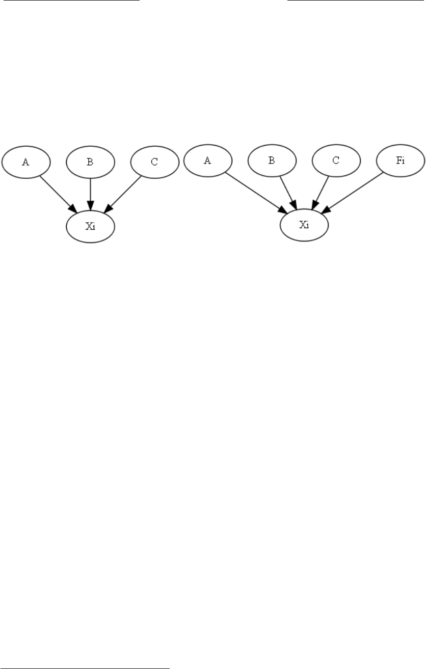
Timeless Decision eory
variable itself. E.g., if we make the sidewalk wet as an experimental manipulation, the
variable X
i
would represent the wetness of the sidewalk, not our decision to make the
sidewalk wet. Presumably, asking for a distribution given do(X
i
= wet) means that the
wetness is caused by our experimental manipulation, not that X
i
becomes uncaused.
Pearl (1988) suggests this alternate representation (shown in Figure 11) of an exper-
imentally manipulable causal diagram. Here the function I(f
i
, pa
i
, u
i
) = f
i
(pa
i
, u
i
).
!"#$%&"'#()"#$*+&,-#.+&#()"#&"/*,*%+,-#.+&#()"#./(,#%0#%()"1#)2$.+#3"*+4,5##!"#
$%&"'#()","#&"/*,*%+,#.,#&"6"+&*+4#%+#"+7*1%+$"+(.'#7.1*.3'",8#,%$"%+"#*,#
$%1"#'*9"':#(%#/)%%,"#(%#3"+&#&%;+#.+*/9#26#.#3*''#%+#()"#,(1""(-#*0#()"#3*''#*,#
<=>#1.()"1#().+#<?5##!"#/%2'&#+%(#&%#()*,#,2//",,02'':-#"7"+#(%#.#0*1,(#
.661%@*$.(*%+#*+#()"#".,*",(#/.,",-#*0#()"#&"/*,*%+,#%0#%()"1#$*+&,#;"1"#
2+/.2,"&5##!"#./)*"7"#%21#,2//",,02'#61"&*/(*%+,#()1%24)#*+,*4)(#*+(%#%()"1#
$*+&,-#2+&"1,(.+&*+4#/%4+*(*7"#&"(.*',8#,%$"%+"#;)%#,"",#.#&%''.1#3*''#%+#()"#
,(1""(#7.'2",#*(-#;*()#.#41".("1#7.'2"#0%1#<=>#().+#<?-#;"*4),#%()"1#0./(%1,#,2/)#.,#
()"#+""&#(%#,(1*&"#%+#(%#;%19-#.+&#&"/*&",#;)"()"1#%1#+%(#(%#6*/9#*(#265##A+&""&-#
()"#;)%'"#0*"'&#%0#&"/*,*%+#()"%1:#1"7%'7",#.1%2+&#.142$"+(,#.3%2(#)%;#%()"1#
$*+&,#&%#%1#,)%2'&#.11*7"#.(#()"*1#&"/*,*%+,-#3.,"&#%+#()"#/%$6'"@#*+("1./(*%+#%0#
&",*1",-#3"'*"0,-#.+&#"+7*1%+$"+(.'#/%+(*+4"+/*",5##B)"#$*+&#*,#+%(#.#,".'"&#
3'./9#3%@5
!):#"$6).,*C"#()*,D##E"/.2,"#()"#,(.+&.1�%1$.'*,$#0%1#/.2,.'#&*.41.$,#
,""$,#(%#,244",(#().(#.#$.+*62'.(*%+-#.+#./(#%0#!"#$%&-#*,#'()*'+,!-##B% #.11*7" #.(#
()"#0%1$2'.#0%1#6F:G@H*I#J#,%$"(*$",#.',%#;1*(("+#6F:G&%F@*II#J#;"#.1"#(%#,"7"1#()"#
7.1*.3'"#K*#01%$#.''#*(,#6.1"+(,#LM*8#;"#"'*$*+.("#()"#/%+&*(*%+.'#61%3.3*' *(:#6F@*G
6.*I#01%$#()"#&*,(1*32(*%+8#;"#1"6'./"#()"#/.'/2'.(*%+#K*#NO#0*F6.*-#2*I#;*()#K*#NO#@*5#
P*+/"#()"#7.1*.3'"#K#).,#+%#6.1"+(,-#&%",+Q(#().(#$.9"#*(#2+/.2,"&D##M/(2.'':-#;"#
/%2'&+Q(#6%,,*3':#1".&#()"#41.6)#*+#()*,#;.:-#,*+/"#K*#1"61","+(,#+%(#%21#!,)%+%"(.
(%#$.+*62'.("#K-#32(#()"#$.+*62'.(".1*.3'"#*(,"'05##R545-#*0#;"#$.9"#()"#
,*&";.'9#;"(#.,#.+#"@6"1*$"+(.'#$.+*62'.(*%+-#()"#7.1*.3'"#K*#;%2'"61","+(#
()"#;"(+",,#%0#()"#,*&";.'9-#+%(#%21#&"/*,*%+#(%#$.9"#()"#,*&";.'9#;"(5#
L1",2$.3':-#.,9*+4#0%1#.#&*,(1*32(*%+#4*7"+#&%FK*O;"(I#$".+,#().(#()"#;"(+",,#*,#
/.2,":#%21#"@6"1*$"+(.'#$.+*62'.(*%+-#+%(#().(#K*#3"/%$",#2+/.2,"&5
L".1'#F?SSTI#,244",(,#()*,#.'("1+.("#1"61","+(.(*%+#%0#.+#"@6"1*$"+(.'':#
$.+*62'.3'"#/.2,.'#&*.41.$N
##########U*#NO#V*&'"-#&%F@*IW
K*#NO#0*FM-#E-#X-#2*I ##########K*#NO#AF0*-#M-#E-#X-#2*I
##########6F@*#G#6.Q*I#O#V#LF@*G6.*I#*0#U*#O#*&'"
##########>#*0#U*#O#&%F@Q*I#.+&#@*#YO#@Q*
ZS
.
/%0'1,.223.
.
/%0'1,.243.
(a)
X
i
← f
i
(A, B, C, u
i
) (13)
!"#$%&"'#()"#$*+&,-#.+&#()"#&"/*,*%+,-#.+&#()"#./(,#%0#%()"1#)2$.+#3"*+4,5##!"#
$%&"'#()","#&"/*,*%+,#.,#&"6"+&*+4#%+#"+7*1%+$"+(.'#7.1*.3'",8#,%$"%+"#*,#
$%1"#'*9"':#(%#/)%%,"#(%#3"+&#&%;+#.+*/9#26#.#3*''#%+#()"#,(1""(-#*0#()"#3*''#*,#
<=>#1.()"1#().+#<?5##!"#/%2'&#+%(#&%#()*,#,2//",,02'':-#"7"+#(%#.#0*1,(#
.661%@*$.(*%+#*+#()"#".,*",(#/.,",-#*0#()"#&"/*,*%+,#%0#%()"1#$*+&,#;"1"#
2+/.2,"&5##!"#./)*"7"#%21#,2//",,02'#61"&*/(*%+,#()1%24)#*+,*4)(#*+(%#%()"1#
$*+&,-#2+&"1,(.+&*+4#/%4+*(*7"#&"(.*',8#,%$"%+"#;)%#,"",#.#&%''.1#3*''#%+#()"#
,(1""(#7.'2",#*(-#;*()#.#41".("1#7.'2"#0%1#<=>#().+#<?-#;"*4),#%()"1#0./(%1,#,2/)#.,#
()"#+""&#(%#,(1*&"#%+#(%#;%19-#.+&#&"/*&",#;)"()"1#%1#+%(#(%#6*/9#*(#265##A+&""&-#
()"#;)%'"#0*"'&#%0#&"/*,*%+#()"%1:#1"7%'7",#.1%2+&#.142$"+(,#.3%2(#)%;#%()"1#
$*+&,#&%#%1#,)%2'&#.11*7"#.(#()"*1#&"/*,*%+,-#3.,"&#%+#()"#/%$6'"@#*+("1./(*%+#%0#
&",*1",-#3"'*"0,-#.+&#"+7*1%+$"+(.'#/%+(*+4"+/*",5##B)"#$*+&#*,#+%(#.#,".'"&#
3'./9#3%@5
!):#"$6).,*C"#()*,D##E"/.2,"#()"#,(.+&.1�%1$.'*,$#0%1#/.2,.'#&*.41.$,#
,""$,#(%#,244",(#().(#.#$.+*62'.(*%+-#.+#./(#%0#!"#$%&-#*,#'()*'+,!-##B% #.11*7" #.(#
()"#0%1$2'.#0%1#6F:G@H*I#J#,%$"(*$",#.',%#;1*(("+#6F:G&%F@*II#J#;"#.1"#(%#,"7"1#()"#
7.1*.3'"#K*#01%$#.''#*(,#6.1"+(,#LM*8#;"#"'*$*+.("#()"#/%+&*(*%+.'#61%3.3*'*(:#6F@*G
6.*I#01%$#()"#&*,(1*32(*%+8#;"#1"6'./"#()"#/.'/2'.(*%+#K*#NO#0*F6.*-#2*I#;*()#K*#NO#@*5#
P*+/"#()"#7.1*.3'"#K#).,#+%#6.1"+(,-#&%",+Q(#().(#$.9"#*(#2+/.2,"&D##M/(2.'':-#;"#
/%2'&+Q(#6%,,*3':#1".&#()"#41.6)#*+#()*,#;.:-#,*+/"#K*#1"61","+(,#+%(#%21#!,)%+%"(.
(%#$.+*62'.("#K-#32(#()"#$.+*62'.(".1*.3'"#*(,"'05##R545-#*0#;"#$.9"#()"#
,*&";.'9#;"(#.,#.+#"@6"1*$"+(.'#$.+*62'.(*%+-#()"#7.1*.3'"#K*#;%2'"61","+(#
()"#;"(+",,#%0#()"#,*&";.'9-#+%(#%21#&"/*,*%+#(%#$.9"#()"#,*&";.'9#;"(5#
L1",2$.3':-#.,9*+4#0%1#.#&*,(1*32(*%+#4*7"+#&%FK*O;"(I#$".+,#().(#()"#;"(+",,#*,#
/.2,":#%21#"@6"1*$"+(.'#$.+*62'.(*%+-#+%(#().(#K*#3"/%$",#2+/.2,"&5
L".1'#F?SSTI#,244",(,#()*,#.'("1+.("#1"61","+(.(*%+#%0#.+#"@6"1*$"+(.'':#
$.+*62'.3'"#/.2,.'#&*.41.$N
##########U*#NO#V*&'"-#&%F@*IW
K*#NO#0*FM-#E-#X-#2*I ##########K*#NO#AF0*-#M-#E-#X-#2*I
##########6F@*#G#6.Q*I#O#V#LF@*G6.*I#*0#U*#O#*&'"
##########>#*0#U*#O#&%F@Q*I#.+&#@*#YO#@Q*
ZS
.
/%0'1,.223.
.
/%0'1,.243.
(b)
F
i
← {idle, do(x
i
)} (14a)
X
i
← I(f
i
, A, B, C, u
i
) (14b)
p(x
i
|pa
0
i
) =
P (x
i
|pa
i
) if F
i
= idle
0 if F
i
= do(x
0
i
) and x
i
6= x
0
i
1 if F
i
= do(x
0
i
) and x
i
= x
0
i
(14c)
Figure 11
e possible values of F
i
include an “idle” function which equals f
i
in G, and functions
(x
i
) for the possible x
i
in X. ese latter functions are independent of PA
i
. us, the
function X
i
= I(f
i
, pa
i
, u
i
) exhibits context-specic independence from A, B, C given
that F
i
takes on the specic value (x
i
); but if F
i
takes on the idle value, then X
i
will
depend on A, B, C.
34
F
i
is meant to represent our act, or our decision, and F
i
= idle
represents the decision to do nothing. Providing that F
i
is itself without parent causes in
the diagram G
0
, P
G
0
(y|F
i
= (x
i
)) = P
G
(y|ˆx
i
). As for attempting to read o implied
independences from the augmented graph, we must rst modify our algorithm to take
account of context-specic independences (Boutilier et al. 1996); but when this is done,
the same set of independences will be predicted.
34. For an explanation of context-specic independence and some methods of exploiting CSI in
Bayesian networks, see (Boutilier et al. 1996).
82

Eliezer Yudkowsky
e formulation in G
0
, though harder to write, is attractive because it has no special
semantics for p(y|x
i
); instead the semantics for (x
i
) emerge as a special case of condi-
tioning on F
i
. However, the variable F
i
itself still seems to be “without cause,” that is,
without parents in the diagram—does this mean that our decisions are acausal? I would
again caution against reading the diagram in this way. e variable SEASON is without
cause in diagram D, but this does not mean that seasons are causeless. In the real world
seasons arise from the long orbit of the Earth about the Sun, the axial tilt of our spin-
ning world, the absorption and emission of heat by deep lakes and buried ground. ese
causes are not beyond physics, nor even physically unusual. As best as science has ever
been able to determine, the changing of the seasons obeys the laws of physics, indeed is
produced by the laws of physics.
What then do we mean by showing the variable SEASON without parents in di-
agram D? We mean simply that the variable SEASON obeys the Markov Condition
relative to diagram D, so that we can nd some way of writing:
SEASON = f
1
(u
1
)p(u
1
) (15a)
RAIN = f
2
(SEASON, u
2
)p(u
2
) (15b)
SPRINKLER = f
3
(SEASON, u
3
)p(u
3
) (15c)
WET = f
4
(RAIN, SEASON, u
4
)p(u
4
) (15d)
SLIPPERY = f
5
(WET, u
5
)p(u
5
) (15e)
such that the probability distributions over u
i
are independent: p(u
1
u
2
u
3
u
4
u
5
) =
p(u
1
)p(u
2
)p(u
3
)p(u
4
)p(u
5
) We require that,whatever the background causes contribut-
ing to SEASON, and whatever the variance in those background causes contributing to
variance in SEASON, these background causes do not aect, e.g., the slipperiness of
the sidewalk, except through the mediating variable of the sidewalk’s wetness. If the
Earth’s exact orbital distance from the Sun (which varies with the season) somehow af-
fected the slipperiness of the sidewalk, we would nd that the predicted independence
p(SLIPPERY|WET) = p(SLIPPERY|WET, SEASON) did not hold. So the diagram
D does not claim that SEASON is without cause, or that the changing season repre-
sents a discontinuity in the laws of physics. D claims that SEASON obeys the Markov
Condition relative to D.
So too with our own decisions, if we represent them in the diagram as Fi. As best as
science has currently been able to determine,there is no special physics invoked in human
neurons (Tegmark 2000). Human minds obey the laws of physics, indeed arise from the
laws of physics, and are continuous in Nature. Our fundamental physical models admit
no Cartesian boundary between atoms within the skull and atoms without. According
to our fundamental physics, all Nature is a single unied ow obeying mathematically
simple low-level rules, including that fuzzily identied subsection of Nature which is the
83

Timeless Decision eory
human species. is is such an astonishing revelation that it is no wonder the physicists
had to break the news to humanity; most ancient philosophers guessed dierently.
Providing that our decisions F
i
obey the Markov condition relative to the other causes
in the diagram, a causal diagram can correctly predict independences. Providing that our
decisions are not conditioned on other variables in the diagram, the do-calculus can produce
correct experimental predictions of joint probabilities. But in real life it is very difficult
for human decisions to obey the Markov condition. We humans are adaptive creatures;
we tend to automatically condition our decisions on every scrap of information available.
us clinical researchers are well-advised to ip a fair coin, or use a pseudo-random
algorithm, when deciding which experimental subjects to assign to the experimental
group, and which to the control group.
What makes a coin fair? Not the long-run frequency of 50% heads; a rigged coin
producing the sequence HTHTHTHT . . . also has this property. Not that the coin’s
landing is unpredictable in principle; a nearby physicist with sufficiently advanced soft-
ware might be able to predict the coin’s landing. But we assume that, if there are any
predictable forces in the coin’s background causes, these variables are unrelated to any
experimental background causes of interest—they obey the Markov property relative to
our causal diagram. is is what makes a coinip a good way to randomize a clinical
trial. e experiment is not actually being randomized. It is being Markovized. It is
Markov-ness, not the elusive property of “randomness,” that is the necessary condition
for our statistics to work correctly.
Human decision is a poor way to “randomize” a clinical trial because the variance in
human decisions does not reliably obey the Markov condition relative to
background causes of interest. If we want to examine the experimental distribution for
p(RAIN|(WET)) to conrm the causal prediction that p(RAIN|(WET)) = p(RAIN),
we’d better ip a coin to decide when to pour water on the sidewalk. Otherwise, despite
our best intentions, we may put o the experimental trial until that annoying rain stops.
A pseudo-random algorithm is a good way to Markovize a clinical trial, unless the
same pseudo-random algorithm acting on the same randseed was used to “randomize”
a previous clinical trial on the same set of patients. Perhaps one might protest, saying:
“e ‘pseudo-random’ algorithm is actually deterministic, and the background propen-
sities of the patients to sickness are xed parameters. What if these two deterministic
parameters should by happenstance possess an objective correlation?” But exactly the
same objection applies to a series of coinips, once the results are affixed to paper. No
reputable medical journal would reject a clinical trial of Progenitorivox on the basis that
the pseudo-random algorithm used was “not really genuinely fundamentally random.”
And no reputable medical journal would accept a clinical trial of Progenitorivox based
84

Eliezer Yudkowsky
on a series of “really genuinely fundamentally random”coinips that had previously been
used to administer a clinical trial of Dismalax to the same set of patients.
Given that, in reality itself, our decisions are not uncaused, it is possible that reality
may throw at us some challenge in which we can only triumph by modeling our decisions
as causal. Indeed, every clinical trial in medicine is a challenge of this kind—modeling
human decisions as causal is what tells us that coinips are superior to human free will
for Markovizing a clinical trial.
So that is the justication for placing an agent’s decision as a node in the diagram,
and moreover, connecting parent causes to the node, permitting us to model the complex
causes of decisions—even our own decisions. at is the way reality actually works, all
considerations of decision theory aside. I intend to show that we can faithfully represent
this aspect of reality without producing absurd decisions—that we can choose wisely
even if we correctly model reality.
I further propose to model decisions as the outputs of an abstract computational pro-
cess. What sort of physically realizable challenge could demand such a diagram? I have
previously proposed that a bounded rationalist needs to model abstract computations
as latent nodes in a causal diagram, whenever the same abstract computation has more
than one physical instantiation. For example, two calculators each set to compute 678
× 987. So we would need to model decisions as the output of an abstract computation,
whenever this abstract computation has more than one physical instantiation.
e AI researcher Hans Moravec, in his book Mind Children (Moravec 1988), sug-
gested that human beings might someday upload themselves from brains to comput-
ers, once computers were sufficiently powerful to simulate human minds. For example,
nanomachines (a la Drexler [1986, 1992]) might swim up to a neuron, scan its full cel-
lular state in as much detail as possible, and then install molecular-scale mechanisms in
and around the neuron which replaced the internal biological machinery of the cell with
molecular-scale nanomachinery. After this operation had been repeated on each neuron
in the brain, the entire causal machinery of the brain would operate in a fashion subject
to deliberate human intervention; and when the process was complete, we could read
out the state of the entire brain and transfer it to an external computer. As Moravec
observed, the patient could theoretically remain awake throughout the entire procedure.
Moravec called this “uploading.” (See also e Story of a Brain [Zubo 1981])
Leaving aside the question of whether future humans will ever undergo such a proce-
dure, uploading is one of the most fascinating thought experiments ever invented. On any
electronic mailing list it is possible to generate a long and interminable argument just by
raising the question of whether your uploaded self is “really you” or “just a copy.” Fortu-
nately that question is wholly orthogonal to this essay. I only need to raise, as a thought
85

Timeless Decision eory
experiment, the possibility of an agent whose decision corresponds to the output of an
abstract computation with more than one physical instantiation.
Human beings run on a naturally evolved computer, the brain, which sadly lacks
such conveniences as a USB 2.0 port and a way to dump state to an external recording
device. e brain also contains mechanisms which are subject to thermal uctuations.
To the extent that thermal uctuations play roles in cognition, an uploaded brain could
use strong pseudo-random algorithms. If the pseudo-random algorithms have the same
long-run frequencies and do not correlate to other cognitive variables, I would expect
cognition to operate essentially the same as before. I therefore propose that we imagine
a world in which neurons work the same way as now, except that thermal uncertainties
have been replaced by pseudo-random algorithms, and neurons can report their exact
states to an external device. If so, brains would be both precisely copyable and precisely
reproducible, making it possible for the same cognitive computation to have more than
one physical instantiation. We would also need some way of precisely recording sensory
inputs, perhaps a simulated environment a la e Matrix (Wachowski and Wachowski
1999), to obtain reproducibility of the agent-environmental interaction.
Exact reproducibility is a strong requirement which I will later relax. Generally in
the real world we do not need to run exact simulations in order to guess at the decisions
of other minds—though our guesses fall short of perfect prediction. However, I nd
that thought experiments involving exactly reproducible computations can greatly clarify
those underlying principles which I think apply to decision problems in general. If
any readers have strong philosophical objections to the notion of reproducible human
cognition, I ask that you substitute a decision agent belonging to a species of agents
who exist on deterministic, copyable substrate. If even this is too much, then I would
suggest trying to follow the general chain of argument until I relax the assumption of
exact reproducibility.
e notion of uploading, or more specically the notion of cognition with copyable
data and reproducible process, provides a mechanism for a physical realization of New-
comb’s Paradox.
Let Andy be an uploaded human, or let Andy be a decision agent belonging to
a species of agents who exist on copyable substrate with reproducible process. At the
start of our experiment, we place Andy in a reproducible environment. At the end of the
experiment, we carry out this procedure: First, we play a recording which (truthfully)
informs Andy that we have already taken our irrevocable action with respect to placing
or not placing $1,000,000 in box B; and this recording asks Andy to select either box B
or both boxes. Andy can take box contents with him when he leaves the reproducible
environment (i.e., Andy nds money in his external bank account, corresponding to the
amounts in any boxes taken, after leaving the Matrix). Or perhaps Andy ordinarily lives
86

Eliezer Yudkowsky
in a reproducible environment and we do not need to specify any special Matrix. Re-
gardless we assume that some act of Andy’s (e.g., pressing a button marked “only B”)
terminates the experiment, in that afterward Andy can no longer take a dierent set of
boxes.
In the middle of the experiment, we copy Andy and his environment, and then sim-
ulate Andy and his environment, using precisely the same recording to inform the sim-
ulated Andy that box B has already been lled or emptied. If all elements in the re-
production work properly, the simulated Andy will reproduce perfectly the Andy who
makes the actual decision between a
B
and a
AB
, perfectly predicting Andy’s action. We
then ll or empty box B according to the decision of the simulated Andy.
is thought experiment preserves the temporal condition that causal decision theo-
rists have traditionally used to argue for the dominance of choosing both boxes. At the
time Andy makes his decision, the box is already lled or empty, and temporal prece-
dence prevents Andy’s local physical instantiation from having any causal eect whatso-
ever upon box B. Nonetheless, choosing both boxes seems less wise than before, once we
specify the mechanism by which the Predictor predicts. Barring cosmic ray strikes on
transistors, it is as impossible for the Predictor to predict incorrectly, as it is impossible
for a calculator computing 678 × 987 in Mongolia to return a dierent result from the
calculator at Neptune.
For those readers who are open to the possibility that uploading is not only physically
possible, but also pragmatically doable using some combination of future nanotechnol-
ogy and future neuroscience, the realization of Newcomb’s Problem right here in our
real world is not out of the question. I regard this as a strong counterargument to those
philosophers who argue that Newcomb’s Problem is logically impossible.
Suppose that Andy presents himself for the experiment at 7AM, is copied immedi-
ately after, and then makes his decision at 8AM. I argue that an external observer who
thinks in causal diagrams should represent Andy’s experience as pictured in Figure 12.
As external observers we may lack the Predictor’s mental power (or computing faculties)
to fully simulate Andy and his reproducible environment—even if we have the ability to
fully scrutinize Andy’s initial condition at Andy
7AM.
Nonetheless, as external observers,
we expect Andy
8AM
to correlate with Andy
Sim,
just as we expect calculators set to com-
pute 678 × 987 to return the same answers at Mongolia and Neptune. We do not expect
observing the common cause Andy
7AM
to screen o Andy
8AM
from Andy
Sim.
We can
organize this aspect of our uncertainty by representing the decisions of both Andy
8AM
and Andy
Sim
as connected to the latent node Andy
Platonic.
We can then (correctly) infer
the behavior of Andy
8AM
from Andy
Sim
and vice versa.
A classical causal decision theorist, acting as an external observer to Andy’s dilemma,
would also infer the behavior of Andy
8AM
from Andy
Sim
and vice versa—treating them
87
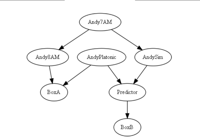
Timeless Decision eory
!"#$%&$'()*#+,"$'-$'"#
.$#/)0#*)12#&3$#
4'$561&+'7"#/$(&)*#
8+.$'#9+'#1+/8:&6(;#
<)1:*&6$"=#&+#<:**0#
"6/:*)&$#!(50#)(5#36"#
'$8'+5:16,*$#
$(-6'+(/$(&#>#$-$(#6<#
.$#3)-$#&3$#),6*6&0#&+#
<:**0#"1':&6(6?$#!(507"#
6(6&6)*#1+(56&6+(#)&#
!(50@!AB#
C+($&3$*$""D#)"#
$%&$'()*#+,"$'-$'"D#.$#
$%8$1&#!(50E!A#&+#
1+''$*)&$#.6&3#!(50F6/D#
G:"&#)"#.$#$%8$1&#
1)*1:*)&+'"#"$&#&+#
1+/8:&$#H@EI#JE@#&+#
'$&:'(#&3$#")/$#
)(".$'"#)&#A+(;+*6)#
)(5#C$8&:($B##K$#5+#(+&#$%8$1&#+,"$'-6(;#&3$#1+//+(#1):"$#!(50@!A#&+#
"1'$$(#+<<#!(50E!A#<'+/#!(50F6/B##K$#1)(#+';)(6?$#&36"#)"8$1&#+<#+:'#
:(1$'&)6(&0#,0#'$8'$"$(&6(;#&3$#5$16"6+("#+<#,+&3#!(50E!A#)(5#!(50F6/#)"#
1+(($1&$5#&+#&3$#*)&$(&#(+5$#!(504*)&+(61B##K$#1)(#&3$(#91+''$1&*0=#6(<$'#&3$#
,$3)-6+'#+<#!(50E!A#<'+/#!(50F6/#)(5#-61$#-$'")B
!#1*)""61)*#1):")*#5$16"6+(#&3$+'6"&D#)1&6(;#)"#)(#$%&$'()*#+,"$'-$'#&+#!(507"#
56*$//)D#.+:*5#)*"+#6(<$'#&3$#,$3)-6+'#+<#!(50E!A#<'+/#!(50F6/#)(5#-61$#-$'")#
>#&'$)&6(;#&3$/#)"#1+''$*)&$5#,$1):"$#+<#&3$6'#1+//+(#1):"$D#!(50@!AB##9L#3)-$#
(+&#"$$(#&3$#M:$"&6+(#+<#N"1'$$(6(;#+<<N#')6"$5B=##O):")*#5$16"6+(#&3$+'6"&"#5+#(+&#
'$;)'5#&3$/"$*-$"#)"#,$6(;#+,*6;)&$5#&+#/+5$*#!"#$%#/6(5"7#)1&6+("#)"#)1):")*B#
P$&#Q+,#,$#)#1):")*#5$16"6+(#&3$+'6"&#.3+#.6&($""$"#)#&3+:")(5#;)/$"#)(5#
+,"$'-$"#&3$#4'$561&+'#&+#)*.)0"#8'$561+''$1&*0B##K3$(#Q+,#"$$"#&3$#($%&#
8*)0$'#13++"$#+(*0#,+%#QD#Q+,#3)"#(+#&'+:,*$#8'$561&6(;#&3)&#,+%#Q#.6**#1+(&)6(#)#
/6**6+(#5+**)'"B
R3$#"6(;:*)'6&0#6(#1):")*#5$16"6+(#&3$+'0#)'6"$"#.3$(#Q+,#$(&$'"#&3$#;)/$#<+'#
36/"$*<D#)(5#/:"&#$-)*:)&$#&3$#$%8$1&$5#:&6*6&6$"#+<#36"#+.(#8+""6,*$#)1&6+("B#
O+("65$'#Q+,#$-)*:)&6(;#&3$#$%8$1&$5#:&6*6&0#+<#&)26(;#+(*0#,+%#QD#<+'#.3613#Q+,#
1+/8:&$"#89QST)UQ=#)(5#89QVT)UQ=B##Q+,#'$)"+("#)"#<+**+."W##NR3$#4'$561&+'#3)"#
)*'$)50#/)5$#36"#/+-$X#"6(1$#L#)/#)#1):")*#5$16"6+(#&3$+'6"&D#&3$#4'$561&+'7"#
/+-$#6"#&+#*$)-$#Q#$/8&0B##R3$'$<+'$#6<#L#&)2$#+(*0#,+%#QD#L#'$1$6-$#(+&36(;BN##R3)&#
6"D#Q+,#$-)*:)&$"#89QST)UQ=#Y#Z#)(5#89QVT)UQ=#)"#Y#S#>#:(*$""#&3$#4'$561&+'#3)"#
/)5$#)#/6"&)2$X#,:&#)&#)(0#')&$#89QS=#)(5#89QV=#1)(#,$)'#(+#'$*)&6+(#&+#Q+,7"#
+.(#)1&6+(B##R36"#8'+,),6*6"&61#6(5$8$(5$(1$#<+**+."#<'+/#Q+,7"#/+5$*#)<&$'#3$#
E[
&'()%$*+,-*
Figure 12
as correlated because of their common cause, Andy
7AM.
(I have not seen the question
of “screening o ” raised.) Causal decision theorists do not regard themselves as being
obligated to model other minds’ actions as acausal. Let Bob be a causal decision theorist
who witnesses a thousand games and observes the Predictor to always predict correctly.
When Bob sees the next player choose only box B, Bob has no trouble predicting that
box B will contain a million dollars.
e singularity in causal decision theory arises when Bob enters the game for him-
self, and must evaluate the expected utilities of his own possible actions. Consider Bob
evaluating the expected utility of taking only box B, for which Bob computes p(B
0
|ˆa
B
)
and p(B
$
|ˆa
B
). Bob reasons as follows: “e Predictor has already made his move; since
I am a causal decision theorist, the Predictor’s move is to leave B empty. erefore if I
take only box B, I receive nothing.” at is, Bob evaluates p(B
0
|ˆa
B
) ∼ 1 and p(B
$
|ˆa
B
)
as ∼ 0—unless the Predictor has made a mistake; but at any rate p(B
0
) and p(B
$
)
can bear no relation to Bob’s own action. is probabilistic independence follows from
Bob’s model after he deletes all parent causes of Andy
8AM
—Bob treats his own decision
as acausal, for that is the prescription of causal decision theory.
But mark this: First, the causal decision theorist now models the expected conse-
quence of his own actions using a causal graph which diers from the graph that suc-
cessfully predicted the outcome of the Predictor’s last thousand games. Does this not
violate the way of science? Is this not an inelegance in the mathematics? If we treat
88

Eliezer Yudkowsky
causal diagrams as attempts to represent reality, which of these two diagrams is nearer
the truth? Why does Bob think he is a special case?
Second, Bob evaluates the consequence of the action a
B
, and asserts p(B
$
|ˆa
B
) ∼ 0,
by visualizing a visibly inconsistent world in which Andy
Sim
and Andy
8AM
return dierent
outputs even though they implement the same abstract computation. is is not a possible
world. It is not even an impossible possible world, as impossible possible worlds are
usually dened. e purpose of reasoning over impossible possible worlds is to manage
a lack of logical omniscience (Lipman 1999) by permitting us to entertain possibilities
that may be logically impossible but which we do not yet know to be logically impossible.
For so long as we do not know Fermat’s Last eorem to be true, we can reason coher-
ently about a possibly impossible possible world where Fermat’s Last eorem is false.
After we prove FLT, then imagining ¬FLT leads to visibly inconsistent mathematics
from which we can readily prove a contradiction; and from a logical contradiction one
may prove anything. e world in which Andy
Sim
and Andy
8AM
output dierent an-
swers for the same abstract computation is not a possibly impossible possible world, but
a denitely impossible possible world. Furthermore, the inconsistency is visible to Bob
at the time he imagines this denitely impossible possible world.
I therefore suggest that, howsoever Bob models his situation, he should use a model
in which there is never a visible logical inconsistency; that is, Bob should never visualize
a possible world in which the same abstract computation produces dierent results on
dierent (faithful, reliable) instantiations. Bob should never visualize that 678 × 987
is 669186 in one place and 669168 in another. One model which has this property
is a timeless decision diagram. I have already drawn one timeless decision diagram,
for Andy’s Newcomb experience; it is diagram D that represents our uncertainty about
Andy’s decision, produced by Andy’s cognition, as uncertainty about the output of an
abstract computation that is multiply instantiated.
I emphasize again that using timeless decision diagrams to analyze Newcomblike
problems and obtain probabilities over Newcomblike outcomes does not commit one to
following a timeless decision algorithm. I emphasize this because philosophy recognizes
a much larger component of de gustibus non disputandum in decision than in probability—
it is simpler to argue beliefs than to argue acts. If someone chooses a 30% probability
of winning a vanilla ice cream cone over a 60% probability of winning a chocolate ice
cream cone, perhaps the person simply doesn’t like chocolate. It may also be that the
person does like chocolate more than vanilla, and that the person has some incorrect
factual belief which leads him to choose the wrong gamble; but this is hard to demon-
strate. In contrast, someone who examines a vanilla ice cream cone and comes to the
conclusion that it is chocolate, or someone who believes the sky to be green, or someone
who believes that 2 + 2 = 3, has arrived to the wrong answer on a question of fact.
89

Timeless Decision eory
Since a timeless decision diagram makes no direct prescription for acts, and of itself as-
signs only probabilities, it is that much less arguable—unless you nd an algorithm that
assigns better-calibrated probabilities.
e timeless decision diagram for Newcomb’s Problem, considered as a prescription
only over probabilities, is as in Figure 12.
e diagram reads the same way for an outside observer or for Andy himself. If I am
uncertain of Andy’s decision—that is, the output of Andy’s decision process, the value of
the latent variable Andy
Platonic
—whether I am Andy or I am an outside observer—then
I am uncertain of the contents of box B. If I assign probabilities over Andy’s possible
decisions (whether I am Andy making a rough advance guess at his own future decision,
or I am an outside observer), and I assign a 60% probability to Andy choosing only box
B, then I assign a 60% probability to box B containing a million dollars. Considering
my probability assessment as a measure over possibly impossible possible worlds, then I
do not assign any measure to denitely impossible possible worlds that contain a logical
inconsistency visible to me. Using standard methods for computing counterfactuals over
the value of the variable Andy
Platonic,
I believe that if the output of Andy’s decision
system were a
B
, then Andy
Sim
would choose a
B
, box B would contain a million dollars,
and Andy
8AM
would leave behind box A. And if the output of Andy’s decision system
were a
AB
, then box B would be empty and Andy
8AM
would take both boxes. is all
holds whether or not I am Andy—I use the same representation, believe the same beliefs
about reality, whether I nd myself inside or outside the system.
Here my analysis temporarily stays, and does not go beyond describing Andy’s beliefs,
because I have not yet presented a timeless decision algorithm.
Suppose the Predictor does not run an exact simulation of Andy. Is it conceivable
that one may produce a faithful prediction of a computation without running that exact
computation?
Suppose Gauss is in primary school and his teacher, as a punishment, sets him to add
up all the numbers between 1 and 100. Immediately he knows that the output of this
computation will be 5050; yet he did not bother to add 2 to 1, then add 3 to the result,
then add 4 to the result, as the teacher intended him to do. Had he done so, the result—
barring an error in his calculations — would have been 5050. A fast computation may
faithfully simulate a slow computation.
Imagine that the Predictor wants to produce a good prediction of Andy (say, to an
accuracy of one error in a thousand games) while expending as little computing power as
possible. Perhaps that is the object of the Predictor’s game, to arrive at veridical answers
efficiently, using less computing power than would be required to simulate every neuron
in Andy’s brain. (What’s the fun in merely running simulations and winning every time,
90

Eliezer Yudkowsky
after all?) If the Predictor is right 999 times out of 1000,that is surely temptation enough
to choose only box B—though it makes the temptation less clear.
How is it possible that the Predictor can predict Andy without simulating him ex-
actly? For that matter, how can we ourselves predict other minds without simulating
them exactly? Suppose that Andy
8AM
—“the real Andy” — nds himself in an environ-
ment with green-painted walls. And suppose that Andy
Sim
nds himself in an environ-
ment with blue-painted walls. We would nonetheless expect—not prove, but probabilis-
tically expect—that Andy
Sim
and Andy
8AM
come to the same conclusion. e Predic-
tor might run a million alternate simulations of Andy in rooms with slightly dierent-
colored walls, all colors except green, and nd that 999 out of 1000 Andys decide to take
only box B. If so, the Predictor might predict with 99.9% condence that the real Andy,
nding himself in a room with green walls, will decide to take only box B.
e color of the wall is not relevant to Andy’s decision—presuming, needless to say,
that Andy does not know which color of the wall tokens the “real Andy.” Otherwise
the Andys in non-green rooms and the Andy in the green room might behave very dif-
ferently; the slight dierence in sensory input would produce a large dierence in their
cognition. But if Andy has no such knowledge—if Andy doesn’t know that green is the
special color—then we can expect the specic color of the room not to inuence Andy’s
decision in any signicant way, even if Andy knows in a purely abstract way that the color
of the room matters somehow. e Andy in a red room thinks, “Oh my gosh! e color
of the room is red! I’d better condition my thoughts on this somehow . . . well, since it’s
red, I’ll choose only box B.” e Andy in a blue room thinks, “Oh my gosh! e color
of the room is blue! I’d better condition my thoughts on this somehow . . . well, since
it’s blue, I’ll choose only box B.” If we’re trying to simulate Andy on the cheap, we can
abstract out the color of the room from our simulation of Andy, since the computation
will probably carry on the same way regardless, and arrive to more or less the same result.
Now it may be that Andy is in such an unstable state that any random perturbation
to Andy’s brain or his environment, even a few neurons, has the potential to ip his
decision. If so the Predictor might nd that 70% of the simulated Andys decided one
way, and 30% another, depending on tiny perturbations. But to the extent that Andy
chooses rationally and for good reasons, we do not expect him to condition his decision
on irrelevant factors such as the exact temperature of the room in degrees Kelvin or the
exact illumination in candlepower. Most descriptions of Newcomblike problems do not
specify the wall color, the room temperature, or the illumination, as weighty arguments.
If a philosopher Phil goes to all the trouble of arguing that tiny perturbations might
inuence Andy’s decision and therefore the Predictor cannot predict correctly, Phil is
probably so strongly opinionated about decision theory and Newcomblike problems that
the Predictor would have no trouble predicting him.
91

Timeless Decision eory
If Andy doesn’t know that the color of the room is signicant, or if Andy doesn’t
start out knowing that the Predictor produces Its predictions through simulation, all the
less reason to expect the color of the room to inuence his thoughts. e Predictor may
be able to abstract out entirely that part of the question, when It imagines a simplied
version of Andy for the purpose of predicting Andy without simulating him. Indeed,
in all the philosophical discussions of Newcomb’s Problem, I have never once heard
someone direct attention to the color of the walls in the room—we don’t think it an
important thought of the agent.
Perhaps the Predictor tries to predict Andy in much the same way that, e.g., you or
I would predict the trajectory of other cars on the street without modeling the cars and
their drivers in atomic detail. e Predictor, being superintelligent, may possess a brain
embracing millions or billions of times the computing power of a human brain, and
better designed to boot—say, for example, avoiding the biases described in Kahneman,
Slovic, and Tversky (1982). Yet the Predictor is so very intelligent that It does not need
to use a billion times human computing power to solve the puzzle of Andy, just as we
do not need to add up all the numbers between 1 and 100 to know the answer. We do
not know in detail how the Predictor predicts, and perhaps Its mind and methods are
beyond human comprehension. We just know that the Predictor wins the game 999
times out of 1000.
I do not think this would be so implausible a predictive accuracy to nd in real life, if
a Predictor came to this planet from afar, or if a superintelligence was produced locally
(say as the outcome of recursive self-improvement in an Articial Intelligence) and hu-
manity survived the aftermath. I don’t expect to nd myself faced with a choice between
two boxes any time soon, but I don’t think that the scenario is physically impossible. If
the humanity of a thousand years hence really wished to do this thing, we could probably
do it—for tradition’s sake, perhaps. I would be skeptical, but not beyond convincing, if
I heard reports of a modern-day human being who could converse with someone for
an hour and then predict their response on Newcomb’s Problem with 90% accuracy.
People do seem to have strong opinions about Newcomb’s Problem and I don’t think
those strong opinions are produced by tiny unpredictable thermal perturbations. Again
I regard this as a counterargument to those philosophers who argue that Newcomb’s
Problem is a logical impossibility.
How can efficient prediction—the prediction of a mind’s behavior without simulating
it neuron by neuron—be taken into account in a causal diagram?
Bayesian networks seem to me poorly suited for representing uncertainty about math-
ematical proofs. If A implies B implies C implies D, then knowing A proves D and
thereby screens o all further uncertainty about D. Bayesian networks are efficient for
representing probabilistic mechanisms. Bayesian networks are useful when, if A causes
92

Eliezer Yudkowsky
B causes C causes D, then knowing C screens o D from B, but knowing A does
not screen o D from B. Mixing uncertainty about mathematical proof and uncer-
tainty about physical mechanisms efficiently is innovation beyond the scope of this essay.
Nonetheless, our uncertainty about mathematical proofs has a denite structure. If A
implies B, then it would be foolish to assign less probability to B than to A. If A implies
B and ¬A implies ¬B, then A ⇐⇒ B, p(A) = p(B) and we may as well treat them
as the same latent node in a causal diagram.
If the Predictor uses an efficient representation of Andy that provably returns the
same answer as Andy—for example, by abstracting out subcomputations that provably
have no eect on the nal answer—then for any output produced by Andy
Platonic
, it
follows deductively that the Predictor’s computation produces the same output, even if
the Predictor’s computation executes in less time than Andy himself. It is then a know-
able logical contradiction for the Andy-computation to choose a
B
and the Predictor’s
computation to predict a
AB
, and we should not visualize a world in which this known
contradiction obtains.
If the Predictor is using a probabilistic prediction of Andy (but an algorithm with
excellent resolution; say, no more than 1 wrong answer out of 1000), this complicates
the question of how to represent our uncertainty about the respective computations. But
note that probabilistic prediction is no stranger to formal mathematics, the most obvi-
ous example being primality testing. e Rabin-Miller probabilistic test for primeness
(Rabin 1980) is guaranteed to pass a composite number for at most 1/4 of the possible
bases. If N independent tests are performed on a composite number, using N randomly
selected bases, then the probability that the composite number passes each test is 1/4
N
or less.
Suppose the Predictor uses a very strong but probabilistic algorithm. If I am an
outside observer, then on witnessing Andy choose only box B, I make a strong inference
about the contents of box B; or if I see that box B is full, I make a strong inference about
Andy’s decision. If I represent Andy
P latonic
and Predictor
Simulation
as dierent latent
nodes, I can’t possibly represent them as unconnected; this would require probabilistic
independence, and there would then be no way for an observer to infer box B’s contents
from witnessing Andy’s decision or vice versa.
I think that probably the best pragmatic way to deal with probabilistic prediction, for
the purpose of Newcomb’s Problem, is to draw a directed arrow from the latent node
representing Andy’s computation to a non-latent node representing the Predictor’s sim-
ulation/prediction, with a conditional probability p(Predictor|Andy) or a mechanism
f
Predictor
(Andy, u
Predictor
). We would only have cause to represent the Predictor’s com-
putation as a latent node, if this computation itself had more than one physical instan-
tiation of interest to us. Another argument is that the Predictor’s simulation probably
93

Timeless Decision eory
reects Andy’s computation, and whether or not this error occurs is a discoverable fact
about the state of the world—the particular approximation that the Predictor chooses
to run. A pragmatic argument for directing the arrow is that if we changed Andy’s
computation (for example, by substituting one value for another in the parameter of
the underlying algorithm), then the Predictor would change Its simulation; but if the
Predictor changed its simulation then the behavior of Andy would not follow suit in
lock-step.
I regard this reasoning as somewhat ad-hoc, and I think the underlying problem is
using Bayesian networks for a purpose (representing uncertainty about related math-
ematical propositions) to which Bayesian networks are not obviously suited. But to
divorce decision theory from causal networks is a project beyond the ambition of this
present essay.
For the purpose of this essay, when I wish to speak of a probabilistic simulation of
a computation, I will draw a directed arrow from the node representing the computation
to a node representing a probabilistic prediction of that computation. Usually I will
choose to analyze thought experiments with multiple faithful instantiations of the same
computation, or a perfect simulation guaranteed to return the same answer, because this
simplies the reasoning considerably. I do not believe that, in any case discussed here,
probabilism changes the advice of TDT if the probabilities approach 1 or 0. I view this
as a desirable property of a decision theory. e dierence between 10
−100
and 0 should
only rarely change our preferences over actions, unless the decision problem is one of
split hairs.
e principle that drives my choice of theory is to update probabilities appropri-
ately. We should avoid visualizing worlds known to be logically impossible; we should
similarly decrease the probability of worlds that are known to be probably logically im-
possible, or that are logically known to be improbable. I have proposed, as a pragmatic
solution, to draw a directed arrow from a computation to a probabilistic simulation of
that computation. If someone drives this theory to failure, in the sense that it ends up
visualizing a knowably inconsistent world or attaching high probability to a knowably
improbable world, it will be necessary to junk that solution and search for a better way
of managing uncertainty.
11.1. Solomon’s Problem
e second most popular Newcomblike problem, after Newcomb’s Problem itself, is a
variant known as Solomon’s Problem. As you may recall from Section 1.2, the formula-
tion of Solomon’s Problem we are using is chewing-gum throat-abscess problem.
Chewing gum has a curative eect on throat abscesses. Natural selection has pro-
duced in people susceptible to throat cancer a tendency to chew gum. It turns out that
94

Eliezer Yudkowsky
a single gene, CGTA, causes people to chew gum and makes them susceptible to throat
cancer. As this causal diagram requires, conditioning on the gene CGTA renders gum-
chewing and throat abscesses statistically independent. We are given these observations:
Chew gum Don’t chew gum
CGTA present: 89% die 99% die
CGTA absent: 8% die 11% die
If we do not know yet whether we carry the gene CGTA, should we decide to chew
gum? If we do nd ourselves deciding to chew gum, we will then be forced to conclude,
from that evidence, that we probably bear the CGTA gene. But chewing gum cannot
possibly cause us to bear the CGTA gene, and gum has been directly demonstrated to
ameliorate throat abscesses.
Is there any conceivable need here to represent our own decision as the output of an
abstract decision process? ere is no Predictor here, no uploaded humans, no exact or
approximate simulation of our decision algorithm. Solomon’s Problem is usually classi-
ed as a Newcomblike problem in the philosophical literature; is it a timeless decision
problem?
Before I answer this question, I wish to pose the following dilemma with respect to
Solomon’s Problem: How would this situation ever occur in real life if the population
were made up of causal decision theorists? In a population composed of causal theo-
rists, or evidential theorists with tickling, everyone would chew gum just as soon as the
statistics on CGTA had been published. In this case, chewing gum provides no evidence
at all about whether you have the gene CGTA—even from the perspective of an out-
side observer. If only some people have heard about the research, then there is a new
variable, “Read the Research,” and conditioning on the observation RTR=rtr+, we nd
that chewing gum no longer correlates with CGTA. Everyone who has heard about the
research, whether they bear the gene CGTA or not, chews gum.
To avoid this breakdown of the underlying hypothesis, let us postulate that most peo-
ple are instinctively evidential decision theorists without tickling. We postulate, for the
sake of thought experiment, a world in which humanity evolved with the heuristic-and-
bias of evidential decision theory. Around 50,000 years ago in this alternate universe, the
rst statisticians began drawing crude but accurate tables of clinical outcomes on cave
walls, and people instinctively began to avoid chewing gum in order to convince them-
selves they did not bear the CGTA gene. Because of the damage this decision caused to
bearers of the CGTA gene (which for some reason was not simply selected out of the
gene pool; maybe the CGTA gene also made its bearers sexy), a mutation rapidly came
to the fore which turned CGTA bearers (and for some reason, only CGTA bearers) into
a dierent kind of decision theorist.
95

Timeless Decision eory
Now we have already specied that most people,in this subjunctive world,are CGTA-
negative evidential decision theorists. We have been told the output of their decision
process; they decide to avoid gum. But now we come to the decision of a person named
Louie. Louie bears a mutation that makes him a new kind of decision theorist . . . a more
powerful decision theorist. Shunned by ordinary decision theorists who do not under-
stand their powers, the new breed of decision theorists band together to form a crime-
ghting group known as the X-eorists . . . Ahem. Excuse me. Louie bears a mutation
that makes him not-an-evidential decision theorist. Louie knows that CGTA-negative
decision theorists choose not to chew gum, and that people who don’t chew gum usu-
ally don’t get throat abscesses. Louie knows that gum helps prevent throat abscesses.
Louie correctly explains this correlation by supposing that population members who
are CGTA-negative are evidential decision theorists, and evidential theorists choose not
to chew gum, and CGTA-negative individuals are less susceptible to throat abscesses.
Louie knows that CGTA-positive decision theorists implement a dierent algorithm
which causes them to decide to chew gum.
Aha! Why “Aha!”, you ask? Whether Louie believes himself to be CGTA-positive
or CGTA-negative, or whether Louie starts out uncertain of this, Louie must model
a world that contains potential copies of his own decision process. e other individuals
are not exact copies of Louie. But we have been proposing a hypothesis under which
all people who implement this algorithm decide this way, and all people who implement
that algorithm decide that other way. It seems that, whatever the dierent inputs and
parameters for separate instantiations of this algorithm, it makes no dierence to the
output (on the appropriate level of abstraction). One CGTA-positive individual reasons,
“To maximize the expected utility of the person that is Mary, should Mary chew gum?”
And the output is, “Mary should chew gum.” And another reasons: “To maximize the
expected utility of the person that is Norman, should Norman chew gum?” And the
output is, “Norman should chew gum.” If in a sense these two computations return
the same answer, it is because in a sense they are the same computation. We need only
substitute “I” for “Mary” and “Norman” to see this. Perhaps, for a species of intelligent
agents sufficiently exact in their evaluation of expected utility, the two computations
would provably return the “same” answer.
Not yet knowing the decision of Mary, but knowing that her computation bore so
close a resemblance to that of Norman, we would infer Mary’s decision from Norman’s
or vice versa. And we would make this inference even after inspecting both their initial
states, if we remained uncertain of the outcome. erefore I propose to model the sim-
ilarity between these two individuals as stemming from a shared abstract computation.
From this entry point, I introduce the following timeless decision diagram, pictured
in Figure 13, of (one possible mechanism for) Solomon’s Problem. Node CGTA takes
96
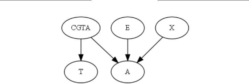
Eliezer Yudkowsky
!"#$%&'()%*+&",%-#(+&.%/%(+&"#012*%&'*%3#44#5(+6%&($*4*))%0*2()(#+%0(76"7$%#3%8#+*%
-#))(94*%$*2'7+()$%3#":%;#4#$#+<)%="#94*$>%
?#0*%@ABC%&7D*)%#+%&'*%E741*)%26&7F%#"%
26&7G.%)&7+0(+6%3#"%@ABCF+*67&(E*%7+0%
@ABCF-#)(&(E*%(+0(E(0174)>%%@ABC%
0("*2&4,%733*2&)%8'7)%7+%7""#5%(+&#:%&'*%
E7"(794*%B.%5'(2'%"*-"*)*+&)%&'"#7&%
79)2*))*)>%%@ABC%74)#%733*2&)%7%
E7"(794*%C.%5'(2'%"*-"*)*+&)%7+%
(+0(E(0174<)%0*2()(#+%5'*&'*"%&#%2'*5%
61$>%%C4)#%)'#5(+6%7""#5)%(+&#%C%7"*%&'*%
+#0*)%H%7+0%I.%"*-"*)*+&(+6%*E(0*+&(74%0*2()(#+%&'*#"()&)%7+0%IFB'*#"()&)>%%H%()%7%
47&*+&%+#0*%5'#)*%E741*%()%&'*%0*2()(#+%#1&-1&%9,%&'*%79)&"72&%2#$-1&7&(#+%H.%
5'(2'%($-4*$*+&)%7+%*E(0*+&(74%0*2()(#+%746#"( &'$%5(&'#1&%&(2D4(+6>%%I%()%&'*%
79)&"72&%2#$-1&7&(#+%&'7&%0*&*"$(+*)%&'*%)'7"*0%9*'7E(#"%#3%IFB'*#"()&)>%%B'*%
31+2&(#+%3JC8@ABC.%H.%I:%*K'(9(&)%7%2#+&*K&F)-*2(3(2%(+0*-*+0*+2*L%(3%@ABC%&7D*)%
#+%&'*%E741*%26&7F.%&'*+%C<)%"*$7(+ (+6%0*-*+0*+2,%()%#+4,%#+%H.%+#&%#+%I>%%/3%
@ABC%&7D*)%#+%&'*%E741*%26&7G.%&'*+%C%0*-*+0)%#+%I%91&%+#&%#+%H>%%B'()%2#+&*K&F
)-*2(3(2%(+0*-*+0*+2*%"*-"*)*+&)%&'*%-"#-#)(&(#+%&'7&%@ABCF+*67&(E*%(+0(E(0174)%
($-4*$*+&%&'*%H%2#$-1&7&(#+%7+0%@ABCF-#)( &(E*%(+0 (E(0174)%($-4*$*+&%&'*%I%
2#$-1&7&(#+>%%M*%D+#5%&'7&%H%&7D*)%#+%&'*%E741*%N7E#(0%61$N%7+0%I%&7D*)%#+%&'*%
E741*%N2'*5%61$N>
C%47&*+&%+#0*%(+%7%&($*4*))%0(76"7$%"*-"*)*+&)%&'*%3(K*0%#1&-1&%#3%7%3(K*0%
2#$-1&7&(#+>%%/3%O#1(*%()%1+2*"&7(+%#3%5'(2'%2#$-1&7&(#+%'*%($-4*$*+&).%&'*%
0(76"7$%"*-"*)*+&)%&'()%1+2*"&7(+&,%1)(+6%7%2#+&*K&F)-*2(3(2%(+0*-*+0*+2*P%7%
E7"(794*%5'(2'%(+0(27&*)%1+2*"&7(+&,%79#1&%5'(2'%746#"(&'$%0*)2"(9*)%O#1(*>%%/+%
&'()%27)*%&'*%67&(+6%E7"(794*%()%@ABC.%5'(2'%74)#%733*2&)%)1)2*-&(9(4(&,%&#%&'"#7&%
79)2*))*)>%%Q1&%@ABC%'7)%+#%7""#5)%(+&#%&'*%79)&"72&%746#"(&'$).%H%7+0%I>%
M'*&'*"%7+%(+0(E(0174%9*7")%&'*%@ABC%6*+*%0#*)%+#&%733*2&%&'*%3(K*0%#1&-1&%#3%7%
0*&*"$(+()&(2%2#$-1&7&(#+%F%(&%#+4,%733*2&)%!"#$"%79)&"72&%2#$-1&7&(#+%&'7&%
(+0(E(0174<)%-',)(274%$7D*1-%(+)&7+&(7&*)>
H(&'*"%O#1(*%#"%7+%#1&)(0*%#9)*"E*".%5'#%9*4(*E*)%&'7&%&'()%0(76"7$%0*)2"(9*)%
O#1(*<)%)(&17&(#+.%9*4(*E*)%&'*%3#44#5(+6P
• A(E*+%&'7&%O#1(*%0*2(0*)%&#%2'*5%61$.%'*%-"#9794,%'7)%&'*%@ABC%6*+*%
7+0%5(44%-"#9794,%0*E*4#-%7%&'"#7&%79)2*))>
• A(E*+%&'7&%O#1(*%0*2(0*)%+#&%&#%2'*5%61$.%'*%-"#9794,%0#*)%+#&%'7E*%&'*%
@ABC%6*+*%7+0%5(44%-"#9794,%+#&%0*E*4#-%7%&'"#7&%79)2*))>
• /3%-*#-4*%5'#%($-4*$*+&*0%2#$-1&7&(#+%H%0*2(0*0%&#%2'*5%61$.%&'*, %
5#140%0*E*4#-%3*5*"%&'"#7&%79)2*))*)>
• /3%&'*%#1&-1&%#3%79)&"72&%2#$-1&7&(#+%I%5*"*%N0#+<&%2'*5%61$N.%-*#-4*%5'#%
($-4*$*+&*0%I%5#140%0*E*4#-%$#"*%&'"#7&%79)2*))*)>
RS
%#&'()*+,-*
Figure 13
on the values cgta- or cgta+, standing for CGTA-negative and CGTA-positive individ-
uals. CGTA directly aects (has an arrow into) the variable T , which represents throat
abscesses. CGTA also aects a variable A, which represents an individual’s decision
whether to chew gum. Also showing arrows into A are the nodes E and X, representing
evidential decision theorists and X-eorists. E is a latent node whose value is the de-
cision output by the abstract computation E, which implements an evidential decision
algorithm without tickling. X is the abstract computation that determines the shared
behavior of X-eorists. e function f
A
(CGT A, E, X) exhibits a context-specic in-
dependence; if CGTA takes on the value cgta-, then A’s remaining dependency is only
on E, not on X. If CGTA takes on the value cgta+, then A depends on X but not on
E. is context-specic independence represents the proposition that CGTA-negative
individuals implement the E computation and CGTA-positive individuals implement
the X computation. We know that E takes on the value “avoid gum”and X takes on the
value “chew gum.”
A latent node in a timeless diagram represents the xed output of a xed computa-
tion. If Louie is uncertain of which computation he implements, the diagram represents
this uncertainty using a context-specic independence: a variable which indicates uncer-
tainty about which algorithm describes Louie. In this case the gating variable is CGTA,
which also aects susceptibility to throat abscesses. But CGTA has no arrows into the
abstract algorithms, E and X. Whether an individual bears the CGTA gene does not
aect the xed output of a deterministic computation—it only aects which abstract
computation that individual’s physical makeup instantiates.
Either Louie or an outside observer, who believes that this diagram describes Louie’s
situation, believes the following:
• Given that Louie decides to chew gum, he probably has the CGTA gene and will
probably develop a throat abscess.
• Given that Louie decides not to chew gum, he probably does not have the CGTA
gene and will probably not develop a throat abscess.
97

Timeless Decision eory
• If people who implemented computation E decided to chew gum, they would de-
velop fewer throat abscesses.
• If the output of abstract computation X were “don’t chew gum,” people who im-
plemented X would develop more throat abscesses.
• e probability that an individual carries the CGTA gene is unaected by the out-
puts of X and E, considered as abstract computations.
Again, as I have not yet introduced a timeless decision algorithm, the analysis does
not yet continue to prescribe a rational decision by Louie. But note that, even consid-
ered intuitively, Louie’s beliefs under these circumstances drain all intuitive force from
the argument that one should choose not to chew gum. Roughly, the naive evidential
theorist thinks: “If only I had chosen not to chew gum; then I would probably not have
the CGTA gene!” Someone using a timeless decision graph thinks: “If my decision (and
the decision of all people sufficiently similar to me that the outputs of our decision algo-
rithms correlate) were to avoid gum, then the whole population would avoid gum, and
avoiding gum wouldn’t be evidence about the CGTA gene. Also I’d be more likely to
get a throat abscess.”
And note that again, this change in thinking amounts to dispelling a denitely im-
possible possible world—refusing to evaluate the attractiveness of an imaginary world
that contains a visible logical inconsistency. If you think you may have the CGTA gene,
then thinking “If only I instead chose to avoid gum—then I would probably not have
the CGTA gene!” visualizes a world in which your decision alters in this way, while the
decisions of other CGTA-positive individuals remain constant. If you all implement the
same abstract computation X, this introduces a visible logical inconsistency: e xed
computation X has one output in your case, and a dierent output everywhere else.
Similarly with the classical causal decision theorist in Newcomb’s problem, except
that now it is the causal decision theorist who evaluates the attractiveness of a visibly
inconsistent possible world. e causal decision theorist says, “e Predictor has already
run its simulation and made its move, so even if I were to choose only box B, it would
still be empty.” ough this may seem more rational than the thought of the eviden-
tial decision theorist, it nonetheless amounts to visualizing an inconsistent world where
Andy
Sim
and Andy
8AM
make dierent decisions even though they implement the same
abstract computation.
12. e Timeless Decision Procedure
e timeless decision procedure evaluates expected utility conditional upon the output of
an abstract decision computation—the very same computation that is currently execut-
98

Eliezer Yudkowsky
ing as a timeless decision procedure—and returns that output such that the universe will
possess maximum expected utility, conditional upon the abstract computation returning
that output.
I delay the formal presentation of a timeless decision algorithm because of some
signicant extra steps I wish to add (related to Jerey’s [1983] proposal of ratiability),
which are best justied by walking through a Newcomblike problem to show why they
are needed. But at the core is a procedure which, in every faithful instantiation of the
same computation, evaluates which abstract output of that computation results in the
best attainable state of the universe, and returns that output. Before adding additional
complexities, I wish to justify this critical innovation from rst principles.
Informally, Newcomb’s Problem is treated as specied in Figure 12.
e abstract computation Andy
P latonic
with instantiations at both Andy
8AM
and
Andy
Sim
computes the expected utility of the universe, if the abstract computation
Andy
P latonic
returns the output a
AB
or alternatively a
B
. Since this computation com-
putes the universe to have higher utility if its output is a
B
, the computation outputs a
B
(in both its instantiations).
Andy still chooses a
B
if Andy believes that the Predictor does not execute an exact
Andy
Sim
, but rather executes a computation such that Andy
8AM
→ a
B
⇒ Andy
Sim
→
a
B
and Andy
8AM
→ a
AB
⇒ Andy
Sim
→ a
AB
. Here X → Y denotes “computa-
tion X produces output Y ” and “X ⇒ Y ” denotes implication, X implies Y . In this
circumstance the two computations may be treated as the same latent node, since our
probability assignments over outputs are necessarily equal.
Andy outputs the same decision if Andy believes the Predictor’s exact physical state
is very probably but not certainly such that the mathematical relation between compu-
tations holds. is can be represented by a gating variable and a context-specic indepe-
dence, selecting between possible computations the Predictor might implement. Given
that Andy’s utility is linear in monetary reward, and that Andy’s probability assignment
to the gating variable shows a signicant probability that the Predictor predicts using
a computation whose output correlates with Andy’s, Andy will still output a
B
.
Informally, the timeless decision diagram D models the content of box B as deter-
mined by the output of the agent’s abstract decision computation. us a timeless de-
cision computation, when it executes, outputs the action a
B
which takes only box B—
outputting this in both instantiations. e timeless decision agent walks o with the full
million.
99

Timeless Decision eory
13. Change and Determination: A Timeless View of Choice
Let us specify an exact belief set—a probability distribution, causal diagram, or timeless
diagram of a problem. Let us specify an exact evidential, causal, or timeless decision al-
gorithm. en the output of this decision computation is xed. Suppose our background
beliefs describe Newcomb’s Problem. Choosing a
AB
is the xed output of a causal deci-
sion computation; choosing a
B
is the xed output of an evidential decision computation;
choosing a
B
is the xed output of a timeless decision computation.
I carefully said that a causal decision agent visualizes a knowable logical inconsis-
tency when he computes the probability p(B
$
|ˆa
B
) ∼ 0. A timeless decision agent also
visualizes a logical inconsistency when she imagines what the world would look like if
her decision computation were to output a
AB
—because a timeless computation actually
outputs a
B
.
A timeless agent visualizes many logically inconsistent worlds in the course of de-
ciding. Every imagined decision, except one, means visualizing a logically inconsistent
world. But if the timeless agent does not yet know her own decision, she does not know
which visualized worlds are logically inconsistent. Even if the timeless agent thinks she
can guess her decision, she does not know her decision as a logical fact—not if she admits
the tiniest possibility that thinking will change her answer. So I cannot claim that causal
decision agents visualize impossible worlds, and timeless agents do not. Rather causal
agents visualize knowably impossible worlds, and timeless agents visualize impossible
worlds they do not know to be impossible.
An agent, in making choices, must visualize worlds in which a deterministic compu-
tation (the decision which is now progressing) returns an output other than the output it
actually returns, though the agent does not yet know her own decision, nor know which
outputs are logically impossible. Within this strange singularity is located nearly all the
confusion in Newcomblike problems.
Evidential decision theory and causal decision theory respectively compute expected
utility as follows:
u(o)p(o|a
i
) (16)
u(o)p(o|ˆa
i
) (17)
Placed side by side, we can see that any dierence in the choice prescribed by eviden-
tial decision theory and causal decision theory, can stem only from dierent probability
assignments over consequences. Evidential decision theory calculates one probable con-
sequence, given the action a
i
, while causal decision theory calculates another. So the
dispute between evidential and causal decision theory is not in any sense a dispute over
ends, or which goals to pursue—the dispute is purely over probability assignments. Can
we say de gustibus non est disputandum about such a conict?
100

Eliezer Yudkowsky
If a dispute boils down to a testable hypothesis about the consequences of actions,
surely resolving the dispute should be easy! We need only test alternative actions,observe
consequences, and see which probability assignment best matches reality.
Unfortunately, evidential decision theory and causal decision theory are eternally
unfalsiable—and so is TDT. e dispute centers on the consequences of logically im-
possible actions, counterfactual worlds where a deterministic computation returns an
output it does not actually return. In evidential decision theory, causal decision the-
ory, and TDT, the observed consequences of the action actually performed will conrm
the prediction made for the performed action. e dispute is over the consequences of
decisions not made.
Any agent’s ability to make a decision, and the specic decision made, is determined
by the agent’s ability to visualize logically impossible counterfactuals. Moreover, the
counterfactual is “What if my currently executing decision computation has an output
other than the one it does?”, when the output of the currently executing computation is
not yet known. is is the confusing singularity at the heart of decision theory.
e dierence between evidential, causal, and TDT rests on dierent prescriptions
for visualizing counterfactuals—untestable counterfactuals on logical impossibilities.
An evidential decision theorist might argue as follows: “We cannot observe the im-
possible world that obtains if my decision computation has an output other than it does.
But I can observe the consequences that occur to other individuals who make decisions
dierent from mine—for example, the rate of throat abscesses in individuals who choose
to chew gum—and that is just what my expected utility computation says it should be.”
A timeless decision theorist might argue as follows: “e causal decision agent com-
putes that even if he chooses a
B
, then box B will still contain nothing. Let him just try
choosing a
B
, and see what happens. And let the evidential decision theorist try chewing
gum, and let him observe what happens. Test out the timeless prescription, just one time
for curiosity; and see whether the consequence is what TDT predicts or what your old
algorithm calculated.”
A causal decision theorist might argue as follows: “Let us try a test in which some
force unknown to the Predictor reaches in from outside and presses the button that
causes me to receive only box B. en I shall have nothing, conrming my expectation.
is is the only proper way to visualize the counterfactual, ‘What if I chose only B
instead?’ If I really did try choosing a
B
on ‘just one time for curiosity’, as you would
have it, then I must predict a dierent set of consequences on that round of the problem
than I do in all other rounds. But if an unknown outside force reached in and pressed
the button ‘take both boxes’for you, you would see that having both boxes is better than
having only one.”
101

Timeless Decision eory
An evidential agent (by supposition CGTA-negative) computes, as the expected con-
sequence of avoiding gum, the observed throat-abscess rate of other (CGTA- negative)
people who avoid gum. is prediction, the only prediction the evidential agent will ever
test, is conrmed by the observed frequency of throat abscesses. Suppose that throat ab-
scesses are uncomfortable but not fatal, and that each new day brings with an indepen-
dent probability of developing a throat abscess for that day—each day is an independent
data point. If the evidential agent could be persuaded to just try chewing gum for a few
months, the observed rate of throat abscesses would falsify the prediction used inside the
evidential decision procedure as the expected consequence of deciding to chew gum. e
observed rate would be the low rate of a CGTA-negative individual who chews gum,
not the high rate of a CGTA-positive individual who chews gum.
A causal decision agent, to correctly predict the consequence even of the single action
decided, must know in advance his own decision. Without knowing his own decision,
the causal decision agent cannot correctly predict (in the course of decision-making) that
the expected consequence of taking both boxes is $1000. If the Predictor has previously
lled box B on 63 of 100 occasions, a causal agent might believe (in the course of making
his decision) that choosing both boxes has a 63% probability of earning $1,001,000—a
prediction falsiable by direct observation, for it deals with the decision actually made.
35
If the causal agent does not know his decision before making his decision, or if the
causal agent truly believes that his action is acausal and independent of the Predictor’s
prediction, the causal agent might prefer to press a third button—a button which takes
both boxes and makes a side bet of $100 that pays 5-for-1 if box B is full. We presume
that this decision also is once-o and irrevocable; the three buttons are presented as
a single decision. So we see that the causal agent, to choose wisely, must know his own
decision in advance—he cannot just update afterward, on pain of stupidity.
If the causal agent is aware of his own decision in advance, then the causal agent
will correctly predict $1000 as the consequence of taking both boxes, and this prediction
will be conrmed by observing the consequence of the decision actually made. But if
the causal agent tries taking only box B, just one time for curiosity, the causal agent
must quickly change the predictions used—so that the causal agent now predicts that
the consequence of taking both boxes is $1,001,000, and the consequence of taking only
one box is $1,000,000.
35. It is falsiable in the sense that any single observation of an empty box provides signicant Bayesian
evidence for the hypothesis “Box B is empty if I take both boxes” over the hypothesis “Box B has a 63%
chance of being full if I take both boxes.” With repeated observations, the probability of the second
hypothesis would become arbitrarily low relative to the rst, regardless of prior odds.
102

Eliezer Yudkowsky
Only the timeless decision agent can test predicted consequences in the intuitively
obvious way, “Try it a dierent way and see what happens.” If the timeless decision
agent tries avoiding gum, or tries taking both boxes, the real-world outcome is the same
consequence predicted as the timeless counterfactual of that action on similar problems.
Here is another sense in which TDT is superior to causal decision theory. Only
the timeless decision procedure calculates internal predictions that are testable, in the
traditional sense of testability as a scientic virtue. We do not let physicists quickly
switch around their predictions (to match that of a rival theory, no less), if we inform
them we intend to perform an unusual experiment.
How should we visualize unobservable,impossible,counterfactual worlds? We cannot
test them by experience. How strange that these counterfactual dreams—unfalsiable,
empty of empirical content—determine our ability to determine our own futures! If two
people wish to visualize dierent untestable counterfactuals, is there no recourse but to
apply the rule of de gustibus non est disputandum? I have so far oered several arguments
for visualizing counterfactuals the timeless way:
1. e counterfactual predictions used by timeless decision agents are directly testable
any time the timeless decision agent pleases,because the timeless agent expects that
trying the action “just once for curiosity” will return the consequence expected of
that action on any similar problem.
2. A timeless counterfactual is not visibly logically inconsistent, if the timeless agent
does not yet know her decision, or if the timeless agent thinks there is even an
innitesimal chance that further thinking might change her mind.
3. A timeless agent uses the same diagram to describe herself as she would use to
describe another agent in her situation; she does not treat herself as a special case.
4. If you visualize logically impossible counterfactuals the way that TDT prescribes,
you will actually win on Newcomblike problems, rather than protesting the unrea-
sonableness of the most rewarded decision.
13.1. Freedom and Necessity
I have called it a logical impossibility that, on a well-dened decision problem, an agent
with a well-dened algorithm should make any decision but the one she does. Yet to
determine her future in accordance with her will, an agent must visualize logically im-
possible worlds—how the world would look if the agent made a dierent decision—not
knowing these worlds to be impossible. e agent does not know her decision until she
chooses, from among all the impossible worlds, the one world that seems to her most
good. is world alone was always real, and all other worlds were impossible from the
beginning, as the agent knows only after she has made her decision.
103
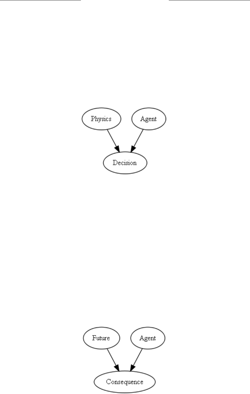
Timeless Decision eory
I have said that this strange singularity at the heart of decision theory is where the
confusion lurks. Not least did I refer to that related debate, often associated with dis-
cussion of Newcomb, called the problem of free will and determinism. I expect that most
of my readers will have already come to their own terms with this so-called problem.
Nonetheless I wish to review it, because the central appeal of causal decision theory
rests on human intuitions about change, determination, and control.
It seems to me that much confusion about free will can be summed up in the causal
diagram depicted in Figure 14. Suppose our decisions are completely determined by
!"##$%&'$"(')&*+%+$,%'-(&'*$.#/&0&/1')&0&(.+,&)'21'
#31%+*%'4'5+6&,'*$.#/&0&'7,$8/&)5&'$9'03&'#-%0:'$"('
#(&%&,0'*3$+*&'+%'03&(&21')&0&(.+,&);''#<)&*+%+$,=+>
?@A!BC!D'E'F'9$('$,&'#-(0+*"/-('6-/"&'$9')&*+%+$,=+:'
-,)'-//')&*+%+$,%'3-6&'#<)&*+%+$,=GD'E'HI''B9'%$:'03&,'
#<JKCB!BLM>?@A!BC!D'E'#<JKCB!BLM>?@A!BC!:'
NOKMPDI''Q$('+9'?@A!BC!')&0&(.+,&%'JKCB!BLM'
8+03'*&(0-+,01:'03&,'03&(&'+%',$03+,5'/&90'$6&('0$'2&'
)&0&(.+,&)'21'03&'6-(+-2/&'NOKMP:'-,)'03&'-//&5&)'
*-"%-/'/+,7'9($.'NOKMP'0$'JKCB!BLM'+%'&R0(-,&$"%I''S&'3-6&',$'+,9/"&,*&'-0'-//'
$6&('$"('$8,'*3$+*&%T'03&1'-(&')&0&(.+,&)'83$//1'-,)'&,0+(&/1'21'#31%+*%I''P3&'
9&&/+,5'8&'3-6&:'$9'2&+,5'+,'*$,0($/'$9'$"('$8,'03$"530%'-,)'-*0+$,%:'+%'2"0'-,'
+//"%+$,'4'+0'+%'(&-//1'#31%+*%'03-0'+%'+,'*$,0($/'03&'83$/&'0+.&I
U&9$(&'03&'+,6&,0+$,'$9'.-03&.-0+*-/'#31%+*%:'-'%+.+/-('9&-('8-%'&R#(&%%&)'21'
&-(/+&('#3+/$%$#3&(%'83$'-%7&)'+9'03&'9"0"(&'8&(&'-/(&-)1')&0&(.+,&);
B9'-//'03&'9"0"(&'+%'-/(&-)1'(&*$()&):'-'2$$7'",(&-)'2"0'
-/(&-)1'8(+00&,:'03&,'83-0'"%&')&*+%+$,V''W&0'03&'
-5&,0'%0(+6&'-%'3&'8+//%:'-,)'3&'8+//',$0'-/0&('03&'
$"0*$.&I''P3&'-5&,0'3-%',$'#-(0'+,')&0&(.+,+,5'03&'
*$,%&X"&,*&'$9'3+%')&*+%+$,I''P3&'*$,%&X"&,*&'+%'
*$#+&)')$8,'9($.'03&'9+R&)'2$$7'$9'03&'9"0"(&:'83+*3'
8-%'&%0-2/+%3&)'+((&%#&*0+6&'$9'3".-,')&&)%I''B9'
#<*$,%&X"&,*&=+>QYPYZKD'E'F:'03&,'03&(&'*-,'2&',$'
9"(03&('+,9/"&,*&'9($.'NOKMPT'#<CLM!K[YKMCK>
QYPYZKD'E'#<CLM!K[YKMCK>QYPYZK:NOKMPDI
S3-0'2$03')+-5(-.%'3-6&'+,'*$..$,'+%'03-0'03&1'#/-*&'03&'-5&,0'$"0%+)&'M-0"(&'
4'$"0%+)&'#31%+*%:'$"0%+)&'03&'9"0"(&I''N,)'03+%'+%'03&'*/-%%+*-/'&(($('$9'J&%*-(0&%:'
83$'%&-/&)'03&'.+,)'$,'$,&'%+)&'$9'-,'",-/0&(-2/&'2$",)-(1:'-,)'03&'8$(/)'"#$,'
03&'$03&(I''@$8'9&8'#&$#/&'&6&('/&-(,'!"#!$%&'(8+03'#31%+*%'4'+,0+.-*1'&,$"53'0$'
%&&'3".-,'2&+,5%'-%'&R+%0+,5')!#*!"'#31%+*%:',$0'$"0%+)&'+0V''Q$('03+%'0("03'$"('
#31%+*%'0&//%'"%:'%$'%"(#(+%+,5'03-0'9&8'-**�'03&'*$,%&X"&,*&%;''N//'(&-/+01'+%'-'
%+,5/&'9/$8:'$,&'",+9+&)'#($*&%%'$2&1+,5'%+.#/&'/$84/&6&/'.-03&.-0+*-/'("/&%:'-,)'
8&'$"(%&/6&%'-'*$,0+,"$"%'#-(0'$9'03+%'9/$8:'
8+03$"0'+,0&(("#0+$,'$('2$",)-(1I''P3-0'83+*3'
+%')&0&(.+,&)'21'3".-,%:'+%'$9',&*&%%+01'
)&0&(.+,&)'21'#31%+*%T'9$('3".-,%'&R+%0'
&,0+(&/1'8+03+,'#31%+*%I''B9'-,'$"0*$.&'8&(&'
,$0')&0&(.+,&)'21'#31%+*%:'+0'*$"/)',$0'
#$%%+2/1'2&')&0&(.+,&)'21'3".-,'*3$+*&I
FHF
+!,-./(012(
+!,-./(032(
+!,-./(042(
Figure 14
physics—given complete knowledge of the past, our present choice is thereby deter-
mined: p(decision
i
|PHYSICS) = 1 for one particular value of decision
i
, and all deci-
sions have p(decision
j
) = 0. If so, then p(DECISION|PHYSICS) =
p(DECISION|PHYSICS, AGENT). For if PHYSICS determines DECISION with
certainty, then there is nothing left over to be determined by the variable AGENT, and
the alleged causal link from AGENT to DECISION is extraneous. We have no inu-
ence at all over our own choices; they are determined wholly and entirely by physics. e
feeling we have,of being in control of our own thoughts and actions, is but an illusion—it
is really physics that is in control the whole time.
Before the invention of mathematical physics, a similar fear was expressed by earlier
philosophers who asked if the future were already determined (see Figure 15). If all the
!"##$%&'$"(')&*+%+$,%'-(&'*$.#/&0&/1')&0&(.+,&)'21'
#31%+*%'4'5+6&,'*$.#/&0&'7,$8/&)5&'$9'03&'#-%0:'$"('
#(&%&,0'*3$+*&'+%'03&(&21')&0&(.+,&);''#<)&*+%+$,=+>
?@A!BC!D'E'F'9$('$,&'#-(0+*"/-('6-/"&'$9')&*+%+$,=+:'
-,)'-//')&*+%+$,%'3-6&'#<)&*+%+$,=GD'E'HI''B9'%$:'03&,'
#<JKCB!BLM>?@A!BC!D'E'#<JKCB!BLM>?@A!BC!:'
NOKMPDI''Q$('+9'?@A!BC!')&0&(.+,&%'JKCB!BLM'
8+03'*&(0-+,01:'03&,'03&(&'+%',$03+,5'/&90'$6&('0$'2&'
)&0&(.+,&)'21'03&'6-(+-2/&'NOKMP:'-,)'03&'-//&5&)'
*-"%-/'/+,7'9($.'NOKMP'0$'JKCB!BLM'+%'&R0(-,&$"%I''S&'3-6&',$'+,9/"&,*&'-0'-//'
$6&('$"('$8,'*3$+*&%T'03&1'-(&')&0&(.+,&)'83$//1'-,)'&,0+(&/1'21'#31%+*%I''P3&'
9&&/+,5'8&'3-6&:'$9'2&+,5'+,'*$,0($/'$9'$"('$8,'03$"530%'-,)'-*0+$,%:'+%'2"0'-,'
+//"%+$,'4'+0'+%'(&-//1'#31%+*%'03-0'+%'+,'*$,0($/'03&'83$/&'0+.&I
U&9$(&'03&'+,6&,0+$,'$9'.-03&.-0+*-/'#31%+*%:'-'%+.+/-('9&-('8-%'&R#(&%%&)'21'
&-(/+&('#3+/$%$#3&(%'83$'-%7&)'+9'03&'9"0"(&'8&(&'-/(&-)1')&0&(.+,&);
B9'-//'03&'9"0"(&'+%'-/(&-)1'(&*$()&):'-'2$$7'",(&-)'2"0'
-/(&-)1'8(+00&,:'03&,'83-0'"%&')&*+%+$,V''W&0'03&'
-5&,0'%0(+6&'-%'3&'8+//%:'-,)'3&'8+//',$0'-/0&('03&'
$"0*$.&I''P3&'-5&,0'3-%',$'#-(0'+,')&0&(.+,+,5'03&'
*$,%&X"&,*&'$9'3+%')&*+%+$,I''P3&'*$,%&X"&,*&'+%'
*$#+&)')$8,'9($.'03&'9+R&)'2$$7'$9'03&'9"0"(&:'83+*3'
8-%'&%0-2/+%3&)'+((&%#&*0+6&'$9'3".-,')&&)%I''B9'
#<*$,%&X"&,*&=+>QYPYZKD'E'F:'03&,'03&(&'*-,'2&',$'
9"(03&('+,9/"&,*&'9($.'NOKMPT'#<CLM!K[YKMCK>
QYPYZKD'E'#<CLM!K[YKMCK>QYPYZK:NOKMPDI
S3-0'2$03')+-5(-.%'3-6&'+,'*$..$,'+%'03-0'03&1'#/-*&'03&'-5&,0'$"0%+)&'M-0"(&'
4'$"0%+)&'#31%+*%:'$"0%+)&'03&'9"0"(&I''N,)'03+%'+%'03&'*/-%%+*-/'&(($('$9'J&%*-(0&%:'
83$'%&-/&)'03&'.+,)'$,'$,&'%+)&'$9'-,'",-/0&(-2/&'2$",)-(1:'-,)'03&'8$(/)'"#$,'
03&'$03&(I''@$8'9&8'#&$#/&'&6&('/&-(,'!"#!$%&'(8+03'#31%+*%'4'+,0+.-*1'&,$"53'0$'
%&&'3".-,'2&+,5%'-%'&R+%0+,5')!#*!"'#31%+*%:',$0'$"0%+)&'+0V''Q$('03+%'0("03'$"('
#31%+*%'0&//%'"%:'%$'%"(#(+%+,5'03-0'9&8'-**�'03&'*$,%&X"&,*&%;''N//'(&-/+01'+%'-'
%+,5/&'9/$8:'$,&'",+9+&)'#($*&%%'$2&1+,5'%+.#/&'/$84/&6&/'.-03&.-0+*-/'("/&%:'-,)'
8&'$"(%&/6&%'-'*$,0+,"$"%'#-(0'$9'03+%'9/$8:'
8+03$"0'+,0&(("#0+$,'$('2$",)-(1I''P3-0'83+*3'
+%')&0&(.+,&)'21'3".-,%:'+%'$9',&*&%%+01'
)&0&(.+,&)'21'#31%+*%T'9$('3".-,%'&R+%0'
&,0+(&/1'8+03+,'#31%+*%I''B9'-,'$"0*$.&'8&(&'
,$0')&0&(.+,&)'21'#31%+*%:'+0'*$"/)',$0'
#$%%+2/1'2&')&0&(.+,&)'21'3".-,'*3$+*&I
FHF
+!,-./(012(
+!,-./(032(
+!,-./(042(
Figure 15
future is already recorded, a book unread but already written, then what use decision?
104
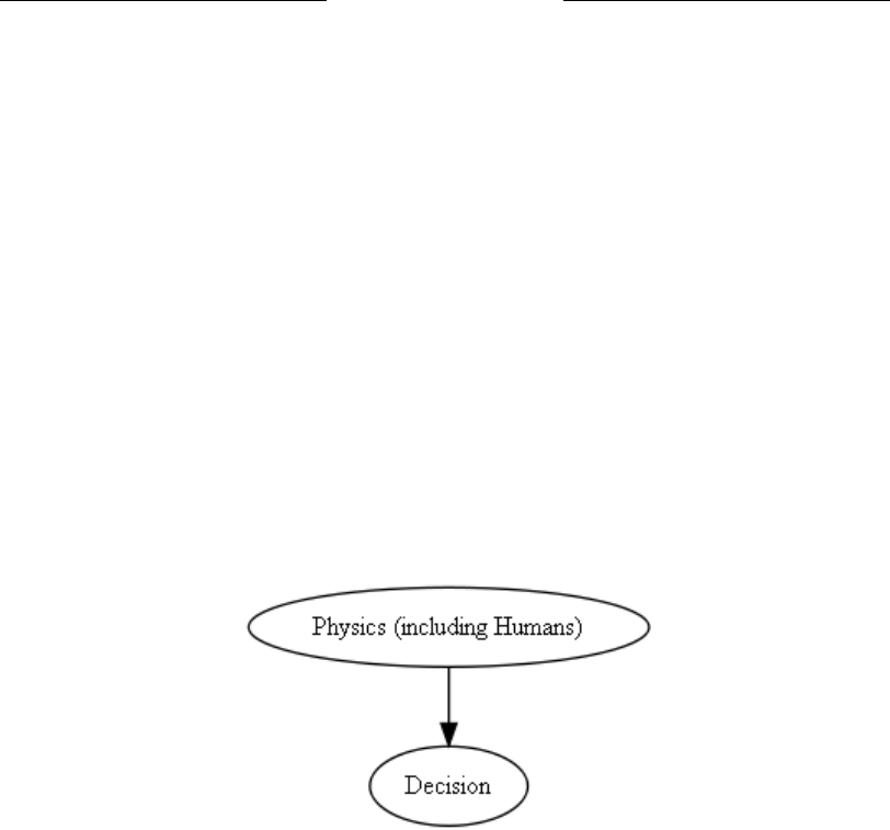
Eliezer Yudkowsky
Let the agent strive as he wills, and he will not alter the outcome. e agent has no
part in determining the consequence of his decision. e consequence is copied down
from the xed book of the future, which was established irrespective of human deeds. If
p(consequence
i
|FUTURE) = 1, then there can be no further inuence from AGENT;
p(CONSEQUENCE|FUTURE) = p(CONSEQUENCE|FUTURE, AGENT).
What both diagrams have in common is that they place the agent outside Nature—
outside physics, outside the future. And this is the classical error of Descartes, who sealed
the mind on one side of an unalterable boundary, and the world upon the other. How
few people ever learn intimacy with physics—intimacy enough to see human beings as
existing within physics, not outside it? For this truth our physics tells us, so surprising
that few accept the consequences: All reality is a single ow, one unied process obeying
simple low-level mathematical rules, and we ourselves a continuous part of this ow,
without interruption or boundary (see Figure 16). at which is determined by humans,
!"##$%&'$"(')&*+%+$,%'-(&'*$.#/&0&/1')&0&(.+,&)'21'
#31%+*%'4'5+6&,'*$.#/&0&'7,$8/&)5&'$9'03&'#-%0:'$"('
#(&%&,0'*3$+*&'+%'03&(&21')&0&(.+,&);''#<)&*+%+$,=+>
?@A!BC!D'E'F'9$('$,&'#-(0+*"/-('6-/"&'$9')&*+%+$,=+:'
-,)'-//')&*+%+$,%'3-6&'#<)&*+%+$,=GD'E'HI''B9'%$:'03&,'
#<JKCB!BLM>?@A!BC!D'E'#<JKCB!BLM>?@A!BC!:'
NOKMPDI''Q$('+9'?@A!BC!')&0&(.+,&%'JKCB!BLM'
8+03'*&(0-+,01:'03&,'03&(&'+%',$03+,5'/&90'$6&('0$'2&'
)&0&(.+,&)'21'03&'6-(+-2/&'NOKMP:'-,)'03&'-//&5&)'
*-"%-/'/+,7'9($.'NOKMP'0$'JKCB!BLM'+%'&R0(-,&$"%I''S&'3-6&',$'+,9/"&,*&'-0'-//'
$6&('$"('$8,'*3$+*&%T'03&1'-(&')&0&(.+,&)'83$//1'-,)'&,0+(&/1'21'#31%+*%I''P3&'
9&&/+,5'8&'3-6&:'$9'2&+,5'+,'*$,0($/'$9'$"('$8,'03$"530%'-,)'-*0+$,%:'+%'2"0'-,'
+//"%+$,'4'+0'+%'(&-//1'#31%+*%'03-0'+%'+,'*$,0($/'03&'83$/&'0+.&I
U&9$(&'03&'+,6&,0+$,'$9'.-03&.-0+*-/'#31%+*%:'-'%+.+/-('9&-('8-%'&R#(&%%&)'21'
&-(/+&('#3+/$%$#3&(%'83$'-%7&)'+9'03&'9"0"(&'8&(&'-/(&-)1')&0&(.+,&);
B9'-//'03&'9"0"(&'+%'-/(&-)1'(&*$()&):'-'2$$7'",(&-)'2"0'
-/(&-)1'8(+00&,:'03&,'83-0'"%&')&*+%+$,V''W&0'03&'
-5&,0'%0(+6&'-%'3&'8+//%:'-,)'3&'8+//',$0'-/0&('03&'
$"0*$.&I''P3&'-5&,0'3-%',$'#-(0'+,')&0&(.+,+,5'03&'
*$,%&X"&,*&'$9'3+%')&*+%+$,I''P3&'*$,%&X"&,*&'+%'
*$#+&)')$8,'9($.'03&'9+R&)'2$$7'$9'03&'9"0"(&:'83+*3'
8-%'&%0-2/+%3&)'+((&%#&*0+6&'$9'3".-,')&&)%I''B9'
#<*$,%&X"&,*&=+>QYPYZKD'E'F:'03&,'03&(&'*-,'2&',$'
9"(03&('+,9/"&,*&'9($.'NOKMPT'#<CLM!K[YKMCK>
QYPYZKD'E'#<CLM!K[YKMCK>QYPYZK:NOKMPDI
S3-0'2$03')+-5(-.%'3-6&'+,'*$..$,'+%'03-0'03&1'#/-*&'03&'-5&,0'$"0%+)&'M-0"(&'
4'$"0%+)&'#31%+*%:'$"0%+)&'03&'9"0"(&I''N,)'03+%'+%'03&'*/-%%+*-/'&(($('$9'J&%*-(0&%:'
83$'%&-/&)'03&'.+,)'$,'$,&'%+)&'$9'-,'",-/0&(-2/&'2$",)-(1:'-,)'03&'8$(/)'"#$,'
03&'$03&(I''@$8'9&8'#&$#/&'&6&('/&-(,'!"#!$%&'(8+03'#31%+*%'4'+,0+.-*1'&,$"53'0$'
%&&'3".-,'2&+,5%'-%'&R+%0+,5')!#*!"'#31%+*%:',$0'$"0%+)&'+0V''Q$('03+%'0("03'$"('
#31%+*%'0&//%'"%:'%$'%"(#(+%+,5'03-0'9&8'-**�'03&'*$,%&X"&,*&%;''N//'(&-/+01'+%'-'
%+,5/&'9/$8:'$,&'",+9+&)'#($*&%%'$2&1+,5'%+.#/&'/$84/&6&/'.-03&.-0+*-/'("/&%:'-,)'
8&'$"(%&/6&%'-'*$,0+,"$"%'#-(0'$9'03+%'9/$8:'
8+03$"0'+,0&(("#0+$,'$('2$",)-(1I''P3-0'83+*3'
+%')&0&(.+,&)'21'3".-,%:'+%'$9',&*&%%+01'
)&0&(.+,&)'21'#31%+*%T'9$('3".-,%'&R+%0'
&,0+(&/1'8+03+,'#31%+*%I''B9'-,'$"0*$.&'8&(&'
,$0')&0&(.+,&)'21'#31%+*%:'+0'*$"/)',$0'
#$%%+2/1'2&')&0&(.+,&)'21'3".-,'*3$+*&I
FHF
+!,-./(012(
+!,-./(032(
+!,-./(042(
Figure 16
is of necessity determined by physics; for humans exist entirely within physics. If an
outcome were not determined by physics, it could not possibly be determined by human
choice.
But for most people who confront this question, “physics” is a strange and foreign
discipline, learned briey in college and then forgotten, or never learned at all; cryptic
equations useful for solving word problems but not for constraining expectations of the
real world, and certainly without human relevance. For the idea that humans are part
of physics to make intuitive sense, we would have to understand our own psychology in
such detail that it blended seamlessly into physics from below.
Psychology is a macroscopic regularity in physics, the way that aerodynamics is a
macroscopic regularity of physics. Our excellent predictive models of airplanes may
make no mention of individual “atoms,” and yet our fundamental physics contains no
fundamental elements corresponding to airow or drag. is does not mean aerody-
namics is incompatible with physics. e science of aerodynamics is how we humans
manage our lack of logical omniscience, our inability to know the implications of our
own beliefs about fundamental physics. We don’t have enough computing power to cal-
105

Timeless Decision eory
culate atomic physical models over entire airplanes. Yet if we look closely enough at an
airplane, with a scanning tunneling microscope for example, we see that an airplane is
indeed made of atoms. e causal rules invoked by the science of aerodynamics do not
exist on a fundamental level within Nature. Aerodynamic laws do not reach in and do
additional things to atoms that would not happen without the laws of aerodynamics as
an additional clause within Nature. If we had enough computing power, we could pro-
duce accurate predictions without any science of aerodynamics—just pure fundamental
physics.
Our science of aerodynamics is not just compatible with,but in a deep sense mandated
by, our science of fundamental physics. If a non-atomic model
36
succeeds in delivering
good empirical predictions of an airplane, this does not falsify our fundamental physics,
but rather conrm it.
e map is not the territory. Nature is a single ow, one continuous piece. Any
division between the science of psychology and the science of physics is a division in
human knowledge, not a division that exists in things themselves. If you dare break up
knowledge into academic elds, sooner or later the unreal boundaries will come back to
bite. So long as psychology and physics feel like separate disciplines, then to say that
physics determines choice feels like saying that psychology cannot determine choice. So
long as electrons and desires feel like dierent things, to say that electrons play a causal
role in choices feels like leaving less room for desires.
A similar error attends visualization of a future which, being already determined,
leaves no room for human choice to aect the outcome.
Physicists, one nds, go about muttering such imprecations as “Space alone, and time
alone,are doomed to fade away; and henceforth only a unity of the two will maintain any
semblance of reality.” (Minkowski 1909)ey tell us that there is no simultaneity, no now
that enfolds the whole changing universe; now only exists locally, in events, which may
come before or after one another, but never be said to happen at the same time. Students
of relativity are told to imagine reality as a single four-dimensional crystal, spacetime, in
which all events are embedded. Relativity was not the beginning of physics clashing with
philosophy built on intuition; Laplace also disturbed the philosophers of his day, when
Laplace spoke of, given an exact picture of the universe as it existed now, computing
all future events. Special Relativity says that there is no now, but any spacelike-tilted
slice through the timeless crystal—any space of apparent simultaneity—will do as well
for Laplace’s purpose, as any other. General Relativity requires that the fundamental
equations of physics exhibit CPT symmetry: If you take an experimental record and
36. E.g. a computer program none of whose data elements model individual atoms.
106

Eliezer Yudkowsky
reverse charge, parity, and the direction of time, all fundamental laws of physics inferred
from the modied record must look exactly the same.
37
In the ordinary human course of visualizing a counterfactual, we alter one variable
in the past or present, and then extrapolate from there, forward in time. e physicists
say poetically to imagine reality as a timeless crystal; so we imagine a static image of
a crystal, static like a painting. We hold that crystal in our minds and visualize making
a single change to it. And because we have imagined a crystal like a static painting,
we see no way to extrapolate the change forward in time, as we customarily do with
counterfactuals. Like imagining dabbing a single spot of paint onto the Mona Lisa, we
imagine that only this one event changes, with no other events changing to match. And
translating this static painting back into our ordinary understanding of time, we suppose
that if an agent chooses dierently, the future is the same for it; altering one event in the
present or past would not alter the future.
is shows only that a static painting is a poor metaphor for reality.
Relativity’s timeless crystal is not a static painting that exists unchanging within time,
so that if you dab a spot of paint onto the painting at time T , nothing else has changed
at time T + 1. Rather, if you learn the physics that relates events within the crystal,
this is all there is or ever was to time. at’s the problem with priming our intuitions
by visualizing a timeless crystal; we tend to interpret that as a static object embedded
in higher-order time. We can see the painting, right there in our mind’s eye, and it
doesn’t change. When we imagine dabbing a spot of paint onto the painting, nothing
else changes, as we move the static painting forward in higher time.
So visualizing the future as a static painting causes your intuitions to return non-
sensical answers about counterfactuals. You can’t observe or test counterfactuals, so you
should pick a rule for counterfactuals that yields rewarding outcomes when applied in
decision theory. I do not see the benet to an agent who believes that if a black hole had
swallowed the entire Solar System in 1933, the Allies would still have won World War
II. at is not how “future” events relate to “past” events within the crystal. To imag-
ine that an agent had made a dierent choice, is disruption enough, for it violates the
natural law which related the agent’s choice to the agent’s prior state. Why add further
disruptions to tweak future events back into exactly the same place? You can imagine if
37. en why do eggs break but not unbreak? No electrons in the egg behave dierently whether
we run the movie forward or backward; but the egg goes from an ordered state to a disordered state.
Any observed macroscopic asymmetry of time must come from thermodynamics and the low-entropy
boundary condition of our past. is includes the phenomenon of apparent quantum collapse, which
arises from the thermodynamic asymmetry of decoherence.
107

Timeless Decision eory
you wish; de counterfactus non est disputandum. But what is the benet to the agent, of
visualizing counterfactuals in this way?
Intuition gone astray says that, if the future is already determined, our choices are
eectless. I think that visualizing a static painting—not a timeless crystal containing
time, but a painted future static within higher-order time—is the mental image that
sends intuition astray.
We can imagine a world where outcomes really are determined in advance. An alien
Author writes a novel, and then sets forth to re-enact this novel with living players. Be-
hind the scenes are subtle mechanisms, intelligent machinery set in place to keep history
on its track, irrespective of the decisions of the players. e Author has decreed World
War II, and it will happen on schedule; if Hitler refuses his destiny, the machines will
alter him back into schedule, or overwrite some other German’s thoughts with dreams of
grandeur. Even if the agents’ decisions took on other values, the background machinery
would tweak events back into place, copying down the outcome from the written book
of the future.
What determines the Author’s world? e background machinery that tweaks events
back into place when they threaten to depart the already-written novel. But our world
has no such background machinery, no robots working behind the scenes—not to my
knowledge. Where is the mechanism by which an already-written future could deter-
mine the outcome regardless of our choices?
Yet if the future is determined, how could we change it?
Our intuitive notion of change comes from observing the same variable at dierent
times. At 7:00 AM the egg is whole, then at 8:00 the same egg is broken; the egg has
changed. We would write EGG
t=7
= egg
whole
, EGG
t=8
= egg
broken
. But this is itself
a judgment of identity—to take the dierent variables EGG
t=7
and EGG
t=8
, which
may have dierent values, and lump the variables together in our minds by calling them
the same egg. A causal diagram, such as the one shown in Figure 17, can express two
interrelated variables, such as “Ination rates inuence employment; employment rates
inuence ination” and yet still be a directed acyclic graph.
It may be the case that employment in 2005 inuences ination in 2005, and that
ination in 2005 inuences employment in 2005—but this only shows that our times
are not split nely enough. We collapsed many separate events into the lump sum of
2005—choices of employers to hire or re, choices of shopkeepers to mark up or mark
down.
If we have any two nodes A, B in a causal diagram, such that A causally aects B,
and B causally aects A, this is more than just a problem with a formalism dened only
for acyclic graphs. It means we have postulated two events, such that A lies in the future
108
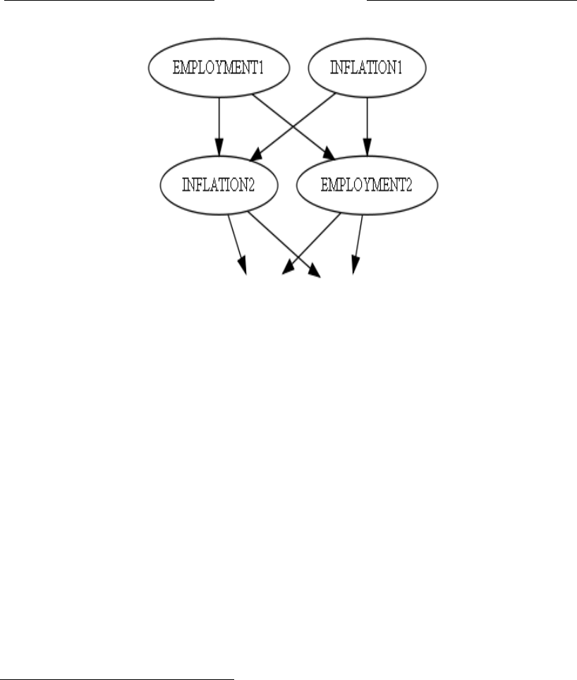
Eliezer Yudkowsky
!"#$%&#'(#")(#*%+(#")%"#
($,-.&$(/"#0/#1223#
0/4-5(/*(+#0/4-%"0./#0/#12236#
%/7#")%"#0/4-%"0./#0/#1223#
0/4-5(/*(+#($,-.&$(/"#0/#
1223#8#'5"#")0+#./-&#+).9+#
")%"#.5:#"0$(+#%:(#/."#+,-0"#
40/(-&#(/.5;)<##=(#*.--%,+(7#
$%/&#+(,%:%"(#(>(/"+#0/".#
")(#-5$,#+5$#.4#1223#8#
*).0*(+#.4#($,-.&(:+#".#)0:(#
.:#40:(6#*).0*(+#.4#
+).,?((,(:+#".#$%:?#5,#.:#
$%:?#7.9/<
!4#9(#)%>(#%/&#"9.#/.7(+#@6#
A#0/#%#*%5+%-#70%;:%$6#+5*)#")%"#@#*%5+%--&#%44(*"+#A6#%/7#A#*%5+%--&#%44(*"+#@6#
")0+#0+#$.:(#")%/#B5+"#%#,:.'-($#90")#%#4.:$%-0+$#7(40/(7#./-.:#%*&*-0*#;:%,)+<#
!"#$(%/+#9(#)%>(#,.+"5-%"(7#"9.#(>(/"+6#+5*)#")%"#@#-0(+#0/#")(#45"5:(#.4#A6#%/7#A#
-0(+#0/#")(#45"5:(#.4#@<##C).:"#.4#'50-70/;#%#"0$(#$%*)0/(#8#*:(%"0/;#%#*-.+(7#
"0$(-0?(#*5:>(#8#")0+#*%//."#)%,,(/<
DE
!#7.#/."#%:;5(#")%"#%#4.:$%-0+$#4.:#*%5+%-#70%;:%$+#,:.)0'0"+#*0:*5-%:#*%5+%-0"&F#
")(#%,,:.,:0%"(#:(+,./+(#".#+5*)#%/#%:;5$(/"#0+#GC.#9)%"HG##I5:#*).0*(#.4#
$%")($%"0*%-#4.:$%-0+$+#7.(+#/."#7("(:$0/(#:(%-0"&<##!4#")(#4.:$%-0+$#4%0-+#".#40"#
:(%-0"�"#0+#")(#4.:$%-0+$#")%"#$5+"#;0>(#9%&<##!$,.:"%/"-&6#,)&+0*+#%,,(%:+#".#
%;:((#90")#$(:(#0/"50"0./#")%"#"0$(#0+#/."#*&*-0*<##@/#!"!#$#)%+#%#+0/;-(#-.*%"0./#0/#
+,%*(#%/7#"0$(<##@#,%:"0*5-%:#(;;#%"#(J%*"-&#KL22@M#$%&#'(#*./+07(:(7#%/#(>(/"<#
@/#(;;#%+#0"#*)%/;(+#.>(:#")(#*.5:+(#.4#).5:+6#$5*)#-(++#G(;;+#0/#;(/(:%-G6#0+#
/."#%/#(>(/"<##%&&!*$'#(#0+#%#:(-%"0./+)0,#'("9((/#"9.#(>(/"+<##!"#0+#4.:'077(/#8#/."#
$(:(-&#'&#.5:#4.:$%-0+$6#'5"#$5*)#$.:(#0$,.:"%/"-&#'&#,)&+0*+#N./*(#%;%0/6#
'%::0/;#*-.+(7#"0$(-0?(#*5:>(+O#8#4.:#%/&#"9.#(>(/"+#@#%/7#A#".#'(#+5*)#")%"#@#0+#
DE
#M%/&#,)&+0*0+"+#'(-0(>(#")%"#"0$(#$%*)0/( +# %:(#0$,.++0'-(6#-.;0*%--&#*./":%70*".:&6#%'+5:76#%/7#
5/0$%;0/%'-(6#,:(*0+(-&#'(*%5+(#"0$(#$%*)0/(+#%--.9#*0:*5-%:#*%5+%-0"&F#%#")(.:&#")%"# ,(:$0"+#
*-.+(7#"0$(-0?(#*5:>(+#0+#+.$("0$(+#:(;%:7(7#%+#G,%").-.;0*%-G#./#")%"#%**.5/"<##P (:)%,+#"0$(#
$%*)0/(+#)*!#0$,.++0'-(6#(>(/#4.:#")%"#>(:&#:(%+./<##!#9.5-7#(>(/#+%&#")%"#! # " ).5;)"#0"#-0?(-&#")%"#
")(#$%B.:0"&#.4#,)&+0*0+"+#%:(#:0;)"#%/7#"0$(#":%>(-#0+#0$,.++0'-(F#04#!#9(:(#%#,)&+0*0+"#%/7#)%7# %/&#
:0;)"#".#%/#.,0/0./<##A5 " # 9( # 7./Q"#%*"5%--&#+#,-#")%"#"0$(#":%>(-#0+#0$,.++0'-(<##R0+".:&#"(%*)(+#5+#
")%"#S%"5:(#*%:(+#>(:&#-0""-(#4.:#9)%"#9(#") 0/ ?# 0+#0$,.++0' -( 6 # -. ;0*%--&#*./":%70*".:&6#%'+5:76#% /7#
5/0$%;0/%'-(<##T)%"#./-&#+"%"(+#).9#)5$%/ # ':%0/+#")0/?#%'.5"#*%5+%-0"&F#%/7#S%"5:(#$%&#)%>(#
.")(:#07(%+<##!4#)5$%/#0/"50"0./+#)%>(#(>.->(7#0/#+5*)#%#9%&#")%"#9(#*%//."#*./ *(0>(#.4#*0:*5-%:#
*%5+%-0"&6#")0+#./-&#+). 9+#")%"#)5/"(:8;%")(:(:+#(/*.5 /"(:(7#/.#*-.+(7#"0$(-0?(#*5:>(+<##C.# ! # 7.#
/."#+%&#")%"#0"#0+#+#,-)./0#0$,.++0'-(#".#)%>(#*0:*5-%:#*%5+%-0"#./ -&#")%"#*0:*5-%:#*%5+%-0"&#)%+#
/(>(:#'((/#.'+(:>(76# %/7#.5:#45/7%$(/"%-#,)&+0*+#$%?(+#0"#0$,.++0'-(#0/#")(#%'+(/*(#.4#%#"0$(#
$%*)0/(<##=)(/#!#9:0"(#G,)&+0*+#4.:'07+#UG6#:(%76#G.5:#*5::(/"#$.7(-#.4#,)&+0*+#N0/#")(#%'+(/*(# .4#
"0$(#$%*)0/(+6#9)0*)#%:(/Q"#0/>.->(7#0/#$.+"#:(%-89.:-7#7(*0+0./#,:.'-($+6#%/7#%:(#,:.'%' -&#
0$,.++0'-(O#4.:'07+#UG<##C).5-7#+.$(#,(:+./# 0/ >(/"#%#"0$(#$%*)0/(6#")0+#+(*"0./#.4# $&#( ++%Z--#
/((7#".#'(#:(>0+(7<
V23
Figure 17
of B, and B lies in the future of A. Short of building a time machine—creating a closed
timelike curve—this cannot happen.
38
I do not argue that a formalism for causal diagrams prohibits circular causality; the
appropriate response to such an argument is “So what?” Our choice of mathematical
formalisms does not determine reality. If the formalism fails to t reality it is the for-
malism that must give way. Importantly, physics appears to agree with mere intuition
that time is not cyclic. An event has a single location in space and time. A particular egg
at exactly 7:00AM may be considered an event. An egg as it changes over the course of
hours, much less “eggs in general,” is not an event. Aecting is a relationship between
two events. It is forbidden—not merely by our formalism, but much more importantly
by physics (once again, barring closed timelike curves)—for any two events A and B
to be such that A is aecting B and B is aecting A. If we conceive that employment
38. Many physicists believe that time machines are impossible, logically contradictory, absurd, and
unimaginable, precisely because time machines allow circular causality; a theory that permits closed time-
like curves is sometimes regarded as “pathological”on that account. Perhaps time machines are impossible,
even for that very reason. I would even say that I thought it likely that the majority of physicists are right
and time travel is impossible; if I were a physicist and had any right to an opinion. But we don’t actually
know that time travel is impossible. History teaches us that Nature cares very little for what we think is
impossible, logically contradictory, absurd, and unimaginable. at only states how human brains think
about causality; and Nature may have other ideas. If human intuitions have evolved in such a way that we
cannot conceive of circular causality, this only shows that hunter-gatherers encountered no closed time-
like curves. So I do not say that it is knowably impossible to have circular causality—only that circular
causality has never been observed, and our fundamental physics makes it impossible in the absence of
a time machine. When I write “physics forbids X,” read, “our current model of physics (in the absence of
time machines, which aren’t involved in most real-world decision problems, and are probably impossible)
forbids X.” Should some person invent a time machine, this section of my essay will need to be revised.
109

Timeless Decision eory
aects ination, and ination aects employment, then we must have lumped together
many dierent events under the name “employment” or “ination.”
What does it mean to change the future?
It is worth taking some time to analyze this confusion, which is built into the foun-
dations of causal decision theory. Recall that we are told to take both boxes because this
decision cannot change the contents of box B.
e future is as determined as the past. Why is it that philosophers are not equally
bothered by the determinism of the past? Every decision any agent ever made, ended
with some particular choice and no other; it became part of our xed past. Today you
ate cereal for breakfast. Your choice could have been something else, but it wasn’t, and it
never will be something else; your choice this morning is now part of the unalterable
past. Why is your decision that lies in the xed past, still said to be the outcome of
free will? In what sense is the xed past free? Even if we suppose that the future is
not determined, how can we blame a murderer for choosing to kill his victims, when
his decision lies in the past, and his decision-variable cannot possibly take on any value
other than the one it had? How can we blame this past decision on the murderer, when
the past is not free? We should really blame the decision on the past.
We may call the past and future “xed,”“determined,”or “unalterable”—these are just
poor metaphors which borrow the image of a painting remaining static in higher-order
time. ere is no higher-order time within which the future could “change”; there is
no higher-order time within which the future could be said to be “xed.” ere is no
higher-order time within which the past could change; there is no higher-order time
within which the past is xed. e future feels like it can change; the past feels like it is
xed; these are both equally illusions.
If we consider a subsystem of a grand system, then we can imagine predicting the
future of this subsystem on the assumption that the subsystem remains undisturbed by
other, outside forces that also exist within the grand system. Call this the future-in-
isolation of the subsystem. Given the exact current state of a subsystem as input, we
suppose an extrapolating algorithm whose output is the computed future-in-isolation of
the subsystem.
If an outside force perturbs the subsystem, we may compute that the subsystem now
possesses a dierent future-in-isolation. It is important to recognize that a future-in-
isolation is a property of a subsystem at a particular time. (Pretend for the moment that
we deal with Newtonian mechanics, so the phrase “at a particular time” is meaningful.)
Hence, the future-in-isolation of a subsystem may change from time to time, like an egg
whole at 7AM and broken at 8AM, as outside forces perturb the subsystem.
e notion of changing a future-in-isolation, seems to me to encapsulate what goes
on in the mind of a human who wishes to change the future. We look at the course of
110

Eliezer Yudkowsky
our lives and say to ourselves: “If this goes on, I shall not prosper; I shall not gain tenure; I
shall never become a millionaire; I will never save the world. . . .” So we set out to change
the future as we expect it, as we predict it; we strive, time passes, and we nd that we now
compute a dierent future for ourselves—I will save the world after all! Have we not,
then, changed the future? Our prediction has changed, from one time to another—and
because the future is the referent of a prediction, it feels to us like the future itself has
changed from one time to another. But this is mixing up the map with the territory.
Our notions of “changing” the future come—once again!—from considering our-
selves as forces external to reality, external to physics, separated by an impenetrable
Cartesian boundary from the rest of the universe. If so, by our acts upon the vast “sub-
system” that is every part of reality except ourselves, we may change (from one time to
another) the future-in-isolation of that tremendous subsystem. But there is a larger sys-
tem, and the grand system’s future does not “change.” A box may appear to change mass,
as we add and subtract toys, yet the universe as a whole always obeys conservation of en-
ergy. Indeed the future cannot “change,” as an egg can change from whole to broken.
Like the past, the future only ever takes on a single value. Mirai wa itsumo tada hitotsu.
Pearl’s exposition of causality likewise divides the universe into subsystems. When
we draw a causal diagram, it makes testable non-experimental predictions, and the same
diagram also makes many dierent testable experimental predictions about the eect of
interventions upon the system. is is a glorious virtue of a hypothesis. But the notion
of intervention, upon which rests so much of the usefulness of causal diagrams, implies
a grand universe divided into things inside the causal diagram, and things outside the
causal diagram. A causal diagram of the entire universe, including all potential exper-
imenters, would make only a single, non-experimental prediction. ere would be no
way to step outside the diagram to intervene.
I hold it a virtue of any decision theory that it should be compatible with a grand-
system view, rather than intrinsically separating the universe into agent and outside. All
else being equal, I prefer a representation which is continuous over the grand universe
and marks no special boundary where the observer is located; as opposed to a representa-
tion which solidies the Cartesian boundary between an observer-decider homunculus
and the environment. One reason is epistemological conservationism, keeping your on-
tology as simple as possible. One reason is that we have seen what strange results come
of modelling your own situation using a dierent hypothesis from the hypothesis that
successfully predicted the outcome for every other agent who stood in your place. But
the most important reason is that Cartesian thinking is factually untrue. ere is not
in fact an impenetrable Cartesian border between the agent and the outside. You need
only drop an anvil onto your skull to feel the force of this argument, as the anvil-matter
smashes continuously through the brain-matter that is yourself thinking. All else being
111

Timeless Decision eory
equal, I prefer a representation which describes the agent as a continuous part of a larger
universe, simply because this representation is closer to being true.
Such a representation may be called naturalistic as contrasted to Cartesian. I am also
fond of Ernest Nagel’s beautiful term, “the view from nowhere” (Nagel 1986), Nagel
meant it as an impossibility, but ever since I heard the term I have thought of it as
the rationalist’s satori. I seek to attain the view from nowhere, and using naturalistic
representations is a step forward.
13.2. Gardner’s Prime Newcomb Problem
Gardner (1974) oers this renement of Newcomb’s Problem: box B, now made trans-
parent like box A, contains a piece of paper with a large integer written on it.
39
You do
not know whether this number is prime or composite, and you have no calculator or any
other means of primality testing. If this number proves to be prime, you will receive $1
million. e Predictor has chosen a prime number if and only if It predicts that you will
take only box B.“Obviously,” says Gardner,“you cannot by the act of will make the large
number change from prime to composite or vice versa.”
Control —the power attributed to acts of will—is the essence of the dispute between
causal decision theory or evidential decision theory. Our act in Newcomb’s Problem
seems to have no way of controlling the xed contents of box B. erefore causal de-
cision theorists argue it cannot possibly be reasonable to take only box B. Letting the
content of box B depend on the primeness of a number makes it clear that the con-
tent of box B is utterly xed and absolutely determined; though this is already given
in the Newcomb’s Problem specication. Interestingly, to show the absolute xity of
box B’s content, Gardner would make the outcome depend on the output of an abstract
computation—a computation which tests the primality of a given integer.
I agree with Gardner that there is no way to change or modify the primeness of a xed
number. e result of a primality test is a deterministic output of a xed computation.
Nothing we do can possibly change the primeness of a number.
So too, nothing we do can possibly change our own decisions.
is phrasing sounds rather less intuitive, does it not? When we imagine a decision,
there are so many futures hanging temptingly before us, and we could pick any one of
them. Even after making our decision (which has only one value and no other), we feel
free to change our minds (although we don’t), and we feel that we could just as easily
pick a dierent choice if we wanted to (but we don’t want to).
39. Technically one cannot write an integer on a piece of paper, as integers are abstract mathematical
objects; but one can write a symbolic representation of an integer on a piece of paper.
112

Eliezer Yudkowsky
It is the sense of innite allowance in our decisions, of controlling the future, to which
I now turn my attention. e heart of Newcomb’s Paradox is the question of whether
our choice controls the contents of box B. An intuitive sense of causable change enhances
the feeling of being in control. An intuitive sense of determinism, of xity, opposes the
feeling of being in control.
But this is subsystem thinking, not grand-system thinking. “Control” is a two-place
predicate,a relation between a controller subsystem and a controlled subsystem. If a sub-
system has a xed future in the sense that its future-in-isolation never changes, then it
cannot be controlled. If a subsystem has a deterministic future, not considered in isola-
tion, but just because the grand system of which it is part has deterministic dynamics,
the subsystem may still be controllable by other subsystems.
What does it mean to “control” a subsystem? ere is more to it than change. When
an egg smashes into the ground, its state changing “whole” to “broken” (from one time
to another), we do not say that the ground controlled the egg.
We speak even of “self-command,”of getting a grip on oneself. Control (Mary, Mary)
binds the two-place predicate to say that Mary is controlled by herself. If the subsystem
is only interacting with itself, would not its future-in-isolation remain constant? Con-
sidered as an abstract property of the entire Mary subsystem, Mary’s future-in-isolation
would remain constant from one time to another. Yet Mary probably conceives of herself
as altering her own future, because her prediction of her self ’s future changes when she
engages in acts of self-control.
13.3. Change and Determination
A causal decision theory is sometimes dened as a decision theory which makes use of
inherently causal language. By this denition, TDT is typed as a causal decision the-
ory. In the realm of statistics, causal language is held in low repute, although spirited
defense by Judea Pearl and others has helped return causality to the mainstream. Pre-
vious statisticians considered causality as poorly dened or undenable, and went to
tremendous lengths to eliminate causal language. Even counterfactuals were preferred
to the raw language of asymmetrical causality, since counterfactuals can be expressed
as pure probability distributions p(A B). A causal Bayesian network can compute
a probability distribution or a counterfactual, but a causal network contains additional
structure found in neither. Unlike a probability distribution or a counterfactual distribu-
tion, a causal network has asymmetrical links between nodes which explicitly represent
asymmetrical causal relations. us the classical causal decision theory of Joyce (1999) is,
from a statistician’s perspective, not irredeemably contaminated by causal language. Clas-
sical causal decision theory only uses counterfactuals and does not explicitly represent
asymmetrical causal links.
113

Timeless Decision eory
Technically, TDT can also be cast in strictly counterfactual form. But the chief dif-
ference between TDT and CDT rests on which probability distributions to assign over
counterfactual outcomes. erefore I have explicitly invoked causal networks, includ-
ing explicitly represented asymmetrical causal links, in describing how timeless decision
agents derive their probability distributions over counterfactuals.
I wish to keep the language of causality, including counterfactuals, while proposing
that the language of change should be considered harmful. Just as previous statisticians
tried to cast out causal language from statistics, I now wish to cast out the language
of change from decision theory. I do not object to speaking of an object changing state
from one time to another. I wish to cast out the language that speaks of futures, outcomes,
or consequences being changed by decision or action.
What should ll the vacuum thus created? I propose that we should speak of deter-
mining the outcome. Does this seem like a mere matter of words? en I propose that
our concepts must be altered in such fashion, that we no longer nd it counterintuitive
to speak of a decision determining an outcome that is “already xed.” Let us take up the
abhorred language of higher-order time, and say that the future is already determined.
Determined by what? By the agent. e future is already written, and we are ourselves
the writers. But, you reply, the agent’s decision can change nothing in the grand sys-
tem, for she herself is deterministic. ere is the notion I wish to cast out from decision
theory. I delete the harmful word change, and leave only the point that her decision
determines the outcome—whether her decision is itself deterministic or not.
114

Eliezer Yudkowsky
References
Allais, Maurice.1953.“Le Comportement de l’Homme Rationnel devant le Risque: Critique des Postulats
et Axiomes de l’Ecole Americaine.” Econometrica 21 (4): 503–546.
Arntzenius, Frank. 2002. “Reections on Sleeping Beauty.” Analysis 62 (1): 53–62.
Aumann, Robert J., Sergiu Hart, and Motty Perry. 1997. “e Absent-Minded Driver.” Games and Eco-
nomic Behavior 20 (1): 102–116.
Bostrom, Nick. 2001. “e Meta-Newcomb Problem.” Analysis 61 (4): 309–310.
Boutilier, Craig, Nir Friedman, Moises Goldszmidt, and Daphne Koller. 1996. “Context-Specic Inde-
pendence in Bayesian Networks.” In Uncertainty in Articial Intelligence (UAI-’96), edited by Eric J.
Horvitz and Finn Jensen, 115–123. San Francisco, CA: Morgan Kaufmann.
Cresswell, Maxwell John. 1970. “Classical Intensional Logics.” eoria 36 (3): 347–372.
Drescher, Gary L. 2006. Good and Real: Demystifying Paradoxes from Physics to Ethics. Bradford Books.
Cambridge, MA: MIT Press.
Drexler, K. Eric. 1986. Engines of Creation. Garden City, NY: Anchor.
. 1992. Nanosystems: Molecular Machinery, Manufacturing, and Computation. New York: Wiley.
Eells, Ellery. 1984. “Metatickles and the Dynamics of Deliberation.” eory and Decision 17 (1): 71–95.
Egan, Andy. 2007. “Some Counterexamples to Causal Decision eory.” Philosophical Review 116 (1):
93–114.
Ekman, Paul.2007. Emotions Revealed: Recognizing Faces and Feelings to Improve Communication and Emo-
tional Life. 2nd ed. New York: Owl Books.
Feynman, Richard P., Robert B. Leighton, and Matthew L. Sands. 1963. e Feynman Lectures on Physics.
3 vols. Reading, MA: Addison-Wesley.
Gardner, Martin. 1974. “Reections on Newcomb’s Problem: A Prediction and Free-Will Dilemma.”
Scientic American, March, 102–108.
Gibbard, Allan, and William L. Harper. 1978. “Counterfactuals and Two Kinds of Expected Utility:
eoretical Foundations.” In Foundations and Applications of Decision eory, edited by Cliord Alan
Hooker,James J. Leach,and Edward F. McClennen,vol. 1.e Western Ontario Series in Philosophy
of Science 13. Boston: D. Reidel.
Hammond, Peter J. 1976. “Changing Tastes and Coherent Dynamic Choice.” Review of Economic Studies
43 (1): 159–173.
Jaynes, E. T. 2003. Probability eory: e Logic of Science. Edited by G. Larry Bretthorst. New York:
Cambridge University Press.
Jerey, Richard C. 1983. e Logic of Decision. 2nd ed. Chicago: Chicago University Press.
Joyce, James M. 1999. e Foundations of Causal Decision eory. Cambridge Studies in Probability, Induc-
tion and Decision eory. New York: Cambridge University Press.
Kahneman, Daniel, Paul Slovic, and Amos Tversky, eds. 1982. Judgment Under Uncertainty: Heuristics and
Biases. New York: Cambridge University Press.
Kahneman, Daniel, and Amos Tversky, eds. 2000. Choices, Values, and Frames. New York: Russell Sage
Foundation.
115

Timeless Decision eory
Ledwig, Marion. 2000. “Newcomb’s Problem.” PhD diss., University of Constance.
Lipman, Barton L. 1999. “Decision eory without Logical Omniscience: Toward an Axiomatic Frame-
work for Bounded Rationality.” Review of Economic Studies 66 (2): 339–361.
McClennen, Edward F. 1985. “Prisoner’s Dilemma and Resolute Choice.” In Paradoxes of Rationality and
Cooperation: Prisoner’s Dilemma and Newcomb’s Problem, edited by Richmond Campbell and Lanning
Snowden, 94–106. Vancouver: University of British Columbia Press.
Minkowski, Hermann. 1909. “Raum und Zeit.” In Jahresberichte der Deutschen Mathematiker-Vereinigung.
Leipzig: B. G. Teubner. http://de.wikisource.org/wiki/Raum_und_Zeit_(Minkowski).
Moravec, Hans P. 1988. Mind Children: e Future of Robot and Human Intelligence. Cambridge, MA:
Harvard University Press.
Nagel, omas. 1986. e View from Nowhere. New York: Oxford University Press.
Nozick, Robert. 1969. “Newcomb’s Problem and Two Principles of Choice.” In Essays in Honor of Carl G.
Hempel: A Tribute on the Occasion of His Sixty-Fifth Birthday, edited by Nicholas Rescher, 114–146.
Synthese Library 24. Dordrecht, e Netherlands: D. Reidel.
. 1993. e Nature of Rationality. Princeton, NJ: Princeton University Press.
Part, Derek. 1986. Reasons and Persons. New York: Oxford University Press.
Pearl, Judea.1988. Probabilistic Reasoning in Intelligent Systems: Networks of Plausible Inference. San Mateo,
CA: Morgan Kaufmann.
. 2000. Causality: Models, Reasoning, and Inference. 1st ed. New York: Cambridge University Press.
Rabin, Michael O. 1980.“Probabilistic Algorithm for Testing Primality.” Journal of Number eory 12 (1):
128–138.
Ramsey, Frank Plumpton. 1931. “Truth and Probability.” In e Foundations of Mathematics and other
Logical Essays, edited by Richard Bevan Braithwaite, 156–198. New York: Harcourt, Brace.
Smigrodzki, Rafal. 2003. “RE:
w ta − talk
Multi-valued Logic, was Bayes vs. Foundationalism.” WTA-Talk. July 15. Accessed June 9, 2012.
http://eugen.leitl.org/wta-talk/6663.html.
Strotz, Robert H. 1955. “Myopia and Inconsistency in Dynamic Utility Maximization.” Review of Eco-
nomic Studies 23 (3): 165–180.
Tegmark, Max. 2000. “Importance of Quantum Decoherence in Brain Processes.” Physical Review E 61
(4): 4194–4206.
Tooby, John,and Leda Cosmides. 1992.“e Psychological Foundations of Culture.”In e Adapted Mind:
Evolutionary Psychology and the Generation of Culture, edited by Jerome H. Barkow, Leda Cosmides,
and John Tooby, 19–136. New York: Oxford University Press.
Von Neumann, John,and Oskar Morgenstern.1944.eory of Games and Economic Behavior. 1st ed.Prince-
ton, NJ: Princeton University Press.
Wachowski, Andy, and Lana Wachowski, dirs. 1999. e Matrix. March 31.
Weiner, Matt. 2004. “A Limiting Case for Causal/Evidential Decision eory.” Opiniatrety: Half- to
Quarter-Baked oughts (blog), December 2. http : / / mattweiner . net / blog / archives /
000406.html.
116

Eliezer Yudkowsky
Yaari, Menahem. 1977. Consistent Utilization of an Exhaustible—or—How to Eat an Appetite-Arousing
Cake. Research Memorandum 26. Center for Research in Mathematical Economics / Game eory,
Hebrew University, Jerusalem.
Zubo, Arnold. 1981. “e Story of a Brain.” In e Mind’s I: Fantasies and Reections on Self and Soul,
edited by Douglas R. Hofstadter and Daniel C. Dennett, 202–211. New York: Basic Books.
117
