Procedure for
Impervious Surface
Mapping
A GIS-based Approach
Prepared by
Pradip Shrestha

Table of Content
Background and Scope 3
Classification and Segmentation 4
Data Compilation 5
Method 6
Pre-processing 7
Processing 10
Post-processing 16
Conclusion 19
Limitations 20
Reference 21
2
This material is based upon work supported by the Department of Energy and the Michigan Energy Office (MEO) under Award Number EE00007478
as part of the Catalyst Communities program. Find this document and more about the CLC Fellowship that supported this project at
graham.umich.edu/clcf.
Background and Scope
Urbanization brings forth the replacement of natural landscapes with built-up surfaces, often
compromising the environmental quality. Other consequences of impervious surface extension
are increased flooding susceptibility, diminishing groundwater recharge, and pollution of
receiving water, thus raising environmental, infrastructural, and health concerns. As billions of
gallons of stormwater runoff and snowmelt that flow from impervious surfaces must be treated,
social demand for flood protection and mitigation rises. To address the issue, cities are
increasingly turning to green infrastructure (GI)
1
as an environmentally viable option for
increasing their capacity to manage stormwater. GI is scalable and mimics natural processes
such as infiltration and evapotranspiration. It has a distinctive advantage over aged grey
infrastructure—systems of gutters, pipes, and tunnels including hydrological function restoration,
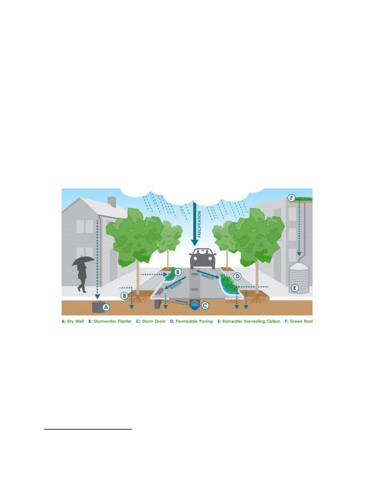
and ecosystem services while accounting for the least carbon footprint (Figure 1).
Figure 1: GI type (source: …………)
GI planning requires a thorough analysis of the surface features and impervious condition
inventory helps to identify best management practices for determining stormwater utility fees,
and emergency management planning. Innovative advances in ortho imagery and LiDAR have
recently enabled the production of more precise impervious-surface maps of areas ranging from
large cities to rural landscapes. These new technologies generate data that can be used for
multiple purposes while requiring fewer resources.
Although field measurements and manual digitization can be used to quantify impervious
surfaces, however, these processes can be time and resource demanding. As such, a robust
methodology, based on data availability, was adapted that leverages machine learning for
1
https://www.epa.gov/green-infrastructure/what-green-infrastructure
3
This material is based upon work supported by the Department of Energy and the Michigan Energy Office (MEO) under Award Number EE00007478
as part of the Catalyst Communities program. Find this document and more about the CLC Fellowship that supported this project at
graham.umich.edu/clcf.

impervious surface identification and extraction from orthoimaginary. This document is the
workflow of the process undertaken. It is intended for knowledgeable users familiar with
technical aspects of land use modeling in an ArcGIS Pro environment.
This guidance is prepared as a revision to the impervious surface mapping
2
by Esri’s Learn
ArcGIS team. This guidance will serve as an accompanying document to the GI feasibility and
inventory mapping. To facilitate its use, this guidance is divided into sections that contain
description of each stage on the flowchart. In addition, pre-processing (before the execution of
classification) and post-processing (after the execution: map composition) stages guidance is
also added to this guidance.
The prerequisite computational system to initiate the process includes-
● Windows 10, 64 bits or higher
● Central processing units (CPUs) multicore processor (atleast i5-i7 series or 10
th
generation)
● RAM capacity higher 16 GB
● Enough physical space available
In addition, having a solid-state drive (SSD) and dedicated graphics processing unit (GPU) will
expedite the computation significantly. Although the process can run directly on the CPU, it will
take longer to run, and the workflow can be overwhelming to the CPU.
Classification and Segmentation
Land Use/Land Cover (LULC) data are an important input for ecological, hydrological, and
agricultural models. Most LULC classifications are either created using pixel-based analysis of
remotely sensed imagery which are often supervised or unsupervised. These pixel-based
procedures examine the spectral properties
3
of each pixel in interest without considering the
associated spatial or contextual information. Using pixel-based classification on high-resolution
imagery may produce a "salt and pepper" effect, which contributes to inaccuracy (Gao and Mas,
2008). In contrast, segmentation, an object-based approach, produces a spectrally homogenous
object where every pixel in an image is given a label of a corresponding class. The object-based
image analysis aggregates pixels based on a segmentation algorithm such as the mean shift
function which groups neighboring pixels that are similar in color, shape, and spectral
characteristics together (Blaschke, 2010). The comparison between the two processes can be
explained as,
● Pixel-based classification: Classification is performed on a pixel-by-pixel basis, using
only the spectral information available for that specific pixel (i.e., values of pixels within
the locality are ignored).
● Object-based segmentation: Classification is done on a localized group of pixels,
considering the spatial properties of land-based features as they relate to each other.
In supervised image classification, the user trains computer algorithms to extract features from
an imaginary. These training samples are drawn as polygons, rectangles, or points, and the
computer learns and scans the rest of the image to identify similar features. However, the
3
Spectral resolution describes the ability of a sensor to define fine wavelength intervals.
2
https://learn.arcgis.com/en/projects/calculate-impervious-surfaces-from-spectral-imagery/
4
This material is based upon work supported by the Department of Energy and the Michigan Energy Office (MEO) under Award Number EE00007478
as part of the Catalyst Communities program. Find this document and more about the CLC Fellowship that supported this project at
graham.umich.edu/clcf.
decision to select classification relies upon the spatial resolution, computational capacity, and
desired output. Although the object-based approach is expected to perform better, however, the
process requires higher computational capacity and is not immune to over-segmentation and
under-segmentation errors (Lui, 2010).
Here, we apply a hybrid approach that augments the segmentation with supervised
classification.
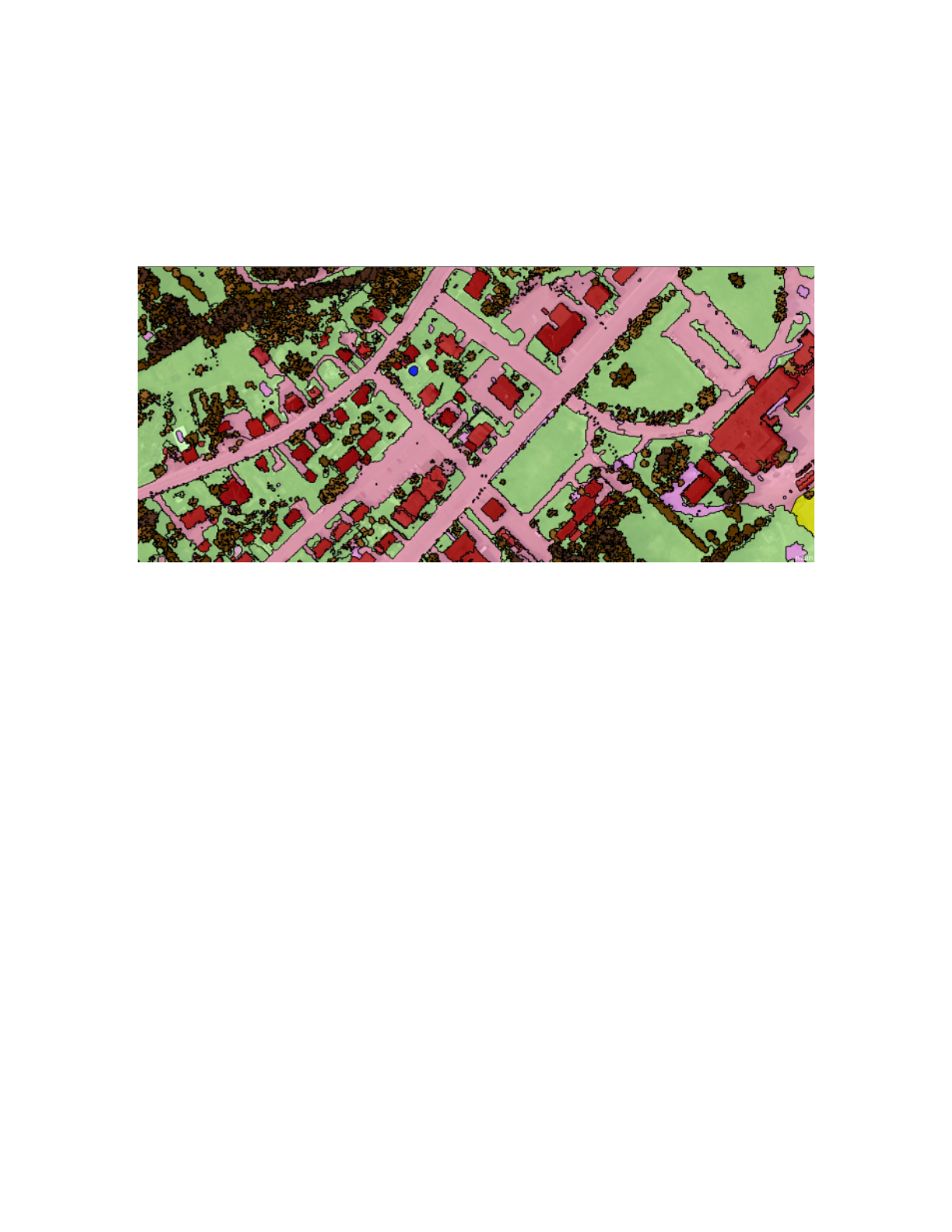
Figure 2: Object-based classification
(https://gisgeography.com/obia-object-based-image-analysis-geobia/)
Data Compilation
The dataset used was captured in East Lansing, spanning across Ingham and Clinton counties
in Michigan. Numerous datasets were used for the analysis, and they are enlisted as follows.
● 2020 Ortho Imagery: A 3-inch (leaf-off) true color multispectral imagery consisting of
four bands was used for imperviousness analysis. In total, 94 raster files, each of
dimension 1000*1000, were used for the city of East Lansing, Michigan. This dataset
was obtained from the DPW East Lansing.
● Parcel layer: A city-wide feature class of land parcel vector dataset was obtained from
DPW East Lansing.
● Ancillary datasets: These include city boundary, road, and building footprint vector data
that were compiled from various sources including Open Street Maps.
5
This material is based upon work supported by the Department of Energy and the Michigan Energy Office (MEO) under Award Number EE00007478
as part of the Catalyst Communities program. Find this document and more about the CLC Fellowship that supported this project at
graham.umich.edu/clcf.
Method
Land use classification can be accomplished using one or more of the following methods, or in
combination: supervised classification is performed by an interpreter; unsupervised
classification (the entire classification process is performed with computation); and object-based
visual interpretation (interpreter sets all objects manually). To determine the impervious surface
features from the imagery, a supervised object-based segmentation approach was applied.
Instead of classifying each pixel, generalized segments will not only reduce the number of
spectral signatures but also addresses the errors and inaccuracies. A snippet of the overall
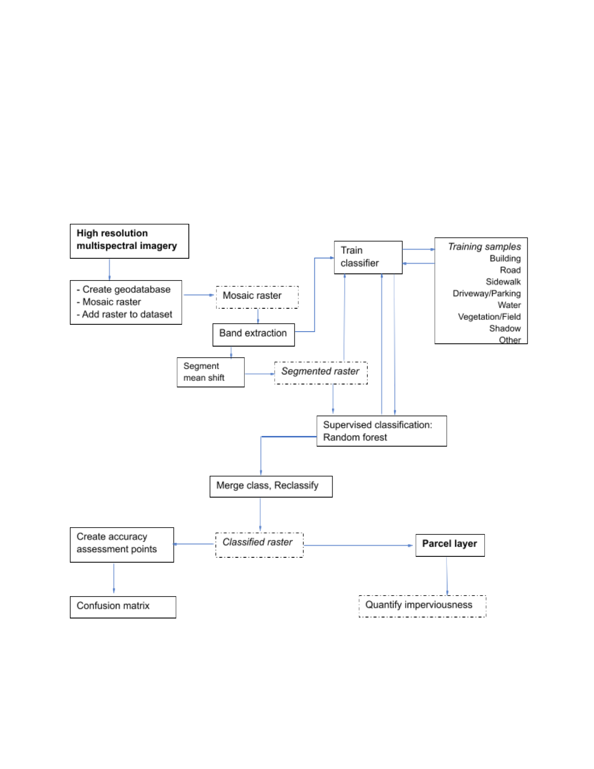
procedure is presented in figure 3.
Figure 3: Detailed methodology flowchart for impervious surface mapping
6
This material is based upon work supported by the Department of Energy and the Michigan Energy Office (MEO) under Award Number EE00007478
as part of the Catalyst Communities program. Find this document and more about the CLC Fellowship that supported this project at
graham.umich.edu/clcf.
Pre-processing
1. Image pre-process
All satellite image data are biased (due to error or distortion), including geometric and
radiometric distortions. This is because the data recorded by the sensor is greatly influenced by
atmospheric conditions, the angle of data capture from the sensor, and the time of data
collection. During the image pre-processing stage, this distortion must be addressed before it
can be used as the basis for interpretation and classification. The raw ortho-image obtained for
the exercise was already corrected and projected to NAD1983 as the datum.
2. Develop mosaic
Before proceeding with the image classification, a mosaic dataset
4
is developed which is a type
of geodatabase structure to manage imagery and raster data effectively. This process not only
addresses the challenge of working with multiple images individually but also helps in
developing a dataset that can be easily accessible for both visualization and analysis.
- After creating a File Geodatabase, from the Geoprocessing panel, type “create mosaic
dataset” and select the first option. Alternatively, from the Catalog pane, right-click on the
geodatabase file with the extension (.gdb), then point to New, and choose Mosaic
Dataset.
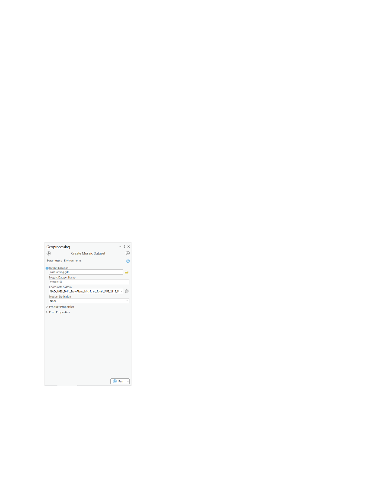
- In the Create Mosaic Dataset window, give the name and location for the dataset, and
define its coordinate system. The coordinate system should be consistent with those on
multispectral imagery. Product Definition field is left blank.
Figure 4: Parameters for creating a mosaic dataset
4
A mosaic dataset is a well-defined geodatabase structure optimized for working with large collections of
imagery and raster.
7
This material is based upon work supported by the Department of Energy and the Michigan Energy Office (MEO) under Award Number EE00007478
as part of the Catalyst Communities program. Find this document and more about the CLC Fellowship that supported this project at
graham.umich.edu/clcf.
The tool executes and creates a new mosaic dataset in the project geodatabase and adds a
mosaic dataset group layer to the contents pane of the map. Next, the multispectral imagery is
associated with the mosaic dataset.
- In the geoprocessing panel, type “Add Rasters to Mosaic Dataset”, hit enter, and select
the first option. Alternatively, From the Catalog pane, in the file geodatabase, right-click
on the mosaic_EL dataset and choose Add Rasters.
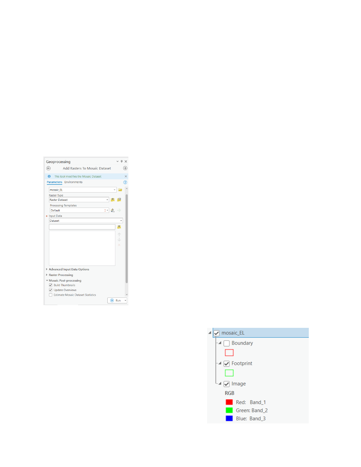
- In the Add Rasters to Mosaic Dataset window, the default Raster Dataset raster type is
selected from the dropdown option.
- Click the Input Data drop-down menu and choose Folder.
● Click the Browse button. Browse to and choose the folder containing imagery.
● Under Raster Processing, select Build Raster Pyramids.
● Under Mosaic Post-Processing, select Build Thumbnails, Update Overviews and click
Run.
Figure 5: Parameters for adding raster to the mosaic dataset
This process will add references to the images on the
disk to the attribute table of the mosaic dataset. Once
the tool is finished, it creates three sublayers in the
contents panel, namely Boundary, Footprint, and
Image.
If all images added to the mosaic dataset are not displaying,
from Catalog, right-click on the mosaic dataset and click
Properties. In the Mosaic Dataset Properties pane, click
8
This material is based upon work supported by the Department of Energy and the Michigan Energy Office (MEO) under Award Number EE00007478
as part of the Catalyst Communities program. Find this document and more about the CLC Fellowship that supported this project at
graham.umich.edu/clcf.
the Defaults tab. Expand Image Properties and change the Maximum Number of Rasters Per Mosaic
to 100.
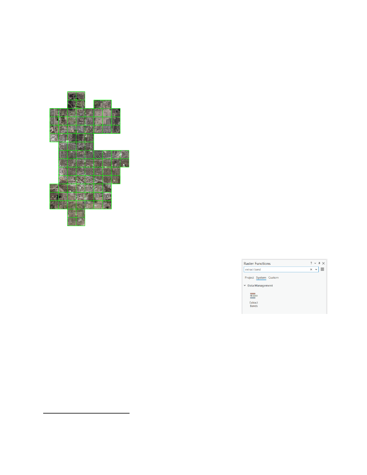
If all run well, the final layout should appear in Figure 6.
Figure 6: Final mosaic with multispectral imaginary (in natural color)
3. Band extraction
Impervious surfaces comprise human-made structures including
buildings, roads, parking lots, and pathways. Pervious surfaces
include vegetation (trees, grass), water bodies, sand, and bare
soil. To distinguish between natural and urban features, band
combination change is applied.
- Select the mosaic dataset and from the ribbon, click the
Imagery tab and in the Analysis group, click Raster
Functions.
- In the Raster functions, type “extract bands” and hit enter.
- In the Raster functions window, in the Parameters tab, set the Method to Band IDs, for
Combination, delete the existing text and type 4 1 3 (with spaces)
5
and click Create
New Layer.
5
This band combination includes Near Infrared (Band 4) for emphasizes vegetation, Red (Band 1) for
human-made objects and vegetation, and Blue (Band 3) that emphasizes water bodies.
9
This material is based upon work supported by the Department of Energy and the Michigan Energy Office (MEO) under Award Number EE00007478
as part of the Catalyst Communities program. Find this document and more about the CLC Fellowship that supported this project at
graham.umich.edu/clcf.
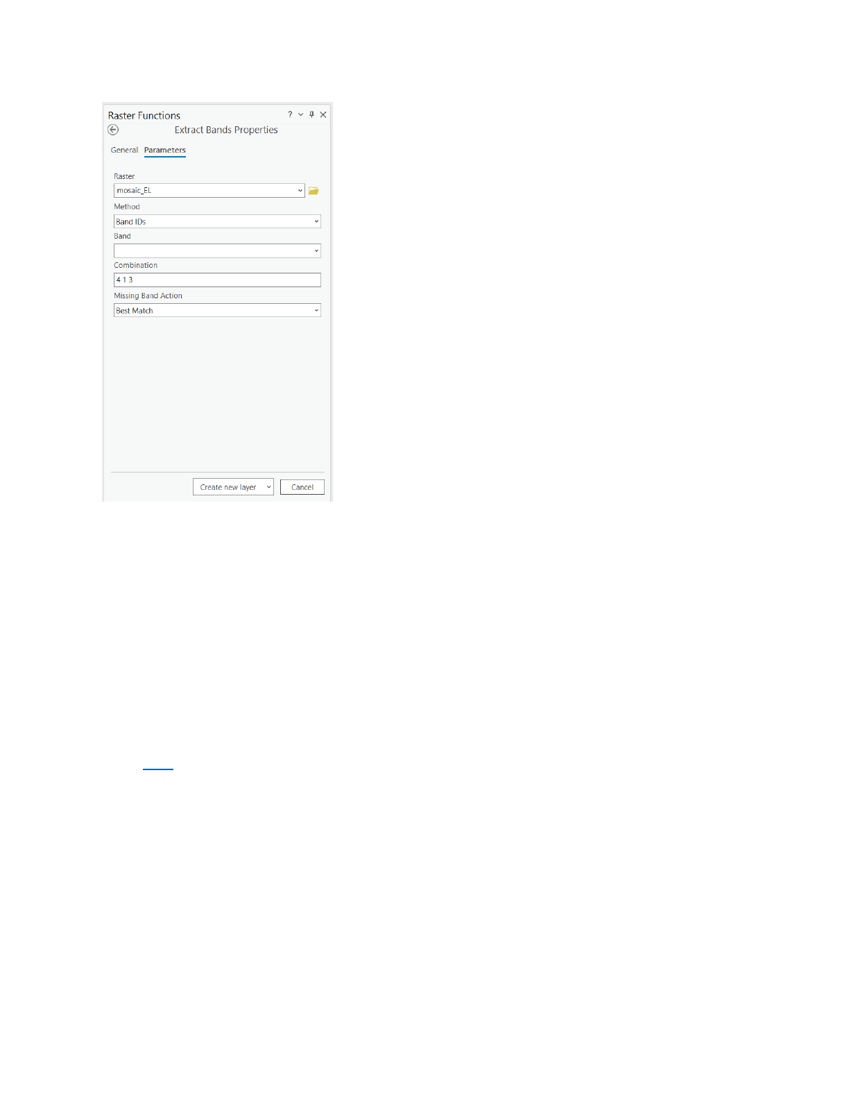
Figure 7: Setting parameters for band extraction
After the process executes, a new layer, named Extracted Bands_mosaic_EL is added to the
map. Although a layer appears in the Contents pane, however, it is not added as data and will
be lost if the layer is removed, or if ArcGIS Pro session terminates for any reason. The whole
classification process runs on the extracted layer.
Processing
1. Segmentation
The object-based classification workflow relies heavily on segmentation. Segmentation is the
outcome of three parameters namely spectral detail, spatial detail, and minimum segment size
which determines how an image is segmented, efficiently. The detail of these parameters can be
found here. Because impervious surface features can include spatial objects of varying sizes
and shapes, spectral information is more important than spatial information.
It is a resource-intensive process of the entire workflow. The image segmentation is based on
the Mean Shift approach.
10
This material is based upon work supported by the Department of Energy and the Michigan Energy Office (MEO) under Award Number EE00007478
as part of the Catalyst Communities program. Find this document and more about the CLC Fellowship that supported this project at
graham.umich.edu/clcf.
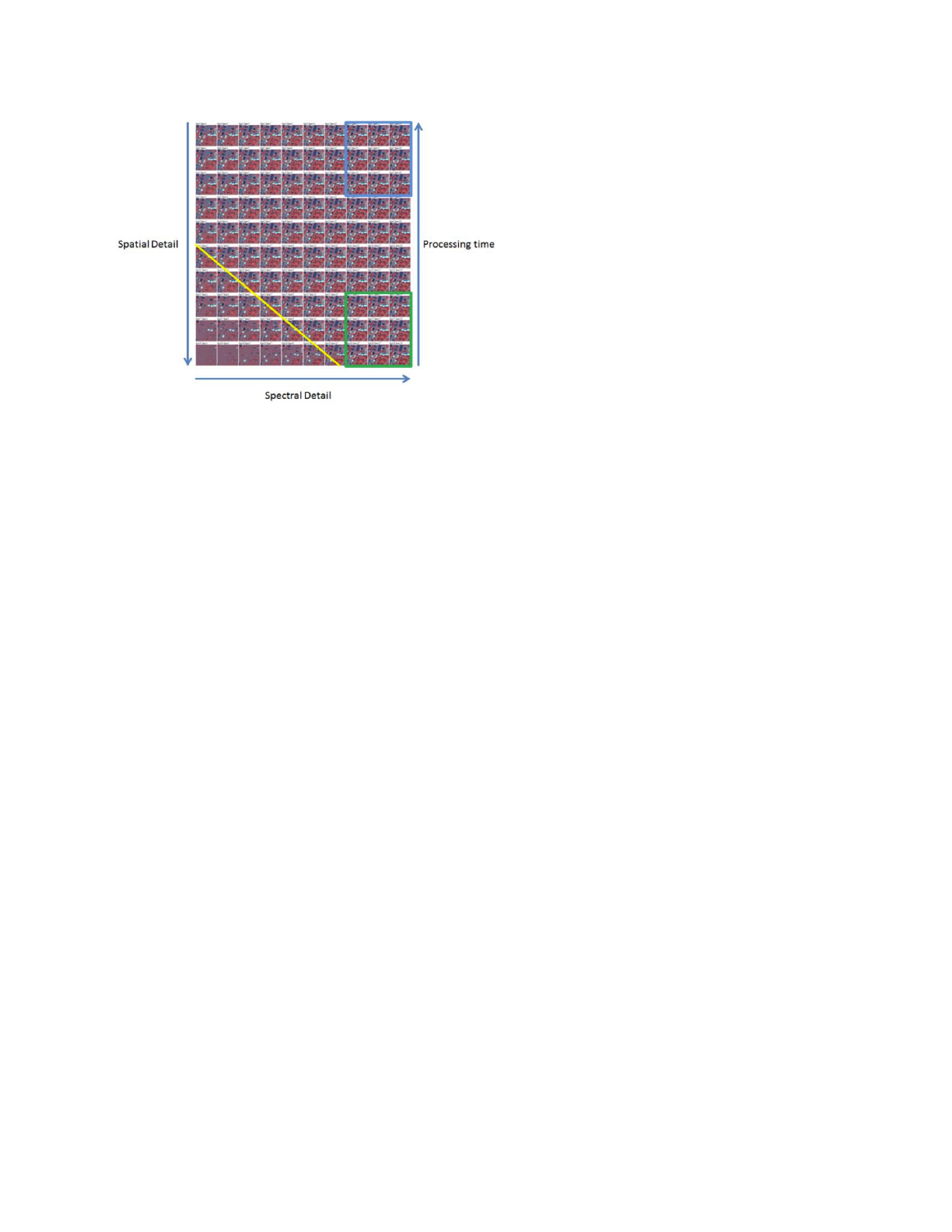
Figure 8: Interrelation between segmentation parameters (Butler, ESRI, 2005)
- In the ribbon, on the Imagery tab, in the Image Classification group, Classification
Tools, click Segmentation.
- In the Segmentation panel, default values are modified as, Spectral detail: 18, Spatial
detail: 12, and Minimum segment size pixel: 3.
- Leave Show Segment Boundaries Only unchecked and click Preview.
- A new layer segmented_181203 is added to the content panel.
- Inspect the segmented image. This image is being generated on the fly, so the
processing will vary depending on the map extent.
If you are dissatisfied with the segmentation result, you can always return to the previous page of the
wizard, change the parameters, and re-run the preview until a satisfactory result is achieved. A good rule
for naming the preview image is using segmented values.
11
This material is based upon work supported by the Department of Energy and the Michigan Energy Office (MEO) under Award Number EE00007478
as part of the Catalyst Communities program. Find this document and more about the CLC Fellowship that supported this project at
graham.umich.edu/clcf.
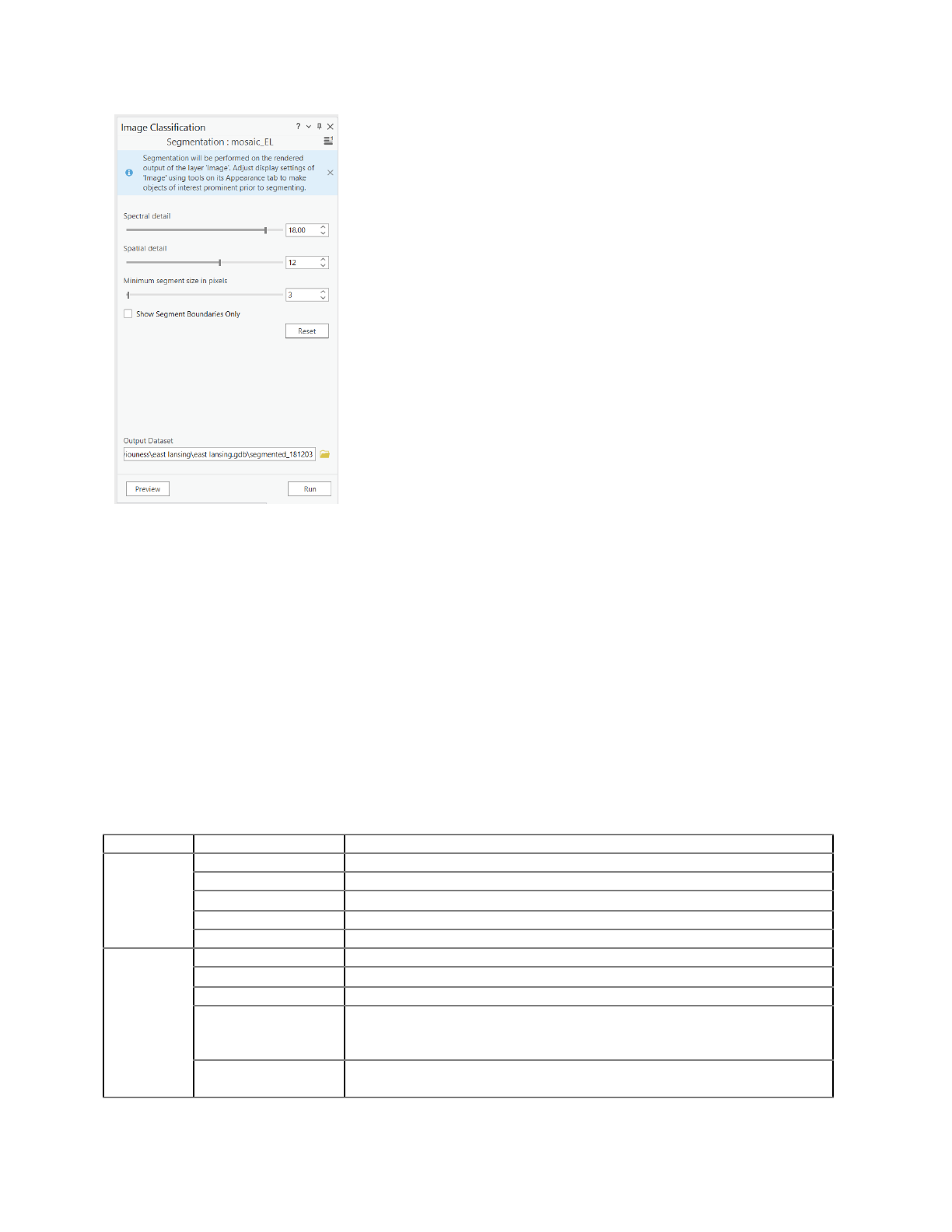
Figure 9: Parameters for segmentation
2. Training samples
This is the most important step in classification, as the quality of training samples serves the
machine learning algorithm with the necessary information to carry out the classification.
Training samples are polygons that represent distinct sample areas of the imagery's various
land-cover types. The training sample guides the classification tool about the various spectral
properties each land cover exhibits.
- In the ribbon, on the Imagery tab, in the Image Classification group, click the Training
Samples Manager. By default, the training sample manager is populated with NLCD
2011 and therefore this needs to be modified to contain two parent classes: Impervious
and Pervious. Following, subclasses are added to each class that represents types of
land cover. The list of classes is presented in table 2.
Table 2. Land cover classes used for analysis
Value
Class Name
Description
20
21
22
23
24
Impervious
Building
Houses, apartments, or any elevated concrete structure
Road
Highways, feeder roads, or concrete linear structure
Driveway/Parking
Parking structures
Sidewalk
Walking or running trails with concrete paving
30
31
32
33
34
Pervious
Vegetation/Field
Trees, grassland, cropland, and fields
Water
All water bodies including rivers, canals, and lakes
Shadow
Shadows do not represent actual surfaces. However, shadows are
usually cast by tall objects such as houses or trees and are more
likely to cover grass or bare earth, which are previous surfaces.
Other
Includes bare earth, barren surface, and any landcover class that is
not impervious but cannot be classified as water, or vegetation
12
This material is based upon work supported by the Department of Energy and the Michigan Energy Office (MEO) under Award Number EE00007478
as part of the Catalyst Communities program. Find this document and more about the CLC Fellowship that supported this project at
graham.umich.edu/clcf.
- All classes are deleted by right-clicking and selecting Remove class.
- After all, classes are removed, right-click on NLCD2011, and select Add New Class
- In the Add New Class window, for Name: “Impervious”, Value: 20, and Color: Gray 20%,
and Click OK.
- Select Impervious, right-click, select Add New Class, and add a class named Building
with a value of 21 and a color of Mango.
- The above steps are repeated until all the desired classes are created, each with unique
value and color.
- Right-click on the NLDC2011, click Edit Properties, and change the name to
“Impervious_Pervious”. Click Save the current classification schema at the top of the
Training Samples Manager panel.
Figure 10: Land use class defined for classification
Now training samples are generated on the segmented image using the aforementioned land
use classes or segment Picker can be used to choose segments directly.
- Select Building, click the Polygon button, and zoom in on an area in the image that has
building clusters.
- Next, collect training data for all the classes. This can be done by selecting a class from
the list, with the Segment Picker active, and clicking on an area in the display to create
a new sample polygon segment or draw a polygon that only comprises a particular land
use class, double click to finish drawing. This adds a row to the wizard for a new training
sample. Repeat this process for numerous buildings in the image.
- In the wizard, select all the building polygons by pressing Shift (on the keyboard), and
above the list of training samples, click the Collapse button
13
This material is based upon work supported by the Department of Energy and the Michigan Energy Office (MEO) under Award Number EE00007478
as part of the Catalyst Communities program. Find this document and more about the CLC Fellowship that supported this project at
graham.umich.edu/clcf.

- The above steps are repeated for each land
use class.
- After all training samples have been
developed, save the training data as a
feature class in the same geodatabase.
When creating training samples, depending on the
spatial resolution of the image, it is rational to create
a high number of samples to represent each
land-use type. In addition, the original image
displayed in natural color or infrared can be used for
drawing polygons.
- Zoom into the image and choose an area that represents a class from the list.
- Pan and zoom around to collect as many samples as possible for each class. In the
classification phase, having a few training samples in each part of the image will yield
good results. Use the keyboard shortcuts available to help you navigate and select
classes. The C shortcut key switches your cursor to the Pan tool.
Important consideration
i. Avoid mixing different classes while drawing polygons.
ii. Capture the full range of spectral signatures for each class.
iii. Collect training data across the entire image, not just focused on a limited
spatial extent.
iv. As a rule of thumb, collect 100 or more for each class.
3. Train classifier and run classification
There are several machine learning classifiers
6
to choose from depending on the classification
type intended to use. Random Trees
7
, a non-parametric classifier, is one of the most accurate
learning algorithms available in the discipline, with a reduced need for normal distribution and a
constant training sample size, and runs efficiently on large databases. Additionally, lighter
computation requirements, insensitivity to overfitting, and adaptability with segmented images
are some of its attractive characteristics. Henceforth, the segmented images and classification
schema developed in the preceding step will be used.
- In the ribbon, on the Imagery tab, in the Image Classification group, click the
Classification Wizard.
- In the Configure window, Classification Method is selected as Supervised from the
drop-down, classification type as Object-based, classification schema is previously
developed “Impervious_Pervious”, output location is the file geodatabase.
7
https://pro.arcgis.com/en/pro-app/latest/tool-reference/spatial-analyst/train-random-trees-classifier.htm
6
https://pro.arcgis.com/en/pro-app/2.8/tool-reference/image-analyst/understanding-segmentation-and-clas
sification.htm
14
This material is based upon work supported by the Department of Energy and the Michigan Energy Office (MEO) under Award Number EE00007478
as part of the Catalyst Communities program. Find this document and more about the CLC Fellowship that supported this project at
graham.umich.edu/clcf.

- Optionally, Segmented Image is selected as segmented_181203, Reference Dataset is
selected as DEM.
- After obtaining all the parameters values, click Next
Figure 11: Parameters for Configure window in classification
- Escape the training sample manager. Click Next.
- Next train classifier, In the Image Classification Wizard pane, in the Train page of the
wizard, select Classifier as Random tree. Under the Segment Attributes, choose Mean
digital number and Standard Deviation, and use the remaining default parameter values
and then click Run.
- Once the training has been completed, the classification preview will be displayed.
- If the classification looks relatively accurate, click Next to save the classification.
Alternations in the training samples can be made by clicking the Previous button, if unsatisfied.
This takes you back to Training Samples Manager where editing of samples can be done.
Generally, collect training samples of misclassified features and assign them to the appropriate
class.
- Once satisfied, click Next and then Run on the Training Samples Manager page to
reclassify using the updated training sample file and again Next to classification preview.
- Click Run on the Classify page to create classification outputs.
- After the process executes, a thematic classified raster is added to the content panel.
Before moving to the Merge Classes page, export the classified raster for later.
15
This material is based upon work supported by the Department of Energy and the Michigan Energy Office (MEO) under Award Number EE00007478
as part of the Catalyst Communities program. Find this document and more about the CLC Fellowship that supported this project at
graham.umich.edu/clcf.
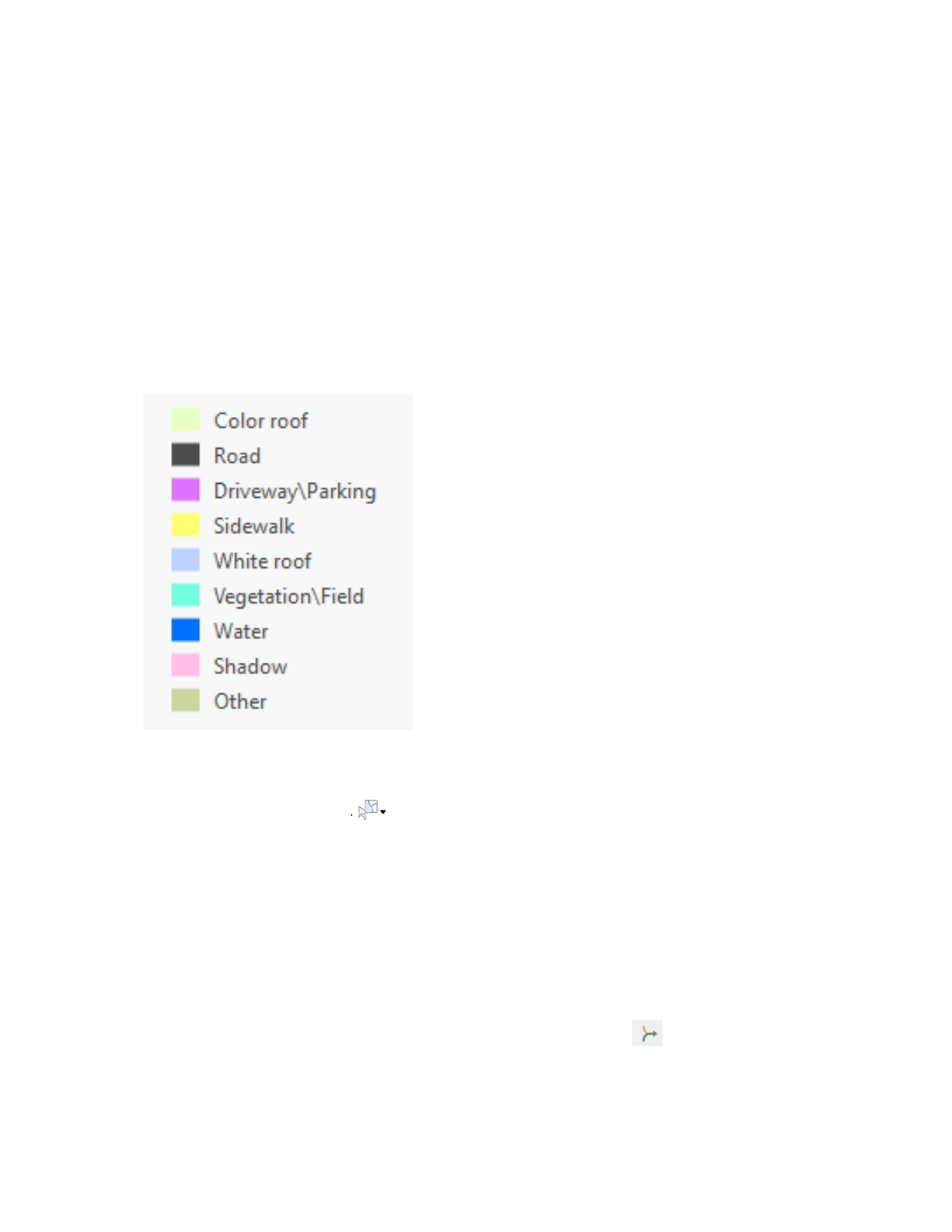
- On the Merge Class page, you can choose to merge your subclasses into their parent
class or keep it as it is. Since we only want impervious and pervious surface features, we
can use the dropdown arrows to choose Impervious and Pervious as the new
classes. When all is done Click Next to generate the updated Impervious Surface map.
- The final page is Reclassify, here you manually edit classes that are visually incorrect
using Reclassify within a region tool to delineate a region where all the class polygons
of one class type are reassigned to another class, or Reclassify an object tool to select
a single class polygon and reassign it to another class.
- Once you have reclassified any incorrect pixels, click Run to generate and Finish to
save the final classification output.
Figure 12: Output obtained from classification wizard
Post-processing
1. Assess classification
To determine the quality of the classified image, an accuracy assessment needs to be
conducted using the statistical procedure. To perform the assessment, first randomly generated
accuracy assessment points are placed throughout the image and a comparison is made with
the classification value (pervious or impervious) to the actual land cover from the original
imagery. Second, a matrix is calculated to determine percent accuracy.
- In the Geoprocessing pane, type “Create accuracy assessment points”, and press Enter.
- In the results list, click Create Accuracy Assessment Points (for Image Analyst or
Spatial Analyst Tools).
- In the Create Accuracy Assessment Points tool, fill the parameters as in figure 14.
16
This material is based upon work supported by the Department of Energy and the Michigan Energy Office (MEO) under Award Number EE00007478
as part of the Catalyst Communities program. Find this document and more about the CLC Fellowship that supported this project at
graham.umich.edu/clcf.
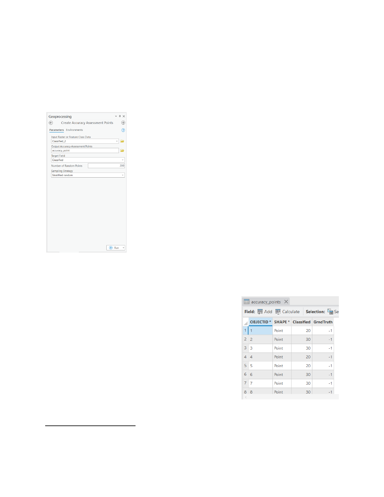
- Select input raster as Classified raster layer Output Accuracy Assessment Points, click
browse button, and browse to Project, Databases, and double-click mosaic_EL.gdb.
- Give it a name, “accuracy point” and save.
- In Target Field, confirm that Classified is selected.
- For Number of Random Points, type 200, and sampling strategy as Equalized stratified
random
8
.
- Click Run.
Figure 13: Accuracy assessment parameters
This will add a new layer with 200 accuracy points to the map.
- In the Contents pane, right-click the accuracy_point layer and choose Attribute Table.
The attribute table contains information for each point location
including ObjectID, Shape fields, Classified, and GrndTruth (or
Ground Truth). The Classified field has values that are either
20 or 40. These numbers represent the classes determined by
the classification process, as they appear in the Classified
raster layer where 20 is impervious and 30 is pervious.
In the GrndTruth field, every value is -1 by default, signaling
that the value is still unknown, and the point needs to be
ground truther. Manual inspection of the imagery for each
point is done and the GrndTruth attributes are edited to either
20 or 30, depending on the type of land cover found.
8
Sampling Strategy parameter determines how points are randomly distributed across the image. It can
be distributed proportionally to the area of each class (Stratified random), equally between each class
(Equalized stratified random), or randomly (Random).
17
This material is based upon work supported by the Department of Energy and the Michigan Energy Office (MEO) under Award Number EE00007478
as part of the Catalyst Communities program. Find this document and more about the CLC Fellowship that supported this project at
graham.umich.edu/clcf.
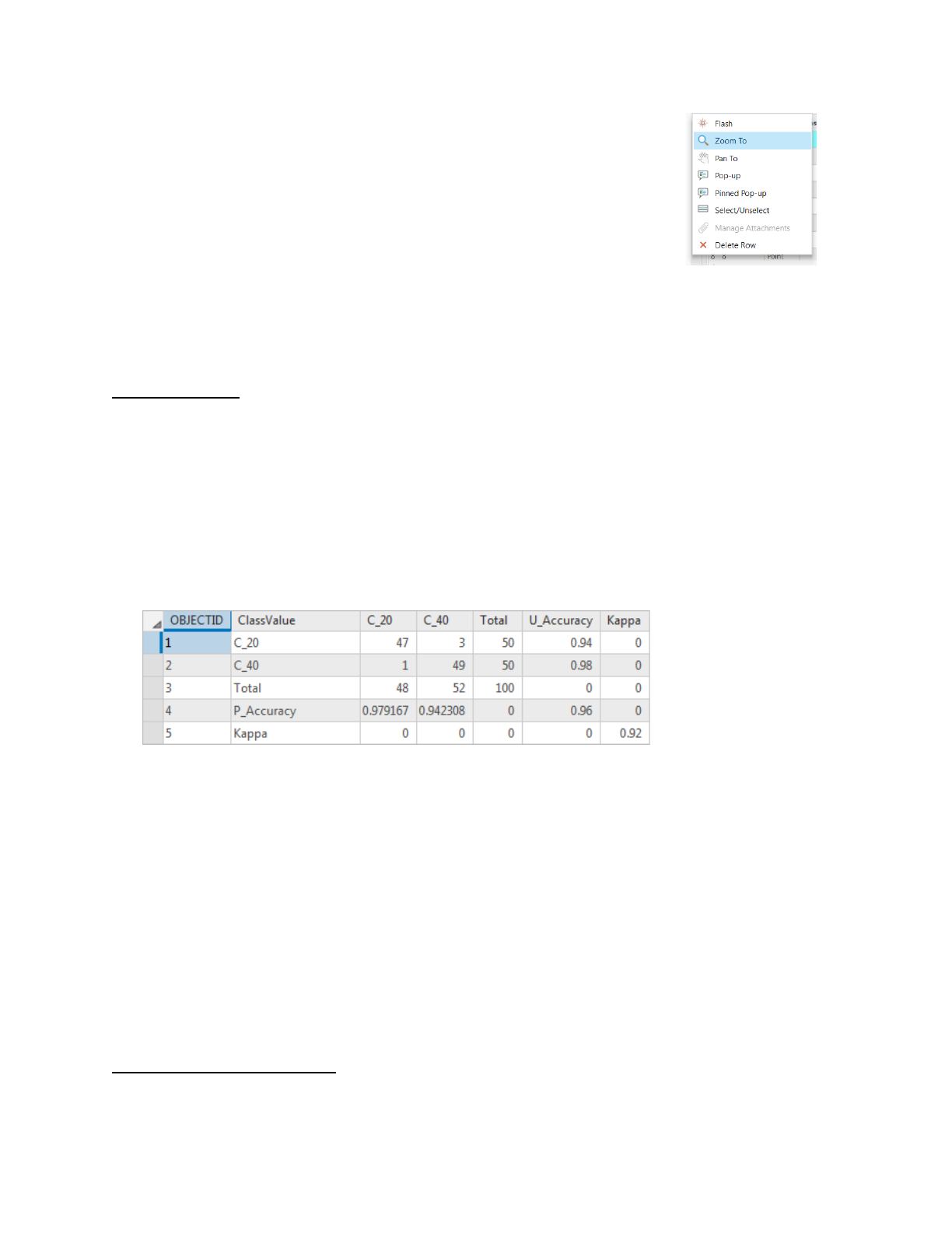
- In the attribute table, click row header 1 to select the feature and
right-click the row header, and choose Zoom To.
- The map zooms to the selected point., zoom in close enough to
the point, depending on the extent of your map and the location of
the point.
- Back in the attribute table, in the GrndTruth column, double-click
the value for the selected feature to edit it. Replace the default
value with either 20 or 30, depending on your observation, and
press Enter.
- Repeat the above procedure for all points.
- On the ribbon, click the Edit tab, in the Manage Edits group, click Save to save all the
edits you made in the attribute table. When prompted to confirm, click Yes.
Confusion matrix
- In the Geoprocessing pane, search for and open the Compute Confusion Matrix tool
(for either Image Analyst Tools or Spatial Analyst Tools).
- In the Compute Confusion Matrix tool, for Input Accuracy Assessment Points, choose
accuracy_point, for Output Confusion Matrix type “Confusion_Matrix” and click Save.
- Click Run.
- A confusion table is created in the Contents pane, under Standalone Tables. Right-click
Confusion_Matrix and choose Open.
An illustration of the confusion matrix is shown in figure 16.
Figure 14: Confusion matrix (ESRI)
The values in the ClassValue column serve as row headers in the table. U_Accuracy is for
user's accuracy and represents the fraction of pixels classified correctly per total classifications.
P_Accuracy is the producer's accuracy and represents the fraction of pixels classified correctly
per total ground truths. Kappa
9
is an overall assessment of the classification's accuracy.
Generally, if the Kappa value were below 70 percent, the classification would probably not be
accurate enough and would need to be revisited to be improved.
Two aspects of the workflow may contribute to classification error and lower Kappa value. First
is an error in segmentation where features may be misclassified if the segmentation parameters
generalize the original image too much or too little. Second, the training samples may have
caused the majority of errors by having too few training samples or training samples that cover a
9
Follow the article to learn on Kappa coefficient.
https://towardsdatascience.com/cohens-kappa-9786ceceab58
18
This material is based upon work supported by the Department of Energy and the Michigan Energy Office (MEO) under Award Number EE00007478
as part of the Catalyst Communities program. Find this document and more about the CLC Fellowship that supported this project at
graham.umich.edu/clcf.
wide range of spectral signatures. Increasing the number of samples or classes may improve
accuracy.
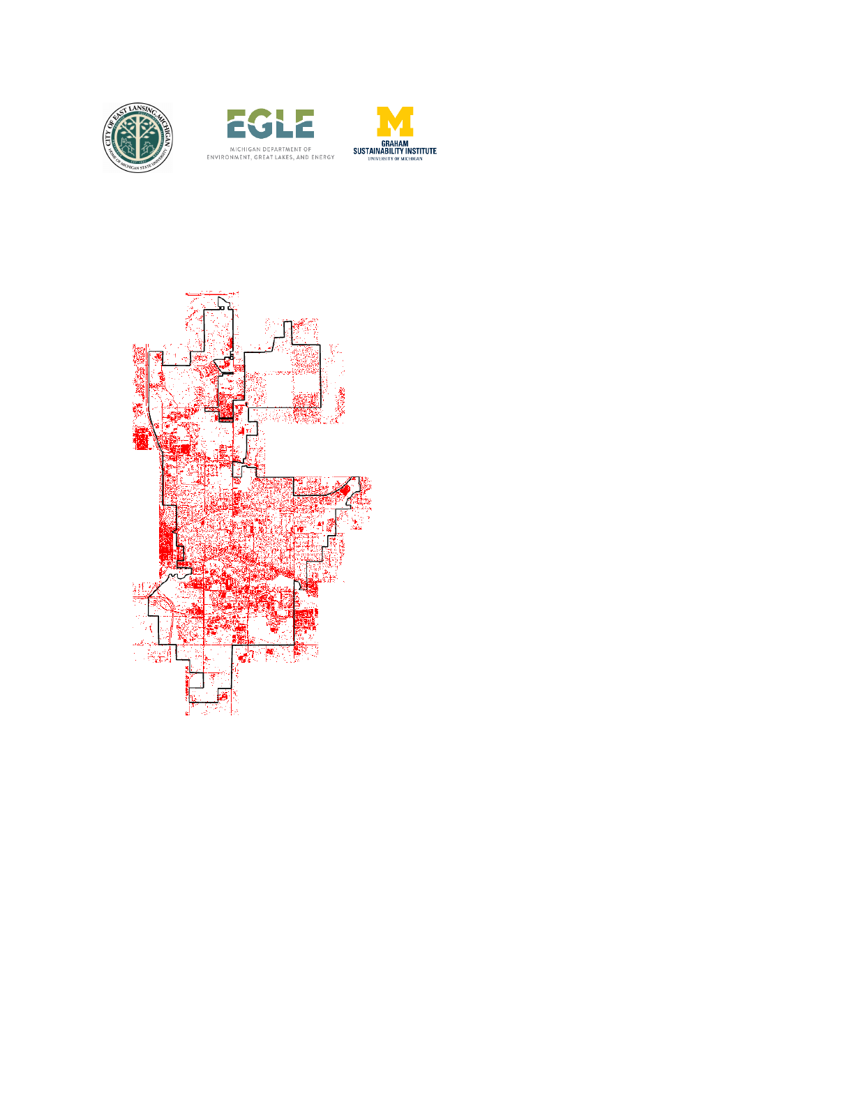
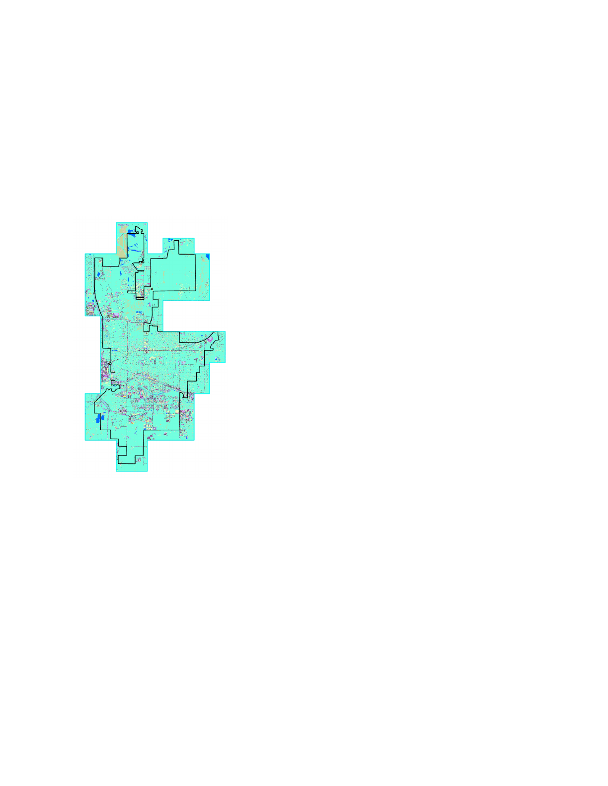
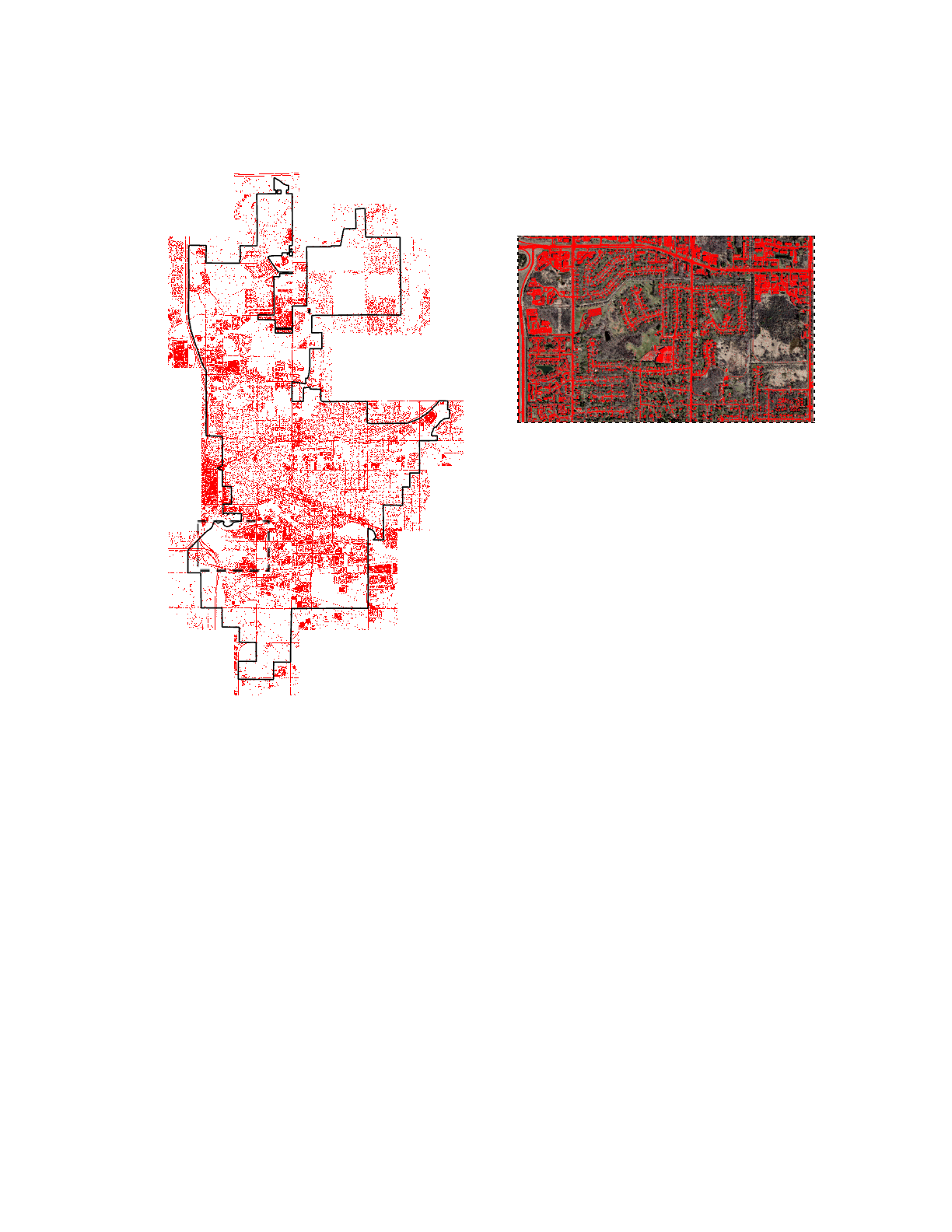
Figure 13: Finalized image showing impervious objects
Conclusion
Land cover classification can be difficult, and it is not always easy to map or separate land cover
categories with high accuracy. However, there are ways to potentially improve the result by
incorporating more data into the analysis, improving training samples, or possibly redefining the
classes of interest. The incorporation of machine learning capabilities into geospatial
technologies makes mapping the impervious surface area in an urban landscape cost-effective,
consistent, and repeatable. Furthermore, one can always investigate other ML algorithms and
platforms (Python, R, QGIS).
The imperviousness layer is the first of its kind for East Lasing, Michigan. Further improvisation
can be made as per the requirement. The layer is based on a solid methodology, up-to-date
data, and improved technology, making it an important policy and planning tool. This data can
be used in conjugation with the hydrological model for flood estimation and forecasting,
19
This material is based upon work supported by the Department of Energy and the Michigan Energy Office (MEO) under Award Number EE00007478
as part of the Catalyst Communities program. Find this document and more about the CLC Fellowship that supported this project at
graham.umich.edu/clcf.

demonstrating the effectiveness of green infrastructure in stormwater management, and urban
landscape research.
Limitations
Despite its capacity for automating impervious surfaces, the process has some limitations that
users need to be cognizant of beforehand. Many factors can affect classification accuracy
including image quality, the reliability of training data and reference/field data, and the accuracy
of the assessment method.
● Although object-based classification, in theories, is expected to perform better, however,
the bottleneck is it drains computer memory and processing time may take hours if not
days.
● While creating training samples, care must be given to collect enough samples for the
class of interest and to make it representative as well as fairly spaces.
● Because no single classifier has yet been demonstrated to satisfactorily classify all of the
land cover classes, there is no best classifier for both performance and accuracy.
Individual evaluations, along with the pros and cons of each method could, however,
provide insight into the applications of the methods compatible with the intent.
20
This material is based upon work supported by the Department of Energy and the Michigan Energy Office (MEO) under Award Number EE00007478
as part of the Catalyst Communities program. Find this document and more about the CLC Fellowship that supported this project at
graham.umich.edu/clcf.

Reference
Gao, Y., & Mas, J. F. (2008). A comparison of the performance of pixel-based and object-based
classifications over images with various spatial resolutions. Online journal of earth
sciences, 2(1), 27-35.
Liu, D., & Xia, F. (2010). Assessing object-based classification: advantages and
limitations. Remote sensing letters, 1(4), 187-194.
Blaschke, T. (2010). Object based image analysis for remote sensing. ISPRS journal of
photogrammetry and remote sensing, 65(1), 2-16.
21
This material is based upon work supported by the Department of Energy and the Michigan Energy Office (MEO) under Award Number EE00007478
as part of the Catalyst Communities program. Find this document and more about the CLC Fellowship that supported this project at
graham.umich.edu/clcf.
