
Outline and terminologies
First-order optimality: Unconstrained problems
First-order optimality: Constrained problems
Second-order optimality conditions
Algorithms
1 First-order optimality: Unconstrained problems
2 First-order optimality: Constrained problems
Constraint qualifications
KKT conditions
Stationarity
Lagrange multipliers
Complementarity
3 Second-order optimality conditions
Critical cone
Unconstrained problems
Constrained problems
4 Algorithms
Penalty methods
SQP
Interior-point methods
Kevin Carlberg Lecture 3: Constrained Optimization
Outline and terminologies
First-order optimality: Unconstrained problems
First-order optimality: Constrained problems
Second-order optimality conditions
Algorithms
Constrained optimization
This lecture considers constrained optimization
minimize
x∈R
n
f (x)
subject to c
i
(x) = 0, i = 1, . . . , n
e
d
j
(x) ≥ 0, j = 1, . . . , n
i
(1)
Equality constraint functions: c
i
: R
n
→ R
Inequality constraint functions: d
j
: R
n
→ R
Feasible set:
Ω = {x | c
i
(x) = 0, d
j
(x) ≥ 0, i = 1, . . . , n
e
, j = 1, . . . , n
i
}
We continue to assume all functions are twice-continuously
differentiable
Kevin Carlberg Lecture 3: Constrained Optimization
Outline and terminologies
First-order optimality: Unconstrained problems
First-order optimality: Constrained problems
Second-order optimality conditions
Algorithms
What is a solution?
x
f(x)
Global minimum: A point x
∗
∈ Ω satisfying f (x
∗
) ≤ f (x)
∀x ∈ Ω
Strong local minimum: A neighborhood N of x
∗
∈ Ω exists
such that f (x
∗
) < f (x) ∀x ∈ N ∩ Ω.
Weak local minima A neighborhood N of x
∗
∈ Ω exists such
that f (x
∗
) ≤ f (x) ∀x ∈ N ∩ Ω.
Kevin Carlberg Lecture 3: Constrained Optimization
Outline and terminologies
First-order optimality: Unconstrained problems
First-order optimality: Constrained problems
Second-order optimality conditions
Algorithms
Convexity
As with the unconstrained case, conditions hold where any local
minimum is the global minimum:
f (x) convex
c
i
(x) affine (c
i
(x) = A
i
x + b
i
) for i = 1, . . . , n
e
d
j
(x) convex for j = 1, . . . , n
i
Kevin Carlberg Lecture 3: Constrained Optimization
Outline and terminologies
First-order optimality: Unconstrained problems
First-order optimality: Constrained problems
Second-order optimality conditions
Algorithms
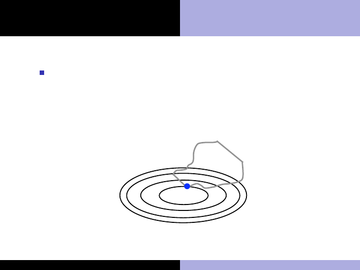
Active set
The active set at a feasible point x ∈ Ω consists of the
equality constraints and the inequality constraints for which
d
j
(x) = 0
A(x) = {c
i
}
n
i
i=1
∪ {d
j
| d
j
(x) = 0}
x
f(x)
d
2
d
3
d
1
Ω
d
4
x
Figure: A(x) = {d
1
, d
3
}
Kevin Carlberg Lecture 3: Constrained Optimization
Outline and terminologies
First-order optimality: Unconstrained problems
First-order optimality: Constrained problems
Second-order optimality conditions
Algorithms
Formulation of first-order conditions
Words
to first-order, the function cannot decrease by moving in feasible
directions
↓
Geometric description
description using the geometry of the feasible set
↓
Algebraic description
description using the equations of the active constraints
The algebraic description is required to actually solve
problems (use equations!)
Kevin Carlberg Lecture 3: Constrained Optimization
Outline and terminologies
First-order optimality: Unconstrained problems
First-order optimality: Constrained problems
Second-order optimality conditions
Algorithms
First-order conditions for unconstrained problems
Geometric description: a weak local minimum is a point x
∗
with a neighborhood N such that f (x
∗
) ≤ f (x) ∀x ∈ N
Algebraic description:
f (x
∗
) ≤ f (x
∗
+ p), ∀p ∈ R
n
“small” (2)
For f (x
∗
) twice-continuously differentiable, Taylor’s theorem is
f (x
∗
+p) = f (x
∗
)+∇f (x
∗
)
T
p+
1
2
p
T
∇
2
f (x
∗
+tp)p, t ∈ (0, 1)
Ignoring the O(kpk
2
) term, (2) becomes
0 ≤ f (x
∗
+ p) − f (x
∗
) ≈ ∇f (x
∗
)
T
p, ∀p ∈ R
n
Since p
T
1
∇f (x
∗
) > 0 implies that p
T
2
∇f (x
∗
) < 0 with
p
2
= −p
1
, we know that strict equality must hold
→ This reduces to the first-order necessary condition:
∇f (x
∗
)
T
p = 0 ∀p ∈ R
n
⇒ ∇f (x
∗
) = 0 (stationary point)
Kevin Carlberg Lecture 3: Constrained Optimization
Outline and terminologies
First-order optimality: Unconstrained problems
First-order optimality: Constrained problems
Second-order optimality conditions
Algorithms
Constraint qualifications
KKT conditions
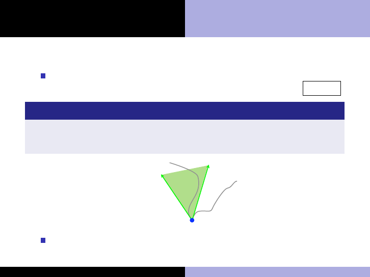
First-order conditions for constrained problems
Geometric description: A weak local minimum is a point x
∗
with a neighborhood N such that f (x
∗
) ≤ f (x) ∀x ∈ N ∩ Ω
Definition (Tangent cone T
Ω
(x
∗
))
The set of all tangents to Ω at x
∗
.
(set of geometrically feasible directions, the limit of N ∩ Ω − x
∗
)
T
Ω
(x
∗
)
x
∗
Ω
Using the tangent cone, we can begin to formulate the
first-order conditions algebraically
Kevin Carlberg Lecture 3: Constrained Optimization
Outline and terminologies
First-order optimality: Unconstrained problems
First-order optimality: Constrained problems
Second-order optimality conditions
Algorithms
Constraint qualifications
KKT conditions
First-order conditions for constrained problems
Geometric description (continued)
The limit of f (x
∗
) ≤ f (x), ∀x ∈ N ∩ Ω is
f (x
∗
) ≤ f (x
∗
+ p), ∀p ∈ T
Ω
(x
∗
) “small”
Using Taylor’s theorem and ignoring high-order terms, this
condition is
0 ≤ f (x
∗
+ p) − f (x
∗
) ≈ ∇f (x
∗
)
T
p, ∀p ∈ T
Ω
(x
∗
)
∇f (x
∗
)
T
p ≥ 0, ∀p ∈ T
Ω
(x
∗
) (3)
→ To first-order, the objective function cannot decrease in any
feasible direction
Kevin Carlberg Lecture 3: Constrained Optimization
Outline and terminologies
First-order optimality: Unconstrained problems
First-order optimality: Constrained problems
Second-order optimality conditions
Algorithms
Constraint qualifications
KKT conditions
Constraint qualifications
(3) is not purely algebraic since T
Ω
(x
∗
) is geometric
We require an algebraic description of the tangent cone in
terms of the constraint equations
Definition (Set of linearized feasible directions F(x))
Given a feasible point x and the active constraint set A(x),
F(x) =
(
p | p satisfies
(
∇c
i
(x)
T
p = 0 ∀i
∇d
j
(x)
T
p ≥ 0 ∀d
j
∈ A(x)
)
The set of linearized feasible directions is the best algebraic
description available, but in general T
Ω
(x) ⊂ F(x)
Constraint qualifications are sufficient for T
Ω
(x) = F(x)
Kevin Carlberg Lecture 3: Constrained Optimization
Outline and terminologies
First-order optimality: Unconstrained problems
First-order optimality: Constrained problems
Second-order optimality conditions
Algorithms
Constraint qualifications
KKT conditions
Example
Consider the following problem
minimize
x∈R
n
f (x) = x
subject to d
1
(x) = x − 3 ≥ 0
x
f(x)
x
∗
T
Ω
(x
∗
)
x
y
!x+3
!2 !1 0 1 2 3 4 5 6
!3
!2
!1
0
1
2
3
4
5
6
x
∗
x
1
x
2
∇d
1
(x
∗
)
∇f(x
∗
)
x
y
!x+3
!2 !1 0 1 2 3 4 5 6
!3
!2
!1
0
1
2
3
4
5
6
x
∗
x
1
x
2
x
∇f(x)
∇d
1
(x)
feasible descent
directions
Since d
0
1
(x
∗
) = 1, pd
0
1
(x
∗
) ≥ 0 for any p ≥ 0, and we have
F(x
∗
) = p, ∀p ≥ 0
Thus, F(x
∗
) = T
Ω
(x
∗
)
√
Kevin Carlberg Lecture 3: Constrained Optimization
Outline and terminologies
First-order optimality: Unconstrained problems
First-order optimality: Constrained problems
Second-order optimality conditions
Algorithms
Constraint qualifications
KKT conditions
Example
Consider the mathematically equivalent reformulation
minimize
x∈R
n
f (x) = x
subject to d
1
(x) = (x − 3)
3
≥ 0
The solution x
∗
= 3 and (geometric) tangent cone T
Ω
(x
∗
) are
unchanged
However, d
0
1
(x
∗
) = 3(3 − 3)
2
= 0 and pd
0
1
(x
∗
) ≥ 0 for any
p ∈ R (positive or negative), and we have
F(x
∗
) = p, ∀p ∈ R X
Thus, T
Ω
(x
∗
) ⊂ F(x
∗
), and directions in F(x
∗
) may actually
be infeasible!
Kevin Carlberg Lecture 3: Constrained Optimization
Outline and terminologies
First-order optimality: Unconstrained problems
First-order optimality: Constrained problems
Second-order optimality conditions
Algorithms
Constraint qualifications
KKT conditions
Constraint qualifications (sufficient for T
Ω
(x
∗
) = F(x
∗
))
Types
Linear independence constraint qualification (LICQ): the
set of active constraint gradients at the solution
{∇c
i
(x
∗
)}
n
i
i=1
∪ {∇d
j
(x
∗
) | d
j
(x
∗
) ∈ A(
∗
x)} is linearly
independent
Linear constraints: all active constraints are linear functions
None of these hold for the last example
We proceed by assuming these conditions hold
(F(x) = T
Ω
(x)) ⇒ the algebraic expression F(x) can be used
to describe geometrically feasible directions at x
Kevin Carlberg Lecture 3: Constrained Optimization
Outline and terminologies
First-order optimality: Unconstrained problems
First-order optimality: Constrained problems
Second-order optimality conditions
Algorithms
Constraint qualifications
KKT conditions
Algebraic description
When constraint qualifications are satisfied, F(x) = T
Ω
(x)
and (3) is
∇f (x
∗
)
T
p ≥ 0, ∀p ∈ F(x
∗
) (4)
What form ∇f (x
∗
) ensures that (4) holds?
Equality constraints: if we set ∇f (x
∗
) =
n
e
P
i=1
γ
i
∇c
i
(x
∗
), then
∇f (x
∗
)
T
p =
P
n
e
i=1
γ
i
∇c
i
(x
∗
)
T
p
= 0, ∀p ∈ F(x
∗
)
√
Inequality constraints: if we set ∇f (x
∗
) =
n
i
P
j=1
λ
j
∇d
j
(x
∗
)
with λ
j
≥ 0, then
∇f (x
∗
)
T
p =
P
n
i
j=1
λ
j
∇d
j
(x
∗
)
T
p
≥ 0, ∀p ∈ F(x
∗
)
√
Kevin Carlberg Lecture 3: Constrained Optimization

Outline and terminologies
First-order optimality: Unconstrained problems
First-order optimality: Constrained problems
Second-order optimality conditions
Algorithms
Constraint qualifications
KKT conditions
Theorem (First-order necessary KKT conditions for local solutions)
If x
∗
is a weak local solution of (1), constraint qualifications hold
∇f (x
∗
) −
n
e
X
i=1
γ
i
∇c
i
(x
∗
) −
n
i
X
j=1
λ
j
∇d
j
(x
∗
) = 0
λ
j
≥ 0, j = 1, . . . , n
i
c
i
(x
∗
) = 0, i = 1, . . . , n
e
d
j
(x
∗
) ≥ 0, j = 1, . . . , n
i
λ
j
d
j
(x
∗
) = 0, j = 1, . . . , n
i
Stationarity, Dual feasibility, Primal feasibility (x
∗
∈ Ω),
Complementarity conditions, Lagrange multipliers γ
i
, λ
j
Kevin Carlberg Lecture 3: Constrained Optimization
Outline and terminologies
First-order optimality: Unconstrained problems
First-order optimality: Constrained problems
Second-order optimality conditions
Algorithms
Constraint qualifications
KKT conditions
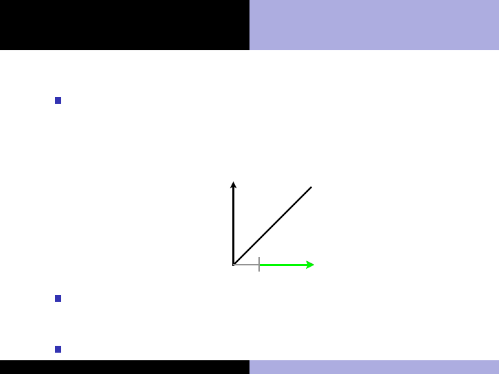
Intuition for stationarity
minimize
x∈R
n
f (x) = x
2
1
+ x
2
2
subject to d
1
(x) = x
1
+ x
2
− 3 ≥ 0
x
f(x)
x
∗
T
Ω
(x
∗
)
x
y
!x+3
!2 !1 0 1 2 3 4 5 6
!3
!2
!1
0
1
2
3
4
5
6
x
∗
x
1
x
2
∇d
1
(x
∗
)
∇f(x
∗
)
The solution is x
∗
= (1.5, 1.5)
Kevin Carlberg Lecture 3: Constrained Optimization
Outline and terminologies
First-order optimality: Unconstrained problems
First-order optimality: Constrained problems
Second-order optimality conditions
Algorithms
Constraint qualifications
KKT conditions
Intuition for stationarity (continued)
The KKT conditions say ∇f (x
∗
) = λ
1
∇d
1
(x
∗
) with λ
1
≥ 0
Here, ∇f (x
∗
) = [3, 3]
T
, while ∇d
1
(x
∗
) = [1.5, 1.5]
T
, so these
conditions are indeed verified with λ
1
= 2 ≥ 0
This is obvious from the figure: if ∇f (x
∗
) and ∇d
1
(x
∗
) were
“misaligned”, there would be some feasible descent directions!
x
f(x)
x
∗
T
Ω
(x
∗
)
x
y
!x+3
!2 !1 0 1 2 3 4 5 6
!3
!2
!1
0
1
2
3
4
5
6
x
∗
x
1
x
2
∇d
1
(x
∗
)
∇f(x
∗
)
x
y
!x+3
!2 !1 0 1 2 3 4 5 6
!3
!2
!1
0
1
2
3
4
5
6
x
∗
x
1
x
2
x
∇f(x)
∇d
1
(x)
feasible descent
directions
This gives us some intuition for stationarity and dual feasibility
Kevin Carlberg Lecture 3: Constrained Optimization

Outline and terminologies
First-order optimality: Unconstrained problems
First-order optimality: Constrained problems
Second-order optimality conditions
Algorithms
Constraint qualifications
KKT conditions
Lagrangian
Definition (Lagrangian)
The Lagrangian for (1) is
L(x, γ, λ) = f (x) −
n
e
P
i=1
γ
i
c
i
(x) −
n
i
P
j=1
λ
j
d
j
(x)
Stationarity in the sense of KKT is equivalent to stationarity
of the Lagrangian with respect to x:
L
x
(x, γ, λ) = ∇f (x) −
n
e
X
i=1
γ
i
∇c
i
(x) −
n
i
X
j=1
λ
j
∇d
j
(x)
KKT stationarity ⇔ L
x
(x
∗
, γ, λ) = 0
Kevin Carlberg Lecture 3: Constrained Optimization
Outline and terminologies
First-order optimality: Unconstrained problems
First-order optimality: Constrained problems
Second-order optimality conditions
Algorithms
Constraint qualifications
KKT conditions
Lagrange multipliers
Lagrange multipliers γ
i
and λ
j
arise in constrained
minimization problems
They tell us something about the sensitivity of f (x
∗
) to the
presence of their constraints. γ
i
and λ
j
indicate how hard f is
“pushing” or “pulling” the solution against c
i
and d
j
.
If we perturb the right-hand side of the i
th
equality constraint
so that c
i
(x) ≥ −k∇c
i
(x
∗
)k, then
df (x
∗
())
d
= −γ
i
k∇c
i
(x
∗
)k.
If the j
th
inequality is perturbed so d
j
(x) ≥ −k∇d
j
(x
∗
)k,
df (x
∗
())
d
= −λ
j
k∇d
i
(x
∗
)k.
Kevin Carlberg Lecture 3: Constrained Optimization

Outline and terminologies
First-order optimality: Unconstrained problems
First-order optimality: Constrained problems
Second-order optimality conditions
Algorithms
Constraint qualifications
KKT conditions
Constraint classification
Definition (Strongly active constraint)
A constraint is strongly active at if it belongs to A(x
∗
) and it has:
a strictly positive Lagrange multiplier for inequality constraints
(λ
j
> 0)
a strictly non-zero Lagrange multiplier for equality constraints
(γ
i
> 0)
Definition (Weakly active constraint)
A constraint is weakly active at if it belongs to A(x
∗
) and it has a
zero-valued Lagrange multiplier (γ
i
= 0 or λ
j
= 0)
Kevin Carlberg Lecture 3: Constrained Optimization
Outline and terminologies
First-order optimality: Unconstrained problems
First-order optimality: Constrained problems
Second-order optimality conditions
Algorithms
Constraint qualifications
KKT conditions
Constraint classification (continued)
Weakly active and inactive constraints “do not participate”
minimize
x∈R
n
f (x) = x
2
1
+ x
2
2
subject to d
1
(x) = x
1
+ x
2
− 3 ≥ 0 (strongly active)
d
2
(x) = x
1
− 1.5 ≥ 0 (weakly active)
d
3
(x) = −x
2
1
− 4x
2
2
+ 5 ≥ 0 (inactive)
x
1
x
2
!1 0 1 2 3 4 5
1
1.5
2
2.5
3
3.5
4
4.5
5
5.5
6
x
y
x = !1 sqrt(!1/4 x
2
+20/4), y = k
x
∗
The solution is unchanged if d
2
and d
3
are removed, so
λ
2
= λ
3
= 0
Kevin Carlberg Lecture 3: Constrained Optimization
Outline and terminologies
First-order optimality: Unconstrained problems
First-order optimality: Constrained problems
Second-order optimality conditions
Algorithms
Constraint qualifications
KKT conditions
Intuition for complementarity
We just saw that non-participating constraints have zero
Lagrange multipliers
The complementarity conditions are
λ
j
d
j
(x
∗
) = 0, j = 1, . . . , n
i
This means that each inequality constraint must be either:
1 Inactive (non-participating): d
j
(x
∗
) > 0, λ
j
= 0,
2 Strongly active (participating): d
j
(x
∗
) = 0 and λ
j
> 0, or
3 Weakly active (active but non-participating): d
j
(x
∗
) = 0 and
λ
j
= 0
Strict complementarity: either case 1 or 2 is true for all
constraints (no constraints are weakly active)
Kevin Carlberg Lecture 3: Constrained Optimization

Outline and terminologies
First-order optimality: Unconstrained problems
First-order optimality: Constrained problems
Second-order optimality conditions
Algorithms
Critical cone
Unconstrained problems
Constrained problems
Second-order optimality conditions
Second-order conditions for constrained optimization play a
“tiebreaking” role: determine whether “undecided” directions
for which p
T
∇f (x
∗
) = 0 will increase or decrease f .
We call these ambiguous directions the “critical cone”
Definition (Critical cone C(x
∗
, γ))
Directions that “adhere” to strongly active constraints and equality
constraints
C(x
∗
, γ) = {w ∈ F(x
∗
) | ∇d
j
(x
∗
)
T
w = 0, ∀ j ∈ A(x
∗
) with λ
j
> 0}
Note that λ
j
> 0 implies the constraint will remain active even
when small changes are made to the objective function!
Kevin Carlberg Lecture 3: Constrained Optimization

Outline and terminologies
First-order optimality: Unconstrained problems
First-order optimality: Constrained problems
Second-order optimality conditions
Algorithms
Critical cone
Unconstrained problems
Constrained problems
Critical cone
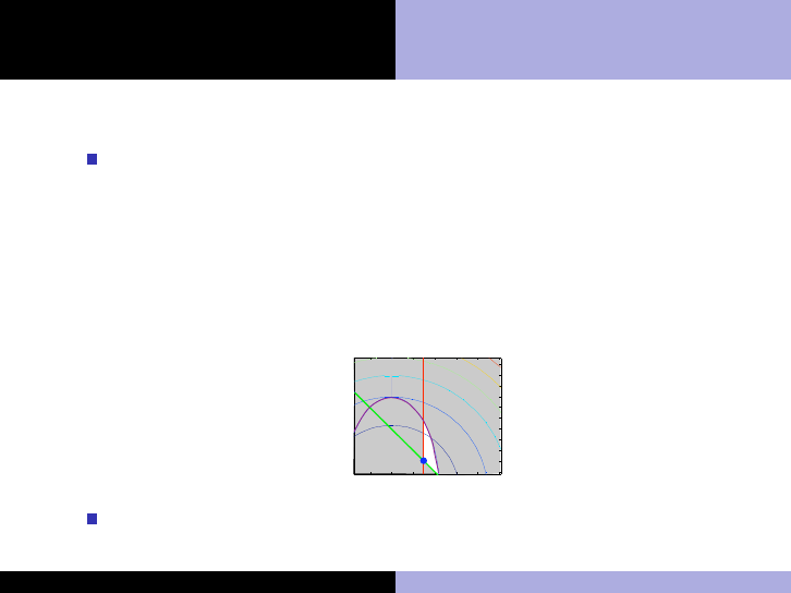
For the problem
minimize
x∈R
n
f (x) = x
2
1
+ x
2
2
subject to d
1
(x) = x
1
+ x
2
− 3 ≥ 0
the critical cone is C(x
∗
, γ) = α(−1, 1), ∀α ∈ R
x
y
!x+3
!2 !1 0 1 2 3 4 5 6
!3
!2
!1
0
1
2
3
4
5
6
x
∗
x
1
x
2
∇d
1
(x
∗
)
∇f(x
∗
)
C(x
∗
, λ)
Kevin Carlberg Lecture 3: Constrained Optimization

Outline and terminologies
First-order optimality: Unconstrained problems
First-order optimality: Constrained problems
Second-order optimality conditions
Algorithms
Critical cone
Unconstrained problems
Constrained problems
Second-order conditions for unconstrained problems
Recall, second-order conditions for unconstrained problems
Theorem (Necessary conditions for a weak local minimum)
A1. ∇f (x
∗
) = 0 (stationary point)
A2. ∇
2
f (x
∗
) is positive semi-definite (p
T
∇
2
f (x
∗
)p ≥ 0 for all
p 6= 0)
Theorem (Sufficient conditions for a strong local minimum)
B1. ∇f (x
∗
) = 0 (stationary point)
B2. ∇
2
f (x
∗
) > 0 is positive definite (p
T
∇
2
f (x
∗
)p > 0 for all
p 6= 0).
Kevin Carlberg Lecture 3: Constrained Optimization

Outline and terminologies
First-order optimality: Unconstrained problems
First-order optimality: Constrained problems
Second-order optimality conditions
Algorithms
Critical cone
Unconstrained problems
Constrained problems
Second-order conditions for constrained problems
We make an analogous statement for constrained problems,
but limit the directions p to the critical cone C(x
∗
, γ)
Theorem (Necessary conditions for a weak local minimum)
D1. KKT conditions hold
D2. p
T
∇
2
L(x
∗
, γ)p ≥ 0 for all p ∈ C(x
∗
, γ)
Theorem (Sufficient conditions for a strong local minimum)
E1. KKT conditions hold
E2. p
T
∇
2
L(x
∗
, γ)p > 0 for all p ∈ C(x
∗
, γ).
Kevin Carlberg Lecture 3: Constrained Optimization
Outline and terminologies
First-order optimality: Unconstrained problems
First-order optimality: Constrained problems
Second-order optimality conditions
Algorithms
Critical cone
Unconstrained problems
Constrained problems
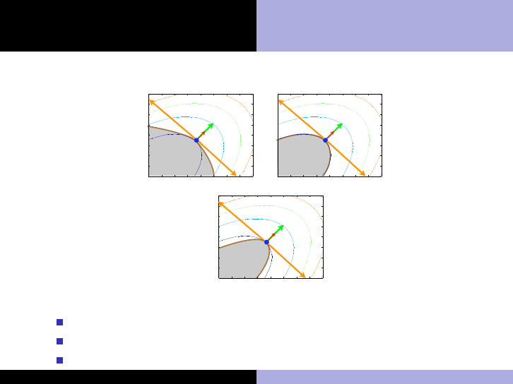
Intuition for second-order conditions
x
∗
x
1
x
2
∇d
1
(x
∗
)
∇f(x
∗
)
x
y
(x+y)
2
+3 (x!y)
2
0 1 2 3 4 5 6 7 8
0
1
2
3
4
5
6
7
8
x
∗
x
1
x
2
∇d
1
(x
∗
)
∇f(x
∗
)
x
y
(x+y)
2
+3 (x!y)
2
0 1 2 3 4 5 6 7 8
0
1
2
3
4
5
6
7
8
x
∗
x
1
x
2
∇d
1
(x
∗
)
∇f(x
∗
)
x
y
(x+y)
2
+3 (x!y)
2
0 1 2 3 4 5 6 7 8
0
1
2
3
4
5
6
7
8
C(x
∗
, λ)
C(x
∗
, λ)
C(x
∗
, λ)
d
1
(x)
d
1
(x)
d
1
(x)
Case I Case 2
Case 3
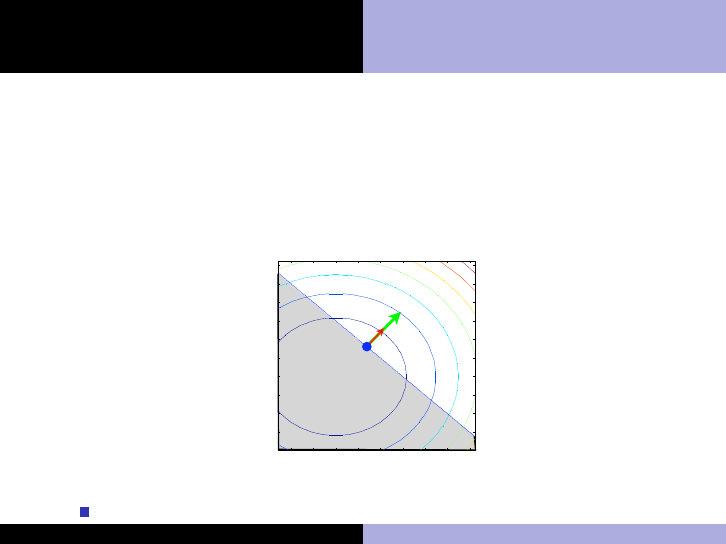
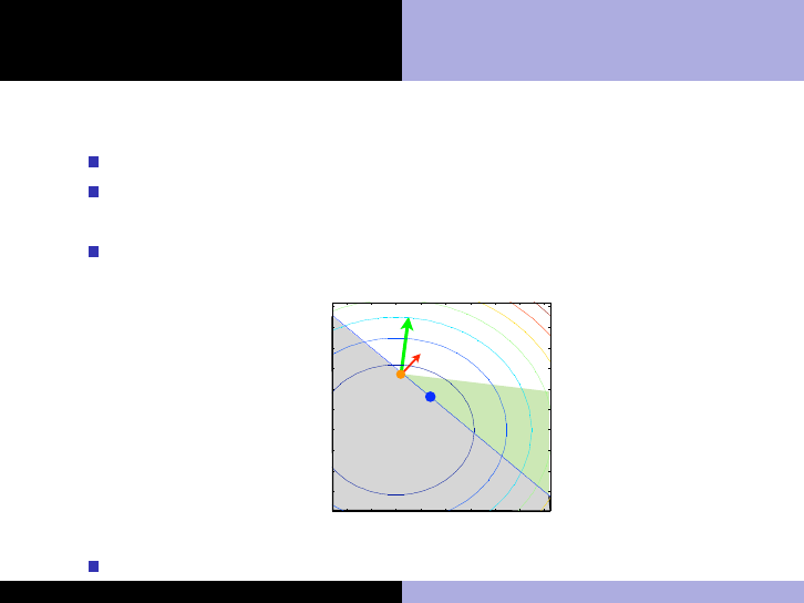
Case 1: E1 and E2 are satisfied (sufficient conditions hold)
Case 2: D1 and D2 are satisfied (necessary conditions hold)
Case 3: D1 holds, D2 does not (necessary conditions failed)
Kevin Carlberg Lecture 3: Constrained Optimization
Outline and terminologies
First-order optimality: Unconstrained problems
First-order optimality: Constrained problems
Second-order optimality conditions
Algorithms
Critical cone
Unconstrained problems
Constrained problems
Next
We now know how to correctly formulate constrained
optimization problems and how to verify whether a given
point x could be a solution (necessary conditions) or is
certainly a solution (sufficient conditions)
Next, we learn algorithms that are use to compute solutions
to these problems
Kevin Carlberg Lecture 3: Constrained Optimization
Outline and terminologies
First-order optimality: Unconstrained problems
First-order optimality: Constrained problems
Second-order optimality conditions
Algorithms
Penalty methods
SQP
Interior-point methods
Constrained optimization algorithms
Linear programming (LP)
Simplex method: created by Dantzig in 1947. Birth of the
modern era in optimization
Interior-point methods
Nonlinear programming (NLP)
Penalty methods
Sequential quadratic programming methods
Interior-point methods
Almost all these methods rely strongly on line-search and
trust region methodologies for unconstrained optimization
Kevin Carlberg Lecture 3: Constrained Optimization
Outline and terminologies
First-order optimality: Unconstrained problems
First-order optimality: Constrained problems
Second-order optimality conditions
Algorithms
Penalty methods
SQP
Interior-point methods
Penalty methods
Penalty methods combine the objective function and
constraints
minimize
x∈R
n
f (x) s.t. c
i
(x) = 0, i = 1, . . . , n
i
↓
minimize
x∈R
n
f (x) +
µ
2
n
i
X
i=1
c
2
i
(x)
A sequence of unconstrained problems is then solved for µ
increasing
Kevin Carlberg Lecture 3: Constrained Optimization

Outline and terminologies
First-order optimality: Unconstrained problems
First-order optimality: Constrained problems
Second-order optimality conditions
Algorithms
Penalty methods
SQP
Interior-point methods
Penalty methods example
Original problem:
minimize
x∈R
2
f (x) = x
2
1
+ 3x
2
, s.t. x
1
+ x
2
− 4 = 0
0
1
2
3
4
0
1
2
3
4
0
5
10
15
20
25
x
x
2
+3 y
y
f
(
x
)
Kevin Carlberg Lecture 3: Constrained Optimization
Outline and terminologies
First-order optimality: Unconstrained problems
First-order optimality: Constrained problems
Second-order optimality conditions
Algorithms
Penalty methods
SQP
Interior-point methods
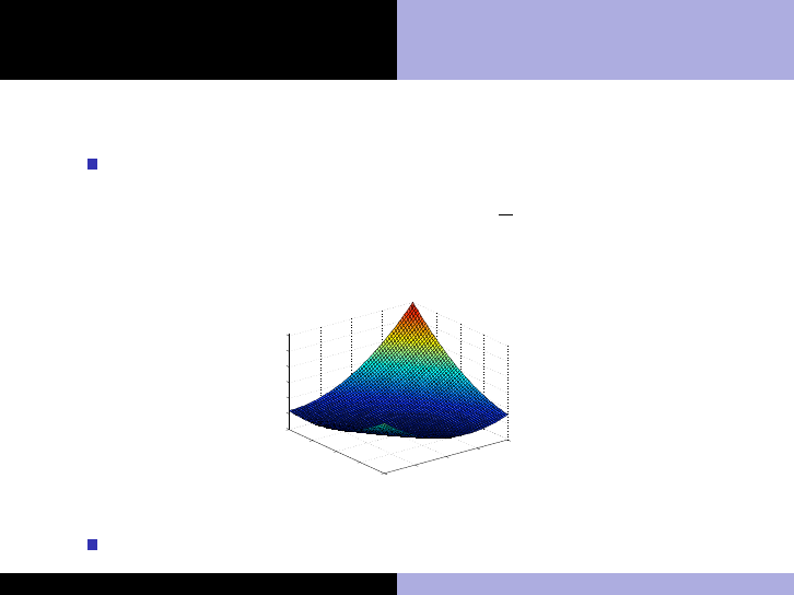
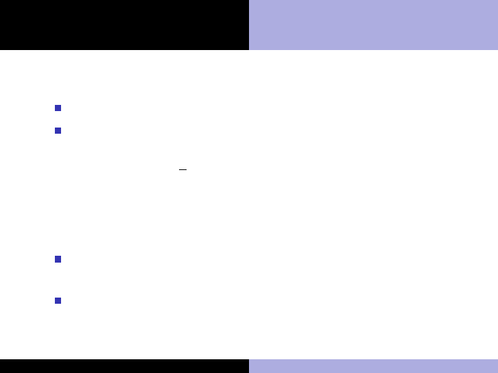
Penalty methods example
Penalty formulation:
minimize
x∈R
2
g(x) = x
2
1
+ 3x
2
+
µ
2
(x
1
+ x
2
− 4)
2
0
1
2
3
4
0
1
2
3
4
0
5
10
15
20
25
x
x
2
+3 y
y
f
(
x
)
0
1
2
3
4
0
1
2
3
4
0
10
20
30
40
50
60
x
x
2
+3 y+µ (x+y! 4)
2
y
g
(
x
)
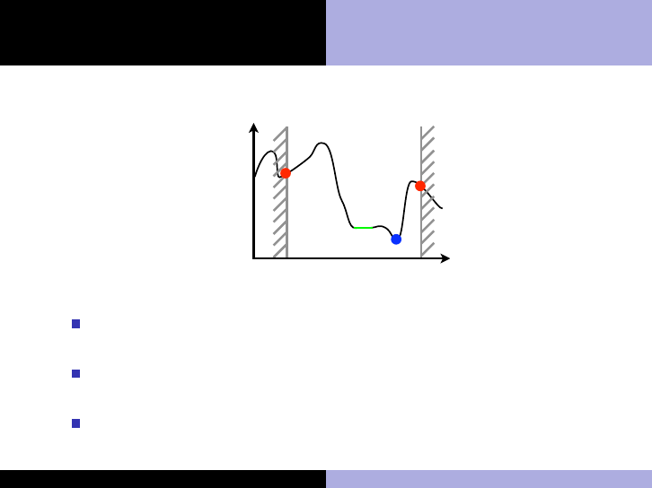
A valley is created along the constraint x
1
+ x
2
− 4 = 0
Kevin Carlberg Lecture 3: Constrained Optimization
Outline and terminologies
First-order optimality: Unconstrained problems
First-order optimality: Constrained problems
Second-order optimality conditions
Algorithms
Penalty methods
SQP
Interior-point methods
Sequential quadratic programming
Perhaps the most effective algorithm
Solve a QP subproblem at each iterate
minimize
p
1
2
p
T
∇
2
xx
L(x
k
, λ
k
)p + ∇f (x
k
)
T
p
subject to ∇c
i
(x
k
)Tp + c
i
(x
k
) = 0, i = 1, . . . , n
e
∇d
j
(x
k
)
T
p + d
j
(x
k
) ≥ 0, j = 1, . . . , n
i
When n
i
= 0, this is equivalent to Newton’s method on the
KKT conditions
When n
i
> 0, this corresponds to an “active set” method,
where we keep track of the set of active constraints A(x
k
) at
each iteration
Kevin Carlberg Lecture 3: Constrained Optimization
Outline and terminologies
First-order optimality: Unconstrained problems
First-order optimality: Constrained problems
Second-order optimality conditions
Algorithms
Penalty methods
SQP
Interior-point methods
Interior-point methods
These methods are also known as “barrier methods,” because
they build a barrier at the inequality constraint boundary
minimize
p
f (x) − µ
m
X
i=1
log s
i
subject to c
i
(x) = 0, i = 1, . . . , n
e
d
j
(x) − s
i
= 0, j = 1, . . . , n
i
Slack variables: s
i
, indicates distance from constraint
boundary
Solve a sequence of problems with µ decreasing
Kevin Carlberg Lecture 3: Constrained Optimization
Outline and terminologies
First-order optimality: Unconstrained problems
First-order optimality: Constrained problems
Second-order optimality conditions
Algorithms
Penalty methods
SQP
Interior-point methods
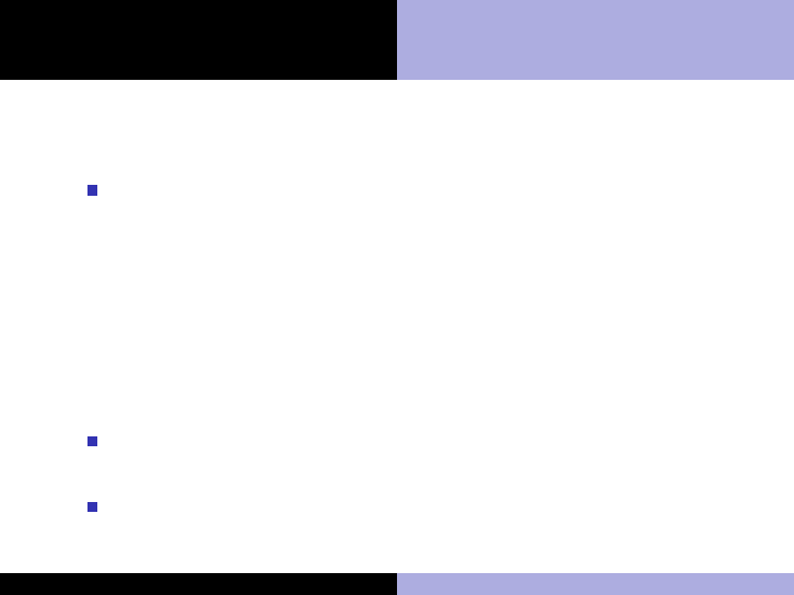
Interior-point methods example
Original problem:
minimize
x∈R
2
f (x) = x
2
1
+ 3x
2
, s.t. − x
1
− x
2
+ 4 ≥ 0
0
1
2
3
4
0
1
2
3
4
0
5
10
15
20
25
x
x
2
+3 y
y
f
(
x
)
Kevin Carlberg Lecture 3: Constrained Optimization
Outline and terminologies
First-order optimality: Unconstrained problems
First-order optimality: Constrained problems
Second-order optimality conditions
Algorithms
Penalty methods
SQP
Interior-point methods
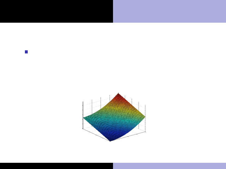
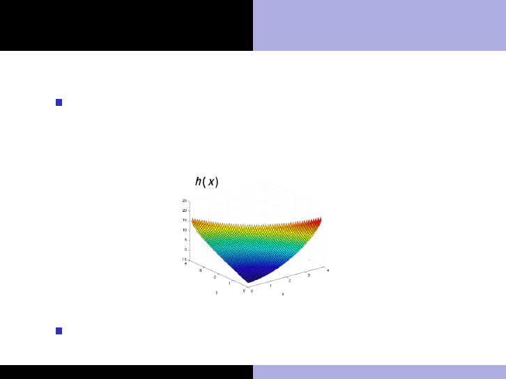
Interior-point methods example
Interior-point formulation:
minimize
x∈R
2
h(x) = x
2
1
+ 3x
2
− log (−x
1
− x
2
+ 4)
A barrier is created along the boundary of the inequality
constraint x
1
+ x
2
− 4 = 0
Kevin Carlberg Lecture 3: Constrained Optimization
Outline and terminologies
First-order optimality: Unconstrained problems
First-order optimality: Constrained problems
Second-order optimality conditions
Algorithms
Penalty methods
SQP
Interior-point methods
Summary
We now now something about:
Modeling and classifying unconstrained and constrained
optimization problems
Identifying local minima (necessary and sufficient conditions)
Solving the problem using numerical optimization algorithms
We next consider the case of PDE-constrained optimization,
which enables us to use to tools learned earlier (finite
elements) in optimal design and control settings, for example
Kevin Carlberg Lecture 3: Constrained Optimization
