Lectures on Symplectic Field Theory
Chris Wendl
Institut f
¨
ur Mathematik, Humboldt-Universit
¨
at zu Berlin, Unter
den Linden 6, 10099 Berlin, Germany
E-mail address: wendl@math.hu-berlin.de
Contents
Preface vii
About the current version ix
Lecture 1. Introduction 1
1.1. In the beginning, Gromov wrote a paper 1
1.2. Hamiltonian Floer homology 4
1.3. Contact manifolds and the Weinstein conjecture 9
1.4. Symplectic cobordisms and their completions 16
1.5. Contact homology and SFT 20
1.6. Two applications 23
Lecture 2. Basics on holomorphic curves 25
2.1. Linearized Cauchy-Riemann operators 25
2.2. Some useful So bolev inequalities 28
2.3. The fundamental elliptic estimate 30
2.4. Regularity 32
2.5. Linear local existence and applications 38
2.6. Simple curves and multiple covers 41
Lecture 3. Asymptotic operators 43
3.1. The linearization in Morse homology 43
3.2. Spectral flow 46
3.3. The Hessian of the contact action functional 57
3.4. The Conley-Zehnder index 61
Lecture 4. Fredholm theory with cylindrical ends 67
4.1. Cauchy-Riemann operators with punctures 67
4.2. A global weak regularity result 70
4.3. Elliptic estimates on cylindrical ends 71
4.4. The semi-Fredholm property 73
4.5. Formal adjoints and proof of the Fredholm property 74
Lecture 5. The index formula 81
5.1. Riemann-Roch with punctures 81
5.2. Some remarks o n the formal adjoint 86
5.3. The index zero case on a torus 90
5.4. A Weitzenb¨ock formula for Cauchy-Riemann operators 92
5.5. Large antilinear perturbations and energy concentration 94
iii
iv Chris Wendl
5.6. Two Cauchy-Riemann type problems on t he plane 96
5.7. A linear g luing argument 97
5.8. Antilinear deformations of asymptotic operators 102
Lecture 6. Symplectic cobordisms and moduli spaces 107
6.1. Stable Hamiltonian structures and their symplectizations 107
6.2. Symplectic cobordisms with stable boundary 113
6.3. Moduli spaces of unparametrized holomorphic curves 117
6.4. Simple curves and multiple covers 118
6.5. A local structure result 120
Lecture 7. Smoothness of the moduli space 121
7.1. Transversality theorems in cobordisms 121
7.2. Functional analytic setup 126
7.3. Teichm¨uller slices 131
7.4. Fredholm regula r ity and the implicit function theorem 132
7.5. A universal moduli space 134
7.6. Applying the Sard-Smale theorem 137
7.7. From C
ε
to C
∞
138
Lecture 8. Transversality in symplectizations 141
8.1. Statement of the theorem a nd discussion 141
8.2. Injective points of the pr ojected curve 144
8.3. Smoothness of the universal moduli space 147
Lecture 9. Asymptotics and compactness 151
9.1. Removal of singularities 152
9.2. Finite energy and asymptotics 155
9.3. Degenerations of holomo r phic curves 170
9.4. The SFT compactness theorem 182
Lecture 10. Cylindrical contact homology and the tight 3-t ori 191
10.1. Contact structures on T
3
and Giroux torsion 191
10.2. Definition of cylindrical contact homology 194
10.3. Computing HC
∗
(T
3
, ξ
k
) 208
Lecture 11. Coherent orientations 225
11.1. Gluing maps and coherence 225
11.2. Permutations of punctures and bad orbits 230
11.3. Orienting moduli spaces in general 232
11.4. The determinant line bundle 234
11.5. Determinant bundles of moduli spaces 237
11.6. An algorithm f or coherent orientations 238
11.7. Permutations and bad orbits revisited 240
Lecture 12. The generating function of SFT 243
12.1. Some important caveats on transversality 243
12.2. Auxiliary data, grading and supercommutativity 244
Lectures on Symplectic Field Theory v
12.3. The definition of H and commutators 247
12.4. Interlude: How to count points in an orbifold 251
12.5. Cylindrical contact homology revisited 256
12.6. Combinatorics of gluing 259
12.7. Some remarks on torsion, coefficients, and conventions 263
Lecture 13. Contact invariants 267
13.1. The Eliashberg-Givent al-Hofer package 268
13.2. SFT generating functions for cobordisms 278
13.3. Full SFT as a BV
∞
-algebra 288
Lecture 14. Transversality and embedding controls in dimension four 295
Lecture 15. Intersection theory for punctured holomorphic curves 297
Lecture 16. Torsion computations and applications 299
Appendix A. Sobo lev spaces 301
A.1. Approximation, extension and embedding theorems 301
A.2. Products, compositions, and r escaling 305
A.3. Spaces of sections of vector bundles 311
A.4. Some remarks on domains with cylindrical ends 316
Appendix B. The Floer C
ε
space 319
Appendix C. Genericity in the space of asymptotic operators 323
Bibliography 329

Preface
This book is a slight ly expanded version of the lecture notes I produced for a
two-semester course taught at University College London in 2015–16, for Ph.D. stu-
dents with a background in basic symplectic geometry and int erest in symplectic
topology and/or geometric analysis. I say “slightly expanded,” although the reader
will quickly notice that most individual chapters contain far more material than can
reasonably fit into a two-ho ur lecture. In reality, much of that material was only
sketched or mentioned in passing during lectures, and I ended up using the notes
to discuss everything that I would like to have explained if I’d had unlimited time.
This includes relatively detailed discussions of several importa nt technical po ints
(e.g. the definition of spectral flow, generic transversality in symplectizations, the
punctured Riemann-Roch formula, finite energy and asymptotics with arbitrary sta-
ble Hamiltonian structures) which a re either incompletely covered by the existing
literature or, in my opinion, simply more difficult to learn from o t her sources than
they should be. For topics that are on the other hand well covered elsewhere, I have
usually not felt obliged to explain every detail, but have tried always to provide
adequate references.
One of the interesting features of SFT is that its foundations ar e— at the time of
this writing—not yet complete. When the original “propaganda paper” [
EGH00]
appeared in 2000, it was widely believed that the technical details would be filled in
within a few years, and several papers introducing important applications of SFT
to contact topology were written under this assumption. Since then, a certain re-
alization has set in that the results in those papers cannot truly be regarded a s
“theorems” in the sense o f mathematics, and it has become less socially acceptable
to preface statements of results with caveats of the form, “t his theorem is dependent
on the foundations of SFT”. At the same time, the need f or a ro bust perturbation
scheme to achieve transversality in SFT spawned the development of a whole new
approach to infinite-dimensional differential geometry, the po lyfol d project [
Hof06],
which is intended for much more general applications but is not yet finished. Opin-
ions vary among symplectic topologists as to how unsatisfied we should all be with
this state of affairs, and what could be done about it—among other things, one could
make an entire course out of the discussion of such issues, but I have not chosen to
do that. My approach is instead to develop the classical
1
analysis of pseudoholo-
morphic curves in symplectizations and symplectic cobordisms, to explain how this
would lead to a t heory of algebraic contact invariants if tr ansversality for multiple
covers were not an issue, and then to use the tools and insights gained fro m this
1
For the purposes of this discussion, the word “classical” may be defined as “not involving the
words polyfold, virtual o r Kuranishi”.
vii
viii Chris Wendl
discussion to prove rigorous mathematical theorems about contact manifolds. Typi-
cally, such theorems can be r egarded informally as consequences of computations in
a (not yet well-defined) theory called SFT, but in a rigorous sense, they are actually
consequences of the methods used in those computations. Examples covered in these
notes include distinguishing t ight conta ct structures on the 3-torus that are homo-
topic but not isomorphic (Lecture
10), a nd the nonexistence of symplectic fillings
or symplectic cobordisms between certain pairs of contact manifolds (Lecture
16).
The choice of applications is o f course biased somewhat toward my own research
interests.
Prerequisites. The stated target audience f or the lecture course was “Ph.D. stu-
dents in differential g eometry or r elat ed fields who are not afraid of analysis”. More
precisely, the notes assume some knowledge of the following topics:
• Differential geometry: manifolds and vector bundles, different ial forms and
Stokes’ theorem, connections, basic familiarity with symplectic manifolds
• Functional analysis: linear operators on Banach spaces, basics of Sobolev
spaces, Fredholm operators
• Differential topology: smooth mapping degree, int ersection numbers, Sard’s
theorem
• Algebraic topology: fundamental group, homology and cohomo logy of man-
ifolds, Poincar´e duality, first Chern class, homological intersection numbers
The following topics a re not considered formal prerequisit es, but some knowledge of
them is likely in any case t o be helpful to the reader, who may want to have a good
reference for them (as suggested below) within arm’s reach:
• Contact manifolds (e.g. Geiges [
Gei08])
• Differential calculus on Banach spaces and Banach manifolds (e.g. these
two books by Lang: [
Lan93] and [Lan99])
• Closed pseudoholomorphic curves (e.g. McDuff-Salamon [
MS04] or my
other book in preparation [
Wend])
• Floer homology (e.g. Salamon [
Sal99] or Audin-Damian [AD14])
Acknowledgements. I wo uld like to thank the students who sat through the
course that gave rise to t hese notes, and in particular Alexandru Cioba and Agust´ın
Moreno for their assistance in editing the first several lectures. My understanding
of Taubes’s approach to the Riemann-Roch formula (explained in Lecture
5) and its
generalization to the punctured case emerged in part from discussions with Chris
Gerig, and I am grateful also to Tim Perutz for helpful hints about Weitzenb¨ock
formula s, and Patrick Massot for patient discussions o f singular integral operators
and elliptic regularity. Thanks also to Michael Hutchings and Janko Latschev for
helping me understand the combinatorial factors in Lecture
12, to Jo Nelson for
helpful comments on coefficients and orbifold singularities, and to Sam Lisi and
Barney Bramham for advice on the Floer C
ε
space.

About the current version
At the time of posting this on the arXiv, Lectures
14, 15 and 16 each consist
of messy handwritten notes t hat have not yet been typed up, but will eventually
appear in the published version of the book. The main goal for those lectures
is to carry out some explicit computations of the torsion invariant introduced at
the end of Lecture
13, and to explain the consequences for filling and cobordism
obstructions, including for instance the classic result that overtwistedness implies
vanishing contact homology and thus obstructs fillability. In keeping with the spirit
of the book, the theorems about torsion in Lecture 16 will need to be understo od
with the usual caveat that they depend on the unfinished f oundations of SFT, but
part of the point is also to extract complete and rigorous proofs of the importa nt
consequences regarding symplectic fillings. Lectures
14 and 15 are more technical
in nature, in t he spirit of Lectures
2 through 9 except that they deal with topics
that are only relevant in low-dimensional settings (and thus significantly increase
the power of the theory in those settings). Aside from dealing with topics that
are valuable in their own rig ht, they specifically precede Lecture
16 because they
introduce techniques that will be used in the computations in that lecture.
As far as the rest of the manuscript is concerned, I have tried to produce some-
thing that is relatively well polished, but I admit I have not tried quite as diligently
for that as I do with most of my research papers. Trying to produce another one
of these lectures every week while teaching the course was a formidable task, and I
had more time to be careful with it in some weeks than in others. I have since gone
back and reworked some portions, but not all, so I apo logize for any sloppiness that
I may have failed so fa r to expunge. All comments and corr ections are welcome,
2
boo k will be posted periodically on my website at
https://www.mathematik.hu-berlin.de/
~
wendl/publications.html#notes
2
especially if those corrections are received before the book goe s to press
ix

LECTURE 1
Introduction
Contents
1.1. In the beginning, Gromov wrote a pa per 1
1.2. Hamiltonian Floer homology 4
1.3. Cont act manifolds and the Weinstein conjecture 9
1.4. Symplectic cobordisms and t he ir completions 16
1.5. Cont act homology and SFT 20
1.6. Two applications 23
1.6.1. Tight contact structures on T
3
23
1.6.2. Filling and cobordism obstructions 23
Symplectic field theory is a general framewor k for defining invariants of contact
manifolds and symplectic cobordisms between them via counts of “asymptotically
cylindrical” pseudoholomorphic curves. In this first lecture, we’ll summarize some
of the historical background of the subject, and then sketch the basic algebraic
formalism of SFT.
1.1. In the beginning, Gr omov wrote a paper
Pseudoholomorphic curves first appeared in symplectic geometry in a 1985 paper
of Gromov [
Gro85]. The development was revolutionary for the field of symplectic
topology, but it was not unprecedented: a few years before this, Donaldson had
demonstrated the power of using elliptic PDEs in geometric contexts to define in-
varia nts of smooth 4-manifolds (see [
DK90]). The PDE that Gro mov used was a
slight generalization of one that was already familiar from complex geometry.
Recall that if M is a smooth 2n-dimensional manifold, an almost complex
structure on M is a smooth linear bundle map J : T M → T M such that J
2
= −1.
This makes the ta ngent spaces of M into complex vector spaces and thus induces an
orientation on M; the pair (M, J) is called an almost complex manifold. In this
context, a Riemann surface is an almost complex manifold of real dimension 2
(hence complex dimension 1), and a pseudoholomorphic curve (also called J-
holomorphic) is a smooth map
u : Σ → M
satisfying the nonlinear Cauchy-Riemann equation
(1.1) T u ◦ j = J ◦T u,
1
2 Chris Wendl
where (Σ, j) is a Riemann surface and (M, J) is an almo st complex manifold ( of
arbitrary dimension). The almo st complex structure J is called integrable if M
is admits the structure of a complex manifold such that J is multiplication by i
in holomorphic coordinate charts. By a basic theorem of the subject, every almost
complex structure in real dimension two is integrable, hence one can always find
local coordinates (s, t) on neighorhoods in Σ such that
j∂
s
= ∂
t
, j∂
t
= −∂
s
.
In these coordinates, (
1.1) takes the form
∂
s
u + J(u)∂
t
u = 0.
The fundamental insight of [Gro85] was that solutions to the equation (1.1)
capture information ab out symplectic structures on M whenever they are related to
J in the fo llowing way.
Definition 1 .1. Suppose (M, ω) is a symplectic manifold. An almost complex
structure J on M is said to be tamed by ω if
ω(X, JX) > 0 for all X ∈ T M with X 6= 0.
Additionally, J is compatible with ω if the pairing
g(X, Y ) := ω(X, JY )
defines a Riemannian metric on M.
We shall denote by J(M) the space of all smooth almost complex structures on
M, with the C
∞
lo c
-topology, and if ω is a symplectic form on M, let
J
τ
(M, ω), J(M, ω) ⊂ J(M)
denote the subsets consisting of almost complex structures that are tamed by or
compatible with ω respectively. Notice that J
τ
(M, ω) is an open subset of J(M),
but J(M, ω) is not. A proof of the following may be found in [
Wend, §2.2], among
other places.
Proposition 1.2. On any symplectic manif old (M, ω), the spa ces J
τ
(M, ω) and
J(M, ω) are ea c h nonempty and contractible.
Tameness implies that the energy of a J-holomorphic curve u : Σ → M,
E(u) :=
Z
Σ
u
∗
ω,
is always nonnegative, and it is strictly po sitive unless u is constant. Notice moreover
that if the domain Σ is closed, then E(u) depends only on the cohomology class
[ω] ∈ H
2
dR
(M) and the homology class
[u] := u
∗
[Σ] ∈ H
2
(M),
so in par ticular, any family of J-holomorphic curves in a fixed homolo gy class sat-
isfies a uniform energy bound. This basic observa t ion is one of the key facts behind
Gromov’s compactness theorem, which states that moduli spaces of closed curves in
a fixed homology class are compact up to “nodal” degenerations.
Lectures on Symplectic Field Theory 3
The most famous application of pseudoholomorphic curves presented in [Gro85]
is Gromov’s nonsqueezing theorem, which wa s t he first known example of an obstruc-
tion for embedding symplectic domains that is subtler than the obvious obstruction
defined by volume. The technolo gy introduced in [
Gro85] also led directly to the
development of the Gromov-Witten inva ri ants (see [
MS04, RT95, RT97]), which
follow the same pattern as Donaldson’s earlier smo oth 4-manifold invariants; they
use counts of J-holomorphic curves to define invariants of symplectic manifolds up
to symplectic deformation equivalence.
Here is another sample application from [
Gro85]. We denote by
A · B ∈ Z
the intersection number between two homolog y classes A, B ∈ H
2
(M) in a closed
oriented 4-ma nif old M.
Theorem 1.3. Suppose (M, ω) is a closed an d co nnected symplectic 4-man ifold
with the following properties:
(i) (M, ω) does not contain any symplectic submanif old S ⊂ M that is diffeo-
morphic to S
2
and satisfies [S] · [S] = −1.
(ii) (M, ω) contain s two s ymp l ectic submanifolds S
1
, S
2
⊂ M which are both
diffeomorphic to S
2
, satisfy
[S
1
] · [S
1
] = [S
2
] · [S
2
] = 0 ,
and have exac tly one i ntersec tion point with each other, which is transv erse
and positive.
Then (M, ω) is symplectomorphic to (S
2
× S
2
, σ
1
⊕ σ
2
), where fo r i = 1, 2, the σ
i
are area forms on S
2
satisfying
Z
S
2
σ
i
= h[ω], [S
i
]i.
Sketch of the proof. Since S
1
and S
2
are both symplectic submanifolds,
one can choose a compat ible almost complex structure J on M for which both of
them are the images of embedded J-holomorphic curves. One then considers the
moduli spaces M
1
(J) a nd M
2
(J) o f equiva lence classes of J-holomorphic spheres
homologous to S
1
and S
2
respectively, where any two such curves are considered
equivalent if one is a reparametrization of the other (in the present setting this just
means they have the same imag e). These spaces are both manifestly no nempty,
and one can argue via Gromov’s compactness theorem for J-holomorphic curves
that both are compact. Moreover, an infinte-dimensional version of the implicit
function theorem implies that both are smooth 2-dimensional manifolds, carrying
canonical orientations, hence both are diffeomorphic to closed surfaces. Fina lly, one
uses positivity of intersections to show that every curve in M
1
(J) intersects every
curve in M
2
(J) exactly once, and this intersection is always transverse and positive;
moreover, any two curves in the same space M
1
(J) or M
2
(J) a r e either ident ical
or disjoint. It follows tha t b oth moduli spaces a r e diffeomorphic to S
2
, and b oth
consist of smooth families of J-holomorphic spheres that foliate M, hence defining

4 Chris Wendl
a diffeomorphism
M
1
(J) × M
2
(J) → M
that sends (u
1
, u
2
) to the unique point in the intersection im u
1
∩im u
2
. This identifies
M with S
2
× S
2
such that each of the submanifolds S
2
× {∗} and {∗} × S
2
are
symplectic. The la tter observation can be used to determine the symplectic for m
up to deformation, so that by the Moser stability theorem, ω is determined up to
isotopy by its cohomology class [ω] ∈ H
2
dR
(S
2
× S
2
), which depends only on the
evaluation of ω on [S
2
×{∗}] and [{∗} ×S
2
] ∈ H
2
(S
2
× S
2
).
For a detailed expo sition of the above proof of Theorem
1.3, see [Wene, Theo-
rem E].
1.2. Hamiltonian Floer homology
Throughout the following, we write
S
1
:= R/Z,
so maps on S
1
are the same as 1-periodic maps on R. One popula r version of the
Arnold conjecture on symplectic fixed points can be stated as follows. Suppose
(M, ω) is a closed symplectic manifo ld and H : S
1
× M → R is a smooth f unc-
tion. Writing H
t
:= H(t, ·) : M → R, H determines a 1-periodic time-dependent
Hamiltonian vector field X
t
via the relation
1
(1.2) ω(X
t
, ·) = −dH
t
.
Conjecture 1.4 (Arnold conjecture). If all 1-periodic orbits of X
t
are nonde-
generate, then the number of these orbits is at least the sum of the Betti numbers
of M.
Here a 1-periodic orbit γ : S
1
→ M of X
t
is called nondegenerate if, denoting
the flow of X
t
by ϕ
t
, the linearized time 1 flow
dϕ
1
(γ(0)) : T
γ(0)
M → T
γ(0)
M
does not have 1 as an eigenvalue. This can be thought of as a Morse condition for
an action functional on the loop space whose critical p oints are periodic orbits; like
Morse critical points, no ndegenerate periodic orbits occur in isolation. To simplify
our lives, let’s restrict attention to contractible orbits and also assume that (M, ω)
is symplectically aspherical, which means
[ω]|
π
2
(M)
= 0.
Then if C
∞
contr
(S
1
, M) denotes the space of all smoothly contractible smooth loops
in M, the symplectic action functional can be defined by
A
H
: C
∞
contr
(S
1
, M) → R : γ 7→ −
Z
D
¯γ
∗
ω +
Z
S
1
H
t
(γ(t)) dt,
1
Elsewhere in the literature, you will sometimes see (
1.2) without the minus s ign on the right
hand side. If you want to know why I s trongly believe that the minus sign be longs there, see
[
Wenc], but to some e xtent this is just a pers onal opinion.

Lectures on Symplectic Field Theory 5
where ¯γ : D → M is any smooth map on the closed unit disk D ⊂ C satisfying
¯γ(e
2πit
) = γ(t),
and the symplectic asphericity condition guarantees that A
H
(γ) does not depend
on the choice of ¯γ.
Exercise 1.5. Regarding C
∞
contr
(S
1
, M) as a Fr´echet manifold with tangent
spaces T
γ
C
∞
contr
(S
1
, M) = Γ(γ
∗
T M), show that the first var iation of the action func-
tional A
H
is
dA
H
(γ)η =
Z
S
1
[ω( ˙γ, η) + dH
t
(η)] dt =
Z
S
1
ω( ˙γ − X
t
(γ), η) dt
for η ∈ Γ(γ
∗
T M). In particular, the critical points of A
H
are precisely the con-
tractible 1-periodic orbits of X
t
.
A few years after Gromov’s int r oduction o f pseudoholomorphic curves, Floer
proved the most important cases of the Arnold conjecture by developing a novel
version of infinite-dimensional Morse theory for the functional A
H
. This approach
mimicked the homological approach to Morse theory which has since been popular-
ized in books such as [
AD14,Sch93], but was apparently only known to experts a t
the time. In Morse homology, one considers a smooth Riemannian manifold (M, g)
with a Morse function f : M → R, and defines a chain complex whose generators
are the critical points of f, graded according to their Morse index. If we denote the
generator corresponding to a given critical point x ∈ Crit(f) by hxi, the boundary
map on this complex is defined by
∂hxi =
X
ind(y)=ind(x)−1
#
M(x, y)
R
hyi,
where M(x, y) denotes the moduli space of negative gradient flow lines u : R → M,
satisfying ∂
s
u = −∇f(u(s)), lim
s→−∞
u(s) = x and lim
s→+∞
u(s) = y. This space
admits a natural R-action by shifting the variable in the domain, and one can show
that for generic choices of f and the metric g, M(x, y)/R is a finite set whenever
ind(x) −ind(y) = 1. The real magic however is contained in the following statement
about the case ind(x) − ind(y) = 2:
Proposition 1.6. For generic ch oices of f and g and any two critical poi nts
x, y ∈ Crit(f ) with ind(x) − ind(y) = 2, M(x, y)/R is homeomorphic to a finite
co llection of circles and open intervals whose end points are canonically i dentified
with the finite set
∂
M(x, y) :=
[
ind(z)=ind(x)−1
M(x, z) ×M(z, y).
We say that M(x, y) has a natural compatification
M(x, y), which has the
topology of a compact 1-manifold with bo undary, and its boundary is the set of
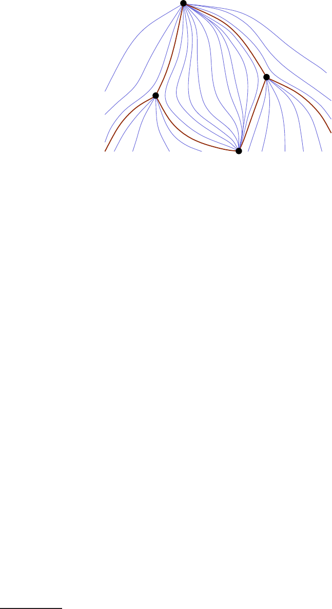
all broken flow lines from x to y, cf. Figure
1.1. This set of broken flow lines
is precisely what is counted if one computes the hyi coefficient of ∂
2
hxi, hence we
deduce
∂
2
= 0
6 Chris Wendl
Figure 1.1. One-parameter families of gradient flow lines on a
Riemannian ma nif old degenerate to broken flow lines.
as a consequence of the fact that compact 1-manifolds always have zero boundary
points when counted with appropriate signs.
2
The homology of the resulting chain
complex can be denoted by HM
∗
(M ; g, f) and is called the Morse homology
of M. The well-known Morse inequalities can then be deduced from a fundamen-
tal theorem stating that HM
∗
(M ; g, f ) is, fo r generic f and g, isomorphic to the
singular homology of M.
With the above notion of Morse homology understood, Floer’s approach to the
Arnold conjecture can now be summarized a s follows:
Step 1: Under suitable technical assumptions, construct a homology theory
HF
∗
(M, ω ; H, {J
t
}),
depending a priori on the choices of a Hamiltonian H : S
1
×M → R with
all 1-periodic orbits nondegenerate, and a generic S
1
-parametrized family
of ω-compatible almost complex structures {J
t
}
t∈S
1
. The generators of the
chain complex a r e the critical points of the symplectic action functional
A
H
, i.e. 1-periodic orbits of the Hamiltonian flow, and t he boundary map
is defined by counting a suitable notio n of gradient flow lines connecting
pairs of orbits (more on this below).
Step 2: Prove that HF
∗
(M, ω) := HF
∗
(M, ω ; H, {J
t
}) is a symplectic invariant,
i.e. it depends on ω, but not on the auxiliary choices H and {J
t
}.
Step 3: Show that if H and {J
t
} are chosen to be time-independent and H is
also C
2
-small, then the chain complex for HF
∗
(M, ω ; H, {J
t
}) is isomor -
phic (with a suitable grading shift) to the chain complex for Morse ho-
mology HM
∗
(M ; g, H) with g := ω(·, J
t
·). The isomorphism between
HM
∗
(M ; g, H) and singular ho mo logy thus implies that the Floer com-
plex must have at least as many generators (i.e. periodic orbits) as there
are generators of H
∗
(M), proving the Arnold conjecture.
2
Counting with signs presumes that we have chosen suitable orientations for the mo duli spaces
M(x, y), a nd this can always be done. Alternatively, one can avoid this issue by counting modulo 2
and thus define a homology theory with Z
2
coefficients.
Lectures on Symplectic Field Theory 7
The implementatio n of Floer’s idea required a different type of analysis than
what is needed for Morse homology. The moduli space M(x, y) in Morse homol-
ogy is simple to understand as the (generically transverse) intersection between the
unstable manifold o f x and t he stable manifold of y with respect to the negative
gradient flow. Conveniently, both of those are finite-dimensional manifolds, with
their dimensions determined by the Morse indices of x and y. We will see in Lec-
ture
3 that no such thing is true for the symplectic action functional: to the extent
that A
H
can be thought of as a Morse function on an infinite-dimensional manifold,
its Morse index and its Morse “co-index” at every critical point are both infinite,
hence the stable and unstable manif olds are not nearly as nice as finite-dimensional
manifolds, providing no reason to expect that their intersection should be. There
are additional problems since C
∞
contr
(S
1
, M) does not have a Banach space topology:
in order to view the negative gradient flow of A
H
as an ODE and make use of the
usual local existence/uniqueness theorems (as in [
Lan99, Chapter IV]), one would
have t o extend to A
H
to a smoot h function on a suitable Hilbert manifold with a
Riemannian metric. There is a very limited range of situations in which o ne can do
this and obt ain a reasonable formula for ∇A
H
, e.g. [
HZ94, §6.2] explains the case
M = T
2n
, in which A
H
can be defined on the Sobolev space H
1/2
(S
1
, R
2n
) and then
studied using Fourier series. This approach is very dependent on the fact that the
torus T
2n
is a quotient of R
2n
; for general symplectic manifo lds (M, ω), one cannot
even define H
1/2
(S
1
, M) since functions of class H
1/2
on S
1
need not be continuous
(H
1/2
is a “Sobolev borderline case” in dimension one).
One of the novelties in F loer’s approach was to refrain from viewing the gradient
flow as an ODE in a Banach space setting, but instead to write down a formal
version of the gradient flow equation and regard it as an elliptic PDE. To this end,
let us regard C
∞
contr
(S
1
, M) formally as a manifold with tangent spaces
T
γ
C
∞
contr
(S
1
, M) := Γ(γ
∗
T M),
choose a formal Riemannian metric on this manifold (i.e. a smoothly varying family
of L
2
inner pr oducts on the spaces Γ(γ
∗
T M)) and write down the resulting equation
for the negative gradient flow. A suitable R iemannian metric can be defined by
choosing a smoo t h S
1
-parametrized family of compatible a lmo st complex structures
{J
t
∈ J(M, ω)}
t∈S
1
,
abbreviated in the following as {J
t
}, and setting
hξ, ηi
L
2
:=
Z
S
1
ω(ξ(t), J
t
η(t)) dt
for ξ, η ∈ Γ(γ
∗
T M). Exercise
1.5 then yields the formula
dA
H
(γ)η = hJ
t
( ˙γ − X
t
(γ)), ηi
L
2
,
so that it seems reasonable to define t he so-called unregularized gradient of A
H
by
(1.3) ∇A
H
(γ) := J
t
( ˙γ − X
t
(γ)) ∈ Γ(γ
∗
T M).
Let us a lso think of a pa t h u : R → C
∞
contr
(S
1
, M) as a map u : R ×S
1
→ M, writing
u(s, t) := u(s)(t). The negative gradient flow equation ∂
s
u + ∇A
H
(u(s)) = 0 then
8 Chris Wendl
Figure 1.2. A f amily of smooth Floer trajectories can degenerate
into a broken Floer trajectory.
becomes the elliptic PDE
(1.4) ∂
s
u + J
t
(u) (∂
t
u −X
t
(u)) = 0.
This is called the Floer equation, and its solutions are often called Floer tra-
jectories. The relevance of Floer homology to our previous discussion of pseudo-
holomorphic curves should now be obvious. Indeed, the resemblance of the Floer
equation to the nonlinear Cauchy-Riemann equation is not merely superficial—we
will see in Lecture 6 that the former can always be viewed as a special case of the
latter. In any case, one can use the same set of ana lytical techniques for both: el-
liptic regularity theory implies that Floer trajectories a r e always smooth, Fredholm
theory and the implicit function theorem imply that (under appropriate assump-
tions) they form smooth finite-dimensional moduli spaces. Most importa ntly, the
same “bubbling off” analysis that underlies Gromov’s compactness theorem can be
used to prove that spaces o f Floer trajectories are compact up to “breaking”, just as
in Morse homology (see Figure 1.2)—this is the main reason for the relation ∂
2
= 0
in Floer homology.
We should mention one complication that does not arise either in the study of
closed holomorphic curves or in finite-dimensional Morse theory. Since the gradient
flow in Morse homolog y takes place on a closed manifold, it is obvious that every
gradient flow line asymptotically approaches critical points at both −∞ and +∞.
The following example shows that in the infinite-dimensional setting of Floer theory,
this is no longer tr ue.
Example 1.7. Consider the Floer equation on M := S
2
= C ∪{∞} with H := 0
and J
t
defined as the standard complex structure i for every t. Then the orbits of X
t
are all constant, a nd a map u : R ×S
1
→ S
2
satisfies the Floer equation if and only
if it is holomorphic. Identifying R × S
1
with C
∗
:= C \ {0} via the biholomorphic
map (s, t) 7→ e
2π(s+it)
, a solution u approaches periodic orbits as s → ±∞ if and
only if the corresponding holomo r phic map C
∗
→ S
2
extends continuously ( and
therefore holomorphically) over 0 and ∞. But this is not true for every holomorphic
map C
∗
→ S
2
, e.g. take any entire function C → C that has an essentia l singularity
at ∞.
Lectures on Symplectic Field Theory 9
Exercise 1.8. Show that in the above example with an essential singularity
at ∞, the symplectic action A
H
(u(s, ·)) is unbounded as s → ∞.
Exercise 1.9. Suppose u : R ×S
1
→ M is a solution to the Floer equation with
lim
s→±∞
u(s, ·) = γ
±
uniformly f or a pair of 1-periodic orbits γ
±
∈ Crit(A
H
). Show
that
(1.5)
A(γ
−
) − A(γ
+
) =
Z
R×S
1
ω(∂
s
u, ∂
t
u −X
t
(u)) ds dt =
Z
R×S
1
ω(∂
s
u, J
t
(u)∂
s
u) ds dt.
The right hand side of (
1.5) is manifestly nonnegative since J
t
is compatible
with ω, and it is strictly po sitive unless γ
−
= γ
+
. It is therefore sensible to call
this expression the energy E(u) of a Floer trajectory. The following converse of
Exercise
1.9 plays a crucial role in the compactness theory for Floer trajectories, a s it
guarantees that all the “levels” in a broken Floer trajectory are asymptotically well
behaved. We will prove a variant of this r esult in t he SFT context (see Prop.
1.23
below) in Lecture 9.
Proposition 1.10. If u : R ×S
1
→ M is a Floer trajectory with E(u) < ∞ and
all 1-periodic orbits of X
t
are non egenera te, then there exist orbits γ
−
, γ
+
∈ Crit(A
H
)
such that lim
s→±∞
u(s, ·) = γ
±
uniformly.
Remark 1.11. It should be emphasized again that we have assumed [ω]|
π
2
(M)
=
0 throughout this discussion; Floer homolog y can also be defined under more general
assumptions, but several details become mor e complicated.
For nice comprehensive treatments of Hamiltonian Floer homology—unfortunat ely
not always with the same sign conventions a s used here—see [
Sal99, AD14]. Note
that this is only one of a few “Floer homologies” that were introduced by Floer in
the late 80’s: the others include Lagrangian intersection Fl oer h o mology [
Flo88a]
(which has since evolved into the Fukaya category, see [
Sei08]), and instanton ho-
mology [
Flo88c], an extension of Donaldson’s gauge-theoretic smooth 4-manifold
invariants to dimension three. The development of new Floer-type theories has
since become a major industry.
1.3. Contact manifolds and t he Weinstein conjecture
A Hamiltonian system on a symplectic manifold (W, ω) is called autonomous if
the Ha miltonian H : W → R does not depend o n time. In this case, the Hamiltonian
vector field X
H
defined by
ω(X
H
, ·) = −dH
is time-independent and its orbits are confined to level sets of H. The images of
these orbits on a given regular level set H
−1
(c) depend on the geometry of H
−1
(c)
but not on H itself, as they are the integral curves (also known as character istics)
of the characteristic line field on H
−1
(c), defined as the unique direction spanned
by a vector X such that ω(X, Y ) = 0 for a ll Y tangent to H
−1
(c). In 1978, Weinstein
[
Wei78] and Rabinowitz [Rab78] proved that certain kinds of regular level sets in
symplectic manifolds are gua ranteed to admit closed characteristics, hence implying
10 Chris Wendl
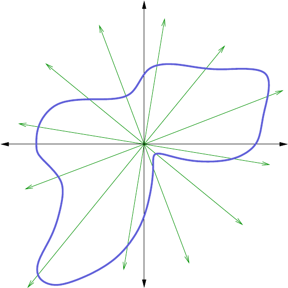
Figure 1.3. A star-shaped hypersurface in Euclidean space
the existence of periodic Hamiltonian orbits. In particular, this is true whenever
H
−1
(c) is a star-shaped hypersurface in the standard symplectic R
2n
(see Figure
1.3).
The following symplectic interpretation of the star-shaped condition provides
both an intuitive reason to believe Rabinowitz’s existence result and motivation for
the more general conjecture of Weinstein. In any symplectic manifold (W, ω), a
Liouville vector field is a smooth vector field V that satisfies
L
V
ω = ω.
By Cart an’s formula for the Lie derivative, the dual 1-form λ defined by λ := ω(V, ·)
satisfies dλ = ω if and only if V is a L iouville vector field; moreover, λ then also
satisfies L
V
λ = λ, and it is referred to as a Liouville form. A hypersurface
M ⊂ (W, ω) is said to be of contact type if it is tr ansverse to a Liouville vector
field defined on a neighborhood of M.
Example 1.12. Using coordinates (q
1
, p
1
, . . . , q
n
, p
n
) on R
2n
, the standard sym-
plectic form is written as
ω
std
:=
n
X
j=1
dp
j
∧ dq
j
,
Lectures on Symplectic Field Theory 11
and the Liouville form λ
std
:=
1
2
P
n
j=1
(p
j
dq
j
−q
j
dp
j
) is dual to the radial Liouville
vector field
V
std
:=
1
2
n
X
j=1
p
j
∂
∂p
j
+ q
j
∂
∂q
j
.
Any star-shaped hypersurface is therefore of contact type.
Exercise 1.13. Suppose (W, ω) is a symplectic manifold of dimension 2n, M ⊂
W is a smoothly embedded and oriented hypersurface, V is a Liouville vector field
defined near M and λ := ω(V, ·) is the dual Liouville form. Define a 1-form on M
by α := λ|
T M
.
(a) Show that V is positively transverse to M if and only if α satisfies
(1.6) α ∧ (dα)
n−1
> 0.
(b) If V is positively transverse to M, choose ǫ > 0 sufficiently small and
consider the embedding
Φ : (−ǫ, ǫ) × M ֒→ W : ( r, x) 7→ ϕ
r
V
(x),
where ϕ
t
V
denotes the time t flow of V . Show that
Φ
∗
λ = e
r
α,
hence Φ
∗
ω = d(e
r
α).
The above exercise presents any contact-type hypersurface M ⊂ (W, ω) as
one member o f a smooth 1-parameter family of contact-type hypersurfaces M
r
:=
ϕ
r
V
(M) ⊂ W , each canonically identified with M such that ω|
T M
r
= e
r
dα. In
particular, the characteristic line fields on M
r
are the same for all r, thus the ex-
istence of a closed characteristic on any of these implies that there also exists one
on M. This observation has sometimes been used to prove such existence theorems,
e.g. it is used in [
HZ94, Chapter 4] to reduce Rabinowitz’s result to an “almost
existence” theorem based o n symplectic capacities. This discussion hopefully makes
the following conjecture seem believable.
Conjecture 1.14 (Weinstein conjecture, symplectic version). Any cl osed contact-
type hypersurface in a symplectic manifold admits a clos ed characteristic.
Weinstein’s conjecture admits a natural rephrasing in t he language of contact
geometry. A 1-form α on an o r iented (2n − 1)-dimensional manifold M is called a
(positive) contact form if it satisfies (
1.6), and the resulting co-oriented hyperplane
field
ξ := ker α ⊂ T M
is then called a (positive and co-oriented) contact structure.
3
We call the pair
(M, ξ) a contact manifold, and r efer to a diffeomorphism ϕ : M → M
′
as a
3
The adjective “positive” refers to the fact that the orie ntation of M agrees with the one deter-
mined by the volume form α ∧(dα)
n−1
; we call α a negative c ontact form if these two orientations
disagree. It is also possible in general to define contact structures without co-orientations, but con-
tact structures of this type will never appear in these notes; for our purp oses, the co-orientation is
always considered to be par t of the data of a contact s tructure.
12 Chris Wendl
contact omorphism from (M, ξ) to (M
′
, ξ
′
) if ϕ
∗
maps ξ to ξ
′
and also preserves
the respective co-orientations. Equivalently, if ξ and ξ
′
are defined via contact forms
α and α
′
respectively, this means
ϕ
∗
α
′
= f α for some f ∈ C
∞
(M, (0, ∞)).
Contact topology studies the cat egory of contact manifolds (M, ξ) up to con-
tactomorphism. The following basic result provides one good reason to regard ξ
rather than α as the geometrically meaningful data, as the result holds for contact
structures, but not for contact forms.
Theorem 1.15 (Gray’s stability theorem). If M is a closed (2n−1)-dimensional
manifold and {ξ
t
}
t∈[0,1]
is a smooth 1-parameter family of contact structures on M,
then there exists a sm ooth 1-parameter family of diffeomorph i s ms {ϕ
t
}
t∈[0,1]
such
that ϕ
0
= Id and (ϕ
t
)
∗
ξ
0
= ξ
t
.
Proof. See [
Gei08, §2.2 ] or [Wend, Theorem 1.6.12].
A corollary is that while the cont act fo rm α induced on a contact- type hyper-
surface M ⊂ (W, ω) via Exercise
1.13 is not unique, its induced cont act structure is
unique up to isotopy. Indeed, the space of all Liouville vector fields transverse to M
is very large (e.g. one can add to V any sufficiently small Hamiltonian vector field),
but it is conv ex, hence any two choices of the induced conta ct form α on M are
connected by a smoot h 1-parameter family of contact forms, implying an isotopy of
contact structures via Gray’s theorem.
Exercise 1.16. If α is a nowhere zero 1-form on M and ξ = ker α, show tha t α
is contact if and only if dα|
ξ
defines a symplectic vector bundle structure on ξ → M.
Moreover, the orientation of ξ determined by this symplectic bundle structure is
compatible with the co-or ientation determined by α and the orientation of M for
which α ∧ (dα)
n−1
> 0.
The following definition is based on the fact that since dα|
ξ
is nondegenerate
when α is contact, ker dα ⊂ T M is always 1-dimensional and transverse to ξ.
Definition 1.17. Given a contact f orm α on M, the Reeb vector field is the
unique vector field R
α
that satisfies
dα(R
α
, ·) ≡ 0, and α(R
α
) ≡ 1.
Exercise 1.18. Show that the flow o f any Reeb vector field R
α
preserves both
ξ = ker α and the symplectic vector bundle structure dα|
ξ
.
Conjecture 1.19 (Weinstein conjecture, contact version). On any closed con-
tact manifold (M, ξ) with contact form α, the Reeb vector field R
α
admits a periodic
orbit.
To see that this is equivalent to the symplectic version of the conjecture, ob-
serve that any contact manifold (M, ξ = ker α) can be viewed as the contact-type
hypersurface {0}× M in the open symplectic manifold
(R × M, d(e
r
α)) ,
called the symplectization of (M, ξ).
Lectures on Symplectic Field Theory 13
Exercise 1.20. Recall that on any smooth manifold M, there is a tautological
1-form λ that locally takes the form λ =
P
n
j=1
p
j
dq
j
in any cho ice of local coo r di-
nates (q
1
, . . . , q
n
) on a neighbood U ⊂ M, with (p
1
, . . . , p
n
) denoting the induced
coordinates on t he cotangent fibers over U. This is a Liouville form, with dλ defin-
ing the canonical symplectic structure of T
∗
M. Now if ξ ⊂ T M is a co-oriented
hyperplane field on M, consider the submanifold
S
ξ
M :=
p ∈ T
∗
M
ker p = ξ and p(X) > 0 for any X ∈ T M pos. transverse to ξ
.
Show that ξ is contact if and only if S
ξ
M is a symplectic submanifold o f (T
∗
M, dλ),
and the Liouville vector field on T
∗
M dual to λ is tangent to S
ξ
M. Moreover, if ξ is
contact, then any choice of contact f orm for ξ determines a diffeomorphism of S
ξ
M
to R × M identifying the L iouville form λ along S
ξ
M with e
r
α.
Remark 1.21. Exercise
1.20 shows that up to symplectomorphism, our defi-
nition of the symplectization of (M, ξ) above actually depends only on ξ and not
on α.
In 1993, Hofer [
Hof93] introduced a new approach to the Weinstein conjecture
that was based in part on ideas of Gromov and Floer. Fix a contact manifold (M, ξ)
with contact form α, and let
J(α) ⊂ J(R × M)
denote the nonempty and cont ractible space o f all almost complex structures J on
R × M satisfying the following conditions:
(1) The natur al translation action on R × M preserves J;
(2) J∂
r
= R
α
and JR
α
= −∂
r
, where r denotes the canonical coordinate on
the R-factor in R × M;
(3) Jξ = ξ and dα(·, J·) |
ξ
defines a bundle metric on ξ.
It is easy to check that any J ∈ J(α) is compatible with the symplectic structure
d(e
r
α) on R × M. Moreover, if γ : R → M is any periodic orbit of R
α
with period
T > 0, then for any J ∈ J(α), the so-called trivial cylinder
u : R × S
1
→ R × M : (s, t) 7→ (T s, γ(T t))
is a J-holomorphic curve. Following Floer, one version of Hofer’s idea would be to
look for J-holomorphic cylinders that satisfy a finite energy condition as in Prop.
1.10
forcing them to approach trivial cylinders asymptotically—the existence of such a
cylinder would then imply the existence of a closed Reeb orbit and thus prove the
Weinstein conjecture. The first hindrance is that the “o bvious” definition of energy
in t his context,
Z
R×S
1
u
∗
d(e
r
α),
is not t he right one: this integral is infinite if u is a trivial cylinder. To circumvent
this, notice that every J ∈ J(α) is also compatible with any symplectic structure
of the form
ω
ϕ
:= d( e
ϕ(r)
α),

14 Chris Wendl
where ϕ is a function chosen freely from the set
(1.7) T :=
ϕ ∈ C
∞
(R, (−1, 1))
ϕ
′
> 0
.
Essentially, choosing ω
ϕ
means identifying R × M with a subset of the bounded
region (−1, 1) × M, in which trivial cylinders have finite symplectic area. Since
there is no preferred choice for the function ϕ, we define the Hofer energy
4
of a
J-holomorphic curve u : Σ → R × M by
(1.8) E(u) := sup
ϕ∈T
Z
Σ
u
∗
ω
ϕ
.
This has the desired property of being finite for trivial cylinders, and it is also
nonnegative, with strict positivity whenever u is not constant.
Another useful observation from [
Hof93] was that if the goal is t o find periodic
orbits, then we need not restrict our attention to J-holomorphic cylinders in par-
ticular. One can more generally consider curves defined on an arbitrary punctured
Riemann surface
˙
Σ := Σ \ Γ,
where (Σ, j) is a closed connected Riemann surface and Γ ⊂ Σ is a finite set of
punctures. For any ζ ∈ Γ, one can find coordinates identifying some punctured
neighborhood o f ζ biholomorphically with the closed punctured disk
˙
D := D \ {0} ⊂ C,
and then identif y this with either the positive or negative half- cylinder
Z
+
:= [0, ∞) ×S
1
, Z
−
:= (−∞, 0] × S
1
via the biholomorphic maps
Z
+
→
˙
D : (s, t) 7→ e
−2π(s+it)
, Z
−
→
˙
D : (s, t) 7→ e
2π(s+it)
.
We will refer to such a choice as a (positive or negative) holomorphic cylindrical
coordinate system near ζ, and in this way, we can present (
˙
Σ, j) as a Riemann
surface with cylindrical ends, i.e. the union of some compact Riemann surface with
boundary with a finite collection of half-cylinders Z
±
on which j takes the standard
form j∂
s
= ∂
t
. Note that the standard cylinder R × S
1
is a special case of this, as
it can be identified biholomorphically with S
2
\ {0, ∞}. Another important special
case is the plane, C = S
2
\ {∞}.
If u : (
˙
Σ, j) → (R × M, J) is a J-holomorphic curve and ζ ∈ Γ is o ne of its
punctures, we will say that u is positively/negatively asymptotic to a T -periodic
Reeb orbit γ : R → M a t ζ if one can choose holomorphic cylindrical coordinates
(s, t) ∈ Z
±
near ζ such that
u(s, t) = exp
(T s,γ(T t))
h(s, t) for |s| sufficiently la rge,
4
Strictly speaking, the energy defined in (
1.8) is not identical to the notion introduced in
[Hof93] and used in many of Hofer’s papers, but it is equivale nt to it in the s ense that uniform
bounds on either notion of energy imply uniform bounds on the other.
Lectures on Symplectic Field Theory 15
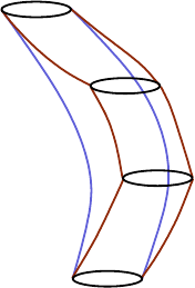
˙
Σ
u
{∞} × M
{−∞} × M
Figure 1.4. An asymptotically cylindrical holomorphic curve in a
symplectization, with g enus 1, one positive puncture and two negative
punctures.
where h(s, t) is a vector field along the trivial cylinder satisfying h(s, ·) → 0 uni-
formly as |s| → ∞, and the exponential map is defined with respect to any R-
invariant choice of Riemannian metric on R×M. We say that u : (
˙
Σ, j) → (R×M, J)
is asymptotically cylindrical if it is (positively or negatively) asymptotic to some
closd Reeb orbit at each of its punctures. Not e that this partitions the finite set of
punctures Γ ⊂ Σ into two subsets,
Γ = Γ
+
∪ Γ
−
,
the positive and negative punctures respectively, see Figure 1.4.
Exercise 1.22. Suppose u : (
˙
Σ, j) → (R×M, J) is an asymptotically cylindrical
J-holomorphic curve, with the asymptotic orbit at each puncture ζ ∈ Γ
±
denoted
by γ
ζ
, having period T
ζ
> 0. Show that
X
ζ∈Γ
+
T
ζ
−
X
ζ∈Γ
−
T
ζ
=
Z
˙
Σ
u
∗
dα ≥ 0,
with equality if and only if the image of u is contained in that of a trivial cylinder.
In particular, u must have at least one positive puncture unless it is constant. Show
also that E(u) is finite and satisfies an upper bound determined o nly by the periods
of the positive asymptotic orbits.
The following analog ue of Prop.
1.10 will be proved in Lecture 9. For simplicity,
we shall state a weakened version of what Hofer proved in [
Hof93], which did not
require any nondegeneracy assumption. A T -periodic Reeb orbit γ : R → M is
called nondegenerate if the Reeb flow ϕ
t
α
has the property t ha t its linearization
along the contact bundle (cf. Exercise 1.18),
dϕ
T
α
(γ(0))|
ξ
γ(0)
: ξ
γ(0)
→ ξ
γ(0)
does not have 1 as an eigenvalue. Note that since R
α
is not time-dependent, closed
Reeb orbits are never completely isolated—they always exist in S
1
-parametrized
families—but t hese families are isolated in the nondegenerate case.

16 Chris Wendl
Proposition 1.23. Suppose (M, ξ) is a closed contact manifold, with a co ntact
form α such that all closed Reeb orbits are nond egenerate. If u : (
˙
Σ, j) → (R×M, J)
is a J-hol omorphic curve with E( u) < ∞ on a punctured Riemann surface such that
none of the punctures are removable, then u is asymptotically cylindrical.
The main r esults in [Hof93] state that under certain assumptions on a closed
contact 3-manifold (M, ξ), namely if either ξ is ove rtwis ted (as defined in [
Eli89])
or π
2
(M) 6= 0, one can find for a ny contact form α on (M, ξ) and any J ∈ J(α) a
finite-energy J-holomor phic plane. By Proposition
1.23, this implies t he existence
of a contractible periodic Reeb orbit and thus proves the Weinstein conjecture in
these settings.
1.4. Symplectic cobordisms and their completions
After the developments described in the previous three sections, it seemed nat-
ural that one might define invariants of contact manifolds via a Floer-type theory
generated by closed Reeb orbits and counting asymptotically cylindrical holomor-
phic curves in symplectizations. This theory is what is now called SFT, and its
basic structure was outlined in a paper by Eliashberg, Giventa l and Hofer [EGH00]
in 2000, t hough some of its analytical foundations remain unfinished in 2016. The
term “field theory” is an allusion to “topological quantum field theories,” which
associate vector spaces to certain geometric objects and morphisms to cobordisms
between those objects. Thus in order to place SFT in its proper setting, we need to
introduce symplectic cobordisms between contact manifolds.
Recall that if M
+
and M
−
are smooth oriented closed manifolds of the same
dimension, an oriented cobordism fr om M
−
to M
+
is a compact smooth oriented
manifold W with oriented boundary
∂W = −M
−
⊔ M
+
,
where −M
−
denotes M
−
with its orientation r eversed. Given positive contact struc-
tures ξ
±
on M
±
, we say that a symplectic manifold (W, ω) is a symplectic cobor-
dism from (M
−
, ξ
−
) to (M
+
, ξ
+
) if W is an oriented cobor dism
5
from M
−
to M
+
such that both components of ∂W are contact-type hypersurfaces with induced con-
tact structures isotopic to ξ
±
. Note that our chosen orientation conventions imply
in this case that the Liouville vector field chosen near ∂W must point outward at
M
+
and inward at M
−
; we say in this case that M
+
is a symplectically convex
boundary component, while M
−
is symplectically concave. As important special
cases, (W, ω) is a symplectic filling of (M
+
, ξ
+
) if M
−
= ∅, and it is a symplectic
cap of (M
−
, ξ
−
) if M
+
= ∅. In the literature, fillings and caps are sometimes also
referred to as conv ex fillings or concave filli ngs respectively.
The contact-type condition implies the existence of a Liouville fo rm λ near ∂W
with dλ = ω, such that by Exercise
1.13, neighborhoods of M
+
and M
−
in W can
be identified with the collars (see Fig ure
1.5)
(−ǫ, 0] × M
+
or [0, ǫ) × M
−
5
We assume of course that W is assigned the orientation determined by its symplectic form.

Lectures on Symplectic Field Theory 17
((−ǫ, 0] × M
+
, d(e
r
α
+
))
([0, ǫ) ×M
−
, d(e
r
α
−
))
(W, ω)
Figure 1.5. A symplectic cobordism with concave bo undary
(M
−
, ξ
−
) and convex boundary (M
+
, ξ
+
), with symplectic collar neigh-
borhoods defined by flowing along Liouville vector fields near the
boundary.
respectively f or sufficiently small ǫ > 0, with λ taking the form
λ = e
r
α
±
,
where α
±
:= λ|
T M
±
are conta ct forms for ξ
±
. The symplectic completion of
(W, ω) is the noncompact symplectic manifold (
c
W , ˆω) defined by attaching cylindri-
cal ends to these collar neighbo rhoods (Figure 1.6):
(
c
W , ˆω) = ((−∞, 0] × M
−
, d(e
r
α
−
)) ∪
M
−
(W, ω)
∪
M
+
([0, ∞) × M
+
, d(e
r
α
+
)) .
(1.9)
In this cont ext, the symplectization (R × M, d(e
r
α)) is symplectomorphic to the
completion of the trivial symplectic cobordism ([0, 1] ×M, d(e
r
α)) from (M, ξ =
ker α) to itself. More generally, the object in the following easy exercise can also
sensibly b e called a trivial symplectic cobordism:
Exercise 1.24. Suppose (M, ξ) is a closed contact manifold with contact form
α, and f
±
: M → R is a pair of functions with f
−
< f
+
everywhere. Show that the
domain
(r, x) ∈ R × M
f
−
(x) ≤ r ≤ f
+
(x)
⊂ R × M
defines a symplectic cobor dism from (M, ξ) to itself, with a global Liouville form
λ = e
r
α inducing contact forms e
f
−
α and e
f
+
α on its concave and convex boundaries
respectively.
We say that (W, ω) is a n exact symplectic cobordism or Liouville cobor-
dism if the Liouville f orm λ can be extended from a neighborhood of ∂W t o define
a global primitive of ω on W . Equivalently, this means that ω admits a global Li-
ouville vector field that points inward at M
−
and outward at M
+
. An exact filling
of (M
+
, ξ
+
) is an exact cobordism whose concave boundary is empty. Observe that
if (W, ω) is exact, then its completion (
c
W , ˆω) also inherits a global Liouville form.
Exercise 1.25. Use Stokes’ theorem to show that there is no such thing as an
exact symplectic cap.
18 Chris Wendl
−
(W, ω)
((−ǫ, 0] × M
+
, d(e
r
α
+
))
([0, ǫ) ×M
−
, d(e
r
α
−
))
([0, ∞) × M
+
, d(e
r
α
+
))
((−∞, 0] ×M
−
, d(e
r
α
−
))
Figure 1.6. The completion of a symplectic cobordism
The above exercise hint s at an important difference between cobordisms in the
symplectic as opposed to the oriented s mooth category: symplectic cobordisms are
not generally reversible. If W is an oriented cobor dism from M
−
to M
+
, then
reversing the orientation of W produces an oriented cobordism from M
+
to M
−
.
But one cannot simply reverse orientations in the symplectic category, since t he
orientation is determined by the symplectic form. For example, many obstructions
to the existence of symplectic fillings of given contact manifolds are known—some
of them defined in terms of SFT—but we do not know any obstructions at all to
symplectic caps, in fact it is known that a ll contact 3-manifolds admit them.
The definitions for holomorphic curves in symplectizations in the previous sec-
tion generalize to completions of symplectic cobo r disms in a fairly straightforward
way since these completions look exactly like symplectizations outside of a compact
subset. Define
J(W, ω, α
+
, α
−
) ⊂ J(
c
W )
as the space of all almost complex structures J on
c
W such tha t
J|
W
∈ J(W, ω), J|
[0,∞)×M
+
∈ J(α
+
) and J|
(−∞,0]×M
−
∈ J(α
−
).
Lectures on Symplectic Field Theory 19
˙
Σ
u
c
W
d(
Figure 1.7. An asymptotically cylindrical holomorphic curve in a
completed symplectic cobordism, with genus 2, one positive puncture
and two negative punctures.
Occasionally it is useful to relax the compatibility condition on W to tameness,
6
i.e. J|
W
∈ J
τ
(W, ω), producing a space that we shall denote by
J
τ
(W, ω, α
+
, α
−
) ⊂ J(
c
W ).
As in Prop.
1.2, both of these spaces are nonempty and contractible. We can then
consider asymptotically cylindrical J-ho lomorphic curves
u : (
˙
Σ = Σ \ (Γ
+
∪ Γ
−
), j) → (
c
W , J),
which are proper maps asymptotic to closed orbits of R
α
±
in M
±
at punctures in Γ
±
,
see Figure
1.7.
One must aga in tinker with the symplectic form on
c
W in order to define a notio n
of energy that is finite when we need it to be. We generalize (
1.7) as
T :=
ϕ ∈ C
∞
(R, (−1, 1))
ϕ
′
> 0 and ϕ(r) = r near r = 0
,
and associate to each ϕ ∈ T a symplectic form ˆω
ϕ
on
c
W defined by
ˆω
ϕ
:=
d(e
ϕ(r)
α
+
) on [0, ∞) × M
+
,
ω on W,
d(e
ϕ(r)
α
−
) on (−∞, 0] ×M
−
.
One can again check that every J ∈ J(W, ω, α
+
, α
−
) or J
τ
(W, ω, α
+
, α
−
) is com-
patible with or, respectively, tamed by ˆω
ϕ
for every ϕ ∈ T . Thus it makes sense to
6
It seems natural to wonder whether one could not also relax the conditions on the cylindrical
ends and requir e J|
ξ
±
to be tamed by dα
±
|
ξ
±
instead o f compatible with it. I do not curr e ntly
know whether this works, but in later lectures we will see some reasons to worry that it might not.

20 Chris Wendl
define the energy of u : (
˙
Σ, j) → (
c
W , J) by
E(u) := sup
ϕ∈T
Z
˙
Σ
u
∗
ˆω
ϕ
.
It will be a straightforward matter to generalize Propo sition
1.23 a nd show that
finite energy implies asymptotically cylindrical behavior in completed cobordisms.
Exercise 1.26. Show tha t if (W, ω) is an exact cobo r dism, then every asymp-
totically cylindrical J-holo mo rphic curve in
c
W has at least one positive puncture.
1.5. Contact homology and SFT
We can now sketch the algebraic structure of SFT. We shall ignore or suppress
several pesky details that are best dealt with later, some of t hem algebraic, others
analytical. Due to analytical problems, some o f the “theorems” t hat we shall (often
imprecisely) state in this section are not yet provable at the current level of tech-
nology, though we exp ect that they will be soon. We shall use quotation marks to
indicate this caveat wherever appropriate.
The standard versions of SFT all define homology theories with varying levels of
algebraic structure which are meant to be invariants of a contact manifold (M, ξ).
The chain complexes always depend on certain auxiliary choices, including a nonde-
generate contact form α and a generic J ∈ J(α). The generators consist of formal
varia bles q
γ
, one f or each
7
closed Reeb orbit γ. In the most straightforward gen-
eralization of Hamiltonian Floer homology, the chain complex is simply a graded
Q-vector space generated by the variables q
γ
, and the boundary map is defined by
∂
CCH
q
γ
=
X
γ
′
#
M(γ, γ
′
)
R
q
γ
′
,
where M(γ, γ
′
) is the moduli space of J-holomorphic cylinders in R × M with a
positive puncture asymptotic to γ and a negative puncture asymptotic to γ
′
, and the
sum ranges over all orbits γ
′
for which this moduli space is 1-dimensional. The count
# (M(γ, γ
′
)/R) is ratio nal, as it includes rational weighting factors that depend on
combinatoria l informatio n and are best not discussed right now.
8
“Theorem” 1.27. If α admits no contractible Reeb orbits, then ∂
2
CCH
= 0, and
the resulting homology is independ ent of the choices of α with this property and
generic J ∈ J(α).
The invariant arising from this result is known as cylindrical contact homol-
ogy, and it is sometimes quite easy to work with when it is well defined, though it
has the disadvantage of not always being defined. Namely, the relation ∂
2
CCH
= 0
can f ail if α admits contra ctible Reeb orbits, because unlike in Floer homology, the
compactification of the space of cylinders M(γ, γ
′
) generally includes objects that
are not broken cylinders. In fact, the objects arising in the “SFT compactification”
7
Actually I should b e making a distinction here between “good” and “bad” Reeb orbits, but
let’s discuss that later; see Lecture
11.
8
Similar combinatorial fac tors ar e hidden behind the symbol “#” in our definitions of ∂
CH
and H, and will be discussed in earnest in Lecture
12.
Lectures on Symplectic Field Theory 21
c
W
c
W
u
k
(M
+
, ξ
+
)
(M
−
, ξ
−
)
v
+
1
v
0
v
−
1
v
−
2
v
−
3
R × M
+
R × M
−
R × M
−
R × M
−
Figure 1.8. Degeneration of a sequence u
k
of finite energy punc-
tured holomorphic curves with genus 2, one positive puncture and two
negative punctures in a symplectic cobo rdism. The limiting holomor-
phic building (v
+
1
, v
0
, v
−
1
, v
−
2
, v
−
3
) in this example has one upper level
living in the symplectization R × M
+
, a ma in level living in
c
W , and
three lower levels, each of which is a (possibly disconnected) finite-
energy punctured nodal holomorphic curve in R × M
−
. The building
has arithmetic genus 2 and the same numbers of positive and negative
punctures a s u
k
.
of moduli spaces of finite-energy curves in completed cobordisms can be quite elab-
orate, see Fig ure
1.8. The combinatorics of the situation are not so bad however
if the cobordism is exact, as is the case for a symplectization: Exercise
1.26 then
prevents curves without positive ends from appear ing. The only possible degen-
erations for cylinders then consist of broken configurations whose levels each have
exactly one positive puncture and arbitrary negative punctures; moreover, all but
one of the negative punctures must eventually be capped off by planes, which is why
“Theorem”
1.27 holds in the absence of planes.
If planes do exist, then one can account for them by defining the chain complex
as an algebra rather than a vector space, producing the theory known as contact
homology. For this, the chain complex is taken t o be a graded unital algebra over
22 Chris Wendl
Q, and we define
∂
CH
q
γ
=
X
(γ
1
,...,γ
m
)
#
M(γ; γ
1
, . . . , γ
m
)
R
q
γ
1
. . . q
γ
m
,
with M( γ; γ
1
, . . . , γ
m
) denoting the moduli space of punctured J-holomorphic spheres
in R × M with a positive puncture at γ and m negative punctures at the orbits
γ
1
, . . . , γ
m
, and the sum ranges over all integers m ≥ 0 and all m-tuples of orbits for
which the moduli space is 1-dimensional. The action of ∂
CH
is then extended to the
whole algebra via a graded Leibniz rule
∂
CH
(q
γ
q
γ
′
) := ( ∂
CH
q
γ
) q
γ
′
+ (−1)
|γ|
q
γ
(∂
CH
q
γ
′
) .
The general compactness and gluing theory for genus zero curves with one positive
puncture now implies:
“Theorem” 1.28. ∂
2
CH
= 0, and the resulting ho mology is (as a graded unital
Q-algebra) independent of the choices α and J.
Maybe yo u’ve noticed the pattern: in order to accommodate more general classes
of holomorphic curves, we need to add more algebraic structure. The full SFT
algebra counts all rigid holomorphic curves in R ×M, including all combinations of
positive and negative punctures and all genera. Here is a brief picture of what it
looks like. Counting all the 1-dimensional mo duli spaces of J-holomo r phic curves
modulo R-translation in R × M produces a formal power series
H :=
X
#
M
g
(γ
+
1
, . . . , γ
+
m
+
; γ
−
1
, . . . , γ
−
m
−
)
.
R
q
γ
−
1
. . . q
γ
−
m
−
p
γ
+
1
. . . p
γ
+
m
+
~
g−1
,
where the sum ranges over all integers g, m
+
, m
−
≥ 0 and tuples of orbits, ~ and p
γ
(one for each orbit γ) ar e additional formal variables, and
M
g
(γ
+
1
, . . . , γ
+
m
+
; γ
−
1
, . . . , γ
−
m
−
)
denotes the moduli space of J-holomorphic curves in R × M with genus g, m
+
positive punctures at the orbits γ
+
1
, . . . , γ
+
m
+
, a nd m
−
negative punctures at the
orbits γ
−
1
, . . . , γ
+
m
−
. We can regard H as an operator on a graded algebra W of
formal power series in the variables {p
γ
}, {q
γ
} and ~, equipped with a graded bracket
operation that satisfies the quantum mechanical commutation relation
[p
γ
, q
γ
] = κ
γ
~,
where κ
γ
is a combinatorial f actor tha t is best igno red for now. Note that due t o the
signs that accompany the grading, odd elements F ∈ W need not satisfy [F, F] = 0,
and H it self is an odd element, thus the following statement is nontrivial; in fact,
it is the algebraic manifestation of the general compactness and gluing theory for
punctured holomorphic curves in symplectizations.
“Theorem” 1.29. [H, H ] = 0, hence by the graded Jacobi id e ntity, H deter-
mines an operator
D
SFT
: W → W : F 7→ [H, F]
satisfying D
2
SFT
= 0. The re sulting homology depend s on (M, ξ) b ut not o n the
auxiliary choices α and J.
Lectures on Symplectic Field Theory 23
It takes some time to understand how pictures such as Figure 1.8 tr anslate
into algebraic relations like [H , H] = 0, but this is a subject we’ll come back to.
There is also an intermediate theory between contact homology and full SFT, called
rational SFT, which counts only g enus zero curves with arbitrary positive and
negative punctures. Algebraically, it is obtained fro m the full SFT alg ebra as a
“semiclassical approximation” by discarding higher-order factors of ~ so that the
commutation bracket in W becomes a gr aded Poisson bracket. We will discuss all
of this in Lecture
12.
1.6. Two applications
We briefly mention two applications that we will b e able to establish rigorously
using the methods developed in t his book. Since SFT itself is not yet well defined
in full generality, this sometimes means using SFT for inspiration while proving
corollaries via more direct methods.
1.6.1. Tight cont act structures on T
3
. The 3-torus T
3
= S
1
×S
1
×S
1
with
coordinates (t, θ, φ) admits a sequence of contact structures
ξ
k
:= ker (cos(2πkt) dθ + sin( 2πkt) dφ) ,
one for each k ∈ N. These cannot be distinguished fr om each other by a ny classical
invariants, e.g. they all have the same Euler class, in fact they are all homotopic as
co-oriented 2-plane fields. Nonetheless:
Theorem 1.30. For k 6= ℓ, (T
3
, ξ
k
) and (T
3
, ξ
ℓ
) are not con tactomorphic.
We will be a ble to prove this in Lecture
10 by rigorously defining and computing
cylindrical contact homology for a suitable choice of contact forms on (T
3
, ξ
k
).
1.6.2. Filling and cobordism obstructions. Consider a closed connected
and oriented surface Σ presented as Σ
+
∪
Γ
Σ
−
, where Σ
±
⊂ Σ are each (not neces-
sarily connected) compact surfaces with a common boundary Γ. By an old result of
Lutz [
Lut77], the 3-manifold S
1
× Σ admits a unique isotopy class of S
1
-invariant
contact structures ξ
Γ
such that the loops S
1
× {z} are positively/negatively trans-
verse to ξ
Γ
for z ∈
˚
Σ
±
and tangent to ξ
Γ
for z ∈ Γ. Now for each k ∈ N, define
(V
k
, ξ
k
) := ( S
1
× Σ, ξ
Γ
)
where Σ = Σ
+
∪
Γ
Σ
−
is chosen such that Γ has k connected compo nents, Σ
−
is
connected with genus zero, a nd Σ
+
is connected with positive genus (see Figure
1.9).
Theorem 1.31. The contact manifolds (V
k
, ξ
k
) d o not admit any symplectic
fillings. Moreo ver, if k > ℓ, then there exists no ex act symplectic cobordism from
(V
k
, ξ
k
) to (V
ℓ
, ξ
ℓ
).
For these examples, one can use explicit constructions from [
Wen13, Avd] to
show that non-exact cobordisms from (V
k
, ξ
k
) to (V
ℓ
, ξ
ℓ
) do exist, and so do exact
cobordisms from (V
ℓ
, ξ
ℓ
) to (V
k
, ξ
k
), thus both the directionality of the cobordism
relation and the distinction between exact and non-exact are crucial. The proof
of the theorem, due to the author with Latschev and Hutchings [
LW11], uses a
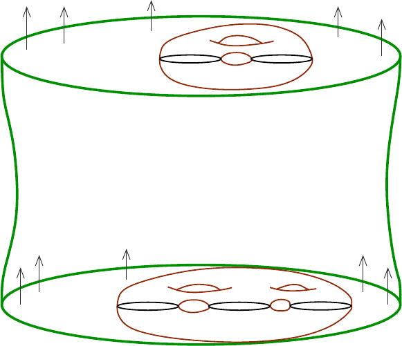
24 Chris Wendl
−
S
1
×
S
1
×
(W, dλ)
(V
2
, ξ
2
)
(V
3
, ξ
3
)
Figure 1.9. This exact symplectic cobordism does not exist.
numerical contact invariant based o n the full SFT algebra—in part icular, the curves
that cause this phenomenon have multiple positive ends and are thus not seen by
contact homology. We will introduce the relevant numerical invariant in Lecture
13
and compute it for these examples in Lecture 16.

LECTURE 2
Basics on holomorphic curves
Contents
2.1. Linearized Cauchy-Riemann operators 25
2.2. Some useful Sobolev inequalities 28
2.3. The fundamental elliptic estimate 30
2.4. Regularity 32
2.4.1. The linear case 33
2.4.2. The nonlinear case 35
2.5. Linear local existence and applications 38
2.6. Simple curves and multiple covers 41
In this lecture we begin studying the analysis of J-holomorphic curves. The
coverage will necessarily be a bit sparse in some places, but more detailed proofs of
everything in this lecture can be found in [
Wend].
2.1. Linearized Cauchy-Riemann operators
In order to motivate the study of linear Cauchy-Riemann type operators, we
begin with a formal discussion of the nonlinear Cauchy-R iemann equation and its
linearization.
Fix a Riemann surface (Σ, j) and almost complex manifold (W, J), and suppose
that we wish to understand the structure of some space of the form
(2.1) {u : Σ → W | T u ◦ j = J ◦ T u plus furt her conditions},
where the “further conditions” (which we will for now leave unspecified) may impose
constraints on e.g. the regularity of u, as well as its boundary and/or asymptotic
behavior. The standard approach in global analysis can be summarized as follows:
Step 1: Construct a smooth Ba nach manifold B of maps u : Σ → W such that all
the solutions we’re interested in will be elements of B. The tangent spaces
T
u
B ar e then Banach spaces of sections of u
∗
T W .
Step 2: Construct a smooth Banach space bundle E → B such that for each u ∈ B,
the fiber E
u
is a Banach space of sections of the vector bundle
Hom
C
(T Σ, u
∗
T W ) → Σ
of complex-antilinear bundle maps (T Σ, j) → (u
∗
T W, J). Since our purpose
is to study a first-order PD E, we need the sections in E
u
to be “one step
less regular” than t he maps in B, e.g. if B consists of maps of Sobolev class
W
k,p
, then the sections in E
u
should be of class W
k−1,p
.
25
26 Chris Wendl
Step 3: Show that
¯
∂
J
: B → E : u 7→ T u + J(u) ◦T u ◦ j
defines a smooth section of E → B, whose zero set is precisely the space o f
solutions (
2.1).
Step 4: Show that under suitable assumptions (e.g. on regular ity and asymptotic
behavior), one can arra nge such t hat for every u ∈
¯
∂
−1
J
(0), the lineariza-
tion of
¯
∂
J
,
D
¯
∂
J
(u) : T
u
B → E
u
is a Fredholm operator and is generically surjective. (In g eometric terms,
this would mean that
¯
∂
J
is transverse to the zero section.)
Step 5: Using the implicit function theorem in Banach spaces (see [
Lan93]), the
surjectivity of D
¯
∂
J
(u) implies that
¯
∂
−1
J
(0) is a smooth finite-dimensional
manifold, with its tangent space at each u ∈
¯
∂
−1
J
(0) canonically identified
with ker D
¯
∂
J
(u), hence the dimension of
¯
∂
−1
J
(0) near u equals the Fredholm
index of D
¯
∂
J
(u).
Without worrying about the fact that these are actually not Banach spaces, a nd
some Sobolev completion is needed, let us assume, for simplicity, tha t the bundle
E → B has as base the space B = C
∞
(Σ, W ) and the fiber over u ∈ B is given by
E
u
=
Hom
C
(T Σ, u
∗
T W ). The linearization of the section ∂
J
at a point u ∈
¯
∂
−1
J
(0)
should then take the form
D
u
: Γ(u
∗
T W ) → Ω
0,1
(Σ, u
∗
T W ),
where t he right hand side denotes the space of u
∗
T W -valued (0, 1)-forms on Σ, or
equivalently, smooth sections of
Hom
C
(T Σ, u
∗
T W ) = T
0,1
Σ ⊗
C
u
∗
T W , where T
0,1
Σ
denotes the (0, 1)-part of the complexified cotangent bundle.
In order to compute such a linearization, we need to make a choice of “connec-
tion” on the bundle E. Choose a connection ∇ on W , and recall the fact that this
naturally induces a connection on the bundles T
0,1
Σ ⊗
C
u
∗
T W and End(u
∗
T W )
by setting ∇(α ⊗ s) = α ⊗ ∇s and (∇J)s = ∇(Js) − J∇s, for s ∈ Γ(u
∗
T W ),
J ∈ End (u
∗
T W ) and α ∈ Γ(T
0,1
Σ). We shall make the ansatz tha t for any smooth
1-parameter family of maps u
ρ
: Σ → W for ρ ∈ (−ǫ, ǫ) and a section η
ρ
∈ E
u
ρ
along t he path (i.e a section of the pullback bundle of E under the map (−ǫ, ǫ) → B
mapping ρ to u
ρ
), the connection takes the f orm
(∇
ρ
η
ρ
)X = ∇
ρ
(η
ρ
(X)),
for X ∈ T Σ, where this expression should be interpreted as the pullback connection
under the map displayed above. The tensorial property of connections implies that
∇
ρ
η
ρ
does not depend on the connection at the values ρ for which η
ρ
= 0.
Given u ∈
∂
−1
J
(0) and η in T
u
B = Γ(u
∗
T W ), take a one-para meter family u
ρ
∈ B
with u
0
= u and ∂
ρ
u
ρ
|
ρ=0
= η. We then have that
D
u
η = ∇
ρ
¯
∂
J
(u
ρ
)
ρ=0
= ∇
ρ
(T u
ρ
+ J(u
ρ
) ◦ T u
ρ
◦ j)|
ρ=0
.
Since
¯
∂
J
u = 0, this is independent of the connection, and we may therefore choose
∇ to be symmetric.
Lectures on Symplectic Field Theory 27
Fix a po int z ∈ Σ and choose local holomorphic coordinates s+it around it . The
symmetry of the connection implies ∇
ρ
∂
s
u
ρ
|
ρ=0
= ∇
s
∂
ρ
u
ρ
|
ρ=0
= ∇
s
η, and similarly
for the variable t. Observing also that ∇
η
J = ∇
∂
ρ
u
ρ
|
ρ=0
J = ∇
ρ
(J(u
ρ
))|
ρ=0
, and
using the above ansatz, we obtain
(D
u
η)∂
s
= ∇
ρ
(∂
s
u
ρ
+ J(u
ρ
) ◦ ∂
t
u
ρ
)|
ρ=0
= ∇
s
η + J(u)∇
t
η + (∇
η
J)∂
t
u
Since D
u
η is an antilinear map, and ∂
t
= j∂
s
, it is therefore determined by its
action on ∂
s
. One can check that the operator on the right hand side below is also
antilinear, and thus removing t he ∂
s
, we obt ain
(2.2) D
u
η = ∇η + J(u) ◦ ∇η ◦ j + (∇
η
J) ◦ T u ◦ j.
Definition 2.1. Fix a complex vector bundle E over a Riemann surface (Σ, j).
A (real) linear Cauchy-Riemann type operator on E is a real-linear first-order
differential operator
D : Γ(E) → Ω
0,1
(Σ, E)
such that for every f ∈ C
∞
(Σ, R) and η ∈ Γ(E),
(2.3) D(fη) = (
¯
∂f)η + f Dη,
where
¯
∂f denotes the complex-valued (0, 1)-form df + i df ◦ j.
Observe that D is complex linear if and only if the Leibniz rule (
2.3) also holds
for all smooth complex-valued f unctions f, not just real-va lued. It is a standard
result in complex geometry that choo sing a complex-linear Cauchy-Riemann type
operator D on E is equivalent t o endowing it with the structure of a holomorphic
vector bundle, where local sections η are defined to be holomorphic if and only
if Dη = 0. Indeed, every holomorphic bundle comes with a canonical Cauchy-
Riemann o perator that is expressed as
¯
∂ in holomorphic trivializations, and in the
other direction, the equivalence follows from a local existence result for solutions to
the equation Dη = 0, proved in §
2.5 below.
1
Exercise 2.2. If D is a linear Cauchy-Riemann type operato r on E, prove that
every other such operator is of the form D + A where A : E →
Hom
C
(T Σ, E) is
a smoo t h linear bundle map. Using this, show that in suitable local trivializations
over a subset U ⊂ Σ identified biholomorphically with an open set in C, every
Cauchy-Riemann type operator D takes the form
D =
¯
∂ + A : C
∞
(U, C
m
) → C
∞
(U, C
m
),
where
¯
∂ = ∂
s
+ i∂
t
in complex coor dina t es z = s + it and A ∈ C
∞
(U, End
R
(C
m
)).
Exercise 2.3. Verify that t he linearized operator D
u
of (
2.2) is a real-linear
Cauchy-Riemann type operator.
1
This statement about the existence of holomorphic vector bundle structure s is true when
the base is a Riemann surface, but not if it is a higher-dimensional complex manifold. In highe r
dimensions there are obstructions, see e.g. [
Kob87].

28 Chris Wendl
2.2. Some useful Sobolev inequalities
In this section, we review a few general properties o f Sobolev spaces that a re
essential for applications in no nlinear analysis. The results stated here are explained
in more detail in Appendix
A.
Throughout this section we consider functions with values in C unless otherwise
specified, and defined on an open domain U in either R
n
or a quotient of R
n
on
which the Lebesgue measure is well defined. Certain regularity assumptions must
generally be placed on the boundary of U in order for all the results stated below
to hold; we will ignore this detail except to mention that the necessary assumptions
are satisfied for the two classes of domains that we are most interested in, which are
U =
˚
D ⊂ C,
U = (0, L) × S
1
⊂ C/Z, 0 < L ≤ ∞.
Here D denotes the closed unit disk and
˚
D is its interior. Certain results will be
specified to hold only for bounded domains, which means in practice that they hold
on
˚
D and (0, L) ×S
1
for any L > 0, but not on (0, ∞) × S
1
.
Recall that f or p ∈ [1, ∞) we define the L
p
norm of a measurable function
f : U → R
m
to be
kfk
L
p
=
Z
U
|f|
p
1/p
.
For the space L
∞
we define the norm to b e the essential supremum of f over U.
Denote by
C
∞
0
(U) ⊂ C
∞
(U)
the set of smooth functions with compact support in U. We say a function f has
a weak j-th partial derivative g if the integration by parts formula holds for all
ϕ ∈ C
∞
0
(U):
Z
U
gϕ = −
Z
U
f ∂
j
ϕ.
Equivalently, this means that g is a partial derivative of f in the sense of distribu-
tions (see e.g. [
LL01]). Higher order weak partial derivatives are defined similarly:
recall tha t for a multiindex α = (i
1
, ...i
n
) we denote
∂
α
f =
∂
|α|
f
∂x
i
1
1
. . . ∂x
i
n
n
,
where |α| :=
P
j
i
j
. We then write ∂
α
f = g if for all ϕ ∈ C
∞
0
(U),
Z
U
gϕ = (−1)
|α|
Z
U
f ∂
α
ϕ.
Now we may define W
k,p
(U) to be the set of functions on U with weak par t ial
derivatives up to order k lying in L
p
, and define the norm of such a function by:
kfk
W
k,p =
X
|α|≤k
k∂
α
fk
L
p
.
Lectures on Symplectic Field Theory 29
As W
k,p
(U) can be regarded as a subset of a k-fold product of L
p
(U), it is a Banach
space, and it is reflexive and separable for 1 < p < ∞.
While the Sobolev spaces W
k,p
(U) are generally defined on open domains, we of-
ten consider the closure
U as the domain for spaces of differentiable functions C
k
(U)
and C
∞
(
U). For instance, C
k
(U) is the Banach space of k-times differentiable func-
tions on U whose derivatives up to order k are bounded and uniformly continuous
on U; note that uniform cont inuity implies the existence of continuous extensions
to the closure
U. Given suitable regularity assumptions for the boundary of U, one
can show (with some effort) that C
k
(
U) is precisely t he set of functions which admit
k-times differentiable extensions to some open set containing
U.
The following two results are special cases of the more general Theorems
A.6
and A.9 in Appendix A, proofs of which may be found e.g. in [AF03].
Proposition 2.4 (Sobolev embedding theorem). Assume 1 ≤ p < ∞, kp > n
and d ≥ 0 is an in teger. Then there exists a continuous inclusion
W
k+d,p
(U) ֒→ C
d
(U),
which is co mpact if U is bounded.
Proposition 2.5 (Rellich- Kondrachov compactness theorem). If 1 ≤ p < ∞
and U is bounded, then the natural inclusion
W
k+1,p
(U) ֒→ W
k,p
(U)
is compact.
Exercise 2.6. Show that Proposition
2.5 fails in general for unbounded do-
mains, e.g. for R.
The next three results for t he case kp > n are proved in §
A.2 as corollar ies of
the Sobolev embedding theorem.
Proposition 2.7 (Banach algebra property). Suppose 1 ≤ p < ∞, kp > n and
0 ≤ m ≤ k. Then the product pairin g (f, g) 7→ fg defines a continuous bilinear map
W
k,p
(U) × W
m,p
(U) → W
m,p
(U).
In particular, W
k,p
(U) is a Banach algebra.
The continuity statements above tr anslate into inequalities between the norms
in the respective spaces. For example, continuous inclusions W
k+d,p
֒→ C
d
and
W
k+1,p
֒→ W
k,p
respectively imply that
kfk
C
d
≤ ckfk
W
k+d,p
kfk
W
k,p
≤ ckfk
W
k+1,p
for some constants c > 0 which may depend on d, k, p or U, but not f. Similarly,
the Banach algebra property implies
kfgk
W
m,p
≤ ckfk
W
k,p kgk
W
m,p
,
where again, the constant c is independent of g and f .

30 Chris Wendl
We state the next r esult only for the case of bounded domains; it does have
an extension to unbounded domains, but the statement becomes more complicated
(cf. Theorem
A.12). Given an open set Ω ⊂ R
n
, we denote
W
k,p
(U, Ω) :=
n
u ∈ W
k,p
(U, R
n
)
u(U) ⊂ Ω
o
.
Note that this is an open subset if kp > n, due to the Sobolev embedding theorem.
Proposition 2.8 (C
k
-continuity property). Assume 1 ≤ p < ∞, kp > n, U is
bo und ed a nd Ω ⊂ R
n
is an open s et. Then the map
C
k
(Ω, R
N
) ×W
k,p
(U, Ω) → W
k,p
(U, R
N
) : (f, u) 7→ f ◦ u
is well defined and continuous.
Remark 2.9 . Though we will not yet use it in this lecture, Propositions
2.4,
2.7 and 2.8 are the essential conditions needed in order to define smooth Banach
manifold structures on spaces of W
k,p
-smooth maps f rom one manifold to another,
cf. [
El˘ı67, Pal68]. This only works under the condition kp > n, as the smooth
category is not well equipped to deal with discontinuous ma ps!
The following rescaling result will be needed for nonlinear regularity arguments;
see Theorem
A.15 in Appendix A for a proof.
Proposition 2.10. Assume p ∈ [1, ∞) and k ∈ N satisfy kp > n, let
˚
D
n
denote the open unit ball in R
n
, and for each f ∈ W
k,p
(
˚
D
n
) and ǫ ∈ (0, 1], define
f
ǫ
∈ W
k,p
(
˚
D
n
) by
f
ǫ
(x) := f(ǫx).
Then there exist constants C > 0 and r > 0 such that for eve ry f ∈ W
k,p
(
˚
D
n
),
kf
ǫ
− f(0) k
W
k,p
(
˚
D
n
)
≤ Cǫ
r
kf − f (0)k
W
k,p
(
˚
D
n
)
for all ǫ ∈ (0, 1].
Exercise 2 .11. Working on a 2 -dimensional domain with kp > 2, prove directly
that for any multiindex α of positive degree k,
k∂
α
f
ǫ
k
L
p
(
˚
D)
≤ ǫ
k−2/p
k∂
α
fk
L
p
(
˚
D)
for f ∈ W
k,p
(
˚
D). Find examples (e.g. in W
1,2
(
˚
D)) to show that no estimate of the
form
k∂
α
f
ǫ
k
L
p
(
˚
D)
≤ C
ǫ
kf − f (0)k
W
k,p
(
˚
D)
with lim
ǫ→0
+
C
ǫ
= 0 is possible when kp ≤ 2.
2.3. The fundamental elliptic estimate
We will make considerable use of the fact t hat the linear first-order differential
operator
¯
∂ := ∂
s
+ i∂
t
: C
∞
(C, C) → C
∞
(C, C)
is elliptic. There is no need to discuss here precisely what ellipticity means in full
generality (see [
Wend, §2.B] if you’re curious about this); in pra ctice, the main
consequence is the following pair of analytical results.

Lectures on Symplectic Field Theory 31
Theorem 2.12. If 1 < p < ∞, then
¯
∂ : W
1,p
(
˚
D) → L
p
(
˚
D) admits a bounded
right inverse T : L
p
(
˚
D) → W
1,p
(
˚
D).
Theorem 2.13. If 1 < p < ∞ and k ∈ N, then there exists a constant c > 0
such that for all f ∈ W
k,p
0
(
˚
D),
kfk
W
k,p ≤ ck
¯
∂fk
W
k−1,p .
Here W
k,p
0
(
˚
D) denotes the W
k,p
-closure of C
∞
0
(
˚
D), the latter being space of
smooth functions on
˚
D with compact suppo r t.
The complete proofs of the two theorems above are rather lengthy, and we shall
refer to [
Wend, §2.6 and 2.A] for the details, but we can at least explain why
they hold in the case p = 2. Fir st, it is straightforward to show that the function
K ∈ L
1
lo c
(C) defined by
K(z) =
1
2πz
is a fundament al solution for the equation
¯
∂u = f, meaning it satisfies
¯
∂K = δ
in the sense o f distributions, where δ denotes the Dirac δ-function. Hence for any
f ∈ C
∞
0
(C), one finds a smooth solution u : C → C to the equation
¯
∂u = f as the
convolution
u(z) = (K ∗ f)(z) :=
Z
C
K(z − ζ) f (ζ) dµ(ζ),
where dµ(ζ) denotes the Lebesgue measure with respect to the variable ζ ∈ C. It
is not hard to show from this formula that whenever f ∈ C
∞
0
, K ∗ f has decaying
behavior at infinity (see [
Wend, Lemma 2.6.13]) . Thus if u ∈ C
∞
0
and
¯
∂u = f, it
follows that u −K ∗f is a holomorphic function on C that decays at infinity, hence
u ≡ K ∗f. Since C
∞
0
(
˚
D) is dense in L
p
(
˚
D) for all p < ∞, Theorem
2.12 now follows
from the claim that for all f ∈ C
∞
0
(
˚
D), there exist estimates of the f orm
(2.4) kK ∗ fk
L
p
(
˚
D)
≤ ckfk
L
p
(
˚
D)
, k∂
j
(K ∗f)k
L
p
(
˚
D)
≤ ckfk
L
p
(
˚
D)
,
with ∂
j
= ∂
s
or ∂
t
for j = 1, 2 r espectively, and the constant c > 0 independent of f.
Exercise 2.14. Use Theorem
2.12 and the remarks above to prove Theorem 2.13
for the case k = 1 with f ∈ C
∞
0
(
˚
D), then extend it to f ∈ W
1,p
0
(
˚
D) by a density
argument. Then extend it to the general case by different iating both f and
¯
∂f.
The first estimate in (2.4) is not too hard if yo u remember your introductory
measure theory class: it follows fro m a general “potential inequality” for convolu-
tion operators (see [
Wend, Lemma 2.6.10]), similar to Young’s inequality, the key
points being that K is locally of class L
1
and
˚
D has finite measure. For the second
inequality, observe that
¯
∂(K ∗f ) = f, and the rest of the first derivative o f K ∗f is
determined by ∂(K ∗f), where
∂ := ∂
s
− i∂
t
.
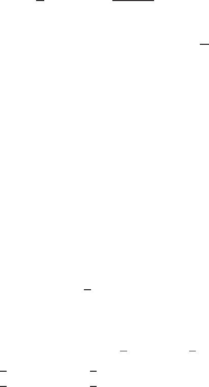
32 Chris Wendl
Differentiat ing K in the sense of distributions provides a formula for ∂(K ∗ f) as a
principal value integral, namely
∂(K ∗f)(z) = −
1
π
lim
ǫ→0
+
Z
|ζ−z|≥ǫ
f(ζ)
(z − ζ)
2
dµ(ζ).
This is a so-called singular integral operat or: it is similar to our pr evious con-
volution operator, but more difficult to handle because the kernel
1
z
2
is not of class
L
1
lo c
on C. The proof of the estimate k∂(K ∗ f) k
L
p
≤ ckf k
L
p
for all f ∈ C
∞
0
(
˚
D)
follows from a r ather difficult general estimate on singular integral operato r s, known
as the Calder´on-Zygmund inequality, cf. [
Wend, §2.A] and the references therein.
The good news however is that the first step in that proof is no t hard: that is the
case p = 2.
As is the case for all elliptic operat ors with constant coefficients, the L
2
-estimate
on the fundament al solution of
¯
∂ admits an easy proof using Fourier t ransforms:
Proposition 2.15 . For all f ∈ C
∞
0
(C), we have k∂(K ∗ f)k
L
2
= kfk
L
2
.
Proof. A sufficient ly nice function u : C → C is related to its Fourier transform
ˆu : C → C by
u(z) =
Z
C
ˆu(ζ)e
2πi(z·ζ)
dµ(ζ)
and thus satisfies the identities
c
¯
∂u(ζ) = 2πiζ ˆu(ζ),
c
∂u(ζ) = 2πi
ζ ˆu(ζ).
Since u = K ∗ f we have ˆu =
ˆ
K
ˆ
f, and since
¯
∂K = δ, we have 2πiζ
ˆ
K = 1. Hence
we may apply Plancharel’s t heorem to deduce
k∂(K ∗f )k
L
2
= k∂uk
L
2
= k
c
∂uk
L
2
= k2 πi
ζ ˆuk
L
2
= k2 πi
ζ
ˆ
K
ˆ
fk
L
2
=
ζ
ζ
2πiζ
ˆ
K
ˆ
f
L
2
=
ζ
ζ
ˆ
f
L
2
= k
ˆ
fk
L
2
= kfk
L
2
.
2.4. Regularity
We will now use the estimate kuk
W
k,p ≤ ck
¯
∂uk
W
k−1,p f r om the previous section
to prove three types of results about solutions to Cauchy-Riemann type equations:
(1) All solutions of reasonable Sobolev-type regularity are smooth.
(2) Any collection of solutions satisfying uniform bounds in certain Sobo lev
norms also locally satisfy uniform C
∞
-bounds.
(3) All reasonable Sobolev-type topologies on spaces of solutions are (locally)
equivalent to the C
∞
-topology.
In the following,
D
r
⊂ C
Lectures on Symplectic Field Theory 33
denotes the closed disk of radius r > 0, and
˚
D
r
denotes its interior. Note that func-
tions of class C
∞
(D
r
) are assumed to be smooth up to the boundary (or equivalently,
on some open neighborhood of D
r
in C), not just on
˚
D
r
.
2.4.1. The linear case. Recall from Exercise
2.2 that every linear Cauchy-
Riemann type operator on a vector bundle of complex rank n locally takes the form
¯
∂ + A, where
¯
∂ = ∂
s
+ i∂
t
, and A is a smooth function with values in End
R
(C
n
).
Using the Sobolev embedding theorem, the following result implies by induction
that solutions u ∈ W
1,p
to the equation (
¯
∂ + A)u = 0 are always smoot h.
Theorem 2.16 (Linear regularity). Assume 1 < p < ∞ and k, m ∈ N.
(1) If u ∈ W
k,p
(
˚
D) satisfies
¯
∂u ∈ W
m,p
(
˚
D), then u is in W
m+1,p
on every
co mpact subset of
˚
D.
(2) Suppose f
ν
∈ W
m,p
(
˚
D) is a sequence converging in the W
m,p
-topo l ogy to
f ∈ W
m,p
(
˚
D) as ν → ∞, and u
ν
∈ W
k,p
(
˚
D) is a sequence with
¯
∂u
ν
= f
ν
.
(a) If there exist uniform bounds on ku
ν
k
W
k,p
and kf
ν
k
W
m,p
over
˚
D as
ν → ∞, then ku
ν
k
W
m+1,p
is also uniformly bounded on every com pact
subset of
˚
D.
(b) If the seq uen ce u
ν
is W
k,p
-convergent on
˚
D to a function u ∈ W
k,p
(
˚
D)
satisfying
¯
∂u = f, then it is a l s o W
m+1,p
-convergent on every compact
subset of
˚
D.
Proof. We begin by proving statement (
2a), assuming t hat statement (1) is
already known, hence u
ν
∈ W
m+1,p
lo c
(
˚
D) since f
ν
∈ W
m,p
(
˚
D). Assume m = k,
since there is otherwise nothing to prove. Then by induction, it suffices t o show
that uniform bounds on ku
ν
k
W
k,p
(
˚
D)
and kf
ν
k
W
k,p
(
˚
D)
imply a uniform bound on
ku
ν
k
W
k+1,p
(
˚
D
r
)
for any g iven r < 1; equivalently, t his would mean there is a uniform
bound on k∂
j
u
ν
k
W
k,p
(
˚
D
r
)
for j = 1, 2. In order to apply the elliptic estimate, we need
to work with functions with compact support in
˚
D, thus choose a smooth bump
function
β ∈ C
∞
0
(
˚
D, [0, 1])
that satisfies β|
D
r
≡ 1. We then have β ∂
j
u
ν
∈ C
∞
0
(
˚
D), so by Theorem
2.13,
k∂
j
u
ν
k
W
k,p
(
˚
D
r
)
≤ kβ ∂
j
u
ν
k
W
k,p
(
˚
D)
≤ c
¯
∂ (β ∂
j
u
ν
)
W
k−1,p
(
˚
D)
≤ ck(
¯
∂β)(∂
j
u
ν
)k
W
k−1,p + ckβ
¯
∂(∂
j
u
ν
)k
W
k−1,p .
(2.5)
The first term on the right hand side is uniformly bounded since
¯
∂β is smo oth and
ku
ν
k
W
k,p
is uniformly bounded. To control the second term, we differentiate the
equation
¯
∂u
ν
= f
ν
, giving
¯
∂(∂
j
u
ν
) = ∂
j
f
ν
.
This also ha s a uniformly bounded W
k−1,p
-norm since kf
ν
k
W
k,p is uniformly bounded.
Since β is smooth, this bounds the second term on the right hand side of (
2.5) as
ν → ∞, and we ar e done.
Statement (
2b) follows by a similar argument bounding k∂
j
(u − u
ν
)k
W
k,p
(
˚
D
r
)
in
terms of ku − u
ν
k
W
k,p
(
˚
D)
and kf − f
ν
k
W
k,p
(
˚
D)
; we leave the details as an exercise.

34 Chris Wendl
Lastly, we prove stat ement (1), where again it suffices to assume
¯
∂u = f ∈
W
k,p
(
˚
D) and show that u|
˚
D
r
∈ W
k+1,p
(
˚
D
r
) for some r < 1. The idea is to use the
same argument that was used for statement (
2a), but with the partial derivatives
∂
j
u replaced by the difference quotients
D
h
j
u(z) :=
u(z + he
j
) −u(z)
h
, j = 1, 2,
where e
1
:= ∂
s
, e
2
:= ∂
t
, and the r ole of the index ν → ∞ is now played by the
parameter h ∈ R \ {0} approaching 0. Note that if u ∈ W
k,p
(
˚
D), t hen β D
h
j
u is a
well-defined function on
˚
D for all |h| 6= 0 sufficiently small and belongs to W
k,p
0
(
˚
D).
The analogue of (
2.5) in this context is then
kD
h
j
uk
W
k,p
(
˚
D
r
)
≤ kβD
h
j
uk
W
k,p
(
˚
D)
≤ c
¯
∂
β D
h
j
u
W
k−1,p
(
˚
D)
≤ ck(
¯
∂β)(D
h
j
u)k
W
k−1,p + ckβ
¯
∂(D
h
j
u)k
W
k−1,p .
The first t erm is bounded independently o f h since ∂
j
u ∈ W
k−1,p
(
˚
D), implying a
uniform W
k−1,p
-bound on D
h
j
u as h → 0. To control the second term, we can apply
the operator D
h
j
to the equation
¯
∂u = f, giving
¯
∂(D
h
j
u) = D
h
j
(
¯
∂u) = D
h
j
f.
This satisfies a W
k−1,p
-bound that is uniform in h since ∂
j
f ∈ W
k−1,p
(
˚
D), so we
conclude t hat for all |h| sufficiently small,
kD
h
j
uk
W
k,p
(
˚
D
r
)
≤ c
for some constant c > 0 tha t does not change as h → 0. By a standard application
of the Banach-Alaoglu theorem (cf. [
Eva98, §5.8.2]), this implies the existence of a
sequence h
ν
→ 0 for which D
h
ν
j
u is W
k,p
-convergent on
˚
D
r
, and its limit is necessarily
∂
j
u, which therefore belongs to W
k,p
. Indeed, if k = 0, the uniform L
p
-bound
on D
h
ν
j
u over
˚
D
r
for any sequence h
ν
→ 0 gives rise to a weakly L
p
-convergent
subsequence via the Banach-Alaoglu theorem. The limit of this subsequence belongs
to L
p
(
˚
D
r
), and it is straightforward to show using the definition of weak derivatives
that this limit is ∂
j
u. One finds the same result for a ny k ∈ N by applying this
argument to higher-order derivatives of ∂
j
u. The conclusion is that u is in W
k+1,p
on
˚
D
r
, since u and both of its first par t ial derivatives belong to W
k,p
.
Exercise 2.17. Show that all three parts of Theorem
2.16 continue to hold if
the operator
¯
∂ is replaced by
¯
∂ + A or
¯
∂ + A
ν
, where A, A
ν
∈ C
∞
(D, End
R
(C
n
))
with A
ν
→ A in C
∞
as ν → ∞.
Exercise 2.18. Use Theorem
2.16(1) to extend Theorem 2.12 to the existence
of a bounded right inverse for
¯
∂ : W
k,p
(
˚
D) → W
k−1,p
(
˚
D).
Hint: For any R > 1, there exists a bounded linear extension o perator E : W
k,p
(
˚
D) →
W
k,p
(
˚
D
R
) with the property (Ef)|
˚
D
= f for all f ∈ W
k,p
(
˚
D); see Theorem
A.4 and
Corollary A.5.
Lectures on Symplectic Field Theory 35
The above exercise can be used to improve the first part of Theorem 2.1 6 to
cover weak solutions of class L
1
lo c
. We start with a classical result about “weakly
holomorphic” functions:
Lemma 2.19. If u ∈ L
1
(
˚
D) satisfies
¯
∂u = 0 in the se nse of distributions, then u
is smooth and holomorphic.
Proof. Taking real and imaginary parts, it suffices to prove that the same
statement holds for the Laplace equation. By mollification, a ny weakly ha r mo nic
function can be approximated in L
1
with smooth harmonic functions. The lat-
ter satisfy the mean value property, which behaves well under L
1
-convergence, so
the result fo llows from the mean value characterization of harmonic functions; see
[
Wend, Lemma 2.6.26] for more details.
Lemma 2.20. Suppose 1 < p < ∞, k ∈ N, and u ∈ L
1
(
˚
D) is a weak solution to
¯
∂u = f for some f ∈ W
k,p
(
˚
D). Then u is of class W
k+1,p
on every compact subset
of
˚
D.
Proof. Let T : W
k,p
(
˚
D) → W
k+1,p
(
˚
D) denote a bounded right inverse of
¯
∂ :
W
k+1,p
(
˚
D) → W
k,p
(
˚
D) as provided by Exercise
2.18. Then u − T f ∈ L
1
(
˚
D) is a
weak solution to
¯
∂(u − T f) = 0 and is thus smooth by Lemma
2.19. In particular,
u − T f restricts to
˚
D
r
for every r < 1 as a function of class W
k+1,p
, implying that
u also has a restriction in W
k+1,p
(
˚
D
r
).
Corollary 2.21 (Weak linear regularity). Suppos e 1 < p < ∞. Then given
A ∈ C
∞
(D, End
R
(C
n
)), eve ry w eak solution u ∈ L
p
(
˚
D, C
n
) of (
¯
∂ +A)u = 0 is smooth
on
˚
D.
2.4.2. The nonlinear case. L ocally, every J-holomorphic curve can be re-
garded as a map u :
˚
D → C
n
satisfying u(0) = 0 and
¯
∂
J
u := ∂
s
u + J(u)∂
t
u = 0,
where J is a smooth almost complex structure on C
n
satisfying J(0) = i. Theo-
rem
2.16 now has the following analogue.
Theorem 2.22 (Nonlinear regularity). Assume 1 < p < ∞ and k ∈ N s atisfy
kp > 2, and fix a smooth almost compl e x structure J on C
n
with J(0) = i.
(1) Every map u ∈ W
k,p
(
˚
D, C
n
) satisfying u(0) = 0 and
¯
∂
J
u = 0 is smooth
on
˚
D.
(2) Suppose J
ν
is a sequence of s mooth alm ost comple x structures on C
n
co n-
verging in C
∞
lo c
to J as ν → ∞, and u
ν
∈ W
k,p
(
˚
D, C
n
) is a sequence of
smooth maps s atisfying
¯
∂
J
ν
u
ν
= 0.
(a) If the maps u
ν
are uniformly W
k,p
-bounded on
˚
D, then they are also
uniformly C
m
-bounded on compact subsets of
˚
D for every m ∈ N.
(b) If the sequence u
ν
is W
k,p
-convergent on
˚
D to a smooth map u :
˚
D →
C
n
, then it is also C
∞
-convergent on every compact subset of
˚
D.

36 Chris Wendl
Our proo f of this will follow much the same outline as the proof of Theorem 2.16,
and indeed, one could use exactly the same argument if J were identically equal to i
(in which case the theorem can also be deduced from complex analysis). The r eason
it works in the general case is tha t if we zoom in on a sufficiently small neighborhood
of the origin in C
n
, then J can be viewed as a C
∞
-small p erturbation of i. To make
this precise, we shall use the following rescaling trick.
Associate to any smooth almost complex structure J on C
n
the function
Q := i − J ∈ C
∞
(C
n
, End
R
(C
n
)).
In terms of Q, the equation ∂
s
u + J(u)∂
t
u = 0 then becomes
(2.6)
¯
∂u − (Q ◦ u)∂
t
u = 0,
where we are regarding Q ◦ u as a function
˚
D → End
R
(C
n
). Given constants R ≥ 1
and ǫ ∈ (0, 1], associate to J and u the functions
b
J : C
n
→ End
R
(C
n
),
b
J(p) := J(p/R),
b
Q : C
n
→ End
R
(C
n
),
b
Q(p) := Q(p/R) = i −
b
J(p),
ˆu :
˚
D → C
n
, u(z) := Ru(ǫz).
(2.7)
Now u satisfies (
2.6) if and only if ˆu satisfies
(2.8)
¯
∂ˆu − (
b
Q ◦ ˆu)∂
t
ˆu = 0.
The rescaled almost complex structure has the convenient feature that if J(0) = i,
then
b
J can be made arbitrarily C
∞
-close to i on the unit disk
D
2n
⊂ C
n
by choosing R sufficiently large, which means k
b
Qk
C
m
(D
2n
)
can be made arbitrarily
small for every m ∈ N. If u is also continuous and satisfies u(0) = 0, then after
fixing some large value for R, we can also choose ǫ ∈ (0 , 1] sufficiently small to ensure
u(
˚
D) ⊂
˚
D
2n
and make k
b
Q ◦ ˆuk
C
0
(D)
arbitrarily small. By Propositions 2 .8 and 2.10,
we can similarly arrang e for k
b
Q ◦ ˆuk
W
k,p to be arbitrarily small if u is of class W
k,p
with kp > 2, and the same will hold for k
b
Q
ν
◦ ˆu
ν
k
W
k,p when ν is large if ku
ν
k
W
k,p
is uniformly bounded and u
ν
(0) → 0. Here of course we abbreviate Q
ν
:= i − J
ν
and
b
Q
ν
(p) := Q
ν
(p/R). The effect is to make equations such as (
2.8) W
k,p
-close
to the linear equation
¯
∂ˆu = 0 if ǫ > 0 and R > 0 are sufficiently small and large
respectively.
The price we pay for this r escaling is t hat if we are able to prove e.g. a uniform
bound on the norms kˆu
ν
k
W
k,p
(
˚
D)
for some sequence u
ν
, then the resulting W
k+1,p
-
bound for u
ν
will be valid only on
˚
D
ǫ
, a very small ball about the origin. But this
is good enough for obtaining estimates over all compact subsets of
˚
D: indeed, we
can always reparametrize u :
˚
D → C
n
to put the origin at some other point and
prove suitable estimates near that point, appealing in the end to the fact that any
compact subset of
˚
D is covered by a finite union of small disks about points.
The need to use this rescaling trick is one of a few reasons why the condition
kp > 2 is needed in Theorem
2.22, while it was irrelevant in the linear case.
Lectures on Symplectic Field Theory 37
Proof of Theorem 2.22. We will prove statement (2a) and leave the rest as
exercises.
By the remarks above, it suffices to prove that if u
ν
:
˚
D → C
n
are smooth J
ν
-
holomorphic curves satisfying a unifo rm bound in W
k,p
(
˚
D), then for some r < 1, the
rescaled
b
J
ν
-holomorphic curves ˆu
ν
:
˚
D → C
n
defined as in (2.7) satisfy a uniform
W
k+1,p
-bound on
˚
D
r
. In fact, it suffices to prove that every subsequence of u
ν
has
a further subsequence for which this is true. Indeed, if the bound for the whole
sequence did not exist, then we would be able to find a subsequence with norms
blowing up to infinity, and no further subsequence of this subsequence could satisfy
a uniform bound. With this understood, we can appeal to the f act that W
k,p
-
bounded sequences are also C
0
-bounded for kp > 2 and thus replace u
ν
with a
subsequence ( still denoted by u
ν
) such that, after a suitable change of coordinat es
on C
n
,
u
ν
(0) → 0.
Our goal is then to show that for a suitable choice of the rescaling parameters ǫ and
R, this subsequence admits a uniform bound on k∂
j
ˆu
ν
k
W
k,p
(
˚
D
r
)
for j = 1, 2 .
The a rgument b egins exactly the same as in the linear case: choose a smooth
bump function
β ∈ C
∞
0
(
˚
D, [0, 1])
that satisfies β|
D
r
≡ 1. We then have β ∂
j
ˆu
ν
∈ C
∞
0
(
˚
D), so by Theorem
2.13,
(2.9) k∂
j
ˆu
ν
k
W
k,p
(
˚
D
r
)
≤ kβ ∂
j
ˆu
ν
k
W
k,p
(
˚
D)
≤ c
¯
∂ (β ∂
j
ˆu
ν
)
W
k−1,p
(
˚
D)
.
Instead of rewriting
¯
∂(β ∂
j
ˆu
ν
) as a sum of two terms, let us derive a PDE satisfied
by β ∂
j
ˆu
ν
. Differentiating the equation
¯
∂ˆu
ν
− (
b
Q
ν
◦ ˆu
ν
)∂
t
ˆu
ν
= 0 gives
¯
∂(∂
j
ˆu
ν
) = ∂
j
(
¯
∂ˆu
ν
) = ( d
b
Q
ν
◦ ˆu
ν
) (∂
j
ˆu
ν
, ∂
t
ˆu
ν
) + (
b
Q
ν
◦ ˆu
ν
)∂
j
∂
t
ˆu
ν
,
thus β ∂
j
ˆu
ν
satisfies
¯
∂(β ∂
j
ˆu
ν
) − (
b
Q
ν
◦ˆu
ν
)∂
t
(β ∂
j
ˆu
ν
)
= β(d
b
Q
ν
◦ ˆu
ν
)(∂
j
ˆu
ν
, ∂
t
ˆu
ν
) +
¯
∂β − (
b
Q
ν
◦ ˆu
ν
)∂
t
β
∂
j
ˆu
ν
= (d
b
Q
ν
◦ ˆu
ν
)(β ∂
j
ˆu
ν
, ∂
t
ˆu
ν
) +
¯
∂β − (
b
Q
ν
◦ ˆu
ν
)∂
t
β
∂
j
ˆu
ν
,
(2.10)
and combining this with (
2.9) gives
(2.11)
kβ ∂
j
ˆu
ν
k
W
k,p
≤ c
(
b
Q
ν
◦ ˆu
ν
)∂
t
(β ∂
j
ˆu
ν
)
W
k−1,p
+ c
(d
b
Q
ν
◦ ˆu
ν
)(β ∂
j
ˆu
ν
, ∂
t
ˆu
ν
)
W
k−1,p
+ c
¯
∂β − (
b
Q
ν
◦ ˆu
ν
)∂
t
β
∂
j
ˆu
ν
W
k−1,p
.
In order to find bounds for the three terms on the right, recall that using Proposi-
tions
2.8 and 2.10 and the assumption u
ν
(0) → 0, we can supp ose
b
Q
ν
◦ ˆu
ν
W
k,p
≤ δ

38 Chris Wendl
for sufficiently la r ge ν, where δ > 0 is a constant that may be assumed arbitrarily
small via suitable choices of the rescaling par ameters ǫ and R. This provides a
uniform bound on the third term in (
2.11), as there is also a continuous product
pairing W
k,p
× W
k−1,p
→ W
k−1,p
by Prop.
2.7, giving an estimate of the form
¯
∂β − (
b
Q
ν
◦ ˆu
ν
)∂
t
β
∂
j
ˆu
ν
W
k−1,p
≤ c
¯
∂β − (
b
Q
ν
◦ ˆu
ν
)∂
t
β
W
k,p
· k∂
j
ˆu
ν
k
W
k−1,p
≤ c
′
kˆu
ν
k
W
k,p ≤ c
′′
.
For the first term on the right side of (
2.11), the product pa iring similarly gives
(
b
Q
ν
◦ ˆu
ν
)∂
t
(β ∂
j
ˆu
ν
)
W
k−1,p
≤ c
b
Q
ν
◦ ˆu
ν
W
k,p
· k∂
t
(β ∂
j
ˆu
ν
)k
W
k−1,p
≤ cδkβ ∂
j
ˆu
ν
k
W
k,p .
Finally, since J
ν
→ J in C
k+1
on compact subsets, we ar e also free to assume after
adjusting the rescaling parameters that
kd
b
Q
ν
◦ ˆu
ν
k
W
k,p
≤ δ,
so we can apply the product pairing W
k,p
×W
k−1,p
→ W
k−1,p
twice to estimate
(d
b
Q
ν
◦ ˆu
ν
)(β ∂
j
ˆu
ν
, ∂
t
ˆu
ν
)
W
k−1,p
≤ c
d
b
Q
ν
◦ ˆu
ν
W
k,p
· kβ ∂
j
ˆu
ν
k
W
k,p · k∂
t
ˆu
ν
k
W
k−1,p
≤ cδkβ ∂
j
ˆu
ν
k
W
k,p · kˆu
ν
k
W
k,p
≤ cc
′
δkβ ∂
j
ˆu
ν
k
W
k,p =: c
′′
δkβ ∂
j
ˆu
ν
k
W
k,p .
Combining the three estimates for the rig ht hand side of (
2.11) now gives
kβ ∂
j
ˆu
ν
k
W
k,p ≤ c + cδkβ ∂
j
ˆu
ν
k
W
k,p ,
so after adjusting the scaling parameters R and ǫ to ensure cδ < 1, we obtain the
uniform bound
kβ ∂
j
ˆu
ν
k
W
k,p ≤
c
1 − cδ
.
This pr ovides the desired unifor m bound on k∂
j
ˆu
ν
k
W
k,p
(
˚
D
r
)
.
Exercise 2.23. Use an analogo us arg ument via difference quotients to prove
statement (
1) in Theorem 2.22. Hint: If you’re anything like me, you might get
stuck trying to estimate t he second term in the difference quotient a nalogue of
(
2.11). The difficulty is that this expression was derived using the chain rule for
derivatives, and there is no similarly simple chain rule for difference quotients. The
trick is to remember that difference quotients only differ from t he corresponding
derivatives by a remainder term. The remainder will produce an extra term in the
difference quotient version of (
2.11), but the extra term can be bounded.
2.5. Linear local existence and applications
The following lemma can be applied in the case A ∈ C
∞
(D, End
C
(C
n
)) to prove
the aforementioned standard fact that complex-linear Cauchy-Riemann type oper-
ators induce holomorphic structures on vector bundles. The version with weakened
regularity will be applied below to prove a useful “unique continuation” result about
solutions to (
¯
∂ + A)f = 0 in the real-linear case.
Lectures on Symplectic Field Theory 39
Lemma 2.24. Assume 2 < p < ∞ and A ∈ L
p
(
˚
D, End
R
(C
n
)). Then for suffi-
ciently small ǫ > 0, the proble m
¯
∂u + Au = 0
u(0) = u
0
has a so l ution u ∈ W
1,p
(
˚
D
ǫ
, C
n
).
Remark 2.25. Note that u :
˚
D
ǫ
→ C
n
in the above statement is only a weak
solution to
¯
∂u + Au = 0, as it is not necessarily differentiable, but by the Sobolev
embedding theorem, it is at least continuous.
Proof of Lemma
2.24. The main idea is that if we take ǫ > 0 sufficiently
small, then t he restriction of
¯
∂ + A to
˚
D
ǫ
can be regarded as a small perturbat ion
of
¯
∂ in t he space of b ounded linear operator s W
1,p
→ L
p
. Since the latter has a
bounded right inverse by Theorem 2.12, the same will be true for the perturbation.
Since p > 2, the Sobolev embedding theorem implies that functions u ∈ W
1,p
are also continuous and bounded by kuk
W
1,p
, thus we can define a bounded linear
operator
Φ : W
1,p
(
˚
D) → L
p
(
˚
D) × C
n
: u 7→ (
¯
∂u, u(0)).
Theorem
2.12 implies that this operator is also surjective and has a bounded right
inverse, namely
L
p
(
˚
D) ×C
n
→ W
1,p
(
˚
D) : (f, u
0
) 7→ T f − T f (0) + u
0
,
where T : L
p
(
˚
D) → W
1,p
(
˚
D) is a right inverse of
¯
∂. Thus any operator sufficiently
close to Φ in the norm topology also has a right inverse. Now define χ
ǫ
: D → R to
be the function that equals 1 on D
ǫ
and 0 outside of it, and let
Φ
ǫ
: W
1,p
(
˚
D) → L
p
(
˚
D) × C
n
: u 7→ ((
¯
∂ + χ
ǫ
A)u, u(0)).
To see that this is a bo unded operator, it suffices to check that W
1,p
→ L
p
: u 7→ Au
is bounded if A ∈ L
p
; indeed,
kAuk
L
p
≤ kAk
L
p
kuk
C
0
≤ ckAk
L
p
kuk
W
1,p
,
again using the Sobolev embedding theorem. Now by this same trick, we find
kΦ
ǫ
u − Φuk = kχ
ǫ
Auk
L
p
(
˚
D)
≤ ckAk
L
p
(
˚
D
ǫ
)
kuk
W
1,p
(
˚
D)
,
thus kΦ
ǫ
− Φk is small if ǫ is small, and it follows that in this case Φ
ǫ
is surjective.
Our desired solution is therefore the restriction of any u ∈ Φ
−1
ǫ
(0, u
0
) to
˚
D
ǫ
.
Here is a corollary, which says that every solution to a real-linear Cauchy-
Riemann type equation looks locally like a holomorphic function in some continuous
local trivialization.
Theorem 2.26 (Similarity principle). Suppose A : D → End
R
(C
n
) is smooth an d
u :
˚
D → C
n
satisfies the equation
¯
∂u + Au = 0 with u(0) = 0 . Then for sufficiently
small ǫ > 0, there exist map s Φ ∈ C
0
(D
ǫ
, End
C
(C
n
)) and f ∈ C
∞
(
˚
D
ǫ
, C
n
) such that
u(z) = Φ(z)f (z),
¯
∂f = 0, and Φ(0) = 1.

40 Chris Wendl
Proof. After shrinking the domain if necessary, we may assume without loss
of generality that the smooth solution u :
˚
D → C
n
is bounded. Choose a map
C : D → End
C
(C
n
) satisfying C(z)u(z) = A(z)u(z) and |C(z)| ≤ |A(z)| for almost
every z ∈ D. Then C ∈ L
∞
(
˚
D, End
C
(C
n
)) and u is a weak solution to (
¯
∂ + C)u = 0.
Note that since we do not know anything about the zero set of u, we cannot assume
C is continuous, but we have no trouble assuming C ∈ L
p
(
˚
D) for every p > 2.
Since
¯
∂+C is now complex linear, we can use Lemma
2.24 to find a complex basis
of W
1,p
-smooth weak solutions to (
¯
∂+C)v = 0 on
˚
D
ǫ
that define the standard basis of
C
n
at 0, and these solutions are continuous by the Sobolev embedding theorem. This
gives rise to a map Φ ∈ C
0
(
˚
D
ǫ
, End
C
(C
n
)) that satisfies (
¯
∂ + C)Φ = 0 in the sense
of distributions and Φ(0) = 1. Since Φ is continuous, we can assume without loss of
generality that Φ(z) is invertible everywhere on
˚
D
ǫ
. Setting f := Φ
−1
u :
˚
D
ǫ
→ C
n
,
the Leibniz rule then implies
0 = (
¯
∂ + C)u = (
¯
∂ + C)(Φf) =
(
¯
∂ + C)Φ
f + Φ(
¯
∂f ) = Φ(
¯
∂f),
thus
¯
∂f = 0, and f is smooth by Lemma
2.19.
Corollary 2.27 (Unique continuation). Suppose D is a linear Cauchy-Riemann
type operator on a vector bundle E over a connected Riemann surface, and η ∈ Γ(E)
satisfies Dη = 0. Then either η is identically zero or its zeroes are isolated.
The similarity principle also has many nice applications for the nonlinear Cauchy-
Riemann equation. Here is ano t her “unique continuation” type result for t he non-
linear case.
Proposition 2.28. Suppose J is a smooth almost complex structure on C
n
and
u, v :
˚
D → C
n
are smooth J-holomorphic curves such that u(0) = v(0) = 0 and
u and v have matching partial derivatives of all orders at 0. Then u ≡ v on a
neighborhood of 0.
Proof. Let h = v − u :
˚
D → C
n
. We have
(2.12) ∂
s
u + J(u(z))∂
t
u = 0
and
∂
s
v + J(u(z))∂
t
v = ∂
s
v + J(v(z))∂
t
v + [J(u(z)) − J(v(z))] ∂
t
v
= −[J(u(z) + h(z)) − J(u(z))] ∂
t
v
= −
Z
1
0
d
dt
J(u(z) + th(z)) dt
∂
t
v
= −
Z
1
0
dJ(u(z) + th(z)) ·h(z) dt
∂
t
v =: −A(z)h(z),
(2.13)
where the last step defines a smooth family of linear maps A(z) ∈ End
R
(C
n
). Sub-
tracting (
2.12) from (2.1 3) gives the linear equation
∂
s
h(z) +
¯
J(z)∂
t
h(z) + A(z)h(z) = 0,
where
¯
J(z) := J(u(z)). This is a linear Cauchy-Riemann type equation on a trivial
complex vector bundle over
˚
D with complex structure
¯
J(z) on the fiber at z. The

Lectures on Symplectic Field Theory 41
similarity principle thus implies h(z) = Φ(z)f(z) near 0 for some holomor phic func-
tion f(z) ∈ C
n
and some continuous map Φ(z) ∈ GL(2n, R) representing a change of
trivialization. Now if h has vanishing derivatives of a ll orders at 0, Taylor’s formula
implies
lim
z→0
|Φ(z)f (z)|
|z|
k
= 0
for all k ∈ N, so f must also have a zero of infinite order and thus f ≡ 0.
2.6. Simple curves and multiple covers
We now prove a global result about the structure of closed J-holomorphic curves.
In Lecture
6 we will be able to generalize it in a straightforward way for punctured
holomorphic curves with a symptotically cylindrical behavior.
Theorem 2.29. Assume (Σ, j) is a closed conn ected Riemann surface, (W, J)
is a smooth almost com plex manifold and u : (Σ, j) → (W, J) is a nonconstant
pseudoholomorphi c curve. Then there exists a fac toriz ation u = v ◦ ϕ, where
• ϕ : (Σ, j) → (Σ
′
, j
′
) is a hol omorphic map of positive degree to another
closed and con nected Riemann surface (Σ
′
, j
′
);
• v : (Σ
′
, j
′
) → (W, J) is a pse udo holomorphic curve which is embed ded except
at a finite set of critical points and self-intersections.
Note that holomorphic maps (Σ, j) → (Σ
′
, j
′
) of degree 1 are always diffeomor-
phisms, so the factorization u = v ◦ ϕ in this case is just a repara metrizatio n, and
u is then called a simple curve. In all other cases, k := deg(ϕ) ≥ 2 and ϕ is in
general a branched cover; we then call u a k-fold branched cover of the simple
curve v.
The main idea in the proof is to construct Σ
′
(minus some punctures) explicitly
as the image of u a fter removing finitely many singular points, so that we can take
v to be the inclusion Σ
′
֒→ W . The map ϕ : Σ → Σ
′
is then uniquely determined.
In order to carr y out this program, we need some information on what the image
of u can look like near each of its singularities. These come in two types, each type
corresponding to one of the lemmas below, both of which should seem immediately
plausible if your intuition comes from complex analysis.
Lemma 2.30 (Intersectio ns). Suppose u : (Σ, j) → (W, J) an d v : (Σ
′
, j
′
) →
(W, J) are two nonconstant pseudoh olomorphic curves with an intersection u(z) =
v(z
′
). Then there exist neighborhoods z ∈ U ⊂ Σ and z
′
∈ U
′
⊂ Σ
′
such that
either u(U) = v(U
′
) or u(U \ {z}) ∩ v(U
′
) = u(U) ∩ v( U
′
\ {z
′
}) = ∅.
Lemma 2.31 (Branching). Suppose u : (Σ, j) → (W, J) is a nonconstant pseudo-
holomorphic curve an d z
0
∈ Σ is a critical point of u. Then a neighborhood U ⊂ Σ
of z
0
ca n be biholom o rphically identified with the unit disk D ⊂ C such that
u(z) = v(z
k
) for z ∈ D = U,
where k ∈ N, and v : D → W is an injective J-holo morphic map w i th no critical
po ints except possibly at the origin.
42 Chris Wendl
These two local results follow from a well-known formula of Micallef and White
[
MW95] describing the local behavior of J-holomorphic curves near critical points
and their intersections. The proof of that theorem is analytically quite involved, but
one can also use a n easier “approximate” version, which is proved in [
Wend, §2.14].
Since both ar e closely relat ed to the phenomenon of unique continuation, you will
not be surprised to learn that the similarity principle plays a role in the proof: the
main idea is again to exploit the fact that locally J is always a small perturbation
of i, hence the local behavior of J-holomorphic curves is also similar to the integrable
case.
Proof of Theorem 2.29. Let Crit(u) = {z ∈ Σ | du(z) = 0} denote t he set
of critical points, and define ∆ ⊂ Σ to be the set of all points z ∈ Σ such that there
exists z
′
∈ Σ and neighborhoods z ∈ U ⊂ Σ and z
′
∈ U
′
⊂ Σ with u(z) = u(z
′
) but
u(U \ {z}) ∩ u(U
′
\ {z
′
}) = ∅.
The lemmas quoted above imply that both of t hese sets are discrete. Both are
therefore finite, and the set
˙
Σ
′
= u(Σ \ ( Crit(u) ∪ ∆)) ⊂ W is then a smooth
submanifold of W with J- invariant tangent spaces, so it inherits a natural complex
structure j
′
for which the inclusion (
˙
Σ
′
, j
′
) ֒→ (W, J) is pseudoholomorphic. We
shall now construct a new Riemann surface (Σ
′
, j
′
) from which (
˙
Σ
′
, j
′
) is obtained
by removing a finite set of points. Let
b
∆ = (Crit(u) ∪ ∆)/ ∼, where two points
in Crit(u) ∪ ∆ are defined to be equivalent whenever they have neighbor hoods in
Σ with identical images under u. Then for each [z] ∈
b
∆, the branching lemma
provides an injective J-holomorphic map u
[z]
from the unit disk D onto the image
of a neighborhood of z under u. We define (Σ
′
, j
′
) by
Σ
′
=
˙
Σ
′
∪
Φ
G
[z]∈
b
∆
D
,
where the gluing map Φ is the disjoint union of the maps u
[z]
: D \{0} →
˙
Σ
′
for each
[z] ∈
b
∆; since this map is holomorphic, the complex structure j
′
extends from
˙
Σ
′
to
Σ
′
. Combining the maps u
[z]
: D → W with the inclusion
˙
Σ
′
֒→ W now defines a
pseudoholomorphic map v : (Σ
′
, j
′
) → (W, J) which restricts to
˙
Σ
′
as an embedding
and otherwise has at most finitely many critical points and double points. Moreover,
the restriction of u to Σ \(Crit(u) ∪∆) defines a holomorphic map to (
˙
Σ
′
, j
′
) which
extends by removal of singularities to a proper holomorphic map ϕ : (Σ, j) → (Σ
′
, j
′
)
such that u = v ◦ ϕ. Its holomorphicity implies that it has positive degree.

LECTURE 3
Asymptotic operators
Contents
3.1. The linearization in Morse homology 43
3.2. Spectral flow 46
3.2.1. Geometry in the space of Fredholm operators 47
3.2.2. Symmetric operators of index zero 49
3.2.3. Perturbation of eigenvalues 52
3.2.4. Homotopies of eigenvalues 55
3.3. The Hessian of the contact action functional 57
3.4. The Conley-Ze hnde r index 61
We now begin with the analysis of the particular class of J-holomorphic curves
that a r e important in SFT. The next three lectures will focus on the linearized
problem, the goal being to prove t hat this linearization is Fredholm and to compute
its index. Using this along with the implicit function theorem and the Sard-Smale
theorem (on genericity of smooth nonlinear Fredholm maps), we will lat er be able
to show that moduli spaces of asymptotically cylindrical J-holomorphic curves are
smooth finite-dimensional manifolds under suitable genericity assumptions.
3.1. The linearization in Morse homology
Since Morse homology is the prototype for all Floer-type theories, we can g ain
useful intuition by recalling how the analysis works for the linearization of the gradi-
ent flow problem in Morse theory. The basic features of the problem were discussed
already in §
1.2.
Assume (M, g) is a closed n-dimensional Riemannian manifold, f : M → R is a
smooth function, and for two critical points x
+
, x
−
∈ Crit(f), consider the moduli
space of parametrized gradient flow lines
M(x
−
, x
+
) :=
u ∈ C
∞
(R, M)
˙u + ∇f (u) = 0, lim
s→±∞
u(s) = x
±
.
The map M(x
−
, x
+
) → M : u 7→ u(0) gives a nat ural identification of M(x
−
, x
+
)
with the intersection between the unstable manifold of x
−
and the stable manifold
of x
+
for the negative gradient flow, and we say the pair (g, f) is Morse-Smale if
f is Morse and this intersection is transverse, in which case M(x
−
, x
+
) is a smooth
manifold with
dim M(x
−
, x
+
) = ind(x
−
) −ind(x
+
).
43

44 Chris Wendl
This can all be proved using finite-dimensional different ial topology, but since that
approach does not work in the study of Floer trajectories or holomorphic curves
in symplectizations, let us instead see how o ne proves it using nonlinear functional
analysis. For more details on the following discussion, see [
Sch93].
Following the strategy laid out in §
2.1, M(x
−
, x
+
) can be identified with the
zero set of a smooth section
σ : B → E : u 7→ ˙u + ∇f(u),
where B is a Banach manifold of maps u : R → M satisfying lim
s→±∞
u(s) = x
±
,
and E → B is a smoot h Banach space bundle whose fibers E
u
contain Γ(u
∗
T M).
The linearization Dσ(u) : T
u
B → E
u
of this section at a zero u ∈ σ
−1
(0) defines a
first-order linear differential operato r
D
u
: Γ(u
∗
T M) → Γ(u
∗
T M)
which takes the form
D
u
η = ∇
s
η + ∇
η
∇f
for any choice of symmetric connection ∇ on M. Taking suitable Sobolev comple-
tions of Γ(u
∗
T M), we are therefore led to consider bounded linear operato r s
1
of the
form
(3.1) D
u
= ∇
s
+ ∇∇f : W
k,p
(u
∗
T M) → W
k−1,p
(u
∗
T M)
for k ∈ N and 1 < p < ∞, and the first task is to prove that whenever x
+
and
x
−
satisfy the Morse condition, this is a Fredholm operator of index ind D
u
=
ind(x
−
) − ind(x
+
).
Choose coordinates near x
+
in which g looks like the standard Euclidean inner
product a t x
+
. This induces a trivialization of u
∗
T M over [T, ∞) for T > 0 suf-
ficiently large, and we are free to assume that the connection ∇ is t he standard
one determined by these coordinat es on [T, ∞) . Using the trivialization to identify
sections β ∈ Γ(u
∗
T M) over [T, ∞) with maps f : [T, ∞) → R
n
, D
u
now acts on f
as
(3.2) (D
u
f)(s) = ∂
s
f(s) + A(s)f(s),
where A(s) ∈ R
n×n
is the matrix of the linear transformation dX(s) : R
n
→ R
n
,
with X(s) ∈ R
n
being the coordinate representatio n of ∇f(u( s)) ∈ T
u(s)
M. As
s → ∞, the zeroth-order term in this expression converges to a symmetric matrix
A
+
:= lim
s→∞
A(s),
which is the coordinate representation of the Hessian ∇
2
f(x
+
). Any choice of coor-
dinates near x
−
produces a similar formula f or D
u
over (−∞, −T ], A(s) converging
as s → −∞ to another symmetric matrix A
−
representing ∇
2
f(x
−
). Both the
Morse condition and the dimension ind(x
−
)−ind(x
+
) can now be expressed entirely
1
We are ignoring an a nalytical subtlety: since u
∗
T M → R ha s no canonic al trivialization and R
is noncompact, it is not completely obvious what the definition of the Sobolev space W
k,p
(u
∗
T M )
should be. We will retur n to this issue in a more gener al context in the next lecture.
Lectures on Symplectic Field Theory 45
in terms of these two matrices: x
±
is Morse if and only if A
±
is invertible, and the
Fredholm index of D
u
will then be
ind(x
−
) −ind(x
+
) = dim E
−
(A
−
) −dim E
−
(A
+
),
where for any symmetric mat rix A we denote by E
−
(A) the direct sum of all its
eigenspaces with negative eigenvalue. The main linear functional analytic result
underlying Morse homology can now be stated as follows (cf. [
Sch93]):
Proposition 3.1. Assume k ∈ N and 1 < p < ∞. Suppose E → R is a
smooth vector bundl e with trivializations fixed in neighborhoods of −∞ and +∞, and
D : W
k,p
(E) → W
k−1,p
(E) is a first-order diffe rential operator which asymptotically
takes the form (
3.2) near ±∞ wi th respect to the cho sen trivializations, where A(s)
is a smooth family of n-by-n matrices with well-defined asymptotic limits A
±
:=
lim
s→±∞
A(s) which are symme tric. If A
+
and A
−
are also invertible, then D is
Fredholm and
(3.3) ind(D) = dim E
−
(A
−
) − dim E
−
(A
+
).
Remark 3.2. The hypothesis that A
±
is invertible in Prop.
3.1 cannot be lifted:
indeed, suppose D is Fredholm but e.g. A
+
has 0 in its spectrum. Then one can
easily perturb A( s) and hence A
+
in two distinct ways producing two distinct values
of dim E
−
(A
+
), pushing the zero eigenvalue either up or down. This produces two
perturbed Fredholm operators that have different indices according to (3.3), but
they also belong to a continuo us family of Fredholm operato r s, and must therefore
have the same index, giving a contradiction.
The formula (
3.3) makes sense of course because E
−
(A
±
) are both finite-dimen-
sional vector spaces, but in F loer-type theories we typically encounter critical points
with infinite Morse index. With this in mind, it is useful to note that (
3.3) can
be rewritten without explicitly referencing E
−
(A
+
) or E
−
(A
−
). Indeed, choose
a continuous path of symmetric matrices {B
t
}
t∈[−1,1]
connecting B(−1) := A
−
to
B(1) := A
+
. The spectrum of B
t
varies continuously with t in the following sense:
one can choose a family of continuous functions
{λ
j
: [−1, 1] → R}
j∈I
for the index set I = {1, . . . , n} such that for every t ∈ [−1, 1], the set of eigenvalues
of B
t
counted with multiplicity is {λ
j
(t)}
j∈I
. The spectral flow from A
−
to A
+
is
then defined as a signed count of the number of paths of eigenvalues that cross from
one side of zero to the other, namely (cf. Theorem
3.3)
µ
spec
(A
−
, A
+
) := #
j ∈ I
λ
j
(−1) < 0 < λ
j
(1)
−#
j ∈ I
λ
j
(−1) > 0 > λ
j
(1)
.
The index formula (3.3) now becomes
ind(D) = µ
spec
(A
−
, A
+
).
This description of the index has the advantag e that it could potentia lly make
sense and give a well-defined integer even if A
±
were symmetric o perators on an
infinite-dimensional Hilbert space: they might bot h have infinitely many positive
46 Chris Wendl
and negative eigenvalues, but only finitely many that cha ng e sign along a path fro m
A
−
to A
+
. We will make this discussion precise in the next section.
3.2. Spectral flow
We will see in §
3.3 that in Floer-type theories, the role of the symmetric linear
transformation T
x
M → T
x
M defined by the Hessian ∇
2
f(x) of a Morse function
f : M → R at a critical point is played by a certain class of symmetric operators on
the space of loops η : S
1
→ R
2n
, namely operators of the form
(3.4) (Aη)(t) := −J
0
∂
t
η(t) − S(t)η(t),
where J
0
denotes the standard complex structure on R
2n
= C
n
, and S : S
1
→
End(R
2n
) is a smooth loop of symmetric matrices. The goal of this section is to
define a no t ion of spectral flow for operators of this type. Regarding A as an
unbounded linear operator on L
2
(S
1
, R
2n
) with dense domain H
1
(S
1
, R
2n
), we will
see that its spectrum consists of isolat ed real eigenvalues with finite multiplicity. We
shall prove:
Theorem 3.3. Assume {S
s
: S
1
→ End(R
2n
)}
s∈[−1,1]
is a sm ooth family of loops
of symmetric matrices, and consider the corresponding 1-parameter fami l y of un-
bo und ed li near operators
A
s
= −J
0
∂
t
− S
s
(t) : L
2
(S
1
, R
2n
) ⊃ H
1
(S
1
, R
2n
) → L
2
(S
1
, R
2n
).
Then there exists a set of continuous functions
{λ
j
: [−1, 1] → R}
j∈Z
such that for every s ∈ [−1, 1], the spectrum of A
s
co nsists of the numbers {λ
j
(s)}
j∈Z
,
ea ch of which is an eigenv alue with finite multiplicity equal to the number of times
it is repeated as j varies in Z.
Moreover, if additionally A
−
:= A
−1
and A
+
:= A
1
bo th have trivial kernel,
then the number µ
spec
(A
−
, A
+
) ∈ Z defined by
#
j ∈ Z
λ
j
(−1) < 0 < λ
j
(1)
− #
j ∈ Z
λ
j
(−1) > 0 > λ
j
(1)
is well defined and depends only on A
−
and A
+
.
We will start by giving a more abstract definition of spectral flow as an int er-
section number between a path of symmetric index 0 Fredholm operators and the
subvariety of noninvertible operators. This relies on the general fact that spaces
of operators with kernel and cokernel of fixed finite dimensions form smooth finite-
codimensional submanifolds in the Banach space of all bounded linear operators.
We explain t his fact in §
3.2.1, and then specialize to the case of symmetric index 0
operators to define the abstract version of spectral flow in §
3.2.2. In §3.2.3, we show
that the spectra of such operators vary continuously under small perturbations, and
in §
3.2.4 we specialize further to operators of the form (3.4) and explain how to
interpret the abstract definition of spectral flow in terms of eigenvalues crossing the
origin in R, leading to a proof o f Theorem
3.3.
Spectral flow can be defined more generally for certain classes of self-adjoint
elliptic partia l differentia l operators, see e.g. [
APS76, RS95], and standard proofs

Lectures on Symplectic Field Theory 47
of its existence typically rely on perturbation results as in [Kat95] for the spectra of
self-adjoint operators. In the following presentation, we have chosen to avoid making
explicit use of self-adjointness and instead focus on the Fredholm property; in this
way t he discussion is mostly self-contained and, in particular, does not require a ny
results from [
Kat95].
3.2.1. Geometry in the space of Fredholm operators. Fix a field
F := R or C.
Given Banach spaces X and Y over F, denote by L
F
(X, Y ) the Banach space of
bounded F-linear ma ps from X to Y , with L
F
(X) := L
F
(X, X), and let
Fred
F
(X, Y ) ⊂ L
F
(X, Y )
denote the open subset consisting of Fredholm operators. Recall that an operator
T ∈ L
F
(X, Y ) is Fredholm if its image is closed,
2
and its kernel and cokernel
(i.e. the quotient coker T := Y / im T) are both finite dimensional. Its index is
defined as
ind
F
(T) := dim
F
ker T − dim
F
coker T ∈ Z.
The index defines a continuous and thus locally constant function Fred
F
(X, Y ) → Z,
and for each i ∈ Z, we shall denote
Fred
i
F
(X, Y ) :=
T ∈ Fred
F
(X, Y )
ind(T) = i
.
We will often have occasion to use the following general construction. Given
T
0
∈ Fred
F
(X, Y ), one can choose splittings into closed linear subspaces
X = V ⊕ K, Y = W ⊕ C
such that K = ker T
0
, W = im T
0
, the quotient projection π
C
: Y → coker T
0
restricts to C ⊂ Y as a n isomorphism, and T
0
|
V
defines an isomorphism from V
to W . Using these splittings, any other T ∈ Fred
F
(X, Y ) can be written in block
form as
T =
A B
C D
,
with T
0
itself written in this way as
A
0
0
0 0
for some Banach space isomorphism
A
0
: V → W . Let O ⊂ Fred
F
(X, Y ) denote the open neighborhood of T
0
for which
the block A is invertible, and define a map
(3.5) Φ : O → Hom
F
(ker T
0
, coker T
0
) : T 7→ D − CA
−1
B.
Lemma 3 .4. The map Φ in (
3.5) is smooth, and holomo rp hic in the cas e F = C,
and its derivative at T
0
defines a surjective bounded linear operator L
F
(X, Y ) →
Hom
F
(ker T
0
, coker T
0
) of the form
dΦ(T
0
)H = π
C
H|
ker T
0
,
2
It is not strictly necessary to require that im T ⊂ Y be closed, as this follows from the
finite-dimensionality of the kernel and cokernel, cf. [
AA02, Cor. 2.17].

48 Chris Wendl
where π
C
denotes the natural projection Y → coker T
0
. Moreover, there exists a
smooth function Ψ : O → L
F
(X) such that for every T ∈ O, Ψ(T) : X → X maps
ker Φ(T) ⊂ ker T
0
isomorphically to ker T.
Proof. Smoothness, holomorphicity
3
and the formula for the derivative are
easily verified fro m the given fo r mula for Φ; in particular, since the blocks B and C
both vanish for T = T
0
, we have
dΦ(T
0
) : L
F
(X, Y ) → Ho m
F
(K, C)
A
′
B
′
C
′
D
′
7→ D
′
.
The map Ψ : O → L
F
(X) = L
F
(V ⊕K) is defined by
Ψ(T) =
1 −A
−1
B
0 1
.
For each T, this is an isomorphism; indeed, its inverse is given by
Ψ(T)
−1
=
1 A
−1
B
0 1
.
Then TΨ(T) =
A 0
C Φ(T)
, and since A is invertible, ker TΨ(T) = {0}⊕ker Φ(T).
Proposition 3.5. For each i ∈ Z and each n onnegative integer k ≥ i, the subset
Fred
i,k
F
(X, Y ) :=
T ∈ Fred
i
F
(X, Y )
dim
F
ker T = k and dim
F
coker T = k − i
admits the structure of a smooth (and complex-analytic if F = C) finite-codimensiona l
Banach subman i f old of L
F
(X, Y ), with
codim
F
Fred
i,k
F
(X, Y ) = k(k − i).
Proof. Applying the implicit function theorem to the map Φ from Lemma
3.4
endows a neighborhood of T
0
in Φ
−1
(0) ⊂ Fred
F
(X, Y ) with the structure of a
smooth Banach submanifold with
codim
F
Φ
−1
(0) = dim
F
Hom
F
(ker T
0
, coker T
0
) = k(k − i).
If F = C, then Φ is also holomo rphic and Φ
−1
(0) is thus a complex-analytic sub-
manifold near T
0
. Now observe that for every T ∈ O,
dim
F
ker T = dim
F
ker Φ(T) ≤ dim
F
ker T
0
= k,
with equality if and only if Φ(T) = 0, hence, since the index is locally constant, we
get Φ
−1
(0) = Fred
i,k
F
(X, Y ) in a neighborhood of T
0
.
3
Holomorphicity in this infinite-dimensio nal setting means the same thing as usual: L
C
(X, Y )
and Hom
C
(ker T
0
, coker T
0
) bo th have natural complex structures if T
0
∈ Fred
C
(X, Y ), and we
require dΦ(T) to commute with them for all T ∈ O.
Lectures on Symplectic Field Theory 49
For real-linear operators of index 0, one can use Prop. 3.5 to define the following
“relative” invariant. Given two Banach space isomorphisms T
±
: X → Y that lie in
the same connected component of Fred
R
(X, Y ), define
µ
spec
Z
2
(T
−
, T
+
) ∈ Z
2
as the parity of the number of times that a generic smooth path [−1, 1] → Fred
0
R
(X, Y )
from T
−
to T
+
passes through operators with nontrivial kernel. This is well
defined due to the following consequences of standard tra nsversality theory (see
Exercise
3.6): first, generic paths {T(t) ∈ Fred
0
R
(X, Y )}
t∈[−1,1]
are transverse to
Fred
0,k
R
(X, Y ) for every k ∈ N, which implies via the codimension formula in Prop.
3.5
that they never intersect Fred
0,k
R
(X, Y ) for k ≥ 2, and their intersections with
Fred
0,1
R
(X, Y ) are transverse and thus isolated. Second, transversality also holds
for generic homotopies
[0, 1] ×[−1, 1] → Fred
0
R
(X, Y ) : (s, t) 7→ T
s
(t)
with fixed end points between any pair of generic paths T
0
(t) and T
1
(t), so that the
set of intersections with Fred
0,k
R
(X, Y ) is again empty for k ≥ 2 and forms a smoot h
1-dimensional submanifold in [0, 1] ×[−1, 1] for k = 1. This submanifold, moreover,
is disjoint from [0, 1] × {−1, 1} since T
s
(±1) = T
±
, and it is also compact since
the set of T ∈ Fred
0
R
(X, Y ) with nontrivial kernel is a closed subset. We therefore
obtain a compact 1-dimensional cobordism between the intersection sets of T
0
and
T
1
respectively with Fred
0,1
R
(X, Y ), implying that the count of intersections modulo 2
does not depend on the choice of generic path.
Exercise 3.6. Convince yourself that the standard results (as in e.g. [
Hir94,
§3.2] about generic transversality of intersections between smoo t h maps f : M → N
and submanifolds A ⊂ N continue to hold—with minimal modifications to the
proofs—when N is an infinite-dimensional Banach manifold and A ⊂ N has finite
codimension.
Exercise 3.7. For matrices A
±
∈ GL(n, R), show that µ
spec
Z
2
(A
−
, A
+
) = 0 if and
only if det A
+
and det A
−
have the same sign.
Remark 3.8. The Z
2
-valued spectral flow µ
spec
Z
2
cannot be lifted to Z without
restricting the class of operators under consideration. See Exercise
3.19.
3.2.2. Symmetric operators of index zero. We now add the following as-
sumptions to the setup from the previous subsection:
• Y is a Hilbert space H over F, with inner product denoted by h , i
H
;
• X is an F-linear subspace D ⊂ H, carrying a Banach space structure for
which the inclusion D ֒→ H is a compact linear operator.
The notation D = X is motivated by the fact that if T ∈ L
F
(D, H), then we can
also regard T as an unbounded operator on H with domain D a nd thus consider
the spectrum of T, see §
3.2.3 below.
Since H is a Hilbert space, the space L
F
(H) of bounded linear o perators from
H to itself contains a distinguished closed linear subspace
L
sym
F
(H) ⊂ L
F
(H),
50 Chris Wendl
consisting of self-adjoint operators. For operators tha t are bounded f rom D to H
but not necessarily defined or bounded on H, there is also the space of symmetric
operators
L
sym
F
(D, H) :=
T ∈ L
F
(D, H)
hx, Tyi
H
= hTx, yi
H
for all x, y ∈ D
.
Important examples of symmetric operators are those which are self-adjoint (see
Remark
3.12 below), though for our purposes, it will suffice to restrict attention to
symmetric operators that are a lso Fredholm with index 0. It turns out that the space
of symmetric operators in Fred
0,1
F
(D, H) is a canonically co-oriented hypersurface in
L
sym
F
(D, H), so t hat the invariant µ
spec
Z
2
(T
−
, T
+
) defined above can be modified to
have integer values when T
±
are symmetric. We will need a slightly more specialized
version of this statement in order to give a general definition of spectral flow.
Fix an operator T
ref
∈ L
sym
F
(D, H) that is Fredholm with index zero, and con-
sider the space
Fred
sym
F
(D, H, T
ref
) :=
T
ref
+ K : D → H
K ∈ L
sym
F
(H)
.
Note t hat the restriction o f each K ∈ L
F
(H) to D is a compact o perator D →
H, thus Fred
sym
F
(D, H, T
ref
) has a natural continuous inclusion into the space of
symmetric Fr edholm o perators with index 0. It is also an affine space over L
sym
F
(H)
and can thus be regarded naturally as a smooth Banach manifold locally modeled
on L
sym
F
(H); in particular, its tangent spaces are
T
T
(Fred
sym
F
(D, H, T
ref
)) = L
sym
F
(H).
A remark about the case F = C is in order: L
sym
C
(D, H) is a real-linear and not a
complex subspace of L
C
(D, H), thus Fred
sym
C
(D, H, T
ref
) is a real Banach manifold
but does not carry a natural complex structure.
Lemma 3.9. For any T ∈ L
sym
F
(D, H) that is Fredholm with index 0, ker T i s the
orthog onal complem ent o f im T in H, hence there exist splittings into closed linear
subspace s
D = V ⊕ K, H = W ⊕ C
where K = C = ker T, W = im T and V = W ∩ D.
Proof. If x ∈ K := ker T, then symmetry implies hx, Tyi
H
= hTx, yi
H
= 0
for all y ∈ D, hence K ⊂ W
⊥
, where W := im T. But since ind T = 0 , the
dimension of ker T equals the codimension of im T, implying that K already has the
largest po ssible dimension for a subspace that intersects W trivially, a nd therefore
W ⊕K = H. Since K is also a subspace of D and the latter is a subspace of H, any
x ∈ D can be written uniquely as x = v + k where k ∈ K and v ∈ W ∩ D = : V .
The continuous inclusion of D into H and the f act that W is closed in H imply that
V is a closed subspace of D.
We now have the following modification of Prop.
3.5.
Proposition 3.10 . For each integer k ≥ 0, the subset
Fred
sym,k
F
(D, H, T
ref
) :=
T ∈ Fred
sym
F
(D, H, T
ref
)
dim
F
ker T = k
Lectures on Symplectic Field Theory 51
is a smooth finite-codimensional Banach submanifold o f Fred
sym
F
(D, H, T
ref
), with
codim
R
Fred
sym,k
F
(D, H, T
ref
) =
(
k(k + 1)/2 if F = R,
k
2
if F = C.
In particular, Fred
sym,1
F
(D, H, T
ref
) is a subma nifold of Fred
sym
F
(D, H, T
ref
) with codi-
mension 1, and moreover, it carries a canonical co-orientation.
Proof. Given T
0
∈ Fred
sym,k
F
(D, H, T
ref
), fix the splittings D = V ⊕ K and
H = W ⊕ K as in Lemma
3.9. Using these in the construction of the map Φ
from (
3.5) produces a neighborhood O ⊂ Fred
sym
F
(D, H, T
ref
) of T
0
such that, by
Lemma
3.4, {T ∈ O | dim
F
ker T = k} = Φ
−1
(0), where
Φ : O → End
F
(K) :
A B
C D
7→ D − CA
−1
B.
Since the splittings are orthogonal, an element T =
A B
C D
∈ O is symmetric if
and only if
hx, Ayi
H
= hAx, yi
H
for all x, y ∈ V ,
hx, Dyi
H
= hDx, yi
H
for all x, y ∈ K,
hx, Byi
H
= hCx, yi
H
for all x ∈ V , y ∈ K,
hx, Cyi
H
= hBx, yi
H
for all x ∈ K, y ∈ V ,
and it follows then that Φ(T) ∈ End
sym
F
(K), where End
sym
F
(K) ⊂ End
F
(K) is the real
vector space of symmetric (or Hermitian when F = C) linear maps on (K, h , i
H
).
We thus have O∩Fred
sym,k
F
(D, H, T
ref
) = Φ
−1
(0) with Φ regarded as a smo oth map
O ∩ Fred
sym
F
(D, H, T
ref
) → End
sym
F
(K). The derivative at T
0
again takes the form
dΦ(T
0
) : L
sym
F
(H) → End
sym
F
(K) :
A
′
B
′
C
′
D
′
7→ D
′
,
where now the block matrix represents an element of L
sym
F
(H) with resp ect to the
splitting H = W ⊕ K. This o perator is evidently surjective, hence by the implicit
function theorem, Φ
−1
(0) is a smooth Banach submanifold with codimension equal
to dim
R
End
sym
F
(K).
Finally, we observe that in the case k = 1, the above identifies Fred
sym,1
F
(D, H, T
ref
)
locally with the zero set of a submersion to End
sym
F
(K), which is a real 1-dimensional
vector space since K is a 1-dimensional vector space over F. The canonical isomor-
phism
R → End
sym
F
(K) : a 7→ a1
thus determines a co-orientat ion on Fred
sym,1
F
(D, H, T
ref
).
The co-orientation of Fred
sym,1
F
(D, H, T
ref
) means that one can now define signed
intersection numbers between Fred
sym,1
F
(D, H, T
ref
) and smooth paths in the ambient
space Fred
sym
F
(D, H, T
ref
). Moreover, the codimensions of Fred
sym,k
F
(D, H, T
ref
) f or
each k ≥ 2 are still at least 3, hence large enough to ensure that generic paths or
52 Chris Wendl
homotopies o f paths will never intersect them. The following notion is therefore
independent of choices.
Definition 3.11. Suppose T
+
: T
−
∈ Fred
sym
F
(D, H, T
ref
) are both Banach
space isomorphisms D → H. The spectral flow
µ
spec
(T
−
, T
+
) ∈ Z
from T
−
to T
+
is then defined as the signed count of intersections of T : [−1, 1] →
Fred
sym
F
(D, H, T
ref
) with Fred
sym,1
F
(D, H, T
ref
), where T : [−1, 1] → Fred
sym
F
(D, H, T
ref
)
is any smooth path that is transverse to Fred
sym,k
F
(D, H, T
ref
) for every k ≥ 1 and
satisfies T(±1) = T
±
.
3.2.3. Perturbation of eigenvalues. Continuing in t he setting of the previous
subsection, we shall now regard each T ∈ Fred
sym
F
(D, H, T
ref
) as an unbounded
operator on H with domain D, see e.g. [
RS80, Chapter VIII]. Notice that for each
scalar λ ∈ F, the operator T−λ also belongs to Fred
sym
F
(D, H, T
ref
). The spectrum
σ(T) ⊂ F
of T is defined as the set of all λ ∈ F for which T − λ : D → H does not ad-
mit a bounded inverse. In particular, λ ∈ σ(T) is an eigenvalue of T whenever
T − λ : D → H has nontrivial kernel, and the dimension of this kernel is called the
multiplicity of the eigenvalue. We call λ a simple eigenvalue if it has multiplic-
ity 1. By a standard argument familiar to both mathematicians and physicists, the
eigenvalues of a symmetric complex-linear operator are always real.
Remark 3.12. If D ⊂ H is dense, then the adjoint of T is defined as an
unbounded operator T
∗
with domain D
∗
satisfying
hx, Tyi
H
= hT
∗
x, yi
H
for all x ∈ D
∗
, y ∈ D,
where D
∗
is the set of all x ∈ H such that there exists z ∈ H satisfying hx, Tyi
H
=
hz, yi
H
for all y ∈ D. O ne says that T is self-adjoint if T = T
∗
, which means
both that T is symmetric and D = D
∗
. In many applications (e.g. in Exercise
3.28),
the latter amounts to a condition on “regularity of weak solutions”. This condition
implies that the inclusion ker T ֒→ (im T)
⊥
—va lid for all symmetric operators—is
also surjective, so if T : D → H is Fredholm, it is then automatic that ind(T) = 0.
Proposition 3.13 . Assume T
0
∈ Fred
sym
F
(D, H, T
ref
). Then:
(1) Every λ ∈ σ(T
0
) is an e i genvalue with fi nite multiplicity.
(2) The spectrum σ(T
0
) is a discrete subset of R.
(3) Suppose λ
0
∈ σ(T
0
) is an eigenvalue with multiplicity m ∈ N a nd ǫ > 0 is
chosen such that no other eigenvalues li e in [λ
0
−ǫ, λ
0
+ ǫ]. Then T
0
has a
neighorhood O ⊂ Fred
sym
F
(D, H, T
ref
) such that for all T ∈ O,
X
λ∈σ(T)∩[λ
0
−ǫ,λ
0
+ǫ]
m(λ) = m,
where m(λ) ∈ N den otes the multiplicity of λ ∈ σ(T).
Lectures on Symplectic Field Theory 53
Proof. For every λ ∈ F, T
0
− λ is a Fredholm operato r with index 0, so it is
a Banach space isomorphism D → H and thus has a bounded inverse if and only
if its kernel is trivial. The Fredholm property also implies that the kernel is finite
dimensional whenever it is nontrivial, so this proves (
1).
For (
2) and ( 3), let us assume F = C, as the case F = R will follow by taking
complexifications of real vector spaces. We claim therefore that σ( T
0
) is a discrete
subset of C. To see t his, suppose λ
0
∈ R is an eigenvalue of T
0
with multiplicity m,
so
T
0
− λ
0
∈ Fred
sym,m
C
(D, H).
By Lemma 3.9, there are splittings D = V ⊕ K and H = W ⊕ K with K =
ker(T
0
− λ
0
), W = im(T
0
− λ
0
) and V = W ∩ D. Any scalar λ ∈ C appears in
block-diagonal form
λ 0
0 λ
with respect to these splittings, and the block form for
T
0
is thus
T
0
=
A
0
+ λ
0
0
0 λ
0
for some Banach space isomorphism A
0
: V → W . Writing nearby operators
T ∈ Fred
C
(D, H) as
A B
C D
, we can imitate the construction in (
3.5) to pro-
duce neighbo r hoods O(T
0
) ⊂ Fred
C
(D, H) of T
0
and D
ǫ
(λ
0
) ⊂ C of λ
0
, admitting
a holomorphic map
Φ : O(T
0
) × D
ǫ
(λ
0
) → End
C
(K) : (T, λ) 7→ (D − λ) − C (A − λ)
−1
B
such that ker(T −λ)
∼
=
ker Φ(T, λ). The set of eigenvalues of T
0
near λ
0
is then the
zero set of the holomorphic function
(3.6) D
ǫ
(λ
0
) → C : λ 7→ det Φ(T
0
, λ).
This function cannot be identically zero since there are no eigenvalues outside of R,
thus the zero at λ
0
is isolated, proving (
2).
To prove (
3), note finally that if t he neighborhood O(T
0
) ⊂ Fred
C
(D, H) of T
0
is sufficiently small, then for every T ∈ O(T
0
), the holomorphic function
f
T
: D
ǫ
(λ
0
) → C : λ 7→ det Φ(T, λ)
has the same alg ebraic count of zeroes in D
ǫ
(λ
0
), all of which lie in [λ
0
− ǫ, λ
0
+ ǫ]
if T is symmetric. Observe moreover that since
∂
λ
Φ(T
0
, λ
0
) = −1 ∈ End
C
(K),
we are free to assume after possibly shrinking ǫ and O(T
0
) that ∂
λ
Φ(T, λ) is always
a nonsingular transformation in End
C
(K). Since Φ(T, λ) is in End
sym
C
(K) and thus
diagonalizable whenever T is symmetric and λ ∈ R, it follows via Exercise
3.14
below that the order of any zero f
T
(λ) = 0 is precisely the multiplicity of λ as an
eigenvalue of T.
54 Chris Wendl
Exercise 3.14. Suppose U ⊂ C is an open subset, A : U → C
n×n
is a ho lomor-
phic map and z
0
∈ U is a point at which A(z
0
) is noninvertible but diagonalizable,
and A
′
(z
0
) ∈ GL(n, C). Show that dim
C
ker A(z
0
) is the order of the zero of the
holomorphic function det A : U → C at z
0
.
The next result implies that for a generic path of symmetric index 0 operators
as appears in our definition of µ
spec
(T
−
, T
+
), the spectral flow is indeed a signed
count of eigenvalues crossing 0.
Proposition 3.15 . Suppose {T
t
∈ Fred
sym
F
(D, H, T
ref
)}
t∈(−1,1)
is a smooth path
and λ
0
∈ R is a simple eigen v alue of T
0
. Then:
(1) For sufficiently sma ll ǫ > 0, there exists a unique smooth function λ :
(−ǫ, ǫ) → R such that λ(0) = λ
0
and λ(t) is a simple eigenva l ue of T
t
for
ea ch t ∈ (−ǫ, ǫ).
(2) The derivative λ
′
(0) is n onzero if and only if the intersection of the path
{T
t
− λ
0
∈ Fred
sym
F
(D, H, T
ref
)}
t∈(−1,1)
with Fred
sym,1
F
(D, H, T
ref
) at t = 0
is transverse, and the sign of λ
′
(0) is then the si gn of the intersection.
Proof. Using the same construction as in the proof of Proposition
3.13, we can
find small numbers ǫ > 0 and δ > 0 such that
(t, λ) ∈ (−ǫ, ǫ) ×(λ
0
−δ, λ
0
+ δ)
λ ∈ σ(T
t
)
= Φ
−1
(0),
where
Φ : (−ǫ, ǫ) × (λ
0
− δ, λ
0
+ δ) → End
sym
F
(K) : (t, λ) 7→ (D
t
−λ) − C
t
(A
t
−λ)
−1
B
t
,
and we write T
t
=
A
t
B
t
C
t
D
t
with respect to splittings D = V ⊕K and H = W ⊕K
with K = ker(T
0
− λ
0
), W = im(T
0
− λ
0
) and V = W ∩ D. In saying this, we’ve
implicitly used the assumption that λ
0
is a simple eigenvalue, as it follows that
dim
F
ker(T − λ) cannot be larger than 1 for any T near T
0
and λ near λ
0
, so that
Φ
−1
(0) catches all nearby eigenva lues. Simplicity also means that End
sym
F
(K) is real
1-dimensional, and we have
∂
t
Φ(0, λ
0
) = ∂
t
D
t
|
t=0
, ∂
λ
Φ(0, λ
0
) = −1.
The implicit function t heorem thus gives Φ
−1
(0) near (0, λ
0
) t he structure of a
smooth 1-manifold with tangent space at (0, λ
0
) spanned by the vector
∂
t
+ (∂
t
D
t
|
t=0
) ∂
λ
,
where we ar e identifying ∂
t
D
t
|
t=0
∈ End
sym
F
(K) with a real number via the natural
isomorphism End
sym
F
(K) = R. Therefore Φ
−1
(0) can be written as the graph of
a uniquely determined smooth function λ, whose derivative at zero is a multiple
of ∂
t
D
t
|
t=0
. This proves both statements in the proposition, since by the proof of
Proposition
3.10, the intersection of {T
t
}
t∈(−1,1)
with Fred
sym,1
F
(D, H, T
ref
) is trans-
verse if and only if ∂
t
D
t
|
t=0
6= 0, and its sign is then the sign of ∂
t
D
t
|
t=0
.
The purpose of t he next lemma is to prevent eigenvalues from escaping to ±∞
under smooth families of operators in Fred
sym
F
(D, H, T
ref
).
Lectures on Symplectic Field Theory 55
Lemma 3.16. Suppose {K
t
∈ L
sym
F
(H)}
t∈(a,b)
is a smooth path of s ymmetric
bo und ed linear operators, and λ : (a, b) → R is a smooth f unc tion such that for every
t ∈ (a, b), λ( t) is a simple eigenvalue of T
t
:= T
ref
+K
t
∈ Fred
sym
F
(D, H, T
ref
). Then
|
˙
λ(t)| ≤ k∂
t
K
t
k
L (H)
for all t ∈ (a, b).
Proof. Since {T
t
− λ(t) ∈ Fred
sym
F
(D, H, T
ref
)}
t∈(a,b)
is a smooth f amily of
operators in Fred
F
(D, H) with 1-dimensional kernel, one can use the local families
of isomorphisms Ψ(T
t
−λ(t)) ∈ L
F
(D) from Lemma
3.4 to find a smoo t h family of
eigenvectors x(t) ∈ ker(T
t
− λ(t)) for t ∈ (a, b). Normalize these so that kx(t)k
H
=
1 fo r all t. Then 0 = ∂
t
hx(t), x(t)i
H
= h˙x(t), x(t)i
H
+ hx(t), ˙x(t)i
H
and λ(t) =
hx(t), T
t
x(t)i
H
, so writing
˙
K
t
:= ∂
t
K
t
= ∂
t
T
t
, we have
˙
λ(t) = ∂
t
hx(t), T
t
x(t)i
H
= hx(t),
˙
K
t
x(t)i
H
+ h˙x(t), T
t
x(t)i
H
+ hx(t), T
t
˙x(t)i
H
= hx(t),
˙
K
t
x(t)i
H
,
as the last two terms in the first line become λ(t) [h˙x(t), x(t)i
H
+ hx(t), ˙x(t)i
H
] = 0
since T
t
is symmetric and T
t
x(t) = λ(t)x(t). We obtain
|
˙
λ(t)| ≤ kx(t)k
H
k
˙
K
t
k
L (H)
kx(t)k
H
= k
˙
K
t
k
L (H)
.
3.2.4. Homotopies of eigenvalues. Specializing further, we now set H and
D equal to the specific real Hilb ert spaces
H := L
2
(S
1
, R
2n
), D := H
1
(S
1
, R
2n
),
and set T
ref
:= −J
0
∂
t
, where J
0
denotes the standard complex structure on R
2n
=
C
n
. Observe that any bounded linear opera t or on L
2
determines a compact operator
H
1
→ L
2
via composition with the compact inclusion. In particular, we shall
consider compact perturbations of −J
0
∂
t
in the form
(3.7) A = −J
0
∂
t
−S(t)
with S : S
1
→ End
sym
R
(R
2n
) smooth. It is straightforward to check t hat this operator
is symmetric with respect to the L
2
-product since S(t) is symmetric for every t. The
following then implies that A ∈ Fred
sym
R
(D, H, T
ref
).
Lemma 3.17. T he operator −J
0
∂
t
: H
1
(S
1
, R
2n
) → L
2
(S
1
, R
2n
) is Fredholm with
index 0.
Proof. Since J
0
defines an isomorphism, it suffices actually to show that the
ordinary differential operato r
∂
t
: H
1
(S
1
, R
2n
) → L
2
(S
1
, R
2n
)
is Fredholm with index 0. The kernel of this operator is the space of constant
functions S
1
→ R
2n
, which has dimension 2n. To compute the dimension of the
cokernel, we o bserve tha t if f = ∂
t
F lies in the image of this operator, we have
R
S
1
f(t) dt = 0 since F is periodic in t. Conversely, if
R
S
1
f(t) dt = 0 with f ∈
56 Chris Wendl
L
2
(S
1
, R
2n
), t hen the function F (s) =
R
s
0
f(t) dt is periodic in s and defines an
element of H
1
(S
1
, R
2n
) satisfying ∂
t
F = f. Hence the image of ∂
t
is exactly the set
im(∂
t
) =
f ∈ L
2
(S
1
, R
2n
)
Z
S
1
f(t) dt = 0
,
which has codimension 2n.
The proof of Theorem
3.3 requires only one more technical ingredient, whose
proof is given in Appendix
C and should probably be skipped on first reading unless
you have already read Lecture
7 or seen similar applications of the Sard-Smale
theorem. You might however find the result plausible in accordance with the notio n
that maps from 2-dimensional domains, such as a map of the form
(−1, 1) ×R → Fred
sym
R
(D, H, T
ref
) : (t, λ) 7→ T
t
− λ
should generically not intersect submanifolds that have codimension 3 or more, such
as Fred
sym,k
R
(D, H, T
ref
) when k ≥ 2.
Lemma 3.18. Fix a smooth map S : [−1, 1] × S
1
→ End
sym
R
(R
2n
) and consider
the 1-parameter family of unbounded linear operators
A
s
:= −J
0
∂
t
− S(s, ·) : L
2
(S
1
, R
2n
) ⊃ H
1
(S
1
, R
2n
) → L
2
(S
1
, R
2n
)
for s ∈ [−1, 1]. One can arrange after a C
∞
-small perturbation of S fixed at s = ±1
that the following conditions hold:
(1) For each s ∈ (−1, 1), all eigenvalues of A
s
are simple.
(2) All intersections of the path
(−1, 1) → Fred
sym
R
(D, H, T
ref
) : s 7→ A
s
with Fred
sym,1
R
(D, H, T
ref
) are transverse.
Proof of Theorem
3.3. Given a smooth family {A
s
}
s∈[−1,1]
as stated in the
theorem, use Lemma
3.18 to obtain a C
∞
-small perturbation for which the eigen-
values are simple for s ∈ (−1, 1) and all intersections with Fred
sym,1
R
(D, H) are
transverse. Proposition
3.15 then implies that the eigenvalues depend smoothly
on s, and Lemma
3.16 imposes a uniform bound on their derivatives with respect
to s so that each one varies only in a bounded subset of R for s ∈ (−1, 1) . The
smooth families of eigenvalues f or s ∈ (−1, 1 ) therefore extend to continuous families
for s ∈ [−1, 1] since the space of noninvertible Fredholm operators with index 0 is
closed. Proposition
3.13 ensures mo r eover that these continuous families hit every
eigenvalue with the correct multiplicity at s = ±1, and by Proposition
3.15, the
formula for µ
spec
(A
−
, A
+
) stated in the theorem is corr ect for the perturbed family
with simple eigenvalues and transverse crossings. To obtain the same result for the
original family, suppose we have a sequence of perturbations {A
ν
s
}
s∈[−1,1]
converging
in C
∞
as ν → ∞ to {A
s
}
s∈[−1,1]
. L emma
3.16 then provides a uniform C
1
-bound
for each sequence of smooth families of eigenvalues, so they have C
0
-convergent sub-
sequences as ν → ∞, giving rise to the continuous families in the statement of the
theorem.
Lectures on Symplectic Field Theory 57
Exercise 3.19. Show tha t the smooth hypersurface of ( no t necessarily sym-
metric!) rank 1 matrices in R
2×2
is not co- orientable. Hint: Consider a path from
1 ∈ R
2×2
to itself for which the two eigenvalues first move from 1 to −1 along R but
then move back to 1 along the unit circle in C. What would be it s integer-valued
spectral flow if such a thing were defined for no n-symmetric matrices?
3.3. The Hessian of the contact action functional
Before returning to contact geometry, let’s quickly revisit the Floer homology for
a time-dependent Hamiltonian {H
t
: M → R}
t∈S
1
on a symplectic manifold (M, ω).
In Lecture
1, we introduced the symplectic a ctio n functional A
H
: C
∞
contr
(S
1
, M) → R
and wrote down t he formula
∇A
H
(γ) = J
t
(γ) ( ˙γ − X
t
(γ)) ∈ Γ(γ
∗
T M) =: T
γ
C
∞
contr
(S
1
, M)
for the “unregularized” gradient of A
H
at a cont ractible loop γ ∈ C
∞
contr
(S
1
, M).
Here X
t
denotes the Hamiltonian vector field and J
t
is a time-dependent family of
compatible almost complex structures, which determines the L
2
-product
hη
1
, η
2
i
L
2
=
Z
S
1
ω(η
1
(t), J
t
η
2
(t)) dt.
The critical po ints of A
H
are the loops γ such that ∇A
H
(γ) = 0. Formally, the
Hessian of A
H
at γ ∈ Crit(A
H
) is the “linearizatio n of A
H
at γ,” which gives a
linear operator
A
γ
:= ∇
2
A
H
(γ) : Γ(γ
∗
T M) → Γ(γ
∗
T M).
To write it down, o ne can choose any connection ∇ o n M, and choose for η ∈
Γ(γ
∗
T M) a smooth family {γ
ρ
: S
1
→ M}
ρ∈(−ǫ,ǫ)
with γ
0
= γ and ∂
ρ
γ
ρ
|
ρ=0
= η, and
then compute
A
γ
η := ∇
ρ
[∇A
H
(γ
ρ
)]|
ρ=0
.
The result is independent of the choice of connection since ∇A
H
(γ) = 0.
Exercise 3.20. Show that if the connection ∇ on M is chosen to be symmetric,
then A
γ
η = J
t
(∇
t
η − ∇
η
X
t
).
We now introduce the class of symmetric operators that appear in asymptotic
formula s in SFT. Fix a (2n − 1)-dimensional contact manifold (M, ξ) with contact
form α, induced Reeb vector field R
α
, and a complex structure J : ξ → ξ compatible
with the symplectic structure dα|
ξ
. L et
π
ξ
: T M → ξ
denote the projection along R
α
. The contact action functional is defined by
A
α
: C
∞
(S
1
, M) → R : γ 7→
Z
S
1
γ
∗
α.
The first variation of this functional fo r γ ∈ C
∞
(S
1
, M) and η ∈ Γ(γ
∗
T M) is
dA
α
(γ)η =
Z
S
1
dα(η, ˙γ) dt = −
Z
S
1
dα(π
ξ
˙γ, η) dt.
58 Chris Wendl
The functional has a built-in degeneracy since it is parametrization-invariant; in
particular, dA
α
(γ)η = 0 whenever η points in the direction of the Reeb vector field,
a symptom of the fact that closed Reeb orbits always come in families related to
each other by repara metrizatio n. A loop γ : S
1
→ M is critical for A
α
if and
only if ˙γ is everywhere tangent to R
α
, allowing for an infinite-dimensional family
of distinct perturbations—however, there exist preferred para metrizatio ns, namely
those fo r which ˙γ is a constant multiple of R
α
, meaning
(3.8) ˙γ = T · R
α
(γ), T := A
α
(γ).
Such a loop corresp onds to a T -periodic solution x : R → M to ˙x = R
α
(x), where
γ(t) = x(T t).
The discussion above indicates that we cannot derive a “Hessian” of A
α
in t he
same straightforward way as in Floer homology, a s t he resulting operator will always
have nontrivial kernel due to the degeneracy in the R
α
direction. To avoid this, we
shall consider only preferred parametrizations γ : S
1
→ M of the for m (
3.8), and
perturbations in directions tangent to ξ, which is transverse to every Reeb orbit.
For η ∈ Γ(γ
∗
ξ), we then have
dA
α
(γ)η =
Z
S
1
dα(−Jπ
ξ
˙γ, Jη) dt = h−Jπ
ξ
˙γ, ηi
L
2
,
where we define an L
2
-product for sections of γ
∗
ξ by
(3.9) hη, η
′
i
L
2
:=
Z
S
1
dα(η, Jη
′
) dt.
It t herefore seems sensible to write
∇A
α
(γ) := −Jπ
ξ
˙γ ∈ Γ(γ
∗
ξ),
and we shall define the Hessian at a critical point γ as the linearization in ξ directions,
i.e.
∇
2
A
α
(γ) : Γ(γ
∗
ξ) → Γ(γ
∗
ξ).
Given η ∈ Γ(γ
∗
ξ), choose a smooth family {γ
ρ
: S
1
→ M}
ρ∈(−ǫ,ǫ)
with γ
0
= γ a nd
∂
ρ
γ
ρ
|
ρ=0
= η, and fix a symmetric connection ∇ on M. Since π
ξ
˙γ = 0, the covariant
derivative of ∇A
α
(γ
ρ
) at ρ = 0 is then
∇
ρ
(−Jπ
ξ
˙γ
ρ
)|
ρ=0
= −J ∇
ρ
(π
ξ
˙γ
ρ
)|
ρ=0
= −J ∇
ρ
[ ˙γ
ρ
− α( ˙γ
ρ
)R
α
(γ
ρ
)]|
ρ=0
= −J (∇
t
η − T ∇
η
R
α
− ∂
ρ
[α( ˙γ
ρ
)] |
ρ=0
· R
α
(γ)) .
In the last term, we can write ∂
ρ
[α( ˙γ
ρ
)] |
ρ=0
= dα(η, ˙γ) + ∂
t
[α(η)] = 0 since ˙γ =
T R
α
(γ) and α(η) = 0 for η ∈ Γ(γ
∗
ξ). O ne can now check that the remaining terms
define a section of γ
∗
ξ, thus we are led to the following definition.
Definition 3.21. Given a loop γ : S
1
→ M parametrizing a closed Reeb orbit
in (M, ξ = ker α) with period T ≡ α( ˙γ), the asymptotic operator associated to γ
is the first-order differential operator on γ
∗
ξ defined by
A
γ
: Γ(γ
∗
ξ) → Γ ( γ
∗
ξ) : η 7→ −J(∇
t
η − T ∇
η
R
α
)
Lectures on Symplectic Field Theory 59
Exercise 3.22. Show t hat A
γ
is symmetric with respect t o the L
2
inner product
(
3.9) on Γ(γ
∗
ξ). Moreover, γ is nondegenerate (see §1.3) if and only if ker A
γ
is
trivial. Hint for nondegeneracy: Consider the pullback of γ
∗
ξ via the cover R →
S
1
= R/Z, and show that solutio ns to ∇
t
η −T ∇
η
R
α
= 0 on the pullback are given
by operating on ξ
γ(0)
with the linearized Reeb flow. To see t his, try differentiating
families of solutions to the equation ˙x = T R
α
(x).
Remark 3.2 3. Another way of phrasing the hint in the the above exercise is
as follows: A
γ
can a lso be written as −J
b
∇
t
, where
b
∇
t
is the unique symplectic
co nnection on (γ
∗
ξ, dα) for which para llel transport is given by the linearized Reeb
flow.
You might be slightly concerned about the sign difference between the two for-
mulas we’ve derived for asymptotic operat ors in conta ct geometry and in Floer
homology. I also find this troubling, but the discrepancy seems to originate from
the fact that our account o f Floer homology has referred always to the negative gra-
dient flow of A
H
, while SFT is actually defined via the posi tive g r adient flow of A
α
.
The words “gradient flow” in SFT must in any case be interpreted very loosely. If
u : [0, ∞) × S
1
→ R × M
is the cylindrical end of a finite-energy J-holomorphic curve for some J ∈ J(α) as
we described in Lecture
1, then u(s, t) does not satisfy anything so straightforward
as ∂
s
− ∇A
α
(u(s, ·)) = 0, but it does satisfy
π
ξ
∂
s
u + Jπ
ξ
∂
t
u = 0,
which can be interpreted as the projection of a positive gradient flow equation to the
contact bundle. This observation is a local symptom of a mo r e important global fact
that follows from Sto kes’ theorem: any asymptotically cylindrical J-holomorphic
curve u :
˙
Σ → R ×M with positive and negative punctures Γ
±
asymptotic to orbits
{γ
z
}
z∈Γ
±
satisfies
X
z∈Γ
+
A
α
(γ) −
X
z∈Γ
−
A
α
(γ) =
Z
˙
Σ
u
∗
dα ≥ 0.
This generalizes the basic fact in Floer ho mo logy that flow lines decrease action and,
conversely, have their energy controlled by the a ctio n.
We would now like to develop some of the general properties of asymptotic
operators. Recall that on any symplectic vector bundle (E, ω), a compat ible complex
structure J determines a Hermitian inner product
hv, wi = ω(v, Jw) + iω(v, w),
and conversely, any Hermitian inner product on a complex vector bundle determines
a symplectic structure via the same relation. For this reason, we shall refer to any
vector bundle E with a compatible pair (J, ω) as a Hermitian vector bundle. A
unitary trivialization of such a bundle is a trivialization that identifies fibers with
R
2n
such that J and ω become the standard complex structure J
0
and symplectic
structure ω
0
respectively.
60 Chris Wendl
Definition 3.24. Fix a Hermitian vector bundle (E, J, ω) over S
1
. An asymp-
totic operat or on (E, J, ω) is any real-linear differential operator A : Γ(E) → Γ(E)
that takes the form
(3.10) A : C
∞
(S
1
, R
2n
) → C
∞
(S
1
, R
2n
) : η 7→ −J
0
∂
t
η − S(t)η
in unitary trivializations, where S : S
1
→ End(R
2n
) is a smooth loop of symmetric
matrices.
Equivalently, an asymptotic operator on (E, J, ω) is any operator of the form
−J∇ where ∇ is a symplectic connection on E.
Exercise 3.25. Show that any asymptotic operator on a Hermitian vector bun-
dle (E, J, ω) over S
1
is symmetric with respect to the real L
2
bundle metric
hη
1
, η
2
i
L
2
:=
Z
S
1
ω(η
1
(t), Jη
2
(t)) dt.
Exercise 3.26. Show that the asymptotic operator A
γ
for a closed Reeb orbit
γ is also an asymptotic opera t or on (γ
∗
ξ, J, dα) in the sense of Definition
3.24.
For f unctiona l analytic purposes, we shall r egard asymptotic operators on Her-
mitian bundles (E, J, ω) as bounded real-linear operators
A : H
1
(E) → L
2
(E).
By Lemma
3.17, all asymptotic operators are then Fr edholm with index 0, and any
two such operators on the same bundle are compact perturbations of each other.
Regarding them a lt ernatively as unbounded symmetric operators on L
2
(E), the
spectral flow
µ
spec
(A
−
, A
+
) ∈ Z
between two such operator s A
±
with tr ivial kernel is defined by choosing any unitary
trivialization to write both in the form −J
0
∂
t
− S(t), and it is independent of this
choice. The following is what we mean when we say tha t critical points of the action
functional have “infinite Morse index” and “infinite Morse co-index”:
Proposition 3.27. Every asymptotic operator has infinitely many eigenvalues
of both signs.
Proof. It is easy to verify that this is true for A
0
:= −J
0
∂
t
: H
1
(S
1
, R
2n
) →
L
2
(S
1
, R
2n
); see the pr oof of theorem
3.34 below. It is therefore also tr ue for A
0
+ ǫ
for any ǫ ∈ R, and this operator has tr ivial kernel whenever ǫ 6∈ 2πZ. For any
other trivialized asymptotic operator A with 0 6∈ σ(A), the result then follows from
Theorem 3.3 since µ
spec
(A
0
+ ǫ, A) is finite, and this is precisely the signed count
of eigenva lues which change sign. The condition 0 6∈ σ(A) can then be lifted by
replacing A with A + ǫ.
Exercise 3.28. Show that asymptotic operators are self-adjoint (as unbounded
operators on L
2
with domain H
1
) in the sense of Remark 3.12.

Lectures on Symplectic Field Theory 61
3.4. The Conley-Zehnder index
We are now in a position to define a suitable replacement for the Morse index in
the context of SFT. We shall say that an asymptotic operator A is nondegenerate
whenever 0 6∈ σ(A). We will begin by defining the Conley-Zehnder index as an
integer-valued invariant of homotopy classes of nondegenerate asymptotic operators
on the trivial Hermitian bundle S
1
× R
2n
; the definition o n arbitrary Hermitian
bundles will then depend on a choice of trivialization.
It is customary elsewhere in the literature (see e.g. [
SZ92]) to adopt a somewhat
different perspective on the Conley-Zehnder index, in which it defines an integer-
valued invariant o f connected components of the space of “nondegenerate symplectic
arcs”
Ψ ∈ C
0
([0, 1], Sp(2n))
Ψ(0) = 1 a nd 1 6∈ σ(Ψ(1))
.
These are two different perspectives on the same notion. A dictionary from ours
to the other perspective is provided by associating to any tr ivialized nondegenerate
asymptotic operator A = −J
0
∂
t
− S(t) the symplectic arc Ψ defined by the initial
value problem
(−J
0
∂
t
− S(t))Ψ(t) = 0, Ψ(0) = 1.
Conversely, any smooth symplectic arc determines via this same formula a smooth
path of symmetric matrices S : [0, 1] → End(R
2n
), producing a mild generalization
of our notion of an asymptotic operator.
4
Definition 3.29. The Conley-Zehnder index associates to every trivialized
nondegenerate asymptotic operator A : H
1
(S
1
, R
2n
) → L
2
(S
1
, R
2n
) as in (
3.10) an
integer
µ
CZ
(A) ∈ Z
determined uniquely by the following properties:
(1) Set µ
CZ
(A) := 0 for the operator A = −J
0
∂
t
−
1 0
0 −1
.
(2) For any two nondegenerate operators A
±
, set
µ
CZ
(A
−
) − µ
CZ
(A
+
) := µ
spec
(A
−
, A
+
).
Definition 3.30. Given a no ndegenerate asymptotic operator A on a Hermitian
bundle (E, J, ω) over S
1
and a choice o f complex trivialization τ for (E, J), the
Conley-Zehnder index of A with respect to τ is the integer
µ
τ
CZ
(A) ∈ Z
defined by choosing any unitary trivialization homotopic to τ to write A as an
operator H
1
(S
1
, R
2n
) → L
2
(S
1
, R
2n
) and then plug ging in Definition
3.29.
4
If S(t) is not continuous on S
1
but is continuous on [0, 1], then −J
0
∂
t
− S(t) cannot be
regarded as a linear operator on C
∞
(S
1
, R
2n
) but is still a very well-b e haved symmetric Fredholm
operator from H
1
(S
1
) to L
2
(S
1
). All of the impor tant functional analytic results in this lecture
can thus be generalized to allow this.
62 Chris Wendl
If γ is a nondegenerate Reeb orbit γ in a (2n −1)-dimensional conta ct manifold
(M, ξ = ker α), then for any complex trivialization τ of γ
∗
ξ → S
1
, t he Conley-
Zehnder index of γ relative to τ is defined as
µ
τ
CZ
(γ) := µ
τ
CZ
(A
γ
).
Remark 3.31. Fr om the perspective of [
SZ92], µ
τ
CZ
(γ) is the Conley-Zehnder
index of the linearized Reeb flow along γ restricted to ξ, expressed via a choice of
unitary t rivialization as a nondegenerate arc in Sp(2n − 2).
Exercise 3.32. Show tha t if A
1
and A
2
are nondegenerate asymptotic o perators
on Hermitian bundles E
1
and E
2
respectively, then A
1
⊕A
2
defines a nondegenerate
asymptotic operator on E
1
⊕ E
2
, and given trivializations τ
j
for j = 1 , 2,
µ
τ
1
⊕τ
2
CZ
(A
1
⊕A
2
) = µ
τ
1
CZ
(A
1
) + µ
τ
2
CZ
(A
2
).
The following is a functional-analytic version of the well-known fact that the
Conley-Zehnder index classifies homotopy classes of nondegenerate symplectic arcs.
Theorem 3 .33. On any Hermitian bundle ( E, J, ω) → S
1
with complex trivial-
ization τ , two nondegenerate asymptotic operators A
±
lie in the same connected com-
po nent of the space of no ndegenerate asymptotic operators if and only if µ
τ
CZ
(A
+
) =
µ
τ
CZ
(A
−
).
Proof. Trivializing the bundle, we need to show that if A
±
= −J
0
∂
t
− S
±
(t)
satisfy µ
spec
(A
−
, A
+
) = 0, then there exists a pa th of asymptotic operators between
them fo r which no eigenvalues cross 0. To see this, we can first choose any path
{A
t
}
t∈[−1,1]
of asymptotic operators with A
±1
= A
±
, and then use Lemma 3.18 to
add generic compact perturbations producing a family
A
′
t
∈ Fred
sym
R
(H
1
, L
2
, A
+
)
t∈[−1,1]
whose intersections with Fred
sym,k
R
(H
1
, L
2
, A
+
) are tr ansverse f or every k ≥ 1, hence
only simple eigenvalues cross 0 and they cross t r ansversely. Any neighboring pair
of crossings with opposite signs can then be eliminated by changing {A
′
t
}
t∈[−1,1]
to
{A
′
t
+ c(t)}
t∈[−1,1]
for a suitable choice of smooth function c : [−1, 1] → R. Since
the spectral flow is zero, one can repeat this modification unt il one obtains a path
of perturbed operators with no crossings, and it is a small perturbation of the path
of asymptotic operators {A
t
+ c(t)}
t∈[−1,1]
. Since A
±
are both no ndegenerate, one
can assume moreover that all eigenvalues of A
t
+ c(t) stay a fixed distance δ > 0
away from 0, where δ is independent of the perturbation. O ne can therefore “turn
off the p erturba tion” as in the proof o f Theorem
3.3, i.e. there exists a sequence of
perturbed paths {A
ν
t
}
t∈[−1,1]
converging to {A
t
+c(t)} whose eigenvalues stay a fixed
distance away from 0, and the same is therefore true fo r the continuous families of
eigenvalues of A
t
+ c(t) obtained as ν → ∞.
To compute Conley-Zehnder indices, Exercise
3.32 shows that it suffices if we
know how to compute t hem for operators on Hermitian line bundles. The next two
theorems provide a tool fo r handling the latter.

Lectures on Symplectic Field Theory 63
Theorem 3.34. Let A = −J
0
∂
t
− S(t) : H
1
(S
1
, R
2
) → L
2
(S
1
, R
2
), where S( t)
is a smooth loop of symmetric 2-by-2 matrices. For each λ ∈ σ(A), denote the
co rresponding eigenspace by E
λ
⊂ H
1
(S
1
, R
2
).
(1) Every nontrivial eigenfunction e
λ
∈ E
λ
is nowhere zero and thus has a
well-defined winding numbe r wind(e
λ
) ∈ Z.
(2) Any two nontrivial eig enfunctions i n the same eigen space E
λ
have the same
winding number.
(3) If λ, µ ∈ σ(A ) satisfy λ < µ, then any two nontrivial eigenfunctions e
λ
∈ E
λ
and e
µ
∈ E
µ
satisfy wind(e
λ
) ≤ wind(e
µ
).
(4) For every k ∈ Z, A has exactly two eigenvalues (co unting m ultiplic i ty) for
which the corresponding eigenfunctions have winding number eq ual to k.
Proof. We follow the proof given in [
HWZ95].
Observe first that (
1) fo llows from the fact that nontrivial eigenfunctions are so-
lutions to an ODE, for which classical existence and uniqueness results are available.
Since the t rivial ma p is a solutio n, every eigenfunction which vanishes at a point
must be itself t r ivial, by uniqueness.
To prove (
2), let ν
0
and ν
1
be nontrivial eigenfunctions for the same eigenvalue λ.
If their winding numbers are different, then there exists t
0
∈ S
1
at which ν
1
(t
0
) is a
nonzero real mult iple of ν
0
(t
0
), so after rescaling, we can assume ν
0
(t
0
) = ν
1
(t
0
). But
ν
0
and ν
1
are both solutions t o the same linear ODE, so this implies ν
0
(t) = ν
1
(t)
for all t and thus contradicts the assumption on the winding numbers.
We first prove the rest for the case S = 0 and the operator A
0
= −J
0
∂
t
. Given
ν ∈ H
1
(S
1
, R
2
), written as ν(t) = (x(t), y(t)), we have that ν is an element of E
λ
for the operator A
0
if and only ( ˙y, −˙x) = λ(x, y). This has solutions of the form
x(t) = A cos(λt) − B sin(λt)
y(t) = B cos(λt) + A sin(λt)
,
for some constants A, B ∈ R, which are defined on S
1
as lo ng as λ ∈ 2πZ. In other
words, the sp ectrum of this operator is σ(A
0
) = 2πZ. Hence ν(t) = ν(0) e
iλt
, which
has winding number
wind(ν) =
λ
2π
Statements (
2) and (3) are now o bvious, and (4) f ollows from the observation tha t E
λ
is two-dimensional, so in this case each eigenvalue is to be counted with multiplicity
two.
For the general case, consider the path of asymptotic operators given by
{A
τ
= −J
0
∂
t
−τS( t)}
τ∈[0,1]
.
Theorem
3.3 gives continuous families {λ
j
: [0, 1] → R}
j∈Z
and {ν
j
: [0, 1] →
H
1
(S
1
, R
2
)}
j∈Z
such that for every τ ∈ [0, 1], ν
j
(τ) is an eigenfunction for the
operator A
τ
with eigenvalue λ
j
(τ), whose multiplicity is given by the number of i ∈ Z
for which λ
i
(τ) = λ
j
(τ), and such that λ
2n+k
(0) = 2πn, f or k = 0, 1 (this eigenva lue
has mult iplicity 2). Now, since the winding number is a homoto py invariant (hence
invariant under deformations), we have
wind(ν
2n+k
(τ)) = wind(ν
2n+k
(0)) = n,
64 Chris Wendl
for k = 0, 1. Moreover, since the winding only depends on the eigenvalue, the only
paths that can possibly meet are λ
2n
and λ
2n+1
, which implies that the multiplicity
of every eigenvalue λ
i
(τ) is at most two, with equality where these two “ br anches”
meet. Hence (
3) and ( 4) follow, where equality in (3) holds if and only if the two
branches of paths of eigenvalues with same winding number end up at different
points.
The theorem implies the existence of a well-defined and nondecreasing function
σ(A) → Z : λ 7→ wind(λ),
where wind(λ) is defined as wind(e
λ
) for a ny nontrivial e
λ
∈ E
λ
, and this function
attains every value exactly twice (counting multiplicity of eigenvalues). Since eigen-
values of A are isolated, we can therefore associate to any nondegenerate asymptotic
operator A on the trivial Hermitian line bundle its extremal winding numbers
and its parity,
α
+
(A) = min
λ∈σ(A)∩(0,∞)
wind(λ) ∈ Z,
α
−
(A) = max
λ∈σ(A)∩(−∞,0)
wind(λ) ∈ Z,
p(A) = α
+
(A) − α
−
(A) ∈ {0, 1}.
(3.11)
Theorem 3.35. If A is a non degenerate asymptotic operator on the trivial Her-
mitian line bundle S
1
× R
2
→ S
1
, then
µ
CZ
(A) = 2α
−
(A) + p(A) = 2α
+
(A) − p(A).
Proof. The operator A
0
= −J
0
∂
t
−
1 0
0 −1
satisfies µ
CZ
(A
0
) = 0 by def-
inition, and it has two constant eigenfunctions with eigenvalues of oppo site signs,
hence
α
−
(A
0
) = α
+
(A
0
) = 0,
consistent with the stated formula. The general case then follows by computing
the spectral flow from A
0
to any other no ndegenerate operator A, and observing
that the winding number associated to any continuous family of eigenvalues (as in
Theorem
3.3) for a path {A
t
}
t∈[−1,1]
of asymptotic operators cannot change.
For any Hermitian line bundle (E, J, ω) over S
1
with a nondegenerate asymptotic
operator A, we can similarly choose a complex trivialization τ to define the winding
numbers α
τ
±
(A) ∈ Z and parity p(A) = α
τ
+
(A) − α
τ
−
(A) ∈ {0, 1}; note that the
dependence on τ cancels out in the last for mula, so that p(A) is independent of
choices. We then can a ssociate to any nondegenerate Reeb orbit γ in a cont act
3-manifold (M, ξ = ker α) with a trivialization τ of γ
∗
ξ the integers α
τ
±
(γ) and p(γ),
such that
µ
τ
CZ
(γ) = 2α
τ
−
(γ) + p(γ) = 2α
τ
+
(γ) − p(γ)
holds.
Lectures on Symplectic Field Theory 65
Exercise 3.36. Given a Hermitian vector bundle (E, J, ω) → S
1
with two com-
plex trivializations τ
j
: E → S
1
× R
2n
for j = 1 , 2, denote by
deg(τ
1
◦ τ
−1
2
) ∈ Z
the winding number of det g : S
1
→ C \ {0}, where g : S
1
→ GL(n, C) is the
transition map appearing in the formula τ
1
◦ τ
−1
2
(t, v) = (t, g(t)v). Show t hat for
any asymptotic operator A on (E, J, ω),
µ
τ
2
CZ
(A) = µ
τ
1
CZ
(A) + 2 deg(τ
2
◦ τ
−1
1
).
Exercise
3.36 provides t he useful f ormula
µ
τ
2
CZ
(γ) = µ
τ
1
CZ
(γ) + 2 deg(τ
2
◦ τ
−1
1
)
for any two trivializations τ
1
, τ
2
of ξ along a nondegenerate Reeb orbit γ. In partic-
ular, this shows that the parity
µ
Z
2
CZ
(γ) := [µ
τ
CZ
(γ)] ∈ Z
2
of the orbit does not depend on a choice of trivialization. We sometimes refer to
even orbits and odd orbits accordingly.
Exercise 3.37. Show that if a Reeb orbit γ : S
1
→ M in a contact 3-manifold
(M, ξ = ker α) is no ndegenerate and has even parity, then the same is true for all of
its multiple covers
γ
k
: S
1
→ M : t 7→ γ(kt), k ∈ N.

LECTURE 4
Fredholm theory with cylindrical ends
Contents
4.1. Cauchy-Riemann operators with punctures 67
4.2. A global weak regularity result 70
4.3. Elliptic estimate s on cylindrical ends 71
4.4. The semi-Fredholm property 73
4.5. Formal adjoints and proof of the Fredholm property 74
In this lecture we will study the class of linear Cauchy-R iemann type operators
that arise by linearizing the nonlinear equation for moduli spaces in SFT. We saw
in the previous lecture that linearizing PDEs over domains with cylindrical ends
naturally leads one to consider certain symmetric asymptotic operators (e.g. the
Hessian of a Morse function at its critical points), which have tr ivial kernel if and only
if a nondegeneracy (i.e. Mor se) condition is satisfied. Our goal in this lecture is to
write down the SFT version of this story and show that the linear Cauchy-Riemann
type operators are Fr edholm if their asymptotic operators are nondegenerate.
4.1. Cauchy-Riemann operators with punctures
The setup throughout this lecture will be as follows.
Assume (Σ, j) is a closed connected Riemann surfa ce of genus g ≥ 0, Γ ⊂ Σ is a
finite set partitioned into two subsets
Γ = Γ
+
∪ Γ
−
,
and
˙
Σ := Σ \ Γ denotes the resulting punctured Riemann surface. We shall fix
a choice of holomorphic cylindrical coordinate near each puncture z ∈ Γ
±
,
meaning the following. Given R ≥ 0, let ( Z
R
±
, i) denote the half-cylinders
Z
R
+
:= [R, ∞) × S
1
, Z
R
−
:= (−∞, −R] × S
1
, Z
±
:= Z
0
±
,
with complex structure i∂
s
= ∂
t
, i∂
t
= −∂
s
in coordinates (s, t) ∈ R × S
1
. The
standard half-cylinders Z
±
are each biholomorphically equivalent to the punctured
disk
˙
D := D \ {0} via the maps
ψ
±
: Z
±
→
˙
D : (s, t) 7→ e
∓2π(s+it)
.
For z ∈ Γ
±
, we choo se a closed neighborhood U
z
⊂ Σ of z with a biho lomorphic
map
ϕ
z
: (
˙
U
z
, j) → (Z
±
, i),
67

68 Chris Wendl
where
˙
U
z
:= U
z
\ {z}, such that ψ
±
◦ ϕ
z
:
˙
U
z
→
˙
D extends holomorphically to
U
z
→ D with z 7→ 0. One can always find such coordinates by choosing holomorphic
coordinates near z. We can thus view the punctured neighborhoods
˙
U
z
⊂
˙
Σ as
cylindrical ends Z
±
.
Suppose (E, J) is a smooth complex vector bundle of rank m over (
˙
Σ, j). An
asymptotically Hermitian structure on (E, J) is a choice of Hermitian vector
bundles (E
z
, J
z
, ω
z
) o f rank m associated t o each puncture z ∈ Γ
±
, together with
choices of complex bundle isomorphisms
E|
˙
U
z
→ pr
∗
2
E
z
covering ϕ
z
:
˙
U
z
→ Z
±
, where pr
2
: Z
±
→ S
1
denotes the natural projection to the
S
1
factor. This isomorphism induces from any unitary trivialization τ of (E
z
, J
z
, ω
z
)
a complex trivialization
(4.1) τ : E|
˙
U
z
→ Z
±
× R
2m
over the cylindrical end, which we will call an asymptotic trivialization near z.
The bundle (E
z
, J
z
, ω
z
) will be referred to as the asymptotic bundle associated
to (E, J) near z.
Fixing asymptotic trivializations near every puncture, we can now define Sobolev
spaces of sections of E by
W
k,p
(E) :=
n
η ∈ W
k,p
lo c
(E)
η
z
∈ W
k,p
(
˚
Z
±
, R
2m
) for every z ∈ Γ
±
o
,
where η
z
: Z
±
→ R
2m
denotes the expression of η|
˙
U
z
in terms of the asymptotic trivi-
alization, and we use the standard a r ea form ds∧dt on Z
±
to define the norm. Since
S
1
is compact, different choices of asymptotic trivialization give rise to equivalent
norms, however:
Exercise 4.1. Convince yo ur self that different choices of asymptotically Her-
mitian structure on E →
˙
Σ can give rise to inequivalent W
k,p
-norms.
Any linear Cauchy-R iemann type operator on E ha s as its target the complex
vector bundle
F :=
Hom
C
(T
˙
Σ, E),
so sections of F are the same thing as E-valued (0, 1)-for ms. An asymptotic trivi-
alization τ as in (
4.1) then also induces a complex trivialization
F |
˙
U
z
→ Z
±
×R
2m
: λ 7→ τ(λ(∂
s
)),
where ∂
s
is the vector field o n
˙
U
z
arising from its identification with Z
±
. This
trivialization yields a corresponding definition for the Sobolev spaces W
k,p
(F ), which
depend on the asymptotically Hermitian structure of E but not on the choices of
asymptotic trivializations. Having ma de these choices, a Cauchy-Riemann type
operator D : Γ(E) → Γ(F ) always appears over
˙
U
z
as a linear map on C
∞
(Z
±
, R
2m
)
of the form
(4.2) Dη(s, t) =
¯
∂η(s, t) + S(s, t)η(s, t),
where
¯
∂ := ∂
s
+ J
0
∂
t
and S ∈ C
∞
(Z
±
, End(R
2m
)).
Lectures on Symplectic Field Theory 69
Definition 4.2. Suppose A
z
is an asymptotic operator on (E
z
, J
z
, ω
z
) and D is
a linear Cauchy-Riemann type operator on (E, J). We say that D is asymptotic to
A
z
at z if D appears in the form (
4.2) with respect to an asymptotic trivialization
near z, with
kS − S
∞
k
C
k
(Z
R
±
)
→ 0 as R → ∞
for all k ∈ N, where S
∞
(s, t) := S
∞
(t) is a smooth loop of symmetric matrices
such that A
z
appears in the correspo nding unitary trivialization of (E
z
, J
z
, ω
z
) a s
−J
0
∂
t
− S
∞
.
Recall that an asymptotic operator is called nondegenerate if 0 is not in its
spectrum, which means it defines an isomorphism H
1
→ L
2
. The objective o f this
lecture will be to prove the fo llowing:
Theorem 4.3. Suppose (E, J) is an asymptotically Hermitian vector bundle
over (
˙
Σ, j), A
z
is a nondegenerate asymptotic operator on the assoc i ated asymptotic
bundle (E
z
, J
z
, ω
z
) for each z ∈ Γ, and D is a linear Cauchy-Riemann type operator
asymptotic to A
z
at each puncture z. Then for every k ∈ N and 1 < p < ∞,
D : W
k,p
(E) → W
k−1,p
(F )
is Fredholm. Moreover, ind D a nd ker D are each independent of k and p, the latter
be i ng a space o f smooth sections whose derivatives of all orders decay to 0 at infinity.
Remark 4.4. The asymptotic decay conditions on S(s, t) in Definition
4.2 can
be relaxed at the cost of limiting the rang e of k ∈ N for which Theorem
4.3 is
valid. To prove that D : W
1,p
→ L
p
is Fr edholm, it suffices to assume S(s, ·) → S
∞
uniformly as |s| → ∞.
The index of D is determined by a generalization of the Riemann-Roch formula
involving the Conley-Zehnder indices µ
τ
CZ
(A
z
) that were introduced in the previous
lecture. We will postpone serious discussion of the index formula until the next
lecture, but here is the statement:
Theorem 4.5. In the setting of Theorem
4.3,
ind D = mχ(
˙
Σ) + 2c
τ
1
(E) +
X
z∈Γ
+
µ
τ
CZ
(A
z
) −
X
z∈Γ
−
µ
τ
CZ
(A
z
),
where τ is an arbitrary choice of asymptotic trivializations , c
τ
1
(E) ∈ Z is the relative
first Chern number of E w i th respect to τ, and the sum is independent of this choice.
For the rest of t his lecture, we maintain as standing assumptions that k ∈ N,
1 < p < ∞, and D is a linear Cauchy-Riemann type operat or on E asymptotic at
the punctures t o a fixed set of asymptotic operators {A
z
}
z∈Γ
. We will not always
need to assume that the A
z
are nondegenerate, so this condition will be specified
whenever it is relevant. For subdomains Σ
0
⊂
˙
Σ, we will sometimes denote the
W
k,p
-norm on sections of E restricted to Σ
0
by
kηk
W
k,p
(Σ
0
)
:= kηk
W
k,p
(E|
Σ
0
)
,

70 Chris Wendl
and we will use the same notation for sections of other bundles such as F =
Hom
C
(T
˙
Σ, E) over this domain when there is no danger of confusion. The space
W
k,p
0
(Σ
0
) ⊂ W
k,p
(E)
is defined in this case as the W
k,p
-closure of the space of smooth sections of E with
compact support in Σ
0
\∂Σ
0
. For some background discussion on Sobolev spaces of
sections of vector bundles, see Appendix
A.
4.2. A global weak regularity result
In Lecture 2 we proved that for 1 < p < ∞, weak solutions of class L
p
lo c
to linear
Cauchy-Riemann type equations are always smooth. Here is a g lobal version of that
result.
Proposition 4.6. Suppose 1 < p < ∞ an d k ∈ N. If η ∈ L
p
(E) weakly satisfies
Dη ∈ W
k−1,p
(F ),
then η ∈ W
k,p
(E).
Proof. By induction, it suffices to show that if η ∈ W
k−1,p
and Dη ∈ W
k−1,p
then η ∈ W
k,p
. We already know that this is true locally, so the task is to bound the
W
k,p
-norm of η on the cylindrical ends. Pick an asymptotic trivialization and write
D on one of the ends Z
±
∼
=
˙
U
z
as
¯
∂ +S(s, t). Let us assume for concreteness that the
puncture is a positive one, and now consider the W
k,p
-norm of η on (N, N +1)×S
1
⊂
˙
U
z
for N ∈ N. Choo sing a smooth bump function β : R × S
1
→ [0, 1] supported in
(N − 1, N + 2) × S
1
with β = 1 on [N, N + 1] × S
1
, we can use the usual elliptic
estimate to write
kηk
W
k,p
((N,N+1)×S
1
)
≤ kβηk
W
k,p
((N−1,N +2)×S
1
)
≤ ck
¯
∂(βη)k
W
k−1,p
((N−1,N +2)×S
1
)
≤ ckηk
W
k−1,p
((N−1,N +2)×S
1
)
+ ck
¯
∂ηk
W
k−1,p
((N−1,N +2)×S
1
)
= ckηk
W
k−1,p
((N−1,N +2)×S
1
)
+ ckDη − Sηk
W
k−1,p
((N−1,N +2)×S
1
)
≤ c
′
kηk
W
k−1,p
((N−1,N +2)×S
1
)
+ c
′
kDηk
W
k−1,p
((N−1,N +2)×S
1
)
.
An important detail here is that the constants in these estimates can be assumed
independent of N: indeed, one can use shifts of the same cutoff function for any N,
and the C
k−1
-norm of S on [N −1, N + 2] ×S
1
is also bo unded uniformly in N since
S(s, t) converges asymptotically to some S
∞
(t). We can therefore take the sum of
this estimate for all N ∈ N, producing
kηk
W
k,p
(
˚
Z
1
+
)
≤ ckηk
W
k−1,p
(
˚
Z
+
)
+ ckDηk
W
k−1,p
(
˚
Z
+
)
.
Corollary 4.7. For 1 < p < ∞, any weak s olution η ∈ L
p
(E) of D η = 0 is
smooth, with derivatives of all orders decaying to 0 at infinity.
Proof. Proposition
4.6 implies η ∈ W
k,p
(E) for every k ∈ N, so smoothness
follows from the Sobolev embedding theorem. Moreover, suppose k and p are large
Lectures on Symplectic Field Theory 71
enough to have a continuous inclusion W
k,p
֒→ C
m
for some m ∈ N. Then the
finiteness of the W
k,p
-norm also implies that for each end
˙
U
z
= Z
±
,
kηk
C
m
(Z
R
±
)
≤ ckηk
W
k,p
(
˚
Z
R
±
)
→ 0 as R → ∞.
4.3. Elliptic estimates on cylindrical ends
The local elliptic estimates for
¯
∂ = ∂
s
+ J
0
∂
t
in Lecture
2 applied to functions
on
˚
D ⊂ C with compact support. Using a finite open covering with a subordinate
partition of unity, it is a straightfor ward matter to tur n these local estimates into
the following global result (cf. [Wend, Lemma 3.3.2]):
Proposition 4.8. If Σ
0
⊂
˙
Σ is a compact 2-dimensional submanifold with
bo und ary, then there exi sts a constant c > 0 s uch that
kηk
W
k,p
(Σ
0
)
≤ ckDηk
W
k−1,p
(Σ
0
)
+ ckηk
W
k−1,p
(Σ
0
)
for all η ∈ W
k,p
0
(Σ
0
).
This unfortunately is unsufficient for the global problem under consideration,
since one has to chop off the cylindrical ends of
˙
Σ in order to obtain a compact
domain. We therefore supplement the previous local estimates with an asymptotic
estimate.
Proposition 4.9. Suppose z ∈ Γ
±
is a puncture such that the asymptotic op-
era tor A
z
is nondegenerate. Then on Z
R
±
⊂
˙
U
z
for sufficiently large R ≥ 0, there
exists a constant c > 0 such that
kηk
W
k,p
(
˚
Z
R
±
)
≤ ckDηk
W
k−1,p
(
˚
Z
R
±
)
for all η ∈ W
k,p
0
(
˚
Z
R
±
).
Remark 4.10. Recall that W
k,p
0
(
˚
Z
R
±
) denotes the W
k,p
-closure of C
∞
0
(
˚
Z
R
±
), so
such functions remain in W
k,p
if they are extended as zero to larger domains con-
taining
˚
Z
R
±
. Note that functions of class W
k,p
0
on
˚
Z
R
±
need not actually have compact
support; in fa ct C
∞
0
is dense in W
k,p
(R × S
1
), see §
A.4.
The proof of this requires a ba sic result about translation-invariant Cauchy-
Riemann type operators on t he cylinder. Other than the elliptic estimates we dis-
cussed in Lecture
2, this is the main analytical ingredient that makes all Floer-type
theories in symplectic geometry work.
Theorem 4.11. Suppose k ∈ N, 1 < p < ∞, and A = −J
0
∂
t
− S( t) is a
nondegenerate as ymptotic operator on the trivial Hermitian vector bundle S
1
×R
2n
→
S
1
. Then the operator
∂
s
− A = ∂
s
+ J
0
∂
t
+ S(t) : W
k,p
(R ×S
1
, R
2n
) → W
k−1,p
(R × S
1
, R
2n
)
is an isomorphism.
A detailed proof of this result f or k = 1 can be found in [
Sal99, Lemma 2.4],
and the general result follows easily from t his using regularity (Proposition
4.6). I
will not attempt to reproduce the proof in Salamon’s notes here since it is somewhat

72 Chris Wendl
involved, but let us informally sketch the first step, which is the interesting part.
The goal is to prove that D
0
:= ∂
s
− A is an invertible operator from H
1
(R × S
1
)
to L
2
(R × S
1
). To gain some intuition on this, consider the special case where t he
asymptotic operator is of the form A = −i∂
t
− C for some constant C ∈ R. O ne
can then write down an inverse o f D
0
explicitly by combining a Fourier transfor m
in t he s variable with a Fourier series in the t variable. That is, sufficiently nice
functions u on R × S
1
can be expressed as
u(s, t) =
X
k∈Z
Z
R
ˆu
k
(σ)e
2πiσs
e
2πikt
dσ,
where the hybrid Fourier transform/series ˆu depends on a continuous variable σ ∈ R
and a discrete variable k ∈ Z. One can then obtain ˆu from u by
ˆu
k
(σ) =
Z
R×S
1
u(s, t)e
−2πiσs
e
−2πikt
ds dt,
and we have the usual derivative formulas
c
∂
s
u
k
(σ) = 2πiσˆu
k
(σ) and
c
∂
t
u
k
(σ) =
2πikˆu
k
(σ). The relation (∂
s
+i∂
t
+C)u = f therefore produces an inversion formula
of the form
ˆu
k
(σ) =
ˆ
f
k
(σ)
2πiσ − 2πk + C
.
This is a nice formula and produces from any f ∈ L
2
an element u ∈ H
1
unless
C ∈ 2πZ, in which case the denominator has a singularity. This condition means C
must not be an eigenvalue o f −i∂
t
, or in other words, A = −i∂
t
−C is nondegenerate.
One can perhaps imagine carrying out a similar argument in the general case using
an orthonormal set of eigenfunctions
1
for A in place of the functions e
2πikt
; this is
presumably part of the idea behind the actual proof in [
Sal99], which uses strongly
continuous semigroups generated by the self-adjoint operato r A.
Proof of Proposition
4.9. Write D = ∂
s
+ J
0
∂
t
+ S(s, t) and D
0
= ∂
s
+
J
0
∂
t
+ S
∞
(t) in an asymptotic trivialization on
˙
U
z
= Z
±
, where the nondegenerate
asymptotic operator is A = −J
0
∂
t
− S
∞
(t) and we a ssume
kS − S
∞
k
C
k−1
(Z
R
±
)
→ 0 as R → ∞.
For η ∈ W
k,p
0
(
˚
Z
R
±
), there is a canonical extension η ∈ W
k,p
(R ×S
1
) that equals zero
outside Z
R
±
, so by Theorem
4.11 we have
kηk
W
k,p
(
˚
Z
R
±
)
= kηk
W
k,p
(R×S
1
)
≤ ckD
0
ηk
W
k−1,p
(R×S
1
)
= ckD
0
ηk
W
k−1,p
(R×S
1
)
.
Rewriting t his in terms o f D gives
kηk
W
k,p
(
˚
Z
R
±
)
≤ ckDηk
W
k−1,p
(Z
R
±
)
+ ck(S
∞
− S)ηk
W
k−1,p
(Z
R
±
)
,
1
Recall from Lecture
3 that the spectrum σ(A) of an arbitr ary asymptotic operator A always
consists only of isolated real eigenvalues, thus one can find λ ∈ R for which λ − A : H
1
(S
1
) →
L
2
(S
1
) is invertible. Its inverse, also known a s the resolvent, then defines a compact self-adjo int
operator (λ − A)
−1
: L
2
(S
1
) → L
2
(S
1
) due to the co mpact inclusion H
1
(S
1
) ֒→ L
2
(S
1
). The
spectral theorem for compa ct self-adjoint operators now provides an orthonormal basis of L
2
(S
1
)
consisting of eigenfunctions of (λ − A)
−1
, which are also eigenfunctions of A.

Lectures on Symplectic Field Theory 73
where the constants c > 0 do not depend on R. For this reason, we are free to make
R ≥ 0 large enough to make the C
k−1
-norm of S
∞
−S on Z
R
±
less than an arbitrarily
small number δ > 0, in which case the above gives
kηk
W
k,p
(
˚
Z
R
±
)
≤ ckDηk
W
k−1,p
(Z
R
±
)
+ cδkηk
W
k−1,p
(Z
R
±
)
,
and thus by the inclusion W
k−1,p
֒→ W
k,p
,
kηk
W
k,p
(
˚
Z
R
±
)
≤
c
1 −cδ
kDηk
W
k−1,p
(Z
R
±
)
.
4.4. The semi-Fredholm property
The standard approach for proving that elliptic operators are Fredholm begins
by proving that they are semi-Fredholm, meaning dim ker D < ∞ and im D is
closed. In most settings, it is no t hard to show that local elliptic estimates give rise
to global estimates of the form kηk
W
k,p ≤ ckDηk
W
k−1,p + kηk
W
k−1,p . The step from
these estimates to the semi-Fredholm property is then provided by the following
lemma.
Lemma 4.12. Suppose X, Y and Z are Banach spaces, T ∈ L (X, Y ), K ∈
L (X, Z) is compact, and there is a constant c > 0 such that for all x ∈ X,
(4.3) kxk
X
≤ ckTxk
Y
+ ckKxk
Z
.
Then ker T is finite dimensional and im T is closed.
Proof. A vector space is finite dimensional if and only if the unit ball in that
space is a compact set, so we begin by proving the la t ter holds fo r ker T. Suppose
x
k
∈ ker T is a bounded sequence. Then since K is a compact operator, Kx
k
has
a convergent subsequence in Z, which is therefore Cauchy. But (
4.3) then implies
that the corresponding subsequence of x
k
in X is also Cauchy, and thus converges.
Since we now know ker T is finite dimensional, we also know there is a closed
complement V ⊂ X with ker T ⊕ V = X. Then the r estriction T|
V
has the same
image as T, thus if y ∈
im T, there is a sequence x
k
∈ V such that Tx
k
→ y.
We claim that x
k
is bounded. If not, t hen T(x
k
/kx
k
k
X
) → 0 and K(x
k
/kx
k
k
X
)
has a convergent subsequence, so (
4.3) implies that a subsequence o f x
k
/kx
k
k
X
also
converges to some x
∞
∈ V with kx
∞
k = 1 and Tx
∞
= 0, a contradiction. But now
since x
k
is bounded, Kx
k
also has a convergent subsequence and Tx
k
converges by
assumption, thus (4.3) yields also a convergent subsequence of x
k
, whose limit x
satisfies Tx = y. This completes the proof that im T is closed.
In the analysis of closed J-holomorphic curves, one makes use of the above lemma
by placing the inclusion W
k−1,p
֒→ W
k,p
in the role of the compact operator K.
Unfortunately, W
k−1,p
֒→ W
k,p
is not compact when the domain
˙
Σ has cylindrical
ends; in contrast to the case of a compact domain, there is no way t o write the norm
on the ends as a finite sum of nor ms for functions on domains of finite measure. To
circumvent this problem, let
Σ
R
⊂
˙
Σ
74 Chris Wendl
denote the compact complement of t he ends
˚
Z
R
±
⊂
˙
U
z
for all z ∈ Γ.
Lemma 4.13. Fix k ∈ N an d 1 < p < ∞, and assume all the A
z
are non-
degenerate. Then for sufficiently large R > 0, there exists a constant c > 0 such
that
kηk
W
k,p
(
˙
Σ)
≤ ckDηk
W
k−1,p
(
˙
Σ)
+ ckηk
W
k−1,p
(Σ
R
)
for all η ∈ W
k,p
(E).
Proof. Fix a smooth cutoff function β ∈ C
∞
0
(Σ
R
) such that β|
Σ
R−1 ≡ 1, and
write
˙
U
R
Γ
⊂
˙
Σ
for the union of all the ends
˚
Z
R
±
⊂
˙
U
z
for z ∈ Γ
+
∪ Γ
−
. Then we can write any
η ∈ W
k,p
(E) as η = βη+(1−β)η so that βη ∈ W
k,p
0
(Σ
R
) and ( 1−β)η ∈ W
k,p
0
(
˙
U
R−1
Γ
).
Choosing R large enough to make Proposition
4.9 valid, we can apply this together
with Proposition
4.8 to show
kηk
W
k,p
(
˙
Σ)
≤ kβηk
W
k,p
(Σ
R
)
+ k(1 − β)ηk
W
k,p
(
˙
U
R−1
Γ
)
≤ ckD(βη)k
W
k−1,p
(Σ
R
)
+ ckβηk
W
k−1,p
(Σ
R
)
+ kD [(1 − β)η] k
W
k−1,p
(
˙
U
R−1
Γ
)
.
After applying the Leipbniz rule and absorbing the norms of β and
¯
∂β into the
constants, this produces the stated inequality since the term involving the W
k−1,p
-
norm of η on the cylindrical ends includes
¯
∂(1−β), which vanishes outside of Σ
R
.
Lemma
4.12 is now applicable since the o perator
W
k,p
(
˙
Σ) → W
k−1,p
(Σ
R
) : η 7→ η|
Σ
R
involves the compact inclusion W
k,p
(Σ
R
) ֒→ W
k−1,p
(Σ
R
) and is thus compact.
Corollary 4.14. If all the A
z
are nondegenerate, then
D : W
k,p
(E) → W
k−1,p
(F )
is semi- Fredholm.
4.5. Formal adjoints and proof of the Fredholm property
In order to show that coker D is also finite dimensional, we will apply the above
arguments to the formal adjoint of D, an operator whose kernel is naturally isomor-
phic to t he cokernel of D. Let us choose Hermitian bundle metrics h , i
E
on E a nd
h , i
F
on F , and fix an area form d vol on
˙
Σ that takes the fo rm d vol = ds ∧ dt
on the cylindrical ends. The formal adjoint of D is then defined as the unique
first-order linear differential operato r
D
∗
: Γ(F ) → Γ(E)
that satisfies the relation
hλ, Dηi
L
2
(F )
= hD
∗
λ, ηi
L
2
(E)
for all η ∈ C
∞
0
(E), λ ∈ C
∞
0
(F ),

Lectures on Symplectic Field Theory 75
where we use the real-valued L
2
-pairings
hη, ξi
L
2
(E)
:= Re
Z
˙
Σ
hη, ξi
E
d vol, for η, ξ ∈ Γ(E),
hα, λi
L
2
(F )
:= Re
Z
˙
Σ
hα, λi
F
d vol, for α, λ ∈ Γ(F ).
The word “formal” refers to the fact that we are not viewing D
∗
as the adjoint of
an unbounded operator on a Hilbert space (cf. [
RS80]); that would be a stronger
condition.
Exercise 4.15. Show that D
∗
is well defined and, for suitable choices of complex
local trivializations of E and F and holomorphic coordinates on open subsets U ⊂
˙
Σ,
can be written locally as
D
∗
= −∂ + A : C
∞
(U, R
2n
) → C
∞
(U, R
2n
)
for some A ∈ C
∞
(U, End(R
2n
)), where ∂ := ∂
s
−J
0
∂
t
.
The f ormula in the above exercise r eveals that D
∗
is also an elliptic operator
2
and thus has the same local properties as D; indeed, −∂ + A can be transformed
into
¯
∂ + B for some zeroth-o r der term B if we conjugate it by a suitable complex-
antilinear change of trivialization. In particular, our local estimates for D and their
consequences, notably Proposition
4.8, are all equally valid for D
∗
.
To obtain suitable asymptotic estimates for D
∗
, let us fix asymptotic trivializa-
tions τ of E, use the corresponding trivializations of F over the ends as described
in §
4.1, and choose the bundle metrics such that both appear standard in these
trivializations over the ends. We will say that the bundle metrics a re compatible
with the asymptotically Hermitian structure of E whenever they are chosen
in this way outside of a compact subset of
˙
Σ. We can then express D as
¯
∂ + S(s, t)
on
˙
U
z
= Z
±
, and integrate by parts to o bt ain
D
∗
= −∂ + S(s, t)
T
.
To identify this expression with a Cauchy-Riemann type o perator, let C :=
1 0
0 −1
denote the R-linear transformation on R
2n
= C
n
representing complex conjugat ion.
Then since C anticommutes with J
0
, we have
(C
−1
D
∗
C)η = −C∂
s
(Cη) + CJ
0
∂
t
(Cη) + CS(s, t)
T
Cη
= −∂
s
η − J
0
∂
t
η + CS(s, t)
T
Cη = −(
¯
∂η − CS(s, t)
T
Cη)
=: −(
¯
∂ +
¯
S(s, t))η,
where we’ve defined
¯
S(s, t) := −CS(s, t)
T
C. Now if the asymptotic operator A
z
at
z ∈ Γ
±
is written in the chosen trivialization as A := −J
0
∂
s
−S
∞
(t), the asymptotic
2
Technically, this property of the formal adjoint is part of the definition of ellipticity: we call a
differential operator elliptic whenever (1) it has the properties necessary for proving fundamental
estimates using Fourier transforms a s we did with
¯
∂ in §
2.3, and (2) its formal adjoint also has this
property. The former requires the principal symbol of the operator to be everywhere injective, and
the latter requires it to be surjective.
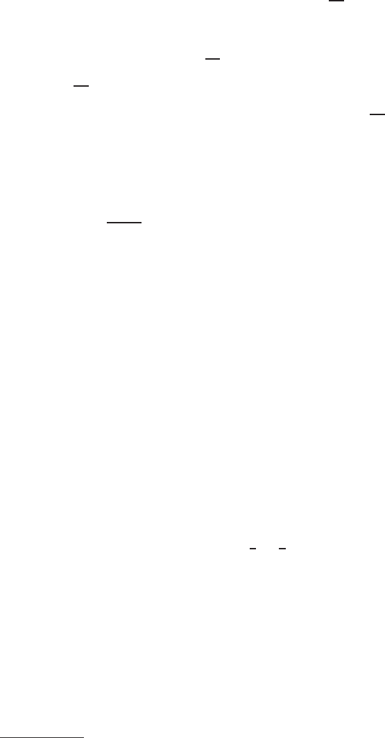
76 Chris Wendl
convergence of S(s, t) implies that similarly
k
¯
S −
¯
S
∞
k
C
k
(Z
R
±
)
→ 0 as R → ∞
for all k ∈ N, where
¯
S
∞
(t) := −CS
∞
(t)C.
This defines a t rivialized asymptotic operator
A = −J
0
∂
t
−
¯
S
∞
(t) to which −D
∗
is
(after a suitable change of trivialization) asymptotic at the puncture z; in particular,
our proof of the global r egularity result, Proposition
4.6, now also works for D
∗
.
Finally, notice t hat A and −
A are conjuga t e: indeed,
(C
−1
AC)η = −CJ
0
∂
t
(Cη) + CCS
∞
(t)C(Cη) = J
0
∂
t
η + S
∞
(t)η = −Aη.
This implies that A is nondegenerate if and only if
A is; applying this assumption
for all of the A
z
, the proofs of Proposition
4.9 and Lemma 4.13 now also go through
for D
∗
.
We’ve proved:
Proposition 4.16. Suppose D
∗
is defined with respect Hermitian bundle metrics
on E and F =
Hom
C
(T
˙
Σ, E) that are compatible with the asymptotically Hermitian
structure of E. If additionally all the as ymptotic operators A
z
are nondegenerate,
then
D
∗
: W
k,p
(F ) → W
k−1,p
(E)
is semi-Fredholm, and its kernel is a space of smooth sections contained in W
m,q
(F )
for all m ∈ N and q ∈ (1, ∞) .
Since ker D
∗
is now known to be finite dimensional, the next result completes
the proof of the Fredholm property for D by showing that its imag e has finite
codimension:
Lemma 4.17. Under the sam e assumptions as in Proposition
4.16,
W
k−1,p
(F ) = im D + ker D
∗
.
Proof. Consider first the case k = 1. Since D : W
1,p
(E) → L
p
(F ) is semi-
Fredholm, its image is closed, hence im D + ker D
∗
is a closed subspace of L
p
(F ).
Then if im D + ker D
∗
6= L
p
(F ), the Hahn-Banach theorem
3
provides a nontrivial
element α ∈ (L
p
(F ))
∗
∼
=
L
q
(F ) for
1
p
+
1
q
= 1 such that
(4.4) hDη + λ, αi
L
2
(F )
= 0 for all η ∈ W
1,p
(E), λ ∈ ker D
∗
.
Choosing λ = 0, this implies in particular
hDη, αi
L
2
(F )
= 0 for a ll η ∈ C
∞
0
(E),
which means that α is a weak solution of class L
q
to the formal adjoint equation
D
∗
α = 0. By Proposiiton
4.6, α is therefore smooth and belong s to ker D
∗
. But
this contradicts (
4.4) if we plug in η = 0 and λ = α, so t his completes the proof for
k = 1.
3
In the case p = 2, one can forego the Hahn-Banach theorem and simply take an L
2
-orthogonal
complement.

Lectures on Symplectic Field Theory 77
For k ≥ 2, suppose α ∈ W
k−1,p
(F ) ⊂ L
p
(F ) is given: then the case k = 1
provides elements η ∈ W
1,p
(E) and λ ∈ ker D
∗
such that Dη + λ = α. Since
Proposition
4.6 implies λ ∈ W
m,q
(F ) for all m ∈ N and q ∈ (1, ∞), we have
Dη = α − λ ∈ W
k−1,p
(F ) and thus, by Prop.
4.6 aga in, η ∈ W
k,p
(E), completing
the proof f or all k ∈ N.
The proof of Theorem 4.3 is now complete, but as long as we’re talking about
the formal adjoint , let us take note of a few more properties t hat will be useful in
the future. Assume from now on tha t all the assumptions of Proposition
4.16 are
satisfied. We can now strengthen Lemma
4.17 as fo llows.
Proposition 4.18. W
k−1,p
(F ) = im D⊕ker D
∗
and W
k−1,p
(E) = im D
∗
⊕ker D.
In particular, the projections defined by these splittings give i s omorphisms
coker D
∼
=
ker D
∗
and coker D
∗
∼
=
ker D,
thus D
∗
: W
k,p
(F ) → W
k−1,p
(E) is a Fredholm operator with
ind D
∗
= −ind D .
Proof. By Lemma
4.17, the first splitting follows if we can show that im D ∩
ker D
∗
= {0}. Recall first (see §
A.4) that C
∞
0
(
˙
Σ) is dense in W
k,p
(
˙
Σ) for every
k ≥ 0 and p ∈ [1, ∞), so the definition of the formal adjoint implies via density and
H¨older’s inequality that if 1 < p, q < ∞ and
1
p
+
1
q
= 1,
(4.5) hλ, D ηi
L
2
(F )
= hD
∗
λ, ηi
L
2
(E)
for all η ∈ W
1,p
(E), λ ∈ W
1,q
(F ).
Now suppose λ ∈ im D ∩ ker D
∗
and write λ = Dη, assuming η ∈ W
k,p
(E). Reg-
ularity implies that since D
∗
λ = 0, λ ∈ W
1,q
(F ), where q can be chosen to satisfy
1
p
+
1
q
= 1. We can therefore apply (
4.5) and obtain
hλ, λi
L
2
(F )
= hλ, Dηi
L
2
(F )
= hD
∗
λ, ηi
L
2
(E)
= 0,
hence λ = 0.
The proof that W
k−1,p
(E) = im D
∗
⊕ ker D is analogous.
This result hints at t he fact that D
∗
is in fact—under some natural extra
assumptions—globally equivalent to another Cauchy-Riemann type operato r. To
see this, let us impose a further constraint on the relation between the Hermitian
bundle metrics h , i
E
and h , i
F
. Note that since the area form d vol is necessarily
j-invariant, it induces a Hermitian structure on T
˙
Σ, namely
hX, Y i
Σ
:= d vol(X, jY ) + i d vol(X, Y ),
which matches the standard bundle metric in the trivializations over the ends defined
via the cylindrical coordinates. This induces real-linear isomorphisms from T
˙
Σ to
the complex-linear and -antilinear parts of the complexified cotangent bundle,
T
˙
Σ → Λ
1,0
T
∗
˙
Σ : X 7→ X
1,0
:= hX, ·i
Σ
,
T
˙
Σ → Λ
0,1
T
∗
˙
Σ : X 7→ X
0,1
:= h·, Xi
Σ
,
where the first isomorphism is complex antilinear and the second is complex linear.
We use these to define Hermitian bundle metrics on Λ
1,0
T
∗
˙
Σ and Λ
0,1
T
∗
˙
Σ in terms

78 Chris Wendl
of the metric on T
˙
Σ; note that this is a straig htforward definition for Λ
0,1
T
∗
˙
Σ, but
since the isomorphism to Λ
1,0
T
∗
˙
Σ is complex antilinear, we really mean
hX
1,0
, Y
1,0
i
Σ
:= hY, Xi
Σ
for X, Y ∈ T
˙
Σ.
Now observe that as a vector bundle with complex structure λ 7→ J ◦ λ, F =
Hom
C
(T
˙
Σ, E) is naturally isomorphic to the complex tensor product
F = Λ
0,1
T
∗
Σ ⊗E.
We can therefore make a natural choice for h , i
F
as the tensor product metric
determined by h , i
Σ
and h , i
E
. It is easy to check that this choice is compatible
with the asymptotically Hermitian structure o f E.
Next, we notice that the area form d vol also induces a natural complex bundle
isomorphism
E → Hom
C
(T
˙
Σ, F ).
Indeed, the right hand side is canonically isomorphic to the complex tensor product
Hom
C
(T
˙
Σ, F ) = Λ
1,0
T
∗
˙
Σ ⊗ F = Λ
1,0
T
∗
˙
Σ ⊗Λ
0,1
T
∗
˙
Σ ⊗ E,
and Λ
1,0
T
∗
˙
Σ⊗Λ
0,1
T
∗
˙
Σ is isomorphic to the trivial complex line bundle ǫ
1
:=
˙
Σ×C →
˙
Σ via
Λ
1,0
T
∗
˙
Σ ⊗ Λ
0,1
T
∗
˙
Σ → ǫ
1
: X
1,0
⊗Y
0,1
7→ X
1,0
(Y ) = hX, Y i
Σ
.
Exercise 4.19. Assuming h , i
F
is cho sen as the tensor product metric described
above, show that under the natural identification of E with Hom
C
(T
˙
Σ, F ),
−D
∗
: Γ(F ) → Ω
1,0
(
˙
Σ, F )
satisfies the Leibniz rule
−D
∗
(fλ) = (∂f)λ + f(−D
∗
λ)
for all f ∈ C
∞
(
˙
Σ, R), where ∂f ∈ Ω
1,0
(
˙
Σ) denotes the complex-valued (1, 0)- form
df − i df ◦ j.
We might summarize this exercise by saying that −D
∗
is an “anti-Cauchy-
Riemann type” operator on F . But such an object is easily transformed into an
honest Cauchy-Riemann type operator: let
¯
F denote the conjugate bundle to F ,
which we define as the same real vector bundle F but with the sign of its complex
structure reversed, so λ 7→ −J ◦ λ. Now there is a canonical isomorphism
Hom
C
(T
˙
Σ, F ) =
Hom
C
(T
˙
Σ,
¯
F ),
and the same operator defines a real-linear map
−D
∗
: Γ(
¯
F ) → Ω
0,1
(
˙
Σ,
¯
F )
which satisfies our usual Leibniz rule for Cauchy-Riemann type operators.
Its asymptotic behavior also fits into the scheme we’ve been describing: we
have already seen this by computing D
∗
on the ends with respect to asymptotic
trivializations. To express this in trivialization-invariant language, observe that each
of the Hermitian bundles (E
z
, J
z
, ω
z
) over S
1
for z ∈ Γ has a conjugate bundle
¯
E
z
with complex structure −J
z
and symplectic structure −ω
z
; it s natural Hermitian

Lectures on Symplectic Field Theory 79
inner product is then the complex conjugate of the one on E
z
. The asymptotic
operator A
z
on E
z
can be expressed as −J
z
b
∇
t
, where
b
∇
t
is a symplectic connection
on (E
z
, ω
z
). Then
b
∇
t
is also a symplectic connection on (
¯
E
z
, −ω
z
), so we naturally
obtain an asymptotic operator on
¯
E
z
in t he form
(4.6)
A
z
:= −A
z
: Γ(
¯
E
z
) → Γ(
¯
E
z
),
where t he sign reversal arises from the reversal of the complex structure. One can
check that if we choose a unitary trivialization of E
z
and the conjugate trivialization
of
¯
E
z
, this relatio nship between A
z
and
A
z
produces precisely the relat ionship
between A = −J
0
∂
t
− S
∞
(t) and
A = −J
0
∂
t
−
¯
S
∞
(t) that we saw previously, with
¯
S
∞
(t) = −CS
∞
(t)C. Let us summarize all this with a theorem.
Theorem 4.20. Assume h , i
F
is chosen to be the tensor product metric on
F = Λ
0,1
T
∗
Σ ⊗ E induced by h , i
E
and the area form d vol. Then under the
isomorphism induced b y d vol from E to Hom
C
(T
˙
Σ, F ) and the natural identification
of the latter with its conj uga te
Hom
C
(T
˙
Σ,
¯
F ), the operator −D
∗
: Γ(F ) → Γ(E)
defines a linear Cauchy-Riemann type o perator on the conjugate bundl e
¯
F ,
−D
∗
: Γ(
¯
F ) → Ω
0,1
(
˙
Σ,
¯
F ),
and it is asymp totic at each puncture z ∈ Γ to the co njugate asymptotic operator
(4.6).

LECTURE 5
The index formula
Contents
5.1. Riemann-Roch with punctures 81
5.2. Some remarks on the formal adjoint 86
5.3. The index zero case on a torus 90
5.4. A Weitzenb¨ock formula for Cauchy-Riemann operators 92
5.5. Large antilinear p e rturbations and energy concentration 94
5.6. Two Cauchy-Riemann type problems on the plane 96
5.7. A linear gluing argument 97
5.8. Antilinea r deformations of asymptotic operators 102
5.1. Riemann-Roch with punctures
As in the previous lecture, let D denote a linear Cauchy-Riemann type operator
on an asymptotically Hermitian vector bundle E of complex ra nk m over a punctured
Riemann surface (
˙
Σ = Σ \ (Γ
+
∪ Γ
−
), j), and assume that D is asymptotic at each
puncture z ∈ Γ to a nondegenerate asymptotic operator A
z
on the asymptotic
bundle (E
z
, J
z
, ω
z
) over S
1
. Writ ing
F :=
Hom
C
(T
˙
Σ, E)
for the bundle o f complex-antilinear homomorphisms T
˙
Σ → E, the main result of
the previous lecture was that
D : W
k,p
(E) → W
k−1,p
(F )
is Fr edholm fo r any k ∈ N and p ∈ (1, ∞), and its kernel and index do not depend
on k or p. The main goal of this lecture is to compute ind(D) ∈ Z.
The index will dep end on the Conley-Zehnder indices µ
τ
CZ
(A
z
) ∈ Z introduced
in Lecture
3, but since these depend on arbitr ary choices of unitary trivializations τ,
we need a way of selecting preferred trivializations. The most natur al condition is to
require that every (E
z
, J
z
, ω
z
) be endowed with a unitary trivialization such that t he
corresponding asymptotic trivializations of (E, J) extend to a global trivialization
1
;
if there is only one puncture z, for instance, then this condition determines µ
τ
CZ
(A
z
)
uniquely. This convention has been used to state the formula for ind(D) in several
of the standard references, e.g. in [HWZ99]. We would prefer however to state a
formula which is also valid when Γ = ∅ and E → Σ is nontrivial. One way to do
1
Note that (E, J) is always globally trivializable unless Γ = ∅, as a punctured s urface can be
retracted to its 1-skeleton.
81

82 Chris Wendl
this is by allowing completely arbitrary asymptotic trivializations, but int r oducing
a topological invariant to measure their failure to extend globally over E.
Definition 5.1. Fix a compact oriented surface S with bo undary. The relative
first Chern number associates to every complex vector bundle (E, J) over S and
trivialization τ of E|
∂S
an integer
c
τ
1
(E) ∈ Z
satisfying the following properties:
(1) If (E, J) → S is a line bundle, then c
τ
1
(E) is the signed count of zeroes for
a generic smooth section η ∈ Γ(E) that appears as a nonzero constant at
∂S with respect to τ.
(2) For any two bundles (E
1
, J
1
) and (E
2
, J
2
) with trivializations τ
1
and τ
2
respectively over ∂S,
c
τ
1
⊕τ
2
1
(E
1
⊕E
2
) = c
τ
1
1
(E
1
) + c
τ
2
1
(E
2
).
These two conditio ns uniquely determine c
τ
1
(E) for all complex vecto r bundles
since bundles of higher rank can always be split into direct sums of line bundles.
The definition clearly matches the usual first Chern number c
1
(E) when ∂S = ∅,
and it extends in an obvious way to the category of asymptotically Hermitian vector
bundles with asymptotic trivializations.
Exercise 5.2. Given two distinct choices of asymptotic trivializations τ
1
and τ
2
for an asymptotically Hermitian bundle E of rank m, show that
c
τ
2
1
(E) = c
τ
1
1
(E) − deg(τ
2
◦ τ
−1
1
),
where deg(τ
2
◦τ
−1
1
) ∈ Z denotes the sum over all punctures of the winding numbers
of the determinants of the transition maps S
1
→ U(m).
2
Exercise 5.3. Combining Exercise 5.2 above with Exercise 3.36, show that for
our asymptotically Hermitian vector bundle E with Cauchy-Riemann type operator
D and asymptotic operators A
z
, the number
2c
τ
1
(E) +
X
z∈Γ
+
µ
τ
CZ
(A
z
) −
X
z∈Γ
−
µ
τ
CZ
(A
z
)
is independent of the choice of asymptotic tr ivializations τ.
The above exercise shows that the right hand side of the following index formula
is independent of all choices.
Theorem 5.4. The Fredho l m index of D is given by
ind D = mχ(
˙
Σ) + 2c
τ
1
(E) +
X
z∈Γ
+
µ
τ
CZ
(A
z
) −
X
z∈Γ
−
µ
τ
CZ
(A
z
),
where m = rank
C
E a nd τ is an arbitrary choice of asymptotic trivializations.
2
Caution: to c ompute this winding number at a neg ative puncture using cylindrical coordinates
(s, t) ∈ (−∞, 0] × S
1
, one must traverse {−s} × S
1
for s ≫ 1 in the wrong direction, as this is
consistent with the or ie ntation induced on {−s}×S
1
as a boundary component of a large compact
sub domain of
˙
Σ.
Lectures on Symplectic Field Theory 83
Notation. Throughout this lecture, we shall denote the integer on the right
hand side in Theorem
5.4 by
I(D) := mχ(
˙
Σ) + 2c
τ
1
(E) +
X
z∈Γ
+
µ
τ
CZ
(A
z
) −
X
z∈Γ
−
µ
τ
CZ
(A
z
) ∈ Z.
Our goal is thus to prove that ind(D) = I(D).
When Γ = ∅, Theorem
5.4 is equivalent to the classical Riemann-Roch f ormula,
which is more often stated f or holomorphic vector bundles over a closed Riemann
surface (Σ, j) with genus g as
(5.1) ind
C
(D
0
) = m(1 − g) + c
1
(E).
This formula assumes that the Cauchy-Riemann type operator D
0
is complex linear,
but an arbitrary real-linear Cauchy-Riemann operator is then of the form D = D
0
+
B, where the zeroth-order term B ∈ Γ(Hom
R
(E, F )) defines a compact perturbation
since the inclusion W
k,p
(Σ) ֒→ W
k−1,p
(Σ) is compact. It follows that D has the same
real Fredholm index as D
0
, namely twice the complex index shown on the right hand
side of (
5.1), which matches what we see in Theorem 5.4.
Remark 5.5. Now seems a good moment to clarify explicitly that all dimensions
(and therefore also Fredholm indices) in this lecture ar e real dimensions, not complex
dimensions, unless otherwise stated.
Reduction t o the complex-linear case does not wo r k in general if there a r e punc-
tures: it remains true that arbit r ary Cauchy-Riemann type operators can be written
as D = D
0
+ B where D
0
is complex linear, but the perturbation introduced by
the zeroth-order term B is not compact since W
k,p
(
˙
Σ) ֒→ W
k−1,p
(
˙
Σ) is not compact
when Γ 6= ∅. Another indication that this idea cannot work is the f act t hat while
the formula in Theorem
5.4 always gives an even integer when Γ = ∅, it can be odd
when there are punctures, in which case D clearly cannot have the same index is
any complex-linear operator . Our proof will therefore have to deal with more than
just the complex category.
The punctured version of Theorem
5.4 was first proved by Schwarz in his the-
sis [
Sch95], its main purpose at the time being to help define algebraic operations
(notably the pair-of-pan ts product) in Hamiltonian Floer homology. Schwarz’s proof
used a “linear gluing” construction that gives a relation between indices of opera-
tors on bundles over surfaces obtained by gluing to gether constituent surfaces along
matching cylindrical ends. Since any surface with ends can be “capped off” to form
a closed surface, one obtains the general index formula if one already knows how to
compute it for closed surfaces and for planes (i.e. caps). For the latter, it is simple
enough to write down model Cauchy-Riemann operators on planes and compute
their kernels and cokernels explicitly, so in this way the general case is reduced to
the classical Riemann-Roch formula. An analogous linear gluing argument for com-
pact surfaces with boundary is used in [MS04, Appendix C] to reduce the general
Riemann-Roch formula to an explicit computatio n for Cauchy-Riemann operators
on the disk with a totally real boundary condition.
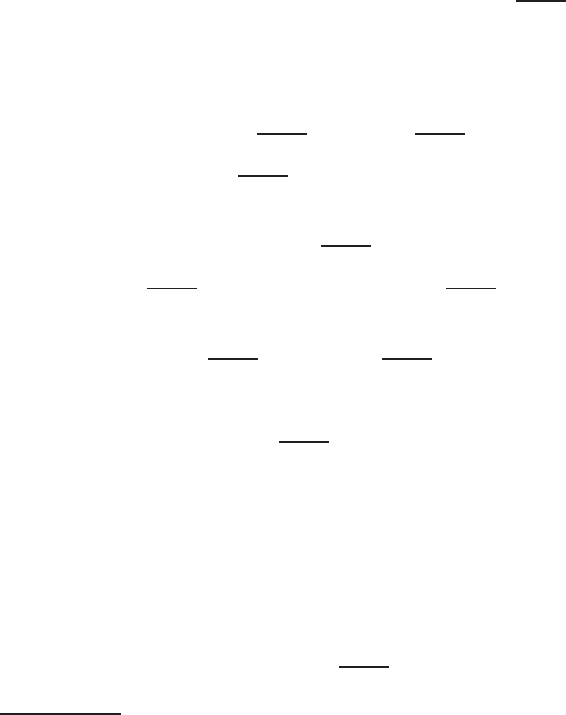
84 Chris Wendl
In this lecture, we will follow a different path and use an argument that was
first sketched by Taubes for the closed case in [
Tau96a, §7], with an additional
argument fo r the punctured case suggested by Chris Gerig [
Ger]. The argument is
(in my opinion) analytically somewhat easier than the more standard a pproaches,
and in addition to proving the formula we need for punctured surfaces, it produces a
new proof in the closed case without assuming the classical Riemann-Roch formula .
It also provides a gentle preview of two analytical phenomena that will later assume
prominent roles in o ur discussion of SFT: bubbling and gluing.
To see the idea behind Taubes’s argument, we can start by noticing an apparent
numerical coincidence in the closed case. Assume (E, J) is a complex line bundle over
a closed Riemann surface (Σ, j), and D : Γ(E) → Γ(F ) = Ω
0,1
(Σ, E) is a Cauchy-
Riemann type operator. We know that ind(D) = ind(D + B) for any zeroth-order
term B ∈ Γ(Hom
R
(E, F )). But E and F are both complex vecto r bundles, so B
can always be split uniquely into its complex-linear and complex-antilinear parts,
i.e. there is a natural splitting of Hom
R
(E, F ) into a direct sum of complex line
bundles
3
Hom
R
(E, F ) = Ho m
C
(E, F ) ⊕ Hom
C
(E, F ).
Out of curiosity, let’s compute the first Chern number of the second factor; this will
be the signed count of zeroes of a generic complex-antilinear zeroth-order perturba-
tion. To start with, note that
Hom
C
(E, F ) = Hom
C
(E, C) ⊗ F,
and then observe that Hom
C
(E, C) and E ar e isomorphic: indeed, any Hermitian
bundle metric h , i
E
on E gives rise to a bundle isomorphism
4
E → Hom
C
(E, C) : η 7→ h·, ηi
E
.
We thus have
Hom
C
(E, F )
∼
=
E ⊗ F , so c
1
(
Hom
C
(E, F )) = c
1
(E) + c
1
(F ). We can
compute c
1
(F ) by the same trick since
F =
Hom
C
(T Σ, E) = Hom
C
(T Σ, C) ⊗ E
∼
=
T Σ ⊗ E,
so c
1
(F ) = c
1
(T Σ) + c
1
(E) = χ(Σ) + c
1
(E), and thus
c
1
(
Hom
C
(E, F )) = χ( Σ) + 2c
1
(E).
Since we’re looking at a line bundle over a surface without punctures, this number
is the same as I(D). This coincidence is too improbable to ignore, and indeed, it
turns out not to be coincidental. Here is an informal statement of a r esult that we
will later prove a more precise version of in order to deduce Theorem 5.4.
“Theorem”. Given a Cauchy-Riemann type operator D : H
1
(E) → L
2
(F ) on a
line bundle (E, J) over a closed Riemann surface ( Σ, j), choose a complex-antilin ear
zeroth-ord er perturbation B ∈ Γ(Hom
C
(E, F )) whos e zeroes are all nondegenerate.
3
Here the complex structure on Hom
R
(E, F ) and its subbundles is defined in terms of the
complex structure of F , i.e. it sends B ∈ Hom
R
(E, F ) to J ◦ B ∈ Hom
R
(E, F ).
4
We are assuming as usual that Hermitian inner products are complex antilinear in the first
argument and linear in the second.

Lectures on Symplectic Field Theory 85
Then for sufficiently large σ > 0, ker(D + σB) is approx i mately spanned by 1-
dimensional space s of sections with support localized near the positive zeroes of B.
In particular, dim ker(D + σB) equals the number of positive ze roes of B.
To deduce ind(D) = I(D) from this, we need to apply the same trick to the
formal adjo int D
∗
. As we will review in §
5.2, −D
∗
can be rega r ded under certain
natural assumptions as a Cauchy-Riemann type operat or on the bundle
¯
F conjugate
to F , a nd the formal adjoint of D + σB then gives rise to a Cauchy-Riemann type
operator of the form
−D
∗
+ σB
′
: Γ(
¯
F ) → Γ(
¯
E) = Ω
0,1
(Σ,
¯
F ),
where B
′
:
¯
F →
¯
E is a lso complex antilinear and has the same zeroes as B, but with
opposite signs. Applying the above “theorem” to −D
∗
thus identifies ker(D + σB)
∗
for sufficiently large σ > 0 with a space whose dimension equals the number of
negative zeroes of B. This gives
ind(D) = ind(D + σB) = dim ker(D + σB) − dim ker(D + σB)
∗
= c
1
(
Hom
C
(E, F )) = I(D).
It’s worth mentioning t hat the “larg e perturbation” argument we’ve just sketched
is only o ne simple example of an idea with a long and illustrious history: another
simple example is the observation by Witten [
Wit82] that a fter choosing a Morse
function on a Riemannian manifold, certain large deformations of the de Rha m
complex lead to an approximation of the Morse complex, with generators of the de
Rham complex having support concent r ated near the critical points of the Morse
function—this yields a somewhat novel proof of de Rham’s theorem. A much deeper
example is Taubes’s isomorphism [
Tau96b] between the Seiberg- Witt en invariant s
of symplectic 4-manifolds and certain ho lomorphic curve invariants: here also, the
idea is to consider a large compact perturbation of the Seiberg-Witten equations and
show tha t , in the limit where t he perturbation becomes infinitely large, solutions of
the Seiberg-Witten equations localize near J- holomorphic curves. For a more recent
exploration of this idea in the context of Dirac operators, see [
Mar].
Before proceeding with the details, let us fix two simplifying assumptions that
can be imposed without loss of generality:
Assumption 5.6. (E, J) has com plex rank 1.
Indeed, an asymptotically Hermitian bundle E of complex rank m ∈ N always
admits a decomposition into asymptotically Hermitian line bundles E = E
1
⊕. . . ⊕
E
m
, producing a cor resp onding splitting of the targ et bundle F = F
1
⊕ . . . ⊕ F
m
.
The operator D need not respect these splittings, but it is always homotopic through
Fredholm operators to one that does: we saw in Theorem
3.33 that the asymptotic
operators A
z
are homotopic through nondegenerate asymptotic operators to any
other operators A
′
z
that have the same Conley-Zehnder indices, so one can choose
A
′
z
to respect the splitting. Any homotopy of Cauchy-Riemann operators following
such a homotopy of nondegenerate asymptotic operat ors then produces a continuous
family of Fredholm operators by the main result of Lecture
4, implying that their
indices do not change. The general index formula then follows from the line bundle

86 Chris Wendl
case since any two Cauchy-Riemann type Fredholm operators D
1
and D
2
over the
same Riemann surface satisfy
ind(D
1
⊕D
2
) = ind(D
1
) + ind(D
2
) and I(D
1
⊕ D
2
) = I(D
1
) + I(D
2
).
Assumption 5.7. k = 1 and p = 2.
This means we will concretely be considering the operator
D : H
1
(E) → L
2
(F ),
where H
1
as usual is an abbreviation for W
1,2
. This assumption is clearly harmless
since we know tha t ind D does not depend on the choice of k and p.
5.2. Some remarks on the formal adjoint
For the beginning of this section we can drop the assumption that (E, J) is a
line bundle and assume rank
C
E = m ∈ N, though later we will again set m = 1.
Recall from the end of Lecture
4 that if we fix global Hermitian structures h , i
E
and h , i
F
on (E, J) a nd (F, J) respectively a nd an ar ea form d vol on
˙
Σ tha t matches
ds ∧dt on the cylindrical ends, then D has a formal adjoint
D
∗
: Γ(F ) → Γ(E)
satisfying
hλ, Dηi
L
2
(F )
= hD
∗
λ, ηi
L
2
(E)
for all η ∈ H
1
(E), λ ∈ H
1
(F ).
Here the real-valued L
2
pairings are defined by
hη, ξi
L
2
(E)
:= Re
Z
˙
Σ
hη, ξi
E
d vol for η, ξ ∈ Γ(E),
and similarly for sections of F . The essential features of the formal adjoint are
that ker D
∗
∼
=
coker D and coker D
∗
∼
=
ker D, hence ind(D
∗
) = −ind(D). R ecall
moreover that d vol induces a natural Hermitian bundle metric on
˙
Σ by
h·, ·i
Σ
= d vo l( ·, j·) + i d vol(·, ·),
which determines a bundle isomorphism
T
˙
Σ → Λ
0,1
T
∗
˙
Σ : X 7→ X
0,1
:= h·, Xi
Σ
,
as well as a complex-antilinear isomorphism
T
˙
Σ → Λ
1,0
T
∗
˙
Σ : X 7→ X
1,0
:= hX, ·i
Σ
.
If h , i
F
is then chosen to be the tensor product metric determined via the natural
isomorphism
F =
Hom
C
(T
˙
Σ, E) = Λ
0,1
T
∗
˙
Σ ⊗ E = T
˙
Σ ⊗ E,
then E admits a natural isomorphism to Λ
1,0
T
∗
˙
Σ ⊗ F such that
−D
∗
: Γ(F ) → Γ(E) = Ω
1,0
(
˙
Σ, F )
becomes an anti-C auchy-Riemann type operator, i.e. it satisfies the Leibniz rule
−D
∗
(fλ) = (∂f)λ + f(−D
∗
λ)
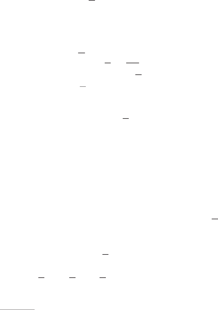
Lectures on Symplectic Field Theory 87
for all f ∈ C
∞
(
˙
Σ, R), with ∂f := df − i df ◦ j ∈ Ω
1,0
(
˙
Σ). Equivalently, −D
∗
defines
a Cauchy-Riemann type operator on the conjugate bundle
¯
F →
˙
Σ, defined as the
real bundle F →
˙
Σ but with the sign of its complex structure reversed; we shall
distinguish this Cauchy-Riemann operator from −D
∗
by writing it as
−D
∗
: Γ(
¯
F ) → Ω
0,1
(
˙
Σ,
¯
F ),
though it is technically the same operator. Recall that t he identity map defines a
natural complex-antilinear isomorphism between any complex vector bundle and its
conjugate bundle; we shall denote this isomorphism generally by
E →
¯
E : v 7→ ¯v,
so in particular it satisfies
cv = ¯c¯v for all scalars c ∈ C, and similarly
D
∗
¯
λ = D
∗
λ
for λ ∈ Γ( F ). The asymptotic operators f or −
D
∗
are
A
z
= −A
z
: Γ(
¯
E
z
) → Γ(
¯
E
z
).
Lemma 5.8. If τ is a choice of asymptotic trivialization on E and ¯τ denotes the
conjugate asymptotic trivialization
5
, then
c
¯τ
1
(
¯
E) = −c
τ
1
(E), and µ
¯τ
CZ
(
A
z
) = −µ
τ
CZ
(A
z
) for all z ∈ Γ.
Proof. Assuming E is a line bundle, suppose η is a generic section of E that
matches a nonzero constant with respect to τ on the cylindrical ends, so c
τ
1
(E) is
the signed count of zeroes of η. Then ¯η ∈ Γ(
¯
E) is similarly a nonzero constant on
the ends with respect t o ¯τ, but the signs of its zeroes are opposite those of η because
they are defined as winding numbers with resp ect to conjugate local trivializations.
This pr oves c
¯τ
1
(
¯
E) = −c
τ
1
(E).
The Conley-Zehnder indices can be computed from the formula
µ
τ
CZ
(A
z
) = α
τ
+
(A
z
) + α
τ
−
(A
z
),
see Theorem
3.35. Here α
τ
−
(A
z
) is the largest possible winding number relative to
τ of an eigenfunction for A
z
with negative eigenvalue, and α
τ
+
(A
z
) is the smallest
possible winding number with positive eigenvalue. The eigenfunctions of A
z
= −A
z
are the same, but the signs of their eigenvalues are reversed, and the signs of their
winding numbers are also reversed because they must be measured relative to the
conjugate trivialization, thus
α
¯τ
±
(
A
z
) = −α
τ
∓
(A
z
),
implying
µ
¯τ
CZ
(
A
z
) = α
¯τ
+
(A
z
) + α
¯τ
−
(A
z
) = −α
τ
−
(A
z
) − α
τ
+
(A
z
) = −µ
τ
CZ
(A
z
).
The above calculations are all valid for line bundles, but the general case f ollows
by taking direct sums.
5
If τ : E|
U
→ U×C
m
is a local trivialization of E with τ(v) = (z, w), the conjugate trivialization
¯τ :
¯
E|
U
→ U × C
m
is defined by ¯τ (¯v) = (z, ¯w).
88 Chris Wendl
We are now able to show that Theorem 5.4 is consistent with what we already
know abo ut the f ormal adjo int.
Proposition 5.9. I(−
D
∗
) = −I(D).
Proof. Under the isomorphism F = Λ
0,1
T
∗
˙
Σ ⊗ E = T
˙
Σ ⊗ E, an asymptotic
trivialization τ on E induces an asymptotic trivialization ∂
s
⊗ τ on F , where ∂
s
denotes the asymptotic trivialization of T
˙
Σ defined via an outward pointing vector
field on the cylindrical ends. Counting zeroes of vector fields then proves c
∂
s
1
(T
˙
Σ) =
χ(
˙
Σ), so
c
∂
s
⊗τ
1
(F ) = c
∂
s
⊗τ
1
(T
˙
Σ ⊗ E) = mc
∂
s
1
(T
˙
Σ) + c
τ
1
(E) = mχ(
˙
Σ) + c
τ
1
(E).
Applying Lemma
5.8 to the conjug ate bundle then gives
c
∂
s
⊗τ
1
(
¯
F ) = −mχ(
˙
Σ) − c
τ
1
(E).
The unitary trivializations of the asymptotic bundles
¯
E
z
corresponding to
∂
s
⊗ τ
are simply ¯τ, thus using Lemma
5.8 again for the Conley-Zehnder terms,
I(−
D
∗
) = mχ(
˙
Σ) + 2c
∂
s
⊗τ
1
(
¯
F ) +
X
z∈Γ
+
µ
¯τ
CZ
(
A
z
) −
X
z∈Γ
−
µ
¯τ
CZ
(
A
z
)
= −mχ(
˙
Σ) − 2c
τ
1
(E) −
X
z∈Γ
+
µ
τ
CZ
(A
z
) +
X
z∈Γ
−
µ
τ
CZ
(A
z
)
= −I(D).
We next consider the effect of an antilinear zeroth-order perturbation on the
formal adjoint. By “antilinear zeroth-order perturbation,” we generally mean a
smooth section
B ∈ Γ(
Hom
C
(E, F )).
It is perhaps easier to understand B in terms of the conjugat e bundle
¯
E: indeed,
there exists a unique
β ∈ Γ (Hom
C
(
¯
E, F ))
such that
Bη = β ¯η,
and this correspondence defines a bundle isomorphism
Hom
C
(E, F ) = Hom
C
(
¯
E, F ).
Exercise 5.10. Assume X and Y are complex vector bundles over the same
base.
(a) Show that
¯
X ⊗
¯
Y is canonically isomorphic to the conjugate bundle of
X ⊗ Y .
(b) Show that Hom
C
(
¯
X,
¯
Y ) is canonically isomorphic to the conjugate bundle of
Hom
C
(X, Y ), and
Hom
C
(
¯
X,
¯
Y ) is canonically isomorphic to the conj ug ate
bundle of
Hom
C
(X, Y ).
(c) Show that Λ
0,1
X :=
Hom
C
(X, C) is canonically isomorphic to the conjugate
bundle of Λ
1,0
X := Hom
C
(X, C).
Lectures on Symplectic Field Theory 89
Define the Cauchy-Riemann type operator
D
B
:= D + B : Γ(E) → Γ(F ) = Ω
0,1
(
˙
Σ, E),
so D
B
η = Dη + β¯η. To write down D
∗
B
, observe that since β :
¯
E → F is a complex-
linear bundle map between Hermitian bundles, it has a complex-linear adjoint
β
†
: F →
¯
E such that hβ
†
λ, ¯ηi
¯
E
= hλ, β ¯ηi
F
for λ ∈ F , ¯η ∈
¯
E.
Here the bundle metric on
¯
E is defined by h¯η,
¯
ξi
¯
E
:= hξ, ηi
E
. We then have
Rehλ, Bηi
F
= Rehλ, β ¯ηi
F
= Rehβ
†
λ, ¯ηi
¯
E
= Rehη,
β
†
λi
E
= Rehβ
†
λ, ηi
E
= Reh
β
†
¯
λ, ηi
E
,
where
β
†
∈ Γ(Ho m
C
(
¯
F , E)) denotes the image of β
†
∈ Γ(Ho m
C
(F,
¯
E)) under the
complex-antilinear identity map from Hom
C
(F,
¯
E) to its conjugate bundle (see Ex-
ercise
5.10). The formal adjoint of D
B
is thus
D
∗
B
= D
∗
+ B
∗
: Γ(F ) → Γ(E),
where B
∗
: F → E is defined by
B
∗
λ :=
β
†
¯
λ.
To write down the resulting Cauchy-Riemann type operator o n
¯
F , we replace B
∗
:
F → E with
B
∗
:
¯
F →
¯
E, defined by
B
∗
¯
λ := B
∗
λ = β
†
λ,
giving a Cauchy-Riemann operator
−
D
∗
B
= −
D
∗
+ (−B
∗
) : Γ(
¯
F ) → Γ(
¯
E) = Ω
0,1
(
˙
Σ,
¯
F ).
The point of writing down this formula is to make the following observat ions:
Lemma 5.11. Th e zeroth-ord er perturbation −
B
∗
:
¯
F →
¯
E appearing in −D
∗
B
has the following properties:
(1) −
B
∗
:
¯
F →
¯
E i s complex antilinear;
(2) There is a natural complex bundle isomorphism
Hom
C
(
¯
F ,
¯
E) = Hom
C
(F,
¯
E)
that ide ntifies −
B
∗
with −β
†
;
(3) If m = 1 and B ∈ Γ(
Hom
C
(E, F )) has only nondegenerate zeroe s, then
−B
∗
∈ Γ(Hom
C
(
¯
F ,
¯
E)) has the sa me zeroes but with o p posi te si gns.
Proof. The first two statements fo llow immediately from the fact that −
B
∗
is the composition of the canonical conjugation map
¯
F → F with the complex-
linear bundle map −β
†
: F →
¯
E. For the third, it suffices to compare what β ∈
Γ(Hom
C
(
¯
E, F )) and −β
†
: Γ(Hom
C
(F,
¯
E)) look like in local trivializatio ns near a
zero: o ne is minus the complex conjugate o f the other, hence their zeroes count with
opposite signs.

90 Chris Wendl
5.3. The index zero case on a torus
As a wa r mup for the general case, we now fill in the details of Taubes’s proof of
Theorem 5.4 in the case
˙
Σ = T
2
:= C \ (Z ⊕ iZ)
and E = T
2
×C, i.e. a trivial line bundle. In t his case I(D) = χ(T
2
) + 2c
1
(E) = 0,
so our a im is to prove ind(D) = 0 . What we will show in fact is that D is homotopic
through a continuous f amily of Fredholm operators to one that is an isomorphism.
Since E and F are now both trivial, it will suffice to consider the operator
D :=
¯
∂ = ∂
s
+ i∂
t
: H
1
(T
2
, C) → L
2
(T
2
, C),
whose formal adjoint is D
∗
:= −∂ = −∂
s
+ i∂
t
. An antilinear zeroth-or der pertur-
bation is then equivalent to a choice of function β : T
2
→ C, giving rise to a family
of operators
D
σ
η :=
¯
∂η + σβ¯η
for σ ∈ R, where ¯η : T
2
→ C now denotes the straightforward complex conjugate
of η. Let us assume t hat β : T
2
→ C is nowhere zero; note that this would not be
possible in more general situations, but is possible here b ecause Hom
C
(
¯
E, F ) is a
trivial bundle.
Lemma 5.12. D
σ
is injective for a ll σ > 0 sufficiently large.
Proof. Elliptic regularity implies any η ∈ ker D
σ
is smooth, so we shall restrict
our attention to smooth functions η : T
2
→ C. We start by comparing the two
second-order differential operators
D
∗
D and D
∗
σ
D
σ
: C
∞
(T
2
, C) → C
∞
(T
2
, C).
Both are nonnegative L
2
-symmetric operators, and in fact the first is simply the
Laplacian
D
∗
D = −∂
¯
∂ = (−∂
s
+ i∂
t
)(∂
s
+ i∂
t
) = −∂
2
s
−∂
2
t
= −∆.
The formal adjoint of D
σ
takes the form
D
∗
σ
η = D
∗
η + σB
∗
η = D
∗
η + σβ ¯η,
thus for any η ∈ C
∞
(T
2
, C),
D
∗
σ
D
σ
η = (D
∗
+ σB
∗
)(D + σB)η
= D
∗
Dη + σ
β
¯
∂η − ∂(β¯η)
+ σ
2
B
∗
Bη
= D
∗
Dη + σ (β∂¯η − (∂β)¯η − β∂¯η) + σ
2
B
∗
Bη
= D
∗
Dη + σ
2
B
∗
Bη − σ( ∂β)¯η.
(5.2)
This is a Weitzenb¨ock formula: its main message is that the Laplacian D
∗
D and
the related operator D
∗
σ
D
σ
differ from each other only by a zeroth-order term t hat

Lectures on Symplectic Field Theory 91
will be positive definite if σ is sufficiently large. Indeed, since β is nowhere zero, we
have |Bη| ≥ c|η| for some constant c > 0, thus
kD
σ
ηk
2
L
2
= hη, D
∗
σ
D
σ
ηi
L
2
= hη, D
∗
Dηi
L
2
+ σ
2
hη, B
∗
Bηi
L
2
− σhη, (∂β)¯ηi
L
2
= kDηk
2
L
2
+ σ
2
kBηk
2
L
2
−σhη, (∂β)¯ηi
L
2
≥
σ
2
c
2
− σk∂βk
C
0
kηk
2
L
2
.
We conclude that as soon as σ > 0 is larg e enough to make the quantity in paren-
theses positive, D
σ
η cannot vanish unless kηk
L
2
= 0.
Proof of Theorem
5.4 for E = T
2
× C. The lemma above shows that one
can add a large antilinear perturbation to D =
¯
∂ making the deformed operator
D
σ
injective. By Lemma
5.11, the same argument applies to the formal adjoint
D
∗
, implying that for sufficiently large σ > 0, D
∗
σ
is injective and thus D
σ
is also
surjective, and therefore an isomorphism. This proves ind(D) = ind(D
σ
) = 0.
Let’s consider which par ticular details o f the setup made the proof above possible.
First, the zeroth-order perturbation is complex antilinear. We used t his, if only
implicitly, in deriving the Weitzenb¨o ck formula (
5.2): the key step is in the third
line, where the two terms involving ∂ ¯η cancel each other out and leave nothing but
zeroth-order terms remaining. This would not have happened if e.g. B : E → F
had been complex linear—we would then have seen terms depending on the first
derivative of η in D
∗
σ
D
σ
η − D
∗
Dη, and this would have killed the whole argument .
The fact that this cancellation happens when the perturba t ion is antilinear probably
looks like magic at this point, but t here is a principle behind it; we will discuss it
further in §
5.4 below, see Remark 5.1 7.
The second crucial fact we used was that β : T
2
→ C is nowhere zero, in
order to obtain the lower bound on kBηk
L
2
in terms of kηk
L
2
. This cannot always
be achieved—it is possible in this special case only because E and F are both
trivial bundles and thus so is Hom
C
(
¯
E, F ). On more general bundles, the best we
could hope for would be to pick β ∈ Γ(Hom
C
(
¯
E, F )) with finitely many zeroes, all
nondegenerate. In this case the above argument fa ils, but it still tells us something.
Suppose Σ
ǫ
⊂ T
2
is a region disjoint fro m the isola ted zeroes of β. Then there exists
a constant c
ǫ
> 0, dependent on the region Σ
ǫ
, such that
kβ¯ηk
2
L
2
(T
2
)
≥ kβ ¯ηk
2
L
2
(Σ
ǫ
)
≥ c
ǫ
kηk
2
L
2
(Σ
ǫ
)
,
so instead of the estimate at the end of the proof above implying D
σ
is injective, we
obtain one of the form
kD
σ
ηk
2
L
2
(T
2
)
≥ c
ǫ
σ
2
kηk
L
2
(Σ
ǫ
)
− cσkηk
2
L
2
(T
2
)
.
To see what this means, imagine we have sequences σ
ν
→ ∞ and η
ν
∈ ker D
σ
ν
,
normalized so that kη
ν
k
L
2
= 1 for all ν. The estimate above then implies
kη
ν
k
2
L
2
(Σ
ǫ
)
≤
c
c
ǫ
σ
ν
→ 0 as ν → ∞,
so while all sections η
ν
have the same amount of “energy” (as measured via their L
2
-
norms), the energy is escaping from Σ
ǫ
as σ
ν
increases. This is true for any domain
Σ
ǫ
disjoint fro m the zeroes, so we conclude that in the limit as σ → ∞, sections in

92 Chris Wendl
ker D
σ
have their energy concentrated in infinitesimally small neighborhoods of the
zeroes of β. We will see in the f ollowing how to extract useful information from this
concentration of energy.
5.4. A Weitzenb¨ock formula for Cauchy-Riemann operators
The Weitzenb¨ock formula (
5.2) can be generalized to a useful relation between
any two Cauchy-Riemann type opera t ors that differ by an antilinear zeroth-order
term. To see t his, we start with a short digression on holomorphic and antiholo mo r -
phic vector bundles.
A smooth function f : C ⊃ U → C is called antiholomorphic if it satisfies
(∂
s
−i∂
t
)f = 0, which means its differential anticommutes with the complex structure
on C. The class of antiholomorphic functions is not closed under composition, but
it is closed under products, hence one can define an antiholomorphic structure
on a complex vector bundle to be a system of local trivializations for which all
transition maps are antiholomorphic. Given the standard correspondence between
holomorphic structures and Cauchy-Riemann type operators, it is easy to establish
a similar correspondence between aniholomorphic structures and (complex-linear)
anti-Cauchy-Riemann type operators, i.e. those which satisfy
D(fη) = (∂f)η + fDη
for all f ∈ C
∞
(
˙
Σ, C), where ∂f := df −i df ◦j ∈ Ω
1,0
(
˙
Σ). We’ve seen one important
example of such an operator already: if D : Γ(E) → Γ(F ) is complex linear, then
−D
∗
is a complex-linear anti-Cauchy-Riemann operator on F and thus endows F
with an antiholo mo r phic structure. Another natural example occurs naturally on
conjugate bundles: if E has a holomorphic structure, then
¯
E inherits from this an
antiholomorphic structure. This is immediate from the fact that f : C ⊃ U → C is
holomorphic if and only if
¯
f : U → C is antiholomorphic. If D : Γ(E) → Γ(F ) =
Ω
0,1
(
˙
Σ, E) is the corresponding complex-linear Cauchy-Riemann type o perator on
E, we shall denote the resulting anti-Cauchy-Riemann operator by
D : Γ(
¯
E) → Γ(
¯
F ) = Ω
1,0
(
˙
Σ,
¯
E),
where by definition
D¯η = Dη.
Exercise 5.13. Show that if X and Y are antiholomorphic vector bundles over
the same base, then X ⊗Y and Hom
C
(X, Y ) both naturally inherit antiholomorphic
bundle structures such that the obvious Leibniz rules are satisfied. Remark: the
proof of this is exactly the same as for ho lomorphic bundles, one only needs t o
change some signs.
Exercise 5.14. Suppose X and Y are complex vector bundles over the same
base, carrying real- linear anti-Cauchy-Riemann operators ∂
X
and ∂
Y
respectively.
Show that H := Hom
R
(X, Y ) then admits a real-linear anti-Cauchy-Riemann oper-
ator ∂
H
such that for all Φ ∈ Γ(H) and η ∈ Γ(X),
∂
Y
(Φη) = (∂
H
Φ)η + Φ(∂
X
η).
Lectures on Symplectic Field Theory 93
Hint: write ∂
X
and ∂
Y
as complex-linear operator s with real-linear zeroth-order
perturbations, and apply Exercise
5.13. Show moreover that any C
k
-bounds satisfied
by the zeroth-o r der terms in ∂
X
and ∂
Y
are inherited by the zeroth-order term in ∂
H
.
The setup for the next result is as follows. We assume again m = 1, so E and F
are line bundles. Fix β ∈ Γ(Hom
C
(
¯
E, F )), define B ∈ Γ(Hom
C
(E, F )) by Bη := β ¯η,
and use this to define the p erturbed Cauchy- Riemann type operator
D
B
:= D + B : Γ(E) → Γ(F ),
whose formal adjoint is D
∗
B
= D
∗
+ B
∗
with B
∗
λ :=
β
†
¯
λ.
Proposition 5.15. The second - order differential ope rators D
∗
D and D
∗
B
D
B
on
E a re related by
D
∗
B
D
B
η = D
∗
D
∗
η + B
∗
Bη − (∂
H
β)¯η,
where ∂
H
is a real- l i near anti-Cauchy-Riemann type operator on Hom
C
(
¯
E, F ). More-
over, if β is C
1
-bounded on
˙
Σ, then ∂
H
β is C
0
-bounded.
Proof. We have real-linear ant i-Cauchy-Riemann operators
D and −D
∗
on
¯
E
and F respectively, so Exercise
5.14 produces an operator ∂
H
on Hom
C
(
¯
E, F ) for
which the Leibniz rule is satisfied. We can then write
D
∗
B
D
B
η = (D
∗
+ B
∗
)(D + B)η
= D
∗
Dη +
β
†
Dη − ( −D
∗
)(β¯η) + B
∗
Bη
= D
∗
Dη +
β
†
D¯η − (∂
H
β)¯η − βD¯η + B
∗
Bη
= D
∗
Dη + B
∗
Bη − (∂
H
β)¯η +
β
†
−β
D¯η.
Here β and
β
†
are both viewed as complex-linear bundle maps
¯
F → E, the latter in
the obvious way, and the former acting as 1 ⊗ β on
¯
F = Λ
1,0
T
∗
˙
Σ ⊗
¯
E with tar get
Λ
1,0
T
∗
˙
Σ ⊗F = Λ
1,0
T
∗
˙
Σ ⊗Λ
0,1
T
∗
˙
Σ ⊗E = E. Choosing unitary local trivializations,
β and β
†
are represented by the same complex-valued function: indeed, the latter
is the transpose of the former as m-by-m complex matrices, but since m = 1 , this
means they are identical.
Finally, we observe that the asymptotic convergence conditions satisfied by D
on the cylindrical ends imply similar conditions for a ll other Cauchy-Riemann and
anti-Cauchy-Riemann operators in this picture, yielding an estimate of the form
k∂
H
βk
C
0
≤ ckβk
C
1
globally on
˙
Σ.
Remark 5.16. The above proof used the assumption m = 1 in order to conclude
β
†
−β ≡ 0. For higher rank bundles, this impo ses a nontrivial condition that must
be satisfied in order fo r the Weitzenb¨ock formula to hold, cf. [
GW].
Remark 5.17. We can now pick out a geometric reason for the miraculous can-
cellation in the Weitzenb¨ock f ormula: the perturbation B is described by a complex
bundle ma p
¯
E → F , where
¯
E and F both have natural antiholomorphic bun-
dle structures defined via the complex-linear parts of
D and −D
∗
respectively. A
complex-linear perturbation B : E → F would not work because E is holomorphic
rather than antiholomorphic: while
D can be fit into the same Leibniz rule with
−D
∗
, the same is not true o f D.
94 Chris Wendl
5.5. Large antilinear perturbations and energy concent ration
We continue in the setting of Proposition
5.15 and set
D
σ
:= D + σB : Γ(E) → Γ(F )
for σ > 0. After a compact perturbation of D, we can without loss of generality
also impose the following assumptions on D, β ∈ Γ(Hom
C
(
¯
E, F )) and the area
form d vol:
(i) All zeroes of β are nondegenerate.
(ii) Both |β| and 1/|β| are bounded outside of a compact subset of
˙
Σ.
(iii) Near each point ζ ∈
˙
Σ with β(ζ) = 0, t here exists a neighborhood D(ζ) ⊂
˙
Σ
of ζ, a holomorphic coordinate chart identifying (D(ζ), j, ζ) with the unit
disk (D, i, 0), and a local trivialization of E over D(ζ) that ident ifies D with
¯
∂ = ∂
s
+ i∂
t
: C
∞
(D, C) → C
∞
(D, C) and β with one of the functions
β(z) = z or β( z) = ¯z,
the former if ζ is a positive zero and the latter if it is negative.
(iv) In the holomorphic coordinate on D(ζ) describ ed above, d vol is the stan-
dard Lebesgue measure.
As in the torus case discussed in §
5.3, we will see that the Weitzenb¨ock formula
implies a concentr ation of energy near the zeroes of β for sections η ∈ ker D
σ
as
σ → ∞. To understand what really happens in this limit, we will use a rescaling
trick. Denote the zero set of β by
Z(β) = Z
+
(β) ∪ Z
−
(β) ⊂
˙
Σ,
partitioned into the positive and negative zeroes. For any η ∈ Γ(E), ζ ∈ Z
±
(β) and
σ > 0, we then define a rescaled function
η
(ζ,σ)
: D
√
σ
→ C : z 7→
1
√
σ
η(z/
√
σ),
where the right hand side denotes the local representation of η on D(ζ) in the chosen
coordinate and trivialization. Notice that the equation D
σ
η = 0 appears in this local
representation as either
¯
∂η + σz ¯η = 0 or
¯
∂η + σ¯z¯η = 0 depending on the sign of ζ,
and the function f := η
(ζ,σ)
then satisfies
¯
∂f + z
¯
f = 0 or
¯
∂f + ¯z
¯
f = 0 on D
√
σ
.
We will take a closer look at these two PDEs in §
5.6 below. But first, observe tha t
by change of variables,
η
(ζ,σ)
L
2
(D
√
σ
)
= kηk
L
2
(D(ζ))
.
Lemma 5.18. Assume σ
ν
→ ∞, and η
ν
∈ ker D
σ
ν
is a sequence s atisfying a
uniform L
2
-bound. Then after passing to a subsequence, the rescaled functions η
ζ
ν
:=
η
(ζ,σ
ν
)
ν
: D
√
σ
ν
→ C for each ζ ∈ Z
±
(β) converge in C
∞
lo c
(C) to smooth func tion s
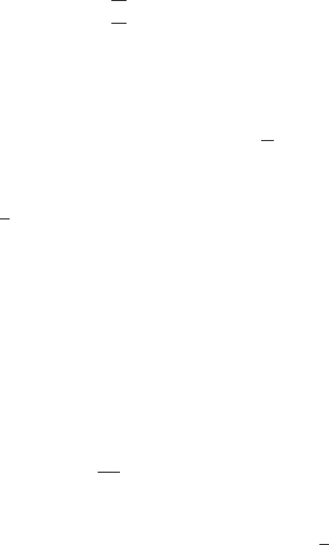
Lectures on Symplectic Field Theory 95
η
ζ
∞
∈ L
2
(C) satisfying
¯
∂η
ζ
∞
+ z
η
ζ
∞
= 0 if ζ ∈ Z
+
(β),
¯
∂η
ζ
∞
+ ¯z
η
ζ
∞
= 0 if ζ ∈ Z
−
(β).
Moreover, i f ξ
ν
∈ ker D
σ
ν
is another sequence with these same properties and con-
vergence ξ
ζ
ν
→ ξ
ζ
∞
, then
lim
ν→∞
hη
ν
, ξ
ν
i
L
2
(E)
=
X
ζ∈Z(β)
hη
ζ
∞
, ξ
ζ
∞
i
L
2
(C)
.
Proof. The uniform L
2
-bound implies uniform bounds on kη
ζ
ν
k
L
2
(D
R
)
for every
R > 0, where ν here is assumed sufficiently large so that R <
√
σ
ν
. Since η
ζ
ν
satisfies
a Cauchy-Riemann type equation on D
R
, the usual elliptic estimates (see Lecture
2)
then imply uniform H
k
-bounds for every k ∈ N on every compact subset in the
interior of D
R
, hence η
ζ
ν
has a C
∞
lo c
-convergent subsequence on C, and the limit η
ζ
∞
clearly satisfies the stated PDE. The uniform L
2
-bound also implies a uniform bound
on kη
ζ
ν
k
L
2
(D
√
σ
ν
)
and thus an R-independent uniform bound on kη
ζ
ν
k
L
2
(D
R
)
as ν → ∞,
implying that η
ζ
∞
is in L
2
(C).
The limit of hη
ν
, ξ
ν
i
L
2
(E)
is now proved using the Weitzenb¨ock formula. Let
˙
Σ
ǫ
:=
˙
Σ \
[
ζ∈Z(β)
D(ζ),
so there exists a constant c > 0 such that β satisfies |β(z)¯v| ≥ c|v| for all v ∈ E
z
,
z ∈
˙
Σ
ǫ
. ( Note that this depends on the assumption of 1/|β| being bounded outside
of a compact subset.) Now by Proposition
5.15,
0 = kD
σ
ν
η
ν
k
2
L
2
(
˙
Σ)
= hη
ν
, D
∗
σ
ν
D
σ
ν
η
ν
i
L
2
(
˙
Σ)
= hη
ν
, D
∗
Dη
ν
i
L
2
(
˙
Σ)
+ σ
2
ν
hη
ν
, B
∗
Bη
ν
i
L
2
(
˙
Σ)
− σ
ν
hη
ν
, (∂
H
β)¯η
ν
i
L
2
(
˙
Σ)
≥ kDη
ν
k
2
L
2
(
˙
Σ)
+ σ
2
ν
c
2
kη
ν
k
2
L
2
(
˙
Σ
ǫ
)
−σ
ν
c
′
kη
ν
k
2
L
2
(
˙
Σ)
≥ σ
2
ν
c
2
kη
ν
k
2
L
2
(
˙
Σ
ǫ
)
− σ
ν
c
′
kη
ν
k
2
L
2
(
˙
Σ)
for some constant c
′
> 0 independent of ν. This implies
kη
ν
k
2
L
2
(
˙
Σ
ǫ
)
≤
c
′
c
2
σ
ν
kη
ν
k
2
L
2
(
˙
Σ)
→ 0 as ν → ∞
since kη
ν
k
L
2
(
˙
Σ)
is uniformly bounded. The same estimate applies to ξ
ν
, so that
hη
ν
, ξ
ν
i
L
2
(
˙
Σ
ǫ
)
→ 0 and thus by change of varia bles,
lim
ν→∞
hη
ν
, ξ
ν
i
L
2
(
˙
Σ)
= lim
ν→∞
X
ζ∈Z(β)
hη
ν
, ξ
ν
i
L
2
(D(ζ))
= lim
ν→∞
X
ζ∈Z(β)
hη
ζ
ν
, ξ
ζ
ν
i
L
2
(D
√
σ
ν
)
=
X
ζ∈Z(β)
hη
ζ
∞
, ξ
ζ
∞
i
L
2
(C)
.

96 Chris Wendl
5.6. Two Cauchy-Riemann type problems on the plane
The rescaling trick in the previous section produced smooth solutions f : C → C
of class L
2
(C) to the two equations
¯
∂f + z
¯
f = 0,
¯
∂f + ¯z
¯
f = 0.
It turns out tha t we can say pr ecisely what all such solutions are. Write D
+
f :=
¯
∂f +
z
¯
f and D
−
f :=
¯
∂f + ¯z
¯
f. Both operators differ from
¯
∂ by antilinear perturbations,
so they satisfy Weitzenb¨ock formulas relating D
∗
±
D
±
to the Laplacian −∆ =
¯
∂
∗
¯
∂ =
−∂
2
s
− ∂
2
t
. Indeed, repeating Proposition
5.15 in these special cases gives
D
∗
+
D
+
f = −∆f + |z|
2
f − 2
¯
f and D
∗
−
D
−
f = −∆f + |z|
2
f.
To make use of this, recall that a smooth function u : U → R on an open subset
U ⊂ C is called subharmonic if it satisfies
−∆u ≤ 0.
Subharmonic functions satisfy a mean value property:
−∆u ≤ 0 on U ⇒ u(z
0
) ≤
1
πr
2
Z
D
r
(z
0
)
u(z) dµ(z) for all D
r
(z
0
) ⊂ U,
where D
r
(z
0
) ⊂ C denotes the disk of radius r > 0 about a point z
0
∈ U, and dµ(z)
is the Lebesgue measure on C; see e.g. [
Eva98, p. 85].
Exercise 5.19. Show that for any smooth complex-valued function f o n an
open subset of C,
∆|f|
2
= 2 Rehf, ∆fi + 2|∇f |
2
,
where h , i denotes the standard Hermitian inner product o n C and |∇f|
2
:=
|∂
s
f|
2
+ |∂
t
f|
2
.
Proposition 5.20 . The equation
¯
∂f + ¯z
¯
f = 0 does not admit any nontrivial
smooth solutions f ∈ L
2
(C, C).
Proof. If f : C → C is smooth with D
−
f = 0, then the Weitzenb¨ock formula
for D
−
implies ∆f = |z|
2
f. Then by Exercise
5.19,
∆|f|
2
= 2 Rehf, |z|
2
fi + 2|∇f|
2
= 2|z|
2
|f|
2
+ 2|∇f|
2
,
implying that |f|
2
: C → R is subharmonic. Now if f(z
0
) 6= 0 f or some z
0
∈ C, the
mean value property implies
Z
D
r
(z
0
)
|f(z)|
2
dµ(z) ≥ πr
2
|f(z
0
)|
2
→ ∞ as r → ∞,
so f 6∈ L
2
(C).
Proposition 5.21. Every smooth so l ution f ∈ L
2
(C, C) to the equation
¯
∂f +
z
¯
f = 0 is a constant real multiple of f
0
(z) := e
−
1
2
|z|
2
.

Lectures on Symplectic Field Theory 97
Proof. We claim first that every smooth solution in L
2
(C, C) of D
+
f = 0 is
purely real valued. The Weitzenb¨ock formula for this case gives ∆f = |z|
2
f −2
¯
f, and
taking the difference between t his equation and its complex conjugate then implies
that u := Im f : C → R satisfies
∆u = (|z|
2
+ 2)u.
Now by Exercise
5.19,
∆(u
2
) = 2|∇u|
2
+ 2(|z|
2
+ 2)u
2
≥ 0,
so u
2
: C → R is subharmonic, and the mean value property implies as in the proof
of Prop.
5.20 that u 6∈ L
2
(C) and hence f 6∈ L
2
(C) unless u ≡ 0. This proves the
claim.
It is easy to check however that f
0
is a solution and is in L
2
(C). Since it is also
nowhere zero, every other solution f must then take the form f(z) = v(z)f
0
(z) for
some real-valued function v : C → R. Since D
+
is a Cauchy-Riemann type operator,
the Leibniz rule then implies
¯
∂v ≡ 0. But the only globally holomo rphic functions
with trivial imaginary parts are constant.
5.7. A linear gluing argument
Now we’re getting somewhere.
Lemma 5.22. Suppose the assumptions of §
5.5 ho ld and β ∈ Γ(Hom
C
(
¯
E, F )) has
I
+
≥ 0 positive and I
−
≥ 0 negative zeroes. Then for all σ > 0 sufficiently large,
dim ker D
σ
≤ I
+
and dim coker D
σ
≤ I
−
.
In particular, for sufficiently l arge σ, D
σ
is injective i f all zeroes of β are n egative
and surjective if all zeroes are positive.
Proof. Arguing by contradiction, suppose there exists a sequence σ
ν
→ ∞ such
that dim ker D
σ
ν
> I
+
, and pick (I
+
+1) sequences of sections η
1
ν
, . . . , η
I
+
+1
ν
∈ ker D
σ
ν
which form L
2
-orthonormal sets for each ν. By Lemma
5.18, we can then extract
a subsequence such that rescaling near the zeroes of β produces C
∞
lo c
-convergent
sequences whose limits f orm an (I
+
+ 1)-dimensional or thonormal set in
M
ζ∈Z(β)
L
2
(C, C),
where the component functions f ∈ L
2
(C, C) for ζ ∈ Z
+
(ζ) satisfy
¯
∂f + z
¯
f = 0,
while those for ζ ∈ Z
−
(ζ) satisfy
¯
∂f + ¯z
¯
f = 0. Proposition
5.20 now implies that
the component functions fo r ζ ∈ Z
−
(ζ) are all trivial, and by Proposition
5.21,
the components for ζ ∈ Z
+
(ζ) belong to 1-dimensional subspaces ker D
+
⊂ L
2
(C)
generated by the function e
−
1
2
|z|
2
. We conclude that the limiting ort honormal set
lives in a precisely I
+
-dimensional subspace
M
ζ∈Z
+
(β)
ker D
+
⊂
M
ζ∈Z(β)
L
2
(C, C),
and this is a cont radiction since there are I
+
+ 1 elements in the set.

98 Chris Wendl
Applying the same argument to the formal adjoint implies similarly dim ker D
∗
σ
≤
I
−
for σ sufficiently large.
We would next like to turn the two inequalities in the above lemma into equal-
ities, which means showing that the I
+
-dimensional subspace of
L
ζ∈Z
+
(β)
L
2
(C, C)
generated by solutions of
¯
∂f +z
¯
f = 0 is isomorphic to ker D
σ
for σ sufficient ly large.
This requires a simple example of a linear gl uing argument, the point of which is
to reverse the “convergence after rescaling” process that we saw in Lemma
5.18.
The first step is a pregluing construction which turns elements of
L
ζ∈Z
+
(β)
ker D
+
into approximate solutions to D
σ
η = 0 for large σ. To this end, fix a smooth bump
function
ρ ∈ C
∞
0
(
˚
D, [0, 1]), ρ|
D
1/2
≡ 1
and define for each ζ ∈ Z
+
(β) and σ > 0 a linear map
Φ
ζ
σ
: ker D
+
→ Γ(E)
such that Φ
ζ
σ
(f) is a section with support in D(ζ) whose expression in our fixed
coordinate and trivialization on that neighborhood is the function
f
ζ
σ
(z) = ρ(z)
√
σf(
√
σz).
Adding up the Φ
ζ
σ
for all ζ ∈ Z
+
(β) then produces a linear map
Φ
σ
:
M
ζ∈Z
+
(β)
ker D
+
→ Γ(E)
whose ima ge consists of sections supported near Z
+
(β), each a linear combination
of cut-o ff Gaussians with energy concentrated in smaller neighbor hoods of Z
+
(β)
for larger σ. These sections are manifestly not in ker D
σ
since they vanish on open
subsets and thus violate unique continuation, but they are close, in a quantit ative
sense:
Lemma 5.23. For each σ > 0, there e xists a constant c
σ
> 0 such that
kD
σ
Φ
σ
(f)k
L
2
≤ c
σ
kfk
L
2
for all f ∈
M
ζ∈Z
+
(β)
ker D
+
,
and c
σ
→ 0 as σ → ∞. Moreover, for every pair f, g ∈
L
ζ∈Z
+
(β)
ker D
+
,
hΦ
σ
(f), Φ
σ
(g)i
L
2
→ hf, gi
L
2
as σ → ∞.
Proof. First, observe that any f ∈
L
ζ∈Z
+
(β)
ker D
+
is described by a collection
of functions {f
ζ
∈ L
2
(C)}
ζ∈β
+
(Z)
which take the form
f
ζ
(z) = K
ζ
e
−
1
2
|z|
2
,
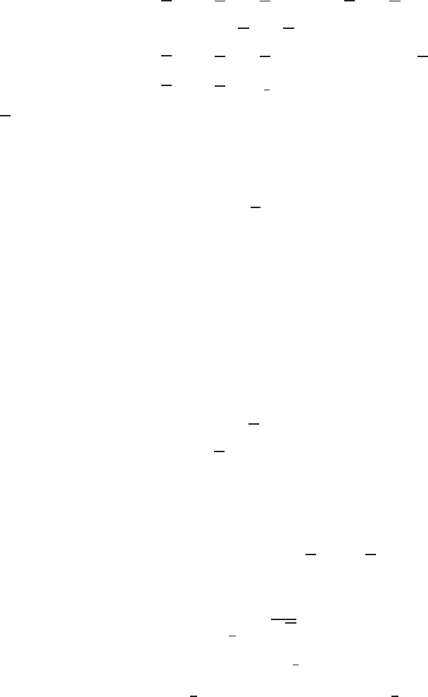
Lectures on Symplectic Field Theory 99
for some constants K
ζ
∈ R. Since each f
ζ
is in ker D
+
, we find
D
σ
Φ
σ
(f)|
D(ζ)
(z) =
∂ρ(z)
√
σf
ζ
(
√
σz) + ρ(z)σ∂f
ζ
(
√
σz)
+ σzρ(z)
√
σf
ζ
(
√
σz)
=
∂ρ(z)
√
σf
ζ
(
√
σz) + ρ(z)σ(D
+
f
ζ
)(
√
σz)
=
∂ρ(z)
√
σK
ζ
e
−
1
2
σ| z|
2
.
(5.3)
Now since
∂ρ = 0 in D
1/2
, we obt ain
kD
σ
Φ
σ
(f)k
2
L
2
=
X
ζ∈Z
+
(β)
Z
D(ζ)
|D
σ
Φ
σ
(f)( z)|
2
dµ(z)
=
X
ζ∈Z
+
(β)
Z
D\D
1/2
|
∂ρ(z)|
2
σK
2
ζ
e
−σ|z|
2
dµ(z)
≤ Iσe
−σ/4
X
ζ∈Z
+
(β)
K
2
ζ
,
where we abbreviate I :=
R
D\D
1/2
¯
∂ρ(z)
2
dµ(z). The norm of f is given by
kfk
2
L
2
=
X
ζ∈Z
+
(β)
Z
C
K
2
ζ
e
−|z|
2
dµ(z) =
Z
C
e
−|z|
2
dµ(z)
X
ζ∈Z
+
(β)
K
2
ζ
.
We conclude that there is a bound of the form
kD
σ
Φ
σ
(f)k
L
2
≤ C
√
σe
−σ/2
kfk
L
2
,
which proves the first stat ement since
√
σe
−σ/2
→ 0 as σ → ∞.
The second statement follows by a change of variable, since
hΦ
σ
(f), Φ
σ
(g)i
L
2
=
X
ζ∈Z
+
(β)
hΦ
σ
(f)|
D(ζ)
, Φ
σ
(g)|
D(ζ)
i
L
2
(D(ζ))
=
X
ζ∈Z
+
(β)
Z
D
ρ
2
(z)σf
ζ
(
√
σz)g
ζ
(
√
σz) dµ(z)
=
X
ζ∈Z
+
(β)
Z
D
√
σ
ρ
2
z
√
σ
f
ζ
(z)g
ζ
(z) dµ(z)
The functions f
ζ
and g
ζ
are both real multiples of e
−
1
2
|z|
2
, so this last integral for each
ζ ∈ Z
+
(β) is bounded between
R
D
√
σ/2
f
ζ
(z)g
ζ
(z) dµ(z) and
R
D
√
σ
f
ζ
(z)g
ζ
(z) dµ(z),
both of which converge to
R
C
f
ζ
(z)g
ζ
(z) dµ(z) a s σ → ∞, thus
lim
σ→ ∞
hΦ
σ
(f), Φ
σ
(g)i
L
2
= hf, gi
L
2
.
To t ur n approximate solutions into actual solutions, let
Π
σ
: L
2
(E) → ker D
σ
denote the orthogonal projection. We will prove:
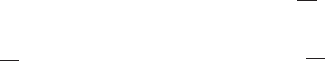
100 Chris Wendl
Proposition 5.24 . If a ll zeroes of β are positive, then the linear map
Π
σ
◦ Φ
σ
:
M
ζ∈Z
+
(β)
ker D
+
→ ker D
σ
is injective for a ll σ > 0 sufficiently large.
This statement says in effect that whenever σ > 0 is large enough and η :=
Φ
σ
(f) ∈ Γ(E) is in the image of the pregluing map, with f normalized by kf k
L
2
= 1,
we can find a “correction” ξ ∈ (ker D
σ
)
⊥
such that
η + ξ 6= 0 but D
σ
(η + ξ) = 0.
An element ξ ∈ (ker D
σ
)
⊥
with the second property certainly exists, and in fact
it’s unique: indeed, the assumption Z
−
(β) = ∅ implies via Lemma
5.22 that D
σ
is
surjective and thus restricts to an isomorphism from (ker D )
⊥
∩ H
1
(E) to L
2
(F ),
with a bounded right inverse
Q
σ
: L
2
(F ) → H
1
(E) ∩ (ker D)
⊥
,
hence ξ := −Q
σ
(D
σ
η). We know moreover from Lemma
5.23 t ha t kηk
L
2
is close
to kfk
L
2
= 1, so to prove η + ξ 6= 0, it would suffice to show kξk
L
2
is small, which
sounds likely since we also know kD
σ
ηk
L
2
is small and Q
σ
is a bounded operator. To
make this reasoning precise, we just need to have some control over kQ
σ
k as σ → ∞,
or equivalently, a quantitat ive measure of the injectivity of D
σ
|
(ker D
σ
)
⊥
∩H
1
(E)
. This
requires one last appeal to the Weitzenb¨ock formula.
Lemma 5.25. Assume all ze roes of β are positive. Then there e xist co nstants
c > 0 and σ
0
such that for all σ > σ
0
,
kηk
L
2
≤ ckD
σ
ηk
L
2
for all η ∈ H
1
(E) ∩ (ker D
σ
)
⊥
.
Proof. Let us instead prove that if zeroes of β are all nega tive, then the same
bound holds for all η ∈ H
1
(E). The stated result follows from this by considering
the formal adjoint and using Exercise
5.26 below. Note that by density, it suffices
to prove the estimate holds for all η ∈ C
∞
0
(E).
Assume therefore that Z
+
(β) = ∅ and, arguing by contradiction, suppose there
exist sequences σ
ν
→ ∞ and η
ν
∈ C
∞
0
(E) with kη
ν
k
L
2
= 1 and
kD
σ
ν
η
ν
k
L
2
→ 0.
The usual rescaling trick and application of the Weitzenb¨ock formula then produces
for each ζ ∈ Z
−
(β) a sequence of functions η
ζ
ν
:= η
(ζ,σ
ν
)
ν
: D
√
σ
ν
→ C which satisfy
X
ζ∈Z
−
(β)
kη
ζ
ν
k
2
L
2
(D
√
σ
ν
)
→ 1 and kD
−
η
ζ
ν
k
L
2
(D
√
σ
ν
)
→ 0
as ν → ∞. Indeed, defining
˙
Σ
ǫ
as in the proof of Lemma
5.18, a similar application
of the Weitzenb¨ock formula yields
kD
σ
ν
η
ν
k
2
L
2
(
˙
Σ)
≥ σ
2
ν
c
2
kη
ν
k
2
L
2
(
˙
Σ
ǫ
)
− σ
ν
c
′
kη
ν
k
2
L
2
(
˙
Σ)
= σ
2
ν
c
2
kη
ν
k
2
L
2
(
˙
Σ
ǫ
)
− σ
ν
c
′
,
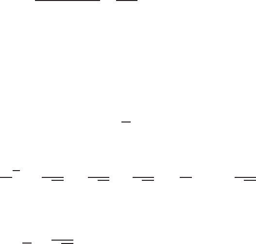
Lectures on Symplectic Field Theory 101
for some c
′
> 0. Thus we obtain
kη
ν
k
2
L
2
(
˙
Σ
ǫ
)
≤
kD
σ
ν
η
ν
k
2
L
2
(
˙
Σ)
c
2
σ
2
ν
+
c
′
σ
ν
c
2
→ 0 as ν → ∞,
so there is again concentrat ion of energy near t he zeroes of t he antilinear perturba-
tion: in particular,
1 = lim
ν→∞
kη
ν
k
2
L
2
(
˙
Σ)
= lim
ν→∞
kη
ν
k
2
L
2
(
˙
Σ
ǫ
)
+ lim
ν→∞
X
ζ∈Z
−
(β)
kη
ν
k
2
L
2
(D(ζ))
= lim
ν→∞
X
ζ∈Z
−
(β)
kη
ζ
ν
k
2
L
2
(D
√
σ
ν
)
.
Moreover, we have
D
−
η
ζ
ν
(z) =
1
σ
ν
∂η
ν
z
√
σ
ν
+
¯z
√
σ
ν
¯η
ν
z
√
σ
ν
=
1
σ
ν
D
σ
ν
η
ν
z
√
σ
ν
.
Taking the square of the norms on each side, we may integrate and use change of
varia bles to obtain
kD
−
η
ζ
ν
k
L
2
(D
√
σ
ν
)
=
1
√
σ
ν
kD
σ
ν
η
ν
k
L
2
(D(ζ))
→ 0 as ν → ∞.
The elliptic estimates from Lecture
2 now provide uniform H
k
-bounds for each η
ζ
ν
on compact subsets of C for every k ∈ N, so tha t a subsequence converges in C
∞
lo c
(C)
to a smooth map η
ζ
∞
∈ L
2
(C, C) satisfying D
−
η
ζ
∞
= 0. But
P
ζ∈Z
−
(β)
kη
ζ
∞
k
2
L
2
(C)
= 1,
so at least one of these solutions is nontrivial and thus contra dicts Proposition
5.20.
Exercise 5.26. Show that for any Fredholm Cauchy-Riemann type operator D
on E, the following two estimates are equivalent, with the same constant c > 0 in
both:
(i) kηk
L
2
(E)
≤ ckDηk
L
2
(F )
for all η ∈ H
1
(E) ∩ (ker D)
⊥
;
(ii) kλk
L
2
(F )
≤ ckD
∗
λk
L
2
(E)
for all λ ∈ H
1
(F ) ∩ (ker D
∗
)
⊥
.
Hint: elliptic regularity implies that for D and D
∗
as bounded linear operators
H
1
→ L
2
, (ker D)
⊥
= im D
∗
and (ker D
∗
)
⊥
= im D.
Proof of Proposition 5.24. If the statement is not true, then there exist
sequences σ
ν
→ ∞ and
f
ν
∈
M
ζ∈Z
+
(β)
ker D
+
such that kf
ν
k
L
2
= 1 and η
ν
:= Φ
σ
ν
(f
ν
) ∈ (ker D
σ
ν
)
⊥
for all ν. Lemmas
5.23
and 5.25 then provide estimates of the form
• kη
ν
k
L
2
→ 1 ,
• kD
σ
ν
η
ν
k
L
2
→ 0 , and
• kη
ν
k
L
2
≤ ckD
σ
ν
η
ν
k
L
2
102 Chris Wendl
as ν → ∞, with c > 0 indep endent of ν. These imply:
1 = lim
ν→∞
kη
ν
k
L
2
≤ lim
ν→∞
ckD
σ
ν
η
ν
k
L
2
= 0.
We’ve proved:
Proposition 5.27. Suppose the ass umptions of §
5.5 hold and that the section
β ∈ Γ( Ho m
C
(
¯
E, F )) has I
+
≥ 0 positive and I
−
≥ 0 negative zeroes. If I
−
= 0, then
D
σ
is surjective with dim ker D
σ
= I
+
for all σ > 0 sufficiently large. If I
+
= 0,
then D
σ
is injective with dim coker D
σ
= I
−
for all σ > 0 suffici e ntly large. In either
ca se,
ind(D
σ
) = I
+
−I
−
for all σ > 0 sufficiently large.
5.8. Antilinear deformations of asymptotic oper at ors
Proposition 5.27 suffices to prove the index formula in the closed case, but there
is an additio na l snag if Γ 6= ∅: since H
1
(
˙
Σ) ֒→ L
2
(
˙
Σ) is not a compact inclusion,
we have no guarantee that D and D
σ
:= D + σB will have t he same index, and
generally they will not. A solution to this problem has been pointed out by Chris
Gerig [
Ger], using a special class of asymptotic operators that also originate in the
work of Taubes (see [
Tau10, Lemma 2.3]).
In general, the only obvious way to guarantee ind(D) = ind(D
σ
) for large σ > 0
is if we can arrange f or ev e ry operator in the family {D
σ
}
σ≥0
to be Fredholm, which
is not automatic since the zeroth-order perturbation B : E → F is required to be
bounded away from zero near ∞ and must therefore change the asymptotic operators
at the punctures. We are therefore led to ask:
Question. For w hat nondegenerate asymptotic operators A : H
1
(E) → L
2
(E)
on a Hermitian line bundle (E, J, ω) → S
1
ca n one find complex-antilin ear bundle
maps B : E → E such that
A
σ
:= A − σB : H
1
(E) → L
2
(E)
is an isomorphism for ev e ry σ ≥ 0?
It turns out that it will suffice to find, for each unitary trivialization σ and every
k ∈ Z, a particular pair (A
k
, B
k
) such that A
k
−σB
k
is nondegenerate for all σ ≥ 0
and µ
τ
CZ
(A
k
) = k. To see why, let us proceed under the assumption that such pairs
can be found, and use them to compute the index:
Lemma 5.28. Given D as in Theorem 5.4, fix asymptotic trivializations τ and
suppose that for each puncture z ∈ Γ there exists an asymptotic operator A
′
z
on
(E
z
, J
z
, ω
z
) with µ
τ
CZ
(A
′
z
) = µ
τ
CZ
(A
z
), such that if A
′
z
is written with respect to τ as
−J
0
∂
t
− S
z
(t), then the deformed asymptotic operator
(5.4) C
∞
(S
1
, R
2
) → C
∞
(S
1
, R
2
) : η 7→ −J
0
∂
t
η − S
z
(t)η − σβ
z
(t)¯η
Lectures on Symplectic Field Theory 103
is nond egen erate for some loop β
z
: S
1
→ C \ {0} and every σ ≥ 0. Then
ind(D) = χ(
˙
Σ) + 2c
τ
1
(E) +
X
z∈Γ
+
wind(β
z
) −
X
z∈Γ
−
wind(β
z
).
Proof. Since µ
τ
CZ
(A
z
) = µ
τ
CZ
(A
′
z
), we can deform A
z
to A
′
z
continuously
through a family of nondegenerate asymptotic operators. It f ollows that we can
deform D throug h a continuous f amily of Fredholm Cauchy-Riemann type oper-
ators to a new operator D
′
whose asymptotic operators are A
′
z
for z ∈ Γ, and
ind(D
′
) = ind(D). We are fr ee to assume in fa ct that D
′
is written with respect to
the trivialization τ on the cylindrical end near z ∈ Γ
±
as
∂
s
+ J
0
∂
t
+ S
z
(t).
Now choose β ∈ Γ(Hom
C
(
¯
E, F )) with nondegenerate zeroes such that the deformed
operators D
σ
η := D
′
η + σβ¯η appear in trivialized form o n the cylindrical end near
z ∈ Γ
±
as
D
σ
η = ∂
s
η + J
0
∂
t
η + S
z
(t)η + σβ
z
(t)¯η.
This means D
σ
is asymptotic at z to (
5.4), which is nondegenerate for every σ ≥ 0,
implying D
σ
is Fredholm for every σ ≥ 0 and thus
ind(D) = ind(D
σ
).
The trivializations τ induce trivializations over the cylindrical ends for
¯
E and
F = Λ
0,1
T
∗
˙
Σ ⊗E, and the expression f or β in the resulting asymptotic trivialization
of Hom
C
(
¯
E, F ) near z ∈ Γ is β
z
(t). It follows that the signed count of zeroes of β is
i(D) := c
τ
1
(Hom
C
(
¯
E, F )) +
X
z∈Γ
+
wind(β
z
) −
X
z∈Γ
−
wind(β
z
)
= χ(
˙
Σ) + 2c
τ
1
(E) +
X
z∈Γ
+
wind(β
z
) −
X
z∈Γ
−
wind(β
z
),
where the computation c
τ
1
(Hom
C
(
¯
E, F )) = χ(
˙
Σ) + 2c
τ
1
(E) follows from the natural
isomorphism
Hom
C
(
¯
E, F ) =
¯
E
∗
⊗ F = E ⊗ F = E ⊗ Λ
0,1
T
∗
˙
Σ ⊗ E = Λ
0,1
T
∗
˙
Σ ⊗ E ⊗ E
= T
˙
Σ ⊗ E ⊗ E.
We are f r ee to assume that all zeroes of β are either positive or negative, depending
on the sign of i(D). Proposition
5.27 then implies ind(D
σ
) = i(D) for la r ge σ.
Notice that instead of nondegenerate families A−σB para metrized by σ ∈ [0, ∞),
it is just as well to find such families which are nondegenerate and have the right
Conley-Zehnder index for all σ > 0, as the σ ≥ 1 portion of this fa mily can be
rewritten as (A −B) −σB for σ ≥ 0. The following lemma thus completes the proof
of Theorem
5.4.
Lemma 5.29. For every k ∈ Z, the trivial Hermitian line bundle over S
1
admits
an asymptotic operator A
k
and a loop β
k
: S
1
→ C \ {0} such that the deformed
asymptotic operators
A
k,σ
η := A
k
η − σβ
k
¯η
104 Chris Wendl
are nondegenerate for every σ > 0 and satisfy
µ
CZ
(A
k,σ
) = wind(β
k
) = k.
Proof. We claim that the choices
A
k
η := −J
0
∂
t
η − πkη and β
k
(t) := e
2πikt
do the trick. We prove this in three steps.
Step 1: k = 0. The a bove formula gives A
0,σ
= −J
0
∂
t
η − σ¯η, in which the
σ = 1 case is precisely the operator that we used in Lecture
3 to norma lize the
Conley-Zehnder index, hence µ
CZ
(A
0,1
) = 0 by definition. More generally, all of
these operators can be expressed in the form A := −J
0
∂
t
− S where S ∈ End
R
(R
2
)
is a constant nonsingular 2-by-2 symmetric matrix that anticommutes with J
0
. We
claim that all asymptotic operators of this f orm are nondegenerate. Indeed, the
conditions S
T
= S and SJ
0
= −J
0
S for J
0
=
0 −1
1 0
imply that S takes the form
a b
b −a
with det S = −a
2
− b
2
6= 0, and moreover S is of this form if and only if
J
0
S also is. In particular, J
0
S is traceless, symmetric, and nonsingular. Solutions
of Aη = 0 then satisfy ˙η = J
0
Sη, which has no periodic solutions since J
0
S has one
positive and one negative eigenvalue, hence ker A = {0}.
Step 2 : even k. There is a cheap trick to deduce the case k = 2m for any m ∈ N
from the k = 0 case. Recall that by Exercise
3.36 in Lecture 3, conjuga t ing A
0,σ
by
a change of trivialization changes it s Conley-Zehnder index by twice the degree of
that change. In particular, the operator
˜
A
0,σ
η := e
2πimt
A
0,σ
(e
−2πimt
η)
is also a nondegenerate asymptotic operator, but with µ
CZ
(
˜
A
0,σ
) = µ
CZ
(A
0,σ
)+2m =
k. Explicitly, we compute
˜
A
0,σ
η = −J
0
∂
t
η − πkη − σke
2πikt
¯η,
so A
k,σ
=
˜
A
0,σ/k
is also nondegenerate for every σ > 0.
Step 3: odd k. Another cheap trick relates each A
k,σ
to A
2k,σ
after an adjustment
in σ. Given an arbitrar y asymptotic operator A = −J
0
∂
t
−S(t) and m ∈ N, define
A
m
:= −J
0
∂
t
− mS(mt).
Geometrically, if A is a trivialized representation for the asymptotic operator of
a Reeb orbit γ : S
1
→ M, then A
m
is the operator fo r the m-fold covered orbit
γ
m
: S
1
→ M : t 7→ γ(mt). It is easy to check in particular that if we define
η
m
(t) := η(mt) for any given loop η : S
1
→ R
2
, then
A
m
η
m
= m(Aη)
m
,
so this gives an embedding of ker A into ker A
m
, implying that whenever A
m
is
nondegenerate for some m ∈ N, so is A. To make use of this, o bserve that
A
2
k,σ
η = −J
0
∂
t
η − π2kη − 2σe
4πikt
¯η = A
2k,2σ
η,
so A
2
k,σ
is nondegenerate for all σ > 0 by Step 2, and therefore so is A
k,σ
.
Lectures on Symplectic Field Theory 105
The proof of Theorem 5.4 is now complete.
Exercise 5 .30. Derive a Weitzenb¨ock formula for asymptotic operat ors and use
it to show that for any asymptotic operator A on the trivial Hermitian line bundle
and any smooth β : S
1
→ C \ {0}, the deformed operators A
σ
η := Aη − σβ¯η are
all nondegenerate for σ > 0 sufficiently large. Deduce from this that µ
CZ
(A
σ
) =
wind(β) for large σ > 0.

LECTURE 6
Symplectic cobordisms and moduli spaces
Contents
6.1. Stable Hamiltonian structures and their symplectizations 107
6.2. Symplectic cobordisms w ith stable boundary 113
6.3. Moduli spaces of unparametrized holomorphic curves 117
6.4. Simple curves and multiple covers 118
6.5. A local structure result 120
In this lecture we introduce the moduli spaces of holomorphic curves that a re
used to define SFT.
6.1. St able Hamiltonian structures and their symplectizations
In Lecture
1, we motivated the notion of a conta ct manifold by considering
hypersurfaces M in a symplectic manifold (W, ω) that satisfy a convexity (also known
as “contact type”) condition. The point of that condition was that it presents M
as one member of a smooth 1-parameter family of hypersurfaces that all have the
same Hamiltonian dynamics; that 1-parameter family furnishes the basic model of
what we call the s ymplectization of M with its induced contact structure. A useful
generalization of this notion was introduced in [
HZ94] and was later recognized to
be the most natural geometric setting for punctured holomorphic curves. It has the
advantage of allowing us to view seemingly distinct theories such as Hamiltonian
Floer homolo gy as special cases of SFT—and even if we are only interested in conta ct
manifolds, the generalization sometimes makes computations easier than they might
be in a purely contact setting.
Recall that every smooth hypersurface M in a 2n-dimensional symplectic mani-
fold (W, ω) has a characteristic line field
ker (ω|
T M
) ⊂ T M,
whose integral curves are the orbits on M of any Hamiltonian vector field generated
by a function H : W → R that has M as a regular level set. We say that M ⊂ (W, ω)
is stable if a neighbor hood of M admits a stabilizing vector field V : this means
that V is transverse to M and the 1-parameter family of hypersurfaces
M
t
:= ϕ
t
V
(M), −ǫ < t < ǫ
generated by the flow ϕ
t
V
of V has the property that each of the diffeomorphisms
M → M
t
defined by flowing along V preserves characteristic line fields.
107
108 Chris Wendl
Exercise 6.1. Show that if V is a stabilizing vector field for M ⊂ (W, ω), then
the 2-form and 1-form pair (Ω, Λ) defined on M by
Ω := ω|
T M
, Λ := ι
V
ω|
T M
has the following properties:
(i) Ω|
ker Λ
is nondegenerate;
(ii) ker Ω ⊂ ker dΛ.
Show moreover that if M is assigned the o rientation for which V is positively trans-
verse to M and ξ := ker Λ ⊂ T M is assigned the natural co-orienta tion determined
by Λ, then the induced orientation of ξ matches the or ientation determined by the
symplectic vector bundle structure Ω|
ξ
, hence condition
(i) can equivalently be writ-
ten as
(iii) Λ ∧ Ω
n−1
> 0
where dim W = 2n.
A stable Hamiltonian structure (or “SHS” for short) on an arbitrary oriented
(2n − 1)-dimensional manifold M is a pair (Ω, Λ) consisting of a closed 2-form Ω
and 1-form Λ such that properties
(ii) and (iii) in Exercise 6.1 are satisfied.
Exercise 6.2. Show that if (Ω, Λ) is a stable Hamiltonian structure, then
ω := d(rΛ) + Ω
is a symplectic form on (−ǫ, ǫ) ×M for ǫ > 0 sufficiently small, where r denotes the
coordinate on (−ǫ, ǫ); moreover, {0}×M is a stable hypersurface in ((−ǫ, ǫ)×M, ω).
Example 6.3. If M ⊂ (W, ω) is a contact type hypersurface, then a Liouville
vector field V t ransverse to M is a stabilizing vector field, and the induced stable
Hamiltonian structure is (dα, α), where α := λ|
T M
with λ := ω(V, ·). We will refer
to this example henceforward as the contact case.
Proposition 6.4. Suppose M ⊂ (W, ω) is a closed stable hypersurface with
stabilizing vector field V and induced stable Hamiltonian structure (Ω, Λ) where
Ω = ω|
T M
and Λ = ι
V
ω|
T M
. Th e n a neighborhood of M in (W, ω) admits a sym-
plectomorphism to ((−ǫ, ǫ) ×M, d(rΛ)+ Ω) for some ǫ > 0, identifying M ⊂ W with
{0} ×M ⊂ (−ǫ, ǫ) × M.
Proof. By the smoo th tubular neighbourhood theorem and the preceeding ex-
ercise, we can view ω
0
= d(rΛ) + Ω as a symplectic form in some neighbourhood
U
0
∼
=
((−ǫ, ǫ) ×M) of M. In this neighbourhood,
(ω
0
−ω)|
M
= 0
by definition of ω
0
and thus
ω
0
−ω = dµ
for some 1-form µ such that µ|
M
= 0. Now define
ω
t
= ω + t dµ

Lectures on Symplectic Field Theory 109
and observe that it is a closed 2-form which can be assumed to be non-degenerate
for a small enough choice of U
0
. Solving the Moser equation
ι
v
t
ω
t
= −µ
yields a well-defined, time-dependent vector field v
t
with the property that v
t
|
M
= 0.
Working back we produce an isotopy a s follows:
dι
v
t
ω
t
= −dµ ⇒
L
v
t
ω
t
= dι
v
t
ω
t
+ ι
v
t
dω
t
= dι
v
t
ω
t
= −dµ = −
dω
t
dt
⇒
d
dt
(ρ
∗
t
ω
t
) = L
v
t
ω
t
+
dω
t
dt
= 0
where ρ
∗
t
is the flow of v
t
. Then
ρ
∗
t
ω
t
= ρ
∗
0
ω = ω
since ρ
0
is the identity. The required symplectomorphism is then
ρ
1
: ρ
−1
1
U
0
→ U
0
and the fact that M is fixed under the isotopy follows from v
t
|
M
= 0.
Example 6.5. In the contact case (Ω, Λ) = (dα, α), the symplectic form on the
collar neighborhood in Propo sition
6.4 can be rewritten as d(e
t
α) by defining the
coordinate t := ln(r + 1). The proposition is easier to prove in this case: one can
construct the collar neighborhood simply by flowing along V , with no need for the
Moser isotopy trick.
A stable Ha miltonian structure H = (Ω, Λ) gives rise to two importa nt additional
objects: a co-o riented hyperplane distribution
ξ := ker Λ,
and a positively transverse vector field R determined by the conditions
Ω(R, ·) ≡ 0 and Λ(R) ≡ 1.
By analogy with the cont act case, we will refer to R as the Reeb vector field of H.
The condition ker Ω ⊂ ker dΛ implies that it reduces to the usual contact notio n of
the Reeb vector field for Λ whenever the latter happens also to be a contact form.
The symplectization of (M, H) for any stable Hamiltonian structure H =
(Ω, Λ) can be defined by choosing suitable diffeomorphisms of (−ǫ, ǫ) × M with
R × M: equivalently, this means we consider R × M with the family of symplectic
forms ω
ϕ
defined by
(6.1) ω
ϕ
:= d ( ϕ(r)Λ) + Ω
where ϕ is chosen arbitrar ily from the set
(6.2) T :=
ϕ ∈ C
∞
(R, (−ǫ, ǫ))
ϕ
′
> 0
.
110 Chris Wendl
Example 6.6. The fo llowing stable Hamiltonian structure places Hamiltonian
Floer homology into the setting of SFT. Suppose (W, ω) is a closed symplectic man-
ifold and H : S
1
×W → R is a smoo th function, and denote H
t
:= H(t, ·) : W → R.
The time-dependent Hamiltonian vector field X
t
defined by dH
t
= −ω(X
t
, ·) can
then be viewed as defining a symplec tic connection on the trivial symplectic fiber
bundle
M := S
1
× W
t
−→ S
1
,
i.e. t he flow of R(t, x) := ∂
t
+ X
t
(x) defines symplectic parallel transport maps
between fibers. The horizontal subbundle fo r this connection is the “symplectic
complement” of the vertical subbundle with respect to the closed 2-form
Ω = ω + dt ∧ dH.
In other words, Ω restricts to the fibers o f M → S
1
as ω and the subbundle
{X ∈ T M | ω(X, ·)|
T ({const}×W )
} is generated by R, so Ω is the connection 2-
form defining the connection, cf. [
MS98]. Setting Λ := dt then makes H := (Ω, Λ)
a stable Hamiltonian structure with Reeb vector field R, and its closed orbits in
homotopy classes that project to S
1
with degree one are in 1-to-1 correspondence
with the 1-periodic Hamiltonian orbits on W . Notice that this is very different from
the contact case: ξ = ker dt is as far as possible from being a cont act structure, it
is instead an integrable distribution whose integral submanifolds are the fibers of
M → S
1
.
Exercise 6.7. Show that for any stable Hamiltonian structure H = (Ω, Λ), the
flow of R preserves ξ = ker Λ along with its symplectic bundle structure Ω|
ξ
.
Definition 6 .8. A T -periodic orbit x : R → M of R is called nondegenerate
if 1 is not an eigenvalue of dϕ
T
|
ξ
x(0)
: ξ
x(0)
→ ξ
x(0)
, where ϕ
t
denotes the flow of R.
Exercise 6.9. Show that in Example 6.6, the notions of nondegeneracy for
closed Reeb orbits on M and for 1-periodic Hamiltonian orbits on W (see Lecture
1)
coincide.
If γ : S
1
→ M parametrizes a T -periodic orbit of R with ˙γ = T · R(γ), then the
formula of Lecture 3 for the asymptotic operator
A
γ
η = −J(∇
t
η − T ∇
η
R)
still makes sense in this more general context, and it defines an L
2
-symmetric oper-
ator on the Hermitian vector bundle (γ
∗
ξ, J, Ω) over S
1
. It can also be interpreted
as a Hessian at a critical point, though for an action functional that is only lo-
cally defined: indeed, while Ω need not be globally exact, it is necessarily exact on
a neighborhood of γ
0
(S
1
) for any given loop γ
0
: S
1
→ M, so one can pick any
primitive λ of Ω on this neighborhood and, for a sufficiently small neighborhood
U(γ
0
) ⊂ C
∞
(S
1
, M) of γ
0
, consider the action functional
(6.3) A
H
: U(γ
0
) → R : γ 7→
Z
S
1
γ
∗
λ.
Lectures on Symplectic Field Theory 111
Its first var iation at γ ∈ U(γ
0
) in the direction η ∈ Γ(γ
∗
ξ) is then
dA
H
(γ)η = −
Z
S
1
Ω( ˙γ, η) dt = h−Jπ
ξ
˙γ, ηi
L
2
,
where π
ξ
: T M → ξ denotes t he projection along R and the L
2
-pairing on γ
∗
ξ
is defined via the bundle metric Ω(·, J·)|
ξ
. This leads us to interpret −Jπ
ξ
˙γ as a
“gradient” ∇A
H
(γ), and if ˙γ = T · R(γ), then differentiat ing this gradient in the
direction of η ∈ Γ(γ
∗
ξ) gives A
γ
η. As one would exp ect, nondegeneracy of γ is
then equivalent to the condition ker A
γ
= {0}, and one can in this case define the
Conley-Zehnder index µ
τ
CZ
(γ) ∈ Z as in Lecture
3, relative to a choice of unitary
trivialization τ for (ξ, J, Ω).
Exercise 6.10. In the setting of Example
6.6, work out the relationship b etween
A
H
and the symplectic action functional for Hamiltonian systems that we discussed
in L ecture
1. (Try not to worry too much about signs.)
Definition 6.11. Given a stable Hamiltonian structure H = (Ω, Λ), denote by
J(H) ⊂ J(R × M)
the space of smooth almost complex structures J on R × M with the following
properties:
• J is invariant under the R-a ctio n on R×M by translation of the first factor;
• J∂
r
= R and JR = −∂
r
, where r denotes the natural coo rdinate on the
first factor;
• J(ξ) = ξ and J|
ξ
is compatible with the symplectic vector bundle structure
Ω|
ξ
.
Notice that if H = (dα, α) for a cont act form α, then J(H) matches the space
J(α) defined in Lecture
1.
Exercise 6.12. Show that every J ∈ J(H) is tamed by all of the symplectic
structures ω
ϕ
as defined in (
6.1) for ϕ ∈ T .
Given J ∈ J(H), we define the energy of a J-holomorphic curve u : (Σ, j) →
(R × M, J) by
E(u) := sup
ϕ∈T
Z
Σ
u
∗
ω
ϕ
.
Exercise
6.12 above implies tha t E(u) ≥ 0, with equality if and only if u is constant.
In t he contact case, this notion o f energy is not identical to the “Hofer energy” that
we defined in Lecture
1, nor to Hofer’s origina l definition from [Hof93], but all three
are equivalent for our purposes since uniform bounds on any of them imply uniform
bounds on the others.
Just as in the contact case, the simplest example of a finite-energy J-holomorphic
curve is a tr ivial cylinder
u
γ
: R × S
1
→ R × M : (s, t) 7→ (T s, γ(t)),
where γ : S
1
→ M is a “constant velocity” parametrization of a T -periodic orbit of
R, i.e. ˙γ = T ·R(γ). More generally, given a punctured Riemann surface (
˙
Σ = Σ\Γ, j)
112 Chris Wendl
with Γ = Γ
+
∪Γ
−
, we consider asymptotically cylindrical J-holomorphic curves
u : (
˙
Σ, j) → (R × M, J), which are assumed to have the property that for each
z ∈ Γ
±
, there exist holomorphic cylindrical coordinates identifying a punctured
neighborhood
˙
U
z
⊂
˙
Σ of z with Z
+
= [0, ∞)×S
1
or Z
−
= (−∞, 0]×S
1
respectively,
and a trivial cylinder u
γ
z
: R ×S
1
→ R ×M such that
u(s, t) = exp
u
γ
z
(s,t)
h
z
(s, t) for |s| sufficiently large,
where h
z
(s, t) is a vector field along u
γ
z
satisfying |h
z
(s, ·)| → 0 uniformly as s →
±∞. As usual, both the norm |h
z
(s, t)| and the exponential map here are assumed
to be defined with respect to a translation-invariant choice of Riemannian metric
on R × M. The vector fields h
z
along u
γ
z
for each z ∈ Γ are sometimes called
asymptotic representatives of u near z.
Asymptotic representatives satisfy a regularity estimate that will be important to
know about, though its proof (given originally in [
HWZ96]) would be too lengthy to
present here. The methods behind the following statement involve a combination of
nonlinear regularity arguments as in Lecture
2 with the asymptotic elliptic estimates
from Lecture
4. To prepare for the statement, note that H induces a splitting of
complex vector bundles
(6.4) T(R × M) = ǫ ⊕ ξ,
where ǫ denotes the trivial complex line bundle generated by the vector field ∂
r
, or
equivalently, the Reeb vector field. It follows that if γ : S
1
→ M is a Reeb orbit
and u
γ
: R × S
1
→ R × M is the corresponding trivial cylinder, then any unitary
trivialization τ of the Hermitian bundle (γ
∗
ξ, J, Ω) natura lly induces a trivialization
of u
∗
γ
T (R × M) .
Proposition 6.13 ([
HWZ96]). Assume J ∈ J(H), u : (
˙
Σ, j) → (R × M, J)
is J-holomorphic and asymptotically cylindrical, and its as ymp totic orbit γ
z
at z ∈
Γ
±
is nondegenerate. Let h(s, t) ∈ C
n
denote the asymptotic repre sentative of u
near z expressed via the trivialization induced b y a c hoice of unitary trivialization
for (γ
∗
z
ξ, J, Ω). If δ > 0 is small enough so that the asymptotic operator A
γ
z
has no
eigenvalues in the closed interval between 0 and ∓δ, then
h(s, t) = e
∓δs
g(s, t)
for some bounded f unc tion g(s, t) ∈ C
n
whose deri v atives of all orders are bounded
as s → ±∞.
Remark 6.14 . The range of δ > 0 for which Prop.
6.13 holds is o pen, thus by
adjusting δ slight ly, o ne can equivalently say that h( s, t) = e
∓δs
g(s, t) where the
derivatives of all orders of g(s, t) decay to zero as s → ±∞.
Exercise 6.15. Convince yourself that the analog ue of Proposition 6.13 in Morse
theory is true. Namely, suppose (M, g) is a Riemannian manif old, f : M → R is
smooth a nd u : R → M is a solution to ˙u + ∇f(u) = 0 with lim
s→±∞
u(s) = x
±
∈
Crit(f), where x
±
are nondegenerate critical points. We can write u(s) asymptoti-
cally as
u(s) = exp
x
±
h
±
(s)

Lectures on Symplectic Field Theory 113
for some functions h
±
(s) ∈ T
x
±
M that are defined for s close to ±∞ and satisfy
|h
±
(s)| → 0 as s → ±∞. Show that if δ > 0 is small enough so that ∇
2
f(x
±
) has
no eigenvalue in the closed interval between 0 and ±δ, then
h
±
(s) = e
∓δs
g
±
(s)
for some functions g
±
(s) with bo unded derivatives o f all orders as s → ±∞.
1
Hint:
fix local coordinates identifying x
±
with 0 ∈ R
n
and first consider the case where
∇f(x) in these coordinates depends linearly on x. Then try to compare u(s) with
solutions of this idealized equation.
Example 6.16. In the setting of Example
6.6, a choice of J ∈ J(H) is equiv-
alent to a choice of smooth S
1
-parametrized family of compatible almost complex
structures {J
t
}
t∈S
1
on (W, ω), and J- holomorphic curves u : (
˙
Σ, j) → (R × M, J)
can be written as
u = (f, v) :
˙
Σ →
R × S
1
× W,
where f : (
˙
Σ, j) → (R × S
1
, i) is holomorphic. In particular, if (
˙
Σ, j) = (R × S
1
, i)
and f is taken to have an extension to S
2
→ S
2
of degree one, then u can be
reparametrized so that f is the identity map, hence u = (Id, v) : R × S
1
→ (R ×
S
1
) ×W is a section of the trivial fiber bundle (R ×S
1
) ×W → R ×S
1
, and one can
check that t he equation satisfied by v : R ×S
1
→ W is precisely the Floer equation
∂
s
v + J
t
(v)( ∂
t
v − X
t
(v)) = 0.
6.2. Symplectic cobordisms with stable boundary
We discussed symplectic cobor disms between contact manifolds in Lecture
1.
Let us now generalize this notion in the context of stable Hamiltonian structures.
A symplectic cobordism with stable boundary is a compact symplectic
manifold (W, ω) with boundary ∂W = −M
−
⊔ M
+
, equipped with a stabilizing
vector field V that points tr ansversely inward at M
−
and outward at M
+
. This
induces stable Hamiltonian structures H
±
= (ω
±
, λ
±
) on M
±
, where
ω
±
:= ω|
T M
±
, λ
±
:= (ι
V
ω)|
T M
±
,
and observe that the orientation conventions for M
+
and M
−
(with the latter car-
rying the opposite of the natural boundary orientation) have been chosen such that
if dim W = 2n,
λ
±
∧ ω
n−1
±
> 0 on M
±
.
We can now identify neighborhoods o f M
±
in ( W, ω) symplectically with collars of
the form
([0, ǫ) ×M
+
, d (rλ
+
) + ω
+
) ,
((−ǫ, 0] × M
−
, d (rλ
−
) + ω
−
) ,
see Figure
6.1.
1
The apparent discrepancy in s igns between this and Proposition
6.13 is due to the fact that
u(s) satisfies a negative gradient flow equation, whereas the nonlinear Cauchy-Riemann equa tion
in symplectizations is interpreted loosely as a positive gradient flow equation.
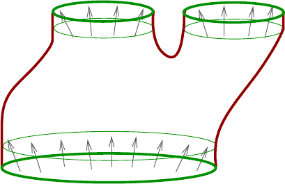
114 Chris Wendl
((−ǫ, 0] × M
+
, d(rλ
+
) + ω
+
)
([0, ǫ) × M
−
, d(rλ
−
) + ω
−
)
(W, ω)
Figure 6.1. A symplectic cobordism with stable boundary compo-
nents ∂W = −M
−
⊔M
+
and symplectic collar neighborhoods induced
by the stable Hamiltonian structures H
±
= (ω
±
, λ
±
) on M
±
.
Modifying (6.2) by
(6.5) T
0
:=
ϕ ∈ C
∞
(R, (−ǫ, ǫ))
ϕ
′
> 0 and ϕ(r) = r for r near 0
,
we can use any ϕ ∈ T
0
to define a symplectic completion (
c
W , ω
ϕ
) of (W, ω) by
c
W :=
(−∞, 0] × M
−
∪
M
−
W ∪
M
+
[0, ∞) × M
+
,
where the above collar neighborhoods are used to g lue the pieces together smoo t hly
and the symplectic form is defined by
ω
ϕ
:=
d (ϕ(r)λ
−
) + ω
−
on (−∞, 0] × M
−
,
ω on W,
d (ϕ(r)λ
+
) + ω
+
on [0, ∞) × M
+
,
see Figure
6.2. For each r
0
≥ 0, we define the compact submanifold
W
r
0
:= ([−r
0
, 0] × M
−
) ∪
M
−
W ∪
M
+
([0, r
0
] × M
+
) ,
and observe that (W
r
0
, ω
ϕ
) is also a symplectic cobordism with stable boundary fo r
every ϕ ∈ T
0
.
Since
c
W is noncompact, almost complex structures J on
c
W will need to satisfy
conditions near infinity in order for moduli spaces of J-holomor phic curves to be well
behaved, but we would like to preserve the f r eedom of choosing arbitrary compatible
or tame almost complex structures in compact subsets.
Definition 6.17. Given ψ ∈ T
0
and r
0
≥ 0, let
J
τ
(ω
ψ
, r
0
, H
+
, H
−
) ⊂ J(
c
W )
denote the space of smooth almost complex structures J on
c
W such tha t:
• J on [r
0
, ∞) ×M
+
matches an element of J(H
+
);
• J on (−∞, −r
0
] × M
−
matches an element of J(H
−
);
• J on W
r
0
is tamed by ω
ψ
.

Lectures on Symplectic Field Theory 115
(W, ω)
((−ǫ, 0] × M
+
, d(rλ
+
) + ω
+
)
([0, ǫ) × M
−
, d(rλ
−
) + ω
−
)
([0, ∞) × M
+
, d(ϕ(r)λ
+
) + ω
+
)
((−∞, 0] ×M
−
, d(ϕ(r)λ
−
) + ω
−
)
Figure 6.2. The completion (
c
W , ω
ϕ
) of a symplectic cobordism
with stable boundary.
Let
J(ω
ψ
, r
0
, H
+
, H
−
) ⊂ J
τ
(ω
ψ
, r
0
, H
+
, H
−
)
denote the subset for which J is additio nally compatible with ω
ψ
on W
r
0
.
Setting
(6.6) T (ψ, r
0
) :=
ϕ ∈ T
0
ϕ ≡ ψ on [−r
0
, r
0
]
,
Exercise
6.12 implies that every J ∈ J(ω
ψ
, r
0
, H
+
, H
−
) is tamed by ω
ϕ
for every
ϕ ∈ T (ψ, r
0
). It is therefore sensible to define the energy of a J-holomorphic curve
u : (Σ, j) → (
c
W , J) by
E(u) := sup
ϕ∈T (ψ,r
0
)
Z
Σ
u
∗
ω
ϕ
.
The notion of asymptotically cylindrical J-holomorphic curves extends in a straight-
forwar d way to the setting of (
c
W , J): such curves are proper maps whose posi-
tive/negative punctures are asymptotic to closed or bits of the Reeb vector field R
±
induced by H
±
on {±∞} × M
±
, see Figure 6.3. The exponential decay estimate
in Proposition
6.13 is also immediately applicable in this more general setting since
asymptotically cylindrical curves in
c
W are indistinguishable near their punctures
from curves in the symplectizations R × M
±
.
It is easy to check that asymptotically cylindrical J-holomorphic curves always
have finite energy. We will prove in Lecture
8 that the converse is also true whenever
the Reeb orbits are nondegenerate.
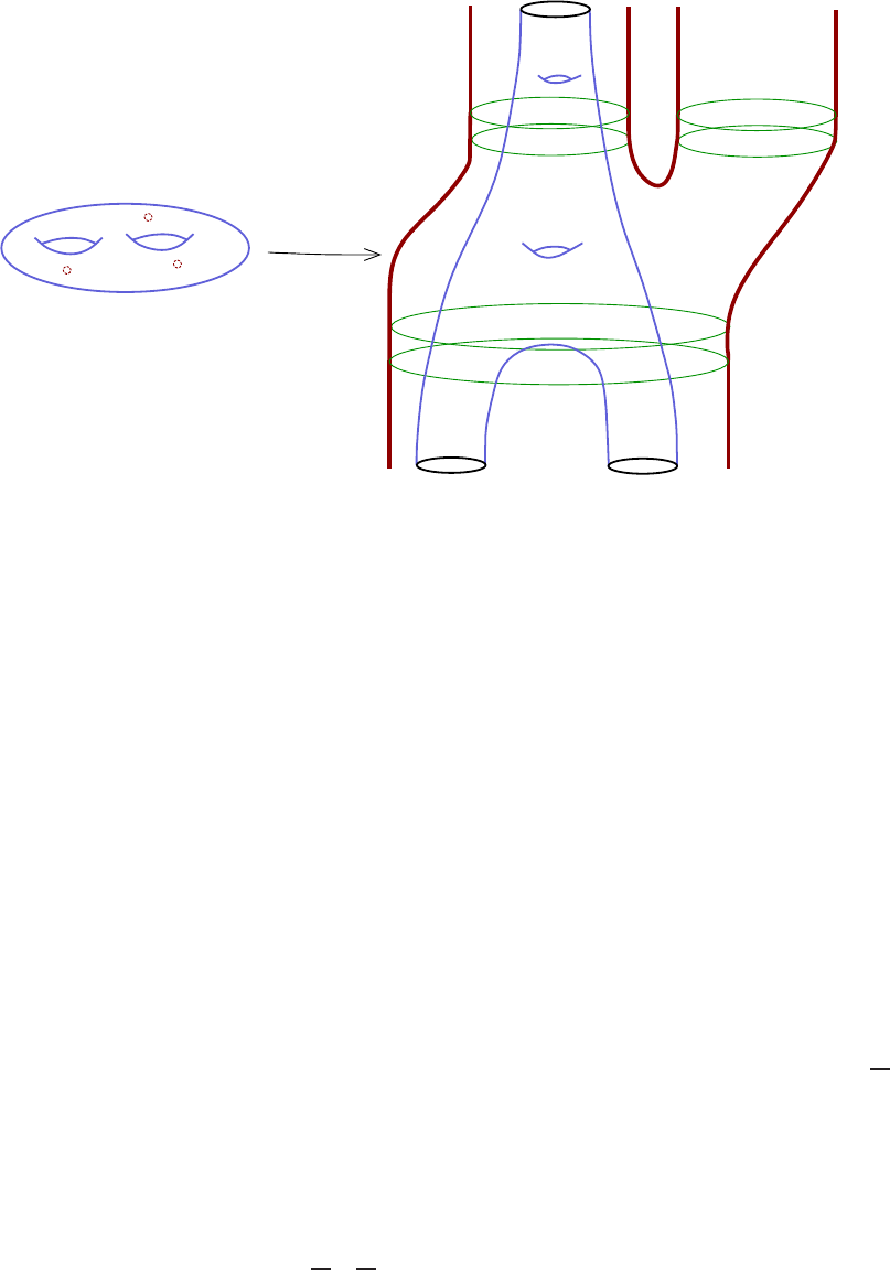
116 Chris Wendl
c
W
˙
Σ
u
Figure 6.3. An asymptotically cylindrical holomorphic curve in
(
c
W , J) with genus 2, one positive puncture and two negative punc-
tures.
Remark 6.18. Strictly speaking, the “trivial stable cobordism”
([0, 1] ×M, d(ϕ(r)Λ, Ω))
induces different stable Hamiltonian structures at M
−
:= {0} × M and M
+
:=
{1} × M, thus o ne cannot technically regard J(H) as contained in any space of
the for m J(ω
ψ
, r
0
, H
+
, H
−
) without inventing questionable new notions such as
the “infinitesimal trivial cobordism” [0, 0] × M (whose completion would be the
symplectization of (M, H)). It is nonetheless true for fairly trivial reasons that most
results about J(ω, r
0
, H
+
, H
−
) apply equally well to J(H), and we shall use this
fact in the following without always mentio ning it.
Every asymptotically cylindrical curve u :
˙
Σ →
c
W has a well-defined relative
homology class, meaning the following. Denote the asymptotic orbits of u at
its punctures z ∈ Γ
±
by γ
z
, and let
¯
γ
±
⊂ M
±
denote the closed 1- dimensional
submanifold defined as the union over z ∈ Γ
±
of the images of the orbits γ
z
. L et
Σ
denote the compact oriented topological surface with bo undar y obtained from
˙
Σ by
appending {±∞} × S
1
to each o f its cylindrical ends, and let π :
c
W → W denote
the retraction defined a s the ident ity o n W and π( r, x) = x ∈ M
±
⊂ ∂W for (r, x)
in [0, ∞) × M
+
or (−∞, 0] × M
−
. Then π ◦ u :
˙
Σ → W has a natural continuous
extension
¯u : (
Σ, ∂Σ) → (W,
¯
γ
+
∪
¯
γ
−
)
and thus represents a relative homology class
[u] ∈ H
2
(W,
¯
γ
+
∪
¯
γ
−
).
Lectures on Symplectic Field Theory 117
6.3. Moduli spaces of unparametrized holomorphic curves
We continue in the setting of a completed symplectic cobordism
c
W with fixed
choices of ψ ∈ T
0
, r
0
≥ 0 and J ∈ J(ω
ψ
, r
0
, H
+
, H
−
). We shall denote by ξ
±
and
R
±
the hyperplane distribution and Reeb vector field respectively determined by
the stable Hamiltonian structure H
±
= (ω
±
, λ
±
).
Fix integers g, m, k
+
, k
−
≥ 0 along with o r dered sets of Reeb orbits
γ
±
= (γ
±
1
, . . . , γ
±
k
±
),
where each γ
±
i
is a closed orbit of R
±
in M
±
. Denote the union of the images of the
γ
±
i
by
¯
γ
±
⊂ M
±
, and choose a relative homology class
A ∈ H
2
(W,
¯
γ
+
∪
¯
γ
−
)
whose image under the boundary map H
2
(W,
¯
γ
+
∪
¯
γ
−
)
∂
−→ H
1
(
¯
γ
+
∪
¯
γ
−
) defined
via the long exact sequence of the pair (W,
¯
γ
+
∪
¯
γ
−
) is
∂A =
k
+
X
i=1
[γ
+
i
] −
k
−
X
i=1
[γ
−
i
] ∈ H
1
(
¯
γ
+
∪
¯
γ
−
).
The moduli space of unparametrized J-holomorphic curves of genus g with m
marked points, homologous to A and asymptotic to (γ
+
, γ
−
) is then defined
as a set of equivalence classes of tuples
M
g,m
(J, A, γ
+
, γ
−
) =
(Σ, j, Γ
+
, Γ
−
, Θ, u)
∼,
where:
(1) (Σ, j) is a closed connected Riemann surface of genus g;
(2) Γ
+
= (z
+
1
, . . . , z
+
k
+
), Γ
−
= (z
−
1
, . . . , z
−
k
−
) and Θ = (ζ
1
, . . . , ζ
m
) are disjoint
ordered sets of distinct points in Σ;
(3) u : (
˙
Σ := Σ \ (Γ
+
∪ Γ
−
), j) → (
c
W , J) is an asymptotically cylindrical J-
holomorphic map with [u] = A, asymptotic at z
±
i
∈ Γ
±
to γ
±
i
for i =
1, . . . , k
±
;
(4) Equivalence
(Σ
0
, j
0
, Γ
+
0
, Γ
−
0
, Θ
0
, u
0
) ∼ (Σ
1
, j
1
, Γ
+
1
, Γ
−
1
, Θ
1
, u
1
)
means the existence o f a biholomo r phic map ψ : (Σ
0
, j
0
) → (Σ
1
, j
1
), taking
Γ
±
0
to Γ
±
1
and Θ
0
to Θ
1
with the ordering preserved, such that
u
1
◦ ψ = u
0
.
We shall usually abuse notation by a bbreviating elements [( Σ, j, Γ
+
, Γ
−
, Θ, u)] in
this moduli space by
u ∈ M
g,m
(J, A, γ
+
, γ
−
).
The automorphism group
Aut(u) = Aut(Σ, j, Γ
+
, Γ
−
, Θ, u)
of u is defined as the group of biholomorphic maps ψ : (Σ, j) → (Σ, j) which act
as the identity on Γ
+
∪ Γ
−
∪ Θ and satisfy u = u ◦ ψ. Clearly the isomorphism
class of this group dep ends only on the equivalence class [(Σ, j, Γ
+
, Γ
−
, Θ, u)] ∈

118 Chris Wendl
M
g,m
(J, A, γ
+
, γ
−
), and we will see in §6.4 below that it is always finite unless
u :
˙
Σ →
c
W is constant. The significance of the marked points is that they determine
an evaluation map
ev : M
g,m
(J, A, γ
+
, γ
−
) →
c
W
m
: [(Σ, j, Γ
+
, Γ
−
, Θ, u)] 7→ (u(ζ
1
), . . . , u(ζ
m
))
where Θ = (ζ
1
, . . . , ζ
m
). For most of our applications we will be free to assume
m = 0, as marked points are not needed for defining the most basic versions of
SFT; the evaluation map does play a prominent role however in more algebraically
elaborate versions of the theory, and especially in the Gromov-Witten invariants
(the “closed case” of SFT).
We will assign a topology to M
g,m
(J, A, γ
+
, γ
−
) in the next lecture by locally
identifying it with subsets of certain manifolds of maps
˙
Σ →
c
W with Sobolev-type
regularity and exponential decay conditions at the ends. In reality, this topology
admits a simpler description: one can define convergence o f a sequence
[(Σ
ν
, j
ν
, Γ
+
ν
, Γ
−
ν
, Θ
ν
, u
ν
)] → [(Σ, j, Γ
+
, Γ
−
, Θ, u)]
to mean that for sufficiently large ν, the equivalence classes in the sequence admit
representatives of the form (Σ, j
′
ν
, Γ
+
, Γ
−
, Θ, u
′
ν
) such that
(1) j
′
ν
→ j in C
∞
;
(2) u
′
ν
→ u in C
∞
lo c
(
˙
Σ,
c
W );
(3) ¯u
′
ν
→ ¯u in C
0
(
Σ, W ).
The proof that this topology matches what we will define in the next lecture in
terms of weighted Sobolev spaces requires a symptotic elliptic regularity arguments
along the lines of Proposition
6.13.
6.4. Simple curves and multiple covers
In Lecture 2, we pr oved that closed J-holomorphic curves ar e all either embedded
in the complement of a finite set or are multiple covers of curves with this property.
The same thing holds in the punctured case:
Theorem 6.1 9. Assume u : (
˙
Σ, j) → (
c
W , J) is a nonconstant as ymptoti-
ca lly cylindrical J-h o l omorphic curve whose asymptotic orbits are all nondegenerate,
where
˙
Σ = Σ \ Γ for some closed Riemann surface (Σ, j) and finite subset Γ ⊂ Σ.
Then there exists a factorization u = v ◦ ϕ, w here
• ϕ : (Σ, j) → (Σ
′
, j
′
) is a hol omorphic map of positive degree to another
closed and con nected Riemann surface (Σ
′
, j
′
);
• v : (
˙
Σ
′
, j
′
) → (
c
W , J) is an asymptotically cylindrical J-holomorphic curve
which is embedd ed except at a finite s et o f critical points and se l f - i ntersec tion s,
where
˙
Σ
′
:= Σ
′
\ Γ
′
with Γ
′
:= ϕ(Γ) and Γ = ϕ
−1
(Γ
′
).
As in the closed case, we call u a simple curve if the holomorphic map ϕ :
(Σ, j) → (Σ
′
, j
′
) is a diffeomorphism, and u is otherwise a k-fold multiple cover
of v with k := deg(ϕ) ≥ 2.
The proof of this theorem is an almost verbatim repeat of the proof of The-
orem
2.29 in Lecture 2, but with one new ingredient added. Recall that in the
Lectures on Symplectic Field Theory 119
closed case, our proof required two lemmas which described the local picture of a J-
holomorphic curve u :
˙
Σ →
c
W near either a double po int u(z
0
) = u(z
1
) for z
0
6= z
1
or
a critical point du(z
0
) = 0. Both statements were completely local and thus equally
valid for no n-closed curves, but we now need similar statements to describe what
kinds of singularities can appear in the neighborhood of a puncture. The following
lemma is due to Siefring [
Sie08] and follows from a “ relative asymptotic formula”
analogous to Proposition
6.13.
Lemma 6.20 (Asymptotics). Assume u : (
˙
Σ = Σ \ Γ, j) → (
c
W , J) i s a s ymptot-
ically cylindrical and is asymptotic at z
0
∈ Γ to a nondegenerate Reeb orbit. Then
a punctured neighborhood
˙
U
z
0
⊂
˙
Σ of z
0
ca n be identified biholomorphically with the
punctured disk
˙
D = D \ {0} such that
u(z) = v(z
k
) for z ∈
˙
D =
˙
U
z
0
,
where k ∈ N and v : (
˙
D, i) → (
c
W , J) is an embedded and asymptotically cylindrical
J-holomorphic curve. Moreover, if u
′
: (
˙
Σ
′
= Σ
′
\ Γ
′
, j
′
) → (
c
W , J) is another
asymptotically cylindrical curve with a puncture z
′
0
∈ Γ
′
, then the ima g es of u near
z
0
and u
′
near z
′
0
are either identical or disjoint.
Exercise 6.21. With Lemma
6.20 in hand, adapt the proof of Theorem 2.29 in
Lecture
2 to prove Theorem 6.19. If you get stuck, see [Nel15, §3.2].
Proposition 6.22. If [(Σ, j, Γ
+
, Γ
−
, Θ, u)] ∈ M
g,m
(J, A, γ
+
, γ
−
) is represented
by a simple curve, then Aut(u) is trivial. If it is represented by a k-fold cover of a
simple curve, then |Aut(u)| ≤ k. In particular, Aut(u) is a l ways finite unless u is
co nstant.
Proof. If u is simple, then it is a diffeomorphism onto its image in a small
neighbourhood of some point, and any map ϕ satisfying u = u ◦ ϕ would be the
identity on such a neighbourhood. By unique continuation, we conclude that Aut(u)
is trivial. In general if u = v ◦ ϕ for some simple
v : Σ
′
→ W
and
ϕ : Σ → Σ
′
a k-fold branched cover, we have
Aut(u) = {f : Σ → Σ | v ◦ ϕ ◦ f = v ◦ ϕ}.
By a similar argument as in the previous case, knowing that v is simple implies we
only need to look at solutions to
ϕ ◦f = ϕ.
Remove the set of branch points B from Σ
′
together with the set ϕ
−1
(B) f rom
Σ, so that ϕ becomes an ho nest covering map. Any ϕ ∈ Aut(u) then defines a
biholomorphic deck transformation of the cover, so it remains to argue that t here
are at most k of them. In fact, there is at most one transformation that takes w
1
to
w
2
for any two given points w
1
, w
2
∈ ϕ
−1
(x). If there were two such transformations
120 Chris Wendl
f and g, then f ◦ g
−1
would be the identity on an open neighbour hood and would
thus be globally the identity by unique continuation.
6.5. A local structure result
The following statement, which we will prove in the next lecture, is the main
goal of most of the analysis we have discussed recently. It is essentially an appli-
cation of the implicit function t heorem for a smooth nonlinear Fredholm section
of a Banach space bundle. The implicit function theorem (see [
Lan93]) implies in
particular that if F is a smoo t h map between Banach spaces such tha t F (x
0
) = 0
and dF (x
0
) is a surjective Fredholm operat or, then F
−1
(0) is a smooth manifold
near x
0
with its dimension equal to the Fredholm index of dF (x
0
). Surjectivity is
an extra hypothesis, referred to in t he statement below as “Fredholm regularity,”
a notion that we will define precisely in t he next lecture. The dimension for mula
should look familiar, but is only an indirect consequence of the index formula for
Cauchy-Riemann type operators tha t we proved in Lecture 5; one also needs to ac-
count for the fact that in defining our moduli space M
g,m
(J, A, γ
+
, γ
−
), we did not
fix the complex structures on our domain curves, hence they ar e free to move about
in the moduli space of Riemann surfaces, whose dimension therefore plays a role in
determining the dimension of M
g,m
(J, A, γ
+
, γ
−
).
Theorem 6.23. The set of Fredholm regular curves forms an open subset
M
reg
g,m
(J, A, γ
+
, γ
−
) ⊂ M
g,m
(J, A, γ
+
, γ
−
)
which naturally admits the structure of a smoo th finite-dimensional orbifold of di-
mension
dim M
reg
g,m
(J, A, γ
+
, γ
−
) = ( n − 3)(2 − 2g − k
+
− k
−
) + 2c
τ
1
(A)
+
k
+
X
i=1
µ
τ
CZ
(γ
+
i
) −
k
−
X
i=1
µ
τ
CZ
(γ
−
i
) + 2m,
where dim W = 2n, τ is a choice of unitary trivia l i zation for (ξ
±
, J, ω
±
) along each
of the asymptotic orbits γ
±
i
, and c
τ
1
(A) denotes the normal first Chern number of the
co mplex vector bundle (u
∗
T
c
W , J) →
˙
Σ with respect to the asymptotic trivialization
determined by τ and the sp l i tting T (R ×M
±
) = ǫ ⊕ξ
±
(cf. (
6.4)). The local isotropy
gro up of M
reg
g,m
(J, A, γ
+
, γ
−
) at u is Aut(u), hence the moduli space is a manifold
near any regular element with trivial automorphism group.
Exercise 6.24. Verify that the number in the above index formula is inde-
pendent of the choice of trivializations τ, and that c
τ
1
(u
∗
T
c
W ) depends only on the
relative homology class A.

LECTURE 7
Smoothness of the moduli space
Contents
7.1. Transversality theorems in cobordisms 121
7.2. Functional analytic setup 126
7.3. Teichm¨uller slices 131
7.4. Fredholm regularity and the implicit function theorem 132
7.5. A universal moduli space 134
7.6. Applying the Sard-Smale theorem 137
7.7. From C
ε
to C
∞
138
In this lecture, we continue the study of the moduli space
M(J) := M
g,m
(J, A, γ
+
, γ
−
).
We assume as before that (W, ω) is a 2n-dimensional symplectic cobordism with
stable boundary ∂W = −M
−
⊔ M
+
inheriting stable Hamiltonian structures H
±
=
(ω
±
, λ
±
) with induced Reeb vector fields R
±
and hyperplane distributions ξ
±
=
ker λ
±
, g, m, k
+
, k
−
≥ 0 are integers, γ
±
= (γ
±
1
, . . . , γ
±
k
±
) are ordered sets of peri-
odic R
±
-orbits in M
±
, and A ∈ H
2
(W,
¯
γ
+
∪
¯
γ
−
) is a relative homology class with
∂A =
P
i
[γ
+
i
] −
P
i
[γ
−
i
] ∈ H
1
(W,
¯
γ
+
∪
¯
γ
−
). The noncompact completion of (W, ω) is
denoted by (
c
W , ω
ψ
) for some fixed function ψ : R → (−ǫ, ǫ) that scales the symplec-
tic form on the cylindrical ends, and r
0
≥ 0 is a fixed constant which determines the
size of the ends [r
0
, ∞) ×M
+
and (−∞, −r
0
] ×M
−
on which we require our almost
complex structures J ∈ J(ω
ψ
, r
0
, H
+
, H
−
) to be R-invariant. The complement of
these ends has closure
W
r
0
:= ([−r
0
, 0] × M
−
) ∪
M
−
W ∪
M
+
([0, r
0
] × M
+
) .
We will often ma ke use of the fact t hat since J matches translation-invariant a lmo st
complex structures in J(H
±
) outside of W
r
0
, there are natural complex vector
bundle splittings
T (R × M
±
) = ǫ ⊕ ξ
±
,
where ǫ denotes the canonically trivial line bundle spanned by ∂
r
and the Reeb
vector field.
7.1. Transversality theorems in cobordisms
We concluded the previous lecture with the stat ement of the following theorem.
121
122 Chris Wendl
Theorem 7.1. If the orbi ts γ
±
i
are all nondegenerate and J ∈ J(ω
ψ
, r
0
, H
+
, H
−
),
then the moduli space M(J) contains an open subset
M
reg
(J) ⊂ M(J)
co nsisting of so-called Fredholm regular curves, which naturally admits the structure
of a smooth finite-dimensi o nal orbifold of dimension
dim M
reg
(J) = (n − 3)(2 − 2g − k
+
−k
−
) + 2c
τ
1
(A)
+
k
+
X
i=1
µ
τ
CZ
(γ
+
i
) −
k
−
X
i=1
µ
τ
CZ
(γ
−
i
) + 2m,
where dim W = 2n, τ is a choice of unitary trivia l i zation for (ξ
±
, J, ω
±
) along each
of the asymptotic orbits γ
±
i
, and c
τ
1
(A) denotes the normal first Chern number of the
co mplex vector bundle (u
∗
T
c
W , J) →
˙
Σ with respect to the asymptotic trivialization
determined by τ and the splitting T (R × M
±
) = ǫ ⊕ ξ
±
. The local isotropy group
of M
reg
(J) at u is Aut(u), hence the moduli space is a manifold near any regular
element with trivia l automorphism g roup.
The integer in the above dimension formula is o ften called the virtual dimen-
sion of M(J) and denoted by
vir-dim M(J) := (n − 3)(2 −2g − k
+
− k
−
) + 2c
τ
1
(A)
+
k
+
X
i=1
µ
τ
CZ
(γ
+
i
) −
k
−
X
i=1
µ
τ
CZ
(γ
−
i
) + 2m.
Ignoring the marked po ints, the virtual dimension of a space M
g,0
(J, A, γ
+
, γ
−
)
containing a curve u : (
˙
Σ, j) → (
c
W , J) with punctures z ∈ Γ
±
and nondegenerate
asymptotic orbits {γ
z
}
z∈Γ
±
is sometimes also called the index of u,
ind(u) := (n − 3)χ(
˙
Σ) + 2c
τ
1
(u
∗
T
c
W ) +
X
z∈Γ
+
µ
τ
CZ
(γ
z
) −
X
z∈Γ
−
µ
τ
CZ
(γ
z
) ∈ Z,
and we will see that it is in fact the Fredholm index of an operator closely related
to the linearized Cauchy- Riemann operator D
u
at u. The word “virtual” refers to
the f act that in general, the regularity condition may fail and thus M(J) might not
be smooth, or if it is, it might actually be of a different dimension (see Example
7.5
below), but in an ideal world where transversality is always satisfied, its dimension
would be vir-dim M(J). This notion makes sense in finite-dimensional contexts as
well: if f : R
n
→ R
m
is a smooth map, then we would say that f
−1
(0) has virtual
dimension n −m, even though f
−1
(0) might in general be all sorts of strange things
other than a smoo t h (n − m)-dimensional manifo ld. In part icular, n − m could
be negative, in which case f
−1
(0) would be empty if transversality were satisfied,
but in general this need not be the case. It is true however that f can always be
pe rturbed to a map whose zero set is an (n − m)-dimensional manifold (or empty
if n − m < 0). The same is true in principle of the nonlinear Cauchy-Riemann
equation, but in general it is a formidably difficult problem to find perturbations
that respect all symmetries inherent in the setup as well as the extra structure

Lectures on Symplectic Field Theory 123
provided by the compatification of M(J), which is usually crucial for meangingful
applications. Such issues require more sophisticated methods than we will discuss
here, but a good place to read a bout them is [
FFGW].
The first goal of this lecture is to define the notion “Fredholm regular” and prove
Theorem
7.1. In practice, however, Fredholm regula rity is a t echnical condition that
can rarely be directly checked. To remedy this, we will also prove a genericity result
for somewhere injective J-holomorphic curves. A smooth map u :
˙
Σ →
c
W is said to
have an injective point z ∈
˙
Σ if
du(z) : T
z
˙
Σ → T
u(z)
c
W is injective and u
−1
(u(z)) = {z}.
If u is a proper map, then it is easy to see that the set of injective points is open in
˙
Σ,
though in general it could also be empty; this is the case e.g. for multiply covered J-
holomorphic curves. We say u is somewhere injective if its set of injective points is
nonempty; for asymptotically cylindrical J-holomorphic curves with no ndegenerate
asymptotic orbits, Theorem
6.19 implies that somewhere injectivity is equivalent to
being simple, i.e. not multiply covered.
Recall that if X is a topological space, a subset Y ⊂ X is called comeager if it
contains a countable intersection of open and dense sets.
1
If X is complete, then the
Baire category theorem implies that comeager subsets are always dense; moreover,
any countable intersection of comeager subsets is also comeager and therefore dense.
Comeager subsets often play the role in infinite dimensions that the term “almost
everywhere” plays in finite dimensions. Informally, we often say that a given state-
ment dependent on a choice of auxiliary data (living in a complete metric space)
is true generically, or “for generic choices,” if it is true whenever the data are
chosen from some comeager subset o f the space of all possible data.
Theorem 7 .2. Fix the same d ata as in Theorem
7.1, an almost complex struc-
ture J
fix
∈ J(ω
ψ
, r
0
, H
+
, H
−
) and an open subset
U ⊂ W
r
0
.
Then there exists a comeager subset
J
reg
U
⊂
n
J ∈ J(ω
ψ
, r
0
, H
+
, H
−
)
J = J
fix
on
c
W \ U
o
,
such that for every J ∈ J
reg
U
, every curve u ∈ M(J) that has an inj ective point
mapped into U is Fredholm regular. In particular, the c urves with this property
define an open subset of M(J) that is a smooth manifold with dimen s i on equal to
its virtual di mension.
Remark 7.3. Since U ⊂
c
W has compact closure, the set
n
J ∈ J(ω
ψ
, r
0
, H
+
, H
−
)
J = J
fix
on
c
W \ U
o
1
Elsewhere in the symplectic literature, comeager subsets are sometimes r eferred to as “sets
of second category,” which is unfortunately slightly at odds with the standa rd mea ning of “second
category,” though it is accurate to say that the complement of a comea ger subset (a lso known as
a “meage r” subset) is a set of firs t category. The term Baire subset is also sometimes used as a
synonym for “comeager subset”.
124 Chris Wendl
has a natural C
∞
-topology that makes it a Fr´echet manifold and thus a complete
metric space, hence comeager subsets of it are dense.
Remark 7.4. Both of the above theorems admit easy extensions to the study
of moduli spaces dependent on finitely many parameters. Concretely, suppose P
is a smooth finite-dimensional manifold and {J
s
}
s∈P
is a smooth family of almost
complex structures satisfying the usual conditions. One can then define a parametric
moduli space
M({J
s
}
s∈P
) =
(s, u)
s ∈ P, u ∈ M(J
s
)
and a notion of parametric regularity for pairs (s, u) ∈ M({J
s
}), which is again an
open condition, such that the space M
reg
({J
s
}) of parametrically regular elements
will be an orbifold of dimension
dim M
reg
({J
s
}) = vir-dim M(J) + dim P.
Similarly, one can show that if the family {J
s
}
s∈P
is allowed to vary on a n open
subset U ⊂ W
r
0
for s lying in some precompact open subset V ⊂ P , then all
elements (s, u) for which s ∈ V and u has an injective point mapping to U will
be parametrically regular. See [
Wend, §4.5] for details in the closed case, which
is not fundamentally different from the punctured case. The standard and most
important example is P = [0, 1] with V = (0, 1), so we consider generic h omotopies
of almost complex structures. Here it is important to observe that while regularity
in the sense of Theorem
7.1 always implies parametric regularity, the converse is
false: there can exist parametrically regular pairs (s, u) ∈ M({J
s
}) for which u is
not a Fredholm regular element of M(J
s
), hence M({J
s
}) may be smooth even if
M(J
s
) is not smooth for some s ∈ P . This can happen in particular whenever s is
a critical value of the projection map
M({J
s
}) → P : (s, u) 7→ s,
see Figure 7 .1. In general these cannot be excluded by making generic choices o f the
homotopy, though it is possible in certain cases using “automatic” transversality re-
sults, which guarantee regularity for all J
s
with no need for genericity (cf. [
Wen10]).
Example 7.5. It is not hard to imagine situations in which transversality must
fail generically for multiply covered curves. Suppose for instance that (W, ω) is an
8-dimensional symplectic manifold with compatible almost complex structure J
0
,
and u
0
: S
2
→ W is a simple J
0
-holomorphic sphere with no punctures and [u
0
] =
A ∈ H
2
(W ), where c
1
(A) = −1. This means u
0
represents an element of a moduli
space M
0,0
(J
0
, A) with
vir-dim M
0,0
(J
0
, A) = 2 − 2g + 2c
1
(A) = 0.
In par t icular if u
0
is regular and {J
s
∈ J(ω)}
s∈R
k is a smooth k-parameter family
of compatible almost complex structures including J
0
, then Remark
7.4 implies that
a neighborhood o f ( 0, u
0
) in the parametric moduli space M({J
s
}) = {(s, u) | s ∈
P, u ∈ M
0,0
(J
s
, A)} is a smooth k-dimensional manifold, and this will be true no
matter how the family {J
s
} is chosen. But for each of the element s (s, u) ∈ M({J
s
})
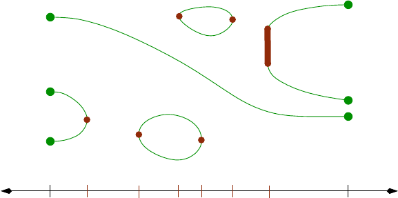
Lectures on Symplectic Field Theory 125
0
1
s
M(J
0
)
M(J
1
)
Figure 7.1. The picture shows a smooth parametric moduli space
M({J
s
}
s∈[0,1]
) a nd its projection M({J
s
}) → [0, 1] : (s, u) 7→ s in a
case where vir-dim M(J
s
) = 0. The parametric moduli space is 1-
dimensional and the spaces M(J
s
) are regular and 0-dimensional for
almost every s ∈ [0, 1], but this need not hold when s is a critical
value of the projection; in the picture, one such space M(J
s
) conta ins
a 1-dimensional component consisting of non-regular curves, so its
dimension differs fro m its virtual dimension.
parametrized by a J-holomorphic map u : (S
2
= C ∪ {∞}, i) → (W, J
s
), there is
also a double cover
u
′
: S
2
→ W : z 7→ u(z
2
),
with [u
′
] = 2A, so u
′
∈ M
0,0
(J
s
, 2A) and
vir-dim M
0,0
(J
s
, 2A) = 2 − 2g + 2c
1
(2A) = −2.
Negative virtual dimension means that M
0,0
(J
0
, 2A) should be empty whenever
Fredholm regularity is achieved, but this is clearly impossible, even generically, since
elements of M
0,0
(J
s
, A) always have double covers belonging to M
0,0
(J
s
, 2A).
Remark 7.6. The most common way t o apply Theorem
7.2 is by setting U
equal to the interior of W
r
0
, so generic perturbations of J are allowed everywhere
except on the regions where it is required to be R-invariant. The theorem then
achieves transversality f or all simple curves that are not confined to the R-invariant
regions. We will show in the next lecture that transversality for all curves of the
latter type can also be achieved by generic perturbations within the spaces J(H
±
) of
compatible R-invariant a lmo st complex structures on t he symplectizations R ×M
±
,
hence generic choices in J(ω
ψ
, r
0
, H
+
, H
−
) do achieve transversality for all simple
curves.
Our proof s of Theorems 7.1 and 7.2 will mostly follow the same line of argument
that is carried out for the closed case in [
Wend, Chapter 4], thus we will not discuss
every detail but will instead emphasize aspects which are unique t o the punctured
case.
126 Chris Wendl
7.2. Functional analytic setup
Fix k ∈ N and p ∈ (1, ∞) with kp > 2, a small number δ ≥ 0, a nd a Riemannian
metric on
c
W that is translation-invariant in the cylindrical ends. Fix also a closed
connected surface Σ of genus g, and disjoint finite ordered sets of distinct points
Γ
±
= (z
±
1
, . . . , z
±
k
±
), Θ = (ζ
1
, . . . , ζ
m
)
in Σ, together with disjoint neighborhoods
U
±
j
⊂ Σ
of each z
±
j
∈ Γ
±
with complex structures j
Γ
and biholomorphic identifications of
(U
±
j
, j
Γ
, z
j
) with (D, i, 0) for each j = 1, . . . , k
±
. This determines holomorphic cylin-
drical coordinates identifying each of the punctured neighborhoods
˙
U
±
j
⊂
˙
Σ := Σ \ (Γ
+
∪ Γ
−
)
biholomorphically with the half-cylinder Z
±
.
For reasons tha t will become clear when we study the linearized Cauchy-Riemann
operator in the punctured setting, we will need to consider exponentially weight ed
Sobolev spaces. Suppose E →
˙
Σ is an asymptotically Hermitian vector bundle:
then the Banach space
W
k,p,δ
(E) ⊂ W
k,p
lo c
(E)
is defined to consist of sections η ∈ W
k,p
lo c
(E) whose represent atives f : Z
±
→ C
m
in
cylindrical coordinates (s, t) ∈ Z
±
and asymptotic trivializations at the ends satisfy
(7.1) ke
±δs
fk
W
k,p
(Z
±
)
< ∞.
The norm of a section η ∈ W
k,p,δ
(E) is defined by adding the W
k,p
-norm o f η over a
large compact subdomain in
˙
Σ to the weighted norms (
7.1) f or each cylindrical end.
If δ = 0, this just produces the usual W
k,p
(E), but for δ > 0, sections in W
k,p,δ
(E)
are guaranteed to have exponential decay at infinity.
Remark 7.7. It is occasionally useful to observe that the definition of W
k,p,δ
(E)
also makes sense when δ < 0. In this case, sections in W
k,p,δ
(E) are of class W
k,p
lo c
but need not be glo bally in W
k,p
(E), as they are also allowed to have exp onential
gro wth at infinity.
We now want to define a Banach manifold of maps u :
˙
Σ →
c
W t ha t will contain
all the asymptotically cylindrical J-holomorphic curves with our particular choice
of asymptotic orbits. Recall that the asymptotically cylindrical condition means
(7.2) u(s, t) = exp
(T
±
j
s,γ
±
j
(t))
h(s, t) for sufficiently large |s|
in suitable cylindrical coordinates (s, t) ∈ Z
±
near each puncture z
±
j
∈ Γ
±
, where
T
±
j
> 0 is the period of the orbit γ
±
j
: S
1
→ M
±
and h(s, t) is a vector field along the
trivial cylinder that decays as s → ±∞. The catch is that this definition was not
formula t ed with respect to a fixed choice of the holomorphic cylindrical coordinates
(s, t); in general the coordinat es in which (
7.2) is valid may depend on u, a nd different
choices of coordinates might be required fo r different maps. One can show however
Lectures on Symplectic Field Theory 127
that any two distinct choices of ho lomorphic cylindrical coordinates are related to
each other by a transformation tha t converges asymptotically to a constant shift,
which implies that for our fixed choice of coordinates (s, t), every asymptotically
cylindrical map can be assumed to satisfy
u(s, t) = exp
(T
±
j
s+a,γ
±
j
(t+b))
h(s, t), lim
s→±∞
h(s, t) = 0
for some constants a ∈ R and b ∈ S
1
. We therefore define the space
B
k,p,δ
:= W
k,p,δ
(
˙
Σ,
c
W ; γ
+
, γ
−
) ⊂ C
0
(
˙
Σ,
c
W )
to consist of all continuous maps u :
˙
Σ →
c
W of the fo r m
u = exp
f
h,
where:
• f :
˙
Σ →
c
W is smooth and, in our fixed cylindrical coordinates (s, t) ∈ Z
±
on neighborhoods of the punctures z
±
j
∈ Γ
±
, takes the form
f(s, t) = (T
±
j
s + a, γ
±
j
(t + b)) fo r |s| sufficiently large,
where a ∈ R and b ∈ S
1
are arbitrar y constants and T
±
j
> 0 is the period
of the Reeb orbit γ
±
j
: S
1
→ M
±
;
• h ∈ W
k,p,δ
(f
∗
T
c
W ).
Though it is not immediate since
˙
Σ is noncompact, one can generalize the ideas
in [
El˘ı67] to give B
k,p,δ
the structure of a smooth, separable and metrizable Banach
manifold. The key point is the condition kp > 2, which guarantees the continuous
inclusion W
k,p,δ
(f
∗
T
c
W ) ֒→ C
0
(f
∗
T
c
W ) as well as Banach algebra and C
k
-continuity
properties, cf. Propositions 2.4, 2.7 and 2.8 in Lecture
2. These pro perties are
needed in order to show that the transition maps between pairs of charts of the
form exp
f
h 7→ h ar e smooth.
The tangent space to B
k,p,δ
at u ∈ B
k,p,δ
can be written as
T
u
B
k,p,δ
= W
k,p,δ
(u
∗
T
c
W ) ⊕ V
Γ
,
where V
Γ
⊂ Γ(u
∗
T
c
W ) is a non-canonical choice of a 2(k
+
+ k
−
)-dimensional vector
space of smooth sections asymptotic at the punctures to constant linear combina-
tions of the vector fields spanning the canonical trivialization of the first factor in
T (R × M
±
) = ǫ ⊕ ξ
±
, i.e. they point in the R- and R
±
-directions. The space V
Γ
appears due to the fact that two distinct elements of B
k,p,δ
are generally asymptotic
to collections of trivial cylinders that differ from each other by k
+
+ k
−
pairs of
constant shifts (a, b) ∈ R × S
1
.
Fix J ∈ J(ω
ψ
, r
0
, H
+
, H
−
) and a smooth complex structure j on Σ that matches
j
Γ
in the neighborhoods U
±
j
of the punctures. The nonlinear Cauchy-Riemann op-
erator is then defined as a smooth section
¯
∂
j,J
: B
k,p,δ
→ E
k−1,p,δ
: u 7→ T u + J ◦ T u ◦ j
of a Banach space bundle
E
k−1,p,δ
→ B
k,p,δ
128 Chris Wendl
with fibers
E
k−1,p,δ
u
= W
k−1,p,δ
(
Hom
C
(T
˙
Σ, u
∗
T
c
W )).
The zero set of
¯
∂
j,J
is the set of all maps u ∈ B
k,p,δ
that are pseudoholomorphic
from (
˙
Σ, j) to (
c
W , J). Note that the smoothness of
¯
∂
j,J
depends mainly on the fact
that J is smoo t h. Indeed, in local coordinates
¯
∂
j,J
looks like u 7→ ∂
s
u + ( J ◦ u)∂
t
u,
in which the most o bviously nonlinear ingredient is u 7→ J ◦ u. If J were only of
class C
k
, then the C
k
-continuity property would imply that t he map u 7→ J ◦ u
sends maps of class W
k,p
continuously to maps of class W
k,p
, and one can use an
inductive argument to show that this map then becomes r-times differentiable if J
is of class C
k+r
, see [
Wend, Lemma 2.12.5]. Moreover, the fact that
¯
∂
j,J
u satisfies
the same expo nential weighting condition as u at t he cylindrical ends depends on
the fact t hat J is R-invariant near infinity.
For u ∈
¯
∂
−1
j,J
(0), t he linearizat ion D
¯
∂
j,J
(u) : T
u
B
k,p,δ
→ E
k−1,p,δ
u
defines a bounded
linear operator
D
u
: W
k,p,δ
(u
∗
T
c
W ) ⊕ V
Γ
→ W
k−1,p,δ
(
Hom
C
(T
˙
Σ, u
∗
T
c
W )).
We derived a formula for this operator in Lecture
2 and showed that it is of Cauchy-
Riemann type. Since V
Γ
is finite dimensional, D
u
will be Fredholm if and o nly if its
restriction to the first factor is Fredholm; denote this restriction by
D
δ
: W
k,p,δ
(u
∗
T
c
W ) → W
k−1,p,δ
(
Hom
C
(T
˙
Σ, u
∗
T
c
W )),
where we’ve chosen the notation to emphasize the dependence o f t his operato r on
the choice of exponential weight δ ≥ 0 in the definition of o ur Banach space. We
will see presently why it’s imp ortant to pay at tention to this detail.
To see whether D
δ
is Fredholm, consider first the special case where u is a trivial
cylinder
u
γ
: R × S
1
→ R × M : (s, t) 7→ (T s, γ(t))
over some Reeb orbit γ : S
1
→ M with period T > 0 in M with stable Hamiltonian
structure H = (ω, λ) on M. In this case, there is a more convenient way to write
down D
u
γ
than the f ormula from Lecture
2. To start with, we use the splitting
T (R × M) = ǫ ⊕ ξ to decompo se u
∗
γ
T (R × M) = u
∗
γ
ǫ ⊕ u
∗
γ
ξ and thus write D
u
γ
in
block form
D
u
γ
=
D
ǫ
u
γ
D
ǫξ
u
γ
D
ξǫ
u
γ
D
ξ
u
γ
.
Exercise 7.8. Suppose D : Γ(E) → Ω
0,1
(
˙
Σ, E) is a linear Cauchy-Riemann
type operator on a vector bundle E with a complex-linear splitting E = E
1
⊕ E
2
,
and
D =
D
11
D
12
D
21
D
22
is the resulting block decomposition of D. Use the Leibniz rule satisfied by D
to show tha t D
11
and D
22
are also Cauchy- Riemann type operators on E
1
and
E
2
respectively, while the off-diagonal terms are tensorial, i.e. they commute with
multiplication by smooth real-valued functions and thus define bundle maps D
12
:
E
2
→ Λ
0,1
T
∗
˙
Σ ⊗E
1
and D
21
: E
1
→ Λ
0,1
T
∗
˙
Σ ⊗ E
2
.

Lectures on Symplectic Field Theory 129
Now observe that if u = (u
R
, u
M
) : R ×S
1
→ R ×M is ano t her cylinder near u
γ
,
the nonlinear opera t or (
¯
∂
j,J
u)∂
s
= ∂
s
u + J ∂
t
u ∈ Γ ( u
∗
T (R × M)) = Γ(u
∗
ǫ ⊕ u
∗
ξ)
takes the form
(
¯
∂
j,J
u)∂
s
=
∂
s
u
R
− λ(∂
t
u
M
) + i (∂
t
u
R
+ λ(∂
t
u
M
))
π
ξ
∂
s
u
M
+ Jπ
ξ
∂
t
u
M
,
where we a re using the canonical trivialization of u
∗
ǫ via ∂
r
and R to express the top
block as a complex-valued function. As we observed in Lecture
3, the bottom block of
this expression can be interpreted in terms of the gradient flow of an actio n functional
A
H
: C
∞
(S
1
) → R, with ∇A
H
(γ) = −Jπ
ξ
∂
t
γ. Linearizing in the direction of a
section η
ξ
∈ Γ(u
∗
γ
ξ) and taking the ξ component thus yields an expression involving
the Hessian of A
H
at the critical point γ, namely
(D
ξ
u
γ
η
ξ
)∂
s
= (∂
s
− A
γ
)η
ξ
.
To compute the blocks D
ǫ
u
γ
and D
ξǫ
u
γ
, notice that D
u
γ
η
ǫ
= 0 whenever η
ǫ
is a constant
linear combination of ∂
r
and R, as η
ǫ
is then the derivative of a smooth family of
J-holomorphic reparametrizations of u
γ
. This is enough to prove D
ξǫ
u
γ
= 0 since
the la t t er is tensorial by Exercise
7.8, and expressing arbitrary sections of u
∗
γ
ǫ as
f∂
r
+ gR, we can apply the Leibniz rule for D
ǫ
u
γ
and conclude
(D
ǫ
u
γ
η
ǫ
)∂
s
= (∂
s
+ i ∂
t
)η
ǫ
in the canonical trivialization. To compute the remaining off-diagonal term, one
needs to compute dr(D
u
γ
η
ξ
) and λ(D
u
γ
η
ξ
) for an arbitrary section η
ξ
∈ Γ(u
∗
γ
ξ),
e.g. by picking a smooth family u
ρ
: R × S
1
→ R × M with ∂
ρ
u
ρ
|
ρ=0
= η
ξ
and a
connection ∇ and computing
dr
∇
ρ
(
¯
∂
j,J
u
ρ
)
ρ=0
and λ
∇
ρ
(
¯
∂
j,J
u
ρ
)
ρ=0
.
This calculation is straightforward but unenlightening, so I will leave it as an exercise
for now—in the next lecture we’ll derive a general formula (see Lemma
8.10), which
implies that since π
ξ
∂
s
u
γ
≡ π
ξ
∂
t
u
γ
≡ 0 in the present setting, D
ǫξ
u
γ
= 0. All t his
leads to the formula
(D
u
γ
η)∂
s
=
∂
s
−
−i∂
t
0
0 A
γ
η.
Here the upper left block is the “trivial” asymptotic operator acting on the tr ivial
line bundle over S
1
. Since every asymptotically cylindrical curve approximates a
trivial cylinder near infinity, one can deduce from this calculuation the following:
Proposition 7.9. The Cauchy-Riemann type operator D
u
on u
∗
T
c
W is as-
ymptotic at its punctures z
±
j
∈ Γ
±
for j = 1, . . . , k
±
to the asymptotic operators
(−i∂
t
) ⊕ A
γ
±
j
on (γ
±
j
)
∗
(ǫ ⊕ ξ
±
).
Perhaps you can now see a problem: even if the orbit s γ
±
j
are all nondegenerate,
the asymptotic operators (−i∂
t
) ⊕A
γ
are degenerate, as they have nontrivial kernel
consisting of constant sections in the first (trivial) factor o f (γ
±
j
)
∗
(ǫ ⊕ ξ
±
). This
implies in particular that
D
0
: W
k,p
(u
∗
T
c
W ) → W
k−1,p
(
Hom
C
(T
˙
Σ, u
∗
T
c
W ))

130 Chris Wendl
is not Fredholm, except of course in the sp ecial case where there are no punctures.
The situation is saved by the exponential weight:
Lemma 7.10. For every δ > 0 sufficiently small, the operator D
δ
is Fredholm
and has index
ind(D
δ
) = nχ(Σ) − (n + 1)#Γ + 2c
τ
1
(u
∗
T
c
W ) +
k
+
X
j=1
µ
τ
CZ
(γ
+
j
) −
k
−
X
j=1
µ
τ
CZ
(γ
−
j
).
Moreover, every element of M(J) can be represen ted by a map u ∈ B
k,p,δ
.
Proof. The second claim fo llows from the exponential decay estimate of Hofer-
Wysocki-Zehnder [
HWZ96] mentioned in t he previous lecture, see Proposition 6.13.
To see that D
δ
: W
k,p,δ
→ W
k−1,p,δ
is Fredholm and to compute its index, we
can identify it with a Cauchy-Riemann type operator fr om W
k,p
to W
k−1,p
. Indeed,
pick any smooth function f :
˙
Σ → R with f (s, t) = ∓δs on the cylindrical ends
near Γ
±
, define Banach space isomorphisms
Φ
δ
: W
k,p
→ W
k,p,δ
: η 7→ e
f
η,
Ψ
δ
: W
k−1,p
→ W
k−1,p,δ
: θ 7→ e
f
θ,
and consider the bounded linear map
D
′
δ
:= Ψ
−1
δ
D
δ
Φ
δ
: W
k,p
(u
∗
T
c
W ) → W
k−1,p
(
Hom
C
(T
˙
Σ, u
∗
T
c
W )).
Using the Leibniz rule for D
δ
, it is straightforward to show that D
′
δ
is also a linear
Cauchy-Riemann type operator. Moreover, suppose D
δ
takes the form
¯
∂ + S(s, t) in
coordinates a nd trivialization on the cylindrical end near z
±
j
, where S(s, t) → S
∞
(t)
as s → ±∞ a nd A
γ
±
j
= −i∂
t
−S
∞
(t). Then D
′
δ
on this same end ta kes the form
D
′
δ
η = e
±δs
(
¯
∂ + S(s, t))(e
∓δs
η) =
¯
∂η + (S(s, t) ∓ δ)η
and is therefore asymptotic t o the perturbed a symptotic operator
˜
A
±
j
:=
(−i∂
t
) ⊕ A
γ
±
j
±δ.
The latter is the direct sum of two asymptotic operators −i∂
t
± δ on the trivial
line bundle and A
γ
±
j
± δ o n (γ
±
j
)
∗
ξ
±
respectively. Since γ
±
j
is nondegenerate by
assumption and the spectrum of A
γ
±
j
is discrete, we can assume ker(A
γ
±
j
±δ) remains
trivial if δ > 0 is sufficient ly small, and the Conley-Zehnder index of this perturbed
operator will be the same as without the perturbation. O n the other ha nd, the
spectrum of −i∂
t
consists of the integer multiples of 2π, thus −i∂
t
±δ also becomes
nondegenerate for any δ > 0 small. Its Conley-Zehnder index can be deduced from
the winding numbers o f its eigenfunctions using Theorem
3.35 in Lecture 3: −i∂
t
has a 2-dimensional nullspace consisting of sections with winding number 0, and
this becomes an eigenspace for the smallest positive eigenvalue if the puncture is
positive or the largest negative eigenvalue if the puncture is negative. Theorem 3.35
thus gives
µ
CZ
(−i∂
t
±δ) = ∓1,
Lectures on Symplectic Field Theory 131
and therefore,
µ
τ
CZ
(
˜
A
±
j
) = ∓1 + µ
τ
CZ
(γ
±
j
).
Plugging this into the general index formula from Lecture
5 t hen gives the stated
result.
Putting back the missing 2(#Γ) dimensions in the domain o f D
u
, we have:
Corollary 7.11. For all δ > 0 sufficiently small, the linearized Cauchy-Riemann
operator D
u
: T
u
B
k,p,δ
→ E
k−1,p,δ
u
is Fredholm with in dex
ind(D
u
) = nχ(Σ) − (n − 1)#Γ + 2c
τ
1
(u
∗
T
c
W ) +
k
+
X
j=1
µ
τ
CZ
(γ
+
j
) −
k
−
X
j=1
µ
τ
CZ
(γ
−
j
).
7.3. Teichm¨uller slices
Since the moduli space M(J) is not defined with reference to any fixed complex
structure on the domains
˙
Σ, we must build t his freedom into the setup. Fo r a more
detailed version of the following discussion, see [
Wend, §4.2 .1].
For any integers g, ℓ ≥ 0, the moduli space of Riemann surfaces of genus g
with ℓ marked point s is a space of equivalence classes
M
g,ℓ
= {(Σ, j, Θ)}
∼
where (Σ, j) is a compact connected surface with genus g, Θ ⊂ Σ is an ordered
set of ℓ points and equivalence is defined via biholomorphic maps that preserve
the marked points with their ordering. This space has been studied extensively in
algebraic geometry, though it can also be understood using the same global analytic
methods that we have been applying for M(J). It is known in particular that M
g,ℓ
is always a smooth orbifold, and for any [(Σ, j, Θ) ] ∈ M
g,ℓ
, it satisfies
(7.3) dim Aut(Σ, j, Θ) − dim M
g,ℓ
= 3χ(Σ) − 2ℓ,
where Aut(Σ, j, Θ) is the group of biholomorphic t ransformations of (Σ, j) that
fix the points in Θ. This group is finite whenever (Σ, j, Θ ) is stable, meaning
χ(Σ \ Θ) < 0, and in that case (
7.3) turns into the well-known dimension formula
dim M
g,ℓ
= −3χ(Σ) + 2ℓ = 6g − 6 + 2ℓ.
This is also the dimension of the Teichm¨uller space
T (Σ, Θ) := J(Σ)/ Diff
0
(Σ, Θ),
where J(Σ) denotes the space of all smo oth complex structures on Σ compatible
with its orientat ion, and Diff
0
(Σ, Θ) is the identity component of the group of dif-
feomorphisms that fix Θ. It is a classical result that T (Σ, Θ ) is a smooth manifold of
the same dimension as M
g,ℓ
, and indeed, the latter can be presented as the quotient
of the former by the discrete action of the mapping class group of (Σ, Θ).
Equation (
7.3) is actually a formula for a Fredholm index. To see how this works,
consider first the case ℓ = 0. The right hand side is then χ(Σ) + 2c
1
(T Σ), which
is, according to Riemann-Roch, the index of the natur al Cauchy-Riemann operator
on T Σ tha t defines it s holomorphic structure. This o perator can also be interpreted

132 Chris Wendl
as the linearizatio n at the identity map of the nonlinear Cauchy-Riemann opera-
tor for holomorphic maps (Σ, j) → (Σ, j), so its kernel is naturally isomorphic to
T
Id
Aut(Σ, j). Similarly, one can show that the cokernel of this operato r is naturally
isomorphic to T
[j]
T (Σ). This discussion r emains valid if marked points are included:
the main difference is then that the Cauchy-Riemann operator on T Σ should be
restricted to a space of vector fields that vanish at Θ, defining a 2ℓ-codimensional
subspace as the domain and thus reducing the index by 2ℓ.
For a proof of t he following, see [
Wend, Chapter 4] and [Wen10, §3.1].
Proposition 7.12. Given a closed Ri e mann surface (Σ, j) with a finite ordered
set Θ ⊂ Σ, there exists a smooth finite-di mensional submanifold T ⊂ J(Σ) with the
following properties:
(1) The map T → T (Σ, Θ) : j
′
7→ [j
′
] i s b i j ective onto a neighborhood of [j] in
T (Σ, Θ);
(2) The subspace T
j
T ⊂ Γ(
End
C
(T Σ)) is complementary in W
k−1,p
(End
C
(T Σ))
to the i mage o f the standard Cauchy-Riemann operator of T Σ acting on the
domain {X ∈ W
k,p
(T Σ) | X|
Θ
= 0};
(3) Every j
′
∈ T equals j near Θ and is invariant under the action of Aut( Σ, j, Θ)
by diffeomorphisms on Σ.
We will r efer to the f amily T ⊂ J(Σ) in this proposition as a Teichm¨uller slice
through j.
7.4. Fredholm regularity and the implicit function theorem
We are now in a position to define the necessary regularity condition and prove
that a neighborhood of any given regular element [(Σ, j
0
, Γ
+
, Γ
−
, Θ, u
0
)] in M(J) is
an orbifold of the stated dimension. Af t er reparametrizing, we can assume without
loss of generality that Σ, Γ
±
and Θ are precisely the dat a that were fixed in §7.2,
and j
0
∈ J(Σ) matches j
Γ
on our fixed coordinate neighbor hoods of Γ
±
. We can
then choose a Teichm¨uller slice
T ⊂ J(Σ)
through j
0
as provided by Prop.
7.12, but with j in that statement replaced by j
0
and Θ replaced by Γ
+
∪ Γ
−
∪ Θ. In particular, T is invariant under the action of
the group
G
0
:= Aut(Σ, j
0
, Γ
+
∪ Γ
−
∪ Θ),
and (
7.3) now becomes
(7.4) dim G
0
−dim T = 3χ( Σ) − 2(k
+
+ k
−
+ m).
There is a na t ur al extension of the nonlinear operator
¯
∂
j,J
in §
7.2 to a smooth
section
¯
∂
J
: T × B
k,p,δ
→ E
k−1,p,δ
: (j, u) 7→ T u + J ◦T u ◦ j
of a Banach space bundle E
k−1,p,δ
→ T × B
k,p,δ
with fibers
E
k−1,p,δ
(j,u)
= W
k−1,p,δ
Hom
C
((T
˙
Σ, j), (u
∗
T
c
W , J))
.

Lectures on Symplectic Field Theory 133
The zero set
¯
∂
−1
J
(0) ⊂ T ×B
k,p,δ
consists of pairs (j, u) for which u : (
˙
Σ, j) → (
c
W , J)
is pseudoholomorphic, and it contains (j
0
, u
0
) by construction. It also admits a
natural action of the automor phism group G
0
,
G
0
×
¯
∂
−1
J
(0) →
¯
∂
−1
J
(0) : (ϕ, (j, u)) 7→ (ϕ
∗
j, u ◦ ϕ),
whose stabilizer at (j
0
, u
0
) is Aut(u
0
), a finite group whenever u
0
is not constant.
Observe that any two elements in the same G
0
-orbit of
¯
∂
−1
J
(0) define equivalent
elements of the moduli space M(J), as they are related to each o ther by a biholo-
morphic repara metrization that fixes the punctures and marked points.
Lemma 7.13. The map
¯
∂
−1
J
(0)
G
0
→ M(J) : [(j, u)] 7→ [(Σ, j, Γ
+
, Γ
−
, Θ, u)]
is a homeomo rp hism between open neighborhoods of [(j
0
, u
0
)] and [(Σ, j
0
, Γ
+
, Γ
−
, Θ, u
0
)].
Proof. This depends fundamentally on the same fact underlying the smooth-
ness of Teichm¨uller space: the action of Diff
0
(Σ, Γ
+
∪ Γ
−
∪ Θ) on J(Σ) is free and
proper.
2
See the proof of [Wend, Theorem 4.3.6].
Definition 7.14. We say that [(Σ, j
0
, Γ
+
, Γ
−
, Θ, u
0
)] is Fredholm regular if
there exists a choice of Teichm¨uller slice T through j
0
such that the linearization
D
¯
∂
J
(j
0
, u
0
) : T
j
0
T ⊕ T
u
0
B
k,p,δ
→ E
k−1,p,δ
(j
0
,u
0
)
is surjective.
One can show that the surjectivity condition in this definition does not actually
depend on the choice of Teichm¨uller slice. This follows from the identification of
T
j
0
T with the cokernel of the natural Cauchy-Riemann operator on T
˙
Σ; see [
Wend,
Lemma 4.3.2].
Proof of Theorem
7.1. The fact that M(J) is an orbifold in a neighbor-
hood o f [(Σ, j
0
, Γ
+
, Γ
−
, Θ, u
0
)] with isotropy group Aut(u
0
) follows from Lemma
7.13
and the implicit function theorem, which gives
¯
∂
−1
J
(0) the structure of a finite-
dimensional manifold near (j
0
, u
0
) if Fredholm regularity is satisfied. There is a bit
of work to be done in showing that transition maps relating any two overlapping
charts that arise in this way from the implicit function t heorem ar e smooth; for this,
we refer aga in t o the proof of Theorem 4.3.6 in [
Wend] and merely comment that
the key ingredient is elliptic regularity.
The dimension of M(J) is
dim M(J) = dim
¯
∂
−1
J
(0) − dim G
0
= ind D
¯
∂
J
(j
0
, u
0
) − dim G
0
.
The restriction o f D
¯
∂
J
(j
0
, u
0
) to T
u
0
B
k,p,δ
is the operator D
u
0
that we studied in
§
7.2, hence
ind D
¯
∂
J
(j
0
, u
0
) = dim T + ind D
u
0
.
2
This is true at least in the stable case, i.e. when χ(
˙
Σ \Θ) < 0. There are finitely many cases
not satisfying this hypo thesis, for which the lemma can be proved by more direct arguments since
explicit descriptions of both Teichm¨uller space and the automorphism groups of Riemann surfaces
are available; see [
Wen10, §3 .1 and §3.2] for more details.
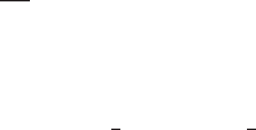
134 Chris Wendl
Using (7.4) to replace dim T − dim G
0
and combining this with Corollary 7.11 now
gives the stated formula for dim M(J).
7.5. A universal moduli space
The remainder of this lecture is devoted to the proo f of Theorem 7.2. The main
tool fo r this purpose is the Sard-Smale t heorem [
Sma65], an infinite-dimensional
version of Sard’s theorem stating that the regular values of a smooth nonlinear
Fredholm map between separable Banach spaces (i.e. a smooth map whose deriv-
ative at every point is a Fr edholm operator) form a comeager subset of the tar get
space. In order to incorporate perturbations of the almost complex structure int o
our functional analytic setup, we need to choose a suitable Banach manifo ld of al-
most complex structures. All known ways of doing this are in some sense non-ideal,
e.g. one could take almost complex structures of class C
k
or W
k,p
, but this neces-
sarily introduces non-smooth almost complex structures into the picture, with the
consequence that the nonlinear Cauchy-Riemann operat or has only finitely many
derivatives. That is not the end of the world, and indeed, this is the approach t aken
in [
MS04], but I will instead present an approach that was introduced by Floer in
[
Flo88b], in terms of what is now called the “ Floer C
ε
space”. The idea is t o work
with a Banach manifold that continuously embeds into the space of smooth almost
complex structures, so that the nonlinear Cauchy-Riemann operator will always be
smooth. It’s a nice trick, but the catch is that we obtain a space that is strictly
smaller than the actual space of smooth almost complex structures we’re interested
in, and has a much stronger topology. The C
ε
space should be viewed as a useful
tool but not a deeply meaningful o bject—you might notice that while some of the
intermediate results stated below depend on its (somewhat ad hoc) definition, The-
orem
7.2 does not. This is due to a general trick described in §7.7 below for turning
results about C
ε
into results about C
∞
.
As in the statement of Theorem
7.2, a ssume U ⊂ W
r
0
is open and J
fix
∈
J(ω
ψ
, r
0
, H
+
, H
−
). Let
J
U
:=
n
J ∈ J(ω
ψ
, r
0
, H
+
, H
−
)
J = J
fix
on
c
W \ U
o
,
and choose any almost complex structure
J
ref
∈ J
U
.
We can regard J
U
as a smooth Fr´echet manifold with tangent spaces
T
J
ref J
U
=
n
Y ∈ Γ
End
C
(T
c
W , J
ref
)
Y |
c
W \U
≡ 0 and ω
ψ
(·, Y ·) + ω
ψ
(Y ·, ·) ≡ 0
o
,
where the antilinearity of Y ∈ T
J
ref
J
U
means that Y is tangent to the space almost
complex structures, and the condition relating it to ω
ψ
means that these structures
are compatible with ω
ψ
. One can check t hat the map
Y 7→ J
Y
:=
1 +
1
2
J
ref
Y
J
ref
1 +
1
2
J
ref
Y
−1

Lectures on Symplectic Field Theory 135
maps a neighborhood of 0 ∈ T
J
ref J
U
bijectively to a neighborhood of J
ref
in J
U
.
We thus fix a sufficiently small constant c > 0 and define the space of “C
ε
-small
perturbations of J
ref
” by
J
ε
U
:=
(
J
Y
∈ J
U
Y ∈ T
J
ref
J
U
with
∞
X
ℓ=0
ε
ℓ
kY k
C
ℓ
(
U)
< c
)
,
where ε := (ε
ℓ
)
∞
ℓ=0
is a fixed sequence of positive numbers with ε
ℓ
→ 0 as ℓ → ∞.
The sum
kY k
C
ε
:=
∞
X
ℓ=0
ε
ℓ
kY k
C
ℓ
(
U)
defines a norm, and the space of smooth sections Y ∈ T
J
ref J
U
for which this norm is
finite is then a separable Banach space; see Appendix
B for a proof of this statement.
This makes J
ε
U
a separable and metrizable Banach manifold, as the map J
Y
7→ Y
can be viewed as a chart identifying it with an open subset of the aforementioned
Banach space. Not every J ∈ J
U
near J
ref
belongs to J
ε
U
, but there is a continuous
inclusion
J
ε
U
֒→ J
U
,
where the lat ter carries its usual C
∞
-topology and J
ε
U
carries the topology induced
by the C
ε
-norm. By a lemma due to Floer, choosing a sequence ε
ℓ
that decays
sufficiently fast makes J
ε
U
large enough to contain perturbations in arbitrary direc-
tions with arbitrarily small support near arbitrary points in U; see Theorem
B.6 in
Appendix
B for a precise version of this statement and its proof. We will assume
from now on that a suitably fast decaying sequence has b een fixed.
We now define a universal moduli space
M
∗
(J
ε
U
) :=
(u, J)
J ∈ J
ε
U
, u ∈ M(J) and
u has an injective point mapped into U
.
The terminology is somewhat unfort una t e, as M
∗
(J
ε
U
) depends on many auxiliary
choices such as J
ref
and (ε
ℓ
)
∞
ℓ=0
and thus should not really be tho ught of as a “uni-
versal” object. Nonetheless:
Lemma 7.15. The universal moduli space M
∗
(J
ε
U
) is a smooth separable Banach
manifold, and the projection M
∗
(J
ε
U
) → J
ε
U
: (u, J) 7→ J is sm ooth.
Proof. As in the proof of Theorem
7.1, one can identify M
∗
(J
ε
U
) locally with
the zero set of a smooth section of a Banach space bundle. Suppo se J
0
∈ J
ε
U
and
[(Σ, j
0
, Γ
+
, Γ
−
, Θ, u
0
)] ∈ M(J
0
) where u
0
:
˙
Σ →
c
W has an inj ective point z
0
with
u
0
(z
0
) ∈ U. Choose a Teichm¨uller slice T through j
0
as in Proposition
7.12 and
consider the smooth section
¯
∂ : T × B
k,p,δ
× J
ε
U
→ E
k−1,p,δ
: (j, u, J) 7→ T u + J ◦ T u ◦ j,
where E
k−1,p,δ
is the obvious extension of our previous Banach space bundle to a
bundle over T × B
k,p,δ
× J
ε
U
. We’re assuming as before that k ∈ N, 1 < p < ∞,
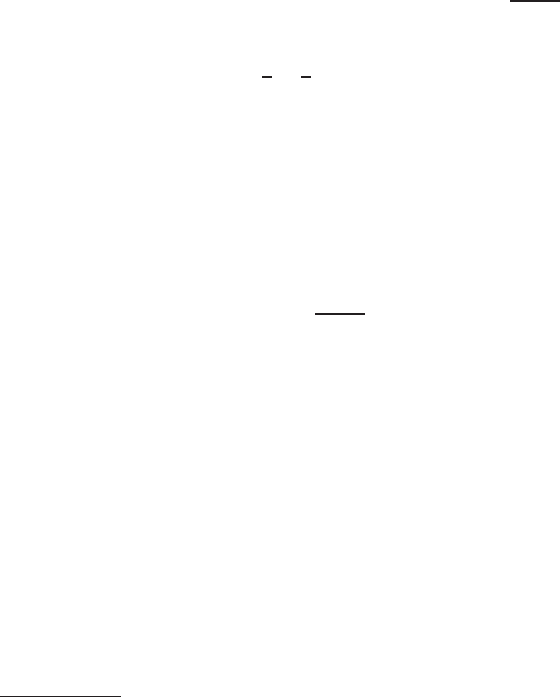
136 Chris Wendl
kp > 2, and δ > 0 is small. A neighbo rhood of (u
0
, J
0
) in M
∗
(J
ε
U
) can then be
identified with a neighborhood of [(j
0
, u
0
, J
0
)] in
¯
∂
−1
(0)
G
0
,
where G
0
:= Aut(Σ, j
0
, Γ
+
∪Γ
−
∪Θ) acts on
¯
∂
−1
(0) by ϕ ·(j, u, J) := (ϕ
∗
j, u ◦ϕ, J).
Since u
0
has an injective point, Aut(u
0
) is trivial and the G
0
-action at (j
0
, u
0
, J
0
)
is therefore free; hence it suffices to show t hat
¯
∂
−1
(0) is a smooth Banach manifold
near (j
0
, u
0
, J
0
). This follows from the implicit function theorem if we can show that
D
¯
∂(j
0
, u
0
, J
0
) : T
j
0
T ⊕ T
u
0
B
k,p,δ
⊕ T
J
0
J
ε
U
→ E
k−1,p,δ
(j
0
,u
0
,J
0
)
is surjective; indeed, the infinite-dimensional implicit function theorem (see [
Lan93])
requires the a dditional hypothesis that D
¯
∂(j
0
, u
0
, J
0
) has a bounded right inverse,
but this is immediate since the restriction of this operator to the f actor T
u
0
B
k,p,δ
is
Fredholm (see Exercise 7.17 b elow). We claim in fact that
T
u
0
B
k,p,δ
⊕T
J
0
J
ε
U
→ E
k−1,p,δ
(j
0
,u
0
,J
0
)
(η, Y ) 7→ D
¯
∂(j
0
, u
0
, J
0
)(0, η, Y ) = D
u
0
η + Y ◦ T u
0
◦ j
0
is surjective. Consider first the case k = 1,
3
so we are looking at a bounded linear
map
W
1,p,δ
(u
∗
0
T
c
W ) ⊕ V
Γ
⊕ T
J
0
J
ε
U
→ L
p,δ
(
Hom
C
(T
˙
Σ, u
∗
0
T
c
W )).
Note that the dual of any space of sections of class L
p,δ
can be identified with
sections of class L
q,−δ
for
1
p
+
1
q
= 1 (recall R emark 7.7). Indeed, choosing a suitable
L
2
-pairing defines a bounded bilinear map
(7.5) h , i
L
2
: L
p,δ
× L
q,−δ
→ R,
and one can use isomorphisms of the form L
p
→ L
p,δ
: η 7→ e
f
η as in the proof
of Lemma
7.10 to prove (L
p,δ
)
∗
∼
=
L
q,−δ
as a corollary of the standard fact that
(L
p
)
∗
∼
=
L
q
. With this understood, observe that since D
u
0
: W
1,p,δ
⊕ V
Γ
→ L
p,δ
is Fredholm, we know by Exercise
7.16 below that the map under consideration
has closed r ange. Thus if it is not surjective, the Hahn-Banach theorem provides
a nontrivial element θ ∈ L
q,−δ
(
Hom
C
(T
˙
Σ, u
∗
0
T
c
W )) that annihilates its image under
the pair ing (
7.5), which amounts to the two conditions
hD
u
0
η, θi
L
2
= 0 for all η ∈ W
1,p,δ
(u
∗
0
T
c
W ) ⊕ V
Γ
,
hY ◦ T u
0
◦ j
0
, θi
L
2
= 0 for all Y ∈ T
J
0
J
ε
U
.
(7.6)
The first relation is valid in particular for all smooth sections η with compact support
and thus means that θ is a weak solution to the formal adjoint equation D
∗
u
0
θ = 0;
applying elliptic regularity and the similarity principle, θ is therefore smooth and has
only isolated zeroes. We will see however that this contradicts the second relation
as long as there exists an injective point z
0
∈
˙
Σ with u
0
(z
0
) ∈ U. Indeed, since the
set of injective point s with this property is open and zeroes of θ are isolated, let
us assume without loss of generality that θ(z
0
) 6= 0. Then by a standa r d lemma
in symplectic linear algebra (see [
Wend, Lemma 4.4.12]), one can find a smooth
3
Since the present discussion is purely linear, it does not require the assumption kp > 2.

Lectures on Symplectic Field Theory 137
section Y ∈ T
J
0
J
U
whose value at u
0
(z
0
) is chosen such that Y ◦ T u
0
◦ j
0
= θ at
z
0
, so their pointwise inner product is positive in some neighborhood of z
0
. But
by Theorem
B.6, one can multiply a small perturbation of Y by a bump function
to produce a section (still denoted by Y ) of class C
ε
so that the pointwise inner
product of Y ◦T u
0
◦j
0
with θ is positive near z
0
but vanishes everywhere else; note
that this requires the assumption u
−1
0
(u
0
(z
0
)) = {z
0
}, so that the value of Y near
u
0
(z
0
) affects the value of Y ◦ T u
0
◦ j
0
near z
0
but nowhere else. This violates the
second condition in (
7.6) and t hus completes the pr oof for k = 1. In the general
case, suppose θ ∈ W
k−1,p,δ
(
Hom
C
(T
˙
Σ, u
∗
0
T
c
W )). Then θ is also of class L
p,δ
, so
surjectivity in the k = 1 case implies the existence of η ∈ W
1,p,δ
and Y ∈ T
J
0
J
ε
U
with D
u
0
η + Y ◦ T u
0
◦ j
0
= θ. Since Y ◦ T u
0
◦ j
0
is smooth with compact support,
one can then use elliptic regularity to show η ∈ W
k,p,δ
, and this proves surjectivity
for ar bitrary k ∈ N and p ∈ (1, ∞).
The implicit function theorem now implies that whenever kp > 2 so that B
k,p,δ
is a well-defined Banach manif old,
¯
∂
−1
(0) is a smooth Banach submanifold of T ×
B
k,p,δ
×J
ε
U
in a neighborhood of (j
0
, u
0
, J
0
). The projection map
¯
∂
−1
(0) → J
ε
U
: (j, u, J) 7→ J
is also smo oth since it is the restriction to a smoo t h submanifold of the obviously
smooth projection map T × B
k,p,δ
× J
ε
U
→ J
ε
U
. Since G
0
acts freely and properly
on
¯
∂
−1
(0), the quotient
¯
∂
−1
/G
0
then inherits a smooth Banach manifold structure
for which the projection is still smooth, and this quotient is identified locally with
M
∗
(J
ε
U
). Smoothness of transition maps is shown via the same regularity arguments
as in the proof of Theorem
7.1.
Exercise 7.16. Show tha t if X, Y and Z are Ba nach spaces, T : X → Y is a
Fredholm operator and A : Z → Y is a bounded linear operator, then the linear
map
L : X ⊕Z → Y : (x, z) 7→ Tx + Az
has closed range. Hint: it might help to write X = V ⊕ker T and Y = W ⊕coker C
so that C
∼
=
coker T and V
T
−→ W is an isomorphism.
Exercise 7.17. Under the same a ssumptions as in Exercise
7.16, show that if
T is surjective, then L has a bounded rig ht inverse.
7.6. Applying the Sard-Smale theorem
We claim now that the smooth map
(7.7) M
∗
(J
ε
U
) → J
ε
U
: (u, J) 7→ J
is a nonlinear Fredholm ma p, i.e. its derivative at every point is a Fredholm oper-
ator. Using the local identification of M
∗
(J
ε
U
) with
¯
∂
−1
(0)/G
0
as in the proof of
Lemma 7.15 and lifting the projection to
¯
∂
−1
(0), the derivative of
¯
∂
−1
(0) → J
ε
U
at
(j
0
, u
0
, J
0
) takes the for m
ker D
¯
∂(j
0
, u
0
, J
0
) → T
J
0
J
ε
U
: (y, η, Y ) 7→ Y.

138 Chris Wendl
The Fredholm property for this projection is a consequence of the Fredholm property
for D
u
0
via the following general lemma, whose proof is a routine matter of linear
algebra (cf. [
Wend, Lemma 4.4.13]):
Lemma 7.18. Under the a s sumptions of Exercise
7.16, suppose L is surjective.
Then the projection
Π : ker L → Z : (x, z) 7→ z
has kernel and cokernel isomorphic to the kernel and cokernel respectively of T :
X → Y .
By the Sard-Smale theorem, the set of regular values of the projection (
7.7) is a
comeager subset
J
ε,reg
U
⊂ J
ε
U
,
and by Lemma
7.18, every (u
0
, J
0
) ∈ M
∗
(J
ε
U
) with J ∈ J
ε,reg
U
then has the pro perty
that
D
¯
∂
J
0
(j
0
, u
0
) : T
j
0
T ⊕ T
u
0
B
k,p,δ
→ E
k−1,p,δ
(j
0
,u
0
)
is surjective, which means u
0
represents a Fredholm regular element of M(J
0
).
7.7. From C
ε
to C
∞
The arguments above would constitute a proof of Theorem
7.2 if we were allowed
to replace the space of smooth almost complex structures J
U
with the space J
ε
U
of
C
ε
-small perturba t ions of J
ref
. Let us define
J
reg
U
⊂ J
U
to be the space of all J ∈ J
U
with the property t hat all curves in M(J) tha t have
injective points mapping to U are Fredholm regular. The theorem claims that this
set is comeager in J
U
. We can already see at t his point that it is dense: indeed, the
Baire category theorem implies that J
ε,reg
U
is dense in J
ε
U
, so in particular there exists
a sequence J
ν
∈ J
ε,reg
U
that converges in to J
ref
in the C
ε
-topology and therefore also
in the C
∞
-topology. The choice of J
ref
∈ J
U
in this discussion was arbitrary, so this
proves density.
To prove that J
reg
U
is not only dense but a lso contains a countable intersection of
open and dense sets in J
U
, we can adapt an argument originally due t o Taubes. The
idea is to present the sets of somewhere injective curves in M(J) as countable unions
of compact subsets M
∗
N
(J) for N ∈ N, and thus present J
reg
U
as a corr esponding
countable intersection of spaces J
reg,N
U
that achieve regularity only for the elements
in M
∗
N
(J). The compactness of M
∗
N
(J) will then permit us to prove that J
reg,N
U
is
not only dense but also open.
The definition of M
∗
N
(J) is motivat ed in part by the knowledge that spaces of
J-holomorphic curves have natural compactifications. We have not yet discussed
the compactification
M(J) of M(J), but we have covered enough of the ana lytical
techniques behind this construction to suffice for the present discussion. Recall first
that the moduli space of Riemann surfaces M
g,ℓ
of genus g with ℓ marked points
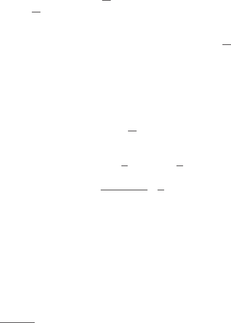
Lectures on Symplectic Field Theory 139
also has a natural compactification whenever 2g + ℓ ≥ 3, known as t he Deligne-
Mumford compactification
M
g,ℓ
⊃ M
g,ℓ
.
The space
M
g,ℓ
consists of “nodal” Riemann surfaces, which can be understood as
objects t hat arise from smooth Riemann surfaces with pair-of-pants decompositions
in the limit where some of the lengths of the circles separating two pairs of pants
from each other may degenerate to 0 (see e.g. [SS92]). We will discuss this in a
bit more detail in Lecture
9; for now, all you really need to know is that M
g,ℓ
is
a compact and metrizable topological space that contains M
g,ℓ
as a n open subset.
Let us fix a metric on M
g,ℓ
and denote the distance function by dist( , ).
Similarly, fix Riemannian metrics on
c
W and
˙
Σ with translation-invariance on
the cylindrical ends and use dist( , ) to denote the distance functions. For N ∈ N
and J ∈ J
U
, we define
M
∗
N
(J) ⊂ M(J)
to be the set of equivalence classes admitting representatives (Σ, j, Γ
+
, Γ
−
, Θ, u) with
the following properties:
• The equivalence class in M
g,k
+
+k
−
+m
represented by ( Σ, j, Γ
+
∪Γ
−
∪Θ) lies
at a distance of at most 1 /N from
M
g,k
+
+k
−
+m
\ M
g,k
+
+k
−
+m
;
4
• sup
z∈
˙
Σ
|du(z)| ≤ N;
• There exists z
0
∈
˙
Σ such that
dist(u(z
0
),
c
W \ U) ≥
1
N
, |du(z
0
)| ≥
1
N
,
and
inf
z∈
˙
Σ\{z
0
}
dist(u(z
0
), u(z))
dist(z
0
, z)
≥
1
N
.
We observe that every element o f M
∗
N
(J) has an injective point mapped into U, and
conversely, every asymptotically cylindrical J-holomor phic curve with that property
belongs to M
∗
N
(J) for N ∈ N sufficiently large. It is crucial to observe that all three
conditions in this definition are closed conditions: morally, we are defining M
∗
N
(J)
to be a closed subset in the compactification of M(J), and it will therefore be
compact.
Define
J
reg,N
U
⊂ J
U
as the set of all J ∈ J
U
for which every element of M
∗
N
(J) is Fredholm regular.
Lemma 7.19. For e v ery N ∈ N, J
reg,N
U
is open and dense.
Proof. Density is immediate, since we’ve seen a lready that every J ∈ J
U
admits
a C
∞
-small perturbation that achieves regularity for all curves in
S
N∈N
M
∗
N
(J).
For openness, suppose the contrary: then there exists J
∞
∈ J
reg,N
U
and a sequence
4
If the stability condition 2g + k
+
+ k
−
+ m ≥ 3 is not satisfied, one should amend this by
asking for the dis tance condition to hold for some tuple (Σ, j, Γ
+
∪Γ
−
, Θ
′
), where Θ
′
is the unio n
of Θ with enough extra marked points to achieve stability.
140 Chris Wendl
J
ν
∈ J
U
\J
reg,N
U
with J
ν
→ J
∞
in the C
∞
-topology. There must also exist a sequence
of curves u
ν
∈ M
∗
N
(J
ν
) that are not Fredholm regular. By the definition of M
∗
N
(J
ν
),
they have domains that are uniformly bounded away fr om the singular part of the
Deligne-Mumford space of Riemann surfaces, so we can extract a subsequence for
which these domains converge. Similarly, the fir st derivatives of u
ν
are uniformly
bounded, implying in particular a uniform W
1,p
-bound locally for some p > 2, and
elliptic regularity (Theorem
2.22 in Lecture 2) turns this into uniform C
∞
-bound
and thus a C
∞
-convergent subsequence u
ν
→ u
∞
∈ M
∗
N
(J
∞
). But u
∞
must then
be Fr edholm regular, which is an open condition, implying that u
ν
is also regular
for ν sufficiently large, and this is a contra diction.
Proof of Theorem 7.2. Since the space of all curves in M(J) with injective
points mapped into U is the union of the spaces M
∗
N
(J) for N ∈ N, we have
J
reg
U
=
\
N∈N
J
reg,N
U
,
which is a countable intersection o f open and dense sets.

LECTURE 8
Transversality in symplectizations
Contents
8.1. Statement of the theorem and discussion 141
8.2. Injective points of the projected curve 144
8.3. Smoothness of the universal moduli space 147
This lecture is an addendum to the transversality discussion in Lecture 7: we
need to prove that Fredholm regularity can also be achieved for generic translation-
invariant almost complex structures on symplectizations.
8.1. St atement of the theorem and discussion
Theorem
7.2 in the previous lecture stated that generic perturbations of J in a
precompact open subset U o f a completed symplectic cobordism suffice to achieve
regularity for all simple holomorphic curves that pass through that subset. In the
more specialized setting of a symplectization R × M with an R-invariant almost
complex structure J ∈ J(H), we need a more specialized transversality result, as
the generic perturbation from Theorem
7.2 cannot be expected to stay in the space
J(H), in particular it will usually not be R-invariant. The f ollowing statement refers
to a stable Hamiltonian structure H = (ω, λ) with induced hyperplane distribution
ξ = ker λ and Reeb vector field R, and we denote by
π
ξ
: T (R × M) → ξ
the projection along the trivial subbundle generated by ∂
r
and R. We assume as
usual that M(J) denotes a moduli space of asymptotically cylindrical J-holomorphic
curves with a fixed genus a nd number of marked points, representing a fixed relative
homology class a nd asymptotic to fixed sets of nondegenerate Reeb orbits a t its
positive and negative punctures.
Theorem 8.1. Suppose M is a closed (2n −1)-dimensional manifold carrying a
stable Hamiltonia n structure H = (ω, λ), J
fix
∈ J(H), and
U ⊂ M
is an open s ubset. Then there exi s ts a comeager subset
J
reg
U
⊂
J ∈ J(H)
J = J
fix
on R × (M \ U)
such that for eve ry J ∈ J
reg
U
, every curve u ∈ M(J) with a representative u :
˙
Σ →
R × M that has an injective point z ∈
˙
Σ satisfying
141
142 Chris Wendl
(i) u(z) ∈ R × U,
(ii) π
ξ
◦ du(z) 6= 0, and
(iii) im (π
ξ
◦ du(z)) ∩ ker (dλ|
ξ
) = {0}
is Fredholm reg ular.
This result is applied most frequently with U = M, in which case the condition
u(z) ∈ R × U is vacuous. The second and third conditions on the injective point z
can be rephrased by asking for the linear map
dλ(π
ξ
T u(X), ·)|
ξ
u(z)
: ξ
u(z)
→ R
to be nontrivial fo r every nonzero X ∈ T
z
˙
Σ. If λ is contact, then this is immediate
whenever π
ξ
T u(X) 6= 0 since dλ|
ξ
is nondegenerate, and the condition π
ξ
T u(X) 6= 0
is also easy to achieve:
Proposition 8.2. If J ∈ J(H), then for any connected J-holomorphic curve
u : (
˙
Σ, j) → (R × M, J), the section
π
ξ
◦ du ∈ Γ(Ho m
C
(T
˙
Σ, u
∗
ξ))
either is identically zero or has only iso l ated zeroes.
As you might guess, this result is a consequence of the similarity principle; see
§
8.2 fo r a proof. Notice that if π
ξ
◦ du ≡ 0, then u is everywhere tangent to the
vector fields ∂
r
and R, so if it is asymptotically cylindrical, then it can only be a
trivial cylinder or a cover thereof.
Proposition 8.3. All trivial cylinders over nondegenerate Reeb orbits hav e in-
dex 0 a nd are Fredholm regular.
Proof. Let u
γ
: R × S
1
→ R × M denote the trivial cylinder over an orbit
γ : S
1
→ M. The virtual dimension formula proved in Lecture
7 gives
ind(u
γ
) = ( n −3)χ(R × S
1
) + 2c
τ
1
(u
∗
γ
T (R × M)) + µ
τ
CZ
(γ) − µ
τ
CZ
(γ)
= 2c
τ
1
(u
∗
γ
T (R × M) ) = 0
since the asymptotic trivialization τ has an obvious extension to a global trivial-
ization of u
∗
γ
ξ, and u
∗
γ
T (R × M) is globally the direct sum of the latter with the
trivial line bundle spanned by ∂
r
and R. Using this splitting, the linearized Cauchy-
Riemann o perator D
u
γ
can be identified with
¯
∂ ⊕ (∂
s
−A
γ
), where
¯
∂ = ∂
s
+ i∂
t
: W
k,p,δ
(R × S
1
, C) ⊕V
Γ
→ W
k−1,p,δ
(R × S
1
, C)
and
∂
s
− A
γ
: W
k,p,δ
(u
∗
γ
ξ) → W
k−1,p,δ
(u
∗
γ
ξ).
Here we are assuming without loss of generality that V
Γ
is a complex 2-dimensional
space of smooth sections of the trivial line bundle spanned by ∂
r
and R that are
constant near infinity, and we are identifying this with a space of smo oth complex-
valued f unctions on R × S
1
. Nondegeneracy implies that ∂
s
− A : W
k,p
→ W
k−1,p
is an isomorphism, recall Theorem
4.11 in Lecture 4. Using weight functions as
in the proof of Lemma
7.10 to define isomorphisms between W
k,p,δ
and W
k,p
, one
can identif y ∂
s
− A
γ
: W
k,p,δ
→ W
k−1,p,δ
with a small perturbation of the same
Lectures on Symplectic Field Theory 143
operator W
k,p
→ W
k−1,p
, hence it is also an isomorphism for δ > 0 sufficiently
small. To see that
¯
∂ : W
k,p,δ
⊕ V
Γ
→ W
k−1,p,δ
is also surjective, observe first that
its index is 2; this follows f r om our calculation of ind(u
γ
) and corresponds to the
fact that dim Aut(R × S
1
, i) = 2. The kernel of this operator consists of bounded
holomorphic C-valued functions on R × S
1
, so it is precisely the real 2 -dimensional
space of constant functions, implying
dim
R
coker(
¯
∂) = dim
R
ker(
¯
∂) − ind
R
(
¯
∂) = 2 − 2 = 0,
so D
u
γ
is surjective.
Corollary 8.4. For any contact form α o n a closed manifold M, there exists
a co meager subset J
reg
(α) ⊂ J(α) such that for every J ∈ J
reg
(α), all somewhere
injective asymptotically cylindrical J-holomorphic curves in R × M are Fredholm
regular.
Note t hat in the setting of Corollary
8.4, a curve t hat is not a cover of a trivial
cylinder always belongs to a smoo th 1-parameter family of curves related to each
other by R-translation, so that the kernel of the linearized Cauchy-Riemann operator
automatically has kernel of dimension at least 1. This precludes Fredholm regularity
for curves of index 0, thus:
Corollary 8.5. If α is a con tact form and J ∈ J
reg
(α), then all simple asymp-
totically cylindrical J-holomorphic curves u : (
˙
Σ, j) → (R ×M, J) other than trivial
cylinders satisfy
ind(u) ≥ 1.
The following example shows that the third condition on the injective point in
Theorem
8.1 cannot be fully removed in general.
Example 8.6 (cf. Examples 6.6 and 6.16 in Lecture
6). Assume (W, ω) is a closed
symplectic manifold of dimension 2 n−2 with a periodic time-dependent Hamiltonian
H : S
1
× W → R, and M := S
1
× W is assigned the stable Ha miltonian structure
(Ω, Λ) := (ω + dt ∧ dH, dt). A choice of J ∈ J(H) is then equivalent to a choice of
t-dependent family of ω-compatible almost complex structures {J
t
∈ J(W, ω)}
t∈S
1
,
and for any t ∈ S
1
and s ∈ R, J
t
-holomorphic curves u : (Σ, j) → (W, J
t
) give rise
to J-holomorphic curves
¯u : (Σ, j) → (R × M, J) : z 7→ (s, t, u(z)).
In particular, when n = 2 one can consider the example where W = Σ is a closed
surface, so curves of this form exist for any choice of J ∈ J(H), no matter how
generic (remember that the domain complex structure j is arbitrary, it is not fixed
in advance). If Σ has genus g and the map u : Σ → Σ has degree 1, then since ¯u
has no punctures a nd satisfies c
1
([¯u]) = c
1
(¯u
∗
T (R ×S
1
×Σ)) = c
1
(T Σ) = χ(Σ), the
index of ¯u is
ind(¯u) = (n − 3)χ(Σ) + 2χ(Σ) = χ(Σ) = 2 − 2g.
This shows that ¯u cannot be Fredholm regular unless g = 0.
144 Chris Wendl
Theorem 8.1 appeared for the first time in the contact case in [Dra04], and
alternative proofs have since appeared in t he appendix of [
Bou06] (for cylinders in
the contact case) and in [
Wena] (under slightly different assumptions in the stable
Hamiltonian setting). What I will describe below is a generalization of Bourgeois’s
proof.
8.2. Injective points of the project ed curve
One point o f difficulty in proving transversality in R × M is that in cont r ast to
the setting of Theorem
7.2, generic perturbations within J(H) can never be truly
local, i.e. if you perturb J near a point (r, x) ∈ R×M, then you are also perturbing it
in a neighborhood of the entire line R ×{x}. We therefore need to know that we can
find a point z ∈
˙
Σ that is the only point where u :
˙
Σ → R ×M pa sses through such
a line; put another way, we need to know that not only u = (u
R
, u
M
) :
˙
Σ → R × M
but also t he projected map u
M
:
˙
Σ → M is somewhere inj ective. The first step in
showing this is Proposition
8.2 above, as the zeroes of the section
π
ξ
◦ du ∈ Γ(Ho m
C
(T
˙
Σ, u
∗
ξ))
are precisely the critical points of u
M
:
˙
Σ → M; everywhere else, u
M
is an immersion
transverse to the Reeb vector field. To prove Proposition
8.2, we shall use the fact
that the vector fields ∂
r
and R generate an integrable J- invariant distribution on
R×M. Indeed, the zeroes of π
ξ
◦du are the points of tangency with this distribution,
hence the result is an immediate consequence of the following statement:
Lemma 8.7. Suppo s e (W, J) is an almost complex manifold, Ξ ⊂ T W is a smooth
integrable J-invariant distribution and u : (Σ, j) → (W, J) is a connected pseudo-
holomorphic curve whose image is n ot contained in a leaf of the foliation generated
by Ξ. Then all points z ∈ Σ with im du(z) ⊂ Ξ are isolated in Σ.
Proof. Statement is local, so assume (Σ, j) = ( D, i) with coordinates s + it,
W = C
n
, and u(0) = 0. Let 2m denote the real dimension of Ξ , and observe that
since Ξ is integrable, we can change coordinates near 0 and assume without loss of
generality that at every point p ∈ C
n
near 0, Ξ
p
= C
m
⊕ {0} ⊂ C
n
= T
p
C
n
. The
J-invariance of Ξ then implies that in coordinates (w, ζ) ∈ C
m
×C
n−m
, J takes the
form
J(w, ζ) =
J
1
(w, ζ) Y (w, ζ)
0 J
2
(w, ζ)
,
where J
2
1
and J
2
2
are both −1, and J
1
Y + Y J
2
= 0. Writing u(z) = (f(z), v(z)) ∈
C
m
×C
n−m
, the Cauchy-Riemann equation ∂
s
u + J(u)∂
t
u = 0 is then equivalent to
the two equations
∂
s
f + J
1
(f, v) ∂
t
f + Y (f, v) ∂
t
v = 0,
∂
s
v + J
2
(f, v) ∂
t
v = 0.
(8.1)
We have im du(z) ⊂ Ξ wherever ∂
s
v = ∂
t
v = 0; notice that it suffices to consider
the condition ∂
s
v = 0 since ∂
t
v = J
2
(f, v) ∂
s
v. Differentiating the second equation
in (
8.1) with respect to s gives
∂
s
(∂
s
v) + J
2
(f, v) ∂
t
(∂
s
v) + ∂
s
[J
2
(f, v)] J
2
(f, v) ∂
s
v = 0,

Lectures on Symplectic Field Theory 145
where in the la st t erm we’ve substituted J
2
(f, v) ∂
s
v for ∂
t
v. Setting
¯
J(z) :=
J
2
(f(z), v(z)) and A(z) := ∂
s
[J
2
(f(z), f(z)] J
2
(f(z), v(z)), this becomes a linear
Cauchy-Riemann type equation ∂
s
(∂
s
v) +
¯
J ∂
t
(∂
s
v) + A(∂
s
v) = 0, so the similarity
principle implies that zeroes of ∂
s
v are isolated unless it is identically zero. The
latter would mean v is constant, so u is contained in a leaf of Ξ.
Lemma 8.8. Suppo se J ∈ J(H), γ : S
1
→ M is a clos ed Ree b o rb i t, and
u = (u
R
, u
M
) : (
˙
Σ, j) → (R × M, J) is an asymptotically cylindrical J-holomorph i c
curve that is not a cover of a trivial cylinder. Then all intersections of the map
u
M
:
˙
Σ → M with the image of the orbit γ are isolated.
Proof. The trivial cylinder over γ is a J-holomorphic curve, so the statement
follows from the fact that two a symptotically cylindrical J-holomorphic curves can
only have isolated intersections unless bo t h are covers of the same simple curve.
We can now prove the statement we need about somewhere injectivity for u
M
:
˙
Σ → M. This result first appear ed in [
HWZ99, Theorem 1.13].
Proposition 8.9. Suppose J ∈ J(H) and
u = (u
R
, u
M
) : (
˙
Σ, j) → (R ×M, J)
is a simple asymptotically cylindrical J-holomorphic curve which is not a trivial
cylinder and has only nondegenerate asymptotic o rb i ts. Then the set of injective
po ints z ∈
˙
Σ of the map u
M
:
˙
Σ → M for which u
M
(z) i s not contained in any of
the asymptotic orbits of u is open and dense.
Proof. Openness is clear, so our main task is to prove density. The idea is
first to show via elementary topological arguments that if the set of injective points
is not dense, then
˙
Σ contains two disjoint open sets on which u
M
is an embedding
with identical images. We will then conclude from this that if u is simple, it must
be equivalent to one of its nontrivial R-translations, and the latter is impossible for
an asymptotically cylindrical curve.
Step 1: We begin by harmlessly removing some discrete sets of points in
˙
Σ tha t
would make the subsequent arguments more complicated. Let
P ⊂ M
denote the union of the images of the asymptotic orbits of u, a finite disjoint union of
circles. Lemma
8.8 implies that u
−1
M
(P ) is a discrete subset of
˙
Σ. By Proposition
8.2,
there is also a discrete set Z ⊂
˙
Σ \ u
−1
M
(P ) containing all points z 6∈ u
−1
M
(P ) where
π
ξ
◦ du(z) = 0, and we claim that
Z
′
:= u
−1
M
(u
M
(Z))
is a discrete subset of
˙
Σ \ u
−1
M
(P ). Indeed, u
M
(Z) is a discrete subset of M \ P
since the points in Z can only accumulate at infinity,
1
hence accumulation points of
u
M
(Z) ⊂ M can occur o nly in P . For each individual point p ∈ u
M
(Z), the f act that
p 6∈ P implies u
−1
M
(p) is compact, and it consists of a discrete (and therefore finite)
1
Actually the asymptotic formula of [
HWZ96] implies that both Z and u
−1
M
(P ) are always
finite for curves that are not cove rs of trivial cylinders, but we do not need to use that here.
146 Chris Wendl
set of points with π
ξ
◦du(z) = 0, plus possibly some other points where π
ξ
◦du(z) 6= 0,
but u
M
is an embedding near each point of the latter type, so that these points of
u
−1
M
(p) must always be isolated and are therefore also finite in number. This proves
the claim, and we conclude that
¨
Σ :=
˙
Σ \
u
−1
M
(P ) ∪ Z
′
an open and dense subset of
˙
Σ, as it is obta ined by removing a discrete subset from
the open and dense subset
˙
Σ \u
−1
M
(P ). To prove the proposition, it will now suffice
to prove that the set of points z ∈
¨
Σ which are injective points of u
M
:
˙
Σ → M is
dense in
¨
Σ. We shall argue by contradiction and assume from now o n t hat density
fails.
Step 2: We will find two open subsets U, V ⊂
˙
Σ such that u
M
restricts to a n
embedding on both, but
U ∩ V = ∅ and u
M
(U) = u
M
(V).
Indeed, assume the set of injective points of u
M
lying in
¨
Σ is not dense in
¨
Σ. Then
there exists a point z
0
∈
¨
Σ with a closed neighborhood D(z
0
) ⊂
¨
Σ such that no
z ∈ D(z
0
) is an inj ective point. Since z ∈
¨
Σ implies π
ξ
◦ du(z) 6= 0, this means that
for every z ∈ D(z
0
), there exists ζ ∈
˙
Σ \{z} with u
M
(z) = u
M
(ζ), and the definition
of
¨
Σ implies ζ is also in
¨
Σ, hence π
ξ
◦du(ζ) 6= 0 and u
M
is a local embedding near ζ.
Since u(z) 6∈ P and u
M
maps
˙
Σ \ u
−1
M
(P ) properly to M \P , we also conclude that
u
−1
M
(u
M
(z)) is finite. Now suppose u
−1
M
(u
M
(z
0
)) = {z
0
, ζ
1
, . . . , ζ
m
}, and let D(ζ
j
) ⊂
¨
Σ
for j = 1, . . . , m denote closed neighborhoods on which u
M
is an embedding. We
claim tha t after possibly shrinking D(z
0
), we can assume
u
M
(D(z
0
)) ⊂
m
[
j=1
u
M
(D(ζ
j
).
Let us first shrink D(z
0
) so that u
M
is an embedding o n D(z
0
), which is possible
since π
ξ
◦du(z
0
) 6= 0. Then if t he claim is false, there exists a sequence z
ν
∈ D(z
0
) of
noninjective points with z
ν
→ z
0
, hence there is also a sequence z
′
ν
∈
¨
Σ \D(z
0
) with
u
M
(z
ν
) = u
M
(z
′
ν
) but z
′
ν
not converging to any of ζ
1
, . . . , ζ
m
. But since u
M
(z
′
ν
) →
u
M
(z
0
) 6∈ P , the points z
′
ν
are confined to a compact subset of
˙
Σ and therefore have
a subsequence z
′
ν
→ z
′
∞
∈
˙
Σ with u
M
(z
′
∞
) = u
M
(z
0
). The limit cannot be z
0
itself
since z
′
ν
6∈ D(z
0
), thus z
′
∞
must be one of the ζ
1
, . . . , ζ
m
, and we have a contradiction.
We claim next that at least one of the sets u
M
(D(z
0
)) ∩ u
M
(D(ζ
j
)) has nonempty
interior. This is a simple exercise in metric space topology: it can be reduced to
the fact that if X is a metric space with closed subsets V, W ⊂ X that both have
empty interior (meaning no open subset of X is contained in V or W ), then V ∪W
also has empty interior. Since the subsets u
M
(D(z
0
)) ∩ u
M
(D(ζ
j
)) ⊂ u
M
(D(z
0
)) for
j = 1, . . . , m are all closed but their union is u
M
(D(z
0
)), they cannot all have empty
interior. This achieves the goal of Step 2.
Step 3: We show that u is biholomorphically equivalent to o ne of its R-translations
τ ·u := (u
R
+ τ, u
M
) :
˙
Σ → R × M
Lectures on Symplectic Field Theory 147
for τ ∈ R \{0}. To see this, note that for J ∈ J(H), the nonlinear Cauchy-Riemann
equation T u ◦ j = J(u) ◦ T u is equivalent to the two equations
du
R
= u
∗
M
λ ◦j,
π
ξ
◦ T u
M
◦ j = J(u
M
) ◦ π
ξ
◦ T u
M
.
(8.2)
Since π
ξ
◦T u
M
:
˙
Σ → u
∗
M
ξ is injective everywhere on the neighborhoods U and V, the
second equation determines j in terms of J on each of these regions; in particular,
the identification of u
M
(U) with u
M
(V) provides a biholomorphic map of V to U
so that u|
U
and u|
V
may be regarded as two J-holomo r phic maps from the same
Riemann surface which differ only in the R-factor. But with j and u
M
both fixed,
the first equation in (
8.2) determines du
R
and thus determines u
R
up to the addition
of a constant τ ∈ R. If τ = 0, t his means u has two disjoint regions on which its
images are identical, contradicting the assumption that u is simple. Thus τ 6= 0,
and since two distinct simple curves can only intersect each other at isolated points,
we conclude u = τ · u up to parametrization.
Step 4: We now derive a contradiction. The relation u = τ · u implies that in
fact u = kτ · u fo r every k ∈ Z, so we obtain a diverging sequence of R-tra nslatio ns
τ
k
→ ∞ such that u and τ
k
· u always have identical images in R × M. It follows
that for some point z ∈
˙
Σ with u(z) = ( r, x) where x is not contained in any of the
asymptotic orbits of u, the points (r − τ
k
, x) are all in the image o f u as τ
k
→ ∞.
But this contradicts the asymptotically cylindrical behavior of u.
8.3. Smoothness of the universal moduli space
The overall outline of the proof o f Theorem 8.1 is the same as for Theorem 7.2:
one needs to define a suitable space J
ε
U
of perturbed almost complex structures,
giving rise to a universal moduli space M
∗
(J
ε
U
) that is a smooth Banach manifold,
and then apply the Sard-Smale theorem to conclude that generic elements of J
ε
U
are regula r values of the projection M
∗
(J
ε
U
) → J
ε
U
: (u, J) 7→ J. If J
ε
U
is a space
of C
ε
-perturbed almost complex structures, then in the final step one can use t he
Taubes tr ick as in §
7.7 to transform the genericity result in J
ε
U
into a genericity
result within t he space J( H) of smooth almost complex structures. The only step
that differs meaningfully fro m what we’ve already discussed is the smoothness of
the universal moduli space, so let us focus on this detail.
Assume J
ref
∈ J(H) with J
ref
= J
fix
outside R×U, and J
ε
U
is a Banach manifold
of C
ε
-small perturbations of J
ref
in J(H) that are also fixed outside of R ×U. The
relevant universal moduli space is then defined by
M
∗
(J
ε
U
) :=
(u, J)
J ∈ J
ε
U
, u ∈ M(J) and
u :
˙
Σ → R × M has an injective point z ∈
˙
Σ with
u(z) ∈ R × U and im (π
ξ
◦ du(z)) ∩ ker (dλ|
ξ
) = {0}
.
Notice that b oth of the constraints satisfied by u at the injective point ar e open.
The local structure of M
∗
(J
ε
U
) near an element (u
0
, J
0
) with representative u
0
:
(
˙
Σ, j
0
) → (R × M, J
0
) can again be described via the zero set of a smooth section
¯
∂ : T × B
k,p,δ
× J
ε
U
→ E
k−1,p,δ
: (j, u, J) 7→ T u ◦ J ◦ T u ◦ j,
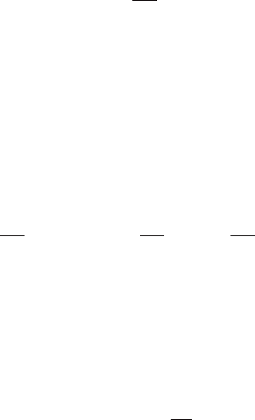
148 Chris Wendl
where T is a Teichm¨uller slice thro ugh j
0
, and it suffices to show that the lineariza-
tion
L : T
u
0
B
k,p,δ
⊕T
J
0
J
ε
U
→ E
k−1,p,δ
(j
0
,u
0
,J
0
)
: (η, Y ) 7→ D
u
0
η + Y ◦ T u
0
◦ j
0
is always surjective. As usual, here we’re assuming k ∈ N, 1 < p < ∞, and the
exp onential weight δ > 0 is small but positive so that D
u
0
is Fredholm. The image
of L is then closed, and focusing on the k = 1 case, if L is not surjective then there
exists a nontrivial element θ ∈ L
q,−δ
(
Hom
C
(T
˙
Σ, u
∗
0
T (R × M))) such t hat
hD
u
0
η, θi
L
2
= 0 for all η ∈ W
1,p,δ
(u
∗
0
T (R × M)) ⊕ V
Γ
,
hY ◦ T u
0
◦ j
0
, θi
L
2
= 0 for all Y ∈ T
J
0
J
ε
U
.
(8.3)
The first conditio n implies via elliptic regularity and the similarity principle that θ
is smooth and has only isolated zeroes. So far this is all the same as in the proof
of Theorem
7.2, but the next step is trickier: since perturbing J
0
within J(H)
only cha nges the action of the almo st complex structure on ξ but not on the trivial
subbundle generated by ∂
r
and R, it is not clear whether the range of values allowed
for Y is large enough to force hY ◦ T u
0
◦ j
0
, θi
L
2
> 0.
To overcome this, let us decompose everything in this picture with respect to
the nat ural splitting
T (R × M) = ǫ ⊕ ξ,
where ǫ denotes the trivial line bundle spanned by ∂
r
and R. In particular, the
domain and target bundles of the Cauchy-Riemann type operator D
u
0
now split as
u
∗
0
T (R × M) = u
∗
0
ǫ ⊕ u
∗
0
ξ,
Hom
C
(T
˙
Σ, u
∗
0
T (R × M) ) = Hom
C
(T
˙
Σ, u
∗
0
ǫ) ⊕ Hom
C
(T
˙
Σ, u
∗
0
ξ),
and we shall write η = (η
ǫ
, η
ξ
) and θ = (θ
ǫ
, θ
ξ
) accordingly. This gives a block
decomposition of D
u
0
as
D
u
0
η =
(D
u
0
η)
ǫ
(D
u
0
η)
ξ
=
D
ǫ
u
0
D
ǫξ
u
0
D
ξǫ
u
0
D
ξ
u
0
η
ǫ
η
ξ
.
It is easy to verify that D
ǫ
u
0
and D
ξ
u
0
each satisfy suitable Leibniz rules and are thus
Cauchy-Riemann type operators on u
∗
0
ǫ and u
∗
0
ξ respectively, while the off-diagonal
terms are both tensorial, i.e. zeroth-order operators. Since perturbations of J
0
in
J(H) only change its action on ξ, Y ∈ T
J
0
J
ε
U
now takes the block form
Y =
0 0
0 Y
ξ
,
where Y
ξ
is a C
ε
-small section of the bundle
End
C
(ξ, J
0
) over M. Assuming the L
2
-
pairings are defined so as to r espect these splittings, the second condition in (
8.3)
now becomes
hY
ξ
◦ π
ξ
◦ T u
0
◦ j
0
, θ
ξ
i
L
2
= 0,
and given any injective point z
0
∈
˙
Σ of (u
0
)
M
:
˙
Σ → M satisfying u
0
(z
0
) ∈ R×U, we
have enough freedom to choose Y
ξ
near R ×{u
0
(z
0
)} such that t his pairing becomes
positive unless
θ
ξ
= 0 near z
0
.

Lectures on Symplectic Field Theory 149
It remains to show that θ
ǫ
also vanishes near z
0
, which will contradict the fa ct that θ
only has isolated zeroes. To this end, notice that the first condition in (
8.3) implies
via separate choices o f the components η
ǫ
and η
ξ
with support near z
0
that
hD
ǫ
u
0
η
ǫ
, θ
ǫ
i
L
2
= 0 for all η
ǫ
supported near z
0
,
hD
ǫξ
u
0
η
ξ
, θ
ǫ
i
L
2
= 0 for all η
ξ
supported near z
0
.
(8.4)
The first of these two conditions gives no new information, since we already know
that θ = (θ
ǫ
, 0) solves an anti-Cauchy-Riemann equation. To get some information
out of the second condition, we will need an explicit formula for D
ǫξ
u
0
.
Lemma 8.10. T he tensorial operator D
ǫξ
u
0
: u
∗
0
ξ →
Hom
C
(T
˙
Σ, u
∗
0
ǫ) takes the form
D
ǫξ
u
0
η
ξ
=
h
−dλ
η
ξ
, J
ξ
0
◦π
ξ
◦ T u(·)
i
∂
r
+
dλ
η
ξ
, π
ξ
◦T u(·)
R.
Proof. As a preliminary step, no tice that −dr ◦ J = λ for any J ∈ J(H);
indeed, the conditions J(ξ) = ξ ⊂ ker dr and J∂
r
= R imply t hat these two 1 -forms
have matching values on ∂
r
, R and ξ. As a consequence, λ◦J
0
= dr, so in particular
λ ◦J
0
is closed.
Choosing local holomorphic coordinates (s, t) in an arbitrary neighborhood in
˙
Σ, we have
(D
ǫξ
u
0
η
ξ
)∂
s
= dr
(D
u
0
η
ξ
)∂
s
∂
r
+ λ
(D
u
0
η
ξ
)∂
s
R.
Extend u
0
:
˙
Σ → R × M to a smooth 1-parameter family of maps {u
ρ
:
˙
Σ →
R × M}
ρ∈R
with ∂
ρ
u
ρ
|
ρ=0
= η
ξ
∈ Γ(u
∗
0
ξ). Then by the definition of the linearized
Cauchy-Riemann opera tor,
(D
u
0
η
ξ
)∂
s
= ∇
ρ
(∂
s
u
ρ
+ J
0
(u
ρ
)∂
t
u
ρ
)|
ρ=0
,
for any choice of connection ∇ on R × M. Since ∂
s
u
0
+ J
0
(u
0
)∂
t
u
0
= 0, we find
λ
(D
u
0
η
ξ
)∂
s
= λ
∇
ρ
(∂
s
u
ρ
+ J
0
(u
ρ
)∂
t
u
ρ
)|
ρ=0
= ∂
ρ
[λ(∂
s
u
ρ
+ J
0
(u
ρ
)∂
t
u
ρ
)]|
ρ=0
= ∂
ρ
[λ(∂
s
u
ρ
)]|
ρ=0
+ ∂
ρ
[(λ ◦ J
0
)(∂
t
u
ρ
)]|
ρ=0
= dλ(η
ξ
, ∂
s
u) + d(λ ◦ J
0
)(η
ξ
, ∂
t
u)
= dλ(η
ξ
, π
ξ
∂
s
u),
where we’ve used the formula
dλ(X, Y ) = L
X
[λ(Y )] − L
Y
[λ(X)] − λ([X, Y ])
and eliminated severa l t erms using the fact t hat λ(η
ξ
) = λ(J
0
η
ξ
) = 0 since η
ξ
is
valued in ξ, plus d(λ ◦ J
0
) = 0. A similar computation gives
dr
(D
u
0
η
ξ
)∂
s
= −dλ(η
ξ
, π
ξ
∂
t
u) = −dλ(η
ξ
, J
0
◦ π
ξ
∂
s
u),
so removing the local coordinates from the picture produces the stated formula.
The following exercise in symplectic linear algebra shows that this bundle map
u
∗
0
ξ →
Hom
C
(T
˙
Σ, u
∗
0
ǫ) is surjective on any fiber over a point z with π
ξ
◦ du
0
(z) 6=
0. (If you have no patience for the exercise, just convince yourself t hat it’s true
whenever dλ|
ξ
is nondegenerate and tames J|
ξ
, i.e. the contact case.)
150 Chris Wendl
Exercise 8.11. Assume V is a finite-dimensional vector space, X, Y ⊂ V are
linearly independent vectors, and Ω is an alternating bilinear form on V . Show that
the real-linear map
A : V → C : v 7→ Ω(v, X) + iΩ(v, Y )
is surjective if and only if Span(X, Y ) ∩ ker Ω = {0}.
Hint: Under the latter condition, one loses no generality by replacing V with a
subspace that is complementary to ker Ω a nd contains Span(X, Y ), in which case
(V, Ω) becomes a symplectic vector space. Now consider the restriction of A to a
2-dimensional subspace transverse t o the symplectic complement of Span(X, Y ).
The conclusion of this discussion is that unless θ
ǫ
vanishes near z
0
, η
ξ
can be
chosen with supp ort near z
0
so that hD
u
0
η
ξ
, θ
ǫ
i
L
2
> 0, violating the second condi-
tion in (
8.4). This proves that θ vanishes altogether near z
0
and thus, by unique
continuation, θ ≡ 0, a contradiction.
We’ve proved that the universal moduli space is smooth as claimed. Since the
rest of the proof of Theorem
8.1 is the same as in the non-R-invariant case, we leave
those details to the reader.
Remark 8.12. You may have noticed tha t in both this and the previous lecture,
our proof that the universal moduli space is smooth relied on a surjectivity result
that was actually stronger than needed: in both cases, we needed to prove that an
operator of the form
T
j
0
T ⊕ T
u
0
B
k,p,δ
⊕ T
J
0
J
ε
U
L
−→ E
k−1,p,δ
(j
0
,u
0
,J
0
)
was surjective, but we ended up proving that its restriction to the smaller domain
T
u
0
B
k,p,δ
⊕T
J
0
J
ε
U
is a lr eady surjective. This technical detail hints at a stronger result
that can be proved using these methods: one can show that not only is M
∗
(J
ε
U
)
smooth but a lso the forget ful map
M
∗
(J
ε
U
) → M
g,k
+
+k
−
+m
([(Σ, j, Γ
+
, Γ
−
, Θ, u)], J) 7→ [(Σ, j, Γ
+
∪ Γ
−
∪ Θ)]
sending a J-holomorphic curve to its underlying domain in the moduli space of
Riemann surfaces is a submersion, cf. the blog post [
Wenb] and its sequel. One can
use this to prove generic t r ansversality results for spaces of J-holomorphic curves
whose domains are constrained within the moduli space of Riemann surfaces, which
can be used to define mor e elabor ate algebraic structures on SFT, e.g. this idea
plays a very prominent role in t he study of Gromov-Witten invariants.

LECTURE 9
Asymptotics and compactness
Contents
9.1. Removal of singularities 152
9.2. Finite energy and asymptotics 155
9.3. Degenerations of holomorphic curves 170
9.3.1. Bubbling 171
9.3.2. Breaking 172
9.3.3. The Deligne-Mumford space of Riemann surfaces 176
9.4. The SFT compactness theorem 182
9.4.1. Nodal curves 182
9.4.2. Holomorphic buildings 183
9.4.3. Convergence 186
9.4.4. Symplectizations, stretching and so forth 187
Moduli spaces of pseudoholomorphic curves are generally not compact, but they
have natural compactifications, obtained by allowing certain types of curves with
singular behavior. For closed holomorphic curves, this fact is known as Gromo v’s
co mpactness theorem, and our main goal in this lecture is to state its generalization
to punctured curves, which is usually called the SFT compactness theorem. The the-
orem was first proved in [
BEH
+
03] (see also [CM05] for an alternative approach),
and we do not have space here to present a complete proof, but we can still describe
the main geometric and ana lytical ideas behind it.
The overar ching theme of this lecture is the notion of bubbling, of which we will
see several examples. Bubbling arises in a natural way from elliptic regularity: recall
that in Lecture
2, we proved that whenever kp > 2, any uniformly W
k,p
-bounded
sequence u
ν
of holomorphic curves is also uniformly C
m
lo c
-bounded for every m ≥ N
(cf. Theorem
2.22). The Arzel`a-Ascoli theorem implies that such sequences have
C
∞
lo c
-convergent subsequences, and this is true in particular whenever u
ν
is uniformly
C
1
-bounded, as a C
1
-bound implies a W
1,p
-bound with p > 2. Let us take note of
this fa ct for future use:
Proposition 9.1. If (W, J
ν
) is a sequence of almost complex manifolds with
J
ν
→ J in C
∞
, then any uniform l y C
1
-bounded sequence of J
ν
-holomorphic maps
u
ν
: D → W has a subsequence convergent in C
∞
lo c
on
˚
D.
If one wants to prove compactness for a moduli space of J-holomor phic curves,
it therefore suffices in general to establish a C
1
-bound. The catch is, of course,
that the first derivatives of u
ν
might not be uniformly bounded, and this is when
151

152 Chris Wendl
interesting things are seen to ha ppen: while the sequence u
ν
is not compact, it
turns out that it becomes compact after removing finitely many points from its
domain, and near those points one can ta ke a sequence of reparametrizations to find
additional nontrivial holomorphic curves in the limit, t he so-called “bubbles”. This
is one of the ways that the “nodal” curves in Gromov’s compactness theorem can
arise, and we will see the same phenomenon at work in several other contexts as
well.
9.1. Removal of singularities
As an important tool for use in the rest of this lecture, we begin with the following
result from [
Gro85]:
Theorem 9.2 (Gromov’s removable singularity theorem). Assume (W, ω) is a
symplectic manifold with a tame almost complex structure J, a nd u : D \ {0} → W
is a J-hol omorphic curve that has its image con tained in a com pact subset o f W and
satisfies
Z
D\{0}
u
∗
ω < ∞.
Then u admits a s mooth extension to D.
We will prove the slightly weaker statement t hat u has a continuous extension.
If dim
R
W = 2, then the smooth extension follows from this by classical complex
analysis; in higher dimensions, one can instead apply results on local elliptic regu-
larity, see e.g. [
MS04]. We will use as a black box the following additional result
from [
Gro85], which is closely related to a standard result about minimal surfaces:
Theorem (Gromov’s monotonicity lemma [
Gro85]). Suppose (W, ω) is a com-
pa ct symplectic manifold (possibly with boundary), J is an ω-tame almost comp l ex
structure, and B
r
(p) ⊂ W denotes the open ball of radius r > 0 about p ∈ W with
respect to the Riemannian metric g(X, Y ) :=
1
2
ω(X, JY ) +
1
2
ω(Y, JX). T hen there
exist constants c, R > 0 such that for all r ∈ (0, R) and p ∈ W with B
r
(p) ⊂ W , ev-
ery prope r non-constant J-holomorphic curve u : (Σ, j) → (B
r
(p), J) passing through
p satisfies
Z
Σ
u
∗
ω ≥ cr
2
.
In t he above statement , (Σ, j) is assumed to be an arbitrary (generally noncom-
pact) Riemann surface without boundary. In applications, one typically has a larger
(e.g. closed or punctured) domain Σ
′
in the picture, and Σ is defined to be the con-
nected component of u
−1
(B
r
(p)) ⊂ Σ
′
containing some point z ∈ u
−1
(p). The main
message of the theorem is tha t u must use up at least a certain amount of energy
for every ball whose center it passes through, so e.g. the portion of the curve passing
through B
r
(p) cannot become arbitrarily “thin” as in Figure
9.1.
Returning to the removable singularity theorem, we shall use the biholomorphic
map
Z
+
:= [0, ∞) × S
1
→ D \ {0} : (s, t) 7→ e
−2π(s+it)
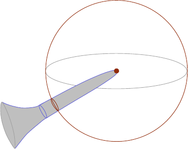
Lectures on Symplectic Field Theory 153
((−
B
r
(p)
p
u(Σ)
u(Σ
′
)
Figure 9.1. The intersection of a J-holomorphic curve u with an
open ball B
r
(p) defines a proper map Σ → B
r
(p). The monotonicity
lemma prevents this map from having arbitrarily small area if it passes
through p.
to transform J-holomorphic maps D \ {0} → W into maps Z
+
→ W , a nd the goal
will be to show that whenever such a map u has precompact image a nd satisfies
R
Z
+
u
∗
ω < ∞, there exists a point p ∈ W such that
(9.1) u(s, ·) → p in C
∞
(S
1
, W ) as s → ∞.
Fix t he obvious flat metric on Z
+
and any Riemannian metric on W in order to
define norms such as |du(s, t)| for (s, t) ∈ Z
+
.
Lemma 9.3. There exists a constant C > 0 such that |du(s, t)| ≤ C for all
(s, t) ∈ Z
+
.
Proof, part 1. Arguing by contradiction, suppo se there exists a sequence z
k
=
(s
k
, t
k
) ∈ Z
+
with |du(z
k
)| =: R
k
→ ∞. Choose a sequence of positive numbers
ǫ
k
> 0 t hat converge to zero but not t oo fast, so that ǫ
k
R
k
→ ∞. We then consider
the sequence of reparametrized maps
v
k
: D
ǫ
k
R
k
→ W : z 7→ u(z
k
+ z/R
k
).
These are also J-holomorphic since z 7→ z
k
+ z/R
k
is holomorphic, and the va lues
of v
k
depend only on the values of u over the ǫ
k
-disk about z
k
. Notice that since
s
k
→ ∞ and ǫ
k
→ 0, we are free to assume that all o f these ǫ
k
-disks a r e disjoint;
moreover, tameness of J implies u
∗
ω ≥ 0 and v
∗
k
ω ≥ 0, thus
X
k
Z
D
ǫ
k
R
k
v
∗
k
ω =
X
k
Z
D
ǫ
k
(z
k
)
u
∗
ω ≤
Z
Z
+
u
∗
ω < ∞,
implying
(9.2)
Z
D
ǫ
k
R
k
v
∗
k
ω → 0 as k → ∞.
We would now like to say something a bout a limit of the maps v
k
as k → ∞, but this
will require a brief pause in the proof, as we don’t yet have quite enough inf ormation
154 Chris Wendl
to do so. We know that the v
k
are uniformly C
0
-bounded since u(Z
+
) is contained
in a compact subset. It would be ideal if we also had a uniform C
1
-bound, as then
elliptic regularity (Prop.
9.1) would give a C
∞
lo c
convergent subsequence on the union
of all the domains D
ǫ
k
R
k
, i.e. on t he entire plane. We have
dv
k
(z) =
1
R
k
du(z
k
+ z/R
k
),
hence |dv
k
(0)| = 1 , but we will need to know more about |du| on the rest of D
ǫ
k
(z
k
)
in order to deduce a C
1
-bound for v
k
on all of D
ǫ
k
R
k
. We’ll come back to this in a
moment. proof to be continued. . .
Here is the auxiliary lemma that is needed to complete the above proo f:
Lemma 9.4 (Hofer). Suppose (X, d) is a com plete metric space, g : X → [0, ∞)
is continuous, x
0
∈ X and ǫ
0
> 0. Then there exist x ∈ X and ǫ > 0 such that,
(a) ǫ ≤ ǫ
0
,
(b) g(x)ǫ ≥ g(x
0
)ǫ
0
,
(c) d(x, x
0
) ≤ 2ǫ
0
, and
(d) g(y) ≤ 2g(x) for all y ∈
B
ǫ
(x).
Proof. If there is no x
1
∈
B
ǫ
0
(x
0
) such that g(x
1
) > 2g(x
0
), then we can
set x = x
0
and ǫ = ǫ
0
and are done. If such a point x
1
does exist, then we set
ǫ
1
:= ǫ
0
/2 and repeat the above process for the pa ir (x
1
, ǫ
1
): that is, if there is
no x
2
∈
B
ǫ
1
(x
1
) with g(x
2
) > 2g(x
1
), we set (x, ǫ) = (x
1
, ǫ
1
) and are finished, and
otherwise define ǫ
2
= ǫ
1
/2 and repeat for (x
2
, ǫ
2
). This process must eventually
terminate, as otherwise we obtain a Cauchy sequence x
n
with g(x
n
) → ∞, which is
impossible if X is complete.
Proof of Lemma
9.3, part 2. Applying Lemma 9.4 to X = Z
+
with g(z) =
|du(z)|, we can replace the original sequences ǫ
k
and z
k
with new sequences for which
all the previously stated properties still hold, but additionally,
|du(z)| ≤ 2|du(z
k
)| for all z ∈ D
ǫ
k
(z
k
).
Our sequence of repara metrizations v
k
then satisfies
|dv
k
(z)| ≤ 2 for all z ∈ D
ǫ
k
R
k
,
so by elliptic regularity, v
k
has a subsequence convergent in C
∞
lo c
(C) to a J-holomorphic
map
v
∞
: C → W
which is not constant since |dv
∞
(0)| = lim
k→∞
|dv
k
(0)| = 1. Informally, we say that
the blow-up of the derivatives at z
k
has caused a plane to “ bubble off”. However,
(
9.2) implies that for every R > 0, one can write ǫ
k
R
k
≥ R for k sufficiently large
and thus
Z
D
R
v
∗
∞
ω = lim
k→∞
Z
D
R
v
∗
k
ω ≤ lim
k→∞
Z
D
ǫ
k
R
k
v
∗
k
ω = 0,
implying
R
C
v
∗
∞
ω = 0. It follows that v
∞
must be constant, so we have a contradic-
tion.
Lectures on Symplectic Field Theory 155
To obtain the uniform limit of u(s, ·) as s → ∞, we now pick any sequence of
nonnegative numbers s
k
→ ∞ and consider the sequence of J-holomorphic half-
cylinders
u
k
: [−s
k
, ∞) × S
1
→ W : (s, t) 7→ u(s + s
k
, t).
By Lemma
9.3, these maps are uniformly C
1
-bounded, so elliptic regularity gives a
subsequence converging in C
∞
lo c
on R × S
1
to a J-holomorphic cylinder
u
∞
: R × S
1
→ W.
Observe that for any c > 0, we can write −s
k
/2 ≤ −c for sufficiently large k and
thus compute
Z
[−c,c]×S
1
u
∗
∞
ω = lim
k→∞
Z
[−c,c,]×S
1
u
∗
k
ω ≤ lim
k→∞
Z
[−s
k
/2,∞)×S
1
u
∗
k
ω
= lim
k→∞
Z
[s
k
/2,∞)×S
1
u
∗
ω = 0
since
R
Z
+
u
∗
ω < ∞. This implies
R
R×S
1
u
∗
∞
ω = 0, so u
∞
is a constant map to some
point p ∈ W , hence after replacing s
k
with a subsequence,
u(s
k
, ·) = u
k
(0, ·) → p in C
∞
(S
1
, W ) as k → ∞.
To finish the proof of (
9.1), we need to show that one cannot find two sequences
s
k
→ ∞ and s
′
k
→ ∞ such that u(s
k
, ·) → p and u(s
′
k
, ·) → p
′
for distinct points
p 6= p
′
∈ W . This is an easy consequence of the monotonicity lemma: indeed,
if two such sequences exist, then we can find a sequence s
′′
k
→ ∞ for which the
loops u(s
′′
k
, ·) alternate between a r bitrarily small neighborhoods of p and p
′
. Since
u is continuous, it must then pass through ∂B
2r
(p) infinitely many times for r > 0
sufficiently small, and in fact there exists an infinite sequence of pairwise disjoint
neighborhoods U
k
⊂ Z
+
such that each
u|
U
k
: U
k
→ B
r
(q
k
)
is a proper map passing through some point q
k
∈ ∂B
2r
(p). The monotonicity lemma
then implies
Z
Z
+
u
∗
ω ≥
X
k
Z
U
k
u
∗
ω ≥
X
k
cr
2
= ∞,
a contradiction.
Exercise 9.5. Given an area form ω on S
2
= C∪{∞} and a finite subset Γ ⊂ S
2
,
show that a holomorphic function f : S
2
\Γ → C has an essential singularity at one
of its punctures if and only if
R
C
f
∗
ω = ∞.
9.2. Finite energy and asymptotics
As further preparation for the compactness discussion, we now prove the long-
awaited converse of the fact that a symptotically cylindrical curves have finite en-
ergy. We work in the setting described in §
6.2: (W, ω) is a symplectic cobordism
with stable boundary ∂W = −M
−
⊔ M
+
carrying stable Hamiltonian structures
156 Chris Wendl
H
±
= (ω
±
, λ
±
) with induced hyperplane distributions ξ
±
= ker λ
±
and Reeb vector
fields R
±
. The completion (
c
W , ω
h
) carries the symplectic structure
ω
h
:=
d (h(r)λ
+
) + ω
+
on [0, ∞) × M
+
ω on W ,
d (h(r)λ
−
) + ω
−
on (−∞, 0] × M
−
,
for some C
0
-small smooth function h(r) with h
′
> 0 that is the identity near r = 0,
and for a fixed constant r
0
, we define a compact subset
W
r
0
:= ([−r
0
, 0] × M
−
) ∪
M
−
W ∪
M
+
([0, r
0
] × M
+
) ⊂
c
W ,
outside of which our ω
h
-tame almost complex structures J ∈ J
τ
(ω
h
, r
0
, H
+
, H
−
)
are required to be translation-invariant and compatible with H
±
. The energy of a
J-holomorphic curve u : (
˙
Σ, j) → (
c
W , J) is defined by
E(u) := sup
f∈T (h,r
0
)
Z
˙
Σ
u
∗
ω
f
,
where
T (h, r
0
) :=
f ∈ C
∞
(R, (−ǫ, ǫ))
f
′
> 0 and f ≡ h near [−r
0
, r
0
]
.
The constant ǫ > 0 should always be a ssumed sufficiently small so that if J
±
∈
J(H
±
) and X ∈ ξ
±
,
(9.3) (ω
±
+ κ dλ
±
)(X, J
±
X) > 0 whenever X 6= 0 a nd κ ∈ (−2ǫ, 2ǫ).
This condition implies that every J ∈ J
τ
(ω
h
, r
0
, H
+
, H
−
) is tamed by every ω
f
for
every f ∈ T (h, r
0
), thus all J-holomorphic curves satisfy E(u) ≥ 0, with equality if
and only if u is constant.
Theorem 9.6. Assume all closed Reeb o rbits in (M
+
, H
+
) and (M
−
, H
−
) are
nondegenerate, J ∈ J
τ
(ω
h
, r
0
, H
+
, H
−
), ( Σ, j) is a closed Riemann surface with
˙
Σ = Σ \Γ for some finite subset Γ ⊂ Σ, and u : (
˙
Σ, j) → (
c
W , J) is a J-holomorphic
curve such that none of the singularities in Γ are removable a nd E(u) < ∞. Then
u is asymptotically cylindrical.
Remark 9.7. The theorem also holds in the setting of a symplectization (R ×
M, J) with J ∈ J(H) for a stable Hamiltonian structure H = (ω, λ) on M. The
only real difference in this case is the slightly simpler definition of energy,
E(u) = sup
f∈T
Z
˙
Σ
u
∗
ω
f
,
where ω
f
:= d
f(r)λ
+ ω and
T =
f ∈ C
∞
(R, (−ǫ, ǫ))
f
′
> 0
.
This change necessitates a few tr ivial modifications to the proof of Theorem
9.6
given below.
Lectures on Symplectic Field Theory 157
Like removal of singularities, Theorem 9.6 is r eally a local result, so let us for-
mulate a more precise and more general statement in t hese terms. Let
˙
D := D \ {0} ⊂ C
and define the two biholomorphic maps
ϕ
+
: Z
+
:= [0, ∞) × S
1
→
˙
D : (s, t) 7→ e
−2π(s+it)
ϕ
−
: Z
−
:= (−∞, 0] × S
1
→
˙
D : (s, t) 7→ e
2π(s+it)
.
(9.4)
Theorem 9.8 . Suppose J ∈ J
τ
(ω
h
, r
0
, H
+
, H
−
) and u :
˙
D →
c
W is a J-
holomorphic map with E(u) < ∞. T hen either the s i ngularity at 0 ∈ D is removable
or u is a proper map. In the latter case the puncture is ei ther positive or negative,
meaning that u maps neigh borhoods of 0 to neighborhoods of {±∞} × M
±
, and the
puncture has a well-defined charge, defined as
Q = lim
ǫ→0
+
Z
∂D
ǫ
u
∗
λ
±
,
which satisfies ±Q > 0. Moreover, the map
(u
R
(s, t), u
M
(s, t)) := u ◦ ϕ
±
(s, t) ∈ R ×M
±
for (s, t) ∈ Z
±
near infinity
satisfies
u
R
(s, ·) − T s → c in C
∞
(S
1
) as s → ±∞
for T := |Q| and a constant c ∈ R, while for every sequence s
k
→ ±∞, one can
restrict to a subsequence such that
u
M
(s
k
, ·) → γ(T ·) in C
∞
(S
1
, M
±
) as k → ∞
for s ome T -periodic Reeb orbit γ : R/T Z → M
±
. If γ is nondegenerate or Morse-
Bott, then in fact
u
M
(s, ·) → γ(T ·) in C
∞
(S
1
, M
±
) as s → ±∞
We will not prove this result in its full strength, as in particular the last step
(when γ is nondegenerate or Morse-Bott) requires some asymptotic elliptic regularity
results that we do not have space to explain here. No t e however that most of the
above statement does not require any nondegeneracy assumption at all. The price
for this level of generality is that if s
k
, s
′
k
→ ±∞ are two distinct sequences, then
we have no guarantee in general that the two Reeb orbits obtained a s limits of
subsequences of u
M
(s
k
, ·) and u
M
(s
′
k
, ·) will be t he same; at present, neither an
example of this rather unpleasant possibility no r any general argument to rule it
out is known. If one of these orbits is assumed to be isolated, however—which is
always true when the Reeb vector field is nondegenerate—then we will be able to
show that both are the same up to parametrization, hence geometrically, u
M
(s, t)
lies in arbitrarily small neighborhoods of the orbit γ as s → ±∞. This turns out to
be also true in the more general Morse-Bott setting, though it is then much harder
to prove since γ need not be isolated. Once u
M
(s, ·) is localized near γ, one can
use the no ndegeneracy condition as we did in t he Fredholm theory of Lecture
4 to
develop asymptotic regularity results that give much finer cont r ol over the behavior
of u
M
as s → ±∞, implying in particular that u
M
(s, ·) → γ(T ·) in C
∞
(S
1
, M
±
).
158 Chris Wendl
For details o n this step, we refer to the original sources: [HWZ96,HWZ01] for the
nondegenerate case, and [
HWZ96, Bou02] when the Reeb vector field is Morse-
Bott. Those pa pers deal exclusively with the contact case, but the setting of general
stable Hamiltonia n structures is also dealt with in [
Sie08].
Ignoring the final step f or now, the proof of Theorem
9.8 will reuse most of the
techniques that we already saw in our proof of removal of singularities in §
9.1. The
main idea is to use a combination of the monotonicity lemma and bubbling analysis
to show that unless u has a removable singularity, it is a proper map, and fo r a ny
sequence s
k
→ ±∞, the holomorphic half-cylinders defined by
u
k
(s, t) = u ◦ ϕ
±
(s + s
k
, t)
on a sequence of increasingly large half-cylinders must have a subsequence converging
in C
∞
lo c
(R ×S
1
) to either a constant map or a trivial cylinder. The first case will turn
out to mean (a s in Theorem
9.2) that the puncture is removable, and the second
implies asymptotic convergence to a closed Reeb orbit.
One maj or difference between the proof of Theorem
9.8 and removal of singu-
larities is that since
c
W is noncompact, sequences of curves in
c
W with uniformly
bounded first derivatives need not be locally C
0
-bounded. This issue will arise both
in the bubbling argument to prove |du
k
(s, t)| ≤ C and in the analysis of the sequence
u
k
itself. In such cases, one can use the R-translation action
(9.5) τ
c
: R × M
±
→ R × M
±
: (r, x) 7→ (r + c, x) for c ∈ R
on suitable subsets of the cylindrical ends t o replace unbounded sequences with
uniformly C
1
-bounded sequences of curves mapping into R ×M
+
or R ×M
−
. These
R-translations a r e the reason why our definition of energy needs to be something
slightly more complicated than just the symplectic area
R
˙
Σ
u
∗
Ω for a single choice
of symplectic form. To understand bubbling in the presence of arbitrarily large
R-translations, we will need the following lemma.
Lemma 9.9. Suppose J ∈ J(H) for some stable Hamiltonian structure H =
(ω, λ) on an odd-dimensional manifold M, a nd u : (
˙
Σ, j) → (R × M, J) is a J-
holomorphic curve s atisfying
E(u) < ∞ and
Z
˙
Σ
u
∗
ω = 0.
If
˙
Σ = C, then u is constant. If
˙
Σ = R × S
1
, then u either is constant or is
biholomorphically equivalent to a trivial cylinder over a closed Reeb orbi t.
Proof. Denote ξ = ker λ and let
π
ξ
: T (R × M) → ξ
denote the projection along the subbundle spanned by ∂
r
(the unit vector field in
the R-direction) and the Reeb vector field R. Then since ω annihilates both ∂
r
and
R, for any local holomo r phic coordinates (s, t) on a subset of
˙
Σ, the compatibility
of J|
ξ
with ω|
ξ
implies
u
∗
ω(∂
s
, ∂
t
) = ω(∂
s
u, ∂
t
u) = ω(∂
s
u, J∂
s
u) = ω(π
ξ
∂
s
u, Jπ
ξ
∂
s
u) ≥ 0 ,
Lectures on Symplectic Field Theory 159
hence
R
˙
Σ
u
∗
ω ≥ 0 for every J-ho lomorphic curve, and equality means that u is
everywhere tangent to the subbundle spanned by ∂
r
and R. This implies that im u
is contained in the image of some J-holomor phic plane of the form
u
γ
: C → R × M : s + it 7→ (s, γ(t)),
where γ : R → M is a (not necessarily periodic) orbit of R. If γ is not periodic,
then u
γ
is embedded, hence there exists a unique (and necessarily holomorphic) map
Φ : (
˙
Σ, j) → (C, i) such that u = u
γ
◦ Φ. If on the other hand γ is periodic with
minimal period T > 0, then u
γ
descends to an embedding of the cylinder
ˆu
γ
: C/iT Z → R × M,
and we can view u
γ
as a covering map to this embedded cylinder. Now t here exists
a unique holomorphic map Φ :
˙
Σ → C/iT Z such that u = ˆu
γ
◦ Φ. If
˙
Σ = C, then
since π
1
(C) = 0 implies that Φ can be lifted to a (necessarily holomorphic) map
e
Φ : C → C with u
γ
◦
e
Φ = u. Relabeling symbols, we conclude that in general if
˙
Σ = C, then u = u
γ
◦ Φ for a holomorphic map Φ : C → C.
Let us consider all cases in which the factorzat ion u = u
γ
◦ Φ exists, where
Φ : (
˙
Σ, j) → (C, i) is holomorphic and
˙
Σ = Σ \ Γ fo r a closed Riemann surface
(Σ, j). We will now use the removable singularity theorem for Φ :
˙
Σ → S
2
\ {0} to
show that unless Φ is constant,
R
˙
Σ
u
∗
ω
f
= ∞ for suitable choices of f ∈ T . This
integral can be rewritten as
(9.6)
Z
˙
Σ
u
∗
ω
f
=
Z
˙
Σ
Φ
∗
u
∗
γ
ω
f
=
Z
˙
Σ
Φ
∗
d (f(s) dt) =
Z
˙
Σ
Φ
∗
(f
′
(s) ds ∧ dt)
since ω
f
= d
f(r) λ
+ω and u
γ
(s, t) = ( s, γ(t)). Since f
′
> 0, f
′
(s) ds∧dt is an area
form on C with infinite area. We claim now that for suitable choices of f ∈ T , one
can find an area form Ω on S
2
= C ∪ {∞} such that Ω ≤ f
′
(s) ds ∧ dt. To see this,
let us change coor dina tes so that ∞ becomes 0: setting Ψ : C
∗
→ C
∗
: z 7→ 1/z, a
slightly tedious but straightforward computation gives
Ψ
∗
(f
′
(s) ds ∧ dt) = f
′
(s/|z|
2
)
1
|z|
4
1 +
(2st)
2
|z|
4
ds ∧ dt
≥ f
′
(s/|z|
2
)
1
|z|
4
ds ∧dt for z = s + it ∈ C \ {0 }.
(9.7)
We need to show t hat this 2- form can be bounded away from 0 as z → 0. Let us
choose f ∈ T such that
(9.8) f( r) = ±
ǫ −
ǫ
2r
for ±r ≥ 1
and extend f arbitrarily to [−1, 1] such that f
′
> 0. We can then find a constant
c > 0 such that f
′
satisfies
f
′
(r) > min
n
c,
ǫ
2r
2
o
for all r ∈ R.

160 Chris Wendl
Plugging this into (9.7) gives
Ψ
∗
(f
′
(s) ds ∧ dt) ≥ min
c
|z|
4
,
ǫ
2s
2
ds ∧dt,
which clearly blows up as |z| → 0. With this established, we observe that for any
number C > 0, the fact that f
′
(s) ds ∧dt has infinite area implies we can choose an
area form Ω on S
2
with
Ω ≤ f
′
(s) ds ∧ dt on S
2
\ {∞} and
Z
S
2
Ω > C.
We now have two possibilities:
(1) If
R
˙
Σ
Φ
∗
Ω < ∞, then Theorem
9.2 implies that the singularities of Φ :
˙
Σ →
C at Γ are all removable, i.e. Φ extends to a holomor phic map (Σ, j) →
(S
2
, i), which has a well-defined mapping degree k ≥ 0. Then
Z
˙
Σ
u
∗
ω
f
=
Z
˙
Σ
Φ
∗
(f
′
(s) ds ∧ dt) ≥
Z
˙
Σ
Φ
∗
Ω =
Z
Σ
Φ
∗
Ω = k
Z
S
2
Ω > kC.
Since C > 0 can be chosen a r bitrarily large, this implies
R
˙
Σ
u
∗
ω
f
= ∞
unless k = 0, meaning Φ is constant.
(2) If
R
˙
Σ
Φ
∗
Ω = ∞ (meaning there is an essential singularity, cf. Exercise
9.5),
then since Φ
∗
(f
′
(s) ds ∧ dt) ≥ Φ
∗
Ω, (
9.6) implies
R
C
u
∗
ω
f
= ∞.
Since u is constant whenever Φ is, this completes the proo f for
˙
Σ = C.
If
˙
Σ = R × S
1
, then it remains to deal with the case where t he facto r izat ion
u = u
γ
◦Φ does not exist because γ is periodic. If the minimal period is T > 0, then
let us in this case redefine u
γ
as a n embedded J-holomorphic trivial cylinder
u
γ
: R × S
1
: (s, t) 7→ (T s, γ(T t)).
Since the new u
γ
is embedded, we can now write u = u
γ
◦Φ for a unique holomorphic
map Φ : R ×S
1
→ R × S
1
. Identif ying R × S
1
biholomorphically with S
2
\ {0, ∞},
we claim that Φ extends to a holomorphic map S
2
→ S
2
. Indeed, by the removable
singularity theorem, this is true if and only if
R
R×S
1
Φ
∗
Ω < ∞ for some area form
Ω on S
2
. Notice that u
∗
γ
ω
f
= T
2
· f
′
(T s) ds ∧ dt, defines an area form o n R × S
1
with finite area for any f ∈ T since
R
∞
−∞
f
′
(s) ds < ∞; this is equivalent to the
observation t hat trivial cylinders always have finite energy. Using the biholomorphic
map (s, t) 7→ e
2π(s+it)
to identif y R ×S
1
with C
∗
= S
2
\{0, ∞} and using coordinat es
z = x + iy on the latter, another tedious but straightforward computation gives
u
∗
γ
ω
f
=
T
2
4π
2
f
′
T
2π
log |z|
|z|
2
dx ∧ dy fo r z = x + iy ∈ C
∗
.
Now suppose f ∈ T is chosen as in (
9.8). Then one can check that the positive
function in front of dx ∧dy in t he above f ormula goes to +∞ as |z| → 0; this means
that one can find an area form Ω o n C with Ω ≤ u
∗
γ
ω
f
on C
∗
. The singularity at
+∞ ∈ S
2
can be handled in a similar way, thus we can find an area form Ω on S
2
Lectures on Symplectic Field Theory 161
such that Ω ≤ u
∗
γ
ω
f
on R × S
1
. Now since E(u) < ∞, we have
Z
R×S
1
Φ
∗
Ω ≤
Z
R×S
1
Φ
∗
u
∗
γ
ω
f
=
Z
R×S
1
u
∗
ω
f
< ∞,
so by Theorem
9.2, Φ ha s a holomorphic extension S
2
→ S
2
, which is then a map
of degree k ≥ 0 with Φ
−1
({0, ∞}) ⊂ {0, ∞}. If k = 0 then Φ is constant, a nd so
is u. Otherwise, Φ is surjective and thus hits both 0 and ∞, but it can only do this
at either 0 o r ∞, thus it either fixes both or interchanges them. After composing
with a biho lomorphic map of S
2
preserving R ×S
1
, we may assume without loss of
generality that Φ(0) = 0 and Φ(∞) = ∞. This makes Φ a polynomial with only one
zero, hence as a map on C ∪{∞}, Φ(z) = cz
k
for some c ∈ C
∗
. Up to biholomorphic
equivalence, Φ(z) is then z
k
, which appears in cylindrical coordinat es as the map
(s, t) 7→ (ks, kt), so u is now the trivial cylinder
u(s, t) = u
γ
(ks, kt) = (kT s, γ(kT t))
over the k-fo ld cover of γ.
Remark 9.10. It may be useful for some a pplicatio ns to observe that L emma
9.9
does not require M to be compact. In contrast, the compactness arguments in this
lecture almost always depend on the assumption that W and M
±
are compact—
without t his, one wo uld need add some explicit assumption to g uarantee local C
0
-
bounds on sequences of holomorphic curves, e.g. the assumption in Theorem 9.2
that u( D \ {0}) is contained in a compact subset.
Before continuing, it is worth noting that neither of the two definitions of energy
stated above (one for curves in
c
W and the o ther for symplectizations) is unique,
i.e. each can be tweaked in various ways such that the results o f this section still
hold. Indeed, the original definitions app ear ing in [
Hof93, BEH
+
03] are slightly
different, but equivalent to these. The next lemma illustrates one further example
of this freedom, which will be useful in some of the a rguments below.
Lemma 9.11. Given a stable Hamiltonian structure H = (ω, λ) on M, a suffi-
ciently small constant ǫ > 0 as in (
9.3), and J ∈ J(H), co nsider the alterna tive
notion of energy for J-holomo rphic curves u : (
˙
Σ, j) → (R × M, J) defined by
E
0
(u) = sup
f∈T
0
Z
˙
Σ
u
∗
ω
f
where ω
f
= d (f(r) λ) + ω and
T
0
=
f ∈ C
∞
(R, (a, b))
f
′
> 0
for some constants −ǫ ≤ a < b ≤ ǫ. Then if E(u) d enotes the energy as written in
Remark
9.7, there exists a constant c > 0, depending on the data a, b, ǫ and H but
not on u, such that
cE(u) ≤ E
0
(u) ≤ E( u).
162 Chris Wendl
Proof. The second of the two inequalities is immediate since T
0
⊂ T . For the
first inequality, note that since ǫ > 0 is small, we can assume there exists a constant
c > 1 such that for every X ∈ T (R × M) and every κ ∈ [−ǫ, ǫ],
(9.9)
1
c
(ω + κ dλ)(X, JX) ≤ ω(X, JX) ≤ c(ω + κ dλ)(X, JX).
This uses (
9.3) and the fa ct that dλ a nnihilat es ker ω. Now suppose f ∈ T , choose
a constant δ ∈ (0, b − a] and define
˜
f ∈ T
0
by
˜
f(r) =
δ
2ǫ
f(r) +
a + b
2
.
Then
˜
f
′
(r) =
δ
2ǫ
f
′
(r), and given a J-holomorphic curve u :
˙
Σ → R × M, we can
write ω
f
= ω + f(r) dλ + f
′
(r) dr ∧ λ and use (
9.9) to estimate
Z
˙
Σ
u
∗
ω
f
=
Z
˙
Σ
u
∗
(ω + f( r) dλ) +
Z
˙
Σ
u
∗
(f
′
(r) dr ∧ λ)
≤ c
Z
˙
Σ
u
∗
ω +
2ǫ
δ
Z
˙
Σ
u
∗
˜
f
′
(r) dr ∧ λ
≤ c
2
Z
˙
Σ
u
∗
ω +
˜
f(r) dλ
+
2ǫ
δ
Z
˙
Σ
u
∗
˜
f
′
(r) dr ∧ λ
.
If c
2
≥
2ǫ
b−a
, then we can choose δ := 2ǫ/c
2
≤ b −a a nd rewrite the last expression a s
c
2
Z
˙
Σ
u
∗
ω +
˜
f(r) dλ
+
2ǫ
δ
Z
˙
Σ
u
∗
˜
f
′
(r) dr ∧ λ
= c
2
Z
˙
Σ
u
∗
ω +
˜
f(r) dλ +
˜
f
′
(r) dr ∧ λ
= c
2
Z
˙
Σ
u
∗
ω
˜
f
≤ c
2
E
0
(u).
On the other hand if c
2
<
2ǫ
b−a
, we can set δ := b − a and write
c
2
Z
˙
Σ
u
∗
ω +
˜
f(r) dλ
+
2ǫ
δ
Z
˙
Σ
u
∗
˜
f
′
(r) dr ∧ λ
≤
2ǫ
b − a
Z
˙
Σ
u
∗
ω +
˜
f(r) dλ +
˜
f
′
(r) dr ∧ λ
=
2ǫ
b −a
Z
˙
Σ
u
∗
ω
˜
f
≤
2ǫ
b − a
E
0
(u).
With this preparation out of the way, we now begin in earnest with the proof
of Theorem
9.8. Assume u :
˙
D →
c
W is a J-holomor phic punctured disk satisfying
E(u) < ∞. Using t he maps ϕ
±
: Z
±
→
˙
D defined in (
9.4), we shall write
u
±
:= u ◦ ϕ
±
: Z
±
→
c
W
and observe tha t these reparametrizations have no impact on the energy, i.e.
E(u
±
) = sup
f∈T (h,r
0
)
Z
Z
±
(u ◦ ϕ
±
)
∗
ω
f
= sup
f∈T (h,r
0
)
Z
˙
D
u
∗
ω
f
= E(u).
Lectures on Symplectic Field Theory 163
Fix a Riemannian metric on
c
W that is translation-invariant on the cylindrical ends,
and fix the standard metric on the half-cylinders Z
±
. We will use these metrics
implicitly whenever referring to quantities such as |du
±
(z)|.
Lemma 9.12. The re exists a constant C > 0 such that |du
+
(s, t)| ≤ C for all
(s, t) ∈ Z
+
.
Proof. We use a bubbling argument as in the proof of Lemma
9.3. Supp ose the
contrary, so t here exists a sequence z
k
= (s
k
, t
k
) ∈ Z
+
with R
k
:= |du
+
(z
k
)| → ∞.
Choose a sequence ǫ
k
> 0 with ǫ
k
→ 0 but ǫ
k
R
k
→ ∞, a nd using Lemma
9.4,
assume without loss of generality that
|du
+
(z)| ≤ 2R
k
for all z ∈ D
ǫ
k
(z
k
).
Define a rescaled sequence of J-holomorphic disks by
v
k
: D
ǫ
k
R
k
→
c
W : z 7→ u ◦ ϕ
+
(z
k
+ z/R
k
).
These satisfy |dv
k
| ≤ 2 on their domains, but they are not necessarily C
1
-bounded
since t heir imag es may escape to infinity. We distinguish three possibilities, at least
one of which must hold:
Case 1: v
k
(0) has a bounded subsequence.
Then the corresponding subsequence of v
k
: D
ǫ
k
R
k
→
c
W is uniformly C
1
-bounded
on every compact subset and thus (by elliptic regularity) has a further subsequence
convergent in C
∞
lo c
(C) to a J-holomorphic plane
v
∞
: C →
c
W
with |dv
∞
(0)| = lim
k→∞
|dv
k
(0)| = 1. But by the same argument we used in the
proof of Lemma
9.3, the fact that
R
Z
+
u
∗
+
ω
f
< ∞ for any choice of f ∈ T (h, r
0
)
implies
Z
C
v
∗
∞
ω
f
= 0,
hence v
∞
is constant, and this is a cont r adiction.
Case 2: v
k
(0) has a subsequence diverging to {+∞} × M
+
.
Restricting to this subsequence, suppose
v
k
(0) ∈ {r
k
} × M
+
,
so r
k
→ ∞, and assume without loss of generality that r
k
> r
0
for all k. Let
˜
R
k
∈ (0, ǫ
k
R
k
] for each k denote the largest radius such that v
k
(D
˜
R
k
) ⊂ (r
0
, ∞)×M
+
.
Then
˜
R
k
→ ∞ since |dv
k
| is bounded. Now using the R-translation maps τ
r
defined
in (
9.5), define
˜v
k
:= τ
−r
k
◦ v
k
|
D
˜
R
k
: D
˜
R
k
→ R ×M
+
.
Since we’re using a translation-invariant metric on [r
0
, ∞) × M
+
, ˜v
k
is now a uni-
formly C
1
lo c
-bounded sequence of maps into R×M
+
. Elliptic regularity thus provides
a subsequence convergent in C
∞
lo c
(C) to a plane
v
∞
: C → R × M
+
,
164 Chris Wendl
which is J
+
-holomorphic, where J
+
∈ J(H
+
) denotes the restriction of J to [r
0
, ∞)×
M
+
, extended over R × M
+
by R-invariance. We claim,
(9.10) E(v
∞
) < ∞ and
Z
C
v
∗
∞
ω
+
= 0,
where E(v
∞
) is now defined as in Remark
9.7. By Lemma 9.11, the first part of the
claim will follow if we can fix a constant a ∈ (−ǫ, ǫ) and establish a uniform bound
Z
C
v
∗
∞
Ω
+
f
≤ C,
with Ω
+
f
:= ω
+
+ d
f(r) λ
+
, for all smooth and strictly increasing f unctions f :
R → (a, ǫ). For convenience in the following, we shall assume a > h(r
0
). Now if f
is such a function, then for any R > 0,
Z
D
R
v
∗
∞
Ω
+
f
= lim
k→∞
Z
D
R
v
∗
k
τ
∗
−r
k
Ω
+
f
= lim
k→∞
Z
D
R
v
∗
k
Ω
+
f
k
,
where f
k
(r) := f(r − r
k
). Notice that the dependence of the last integral on f
k
is
limited to the interval (r
0
, ∞) since v
k
(D
R
) ⊂ (r
0
, ∞) × M
+
. Then since f > a >
h(r
0
) by assumption, there exists for each k a function h
k
∈ T (h, r
0
) that matches
f
k
outside some neighborhood of (−∞, r
0
] and thus satisfies
Z
D
R
v
∗
k
Ω
+
f
k
=
Z
D
R
v
∗
k
ω
h
k
≤
Z
D
ǫ
k
R
k
v
∗
k
ω
h
k
=
Z
D
ǫ
k
(z
k
)
u
∗
+
ω
h
k
≤
Z
Z
+
u
∗
+
ω
h
k
≤ E(u).
This is true for every R > 0 and thus proves the first part of (
9.10). To establish the
second part, fix R > 0 again and pick any f ∈ T (h, r
0
). Observe that since we can
assume (after perhaps passing to a subsequence) the disks D
ǫ
k
(z
k
) are all disjoint,
0 = lim
k→∞
Z
D
ǫ
k
(z
k
)
u
∗
+
ω
f
= lim
k→∞
Z
D
ǫ
k
R
k
v
∗
k
ω
f
= lim
k→∞
Z
D
ǫ
k
R
k
˜v
∗
k
τ
∗
r
k
ω
f
≥ lim
k→∞
Z
D
R
˜v
∗
k
τ
∗
r
k
ω
f
= lim
k→∞
Z
D
R
˜v
∗
k
Ω
+
f
k
,
where now f
k
(r) := f(r + r
k
). Wr iting Ω
+
f
k
= ω
+
+ d
f
k
(r) λ
+
= ω
+
+ f
k
(r) dλ
+
+
f
′
k
(r) dr ∧ λ
+
, we can choose f such that f
′
(r) = f
′
(r + r
k
) → 0 as k → ∞,
so the third term contributes nothing to the integral. For the second term, let
f
+
:= lim
k→∞
f
k
(r) = lim
r→∞
f(r), so the calculation above becomes
0 ≥
Z
D
R
v
∗
∞
(ω
+
+ f
+
dλ
+
) .
Now observe that since f
+
∈ [−ǫ, ǫ], condition (
9.3) implies that the 2-form ω
+
+
f
+
dλ
+
is nondegenerate on ξ
+
, and it also annihilates ∂
r
and R
+
, so the vanishing
of this integr al implies that v
∞
is everywhere tangent to ∂
r
and R
+
over D
R
. But
R > 0 was arbitrary, so this is true on the whole plane, which is equivalent to
R
C
v
∗
∞
ω
+
= 0. With the claim established, we apply Lemma
9.9 and conclude that
v
∞
is constant, contr adicting the fact that |dv
∞
(0)| = 1 .
Case 3: v
k
(0) has a subsequence diverging to {−∞} × M
−
.
This is simply the mirror image of case 2: writing the restriction of J to (−∞, −r
0
]×
Lectures on Symplectic Field Theory 165
M
−
as J
−
, one can follow t he same bubbling argument but tr anslate up and instead
of down, giving rise to a limiting nonconstant J
−
-holomorphic plane v
∞
: C →
R ×M
−
that has finite energy but
R
C
v
∗
∞
ω
−
= 0, in contradiction to Lemma
9.9.
Consider now a sequence s
k
→ ∞ and construct the J-holomorphic half-cylinders
u
k
: [−s
k
, ∞) × S
1
→
c
W : (s, t) 7→ u
+
(s + s
k
, t).
The derivatives |du
k
| are uniformly bounded due to Lemma
9.12, though again, u
k
might fail to be uniformly bounded in C
0
. We distinguish three cases.
Case 1: u
k
(0, 0) has a bounded subsequence.
Then the corresponding subsequence of u
k
is uniformly C
1
-bounded on compact
subsets and thus has a further subsequence converging in C
∞
lo c
(R × S
1
) to a J-
holomorphic cylinder
u
∞
: R ×S
1
→
c
W .
For any f ∈ T (h, r
0
) and any c > 0, we have
Z
[−c,c]×S
1
u
∗
∞
ω
f
= lim
k→∞
Z
[−c,c]×S
1
u
∗
k
ω
f
≤ lim
k→∞
Z
[−s
k
/2,∞)×S
1
u
∗
k
ω
f
= lim
k→∞
Z
[s
k
/2,∞)×S
1
u
∗
+
ω
f
= 0
(9.11)
since
R
Z
+
u
∗
+
ω
f
< ∞. It follows that
R
R×S
1
u
∗
∞
ω
f
= 0, so u
∞
is a constant map to
some point p ∈
c
W , implying that after passing to a subsequence of s
k
,
u
+
(s
k
, ·) → p in C
∞
(S
1
,
c
W ) as k → ∞.
Case 2: u
k
(0, 0) has a subsequence diverging to {+∞} ×M
+
.
Passing to the corresponding subsequence of u
k
, suppose
u
k
(0, 0) ∈ {r
k
} × M
+
,
so r
k
→ ∞. Since the derivatives |du
k
| are uniformly bounded, we can then find a
sequence of intervals [−R
−
k
, R
+
k
] ⊂ [−s
k
, ∞) such that
u
k
([−R
−
k
, R
+
k
] × S
1
) ⊂ [r
0
, ∞) × M
+
and R
±
k
→ ∞.
Now the t r anslated sequence
τ
−r
k
◦ u
k
|
[−R
−
k
,R
+
k
]×S
1
: [−R
−
k
, R
+
k
] × S
1
→ R × M
+
is uniformly C
1
-bounded on compact subsets and thus has a subsequence coverging
in C
∞
lo c
to a J
+
-holomorphic cylinder
u
∞
: R × S
1
→ R × M
+
,
where J
+
again denotes the restriction of J t o [r
0
, ∞) ×M
+
, extended over R ×M
+
by R-tra nslation. We claim that this cylinder satisfies
E(u
∞
) < ∞ and
Z
R×S
1
u
∗
∞
ω
+
= 0.
166 Chris Wendl
The proof of this should be an easy exercise if you understood the proofs of (9.10)
and (
9.11) above, so I will leave it as such. Lemma 9.9 now implies that u
∞
is either
constant or is a reparametrization of a trivial cylinder
u
γ
: R × S
1
→ R × M
+
: (s, t) 7→ (T s, γ(T t))
for some Reeb orbit γ : R/T Z → M
+
with period T > 0. More precisely, all the
biholomorphic reparametrizations of R × S
1
are of the form (s, t) 7→ (±s + a, ±t +
b), thus after shifting the parametrization of γ, we can write u
∞
without loss of
generality in the f orm
(9.12) u
∞
(s, t) = ( ±T s + a, γ(±T t))
for some constant a ∈ R and a choice of signs to be determined below (see Lemma
9.16).
Case 3: u
k
(0, 0) has a subsequence diverging to {−∞} × M
−
.
Writing J
−
:= J|
(−∞,−r
0
]×M
−
∈ J( H
−
) a nd imitating the argument for case 2, we
suppose u
k
(0, 0) ∈ {−r
k
} × M
−
with r
k
→ ∞ and obtain a subsequence fo r which
τ
r
k
◦ u
k
converges in C
∞
lo c
(R × S
1
) to a J
−
-holomorphic cylinder u
∞
: R × S
1
→
R ×M
−
, where u
∞
is either a constant or takes the form (
9.12) for some orbit Reeb
γ : R/T Z → M
−
of period T > 0.
Here is one easy consequence of the discussion so far. Use the Riemannian metric
on
c
W to define a metric dist
C
0
(·, ·) on the space of continuous loops S
1
→
c
W .
Lemma 9.13. Given δ > 0, there exists s
0
≥ 0 such that f or every s ≥ s
0
, the
loop u
+
(s, ·) : S
1
→
c
W satisfies
dist
C
0
(u
+
(s, ·), ℓ) < δ,
where ℓ : S
1
→
c
W either is cons tant or is a loop of the form ℓ(t) = (r, γ(±T t)) in
[r
0
, ∞)×M
+
or (−∞, r
0
]×M
−
for som e constant r ∈ R and Reeb orbit γ : R/T Z →
M
±
of period T > 0.
Proof. If not, then there exists a sequence s
k
→ ∞ such that each of the loops
u
+
(s
k
, ·) lies at C
0
-distance at least δ away from any loop of the above form. How-
ever, the preceding discussion then gives a subsequence for which u(s
k
, ·) becomes
arbitrarily C
∞
-close to such a loop, so this is a contradiction.
Lemma 9.14. If u :
˙
D →
c
W is not bounded, then it is proper.
Proof. We use the monotonicity lemma. Suppose there exists a sequence
(s
k
, t
k
) ∈ Z
+
such that u
+
(s
k
, t
k
) diverges to {+∞} × M
+
. This implies s
k
→ ∞,
and we claim then that for every R ≥ r
0
, there exists s
0
≥ 0 such that
u
+
((s
0
, ∞) × S
1
) ⊂ (R, ∞) × M
+
.
If not, then we find R ≥ r
0
and a sequence (s
′
k
, t
′
k
) ∈ Z
+
with s
′
k
→ ∞ such
that u
+
(s
′
k
, t
′
k
) 6∈ (R, ∞) × M
+
for every k. By continuity, we are free to suppose
u
+
(s
′
k
, t
′
k
) ∈ {R}×M
+
for all k since Lemma
9.13 implies u
+
({s
k
}×S
1
) ⊂ (2R, ∞)×
M
+
for k sufficiently large. Using Lemma
9.13 again, we also have
u
+
({s
′
k
} × S
1
) ⊂ (R − 1, R + 1) × M
+

Lectures on Symplectic Field Theory 167
for all k large. Assuming 2R > R + 2 without loss o f generality, we can therefore
find infinitely many pairwise disjoint annuli of the form [s
′
k
, s
j
]×S
1
⊂ Z
+
containing
open sets that u maps properly to small balls centered at points in {R + 2} × M
+
.
Choosing any f ∈ T (h, r
0
), the monotonicity lemma implies that each of these
contributes at least some fixed amount to
R
Z
+
u
∗
+
ω
f
, contradicting the assumption
that E(u) < ∞.
1
A similar argument works if u
+
(s
k
, t
k
) diverges to {−∞}×M
−
, proving that for
every R ≥ r
0
, there exists s
0
≥ 0 with
u
+
((s
0
, ∞) ×S
1
) ⊂ (−∞, −R) ×M
−
.
If u is bounded, t hen the singularity at 0 is removable by Theorem
9.2. If not,
then Lemma
9.14 implies that it maps neighborhoods of the puncture to neighbor-
hoods of either {+∞}× M
+
or {−∞} × M
−
, and we shall refer to the puncture as
po sitive or neg ative accordingly.
Lemma 9.15. If the p unc ture is positive/negative, then the li mit
Q := lim
s→∞
Z
S
1
u
+
(s, ·)
∗
λ
±
∈ R
exists.
Proof. If the puncture is positive, fix s
0
≥ 0 such that u
+
([s
0
, ∞) × S
1
) ⊂
[r
0
, ∞) × M
+
. Then by Stokes’ theorem, it suffices to show t hat the integral
R
[s
0
,∞)×S
1
u
∗
+
dλ
+
exists, which is true if
(9.13)
Z
[s
0
,∞)×S
1
u
∗
+
dλ
+
< ∞.
We claim first that
R
[s
0
,∞)×S
1
u
∗
+
ω
+
< ∞. Indeed, for any s > s
0
and f ∈ T (h, r
0
),
we have
E(u) ≥
Z
[s
0
,s]×S
1
u
∗
+
ω
f
=
Z
[s
0
,s]×S
1
u
∗
+
ω
+
+
Z
[s
0
,s]×S
1
u
∗
+
d (f(r) λ
+
) .
Applying Stokes’ theorem, the second term becomes the sum of some number not
dependent on s and the integral
Z
S
1
u
+
(s, ·)
∗
(f(r) λ
+
) =
Z
S
1
[f ◦ u
+
(s, ·)] u
+
(s, ·)
∗
λ
+
,
which is bounded as s → ∞ since f and |du
+
| are both b ounded. This proves that
R
[s
0
,s]×S
1
u
∗
+
ω
+
is also bounded as s → ∞, and since u
∗
+
ω
+
≥ 0, the claim follows.
Now observe that since dλ
+
annihilates the kernel of ω
+
and the latter tames J
on ξ
+
, there exists a constant c > 0 such that |u
∗
+
dλ
+
| ≤ c|u
∗
+
ω
+
|, implying (
9.13).
An analogo us argument works if the puncture is negative.
1
The fact that
c
W is noncompact is not a pro ble m for this application of the monotonicity
lemma, as we are only using it in the compact subset W
2R
⊂
c
W .
168 Chris Wendl
The number Q ∈ R defined in the above lemma matches what we referred to in
the statement of Theorem
9.8 as the charge of the puncture.
Lemma 9.16. If the puncture is nonremovable and Q 6= 0, then the puncture is
po sitive/negative if an d only if Q > 0 or Q < 0 respectively. In either case, give n any
sequence s
k
→ ∞ with u
+
(s
k
, 0) ∈ {±r
k
}×M
±
, one can find a sequen ce R
k
∈ [0, s
k
]
with R
k
→ ∞ such that u
+
maps [s
k
− R
k
, ∞) × S
1
into the positive/negative
cylindrical end for every k, and the sequence of half-cylinders
u
k
: [−R
k
, ∞) ×S
1
→ R ×M
+
or u
k
: (−∞, R
k
] × S
1
→ R × M
−
defined by u
k
(s, t) = τ
∓r
k
◦u
±
(s±s
k
, t) has a subsequence con v erge nt in C
∞
lo c
(R ×S
1
)
to a J
±
-holomorphic cylinder of the form
u
∞
: R ×S
1
→ R ×M
±
: (s, t) 7→ (T s + a, γ(T t))
for some constant a ∈ R and Reeb orb it γ : R/T Z → M
±
with period T := ±Q.
Proof. Assume the puncture is either positive or negative and Q 6= 0. In the
discussion preceding Lemma
9.13, we showed that the sequence u
′
(s, t) := τ
∓r
k
◦
u
+
(s + s
k
, t) defined on [−R
k
, ∞) × S
1
has a subsequence convergent in C
∞
lo c
to a
J
±
-holomorphic cylinder u
′
∞
: R × S
1
→ R × M
±
which is either constant or of the
form
(9.14) u
′
∞
(s, t) = ( σT s + a, γ(σT t))
for some a ∈ R, σ = ±1 and a Reeb orbit γ : R/T Z → M
±
of period T > 0. We
then have
0 6= Q = lim
s→∞
Z
S
1
u
+
(s, ·)
∗
λ
±
= lim
k→∞
Z
S
1
u
′
k
(0, ·)
∗
λ
±
=
Z
S
1
u
′
∞
(0, ·)
∗
λ
±
,
so u
′
∞
cannot be constant , and from (
9.14) we deduce Q = σT , hence u
′
∞
(s, t) =
(Qs + a, γ(Qt)). Writing u
+
(s, t) = (u
R
(s, t), u
M
(s, t)) ∈ R × M
±
for s sufficiently
large, it follows that every sequence s
k
→ ∞ admits a subsequence for which
∂
s
u
R
(s
k
, ·) → Q in C
∞
(S
1
, R),
and consequently ∂
s
u
R
(s, ·) → Q in C
∞
(S
1
, R) as s → ∞. This proves that the sign
of Q matches the sign of the puncture whenever Q 6= 0. The stated formula for u
∞
now follows by adjusting all the appropriate signs in the case Q < 0.
Lemma 9.17. If the p unc ture is nonremovab l e, then Q 6= 0.
Proof. Assume on the contrary that u is a proper map, say with a positive
puncture, but Q = 0. In this case, the arg ument of the previous lemma shows that
the limiting map u
∞
: R × S
1
→ R × M
+
will always be constant, thus for every
sequence s
k
→ ∞, t here exists a point p ∈ M
+
such that u
+
(s
k
, 0) ∈ {r
k
} × M
+
with r
k
→ ∞ and
τ
−r
k
◦ u
+
(s
k
, ·) → (0, p) ∈ R × M
+
in C
∞
(S
1
, R × M
+
) as k → ∞.
In particular, this implies that all derivatives of u
+
decay t o 0 as s → ∞. Intuitively,
this should suggest to you that portions of u
+
near infinity will have improbably
small symplectic area, perhaps violating the monotonicity lemma—t his will t urn out
Lectures on Symplectic Field Theory 169
to be true, but we have to be a bit clever with our argument since u
+
is unbounded.
We will make this argument precise by translating pieces of u
+
downward so that
we only compute it s symplectic area in [0, 2] × M
+
. Fix a function f : R → (−ǫ, ǫ)
with f
′
> 0 and set Ω
+
f
= ω
+
+ d (f(r) λ
+
).
Given a small number δ > 0, we can find s
0
≥ 0 such that |du
+
(s, t)| < δ for all
s ≥ s
0
and each of the loops u
+
(s, ·) for s ≥ s
0
is δ-close to a constant in C
1
(S
1
).
Assume u
+
(s
0
, 0) ∈ {R}×M
+
and choose s
1
> s
0
such that u
+
(s
1
, 0) ∈ {R+2}×M
+
,
which is possible since u
+
(s, t) → {+∞} × M
+
as s → ∞. Now consider the J
+
-
holomorphic annulus
v
δ
:= τ
−R
◦ u
+
|
[s
0
,s
1
]×S
1
: [s
0
, s
1
] × S
1
→ R × M
+
.
We claim that
R
[s
0
,s
1
]×S
1
v
∗
δ
Ω
+
f
can be made arbitrarily small by choosing δ suitably
small. Indeed, we can use Stokes’ theorem to write this integral as
Z
[s
0
,s
1
]×S
1
v
∗
δ
Ω
+
f
=
Z
[s
0
,s
1
]×S
1
v
∗
δ
ω
+
+
Z
[s
0
,s
1
]×S
1
v
∗
δ
d (f(r) λ
+
)
=
Z
[s
0
,s
1
]×S
1
v
∗
δ
ω
+
+
Z
S
1
[v
δ
(s
1
, ·)
∗
(f(r) λ
+
) −v
δ
(s
0
, ·)
∗
(f(r) λ
+
)] .
The second term is small because f (r) is bounded and |v
δ
(s, ·)
∗
λ
+
| is small in pro-
portion to |dv
δ
(s, t)| = |du
+
(s, t)| for s ≥ s
0
. For the fir st term, observe that since
both of the loops v
δ
(s
i
, ·) fo r i = 0, 1 are nearly constant, they are contractible and
can be filled in with disks ¯v
i
: D → R × M
+
for which
R
D
¯v
∗
i
ω
+
may be assumed
arbitrarily small. Moreover, since all of the loops v
δ
(s, ·) are similarly contractible,
the union of these two disks with the annulus v
δ
defines a closed cycle in M
+
that is
trivial in H
2
(M
+
), hence the integral of the closed 2-fo rm ω
+
over this cycle vanishes,
implying
Z
[s
0
,s
1
]×S
1
v
∗
δ
ω
+
=
Z
D
¯v
∗
1
ω
+
−
Z
D
¯v
∗
0
ω
+
,
which is therefore arbitrarily small, and this proves the claim.
To finish, notice that since v
δ
maps its boundary component s to small neighbor -
hoods o f {0} × M
+
and {2} × M
+
, one can fix a suitable choice of radius r
1
> 0
such that v
δ
must pass through a point in p ∈ {1}×M
+
for which the boundar y of
v
δ
is outside the ball B
r
1
(p). The monotonicity lemma then bounds the symplectic
area of v
δ
from below by a constant times r
2
1
, but since we can also make this area
arbitrarily small by choosing δ smaller, this is a contr adiction.
As usual, the case of a negative puncture can be handled similarly.
We’ve now proved every statement in Theorem
9.8 up to the final detail about
the case where the asymptotic orbit is nondegenerate or Morse-Bott . The com-
plete proof of this part requires delicate analytical results from [
HWZ96,HWZ01,
HWZ96, Bou02], but we can explain the first step for the nondegenerate case.
In the following, we say that a closed Reeb orbit γ : R/T Z → M
±
is isolated if,
after rescaling the domain to write it as an element of C
∞
(S
1
, M
±
), there exists
a neighborhood γ ∈ U ⊂ C
∞
(S
1
, M
±
) such that all closed Reeb orbits in U are
reparametrizations of γ.
170 Chris Wendl
Lemma 9.18. Suppose the puncture is nonremovable, write
u
+
(s, t) = ( u
R
(s, t), u
M
(s, t)) ∈ R × M
±
for s ≥ 0 sufficie ntly large, and suppose s
k
→ ∞ is a sequence an d γ : R/T Z → M
±
is a Reeb o rbit such that
u
M
(s
k
, ·) → γ(T ·) in C
∞
(S
1
, M
±
).
If γ is isolated, then for every neighborhood U ⊂ C
∞
(S
1
, M
±
) of the set of parametriza-
tions {γ(· + θ) | θ ∈ S
1
}, we ha ve u
M
(s, ·) ∈ U for all sufficiently large s.
Proof. Note first that if γ is isolated, then its image admits a neighborhood
im γ ⊂ V ⊂ M
±
such that no point in V \ im γ is cont ained in another Reeb
orbit of period T . Indeed, we could otherwise find a sequence of T -periodic Reeb
orbits passing throug h a sequence of points in V \ im γ that converge to a point
in im γ. Since their derivatives are determined by the Reeb vector field and are
therefore bounded, the Arzel`a-Ascoli theorem then gives a subsequence of these
orbits converging to a reparametrization of γ, contradicting the assumption that γ
is isolated.
Arguing by contradiction, suppose now that there exists a sequence s
′
k
→ ∞
with u
M
(s
k
, ·) 6∈ U for all k. We can nonetheless restrict to a subsequence for which
u
M
(s
′
k
, ·) converges to some Reeb orbit ˜γ : R/T Z → M
±
. Then ˜γ is disjoint from
γ, and by continuity, one can find a sequence s
′′
k
→ ∞ for which each u
M
(s
′′
k
, 0)
lies in the region V some fixed distance away fr om im γ. There must then be a
subsequence for which u
M
(s
′′
k
, ·) converg es to another T -periodic or bit , but this is
impossible since no such orbits exist in V \ im γ.
9.3. Degenerations of holomorphic curves
To motivate the SFT compactness theorem, we shall now discuss three examples
of phenomena that can prevent a sequence of ho lomorphic curves from having a
compact subsequence. The theorem will then tell us that these three things are, in
essence, the only things that can g o wrong.
Throughout this section and the next, assume J
k
→ J ∈ J
τ
(ω
h
, r
0
, H
+
, H
−
)
is a C
∞
-convergent sequence of ta me almost complex structures on the completed
cobordism
c
W . More generally, one can also allow the data ω, h and H
±
to vary
in C
∞
-convergent sequences, but let’s not clutter the notation too much. We shall
denote the restrictions of J to the cylindrical ends by
J
+
:= J|
[r
0
,∞)×M
+
∈ J(H
+
), J
−
:= J|
(−∞,−r
0
]×M
−
∈ J(H
−
).
Suppose
u
k
:= [(Σ
k
, j
k
, Γ
+
k
, Γ
−
k
, Θ
k
, u
k
)] ∈ M
g,m
(J
k
, A
k
, γ
+
, γ
−
)
is a sequence of J
k
-holomorphic curves in
c
W with fixed genus g ≥ 0 and m ≥ 0
marked points, va rying relative ho mo logy classes A
k
∈ H
2
(W,
¯
γ
+
∪
¯
γ
−
) a nd fixed
collections of asymptotic orbits γ
±
= (γ
±
1
, . . . , γ
±
m
±
). Observe that the energies
E(u
k
) depend only on the orbits γ
±
and relative homology classes A
k
, so in partic-
ular, E(u
k
) is uniformly bounded whenever the relative homology class is also fixed.
The fundamental question of this section is:
Lectures on Symplectic Field Theory 171
Question. If E(u
k
) is uniformly bounded and no s ubsequence o f u
k
co nverges to
an elem ent of M
g,m
(J, A, γ
+
, γ
−
) for any A ∈ H
2
(W,
¯
γ
+
∪
¯
γ
−
), what can happen?
9.3.1. Bubbling. Suppose (Σ
k
, j
k
, Γ
+
k
, Γ
−
k
, Θ
k
) = (Σ, j, Γ
+
, Γ
−
, θ) is a fixed se-
quence of domains, and choose Riemannian metrics on
˙
Σ = Σ \ Γ and
c
W that are
translation-invar iant on the cylindrical ends of both. Suppose there exists a point
ζ
0
∈
˙
Σ such that u
k
(ζ
0
) is contained in a compact subset for all k. Suppose also
that the maps u
k
:
˙
Σ →
c
W are locally C
1
-bounded outside some finite subset
Γ
′
= {ζ
1
, . . . , ζ
N
} ⊂
˙
Σ,
i.e. for every compact set K ⊂
˙
Σ \ Γ
′
, there exists a constant C
K
> 0 independent
of k such that
|du
k
| ≤ C
K
on K.
Then elliptic regularity gives a subsequence that converges in C
∞
lo c
(
˙
Σ \ Γ
′
) to a J-
holomorphic curve
u
∞
:
˙
Σ \ Γ
′
→
c
W
with E(u
∞
) ≤ lim sup E(u
k
) < ∞, thus all the punctures Γ
+
∪ Γ
−
∪ Γ
′
of u
∞
are
either removable or positively or negatively asymptotic to Reeb orbits. We cannot
be sure that the asymptotic behavior of u
∞
at Γ
±
is the same as for u
k
, but let’s
assume this for now (§
9.3.2 below discusses some things that can happen if this does
not hold). Then to complete the picture, we need to understand not only what u
∞
is doing at the additional punctures Γ
′
, but also what is happening to u
k
near these
points as its first derivative blows up. For t his we can apply the familiar r escaling
trick: choose for each ζ
i
a sequence z
i
k
→ ζ
i
such that |du
k
(z
i
k
)| =: R
k
→ ∞, a long
with a sequence ǫ
k
→ 0 with ǫ
k
R
k
→ ∞, and using Lemma
9.4, assume without loss
of generality that |du
k
(z)| ≤ 2R
k
for all z in the ǫ
k
-ball about z
i
k
. For convenience,
we can choose a holo mo r phic coordinate system identifying a neighbor hood of ζ
i
with D ⊂ C and placing ζ
i
at the origin, so z
i
k
→ 0 in these coordinates, and
assume without loss of generality that they identify our chosen metric near ζ
i
with
the Euclidean metric. Now setting
v
i
k
(z) = u(z
i
k
+ z/R
k
) for z ∈ D
ǫ
k
R
k
gives a sequence of J
k
-holomorphic maps v
i
k
: D
ǫ
k
R
k
→
c
W whose energies and first
derivatives are both unifor mly bounded. As in the a r guments of §2, we now have
three possibilities:
• If u
i
k
(z
i
k
) has a bounded subsequence, t hen the corresponding subsequence
of v
i
k
converges in C
∞
lo c
(C) to a J-holomorphic plane v
i
∞
: C →
c
W with finite
energy.
• If u
k
(z
i
k
) has a subsequence diverging to {±∞} × M
±
, then translating
v
i
k
by the R-action produces a limiting finite-energy plane v
i
∞
in t he posi-
tive/negative symplectization R × M
±
.
Viewing C a s the punctured sphere S
2
\ {∞}, the singularity of v
i
∞
at ∞ may be
removable, in which case v
i
∞
extends to a J-holomorphic sphere and we say that u
k
has “bubbled off a sphere” at ζ
i
. Alternatively, v
i
∞
may be positively or negatively
asymptotic to a Reeb orbit at ∞.
172 Chris Wendl
Figure 9.2 shows two scenarios that could occur for a sequence in which |du
k
|
blows up at three points Γ
′
= {ζ
1
, ζ
2
, ζ
3
}. Both scenarios show u
∞
with ζ
1
and ζ
2
as removable singularities and ζ
3
as a negative puncture, but the behavior of the
vario us v
i
∞
reveals a wide spectrum of possibilities. In the lower-left picture, the
points u
k
(z
1
k
) are bounded and bubble off a sphere v
1
∞
: S
2
→
c
W . The picture shows
that v
1
∞
passes through u
∞
(ζ
1
) at some point; this does not follow from our argument
so far, but in this situat ion one can use a more careful analysis of u
k
near ζ
1
to show
that it must be true, i.e. “bubbles connect”. At ζ
3
, we have u
k
(z
3
k
) → {−∞} ×M
−
and v
3
∞
is a plane in R ×M
−
with a positive puncture asymptotic to the same orbit
as ζ
3
; the coincidence of these orbits is another detail that does not follow from the
analysis above but turns out to be true in the general picture. The situation at
ζ
2
allows two different interpretations: v
2
∞
could be the plane with negative end in
R ×M
+
, meaning u
k
(z
2
k
) → {+∞}×M
+
, and the picture then shows an additional
plane in
c
W with a positive end approaching the same a symptotic orbit as v
2
∞
as well
as a point passing thr ough u
∞
(ζ
2
). One would need to choose a different rescaled
sequence near ζ
2
to find this extra plane, but as we will see, the SFT compactness
theorem dictates that some such object must be there. Alternatively, u
k
(z
2
k
) could
also be bounded at ζ
2
, in which case v
2
∞
must be the plane in
c
W with positive
end, and the extra plane above this is something that one could find via a different
choice of rescaled sequence. In general, the range of actual possibilities can involve
arbitrarily many additional curves that could be discovered via different choices of
rescaled sequences: e.g. there could be entire “bubble trees” as shown in the lower-
right picture, where each v
i
∞
is only one of several curves that arise a s limits of
different parametrizations of u
k
near ζ
i
. O ne good place to read about the analysis
of bubble trees is [
HWZ03, §4].
9.3.2. Breaking. Figure
9.2 already shows some phenomena that could be in-
terpreted as “breaking” in the Floer-theoretic sense, but breaking can also ha ppen
when no derivatives are blowing up, simply due to the f act that our domains are non-
compact. Figures 9.3 and 9.4 show three such scenarios, where we assume again that
(Σ
k
, j
k
, Γ
+
k
, Γ
−
k
, Θ
k
) = ( Σ, j, Γ
+
, Γ
−
, Θ) is a fixed sequence of domains, and
˙
Σ = Σ\Γ
and
c
W carry Riemannian metrics t hat are translation-invariant on the cylindrical
ends such that
|du
k
| ≤ C everywhere on
˙
Σ
for some constant C > 0 independent o f k. This is a stronger conditio n than we had
in §
9.3.1, and if there exists a point ζ
0
∈
˙
Σ such that u
k
(ζ
0
) is bounded, it implies
that u
∞
converges in C
∞
lo c
(
˙
Σ) to a J-ho lomorphic map
u
∞
:
˙
Σ →
c
W
with E(u
∞
) ≤ lim sup E(u
k
) < ∞. Convergence in C
∞
lo c
is, however, not very strong:
there may in general b e no r elat ion between the asymptotic behavior of u
∞
and u
k
at corresponding punctures, e.g. the top scenario in Figure
9.3 shows a case in
which a negat ive puncture of u
k
becomes a removable singularity of u
∞
. Whenever
this happens, there must be more to the story: in this example, one can choose
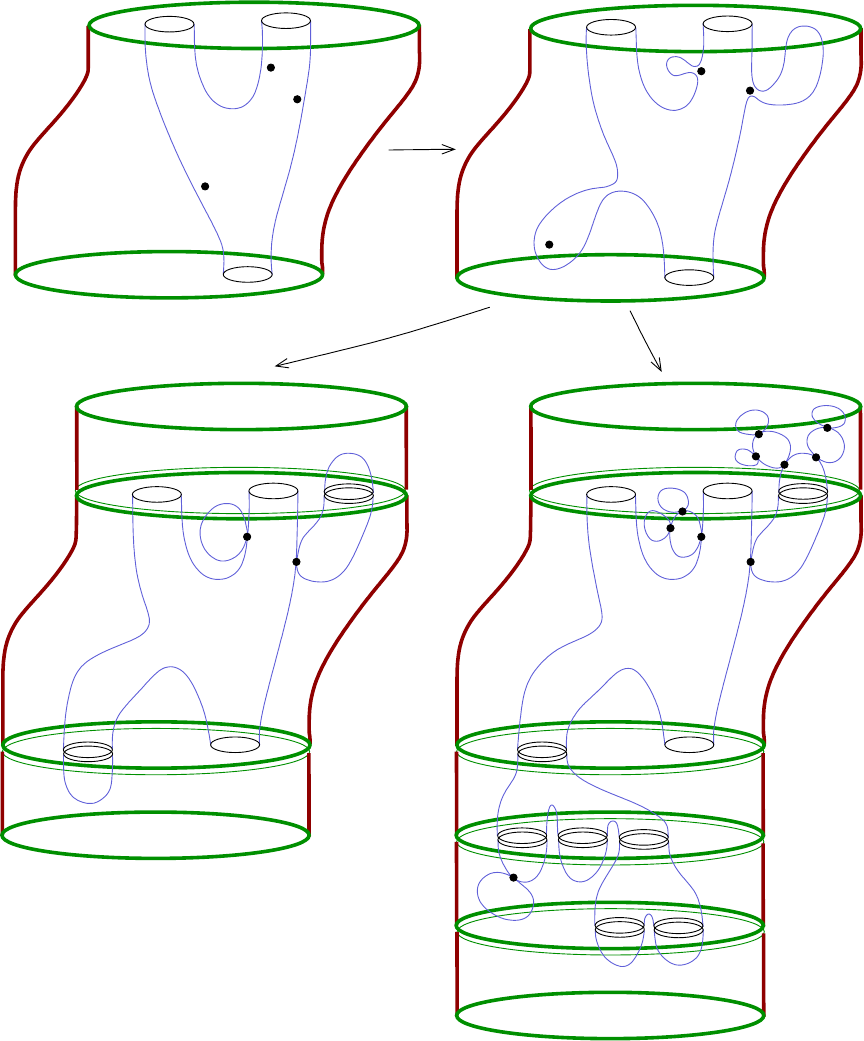
Lectures on Symplectic Field Theory 173
c
W
c
W
c
W
R × M
+
R × M
−
R × M
−
R × M
−
ζ
1
ζ
1 ζ
1
ζ
1
ζ
2
ζ
2
ζ
2
ζ
2
ζ
3
ζ
3
ζ
3
ζ
3
u
k
u
k
u
∞
u
∞
v
1
∞
v
3
∞
Figure 9.2. Two possible pictures of spheres and/or planes that
can bubble off when the first derivative blows up near three points.
holomorphic cylindrical coordinates (s, t) ∈ (−∞, 0] × S
1
⊂
˙
Σ near the negative
puncture of u
k
and find a sequence s
k
→ ∞ such that the sequence of half-cylinders
(−∞, s
k
] × S
1
→
c
W : (s, t) 7→ u
k
(s − s
k
, t)
174 Chris Wendl
is uniformly C
1
-bounded and thus converges in C
∞
lo c
(R × S
1
) to a finite-energy J-
holomorphic cylinder v
−
: R × S
1
→
c
W . In the picture, v
−
turns out to have a
removable singularity at +∞ mapping to the same point as the removable singularity
of u
∞
, and it s negative puncture appro aches the same orbit as the negative puncture
of u
k
.
More complicated things can happen in general: the bot t om scenario in this same
figure shows a case where all three singularities of u
∞
are removable, thus it extends
to a closed curve, while at one of the positive cylindrical ends [0, ∞) × S
1
⊂
˙
Σ of
u
k
, we can find a sequence s
k
→ ∞ such that the half-cylinders
[−s
k
, ∞) × S
1
→
c
W : (s, t) 7→ u
k
(s + s
k
, t)
are uniformly C
1
-bounded and converge in C
∞
lo c
(R ×S
1
) to a J-holomorphic cylinder
v
1
+
: R × S
1
→
c
W with one removable singularity and one positive puncture. At
the other positive end, we can perform the same trick in two distinct ways for two
sequences s
k
→ ∞, one diverging faster than t he ot her: the result is a pair of J-
holomorphic cylinders v
2
+
, v
3
+
: R × S
1
→
c
W , the former with both singularities
removable (thus forming a holomorphic sphere in the picture), and the latter with
one removable singularity and one positive puncture.
It can get weirder. Remember that
c
W is also noncompact!
In each of the above scenarios, we tacitly assumed that all of the various se-
quences obtained by reparametrizing portions of u
k
were locally C
0
-bounded, thus
all of the limits were curves in
c
W . But it may also happen that some of these se-
quences are C
0
lo c
-bounded while others locally diverge toward {±∞} × M
±
; in fact,
two such sequences that both diverge toward, say, {+∞}× M
+
, might even locally
diverge infinitely far f rom each other, meaning one of them approaches {+∞}×M
+
quantitatively faster than the ot her. This phenomenon leads to the notion of limiting
curves with multiple levels.
In Figure
9.4, we see a scenario in which u
k
satisfies the same conditions as above,
except that instead of u
k
(ζ
0
) b eing bounded, it diverges to {+∞} × M
+
. It follows
that after applying suitable R-translations, a subsequence converges in C
∞
lo c
(
˙
Σ) to a
J
+
-holomorphic curve
u
∞
:
˙
Σ → R × M
+
with finite energy. In the example, all three of its punctures are nonremovable, but
two of them approach orbits that have nothing to do with the asymptotic orbits
of u
k
. Now observe that since u
k
has a negative cylindrical end (−∞, 0] × S
1
⊂
˙
Σ,
one can necessarily find a sequence s
k
→ ∞ such that u
k
(−s
k
, 0) is bounded, and
the sequence of half-cylinders
(−∞, s
k
] × S
1
→
c
W : (s, t) 7→ u
k
(s − s
k
, t)
is then unifo rmly C
1
-bounded and thus has a subsequence convergent in C
∞
lo c
(R×S
1
)
to a finite-energy J-holomorphic cylinder v
0
: R × S
1
→
c
W . In the picture, v
0
has
both a positive and a negative puncture, but its negative end again approaches a
different Reeb orbit from the negative ends of u
k
, so one can deduce that there
must be still more happening near −∞: there exists another sequence s
′
k
→ ∞ with
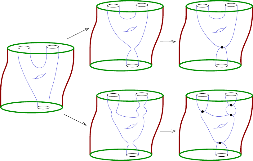
Lectures on Symplectic Field Theory 175
u
k
u
k
u
k
u
∞
u
∞
v
1
+
v
2
+
v
3
+
v
−
v
−
Figure 9.3. Even with fixed conformal structures on t he domains
and without bubbling, a sequence o f punctured holomorphic curves in
c
W can break to produce multiple curves in
c
W with extra removable
punctures. The picture shows two such scenarios.
s
′
k
−s
k
→ ∞ such that suitable R-translations of the half-cylinders
(−∞, s
k
] × S
1
→ (−∞, −r
0
] × M
−
: (s, t) 7→ u
k
(s −s
′
k
, t)
define uniformly C
1
-bounded maps into R×M
−
, giving a subsequence that converges
in C
∞
lo c
(R × S
1
) to a finite- energy J
−
-holomorphic cylinder
v
−
: R × S
1
→ R × M
−
.
Finally, the fact that u
∞
has a positive asymptotic or bit different from those of u
k
indicates that something more must also be happening near + ∞: in the example,
one of the positive ends [0, ∞) × S
1
⊂
˙
Σ admits a sequence s
k
→ ∞ such that
u
k
(s
k
, 0) ∈ {r
k
} × M
+
for some r
k
→ ∞, and suitable R-translations of
[−s
k
, ∞) ×S
1
→ [r
0
, ∞) × M
+
: (s, t) 7→ u
k
(s + s
k
, t)
become a uniformly C
1
-bounded sequence of half-cylinders in R × M
+
, with a sub-
sequence converging in C
∞
lo c
(R × S
1
) to a finite- energy J
+
-holomorphic cylinder
v
2
+
: R ×S
1
→ R ×M
+
that connects the errant asymptotic orbit of u
∞
to the corresponding orbit of u
k
. One
can now perform the same tr ick at the other positive end of
˙
Σ, as there necessarily
also exists a sequence s
′
k
→ ∞ in this end such that u
k
(s
′
k
, 0) ∈ {r
k
} × M
+
for
the same sequence r
k
→ ∞ as in the above discussion. The resulting limit curve
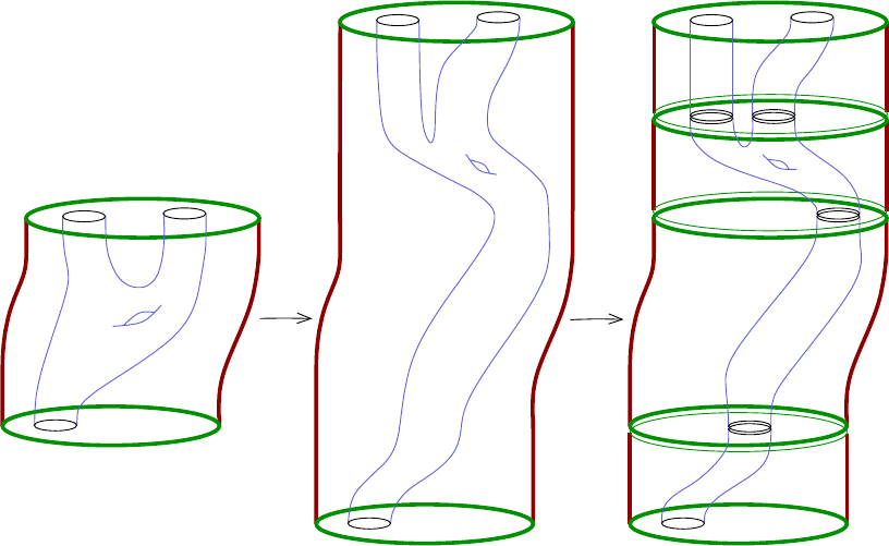
176 Chris Wendl
c
W
c
W
c
W
R × M
+
R × M
+
R × M
−
u
k
u
k
u
∞
v
1
+
v
2
+
v
0
v
−
Figure 9.4. Different portions o f a breaking sequence of curves may
also become infinitely far apar t in the limit, so that some live in
c
W
while others live in the symplectization of M
+
or M
−
.
v
1
+
: R ×S
1
→ R × M
+
however is not guaranteed to be interesting: in the picture,
it turns out to be a trivial cylinder.
The type of degeneration shown in Figure
9.4 happens whenever the sequence u
k
does interesting things in multiple regions of its domain that are sent increasingly
far away from each other in the image. The usual picture of
c
W that collapses
the cylindrical ends to a finite size therefore becomes increasingly inadequate for
visualizing u
k
as k → ∞: the middle picture in Figure
9.4 deals with this by
expanding the scale of the cylindrical ends so that the convergence to upper and
lower levels becomes visible.
9.3.3. The Deligne-Mumford space of Riemann surfaces. We next need
to relax the assumption that the Riemann surfaces (Σ
k
, j
k
, Γ
+
k
⊔Γ
−
k
⊔Θ
k
) are fixed.
Recall that for integers g ≥ 0 a nd ℓ ≥ 0, the moduli space of pointed Riemann
surfaces is the space of equivalence classes
M
g,ℓ
= {(Σ, j, Θ)}
∼,
where (Σ, j) is a closed connected Riemann surface of g enus g, Θ ⊂ Σ is an or-
dered set of ℓ distinct points, and (Σ, j, Θ) ∼ (Σ
′
, j
′
, Θ
′
) whenever there exists a
biholomorphic map ϕ : (Σ, j) → (Σ
′
, j
′
) taking Θ t o Θ
′
with the ordering preserved.
This space is fairly easy to understand in the finitely many cases with 2g + ℓ < 3,
e.g. M
0,ℓ
is a one-point space for each ℓ ≤ 3. We say that (Σ, j, Θ) is stable when-
ever χ(Σ \ Θ ) < 0, which means 2g + ℓ ≥ 3. In the stable case, one can show
that every pointed Riemann surface has a finite automorphism gro up, and M
g,ℓ
is a
Lectures on Symplectic Field Theory 177
smooth orbifold o f dimension 6g −6 + 2ℓ. It is generally not compact, but it admits
a natural compactification
M
g,ℓ
⊃ M
g,ℓ
,
known as the Deligne-Mumford c ompactification. We shall now give a sketch
of this construction from t he perspective of hyperbolic geometry; for more details,
see [Hum97, SS92].
We recall first the f ollowing standard result.
Theorem (Uniformization theorem). Every simp l y connected Riemann surface
is biholomorphically equivalent to either the Riemann sphere S
2
= C ∪ {∞}, the
co mplex plane C or the upper half plane H = {Im z > 0} ⊂ C.
The uniformization theorem implies that every Riemann surface can be presented
as a quotient of either ( S
2
, i), (C, i) or (H, i) by some f reely acting discrete group
of biholomorphic transformations. The only punctured surface
˙
Σ = Σ \ Θ that has
S
2
as its universal cover is S
2
itself. It is almost as easy to see which surfaces are
covered by C, as the only biholomorphic tr ansformations on (C, i) with no fixed
points are the translations, so every freely acting discrete subgroup of Aut(C, i) is
either trivial, a cyclic group of translations or a latt ice. The resulting quotients are,
respectively, (C, i), (R × S
1
, i)
∼
=
(C \ {0}, i) and the unpunctured tori (T
2
, j). All
stable pointed Riemann surfaces are thus quotients o f (H, i).
Proposition 9.19. There exists on (H, i) a compl e te Riemannian metric g
P
of
co nstant c urvature −1 that defines the same conformal structure as i and has the
pro perty that all conformal transformations on (H, i) are also i sometries of (H, g
P
).
Proof. We define g
P
at z = x + iy ∈ H by
g
P
=
1
y
2
g
E
,
where g
E
is the Euclidean metric. The conformal transformat ions on (H, i) are given
by fractional linear t ransformations
Aut(H, i) =
ϕ(z) =
az + b
cz + d
a, b, c, d ∈ R, ad − bc = 1
{±1}
= SL(2, R)/{±1} =: PSL(2, R),
and one can check that each of these defines an isometry with respect to g
P
. One
can also compute that g
P
has curvature −1, and the geodesics of g
P
are precisely
the lines and semicircles tha t meet R orthogona lly, parametrized so that they exist
for all forward and backward time, thus g
P
is complete. For more details on all o f
this, the book by Hummel [
Hum97] is highly recommended.
By lifting to universal covers, this implies the following.
Corollary 9.20. For every pointed Riemann surface (Σ, j, Θ) such that χ(Σ \
Θ) < 0, the punctured Riemann surface (Σ \ Θ, j) admits a complete Riemannian
metric g
j
of constant curvature −1 that defines the same conformal structure as j,
and has the property that all biholom o rphic transform ations on (Σ \ Θ, j) are also
isometries of (Σ \ Θ, g
j
).
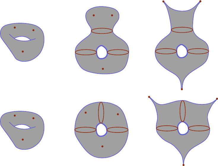
178 Chris Wendl
=
==
=
Figure 9.5. Two distinct pair-of-pants decomp ositions for t he same
genus 1 R iemann surface with three marked points. The decomposi-
tions are shown from two perspectives: the pictures at the right are
meant to give a more accurate impression of the Poincar´e metric,
which becomes singular and forms a cusp at each marked point .
The metric g
j
in this corollary is often called the Poincar´e metric . It is uniquely
determined by j.
Every class in π
1
(
˙
Σ) contains a unique geodesic for g
j
. Now suppose C ⊂
˙
Σ is a
union of disjoint embedded geodesics such tha t each connected component of
˙
Σ \C
has the homotopy type of a disk with two holes. The components are then called
singular pairs of pants, and the result is called a pair-of-pants decomposition
of (
˙
Σ, j). Two examples for the case g = 1 and ℓ = 3 are shown in Figure
9.5.
A pa ir -of-pants decomposition for (Σ, j, Θ ) gives rise to a local par ametrization
of M
g,ℓ
near [(Σ, j, Θ)], known as the Fenchel-Nielsen coordinates. These consist
of two parameters that can be associated to each of t he geodesics γ ⊂ Σ in the
decomposition, namely the length ℓ(γ) > 0 of the geodesic and a twist parameter
θ(γ) ∈ S
1
, which describes how the two neighboring pairs of pants are glued together
along γ. Note t hat by computing Euler characteristics, there a re always exactly
−χ(Σ \Θ) = 2g −2 + ℓ pairs of pants in a decomposition, so that the total number
of geodesics involved is [3(2g − 2 + ℓ) − ℓ] /2 = 3g −3 + ℓ, thus one can read off the
formula dim M
g,ℓ
= 6g − 6 + 2ℓ from this geometric picture.
One can also see the noncompactness of M
g,ℓ
in this picture quite concretely:
the twist parameters belong to a compact space, but each length parameter can

Lectures on Symplectic Field Theory 179
potentially shrink to 0 or blow up to ∞ as j (and hence g
j
) is deformed. It turns
out that the latter possibility is an illusion, but one may need to switch to a different
pair-of-pants decomposition to see why:
Theorem. For every pair of integers g ≥ 0 and ℓ ≥ 0 with 2g + ℓ ≥ 3, there
exists a constant C = C(g, ℓ) > 0 such that every [(Σ, j, Θ)] ∈ M
g,ℓ
admits a pair-
of-pants decomposition in which all geodesics bounding the pairs of pants have length
at most C.
This theorem implies that from a hyperbolic perspective, the only meaningful
way for stable pointed Riemann surfaces to degenerate is when some of the bounding
geodesics in a pair-of-pants decomposition shrink to length zero. Figure
9.6 shows
several examples of degenerate Riemann surfaces that can arise in this way for g = 1
and ℓ = 3, giving elements of the space that we will now define as
M
1,3
.
Definition 9.21. A nodal Riemann surface with ℓ ≥ 0 marked points and
N ≥ 0 nodes is a tuple (S, j, Θ , ∆) consisting of:
• A closed but not necessarily connected Riemann surface (S, j);
• An ordered set of ℓ points Θ ⊂ S;
• An unordered set of 2N points ∆ ⊂ S \ Θ equipped with an involution
σ : ∆ → ∆. Each pair {z, σ(z)} for z ∈ ∆ is referred to as a node.
Let
b
S denote the closed surface obtained by performing connected sums o n S at
each node {z
+
, z
−
} ⊂ ∆. We then say that (S, j, Θ, ∆) is connected if and only if
b
S is connected, and the genus of
b
S is called the arithmetic genus of (S, j, Θ, ∆).
We say that (S, j, Θ, ∆) is stable if every connected component of S \ (Θ ∪ ∆)
has negative Euler characteristic. Finally, two nodal Riemann surfaces (S, j, Θ, ∆)
and (S
′
, j
′
, Θ
′
, ∆
′
) are considered equivalent if there exists a biholomorphic map
ϕ : (S, j) → (S
′
, j
′
) taking Θ to Θ
′
with the ordering preserved and taking ∆ to ∆
′
such that nodes are mapped to nodes.
The nodes {z
+
, z
−
} ⊂ ∆ are typically represented in pictures as self-intersections
of S, cf. Figure
9.6. We can think of the stable nodal surfaces as precisely those
which admit (possibly singular) pair-of-pants decompositions. All noda l Riemann
surfaces we consider will be assumed connected in the sense defined above unless
otherwise noted; note that S itself can nonetheless be disconnected, as is the case
in f our out of the six nodal surfaces shown in Figure
9.6.
We now intr oduce some further terminology and notation that will be useful
in the next section as well. Whenever
˙
Σ = Σ \ Γ is obtained by puncturing a
Riemann surface (Σ, j) at finitely many points Γ ⊂ Σ, we shall define the circle
compactification
Σ :=
˙
Σ ∪
[
z∈Γ
δ
z
,
where f or each z ∈ Γ, the circle δ
z
is defined as a “ha lf-projectivization” of the
tangent space at z:
δ
z
:= (T
z
Σ \ {0})
.
R
∗
+
,
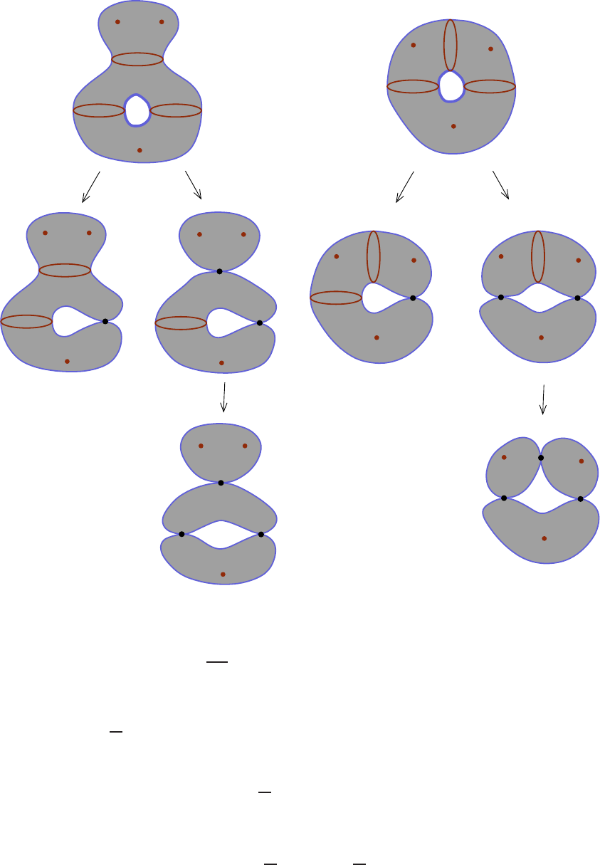
180 Chris Wendl
Figure 9.6. Starting from each of the pair-of-pants decompositions
for the g = 1 and ℓ = 3 case from Figure
9.5, shrinking geodesic
lengths to zero produces various examples of stable nodal Riemann
surfaces belonging to
M
1,3
.
with the positive real numbers R
∗
+
acting by scalar multiplication. To understand
the topology of
Σ, one can equivalently define it by choosing holomorphic cylindrical
coordinates [0, ∞) × S
1
⊂
˙
Σ near each z, and replacing the open half-cylinder with
[0, ∞] × S
1
, where δ
z
is now the circle at infinity {∞} × S
1
. There is no natural
choice of global smooth structure on
Σ, but it is homeomorphic to an oriented surface
with boundary and carries both smooth and conformal structures on its interior, due
to the obvious identification
˙
Σ =
Σ \
[
z∈Γ
δ
z
⊂ Σ.
Lectures on Symplectic Field Theory 181
The conformal structure of Σ at each z ∈ Γ does induce on each of the circles δ
z
an
orthogonal structure, meaning a preferred class of homeomorphisms to S
1
that
are all related to each other by rotations. One can therefore speak of ort hogonal
maps δ
z
→ δ
z
′
for z, z
′
∈ Γ , which ar e always homeomorphisms and can either
preserve or reverse orientation.
Now if (S, j, Θ, ∆) is a nodal R iemann surface, we let
˙
S = S \ ∆ and f orm the
circle compactification
S, which has the topology of a compact oriented surface with
boundary. Given a node {z
+
, z
−
} ⊂ ∆, a decoration for {z
+
, z
−
} is a choice of
orientation reversing orthogonal map
Φ : δ
z
+
→ δ
z
−
.
We say that (S, j, Θ, ∆) is a decorated nodal surface if it is equipped with a
choice of decoration Φ for every node, or partially decorated if Φ is defined for
some subset of the nodes. A partial decoration Φ gives rise to another compact
oriented surface
b
S
Φ
:=
S
∼,
where the equivalence relation identifies δ
z
+
with δ
z
−
via Φ for each decorated node
{z
+
, z
−
} ⊂ ∆. Note that if every node is decorated, then
b
S
Φ
has the topology of a
closed connected and oriented surface whose genus defines the arithmetic genus of
(S, j, Θ, ∆) according to Definition
9.21. We shall denote the collection of special
circles in
b
S
Φ
where boundray components δ
z
+
, δ
z
−
⊂ ∂
S have been ident ified by
C
Φ
⊂
b
S
Φ
.
Since
b
S
Φ
\ (∂
b
S
Φ
∪ C
Φ
) has a natural identification with
˙
S, it inherits smooth and
conformal structures which degenerate along C
Φ
and ∂
b
S
Φ
. We will say that two
partially decorated nodal Riemann surfaces (S, j, Θ, ∆, Φ) and (S
′
, j
′
, Θ
′
, ∆
′
, Φ
′
) are
equivalent if (S, j, Θ, ∆) and (S
′
, j
′
, Θ
′
, ∆
′
) are equivalent via a biholomorphic map
ϕ : (S, j) → (S
′
, j
′
) that extends continuously from
˙
S →
˙
S
′
to a homeomorphism
b
S
Φ
→
b
S
′
Φ
′
.
Now if 2g + ℓ ≥ 3, define
M
g,ℓ
as the set of equivalence classes of stable nodal
Riemann surfaces with ℓ marked points and arithmetic genus g. There is a natural
inclusion
M
g,ℓ
⊂
M
g,ℓ
by r egarding each pointed Riemann surface (Σ, j, Θ) as a nodal Riemann surface
(Σ, j, Θ, ∆) with ∆ = ∅. The most important property of
M
g,ℓ
is that it admits
the structure of a compact metrizable topological space for which the inclusion
M
g,ℓ
֒→
M
g,ℓ
is cont inuous onto an open subset. Rather than formulating all of
this in precise terms, let us state the main corollary that is important to know in
practice.
Theorem 9.22. Fix g ≥ 0 and ℓ ≥ 0 with 2g + ℓ ≥ 3. Then for any sequence
[(Σ
k
, j
k
, Θ
k
)] ∈ M
g,ℓ
, there exists a stable nodal Riemann surface [(S, j, Θ, ∆)] ∈
M
g,ℓ
such that a f ter restricting to a subsequence,
[(Σ
k
, j
k
, Θ
k
)] → [(S, j, Θ, ∆)]
182 Chris Wendl
in the follo wing sense: (S, j, Θ, ∆) admits a decoration Φ such that for sufficie ntly
large k, there are ho meomorphisms
ϕ :
b
S
Φ
→ Σ
k
,
smooth outside of C
Φ
, which map Θ to Θ
k
pre s erving the ordering and satisfy
ϕ
∗
j
k
→ j in C
∞
lo c
(
b
S
Φ
\ C
∆
).
As one mig ht gather from the above statement, one could just a s well define a
compact metrizable topology on the space of equivalence classes of decorated nodal
Riemann surfaces and then characterize the topology of
M
g,ℓ
via the natural pro-
jection that forgets the decorations.
Exercise 9.23. The space M
0,4
has a natural identification with S
2
\{0, 1, ∞},
defined by choosing the unique identification of any 4-pointed Riemann sphere
(S
2
, j, (z
1
, z
2
, z
3
, z
4
)) with C ∪ {∞} such that z
1
, z
2
, z
3
are identified with 0, 1, ∞
respectively, while z
4
is sent to some point in S
2
\{0, 1, ∞}. Show that this extends
continuously to an identification of
M
0,4
with S
2
. What do the t hree nodal curves
in
M
0,4
\ M
0,4
look like in terms of pair-of-pants decompositions?
9.4. The SFT compactness theorem
We now introduce the natural compactification of M
g,m
(J, A, γ
+
, γ
−
).
9.4.1. Nodal curves. A punctured J-holomorphic nodal curve in (
c
W , J)
with m ≥ 0 marked points consists of the data (S, j, Γ
+
, Γ
−
, Θ, ∆, u), where
• (S, j, Γ
+
⊔ Γ
−
⊔ Θ, ∆) is a nodal Riemann surface, with |Θ| = m;
• u : (
˙
S, j) → (
c
W , J) for
˙
S := S \ (Γ
+
∪ Γ
−
) is an asymptotically cylindrical
J-holomorphic map with p ositive punctures Γ
+
and negative punctures Γ
−
such that for each node {z
+
, z
−
} ⊂ ∆, u(z
+
) = u(z
−
).
Equivalence of two nodal curves
(S
0
, j
0
, Γ
+
0
, Γ
−
0
, Θ
0
, ∆
0
, u
0
) ∼ (S
1
, j
1
, Γ
+
1
, Γ
−
1
, Θ
1
, ∆
1
, u
1
)
is defined as the existence of an equivalence of nodal Riemann surfaces ϕ : (S
0
, j
0
, Γ
+
0
⊔
Γ
−
0
⊔ Θ
0
, ∆
0
) → (S
1
, j
1
, Γ
+
1
⊔ Γ
−
1
⊔ Θ
1
, ∆
1
) such that u
0
= u
1
◦ ϕ. We say that
(S, j, Γ
+
, Γ
−
, Θ, ∆, u) is connected if and only if the nodal Riemann surface (S, j, Γ
+
⊔
Γ
−
⊔Θ, ∆) is connected, and its arithmetic genus is then defined to be the arith-
metic genus of the latter. We say that (S, j, Γ
+
, Γ
−
, Θ, ∆, u) is stable if every con-
nected compo nent of S \(Γ
+
∪Γ
−
∪Θ ∪∆) on which u is constant has negative Euler
characteristic. Note that the underlying nodal Riemann surface (S, j, Γ
+
⊔Γ
−
⊔Θ, ∆)
need not be stable in general.
Nodal curves are sometimes also referred to as holomorphic buildings of hei ght 1.
These are the objects that form the Grom ov compactification of M
g,m
(J, A) when W
is a closed symplectic ma nif old. One can now roug hly imagine how the compactness
theorem in that setting is proved: given a converging sequence of almost complex
structures J
k
→ J and a sequence [( Σ
k
, j
k
, Θ
k
, u
k
)] ∈ M
g,m
(J
k
, A
k
) with unifo rmly
bounded energy, we can first add some auxiliary marked points if necessary to assume
that 2g +m ≥ 3. Now a subsequence of the domains [(Σ
k
, j
k
, Θ
k
)] ∈ M
g,m
converges

Lectures on Symplectic Field Theory 183
to an element of the Deligne-Mumford space [(S, j, Θ, ∆)] ∈ M
g,m
. Concretely,
this means that for large k, our sequence in M
g,m
(J
k
, A
k
) admits representatives
(Σ, j
′
k
, Θ, u
′
k
), with Σ a fixed surface with fixed marked points Θ ⊂ Σ, and (S, j, Θ, ∆)
admits decoratio ns Φ so t hat one can identify
b
S
Φ
with Σ and find
j
′
k
→ j in C
∞
lo c
(Σ \ C)
for some collection of disjoint circles C ⊂ Σ. The connected component s o f (Σ\C, j)
are then biholomorphically equivalent to t he connected components of (S \ ∆, j) ,
and if the newly reparametrized maps u
′
k
: Σ → W a r e uniformly C
1
lo c
-bounded o n
Σ \ C, then a subsequence converges in C
∞
lo c
(Σ \ C) to a limiting finite-energy J-
holomorphic map u
∞
: (S \∆, j) → (W, J), whose singularities a t ∆ are removable.
In particularly nice cases, this may be the end of the story, and our subsequence
of [(Σ
k
, j
k
, Θ
k
, u
k
)] ∈ M
g,m
(J
k
, A
k
) converges to the nodal curve [(S, j, Θ, ∆, u
∞
)];
in particular the domain [(S, j, Θ, ∆)] in this case is stable and is thus an element
of
M
g,m
. But more complicated things can also happen, e.g. u
′
k
might not be
C
1
-bounded, in which case there is bubbling. The bubbles that arise will be either
planes or spheres, so they produce extra doma in compo nents with nonnegative Euler
characteristic, but since they are never constant, the limiting noda l curve is still
considered stable. Similarly, since Σ\C is not compact, there can also be breaking as
in Figure
9.3, producing more non-stable domain components which can b e cylinders
in addition to planes and spheres—but again, the limiting map on these components
will never be constant.
9.4.2. Holomorphic buildings. Only a small subset o f the phenomena ob-
served in §
9.3 can be described via nodal curves: we’ve seen that in general, we also
have to allow “broken” curves with mult iple “levels”. This notion can be formalized
as f ollows.
Given integers g, m, N
+
, N
−
≥ 0, a holomorphic building of height N
−
|1|N
+
with ar it hmetic genus g and m marked points is a tuple
u = (S, j, Γ
+
, Γ
−
, Θ, ∆
nd
, ∆
br
, L, Φ, u),
with the va r ious data defined as follows:
• The domain (S, j, Γ
+
⊔Γ
−
⊔Θ, ∆
nd
⊔∆
br
) is a connected but not necessarily
stable nodal Riemann surface of arithmetic genus g, where |Θ| = m, and
the involution on ∆
nd
⊔∆
br
is assumed to preserve the subsets ∆
nd
and ∆
br
.
Matched pairs in these subsets are called the nodes and breaking pairs
respectively of u. The marked points of u are the point s in Θ, while Γ
+
and Γ
−
are its positive and negative punctures respectively.
• The level structure is a locally constant function
L : S → {−N
−
, . . . , −1, 0, 1 , . . . , N
+
}
that attains every value in {−N
−
, . . . , N
+
} except possibly 0, and satisfies:
(1) L(z
+
) = L(z
−
) for each node {z
+
, z
−
} ⊂ ∆
nd
;
(2) Each breaking pair {z
+
, z
−
} ⊂ ∆
br
can be la belled such that L(z
+
) −
L(z
−
) = 1;
(3) L(Γ
+
) = {N
+
} and L(Γ
−
) = {−N
−
}.
184 Chris Wendl
• The decoration is a choice of orientation- r eversing orthogonal map
δ
z
+
Φ
−→ δ
z
−
for each breaking pair {z
+
, z
−
} ⊂ ∆
br
.
• The map is an asymptotically cylindrical pseudoholomorphic curve
u : (
˙
S := S \ (Γ
+
∪ Γ
−
∪ ∆
br
), j) →
G
N∈{−N
−
,...,N
+
}
(
c
W
N
, J
N
),
where
(
c
W
N
, J
N
) :=
(R ×M
+
, J
+
) for N ∈ {1, . . . , N
+
},
(
c
W , J) for N = 0,
(R ×M
−
, J
−
) for N ∈ {−N
−
, . . . , −1},
and u sends
˙
S ∩ L
−1
(N) into
c
W
N
for each N, with positive punctures at
Γ
+
and negative punctures at Γ
−
. Moreover,
u(z
+
) = u(z
−
) for every node {z
+
, z
−
} ⊂ ∆
nd
,
and for each breaking pair {z
+
, z
−
} ⊂ ∆
br
labelled with L(z
+
)−L(z
−
) = 1,
u has a positive puncture at z
−
and a negative puncture at z
+
asymptotic
to the same orbit, such that if u
+
: δ
z
+
→ M
±
and u
−
: δ
z
−
→ M
±
denote
the induced asymptotic parametrizations of the orbit, then
u
+
= u
−
◦ Φ : δ
z
+
→ M
±
.
The following additional notation and terminology for the building u will be
useful to keep in mind. For each N ∈ {−N
−
, . . . , 0, . . . , N
+
}, denote
˙
S
N
:=
S \ (Γ
+
∪ Γ
−
∪ ∆
br
)
∩ L
−1
(N),
and denote the restriction of u to this subset by
u
N
:
˙
S
N
→
R × M
+
if N > 0,
c
W if N = 0,
R × M
−
if N < 0.
Including Θ ∩L
−1
(N) and ∆
nd
∩L
−1
(N) in the data defines u
N
as a (generally dis-
connected) nodal curve with mar ked points, whose positive punctures are in bijective
correspondence with the negative punctures of u
N+1
if N < N
+
. We call u
N
the
Nth level of u, and all it an upper or lower level if N > 0 or N < 0 respectively,
and the main level if N = 0. By convention, every holomorphic building in
c
W ha s
exactly one main level (which lives in
c
W itself) and arbitrary nonnegative numbers
of upper and lower levels (which live in the symplectizations R ×M
±
). One slightly
subtle detail is that it is possible for the main level to b e empty, meaning 0 is not in
the image of the level function L. The requirement that L should attain every o t her
value from −L
−
to L
+
is a convention to ensure tha t upper and lower levels are not
empty, so e.g. if a building has an empty main level and no lower levels, then the
lowest nonempty upper level is always labelled 1 instead of something arbitrary.
Lectures on Symplectic Field Theory 185
The p ositive punctures of the topmost level of u a r e Γ
+
, and the negative punc-
tures of the bottommost level are Γ
−
, so these give rise to lists of positive/negative
asymptotic orbits γ
±
= (γ
±
1
, . . . , γ
±
k
±
) in M
±
. There is also a relative homology class
[u] ∈ H
2
(W,
¯
γ
+
∪
¯
γ
−
).
To define this, recall from §
6.2 how it was defined for smooth curves u :
˙
Σ →
c
W : we
considered the retraction π :
c
W → W that collapses each cylindrical end to M
±
⊂
∂W , and noted that since u is asymptotically cylindrical, the map π ◦ u :
˙
Σ → W
extends to a continuous map on the circle compactification,
¯u :
Σ → W,
whose relative homology class gives the definition of [u]. The conditions on nodes
and breaking orbits allow us to perform a similar trick for the building u, using the
map
π :
G
N∈{−N
−
,...,N
+
}
c
W
N
→ W
which acts as the identity on W but collapses cylindrical ends of
c
W to ∂W and
similarly collapses each copy of R × M
±
to M
±
⊂ ∂W . Extending the decora-
tions Φ arbitrarily to decorations of the nodes ∆
nd
, one can then take the circle
compactification of
˙
S := S \ (Γ
+
∪ Γ
−
∪ ∆
nd
∪ ∆
br
) a nd glue matching b oundary
components together along Φ to form a compact surface with boundary
S
Φ
such
that π ◦ u :
˙
S → W extends to a continuous map
¯u :
S
Φ
→ W.
Its relative homology class defines [u] ∈ H
2
(W,
¯
γ
+
∪
¯
γ
−
).
We say that the building u is stable if two properties hold:
(1) Every connected component of S \(Γ
+
∪Γ
−
∪Θ ∪∆
nd
∪∆
br
) on which the
map u is constant has negative Euler characteristic;
(2) There is no N ∈ {−N
−
, . . . , N
+
} for which the Nth level consists entirely
of a disjoint union of tr ivial cylinders without any marked points or nodes.
An equivalence between two holomorphic buildings
u
i
= (S
i
, j
i
, Γ
+
i
, Γ
−
i
, Θ
i
, ∆
nd
i
, ∆
br
i
, L
i
, Φ
i
, u
i
), i = 0, 1
is defined as an equivalence of partially decorated nodal Riemann surfaces
(S
0
, j
0
, Γ
+
0
⊔ Γ
+
0
⊔ Θ
0
, ∆
nd
0
⊔ ∆
br
0
, Φ
0
)
ϕ
−→ (S
1
, j
1
, Γ
+
1
⊔ Γ
+
1
⊔ Θ
1
, ∆
nd
1
⊔ ∆
br
1
, Φ
1
)
such that ϕ(Γ
±
0
) = Γ
±
1
, ϕ(Θ
0
) = Θ
1
, ϕ(∆
nd
0
) = ∆
nd
1
, ϕ(∆
br
0
) = ∆
br
1
, L
1
◦ϕ = L
0
, and
u
0
1
◦ ϕ = u
0
0
,
while
u
N
1
◦ ϕ = u
N
0
up to R-translation f or each N 6= 0.
Given lists of or bits γ
±
and a relative homology class A, the set of equivalence
classes of stable holomorphic buildings in (
c
W , J) with arithmetic genus g and m
186 Chris Wendl
marked point s, positively/negatively asymptotic to γ
±
and homologous to A will be
denoted by
M
g,m
(J, A, γ
+
, γ
−
).
Observe that for any A 6= 0, there is a natural inclusion M
g,m
(J, A, γ
+
, γ
−
) ⊂
M
g,m
(J, A, γ
+
, γ
−
) defined by regarding J-holomorphic curves in M
g,m
(J, A, γ
+
, γ
−
)
as buildings with no upper or lower levels and no nodes. Such buildings are always
stable if A 6= 0 because they are not constant.
9.4.3. Convergence. For a general definition of the topology of
M
g,m
(J, A, γ
+
, γ
−
)
and the proof that it is bo th compact and metrizable, we refer to [
BEH
+
03] or the
more comprehensive treatment in [
Abb14]. The following statement contains all
the details about the topology that one usually needs to know in practice (see Fig-
ure
9.7).
Theorem 9.24. Fix integers g ≥ 0 and m ≥ 0, and a ssume all Reeb orbits in
(M, H
+
) and (M, H
−
) are nondegene rate. Then for any sequence
[(Σ
k
, j
k
, Γ
+
k
, Γ
−
k
, Θ
k
, u
k
)] ∈ M
g,m
(J
k
, A
k
, γ
+
, γ
−
)
of nonconstant J
k
-holomorphic curves in
c
W with uniformly bounded energy E(u
k
),
there exists a stable holomorphic building
[u
∞
] = [(S, j, Γ
+
, Γ
−
, Θ, ∆
nd
, ∆
br
, L, Φ, u
∞
)] ∈
M
g,m
(J, A, γ
+
, γ
−
)
such that after restricting to a subsequen ce, [(Σ
k
, j
k
, Γ
+
k
, Γ
−
k
, Θ
k
, u
k
)] → [u
∞
] in the
following sense. The decoration s Φ at ∆
br
ca n be extended to decoration s at ∆
nd
so that if
b
S
Φ
denotes the closed oriented topological 2-manifold o btained from S \
(∆
nd
∪ ∆
br
) by gluing circle compactifications along Φ, then for k sufficien tly large,
there exist h omeomorphisms
ϕ
k
:
b
S
Φ
→ Σ
k
that are smooth outside of C
Φ
, map Γ
+
⊔Γ
−
⊔Θ to Γ
+
k
⊔Γ
−
k
⊔Θ
k
with the ordering
pre s erved, and satisfy
ϕ
∗
k
j
k
→ j in C
∞
lo c
(
b
S
Φ
\ C
Φ
).
Moreover for N = {−N
−
, . . . , 0, . . . , N}, let
v
N
k
:= u
k
◦ ϕ
k
|
¨
S
N
:
¨
S
N
→
c
W ,
with
¨
S
N
:=
S \ (Γ
+
∪ Γ
−
∪ ∆
nd
∪ ∆
br
)
∩ L
−1
(N) regarded as a subset of
b
S
Φ
\ C
Φ
.
Then:
(1) v
0
k
→ u
N
∞
in C
∞
lo c
(
¨
S
N
,
c
W );
(2) For each ±N > 0, v
N
k
has image in the po sitive/negative cylin drical end for
all k sufficiently large, and there exists a seq uence r
N
k
→ ±∞ such that the
resulting R-translations converge:
τ
−r
N
k
◦ v
N
k
→ u
N
∞
in C
∞
lo c
(
¨
S
N
, R × M
±
).
Lectures on Symplectic Field Theory 187
The rates of divergence of the seq uences r
N
k
→ ±∞ are related by
r
N+1
k
− r
N
k
→ +∞ for all N < N
+
.
Finally, let
S
Φ
denote the co mpact topological surface with boundary defined as the
circle compactification of
b
S
Φ
\(Γ
+
∪Γ
−
), and let Σ
k
denote the circle compactification
of
˙
Σ
k
:= Σ
k
\ (Γ
+
k
∪ Γ
−
k
). Then for all k large, ϕ
k
extends to a continuous map
¯ϕ
k
:
S
Φ
→ Σ
k
such that
¯u
k
◦ ¯ϕ
k
→ ¯u
∞
in C
0
(
S
Φ
, W ).
Remark 9.25. The t heorem is also true under the more general hypothesis
that the Reeb vector fields are Morse-Bott. In this case, one can also allow the
asymptotic Reeb orbits of the sequence to vary, as long as the sum of their periods is
uniformly bounded—such a bound plays the role of an energy bound and g uarantees
a convergent subsequence of orbits via the Arzel`a-Ascoli theorem.
Remark 9.26. Stability of the limit in Theorem
9.24 is guaranteed for the same
reasons as in our discussion of Gromov compactness in §
9.4.1: stable domains de-
generate to stable nodal domains as geodesics in pair-of-pants decompositions shrink
to zero length, while bubbling and breaking produce additional domain components
that ar e not stable but on which the maps are never trivial. Moreover, stability guar-
antees the uniqueness of the limiting building for any convergent sequence, i.e. it is
the reason why
M
g,m
(J, A, γ
+
, γ
−
) is a Hausdorff space. Indeed, if u
k
converges to a
stable building u
∞
, then under the notion of convergence described in the theorem,
it will also converge to a building u
′
∞
constructed out of u
∞
by adding to S an extra
spherical component, att aching it to the rest by a single node and extending t he map
u
∞
to be constant on the extra component. One can also insert extra levels into
u
∞
that consist only of trivial cylinders, and u
k
will still converge to the resulting
building. But these modifications produce buildings that are not stable and thus
are not elements of M
g,m
(J, A, γ
+
, γ
−
).
9.4.4. Symplectizations, stretching and so forth. A few minor modifica-
tions to the above discussion are necessary t o compactify the moduli space of curves
in a symplectization (R×M, J) for J ∈ J(H). It is possible to view this as a special
case of a completed symplectic cobordism, but this perspective produces a certain
amount of extraneous data that is not meaningful. The key observation is that in
the presence of an R-action, one should really compactify M
g,m
(J, A, γ
+
, γ
−
)
R
instead of M
g,m
(J, A, γ
+
, γ
−
). The compactification
M
g,m
(J, A, γ
+
, γ
−
) then con-
sists of holomorphic buildings as defined in §
9.4.2, but since all levels live in the
same symplectization R × M, there is no longer a distinguished main level or any
meaningful notion of upper vs. lower levels; the level structure is simply a function
L : S → {1, . . . , N} for some N ∈ N, and equivalence of buildings must permit
R-translations within each level. Fo r these reasons, the SFT compactness theorem
in symplectizations has a few qualitative differences, but is still very much analogous
to Theorem
9.24.
188 Chris Wendl
c
W
c
W
R × M
+
R × M
−
R × M
−
R × M
−
M
+
M
−
Figure 9.7. Convergence to a building with arithmetic genus 2, one
upper level and t hree lower levels.
To complete the picture, we should mention one more type of compactness theo-
rem that appears in [
BEH
+
03], which is colloquially described as stretching the
neck. The geometric idea is as follows: suppose (W, ω) is a closed symplectic
manifold and M ⊂ W is a stable hypersurface that separates W into two pieces
W = W
−
∪
M
W
+
, with an induced stable Hamiltonian structure H = (ω, λ) that
orients M as the boundary of W
−
.
2
A neighborhood of M in (W, ω) can then be
identified symplectically with
(N
ǫ
, ω
ǫ
) := ( ( −ǫ, ǫ) × M, d(rλ) + ω)
for sufficiently small ǫ > 0. The idea now is to replace N
ǫ
with lar ger collars of the
form
((−T, T ) × M, d (f(r)λ) + ω) ,
with C
0
-small functions f chosen with f
′
> 0 so that the collar can be glued in
smoothly to replace (N
ǫ
, ω
ǫ
). This collar looks like a piece of the symplectization of
(M, H), thus we are free to choose tame almost complex structures whose restrictions
to the inserted collar belong t o J(H). Symplectic manifolds constructed in this
2
The assumption that M ⊂ W s eparates W is ine ssential, but makes certain details in this
discussion more conve nie nt.
Lectures on Symplectic Field Theory 189
way are all symplectomorphic, but their almost complex structures degenerate as
one takes T → ∞. Given a sequence T
k
→ ∞ and a corresponding degenerating
sequence J
k
, a sequence u
k
of J
k
-holomorphic curves with bounded energy converges
to yet another form of holo mo rphic building, this time involving a bottom level in
c
W
−
:= W
−
∪
M
([0, ∞) × M) with positive punctures approaching orbits in M, some
finite number of middle levels that live in the symplectization of M, and a top level
that lives in
c
W
+
:= ((−∞, 0] × M) ∪
M
W
+
with negative punctures approaching M.
A very po pula r example for applications arises from Lagrangian submanifolds
L ⊂ W . By the Weinstein neighborhood theorem, L always has a neighborhood
W
−
symplectomorphic to a neighborhood of the zero-section in T
∗
L, so M := ∂W
−
is a contact-type hypersurface conta cto morphic to the unit cotangent bundle of L.
Stretching the neck then yields T
∗
L as the completion of W
−
, and W \L as the com-
pletion of W
+
:= W \
˚
W
−
. This construction has often been used in order to study
Lagrangian submanifolds via SFT-type methods, see e.g. [
EGH00, Theorem 1.7.5]
and [
Eva10, CM].

LECTURE 10
Cylindrical contact homology and the tight 3-tori
Contents
10.1. Contact structures on T
3
and Giroux torsion 191
10.2. Definition of cylindrical contact homology 194
10.2.1. Preliminary remarks 194
10.2.2. A compactness result for cylinders 197
10.2.3. The chain complex 202
10.2.4. The homology 202
10.2.5. Chain maps 204
10.2.6. Chain homotopies 205
10.2.7. Proof of invariance 206
10.3. Computing HC
∗
(T
3
, ξ
k
) 208
10.3.1. The Morse-Bott setup 208
10.3.2. A digression on the Floer equation 210
10.3.3. Admissible data for (T
3
, ξ
k
) 219
We’ve now developed enough of the technical machinery of holomorphic curves
to be able to give a rigor ous construction of t he most basic version of SFT and apply
it to a problem in contact t opology.
10.1. Contact str uctures on T
3
and Giroux torsion
As a motivating goal in this lecture, we will prove a result about the classification
of contact structures on T
3
= S
1
× S
1
× S
1
. Denote the three global coordinates
on T
3
valued in S
1
= R/Z by (ρ, φ, θ), and for any k ∈ N, consider t he contact
structure
ξ
k
:= ker α
k
, where α
k
:= cos ( 2πkρ) dθ + sin(2πkρ) dφ.
It is an easy exercise to verify tha t these all satisfy the contact condition α
k
∧dα
k
> 0;
see Figure
10.1 f or a visual representation. The following result is originally due to
Giroux [
Gir94] and Kanda [Kan97].
Theorem 10.1. For each pair of positive integers k 6= ℓ, the contact manifolds
(T
3
, ξ
k
) and (T
3
, ξ
ℓ
) are not con tactomorphic.
One of the reasons this result is interesting is that it cannot be proved using
any so-called “classical” invariants, i.e. invariants coming from algebraic topology.
An example of a classical invar iant would be the Euler class of the oriented vector
bundle ξ
k
→ T
3
, or anything else that depends only on the isomorphism class of this
191
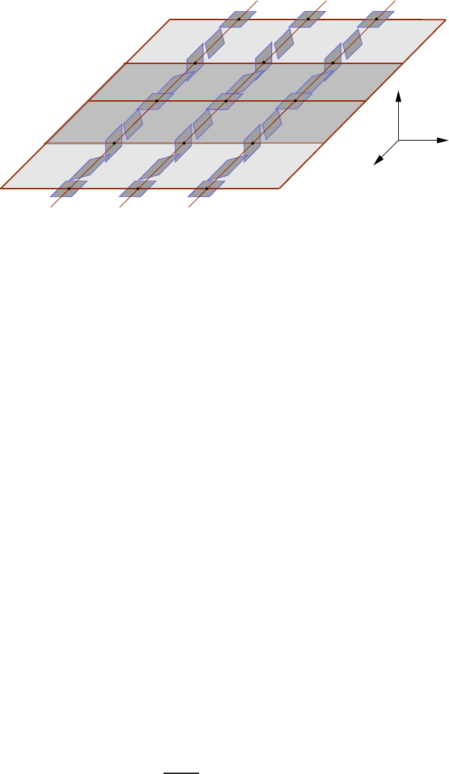
192 Chris Wendl
ρ
φ
θ
Figure 10.1. The contact structures ξ
k
on T
3
can be constructed
by gluing k copies of t he same model [0, 1]×T
2
to each other cyclically.
bundle. The following observation shows that such invariants will never distinguish
ξ
k
from ξ
ℓ
.
Proposition 10.2. For e very k, ℓ ∈ N, ξ
k
and ξ
ℓ
are homotopic through a
smooth family of oriented 2-plan e fields on T
3
.
Proof. In f act, all the ξ
k
can be deformed smoothly t o ker dρ, via the homotopy
ker [(1 − s) α
k
+ s dρ] , s ∈ [0, 1].
Remark 10.3. One can check in fact that the 1-form in the homotopy given
above is cont act for every s ∈ [0, 1 ) , so Gray’s stability theorem implies that every
ξ
k
is isotopic to an arbitrarily small perturbat ion of the foliation ker dρ. In [
Gir94],
Giroux used this observation to show that all of them are what we now call weakly
symplectica lly fillab l e. If ker dρ were also contact, then Gray’s theorem would imply
that ξ
k
and ξ
ℓ
are always isotopic. Thus Theorem
10.1 indicates the impo ssibility
of modifying a homotopy from ξ
k
to ξ
ℓ
into o ne that passes only through contact
structures.
Let us place this discussion in a larger context. Using the coordinates (ρ, φ, θ)
on R × T
2
, a pair of smooth functions f, g : R → R gives rise to a contact form
α = f(ρ) dθ + g(ρ) dφ
whenever the function D(ρ) := f (ρ)g
′
(ρ) −f
′
(ρ)g(ρ) is everywhere positive. Indeed,
we have α ∧dα = D(ρ) dρ ∧dφ ∧dθ, and one easily derives a similar formula for the
Reeb vector field,
R
α
=
1
D(ρ)
[g
′
(ρ) ∂
θ
− f
′
(ρ) ∂
φ
] .
The condition D > 0 means geometrically that the path (f, g) : R → R
2
winds
counterclockwise around the origin with its angular coordinate strictly increasing.
The simplest special case is the contact form
α
GT
:= cos ( 2πρ) dθ + sin(2πρ) dφ,
Lectures on Symplectic Field Theory 193
which matches the formula for α
1
on T
3
given above. Let ξ
GT
:= ker α
GT
on R ×T
2
.
Definition 10.4. The Giroux torsion GT(M, ξ) ∈ N ∪ {0, ∞} of a contact
3-manifold (M, ξ) is the supremum of the set of positive int egers k such that there
exists a contact embedding
[0, k] × T
2
, ξ
GT
֒→ (M, ξ).
We write GT(M, ξ) = 0 if no such embedding exists for any k, and GT(M, ξ) = ∞
if it exists for all k.
Example 10.5. The tori (T
3
, ξ
k
) for k ≥ Z a r e contactomorphic to (R×T
2
, ξ
GT
)/kZ,
with kZ acting by translation o f the ρ-coordinate. Thus GT(T
3
, ξ
k
) ≥ k −1.
A 2-torus T ⊂ (M, ξ) embedded in a contact 3-manifold is called pre-Lagrangian
if a neighborhood of T in (M, ξ) admits a contactomo r phism to a neighborhood of
{0}×T
2
in (R ×T
2
, ξ
GT
), identifying T with {0}×T
2
. The neighborhood in R ×T
2
can be arbitrarily small, thus the existence of a pre-Lagrangian torus does not imply
GT(M, ξ) > 0; in fact, pre-Lagrangian tori always exist in abundance, e.g. as bound-
aries of neighborhoods of transverse knots (using the contact model provided by the
transverse neighborhood theorem). But given any pre-Lagrangian torus T ⊂ ( M, ξ),
one can make a local modification of ξ near T to produce a new contact structure (up
to isotopy) with positive Giroux torsion. Define (M
′
, ξ
′
) f r om (M, ξ) by replacing
the small neighborhood ((−ǫ, ǫ) ×T
2
, ξ
GT
) with ((−ǫ, 1 + ǫ) ×T
2
, ξ
GT
), then identify
M
′
with M by a choice of compactly supported diffeomorphism (−ǫ, 1+ǫ) → (−ǫ, ǫ).
There is now an obvious contact embedding of ([0, 1] × T
2
, ξ
GT
) into (M, ξ
′
), hence
GT(M, ξ
′
) ≥ 1. Moreover, one can adapt the proof o f Prop.
10.2 above to show
that ξ
′
is homotopic to ξ through a smooth family of or iented 2-plane fields. The
operation changing ξ to ξ
′
is known as a Lutz twist along T . In this language, we
see that for each k ∈ N, (T
3
, ξ
k+1
) is obtained from (T
3
, ξ
k
) by performing a Lutz
twist along {0}× T
2
.
The invariant GT(M, ξ) is easy to define, but hard to compute in general. The
natural guess,
GT(T
3
, ξ
k
) = k − 1,
turns out to be correct, as was shown in [
Gir00], so this is one way to prove
Theorem
10.1, but not the approach we will take. The following example shows
that one must in any case be careful with such guesses.
Example 10.6. For each k ∈ N, define a model o f S
1
× S
2
by
S
1
×S
2
∼
=
[0, k + 1/2] ×T
2
∼
where the equivalence relation identifies (ρ, φ, θ) ∼ (ρ, φ
′
, θ) for ρ ∈ {0, k + 1/2} and
every θ, φ, φ
′
∈ S
1
. Near ρ = 0 and ρ = k+1/2, this means thinking of (ρ, φ) as polar
coordinates, so the two subsets {ρ = 0} and {ρ = k + 1/2} become circles of the
form S
1
×{const} embedded in S
1
×S
2
. Since the φ-coordina t e is singular at these
two circles, the contact fo r m α
GT
needs to be modified slightly in this region before
it will descend to a smooth contact form on S
1
×S
2
: this can be done by a C
0
-small
194 Chris Wendl
modification of the form f(ρ) dθ + g(ρ) dφ, and the resulting contact structure is
then uniquely determined up t o isotopy. We shall call this contact manifold
(S
1
× S
2
, ξ
k
).
Now observe that for each k ∈ N, (S
1
× S
2
, ξ
k+1
) is obtained from (S
1
× S
2
, ξ
k
) by
a Lutz twist. However, both contact manifolds are also over twisted: recall that a
contact 3-manifold (M, ξ) is overtwisted whenever it contains an embedded closed
2-disk D ⊂ M such that T ( ∂D) ⊂ ξ but T D|
∂D
⋔ ξ. (Exercise: find a disk with this
property in (S
1
× S
2
, ξ
k
)!) Eliashberg’s flexibility theorem for overtwisted contact
structures [
Eli89] implies that whenever ξ and ξ
′
are two contact structures on a
closed 3-manifold that a re both overtwisted and are homotopic as oriented 2 -plane
fields, t hey are actually isotopic. As a consequence, the contact structures ξ
k
on
S
1
×S
2
defined above for every k ∈ N are all isotopic to each other. As tends to be
the case with most interesting h-principles, the isotopy is very hard to see concretely,
but it must exist.
Exercise 10.7. Show that if (M, ξ) is a closed overtwisted contact 3-manifold,
then G T(M, ξ) = ∞.
In contrast to the S
1
×S
2
example ab ove, the contact manifolds (T
3
, ξ
k
) are not
overtwisted, they are tight—in fact, the classification of contact structures on T
3
by Giroux [
Gir94, Gir99, Gir00] and K anda [Kan97] states that these are all of
the tight contact structures on T
3
up to contactomorphism. We will use cylindrical
contact homology to show that they are not contactomorphic to each other. The
reader should keep Example 10.6 in mind and try to spot the reason why the same
argument cannot work for (S
1
× S
2
, ξ
k
).
Remark 10.8. It has b een conjectured that the converse of Exercise
10.7 mig ht
also hold, so every closed tight contact 3-manifold would have finite Giroux torsion.
This conj ecture is wide open.
10.2. Definition of cylindrical contact homology
10.2.1. Preliminary remarks. Cylindrical contact homology is the natural
“first attempt” at using holomorphic curves in symplectizations to define a Floer-
type invariant of contact manifolds (M, ξ). The idea is to define a cha in complex
generated by Reeb orbits in M and a differential ∂ that counts holomor phic cylinders
in R × M. We already know some pretty good reasons why this idea cannot work
in general: in order to prove ∂
2
= 0, we need to be a ble to identify the space of
rigid “broken” holomorphic cylinders (these a r e what is counted by ∂
2
) with the
boundary of the compactified 1-dimensional space of index 2 cylinders (up to R-
translation). But this compactified boundary has more than just broken cylinders
in it, see Figure
10.2. In order to define cylindrical contact homology, one must
therefore restrict to situations in which complicated pictures like Fig ur e
10.2 cannot
occur. The first useful remark in this direction is that since we are working with
a stable Hamiltonian structure o f t he form (dα, α) for a contact form α, a certain
subset of the scenarios allowed by the SFT compactness theorem can be excluded
immediately. Indeed:
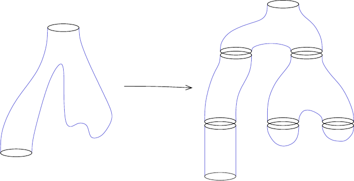
Lectures on Symplectic Field Theory 195
Figure 10.2. A family of holomorphic cylinders can converge in
the SFT topology to buildings that include more complicated curves
than cylinders—this is why cylindrical contact homolo gy is not well
defined for all contact manifolds.
Proposition 10 .9. If J ∈ J(α) and u : (
˙
Σ, j) → (R×M, J) is an asymptotically
cylindrical J-holomorphic curve, then u h as at least one positive puncture.
Let us give two proofs of this result, since both contain useful ideas. As prepara-
tion for the first proof, recall the definition of energy for curves in symplectizations
of contact manifolds that we wrote down in Lecture
1:
E(u) := sup
f∈T
Z
˙
Σ
u
∗
d(e
f(r)
α),
where
T :=
f ∈ C
∞
(R, (−1, 1))
f
′
> 0
.
This formula is not identical to the definition of energy used in Lecture
9, but it
is equivalent in the sense that any uniform bounds on one imply similar unifo r m
bounds on the other.
First proof of Proposition
10.9. Denote the positive and negative punc-
tures of u :
˙
Σ → R × M by Γ
+
and Γ
−
respectively, and suppose u is asymptotic
at z ∈ Γ
±
to the orbit γ
z
with period T
z
> 0. Choose any f ∈ T and denote
f
±
:= lim
r→±∞
f(r) ∈ [−1, 1]. Since d(e
f(r)
α) tames J ∈ J(α), Stokes’ theorem
gives
(10.1) 0 ≤ E(u) = e
f
+
X
z∈Γ
+
T
z
− e
f
−
X
z∈Γ
−
T
z
,
hence Γ
+
cannot be empty.
Remark 10.10. The proof via Stokes’ theorem works just as well if instead of
R × M, u lives in the completion of an exact symplectic cobordism (W, ω) with
concave boundary (M
−
, ξ
−
= ker α
−
) and convex boundary (M
+
, ξ
+
= ker α
+
).
196 Chris Wendl
Recall that this means ∂W = −M
−
⊔ M
+
, and ω = dλ for a 1-form λ that restricts
to positive conta ct forms λ|
T M
±
= α
±
. As in Lecture
1, we will write
J(W, ω, α
+
, α
−
) ⊂ J(
c
W )
for the space of almost complex structures J on
c
W := ((−∞, 0] × M
−
) ∪
M
−
W ∪
M
+
([0, ∞) × M
+
) that a re compatible with ω on W and belong to J(α
±
) on the cylin-
drical ends. The energy o f a J-ho lomorphic curve u : (
˙
Σ, j) → (
c
W , J) is then
E(u) := sup
f∈T
Z
˙
Σ
u
∗
dλ
f
,
where T := {f ∈ C
∞
(R, (−1, 1)) | f
′
> 0 and f(r) = r near r = 0} and
λ
f
:=
e
f(r)
α
+
on [0, ∞) × M
+
,
λ on W ,
e
f(r)
α
−
on (−∞, 0] ×M
−
.
The above proof now generalizes verbatim to show that u must always have a positive
puncture. Notice that in both settings, the argument also gives a unifor m bound
for the energy in terms of the periods of the positive asymptotic orbits.
Remark 10.11. We can also prove Pro p.
10.9 using the fact that u
∗
dα ≥ 0 for
any u : (
˙
Σ, j) → (R × M, J) with J ∈ J(α). Indeed, Stokes’ theorem then gives
(10.2) 0 ≤
Z
˙
Σ
u
∗
dα =
X
z∈Γ
+
T
z
−
X
z∈Γ
−
T
z
.
The quantity
R
˙
Σ
u
∗
dα is sometimes called the contact area of u. This version of
the argument however does not easily generalize to arbit r ary exact cobordisms.
The second proof is based on the maximum principle for subharmonic functions.
Proposition 10.12. Suppose J ∈ J(α) and u = (u
R
, u
M
) : (
˙
Σ, j) → (R ×M, J)
is J-holomorphic , where
˙
Σ has no bo und ary. Then u
R
:
˙
Σ → R has no local maxima.
Proof. In any local holomorphic coordinates (s, t) on a region in
˙
Σ, the non-
linear Cauchy-Riemann equation for u is equivalent to the system of equations
∂
s
u
R
− α(∂
t
u
M
) = 0,
∂
t
u
R
+ α(∂
s
u
M
) = 0,
π
ξ
∂
s
u
M
+ Jπ
ξ
∂
t
u
M
= 0,
where π
ξ
: T M → ξ denotes the projection along the Reeb vector field. This gives
−∆u
R
= −∂
2
s
u
R
−∂
2
t
u
R
= −∂
s
[α(∂
t
u
M
)] + ∂
t
[α(∂
s
u
M
)]
= −dα(∂
s
u
M
, ∂
t
u
M
) = −dα(π
ξ
∂
s
u
M
, Jπ
ξ
∂
s
u
M
) ≤ 0
since J|
ξ
is tamed by dα|
ξ
, hence u
R
is subharmonic. The result thus follows from
the maximum principle, see e.g. [
Eva98].

Lectures on Symplectic Field Theory 197
Second proof of Proposition
10.9. If u = (u
R
, u
M
) :
˙
Σ → R × M ha s
no p ositive puncture then u
R
:
˙
Σ → R is a proper function bounded above, and
therefore has a local maximum, contradicting Proposition
10.12.
Remark 10.13. The proof via the maximum principle does not generalize to
arbitrary exact cobordisms (W, dλ), but it does work in Stein cobordisms, i.e. if λ
f
and J are related by λ
f
= −dF ◦J for some plurisubharmonic function F :
c
W → R,
then F ◦ u :
˙
Σ → R is subharmonic (cf. [
CE12]).
With these preliminaries understo od, the next two exercises reveal one natural
setting in which breaking of cylinders can be kept under control. Both exercises are
essentially combina torial.
Exercise 10.14. Suppose u is a stable J-holomorphic building in a completed
symplectic cobordism
c
W with the following properties:
(1) u has arithmetic genus 0 and exactly one positive puncture;
(2) every connected component of u has at least one positive puncture.
Show that u has no nodes, and all of its connected component s have exa ctly one
positive puncture.
Exercise 10.15. Suppose tha t in addition t o the conditions of Exercise
10.14,
u has exactly one negative puncture a nd no connected component of u is a plane.
Show that every level of u then consists of a single cylinder with one positive and
one negat ive end.
Exercise
10.15 makes it reasonable to define a Floer-type theory counting only
cylinders in any setting where planes can be excluded, for instance because the Reeb
vector field has no contractible orbits. This is not always possible, e.g. Hof er [
Hof93]
proved that on overtwisted contact manifolds, there is always a plane (which is why
the Weinstein conjecture holds). So the invariant we construct will not be defined
in such settings, but it happens to be ideally suited to the study of (T
3
, ξ
k
).
10.2.2. A compactness result for cylinders. Fix a closed contact manifold
(M, ξ) of dimension 2n −1 and a primitive homot opy class of loops h ∈ [S
1
, M]. By
primitive, we mean that h is not equal to Nh
′
for any h
′
∈ [S
1
, M] and an integer
N > 1, and this assumption will be crucial for technical reasons in the following.
1
Given a contact form α fo r ξ, let
P
h
(α)
denote the set of closed Reeb orbits homotopic to h, where two Reeb o rbits are
identified if they differ only by parametrization.
Definition 10.16. Given a cont act manifold (M, ξ) and a primitive homotopy
class h ∈ [S
1
, M], we will say that a contact form α for ξ is h-admissible if:
(1) All orbits in P
h
(α) are nondegenerate;
1
It is to be expec ted that cylindrical contact homology can be defined also for non-primitive
homotopy clas ses, but this would require more sophisticated metho ds to address transversality
problems. The assumption that h is primitive allows us to assume that all holomorphic curves in
the discussion are somewhere injective, hence they ar e always regular if J is generic.
198 Chris Wendl
(2) There are no contractible closed Reeb orbits.
Similarly, we will say that (M, ξ) is h-admissible if a conta ct form with the above
properties exists.
Definition 10.17. Given h ∈ [S
1
, M] and an h-admissible contact form α on
(M, ξ), we will say that an almost complex structure J ∈ J(α) is h-regular if every
J-holomorphic cylinder in R×M with a positive and a nega t ive end both asymptotic
to orbits in P
h
(α) is Fredholm regula r .
Proposition 10.18. If h ∈ [S
1
, M] is a primitive homotopy clas s of loops and
α is h-admissible on (M, ξ), then the space of h-regular almo s t complex structures
is comeager in J(α).
Proof. Since h is primitive, the asymptotic orbits for t he relevant holomorphic
cylinders cannot be multiply covered, hence all of these cylinders are somewhere
injective. The result therefore follows from the standard transversality results proved
in L ecture
8 for somewhere injective curves in symplectizations.
Proposition 10.19. Given an h-admissibl e contact form α, an h-regular almos t
co mplex structure J ∈ J( α) and an orbit γ ∈ P
h
(α), suppose u
k
is a sequence of
J-holomorphic cylinders in R ×M w i th one positive puncture at γ and o ne negative
puncture. Then u
k
has a subseq uence convergent in the SFT topology to a broken
J-holomorphic cylinder, i.e. a stable building u
∞
whose levels u
1
∞
, . . . , u
N
+
∞
are each
cylinders with one positive and one negative puncture. Moreover, each level satisfies
ind(u
N
∞
) ≥ 1, thus for large k in the convergent subsequence,
ind(u
k
) =
N
+
X
N=1
ind(u
N
∞
) ≥ N
+
.
Proof. Let’s start with some ba d news: the standard SFT compactness the-
orem is not applicable in this situation, because we have not assumed that α is
nondegenerate, nor even Morse Bott—there is no a ssumption at all about Reeb or-
bits in homotopy classes o t her than h and 0. This fa ir ly loose set of hypotheses is
very convenient in applications, as nondegeneracy of a contact form is generally a
quite difficult conditio n t o check. The price we pay is that we will have to prove
compactness manually instead of applying the big theorem (see Remark
10.20). For -
tunately, it is not that hard: the crucial point is tha t in the situation at hand, there
can be no bubbling at all.
Indeed, we claim that the given sequence u
k
: (R × S
1
, i) → (R × M, J) must
satisfy a uniform bound
|du
k
| ≤ C
with respect to any translation-invariant Riemannian metrics on R ×S
1
and R ×M.
To see this, note first that since a ll the u
k
have the same positive asymptotic orbit γ,
their energies are uniformly bounded via (
10.1). Thus if |du
k
(z
k
)| → ∞ for some
sequence z
k
∈ R × S
1
, we can perform the usual rescaling trick from Lecture
9 and
deduce the existence of a nonconstant finite-energy plane v
∞
: C → R × M. Its
singularity at ∞ cannot be removable since this would produce a nonconstant J-
holomorphic sphere, violating Proposition
10.9. It follows t hat v
∞
is asymptotic to a

Lectures on Symplectic Field Theory 199
Reeb or bit at ∞, but this is a lso impossible since α does not admit any contractible
orbits, and the claim is thus proved.
Suppose now that γ has period T
+
> 0, and observe that by nondegeneracy, the
set
P
h
(α, T
+
) :=
γ ∈ P
h
(α)
γ has period at most T
+
is finite. Let
A
h
(α), A
h
(α, T
+
) ⊂ (0, ∞)
denote the set of all periods of orbits in P
h
(α) and P
h
(α, T
+
) respectively. By
(
10.2), the negative asymptotic orbit of each u
k
is in P
h
(α, T
+
), so we can take a
subsequence and assume that these are all the same orbit; call it γ
−
∈ P
h
(α, T
+
)
and its period T
−
∈ A
h
(α, T
+
). If T
−
= T
+
then u
∗
k
dα ≡ 0 for all k, implying that
all u
k
are the trivial cylinder over γ and thus trivially converg e. Assume therefore
T
−
< T
+
. Then since u
∗
k
dα ≥ 0, Stokes’ theorem implies that for each k, the function
R → R : s 7→
Z
S
1
u
k
(s, ·)
∗
α
is increasing and is a surjective map onto (T
−
, T
+
). The uniform bound on the
derivatives implies that for a ny sequences s
k
, r
k
∈ R with u
k
(s
k
, 0) ∈ {r
k
}×M, the
sequence
2
v
k
: R × S
1
→ R × M : (s, t) 7→ τ
−r
k
◦ u
k
(s + s
k
, t)
has a subsequence convergent in C
∞
lo c
(R × S
1
) to some finite- energy J-holomorphic
cylinder
v
∞
: R × S
1
→ R × M,
which necessarily satisfies
Z
S
1
v
∞
(s, ·)
∗
α = lim
k→∞
Z
S
1
u
k
(s + s
k
, ·)
∗
α ∈ [T
−
, T
+
]
for every s ∈ R. This proves that v
∞
is nonconstant, with a positive puncture at
s = ∞ and negative puncture at s = −∞, and both of its asymptotic orbits are
in P
h
(α, T
+
).
3
If v
∞
is not a trivial cylinder, then it therefore satisfies
Z
R×S
1
v
∗
∞
dα ≥ δ,
where δ is any positive number less than t he smallest distance between neighboring
elements of A
h
(α, T
+
).
Let us call a sequence s
k
∈ R nontrivial whenever the limiting cylinder v
∞
obtained by the a bove procedure is no t a trivial cylinder, and call two such sequences
s
k
and s
′
k
co mpatible if s
k
−s
′
k
is not bounded. We claim now t hat if s
1
k
, . . . , s
m
k
is a
collection of nontrivial sequences that are all compatible with each other, then
m <
2(T
+
− T
−
)
δ
.
2
Recall from Lecture
9 that we deno te the R-translation action on R×M by τ
c
(r, x) := (r+c, x).
3
For an alternative argument that v
∞
must have a p ositive puncture at s = ∞ and negative
at s = −∞, see Figure
10.3.
200 Chris Wendl
Indeed, we can assume after ordering our collection appropriately and restricting
to a subsequence that s
N+1
k
− s
N
k
→ ∞ for each N = 1, . . . , m − 1, and let v
N
∞
:
R × S
1
→ R × M denote the limits of the corresponding convergent subsequences.
Then we can find R > 0 such that
Z
[−R,R]×S
1
(v
N
∞
)
∗
dα >
δ
2
and thus
Z
[s
N
k
−R,s
N
k
+R]×S
1
u
∗
k
dα >
δ
2
for each N = 1, . . . , m for sufficiently large k. But these domains are also all disjoint
for sufficiently large k, implying
T
+
−T
−
=
Z
R×S
1
u
∗
k
dα ≥
m
X
N=1
Z
[s
N
k
−R,s
N
k
+R]×S
1
u
∗
k
dα >
δm
2
.
We’ve shown that there exists a maximal collection of nontrivial sequences
s
1
k
, . . . , s
N
+
k
∈ R satisfying s
N+1
k
− s
N
k
→ ∞ for each N, such that if u
k
(s
N
k
, 0) ∈
{r
N
k
} ×M, then after restricting to a subsequence, the cylinders
v
N
k
(s, t) := τ
−r
N
k
◦ u
k
(s + s
N
k
, t)
each converge in C
∞
lo c
(R × S
1
) as k → ∞ to a nontrivial J-holomorphic cylinder
u
N
∞
: R × S
1
→ R × M. Let γ
±
N
denote the asymptotic orbit of u
N
∞
at s = ±∞. We
claim,
γ
+
N
= γ
−
N+1
for each N = 1 , . . . , N
+
− 1.
If γ
+
N
6= γ
−
N+1
for some N, choose a neighborhood U ⊂ M of the image of γ
+
N
that
does not intersect any other o r bit in P
h
(α, T
+
). Then since each u
k
is continuous,
there must exist a sequence s
′
k
∈ R with
s
′
k
−s
N
k
→ ∞ and s
N+1
k
−s
′
k
→ ∞
such that u
k
(s
′
k
, 0) lies in U for all k but stays a positive distance away from the
image of γ
+
N
. A subsequence of (s, t) 7→ u
k
(s + s
′
k
, t) then converges after suitable
R-translations to a cylinder u
′
∞
: R × S
1
→ R × M that cannot be trivial since
u
′
∞
(0, 0) is not contained in any orbit in P
h
(α, T
+
). This contradicts the assumption
that our collection s
1
k
, . . . , s
N
+
k
is maximal. A similar arg ument shows
γ
−
1
= γ
−
and γ
+
N
+
= γ,
so the curves u
1
∞
, . . . , u
N
+
∞
form the levels of a stable holomorphic building u
∞
. A
similar argument by contradiction also shows that the sequence u
k
must converge
in t he SFT topology to u
∞
.
Finally, note that since all the breaking orbits in u
∞
are homotopic to h a nd J
is h-r egular, the levels u
N
∞
are Fredholm regular. Since all of them also come in 1-
parameter families of distinct curves related by the R-action, this implies ind(u
N
∞
) ≥
1 for each N = 1, . . . , N
+
.
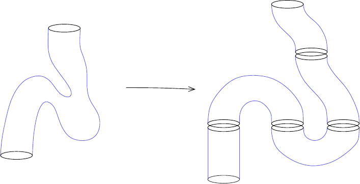
Lectures on Symplectic Field Theory 201
Figure 10.3. A degenerating sequence of holomorphic cylinders
u
k
: R ×S
1
→ R ×M cannot have a limiting level with a puncture of
the “wrong” sign unless u
k
violates the maximum principle for large k.
Remark 10.20. Nondegeneracy or Morse-Bott conditions are r equired fo r sev-
eral reasons in the proof of SFT compactness, and indeed, the theorem is not true
in general without some such assumption. One can see this by considering what
happens to a sequence u
k
of J
k
-holomorphic curves where J
k
→ J
∞
is compati-
ble with a sequence of nondegenerate contact forms α
k
converging to one that is
only Morse-Bott. A compactness theorem for this scenario is proved in [
Bou02],
but it requires more general limiting objects t han holomorphic buildings. On the
other hand, it is useful for certain kinds of applicatio ns to know when one can do
without nondegeneracy assumptions and prove compactness anyway. There ar e two
main advantages to knowing that all Reeb orbits are nondegenerate or belong to
Morse-Bott families:
(1) It implies t ha t the set o f all periods of closed orbits, the so-called action
spectrum of α, is a discrete subset of (0, ∞) ; in fact, for any T > 0, the
set of all periods less than T is finite. Using the relations (10 .1) and (10.2),
this implies lower bounds o n the possible energies of limiting components
and thus helps show t hat only finitely many such components can arise.
(2) Curves asymptotic to nondegenerate or Morse-Bott orbits also satisfy ex-
ponent ial convergence estimates proved in [
HWZ96, HWZ01, HW Z96,
Bou02], and similar asymptotic estimates yield a result about “long cylin-
ders with small area” (see [
HWZ02] and [BEH
+
03, Prop. 5.7]) which
helps in proving that neighboring levels connect to each other along break-
ing orbits.
Our situation in Proposition
10.19 was simple enough to avoid using the “long
cylinder” lemma, and we did use the discreteness of the actio n spectrum, but only
needed it f or orbits in P
h
(α) since we were able to rule out bubbling in the first
step. An alternative would have been to assume that all orbits (in all homotopy
classes) with period up to the period of γ a r e nondegenerate: then (
10.2) implies

202 Chris Wendl
that degenerate orbits never play any role in the main arguments of [BEH
+
03], so
the big theorem becomes saf e to use.
10.2.3. The chain complex. We now define a Z
2
-graded chain complex with
coefficients in Z
2
and generators hγi fo r γ ∈ P
h
(α), i.e.
CC
h
∗
(M, α) :=
M
γ∈P
h
(α)
Z
2
.
The degree of each generator hγi ∈ CC
h
∗
(M, α) is defined by
|hγi| = n − 3 + µ
CZ
(γ) ∈ Z
2
,
where µ
CZ
(γ) ∈ Z
2
denotes the pa r ity o f the Conley-Zehnder index with respect to
any choice of trivialization. The choice t o write n −3 in front of this is a convention
that will make no diff erence at all in this lecture, but it is consistent with a Z-
grading that we will be able to define under suitable assumptions in Lecture
12. To
define the differentia l on CC
h
∗
(M, α), choose an h-regular almost complex structure
J ∈ J(α). Given Reeb orbits γ
+
, γ
−
∈ P
h
(α) and a number I ∈ Z, let
M
I
(J, γ
+
, γ
−
)
denote the space of all R-equivalence classes of index I holomorphic cylinders in (R×
M, J) asymptotic to γ
±
at ±∞, i.e. the union of all components M
0,0
(J, A, γ
+
, γ
−
)/R
for which vir-dim M
0,0
(J, A, γ
+
, γ
−
) = I. Since J is h-regular, all the curves in
M
I
(J, γ
+
, γ
−
) are Fredholm regula r, so if I ≥ 1, M
I
(J, γ
+
, γ
−
) is a smooth mani-
fold with
dim M
I
(J, γ
+
, γ
−
) = I − 1.
Similarly, M
0
(J, γ
+
, γ
−
) only contains trivial cylinders and is thus empty unless
γ
+
= γ
−
, and M
I
(J, γ
+
, γ
−
) is always empty for I < 0. In particular, M
1
(J, γ
+
, γ
−
)
is a discrete set whenever γ
+
6= γ
−
, and by Proposition
10.19, it is also compact,
hence finite. We can therefore define
∂hγi =
X
γ
′
∈P
h
(α)
#
2
M
1
(J, γ, γ
′
)hγ
′
i,
where for any set X, we denote by #
2
X the cardinality of X modulo 2. The operator
∂ has odd degree with respect to the grading since every index 1 holo mo r phic cylinder
u with asymptotic orbits γ
+
and γ
−
satisfies
ind(u) = 1 = µ
τ
CZ
(γ
+
) − µ
τ
CZ
(γ
−
)
for suitable choices of the trivialization τ .
10.2.4. The homology. Following the standard Floer theoretic prescription,
the relation ∂
2
= 0 should arise by viewing the compactification
M
2
(J, γ
+
, γ
−
) for
each γ
+
, γ
−
∈ P
h
(α) as a compact 1 -manifold whose boundary is identified with the
set of rig id broken cylinders, as these are what is counted by ∂
2
. Here
M
2
(J, γ
+
, γ
−
)

Lectures on Symplectic Field Theory 203
is defined as the closure of M
2
(J, γ
+
, γ
−
) in the space of all J-holomorphic buildings
in R × M modulo R-t r anslation. Proposition
10.19 gives a natural inclusion
M
2
(J, γ
+
, γ
−
) \ M
2
(J, γ
+
, γ
−
) ⊂
G
γ
0
∈P
h
(α)
M
1
(J, γ
+
, γ
0
) × M
1
(J, γ
0
, γ
−
).
We therefore need an inclusion in the other direction, and for this we need to say
a word about gluing. We have not had time to discuss gluing in earnest in these
notes, and we will not do so now either, but the basic idea should be familiar from
Floer homology: given u
+
∈ M
1
(J, γ
+
, γ
0
) and u
−
∈ M
1
(J, γ
0
, γ
−
), one would
like to show that there exists a unique (up to R-translation) one-parameter family
{u
R
∈ M
2
(J, γ
+
, γ
−
)}
R∈[R
0
,∞)
such that u
R
converges as R → ∞ to the building
u
∞
with bottom level u
−
and top level u
+
. One starts by constructing a family of
preglued maps
˜u
R
: R ×S
1
→ R ×M,
meaning a smooth family of maps which converge in the SFT topology as R → ∞ to
u
∞
but are only approximately J-holomorphic. More precisely, fix parametrizations
of u
−
and u
+
and a parametrization of the orbit γ
0
: R/T Z → M such that
u
+
(s, t) = exp
(T s,γ
0
(T t))
h
+
(s, t) for s ≪ 0,
u
−
(s, t) = exp
(T s,γ
0
(T t))
h
−
(s, t) for s ≫ 0,
where h
±
are vector fields along the trivial cylinder satisfying lim
s→∓∞
h
±
(s, t) = 0.
By interpolat ing between suitable reparametrizations of h
+
and h
−
, one can now
define ˜u
R
such that
˜u
R
(s, t) = τ
2RT
◦ u
+
(s −2R, t) for s ≥ R,
˜u
R
(s, t) ≈ (T s, γ
0
(T t)) for s ∈ [−R, R],
˜u
R
(s, t) = τ
−2RT
◦ u
−
(s + 2R, t) for s ≤ −R,
¯
∂
J
˜u
R
→ 0 as R → ∞.
Given regularity of u
+
and u
−
, one can now use a quantita t ive version of the implicit
function t heorem (cf. [
MS04, §3.5]) to show that a distinguished J-holomorphic
cylinder u
R
close to ˜u
R
exists for all R sufficient ly large. For a more detailed synopsis
of the analysis involved, see [
Nel13, Chapter 7], and [AD14, Chapters 9 and 13]
for the analogous story in Floer homology. The result is:
Proposition 10.21. For an h-admissible α, an h-reg ular J ∈ J(α) and a ny two
orbits γ
+
, γ
−
∈ P
h
(α), the space
M
2
(J, γ
+
, γ
−
) admits the structure of a compact
1-dimensional manifol d with boundary, where its boundary points can be identified
naturall y with
F
γ
0
∈P
h
(α)
M
1
(J, γ
+
, γ
0
) × M
1
(J, γ
0
, γ
−
).
Corollary 10.22. The homomorphi sm ∂ : CC
h
∗
(M, α) → CC
h
∗−1
(M, α) satis-
fies ∂
2
= 0.
We shall denote the homology of this chain complex by
HC
h
∗
(M, α, J) := H
∗
CC
h
∗
(M, α), ∂
.

204 Chris Wendl
The goal of the rest of this section is to prove that up to natural isomorphisms,
HC
h
∗
(M, α, J) depends on (M, ξ) and h but no t on the auxiliary data α a nd J.
10.2.5. Chain maps. For any constant c > 0, there is an obvious bijection
between the generators of CC
h
∗
(M, α) and CC
h
∗
(M, cα), as t he rescaling changes
periods of orbits but not the set of closed orbits itself. Moreover, if J ∈ J(α) and
J
c
∈ J(cα) are defined to match on ξ, then there is a biholomorphic diffeomorphism
(R × M, J) → (R × M, J
c
) : (r, x) 7→ (cr, x),
thus giving a bijective correspondence between the moduli spaces of J-holomorphic
and J
c
-holomorphic curves. It follows that our bijection of chain complexes is also
a chain map and therefore defines a canonical isomorphism
(10.3) HC
h
∗
(M, α, J) = HC
h
∗
(M, cα, J
c
).
Next suppose α
−
and α
+
are two distinct contact f orms for ξ, hence
α
±
= e
f
±
α
for some fixed contact form α and a pair of smooth functions f
±
: M → R. After
rescaling α
+
by a constant, we are free to assume f
+
> f
−
everywhere. Fix h-regular
almost complex structures J
±
∈ J(α
±
) and let
∂
±
: CC
h
∗
(M, α
±
) → CC
h
∗−1
(M, α
±
)
denote the resulting differentials on the two chain complexes. The region
W :=
(r, x) ∈ R × M
f
−
(x) ≤ r ≤ f
+
(x)
now defines an exact symplectic cobordism from (M, ξ) to itself: more precisely,
setting
M
±
:=
(f
±
(x), x) ∈ W
x ∈ M
gives ∂W = −M
−
⊔ M
+
, and the Lio uville form λ := e
r
α satisfies λ|
T M
±
= α
±
.
Choose a generic dλ-compatible almost complex structure J on the completion
c
W
that restricts to J
±
on the cylindrical ends. Now given γ
+
∈ P
h
(α
+
) and γ
−
∈
P
h
(α
−
) and a number I ∈ Z, we shall denote by
M
I
(J, γ
+
, γ
−
)
the union of all components M
0,0
(J, A, γ
+
, γ
−
) that have virtual dimension I. Note
that we a r e not dividing by any R-action here since J need not be R-invariant.
Since γ
±
are still guaranteed to be simply covered, curves in M
I
(J, γ
+
, γ
−
) are
again a lways somewhere injective and therefore regular, hence M
I
(J, γ
+
, γ
−
) is a
smooth manifold with
dim M
I
(J, γ
+
, γ
−
) = I
if I ≥ 0, and M
I
(J, γ
+
, γ
−
) = ∅ for I < 0. The compactification
M
I
(J, γ
+
, γ
−
) is
described via the following straightforward generalization of Proposition 10.19:

Lectures on Symplectic Field Theory 205
Proposition 10.23. For J as described above, suppose u
k
is a sequence of J-
holomorphic cylinders in
c
W wi th one positive puncture at an orbit γ ∈ P
h
(α
+
) and
one negative puncture. Then u
k
has a subsequence con vergent in the SFT topology
to a broken J-holomorphic cylinder, i.e. a stable building u
∞
whose levels u
N
∞
for
N = −N
−
, . . . , −1, 0, 1 , . . . , N
+
are each c ylin d ers with one posi tive and one negative
puncture, livi ng in R × M
±
for ±N > 0 and
c
W for N = 0. Moreover, the levels
satisfy ind(u
0
∞
) ≥ 0 and ind(u
N
∞
) ≥ 1 for N 6= 0, thus for large k in the convergent
subsequence ,
ind(u
k
) =
N
+
X
N=−N
−
ind(u
N
∞
) ≥ N
−
+ N
+
.
It follows that the set M
0
(J, γ
+
, γ
−
) is always finite, and we use this t o define a
map
Φ
J
: CC
h
∗
(M, α
+
) → CC
h
∗
(M, α
−
) : hγi 7→
X
γ
′
∈P
h
(α
−
)
#
2
M
0
(J, γ, γ
′
)hγ
′
i.
This map preserves degrees since it counts index 0 curves, and we claim that it is a
chain map:
Φ
J
◦ ∂
+
= ∂
−
◦ Φ
J
.
This follows from t he fact that by Proposition
10.23 (in conjunction with a cor r e-
sponding gluing theorem),
M
1
(J, γ
+
, γ
−
) is a compact 1-manifold whose boundary
consists of two types of broken cylinders, depending whether the index 1 curve
appears in an upper or lower level:
∂
M
1
(J, γ
+
, γ
−
) =
G
γ
0
∈P
h
(α
+
)
M
1
(J
+
, γ
+
, γ
0
) × M
0
(J, γ
0
, γ
−
)
∪
G
γ
0
∈P
h
(α
−
)
M
0
(J, γ
+
, γ
0
) × M
1
(J
−
, γ
0
, γ
−
)
.
Counting broken cylinders of the first type gives the coefficient in front of hγ
−
i in
Φ
J
◦ ∂
+
(hγ
+
i), and the second type gives ∂
−
◦ Φ
J
(hγ
+
i).
It follows that Φ
J
descends to a homomor phism
(10.4) Φ
J
: HC
h
∗
(M, α
+
, J
+
) → HC
h
∗
(M, α
−
, J
−
).
10.2.6. Chain homotopies. We claim that the map Φ
J
in (
10.4) does no t
depend on J. To see this, suppose J
0
and J
1
are two generic choices of compatible
almost complex structures on
c
W that both match J
±
on the cylindrical ends. The
space of almost complex structures with these properties is contractible, so we can
find a smooth path
{J
s
}
s∈[0,1]
connecting them. For I ∈ Z, consider the parametric moduli space
M
I
({J
s
}, γ
+
, γ
−
) :=
(s, u)
s ∈ [0, 1], u ∈ M
I
(J
s
, γ
+
, γ
−
)
.

206 Chris Wendl
As we observed in Remark 7.4, a generic choice of the homotopy {J
s
} makes
M
I
({J
s
}) a smooth manifold with
dim M
I
({J
s
}, γ
+
, γ
−
) = I + 1
whenever I ≥ −1, and M
I
({J
s
}, γ
+
, γ
−
) = ∅ when I < −1. Adapting Proposi-
tion
10.23 to allow for a converging sequence of almost complex structures, it im-
plies that M
−1
({J
s
}, γ
+
, γ
−
) is compact and thus finite, so we can use it to define
a homomorphism of odd degree by
H : CC
h
∗
(M, α
+
) → CC
h
∗+1
(M, α
−
) : hγi 7→
X
γ
′
∈P
h
(α
−
)
#M
−1
({J
s
}, γ, γ
′
)hγ
′
i.
We claim that this is a chain homotopy between Φ
J
0
and Φ
J
1
, i.e.
Φ
J
1
−Φ
J
0
= ∂
−
◦ H + H ◦ ∂
+
.
This follows by looking at the boundary of the compactified 1-dimensional space
M
0
({J
s
}, γ
+
, γ
−
), which consists of four types of objects:
(1) Pairs (0, u) with u ∈ M
0
(J
0
, γ
+
, γ
−
), which ar e count ed by Φ
J
0
.
(2) Pairs (1, u) with u ∈ M
0
(J
1
, γ
+
, γ
−
), which ar e count ed by Φ
J
1
.
(3) Pairs (s, u) with u a broken cylinder with upper level u
+
∈ M
1
(J
+
, γ
+
, γ
0
)
and main level u
0
∈ M
−1
(J
s
, γ
0
, γ
−
) for some s ∈ (0, 1); these are counted
by H ◦ ∂
+
.
(4) Pairs (s, u) with u a broken cylinder with lower level u
−
∈ M
1
(J
−
, γ
0
, γ
−
)
and main level u
0
∈ M
−1
(J
s
, γ
+
, γ
0
) for some s ∈ (0, 1); these are counted
by ∂
−
◦ H.
The sum Φ
J
0
+ Φ
J
1
+ ∂
−
◦ H + H ◦ ∂
+
therefore counts (modulo 2) the boundary
points of a compact 1-manifold, so it vanishes.
Since the action of Φ
J
on homology no longer depends on J, we will denote it
from now on by
Φ : HC
h
∗
(M, α
+
, J
+
) → HC
h
∗
(M, α
−
, J
−
).
It is well defined for any pair of h-admissible contact forms α
±
and h-regular J
±
∈
J(α
±
) since one can first rescale α
+
to assume α
±
= e
f
±
α with f
+
> f
−
, using the
canonical isomor phism (
10.3).
10.2.7. Proof of invariance. We claim that for any h-admissible α and h-
regular J ∈ J(α), t he cobordism map
Φ : HC
h
∗
(M, α, J) → HC
h
∗
(M, α, J)
is the ident ity. Indeed, the literal meaning of this statement is that for any c > 1,
the composition of the canonical isomorphism (10.3) with the ma p
Φ : HC
h
∗
(M, cα, J
c
) → HC
h
∗
(M, α, J)
defined by counting index 0 cylinders in a trivial cobordism from (M, α, J) to
(M, cα, J
c
) is the identity. Writing c = e
a
for a > 0, the Liouville cobordism in
question is simply
(W, dλ) = ([0, a] × M, d(e
r
α)),
Lectures on Symplectic Field Theory 207
and one can choose a compatible almost complex structure on this which matches
J and J
c
on ξ while taking ∂
r
to g(r)R
α
for a suitable function g with g(r) = 1
near r = 0 and g(r) = 1/c near r = a. The resulting almost complex manifold
is biholomorphically diffeomorphic to the usual symplectization (R × M, J), so our
count of index 0 cylinders is equivalent to the count of such cylinders in (R ×M, J).
The latter are simply the trivial cylinders, all of which are Fredholm regular, so
counting these defines the identity map on the chain complex.
Finally, we need to show that f or any three h-admissible pair s (α
i
, J
i
) with i =
0, 1, 2, the cobordism maps Φ
ij
: HC
h
∗
(M, α
j
, J
j
) → HC
h
∗
(M, α
i
, J
i
) satisfy
(10.5) Φ
21
◦ Φ
10
= Φ
20
.
We will only sketch this part: the idea is to use a stretching construction. After
rescaling, suppo se without loss of generality that α
i
= e
f
i
α with f
2
> f
1
> f
0
. Then
the cobordism
W
20
:=
(r, x)
f
0
(x) ≤ r ≤ f
2
(x)
contains a contact-type hypersurface
M
1
:=
(f
1
(x), x)
x ∈ M
⊂ W
20
.
As described at the end of Lecture
9, one can now choose a sequence of compatible
almost complex structures {J
N
20
}
N∈N
on
c
W
20
that are fixed outside a neighborhood
of M
1
but degenerate in this neighborhood as N → ∞, equivalent to replacing a
small tubular neighborhood of M
1
with increasingly large colla r s [−N, N] × M in
which J
N
20
belongs to J(α
1
). The resulting chain maps
Φ
J
N
20
: CC
h
∗
(M, α
2
, J
2
) → CC
h
∗
(M, α
0
, J
0
)
are chain homotopic for all N, but as N → ∞, the index 0 cylinders counted by
these maps converge to buildings with two levels, t he top one an index 0 cylinder
in the completion of a cobordism from ( M, α
1
, J
1
) to (M, α
2
, J
2
), while the bottom
one a lso has index 0 and lives in a cobordism from (M, α
0
, J
0
) to (M, α
1
, J
1
). The
composition Φ
21
◦ Φ
10
counts these broken cylinders, so this proves (
10.5).
In particular, we conclude now that each of the cobordism maps
Φ : HC
h
∗
(M, α
+
, J
+
) → HC
h
∗
(M, α
−
, J
−
)
is an isomorphism, since composing it with a cobordism map in the opposite di-
rection must give the identity. The isomorphism class of HC
h
∗
(M, α, J) is therefore
independent of the auxiliary da t a (α, J), and will be denoted by
HC
h
∗
(M, ξ).
This is the cylindrical contact homology o f (M, ξ) in the homoto py class h. It
is defined for any primitive homoto py class h ∈ [S
1
, M] and closed contact manifold
that is h-admissible in the sense of Definition
10.16. It is also invariant under
contactomorphisms in the following sense:
Proposition 10 .24. Suppose ϕ : (M
0
, ξ
0
) → (M
1
, ξ
1
) is a contactomorphism
with ϕ
∗
h
0
= h
1
, where h
0
∈ [S
1
, M] is a primitive homotopy class of loops, and
(M
1
, ξ
1
) is h
1
-admissible. Then (M
0
, ξ
0
) is h
0
-admissible, and HC
h
0
∗
(M
0
, ξ
0
)
∼
=
HC
h
1
∗
(M
1
, ξ
1
).
208 Chris Wendl
Proof. Given an h
1
-admissible contact form α
1
on (M
1
, ξ
1
) and an h
1
-regular
J
1
∈ J(α
1
), the contact fo r m α
0
:= ϕ
∗
α
1
on M
0
is h
0
-admissible since ϕ defines a
bijection from P
h
0
(α
0
) to P
h
1
(α
1
) and also a bijection between the sets of contractible
Reeb orbits for α
0
and α
1
. Since ϕ
∗
ξ
0
= ξ
1
, α
0
is a contact form for (M
0
, ξ
0
), hence
the latter is h
0
-admissible. The diffeomorphism ˜ϕ := Id × ϕ : R × M
0
→ R × M
1
then maps ∂
r
to ∂
r
, R
α
0
to R
α
1
and ξ
0
to ξ
1
, thus J
0
:= ˜ϕ
∗
J
1
∈ J(α
0
), so ˜ϕ defines
a biholomorphic map (R × M
0
, J
0
) → (R × M
1
, J
1
) and thus a bijection between
the sets of holomorphic cylinders in each. It f ollows tha t J
0
is h
0
-regular, and the
bijection P
h
0
(α
0
) → P
h
1
(α
1
) defines an isomorphism between the chain complexes
defining HC
h
0
∗
(M
0
, α
0
, J
0
) and HC
h
1
∗
(M
1
, α
1
, J
1
).
10.3. Computing HC
∗
(T
3
, ξ
k
)
10.3.1. The Morse-Bot t setup. The contact form α
k
on T
3
defined at the
beginning of this lecture has Reeb vector field
R
k
(ρ, φ, θ) = cos(2πkρ) ∂
θ
+ sin(2πkρ) ∂
φ
.
Its Reeb orbits therefore preserve and define linear foliations on each of the tori
{ρ} × T
2
. In particular, none of the closed orbits are contractible, though all of
them a re also degenerate, as they all come in S
1
-parametrized families foliating
{const} × T
2
. For certain homotopy classes h ∈ [S
1
, T
3
], this yields a very easy
computation of HC
h
∗
(T
3
, ξ
k
), namely whenever h contains no periodic o r bit s:
Theorem 1 0.25. Suppose h ∈ [S
1
, T
3
] is any primitive homotopy class of loops
such that the projection p : T
3
→ S
1
: (ρ, φ, θ) 7→ ρ satisfies p
∗
h 6= 0 ∈ [S
1
, S
1
]. Then
α
k
is h-admissible and the resulting contact homology HC
h
∗
(T
3
, ξ
k
) is trivial.
Now for the interesting part. Every primitive class h ∈ [S
1
, T
3
] not covered
by Theorem
10.25 contains closed orbits of R
k
, all of t hem degenerate since they
come in S
1
-parametrized families foliating the tori {const}×T
2
. This ma kes it not
immediately clear whether (T
3
, ξ
k
) is h-admissible, though the following observation
in conjunction with Proposition
10.24 shows that if HC
h
∗
(T
3
, ξ
k
) can be defined, it
will be the same for all the homoto py classes under consideration.
Lemma 10.26. Suppose h
0
, h
1
∈ [S
1
, T
3
] are primitive homotopy class es that are
bo th ma pped to the trivial class under the pro j ection T
3
→ S
1
: (ρ, φ, θ) 7→ ρ. Then
there exists a co ntactomorphism ϕ : (T
3
, ξ
k
) → (T
3
, ξ
k
) satisfying ϕ
∗
h
0
= h
1
.
Proof. We can represent h
i
for i = 0, 1 by loo ps of the form γ
i
(t) = (0, β
i
(t)) ∈
S
1
×T
2
, where the loops β
i
: S
1
→ T
2
are embedded and thus represent generators
of π
1
(T
2
) = Z
2
. One can thus find a matrix
m n
p q
∈ SL(2, Z) such that the
diffeomorphism
ϕ : T
3
→ T
3
: (ρ, φ, θ) 7→ ( ρ, mφ + nθ, pφ + qθ)
satisfies ϕ
∗
h
0
= h
1
. We have
ϕ
∗
α
k
= [q cos(2πkρ) + n sin(2πkρ)] dθ + [p cos(2πkρ) + m sin(2πkρ)] dφ
=: F (ρ) dθ + G(ρ) dφ.
Lectures on Symplectic Field Theory 209
The loop (F, G) : S
1
→ R
2
satisfies
F (ρ)
G(ρ)
=
q n
p m
cos(2πkρ)
sin(2πkρ)
,
where
q n
p m
∈ SL(2, Z), thus (F, G) winds k times about the origin. Any choice
of homotopy from (F, G) to (cos(2πkρ), sin(2πkρ)) through loops (F
s
, G
s
) : S
1
→ R
2
winding k t imes about the origin with positive rot ational velocity then gives rise to
a homotopy from ϕ
∗
α
k
to α
k
through contact forms F
s
(ρ) dθ + G
s
(ρ) dφ. Gray’s
stability theorem therefore yields a conta cto mo r phism ψ : (T
3
, ξ
k
) → ( T
3
, ker ϕ
∗
α
k
)
with ψ smoothly isotopic to the identity. The map ϕ ◦ψ is thus a cont actomorphism
of (T
3
, ξ
k
) with (ϕ ◦ ψ)
∗
h
0
= ϕ
∗
ψ
∗
h
0
= ϕ
∗
h
0
= h
1
.
In light of the lemma, we are free from now on to restrict our attention to the
particular homotopy class
h := [t 7→ (0, 0, t)],
which is the homotopy class of the 1-periodic orbits foliating the k t ori
T
m
:= {m/k} × T
2
, m = 0, . . . , k − 1
since R
k
(m/k, φ, θ) = ∂
θ
. Though the orbits on these t ori are degenerate, it is not
hard to show that they all satisfy the Morse-Bott condition; in fact, α
k
is a Morse-
Bott contact form. We will explain a self-contained computation of HC
h
∗
(T
3
, ξ
k
) in
the next two sections without using the Morse-Bott condition—but first, it seems
worthwhile to sketch how one can guess the answer using Morse-Bott data.
Bourgeois’s t hesis [
Bou02] gives a prescription for calculating contact homology
in Morse-Bot t settings, i.e. for deducing what orbits and what holomorphic curves
will appear under certain standard ways of perturbing the Morse-Bott contact form
to make it nondegenerate. Notice first that the only orbits in P
h
(α
k
) are t he ones
that foliate the k tori T
0
, . . . , T
k−1
, and they all have period 1. By (
10.2), it follows
that for any J ∈ J(α
k
), there can be no nontrivial J-holomorphic cylinders connect-
ing two orbits in P
h
(α
k
). This makes the calculation of HC
h
∗
(T
3
, ξ
k
) sound trivial,
but of course there is more to the story since α
k
is not admissible; indeed, the chain
complex CC
∗
(T
3
, α
k
) is not even well defined. The prescription in [
Bou02] now
gives the following. Each of the families of orbits in T
0
, . . . , T
k−1
is parametrized
by S
1
, and by a standard perturbation technique, any choice o f a Morse function
f
m
: S
1
→ R for m = 0, . . . , k − 1 yields a contact form α
′
k
that is C
∞
-close to α
k
,
matches it outside a neighborhood of T
m
, but has a nondegenerate R eeb orbit on T
m
for each critical point of f
m
, while every other closed orbit in the perturbed region
can be assumed to have arbitrarily large period. Mor eover, there is a corresponding
perturbation from J ∈ J(α
k
) to J
′
∈ J(α
′
k
) such that every gradient flow line of the
function f
m
: S
1
→ R gives rise to a J
′
-holomorphic cylinder in R × T
3
connecting
the corresponding nondegenerate Reeb orbits along T
m
. In the present situation,
since no J-holomorphic cylinders of the relevant type exist before the perturbation,
the only ones after the perturbation are those t hat come from gradient flow lines.
Now imagine performing a similar perturbation near every T
0
, . . . , T
k−1
, using
Morse functions f
0
, . . . , f
k−1
: S
1
→ R that each have exactly two critical points.
210 Chris Wendl
For the perturbed contact form α
′
k
, P
h
(α
′
k
) now consists of exactly 2k o r bit s
γ
±
0
, . . . , γ
±
k−1
∈ P
h
(α
′
k
),
where we denote by γ
+
m
and γ
−
m
the o r bits on T
m
corresponding to the maximum
and minimum of f
m
respectively. For the obvious choice of trivialization τ for the
contact bundle along γ
±
m
, one can relate the Conley-Zehnder indices to the Morse
indices of the cor r esponding critical points, giving
µ
τ
CZ
(γ
+
m
) = 0, µ
τ
CZ
(γ
−
m
) = 1, m = 0, . . . , k − 1.
Moreover, the two gradient flow lines connecting ma ximum and minimum f or each
f
m
give rise two exactly two holomorphic cylinders in M
1
(J
′
, γ
−
m
, γ
+
m
) for each m =
0, . . . , k − 1, and these are a ll t he curves that a re counted for the differential on
CC
h
∗
(T
3
, α
′
k
, J
′
). Counting modulo 2, we thus have
∂hγ
±
m
i = 0 f or all m = 0, . . . , k − 1,
implying
HC
h
∗
(T
3
, α
′
k
, J
′
) =
(
Z
k
2
∗ = odd,
Z
k
2
∗ = even .
Let us state this as a theorem.
Theorem 10.27. Suppose h ∈ [S
1
, T
3
] i s a pri mitive homotopy cla ss that maps
to the trivial class under the projection T
3
→ S
1
: (ρ, φ, θ) 7→ ρ. Then (T
3
, ξ
k
) is
h-admissible and
HC
h
∗
(T
3
, ξ
k
)
∼
=
(
Z
k
2
∗ = odd,
Z
k
2
∗ = even.
Theorem
10.1 is an immediate corollary of this: indeed, if ϕ : (T
3
, ξ
k
) → (T
3
, ξ
ℓ
)
is a contactomorphism, choose any h ∈ [S
1
, T
3
] for which Theorem
10.27 applies,
and let h
0
:= ϕ
∗
h ∈ [S
1
, T
3
]. Then HC
h
∗
(T
3
, ξ
ℓ
)
∼
=
Z
2ℓ
2
implies via Proposition
10.24
that HC
h
0
∗
(T
3
, ξ
k
)
∼
=
Z
2ℓ
2
. But Theorems
10.25 and 10.27 imply that the latter is
also either 0 or Z
2k
2
, hence k = ℓ.
10.3.2. A digression on the Floer equation. In preparat ion for giving a self-
contained proof of Theorem
10.27, we now explain a general procedure for relating
holomorphic cylinders in a symplectization to solutions of the Floer equation. This
idea is loosely inspired by arg uments in [
EKP06].
To motivate what follows, not ice that on a neighborhood of T
0
= {0} × T
2
⊂
(T
3
, ξ
k
), we can write
α
k
= cos(2πkρ) (dθ + β) ,
where β := tan(2πkρ) dφ defines a Liouville form on the annulus A := [−1/8, 1/8] ×
S
1
with coordinates (ρ, φ). This makes the neighborhood A ×S
1
⊂ ( T
3
, ξ
k
) a special
case of the following general construction.
Lectures on Symplectic Field Theory 211
Definition 10.28. Suppose V is a 2n-dimensional manifold with an exact sym-
plectic form dβ. The contact manifold (V × S
1
, ker(dθ + β)) is then called the
contact iz ation of (V, β).
4
Here θ denotes the coordinate on the S
1
factor.
It’s easy to check that dθ + β is indeed a contact form on V × S
1
whenever dβ
is symplectic on V : the latter means (dβ)
n
> 0 on V , so
(dθ + β) ∧ [d(dθ + β)]
n
= (dθ + β) ∧ (dβ)
n
= dθ ∧ (dβ)
n
> 0.
Now here’s a cute trick one can play with contactizations. For t he rest of this
subsection, assume
(V, dβ)
is an arbitra r y compact 2n-dimensional exact symplectic ma nif old with boundary.
Fix a smooth function
H : V × S
1
→ R,
which we shall think of in the following as a time-dependent Hamiltonian H
θ
:=
H(·, θ) : V → R on (V, dβ). The 2- form on V × S
1
defined by
Ω = dβ + dθ ∧ dH = d(β − H dθ)
is then fiberwis e symplectic, meaning its restriction to each of the fibers of the
projection map V ×S
1
→ S
1
is symplectic. We claim that for every ǫ > 0 sufficiently
small,
λ
ǫ
:= dθ + ǫ(β − H dθ)
defines a contact for m on V × S
1
. This is a var iation on the construction that was
used by Thurston and Winkelnkemper [
TW75] to define contact forms out of open
boo k decompositions, and the proof is simple enough: since dλ
ǫ
= ǫΩ, we just need
to check tha t λ
ǫ
∧ Ω
n
> 0 for ǫ > 0 sufficiently small, and indeed,
λ
ǫ
∧ Ω
n
= dθ ∧ (dβ)
n
+ ǫ(β − H dθ) ∧ Ω
n
> 0
since the first term is a volume form and ǫ is small. To see the relation between λ
ǫ
and the contactization, we can write
λ
ǫ
= (1 − ǫH) dθ + ǫβ = (1 − ǫH)
dθ +
ǫ
1 − ǫH
β
and observe tha t
ǫ
1−ǫH
β is also a Lio uville form on V whenever H is θ-independent
and ǫ > 0 is sufficiently small.
The Reeb vector fields R
ǫ
for λ
ǫ
vary with ǫ, but their directions do not, since
dλ
ǫ
= ǫΩ has the same kernel for every ǫ. Moreover, while λ
ǫ
ceases to be a cont act
form when ǫ → 0, the Reeb vector fields still have a well-defined limit: they converge
as ǫ → 0 to the unique vector field R
0
satisfying
dθ(R
0
) ≡ 1 and Ω(R
0
, ·) ≡ 0.
The latter can be written more explicitly as
R
0
= ∂
θ
+ X
θ
,
4
Elsewhere in the literature, the contactization is also often defined as V ×R instead of V ×S
1
.
The usage here is consistent with [
MNW13].
212 Chris Wendl
where X
θ
is the time-dependent Hamiltonian vector field determined by H
θ
, i.e. via
the condition
dβ(X
θ
, ·) = −dH
θ
.
As one can easily compute, the reason for this nice behavior as ǫ → 0 is that the R
ǫ
are also the Reeb vector fields for a smooth family of stable Hamiltonian structures:
Proposition 10.29. The pairs H
ǫ
:= (Ω, λ
ǫ
) for ǫ ≥ 0 sufficiently small define a
smooth family of stable Hamiltonian structures whose Reeb vec tor fi e l ds are R
ǫ
.
We shall write the hyperplane distributions induced by H
ǫ
as
Ξ
ǫ
:= ker λ
ǫ
⊂ T (V × S
1
).
These are contact structures fo r ǫ > 0 small, and the space J(H
ǫ
) o f R-invariant
almost complex structures on R × (V × S
1
) compatible with H
ǫ
is then identical
to J(λ
ǫ
). On the other hand for ǫ = 0, Ξ
0
= ker dθ is a fo liation, namely it is the
vertical subbundle of the trivial fibration V ×S
1
→ S
1
. To interpret H
0
, notice that
its closed Reeb orbits in the homotopy class of γ : S
1
→ V × S
1
: t 7→ (const, t) are
all of the form γ(t) = (x(t), t) where x : S
1
→ V is a contractible 1- periodic orbit
of X
θ
. Moreover, suppose J ∈ J(H
0
), which is equivalent to a choice o f compatible
complex structure on the symplectic bundle (Ξ
0
, Ω|
Ξ
0
), or in other words, an S
1
-
parametrized f amily of dβ-compatible almost complex structures {J
θ
}
θ∈S
1
on V .
Then if
u = (f, v, g) : R × S
1
→ R ×(V × S
1
)
is a J-holomorphic cylinder asymptotic at {±∞} × S
1
to two orbits of the form
described above, the nonlinear Cauchy-Riemann equation for u turns out to imply
that (f, g) : R×S
1
→ R×S
1
is a holomorphic map with degree 1 sending {±∞}×S
1
to {±∞}×S
1
, and we can therefore choo se a unique biholomorphic reparametriza-
tion of u so that (f, g) becomes the identity map. Having done this, the equation
satisfied by v : R × S
1
→ V is now
∂
s
v + J
t
(v)( ∂
t
v − X
t
(v)) = 0,
in other words, the Floer equation for the dat a {J
θ
}
θ∈S
1
and {H
θ
}
θ∈S
1
.
To complete the analogy, notice that since Ω is exact, we can write down a
natural symplectic action functional with respect to each H
ǫ
as
A
ǫ
: C
∞
(S
1
, V × S
1
) → R : γ 7→
Z
S
1
γ
∗
(β − H dθ).
For loops o f the form γ(t) = (x(t), t) with x : S
1
→ V contractible, this reduces
(give or take a sign—see Remark
10.32) t o the usual formula for the Floer actio n
functional
(10.6) A
H
(γ) =
Z
S
1
x
∗
β −
Z
S
1
H(x(t)) dt =
Z
D
¯x
∗
dβ −
Z
S
1
H(x(t)) dt,
where ¯x : D → V is any map satisfying ¯x|
∂D
= x. Stokes’ theorem gives an easy
relation between the action and the so-called Ω-ene rgy if u : R ×S
1
→ R ×(V ×S
1
)
Lectures on Symplectic Field Theory 213
is a J-holomorphic curve for J ∈ J(H
ǫ
) and is positively/negatively asymptotic to
orbits γ
±
: S
1
→ V × S
1
at s = ±∞: we have
0 ≤
Z
R×S
1
u
∗
Ω = A
ǫ
(γ
+
) −A
ǫ
(γ
−
).
If u(s, t) = (s, v(s, t), t), then the left hand side is identical to the definition of energy
in Floer homology, namely
E
H
(v) :=
Z
R×S
1
dβ(∂
s
v, ∂
t
v − X
t
(v)) ds ∧ dt =
Z
R×S
1
dβ(∂
s
v, J
t
(v)∂
s
v) ds ∧ dt,
thus giving the f amiliar relation
(10.7) E
H
(v) = A
H
(γ
+
) − A
H
(γ
−
).
To relate this to the usual notion of energy with respect to a stable Hamiltonian
structure, we write the usual formula
E
ǫ
(u) := sup
ϕ∈T
Z
˙
Σ
u
∗
d
ϕ(r)λ
ǫ
+ Ω
,
with T :=
ϕ ∈ C
∞
(R, (−ǫ
0
, ǫ
0
))
ϕ
′
> 0
for some constant ǫ
0
> 0 sufficiently
small. Notice first tha t for any fixed ǫ, Stokes’ theorem gives a bound for E
ǫ
(u) in
terms of the asymptotic orbits of u since Ω is exact. Finally, in the case ǫ = 0 with
u(s, t) = (s, v(s, t), t), we find
E
0
(u) = sup
ϕ∈T
Z
R×S
1
ϕ
′
(s) ds ∧ dt +
Z
R×S
1
u
∗
Ω = 2ǫ
0
+ E
H
(v),
so bo unds on E
0
(u) are equiva lent to bounds on the Floer homological energy E
H
(v).
The basic fa ct that Floer trajectories v : R × S
1
→ V with E
H
(v) < ∞ are asymp-
totic to contra ctible 1-periodic Hamiltonian orbits can now be regarded as a corollary
of our Theorem
9.6.
The above discussion gives a one-to-one correspo ndence between a certain mod-
uli space of unparametrized J-holomor phic cylinders in R ×(V ×S
1
) and the mod-
uli space of Floer trajectories between contractible 1-periodic orbits in (V, dβ) with
Hamiltonian f unction H. If we can adequately understand the moduli space of Floer
trajectories—in particular if we can classify them and prove that they are regular—
then the idea will be to extend this classification via the implicit function theorem to
any J
ǫ
∈ J(λ
ǫ
) sufficiently close to J for ǫ > 0 small. As the reader may be aware,
classifying Floer trajectories is also not easy in general, but it does become easy
under certain conditions. Simple examples of cont ractible 1 -periodic Hamilto nian
orbits are furnished by the constant loops γ(t) = x at critical points x ∈ Crit(H),
and for each such orbit, γ
∗
Ξ
0
has a canonical homo t opy class of unitary trivializa-
tions, the so-called constant trivialization. The following fundamental r esult is
commonly used in proving the isomorphism from Hamiltonian Floer homology to
singular homology.
Theorem 10.30. Suppose H : V → R is a smooth Morse function with no
critica l poi nts o n the bo und ary, J is a fixed dβ-compatible almost complex s tructure
on V , and the gradient flow of H with respect to the metric dβ(·, J·) is Morse-Smale
214 Chris Wendl
and transverse to ∂V . Given δ > 0, let H
δ
:= δH : V → R, with Hamiltonian vector
field X
H
δ = δX
H
, and consider the stable Hamil toni an structure
H
δ
0
:= (dβ + dθ ∧ dH
δ
, dθ)
on V × S
1
with induced Reeb vector field R
δ
0
= ∂
θ
+ X
H
δ . Then for all δ > 0
sufficiently small, the following statements hold.
(1) The 1-periodic R
δ
0
-orbit γ
x
: S
1
→ V × S
1
: t 7→ (x, t) arising from any
critica l point x ∈ Crit(H) is nondegenerate, and its Conley-Zehnd e r index
relative to the constant trivializa tion τ i s related to the Morse index ind(x) ∈
{0, . . . , 2n} by
(10.8) µ
τ
CZ
(γ
x
) = n − ind(x).
(2) Any trajectory γ : R → V satisfying the negative gradient flow question
˙γ = −∇H
δ
(γ) gives rise to a Fredholm regular solution v : R × S
1
→ V :
(s, t) 7→ γ(s) of the time-ind ependent Floer equation
(10.9) ∂
s
v + J(v)(∂
t
v − X
H
δ (v)) = 0,
and the virtual dimensions of the spa ces of Floer trajectories near v and
gra dient flow trajectories near γ are the same.
(3) Every 1-periodic orbit of X
H
δ in
˚
V is a constant loop at a critical point
of H.
(4) Every finite-energy solution v : R×S
1
→
˚
V of (
10.9) is of the f orm v(s, t) =
γ(s) for some negative gradient flow trajectory γ : R → V .
Proof. The following proo f is based on arguments in [
SZ92], see in particular
Theorem 7.3.
For the first statement, let γ(t) = (x, t) for x ∈ Crit(H) and recall from Lecture
3
the formula for the asymptotic operato r of a 1-periodic orbit,
A
γ
: Γ(γ
∗
Ξ
0
) → Γ(γ
∗
Ξ
0
) : η 7→ −J
∇
t
η − ∇
η
R
δ
0
,
where ∇ is any symmetric connection on V ×S
1
. Identifying Γ(γ
∗
Ξ
0
) in the natural
way with C
∞
(S
1
, T
x
V ), using the trivial connection a nd writing R
δ
0
(z, θ) = ∂
θ
+
X
H
δ
(z) = ∂
θ
+ δJ(z)∇H(z), A
γ
becomes the operator
A
γ
= −J∂
t
− δ∇
2
H(x)
on C
∞
(S
1
, T
x
V ), where ∇
2
H(x) : T
x
V → T
x
V denotes the Hessian of H at x.
Choosing a unitary basis for T
x
V ident ifies this with −J
0
∂
t
−δS for some symmetric
2n-by- 2n ma t r ix S and the standard complex structure J
0
=
0 −1
1 0
, so ker A
γ
corresponds to the space of 1-periodic solutions to ˙η = δJ
0
Sη. The Morse condition
implies that S is nonsingular, so the eigenvalues of δJ
0
S are all nonzero, but they
are also small since δ is small. It follows t ha t nontrivial solutions of ˙η = δJ
0
Sη
cannot be 1-periodic if S is nonsingular and δ is sufficiently small, thus proving that
ker A
γ
is trivial, hence γ is nondegenerate.
Lectures on Symplectic Field Theory 215
To calculate µ
τ
CZ
(γ), note that λ ∈ σ(A
γ
) if and only if there exists a nontrivial
1-periodic solution η to the equation
˙η = J
0
(δS + λ)η.
If δ and λ are both close to 0, then the same argument again implies that no such
solution exists unless δS + λ is singular, meaning λ ∈ σ(−δS). On the other hand,
any constant loo p η(t) ∈ ker(λ+δS) furnishes an element of the λ-eigenspace of A
γ
,
so we obtain a bijection between the spectra of A
γ
and −δS in some neighborhood
of 0. It follows that if S
±
denotes a pair of nonsingular symmetric matrices defining
asymptotic operators A
±
= −J
0
∂
t
− δS
±
, then the spectral flows are related by
µ
spec
(A
−
, A
+
) = −µ
spec
(S
−
, S
+
)
when δ > 0 is sufficiently small. Denoting the maximal negative-definite subspace
of S
±
by E
−
(S
±
), this relation implies
dim E
−
(S
+
) − dim E
−
(S
−
) = µ
CZ
(A
−
) − µ
CZ
(A
+
).
Now suppose S
+
is a coo rdinate expression for the Hessian ∇
2
H(x), hence dim E
−
(S
+
) =
ind(x) and µ
CZ
(A
+
) = µ
τ
CZ
(γ). Choosing S
−
=
1 0
0 −1
then gives dim E
−
(S
−
) =
n a nd µ
CZ
(A
−
) = 0 by definition, so µ
τ
CZ
(γ) = n − ind(x) follows.
The second statement follows in a similar manner by writing down and compar-
ing the linearized operators for the Floer equation and the negative gradient flow
equation. Let’s leave this as a n exercise.
For the third statement, suppose we have a sequence δ
k
→ 0 and a sequence o f
loops x
k
: S
1
→
˚
V satisfying ˙x
k
= X
H
δ
k
(x
k
) = δ
k
X
H
(x
k
). Pick a number c > 0
small enough for part (1) of the t heorem to hold with δ = c, choose a sequence of
integers N
k
∈ N such that
N
k
δ
k
→ c,
and consider the loops y
k
: S
1
→
˚
V : t 7→ x
k
(N
k
t). These satisfy
˙y
k
= N
k
δ
k
X
H
(y
k
),
and since X
H
is C
∞
-bounded o n V and N
k
δ
k
is also bounded, the Arzel`a-Ascoli
theorem provides a subsequence with
y
k
→ y
∞
in C
∞
(S
1
, V ),
where y
∞
: S
1
→ V satisfies ˙y
∞
= X
H
c
(y
∞
) for H
c
:= cH : V → R. But y
∞
is
also constant: indeed, since y
k
(t + 1/N
k
) = y
k
(t) and N
k
→ ∞, we can find for any
t ∈ S
1
a sequence q
k
∈ Z satisfying q
k
/N
k
→ t, so
(10.10) y
∞
(t) = lim
k→∞
y
k
(q
k
/N
k
) = lim
k→∞
y
k
(0) = y
∞
(0).
Since the constant orbit y
∞
is nondegenerate by part (1) of the theorem, there can
only be one sequence of solutions to ˙y
k
= X
H
N
k
δ
k
(y
k
) converging t o y
∞
, and we
conclude t hat y
k
is also constant for all k sufficiently large.
We will now use a similar trick to prove the fourth statement in the theorem.
We shall work under the additional assumption that
(10.11) |ind(x) − ind(y)| ≤ 1 for all pairs x, y ∈ Crit ( H),

216 Chris Wendl
which suffices for the application in §10.3 .3 below.
5
Suppose to the contrary that there exists a sequence of positive numbers δ
k
→ 0
with finite-energy solutions v
k
: R × S
1
→
˚
V of the equation ∂
s
v
k
+ J(v
k
)(∂
t
v
k
−
X
H
δ
k
(v
k
)) = 0, where each v
k
(s, t) is not t- independent. By part (3) of the theorem,
we can restrict to a subsequence and assume each v
k
for large k is asymptotic to
a fixed pair of critical points x
±
= lim
s→±∞
v
k
(s, ·) ∈ Crit(H), and x
+
6= x
−
since
v
k
would otherwise by constant and therefore t-independent. Choose a sequence
N
k
∈ N with
N
k
→ ∞ and N
k
δ
k
→ c,
where c > 0 is chosen sufficiently small for the first three statements in the theorem
to hold with δ = c. Define w
k
: R × S
1
→ V by
w
k
(s, t) = v
k
(N
k
s, N
k
t).
Then w
k
satisfies ano ther time-independent Floer equation,
(10.12) ∂
s
w
k
+ J(w
k
) (∂
t
w
k
− X
H
N
k
δ
k
(w
k
)) = 0,
where the Hamiltonian functions H
N
k
δ
k
converge to H
c
. The standard compactness
theorem for Floer t rajectories should now imply that a subsequence o f w
k
converges
to a broken Floer trajectory whose levels will be t-independent. Since the setting
may seem a bit nonstandard, here are some details.
The sequence w
k
is uniformly C
0
-bounded since V is compact. We claim that
it is also C
1
-bounded. If not, then there is a sequence z
k
= (s
k
, t
k
) ∈ R × S
1
with
|dw
k
(z
k
)| =: R
k
→ ∞, and we can use the usual rescaling trick from Lecture
9 to
define a sequence
f
k
: D
ǫ
k
R
k
→ V : z 7→ w
k
(z
k
+ z/R
k
)
for a suitable sequence ǫ
k
→ 0 with ǫ
k
R
k
→ ∞ and |dw
k
(z)| ≤ 2R
k
for all z ∈
D
ǫ
k
(z
k
). The latter implies that f
k
satisfies a local C
1
-bound independent of k, and
since
∂
s
f
k
+ J(f
k
)
∂
t
f
k
−
1
R
k
J(f
k
)X
H
N
k
δ
k
(f
k
)
,
elliptic regularity (see Remark
10.31 below) provides a subsequence fo r which f
k
converges in C
∞
lo c
(C, V ) to a J-holomorphic plane f
∞
: C → V , which is nonconstant
since
|df
∞
(0)| = lim
k→∞
|df
k
(0)| = 1 .
Since v
k
and therefore w
k
are all asymptotic to fixed constant orbits x
±
, we have a
uniform bound on the Floer energies of w
k
,
E
H
N
k
δ
k
(w
k
) = A
H
N
k
δ
k
(x
+
) − A
H
N
k
δ
k
(x
−
) = N
k
δ
k
[H(x
−
) − H(x
+
)] ,
(10.13)
5
Lifting this assumption requires gluing, whereas we shall only ne e d the usual implicit function
theorem for Fredholm regular solutions of the Floer equa tion.
Lectures on Symplectic Field Theory 217
where the right hand side is bounded since N
k
δ
k
→ c. Using change o f variables and
the fact t hat dβ(∂
s
f
k
, J(f
k
) ∂
s
f
k
) ≥ 0, this implies a uniform bound
Z
D
ǫ
k
R
k
dβ(∂
s
f
k
,J(f
k
) ∂
s
f
k
) ds ∧ dt =
Z
D
ǫ
k
(z
k
)
dβ(∂
s
v
k
, J(v
k
) ∂
s
v
k
) ds ∧ dt
≤
Z
R×S
1
dβ(∂
s
v
k
, J(v
k
) ∂
s
v
k
) ds ∧ dt = E
H
N
k
δ
k
(w
k
) ≤ C,
thus
Z
C
f
∗
∞
dβ =
Z
C
dβ(∂
s
f
∞
, ∂
t
f
∞
) ds ∧dt =
Z
C
dβ(∂
s
f
∞
, J(f
∞
) ∂
s
f
∞
) ds ∧ dt < ∞.
The removable singularity theorem now extends f
∞
to a nonconstant J-holomo r phic
sphere f
∞
: S
2
→ V , but this violates St okes’ theorem since J is tamed by an exact
symplectic form.
We’ve now shown that the sequence w
k
: R ×S
1
→ V is unifor mly C
1
-bounded,
and it has bounded energy due to (
10.13). Pick any sequence s
k
∈ R a nd consider
the sequence of translated Floer trajectories
˜w
k
(s, t) := w
k
(s + s
k
, t).
These are also uniformly C
1
-bounded, so by elliptic regularity (see Remark 10 .31
again), a subsequence converges in C
∞
lo c
(R×S
1
) to a map w
∞
: R×S
1
→ V satisfying
∂
s
w
∞
+ J(w
∞
) (∂
t
w
∞
− X
H
c
(w
∞
)) = 0,
and it has finite energy E
H
c
(w
∞
) < ∞ due to (
10.13), implying that w
∞
is asymp-
totic to a pair of 1-periodic orbit s of X
H
c
as s → ±∞. By the same arg ument used
in (
10.10) above, w
∞
is also t-independent. It follows that w
∞
(s, t) = γ
∞
(s) for
some nonconstant g radient flow trajectory γ
∞
: R →
˚
V . Depending on t he choice of
sequence s
k
, this trajectory may or may not be constant, but we can always choose
s
k
to guarantee that γ
∞
is not constant: indeed, since each w
k
is asymptotic to two
separate critical point s at ±∞, s
k
∈ R can be chosen such t hat w
k
(s
k
, 0) stays a
fixed distance away from every critical point of H, and then
w
∞
(0, 0) = lim
k→∞
w
k
(s
k
, 0) 6∈ Crit(H
c
).
One can now adapt the argument of Proposition
10.19 to find various sequences s
k
∈
R that yield potentia lly separate limiting trajectories forming the levels of a broken
trajectory, which is the limit of w
k
in the Floer topology. But since all the levels
are t-independent and the gradient flow of H
c
is Morse-Smale, condition (
10.11)
implies that the most complicated (and therefore the only) limit possible involves
a single level w
∞
(s, t) = γ(s), which is a gradient flow trajectory between critical
points whose Morse indices differ by 1. This trajectory is Fredholm regular and has
index 1 due to par t (2) of the theorem, thus by the implicit function theorem, the
only solutions to (
10.12) that can converge to w
∞
are the obvious reparametrizations
of γ, i.e. they are also t-independent. This is a contradiction.
Remark 10.31. In previous lectures we’ve used the theorem that “C
1
-bounds
imply C
∞
-bounds” to prove compactness for J-holomorphic curves, but not for
218 Chris Wendl
solutions of inhomogeneous Cauchy-Riemann type equations such as the Floer tra-
jectories w
k
and rescalings f
k
in t he above proof. There is an easy trick to reduce
these to our standard setup: as we’ve already seen, solutions of the Floer equation
are equivalent to honest pseudoholomorphic curves in the symplectization of a cer-
tain stable Hamiltonian structure, which is a manifold of two dimensions higher.
A similar trick can be used for any inhomogeneous Cauchy-Riemann type equa-
tion
¯
∂
J
f = ν, reducing it to an honest Cauchy-Riemann type equation at the cost of
adding two dimensions. This trick was used already by Gromov, see [
Gro85, 1.4.C].
Remark 10.3 2. You may notice with some horror that (10.8) differs by a sign
from what is stated in [
SZ92]. As far as I can tell, the discrepancy arises from
the fact that while Floer homology is traditionally defined in terms of a negative
gradient flow for the a ctio n functional, SFT is based on a posi tive gradient flow—
this is also why the a ctio n functional in ( 10.6) differs by a sign from what we saw
in Lecture
1. If one takes as an axiom that the Conley-Zehnder index should serve
as a “relative Morse index” for the action functional, then changing the sign of the
functional also reverses the signs of Conley-Zehnder indices, so as a result there
appear to be two parallel sign conventions for Conley-Zehnder indices in different
sectors of the literature. I’m sorry. It’s not my fault.
Returning now to the family H
ǫ
, choose δ > 0 sufficiently small for Theo-
rem
10.30 to hold and define a modified family of stable Hamiltonian structures
on V × S
1
by
H
δ
ǫ
= (Ω
δ
, λ
δ
ǫ
),
where
Ω
δ
:= dβ + dθ ∧ dH
δ
and λ
δ
ǫ
:= dθ + ǫ(β − H
δ
dθ).
Denote the induced hyperplane distributions and Reeb vector fields by Ξ
δ
ǫ
and R
δ
ǫ
respectively. We have only changed the Hamiltonian H by rescaling, so all previous
statements about H
ǫ
also apply to H
δ
ǫ
, in particular λ
δ
ǫ
is contact and J(H
δ
ǫ
) = J(λ
δ
ǫ
)
for all ǫ > 0 sufficiently small, though the upper bound for the allowed range of ǫ
may now depend on δ. Once δ > 0 is fixed by the requirements of Theorem
10.30,
we are still free to take ǫ > 0 is small as we like.
Theorem 10.33. Assume the same hypotheses as in Theorem
10.30, including
(
10.11), and denote the unique extension of J to a n R-invariant almost complex
structure in J(H
δ
0
) by J
0
. Given δ sufficiently small and a ny smooth family of
co mpatible R-invariant almost com plex structures J
ǫ
∈ J(H
δ
ǫ
) matching J
0
at ǫ = 0,
there exists ǫ
0
> 0 such that every critical point x ∈ Crit(H) gives rise to a smooth
family of nondegenerate closed R
δ
ǫ
-orbits
x
ǫ
: S
1
→ V × S
1
ǫ ∈ [0, ǫ
0
]
with x
0
(t) = ( x, t), an d every gradient flow trajectory γ : R → V for H gives rise to
a smooth famil y of Fredholm regular J
ǫ
-holomorphic cylinders
u
ǫ
γ
: R × S
1
→ R × (V × S
1
) ǫ ∈ [0, ǫ
0
]
with u
0
γ
(s, t) = ( s, γ(δs), t). Moreover, for all ǫ ∈ [0, ǫ
0
], every closed R
δ
ǫ
-orbit homo-
topic to t 7→ (const, t) belongs to one of the families x
ǫ
up to parametrization, and
Lectures on Symplectic Field Theory 219
every J
ǫ
-holomorphic cylinder with a positive and a negative end asymptotic to orbits
of this type belongs to one of the families u
ǫ
γ
, up to biholomorphic parametrization.
Proof. The first part is immediate from the implicit function theorem since the
orbits x
0
(t) = ( x, t) are nondegenerate and t he curves u
0
γ
(s, t) = ( s, γ(δs), t) are Fred-
holm r egula r by Theorem
10.30. For the uniqueness statement, o bserve that if ǫ
k
→ 0
and γ
k
is a sequence of R
δ
ǫ
k
-orbits in the relevant homotopy class, then their p eriods
are uniformly bounded, so Arzel`a -Ascoli gives a subsequence convergent to a closed
R
δ
0
-orbit, which is a nondegenerate orbit of the form x
0
(t) = (x, t) for x ∈ Crit(H)
by Theorem
10.30, so sequences converging to this orbit are unique by the implicit
function theorem. A similar ar gument proves uniqueness of J
ǫ
-holomorphic cylin-
ders: if ǫ
k
→ 0 and u
k
is a J
ǫ
k
-holomorphic sequence, then first by the uniqueness
of the orbits, we can extract a subsequence for which all u
k
are asymptotic at both
ends to orbits in fixed families x
ǫ
k
±
converging to x
0
±
(t) = (x
±
, t) as k → ∞. Since
Ω is exact, Stokes’ theorem then gives a uniform bound on the energies E
ǫ
k
(u
k
).
Since all R
δ
0
-orbits in the relevant homotopy class are nondegenerate and none are
contractible, one can now prove a s in Proposition
10.19 that u
k
has a subsequence
convergent to a finite-energy stable J
0
-holomorphic building u
∞
consisting only of
cylinders. Its levels ar e asymptotic to orbits of the form x(t) = (x, t) for x ∈ Crit(H),
thus they can be parametrized as (s, t) 7→ (s, v(s, t), t) fo r v : R ×S
1
→ V satisfying
the H
δ
-Floer equation, hence v( s, t) = γ( δs) by Theorem
10.30. Now since ∇H is
Morse-Smale and indices of critical points can only differ by at most 1, the building
u
∞
can have at most one nontrivial level u
∞
(s, t) = (s, γ(δs), t), implying u
k
→ u
∞
.
Since u
∞
is Fredholm regular, the implicit function theorem does the rest.
10.3.3. Admissible data for (T
3
, ξ
k
). We now complete the computation of
the cylindrical contact homology HC
h
∗
(T
3
, ξ
k
). We can assume via Lemma
10.26
that h is the homotopy class of the orbits in the special set of tori
T
m
= {m/k} × T
2
⊂ T
3
, m = 0, . . . , k − 1.
Let’s focus for now on the case k = 1, as the general case will simply be a k-fold
cover of this. Thanks to the Morse-Bott discussion in §
10.3.1, we know what we’re
looking for: we want an h-admissible contact form α for (T
3
, ξ
1
) such that P
h
(α)
contains exactly two orbits, both in T
0
⊂ T
3
, along with an h-regular J ∈ J(α) such
that the differential on CC
h
∗
(T
3
, α) counts exactly two J-holomorphic cylinders that
connect the two orbits in T
0
. L et A denote the annulus
A = [−1, 1] × S
1
with coo r dina tes (ρ, φ). This will play the role of the Liouville manifold (V, dβ) from
the previous section, and we set
β := ρ dφ.
For the Hamiltonian H : A → R, choose a Morse function with the following
properties:
(1) H has a minimum at x
0
= (0, 0), an index 1 critical point at x
1
= (0, 1/2),
and no other critical points;
(2) H(ρ, φ) = |ρ| for 1/2 ≤ |ρ| ≤ 1;
220 Chris Wendl
(3) The gradient flow of H with respect to the standard Euclidean metric on
[−1, 1] × S
1
is Morse-Smale.
Fix a number δ > 0 sufficiently small so that Theorem
10.30 applies for Floer
trajectories of H
δ
:= δH in A, and since it will turn o ut to be useful in Lemma
10.34
below, assume without loss of generality
δ ∈ Q.
Then following the prescription described above, we consider the family of stable
Hamiltonian structures H
δ
ǫ
= (Ω
δ
, λ
δ
ǫ
) on A × S
1
for ǫ ≥ 0 small, where
λ
δ
ǫ
= (1 − ǫδH) dθ + ǫρ dφ, Ω
δ
= dρ ∧dφ + δ dθ ∧ dH,
with induced Reeb vector fields R
δ
ǫ
and hyperplane distributions Ξ
δ
ǫ
:= ker λ
δ
ǫ
.
Choose J
ǫ
∈ J(H
δ
ǫ
) to be any smoot h family such that J
0
|
Ξ
δ
0
matches the stan-
dard complex structure on A defined by J
0
∂
ρ
= ∂
φ
. Then for all ǫ > 0 sufficiently
small, Theorems
10.30 and 10.33 give a complete classification of all closed R
δ
ǫ
-orbits
in A × S
1
homotopic to t 7→ (0, 0, t), as well as a classification of all J
ǫ
-holomorphic
cylinders asymptotic t o them. Up to parametrization, there are exactly two such
orbits,
γ
ǫ
i
: S
1
→ A × S
1
, i = 0, 1 ,
which correspond to the Morse critical points x
0
and x
1
and thus by (
10.8) have
Conley-Zehnder indices
µ
τ
CZ
(γ
ǫ
i
) = 1 − ind(x
i
) = 1 − i ∈ {0, 1}
relative t o the constant trivialization τ. There are also exactly two J
ǫ
-holomorphic
cylinders
u
ǫ
±
: R × S
1
→ R ×(A × S
1
),
corresponding to the two negative gradient flow lines that descend from x
1
to x
0
,
thus the u
ǫ
±
are index 1 curves with a negative end approaching γ
ǫ
1
and a positive
end approaching γ
ǫ
0
. If we can suitably embed this model into (T
3
, ξ
1
) and show that
all the orbits and curves needing to be counted a r e contained in t he model, then we
will have a complete description of HC
h
∗
(T
3
, ξ
1
), with two generators hγ
ǫ
0
i and hγ
ǫ
1
i,
of even and odd degree respectively, satisfying
∂hγ
ǫ
0
i = 2hγ
ǫ
1
i = 0 and ∂hγ
ǫ
1
i = 0
since the former counts two curves and the latter counts none.
Lemma 1 0.34. For any ǫ > 0 sufficiently small, there exists a contact embedding
of
(A × S
1
, ker λ
δ
ǫ
) ֒→ (T
3
, ξ
1
)
identifying the homotopy class of the loops t 7→ (0, 0, t) in A ×S
1
with h. Moreover,
the contact fo rm λ
δ
ǫ
and almost co mplex structure J
ǫ
∈ J(H
δ
ǫ
) can then be extended to
an h-admissible contact form α on (T
3
, ξ
1
) and an h-regular almost complex structure
J ∈ J(α) such that γ
ǫ
0
and γ
ǫ
1
are the o nly orbits in P
h
(α), and all J-holomorphic
cylinders with a positive and a n egative end asymptotic to either of these orbits are
co ntained in the interior of A × S
1
.
Lectures on Symplectic Field Theory 221
Proof. We’ve chosen β and H so that in the region 1/2 ≤ |ρ| ≤ 1,
α := λ
δ
ǫ
= (1 − ǫδ|ρ|) dθ + ǫρ dφ =: f(ρ) dθ + g(ρ) dφ,
so the Reeb vector field on this region has the form
1
D(ρ)
(g
′
(ρ) ∂
θ
−f
′
(ρ) ∂
φ
). Notice
that
f
′
(ρ)
g
′
(ρ)
= ∓
ǫδ
ǫ
= ∓δ,
and we assumed δ ∈ Q, so the Reeb orbit s in this region are all periodic. Next, pick
a large number N ≫ 1 and extend α to a contact fo r m on [−N, N] × S
1
× S
1
via
the same formula. Now extend the pa th (f, g) : [−N, N] → R
2
to R such that it has
period 2N + 2 and winds once around the origin over the interval [−N − 1, N + 1],
with positive angular velocity. This produces a contact form α on
T
3
N
:=
R
.
(2N + 2)Z
× S
1
× S
1
which takes the form f (ρ) dθ + g(ρ) dφ outside of |ρ| ≤ 1/2. We claim in fact that
α is homotopic through contact forms to one that takes this form glo bally, where
(f, g) may be assumed to be a smooth loop winding once around the orig in. To see
this, one need only ho mo t op H in the region |ρ| ≤ 1/2 to a Morse-Bott function that
depends only on the ρ-coordinate; the contact condition holds for all Hamiltonians
in this ho mo topy as long as ǫ > 0 is sufficiently small. With this understood, the
obvious diffeomorphism
T
3
N
→ T
3
: (ρ, φ, θ) 7→
ρ
2N + 2
, φ, θ
pushes ker α forward to a conta ct structure isotopic to one of the fo rm F (ρ) dθ +
G(ρ) dφ for a loop (F, G) : S
1
→ R
2
winding once around the origin, so ta king a
homotopy of this loop to (cos(2πρ), sin(2πρ)) and applying Gray’s stability theorem
produces a contactomorphism
(T
3
N
, ker α) → (T
3
, ξ
1
)
that is isotopic to the above diffeomorphism.
The construction clearly guarantees that no closed Reeb orbit of α outside A×S
1
is homotopic to the preferred class h, and there ar e also no contractible orbits, so
α is an h- admissible contact form on T
3
N
. Cho ose any extension of J
ǫ
to some
J ∈ J(α) on T
3
N
. We claim now that if N is cho sen sufficiently large, then no
J-holomorphic cylinder in R × T
3
N
with one positive end at either of the orbits γ
ǫ
i
can ever venture outside the region R × (−1/2 , 1/2) × T
2
. Suppose in pa r ticular
that u is such a curve and its image intersects R × {1/2} × T
2
. Since the entire
region [1/2 , N] ×T
2
is foliated by closed Reeb orbits, we can define Υ to be the set
of Reeb orbits γ in that region for which the image of u intersects R × γ. This is a
closed subset of the connected topological space of all Reeb orbits in [1/2, N] × T
2
:
indeed, if γ
k
∈ Υ is a sequence converging to some orbit γ
∞
, then u(z
k
) ∈ R × γ
k
for some sequence z
k
∈ R ×S
1
, which must be contained in a compact subset since
the asymptotic orbits of u lie outside of [1/2, N] × T
2
, hence z
k
has a convergent
subsequence z
k
→ z
∞
∈ R × S
1
with u(z
∞
) ∈ R × γ
∞
, proving γ
∞
∈ Υ. We claim
that Υ is also an open subset of the space of orbits in [1/2, N] × T
2
. This follows

222 Chris Wendl
from positivity of intersections, as every R × γ is also a J-holomorphic curve: if
u(z) ∈ R ×γ, then for every other closed orbit γ
′
close enough to γ, there is a p oint
z
′
∈ R × S
1
near z with u(z
′
) ∈ R × γ
′
. This proves that, in fact, u passes through
R × γ for every or bit γ in t he region [1/2, N] × T
2
. We will now use this to show
that if N is sufficiently large, the contact area of u will be larger than is allowed by
Stokes’ theorem.
Let us write
u(s, t) = (r(s, t), ρ(s, t), φ(s, t), θ(s, t)) ∈ R ×
R
(2N + 2)Z
×S
1
× S
1
and choose two points ρ
1
∈ [1/2, 1] and ρ
2
∈ [N − 1 , N] which are both regular
values of the function ρ : R × S
1
→ R/(2N + 2)Z. The intersections of u with the
orbits in [1/2, N] ×T
2
imply that the function ρ(s, t) attains every value in [1/2, N],
and since the asymptotic limits of u lie outside t his region,
U := ρ
−1
([ρ
1
, ρ
2
]) ⊂ R × S
1
is then a nonempty and compact smoot h submanifold with boundary
∂U = −C
1
⊔ C
2
,
where C
i
:= ρ
−1
(ρ
i
) f or i = 1, 2. Restricting u t o the multicurves C
i
then gives a
pair of smooth maps
w
i
: C
i
→ T
2
: (s, t) 7→ (φ(s, t), θ(s, t)), i = 1, 2,
which are homologous to each other. Denote the generators o f H
1
(T
2
) corresponding
to the φ- and θ-coordinates by ℓ
φ
and ℓ
θ
respectively, and suppose [w
i
] = mℓ
φ
+ nℓ
θ
for m, n ∈ Z. The key observation now is that the restriction of α to each of the
tori {ρ
i
} × T
2
is a closed 1-f orm, thus for each i = 1, 2,
R
C
i
u
∗
α depends only on
the homology class mℓ
φ
+ nℓ
θ
∈ H
1
(T
2
) and not a ny further on the maps w
i
. In
particular,
Z
C
i
u
∗
α = f(ρ
i
)n + g(ρ
i
)m
for i = 1, 2. We now compute,
Z
U
u
∗
dα =
Z
C
2
u
∗
α −
Z
C
1
u
∗
α = n[f(ρ
2
) −f(ρ
1
)] + m[g(ρ
2
) − g(ρ
1
)]
= n[(1 − ǫδρ
2
) −(1 − ǫδρ
1
)] + m[ǫρ
2
−ǫρ
1
]
= ǫ(ρ
2
− ρ
1
)(m − nδ)
This integral ha s to be positive since u
∗
dα ≥ 0 and u is no t a trivial cylinder, thus
m − nδ > 0. Moreover, δ was assumed rational, so if δ = p/q for some p, q ∈ N, we
have
m − nδ =
1
q
(mq − np) ≥
1
q
,
implying
Z
R×S
1
u
∗
dα ≥
Z
U
u
∗
dα ≥
ǫ
q
(ρ
2
− ρ
1
) ≥
ǫ(N − 2)
q
.
Having chosen δ (which determines q) and ǫ in advance, we are free to make N a s
large as we like. But by (
10.2),
R
R×S
1
u
∗
dα cannot be any larger than the period
Lectures on Symplectic Field Theory 223
of its positive asymptotic orbit, which does not depend on N. So this gives a
contradiction, proving that u cannot touch the region {ρ ≥ 1/2}. The mirror image
of this argument shows that u also cannot touch the region {ρ ≤ −1/2}.
With Lemma
10.34 in hand, the calculatio n of HC
h
∗
(T
3
N
, α, J) for sufficiently
large N is straightf orward: there is one odd generator and one even generator, with
a trivial differential, g iving
HC
h
∗
(T
3
, ξ
1
)
∼
=
(
Z
2
∗ = odd,
Z
2
∗ = even.
This calculation can now be extended to (T
3
, ξ
k
) by a cheap trick: using the contac-
tomorphism (T
3
N
, ker α) → (T
3
, ξ
1
), let us identify T
3
N
with T
3
and write α = F α
1
for some function F : T
3
→ (0, ∞). Then the k-fold covering map
Φ
k
: T
3
→ T
3
: (ρ, φ, θ) 7→ (kρ, φ, θ)
maps t he homotopy class h to itself and pulls back ξ
1
to ξ
k
, so Φ
∗
k
α is a contact form
for ξ
k
. It is also h-admissible: indeed, Φ
∗
k
α admits no contractible orbits since they
would project down to contractible orbits on (T
3
, α), and every orbit in P
h
(Φ
∗
k
α)
projects to one in P
h
(α), hence they are all no ndegenerate. The almost complex
structure Φ
∗
k
J ∈ J(Φ
∗
k
α) then makes the map Id ×Φ
k
: (R ×T
3
, Φ
∗
k
J) → (R ×T
3
, J)
holomorphic, so every Φ
∗
k
J-holomorphic cylinder counted by HC
h
∗
(T
3
, Φ
∗
k
α, Φ
∗
k
J)
projects to a J-holomorphic cylinder counted by HC
h
∗
(T
3
, α, J), and conversely,
each orbit in P
h
(α) and each J-holomorphic cylinder has exactly k lifts to the cover.
The generators of CC
h
∗
(T
3
, Φ
∗
k
α) thus consist of 2k orbits, k odd and k even, with
2k connecting Φ
∗
k
J-holomorphic cylinders that cancel each other in pairs, giving a
trivial differential. In summary:
HC
h
∗
(T
3
, ξ
k
)
∼
=
(
Z
k
2
∗ = odd,
Z
k
2
∗ = even.

LECTURE 11
Coherent orientations
Contents
11.1. Gluing maps and coherence 225
11.2. Permutations of punctures a nd bad orbit s 230
11.3. Orienting moduli spaces in general 232
11.4. The determinant line bundle 234
11.5. Determinant bundles of moduli spaces 237
11.6. An algorithm for coherent orientations 238
11.7. Permutations and bad orbits revisited 240
11.1. Gluing maps and coherence
This lecture will be concerned with orienting the moduli spaces
M(J) := M
g,m
(J, A, γ
+
, γ
−
)
of J-holomorphic curves in a completed symplectic cobordism
c
W , in cases where
they are smooth. We assume as usual that all Reeb orbits are nondegenerate so
that the usual linearized Cauchy-Riemann operators are Fredholm.
For SFT and other F loer-type theories, it is no t enough to know that each
component of M(J) is orientable—relations like ∂
2
= 0 rely on having certain
compatibility conditio ns between the orientations on different components. The
point is that whenever a space of broken curves is meant to be interpreted as the
boundary of some other compactified moduli space, we need to make sure that it
carries the boundary orientation. This compatibility is what is known as coherence,
and in order to define it properly, we need to return to the subject of gluing.
Our discussion of gluing in L ecture 10 was fairly simple because it was limited
to somewhere injective holomorphic cylinders that could only break along simply
covered Reeb orbits. Recall however that more g eneral holomorphic buildings carry
a certain amount of extra structure that was not relevant in tha t simple case. Even
in a building u that has only two nontrivial levels u
−
and u
+
, the breaking punctures
carry decorations: i.e. if {z
+
, z
−
} is a breaking pair in u, then the decoration defines
an orientation-r eversing orthogonal map
δ
z
+
Φ
−→ δ
z
−
between the two “circles at infinity” δ
z
±
associated to the punctures z
±
(see §
9.3.3).
This extra informat ion is uniquely determined if the breaking orbit is simply covered,
but at a multiply covered breaking orbit there is ambiguity, and the decoration
225

226 Chris Wendl
cannot be deduced fro m knowledge of u
−
and u
+
alone. We therefore need to
consider moduli spaces of curves with a bit of extra structure.
For each Reeb orbit γ in M
+
or M
−
, choose a point on it s image
p
γ
∈ im γ ⊂ M
±
.
For a J-holomorphic curve u : (
˙
Σ = Σ \ (Γ
+
∪ Γ
−
), j) → (
c
W , J) with a puncture
z ∈ Γ
±
asymptotic to γ, an asymptotic marker is a choice of a ray ℓ ⊂ T
z
Σ such
that
lim
t→0
+
u(c(t)) = (±∞, p
γ
)
for any smooth path c(t) ∈ Σ with c(0) = z and 0 6= ˙c(0) ∈ ℓ. If γ has covering
multiplicity m ∈ N, then there are exactly m choices of asymptotic markers at z,
related to each other by the action on T
z
Σ by the mth roots of unity. We shall
denote
M
$
(J) := M
$
g,m
(J, A, γ
+
, γ
−
) :=
(Σ, j, Γ
+
, Γ
−
, Θ, u, ℓ)
∼,
where (Σ, j, Γ
+
, Γ
−
, Θ, u) represents an element of M
g,m
(J, A, γ
+
, γ
−
), ℓ denotes an
assignment of asymptotic markers to every puncture z ∈ Γ
±
, and
(Σ
0
, j
0
, Γ
+
0
, Γ
−
0
, Θ
0
, u
0
, ℓ
0
) ∼ (Σ
1
, j
1
, Γ
+
1
, Γ
−
1
, Θ
1
, u
1
, ℓ
1
)
means t he existence of a biholomorphic map ψ : (Σ
0
, j
0
) → ( Σ
1
, j
1
) which defines
an equivalence of (Σ
0
, j
0
, Γ
+
0
, Γ
−
0
, Θ
0
, u
0
) with (Σ
1
, j
1
, Γ
+
1
, Γ
−
1
, Θ
1
, u
1
) and satisfies
ψ
∗
ℓ
0
= ℓ
1
. There is a natural surjection
M
$
(J) → M(J)
defined by for getting the markers. We will say tha t an element u ∈ M
$
(J) is
Fredholm regular whenever its ima ge under the map to M(J) is regular. Let
M
$,reg
(J) = M
$,reg
g,m
(J, A, γ
+
, γ
−
) ⊂ M
$
(J)
denote the open subset consisting of Fredholm regular curves with asymptotic mark-
ers. Note that comp onents of M(J) and M
$
(J) consisting of closed curves are
identical spaces; components with punctures have the following simple relationship
to each other.
Proposition 11.1. Each component of M
$,reg
(J) consisting of curves with at
least one puncture admits the structure of a smooth manifold, whose dimension on
ea ch connected component matches that of M
reg
(J). Moreover, the natural ma p
M
$,reg
(J) → M
reg
(J)
is smooth, and the preimage of a curve u ∈ M
reg
(J) with asymptotic orbits {γ
z
}
z∈Γ
of covering multiplicities {κ
z
}
z∈Γ
co ntains exactly
Q
z∈Γ
κ
z
|Aut(u)|
distinct eleme nts.

Lectures on Symplectic Field Theory 227
Proof. The smooth structure of M
$,reg
(J) arises from the same argument we
used in Lecture
7 for M
reg
(J), supplemented by the following remarks: fir st, ev-
ery nont r ivial automor phism ψ ∈ Aut(u) fo r u ∈ M(J) acts nontrivially on the
asymptotic markers. Indeed, ψ is required to fix each of the punctures and is a bi-
holomorphic map with ψ
k
≡ Id for some k ∈ N, thus it takes the form z 7→ e
2πim/k
in
suitable holomorphic coordinat es near each puncture for suitable integers m, k ∈ Z.
If m = 0, then unique continuation implies ψ ≡ Id, and otherwise ψ changes the
asymptotic marker at every puncture. With this understood, one can define as
in §
7.4 a local identification of M
$
(J) with
¯
∂
−1
J
(0)/ Aut(Σ, j
0
, Γ ∪Θ), where
¯
∂
−1
J
(0)
includes inf ormation about asymptotic markers and is a smooth manifold by t he im-
plicit function t heorem, but Aut(Σ, j
0
, Γ ∪Θ) acts on it freely, producing a quotient
with no isotropy.
Finally, if (Σ, j, Γ ∪Θ, u) represents an element of M(J) with asymptotic orbits
{γ
z
}
z∈Γ
, then the number of possible choices of asymptotic markers is precisely
Q
z∈Γ
κ
z
. However, not a ll of these produce inequivalent elements of M
$
(J): indeed,
the previous paragraph shows that Aut(u) acts freely on the set of all choices of
markers, so that the total number of inequivalent choices is as stated.
Suppose u
+
and u
−
are two (possibly disconnected and/or nodal) ho lomorphic
curves, with asymptotic markers, such that the number of negative punctures of u
+
equals the number of positive punctures of u
−
, and the asymptotic orbit of u
+
at
its ith negative puncture matches that of u
−
at its ith p ositive puncture for every i.
Then the pair (u
−
, u
+
) naturally determines a holomorphic building: indeed, t he
breaking punctures admit unique decorations determined by identifying the markers
on u
+
with the markers at corresponding punctures o f u
−
.
Let us now consider a concrete example of a gluing scenario. Figure
11.1 shows
the degeneration of a sequence of curves in M
3,4
(J, A
k
, (γ
4
, γ
5
), γ
−
) to a building
u ∈
M
3,4
(J, A + B + C, (γ
4
, γ
5
), γ
−
) with one main level and one upper level. The
main level is a connected curve u
A
∈ M
1,2
(J, A, (γ
1
, γ
2
, γ
3
), γ
−
), and the upp er level
consists of two connected curves
u
B
∈ M
1,1
(J
+
, B, γ
4
, (γ
1
, γ
2
)), u
C
∈ M
0,1
(J
+
, C, γ
5
, γ
3
).
One can endow each of these curves with asymptotic markers compatible with the
decoration of u; this is a non-unique choice, but e.g. if one chooses markers for u
A
arbitrarily, then the markers a t the negative punctures of u
B
and u
C
are uniquely
determined. Now if a ll three curves are Fredholm regular, then a substantial general-
ization of the gluing procedure outlined in Lecture 1 0 provides open neighbo rhoods
U
$
A
and U
$
BC
,
u
A
∈ U
$
A
⊂ M
$
1,2
(J, A, (γ
1
, γ
2
, γ
3
)),
[(u
B
, u
c
)] ∈ U
$
BC
⊂
M
$
1,1
(J
+
, B, γ
4
, (γ
1
, γ
2
)) × M
$
0,1
(J
+
, C, γ
5
, γ
3
)
.
R
which are smooth manifolds of dimensions
dim U
$
A
= vir-dim M
1,2
(J, A, (γ
1
, γ
2
, γ
3
)),
dim U
$
BC
= vir-dim M
1,1
(J
+
, B, γ
4
, (γ
1
, γ
2
)) + vir-dim M
0,1
(J
+
, C, γ
5
, γ
3
) −1,
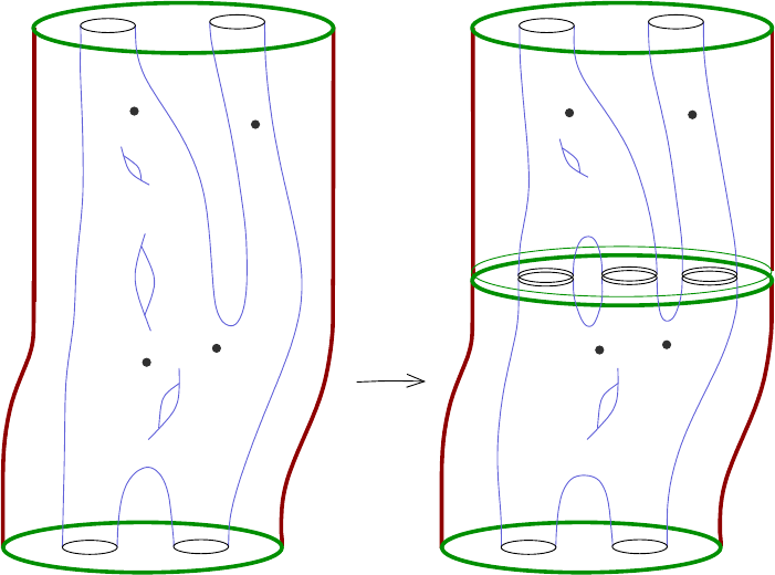
228 Chris Wendl
u
A
u
B
u
C
γ
−
γ
−
γ
1
γ
2
γ
3
γ
4
γ
4
γ
5
γ
5
c
W
c
W
R × M
+
Figure 11.1. The degeneration scenario behind the gluing map (
11.1)
along with a smooth embedding
(11.1) Ψ : [R
0
, ∞) × U
$
A
×U
$
BC
֒→ M
$
3,4
(J, A + B + C, (γ
4
, γ
5
), γ
−
),
defined for R
0
≫ 1 . This is an example of a gluing map: it has the property that
for any u ∈ U
$
A
and v ∈ U
$
BC
, Ψ(R, u, v) converges in the SFT topolo gy a s R → ∞
to the unique building (with asymptotic markers) having main level u and upper
level v, and moreover, every sequence of smooth curves degenerating in this way is
eventually in the image of Ψ.
In analogous ways one can define gluing maps for buildings with a main level and
a lower level, or more than two levels, or multiple levels in a symplectization (always
dividing symplectization levels by the R-action). It’s important to notice that in all
such scenarios, the domain and target of t he gluing ma p have the same dimension,
e.g. the dimension of both sides of (11.1) is the sum of the virtual dimensions of t he
three moduli spaces concerned.
Definition 11.2. A set of orientations for the connected components of M
$
(J)
and M
$
(J
±
) is called coherent if all gluing ma ps are orientation preserving.
Stated in this way, this definition is based on the pretense that we never have to
worry about non-regular curves in any components of M
$
(J), and that is of course
false—sometimes regularity cannot be achieved, in particular for multiply covered
curves. As we’ll see though in §
11.4, the question of orientations can be reframed in
a way that completely disjoins it from the question of regularity, thus we will later
be able to state a more general version of the above definition that is independent
Lectures on Symplectic Field Theory 229
of regularity (see Definition 11.14). The main result whose proof we will outline in
the next few sections is then:
Theorem 11.3. Coherent orientations exist.
But there is also some ba d news. The space M
$
(J) with asymptotic markers
is not actually the space we want to orient. In fact, even the usual moduli space
M(J) has a certain amount of extra information in it that we’d rather not keep
track of when we don’t have to, for instance the ordering of the punctures. Can we
forget this information without forgetting the orientation of the moduli space? Not
always:
Proposition 11.4. Suppose
ˆ
γ
+
= (γ
+
1
, . . . , γ
+
k
+
), and
ˇ
γ
+
is a similar ord ered l ist
of Reeb orbits obtained from
ˆ
γ
+
by exchan ging γ
+
j
with γ
+
k
for som e 1 ≤ j < k ≤ k
+
.
Then for any choice of coherent orientations , the natural map
M
$
g,m
(J, A,
ˆ
γ
+
, γ
−
) → M
$
g,m
(J, A,
ˇ
γ
+
, γ
−
)
defined by permuting the corresponding punctures z
+
j
, z
+
k
∈ Γ
+
along with their as-
ymptotic markers is orientation reversing i f and only if the numbers
n − 3 + µ
CZ
(γ
+
i
)
for i = j, k are both odd. A similar statement holds for permutations of negative
punctures.
This result is the reason for the super-commutative algebra that we will see in
the next lecture. What about forgetting the markers? It turns out that we can
sometimes do that as well, but again not always.
Proposition 11.5. Suppo se M
$
g,m
(J, A, γ
+
, γ
−
) → M
$
g,m
(J, A, γ
+
, γ
−
) is the
map defined by multiplying the asymptotic marker by e
2πi/m
at one of the punctures
for which the asymptotic orbit is an m-fo l d cover γ
m
of a simpl e orbit γ. For any
choice of coherent ori e ntations, this ma p reverse orientation if and only if m is even
and µ
CZ
(γ
m
) −µ
CZ
(γ) is odd.
Note that in both of the above propositions, only the odd/even parity of the
Conley-Zehnder indices matters, so there is no need to choose trivializations. Propo-
sition
11.5 mot ivates one of the more mysterious technical definitions in SFT.
Definition 1 1.6. A closed nondegenerate Reeb orbit γ is called a bad orbit if
it is an m-fold cover of some simple or bit γ
′
where m is even and µ
CZ
(γ) − µ
CZ
(γ
′
)
is odd. Orbits tha t are not bad are called good.
The upshot is that coherent orientations can be defined on the union of all
components M
g,m
(J, A, γ
+
, γ
−
) for which all of the orbits in the lists γ
+
and γ
−
are
good. This does not mean that moduli spaces involving bad orbits cannot be dealt
with—in fact, such moduli spaces have the convenient property that the number of
distinct choices of asymptotic markers is always even, and every such choice can be
cancelled by an alt ernat ive choice that induces the opposite orientation. Fo r this
reason, while bad orbits certainly can appear in breaking of holomorphic curves, we
will see that they do not need to serve as generators of SFT.

230 Chris Wendl
11.2. Permutations of punctures and bad orbits
Before addressing the actual construction of coherent orienta tions, we can al-
ready give heuristic proofs of Propositions 11.4 a nd 1 1.5. They are not fully rigor-
ous because they ar e based on the same pretense as Definition
11.2, namely that
all curves we ever have to worry about (including multiple covers) are regula r . But
we will be able to turn these into precise arguments in §
11.7, after discussing the
determinant line bundle.
Heuristic proof of Proposition
11.4. To simplify the notation, suppose
ˆ
γ
+
consists of only two orbits, so
ˆ
γ
+
= (γ
1
, γ
2
) and
ˇ
γ
+
= (γ
2
, γ
1
). Consider the
gluing scenario shown in Figure
11.2, where u ∈ M
$
g,m
(J, A, (γ
1
, γ
2
), γ
−
) needs to
be glued to a disjoint union of two planes
u
B
∈ M
$
0,0
(J
+
, B, ∅, γ
1
), u
C
∈ M
$
0,0
(J
+
, C, ∅, γ
2
).
You might object that there’s no guarantee that such planes must exist in R ×M
+
,
e.g. the orbits γ
1
and γ
2
might not even be contractible. This concern is valid so
far as it goes, but it misses the point: since we’re talking about gluing rather than
compactness, we do not need any seriously global infor mation about
c
W and M
+
,
as the gluing process doesn’t depend on anything o ut side a small neighborhood of
the curves we’re considering. Thus we are free to change the global structure of
M
+
elsewhere so that the planes u
B
and u
C
will exist.
1
If you still can’t imagine
how one might do this, try not to worry about it and just think of Figure
11.2 as a
thought-experiment: it’s a situation that certainly does sometimes happen, so when
it does, let’s see what it implies about orientations.
Assuming all three curves in the picture are r egula r , there will be smooth open
neighborhoods
u ∈ U
12
⊂ M
$
g,m
(J, A, (γ
1
, γ
2
), γ
−
)
[(u
B
, u
C
)] ∈ U
BC
⊂
M
$
0,0
(J
+
, B, ∅, γ
1
) ×M
$
0,0
(J
+
, C, ∅, γ
2
)
.
R
and a gluing map
Ψ
BC
: [R
0
, ∞) ×U
12
×U
BC
֒→ M
$
g,m
(J, A + B + C, ∅, γ
−
),
which must be orientation preserving by assumption. But reversing the order of the
product M
$
0,0
(J
+
, B, ∅, γ
1
)×M
$
0,0
(J
+
, C, ∅, γ
2
) and letting u
′
∈ M
$
g,m
(J, A, (γ
2
, γ
1
), γ
−
)
denote the image of u under the map that switches the order of its positive punc-
tures, there are also smooth open neighborhoods
u
′
∈ U
21
⊂ M
$
g,m
(J, A, (γ
2
, γ
1
), γ
−
)
[(u
C
, u
B
)] ∈ U
CB
⊂
M
$
0,0
(J
+
, C, ∅, γ
2
) × M
$
0,0
(J
+
, B, ∅, γ
1
)
.
R
and a gluing map
Ψ
CB
: [R
0
, ∞) ×U
21
×U
CB
֒→ M
$
g,m
(J, A + B + C, ∅, γ
−
).
1
Of course by the maximum principle, planes with only negative ends will not exist in R ×M
+
if this is the symplectization of a contact manifold. But we could also change the contact data to
a stable Hamiltonian structure for which such planes are allowed.
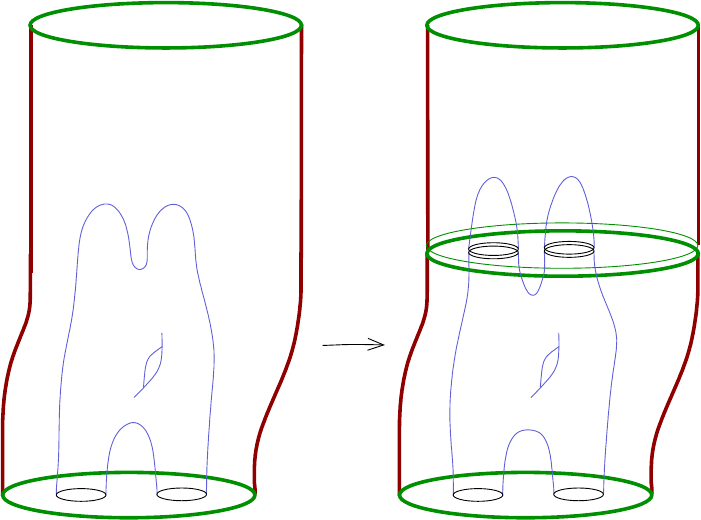
Lectures on Symplectic Field Theory 231
u
B
u
C
u
γ
−
γ
−
γ
1
γ
2
c
W
c
W
R × M
+
Figure 11.2. The gluing thought-experiment used for proving
Propositions 11.4 and 11.5.
If both of these gluing maps preserve orientation, then the effect on orientations of
the map fro m M
$
g,m
(J, A, (γ
1
, γ
2
), γ
−
) to M
$
g,m
(J, A, (γ
2
, γ
1
), γ
−
) defined by inter-
changing the positive punctures must be the same as that of the map
M
$
0,0
(J
+
, B, ∅, γ
1
) × M
$
0,0
(J
+
, C, ∅, γ
2
) → M
$
0,0
(J
+
, C, ∅, γ
2
) ×M
$
0,0
(J
+
, B, ∅, γ
1
)
(u
B
, u
C
) 7→ (u
C
, u
B
).
The latter is orientation reversing if and only if both moduli spaces of planes are
odd dimensional, which means n − 3 + µ
CZ
(γ
i
) is odd for i = 1, 2.
Heuristic proof of Proposition
11.5. Let us reuse the t hought-experiment
of Figure
11.2, but with different details in focus. Suppose γ
1
in the picture is an
m-fold covered orbit γ
m
, where γ is simply covered, and suppose that u
B
is also an
m-fold cover, taking t he form
u
B
(z) = v(z
m
)
for a somewhere injective plane v ∈ M
0,0
(J
+
, B
0
, ∅, γ). We’re going to assume again
that all curves in the discussion are regular, including the multiple cover u
B
; while
this doesn’t sound very plausible, we will see once the determinant line bundle enters
the picture in §
11.4 that it is an irrelevant detail. Now, u
B
has a cyclic automorphism
group
Aut(u
B
) = Z
m
⊂ U(1)
which acts freely on the set o f m choices of asymptotic ma r ker for u
B
. Then if we
act with the same element of Z
m
on u
B
and on the corresponding asymptotic marker
232 Chris Wendl
for u, the building is unchanged, as it has the same decoration. Coherence therefore
implies that the effect on orientations of the map fro m M
$
g,m
(J, A, (γ
1
, γ
2
), γ
−
) to
itself defined by acting with the canonical generator of Z
m
⊂ U(1) on the marker at
γ
1
is the same as the effect of the map M
$
0,0
(J
+
, mB
0
, ∅, γ
m
) → M
$
0,0
(J
+
, mB
0
, ∅, γ
m
)
defined by composing u
B
: C → R × M
+
with ψ(z) := e
2πi/m
z.
The derivative of this map from M
$
0,0
(J
+
, mB
0
, ∅, γ
m
) to itself at u
B
defines a
linear self-map
Ψ : T
u
B
M
0,0
(J
+
, mB
0
, ∅, γ
m
) → T
u
B
M
0,0
(J
+
, mB
0
, ∅, γ
m
)
with Ψ
m
= 1. The latter implies that Ψ cannot reverse orientation if m is odd. If
m is even, observe t hat the representation theory of Z
m
gives a decomp osition
T
u
B
M
0,0
(J
+
, mB
0
, ∅, γ
m
) = V
1
⊕ V
−1
⊕ V
rot
,
where Ψ acts on V
±1
as ±1, and V
rot
is a direct sum of real 2-dimensional subspaces
on which Ψ acts by rotations (and therefore preserves orientations). Thus Ψ reverses
the orientation of T
u
B
M
0,0
(J
+
, mB
0
, ∅, γ
m
) if and only if dim V
−1
is odd. As we will
review in the next section, T
u
B
M
0,0
(J
+
, mB
0
, ∅, γ
m
) is a space of holomor phic sec-
tions of u
∗
B
T (R ×M
+
) modulo a subspace defined via the linearized auto mo rphisms
of C, so V
1
consists o f precisely those sections η that satisfy η = η ◦ψ, meaning they
are m-fo ld covers of sections of v
∗
T (R×M
+
). This defines a bijective correspondence
between V
1
and T
v
M
0,0
(J
+
, B
0
, ∅, γ), so
dim V
−1
= dim M
0,0
(J
+
, mB
0
, ∅, γ
m
) −dim M
0,0
(J
+
, B
0
, ∅, γ) (mod 2).
The result then comes from plugging in the dimension formulas for these two moduli
spaces.
11.3. Or ienting moduli spaces in general
We now discuss concretely what is involved in orienting a moduli space of J-
holomorphic curves.
Recall from Lecture
7 that whenever a curve u
0
: (
˙
Σ = Σ \Γ, j
0
) → (
c
W , J) with
marked points Θ ⊂
˙
Σ is Fredholm regular, a neighborhood of u
0
in M(J) can be
identified with
¯
∂
−1
J
(0)
G
0
,
where G
0
= Aut(Σ, j
0
, Γ ∪ Θ) and
¯
∂
J
is the smooth Fredholm section
T × B
k,p,δ
→ E
k−1,p,δ
: (j, u) 7→ T u + J ◦T u ◦ j,
defined on the product of a G
0
-invariant Teichm¨uller slice T through j
0
with a
Banach manifold B
k,p,δ
of W
k,p
-smooth maps
˙
Σ →
c
W satisfying an exponential
decay condition at the cylindrical ends. Here G
0
acts on
¯
∂
−1
J
(0) by
(11.2) G
0
×
¯
∂
−1
J
(0) →
¯
∂
−1
J
(0) : (ϕ, (j, u)) 7→ (ϕ
∗
j, u ◦ ϕ).
Regularity means tha t the linearizatio n D
¯
∂
J
(j
0
, u
0
) : T
j
0
T ⊕ T
u
0
B
k,p,δ
→ E
k−1,p,δ
(j
0
,u
0
)
is
surjective, and the implicit function theorem then gives a natural identification
T
u
0
M(J) = ker D
¯
∂
J
(j
0
, u
0
)
aut(Σ, j
0
, Γ ∪ Θ),
Lectures on Symplectic Field Theory 233
where aut(Σ, j
0
, Γ ∪Θ) denotes the Lie alg ebra of G
0
, which acts on ker D
¯
∂
J
(j
0
, u
0
) by
differentiating (
11.2).
2
This action actually defines an inclusion of aut(Σ, j
0
, Γ ∪Θ)
into ker D
¯
∂
J
(j
0
, u
0
) whenever u
0
is not constant, thus we can regard aut(Σ, j
0
, Γ∪Θ)
as a subspace of ker D
¯
∂
J
(j
0
, u
0
).
As outlined in Proposition
11.1, the space M
$
(J) with asymptotic markers a d-
mits a similar local description: here one only needs to enhance the structure of the
Banach manifold B
k,p,δ
with information about asymptotic markers at each punc-
ture, so the Banach manifold needed to describe M
$
(J) is a finite covering space
of B
k,p,δ
. The rest of the discussion is identical, except for the fact that when markers
are included, G
0
always acts freely on
¯
∂
−1
J
(0).
We now make a useful observation about the spaces aut(Σ, j
0
, Γ ∪ Θ) and T
j
0
T :
namely, they both carry natural complex structures and are thus canonically or i-
ented. This follows from the fact that both the automorphism group G
0
and the
Teichm¨uller space T (Σ, Γ∪Θ) = J(Σ)
Diff
0
(Σ, Γ∪Θ) are naturally complex mani-
folds. On the linearized level, one way to see it is via the fact—mentioned previously
in §
6.3—that aut(Σ, j
0
, Γ ∪Θ) and T
[j
0
]
T (Σ, Γ ∪Θ) can be naturally identified with
the kernel and cokernel respectively of the natural linear Cauchy-Riemann type
operator on ( Σ, j
0
),
(11.3) D
Id
: W
k,p
Γ∪Θ
(T Σ) → W
k−1,p
(End
C
(T Σ)),
which is the linearization at Id of the nonlinear operator that detects holomorphic
maps (Σ, j
0
) → (Σ, j
0
). This operator is equivalent to the operator that defines the
holomorphic structure of T Σ, thus it is complex linear. To handle the punctures
and marked points, one needs to restrict the nonlinear operator to the space of
W
k,p
-smooth maps Σ → Σ that fix every point in Γ ∪ Θ, thus the domain of the
linearization becomes the finite-codimensional subspace
W
k,p
Γ∪Θ
(T Σ) :=
X ∈ W
k,p
(T Σ)
X|
Γ∪Θ
= 0
.
This subspace is still complex, thus so is (
11.3), and its kernel and cokernel inherit
natural complex structures.
The complex structure on aut(Σ, j
0
, Γ∪Θ) means that defining an orientation on
the tangent space T
u
0
M
$
(J) is equivalent to defining one on ker D
¯
∂
J
(j
0
, u
0
). The
latter operator takes the form
D
¯
∂
J
(j
0
, u
0
) : T
j
0
T ⊕ T
u
0
B
k,p,δ
→ E
k−1,p,δ
(j
0
,u
0
)
: (y, η) 7→ J ◦ T u
0
◦ y + D
u
0
η,
where D
u
0
: W
k,p,δ
(u
∗
0
T
c
W ) ⊕ V
Γ
→ W
k−1,p,δ
(Hom
C
(T
˙
Σ, u
∗
0
T
c
W )) is the usual lin-
earized Cauchy-Riemann operat or at u
0
, with V
Γ
denoting a complex (#Γ)-dimensional
space of smoo th sections that are constant near infinity.. The remarks above and
the fact t hat u
0
is J-ho lomorphic imply that the first term in this operator,
T
j
0
T → E
k−1,p,δ
(j
0
,u
0
)
: y 7→ J ◦ T u
0
◦ y
2
The presence o f aut(Σ, j
0
, Γ ∪ Θ) in this discussion is only r e levant in the finite set of “non-
stable” cases where χ(
˙
Σ \ Θ) ≥ 0, since otherwise G
0
is finite and thus aut(Σ, j
0
, Γ ∪ Θ) is trivial.

234 Chris Wendl
is a complex-linear map. Now if D
u
0
happens also to be a complex-linear map, t hen
we are done, because ker D
¯
∂
J
(j
0
, u
0
) will then be a complex vector space and inherit
a natural orientation.
In general, D
u
0
is not complex linear, though it does have a comple x-linear part,
D
C
u
0
η :=
1
2
(D
u
0
η − JD
u
0
(Jη)) ,
which is also a Cauchy-Riemann type operator . The space of all Cauchy-Riemann
type operators on a fixed vector bundle is affine, so one can interpo late from D
u
0
to D
C
u
0
through a path of Cauchy-Riemann type operator s, though they may not all
be Fr edholm—t his depends on the asymptotic operato r s at the punctures. In the
special case however where there are no punctures, one can easily imagine making
use of this idea: if
˙
Σ = Σ is a closed surface, then the obvious homotopy from D
u
0
to its complex-linear part yields a homotopy from D
¯
∂
J
(j
0
, u
0
) to its complex-linear
part, and if every operator along this homotopy happens to be surjective, then the
canonical orientation defined on the kernel of t he complex-linear operator determines
an orientation on ker D
¯
∂
J
(j
0
, u
0
).
There are two obvious problems with the above discussion:
(1) We have no way to ensure tha t every operator in the homotopy from
D
¯
∂
J
(j
0
, u
0
) to its complex-linear part is surjective;
(2) If there are punctures, then we cannot even expect every operator in this
homotopy to be Fredholm.
The first pr oblem motivates the desire to define a notion of orientations for a
Fredholm operator T that does not require T to be surjective but reduces to the
usual notion of orienting ker T whenever it is. The solution to this problem is
the determinant line bundle, which we will discuss in the next section. With this
object in hand, the above discussion for the case of closed curves can be made
rigorous, so that all smooth moduli spaces of closed J-holomorphic curves inherit
canonical orientations. One of the advantages of using the determinant line bundle
is that the question of orientations becomes entirely disjoined from the question of
transversality: if one can orient the determinant line bundle then moduli spaces of
regular curves inherit orientations, but orienting the determinant bundle does not
require knowing in advance whether the curves are regular.
The second problem is obviously significant because in the punctured case, mod-
uli spaces of J-holomorphic curves sometimes have odd real dimension, making it
clearly impossible to homotop D
¯
∂
J
(j
0
, u
0
) through Fredholm opera t ors to one that
is complex linear. The solution in this case will be to define orientations algorithmi-
cally via the coherence condition, and we will describe a suitable algorithm for this
in §
11.6.
11.4. The determinant line bundle
Fix real Banach spaces X and Y and let Fred
R
(X, Y ) denote the space of real-
linear Fredholm operators, viewed as an o pen subset of the Banach space L
R
(X, Y )
of all bounded linear operators. We’ll use the following notat ion throughout: if V
Lectures on Symplectic Field Theory 235
is an n-dimensional real vector space, then the top-dimensional exterior power of V
is denoted by
Λ
max
V := Λ
n
V.
This 1-dimensional real vector space is spanned by any wedge product of the form
v
1
∧. . . ∧v
n
where (v
1
, . . . , v
n
) is a basis of V . Denoting the dual space of V by V
∗
,
note that there is a canonical isomorphism (Λ
max
V )
∗
= Λ
max
V
∗
. If dim V = 0, then
we adopt the convention Λ
max
V = R.
Definition 11.7. Given T ∈ Fred
R
(X, Y ), the determinant line of T is the
real 1-dimensional vector space
det(T) = (Λ
max
ker T) ⊗ (Λ
max
coker T)
∗
.
Our main goal in this section is to prove:
Theorem 11.8. There exists a topological vector bundle det(X, Y )
π
−→ Fred
R
(X, Y )
of real rank 1 such that π
−1
(T) = det(T) for each T ∈ Fr ed
R
(X, Y ).
Observe that whenever T ∈ Fred
R
(X, Y ) is surjective, det(T) = Λ
max
ker T, so
an orientation of det(T) is equivalent to an orientation of ker T. More generally,
an orientation of det(T) is equivalent to an orientation for ker T ⊕ coker T. If T is
an isomorphism, then det(T) is simply R, so an orientation of det(T) amounts to a
choice of sign ±1.
To construct local trivializations of det(X, Y ) → Fred
R
(X, Y ), we start with
the case where X and Y are both finite dimensional. Note that in this case, every
linear map is Fredholm, including the zero map, and its determinant is simply
Λ
max
X ⊗ (Λ
max
Y )
∗
.
Lemma 11.9. Suppose X and Y are real vec tor space s of finite dimensions n and
m respectively. Then for e very T ∈ L
R
(X, Y ), there exists a canonical isomorphism
(Λ
max
ker T) ⊗ (Λ
max
coker T)
∗
= (Λ
max
V ) ⊗ (Λ
max
W )
∗
.
Proof. Suppose dim ker T = k and dim coker T = ℓ, so ind(T) = k−ℓ = n−m,
thus n − k = m − ℓ. We define a linear map Φ : (Λ
n
X) ⊗ (Λ
m
Y )
∗
→
Λ
k
ker T
⊗
Λ
ℓ
coker T
∗
via the following procedure. Fix x ∈ Λ
n
X a nd y
∗
∈ ( Λ
m
Y )
∗
and
suppose both a re nontrivial. Then for any nontrivial element k ∈ Λ
k
ker T, there
exists a unique element v ∈ Λ
n−k
(X/ ker T) such that for any subspace V ⊂ X
complementary to ker T, the element
˜
v ∈ Λ
n−k
V ⊂ Λ
n−k
X o btained from v by
inverting the na t ur al isomorphism V → X/ ker T induced by the projection X →
X/ ker T satisfies
k ∧
˜
v = x.
The map T descends to an isomorphism X/ ker T → im T and thus induces an iso-
morphism Λ
n−k
(X/ ker T) → Λ
m−ℓ
(im T) ⊂ Λ
m−ℓ
Y , which takes v to a nontrivial
element Tv. There is then a unique element c ∈ Λ
ℓ
coker T = Λ
ℓ
(Y/ im T) such
that for any subspace W ⊂ Y complementary to im T, the element
˜
c ∈ Λ
ℓ
W ⊂ Λ
ℓ
Y
obtained from c by inverting the isomorphism W → Y/ im T induced by the pro-
jection Y → Y / im T satisfies
y
∗
(
˜
c ∧ Tv) = 1.
236 Chris Wendl
Now define Φ as the unique linear map such that
Φ(x ⊗y
∗
) = k ⊗c
∗
,
where c
∗
∈ (Λ
ℓ
coker T)
∗
is defined by c
∗
(c) = 1. It is straightforward to check
that this definition does not depend on a ny choices: indeed, if we replace k by λk
for some λ ∈ R \ {0} in the above procedure, then v is replaced by
1
λ
v, hence Tv
becomes
1
λ
Tv, c becomes λc and c
∗
therefore becomes
1
λ
c
∗
, so that k⊗c
∗
is replaced
by
(λk) ⊗
1
λ
c
∗
= k ⊗ c
∗
.
To construct local trivializatio ns of det(X, Y ) in the infinite-dimensional case,
recall the following construction from Lecture
3. Given T
0
∈ Fred
R
(X, Y ), we can
write X = V ⊕ K and Y = W ⊕ C where K = ker T
0
, C
∼
=
coker T
0
, W = im T
0
and T
0
|
V
: V → W is a n isomorphism. We shall use these splittings to write any
other operator T ∈ Fred
R
(X, Y ) as
T =
A B
C D
and let U ⊂ Fred
R
(X, Y ) denote the open neighborhood of T
0
for which the block
A : V → W is invertible. This gives rise to a pair of smooth maps
Φ : U → L
R
(K, C) : T 7→ D − CA
−1
B
and
F : U → L
R
(V ⊕ K) = L
R
(X) : T 7→
1 −A
−1
B
0 1
,
such that F (T) is always invertible and maps {0}⊕ker Φ(T) isomorphically to ker T.
Similarly, there is a smooth map
G : U → L
R
(W ⊕ C) = L
R
(Y ) : T 7→
1 0
−CA
−1
1
such that G(T) is always invertible and maps im T isomorphically to W ⊕im Φ(T),
so it descends to an isomorphism of coker T to coker Φ(T). Given the canonical iso-
morphism det(Φ(T)) = Λ
max
K ⊗(Λ
max
C)
∗
= det(T
0
) from Lemma
11.9, the result-
ing smooth families of isomorphisms ker T → ker Φ(T) and coker T → coker Φ(T)
determine a local trivialization
det(X, Y )|
U
→ U × det(T
0
).
I will leave it as an exercise for the reader to check that the r esulting transition
maps are cont inuous.
3
3
This detail should not be underestimated, e.g. [
MW, §7.4] observes that the local trivializa-
tions constructed in [
MS04, §A.2] are, unfortunately, no t continuously compatible. See [Zin] for
further disc ussion of this point. If you discover that my local trivializations are also not continu-
ously compatible, please let me know.

Lectures on Symplectic Field Theory 237
Exercise 11.10. Show that if X and Y are complex Banach spaces, then
the restriction of det(X, Y ) to the subspace of complex-linear Fredholm operators
Fred
C
(X, Y ) ⊂ Fred
R
(X, Y ) admits a canonical orientation compatible with the
complex structures of ker T and coker T for each T ∈ Fred
C
(X, Y ). Show also that
whenever T ∈ Fred
C
(X, Y ) is an isomorphism, the canonical orientation of det(T)
agrees with the standard orientation of R.
The orientation of det(T) for T ∈ Fred
C
(X, Y ) described in Exercise
11.10 is
called the complex orientation.
11.5. Determinant bundles of moduli spaces
Combining ideas from the previous two sections, let
det(J) → M
$
(J)
denote the topolo gical line bundle that associates to a ny u ∈ M
$
g,m
(J, A, γ
+
, γ
−
)
the determinant line of the Fredholm operator
D
u
: W
k,p,δ
(u
∗
T
c
W ) ⊕ V
Γ
→ W
k−1,p,δ
(
Hom
C
(T
˙
Σ, u
∗
T
c
W )).
One can construct local trivializations for this bundle using Theorem
11.8 and any
choice of local trivializations for the Banach space bundles T B
k,p,δ
and E
k−1,p,δ
.
Proposition 11.11. Any orientation of det(J) → M
$
(J) canonically deter-
mines an orientation of M
reg
(J).
Proof. As explained in §
11.3, an orientation of M
reg
(J) near a part icular curve
u
0
: (
˙
Σ, j
0
) → (
c
W , J) is equivalent t o a continuously varying choice of orientations
for the kernels
ker D
¯
∂
J
(j, u) ⊂ T
j
T ⊕ T
u
B
k,p,δ
for all (j, u) ∈
¯
∂
−1
J
(0), where T is a Teichm¨uller slice through j
0
. The operator
D
¯
∂
J
(j, u) is of the form
L(y, η) := J ◦T u ◦ y + D
u
η
and thus is homotopic through Fredholm operators to
L
0
(y, η) := D
u
η,
namely via the homotopy L
s
(y, η) := sJ ◦T u ◦y +D
u
η for s ∈ [0, 1]. The kernel and
cokernel of L
0
are T
j
T ⊕ ker D
u
and coker D
u
respectively, and since T
j
T carries a
complex structure, the orientation of det(D
u
) naturally determines an orientation
of det(L
0
). Using the homotopy L
s
, this determines orientations of det(D
¯
∂
J
(j, u))
and thus orientat ions of ker D
¯
∂
J
(j, u) fo r all (j, u) near (j
0
, u
0
), and this orientation
does no t depend o n the choice of Teichm¨uller slice since the operators D
u
also do
not.
From now on, when we speak of an orientation of M
$
(J), we will actually
mean a n orientation of t he bundle det(J) → M
$
(J). The above proposition implies
that this is equivalent to what we want in applications, but one advantage of talking
about det(J) is that there is no need to limit the discussion to curves that a r e

238 Chris Wendl
regular, i.e. the notion of an orientation of M
$
(J) now makes sense even though
M
$
(J) is not globally a smooth object.
Proposition 11.1 2. Suppose all Reeb orbits in γ
±
have the property that their
asymptotic operators are complex linear. Then M
$
g,m
(J, A, γ
+
, γ
−
) admits a natural
orientation, known as the complex orientation.
Proof. Having complex-linear asymptotic operators implies that the obvious
homotopy from each Cauchy- Riemann operator D
u
to its complex-linear part does
not change the a symptotic operators and is therefore a homotopy through Fred-
holm operators. We therefore have a continuo usly varying homotopy of each of the
relevant fibers of det(J) to the determinant bundle over a family of complex-linear
operators, which inherit the complex orientation described in Exercise
11.10.
Proposition
11.12 applies in particular to all moduli spaces of closed J- holomorphic
curves, and thus solves the orientation problem in that case.
11.6. An algorithm for coherent o rientations
We now briefly describe the construction of coherent o r ientations due to Bour-
geois and Mohnke [BM04]. A slightly different construction is described in [EGH00],
though it appears to have minor erro r s in some details.
Recall from Lecture
4 the notion of a n asymptotically Hermitian vector bundle
(E, J) over a punctured Riemann surface (
˙
Σ, j). Here (
˙
Σ, j) is endowed with the
extra structure of fixed cylindrical ends (
˙
U
z
, j)
∼
=
(Z
±
, i) f or each puncture z ∈ Γ
±
,
which determines a choice of asymptotic markers. Likewise, the bundle E comes
with an a symptotic bundle (E
z
, J
z
, ω
z
) → S
1
associated to each puncture, carrying
compatible complex and symplectic structures. We shall now endow E with a bit
more structure that is always naturally present in the case E = u
∗
T
c
W : namely,
assume each of the asymptotic bundles comes with a splitting
(11.4) (E
z
, J
z
, ω
z
) = ( C ⊕
b
E
z
, i ⊕
ˆ
J
z
, ω
0
⊕ ˆω
z
),
where ω
0
is the standard symplectic structure on the trivial complex line bundle
(C, i) over S
1
, and (
b
E
z
,
ˆ
J
z
, ˆω
z
) → S
1
is anot her Hermitian bundle. Fix a choice
{A
z
}
z∈Γ
of nondegenerate asymptotic operator s on each of the bundles (
b
E
z
,
ˆ
J
z
, ˆω
z
),
and define the topological space
CR(E, {A
z
}
z∈Γ
)
to consist of all Cauchy-Riemann type operators on E that are asymptotic at the
punctures z ∈ Γ to the asymptotic operators
(−i∂
t
) ⊕ A
z
: Γ(C ⊕
b
E
z
) → Γ(C ⊕
b
E
z
).
This is an affine space, so it is contractible, and if δ > 0 is sufficiently small
and V
Γ
⊂ Γ(E) denotes a complex (#Γ)-dimensional space of smooth sections
that take constant values in C ⊕ {0} ⊂ E
z
near each puncture z, then every
D ∈ CR(E, {A
z
}
z∈Γ
) determines a Fredholm operator
D : W
k,p,δ
(E) ⊕ V
Γ
→ W
k−1,p,δ
(Hom
C
(T Σ, E)).
Lectures on Symplectic Field Theory 239
It follows that a choice of orientation of the determinant line for a ny one o f these
operators determines an orientatio n for all of them. The point of this construction
is that every u ∈ M
$
(J) determines an operator D
u
belonging to a space of this
form.
We now construct a gluing operation for Cauchy-Riemann operators that lin-
earizes the gluing maps described in §11.1. Suppose (E
i
, J
i
) → (
˙
Σ
i
= Σ
i
\Γ
i
, j
i
) for
i = 0, 1 is a pair of asymptotically Hermitian bundles of the same rank, endowed
with asymptotic splittings as in (
11.4) and asymptotic operators {A
z
}
z∈Γ
i
, and that
there exists a pair of punctures z
0
∈ Γ
+
0
and z
1
∈ Γ
−
1
such that some unitary bundle
isomorphism
b
E
1
z
1
∼
=
−→
b
E
0
z
0
identifies A
z
1
with A
z
0
. Note that such an isomorphism is uniquely determined up
to homotopy whenever it exists. For R > 0, we can define a family of glued Riemann
surfaces
(
˙
Σ
R
= Σ
R
\ Γ
R
, j
R
)
by cutting off the ends (R, ∞) × S
1
⊂
˙
U
z
0
and (−∞, −R) × S
1
⊂
˙
U
z
1
and g luing
{R} × S
1
⊂
˙
Σ
0
to {−R} × S
1
⊂
˙
Σ
1
. The glued Riemann surface contains an
annulus biholomorphic to ([−R, R] × S
1
, i) in place of the infinite cylindrical ends
at the punctures z
0
and z
1
. The unita ry isomorphism
b
E
1
z
1
→
b
E
0
z
0
then determines
an isomorphism E
1
z
1
→ E
0
z
0
via the splitting (
11.4) and hence an asymptotically
Hermitian bundle
(E
R
, J
R
) → (
˙
Σ
R
, J
R
).
Using cutoff functions in the neck [−R, R] × S
1
, any Cauchy-Riemann operators
D
i
∈ CR(E
i
, {A
z
}
z∈Γ
i
) for i = 0, 1 now determine a f amily of operators
D
R
∈ CR(E
R
, {A
z
}
z∈Γ
R
)
uniquely up to homotopy. Analogously to the gluing maps in §11.1, one can a r-
range this construction so that the operators D
R
converge in some sense to the pair
(D
0
, D
1
) as R → ∞, which has the following consequence:
Lemma 11.13 ([BM04, Corollary 7]). For R > 0 sufficiently large, there is a
natural isomorphism
det(D
0
) ⊗ det(D
1
) → det(D
R
)
that is d efined up to homotopy.
Up to some additional direct sums and quotients by finite-dimensional complex
vector spaces, this isomorphism should be understood as the linearization of a glu-
ing map between moduli spaces, generalized to a setting in which the holomorphic
curves involved need not be regular. To orient M
$
(J) coherently, it now suffices to
choose orientations for the operators in CR(E, {A
z
}
z∈Γ
) that vary continuously un-
der deformations of j and E and are preserved by t he isomorphisms of Lemma
11.13.
This mo tivates the f ollowing generalization of Definition
11.2.
Definition 11.14. A system of coherent orientations is an assignment to
each asymptotically Hermitian bundle (E, J) → (
˙
Σ, j) with asymptotic splittings as
in (
11.4) and asymptotic o perators {A
z
}
z∈Γ
of an orientation for the determinant
240 Chris Wendl
line of each D ∈ CR(E, {A
z
}), such that these orienta t ions vary continuously with
D as well as the data j and J, and such that the isomorphisms in Lemma
11.13 are
always orientation preserving.
The prescription of [
BM04] to construct such systems is now as follows.
(1) For any trivial bundle E over
˙
Σ = C with ∞ as a negative puncture and any
asymptotic operator A
∞
, choose an arbitrary cont inuous family of orien-
tations for the operators in CR(E, {A
∞
}), subject only to the requirement
that these should match the complex orientation whenever A
∞
is complex
linear.
(2) For any trivial bundle E
−
over
˙
Σ = C with ∞ as a positive puncture, any
asymptotic operator A
∞
and any D
−
∈ CR(E
−
, {A
∞
}), let E
+
denote the
trivial bundle over C with a negative puncture as in step (1), choose any
D
+
∈ CR(E
+
, {A
∞
}) and construct the resulting family of glued operators
D
R
∈ CR(E
R
),
where t he E
R
are trivial bundles over S
2
. Since S
2
has no punctures, D
R
has a natural complex orientation, so define the orientation of D
−
to be
the one that is compatible via Lemma
11.13 with this and the orientation
chosen for D
+
in step (1).
(3) For an arbitrary (E, J) → (
˙
Σ, j), glue positive and negative planes to
˙
Σ to
produce a bundle over a closed surface
b
Σ, and define t he or ientation of any
D ∈ CR(E, {A
z
}
z∈Γ
) to be compatible via Lemma
11.13 with the choices
in steps (1) and (2) and the complex orientation for operators over
b
Σ.
It should be easy to convince yourself that if we now vary the bundle (E, J) →
(
˙
Σ, j) or the operators on this bundle (but not the asymptotic operators!) contin-
uously, the capping procedure described in step (3) above produces a continuous
family of Cauchy-Riemann type operators on bundles over closed Riemann surfaces.
Since these all carry the complex orientation, t he resulting orientations of the orig-
inal operators vary continuously. It is similarly clear from the construction that
any Cauchy-Riemann operator whose asymptotic operators are all complex linear
will end up with the complex orientation. Bourgeois and Mohnke use t his fact to
prove that any system of orientations constructed in this way is compatible with
all possible linear gluing maps arising from Lemma
11.13. The idea is to reduce
it to the complex-linear case by gluing cylinders to the ends of any asymptotically
Hermitian bundle so that the asymptotic operators can be changed at will; see
[BM04, Prop osition 8].
11.7. Permutations and bad orbits revisited
The heuristic proofs in §
11.2 can now be ma de precise in the following way.
Suppose D ∈ CR(E, {A
z
}
z∈Γ
), and D
′
is the same operator after interchanging
two of the punctures in Γ. Imagine gluing (E, J) → (
˙
Σ, j) to trivial bundles E
1
and
E
2
over planes in order to cap off the two punctures that are being interchanged,
and choose Cauchy-Riemann operators D
1
and D
2
on these planes to form a glued
operator on the capped surfa ce. This capping procedure is done one plane at a time,
Lectures on Symplectic Field Theory 241
and the order of the two punctures determines which pla ne is glued first. Compati-
bility with the isomorphisms of Lemma
11.13 then dictates that the orientations of
det(D) and det(D
′
) match if and only if the orientations of det(D
1
) ⊗ det(D
2
) and
det(D
2
)⊗det(D
1
) match. Since o r ientations of det(D
i
) for i = 1, 2 are equivalent to
orientations of ker D
i
⊕coker D
i
, reversing the order of the tensor product changes
orientations if and only if both of these direct sums are odd dimensional, which
means ind(D
1
) and ind (D
2
) are both odd. If the bundles have complex rank n and
the asymptotic operators are A
i
for k = 1, 2, we have
ind(D
i
) = nχ(C) ±µ
CZ
((−i∂
t
⊕ A
i
) ±δ) = n − 1 ± µ
CZ
(A
i
),
which matches n − 3 + µ
CZ
(A
i
) modulo 2. This proves Proposition
11.4.
Similarly for Proposition
11.5, we consider the action of the generator ψ ∈ Z
m
on det(D) where ψ rotates the cylindrical end by 1/m at some puncture where the
trivialized asymptotic operator A is of the form −i∂
t
−S(mt) for a loop of symmetric
matrices S(t). Capping off this puncture with a plane carrying a Cauchy-R iemann
operator D
∞
, coherence dictates that the same tra nsfor mation must act the same
way on the orientation of det(D
∞
). Since ψ
m
= 1, ψ cannot r everse this orientation
if m is odd. To understand the case of m even, note first that we are free to
choose D
∞
so that it is an m-fold cover, meaning it is related to the branched cover
ϕ : C → C : z 7→ z
m
by
D
∞
(η ◦ ϕ) = ϕ
∗
b
D
∞
η
for some other Cauchy-Riemann operator
b
D
∞
, which is asymptotic to
ˆ
A := −i∂
t
−
S(t). Now the group Z
m
generated by ψ acts on ker D
∞
and coker D
∞
, so represen-
tation theory tells us
ker D
∞
= V
1
⊕ V
−1
⊕ V
rot
coker D
∞
= W
1
⊕ W
−1
⊕ W
rot
,
where ψ acts on V
±1
and W
±1
as ±1 and acts as orientation-preserving rotations on
V
rot
and W
rot
. It follows that ψ reverses the orientat ion of ker D
∞
⊕coker D
∞
if and
only if dim V
−1
−dim W
−1
is odd. Now observe that there are natural isomorphisms
V
1
= ker
b
D
∞
, W
1
= coker
b
D
∞
,
hence
dim V
−1
−dim W
−1
= ind(D
∞
) − ind(
b
D
∞
) (mod 2).
This diff erence in Fredholm indices is precisely µ
CZ
(A) − µ
CZ
(
ˆ
A) up to a sign, and
this completes the proof o f Proposition
11.5.

LECTURE 12
The generating function of S FT
Contents
12.1. Some important caveats on transversality 243
12.2. Auxiliary data, grading and supercommutativity 244
12.3. The definition of H and commutators 247
12.4. Interlude : How to count points in an orbifold 251
12.5. Cylindrical contact homology revisited 256
12.6. Combinatorics of gluing 259
12.7. Some remarks on torsion, coefficients, and conventions 263
12.7.1. What if H
1
(M) has torsion? 263
12.7.2. Combinatorial conventions 263
12.7.3. Coefficients: Q, Z or Z
2
? 264
It is time to begin deriving algebraic consequences fro m the analytical results of
the previous lectures. We saw the simplest possible example of this in Lecture
10,
where the behavior of holomorphic cylinders in symplectizations of contact mani-
folds without contractible R eeb orbits led to a rudimentary version of cylindrical
contact homology HC
∗
(M, ξ) with Z
2
coefficients. Unfortunat ely, the condition on
contractible orbits means that this version of HC
∗
(M, ξ) cannot always be defined,
and even when it can, it only counts cylinders—we wo uld only expect it to capture
a small fragment of the infor ma t ion contained in more general moduli spaces of
holomorphic curves. Extracting information from these general moduli spaces will
require enlarging our algebraic notion of what a Floer-type theory can look like.
12.1. Some important caveats on transversality
For this and the next lecture, we fix the following fantastically optimistic as-
sumption:
Assumption 1 2.1 (science fiction). One can ch oose s uitably compatible almost
co mplex structures so that all pseudoholomorphic curves are Fredholm regular.
This assumption held in Lecture 10 for the curves we were interested in, because
they were all guaranteed for topolo gical reasons to be somewhere injective. It can
also be shown to hold under some very restrictive conditions on Conley-Zehnder
indices in dimension three, see [N el15, Nel13]. Both of those are very lucky situ-
ations, and as we’ve discussed befo re, the assumption cannot generally be achieved
merely by perturbing J generically—it must sometimes fail for curves that are mul-
tiply covered, and such curves always exist (see §
12.4 for more on this). The only
243

244 Chris Wendl
way in reality to ensure something like Assumption 12.1 is to perturb the nonlin-
ear Cauchy-Riemann equation more abstractly, e.g. by replacing
¯
∂
J
u = 0 with an
inhomogeneous equation of the form
¯
∂
J
u = ν
for a generic perturbation ν. This is the standard technique in certain versions of
Gromov-Witten theory, see e.g. [
RT95, RT97]. Alternatively, one can allow J to
depend g enerically on points in the domain rather than just points in the target,
as in [
MS04, §7.3]. Both approaches eliminate the initial problem with multiple
covers, but they both also run into serious and subtle difficulties concerning the r e-
lationship between M(J) and the strata of its compactification
M(J). As observed
in [
Sal99, §5], the possibility of symmetry in strata of M(J) makes it necessary
for any sufficiently general abstract perturbation scheme to involve multivalued per-
turbations, and it is important for these perturbations to be “coherent” in a sense
analogous to our discussion of orientations in the previous lecture. These notions
have no t yet a ll been developed in a sufficiently consistent and general way to give
a rigorous definition o f SFT, though there has been much progress: this is the main
objective of the long -running polyfold project by Hofer-Wysocki-Zehnder [
Hof06].
Recently, a quite different and much more topological approach has been proposed
by John Pardon [
Par].
For most of this lecture we will ignore these subtleties and simply adopt As-
sumption
12.1 as a convenient fiction, thus pretending that all components o f M(J)
are smooth orbifolds of the correct dimension and all gluing maps are smoot h. All
“theorems” stated under this assumption should be read with the caveat that they
are only true in a fictional world in which the assumption holds. Even if it is a
fiction, o ne can get quite far with this point of view: it is still possible not only
to deduce t he essential structure o f what we assume will someday be a rigorously
defined polyfold-based SFT, but also to infer the existence of certain contact in-
varia nts that have interesting rigorous applications requiring only well-established
techniques, e.g. the cobordism obstructions discovered in [
LW11].
12.2. Auxiliary data, grading and supercommutativity
The goal is to define an invariant o f closed (2n − 1)-dimensional conta ct mani-
folds ( M, ξ) with closed nondegenerate Reeb or bits as generators and a Floer-type
differential counting J-holomorphic curves in the symplectization (R × M, d(e
r
α)).
The auxiliary data we choose must obviously therefore include a nondegenerate con-
tact form α and a generic J ∈ J(α), f or which we shall assume Assumption 12.1
holds. For convenience, we will also assume throughout mo st of this lecture:
Assumption 12.2. H
1
(M) is torsion free.
This is needed mainly in o r der to be able to define an integer gr ading, though
without this assumption, it is still always possible to define a Z
2
-grading—see §
12.7.1
for more on what to do when Assumption 12 .2 does not hold. We now supplement
the auxiliary data (α, J) with the following additional choices:
Lectures on Symplectic Field Theory 245
(1) Coherent orientatio ns as in Lecture
11 for t he moduli spaces M
$
(J) with
asymptotic markers.
(2) A collection of reference curves
S
1
∼
=
C
1
, . . . , C
r
⊂ M
whose homology classes form a basis of H
1
(M).
(3) A unitary trivialization of ξ along each of the reference curves C
1
, . . . , C
r
,
denoted collectively by τ.
(4) A spanning surface C
γ
for each periodic Reeb orbit γ: this is a smooth
map of a compact and or iented surface with boundary into M such that
∂C
γ
=
X
i
m
i
[C
i
] − [γ]
in t he sense of singular 2-chains, where m
i
∈ Z are the unique coefficients
with [γ] =
P
i
m
i
[C
i
] ∈ H
1
(M).
These choices determine the following. To any collections of R eeb orbits γ
±
=
(γ
±
1
, . . . , γ
±
k
±
) and any relative homology class A ∈ H
2
(M,
¯
γ
+
∪
¯
γ
−
) with ∂A =
P
i
[γ
+
i
] −
P
j
[γ
−
j
], we can now associate a cycle in absolute homology,
A +
X
i
C
γ
+
i
−
X
j
C
γ
−
j
∈ H
2
(M).
Indeed, the boundary of this real 2-chain is a sum of linear combinations of the
reference curves C
i
, which add up to zero because
P
i
[γ
+
i
] and
P
j
[γ
−
j
] are homolo-
gous. We shall abuse notation and use this correspondence to associate the absolute
homology class
[u] ∈ H
2
(M)
to any asymptotically cylindrical holomor phic curve u in R × M. Adapting the
previous notation,
M
g,m
(J, A, γ
+
, γ
−
)
for A ∈ H
2
(M) will now denote a moduli space of curves whose r elative homology
classes glue to the chosen capping surfaces to form A.
Secondly, the cho sen trivializations τ along the reference curves can be pulled
back and extended over every capping surface C
γ
, giving trivializations of ξ along
every orbit γ uniquely up to homotopy. We shall define
µ
CZ
(γ) ∈ Z
from now on to mean the Conley-Zehnder index of γ relative to this trivialization.
Exercise 12.3. Show that if H
1
(M) has no torsion and u :
˙
Σ → R × M is
asymptotically cylindrical, then its relative first Chern number with respect to the
trivializations τ described above satisfies
c
τ
1
(u
∗
T (R × M)) = c
1
([u]),
where c
1
([u]) denotes the evaluation of c
1
(ξ) ∈ H
2
(M) on [u] ∈ H
2
(M).
246 Chris Wendl
By Exercise
12.3, the index o f a curve u : (
˙
Σ = Σ \ Γ, j) → (R × M, J) with
[u] = A ∈ H
2
(M) and a symptotic orbits {γ
z
}
z∈Γ
±
can now be written as
(12.1) ind ( u) = −χ(
˙
Σ) + 2c
1
(A) +
X
z∈Γ
+
µ
CZ
(γ
z
) −
X
z∈Γ
−
µ
CZ
(γ
z
).
In order to keep track of ho mo logy classes of holomorphic curves algebraically,
we can define our theory to have coefficients in the group ring Q[H
2
(M)], or more
generally,
R := Q[H
2
(M)/G]
for a given subgroup G ⊂ H
2
(M). Elements of R will be written as finite sums
X
i
c
i
e
A
i
∈ R, c
i
∈ Q, A
i
∈ H
2
(M)/G,
where the multiplicative structure of the group ring is derived from the additive
structure of H
2
(M)/G by e
A
e
B
:= e
A+B
. The most common examples of G are
H
2
(M) and the trivial subgroup, giving R = Q or R = Q[H
2
(M)] respectively. We
will see a geometrically meaningful example in between these two extremes in the
next lecture.
Finally, we define certain formal variables which have degrees in Z or Z
2N
for
some N ∈ N, and will serve as generators in our graded algebra. To each closed
Reeb orbit γ we associate two variables, q
γ
, p
γ
, whose integer-valued degrees are
|q
γ
| = n − 3 + µ
CZ
(γ), |p
γ
| = n − 3 − µ
CZ
(γ).
To remember these numbers, think of the index of a J-holomorphic plane u positively
or negatively asymptotic to γ, with [u] = 0.
We also assign a n integer grading to the group ring Q[H
2
(M)] such that r ational
numbers have degree 0 and
|e
A
| = −2c
1
(A), for A ∈ H
2
(M).
If c
1
(A) = 0 for every A ∈ G, in particular if c
1
(ξ) = 0, then this descends to an
integer grading on the ring R = Q[H
2
(M)/G]. Otherwise, R inherits a Z
2N
-grading,
where
N := min
c
1
(A) > 0
A ∈ G
.
A Z
2
-grading is well defined in every case.
The algebra will include one additional formal variable ~, which is defined to
have degree
|~| = 2(n − 3) .
The degrees of ~ and the p
γ
and q
γ
varia bles should all be interpreted modulo 2N
if c
1
(ξ)|
G
6= 0.
The algebra of SFT uses monomials in the variables p
γ
and q
γ
respectively to
encode sets of positive and negative asymptotic orbits of holomorphic curves, while
the gro up ring R = Q[H
2
(M)/G] is used to keep track of the homology classes of
such curves, and powers of ~ are used to keep track of their genus. More precisely,
Lectures on Symplectic Field Theory 247
given g ≥ 0, A ∈ H
2
(M) and ordered lists of Reeb orbits γ
±
= (γ
±
1
, . . . , γ
±
k
±
), we
encode the moduli space M
g,0
(J, A, γ
+
, γ
−
) formally via the product
(12.2) e
A
~
g−1
q
γ
−
p
γ
+
:= e
A
~
g−1
q
γ
−
1
. . . q
γ
−
k
−
p
γ
+
1
. . . p
γ
+
k
+
,
where we are abusing notation by identifying A with its equivalence class in H
2
(M)/G
if G is nontrivial. Notice that according t o the above definitions, this expression has
degree
|e
A
~
g−1
q
γ
−
p
γ
+
| = |e
A
| + (g − 1) |~| +
k
−
X
i=1
(n − 3 ) + µ
CZ
(γ
−
i
)
+
k
+
X
i=1
(n − 3 ) − µ
CZ
(γ
+
i
)
= −2c
1
(A) + (2g − 2 + k
+
+ k
−
)(n − 3) −
k
+
X
i=1
µ
CZ
(γ
+
i
) +
k
−
X
i=1
µ
CZ
(γ
−
i
)
= −vir-dim M
g,0
(J, A, γ
+
, γ
−
),
(12.3)
interpreted modulo 2N if c
1
(ξ)|
G
6= 0. The orientation results in Lecture
11 suggest
introducing a supercommutativity relation for the variables q
γ
and p
γ
: defining the
graded commutator bracket by
(12.4) [F, G] := F G − (−1)
|F ||G|
GF,
we define a relation on the set of all monomials of the form q
γ
−
p
γ
+
by setting
(12.5) [q
γ
1
, q
γ
2
] = [p
γ
1
, p
γ
2
] = 0
for all pairs of orbits γ
1
and γ
2
. As a consequence, permuting the orbits in the lists
γ
±
changes the sign of t he monomial (
12.2) if and only if it changes the orientat ion
of the corresponding moduli space. In particular, any product t hat includes multiple
copies of an odd generator q
γ
or p
γ
is identified with 0. This accounts fo r the fact that
any rigid moduli space M
g,0
(J, A, γ
+
, γ
−
) with two copies of γ among its positive or
negative asymptotic orbits contains zero curves when counted with the correct signs:
every curve is cancelled by a curve that looks identical except for a permutation of
two of its punctures.
12.3. The definition of H and commutators
To write down the SFT generating function, let
M
σ
(J) := M(J)
∼
denote the space of equivalence classes where two curves are considered equivalent
if they have parametrizations that differ only in the ordering of the punctures. This
space is in some sense mo re geometrically natural than M(J) or M
$
(J), but due to
the orientation results in the previous lecture, less convenient for technical reasons.

248 Chris Wendl
Given u : (
˙
Σ, j) → (R × M, J) representing a nonconstant element of M
σ
(J) with
no marked points, it is natural to define
Aut
σ
(u) ⊂ Aut(Σ, j)
as the (necessarily finite) group of biholomorphic transformations ϕ : (Σ, j) → (Σ, j)
satisfying u = u ◦ ϕ; in particular, elements of Aut
σ
(u) are allowed to permute the
punctures, so Aut
σ
(u) is generally a larger group than the usual Aut(u). For k ∈ Z,
let
M
σ
k
(J) ⊂ M
σ
(J)
denote the subset consisting of index k curves that have no marked points and whose
asymptotic orbits are all g ood (see Definition
11.6 in Lecture 11).
We now define the SFT generating function as a formal power series
(12.6) H =
X
u∈M
σ
1
(J)/R
ǫ(u)
|Aut
σ
(u)|
~
g−1
e
A
q
γ
−
p
γ
+
,
where t he terms of each monomial a r e determined by u ∈ M
σ
1
(J) as follows:
• g is the genus of u;
• A is the equivalence class of [u] ∈ H
2
(M) in H
2
(M)/G;
• γ
±
= (γ
±
1
, . . . , γ
±
k
±
) are the asymptotic orbits of u after arbitrarily fixing
orderings of its positive and negative punctures;
• ǫ(u) ∈ {1, −1} is determined by the chosen coherent orientations on M
$
(J).
Specifically, g iven the chosen ordering of the punctures and an arbitrary
choice of asymptotic markers at each puncture, u determines a 1-dimensional
connected component of M
$
(J), and we define ǫ(u) = +1 if and only if the
coherent orientation of M
$
(J) matches its tautological orientation deter-
mined by the R-action.
Note that while both ǫ(u) and the corresponding mo nomial q
γ
−
p
γ
+
depend on a
choice of orderings of the punctures, their product does not depend on this choice.
Moreover, ǫ(u) does not depend on the choice of asymptotic markers since curves
with bad asymptotic orbits are excluded from M
σ
1
(J). Since every monomial in H
corresponds to a holomorphic curve of index 1, (
12.3) implies
|H| = −1.
There are various combinatorially more elaborate ways t o rewrite H. For any
Reeb orbit γ, let
κ
γ
:= cov(γ) ∈ N
denote its covering multiplicity, and for a finite list of orbits γ = (γ
1
, . . . , γ
k
), let
κ
γ
:=
k
Y
i=1
κ
γ
i
.
Given u ∈ M
σ
(J) with k
±
≥ 0 positive/negative punctures asymptotic to the set
of orbits γ
±
= (γ
1
±
, . . . , γ
k
±
±
), there are k
+
!k
−
!κ
γ
+
κ
γ
−
ways to order the punctures
and choose asymptotic markers, but some of them are equivalent since (by an easy

Lectures on Symplectic Field Theory 249
varia t ion on Proposition 11 .1) the finite group Aut
σ
(u) acts freely on this set of
choices. As a result, (
12.6) is the same as
(12.7) H =
X
u∈M
$
1
(J)/R
ǫ(u)
k
+
!k
−
!κ
γ
+
κ
γ
−
~
g−1
e
A
q
γ
−
p
γ
+
,
where M
$
1
(J) denotes the space of all index 1 curves without marked points in
M
$
(J), and the rest of the mononomial is determined by the condition that u
belongs to M
$
g,0
(J, A, γ
+
, γ
−
), with no need for any arbitrary choices. Another way
of writing this is
(12.8) H =
X
g,A,γ
+
,γ
−
#
M
$
g,0
(J, A, γ
+
, γ
−
)
R
k
+
!k
−
!κ
γ
+
κ
γ
−
~
g−1
e
A
q
γ
−
p
γ
+
,
where t he sum ranges over all integers g ≥ 0, homolo gy classes A ∈ H
2
(M) and
ordered tuples of Reeb orbits γ
±
= (γ
±
1
, . . . , γ
±
k
±
), and #
M
$
g,0
(J, A, γ
+
, γ
−
)
R
∈
Z is the signed count of index 1 connected components in M
$
g,0
(J, A, γ
+
, γ
−
). Fo r
fixed g and γ
±
, the union of these spaces for all A ∈ H
2
(M) is finite due t o SFT
compactness, as the energy of curves in (R ×M, d(e
t
α)) is computed by integrating
exact symplectic forms and thus (by Stokes) admits a uniform upper bound in terms
of γ
+
. For this reason, (
12.8) defines a forma l power series in the p variables and
in ~, with coefficients that are polynomia l s in the q va r iables and the group ring R.
We played a slight ly sneaky trick in writing down (
12.7) and (12.8): these sum-
mations to not exclude bad orbits, whereas (
12.6) was a sum over curves u that are
not asymptotic to any bad orbits— a necessary exclusion in that case because ǫ(u)
would otherwise depend o n choices of asymptotic markers. The reason bad orbits
are a llowed in (12.8) is that their total contribution adds up to zero: indeed, bad
orbits are always multiple covers with even multiplicity, so whenever u ∈ M
$
(J)
has a puncture approaching a bad orbit with multiplicity 2m, there ar e exactly
2m − 1 other elements of M
$
(J) that differ only by a dj ustment o f the marker at
that one puncture, and by Proposition
11.5, half of these cancel out the other half
in the signed count. We’ve already seen that a similar remark explains the harmless
absence from (
12.8) of terms with multiple facto r s of any odd generator q
γ
or p
γ
.
Remark 12.4. Readers famliar with Floer homology may see a resemblance
between the group ring R = Q[H
2
(M)/G] and the Novikov r ings that often appear
in Floer homology, tho ugh R is not a Novikov ring since it only allows finite sums.
In Floer homology, the Novikov ring sometimes must be included because counts of
curves may fail to be finite, though they only do so if the energies of those curves
blow up. The situation above is somewhat different: since the symplectization is an
exact symplectic manifold, Stokes’ theorem implies t hat energy cannot blow up if
the po sitive asymptotic orbits ar e fixed, and o ne therefore obtains well-defined curve
counts no matter the choice of the coefficient ring R. The use of the gr oup ring is
convenient however for two reasons: first, without it one cannot always define an
integer grading, and second, different choices of coefficients can sometimes be used
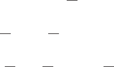
250 Chris Wendl
to detect different geometric phenomena via SFT. We will see an example of t he
latter in Lecture
13.
The compactness and gluing theory of SFT is encoded algebraically by viewing H
as an element on a noncommutative operator algebra determined by the commutator
relations
[p
γ
, q
γ
] = κ
γ
~
[p
γ
, q
γ
′
] = 0 if γ 6= γ
′
.
(12.9)
Here [ , ] again denotes the graded commutator (
12.4), so “commuting” generators
actually anticommute whenever they ar e both odd. The rest of the multiplicative
structure of this algebra is determined by requiring all elements of R and powers
of ~ (all of which are even generators) to commute with everything, meaning all
operators are R[[~]]-linear.
One concrete representation of this operator algebra is as follows: let A denote
the graded supercommutative unital algebra over R g enerated by the set
q
γ
γ a good Reeb orbit
.
The ring of formal power series A[[~]] is then an R[[~]]-module. Define each of the
generators q
γ
to be R[[~]]-linear operators on A[[~]] via multiplication fr om the left,
and define p
γ
: A[[~]] → A[[~]] by
(12.10) p
γ
= κ
γ
~
∂
∂q
γ
.
Here the R[[~]]-linear partial derivative operator is defined via
∂
∂q
γ
q
γ
= 1,
∂
∂q
γ
q
γ
′
= 0 for γ 6= γ
′
and the graded Leibniz rule
∂
∂q
γ
(F G) =
∂F
∂q
γ
G + (−1)
|q
γ
||F |
F
∂G
∂q
γ
for all homogeneous elements F, G ∈ A[[~]].
Exercise 12.5. Check that the operator p
γ
: A[[~]] → A[[~]] defined above has
the correct degree and satisfies the commutation relations (
12.5) and ( 12.9).
Notice that while H contains terms of order −1 in ~, every term also conta ins
at least one p
γ
varia ble since all index 1 holomorphic curves in (R ×M, d(e
t
α)) have
at least one positive puncture. The substitution (
12.10) thus produces a differential
operator in which every term contains a nonnegative power of ~, giving a well-defined
R[[~]]-linear operato r
D
SFT
: A[[~]]
H
−→ A[[~]].
The following may be regarded a s the fundamental theorem of SFT.
Theorem 12.6. H
2
= 0.

Lectures on Symplectic Field Theory 251
We will discuss in §12.6 how this relation follows from the compactness and
gluing theory of punctured holomorphic curves, and we will use it in Lecture
13 to
define various Floer-type contact inva r iants. The first and most obvious of these is
the homology
H
SFT
∗
(M, ξ) := H
∗
(A[[~]], D
SFT
),
which will tur n out to be an invariant of (M, ξ) in the sense that any two choices
of α, J and the other auxiliary data described in §
12.2 gives rise to a functorial
isomorphism between the two graded homology groups. No t ice that while A[[~]] is
an algebra, its product structure does not descend to H
SFT
∗
(M, ξ) since D
SFT
is not a
derivation— indeed, it is a fo r ma l sum of different ial operators of all orders, not just
order one. In the next lecture we will discuss various ways to produce homo logical
invariants out of H with nicer algebraic structures.
On the other ha nd, it is fairly easy to understand the geometric meaning of the
complex (A[[~]], D
SFT
) in Floer-theoretic terms. Each individual curve u ∈ M
σ
1
(J)
with g enus g, homology class A ∈ H
2
(M) and asymptotic orbits γ
±
= (γ
±
1
, . . . , γ
±
k
±
)
contributes to D
SFT
the differential operator
ǫ(u)
|Aut
σ
(u)|
κ
γ
+
~
g+k
+
−1
e
A
q
γ
−
1
. . . q
γ
−
k
−
∂
∂q
γ
+
1
. . .
∂
∂q
γ
+
k
+
.
Applying this operator to a monomial q
γ
1
. . . q
γ
m
∈ A[[~]] that does not contain all of
the generators q
γ
+
1
, . . . , q
γ
+
k
+
will produce zero, and its effect on a product that does
contain all of these generators will be to eliminate them and multiply q
γ
−
1
. . . q
γ
−
k
−
by
whatever remains, plus some combinatorial factors and signs that may ar ise from
differentiating by the same q
γ
more than once. Ignoring the combinatorics and
signs for the mo ment, this operation on q
γ
1
. . . q
γ
m
has a g eometric interpretation:
it counts all po tentially disconnected J-holomorphic curves of index 1 (i.e. disjoint
unions of u with trivial cylinders) that have γ
1
, . . . , γ
m
as their positive asymptotic
orbits; see Figure
12.1. In other words, the action of D
SFT
on each monomial q
γ
for
γ = (γ
1
, . . . , γ
m
) is determined by a f ormula of the form
(12.11) D
SFT
q
γ
=
∞
X
g=0
X
A∈H
2
(M)
X
γ
′
m
X
k=1
~
g+k−1
e
A
n
g
(γ, γ
′
, k)q
γ
′
,
where n
g
(γ, γ
′
, k) is a product of some combinatorial factors with a signed count of
generally disconnected index 1 holomorphic curves of genus g and homology class A
with positive ends at γ and negative ends at γ
′
, such that the nontrivial connected
component has exactly k positive ends. The presence of t he combinatorial factors
hidden in n
g
(γ, γ
′
, k) is a slightly subtle po int which we will try to clarify in the
following sections.
12.4. Interlude: How to count points in an orbifold
As in all versions of Floer theory, the proof that H
2
= 0 is based on the fact that
certain moduli spaces are compact oriented 1-dimensional manifolds with bound-
ary, and the signed count of their boundary points is therefore zero. We must be
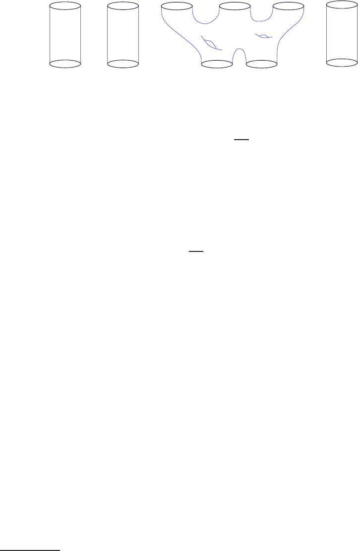
252 Chris Wendl
γ
1
γ
2
γ
3
γ
4
γ
5
γ
6
γ
7
γ
8
u
Figure 12.1. Counting disjoint unio ns of index 1 curves u ∈
M
2,0
(J, A, (γ
3
, γ
4
, γ
5
), (γ
7
, γ
8
)) with some trivial cylinders contributes
a multiple of ~
4
e
A
q
γ
1
q
γ
2
q
γ
7
q
γ
8
q
γ
6
to D
SFT
(q
γ
1
q
γ
2
q
γ
3
q
γ
4
q
γ
5
q
γ
6
).
careful of course because, strictly speaking,
M(J) is not a manif old even when
Assumption
12.1 holds—it is an orbifold, with the possibility of singularities at mul-
tiply covered curves with no ntrivial automorphism groups. On the other hand, one
can show that (after excluding curves with bad asymptotic orbits) it is an oriented
orbifold, and oriented 1-dimensional o r bif olds happen to be very simple objects:
since smooth finite gro up actions on R cannot be nontrivial without reversing ori-
entation, all oriented 1-dimensional orbifolds are actually manifolds, suggesting the
simple f ormula
“#∂
M
1
(J) = 0.”
I have placed this formula in quotation marks for a reason. The reality of the
situation is somewhat more complicated.
This is in fact where it becomes important to remember t hat Assumption 12.1, in
the way that we stated it, really is not just science fiction but fa ntasy: transversality
is sometimes impossible to achieve for multiple covers, and we must therefore at least
have a sensible back-up plan for such cases. To see the problem, remember that our
local structure theorem for M(J) was proved by identifying it in a neighborhood o f
any curve u
0
: (
˙
Σ, j
0
) → (R × M, J) with a set of the form
¯
∂
−1
J
(0)
G,
where
¯
∂
J
: T ×B
k,p,δ
→ E
k−1,p,δ
is a smooth section of a Banach space bundle E
k−1,p,δ
over the product of a Teichm¨uller slice T through j
0
with a Banach manifold B
k,p,δ
of maps
˙
Σ → R × M, and G is the group of automorphisms of j
0
, whose action on
the base
1
G × (T × B
k,p,δ
) → T × B
k,p,δ
: (ψ, (j, u)) 7→ (ψ
∗
j, u ◦ ψ)
preserves
¯
∂
−1
J
(0). In fact, the action of G on T ×B
k,p,δ
is covered by a natural action
on the bundle E
k−1,p,δ
, and the reason fo r it preserving the zero-set is that
¯
∂
J
is an
equivariant section,
¯
∂
J
(ψ
∗
j, u ◦ ψ) = ψ
∗
¯
∂
J
(j, u).
1
As you may k now if you’ve ever heard a talk abo ut polyfolds, there are some analytical
problems with this discussion if G is a Lie group of positive dimension: its action on the infinite-
dimensional manifold B
k,p,δ
of non-smooth maps cannot then be considered smooth in any con-
ventional sense. This proble m leads to the introduction of sc-smooth structures, cf. [
HWZ07].
There is no problem however if G is finite, e.g. if the under lying Riemann surface is stable, which
we may as well assume for this discussion.
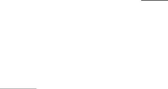
Lectures on Symplectic Field Theory 253
If G is finite, then another way to say this is that
¯
∂
J
is a smooth Fredholm section
of the infinite-dimensional orbibundle E
k−1,p,δ
/G over the orbifold (T × B
k,p,δ
)/G,
whose isotr opy g r oup at (j
0
, u
0
) is Aut(u
0
). This section is transverse to the zero-
section if and only if the usual regularity condition holds, making
¯
∂
−1
J
(0)/G a sub orb-
ifold of (T ×B
k,p,δ
)/G whose isotropy group at (j
0
, u
0
) is some quotient of Aut(u
0
).
Remark 12 .7. Most sensible definitions of the term orbifold (cf. [
ALR07,Dav,
FO99]) require local models of the form U/G, where U is a G-invariant open subset
of a vector space on which the finite group G acts smoothly and effectively—the
latter condition is necessary in order to have isotropy groups t hat are well-defined
up to isomorphism at every point. In the above example, G acts effectively on
T × B
k,p,δ
but might have a nontrivial subgroup H ⊂ G of transformations that
fix every element of
¯
∂
−1
J
(0), in which case the G-action on
¯
∂
−1
J
(0) can be replaced
by an effective actio n of G/H. The isotropy group of (j
0
, u
0
) ∈
¯
∂
−1
J
(0)/G is then
Aut(u
0
)/(Aut(u
0
) ∩ H).
Now to see just how unreasonably optimistic Assumption
12.1 is, not ice that it’s
easy to think up examples of smooth orbibundles in which zeroes of sections can
never be regular if they have nontrivial isotropy.
Example 12.8. Let M = C/Z
2
with Z
2
acting as the antipodal map, and
consider the trivial complex line bundle E = M × C = (C × C)/Z
2
, where the Z
2
action on C × C identifies (z, v) with (−z, v). A smooth function f : C → C then
represents a section of t he orbibundle E → M if and only if f(z) = f (−z) for all z.
This implies t hat if f(0) = 0, then df(0) = 0. It is possible to perturb f generically
to a section that is transverse to the zero-section, but such a perturbation can never
have zeroes at 0.
Of course, we do know how to assign Z-valued orders to degenerate zeroes of
sections, e.g. f(z) = z
2
defines a section of E → M with a zero of order 2 at 0.
Notice however that if we perturb this to f
ǫ
(z) = z
2
+ ǫ for ǫ > 0 small, then f
ǫ
has
two simple zeroes at points near the origin, but they are actually the same point in
C/Z
2
, giving a count of only 1 zero. This means that if we give the zero of f at the
origin its full weight, then we are counting wrongly—the resulting count will not be
homotopy invariant. The correct algebraic count of zero es is evidently
(12.12) #f
−1
(0) :=
X
z∈f
−1
(0)⊂M
ord(f; z)
κ
z
∈ Q,
where ord(f ; z) ∈ Z is the order of t he zero (computed in t he usual way as a winding
number, or in higher dimensions as the degree of a map of spheres, cf. [
Mil97]), and
κ
z
∈ N denotes the order of the isotropy g r oup at z.
Exercise 12.9. Convince yourself that for any smooth oriented orbibundle E →
M of real ra nk m over a compact, smooth and oriented m-dimensional orbifold M
without boundary, the count (
12.12) gives the same result for any section with
isolated zeroes.
2
Hint: The space of sections of an orbibundle is still a vector space, so any two
2
If you’re still not sure what an orbibundle is, a definition can be found in [
FO99, Chapter 1].

254 Chris Wendl
are homo t opic. Since M and [0, 1] are both compact, it suffices to focus on small
perturbations of a single section on a single orbifold chart.
For a slightly different perspective on (
12.12), consider the special case of a closed
orbifold that is the quotient of a closed manifold
f
M by an effective orientation-
preserving finite group action,
M =
f
M/G.
Suppose
e
E →
f
M is an oriented vector bundle with rank equal to dim M, and G also
acts on
e
E by orientation-preserving linear bundle maps that cover its action on
f
M,
so the quotient
E =
e
E/G → M
is an orbibundle. A section f : M → E is then equivalent to a G-equivariant section
˜
f :
f
M →
e
E, and the signed count of zeroes
#
˜
f
−1
(0) =
X
z∈
˜
f
−1
(0)⊂
f
M
ord(
˜
f; z) ∈ Z
is of course the same for any section that has only isolated zeroes. It can also be
expressed in terms of f since any z ∈ f
−1
(0) ⊂ M has exactly |G|/κ
z
lifts to points
in
˜
f
−1
(0) ⊂
f
M, implying
#
˜
f
−1
(0) =
X
z∈f
−1
(0)⊂M
|G|
κ
z
ord(f; z)
and thus #f
−1
(0) =
1
|G|
#
˜
f
−1
(0). The invariance of ( 12.12) is now an immediate
consequence of the invaria nce of #
˜
f
−1
(0), which follows from the standard argument
as in [
Mil97].
Now, if you enjoyed reading [
Mil97] as much as I did, then it may seem tempting
to try proving invaria nce of (
12.12) in general by choo sing a generic homotopy
H : [0, 1] × M → E between two generic sections f
0
and f
1
and showing that
H
−1
(0) ⊂ [0, 1] × M is a compact oriented 1-dimensional o rbifold with boundary.
As we observed at t he beginning of this section, H
−1
(0) is then actually a manifo ld,
so the signed count of its boundary points should be zero. But this would give
the wrong result: it would sugg est that
P
z∈f
−1
(0)⊂M
ord(f; z) should be homotopy
invariant, without the ratio nal weights, and we’ve a lr eady seen that this is not true.
What is going on here? The answer is that the ho mo gopy H cannot in general be
made transverse to the zero-section, now matter how generically we perturb it! It
is an illustration of the fundamental conflict between the notions of genericity and
eq uivariance.
Example 12.10 . Let M = C/Z
2
as in Example
12.8, but define the complex
orbibundle E → M by
E = (C × C)
(z, v) ∼ (−z, −v),
i.e. the Z
2
-action also acts antipodally on fibers. Now a smooth function f : C → C
defines a section of E if and only if f(−z) = −f(z), hence all such sections have a

Lectures on Symplectic Field Theory 255
zero a t the origin. Compare the two sections
f
0
(x + iy) = x + iy, f
1
(x + iy) = (x
3
− x) + iy.
They have qualitatively the same behavior near infinity, meaning in particular that
they are homotopic thro ugh a family of sections whose zeroes are confined to some
compact subset, thus we expect the algebraic count of zeroes to be the same for both.
This is true if the count is defined by (
12.12): we have #f
−1
0
(0) = #f
−1
1
(0) =
1
2
, in
particular the nega tive zero of f
1
at the origin counts fo r −1/2 while the positive
zero at (1, 0) ∼ (−1, 0 ) counts f or 1. We see that the inclusion of the rational weight s
1
κ
x
is crucial for this result. Notice that if H : [0, 1] × M → E is a homotopy o f
sections fr om f
0
to f
1
, then H(τ, 0) = 0 for all τ, thus ∂
τ
H(τ, 0) vanishes and
dH(τ, 0) = df
τ
(0)
where f
τ
= H(τ, ·). But df
τ
(0) cannot be an isomorphism for all τ ∈ (0, 1) since
df
0
(0) preserves orientation while df
1
(0) reverses it. This is not a problem that can
be fixed by making H more generic—the homotopy will never be transverse to the
zero-section, no matter what we do.
The need to address issues of the type raised by the above examples leads na t u-
rally to the notion of multisections as outlined in [
Sal99, §5] and [FO99], and this
is a major f eat ur e of the analysis under development by Hofer-Wysocki-Zehnder, see
for example [
HWZ10]. In Example 12.10 for instance, one can consider functions
f : C → Sym
2
(C) := (C × C)
(z
1
, z
2
) ∼ (z
2
, z
1
),
which can be regarded as doubly-valued sections of E → M if f is Z
2
-equivariant
for the antipodal a ctio n of Z
2
on the symmetric product Sym
2
(C). Such a section
is considered single-valued at any point z where f(z) is of the form [(v, v)], so o ne
can now ima gine homotopies from f
0
to f
1
through doubly-valued sections. One
advantage of this generalization is that f can now take nonzero va lues of the form
[(v, −v)] a t the origin, e.g. if g : C → C is any odd function, then
f(z) := [(g(z) + c, g(z) − c)]
is a well-defined multisection for every c ∈ C.
Exercise 12.11. Find a homotopy between the sections f
0
and f
1
of Exam-
ple
12.10 through doubly-valued sections, such that the homot opy is transverse to
the zero-section.
You may notice if you work out Exercise
12.11 that the zero set of the homotopy
in [0, 1] × M is still not submanifold or suborbifold. Instead, it naturally carries
the structure of a w eighted branched manifold with boundary. The rational weights
attached to every point in this object can be used to explain the weights appearing
in (
12.12) and thus give a Milnor-style proof that #f
−1
(0) ∈ Q is invariant.
We will no t discuss multisections or weighted branched manifolds any further,
but the main takeaway from this discussion should be that the “right” way to count
0-dimensional orbifolds algebraically is always some version of (
12.12), and the count
in general is a rational number, not an integer. We’ve discussed this above from
the perspective of obtaining a homotopy-invariant count, but the same logic a pplies
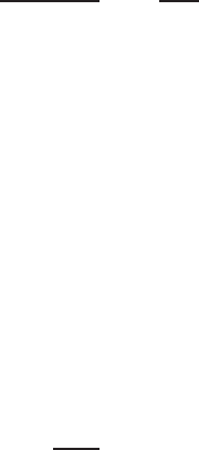
256 Chris Wendl
to any Floer-type theory since the relation ∂
2
= 0 is typically based on similar
arguments via 1-dimensional moduli spaces with boundary. While a more simplistic
notion of counting may produce well-defined homology theories in isolated cases
where Assumption
12.1 holds (e.g. in [Nel15]), we cannot expect it to generalize
beyond these cases, due to the fundamental conflict between transversality and
equivariance. On the other hand, it will be possible in our situation to r emove
isotropy from the picture by lifting to moduli spaces with asymptotic markers; the
moduli space we’re interested in is always the quotient of this larger space by a
finite group action, so the situation is analogous t o replacing an orbibundle E =
e
E/G →
f
M/G by an ordinary vector bundle
e
E over a manifold
f
M. In the infinite-
dimensional setting, transversality is still a hard problem, but having lifted to a
manifold and thus removed t he need for equivariance, there is no longer any a priori
reason why it cannot be solved by choosing sufficiently generic perturbations. This
makes counting curves with rational weights seem a much more promising method
for defining invaria nts, and we will adopt this perspective in the discussion to follow.
12.5. Cylindrical contact homology revisited
Under an extra assumption on the complex (A[[~]], D
SFT
), we can recover from
it a more general version of the cylindrical conta ct homology we saw in Lecture
10.
Suppose in part icular that there are no index 1 holo mo r phic planes in R × M, so
every term in ~H has at least one factor of either ~ or one o f the q
γ
varia bles. Then
D
SFT
=
X
γ,γ
′
,A
κ
γ
X
u∈M
0,0
(J,A,γ,γ
′
)/R
ǫ(u)
|Aut(u)|
e
A
q
γ
′
∂
∂q
γ
+ . . . ,
where the first sum is over all pairs of good Reeb orbits γ and γ
′
, and the ellipsis
is a sum of terms that all include at least a positive power of ~ or two q
γ
varia bles
or two partial derivatives. Let us abbreviate t he spaces M
0,0
(J, A, γ, γ
′
)/R of R-
equivalence classes of J-holomor phic cylinders by M
A
(γ, γ
′
), and notice that for
any u ∈ M
A
(γ, γ
′
), the automorphism group is a cyclic group of order equal to the
covering multiplicity
|Aut(u)| = κ
u
:= cov(u) ∈ N.
Thus for any single g enerato r q
γ
, we have
D
SFT
q
γ
= ∂
CCH
q
γ
+ O(|q|
2
, ~),
where
(12.13) ∂
CCH
q
γ
:= κ
γ
X
γ
′
,A
X
u∈M
A
(γ,γ
′
)
ǫ(u)
κ
u
e
A
q
γ
′
.
The fact that D
2
SFT
= 0 thus implies
∂
2
CCH
= 0,
and the homology of the graded R-module generated by {q
γ
| γ good} with differ-
ential ∂
CCH
is an obvious generalization of the cylindrical contact homology from
Lecture
10. What we saw there was a special case of this where the combinatorial
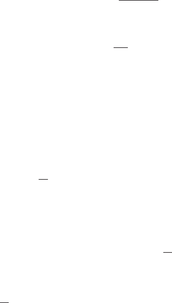
Lectures on Symplectic Field Theory 257
factor κ
γ
/κ
u
did not appear because we were restricting to a homotopy class in which
all orbits were simply covered, and all holomorphic cylinders were thus somewhere
injective.
The presence of the factor κ
γ
/κ
u
deserves further comment. According to the
above formula, we have
∂
2
CCH
q
γ
=
X
γ
′
,γ
′′
,A,A
′
X
u∈M
A
(γ,γ
′
)
X
v∈M
A
′
(γ
′
,γ
′′
)
e
A+A
′
κ
γ
κ
γ
′
ǫ(u)ǫ(v)
κ
u
κ
v
q
γ
′′
,
hence ∂
2
CCH
= 0 holds if and only if for all A ∈ H
2
(M) and all pairs of good orbits
γ
+
, γ
−
,
(12.14)
X
γ
0
X
B+C=A
X
(u,v)∈M
B
(γ
+
,γ
0
)×M
C
(γ
0
,γ
−
)
κ
γ
0
κ
u
κ
v
ǫ(u)ǫ(v)
= 0.
If γ
+
and γ
−
happen to be simply covered orbits, then u and v in this expression
always have trivial automorphism groups and it is clear what this sum means: every
such pair (u, v) ∈ M
B
(γ
+
, γ
0
)×M
C
(γ
0
, γ
−
) corresponds to exactly κ
γ
0
distinct holo-
morphic buildings obtained by different choices of decoration, so (
12.14) is the count
of boundary points of t he compactified 1-dimensional manif old of index 2 cylinders
M
A
(γ
+
, γ
−
)/R. This sum skips over all bad orbits γ
0
, but this is fine because when-
ever the breaking orbit is bad, there are evenly many cho ices of decoration such that
half of these choices cancel the other half when counted with the correct signs.
To understand why this formula is still correct in the presence of automorphisms,
let us outline two equivalent approaches.
The easiest o ption is to instead consider moduli spaces with asymptotic markers,
which never have automorphisms: removing unnecessary factors of κ
γ
+
and κ
γ
−
then
transforms (
12.14) into
X
γ
0
X
B+C=A
1
κ
γ
0
#M
$
B
(γ
+
, γ
0
) · #M
$
C
(γ
0
, γ
−
) = 0.
Now since each pair (u, v) ∈ M
$
B
(γ
+
, γ
0
)×M
$
C
(γ
0
, γ
−
) carries a canonical decoration
and thus determines a holo mo rphic building, the division by κ
γ
0
accounts for the
fact that #M
$
B
(γ
+
, γ
0
) · #M
$
C
(γ
0
, γ
−
) overcounts the set of broken cylinders from
γ
+
to γ
−
with asymptotic markers at γ
±
by precisely this factor, as a simultaneous
adjustment of the marker at γ
0
in both u ∈ M
$
B
(γ
+
, γ
0
) and v ∈ M
$
C
(γ
0
, γ
−
)
produces the same decoration and therefore the same building.
The following alternative perspective will be more useful when we generalize
beyond cylinders in the next section. We can directly count po ints in ∂
M
A
(γ
+
, γ
−
),
though as we saw in §
12.4, rational weights should be included in the count whenever
there is isotropy. Let us write
M
A
(γ
+
, γ
−
) = M
$
A
(γ
+
, γ
−
)/G,
where G
∼
=
Z
κ
γ
+
× Z
κ
γ
−
is a finite gr oup acting by adjustment of the asymptotic
markers. Since
M
$
A
(γ
+
, γ
−
) is a compact oriented 1-manifold with boundary under
Assumption
12.1, the signed count of its boundary points is 0. We can ignore
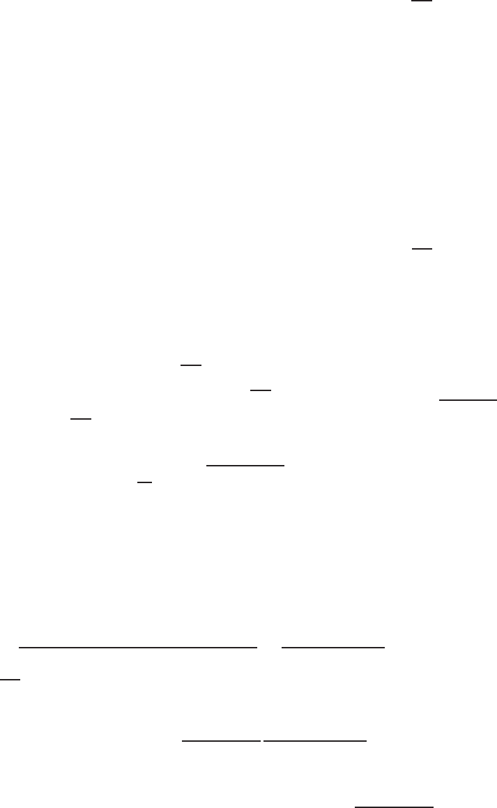
258 Chris Wendl
buildings broken along bad orbits in this count, since these always come in cancelling
pairs. Let us now transform this into a count of buildings (u|Φ|v) ∈ ∂
M
A
(γ
+
, γ
−
)
broken along good orbits γ
0
: here u ∈ M
B
(γ
+
, γ
0
) and v ∈ M
C
(γ
0
, γ
−
) for some
homology classes with B + C = A, and Φ is a decoration which describes how to
glue the ends of u and v at γ
0
. The automorphism group o f such a building is the
subgroup
Aut(u|Φ|v) ⊂ Aut(u) × Aut(v)
consisting of all pairs (ϕ, ψ) ∈ Aut(u) ×Aut(v) that define the same rotation at t he
two punctures asymptotic to γ
0
; note that this group does not actually depend on
the decoration Φ. Since we’re talking about cylinders, we can be much more specific:
we have Aut( u) = Z
κ
u
and Aut(v) = Z
κ
v
, and if both are regarded as subgroups of
U(1),
Aut(u|Φ|v) = Z
κ
u
∩ Z
κ
v
= Z
gcd(κ
u
,κ
v
)
,
which is injected into Aut(u)×Aut(v) by ψ 7→ (ψ, ψ) . The boundary of
M
$
A
(γ
+
, γ
−
)
can be understood likewise as a space of equivalence classes
[(u, v)] ∈
M
$
B
(γ
+
, γ
0
) × M
$
C
(γ
0
, γ
−
)
∼,
where two such pairs are equiva lent if their asymptotic markers at the ends as-
ymptotic to γ
0
determine the same decoration. Now observe t ha t the gr oup G
∼
=
Z
κ
γ
+
×Z
κ
γ
−
also acts on buildings in ∂
M
$
A
(γ
+
, γ
−
), and the stabilizer of this action
at (u, v) is Aut(u|Φ|v), hence each (u|Φ|v) ∈ ∂
M
A
(γ
+
, γ
−
) gives rise to
|G|
gcd(κ
u
,κ
v
)
terms in the count of ∂
M
$
A
(γ
+
, γ
−
), implying
(12.15)
X
(u|Φ|v)∈∂
M
A
(γ
+
,γ
−
)
ǫ(u)ǫ(v)
gcd(κ
u
, κ
v
)
= 0.
Finally, notice that while each pair (u, v) ∈ M
B
(γ
+
, γ
0
) × M
C
(γ
0
, γ
−
) determines
buildings with κ
γ
0
distinct choices of decoration, some of these buildings may be
equivalent: every pair of automorphisms ( ϕ, ψ) ∈ Aut(u) × Aut(v) transforms a
building (u|Φ|v) by potentially changing the decoration Φ, thus producing an equiv-
alent building. This action on buildings is trivial if and only if (ϕ, ψ) ∈ Aut(u|Φ|v),
hence every pair (u, v) ∈ M
B
(γ
+
, γ
0
) × M
C
(γ
0
, γ
−
) gives rise t o exactly
κ
γ
0
(Aut(u) × Aut(v))
Aut(u|Φ|v)
=
κ
γ
0
gcd(κ
u
, κ
v
)
κ
u
κ
v
elements of ∂
M
A
(γ
+
, γ
−
), so that (12.15) becomes
X
γ
0
X
B+C=A
X
(u,v)∈M
B
(γ
+
,γ
0
)×M
C
(γ
0
,γ
−
)
ǫ(u)ǫ(v)
gcd(κ
u
, κ
v
)
κ
γ
0
gcd(κ
u
, κ
v
)
κ
u
κ
v
=
X
γ
0
X
B+C=A
X
(u,v)∈M
B
(γ
+
,γ
0
)×M
C
(γ
0
,γ
−
)
ǫ(u)ǫ(v) κ
γ
0
κ
u
κ
v
= 0,
reproducing (
12.14).
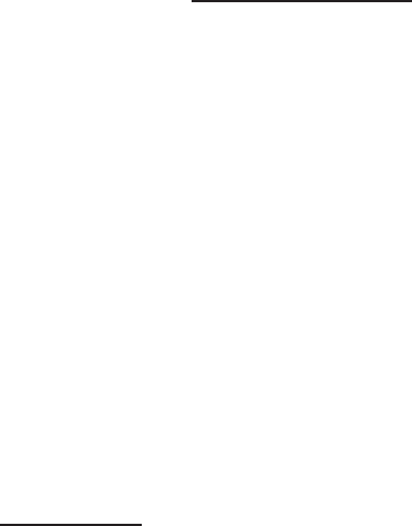
Lectures on Symplectic Field Theory 259
12.6. Combinatorics of gluing
Now let’s try to justify the formula H
2
= 0. The product of H with itself is the
formal sum over all pairs of index 1 curves u, v ∈ M
σ
1
(J)/R of certain monomials:
in particular if these two curves respectively have genus g
u
and g
v
, homology classes
A
u
and A
v
, and asymptotic orbits γ
±
u
and γ
±
v
, then the corresponding term in H
2
is
ǫ(u)ǫ(v)
|Aut
σ
(u)||Aut
σ
(v)|
~
g
u
+g
v
−2
e
A
u
+A
v
q
γ
−
u
p
γ
+
u
q
γ
−
v
p
γ
+
v
.
Before we can add up a ll monomials of this form, we need to put all the q and p
varia bles in the same order: within each of the products q
γ
−
u
, p
γ
+
u
and so forth this is
simply a matter of permuting the variables and chang ing signs as appropriate, but
the interesting par t is the product p
γ
+
u
q
γ
−
v
, for which we can apply the commutation
relations (
12.9) to put all q variables before all p variables. Before discussing how
this works in general, let us consider a more specific example.
Assume γ
i
for i = 1, 2 are two specific orbits with n − 3 + µ
CZ
(γ
i
) even, so the
corresponding q and p var iables have even degree, and suppose
γ
+
u
= (γ
1
, γ
1
, γ
2
), γ
−
v
= (γ
1
, γ
1
).
After applying t he relation p
γ
1
q
γ
1
= q
γ
1
p
γ
1
+ κ
γ
1
~ a total of five times, one obtains
the expansion
p
γ
1
p
γ
1
p
γ
2
q
γ
1
q
γ
1
= q
2
γ
1
p
2
γ
1
p
γ
2
+ 4κ
γ
1
~q
γ
1
p
γ
1
p
γ
2
+ 2κ
2
γ
1
~
2
p
γ
2
,
thus contributing a total o f three terms to H
2
, namely the products o f the factor
ǫ(u)ǫ(v)
|Aut(u)||Aut(v)|
e
A
u
+A
v
with each of the expressions
~
g
u
+g
v
−2
q
γ
−
u
q
2
γ
1
p
2
γ
1
p
γ
2
p
γ
+
v
,(12.16)
4κ
γ
1
~
g
u
+g
v
−1
q
γ
−
u
q
γ
1
p
γ
1
p
γ
2
p
γ
+
v
,(12.17)
2κ
2
γ
1
~
g
u
+g
v
q
γ
−
u
p
γ
2
p
γ
+
v
.(12.18)
As shown in Figure
12.2, this sum of three terms can be interpreted as the count of
all possible ho lomrphic buildings obtained by gluing v on top of u together with a
collection of trivial cylinders. Indeed, since γ
+
u
and γ
−
v
include two matching orbits
(which also happen to be the same one), there are several choices to be made:
(1) The top-right picture shows what we might call the “stupid gluing,” in
which no ends of u a re matched with any ends of v, but all are instead
glued to trivial cylinders, thus producing a disconnected building. This
possibility is encoded by (
12.16), and we will see that in the total sum
forming H
2
, this term gets cancelled out by a similar term for the stupid
gluing of u on top of v.
(2) The lower-left picture shows the building obtained by gluing one end of
u to an end of v alo ng the matching orbit γ
1
. This option is encoded
by (
12.17), where t he factor 4κ
γ
1
appears because there are precisely 4κ
γ
1
distinct buildings of this type: indeed, there are four choices of which end
of u should be glued to which end of v, and for each of these, a further κ
γ
1
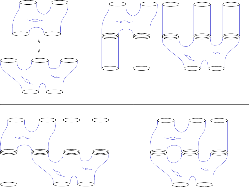
260 Chris Wendl
u
u
u
u
v
v
v
v
γ
1
γ
1
γ
1
γ
1
γ
1
γ
1
γ
1
γ
1
γ
1
γ
1
γ
1
γ
1
γ
1
γ
2
γ
2
γ
2
γ
2
γ
−
u
γ
−
u
γ
−
u
γ
−
u
γ
+
v
γ
+
v
γ
+
v
γ
+
v
Figure 12.2. Three possible ways of gluing the curves u and v
along with trivial cylinders to form index 2 curves.
choices of the decoration. The arithmetic genus of the resulting building is
g
u
+ g
v
, as represented by the factor ~
g
u
+g
v
−1
.
(3) The lower-right picture is enco ded by (
12.18): here there are two choices of
bijections between the two pair s of punctures asymptotic to γ
1
, and taking
the choices of decoration at each breaking orbit into account, we obtain the
combinatoria l factor 2κ
2
γ
1
. The presence of two nontrivial breaking orbits
increases the arithmetic genus to g
u
+g
v
+1, as encoded in the factor ~
g
u
+g
v
.
You may now be able to extrapolate from the above example why the commu-
tator algebra we’ve defined enco des gluing of holomorphic curves in the symplec-
tization and thus leads to the relation H
2
= 0. Think of the algorithm by which
you change q
γ
−
u
p
γ
+
u
q
γ
−
v
p
γ
+
u
into a sum of products with all q’s appearing before p’s:
for the first q you see appearing after a p, move it past each p for different orbits
(changing signs as necessary) until it encounters a p for the same orbit. Now you
replace p
γ
q
γ
with (−1)
|p
γ
||q
γ
|
q
γ
p
γ
+ κ
γ
~, turning one pr oduct into a sum of two. This
represents a choice between two options: either you move q
γ
past p
γ
and apply the
Lectures on Symplectic Field Theory 261
usual sign change, or you eliminate them both but replace t hem with the combina-
torial factor κ
γ
and an extra ~. Then you continue t his process until all q’s appear
before all p’s.
The key point is t ha t the process of gluing v on top of u in all possible ways is
governed by e xactly the same algorithm: first consider the disjoint union of the two
curves as a single disconnected curve, with its punctures o r dered in the same way
in which their orbits appear in t he monomial. Now reorder negative punctures of v
and positive punctures of u, changing orientations a s appropriate, until yo u see two
such punctures next to each other approaching the same orbit γ. Here you have two
options: either glue them together, or don’t glue them but exchange t heir order. If
you exchange the order, then you may again have to change orientatio ns (depending
on the parity of n − 3 + µ
CZ
(γ)), but if you glue, then you have κ
γ
distinct choices
of decoration and will also increase the arithmetic genus of the eventual building
by 1. In this way, every individual term in the final expansion of q
γ
−
u
p
γ
+
u
q
γ
−
v
p
γ
+
u
represents a particular choice of which positive of ends of u should or should not be
glued to which negative ends of v. Additional factors of ~ appear to keep track of
the increase in arithmetic genus, and covering multiplicities o f t he breaking orbits
also appear due to distinct choices of decorations. At the end these must still be
divided by orders of automorphism groups in order to avoid counting equivalent
buildings separately. Fleshing out these details leads to t he following explanation
for the relation H
2
= 0:
Proposition 12 .12. Let ∂
M
σ
2
(J) denote the space of two-level ho l omorphic
buildings in
M(J) that have total index 2 and no bad asymptotic or breaking orbits,
divided by the equivalence relation that forgets the order of the punctures. Then
H
2
=
X
u∈∂
M
σ
2
(J)
ǫ(u)
|Aut
σ
(u)|
~
g−1
e
A
q
γ
−
p
γ
+
,
where the terms in each monomial are determined by u ∈ ∂
M
σ
2
(J) as follows:
(1) g is the arithmetic genus of u;
(2) A is the equivalence class of [u] ∈ H
2
(M) in H
2
(M)/G;
(3) γ
±
= (γ
±
1
, . . . , γ
±
k
±
) are the asymptotic orbits of u after arbitrarily fixing
ord erings of i ts positive and negative punctures;
(4) ǫ(u) ∈ {1, −1} is the boundary orientation at u determined by the chosen
co herent o rientations on M
$
(J). Speci fically, given the c hosen orderin g of
the punctures and an arbitrary choice of asymptotic markers at each punc-
ture, u determines a boundary point of a 1-dimension al co nnected compo-
nent of
M
$
(J), and we define ǫ(u) = +1 if and only if the orientation of
M
$
(J) at this poi nt is outward.
Once again ǫ(u) and q
γ
−
p
γ
+
change signs in the same way under any reordering
of the punctures, so t heir product is well defined, and there is no dependence on
choices of markers since bad orbits have been excluded.
262 Chris Wendl
Proof of Proposition 12.12. Our original f ormula for H gives rise to an
expansion
H
2
=
X
(u,v)∈M
σ
1
(J)/R×M
σ
1
(J)/R
ǫ(u)ǫ(v)
|Aut
σ
(u)||Aut
σ
(v)|
~
g
u
+g
v
−2
e
A
u
+A
v
q
γ
−
u
p
γ
+
u
q
γ
−
v
p
γ
+
v
.
As explained in the previous paragraph, the process of reordering p
γ
+
u
q
γ
−
v
to put all
q’s befo re p’s produces an expansion, each term of which can be identified with a
specific choice of which positive punctures of u should be g lued to which negative
punctures of v. If k punctures are glued, then the resulting power of ~ is g
u
+
g
v
−2+ k, corresponding to the fact that the resulting building has arithmetic genus
g
u
+g
v
+k−1. We claim that t he term for k = 0 is cancelled out by the corresponding
term of H
2
that has the roles of u and v reversed. To see this, imagine first the case
where u and v have no asymptotic orbits in common, hence no nontrivial gluings
are possible and all the q and p variables in the expression supercommut e with each
other. Then since both curves have index 1, the monomials q
γ
−
u
p
γ
+
u
and q
γ
−
v
p
γ
+
v
must
both have odd degree, implying
q
γ
−
u
p
γ
+
u
q
γ
−
v
p
γ
+
v
= −q
γ
−
v
p
γ
+
v
q
γ
−
u
p
γ
+
u
and thus the desired cancellation. If u and v do have orbits in common, then t he
result for the k = 0 terms is still not any different from this: all signs still change
in t he same way when applying [p
γ
, q
γ
] = κ
γ
~ to change p
γ
q
γ
into q
γ
p
γ
, we simply
ignore the extra term κ
γ
~ since it is only relevant for gluings with k > 0. This
proves the claim, and consequently, that the expansion resulting from the curves u
and v has no term containing ~
g
u
+g
v
−2
.
The combinatorial factors can be explained a s follows. The commutator expan-
sion for p
γ
+
u
q
γ
−
v
automatically produces combinator ial factors that count the different
possible gluings, but if u and v have automorphisms, then not all of these give in-
equivalent buildings. This part of the discussion is a straightfor ward extension of
what we did for cylindrical contact ho mo logy at the end of §
12.5. Indeed, the a ctual
set of inequivalent buildings is the quotient of this larger set by an action of
(Aut
σ
(u) × Aut
σ
(v))
Aut
σ
(u),
where for a building u formed by endowing the pa ir (u, v) with decorations, Aut
σ
(u)
denotes the subgroup consisting of pairs (ϕ, ψ) ∈ Aut
σ
(u) × Aut
σ
(v) that preserve
pairs of breaking punctures along with their decorations. This is what changes the
factor
1
|Aut
σ
(u)||Aut
σ
(v)|
into
1
|Aut
σ
(u)|
as in the statement of the proposition.
The theorem that H
2
= 0 now follows once you believe the propag anda from
§
12.4, arguing that
P
u∈∂
M
σ
2
(J)
ǫ(u)
|Aut
σ
(u)|
is the correct way to count the bo undar y
points of M
σ
2
(J). As we did with cylindrical contact homology, we can use the obvi-
ous projection
M
$
(J) → M
σ
(J) to reduce t his to the fact that if the 1-dimensional
components of
M
$
(J) are manifolds (which is true if Assumption 12.1 holds), then
the integer-valued signed count of their boundary points va nishes.

Lectures on Symplectic Field Theory 263
12.7. Some remarks on torsion, coefficients, and conventions
12.7.1. What if H
1
(M) has torsion? The main consequence for SFT if H
1
(M)
has torsion is that one cannot define an integer gr ading, though there is always a
canonical Z
2
-grading.
3
The setup in §12.2 must now be modified as follows. The
reference curves
C
1
, . . . , C
r
⊂ M
are required to fo rm a basis of H
1
(M)/torsion, so for every integral homology class
[γ], there is a unique collection of integers m
1
, . . . , m
r
such that [γ] =
P
i
m
i
[C
i
] ∈
H
1
(M; Q). Instead of spanning surfaces for each orbit, one can define spanning
chains C
γ
, which are singular 2-chains with rational coefficients satisfying
∂C
γ
=
X
i
m
i
[C
i
] − [γ]
for the aforementioned set of integers m
i
∈ Z. Note that C
γ
must in general
have nonintegral coefficients since
P
i
m
i
[C
i
] and [γ] mig ht not be homologous in
H
1
(M; Z), so C
γ
cannot always be represented by a smooth map of a surface. One
consequence of this is that the absolute homology class associated to an asymptoti-
cally cylindrical holomorphic curve u :
˙
Σ → R × M will now be rational,
[u] ∈ H
2
(M; Q),
and we must therefore take G to be a linear subspace
G ⊂ H
2
(M; Q).
Another consequence is that we cannot use capping chains to transfer trivializations
from the reference curves to the orbits, so there is no na tural way to define µ
CZ
(γ)
as a n integer. The easiest thing to do instead is to take the mod 2 Conley-Zehnder
index
µ
CZ
(γ) ∈ Z
2
and define all degrees of generators as either even or odd with no further distinction.
In par t icular, we now have
|q
γ
| = n − 3 + µ
CZ
(γ) ∈ Z
2
, |p
γ
| = n − 3 − µ
CZ
(γ) ∈ Z
2
,
while ~ and all elements of R = Q[H
2
(M; Q)/G] are even. With these modifications,
the rest of the discussion also becomes valid for the case where H
1
(M) has torsion,
and leads to Z
2
-graded contact invariants.
12.7.2. Combinatorial conventions. The combinatorial factors appearing in
our definition of H may at first look slightly different from what appears elsewhere in
the literature. Actually, most papers seem to ag ree on this detail, but va r ious subtle
differences and ambiguities in notation mean that it sometimes requires intense
concentration to recognize this fact.
The original propaganda paper [
EGH00] expresses everything in terms of moduli
spaces with asymptotic markers, and the f ormula for H in §2.2.3 of that paper (which
3
In fact ther e is a bit more than a Z
2
-grading, see [
EGH00, §2.9.1].
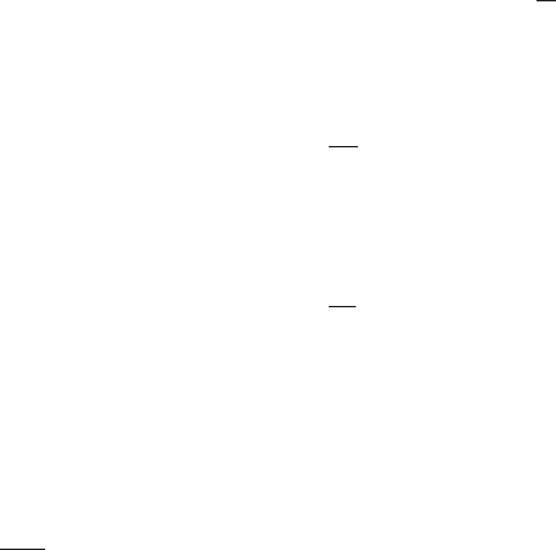
264 Chris Wendl
is expressed in a slightly more general fo r m involving ma rked points) agrees with
our (
12.8).
Cieliebak and Latschev [
CL09, §2] write down the same formula in terms of mod-
uli spaces that have no asymptotic markers but remember the order of the punctures,
thus it includes some factorials that do not appear in (
12.6) but is missing the κ
γ
terms of (
12.8). The notation n
g
(Γ
−
, Γ
+
) used in [CL09] for curve counts must be
understood implicitly to include rational weights arising from automorphisms (or
multivalued perturbations, as the case may be).
My paper with Latschev [LW11] uses moduli spaces with asymptotic markers
and attempts to write down the same formula as in [
EGH00, CL09], but gets it
slightly wrong due to some missing κ
γ
terms that should appear in front of each
∂
∂q
γ
.
Mea culpa.
For cylindrical contact homology, the combinatorial factors in §
12.5 also a gree
with what appears in [
Bou03]. As observed by Nelson [Nel13, Remark 8.3], there
are other conventions for ∂
CCH
that appear in the literature and lead to equivalent
theories: in particular it is possible to replace (
12.13) with
∂
CCH
q
γ
:=
X
γ
′
,A
κ
γ
′
X
u∈M
A
(γ,γ
′
)
ǫ(u)
κ
u
e
A
q
γ
′
.
One can derive this from the same definition of H by applying a “change of co-
ordinates” to the algebra A[[~]], or equivalently, by choosing a slightly different
representation o f the operator algebra defined by the p
γ
and q
γ
varia bles. To avoid
confusion, let us write the generators of A as x
γ
instead of q
γ
, and then define the
operators q
γ
and p
γ
on A[[~]] by
q
γ
= κ
γ
x
γ
, p
γ
= ~
∂
∂x
γ
.
These operators still satisfy [p
γ
, q
γ
] = κ
γ
~ and thus define an equivalent theory, but
the resulting differential operat or D
SFT
on A[[~]] now includes extra factors of κ
γ
for the negative punctures instead of the positive punctures.
12.7.3. Coefficients: Q, Z or Z
2
? While we were able to use Z
2
coefficients
for cylindrical cont act homology in a primitive homotopy class in Lecture
10, a quick
glance at any version of the formula for H should make the reader very skeptical
about doing this fo r more general versions of SFT. The existence of curves with
automorphisms means that H always contains terms with rational (but nonintegral)
coefficients. And this is only what is true in the fictional world of Assumption
12.1:
in the general version of the theory, we exp ect to have to replace expressions like
P
u
ǫ(u)
|Aut(u)|
with counts of 0-dimensional weighted branched orbifolds with rational
weights, arising as zero-sets of generic multisections. In this case we not only obtain
rational counts but may also lose all control over the sizes of the denominators.
A similar phenomenon occurs in general versions of Gromov-Witten t heory. For
instance, in the approach of Cieliebak-Mohnke [
CM07] for the rational Gromov-
Witten invariants of a closed symplectic manifold (W
2n
, ω) with [ω] ∈ H
2
(W ; Q),
the invariants are defined by replacing the usual moduli space M
0,m
(J, A) by a space

Lectures on Symplectic Field Theory 265
M
0,m+N
(J, A; Y ) consisting of J-holomorphic spheres u : S
2
→ W with some large
number of auxiliary marked points ζ
1
, . . . , ζ
N
required to satisfy the condition
u(ζ
i
) ∈ Y, i = 1, . . . , N.
Here Y
2n−2
⊂ W
2n
is a J-holomorphic hypersurface with [Y ] = D · PD([ω]) ∈
H
2n−2
(W ) for some degree D ∈ N, and the number of extra marked points is deter-
mined by
N = A · [Y ] = Dh[ω], Ai,
so positivity of intersections implies that u only intersects Y at the auxiliary marked
points. These auxiliary points are convenient for technical reasons involving trans-
versality—their role is vaguely analogous to the way that asymptotic markers get
rid of isotr opy in SFT—but they are not geometrically meaningful, as we’d actually
prefer t o count curves in M
0,m
(J, A). Every such curve has N intersections with Y ,
so accounting for permutations, it lifts to N! distinct elements of M
0,m+N
(J, A; Y ),
and the correct count is therefore obtained as an integer count of curves in the latter
space divided by N!. Perturbing to achieve transversality breaks the symmetry,
however, so there is no guarantee that counting curves in M
0,m+N
(J, A; Y ) will
produce a multiple of N!, and moreover, N could be arbitrarily large since one
needs to take hypersurfaces of arbitrarily large degree in o r der to show that the
invariants don’t depend on this choice. For these reasons, the resulting Gromov-
Witten invariants are rational numbers rather than integers, and their denominators
cannot b e predicted or bounded.
The upshot of this discussion is that there is probably no hope of defining SFT
with integer coefficients in general, much less with Z
2
coefficients—for this reason
the inclusion of orientations in the picture is unavoidable. That is the bad news.
The good news however is that whenever formulas like
P
u
ǫ(u)
|Aut(u)|
can be taken
literally as a count of curves, the chain complex (A[[~]], D
SFT
) can in fact be defined
with Z coefficients, and one can even reduce to a Z
2
version in order to ignore signs.
A special case of this was observed for cylindrical contact homology in [
Nel15, Re-
mark 1.5], and you may notice it already when you look at the formula (
12.13) for
∂
CCH
: the factor κ
γ
/κ
u
is always an integer since the multiplicity of a holomorphic
cylinder always divides the covering multiplicity of both its asymptotic orbits. Sur-
prisingly, something similar turns out t o be tr ue for the much larger chain complex
of SFT. The following result is stated under Assumption
12.1 for safety’s sake, but in
light of the discussion in §
12.4, we should expect it to hold somewhat more generally.
Proposition 12.1 3. If Assumption
12.1 holds then the rational coefficients
n
g
(γ, γ
′
, k) in the formula (
12.11) for D
SFT
q
γ
are all integers.
Corollary 1 2.14. Under Assumption
12.1, there exist well-de fined chain com-
plexes
(A
Z
[[~]], D
SFT
) and (A
Z
2
[[~]], D
SFT
),
where for a general commutative ring R, A
R
denotes the graded supercommutative
unital algeb ra over R[H
2
(M)/G] generated by the q
γ
variables for good Reeb orbits γ.
The differentials D
SFT
on A
Z
[[~]] and A
Z
2
[[~]] are defined by the same formula as
on A[[~]], where in the Z
2
ca se we are free to se t all signs ǫ(u) equal to 1.
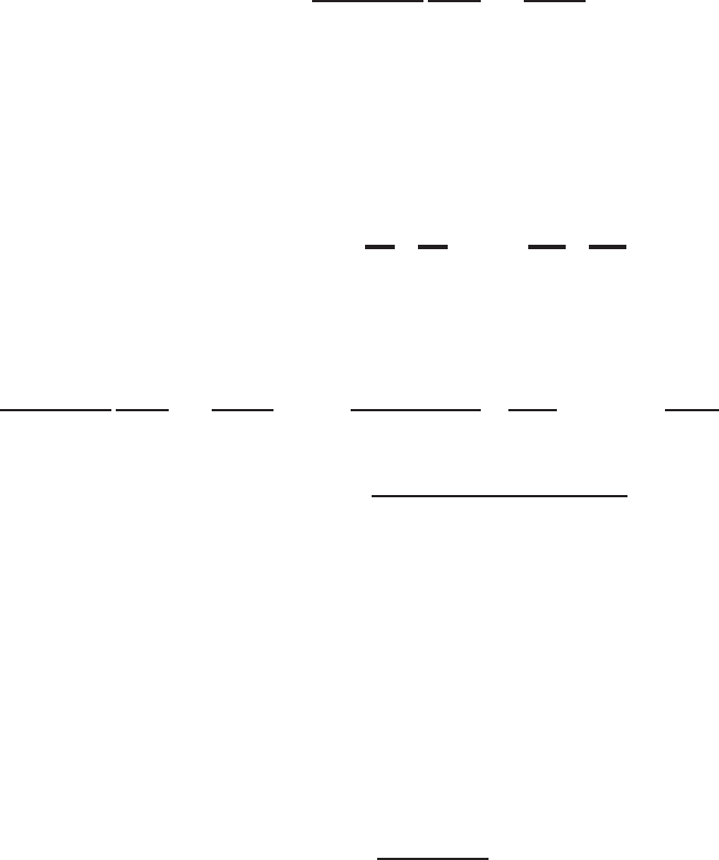
266 Chris Wendl
Proof of Proposition 12.13. We need to show that expressions of the f orm
κ
γ
+
|Aut
σ
(u)|
∂
∂q
γ
+
1
. . .
∂
∂q
γ
+
k
+
q
γ
produce integer coefficients for every holomorphic curve u with asymptotic orbits
γ
±
= (γ
±
1
, . . . , γ
±
k
±
) and every tuple γ = (γ
1
, . . . , γ
m
). It suffices to consider the
special case γ = γ
+
, as the derivative in question is only no nzero on monomials
that are divisible by q
γ
+
. Up to a sign change, we can reorder the orbits and write
γ
+
in t he form
γ
+
= (γ
1
, . . . , γ
1
|
{z }
m
1
, . . . , γ
N
, . . . , γ
N
| {z }
m
N
)
for some finite set of distinct orbits γ
1
, . . . , γ
N
and numbers m
i
∈ N, i = 1, . . . , N.
We then have
κ
γ
+
|Aut
σ
(u)|
∂
∂q
γ
+
1
. . .
∂
∂q
γ
+
k
+
q
γ
+
=
κ
m
1
γ
1
. . . κ
m
N
γ
N
|Aut
σ
(u)|
∂
∂q
γ
1
m
1
. . .
∂
∂q
γ
N
m
N
q
m
1
γ
1
. . . q
m
N
γ
N
= ±
κ
m
1
γ
1
. . . κ
m
N
γ
N
m
1
! . . . m
N
!
|Aut
σ
(u)|
.
(12.19)
We claim that this number is always an integer. Indeed, if Aut
σ
(u) is nontrivial, then
u :
˙
Σ → R × M is a multiple cover u = v ◦ ϕ for some holo morphic branched cover
ϕ : (Σ, j) → (Σ
′
, j
′
) and somewhere injective curve v : (
˙
Σ
′
= Σ
′
\Γ
′
, j
′
) → (R×M, J).
Automorphisms ψ ∈ Aut
σ
(u) thus define biholomorphic maps o n (Σ, j) that permute
each of the sets of punctures asymptotic to the same orbit. Given any puncture
z ∈ Γ where u is asymptotic to γ
i
, the Aut
σ
(u)-orbit of z consists of ℓ ≤ m
i
other
punctures also asymptotic to γ
i
, and its stabilizer is a cyclic subgroup of order
k = |Aut
σ
(u)|/ℓ, acting on a neighborhood of z by biholomorphic rota tions. It
follows that κ
γ
i
is divisible by k, hence
κ
γ
i
ℓ
|Aut
σ
(u)|
∈ N,
and (
12.19) is a multiple of this.
Remark 12.15. Since 1 = −1 in A
Z
2
, anticommuting elements of A
Z
2
[[~]] ac-
tually commute, so unless one imposes extra algebraic conditions in the case of Z
2
coefficients, higher powers of odd generators p
γ
and q
γ
do not vanish. Nonetheless,
these powers still do not appear in H, so the complex (A
Z
2
[[~]], D
SFT
) ignores curves
with multiple ends approaching an orbit of odd degree (and also bad orbits, for that
matter).
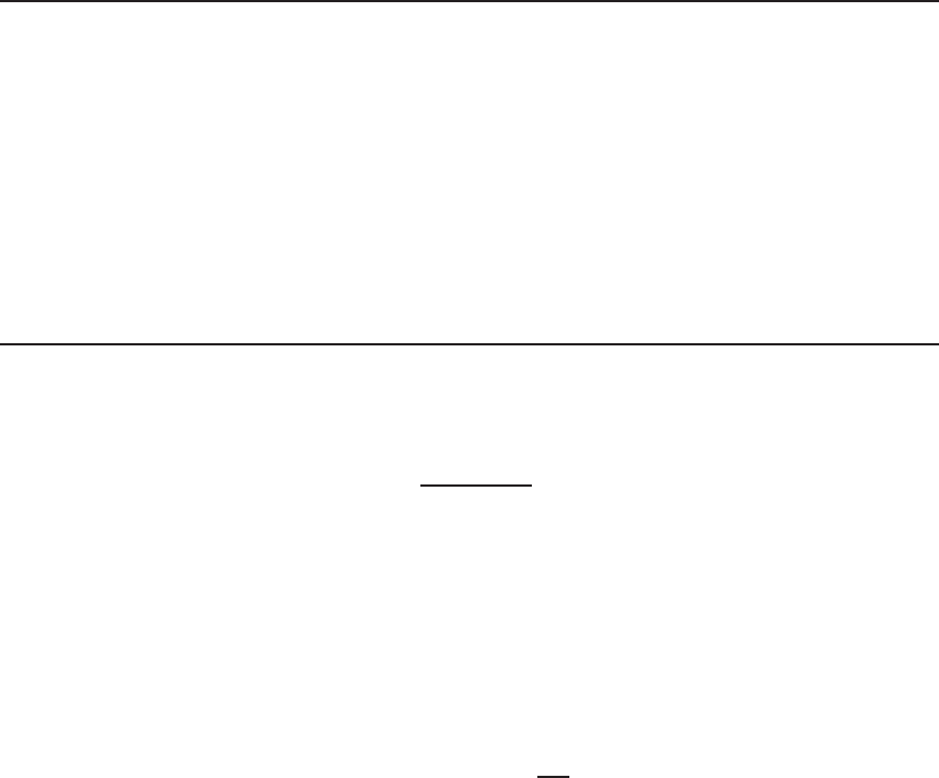
LECTURE 13
Contact invariants
Contents
13.1. The Eliashberg-Givental-Hofer package 268
13.1.1. Full S FT as a Weyl superalgebra 268
13.1.2. The semiclassical limit: rational SFT 272
13.1.3. The contact homology algebra 275
13.1.4. Algebraic overtwistedness 276
13.2. SFT generating functions for cobordisms 278
13.2.1. Weak, strong and stable cobordisms 278
13.2.2. Counting disconnected index 0 curves 283
13.3. Full SFT as a BV
∞
-algebra 288
13.3.1. Cobordism maps and invariance 289
13.3.2. Algebraic torsion 292
In the previous lecture, we introduced an operator algebra defined via the su-
percommutators [p
γ
, q
γ
] = κ
γ
~, then we defined the SFT generating function
H =
X
u∈M
σ
1
(J)/R
ǫ(u)
|Aut
σ
(u)|
~
g−1
e
A
q
γ
−
p
γ
+
and proved (modulo transversality) that H
2
= 0. The generating function is a formal
power series whose coefficients are r ational counts of holomorphic curves, and these
counts are strongly dependent on the cho ices of contact form α, almost complex
structure J ∈ J(α) and further auxiliary data such as coherent orient ations. Thus
in contrast to G r omov-Witten theory, the generating function does not define an
invariant, but one can follow the standard prescription of Floer-type theories and
define inva r iants via homology. We saw that fo r the natural represent ation A[[~]] of
the operator a lgebra defined by setting p
γ
= κ
γ
~
∂
∂q
γ
, H defines a differential operator
D
SFT
: A[[~]] → A[[~]] with D
2
SFT
= 0. One of our g oals in this lecture will be to
explain (again modulo transversality) why the resulting homology
H
SFT
∗
(M, ξ; R) = H
∗
(A[[~]], D
SFT
)
is an invariant of the contact structure. We will then use it to define simpler nu-
merical invariants that detect symplectic fillability properties of contact manifolds.
But first, A[[~]] is not the only possible r epresent ation of the operato r algebra
of SFT: other choices lead to different inva riants with different algebraic structures.
Let’s begin by describing the original hierarchy of contact invariants that were out-
lined in [
EGH00].
267

268 Chris Wendl
Remark 13.1. Throughout this lecture, we assume for simplicity that H
2
(M)
has no torsion, and the same assumption is made about cobordisms in §
13.2.2. Only
minor changes are necessary if this condition is lifted, e.g. one could then replace a ll
instances of H
2
(M) with H
2
(M; Q) and assume always that the grading is Z
2
; see
§12.7.1.
13.1. The Eliashberg-Givental-Hofer package
In the following, (M, ξ) is a (2n − 1)-dimensional closed contact manif old with
a contact form α and almost complex structure J ∈ J(α) for which the optimistic
transversality condition (Assumption 12.1) of Lecture 12 is assumed to hold. We
fix also the auxiliary data described in §
12.2, plus a choice of subgroup G ⊂ H
2
(M)
which determines the coefficient ring
R = Q[H
2
(M)/G].
Each of the differential graded algebras described below then carries the same grad-
ing that was described in that lecture, i.e. there is always a t least a Z
2
-grading, and
it lifts to Z if H
1
(M) is torsion free and c
1
(ξ)|
G
= 0, or possibly Z
2N
if N ∈ N is the
smallest possible value for c
1
(A) with A ∈ G.
13.1.1. Full SFT as a Weyl superalgebra. We start with some seemingly
trivial algebraic observations. First, the relation H
2
= 0 is equivalent to
[H, H] = 0.
Remember that [ , ] is a super-commutator, so [F, F] = 0 holds automatically fo r
operators F with even degree, but H is odd, and for odd operators the commutator
is defined by [F, G] = FG + GF, hence [H, H] = 2H
2
. Formally sp eaking [ , ] is a
super Lie bracket and thus satisfies the “super Jacobi identity”:
(13.1)
F, [G, K]
+ (−1)
|F||G|+|F||K|
G, [K, F]
+ (−1)
|F||K| +|G||K|
K, [F, G]
= 0.
A consequence of this is that in order to create a homolo gy theory out of H, we don’t
absolutely need to find a representatio n of the entire operator algebra: it suffices
to find a representation of the induced super Lie algebra. Indeed, suppose V is a
graded R[[~]]-module and L is a linear grading-preserving ma p that associat es to
operators F (expressed as power series functions of p’s, q’s and ~ with coefficients
in R) an R[[~]]-linear map
L
F
: V → V
such that
L
[F,G]
= L
F
L
G
− (−1)
|F||G|
L
G
L
F
for every pair of operators F, G. Then the R[[~]]- linear map L
H
: V → V satisfies
L
2
H
=
1
2
[L
H
, L
H
] =
1
2
L
[H,H]
= 0,
hence (V, L
H
) is a chain complex. The complex (A[[~]], D
SFT
) was a special case of
this, in which we represented the super Lie algebra via a faithful representation o f
the whole operator algebra.
Exercise 13.2. Verify (
13.1).

Lectures on Symplectic Field Theory 269
Remark 13.3 (supersymmetric sign rules). To see where the signs in (1 3.1)
come fr om, it suffices to know the following basic rule of superalgebra: for any
pair of Z
2
-graded vector spaces V and W , the natural “commutation” isomorphism
c : V ⊗ W → W ⊗ V is defined on homogeneous elements by
c(v ⊗ w) = (−1)
|v||w|
w ⊗ v.
For any permutation of a finite tuple of Z
2
-graded vector spaces, one can derive the
appropriate isomorphism from this: in particular the cyclic permutation isomor-
phism σ : X ⊗ Y ⊗ Z → Y ⊗ Z ⊗ X takes the form
σ = (1 ⊗ c
23
) ◦ (c
12
⊗ 1) : x ⊗ y ⊗ z 7→ (−1)
|x||y|+|x||z|
y ⊗ z ⊗ x.
Writing the Jacobi identity as [·, [·, ·]] ◦ (1 + σ + σ
2
) = 0 then produces (
13.1). In
this sense, it only differs from the usual Jacobi identity in being based on a different
definition of the commutation isomorphism V ⊗ W → W ⊗ V . For more on this
perspective, see [Var04, §3.1].
Now here is a different kind of example, where the representation does not respect
the product structure o f the operator algebra but does resp ect its Lie bracket. Let
W denote the graded unital algebra consisting of formal power series
X
γ,k
f
γ,k
(q)~
k
p
γ
,
where the sum ranges over all integers k ≥ 0 and all ordered sets γ = (γ
1
, . . . , γ
m
)
of good Reeb orbits for m ≥ 0, and the f
γ,k
are polynomial functions of the q
γ
varia bles, with coefficients in R. Note that t he case of the empty set of orbits is
included here, which means p
γ
= 1. The multiplicative structure of W is defined
via the usual (super)commutation relations, and its elements can be interpreted as
operators. If we now associate to each F ∈ W the R[[~]]-linear map
D
F
: W → W : G 7→ [F, G],
then the Jacobi identity (
13.1) implies
D
[F,G]
= D
F
D
G
−(−1)
|F||G|
D
G
D
F
.
This is just the graded version of the standard adjoint representation of a Lie algebra.
The only problem in applying this idea to define a differential
(13.2) D
H
: W → W : F 7→ [H , F]
is that H is not technically an element of W: indeed, H conta ins terms of order −1
in ~, thus
H ∈
1
~
W.
On the other hand, the failure of supercommutativity in W is a “phenomenon o f
order ~,” i.e. since every nontrivial commutator contains a factor of ~, we have
[F, G] = O(~) for all F, G ∈ W.
Here and in the following we use the symbol
O(~
k
)

270 Chris Wendl
to denote any element of the form ~
k
F for F ∈ W. As a consequence, [H, F] ∈ W
whenever F ∈ W, hence (
13.2) is well defined, and the Jacobi identity now implies
D
2
H
= 0.
The homology of the resulting chain complex gives another version of what is often
called full SFT,
H
W
∗
(M, ξ; R) := H
∗
(W, D
H
).
A proof (modulo tr ansversality) that this defines a contact invariant is outlined in
[
EGH00, §2], but it is algebraically somewhat more involved than for H
SFT
∗
(M, ξ; R),
so I will skip it since I don’t have any applications of H
W
∗
(M, ξ; R) in mind. As far
as I am aware, no contact topological applications of this invariant or computations
of it (outside the trivial case—see §
13.1.4 below) have yet appeared in the literature.
This is a pity, because H
W
∗
(M, ξ; R) actually has much mo re algebraic structure t han
H
SFT
∗
(M, ξ; R). Indeed, using the identities
[F, GK] = [F, G]K + (−1)
|F||G|
G[F, K],
[FG, K] = F[G, K] + (−1)
|G||K|
[F, K]G,
(13.3)
one sees that D
H
: W → W satisfies a graded Leibniz rule,
D
H
(FG) = (D
H
F)G + (−1)
|F|
F D
H
G.
It follows that D
H
: W → W is also a derivation with respect to the bracket structure
on W, i.e.
D
H
[F, G] = [D
H
F, G] + ( −1)
|F|
[F, D
H
G]
for all F, G ∈ W. As a consequence, the product and bracket structures on W
descend to H
W
∗
(M, ξ; R), giving it the structure of a Weyl superalgebra.
As a matt er of interest, we observe that (W, D
H
), as with (A[[~]], D
SFT
) in the
previous lecture, can be defined with Z or Z
2
coefficients whenever the transversality
results are good enough to take the usual expression
P
u
ǫ(u)
|Aut
σ
(u)|
literally as a count
of holomorphic curves. This result is of limited interest since it cannot hold in gen-
eral cases where transversality for multiple covers is impossible without multivalued
perturbations—nonetheless I find it amusing.
1
Proposition 13.4. If Assumption 12.1 in Lecture 1 2 hold s, then D
H
is also well
defined if the ring R = Q[H
2
(M)/G] i s replaced by Z[H
2
(M)/G] or Z
2
[H
2
(M)/G].
Proof. Since D
H
is a derivation, it suffices to check that for every good Reeb
orbit γ, D
H
q
γ
and D
H
p
γ
are each sums of monomials of the form ce
A
~
k
q
γ
−
p
γ
+
with
1
The same arguments used to define SFT chain complexes over the integers can also be applied
to the chain maps involved in the proof of invariance (see §
13.3.1), so the SFT invariants should
be defined over the integers if transversality can be achieved for multiple covers. There are known
situations however in which this cannot hold: even if the chain complexes are well defined over Z,
invariance may hold only over Q, due to the failure of transversality in cobordisms. See [
Hut].
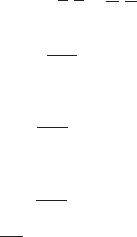
Lectures on Symplectic Field Theory 271
coefficients c ∈ Z. Suppose u ∈ M
1
(J) is an index 1 holomorphic curve with positive
and/or negat ive asymptotic orbits
γ
±
= (γ
±
1
, . . . , γ
±
1
|
{z }
m
±
1
, . . . , γ
±
k
±
, . . . , γ
±
k
±
|
{z }
m
±
k
±
),
where γ
±
i
6= γ
±
j
for i 6= j. We can assume all the or bit s γ
±
i
are good and that m
±
i
= 1
whenever n − 3 + µ
CZ
(γ
±
i
) is odd. Up to a sign and factors of e
A
and ~ which are
not relevant to this discussion, u then contributes a monomial
H
u
:=
1
|Aut
σ
(u)|
q
m
−
1
γ
−
1
. . . q
m
−
k
−
γ
−
k
−
p
m
+
1
γ
+
1
. . . p
m
+
k
+
γ
+
k
+
to H. The commutator [H
u
, q
γ
] vanishes unless γ is one of the orbits γ
+
1
, . . . , γ
+
k
+
,
so supp ose γ = γ
+
k
+
. If n − 3 + µ
CZ
(γ) is odd, then m := m
+
k
+
= 1, and (
13.3) with
[p
γ
, q
γ
] = κ
γ
~ implies
[H
u
, q
γ
] =
1
|Aut
σ
(u)|
q
m
−
1
γ
−
1
. . . q
m
−
k
−
γ
−
k
−
p
m
+
1
γ
+
1
. . . p
m
+
k
+
−1
γ
+
k
+
−1
p
γ
, q
γ
=
κ
γ
|Aut
σ
(u)|
~q
m
−
1
γ
−
1
. . . q
m
−
k
−
γ
−
k
−
p
m
+
1
γ
+
1
. . . p
m
+
k
+
−1
γ
+
k
+
−1
.
The fraction in front of this expression is an integer since u can have only one
end asymptotic to γ, and κ
γ
is thus divisible by the covering multiplicity of u. If
n − 3 + µ
CZ
(γ) is even, then we generalize this calculation by using (
13.3) to write
[p
m
γ
, q
γ
] = mκ
γ
~p
m−1
γ
,
so then,
[H
u
, q
γ
] =
1
|Aut
σ
(u)|
q
m
−
1
γ
−
1
. . . q
m
−
k
−
γ
−
k
−
p
m
+
1
γ
+
1
. . . p
m
+
k
+
−1
γ
+
k
+
−1
p
m
γ
, q
γ
=
κ
γ
m
|Aut
σ
(u)|
~q
m
−
1
γ
−
1
. . . q
m
−
k
−
γ
−
k
−
p
m
+
1
γ
+
1
. . . p
m
+
k
+
−1
γ
+
k
+
−1
p
m−1
γ
.
To see that
κ
γ
m
|Aut
σ
(u)|
is always an integer, recall fr om our proof of Prop.
12.13 in
the previous lecture that transformations in Aut
σ
(u) permute each of the sets of
punctures that are asymptotic to the same Reeb orbit. Suppose the set of positive
punctures of u asymptotic to γ is partitioned by the Aut
σ
(u)-action into N subsets,
each consisting of ℓ
1
, . . . , ℓ
N
punctures, where ℓ
1
+ . . . + ℓ
N
= m. If z is a puncture
in t he ith of t hese subsets, then its stabilizer is a cyclic subgroup of order k
i
acting
on a neighborhood of z by biholomorphic rotations, where k
i
ℓ
i
= |Aut
σ
(u)|. Each
of these orders k
i
necessarily divides the multiplicity κ
γ
, so we can write k
i
a
i
= κ
γ
for some a
i
∈ N. Putting all this together, we have
κ
γ
m =
N
X
i=1
κ
γ
ℓ
i
=
N
X
i=1
k
i
a
i
ℓ
i
= |Aut
σ
(u)|
N
X
i=1
a
i
.
Following this same procedure, you should now be able to verify on your own
that the coefficient appearing in [H
u
, p
γ
] is also always an integer. The existence
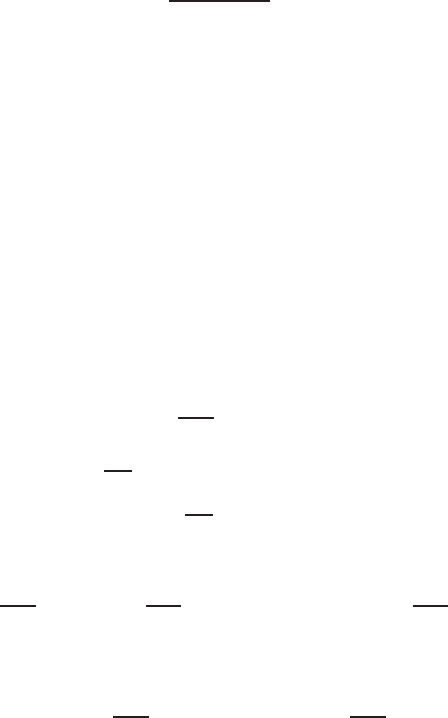
272 Chris Wendl
of a chain complex with Z
2
coefficients follows from this simply by projecting Z
to Z
2
.
13.1.2. The semiclassical limit: r at ional SFT. The idea of rational sym-
plectic field theory (RSFT) is to extract as much inf ormation as possible f rom genus
zero holomorphic curves but ig nore curves of higher genus. The algebra of SFT
provides a fairly obvious mechanism for this: RSFT should be what SFT becomes
in t he “limit as ~ → 0,” i.e. the classical approximation to a quantum theory. Let
P := W
~W,
so P is a graded unital algebra generated by the p
γ
and q
γ
varia bles and the co-
efficient ring R, but it does not include ~ a s a generator. Since all commutators
in W are in ~W, the product structure of P is supercommutative. Let us use the
distinction between capital and lowercase letters to denote the quotient projection
W → P : F 7→ f.
We will make an exception for the letter “H”: recall that H is not an element of W
since its genus zero terms have order −1 in ~, but ~H ∈ W, so we will define
h =
X
u
ǫ(u)
|Aut
σ
(u)|
e
A
q
γ
−
p
γ
+
∈ P
to be the image of ~H under the projection. The sum in this expression ranges
over all R-equivalence classes of index 1 curves with genus zero, so h will serve as
the generating function of RSFT. To encode gluing of genus zero terms, note first
that the commutator operation would not be appropriate since it prodcues terms
for every possible gluing of two curves, including those which glue genus zero curves
along more than one breaking orbit to produce buildings with positive arithmetic
genus. We need instead to have an algebraic operation on P that encodes gluing
along o nly one breaking orbit at a time.
You already know what to expect if you’ve ever taken a quantum mechanics
course: in t he “classical limit,” commutators become Poisson brackets. To express
this properly, we need to make a distinction between differential operators operating
from the left or the right: let
−−→
∂
∂q
γ
: W → W
denote the usual operator
∂
∂q
γ
, which was previously defined on A[[~]] but has an
obvious extension to W such that
−→
∂
∂q
γ
p
γ
′
= 0 for all γ
′
. This operator satisfies the
graded Leibniz rule
−−→
∂
∂q
γ
(FG) =
−−→
∂
∂q
γ
F
!
G + (−1)
|q
γ
||F|
F
−−→
∂
∂q
γ
G
!
.
The related opera tor
←−−
∂
∂q
γ
: W → W : F 7→ F
←−−
∂
∂q
γ
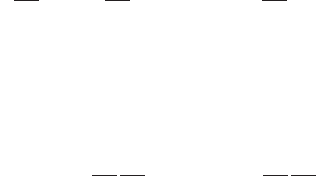
Lectures on Symplectic Field Theory 273
is defined exactly the same way on individual var iables p
γ
and q
γ
, but satisfies a
slightly different L eibniz rule,
(FG)
←−−
∂
∂q
γ
= F
G
←−−
∂
∂q
γ
!
+ (−1)
|q
γ
||G|
F
←−−
∂
∂q
γ
!
G.
The point of writing
←−
∂
∂q
γ
so that it acts from the right is to obey the usual conventions
of superalgebra: signs change whenever the order of two odd elements (or operators)
is interchanged. Partial deriva tives with respect to p
γ
can be defined analogously
on W. With this notation in hand, the graded Poisson bracket on W is defined
by
(13.4) {F, G} =
X
γ
κ
γ
F
←−−
∂
∂p
γ
−−→
∂
∂q
γ
G − (−1)
|F||G|
G
←−−
∂
∂p
γ
−−→
∂
∂q
γ
F
!
,
where the sum r anges over all good Reeb orbits. In the same manner, the differential
operators and the bracket { , } can also be defined on P.
It is easy to check that { , } on W almost satisfies a version of (
13.3): we have
{F, GK} = {F, G}K + (−1)
|F||G|
G{F, K}+ O(~),
{FG, K} = F{G, K} + (−1)
|G||K|
{F, K}G + O(~)
(13.5)
for all F, G, K ∈ W. The extra terms denoted by O(~) arise from the fact that
in proving (
13.5), we must sometimes reorder products FG by writing them as
(−1)
|F||G|
GF + [F, G], where [F, G] = O(~). Since the terms with ~ disappear in
P, the relations become exact in P:
{f, gk} = {f, g}k + (−1)
|f ||g|
g{f, k},
{fg, k} = f{g, k} + (−1)
|g||k|
{f, k}g
(13.6)
for all f, g, k ∈ P.
Proposition 13.5 . For all F, G ∈ W,
[F, G] = ~{f, g } + O(~
2
),
and { , } satisfies the conditions of a super Lie bracket on P.
Remark 13.6. In formulas like the one in the above proposition, we interpret
{f, g} ∈ P as an element of W via any choice of R-linear inclusion P ֒→ W that acts
as the identity on the generators p
γ
, q
γ
. There is ambiguity in this choice due to the
noncommutativity of W, but the ambiguity is in ~W and thus makes no difference
to the formula.
Proof of Proposition
13.5. The formula is easily checked when F and G
are individual variables of the form p
γ
or q
γ
; in fa ct the extra term O(~
2
) can be
omitted in these cases. The case where F and G are general monomials follows from
this via (
13.3) and (13.5) using induction on the number of va riables in the product.
This implies the general case via bilinearity.

274 Chris Wendl
Given the f ormula, the condition {f, g} + (−1)
|f ||g|
{g, f} = 0 and the Poisson
version of the super Jacobi identity (
13.1) follow from the corresponding properties
of [ , ].
The proposition implies that our genus zero generating function h ∈ P satisfies
0 = ~
2
[H, H] = [~H, ~H] = ~{h, h} + O(~
2
), thus
{h, h} = 0.
This relation can be interpreted as the count of boundary points of all 1-dimensional
moduli spaces of genus zero curves: indeed, any pair of genus two curves u, v ∈
M
σ
1
(J)/R constributes to {h, h} a term of the form
X
γ
κ
γ
|Aut
σ
(u)||Aut
σ
(v)|
e
A
u
+A
v
q
γ
−
u
p
γ
+
u
←−−
∂
∂p
γ
!
−−→
∂
∂q
γ
q
γ
−
v
!
p
γ
+
v
,
plus a corresponding term with the roles of u and v reversed. This sums all the mono-
mials that one can construct by cancelling one p
γ
varia ble from u with a matching
q
γ
varia ble from v, in other words, constructing a building by gluing v on top of u
along o ne matching Reeb orbit.
The graded Jacobi identity will a gain imply that any r epresent ation of the super
Lie alg ebra (P, { , }) gives rise to a chain complex with h as its differential. For
example we can take the adjoint representation,
P → End
R
(P) : f 7→ d
f
, d
f
g := {f, g},
which satisfies d
{f ,g}
= d
f
d
g
−(−1)
|f ||g|
d
g
d
f
due to the Jacobi ident ity. Then d
2
h
= 0
since h has odd degree and {h, h} = 0, and the homology of rational SFT is
defined as
H
RSFT
∗
(M, ξ; R) := H
∗
(P, d
h
).
We again refer to [
EGH00] for an argument that H
RSFT
∗
(M, ξ; R) is an invariant
of the contact structure. Notice that Proposition
13.5 yields a simple relationship
between the chain complexes (W, D
H
) and (P, d
h
), namely
(13.7) D
H
F = d
h
f + O(~),
where d
h
f is interpreted as an element of W via Remark
13.6. In other words, the
projection W → P : F → f is a chain map. Moreover, d
H
is a derivation on P with
respect to both the product a nd the Poisson bracket: this follows via Proposition
13.5
and (13.7) from the fact that D
H
satisfies the corresponding properties on W. We
conclude that H
RSFT
∗
(M, ξ; R) inherits the structure of a Poisson superalgebra, and
the map
H
W
∗
(M, ξ; R) → H
RSFT
∗
(M, ξ; R)
induced by the chain map (W, D
H
) → (P, d
h
) is both a n algebra homomorphism
and a homomorphism of gr aded super Lie algebras.
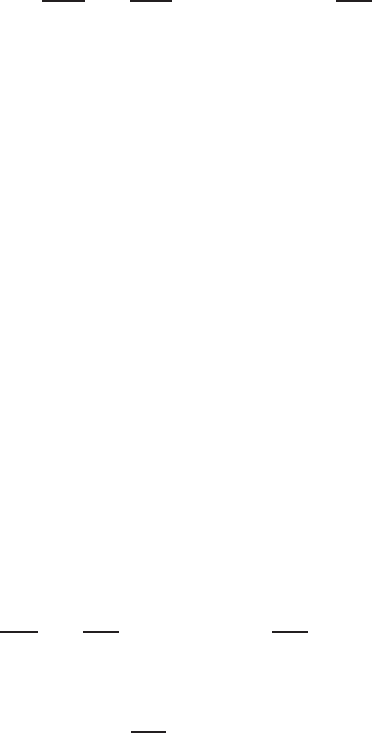
Lectures on Symplectic Field Theory 275
13.1.3. The contact homology algebra. Contact homology is the most pop-
ular tool in the SFT package and was probably the first to be understood beyond t he
more straightforward cylindrical theory. In situations where cylindrical contact ho-
mology cannot be defined due to bubbling of holomorphic planes, the next simplest
thing one can do is to define a theory t hat counts genus zero curves with one positive
end but arbitrary numbers of negat ive ends (cf. Exercise
10.14 in Lecture 10).
The proper algebraic setting for such a theory turns out t o be the algebra A
generated by the q
γ
varia bles, and it can be derived from RSFT by setting all p
γ
varia bles to zero. Using the obvious inclusion A ֒→ P, define ∂
CH
: A → A by
∂
CH
f = d
h
f|
p=0
.
We can thus write d
h
f = ∂
CH
f + O(p), where
O(p
k
)
will be used generally to denote any formal sum consisting exclusively of terms of
the form p
γ
1
. . . p
γ
k
f for f ∈ P. Now observe that for any good orbit γ,
d
h
p
γ
= {h, p
γ
} = −(−1)
|p
γ
|
X
γ
′
p
γ
←−−
∂
∂p
γ
′
!
−−→
∂
∂q
γ
′
h
!
= −(−1)
|p
γ
|
∂h
∂q
γ
= O(p)
since every term in h has at least one p variable. It follows that d
h
(O(p)) = O(p),
so the fact t hat d
2
h
= 0 implies ∂
2
CH
= 0, and contact homology is defined as
HC
∗
(M, ξ; R) := H
∗
(A, ∂
CH
).
Since d
h
is a derivation on P, the formula d
h
f = ∂
CH
f + O(p) implies that ∂
CH
is
likewise a derivation on A, so HC
∗
(M, ξ; R) ha s the structure of a graded super-
commutative algebra with unit. Moreover, the proj ection P → A : f 7→ f|
p=0
is a
chain map, giving rise to an algebra homomorphism
H
RSFT
∗
(M, ξ; R) → HC
∗
(M, ξ; R).
The invariance of HC
∗
(M, ξ; R) will follow from the invar iance of H
SFT
∗
(M, ξ; R), to
be discussed in §
13.3.1 below.
To interpret ∂
CH
, we can separate the part of h that is linear in p variables,
writing
h =
X
γ
h
γ
(q)p
γ
+ O(p
2
),
where fo r each good Reeb orbit γ, h
γ
(q) denotes a polynomial in q variables with
coefficients in R. Since elements f ∈ A have no dependence on p variables, we then
have
d
h
f = {h, f} =
X
γ
κ
γ
h
←−−
∂
∂p
γ
!
−−→
∂
∂q
γ
f
!
=
X
γ
κ
γ
h
γ
∂f
∂q
γ
+ O(p),
hence
∂
CH
f =
X
γ
κ
γ
h
γ
∂f
∂q
γ
.

276 Chris Wendl
In par t icular, ∂
CH
acts on each generator q
γ
∈ A as
∂
CH
q
γ
= κ
γ
h
γ
=
X
u
ǫ(u)κ
γ
Aut
σ
(u)
e
A
q
γ
−
,
where the sum is over all R-equivalence classes of index 1 J-holomorphic curves u
with genus zero, one positive end at γ, and negative ends γ
−
, and homology class
A ∈ H
2
(M)/G.
13.1.4. Algebraic overtwistedness. Even the simplest of the three differen-
tial graded algebras described above is too large to compute in most cases. The
major exception is the case of overtwisted contact manifolds.
Theorem 1 3.7. If (M, ξ) is overtwisted, then HC
∗
(M, ξ; R) = 0 for all choices
of the coeffic i ent ring R.
Remark 13.8. If X is a n algebra with unit, then saying X = 0 is equivalent to
saying that 1 = 0 in X.
The notion of overtwisted contact structures in dimension three was intro duced
by Eliashberg in [
Eli89], who proved that they are flexible in the sense that their
classification up to isotopy reduces to the purely obstruction-theoretic classification
of almost contact structures up to homotopy. This means in effect that an over-
twisted contact structure carries no distinctly contact geometric information, so it
should not be surprising when “interesting” contact invariants such as HC
∗
(M, ξ)
vanish. The three-dimensional case of Theorem
13.7 seems to have been among the
earliest insights about SFT: its first a ppearance in the lit era ture was in [
Eli98], and
a proof later appeared in a paper by Mei-Lin Yau [
Yau06], which includes a brief
appendix sketching Eliashberg’s original proof. We will discuss Eliashberg’s proof
in detail in Lecture
16.
The definitive higher-dimensional no tion of overtwistedness was introduced a few
years ago by Borman-Eliashberg-Murphy [
BEM15], following earlier steps in this
direction by Niederkr¨uger [
Nie06] and others. There are now two known proofs of
Theorem
13.7 in higher dimensions: the first uses the fact that since overtwisted
contact manifolds are flexible, they always admit an embedding of a plastikstufe,
which implies vanishing of contact homology by an unpublished result of Bourgeois
and Niederkr¨uger (see [Bou09, Theorem 4.10] for a sketch of the argument) . The
second argument app eals to an even more recent result of Casals-Murphy-Presas
[
CMP] showing that (M, ξ) is overtwisted if and only if it is supported by a nega-
tively stabilized open book, in which case HC
∗
(M, ξ) = 0 was proven by Bourgeois
and van Koert [
BvK10].
It is not known whether the vanishing of contact homolog y characterizes over-
twistedness, i.e. there ar e not yet any examples of tight contact manifolds with
HC
∗
(M, ξ) = 0. I will go out o n a limb and say that such examples seem unlikely
to exist in dimension three but are much more likely in higher dimensions; in fact
vario us candidates are known [
MNW13,CDvK], but we do not yet have adequate
methods to prove that any of them are tight. The ana logous question about Legen-
drian submanifolds and relative contact homology was recently answered by Ekholm
Lectures on Symplectic Field Theory 277
[Ekh], giving examples of Legendrians tha t are not loose in the sense of Murphy
[
Mur] but have vanishing L egendrian contact homology.
Nevertheless, the lack of known counterexamples has given rise to the following
definition.
Definition 13.9. A closed contact manifold (M, ξ) is algebraically over-
twisted if HC
∗
(M, ξ; R) = 0 for every choice of the coefficient ring R.
Remark 13.10. The coefficient ring is not always mentioned in statements of t he
above definition, but it should be. We will see in §13.3.2 below that this detail makes
a difference to issues like symplectic filling obstructions. Note that for any nested
pair of subgroups G ⊂ G
′
⊂ H
2
(M), the natural projection H
2
(M)/G
′
→ H
2
(M)/G
induces an algebra homomorphism
HC
∗
(M, ξ; Q[H
2
(M)/G
′
]) → HC
∗
(M, ξ; Q[H
2
(M)/G]).
Since algebra homomorphisms necessarily map 1 7→ 1 and 0 7→ 0, the target of
this map must vanish whenever its domain does, so for checking Definition
13.9, it
suffices to check the case R = Q[H
2
(M)].
We’ve seen above that there exist algebra homomorphisms
(13.8) H
W
∗
(M, ξ; R) → H
RSFT
∗
(M, ξ; R) → HC
∗
(M, ξ; R),
thus the vanishing of either o f the algebras H
W
∗
(M, ξ; R) or H
RSFT
∗
(M, ξ; R) with
all coefficient rings R is another sufficient condition for algebraic overtwistedness.
Bourgeois and Niederkr¨uger observed that, in fact, these conditions are also neces-
sary:
Theorem 13.11 ( [
BN10]). For any coefficient ring R, the following conditions
are equivalent:
(1) HC
∗
(M, ξ; R) = 0,
(2) H
RSFT
∗
(M, ξ; R) = 0,
(3) H
SFT
∗
(M, ξ; R) = 0.
Proof. The implications (3) ⇒ (2) ⇒ (1) are immediate from t he algebra
homomorphisms (
13.8), thus it will suffice to prove (1) ⇒ (3). Suppose 1 = 0 ∈
HC
∗
(M, ξ; R), which means ∂
CH
f = 1 for some f ∈ A. Using the obvious inclusion
A ֒→ W, this means
D
H
f = 1 − G,
where G = O(p, ~), i.e. G is a sum of terms that a ll contain at least o ne p
γ
varia ble
or a power of ~. It follows that G
k
= O(p
k
, ~
k
) for all k ∈ N, and the infinite sum
∞
X
k=0
G
k
is therefore an element of W, as the coefficient in front of any fixed monomial ~
k
p
γ
in
this sum is a polynomial function of the q var iables. This sum is then a multiplicative
inverse of 1 − G, and since
0 = D
2
H
f = 0 = −D
H
G,
278 Chris Wendl
it also satisfies D
H
((1 − G)
−1
) = 0. Using the fact that D
H
is a derivation, we
therefore have
D
H
(1 −G)
−1
f
= (1 − G)
−1
(1 −G) = 1,
implying 1 = 0 ∈ H
SFT
∗
(M, ξ; R).
13.2. SFT generating functions for cobordisms
All invariance proofs in SFT are based on a generating function analogous to
H that counts index 0 holomorphic curves in symplectic cobordisms. The basic
definition is a straightfor ward extension of what we saw in Lecture
12, but there
is an added wrinkle due to the fact that, in general, one must include disconnected
curves in the count.
13.2.1. Weak, strong and stable cobordisms. F ir st some remarks about
the category we are working in. Since t he stated purpose of SFT is to define invari-
ants of contact structures, we have been working since Lecture
12 with symplectiza-
tions of contact manifolds rather than more general stable Hamiltonian structures.
We’ve made use of this restriction on several occasions, namely so t hat we can
assume:
(1) All nontrivial holomo r phic curves in R ×M have at least one positive punc-
ture;
(2) The energy of a holomorphic curve in R × M can be bounded in terms of
its positive asymptotic orbits.
It will be useful however for certain applications to permit a slightly wider class of
stable Hamiltonian structure. Recall that a hypersurface V in an almo st complex
manifold (W, J) is called pseudo convex if the ma ximal complex subbundle
ξ := T V ∩ J(T V ) ⊂ T V
defines a contact structure on V whose cano nical conformal symplectic bundle struc-
ture tames J|
ξ
. For example, if α is a conta ct form on M and J ∈ J(α), then each of
the hypersurfaces {const}×M is pseudoconvex in (R×M, J). The contact structure
ξ induces an orientation on the hypersurface V ; if V comes with its own orient ation
(e.g. as a boundary component of W ), then we call it pseudoconvex if ξ is a positive
contact structure with respect to this or ientation, and pseudoconcave otherwise.
For example, if (W, ω) is a symplectic cobordism from (M
−
, ξ
−
) to (M
+
, ξ
+
) and
J ∈ J(W, ω, α
+
, α
−
), then M
+
is pseudoconvex and M
−
is pseudoconcave.
Definition 1 3.12. Given an odd-dimensional manifold M, we will say that an
almost complex structure J on R×M is pseudoconvex if {r}×M is a pseudoconvex
hypersurface in (R ×M, J) f or every r ∈ R, with the induced orientation such that
∂
r
and {r}× M are positively transverse.
If H = (ω, λ) is a stable Hamiltonian structure on M, t hen pseudoconvexity of
J ∈ J(H) imposes conditions on H, in particular λ must be a contact form. It also
requires J|
ξ
to be tamed by dλ|
ξ
, but unlike the case when J ∈ J(λ), J|
ξ
need not be
co mpatible with it , i.e. the positive bilinear form dλ(·, J·)|
ξ
need not be symmetric.
As always, J|
ξ
must be compatible with ω|
ξ
, but ω need not be an exact form for
Lectures on Symplectic Field Theory 279
this to hold—the freedom to chang e [ω] ∈ H
2
dR
(M) will be the main benefit of this
generalization, particularly when we discuss weak symplectic fillings below.
Proposition 13.13. Suppose H = (ω, λ) is a stable Hamiltonian structure on
a closed manifold M and J ∈ J(H) is pseudoconvex. Then all nonconstant finite-
energy J-holomorphic curves in R × M have at least one positive puncture, and
their energies satisfy a unif orm upper bound i n terms of the periods of their positive
asymptotic orbits.
Proof. It is straightforwa rd t o check that either of the two proofs of Proposi-
tion
10.9 given in Lecture 10 generalizes to any J on R × M that is pseudoconvex.
In particular, pseudoconvexity implies tha t if u : (
˙
Σ, j) → (R × M, J) is a J-
holomorphic curve, then u
∗
dλ ≥ 0, with equality only at points where u is tangent
to ∂
r
and the Reeb vector field. Stokes’ theorem thus gives
(13.9) 0 ≤
Z
˙
Σ
u
∗
dλ =
X
z∈Γ
+
T
z
−
X
z∈Γ
−
T
z
,
where T
z
> 0 denotes the period of the asymptotic orbit at each positive/negat ive
puncture z ∈ Γ
±
. Since J|
ξ
is also ta med by ω|
ξ
and ω annihilates the Reeb vector
field, we similarly have u
∗
ω ≥ 0 , with the same condition for equality, and the
compactness of M then implies an estimate of the form
0 ≤ u
∗
ω ≤ cu
∗
dλ
for every J- holomorphic curve u : (
˙
Σ, j) → (R × M, J), with a constant c > 0 that
depends only on M, H and J. In light of (
13.9), this implies an upper bound on
R
˙
Σ
u
∗
ω in terms of the periods T
z
for z ∈ Γ
+
. Writing ω
ϕ
= ω +d(ϕ(r)λ) for suitable
C
0
-small increasing functions ϕ : R → R, we can then apply Stokes’ theorem to the
second t erm in
E(u) = sup
ϕ
Z
˙
Σ
u
∗
ω
ϕ
=
Z
˙
Σ
u
∗
ω + sup
ϕ
Z
˙
Σ
u
∗
d(ϕ(r)λ) ,
implying a similar upper bound f or E(u).
Corollary 13.14. For a ny stable Hamiltonian structure H = (ω, λ) with a
nondegenerate Reeb vector fi eld R
H
and a pseudoconvex J ∈ J(H), one can use
closed R
H
-orbits and count J-holomorphic curves in R × M to defin e the ch ain
co mplexes (A[[~]], D
SFT
), (W, D
H
), (P, d
h
) and (A, ∂
CH
).
We shall denote the homologies of the above chain complexes with coefficients
in R = Q[H
2
(M)/G] by
H
SFT
∗
(M, H, J; R), H
W
∗
(M, H, J; R), H
RSFT
∗
(M, H, J; R), HC
∗
(M, H, J; R).
We make no claim at this point about these homologies being invariant . For t he
examples that we actually care about, this will turn out to be an irrelevant question
due to Propo sition
13.16 and Exercise 13.32 below.
Example 13.15 . Suppose α is a contact form on (M, ξ) and H = (Ω, α) is a
stable Hamiltonian structure. Then for all constants c > 0 sufficiently large, H
c
:=
(Ω + c dα, α) is also a stable Hamiltonian structure and there exists a pseudoconvex

280 Chris Wendl
J
c
∈ J(H
c
). To see the latter, notice that H
′
c
:=
1
c
Ω + dα, α
is another family of
stable Hamiltonian structures, with J(H
′
c
) = J(H
c
) for all c, and H
′
c
→ (dα, α) as
c → ∞. Thus one can select J
c
∈ J(H
c
) converging to some J
∞
∈ J(α) as c → ∞,
and these are pseudoconvex for c > 0 sufficiently large since J
∞
is.
Proposition 13.16. In the setting of Example
13.15, assume α is nondegenerate
and J
∞
∈ J(α) is generic. If HC
∗
(M, ξ; R) = 0, then HC
∗
(M, H
c
, J
c
; R) also
vanishes for all c > 0 sufficiently large.
Proof. We will assume in the following that the usual (unrealistic) transver-
sality assumptions hold, but the essential idea of the argument would not change in
the presence of abstract perturbations.
Let ( A, ∂
∞
CH
) denote the contact homology chain complex generated by closed
R
α
-orbits, with ∂
∞
CH
counting J
∞
-holomorphic curves in R × M. The assumption
HC
∗
(M, ξ; R) = 0 means there exists an element f ∈ A with ∂
∞
CH
f = 1. Here f is
a polynomial function of the q
γ
varia bles, and ∂
∞
CH
f counts a specific finite set of
Fredholm regular index 1 curves in (R ×M, J
∞
). Now let (A, ∂
c
CH
) denote the chain
complex for HC
∗
(M, H
c
, J
c
; R), and notice that since the stable Hamiltonia n struc-
tures (dα, α) and H
c
define matching Reeb vector fields, the set of generators is un-
changed. There is also no change to this complex if we replace H
c
= (Ω+c dα, α) by
H
′
c
=
1
c
Ω + dα, α
: this changes the energies of individual J
c
-holomorphic curves,
but the sets of finite-energy curves are still the same in both cases. We can assume
J
c
→ J
∞
in C
∞
as c → ∞. The implicit function theorem then extends each of
the finitely many J
∞
-holomorphic curves counted by ∂
∞
f uniquely to a smooth 1-
parameter family of J
c
-holomorphic curves for c > 0 sufficiently large.
2
We claim
that these are the only curves counted by ∂
c
CH
f when c > 0 is large. Indeed, there
would otherwise exist a sequence c
k
→ ∞ for which additional J
c
k
-holomorphic
index 1 curves u
k
contribute to ∂
c
k
CH
f, and since f has only finitely many terms rep-
resenting possible positive asymptotic orbits, we can find a subsequence for which all
the u
k
have the same positive asymptotic orbits. A further subsequence then has all
the same negative asymptotic orbits as well since the Reeb flow is nondegenerate and
the total period of the negative orbits is bounded by the total period of the positive
orbits. Finally, since the sequence of stable Hamiltonian structures H
′
c
k
converges to
(dα, α), the curves u
k
have uniformly bounded energy with respect to H
′
c
k
, so that
SFT compactness yields a subsequence converging to a J
∞
-holomorphic building of
index 1, which can only be one of the curves counted by ∂
∞
CH
f. This contradicts the
uniqueness in the implicit function theorem and thus proves t he claim. We conclude
that for all c > 0 sufficiently lar ge, ∂
c
CH
f = 1.
Definition 13.17. Assume (W, ω) is a symplectic cobordism with stable bound-
ary ∂W = −M
−
⊔ M
+
, with induced stable Hamiltonian structures H
±
= (ω
±
, λ
±
)
at M
±
, and suppose J is an almo st complex structure on the completion
c
W that is
ω-tame on W and belongs to J(H
±
) on the cylindrical ends. We will say that J
2
In cas e you are co nc erned about the parametric moduli space being an orbifold instead of a
manifold, just add asymptotic markers so that there is no isotropy, and divide by the appropriate
combinatorial factors to count.

Lectures on Symplectic Field Theory 281
is pseudoconvex near infinity
3
if the R-invariant almost complex structures J
±
defined by restricting J to [0 , ∞) × M
+
and (−∞, 0] × M
−
are bo th pseudoconvex.
Note that the condition on J in the above definition can only be satisfied if λ
±
are both positive contact forms on M
±
, but the 2 -forms ω
±
need not be exact.
Proving conta ct invaria nce of SFT r equires counting curves in trivial exact sym-
plectic cobordisms, but it is also natural to try to say t hings about non-exact
strong symplectic cobordisms using SFT.
4
These fit naturally into our previously
established picture since every strong cobordism has collar neighborhoods near the
boundary in which it matches the symplectization of a cont act manifold. The fol-
lowing more general notion of cobordism is also natural from a conta ct topological
perspective, but fits less easily int o the SFT picture.
Definition 13.18 ([
MNW13]). Given closed contact manifolds (M
+
, ξ
+
) and
(M
−
, ξ
−
) of dimension 2n − 1, a weak symplectic cobordism from (M
−
, ξ
−
) to
(M
+
, ξ
+
) is a compact symplectic manifo ld (W, ω) with ∂W = −M
−
⊔M
+
admitting
an ω-tame almost complex structure J for which the almost complex manifold (W, J)
is pseudoconvex at M
+
and pseudoconcave at M
−
, with
ξ
±
= T M
±
∩ J(T M
±
).
Weak cobo r disms are characterized by the existence of a tame almost complex
structure J whose restriction to ξ
±
is tamed by two symplectic bundle structures,
ω|
ξ
±
and dα
±
|
ξ
±
(for any choices of contact forms α
±
defining ξ
±
). Notice that
in dimension 4, the second condition is mostly va cuous, and the weak cobordism
condition just reduces to
ω|
ξ
±
> 0.
In t his form, the low-dimensional case of Definition 13.18 has been ar ound since the
late 198 0’s, and there are many interesting results about it, e.g. examples of contact
3-manifolds that are weakly but not strongly fillable [
Gir94, Eli96]. We will see in
§
13.3.2 that this distinction is detectable via SFT. Higher-dimensional examples of
this phenomenon were found in [
MNW13].
One major difference between weak and strong cobordisms is that the latter are
always exact near the boundary, as the Liouville vector field is dual to a primitive
of ω. It turns out that up to deformat ion, weak fillings that are exact at t he
boundary are the same thing as strong filling s—t his was first observed by Eliashberg
in dimension three [
Eli91, Prop. 3.1], and was extended to higher dimensions in
[
MNW13]:
Proposition 13.19. Suppose (W, ω) is a weak filling of a (2n − 1)-dimensiona l
co ntact manifold (M, ξ) such that ω|
T M
is exact. Then after a homotopy of ω through
3
If I were being hypercorr ect about use of language, I might insist on saying that J is “pseu-
doconvex near +∞ and pseudoconcave ne ar −∞,” as the orientation reversal at the negative
boundary makes M
−
technically a pseudoconcave hypers urface in (
c
W , J), not pseudoconvex. But
this definition will only be useful to us in cases where M
−
= ∅, so my linguistic guilt is limited.
4
By strong cobordism, we mean the us ual notion of a compact symplectic manifold with convex
and/or concave bo undary components (see §
1.4). The word “strong” is included in order to contrast
this notion with its weaker cousin described in Definition
13.18.
282 Chris Wendl
a family of symplectic forms that va ry only in a collar neighborhood of ∂W and define
weak fillings of (M, ξ), (W, ω) is a strong filling of (M, ξ).
Proof. Choose any contact form α for ξ, denote its Reeb vector field by R
α
,
and let Ω = ω|
T M
. Identify a collar neighborhood of ∂W in W smoothly with
(−ǫ, 0] ×M, with the coordinate on ( −ǫ, 0] denoted by r, such that ∂
r
and R
α
span
the symplectic complement of ξ at ∂W and satisfy ω(∂
r
, R
α
) = 1. Then ω and
Ω + d(rα) are cohomologous symplectic forms on (−ǫ, 0] × M that match at r = 0,
hence a Moser deformation argument implies they are isotopic. We can therefore
assume without loss of generality that ω = Ω + d(rα) on the collar near ∂W .
By assumption, Ω = dη for some 1-for m η on M, and since (W, ω) is a weak
filling of (M, ξ = ker α), we can choose a complex structure J
ξ
on ξ that is tamed
by both dα|
ξ
and dη|
ξ
. Now choose a smooth cutoff function β : [0, ∞) → [0, 1] that
has compact support and equals 1 near 0 . We claim tha t
ω := d(β(r)η) + d(rα)
is a symplectic form on [0, ∞) × M if |β
′
| is sufficiently small. Indeed, writing
ω = dr ∧ (α + β
′
(r) η) + [β(r) dη + r dα], we have
ω
n
= n dr ∧ α ∧ [β(r) dη + r dα]
n−1
+ nβ
′
(r) dr ∧ η ∧ [β(r) dη + r dα]
n−1
.
The first term is positive and bounded away fr om zero since dη|
ξ
and dα|
ξ
both
tame J
ξ
, hence do does β dη + r dα|
ξ
. The second term is then harmless if |β
′
| is
sufficiently small, proving ω
n
> 0.
This defines an extension of the original weak filling to a symplectic completion
c
W = W ∪
M
([0, ∞) × M), and for each r
0
≥ 0, the compact subdomains defined
by r ≤ r
0
define weak fillings o f ({r
0
} × M, ξ) since ω|
ξ
= (β(r
0
) dη + r
0
dα)|
ξ
also
tames J
ξ
. Notice that for r
0
sufficiently large, the dη term disappears, so ω has a
primitive that restricts to {r
0
} × M as a contact form for ξ, meaning we have a
strong filling of this hypersurface. The desired deformatio n of ω can therefore be
defined by pulling back via a smooth family of diffeomorphisms (−ǫ, 0] → (−ǫ, r
0
],
where r
0
varies from 0 to a sufficiently larg e constant.
Unlike strong cobordisms, being a weak cobordism is an open condition: if (W, ω)
is a weak cobordism, then so is (W, ω + ǫσ) for any ǫ > 0 sufficiently small and a
closed 2-f orm σ, which need not be exact at ∂W . As a consequence, the cylindrical
ends of a completed weak cobordism cannot always be deformed to look like the
symplectization of a contact manifold. This is where Definition
13.17 comes in
useful. The proof of the next lemma is very much analogous to Proposition
13.19.
Lemma 13.20 ([
MNW13, Lemma 2.10]). Suppose (W, ω) is a weak filling of
a (2n − 1)-dimensional contact manifold (M, ξ), α is a contact form for ξ and Ω
is a closed 2-form on M with [Ω] = [ω|
T M
] ∈ H
2
dR
(M). Then for any constant
c > 0 sufficiently large, after a homotopy of ω through a family of symplectic forms
that vary only in a collar neighborhood of ∂W and define weak fillings of (M, ξ),
ω|
T M
= Ω + c dα.
The following result then provides a suitable model that can be used as Ω in
the above lemma when ω|
T M
is nonexact. The stat ement b elow is restricted to the
Lectures on Symplectic Field Theory 283
case where [ω|
T M
] is a rational cohomology class; the reason for this is that it relies
on a Donaldson-type existence result for contact submanifolds obtained as zero-sets
of approximately holomorphic sections, due to Ibort, Mar t i´ınez-Torres and Presas
[
IMTP00]. It seems likely that the rationality condition could be lifted with more
work, and in dimension three this is known to b e true; see [
NW11, Prop. 2.6].
Lemma 13.21 ([
CV15, Prop. 2.18]). For any rational cohomology cl ass η ∈
H
2
(M; Q) on a closed (2n − 1)-dimensional contact manifold (M, ξ), there exists
a closed 2-form Ω and a nondegenerate contact form α for ξ such that (Ω, α) is a
stable Hamiltonia n structure.
Combining all of the above results (including Example
13.15) proves:
Proposition 13.22. Suppose (W, ω) is a weak filling of a (2n − 1)-dimensiona l
co ntact manifold (M, ξ) such that [ω|
T M
] ∈ H
2
dR
(M) is rational or n = 2. Fix a
nondegenerate contact form α f or ξ. Then there exists a closed 2 - form Ω cohomol-
og ous to ω|
T M
such that H := (Ω, α) is a stable Hamiltonian structure, and for
all c > 0 sufficiently l arge , ω can be deformed in a collar neighborhood of ∂W ,
through a family of symplectic forms defi ning weak fillings of (M, ξ), to a new weak
filling for which ∂W is also stable and inherits the stable Hamiltonian structure
H
c
:= (Ω + c dα, α). In particular, after this deformation, the completed stable fill-
ing admits a tame almost complex s tructure that is pseudoconvex near infinity and
may be assumed C
∞
-close to any given J ∈ J(α).
We will use this in §
13.3.2 to define obstructions to weak fillability via SFT.
Remark 13.23. There is apparently no analogue of Propositions
13.19 and 13.22
for negative boundary components of weak cobordisms, and this is one of a few
reasons why they are not often discussed. For example, if L is a Lagrangian torus
in the standard symplectic 4-ball D
4
, t hen the complement of a neighborhood of
L in B
4
defines a strong cobordism from the standard contact T
3
to S
3
. The
symplectic form on this cobordism is obviously exact, but if any result analogous to
Proposition
13.19 were to hold at the concave boundary, then we could deform it to
a Liouville cobo r dism. No such Liouville cobordism exists—it would imply that the
Lagrangian L ⊂ B
4
is exact, thus violating Gromov’s famous t heorem [
Gro85] on
exact Lagrangians.
13.2.2. Counting disconnected index 0 curves. Fix a symplectic cobor-
dism (W, ω) with stable boundary ∂W = −M
−
⊔ M
+
carrying stable Hamiltonian
structures H
±
= (ω
±
, λ
±
), along with a generic almost complex structure J that is
ω-tame on W , belongs to J( H
±
) on the cylindrical ends, and is pseudoconvex near
infinity. This implies that the stabilizing 1-forms λ
±
are both contact forms. Let us
also assume t ha t the λ
±
are bo th nondegenerate, and that the induced R-invariant
almost complex structures J
±
∈ J(H
±
) are sufficiently generic to achieve regularity
for all holomorphic curves under consideration. In particular, these assumptions
mean that all the usual SFT chain complexes are well defined for (M
±
, H
±
, J
±
; R
±
)
with any choice of coefficient ring R
±
= Q[H
2
(M
±
)/G
±
]. Denote the corresponding
SFT g enerating functions by H
±
.
284 Chris Wendl
Recall from Lecture 12 that the auxiliary data on M
+
and M
−
includes a choice
of capping surface C
γ
for each closed Reeb orbit γ (or a capping chain with rational
coefficients if H
1
(M
±
) has torsion). These surfaces satisfy
∂C
γ
=
X
i
m
i
[C
±
i
] − [γ],
where the m
i
are integers and C
±
i
⊂ M
±
are fixed curves forming a basis of H
1
(M
±
).
Assume H
1
(W ) is torsion free, in which case the same is true of H
1
(M
+
) and
H
1
(M
−
). (Only minor modifications a r e needed if this assumption f ails to hold,
see Remark
13.1.) We can then fix the following additional auxiliary data:
(1) A collection of reference curves
S
1
∼
=
C
1
, . . . , C
r
⊂ W
whose homology classes from a basis of H
1
(W ).
(2) A unitary trivialization o f T W along each of the reference curves C
1
, . . . , C
r
,
denoted collectively by τ.
(3) A spanning surface S
±
i
for each of the positive/negative reference curves
C
±
i
⊂ M
±
, i.e. a smooth map of a compact and orient ed surface with
boundary into W such that
∂S
±
i
=
X
j
m
ji
[C
j
] − [C
±
i
]
in the sense of singular 2-chains, where m
ji
∈ Z are the unique coefficients
with [C
±
i
] =
P
j
m
ji
[C
j
] ∈ H
1
(W ).
Now to any collections of orbits γ
±
= (γ
±
1
, . . . , γ
±
k
±
) in M
±
and a relative homol-
ogy class A ∈ H
2
(W,
¯
γ
+
∪
¯
γ
−
) with ∂A =
P
i
[γ
+
i
] −
P
j
[γ
−
j
], we can associate an
absolute homology class in two steps: first add A to suitable sums of the capping
surfaces C
γ
±
i
producing a 2-chain whose boundary is a linear combination of positive
and negative reference curves, then a dd a suitable linear combination of the S
±
i
so
that the boundary becomes the trivial linear combination of C
1
, . . . , C
r
. With this
understood, we can now associate an a bsolute homology class
[u] ∈ H
2
(W )
to any asymptotically cylindrical J-holomorphic curve u : (
˙
Σ, j) → (
c
W , J), and
this defines the notation M
g,m
(J, A, γ
+
, γ
−
) with A ∈ H
2
(W ). We now require the
trivializations of ξ
±
along each C
±
i
to be compatible with τ in the sense that they
extend to tr ivializations of T W along the capping surfaces S
±
i
. With this convention,
the Fredholm index formula takes the expected form
ind(u) = (n − 3)χ(
˙
Σ) + 2c
1
([u]) +
k
+
X
i=1
µ
CZ
(γ
i
) −
k
−
X
j=1
µ
CZ
(γ
j
).
If H
1
(W ) has torsion, then this whole discussion can be adapted as in §
12.7.1 by re-
placing integral homology with rational homology and capping surfaces with capping
chains, and the Conley-Zehnder indices can be defined modulo 2.
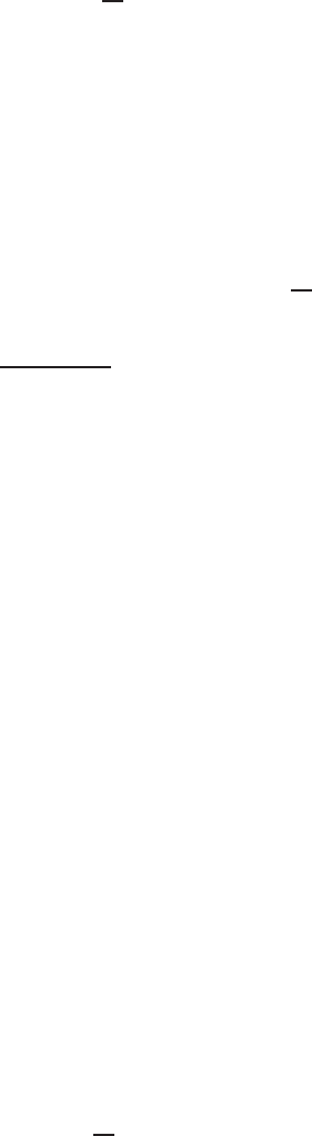
Lectures on Symplectic Field Theory 285
We will also need to impose a compatibility condition relating the coefficient
rings R
±
= Q[H
2
(M
±
)/G
±
] to a corresponding choice on the cobordism W . Choo se
a subgroup G ⊂ H
2
(W ) such that
(13.10) h[ω], Ai = 0 for all A ∈ G,
and such that the maps H
2
(M
±
) → H
2
(W ) induced by the inclusions M
±
֒→ W
send G
±
into G. If [ω] 6= 0 ∈ H
2
dR
(W ), then we will have to deal with noncompact
sequences of J-holomorphic curves that have unbounded energy, so it becomes nec-
essary to “complete” R to a Novikov ring
R, which contains R but also includes
infinite formal sums
∞
X
i=1
c
i
e
A
i
such that h[ω], A
i
i → +∞ as i → ∞.
Note that the evaluatio n h[ω], Ai ∈ R is well defined for A ∈ H
2
(W )/G due to
(
13.10).
Analogously to our definition of H in Lecture
12, the generating function for
index 0 curves in
c
W is defined as a formal power series in the variables ~, q
γ
(for
orbits in M
−
), and p
γ
(for o r bit s in M
+
), with coefficients in
R:
(13.11) F =
X
u∈M
σ
0
(J)
ǫ(u)
|Aut
σ
(u)|
~
g−1
e
A
q
γ
−
p
γ
+
,
where M
σ
0
(J) denotes the moduli space of connected J-holomorphic curves u in
c
W with ind(u) = 0 and only good asymptotic orbits, modulo permutations of the
punctures, and for each u:
• g is the genus of u;
• A is the equivalence class of [u] ∈ H
2
(W ) in H
2
(W )/G;
• γ
±
= (γ
±
1
, . . . , γ
±
k
±
) are the asymptotic orbits of u after arbitrarily fixing
orderings of its positive and negative punctures;
• ǫ(u) ∈ {1 , −1} is the sign of u as a point in the 0-dimensional compo-
nent of M
$
(J) (after choosing an ordering of the punctures and asymptotic
markers), relative to a choice of coherent orientatio ns on M
$
(J).
As usual, the product ǫ(u)q
γ
−
p
γ
+
is independent of choices. We shall regard F as
an element in an enlarged operator algebra that includes q and p variables for good
orbits in both M
+
and M
−
, related to each other by the supercommutation relations
[p
γ
−
, q
γ
+
] = [p
γ
+
, q
γ
−
] = [q
γ
−
, q
γ
+
] = [p
γ
−
, p
γ
+
] = 0
whenever γ
−
is an o r bit in M
−
and γ
+
is an orbit in M
+
. Since all curves counted
by F have index 0, F is homogeneous with degree
|F| = 0.
Notice that for any fixed monomial q
γ
−
p
γ
+
, the corresponding set of curves in M
σ
0
(J)
may be infinite if ω is nonexact, but SFT compactness implies that the set of such
curves with any given bound on
R
˙
Σ
u
∗
ω is bounded. As a consequence, the coefficient
of q
γ
−
p
γ
+
in F belongs to the Novikov ring
R.
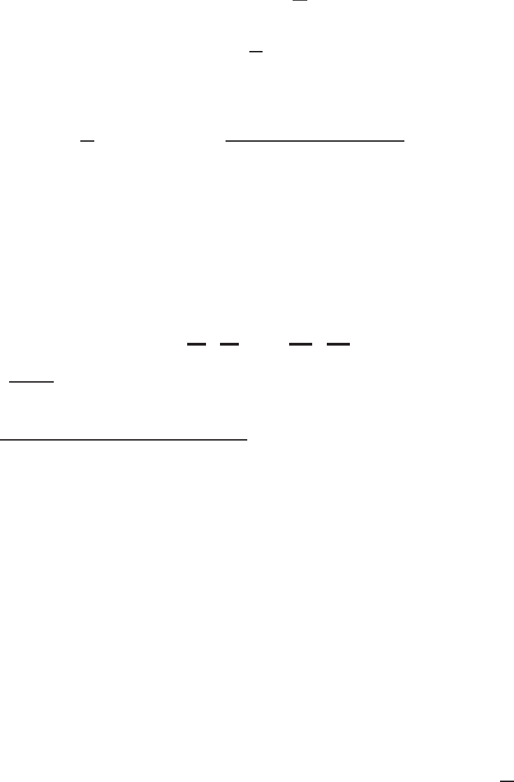
286 Chris Wendl
Consider next the series
exp(F) :=
∞
X
k=0
1
k!
F
k
.
We will be able to view this as a formal power series in q and p variables a nd a formal
Laurent series in ~ with coefficients in
R, though it is not obvious at first glance
whether its coefficients a r e in any sense finite. We will deduce this after interpreting
it as a count of disconnected index 0 curves: first, write
exp(F) =
∞
X
k=0
1
k!
X
(u
1
,...,u
k
)∈(M
σ
0
(J))
k
ǫ(u
1
) . . . ǫ(u
k
)
|Aut
σ
(u
1
)|. . . |Aut
σ
(u
k
)|
~
g
1
+...+g
k
−k
e
A
1
+...A
k
· q
γ
−
1
p
γ
+
1
. . . q
γ
−
k
p
γ
+
k
!
.
Observe that since each of the curves u
i
∈ M
σ
0
(J) in this expansion has index 0,
the monomials q
γ
−
i
p
γ
+
i
all have even degree and thus the order in which they are
written does not matter. Now for a given collection of distinct curves v
1
, . . . , v
N
and
integers k
1
, . . . , k
N
∈ N with k
1
+ . . . + k
N
= k, the various permutations of
(u
1
, . . . , u
k
) := ( v
1
, . . . , v
1
|
{z }
k
1
, . . . , v
N
, . . . , v
N
|
{z }
k
N
) ∈ (M
σ
0
(J))
k
occur
k!
k
1
!...k
N
!
times in the above sum, so if we forg et the ordering, then the contri-
bution of this particular k-tuple of curves to exp(F) is
ǫ(u
1
) . . . ǫ(u
k
)
k
1
! . . . k
N
!|Aut
σ
(u
1
)|. . . |Aut
σ
(u
k
)|
~
g
1
+...+g
k
−k
e
A
1
+...+A
k
q
γ
−
1
p
γ
+
1
. . . q
γ
−
k
p
γ
+
k
.
Notice next that the denominator k
1
! . . . k
N
!|Aut
σ
(u
1
)|. . . |Aut
σ
(u
k
)| is the order of
the automorphism group of the dis connected curve formed by the disjoint union of
u
1
, . . . , u
k
: t he extra factors k
i
! come from automorphisms that permute connected
components of the do ma in. Thus exp(F) can also be written as in (
13.11), but with
M
σ
0
(J) replaced by the moduli space of potentially disconnected index 0 curves with
unordered punctures, and g −1 generalized to g
1
+. . .+g
k
−k fo r any curve that has
k connected components of genera g
1
, . . . , g
k
. One subtlety that was glossed over in
the above discussion: the sum also includes the unique curve with zero components,
i.e. the “empty” J- holomorphic curve, which app ear s as the initial 1 in the series
expansion of exp(F).
With this interpretation of exp(F) understood, we can now address the possibil-
ity that the infinite sum defining exp(F) might include infinitely many terms for a
given monomial ~
m
q
γ
−
p
γ
+
, i.e. tha t there are infinitely many disconnected index 0
curves with fixed asymptotic orbits and a fixed sum of the genera minus the number
of connected components. We claim that this can indeed, happ en, but only if the
curves belong to a sequence of homolo gy classes A
i
∈ H
2
(M)/G with h[ω], A
i
i → ∞,
hence the coefficient of ~
m
q
γ
−
p
γ
+
in exp (F) belongs to the Novikov ring
R. The
danger here comes only from closed curves, since a disjoint union of two curves
with punctures always has strictly more punctures. Notice also that for any given

Lectures on Symplectic Field Theory 287
tuples of orbits γ
±
, there exists a number c ∈ R depending only on these o rbits a nd
the chosen capping surfaces such that every (possibly disconnected) J-holomorphic
curve u :
˙
Σ →
c
W asymptotic to γ
±
satisfies
h[ω], [u]i ≥ c.
This follows from the fact that the integral of ω over the relative homology class of
u always has a nonnegative integrand.
Lemma 13.24. Given constants C ∈ R and k ∈ Z, there exists a number N ∈ N
such that if u : (Σ, j) → (
c
W , J) is a cl osed J-holomorphic curve satisfying
R
Σ
u
∗
ω ≤
C, with m connected components of genera g
1
, . . . , g
m
satisfying g
1
+. . .+g
m
−m = k,
then m ≤ N.
Proof. Note first that for each integer g ≥ 0, there is an energy thresh-
old, i.e. a constant c
g
> 0 such that every nonconstant closed and connected J-
holomorphic curve u : Σ →
c
W of genus g has
Z
Σ
u
∗
ω ≥ c
g
.
This is an easy consequence of SFT compactness: indeed, if there were no such
constant, then we would find a sequence u
k
: Σ →
c
W of connected closed curves
with genus g such that
E(u
k
) =
Z
Σ
u
∗
ω → 0;
here we have used the fact that Σ is closed and
R
Σ
u
∗
ω
ϕ
depends only on the homology
class o f u in order to simplify the usual definition o f energy for asymptotically
cylindrical curves. SFT compactness then gives a subsequence of u
k
that converges
to a stable holomorphic building in which every component has zero energy and is
therefore constant. Since there ar e no marked points in the picture, no such building
exists, so this is a contradiction.
Now if u is a disconnected curve satisfying t he stated conditions, the bound on
R
Σ
u
∗
ω combines with the energy threshold to give a bound for each g ≥ 0 on the
number o f connected components of u with genus g. In particular, there is a bound
on the number of components with genus 0 or 1. All other components contribute
positively to the left hand side of t he relation
P
m
i=1
(g
i
− 1) = k, so this implies a
universal bound on m.
Corollary 13.25. Fix constants C ∈ R an d k ∈ Z, a nd tuples of Reeb orbits
γ
±
, and assume that the usual transversality conditions hold. Then there exist at
most finitely many potentially disconnected J-holomorphic curves u :
˙
Σ →
c
W with
index 0 such that the number of connected com ponents m and the genera g
1
, . . . , g
m
of its co mponents satisfy g
1
+ . . . + g
m
− m = k.
Corollary 13.26. The expression exp(F) is a formal power series in q and p
variables and a formal Laurent series in ~, with coefficients in the Novikov ring
R.

288 Chris Wendl
The necessity of considering disconnected curves becomes clear when one tries to
translate the compactness and gluing theory of J-holomorphic curves in
c
W into alge-
braic relations. In particular, consider the 1-dimensional moduli space of connected
index 1 curves in
c
W with genus g. The boundary points of the compactification of
this space consist of two types of buildings:
Type 1 : A main level of index 0 and an upper level of index 1;
Type 2 : A main level of index 0 and a lower level of index 1.
This is clear under the usual transversality assumptions since regular curves in
c
W
must have index at least 0, while regular curves in the symplectizations R × M
±
have index at least 1 unless they are trivial cylinders. The building must also be
connected and have arithmetic genus g, but there is nothing to guarantee that each
individual level is connected. In f act, we already saw this issue in Lecture
12 when
proving H
2
= 0, but it was simpler to deal with there, because disconnected regular
curves of index 1 in a symplectization always have a unique nontrivial compo nent,
while the rest are trivial cylinders. In the cobordism
c
W , on the other hand, a
disconnected index 0 curve can be formed by any disjoint union of index 0 curves,
all of which are nontrivial. Exponentiation provides a convenient way to encode all
data about disconnected curves in terms of connected curves.
Since the union of all buildings of types 1 and 2 described above forms the
boundary of a compact oriented 1-manifold, the count of these buildings is zero,
and this fact is encoded in the so-called master equation
(13.12) H
−
exp(F)|
p
−
=0
− exp(F)H
+
|
q
+
=0
= 0,
where the expressions “p
−
= 0” and “q
+
= 0” mean that we discard all terms in
H
−
exp(F) −exp ( F)H
+
containing any variables p
γ
for o rbits in M
−
or q
γ
for orbits
in M
+
. The resulting expression is therefore a formal power series in q variables
for or bits in M
−
and p variables for orbits in M
+
, representing a count of generally
disconnected index 1 holomorphic buildings in
c
W with the specified asymptotics.
The various ways to form such buildings by choices o f gluings is again encoded by
the commutator algebra. The master equation (
13.12) can be used to prove the
chain map property for counts of curves in cobordisms, thus it is an essential piece
of the invariance proo f for each of the homology theories introduced above.
Exercise 13.27. Fill in the details of the proof of (
13.12).
13.3. Full SFT as a BV
∞
-algebra
In this section we discuss the specific theory H
SFT
∗
(M, ξ; R), defined as the ho-
mology of the chain complex (A[[~]], D
SFT
). The case G = H
2
(M) with trivial gr oup
ring coefficients Q[H
2
(M)/G] = Q will be a bbreviated as
H
SFT
∗
(M, ξ) := H
SFT
∗
(M, ξ; Q).
As we defined it, D
SFT
acts on A[[~]] by treating the g enerating function H as a
differential operator via the substitution
(13.13) p
γ
= κ
γ
~
∂
∂q
γ
.

Lectures on Symplectic Field Theory 289
According to [CL09], this makes (A[[~]], D
SFT
) into a BV
∞
-algebra; we’ll have no
particular need to discuss here what that means, but one convenient featur e is the
expansion
(13.14) D
SFT
=
1
~
∞
X
k=1
D
(k)
SFT
~
k
,
in which each D
(k)
SFT
: A → A is a differential operato r of order ≤ k (see [
CL09, §5]).
For each k ∈ N, D
(k)
SFT
is a count o f all index 1 holomorphic curves that have genus
g ≥ 0 and m ≥ 1 positive punctures such that g + m = k. In particular, D
(1)
SFT
is simply the cont act ho mo logy differential ∂
CH
, and the expansion (
13.14) implies
together with D
2
SFT
= 0 t hat (D
(1)
SFT
)
2
= 0, hence we again see the chain complex
for contact homology hidden inside a version of the “full” SFT complex.
13.3.1. Cobordism maps and invariance. One can use the master equation
(
13.12) to prove invariance of H
SFT
∗
(M, ξ; R) by a stra ightforward generalization o f
the usual Floer-theoretic argument. Suppose (W, dλ) is an exact symplectic cobor-
dism from (M
−
, ξ
−
) to (M
+
, ξ
+
) with λ|
T M
±
= α
±
, and choose a generic almost
complex structure J on
c
W that is dλ-compatible on W and restricts to the cylin-
drical ends as generic elements J
±
∈ J(α
±
). Let (A
±
[[~]], D
±
SFT
) denote the chain
complexes associated to the data (α
±
, J
±
), and for simplicity in this initial discus-
sion, choose the trivial coefficient ring R = Q for both. We then define a map
Φ : A
+
[[~]] → A
−
[[~]] : f 7→ exp(F)f|
q
+
=0
,
where the generating function exp(F) is regarded as a differential operator via the
substitution (
13.13), with e
A
:= 1 for all A ∈ H
2
(W ) since we are using t r ivial
coefficients, and “q
+
= 0” means that after applying exp(F) to change f into a
function of q variables for orbits in both M
+
and M
−
, we discard all terms that
involve orbits in M
+
. The exactness of the cobordism implies that negative powers
of ~ do not appear in Φf, thus producing an element of A
−
[[~]]: indeed, since there
are no holomorphic curves in
c
W without positive punctures, every term in F contains
at least one p variable, so that negative powers of ~ do not appear in exp(F) after
applying (
13.13).
The master equation for F now translates into the fact that Φ is a chain map,
D
−
SFT
◦ Φ − Φ ◦ D
+
SFT
,
thus it descends to homology. The geometric meaning o f Φ is straightforward to
describe: a nalogous to (
12.11) in Lecture 12, we can write
(13.15) Φq
γ
=
∞
X
g=0
X
γ
′
~
g+k−1
n
g
(γ, γ
′
, k)q
γ
′
,
where n
g
(γ, γ
′
, k) is a product of some combinatorial factors with a signed count
of disconnected index 0 holomorphic curves with connected components of genus
g
1
, . . . , g
m
satisfying g
1
+ . . . + g
m
− m = g − 1, and with positive ends at γ and
negative ends at γ
′
, where k is the number of positive ends.
290 Chris Wendl
Let’s discuss two applications of the cobordism map Φ. First, note that if W is a
trivial symplectic cobordism [0, 1] ×M, then the above discussion can easily be gen-
eralized with (A
±
, D
±
SFT
) both defined over the same group ring R = Q[H
2
(M)/G]
for any choice of G ⊂ H
2
(M). There is no need to consider a Novikov ring in
defining F here since the cobordism is exact. We therefore obtain a chain map
with arbitrary group ring coefficients, and extending this discussion along standard
Floer-theoretic principles will imply that the chain map is an isomorphism: this can
be used in particular to prove that H
SFT
∗
(M, ξ; R) does not depend on the choices of
contact form and almost complex structure. There a r e two additional steps involved
in this ar gument: first, one needs to use a chain homotopy to prove that Φ does
not depend on the choice o f almost complex structure J on
c
W . Given a g eneric
homotopy {J
s
}
s∈[0,1]
, the chain homotopy map
Ψ : A
+
[[~]] → A
−
[[~]]
is defined as a differential operator in the same manner as Φ, but counting pairs
(s, u) where s ∈ [0, 1] is a parameter value for which J
s
is nongeneric and u is a
disconnected J
s
-holomorphic curve in
c
W with index −1. We saw how this works
for cylindrical contact homology in Lecture
10, but there is a new subtlety now
that should be mentioned: in principle, a d isconnected index −1 curve in
c
W could
have arbitrarily many components, including perhaps many with index −1 a nd oth-
ers with arbitrarily large index. Even worse, the compactified 1-dimensional space
of pairs (s, u) for J
s
-holomorphic curves u of index 0 may include buildings that
have symplectization levels of index greater than 1, balanced by disjoint unions of
many index −1 curves in the main level. This sounds hor r ible, but it can actu-
ally be ignored, for the following reason: first, since there are only finitely many
pairs (s, u) where u is a connected J
s
-holomorphic curve with index −1, one can (if
transversality is achievable at all) use a genericity argument to assume without loss
of generality that for any given s ∈ [0, 1], at most one connected index −1 curve ex-
ists. This means that in any building that has multiple index −1 components, those
components are just multiple copies of the same curve. Now, since that curve has
odd index, it is represented by a monomial q
γ
−
p
γ
+
that contains an odd number of
odd generators, and any nontrivial product of such generators therefore disappears
in A since odd generators anticommute with themselves. This algebraic miracle
encodes a convenient fact about coherent orientations: whenever one of the horrible
buildings described ab ove appears, one can reorder two of the index −1 components
to produce from it a different building t hat lives in a moduli space with the opposite
orientation. Gluing this building back together then produces a continuation of the
1-dimensional moduli space, so that the horrible building can actually be interpreted
as an “interior” point of the 1-dimensional space, rather than boundary. The actual
count of boundary points is then exactly what we want it to be: it is represented
algebraically by the chain homotopy relation!
Finally, compositions of cobordism maps can be understood via a stretching
argument that is not substantia lly different f rom the case of cylindrical contact
homology. Since the trivial cobordism with R-invariant data gives a cobordism
map that just counts trivial cylinders and is therefore the identity, it follows that
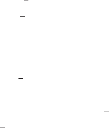
Lectures on Symplectic Field Theory 291
cobordism maps relating different pairs of dat a (α
±
, J
±
) are always invertible, and
this proves the invariance of H
SFT
∗
(M, ξ; R).
The second applicatio n concerns nontrivial exact cobordisms, and it is immediate
from the fact that Φ is a chain map:
Theorem 13.28. Any exact cobordism (W, dλ) from (M
−
, ξ
−
) to (M
+
, ξ
+
) gives
rise to a Q[[~]]-linear map
H
SFT
∗
(M
+
, ξ
+
) → H
SFT
∗
(M
−
, ξ
−
).
It is much more complicated to say what ha ppens in the event of a nonexact
cobordism, but slightly easier if we restrict o ur attention to fillings, i.e. the case with
M
−
= ∅. Assume (W, ω) is a compact symplectic manif old with stable boundary M,
inheriting a stable Hamiltonian structure H = (Ω, α) for which α is a nondegenerate
contact form, and assume also that the completion
c
W admits an almost complex
structure J that is ω-ta me on W and has a pseudoconvex restriction J
+
∈ J(H) to
the cylindrical end. We saw in Proposition
13.22 that these conditions can always
be achieved for a weak filling after deforming the symplectic structure. Let
G := ker[ω] := {A ∈ H
2
(W ) | h[ω], Ai = 0},
and choose G
+
⊂ H
2
(M) to be any subgroup such t hat the map H
2
(M) → H
2
(W )
induced by t he inclusion M ֒→ W sends G
+
into G. In ot her words, G
+
can be any
subgroup of ker[Ω] ⊂ H
2
(M). Define the group rings
R
+
= Q[H
2
(M)/G
+
], R = Q[H
2
(W )/ ker[ω]],
with the Novikov completion of R denoted by
R. The map H
2
(M)/G
+
→ H
2
(W )/G
induced by M ֒→ W then gives a natural ring homomorphism
(13.16) R
+
→ R.
If ω is not exact, then it may no longer be true that every term in F has at least
one p varia ble. Let us write
F = F
0
+ F
1
,
where F
0
contains no p variables a nd F
1
= O(p), i.e. F
0
counts all closed curves
in
c
W , and F
1
counts everything else. Since F
0
and F
1
have even degree, they
commute, and thus
exp(F) = exp( F
0
) exp(F
1
).
where exp(F
0
) is an invertible element of R[[~, ~
−1
]] since exp ( −F
0
) exp(F
0
) = 1.
By the master equation,
exp(F
0
) exp(F
1
)H = O( q),
hence exp(F
1
)H = exp(−F
0
)O(q) = O(q) since exp( −F
0
) contains no p variables.
Using the substitution (
13.13), and using (13.16) to map coefficients in R
+
to R, it
follows that exp(F
1
) gives rise to a differential operator
Φ : A[[~]] →
R[[~]] : f 7→ exp(F
1
)f|
q=0
,
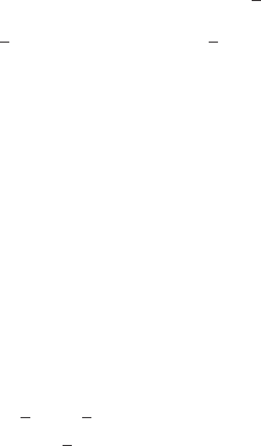
292 Chris Wendl
which is a chain map to the SFT of the empty set with Novikov coefficients, meaning
Φ ◦D
SFT
= 0.
This chain map counts the disconnected index 0 curves in
c
W whose connected
components all have at least one positive puncture.
Theorem 13.29. Suppose (W, ω) is a compact symplectic manifold with s ta-
ble boundary (M, H = (Ω, α)), whe re α i s a no ndegenerate co ntact form, and its
co mpletion
c
W admits an almost complex structure that is ω-tame on W and has
a generic and pseudoconv ex restriction J
+
∈ J(H) to the cylindrica l end. Let
R
denote the Novikov comp l e tion of Q[H
2
(W )/ ker[ω]], and let R
+
= Q[H
2
(M)/G
+
],
where G
+
⊂ H
2
(M) is any subgroup on which the evaluation of [Ω] ∈ H
2
dR
(M)
vanishes. Then there exists an
R[[~]]-linear map H
SFT
∗
(M, H, J
+
; R
+
) → R[[~]].
13.3.2. Algebraic torsion. We can now generalize the notion of algebraic
overtwistedness. Notice that since every term in D
SFT
is a differential operator
of order at least 1,
D
SFT
f = 0 for all f ∈ R[[~]],
hence every element o f the extended coefficient ring R[[~]] represents an element
of H
SFT
∗
(M, ξ; R) that may or may not be trivial. Since D
SFT
commutes with all
elements of R[[~]], t he subset consisting of elements that are t rivial in homology
forms an ideal. The following definition originates in [
LW11].
Definition 13.30. We say that a closed contact manifold (M, ξ) has algebraic
torsion of order k (or k-torsion for short) with coefficients in R if
[~
k
] = 0 ∈ H
SFT
∗
(M, ξ; R).
The numerical invariant
AT(M, ξ; R) ∈ N ∪{0, ∞}
is defined to be the smallest integer k such that (M, ξ) has algebraic k-torsion but
no (k − 1)-torsion, or ∞ if there is no algebraic torsion of any order.
Several consequences of algebraic torsion can be read off quickly from the prop-
erties of SFT cobordism ma ps. Consider first the case of trivial coefficients R = Q,
which we shall refer to as untwisted algebraic torsion and abbreviate
AT(M, ξ) := AT(M, ξ; Q).
If (W, ω) is a strong filling of (M, ξ), then the hypotheses of Theorem
13.29 are
fulfilled even with G
+
= H
2
(M) since ω is exact at the boundary, thus we obtain
a Q[[~]]-linear map H
SFT
∗
(M, ξ) →
R[[~]], with R denoting the Novikov completion
of Q[H
2
(W )/ ker[ω]]. If [~
k
] = 0 ∈ H
SFT
∗
(M, ξ), then the cobordism map implies a
contradiction since ~
k
does not equal 0 in
R[[~]]. Similarly, if (W, dλ) is an exact
cobordism fro m (M
−
, ξ
−
) to (M
+
, ξ
+
), then the cobordism map H
SFT
∗
(M
+
, ξ
+
) →
H
SFT
∗
(M
−
, ξ
−
) of Theorem
13.28 is also Q[[~]]-linear, and thus any algebraic k-torsion
in ( M
+
, ξ
+
) is inherited by (M
−
, ξ
−
). This proves:
Lectures on Symplectic Field Theory 293
Theorem 13.31. Contact manifolds with AT(M, ξ) < ∞ are not strongly fillabl e.
Moreover, if there exists an exac t symplectic cobordi sm from (M
−
, ξ
−
) to (M
+
, ξ
+
),
then AT(M
−
, ξ
−
) ≤ AT(M
+
, ξ
+
).
It is known (see [Wen13]) that the second part of t he above theorem does not
hold for strong symplectic cobordisms in g eneral, so exactness of cobordisms is a
meaningful symplectic topological condition, not just a technical hypothesis. It is
also known thanks to a construction of Ghiggini [
Ghi05] that strong and exact
fillability are not equivalent conditions, but Ghiggini’s proof of this uses Heegaard
Floer homology; thus far it is not known whether this phenomenon can be detected
via SF T or other holomorphic curve techniques.
There are also many known examples of contact manifolds that have untwisted
algebraic torsion but a r e weakly fillable. The simplest are the tight tori (T
3
, ξ
k
)
for k ≥ 2, for which weak fillings were first constructed by Giroux [Gir94], but
Eliashberg [
Eli96] showed tha t strong fillings do not exist, and we will see in Lec-
ture
16 that AT(T
3
, ξ
k
) = 1. The weak/strong distinction can often be detected via
the choice of coefficients in SFT. We saw in §
13.2.1 that a weak filling of a contact
manifold (M, ξ) can always be deformed so as to have stable boundary with data
(H = (Ω, α), J
+
) for which α is a nondegenerate contact form a nd J
+
is C
∞
-close to
any given element of J(α). Pro position 13.16 showed that if (M, ξ) is algebraically
overtwisted, then the contact homology for the stable Hamiltonian data ( H, J
+
) can
also be made to vanish.
Exercise 13.32. Generalize the proof of Prop.
13.16 to show that if (M, ξ) ha s
algebraic k-torsion with coefficients in R, then also [~
k
] = 0 ∈ H
SFT
∗
(M, H
c
, J
c
; R)
for sufficiently large c > 0.
It then follows using Theorem
13.29 that a lgebraic torsion with suitably twisted
coefficients a lso gives a n obstruction to weak filling . L et us say that (M, ξ) has fully
twisted algebraic k-torsion whenever [~
k
] = 0 ∈ H
SFT
∗
(M, ξ; Q[H
2
(M)]). Note that
in parallel with Remark 13.10, any nested pair of subgroups G ⊂ G
′
⊂ H
2
(M) gives
rise to a map
H
SFT
∗
(M, ξ; Q[H
2
(M)/G
′
]) → H
SFT
∗
(M, ξ; Q[H
2
(M)/G]),
which is a morphism in the sense that it ma ps the unit and all powers of ~ to
themselves. This implies that (M, ξ) has fully twisted k-torsion if and only if it has
k-to r sion for every choice of coefficients.
Theorem 13.33. If (M, ξ) is a closed contact manifold with a finite o rder of
algebraic torsion w i th coefficients in R = Q[H
2
(M)/G] for some subgroup G, then
(M, ξ) does not admit any weak symplectic filling (W, ω) for which [ω|
T M
] ∈ H
2
dR
(M)
is rational and annihilates all elements of G. In particular, if (M, ξ) has fully twisted
algebraic torsion of some finite order, then it is not weakly fillable.
Remark 13.34. The rationality condition in Theorem 13.33 can probably be
lifted, and is known to be unnecessary at least in dimension three. It is clear in any
case that if (M, ξ) admits a weak filling (W, ω), then one can always make a small
perturbation of ω to produce a weak filling for which [ω|
T M
] ∈ H
2
(M; Q).
294 Chris Wendl
We will see some concrete examples of algebraic torsion computations in Lec-
ture
16. Let us conclude this discussion for now with the observation that algebraic
torsion of order zero is a notion we’ve seen before:
Proposition 13.35. For any closed contact ma nifold (M, ξ) and group ring
R = Q[H
2
(M)/G], the follow i ng conditions are equivalent:
(1) (M, ξ) has algebraic 0-torsion (with coefficients in R);
(2) (M, ξ) is al gebraically overtwisted (with coefficients in R);
(3) H
SFT
∗
(M, ξ; R) = 0.
Proof. It is obvious that (
3) implies (1). Since D
SFT
f = ∂
CH
f +O(~) for f ∈ A,
the R[[~]]-linear map
A[[~]] → A : F 7→ F|
~=0
defines a chain map (A[[~]], D) → (A, ∂
CH
) and thus descends to an R[[~]]-linear
map H
SFT
∗
(M, ξ; R) → HC
∗
(M, ξ; R). The existence of this map proves that (
1)
implies (
2).
To prove that (
2) implies (3), recall first that if there exists f ∈ A with ∂
CH
f =
1, then the fact that HC
∗
(M, ξ; R) = 0 follows easily since for any g ∈ A with
∂
CH
g = 0, the graded Leibniz rule implies ∂
CH
(fg) = (∂
CH
f)g − f(∂
CH
g) = g. This
works because ∂
CH
is a derivation—but D
SFT
is not one, so the same trick will not
quite work for D
SFT
. The trick in proving H
SFT
∗
(M, ξ; R) = 0 will be to quantify
the failure o f D
SFT
to be a derivation. For our purposes, it suffices to know that
(13.17) D
SFT
(FG) = (D
SFT
F)G + (−1)
|F|
F(D
SFT
G) + O(~)
holds for all F, G ∈ A[[~]], which follows from the fact that ∂
CH
is a derivation.
With this remark out of the way, suppose f ∈ A satisfies ∂
CH
f = 1, in which case
(13.18) D
SFT
f = 1 + ~G
for some G ∈ A[[~]]. We claim then that for any Q ∈ A[[~]] with D
SFT
Q = 0, there
exists Q
1
∈ A[[~]] with
(13.19) D
SFT
(fQ) = Q + ~Q
1
and D
SFT
Q
1
= 0. Indeed, (
13.19) follows from (13 .17) and (13.18) since D
SFT
Q = 0,
and D
SFT
Q
1
= 0 then follows by applying D
SFT
to (
13.19) and using D
2
SFT
= 0.
Fixing Q
0
:= Q ∈ A[[~]], we can now define a sequence Q
k
∈ A[[~]] satisfying
D
SFT
Q
k
= 0 for all integers k ≥ 0 via the inductive condition
D
SFT
(fQ
k
) = Q
k
+ ~Q
k+1
.
Then
P
∞
k=0
(−1)
k
~
k
Q
k
∈ A[[~]], and
D
SFT
f
∞
X
k=0
(−1)
k
~
k
Q
k
!
= Q.

APPENDIX A
Sobolev spaces
Contents
A.1. Approximation, extension and embedding theorems 301
A.2. Products, compositions, and rescaling 305
A.3. Spaces of sections of vector bundles 311
A.4. Some remarks on domains with cylindrical e nds 316
In this appendix, we review some of the standard properties of Sobolev spaces,
in particular using them to prove Propositions
2.7, 2.8 and 2.10 from §2 .2, and
elucidating the construction of Sobolev spaces of sections on vector bundles. A
good reference for the necessary background material is [
AF03].
A.1. Approximation, extension and embedding theorems
Unless otherwise noted, all functions in the following are a ssumed to be defined
on a nonempty open subset
U ⊂ R
n
with its standard Lebesgue measure, and taking values in a finite-dimensional normed
vector space that will usually not need to be specified, though occasionally we will
assume it is R o r C so that one can define products of functions. The domain U
will also sometimes have additional conditions specified such as b oundedness or reg-
ularity at the boundary, tho ugh we will try not to add too many more restrictions
than are really needed. The most useful assumption t o impose on U is known as
the strong local Lipschitz condition: if U is bounded, then it means simply that
near every boundary point of U, one can find smooth local coordinates in which
U looks like the region bounded by the graph of a Lipschitz-continuous function,
and in this case we call U a bounded Lipschitz domain. If U is unbounded,
then one needs to impose extra conditions guaranteeing e.g. uniformity of Lipschitz
constants, and the precise definition becomes a bit lengthy (see [
AF03, §4.9]). For
our purposes, all we really need to know about the strong local Lipschitz condition
is that that it is satisfied bo th by bo unded Lipschitz domains and by relatively
tame unbounded domains such as (0, 1) ×(0, ∞) ⊂ R
2
which have smooth boundary
with finitely many corners. We will repeatedly need to use the generalized version
of H¨older’s inequality, which states that for any finite collection of measurable
301
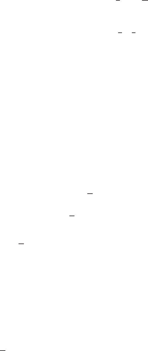
302 Chris Wendl
functions f
1
, . . . , f
m
,
(A.1)
m
Y
i=1
|f
i
|
L
p
≤
m
Y
i=1
kf
i
k
L
p
i
for 1 ≤ p ≤ p
1
, . . . , p
m
≤ ∞ with
1
p
=
m
X
i=1
1
p
i
.
This is an easy corollary of t he standard version,
|f|· |g|
L
1
≤ kfk
L
p
·kgk
L
q
whenever 1 ≤ p, q ≤ ∞ and 1 =
1
p
+
1
q
.
For an integer k ≥ 0 and real number p ∈ [1 , ∞] we define W
k,p
(U) as in §
2.2 to be
the Ba nach space of all f ∈ L
p
(U) which have weak partial derivatives ∂
α
f ∈ L
p
(U)
for all |α| ≤ k. For p = 2, these spaces are also often denoted by
H
k
(U) := W
k,2
(U),
and they admit Hilbert space structures with inner product
hf, gi
H
k
=
X
|β|≤k
h∂
α
f, ∂
α
gi
L
2
.
We denote by
W
k,p
0
(U) ⊂ W
k,p
(U), H
k
0
(U) ⊂ H
k
(U)
the closed subspaces defined as the closures of C
∞
0
(U) with respect to the relevant
norms. Since C
∞
0
(U) is dense in L
p
(U) for 1 ≤ p < ∞ (see e.g. [
LL01, §2.19]),
there is no difference between W
0,p
(U) and W
0,p
0
(U) for p < ∞, but in general
W
k,p
0
(U) 6= W
k,p
(U) for k ≥ 1, with a few not able exceptions such as the case
U = R
n
(cf. Corollary
A.2 below). Let
W
k,p
lo c
(U) :=
functions f on U
f ∈ W
k,p
(V) for all open subsets V ⊂ U
with compact closure
V ⊂ U
,
and we say that a sequence f
j
∈ W
k,p
lo c
(U) converges in W
k,p
lo c
to f ∈ W
k,p
lo c
(U) if
the restrictions to all precompact open subsets V ⊂
V ⊂ U converge in W
k,p
(V).
Recall that for k ∈ {0, 1, 2, . . . , ∞}, C
k
(U) denotes the space of functions on U with
continuous derivatives up to o rder k, while
C
k
(
U) ⊂ C
k
(U)
is the space of f ∈ C
k
(U) such that for all |α| ≤ k, ∂
α
f is bounded and uniformly
continuous.
Theorem A.1 ([
AF03, §3.17, 3.22]). For any open subset U ⊂ R
n
, and any
k ≥ 0, 1 ≤ p < ∞, the subspace
C
∞
(U) ∩ W
k,p
(U) ⊂ W
k,p
(U)
is dense. Moreover, if U ⊂ R
n
satisfies the strong local Lipschitz condition, then the
space
n
f ∈ C
∞
(U)
f =
˜
f|
U
for some
˜
f ∈ C
∞
0
(R
n
)
o
is also d ense in W
k,p
(U), so in particular,
C
∞
(
U) ∩ W
k,p
(U) ⊂ W
k,p
(U)
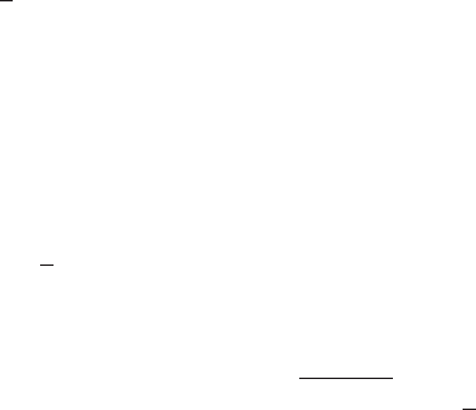
Lectures on Symplectic Field Theory 303
is dense.
Corollary A.2. The space C
∞
0
(R
n
) is dense in W
k,p
(R
n
) for every k ≥ 0 and
p ∈ [1, ∞).
Here is another useful char acterization of W
k,p
0
(U):
Theorem A.3 ([
AF03, §5.29]). Assume U ⊂ R
n
is an open subset satisfying the
strong local Lipschitz condition. Th en a function f ∈ W
k,p
(U) belongs to W
k,p
0
(U)
if and only if the function
˜
f on R
n
defined to match f on U and 0 everywhere else
be l ongs to W
k,p
(R
n
).
While it is obvious from the definitions that functions in W
k,p
0
(U) always admit
extensions of class W
k,p
over R
n
, this is much less obvious for functions in W
k,p
(U)
in general, and it is not true without sufficient assumptions about the regularity
of ∂U. For our purposes it suffices to consider the following case.
Theorem A.4 ( [
AF03, §5.22]). Assume U ⊂ R
n
is a bounded open subset such
that ∂
U is a submanifold of class C
m
for some m ∈ {1, 2, 3, . . . , ∞}. Then there
exists a linear o perator E that maps functions defin ed almost everywh e re on U to
functions defined a l most everywhere on R
n
and has the follow i ng properties:
• For every function f on U, Ef|
U
≡ f almost everywhe re;
• For every nonn egative integer k ≤ m and every p ∈ [1, ∞), E define s a
bo und ed linear operator W
k,p
(U) → W
k,p
(R
n
).
Corollary A.5. Suppose U, U
′
⊂ R
n
are open subsets such that U has com pact
closure contained in U
′
. If U satisfies the hypo thes i s of Theorem
A.4, then the
resulting extension operator E can be chosen such that it maps each W
k,p
(U) for
k ≤ m and 1 ≤ p < ∞ into W
k,p
0
(U
′
).
Proof. Choose a smooth function ρ : U
′
→ [0 , 1] that has compact support and
equals 1 on
U, then replace the o perator E given by Theorem A.4 with the operat or
f 7→ ρ · Ef .
To state the Sobolev embedding theorem in its pro per generality, recall tha t for
0 < α ≤ 1, the H¨older seminorm of a f unction f o n U is defined by
|f|
C
α
:= |f|
C
α
(U)
:= sup
x6=y∈U
|f(x) − f (y)|
|x − y|
α
,
and C
k,α
(U) is then defined as the Banach space of functions f ∈ C
k
(
U) for which
the nor m
kfk
C
k,α := kfk
C
k + max
|β|=k
|∂
β
f|
C
α
is finite. In reading the following statement, it is important to remember that
elements of W
k,p
(U) are technically not f unctions, but r ather equivalence classes
of functions defined almost everywhere. Thus when we say e.g. that there is an
inclusion W
k,p
(U) ֒→ C
m,α
(U), the literal meaning is that for every function f
representing an element of W
k,p
(U), one can change the values of f in a unique way
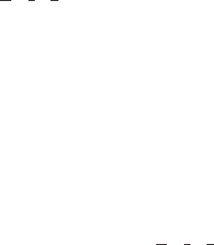
304 Chris Wendl
on some set of measure zero in U so that after this change, f ∈ C
m,α
(U). Continuity
of the inclusion means tha t there is a bound of the form
kfk
C
m,α
≤ ckfk
W
k,p
for all f ∈ W
k,p
(U), where c > 0 is a constant which may in general depend on m,
α, k, p and U, but not on f .
Theorem A.6 ([
AF03, §4.12]). Assume U ⊂ R
n
is an open subset satisfying
the strong local Lipschitz co ndition, k ≥ 1 is an integer and 1 ≤ p < ∞.
(1) If kp > n and k − n/p < 1, then there exist continuous inclusions
W
k,p
(U) ֒→ C
0,α
(U) for each α ∈ (0, k − n/p],
W
k,p
(U) ֒→ L
q
(U) for each q ∈ [p, ∞].
(2) If kp < n and p
∗
> p is defined by the condition
1
p
∗
=
1
p
−
k
n
,
then there ex ist continuous inclusions
W
k,p
(U) ֒→ L
q
(U), for each q ∈ [p, p
∗
].
(3) If kp = n, then there exist continuous inclusions
W
k,p
(U) ֒→ L
q
(U), for each q ∈ [p, ∞).
Moreover, the spaces W
k,p
0
(U) admit similar inclusion s under no assumption on the
open subset U ⊂ R
n
.
Under the same assumption on the domain U, one can apply Theorem
A.6 to suc-
cessive derivatives of functions in W
k,p
(U) and thus o bt ain the f ollowing inclusions
for any integer d ≥ 0:
(A.2) W
k+d,p
(U) ֒→ C
d,α
(U) if kp > n and 0 < α ≤ k − n/p < 1,
(A.3) W
k+d,p
(U) ֒→ W
d,q
(U) if kp > n and p ≤ q ≤ ∞,
(A.4) W
k+d,p
(U) ֒→ W
d,q
(U) if kp < n and p ≤ q ≤ p
∗
, with
1
p
∗
=
1
p
−
k
n
,
(A.5) W
k+d,p
(U) ֒→ W
d,q
(U) if kp = n and p ≤ q < ∞.
This last inclusion can then be composed with (
A.2) for an arbitrarily large choice
of q, giving another inclusion
(A.6) W
k+d,p
(U) ֒→ C
d−1,α
(U) if kp = n and 0 < α < 1.
Remark A.7. The embedding theorem suggests that one should intuitively think
of W
k,p
(U) as consisting of functions with “k − n/p continuous derivatives,” where
the number k −n/p may in general be a non-integer and/or negative. This provides
a useful mnemonic for results about embeddings of one Sobolev space into another,
such as the following.

Lectures on Symplectic Field Theory 305
Corollary A.8. Assume U ⊂ R
n
is an open subset satisfying the strong local
Lipschitz condition, 1 ≤ p, q < ∞, and k, m ≥ 0 are integers satisfying
k ≥ m, p ≤ q, and k −
n
p
≥ m −
n
q
.
Then there exists a continuous incl usion W
k,p
(U) ֒→ W
m,q
(U).
By the Arzel`a-Ascoli theorem, the natural inclusion
C
k,α
′
(U) ֒→ C
k,α
(U)
for α < α
′
is a compact operator whenever U ⊂ R
n
is bounded. It follows that if U ⊂
R
n
in (
A.2) is bounded and α is strictly less than the extremal value k − n/p, then
the inclusion (
A.2) is also compact. A similar statement holds for the inclusion (A.4)
when p ≤ q < p
∗
, and this is known as the Rellich-Kondrachov compactness
theorem. We summarize these as f ollows:
Theorem A.9 ([
AF03, §6.3]). Assume U ⊂ R
n
is a bounded Lipschitz d omain,
k ≥ 1 and d ≥ 0 are integers and 1 ≤ p < ∞.
(1) If kp > n and k − n/p < 1, then the inclusions
W
k+d,p
(U) ֒→ C
d,α
(U) for α ∈ ( 0, k − n/p),
W
k+d,p
(U) ֒→ W
d,q
(U) for q ∈ [p, ∞)
are compact.
(2) If kp ≤ n and p
∗
∈ (p, ∞] is defined by the condition 1/p
∗
= 1/p − k/n,
then the inclusions
W
k+d,p
(U) ֒→ W
d,q
(U) for q ∈ [p, p
∗
)
are compact.
In particular, the continuous i nclusion W
k,p
(U) ֒→ W
m,q
(U) in Corollary
A.8 is
co mpact whenever the inequality k − n/p ≥ m − n/q is strict.
A.2. Products, compositions, and rescaling
We now restate and prove Propositions
2.7, 2.8 and 2 .10 from §2.2. These are
all corollaries of the Sobolev embedding theorem, so in particular they hold for the
same class of domains U ⊂ R
n
, and the restrictions on U can be dropped at the cost
of replacing each space W
k,p
by W
k,p
0
.
We begin by generalizing Prop.
2.7, hence we consider Sobolev spaces of functions
valued in R or C so that po intwise products of functions are well defined almost
everywhere. We say that there is a continuous product map,
W
k
1
,p
1
(U) × . . . × W
k
m
,p
m
(U) → W
k,p
(U),
or a continuous product pairing in the case m = 2, if for every set of functions
f
i
∈ W
k
i
,p
i
(U) with i = 1, . . . , m, the pointwise product function f
1
· . . . · f
m
is in
W
k,p
(U) and there is an estimate of the form
kf
1
· . . . · f
m
k
W
k,p ≤ ckf
1
k
W
k
1
,p
1
· . . . · kf
m
k
W
k
m
,p
m
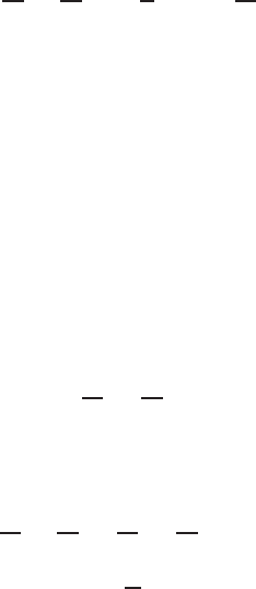
306 Chris Wendl
for some constant c > 0 not dep ending on f
1
, . . . , f
m
. The case m = 2, k
1
= k
2
= k
and p
1
= p
2
= p is especially interesting, as the space W
k,p
(U) is then a Banach
algebra. More generally, one can ask under what circumstances multiplication by
functions of class W
k,p
defines a bounded linear operator on functions o f class W
m,q
.
A hint about this comes from the world of classically differentiable functions: mul-
tiplication by C
k
-smooth functions defines a continuous ma p C
m
→ C
m
if and only
if k ≥ m. The corresponding answer in Sobolev spaces turns out to be that func-
tions of class W
k,p
need to have strictly more than zero derivatives in the sense of
Remark
A.7, and at least as many derivatives a s functions of class W
m,q
.
Theorem A.10. Assume U ⊂ R
n
is an ope n subset satisfying the strong local
Lipschitz condition, k, p, m and q sa tisfy the same numerical hypotheses as in
Corollary
A.8 (so in particular W
k,p
(U) embeds continuously into W
m,q
(U)), and
kp > n. Then there exists a continuous prod uct pairing
W
k,p
(U, C) × W
m,q
(U, C) → W
m,q
(U, C) : (f, g) 7→ f g.
The following preparatory lemma will be useful both for proving the product
estimate and for f urther results below. It is an easy consequence of Theorem A.6
and H¨older’s inequality.
Lemma A.11. Assume U ⊂ R
n
is an open subset satisfying the strong lo-
ca l Lipschitz condition, m ≥ 2 is an integer, and we are given positive numbers
p
1
, . . . , p
m
≥ 1 an d integers k
1
, . . . , k
m
≥ 0. Let I :=
i ∈ {1, . . . , m}
k
i
p
i
≤ n
.
Then for any q ≥ 1 s a tisfying
X
i∈I
1
p
i
−
k
i
n
<
1
q
≤
m
X
i=1
1
p
i
,
there is a continuous product map
W
k
1
,p
1
(U) × . . . × W
k
m
,p
m
(U) → L
q
(U).
Proof. By the generalized H¨older inequality (
A.1), it suffices to show that for
any q ≥ 1 in the stated ra nge, one can find numbers q
1
, . . . , q
m
∈ [q, ∞] satisfying
1/q = 1/q
1
+ . . . + 1/q
m
for which Theorem
A.6 provides continuous inclusions
W
k
i
,p
i
(U) ֒→ L
q
i
(U)
for each i = 1 , . . . , m. Whenever k
i
p
i
> n, this inclusion is valid with q
i
chosen freely
from the interval [p
i
, ∞], so 1/q
i
can then take any value subject to the constraint
0 ≤
1
q
i
≤
1
p
i
.
If on the other hand k
i
p
i
≤ n, then we can arrange 1/q
i
to take any value in the
range
1
p
i
−
k
i
n
<
1
q
i
≤
1
p
i
.
Adding these up, the range of values for
P
i
1
q
i
that we can achieve in this way covers
the stated interval.
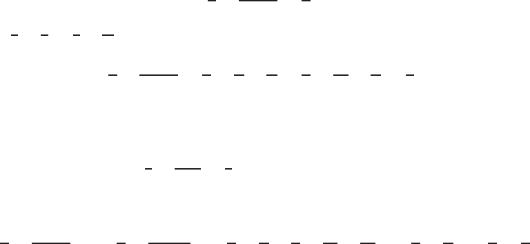
Lectures on Symplectic Field Theory 307
Proof of Theorem A.10. By density o f smooth functions, it suffices to prove
that an estimate of the form
kfgk
W
m,q
≤ ckfk
W
k,p
kgk
W
m,q
holds for all f ∈ C
∞
(U) ∩ W
k,p
(U) and g ∈ C
∞
(U) ∩ W
m,q
(U). Equivalently, we
need to show that for all f and g of this type and every multiindex α of degree
|α| ≤ m, there is a constant c > 0 independent of f and g such that
k∂
α
(fg)k
L
q
≤ ckfk
W
k,p
kgk
W
m,q
.
Since f and g are smooth, we are free to use the product rule in computing ∂
α
(fg),
which will then be a linear combination of terms of the form ∂
β
f · ∂
γ
g where |α| =
|β| + |γ|, hence we have reduced the problem to proving a bound
k∂
β
f · ∂
γ
gk
L
q
≤ ckfk
W
k,p kgk
W
m,q
for every pair of multiindices β, γ with |β| + |γ| ≤ m. Since ∂
β
f ∈ W
k−|β|,p
(U) and
∂
γ
f ∈ W
m−|γ| ,q
(U), the result follows if we can assume that for every pair of integers
a, b ≥ 0 satisfying a + b ≤ m, there exists a continuous product pairing
(A.7) W
k−a,p
(U) × W
m−b,q
(U) → L
q
(U).
If (k −a)p > n, then W
k−a,p
֒→ L
∞
and (
A.7) is immediate since W
m−b,q
֒→ L
q
(U).
For the remaining cases, we shall apply Lemma
A.11, noting that the condition
1/q ≤ 1/p + 1/q is trivially satisfied.
If (m −b)q > n but (k −a)p ≤ n, then the hypotheses of the lemma a re satisfied
if and only if
1
p
−
k − a
n
<
1
q
.
Since
1
p
−
k
n
≤
1
q
−
m
n
by assumption, we have
1
p
−
k − a
n
=
1
p
−
k
n
+
a
n
≤
1
q
−
m
n
+
a
n
≤
1
q
since a ≤ m, a nd equality holds only if a = m, b = 0 and k − n/p = m − n/q,
which implies mq > n. In this case W
m−b,q
= W
m,q
֒→ L
∞
, and the pairing (
A.7)
follows because W
k−a,p
= W
k−m,p
embeds continuously into L
q
: the latter follows
from Theorem
A.6 since
1
p
−
k−m
n
=
1
q
.
Finally, when (k − a)p ≤ n a nd (m − b)q ≤ n, the hypotheses of the lemma are
satisfied since
1
p
−
k − a
n
+
1
q
−
m −b
n
≤
1
p
−
k
n
+
1
q
−
m
n
+
m
n
=
1
p
−
k
n
+
1
q
<
1
q
,
where we’ve used the assumption kp > n and the fact that a + b ≤ m.
The next result generalizes Proposition
2.8 and concerns the following question:
if f : U → R
m
is a f unction o f class W
k,p
whose graph lies in some open subset
V ⊂ U × R
m
, and Ψ : V → R
N
is another function, under what conditions can we
conclude t hat the function
U → R
N
: x 7→ Ψ(x, f(x))
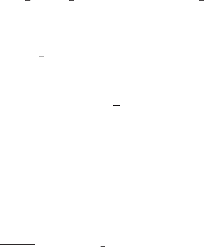
308 Chris Wendl
is in W
k,p
(U, R
N
)? We will abbreviate this f unction in t he following by Ψ ◦(Id ×f),
and we would also like t o know whether it depends continuously (in the W
k,p
-
topology) on f and Ψ. The following t heorem is stated rather generally, but on first
reading you may prefer to a ssume U ⊂ R
n
is bounded, in which case some of t he
hypot heses become vacuous. We will say that an open subset V ⊂ U × R
m
is a
star-shaped neighborhood of f : U → R
m
if it contains the graph of f
0
and
(x, v) ∈ V ⇒ (x, tv + (1 − t)f
0
(x)) ∈ V for all t ∈ [0, 1].
Theorem A.12. Assume U ⊂ R
n
is an ope n subset satisfying the strong local
Lipschitz condition, p ∈ [1, ∞) and k ∈ N satisfy kp > n, and V ⊂ U × R
m
is a star-sha ped neighborhood of some function f
0
∈ W
k,p
(U, R
m
). Assume also
O
k,p
(U; V) ⊂ W
k,p
(U, R
m
) is an open neighborhood of f
0
such that
(x, f(x)) ∈ V for all x ∈ U and f ∈ O
k,p
(U; V),
and O
k
(
V, R
N
) ⊂ C
k
(V, R
N
) is a subset such that a ll Ψ ∈ O
k
(V, R
n
) have the
following properties:
1
(1) There exists a bounded subset K ⊂ U such that Ψ(x, v) is independent of x
for all x ∈ U \ K;
(2) Ψ ◦ (Id × f
0
) ∈ L
p
(U, R
N
).
Then there is a well-de fined and continuous map
O
k
(V, R
N
) × O
k,p
(U; V) → W
k,p
(U, R
N
) : (Ψ , f ) 7→ Ψ ◦ (Id × f ).
Proof. We will show first that if f ∈ O
k,p
(U; V) is smooth, then Ψ ◦ (Id ×
f) belongs to W
k,p
(U, R
N
) for every Ψ ∈ O
k
(
V, R
N
). Since V is a star-shaped
neighborhood o f f
0
, we have
|Ψ(x, f( x))−Ψ(x, f
0
(x))| =
Z
1
0
d
dt
Ψ
x, tf(x) + (1 − t)f
0
(x)
dt
≤
Z
1
0
|D
2
Ψ
x, tf(x) + (1 − t)f
0
(x)
|dt
· |f(x) − f
0
(x)|
≤ kΨk
C
1
(V)
· |f(x) − f
0
(x)|
for all x ∈ U, implying
kΨ ◦ (Id × f) − Ψ ◦ (Id × f
0
)k
L
p
≤ kΨk
C
1
(V)
· kf − f
0
k
L
p
,
hence Ψ ◦ (Id × f) ∈ L
p
(U, R
N
).
For ℓ = 1, . . . , k, we can regard the ℓth derivative of Ψ with respect to variables
in R
m
as a bounded and uniformly continuous map from V into the vector space of
symmetric ℓ-multilinear maps from R
m
to R
N
, denoting this by
D
ℓ
2
Ψ : V → Hom((R
m
)
⊗ℓ
, R
N
).
Denote the partial derivatives with respect to variables in U ⊂ R
n
by
D
β
1
Ψ : V → R
N
,
1
Both of the conditions on Ψ ∈ O
k
(
V, R
n
) are vacuous if U ⊂ R
n
is bounded.
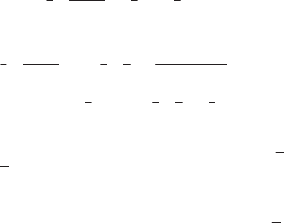
Lectures on Symplectic Field Theory 309
where β is a multiindex in n variables. Now for any multiindex α with |α| ≤ k, the
derivative ∂
α
(Ψ ◦(Id ×f)) is a linear combination of product functions of the form
(A.8) (D
γ
1
D
ℓ
2
Ψ ◦ (Id × f))(∂
β
1
f, . . . , ∂
β
ℓ
f) : U → R
N
,
where ℓ + |γ| ∈ {1, . . . , |α|} a nd |β
1
| + . . . + |β
ℓ
| = |α| − |γ|. If ℓ = 0 but |γ| > 0,
then this expression is clearly in L
p
(U, R
N
) since it is continuous and D
γ
1
Ψ(x, v) = 0
for x ∈ U \ K, where K is bounded. For ℓ ≥ 1, it satisfies
(D
γ
1
D
ℓ
2
Ψ ◦ (Id × f))(∂
β
1
f, . . . , ∂
β
ℓ
f)
L
p
(U)
≤ kD
γ
1
D
ℓ
2
Ψk
C
0
(V)
·
ℓ
Y
j=1
|∂
β
j
f|
L
p
(U)
if the product on the r ight hand side has finite L
p
-norm. The latter is trivially
true if ℓ = 1. To deal with the ℓ ≥ 2 case, note that ∂
β
j
f ∈ W
k−|β
j
|,p
(U) for each
j = 1, . . . , ℓ, so the necessary bound will follow from the existence of a continuous
product map
W
k−m
1
,p
(U) × . . . × W
k−m
ℓ
,p
(U) → L
p
(U)
for m
j
:= |β
j
|, and we claim that such a product map does exist whenever kp > n
and m
1
, . . . , m
ℓ
≥ 0 are integers satisfying m
1
+ . . . + m
ℓ
≤ k. To see this, note
first tha t since W
k−m
j
,p
֒→ L
∞
whenever (k − m
j
)p > n, it suffices to prove the
claim under the assumption that (k − m
j
)p ≤ n for every j = 1, . . . , ℓ. In this case,
Lemma
A.11 provides the desired product map if the condition
ℓ
X
j=1
1
p
−
k − m
j
n
<
1
p
≤
ℓ
X
j=1
1
p
is satisfied. And it is: using kp > n, ℓ ≥ 2 and m
1
+ . . . + m
ℓ
≤ k, we find
ℓ
X
j=1
1
p
−
k − m
j
n
= ℓ
1
p
−
k
n
+
m
1
+ . . . + m
ℓ
n
≤
1
p
+ (ℓ − 1)
1
p
−
k
n
<
1
p
.
This pr oves that Ψ ◦ (Id × f) ∈ W
k,p
(U, R
N
).
Next, suppose f ∈ O
k,p
(U; V) is not necessarily smooth but f
i
∈ O
k,p
(U; V) is
a sequence of smooth functions converging to f in W
k,p
, while Ψ
i
∈ O
k
(
V, R
N
)
converges to Ψ ∈ O
k
(
V, R
N
) in C
k
. Then the same a rgument we used to estimate
kΨ ◦ (Id ×f) − Ψ ◦ (Id × f
0
)k
L
p
shows that Ψ ◦ (Id × f
i
) → Ψ ◦(Id ×f) in L
p
, and
since f
i
is also C
0
-convergent, the compactly supported functions D
γ
1
Ψ ◦ (Id × f
i
)
converge to D
γ
1
Ψ ◦ (Id × f) in L
p
for each multiindex with 1 ≤ |γ| ≤ k. For ℓ ≥ 1
and |γ| + ℓ ≤ k, D
γ
1
D
ℓ
2
Ψ
i
◦ (Id × f
i
) converges to D
γ
1
D
ℓ
2
Ψ ◦ (Id × f) in C
0
(
U, R
N
),
and each of the derivatives ∂
β
j
f
i
appearing in (
A.8) also converges in L
p
(U). In
light of the continuous product maps discussed above, it follows that each derivative
∂
α
(Ψ
i
◦ (Id × f
i
)) for |α| ≤ k is L
p
-convergent, and its limit is necessarily the
corresponding weak derivative ∂
α
(Ψ ◦ ( Id × f)), hence (see Exercise A.13 below)
Ψ ◦ (Id × f) ∈ W
k,p
(U, R
N
) and Ψ
i
◦ (Id ×f
i
)
W
k,p
−→ Ψ ◦ (Id × f).

310 Chris Wendl
Exercise A.13. Show that if f
i
is a sequence of smooth functions on an open set
U ⊂ R
n
with f
i
L
p
→ f a nd ∂
α
f
i
L
p
→ g for some multiindex α and functions f, g ∈ L
p
(U),
then ∂
α
f = g in the sense of distributions.
The following result on coordinate transformations of the domain can b e proved
in an analogous way to Theorem
A.12, though it is considerably easier since there is
no need to worry about Sobolev product maps (and thus no need to assume kp > n
or impose regularity conditions on the domain).
Theorem A.14 ([
AF03, §3.41]) . Assume k ∈ N, 1 ≤ p ≤ ∞, and U, U
′
⊂
R
n
are open subsets with a C
k
-smooth diffeomorphism ϕ : U → U
′
such that all
derivatives of ϕ an d ϕ
−1
up to o rder k are bo und ed and uniformly continuous. Then
there is a well-defined Banach s pace isomorphism
W
k,p
(U
′
) → W
k,p
(U) : f 7→ f ◦ ϕ.
We now r estate and prove Proposition 2.10. We denote by
˚
D
n
,
˚
D
n
ǫ
⊂ R
n
the open
balls of radius 1 and ǫ respectively about the origin.
Theorem A.15. Assume p ∈ [1, ∞) and k ∈ N satisfy kp > n, and for each
f ∈ W
k,p
(
˚
D
n
) and ǫ ∈ (0, 1], define f
ǫ
∈ W
k,p
(
˚
D
n
) by
f
ǫ
(x) := f(ǫx).
Then there exist constants C > 0 and r > 0 such that for eve ry f ∈ W
k,p
(
˚
D
n
),
kf
ǫ
− f(0) k
W
k,p
(
˚
D
n
)
≤ Cǫ
r
kf − f (0)k
W
k,p
(
˚
D
n
)
for all ǫ ∈ (0, 1].
Proof. Let β denote a multiindex of order |β| = k. Then using a change of
varia bles, we have
k∂
β
(f
ǫ
− f(0) ) k
p
L
p
(
˚
D
n
)
= ǫ
kp
Z
D
n
|∂
β
f(ǫx)|
p
= ǫ
kp−n
Z
D
n
ǫ
|∂
β
f(x)|
p
≤ ǫ
kp−n
k∂
β
fk
p
L
p
(
˚
D
n
)
≤ ǫ
kp−n
kf − f(0)k
p
W
k,p
(
˚
D
n
)
,
and ǫ
kp−n
→ 0 as ǫ → 0 since kp − n > 0.
Next, suppose |β| = m ∈ {1, . . . , k −1}. Then ∂
β
f and ∂
β
f
ǫ
are in W
k−m,p
(
˚
D
n
),
and if (k − m)p < n, Theorem
A.6 gives a continuous inclusion
(A.9) W
k−m,p
(
˚
D
n
) ֒→ L
q
(
˚
D
n
)
with q > p satisfying 1/q + (k −m)/n = 1/p. Likewise, if (k −m)p ≥ n, then (
A.9)
is a continuous inclusion for arbitrarily large choices of q ≥ p. We will therefore
assume in general that (
A.9) holds with q ∈ (p, ∞) satisfying
1
q
+
1
r
=
1
p
,
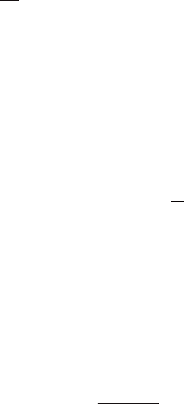
Lectures on Symplectic Field Theory 311
where r =
n
k−m
if (k − m)p < n and otherwise r = p + δ for some δ > 0 which may
be chosen arbitrarily small. Given this, we use H¨older’s inequality and find
k∂
β
(f
ǫ
− f(0) ) k
p
L
p
(
˚
D
n
)
= ǫ
mp
Z
D
n
|∂
β
f(ǫx)|
p
= ǫ
mp−n
Z
D
n
ǫ
|∂
β
f(x)|
p
≤ ǫ
mp−n
k∂
β
fk
p
L
q
(
˚
D
n
ǫ
)
k1k
p
L
r
(
˚
D
n
ǫ
)
≤ ǫ
mp−n
[Vol(D
n
ǫ
)]
p/r
k∂
β
fk
p
L
q
(
˚
D
n
)
≤ cǫ
mp−n
[Vol(D
n
ǫ
)]
p/r
k∂
β
fk
p
W
k−m,p
(
˚
D
n
)
≤ cǫ
mp−n
[Vol(D
n
ǫ
)]
p/r
kf − f(0)k
p
W
k,p
(
˚
D
n
)
for some constant c > 0. Writing Vol(D
n
ǫ
) = Cǫ
n
for a suitable constant C > 0, the
exp onent on ǫ in this expression becomes
mp − n +
np
r
,
which is positive whenever r = p + δ with δ > 0 sufficiently small since m ≥ 1, and
in t he case r = n/(k − m), it becomes simply kp − n > 0.
Finally, to bound the L
p
-norm of f
ǫ
−f (0) itself, we can use the fact that f ∈ W
k,p
is H¨older continuous, i.e. it satisfies
|f(x) − f (0)| ≤ ckf − f (0)k
W
k,p
(
˚
D
n
)
|x|
α
for all x ∈
˚
D
n
for suitable constants c > 0 and α ∈ (0, 1). Thus
kf
ǫ
− f(0) k
p
L
p
(
˚
D
n
)
=
Z
D
n
|f(ǫx) − f(0)|
p
≤ c
p
kf − f(0)k
p
W
k,p
Z
D
n
|ǫx|
αp
= c
p
kf − f(0)k
p
W
k,p
ǫ
αp
Z
D
n
|x|
αp
= ǫ
αp
c
p
Vol(S
n−1
)
αp + n
kf − f (0)k
p
W
k,p
.
A.3. Spaces of sections of vector bundles
In this section, fix a field
F := R or C,
assume M is a smooth n-dimensional manifold, possibly with boundary, and π :
E → M is a smooth vector bundle o f r ank m over F. This comes with a “bundle
atlas” A(π), a set whose elements α ∈ A(π) each consist of the following data:
(1) An open subset U
α
⊂ M;
(2) A smooth local coordinate chart ϕ
α
: U
α
∼
=
−→ Ω
α
, where Ω
α
is an open
subset of R
n
+
:= {(x
1
, . . . , x
n
) ∈ R
n
| x
n
≥ 0};
(3) A smooth local trivialization Φ
α
: E|
U
α
∼
=
−→ U
α
×F
m
.
312 Chris Wendl
Smoothness of ϕ
α
and Φ
α
means as usual that for every pair α, β ∈ A(π), the
coordinate transformations
ϕ
βα
:= ϕ
−1
β
◦ ϕ
α
: Ω
αβ
∼
=
−→ Ω
βα
, Ω
αβ
:= ϕ
α
(U
α
∩ U
β
)
and transition maps
g
βα
: U
α
∩ U
β
→ GL(m, F) such that Φ
β
◦ Φ
−1
α
(x, v) = (x, g
βα
(x)v)
for x ∈ U
α
∩ U
β
, v ∈ F
m
are smooth, and we shall assume the bundle atlas is maximal in the sense that
any triple (U, ϕ, Φ) that is smoothly compatible with every α ∈ A(π) also belongs
to A( π).
Any α ∈ A(π) now associates to sections η : M → E their local coordinate
representatives
η
α
:= pr
2
◦Φ
α
◦ η ◦ ϕ
−1
α
: Ω
α
→ F
m
,
where pr
2
: U
α
× F
m
→ F
m
is the projection, and the representa tives with respect
to two distinct α, β ∈ A(π) are related by
η
β
= (g
βα
◦ ϕ
−1
β
)(η
α
◦ ϕ
αβ
) on Ω
βα
⊂ Ω
β
.
For p ∈ [1, ∞] and each integer k ≥ 0, we t hen define the topological vector space
of sections of class W
k,p
lo c
by
W
k,p
lo c
(E) :=
η : M → E
sections such that η
α
∈ W
k,p
lo c
(
˚
Ω
α
, F
m
)
for all α ∈ A(π)
,
where convergence η
j
→ η in W
k,p
lo c
(E) means tha t η
α
j
→ η
α
in W
k,p
lo c
(
˚
Ω
α
, F
m
) for all
α ∈ A(π). Note that Ω
α
is no t necessarily an open subset of R
n
since it may cont ain
points in ∂R
n
+
= R
n−1
× {0}, but its interior
˚
Ω
α
is open in R
n
, and W
k,p
lo c
(
˚
Ω
α
) is
thus defined as in §
A.1. Strictly speaking, element s of η ∈ W
k,p
lo c
(E) are not sections
but equivalence classes of sections defined almost everywhere—the latter notion is
defined with respect to any measure a r ising from a smooth volume element on M,
and it does not depend on this choice.
It t ur ns out that W
k,p
lo c
(E) can be given the structure of a Banach space if M is
compact. This follows from the fact that M can then be covered by a finite subset of
the atlas A(π), but we must be a little bit careful: not all charts in A(π) are equally
suitable for defining W
k,p
-norms on sections, because e.g. even a nice smooth section
η ∈ Γ(E) may have kη
α
k
W
k,p
(
˚
Ω
α
)
= ∞ if Ω
α
⊂ R
n
+
is unbounded. One way to deal
with this is as follows: we will say that α ∈ A(π) is a precompact chart if there
exists α
′
∈ A(π) and a compact subset K ⊂ M such that
U
α
⊂ K ⊂ U
α
′
.
When this is the case, Ω
α
⊂ R
n
+
is necessarily bounded, and the transition maps
between two precompact charts necessarily have bounded derivatives of all orders,
as they are restrictions to precompact subsets of maps that are smooth on larger
domains. If M is compact, then one can always find a finite subset I ⊂ A(π)
consisting of precompact charts such that M =
S
α∈I
U
α
.
Lectures on Symplectic Field Theory 313
Definition A.16. Suppose E → M is a smooth vector bundle over a compact
manifold M, and I ⊂ A( π) is a finite set of precompact chart s such that {U
α
}
α∈I
is an open cover of M. We then define W
k,p
(E) as the vector space of all sections
η : M → E for which the norm
kηk
W
k,p := kηk
W
k,p
(E)
:=
X
α∈I
kη
α
k
W
k,p
(
˚
Ω
α
)
is finite.
The norm in the above definition depends on auxiliary choices, but it is easy to
see that the resulting definition of the space W
k,p
(E) and its topology do not. In
fact:
Proposition A.17. If M is compact, then W
k,p
(E) = W
k,p
lo c
(E), and a sequence
η
j
co nverges to η in W
k,p
lo c
(E) if and only if the norm given in Definition
A.16 satisfies
kη
j
−ηk
W
k,p
(E)
→ 0.
The proposition is an immediate consequence of the following.
Lemma A.18. Suppose M is a sm ooth manifold, π : E → M is a smooth vector
bundle, {β} ∪ J ⊂ A(π) is a finite collection of charts such that M =
S
α∈J
U
α
and
all coord i nate transformations and tran sition maps relating any two charts in the
co llection {β} ∪ J have bounded derivatives of all ord ers (e.g. it suffices to assume
all are precompact). Then there exists a constant c > 0 s uch that
kη
β
k
W
k,p
(
˚
Ω
β
)
≤ c
X
α∈J
kη
α
k
W
k,p
(
˚
Ω
α
)
for all sec tions η : M → E with η
α
∈ W
k,p
(
˚
Ω
α
) for every α ∈ J.
Proof. Choose a partition of unity {ρ
α
: M → [0, 1]}
α∈J
subordinate to the
finite open cover {U
α
}
α∈J
. Now η =
P
α∈J
ρ
α
η, and each ρ
α
η is supported in U
α
, so
(ρ
α
η)
β
has suppo rt in Ω
βα
= ϕ
β
(U
α
∩ U
β
). Thus using Theorem
A.14 with the f act
that g
βα
, ϕ
−1
β
, ϕ
αβ
and ϕ
βα
= ϕ
−1
αβ
are all smoot h functions with bounded derivatives
of all orders on the domains in question, we find
kη
β
k
W
k,p
(
˚
Ω
β
)
=
X
α∈J
(ρ
α
η)
β
W
k,p
(
˚
Ω
β
)
≤
X
α∈J
k(ρ
α
η)
β
k
W
k,p
(
˚
Ω
βα
)
=
X
α∈J
k(ρ
α
◦ ϕ
−1
β
)(g
βα
◦ ϕ
−1
β
)(η
α
◦ ϕ
αβ
)k
W
k,p
(
˚
Ω
βα
)
≤ c
X
α∈J
kη
α
k
W
k,p
(
˚
Ω
αβ
)
≤ c
X
α∈J
kη
α
k
W
k,p
(
˚
Ω
α
)
.
Corollary A.19. If M is compact, then the norm on W
k,p
(E) given by Defi-
nition
A.16 is independent of all auxilia ry choices up to equivalence of norms.
Theorem A.20. For any smooth v ector b undle π : E → M over a compact
manifold M, W
k,p
(E) is a Banach space .
314 Chris Wendl
Proof. If η
j
∈ W
k,p
(E) is a Cauchy sequence, then for some chosen finite
collection I ⊂ A(π) of precompact charts covering M, t he sequences η
α
j
for α ∈ I are
Cauchy in W
k,p
(
˚
Ω
α
) and thus have limits ξ
(α)
∈ W
k,p
(
˚
Ω
α
, F
m
). Choosing a part ition
of unity {ρ
α
: M → [0, 1]}
α∈I
subordinate to {U
α
}
α∈I
, we can now associate to each
α ∈ I a section η
∞,α
∈ W
k,p
(E) characterized uniquely by the condition that it
vanishes outside of U
α
and is represented in the trivialization on U
α
by
η
α
∞,α
= (ρ
α
◦ ϕ
−1
α
)ξ
(α)
.
We claim that ρ
α
η
j
→ η
∞,α
in W
k,p
(E) for each α ∈ I. Indeed, we have
(ρ
α
η
j
)
α
= (ρ
α
◦ ϕ
−1
α
)η
α
j
→ (ρ
α
◦ ϕ
−1
α
)ξ
(α)
= η
α
∞,α
in W
k,p
(
˚
Ω
α
)
since η
α
j
→ ξ
(α)
. For all other β ∈ I not equal to α, (ρ
α
η
j
)
β
− η
β
∞,α
∈ W
k,p
(
˚
Ω
β
, F
m
)
has suppo rt in Ω
βα
= ϕ
β
(U
α
∩ U
β
), thus
k(ρ
α
η
j
)
β
−η
β
∞,α
k
W
k,p
(
˚
Ω
β
)
= k(ρ
α
η
j
)
β
−η
β
∞,α
k
W
k,p
(
˚
Ω
βα
)
≤ ck(ρ
α
η
j
)
α
− η
α
∞,α
k
W
k,p
(
˚
Ω
α
)
,
where the inequality comes from Lemma
A.18 after replacing M with U
α
, and U
β
with U
β
∩ U
α
(note that the lemma does not require M to be compact). With the
claim established, we have
η
j
=
X
α∈I
ρ
α
η
j
→
X
α∈I
η
∞,α
in W
k,p
(E).
Exercise A.21 . For U ⊂ R
n
an open subset, the space W
k,p
lo c
(U) was defined in
§
A.1, but one can give it an alternative definition in the present context by viewing
functions on U as sections of a trivial vector bundle over U, with the latter viewed
as a noncompact smooth n-manifold. Show that these two definitions of W
k,p
lo c
(U)
are equivalent.
Exercise A.22. Suppose U ⊂ R
n
is a bounded open subset with smooth bound-
ary, so its closure U ⊂ R
n
is a smooth compact submanifold with boundary, and let
E →
U be a trivial vector bundle. Show that there is a canonical Banach space iso-
morphism between W
k,p
(U) as defined in §
A.1 and W
k,p
(E) as defined in the present
section. Hint: Recall that sections in W
k,p
(E) are only required to be defined almost
everywhere, so in particular if the domain M is a manifold with boundary, they need
not be well defined on ∂M.
In light of Exercise
A.22, the natural generalization of W
k,p
0
(U) in the present
setting is
W
k,p
0
(E) := C
∞
0
(E|
M\∂M
),
i.e. it is the closure in the W
k,p
-norm of t he space of smooth sections that vanish
near t he boundary. Density of smooth sections will imply that this is the same as
W
k,p
(E) if M is closed, but in general W
k,p
0
(E) is a closed subspace of W
k,p
(E).
The partit ion of unity argument in Theorem
A.20 contains all the essential ideas
needed to generalize results about Sobolev spaces on domains in R
n
to compact
manifolds. We now state the essential results, leaving the proofs as exercises.
Lectures on Symplectic Field Theory 315
Theorem A.23. Assume M is a smooth compact n-manifold, possibly with
bo und ary, π : E → M is a smooth vector bundle of finite rank, k ≥ 0 is an in-
teger and 1 ≤ p < ∞. Then the Banach space W
k,p
(E) has the following properties.
(1) The space Γ(E) of smooth sec tion s is dense in W
k,p
(E).
(2) If N ⊂ M is a smooth compact n-dimension al submanifold with boundary,
then there ex ists a bounded linear operator
E : W
k,p
(E|
N
) → W
k,p
0
(E)
which is an extension o perator in the sense that Eη|
N
= η for all η ∈
W
k,p
(E|
N
). Moreover, a s ection η ∈ W
k,p
(E|
N
) belon g s to W
k,p
0
(E|
N
) if
and only if the section ˜η defined to match η on N and to vanish on M \N
be l ongs to W
k,p
(E).
(3) If kp > n, then for each integer d ≥ 0, there e xists a continuous and compact
inclusion
W
k+d,p
(E) ֒→ C
d
(E).
(4) The natural inc lusion
W
k+1,p
(E) ֒→ W
k,p
(E)
is compact.
(5) Suppose F, G → M are smooth v ector bundles such that there exi s ts a
smooth bundle map
E ⊗ F → G : η ⊗ ξ 7→ η · ξ.
Then if kp > n and 0 ≤ m ≤ k, there exists a continuous product pairing
W
k,p
(E) × W
m,p
(F ) → W
m,p
(G) : ( η, ξ) 7→ η · ξ.
In pa rticular, products of W
k,p
sections give W
k,p
sections whenever kp > n.
(6) Suppose F → M is another smooth vec tor bundle, V ⊂ E is an open subset
that intersects every fiber of E, a nd we consider the spaces
W
k,p
(V) :=
η ∈ W
k,p
(E)
η(M) ⊂ V
and
C
k
M
(V, F ) :=
Φ : V → F | fiber-preserving maps of class C
k
,
where the latter is assigned the topology o f C
k
-convergence on compact sub-
sets. If kp > n, then W
k,p
(V) is an o pen subset of W
k,p
(E), and the map
C
k
M
(V, F ) × W
k,p
(V) → W
k,p
(F ) : (Φ, η) 7→ Φ ◦ η
is well defined and continuous.
(7) If N is another smooth com pact manifol d and ϕ : N → M is a smooth
diffeomorphism, then there is a Banach space isomorphism
W
k,p
(E) → W
k,p
(ϕ
∗
E) : η 7→ η ◦ ϕ.
316 Chris Wendl
A.4. Some remarks on domains with c ylindrical ends
For bundles π : E → M with M noncompact, W
k,p
(E) is not generally well
defined without making additional choices. When M =
˙
Σ = Σ \ Γ is a punctured
Riemann surface and π : E →
˙
Σ is equipped with an asymptotically Hermitian struc-
ture {(E
z
, J
z
, ω
z
)}
z∈Γ
, one nice way to define W
k,p
(E) was introduced in §
4.1: one
takes it to be the space of sections in W
k,p
lo c
(E) whose W
k,p
-norms on each cylindrical
end are finite with resp ect to a choice of asymptotic trivialization. This definition
requires the convenient fact that complex vector bundles over S
1
are always triv-
ial, though one can also do without t his by using the ideas in the previous section.
Indeed, any collection of local trivializations on the asymptotic bundle E
z
→ S
1
covering S
1
gives rise via the asymptotically Hermitian structure t o a collection of
trivializations on E covering the corresponding cylindrical end
˙
U
z
. The key fact
is then that S
1
is compact, hence one can always choose such a covering to be fi-
nite: combining this with a finite covering of
˙
Σ in the complement of its cylindrical
ends by precompact chart s, we obtain a covering of
˙
Σ by a finite collection of bun-
dle charts t hat are not all precompact, but nonetheless have the property that all
transition maps have bounded derivatives of all orders. This is enough to define a
W
k,p
-norm for sections of E →
˙
Σ as in Definition
A.16 and to prove that it does
not depend on the choices of charts or local trivializations, though it does depend
on the asymptotically Hermitian structure.
With this definition understood, one can easily generalize the Sobolev embedding
theorem and other important statements in Theorem
A.23 to the setting of an
asymptotically Hermitian bundle over a punctured Riemann surface. We shall leave
the details of this generalization as an exercise, but take the opportunity to point
out a few important differences from t he compact case.
First, since
˙
Σ is not compact, neither are t he inclusions
W
k+d,p
(E) ֒→ C
d
(E), W
k+1,p
(E) ֒→ W
k,p
(E).
The proof o f compactness fails due to the fact that cylindrical ends require local
trivializations over unbounded doma ins of the form ( 0, ∞) × (0, 1) ⊂ R
2
, for which
Theorem
A.9 does not hold. And indeed, considering unbounded shifts on the
infinite cylinder
˙
Σ = R ×S
1
, it is easy to find a sequence of W
k,p
-bounded functions
with kp > 2 that do not have a C
0
-convergent subsequence. That is the bad news.
The good news is that if η ∈ W
k+d,p
(E) for kp > 2, then one can say considerably
more about η t han just that it is C
d
-smooth. Indeed, restricting t o one of the
cylindrical ends [0, ∞) × S
1
⊂
˙
Σ, notice that finiteness of the W
k+d,p
-norm over
˙
Σ
implies
kηk
W
k+d,p
((R,∞)×S
1
)
→ 0 as R → ∞.
Since these domains are all naturally diffeomorphic for different values of R, the
C
d
-norm of η over (R, ∞) ×S
1
is bounded by t he W
k+d,p
-norm via a constant that
does not depend on R, so this implies an asymptotic decay condition
kηk
C
d
([R,∞)×S
1
)
→ 0 as R → ∞
for every η ∈ W
k+d,p
(E).
Lectures on Symplectic Field Theory 317
Here is another useful piece of good news: since
˙
Σ does not have boundary,
W
k,p
(E) = W
k,p
0
(E).
Theorem A.24. Given an asymptotically Hermitian bundle E over a punctured
Riemann surface
˙
Σ, the space C
∞
0
(E) of smooth s ections with compact support is
dense in W
k,p
(E) for all k ≥ 0 and 1 ≤ p < ∞.
Proof. We can assume as in Definition
A.16 that the W
k,p
-norm for sections η
of E is given by
kηk
W
k,p
=
X
α∈I
kη
α
k
W
k,p
(Ω
α
)
,
where I ⊂ A(π) is a finite collection of bundle charts
α =
ϕ
α
: U
α
∼
=
−→ Ω
α
, Φ
α
: E|
U
α
∼
=
−→ U
α
×C
n
such that each of the open sets Ω
α
⊂ C is either bounded or (for charts over the
cylindrical ends) of the form
Ω
α
= (0, ∞) ×ω
α
⊂ R
2
= C
for some bounded open subset ω
α
⊂ R. Now given η ∈ W
k,p
(E), Theorem
A.1
provides f or each α ∈ I a sequence η
α
j
∈ W
k,p
(Ω
α
) of smo oth functions with bounded
support such that η
α
j
→ η
α
in W
k,p
(Ω
α
). Choose a partition of unity {ρ
α
:
˙
Σ →
[0, 1]}
α∈I
subordinate to the open cover {U
α
}
α∈I
and let
η
j
:=
X
α∈I
ρ
α
(η
α
j
◦ ϕ
α
) ∈ W
k,p
(E).
These sections are smoo t h and have compact support since the η
α
j
have bounded
support in Ω
α
, and they converge in W
k,p
to η.
APPENDIX B
The Floer C
ε
space
The C
ε
-topology for functions was introduced by Floer [
Flo88b] to provide a Ba-
nach manifo ld of perturbed geometric structures without departing from the smo oth
category: it is a way to circumvent the annoying fact that spaces of smooth functions
which ar ise naturally in geometric settings are not Banach spaces. The construction
of C
ε
spaces generally depends on several arbitrary choices and is thus far from
canonical, but this detail is unimpor t ant since the C
ε
space itself is never the main
object of interest. What is important is merely the properties that it has, namely
that it not only embeds continuously into C
∞
and contains an abundance of non-
trivial functions, but also is a separable Banach space and can therefore be used in
the Sa r d-Smale theorem for genericity arguments. We shall prove these facts in this
appendix.
Fix a smooth finite-rank vector bundle π : E → M over a finite-dimensional
compact manifold M, possibly with boundary. For each integer k ≥ 0, we denote by
C
k
(E) the Banach space of C
k
-smooth sections of E; note that the norm on C
k
(E)
depends on various auxiliary choices but is well defined up to equivalence of norms
since M is compact. Now if (ε
k
)
∞
k=0
is a sequence of positive numbers with ε
k
→ 0,
set
C
ε
(E) =
η ∈ Γ(E)
kηk
C
ε
< ∞
,
where t he C
ε
-norm is defined by
(B.1) kηk
C
ε
=
∞
X
k=0
ε
k
kηk
C
k .
The norm for C
ε
(E) is somewhat more delicate than for C
k
(E), e.g. its equivalence
class is not obviously independent of auxiliary choices. This remark is meant as
a sanity check, but it should not cause extra concern since, in practice, the space
C
ε
(E) is typically rega rded as an auxiliary choice in it self. In many applications,
one fixes an o pen subset U ⊂ M and considers the closed subspace
C
ε
(E; U) =
η ∈ C
ε
(E)
η|
M\U
≡ 0
.
Remark B.1 . The requirement for M to be compact can be r elaxed as long as
U ⊂ M has compact closure: e.g. in one situation of frequent interest in this book,
we take M to be the noncompact completion of a symplectic cobor dism. In this case
C
ε
(E; U) can be defined as a closed subspace of C
ε
(E|
M
0
) where M
0
⊂ M is any
compact manifold with boundary that contains the closure of U. For this reason,
we lose no generality in cont inuing under the assumption that M is compact.
319
320 Chris Wendl
In order to prove things about C
ε
(E), we will need to specify a more precise
definition of the C
k
-norms. To this end, define a sequence of vector bundles E
(k)
→
M for integers k ≥ 0 inductively by
E
(0)
:= E, E
(k+1)
:= Hom(T M, E
(k)
).
Choose connections and bundle metrics on both T M and E; these induce connec-
tions and bundle metrics on each of the E
(k)
, so that f or any section ξ ∈ Γ(E
(k)
),
the covariant derivative ∇ξ is now a section of E
(k+1)
. In particular for η ∈ Γ(E),
we can define the “kth covariant derivative” of η a s a section
∇
k
η ∈ Γ(E
(k)
).
Using the bundle metrics to define C
0
-norms for sections of E
(k)
, we can t hen define
kηk
C
k
(E)
=
k
X
m=0
k∇
m
ηk
C
0
(E
(m)
)
,
where by convention ∇
0
η := η. We will assume throughout the following that the
C
k
-norms appearing in (
B.1) are defined in this way.
Theorem B.2. C
ε
(E) is a Banach space.
Proof. We need to show that C
ε
-Cauchy sequences converge in the C
ε
-norm.
It is clear from the definitions that if η
j
∈ C
ε
(E) is Cauchy, then η
j
is also C
k
-
Cauchy for every k ≥ 0, hence its derivatives ∇
k
η
j
for every k are C
0
-convergent
to continuous sections ξ
k
of E
(k)
. This convergence implies that ξ
k+1
= ∇ξ
k
in
the sense of distributions, hence by the equivalence of classical and distributional
derivatives (see e.g. [
LL01, §6.10]), η
∞
:= ξ
0
is smooth with ∇
k
η
∞
= ξ
k
, so that
∇
k
η
j
→ ∇
k
η
∞
in C
0
(E
(k)
) for all k.
We claim η
∞
∈ C
ε
(E). Choose N > 0 such that kη
i
−η
j
k
C
ε
< 1 for all i, j ≥ N.
Then for every m ∈ N and every i ≥ N,
m
X
k=0
ε
k
kη
i
k
C
k ≤
m
X
k=0
ε
k
kη
i
− η
N
k
C
k +
m
X
k=0
ε
k
kη
N
k
C
k
≤ kη
i
− η
N
k
C
ε
+ kη
N
k
C
ε
< 1 + kη
N
k
C
ε
.
Fixing m and letting i → ∞, we then have
m
X
k=0
ε
k
kη
∞
k
C
k
≤ 1 + kη
N
k
C
ε
for all m, so we can now let m → ∞ and conclude kη
∞
k
C
ε
≤ 1 + kη
N
k
C
ε
< ∞.
The argument that kη
j
→ η
∞
k
C
ε
→ 0 as j → ∞ is similar: pick ǫ > 0 and N
such that kη
i
−η
j
k
C
ε
< ǫ for all i, j ≥ N. Then for a fixed m ∈ N, we can let i → ∞
in t he expression
P
m
k=0
ε
k
kη
i
− η
j
k
C
k < ǫ, giving
m
X
k=0
ε
k
kη
∞
− η
j
k
C
k
≤ ǫ.
This is true for every m, so we can take m → ∞ and conclude kη
∞
− η
j
k
C
ε
≤ ǫ for
all j ≥ N.

Lectures on Symplectic Field Theory 321
To show that C
ε
(E) is also separable, we will follow a hint
1
from [HS95] and
embed it isometrically into another Banach space t hat can be more easily shown to
be separable. For each integer k ≥ 0, define t he vector bundle
F
(k)
= E
(0)
⊕ . . . ⊕ E
(k)
,
and let X
ε
denote the vector space of all sequences
ξ := (ξ
0
, ξ
1
, ξ
2
, . . .) ∈
∞
Y
k=0
C
0
(F
(k)
)
such that
kξk
X
ε
:=
∞
X
k=0
ε
k
kξ
k
k
C
0
< ∞.
Exercise B.3. Adapt the proof of Theorem
B.2 to show that X
ε
is also a Banach
space.
Lemma B.4. X
ε
is separable.
Proof. Since C
0
(F
(k)
) is separable for each k ≥ 0, we can fix countable dense
subsets P
k
⊂ C
0
(F
(k)
). The set
P :=
(ξ
0
, . . . , ξ
N
, 0, 0, . . .) ∈ X
ε
N ≥ 0 and ξ
k
∈ P
k
for all k = 0, . . . , N
is then countable and dense in X
ε
.
Theorem B.5. C
ε
(E) is separable.
Proof. Consider the injective linear map
C
ε
(E) ֒→ X
ε
: η 7→
η, (η, ∇η), (η, ∇η, ∇
2
η), . . .
.
This is a n isometric embedding and thus presents C
ε
(E) as a closed linear subspace
of X
ε
, hence the theorem follows from Lemma
B.4 and the fa ct that subspaces of
separable metric spaces are always separable.
Note that given any open subset U ⊂ M, Theorems
B.2 and B.5 also hold for
C
ε
(E; U), as a closed subspace of C
ε
(E). So far in this discussion, however, there has
been no guarantee that C
ε
(E) or C
ε
(E; U) contains anything other than the zero-
section, though it is clear that in theory, one should always be able to enlarge the
space by choosing new sequences ε
k
that converg e to zero faster. The following result
says that C
ε
(E; U) can a lways be ma de large enough t o be useful in applications.
Theorem B.6. Given an open subset U ⊂ M, the sequence ε
k
ca n be chosen to
have the following properties:
(1) C
ε
(E; U) is dense in the s pace of continuous sections vanishin g outside U.
(2) Given any point p ∈ U, a neighborhood N
p
⊂ U of p, a number δ > 0 and
a continuous s ection η
0
of E, there exists a section η ∈ Γ(E) and a smooth
co mpactly supported function β : N
p
→ [0 , 1] such that
βη ∈ C
ε
(E; U), β(p)η(p) = η
0
(p), and kη − η
0
k
C
0
< δ.
1
Thanks to Sam Lisi for e xplaining to me w hat the hint in [
HS95] was referring to.
322 Chris Wendl
Proof. Note first that it suffices to find two separate sequences ε
k
and ε
′
k
that
have the first a nd second property resp ectively, as the sequence of minima min(ε
k
, ε
′
k
)
will then have both properties.
The following construction for the first property is based on a suggestion by
Barney Bramham. Observe first that the space C
0
(E; U) of continuous sections
vanishing outside U is a closed subspace of C
0
(E) and is thus separable, so we can
choose a countable C
0
-dense subset P ⊂ C
0
(E; U). Moreover, the space of smooth
sections vanishing outside U is dense in C
0
(E; U), hence we can assume without loss
of generality that the sections in P are smooth. Now write P = {η
1
, η
2
, η
3
, . . .} and
define ε
k
> 0 for every integer k ≥ 0 to have the property
ε
k
<
1
2
k
min
1
kη
1
k
C
k
, . . . ,
1
kη
k
k
C
k
.
Then every η
j
is in C
ε
(E; U), as
kη
j
k
C
ε
<
j−1
X
k=0
ε
k
kη
j
k
C
k
+
∞
X
k=j
1
2
k
< ∞.
The second property is essentially local, so it can be deduced from Lemma
B.7
below.
Lemma B.7. Suppose β :
˚
D
n
→ [0 , 1] is a smooth function with compact support
on the open unit ball
˚
D
n
⊂ R
n
and β(0) = 1. One can choo s e a sequence of posi tive
numbers ε
k
→ 0 such that for every η
0
∈ R
m
and r > 0 , the function η : R
n
→ R
m
defined by
η(p) := β(p/r)η
0
satisfies
P
∞
k=0
ε
k
kηk
C
k < ∞.
Proof. Define ε
k
> 0 so tha t for k ≥ 1,
ε
k
=
1
k
k
kβk
C
k
.
Then
∞
X
k=1
ε
k
kηk
C
k ≤
∞
X
k=1
1
k
k
kβk
C
k
kβk
C
k
r
k
=
∞
X
k=1
1/r
k
k
< ∞.
APPENDIX C
Genericity in the space of asymptotic operators
The purpose of this appendix is to prove Lemma
3.18, which was needed for
our definition of spectral flow in §
3.2. The proof combines some ideas from that
section with the technique used in Lecture
7 to prove generic transversality of moduli
spaces via the Sard-Smale theorem. Some knowledge of that technique should thus
be considered a prerequisite for this appendix; if you have never seen it before and
were directed here aft er reading the statement of Lemma 3 .18, you might want to
skip this for now and come back after you’ve read as far as Lecture
7.
Recalling the notation from Lecture
3, we fix the real Hilb ert spaces
H = L
2
(S
1
, R
2n
), D = H
1
(S
1
, R
2n
),
the symmetric index 0 Fredholm operator
T
ref
= −J
0
∂
t
: D → H
and, given a smooth loop of symmetric matrices S : S
1
→ End
sym
R
(R
2n
), refer to any
operator of the form
A = −J
0
∂
t
− S : D → H
as a n asymptotic operator. Such operat ors belong to the space of symmetric
compact perturbations of T
ref
,
Fred
sym
R
(D, H, T
ref
) =
T
ref
+ K : D → H
K ∈ L
sym
R
(H)
,
which we regard as a smooth Banach manifold via its obvious identification with
the space L
sym
R
(H) of symmetric b ounded linear operators on H. For k ∈ N, we
denote by
Fred
sym,k
R
(D, H, T
ref
) ⊂ Fred
sym
R
(D, H, T
ref
)
the finite-codimensional submanifold determined by the condition dim
R
ker A =
dim
R
coker A = k.
Here is the statement of Lemma
3.18 again.
Lemma. Fix a smooth map S : [−1, 1 ] × S
1
→ End
sym
R
(R
2n
) and consider the
1-parameter family of operators
A
s
:= −J
0
∂
t
− S(s, ·) ∈ Fred
sym
R
(D, H, T
ref
)
for s ∈ [−1, 1]. Then a f ter a C
∞
-small perturbation of S fixed at s = ±1, one can
assume the following:
(1) For every s ∈ (−1, 1), all eigenv alues of A
s
(regarded as an unbounded
operator on H) are simple.
323
324 Chris Wendl
(2) All intersections of the path
(−1, 1) → Fred
sym
R
(D, H, T
ref
) : s 7→ A
s
with Fred
sym,1
R
(D, H, T
ref
) are transverse.
We shall now prove this by constructing a Floer- type space of C
ε
-smooth (see
Appendix
B) perturbed families of asymptotic operator s, and using the Sard-Smale
theorem to find a countable collection of comeager subsets whose intersection con-
tains perturbations achieving the desired conditions.
Choose a sequence of positive numbers (ε)
∞
k=0
with ε
k
→ 0 to define a separable
Banach space
A
ε
:=
B ∈ C
∞
([−1, 1] × S
1
, End
sym
R
(R
2n
))
kBk
C
ε
< ∞ a nd B(±1, ·) ≡ 0
,
and assume via Theorem
B.6 that A
ε
is dense in the Banach space of continuous
functions [−1, 1] × S
1
→ End
sym
R
(R
2n
) vanishing at {±1} × S
1
. We then consider
perturbed 1-parameter families of asymptotic operators of the form
A
B
s
:= A
s
+ B(s, ·) : D → H
for B ∈ A
ε
, s ∈ [−1, 1]. For each k ∈ N and B ∈ A
ε
, define the set
V
k
(B) =
(s, λ) ∈ (−1, 1) × R
dim
R
ker
A
B
s
− λ
= k
.
To show that eigenvalues are generically simple, we need to show that for a comeager
set of choices of B ∈ A
ε
, V
k
(B) is empty f or all k ≥ 2. Given (s
0
, λ
0
) ∈ V
k
(B),
recall fr om §
3.2 that there exist decompositions
D = V ⊕ K, H = W ⊕ K
where K = ker
A
B
s
0
− λ
0
, W = im
A
B
s
0
− λ
0
is the L
2
-orthogonal complement
of K, and V = W ∩ D, so that any symmetric bounded linear operato r T in a
sufficiently small neighborhood O ⊂ L
sym
R
(D, H) of A
B
s
0
− λ
0
can be written in
block form
T =
A B
C D
with A : V → W invertible, giving rise to a smooth map
Φ : O → End
sym
R
(K) : T 7→ D − CA
−1
B
whose zero-set is precisely the set of nearby symmetric operators with k-dimensional
kernel. A neighbor hood of (s
0
, λ
0
) in V
k
(B) can thus be identified with the zero-set
of the map
Ψ
B
(s, λ) := Φ(A
B
s
− λ) ∈ End
sym
R
(K),
defined for (s, λ) ∈ (−1, 1)×R sufficiently close to (s
0
, λ
0
). Notice that the derivative
dΨ
B
(s, λ) : R ⊕ R → End
sym
R
(K) is Fredholm since its domain and targ et are both
finite dimensional, and it can only ever be surjective when k = dim
R
K = 1.
The following space will now play the role of a “universal moduli space” as in
Lecture
7: let
V
k
=
(s, λ, B) ∈ (−1, 1) × R × A
ε
(s, λ) ∈ V
k
(B)
.

Lectures on Symplectic Field Theory 325
The proof that t his is a smooth Banach manifold depends on the following algebraic
lemma.
Lemma C.1. Fix an asymptotic operator A = −J
0
∂
t
−S an d a linear tran sfor-
mation
Υ : ker A → ker A
that is symmetric with respect to the L
2
-product. Then there e xists a smooth loo p
B : S
1
→ End
sym
(R
2n
) such that
hη, Bξi
L
2
= hη, Υξi
L
2
for all η, ξ ∈ ker A.
Proof. Note first that every nontrivial loop η ∈ ker A ⊂ H
1
(S
1
, R
2n
) is smoo t h
and nowhere zero since it satisfies a linear first-order ODE with smooth coeffi-
cients. It follows that if we fix a basis (η
1
, . . . , η
k
) f or ker A, then the vectors
η
1
(t), . . . , η
k
(t) ∈ R
2n
are also linearly independent for all t ∈ S
1
and thus span
a smooth S
1
-family of k-dimensional subspaces V
t
⊂ R
2n
, each equipped with a
distinguished basis. It follows that there exists a unique smoo t h S
1
-family of linear
transformations
b
B(t) : V
t
→ V
t
such that for every η ∈ ker A,
b
B(t)η(t) = (Υη)(t)
for all t. Extend
b
B(t) arbitrarily to a smooth family of linear maps on R
2n
.
The matrices
b
B(t) ∈ End
R
(R
2n
) need not be symmetric, but they do satisfy
hη,
b
Bξi
L
2
= hη, Υξi
L
2
for all η, ξ ∈ ker A.
Since Υ is symmetric, this implies mo r eover that for all η, ξ ∈ ker A,
hη, Υξi
L
2
= hξ, Υηi
L
2
= hξ,
b
Bηi
L
2
= hη,
b
B
T
ξi
L
2
.
The loop B :=
1
2
(
b
B +
b
B
T
) thus has the desired properties.
Now using the previously described construction in the space of symmetric Fred-
holm operators, a neighborhood of any point (s
0
, λ
0
, B
0
) in V
k
can be identified with
the zero-set of a smooth map of the form
Ψ(s, λ, B) := Ψ
B
(s, λ) ∈ End
sym
F
(K),
defined fo r all (s, λ, B) sufficiently close to (s
0
, λ
0
, B
0
) in (−1, 1) × R × A
ε
, where
K = ker
A
B
0
s
0
− λ
0
. The partial derivative of Ψ with respect to the third variable
at (s
0
, λ
0
, B
0
) is then a linear map
L := D
3
Ψ(s
0
, λ
0
, B
0
) : A
ε
→ End
sym
R
(K)
of the form
(C.1) LB : K → K : η 7→ π
K
(B(s
0
, ·)η),
where π
K
: W ⊕K → K is the orthogonal proj ection. We claim tha t L is surjective.
Indeed, for any Υ ∈ End
sym
R
(K), Lemma
C.1 provides a smooth loop C
0
: S
1
→
End
sym
R
(K) such that
π
K
(C
0
η) = Υη for all η ∈ K,
and this can be extended t o a smooth function C : [−1, 1] × S
1
→ End
sym
R
(K)
satisfying C(s
0
, ·) ≡ C
0
and C(±1, ·) ≡ 0 since s
0
6= ±1. The function C might fail
326 Chris Wendl
to be of class C
ε
, but since it can be approximated arbitrarily well in the C
0
-norm
by functions in A
ε
, we conclude that the image of L is dense in End
sym
R
(K). Since
the latter is finite dimensional, the claim follows.
The implicit function theorem now gives V
k
the structure of a smooth Banach
submanifold of (−1, 1)×R ×A
ε
, and it is separable since the latter is also separable.
Consider the projection
(C.2) π : V
k
→ A
ε
: (s, λ, B) 7→ B,
which is a smooth map of separable Banach manifolds whose fibers π
−1
(B) are the
spaces V
k
(B). Using Lemma
7.18, the fact that each map Ψ
B
is Fredholm implies
that π is also a Fredholm map, so the Sard-Smale theorem implies that the regular
values of π form a comeager subset
A
reg,k
ε
⊂ A
ε
.
The intersection
A
reg
ε
:=
\
k∈N
A
reg,k
ε
is then another comeager subset of A
ε
, with the property that for each B ∈ A
reg
ε
and every (s, λ) ∈ V
k
(B), dΨ
B
(s, λ) is (by L emma
7.18) surjective. As was observed
previously, this is impossible for dimensional reasons if k ≥ 2, implying that V
k
(B)
is then empty.
To find perturbations that also achieve the transversality condition, we use a
similar a r gument: define for each B ∈ A
ε
the subset
V
0
(B) =
s ∈ (−1, 1)
dim
R
ker A
B
s
= 1
,
along with the corresponding universal set
V
0
=
(s, B) ∈ (−1, 1) × A
ε
s ∈ V
0
(B)
.
A neighborhood of any (s
0
, B
0
) in V
0
is then the zero-set of a smooth map of the
form
Ψ(s, B) = Φ(A
B
s
) ∈ End
sym
R
(ker A
B
0
s
0
),
defined fo r all (s, B) ∈ (−1, 1) × A
ε
close enough to (s
0
, B
0
). For a fixed B ∈ A
ε
near B
0
and s
1
∈ V
0
(B) near s
0
, a neighborhood of s
1
in V
0
(B) is then the zero-set
of Ψ
B
(s) := Ψ(s, B), and t he intersection of the path s 7→ A
s
∈ Fred
sym
R
(D, H, T
ref
)
with Fred
sym,1
R
(D, H, T
ref
) at s = s
1
is tra nsverse if and only if
dΨ
B
(s
1
) : R → End
sym
R
(ker A
B
0
s
0
)
is surjective. At (s
0
, B
0
), the partial deriva t ive of Ψ with respect to B is again the
same operator
L = D
2
Ψ(s
0
, B
0
) : A
ε
→ End
sym
R
(ker A
B
0
s
0
)
as in (
C.1), which we’ve already seen is surjective due to Lemma C.1. Thus one can
apply the Sard-Smale theorem to the projection
V
0
→ A
ε
: (s, B) 7→ B,
obtaining a comeager subset A
reg,0
ε
⊂ A
ε
such that all paths A
s
+ B(s, ·) for B ∈
A
reg,0
ε
satisfy the required transversality condition. The comeager subset A
reg,0
ε
∩

Bibliography
[Abb14] C. Abbas, An introduction to compactness results in symplectic field theory, Springer,
Heidelberg, 2014. MR31571 46
[AA02] Y. A. Abramovich and C. D. Aliprantis, An invitation to operator theory, Graduate
Studies in Mathematics, vol. 50, American Mathematical Society, Providence, RI, 2002.
[AF03] R. A. Adams and J. J. F. Fo urnier, Sobolev spaces, 2 nd ed., Pure and Applied Mathe-
matics (Amsterdam), vol. 140, Elsevier/Academic Press, Amsterdam, 2003.
[ALR07] A. Adem, J. Leida, and Y. Ruan, Or bifolds and stringy topology, Cambridge Tracts in
Mathematics, vol. 171, Cambridge University Press, Cambridge, 2007.
[APS76] M. F. Atiyah, V. K. Patodi, and I. M. Singer, Spectral asymmetry and Riemannian
geometry. III, Math. Proc. Cambridge Philos. Soc. 79 (1976), no. 1, 71–99.
[AD14] M. Audin and M. Damian, Morse theory and Floer homology, Universitext, Springer,
London; EDP Sciences, Les Ulis, 2014. Translated from the 2010 French original by
Reinie Ern´e .
[Avd] R. Avdek, Liouville hypersurfaces and connect sum cobordisms. Preprint
arXiv:1204.3145.
[BEM15] M. S. Borman, Y. Eliashberg, and E. Murphy, Existence and classification of overtwisted
contact structures in all dimensions, Acta Ma th. 215 (2015), no. 2, 281–361.
[Bou02] F. Bourgeois, A Morse-Bott approach to contact homology, Ph.D. Thesis, Stanford Uni-
versity, 2002.
[Bou03]
, Int roduction to Contact Homology (2003). Lecture notes fro m the sum-
mer school “Courbes ho lomorphes et Topolog ie de contact” in Berder, available at
http://www.math.u-psud.fr/
~
bourgeois/papers/berder.html.
[Bou06]
, Contact homology and homotopy groups of the space of contact structures,
Math. Res. Lett. 13 (2006), no. 1, 71–85.
[Bou09] , A survey of contact homology, New perspectives and challenges in symplectic
field theory, CRM Proc. Lecture Notes, vol. 49, Amer. Math. Soc., Providence, RI,
2009, pp. 45–71.
[BEH
+
03] F. Bourgeois, Y. Eliashberg, H. Hofer, K. Wysocki, and E. Zehnder, Compactness results
in symplectic field theory, Geom. Topol. 7 (2003), 799–88 8.
[BM04] F. Bourgeois and K. Mohnke, Coherent orientations in symplectic field theory, Math.
Z. 248 (2004), no. 1, 123 –146.
[BN10] F. Bourgeois and K. Niederkr¨uger, Towards a good definition of algebraically overtwisted,
Expo. Math. 28 (2010 ), no. 1, 85–100.
[BvK10] F. Bourgeois and O. van Koert, Contact homology of left-handed stabilizations and
plumbing of open books, Commun. Contemp. Math. 12 (2010), no. 2 , 223–263.
[CMP] R. Casals, E . Murphy, and F. Presas, Geometric criteria for overtwistedness. Preprint
arXiv:1503.06221.
[CDvK] R. Chiang, F. Ding, and O. van Koert, Non-fillable invariant contact structures on
principal circle bundles and left-handed twists. Preprint
arXiv:1312.3526.
[CE12] K. C ie liebak and Y. Eliashberg, From Stein to Weinstein and back: symplectic geometry
of affine complex manifolds, American Mathematical Society Colloquium Publications,
vol. 59, American Mathematical Society, Providence, RI, 2012.
329

330 Chris Wendl
[CL09] K. Cielieba k and J. L atschev, The role of string topology in symplectic field theory,
New pers pectives and challenges in symplectic field theory, CRM Proc . Lecture Notes,
vol. 49, Amer. Math. Soc., Providence, RI, 2009, pp. 113–146 .
[CM05] K. Cie lie bak and K. Mohnke, Compactness for punctured holomorphic curves, J. Sym-
plectic Geom. 3 (2005), no. 4, 589 –654. Conference on Symplectic Topology.
[CM07] K. Cieliebak and K. Mohnke, Symplectic hypersurfaces and transversality in Gromov-
Witten theory, J. Symplectic Geom. 5 (2007), no. 3, 281–356.
[CM]
, Punctured holomorphic curves and Lagrangian embeddings. Preprint
arXiv:1411.1870.
[CV15] K. Cieliebak and E. Volkov, First steps in stable Hamiltonian topology, J. Eur. Math.
Soc. (JEMS) 17 (2015), no. 2, 32 1–404.
[Dav] M. W. Davis, Lectures on orbifolds and reflection groups. Available at
https://people.math.osu.edu/davis.12/papers/lectures%20on%20orbifolds.pdf.
[DK90] S. K. Donaldson and P. B. Kronheimer, The geometry of four-manifolds, O xford Math-
ematical Monographs, The Clarendon Press Oxford University Press, New York , 1990.
Oxford Science Publications.
[Dra04] D. L. Dragnev, Fredholm t heory and transversality for noncompact pseudoholomorphic
maps in symplectizations, Comm. Pure Appl. Math. 57 (2004), no. 6, 726–76 3.
[Ekh] T. Ekholm, N on-loose Legendrian spheres with trivial Contact Homology DGA. Preprint
arXiv:1502.04526.
[Eli89] Y. Eliashberg, Classification of overtwisted contact structures on 3-manifolds, Invent.
Math. 98 (1989), no. 3, 623–637.
[Eli91] Y. Eliashberg, On symplectic manifolds with some contact properties, J. Differential
Geom. 33 (1991 ), no. 1, 233–238.
[Eli96] Y. Eliashberg, Unique holomorphically fillable contact structure on the 3-torus, Internat.
Math. Res. Notices 2 (1996), 77–82.
[Eli98] Y. Eliashberg, Invariants in contact topology, Proceeding s of the International Congress
of Mathematicians, Vol. II (Berlin, 1998), 19 98, pp. 327–33 8.
[EGH00] Y. Eliashberg, A. Givental, and H. Hofer, Introduction to symplectic field theory, Geom.
Funct. Anal., Spe cial Volume (2000), 560–673.
[EKP06] Y. Eliashberg, S. S. Kim, and L. Polterovich, Geometry of contact transformations and
domains: orderability versus squeezing, Geom. Topol. 10 (200 6), 1635–1747.
[El˘ı67] H. I. El˘ıasson, Geometry of manifolds of maps, J . Differential Geometry 1 (1967), 169–
194.
[Eva98] L. C. Evans, Partial differential equations, Graduate Studies in Mathematics, vol. 19,
American Mathematical Society, Providence, RI, 1998.
[Eva10] J. D. Evans, Lagrangian spheres in del Pezzo surfaces, J. Topol. 3 (201 0), no. 1, 181–227.
[FFGW] O. Fabert, J. W. Fish, R. Golovko, and K. Wehrheim, Polyfolds: A First and Second
Look. Pr eprint
arXiv:1210.6670.
[Flo88a] A. Floer, Morse theory for Lagrangian intersections, J . Differential Geom. 28 (1988),
no. 3, 513–547.
[Flo88b]
, The unregularized gradient flow of the symplectic action, Comm. Pure Appl.
Math. 41 (1988), no. 6, 775–813.
[Flo88c] , An instanton-invariant for 3-manifolds, Comm. Math. Phys. 118 (1988), no. 2,
215–240.
[FO99] K. Fukaya and K. Ono, Arnold conjecture and Gromov-Witten invariant, Topolo gy 38
(1999), no. 5, 933–1048.
[Gei08] H. Geiges , An introduction to contact topology, Cambridge Studies in Advanced Math-
ematics, vol. 109, Cambridge University Press, Cambridge, 20 08.
[Ger] C. Ge rig, Ph.D. Thesis, University of California, Berkeley. I n preparation.
[GW] C. Gerig and C. Wendl, Generic transversality for unbranched covers of closed pseudo-
holomorphic curves. To appear in Comm. Pur e Appl. Math., Preprint
arXiv:1407.0678.

Lectures on Symplectic Field Theory 331
[Ghi05] P. Ghiggini, Strongly fillable contact 3-manifolds without Stein fillings, Geom. Topol. 9
(2005), 1677–1687.
[Gir94] E. Giroux, Une structure de contact, mˆeme tendue, est plus ou moins tordue, Ann. Sci.
´
Ecole Norm. Sup. (4) 27 (1994 ), no. 6, 697–705 (French, with English summar y).
[Gir99]
, Une infinit´e de structures de contact tendues su r une infinit´e de vari´et´es, Invent.
Math. 135 (1999 ), no. 3, 789–802 (French).
[Gir00] , Structures de contact en dimension trois et bifurcations des feuilletages de
surfaces, Invent. Math. 141 (2000), no. 3, 615–689 (French).
[Gro85] M. Gromov, Pseudoholomorphic cu rves in symplectic manifolds, Invent. Math. 82
(1985), no. 2, 307–347.
[Hir94] M. W. Hirs ch, Differential topology, Springer-Verlag, New York, 1994.
[Hof93] H. Hofer, Pseudoholomorphic curves in symplectizations with applications to the Wein-
stein conjecture in dimension three, Invent. Math. 114 (1993), no. 3, 515–563.
[Hof06] H. Hofer, A general Fredholm theory and applications, Current developments in math-
ematics, 2004, Int. Press , Somerville, MA, 2006, pp. 1–71.
[HS95] H. Hofer and D. A. Salamon, Floer homology and Novikov rings, The Floer memorial
volume, Prog r. Math., vol. 133, Birk h¨a user, Basel, 1995, pp. 483–524.
[HWZ95] H. Hofer, K. Wysocki, and E. Zehnder, Properties of pseudo-holomorphic curves in
symplectisations. II. Embedding controls and algebraic invariants, Geom. Funct. Anal.
5 (1995), no. 2, 270 –328.
[HWZ96]
, Properties of pseudoholom orphic curves in symplectisations. I. Asymptotics,
Ann. Inst. H. Poincar´e Anal. Non Lin´eaire 13 (1996), no. 3, 337–379.
[HWZ01] , The asymptotic behavior of a finite energy plane (2001). FIM preprint, available
at
http://e-collection.library.ethz.ch/view/eth:25385.
[HWZ96] , Properties of pseudoholomorphic curves in symplectisations. IV. Asymptotics
with degeneracies, Contact and symplectic geometry (Cambridge, 1994), 1996, pp. 78–
117.
[HWZ99]
, Properties of pseudoholomorphic curves in symplectizations. III. Fredholm the-
ory, Topics in nonlinear analysis, 1999, pp. 381–475.
[HWZ02]
, Finite energy cylinders of small area, Ergodic Theory Dynam. Systems 22
(2002), no. 5, 1451–1486.
[HWZ03]
, Finite energy foliations of tight three-spheres and Hamiltonian dynamics, Ann.
of Math. (2) 157 (2003), no. 1, 125– 255.
[HWZ07]
, A general Fredholm theory. I. A splicing-based differential geometry, J. Eur .
Math. Soc. (JEMS) 9 (2007), no. 4, 841–876.
[HWZ10] , Integration theory on the zero sets of polyfold Fredholm sections, Math. Ann.
346 (2010), no. 1, 139–198.
[HZ94] H. Hofer and E. Zehnder, Symplectic invariants and Hamiltonian dynamics, Birkh¨auser
Verlag, Basel, 1994.
[Hum97] C. Hummel, Gromov’s compactness theorem for pseudo-holomorphic curves, Progre ss
in Mathematics, vol. 151, Birkh¨auser Verlag, Basel, 19 97.
[Hut] M. Hutchings, Is cylindrical contact homology defined with integer coefficients?. Blog
post, available at
https://floerhomology.wordpress.com/2014/12/15/.
[IMTP00] A. Ibort, D. Mart´ınez-Torres, and F. Pre sas, On the construction of contact submani-
folds with prescribed topology, J. Differe ntial Geom. 56 (2000), no. 2, 235–283.
[Kan97] Y. Kanda, The classification of tight contact structures on the 3-torus, Comm. Anal.
Geom. 5 (1997), no. 3, 413– 438.
[Kat95] T. Kato, Perturbation theory for linear operators, Classics in Mathematics, Springer-
Verlag, Berlin, 1995. Reprint of the 1980 edition.
[Kob87] S. Kobayashi, Differential geometry of complex vector bundles, Publications of the Math-
ematical Society of Japan, vol. 15, Princ eton University Press, Princeton, NJ, 1987.
Kanˆo Memorial Lectures, 5.

332 Chris Wendl
[Lan93] S. Lang, Real and functional analysis, 3rd ed., Springer-Verlag, New York, 1993.
[Lan99]
, Fundamentals of differential geometry, Springer-Verlag, New York, 1999.
[LW11] J. Latschev and C. Wendl, Algebraic torsion in contact manifolds, Geom. Funct. Anal.
21 (2011), no. 5, 1144–1195. With an a ppendix by Michael Hutchings.
[LL01] E. H. Lieb and M. Loss, Analysis, 2nd ed., Graduate Studies in Mathematics, vol. 14,
American Mathematical Society, Providence, RI, 2001.
[Lut77] R. Lutz, Structures de contact sur les fibr´es principaux en cercles de dimension trois,
Ann. Inst. Fourier (Gre noble) 27 (1977), no. 3, ix, 1–15 (French, with English summary).
[Mar] M. Maridakis, Spinor pairs and the concentration principle for Dirac operators. Preprint
arXiv:1510.07004.
[MNW13] P. Massot, K. Niederkr¨uger, and C. Wendl, Weak and strong fillability of higher dimen-
sional contact manifolds, Invent. Math. 192 (2013), no. 2, 287–373.
[MS98] D. McDuff and D. Salamon, Introduction to symplectic topology, The Clarendon P ress
Oxford University Press, New York, 1998.
[MS04]
, J-holomorphic curves and symplectic topology, American Mathematical Soci-
ety, Providence, RI, 20 04.
[MW] D. McDuff and K. We hrheim, Kuranishi atlases with trivial isotropy - the 2013 state of
affairs. Preprint
arXiv:1208.1340v8.
[MW95] M. J. Micallef and B. White, The s tructure of branch points in minimal surfaces and
in pseudoholomorphic curves, Ann. of Math. (2) 141 (1995), no. 1, 35–85.
[Mil97] J. W. Milnor, Topology from the differentiable viewpoint, Princeton Landmarks in Math-
ematics, Princeton University Press , Princeton, NJ, 1997. Based on notes by Dav id W.
Weaver; Revised reprint of the 1965 orig inal.
[Mur] E. Murphy, Loose Legendrian embeddings in high dimensional contact manifolds.
Preprint
arXiv:1201.2245.
[Nel13] J. Nelson, Applications of automatic transversality in contact homology, Ph.D. Thesis,
University of Wisconsin at Madison, 2013.
[Nel15]
, Automatic transversality in contact homology I: regularity, Abh. Math. Semin.
Univ. Hambg. 85 (2015), no. 2, 125–179.
[Nie06] K. Niederkr¨uger, The plastikstufe—a generalization of the overtwisted disk to higher
dimensions, Algebr. Geom. Topol. 6 (2006), 2473–2508.
[NW11] K. Niederk r¨uger and C. Wendl, Weak symplectic fillings and holomorphic curves, Ann.
Sci.
´
Ecole Norm. Sup. (4) 44 (2011 ), no. 5, 801–853.
[Pal68] R. S. Palais, Foundations of global non-linear analysis, W. A. Benjamin, Inc., New
York-Amsterdam, 19 68.
[Par] J. Pardon, Contact homology and virtual fundamental cycles. Preprint
arXiv:1508.03873.
[Rab78] P. H. Rabinowitz, Periodic solutions of Hamiltonian systems, Comm. Pure Appl. Math.
31 (1978), no. 2, 157–184.
[RS80] M. Reed and B. Simon, Methods of modern mathematical physics. I, 2nd ed., Aca-
demic Press, Inc. [Harcourt Brace Jovanovich, Publishers], New York, 1980. Functional
analysis.
[RS95] J. Robbin and D. Salamon, The spectral flow and the Maslov index, Bull. London Math.
Soc. 27 (1995 ), no. 1, 1–33.
[RT95] Y. Ruan and G. Tian, A mathematical theory of quantum cohomology, J. Differential
Geom. 42 (1995 ), no. 2, 259–367.
[RT97]
, Higher genus symplectic invariants and sigma models coupled with gravity,
Invent. Math. 130 (1997), 455–516.
[Sal99] D. Salamon, Lectures on Floer homology, Symplectic g e ometry and topology (Park City,
UT, 1997), IAS/Park City Math. Ser., vol. 7, Amer. Math. Soc., Providence, RI, 1999,
pp. 143–229.

Lectures on Symplectic Field Theory 333
[SZ92] D. Salamon and E. Zehnder, Morse theory for periodic solutions of Hamiltonian systems
and the Maslov index, Comm. Pure Appl. Math. 45 (1992), no. 10, 130 3–1360.
[Sch93] M. Schwarz, Morse homology, Progress in Mathematics, vol. 111, Birkh¨auser Verlag,
Basel, 1993.
[Sch95]
, Cohomology operations from S
1
-cobordisms in Floer homology, Ph.D. Thesis,
ETH Z¨urich, 19 95.
[Sei08] P. Seidel, Fukaya categories and Picard-Lefschetz theory, Zurich Lectures in Advanced
Mathematics, European Mathematical Society (EMS), Z¨urich, 2008.
[SS92] M. Sepp¨al¨a and T. Sorvali, Geometry of Riemann surfaces and Teichm¨uller spaces,
North-Holland Mathematics Studies, vol. 169, North-Holland Publishing Co., Amster-
dam, 1992.
[Sie08] R. Siefring, Relative asymptotic behavior of pseudoholomorphic half-cylinders, Comm.
Pure Appl. Math. 61 (2008), no. 12, 1631–1684.
[Sma65] S. Smale, An infi nite dimensional version of S ard’s theorem, Amer. J. Ma th. 87 (1965),
861–866.
[Tau96a] C. H. Taubes, Counting pseudo-holomorphic submanifolds in dimension 4, J. Differential
Geom. 44 (1996 ), no. 4, 818–893.
[Tau96b] C. H. Taub es, SW ⇒ Gr: from the Seiberg-Witten equations to pseudo-holomorphic
curves, J. Amer. Math. Soc. 9 (1996), no. 3, 84 5–918.
[Tau10] C. H. Taubes, Embedded contact homology and Seiberg-Witten Floer cohomology I,
Geom. Topol. 14 (2010), no. 5, 2497–2581.
[TW75] W. P. Thurston and H. E. Winkelnkemper, On the existence of contact forms, Proc.
Amer. Math. Soc. 52 (1975), 345–347.
[Var04] V. S. Varadarajan, Supersymmetry for mathematicians: an introduct ion, Courant Lec-
ture Notes in Mathematics, vol. 1 1, New York University, Courant Institute of Mathe-
matical Sciences, New York; American Mathematica l Society, Providence, RI, 2004.
[Wei78] A. Weinstein, Periodic orbits for convex Hamiltonian systems, Ann. of Math. (2) 108
(1978), no. 3, 507–518.
[Wen10] C. Wendl, Automatic transversality and orbifolds of punctured holomorphic curves in
dimension four, Comment. Math. Helv. 85 (2010), no. 2, 347–407.
[Wen13]
, Non-exact symplectic cobordisms between contact 3-manifolds, J. Differential
Geom. 95 (2013 ), no. 1, 121–182.
[Wena]
, Generic transversality in symplectizations. Two-part blog post, available at
https://symplecticfieldtheorist.wordpress.com/2014/11/27/.
[Wenb] , Some bad news about the forgetful map in SFT. Blog post, available at
https://symplecticfieldtheorist.wordpress.com/2015/07/16/.
[Wenc]
, Signs (or how to annoy a symplectic topologist). Blog post, available at
https://symplecticfieldtheorist.wordpress.com/2015/08/23/.
[Wend] , Lectures on holomorphic curves in symplectic and contact geometry. Ver-
sion 3.3,
http://www.math.hu-berlin.de/
~
wendl/pub/jhol_bookv33.pdf.
[Wene] , Holomorphic curves in low dimensions: from symplectic ruled surfaces to planar
contact manifolds. To appea r in Springer Lecture Notes in Mathematics; preliminary
version available at
http://www.math.hu-berlin.de/
~
wendl/pub/rationalRuled.pdf
.
[Wit82] E. Witten, Supersymmetry and Morse theory, J. Differential Geom. 17 (1982), no. 4,
661–692 (1983).
[Yau06] M.-L. Yau, Vanishing of the contact homology of overtwisted contact 3-manifolds, Bull.
Inst. Math. Acad. Sin. (N.S.) 1 (2006), no. 2, 211–229. With an app e ndix by Yakov
Eliashberg.
[Zin] A. Zinger, The determinant line bundle for Fredholm operators: construction, properties,
and classification. Preprint
arXiv:1304.6368.
