NBER WORKING PAPER SERIES
AIR POLLUTION AND MENTAL HEALTH:
EVIDENCE FROM CHINA
Shuai Chen
Paulina Oliva
Peng Zhang
Working Paper 24686
http://www.nber.org/papers/w24686
NATIONAL BUREAU OF ECONOMIC RESEARCH
1050 Massachusetts Avenue
Cambridge, MA 02138
June 2018
We thank Jianghao Wang for providing excellent research assistance. We thank John Strauss, and
the attendees to the Biostats and Environmental Health Seminar at USC for their valuable
comments. Any remaining errors are our own. The views expressed herein are those of the
authors and do not necessarily reflect the views of the National Bureau of Economic Research.
NBER working papers are circulated for discussion and comment purposes. They have not been
peer-reviewed or been subject to the review by the NBER Board of Directors that accompanies
official NBER publications.
© 2018 by Shuai Chen, Paulina Oliva, and Peng Zhang. All rights reserved. Short sections of
text, not to exceed two paragraphs, may be quoted without explicit permission provided that full
credit, including © notice, is given to the source.

Air Pollution and Mental Health: Evidence from China
Shuai Chen, Paulina Oliva, and Peng Zhang
NBER Working Paper No. 24686
June 2018
JEL No. I15,I18,O53,Q51,Q53
ABSTRACT
A large body of literature estimates the effect of air pollution on health. However, most of these
studies have focused on physical health, while the effect on mental health is limited. Using the
China Family Panel Studies (CFPS) covering 12,615 urban residents during 2014 – 2015, we find
significantly positive effect of air pollution – instrumented by thermal inversions – on mental
illness. Specifically, a one-standard-deviation (18.04 μg/m3) increase in average PM
2.5
concentrations in the past month increases the probability of having a score that is associated with
severe mental illness by 6.67 percentage points, or 0.33 standard deviations. Based on average
health expenditures associated with mental illness and rates of treatment among those with
symptoms, we calculate that these effects induce a total annual cost of USD 22.88 billion in
health expenditures only. This cost is on a similar scale to pollution costs stemming from
mortality, labor productivity, and dementia.
Shuai Chen
China Academy of Rural Development (CARD)
Zhejiang University
Paulina Oliva
Department of Economics
Kaprielian Hall (KAP), 300
University of Southern California
Los Angeles, CA 90089
and NBER
Peng Zhang
School of Accounting and Finance
M507C Li Ka Shing Tower
The Hong Kong Polytechnic University
Hung Hom Kowloon, Hong Kong

2
1 Introduction
Understanding the health costs associated with air pollution is important from a public
and private perspective. From a public perspective, correctly quantifying the totality of health
costs is important as regulators set air pollution standards partly based on cost-benefit
calculations.
1
As of today, the benefit side of the cost-benefit analysis used for policy purposes
is mostly comprised of avoided mortality and morbidity costs, for which there is ample
empirical evidence (Chay and Greenstone, 2003; Neidell, 2004; Currie and Neidell, 2005;
Neidell, 2009; Currie and Walker, 2011; Chen et al., 2013; Anderson, 2015; Arceo et al., 2016;
Deryugina et al., 2016; Knittel et al., 2016; Schlenker and Walker, 2016; Deschênes et al., 2017;
Ebenstein et al., 2017). A more comprehensive calculation of the costs associated with air
pollution acknowledges that individuals optimize their level of protection through actions such
as staying indoors (Neidell, 2009), medication purchases (Deschênes et al., 2017), purchases
of air purifiers and facemasks (Ito and Zhang, 2016; Zhang and Mu, 2017), and location choices
(Chen et al., 2017); all of which are costly (Harrington and Portney, 1987). Up to now, most
of the epidemiological and economics studies have focused on physical health outcomes, while
studies of the effect on mental health are limited.
2
This paper contributes to filling this research
gap by estimating the short-run effect of air pollution on mental health.
Mental health refers to a state of well-being in which an individual can cope with stress,
work productively, and is able to make contribution to the community (World Health
1
U.S. Environmental Protection Agency (EPA), “Benefits Mapping and Analysis Program”,
https://www.epa.gov/benmap/how-benmap-ce-estimates-health-and-economic-effects-air-pollution
.
2
An important exception is the recent work by Bishop et al. (2017) on the effect of chronic air pollution
exposure on dementia. Dementia and mental illness are closely related, but differ in terms of symptoms
(Regan, 2016). The most common form of dementia is the Alzheimer’s disease, which significantly damages
the memory function in the brian and causes a variety of symptoms including difficulty in communicating,
increased memory issues, general confusion, and personality and emotional changes. The Alzheimer’s
disease is more likely to occur for the elderly aged 65 or above. The most common symptoms of mental
illness, on the other hand, are depression and anxiety.

3
Organization (WHO), 2014). According to the WHO, “Health is a state of complete physical,
mental and social well-being and not merely the absence of disease or infirmity”.
3
Mental
illness has received increased public attention as we learn more about the size of the population
worldwide that is likely affected and the costs associated with it. The WHO estimated that 450
million people suffered from mental illness worldwide (WHO, 2007). It is estimated that
mental illness is responsible for 13% of the global disease burden (Collins et al., 2011),
accounts for more than 140 million disability-adjusted life years (Whiteford et al., 2013), and
cost USD 2.5 trillion in 2010; which is roughly 50% of the entire global health spending for
that year (WHO, 2010).
In this paper, we aim to estimate the causal effect of air pollution on mental health in
China. We measure air pollution as the concentration of very fine particulate matter, or
particulates with a diameter less than 2.5 micrometers (PM
2.5
). However, because of our
research design, we will not be able to isolate the effects of different air pollutants on mental
health. Our focus on PM
2.5
follows the findings in health sciences, which show that PM
2.5
could
be inhaled into the human body and increase oxidative stress and systemic inflammation. These
reactions, in turn, can exacerbate depression and anxiety (Calderon-Garciduenas et al., 2003;
Sørensen et al., 2003; MohanKumar et al., 2008, Salim et al., 2012, Power et al., 2015). In
addition, PM
2.5
could induce respiratory or cardiac medical conditions (Delfino, 2002; United
States Environmental Protection Agency (EPA), 2008, 2009; Ling and van Eeden, 2009),
which may further increase depression and anxiety through several channels (Brenes, 2003;
Scott et al., 2007; Yohannes et al., 2010; Spitzer et al., 2011). Because the main measure of air
pollution we use is PM
2.5
, we use air pollution and PM
2.5
interchangeably throughout the paper.
Identifying the causal effect of air pollution on mental health illness is challenging for
three reasons. First, air pollution is typically correlated with confounders such as income and
3
http://www.who.int/features/factfiles/mental_health/en/.
4
local economic conditions, which are also important determinants of mental illness (Gardner
and Oswald, 2007; Charles and DeCicca, 2008). Omitting such confounders may bias the
estimates downward if they are positively correlated with pollution and negatively affect the
incidence of mental illness. The second empirical challenge is the reverse causality. Since
mental health may have a direct effect on human productivity (WHO, 2002), this could, in turn,
affect the level of emissions related to economic activity. This type of reverse causality would
further bias the estimates downward. The third challenge is classic measurement error, as air
pollution at a specific location is likely to be measured with error or subject to human
manipulation (Ghanem and Zhang, 2014; Sullivan, 2017). This will attenuate the estimates
towards zero.
To overcome the endogeneity of air pollution, we apply an instrumental variables (IV)
approach, where we instrument air pollution using thermal inversions. Thermal inversions
occur when a mass of hot air is above the cold air and thus air pollutants near the ground are
trapped. As a meteorological phenomenon, the occurrence of a thermal inversion is
independent of economic activity. Thermal inversions significantly affect air pollution
concentrations and have been used as an IV for air pollution in several previous studies (Jans
et al., 2014; Hicks et al., 2015; Arceo et al., 2016; Fu et al., 2017; Chen et al., 2017).
Our measure of mental health comes from the nationally representative China Family
Panel Studies (CFPS) in 2014, which interviewed 15,618 rural and 12,650 urban adult residents
across 162 counties from July 3
rd
2014 to March 31th 2015 in China. The CFPS includes six
questions which comprise the internationally validated Kessler Psychological Distress Scale
(K6) ranging from 0 – 24 on the frequency of the following mental illness symptoms over the
past month prior to interview: depression, nervousness, restlessness, hopelessness, effort, and
worthlessness (Kessler et al., 2002, 2003; Prochaska et al., 2012). We exploit variation in short-
run PM
2.5
exposure induced by thermal inversions in the month prior to the interview date. In
5
order to avoid confounding mechanisms stemming from sorting or demographic differences
across areas with high and low mean frequencies of thermal inversions, we only exploit thermal
inversions variation over time (i.e., conditional on location fixed effects). In addition, the
variation we use is net of flexible functions of weather and seasons that could have an
independent effect on mental health.
We find both economically and statistically significant positive effect of PM
2.5
on
mental illness. In particular, a one-standard-deviation (18.04 microgram per cubic meter
(μg/m
3
)) increase in average PM
2.5
concentrations in the past month increases the K6 score by
0.38 standard deviations. As a comparison, the OLS estimate is close to zero and even negative
in some specifications, with no statistical significance. Following the prior literature in
psychology and medicine, we then define a dummy variable for severe mental illness when the
K6 score is equal or above 13 (Kessler et al., 2002; Prochaska et al., 2012). We find that a one-
standard-deviation increase in average PM
2.5
concentrations in the past month increases the
probability of having severe mental illness by 6.67 percentage points, or 0.33 standard
deviations.
Taking advantage of the rich survey questionnaire, we explore several indirect channels
through which PM
2.5
affects mental health, including exercise and physical health (Taylor,
Sallis, and Needle, 1985; Brenes, 2003). We find weak and small effect of PM
2.5
on exercise
and physical health, suggesting that PM
2.5
mainly affects mental health through direct channels
(brain function) or other indirect channels beyond the observable measures of exercise and
physical health that the survey includes. We also conduct a heterogeneity analysis and find that
the effect is the largest for male, ages above 60, and highly educated (with a college degree or
above).

6
This paper makes three primary contributions. First, to our best knowledge, this is the
first estimate on the causal effect of short-run air pollution on mental health.
4
Second, an
emerging literature has been focused on the determinants of psychological well-being and
mental health, such as money (Gardner and Oswald, 2007), local labor market conditions
(Charles and DeCicca, 2008), neighborhood (Katz et al., 2001; Kling et al., 2007), migration
(Stillman et al., 2009), temperature shocks in utero (Adhvaryu et al., 2015), and early life
circumstances (Adhvaryu et al., 2016). This paper adds to this growing literature by providing
a new determinant: air pollution. Third, a rapidly growing literature has focused on the effect
of air pollution on outcomes that are beyond physical health, such as school attendance (Currie
et al., 2009), test scores (Ebenstein et al., 2016), labor productivity (Graff Zivin and Neidell,
2012; Chang et al., 2016; Fu et al., 2017; Chang et al., forthcoming; He et al., forthcoming),
labor supply (Hanna and Oliva, 2015), and decision making (Heyes et al., 2016; Chew et al.,
2018; Chang et al., forthcoming). This paper provides a new outcome of interest, which is
mental health, and sheds light on whether our effects are partially a biproduct of other
adjustments to air pollution such as exercise and physical health.
The effects we find are economically meaningful. Our low-bound estimate indicates
that a one-standard-deviation increase in PM
2.5
concentrations induces a total annual cost of
USD 22.88 billion, or 0.22% of China’s GDP in terms of additional medical expenditure on
mental illness.
5
These estimates are comparable to studies focus on the effect of PM
2.5
on
mortality (Deryugina et al., 2016), labor productivity (Chang et al., 2016; Fu et al., 2017), and
dementia (Bishop et al., 2017).
6
Our results suggest that omitting mental health effects is likely
to underestimate the overall health cost of air pollution.
4
Various studies in the health science literature (Mehta et al., 2015; Power et al., 2015; Pun et al., 2016) and
one study in the economics literature (Zhang et al., 2017) find correlations between air pollution and mental
health.
5
China’s norminal GDP in 2014 is USD 10.48 trillion.
6
For example, a one-standard-deviation decrease in PM
2.5
concentrations brings an annual benefit of USD
30.16 billion in terms of avoided mortality in the U.S. (Deryugina et al., 2016), an annual benefit of USD 7.09

7
The remainder of the paper is organized as follows. Section 2 describes the possible
channels through which air pollution affects mental health. We discuss our empirical model
and identification strategy in Section 3 and describe the data sources and summary statistics in
Section 4. Section 5 presents the regression results, robustness checks, mechanism tests, and
heterogeneity analysis. We discuss the welfare implications and conclude in Section 6.
2 Mechanisms
There are several mechanisms through which PM
2.5
could affect mental health. Fine
particulate matter could affect mental health directly through induction of systemic or brain-
based oxidative stress and inflammation (Power et al., 2015).
7
Many studies find that air
pollutants, especially particulate matter, induce systemic or brain-base oxidative stress and
inflammation (Calderon-Garciduenas et al., 2003; Sørensen et al., 2003; MohanKumar et al.,
2008), which significantly damage cytokine signaling (Salim et al., 2012). Cytokines, a broad
and loose category of small proteins, play an important role in regulating brain functions
including neural circuitry of mood. Dysregulation in cytokine signaling could lead to
occurrence of depression, anxiety, and cognitive dysfunction (Salim et al., 2012).
PM
2.5
could also affect mental health through induction of respiratory or cardiac
medical conditions (Power et al., 2015). A large body of literature has found that air pollution
can reduce lung function, induce reactive airway diseases − such as asthma and chronic
obstructive pulmonary disease, and congestive heart failure (Delfino, 2002; EPA, 2008, 2009;
Ling and van Eeden, 2009) − which can further increase anxiety and other mental illness
(Brenes, 2003; Scott et al., 2007; Yohannes et al., 2010; Spitzer et al., 2011). For example,
billion in terms of increased labor productivity in the U.S. (Chang et al., 2016) and USD 76.11 billion in China
(Fu et al., 2017). See detailed discussion in Section 6.
7
Oxidative stress refers to a state where the level of oxidants produced by biological reactions exceeds the
oxidants scavenging capacity of the cell.
8
anxiety may occur because of fear, stress, and misinterpretation of respiratory or cardiac
symptoms. Dysfunctional breathing and heart performance may also lead to mental illness
through a purely physiological reaction to oxygenation changes.
It is possible that air pollution affects mental health through other indirect channels.
For example, evidence shows that air pollution could significantly reduce labor productivity
(Graff Zivin and Neidell, 2012; Chang et al., 2016; Fu et al., 2017; Chang et al., forthcoming;
He et al., forthcoming) and may further reduce workers’ income, which is an important
determinant of mental health (Gardner and Oswald, 2007; Golberstein, 2015). The reduced
labor productivity due to air pollution may create work stress and fear of unemployment; both
of which are found to significantly affect mental health (Kopp et al., 2007; Charles and
DeCicca, 2008; Wang et al., 2008; Paul and Moser, 2009).
Air pollution may also affect mental health through adaptive responses such as the
reduction of physical activity. Neidell (2009) finds that people tend to stay indoors to avoid air
pollution; and thus, may spend less time on outdoor exercise and other physical activities,
which alleviate mental illness (Taylor, Sallis, and Needle, 1985; Glenister, 1996; Beebe et al.,
2005).
3 Empirical Strategy
Our goal is to estimate the causal effect of air pollution, measured as PM
2.5
concentration, on mental health. There are three potential empirical challenges. The first one
is omitted-variable bias. Air pollution is typically correlated with local economic conditions.
For example, economically developed regions may also be more polluted. If one compares two
counties with different pollution levels, people in the polluted county may have a lower
prevalence of mental illness because of better access to treatment, or because of higher income.
In other words, the confounding factor (local economic conditions) induces a negative
9
correlation between air pollution and mental illness. Note that county fixed effects will absorb
permanent differences in economic activity across counties; but cannot absorb time-varying
differences within county, which can still bias the estimates downward. One can also directly
control for these time-varying differences, such as GDP or income, but the inclusion of these
endogenous control variables may induce the “over controlling problem”, as they themselves
may be the outcome of the variable of interest: air pollution. In addition, GDP or income
measures available are often imperfect measures of the economic conditions each individual in
the sample is exposed to.
The second empirical challenge is reverse causality. Mental health can have an effect
on human productivity (WHO, 2002), which can in turn affect anthropogenic emissions and
air pollution. This reverse causality can potentially further bias the estimates downwards. The
third challenge is the measurement error. Since pollution is likely to be measured with error
(Sullivan, 2017) and, in developing countries, may also be subject to human manipulation
(Ghanem and Zhang, 2014), estimates will be biased towards zero.
Our approach to overcoming these identification challenges is to use short-run random
variation in air pollution across interview dates induced by exogenous variation in thermal
inversions within each county. A thermal inversion is a common meteorological phenomenon
that frequently increases the concentration of air pollution near the ground. Normally,
temperature decreases as altitude increases. Under these normal conditions, air pollutants can
rise to upper atmospheric layers and disperse. Only under relatively rare meteorological
circumstances, temperature in an upper atmospheric layer is higher than the layers below. This
constitutes a thermal inversion. The warm layer of air traps pollution near the ground by
reducing vertical circulation. The formation of a thermal inversion depends on the
confabulation of multiple meteorological factors (Arceo et al., 2016), and it is thus independent
of economic activity. A thermal inversion in itself does not present a health risk (Arceo et al.,
10
2016). Thermal inversions, however, do coincide with meteorological patterns at ground-level
such as low temperatures in some regions and high temperatures in others (Chen et al., 2017).
Therefore, it is important to control for weather at ground level, which could have an
independent effect on economic activity and/or mental health. Thermal inversions have been
used as IV for pollution in multiple studies (Jans et al., 2014; Hicks et al., 2015; Arceo et al.,
2016; Fu et al., 2017; Chen et al., 2017).
Figure 1 plots the daily time trend of thermal inversion frequency and PM
2.5
from July
3
rd
2014 to March 31th 2015, the course of our study period. The blue line represents average
PM
2.5
in μg/m
3
for all 162 counties across every day, while the red line represents average
number of thermal inversions in the same counties and days. Because the occurrence of a
thermal inversion is determined for each six-hour period (see Section 4.3 for details), it ranges
from zero to four for each day-county observation. The figure shows a strong positive
correlation between daily thermal inversions and PM
2.5
.
[Insert Figure 1 here]
We propose to estimate the following 2SLS model to measure the causal effect of air
pollution on mental health
=
+
(
)
,()
+
(
)
,
(
)
+
()
+
(
)
+
(1)
(
)
,()
=
+
(
)
,()
+
(
)
,
(
)
+
()
+
(
)
+
, (2)
where the variable
denotes the mental illness for each respondent . We have two
measures for
. The first is the raw K6 score, which is the sum of points across the six
questions regarding the state of an individual’s mental illness in the past month prior to the
interview. We do not use the logarithm of the K6 score since around 34% observations are zero.
The second measure is a dummy variable which equals to one if the K6 score is equal or larger

11
than 13, to indicate severe mental illness (Kessler et al., 2002; Prochaska et al., 2012). The
details of the mental health data are described in Section 4.1.
We use
to represent the county in which individual resides, and
to denote the
date individual is interviewed. Our variable of interest in the right-hand side in equation (1)
is
(
)
,()
, which measures the average concentration of PM
2.5
in the past month prior to
interview date for county in which individual resides. We explore the robustness of
different exposure windows in Section 5.1. We instrument PM
2.5
using the total number of
thermal inversions in the same period and county, denoted by
(
)
,()
(see Section 4.2 for
details). We include flexible weather controls, denoted by (
(
)
,()
). These controls include
the number of days within each 5 °C interval constructed using daily average temperature,
8
second order polynomials in average relative humidity, wind speed, and sunshine duration, and
cumulative precipitation in the past month. We include these weather controls because they
may be correlated with thermal inversions (Arceo et al., 2016) and may also have an
independent effect on mental health (Adhvaryu et al., 2015). Importantly, our results are robust
to excluding those weather controls. We use county fixed effects,
()
, to control for
permanent differences in air pollution concentrations across counties. In addition, because
thermal inversions are highly seasonal (see Figure 1), we use year-by-month fixed effects,
(
)
, to pick up any country-wide seasonal trends seasonal illness (such as the flu),
macroeconomic trends, etc., that could also be correlated with mental health. These controls
are important, as thermal inversions may also have a seasonal nature independently of weather.
In sum, the variation in thermal inversions that we use as an instrument is net of permanent
differences across counties, weather at the ground level, and seasonal effects.
8
We do not construct finer bins such as 1°C because our exposure window is only one month. Therefore, there
will be too many empty values if we use finer bins. Our results are also robust when we use polynomials in
month averaged temperature.

12
Two econometric specification details are worth noting. First, we employ the two-way
clustering (Cameron et al., 2011) and cluster the standard errors at both county and date level,
which is the variation we are using for our IV. Second, our baseline regression models are
weighted by sample weights of each individual, which is the ratio of local population to the
interviewed population, to make our estimates nationally representative. Our results are robust
to omitting these weights.
4 Data
4.1 Mental Health
Our data on mental health is from the CFPS on adult population with age equal or above
16 in 2014.
9
The CFPS 2014 is a nationally representative survey on detailed demographic
information covering 15,618 rural and 12,650 urban adult residents across 162 counties in 25
provinces in China from July 3
rd
2014 to March 31th 2015. Figure 2 depicts the location of the
counties represented in the survey. Dark color indicates higher number of urban residents who
are interviewed. Most surveyed counties are located in the east and central China, which also
has the highest population density. Figure 2 also depicts the location of the pollution stations.
There are 1,498 stations in total. We focus on urban residents as most pollution monitoring
stations are located in urban areas.
10
In our estimation we have 12,615 observations because
35 people refuse to answer the question on mental health.
[Insert Figure 2 here]
9
The CFPS can be downloaded at http://www.isss.edu.cn/cfps/. Althought the survey was conducted in 2010,
2012, and 2014, we only use data from 2014 onwards because the daily pollution data on detailed air pollutants
are only available since 2013.
10
We do not find significant effects for rural residents and for the whole sample including both rural and urban
residents. Rural residents account for 55% of total observation. Table A1 in the online appendix reports
estimates for rural residents and the whole sample.

13
The CFPS includes six questions on the state of an individual’s mental health in the
month prior to being interviewed. These questions comprise the K6 scale, which was developed
by Kessler et al. (2002) and supported by the U.S. National Center for Health Statistics and is
used by the U.S. National Health Interview Survey as well as in the annual National Household
Survey on Drug Abuse.
11
The K6 screening instrument is internationally validated and has
proven to be as effective as the longer K10 instrument which has been widely used in the
literature (Kessler et al., 2003; Prochaska et al., 2012). The screening performance of the K6
instrument has also shown to have comparable screening performance to CES-D, another
widely used screening instrument for depressive symptoms (Sakurai et al., 2011).
The 6 questions in the K6 instrument ask: During the past month, about how often did
you feel
• so depressed that nothing could cheer you up?
• nervous?
• restless or fidgety?
• hopeless?
• that everything was an effort?
• worthless?
Respondents have five options to choose: Never (zero points), a little of the time (one
point), half of the time (two points), most of the time (three points), and almost every day (four
points). The K6 score is then computed by summing up points across all six questions.
Therefore, the K6 score ranges from zero to 24, with higher scores indicating worse mental
illness. Other than using the K6 score to measure the mental illness, we also use a dummy
11
See https://www.cdc.gov/nchs/products/databriefs/db203.htm.

14
variable to indicate severe mental illness, which is defined when the K6 score is equal or larger
than 13 (Kessler et al., 2002; Prochaska et al., 2012). The CFPS reports the county code and
interview date for each respondent, which we use to match with pollution exposure in the prior
month, as well as thermal inversions and weather data.
4.2 Pollution
Data on PM
2.5
are obtained from web-scratching the website of the China National
Environmental Monitoring Center (CNEMC), which is affiliated to the Ministry of
Environmental Protection of China. Starting from January 2013, the CNEMC publishes real-
time hourly Air Quality Index (AQI) and specific air pollutants including PM
2.5
, PM
10
, ozone
(O
3
), sulfur dioxide (SO
2
), nitrogen dioxide (NO
2
), and carbon monoxide (CO) for around
1,400 monitoring stations.
12
See Figure 2 for spatial distribution of these stations.
We match the pollution data to the CFPS data using the following methods. First, we
use the inverse-distance weighting (IDW) method to convert pollution data for each hour from
station to county. The IDW method is widely used in the literature to impute either pollution
or weather data (Currie and Neidell, 2005; Deschênes and Greenstone, 2007; Schlenker and
Walker, 2016).
13
The basic algorithm takes the weighted average of all monitoring stations
within a certain radius of the centroid of each county. We choose 100 kilometers (km) as our
threshold radius and our results are robust to different radii. Second, we match pollution data
to each respondent by the county code and then average pollution hourly pollution
concentrations in the month prior to the date of the interview.
12
The data can be viewed at http://106.37.208.233:20035/. One may need to install the Microsft Siverlight.
13
This method has been recently criticized by Sullivan (2017) in the context of point pollution sources. In the
context of a difference-in-difference design that uses opening and closing of point sources as the source of
random variation in air pollution, the interpolation created by the IDW may smooth out sharp spatial differences
in exposure creating bias in the estimates in either direction. However, when using thermal inversions as the
source of variation for air pollution, there are no sharp spatial differences and IDW will not create bias in the
estimates.

15
4.3 Thermal Inversions
We obtain thermal inversion data from the product M2I6NPANA version 5.12.4 from
the Modern-Era Retrospective analysis for Research and Applications version 2 (MERRA-2)
released by the National Aeronautics and Space Administration (NASA) of the U.S.
14
MERRA-2 divides the earth by 0.5 × 0.625-degree grid (around 50 × 60-km grid), and reports
the air temperature for each 42 sea-level pressure layers for every six hours starting from 1980.
We average temperatures across grid points within a county for each six hour and for each
layer, and define a thermal inversion for each six-hour period in each county if the temperature
in the first layer (110 meters) is lower than that in the second layer (320 meters). We also
conduct a robustness check by coding inversions using differences in temperature between the
first and third layers (540 meters). We then aggregate the number of thermal inversions in the
month prior to each interview date and match to each respondent in the CFPS data by county
and date of interview.
4.4 Weather
We obtain the weather data from the China Meteorological Data Service Center
(CMDC), which is affiliated to the National Meteorological Information Center of China.
15
The CMDC records daily maximum, minimum, and average temperatures, precipitation,
relative humidity, wind speed, and sunshine duration for 820 weather stations in China. We
convert weather data from station to county again using the IDW method. We then match with
each respondent by county. We use averages of relative humidity, wind speed, and sunshine
duration and aggregate precipitation for the month prior to the interview. We calculate the
14
The data can be downloaded at
https://disc.sci.gsfc.nasa.gov/uui/datasets/M2I6NPANA\_V5.12.4/summary?keywords=\%22MERRA-
2\%22\%20M2I6NPANA\&start=1920-01-01\&end=2017-01-16.
15
The data can be obtained at http://data.cma.cn/.
16
number of days within each 5 °C interval using daily average temperature (the average between
daily maximum and minimum temperatures) to allow for non-linear impacts of temperature on
mental health (Deschênes and Greenstone, 2011).
4.5 Summary Statistics
Table 1 reports the summary statistics for mental health, air pollutants, and thermal
inversions. The unit of each observation is the respondent. We have 12,615 respondents from
162 counties during the period of July 3
rd
2014 to March 31th 2015. Figure A1 in the online
appendix plots the number of people interviewed each day.
[Insert Table 1 here]
First, we discuss our mental health statistics. We use the raw K6 score as one of our
measurements of mental illness. The K6 score ranges from zero to 24, with an average of 2.96.
This is equivalent to a respondent who chooses the option “a little of the time" to three of the
six questions. Figure 3 plots the histogram of the K6 score. Overall, the density is decreasing
with the size of the score, but one can observe a great variation across respondents. We also
define a dummy variable which is equal to one if the K6 score is equal or greater than 13 and
zero otherwise to denote severe mental illness. In our sample, around 4.38% of respondents
have symptoms consistent with severe mental illness. This rate is slightly lower than the rate
found in the U.S., which is 6% (Kessler et al., 1996).
Given that the survey is nationally representative, we estimate that around 49.93 million
(1.14 billion × 0.0438) of the adult population in China suffer from severe mental illness. We
also present the summary statistics for each individual question on mental illness. The mean
varies from 0.28 to 0.75, with the symptom described as “feeling depressed” having the highest
mean value. Figure A2 in the online appendix plots the histogram of each specific mental
illness symptom.
17
[Insert Figure 3 here]
Next, we discuss summary statistics for air pollution and thermal inversions. The mean
of the monthly average of PM
2.5
concentrations is 47.71 μg/m
3
, which is nearly five times
higher than the standard of 10 μg/m
3
of annual mean recommended by WHO (WHO, 2005). It
varies from 13.46 to 160.19 μg/m
3
, with a standard deviation of 18.04 μg/m
3
. In terms of our
IV, the average number of thermal inversions in the past month prior to the interview is 11.74.
Note that the occurrence of a thermal inversion is determined within each six-hour period, and
thus the probability of occurrence of a thermal inversion in at least one of a day’s four 6-hour
intervals is 9.78%.
5 Results
5.1 First-stage Results
Figure 1 shows a strong raw correlation between thermal inversions and air pollution.
In this section, we formally test the first stage by estimating Equation (2), which includes our
full set of controls. Table 2 reports our estimates for various specifications. In column (1) we
include county fixed effects which control for county-specific time-invariant characteristics.
We also include year-by-month fixed effects to control for year-specific seasonality, as one
can observe a seasonal pattern of thermal inversions in Figure 1. In column (2) we add weather
controls, including 5 °C temperature bins, second order polynomials in average relative
humidity, wind speed, sunshine duration, and cumulative precipitation. In the last column we
weight our regression by sample weights to make our estimates nationally representative.
[Insert Table 2 here]
We find significantly positive effects of thermal inversions on PM
2.5
concentrations.
Take column (3), the baseline specification, as an example. We find that one more occurrence
18
of a thermal inversion during the past month increases the monthly average PM
2.5
concentrations by 0.30 μg/m
3
, or 0.63% evaluated at the mean. Put in another way, we find that
a one-standard-deviation increase in thermal inversions (13.32 units) increases the
concentration of PM
2.5
by 0.22 standard deviations. We also report the Kleibergen-Paap rk
Wald (KP) F-statistic (Kleibergen and Paap, 2006), which are all larger than the Stock-Yogo
weak identification test critical values at 10% maximal IV size of 16.38 (Stock and Yogo,
2005), indicating a strong first stage.
5.2 Second-stage Results
Panel A of Table 3 presents the IV estimate on the effect of PM
2.5
on mental illness
across various specifications. The regression models are estimated using Equation (1). As a
comparison, we also include the OLS estimate in Panel B. We have two measures of mental
illness: The K6 score (columns (1) – (3)) and an indicator function for the K6 score being equal
or greater than 13 (columns (4) – (6)), which indicates severe mental illness.
[Insert Table 3 here]
We find an economically and statistically significant positive effect of PM
2.5
on the K6
score using the IV estimate. In column (1), we start by only including county fixed effects and
year-by-month fixed effects. Our estimate suggests that a 1 µg/m
3
increase in PM
2.5
concentrations increases the K6 score by 0.0480 units, which is statistically significant at the
5% level. In column (2), we add weather controls, to ensure that air pollution is the only channel
through which thermal inversion affects mental illness. The estimate slightly increases to
0.0527 and remains statistically significant at the 5% level. In the last column, we weight our
regression by sample weights, to make our estimate nationally representative of the urban
population. The estimate further increases to 0.0788 and becomes statistically significant at the
1% level. This is our preferred estimate (here forth baseline estimate) as it includes the full set
19
of controls and is representative of the average urban adult. Since the standard deviations of
PM
2.5
and the K6 score are 18.04 and 3.76, our baseline estimate implies that a one-standard-
deviation increase in PM
2.5
increases the K6 score by 0.38 standard deviations.
We find an effect that is similar in magnitude when the dependent variable is severe
mental illness. Our baseline estimate in column (6) suggests that a 1 µg/m
3
increase in PM
2.5
concentrations increases the probability of having severe mental illness by 0.37%. Since the
percentage having a K6 score consistent with severe mental illness in our sample is 4.38%, the
marginal effect is equivalent to 8.45% of the mean. Converting to standard deviations, we find
that a one-standard-deviation increase in PM
2.5
concentration increases the probability of
having severe mental illness by 6.67%, or 0.33 standard deviations. The adult population in
China in 2014 is 1.14 billion (China Statistical Yearbook, 2015). Therefore, our estimates
suggest that a one-standard-deviation increase in PM
2.5
(18.04 µg/m
3
) induces a K6 score
consistent with mental illness in 76.04 million adults. Note that the above estimates are
estimated using 2SLS for both the continuous and the discrete measures of mental health. The
estimates on the effect of air pollution on severe mental illness using the IV probit model are
presented in Table 5 (Column 6) and remain robust.
Our IV estimates suggest a significantly positive effect of PM
2.5
on mental illness. On
the contrary, the OLS estimates (reported in Panel B of Table 3) are not statistically significant
and much smaller in magnitude. These findings are consistent with OLS estimates being
severely biased downwards because of the omitted variables, reverse causality, and classical
measurement error.
In our baseline models, we use either continuous or discrete versions of the K6 score,
which is the sum of points across all six questions regarding each symptom. To explore whether
our estimates are driven by any symptom in particular, we report the IV estimates on the effect
20
of PM
2.5
on the score of each individual symptom ranging from zero to four in Table 4. Note
that a higher score means a stronger prevalence of that symptom.
We find statistically positive effects of PM
2.5
and similar magnitudes on five of the
symptoms, including depression, restlessness, hopelessness, difficulty, and worthlessness.
Though the effect on nervousness is not statistically significant, the sign remains positive.
Therefore, we conclude that our estimates are not driven predominantly by any single symptom.
[Insert Table 4 here]
In our baseline estimation we explore the effect of air pollution during the past month
prior to the interview. However, having variation in the date of the interview in our sample
allows us to investigate whether the effects of pollution are cumulative or influence the
respondent’s answer only on the day they were interviewed. In Figure 4 we explore different
exposure windows, ranging from past one year to the contemporaneous PM
2.5
on the same day
of the interview. We also explore the effect of PM
2.5
in subsequent days, from one week to one
year. Estimating the effect of leads in the exposure window serves as a placebo test, as truly
exogenous variation in pollution captured by thermal inversions should not be correlated with
past mental health. Circles denote the point estimates and whispers indicate the 95% confidence
interval. Due to space limitations, we only report one side of the 95% confidence interval for
one-year lag, half-year lag, two-week lead, three-week lead, and one-month lead. Our baseline
estimation, which is one-month lag, is labelled in red. We also highlight the estimate on the
interview day using red dash lines. The dependent variables are the K6 score in Panel A and
an indicator for severe mental illness in Panel B.
[Insert Figure 4 here]
We find insignificant effects of PM
2.5
in one year, half year, three months, and two
months prior to the interview. The effect is very imprecisely estimated for long lags. Our
baseline specification, which perfectly matches the recall window in the mental health survey,
21
finds a significantly positive effect of PM
2.5
on mental illness that is larger than any shorter
window. However, shorter windows – including three weeks, two weeks, and one week – also
have significantly positive effects. This is intuitive since these exposure windows still lie within
one month. Interestingly, when we use the PM
2.5
on the interview day, we find a very precisely
estimated zero effect. This gives us confidence that we are not capturing same-day effects in
mood or decision making, which have been explored by previous literature (Heyes et al., 2016).
Our interpretation of these results are that (a) we do not find evidence that the effects of air
pollution on the mental health symptoms we study persist for longer than three months; and (b)
our results are not capturing the effects of same-day-exposure on mood or decision making.
Also, people seem to match well their recollection of mental health symptoms to the window
specified in the survey.
When we construct the exposure window using PM
2.5
after the interview date, we find
insignificant and very imprecise effects for all exposure windows, ranging from one week to
one year. This lends confidence to the validity of our exclusion restriction and suggests that
our estimates are indeed causal and are not driven by any spurious correlations.
We conduct various robustness checks in Table 5. Dependent variables are the K6 score
in Panel A and severe mental illness in Panel B. We start by testing the robustness of
interpolation on air pollution data. In our baseline model, we use the IDW method to convert
pollution data from station to county with a radius of 100 km. In column (2), we narrow the
radius to 50 km and, consequently, lose around 14% observations from counties that do not
have pollution stations within a 50-km radius. The estimate remains of similar magnitude and
also statistically significant at the 5% significance level. Importantly, the standard errors in this
specification are not smaller than in our baseline specification, suggesting that the 2SLS
estimation is eliminating the classical measurement error bias. In column (3), we use a radius
of 150 km and the estimate remains of similar magnitude and significance than in our baseline.

22
In column (4), we assign the air pollution data to the county using the nearest pollution station.
In this specification, the estimate increases from 0.0788 to 0.1207. However, the KP F-statistic
decreased from 36.04 to 19.86. Although this value is still above the Stock-Yogo critical value
for at 10% maximal size, we believe the estimates using the IDW method, which have a much
stronger first stage, are more reliable.
We then test the robustness to alternative ways of constructing our instrumental
variable. In our baseline model, we code the existence of a thermal inversion whenever the
temperature in the second layer (320 meters) is higher than the temperature in the ground layer
(110 meters). In column (5), we replace the layer at 320 meters with the layer at 540 meters.
This changes the estimate little but the KP F-statistics become smaller.
Finally, we test the robustness of our functional form in the last column. Our baseline
model uses the 2SLS model to estimate the effect of PM
2.5
on severe mental illness. In column
(6), we use the IV-probit model and report the marginal effect evaluated at the mean PM
2.5
.
The estimate remains significant at the 5% significance level and is quite close to the baseline
in terms of magnitude.
[Insert Table 5 here]
5.3 Mechanisms and Heterogeneity
As discussed in Section 2, there are both direct (brain function) and indirect (physical
health, productivity, and behavior) channels through which air pollution could affect mental
health. Although we cannot test for the importance of the direct channels, we can test for the
role of some indirect channels such as exercise and physical health in Table 6.
16
16
We do not test the channel through labor productivity since there is no accurate measurement of labor
productivity in the data. There are numerous studies focus on air pollution and labor productivity. For example,
see Graff Zivin and Neidell (2012), Adhvaryu et al. (2014), Chang et al. (2016), Fu et al., (2017), Chang et al.,
(forthcoming), and He et al., (forthcoming). We also do not test the channel through income because income is
reported within the past year, which does not match the time window of mental health (one month).
23
[Insert Table 6 here]
Columns (1) to (3) report the effect of PM
2.5
on exercise. In column (1), the dependent
variable is a dummy variable which equals one if the respondent exercised in the week prior to
the interview, and zero otherwise. We find that a 1 µg/m
3
increase in PM
2.5
concentration in
the past week decreases the probability of exercising by 0.49%, which is 1.05% of the mean.
In column (2), the dependent variable is the number of times in the last week that the person
exercised. We find that a 1 µg/m
3
increase in PM
2.5
concentrations in the past week decreases
exercise by 0.0068 times, or 0.28% of the mean. In column (3), the dependent variable is hours
of exercise. We find that 1 µg/m
3
increase in PM
2.5
concentrations decreases exercise time by
0.0448 hours, or 1.33% of the mean, which is only significant at the 10 percent level.
To compare the magnitude of the pollution effect on exercise and mental health, we
convert the estimated impacts to standard deviation units. We find that a one-standard-
deviation increase in PM
2.5
concentrations reduces exercise times by 0.04 standard deviations
and exercise hours by 0.13 standard deviations. This is much smaller than the pollution effect
on mental health, in which we find that a one-standard-deviation increase in PM
2.5
concentrations increases the K6 score by 0.38 standard deviations and the probability of having
severe mental illness by 0.33 standard deviations.
Columns (4) and (5) report the effect of PM
2.5
on physical illness. The dependent
variable in column (4) is a dummy variable which equals to one if the respondent was sick in
the past two weeks before the interview and zero otherwise. Though the sign of the estimate is
positive, it is statistically insignificant and very small in magnitude. In column (5), the
dependent variable is the degree of sickness from one to five with one for not serious and five
for very serious. This measure is conditional on the respondent having reported being sick.
Thus, we only have 30% of observations compared to column (4). We find a weakly significant
positive effect of PM
2.5
on the degree of sickness, and again, the estimate is quite small in

24
magnitude. Specifically, a 1 µg/m
3
increase in PM
2.5
concentrations increases the degree of
sickness by 0.0089 units, or 0.29% of the mean. In the last column, the dependent variable is
the self-rated health status in the past month. The health status varies from one to five, with
one for very healthy and five for very unhealthy. Thus, a higher value indicates a higher degree
of unhealthiness. We find a weakly significant positive effect of PM
2.5
on self-reported
unhealthiness. Specifically, a 1 µg/m
3
increase in PM
2.5
concentrations increases the degree of
unhealthiness by 0.0092 units, or 0.31% of the mean.
We again convert all estimated coefficients on illness and self-rated health to standard
deviation units to compare with the pollution effect on mental health. We find that a one-
standard-deviation increase in PM
2.5
concentrations increases the degree of sickness by 0.11
standard deviations and the degree of self-rated unhealthiness by 0.14 standard deviations.
These effects are smaller than the pollution effect on mental health.
Overall, we find weaker and smaller pollution effects on exercise and physical health.
To us, this suggests that important mechanisms linking air pollution to mental health could be
either direct (brain function) or outside of the ones studied and measured in Table 6.
In addition to studying self-reported health and exercise measures, we can explore
whether the effects are heterogeneous across different populations. We start by focusing on
gender and education in Table 7. Dependent variables are the K6 score in columns (1) – (4),
and severe mental illness in columns (5) – (8). Regression models are estimated separately for
each subsample. We also report the mean and the standard deviation of the dependent variable
for each subsample.
[Insert Table 7 here]
Male respondents account for about 48% of our sample and have a lower average K6
score and severe mental illness prevalence than female respondents. This pattern has been well
documented in the past and attributed to lower self-esteem and higher rates of interpersonal

25
stressors among women, as well as higher rates of violence and childhood sexual abuse
(Riecher-Rössler, 2017). Interestingly, we find that the marginal effect of PM
2.5
on mental
illness is larger for male than for female. In particular, we find that for men a 1 µg/m
3
increase
in PM
2.5
concentration increases the K6 score by 0.0986 units (3.74%) and the probability of
having severe mental illness by 0.55%. In contrast, the respective increases for women are
0.0575 units (1.75%) and 0.18%, and the latter is also not statistically significant. Although
these results seem slightly puzzling, there are several plausible reasons why this could be the
case: differences in exposure to outdoor pollution (which is the type of pollution captured by
our main variable of interest), non-linear effects of pollution on mental health, or larger
vulnerability of male individuals to air pollution.
In terms of age, elderly (age >=60) account for nearly 25% of the total sample, with
slightly higher K6 score, but they have a much higher prevalence of severe mental illness than
the population aged below 60. The age differences we find are consistent with prior literature,
which also finds that controlling for physical health substantially reduces the correlation
between age and mental health (Lei et al. 2014a). We find much larger effects of PM
2.5
among
the elderly, suggesting that their mental well-being is more vulnerable to air pollution.
We further explore the heterogeneity by educational level in Table 8. We divide the
sample by three educational groups: primary school or below (columns (1) and (4)), junior high
or high school (columns (2) and (5)), and college or above (columns (3) and (6)). The summary
statistics (the fourth row) shows that mental illness is most severe among the lower educated.
This is also consistent with other studies in China that focus on mental health correlates among
adults (Lei et al. 2014a). However, we find that the marginal effect of air pollution is the highest
among the highly educated population. This finding is somewhat surprising, as self-reported
and objective health measures are the highest among the highly educated (Lei et al. 2014b) and
it is reasonable to believe that poor baseline health could increase the vulnerability to the effects
26
of air pollution. Potential reasons for this difference include higher rates of exercise among the
highly educated and jobs that are more demanding on cognitive ability. If pollution affects
cognitive ability, the economic cost induced by air pollution may be particularly high for the
highly educated.
[Insert Table 8 here]
We also divide the sample by indoor or outdoor based on their workplace and report
the estimates in Table 9. Noted that this is conditional on the respondent is employed. Therefore,
we only have 36% of the observations in our main sample. We find both significant and similar
effects of air pollution on indoor and outdoor workers, suggesting that exposure does not
change substantially with time spent outdoors for work.
[Insert Table 9 here]
6 Discussion and Conclusion
We find significantly positive effects of air pollution on mental illness. In particular, a
one-standard-deviation increase in PM
2.5
concentrations (18.04 µg/m
3
) increases the
probability of having severe mental illness by 6.67%, or induces severe mental health
symptoms among 76.04 million adults. How large are these estimates? According to Xu et al.
(2016), the annual cost of mental illness in China is USD 3,665 in 2013 for individual patients.
If all patients get treated, the corresponding annual cost is USD 279 billion. Phillips et al. (2009)
find that 8.2% of patients with mental illness would seek medical treatment in China. Therefore,
our lower-bound estimate suggests a one-standard-deviation increase in PM
2.5
is associated
with an annual economic cost of USD 22.88 billion in terms of additional medical expenditure
on mental illness.
We compare our estimates with several strands of literature that focus on the economic
cost of air pollution. To make the estimates comparable, we only include papers that report
27
economic benefits of reducing PM
2.5
and normalize the estimates by per one-standard-
deviation change in PM
2.5
concentrations.
First, we compare our estimate with Deryugina et al. (2016), which estimate the effect
of PM
2.5
on mortality in the U.S. They find that the national average PM
2.5
concentrations in
the U.S. decreased by 3.65 µg/m
3
during the period of 1999-2011, which led to a corresponding
benefit of USD 15 billion per year in term of avoided mortality. This implies that a one-
standard-deviation decrease in PM
2.5
(7.34 µg/m
3
) brings an annual benefit of USD 30.16
billion, which is comparable to our estimate. Note that the magnitude of the standard deviations
in PM
2.5
in the US are much smaller than in China. However, even for a comparable amount
of variation, the calculations would remain of a similar order of magnitude.
Second, we compare our estimate with two studies that focus on labor productivity.
Chang et al. (2016) find that during the period 1999-2008, the national average of PM
2.5
concentrations in the U.S. decreased by 2.79 µg/m
3
, which led to an aggregate labor savings of
USD 19.5 billion. Therefore, we can conclude that a one-standard-deviation decrease in PM
2.5
concentrations (10.14 µg/m
3
) increases labor productivity in the U.S. by USD 7.09 billion
annually. A similar exercise is conducted by Fu et al. (2017) in China, but with more
comprehensive manufacturing data. They find that a one-standard-deviation decrease in PM
2.5
concentrations (25.46 µg/m
3
) increases manufacturing productivity in China by USD 76.11
billion annually. Our estimate lies between these two estimates.
Third, we compare our estimate with Bishop et al. (2017), which study the long-term
exposure to PM
2.5
on dementia in the U.S. They find that reducing annual average
concentrations of PM
2.5
by 1 µg/m
3
reduces the rate of dementia by 1-3%, which corresponds
to a reduction in direct medical expenditures on dementia by USD 3.5-10.5 billion per year.
Because the standard deviation of PM
2.5
is not reported in Bishop et al. (2017), we convert our
estimate from USD 22.88 billion per standard deviation increase (18.04 µg/m
3
) to USD 1.27

28
billion per µg/m
3
. Our estimate is smaller than the estimate in Bishop et al. (2017) but is of the
same order of magnitude.
Our estimates have important policy implications in designing optimal environmental
policy in China. For example, on September 10
th
2013, the State Council issued the “Air
Pollution Prevention and Control Action Plan”.
17
The plan aims at reducing the urban
concentration of PM
2.5
by 25%, 20%, and 15% in Beijing-Tianjin-Hebei, the Yangtze River
Delta, and the Pearl River Delta regions respectively by 2017 relative to 2012. Using the lower-
bound of our estimates and the midpoint of these three goals (20%), we find a gain of USD
12.10 billion (0.12% of GDP) in terms of avoided medical expenditure on mental illness.
The Chinese government has made several policies to address the mental illness issues.
For example, in 2009, the government has issued the New Healthcare Reform Plan, which
includes major mental disorders in the public health care scheme.
18
In 2012, the first National
Mental Health Law was approved by the National People’s Congress.
19
In 2015, the State
Council launched the National Mental Health Working Plan (2015-2020) to improve mental
health care services.
20
Our paper shows that reducing air pollution could be an important
additional way to address the prevalence of mental health illness.
17
See http://www.gov.cn/zwgk/2013-09/12/content_2486773.htm (in Chinese).
18
See http://www.gov.cn/zwgk/2009-04/07/content_1279256.htm (in Chinese).
19
See http://www.moh.gov.cn/zwgkzt/pfl/201301/20969fdf44934b86a0729fb4de33e1ff.shtml (in Chinese).
20
See http://www.nhfpc.gov.cn/jkj/s5888/201506/1e7c77dcfeb4440892b7dfd19fa82bdd.shtml (in Chinese).

29
References
Adhvaryu, Achyuta, Namrata Kala, and Anant Nyshadham. 2014. “Management and
shocks to worker productivity: evidence from air pollution exposure in an Indian
garment factory.” Working Paper.
Adhvaryu, Achyuta, James Fenske, Namrata Kala, Anant Nyshadham. 2015. “Fetal
origins of mental health: Evidence from Africa.” Centre for the Study of African
Economies, University of Oxford, Working Paper.
Adhvaryu, Achyuta, James Fenske, and Anant Nyshadham. 2016. “Early life
circumstance and adult mental health.” University of Oxford, Department of
Economics Working Papers 698.
Anderson, Michael L. 2015. “As the wind blows: The effects of long-term exposure to
air pollution on mortality.” NBER Working Paper, W21578.
Arceo, Eva, Rema Hanna, and Paulina Oliva. 2016. “Does the effect of pollution on
infant mortality differ between developing and developed countries? Evidence from
Mexico City.” The Economic Journal 126 (591):257–280.
Beebe, Lora Humphrey, Lili Tian, Nancy Morris, Ann Goodwin, Staccie Swant Allen,
and John Kuldau. 2005. “Effects of exercise on mental and physical health parameters
of persons with schizophrenia.” Issues in Mental Health Nursing 26 (6):661–676.
Bishop, Kelly C., Jonathan D. Ketcham, and Nicolai V. Kuminoff. 2017. “Hazed and
confused: Air pollution, dementia, and financial decision making”. Working Paper.
Brenes, Gretchen A. 2003. “Anxiety and chronic obstructive pulmonary disease:
prevalence, impact, and treatment.” Psychosomatic Medicine 65 (6):963–970.
Calderon-Garciduenas, Lilian, Robert R Maronpot, Ricardo Torres-Jardon, Carlos
Henriquez-Roldan, Robert Schoonhoven, Hilda Acuna-Ayala, Anna Villarreal-
Calderon, Jun Nakamura, Reshan Fernando, William Reed et al. 2003. “DNA damage
in nasal and brain tissues of canines exposed to air pollutants is associated with
evidence of chronic brain inflammation and neurodegeneration.” Toxicologic
Pathology 31 (5):524–538.
Cameron, A Colin, Jonah B Gelbach, and Douglas L Miller. 2011. “Robust inference
with multiway clustering.” Journal of Business & Economic Statistics 29 (2):238–
249.

30
Chang, Tom, Joshua Graff Zivin, Tal Gross, and Matthew Neidell. 2016. “Particulate
pollution and the productivity of pear packers.” American Economic Journal:
Economic Policy 8 (3):141–69.
Chang, Tom, Wei Huang, and Yongxiang Wang. Forthcoming. “Something in the air:
Pollution and the demand for health insurance.” Review of Economic Studies.
Chang, Tom, Joshua Graff Zivin, Tal Gross, and Matthew Neidell. Forthcoming. “The
effect of pollution on worker productivity: evidence from call-center workers in
China”. American Economic Journal: Applied Economics.
Charles, Kerwin Kofi and Philip DeCicca. 2008. “Local labor market fluctuations and
health: is there a connection and for whom?” Journal of Health Economics 27
(6):1532–1550.
Chay, Kenneth Y and Michael Greenstone. 2003. “The impact of air pollution on
infant mortality: Evidence from geographic variation in pollution shocks induced by a
recession.” The Quarterly Journal of Economics: 1121–1167.
Chen, Yuyu, Avraham Ebenstein, Michael Greenstone, and Hongbin Li. 2013.
“Evidence on the impact of sustained exposure to air pollution on life expectancy
from China’s Huai River policy.” Proceedings of the National Academy of Sciences
110 (32):12936–12941.
Chen, Shuai, Paulina Oliva, and Peng Zhang. 2017. “The effect of air pollution on
migration: Evidence from China.” NBER Working Paper, W24036.
Chew, Soo Hong, Wei Huang, and Xun Li. 2018. “Does haze cloud decision making?
A natural laboratory experiment”. SSRN Working Paper.
China Statistical Yearbook. 2015. National Bureau of Statistics of China.
http://www.stats.gov.cn/tjsj/ndsj/2015/indexeh.htm.
Collins, Pamela Y, Vikram Patel, Sarah S Joestl, Dana March, Thomas R Insel,
Abdallah S Daar, Isabel A Bordin, E Jane Costello, Maureen Durkin, Christopher
Fairburn et al. 2011. “Grand challenges in global mental health.” Nature 475
(7354):27–30.
Currie, Janet. 2011. “Inequality at birth: Some causes and consequences.” The
American Economic Review 101 (3):1–22.
Currie, Janet and Reed Walker. 2011. “Traffic Congestion and Infant Health: Evidence
from E-ZPass.” American Economic Journal: Applied Economics, 3: 65-90.

31
Currie, Janet and Matthew Neidell. 2005. “Air pollution and infant health: what can
we learn from California’s recent experience?” The Quarterly Journal of Economics
120 (3):1003–1030.
Currie, Janet, Eric A. Hanushek, E. Megan Kahn, Matthew Neidell, and Steven G.
Rivkin. 2009. “Does pollution increase school absences?” The Review of Economics
and Statistics 91, no. 4: 682-694.
Delfino, Ralph J. 2002. “Epidemiologic evidence for asthma and exposure to air
toxics: linkages between occupational, indoor, and community air pollution research.”
Environmental Health Perspectives 110 (Suppl 4):573.
Demyttenaere, Koen, Ronny Bruffaerts, Jose Posada-Villa, Isabelle Gasquet, Viviane
Kovess, JPeal Lepine, Matthias C Angermeyer, Sebastian Bernert, Giovanni de
Girolamo, Pierluigi Morosini et al. 2004. “Prevalence, severity, and unmet need for
treatment of mental disorders in the World Health Organization World Mental Health
Surveys.” Jama 291 (21):2581–2590.
Deryugina, Tatyana, Garth Heutel, Nolan H Miller, David Molitor, and Julian Reif.
2016. “The mortality and medical costs of air pollution: Evidence from changes in
wind direction.” NBER Working Paper W22796.
Deschênes, Olivier and Michael Greenstone. 2007. “The economic impacts of climate
change: evidence from agricultural output and random fluctuations in weather.” The
American Economic Review 97 (1):354–385.
Deschênes, Olivier and Michael Greenstone. 2011. “Climate change, mortality, and
adaptation: evidence from annual fluctuations in weather in the US.” American
Economic Journal: Applied Economics 3 (4):152–185.
Deschênes, Olivier, Michael Greenstone, and Joseph S Shapiro. 2017. “Defensive
investments and the demand for air quality: Evidence from the NO
x
budget program
and ozone reductions.” The American Economic Review 107(10):2958-89.
Eagles, John M. 1994. “The relationship between mood and daily hours of sunlight in
rapid cycling bipolar illness.” Biological Psychiatry 36 (6):422–424.
Ebenstein, Avraham, Victor Lavy, and Sefi Roth. 2016. “The long-run economic
consequences of high-stakes examinations: evidence from transitory variation in
pollution.” American Economic Journal: Applied Economics 8, no. 4: 36-65.
Ebenstein, Avraham, Maoyong Fan, Michael Greenstone, Guojun He, Peng Yin, and
Maigeng Zhou. 2015. “Growth, pollution, and life expectancy: China from 1991–
2012.” The American Economic Review Papers and Proceedings 105 (5):226–231.

32
Ebenstein, Avraham, Maoyong Fan, Michael Greenstone, Guojun He, and Maigeng
Zhou. 2017. “New evidence on the impact of sustained exposure to air pollution on
life expectancy from China’s Huai River Policy.” Proceedings of the National
Academy of Sciences 114, no. 39: 10384-10389.
EPA. 2008. “Final Report: Integrated Science Assessment for Sulfur Oxides.”
https://cfpub.epa.gov/ncea/isa/recordisplay.cfm?deid=198843.
EPA. 2009. “Final Report: Integrated Science Assessment for Particulate Matter.”
https://cfpub.epa.gov/ncea/risk/recordisplay.cfm?deid=216546.
Fu, Shihe, V Brian Viard, and Peng Zhang. 2017. “Air pollution and manufacturing
firm productivity: National Estimates for China.” SSRN Working Paper.
Gardner, Jonathan and Andrew J Oswald. 2007. “Money and mental wellbeing: A
longitudinal study of medium-sized lottery wins.” Journal of Health Economics 26
(1):49–60.
Ghanem, Dalia and Junjie Zhang. 2014. “"Effortless perfection": Do Chinese cities
manipulate air pollution data?” Journal of Environmental Economics and
Management 68 (2):203–225.
Glenister, David. 1996. “Exercise and mental health: a review.” Journal of the Royal
Society of Health 116 (1):7–13.
Golberstein, Ezra. 2015. “The effects of income on mental health: evidence from the
social security notch.” The Journal of Mental Health Policy and Economics 18 (1):27.
Graff Zivin, Joshua and Matthew Neidell. 2012. “The impact of pollution on worker
productivity.” The American Economic Review 102 (7):3652–3673.
Graff Zivin, Joshua and Matthew Neidell. 2013. “Environment, health, and human
capital.” Journal of Economic Literature 51 (3):689–730.
Harrington, Winston and Paul R. Portney, 1987. “Valuing the Benefits of Health and
Safety Regulation”, Journal of Urban Economics, 22:101-112.
Hanna, Rema, and Paulina Oliva. 2015. “The effect of pollution on labor supply:
Evidence from a natural experiment in Mexico City.” Journal of Public Economics
122 (2015): 68-79.

33
He, Jiaxiu, Haoming Liu, and Alberto Salvo. Forthcoming. “Severe air pollution and
labor productivity: evidence from industrial towns in China.” American Economic
Journal: Applied Economics.
Heyes, Anthony, Matthew Neidell, and Soodeh Saberian. 2016. “The effect of air
pollution on investor behavior: Evidence from the S&P 500”. NBER Working Paper,
W22753.
Hicks, Daniel, Patrick Marsh, and Paulina Oliva. 2015. “Air pollution and procyclical
mortality: Causal evidence from thermal inversions.” Working Paper.
Ito, Koichiro, and Shuang Zhang. 2016. “Willingness to pay for clean air: evidence
from air purifier markets in China”. NBER Working Paper W22367.
Isen, Adam, Maya Rossin-Slater, and W. Reed Walker. 2017. “Every breath you
take—Every dollar you’ll make: The long-term consequences of the Clean Air Act of
1970.” Journal of Political Economy 125, no. 3: 848-902.
Jacobson, Mark Z. 2002. Atmospheric pollution: history, science, and regulation.
Cambridge University Press.
Jans, Jenny, Per Johansson, and Peter Nilsson. 2014. “Economic status, air Quality,
and child Health: Evidence from inversion episodes.” Working Paper.
Kaiser, Dale P and Yun Qian. 2002. “Decreasing trends in sunshine duration over
China for 1954–1998: indication of increased haze pollution?” Geophysical Research
Letters 29 (21).
Katz, Lawrence F, Jeffrey R Kling, and Jeffrey B Liebman. 2001. “Moving to
opportunity in Boston: Early results of a randomized mobility experiment.” The
Quarterly Journal of Economics 116 (2):607–654.
Kessler, Ronald C., Patricia A. Berglund, Shanyang Zhao, Philip J. Leaf, Anthony C.
Kouzis, Martha L. Bruce, Robert M. Friedman et al. "The 12-month prevalence and
correlates of serious mental illness (SMI)." Mental Health, United States5600 (1996).
Kessler, Ronald C., Gavin Andrews, Lisa J. Colpe, Eva Hiripi, Daniel K. Mroczek, S-
LT Normand, Ellen E. Walters, and Alan M. Zaslavsky. “Short screening scales to
monitor population prevalences and trends in non-specific psychological
distress.” Psychological medicine 32, no. 6 (2002): 959-976.
Kessler, Ronald C, Peggy R Barker, Lisa J Colpe, Joan F Epstein, Joseph C Gfroerer,
Eva Hiripi, Mary J Howes, Sharon-Lise T Normand, Ronald W Manderscheid, Ellen
34
E Walters et al. 2003. “Screening for serious mental illness in the general population.”
Archives of general psychiatry 60 (2):184–189.
Kleibergen, Frank and Richard Paap. 2006. “Generalized reduced rank tests using the
singular value decomposition.” Journal of Econometrics 133 (1):97–126.
Kling, Jeffrey R, Jeffrey B Liebman, and Lawrence F Katz. 2007. “Experimental
analysis of neighborhood effects.” Econometrica 75 (1):83–119.
Knittel, Christopher R, Douglas L Miller, and Nicholas J Sanders. 2016. “Caution,
drivers! Children present: Traffic, pollution, and infant health.” Review of Economics
and Statistics 98 (2):350–366.
Kopp, Maria S, Adrienne Stauder, György Purebl, Imre Janszky, and Árpád Skrabski.
2007. “Work stress and mental health in a changing society.” European Journal of
Public Health 18 (3):238–244.
Lei, Xiaoyan, Xiaoting Sun, John Strauss, Peng Zhang, Yaohui Zhao. 2014a.
“Depressive symptoms and SES among the mid-aged and elderly in China: Evidence
from the China Health and Retirement Longitudinal Study national baseline” Social
Science & Medicine 120: 224-232.
Lei, Xiaoyan, Xiaoting Sun, John Strauss, Yohui Zhao, Gonghuan Yang, Perry Hu,
Yisong hu, and Xiangjun Yin. 2014b. “Health outcomes and socio-economic status
among the mid-aged and elderly in China: Evidence from the CHARLS national
baseline data”, The Journal of the Economics of Ageing 3:29-43.
Ling, Sean H and Stephan F van Eeden. 2009. “Particulate matter air pollution
exposure: role in the development and exacerbation of chronic obstructive pulmonary
disease.” International Journal of Chronic Obstructive Pulmonary Disease 4:233.
Lleras-Muney, Adriana. 2010. “The needs of the army using compulsory relocation in
the military to estimate the effect of air pollutants on children’s health.” Journal of
Human Resources 45 (3):549–590.
Mehta, Amar J, Laura D Kubzansky, Brent A Coull, Itai Kloog, Petros Koutrakis,
David Sparrow, Avron Spiro, Pantel Vokonas, and Joel Schwartz. 2015.
“Associations between air pollution and perceived stress: The Veterans
Administration Normative Aging Study.” Environmental Health 14 (1):10.
MohanKumar, Sheba MJ, Arezoo Campbell, Michelle Block, and Bellina Veronesi.
2008. “Particulate matter, oxidative stress and neurotoxicity.” Neurotoxicology 29
(3):479–488.

35
Neidell, Matthew. 2004. “Air Pollution, Health, and Socio-economic Status: The Effect of
Outdoor Air Quality on Childhood Asthma.” Journal of Health Economics, 23(6): 12099-
1236.
Neidell, Matthew. 2009. “Information, avoidance behavior, and health: The effect of
Ozone on asthma hospitalizations.” Journal of Human Resources 44 (2):450–478.
Paul, Karsten I and Klaus Moser. 2009. “Unemployment impairs mental health: Meta-
analyses.” Journal of Vocational Behavior 74 (3):264–282.
Phillips, Michael R., Jingxuan Zhang, Qichang Shi, Zhiqiang Song, Zhijie Ding,
Shutao Pang, Xianyun Li, Yali Zhang, and Zhiqing Wang. "Prevalence, treatment,
and associated disability of mental disorders in four provinces in China during 2001–
05: an epidemiological survey." The Lancet 373, no. 9680 (2009): 2041-2053.
Power, Melinda C, Marianthi-Anna Kioumourtzoglou, Jaime E Hart, Olivia I
Okereke, Francine Laden, and Marc G Weisskopf. 2015. “The relation between past
exposure to fine particulate air pollution and prevalent anxiety: observational cohort
study.” BMJ 350:h1111.
Prochaska, Judith J., Hai-Yen Sung, Wendy Max, Yanling Shi, and Michael Ong.
2012. “Validity study on the K6 scale as a measure of moderate mental distress based
on mental health treatment need and utilization”. International Journal of Methods in
Psychiatric Research 21, no. 2: 88-97.
Pun, Vivian C, Justin Manjourides, and Helen Suh. 2016. “Association of ambient air
pollution with depressive and anxiety symptoms in older adults: results from the
NSHAP study.” Environmental health perspectives 125 (3):342.
Regan, Marguerite. 2016. “The interface between dementia and mental health: An
evidence review”. London: Mental Health Foundation.
Riecher-Rössler, Anita. 2017. “Sex and gender differences in mental disorders.” The
Lancet Psychiatry 4, no. 1: 8-9.
Sakurai, Keiko, Akihiro Nishi, Kyoko Kondo, Kosuke Yanagida, and Norito
Kawakami 2011. “Screening performance of K6/K10 and other screening instruments
for mood and anxiety disorders in Japan”. Psychiatry and Clinical Neurosciences
65:434-441.
Salim, Samina, Gaurav Chugh, and Mohammad Asghar. 2012. “Inflammation in
anxiety.” Advances in Protein Chemistry and Structural Biology 88:1.

36
Schlenker, Wolfram and W Reed Walker. 2016. “Airports, air Pollution, and
contemporaneous Health.” Review of Economic Studies 83 (2):768–809.
Scott, Kate M, Michael Von Korff, Johan Ormel, Ming-yuan Zhang, Ronny
Bruffaerts, Jordi Alonso, Ronald C Kessler, Hisateru Tachimori, Elie Karam, Daphna
Levinson et al. 2007. “Mental disorders among adults with asthma: results from the
World Mental Health Survey.” General Hospital Psychiatry 29 (2):123–133.
Sørensen, Mette, Bahram Daneshvar, Max Hansen, Lars O Dragsted, Ole Hertel,
Lisbeth Knudsen, and Steffen Loft. 2003. “Personal PM
2.5
exposure and markers of
oxidative stress in blood.” Environmental Health Perspectives 111 (2):161.
Spitzer, Carsten, Sven Gläser, Hans J Grabe, Ralf Ewert, Sven Barnow, Stephan B
Felix, Harald J Freyberger, Henry Völzke, Beate Koch, and Christoph Schäper. 2011.
“Mental health problems, obstructive lung disease and lung function: findings from
the general population.” Journal of Psychosomatic Research 71 (3):174–179.
Stillman, Steven, David McKenzie, and John Gibson. 2009. “Migration and mental
health: Evidence from a natural experiment.” Journal of Health Economics 28
(3):677–687.
Stock, James H and Motohiro Yogo. 2005. “Testing for weak instruments in linear IV
regression.” Working Paper.
Sullivan, Daniel M. 2017. “The true cost of air pollution: evidence from the housing
market”. Working Paper.
Taylor, C Barr, James F Sallis, and Richard Needle. 1985. “The relation of physical
activity and exercise to mental health.” Public Health Reports 100 (2):195.
Tietjen, Glen H and Daniel F Kripke. 1994. “Suicides in California (1968–1977):
absence of seasonality in Los Angeles and Sacramento counties.” Psychiatry
Research 53 (2):161–172.
Wang, JianLi, Alain Lesage, Norbert Schmitz, and Aline Drapeau. 2008. “The
relationship between work stress and mental disorders in men and women: findings
from a population-based study.” Journal of Epidemiology & Community Health 62
(1):42–47.
Whiteford, Harvey A, Louisa Degenhardt, Jürgen Rehm, Amanda J Baxter, Alize J
Ferrari, Holly E Erskine, Fiona J Charlson, Rosana E Norman, Abraham D Flaxman,
Nicole Johns et al. 2013. “Global burden of disease attributable to mental and
substance use disorders: findings from the Global Burden of Disease Study 2010.”
The Lancet 382 (9904):1575–1586.

37
WHO. 2002. “Mental health and work: Impact, issues and good practices.”
http://www.who.int/mental_health/media/en/712.pdf.
WHO. 2005. “WHO Air quality guidelines for particulate matter, ozone, nitrogen,
dioxide and sulfur dioxide.”
http://apps.who.int/iris/bitstream/10665/69477/1/WHO_SDE_PHE_OEH_06.02_eng.
pdf.
WHO. 2007. “The world health report 2007 – A safer future: global public health
security in the 21
st
century.” http://www.who.int/whr/2007/en/.
WHO. 2010. “Global status report on noncommunicable diseases 2010.”
http://www.who.int/nmh/publications/ncd_report2010/en/.
WHO. 2014. “Mental health: a state of well-being.”
http://www.who.int/features/factfiles/mental_health/en/.
Xu, Junfang, Jian Wang, Anders Wimo, and Chengxuan Qiu. 2016. “The economic
burden of mental disorders in China, 2005–2013: implications for health policy.”
BMC psychiatry 16, no. 1: 137.
Yohannes, AM, TG Willgoss, RC Baldwin, and MJ Connolly. 2010. “Depression and
anxiety in chronic heart failure and chronic obstructive pulmonary disease:
prevalence, relevance, clinical implications and management principles.”
International Journal of Geriatric Psychiatry 25 (12):1209–1221.
Zhang, Junjie, and Quan Mu. Forthcoming. “Air pollution and defensive
expenditures: Evidence from particulate-filtering facemasks”. Journal of
Environmental Economics and Management.
Zhang, Xin, Xiaobo Zhang, and Xi Chen. 2017. “Happiness in the air: How does a
dirty sky affect mental health and subjective well-being?” Journal of Environmental
Economics and Management 85:81–94.
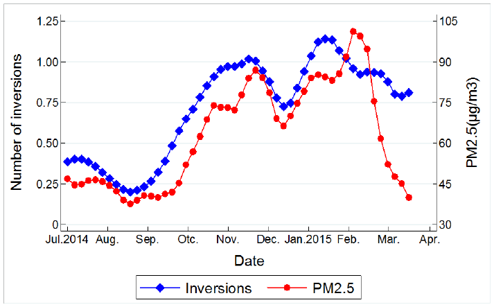
38
Figure 1. Time Trend of PM
2.5
and Thermal Inversion
Notes: This figure plots the average concentrations of PM
2.5
and average number of thermal
inversions for all 162 counties in each day from July 3
rd
2014 to March 31th 2015, the course
of our study period.
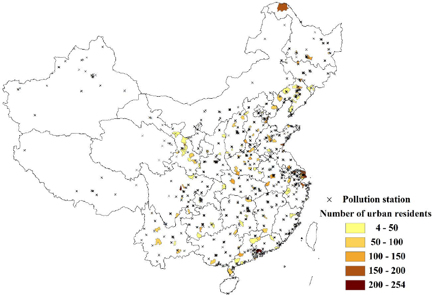
39
Figure 2. Survey Counties and Pollution Stations
Notes: This figure depicts the survey counties and pollution monitoring stations. Dark color
indicates higher number of urban residents who are interviewed. Number of urban
residents=12,615. Number of counties=162. Number of pollution stations=1,498.
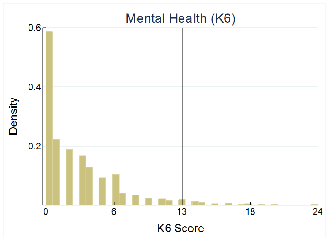
40
Figure 3. Histogram of the K6 Score
Notes: This figure plots the histogram of the K6 score, ranging from 0 to 24. The vertical black
line indicates the cutoff of 13, which is used to define severe mental illness if the K6 score is
equal or above the cutoff.
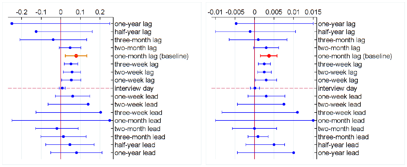
41
Panel A: Impact of PM
2.5
on the K6 score Panel B: Impact of PM
2.5
on severe mental illness
Figure 4. Lagged and Lead Impacts
Notes: This figure depicts the impacts of PM
2.5
on the K6 score (Panel A) and severe mental illness (Panel B). PM
2.5
is calculated using the average from one-
year lag to one-year lead. The circle denotes the point estimate and the whisker denotes the 95% confidence interval. The red circle denotes the baseline estimate,
in which pollution is constructed using the average one month prior to the interview. Due to space limitations, we only present one side of the 95% confidence
intervals for certain periods.

42
Table 1. Summary Statistics
Variable Unit Mean SD Min Max
Mental health
The K6 score Index (0-24) 2.96 3.76 0 24
Severe mental illness
%
4.38
20.47
0
100
Depression 0-never; 4-almost everyday 0.75 0.92 0 4
Nervousness
0-never; 4-almost everyday
0.59
0.87
0
4
Restlessness 0-never; 4-almost everyday 0.50 0.82 0 4
Hopelessness 0-never; 4-almost everyday 0.31 0.72 0 4
Difficulty
0-never; 4-almost everyday
0.51
0.85
0
4
Worthlessness 0-never; 4-almost everyday 0.28 0.69 0 4
Air pollution
PM
2.5
μg/m
3
47.71 18.04 13.46 160.19
Thermal inversions
Inversions
Number
11.74
13.32
0
93
Notes: N=12,615. Unit of observation is respondent. The survey covers 162 counties
during the period of July 3
rd
2014 to March 31
th
2015. The interview surveyed the
mental health one month prior to the interview day for adult population (age >=16).
The K6 score is the sum of the points across the six individual symptoms. The severe
mental illness is a dummy variable which equals to one if the K6 score is above or equal
to 13, and zero otherwise. Each specific symptom is coded from zero to four, with zero
indicating never, one a little of the time, two half of the time, three most of the time,
and four all most every day. The concentrations of air pollutants are reported in each
day, and then is averaged to the month. The existence of thermal inversion is determined
within each six-hour period, and then aggregated to the month.

43
Table 2. First-stage Estimation: Effect of Thermal Inversions on PM
2.5
PM
2.5
(1)
(2)
(3)
Thermal inversions 0.3506*** 0.3013*** 0.3024***
(0.0370)
(0.0239)
(0.0317)
R-squared 0.8587 0.8926 0.9022
County FE Yes Yes Yes
Year-by-month FE
Yes
Yes
Yes
Weather controls No Yes Yes
Sample weights
No
No
Yes
KP F-statistic 35.26 50.59 36.04
Notes: N=12,615. Dependent variable is PM
2.5
. Regression models are estimated
using Equation (2). Weather controls include 5 °C temperature bins, second order
polynomials in average relative humidity, wind speed, sunshine duration, and
cumulative precipitation. Standard errors are listed in parentheses and clustered
by both county and date (two-way clustering). *** p<0.01, ** p<0.05, * p<0.1.

44
Table 3. Second-stage Estimation: Effect of Air Pollution on Mental Health
The K6 Score
Severe Mental Illness
(1)
(2)
(3)
(4)
(5)
(6)
Panel A: IV
PM
2.5
0.0480** 0.0527** 0.0788*** 0.0022*** 0.0024*** 0.0037***
(0.0212) (0.0252) (0.0280) (0.0008) (0.0009) (0.0011)
KP F-statistics
35.26
50.59
36.04
35.26
50.59
36.04
Panel B: OLS
PM
2.5
0.0005 -0.0045 -0.0110 0.0002 -0.0002 -0.0004
(0.0066)
(0.0074)
(0.0075)
(0.0002)
(0.0003)
(0.0005)
County FE Yes Yes Yes Yes Yes Yes
Year-by-month FE
Yes
Yes
Yes
Yes
Yes
Yes
Weather controls No Yes Yes No Yes Yes
Sample weights
No
No
Yes
No
No
Yes
Notes: N=12,615. Dependent variables are the K6 score in columns (1) – (3) and severe mental
illness in columns (4)
– (6). Severe mental illness is a dummy variable which equals to one if the
K6 score is equal or larger than 13. Panel A is the IV estimate, in which we use number of thermal
inversions to instrument PM
2.5
. Panel B is the OLS estimate. Weather controls include 5 °C
temperature bins, second order polynomials in average relative humidity, wind speed, and
sunshine duration, and cumulative precipitation. Standard errors are listed in parentheses and
clustered by both county and date (two-way clustering). *** p<0.01, ** p<0.05, * p<0.1.

45
Table 4. Effect of Air Pollution on Mental Health: By Symptom
About how often do you feel
Depression
Nervousness
Restlessness
Hopelessness
Difficulty
Worthlessness
(1) (2) (3) (4) (5) (6)
PM
2.5
0.0155** 0.0045 0.0134*** 0.0150*** 0.0183*** 0.0123**
(0.0073) (0.0062) (0.0044) (0.0048) (0.0055) (0.0049)
Observations 12,657 12,659 12,660 12,638 12,657 12,649
County FE Yes Yes Yes Yes Yes Yes
Year-by-month FE
Yes
Yes
Yes
Yes
Yes
Yes
Weather controls Yes Yes Yes Yes Yes Yes
Sample weights
Yes
Yes
Yes
Yes
Yes
Yes
KP F-statistic 36.17 36.19 36.20 36.11 36.15 36.09
Notes: Dependent variables are scores of each specific symptom ranging from zero to four. Higher score means
stronger prevalence of that symptom.
Weather controls include 5 °C temperature bins, second order polynomials
in average relative humidity, wind speed, and sunshine duration, and cumulative precipitation. Standard errors are
listed in parentheses and clustered by both county and date (two-way clustering). *** p<0.01, ** p<0.05, * p<0.1.

46
Table 5. Robustness Checks
Baseline
IDW Interpolation
Alternative layer
of inversion
Functional form
Radius=50km Radius=150km Nearest station
(1)
(2)
(3)
(4)
(5)
(6)
Panel A: The K6 score
PM
2.5
0.0788*** 0.0664** 0.0819*** 0.1207*** 0.0807**
(0.0280)
(0.0320)
(0.0287)
(0.0428)
(0.0357)
KP F-statistic 36.04 27.69 35.59 19.86 16.64
Panel B: Severe mental illness
IV-Probit
PM
2.5
0.0037*** 0.0038*** 0.0038*** 0.0054*** 0.0041** 0.0040**
(0.0011) (0.0011) (0.0010) (0.0017) (0.0018) (0.0019)
KP F-statistic
36.04
27.69
35.59
19.86
16.64
----
Observations
12,615
10,910
12,844
12,430
12,615
12,615
Notes: Dependent variables are K6 score in Panel A and a dummy variable for severe mental illness in Panel B. Column (1)
is the baseline model. Columns (2) – (4) tests the robustness of interpolation of air pollution data. Columns (2) and (3) use
the IDW method with 50 km and 150 km radius respectively. In column (4), we assign the pollution data from station to
county using the nearest station. Column (5) tests the robustness of construction of the IV. In the baseline model, we determine
an existence of a thermal inversion if the temperature in the higher layer (320 meters) is higher than that in the ground layer
(110 meters). We change the higher layer to 540 meters in column (5). Column (6) tests the robustness of the functional form.
In Panel B, since the dependent variable is a dummy variable, we use the IV probit model, instead of the 2SLS model in the
baseline. The estimates reported here is the marginal effects evaluated at the mean level. All models include county fixed
effects, year-by-month fixed effects, and weather controls. Weather controls include 5 °C temperature bins, second order
polynomials in average relative humidity, wind speed, and sunshine duration, and cumulative precipitation. Standard errors
are listed in parentheses and clustered by both county and date (two-way clustering) . *** p<0.01, ** p<0.05, * p<0.1.

47
Table 6. Mechanism Tests
Exercise (past 1 week)
Sickness (past 2 weeks)
Self-rated health (past 1 month)
(1)
(2)
(3)
(4)
(5)
(6)
1-yes, 0-no times hours 1-yes, 0-no 1-not serious, 5-very serious 1-very healthy, 5-very unhealthy
PM
2.5
-0.0049** -0.0068* -0.0448** 0.0020 0.0089* 0.0092*
(0.0022) (0.0035) (0.0209) (0.0019) (0.0052) (0.0056)
Observations 12,664 12,663 12,670 12,670 3,806 12,668
Mean of Dep. Var.
0.4670
2.4008
3.3681
0.2917
3.1140
2.9698
S.D. of Dep. Var. 0.4989 3.1324 6.4268 0.4545 1.4053 1.1816
County FE Yes Yes Yes Yes Yes Yes
Year-by-month FE
Yes
Yes
Yes
Yes
Yes
Yes
Weather controls Yes Yes Yes Yes Yes Yes
Sample weights
Yes
Yes
Yes
Yes
Yes
Yes
KP F-statistic 48.73 48.57 48.72 44.92 59.36 36.30
Notes: Dependent variables are a dummy variable which equals to one if respondent exercises in the past week in column (1), times of
exercise in column (2), hours of exercise in column (3), a dummy variable which equals to one if respondent was sick in the past two weeks
in column (4), degree of illness from one to five with one for not serious and five for very serious in column (5), degree of self-rated health
status from one to five with one for very healthy and five for very unhealthy in column (6). PM
2.5
is calculated using the average for the
corresponding exposure window and is instrumented using thermal inversion. Weather controls include 5 °C temperature bins, second order
polynomials in average relative humidity, wind speed, and sunshine duration, and cumulative precipitation. Standard errors are listed in
parentheses and clustered by both county and date (two-way clustering). *** p<0.01, ** p<0.05, * p<0.1.

48
Table 7. Effect of Air Pollution on Mental Health: By Gender and Cohort
The K6 Score
Severe Mental Illness
(1)
(2)
(3)
(4)
(5)
(6)
(7)
(8)
Male Female Age 16-60 Age >=60 Male Female Age 16-60 Age >=60
PM
2.5
0.0986*** 0.0575* 0.0611** 0.1499** 0.0055*** 0.0018 0.0031*** 0.0059
(0.0268) (0.0342) (0.0298) (0.0599) (0.0018) (0.0014) (0.0011) (0.0037)
Observations 6,093 6,522 9,446 3,169 6,093 6,522 9,446 3,169
Mean of Dep. Var.
2.6378
3.2799
2.9504
3.0281
0.0361
0.0512
0.0377
0.0626
S.D. of Dep. Var. 3.5378 3.9405 3.5819 4.2683 0.1867 0.2204 0.1905 0.2422
County FE Yes Yes Yes Yes Yes Yes Yes Yes
Year-by-month FE
Yes
Yes
Yes
Yes
Yes
Yes
Yes
Yes
Weather controls Yes Yes Yes Yes Yes Yes Yes Yes
Sample weights
Yes
Yes
Yes
Yes
Yes
Yes
Yes
Yes
KP F-statistic 25.14 43.22 32.11 27.20 25.14 43.22 32.11 27.20
Notes: Dependent variables are the K6 score in columns (1) – (4) and severe mental illness in column (5) – (8).
Regression models are estimated separately for each subsample. Weather controls include 5 °C temperature bins, second
order polynomials in average relative humidity, wind speed, and sunshine duration, and cumulative precipitation.
Standard errors are listed in parentheses and clustered by both county and date (two-way clustering). *** p<0.01, **
p<0.05, * p<0.1.

49
Table 8. Effect of Air Pollution on Mental Health: By Education
The K6 Score
Severe Mental Illness
(1)
(2)
(3)
(4)
(5)
(6)
Primary school
or below
Junior high
or high school
College or above
Primary school
or below
Junior high
or high school
College or above
PM
2.5
0.0046 0.1200** 0.1700*** 0.0004 0.0058** 0.0115**
(0.0407)
(0.0516)
(0.0611)
(0.0020)
(0.0029)
(0.0057)
Observations
4,448
3,478
3,416
4,448
3,478
3,416
Mean of Dep. Var. 3.3757 2.7713 2.6825 0.0625 0.0356 0.0282
S.D. of Dep. Var. 4.2096 3.5471 3.3062 0.2421 0.1854 0.1655
County FE
Yes
Yes
Yes
Yes
Yes
Yes
Year-by-month FE Yes Yes Yes Yes Yes Yes
Weather Controls
Yes
Yes
Yes
Yes
Yes
Yes
Sample weights Yes Yes Yes Yes Yes Yes
KP F-statistic 23.15 34.94 21.67 23.15 34.94 21.67
Notes: Dependent variables are K6 score in columns (1) – (3) and severe mental illness in column (4) – (6). Regression models
are estimated separately for each subsample. Weather controls include 5 °C temperature bins, second order polynomials in
average relative humidity, wind speed, and sunshine duration, and cumulative precipitation. Standard errors are listed in
parentheses and clustered by both county and date (two-way clustering). *** p<0.01, ** p<0.05, * p<0.1.

50
Table 9. Effect of Air Pollution on Mental Health: By Workplace
K6 Score
Severe Mental Illness
Workplace Indoor Outdoor
Indoor Outdoor
(1) (2)
(3) (4)
PM
2.5
0.0714** 0.0847***
0.0029* 0.0038***
(0.0355)
(0.0304)
(0.0015)
(0.0011)
Observations 3,232 1,248
3,232 1,248
Mean of Dep. Var.
2.8122
2.9113
0.0317
0.0397
S.D. of Dep. Var. 3.4184 3.4823 0.1754 0.1954
County FE Yes Yes
Yes Yes
Year-by-month FE
Yes
Yes
Yes
Yes
Weather controls Yes Yes
Yes Yes
Sample weights
Yes
Yes
Yes
Yes
KP F-statistic 26.19 21.61
26.19 21.61
Notes: Dependent variables are K6 score in columns (1) – (2), and a dummy
variable for severe mental illness in columns (3) – (4). In columns (1) and
(3), we focus on respondents whose workplace is indoor only. In columns (2)
and (4), we focus on respondents whose workplace is outdoor only. Weather
controls include 5 °C temperature bins, second order polynomials in average
relative humidity, wind speed, and sunshine duration, and cumulative
precipitation. Standard errors are listed in parentheses and clustered by both
county and date (two-way clustering). *** p<0.01, ** p<0.05, * p<0.1.
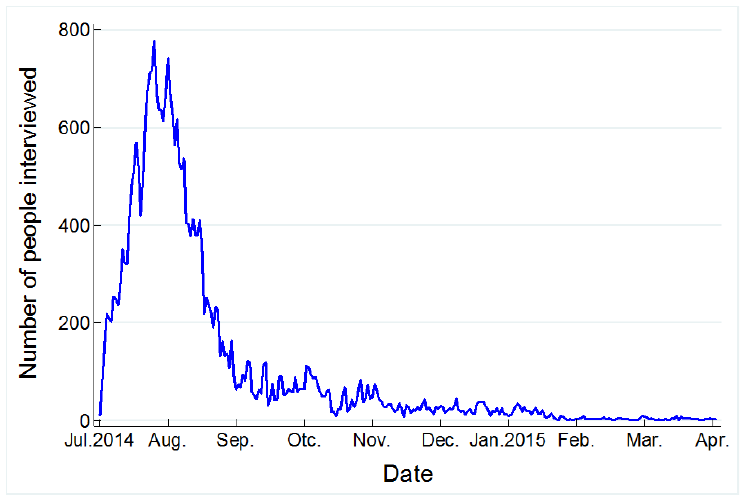
51
Online Appendix
Figure A1. Number of People Interviewed in Each Day
Notes: This figure plots the number of people interviewed in each day from July 3
rd
2014 to
March 31th 2015, the course of our study period.
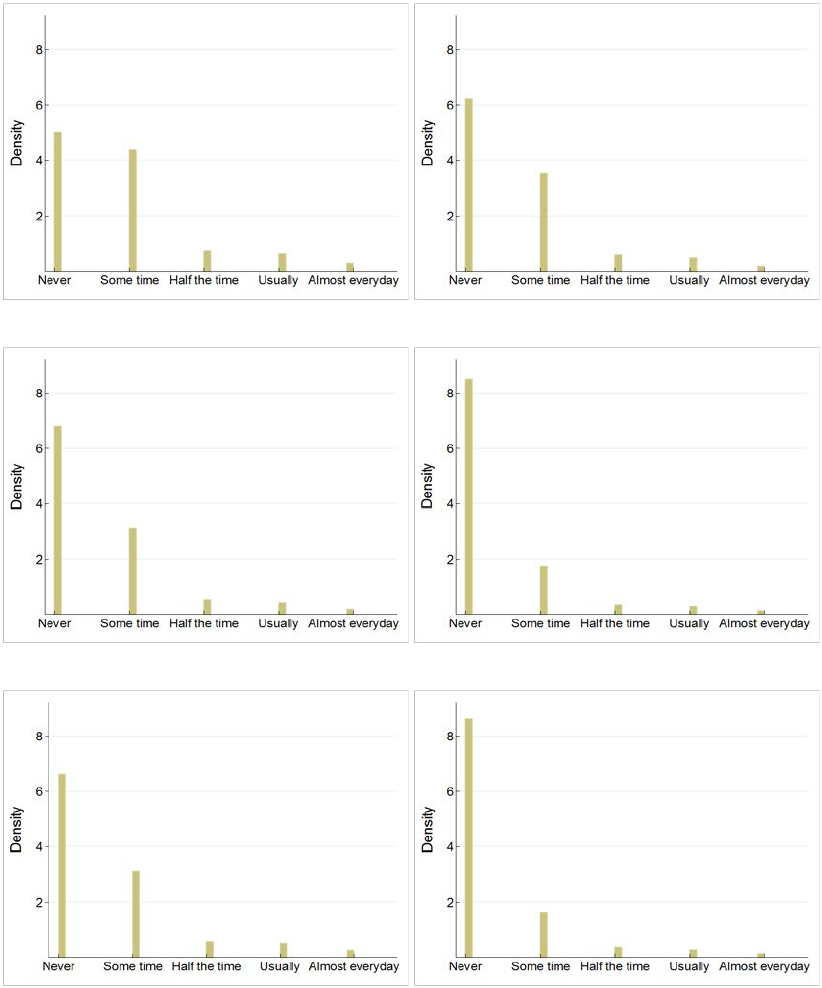
52
Panel A: Depression Panel B: Nervousness
Panel C: Restlessness Panel D: Hopelessness
Panel E: Difficulty Panel F: Worthlessness
Figure A2. Histogram of Specific Mental Illness Symptom
Notes: This figure plots the histogram of each specific mental disorder symptom.

53
Table A1. Effect of Air Pollution on Mental Health: By Residence
The K6 Score Severe Mental Illness
Urban Rural Total Urban Rural Total
(1)
(2)
(3)
(4)
(5)
(6)
PM
2.5
0.0788***
-0.0513
0.0187
0.0037***
-0.0009
0.0008
(0.0280) (0.0446) (0.0261) (0.0011) (0.0010) (0.0013)
Observations
12,615
15,618
28,233
12,615
15,618
28,233
County FE Yes Yes Yes Yes Yes Yes
Year-by-month FE
Yes
Yes
Yes
Yes
Yes
Yes
Weather controls Yes Yes Yes Yes Yes Yes
Sample weights Yes Yes Yes Yes Yes Yes
KP F-statistic
36.04
17.62
52.24
36.04
17.62
52.24
Notes: Dependent variables are K6 scores in columns (1) – (3), and a dummy variable for
severe mental disorders in columns (4) – (6). In columns (1) and (4), we focus on urban
residents only. In columns (2) and (5), we focus on rural residents only. In columns (3) and
(6), we focus on both urban and rural residents. Weather controls include 5 °C temperature
bins, second order polynomials in average relative humidity, wind speed, and sunshine
duration, and cumulative precipitation. Standard errors are listed in parentheses and clustered
by both county and date (two-way clustering). *** p<0.01, ** p<0.05, * p<0.1.
