
Bartik Instruments:
An Applied Introduction
Matthias Breuer
*
This version: December 2021
Abstract
This article provides an applied introduction to Bartik instruments. The instruments
attempt to reduce familiar endogeneity concerns in differential exposure designs
(e.g., panel regressions with unit and time fixed effects). They isolate treatment
variation due to the differential impact of common shocks on units with distinct
pre-determined exposures. As a result, the instruments purge the treatment variation
of possibly confounding factors varying across units over time. Given their broad
applicability, Bartik instruments promise to provide researchers with a versatile
new tool in their empirical toolbox to investigate relevant accounting questions.
Keywords: Bartik Instruments; Shift Shares; Simulated Instruments
JEL Classification: C51, M40
Acknowledgements:
I thank Ed deHaan (editor), two anonymous reviewers, Lulseged Asegu, John Barrios, Thomas
Bourveau, Raphael Duguay, Sehwa Kim, Christian Leuz, Anthony Le, Rongchen Li, Miguel
Minutti-Meza, Harm Schütt, Felix Vetter, Li Yang, and participants at the 2021 FARS and Journal
of Financial Reporting: Research Methods Mini-Conference for helpful comments and
discussions. All errors are my own. The simulation code is available at:
https://github.com/mb4468/bartik_intro
*
Columbia University, Graduate School of Business - m[email protected]
1
1 Introduction
Accounting research overwhelmingly relies on observational data, often panel data (i.e.,
data containing multiple units over time), to empirically examine core accounting questions. While
panel data allow reducing concerns about static differences across units and common changes over
time via unit and time fixed effects (deHaan 2021), we typically remain worried about first-order
endogeneity issues such as reverse causality, simultaneity, and omitted variable bias. In examining
the impact of accounting quality on the cost of capital, for example, we may worry that observed
changes in capital costs may cause accounting quality changes, instead of the other way around
(Balakrishnan et al. 2014; Lo 2014). We may also worry that changes in capital costs and
accounting quality commingle supply and demand forces (Gerakos and Syverson 2017). Lastly,
and most prominently, we tend to worry that other omitted factors (e.g., operating activities) drive
both, changes in capital costs and accounting quality (Hribar and Nichols 2007; Beyer et al. 2010).
To alleviate these endogeneity concerns, we could, in principle, use instrumental variables. In
practice, the use of instrumental variables in accounting research is limited though given the
challenge to identify credible instruments that explain the treatment and only affect the outcome
of interest through their impact on the treatment (Larcker and Rusticus 2010).
This article provides an applied introduction to Bartik or shift-share instruments, a class of
instruments that can be constructed in various settings, including typical accounting settings.
Pioneered by Bartik (1991), these instruments aim to focus on the plausibly (more) exogenous
subpart of the treatment variation of interest due to the differential impact of common shocks on
units with distinct pre-determined exposures. They are particularly useful for reducing
endogeneity concerns in differential exposure designs (e.g., panel regressions with unit and time
effects), one of the most popular designs in recent accounting studies (deHaan 2021; Armstrong

2
et al. 2021). Notably, the idea behind Bartik instruments is closely related to the familiar
difference-in-differences approach which exploits the differential impact of a common shock on
treated and control firms. Unlike standard difference-in-differences designs, Bartik instruments
tend to exploit continuous instead of dichotomous treatment exposures though.
In the canonical example, Bartik (1991) develops this class of instruments to estimate the
impact of county-level employment changes, due to labor demand shifts, on wages. Like the
accounting-quality and cost-of-capital relation, the employment-wage relation is challenging to
identify due to concerns about reverse causality, simultaneity, and omitted factors. To isolate
plausibly exogenous variation in counties’ employment rates, Bartik exploits the fact that
nationwide trends in industry employment rates (e.g., a decline in US manufacturing employment)
impact counties’ employment rates differently, depending on their pre-existing industrial structure
(e.g., their share of employment in manufacturing). This subpart of the variation in counties’
employment rates is less likely to reflect changes due to local wage developments (reverse
causality), local shifts in labor supply (simultaneity), or omitted factors such as local growth
opportunities (omitted variable bias).
Bartik instruments have been frequently used in empirical studies in economics for more
than two decades (e.g., Blanchard and Katz 1992; Card 2009; Autor et al. 2013).
1
Yet, they have
only recently found their way into accounting research. An important barrier to the adoption of
Bartik instruments is their added complexity compared to typical instrumental variables and
difference-in-differences approaches (e.g., due to their multidimensionality and continuous
treatment exposures). A recent methodological literature attempts to address the complexity
1
Recent studies, for example, use Bartik instruments to examine topical and important questions such as the impact
of pandemic-related policies (Granja et al. 2021) and the causes behind the decline of the natural interest rate over the
past decades (Mian et al. 2021).
3
concern by formally exploring and clarifying the conditions under which Bartik instruments allow
for causal inferences (e.g., Goldsmith-Pinkham et al. 2020; Borusyak et al. 2021; Borusyak and
Hull 2020).
To aid the adoption of Bartik instruments in accounting research, I complement the formal
discussion in the recent methodological literature with an applied introduction to this class of
instruments. I specifically focus on the empirical challenge addressed by Bartik instruments, the
general idea behind the construction of the instruments, the conceptual links to approaches familiar
to accounting researchers (e.g., instrumental variables and difference-in-differences designs), and
practical considerations in implementing the instruments and assessing their validity.
As the leading example, I use the canonical application of Bartik instruments to the
estimation of the employment-wage relation (Bartik 1991). Although this specific application may
be of lesser concern to accounting researchers, the empirical challenge underlying this example is
present in many accounting settings and the proposed empirical approach can be applied in various
accounting settings. To highlight the relevance for accounting research, I discuss a possible
application of Bartik instruments to the question of how accounting quality impacts the cost of
capital and present recent applications of Bartik instruments in accounting research.
This article is structured as follows. In Section 2, I introduce the canonical application of
Bartik instruments to the estimation of the employment-wage relation. In Section 3, I discuss the
general idea behind the construction and use of the instruments. In Section 4, I highlight a special
case of the instruments designed for threshold-based regulations. In Section 5, I describe select
examples of applications of Bartik instruments in accounting research. I conclude in Section 6.
2 Canonical Bartik Example
In Bartik’s canonical application, we are interested in estimating the impact of employment

4
changes, due to labor demand shifts, on wages.
2
We observe panel data on employment rates (x
i,t
)
and wages (y
i,t
) for counties (i) over time (t). The panel data allow us to account for cross-sectional
differences across counties using county fixed effects and common time trends using time fixed
effects. However, we remain concerned that reverse causality, simultaneity, and time-varying
correlated omitted factors could confound our estimate of interest. Local employment, for
example, may increase due to local wage increases, instead of the other way around. Additionally,
local wages and employment are not only determined by labor-demand shifts, but also reflect
labor-supply shifts. Labor-supply shifts, however, exhibit the opposite effect on wages as labor-
demand shifts (i.e., positive supply shifts decrease wages, whereas positive demand shifts increase
wages). Simultaneous supply shifts, accordingly, threaten to bias our estimate downward. Lastly,
and most prominently, we worry that other factors such as local technology shocks, growth
opportunities, or financing conditions affect both, changes in wages and employment.
To address the endogeneity concerns, Bartik proposes an instrumental variable approach.
The basic idea behind instrumental variable approaches is to find another variable, the instrument
(z
i,t
), that drives part of the treatment variation (x
i,t
), and only affects the outcome (y
i,t
) through its
impact on the treatment (e.g., Wright 1928; Angrist and Krueger 2001). To construct such
instrument, Bartik first notes that the local employment rates can be represented by the sum-
product of two industry-level components: the employment rate (e
i,k,t
) and the employment share
(w
i,k,t
) of a given industry (k) in a given county. Based on this insight, he constructs an instrument
for local employment rates by weighting nationwide employment rates (e
k,t
) for each industry (k)
with pre-determined (e.g., initial) county-industry-level employment shares (w
i,k
).
2
The structural parameter of interest is the (inverse) labor-supply elasticity, that is, the slope of the labor-supply curve.
To identify the elasticity, we need to hold the supply curve fixed and only shift the demand curve.
5
The instrument essentially isolates variation in local employment-rate changes due to
differential impacts of national employment trends on local counties arising from the counties’
distinct industrial structure. The employment rate in the US manufacturing sector, for example,
declined in response to import competition from China. This nationwide trend affected counties
with a historically strong manufacturing sector more adversely than other counties (Autor et al.
2013). By focusing on such differential impact of nationwide trends on distinct counties, the
instrument purges the treatment of variation due to county-specific changes in industrial structure
or employment rates. As a result, the instrument’s variation in employment rates cannot be driven
by local wages (i.e., reverse causality). Similarly, the instrument, by construction, does not vary
with local factors such as technological shocks and growth opportunities, reducing first-order
omitted variable concerns. In addition, Bartik argues that the differential exposure of counties to
nationwide employment trends likely captures variation in industry-specific labor-demand shifts
rather than local labor-supply shifts. The basic idea behind this argument is that differences in
industry-employment shares across counties tend to reflect the relative importance of industries
exporting to national or even international markets, not locally oriented industries (Bartik 1991, p.
274). As a result, the instrument can be expected to capture industry-specific labor-demand shifts
due to nationwide trends in the competitiveness and fortunes of a given industry (e.g., the
reallocation of manufacturing from the US to China). While the ultimate validity of the instrument
remains an identifying assumption (e.g., rests on the plausibility of theoretical and institutional
arguments), the instrument construction tends to reduce first-order endogeneity concerns by
focusing on a plausibly more exogenous subpart of the variation in local employment rates.
Notably, the endogeneity issues in the canonical Bartik example are familiar to accounting
researchers and the proposed instrumental variable approach can be implemented in and adapted

6
to various settings, including typical accounting settings. To clarify the idea behind Bartik
instruments and illustrate their wide-ranging applicability, I discuss the general approach
underlying the construction and use of the instruments in the next section.
3 General Approach: Bartik Instrument
3.1 Empirical Challenge
Bartik instruments aim to address familiar endogeneity concerns (e.g., reverse causality,
simultaneity, and correlated omitted variables). The instruments are particularly useful in cases
where we can exploit multidimensional data (e.g., panel data with observations for multiple units,
i = {1,...,I}, over time, t = {1,...,T}). In these cases, we can take advantage of the multidimensional
data structure to account for first-order endogeneity concerns related to the treatment of interest
(x
i,t
) by including fixed effects for each dimension (i.e., unit effects, α
i
, and time effects, α
t
):
3
(1)
The identifying variation in such differential exposure designs is limited to differential
changes across units over time. This variation is often less confounded than the full treatment
variation. We, for example, do not need to worry about static differences in terms of industrial
structure and economic activity across counties, after accounting for county fixed effects.
Similarly, we do not need to worry about common trends in industrial structure and economic
activity, after accounting for time fixed effects. Still, even the variation in differential exposure
designs is subject to endogeneity concerns (
) relating to reverse causality,
simultaneity, and correlated omitted factors varying at the level of the differential exposure (i.e.,
3
Bartik (1991) uses a changes specification. As differential exposure designs using fixed effects are more prevalent
in accounting research, I opt to introduce Bartik instruments using a levels specification with unit and time fixed
effects. This within-unit design implicitly exploits changes.

7
at the unit-time level (i,t)). Such factors (e.g., growth opportunities, technology shocks,
competitive threats, financing needs, and the like) are typically abundant and unobservable to us.
Accordingly, we cannot simply control for such factors. Instead, Bartik (1991) proposes the use of
a novel type of instrument to address the endogeneity concerns.
3.2 Instrument Construction
Bartik instruments reduce endogeneity concerns by focusing on a subset of the differential
exposure variation that is plausibly exogenous (e.g., uncorrelated with local growth opportunities).
To construct such variation, we must first identify a subdimension (k) which allows decomposing
the treatment variation (x
i,t
). In the canonical example of Bartik (1991), the treatment (i.e., county-
level employment rates) can be decomposed into industry-specific employment rates (e
i,t,k
) in a
given county weighted by industry-specific employment shares (w
i,t,k
):
(2)
This decomposition is an identity. It does not require any assumption. The only requirement
for such decomposition to be useful for constructing a Bartik instrument is that the individual
components are observable.
4
In the case of Bartik (1991), this means we need to observe
employment data at the county-industry level, not just at the county level. Notably, this
requirement does not pertain to the outcome data (e.g., wages) as the ultimate regression is still
run at the county-level, not county-industry level.
The decomposition shows that both components, the shares (w
i,t,k
) and the rates (e
i,t,k
), vary
at the level of the identifying assumption (i.e., across counties over time (i,t)). Accordingly, we
need to worry about any factors determining wages and driving changes in counties’ industrial
4
For the canonical example, we only need to observe the employment share at the county-industry level. For the
employment rate, we can use national industry statistics.

8
structure and/or industry-specific employment rates.
To reduce the number of possibly confounding factors, Bartik instruments (
) focus on
plausibly exogenous dimensions of the components making up the treatment (x
i,t
). In Bartik (1991),
those dimensions are the pre-determined industry-specific employment shares in a given county
level (w
i,k
) and nationwide industry-specific employment rates (e
t,k
):
(3)
While the pre-determined shares and the nationwide rates are unlikely to be randomly
assigned, the idea is that, compared to the full treatment variation, the pre-determined shares and
nationwide rates are less likely to reflect current choices (e.g., responses to local growth
opportunities) at the county level. Importantly, the instrument exclusively focuses on changes in
county-level employment rates due to the interaction of pre-determined shares and nationwide
rates. It does not use level differences in shares or rates across counties or over time. Hence, the
Bartik instrument can be viewed as following the logic underlying the familiar difference-in-
differences approach (Section 3.3.2).
More generally, Bartik instruments focus on the inner product of a pre-determined share
varying across units (i,k) (e.g., local employment shares as of the beginning of the sample) and a
common trend (t,k) (e.g., changes in nationwide employment rates over time). Hence, the
instruments only vary at the level of the identifying variation (i,t) due to the differential impact of
common trends on local units with distinct pre-determined shares.
5
Notably, the instruments, by
construction, do not vary across units over time due to endogenous changes of the shares (e.g.,
changes in industrial structure of counties) or endogenous unit-specific trends (e.g., county-
5
Hence, Bartik instruments are also often referred to as shift-share instruments.
9
specific employment rate shocks). This feature reduces concerns about reverse causality,
simultaneity, and important correlated omitted factors.
To see this point more formally, we can decompose the full treatment variation into the
Bartik variation, driven by the interaction of pre-determined shares (w
i,k
) and common shocks (e
t,k
),
and unit-specific changes in shares and shocks:
(4)
The unit-specific changes in the shares and shocks (e.g., (e
i,t,k
− e
t,k
)) can be correlated with a host
of possibly confounding factors (e.g., local growth opportunities). These timevarying factors
cannot be controlled for via unit and time fixed effects. By contrast, unit and time fixed effects can
control for first-order endogeneity concerns related to the Bartik instrument’s variation:
endogenous differences across units correlated with the shares and endogenous changes over time
correlated with the common trends. Accordingly, conditional on the fixed effects, Bartik
instruments isolate plausibly exogenous variation due to the differential impact of common trends
on units with distinct pre-determined shares.
3.3 Identifying Conditions
The construction of Bartik instruments can reduce endogeneity concerns if certain

10
conditions are satisfied. In the following subsections, I provide an intuition for the relevant
conditions by analogy to two related and familiar empirical approaches: instrumental variables
(IV) and difference-in-differences (DID) approaches. For a formal derivation of the relevant
conditions, see the excellent discussions in Goldsmith-Pinkham et al. (2020), Borusyak et al.
(2021), and Borusyak and Hull (2020).
3.3.1 Instrumental Variables Approach
As the name already reveals, Bartik instruments are just a particular type of instrument.
They follow the basic idea of the instrumental variable approach: isolating a plausibly exogenous
subpart of the treatment variation. Bartik instruments do so explicitly by starting with the full
treatment variation, decomposing it to its key dimensions, and then focusing on the most plausibly
exogenous parts of these dimensions (e.g., pre-determined shares and common trends).
6
Accordingly, the familiar instrumental variable conditions apply. The first condition is the
relevance condition. It is a necessary condition. It requires that the instrument is a key determinant
of the treatment (
). For Bartik instruments, this condition essentially requires
some degree of persistence in the pre-determined shares (w
i,k
) and commonality in the trend across
units (e
t,k
). In particular, the pre-determined shares need to be predictive of the actual shares during
the sample period for the Bartik instrument to be relevant. Similarly, the common trend (e.g.,
changes in nationwide employment rates per industry) needs to be predictive of the trend observed
in individual units (e.g., at the county-industry level).
The relevance condition is typically satisfied for Bartik instruments, because the
6
This approach is in the spirit of familiar instrumental variable approaches using lagged values or industry averages
to reduce concerns about reverse causality and unit-specific omitted factors. Unlike these familiar approaches,
however, the Bartik approach isolates the interaction of pre-determined characteristics and common trends. It does
not simply use variation in the pre-determined characteristics over time or variation in common characteristics across
units. As Reiss and Wolak (2007) and Larcker and Rusticus (2010) point out, this variation is unlikely to be plausibly
exogenous.

11
instruments, by construction, capture important dimensions of the treatment variation. To test the
condition, we can run the usual first-stage regression:
(5)
The first-stage coefficient (β
FS
) should be positive and significant as long the shares are somewhat
persistent and there is some commonality in trends across units.
Bartik instruments may not one-for-one determine the treatment of interest (i.e., β
FS
can be
different from one). Accordingly, the following reduced-form regression can yield a coefficient
estimate which quantifies the impact of the instrument instead of our treatment of interest:
(6)
To obtain a quantification in terms of the treatment of interest, we can scale the reduced-form
coefficient (β
RF
) by the first-stage coefficient (β
FS
). The resulting coefficient is the second-stage
coefficient (β
SS
= β
RF
/β
FS
), which quantifies the impact of the instrumented treatment. Accordingly,
we can adjust for variation in the relevance of the Bartik instruments (e.g., due to systematic
deviations from persistence or commonality) by following the standard two-stage instrumental
variable approach. We should not adjust for limited persistence or commonality by simply using
the actual instead of the pre-determined shares as our right-hand-side variation. As discussed
earlier, this OLS approach would raise substantial endogeneity concerns.
For the instrumented coefficient estimate to be unbiased, we need the second condition
underlying the instrumental variables approach: the exclusion restriction. It requires that the
instrument is (conditionally) independent of other determinants of the outcome
(
).
7
This condition is the identifying assumption. It is untestable (i.e., remains
7
Besides independence, the exclusion restriction requires that the instrument affects the outcome only through its
impact on the treatment. This (sub)condition is often plausible in the case of Bartik instruments given that the

12
an assumption). The plausibility of this assumption needs to be argued for with the help of theory
and institutional details. Goldsmith-Pinkham et al. (2020), Borusyak et al. (2021), and Borusyak
and Hull (2020) explore different sets of formal assumptions (e.g., exogeneity of the shares vs. the
shocks) required for the validity of the exclusion restriction for Bartik instruments. In the following
subsection, I attempt to provide an intuitive understanding for the identifying assumption of Bartik
instruments, when used in a differential exposure design, by analogy to the familiar difference-in-
differences approach and its identifying assumption.
3.3.2 Difference-in-Differences Approach
Bartik instruments essentially focus on the subpart in the treatment variation that is driven
by the interaction of a pre-determined characteristic varying across units and a common trend
varying over time. This approach is reminiscent of the familiar difference-indifferences approach.
The difference-in-differences approach exploits the differential impact of a common dimension
(e.g., time) across units with distinct pre-determined characteristics (e.g., treatment status):
(7)
The canonical difference-in-differences approach exploits the interaction of a dichotomous
pre-determined treatment indicator varying across units (
) with a dichotomous time indicator (1
t
)
as its treatment variation:
(8)
In the IFRS literature, for example, the treatment indicator takes the value of one for European
firms and zero for US firms; and the time indicator takes the value of one for years from 2005
instruments explicitly focus on a subpart of the treatment variation rather than use a completely distinct source of
variation. The only-through (or one-channel) condition may be violated though if there are spillovers across counties
(e.g., Berg et al. 2021). Nationwide employment trends, for example, may directly affect local counties’ outcomes by
luring employees away from a given county toward other booming counties elsewhere in the nation (which drive the
nationwide trend). Such spillovers (e.g., across counties) can invalidate or complicate the use of Bartik instruments.

13
onward and zero before 2005 (e.g., Christensen et al. 2013).
The same logic extends to difference-in-differences designs with continuous treatments:
(9)
Bloomfield (2021), for example, examines the differential impact of Compensation Discussion
and Analysis (CD&A) disclosure requirements after 2006 on firms with varying levels of pre-
determined market shares (x
i
).
8
The common idea behind these approaches is to exclusively focus on the interaction of a
characteristic varying at the unit dimension (i) and one varying at the time dimension (t), while
accounting for level differences across units and time using unit and time fixed effects. As a result,
the treatment only varies at the identifying unit-time level (i,t) (e.g., firm-year level) due to the
interaction of a unit-fixed component (e.g., treatment status) and a time-fixed component (e.g., pre
vs. post period). It does not vary at the identifying unit-time level due to either of the components
varying both at the unit and time dimension. This feature reduces the number of potentially
correlated omitted variables that we must worry about.
9
The identifying assumption underlying the difference-in-differences approaches is that the
interaction between a characteristic varying across units (i) and another characteristic varying
8
Notably, difference-in-differences designs with the share of treated firms in a given unit (e.g., county) as the
continuous treatment variable are just a special (and simple) case of a Bartik instrument (e.g., Breuer et al. 2020). To
see the equivalence, note that the treatment indicator
for firm k in county i corresponds to the pre-determined
share, w
i,k
. Similarly, an indicator
taking the value of one for treated firms in the post period corresponds to the
common trend, e
t,k
. Accordingly, the Bartik instrument is given by:
,
which corresponds to the continuous treatment-share difference-in-differences design.
9
In difference-in-differences designs, just as in the construction of Bartik instruments, the treatment exposure (e.g.,
treatment indicator) should be pre-determined and held fixed. This approach avoids conflating the intent-to-treat effect
with endogenous selection into or out of the treatment status over time. As described in the previous section, we can
adjust the intent-to-treat estimate for imperfect compliance via the two-stage instrumental variable approach to arrive
at the treatment effect on the treated.

14
across time (t) is conditionally independent, after controlling for the level differences of both
dimensions (i and t). For the canonical case of a temporal difference-in-differences approach (i.e.,
where one of the dimensions is time), this assumption translates into the familiar parallel-trends
assumption. That is, levels across units can be different, but trends over time across units should
be the same absent any treatment. More generally, it requires that there are no other factors that
are correlated with the interaction and differentially impact outcomes across units.
10
By analogy, Bartik instruments (in differential exposure designs) can be viewed as relying
on the same basic identifying assumption. Goldsmith-Pinkham et al. (2020) illustrates that the
parallel-trends assumption corresponds to the conditional share-exogeneity assumption for Bartik
instruments. This assumption requires that there are no other factors correlated with the pre-
determined shares that can explain why a common trend affects units differentially. Accordingly,
the pre-determined shares can be correlated with levels of omitted factors but should not be
correlated with differential changes of those factors, just as we know it from the parallel-trends
assumption in standard difference-in-differences designs.
Alternatively, Borusyak et al. (2021) show that Bartik instruments can also be valid under
the conditional shock-exogeneity assumption. This assumption requires the common shocks to be
as-good-as-randomly assigned and large in number. Notably, this alternative assumption does not
require the exogeneity of the shares and the corresponding parallel-trends assumption.
11
Accordingly, concerns about endogenous shocks or shares alone do not invalidate the use of Bartik
instruments. Which of the identifying assumptions is most plausible in a given setting depends on
theory and institutional knowledge, as usual in design-based research (e.g., Leuz and Wysocki
10
Recent research by Callaway et al. (2021) shows that effect of continuous treatments can be identified under a
generalized parallel trends assumption that is similar to the binary treatment case. Its interpretation can be particularly
challenging due to treatment effect heterogeneity though. For a related discussion, see Section 3.4.3.
11
Intuitively, bias from endogenous shares cancels out in case of exogenous shocks as the shares sum to one.

15
2016).
3.4 Practical Considerations
Bartik instruments, by combining variation from three dimensions (i, t, and k), exploit
continuous treatment variation (e.g., Angrist and Imbens 1995). This variation can aid
identification by exploiting more heterogeneity in the exposure to a treatment than a typical
dichotomous difference-in-differences design. At the same time, it complicates the understanding
of the identifying variation and the interpretation of the resulting estimates.
12
These “black box”
concerns can be reduced by complementing the estimates from Bartik instruments with descriptive
statistics and diagnostic tests.
3.4.1 Extent and Sources of Variation
In a first set of tests, we can explore the extent and sources of the Bartik instrument’s
variation. Descriptive statistics on the distribution of the instrument (z
i,t
) or instrumented treatment
(
) can inform us about the range and frequency of treatment values spanned by the instrument.
This information not only helps us to understand the treated population, but also to interpret the
instrumented treatment-effect estimate, as the estimate reflects a weighted average across the
various treatment values. Descriptive statistics on the distributions of the individual components
of the Bartik instrument (w
i,k
and e
t,k
) can additionally inform us about the underlying sources of
the instrument’s variation. These statistics, for example, can tell us about differences in county-
level employment shares and national employment rates across industries (i.e., the subdimension
k). Hence, they help us understand which component (e.g., pre-determined employment shares or
12
This issue is reminiscent of the trade-off between the extent of treatment variation (e.g., the number of shocks)
versus the ease of interpretation of the treatment estimate in generalized difference-in-differences designs (e.g., de
Chaisemartin and D’Haultfœuille 2020; Barrios 2021; Goodman-Bacon 2021). Multiple shocks reduce concerns about
concurrent events but complicate the interpretation of the weighted average treatment effect, especially in case of
treatment effect heterogeneity (e.g., across units or time).
16
national employment rate trends) or subdimension (e.g., manufacturing vs. service industry)
primarily drives the instrument’s variation.
Importantly, we want to explore both the raw variation in the instrument and its
residualized variation, after accounting for the fixed effects of the differential exposure design
(e.g., unit i and time t effects). While the raw variation allows assessing the levels of the instrument
(e.g., across counties), the residualized variation provides the relevant information for
understanding the variation exploited in the differential exposure design (deHaan 2021). To
describe the levels and variation, we can make use of graphical illustrations. We, for example, can
use histograms or box plots to illustrate the raw and residualized levels and variation of the
instrument and its components along the various dimensions (i, t, and k).
3.4.2 Correlated Factors
In a second set of tests, we can examine possible bias from confounding factors correlated
with the Bartik instrument’s variation. In the spirit of the confounder analysis in Breuer (2021),
we can regress the full treatment variation (x
i,t
) and the instrument (z
i,t
) on observable confounders
(e.g., proxies for growth opportunities) and the fixed effects of the differential exposure design
(e.g., unit i and time t effects). If the observable confounders are important, they will explain a
notably fraction of the treatment’s residual variation (i.e., the within-R
2
after purging the fixed
effects). By contrast, the observable confounders should explain significantly less of the
instrument’s residual variation if the instrument is successful in reducing correlated variable
concerns.
In a similar vein, we can gauge the importance of correlated omitted variables by running
our differential exposure designs with and without controls for observable confounders. Following
Oster (2019), we would want to see a limited change of the instrument’s coefficient value upon

17
inclusion of the observable confounders. At the same time, we would want to see a substantial
increase in the explanatory power of the design with controls for the observable confounders. The
combination of these two patterns would suggest that the observable confounders are indeed
important determinants of our outcome of interest but do not seem to be significantly correlated
with our instrument. Hence, we can be confident that endogeneity concerns related to the observed
confounders are successfully allayed by the instrument. We can even hope that endogeneity
concerns related to unobserved confounders may similarly be allayed if we have good reasons to
expect that, compared to the observed factors, unobserved factors are less important determinants
of the outcome or less correlated with the instrument. Admittedly though, this condition is typically
challenging to argue for and naturally subjective.
Lastly, we can try to explicitly control for concerns that the differential impact identified
with the Bartik instrument reflects other factors correlated with the underlying characteristics (e.g.,
pre-determined shares and common trends). We, for example, can construct controls by using one
of the two characteristics underlying the Bartik instruments (e.g., pre-determined shares) and
combining it with other trends (e.g., common production trends instead of employment trends).
13
By constructing and including these controls, we can reduce concerns that the Bartik instruments’
differential impact across units with distinct pre-determined shares occurs due to trends in
variables (e.g., production) other than the one used in the Bartik instrument construction (e.g.,
employment).
14
This approach is akin to interacting control variables with unit (i) and/or post-
13
Similarly, we can interact the common trend of interest (e.g., industry employment rates) with other pre-determined
shares (e.g., industry shares of production or external finance dependence).
14
In this vein, Borusyak and Hull (2020) propose constructing a control for the non-random exposure of units to
exogenous shocks by combining the endogenous shares with various possible shocks. The average of such (placebo)
Bartik instruments, constructed using possible shocks instead of the actual shock realization, provides a useful control
for the possibility that some units are just naturally more exposed to certain shocks than others. This placebo control
can be included in the differential exposure design. Alternatively, it can directly be deducted from the Bartik

18
period (t) indicators in standard difference-in-differences designs. This controlling approach is
useful if we worry that other factors exhibit a differential relation (across units) or changing
relation (over time) with the outcomes. It is noteworthy though that this approach may control
away part of the effect we are interested in (e.g., if the other factors only change due to our
treatment). Accordingly, we should not necessarily reject the validity of a given Bartik instrument
just because its coefficient attenuates/changes with the inclusion of these Bartik-instrument-like
controls.
3.4.3 Treatment Heterogeneity
In a third set of tests, we can examine possible heterogeneity in the Bartik instrument’s
treatment effect. To this end, we can rerun our Bartik estimation dropping each unit (i), time (t),
or subdimension (k) at a time, in the spirit of a jackknife approach. If the resulting estimates are
relatively stable, the treatment effect does not appear to be driven by any given unit, time period,
or subdimension (e.g., industry). This result would be comforting as it suggests that there is limited
treatment-effect heterogeneity, which simplifies the interpretation of the (weighted average)
treatment effect. It would further suggest that there is limited risk for bias from any given unit,
time period, or subdimension, as none individually is chiefly driving the treatment effect. If, by
contrast, the estimates are sensitive to the exclusion of individual units, time periods, or
subdimensions, we must worry about heterogeneity or bias.
To differentiate between heterogeneity and potential bias, Goldsmith-Pinkham et al. (2020)
provide a possible way to decompose the Bartik estimate. They recast the Bartik instrument
approach as a generalized method of moments (GMM) approach with multiple instruments (e.g.,
instrument. Borusyak and Hull (2020) even suggest that deducting such placebo control from the raw treatment
variation can in some cases be enough to reduce bias. The benefit of this approach, compared to the usual Bartik
approach, is that we can use more variation than would be used by the Bartik instrument, which focuses on a specific
subpart of the full treatment variation.

19
county-industry shares). In this framework, the Bartik estimate is a weighted combination of just-
identified estimates based on each instrument (e.g., the shares).
15
This decomposition allows
explicitly assessing the heterogeneity across estimates and the importance of individual estimates
(i.e., their weights). The importance of the individual estimates helps understanding which source
of the treatment variation chiefly drives the Bartik instrument. Ideally, we would like to see
dispersed and exclusively positive weights. In that case, no individual source of variation
dominates the Bartik estimate and the interpretation of the Bartik instrument is simplified. By
contrast, if any individual estimate exhibits an outsized weight, the weighted average Bartik
estimate may be susceptible to bias due to factors correlated with the instrument (i.e., share)
identifying the dominating estimate. Similarly, if there are several estimates receiving negative
weights, the Bartik instrument may provide a hard-to-interpret combination of individual effects
of limited interest. This concern is related to the complication of interpreting the weighted average
effect in generalized difference-indifferences designs (e.g., de Chaisemartin and D’Haultfœuille
2020; Barrios 2021; Goodman-Bacon 2021).
3.5 Numerical Example
We can make the general insights about the construction of Bartik instruments and their
estimation more concrete with a numerical example using simulated data. In the spirit of the
canonical Bartik example, the simulated data features mean-reverting local industry employment
shares, local industry employment rates with a common (nationwide) industry-specific factor, and
a confounder affecting both employment (shares and rates) and wages in a given county, industry,
15
The insights and diagnostic tests described in Goldsmith-Pinkham et al. (2020) are based on a framework which
assumes conditional share exogeneity. By contrast, the insights and tests described in Borusyak et al. (2021) are based
on a framework which assumes conditional shock exogeneity. Borusyak et al. (2021) stress that we should choose the
appropriate diagnostic tests ex ante based on which of the two distinct assumptions is most plausible in our particular
setting.

20
and year.
16
,
17
Table 1 shows an excerpt of the data for two counties (150 and 151), two years (1 and 2),
and two industries (10 and 11). We observe that the employment shares (w
i,t,k
) and employment
rates (e
i,t,k
) vary across counties (i), years (t), and industries (k). The sum-product of local industry
employment shares and local industry employment rates generates the county-level employment
rate (
), which represents our county-year-varying treatment of interest.
The Bartik instrument (
) also varies at the county-year level. Unlike
the full treatment variation, the instrument, however, is generated by taking the sum-product of
pre-determined local industry employment shares (w
i,k
) and time-varying nationwide industry
employment rates (e
t,k
). The pre-determined local industry employment shares are constructed by
using the employment shares in a given county and industry observed in the first year of the panel
across all subsequent years. Accordingly, the share for industry 10 in county 150 is 3.1% in the
first year and every sample year thereafter (highlighted in bold). The nationwide industry
employment rates are constructed by aggregating the local industry employment rates across
16
The simulated data comprise 1,000 counties, 30 industries, and 15 years. For simplicity, the data abstract from
confounding heterogeneity across counties and years, as this heterogeneity would be accounted for by the fixed effects
structure (e.g., Gormley and Matsa 2013). The only confounder in the data is a factor driving wages and employment
(rates) in random county-industry-year combinations. For the specific parameterization of the simulation, please refer
to the program code.
17
I deviate from the actual implementation in Bartik (1991) by using a hypothetical county-industry employment rate.
In the actual data, such rate is not available at the industry level (e.g., because we do not know how many employees
would work in a given industry). For the sake of illustrating Bartik instruments, the use of such employment rate has
two benefits. First, the employment rate, in contrast to total employment, exhibits a convenient scale that is comparable
across various aggregation levels (e.g., county vs. national rates). As a result, the treatment and Bartik instrument
exhibit the same scale and the instrument represents a direct decomposition of the treatment. Second, the employment
rate allows separating the employment shares and shocks. As a result, we can examine the impact of confounders on
either of the components. Using total employment as the basis for both the shares and shocks, by contrast, would not
allow such separate investigation. Given that Bartik instruments often use distinct shares (e.g., import shares) and
shocks (e.g., leniency laws), such separate evaluation appears useful. I caution though that the employment-rate
approach is not immediately applicable to the available employment and wage data. To apply the Bartik logic to actual
employment and wage data, one would have to use an appropriate scaler (e.g., total county-level employment) or use
a logarithmic transformation of employment (e.g., Bartik 1991).

21
counties using local employment data.
18
As a result, the employment rate for industry 10 in county
150 varies from year 1 (81.1%) to year 2 (82.3%). This time-series variation, however, is only due
to the nationwide employment rate trend. Accordingly, the rate for industry 10 in a given year is
the same in both counties 150 and 151 (e.g., 81.1% in year 1; highlighted in bold).
By construction, the Bartik instrument is purged of treatment variation due to local
industry-specific factors (e.g., growth opportunities). Hence, it uses only a subpart of the full
treatment variation. While this approach reduces power, it also reduces endogeneity concerns as
the instrument is widely uncorrelated with local industry-specific confounders affecting both local
employment (shares and rates) and wages.
Table 2 documents the bias-variance trade-off. Panel A shows estimates from OLS and IV
regressions in a simulated sample without a confounder correlated with both local industry
employment and wages. Absent a confounder, the OLS estimate closely approximates the true
impact of employment rates on wages (β = 1), as parameterized in the simulated data. The reduced-
form estimate, which uses the instrument (z
i,t
) instead of the full treatment variation (x
i,t
) as the
right-hand-side variation, also produces a positive coefficient estimate. The magnitude of the
estimate (β
OLS
= 0.515) is attenuated though. The first-stage regression shows the reason for the
attenuation. The instrument does not one-for-one translate into greater local employment rates.
Although the first-stage estimate is less than one (β
FS
= 0.493), it nevertheless indicates that the
instrument is highly relevant. Its sizable t-statistic of 23.64 translates into an F-statistic of over
18
The simulated data contain employment levels (in terms of number of employees) at the county-industry-year level.
With this granular data, we can calculate the nationwide industry employment rate excluding the own employment
rate of each county-industry-year. This leave-one-out approach addresses finite sample bias (Goldsmith-Pinkham et
al. 2020). This adjustment matters little if our data span a large number of counties. In this case, we can neglect the
adjustment, especially if data constrains us to observing only aggregate data (e.g., nationwide industry employment
rates instead of local employment rates and levels), such that we cannot reconstruct the adjusted nationwide rate from
bottom up.

22
500.
19
A high relevance is typical for Bartik instruments, given they are constructed using two key
sources of the full treatment variation. After adjusting the reduced-form estimate with the first-
stage estimate, the second-stage (IV) estimate closely approximates the true impact (β
IV
= β
RF
/β
FS
= 0.515/0.493 = 1.045), just like the OLS estimate. Notably, however, the OLS coefficient is
estimated with substantially greater precision (t-stat: 12.54) than the IV coefficient (t-stat: 4.07).
The greater precision is owed to the fact that the full treatment variation uses more variation than
the Bartik instrument. Absent local time-varying confounders, we can use all the variation
available to us (i.e., x
i,t
).
In the presence of local confounders, we not only care about precision but also need to
worry about bias. Panel B documents the impact of an omitted factor, such as growth opportunities,
which positively impacts both local industry employment rates (e
i,t,k
) and wages (y
i,t,k
). The
presence of such factor biases the OLS estimate (β
OLS
= 4.937) significantly upwards. By contrast,
the second-stage (IV) estimate (β
IV
= 0.982) remains close to the true value. Panel C, likewise,
documents the impact of an omitted factor, such as skill- or capital-biased technological change,
which negatively impacts local industry employment rates and positively impacts wages. The
presence of such factor biases the OLS estimate (β
OLS
= −2.929) significantly downwards. By
contrast, the second-stage (IV) estimate (β
IV
= 1.114) remains close to the true value again.
The estimates in Panels B and C document that, while the Bartik instrument comes with
less precision, it promises to significantly reduce bias arising from local time-varying
confounders.
20
Figure 1 reinforces this insight. For varying levels of impact of the confounder on
19
The partial F-statistic of interest for the first-stage relevance is basically the squared t-statistic of the instrument.
20
The inferences in the simulation are based on standard errors clustered at the county level. Adão et al. (2019)
highlight that cross-unit correlations (e.g., due to similar shares) can complicate inference in shift-share designs. For
a formal treatment of the issue and practical solutions (e.g., programs to adjust the standard errors appropriately), refer
to Adão et al. (2019) and Borusyak and Hull (2020).

23
local industry employment rates (e
i,t,k
), it documents coefficient estimates and confidence intervals
obtained using the OLS and the IV approaches. While the confidence intervals of the OLS
estimates are significantly narrower, the coefficient estimates exhibit substantial bias compared to
the IV estimates. Figure 2 documents that the bias in the OLS estimates is amplified if the
confounding factor not only impacts the local industry employment rate, but also increases the
local industry employment share (w
i,t,k
). This pattern highlights that bias in the estimates is largest
if the confounder impacts the more important industries.
21
4 Special Case: Simulated Instrument
The Bartik instrument logic not only applies to panel data with information on units (i)
over time (t) but also extends to cross-sectional data with information on units (i) (e.g., industries)
across any other dimension (j) (e.g., countries).
22
A special case of Bartik instruments for cross-
sectional data are the so-called simulated instruments (e.g., Currie and Gruber 1996; Goldsmith-
Pinkham et al. 2020). These instruments exploit cross-sectional variation generated by thresholds,
a frequent feature in accounting-related regulations and contracts (e.g., Degeorge et al. 1999;
Dichev and Skinner 2002; Iliev 2010; Bernard et al. 2018; Breuer et al. 2018). They are related to
regression discontinuity designs (e.g., Lee and Lemieux 2010). Unlike regression discontinuity
designs, simulated instruments, however, do not exploit local variation in the treatment status of
firms just around a given threshold. Instead, they can be used to generate plausibly exogenous
21
The increasing influence of confounders with the importance of a given unit of the subdimension (e.g., industry)
highlights why we care about understanding which dimensions chiefly drive the Bartik instrument variation (Section
3.4).
22
Similarly, the logic of time-series difference-in-differences designs extends to cross-sectional difference-in-
differences designs:
. Rajan and Zingales (1998), for example, exploit the differential impact of
country-level financial development (x
j
) on industries with distinct pre-determined external financing dependence (x
i
)
to examine the impact of financial development on growth.
24
variation in the share of treated firms. Hence, they lend themselves to a market-level instead of a
firm-level investigation and do not merely identify a very local treatment effect.
Simulated instruments can, for example, be used to examine the impact of size-based
regulation varying across countries (e.g., due to distinct reporting thresholds) on product-market
outcomes such as market-share concentration (e.g., to gauge the proprietary cost of reporting). A
simple regression of market-share concentration (y
i,j
) on the share of regulated firms in a given
industry and country (x
i,j
) (i.e., firms above a given country’s threshold) would raise several
endogeneity concerns. We, for example, would be worried that some industries (e.g., capital-
intensive industries) or countries (e.g., France) have systematically higher market-share
concentrations and more large firms (i.e., a higher share of regulated firms) than others. These
systematic differences across industries and countries can be addressed in a differential exposure
design through industry and country fixed effects:
(10)
Still, we would remain concerned that reverse causality, simultaneity, and omitted factors varying
at the country-industry level (i,j) could confound our estimation. We, for example, would worry
that barriers to entry vary not only across industries and countries but also at the country-industry
level. Entry barriers in the manufacturing industry in France, for example, could be particularly
high compared to both the barriers in other French industries and the manufacturing industry in
Britain. Such differential variation in entry barriers would threaten to introduce omitted variable
bias, as the barriers, by favoring larger firms, tend to increase both market-share concentration and
the share of firms above thresholds.
Following the Bartik logic, we can reduce endogeneity concerns by using simulated
instruments. To construct such instruments, we must first decompose the share of regulated firms

25
(x
i,j
) to a subdimension (k). The relevant subdimension in this case is the firm level:
(11)
The share of regulated firms is equivalent to the country-industry-level average of a firm-level
indicator taking the value of one if a given firm’s size (s
i,j,k
) is above its country’s threshold (
),
and zero otherwise. This decomposition shows that the share of regulated firms not only varies
because of differences in countries’ thresholds, but also because firms in a given industry may be
larger in one country than in another. The latter variation is likely driven by a host of country-
industry-specific factors (e.g., entry barriers) which are hard to control for.
In the spirit of the Bartik instrument construction, simulated instruments (
) focus on the
plausibly exogenous dimensions of the components making up the share of regulated firms. Those
dimensions are the industry-specific (not country-industry-specific) firm-size distributions (s
i,k
)
and countries’ thresholds (
):
(12)
The industry-specific firm-size distributions can be constructed by pooling all firms in a given
industry across countries. This approach provides a typical or “simulated” distribution of firm sizes
which is representative for the entire sample of countries. It is akin to using a nationwide
employment rate per industry instead of the county-industry-specific employment rates in the
construction of the canonical Bartik instrument.
The simulated instrument captures the share of firms in a given industry and country that
would typically be regulated had the country’s threshold been applied to the industry’s
representative firm-size distribution. It only varies at the country-industry level, that is, the level

26
of the identifying variation (i,j), as a result of the differential impact of countries’ thresholds on
different industries. Such differential impact occurs because some industries are naturally more
affected by a given threshold than others. A threshold exempting firms with less than 50 employees
from reporting requirements, for example, will systematically affect labor-intensive industries,
where more firms have a high number of employees, more than capital-intensive industries.
Notably, the simulated instrument, by construction, does not vary due to endogenous
differences in firm sizes in a given industry across countries. By using the same firm-size
distribution for the manufacturing industry in France and Britain, for example, the share of
regulated firms only varies across those two country-industries due to differences in those
countries’ regulatory thresholds. It does not vary because one country’s industry has higher
barriers to entry than the other. Hence, we are less worried that omitted country-industry-specific
factors, such as entry barriers, confound our estimation.
5 Accounting Applications
Bartik instruments promise to provide researchers with a new tool in their empirical
toolbox to provide credible inferences regarding questions of interest to the accounting literature.
To illustrate the usefulness for accounting research, I discuss a possible application to the core
accounting question of how accounting quality impacts the cost of capital, present two recent
examples of accounting studies using Bartik and simulated instruments in detail, and list further
studies using versions of Bartik instruments.
23
5.1 Possible Application
The impact of accounting quality on the cost of capital is a question of vital interest to the
23
I chose the specific examples due to my familiarity with the studies, not because they are the only accounting studies
using Bartik instruments.
27
accounting literature (Lambert et al. 2007; Beyer et al. 2010). Estimating this impact is challenging
though, even with panel data. As discussed earlier, endogeneity concerns such as reverse causality,
simultaneity, and correlated omitted factors loom large, just as with the estimation of the
employment-wage relation in the canonical Bartik application.
We can attempt to reduce the endogeneity concerns by using a Bartik instrument that
focuses on a subpart of firms’ accounting quality variation that is plausibly more exogenous than
the full accounting-quality variation. To construct such instrument, we need to first consider a
subdimension along which we can decompose firms’ accounting quality. We, for example, could
use the locations of multi-establishment firms or the industries of multi-segment firms as relevant
subdimensions. We can then create firm-time varying Bartik instruments by weighting location-
specific or industry-wide accounting quality measures with the respective pre-determined sales
share of a given firm in a given location or industry. As location-specific or industry-wide
accounting-quality measures, we could consider outcome-based measures such as the average
earnings/accruals quality or the total number of restatements, comment letters, or AAERs
(excluding each firm’s own value) (e.g., Leuz et al. 2003; Dechow et al. 2010; Nikolaev 2018; Du
et al. 2020; Breuer and Schütt 2021; Nissim 2021).
In a firm-level differential exposure design with firm and year fixed effects, the Bartik
instrument would capture the differential impact of location-specific or industry-wide trends in
accounting-quality outcomes on firms with distinct pre-determined exposures to those locations or
industries. This instrumented treatment variation can be expected to be more plausibly exogenous
than firms’ observed accounting quality (e.g., a restatement indicator). In particular, the
instrumented treatment variation does not vary due to firms’ changes in their industrial focus over
time or idiosyncratic accounting-quality changes that could be due to a host of time-varying factors
28
(e.g., an increase in operating volatility) (e.g., Hribar and Nichols 2007). Notably, the instrumented
treatment variation is also more plausibly exogenous than alternative instruments used (and
criticized) in the literature such as the industry-level average of accounting quality (Larcker and
Rusticus 2010). The industry-level average may reflect changes in economic fundamentals (e.g.,
operating volatility) common to the entire industry. By contrast, the instrumented treatment
variation does not merely vary at the industry-year level. Rather, it varies at the firm-year level
due to the differential exposure of multi-segment firms to various industries. This additional level
of treatment variation allows controlling for any confounding factors varying at the industry level
via industry-year fixed effects. This finer level of variation is not available for the industry-average
instrument, which would be subsumed by the fixed effects (deHaan 2021). Despite these
identification benefits, the outcome-based Bartik instrument is still subject to important
endogeneity concerns. The instrument, for example, could primarily capture changes in the
operating environment in the various industries that multi-segment firms operate in instead of
isolate accounting-related changes.
To improve the identification, we can consider constructing the Bartik instrument using
location-specific or industry-wide shocks to accounting-quality inputs or incentives, instead of
outcomes. We could, for example, use variation in location- or industry-specific changes in
standards, regulations, or enforcement (e.g., Jackson and Roe 2009; Kedia and Rajgopal 2011;
Blackburne 2014; Christensen et al. 2020; Wu 2020). Using these accounting-specific shocks
instead of broad trends in accounting-quality outcomes would allow us to more confidently
attribute the impact of the instrument on firms’ cost of capital to the impact of accounting quality
as opposed to economic fundamentals. Notably, using these shocks as part of a Bartik instrument
instead of a standard difference-in-differences design, with a dichotomous treatment, allows

29
exploiting finer treatment variation due to the differential exposures of firms to the various shocks.
The finer variation allows accounting for broad location- or industry-specific changes via location-
and industry-year fixed effects, as multilocation/segment firms are exposed to various shocks to
different degrees.
This potential application of Bartik instruments to the question of how accounting quality
impacts the cost of capital illustrates the versatility of the generic Bartik approach and its promise
for future accounting research. It also demonstrates that the specific implementation of Bartik
instruments and the choice of the relevant subdimension, in particular, depends on two factors: the
availability of granular data (e.g., sales by location or industry per firm) and the level of the
common shocks (e.g., location- or industry-specific regulations).
24
If data are available for multiple
subdimensions, we would want to select the subdimension with the most plausibly exogenous
shares or shocks (e.g., industry-level enforcement reforms). This judgement needs to be based on
theoretical and institutional arguments. If several of the subdimensions promise to be useful in
constructing valid instruments, we can also construct multiple instruments. Multiple instruments
can be used separately but also jointly. The joint use allows examining the validity of individual
instruments via tests for overidentifying restrictions (Sargan 1958; Hansen 1982; Chao et al. 2014).
Given the increasing availability of granular data on firms (e.g., establishment-level data) and
regulatory actions at distinct levels (e.g., industry-specific guidance), I expect Bartik instruments
to find applications in various streams of the accounting literature. In the next section, I describe
some recent examples of such applications.
24
In the absence of granular firm-level data, we can still construct Bartik instruments at more aggregate levels such
as the industry or location level (e.g., Bourveau et al. 2020). Treatment variation at such aggregate levels is often used
in firm-level designs in accounting research (e.g., state-level policy adoptions) (Armstrong et al. 2021).
30
5.2 Recent Applications
Bourveau et al. (2020) provide a recent example for an application of Bartik instruments
in accounting research. They study the impact of product-market collusion incentives on firms’
public disclosures. To examine this question empirically, they face two issues. First, successful
product-market collusion, by its very nature, tends to be unobservable. Second, observable
measures related to collusion incentives (e.g., market-share concentration, cartel-detection rates,
or strategic alliances) tend to be related to a host of other determinants of disclosure (e.g.,
proprietary costs, external financing needs, and business-cycle variation).
To identify plausibly exogenous variation in collusion incentives, Bourveau et al. (2020)
build a time-varying industry-level measure of collusion incentives of US firms (z
i,t
; where i
denotes industries and t denotes time). Following the logic of Bartik instruments, this measure
combines a pre-determined import share (w
i,k
), capturing the share of industry i’s sales imported
from country k out of all industry i’s sales in 1990, and a common shock (e
t,k
), capturing the
staggered adoption of leniency laws in foreign country k across time t. This measure captures the
differential impact of foreign countries’ adoption timing of leniency laws on industries with
distinct (pre-determined) product-market links to the foreign countries. Japan, for example,
strengthened its anti-collusion efforts through the introduction of leniency laws in 2005. The
instrument exploits the fact that the automobile industry in the US is especially affected by this
shock because a significant portion of its imports comes from Japan. Unlike other industry- or
firm-year measures of collusion incentives (e.g., engagements in strategic alliances), the Bartik
instrument’s variation is less likely to be confounded by other factors determining firms’ public
disclosures (e.g., external financing needs).
Breuer (2021) provides an example for an application of simulated instruments in

31
accounting research. In that study, I examine how financial-reporting mandates in Europe impact
industry-wide competition and resource allocation. To measure the exposure of a given industry
to the mandates, I use the share of firms in a given industry exceeding a given European country’s
size-based financial-reporting thresholds (x
i,j
; where i denotes industries and j denotes countries).
As discussed in Section 4, we may worry that this share is driven by other determinants of
competition and resource allocation. Entry barriers, for example, by favoring large firms, can lead
to both, greater market-share concentration and more firms above countries’ thresholds. Consistent
with such confounding influence, I, for example, observe that the share of regulated firms is
strongly positively associated with both market-share concentration and firm size.
To reduce endogeneity concerns, I use a “simulated” share of regulated firms following the
logic of simulated instruments. I construct this share (z
i,j
) by calculating the share of firms
exceeding a given country’s size thresholds (
) in a representative Europe-wide sample of firms
(k) in a given industry (with firm sizes s
i,k
).
25
This simulated instrument captures the differential
impact of countries’ thresholds on industries with systematically distinct firm-size distributions
(e.g., labor- vs. capital-intensive industries). A threshold exempting firms below 50 employees
from reporting requirements, for example, affects a greater share of firms in labor-intensive
industries, where more firms will have 50-plus employees, than in capital-intensive industries.
Unlike the actual share of regulated firms in a given industry, the simulated instrument does not
vary with idiosyncratic differences in industry-level firm-size distributions across countries. This
feature reduces concerns about omitted factors driving both the share of regulated firms and
competition measures. Notably, I observe that the simulated share, unlike the actual share, is not
associated with endogenous firm-size differences across countries and industries. As a result, the
25
To obtain such sample, we can simply pool all firms in a given industry across all European sample countries.
32
sign of the association between the share of regulated firms and market-share concentration flips
when using the simulated instrument. The instrumented estimate suggests that more financial-
reporting regulation (e.g., disclosure) appears to reduce rather than increase local market-share
concentration, consistent with proprietary-cost theories.
Other recent studies in accounting research using versions of Bartik instruments include,
for example, Breuer et al. (2020), Granja and Moreira (2020), Duguay (2021), and Kim (2021).
Table 3 provides an overview of the instruments used in these studies. Several of the studies use
Bartik-like instruments to learn about market-level effects (e.g., at the county level). The
instruments, however, can also be used to study firm-level responses (e.g., because the Bartik
instrument varies at the firm level or because the outcome of interest varies at the firm level).
Overall, I expect Bartik instruments to find applications in a vast array of settings, especially given
the increasing availability of granular data (e.g., on economic activity in subdimensions such as
industries, segments, or locations), which enables the treatment decomposition and instrument
construction.
6 Conclusion
Bartik instruments can reduce endogeneity concerns in differential exposure designs (e.g.,
panel regressions with unit and time effects), which are frequently used in accounting research. In
these designs, the treatment effect is identified by differential changes across units over time.
Accordingly, we are concerned about the influence of omitted factors that vary both across units
and over time (e.g., growth opportunities). Bartik instruments attempt to reduce this concern by
focusing on a plausibly exogenous subset of the treatment variation.
Bartik instruments are constructed in two steps. First, we decompose the treatment
variation to a common subdimension. In the canonical Bartik application, we, for example,
33
decompose county-level employment rates into county-industry employment-shares and county-
industry employment rates. Next, we focus only on the variation driven by pre-determined
characteristics and common shocks. In the canonical application, we, for example, use the
interaction of pre-determined county-industry employment shares and nationwide industry
employment rates as our instrument.
Bartik instruments isolate the subpart of the treatment variation across units over time due
to the differential impact of common trends on units with distinct pre-determined exposures.
Accordingly, the instruments, by construction, are typically highly correlated with the full
treatment variation. Importantly, however, the instruments do not vary across units over time as a
result of unit-time specific shocks or changes (e.g., local growth opportunities), unlike the full
treatment variation. Hence, compared to the full treatment variation, the instruments are less likely
to be unduly confounded by omitted factors.
The logic behind Bartik instruments is related to familiar approaches (instrumental
variables and difference-in-differences designs) and extends to several applications and settings.
For the special case of cross-sectional data and (regulatory) thresholds, for example, we can
construct simulated instruments, following the Bartik logic. Given this broad applicability, Bartik
instruments and their variants promise to provide accounting researchers with a versatile new tool
in their empirical toolbox to study accounting questions. This tool, by exploiting continuous
variation in the exposure of units to common shocks, may prove particularly useful to accounting
research as we often lack truly unaffected control groups (Leuz and Wysocki 2016). While this
tool is no silver bullet, if properly applied, it can be expected to at least help reduce important
endogeneity concerns frequently faced in accounting research.

34
References
Adão, R., M. Kolesár, and E. Morales. 2019. Shift-share designs: Theory and inference. Quarterly
Journal of Economics 134 (4): 1949–2010.
Angrist, J.D., and G.W. Imbens. 1995. Two-stage least squares estimation of average causal effects
in models with variable treatment intensity. Journal of the American Statistical Association
90 (430): 431–442.
Angrist, J.D., and A.B. Krueger. 2001. Instrumental variables and the search for identification:
From supply and demand to natural experiments. Journal of Economic Perspectives 15 (4):
69–85.
Armstrong, C., J. Kepler, D. Samuels, and D. Taylor. 2021. The evolution of empirical methods in
accounting research and the growth of quasi-experiments. Working paper, University of
Pennsylvania, Stanford University, University of Chicago. Available at:
www.ssrn.com/abstract_id=3935088.
Autor, D.H., D. Dorn, and G.H. Hanson. 2013. The China syndrome: Local labor market effects
of import competition in the United States. American Economic Review 103 (6): 2121–68.
Balakrishnan, K., M.B. Billings, B. Kelly, and A. Ljungqvist. 2014. Shaping liquidity: On the
causal effects of voluntary disclosure. Journal of Finance 69 (5): 2237–2278.
Barrios, J.M. 2021. Staggeringly problematic: A primer on staggered DiD for accounting
researchers. Working paper, Washington University in St. Louis. Available at:
www.ssrn.com/abstract_id=3794859.
Bartik, T.J., 1991, Who benefits from state and local economic development policies? W.E. Upjohn
Institute for Employment Research.
Berg, T., M. Reisinger, and D. Streitz. 2021. Spillover effects in empirical corporate finance.
Journal of Financial Economics 142 (3): 1109-1127
Bernard, D., D. Burgstahler, and D. Kaya. 2018. Size management by European private firms to
minimize proprietary costs of disclosure. Journal of Accounting and Economics 66 (1):
94–122.
Beyer, A., D.A. Cohen, T.Z. Lys, and B.R. Walther. 2010. The financial reporting environment:
Review of the recent literature. Journal of Accounting and Economics 50 (2): 296–343.
Blackburne, T., 2014. Regulatory oversight and reporting incentives: Evidence from SEC budget
allocations. Dissertation, University of Pennsylvania. Available at:
https://repository.upenn.edu/edissertations/1209/.
Blanchard, O.J., and L.F. Katz. 1992. Regional Evolutions. Brookings Papers on Economic
Activity 23 (1): 1–76.
Bloomfield, M.J. 2021. Compensation disclosures and strategic commitment: Evidence from
revenue-based pay. Journal of Financial Economics 141 (2): 620–643.
Borusyak, K., and P. Hull. 2020. Non-random exposure to exogenous shocks: Theory and
applications. Working Paper 27845, National Bureau of Economic Research. Available at:
https://www.nber.org/papers/w27845.

35
Borusyak, K., P. Hull, and X. Jaravel. 2021. Quasi-experimental shift-share research designs.
Review of Economic Studies (forthcoming).
Bourveau, T., G. She, and A. Zaldokas. 2020. Corporate disclosure as a tacit coordination
mechanism: Evidence from cartel enforcement regulations. Journal of Accounting
Research 58 (2): 295–332.
Breuer, M. 2021. How does financial-reporting regulation affect industry-wide resource
allocation? Journal of Accounting Research 59 (1): 59–110.
Breuer, M., K. Hombach, and M.A. Müller. 2018. How does financial reporting regulation affect
firms’ banking? Review of Financial Studies 31 (4): 1265–1297.
Breuer, M., C. Leuz, and S. Vanhaverbeke. 2020. Reporting regulation and corporate innovation.
Working Paper 26291, National Bureau of Economic Research. Available at:
https://www.nber.org/papers/w26291.
Breuer, M., and H.H. Schütt. 2021. Accounting for uncertainty: An application of Bayesian
methods to accruals models. Review of Accounting Studies (forthcoming).
Callaway, B., A. Goodman-Bacon, and P.H.C. Sant’Anna. 2021. Difference-in-Differences with a
Continuous Treatment. Working paper, University of Georgia, Federal Reserve Bank of
Minneapolis, and Vanderbilt University. Available at: https://arxiv.org/abs/2107.02637
Card, D. 2009. Immigration and inequality. American Economic Review 99 (2): 1–21.
Chao, J.C., J.A. Hausman, W.K. Newey, N.R. Swanson, and T. Woutersen. 2014. Testing
overidentifying restrictions with many instruments and heteroskedasticity. Journal of
Econometrics 178: 15–21. Annals Issue: Misspecification Test Methods in Econometrics.
Christensen, H.B., L. Hail, and C. Leuz. 2013. Mandatory IFRS reporting and changes in
enforcement. Journal of Accounting and Economics 56 (2): 147–177. Conference Issue on
Accounting Research on Classic and Contemporary Issues.
Christensen, H.B., L.Y. Liu, and M. Maffett. 2020. Proactive financial reporting enforcement and
shareholder wealth. Journal of Accounting and Economics 69 (2): 101267.
Currie, J., and J. Gruber. 1996. Saving babies: The efficacy and cost of recent changes in the
Medicaid eligibility of pregnant women. Journal of Political Economy 104 (6): 1263–1296.
de Chaisemartin, C., and X. D’Haultfœuille. 2020. Two-way fixed effects estimators with
heterogeneous treatment effects. American Economic Review 110 (9): 2964–96.
Dechow, P., W. Ge, and C. Schrand. 2010. Understanding earnings quality: A review of the
proxies, their determinants and their consequences. Journal of Accounting and Economics
50 (2): 344–401.
Degeorge, F., J. Patel, and R. Zeckhauser. 1999. Earnings management to exceed thresholds.
Journal of Business 72 (1): 1–33.
deHaan, E. 2021. Using and interpreting fixed effects models. Working paper, University of
Washington. Available at: www.ssrn.com/abstract_id=3699777.
Dichev, I.D., and D.J. Skinner. 2002. Large–sample evidence on the debt covenant hypothesis.
Journal of Accounting Research 40 (4): 1091–1123.

36
Du, K., S. Huddart, L. Xue, and Y. Zhang. 2020. Using a hidden Markov model to measure
earnings quality. Journal of Accounting and Economics 69 (2): 101281.
Duguay, R. 2021. The economic consequences of financial audit regulation in the charitable sector.
Journal of Accounting Research (forthcoming).
Gerakos, J., and C. Syverson. 2017. Audit firms face downward-sloping demand curves and the
audit market is far from perfectly competitive. Review of Accounting Studies 22 (2): 1582–
1594.
Goldsmith-Pinkham, P., I. Sorkin, and H. Swift. 2020. Bartik instruments: What, when, why, and
how. American Economic Review 110 (8): 2586–2624.
Goodman-Bacon, A. 2021. Difference-in-differences with variation in treatment timing. Journal
of Econometrics 225 (2): 254-277.
Gormley, T.A., and D.A. Matsa. 2013. Common errors: How to (and not to) control for unobserved
heterogeneity. Review of Financial Studies 27 (2): 617–661.
Granja, J., C. Makridis, C. Yannelis, and E. Zwick. 2021. Did the paycheck protection program
hit the target? Working Paper 27095, National Bureau of Economic Research. Available
at: https://www.nber.org/papers/w27095.
Granja, J., and S. Moreira. 2020. Product innovation and credit market disruptions. Working
paper, University of Chicago, Northwestern University. Available at:
www.ssrn.com/abstract_id=3477726.
Hansen, L.P. 1982. Large sample properties of generalized method of moments estimators.
Econometrica 50 (4): 1029–1054.
Hribar, P., and C.D. Nichols. 2007. The use of unsigned earnings quality measures in tests of
earnings management. Journal of Accounting Research 45 (5): 1017–1053.
Iliev, P. 2010. The effect of SOX section 404: Costs, earnings quality, and stock prices. Journal
of Finance 65 (3): 1163–1196.
Jackson, H.E., and M.J. Roe. 2009. Public and private enforcement of securities laws: Resource-
based evidence. Journal of Financial Economics 93 (2): 207–238.
Kedia, S., and S. Rajgopal. 2011. Do the SEC’s enforcement preferences affect corporate
misconduct? Journal of Accounting and Economics 51 (3): 259–278.
Kim, S. 2021. Delays in banks’ loan loss provisioning and economic downturns: Evidence from
the U.S. housing market. Journal of Accounting Research (forthcoming).
Lambert, R., C. Leuz, and R.E. Verrecchia. 2007. Accounting information, disclosure, and the cost
of capital. Journal of Accounting Research 45 (2): 385–420.
Larcker, D.F., and T.O. Rusticus. 2010. On the use of instrumental variables in accounting
research. Journal of Accounting and Economics 49 (3): 186–205.
Lee, D.S., and T. Lemieux. 2010. Regression discontinuity designs in economics. Journal of
Economic Literature 48 (2): 281–355.
Leuz, C., D. Nanda, and P.D. Wysocki. 2003. Earnings management and investor protection: An
international comparison. Journal of Financial Economics 69 (3): 505–527.

37
Leuz, C., and P.D. Wysocki. 2016. The economics of disclosure and financial reporting regulation:
Evidence and suggestions for future research. Journal of Accounting Research 54 (2): 525–
622.
Lo, A.K. 2014. Do declines in bank health affect borrowers’ voluntary disclosures? Evidence from
international propagation of banking shocks. Journal of Accounting Research 52 (2): 541–
581.
Mian, A.R., L. Straub, and A. Sufi. 2021. What explains the decline in r*? Rising income inequality
versus demographic shifts. Becker Friedman Institute for Economics Working Paper No.
2021-104, University of Chicago. Available at: https://bfi.uchicago.edu/BFI_WP_2021-
104.
Nikolaev, V.V. 2018. Identifying accounting quality. Working paper, University of Chicago.
Available at: www.ssrn.com/abstract_id=2484958.
Nissim, D. 2021. Earnings quality. Working paper, Columbia University. Available at:
www.ssrn.com/abstract_id=3794378.
Oster, E. 2019. Unobservable selection and coefficient stability: Theory and evidence. Journal of
Business & Economic Statistics 37 (2): 187–204.
Rajan, R.G., and L. Zingales. 1998. Financial dependence and growth. American Economic Review
88 (3): 559–586.
Reiss, P.C., and F.A. Wolak. 2007. Structural econometric modeling: Rationales and examples
from industrial organization. Volume 6 of Handbook of Econometrics, 4277– 4415
(Elsevier).
Sargan, J.D. 1958. The estimation of economic relationships using instrumental variables.
Econometrica 26 (3): 393–415.
Wright, P.G. 1928. The tariff on animal and vegetable oils. Investigations in International
Commercial Policies (Macmillan).
Wu, X. 2020. SEC regulations and firms. Working paper, University of California, Berkeley.
Available at: www.ssrn.com/abstract_id=3625115.
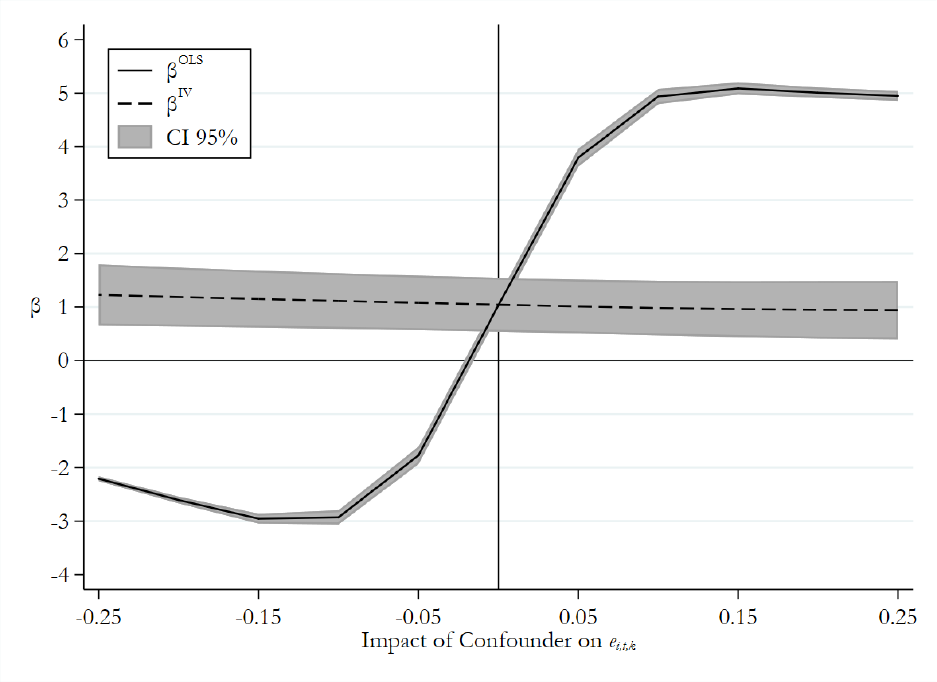
38
Figure 1: OLS vs. IV Estimates
The figure shows the impact of a confounding factor on the OLS and IV coefficient estimates from
regressions of wages on employment rates (controlling for county and year effects) using simulated
data. The coefficients are estimated in samples with varying degrees of impact of a confounding
factor on employment rates. The y-axis captures the values of the coefficient estimate. The x-axis
captures the various levels of impact of the confounder on county-industry employment rates (e
i,t,k
)
across the simulated samples. The solid black line plots the OLS coefficient estimates across
samples. The dashed black line plots the IV coefficient estimates across samples. The grey area
plots the 95% confidence interval based on standard errors clustered at the county level. For the
specific parameterization of the simulations, please refer to the program code.
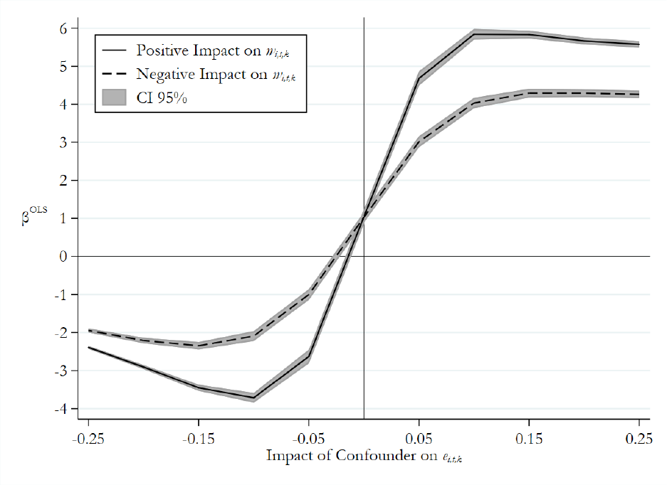
39
Figure 2: OLS Bias
The figure shows the impact of a confounding factor on the OLS coefficient estimates from
regressions of wages on employment rates (controlling for county and year effects) using simulated
data. The coefficients are estimated in samples with varying degrees of impact of a confounding
factor on employment rates and employment shares. The y-axis captures the values of the
coefficient estimate. The x-axis captures the various levels of impact of the confounder on county-
industry employment rates (e
i,t,k
) across the simulated samples. The solid black line plots the OLS
coefficient estimates for simulated samples with a positive impact of the confounder on county-
industry employment shares (w
i,t,k
). The dashed black line plots the OLS coefficient estimates for
simulated samples with a negative impact of the confounder on county-industry employment
shares (w
i,t,k
). The grey area plots the 95% confidence interval based on standard errors clustered
at the county level. For the specific parameterization of the simulations, please refer to the program
code.

40
Table 1: Bartik Instrument Construction
The table presents an excerpt of the simulated data. It shows the county-level treatment and
instrument values and their respective county-industry-level components for two counties (i), years
(t), and industries (k). w
i,t,k
is the time-varying county-industry employment share, e
i,t,k
is the time-
varying county-industry employment rate, x
i,t
is the time-varying county employment rate (i.e., the
treatment), w
i,k
is the pre-determined county-industry employment share, e
t,k
is the time-varying
nationwide industry employment rate, and z
i,t
is the Bartik instrument. For the specific
parameterization of the simulation, please refer to the program code.
Panel
Treatment
Instrument
County i
Year t
Industry k
w
i,t,k
e
i,t,k
x
i,t
w
i,k
e
t,k
z
i,t
150
1
10
0.031
0.778
0.845
0.031
0.811
0.852
150
1
11
0.044
0.814
0.845
0.044
0.846
0.852
…
…
…
…
…
…
…
…
…
150
2
10
0.014
0.788
0.847
0.031
0.823
0.853
150
2
11
0.053
0.800
0.847
0.044
0.824
0.853
…
…
…
…
…
…
…
…
…
151
1
10
0.014
0.824
0.853
0.014
0.811
0.846
151
1
11
0.041
0.868
0.853
0.041
0.846
0.846
…
…
…
…
…
…
…
…
…
151
2
10
0.017
0.840
0.854
0.014
0.823
0.843
151
2
11
0.038
0.833
0.854
0.041
0.824
0.843

41
Table 2: Bartik Instrument Estimation
The table presents OLS, reduced-form, and two-stage IV estimates from county-level regressions
of wages on employment rates using simulated data. y
i,t
are county-level (log) wages. x
i,t
is the
county-level employment rate. z
i,t
is the Bartik instrument. Panel A presents estimates using
simulated data without a confounding factor affecting wages and employment rates. Panel B
presents estimates using simulated data with a confounding factor positively affecting both wages
and employment rates (e.g., growth opportunities). Panel C presents estimates using simulated data
with a confounding factor positively affecting wages and negatively affecting employment rates
(e.g., skill/capital-biased technological change). Across the three panels, the true impact of
employment rates on wages is β = 1. For more detail on the specific parameterization of the
simulations, please refer to the program code. All regressions include county and year fixed effects.
The t-statistics (in parentheses) are based on standard errors clustered at the county level. *, **,
*** denote statistical significance at the 10, 5, and 1 percent level (two-tailed), respectively.
Panel A: Uncorrelated Factor
Model
OLS
Reduced Form
First Stage
Second Stage
Outcome
y
i,t
y
i,t
x
i,t
y
i,t
x
i,t
1.035***
1.045***
(12.54)
(4.07)
z
i,t
0.515***
0.493***
(4.03)
(23.64)
County FE
Yes
Yes
Yes
Yes
Year FE
Yes
Yes
Yes
Yes
Observations
15,000
15,000
15,000
15,000
Clusters
1,000
1,000
1,000
1,000
R
2
0.164
0.153
0.630
-
Panel B: Positively Correlated Factor
Model
OLS
Reduced Form
First Stage
Second Stage
Outcome
y
i,t
y
i,t
x
i,t
y
i,t
x
i,t
4.937***
0.982***
(67.53)
(3.78)
z
i,t
0.488***
0.497***
(3.49)
(21.29)
County FE
Yes
Yes
Yes
Yes
Year FE
Yes
Yes
Yes
Yes
Observations
15,000
15,000
15,000
15,000
Clusters
1,000
1,000
1,000
1,000
R
2
0.506
0.141
0.515
-

42
Panel C: Negatively Correlated Factor
Model
OLS
Reduced Form
First Stage
Second Stage
Outcome
y
i,t
y
i,t
x
i,t
y
i,t
x
i,t
-2.929***
1.114***
(-43.34)
(4.21)
z
i,t
0.538***
0.483***
(4.59)
(20.20)
County FE
Yes
Yes
Yes
Yes
Year FE
Yes
Yes
Yes
Yes
Observations
15,000
15,000
15,000
15,000
Clusters
1,000
1,000
1,000
1,000
R
2
0.352
0.167
0.504
-

43
Table 3: Examples of Bartik Instruments in Accounting Research
The table presents an overview of select examples of recent accounting research using versions of Bartik and simulated instruments. For each
of the studies, it lists the treatment of interest (x
i,t
or x
i,j
), the components underlying the instrument – pre-determined shares of characteristics
(w
i,k
or s
i,k
) and the common trends or shocks (e
t,k
or
) – and the combination of these components resulting in a Bartik or simulated instrument
(z
i,t
or z
i,j
). Although all of the studies use a version of Bartik instruments, not all of them use the granularity afforded by Bartik instruments to
the full extent. Kim (2021), for example, uses a common (crisis) time trend, whereas Granja and Moreira (2020) use bank-specific trends.
Study
Treatment
Share/Characteristic
Trend/Shock
Instrument
(i,t,k) or (i,j,k)
x
i,t
or x
i,j
w
i,k
or s
i,k
e
t,k
or
z
i,t
or z
i,j
Bourveau et al. (2020)
(i: industry; t: time; k: country)
Collusion incentives
(industry-time)
Share of industry sales imported
by foreign country in 1990
Foreign country’s leniency
law adoption timing
Inner product of
share and shock
Breuer (2021)
(i: industry; j: country; k: firm)
Regulatory scope
(country-industry)
Firm-size distribution
in European industry
Country’s size-based
thresholds
Simulated share
above thresholds
Breuer et al. (2020)
(i: county-industry; t: time; k: firm)
Enforcement exposure
(county-industry-time)
County-industry’s share of
limited-liability firms before 2007
Enforcement reform of limited-
liability firms’ reporting in 2007
Interaction of
share and shock
Duguay (2021)
(i: sector; j: state: k: charity)
Charity audit mandate
(state-sector)
Charity-size distribution
in US charity-activity sector
State’s size-based
audit threshold
Simulated share
above threshold
Granja and Moreira (2020)
(i: county; t: time; k: bank)
Credit disruption
(county-time)
Bank’s market share in
county before crisis
Bank’s nationwide lending
contraction during crisis
Inner product of
share and trend
Kim (2021)
(i: ZIP-code; t: time; k: bank)
Loan-loss delay
(ZIP-code-time)
Bank’s pre-crisis loan-loss delay
weighted by local market share
Financial crisis
indicator
Interaction of
share and shock
