
159159
5
c h a p t e r
This chapter investigates whether fiscal policy should
be used to combat business cycle fluctuations, especially
downturns. Can discretionary fiscal policy successfully
stimulate output? Or does it do more harm than good?
New evidence presented here, from emerging as well as
advanced economies, indicates that the effects of fiscal
stimulus can be positive, albeit modest. But policymak-
ers must be very careful about how stimulus pack-
ages are implemented, ensuring that they are timely
and that they are not likely to become entrenched and
raise concerns about debt sustainability. The chapter
concludes with a discussion of how automatic stabiliz-
ers could be made more effective and how governance
improvements could reduce “debt bias” concerns related
to discretionary actions.
I
n recent months, as economies have been
buffeted by falling asset prices, rising costs
for raw materials and credit, and waning
confidence, there have been renewed calls
for governments to actively use fiscal policy to
support efforts taken by central banks to prevent
sharp declines in activity. Once again, there is a
lively debate about the appropriate role of fiscal
policy in managing the business cycle, especially
during a downturn: Are discretionary fiscal
actions helpful, or do they sometimes do more
harm than good? When is a discretionary pack-
age most effective? When is it better simply to
let automatic stabilizers do the job?
The debate over the appropriate role of fis-
cal policy in managing the business cycle has
persisted for many years. One school of thought
argues that taxes, transfers, and spending can
be used judiciously to lean against fluctuations
in economic activity, especially to the extent that
economic fluctuations are mainly due to mar-
kets falling out of equilibrium instead of react-
ing to changes in fundamental factors such as
productivity. Others contend that fiscal policy
actions are generally either ineffective or make
things worse, because the actions are ill timed
or they create damaging distortions. This latter
point of view has dominated the debate over the
past two decades; consequently, fiscal policy has
taken a backseat to monetary policy. But there
also has been a recognition that there are times
when monetary policy needs the support of fis
-
cal stimulus, such as when nominal interest rates
approach zero or the channels of monetary
policy transmission are in some way impeded.
Against this background, this chapter takes
a fresh look at the role of fiscal policy during
economic downturns. The main objectives are
to (1) analyze how fiscal policy has typically
responded during downturns; (2) examine the
effects on economic activity of fiscal stimulus
during downturns; (3) identify the main fac-
tors that affect the outcomes of fiscal policy
interventions; and (4) offer policy suggestions,
in light of both empirical evidence and insights
from theoretical work, on (a) whether and when
to use discretionary fiscal policy, (b) the implica
-
tions of using various fiscal policy instruments,
and (c) the appropriate balance between auto-
matic stabilizers and discretionary actions.
This chapter seeks to contribute to the con-
siderable literature on fiscal policy as a counter-
cyclical tool in three ways. First, it specifically
evaluates whether discretionary fiscal policy
responses to downturns have been timely and
temporary. Second, whereas most previous
studies have focused on the effects of policy in
advanced economies, this chapter also looks
at evidence for emerging economies. Finally,
the chapter complements the empirical analy-
sis with simulation analysis designed to assess
how fiscal multipliers depend on the choice of
The main authors of this chapter are Alasdair Scott
(team leader), Steven Barnett, Mark De Broeck, Anna
Ivanova, Daehaeng Kim, Michael Kumhof, Douglas
Laxton, Daniel Leigh, Sven Jari Stehn, and Steven
Symansky, with support from Elaine Hensle, Annette
Kyobe, Susanna Mursula, and Ben Sutton.
FISCAL POLICY AS A COUNTERCYCLICAL TOOL
CHAPTER 5 Fiscal Policy as a countercyclical tool
160
fiscal instruments and the characteristics of the
economy.
The policy record shows that discretionary
fiscal policy has been more timely than some
critiques suggest. But there are valid concerns
about whether fiscal stimulus packages will be
temporary and the implications for the path
of government debt. Empirical evidence sug-
gests that discretionary fiscal stimulus has a
moderately positive effect on output growth
in advanced economies. However, the effects
appear to be constrained in emerging econo-
mies. This might be because of credibility
issues, especially debt concerns. Simulation
experiments show that fiscal multipliers can
vary considerably, depending on the instrument
used, the degree of monetary policy accom-
modation, and the type of economy. Consistent
with the empirical evidence, increases in interest
rate risk premiums as a result of debt concerns
can render fiscal multipliers negative, suggesting
that discretionary fiscal stimulus may do more
harm than good.
Does this mean there is no role for counter-
cyclical fiscal policy? In practice, the extent of
automatic stabilizers has been related to the size
of government, but more extensive government
is generally associated with lower growth. Given
this dichotomy, it is worth investigating further
whether countercyclical fiscal rules and the fiscal
policy framework can be designed to increase
the ability of fiscal policy to smooth fluctua-
tions in output and income over the course of
business cycles—without increasing the size of
government or placing debt stability at risk.
The chapter is organized as follows. The next
section provides a brief review of the empirical
and theoretical literature on the role of fiscal
policy in stabilizing output. The following two
sections present, first, the results of new empiri-
cal work that characterizes how fiscal policy
has been used in both advanced and emerging
economies and then an analysis of its effects.
The subsequent section uses formal simula-
tion-based analysis to examine the effectiveness
of various stimulus options and the effects of
various macroeconomic factors when the policy
is implemented. The concluding section offers
some policy suggestions.
Understanding the Fiscal Policy Debate
Fiscal policy can work in two general ways to
stabilize the business cycle. One way is through
automatic stabilizers, which arise from parts of
the fiscal system that naturally vary with changes
in economic activity—for example, as output
falls, tax revenues also fall and unemployment
payments rise.
1
Discretionary fiscal policy, on the
other hand, involves active changes in policies
that affect government expenditures, taxes, and
transfers and are often undertaken for reasons
other than stabilization.
By their nature, automatic stabilizers play an
immediate role during downturns. But they are
usually by-products of other fiscal policy objec-
tives. As such, the size of automatic stabilizers
tends to be associated with the size of govern-
ment (see, for example, Fatás and Mihov, 2001),
suggesting that an increase in the size of govern-
ment can help dampen output volatility (see
Galí, 1994). However, many argue that a larger
government acts as a drag on growth over the
longer term. Hence, there is a potential con-
flict between increasing stability and increasing
economic efficiency. Moreover, the effectiveness
of automatic stabilizers may be more a matter of
proper design than size.
Because automatic stabilizers are often limited
in scope—Box 5.1 reviews the extent of auto-
matic stabilizers across economies—the active
use of discretionary fiscal measures is often
promoted as a countercyclical tool. Skeptics,
however, question governments’ ability to deliver
well-timed measures as well as the macroeco-
nomic effects of discretionary fiscal measures
and the longer-term implications for fiscal
sustainability.
1
Hence, the strength of automatic stabilizers depends
on the size of transfers (such as the scope of unemploy-
ment insurance), the progressivity of the tax system, and
the effects of taxes and transfers on labor participation
and demand for workers and capital.
161
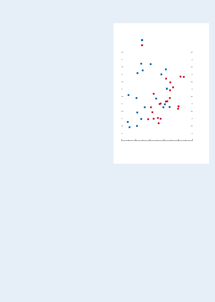
How important are automatic stabilizers?
This box looks at their quantitative impact
on the fiscal balance, especially in compari-
son with discretionary fiscal policy. First, the
impact of automatic stabilizers on the primary
balance varies across countries. The volatil-
ity in the primary balance is more a result of
changes in discretionary policy than of auto-
matic stabilizers. However, for many countries,
changes in discretionary policy are not well
synchronized with the business cycle, suggest-
ing that automatic stabilizers are often a more
important source of systematic countercyclical
policy actions.
Automatic stabilizers are measured using
the change in the cyclical balances estimated
in the event analysis in the main text of this
chapter.
1
The impact of automatic stabiliz-
ers on fiscal outcomes varies across countries
and is positively related to both government
size and output volatility. Government size is a
good proxy for the size of automatic stabilizers,
and provides the horizontal axis in the first
figure.
2
Realized volatility in the cyclical bal-
ance—measured as the standard deviation of
the change in the cyclical balance—is roughly
equal to government size times the volatil-
ity in the output gap. The first figure shows
that even though emerging economies have
smaller governments, they tend to experience
higher volatility in the cyclical balance than
advanced economies. This is largely because
emerging economies have more volatile output
gaps. However, looking separately at emerging
economies and advanced economies (to control
for the higher output volatility in emerging
economies), there is a positive relationship
between government size and cyclical bal-
ance volatility—that is, countries with larger
The main author of this box is Steven Barnett.
1
The elasticity-based measure is used for the analysis
in this box. The sample period is 1992–2007.
2
Balassone and Kumar (2007), Box 4.2, explains
why this holds. This general finding is robust to
income elasticity assumptions.
automatic stabilizers have more variation in the
cyclical balance.
3
Changes in discretionary fiscal policy,
however, account for more of the volatility of
primary balances than automatic stabilizers. On
average, the volatility of the cyclically adjusted
balance is about three times greater than that
of the cyclical balance. This is true for advanced
economies and for emerging economies. But
the extent to which these policy changes play a
countercyclical role depends on how well they
are synchronized with the business cycle. To
examine this empirically, a measure of the cycli-
cality of fiscal policy discretion is compared with
3
Government size, however, is often found to
be negatively correlated with output volatility (for
example, Andrés, Doménech, and Fatás, 2008), which
would dampen the otherwise mechanical positive
relationship between government size and cyclical
balance volatility.
Box 5.1. Differences in the Extent of Automatic Stabilizers and Their Relationship with
Discretionary Fiscal Policy
understanding the Fiscal Policy debate
10 20 30 40 50 60
0.0
0.2
0.4
0.6
0.8
1.0
1.2
Volatility in Cyclical Balance
Source: IMF staff calculations.
Standard deviation of change in cyclical balance
Government size (percent of GDP)
Emerging economies
Advanced economies
CHAPTER 5 Fiscal Policy as a countercyclical tool
162
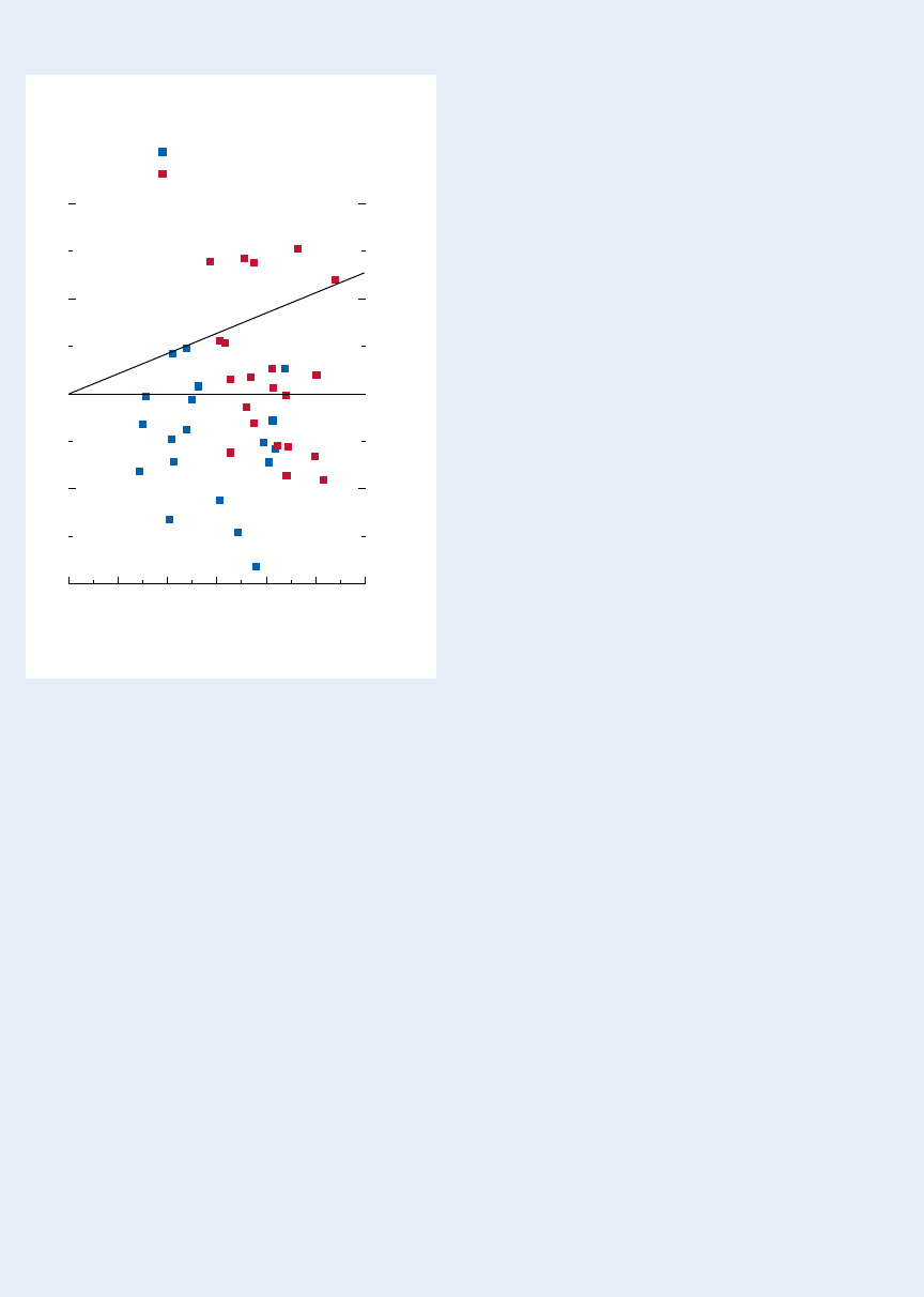
the size of automatic stabilizers.
4
The second fig-
ure shows that discretionary fiscal policy tends
to be more countercyclical in advanced econo-
mies (when the countercyclicality of discretion
is greater than zero), but is often procyclical in
emerging economies (below zero). The units
on the two axes are comparable and indicate
the percentage point change in the respective
balance (after dividing by 100) for a 1 percent
-
age point increase in the output gap. If a coun-
try lies above the 45-degree line, it indicates that
discretionary policy makes overall fiscal policy
more countercyclical than automatic stabilizers
4
Cyclicality of fiscal policy is measured by a regres-
sion, run in first differences, with the cyclically
adjusted primary balance as the dependent variable
and the output gap as the explanatory one. A positive
coefficient indicates a more countercyclical policy.
This regression, however, is potentially problematic in
that it ignores the relationship (endogeneity) between
fiscal policy and the output gap.
do. As can be seen, this happens in only a few
cases, including some of the Anglophone coun-
tries with smaller governments, as well as some
of the Nordic ones with larger governments.
However, there is little systematic evidence that
countries with smaller governments compensate
for weaker automatic stabilizers by using more
discretion.
Together, these findings would suggest that
(1) automatic stabilizers have, in general,
played a more consistently countercyclical role
than discretionary fiscal policy, and (2) changes
in discretionary fiscal policy are either poorly
timed or related to factors other than output
stabilization. A caveat, however, is that fiscal
policy discretion is measured by the cyclically
adjusted balance, which, as discussed in the
main text, is an imperfect proxy, because it may
also capture factors unrelated to discretionary
changes, notably asset price fluctuations.
Asset price movements directly affect
financial transaction and capital gains taxes,
but they also have broader, indirect revenue
implications, notably through a wealth effect
on consumption. To the extent that these
movements do not fully track the business
cycle (for example, amplified fluctuations rela-
tive to those of the output gap), the revenue
effects will not be captured by conventional
tax revenue elasticities and will be part of the
cyclically adjusted component of revenue. In
an unpublished study, the IMF staff prepared
econometric estimates of the short-run sen-
sitivity of cyclically adjusted tax revenue to
house and equity price fluctuations in the G7
countries. The cyclically adjusted revenue data
are computed using the conventional adjust-
ment methods, ensuring consistency of the
results. The estimates suggest that a 1 percent
decline in both house and equity prices could
reduce total tax revenue by up to almost 1
percent, with the house price decline account-
ing for most of the drop. The estimates also
indicate that Canada, Japan, the United King-
dom, and the United States are more sensitive
to house and equity price fluctuations than
the continental European G7.
Box 5.1 (concluded)
0 10 20 30 40 50 60
-100
-50
0
50
100
Cyclicality of Structural Balance
Source: IMF staff calculations.
Cyclicality of discretion
Government size (percent of GDP)
Emerging economies
Advanced economies

163
These skeptics argue that discretionary fiscal
measures cannot be delivered quickly enough
by legislatures, especially compared with the
speed with which a central bank can change
its policy rate. Hence, there is a risk that fiscal
stimulus will arrive just as the economy recovers
from a downturn. Moreover, argue the critics,
fiscal stimulus measures are not likely to be well
targeted, but are likely instead to be directed
to wasteful and distortionary public spending
and revenue measures more responsive to the
pressures of interest groups than the needs of
the economy. Furthermore, they are not likely
to be withdrawn sufficiently quickly to pre-
serve fiscal sustainability. For instance, there is
widespread evidence that fiscal policy in emerg-
ing and less developed economies is procyclical
rather than countercyclical, in part because of
political incentives to run larger deficits in good
times, when financing is available (Talvi and
Végh, 2000).
Even if fiscal stimulus can be delivered
quickly, does that justify the use of discretionary
fiscal policy? There is still considerable debate
and little theoretical consensus. A textbook
Keynesian position is that private consumption
and investment are driven by current income,
with the implication that output is highly
responsive to changes in fiscal policy. But fiscal
policy can be much less effective in an open
economy, depending on the degree of capital
mobility and the exchange rate regime, because
fiscal stimulus might simply “leak out.” In addi-
tion to the standard crowding-out arguments,
many neoclassical theorists emphasize the role
of expectations about future income and taxes,
arguing that fiscal multipliers are likely to be
small because forward-looking households will
figure out that temporary fiscal stimulus mat
-
ters little to their lifetime income; multipliers
may even be negative, if increased government
expenditures lead to offsetting reductions in
private consumption and investment.
2
By con-
2
For example, the well-known Ricardian equivalence
critique of Barro (1974) argues that households and
firms understand that deficits accompanied by future tax
trast, recent work using so-called New Keynesian
models argues that an increase in government
consumption still can have positive consump-
tion and real wage effects, if there are nominal
and real rigidities and liquidity constraints (see,
for example, Galí, 2006). These models also
suggest that not all temporary fiscal measures
are ineffective: policies that affect the incentive
to switch the timing of consumption—such as
changes in consumption taxes—are likely to be
most effective when they are understood to be
temporary rather than permanent.
In recent years, four factors may have become
increasingly relevant:
•
The extent of market rigidities: Rigidities in goods
and labor markets may have decreased over
time, as a result of microeconomic reforms,
and access to credit may have become more
widely available, reducing fiscal multipliers.
•
The monetary policy framework: The impact of
fiscal policy can be expected to increase if it
is accommodated by monetary policy, thus
alleviating the crowding-out effect.
•
Globalization and openness: To the extent that
economies are more integrated—that is, an
increasing share of domestic demand falls on
imported goods—discretionary fiscal policy
will be less effective today than previously.
•
Financial innovation: Deregulation of finan-
cial markets and increased access to global
capital may have eased credit constraints on
households and firms, with the implication
that consumption and investment are less con-
strained by current income and less respon-
sive to discretionary fiscal policy measures.
However, cross-border financial integration
can also reduce the sensitivity of interest rates
to government borrowing and ease crowding-
out effects.
Unfortunately, empirical work has not settled
the theoretical debates. Estimates of fiscal multi-
rises leave them no better off in net present value terms,
and therefore they save rather than spend temporary
(lump-sum) tax cuts. Neoclassical models often exhibit
negative wealth effects following increases in govern-
ment spending that are strong enough to reduce private
consumption and investment.
how has discretionary Fiscal Policy tyPically resPonded?

CHAPTER 5 Fiscal Policy as a countercyclical tool
164
Perhaps surprisingly, the empirical literature
on the effects of fiscal policy does not provide a
clear answer to the simple question of whether
discretionary fiscal policy can successfully
stimulate the economy during downturns. Esti-
mates of the effects of fiscal policy on many key
macroeconomic variables can differ not merely
in degree but in sign. This box aims to show
why demonstrating conclusively what happens as
a result of discretionary fiscal policy is, in fact,
extremely difficult.
Any empirical work on this issue faces the
following problems: (1) Every assessment of
the impact of a policy change must take into
account the economic circumstances when the
policy was implemented. (2) A fiscal stimulus
can be achieved by many different combina-
tions of taxes, transfers, and spending, each of
which can have different effects. (3) There will
sometimes be a difference between the date on
which a change in fiscal policy is measured from
the data and the date on which the policy was
common knowledge to households and firms.
(4) Policy measures and economic activity are
both endogenous—they depend on each other
at the same time—and so it is not immediately
clear what determines what just by looking
at simple correlations. This last problem is
arguably the most difficult to overcome. The
researcher must somehow strip out those parts
of changes in taxes, transfers, and spending that
occur passively (such as from automatic stabiliz-
ers) from those that represent the true policy
initiative, and use that measure of fiscal impulse
to determine the effects on economic activity.
To illustrate, suppose overall fiscal policy, g,
evolves according to
g = (a + b)y + h, (1)
where y is the output gap. For simplicity, one
can think of g as representing only government
expenditures, so that a stimulus occurs when
g is positive. There are two reactions of fiscal
policy to the state of the economy: an automatic
component, represented by a, and a system-
atic discretionary component, represented by
b. Unexpected discretionary fiscal policy is
denoted by h.
Now suppose that the output process is
y = dg + ε, (2)
where d is the fiscal multiplier and ε repre-
sents shocks independent of policy. There are
two significant problems presented by this
system. First, we have a classic simultaneity
problem—attempting to assess the effects of
fiscal policy on output by estimating (1) will
result in biased estimates. The second prob-
lem is a measurement problem—the difficulty
of distinguishing systematic discretionary
policy changes from automatic stabilizers. The
elasticity-based fiscal impulse measure can be
thought of as using OECD estimates of a and
constructing
f
~
= f – ay.
Estimating the cyclicality of this measure is
equivalent to estimating the parameter b.
1,2
When examining the effectiveness of fiscal
policy in the regression framework, a fiscal
impulse measure that mistakenly includes cycli-
cal changes generated by automatic stabilizers
will lead to invalid inferences about the effects
of discretionary fiscal policy. The second fiscal
impulse measure therefore focuses entirely
on h, the effects of unexpected fiscal policy
shocks.
3
Other approaches in the literature attempt
to address the same issues. Structural vector
autoregressions (SVARs) use statistical criteria
to estimate shocks to fiscal policy and measure
1
See also Galí and Perotti (2003) for an application
of the same method.
2
When looking at the reaction of fiscal policy in
emerging economies, it is necessary to make the
“zero-one” assumption of income elasticities of expen-
ditures and revenues, which is a cruder approach to
measuring a but conceptually the same.
3
For precise details on how the fiscal impulse mea-
sures are constructed, see Appendix 5.1.
Box 5.2. Why Is It So Hard to Determine the Effects of Fiscal Stimulus?
The main author of this box is Alasdair Scott.

165
how has discretionary Fiscal Policy tyPically resPonded?
how well those shocks can explain movements
in output that are not accounted for by other
economic shocks. Three problems are poten-
tially relevant. As with reduced-form regressions,
statistical assumptions need to be made to iden-
tify the fiscal shocks. Second, most VARs ignore
the importance of debt dynamics in condition-
ing responses (whether or not a temporary rise
in debt causes households and firms to expect
future higher taxes is a key distinction between
Keynesian and classical views on the effective-
ness of discretionary fiscal policy).
4
Finally, as
with reduced-form regressions, VARs might not
reliably be able to resolve the timing issue.
By contrast, “narrative” approaches estimate
policy-driven changes in fiscal stimulus by look-
ing directly at the historical record of legisla-
tion and public statements. The advantage of
this approach is that careful attention can be
directed to picking the timing of the shocks by
examining carefully when policy decisions were
made and announced. But such studies are very
resource intensive, making their application
across countries almost impossible. Further,
they are subjective, just as VARs and reduced-
form analysis rely on identifying assumptions. In
practice, analysis has centered around a small
number of extraordinary episodes of military
buildups, and there are questions as to how
much can be learned from such episodes about
discretionary fiscal policy during downturns.
A final approach examines specific “natural
experiments,” such as the effects of tax rebates.
4
See Chung and Leeper (2007). Favero and Giavazzi
(2007) do include debt stock.
The advantage of this approach is that it can
be directed at specific episodes for which it is
relatively easy to identify the policy change and
its intent. The corresponding disadvantage is
that, by examining a specific case, it can be hard
to draw broader lessons for policy.
This empirical work provides a mixed
picture of the ability of government spend-
ing to stimulate private demand.
5
(There is
less evidence about revenue-based measures.)
Moreover, there appears to be a pattern
between the method used and the qualitative
results obtained. The table summarizes the
results of a selection of prominent papers in
the literature in terms of the signs of responses
of key variables to discretionary increases in
government spending.
In particular, SVAR-based studies in which
fiscal interventions are identified by assum-
ing that government spending is predeter-
mined within the quarter (see Blanchard and
Perotti, 2002) tend to find relatively strong
positive effects, whereas narrative stud
-
ies that rely on the reactions to episodes of
extraordinary spending have tended to find
much weaker, and even negative, relation-
ships between episodes of fiscal stimulus and
5
Results from case studies usually find positive
effects, but the effects are generally not as strong as
those generated by VAR studies. Studies of the 1975
tax rebates generally conclude that the effects were
positive but modest (that is, short-run multipliers of
about 0.2–0.5); see Modigliani and Steindel (1977)
and Blinder (1981). Studies of the 2001 tax rebates
have generated similar results; see Shapiro and
Slemrod (2002).
Assessment of Impacts of Discretionary Fiscal Policy Stimulus by Empirical Method
Output Private Consumption
Private Investment
in Durables
Private
Capital Investment
VAR studies Neutral to positive Neutral to positive Negative to positive Negative to positive
Narrative studies Positive Negative Negative . . .
Case studies Positive Positive . . . . . .
Note: Studies placed in the vector autoregression (VAR) category include Fatás and Mihov (2001); Mountford and Uhlig (2002);
Blanchard and Perotti (2002); and Galí, López-Salido, and Vallés (2007). Studies placed in the narrative category include Ramey and
Shapiro (1998) and Edelberg, Eichenbaum, and Fisher (1999). Case studies include Johnson, Parker, and Souleles (2006).

CHAPTER 5 Fiscal Policy as a countercyclical tool
166
pliers cover a wide range, from positive through
insignificant to negative.
3
One reason is that
taking account of all the appropriate condition-
ing factors can be very difficult. Another reason
is methodological. Put simply, separating out
changes in discretionary fiscal policy from auto-
matic stabilizers and evaluating their effects is
very difficult—in particular, fiscal policy simul-
taneously both responds to and causes changes
in economic activity. This “endogeneity prob-
lem” poses a major challenge for estimating the
effects of fiscal policy, as discussed in Box 5.2.
How Has Discretionary Fiscal Policy
Typically Responded?
The previous section identified two types of
critique of fiscal policy: skepticism that discre-
tionary fiscal policy can be delivered efficiently,
owing to political constraints, and doubts that
it can be effective, for economic reasons. These
critiques frame the empirical analysis in this
3
A typical range of expenditure multipliers would be
from 0.5 (for example, Mountford and Uhlig, 2002) to
about 1 (for example, Blanchard and Perotti, 2002). But
Perotti (2007) has outliers as high as 4 and Krogstrup
(2002) as low as –2.
section, which examines how fiscal policy has
typically responded to downturns.
Defining economic downturns and measur-
ing fiscal stimulus are inevitably somewhat
subjective exercises. In the analysis that follows,
downturns are defined as periods during which
either the growth rate is negative or the output
gap is unusually negative, the precise thresh-
old depending on whether quarterly or annual
data are used. This definition is arguably more
sensible than defining a downturn simply in
terms of negative growth, because that would
miss periods during which output is significantly
below potential but still rising.
The measures of fiscal stimulus used in this
chapter all start with the primary fiscal balance,
the difference between total general govern-
ment revenues and expenditure net of interest
payments on consolidated general government
liabilities. Changes in the primary balance can
arise passively, as revenues and expenditures rise
and fall with economic activity, or actively, as
governments make choices about tax, transfer,
and spending policies. What is needed, there-
fore, is a measure of the cyclically adjusted pri-
mary balance, the intuition being that changes
in the cyclically adjusted primary balance should
reflect changes in policy. The first part of this
consumption.
6
Ramey (2008) suggests that this
difference relates to the way that VARs treat
timing—if discretionary fiscal policy measures
are pre-announced, and households decrease
their spending right away (as predicted by neo-
classical theory), VARs that measure the effect
based on actual changes to fiscal balances or
components might record a rise in the growth
rate of consumption on that date. This would
support a Keynesian view of fiscal policy, but
in fact the growth in consumption is driven
6
Note, however, that narrative studies of the effects
of tax changes find very large multipliers—see Romer
and Romer (2007).
by recovery from the previous fall. Narra-
tive approaches, on the other hand, take into
account the moment discretionary measures
are announced.
7
Compared with these studies,
the reduced-form approach employed in this
chapter is conceptually closest to the SVAR
approach of Blanchard and Perotti (2002); to
the extent that the timing criticism applies to
this paper and those like it, it also applies to
our methodology. However, a comparative nar-
rative study of all 41 economies in this study is
beyond the scope of this chapter.
7
But see also the rebuttal in Perotti (2007).
Box 5.2 (concluded)
167
section looks at the responses of fiscal policy
to changes in economic activity, identifying
automatic stabilizers with changes in the cycli-
cal component of the primary balance and
discretionary fiscal policy with changes in the
cyclically adjusted primary balance.
4
Construct-
ing this measure requires two slightly different
approaches, depending on the information
available for the economies being analyzed.
Evidence on the Responsiveness of Fiscal Policy
The empirical investigation begins with
analysis of advanced economies, for which long
spans of fiscal data are available on a quarterly
basis.
5
Discretionary fiscal actions are those that
change the cyclically adjusted budget balance,
using estimates of the output gap together with
estimates of income elasticities of revenues and
expenditures to extract the cyclical component
from the budget.
6
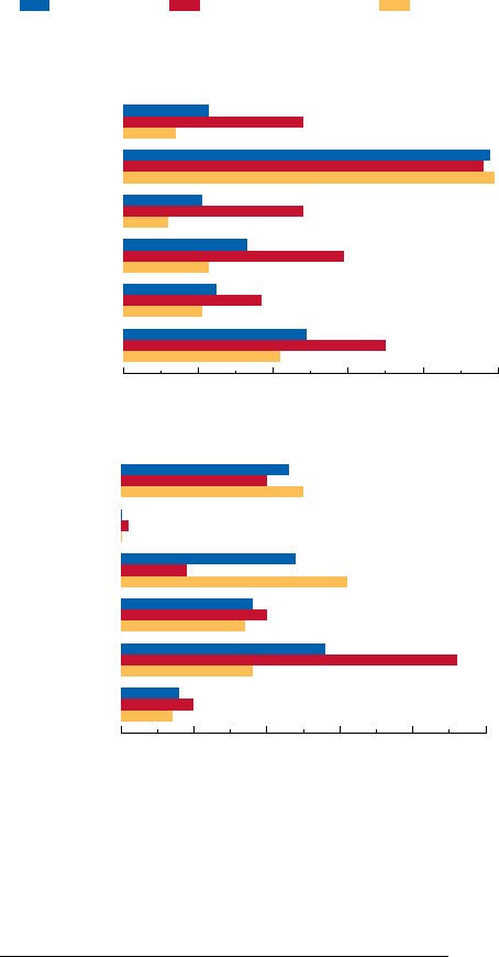
Figure 5.1 presents a sum-
mary of policy responses in G7 economies over
the past four decades. The numbers indicate
that discretionary fiscal stimulus has been deliv-
ered in downturns, but it has been used much
less frequently than automatic stabilizers and
monetary policy. Discretionary fiscal stimulus
has been used in about 23 percent of all down
-
turn quarters—less than half as frequently as
interest-rate easing—whereas automatic stabi-
lizers are observed in well over 95 percent of
downturns (upper panel).
7
Discretionary policy
4
As defined in Box 5.1 and the event analysis, the
cyclically adjusted balance is a residual and embodies all
changes in the primary balance not removed by cyclical
adjustment. This includes many factors not necessar-
ily related to output stabilization, such as the impact of
structural reform, one-off items, and other economic
events (including asset price changes that are not cyclical
in nature and could therefore be identified as “auto-
matic” changes in the fiscal balance—see Jaeger and
Schuknecht, 2007).
5
For further details about the following analysis, see
Leigh and Stehn (forthcoming).
6
These elasticities are taken from the OECD Economic
Outlook; see Appendix 5.1 for details.
7
Note that automatic stabilizers do not necessarily
ease in all downturns, because the applied definition of
a downturn does not rule out an increase in growth or
the output gap (as long as the output gap is unusually
negative).
how has discretionary Fiscal Policy tyPically resPonded?
Discretionary fiscal policy has been used less frequently than monetary policy and
automatic stabilizers during downturns, and has taken longer to arrive.
0 1 2 3 4 5
0 20 40 60 80 100
Source: IMF staff calculations.
G7 comprises Canada, France, Germany, Italy, Japan, United Kingdom, and United
States.
Share of downturns with easing in:
Lag after start of downturn until policies eased
Figure 5.1. How Often and Quickly Has Fiscal Stimulus
Been Used in G7 Economies?
Group of 7 (G7) Anglophone G7 countries Other G7
Cyclically adjusted
primary balance
Cyclically adjusted
current spending
Cyclically adjusted
revenue
Cyclical primary
balance
Nominal policy
interest rate
Capital spending
Cyclically adjusted
primary balance
Cyclically adjusted
current spending
Cyclically adjusted
revenue
Cyclical primary
balance
Nominal policy
interest rate
Capital spending
Quarters
Percent
1
1
CHAPTER 5 Fiscal Policy as a countercyclical tool
168
also arrives later, on average about two and a
half quarters after the onset of a downturn, and
about one and a half quarters after interest-rate
easing (lower panel). Capital spending is par-
ticularly slow, with an arrival lag of almost four
quarters. By contrast, automatic fiscal easing,
proxied by a fall in the cyclical primary balance,
occurred in almost all downturns in the quarter
of the downturn itself.
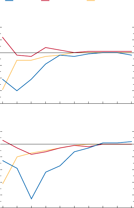
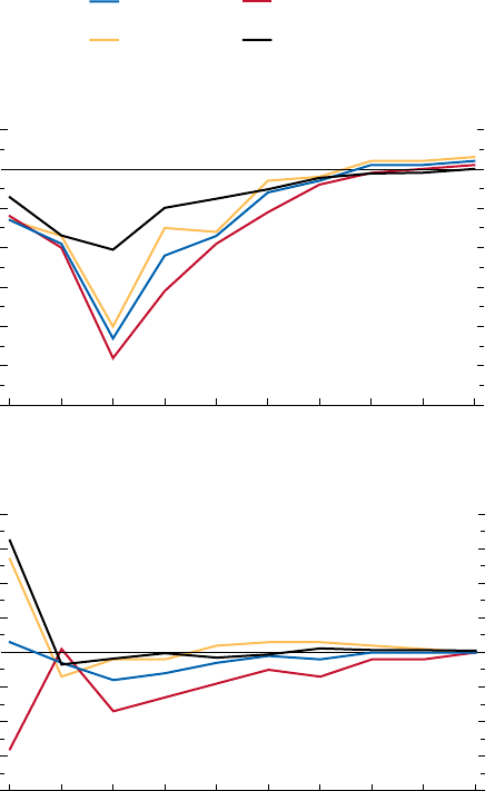
The size of discretionary fiscal easing is also
much smaller on average than that of automatic
stabilizers. Figure 5.2 shows average impulse
responses of discretionary fiscal measures,
automatic stabilizers, and interest rates for the
G7 economies, drawing from vector autoregres-
sions (VARs) estimated for two samples, an
“early” sample covering 1980:Q1–1991:Q4 and
a “late” sample covering 1992:Q1–2007:Q4.
8
In
both samples, the discretionary fiscal easing is
much smaller than the automatic stabilizers and
is slower to arrive than both changes in interest
rates and automatic stabilizers. However, a com-
parison of the two panels also suggests that the
countercyclical response of discretionary fiscal
policy has strengthened since the early 1990s.
9
The responses of spending and revenue compo-
nents in the early sample reflect a combination
of mildly procyclical revenue increases, small
countercyclical current spending increases, and
large procyclical capital spending cuts. The
greater degree of fiscal policy countercyclical-
ity observed since the early 1990s is the result
of cuts in revenues, larger increases in current
spending, and smaller procyclical cuts in capital
spending. The response of automatic stabiliz-
8
See Appendix 5.1 for more details. Note that, unlike
much of the VAR literature, the analysis presented here
does not evaluate the response of growth to fiscal policy
shocks. Rather, the focus is on the response of fiscal
policy variables to changes in growth.
9
In the early sample, discretionary fiscal policy is pro-
cyclical on impact and provides a cumulative procyclical
contraction of around 0.1 percentage point of potential
GDP over four quarters. In the later sample, even though
discretionary policy still produces no stimulus on impact,
it leads to a cumulative stimulus of 0.2 percentage point
over four quarters. This finding is consistent with, for
example, Galí and Perotti (2003) and World Economic
Outlook (September 2003).
0 1 2 3 4 5 6 7 8 9
-0.5
-0.4
-0.3
-0.2
-0.1
0.0
0.1
0 1 2 3 4 5 6 7 8 9
-0.4
-0.3
-0.2
-0.1
0.0
0.1
0.2
Source: IMF staff calculations.
Early Sample (1980:Q1–91:Q4)
Late Sample (1992:Q1–2007:Q4)
Following an unexpected 1 percentage point fall in growth below potential, interest
rates and the automatic component of the fiscal balance ease on impact;
discretionary fiscal stimulus takes longer to arrive. In recent years, discretionary
fiscal policy has become more countercyclical.
Figure 5.2. How Strong Was the Fiscal Policy Response
in G7 Economies?
(Percentage point deviation; quarters on x-axis; shock occurs in period
zero)
Interest rate Discretionary policy Automatic stabilizers
169
ers remained unchanged in the second sample,
while that of monetary policy strengthened.
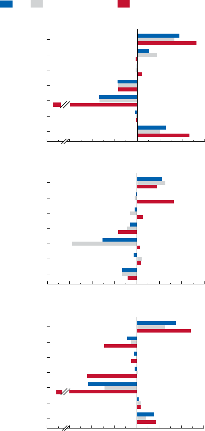
Figure 5.3
shows that there are noticeable
cross-country differences across advanced econo
-
mies. Discretionary fiscal policy and monetary
policy have been more timely and more coun-
tercyclical in the United States, Canada, and the
United Kingdom (the G7’s three Anglophone
countries) than in the rest of the G7. The
other Organization for Economic Cooperation
and Development (OECD) member countries
display even weaker countercyclicality than the
United States, Canada, and the United Kingdom
in both monetary and discretionary fiscal policy.
Data Uncertainties and the Risk of Debt Bias
A concern that often arises regarding coun-
tercyclical fiscal activism is that policymakers
may respond in an asymmetric manner, easing
in downturns and not tightening sufficiently in
upturns, implying a permanent increase in the
public-debt-to-GDP ratio with potentially adverse
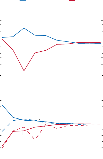
consequences for long-run growth. To investi-
gate whether fiscal policy in G7 countries has
displayed such an asymmetric tendency, the VAR
framework is adapted to allow for an asymmetric
response to upturns and downturns (see Appen-
dix 5.1). The results suggest that both fiscal
policy and monetary policy are subject to an eas-
ing bias; that is, more easing during downturns
than tightening during upturns (Figure 5.4). In
contrast, automatic stabilizers respond in a sym-
metric way, with the easing observed in down-
turns almost exactly offset by tightening during
upturns.
Hence, although discretionary fiscal policy
has been actively used, there are valid concerns
about debt bias. For illustration, a case study
of tax-based stimulus legislation in the United
States is provided in Box 5.3. The study finds
that, although reasonably timely, 38 percent of
cyclically motivated tax cuts were permanent.
An additional concern in the analysis of
countercyclical fiscal activism is that policymak-
ers face substantial uncertainties regarding the
cyclical position and run the risk of destabilizing
are Fiscal Policy reactions diFFerent in emerging and advanced economies?
0 1 2 3 4 5 6 7 8 9
-0.4
-0.3
-0.2
-0.1
0.0
0.1
0.2
0.3
0.4
0 1 2 3 4 5 6 7 8 9
-0.6
-0.5
-0.4
-0.3
-0.2
-0.1
0.0
0.1
Source: IMF staff calculations.
Change in interest rate
Change in discretionary fiscal balance
Following an unexpected 1 percentage point fall in growth below potential,
Anglophone countries have provided both monetary and fiscal stimulus; the rest of
the Organization for Economic Cooperation and Development (OECD) countries have
provided a weaker monetary response and procyclical discretionary fiscal tightening.
The figure displays policy responses for the late sample (1992:Q1–2007:Q4).
Figure 5.3. How Have Fiscal Policy Responses Varied
across Advanced Economies?
(Percentage point deviation; quarters on x-axis; shock occurs in period
zero)
Group of 7 (G7)
Other G7
Anglophone G7 countries
Other OECD
CHAPTER 5 Fiscal Policy as a countercyclical tool
170
the economy by responding to erroneously per-
ceived downturns. This appears to be a serious
problem, based on an assessment of the reliabil-
ity of preliminary GDP estimates produced by
national authorities.
10
There is a strong negative
relationship between preliminary growth esti-
mates and subsequent revisions. Forty percent
of preliminary estimates indicating negative
quarter-over-quarter growth were subsequently
revised to positive growth.
11
Forecast efficiency
tests find strong evidence of a bias toward pes-
simism in preliminary growth estimates.
12
To investigate how fiscal policy in G7 coun-
tries has been affected by errors in growth
estimates, the VAR framework is augmented
with growth-estimation errors (see Appendix
5.1). The results reported in Figure 5.5 confirm
that both fiscal and interest rate policy have
been affected by errors in preliminary growth
estimates, with a 1 percentage point fall in
perceived growth relative to final revised growth
associated with an easing in interest rates and
the discretionary fiscal-balance-to-potential GDP
ratio by about 0.2 percentage point. This finding
suggests that concern over policy errors is well
founded, especially as fiscal policy decisions
appear to be less easily reversed than monetary
policy decisions, and fiscal policy errors bear
potentially long-lived consequences for debt.
Are Fiscal Policy Reactions Different in
Emerging and Advanced Economies?
Some of the reservations about the applica-
tion of discretionary fiscal policy may apply
even more strongly in less advanced economies.
Unfortunately, although the data in the previous
section were available at quarterly frequency,
consistent data for a broader set of econo-
10
See Appendix 5.1. See also Cimadomo (2008) for
further analysis of fiscal policy using real-time data.
11
At the same time, 30 percent of quarters that, accord-
ing to the final data actually had negative growth, showed
positive growth in preliminary estimates.
12
While remaining statistically significant, this bias
appears to have declined in recent years, possibly reflect-
ing the more stable and predictable growth environment.
0 1 2 3 4 5 6 7 8 9
-0.6
-0.4
-0.2
0.0
0.2
0.4
0 1 2 3 4 5 6 7 8 9
-1.0
-0.8
-0.6
-0.4
-0.2
0.0
0.2
0.4
0.6
Source: IMF staff calculations.
Change in interest rate
Change in fiscal balances
Following a 1 percentage point shock to growth, both discretionary fiscal policy and
monetary policy are subject to an easing bias, with more stimulus during downturns
than tightening during upturns. In contrast, automatic stabilizers respond
symmetrically to upturns and downturns. The figure displays policy responses for
the late sample (1992:Q1–2007:Q4).
Figure 5.4. Is There a Bias toward Easing during
Downturns in G7 Economies?
(Percentage point deviation; quarters on x-axis; shock occurs in period
zero)
Upturn Downturn
Automatic stabilizers
Discretionary policy
Automatic
stabilizers
Discretionary policy
171
mies are available only at annual frequency.
In what follows, the analysis uses a sample of
21 advanced economies and 20 emerging econo
-
mies, covering the period from 1970 to 2007.
13
The definition of “downturn” is conceptually
the same as used previously with the quarterly
data, but “unusually negative” is now defined
as below –0.5 standard deviation of the output
gap, on account of the use of annual data.
14
For advanced economies, OECD estimates of
income elasticities of revenues and expendi-
tures are used to calculate the cyclical balance.
However, such estimates are not available for
emerging economies, and so it is assumed
that revenues move one-for-one with the busi-
ness cycle, but expenditures do not—that is,
the income elasticity of revenues is 1 and the
income elasticity of expenditures is zero (see
Appendix 5.1 for details). A fiscal expansion is
then defined as a negative change in the cycli-
cally adjusted primary balance of more than
0.25 percentage point and a fiscal contraction
as a positive change of more than 0.25 percent
-
age point. When the change in the cyclically
adjusted primary balance is less than 0.25 per
-
centage point (either positive or negative), fiscal
policy is considered neutral. Hence, we have
three states for the fiscal stance: stimulus (397
episodes), neutral (155 episodes), and tighten-
ing (437 episodes).
In addition to the assumptions necessarily
imposed when choosing data sets and defini-
tions, a number of caveats apply to analysis using
these measures. In particular, the use of annual
data limits the ability to accurately characterize
fiscal interventions that begin and end within
a year. Second, what is relevant is policymak-
ers’ perceptions of the state of the economy in
real time, which might differ substantially from
inferences made using revised data, but, in the
13
See Appendix 5.1 for a list of economies and episodes
of downturns.
14
Correspondingly, upturns are defined as episodes
during which the output gap is above 0.5 standard devia-
tion. Potential output is measured using the Hodrick-
Prescott filter, with λ set to 6.25, the value recommended
in Ravn and Uhlig (2002).
the macroeconomic eFFects oF discretionary Fiscal Policy
Following an erroneously perceived 1 percentage point fall in growth, both
discretionary fiscal policy and monetary policy have eased, particularly in
Anglophone countries. The figure displays policy responses for the late sample
(1992:Q1–2007:Q4).
0 1 2 3 4 5 6 7 8 9
-0.25
-0.20
-0.15
-0.10
-0.05
0.00
0.05
0 1 2 3 4 5 6 7 8 9
-0.4
-0.3
-0.2
-0.1
0.0
0.1
Source: IMF staff calculations.
Change in interest rate
Change in fiscal balances
Figure 5.5. Did G7 Economies Respond to Erroneously
Perceived Downturns?
(Percentage point deviation; quarters on x-axis; shock occurs in period
zero)
Group of 7 (G7) Other G7Anglophone G7 countries

CHAPTER 5 Fiscal Policy as a countercyclical tool
172
This box takes a closer look at whether fiscal
interventions in the United States have been
timely, temporary, and targeted (TTT). A
recent data set compiled by Romer and Romer
(2007) of all significant tax changes signed
into law since 1945 permits a detailed analysis
of this issue. By consulting official documents,
Romer and Romer distinguish tax changes
that were explicitly motivated by cyclical
considerations from those motivated by other
factors, including long-run growth support,
debt reduction, and the financing of additional
expenditures. Of all the 50 significant federal
tax actions identified, 7 were assessed as cycli-
cal, and, of these, 5 were tax cuts designed to
stimulate short-run growth.
This box focuses on these five tax cuts,
implemented between 1970 and 2002, as well
as the Economic Stimulus Act, signed into law
in February 2008. The box assesses how quickly
after the onset of a downturn the tax cuts were
legislated and implemented, how temporary
they were, and how well targeted they were. In
assessing how close to a downturn the tax cuts
arrived, the analysis defines a downturn as in
the main text. Growth data to assess the 2008:
Q2 stimulus are not yet available.
The main results are as follows:
•
Timeliness: Four out of the five cyclically moti-
vated tax cuts occurred within one quarter of
a downturn (see table). In the case of 2002,
the stimulus arrived three quarters after the
downturn. The average implementation lag of
tax cuts; that is, the delay between the signing
of the legislation into law and its impact on
revenue, was one quarter.
•
Temporariness: Although only one of the six
cyclically motivated tax cuts was permanent,
the remainder contained a permanent
component (see table). In particular, about
79 percent of the tax cuts were designed to be
temporary, with an average planned dura-
tion of two quarters. Some of the tax cuts
were subsequently extended, so that a smaller
proportion—62 percent—actually ended up
Box 5.3. Have U.S. Tax Cuts Been “TTT”?
The main authors of this box are Daniel Leigh and
Sven Jari Stehn.
How Timely, Temporary, and Targeted Were the Tax Cuts?
Legislated Tax Cut
Timeliness
Temporariness
1
Targeting
Date
stimulus
arrived
Name of
act
Size of
stimulus
(percent
of GDP)
Date of
nearest
downturn
2
Inside
lag
(quarters)
3
Proportion temporary
Duration of temporary
portion (quarters)
Bang-
for-the-
buck score
4
Planned Actual Planned Actual
1970:Q1 Tax Reform 1.2 1970:Q1 1 0 0 permanent 1.0
1975:Q2 Tax Reduction 3.6 1975:Q1 1 97 78 2.3 1.0 2.5
1977:Q3 Tax Reduction
and Simplification
1.0 1977:Q4 1 77 67 1.3 1.0 1.9
2001:Q3 Economic Growth
and Tax Relief
Reconciliation
1.7 2001:Q3 1 100 100 1.3 1.3 2.4
2002:Q2 Job Creation
and Worker
Assistance
1.7 2001:Q3 1 100 67 3.7 4.0 1.3
2008:Q2 Economic Stimulus 1.1 . . . 1 100 . . . 1.6 . . . 2.7
Mean 1.6 . . . 1 79 62 2.0 1.8 2.0
1
Temporary stimulus is defined as a stimulus that expires. Actual duration may exceed planned duration because of legislated
extensions.
2
Downturn is defined as a quarter with negative or below-trend growth and an output gap more than one standard deviation below
zero.
3
Inside lag denotes the period between the date the stimulus was signed into law and the date it was implemented (quarter in which
tax liabilities actually changed).
4
Bang-for-the-buck score (3 = high, 2 = medium, 1 = low) indicates the degree of cost-effectiveness according to CBO (2008)
classification.

173
absence of consistent real-time vintages of data,
it is difficult to adjust for this difference.
Bearing these caveats in mind, the analysis
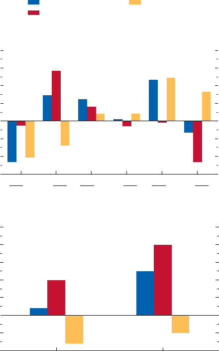
identified the following stylized facts:
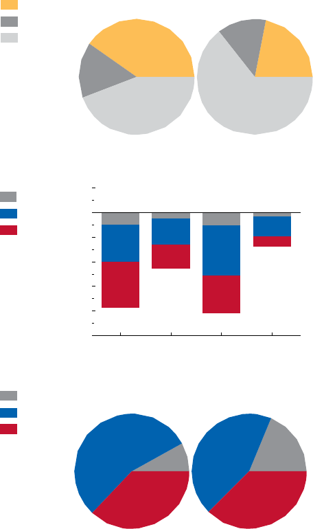
• Emerging economies respond during down
-
turns with fiscal stimulus only half as fre-
quently as advanced economies: 22 percent
versus 41 percent (Figure 5.6, top panel).
When emerging economies do implement fis-
cal stimulus, the response is slightly higher, as
measured by changes in the cyclically adjusted
primary balance as a percent of potential
GDP (Figure 5.6, middle panel, first and third
bars). But this is because downturns are larger
(Figure 5.6, middle panel, second and fourth
bars).
• In just over one-third of episodes, fiscal stimu
-
lus involved a mixture of revenue and expen-
diture changes. Of those that relied mainly on
one kind of stimulus, expenditure measures
dominate for both advanced and emerging
economies (Figure 5.6, bottom panel).
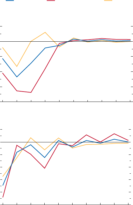
• In emerging economies, changes in the over
-
all primary balance are usually procyclical,
despite countercyclical effects from automatic
stabilizers (Figure 5.7, top panel).
15
And they
are more procyclical in downturns when
15
This finding is consistent with Kaminsky, Reinhart,
and Végh (2004) and a number of other studies. It holds
advanced economies are simultaneously expe-
riencing downturns, consistent with rises in
external financing premiums (Figure 5.7, bot
-
tom panel). In advanced economies, changes
in the primary fiscal balance are, on average,
countercyclical, mostly because of automatic
stabilizers, as measured by changes in the
cyclical balance.
The Macroeconomic Effects of
Discretionary Fiscal Policy
Having defined downturns and episodes of
fiscal stimulus, this section turns to the central
question: What are the macroeconomic effects
of discretionary fiscal policy, especially during
downturns? An event analysis identifies some
of the basic patterns, using the same elasticity-
based fiscal impulse measure as in the previous
section, and then regressions provide a more
systematic assessment of cause and effect.
An Event Analysis of Episodes of Downturns and
Fiscal Stimulus
The event analysis shows the dynamics of key
macroeconomic variables—real GDP growth, the
across both fixed and floating exchange rate regimes at
the time of the episode.
the macroeconomic eFFects oF discretionary Fiscal Policy
being temporary, and 38 percent became
permanent.
•
Targeting: The targeting efficiency of each
tax cut package is assessed using the cost-
effectiveness classification scheme of the
Congressional Budget Office (CBO, 2008),
which indicates the likely bang-for-the-buck
impact on aggregate demand of a range of
possible fiscal stimulus tools. Based on this
classification scheme, three out of the six
cyclically motivated tax cuts are classified as
cost-effective. More than half of the content
of these three tax packages consisted of per-
sonal direct transfers and personal lump-sum
rebates—two fiscal tools assessed as being
the most cost-effective by the CBO. The most
recent, 2008, stimulus scored highest on this
account, followed by 1975 and 2001. The
least cost-effective stimulus measures were
the 1970 and 2002 tax reductions, the bulk
of which consisted of corporate lump-sum
rebates and personal and corporate tax-rate
reductions.
Hence, for the most part, fiscal interventions
in the United States have been timely, but not
always temporary or well targeted.
Box 5.3 (concluded)
CHAPTER 5 Fiscal Policy as a countercyclical tool
174
debt-to-GDP ratio, inflation, exchange rates, the
current account, and money growth—around
episodes of downturns. Table 5.1 and Figure 5.8
show how macroeconomic variables move
together with fiscal stimulus before, during, and
after downturns. As expected, the debt-to-GDP
ratio increases following a fiscal stimulus and
improves when it tightens, while current account
balances improve in the downturn year when
there is tightening and deteriorate when there is
stimulus. But for other variables, the results are
generally ambiguous. In particular, growth rates
are larger in episodes without fiscal stimulus, but
the change in growth rates from the downturn
year to the first year after the downturn is some-
what larger when there is fiscal stimulus. These
observations are common across advanced and
emerging economies.
Table 5.2
shows median values of real GDP
growth across all economies during episodes
of downturns and fiscal stimulus for a num-
ber of variables that theory suggests could
have important effects: public debt, current
account balances, trade openness, and the
exchange rate regime.
16
Figure 5.9 shows the
difference between growth rates in the year of
the downturn and the year following. Looking
across these conditioning factors, there is little
discernible difference in the impact of fiscal
policy from variations in the current account
balance, openness to trade, and the exchange
rate regime, despite what theory suggests. How-
ever, the level of public debt does appear to be
associated with consistent differences in growth
outcomes—economies that implement fiscal
stimulus and have high public debt going into
a downturn typically experience lower growth
rates before and after the downturn year and
16
For the first three of these variables, the results are
divided into “high” and “low” cases, based on the average
for that variable three years before the recession episode.
The thresholds for high and low are the median values of
the overall sample, except debt, for which the threshold
for high debt is 75 percent for advanced economies
and 25 percent for emerging economies. Exchange
rate regimes are categorized according to whether the
exchange rate was fixed or floating in the first year of the
downturn.
Advanced
economies
Emerging
economies
Both
Expenditure
Revenue
Total number of responding economies that pursued stimulus driven by:
-2.5
-2.0
-1.5
-1.0
-0.5
0.0
0.5
Figure 5.6. Composition of Fiscal Stimulus during
Downturns for Advanced and Emerging Economies
The pie charts at the top show the types of fiscal policy response—stimulus,
neutral, or tightening—during episodes of downturns for advanced economies and
emerging economies. The bar chart indicates the average size of fiscal stimulus.
Areas indicate the average proportion of the total sample stimulus from changes in
revenues only, changes in expenditures, or both. The pie charts at the bottom
indicate the frequency of using revenue only, changes in expenditures, or both for
advanced economies and emerging economies.
Average change in cyclically adjusted primary balance during downturns
Emerging
economies
Advanced
economies
Total number of fiscal responses during downturns
6
34
23
5
3
7
Tightening
Neutral
Stimulus
47
24
68
64
16
10
Both
Expenditure
Revenue
1,2
Emerging
economies
Advanced
economies
Source: IMF staff calculations.
Average change in cyclically adjusted primary balance associated with various types of
fiscal stimulus weighted by the share of fiscal stimulus cases of a particular type among
countries that responded with fiscal stimulus during downturns.
For each group of economies the left-hand column is the change in cyclically adjusted
primary balance in percent of GDP. The right-hand column is the change in cyclically
adjusted primary balance in percent of GDP scaled by the standard deviations of changes
in output gap.
1
2
Unadjusted Scaled
Unadjusted Scaled
175
less of a pickup in growth in the year following
fiscal stimulus, whereas high-debt economies
that implement fiscal tightening experience
stronger gains in growth.
Turning to the ways fiscal policy was imple-
mented, economies that employed a combi-
nation of revenue and expenditure stimulus
experienced less-severe downturns compared
with those that relied on revenue or expenditure
measures alone, although revenue-based policies
were associated with faster recoveries and higher
growth in the years following (Table 5.3).
17
Con-
versely, expenditure-based fiscal tightening was
associated with higher growth in years following
the downturn.
In summary, the event analysis indicates that
taking into account debt and the composition
of fiscal stimulus could be important to under-
standing the effects of fiscal policy. Conversely,
it is difficult to see clear patterns with other vari-
ables that theory indicates could be important.
Regression Analysis
Event analysis records only associations
between fiscal stance and the dynamics of
the macroeconomic variable in question, but
indicates nothing about causation between the
variables.
18
Further, by characterizing variables
according to simple categories and considering
them one by one in isolation from one another
might hide important information about the
size of and interaction between variables. A
regression framework is used to address this.
The conceptual framework for these
regressions is an examination of the effects
of discretionary fiscal policy on real GDP growth,
while controlling for the potential effects from
monetary policy and other sources of demand
17
The small sample size of episodes involving revenue
impulse, however, warrants caution in interpreting these
results.
18
Growth associations are a prime example: If there are
lower growth rates in downturns when fiscal policy was
very aggressive, is the appropriate conclusion that fiscal
policy is not effective or that fiscal policy had to be very
aggressive because the downturn was very severe?
the macroeconomic eFFects oF discretionary Fiscal Policy
ADV EME ADV EME ADV EME
-0.6
-0.4
-0.2
0.0
0.2
0.4
0.6
0.8
Source: IMF staff calculations.
Average change in the balance scaled by the standard deviations of changes in output
gap. A good year is defined as a year in which the GDP-weighted average gap of advanced
economies is below the median GDP-weighted average gap of advanced economies across
all years.
Responses of advanced and emerging economies, depending on position in cycle
The upper bar chart shows average fiscal policy responses for advanced (ADV) and
emerging (EME) economies in (left to right) GDP downturn episodes, neutral
episodes, and upturn episodes. A negative number indicates fiscal stimulus.
Discretionary fiscal policy is associated with the cyclically adjusted primary balance.
The lower bar chart shows average fiscal policy responses in emerging economies
when advanced economies are in upturns and downturns. In both charts, the
average change in the balance is scaled by the standard deviations of changes in the
output gap.
Figure 5.7. Fiscal Policy Responses in Downturns and
Upturns
(Average change, percent of GDP)
Change in primary balance
Change in cyclically adjusted primary balance
Change in cyclical balance
Downturn Neutral Upturn
1
Good year Bad year
-0.4
-0.2
0.0
0.2
0.4
0.6
0.8
1.0
Response of emerging economies to downturn, depending on position of
advanced economies in cycle
1

CHAPTER 5 Fiscal Policy as a countercyclical tool
176
stimulus, and taking into account factors that
might affect the transmission of fiscal stimulus.
The main regressor of interest is the fiscal
impulse measure.
19
Ideally, the fiscal impulse
measure would pick up all discretionary changes
in fiscal stance, whether from systematic reac-
tions to the state of the economy or nonsystem-
atic (that is, unexpected) discretionary actions.
The systematic component of the fiscal impulse
measure is, however, endogenous, which leads
to problems with statistical inference. Moreover,
as discussed in Box 5.2, it is very difficult to
distinguish systematic changes in fiscal policy
from automatic stabilizers. In principle, the
elasticity-based fiscal impulse measure used in
the previous section should achieve this, but
19
Note that all the variables are now continuous and no
longer use the categories of the event analysis.
unless the elasticities are perfectly accurate for
each period—and potential output is measured
correctly—this type of fiscal impulse measure
will likely suffer from additional, measurement-
error-related endogeneity, undermining the
validity of the regressions.
To reduce these endogeneity problems and
check for robustness, a second fiscal impulse
measure is used that focuses exclusively on
the nonsystematic component of discretion-
ary fiscal policy (as is also the case in the fiscal
literature that uses structural vector autoregres-
sion (SVAR) and “narrative” approaches; see
Box 5.2). This measure aims to identify unex
-
pected changes in fiscal stance, based for each
country on separate regressions of revenues
and expenditures on output growth and a time
trend—see Appendix 5.1 for details. (In what
follows, this measure will be referred to as the
Table 5.1. Macroeconomic Indicators around Downturns, with and without a Fiscal Impulse: All
Economies
1
Median
Number of
Observations
in Downturn
Three-Year
Average before
Downturn
One Year
before
Downturn
Year of
Downturn
One Year
after
Downturn
Four-Year
Average after
Downturn
Real GDP growth
Fiscal stimulus 51 3.1 2.2 –0.1 3.6 3.2
Fiscal tightening 83 2.5 2.8 0.7 4.2 3.6
Change in debt-to-GDP ratio
Fiscal stimulus 43 –1.4 –0.5 2.2 1.1 0.8
Fiscal tightening 61 1.4 1.5 1.2 –0.9 –1.2
Change in cyclically adjusted
primary balance
Fiscal stimulus 51 0.0 –0.2 –1.1 0.0 0.2
Fiscal tightening 83 0.0 0.1 1.6 –0.2 0.2
Inflation
Fiscal stimulus 48 5.6 5.5 4.7 3.0 2.7
Fiscal tightening 78 7.1 6.2 5.2 5.0 5.1
Change in nominal exchange rate
2
Fiscal stimulus 41 –0.6 0.0 2.9 –0.5 0.1
Fiscal tightening 72 4.6 3.3 7.9 3.5 2.3
Current account surplus
Fiscal stimulus 51 –2.4 –2.9 –0.8 –0.9 –1.2
Fiscal tightening 81 –0.9 –0.8 0.0 0.2 –0.1
Real money growth
Fiscal stimulus 32 5.0 2.6 1.7 4.2 4.8
Fiscal tightening 54 4.6 4.3 3.3 4.9 5.0
Note: For each variable, the median is recorded for the three categories of fiscal stance during the first year of the downturn: stimulus, neutral
policy, and tightening. In each case, values are recorded for the average of the median three years before the downturn, one year before the
downturn, the first year of the downturn itself, one year after the whole downturn episode, and the average for the four years after the downturn
episode. Note that some downturns last for more than one year. In a multiyear downturn, the year after the downturn is the first year after the
last downturn year.
1
Fiscal impulse identified during the first year of a downturn as a decline in the cyclically adjusted primary balance to GDP below 0.25 percentage
point of GDP.
2
Exchange rate is given as local currency/U.S. dollars (+ sign denotes a depreciation).
177
the macroeconomic eFFects oF discretionary Fiscal Policy
regression-based fiscal impulse measure, to dis-
tinguish it from the elasticity-based measure.)
Other regressors include two lags of real GDP
growth, to control for endogenous inertia in the
economy; real money growth (contemporaneous
and two lags), as a measure of monetary policy;
changes in foreign demand (contemporaneous
and two lags); and government size. These were
found to be significant at the 10 percent level
and were retained in all regression specifications
that follow.
Table 5.4
presents the key results in terms
of responses of real GDP to a 1 percent fiscal
impulse, using both the elasticity-based and
regression-based fiscal impulse measures.
20
The
values show the output effects in the year of the
fiscal intervention and three years later, with a
positive number indicating that positive fiscal
stimulus raises output.
21
The results for the base-
line specification are presented in the first row.
For both fiscal impulse measures, the estimated
effect of fiscal stimulus on output growth in the
baseline specification is weak—closer to zero
than the Keynesian assumption of 1 or more—
and turns negative after three years. However, as
can be seen in the second and third rows of the
table, this conceals important differences across
countries. In advanced economies, the multipli-
ers are statistically significant and moderately
positive—a 1 percentage point fiscal stimulus
leads to an increase in real GDP growth of about
0.1 percent on impact, and up to 0.5 percent
above its level in year 0 after three years. This is
broadly comparable with the effects found from
previous SVAR studies and case studies. By con-
trast, although emerging economies see impact
effects similar to those of advanced economies,
the effects on output in the medium term are
consistently negative across both fiscal impulse
measures—for these economies, discretionary
20
See Appendix 5.1 for tables of coefficient estimates
and regression diagnostics.
21
Note, however, that the regressions underlying the
first nine rows do not distinguish between fiscal stimulus
and fiscal tightening—a negative effect on output from
fiscal tightening is therefore assumed to be consistent
with a positive effect from fiscal stimulus.
Figure 5.8. Macroeconomic Indicators after Downturns,
with and without a Fiscal Stimulus
The bar charts indicate changes in macroeconomic indicators from the year of
downturn to the first year after downturn.
Source: IMF staff calculations.
Fiscal stimulus during the first year of a downturn is defined as a decline in the cyclically
adjusted primary balance to GDP below 0.25 percentage point of GDP.
Exchange rate is given as local currency/U.S. dollar (+ sign denotes a depreciation).
Value for emerging economies with fiscal stimulus is –10.5; with fiscal tightening, –21.2.
Fiscal tightening
1
-8 -6 -4 -2 0 2 4 6
Emerging economies
Advanced economies
All
Fiscal stimulus
Neutral fiscal policy
64
2
0-2
-4
-6-11
Change in current
account balance
Change in nominal
exchange rate
Change in inflation
Change in real GDP
growth
Debt-to-GDP ratio
Cyclically adjusted
primary balance
Real money growth
2
2
1
64
2
0-2
-4
-6-22
Change in current
account balance
Change in nominal
exchange rate
Change in inflation
Change in real GDP
growth
Debt-to-GDP ratio
Cyclically adjusted
primary balance
Real money growth
2
Change in current
account balance
Change in nominal
exchange rate
Change in inflation
Change in real GDP
growth
Debt-to-GDP ratio
Cyclically adjusted
primary balance
Real money growth
2

CHAPTER 5 Fiscal Policy as a countercyclical tool
178
fiscal policy does indeed appear to do more
harm than good.
The output responses shown in the next six
rows of the table indicate that, overall, rev
-
enue-based stimulus measures seem to be more
effective in boosting real GDP than expendi-
ture-based measures, particularly in the medium
term and in advanced economies. Expenditure-
based impulses are found to have consistently
negative effects in emerging economies after
three years, perhaps reflecting concerns that,
once implemented, increased expenditures are
difficult to remove.
A key question is whether discretionary fiscal
policy can successfully stimulate the economy
during downturns. This is addressed in the final
four rows of the table. When controlling for
downturns, the general effects of fiscal interven-
tions appear to be positive and, if anything, show
slightly stronger effects than the baseline specifi-
cation. However, it is possible that the results for
these multipliers are driven by strong negative
effects from fiscal tightening and do not reflect
significantly positive effects from fiscal stimulus.
When controlling specifically for the effects of
fiscal stimulus, the effects are in fact consistently
negative across the two fiscal impulse measures
(although there is some improvement in output
growth in the years that follow, such that the
level of output is less negative than initially).
What could be driving such a different result?
One concern is that the fiscal impulse measures
are not adequately dealing with the endogeneity
problem, especially the elasticity-based measure,
which could lead to biased results.
22
If it is not a
measurement problem, the effects could depend
on private sector expectations of the debt
implications of the fiscal stimulus. The final two
rows show how the effects depend on the level
of public debt at the time of the intervention. In
low-debt economies, the initial effect of a fiscal
stimulus is negative, but there is a positive effect
on growth in the years that follow, such that the
net effect after three years is relatively nega-
tive when using the elasticity-based measure,
and positive when using the regression-based
measure. By contrast, in high-debt economies
22
For example, during downturns both fiscal revenues
and output fall. To the extent that the regressions do
not correct for the response of automatic stabilizers,
an automatic response might be picked up as a fiscal
stimulus, which, unsurprisingly, is identified as “inef-
fective” in the regressions. This is more likely in the
elasticity-based approach—the assumption of unit-rev-
enue elasticities for emerging economies, for example,
may well be too low. This would tend to bias results,
especially for the short run.
Table 5.2. Real GDP Growth and Fiscal Impulse under Various Initial Conditions: All Economies
1,2
Conditioning Variables
3
Number of
Observations in
Downturn
Three-Year
Average
before Downturn
One Year
before
Downturn
Year of
Downturn
Real GDP Growth
One Year after
Downturn
Four-Year
Average after
Downturn
Public debt
High 13 2.1 1.5 –0.1 2.7 2.0
Low 30 3.1 2.4 –0.3 3.6 3.2
Current account balance
4
High 22 2.7 2.4 0.3 2.6 2.4
Low 27 3.2 2.0 –0.7 3.9 3.4
Openness to trade
High 24 3.0 2.6 –0.1 2.7 3.1
Low 25 3.4 1.6 –0.3 3.9 3.4
Exchange rate
Fixed 20 2.8 2.0 –0.3 3.1 3.0
Floating 26 3.1 1.9 0.2 3.7 3.3
1
Fiscal impulse is identified during the first year of a downturn as a decline in the cyclically adjusted primary-balance-to-GDP ratio below 0.25
percentage point of GDP.
2
Initial conditions for variables are defined as a three-year average before the year of a downturn.
3
The threshold for high debt is 75 percent for advanced economies and 25 percent for emerging economies. All other variable thresholds are
the median of the variable across the sample.
4
A positive value for the current account balance indicates a surplus; a negative value indicates a deficit.
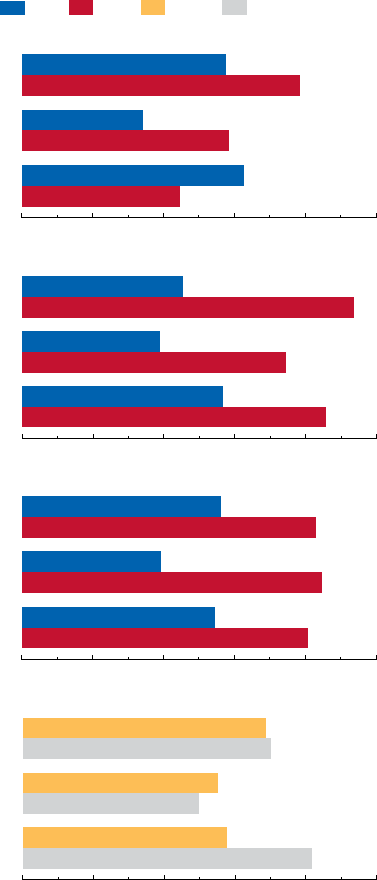
179
the effect is consistently large and persistently
negative. This suggests that concerns about fiscal
sustainability may be dominating spending deci-
sions, even if current fiscal policy would tradi-
tionally be thought of as stimulatory.
23
Additional regressions were run that included
interaction terms of the fiscal impulse measure
and dummies indicating (1) high or low open-
ness to trade; (2) high or low levels of financial
development, as a measure of liquidity con-
straints; (3) fixed versus floating exchange rate
regimes; and (4) high or low current account
surpluses, as a measure of external sustainabil-
ity. Higher levels of trade openness and finan-
cial development yield higher multipliers, and
multipliers are higher under floating exchange
rate regimes. These results run contrary to
economic theory, suggesting that debt concerns
might dominate the effectiveness of fiscal policy.
Indeed, higher-than-average current account
balances (generally surpluses) tend to be associ-
ated with larger multipliers.
24
Finally, running
the baseline regression using two different time
subsamples yields a cautionary note: multipliers
have apparently been weaker in recent years.
25
The evidence from this analysis indicates that
discretionary fiscal policy can successfully stimu-
late output growth, especially if it is revenue-
based. But there are reasons for caution in
employing stimulus packages during downturns,
with evidence suggesting that, if it is to work at
all, it will do so only when underlying fiscal posi-
tions are sound. This indicates that governments
need to improve balances during upturns and
make credible commitments that stimulus pack-
ages will not threaten debt sustainability.
23
The effects of both fiscal stimulus and fiscal tighten-
ing are much worse when controlling for severe down-
turns. See Appendix 5.1 for more details.
24
In the medium term, the multipliers are positive
when using the regression-based fiscal impulse measure
but still negative when using the elasticity-based fiscal
impulse measure.
25
This is particularly true for advanced economies. One
potential explanation, consistent with both the empiri-
cal evidence and the simulations presented later, is that
monetary policy has become less accommodative in those
economies.
a simulation-based PersPective on Fiscal stimulus
Figure 5.9. Changes in Real GDP Growth and Fiscal
Policies under Various Initial Conditions
The bar charts indicate changes in real GDP growth from year of downturn to first
year after downturn, differentiated by macroeconomic conditions three years before
the downturn (debt, current account, openness to trade, and money growth) and by
the exchange rate regime and composition of fiscal impulse in the year of downturn.
Source: IMF staff calculations.
The threshold for high debt is 75 percent for advanced economies and 25 percent for
emerging economies. The thresholds for current account balance and trade openness are
the median of the variable across the sample.
1
High Low FloatingFixed
1 1
0 1 2 3 4 5
Public debt
Current account balance
0 1 2 3 4 5
Openness to trade
Exchange rate
0 1 2 3 4 5
0 1 2 3 4 5
Fiscal stimulus
Neutral policy
Fiscal tightening
Fiscal stimulus
Neutral policy
Fiscal tightening
Fiscal stimulus
Neutral policy
Fiscal tightening
Fiscal stimulus
Neutral policy
Fiscal tightening

CHAPTER 5 Fiscal Policy as a countercyclical tool
180
A Simulation-Based Perspective on
Fiscal Stimulus
The previous section finds some evidence
for moderately positive multipliers, but with
important caveats about the type of economy,
the composition of the fiscal impulse, and the
level of debt. Clearly, there is a large number
of potentially important factors that policymak-
ers need to take into account when designing a
discretionary fiscal policy action. The objective
of this section is to examine, in a controlled
setting, how the effects of fiscal stimulus depend
on the structure of the economy in question.
The model used is an annual version of the
Global Integrated Monetary and Fiscal Model
(GIMF). GIMF is a multicountry dynamic sto-
chastic general equilibrium model that includes
a number of useful features relative to existing
monetary business cycle models (such as both
myopic and liquidity-constrained consumers
and potential long-term productivity benefits
from government investment) and a wide range
of fiscal instruments affecting household and
business intertemporal choices (government
investment, labor taxes, consumption taxes, and
transfers to households).
26
26
The country blocs are the United States, the euro
area, Japan, emerging Asia, and the remaining econo-
mies. For a more detailed description of the model, see
Kumhof and Laxton (2008).
The first exercise compares outcomes for key
macroeconomic variables using various fiscal
policy instruments for a large economy, cali-
brated to match the United States. The results
are presented in Figure 5.10. The shock is a
temporary fiscal expansion, calibrated to deliver
a primary deficit that is 1 percent above baseline
in year 1 and 0.5 percent above baseline in year
2. Thereafter, a fiscal reaction function ensures
that debt is brought back to its initial level by
raising lump-sum taxes. The fiscal stimulus is
completely unanticipated in the first year, but
its time profile, including the further stimulus
in year 2 and the longer-term implications for
taxes, is fully understood once initiated. Each
row of Figure 5.10 shows the reactions of, from
left to right, GDP (in percentage deviations
from the baseline), inflation and nominal inter-
est rates (in percentage point deviations from
baseline), and real interest rates (in percentage
point deviations from baseline). Going down
the figure, successive rows show the impact of
various fiscal instruments: government invest-
ment, consumption taxes, labor income taxes,
and transfers to households. In each panel, two
responses are shown: one in which nominal
interest rates are assumed to react to expected
deviations of inflation from target, and one in
which nominal interest rates are held constant
for the initial two years, thereby accommodating
the fiscal stimulus.
Table 5.3. Real GDP Growth and Fiscal Impulse by Composition: All Economies
1,2
Conditioning Variables
Number of
Observations
in Downturn
Three-Year
Average before
Downturn
One Year
before
Downturn
Year of
Downturn
Real GDP Growth
One Year
after
Downturn
Four-Year
Average after
Downturn
Fiscal stimulus
Revenue-based impulse 5 4.4 2.8 –0.7 3.6 4.1
Expenditure-based impulse 31 3.1 2.0 –0.4 2.9 3.0
Both expenditure and revenue
impulses 15 3.0 1.6 0.6 4.1 3.5
Fiscal tightening
Revenue-based impulse 31 2.4 2.3 –0.2 3.3 3.1
Expenditure-based impulse 17 2.8 3.2 1.2 5.0 4.3
Both expenditure and revenue
impulses 35 2.7 3.3 1.1 4.3 4.2
1
Fiscal impulse is identified during the first year of a downturn as a decline in the cyclically adjusted primary balance to GDP below
0.25 percentage point of GDP.
2
Initial conditions for variables are defined as a three-year average before the year of a downturn.

181
In each case, there are no long-run changes
in potential output; eventually, each of the
variables will return to zero.
27
Hence, the experi-
ment focuses on the differences in the short-run
impact of the policy measures. The results show
the following:
• For the same increase in deficit, there are
large differences in the size of short-run mul-
tipliers across instruments. On the assump-
tion that it can be implemented immediately
and efficiently, government investment has
a larger effect than other measures.
28
This
is because it has a direct effect on aggregate
demand, whereas the effects of taxes and
transfers depend on propensities to consume.
Investment also has the largest effect on infla-
tion and real interest rates.
27
This is also true for government investment, but in
this case the effect on output is much more long lived,
because government infrastructure capital has productive
benefits that depreciate only slowly over time.
28
This is in contrast to the empirical results, which
showed more positive effects from revenue-based stimu-
lus. In these simulations, private agents understand that
debt will be maintained at initial levels. In practice, it
could be that expenditure-based packages are more likely
to be made permanent and therefore raise concerns
about debt sustainability.
• The monetary policy regime plays a key role
in the effectiveness of fiscal stimulus—with
accommodation, the output multipliers
are up to twice as large, and the effects are
more persistent.
29
Concomitantly, inflation
is higher. The difference is least for labor
taxes, because lowering labor taxes increases
incentives for work as well as consumption. As
a result, a supply response mutes the inflation-
ary impact. It can also be shown that without
monetary accommodation, multipliers are
smaller when prices are more flexible.
30
This
is because inflation increases more strongly
following the stimulus, thereby necessitating
a more aggressive hike in interest rates that
reduces the output response. With monetary
accommodation, greater price flexibility has
the opposite effect, because higher inflation
implies a larger drop in real interest rates.
• Cuts in the consumption tax and temporar
-
ily higher household transfers have a clear
29
This is consistent with the view that fiscal policy could
be most effective when monetary policy is least effective,
such as when nominal interest rates are close to zero or
the monetary harmonization mechanism is imparied.
30
Simulations for different degrees of price flexibility
are not shown in Figure 5.7.
a simulation-based PersPective on Fiscal stimulus
Table 5.4. Responses of Real GDP to Discretionary Fiscal Policy Changes
Real GDP Response
Elasticity-based fiscal impulse measure Regression-based fiscal impulse measure
Effect in: Year zero Year three Year zero Year three
(with respect to positive fiscal impulse by 1 percentage point of GDP)
Baseline specification 0.15 –0.16 0.08 –0.02
Country differences
Advanced economies only 0.12 0.13 0.11 0.51
Emerging economies only 0.21 –0.03 0.10 –0.09
Composition
Revenue-based policy changes 0.21 0.12 0.10 0.14
Expenditure-based policy changes 0.13 –0.21 0.06 –0.06
Composition: advanced economies only
Revenue-based policy changes 0.35 0.59 0.01 0.40
Expenditure-based policy changes –0.09 –0.26 0.15 0.52
Composition: emerging economies only
Revenue-based policy changes 0.23 0.23 0.13 0.17
Expenditure-based policy changes 0.20 –0.18 0.08 –0.23
Downturns 0.29 0.00 0.10 0.04
Fiscal stimulus only –1.30 –0.88 –0.87 –0.29
Fiscal stimulus only, high initial debt –1.75 –2.05 –1.05 –0.80
Fiscal stimulus only, low initial debt –0.96 –0.36 –0.65 0.13
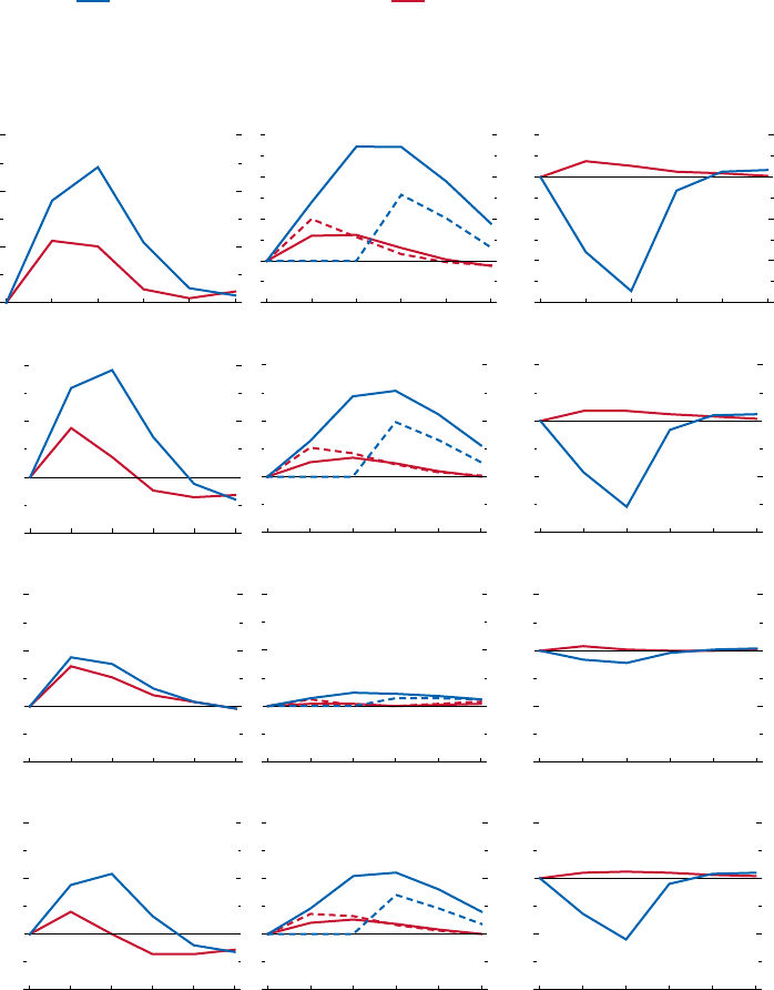
CHAPTER 5 Fiscal Policy as a countercyclical tool
182
0 1 2 3 4 5
-1
0
1
2
3
Source: IMF staff calculations.
Figure 5.10. Effect of Fiscal Expansion in a Large Economy
(Deviation from baseline; years on x-axis; shock occurs in year 0)
Impulse responses to 1 percent increase in deficit in year 1 and 0.5 percent increase in deficit in year 2.
0 1 2 3 4 5
-3
-2
-1
0
1
0 1 2 3 4 5
0
1
2
3
0 1 2 3 4 5
-1.0
-0.5
0.0
0.5
0 1 2 3 4 5
-0.25
0.00
0.25
0.50
0 1 2 3 4 5
-0.5
0.0
0.5
1.0
0 1 2 3 4 5
-0.25
0.00
0.25
0.50
0 1 2 3 4 5
-1.0
-0.5
0.0
0.5
0 1 2 3 4 5
-0.25
0.00
0.25
0.50
0 1 2 3 4 5
-1.0
-0.5
0.0
0.5
0 1 2 3 4 5
-0.5
0.0
0.5
1.0
0 1 2 3 4 5
-0.5
0.0
0.5
1.0
With monetary accommodation
Without monetary accommodation
GDP
(percent)
Inflation (solid) and
Nominal Interest Rate (dashed)
(percentage points)
Real Interest Rate
(percentage points)
Transfers
Government Investment
Consumption Taxes
Labor Taxes
183
“tilting” effect on output (output is above,
then below baseline), because they provide
incentives to bring forward consumption and
investment.
31
Cuts in labor taxes, on the other
hand, generate a more consistently positive
supply response.
If policy measures are made permanent and
financed by an increase in debt, then long-run
supply and debt effects become much more
important. For all fiscal instruments, higher debt
tends to crowd out private output because it
leads to higher real interest rates.
32
When there
is a permanent increase in transfers, regardless
of short-run monetary accommodation, the real
interest rate rises in the long run, which reduces
output or, at best, leaves it unchanged. Lower
tax rates, on the other hand, reduce supply
distortions, and therefore generate permanent
increases in output, more so when labor taxes
are lowered than when consumption taxes are
lowered. Making lower tax rates permanent
could raise the short-term impact, depending
on the balance between the positive supply-side
effect and negative interest rate effects. The
effects from permanently higher government
investment depend on whether the spending
can generate a higher rate of return than if the
resources were available to private investors.
How do the multipliers differ according to
the characteristics of the economy? Additional
simulations show the following:
• For any given size of fiscal stimulus, multi
-
pliers are lower in smaller and more open
economies—see Figure 5.11—although those
for labor taxes fall by less.
33
31
This is an example of a temporary fiscal policy
change that is effective because of forward-looking expec-
tations, showing that the “permanent income” criticism of
temporary policy measures does not always hold.
32
In small countries—that is, small enough that inter-
est rates are exogenous—this is still likely to happen.
The degree depends on changes in interest rate risk
premiums.
33
The empirical results in the previous section point to
the opposite result: multipliers are higher in smaller and
more open economies. This suggests that the measure
of openness used in the regressions is picking up other
effects not accounted for in these simulations.
• A higher share of liquidity-constrained con-
sumers, as might be expected in most emerg-
ing economies, results in significantly larger
multipliers.
• At the same time, fiscal stimulus may lead, in
high-debt emerging economies, to an increase
in real interest rates as market participants
demand a higher interest rate risk premium.
This reduces output multipliers, especially
for revenue-based measures, as shown in
Figure 5.12
. If the increase in interest rate
risk premiums is large enough, the multipli-
ers are negative. It is possible that this is the
mechanism driving the negative results of
fiscal stimulus seen from the empirical work
in Table 5.4.
These results indicate that the effects of fiscal
stimulus are likely to vary considerably, depend-
ing on how the stimulus is implemented and on
the type of economy. The results support the
idea that the degree of monetary policy accom-
modation is important, which may have played
a role in the smaller estimates of fiscal multipli-
ers in recent years. This is not to say that fiscal
policy cannot work; rather, it is likely to be most
effective when monetary policy is constrained
and ineffective (see also Blinder, 2006). The
results also illustrate a potentially important
mechanism by which concerns about public
debt sustainability could lower fiscal multipliers
to a point at which discretionary fiscal policy
would do more harm than good.
Conclusions and Policy Considerations
This chapter addresses a simple question:
What are the effects of fiscal policy during
downturns? The analysis indicates that the
answer is complicated and highly dependent on
an economy’s characteristics.
One obvious appeal of discretionary fiscal
policy is that governments can potentially have
a quick effect on spending power, whereas the
effects of monetary policy are subject to long
and sometimes uncertain lags. And in practice,
the policy record in advanced economies shows
that discretionary fiscal policy has been used
a simulation-based PersPective on Fiscal stimulus
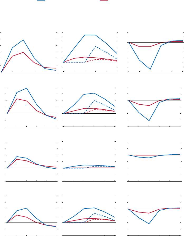
CHAPTER 5 Fiscal Policy as a countercyclical tool
184
0 1 2 3 4 5
-1
0
1
2
3
Source: IMF staff calculations.
Figure 5.11. Fiscal Expansion in a Large Economy Compared with a Small Open
Economy with Monetary Accommodation
(Deviation from baseline; years on x-axis; shock occurs in year 0)
Impulse responses to 1 percent increase in deficit in year 1 and 0.5 percent increase in deficit in year 2.
0 1 2 3 4 5
-3
-2
-1
0
1
0 1 2 3 4 5
0
1
2
3
0 1 2 3 4 5
-1.0
-0.5
0.0
0.5
0 1 2 3 4 5
-0.25
0.00
0.25
0.50
0 1 2 3 4 5
-0.5
0.0
0.5
1.0
0 1 2 3 4 5
-0.25
0.00
0.25
0.50
0 1 2 3 4 5
-1.0
-0.5
0.0
0.5
0 1 2 3 4 5
-0.25
0.00
0.25
0.50
0 1 2 3 4 5
-1.0
-0.5
0.0
0.5
0 1 2 3 4 5
-0.5
0.0
0.5
1.0
0 1 2 3 4 5
-0.5
0.0
0.5
1.0
Large economy
Small open economy
GDP
(percent)
Inflation (solid) and
Nominal Interest Rate (dashed)
(percentage points)
Real Interest Rate
(percentage points)
Transfers
Government Investment
Consumption Taxes
Labor Taxes
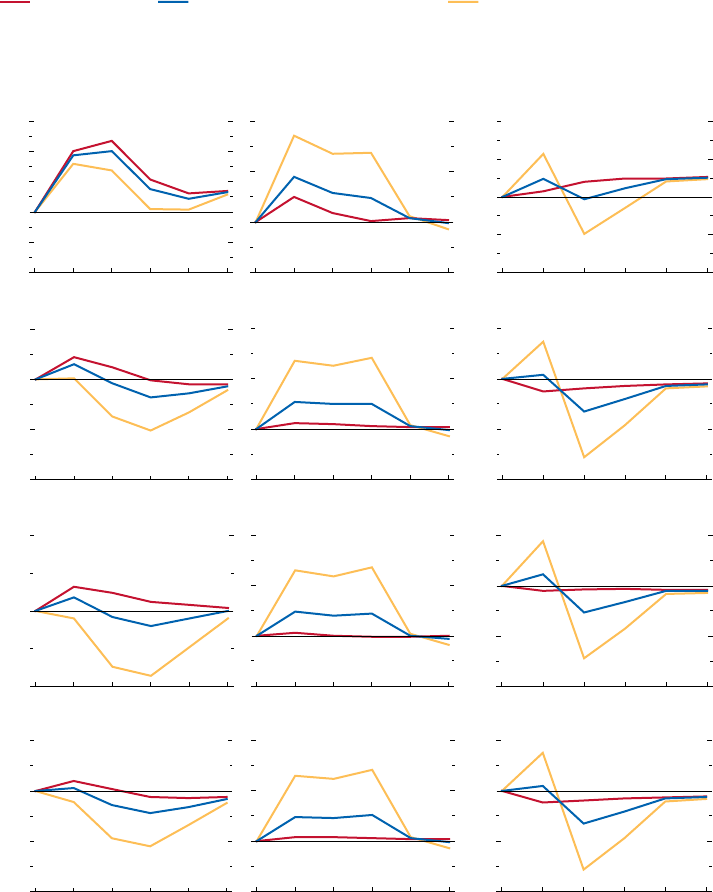
185
0 1 2 3 4 5
-0.5
0.0
0.5
1.0
Source: IMF staff calculations.
Figure 5.12. Effect of Fiscal Expansion in a Small Economy with Market-Risk-Premium
Reaction
(Deviation from baseline; years on x-axis; shock occurs in year 0)
Impulse responses to 1 percent increase in deficit in year 1 and 0.5 percent increase in year 2.
0 1 2 3 4 5
-2
-1
0
1
2
0 1 2 3 4 5
-1.0
-0.5
0.0
0.5
1.0
1.5
0 1 2 3 4 5
-2
-1
0
1
0 1 2 3 4 5
-1.0
-0.5
0.0
0.5
0 1 2 3 4 5
-0.5
0.0
0.5
1.0
0 1 2 3 4 5
-0.5
0.0
0.5
0 1 2 3 4 5
-2
-1
0
1
0 1 2 3 4 5
-1.0
-0.5
0.0
0.5
0 1 2 3 4 5
-2
-1
0
1
0 1 2 3 4 5
-0.5
0.0
0.5
1.0
0 1 2 3 4 5
-0.5
0.0
0.5
1.0
GDP
(percent)
Inflation
(percentage points)
Real Interest Rate
(percentage points)
Transfers
Government Investment
Consumption Taxes
Labor Taxes
Fiscal expansion
Fiscal expansion with small market reaction Fiscal expansion with large market reaction
conclusions and Policy considerations
CHAPTER 5 Fiscal Policy as a countercyclical tool
186
actively, although not nearly as much as auto-
matic stabilizers or monetary policy. However,
discretionary measures have typically been
implemented later than automatic stabilizers
and changes in monetary stance; they are more
often a response to downturns than upturns,
sometimes more than necessary; and stimulus
measures have often been made permanent,
which has had adverse implications for fiscal
sustainability.
An examination of the average effects of
discretionary fiscal policy across a combined
sample of advanced and emerging economies
does not provide strong evidence of counter-
cyclical effects on activity. However, a closer
analysis suggests that the effects are moderately
countercyclical in advanced economies. By
contrast, there is only weak evidence for coun-
tercylical effects in emerging economies, and
only initially, with indications that effects turn
negative in subsequent years. Revenue-based
stimulus measures seem to be more effective
at boosting output than expenditure-based
measures, especially in emerging economies,
perhaps reflecting concerns that, once imple-
mented, increased expenditures are difficult
to remove.
These empirical findings are broadly con-
sistent with simulations from a multiperiod
general equilibrium model. The simulations
show how the fiscal multiplier can vary from
Keynesian (1 or greater) to negative, depend
-
ing on the instrument used and the type of
economy. In particular, the multiplier is lower
when monetary reaction does not accommodate
the fiscal stimulus and when there is a strong
increase in risk premiums following fiscal stimu-
lus (such as when concerns about servicing
debt obligations are high). Increased govern-
ment spending can be the most direct means
of increasing output, if it can be implemented
quickly. On the other hand, it is the most
inflationary. Tax changes that provide greater
rewards for work effort or incentives for bring-
ing consumption forward might be nearly as
effective in supporting economic activity, with
less risk of inflation.
Given both the interest in fiscal policy as a
countercyclical tool and the evidence that discre-
tionary fiscal stimulus can have adverse effects,
should governments rely more on automatic
stabilizers? Or is it possible to design alternative
countercyclical fiscal policy mechanisms that
would respond symmetrically and more quickly
to changes in the state of economy?
34
There are two broad possibilities, each with its
advantages and disadvantages.
Increasing the responsiveness of automatic stabiliz-
ers: The extent of passive automatic stabilizers
could be augmented, for example, by increas-
ing the progressivity of the revenue system.
Such mechanisms would work automatically
and would not necessarily increase the size
of government. A related approach would be
to change certain tax, transfer, or spending
programs to introduce links to the state of
the economy following simple rules, akin to
the Taylor rule for setting interest rates. This
could be done by implementing pre-approved
temporary spending programs or raising
unemployment insurance benefits once the
unemployment rate reaches a certain threshold.
An advantage of such an approach would be its
transparency.
However, such schemes could also bring
unintended consequences that would need
to be weighed against possible stabilization
benefits. A system of temporary consumption
tax changes could lead to self-fulfilling falls in
current consumption if tax cuts were antici-
pated. Proposals that call for automatic triggers
in response to cyclical developments are also
problematic because there are no completely
reliable real-time measures of the state of the
economy. Responses based on previous periods’
outcomes—such as an automatic tax rebate—
could be more accurate and less distortionary
but might not be as well targeted as those that
34
This idea goes back at least to Musgrave (1959, p.
512), who coined the phrase “formula flexibility” to
describe a system in which changes in taxes and/or
expenditures would be legislated in advance to respond
to changes in income. More recently, versions have been
advocated in Seidman (2003).

187
are based on current income. It might also be
difficult to develop predetermined state-contin-
gent spending programs that are a well-targeted
and efficient use of public money (Solow, 2005).
Furthermore, all of the above could introduce
distortions: schemes to increase tax progressiv-
ity or tie unemployment insurance generosity to
the state of the economy would likely alter work
incentives, and might prove politically difficult
to adhere to during upturns. Thus, they would
have to flanked with measures to improve the
targeting of support during downturns. Better
targeting, however, is likely to pose administra-
tive challenges that could prove expensive to
address.
Changes in fiscal policy governance: Broader
reforms could bolster the credibility of discre-
tionary policy actions, in particular, to reduce
the risk of debt bias. This might involve estab-
lishing an independent, nonpartisan govern-
ment agency, such as already exist in many
countries—a sort of “fiscal watchdog”—charged
with identifying changes in the cyclical state of
the economy, assessing the extent to which fiscal
policy is consistent with medium-term objectives,
and providing advice on various policy mea-
sures.
35
This would minimize partisan judgment
in the evaluation of economic information and
would avoid relying solely on statistical mea-
sures of the state of the economy, which can be
imprecise. In addition, this arrangement could
increase the timeliness and temporariness of
the fiscal impulse. Such agencies could also be
entrusted with giving advice on which tax and
expenditure parameters to vary, as they indeed
already do in a number of countries.
36
35
For example, the objective of the Swedish Fiscal
Policy Council is to provide an independent evaluation of
the Swedish government’s fiscal policy, including whether
fiscal policy is consistent with the state of the economy in
the business cycle.
36
Some have even proposed that governments del-
egate limited fiscal responsibility to these nonpartisan
agencies, for exclusive use in macroeconomic stabiliza-
tion (see Ball, 1997, and Calmfors, 2003). Under exist-
ing proposals, such agencies could vary certain tax or
expenditure parameters, within certain limits set out by
the legislative branch and on the basis of a narrow stabi-
Clearly, a careful examination of the poten-
tial costs and risks of such systems would
be required before implementing any such
approaches. In addition to the choice of fiscal
instruments and the administrative complexities
of changing tax rates or expenditure plans, the
system would have to be coordinated with mone-
tary policy goals (see Taylor, 2000). Nonetheless,
given the limitations of automatic stabilizers as
currently implemented and the risks associated
with discretionary fiscal policy, the idea deserves
further examination.
Appendix 5.1. Data and Empirical
Methods
Evidence on the Responsiveness of Fiscal Policy
Quarterly data on the output gap and real
GDP growth are taken from the OECD Economic
Outlook, and are seasonally adjusted. Downturns
are defined as quarters in which growth is either
negative or below potential, with the output gap
more than one standard deviation below zero.
Changes in monetary policy are proxied by the
quarterly change in the nominal short-term
interest rate taken from the IMF’s International
Financial Statistics database. All changes are
quarter-over-quarter and unannualized. The
analysis focuses on “large” changes in discretion-
ary fiscal variables, defined as those that exceed
0.25 percent of GDP a quarter. Similarly, discre
-
tionary changes in nominal short-term interest
rates are defined as those that exceed 0.25 per
-
cent in one quarter.
The vector autoregression (VAR) is estimated
for each country using quarterly data. The vari-
ables included in the VARs, and their ordering,
are as follows: actual real GDP growth minus
potential real GDP growth, inflation (based
lization mandate supplemented by strict accountability
requirements. A weakness of such proposals is they pres-
ent a challenge regarding the role of government and
they make it dificult to establish a dividing line between
the agency and government in terms of countercyclical
fiscal policy (see Debrun, Hauner, and Kumar, 2008, for
a detailed survey).
aPPendix 5.1. data and emPirical methods
CHAPTER 5 Fiscal Policy as a countercyclical tool
188
on the GDP deflator), changes in the nominal
interest rate, changes in the primary cyclically
adjusted fiscal balance, and changes in the
automatic (cyclical) fiscal balance. This order-
ing implies that although policy variables can
respond to growth and inflation shocks within
one quarter, the transmission lag from policy
variables to growth and inflation is at least one
quarter. Two lags of each variable are included
in the VAR.
Data Uncertainties and the Risk of Debt Bias
For the purposes of testing for asymmetric
responses, each VAR now includes the follow-
ing variables: growth when the economy is in a
downturn and zero otherwise; growth when the
economy is in an upturn and zero otherwise;
and the previously included variables, that is,
inflation, changes in nominal interest rates, and
changes in fiscal balances. As before, downturns
are defined as quarters in which growth is either
negative or below potential, with the output gap
more than one standard deviation below zero.
The results are robust to changing the order-
ing of the two halves of growth (downturns and
upturns) in the VAR, to alternative ordering
for the fiscal and monetary policy variables,
and to including a time trend in each equation.
Because the VAR is specified in first differences,
any trend in fiscal balances over the sample
period affects the constant term in the fiscal bal-
ance equation.
For the purposes of testing the reliability of
preliminary GDP estimates, the analysis updates
the estimates of Faust, Rogers, and Wright
(2005), which used data ending in 1997. Revi
-
sions are defined as the difference between the
data as they stood in the most recent OECD
Monthly Economic Indicators (June 2008) and
the data when they were first published in the
Monthly Economic Indicators. For the United
States, the United Kingdom, and Canada,
preliminary data are available beginning
in 1965:Q1. For Japan, the starting date is 1970:
Q1; for Italy and Germany, 1979:Q4; and for
France, 1987:Q4.
For the purposes of evaluating the effect
of growth estimation errors, each VAR now
includes the preliminary estimation errors in
addition to the previously included variables.
The estimation errors are ordered in the
VARs after growth and inflation but before the
policy variables. The results are robust to alter-
native ordering among the errors and policy
variables.
Policy Reactions in Emerging and Advanced
Economies
The analysis uses a sample of 21 advanced
economies and 20 emerging economies from
the IMF’s World Economic Outlook (WEO)
database, covering the period from 1970
to 2007.
37
The sample includes annual data for
general government revenues and expenditures
(net of interest payments). Other macroeco-
nomic data (for example, for external balances
and inflation) are sourced from the World
Bank’s World Development Indicators database,
the WEO database, and other public sources.
The list of economies and episodes of down
-
turn is in Table 5.5 (with years of fiscal stimu-
lus in bold).
In addition to the WEO data, an examina-
tion was made using the IMF’s Government
Finance Statistics Manual (GFS) data. One
advantage of this data set is that it offers
greater disaggregation—revenues can be bro-
ken down into personal, corporate, consump-
tion, and trade. Taxes and expenditures can be
broken down into household, nonprofit institu-
tion, and corporate transfers (subsidies); inter-
est; government employee wages; and other
expenditures as well as capital spending. More-
disaggregated data potentially allow for finer
distinctions regarding the income elasticities
of taxes and spending and therefore a more
accurate measure of automatic versus cyclical
adjustments in revenues and expenditures.
Extensive comparisons were made between
37
Owing to data limitations, India was dropped from
the sample used for regressions.

189
WEO and GFS data for the same selection of
countries. Two major problems arose. First, to
create a sufficiently long time series, various
GFS vintages needed to be spliced together,
leading to situations in which the components
listed above jumped at the splice points, appar-
ently simply because of reclassifications. This
led to spurious measures of fiscal impulses,
taking away the theoretical advantage of using
these data. Second, long time series of GFS
data are available only for central govern-
ment. This can present a deceptive picture of
changes in fiscal policy. For example, estimates
of fiscal impulses at the central level of govern-
ment were found to be countercyclical (with
the output cycle) for all countries. This finding
deserves more investigation, but is outside the
scope of this study.
Fiscal Impulse Measures
The elasticity-based fiscal impulse measure
used for the stylized facts, event analysis, and
regressions is a cyclically adjusted primary bal-
ance, calculated as
Y
t
real
capb
t
= r
t
– e
t
P
————,
Y
t
tr–real
where r
t
is the revenue-to-GDP ratio in period t,
e
t
P
is the primary expenditure-to-GDP ratio in
period t, and Y
t
real
/Y
t
tr–real
is real output divided
by potential (trend) output in period t. These
estimates of the cyclically adjusted balance
rely on output gap estimates derived using a
time-series filter, which may not work well when
supply shocks are frequent and large, as for
many emerging economies. Applying the same
elasticities across economies (as assumed for
emerging economies), where one has a low elas-
ticity of taxes to output and another has a high
elasticity of taxes to output could lead to results
implying that the former uses discretionary
fiscal policy more actively than the latter,
whereas in fact the cause is stronger automatic
stabilizers.
The regression-based fiscal impulse measure
used for the regressions is constructed as the
Table 5.5. List of Countries and Downturn
Episodes
Country Years in Downturn
Argentina 1975, 1976, 1978, 1981, 1982, 1985, 1988,
1989, 1990, 1995, 1999, 2000, 2001, 2002
Australia
1972, 1978, 1982, 1983, 1991, 1992
Austria
1975, 1978, 1981, 1988, 1997
Belgium
1975, 1977, 1987, 1993, 2003
Brazil 1970, 1981, 1983, 1990, 1992
Canada
1975, 1982, 1991, 1992
Chile
1972, 1973, 1975, 1982, 1983, 1999
China 1976, 1990, 1991
Colombia
1976, 1977, 1983, 1985, 1991, 1992, 1999
Czech Republic
1990, 1991, 1992, 1997, 1998
Denmark
1974, 1975, 1980, 1981, 1983, 1988, 1993,
2003
Egypt 1973, 1974, 1981
Finland
1977, 1978, 1991, 1992, 1993
France
1975, 1986, 1987, 1993, 1997
Germany
1975, 1982, 1989, 1990, 1993, 2003
Greece 1974, 1981, 1982, 1983, 1987, 1993
Hungary
1985, 1988, 1990, 1991
Iceland
1975, 1976, 1983, 1985, 1988, 1991, 1992,
2003
India 1972, 1974, 1979, 1980, 1987, 2002
Indonesia 1998
Ireland 1975, 1976, 1983, 1993, 1994
Italy
1972, 1975, 1980, 1983, 1993, 2003
Japan
1974, 1975, 1987, 1994, 1998, 1999
Malaysia
1971, 1975, 1985, 1986, 1987, 1998
Mexico 1977, 1982, 1983, 1986, 1988, 1995, 2001
Netherlands
1975, 1980, 1981, 1982, 1993, 2003, 2005
New Zealand
1972, 1976, 1977, 1979, 1983, 1991, 1992,
1998
Pakistan 1970, 1972, 2002, 2003
Poland
1980, 1981, 1982, 1984, 1990, 1991
Portugal
1975, 1984, 1985, 1986, 1993, 2003
Romania
1975, 1985, 1988, 1989, 1990, 1991, 1992,
1997, 1998, 1999
Slovak Republic 1990, 1991, 1992, 1993
Slovenia 1976, 1983, 1987, 1988, 1990, 1991, 1992
South Africa
1977, 1978, 1982, 1983, 1985, 1986, 1990,
1991, 1992
Spain
1971, 1981, 1985, 1986, 1993
Sweden
1977, 1981, 1983, 1991, 1992, 1993, 2003
Switzerland
1975, 1976, 1978, 1982, 1983, 1991, 1993,
2003
Turkey 1973, 1979, 1980, 1989, 1994, 1999, 2001
Ukraine 1987, 1990, 1991, 1992, 1993, 1994, 1996,
1997, 1998, 1999
United Kingdom
1971, 1974, 1975, 1980, 1981, 1991, 1992
United States
1970, 1974, 1975, 1980, 1982, 1991
1
Years in bold correspond to use of a fiscal stimulus in a
downturn, with fiscal stimulus defined as a decline in the cyclically
adjusted primary balance to GDP below 0.25 percentage point of
GDP.
aPPendix 5.1. data and emPirical methods
CHAPTER 5 Fiscal Policy as a countercyclical tool
190
difference between a hypothetical primary
deficit in period t assuming no changes in the
economic environment and the actual primary
deficit in period t–1. As a first step, note that
the actual primary balance in period t can be
expressed as a function of the discretionary
policies, P
t
, and the economic environment
prevailing in that period, E
t
:
B
t
= B(P
t
,E
t
).
The change in the primary balance with respect
to the previous year can then be decomposed as
follows:
DB
t
= B(P
t
, E
t
) – B(P
t–1
, E
t–1
)
= [B(P
t
, E
t
) – B(P
t
, E
t–1
)] + [B(P
t
, E
t–1
)
–
B(P
t–1
, E
t–1
)]
= DB
t
E
+ DB
t
P
.
The term B(P
t
, E
t–1
) captures what the primary
balance would have been under the period
t policies, assuming the economic environ-
ment was the same as in period t–1. It is then
possible to break the change in the balance
into two elements. The first element,
DB
t
E
,
represents the fiscal effects of changes in the
economic environment from
E
t–1
to E
t
. The
second element,
DB
t
P
, captures the change in
the balance as a result of changes in discretion-
ary policies.
In practice, the initial step for calculating the
regression-based measure of fiscal impulse is to
estimate the following equations, assuming real
GDP growth is a good proxy for the economic
environment:
R
t
= a
R
+ b
R
· growth
t
+ g
R
· trend
t
+ u
t
G
t
= a
E
+ b
E
· growth
t
+ g
E
· trend
t
+ e
t
,
where R is general government revenue in per-
cent of GDP, G is general government primary
expenditure in percent of GDP, growth is real
GDP growth, trend is a time trend, and u and
e are residuals. The growth-adjusted revenue,
which indicates what the revenue would have
been in period t if the growth rate remained
unchanged from the previous period, is com-
puted as R
t
(growth
t–1
) = a
ˆ
R
+ b
ˆ
R
· growth
t–1
+
g
ˆ
R
· trend
t
+ uˆ
t
. The growth-adjusted primary
expenditure is computed in the same way, as
G
t
(growth
t–1
) = a
ˆ
E
+ b
ˆ
E
· growth
t–1
+ g
ˆ
E
· trend
t
+ eˆ
t
.
The measure for the primary balance that would
have prevailed in period t if the growth rate had
been equal to that in period t – 1, B(P
t
, E
t–1
),
can then be calculated as
R
t
(growth
t--1
) –
E
t
(growth
t–1
). The actual primary balance in the
previous period, B(P
t–1
, E
t–1
), is simply R
t–1
– G
t–1
.
The final step in the construction of the fis-
cal impulse measure is to take the difference
between the growth-adjusted measure for the
primary balance in period t and the primary bal-
ance in the previous period:
Fiscal impulse
t
= [R
t
(growth
t–1
) – G
t
(growth
t–1
)]
– [
R
t–1
– G
t–1
]
= (g
ˆ
R
– g
ˆ
E
) + (u
ˆ
t
– u
ˆ
t–1
)
– (
e
ˆ
t
– e
ˆ
t–1
).
Note that although uˆ
t
and eˆ
t
can be expected
to be uncorrelated with y
t
, uˆ
t–1
and eˆ
t–1
are cor-
related with y
t
.
Regression Analysis
Dynamic panel regressions were run using the
Arellano-Bond estimator.
38
The multipliers presented in Table 5.4
are derived from regression results shown
in Table 5.6 (using the elasticity-based fiscal
impulse measure) and Table 5.7 (using the
regression-based fiscal impulse measure). Note
that, because it is based on the primary balance,
a negative change in the regression-based mea-
sure represents fiscal stimulus, so that a negative
coefficient indicates that fiscal stimulus typically
has a positive effect on real GDP growth. A posi-
tive coefficient on the expenditures-only fiscal
impulse or a negative coefficient on the rev-
enue-only fiscal impulse indicate positive effects
on growth.
38
Experiments were also run with single-equation
regressions for individual economies. In most cases,
the results were insignificant, indicating that there
was insufficient variation in the short time samples to
adequately differentiate the effects of fiscal stimulus on
output growth.

191
Table 5.6. Discretionary Fiscal Policy and Growth: Regression Results with Arellano-Bond Dynamic
Panel Estimator Using Elasticity-Based Fiscal Impulse Measure
1
aPPendix 5.1. data and emPirical methods
Right-Hand-Side Variables
Baseline
Specification
Country
Differences,
Advanced
Economies
Country
Differences,
Emerging
Economies Downturns Components
Components,
Advanced
Economies
Components,
Emerging
Economies
Real GDP growth
Lag1 0.36 0.53 0.33 0.42 0.37 0.53 0.31
(4.18) (8.11) (3.11) (7.21) (4.08) (8.52) (2.87)
Lag2 –0.01 –0.04 0.06 0.11 0.02 –0.04 0.08
(–0.15) (–0.85) (1.11) (2.83) (0.49) (–0.67) (1.47)
Changes in cyclically adjusted
primary balance (dCAPB)
–0.15 –0.12 –0.21 . . . . . . . . . . . .
(–1.93) (–1.89) (–2.51) . . . . . . . . . . . .
Lag1 0.14 0.01 0.13 . . . . . . . . . . . .
(3.03) (0.28) (2.01) . . . . . . . . . . . .
Lag2 0.13 0.05 0.12 . . . . . . . . . . . .
(3.78) (0.90) (3.44) . . . . . . . . . . . .
Changes in cyclically adjusted
primary expenditure
. . . . . . . . . . . . 0.13 –0.09 0.20
. . . . . . . . . . . . (1.34) (–0.83) (1.59)
Lag1 . . . . . . . . . . . . –0.16 0.00 –0.21
. . . . . . . . . . . . (–2.66) (0.13) (–2.39)
Changes in revenue . . . . . . . . . . . . –0.21 –0.35 –0.23
. . . . . . . . . . . . (–3.42) (–3.97) (–3.35)
Lag1 . . . . . . . . . . . . 0.05 0.02 0.03
. . . . . . . . . . . . (1.10) (0.29) (0.49)
Lag2 . . . . . . . . . . . . 0.10 0.02 0.06
. . . . . . . . . . . . (2.23) (0.32) (1.31)
Neutral dummy x positive
fiscal impulse x dCAPB
. . . . . . . . . –0.35 . . . . . . . . .
. . . . . . . . . (–2.84) . . . . . . . . .
Lag1 . . . . . . . . . –0.15 . . . . . . . . .
. . . . . . . . . (–1.45) . . . . . . . . .
Lag2 . . . . . . . . . 0.10 . . . . . . . . .
. . . . . . . . . (1.13) . . . . . . . . .
Neutral dummy x negative
fiscal impulse x dCAPB
. . . . . . . . . –0.06 . . . . . . . . .
. . . . . . . . . (–0.71) . . . . . . . . .
Lag1 . . . . . . . . . 0.19 . . . . . . . . .
. . . . . . . . . (1.82) . . . . . . . . .
Lag2
. . . . . . . . . 0.13 . . . . . . . . .
. . . . . . . . . (1.74) . . . . . . . . .
Downturn dummy x positive
fiscal impulse x high-debt
dummy x dCAPB
. . . . . . . . . 1.75 . . . . . . . . .
. . . . . . . . . (2.36) . . . . . . . . .
Lag1 . . . . . . . . . –0.30 . . . . . . . . .
. . . . . . . . . (–0.54) . . . . . . . . .
Lag2 . . . . . . . . . –0.51 . . . . . . . . .
. . . . . . . . . (–0.98) . . . . . . . . .
Downturn dummy x positive
fiscal impulse x low-debt
dummy x dCAPB
. . . . . . . . . 0.96 . . . . . . . . .
. . . . . . . . . (3.59) . . . . . . . . .
Lag1 . . . . . . . . . –0.50 . . . . . . . . .
. . . . . . . . . (–3.60) . . . . . . . . .
Lag2 . . . . . . . . . –0.42 . . . . . . . . .
. . . . . . . . . (–2.19) . . . . . . . . .
Downturn dummy x negative
fiscal impulse x high-debt
dummy x dCAPB
. . . . . . . . . –0.44 . . . . . . . . .
(–2.05)
Lag1 0.44
(1.98)
Lag2 0.15
(1.59)

CHAPTER 5 Fiscal Policy as a countercyclical tool
192
Right-Hand-Side Variables
Baseline
Specification
Country
Differences,
Advanced
Economies
Country
Differences,
Emerging
Economies Downturns Components
Components,
Advanced
Economies
Components,
Emerging
Economies
Downturn dummy x negative
fiscal impulse x low-debt
dummy x dCAPB
. . . . . . . . . –0.52 . . . . . . . . .
. . . . . . . . . (–3.75) . . . . . . . . .
Lag1 . . . . . . . . . 0.50 . . . . . . . . .
. . . . . . . . . (2.39) . . . . . . . . .
Lag2 . . . . . . . . . 0.21 . . . . . . . . .
. . . . . . . . . (1.65) . . . . . . . . .
Deep downturn dummy x
positive fiscal impulse x
dCAPB
. . . . . . . . . 0.00 . . . . . . . . .
. . . . . . . . . (0.00) . . . . . . . . .
Lag1 . . . . . . . . . –0.80 . . . . . . . . .
. . . . . . . . . (–4.76) . . . . . . . . .
Lag2 . . . . . . . . . 0.84 . . . . . . . . .
. . . . . . . . . (4.00) . . . . . . . . .
Deep downturn dummy x
negative fiscal impulse x
dCAPB
. . . . . . . . . 0.28 . . . . . . . . .
. . . . . . . . . (1.53) . . . . . . . . .
Lag1 . . . . . . . . . 0.00 . . . . . . . . .
. . . . . . . . . (0.00) . . . . . . . . .
Lag2 . . . . . . . . . 0.57 . . . . . . . . .
. . . . . . . . . (3.63) . . . . . . . . .
Upturn dummy x positive
fiscal impulse x dCAPB
. . . . . . . . . –0.80 . . . . . . . . .
. . . . . . . . . (–4.76) . . . . . . . . .
Lag1 . . . . . . . . . 0.84 . . . . . . . . .
. . . . . . . . . (4.00) . . . . . . . . .
Lag2 . . . . . . . . . 0.28 . . . . . . . . .
. . . . . . . . . (1.53) . . . . . . . . .
Upturn dummy x negative
fiscal impulse x dCAPB
. . . . . . . . . 0.57 . . . . . . . . .
. . . . . . . . . (3.63) . . . . . . . . .
Lag1 . . . . . . . . . –0.86 . . . . . . . . .
. . . . . . . . . (–3.95) . . . . . . . . .
Lag2 . . . . . . . . . –0.57 . . . . . . . . .
. . . . . . . . . (–3.10) . . . . . . . . .
Real money growth 0.04 0.02 0.07 0.05 0.05 0.02 0.07
(1.67) (0.95) (2.16) (1.94) (1.96) (1.13) (2.16)
Lag1 0.02 0.01 0.03 –0.01 0.02 0.01 0.03
(0.91) (0.46) (1.02) (–0.46) (0.90) (1.35) (1.17)
Lag2 –0.02 0.00 –0.02 –0.02 –0.02 0.00 –0.02
(–1.30) (0.22) (–1.05) (–1.02) (–1.17) (–0.23) (–1.18)
Government size –0.03 –0.01 –0.04 –0.02 –0.03 –0.02 –0.04
(–1.97) (–0.99) (–1.56) (–2.16) (–1.88) (–1.55) (–1.45)
Trade-weighted growth of
trading partners
0.35 0.10 0.42 0.17 0.33 –0.01 0.44
(2.06) (0.71) (1.81) (1.37) (1.96) (–0.06) (1.77)
EMU dummy
2
–0.80 –0.13 . . . –0.67 –0.78 –0.12 . . .
(–2.35) (–0.50) . . . (–2.50) (–2.58) (–0.47) . . .
Number of observations 796 487 309 650 796 487 309
Number of countries 40 21 19 40 40 21 19
p-value for Sargan test of
overidentifying restrictions
0.000 0.000 0.003 0.000 0.000 0.011 0.002
p-value for Hansen test of
overidentifying restrictions
1.000 1.000 1.000 1.000 1.000 1.000 1.000
p-value for the test of
no-second-order serial
correlation
0.811 0.270 0.868 0.010 0.606 0.242 0.845
1
Dependent variable is real GDP growth. All regressions also included a set of time dummies.
2
EMU = European Monetary Union.
Table 5.6 (continued)

193
Table 5.7. Discretionary Fiscal Policy and Growth: Regression Results with Arellano-Bond Dynamic
Panel Estimator Using Regression-Based Fiscal Impulse Measure
1
Right-Hand-Side Variables Baseline
Country
Differences,
Advanced
Economies
Country
Differences,
Emerging
Economies Downturns Components
Components,
Advanced
Economies
Components,
Emerging
Economies
Real GDP growth
Lag1 0.37 0.54 0.30 0.43 0.38 0.56 0.29
(3.86) (8.09) (2.67) (7.10) (3.73) (7.58) (2.51)
Lag2 –0.03 –0.01 0.04 0.12 –0.03 –0.01 0.05
(–0.71) (–0.18) (0.83) (3.04) (–0.68) (–0.25) (0.86)
Changes in cyclically adjusted
primary balance (dCAPB)
–0.08 –0.11 –0.10 . . . . . . . . . …
(–1.18) (–1.81) (–1.50) . . . . . . . . . …
Lag1 0.04 –0.14 0.08 . . . . . . . . . …
(0.79) (–3.18) (1.25) . . . . . . . . . …
Lag2 0.06 –0.02 0.10 . . . . . . . . . …
(1.89) (–0.33) (2.00) . . . . . . . . . …
Changes in cyclically adjusted
primary expenditure
. . . . . . . . . . . . 0.06 0.15 0.08
. . . . . . . . . . . . (0.84) (2.27) (0.87)
Lag1 . . . . . . . . . . . . –0.05 0.13 –0.14
. . . . . . . . . . . . (–1.13) (2.89) (–1.78)
Lag2 . . . . . . . . . . . . –0.06 –0.01 –0.12
. . . . . . . . . . . . (–1.62) (–0.20) (–1.77)
Changes in revenue . . . . . . . . . . . . –0.10 –0.01 –0.13
. . . . . . . . . . . . (–1.87) (–0.17) (–1.90)
Lag1 . . . . . . . . . . . . –0.02 –0.13 –0.01
. . . . . . . . . . . . (–0.36) (–1.85) (–0.18)
Lag2 . . . . . . . . . . . . 0.03 –0.08 0.03
. . . . . . . . . . . . (0.97) (–1.29) (0.53)
Neutral dummy x positive
fiscal impulse x dCAPB
. . . . . . . . . –0.39 . . . . . . …
. . . . . . . . . (–3.15) . . . . . . …
Lag1 . . . . . . . . . –0.17 . . . . . . …
. . . . . . . . . (–2.43) . . . . . . …
Lag2 . . . . . . . . . 0.08 . . . . . . …
. . . . . . . . . (0.79) . . . . . . …
Neutral dummy x negative
fiscal impulse x dCAPB
. . . . . . . . . 0.07 . . . . . . …
. . . . . . . . . (0.51) . . . . . . …
Lag1 . . . . . . . . . 0.03 . . . . . . …
. . . . . . . . . (0.31) . . . . . . …
Lag2 . . . . . . . . . 0.19 . . . . . . …
. . . . . . . . . (2.28) . . . . . . …
Downturn dummy x positive
fiscal impulse x high debt
dummy x dCAPB
. . . . . . . . . 1.05 . . . . . . . . .
. . . . . . . . . (2.58) . . . . . . . . .
Lag1 . . . . . . . . . –0.37 . . . . . . . . .
. . . . . . . . . (–1.12) . . . . . . . . .
Lag2 . . . . . . . . . –0.38 . . . . . . . . .
. . . . . . . . . (–1.54) . . . . . . . . .
Downturn dummy x positive
fiscal impulse x low debt
dummy x dCAPB
. . . . . . . . . 0.65 . . . . . . . . .
. . . . . . . . . (4.87) . . . . . . . . .
Lag1 . . . . . . . . . –0.53 . . . . . . . . .
. . . . . . . . . (–5.50) . . . . . . . . .
Lag2 . . . . . . . . . –0.33 . . . . . . . . .
. . . . . . . . . (–2.52) . . . . . . . . .
aPPendix 5.1. data and emPirical methods

CHAPTER 5 Fiscal Policy as a countercyclical tool
194
Table 5.7 (concluded)
Right-Hand-Side Variables Baseline
Country
Differences,
Advanced
Economies
Country
Differences,
Emerging
Economies Downturns Components
Components,
Advanced
Economies
Components,
Emerging
Economies
Downturn dummy x negative
fiscal impulse x high debt
dummy x dCAPB
. . . . . . . . . –0.40 . . . . . . . . .
. . . . . . . . . (–1.93) . . . . . . . . .
Lag1 . . . . . . . . . 0.34 . . . . . . . . .
. . . . . . . . . (1.87) . . . . . . . . .
Lag2 . . . . . . . . . 0.14 . . . . . . . . .
. . . . . . . . . (1.29) . . . . . . . . .
Downturn dummy x negative
fiscal impulse x low debt
dummy x dCAPB
. . . . . . . . . –0.46 . . . . . . . . .
. . . . . . . . . (–3.24) . . . . . . . . .
Lag1 . . . . . . . . . 0.30 . . . . . . . . .
. . . . . . . . . (1.29) . . . . . . . . .
Lag2 . . . . . . . . . 0.21 . . . . . . . . .
. . . . . . . . . (1.69) . . . . . . . . .
Upturn dummy x positive
fiscal impulse x dCAPB
. . . . . . . . . –0.91 . . . . . . . . .
. . . . . . . . . (–4.59) . . . . . . . . .
Lag1 . . . . . . . . . 0.86 . . . . . . . . .
. . . . . . . . . (3.67) . . . . . . . . .
Lag2 . . . . . . . . . 0.19 . . . . . . . . .
. . . . . . . . . (0.84) . . . . . . . . .
Upturn dummy x negative
fiscal impulse x dCAPB
. . . . . . . . . 0.57 . . . . . . . . .
. . . . . . . . . (4.27) . . . . . . . . .
Lag1 . . . . . . . . . –0.91 . . . . . . . . .
. . . . . . . . . (–5.62) . . . . . . . . .
Lag2 . . . . . . . . . –0.37 . . . . . . . . .
. . . . . . . . . (–2.04) . . . . . . . . .
Real money growth 0.05 0.02 0.07 0.05 0.06 0.02 0.08
(1.92) (1.06) (2.41) (1.92) (2.19) (1.11) (2.65)
Lag1 0.01 0.01 0.03 –0.01 0.01 0.01 0.03
(0.83) (0.50) (1.03) (–0.43) (0.85) (0.50) (0.99)
Lag2 –0.02 0.00 –0.02 –0.02 –0.02 0.00 –0.02
(–1.37) (0.15) (–0.97) (–1.03) (–1.34) (0.27) (–0.94)
Government size –0.04 –0.01 –0.04 –0.02 –0.04 –0.01 –0.04
(–2.44) (–1.00) (–1.62) (–2.26) (–2.17) (–0.97) (–1.36)
Trade-weighted growth of
trading partners
0.34 0.08 0.40 0.16 0.35 0.08 0.43
(1.93) (0.60) (1.77) (1.29) (1.93) (0.54) (1.69)
EMU dummy –0.79 –0.19 –0.71 –0.82 –0.19 . . .
(–2.28) (–0.80) (–2.61) (–2.50) (–0.83) . . .
Number of observations 796 487 309 650 796 487 309
Number of countries 40 21 19 40 40 21 19
p-value for Sargan test of
overidentifying restrictions
0.000 0.000 0.001 0.000 0 0.004 0.003
p-value for Hansen test of
overidentifying restrictions
1.000 1.000 1.000 1.000 1.000 1.000 1.000
p-value for the test of no
second order serial
correlation
0.790 0.254 0.758 0.019 0.739 0.428 0.641
1
Dependent variable is real GDP growth. All regressions also included a set of time dummies.
195
References
Andrés, Javier, Rafael Doménech, and Antonio Fatás,
2008, “The Stabilizing Role of Government Size,”
Journal of Economic Dynamics and Control, Vol. 32
(February), pp. 571–93.
Balassone, Fabrizio, and Manmohan S. Kumar, 2007,
“Cyclicality of Fiscal Policy,” in Promoting Fiscal
Discipline
, ed. by Manmohan S. Kumar and Teresa
Ter-Minassian (Washington: International Monetary
Fund).
Ball, Laurence, 1997, “A Proposal for the Next Macro
-
economic Reform,” Victoria Economic Commentaries,
Vol. 14 (March), pp. 1–7.
Barro, Robert J., 1974, “Are Government Bonds
Net Wealth?” Journal of Political Economy, Vol. 82
(November–December), pp. 1095–1117.
Blanchard, Olivier, and Roberto Perotti, 2002, “An
Empirical Characterization of the Dynamic Effects
of Changes in Government Deficit and Taxes on
Output,” Quarterly Journal of Economics, Vol. 117
(November), pp. 1329–68.
Blinder, Alan S., 1981, “Temporary Income Taxes and
Consumer Spending,” Journal of Political Economy,
Vol. 89 (February), pp. 26–53.
———, 2006, “The Case Against the Case Against
Discretionary Fiscal Policy,” in The Macroeconomics
of Fiscal Policy, ed. by Richard W. Kopcke, Geoffrey
M.B. Tootell, and Robert K. Triest (Cambridge,
Massachusetts: The MIT Press).
Calmfors, Lars, 2003, “Fiscal Policy to Stablise the
Domestic Economy in the EMU: What Can We
Learn from Monetary Policy?” CESifo Economic Stud-
ies, Vol. 49, No. 3, pp. 319–53.
Chung, Hess, and Eric M. Leeper, 2007, “What Has
Financed Government Debt?” NBER Working
Paper No. 13425 (Cambridge, Massachusetts:
National Bureau of Economic Research).
Cimadomo, Jacopo, 2008, “Fiscal Policy in Real Time,”
ECB Working Paper No. 919 (Frankfurt am Main:
European Central Bank).
Congressional Budget Office (CBO), 2008, “Options
for Responding to Short-Term Economic Weak-
ness,” Congressional Budget Office Paper
(Washington).
Debrun, Xavier, David Hauner, and Manmohan S.
Kumar, 2008, “The Role for Fiscal Agencies,” in
The Quality of Public Finances: Findings of the Economic
Policy Committee-Working Group (2004–2007), ed. by
Servaas Deroose and Christian Kastrop, Occa-
sional Paper 37 (Brussels: Directorate-General
for Economic and Financial Affairs, European
Commission).
Edelberg, Wendy, Martin Eichenbaum, and Jonas
D.M. Fisher, 1999, “Understanding the Effects of
a Shock to Government Purchases,” Review of Eco-
nomic Dynamics, Vol. 2 (January), pp. 166–206.
Fatás, Antonio, and Ilian Mihov, 2001, “The Effects
of Fiscal Policy on Consumption and Employment:
Theory and Evidence,” CEPR Discussion Paper
No. 2760 (London: Centre for Economic Policy
Research).
Faust, Jon, John H. Rogers, and Jonathan Wright,
2005, “News and Noise in G-7 GDP Announce-
ments,” Journal of Money, Credit and Banking, Vol. 37
(June), pp. 403–19.
Favero, Carlo, and Francesco Giavazzi, 2007, “Debt
and the Effects of Fiscal Policy,” NBER Working
Paper No. 12822 (Cambridge, Massachusetts:
National Bureau of Economic Research).
Galí, Jordi, 1994, “Government Size and Macroeco-
nomic Stability,” European Economic Review, Vol. 38
(January), pp. 117–32.
———, 2006, “Fluctuating Macro Policies and the Fis-
cal Theory of the Price Level: Comment,” in NBER
Macroeconomic Annual 2006 (Cambridge, Massachu-
setts: MIT Press), pp. 299–305.
———, J. David López-Salido, and Javier Vallés,
2007, “Understanding the Effects of Government
Spending on Consumption,” Journal of the European
Economic Association, Vol. 5 (March) pp. 227–70.
Galí, Jordi, and Roberto Perotti, 2003, “Fiscal Policy
and Monetary Integration in Europe,” Economic
Policy, Vol. 37 (October), pp. 533–72.
Jaeger, Albert, and Ludger Schuknecht, 2007,
“Boom-Bust Phases in Asset Prices and Fiscal Policy
Behavior,” Emerging Markets Finance and Trade, Vol.
43 (November), pp. 45–66.
Johnson, David S., Jonathan A. Parker, and Nicholas
S. Souleles, 2006, “Household Expenditure and the
Income Tax Rebates of 2001,” American Economic
Review, Vol. 96 (December), pp. 1589–610.
Kaminsky, Graciela L., Carmen M. Reinhart, and
Carlos A. Végh, 2004, “When It Rains, It Pours:
Procyclical Capital Flows and Macroeconomic Poli-
cies,” NBER Working Paper No. 10780 (Cambridge,
Massachusetts: National Bureau of Economic
Research).
Krogstrup, Signe, 2002, “Should We Pay Attention
to Indicators of Fiscal Impact on Demand?” HEI
Working Paper No. 01/2002 (Geneva: Graduate
Institute of International Studies).
reFerences
CHAPTER 5 Fiscal Policy as a countercyclical tool
196
Kumhof, Michael, and Douglas Laxton, 2008, “The
Global Integrated Monetary Fiscal Model” (unpub-
lished; Washington: International Monetary Fund).
Leigh, Daniel, and Sven Jari Stehn, forthcoming,
“Fiscal and Monetary Policy during Downturns: Evi-
dence from the G7,” Working Paper (Washington:
International Monetary Fund).
Modigliani, Franco, and Charles Steindel, 1977, “Is
a Tax Rebate an Effective Tool for Stabilization
Policy?” Brookings Papers on Economic Activity: 1,
Brookings Institution, pp. 175–209.
Mountford, Andrew, and Harald Uhlig, 2002, “What
Are the Effects of Fiscal Policy Shocks?” CEPR
Discussion Paper No. 3338 (London: Centre for
Economic Policy Research).
Musgrave, Richard A., 1959, The Theory of Public
Finance: A Study in Public Economy (New York:
McGraw-Hill).
Organization for Economic Cooperation and Develop-
ment, Monthly Economic Indicators (Paris, various
issues).
Perotti, Roberto, 2007, “In Search of the Transmission
Mechanism of Fiscal Policy,” NBER Working Paper
No. 13143 (Cambridge, Massachusetts: National
Bureau of Economic Research).
Ramey, Valerie A., 2008, “Identifying Govern-
ment Spending Shocks: It’s All in the Timing”
(unpublished).
———, and Matthew D. Shapiro, 1998, “Costly Capital
Reallocation and the Effects of Government Spend-
ing,” Carnegie-Rochester Conference Series on Public
Policy, Vol. 48 (June), pp. 145–94.
Ravn, Morten O., and Harald Uhlig, 2002, “On Adjust-
ing the Hodrick-Prescott Filter for the Frequency of
Observations,” Review of Economics and Statistics, Vol.
84 (May), pp. 371–76.
Romer, Christina D., and David H. Romer, 2007,
“The Macroeconomic Effects of Tax Changes: Esti-
mates Based on a New Measure of Fiscal Shocks,”
NBER Working Paper No. 13264 (Cambridge,
Massachusetts: National Bureau of Economic
Research).
Seidman, Laurence S., 2003, Automatic Fiscal Poli-
cies to Combat Recessions (Armonk, New York: M.E.
Sharpe).
Shapiro, Matthew D., and Joel B. Slemrod, 2002, “Did
the 2001 Tax Rebate Stimulate Spending? Evidence
from Taxpayer Surveys,” NBER Working Paper No.
9308 (Cambridge, Massachusetts: National Bureau
of Economic Research).
Solow, Robert M., 2005, “Rethinking Fiscal Policy,”
Oxford Review of Economic Policy, Vol. 21 (Winter),
pp. 509–14.
Talvi, Ernesto, and Carlos A. Végh, 2000, “Tax Base
Variability and Procyclical Fiscal Policy,” NBER
Working Paper No. 7499 (Cambridge, Massachu-
setts: National Bureau of Economic Research).
Taylor, John B., 2000, “Reassessing Discretionary Fiscal
Policy,” Journal of Economic Perspectives, Vol. 14 (Sum-
mer), pp. 21–36.
