19
th
World Conference on Non-Destructive Testing 2016
1
License:
http://creativecommons.org/licenses/by-nd/3.0/
Ray Tracing Boundary Value Problems: Simulation
and SAFT Reconstruction for Ultrasonic Testing
Sebastian GÖTSCHEL
1
, Christian HÖHNE
2
, Sanjeevareddy KOLKOORI
2
,
Steffen MITZSCHERLING
2
, Jens PRAGER
2
, Martin WEISER
1
1
Konrad-Zuse-Zentrum für Informationstechnik Berlin (ZIB), Berlin, Germany
2
BAM Bundesanstalt für Materialforschung und -prüfung, Berlin, Germany
Contact e-mail: goetschel@zib.de
Abstract. The application of advanced imaging techniques for the ultrasonic
inspection of inhomogeneous anisotropic materials like austenitic and dissimilar
welds requires information about acoustic wave propagation through the material, in
particular travel times between two points in the material. Forward ray tracing is a
popular approach to determine traveling paths and arrival times but is ill suited for
inverse problems since a large number of rays have to be computed in order to arrive
at prescribed end points.
In this contribution we discuss boundary value problems for acoustic rays,
where the ray path between two given points is determined by solving the eikonal
equation. The implementation of such a two point boundary value ray tracer for
sound field simulations through an austenitic weld is described and its efficiency as
well as the obtained results are compared to those of a forward ray tracer. The
results are validated by comparison with experimental results and commercially
available UT simulation tools.
As an application, we discuss an implementation of the method for SAFT
(Synthetic Aperture Focusing Technique) reconstruction. The ray tracer calculates
the required travel time through the anisotropic columnar grain structure of the
austenitic weld. There, the formulation of ray tracing as a boundary value problem
allows a straightforward derivation of the ray path from a given transducer position
to any pixel in the reconstruction area and reduces the computational cost
considerably.
Introduction
Ultrasonic testing of inhomogeneous anisotropic materials, e.g., austenitic welds, has been
a subject of increasing interest in recent years [1-6]. A main difficulty in the application of
ultrasonic inspection techniques to anisotropic materials lies in the fact that in such
materials sound velocity and refraction index depend on the phase direction of an incident
wave, and phase direction and direction of energy propagation are no longer identical. This
can lead to effects like beam skewing, beam splitting, or focusing and defocusing of sound
fields [7, 8]. Inhomogeneous anisotropic media might consist of several homogeneous
layers of different anisotropic materials or, as is the case for austenitic welds [7], be a
structure with continuously varying anisotropic properties. In the latter case, ultrasonic
More info about this article: http://ndt.net/?id=19437

2
waves will no longer propagate in a straight line or even piecewise straight trajectory, but
along a curved path with varying sound velocity. Taking the aforementioned effects into
account is necessary when evaluating data acquired by ultrasonic inspections of such
materials.
The approach to use acoustic ray tracing to obtain information about
inhomogeneous anisotropic structures, namely austenitic welds, was mainly developed in
the 1980s. Basically, the comparison of simulated and measured travel times between a
transducer and a receiver is used for fitting a parametric model of anisotropies or material
defects. Since then, a variety of publications deal with different aspects of the method. One
feature common to most of the work is the use of forward propagation of rays,
mathematically speaking as initial value problems for ordinary differential equations. As
the ray paths and hence their end points are not known in advance, many rays have to be
computed in order to cover all receiver positions.
Here, we consider the formulation of the ray tracing problem as a two point
boundary value problem as is common in isotropic seismic inversion [9, 10]. As both start
and end point of the rays are prescribed, comparatively few boundary value problems need
to be solved.
1. Boundary Value Ray Tracing in Layered Media
1.1 Mathematical Model
In inhomogeneous anisotropic media, the ray tracing ordinary differential equations
(ODEs) are given as
Here,
are the density normalized elastic parameters, is 3D-position in Cartesian
coordinates, denotes the travel time of the wave under consideration, and is called
slowness vector. The eigenvectors of the Christoffel matrix
are denoted by
. Throughout the paper we use the Einstein summation convention for
brevity.
For many applications it is of special interest to find one specific ray, connecting a
sender and a receiver with known positions
, such that the initial slowness vector
is to be determined. Mathematically, this is a two-point boundary value problem consisting
of the ray tracing system above, together with boundary conditions
where
The unknown time when the ray reaches the receiver, can be handled by
transforming the system to a fixed time interval
instead of
and adding
one equation for the constant final time . For the required seventh boundary condition in
this formulation we choose to prescribe an initial magnitude of the slowness vector,
assuming the sender to be in an isotropic material with speed of sound .
In layered structures, like dissimilar welds, the elastic parameters
are
discontinuous at the material boundaries. When the ray arrives at such an interface,
refraction occurs, such that the slowness vectors of transmitted and reflected waves have to
be computed. Refraction into an isotropic medium can be easily handled by computing

3
where the interface normal is oriented against the incident wave, and denote the
refracted slowness vector and the wave speed of the generated refracted wave. The plus
sign corresponds to the transmitted wave, the minus sign gives the reflected wave. The
relation holds for any wave type (compressional or shear). For refraction into an anisotropic
medium the computations are more involved and require the solution of an algebraic
equation of sixth order. We do not repeat the details here but refer to the literature, e.g., [11,
12].
The formulation as an ODE-boundary value problem allows to incorporate
continuously varying elastic parameters without the need for an artificial discretization of
the weld into layers or cells.
1.2 Solution method
The solution of such system can be computed numerically using shooting or collocation
methods [13]. The simple single shooting aims at finding an initial value
such that
the corresponding solution of the initial value problem satisfies the terminal boundary
conditions. This is done by finding a zero of the–in general nonlinear–boundary condition
using Newton's method. The required derivatives can either be computed using the
variational equations derived from the initial value problem [14], or with finite differences.
As this information is required for amplitude computations as well, the computational
overhead for the shooting method is small.
1.3 Numerical Results
For testing the proposed method, as well as for SAFT reconstruction in Section 2, we
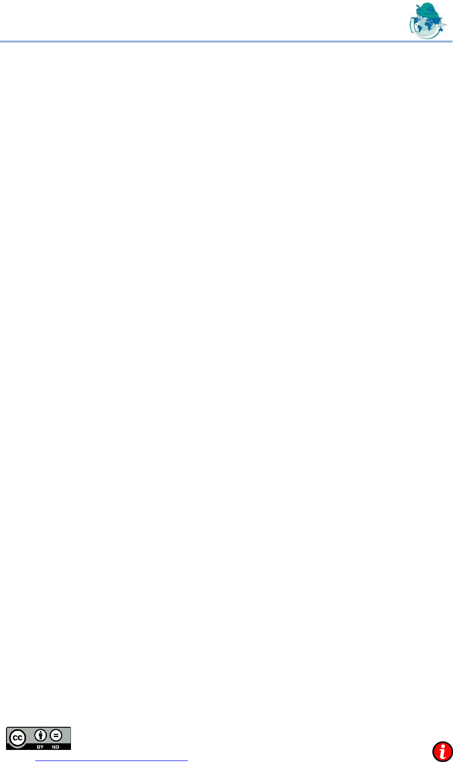
consider a specimen consisting of ferritic steel with an attached buffer, joined by a
dissimilar weld to a component of austenitic steel. On top of the object, a perspex layer is
added to account for the perspex wedge of the transducers used in the experiments. To
describe the crystal orientation in the weld, we use the Ogilvy model [15]. See Figure 1 for
a sketch. For the isotropic base materials, longitudinal sound velocities of 5619 m/s for
austenitic and 5935 m/s for ferritic steel were used. In the perspex zone, the sound velocity
was set to 2730 m/s. The elastic constants of weld and buffer material are (in GPa) given as
, with
density 7980 kg/m
3
. More details can be found in [6].
For the ODE formulation of the boundary value ray tracing, we use the continuously
varying crystal orientations directly. As a comparison, we also consider a layer model,
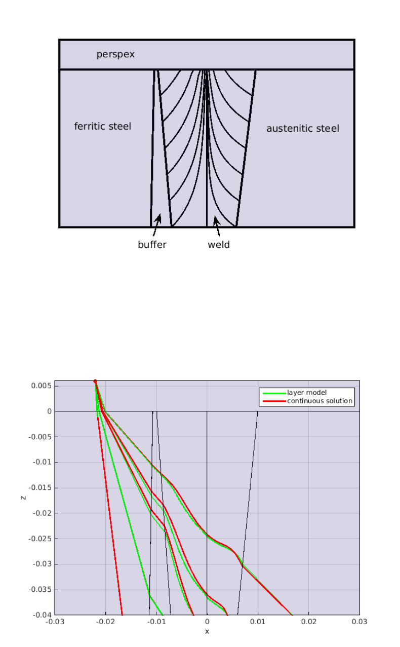
where the weld is discretized into layers of constant grain orientation. In Figure 2, we
exemplarily show five rays computed with the continuous ODE model and the layer model
in a cross section of the weld. Small differences are visible inside the weld, as expected.
Two of the plotted rays differ already inside the isotropic region and the buffer, which is
due so slightly differing paths in y-direction (along the weld, not plotted here). In Figure 3,
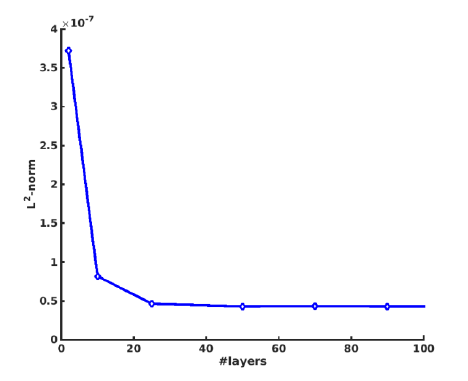
the
-norm of the difference of the -component (position) between the
continuous ODE solution and its approximation by the layered structure model with
increasing number of layers. With about 25 layers, the accuracy of the layer model matches
the prescribed tolerances of the ODE solver, with an average 0.1mm deviation between
of continuous and layer model.
4
Fig. 1. Sketch of the considered geometry. The height of the weld is 32mm with an additional 6mm perspex
layer. The buffer has a layback angle of 11° and a constant crystal orientation of 82°, the weld has a layback
angle of 8° and the crystal orientation given by the Ogilvy model with parameters
. The extension of the weld is 9.945 mm at the top and
(5.9825 mm, 7.17 mm) at the bottom, right and left of the weld center. The x-coordinates of the buffer are
10.7 mm left of the weld center at the top, and 11.39 mm at the bottom.
Fig. 2. Comparison of boundary value ray tracing using a layer model (green) and a continuous model for the
for the grain orientation (red) along a cross section of the specimen. As expected, small differences between
the layer model and the ODE solution are visible inside the weld.
5
Fig. 3. L
2
-norm of the difference between continuous solution of the boundary value problem and its
approximation by the layer mode with increasing number of layers for the second from right ray in Figure 2.
The computational cost of boundary value ray tracing is considerably higher than for initial
value problems, as it involves derivative computations and a Newton iteration to satisfy the
boundary conditions. Computing the required Jacobian matrix for the seven components of
the ray tracing system involves the computation of 49 additional rays. However, as soon as
not only the time of flight is of interest, but the amplitudes at a receiver position, this matrix
is needed anyway. Thus, the computational overhead is determined by the number of
required Newton steps. This number strongly depends on the initial guess for the ray, and,
in our numerical experiments, varied between five and 40, where the prescribed accuracy
for finding a zero of the boundary condition was a distance of . If not single rays are
to be computed, but a scan of some region of interest (given by some set of receiver
positions), the average number of Newton steps can be reduced by using the last computed
ray as an initial guess for solving the boundary value problem for the next receiver position.
For example, scanning along the -axis for fixed -coordinates of a receiver, the
average number of Newton iterations was reduced from 21.7 to 2.3 per z-coordinate, with
one Newton iteration taking on average 1.3 s. For scans along the - and -axis similar
reductions in iteration counts were obtained.
2. Combination with SAFT
2.1 SAFT
The synthetic aperture focusing technique (SAFT) is an imaging technique used in
ultrasonic inspection. It allows a straightforward interpretation of measured data and offers
a higher detectability of flaws compared with B-scan images by improving the SNR [16].
The basic idea is to move the transducer over the surface and take pulse echo measurements
(A-scans) from different positions along the path. The region of interest is discretized into a
grid of cells where all cells are initialized with a value of 0. For a given cell the times of
flight to the different transducers at sender and receiver positions is calculated and the
corresponding amplitudes found at these times in the respective A-scans are added to the
cell value. If a reflector is present within a cell, the signals will add up constructively,
increasing the amplitude. Otherwise, they will be added with a random phase shift,
canceling each other on average. Repeating this procedure for all cells within the region of
interest will lead to an image of the flaws in that region. Details of the algorithm can be
6
found, e.g., in [17].
Calculating the times of flight between a defined transducer position and a
particular cell within an inhomogeneous anisotropic structure is a nontrivial task and
requires modeling of the sound field propagation through the structure by ray tracing or
other means. A detailed description of the use of forward ray tracing in combination with
SAFT (RT-SAFT) for the imaging of transverse cracks in austenitic and dissimilar welds
can be found in [6]. The basic idea of RT-SAFT with forward ray tracing is to define a ray
bundle emanating from the source point, trace each ray individually, calculate the times of
flight along the ray paths and store them in a look up array for each cell the ray passes
through. This look up array can then be used to determine the times of flight relative to
each transducer position from which measurements were taken as long as the
inhomogeneous anisotropic structure can be assumed to be invariant in scan direction
(which is the case for weld inspections with scans along the weld run direction). When
modeling the ray bundle, a sufficient number of rays has to be chosen to ensure that every
cell within the region of interest is hit at least once. This means that cells close to the source
point will be hit by a large number of rays while at a greater distance single cells might be
missed entirely if focusing effects occur within the inhomogeneous anisotropic structure.
With the use of a two point boundary value ray tracer instead of simple forward
modeling, we can specify start and end point of each ray. This allows us to ensure that the
look up array is fully populated, i.e. the time of flight is calculated for each cell within the
region of interest. Preventing gaps in the look up array ensures that all data taken from
measurements that are relevant to the region of interest will be processed during the SAFT
reconstruction which should have a positive impact on the quality of the SAFT image by
avoiding needless loss of information about the region of interest. Furthermore, by
choosing the endpoints of each ray appropriately, we can ensure that the times of flight are
calculated between the source point and the exact center of the cell that is to be evaluated.
Compared to taking the time of flight at a more or less random point within the cell through
which a forward modeled ray passes, this allows for a more accurate SAFT reconstruction
in the sense that phase shifts due to errors in times of flight are minimized, thus further
enhancing the quality of the obtained image.
Additionally, an adaptive strategy for populating the travel time matrix is easily
implemented. In a first step, the weld is discretized using large cells, such that only
comparatively few rays have to be computed. These travel times can then be used in a
SAFT reconstruction to determine a smaller region of interest. In this area, better
approximations of the times of flight can be obtained using a finer discretization and a
second ray tracing step for the new cells. As the previously computed neighboring rays can
be used as a good initial guess, only very few Newton iterations will be required.
2.2 Results and Discussion
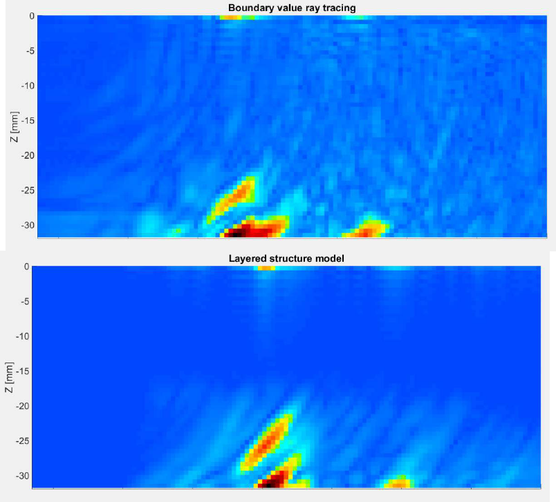
To verify the boundary value ray tracing approach it is compared to the initial value ray
tracing. Therefore, a specimen that contains an artificial flaw (notch, 6 mm depth) was
scanned via impulse-echo technique. The measured signal values are allocated to the
volume cells as explained in section 2.1 resulting in the SAFT reconstructions shown in
Figure 4.
7
Fig. 3. Comparison of SAFT results using and the boundary value problem formulation (top) and a layer
model with initial value ray tracing (bottom) for ray tracing.
The reconstruction of a notch results in two spots where the summed signals gain local
amplitude maxima: One at the base of the notch and one at its tip. Both models reconstruct
the flaw in the correct depth (26 mm to 32 mm). For the boundary value ray tracing, the
mapping of the flaw is better and the microstructure of the weld (e.g. grains) is better
defined, while the initial value ray tracing produces a more diffuse reconstruction. The
reason can be found in the calculation of the travel times: A ray that hits the center of each
cell minimizes the error of the calculated travel times.
Compared to populating the travel time matrix with initial value ray tracing, where
only 908 of 4680 cells are hit by a ray and thus have an associated time of flight, using the
approach described in this paper allowed to obtain times of flight for 4592 cells. Only for
cells close to the top surface , no rays could be found, mostly due to total reflection
of the ray at the perspex and buffer interfaces. On average, five Newton iterations were
required per cell, with a computation time of 1.28 s per Newton iteration on an AMD
Opteron 2.8 GHz, i.e. 0.0023 s per ray (as 7 + 49 initial value problems have to be solved, 7
for the ray itself, 49 for the derivatives). As is to be expected, initial value ray tracing is
computationally slightly cheaper, with 4.5 s per populated cell. The computation time for
boundary value ray tracing can further be reduced using the adaptive strategy outlined
above.
Another difference of both approaches is the coverage of the reconstruction plane.
Here, the signals in depths above -15 mm contain no information, since the sound cones of
8
the measurement did not reach this area. By matching the modeling to the measurement
parameter, the calculation time can be reduced further.
References
[1] K.J. Langenberg, R. Hannemann, T. Kaczorowski, R. Marklein, B. Koehler, C. Schurig, F. Walte.
Application of modeling techniques for ultrasonic weld inspection. NDT&E International 33:465-480, 2000.
[2] Analytical methods for modeling of ultrasonic nondestructive testing of anisotropic media. Ultrasonics
42:213-219, 2004.
[3] A. Shlivinsky, K.J. Langenberg. Defect imaging with elastic waves in inhomogeneous-anisotropic
materials with composite geometries. Ultrasonics 46:89-104, 2007.
[4] M. Kröning, A. Bulavinov, K.M. Reddy, F. Walte, M. Dalichow. Improving the inspectability of stainless-
steel and dissimilar metal welded joints using inverse phase-matching of phased array time-domain signals.
Proceedings of the 17th WCNDT, Shanghai, paper 451, 2008.
[5] S. Prudikov, A. Bulavinov, R. Pinchuk. Innovative ultrasonic testing (UT) of nuclear components by
sampling phased array with 3D visualization of inspection results. DGZfP Proceedings BB 125, paper
Th.2.C.6, 2010.
[6] C. Höhne, S. Kolkoori, M.U. Rahman, R. Boehm, J. Prager. SAFT imaging of transverse cracks in
asutenitic and dissimilar welds. J. Nondestruct. Eval. 32(1):51-66, 2013.
[7] K. Matthies et al., Ultraschallprüfung von austenitischen Werkstoffen. DVS Media GmbH, Berlin, 2009.
[8] K.J. Langenberg, R. Marklein, K. Mayer. Theoretische Grundlagen der zerstörungsfreien Materialprüfung
mit Ultraschall. Oldenburg Wissenschaftsverlag, München, 2009.
[9] B.R. Julian, D. Gubbins. Three-Dimensional Seismic Ray Tracing. J. Geophys. 43:95-113, 1977.
[10] H. Le Meur, J. Virieux, P. Podvin. Seismic tomography of the Gulf of Corinth: a comparison of methods.
Ann. Geofis. 40(1):1-24, 1997.
[11] V. Cerveny. Seismic Ray Theory. Cambridge University Press, 2005.
[12] S.I. Rokhlin, T.K. Bolland, L. Adler. Reflection and refraction of elastic waves on a plane interface
between two generally anisotropic media. J. Acoust. Soc. Am. 79(4):906-918, 1986.
[13] P. Deuflhard, F. Bornemann. Scientific Computing with Ordinary Differential Equations. Springer, 2002.
[14] P. Deuflhard. Newton Methods for Nonlinear Problems. Affine Invariance and Adaptive Algorithms.
Springer, 2006.
[15] J.A. Ogilvy. Computerized ultrasonic ray tracing in austenitic steel. NDT International 18(2):67-77,
1985.
[16] M. Spies, H. Rieder. Sythetic aperture focusing of ultrasonic inspection data to enhance the probability of
detection in strongly attenuating materials. NDT&E International 43:425-431, 2010.
[17] W. Müller, V. Schmitz, G. Schäfer. Reconstruction by the synthetic aperture focusing technique (SAFT).
Nuclear Engineering and Design 94:393-404, 1986.
