Why bother with Bayesian t-tests?
Fintan Costello
School of Computer Science and Informatics,
University College Dublin
and
Paul Watts
Department of Theoretical Physics,
National University of Ireland Maynooth
November 7, 2022
Abstract
Given the well-known and fundamental problems with hypothesis testing via clas-
sical (point-form) significance tests, there has been a general move to alternative
approaches, often focused on the Bayesian t-test. We show that the Bayesian t-test
approach does not address the observed problems with classical significance testing,
that Bayesian and classical t-tests are mathematically equivalent and linearly related
in order of magnitude (so that the Bayesian t-test providing no further information
beyond that given by point-form significance tests), and that Bayesian t-tests are
subject to serious risks of misinterpretation, in some cases more problematic than
seen for classical tests (with, for example, a negative sample mean in an experiment
giving strong Bayesian t-test evidence in favour of a positive population mean). We
do not suggest a return to the classical, point-form significance approach to hypothe-
sis testing. Instead we argue for an alternative distributional approach to significance
testing, which addresses the observed problems with classical hypothesis testing and
provides a natural link between the Bayesian and frequentist approaches.
Keywords: Hypothesis Testing; Significance; Replication
1
arXiv:2211.02613v1 [math.ST] 4 Nov 2022
1 Introduction
It is clear that classical or point-form significance testing has serious problems: many sta-
tistically significant experimental results fail to occur reliably in replications (e.g. Camerer
et al., 2018; Open Science Collaboration et al., 2015; Klein et al., 2018, 2014), the chance
of getting a statistically significant p-value increases with sample size, irrespective of the
presence or absence of a true effect (Thompson, 1998) and point-form null hypotheses are
always false (and to quote Cohen, 2016: “if the null hypothesis is always false, what’s the
big deal about rejecting it?”). In an attempt to address these problems various researchers
have argued for a move to Bayesian hypothesis testing approaches, with a particular focus
on generalisations of Jeffrey’s Bayesian t-test, which involves a Bayes Factor comparison
with a nested, point-form null hypothesis (Jeffreys, 1948; G¨onen et al., 2005; Fox and
Dimmic, 2006; Rouder et al., 2009; Wang and Liu, 2016; Schmalz et al., 2021). In this
paper we show that this Bayesian t-test approach does not, in fact, address any of these
problems with classical null hypothesis testing. Instead, the Bayesian t-test involves com-
parison against a point-form null which we know is always false (so what’s the big deal
about getting evidence against it?); the form of the Bayesian t-test means that probability
of getting Bayesian evidence against the null increases with sample size, irrespective of the
presence or absence of a true effect; and the Bayesian t-test gives results which are simply a
linear transformation of those obtained in classical significance tests and so are necessarily
subject to the same problems of replication and reliability as seen in classical tests. We
also show that the Bayesian t-test is subject to serious risks of misinterpretation, arguably
more problematic than those seen for classical tests. We demonstrate these points in detail
below, beginning with a derivation of the general Bayesian t-test and next showing that
these problems all hold with this general form (and so hold for all specific instantiations).
We the argue that researchers should move to hypothesis testing relative to distributional
rather than point-form nulls, and show that the distributional approach does not suffer
from any of these issues and further, naturally relates the Bayesian and frequentist ap-
proaches to hypothesis testing. We conclude by briefly giving our view of the roles that
Bayesian and frequentist statistical tools can play in scientific research.
2

2 The Bayesian t-test
The Bayesian t-test is a specific type of Bayes Factor test, originally developed by Jeffreys
(1948) and extended in various different ways by a range of other researchers. The Bayes
Factor
BF
10
=
p(y|H
1
)
p(y|H
0
)
is the ratio of the likelihood of observed data y under hypothesis H
1
to its likelihood under
H
0
: the higher the value of BF
10
, the more Bayesian evidence our data y gives in favour
of H
1
and against H
0
. More specifically, hypotheses or models H
0
and H
1
are taken to be
probability distributions with some parameter values fixed and some parameters following
specified prior distributions, and p(y|H) is estimated in terms of the density of the H
distribution integrated over those priors (the marginal likelihood). A Bayesian t-test is a
Bayes Factor test where the observed data takes the form of a t statistic, and where the
hypothesis H
0
is the null hypothesis used in the classical t-test. Various forms of Bayesian
t-test have been proposed in the literature: while each uses a different form of alternative
hypothesis H
1
, all have the same statistic t and the same null hypothesis H
0
.
Here we present Bayesian t-test in the context of a one-sample test, but with a generic
structure which covers all possible forms of alternative hypothesis H
1
. We assume an
experiment involving N measurements or observations X with observed sample mean X,
degrees of freedom ν and sample variance
S
2
=
1
ν
X
(X − X)
2
We assume that observations X follow a normal distribution
X ∼ N(µ, σ
2
)
for unknown parameters µ and σ, which means that
νS
2
σ
2
follows a χ
2
distribution with ν degrees of freedom. We let
d =
X
S
2
3

represent the sample effect in this experiment and define the variable
t =
X
S
√
N = d
√
N
Our null hypothesis is that µ = 0: that observations X follow the normal distribution
X ∼ N(0, σ
2
)
with unknown variance σ
2
(the null hypothesis in a classical t-test), so hypothesis H
0
is
H
0
: X ∼ N(0, σ
2
/N) (1)
and so the variable
X
√
σ
2
/N
q
νS
2
σ
2
/ν
= t
follows a T distribution with ν degrees of freedom.
We take the alternative hypothesis H
1
to have parameters σ, m and σ
m
such that
observations X follow the Normal distribution
X ∼ N(µ, σ
2
)
and µ itself follows the Normal distribution
µ ∼ N(m, σ
2
m
)
so that for given values of σ, σ
m
and m we see that X follows the distribution
X ∼
Z
∞
0
N(µ, σ
2
/N)N(µ|m, σ
2
m
)dµ
= N(m, σ
2
/N + σ
2
m
) = N
m, (σ
2
/N)
1 +
σ
2
m
σ
2
N
Defining σ
δ
= σ
m
/σ (so that σ
2
δ
is the variance of the effect size δ = µ/σ) this means that
our hypothesis H
1
is
H
1
: X ∼ N(m, (σ
2
/N)
1 + σ
2
δ
N
)
(2)
so that for fixed values of m and σ
δ
the variable
t
p
1 + σ
2
δ
N
=
X−m
q
(σ
2
/N )
[
1+σ
2
δ
N
]
+
m
q
(σ
2
/N )
[
1+σ
2
δ
N
]
q
νS
2
σ
2
/ν
4

follows a non-central T distribution with ν degrees of freedom and non-centrality parameter
m
p
(σ
2
/N) [1 + σ
2
δ
N]
=
δ
p
1/N + σ
2
δ
Letting T
v
represent the standard (central) T distribution with ν degrees of freedom
and T
ν
(θ) represent the non-central T distribution ν degrees of freedom and non-centrality
parameter θ, we can thus express our two hypotheses H
0
and H
1
in equivalent forms as
H
0
: t ∼ T
ν
(3)
and
H
1
:
t
p
1 + σ
2
δ
N
∼ T
ν
δ
p
1/N + σ
2
δ
!
(4)
In the Bayesian approach the likelihoods p(t|H
0
) and p(t|H
1
) are taken to be equal to
the density of these these distributions at the values given in H
0
and H
1
. Taking f
ν
(t)
to be the density of the standard T distribution at t and f
ν
(t; θ) to be the density of the
non-central T with parameter θ the density of H
0
at t is
p(t|H
0
) = f
ν
(t)
and the density of H
1
at
t
p
1 + σ
2
δ
N
is
p(t|H
1
) =
1
p
1 + σ
2
δ
N
f
ν
t
p
1 + σ
2
δ
N
;
δ
p
1/N + σ
2
δ
!
giving
BF
10
=
1
√
1+σ
2
δ
N
f
ν
t
√
1+σ
2
δ
N
;
δ
√
1/N +σ
2
δ
f
ν
(t)
(5)
Equation 5 represents, for example, a one-sample instantiation of the Bayesian t-test of
G¨onen et al. (G¨onen et al., 2005; Gronau et al., 2019) and, taking δ = 0 and adding a
χ
2
(1) prior on σ
δ
, represents the one-sample JZS Bayesian t-test of Rouder et al. (2009).
Other forms of the Bayesian t test are produced by assuming different prior distributions
for the parameters δ and δ
σ
or by expanding the hypotheses in various ways (Jeffrey’s
original formulation, for example, involves splitting H
1
into three component hypotheses);
5

all approaches, however, take some analog of these H
0
and H
1
distributions as their starting
point, and so this presentation characterises the general Bayesian t-test.
A core distinction between different forms of Bayesian t-test concerns the choice of value
or prior for δ (and so for m, the mean for the distribution of µ in the alternative hypothesis
H
1
). Default or local tests assume that δ is either equal to 0 (a delta distribution) or has
a mean of 0. This implies that m is also equal to or has a mean of 0, and so in these tests
both H
0
and H
1
assume the same mean for X. Informed or non-local tests, by contrast,
assume that δ is equal to or distributed around some non-zero value chosen on the basis of
prior knowledge in some way, so that X is assumed to have a different mean in H
1
than
in H
0
. In the next section we discuss various problems of interpretation that arise with
default or local tests.
2.1 Problems of interpretation: default tests
Two points are immediately evident from this general presentation of the Bayesian t-test.
First, distribution H
0
is the null hypothesis distribution that underlies the classical or
point-form t-test (which also assumes that X is normally distributed around a mean of 0
with variance σ
2
/N). The point-form null hypothesis, however, is always false: and so it
is not clear what is to be gained by testing against it. Second, for default tests with δ = 0
(and so m = 0) hypotheses H
0
and H
1
differ only in the variance they assign to X (compare
Equation 1 to Equation 2 with m = 0). Here there is a serious risk of misinterpretation,
arising because researchers commonly take default Bayesian t-test results in favour of H
1
as giving evidence that the population mean differs from 0 (that is, evidence of a significant
effect). This is clearly incorrect: in a default test H
1
assumes that the population mean is
0, and we cannot take evidence in favour of H
1
as evidence against this assumption.
2.2 Bayesian evidence but no real effect
For any fixed value of σ, the variance of X in H
0
falls with rising N to a limit of 0, since
that variance is σ
2
/N. This means that the probability of getting any value X 6= 0 under
H
0
similarly falls to 0 with rising N; and so, for any positive value y and any sample effect
d 6= 0, there exists some N
0
such that p(t|H
0
) = p(d
√
N|H
0
) < y for all N ≥ N
0
.
6

For any fixed values of σ, m and σ
m
, however, the variance of X in H
1
falls with rising
N to a limit of σ
2
m
(since that variance is σ
2
/N + σ
2
m
). This means that for any sample
effect d 6= 0 there will thus exist some value N
0
such that p(d
√
N|H
1
) > p(d
√
N|H
0
) holds
for all N ≥ N
0
. Given this we see that
lim
N→∞
BF
10
= lim
N→∞
p(t|H
1
)
p(t|H
0
)
= ∞
necessarily holds for any value X 6= 0 (and hence any t 6= 0) and any required level of
evidence in favour of the alternative hypothesis in a Bayesian t-test can be obtained with
large enough sample size N, irrespective of the presence or absence of a true effect for both
default and informed tests and irrespective of the choice of priors.
2.3 Problems of interpretation: informed tests
Comparing Equations 1 and 2 we see that for informed tests with m 6= 0, H
0
and H
1
differ both in their assumed means and in their models of variance for X. This means that
evidence against H
0
and in favour of H
1
may arise as a consequence of this difference in
variance alone; again, this leads to a serious risk of interpretation, where researchers may
assume that evidence in favour of H
1
indicates that the population mean is closer to or
more consistent with the alternative mean m than the null mean 0. This is not the case.
It may be useful to give a concrete example of the problem. Suppose we have a one-
sample experiment with sample size N = 50 (and so ν = 49) and that in our null hypothesis
we assume δ = 0 (there is no effect) and our alternative hypothesis we assume δ = 0.5 (there
is a medium-sized positive effect). For our Bayesian analysis, we make the standard choice
of simple unit-information prior for δ of σ
δ
= 1. Suppose we observe a medium-sized
negative effect in our experiment of d = −0.5 (so that t = −0.5
√
50). Then applying
Equation 5 we have a Bayesian t-test comparing H
1
to H
0
of
BF
10
=
1
√
1+σ
2
δ
N
f
ν
t
√
1+σ
2
δ
N
;
δ
√
1/N +σ
2
δ
f
ν
(t)
=
1
√
1+50
f
49
−0.5
√
50
√
1+50
,
0.5
√
1+1/50
f
49
−0.5
√
50
≈ 25
This is strong Bayesian evidence in favour of the alternative hypothesis H
1
, and if we mis-
takenly assume that BF
10
gives evidence about the hypothesised effect δ (as opposed to
7
the effect-plus-variance model H
1
), we will be led to the nonsensical conclusion that ob-
serving a medium-sized negative effect in our experiment gives us strong Bayesian evidence
in favour of a medium-sized positive effect.
Note that we pick on this one-sample instantiation of the G¨onen et al. (2005) t-test here
only because of its clarity and simplicity of presentation: the general problem (of negative
results giving apparently strong evidence in favour of a positive hypothesis) applies for all
informed or non-local Bayesian t tests, and arises, as before, because the variance of H
0
falls to 0 with rising N while the variance of H
1
does not.
2.4 Default Bayesian t-tests and classical t-tests are equivalent
Our last point involves the relationship between the Bayesian and classical t-tests. It has
long been observed that Bayesian t-test evidence in favour of the alternative and classical
point-form evidence against the null are essentially equivalent (to quote Jeffreys: “As a
matter of fact I have applied my significance tests to numerous applications that have also
been worked out by Fisher’s, and have not yet found a disagreement in the actual decisions
reached”; cited in Ly et al., 2016); here we explain why this relationship holds.
We first note that for large ν we have T
ν
≈ Φ (the standard T distribution is well
approximated by the standard Normal distribution) and that for the standard Normal
distribution the Mills ratio
M(x) =
Φ(−|x|)
φ(x)
(the ratio of the cumulative Normal function at −|x| to the probability density at x) has
the well-known asymptotic approximation
M(x) ≈
1
|x|
(6)
which is relatively accurate for |x| > 3 (e.g. Small, 2010, pp. 43). This means that the
classical p value for a given t is approximated by
p = 2T
ν
(−|t|) ≈ 2Φ(−|t|) ≈
2φ(t)
|t|
and substituting the expression for the standard Normal density
φ(x) =
1
√
2π
e
−
x
2
2
8

and taking the log gives
log(1/p) ≈
t
2
2
+ log(|t|) + log
p
π/2
For a default Bayesian t-test with δ = 0 we have
BF
10
=
1
√
1+σ
2
δ
N
f
ν
t
√
1+σ
2
δ
N
f
ν
(t)
≈
1
√
1+σ
2
δ
N
φ
t
√
1+σ
2
δ
N
φ(t)
and again substituting and taking the log gives
log(BF
10
) ≈
t
2
2
1 −
1
2(1 + σ
2
δ
N)
− log
q
1 + σ
2
δ
N
≈
t
2
2
− log
q
1 + σ
2
δ
N
and thus
log(BF
10
) ≈ log(1/p) −log(|t|) −log
q
π(1 + σ
2
δ
N)/2
It is clear that large changes in the value of t cause large changes in the value of t
2
/2
but much smaller changes in log |t|. This means that if we have a set of experiments with
approximately the same sample size N (so that changes in the log(
p
π(1 + σ
2
δ
N)/2) term
across experiments are small) the we expect
log BF
10
≈ log 1/p + C
to hold across a given set of experiments for some constant
C = −
log
|t|
q
π(1 + σ
2
δ
N)/2
where hxi indicates the average value of x in those experiments. This tells us that the
Bayesian t-test BF
10
and the point-form significance p are equivalent, at least in terms
of order of magnitude. Our main concern when considering statistical significance (or
Bayesian evidence) is in the order of magnitude of our result rather than its exact value:
in this context the Bayesian BF
10
and the classical p-value convey the same information,
and the two tests are essentially the same.
2.5 Testing the equivalence between p and BF
We tested this predicted relationship between Bayesian and classical t-tests using data
from the first Many Labs replication project (Klein et al., 2014). This involved the replica-
tion of 16 different experimental tasks investigating a variety of classic and contemporary
9
psychological effects covering a range of different topics. Each experiment was originally
published in the cognitive or social psychology literature, and was replicated by researchers
in around 36 different sites. Of these 16 tasks, 11 involved independent t-tests: we down-
loaded the data on all experimental replications of these 11 tasks (396 experiments in total)
and used the standard R t.test function (R Core Team, 2021) to calculate the t-test p and
the ttest.tstat function (from the BayesFactor package, Morey and Rouder, 2021) to calcu-
late the Bayesian t-test BF
10
for each of these experiments. The R script for this analysis
is available online (see Supplementary Materials).
This particular form of Bayesian t-test is a default test assuming an alternative hypoth-
esis H
1
with δ = 0 and and with effect sizes distributed normally around δ with variance
σ
2
δ
which itself follows an inverse χ
2
distribution with 1 degree of freedom. Under this
prior σ
2
δ
is distributed around 1: this prior is therefore equivalent to, though slightly less
informative than, the unit information prior σ
2
δ
= 1 we used in our earlier example.
Since the t-tests in this dataset were all independent two-sample tests with N
1
samples
in one group and N
2
in the other, we took the effective sample size in each experiment to
be
N
eff
=
1
1/N
1
+ 1/N
2
and calculated the value
−log
|t|
q
π(1 + N
eff
)/2
for each experiment in this dataset, and took C to be the mean of these values, giving
C = −2.81 for these experiments. Our prediction is that log(BF
10
) and log(1/p) will have
a linear relation in these experiments, with a slope of 1 and an intercept of C. To test this
prediction we took the p and BF
10
values for each individual experiment and calculated the
best-fitting log(BF
10
) vs log(1/p) line relating these values. The best-fitting line had a slope
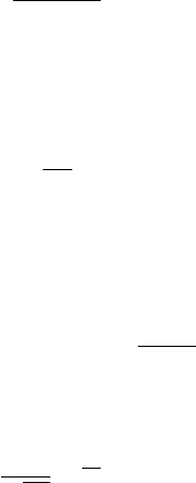
of 1.02 and an intercept of −2.81 ± 0.015 (see Figure 1): the predicted value C = −2.81
fell within this (quite narrow) interval, confirming the predicted relationship.
10
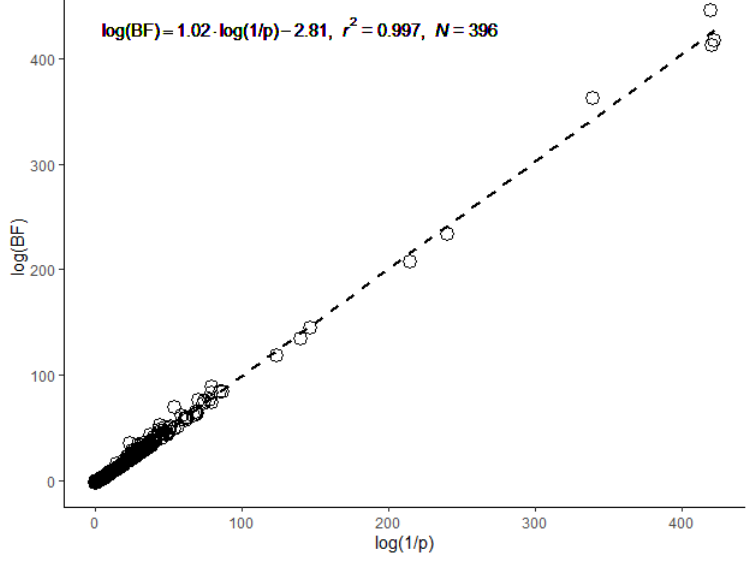
Figure 1: Scatterplot of log(BF
10
) vs log(1/p) for the 396 t-test experiments in the Many
Labs 1 dataset, with the line of best fit. The fit is extremely good, with the line accounting
for more than 99% of the variance in values; the slope is almost exactly the predicted value
(1.02 vs 1), and the intercept of −2.81 matches the predicted C = −2.81 value exactly.
3 Distributional null hypothesis testing
We’ve given a general characterisation of the Bayesian t-test and shown that this general
form of the test, and so all specific instantiations, suffer from a series of problems: all
compare an alternative H
1
against a null H
0
that we already know to be false; all give
increasing evidence for H
1
irrespective of the presence or absence of any real effect; none
give specific evidence about the population mean but instead give evidence about the
variance of that mean; and (under a series of approximations) all are essentially equivalent
to the classical t-test against a point-form null, providing no further information.
These problems arise from the use of the classical null hypothesis as H
0
in the Bayesian t-
test approach, and from the fact that the two hypotheses H
1
and H
0
being compared differ
11
in both their model of variance and (for informed tests) in their assumed mean. Given
these problems it seems unlikely that a move to Bayesian rather than classical hypothesis
testing against the point-form null hypothesis will in any way address the problems with
reliability and replication that we see in scientific research. As an alternative, we suggest
that researchers consider Fisherian evidential testing against a single null hypothesis, but
with a distributional rather than a point form null. This is an approach where the statistical
model is that observations X follow the Normal distribution
X ∼ N(µ, σ
2
)
for unknown σ
2
and where µ itself follows the Normal distribution
µ ∼ N(m, σ
2
m
)
and where the null hypothesis is m = 0. We have recently proposed a distributional
null hypothesis testing model following this approach which takes σ
2
m
to represent the
variance in experimental means across replications of a given experiment. The null is
not always false in this model; evidence against the null in this model does not rise with
sample size irrespective of the presence or absence of a real effect; and further, when the
between-experiment variance of means is obtained from sample data, this model estimates
the probability of replication of results in a way which reliably matches observed rates of
experimental replication (for a detailed presentation, see Costello and Watts, 2022).
This distributional approach depends on a parameter b = σ
2
m
/σ
2
representing the ra-
tio of between-experiment variance in means to within-experiment variance in individual
responses. While this parameter is mathematically identical to the effect size variance σ
2
δ
used in the derivation of the Bayesian t-test given above, it has a different meaning: where
σ
2
δ
represents prior uncertainty about the effect (and so is subjective in nature), b repre-
sents the relative variation in experimental means across different experiments and so is
estimated from sample data (just as within-experiment variation σ is estimated from sam-
ple data). Further, where in a Bayesian t-test it is natural to choose an uninformative prior
for σ
2
δ
, in the distributional approach the choice of value for b represents a trade-off between
Type I and Type II error: a high value for b means high assumed between-experiment
variance and so low Type I error (but high type II error), while a low assumed value for b
means low between-experiment variance and so high Type I error (but low type II error)
12

This distributional null approach can also be applied to the comparison of null and
alternative hypotheses; in this approach these two hypotheses are
H
0
:
t
√
1 + bN
∼ T
ν
t
√
1 + bN
and
H
1
:
t
√
1 + bN
∼ T
ν
t
√
1 + bN
;
δ
p
1/N + b
!
and the Bayes Factor ratio for the alternative hypothesis H
1
against the null H
0
is the ratio
of densities of these two distributions
BF
10
=
1
√
1+bN
f
ν
−|t|
√
1+bN
;
δ
√
1/N +b
1
√
1+bN
f
ν
−|t|
√
1+bN
and since both hypotheses H
0
and H
1
necessarily assume the same variance for X but
different means, Bayesian evidence in favour of H
1
indicates that the observed data is more
consistent with the mean in H
1
than the mean in H
0
. We can illustrate this using the same
one-sample experiment described earlier with sample size N = 50 (and so ν = 49), a null
hypothesis δ = 0 (there is no effect) an alternative hypothesis δ = 0.5 (there is a medium-
sized positive effect) and assuming, purely for comparison purposes, a unit-information
value of b = 1. This gives
BF
10
=
f
ν
−|t|
√
1+bN
;
δ
√
1/N +b
f
ν
−|t|
√
1+bN
=
f
49
−0.5
√
50
√
1+50
,
0.5
√
1+1/50
f
49
−0.5
√
50
√
1+50
= 0.69
and the test gives weak evidence in favour of H
0
, which is just as we would expect given
that the observed result d = −0.5 is not strongly consistent with either H
0
or H
1
, but is
slightly more consistent with H
0
.
In the distributional approach the significance of a given result t relative to H
0
is
p
sig
(t|H
0
) = 2T
ν
−|t|
√
1 + bN
while its significance relative to an alternative hypothesis of some effect size δ is
p
sig
(t|H
1
) = 2T
ν
−|t|
√
1 + bN
;
δ
p
1/N + b
!
13

and there is a linear relationship between these measures of significance and the Bayes
Factor measures of evidence. To see this we approximate both these T distributions with
corresponding Normal distributions (a rough approximation since it takes the Normal to
approximate the non-central T ) giving
p
sig
(t|H
0
) ≈ 2Φ
−|d|
p
1/N + b
!
and
p
sig
(t|H
1
) ≈ 2Φ
−|d − δ|
p
1/N + b
!
and relating to Mills ratio gives
BF
10
≈
p
sig
(t|H
1
)
p
sig
(t|H
0
)
M
−|d|
√
1/N +b
M
−|d−δ|
√
1/N +b
We are primarily concerned here with results d which are close to 0 or to δ (giving
evidence in favour of one hypothesis or the other), and so have the Mills ratio argument x
approaching 0 for one or other hypothesis. The approximation in Equation (6) diverges as
x → 0, however; and so, since φ(0) =
p
π/2, we use the modified approximation
M(x) ≈
1
p
2/π + |x|
which is relatively close to M(x) for x < 3 and which asymptotically approaches Equation
(6) (and so M(x)) as x → ∞. Given this we see that the Bayes Factor and the ratio of
distributional significance have the approximate relationship
BF
10
≈
p
sig
(t|H
1
)
p
sig
(t|H
0
)
p
2b/π + |d − δ|
p
2b/π + |d|
and the Bayes Factor measure of relative evidence for H
1
over H
0
given by result t is, to a
first approximation, simply a linear transformation of the distributional significance ratio
for t under H
1
and H
0
.
4 Discussion
Our focus so far has been on the relationship between Bayesian and frequentist approaches
to hypothesis testing in a particularly simple situation: the t test. Here we briefly discuss
14
the relationship between these two approaches more generally. We take as our starting point
a account of the Bayesian/frequentist distinction as given in a recent primer on Bayesian
statistics:
The key difference between Bayesian and frequentist inference is that frequen-
tists do not consider probability statements about the unknown parameters to be
useful. Instead, the unknown parameters are considered to be fixed; the likeli-
hood is the conditional probability distribution p(y|θ) of the data (y), given fixed
parameters (θ). In Bayesian inference, unknown parameters are referred to as
random variables in order to make probability statements about them. The (ob-
served) data are treated as fixed, whereas the parameter values are varied; the
likelihood is a function of θ for the fixed data y.
(van de Schoot et al., 2021, p. 7)
We expand on this account by noting that in both frequentist and Bayesian approaches
we have some theory of the generative process producing data y. This theory gives us two
things: first, an overall statistical model M with some set of independent parameters θ such
that y is assumed to follow the distribution y ∼ M(θ); and second, a list H containing,
for each parameter θ
i
, a particular selected value for that parameter (with some associated
uncertainty or variance in that value). The variances associated with parameter values in
H allows us to distinguish between fixed and free parameters in our theory. A parameter
value is fixed by theory, in this view, when our theory requires a specific value for H
i
so that
any change to that value would necessarily require us to abandon the theory: the variance
of a fixed parameter is thus necessarily 0 in this theory. If a parameter is not fixed it is
free, and its value must be estimated from data in some way, so that any such estimated
value, and any change in that value, remains consistent with our theory (and such that the
current best estimate, and its variance, is given by H
i
).
Both frequentist and Bayesian approaches typically assume the overall model M is fixed,
and consider either testing or updating values of the parameter values H (“the” hypothesis).
Frequentist inference considers p(y|H): the probability distribution for data y conditional
on θ = H (on the assumption that the parameters are as described in H). Bayesian
15
inference considers p(H
new
|y, H): the updated parameter descriptions H
new
, conditional
on data y and on the prior values H. This common structure means that both forms
of statistical inference fall within a single unified framework defined by M and H: any
Bayesian prior H can be tested via the frequentist inference p(y|H) and any frequentist
hypothesis H about θ can be updated via the Bayesian inference p(H
new
|y, H). Indeed both
forms of inference can be applied to the same data y, by asking whether y is consistent
with H and, if not, updating to produce a more consistent description H
new
and then
asking whether y is consistent with this new description (these are the prior and posterior
predictive checks commonly recommended in standard Bayesian workflows, even though
these checks involve a frequentist hypothesis test; see e.g. Gelman et al., 2020; Schad et al.,
2021). Note that for parameter values H
i
with variance of 0 (fixed by theory) this updating
process will never cause any change in H
i
. This means that if p(y|H
new
) is less than some
significance criterion α, we can conclude that data y is inconsistent with our overall theory
in some way: that updating to produce a set of parameter values consistent with the data
would either require us to change some values that are fixed in that theory, to abandon
our prior estimates H for some or all of those values (which by assumption were consistent
with that theory) or to abandon our statistical model M.
It is necessarily the case in this unified framework that any form of hypothesis testing
(that is, any situation where we ask whether data y is consistent with some H) will nec-
essarily involve the frequentist inference p(y|H) in some way. It should not be surprising,
therefore, that the default Bayesian t test and the classical t test are essentially equivalent;
the equivalence arises because both depend on inferences of the form p(y|H).
SUPPLEMENTARY MATERIAL
The R script used in this paper available at https://osf.io/qajvu, and automatically
downloads the Many Labs 1 dataset, carries out the analysis, and generates Figure 1.
16
References
Camerer, C. F., A. Dreber, F. Holzmeister, T.-H. Ho, J. Huber, M. Johannesson, M. Kirch-
ler, G. Nave, B. A. Nosek, T. Pfeiffer, et al. (2018). Evaluating the Replicability of Social
Science Experiments in Nature and Science Between 2010 and 2015. Nature Human Be-
haviour 2 (9), 637–644.
Costello, F. and P. Watts (2022). How to Tell When a Result Will Replicate: Significance
and Replication in Distributional Null Hypothesis Tests. Submitted.
Fox, R. J. and M. W. Dimmic (2006). A Two-Sample Bayesian T-Test for Microarray
Data. BMC Bioinformatics 7 (1), 1–11.
Gelman, A., A. Vehtari, D. Simpson, C. C. Margossian, B. Carpenter, Y. Yao, L. Kennedy,
J. Gabry, P.-C. B¨urkner, and M. Modr´ak (2020). Bayesian Workflow. arXiv Preprint
arXiv:2011.01808 .
G¨onen, M., W. O. Johnson, Y. Lu, and P. H. Westfall (2005). The Bayesian Two-Sample
T Test. The American Statistician 59 (3), 252–257.
Gronau, Q. F., A. Ly, and E.-J. Wagenmakers (2019). Informed Bayesian T-Tests. The
American Statistician.
Jeffreys, H. (1948). The Theory of Probability. OUP Oxford.
Klein, R. A., K. A. Ratliff, M. Vianello, R. B. Adams Jr,
ˇ
S. Bahn´ık, M. J. Bernstein,
K. Bocian, M. J. Brandt, B. Brooks, C. C. Brumbaugh, et al. (2014). Investigating
Variation in Replicability. Social Psychology 45 (3), 142–152.
Klein, R. A., M. Vianello, F. Hasselman, B. G. Adams, R. B. Adams Jr, S. Alper, M. Ave-
yard, J. R. Axt, M. T. Babalola,
ˇ
S. Bahn´ık, et al. (2018). Many Labs 2: Investigating
Variation in Replicability Across Samples and Settings. Advances in Methods and Prac-
tices in Psychological Science 1 (4), 443–490.
Ly, A., J. Verhagen, and E.-J. Wagenmakers (2016). Harold Jeffreys?s Default Bayes Factor
17
Hypothesis Tests: Explanation, Extension, and Application in Psychology. Journal of
Mathematical Psychology 72, 19–32.
Morey, R. D. and J. N. Rouder (2021). BayesFactor: Computation of Bayes Factors for
Common Designs. R package version 0.9.12-4.3.
Open Science Collaboration et al. (2015). Estimating the Reproducibility of Psychological
Science. Science 349 (6251), aac4716.
R Core Team (2021). R: A Language and Environment for Statistical Computing. Vienna,
Austria: R Foundation for Statistical Computing.
Rouder, J. N., P. L. Speckman, D. Sun, R. D. Morey, and G. Iverson (2009). Bayesian
T Tests for Accepting and Rejecting the Null Hypothesis. Psychonomic Bulletin &
Review 16 (2), 225–237.
Schad, D. J., M. Betancourt, and S. Vasishth (2021). Toward a Principled Bayesian Work-
flow in Cognitive Science. Psychological Methods 26 (1), 103.
Schmalz, X., J. Biurrun Manresa, and L. Zhang (2021). What Is a Bayes Factor? Psycho-
logical Methods.
Small, C. G. (2010). Expansions and Asymptotics for Statistics. Chapman and Hall/CRC.
Thompson, B. (1998). In Praise of Brilliance: Where That Praise Really Belongs. American
Psychologist 53 (7), 799–800.
van de Schoot, R., S. Depaoli, R. King, B. Kramer, K. M¨artens, M. G. Tadesse, M. Van-
nucci, A. Gelman, D. Veen, J. Willemsen, et al. (2021). Bayesian Statistics and Modelling.
Nature Reviews Methods Primers 1 (1), 1–26.
Wang, M. and G. Liu (2016). A Simple Two-Sample Bayesian T-Test for Hypothesis
Testing. The American Statistician 70 (2), 195–201.
18
