Bayesian t tests for accepting and rejecting the null hypothesis

Advances in science often come from identifying

invariances—those elements that stay constant when oth-

ers change. Kepler, for example, described the motion of

planets. From an Earth-bound vantage point, planets seem

to have strange and variable orbits. Not only do they differ

in their speeds and locations, they even appear to back-

track at times (a phenomenon known as retrograde mo-

tion). Although planetary orbits appear variable, Kepler

identified invariants in planetary motion. For example, all

orbits follow ellipses in which the square of the orbital pe-

riod is proportional to the cube of the orbital radius. These

invariances formed the basis for Newton’s subsequent the-

ory of mechanics (Hawking, 2002). A similar story holds

in genetics, where Mendel’s discovery of invariant ratios

in phenotypes served as an important precursor for the

construction of genetic theory.

Although the search for invariances has often motivated

theory in other domains, it has not had as much impact

in psychology. Invariances are statements of equality,

sameness, or lack of association, whereas in practice, the

psychological field has a Popperian orientation, in which

demonstrations of effects or associations are valued more

than demonstrations of invariances (Meehl, 1978). As a

contrast, we offer below a few examples of how scientific

inquiry in cognitive psychology has benefited from con-

sideration of invariances:

1. It is often of great practical and theoretical interest to

determine whether performance is invariant to readily ob-

servable variables. For example, several researchers have

assessed whether cognitive skills vary with gender (e.g.,

Shibley Hyde, 2005, 2007). To believe that only effects

of genders, rather than invariances across genders, will

appear in performance strikes us as an extreme position.

A second example comes from the domain of subliminal

priming (see, e.g., Dehaene et al., 1998): To prove that

subliminal priming occurs, it must be shown that detection

or identification of the primes does not vary from chance

(see Reingold & Merikle, 1988; Rouder, Morey, Speck-

man, & Pratte, 2007).

2. Conservation laws are instantiations of invariances.

An example of a proposed conservation law is the Weber–

Fechner law (Fechner, 1860/1966), which states that the

detectability of a briefly flashed stimulus is a function of

its intensity divided by the intensity of the background.

Accordingly, performance should be invariant when the

intensities of the flash and background are multiplied by

the same constant. Another example of a proposed conser-

vation law is the choice rule (Clarke, 1957; Luce, 1959;

Shepard, 1957), which states that the preference for a

choice is a function of the ratio of its utility divided by

the summed utility of all available choices. The key in-

variance here concerns ratios of preferences between any

two choices—for example, the preference for Choice A

divided by that for Choice B. This ratio should not vary

when choices are added or taken away from the set of

available options.

3. Testing invariances is critical for validating paramet-

ric descriptions. Consider the example of Stevens (1957),

who proposed that sensation follows a power function of

intensity. It is reasonable to expect that the exponent of

Bayesian t tests for accepting

and rejecting the null hypothesis

JEFFREY N. ROUDER, PAUL L. SPECKMAN, DONGCHU SUN, AND RICHARD D. MOREY

University of Missouri, Columbia, Missouri

AND

GEOFFREY IVERSON

University of California, Irvine, California

Progress in science often comes from discovering invariances in relationships among variables; these

invariances often correspond to null hypotheses. As is commonly known, it is not possible to state evidence

for the null hypothesis in conventional significance testing. Here we highlight a Bayes factor alternative to

the conventional t test that will allow researchers to express preference for either the null hypothesis or the

alternative. The Bayes factor has a natural and straightforward interpretation, is based on reasonable assump-

tions, and has better properties than other methods of inference that have been advocated in the psychological

literature. To facilitate use of the Bayes factor, we provide an easy-to-use, Web-based program that performs

the necessary calculations.

Psychonomic Bulletin & Review

2009, 16 (2), 225-237

doi:10.3758/PBR.16.2.225

J. N. Rouder, r[email protected]

226 ROUDER, SPECKMAN, SUN, MOREY, AND IVERSON

Critiques of Inference by Significance Tests

Before introducing Bayes factors, we present two re-

lated critiques of classic null-hypothesis significance

tests: (1) They do not allow researchers to state evidence

for the null hypothesis, and, perhaps more importantly,

(2) they overstate the evidence against the null hypoth-

esis. To make these critiques concrete, assume that each of

N participants performs a task in two different experimen-

tal conditions. Let x

and x

denote the ith participant’s

mean RT in each of the two conditions, and let y

denote

the difference between these mean RTs. A typical test of

the effect of conditions is a one-sample t test to assess

whether the population mean of y

is different from zero.

The model underlying this test is

iid

Normal(, À

), i  1, . . . , N.

The null hypothesis, denoted H

, corresponds to   0.

The alternative, denoted H

, corresponds to  p 0.

The first critique, that null-hypothesis significance tests

do not allow the analyst to state evidence for the null hy-

pothesis, can be seen by considering how p values depend

on sample size. Significance tests seem quite reasonable

if the null is false. In this case, the t values tend to become

larger as sample size is increased; this in turn increases

the probability of correctly rejecting the null. In the large-

sample limit—that is, as the sample size becomes arbi-

trarily large—the t value grows without bound, and the

p value converges to zero. This behavior is desirable, be-

cause it implies that the null will always be rejected in

the large-sample limit when the null is false. Research-

ers, therefore, can rest assured that increasing sample size

will, on average, result in a gain of evidence against the

null when the null is, indeed, false.

The situation is less desirable, however, if the null is

true. When the null is true, the t values do not converge

to any limit with increasing sample size. For sample sizes

greater than 30 or so, the distribution of t values is well

approximated by a standard normal distribution. Cor-

responding p values are also distributed; when the null

is true, all p values are equally likely—that is, they are

distributed uniformly between 0 and 1. This distribution

holds regardless of sample size. The consequence of this

fact is that researchers cannot increase the sample size to

gain evidence for the null, because increasing the sample

size does not affect the distribution of p values. Of course,

this behavior is part of the design of significance tests and

reflects Fisher’s view that null hypotheses are only to be

rejected and never accepted (Meehl, 1978).

One pernicious and little-appreciated consequence

of the inability to gain evidence for the null is that sig-

nificance tests tend to overstate the evidence against it

(Edwards et al., 1963; Goodman, 1999; Jeffreys, 1961;

Sellke, Bayarri, & Berger, 2001; Wagenmakers & Grün-

wald, 2006). A rejection of the null hypothesis may be an

exaggeration of the evidence for an effect. To show this

overstatement, we start by considering the behavior of sig-

nificance tests in the large-sample limit. It is reasonable

to expect that in this limit, a method of inference always

yields the correct answer. In statistics, this property is

the power function will vary across variables of different

intensities, such as brightness or loudness. As pointed out

by Augustin (2008), however, it is critical that the expo-

nent be constant for a given-intensity variable. Exponents

should not, for instance, depend on the specific levels cho-

sen in an experiment. Another example of a parametric

description is from Logan (1988, 1992), who proposed

that response time (RT) decreases with practice as a power

function. For this description to be valid, an invariance in

the exponent across various experimental elements would

be expected (e.g., in alphabet arithmetic, the power should

be invariant across addends).

4. Assessing invariances is also critical for showing se-

lective influence, which is a key method of benchmarking

formal models. Debner and Jacoby (1994), for instance,

tested Jacoby’s (1991) process dissociation model by

manipulating attention at study in a memory task. This

manipulation should affect parameters that index con-

scious processes but not those that index automatic ones.

Similarly, the theory of signal detection (Green & Swets,

1966) stipulates that base-rate manipulations affect cri-

teria but not sensitivity. Hence, an invariance of sensitiv-

ity over this manipulation is to be expected (Egan, 1975;

Swets, 1996).

This small, selective set of examples demonstrates the

appeal of testing invariances for theory building. Even so,

it is worth considering the argument that invariances do

not exist, at least not exactly. Cohen (1994), for example,

started with the proposition that all variables affect all oth-

ers to some, possibly small, extent. Fortunately, there is

no real contradiction between adhering to Cohen’s view

that invariances cannot hold exactly and assessing invari-

ances for theory building. The key here is that invariances

may not hold exactly for relatively trivial reasons that are

outside the domain of study. When they hold only approxi-

mately, they often provide a more parsimonious descrip-

tion of data than do the alternatives and can serve as guid-

ance for theory development. Hence, whether one believes

that invariances may hold exactly or only approximately,

the search for them is intellectually compelling.

Perhaps the biggest hurdle to assessing invariances is

methodological. Invariances correspond to the null hy-

pothesis of equality, but conventional significance tests do

not allow the analyst to state evidence for a null hypoth-

esis. If an invariance holds, even approximately, then the

best-case significance test outcome is a failure to reject,

which is interpreted as a state of ignorance. In this article,

we recommend Bayes factors (Kass & Raftery, 1995) as a

principled method of inference for assessing both invari-

ances and differences. Bayes factors have been recom-

mended previously in the psychological literature (see,

e.g., Edwards, Lindman, & Savage, 1963; Lee & Wagen-

makers, 2005; Myung & Pitt, 1997; Wagenmakers, 2007).

In this article, we develop Bayes factor tests for paired

(one-sample) and grouped (two-sample) t tests. Moreover,

we provide a freely available, easy-to-use, Web-based pro-

gram for this analysis (available at pcl.missouri.edu). We

anticipate that the approach presented here will generalize

to factorial designs across several variables.

BAY E S FACTOR 227

null if the alternative is typical (  30) but favors the

alternative if the alternative is a small effect (  10). It

is an undeniable fact that inference depends on how much

weight the researcher places on various alternatives. Sub-

sequently, we will discuss strategies for weighting alterna-

tives. The second lesson is that significance tests overstate

the evidence against the null in finite samples because the

null may be more plausible than other reasonable alterna-

tives. As a rule of thumb, inference based on evaluating a

null without comparison to alternatives tends to overstate

the evidence against the null. Some examples of this ten-

dency include:

Confidence intervals (CIs). Cumming and Finch (2001),

Masson and Loftus (2003), and Kline (2004), among

many others, have recommended using CIs for inference.

We recommend CIs for reporting data, but not for infer-

ence (Rouder & Morey, 2005). The problem with confi-

dence intervals for inference is that they, like significance

tests, have a fixed probability of including the null when

the null is true, regardless of sample size. This property

implies that evidence cannot be gained for the null, and,

consequently, there is a tendency to overstate the evidence

against it. For the one-sample case, the null is rejected if

the CI around the mean does not include zero. This test is,

of course, equivalent to significance testing and suffers

analogously to the example above.

Probability of replication (p

rep

). Killeen (2005, 2006)

recommends computing the predictive posterior prob-

ability that a different sample from the same experiment

would yield an effect with the same sign as the original.

Inference is performed by rejecting the null if this prob-

ability is sufficiently large. Although this approach may

appear attractive, it is not designed to assess the replica-

termed consistency, and inconsistent inferential methods

strike us as unsatisfying. If the null is false ( p 0), signif-

icance tests are consistent: The p values converge to zero,

and the null is always rejected. If the null is true (  0),

however, significance tests are inconsistent: Even in the

large-sample limit, the analyst mistakenly rejects the null

with probability (. This inconsistency is a bias to over-

state the evidence against the null. This bias would be of

only theoretical interest if it held exclusively in the large-

sample limit. But in fact, it holds for realistic sample sizes

as well, and therefore is of practical concern. To show this

bias in realistic sample sizes, we present an argument mo-

tivated by that of Sellke et al.

Suppose that each of 100 participants provides 100 RT

measurements in each of two conditions. Let us assume

that RTs for each individual in each condition have a stan-

dard deviation (std) of 300 msec, which is reasonable for

RTs with means between 500 and 1,000 msec. The analyst

tabulates participant-by-condition means, denoted x

and

. These participant-by-condition means have standard

deviations of 300/·100  30. From these means, partici-

pant difference scores, y

 x

 x

, are calculated, and

the standard deviation

of y

is ·2  30 . 42. Let us as-

sume that the difference scores reveal a y

 10-msec RT

advantage for one experimental condition over the other.

The t statistic is t  ·N  y/std( y)  10  10 / 42  2.38.

The associated p value is about .02. The conventional

wisdom is that this is a case in which the null hypothesis

is not tenable. We show below that this conclusion is an

overstatement.

One way of quantifying the evidence in the data is to

compute the likelihood of observing a t value of 2.38

under various hypotheses. The likelihood of t  2.38 for

the null is the density of a t distribution with 99 degrees of

freedom evaluated at 2.38. This likelihood is small, about

.025. Differences in RTs tend to vary across tasks, but even

so, it is common for reliable differences to be 30 msec or

more. The likelihood that t  2.38 for the more typical

difference of 30 msec is the density of a noncentral t dis-

tribution with 99 degrees of freedom and a noncentrality

parameter of (·N )/À, which is about 7.1. This likelihood

is quite small, about .000006. The likelihood ratio of the

null versus this typical effect is about 3,800:1 in favor of

the null. Hence, a likelihood ratio test of the null versus a

typical effect strongly favors the null.

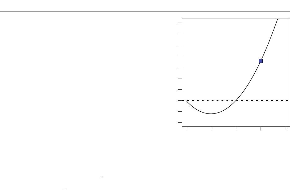
Figure 1 shows this likelihood ratio for a range of al-

ternatives. The filled square shows the likelihood ratio for

the example above of the null hypothesis versus a typical

effect of 30 msec. The null has greater likelihood for all

effects greater than about 20 msec. The fact that there is

a large range of reasonable alternatives against which the

null is preferable is not captured by the p value. In view of

this fact, rejection of null hypotheses by consideration of

p values under the null strikes us, as well as several other

commentators, as problematic.

There are two related lessons from the demonstration

above. The first is that the choice of alternative matters.

The evidence in the example above provides different sup-

port for the null depending on the alternative. It favors the

Likelihood Ratio (Null/Alternative)

0 10203040

Alternative (msec)

0.01

1,000

1E+05

Figure 1. Likelihood ratio (null/alternative) as a function of the

alternative for a hypothetical data set (t  2.38, 100 participants

observing 100 trials in each of two conditions). Even though the

null is rejected by a standard significance test, there is not strong

evidence against it as compared with the specific alternative.

228 ROUDER, SPECKMAN, SUN, MOREY, AND IVERSON

observed data are termed posterior; an appropriate statis-

tic for comparing hypotheses is the posterior odds:

7









data

where H

and H

denote the null and alternative hypoth-

eses, respectively. Odds are directly interpretable. For in-

stance, if 6  19, the null is 19 times more probable than

the alternative, given the data. As Laplace first noted al-

most 200 years ago, computing posterior odds on hypoth-

eses is natural for scientific communication (as cited in

Gillispie, Fox, & Grattan-Guinness, 1997, p. 16). Jeffreys

recommends that odds greater than 3 be considered “some

evidence,” odds greater than 10 be considered “strong

evidence,” and odds greater than 30 be considered “very

strong evidence” for one hypothesis over another.

The posterior odds are given by



7















data















The term Pr(H

)/Pr(H

) is the prior odds. In practice,

it is often natural to set the prior odds to 1.0, a position

that favors neither the null nor the alternative. The terms

f(data | H

) and f(data | H

) are called the marginal like-

lihoods and are denoted more succinctly as M

and M

respectively. The posterior odds is, therefore,



7 r











All of the evidence from the data is expressed in the ratio

of marginal likelihoods. This ratio is termed the Bayes

factor (Jeffreys, 1961; Kass & Raftery, 1995) and is de-

noted by B

 .

Consequently,



7 r











Marginal likelihoods for a given hypothesis H are given

Mfpd

HHH





QQQQQQ

(; ) () ,y

where 

denotes the parameter space under hypothesis

H, f

denotes the probability density function of the data

under hypothesis H, y denotes the data, and p

denotes

the prior distribution on the parameters. This equation is

most profitably viewed as a continuous average of likeli-

hoods in which priors p

serve as the weights. If a prior

places weight on parameter values that are very unlikely

to have produced the data, the associated low likelihood

values will drag down the average. Hence, in order for the

marginal likelihood of a model to be competitive, the prior

should not attribute undue mass to unreasonable param-

eter values. As will be discussed in the next section, this

bility of invariances. As discussed by Wagenmakers and

Grünwald (2006), p

rep

is logically similar to p values in

that the distribution does not change with sample size

when the null holds. As such, it is open to the critiques of

p values above.

Neyman–Pearson (NP) hypothesis testing with fixed (.

In NP testing, the researcher may specify an alternative to

the null and then choose a decision criterion on the basis

of consideration of Type I and Type II error rates. Typically,

however, psychologists fix the decision criterion with ref-

erence to the null alone—that is, with fixed (, say ( 

.05. This choice is not necessitated by NP testing per se;

instead, it is a matter of convention in practice. With this

choice, NP is similar to Fisher significance testing based

on p values, at least for many common tests (see Lehmann,

1993, for details). Consequently, it is similarly biased to-

ward overstating the evidence against the null. This point is

made elegantly by Raftery (1995). NP testing can be made

consistent by allowing Type I error rates to decrease toward

zero as the sample size increases. How this rate should de-

crease with sample size, however, is neither obvious nor

stipulated by the statistical theory underlying NP testing.

The Akaike information criterion (AIC). The AIC

(Akaike, 1974) is a method of model selection (rather than

testing) that is occasionally used in psychology (exam-

ples include Ashby & Maddox, 1992; Rouder & Ratcliff,

2004). One advantage of the AIC is that it seemingly may

be used to state evidence for the null hypothesis. To use

the AIC, each model is given a score:

AIC  2 log L  2k,

where L is the maximum likelihood under the model and k

is the number of required parameters. The model with the

lowest AIC is preferred. AIC, however, has a bias to over-

state the evidence against the null. This bias is easily seen

in the large-sample limit for the one-sample case. If the

AIC is consistent, the Type I error rate should decrease to

zero in the large-sample limit. According to AIC, the al-

ternative is preferred when 2 log (L

 L

)  2, and the

Type I error rate is the probability of this event when the

null is true. Under the null, the quantity 2 log (L

 L

)

is asymptotically distributed as a chi-square with one de-

gree of freedom (see Bishop, Fienberg, & Holland, 1975).

The Type I error rate in the limit is therefore the prob-

ability that this chi-square distribution is greater than 2.0,

which is about .157 rather than 0.

In summary, conventional significance tests do not

allow the researcher to state evidence for the null. Hence,

they are not appropriate for competitively testing the null

against the alternative. As mentioned previously, invari-

ances may play a substantial role in theory building.

Hence, methods for testing them are needed.

Bayes Factors

We advocate inference by Bayes factors (Jeffreys, 1961;

Kass & Raftery, 1995). This method is logically sound and

yields a straightforward and natural interpretation of the

evidence afforded by data. In Bayesian statistics, it is pos-

sible to compute the probability of a hypothesis condition-

ally on observed data. Quantities that are conditional on

BAY E S FACTOR 229

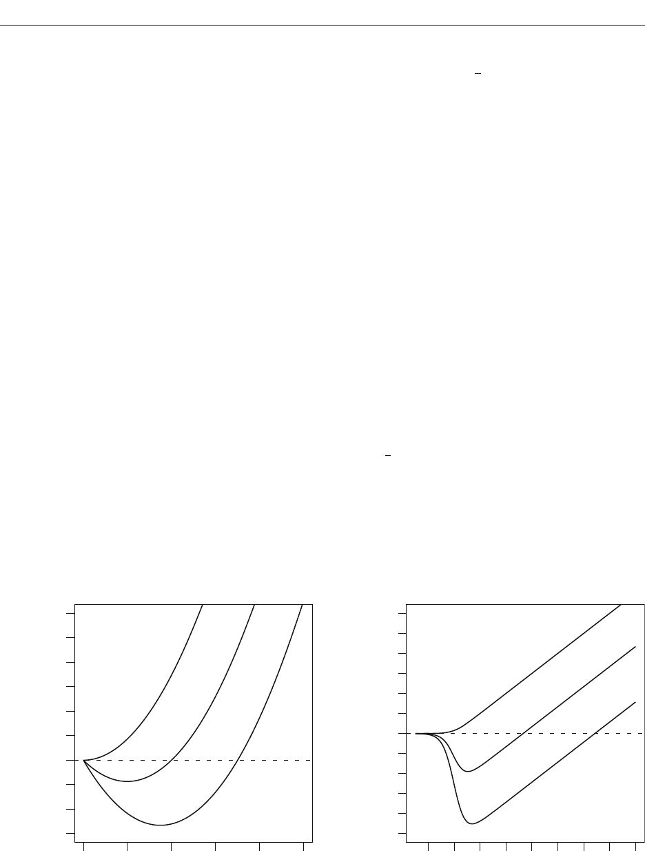
is specified. Figure 2A shows the effect of the choice of

the alternative, 

(measured in units of À), on the Bayes

factor for a few values of y (also measured in units of À)

when N  100.

This simple example illustrates that as

the alternative is placed farther from the observed data,

the Bayes factor increasingly favors the null. Moreover,

when the alternative is unrealistically far from the data,

the Bayes factor provides unbounded support for the null

hypothesis over this alternative. This insight that unreal-

istic alternatives yield support for the null will be utilized

in specifying appropriate alternatives.

In the example above, we assumed that the alternative was

at a single point. This assumption, however, is too restrictive

to be practical. Instead, it is more realistic to consider an

alternative that is a distribution across a range of outcomes.

For example, we may place a normal prior on :

Å ~ Normal(0, À



The normal is centered around zero to indicate no prior com-

mitment about the direction of effects. To use this normal

prior, the analyst must set À



a priori. The critical question

is how the choice of À



affects the Bayes factor.

One might

set À



 @, which specifies no prior information about . In

fact, this setting is used as a noninformative prior in Bayes-

ian estimation of  (see, e.g., Rouder & Lu, 2005).

Figure 2B shows the effect of the choice of À



(mea-

sured in units of À) on the resulting Bayes factor for a few

values of y (also measured in units of À) when N  100.

As À



becomes large, the value of B

increases, too. To

understand why this behavior occurs, it is helpful to recall

that the marginal likelihood of a composite hypothesis is

the weighted average of the likelihood over all constituent

point hypotheses, where the prior serves as the weight. As

fact is important in understanding why analysts must com-

mit to reasonable alternatives for principled inference.

For the one-sample application, the null model has a

single parameter, À

, and the alternative model has two

parameters, À

and . The marginal likelihoods are

Mf pd











y |

SSS

and

Mf pdd











c

¯¯

y |, , .

MS MS S M

For the one-sample case, priors are needed on À

to de-

scribe the null hypothesis. Likewise, priors are needed on

 and À

to describe the alternative. There are two different

schools of thought on how to choose priors in Bayesian

analysis. According to the first, subjective Bayes, school,

priors should reflect the analyst’s a priori beliefs about

parameters. These beliefs are informed by the theoreti-

cal and experimental context. According to the second,

objective Bayes, school, priors should reflect as few as-

sumptions as possible. In this article, we take the objective

approach; that is, we seek priors that reflect a minimum

degree of information.

The Role of Priors

In this section, we discuss how the choice of priors af-

fects the resulting Bayes factor. This discussion directly

motivates our recommendations and serves as a basis for

interpreting and understanding Bayes factors.

It is easiest to build intuition about the role of the pri-

ors in a simple case. Assume that À

is known and the

alternative is a point much like the null. The null is given

by   0; the alternative is given by   

, where 

Alternative 

(Units of )

Bayes Factor B

0.0 0.2 0.4 0.6 0.8 1.0

–

= 0

Prior Standard Deviation 



(Units of )

Bayes Factor B

0.01 1 10 1,000 1E+05

–

= 0.2

–

= 0.35

0.001

0.1

1,000

1E+05

1E–05

0.01

100

1E+05

–

= 0

–

= 0.15

–

= 0.22

Figure 2. (A) Bayes factors as a function of the alternative. (B) Bayes factors as a function of prior standard deviation À



for a nor-

mally distributed alternative. Lines depict different sample means (measured in units of standard deviation À).

230 ROUDER, SPECKMAN, SUN, MOREY, AND IVERSON

ily. The advantage of this effect-size parameterization is

that researchers have an intrinsic scale about the ranges

of effect sizes that applies broadly across different tasks

and populations. For instance, effect sizes of 1.0 are large;

those of .02 are very small. Importantly, we can use this

knowledge to avoid placing too much weight on unrea-

sonable effect-size values. For instance, we can all agree

that priors that place substantial mass on effect sizes over

6 are unrealistic; if a phenomenon yielded such large ef-

fect sizes, it would be so obvious as to make experiments

hardly necessary.

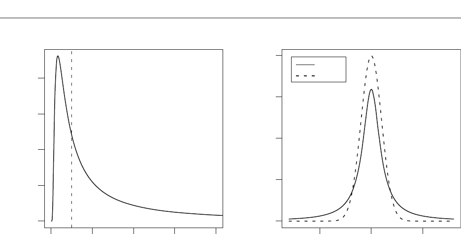
One reasonable setting is À

 1. The corresponding

prior on effect size, a standard normal, is shown in Fig-

ure 3B (dashed line) and is known as the unit-information

prior. The setting is reasonable because the distribution of

effect sizes under the alternative does not include much

mass on highly implausible effect sizes such as 6. One ad-

vantage of this setting is that small effects are assumed to

occur with greater frequency than large ones, which is in

accordance with what experimentalists tend to find. With

this setting, it can be shown that the alternative has only a

small amount of information—in fact, the amount in any

single observation (see Kass & Wasserman, 1995). In fact,

the unit-information prior underlies the Bayesian infor-

mation criterion (BIC; Raftery, 1995; Schwarz, 1978).

With the normal prior, the analyst commits to a single,

specific value for À

, such as À

 1. There is, however,

an even less informative formulation: Instead of setting À

to a single value, it can be allowed to range over a distribu-

tion of values. Zellner and Siow (1980) recommend the

following prior distribution for À

itself:

ÅÀ

~ inverse chi-square(1).



is increased, there is greater relative weight on larger

values of . Unreasonably large values of  under the al-

ternatives provide increased support for the null (as shown

in Figure 2A). When these unreasonably large values of

 have increasing weight, the average favors the null to a

greater extent. Hence, specifications of alternatives that

weight unreasonably large effects heavily will yield Bayes

factors that too heavily support the null. Moreover, the set-

ting of À



 @ implies that the Bayes factor provides un-

bounded support for the null, a fact known as the Jeffreys–

Lindley paradox (Lindley, 1957). Therefore, arbitrarily

diffuse priors are not appropriate for hypothesis testing.

To use the normal prior for the alternative, the re-

searcher must specify reasonable values for the variance



. One approach is to customize this choice for the para-

digm at hand. For example, the choice À



 20 msec may

be reasonable for exploring small effects such as those in

priming experiments. The value of À



should be greater

with more-variable data, such as those from complicated

tasks or from clinical populations.

A well-known and attractive alternative to placing pri-

ors on the mean  is to place them on effect size, where

effect size is denoted by Y and given as Y  /À. The null

hypothesis is Y  0. Alternatives may be specified as a

normal prior on effect size:

ÅY ~ Normal(0, À

where À

is specified a priori (Gönen, Johnson, Lu, &

Westfall, 2005). Reparameterizing the model in terms

of effect size Y rather than mean  does not change the

basic nature of the role of the prior. If À

is set unrealisti-

cally high, the Bayes factor will favor the null too heav-

02468

0.0

0.1

0.2

0.3

0.4

Prior Variance 



Density

0.0

0.1

0.2

0.3

0.4

Density

−5 0 5

Effect Size 

Cauchy

Normal

Figure 3. (A) Density of the inverse-chi-square prior distribution on À

. (B) Densities of the Cauchy (solid line) and normal (dashed

line) prior distributions on effect size Y.

BAY E S FACTOR 231

of Zellner and Siow. The JZS prior serves as the objective

prior for the one- and two-sample cases.

A Bayes-Factor One-Sample t Test

In the previous section, we outlined the JZS and unit-

information priors, with the JZS prior being noninforma-

tive for the one-sample case. In this section, we present

and discuss the Bayes factors for the JZS prior. The first

step in derivation is to compute marginal likelihoods M

and M

(by averaging the likelihoods with weights given

by the priors). These marginal likelihoods are then divided

to yield the Bayes factor. At the end of this process, Equa-

tion 1 (below) results for the Bayes factor, where t is the

conventional t statistic (see, e.g., Hays, 1994), N is the

number of observations, and v  N  1 is the degrees

of freedom. We refer to Equation 1 as the JZS Bayes fac-

tor for the one-sample problem. We recommend this JZS

Bayes factor as a default for conducting Bayesian t tests.

To our knowledge, Equation 1 is novel. The derivation is

straightforward and tedious and not particularly informa-

tive. Gönen et al. (2005) provided the analogous equation

for the unit-information Bayes factor. Liang et al. (2008)

provided the corresponding JZS Bayes factors for testing

slopes in a regression model.

Although Equation 1 may look daunting, it is simple to

use. Researchers need only provide the sample size N and

the observed t value. There is no need to input raw data.

The integration is over a single dimension and is compu-

tationally straightforward. We provide a freely available

Web-based program that computes the JZS Bayes fac-

tor for input values of t and N (pcl.missouri.edu). It also

computes the unit-information Bayes factor—that is, the

Bayes factor when the unit-information prior is assumed.

Table 1 provides critical t values needed for JZS Bayes

factor values of 1/10, 1/3, 3, and 10 as a function of sam-

ple size. This table is analogous in form to conventional

t value tables for given p value criteria. For instance, sup-

pose a researcher observes a t value of 3.3 for 100 obser-

vations. This t value favors the alternative and corresponds

to a JZS Bayes factor less than 1/10 because it exceeds

the critical value of 3.2 reported in the table. Likewise,

suppose a researcher observes a t value of 0.5. The cor-

responding JZS Bayes factor is greater than 10 because

the t value is smaller than 0.69, the corresponding criti-

cal value in Table 1. Because the Bayes factor is directly

interpretable as an odds ratio, it may be reported without

reference to cutoffs such as 3 or 1/10. Readers may decide

the meaning of odds ratios for themselves.

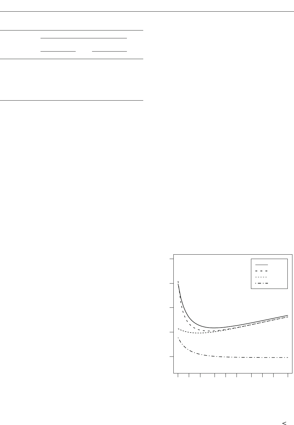
Figure 4 shows the critical t value needed for JZS Bayes

factors of 1/10, a substantial amount of evidence in favor

of the alternative (solid line). For large sample sizes, in-

The inverse chi-square family provides useful priors in

Bayesian statistics (see, e.g., Gelman, Carlin, Stern, &

Rubin, 2004). The density function of the inverse chi-

square with one degree of freedom is shown in Figure 3A.

Mass falls off for very small and very large values of À

;

that is, À

is constrained to be somewhat near 1.0. This

specification is less informative than the previously dis-

cussed unit-information prior, which requires À

 1.

Even though we explicitly place a prior on À

, there is a

corresponding prior on effect size obtained by integrating

out À

. Liang, Paulo, Molina, Clyde, and Berger (2008)

noted that placing a normal on effect size with a variance

that is distributed as an inverse chi-square is equivalent to

placing the following prior on effect size:

ÅY ~ Cauchy.

The Cauchy distribution is a t distribution with a single

degree of freedom. It has tails so heavy that neither its

mean nor its variance exist. A comparison of the Cauchy

prior to the unit-information prior is shown in Figure 3B.

As can be seen, the Cauchy allows for more mass on large

effects than the standard normal. Consequently, Bayes

factors with the Cauchy prior favor the null a bit more

than those with the unit-information prior. It is important

to note that the Cauchy was not assumed directly; it results

from the assumption of a normal distribution on Y with

variance À

distributed as an inverse chi-square. Jeffreys

(1961) was the first to consider the Cauchy specification

of the alternative for Bayes factor calculations.

In the preceding analyses, we assumed that À

, the vari-

ability in the data, is known. Fortunately, it is relatively easy

to relax this assumption. The intuition from the preceding

discussion is that priors on parameters cannot be too vari-

able, because they then include a number of unreasonable

values that, when included in the average, lower the mar-

ginal likelihood. This intuition is critical for comparisons of

models when a parameter enters into only one of the models,

as is the case for parameter Y. It is much less critical when

the parameter in question enters into both models, as is the

case for parameter À

. In this case, having mass on unrealis-

tic values lowers the marginal likelihood of both models, and

this effect cancels in the Bayes factor ratio. For the one- and

two-sample cases, a very broad noninformative prior on À

is possible. We make a standard choice: p(À

)  1/À

. This

prior is known as the Jeffreys prior on variance (Jeffreys,

1961). The justification for this choice, though beyond the

scope of this article, is provided in all Bayesian textbooks.

With this choice for À

, the specification of priors is

complete. We refer to the combination of the Cauchy on ef-

fect size and the Jeffreys prior on variance as the JZS prior,

in order to acknowledge the contributions of Jeffreys and













()/

()

ge dg





()/

///()

()

12 32 1 2

(1)

232 ROUDER, SPECKMAN, SUN, MOREY, AND IVERSON

training was effective. The reported F value corresponds

to a t value of 2.39. The JZS Bayes factor for this contrast

is 0.63, which is about 1.6 to 1 in favor of the alternative.

These odds, however, do not constitute much evidence for

the effectiveness of the training program.

Subjectivity in Priors

The JZS prior is designed to minimize assumptions

about the range of effect size, and in this sense it is an

objective prior. In many cases, researchers have knowl-

edge of the domain that may improve inference. This

knowledge may be incorporated by changing the form

of the prior. On a rather mundane level, a researcher may

believe that psychologists tend not to run experiments to

search for effects so large that they may be confirmed

with 10 or fewer observations. This belief implies that

effect sizes much greater than 2.0 in magnitude are im-

probable, because larger effect sizes would be evident

with only a handful of observations. This belief, which

strikes us as reasonable in many contexts, might lead

some analysts to choose the unit-information Bayes

factor over the JZS Bayes factor, since the tails of the

normal prior on effect size fall more quickly than those

of the Cauchy (see Figure 3B). We recommend that re-

searchers incorporate information when they believe it

to be appropriate. If they have no such information or

wish not to commit to any, the JZS prior can serve as

the noninformative default. The Web-based program also

calculates unit-information Bayes factors.

Researchers may also incorporate expectations and

goals for specific experimental contexts by tuning the

scale of the prior on effect size. The JZS prior on effect

creasingly larger t values are needed to maintain the same

odds. This behavior ensures that the JZS Bayes factor

does not favor the alternative when there are small effects

in large samples. The dashed-and-dotted line shows the

needed t value for p  .05. This t value does not increase

with sample size. Also shown is the curve for the unit-

information Bayes factor (longer dashed line), which is

derived from the unit-information prior (À

 1) with a

noninformative Jeffreys prior on À

—that is, p(À

)  1/À

As can be seen, the unit-information Bayes factor behaves

similarly to the JZS Bayes factor. The shorter dashed line

is for the BIC, which is discussed subsequently.

Figure 4 reveals that inference with a criterial p value

of .05 admits much lower t values as evidence against the

null hypothesis than do Bayesian methods with criterial

odds of 10:1. This difference has implications in practice.

We highlight a few recent examples from the literature

in which researchers have rejected the null even though

the posterior odds do not indicate that such a rejection is

warranted. Grider and Malmberg (2008) assessed whether

participants remembered emotional words better than

neutral ones in a recognition memory task. In their Experi-

ment 3, they used a forced choice paradigm in which the

targets and lures at test had the same emotional valence.

The advantage of this design is that any difference in ac-

curacy could not be due to a response bias for a particular

emotional-valence level. Grider and Malmberg claimed

that emotional words were remembered better than neutral

ones on the basis of two paired t tests on accuracy: one

between neutral and positive words [.76 vs. .80; t(79) 

2.24] and one between neutral and negative words [.76 vs.

.79; t(79)  2.03]. The JZS Bayes factors for these t val-

ues and the sample size of N  80 may be obtained from

the Web-based program. The resulting values are B



1.02 and B

 1.56 for the two tests, which can only be

considered as ambiguous evidence. The latter contrast is

especially interesting because the evidence favors the null

slightly (odds of 3:2), even though the null is rejected by

a significance test with p  .05.

Another example comes from Plant and Peruche

(2005), who assessed whether a sensitivity training pro-

gram reduced the likelihood that law enforcement offi-

cers mistakenly shot civilians in a computer simulation.

They assessed how 48 participating officers performed

before and after training. On the basis of a significant one-

sample F test [F(1,47)  5.70], they concluded that the

Table 1

Critical t Values

JZS Bayes Factor Value

Favors Null

Favors

Alternative

N 10 3 1/3 1/10

5 – 0.40 3.15 4.97

10 – 0.89 2.73 3.60

20 – 1.20 2.64 3.26

50 – 1.51 2.68 3.17

100 0.69 1.72 2.76 3.20

200 1.08 1.90 2.86 3.27

500 1.44 2.12 2.99 3.38

Sample Size

Critical t Value

55020 200 1,000 5,000

JZS BF

Unit BF

BIC

p value

Figure 4. Critical t values needed for posterior odds of 10:1

favoring the alternative for the JZS Bayes factor (solid line), the

unit-information Bayes factor (longer dashed line), and the BIC

(shorter dashed line), as well as critical t values needed for p  .05

(dashed-and-dotted line).

BAY E S FACTOR 233

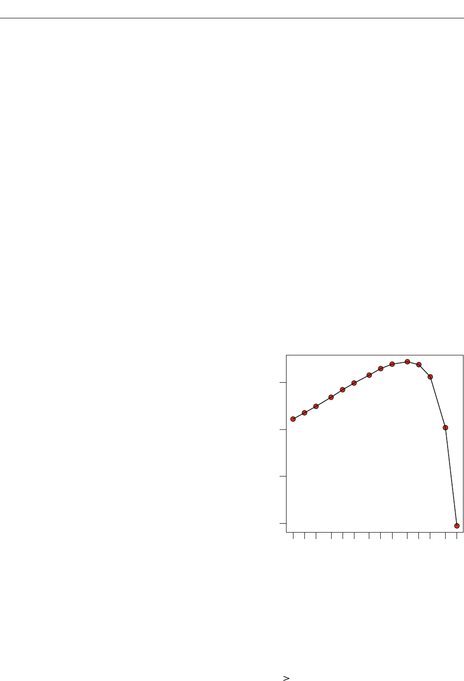
Figure 5 shows how the Bayes factor depends on sample

size for the small true effect size of Y  .02. For small to

moderate sample sizes, the Bayes factor supports the null.

As the sample size becomes exceedingly large, however,

the small deviations from the null are consequential, and

the Bayes factor yields less support for the null. In the large-

sample limit, the Bayes factor favors the alternative, since

the null is not exactly true. This behavior strikes us as ideal.

With smaller sample sizes that are insufficient to differenti-

ate between approximate and exact invariances, the Bayes

factors allows researchers to gain evidence for the null.

This evidence may be interpreted as support for at least an

approximate invariance. In very large samples, however,

the Bayes factor allows for the discovery of small perturba-

tions that negate the existence of an exact invariance. In

sum, the Bayes factor favors the more parsimonious null-

model description with small observed effect sizes unless

the sample size is so large that even these small effects are

not compatible with the null relative to the alternative.

Extension to Two-Sample Designs

The Bayes factor in Equation 1 is applicable for one-

sample designs and is analogous to a paired t test. One-

sample designs are common in experimental psychology

because variables are often manipulated in a within-

subjects manner. Between-subjects designs are also com-

mon and are often used to compare participant variables

such as age or gender. For cases with two independent

size can be generalized to Y ~ r  Cauchy, where r is a

scale factor.

The unit-information prior can be scaled,

too: Y ~ Normal(0, r

). In this case, however, the term

unit-information prior may be misleading, and we pre-

fer the term scaled-information prior.

For both JZS and

scaled-information priors, as r is increased, the Bayes fac-

tor provides increased support for the null. In Equation 1,

the scale r is implicitly set to 1.0, which serves as a natural

benchmark. Smaller values of r, say 0.5, may be appropri-

ate when small effect sizes are expected a priori; larger

values of r are appropriate when large effect sizes are ex-

pected. The choice of r may be affected by theoretical con-

siderations, as well: Smaller values are appropriate when

small differences are of theoretical importance, whereas

larger values are appropriate when small differences most

likely reflect nuisances and are of little theoretical impor-

tance. In all cases, the value of r should be chosen prior to

analysis and without influence from the data. In summary,

r  1.0 is recommended, though a priori adjustments may

be warranted in certain contexts. The aforementioned

Web-based program allows researchers to specify r, with

r  1.0 serving as a default.

It may appear that Bayes factors are too dependent on

the prior to be of much use. Perhaps researchers can en-

gineer any result they wish by surreptitiously choosing a

self-serving prior. This appearance is deceiving. Bayes fac-

tors are not particularly sensitive to reasonable variation

in priors, at least not with moderate sample sizes. In prac-

tice, dramatic changes in the priors often have marginal

effects on the results. The previous example of the results

from Grider and Malmberg (2008) is useful for making this

point. The t value of 2.03 actually corresponded to slight

evidence for the null (B

 1.56), even though the null

was rejected at the p  .05 level. A reasonable conclusion

is that there was not enough evidence in the experiment

to express preference for either the null or the alternative

hypothesis. The unit-information Bayes factor in this case

is 1.21, which leads to the same conclusion. Suppose we

commit a priori to an alternative that is characterized by

very small effect sizes for Grider and Malmberg’s experi-

ments. Setting r  0.1, which seems too low, results in a

JZS Bayes factor of 0.59. Although this value now slightly

favors the alternative, it does not support a preference for it.

For Grider and Malmberg’s data, any reasonable prior leads

to the same conclusion, that the evidence does not support

a preference. In general, researchers may differ in their

choice of priors. If these differences are reasonable, they

will have only modest effects on the resulting conclusions.

Bayes Factors With Small Effects

Previously, we considered the argument that invariances

are only true approximately and never exactly (Cohen,

1994). In this section, we explore the behavior of Bayes

factors when an invariance holds approximately rather

than exactly. As discussed previously, the view that the

null can never hold exactly does not negate its usefulness

as an idealization. Our main question is whether the Bayes

factor provides an appropriate decision about whether the

null or the alternative provides a better description of the

data for very small true effect sizes.

Bayes Factor

100

200

500

1,000

2,000

5,000

10,000

20,000

50,000

1E+05

0.01

0.1

Sample Size

Figure 5. Bayes factors for a small true effect size (.02). Shown

is the expected unit-information Bayes factor as a function of

sample size. These expected values are obtained by a Monte Carlo

simulation in which data are repeatedly sampled from a normal

distribution with effect size Y  .02. As shown, the Bayes factor

allows researchers to gain evidence for the approximate invari-

ance with sample sizes below 5,000 and to gain evidence for small

effects with sample sizes over 50,000. The JZS Bayes factor acts

similarly, although the evaluation of the integral is unstable for

sample sizes

5,000.

234 ROUDER, SPECKMAN, SUN, MOREY, AND IVERSON

Consequently,

.



We have included critical t values for B

 1/10 (10:1

favoring the alternative) in Figure 4. As can be seen, the

BIC behaves well for large samples.

BIC is an asymptotic approximation to a Bayes factor

with certain priors (Raftery, 1995). For the one-sample

case, these priors are

SSS

MMS

222

Normal









where R  y

and RÀ

 (1/N )( y

 y)

are the maximum

likelihood estimators of  and À

, respectively. These

priors are more informative than the ones we advocate.

There are two main differences: (1) The prior variance on

 is the sample variance. In Bayesian inference, it is not

valid to specify a prior that depends on the observed data.

The justification for this prior is that it is a convenient

large-sample approximation for a unit-information prior.

Hence, it may only be interpreted for large-sized samples.

The JZS and unit-information priors, on the other hand,

do not depend on the observed data. As a consequence,

the resulting Bayes factors may be interpreted with confi-

dence for all sample sizes. (2) Because BIC approximates

a unit-information prior, it is slightly more informative

than the JZS prior. As such, the resulting BIC values will

slightly favor the alternative more than the JZS Bayes fac-

tor would.

BIC is not well-suited for mixed models, such as

within-subjects ANOVA. The problem is that BIC is based

on counting parameters. The more parameters a model

has, the more it is penalized for complexity. In standard

between-subjects designs with fixed effects, the number

of parameters is unambiguous. In mixed designs, however,

each participant is modeled as a random effect that is nei-

ther entirely free (the effects must conform to a particu-

lar distribution) nor heavily constrained. It is not obvious

how these random effects are to be counted or penalized in

BIC. Bayes factors also penalize complex models, but they

do so without recourse to counting parameters. Instead,

complex models are penalized by the diversity of data pat-

terns they explain (Myung & Pitt, 1997). It is known that

JZS priors extend well to simple random- effects models

(García-Donato & Sun, 2007), and we anticipate that they

may be used more generally in mixed models, especially

with within-subjects factorial designs.

General Discussion

There has been a long-lasting and voluminous debate

in both psychology and statistics on the value of sig-

nificance tests. Most of this debate has centered on the

proper way to test for effects. We advocate a different

focus: Psychologists should search for theoretically in-

teresting invariances or regularities in data. Conventional

significance tests are ill-suited for stating evidence for

groups, the two-sample (groups) t test is appropriate.

Below is the development of the JZS Bayes factor for the

two-sample case.

Let x

and y

denote the ith observations in the first and

second groups, respectively. These observations are con-

ventionally modeled as

iid

Normal







, i  1, . . . , N

iid

Normal







, , i  1, . . . , N

where  and ( denote the grand mean and total effect,

respectively, and N

and N

denote the sample size for the

first and second groups, respectively. The null hypoth-

esis corresponds to (  0. As before, it is convenient to

consider an effect size, Y  (/À. In this parameterization,

the null hypothesis corresponds to Y  0; the JZS prior

for Y under the alternative is given by

ÅY ~ Cauchy.

Priors are needed for  and À

. Fortunately, these pa-

rameters are common to both models, and the resulting

Bayes factor is relatively robust to the choice. The Jeffreys

noninformative prior on À

, p(À

)  1/À

, is appropriate.

A noninformative prior may also be placed on . In this

prior, all values of  are equally likely; this prior is de-

noted p()  1.

Equation 1 may be adapted to compute the two-sample

JZS Bayes factor with the following three substitutions:

(1) The value of t is the observed two-sample (grouped)

t value; (2) the effective sample size is N  N

/(N



); and (3) the degrees of freedom are v  N

 N

 2.

Our Web-based program also computes JZS and unit

Bayes factors for this two-sample case; the user need only

input both sample sizes and the group t value.

Bayesian Information Criterion

The BIC (Schwarz, 1978) is a Bayesian model selec-

tion technique that has been recommended in psychology

(see, e.g., Wagenmakers, 2007). In the BIC, each model

is given a score:

BIC  2 log L  k log N,

where L is the maximum likelihood of the model, N is the

sample size, and k is the number of parameters. Models

with lower BIC scores are preferred to models with higher

ones. As pointed out by Raftery (1995), differences in

BIC scores may be converted into an approximate Bayes

factor:

exp ,



BIC BIC

where BIC

and BIC

are the BIC scores for the null and

the alternative, respectively. For the one-sample case, it is

straightforward to show that

BIC BIC

 



N

Nlog log .

BAY E S FACTOR 235

Ashby, F. G., & Maddox, W. T. (1992). Complex decision rules in cat-

egorization: Contrasting novice and experienced performance. Jour-

nal of Experimental Psychology: Human Perception & Performance,

18, 50-71.

Augustin, T. (2008). Stevens’ power law and the problem of meaning-

fulness. Acta Psychologica, 128, 176.

Berger, J. O., & Berry, D. A. (1988). Analyzing data: Is objectivity

possible? American Scientist, 76, 159-165.

Bishop, Y. M. M., Fienberg, S. E., & Holland, P. W. (1975). Discrete

multivariate analysis: Theory and practice. Cambridge, MA: MIT

Press.

Clarke, F. R. (1957). Constant-ratio rule for confusion matrices in

speech communication. Journal of the Acoustical Society of America,

29, 715-720.

Cohen, J. (1994). The earth is round ( p  .05). American Psychologist,

49, 997-1003.

Cumming, G., & Finch, S. (2001). A primer on the understanding, use,

and calculation of confidence intervals based on central and noncentral

distributions. Educational & Psychological Measurement, 61, 532-574.

Debner, J. A., & Jacoby, L. L. (1994). Unconscious perception: Atten-

tion, awareness, and control. Journal of Experimental Psychology:

Learning, Memory, & Cognition, 20, 304-317.

Dehaene, S., Naccache, L., Le Clec’H, G., Koechlin, E., Muel-

ler, M., Dehaene-Lambertz, G., et al. (1998). Imaging uncon-

scious semantic priming. Nature, 395, 597-600.

Edwards, W., Lindman, H., & Savage, L. J. (1963). Bayesian statisti-

cal inference for psychological research. Psychological Review, 70,

193-242.

Egan, J. P. (1975). Signal detection theory and ROC-analysis. New

York: Academic Press.

Fechner, G. T. (1966). Elements of psychophysics. New York: Holt,

Rinehart & Winston. (Original work published 1860)

García-Donato, G., & Sun, D. (2007). Objective priors for hypothesis

testing in one-way random effects models. Canadian Journal of Sta-

tistics, 35, 303-320.

Gelman, A., Carlin, J. B., Stern, H. S., & Rubin, D. B. (2004). Bayes-

ian data analysis (2nd ed.). Boca Raton, FL: Chapman & Hall.

Gillispie, C. C., Fox, R., & Grattan-Guinness, I. (1997). Pierre-

Simon Laplace, 1749–1827: A life in exact science. Princeton, NJ:

Princeton University Press.

Gönen, M., Johnson, W. O., Lu, Y., & Westfall, P. H. (2005). The

Bayesian two-sample t test. American Statistician, 59, 252-257.

Goodman, S. N. (1999). Toward evidence-based medical statistics:

I. The p value fallacy. Annals of Internal Medicine, 130, 995-1004.

Green, D. M., & Swets, J. A. (1966). Signal detection theory and

psychophysics. New York: Wiley.

Grider, R. C., & Malmberg, K. J. (2008). Discriminating between

changes in bias and changes in accuracy for recognition memory of

emotional stimuli. Memory & Cognition, 36, 933-946.

Hawking, S. (E

D.) (2002). On the shoulders of giants: The great works

of physics and astronomy. Philadelphia: Running Press.

Hays, W. L. (1994). Statistics (5th ed.). Fort Worth, TX: Harcourt

Brace.

Jacoby, L. L. (1991). A process dissociation framework: Separating

automatic from intentional uses of memory. Journal of Memory &

Language, 30, 513-541.

Jeffreys, H. (1961). Theory of probability (3rd ed.). Oxford: Oxford

University Press, Clarendon Press.

Kass, R. E., & Raftery, A. E. (1995). Bayes factors. Journal of the

American Statistical Association, 90, 773-795.

Kass, R. E., & Wasserman, L. (1995). A reference Bayesian test for

nested hypotheses with large samples. Journal of the American Statis-

tical Association, 90, 928-934.

Killeen, P. R. (2005). An alternative to null-hypothesis significance

tests. Psychological Science, 16, 345-353.

Killeen, P. R. (2006). Beyond statistical inference: A decision theory

for science. Psychonomic Bulletin & Review, 13, 549-562.

Kline, R. B. (2004). Beyond significance testing: Reforming data

analysis methods in behavioral research. Washington, DC: American

Psychological Association.

Lee, M. D., & Wagenmakers, E.-J. (2005). Bayesian statistical infer-

ence in psychology: Comment on Trafimow (2003). Psychological

Review, 112, 662-668.

invariances and, as a consequence, overstate the evidence

against them.

It is reasonable to ask whether hypothesis testing is always

necessary. In many ways, hypothesis testing has been em-

ployed in experimental psychology too often and too hast-

ily, without sufficient attention to what may be learned by

exploratory examination for structure in data (Tukey, 1977).

To observe structure, it is often sufficient to plot estimates

of appropriate quantities along with measures of estimation

error (Rouder & Morey, 2005). As a rule of thumb, hypoth-

esis testing should be reserved for those cases in which the

researcher will entertain the null as theoretically interesting

and plausible, at least approximately.

Researchers willing to perform hypothesis testing must

realize that the endeavor is inherently subjective (Berger

& Berry, 1988). For any data set, the null will be superior

to some alternatives and inferior to others. Therefore, it

is necessary to commit to specific alternatives, with the

resulting evidence dependent to some degree on this com-

mitment. This commitment is essential to and unavoid-

able for sound hypothesis testing in both frequentist and

Bayesian settings. We advocate Bayes factors because

their interpretation is straightforward and natural. More-

over, in Bayesian analysis, the elements of subjectivity

are transparent rather than hidden (Wagenmakers, Lee,

Lodewyckx, & Iverson, 2008).

This commitment to specify judicious and reasoned al-

ternatives places a burden on the analyst. We have provided

default settings appropriate to generic situations. Nonethe-

less, these recommendations are just that and should not be

used blindly. Moreover, analysts can and should consider

their goals and expectations when specifying priors. Sim-

ply put, principled inference is a thoughtful process that

cannot be performed by rigid adherence to defaults.

There is no loss in dispensing with the illusion of ob-

jectivity in hypothesis testing. Researchers are acclimated

to elements of social negotiation and subjectivity in sci-

entific endeavors. Negotiating the appropriateness of vari-

ous alternatives is no more troubling than negotiating the

appropriateness of other elements, including design, oper-

ationalization, and interpretation. As part of the everyday

practice of psychological science, we have the communal

infrastructure to evaluate and critique the specification of

alternatives. This view of negotiated alternatives is vastly

preferable to the current practice, in which significance

tests are mistakenly regarded as objective. Even though

inference is subjective, we can agree on the boundaries

of reasonable alternatives. The sooner we adopt inference

based on specifying alternatives, the better.

AUTHOR NOTE

We are grateful for valuable comments from Michael Pratte, E.-J.

Wagenmakers, and Peter Dixon. This research was supported by NSF

Grant SES-0720229 and NIMH Grant R01-MH071418. Please address

correspondence to J. N. Rouder, Department of Psychological Sciences,

210 McAlester Hall, University of Missouri, Columbia, MO 65211

(e-mail: [email protected]).

REFERENCES

Akaike, H. (1974). A new look at the statistical model identification.

IEEE Transactions on Automatic Control, 19, 716-723.

236 ROUDER, SPECKMAN, SUN, MOREY, AND IVERSON

Rouder, J. N., Morey, R. D., Speckman, P. L., & Pratte, M. S.

(2007). Detecting chance: A solution to the null sensitivity problem

in subliminal priming. Psychonomic Bulletin & Review, 14, 597-

605.

Rouder, J. N., & Ratcliff, R. (2004). Comparing categorization mod-

els. Journal of Experimental Psychology: General, 133, 63-82.

Schwarz, G. (1978). Estimating the dimension of a model. Annals of

Statistics, 6, 461-464.

Sellke, T., Bayarri, M. J., & Berger, J. O. (2001). Calibration of

p values for testing precise null hypotheses. American Statistician,

55, 62-71.

Shepard, R. N. (1957). Stimulus and response generalization: A sto-

chastic model relating generalization to distance in psychological

space. Psychometrika, 22, 325-345.

Shibley Hyde, J. (2005). The gender similarities hypothesis. American

Psychologist, 60, 581-592.

Shibley Hyde, J. (2007). New directions in the study of gender simi-

larities and differences. Current Directions in Psychological Science,

16, 259-263.

Stevens, S. S. (1957). On the psychophysical law. Psychological Re-

view, 64, 153-181.

Swets, J. A. (1996). Signal detection theory and ROC analysis in psy-

chology and diagnostics: Collected papers. Mahwah, NJ: Erlbaum.

Tukey, J. W. (1977). Exploratory data analysis. Reading, MA: Addison-

Wesley.

Wagenmakers, E.-J. (2007). A practical solution to the pervasive prob-

lem of p values. Psychonomic Bulletin & Review, 14, 779-804.

Wagenmakers, E.-J., & Grünwald, P. (2006). A Bayesian perspective

on hypothesis testing: A comment on Killeen (2005). Psychological

Science, 17, 641-642.

Wagenmakers, E.-J., Lee, M. D., Lodewyckx, T., & Iverson, G.

(2008). Bayesian versus frequentist inference. In H. Hoijtink, I. Klug-

kist, & P. A. Boelen (Eds.), Bayesian evaluation of informative hypo-

theses in psychology (pp. 181-207). New York: Springer.

Zellner, A., & Siow, A. (1980). Posterior odds ratios for selected re-

gression hypotheses. In J. M. Bernardo, M. H. DeGroot, D. V. Lindley,

& A. F. M. Smith (Eds.), Bayesian statistics: Proceedings of the First

International Meeting (pp. 585-603). Valencia: University of Valencia

Press.

Lehmann, E. L. (1993). The Fisher, Neyman–Pearson theories of testing

hypotheses: One theory or two? Journal of the American Statistical

Association, 88, 1242-1249.

Liang, F., Paulo, R., Molina, G., Clyde, M. A., & Berger, J. O.

(2008). Mixtures of g priors for Bayesian variable selection. Journal

of the American Statistical Association, 103, 410-423.

Lindley, D. V. (1957). A statistical paradox. Biometrika, 44,

187-192.

Logan, G. D. (1988). Toward an instance theory of automatization.

Psychological Review, 95, 492-527.

Logan, G. D. (1992). Shapes of reaction-time distributions and shapes

of learning curves: A test of the instance theory of automaticity. Jour-

nal of Experimental Psychology: Learning, Memory, & Cognition,

18, 883-914.

Luce, R. D. (1959). Individual choice behavior: A theoretical analysis.

New York: Wiley.

Masson, M. E. J., & Loftus, G. R. (2003). Using confidence intervals

for graphically based data interpretation. Canadian Journal of Experi-

mental Psychology, 57, 203-220.

Meehl, P. E. (1978). Theoretical risks and tabular asterisks: Sir Karl, Sir

Ronald, and the slow progress of soft psychology. Journal of Consult-

ing & Clinical Psychology, 46, 806-834.

Myung, I.-J., & Pitt, M. A. (1997). Applying Occam’s razor in model-

ing cognition: A Bayesian approach. Psychonomic Bulletin & Review,

4, 79-95.

Plant, E. A., & Peruche, B. M. (2005). The consequences of race for

police officers’ responses to criminal suspects. Psychological Science,

16, 180-183.

Raftery, A. E. (1995). Bayesian model selection in social research.

Sociological Methodology, 25, 111-163.

Reingold, E. M., & Merikle, P. M. (1988). Using direct and indirect

measures to study perception without awareness. Perception & Psy-

chophysics, 44, 563-575.

Rouder, J. N., & Lu, J. (2005). An introduction to Bayesian hierarchical

models with an application in the theory of signal detection. Psycho-

nomic Bulletin & Review, 12, 573-604.

Rouder, J. N., & Morey, R. D. (2005). Relational and arelational con-

fidence intervals: A comment on Fidler, Thomason, Cumming, Finch,

and Leeman (2004). Psychological Science, 16, 77-79.

NOTES

1. The calculation of the standard deviation of y

assumes that there are no participant-by-item interactions. This assumption

is made for computational convenience, and the presence of such interactions does not threaten the validity of the argument

that significance tests overstate the evidence against the null hypothesis.

2. For the case in which the alternative is a point and À is known,

2















exp ,

exp .







The Bayes factor is given by

2 





exp .

This Bayes factor is a function of y/À, the observed effect size, and 

/À, the effect size of the alternative.

3. The Bayes factor with the normal prior is





SFS

exp

where



N



This Bayes factor depends only on the observed effect size y/À and the ratio À



/À.

BAY E S FACTOR 237

4. The scaled JZS Bayes factor is

Ngr















()/

rrv

12 32















()/

()

ddg

where r is the scale factor.

5. The scaled-information Bayes factor is















()/







v()/

where r is the scale factor. The unit-information Bayes factor holds when r  1.

6. There is a more principled Bayes factor calculation for those who believe that the null can never be true a priori. The null

may be specified as a composite—that is, as a distribution of effect sizes. A reasonable choice is that under the null, the effect

size is normally distributed with a mean of 0 and a small standard deviation of, say, .05. If this standard deviation is much

smaller than that for the alternative, then the JZS Bayes factor serves as a suitable approximation for moderate sample sizes.

(Manuscript received June 4, 2008;

revision accepted for publication August 27, 2008.)