
© 2020 International Monetary Fund
IMF Country Report No. 20/40
JAPAN
SELECTED ISSUES
This Selected Issues paper on Japan was prepared by a staff team of the International
Monetary Fund as background documentation for the periodic consultation with the
member country. It is based on the information available at the time it was completed on
January 14, 2020.
Copies of this report are available to the public from
International Monetary Fund • Publication Services
PO Box 92780 • Washington, D.C. 20090
Telephone: (202) 623-7430 • Fax: (202) 623-7201
E-mail: publications@imf.org Web: http://www.imf.org
Price: $18.00 per printed copy
International Monetary Fund
Washington, D.C.
February 2020
JAPAN
SELECTED ISSUES
Approved By
Asia and Pacific
Department
Prepared by a team led by Paul Cashin and Todd Schneider,
with individual chapters authored by Mariana Colacelli,
Takuma Hisanaga, Gee Hee Hong (all APD), Anh Thi Ngoc
Nguyen, Takuya Kamoshida, Siegfried Steinlein (all OAP),
Adrian Peralta-Alva (AFR), Mehdi Raissi (FAD), Niklas
Westelius (FIN), Yuko Hashimoto, Cyril Rebillard (both RES),
Sandra Lizarazo Ruiz (SPR), Kamiar Mohaddes, Xiaoxiao
Zhang (both University of Cambridge) and Yuki Yao
(University of Minnesota).
DISAPPEARING CITIES: DEMOGRAPHIC HEADWINDS AND THEIR IMPACT ON
JAPAN’S HOUSING MARKET ________________________________________________________ 5
A. Motivation ___________________________________________________________________________ 5
B. Demographics and Housing Prices in Japan __________________________________________ 6
C. Modeling Population Growth and Housing Prices ___________________________________ 8
D. Why are Japanese Moving to Large Cities? ________________________________________ 11
E. Policy Implications _________________________________________________________________ 12
References ____________________________________________________________________________ 15
BOX
1. Recent Developments in Residential Property Prices in Japan ______________________ 14
FIGURES
1. Population Change by Prefectures Between 1996-2015 ______________________________ 6
2. Household Statistics__________________________________________________________________ 7
3. House Price Change by Prefecture ___________________________________________________ 8
4. Population Growth and Housing Price Change _______________________________________ 9
5. Changes in House Price and Net Migration Flows __________________________________ 10
6. Education and House Prices ________________________________________________________ 12
CONTENTS
January 14, 2020

JAPAN
2 INTERNATIONAL MONETARY FUND
TABLE
1. Empirical Analysis of Land Price and Population Changes __________________________ 11
IS AUTOMATION THE ANSWER TO JAPAN’S DEMOGRAPHIC CHALLENGES? ___ 16
A. Motivation _________________________________________________________________________ 16
B. Framework of Analysis _____________________________________________________________ 17
C. Main Findings ______________________________________________________________________ 19
D. Conclusions ________________________________________________________________________ 21
References ____________________________________________________________________________ 23
JAPAN’S FERTILITY RATE ___________________________________________________________ 24
A. Introduction _______________________________________________________________________ 24
B. Overview of Japan’s Fertility Rate __________________________________________________ 25
C. Empirical Analysis: Data and Methodology_________________________________________ 27
D. Results _____________________________________________________________________________ 29
E. Policy Implications and Conclusions ________________________________________________ 30
References ____________________________________________________________________________ 32
FIGURE
1. Japan’s Fertility Rate–Stylized Facts ________________________________________________ 25
TABLE
1. Estimation Results of Total Fertility Rate by Prefecture, 2001–15 ___________________ 31
TWENTY YEARS OF INDEPENDENCE: LESSONS AND WAY FORWARD FOR THE
BANK OF JAPAN ____________________________________________________________________ 34
A. Evolution of the Bank of Japan’s Policy Objectives and Goal _______________________ 34
B. Unconventional Strategies to Reflate the Economy ________________________________ 35
C. Communication Strategies and Inflation Expectations _____________________________ 40
D. Lessons Learned and Way Forward ________________________________________________ 42
E. Conclusions ________________________________________________________________________ 46
References ____________________________________________________________________________ 48
FIGURES
1. Inflation and GDP Growth, 1998–2019 _____________________________________________ 36
2. Monetary Policy Operations, 1998–2019 ___________________________________________ 36
TABLES
1. Monetary and Financial Stability Objectives and Goals of Selected Central Banks __ 44

JAPAN
INTERNATIONAL MONETARY FUND 3
2. Publication of Forecasts and Risk Assessments by Selected Central Banks _________ 47
JAPAN’S BOOM IN INBOUND TOURISM ___________________________________________ 50
A. Introduction _______________________________________________________________________ 50
B. Development and Impact of Inbound Tourism _____________________________________ 50
C. Tourism Promotion Policies ________________________________________________________ 57
D. Determinants of Inbound Tourism _________________________________________________ 57
E. Conclusions and Policies ___________________________________________________________ 59
References ____________________________________________________________________________ 61
FIGURES
1. International Arrivals _______________________________________________________________ 51
2. Tourism Expenditure _______________________________________________________________ 52
3. Tourism Contribution, Growth and Jobs ____________________________________________ 53
4. Overnight Stays of Inbound Visitors in Prefectures _________________________________ 56
5. Tourism Impact at Regional and Prefectural Level __________________________________ 56
6. Government Efforts to Boost Tourism ______________________________________________ 58
TABLE
1. Determinants of Tourist Arrivals to Japan, 1996-2018 ______________________________ 59
ANNEXES
I. Tourists’ Spending and Composition (2018) ________________________________________ 62
II. 2016 Tourism Strategy _____________________________________________________________ 63
JAPAN’S FOREIGN ASSETS AND LIABILITIES: IMPLICATIONS FOR THE EXTERNAL
ACCOUNTS __________________________________________________________________________ 64
A. What Has Driven the Increase in Japan’s Income Balance? _________________________ 64
B. How Does Japan’s Income Balance Compare to Peers? ____________________________ 66
C. Interconnectedness Between the Trade and Income Balances _____________________ 69
D. Does the Change in Current Account Composition Towards Income Balance Affect
its Responsiveness to the Real Exchange Rate? _______________________________________ 71
E. Conclusions ________________________________________________________________________ 73
References ____________________________________________________________________________ 75
FIGURES
1. Japan’s Increasing Income Balance and its Drivers _________________________________ 65
2. Geographical Allocation of FDI Assets, and Impact on Yields _______________________ 68
3. Negative Correlation Between Trade and Income Balances ________________________ 70

JAPAN
4 INTERNATIONAL MONETARY FUND
TABLES
1. Japan and G6 Income Balance – Contributions of Stocks and Yields _______________ 67
2. Theoretical Effects of REER Appreciation on Trade and Income Balances __________ 72
JAPANESE BUSINESS CYCLES, EXTERNAL SHOCKS, AND SPILLOVERS ___________ 77
A. Introduction _______________________________________________________________________ 77
B. Modelling the Global Economy ____________________________________________________ 78
C. Spillover Analysis __________________________________________________________________ 80
References ____________________________________________________________________________ 85
TABLE
1. Countries in the GVAR Model ______________________________________________________ 79

JAPAN
INTERNATIONAL MONETARY FUND 5
DISAPPEARING CITIES: DEMOGRAPHIC HEADWINDS
AND THEIR IMPACT ON JAPAN’S HOUSING MARKET
1
Japan’s population is rapidly aging and shrinking, and doing so unevenly across regions. Large cities,
notably the Greater Tokyo area, are experiencing net migration inflows, while other regions are
experiencing net migration outflows. In this chapter, we assess the regional differences in population
dynamics and their implications for house price developments in Japan. Due to the durability of housing
compared to other forms of investment, the magnitude of house price declines associated with
population losses is larger than that of house price increases associated with population gains. These
model-based predictions are likely to underestimate the actual fall in house prices associated with future
population losses, as expectations of lower housing prices in the future could trigger more population
outflows and disposal of houses, especially in rural areas. We suggest policy measures to help close
regional disparities and avoid potential over-investment by taking account of demographic trends for
housing supply.
A. Motivation
1. Japan is at the leading edge of global demographic change, facing not only a
shrinking, but also a rapidly aging population. According to official projections, Japan’s total
population will continue to decline, after reaching a peak in 2010. In addition to its shrinking
population, another demographic challenge for Japan is its aging population. The old age
dependency ratio (measured as old-age population as a share of working-age group) has been on
the rise—the ratio exceeded 40 percent in 2014 and is expected to accelerate, reaching above
70 percent in the next 50 years.
2. Rural areas are facing more adverse population trends than urban areas. Different
regions in Japan are experiencing the demographic transition (an aging and shrinking population) at
a different pace. Large cities, particularly the Greater Tokyo area, are experiencing net migration
inflows, driven by younger Japanese seeking education and jobs. For other regions of Japan,
population is declining and aging rapidly, as low fertility and outflows of the young exacerbate
adverse demographic trends. Altogether, the regional disparities are growing, led by the divergence
of demographic trends across regions.
3. Housing market and real estate prices are one important channel through which
demographics affect the macroeconomy. According to Japan’s National Survey of Family Income
and Expenditure of 2014, dwelling-related liabilities (purchase of house and/or land) consists of
about 75 to 90 percent of total household liabilities. In addition, land and real estate are strong
collateral for household and business lending. Therefore, a fall in housing prices has important
implications for household wealth and the health of household and bank balance sheets.
1
Prepared by Yuko Hashimoto (RES), Gee Hee Hong (APD), and Xiaoxiao Zhang (University of Cambridge).
JAPAN
6 INTERNATIONAL MONETARY FUND
4. This chapter assesses the relationship between demographic trends and housing prices
in Japan. Among various issues in the context of regional disparities, we focus on regional
differences in population dynamics to try and understand to what extent demographic trends have
influenced housing market prices in Japan in the past twenty years. First, we document how
demographic trends and housing prices have evolved over time across Japanese regions. Second,
we ask to what extent demographic trends are drivers of housing price dynamics in Japan and how
this relationship has evolved over time. We then look at the potential drivers of uneven population
growth across regions and offer policy recommendations to help address regional disparities in
housing price developments.
B. Demographics and Housing Prices in Japan
5. Japan’s declining and aging population generates an oversupply of houses,
particularly in rural areas. According to the Ministry of Infrastructure, Land, and Transportation,
nearly 13 percent of Japan’s total dwellings are vacant. These unoccupied houses are referred to as
“Akiya” and are sold for free (or at a negative price). In the next 15 years, the number of vacant
houses will increase to a staggering 21.7 million houses, or about one-third of total dwellings in
Japan. This phenomenon is observed in all parts of Japan, but particularly in rural areas, where the
population is shrinking at a faster pace than in urban areas.
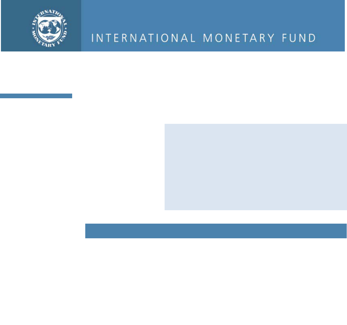
6. Japanese are moving to the four largest cities—Tokyo, Osaka, Nagoya and Fukuoka.
Population change at the prefecture-level can be characterized by inflows of people into these cities.
In the past two decades, the population of the Greater Tokyo area, including Tokyo, Saitama, Chiba
and Kanagawa prefectures, grew by about 10 percent, while Hokkaido lost about 6 percent of its
population (Figure 1). As a result, prefecture-level population concentration increased in the four
cities, with Tokyo’s population increasing by the largest magnitude of 1.3 percentage points, and
Hokkaido decreasing by the largest magnitude of 0.3 percentage points.
Figure 1. Japan: Population Change by Prefectures Between 1996-2015 (in percent)
In the past two decades, population declined in rural areas, but concentrated in large cities.
Sources: Statistics Bureau of Japan, Cabinet Office
JAPAN
INTERNATIONAL MONETARY FUND 7
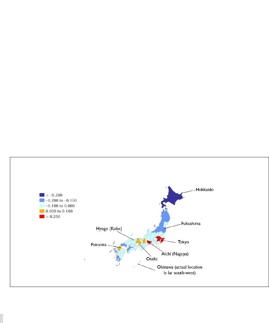
7. Despite the shrinking population, the total number of households in Japan has not
declined (see Figure 2). The number of households increased by 76 percent from 1970 to 2015.
During this period, the increase was greater for large cities (which increased by 116 percent) than for
rural areas (which increased by 18 percent). As a result, the total number of households in 2018
stands at around 50 million. However, the average size of a family has declined steadily, with an
increase in both the shares of the nuclear family and one-person family.
Figure 2. Japan: Household Statistics
8. Japan’s housing prices have gone through a large swing since the early 1990s.
2
Housing price movements in Japan can be grouped into five time periods: (1) pre-bubble period, (2)
post-bubble period until 2001, (3) mini-bubble between 2002–08, (4) pre-Abenomics and (5)
Abenomics period. With the economic expansion
experienced in the 1970s and 1980s, housing
prices in Japan increased until the years leading
up to the so-called ‘Bubble Period’ of the early
1990s. Beginning in 1988, price appreciation
intensified, increasing by 6 percent annually on
average. The bubble collapsed with a sharp
decline in housing prices until 1994. The price has
been on a declining trend since then, with a short-
lived period of a “Mini bubble (2002–08)”, and a
recent minor recovery in housing prices after
2014. Since the beginning of Abenomics, prices
have started to increase gradually (increasing by 2.7 percent since 2014 and by 0.7 percent in 2018).
With the recent increase in housing prices, they have recovered to the level last observed in 2013.
2
Throughout the chapter, with the exception of Box 1, residential land prices are used as a proxy for housing prices.
-40 -20 0 20 40 60 80 100 120
Japan average
Population concentrated area
Other areas
Aomori-ken
Iwate-ken
Miyagi-ken
Akita-ken
Yamagata-ken
Fukushima-ken
Yamaguchi-ken
Nagasaki-ken
Kagoshima-ken
Number of Households Family Members per Household
Japan: Households and Family Members
(Percent change between 1970 and 2015)
Source: Statistics Bureau of Japan.
0
10,000,000
20,000,000
30,000,000
40,000,000
50,000,000
60,000,000
70,000,000
1960 1980 1995 2010 2017 2020 2023 2026 2029 2032 2035 2038
One-person Nuclear family Other
Japan: Number of Households
Source: Statistics Bureau of Japan.
0
20,000
40,000
60,000
80,000
100,000
120,000
140,000
160,000
180,000
1975
1979
1983
1987
1991
1995
1999
2003
2007
2011
2015
Japan: Residential Land Price
(Yen/m
2
, Average Across Prefectures, Public Assessment Value)
Source: Ministry of Land, Infrastructure, Transport and Tourism.
2018
JAPAN
8 INTERNATIONAL MONETARY FUND
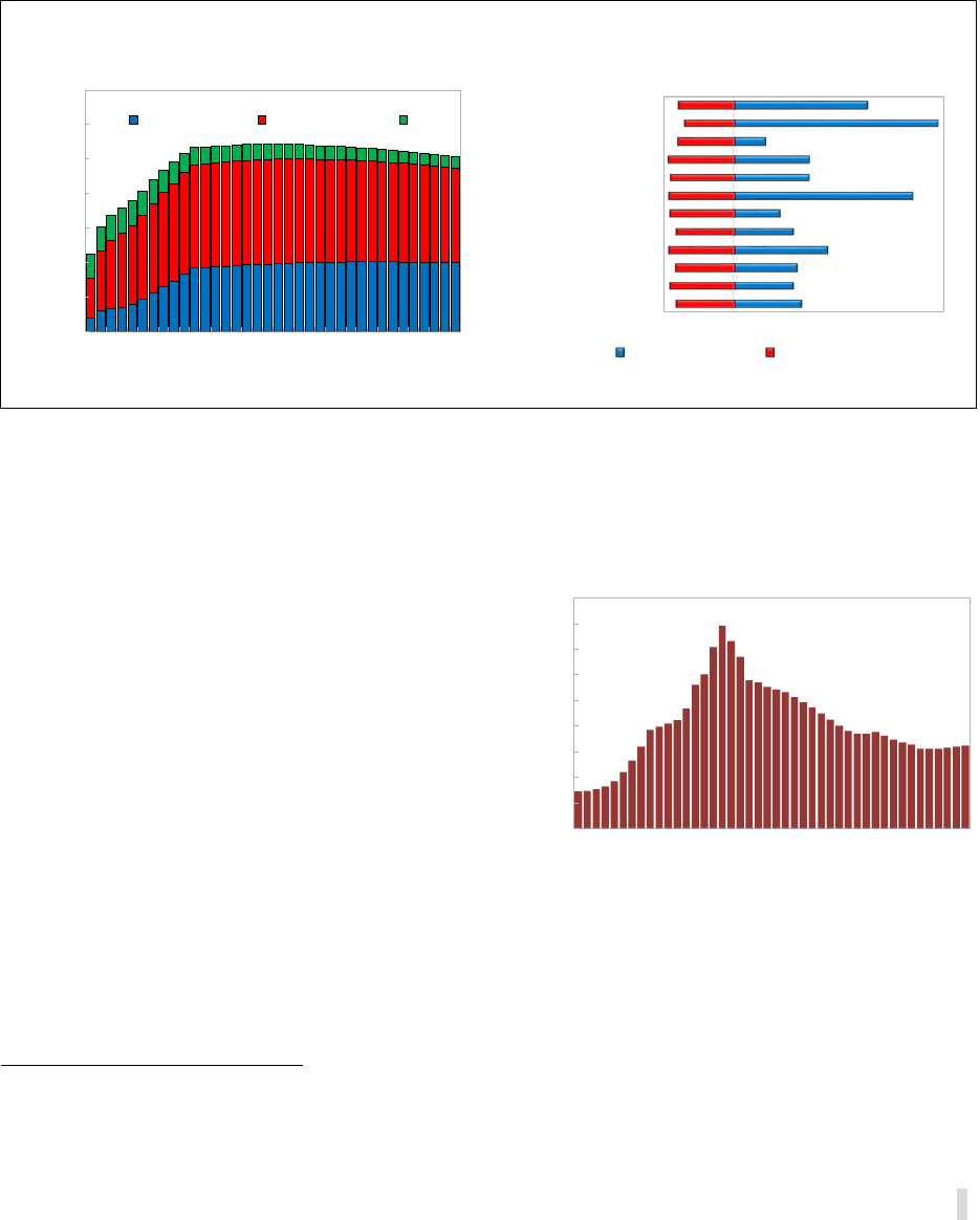
9. There is a clear regional dispersion in terms of housing price changes since the Bubble
Period burst in the early 1990s.
3
Figure 3 shows the growth rate of housing prices across
prefectures. The map on the left shows the price change since 2002, demonstrating that all
prefectures, except for Tokyo, experienced a decline in housing prices (by between -5 to -15
percent). The map on the right shows prefecture-level house price changes since 2014. Compared to
the left map, numerous prefectures experienced house price appreciation in recent years (average
1.9 percent nationwide since the beginning of Abenomics in 2013). The range, however, varies
greatly: largest gains are seen in Miyagi and Fukushima prefectures by 18 percent (likely related to
the reconstructions after the earthquake), followed by Tokyo (16 percent), while large losses are
seen in Akita (-6.5 percent), Shimane (-5.5 percent) and Yamanashi (-4.8 percent) prefectures. See
Box 1 for recent developments in housing prices in Japan and their potential drivers.
Figure 3. Japan: House Price Change by Prefecture
(in percent)
2002–2018: Tokyo-to is the only prefecture with an increase
in house prices since 2002.
2014–2018: Since 2014, an increase in house prices is
observed for other prefectures.
Source: Ministry of Land, Infrastructure, Transport and Tourism.
C. Modeling Population Growth and Housing Prices
In this section, we assess the long-term relationship between population growth and housing prices
using prefecture-level data, motivated by the ‘durable housing’ model developed by Glaeser and
Gyourko (2005).
3
According to the National Survey of Family Income and Expenditure (2014, for two-person households), there is
great variation across prefectures as to how much household wealth can be explained by housing. With housing
accounting for an average of 66 percent of household wealth (nationwide, likely exaggerated as it focuses on two-
person households, who are likely to have a house), this is somewhat lower than other advanced economies – United
States about 70 percent, Spain, Greece, Italy around 80 percent. For Japanese prefectures, this ranges from 52
percent (Shinamane prefecture) to Tokyo (80 percent), and Okinawa (above 90 percent).

JAPAN
INTERNATIONAL MONETARY FUND 9
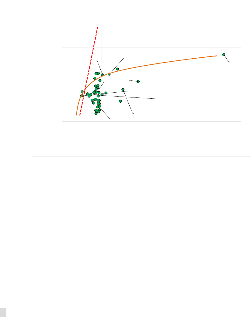
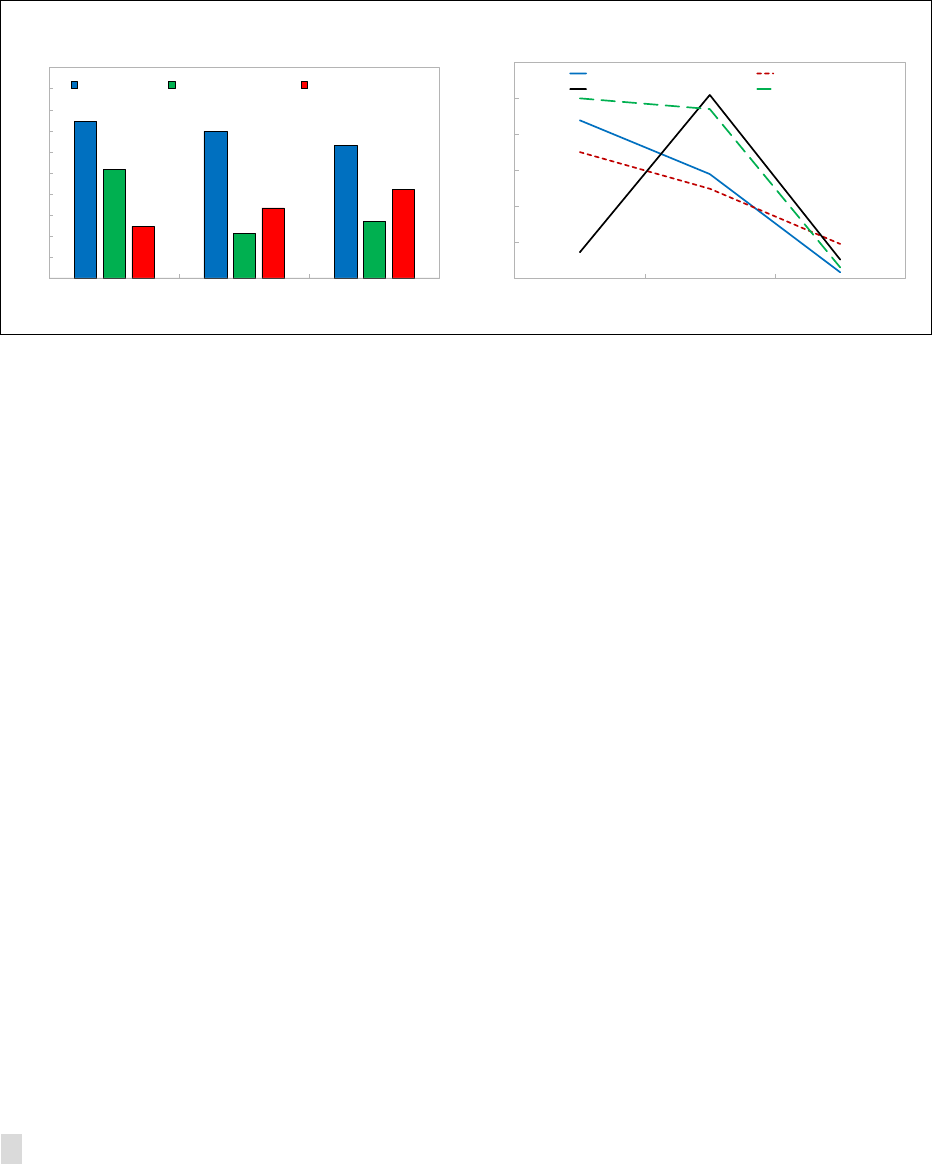
10. A simple durable housing model proposes a nonlinear relationship between changes in
housing prices and population growth. The non-linear relationship is that the magnitude of the
fall in housing price associated with population decline is larger than that of housing price rise from
population increase of the same magnitude. The ‘durable housing’ model by Glaeser and Gyourko
(2005) suggests that such an asymmetric relationship is due to the durability of housing, where
housing supply is elastic when new houses are built, while not elastic when houses need to be
demolished. This leads to a kinked supply-curve of housing. In this model, net inflows of population
increase demand for houses, and housing prices increase (P
2
). On the other hand, population
outflows of the same magnitude lower the demand for houses (P
3
), where the change in housing
price is larger than that with net inflows. If at the same time the supply of houses increases due to
sales by owners who move out from the region, a further decline in housing prices can be expected
(P
4
) (Figure 4).
Figure 4. Japan: Population Growth and Housing Price Change
(Glaeser and Gyourko (2005))
D3
D1
Q
Source: Glaeser and Gyourko (2005).
Note: MPPC is minimum profitable production costs.
11. The theoretical model predicts that cities with negative population growth experience
a large decline in housing prices. Following Glaeser and Gyourko (2005), we run the following
regression:
∆P
i,t
= α+ β * POPLOSS
i,t-1
+ γ * POPGAIN
i,t-1
+ ε
it
,
where P is the publicly-assessed residential land price adjusted for inflation (in Yen/meter
) as a
proxy for housing prices; POPLOSS variable takes on a value of zero if prefecture i’s population grew
during period t and equals the prefecture’s actual percentage decline in population if the prefecture
lost population during the period. Similarly, POPGAIN variable takes on a value of zero if prefecture i
experienced population loss during period t, and equals the actual population growth rate if the
prefecture gained population. The expected signs of coefficients of β and γ are positive, and that β >
Population decline
Population growth
P* = MPPC
P
Q*
D2
P
3
P
2
S
S2
P
4
JAPAN
10 INTERNATIONAL MONETARY FUND
γ. This implies that a price decline is larger (β) for a given loss of population (POPLOSS <0) than a
price increase (γ) for a given population increase (POPGAIN >0). In order to account for the lagged
impact of population on housing price, we use POPLOSS and POPGAIN of t-1 in the regressions. We
also add the variables “old dependency ratio” and “vacancy rate” (both in percentage change with
one lag) to control for other factors that might affect demand for and supply of houses. Figure 5
shows a simple correlation between housing price change and net migration flows over the period
of 1996–2018. This simple correlation supports the prediction of non-linearity (orange line), as
housing price growth in Tokyo-to is much lower than what is predicted by the relationship between
the two variables in other prefectures (dotted red line).
Figure 5. Japan: Changes in House Price and Net Migration Flows
(x-axis: thousands of persons, y-axis: percent, 1996-2018)
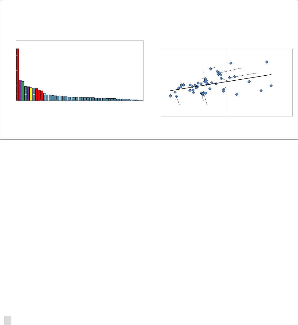
12. Panel regressions using prefecture-level housing prices and population dynamics
confirm this non-linear relationship. Table 1 shows regression results based on panel data of the
annual change in population and real land prices across three different time periods: (i) 1970–2015,
(ii) the past two decades since the collapse of the asset bubble, covering 1996-2015, and (iii) more
recent periods over 2010–15. Results show that during 1970–2015 (column 1), the estimated
coefficient for population loss is higher than that of population gain, confirming the prediction by
Glaeser and Gyourko (2005) that housing prices fall faster with declining population than they
increase with a growing population. However, in more recent periods, while the correlation between
housing price decline and population decline stays robust, the relationship between housing price
increase and population increase disappears. This confirms the overall decline in housing prices
across regions since the early-1990s bubble burst, regardless of the extent of population growth.
13. In reality, negative effects on housing prices from population decline may be even larger
than the model-based predictions. The results suggest a larger decline in housing prices associated
Hokkaido
Aomori-ken
Akita-ken
Gumma
-ken
Saitama-ken
Chiba-ken
Tokyo
-to
Kanagawa-ken
Aichi
-ken
Kyoto-fu
Osaka-fu
Fukuoka-ken
Okinawa-ken
-70
-60
-50
-40
-30
-20
-10
0
10
20
-20 -10 0 10 20 30 40 50 60 70
Change in House Prices
Average net migration flows (thousands of persons)
Source: Ministry of Land, Infrastructure, Transport and Tourism.

JAPAN
INTERNATIONAL MONETARY FUND 11
with population loss than a housing price increase with the same size of population gain. The model,
however, does not factor in households’ expectations on future house price developments and their
potential impact on house prices. In fact, residents expecting a housing price decline may sell their
houses and have less incentive to own houses, which will add to already-existing oversupply of houses
and create further downward pressures on housing prices. This vicious cycle may lead to a larger decline
in house prices in regions with declining population more than the model-based predictions.
D. Why are Japanese Moving to Large Cities?
The proximate cause of regional disparities in population dynamics and related housing price
dynamics is the continuous inflow of population into large cities. This section explores several factors
that influence population concentration in large cities.
14. Large cities offer jobs and education for younger Japanese. There exists a large variation
across prefectures in terms of the share of population with higher education—for rural prefectures
such as Akita and Aomori, the share of population with university degrees or higher make up about
5 percent of the population. This contrasts with Tokyo or Kanagawa (a prefecture in the suburbs of
Tokyo) that has close to 20 percent of its total population with higher education (university degree
or above). The chart below shows that higher education opportunities are also far greater in large
cities (colored bars) than in others: this is one factor that underpins the younger generation moving
out from their home prefectures (Figure 6, left chart).
Table 1. Japan: Empirical Analysis of Land Price and Population Changes
VARIABLES
HHLOSS 5.961 12.44 15.77* - - - 24.01*** 23.85*** 23.92***
(4.446) (7.504) (8.005) (4.410) (4.235) (4.252)
HHGAIN 3.091*** 1.818** 3.011*** 7.004*** 3.785 7.700** 0.357 0.443 0.567
(0.783) (0.819) (1.097) (1.559) (2.321) (3.203) (0.797) (0.851) (0.809)
Δ ln OLDDEP -1.516*** -1.721*** -3.047** -5.279* -0.177 -0.165
(0.355) (0.391) (1.438) (2.641) (0.298) (0.317)
Δ ln Vacancy rate -0.305* -0.425 0.0400
(0.153) (0.268) (0.196)
Constant -0.145** 0.165* 0.727*** -0.427*** 0.244 0.938** -0.216*** -0.188*** -0.200***
(0.0606) (0.0961) (0.0984) (0.116) (0.356) (0.460) (0.0375) (0.0495) (0.0714)
Observations 376 376 329 188 188 141 141 141 141
R-squared 0.703 0.720 0.747 0.647 0.663 0.720 0.340 0.342 0.343
Number of code 47 47 47 47 47 47 47 47 47
Fixed effects Y Y Y Y Y Y Y Y Y
Time effects Y Y Y Y Y Y Y Y Y
Source: Authors' estimations.
Robust standard errors in parentheses
*** p<0.01, ** p<0.05, * p<0.1
Dependent variable: %Δ real land price
1970-2015
1970-2000
2000-2015
JAPAN
12 INTERNATIONAL MONETARY FUND
15. Some studies show that skilled workers are better at generating growth in
endogenous amenities, increasing the value of housing (Shapiro, 2006; Glaeser and Saiz, 2004).
Service amenities, including health care and retail stores, are also concentrated in large cities. These
factors compose a core part of the local standard of living, and it is natural that people would prefer
to live in areas which have easy access to these amenities. For example, according to 2016 data of
social indicators by Statistics Bureau of Japan, the number of general hospitals (per 100 square
kilometers of habitable area) was 6 for Japan on average, of which the largest was 42.4 for Tokyo
and the lowest was 1.7 for Akita prefecture. Demand for amenities can explain the positive
correlation between housing price changes and the share of the educated population (Figure 6,
right chart), as affordability of these services increases with income.
Figure 6. Japan: Education and House Prices
Higher-education facilities are concentrated in four major
cities.
Housing price growth is positively correlated with the share of
the population with higher education qualifications.
E. Policy Implications
16. Policies to address regional disparities are crucial to prevent an excessive fall in
housing prices in rural areas. In 2014, the Abe administration established the headquarters for
regional revitalization in the Cabinet Office to promote even growth between rural and urban areas,
and help retain population and talents in rural areas. To assist rural areas, the government
introduced tax incentives for companies that either shifted their core functions or expanded the
operations of their headquarters already located in other parts of the country. Also, tax incentives
were provided to households who moved outside the capital area.
17. Forward-looking policies on housing supply and real estate investment that
incorporate demographic trends are necessary to prevent a further decline in housing prices.
Vacant houses create various social issues, but also have negative externalities in terms of prices, as
Hokkaido
Aomori-ken
Iwate-ken
Miyagi-ken
Akita-ken
Yamagata-ken
Fukushima-ken
Ibaraki-ken
Gumma-ken
Saitama
-
ken
Chiba-ken
Tokyo-to
Kanagawa-ken
Toyama-ken
Gifu-ken
Aichi-ken
Shiga-ken
Kyoto-fu
Osaka-fu
Hyogo-ken
Nara-ken
Shimane-ken
Okayama-ken
Hiroshima-ken
Kochi-ken
Fukuoka-ken
Nagasaki-ken
Kumamoto-ken
Okinawa-ken
0
5
10
15
20
25
-30 -20 -10 0 10 20 30
Japan: Human Capital and Housing Price Change
(X-axis: Change of Housing Prices Between 2011-2018, Y-axis: Share of University
and Graduate Degrees)
Source: Statistics Bureau of Japan; and IMF Staff Calculations.
0
20
40
60
80
100
120
140
160
Tokyo-to
Osaka-fu
Aichi-ken
Hokkaido
Hyogo-ken
Fukuoka-ken
Kyoto-fu
Kanagawa-ken
Saitama-ken
Chiba-ken
Hiroshima-ken
Niigata
-ken
Okayama-ken
Miyagi-ken
Gumma
-ken
Ishikawa-ken
Gifu-ken
Shizuoka
-ken
Nara-ken
Aomori
-ken
Yamaguchi-ken
Ibaraki-ken
Toc h i gi -ken
Nagano-ken
Kumamoto-ken
Fukushima
-ken
Shiga-ken
Nagasaki-ken
Okinawa-ken
Akita-ken
Yamanashi
-ken
Mie-ken
Miyazaki-ken
Iwate
-ken
Yamagata
-ken
Fukui-ken
Kagoshima-ken
Toyama-ken
Ehime-ken
Oita-ken
Tokushima-ken
Kagawa-ken
Wakayama-ken
Tottori-ken
Kochi-ken
Shimane-ken
Saga-ken
Japan: Number of Colleges and Universities by Prefecture
Source: Statistics Bureau of Japan, 2017

JAPAN
INTERNATIONAL MONETARY FUND 13
the presence of vacant houses tends to bring down the value of other houses in the neighborhood.
4
A regional supply of housing that factors in future demographic trends would help avoid potential
over-investment in real estate, decrease the number of vacant houses, and help place upward
pressure on housing prices.
4
It used to be that the tax rate on land is reduced to one sixth of the appraised value if there remains a residential
structure on the land. The initial motivation for this regulation was to accelerate the high utilization of land by giving
an incentive to home construction during the years when the population grew. However, this tax incentive is one of
the causes of the high vacancy rate in Japan, as the owner of the property had an incentive to leave the property as
is, without demolishing the structure, to benefit from the lower property tax rate. New legislation was enacted in
2014 to accelerate the demolition of vacant houses.
JAPAN
14 INTERNATIONAL MONETARY FUND
Box 1. Recent Developments in Residential Property Prices in Japan
Prices of high-rise condominiums in some Japanese cities have risen notably in recent years.
According to the annual survey of commercial and residential land price by the Ministry of Land,
Infrastructure, Transport and Tourism, which was released in July, the national average of residential land
prices declined by 0.1 percent. However, prices rose in Tokyo, Osaka and Nagoya by 0.9 percent on the back
of solid demand for condominiums and offices.
Condominium prices have appreciated since the beginning of Abenomics in 2013. Prices of certain
types of housings in large cities and some tourist destinations have appreciated rapidly (text figure).
Condominium prices have increased by 23 percent at the national level since 2013. Prices for new
condominiums in the Greater Tokyo area in 2018 averaged ¥71.4 million (about $650,000), according to data
from the Real Estate Economic Institution.
1
Recent Developments in Japan’s Residential Property Prices
Potential drivers of property price appreciation are the ultra-low interest rate environment, an
increase in tourism, and the inheritance tax. The prolonged low interest rate environment incentivizes
Japanese banks, mostly serving domestic clients, to increase real estate lending. An influx of foreigners in
tourist destinations has also led to increased investment in real estate. Finally, demand for condominiums to
avoid the inheritance tax is also generating upward price pressures.
2
1
IMF (2017) concluded that condominium prices appear to be moderately overvalued in Tokyo, Osaka, and several outer regions,
exceeding the values predicted by fundamentals by 5 to 10 percent.
2
There is anecdotal evidence that valuations for tax assessment purposes make condominiums an attractive bequest compared
to financial assets, as condominium prices are evaluated below market value and financial assets are evaluated at market value.
So, there is a strong tax incentive for Japanese households to hold real estate and take out housing loans, since the latter is tax
deductible at market value if one is to carry out a bequest.
80
100
120
140
160
180
200
220
Apr-08 Jun-09 Aug-10 Oct-11 Dec-12 Feb-14 Apr-15 Jun-16
Tokyo including suburbs Osaka including suburbs
Hokkaido Tohoku
Kyushu-Okinawa Japan (nationwide)
Condominium Prices
(2010=100, NSA)
Source: Ministry of Land, Infrastructure, Transport and Tourism
80
90
100
110
120
130
140
150
2008 - Apr
2009 - Apr
2010 - Apr
2011 - Apr
2012 - Apr
2013 - Apr
2014 - Apr
2015 - Apr
2016 - Apr
2017 - Apr
2018 - Apr
Residential Property
Residential Land
Detached House
Condominiums
Residential Property Price Index
(2010=100, NSA)
Source: Ministry of Land, Infrastructure, Transport and Tourism

JAPAN
INTERNATIONAL MONETARY FUND 15
References
Glaeser, Edward and Joseph Gyourko, 2005, “Urban Decline and Durable Housing,” Journal of
Political Economy, Vol. 113 (2), pp. 345-75.
Glaeser, Edward and Albert Saiz, 2004, “The Rise of the Skilled City,” Brookings-Wharton Papers on
Urban Affairs: 2004, pp. 95-103.
International Monetary Fund, 2017, “Japan: Financial System Stability Assessment,” IMF Country
Report No. 17/244, Washington DC.
Shapiro, Jesse, 2006, “Smart Cities: Quality of Life, Productivity, and the Growth Effects of Human
Capital,” The Review of Economics and Statistics, Vol. 88 (2), pp. 324-35.
JAPAN
16 INTERNATIONAL MONETARY FUND
IS AUTOMATION THE ANSWER TO JAPAN’S
DEMOGRAPHIC CHALLENGES?
1
Japan’s demographic transition will pose grave challenges for fiscal sustainability under the current
social security system. At the same time, Japan’s shrinking and aging population is expected to worsen
inequality in terms of market income. Automation and artificial intelligence technology have been
seen as a potential answer to the macroeconomic issues generated by population aging, though it is
not clear to what extent the new technology will mitigate the impact of demographic change on
growth and income distribution. Simulation results from a calibrated multi-sector general equilibrium
overlapping generations model suggest that automation can potentially offset the impact of
population aging on real output, but cannot fully eliminate fiscal pressures arising from demographic
transition. Nonetheless, for an aging society such as Japan, automation may improve distributional
outcomes.
A. Motivation
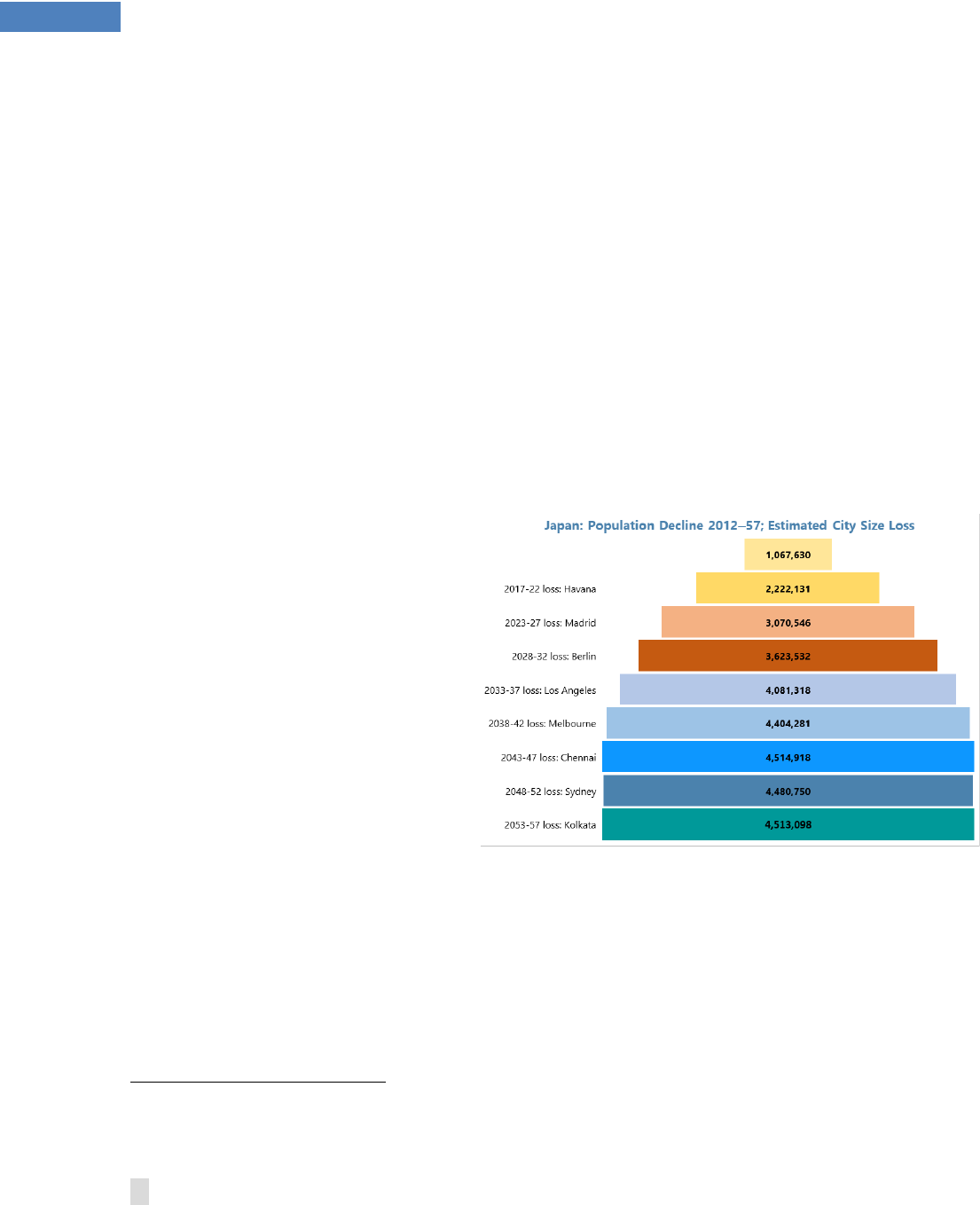
1. Adverse demographic trends in Japan have serious implications for its long-term
growth prospects and fiscal sustainability. Official projections anticipate that Japan’s population
will decline by 25 percent in the next 40
years. A rapidly shrinking and aging
population and labor force constitute
severe demographic headwinds to
future productivity and growth. IMF staff
simulations estimate that under current
policies, the level of Japan’s real GDP
will decline by over 25 percent in about
40 years due to demographics relative
to a projection for real GDP where
productivity and population grow at
their recent pace (Colacelli and
Fernandez-Corugedo, 2018). Adverse
demographic trends place significant
pressures on fiscal sustainability, as age-
related public expenditures rise while tax revenues shrink with the declining labor force (IMF 2018,
Kitao, 2015 and McGrattan et al. 2018).
2. Income inequality in Japan has been increasing, and population aging might
exacerbate this trend. As in other advanced economies, inequality in Japan, especially income
inequality, has been rising (Colacelli and Le, 2018). Intergenerational inequality is an important
1
Prepared by Gee Hee Hong (APD), Sandra Lizarazo Ruiz (SPR), Adrian Peralta-Alva (AFR) and Yuki Yao (University of
Minnesota).
Sources: Japan National I nstitute of Population and Social Security Research; United Nations Statistics
Division, IMF (2018)
2012-2017 Japan population loss:
equivalent to Stockholm

JAPAN
INTERNATIONAL MONETARY FUND 17
aspect of growing inequality in Japan. Pre-tax and transfers income inequality is higher among older
generations than among younger generations. Elderly Japanese are wealthier than younger
Japanese, where the old have more saving and benefit more from fiscal redistribution (via taxes and
transfers). Such intergenerational inequality may be worsened in the context of an aging population.
3. The Japanese government envisages automation and artificial intelligence (AI)
technology as offsetting its declining population and labor force. The Japanese government’s
2014 “Japan Revitalization Strategy,” envisaged a “New Industrial Revolution Driven by Robots.” The
Japanese government launched the ‘Society 5.0’ initiative in 2019, with the aim to better utilize and
disseminate robots across Japan.
2
The initiatives highlighted several sectors that will benefit from
greater usage of robots and AI technology. These sectors include health care, transportation,
infrastructure, and FinTech.
4. This chapter aims to quantitatively assess the macroeconomic and distributional
implications of automation in Japan. Labor saving technologies—automation and AI
technology—change the way production takes place and by so doing can potentially increase
productivity levels in the economy. At the same time, these technologies can disrupt labor market
dynamics and displace labor in certain productive sectors, while expanding labor demand in other
sectors. As the impact of automation and AI technologies is expected to differ for different types of
workers, the widespread adoption of these technologies might further increase market income
inequality and can result in increased income polarization. A proper assessment and quantification
of the macroeconomic and distributional outcomes requires a general equilibrium framework that
can account for the direct and indirect effects that these new technologies have on labor demand,
labor incomes, private investment and aggregate economic activity.
B. Framework of Analysis
5. The analysis is based on a multi-sector general equilibrium overlapping generations
model developed for the quantitative analysis of the macroeconomic and distributional
effects of aging.
3
This model has a rich production structure that encompasses manufacturing, low
tech-services and the high-tech services sector.
4
We assume that goods in these sectors are
produced using different combinations of factors (tangible and intangible capital, as well as low-,
mid- and high-skill labor)—see text figures below. Households vary by generation and skill level, and
face different levels of taxation and transfers. On the spending side, households receive age-
dependent transfers—pension benefits as well as health and long-term care. On the other hand,
financing instruments include time-varying progressive labor income taxation (including social
security contributions), consumption or value-added tax (VAT), corporate income tax, and
2
The ‘Society 5.0’ initiatives are to create a society that address various social challenges that Japan faces by
incorporating the innovations of the fourth industrial revolution into every industry and social life
(https://www.japan.go.jp/abenomics/_userdata/abenomics/pdf/society_5.0.pdf).
3
For details on such a model tailored to Japan, see McGrattan et al. (2018) and Hong, Lizarazo Ruiz, Peralta-Alva and
Yao (forthcoming).
4
The sectorial structure assumed for this model is similar to Lizarazo Ruiz et al. (2017).
JAPAN
18 INTERNATIONAL MONETARY FUND
government debt. These instruments and related parameters are tailored to Japan’s data at the
macro and micro level, building upon McGrattan et al. (2018). In addition, the model’s assumed
demographic transition closely follows the Japanese authorities’ own projections to capture the
dynamics of age-related costs. The analysis considers a baseline steady-state scenario that
corresponds to the period 2000–11, before Japan’s population started to decline, which began in
2012. This period is used to calibrate the model to Japan.
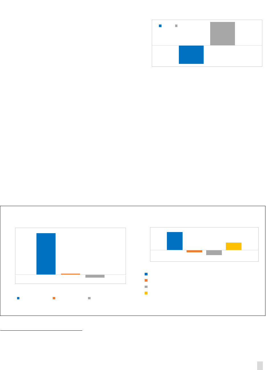
6. The first scenario (labeled as ‘Aging’) considers a long-term scenario in which annual
population growth is shrinking by 1 percent. Under this scenario, social security system (transfers,
pensions and health expenditures), tax rates (except for VAT rates), and the public debt-to-GDP ratio
are anchored at their 2019 levels; age-related fiscal costs of supporting the social security system are
financed through permanent VAT rate increases. A comparison of this scenario with the baseline
scenario permits an assessment of the macroeconomic and distributional impact of aging.
7. The second scenario (labeled as ‘Aging + Robots’) allows for the introduction of
automation and technological change in addition to aging. This scenario has the same
underlying assumptions about negative population growth, the social security and taxation system,
and public debt-to-GDP ratio as the ‘aging’ scenario. In addition, we introduce a higher elasticity
substitution of low- and mid-skilled labor by capital in manufacturing and the high-tech services
sector. This allows some tasks that had to be previously undertaken using labor can now be done
using capital. We also introduce a reduction in the relative price of capital to wages to represent the
fact that with technological change, capital (robots) becomes more affordable. As the exact pace of
technological progress in the future is unknown, we assume that this process will be such that in the
next 40 years, Japan’s share of labor income in GDP will fall by the same amount it fell between 1980
and 2012 (approximately 5 percentage points) and that the relative price of capital goods (robots) to
average wages will fall at an average of 0.5 percent per year. The latter corresponds to the average
decline in the relative price of all private fixed assets to wages between 2000 and 2012 in the United
States.
0
10
20
30
40
50
60
70
80
90
100
Low Tech Services Manufacturing High Tech Services
Labor intensity Share of Employment Share of Consumption
Japan: Industry Characteristics in Three Sectors
(in percent)
Sources: Ministry of Economy, Trade and Industry, IMF Staff calculations.
0
10
20
30
40
50
60
High School and less College Above College
Low Tech Service Manufacturing
High Tech Service Japan Population
Japan: Skill distribution by Sector
(in percent)
Source: IMF Staff calculations.
JAPAN
INTERNATIONAL MONETARY FUND 19
C. Main Findings
8. In the baseline scenario, the long-term
macroeconomic costs of Japan’s declining and
shrinking population are substantial. Even if we
assume that total factor productivity growth is not
affected by a decline in population growth, the level
of GDP will fall by 8 percent with respect to the
levels observed between 2000 and 2010. Less
workers and less demand due to an aging and
shrinking population will lead to a decline in total
output. On the other hand, fiscal spending will
increase largely due to age-related spending. VAT
rates (or consumption tax rates) will have to increase permanently by 10 percentage points to
maintain the debt-to-GDP ratio at the level observed in 2019 (that is, at about 230 percent).
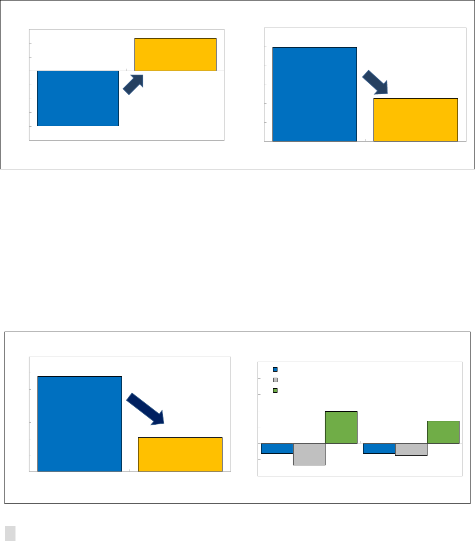
9. The distributional effects of the demographic transition are troublesome. Our analysis
shows that even though the wages of low-skilled workers increase with aging, market income
inequality rises dramatically, with the Gini coefficient rising by five points (see text charts below).
5
The increase in market income inequality is the net result of two opposing forces: on the one hand,
labor income becomes slightly more equally distributed, but on the other hand, the share of those
whose total income is mainly determined by labor income (young households) falls, while the share
of those whose total income is mainly determined by asset and wealth (older households) increases.
As the distribution of wealth is much more unequal than the distribution of wages (as period by
period differences in wages compound through time), market income distribution becomes much
more unequal as a result of the demographic transition.
5
According to the OECD, Japan’s last observed (2015) market income Gini coefficient was 50.4—almost identical to
the market Gini coefficient for the United States in 2015 (50.6).
2.2
0.0
-0.2
-0.5
0.0
0.5
1.0
1.5
2.0
2.5
Aging
Low skill wage Mid skill wage High skill wage
Source: IMF Staff calculations.
Japan: Wages by Skill Level (Aging Scenario)
(Percent change)
-7.9
10.0
-9
-7
-5
-3
-1
1
3
5
7
9
11
Aging
GDP VAT rate
Source: IMF Staff calculations.
Japan: Impact of Aging on GDP Level and VAT rate
(Percent change and percentage point change)
4.8
-0.6
-1.3
2.0
-3.0
-1.0
1.0
3.0
5.0
Aging
Gini market income
Share of market income bottom 20 percent
Share of market income middle segement of population
Share of market income top 20 percent
Source: IMF Staff calculations.
Japan: Distribution of Income (Aging Scenario)
(Percentage point changes)
JAPAN
20 INTERNATIONAL MONETARY FUND
10. If technological change continues at its current speed, automation could offset the
impact of population aging on per-capita GDP. Automation (“aging + robots” scenario) might
raise per-capita GDP by 4 percentage points above the average level seen during the period 2000–
11 (see left panel of text chart below). However, automation will not suffice to eliminate fiscal
pressures. Higher aggregate levels of age-related fiscal expenditures will still require an increase in
VAT rates, though the necessary VAT rate increase is half that without automation, rising by 10
percentage points (Aging scenario) and by only 5 percentage points (Aging + Robots scenario).
11. In an aging society, automation could reduce market income inequality. While the
direct impact of automation implies the replacement of workers with robots, the indirect effects of
automation—between-industry shift effects and final demand effects—allow for an important
increase in labor demand that pushes up wages for all workers (Autor and Salomons, 2018). In our
analysis, automation leads to a reduction in market income inequality (see left panel in text chart
below). This is due to the differentiated increase in wages by skill levels. With automation, the share
of market income for the top 20 percent of the population increases, but the increase is smaller than
in the aging-only scenario. The share of market income for middle segment declines with
automation, but the decline is smaller than in the aging-only scenario (see right panel in text chart).
-10
-8
-6
-4
-2
0
2
4
6
Aging Aging + Robots
Japan: GDP Levels - Different Scenarios
(In percent)
Source: IMF Staff calculations.
0
2
4
6
8
10
12
Aging Aging + Robots
Japan: Increase in VAT Rate Needed for Fiscal Sustainability
(Percentage point change)
Source: IMF Staff calculations.
3.6
3.8
4
4.2
4.4
4.6
4.8
5
Aging Aging + Robots
Japan: Changes in the Gini Index (Market Income)
(Percentage point change compared to the baseline)
Source: IMF Staff calculations.
-2
-1
0
1
2
3
4
5
Aging Aging + Robots
Share of market income bottom 20 percent
Share of market income middle segement of population
Share of market income top 20 percent
Japan: Changes in the Share of Market Income by Income Group
(Percentage point change compared to the baseline)
Source: IMF Staff calculations.

JAPAN
INTERNATIONAL MONETARY FUND 21
12. Through its impact in facilitating the financing of the social security system,
automation can help reduce disposable income (and consumption) inequality. As automation
improves market income and makes possible the financing of the social security system with a
smaller increase in VAT tax rates (making the impact of such increases less regressive), automation
improves the distribution of consumption, with the Gini index using disposable income falling by 2
percentage points (see left panel of text chart below).
6
The share of consumption for the bottom 20
percent and middle-segment of the population increases in the aging scenario, but the increases are
larger with automation (see right panel of text chart).
D. Conclusions
13. The extent to which automation can help mitigate the challenges brought by the
demographic transition in Japan depends on whether or not technological change occurs at
its current speed of progress and breadth of reach. Our analysis hinges critically on the
assumptions made on the nature and speed of future technological progress. There is a great deal
of uncertainty as to how this progress will unfold, but recent studies show that our assumption that
technological progress will be as fast as past years may be an upper bound. Nordhaus (2015)
discusses that in recent periods, technological change—measured by the rate of decline of capital
prices to labor wage rate—does not seem to be accelerating and may even be slowing. In a similar
fashion, IMF (2017) finds that the growth rate of cyclically-adjusted total factor productivity for
advanced economies between 2008–14 is about half the rate of growth observed between 2003–07,
and approximately one fifth the rate of growth observed between 1990 and 2002.
14. To reap the maximum benefits from automation to offset the adverse impact of a
declining population, investment in technology, innovation and education will need to have a
high rate of return. If the future growth rate of technological change is only one half that observed
between 2000–12 (also half the assumed rate underlying our analysis), automation would not suffice
6
According to the OECD, Japan’s disposable income Gini was 33.9 in 2015.
-2.5
-2
-1.5
-1
-0.5
0
Aging Aging + Robots
Japan: Changes in the Gini Index (Consumption)
(Percentage Point Change Compared to the Baseline)
Source: IMF Staff calculations.
-1.5
-1
-0.5
0
0.5
1
Aging Aging + Robots
Share of consumption bottom 20 percent
Share of consumption middle segement of population
Share of consumption top 20 percent
Japan: Changes in the Share of Consumption by Income Group
(Percentage Point Change Compared to the Baseline)
Source: IMF Staff calculations.

JAPAN
22 INTERNATIONAL MONETARY FUND
to prevent the fall of per-capita GDP caused by the demographic transition in Japan. This suggests
that measures that help ensure that technological innovation is successful will have a large
economic dividend. Efforts should be made to encourage spending on research and development,
and improve education levels, to help familiarize workers with new technologies and enhance their
labor productivity.
15. At the same time, policies to address the distributional consequences of automation
are important. One aspect not yet considered in this analysis, which deserves further attention, is
the impact of automation on gender inequality and inequality across generations. Hamaguchi and
Kondo (2018) estimate that female workers in Japan are exposed to higher risk of being replaced by
‘computerization’ than male workers. Similarly, elderly workers often enter the work force as part-
time workers in sectors that require low-skills, and are thus more likely to be replaced by
automation. Strong and effective social safety nets will be crucial to protect these workers, since
disruptions of some traditional labor and social contracts due to automation are highly likely during
Japan’s demographic transition.

JAPAN
INTERNATIONAL MONETARY FUND 23
References
Autor, David and Anna Salomons, 2018, “Is Automation Labor-Displacing? Productivity Growth,
Employment, and the Labor Share,” Brookings Paper on Economic Activity.
Colacelli, Mariana and Emilio Fernandez-Corugedo, 2018, “Macroeconomic Effects of Japan’s
Demographics: Can Structural Reforms Reverse Them?” IMF Working Paper 18/248.
Colacelli, Mariana and Anh Le, 2018, “Inequality in Japan: Generational, Gender and Regional
Considerations,” in “Japan: Selected Issues,” IMF Country Report 18/334.
Hamaguchi, N. and K. Kondo, 2017, “Regional Employment and Artificial Intelligence,” RIETI
Discussion Paper, 17-K-023. Research Institute of Economy, Trade, and Industry, Tokyo.
Hong, G., A. Le, and T. Schneider, 2018, “Land of the Rising Robots,” Finance & Development, June
2018, Vol. 55 (2), pp. 28–31.
Hong, G., S. Lizarazo Ruiz, A. Peralta-Alva, and Y. Yao, forthcoming, “Is Automation the Answer to
Japan’s Demographic Challenges?”, IMF Working Paper.
International Monetary Fund, 2017, “Gone with the Headwinds: Global Productivity,” IMF Staff
Discussion Note, SDN/17/04.
International Monetary Fund, 2018, “Japan: Article IV Consultation – Staff Report,” IMF Country
Report 18/333.
Kitao, Sagiri, 2015, “Fiscal Cost of Demographic Transition in Japan, “Journal of Economic Dynamics
and Control, Vol. 25, pp. 37–58.
Lizarazo Ruiz, S., A. Peralta-Alva, and D. Puy, 2017, “Macroeconomic and Distributional Effects of
Personal Income Tax Reforms: A Heterogeneous Agent Model Approach for the U.S.” IMF Working
Paper 17/192.
McGrattan, E., K. Miyachi, and A. Peralta-Alva, 2018, “On Financing Retirement, Health, and Long-
Term Care in Japan,” IMF Working Paper 18/249.
Nordhaus, William, 2015, “Are We Approaching an Economic Singularity? Information Technology
and The Future of Economic Growth,” Cowles Foundation Discussion Paper No. 2021, New Haven:
Yale University.
JAPAN
24 INTERNATIONAL MONETARY FUND
JAPAN’S FERTILITY RATE
1
Japan’s population is projected to decline by more than 25 percent in the next 40 years, if the current
low fertility rate persists. This overwhelming demographic challenge ahead of Japan leads to
consideration as to whether there are policies the authorities can implement to affect the fertility rate.
This chapter takes stock of recent developments with respect to Japan’s fertility rate, and argues that a
combination of policies could raise the fertility rate if implemented in a coordinated and sustained
manner.
A. Introduction
1. Japan’s population is projected to decline by more than 25 percent in the next 40
years, if the current low fertility rate persists. Japan’s total fertility rate (sum of the age-specific
birth rates of women aged 15 to 49) stood at 1.4 children per woman in 2018, which is well below
the population replacement level of 2.1.
2
In addition,
a large gap remains between the actual fertility rate
and the “desired” rate of 1.8—the latter being the
rate expected if people had their desired number of
children. This gap raises the question as to whether
public policies can help increase Japan’s fertility rate
by removing potential obstacles. A higher fertility
rate could have positive impacts on aggregate GDP
over the long-run, by increasing the size of the labor
force and helping stabilize public debt (as a share of
GDP). At the same time, this policy objective needs
to be mutually consistent and reinforcing with other
public policy objectives. For example, the IMF has
stressed the need to promote female labor force
participation—see IMF (2018), Colacelli and
Fernandez-Corugedo (2018). However, if not
accompanied by sufficient support for working couples with small children, higher FLFP could
potentially increase the opportunity cost of giving birth and thereby lower the fertility rate. The
Japanese government has stepped up its support for households with children, with notable
measures being increasing the availability of childcare facilities and making preschool and childcare
free. This chapter takes stock of recent developments in Japan’s fertility rate, and discusses whether
public policy can help increase the fertility rate.
1
Prepared by Takuma Hisanaga (APD).
2
The total fertility rate in a specific year is defined as the total number of children that would be born to each woman
if she were to live to the end of her child-bearing years and give birth to children in alignment with the prevailing
age-specific fertility rates. This indicator is measured in children per woman. See OECD (2019).
JAPAN
INTERNATIONAL MONETARY FUND 25
B. Overview of Japan’s Fertility Rate
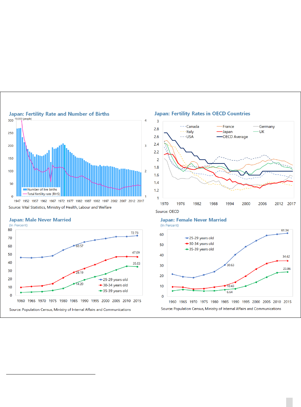
2. Japan’s fertility rate has improved in recent years but remains low at 1.4 children per
woman. After the second baby boom in the early 1970s, Japan’s fertility rate declined until it
bottomed out at 1.26 in 2005 (see top-left chart of Figure 1). This declining trend of fertility mirrors
the trend increase in the percentage of late-married and non-married (see the bottom two charts of
Figure 1). The marriage rate (the number of marriages per population of 1,000 persons) in Japan
halved from around 10 in the early 1970s to around 5 in 2015. In more recent years, Japan’s fertility
rate has marginally recovered, but remains low at around 1.4 children per woman—well below the
population replacement rate of 2.1, and lower than all other G7 countries except Italy (see the top-
right chart of Figure 1).
3. A gap exists between the actual and desired number of children per couple. According
to a survey by the National Institute of Population and Social Security Research (the NIPSSR), an
ideal number of children for a couple is 2.32 on average.
3
However, those couples plan to have on
average 2.01 children—the sum of the number of children already born (1.68) and the number of
3
See NIPSSR (2015).
Figure 1. Japan’s Fertility Rate–Stylized Facts
JAPAN
26 INTERNATIONAL MONETARY FUND
additional children the couple plans to have (0.33). On the other hand, while the unmarried rate of
females aged 30–34 has risen to about 35 percent, 90 percent of unmarried females aged 18–34
intend to marry in the future. Based on the NIPSSR survey and other data, the government estimates
the “desired” fertility rate of 1.8
4
that could be achieved through closing the gap between the actual
and desired number of children, and removing obstacles to higher fertility rates.
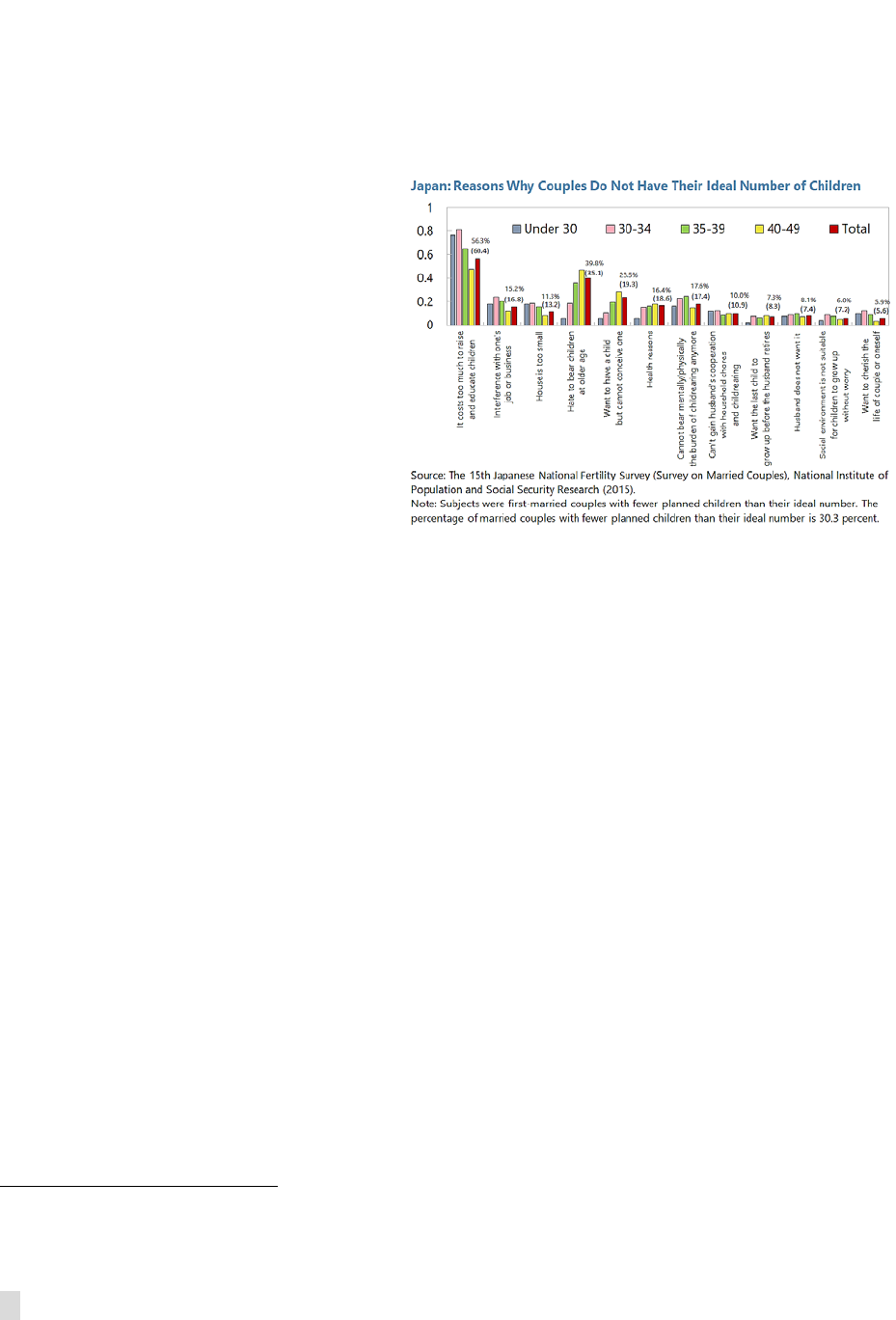
4. The direct cost of childbearing
seems to be the most important factor
which prevents couples from attaining
their ideal number of children. The
NIPSSR 2015 survey summarizes the
reasons why couples do not have their
ideal number of children. The top reason
cited by 56 percent of couples is the cost
of childbearing; this is followed by the
reluctance to bear a child at an advanced
age (40 percent).
5. The opportunity cost of
childbearing also matters. During the period of Abenomics, Japan’s female labor force
participation rates (FLFP) have substantially increased from 63 percent in 2012 to 71 percent in 2018
(for those aged 15 to 64), according to OECD Employment and Labour Market Statistics. A higher
FLFP could increase household incomes and make the cost of childbearing affordable (i.e., the
income effect). On the other hand, higher FLFP could increase the opportunity cost of having
children as females typically need to leave their workplaces for a certain period of time (i.e., the
substitution effect). In fact, according to the NIPSSR (2015) survey, about 15 percent of couples
responded that their jobs/businesses are one of the main reasons for the gap between the actual
and desired number of children, which can be seen as a measure of the opportunity cost of having
children.
4
This rate is based on the planned number of children for a couple, as well as other statistics including the share of
single people who hope to marry and the desired number of children of single people.
JAPAN
INTERNATIONAL MONETARY FUND 27
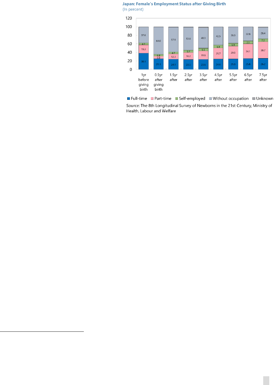
6. The opportunity cost of having children is high for full-time workers. According to a
longitudinal survey of Japanese newborns
in 2010, the total share of female workers
sharply dropped after giving birth from 62
percent to 35 percent (see Ministry of
Health, Labour and Welfare (2019)). The
total share of female workers gradually
recovered to the level before childbirth (61
percent) about 5.5 years after giving birth.
However, as illustrated in the text chart on
the right, most of the female workers re-
entered the job market as part-time
workers. The share of full-time workers
dropped from 38 percent to 25 percent
after childbirth and remained low at
around 26 percent even 7.5 years after giving birth. The MHLW survey suggests that a number of
full-time female workers give up full-time status after childbirth, which has enduring implications for
their lifetime income and employment benefits.
C. Empirical Analysis: Data and Methodology
7. This section provides a simple empirical analysis to study the possible drivers of
Japan’s fertility rate. D'Addio and Mira d'Ercole (2005) discussed the historical development of
fertility rates across OECD countries and showed that, based on a static cross-section analysis,
fertility rates are lower when the direct costs of childbearing are higher. Regarding the impact of
increased FLFP, they calculated that the correlation between female employment rates and total
fertility rates in OECD countries turned from negative to positive in the late 1980s. Using a dynamic
panel data model, they observed that the fertility rate is higher when (i) female employment rates
are higher, and/or (ii) the ratio of female to male wages is lower. In this section, an approach similar
to D'Addio and Mira d'Ercole (2005) is applied to Japan’s prefecture-level panel data to study Japan
specific features.
5
8. A panel dataset was constructed that covers data for 47 prefectures for the period
2001 to 2015. In the panel regression analysis, the dependent variable is the prefecture-level total
fertility rate, and five variables that might affect the total fertility rate are included as explanatory
variables:
• Education costs. The share of education expenses in total expenditures for non-single households
is derived from the Family Income and Expenditure Survey conducted by the Ministry of Internal
5
Among the previous studies of the fertility rate in Japan, Abe and Harada (2008) observed that, based on a cross-
section analysis of municipal-level data, a rise in female wages had a negative impact on the fertility rate, and that the
impact of improved availability of childcare facilities on the fertility rate was positive. Kato (2018) also analyzed
municipal-level data to find a positive impact of the female labor participation rate on the total fertility rate.

JAPAN
28 INTERNATIONAL MONETARY FUND
Affairs and Communications. As this could be viewed as a proxy for the direct cost of child-
rearing, the expected sign is negative for the relationship between the total fertility rate and
education costs.
• Female labor force participation rate. The prefectural labor force participation rates (ratios of
labor force over the population) for women between 15 and 64 years old are derived from data
of the National Census.
6
Based on the findings by D'Addio and Mira d'Ercole (2005), the
expected sign is positive for the relationship between the FLFP rate and the total fertility rate.
• Wage gap. Ratios of female to male monthly wages (a higher ratio indicates a smaller wage gap
between male and female) are used to measure the gap. The wage is average monthly
contractual cash earnings in the MHLW’s Basic Survey on Wage Structure. D'Addio and Mira
d'Ercole (2005) find that a smaller wage gap (i.e., a higher ratio of female to male wages) implies
a larger opportunity cost due to foregone income during maternity leave, leading to lower
fertility rates. However, in the case of Japan, female workers often give up their full-time status
after childbirth, as discussed in the previous section. Hence, a large wage gap could reflect
changes in women’s employment status after childbirth in Japan. Provided that the observed
large wage gap (i.e., a low ratio of female to male wages) is attributable to a large share of
female part-time workers after childbirth, the opportunity cost of giving birth would increase
over the long-run, which could lower the fertility rate. Furthermore, a smaller wage gap is
expected to yield better income prospects after childbirth, which increases the affordability of
childbearing. In light of these factors, the expected sign of the wage gap-total fertility rate
relationship could be positive, which would run contrary to the findings of D'Addio and Mira
d'Ercole (2005).
• Availability of childcare facilities. The capacity (sum of authorized quotas of children) of childcare
facilities for each prefecture is obtained from the MHLW’s Survey of Social Welfare Institutions.
Following Unayama (2009), the capacity is divided by the female population between 20 and 44
years old to make it comparable across prefectures. This variable can be viewed as an indication
of commitment to child-friendly policies by prefectural governments. The expected sign of the
relationship between total fertility rate and childcare facilities is positive.
• Unemployment rate. Prefecture-level unemployment rates are obtained from the Statistics
Bureau’s model-based estimates, based on data from the Labor Force Survey. This variable is
introduced to factor in macroeconomic conditions, and the expected sign of the unemployment
rate-total fertility rate relationship is negative.
9. The Pooled-Mean Group estimator is the preferred model. The simple pooled OLS
regression model does not allow for prefecture-specific effects. A commonly-used alternative, the
fixed effects estimator, takes account of prefecture-specific effects, but fails to deal with the issue of
the endogeneity of explanatory variables with respect to the total fertility rate. In order to deal with
the endogeneity issue, the PMG (Pooled Mean Group) estimator proposed by Pesaran et al. (1999) is
6
As the National Census is a quinquennial survey, values for gap years are filled by linear interpolation.

JAPAN
INTERNATIONAL MONETARY FUND 29
used here, following the approach of D'Addio and Mira d'Ercole (2005). The PMG estimator
distinguishes long-run and short-run dynamics. Coefficients for long-run effects are assumed to be
identical across prefectures, while those for short-run effects are allowed to differ. The other model
used in D'Addio and Mira d'Ercole (2005), a GMM (Generalized Method of Moments)-System
estimator developed by Arellano and Bover (1995) and Blundell and Bond (1998), is a less preferred
option here, because the post-estimation Sargan test rejected the null hypothesis that over-
identifying restrictions are valid, indicating a potential misspecification (see Table 1). Therefore, the
discussion hereafter is based on the PMG estimates, with a focus on the long-run dynamics, while
turning to the GMM estimates as a complementary reference.
D. Results
10. Every explanatory variable has a statistically-significant impact on the prefectural
fertility rate in the long-run. Table 1 shows the results:
• Wage gap. A rise in the female wage relative to the male wage (a smaller gap between male and
female wages) has a positive impact on fertility rates in the long-run. This supports the argument
that a smaller wage gap could indicate lower opportunity costs of childbirth over the long-run,
and make childbearing more affordable. On the other hand, the sign is negative in the short-run.
A possible interpretation of this negative short-run effect is that a smaller wage gap could lower
the fertility rate in the short-run due to a larger foregone income during maternity leave.
• Female labor force participation rate. A higher female labor force participation rate has a positive
impact on the fertility rate in the long-run, in line with the findings of D'Addio and Mira d'Ercole
(2005). The long-run result indicates that a one-percentage point increase in the FLFP rate is
associated with a 0.04 increase in the fertility rate (see Table 1). Meanwhile, the sign is negative
in the short-run, possibly pointing to a negative impact of opportunity costs on the fertility rate,
as discussed above.
• Education costs. A reduction in education costs has a positive impact on the fertility rate in the
long run, though this was not confirmed in the GMM estimates. The short-run coefficient is not
statistically significant.
• Childcare facilities. An increase in childcare facilities has a positive impact on the fertility rate
both in the short run and long run, demonstrating the potential effectiveness of child-friendly
policies in raising the total fertility rate.
• Unemployment rate. The sign of the long-run coefficient is positive, while it is negative in the
short run. The coefficient is statistically insignificant in the GMM estimates. This positive
correlation could imply a low opportunity cost of childbearing when unemployment rates are
high, though further analysis is warranted on this point.

JAPAN
30 INTERNATIONAL MONETARY FUND
E. Policy Implications and Conclusions
11. The Japanese government’s Work Style Reform, which has intensified since 2016,
could have a positive impact on the fertility rate.
7
Introduction of public policies to reduce the
unwilling exclusion of female workers from the labor market following childbirth could raise the
fertility rate over the long-term. It is of particular importance to nurture a working and social
environment where female regular workers can retain regular-worker status after childbirth, if they
wish to. Potential measures the authorities could undertake to achieve this goal include: (i) further
increasing childcare availability; (ii) rewarding firms with high retention rates of female employees
after childbirth; and (iii) eliminating disincentives to regular and full-time work embedded in the tax
and social security systems (see IMF (2019)). The impact on the fertility rate could be reinforced by
measures to alleviate the direct cost of childbearing, such as lowering education and childcare costs.
12. Public policies supporting fertility should be implemented in a coordinated and
sustained manner. Since the impact of each policy on the fertility rate is relatively small, a wide
array of policies needs to be put in place in a coordinated, mutually-reinforcing manner in order to
make a meaningful impact on the fertility rate. Lastly, the negative short-run effects of female labor
force participation and the wage gap on the total fertility rate point to a need for the authorities to
be persistent—sustaining public policies to support fertility even if the fertility rate is negatively
affected in the short-run.
7
See also Box 2 of International Monetary Fund (2019) Japan: Article IV Consultation—Staff Report, for a case study of
the experience of Nagi-town in Okayama Prefecture.

JAPAN
INTERNATIONAL MONETARY FUND 31
Table 1. Japan: Estimation Results of Total Fertility Rate by Prefecture, 2001–15
(1)
(2) (3)
PMG PMG
(long-run
coefficients)
(short-run
coefficients)
Wage gap 1.039*** 0.402***
(0.198) (0.0815)
FLFP 4.003*** 0.787***
(0.583) (0.214)
Education costs -1.170** -0.0518
(0.507) (0.226)
Childcare facilities 3.153*** 1.151***
(0.811) (0.211)
Unemployment rate 4.442*** -0.116
(0.655) (0.266)
Lag of total fertility rate 0.438***
(0.0340)
Error correction term -0.385***
(0.0353)
Change in wage gap -0.355***
(0.0835)
Change in FLFP -10.29***
(2.774)
Change in education costs 0.135
(0.172)
Change in childcare facilities 1.015*
(0.564)
Change in unemployment rate -0.888*
(0.465)
Constant -0.873*** -0.116
(0.0814)
(0.0999)
Observations 658 658 658
Sargan test (p-value) 0.000
VARIABLES
GMM-SYS
Note: PMG denotes Pooled Mean Group; GMM-SYS denotes Generalized Method of Moments-System.
Prefectural data is for the period 2001-15 for 47 prefectures.
Standard errors in parentheses; *** p<0.01, ** p<0.05, * p<0.1
Source: Author's calculations.

JAPAN
32 INTERNATIONAL MONETARY FUND
References
Abe, K. and Y. Harada, 2008, “Effects of Policies to Support Child-Rearing on Fertility Rate: Analysis of
Municipalities’ Data”, Kaikei-kensa Kenkyu, Vol. 38 (in Japanese).
Asano, T. and N. Yamagata, 2010, “Measures to Support the Fertility Rate and their Policy Impacts",
Graduate School of Public Policy, The University of Tokyo.
D'Addio, A.C. and M. Mira d'Ercole, 2005, “Trends and Determinants of Fertility Rates in OECD
Countries: The Role of Policies”, OECD Social, Employment and Migration Working Papers No. 27,
OECD: Paris.
Arellano, M. and O. Bover, 1995, "Another Look at the Instrumental-Variable Estimation of Error
Component Models", Journal of Econometrics, Vol. 68, pp. 29-52.
Blundell, R. and S. Bond, 1998, "Initial Conditions and Moment Restrictions in Dynamic Panel Data
Models", Journal of Econometrics, Vol. 87, pp. 115-43.
Cabinet Office of Japan, 2019, Annual Report on the Declining Birthrate 2019, Tokyo.
Colacelli, M. and E. Fernandez-Corugedo, 2018, “Macroeconomic Effects of Japan’s Demographics:
Can Structural Reforms Reverse Them?”, IMF Working Paper 18/248.
International Monetary Fund, 2018, “Japan: Article IV Consultation—Staff Report,” IMF Country
Report 18/333.
International Monetary Fund, 2019, “Japan: Article IV Consultation—Staff Report,” IMF Country
Report.
Kato, H., 2018, “The Analysis on Disparities of Fertility Rate of Japanese Municipalities”, Policy
Research Institute, Ministry of Finance, Japan, Public Policy Review, Vol.14, No. 1.
Ministry of Health, Labour and Welfare, 2019, “The Eighth Longitudinal Survey of Newborns in the
21st Century (2010 Cohort)” (in Japanese), Tokyo.
National Institute of Population and Social Security Research, 2015, “The Fifteenth Japanese National
Fertility Survey,” Tokyo.
OECD, 2019, Social and Welfare Statistics, OECD: Paris.
Pesaran, M.H., Y. Shin and R.P. Smith, 1999, "Pooled Mean Group Estimation of Dynamic
Heterogeneous Panels", Journal of the American Statistical Association, Vol. 94, pp. 621-34.
Pesaran, M.H. and R.P. Smith, 1995, "Estimating Long-run Relationships from Dynamic
Heterogeneous Panels", Journal of Econometrics, Vol. 68, pp. 79-113.

JAPAN
INTERNATIONAL MONETARY FUND 33
Toda, A., 2007, “Empirical Analysis of Fertility Rates - Focus on its Relationship with the State of
Economic Activity and Family Policy”, RIETI Discussion Paper Series 07-J-007 (in Japanese), Tokyo.
Unayama, S., 2009, “Policy Responses to the Low Fertility and Aging and Female Labor Participation –
Analysis of Prefectures’ Data”, RIETI Discussion Paper Series 10-J004 (in Japanese), Tokyo.
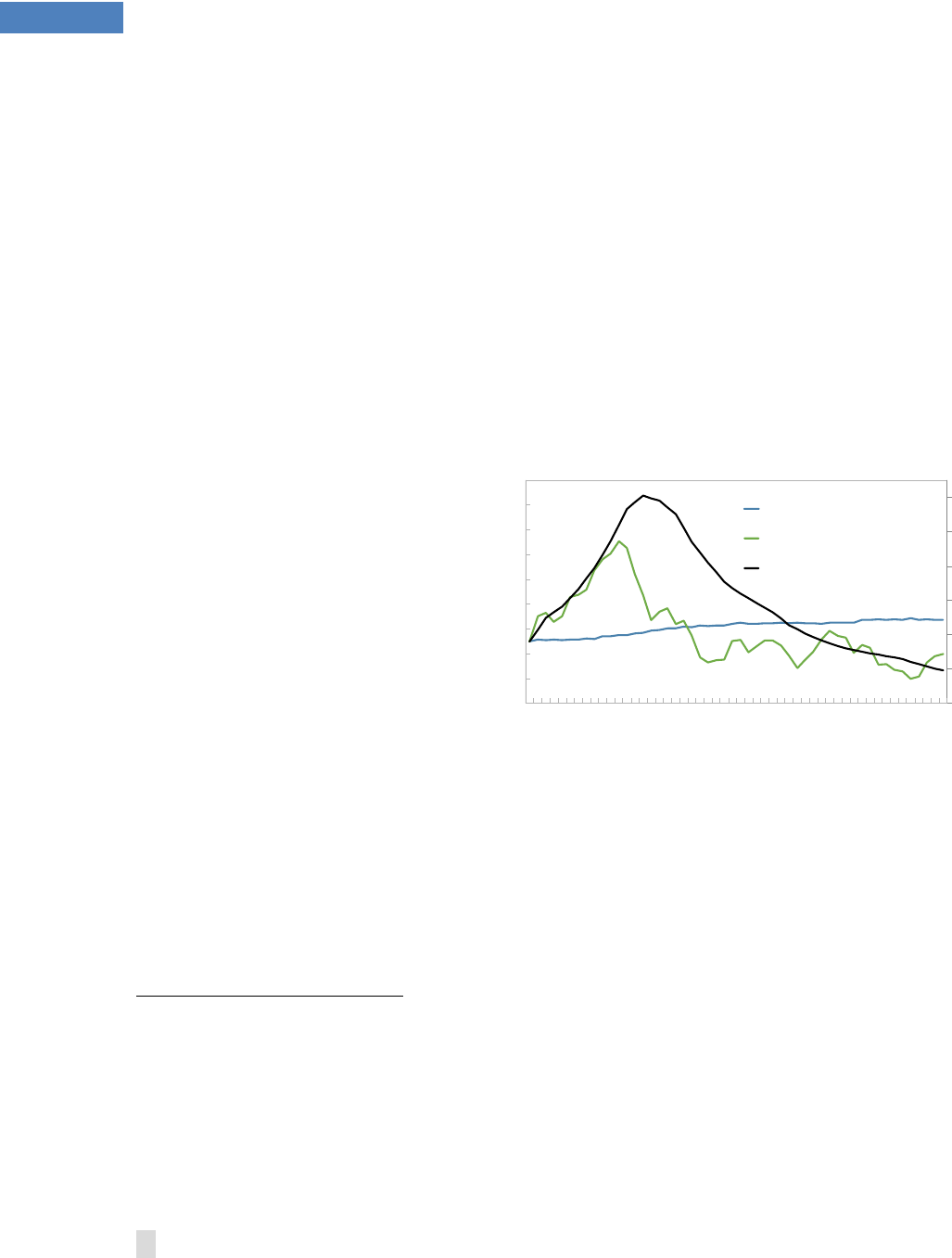
JAPAN
34 INTERNATIONAL MONETARY FUND
TWENTY YEARS OF INDEPENDENCE: LESSONS AND
WAY FORWARD FOR THE BANK OF JAPAN
1
The Bank of Japan has used unconventional monetary policies (UMPs) to fight deflation and stabilize
the financial system since its independence in the late 1990s. While the BoJ’s reflation efforts have
evolved over time, inflation has remained stubbornly low. The purpose of this chapter is to examine
monetary policy in Japan over the past twenty years, in order to draw relevant lessons and propose
ways to strengthen the Bank of Japan’s policy framework. In doing so the analysis focuses on three
aspects of monetary policy: (i) objectives and goals, (ii) policy strategies, and (iii) the communication
framework.
A. Evolution of the Bank of Japan’s Policy Objectives and Goal
1. In the late 1990s, the central bank law was revised to give the Bank of Japan (BoJ)
greater independence and clarify
its policy objectives. Following the
collapse of Japan’s asset price bubble
in the early 1990s, two important
lessons emerged: (i) stable and low
inflation was not sufficient to ensure
financial stability and soundness of
the national economy, and (ii) the
BoJ needed greater independence
from the government to secure
credibility with the public and
financial markets. Consequently, a
new central bank law was adopted in
1998, separating the BoJ from the
Ministry of Finance and providing the legal underpinning for a broad-based policy approach with
explicit policy objectives to (i) achieve price stability and (ii) contribute to the stability of the financial
system.
2
3
2. The importance of the BoJ’s price stability objective has increased over time along
with greater goal transparency. While the revised Bank of Japan Act (1998) specified the BoJ’s
1
Prepared by Niklas Westelius (FIN).
2
The new Bank of Japan Act (Act No. 89 of June 1997) was enacted in 1997 by the Diet, and came into effect in April
1998.
3
The BoJ’s objective under the previous Bank of Japan Act (1942) was to help maximize the potential growth of the
economy (Ito, 2004). The 1998 Act states that the objective for monetary policy should be “aimed at achieving price
stability, thereby contributing to the sound development of the national economy” (Article 2) and that the purpose of
the bank is to “[…] ensure smooth settlement of funds among banks and other financial institutions, thereby
contributing to the maintenance of stability of the financial system” (Article 1).
-3
-1
1
3
5
7
9
50
70
90
110
130
150
170
190
210
230
1987Q1
1987Q4
1988Q3
1989Q2
1990Q1
1990Q4
1991Q3
1992Q2
1993Q1
1993Q4
1994Q3
1995Q2
1996Q1
1996Q4
1997Q3
1998Q2
1999Q1
1999Q4
Consumer Price Index
Nikkei Stock Price Index
Urban Land Price Index
Japan: Asset and Consumer Prices, 1987-1999
(Index=100, 1987)
Source: Haver Analytics.
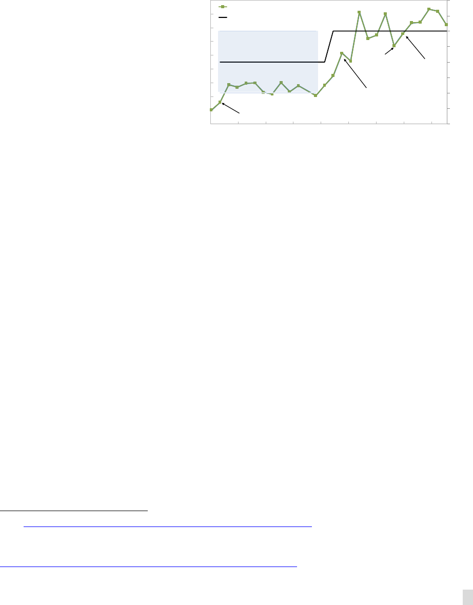
JAPAN
INTERNATIONAL MONETARY FUND 35
policy objectives, it gave the Bank autonomy to determine their relative importance and to set specific
policy goals.
• Relative weight on policy objectives. During 2000–06, financial and price stability issues were front and
center for the BoJ. Non-performing
loans weighed on financial
intermediation while deflation
became more pronounced. Over
time, however, as financial
vulnerabilities became less
prevalent and the urgency to
reflate the economy more pressing,
the price stability objective grew in
importance. This was particularly
true following the government’s
introduction of Abenomics in 2012
(see text figure) which put forth an
ambitious policy agenda to raise
growth and exit deflation.
• Goal transparency. Despite early discussions about adopting an explicit inflation target, the
exact definition of “price stability” remained vague following BoJ’s independence. Fearing that a
numerical inflation goal would reduce policy flexibility, the BoJ broadly defined price stability as
a situation that was “neither deflationary nor inflationary.”
4
However, in 2006—as part of a new
monetary policy strategy—the BoJ saw the need for greater clarity regarding its price stability
target. Consequently, the BoJ Board decided to disclose that individual Board members’
understanding of medium to long-term price stability ranged between 0 and 2 percent with a
median of around 1 percent. Six year later, shortly after the U.S. Federal Reserve announced a 2
percent inflation goal, the BoJ adopted a single numerical inflation goal of 1 percent to help
clarify its policy stance. Importantly, the new price stability goal was not tied to the views of
Board members but to that of the institution. Finally, a year later—with the introduction of
Abenomics and in line with other major central banks— the 1 percent goal was replaced by a 2
percent inflation target.
5
Hence, it took the BoJ almost 15 years before adopting a clear and
transparent goal for its price stability objective (Figure 1).
B. Unconventional Strategies to Reflate the Economy
3. Shortly after independence, the BoJ adopted UMPs to exit deflation and safeguard
financial stability. In the late 1990s and early 2000s the Japanese economy was facing slowing
4
See https://www.boj.or.jp/en/announcements/release_2000/k001013a.htm/
5
The use of “goal” in 2012 reflected the belief that “target” might be construed as meaning rigidly conducting
monetary policy with only price developments taken into account. See
https://www.boj.or.jp/en/mopo/mpmsche_minu/minu_2013/g130122.pdf
-1.0
-0.5
0.0
0.5
1.0
1.5
2.0
2.5
3.0
90
100
110
120
130
140
150
160
170
180
Dec-05 Jul-07 Feb-09 Sep-10 Apr-12 Nov-13 Jun-15 Jan-17 Aug-18
Relative awarness of price stability objective
Inflation goal/target (rhs)
Japan: The BoJ's Price Stability Target and the Public's Awareness of
the Price Stability Objective relative to Financial Stability Objective
1
(Index Dec 2005=100)
1
The measure is calculated as the ratio between the share of respondents saying they have knowledge of the
price objective to the share of respondents saying they have knowledge of the financial stability objective
Source: Bank of Japan; Opinion Survey on the General Public's Mindset and Behavior.
Introduction of
NIRP (Jan 2016)
Introduction of inflation
target (Jan 2013) and
QQE (April 2013)
Introduction of the new monetary policy framework
(March 2006), including the "understanding of price
stability" between0 and 2 percent and
Introduction of
YCC (Sept 2016)
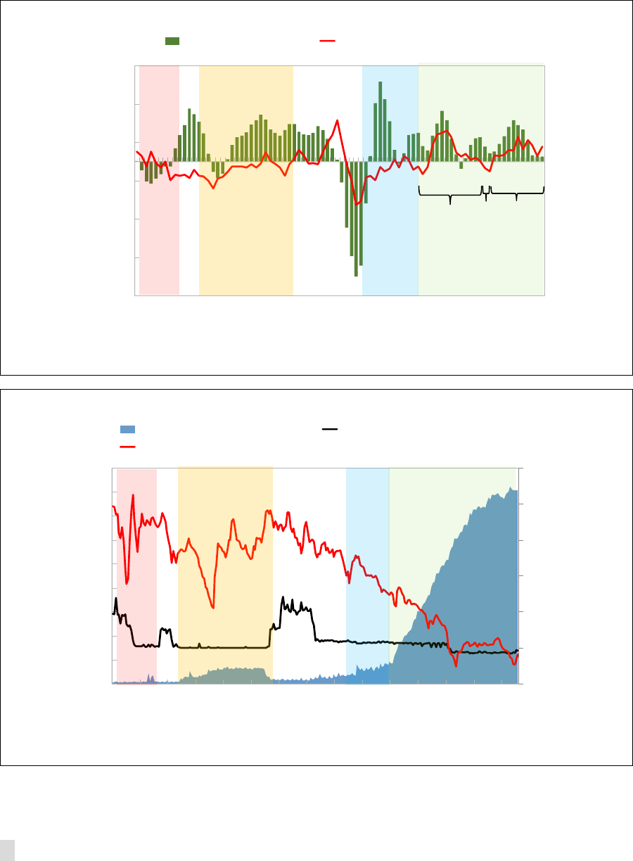
JAPAN
36 INTERNATIONAL MONETARY FUND
demand, declining consumer prices, and financial instability due to a confluence of factors, including
the 1997 consumption tax hike, a domestic banking crisis, and the Asian Financial Crisis (see Figure 1
and 2). With the policy rate close to the zero-lower bound (ZLB), the BoJ embarked on a number of
unconventional policy measures.
Figure 1. Japan: Inflation and GDP Growth, 1998–2019
Figure 2. Japan: Monetary Policy Operations, 1998–2019
-7.0
-5.0
-3.0
-1.0
1.0
3.0
5.0
1998Q1
1999Q1
2000Q1
2001Q1
2002Q1
2003Q1
2004Q1
2005Q1
2006Q1
2007Q1
2008Q1
2009Q1
2010Q1
2011Q1
2012Q1
2013Q1
2014Q1
2015Q1
2016Q1
2017Q1
2018Q1
2019Q1
GDP growth (annual) Inflation (core, exl. consumption tax)
Source: Haver Analytics.
ZIRP
ZIRP+QEP
CE
Abenomics
QQE/
NIRP
QQE/
NIRP/
YCC
QQE
-0.5
0.0
0.5
1.0
1.5
2.0
2.5
0
50
100
150
200
250
300
350
400
450
Jan-98
Jul-99
Jan-01
Jul-02
Jan-04
Jul-05
Jan-07
Jul-08
Jan-10
Jul-11
Jan-13
Jul-14
Jan-16
Jul-17
Jan-19
Current account balance (Trill. yen) Policy rate (rhs, percent)
JGB 10-year yield (rhs)
Source: Haver Analytics.
ZIRP
ZIRP+QEP
CE
QQE/NIRP/YCC
Nov
-19
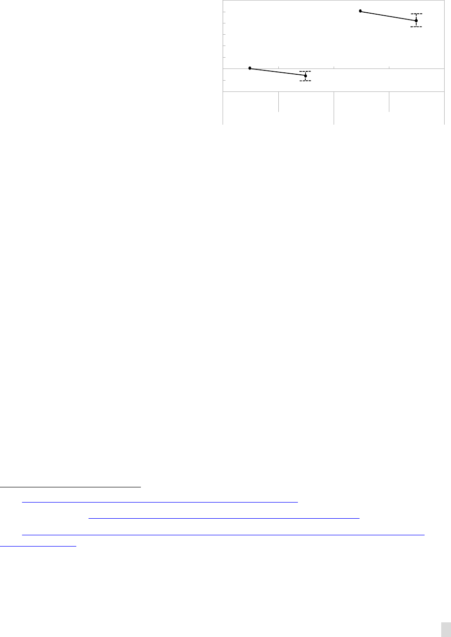
JAPAN
INTERNATIONAL MONETARY FUND 37
• Zero Interest Rate Policy (ZIRP). In
February 1999, the BoJ lowered the
policy rate “as low as possible” and
later added that ZIRP would continue
until deflationary concerns subsided.
However, by August 2000, the BoJ
judged that current economic
conditions had improved enough to
exit ZIRP and raised the overnight call
rate into positive territory. This
normalization effort, however,
occurred despite a slightly unfavorable
outlook (see text figure).
• Quantitative Easing Policy (QEP). The economy weakened substantially in early 2001 and the BoJ
decided to re-instate ZIRP and reinforce it with QEP. The new policy strategy entailed a change in
policy instrument—from the short-term rate to quantity of reserves—and purchases of long-term
JGBs to increase the monetary base. To convince markets that the policy would be maintained, the
Board committed to maintain ZIRP until core inflation became stably above zero or recorded an
increase year on year.
6
• Measures to ensure financial stability. Financial system stress occurred several times during this
period, causing liquidity and risk premia to rise. Apart from the liquidity support through QEP, the
BoJ also took specific steps to target pockets of financial vulnerability, including widening the range
of acceptable collateral for its fund providing operations and allowing banks to sell stocks directly to
the BoJ.
7
4. In 2006, the BoJ started to normalize policy as economic conditions improved. In early
2006, economic growth had recovered, inflation was rising, and financial and corporate sectors were in
the best shape in over a decade.
8
Moreover, the legacy problem of non-performing loans, which had
hampered financial intermediation, was largely resolved. Hence, in March 2006 the BoJ judged that the
conditions for exiting QEP had been met and re-introduced the overnight interest rate as the main policy
tool. However, similar to the 2000 episode, the BoJ’s economic forecast published around the time of the
decision did not seem to indicate a strong case for normalization.
9
6
See https://www.boj.or.jp/en/announcements/release_2003/k031010b.htm/
7
See Ueda (2012) and https://www.boj.or.jp/en/announcements/release_2002/fss0210c.htm/
8
See https://www.imf.org/en/Publications/CR/Issues/2016/12/31/Japan-Staff-Report-for-the-2006-Article-IV-
Consultation-19484
9
At the time, the BoJ projected the two-year-ahead core inflation at slightly below one percent, with core inflation
being positive for three consecutive months and expected to remain positive going forward. Moreover, according to
the minutes from the policy meeting on March 9, 2006, many Board members judged that the output gap was only
gradually narrowing, and unit labor costs were facing weakening downward pressures.
-1.0
-0.5
0.0
0.5
1.0
1.5
2.0
2.5
3.0
Latest Obs. June
2000
Forecast for March
2001
Latest Obs. Q1:2000 Forecast for March
2001
Inflation GDP growth
Japan: BoJ: Forecasts when Exiting ZIRP in August 2000
(In percent)
Sources: BoJ
Note: The March 2001 forecasts were published in October 2000. The intervals around the forecasts
indicate the range of Board members' forecasts
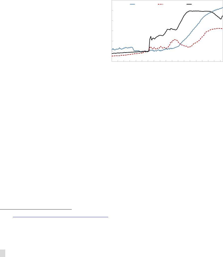
JAPAN
38 INTERNATIONAL MONETARY FUND
5. The BoJ also introduced a new monetary policy framework to improve policy
predictability while preserving flexibility. The framework consisted of two components. First, the
BoJ Board members decided to disclose their “understanding” of price stability (ranging from 0 to 2
percent). Second, policy decisions were to be guided by a “two perspective” approach. The first
perspective entailed an assessment of whether the near-term outlook (1-2 years) followed a path of
sustainable growth under price stability. The second perspective was to examine various risks to the
outlook over the longer term, including financial stability risks.
6. The BoJ was relatively slow in returning to UMPs following the Global Financial Crisis
(GFC). In the summer of 2008, the GFC
significantly depressed economic activity
and caused a sharp drop in inflation
(Figure 1). The overnight rate was again
lowered to the ZLB and number of
measures were taken to strengthen
financial institutions and market
functioning.
10
However, it was not until
October 2010 that the BoJ reverted back
to quantitative easing by introducing its
Comprehensive Monetary Easing (CE)
framework. The CE framework re-
introduced ZIRP together with an asset
purchase program consisting not only of
JGB purchases, but also risky assets to reduce term and risk premia.
11
However, compared to the U.S.
Federal Reserve and the European Central Bank (ECB), the BoJ’s response to the GFC was more
protracted and smaller in size (see text figure).
7. In 2013, the BoJ scaled up its quantitative easing program to quickly boost inflation
expectations and achieve the new two percent price stability target. The policy shift occurred in
the context of Abenomics—a coordinated policy effort by the BoJ and the government to (i) achieve
the new two percent inflation target, (ii) boost potential growth and increase competitiveness, and
(ii) ensure long-run debt sustainability.
• Quantitative and Qualitative Easing (QQE). In April 2013, just a few months after raising the price
stability target to 2 percent, the BoJ introduced QQE—a significant scale-up of CE—consisting of
a sharp increase in purchases of JGBs and risky assets. Under QQE, the BoJ explicitly committed
to increase its annual purchase JGBs holdings by about ¥50 trillion per year. The new program
signaled a determined effort by the BoJ to back up its commitment to the higher inflation target
through strong and transparent actions. The new strategy appeared initially successful. Inflation
10
See https://www.boj.or.jp/en/mopo/outline/cfc.htm/
11
The risky asset purchases covered corporate bonds, commercial paper, exchange-traded funds (ETFs), and real
estate investment trusts (REITs).
0
100
200
300
400
500
600
Jan-03
Dec-03
Nov-04
Oct-05
Sep-06
Aug-07
Jul-08
Jun-09
May-10
Apr-11
Mar-12
Feb-13
Jan-14
Dec-14
Nov-15
Oct-16
Sep-17
Aug-18
Jul-19
BoJ ECB U.S. Fed
Size of Balance Sheet: BoJ, ECB and U.S. Federal Reserve
(index=100; August 2008)
Source: FRED
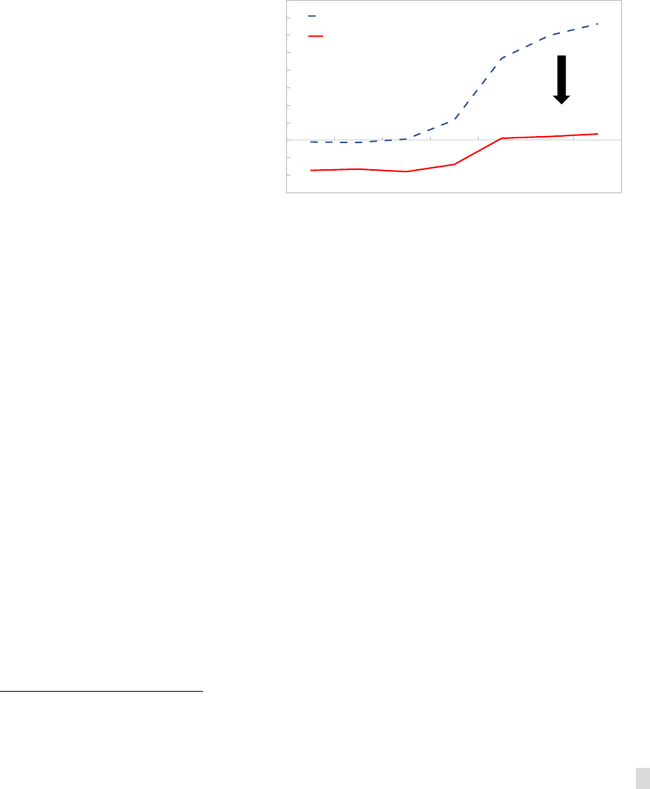
JAPAN
INTERNATIONAL MONETARY FUND 39
rose, the exchange rate depreciated, and growth picked up. However, economic conditions
started to deteriorate in the second half of 2014 as a fall in oil prices and weak demand
following the consumption tax rate hike in April 2014 exerted downward pressure on inflation
and growth.
12
• Negative Interest Rate Policy (NIRP). Despite the scale-up of QQE, domestic growth weakened
further in 2015, and inflation
continued to fall (Figure 1).
Moreover, concerns were
emerging that the BoJ would
soon run out of JGBs to
purchase and that options to
further stimulate the economy
were limited. To dispel these
concerns, the BoJ surprised
market participant in early 2016
by lowering the interest rate on
excess reserves into negative
territory. The intention was to
put downward pressure on
short-term interest rates and raise inflation expectations by re-confirming the Bank’s
commitment to achieving the inflation target. However, the impact on yields was larger than
anticipated, leading to a significant flattening of the yield curve (see text figure). The large
compression of term spreads triggered worries about financial sector side-effects (i.e., increased
risk taking and further decline in profitability of financial institutions).
8. In 2016, the BoJ changed policy strategy again amid concerns about financial side-
effects and persistently-low inflation expectations. With actual and expected inflation still below
target more than three years after the introduction of QQE, the BoJ launched a comprehensive
review of its monetary policy framework. The review was published in September 2016 and
concluded that (i) the lowering of real interest rates along the yield curve had been the most
effective tool to stimulate economic activity, and (ii) inflation expectations had proven to be more
backward-looking than previously thought. Based on these observations the BoJ changed strategy.
• Digging in for the long-run. Instead of aiming for a quick reflation, the BoJ switched to a more
protracted reflation approach that was more compatible with the adaptive nature of Japanese
inflation expectations. Specifically, by generating a persistent positive output gap through
sustained accommodative policy, realized inflation would gradually rise and eventually re-anchor
inflation expectations at the two percent target. However, this prolonged “high-pressure”
12
The BoJ responded to the weakening economy in October 2014 by raising the annual increase of JGB holdings
from ¥50 trillion to ¥80 trillion.
-0.6
-0.4
-0.2
0.0
0.2
0.4
0.6
0.8
1.0
1.2
1.4
1.6
1-year
2-year 5-year 10-year 20--year
30-year 40-year
Jan 28 2016, Day before NIRP
July 6 2016 (Lowest YC after NIRP)
Japan: Flattening of the Yield Curve Following NIRP
(In Percent)
Source: Haver Analytics.

JAPAN
40 INTERNATIONAL MONETARY FUND
strategy would need to be complemented by measures to mitigate financial side-effects and
ensure policy sustainability.
• The Yield Curve Control (YCC) framework. To support the new reflation strategy, the BoJ
implemented a new operational framework. The purpose of YCC was to shape the yield curve by
targeting both the short-term interest rate (NIRP) and the long-term interest rate (10-year JGB
yield). By buying JGBs along the entire yield curve, the BoJ would be able to prevent the long
end of the curve from falling while keeping the short end unchanged. This would make
monetary accommodation more sustainable since lending rates are benchmarked to short- to
medium-term interest rates, while the profitability of financial institutions such as pension funds
and insurers is influenced by long-term term spreads.
13
Moreover, the YCC would allow the BoJ
to reduce JGB purchases and hence address concerns that it was running out of JGBs to buy.
9. While macroeconomic outcomes have somewhat improved under YCC, actual and
expected inflation remain below the inflation target and financial side-effects continue to
accumulate. Economic growth has average above potential since 2016 and core inflation appears to
have stabilized at slightly below one percent. Moreover, the yield curve has steepened compared to
the levels seen right before the implementation of YCC, and the BoJ’s purchases of JGBs have fallen
markedly. However, little progress has been made in terms of permanently lifting inflation
expectations. Moreover, low bank profitability and search for yield by financial institutions still pose
a significant risk to financial stability over the medium-term.
C. Communication Strategies and Inflation Expectations
10. Pre-Abenomics, unconventional monetary policy communication focused on exploring
the so-called “duration effect.” The duration effect was intended to influence market expectations
about the future course of monetary policy, and hence stabilize interest rates at a low level and lift
inflation expectations
.
14
Initially, under QEP, the BoJ communicated that monetary easing would
“continue until the CPI (excluding perishables) registers stably a zero percent or an increase year on
year.”
15
While this commitment reduced uncertainty about the policy rate and laid out relatively
clear exit conditions, it was largely backward looking and did not tie policy to a price stability target.
This was somewhat reversed with the introduction of the “two-perspective approach” in 2006 which
anchored policy guidance in a medium-term numerical “understanding” of price stability. For
instance, when introducing CE in 2010, the BoJ stated that it would “maintain the virtually zero
interest rate policy until price stability is in sight on the basis of the “understanding of medium- to
long-term price stability.” While this guidance was better tied to the price stability objective and
hence more forward looking, it was more ambiguous regarding exit conditions.
13
See speech by Governor Kuroda (2017):
https://www.boj.or.jp/en/announcements/press/koen_2017/ko171114a.htm/
14
See Fujiki and Shiratsuka (2002).
15
See https://www.boj.or.jp/en/announcements/release_2001/k010319b.htm/
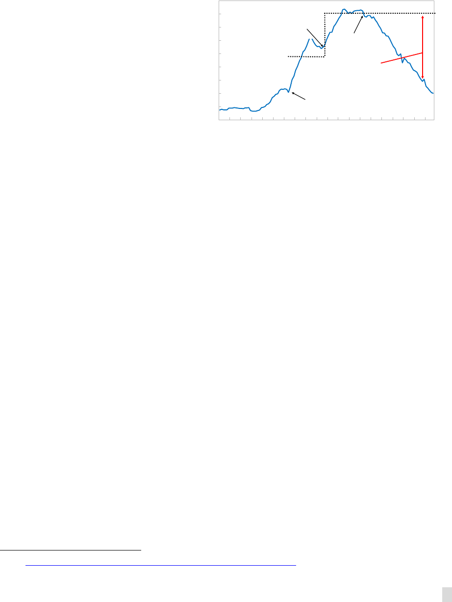
JAPAN
INTERNATIONAL MONETARY FUND 41
11. The BoJ’s communication strategy changed drastically with the introduction of the
two percent inflation target. The new communication strategy focused on quickly re-anchoring
inflation expectations at the higher price
stability target. First, by promising to
achieve the price stability target “at the
earliest possible time, with a time horizon
of about two years,“ the BoJ deviated
from its previous position that price
stability should be pursued over the
medium to long-term.
16
Second, the
time-dependent guidance indirectly
implied an almost unconditional
commitment to price stability, effectively
deprioritizing other objectives. Third, by
committing to the massive increase in
JGB purchases, the BoJ showed that it
was willing to back up its verbal commitment to the inflation target with strong and transparent
policy actions.
12. The 2016 shift to a gradual reflation approach under YCC required the BoJ to once
again adjust its communication strategy. In line with the new gradual reflation approach under
YCC, the time horizon for achieving the inflation target was gradually de-emphasized. Moreover, BoJ
Board members began to acknowledge financial side-effects more prominently, while arguing that
the new framework was more flexible and sustainable. In addition to YCC, the BoJ also tried to make
inflation expectations more forward-looking by committing to expand the monetary base until the
inflation target was achieved (e.g., the so-called overshooting commitment). Policy guidance,
however, became more complicated. Despite switching operationally from quantity to interest rate
targeting under YCC, the BoJ was reluctant to abandon its quantitative guidance on JGB purchases.
This has resulted in a growing discrepancy between the quantity guidance and actual JGB purchases
(see text figure).
13. In 2018, speculation of a premature normalization prompted the BoJ to introduce
explicit forward guidance on policy rates. In response to upward pressure on the 10-year JGB
yield in the summer of 2018, the BoJ (i) increased the variability range around the zero percent yield
target and (ii) strengthened its commitment to achieving 2 percent inflation by introducing forward
guidance for policy rates. Initially, the forward guidance was time-dependent to ensure that rates
would remain low beyond the implementation of the scheduled October 2019 consumption tax rate
increase. However, in the fall of 2019, the BoJ shifted to a more state-based guidance by committing
to keep short- and long-term interest rates low “as long as it is necessary to pay close attention to the
possibility that the momentum toward achieving the price stability target will be lost.”
16
See https://www.boj.or.jp/en/announcements/release_2012/k120214b.pdf
0
10
20
30
40
50
60
70
80
90
Jan-10
Jul-10
Jan-11
Jul-11
Jan-12
Jul-12
Jan-13
Jul-13
Jan-14
Jul-14
Jan-15
Jul-15
Jan-16
Jul-16
Jan-17
Jul-17
Jan-18
Jul-18
Jan-19
Jul-19
Japan: Annual Change in the BoJ's JGB Holdings, 2010-19
(Trillion Yen)
Source: Haver Analytics.
October 2014: JGB
guidance raised to
¥80 trillion
September 2016:
YCC introduced
Growing gap
relative to the
¥80 trillion
policy guidance
April 2013: QQE
introduced: JGB
guidance of ¥50
trillion
Nov-19

JAPAN
42 INTERNATIONAL MONETARY FUND
D. Lessons Learned and Way Forward
14. Based on the BoJ’s twenty years of reflation experience, there are a number of
measures that could be taken to strengthen the overall monetary policy framework. In
particular, the BoJ could: (i) clarify its commitment to the inflation target while increasing policy
flexibility to address competing objectives, (ii) improve the internal decision-making process, and
(iii) simplify and strengthen its communication framework.
Policy Objectives and Goals
15. The lack of stability and clarity of policy objectives have complicated policy
implementation and hampered reflation efforts. During the early years, the relatively large
weight on the financial stability objective combined with the absence of a clear price stability target
may have contributed to insufficient monetary stimulus and a bias towards premature policy
normalization (e.g., the 2000 and 2006 episodes). On the other hand, the large relative weight on
price stability combined with an over-optimism to achieve the inflation target during the
QQE/NIRP/YCC period has likely negatively impacted policy credibility and contributed to keeping
inflation expectations persistently low. In particular, the emphasis on achieving the price stability
target “as soon as possible” together with unrealistic inflation forecasts have been particularly
problematic given limited policy space, a clogged monetary transmission, and rising financial
stability costs. Finding the right balance between the price and financial stability objectives and
setting realistic conditions for achieving the inflation target is key to improve policy credibility and
better anchor long-run inflation expectations.
16. The BoJ should consider strengthening and clarifying its commitment to the target
while increasing policy flexibility to address financial stability concerns. Specifically, the BoJ
could announce a comprehensive review of its price stability objective—similar to the reviews
conducted in 2000, 2006, and 2013. The review would allow the BoJ to:
• Re-confirm or re-evaluate the inflation level viewed as consistent with price stability. Moreover,
the BoJ should clarify that the price stability target will be achieved over the medium- to long-
term. This would help dispel a lingering perception that the BoJ is trying to achieve the two
percent target as soon as possible regardless of the short-term costs.
• Introduce a range around the inflation target. This would enable a more gradual reflation process
that is more consistent with realistic inflation projections while also providing more flexibility to
credibly address financial side-effects.
• Better communicate its views on the trade-offs between financial stability and price stability
objectives. The BoJ should clarify that it is not excessively focused on inflation, but that other
objectives, including financial stability, also matter for monetary policy. This would help avoid
speculation of premature normalization and a loss of credibility when financial stability costs
rise.

JAPAN
INTERNATIONAL MONETARY FUND 43
17. The re-evaluation of the inflation target and introduction of greater policy flexibility
would need to be carefully communicated. A target range and a longer time horizon would allow
the BoJ to more effectively take into account (i) downward pressure on inflation from structural
forces, (ii) limited available policy space, and (iii) financial sector side-effects. However, these
adjustments could be interpreted as a reduced commitment to the inflation target and hence
depress inflation expectations. It is therefore crucial to communicate these adjustments in a careful
and systematic manner. For instance, an announcement of a comprehensive review of the price
stability objective would allow the BoJ to clearly lay out the underlying motivation and rationale for
the changes. Indeed, the BoJ could replicate the communication strategy of the YCC, which
successfully allowed the Bank to reduce JGB purchases without triggering policy normalization
concerns. Moreover, the BoJ could point out that introducing a target range and a longer time
horizon is largely consistent with the practice of other major central banks. Indeed, as shown in
Table 1, several major central banks specify a tolerance range around their inflation target while
emphasizing the medium- to long-term nature of the target horizon.
Policy Strategy and Communication
18. Policy decisions should have been more forward looking and better tied to policy
goals. As argued by Governor Kuroda, the BoJ’s pre-Abenomics commitment to reflation was at
times ambiguous and likely rendered monetary policy insufficient to raise inflation expectations.
17
The absence of an explicit long-term price stability target in the early days may have complicated
policy discussions and the ability to manage inflation expectations.
18
In addition, there appears to
have been a tendency to place a large weight on current instead of future economic conditions
when setting policy. This is particularly problematic given that monetary policy works with a lag.
Moreover, discussions during policy deliberations tend to focus on current policy settings rather
than the entire future policy path. Indeed, these features of the decision-making process may partly
explain the premature nature of the two normalization episodes (2000 and 2006) and the delayed
response to the GFC. The “two-perspective approach” implemented in 2006 and the subsequent
clarifications of the numerical value of the price stability target clearly improved matters. However,
even today, it is unclear how policy decisions are systematically guided by the BoJ Board’s economic
forecasts and the two percent inflation target.
17
See https://www.boj.or.jp/en/announcements/press/koen_2017/ko171114a.htm/
18
As pointed out by Orphanides (2018), the lack of definition for price stability implied that BoJ Board members
could use their discretion to define the inflation goal. The obvious problem with such a situation is that alternative
policy goals imply different policy settings.

JAPAN
44 INTERNATIONAL MONETARY FUND
Table 1. Japan: Monetary and Financial Stability Objectives and Goals of Selected Central Banks
Objective(s) Target/range Horizon
Reserve Bank
of Australia
(RBA)
Price stability (taking
into account activity and
employment levels)
2-3 %
Medium-term average Promote overall financial stability
Council of Financial Regulators (incl. RBA). Power
resides with members. Australian Prudential
Regulation Authority (APRA) is responsible for
MaPP
Bank of
Canada (BoC)
Price stability 2% +/-1%
Six to eight quarters
depending shock
persistence
Fostering a stable and efficient financial
system
Powers over macroprudential tools lie with the
Department of Finance and OSFI.
Bank of
England (BoE)
Price stability
2 % target; Letter
to Government if
outside 1-3%
range
None
Protect and enhance the stability of the
financial system
BoE's Financial Policy Committee (FPC) identifies,
monitors and takes action to remove or reduce
systemic risks.
Bank of Japan
(BoJ)
Price stability 2% As soon as possible
Contribute to the maintenance of
stability of the financial system
The
Financial Sevices Agency is the designated
regulatory and supervisory authority for all
financial institutions and responsible for the
implementation of macroprudential policy in
Japan. The BoJ also assesses systemic risks and
conduct on-site examinations and offsite
it i
European
Central Bank
(ECB)
Price stability Below 2 % Medium-term
Contribute to the smooth conduct of
policies pursued by competent
authorities relating to the prudential
supervision of credit institutions and the
stability of the financial system
Macroprudential policy is a shared competency
between national authorities and the ECB.
Reserve Bank
of New
Zealand
(RBNZ)
Price stability and
maximum sustainable
employment
2% +/-1%
Medium-term with a
focus on keeping future
inflation near the 2
percent mid-point
Promote a sound and efficient financial
system
RBNZ is responsible for macroprudential policy.
Ministry of Finance is consulted ahead of policy
decisions.
Riksbanken Price stability
2 % with a
variation band of
1-3%
None
Promote stability in the financial system
as a whole
Financial Stability Council
(incl. Riksbanken).
Powers reside with members. The Financial
Supervisory Authority is responsible for MaPP
U.S. Federal
Reserve (U.S.
Fed)
Price stability and
maximum employment
2%
Long-run goal
Foster the safety and soundness of
individual institutions and promote
financial stability (shared with other
government agencies)
Financial Stability Oversight Council (FSOC) -
includes all regulatory agencies (incl the FRB).
FSCO is consultative and powers reside with
members.
Sources: IMF; BoC; BoE; BoJ;ECB; RBNZ; Riskabanken; and U.S Fed
Central Bank
Monetary Policy
Financial Stability Objective
Macroprudential Policy Responsibility

JAPAN
INTERNATIONAL MONETARY FUND 45
19. The communication strategy under Abenomics has at times been overly ambitious,
ambiguous, and complicated. The commitment to achieve the inflation target in 2013 was an
improvement and stood in sharp contrast to the pre-Abenomics period. However, one potential
drawback was that the commitment was likely too extreme, hence resulting in reduced policy
credibility. In particular, by communicating an unrealistic target horizon and overselling the available
policy space to stimulate the economy, the public gradually come to discount the BoJ’s ability to
achieve the inflation target. Moreover, communication during QQE/NIRP/YCC did not adequately
ensure policy predictability and probably added to policy uncertainty and ambiguity. This is perhaps
best illustrated by the surprise implementation of the NIRP, and the BoJ’s reluctance to remove
redundant policy guidance when changing policy framework (i.e., keeping both quantitative and
interest rate guidance under YCC). Overall, there is a need for the BoJ to better explain how its policy
strategy can achieve the price stability target based on current and forecast economic conditions.
Indeed, anchoring long-run inflation expectations at the 2 percent target critically depends on
whether the public believes that the BoJ’s policy strategy and associated actions are consistent with
achieving the target.
20. Implementation of Inflation Forecast Targeting (IFT) could strengthen the policy
decision process and the BoJ’s ability to manage inflation expectations. The IFT framework was
originally proposed by Svensson (1997) and has since been adopted by a number of central banks.
19
IFT provides an intuitive and structured approach to policy making which enables a central bank to
effectively communicate its strategy and manage expectations.
20
The following adjustments could
be made in the case of the BoJ.
• Strengthen the decision-making process. In preparation for a monetary policy meeting (MPM),
BoJ staff could construct inflation and growth forecasts based on given policy rate-paths and the
latest economic information.
21
These forecasts and associated policy paths would then be
presented to the Board members at the MPM. They would vote on which policy path best fulfills
the BoJ’s mandate.
22
Hence, in contrast to today’s practice, the Board’s decision would not just
take into account changes to current policy tools, but also the entire future path of policy
decisions.
• Publish the policy path and the associated economic forecast. Following the policy decision, the
policy path and corresponding economic forecast should be published in the BoJ’s Economic
Outlook Report. In addition, a detailed discussion to motivate the policy path and the forecast is
crucial to make them credible. The outlook report should also discuss alternative scenarios to
clarify implications of selected shocks. This would help generate a better understanding of the
BoJ’s approach to managing macroeconomic risks, and thus help improve policy predictability. It
19
See Clinton et al (2015).
20
This discussion closely follows Svensson (2019) and Arbatli et al (2016).
21
While Svensson (2019) discusses an exogenous policy rate path, Clinton et al (2015) advocates for an
endogenously determined policy rate path that is determined by a reaction function.
22
Note that while the forecast is a key input into the policy decision, the process does not exclude individual Board
members from incorporating their own judgment.

JAPAN
46 INTERNATIONAL MONETARY FUND
would also reinforce that the baseline forecast of the policy path is conditional on economic
developments.
• Simplify the communication strategy. To improve communication with financial markets and the
public, the BoJ needs to simplify its policy guidance. Specifically, the quantity guidance on JGB
purchases should be abandoned and the inflation overshooting commitment should be de-
linked from the monetary base. Note that if the BoJ was to publish the policy path associated
with the forecast, then the forward guidance currently applied to policy rates would be
redundant.
21. Inflation Forecast Targeting has been fully or partially adopted by other major central
banks and would not constitute a drastic change from the BoJ’s current practices. Presently,
the BoJ publishes economic projections by individual Board members that takes into account the
effects of past policy decisions and financial market expectations regarding future policy. Hence, the
forecasts do not incorporate the current policy decision nor the Board’s view on future policy
settings. Adopting the IFT framework would imply a discontinuation of this practice in favor of
publishing a staff forecast that is consistent with the Board’s view on current and future policy
decisions. A commonly-voiced concern is that removing individual Board members’ projections
would reduce transparency (i.e., the public can no longer observe the diversity in views). This
concern could be addressed by allowing dissenting views to be reflected in the Summary of
Opinions—currently published shortly after a MPM. Importantly, the guiding principles behind IFT
are similar to the BoJ’s existing guidelines for conduct of monetary policy. Indeed, publishing the
baseline staff forecast together with alternative risk scenarios could be viewed as a quantification of
the “two-perspective approach” current employed. Finally, IFT has been adopted by a number of
central banks in both emerging and advanced countries. Table 2 shows the publication policies by
selected central banks regarding the baseline forecast, the associated policy path assumption, and
risk assessments. Indeed, most central banks publish both the baseline forecast as well as the
assumed underlying policy path.
E. Conclusions
22. This chapter analyzes the Bank of Japan’s twenty-year effort to reflate the Japanese
economy. Three main lessons can be drawn. First, the lack of stability and clarity of the BoJ’s price
stability objective has complicated policy implementation and hampered reflation efforts. Second,
policy decisions have not been sufficiently forward-looking and could have been better tied to
policy goals. Third, the BoJ’s communication strategy has at times been overly ambitious,
ambiguous, and complicated. To address these weaknesses the BoJ could consider: (i) increasing
policy flexibility by introducing an inflation range around the target while emphasizing the medium-
to long-term nature of achieving the price stability objective; (ii) adopting Inflation Forecast
Targeting to improve policy credibility and predictability; and (iii) simplifying its policy guidance by
abandoning the quantity guidance on JGB purchases and de-linking the inflation overshooting
commitment from the monetary base.

JAPAN
INTERNATIONAL MONETARY FUND 47
Table 2. Japan: Publication of Forecasts and Risk Assessments by Selected Central Banks
v
Central Bank Publication of Forecast Policy Path Assumption Publication of Risk Assessment
Reserve Bank of
Australia (RBA)
Staff forecast is published
quarterly; No policy path
assumption is published
Policy path is in line with financial
markets
Uncertainty bands around forecast;
Risks to the outlook discussed in
detail.
Bank of Canada
(BoC)
Staff forecast is published
quarterly; No policy path
assumption is published
Policy path endogenously
determined within the model
Risks to outlook discussed in detail;
Sometimes quantified risk
assessments.
Bank of England
(BoE)
Staff forecast is published
quarterly; Policy path assumption
is published
Two assumptions are used: The
policy path is either (i) in line with
financial markets or (ii) assumed to
be constant.
Uncertainty bands around
forecasts; Key judgments and risks;
Occasional quantification of
alternative risk scenarios.
Bank of Japan
(BoJ)
Forecasts of individual Board
members are published; No
policy path is published
Policy path is in line with financial
markets
General assessment of risks to the
outlook.
European
Central Bank
(ECB)
Staff forecast published quarterly.
Policy path assumption published
Policy path is in line with financial
markets
Uncertainty bands around forecast;
Quantification of alternative
scenarios (e.g. oil price, and
exchange rate path).
Reserve Bank of
New Zealand
(RBNZ)
Staff forecast published quarterly.
Policy path assumption published
Policy path endogenously
determined within the model
Key assumptions and uncertainties
to the outlook; Alternative
scenarios sometimes included.
Riksbanken
Staff forecasts published six times
per year; Policy path assumption
published
Policy path endogenously
determined within the model
Detailed discussion of uncertainties
and risks; Sometimes quantitative
risk assessments and policy
responses discussed.
U.S. Federal
Reserve (U.S.
Fed)
No monetary policy/inflation
report; Projections by Board
members published four times
per year, including individual
policy path projections.
Individual members pick a policy
path deemed most likely to foster
outcomes for economic activity and
inflation that best satisfy the
mandate.
The Fed does not publish a
monetary policy report; No
substantial risk assessment
discussed in policy statement.
Sources: IMF; BoC; BoE; BoJ; ECB; RBNZ; Riksbanken; and U.S. Federal Reserve.

JAPAN
48 INTERNATIONAL MONETARY FUND
References
Arbatli, Elif, Dennis Botman, Kevin Clinton, Pietro Cova, Vitor Gaspar, Zoltan Jakab, Douglas Laxton,
Constant Aime Lonkeng Ngouana, Joannes Mongardini and Hou Wang, 2016, “Reflating Japan: Time
to Get Unconventional?”, IMF Working Paper 16/157.
Bartsch, Elga, Jean Boivin, Stanley Fischer, and Philipp Hildebrand, 2019, “Dealing with the Next
Downturn: From Unconventional Monetary Policy to Unprecedented Policy Coordination,” Blackrock
Investment Institute.
Clinton, Kevin, Charles Freedman, Michel Juillard, Ondra Kamenik, Douglas Laxton, and Hou Wang,
2015, “Inflation-Forecast Targeting: Applying the Principle of Transparency.” IMF Working Paper
15/132.
Fujiki, Hiroshi, and Shigenori Shiratsuka, 2002, ”Policy Duration Effect under the Zero Interest Rate
Policy in 1999–2000: Evidence from Japan’s Money Market Data,” Monetary and Economic Studies,
Institute for Monetary and Economic Studies, Bank of Japan, Vol. 20(1), pp. 1–31, January.
Financial Stability Board, 2016, https://www.fsb.org/2016/12/peer-review-of-japan/
IMF, 2017, Financial System Stability Assessment,
https://www.imf.org/en/Publications/CR/Issues/2017/07/31/Japan-Financial-System-Stability-
Assessment-45151
Ito, Takatoshi, 2004, “Inflation Targeting and Japan: Why Has the Bank of Japan not Adopted
Inflation Targeting?,” NBER Working Paper 10818.
Ito, Takatoshi, and Frederic S Mishkin, 2005, “Monetary Policy in Japan: Problems and Solutions,” in
Reviving Japan’s Economy, edited by Ito Takatoshi, David Weinstein, and Patrick Hugh, pp. 131–201.
MIT Press.
Krugman, Paul, 2015, “Rethinking Japan,” in The New York Times, October 20, 2015, available at
http://mobile.nytimes.com/blogs/krugman/2015/10/20/rethinking-japan/
Lim, Cheng Hoon, Ivo Krznar, Fabian Lipinsky, Akira Otani, and Xiaoyong Wu, 2013, “The
Macroprudential Framework : Policy Responsiveness and Institutional Arrangements,” IMF Working
Paper 13/166.
Orphanides, Athanasios, 2018, "The Boundaries of Central Bank Independence: Lessons from
Unconventional Times," IMES Discussion Paper Series 18-E-10, Institute for Monetary and Economic
Studies, Bank of Japan.
Sims, C.A., 2016, “Fiscal Policy, Monetary Policy and Central Bank Independence.” Federal Reserve
Bank of Kansas City, Economic Policy Symposium, Jackson Hole, August.

JAPAN
INTERNATIONAL MONETARY FUND 49
Svensson, Lars, E.O., 1997, “Inflation Forecast Targeting: Implementing and Monitoring Inflation
Targets,” European Economic Review, Vol. 41, pp. 1111–46.
Svensson, Lars. E.O., 2000, “The Zero Lower Bound in an Open Economy: A Foolproof Way of
Escaping from a Liquidity Trap,” NBER Working Paper 7957.
Svensson, Lars, E.O., 2019, “Monetary Policy Strategies for the Federal Reserve.” International Journal
of Central Banking, forthcoming.
Turner, Adair, 2015, “The Case for Monetary Finance – An Essentially Political Issue”, paper presented
at the IMF 16th Jacques Polak Annual Research Conference, November 2015, available at
http://www.imf.org/external/np/res/seminars/2015/arc/pdf/adair.pdf
Ueda, Kazuo, 2012, “Deleveraging and Monetary Policy: Japan since the 1990s and the United States
since 2007.” Journal of Economic Perspectives, Vol. 26, pp. 177-202.

JAPAN
50 INTERNATIONAL MONETARY FUND
JAPAN’S BOOM IN INBOUND TOURISM
1
The number of inbound tourists to Japan has tripled since 2012 to more than 30 million visitors.
Foreign tourists have become the growth engine of the domestic tourism industry, which now accounts
for two percent of nominal GDP and contributes to Japan’s current account surplus. Government
policies, such as relaxation of visa requirements, were instrumental in these developments. However,
two thirds of foreign visitors come from only three Asian countries, and the economic impact within
Japan remains concentrated in a few “tourism hotspots”. Achieving the government’s objectives of
attracting 60 million visitors by 2030 and using tourism as an instrument for regional revitalization
requires intensified efforts to diversify source markets and promote experience-oriented regional
tourism.
A. Introduction
1. In line with government objectives and policies, inbound tourism has expanded rapidly
in Japan. This has injected significant dynamism into the domestic tourism industry, which has
become an increasingly important sector, contributing around 2 percent to nominal GDP. Without
foreign tourists, the industry would ultimately face a shrinking market as the resident population is
aging and shrinking in number. The government actively promotes inbound tourism, sees it as a key
instrument for regional revitalization, and aims at 60 million annual tourist arrivals by 2030.
2
2. This chapter explores developments in, the impact from, and determinants of foreign
tourist inflows into Japan. The general picture of recent tourism developments in Japan and
economic impact are presented in Section B. Section C examines the role of government policies.
Section D presents model-based results on the determinants of tourist arrivals. Section E concludes.
B. Development and Impact of Inbound Tourism
3. The number of foreign tourists has tripled since 2012, with an average annual growth
rate in tourist arrivals of twenty-five percent during the 2013–18 period (Figure 1). While there
had already been an upward trend, interrupted by the Global Financial Crisis and the 2011 Great East
Japan Earthquake, foreign tourist numbers took off after 2012 and tripled to more than 30 million by
2018. This growth has been supported by relaxation of visa requirements for countries that require a
visa and reinvigorated tourism promotion policies.
4. Tourists come predominantly from Asia. While the number of tourists from North
America, Europe and Australia more than doubled, it increased even more from Asian countries—
sixfold in the case of China and almost fourfold in other Asian countries (excluding China). Asia is
now providing almost 85 percent of all visitors to Japan, up from a more modest 75 percent in 2012,
1
Prepared by Anh Thi Ngoc Nguyen, Takuya Kamoshida and Siegfried Steinlein (all OAP).
2
See Council for a Tourism Vision to Support the Future of Japan (2016).
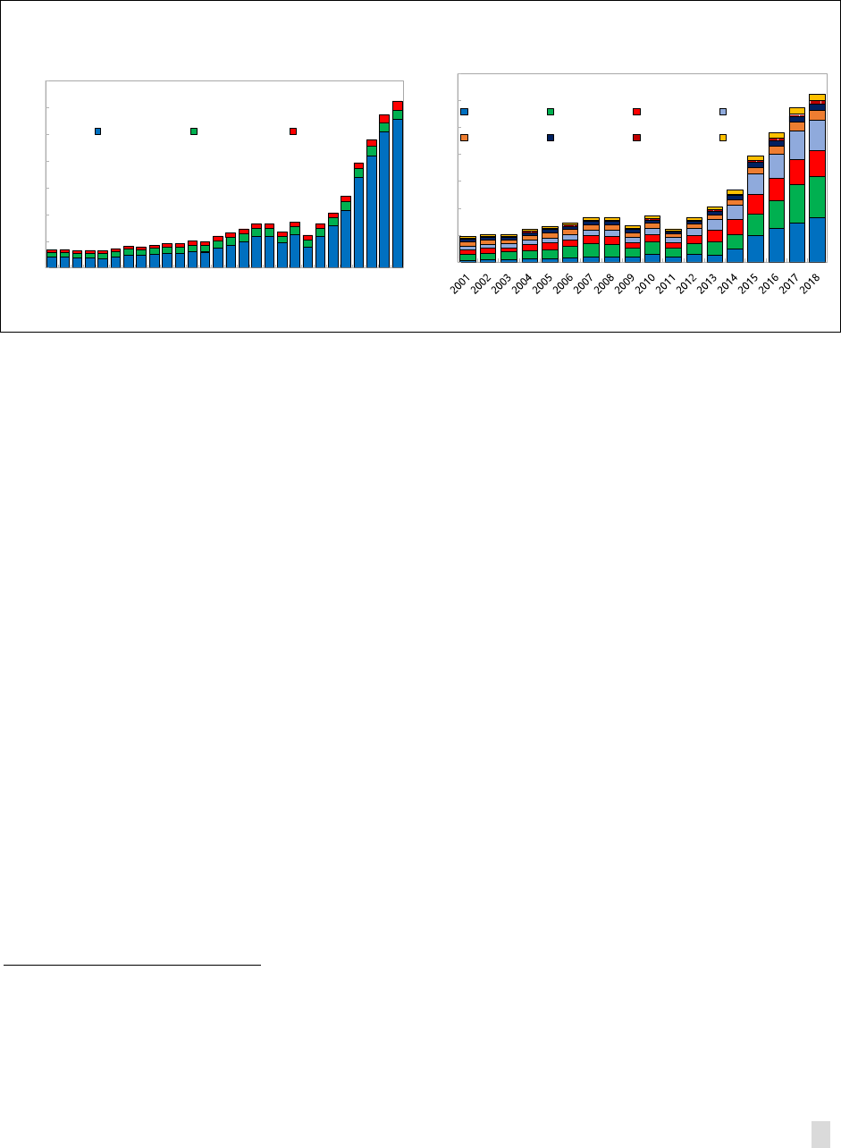
JAPAN
INTERNATIONAL MONETARY FUND 51
with China (27 percent), South Korea (24 percent), and Taiwan (Province of China) (15 percent) being
the three largest sources of tourists.
3
Figure 1. Japan: International Arrivals
5. Foreigners have become the growth engine of the Japanese tourism industry. The
amount spent by international visitors quadrupled since 2012 to ¥4½ trillion in 2018, driven by
tourist numbers rather than increased per-capita spending, which peaked in 2015 (Figure 2).
According to World Tourism Organization data, this upward trend in tourist aggregate expenditure
has enabled Japan to jump into the top 10 countries worldwide in terms of inbound tourism
expenditure (9 ranks up from 2012).
4
It also increased the share of international visitors in total
domestic travel consumption to more than 17 percent.
6. Tourism spending patterns differ across origin countries. Asian visitors generally spend
less in total but relatively more on shopping—more than half of their budget in the case of Chinese
tourists (see Annex I). In contrast, longer stays make the budget for accommodation the largest
share of expenditure in the case of tourists from non-Asian advanced countries. The Japanese
government is enhancing its tourism promotion in these higher-income markets to attract additional
long-stay visitors and thus, boost per capita tourist spending.
3
Since the share of business and other non-tourist travelers has remained constant, the terms “international visitor”
and “tourist” are used interchangeably in this chapter.
4
Latest available data are from 2017. See World Tourism Organization (2019) Compendium of Tourism Statistics
dataset. Ministry of Land, Infrastructure and Transport (2019) Tourism White Paper has Japan as the 11
th
-ranked
country.
0
5
10
15
20
25
30
35
China South Korea Taiwan Other Asia
North America Europe Australia Other
Source: Japan National Tourism Organization.
Japan: International Visitors by Nationality
(In million)
0
5
10
15
20
25
30
35
1991
1992
1993
1994
1995
1996
1997
1998
1999
2000
2001
2002
2003
2004
2005
2006
2007
2008
2009
2010
2011
2012
2013
2014
2015
2016
2017
2018
Tourists Business Others
Source: Haver Analytics.
Japan: International Visitors by Purpose
(In million)
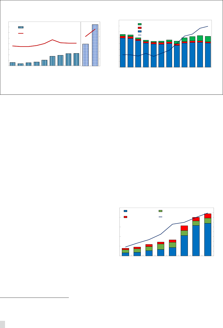
JAPAN
52 INTERNATIONAL MONETARY FUND
Figure 2. Japan: Tourism Expenditure
7. The surge in foreign tourists has enabled tourism to become an increasingly important
sector of the economy (Figure 3):
• The tourism industry contributes some two percent to nominal GDP. According to the latest
available estimates for 2017, tourism GDP stands at ¥11 trillion.
5
Tourism contributed 4.1 percent
to total nominal GDP growth in the 2012–17 period.
• The tourism industry has become an important job creator. Retail sales and accommodation
and food services, two of the main service industries related to tourism, were the 3rd-largest and
the 5th-largest job creators in the 2012–17 period.
• The tourism boom has induced large investments. Specifically, a boost to accommodation
investment in 2016 reflected a steep
increase in overnight stays in 2015. In 2018,
tourism-related investments amounted to
0.2 percent of GDP. However,
accommodation demand has increased
more rapidly than supply, resulting in
increasing occupancy rates for all types of
lodging (up from 55 percent in 2012 to an
average of 61 percent in 2018). Lodging
capacity constraints are likely to induce
further investment, especially with the
upcoming 2020 Olympic and Paralympic
Games in Tokyo and the World EXPO in Osaka in 2025.
5
The Japan Tourism Agency (JTA) measures “tourism GDP” (“tourism direct GDP”) from the production side based on
the value added of tourism-related sectors (tourism satellite account, following UNWTO (2010)).
0
2
4
6
8
10
12
14
16
18
20
0
5
10
15
20
25
30
35
40
2007 2008 2009 2010 2011 2012 2013 2014 2015 2016 2017 2018
International visitors
Japanese travel aboard (domestic spending)
Japanese domestic travel
Share (rhs) 1/
Note: 1/ The share of international visitors' expenditure in total tourism expenditure.
Source: Japan Tourism Agency.
Japan: Total Tourism Expenditure
(JPY trillion, rhs; In percent)
1.1
0.8
1.1
1.4
2.0
3.5
3.7
4.4
4.5
0
2
4
6
8
10
12
14
16
2010 2011 2012 2013 2014 2015 2016 2017 2018
Expenditure amount (lhs)
Spending per capita (rhs)
Source: Japan National Tourism Organization.
Note: Numbers indicate the inbound expenditure amount.
Japan: Inbound Tourism Expenditure
(JPY trillion, rhs: JPY ten thousand)
8
15
0
5
10
15
20
25
30
2020 2030
0
10
20
30
40
50
60
70
80
90
100
0
0.3
0.6
0.9
1.2
1.5
2011 2012 2013
2014
2015 2016 2017 2018
accommodation (ls) restaurant (ls)
residential-hybrid (ls) overnight stays (rs)
Source: Japan National Tourism Organization, Ministry of Land, Infrastructure and
Transport
, Japan; IMF staff calculations.
Japan: Tourism-Related Investment Amount
(lhs: value of building starts, JPY trillion; rhs: stays, million)
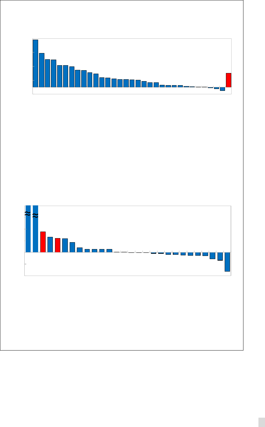
JAPAN
INTERNATIONAL MONETARY FUND 53
Figure 3. Japan: Tourism Contribution, Growth and Jobs
-10
-5
0
5
10
15
20
Health & social
Scientific & technical
Wholesale and retails
ICTs
Accommodation & food
Other service activities
Real estate
Public administration
Transport & postal
M/General machinery
M/Transport
M/Chemicals
Finance and insurance
M/Petroleum & coal
M/Pulp & paper products
Mining
M/Non-metallic
Energy
M/Food & beverages
M/Electrical machines
Education
M/Metal
M/Basic metal
M/Textile
M/Electronic components
M/ICTs equipment
Construction
Agriculture
Note: M indicates Agriculture, Energy and Manufacturing industries, respectively.
Source: Japan System
of National Account.
Japan: Contribution Employment Growth by Sectors
(2012-17, In percent)
60
-2
2
6
10
14
Construction
Scientific & technical
E/Electricity supply
Health & social
Wholesale and retail
M/Transport
M/General machinery
Transport & postal
Real estate
M/Chemicals
Accommodation &food
M/Basic metal
ICTs
M/Electronic components
M/Petroleum & coal
Education
M/Food & beverages
M/Electrical machinery
Public administration
M/Metal
A/Agriculture
M/Pulp & paper product
E/Gas and water supply
M/Non-metallic
Other service activities
A/Fishing
Finance and insurance
A/Forestry
Mining
M/Textile
M/Printing
M/ICT equipment
tourism GDP
Note: A, E, M indicate Agriculture, Energy and Manufacturing industries, respectively.
Source: Japan System of National Account and Japan Tourism Sattellite Account.
Japan: Contribution to GDP Growth by Sectors
(2012-2017, In percent)

JAPAN
54 INTERNATIONAL MONETARY FUND
8. Inbound tourism also contributes to Japan’s current account surplus. After turning
positive for the first time in 2015, Japan’s travel services surplus reached almost one half of one
percent of GDP in 2018. This reflects a steep upward trend of travel credits since 2011, and the
erosion of travel debits. The latter has been dominated by a fall in the overseas spending of
Japanese tourists rather than a decline in their annual headcount, which has fluctuated around
17 million persons.
6
The structural change in the services balance has been significant. Compared to
10 years ago, the travel balance has been transformed from the largest deficit factor into the
second-largest surplus factor of the services account, after income from intellectual property (MLIT,
2019).
Travel Service Balance
9. According to international comparisons, Japan’s tourism industry has further potential
to expand. The GDP share of Japan’s tourism
industry in 2016 was only 1.9 percent
compared to the OECD average of 4.8 percent.
In contrast, the industry’s employment share of
9.6 percent is among the highest in the OECD
(see text figure).
7
The divergence between GDP
share and employment share suggests a likely
potential for labor productivity increases that
would also help alleviate growth constraints for
the industry stemming from labor shortages.
6
See Japan National Tourism Organization at https://statistics.jnto.go.jp/en/graph/#graph--outbound--outgoing--
transition
7
Data drawn from the OECD Tourism Statistics database. Employment is employment in the tourism industry.
0.0
0.2
0.4
0.6
0.8
1.0
2006
2007
2008
2009
2010
2011
2012
2013
2014
2015
2016
2017
2018
Credit Debit
Source: Bank of Japan; IMF staff calculations.
Japan: Travel Credit to GDP Ratio
(In percent)
-15
-10
-5
0
5
10
15
20
1996
1998
2000
2002
2004
2006
2008
2010
2012
2014
2016
2018
Goods
Service/Transport
Service/Travel
Service/Other
Source: Bank of Japan.
Japan: Goods and Service Balance
(JPY trillion)
1.9
9.6
0
4
8
12
16
20
Australia
Austria
Canada
Czech Republic
Denmark
Finland
France
Greece
Iceland
Israel
Japan
Lithuania
Mexico
Netherlands
New Zealand
Norway
Portugal
Slovak Republic
Spain
Sweden
Switzerland
United States
Tourism, percent of GDP
Tourism, percent of GDP, average
Tourism, percent of employment
Tourism, percent of employment, average
Selected Countries: Direct Economic Impact of Tourism
Source:
OECD Tourism Statistics database.
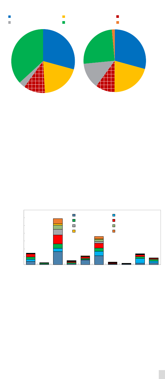
JAPAN
INTERNATIONAL MONETARY FUND 55
10. Japan also has potential to boost inbound tourist spending. In an international
comparison with tourism-competitor Thailand, visitors from America, Europe and Oceania tend to
spend more days with a total of
$200-$600 more in per capita
expenditure in Thailand than in
Japan. In terms of tourist spending
composition, significant differences
lay in spending on entertainment
and shopping: 15 percent of
tourists’ budget in Thailand is spent
on entertainment services, while the
corresponding figure is 3 percent in
Japan (see text figure). As
entertainment spending has a high
marginal effect on tourist
expenditure (MLIT, 2019),
promoting entertainment services should continue to be a priority, along with attracting tourists
from high-income countries to boost per capita tourist spending.
11. The tourism boom remains regionally concentrated within Japan. Foreign tourists have
increasingly been venturing into outlying regions, but remain highly concentrated in and around
Tokyo (Kanto region), in the Osaka/Kyoto area (Kinki region), in Hokkaido, and in Okinawa (Figure
4). Diversification across origin countries differs, too: almost half of the foreign visitors in the
Kyushu region are South Korean; and in Kanto and Kinki, 30 percent are Chinese.
12. The concentration in numbers
is mirrored in spending and
investment (Figure 5). As per-capita
spending is also higher in tourist
hotspots, both Kanto and Kinki regions
receive more than 70 percent of total
foreign tourist expenditure. In a similar
vein, although larger in all regions,
accommodation investment remains
concentrated.
29.5
20.1
11.0
3.3
37.1
Accommodation Food and drink Transportation
Entertainment service Shopping Medical care
Source: Japan Tourism Agency, Thailand Ministry of Tourism and Sports; and
IMF staff calculations.
Thailand
Japan and Thailand: Tourist Spending Breakdown
29.2
20.9
10.0
13.4
25.0
1.5
Japan
0
5
10
15
20
25
30
35
Hokkaido
Tohoku
Kanto
Hokuriku
Chubu
Kinki
Chugoku
Shikoku
Kyushu
Okinawa
China South Korea
Taiwan Other Asia
North America
Europe
Australia others
Japan: Overnight Stays of International Visitors by Region (2018)
(Million stays)
Source: Japan National Tourism Organization; IMF staff calculations.
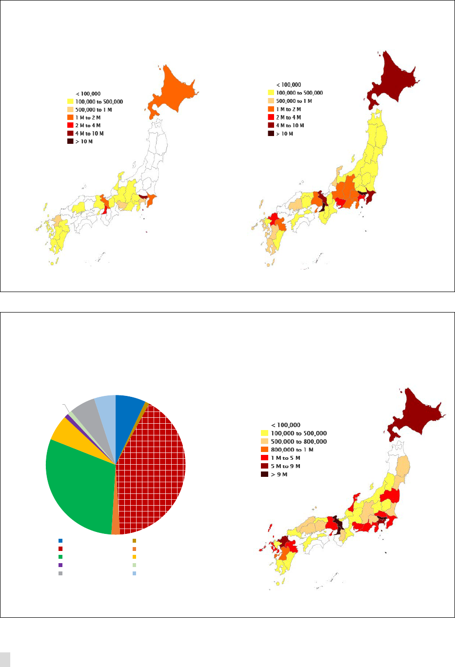
JAPAN
56 INTERNATIONAL MONETARY FUND
Figure 4. Japan: Overnight Stays of Inbound Visitors in Prefectures
Source: Japan Tourism Agency.
Figure 5. Japan: Tourism Impact at Regional and Prefectural Level
Japan: Distribution of Inbound Tourism Expenditure by
Region
(In percent, 2017)
Japan: Accommodation Investment by Prefecture
(2018)
(2018, JPY ten thousand)
Source: MLIT (2018).
Note: Regions' sequence is from North to South.
Source: Ministry of Land, Infrastructure and Transport,
Japan.
7%
1%
41%
2%
30%
6%
1%
1%
6%
5%
Hokkaido Tohoku
Kanto Hokuriku Shinetsu
Kinki Chubu
Chugoku Shikoku
Kyushu Okinawa
Japan: Number of overnight stays
(2018)
Japan: Number of overnight stays
(2012)

JAPAN
INTERNATIONAL MONETARY FUND 57
C. Tourism Promotion Policies
13. Tourism promotion, including for regional revitalization, has been stepped up under
Abenomics, with ambitious targets. While
promotion efforts started in the last decade
and considered tourism as an instrument for
regional revitalization, tourism policies have
been reinvigorated since 2012.
8
A Tourism
Strategy Promotion Council was established
and regularly meets on the basis of its most
recent strategy of 2016. Based on the 2016
Tourism Strategy, a broad array of policy
measures aim at enhancing regional
attractiveness, industry competitiveness, and travel comfort. Annex II presents its visions and key
reforms, including a listing of various reforms to reinvigorate the tourism industry.
14. Tourism policies have been supported by an increase in budgets of relevant agencies,
more tax-free shops, more direct flights, and relaxation of visa requirements (Figure 6).
9
In
January 2019, an international tourist departure tax was introduced as a financing vehicle for the
tourism budget. With the new income, the budget is set to almost double to ¥66.6 billion in FY 2019.
Over 40 countries, mainly in Asia and the Pacific, have been granted relaxation of visa requirements by
either multiple-entry visa introduction or visa exemptions during the 2013–18 period.
15. Japan has also attracted major international events. In line with the 2016 strategy, Japan
has attracted high-profile events, such as the 2019 Rugby World Cup, the 2020 Olympic and
Paralympic Games, and EXPO 2025. These events are likely to have significant income multiplier
effects.
D. Determinants of Inbound Tourism
16. There are several key determinants of tourist arrivals into Japan. Following the work of
Pesaran et al. (1999), we estimate panel autoregressive distributed lag (ARDL) regressions using
quarterly data for Japan inbound tourists. The ARDL method avoids the need for pre-testing the
order of integration given that they are valid whether the variables of interest are stationary or
integrated (of order one).
10
It is also robust to omitted variables bias and simultaneous
8
These early efforts included a “Visit Japan Campaign” (2003), the “Basic Law for the Promotion of a Tourism-
Oriented Country” (2006), and the creation of the Japan Tourism Agency (JTA) in 2008.
9
The agencies at the national level are the Japan Tourism Agency (JTA) and the Japan National Tourism Organization
(JNTO), a sub-body of JTA. While JTA is in charge of tourism policies, JNTO is specialized in executing the “Visit Japan
Campaign” and other tourism marketing activities.
10
Pesaran (1997) and Pesaran, Shin, and Smith (1999) show that the traditional ARDL approach can be used for long-
run analysis, and that the ARDL methodology is valid regardless of whether the regressors are exogenous, or
endogenous, and irrespective of whether the underlying variables are I(0) or I(1).
Targets for Foreign Visitors
Actual
2018 2020 2030
Arrivals (people, mil) 31.2 40 60
Spending (JPY, tril) 4.5 8 15
Overnight stays in regions*
(guest nights, mil)
38.5 70 130
Repeat visitors (people, mil) 19.4 24 36
Target year
Sources: Japan Tourism Agency, Japan National Tourism Organization.
* Excluding the metropolitan areas: Tokyo, Kanagawa, Chiba, Saitama,
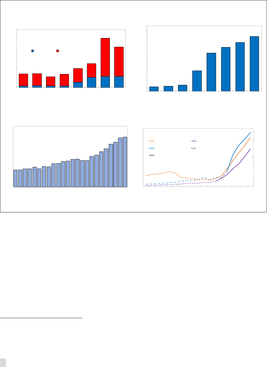
JAPAN
58 INTERNATIONAL MONETARY FUND
determination of growth regressors.
11
As shown in Table 1, origin country GDP, relative prices, visa
policies, and natural disasters have a statistically-significant impact on the number of tourist arrivals.
Figure 6. Japan: Government Efforts to Boost Tourism
17. Visa relaxation policies for Asian countries has successfully increased tourist numbers (Table
1, Panel A).
12
The introduction of multiple-entry visas helped increase the number of tourists from China by
121 percent and from other emerging Asian countries by 55 percent (long-run effect). Similarly, introducing
visa-free travel for some emerging Asian countries boosted the number of tourists by 134 percent.
18. Income levels in source countries and bilateral real exchange rates play an important role in
affecting inbound tourism. These factors appear to be important for all origin countries, with price
elasticities being highest for advanced Asia. The high price elasticities point to a large exposure of Japan
tourism demand to changes in exchange rates and prices. Accompanied by the safe-haven status of the
11
The lag order of the ARDL regressions were selected using the Bayesian Information Criterion with a maximum lag
length set to 4.
12
Tourist arrivals from the included thirty-four origin countries accounted for 99 percent of total arrivals to Japan in
2018.
0
10000
20000
30000
40000
50000
60000
2010 2011 2012 2013 2014 2015 2016 2017
JNTO JNTO excluded
Sources: Ministry of Finance, Japan; and IMF staff calculations.
Japan: JTA Expenditure for Tourism Promotion
(In million of Japanese Yen)
0
10000
20000
30000
40000
50000
60000
2012 2013 2014 2015 2016 2017 2018 2019
Source: Ministry of Land, Infrastructure and Transport (MLIT), Japan.
Japan: Number of Tax-free Shops
0
1.5
3
4.5
6
7.5
9
0.0
0.1
0.2
0.3
0.4
0.5
0.6
2000
2001
2002
2003
2004
2005
2006
2007
2008
2009
2010
2011
2012
2013
2014
2015
2016
2017
2018
Philippines Vietnam
China (rhs) Before visa relaxation
After visa relaxation
Japan: Multiple Visa Introduction for Asian Countries
(In million, number of visitors)
Source: Japan National Tourism Organization.
0
1000
2000
3000
4000
5000
6000
1995
1996
1997
1998
1999
2000
2001
2002
2003
2004
2005
2006
2007
2008
2009
2010
2011
2012
2013
2014
2015
2016
2017
2018
Japan: Number of Direct Flights
Souce: Ministry of Land, Infrastructure and Transport (MLIT), Japan.

JAPAN
INTERNATIONAL MONETARY FUND 59
Japanese yen and a high possibility of sudden yen appreciation (Han and Westelius, 2019), this could hinder
the recent increase in inbound tourism.
19. In the short-run, natural disasters could have a large and prolonged impact on Japan
tourism demand (Table 1, Panel B). The natural disaster dummy shows simultaneous negative impact on
tourism demand from most source markets. The number of emerging Asia tourists could decrease by 11–
14 percent in the period a disaster occurs. The impact of natural disasters becomes even larger in the
following period, with a 43 percent fall in tourist numbers in the case of emerging Asia. The negative impact
lasts until the second lag for non-Asian tourists, with tourist numbers 3.5 percent lower than before the
disaster (lasting even after 9 months).
Table 1. Determinants of Tourist Arrivals to Japan, 1996-2018
Note: ARDL regressions. Standard errors in parentheses. *** p<0.01, ** p<0.05, * p<0.1
Source: IMF staff estimates.
E. Conclusions and Policies
20. As part of Abenomics, the government has been successfully promoting inbound
tourism. The number of inbound tourists has tripled since 2012, and the domestic tourism industry
now contributes about two percent of nominal GDP (¥11 trillion in absolute terms). Policies, such as
relaxation of visa requirements, have played an important role, and all indicators have been moving
closer to the government’s ambitious 2020 targets. However, the economic impact of tourism within
Japan remains concentrated in a few “hotspots”, and tourists come predominantly from only three
Asian source markets.
Dependent variable
(1) (2) (3) (4)
China Emerging Asia Advanced Asia Non-Asia
Origin country GDP 2.214*** 3.936*** 2.648*** 5.492***
(0.240) (0.248) (0.488) (0.838)
Bilateral real exchange rate 1.385* 0.679*** 2.606*** 1.131***
(0.723) (0.227) (0.245) (0.345)
Prices in alternative destinations
-1.787 -1.536*** 0.369 0.488
(1.216) (0.318) (0.352) (0.338)
Multiple visa dummy 1.210*** 0.547***
(0.213) (0.109)
Visa requirement dummy -1.340*** 0.235 3.923
(0.115) (0.143) (4.509)
Error-correction term -0.680*** -0.290** -0.225*** -0.0799***
(0.176) (0.130) (0.0757) (0.0133)
Disaster
0.131 -0.143*** -0.110* -0.107***
(0.170) (0.0374) (0.0624) (0.0125)
One period after disaster
-0.308* -0.431*** -0.336*** -0.272***
(0.172) (0.0526) (0.0621) (0.0222)
Two periods after disaster
0.275 0.0347 0.0479** -0.0354*
(0.181) (0.0439) (0.0228) (0.0187)
Maximized log likelihood
175.43 142.13 791.78
Observations
87 482 435 1,874
Number of country
1 6 5 22
∆ln(tourist arrivals)
Country/Group
Panel B: Short-run effects
Panel A: Long-run effects

JAPAN
60 INTERNATIONAL MONETARY FUND
21. Strengthened policies will help enlarge Japan’s share in the growing global tourism
market and attract more tourists to regional Japan. To achieve its next level of targets in 2030, in
its continuous review of policies and action plans, the government could pay special attention to the
following priorities:
• Continued regional diversification within Japan: A strengthening of the authorities’ approach to
foster travel convenience and industry competitiveness in Japan’s regions would include: broader
and more accessible information dissemination about regional attractions; more low-cost flight
connections to regional airports; and the creation of regional sightseeing corridors. Enhanced
coordination between national and sub-national stakeholders, such as the Japan National Tourist
Organization and local Destination Management/Marketing Organizations, is key.
13
• Diversification of tourism source markets: To reduce risks from idiosyncratic shocks in
dominant source markets, an intensified diversification strategy could target a broader set of
Asian emerging markets, including through additional relaxation of visa requirements and flight
connections.
• More experience-orientated tourism and “Japan branding”: Bringing more tourists into the
regions would also foster the transition from shopping-oriented to experience-oriented tourism,
which is particularly pertinent to Asian tourists. In turn, experience-oriented regional tourism
would further differentiate the tourism brand of Japan, and potentially decrease the price
sensitivity of demand. It could also incentivize longer stays, repeat visits, and more tourism
spending.
• Disaster resilience: Since international tourists have typically an adverse reaction to a post-
disaster situation, countermeasures to mitigate the disaster impact on Japanese tourism are
necessary not only in disaster-affected areas but also unaffected areas. Implementation of a
disaster information policy, including fostering the efficient and accurate provision of
information during and after a natural disaster, will help avoid adverse tourist reactions, as well
as assist tourists in rescheduling their visits to Japan.
22. Any forthcoming increase in tourism demand would need to be synchronized with
enhanced supply of tourism services, including labor and tourism infrastructure. While
fostering labor-saving efficiency gains, more foreign labor (as well as increased female and elderly
labor market participation) will need to be considered as the labor force shrinks. In addition,
continuing to build tourism infrastructure—such as free Wi-fi, multilingual signage, and cashless
payment systems—are among the top priorities to ease tourists’ anxiety.
14
13
Destination Management/Marketing Organizations (DMOs) are joint private/public organizations, usually
including diversified stakeholders in transportation, culture/historical sites, and accommodation. They are expected to
play a role in helping invigorate the regional tourism industry by developing and marketing local tourism attractions
in their regions. Japan aims at creating 100 world-class DMOs across the country by 2020.
14
A Japan Tourism Agency (2019) survey showed that the most uncomfortable issues tourists encounter when
traveling in Japan are lack of public Wi-fi, poor non-Japanese language skills, lack of multilingual signage (including
for public transportation), and the lack of cutting-edge payment settlement methods.

JAPAN
INTERNATIONAL MONETARY FUND 61
References
Han, Fei, and Niklas J. Westelius, 2019, “Anatomy of Sudden Yen Appreciations,” IMF Working Paper
19/136.
Japan Tourism Agency (JTA), 2019, “Inconvenience and Dissatisfaction to the Acceptance
Environment of Japan Which Inbound Tourists Feel” (in Japanese), Japan Tourism Agency: Tokyo.
Retrieved from https://www.mlit.go.jp/common/001281549.pdf
Council for a Tourism Vision to Support the Future of Japan, 2016, New Tourism Strategy to
Invigorate the Japanese Economy, Ministry of Land, Infrastructure and Transport: Tokyo.
Ministry of Land, Infrastructure and Transport (MLIT), 2018, Tourism White Paper, Ministry of Land,
Infrastructure and Transport: Tokyo.
Ministry of Land, Infrastructure and Transport (MLIT), 2019, Tourism White Paper, Ministry of Land,
Infrastructure and Transport: Tokyo.
Pesaran, M. Hashem, 1997, “The Role of Economic Theory in Modelling the Long Run,” The
Economic Journal, Vol. 107 (440), pp. 178–91.
Pesaran, M. Hashem, Yongcheol Shin and Ron P. Smith, 1999, Pooled Mean Group Estimation of
Dynamic Heterogeneous Panels, Journal of the American Statistical Association, Vol. 94 (446), pp.
621–34.
United Nations World Tourism Organization (UNWTO), 2010, Tourism Satellite Account:
Recommended Methodological Framework 2008, United Nations World Tourism Organization, New
York.

JAPAN
62 INTERNATIONAL MONETARY FUND
Annex I. Tourists’ Spending and Composition (2018)
Accommodation
Food and
Drink
Transportation
Entertainment
Service
Shopping
China
9.7 224870 21.3 17.8 7.5 3.6 49.9
Indonesia
12.1 141419 34.0 20.6 14.8 3.9 26.6
Malaysia
10.2 137612 32.7 22.1 11.9 4.7 28.6
Thailand
8.8 124421 29.6 22.3 12.1 3.5 32.3
South Korea
4.4 78084 32.0 25.6 9.8 5.0 27.6
Taiwan (Province of China)
6.8 127579 27.7 22.1 10.6 4.0 35.6
Hong Kong SAR
6.3 154581 29.5 23.9 10.8 3.3 32.5
Singapore
8.3 172821 36.6 24.0 11.5 3.7 24.1
United States
13.5 191539 43.0 26.4 14.3 4.1 12.2
Canada
12.1 183218 40.9 25.9 15.1 4.4 13.7
Australia
13.3 242041 41.0 24.3 14.4 6.7 13.5
France
18.4 215786 39.6 26.4 15.5 3.4 15.0
Germany
13.9 191736 44.1 24.8 14.8 3.1 13.2
United Kingdom
13.8 220929 45.6 25.4 15.0 3.8 10.2
Source: Japan Tourism Agency; IMF staff calculations.
Advanced
Length of
Stay (days)
Spending Per
Capita
(in JPY)
Of which (%)
Emerging Asia
Advanced Asia
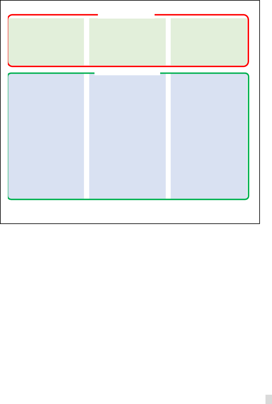
JAPAN
INTERNATIONAL MONETARY FUND 63
Annex II. 2016 Tourism Strategy
Source: Council for a Tourism Vision to Support the Future of Japan (2016).
Maximizing the attractiveness
of tourism resources in order
to make tourism the base of
regional revitalization
Foster innovation in the
tourism industry to boost its
international competitiveness
and develop it into a core
industry
Ensure all visitors can enjoy a
satisfying, comfortable and
stress-free sightseeing
experience
・Allow domestic and international
visitors entry to “publicly owned
heritage sites”
・Shift the balance of heritage policy
from “an over-emphasis on
preservation only” to allow a greater
understanding of the sites by tourists
・Turn the current “national parks”
into world-class “national parks”
・Create “landscaping plans” for
major tourism areas to improve
townscapes
・Review regulations and restrictions
in order to make the tourism industry
more productive
・Develop new longer-stay markets
・Create and develop world-class
Destination Management/Marketing
Organizations (DMOs)
・Renew and revitalize hot spring
resorts and local towns through
better management
・Promotion of MICE (Meetings,
Incentives, Conferencing, Exhibitions)
・Strategic relaxation of visa
requirements
・Greatly improve hard and soft
infrastructure to realize the most
pleasant accommodation
environment in the world
・Promotion of information
dissemination in multiple languages
・Complete “regional revitalization
corridors” to allow comfortable
travel to every corner of Japan
・Functional enhancement of local
airports and the promotion of Low-
Cost Carrier (LCC) services
・Reforming the system of “work
days” and “days off” towards
realizing a more vibrant society
・Comprehensive design promotion
activities for the 2020 Tokyo Olympic
and Paralympic Games
Proposed reforms
3 visions

JAPAN
64 INTERNATIONAL MONETARY FUND
JAPAN’S FOREIGN ASSETS AND LIABILITIES:
IMPLICATIONS FOR THE EXTERNAL ACCOUNTS
1
The composition of Japan’s external current account balance has changed over time, with the trade
surplus decreasing while the income balance has increased. Japan’s higher income balance primarily
reflects its growing net foreign asset position and higher corporate saving. A comparison with peer
countries also reveals the role of relatively high yields on foreign direct investment (FDI) assets held by
Japan—arising from differences in geographical positioning but also, possibly, reflecting profit shifting.
The comparison with peers points to the very low FDI liabilities in Japan, suggesting scope for
improving corporate governance and reducing barriers to entry in some sectors, and possible
measurement issues. Despite the changing composition of Japan’s current account balance over time,
its response to exchange rate movements operates mostly through the trade channel given relatively
higher gross trade flows than income flows, with a small but reinforcing contribution from the income
balance.
A. What Has Driven the Increase in Japan’s Income Balance?
1. The progressive increase in Japan’s income balance primarily reflects net revenues
from an increasingly positive net foreign asset (NFA) position. Japan’s primary income balance is
composed almost exclusively of investment income, which has grown in tandem with the growing
NFA position, from close to in balance in 1980 to a positive 60 percent of GDP in 2018 (Figure 1, top
right panel). Japan’s present NFA is the highest in the world, at $3 trillion.
2. The increase in Japan’s income balance since the mid-1990s can be attributed mostly
to the corporate sector, and is linked to the increase in corporate saving. The investment
income balance is the sum of net property income of all sectors of the domestic economy
(corporates, households, public sector).
2
In Japan, corporate net property income and the investment
income balance have had a parallel trend increase since the mid-1990s, while household and
government net property income have remained broadly flat (Figure 1, middle left panel). In turn,
the increase in corporate net property income has been a key driver of the increase in corporate
saving (see Japan 2019 Article IV Consultation – Staff Report, Annex XIII). Indeed, the rise in Japan’s
NFA is itself the product of persistent current account surpluses which have been increasingly driven
by growing corporate saving (Figure 1, middle right panel). In line with this, Hashimoto and Kinoshita
(2016) underline the role played by corporate balance sheet adjustment and the rise in corporate
saving in the increase in Japanese corporates’ financial net wealth.
1
Prepared by Mariana Colacelli (APD) and Cyril Rebillard (RES). Deepali Gautam (RES) and Albe Gjonbalaj (APD)
provided valuable research assistance.
2
Strictly speaking, the investment income balance is net property income of the domestic economy, excluding rents.
However, net income from rents by sector tend to be small and stable over time.
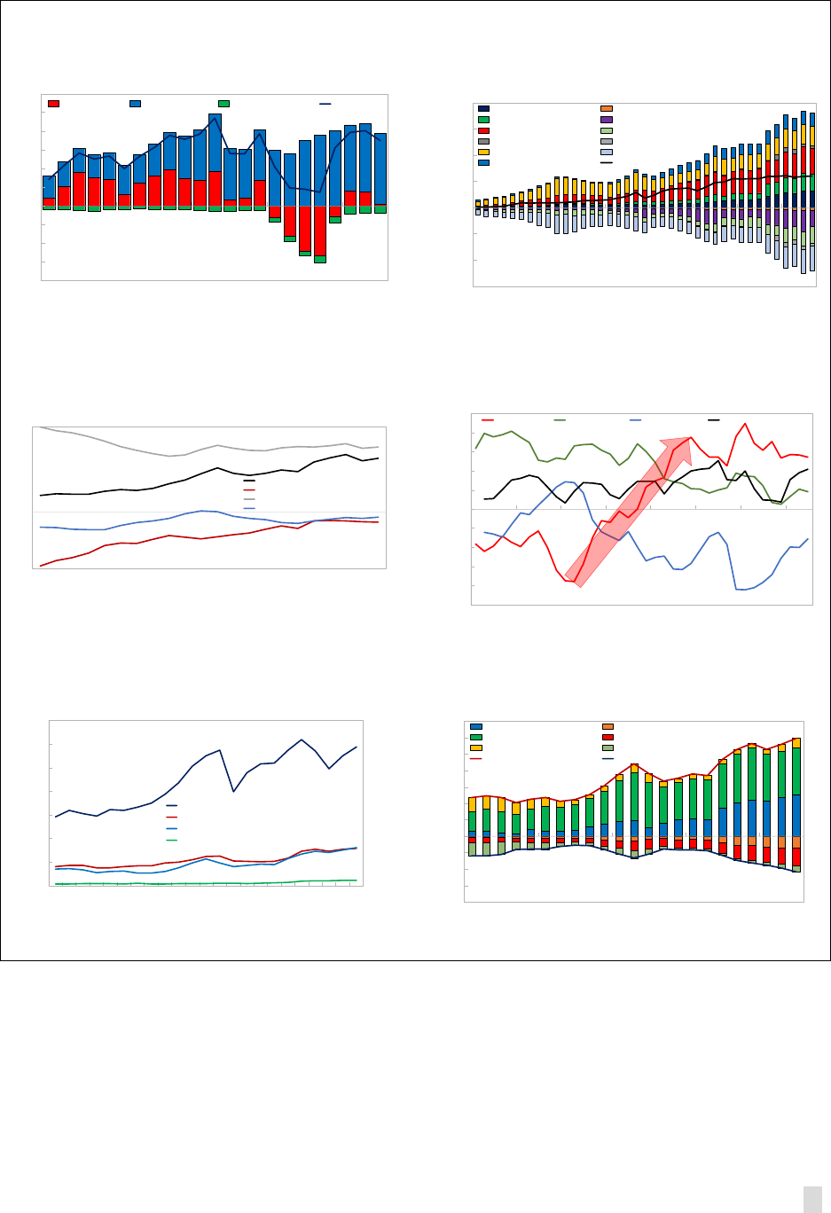
JAPAN
INTERNATIONAL MONETARY FUND 65
Figure 1. Japan’s Increasing Income Balance and its Drivers
3. In terms of gross flows within the external current account, the respective importance
of the trade account and the income account have remained broadly unchanged over time
(Figure 1, bottom left panel). Both gross income flows (defined as the sum of credits and debits) and
gross trade flows have nearly doubled in 20 years. As a result, the ratio of gross income (primary,
secondary) flows to gross trade (goods, services) flows has increased only moderately, from 21
-4
-3
-2
-1
0
1
2
3
4
5
6
1996
1997
1998
1999
2000
2001
2002
2003
2004
2005
2006
2007
2008
2009
2010
2011
2012
2013
2014
2015
2016
2017
2018
Trade balance Primary Income Secondary Income CA balance
Sources: IMF BOP data; National authorities; and IMF WEO data.
Japan: Current Account Decomposition: Trade and Income Balances
(In percent of GDP)
-150
-100
-50
0
50
100
150
200
1980
1982
1984
1986
1988
1990
1992
1994
1996
1998
2000
2002
2004
2006
2008
2010
2012
2014
2016
2018
Assets, FDI Liabilities, FDI
Assets, Portfolio Equity Liabilities, Portfolio Equity
Assets, Portfolio Debt Liabilities, Portfolio Debt
Assets, Fin. Derivatives Liabilities, Fin. Derivatives
Assets, Other Liabilities, Other
Assets, FX reserves NIIP
Japan: Decomposition of Net International Investment Position
(In percent of GDP)
Source: Lane & Milesi-Ferretti database, External Wealth of Nations, 2018.
-4
-3
-2
-1
0
1
2
3
4
5
6
1996
1997
1998
1999
2000
2001
2002
2003
2004
2005
2006
2007
2008
2009
2010
2011
2012
2013
2014
2015
2016
2017
Investment Income Balance
Net property income: Corporates
Net property income: Households
Net property income: Government
Japan: Investment Income Balance and Net Property
Income by Sector
(In percent of GDP)
Sources: AMECO database; OECD national accounts dataset; IMF BOP data;
National authorities; and IMF WEO data.
-10
-8
-6
-4
-2
0
2
4
6
8
10
1980 1984 1988 1992 1996 2000 2004 2008 2012 2016
Corporates Households Government Total Economy
Japan: Gross Saving minus Investment
(In percent of GDP)
Source: AMECO database.
2017
0
5
10
15
20
25
30
35
1996
1997
1998
1999
2000
2001
2002
2003
2004
2005
2006
2007
2008
2009
2010
2011
2012
2013
2014
2015
2016
2017
2018
Goods: Exports+Imports
Services: Exports+Imports
Primary Income: Credit+Debit
Secondary Income: Credit+Debit
Japan: Current Account: Trade and Income Gross Flows
(In percent of GDP)
Sources: IMF, BOP data; National authorities; and IMF, WEO data.
-4
-3
-2
-1
0
1
2
3
4
5
6
7
1996
1997
1998
1999
2000
2001
2002
2003
2004
2005
2006
2007
2008
2009
2010
2011
2012
2013
2014
2015
2016
2017
2018
Direct Investment, Credit
Direct Investment, Debit
Portfolio Investment, Credit Portfolio Investment, Debit
Other Investment, Credit
Other Investment, Debit
Investment Income, Credit Investment Income, Debit
Japan: Investment Income Decomposition
(In percent of GDP)
Sources: IMF, BOP data; National authorities; and IMF, WEO data.
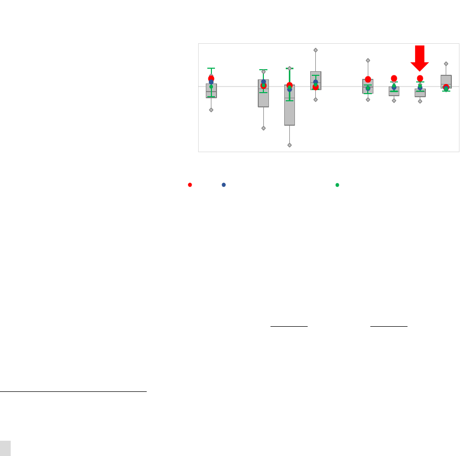
JAPAN
66 INTERNATIONAL MONETARY FUND
percent in 1996 to 25 percent in 2018.
3
More generally, gross trade flows remain predominant within
the current account for all countries, with the relative importance of income flows being somewhat
higher in advanced economies. Indeed, while trade integration has progressed in both advanced and
emerging economies, financial integration is greater in advanced economies, including due to
reduced access to international capital markets in some emerging and developing economies.
4. Japan’s relatively large income balance is primarily the result of an asymmetric income
account. With gross income flows growing in tandem with gross trade flows over the past two
decades, it is the asymmetric nature of the expansion of income flows, rather than their size, that
explains Japan’s large and growing income balance. In particular, income credits are significantly
larger than debits for most components of Japan’s investment income (Figure 1, bottom right panel).
B. How Does Japan’s Income Balance Compare to Peers?
5. Japan’s external income balance is exceptionally large. From an accounting perspective,
Japan’s larger-than-average current account balance is associated with a trade balance that is close
to median (among G6, advanced
economies, or among a 100-
country sample), but includes an
exceptionally large primary income
balance (investment income in
particular, see text chart). To shed
further light on the reasons behind
Japan’s large income balance, we
decompose the difference between
the investment income balance of
Japan and G6 countries (Canada,
France, Germany, Italy, United
Kingdom, United States),
highlighting the respective
contributions of stocks and yields.
6. Japan’s investment income balance is significantly larger than that of G6 countries. The
3.5 percentage points of GDP difference in investment income balance
can be described
in the equation below, where S denotes stocks and Y denotes implicit yields:
=
.
+
2
+
.
+
2
{
,
}
3
Accommodative monetary policies have constrained interest flows in recent years; the ratio of income flows to trade
flows may increase in the future when monetary policy normalizes.
-30
-25
-20
-15
-10
-5
0
5
10
15
20
Current
account
balance
Trade
balance
Trade
balance
(goods)
Trade
balance
(services)
Total
Income
Balance
Primary
Income
Balance
Investment
Income
Balance
Secondary
Income
Balance
Japan Advanced Economies: Median G7 ex-Japan: Unweighted average
Current Account, Trade, Income Balances: Japan vs. Other
Countries (2015
-17)
(In percent of GDP)
Note: Boxes (diamonds) show 25-75 (10
-90) percentiles
in the 100-country sample.
Sources: IMF, BOP data; National authorities; and IMF, WEO data.

JAPAN
INTERNATIONAL MONETARY FUND 67
For each category k of foreign asset/liability, the difference in income flows between Japan and G6
can be decomposed into: (i) the contribution of stock positions, measured by the difference in stock
positions
multiplied by the average implicit yield
, and (ii) the contribution of implicit
yields, measured by the difference in implicit yields
multiplied by the average stock
position
. Decomposition results for the difference between the investment income of Japan
and G6 are presented in Table 1.
4
Table 1. Japan and G6 Income Balance – Contributions of Stocks and Yields
(2015–17 average)
Source: IMF BOP data; National authorities; IMF WEO data; Lane & Milesi-Ferretti database, External Wealth of Nations, 2018; and Authors’
calculations.
7. On the asset (or credit) side of the income-account-difference decomposition, while
Japan holds fewer foreign assets than the G6, yields are higher. Overall, foreign assets explain a
small part of the higher investment income balance in Japan relative to G6 countries (only 0.3
percentage points of 3.5 percentage points of GDP difference). This is particularly the case for FDI:
Japan has relatively low FDI assets compared to G6 countries, but significantly higher yields. Several
factors may help explain the higher returns on Japanese investment abroad:
• A more favorable geographical allocation of FDI assets, as Japan has a larger share of FDI in
high-growth emerging Asia as well as the United States (Figure 2, left chart). This difference may
explain around one percentage point of the higher yields in Japan than in G6 on average since
2000 (Figure 2, right chart).
• Profit shifting through transfer pricing may artificially boost investment income credits and
suppress export figures. In the case of the United States, Wright and Zucman (2018) attribute the
abnormally high returns on foreign investment (with a positive U.S. income balance, despite a
negative NFA) in part to profit shifting. Tørsløv, Wier and Zucman (2018) estimate that $28
billion (0.6 percent of GDP) of profits were shifted out of Japan in 2015. Assuming that profit
shifting mainly distorted Japan’s direct investment income credits (and not the FDI asset
position), Japan’s “corrected” implied yield on FDI assets would be around 2 percentage points
4
Changing the comparator group, e.g. considering advanced creditor countries (Belgium, Denmark, Germany, Israel,
Korea) instead of G6 leads to similar results.
Total FDI
Portfolio
Equity
Portfolio
Debt
Other Total FDI
Portfolio
Equity
Portfolio
Debt
Other
Income flows % of GDP 3.7 5.5 2.2 1.0 1.9 0.3 1.8 0.6 0.7 0.3 0.2
Stocks % of GDP 62.1 146.2 29.6 30.5 51.3 34.7 109.5 5.0 35.3 26.2 43.0
Implied Yields percent 3.8% 7.5% 3.4% 3.7% 0.9% 1.6% 12.9% 1.9% 1.0% 0.5%
Income flows % of GDP 0.2
5.2 2.6 1.0 1.0 0.6 5.0 1.6 1.0 1.8 0.6
Stocks % of GDP -4.5 225.1 60.0 48.9 41.0 75.2 231.8 48.5 34.1 73.4 75.9
Implied Yields percent 2.3% 4.3% 2.0% 2.5% 0.8% 2.1% 3.3% 2.9% 2.4% 0.8%
Income flows
% of GDP
3.5
0.3 -0.4 0.1 0.9 -0.3 -3.2 -0.9 -0.3 -1.5 -0.4
Stocks
% of GDP 2.2 -2.3 -1.8 -0.5 0.3 -0.4 -4.5 -3.5 0.0 -0.8 -0.2
Implied Yields % of GDP 1.4 2.7 1.4 0.6 0.6 0.1 1.3 2.6 -0.3 -0.7 -0.2
Contributions to
Income Balance
difference
Total
(net)
ASSETS
LIABILITIES
Japan
G7 ex-Japan:
unweighted average
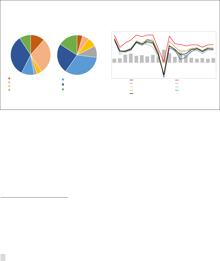
JAPAN
68 INTERNATIONAL MONETARY FUND
lower than at present.
5
Japan’s move from a worldwide to a territorial tax system in 2009, while
fostering dividend repatriation (Hasegawa and Kiyota, 2017) and reducing foreign cash holdings
(Xing, 2018), may also have led to an intensification of transfer mispricing and profit shifting, as
suggested by evidence based on the United Kingdom experience (Liu, Schmidt-Eisenlohr and
Guo, 2017).
• Other potential measurement issues. High yields on foreign assets could also be a sign of
potential measurement issues (see more below).
Figure 2. Japan: Geographical Allocation of FDI Assets, and Impact on Yields
8. On the liabilities (or debit) side of the income-account-difference decomposition,
Japan’s stock of foreign liabilities is much smaller than that of G6 countries, especially for FDI
but also for portfolio debt. This leads to a large contribution to the overall difference of
investment income balances (3.2 out of the 3.5 percentage points of GDP difference).
• FDI liabilities. The fact that implicit yields paid on FDI liabilities are very high in Japan (close to
13 percent; see Table 1) suggests measurement issues, possibly on the valuation of FDI
liabilities.
6
That said, adjusting implicit yields to the G6 level, while leaving FDI income payments
unchanged, would only “correct” Japan’s stock of FDI liabilities from 5 to 20 percent of GDP, i.e.
still a level of FDI liabilities significantly below the G6 average level (at about 50 percent of GDP).
5
While profit shifting may partly explain Japan’s high implied yields on FDI assets, both in absolute and relative to
advanced economies (with profit shifting occurring mainly between large advanced economies and advanced tax
havens, and thus being broadly neutral for advanced economies as a group), it does not explain the difference
relative to G6 countries. Indeed, G6 economies are also affected by profit shifting, and their “corrected” implied yields
on FDI assets would also be around 2 percentage points lower.
6
To the extent that a firm is included in national statistics, both its stock and flows of FDI should be captured, making
it unlikely that macroeconomic aggregates omit FDI stocks without also omitting the corresponding flows.
Measurement issues are more likely to lie in the method used to value the stock of FDI.
11.4%
29.2%
4.1%
2.4%
10.3%
33.3%
9.2%
Advanced Asia
Emerging Asia
Latin America & Caribbean
CIS, CESEE, MENAP, SSA
Japan
4.5%
5.4%
7.5%
9.4%
32.8%
24.4%
15.9%
Euro Area
United States
Other advanced
G6, unweighted
average
Geography of Outward FDI (2013-17)
(Ultimate investor, excluding SPEs)
Source:
Damgaard, Elkjaer, and Johannesen (2019).
-3
-2
-1
0
1
2
3
4
5
6
2000 2002 2004 2006 2008 2010
2012
2014 2016 2018
FDI Return Differential (JPN-G6) Japan
United States Canada
United Kingdom
France
Germany Italy
G6 (unweighted)
Proxy for FDI Asset Yields: Real GDP Growth in Partner
Countries
(Weighted average using outward FDI positions - Ultimate Investor)
Sources: Damgaard, Elkjaer, and Johannesen (2019); World Bank WDI;
and Authors’ calculations.
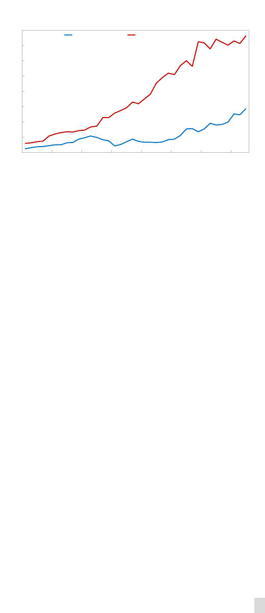
JAPAN
INTERNATIONAL MONETARY FUND 69
The low level of inward FDI in Japan has long been recognized in the academic literature,
including in relation to measurement issues and corporate governance (Lawrence, 1993; Ito and
Fukao, 2005; and Hoshi, 2018).
• Portfolio debt. Portfolio debt income paid is small in Japan, due to both (i) low portfolio debt
liabilities, and (ii) low implicit yields.
On the government side, public
foreign borrowing is indeed relatively
low, especially when compared with
G6 countries, due to the large pool of
domestic saving available and
domestic investors’ willingness to
hold Japanese public debt (strong
home bias). On the corporate side,
low corporate bond liabilities can be
linked to the rise of corporate saving
and the associated corporate
deleveraging after the Japanese real
estate bubble burst at the start of the 1990s. Indeed, while portfolio debt liabilities were
following similar trends in Japan and in G6 countries in the 1980s, Japan’s portfolio debt
liabilities started to diverge from the trend in G6 countries after the bubble burst and as a
consequence of corporate deleveraging (text chart). Finally, Japan’s implied yields on portfolio
debt are also lower than in G6 countries, due to the extremely accommodative monetary policy
and low credit risk in Japan.
C. Interconnectedness Between the Trade and Income Balances
9. In most countries, including Japan, the current account balance has a high and positive
correlation with the trade balance (Figure 3, left panel, left bars). Indeed, most country-specific
correlations between the current account and the trade balance (for the period 1980-2018 or longest
available) are close to one (0.76 for Japan). Conversely, country-specific correlations between the
current account balance and the income balance (total, primary, or secondary) tend to be much
weaker, although there is substantial heterogeneity across countries.
10. On the other hand, the income balance is negatively correlated with the trade balance
(Figure 3, left panel, right bars). Country-specific correlations between the trade balance and the
income balance (total, primary, or secondary) are generally negative (-0.58 for both the total and
primary income balances for Japan), with substantial heterogeneity across countries, especially for
the secondary income balance. Several mechanisms may contribute to the observed negative
correlation between the income and trade balances, including:
0
10
20
30
40
50
60
70
80
1980
1982
1984
1986
1988
1990
1992
1994
1996
1998
2000
2002
2004
2006
2008
2010
2012
2014
2016
Japan G6 unweighted average
Portfolio Debt Liabilities
(In percent of GDP)
Source: Lane & Milesi-Ferretti database, External Wealth of Nations, 2018.
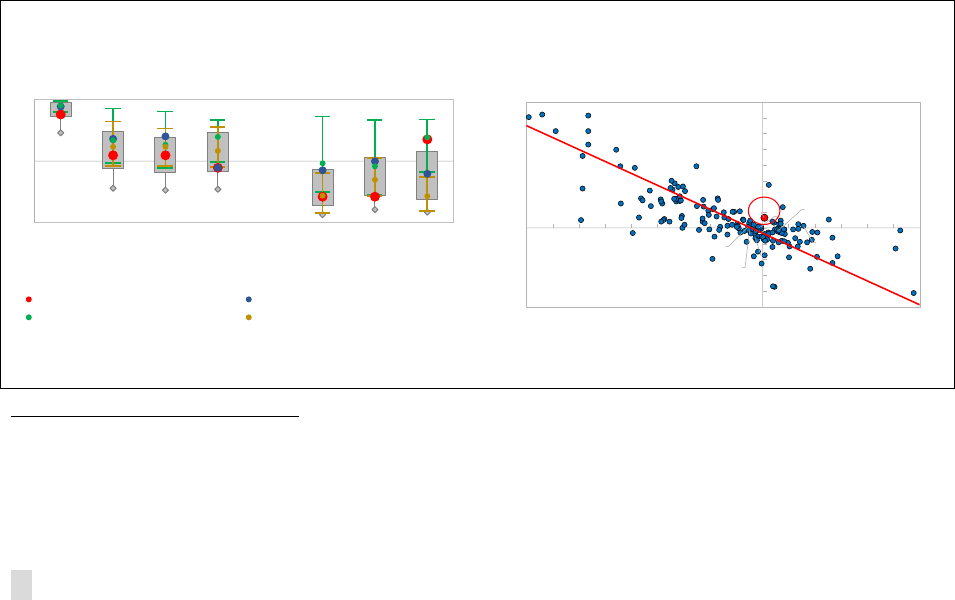
JAPAN
70 INTERNATIONAL MONETARY FUND
• General mechanisms:
• Aging. As countries age, they tend to accumulate net external assets to provide for consumption
during old age, leading to an increasing income balance in the earlier phases of aging. In more
advanced phases of aging, particularly the post-retirement phase, such countries are expected to
start dissaving and increase imports, moving towards trade deficits.
• Income effect. When the income balance increases, agents may consume the additional
income, leading to higher imports and lowering the trade balance. This effect likely depends
on the marginal propensity to consume of households receiving the income: likely higher for
secondary income (as migrant remittances flow to relatively poorer households), and lower
for primary income (as firm shareholders tend to be wealthier).
7
• Market pressure. Countries with high net debtor positions (and negative income balance)
may need to run trade surpluses to meet external debt service obligations on their stock of
foreign borrowing.
• Other mechanisms linked to globalization and the growing role of multinational firms may
help explain the negative correlation between the income and trade balances as these forces
have increasingly blurred the attribution of income between both balances:
• Offshoring. As firms move their production facilities overseas, goods exports are
progressively substituted by income receipts.
8
• Profit shifting, with transfer pricing affecting the trade and income balance in opposite and
offsetting ways.
Figure 3. Japan: Negative Correlation Between Trade and Income Balances
7
When restricting the sample to the top 30 percent of economies with largest income flows (total, primary,
secondary), correlations are more negative, especially for secondary income.
8
Offshoring may also lead to increased services exports (intellectual property revenue including royalty payments
and patent fees from overseas subsidiaries).
ARG
AUS
AUT
BEL
BRA
CAN
CHL
CHN
COL
CRI
CZE
DNK
EGY
FIN
FRA
DEU
GRC
GTM
HUN
IND
IDN
IRL
ISR
ITA
JPN
KOR
MYS
MEX
MAR
NLD
NZL
NOR
PAK
PER
PHL
POL
PRT
RUS
ZAF
ESP
LKA
SWE
CHE
THA
TUN
TUR
GBR
USA
URY
CYP
EST
HKG
ISL
LVA
LTU
MLT
SGP
SVK
SVN
AFG
ALB
DZA
AGO
ATG
ARM
AZE
BHS
BHR
BGD
BLR
BLZ
BEN
BTN
BOL
BIH
BWA
BRN
BGR
BFA
BDI
KHM
CMR
CPV
COD
HRV
DJI
DMA
DOM
ECU
SLV
ETH
FJI
GMB
GEO
GHA
GRD
GIN
HTI
HND
IRQ
JAM
JOR
KAZ
KEN
UVK
KWT
KGZ
LAO
LBN
LSO
LBR
MKD
MDG
MWI
MDV
MRT
MUS
MDA
MNG
MNE
MOZ
MMR
NAM
NPL
NIC
NER
NGA
OMN
PAN
PNG
PRY
QAT
ROU
RWA
WSM
STP
SAU
SRB
SYC
SLB
SSD
KNA
LCA
VCT
SDN
SUR
SWZ
TJK
TZA
TLS
TON
TTO
UGA
UKR
VNM
ZMB
ZWE
y = -0.7582x - 1.6086
R² = 0.6769
-25
-20
-15
-10
-5
0
5
10
15
20
25
30
35
40
-45 -40 -35 -30 -25 -20
-15
-10 -5 0 5 10
15
20 25 30
Income balance (% of GDP)
Trade balance (G&S, % of GDP)
Trade Balance and Income Balance Across Countries
(average 2015-2017)
Sources: IMF BOP data; National authorities; and IMF WEO data.
-1
0
1
CA balance
& Trade
balance
CA balance
& Income
balance
CA balance
& Primary
Income
balance
CA balance
&
Secondary
Income
balance
Income
balance &
Trade
balance
Trade
balance &
Primary
Income
balance
Trade
balance &
Secondary
Income
balance
Japan Advanced Economies: Median
G7 ex-Japan: Unweighted average Top 30% with largest income flows: Median
Sources: IMF BOP data; National authorities; and IMF WEO data.
Note: Correlations are calculated between two variables expressed in % of GDP, using annual data,
over the longest period available.
Correlations Between Current Account and its
Components: Japan vs. Other Countries

JAPAN
INTERNATIONAL MONETARY FUND 71
11. Such an offsetting pattern between the trade balance and the income balance is also
observed across countries (Figure 3, right panel). Countries with a large population living abroad,
receiving sizable migrants’ remittances, tend to be located in the upper-left quadrant of the chart,
illustrating the income effect. Low-tax jurisdictions, in turn, tend to appear in the lower-right
quadrant due to distortions in the composition of their current account, reflecting profit shifting and
the large role of multinational firms. Conversely, less countries are located in the upper-right and
lower-left quadrants, illustrating respectively the income effect and market pressures.
D. Does the Change in Current Account Composition Towards Income
Balance Affect its Responsiveness to the Real Exchange Rate?
12. When facing movements in the real exchange rate (REER), there are several
mechanisms at play affecting the response of the income balance. While the trade balance
response to REER changes has been widely studied, there is less literature on the income balance
response (Alberola et al, 2018).
9
We propose that the income balance response can be decomposed
into a mechanical effect (depending on the currency composition of foreign assets and liabilities)
and an economic effect, as follows:
• Mechanical effect. For most countries, foreign assets tend to be denominated in foreign
currency, implying that a REER appreciation would lead to a mechanical decrease in foreign
assets and income credits (expressed as percentage of GDP). For example, in 2017 the share of
foreign assets denominated in foreign currency was around 70 percent in the United States, 85
percent in Japan, and nearly 100 percent in the median emerging economy (EME), while it has
been lower in the median G6 country since 1999 (at around 50 percent) following the creation of
the euro (Juvenal et al, 2019). However, the currency denomination of foreign liabilities is more
heterogenous across countries, with advanced economies better able to borrow from abroad in
domestic currency. For example in 2017, 85 percent of the United States’ foreign liabilities were
denominated in domestic currency, compared to 82 percent for the median G6 economy and 67
percent for Japan. This pattern implies a limited mechanical effect from a REER appreciation on
foreign liabilities and income debits. On the other hand, EME more often borrow in foreign
currency due to the “original sin,” delivering a mechanical decrease in foreign liabilities and
income debits when the REER appreciates (80 percent of EME’s foreign liabilities in 1990 were
denominated in foreign currency, although that share has declined to 40 percent in 2017).
10
• Economic effect. For small open economies and countries with low outward spillovers, a REER
appreciation (of domestic currency against all other currencies) is unlikely to have a significant
9
Adler and Garcia-Macia (2018) analyze NFA returns defined as the income balance plus NFA valuation changes. With
valuation changes often large and volatile, results obtained for NFA returns in Adler and Garcia-Macia’s analysis do
not directly apply to the income balance on its own (as studied here).
10
In this simplified presentation, we are not taking into account the potential effect that the REER appreciation may
have on GDP (expressed in domestic currency), which would likely be much smaller than the mechanical effects on
income credits and debits.

JAPAN
72 INTERNATIONAL MONETARY FUND
impact on growth and profits in the rest of the world, so it is not expected to affect income
credits (except for the mechanical effect mentioned above). However, a REER appreciation may
reduce domestic economic activity and profits (especially for exporting firms that become less
competitive), and may thus lead to lower income debits (expressed as percentage of GDP) to the
extent that firms operating in the domestic economy are, at least partially, owned abroad.
13. Depending on the net foreign asset position of the country, the income balance
response may reinforce or offset the trade balance response to a REER appreciation. Expected
effects of a REER appreciation are summarized in Table 2. Overall, both income credits and debits are
expected to decrease following a REER appreciation, with the resulting overall effect on the income
balance depending on the respective size of the credit and debit channels. In countries with a large
net creditor position like Japan, a REER appreciation would likely lead to a decrease in the income
balance, as long as the income credit channel dominates (with income credits being larger than
income debits). In such countries, the income balance response would therefore reinforce the usual
negative trade balance response to a REER appreciation. Conversely, in countries with a large net
debtor position, the income debit channel may dominate and a REER appreciation would likely lead
to an increase in the income balance, partially counterbalancing the trade balance response.
Table 2. Japan: Theoretical Effects of REER Appreciation on Trade and Income Balances
14. Preliminary empirical results suggest that in Japan, the income balance response to
changes in the real exchange rate would amplify the trade balance response, although the
effect would be quantitatively modest. Using quarterly and annual IMF BoP data on a panel of 40
countries over 1986–2018, and controlling for the size of foreign assets (resp. liabilities) and related
yields, we estimate separately the income credit and income debit elasticities to the real exchange
rate. Both are generally found to be negative, as predicted by our proposed channels, although
estimates vary under different econometric specifications. Country-specific income balance semi-
elasticities are then derived using ratios of income credit and debit to GDP. For all 40 studied
countries, income balance semi-elasticities are found to be significantly smaller than corresponding
Price
effect
Volume
effect
TOTAL TB
Response
1
Economic
channel
ADV EME
Exports value + -- -
Income credit - -
0
2
-
-- -
Imports value
- ++ +
Income debit
0
3
- - -
- --
Trade balance -- Income balance - ? + ? - +
--
4
--- -
4
1
If the Marshall-Lerner condition is satisfied
2
For a small open economy and countries with small outward spillovers
3
If the country is able to borrow from abroad only in domestic currency
4
If the trade channel dominates the income channel, as expected given relatively larger gross trade flows than income flows
Note 1: "+" represents a smaller increase than "++" while "-" represents a smaller decrease than "--"
Note 2: Grey shading represents the theoretical prediction for Japan
Trade Balance (TB)
Mechanical
channel
TOTAL IB Response
Income Balance (IB)
Current Account (CA)
TOTAL
Large
(-)
NFA
OVERALL
Large
(+)
NFA
Large
(-)
NFA
OVERALL
Large
(+)
NFA

JAPAN
INTERNATIONAL MONETARY FUND 73
trade balance semi-elasticities, because gross income flows are smaller than gross trade flows (which
importantly affects the relative weights of income and trade balance semi-elasticities). For Japan, as
for other large net creditor countries, we find evidence that the income balance response to changes
in the real exchange rate would marginally reinforce the trade balance response. Overall, the current
account response to changes in REER in Japan is estimated to be marginally larger when we take
into account the income balance response, in addition to the usual trade balance response.
11
E. Conclusions
15. The gradual increase in Japan’s income balance primarily reflects net revenues from an
increasingly positive NFA position. Japan’s high income balance is primarily the result of a highly
asymmetric income account. The Japanese income balance has been increasing over time, in line
with a larger NFA position reflecting past current account surpluses and the increase in corporate
saving. When compared with G6 peer countries, Japan’s relatively high income balance is due to:
• higher yields on investment abroad, especially on FDI (from “better” geographical positioning and
possibly profit shifting), which more than offset a somewhat lower stock of foreign assets;
• much lower FDI liabilities (due to possible measurement issues, corporate governance, or
regulatory and administrative issues) and lower portfolio debt liabilities (due to strong home bias
and corporate deleveraging); and
• lower yields on portfolio debt liabilities (linked to extremely accommodative monetary policy and
low credit risk in Japan).
16. Offsetting patterns between the trade and income balances, within the external
current account, highlight their interconnectedness and the blurring impact of globalization
and multinational firms on the attribution of income. For one, gross trade flows continue to be
significantly larger than gross income flows. In addition, Japan’s current account balance is highly
and positively correlated with its trade balance, while the positive correlation with its income balance
is much weaker. At the same time, the income balance is negatively correlated with the trade
balance, possibly reflecting several mechanisms including (i) aging, (ii) an income effect, (iii) market
pressures, but also (iv) offshoring and (v) profit shifting through transfer pricing.
17. For Japan, the income balance response to changes in the real exchange rate is
estimated to reinforce the trade balance response, although only marginally. Preliminary
estimates indicate that income credits and debits tend to decrease with a REER appreciation, with a
dominant income credit channel for large net creditor countries such as Japan. However, the income
balance response to the REER is significantly smaller than the trade balance response due to
relatively low gross income flows.
11
In addition to the overall effect of REER changes on total income credits and debits, Colacelli, Rebillard and Gautam
(forthcoming) compute the mechanical effect separately, using data from Juvenal et al (2019), to disentangle and
estimate the economic effect.

JAPAN
74 INTERNATIONAL MONETARY FUND
18. Continued efforts towards promoting FDI inflows would likely contribute to boosting
income debits and reducing the relatively high external income balance in Japan. While the
promotion of inward FDI has been one of the policy goals of Abenomics’ structural reforms, recent
evidence suggests that additional steps are needed to further boost inward FDI to the level of peer
countries (Hoshi, 2018). Larger inward FDI would also support Japan’s productivity growth. Steps to
boost inward FDI could include addressing corporate governance issues (with Japan’s corporate
governance being an “insider system” with limited power for shareholders, potentially discouraging
foreign ownership; see e.g. Hoshi, 2018) and regulatory and administrative issues, including by
reducing the cost of doing business. The latter is in line with IMF advice to reform product markets,
by reducing barriers to entry in some industries as well as accelerate deregulation of agricultural and
professional services sectors, in order to foster growth and investment (IMF, 2018).
19. Adjustment of Japan’s external current account via the exchange rate is estimated to
mainly operate through the trade balance, with marginal support from the income balance.
The compositional change in Japan’s current account balance over recent decades, with the income
balance being more prominent, does not in itself fundamentally modify the external adjustment
process via the exchange rate, which is estimated to operate mainly through the trade balance. In
the case of Japan, the response of the income balance to exchange rate movements may actually
amplify the response through the usual trade channel.

JAPAN
INTERNATIONAL MONETARY FUND 75
References
Adler, Gustavo, and Daniel Garcia-Macia, 2018, “The Stabilizing Role of Net Foreign Asset Returns,”
IMF Working Paper 18/79.
Alberola, Enrique, Angel Estrada, and Francesca Viani, 2018, “Global Imbalances from a Stock
Perspective: The Asymmetry Between Creditors and Debtors,” BIS Working Paper No. 707.
Colacelli, Mariana, Cyril Rebillard, and Deepali Gautam (forthcoming), “Japan’s Foreign Assets and
Liabilities: Implications for the External Accounts,” IMF Working Paper.
Damgaard, Jannick, Thomas Elkjaer, and Niels Johannesen, 2019, “What Is Real and What Is Not in
the Global FDI Network,” IMF Working Paper 19/274.
Hasegawa, Makoto, and Kozo Kiyota, 2017, “The Effect of Moving to a Territorial Tax System on
Profit Repatriation: Evidence from Japan,” Journal of Public Economics, Vol. 153, pp. 92-110.
Hashimoto, Yuko, and Noriaki Kinoshita, 2016, “The Financial Wealth of Corporations: A First Look at
Sectoral Balance Sheet Data,” IMF Working Paper 16/11.
Hoshi, Takeo, 2018, “Has Abenomics Succeeded in Raising Japan’s Inward Foreign Direct
Investment?” Asian Economic Policy Review, Vol. 13, pp. 149–68.
International Monetary Fund, 2018, “Japan: 2018 Article IV Consultation – Staff Report,” Country
Report 18/333, International Monetary Fund.
Ito, Keiko, and Kyoji Fukao, 2005, “Foreign Direct Investment and Trade in Japan: An Empirical
Analysis Based on the Establishment and Enterprise Census for 1996,” Journal of the Japanese and
International Economies, Vol. 19, pp. 414–55.
Juvenal, Luciana, Deepali Gautam, Agustín Bénétrix, and Martin Schmitz, 2019, “Cross-Border
Currency Exposures. New Evidence Based on an Enhanced and Updated Dataset,” IMF Working
Paper 19/299.
Lane, Philip R., and Gian-Maria Milesi-Ferretti, 2018, “The External Wealth of Nations Revisited:
International Financial Integration in the Aftermath of the Global Financial Crisis,” IMF Economic
Review, Vol. 66, pp. 189–222.
Lawrence, Robert Z., 1993, “Japan’s Low Levels of Inward Investment: The Role of Inhibitions on
Acquisitions,” in Foreign Direct Investment. K. A. Froot, ed. Chicago: University of Chicago Press, pp.
85–107.
Liu, Li, Tim Schmidt-Eisenlohr, and Dongxian Guo, 2017, “International Transfer Pricing and Tax
Avoidance: Evidence from Linked Trade-Tax Statistics in the UK,” CESifo Working Paper No. 6594.

JAPAN
76 INTERNATIONAL MONETARY FUND
Tørsløv, Thomas R., Ludvig S. Wier, and Gabriel Zucman, 2018, “The Missing Profits of Nations,” NBER
Working Paper No. 24701.
Wright, Thomas, and Gabriel Zucman, 2018, “The Exorbitant Tax Privilege,” NBER Working Paper No.
24983.
Xing, Jing, 2018, “Territorial Tax System Reform and Multinationals’ Foreign Cash Holdings: New
Evidence from Japan,” Journal of Corporate Finance, Vol. 49, pp. 252-82.

JAPAN
INTERNATIONAL MONETARY FUND 77
JAPANESE BUSINESS CYCLES, EXTERNAL SHOCKS,
AND SPILLOVERS
1
This chapter develops a quarterly macro-econometric model for Japan, and integrates it within a
compact model of the world economy (including the global oil market). A Global Vector Autoregression
(GVAR) model is used to evaluate the nature and strength of: economic linkages between globally-
systemic countries (including Japan); the size and speed of the international transmission of stress in
global financial markets; as well as a global growth slowdown. It also examines outward spillovers
from Japan to the rest of the world and how they have changed over time. Spillovers are transmitted
across economies via trade, financial, and commodity price linkages. The results show that all regions
are more sensitive to developments in China than to output shocks in the Euro Area, the United States,
or Japan. Stress in global financial markets can amplify spillovers from growth shocks in systemic
economies. While outward spillovers from Japan output shocks have become smaller over time, they
remain important for Asia-Pacific economies and the global economy.
A. Introduction
1. A Global Vector Autoregression (GVAR) model is used to determine the size and speed
of the transmission of different shocks to/from Japan. We use a dynamic multi-country
framework for the analysis—see Cashin et al. (2014), Cashin et al. (2016), Cashin et al. (2017b),
Mohaddes and Pesaran (2016), and Mohaddes and Raissi (2018a). The framework comprises 33
country/region-specific models. These individual models are solved in a global setting where core
macroeconomic variables of each economy are related to corresponding foreign variables
(constructed exclusively to match the international trade pattern of the country under consideration).
The model has both real and financial variables: real GDP, inflation, primary balance to GDP ratio,
public debt to GDP ratio, real exchange rate, short and long-term interest rates, an index of financial
market stress, and the price of oil. This framework can account for various transmission channels,
including not only trade relationships but also financial and commodity price linkages—see Dees et
al. (2007). All data are quarterly in frequency, for the period 1981Q2 to 2018Q2.
2. The results show that output shocks emanating in globally-systemic economies have
important cross-country effects, including for the Japanese economy. Following a one percent
decline in China’s GDP, economic activity falls by about 0.3 percent for the median Asian economy
(and about 0.25 percent for Japan) and 0.2 percent for the median economy in Europe and the
Americas. The corresponding number for the fall in GDP of the median Asian economy in response
to a similar growth slowdown in the United States is about 0.2 percent after one year. Adverse
spillovers from the Euro Area slowdown are modest (assuming limited financial stress in the Euro
Area). These results show that countries are becoming more sensitive to developments in China than
to shocks in the Euro Area or the United States, in line with the direction of evolving trade patterns
and the emergence of China as a key driver of the global economy. In response to a financial stress
1
Prepared by Paul Cashin (APD), Kamiar Mohaddes (University of Cambridge), and Mehdi Raissi (FAD).

JAPAN
78 INTERNATIONAL MONETARY FUND
shock, real GDP growth slows worldwide (by 0.2 percentage points on average). Finally, while
outward spillovers from Japan output shocks have reduced over time, they do have global
implications (albeit to a lesser extent than those of China and the United States), and are stronger in
its Asia-Pacific geographical proximity.
B. Modelling the Global Economy
3. We employ the GVAR methodology to analyze the international macroeconomic
transmission of shocks, with a focus on the Japanese economy. This framework takes into
account both the temporal and cross-sectional dimensions of the data; real and financial drivers of
economic activity; interlinkages and spillovers that exist between different regions; and the effects of
unobserved or observed common factors (e.g. commodity prices and financial risk). This is crucial as
the impact of shocks cannot be reduced to a single country but rather involves multiple regions, and
this impact may be amplified or dampened depending on the degree of openness of the countries
and their trade structure. Before describing the data and our model specification, we provide a short
exposition of the GVAR methodology.
The Global VAR Methodology
4. The Global VAR methodology consists of two main steps. First, each country is modeled
individually as a small open economy (except for the United States) by estimating country-specific
vector error correction models in which domestic variables are related to both country-specific
foreign variables and global variables that are common across all countries (such as oil prices and
financial market stress). Second, a global model is constructed combining all the estimated country-
specific models and linking them with a matrix of predetermined cross-country linkages. More
specifically, we consider + 1 countries in the global economy, indexed by = 0,1, … , . Except for
the United States, which we label as 0 and take to be the reference country; all other countries are
modelled as small open economies. This set of country-specific models is used to build the GVAR
framework.
GVAR Literature and Spillovers
5. The GVAR is a modelling framework of the world economy designed to explicitly
model economic and financial interdependencies across markets and countries at national and
international levels. The framework was originally proposed by Pesaran et al. (2004) and further
developed by Dees et al. (2007). It links individual country-specific models in a coherent manner to
form a global modelling framework by using time series, panel data, and factor analysis techniques.
It has been used in bank stress testing; the analysis of China’s growing importance for the rest of the
world economy (Cashin et al. (2016, 2017b)); the international macroeconomic transmission of
weather shocks (Cashin et al. 2017a); the impact of commodity price shocks (see Mohaddes and
Pesaran (2016) for the global macroeconomic consequences of country-specific oil-supply shocks
and Cashin et al. 2014 for the differential effects of demand- and supply-driven commodity price
shocks); other real and financial shocks, as well as in forecasting applications. For an extensive survey
of developments in GVAR modelling, see Chudik and Pesaran (2016).

JAPAN
INTERNATIONAL MONETARY FUND 79
6. The issue of spillovers from financial and growth shocks in systemic economies has
received extensive attention in the literature. Important papers include coverage in the IMF’s
Spillover Reports (IMF 2012, 2014a) and Regional Economic Outlooks for Asia and the Pacific (IMF
2014b, 2015, 2016). Cashin et al. (2017b) and Dizioli and others (2016) find that a slowdown and
rebalancing in China can have significant spillovers to ASEAN-5 economies, particularly those with
higher trade exposures to China and commodity exporters. They also show that a surge in global
financial market volatility could translate into a fall in world economic growth of around 0.3
percentage points after one year. Cashin et al. (2016) and Kose et al. (2017) study spillovers from the
U.S. growth slowdown. Dees et al. (2007) explore the international linkages of the Euro Area. This
chapter contributes to the literature in several dimensions. First, the price of oil in the model is
determined in international markets, thereby being affected by both global demand and supply
conditions. An index of stress in global financial markets is added to the model, to account for the
financial contagion channel of impact. Second, the chapter investigates the extent to which the
global impact of a slowdown in Japan has changed over the past three decades. Third, the
estimation sample of the GVAR model is extended from 2013Q1 to 2018Q2.
Model Specification
7. The GVAR model includes 33 economies, which together cover more than 90 percent
of world GDP (see Table 1). We obtain quarterly data (for the period 1979Q1–2016Q4) from
Mohaddes and Raissi (2018b) on oil prices, domestic macroeconomic variables (treated as
endogenous) and country-specific foreign variables (taken to be weakly exogenous) for the 33
economies, and update this data until 2018Q2.
Table 1. Japan: Countries in the GVAR Model
Source: Mohaddes and Raissi (2018b).
Asia and Pacific North America Europe
Australia
Canada Austria
China
Mexico Belgium
India
United States Finland
Indonesia France
Japan South America Germany
Korea Argentina Italy
Malaysia Brazil Netherlands
New Zealand Chile Norway
Philippines Peru Spain
Singapore Sweden
Thailand
Middle East and
Africa
Switzerland
Saudi Arabia Turkey
South Africa United Kingdom
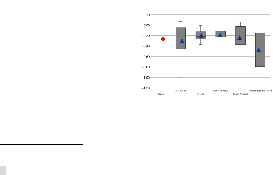
JAPAN
80 INTERNATIONAL MONETARY FUND
8. The modeling framework includes an index of financial stress (
) in advanced
economies. The
for advanced countries is constructed by Cardarelli et al. (2009) as an average
of the following indicators: the beta of banking sector stocks; TED spread; the slope of the yield
curve; corporate bond spreads; stock market returns; time-varying stock return volatility; and time-
varying effective exchange rate volatility. Such an index facilitates the identification of large shifts in
asset prices (stock and bond market returns); an abrupt increase in risk/uncertainty (stock and
foreign exchange volatility); liquidity tightening (TED spreads); and the health of the banking system
(the beta of banking sector stocks and the yield curve). We model
as a common variable, in
other words, it is included as a weakly exogenous variable in each of the 33 country/region-specific
models, but we allow for feedback effects from any of the macro variables to
.
9. Given the importance of oil shocks for the global economy, the modeling framework
also includes nominal oil prices in U.S. dollars in the country-specific models. We allow for oil
prices to be determined in global commodity markets rather in the U.S. model alone (as is more
standard in the literature), given that oil prices are also affected by, for instance, any disruptions to
oil supply in the Middle East. Therefore, in contrast to the existing GVAR literature, we model the oil
price equation separately and then introduce the price of oil as a weakly exogenous variable in all
countries, thereby allowing both demand and supply conditions to influence the oil price directly.
2
C. Spillover Analysis
10. This section analyzes inward spillovers to Japan from: (i) macroeconomic shocks in other
systemic economies (China, the Euro Area, and the United States), (ii) a potential global growth
slowdown, and (iii) stress in global financial markets. It also studies outward spillovers from Japan to
other Asian countries and globally.
China Slowdown
11. China’s real GDP growth is slowing—
from an average of about 10 percent over the
period 1980–2013 to an average of 6½ percent
between 2017 and 2019. These developments,
together with market concerns about the future
performance of the Chinese economy (also
affected by trade tensions with the United States),
are resulting in spillovers to other economies
(especially to countries in the Asia-Pacific region)
through trade links, weaker commodity prices,
and financial linkages. The results of the GVAR
model show that a one percent negative GDP
shock in China translates into lower economic
2
See Cashin et al. (2017a), Mohaddes and Pesaran (2016), for a similar approach.
-1.20
-1.00
-0.80
-0.60
-0.40
-0.20
0.00
0.20
Responses of Output to a Negative GDP Shock in China
(In percent)
Source: Author’s estimates.
Note: Figure depicts annual percent change in output of a
group of countries associated with a 1 percent decline in GDP
of China. Symbols
— and ∆ denote the median and average
responses across countries in each group. The boxes show the
25th
–75th percentile responses and the whiskers show the
minimum and maximum responses.
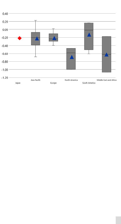
JAPAN
INTERNATIONAL MONETARY FUND 81
growth globally (text chart). Countries with large trade exposures to China are most vulnerable to a
slowdown in this country. The effects on the GDP of Asia and Pacific countries are generally large
(with the median effect being 0.3 percent after one year) owing to strong trade linkages with China.
Countries in Europe and North America also suffer a decline in economic output when China’s
growth slows—by about 0.2 percent each after one year (because some are included in the supply
chain of China). Turning to South American, Middle East and African countries, following a negative
GDP shock in China, the median output of these countries falls by about 0.2 and 0.4 percent,
respectively, largely owing to weaker commodity prices. These findings are somewhat to be
expected given the emergence of China as a key driver of the global economy in recent decades.
Following a negative China GDP shock, real median output in Japan falls by about 0.25 percent after
one year.
United States Slowdown
12. As a result of the dominance of the United States in the global economy, any
slowdown in this country can bring about negative spillovers to other economies. Lower
commodity prices are one channel through
which a negative U.S. shock affects countries,
conveying a negative impact on growth
prospects of commodity-exporters (e.g.
Middle East and Africa). The median effects of
a one percent negative U.S. output shock for
output in North American countries are the
largest (in absolute values)—median output
falling by about 0.65 percent owing to strong
trade links between Mexico, Canada, and the
United States. Furthermore, the continuing
dominance of U.S. debt and equity markets,
backed by the strong global role of the U.S.
dollar, plays an important role in spillovers to
other countries. The results of the GVAR
model show that the influence of the U.S. on
other economies remains larger than direct
trade ties would suggest, owing to third-market effects together with increased financial integration
that tends to foster the international transmission of business cycles (text chart). For instance,
following a negative U.S. GDP shock, real median output in Europe and Asia falls by about
0.2 percent after one year. Similarly, following a negative U.S. GDP shock, real median output in
Japan falls by about 0.2 percent after one year.
Euro Area Slowdown
13. The adverse impact on output of a one percent negative GDP shock in the Euro Area is
most significant for other European countries. Median output in European countries falls by 0.65
percent after one year following the shock (text chart). Beyond Europe, growth spillovers vary from
-1.20
-1.00
-0.80
-0.60
-0.40
-0.20
0.00
0.20
0.40
Responses of Output to a Negative GDP Shock in United States
(In percent)
Source: Author’s estimates.
Note: Figure depicts annual percent change in output of a
group of countries associated with a 1 percent decline in GDP
of the
United States. Symbols —
and ∆ denote the median and
average responses across countries in each group. The boxes
show the 25th
–75th percentile responses and the whiskers
show the minimum and maximum responses.
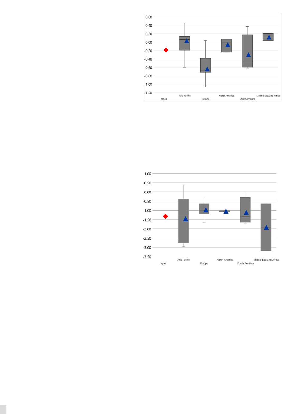
JAPAN
82 INTERNATIONAL MONETARY FUND
country to country. High dependencies are
observed for South American countries, with
annual output elasticity of about 0.3 operating
via trade and commodity-price channels. For
other countries/regions, the impact is modest
(assuming limited financial stress in the Euro
Area). Following a negative Euro Area GDP
shock, real median output in Japan falls by about
0.2 percent after one year.
Global Growth Slowdown
14. Trade policy uncertainty, geopolitical
tensions, and idiosyncratic stress in key
emerging market economies weighed on
global growth in the second half of 2019.
While accommodative global financial
conditions have continued, raising growth
prospects for 2020, growth forecasts in key
emerging market economies remained subdued.
Should downside risks to global growth
materialize, and be accompanied by rapidly
deteriorating financial sentiment, the results
from the GVAR model suggest that countries in
Asia-Pacific or Middle East and Africa would be
disproportionately affected, owing to third-
market effects (text chart). Specifically, following
a one percent fall in global GDP, the median
country in the Asia-Pacific region could
experience a reduction in GDP of about
1.5 percent after one year. The median impact is
even larger in the Middle East and Africa region
given a demand-driven reduction in global
commodity prices. Similar to the rest of Asia-
Pacific region, following a negative global GDP
shock, real median output in Japan falls by about
1.3 percent after one year.
Stress in Global Financial Markets
15. Stress in global financial markets could emanate from an increase in risk premiums in
reaction to a decline in investor sentiment triggered by a deteriorating outlook, or weak
policy frameworks amidst concerns about debt sustainability in some advanced economies.
Such shocks could lead to higher interest rates, exchange rate volatility, corrections in stretched
-1.20
-1.00
-0.80
-0.60
-0.40
-0.20
0.00
0.20
0.40
0.60
Responses of Output to a Negative GDP Shock in Euro Area
(In percent)
Source: Author’s estimates.
Note: Figure depicts annual percent change in output of a
group of countries associated with a 1 percent decline in GDP
of Euro Area. Symbols
— and ∆ denote the median and
average responses across countries in each group. The boxes
show the 25th
–75th percentile responses and the whiskers
show the minimum and maximum responses.
-3.50
-3.00
-2.50
-2.00
-1.50
-1.00
-0.50
0.00
0.50
1.00
Responses of Output to a Negative Global GDP Shock
(In percent)
Source: Author’s estimates.
Note: Figure depicts annual percent change in output of a
group of countries associated with a 1 percent decline in
Global GDP. Symbols
— and ∆ denote the median and
average responses across countries in each group. The
boxes show the 25th
–75th percentile responses and the
whiskers show the minimum and maximum responses.
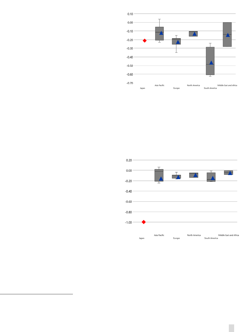
JAPAN
INTERNATIONAL MONETARY FUND 83
asset valuations (for example, equity and real estate), and sudden international financial flow
reversals. These developments would strain
leveraged companies, households, and sovereigns;
worsen bank balance sheets and profitability; and
damage the public finances of advanced and
emerging market economies. Cashin et al. (2017b)
discuss the implications of financial stress in
advanced economies, and point to potentially
sizable spillovers from such shocks.
16. The GVAR model results indicate that in
response to potential stress in advanced
economies’ financial markets, global economic
growth decelerates in the short-run. More
specifically, a one standard deviation shock to the
financial stress index (FSI)
3
translates into slower
global economic activity—with world output
falling by around 0.2 percent below the pre-shock
level on average over the first year (text chart). The
growth impact on different countries/regions
depends on the magnitude and duration of the
FSI shock; countries’ economic fundamentals; and
the size of safe-haven flows. For instance, model
estimates show that the impact is greatest in
South America. Growth spillovers to the median
Asian country is about 0.1 percent. Following a
negative shock to the financial stress index, real
median output in Japan falls by about 0.2 percent
after one year.
Outward Spillovers from Japan
17. Outward spillovers from Japan to
other Asian economies and the rest of the
world are important. The results from the GVAR
model indicate that output shocks in Japan
matter, particularly for its immediate
neighborhood, but also have global implications
(albeit to a lesser extent than those of China, the
United States, and the Euro Area). A one percent
3
A one standard deviation positive shock to FSI in advanced economies is two-thirds of the shock that occurred
during the European sovereign debt crisis, and one-tenth of the shock that occurred during the Global Financial
Crisis.
-0.70
-0.60
-0.50
-0.40
-0.30
-0.20
-0.10
0.00
0.10
Responses of Output to Potential Stress in Global Financial Markets
(In percent)
Source: Author’s estimates.
Note: Figure depicts annual percent change in output of a
group of countries associated with a one
-standard deviation
positive shock to FSI. Symbols
—
and ∆ denote the median and
average responses across countries in each group. The boxes
show the 25th
–75th percentile responses and the whiskers
show the minimum and maximum responses.
-1.20
-1.00
-0.80
-0.60
-0.40
-0.20
0.00
0.20
Responses of Output to a Negative GDP Shock in Japan
(2014
-16 Weights)
(In percent)
Source: Author’s estimates.
Note: Figure depicts annual percent change in output of a
group of countries associated with a 1 percent decline in
GDP of Japan. Symbols
— and ∆ denote the median and
average responses across countries in each group. The
boxes show the 25th
–75th percentile responses and the
whiskers show the minimum and maximum responses.
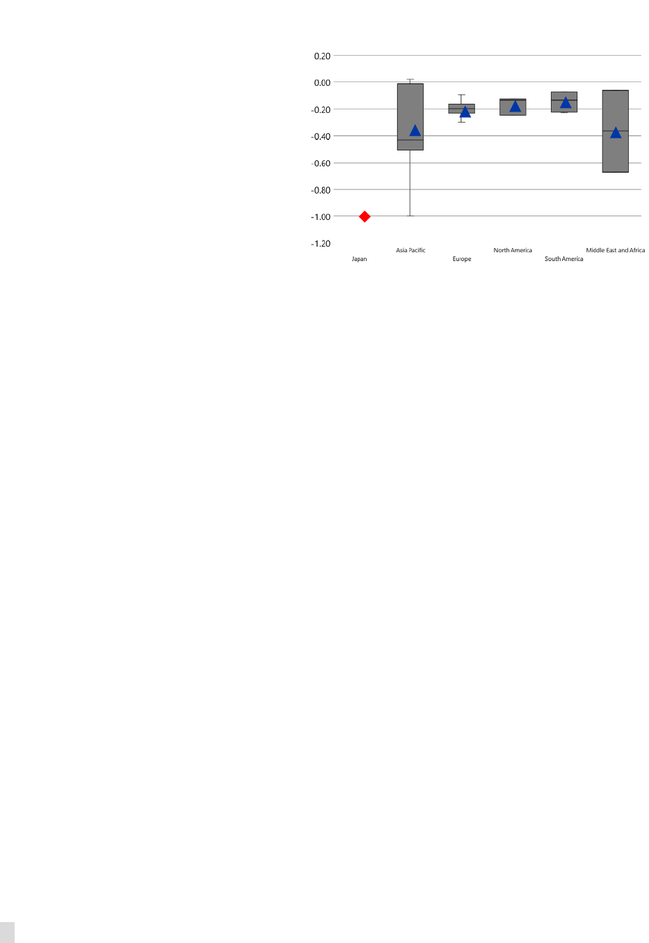
JAPAN
84 INTERNATIONAL MONETARY FUND
decline in the GDP of Japan (using 2014-16
trade weights) generates relatively large
output losses in other Asian countries,
corresponding to around 0.2 percent after
one year (text chart). This indicates that the
influence of output shocks emanating from
Japan remains important for countries in the
Asia-Pacific region. However, a Japanese
slowdown only has a modest negative effect
in other non-Asian regions (with a median
effect of about 0.1 percent). To investigate
whether the global impact of a negative
output shock in Japan has changed over the
past three decades, we re-estimated the
GVAR model using trade weights averaged
over 1984 to 1986 (text chart). Comparing
these results with those obtained from our
original specification (using 2014–16 trade
weights), the results from the GVAR model
indicate that the impact of the Japan output
shock has declined significantly over the past thirty years. Following a negative Japan GDP shock
(using 1984-86 trade weights), real median output declines in other Asian countries by about 0.4
percent after one year, with output losses in other regions of around 0.3 percent after one year. This
finding suggests that the influence of negative Japan output shocks on the global economy has
become smaller in recent decades.
-1.20
-1.00
-0.80
-0.60
-0.40
-0.20
0.00
0.20
Responses of Output to a Negative GDP Shock in Japan
(1984
-86 Weights)
(In percent)
Source: Author’s estimates.
Note: Figure depicts annual percent change in output of a
group of countries associated with a 1 percent decline in
GDP of Japan. Symbols
— and ∆ denote the median and
average responses across countries in each group. The boxes
show the 25th
–75th percentile responses and the whiskers
show the minimum and maximum responses.

JAPAN
INTERNATIONAL MONETARY FUND 85
References
Cardarelli, R., S. Elekdag, and S. Lall, 2009, “Financial Stress, Downturns, and Recoveries.” IMF
Working Paper 09/100, International Monetary Fund, Washington, DC.
Cashin, P., K. Mohaddes, M. Raissi, and M. Raissi, 2014, “The Differential Effects of Oil Demand and
Supply Shocks on the Global Economy,” Energy Economics, Vol. 44, pp. 113-34.
Cashin, P., K. Mohaddes, and M. Raissi, 2016, “The Global Impact of the Systemic Economies and
MENA Business Cycles,” In I.A. Elbadawi and H. Selim (eds.), Understanding and Avoiding the Oil
Curse in Resource-Rich Arab Economies, Cambridge University Press: Cambridge, pp. 16-43.
Cashin, P., K. Mohaddes, and M. Raissi, 2017a, “Fair Weather or Foul? The Macroeconomic Effects of
El Niño,” Journal of International Economics, Vol. 106, pp. 37-54.
Cashin, P., K. Mohaddes, and M. Raissi, 2017b, “China’s Slowdown and Global Financial Market
Volatility: Is World Growth Losing Out?” Emerging Markets Review, Vol. 31, pp. 164-75.
Chudik, A. and M.H. Pesaran, 2016, “Theory and Practice of GVAR Modeling,” Journal of Economic
Surveys, Vol. 30, pp. 165-97.
Dees, S., F. di Mauro, M.H. Pesaran, and L.V. Smith, 2007, “Exploring the International Linkages of the
Euro Area: A Global VAR Analysis,” Journal of Applied Econometrics, Vol. 22, pp. 1-38.
Dizioli, A., J. Guajardo, V. Klyuev, and M. Raissi, 2016, “Spillovers from China’s Growth Slowdown and
Rebalancing to the ASEAN-5 Economies,” IMF Working Paper 16/170, International Monetary Fund,
Washington, DC.
International Monetary Fund, 2012, 2012 Spillover Report. July, Washington, DC.
–––––––, 2014a, IMF Multilateral Policy Issues Report: 2014 Spillover Report. June, Washington, DC.
–––––––, 2014b, Regional Economic Outlook: Asia and the Pacific. Washington, DC, April.
–––––––, 2015, Regional Economic Outlook: Asia and the Pacific. Washington, DC, May.
–––––––, 2016, Regional Economic Outlook: Asia and the Pacific. Washington, DC, May.
–––––––, 2019, World Economic Outlook: Global Manufacturing Downturn, Rising Trade Barriers.
Washington DC, October.
Kose, A., C. Lakatos, F. Ohnsorge, and M. Stocker, 2017, “The Global Role of the U.S. Economy:
Linkages, Policies and Spillovers,” Policy Research Working Paper 7962, World Bank: Washington, DC.
Mohaddes, K. and M.H. Pesaran, 2016, “Country-Specific Oil Supply Shocks and the Global Economy:
A Counterfactual Analysis,” Energy Economics, Vol. 59, pp. 382-99.

JAPAN
86 INTERNATIONAL MONETARY FUND
Mohaddes, K. and M. Raissi, 2018a, “The U.S. Oil Supply Revolution and the Global Economy,”
Empirical Economics, pp. 1-32.
Mohaddes, K. and M. Raissi, 2018b, “Compilation, Revision and Updating of the Global VAR (GVAR)
Database, 1979Q2-2016Q4,” University of Cambridge: Faculty of Economics (mimeo).
Pesaran, M.H., T. Schuermann, and S. Weiner, 2004, “Modelling Regional Interdependencies Using a
Global Error-Correcting Macroeconometric Model,” Journal of Business and Economics Statistics, Vol.
22, pp. 129-62.
