Biacore Assay Handbook

GE Healthcare

Life Sciences

Biacore™ Assay Handbook

Biacore Assay Handbook 29-0194-00 Edition AA 1

1 Introduction

1.1 What Biacore™ systems measure .............................................. 5

1.2 Where Biacore systems are used ................................................ 5

1.3 Scope of this book .......................................................................... 6

1.4 Biacore system range ................................................................... 6

1.5 Biacore terminology ...................................................................... 7

2 Application overview

2.1 Screening and detecting binding partners ............................... 9

2.2 Kinetics and affinity measurements ........................................ 10

2.2.1 Kinetic analysis...........................................................................................10

2.2.2 Affinity analysis..........................................................................................11

2.3 Concentration measurements .................................................. 13

2.3.1 Calibrated assays......................................................................................13

2.3.2 Calibration-free concentration analysis (CFCA)............................14

2.4 Mapping binding sites ................................................................. 14

3 General considerations

3.1 Sensor surfaces ............................................................................ 17

3.1.1 General properties....................................................................................17

3.1.2 Sensor surface types................................................................................17

3.2 Attaching the ligand .................................................................... 19

3.2.1 Covalent immobilization ........................................................................19

3.2.2 High affinity capture ................................................................................21

3.2.3 Response levels..........................................................................................21

3.3 General buffer considerations ................................................... 23

3.3.1 Buffer substances......................................................................................23

3.3.2 Ionic strength ..............................................................................................23

3.3.3 Additives........................................................................................................24

3.3.4 Buffer preparation ....................................................................................25

3.4 Matching sample and running buffer ...................................... 26

3.4.1 Matching refractive index......................................................................26

3.4.2 Matching buffer composition...............................................................27

3.4.3 Matching buffer environment in practice.......................................28

3.5 Dilution series and replicates .................................................... 28

3.5.1 Dilution series..............................................................................................28

3.5.2 Replicates .....................................................................................................29

3.6 Preparing vials and microplates ............................................... 30

4 Screening and detecting binding partners

4.1 Small molecule screening ........................................................... 32

4.1.1 Goals...............................................................................................................32

4.1.2 Sensor surface preparation..................................................................32

4.1.3 Sample preparation .................................................................................32

4.1.4 Buffers............................................................................................................32

2 Biacore Assay Handbook 29-0194-00 Edition AA

4.1.5 Analysis conditions...................................................................................33

4.1.6 Evaluating results......................................................................................34

4.2 Antibody screening ......................................................................35

4.2.1 Goals...............................................................................................................35

4.2.2 Sensor surface preparation..................................................................36

4.2.3 Sample preparation .................................................................................36

4.2.4 Buffers............................................................................................................36

4.2.5 Analysis conditions...................................................................................36

4.2.6 Evaluating results......................................................................................37

4.3 Immunogenicity testing ..............................................................38

4.3.1 Goals and challenges..............................................................................38

5 Kinetics and affinity measurements

5.1 Approaches ....................................................................................39

5.1.1 Single- and multi-cycle kinetics...........................................................39

5.1.2 2-over-2 kinetics........................................................................................39

5.1.3 Comparative estimates of kinetics and affinity............................40

5.2 Sensor surface preparation ........................................................40

5.3 Buffers ............................................................................................41

5.4 Sample preparation .....................................................................41

5.5 Sample concentrations ...............................................................42

6 Epitope mapping

6.1 Pair-wise binding ..........................................................................45

6.1.1 Principle.........................................................................................................45

6.1.2 Evaluation.....................................................................................................46

6.2 Peptide inhibition .........................................................................48

7 Troubleshooting assays

7.1 Troubleshooting ligand attachment .........................................49

7.1.1 Covalently attached ligand...................................................................49

7.1.2 Captured ligand .........................................................................................50

7.2 Troubleshooting analyte binding ..............................................51

7.2.1 Analyte capacity too low .......................................................................51

7.2.2 Analyte binding too high........................................................................51

7.3 Dealing with non-specific and unwanted binding .................51

7.3.1 Non-specific binding................................................................................51

7.3.2 Unwanted binding....................................................................................52

7.4 Unexpected sensorgram shapes ...............................................52

7.4.1 Unstable baseline......................................................................................53

7.4.2 Sample response below baseline.......................................................54

7.4.3 “Humpbacked” sensorgrams...............................................................55

7.4.4 Anomalous response during buffer flow ........................................55

7.4.5 Response subtraction spikes................................................................56

7.4.6 Regular disturbances ..............................................................................56

Biacore Assay Handbook 29-0194-00 Edition AA 3

Appendix A Analysis of kinetics and concentration measurements

A.1 Basic principles of kinetics and affinity ................................... 57

A.1.1 Kinetic rate equations .............................................................................57

A.1.2 Steady-state affinity equations...........................................................59

A.1.3 Fitting procedure.......................................................................................59

A.1.4 Assessing the fit .........................................................................................60

A.2 Interaction models for kinetics ................................................. 62

A.2.1 1:1 binding....................................................................................................62

A.2.2 1:1 dissociation ..........................................................................................63

A.2.3 Bivalent analyte binding ........................................................................63

A.2.4 Heterogeneous ligand.............................................................................64

A.2.5 Interaction models for affinity .............................................................64

A.3 Concentration measurements .................................................. 64

A.3.1 Calibration curve fitting..........................................................................64

A.3.2 Calibration trends......................................................................................65

A.3.3 Calibration-free concentration analysis..........................................65

Appendix B Solvent correction principles and practice

B.1 Introduction .................................................................................. 67

B.2 Requirement for solvent correction ......................................... 67

B.3 Solvent correction principles ..................................................... 68

B.4 Preparing solutions for solvent correction ............................. 69

B.5 Assessing solvent correction procedures ............................... 69

4 Biacore Assay Handbook 29-0194-00 Edition AA

Biacore Assay Handbook 29-0194-00 Edition AA 5

Introduction 1

1 Introduction

1.1 What Biacore™ systems measure

Biacore systems monitor molecular interactions in real time, using a non-

invasive label-free technology that responds to changes in the concentration of

molecules at a sensor surface as molecules bind to or dissociate from the

surface. The detection principle is based on surface plasmon resonance (SPR),

that is sensitive to changes in refractive index within about 150 nm from the

sensor surface. To study the interaction between two binding partners, one

partner is attached to the surface and the other is passed over the surface in a

continuous flow of sample solution. The SPR response is directly proportional to

the change in mass concentration close to the surface.

Biacore systems can be used to study interactions involving (in principle) any

kind of molecule, from organic drug candidates to proteins, nucleic acids,

glycoproteins and even viruses and whole cells. Since the response is a measure

of the change in mass concentration, the response per molar unit of interactant

is proportional to the molecular weight (smaller molecules give lower molar

responses). The practical lower limit for detection of small molecules with

today’s instrumentation is about 100 Da.

The detection principle does not require any of the interactants to be labeled,

and measurements can be performed on complex mixtures such as cell culture

supernatants or cell extracts as well as purified interactants. The identity of the

interactant monitored in a complex sample matrix is determined by the

interaction specificity of the partner attached to the surface. The SPR detection

principle is non-invasive and works equally well on clear and colored or opaque

samples.

1.2 Where Biacore systems are used

Measurements with Biacore systems provide valuable information in a number

of application areas:

• detection of specific molecules such as anti-drug antibodies in

immunogenicity studies

• screening for binding partners and ranking of binding ability, for instance

in drug discovery and biopharmaceutical development

• determination of simultaneous interaction capabilities, for example

epitope mapping with monoclonal antibodies

1 Introduction

1.3 Scope of this book

6 Biacore Assay Handbook 29-0194-00 Edition AA

• determination of interactant concentration in samples, from

measurements under conditions where interaction levels can be related to

concentration

• measurement of interaction kinetics and affinity, made possible by real-

time detection of interaction events

Biacore systems are used primarily in pharmaceutical development, quality

control and basic life science research.

1.3 Scope of this book

This book gives a general overview of the different types of Biacore-based

applications, together with advice and recommendations on preparation of the

sensor surface, preparation of samples and design and optimization of different

assays. Troubleshooting guidelines to help in interpreting unsatisfactory results

are also included.

The information is presented in general terms, without reference to specific

Biacore systems. Use this handbook together with the specific user

documentation for your Biacore system, which will describe how to implement

the assay principles in the instrument and system software.

1.4 Biacore system range

All Biacore systems exploit the same detection principle and use essentially the

same range of sensor surfaces (see Section 3.1), with a controlled flow system

for delivery of samples and reagents to the sensor surface. Individual systems

differ primarily in capacity and degree of automation, and are suited to use in

different laboratory contexts:

• Entry-level systems like Biacore X100 have one or two pairs of flow cells

(where one cell in a pair is used for detecting the interaction and the other

as a reference cell where required) and can handle only relatively few

samples without user intervention.

• Advanced systems may have multiple detection spots (in Biacore 4000, for

example, 20 detection spots are divided between 4 flow cells for parallel

analysis of multiple samples) and unattended sample handling capacity

for 1500 samples or more.

While the available options for assay development and execution may vary

between the different systems, the same general principles apply to all systems.

This book will focus as far as possible on common principles of Biacore assays,

keeping system-specific information to a minimum.

Biacore Assay Handbook 29-0194-00 Edition AA 7

Introduction 1

1.5 Biacore terminology

Biacore systems monitor the interaction between two molecules, of which one

is attached to the sensor surface and the other is free in solution. The following

terms are used in the context of Biacore-based assays:

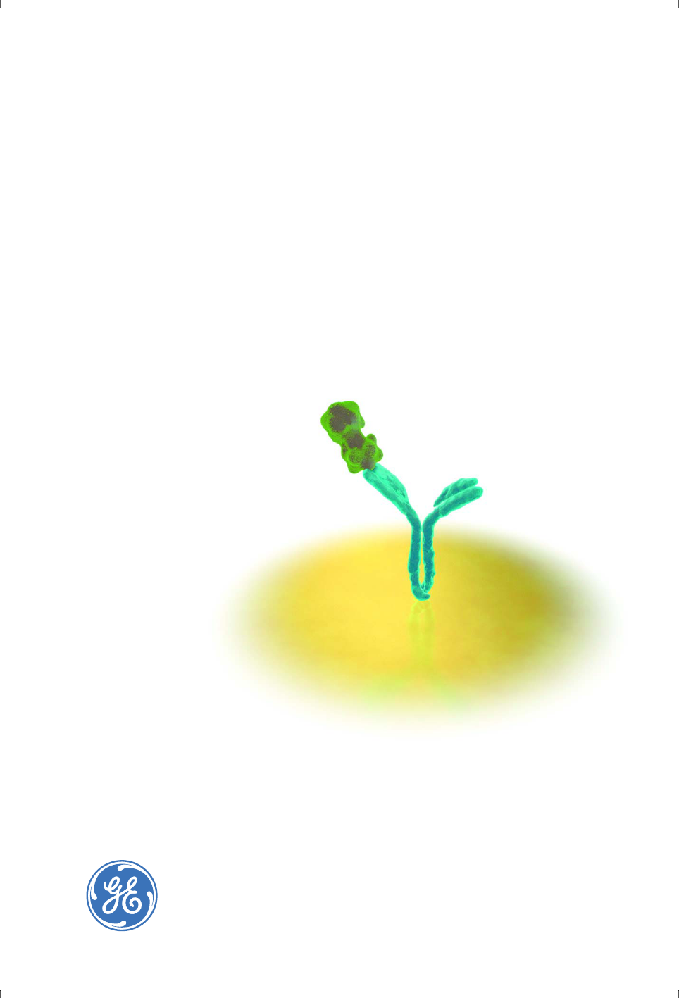
• The interaction partner attached to the surface is called the ligand (Figure

1-1). In drug discovery and development work, the ligand is sometimes

referred to as the target molecule.

Note: The term “ligand” is applied here in analogy with terminology used in

affinity chromatography contexts, and does not imply that the

surface-attached molecule is a ligand for a cellular receptor.

• The ligand may be attached to the surface either by covalent

immobilization using chemical coupling reagents or by capturing through

high affinity binding to an immobilized capturing molecule.

•The analyte is the interaction partner that is passed in solution over the

ligand (Figure 1-1).

Figure 1-1. The ligand is the interaction partner that is attached to the sensor

surface. The ligand may be immobilized directly on the surface (left) or attached

through binding to an immobilized capturing molecule (right). The analyte is free in

solution and binds to the immobilized ligand.

• In indirect assay formats the analyte is detected using a secondary

detecting molecule, which can bind to both analyte in solution and ligand

on the sensor surface. The observed response is derived from binding of

detecting molecule to the ligand: the presence of analyte in the sample

inhibits this binding so that the response is inversely related to the amount

of analyte.

• Analysis is performed by injecting sample over the surface in a carefully

controlled fashion. The sample is carried in a continuous flow of buffer,

termed running buffer.

• Response is measured in resonance units (RU). The response is directly

proportional to the concentration of biomolecules on the surface.

ligand

analyte

sensor

surface

ligand

analyte

capturing

molecule

1 Introduction

1.5 Biacore terminology

8 Biacore Assay Handbook 29-0194-00 Edition AA

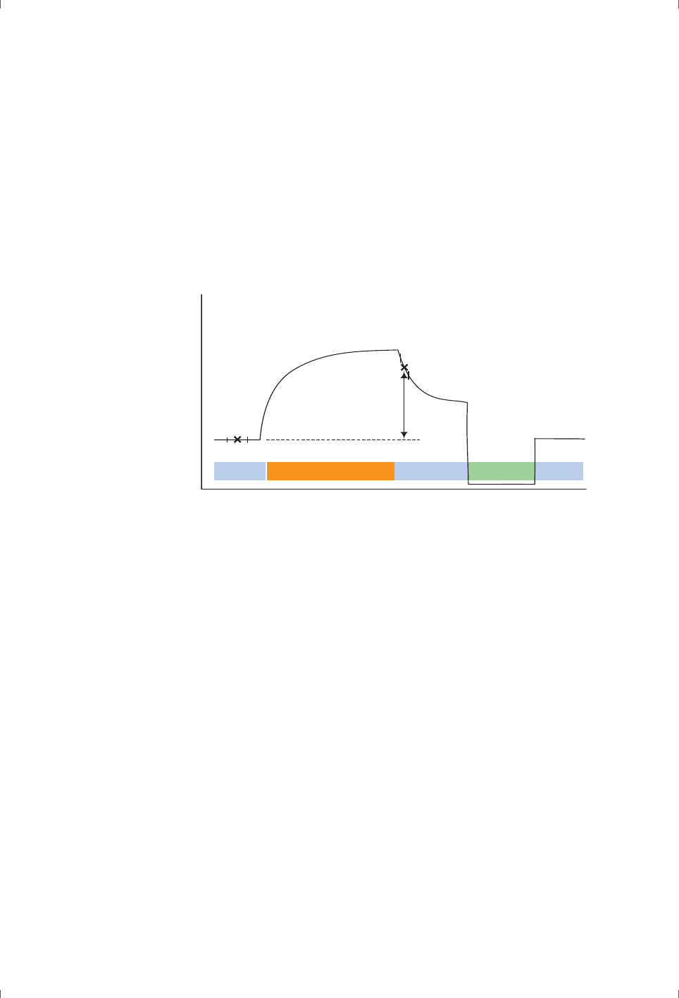
•A sensorgram is a plot of response against time, showing the progress of

the interaction (Figure 1-2). This curve is displayed directly on the

computer screen during the course of an analysis.

•A report point records the response on a sensorgram at a specific time

averaged over a short time window, as well as the slope of the sensorgram

over the window. The response may be absolute (above a fixed zero level

determined by the detector) or relative to the response at another

specified report point (Figure 1-2).

Figure 1-2. Schematic illustration of a sensorgram. The bars below the sensorgram

curve indicate the solutions that pass over the sensor surface.

• Regeneration is the process of removing bound analyte from the surface

after an analysis cycle without damaging the ligand, in preparation for a

new cycle. For ligand that is captured rather than immobilized,

regeneration usually removes the ligand and leaves the capturing

molecule intact.

• SPR detection monitors changes in refractive index close to the surface,

and differences in refractive index between running buffer and injected

sample will be recorded as a rapid shift in response at the beginning and

end of the injection. This is referred to as a bulk refractive index effect or

bulk shift.

• Naming conventions for kinetic and affinity constants vary considerably in

the literature. Throughout this book (and in other Biacore documentation),

rate constants are identified with lower-case letters (k

for association rate

constant and k

for dissociation rate constant), while equilibrium or affinity

constants are written with upper-case letters (K

for the equilibrium

association constant and K

for the equilibrium dissociation constant).

Absolute

response (RU)

Report point

(baseline)

Report point

(response)

Relative

response (RU)

Running

buffer

Running

buffer

Running

buffer

Sample

Regeneration

solution

Time

Biacore Assay Handbook 29-0194-00 Edition AA 9

Application overview 2

2 Application overview

This chapter gives an overview of the major application areas for Biacore

systems. These are

• Screening for binding partners, including immunogenicity testing

• Measurement of interaction kinetics and affinity

• Measuring concentration

• Mapping binding site topography

Subsequent chapters in this Handbook consider screening, kinetics/affinity and

binding site topography in more detail. Measurement of concentration is

discussed in a separate Handbook (Biacore Concentration Analysis Handbook).

2.1 Screening and detecting binding partners

Because Biacore systems exploit surface plasmon resonance (SPR), a generic

detection technology that requires no labels, they are well suited to screening

for binding partners in pharmaceutical and biopharmaceutical development

and immunogenicity testing.

The response in a Biacore system is directly related to the change in mass

concentration on the surface, so that molar responses (i.e. responses for a given

number of molecules) are proportional to the size of the molecule involved. A

given response will represent a higher molar concentration of a small molecule

than a large one: conversely, a given number of molecules binding to the

surface will give a lower response if the molecule is small. The relationship

between response and surface concentration is essentially constant for

proteins regardless of amino acid composition and sequence, and is similar for

most other biological macromolecules.

Note: In early literature related to Biacore, 1 RU was stated to be approximately

equivalent to a change in surface concentration of 1 pg/mm

. This

relationship holds roughly for proteins on Sensor Chip CM5. Beware of

applying the conversion to non-protein molecules and other types of

sensor chip. Response values from Biacore systems should always be

quoted in RU, not in units of surface concentration.

Measurements can be made on complex samples such as cell culture medium

or body fluids: the specificity of the observed response is determined primarily

by the choice of ligand attached to the surface. This is particularly useful in

applications such as antibody screening and immunogenicity testing: for

example, screening with an antigen as ligand will detect only specific

antibodies, while using an ligand directed towards a common region of a given

antibody class will detect that class regardless of antigen specificity.

2 Application overview

2.2 Kinetics and affinity measurements

10 Biacore Assay Handbook 29-0194-00 Edition AA

2.2 Kinetics and affinity measurements

Determination of interaction kinetics is perhaps the most characteristic

application for Biacore systems. The label-free real-time detection allows

interactions to be monitored with high resolution as they happen, and the

results can be interpreted in relation to a mathematical model of the interaction

mechanism to evaluate kinetic parameters (association and dissociation rate

constants). Affinity constants, which reflect the strength of binding but not the

rate, can be derived either from the rate constants or from analysis of the level

of binding at steady state. The theory of kinetic and affinity analysis is described

in Appendix A.

Note: The term “kinetics” is used in this handbook to refer to interaction kinetics.

The kinetics of other processes such as enzyme-catalyzed reactions are

not normally amenable to study in Biacore systems.

2.2.1 Kinetic analysis

Interaction kinetics are analyzed by monitoring the interaction as a function of

time over a range of analyte concentrations, and then fitting the whole data set

to a mathematical model describing the interaction. The association phase

(during sample injection) contains information on both association and

dissociation processes, while only dissociation occurs during the dissociation

phase (after sample injection, when buffer flow removes dissociated analyte

molecules).

It is important to be aware that the results of kinetic analysis are relevant only

in the context of the interaction model chosen for the evaluation. It is not strictly

possible to derive a model from the observed binding behavior, although the

shape of the sensorgrams can sometimes give clues for the choice of

appropriate models. Fitting the data to a mathematical model does not provide

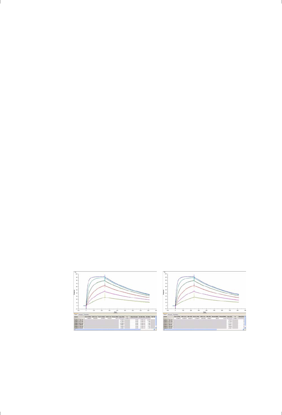
evidence of the interaction mechanism (Figure 2-1).

Figure 2-1. Fitting experimental data to a mathematical model does not prove that the

model is appropriate, and the same data may fit acceptably to several models. In this

example, the closeness of fit cannot distinguish confidently between a bivalent analyte

model (left) and a heterogeneous ligand model (right).

Biacore Assay Handbook 29-0194-00 Edition AA 11

Application overview 2

Assay set-up

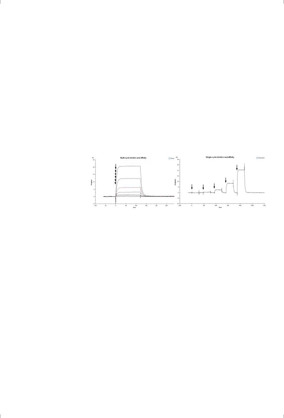
There are currently two ways of setting up a kinetic analysis experiment (Figure

2-2):

• Multi-cycle kinetics runs each analyte concentration in a separate cycle,

regenerating the surface after each sample injection. It is important that

regeneration is optimized (see Biacore Sensor Surface Handbook for more

information) so that the surface properties are consistent from cycle to

cycle.

• Single-cycle kinetics runs a series of analyte concentrations in one cycle,

with no regeneration between sample injections. This approach is valuable

in situations where acceptable regeneration cannot be achieved, but is

more sensitive to response drift since the cycle time is longer.

Figure 2-2. In multi-cycle kinetics and affinity determinations (left), each sample is injected

in a separate cycle. The concentration series is presented as an overlay plot aligned at the

start of the injection in the evaluation software.

In single-cycle determinations (right), the samples are injected sequentially in the same

cycle.

Arrows in the illustrations mark the start of sample injections.

2.2.2 Affinity analysis

Interaction affinity may be determined in three independent ways using Biacore

systems: calculation from kinetic constants, measurement of steady-state

binding levels and determination of affinity in solution.

Affinity constants from kinetics

For simple 1:1 binding, the affinity constant is equal to the ratio of the rate

constants (equilibrium association constant K

= k

, equilibrium dissociation

constant K

= k

, see Appendix A). Values for affinity constants can therefore

be derived from kinetic measurements.

Note that these values, like the values for rate constants, are only valid in the

context of the model used to analyze the binding data. More complex binding

mechanisms do not always give straightforward relationships between affinity

and kinetics, and it may only be possible to derive affinity constants from kinetic

constants for values obtained with a simple interaction model.

2 Application overview

2.2 Kinetics and affinity measurements

12 Biacore Assay Handbook 29-0194-00 Edition AA

Steady state affinity

Analyzing the level of steady state or equilibrium binding as a function of

interactant concentrations is the foundation for many standard techniques for

determining interaction affinity. The basic relationship between concentrations

of interactants and complex and the affinity is described in Appendix A. Affinity

constants may be derived from the experimental data from linearized plots such

as Scatchard plots or (as supported in Biacore software) by direct analysis of a

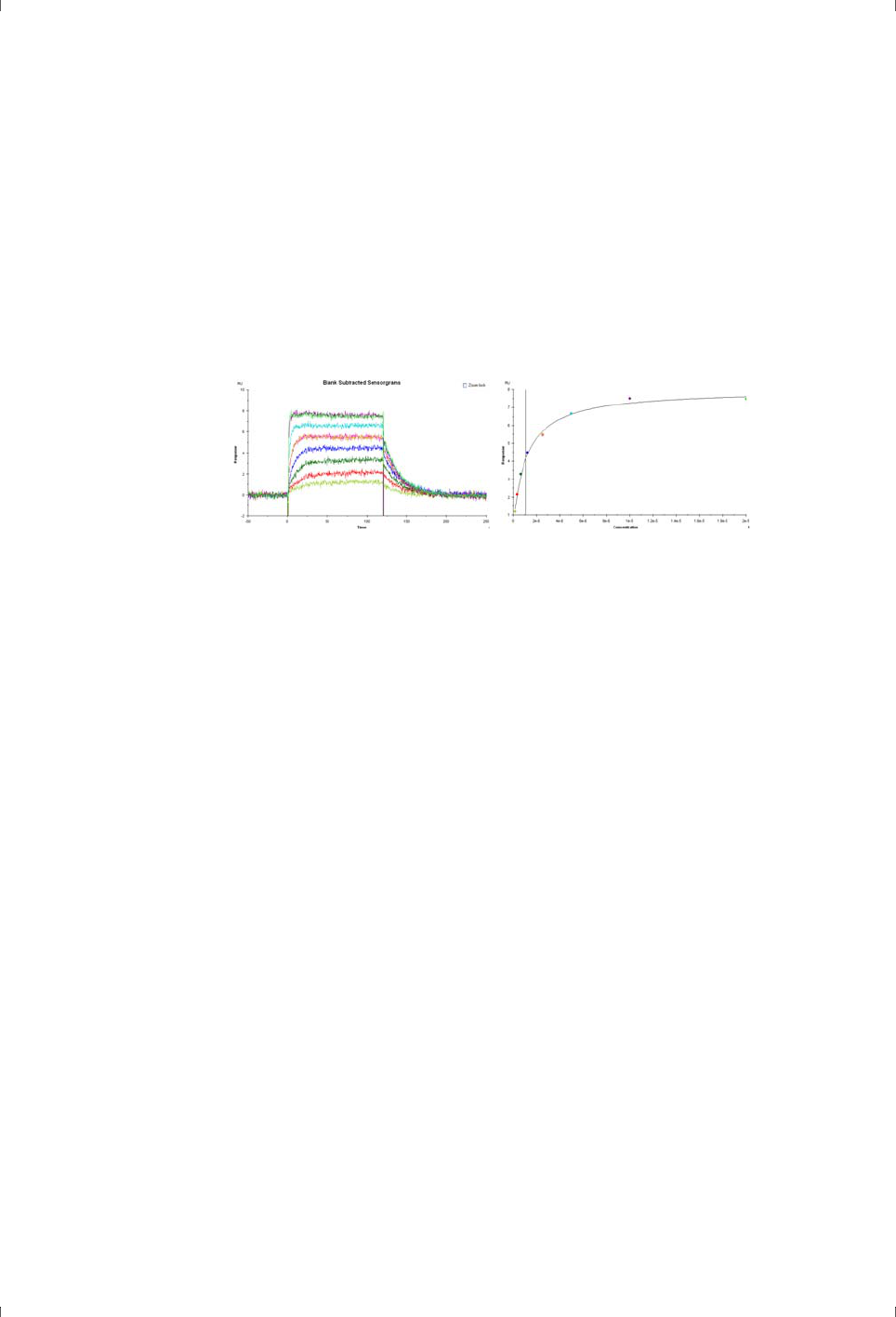
plot of amount of complex against analyte concentration (Figure 2-3).

Figure 2-3. Sensorgrams (left) and corresponding plot of steady state response against

concentration (right) for determination of binding affinity. The vertical line in the right-

hand plot indicates the value of the calculated equilibrium dissociation constant K

Analysis of steady-state binding data by fitting the curve of binding level against

concentration can only be applied to 1:1 binding. A model for 1:1 binding at two

independent ligand sites can be useful in some circumstances, but more

complex models are not sufficiently robust for analysis of the data. It is however

possible to apply classical Scatchard analysis to data obtained from Biacore

systems, to give some indication of the causes of deviation from 1:1 binding

behavior.

It may be thought that the same experiment can in principle provide data for

both kinetics and steady state binding, offering two independent affinity values

from one set of data. In practice, however, restrictions on the injected volume of

sample (and therefore the contact time between sample and the sensor surface)

mean that interactions that give measurable kinetics seldom reach steady state

and vice versa. The affinity for a given interaction can therefore usually be

derived from kinetics or steady state measurements but seldom both.

Affinity in solution

The principle of measuring affinity in solution with Biacore systems is to

determine the free concentration (and therefore the concentration of complex)

in mixtures of known interactant concentrations, using the Biacore system for

the concentration assay. Commonly, the assay is set up with one interactant A

(or an analogue thereof) on the surface. A calibration curve is established for

determining the concentration of the second interactant B. Mixtures containing

variable concentrations of A and a fixed concentration of B are allowed to reach

equilibrium and then analyzed for the free concentration of B. The results are

analyzed using standard tools for affinity measurements. A requirement of this

Biacore Assay Handbook 29-0194-00 Edition AA 13

Application overview 2

approach is that only free B and not complex AB can bind to the surface-

attached A.

While the requirement for calibrated concentration measurements of analyte B

makes this approach somewhat cumbersome, the main advantage is that

samples can be incubated as long as necessary to reach steady state.

Measurements are therefore not limited by the available contact time between

sample and sensor surface.

2.3 Concentration measurements

Biacore systems can be used for measurement of analyte concentrations

because the amount of analyte that binds to the surface under appropriate

conditions can be related to the concentration of analyte in the sample. In

calibrated assays, the response is related to the analyte concentration through

a calibration curve, prepared with standards containing known analyte

concentrations. This approach is analogous to many other established methods

of concentration measurement. Calibration-free concentration analysis (CFCA) is

an alternative approach supported in some Biacore systems, where

concentrations are derived from the observed rate of diffusion-limited binding

without reference to a calibration curve.

Concentration assays using Biacore systems are described in detail in the

Biacore Concentration Analysis Handbook.

2.3.1 Calibrated assays

Calibrated concentration measurements may be designed as direct or indirect

assays.

• Direct assays measure analyte bound directly to the ligand on the sensor

surface. This approach is suitable for macromolecular analytes (molecular

weight > 5000 daltons): direct detection of smaller molecules is possible

but the useful range of the assay is generally limited in such cases.

Response enhancement or sandwich approaches can be used to amplify

the response obtained and/or to increase the selectivity of the assay.

• Indirect or competition assays provide an indirect measure of analyte

concentration, and are most useful for low molecular weight analytes. The

commonest format for indirect assays is the solution competition or

inhibition approach, where a known amount of an interacting partner

called the detecting molecule is mixed with the sample, and the amount of

free detecting molecule remaining in the mixture is measured. In the

surface competition method, analyte and a high molecular weight

analogue (often a protein conjugate) compete for binding to a common

partner on the sensor chip surface. In both competition assay formats, the

response obtained is inversely related to the concentration of analyte in

the sample.

2 Application overview

2.4 Mapping binding sites

14 Biacore Assay Handbook 29-0194-00 Edition AA

Measuring concentration in a calibrated assay, whether direct or indirect, relies

on the ability to establish a calibration curve using standards of known

concentration. The results for unknown samples are always obtained with

reference to the standard, and represent “true” concentrations only insofar as

the standard concentrations are reliable. More detailed discussion may be

found in the Biacore Concentration Analysis Handbook.

2.3.2 Calibration-free concentration analysis (CFCA)

Calibration-free assays are based on the relationship between the diffusion

properties of the analyte and the absolute analyte concentration. The

concentration is calculated from knowledge of the diffusion coefficient of the

analyte together with analysis of the observed binding rate under partially

diffusion-limited conditions. This approach can be useful in situations where no

satisfactory calibrant is available for the analyte under study, or when it is

important to determine “true” concentrations as closely as possible. Calibration-

free assays are always set up in the direct binding format.

The requirement for binding under partially diffusion-controlled conditions

limits the dynamic range of CFCA and restricts the approach to analysis of

macromolecules (molecular weight above 5,000 Da).

2.4 Mapping binding sites

Binding sites on a macromolecule can be mapped by testing the ability of

multiple binding partners to bind independently or to compete with each other.

Two binding partners that are directed towards distinct binding sites will be able

to bind simultaneously, while partners that are directed towards interfering

sites will compete with each other. This kind of analysis is most common in

studies of antibody specificity (where it is called epitope mapping, see Figure

2-4), although it can in principle be applied to any investigation of multiple

binding sites on a macromolecule.

Figure 2-4. Different antibodies can bind simultaneously to distinct and spatially

separated epitopes (left), but not to common or overlapping epitopes (right).

Biacore Assay Handbook 29-0194-00 Edition AA 15

Application overview 2

Epitope mapping can be performed using two distinct approaches:

• Pair-wise binding tests the ability of pairs of antibodies to bind

simultaneously to the same antigen. Simultaneous binding is a clear

indication of distinct epitopes, while interference can result from binding

to the same or closely situated epitopes, or for example from a

conformational change in the antigen induced by binding of one antibody

that hides the epitope for the other.

• Peptide inhibition studies test the ability of peptides that represent specific

regions on the antigen to inhibit binding of single antibodies. A peptide

that blocks antibody binding is taken to represent at least a part of the

physical epitope for that antibody.

2 Application overview

2.4 Mapping binding sites

16 Biacore Assay Handbook 29-0194-00 Edition AA

Biacore Assay Handbook 29-0194-00 Edition AA 17

General considerations 3

3 General considerations

This chapter discusses aspects of working with Biacore systems that are

common to all application areas.

3.1 Sensor surfaces

3.1.1 General properties

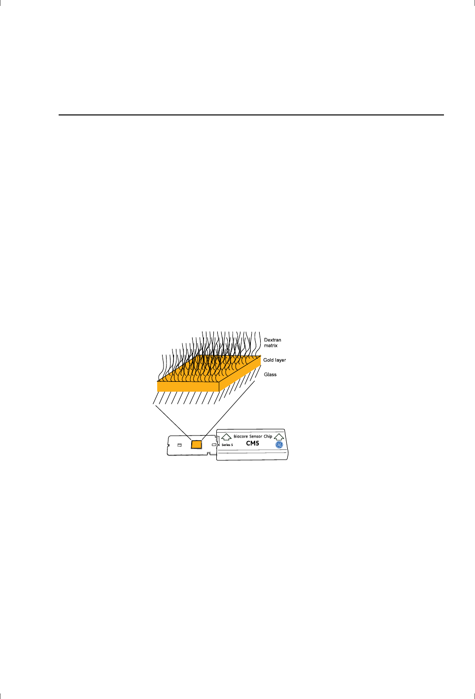
The sensor chip in Biacore systems consists of a glass slide coated with a thin

layer of gold. These components, together with the docking system for

mounting the sensor chip in the optical system, are required for generation of

an SPR signal. To provide a suitable environment for the molecular interactions

being studied, the gold surface is covered by a linker layer and (on most sensor

chip types) a matrix of modified dextran (Figure 3-1). It is the surface matrix that

determines the properties of the sensor chip with respect to ligand attachment

and molecular interaction.

Figure 3-1. Schematic illustration of the structure of the sensor chip surface on CM-series

chips.

3.1.2 Sensor surface types

GE Healthcare offers a range of sensor surfaces designed for different

application requirements, as summarized in Table 3-1. Detailed descriptions of

sensor chip types may be found in the Biacore Sensor Surface Handbook and

on www.gelifesciences.com/biacore.

3 General considerations

3.1 Sensor surfaces

18 Biacore Assay Handbook 29-0194-00 Edition AA

Table 3-1. Characteristics and application areas for sensor chips.

Sensor Chip Characteristics Use

CM-series sensor chips (carboxymethyl-dextran surface matrix)

CM5 Moderate capacity General purpose

CM7 High capacity High immobilization levels for

work with low molecular

weight analytes (not suitable

for protein analytes or capture

applications).

CM4 Low capacity

(low substitution density)

Low immobilization levels for

kinetics.

May help to reduce non-

specific binding from complex

samples.

CM3 Low capacity

(shorter dextran chains)

Large particulate analytes

(viruses and cells).

Low immobilization levels for

kinetics.

May help to reduce non-

specific binding from complex

samples.

C1 Flat surface, no dextran

matrix. Carboxyl groups

directly attached to the

surface linker layer.

Restricted mobility of

attached ligand.

Large particulate analytes

(viruses and cells).

Hydrophobic surfaces

HPA No surface matrix or

attached groups

Direct adsorption of lipid

monolayers, with or without

associated proteins.

L1 Dextran matrix

substituted with

lipophilic residues

Capture of intact lipid vesicles.

Biacore Assay Handbook 29-0194-00 Edition AA 19

General considerations 3

3.2 Attaching the ligand

In broad terms, there are two main approaches to attaching macromolecular

ligands to the sensor surface, covalent immobilization and high affinity capture.

Details of these alternatives may be found in the Biacore Sensor Surface

Handbook.

3.2.1 Covalent immobilization

Covalent immobilization involves irreversible chemical attachment of the ligand

to the surface, usually to the carboxymethyl groups on CM-series sensor chips.

The ligand remains on the surface throughout the lifetime of the sensor chip,

and is regenerated to remove non-covalently bound molecules after each

analysis cycle.

Covalent immobilization may exploit amine, thiol (either native or introduced) or

aldehyde groups (obtained by oxidation of cis-diols) on the ligand. Amine

coupling is the most widely used alternative.

Conditions for immobilization

The concentration of ligand in the surface matrix for analysis in Biacore systems

is many times higher than that in a typical bulk solution: immobilization of a

protein at a response level of 100 RU on Sensor Chip CM5 corresponds roughly

to a bulk concentration of 1 mg/ml in the surface matrix, while typical bulk

concentrations used for immobilization are 50-100 µg/ml. In most

immobilization methods, ligand is concentrated on the surface by a process of

electrostatic pre-concentration. This occurs when the pH of the ligand solution is

below the isoelectric point of the ligand, so that the ligand carries a net positive

charge, but above the pKa (3.5) of carboxyl groups on the surface so that the

Surfaces for ligand capture

SA Streptavidin covalently

attached to dextran

matrix

Permanent capture of

biotinylated molecules

CAP Oligonucleotide

covalently attached to

dextran matrix

Reversible capture of

biotinylated ligands, mediated

by a streptavidin-carrying

complementary

oligonucleotide.

NTA Nitrilotriacetic acid

covalently attached to

dextran matrix

Capture of histidine-tagged

ligands

Sensor Chip Characteristics Use

3 General considerations

3.2 Attaching the ligand

20 Biacore Assay Handbook 29-0194-00 Edition AA

surface is negatively charged. Low ionic strength favors the electrostatic

interaction, and buffers with 10-20 mM total cation concentration are generally

recommended.

Choice of immobilization chemistry

Many macromolecules can be immobilized as ligands on the sensor surface

without significantly interfering with the interaction being studied, provided that

the coupling chemistry involves groups that are distant from the site of

interaction. Chemistries such as amine coupling that target common groups

may result in a mixture of ligand molecules on the surface with different points

of attachment: in some cases, ligand may be partially inactivated with respect

to interaction by the attachment, but this does not matter as long as sufficient

active molecules are present. More specific chemistry such as thiol coupling

may be used to reduce the variation in orientation of the attached molecules, or

even to determine precisely how the molecules will be attached (if the ligand

contains only a single target group for attachment).

Figure 3-2. Amine coupling is frequently successful, but in this example (immobilization of

a hormone receptor) amine coupling destroys the ligand activity completely. The best

results are obtained with high affinity capture.

Amine coupling

Immobilized: 10,000 RU

Activity: undetectable

Thiol coupling

Immobilized: 12,000 RU

Activity: 5%

Poly-histidine tag capture

Immobilized: 2,000 RU

Activity: 20%

Biacore Assay Handbook 29-0194-00 Edition AA 21

General considerations 3

Amine coupling is generally applicable to a wide range of protein ligands, and is

often the most convenient method of attachment. However, testing a range of

attachment chemistries can be worthwhile in critical cases: Figure 3-2

illustrates results from immobilization of a hormone receptor where amine

coupling gave a fully acceptable immobilization level but activity was preserved

better by thiol coupling. High affinity capture of poly-histidine tagged receptor

on Sensor Chip NTA gave however the best yield in terms of binding activity

(tested by binding of hormone) per immobilized RU.

3.2.2 High affinity capture

High affinity capture refers to attachment of ligand by binding to an

immobilized capturing molecule, and offers advantages over covalent

immobilization in a number of situations:

• Capture does not require any chemical modification of the ligand and can

be performed in physiological buffer conditions. It can therefore be used

with ligands that are not amenable to covalent immobilization.

• Normally, regeneration of the surface with a captured ligand involves

removal of ligand together with other bound molecules, leaving the

capturing molecule ready bind fresh ligand for the next cycle. While this

procedure increases consumption of ligand, it removes the requirement

that ligand is not damaged by regeneration and allows the ligand to be

changed between analysis cycles on the same sensor chip.

• Capture may be used to attach a specific ligand from a complex sample,

provided the capturing interaction is sufficiently selective. Covalent

immobilization of ligand from such samples would require prior

purification of the ligand.

Conditions for ligand capture are dictated by the requirements of the capturing

interaction, and capturing is normally performed in the same buffer conditions

as the interaction being studied. It is however important that the capturing

interaction is reasonably stable under the chosen conditions, so that ligand

does not dissociate significantly during sample analysis. Demands on capturing

stability vary with different applications, and are highest for kinetic and affinity

analyses, since loss of ligand will cause a fall in response as well as reducing the

analyte binding capacity of the surface. Simpler applications such as detection

and screening may tolerate more loss of ligand during sample injection.

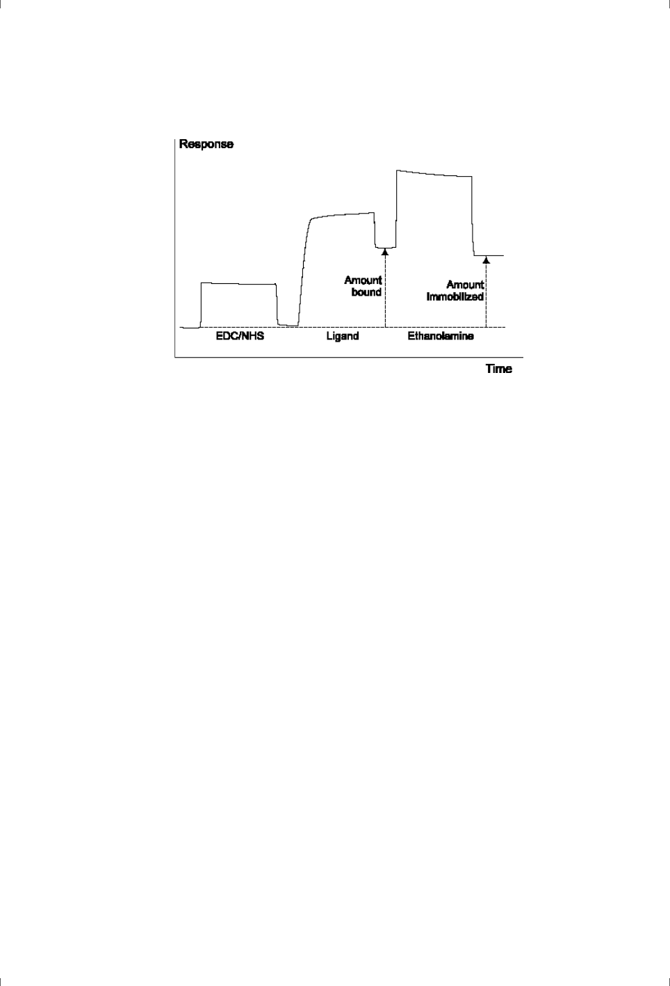
3.2.3 Response levels

One of the issues in preparing the sensor surface for a given application is the

question of how much ligand that should be attached. All steps in the

attachment process are monitored in the instrument, and the amount of

attached ligand is in principle given directly by the response above baseline

(Figure 3-3).

3 General considerations

3.2 Attaching the ligand

22 Biacore Assay Handbook 29-0194-00 Edition AA

Figure 3-3. Sensorgram from a typical amine coupling, illustrating the distinction between

the amount of ligand bound and the amount immobilized.

Note: Even activation of the surface with EDC/NHS can be detected as a small

increase in response. When the response from immobilized ligand is low,

it may be more appropriate to estimate the ligand level from the response

after activation rather than the baseline at the start of the immobilization

procedure.

A more relevant parameter in designing and preparing a surface is however the

analyte binding capacity (called

Rmax

, for maximum response), since this will

determine the expected response range from samples. The amount of ligand on

the surface as measured from the increase in response gives an indication of

the theoretical analyte binding capacity of the surface, provided that the relative

sizes of ligand and analyte are known. Assuming a 1:1 binding stoichiometry:

The practical analyte binding capacity is obtained experimentally by injecting

analyte at a high concentration to saturate the surface (or by extrapolating

binding levels from measurements at a series of concentrations). Comparison of

the theoretical and practical R

max

values provides a measure of the activity of

surface-attached ligand. Protein preparations are seldom 100% active, and for

generic attachment methods such as amine coupling, activities in the region of

70% and above may be expected.

The shape of the sensorgram from the attachment procedure can provide

guidance in choosing appropriate conditions. Bear in mind that the amount of

ligand immobilized will generally be less than the amount bound during

preconcentration. Most Biacore systems support a mode of ligand

immobilization using amine coupling that exploits the information from a brief

max

RU

analyte MW

ligand MW

----------------------------- -

immobilized ligand level (RU)=

Biacore Assay Handbook 29-0194-00 Edition AA 23

General considerations 3

preconcentration injection to adapt the immobilization process to reach a

specified level.

• The sensorgram slope and shape during protein injection indicates the

efficiency of electrostatic preconcentration. Try to use a combination of

ligand concentration and injection time so that the amount bound reaches

a plateau. This will contribute to the robustness of the immobilization

procedure.

• The relative response levels before and after deactivation of the surface

indicate how well the electrostatically bound protein has become

covalently attached. Deactivation washes out non-covalently bound

material: a reduction in response may be observed after deactivation but

this does not affect the assay as long as sufficient ligand is attached to the

surface.

If the immobilization works in principle satisfactorily but the amount of ligand

attached is not suitable for the assay, adjust one or more of the parameters

ligand concentration, immobilization pH, ligand injection time and surface

activation time.

3.3 General buffer considerations

3.3.1 Buffer substances

In general, Biacore systems are compatible with most buffer substances used in

biological studies. Exceptions may be dictated by specific properties of the

interacting molecules or by the situation where the buffer is used (for example,

the primary amine groups in Tris preclude the use of this buffer for attaching

ligand by amine coupling).

HEPES (4-(2-hydroxyethyl)-1-piperazineethanesulfonic acid, pK

7.55) is a

satisfactory buffer substance for many protein-protein interactions, and ready-

to-use buffers based on 10 mM HEPES are available for use with Biacore

systems.

Phosphate-based buffers are often more suitable for work with low molecular

weight analytes since organic buffers such as HEPES can bind to the ligand and

interfere with accurate detection of low molecular weight compounds.

3.3.2 Ionic strength

Physiological ionic strength buffers (containing 0.15 M monovalent cations) are

recommended unless other requirements are imposed by the interaction being

studied. Reducing the ionic strength will increase the tendency for non-specific

electrostatic binding of molecules from the sample to the sensor surface. Higher

ionic strength may be tested if non-specific binding is a problem.

3 General considerations

3.3 General buffer considerations

24 Biacore Assay Handbook 29-0194-00 Edition AA

3.3.3 Additives

Detergent

Inclusion of non-ionic detergent (0.05% Surfactant P20, Tween™ or equivalent)

in all buffers is recommended to minimize deposition of protein and other

biomolecules in the flow system. The detergent should be included at a

concentration above the critical micelle concentration (CMC). At lower

concentrations, the detergent itself can accumulate in the flow system and lead

to unwanted response effects as it is released (see FIgure 3-4).

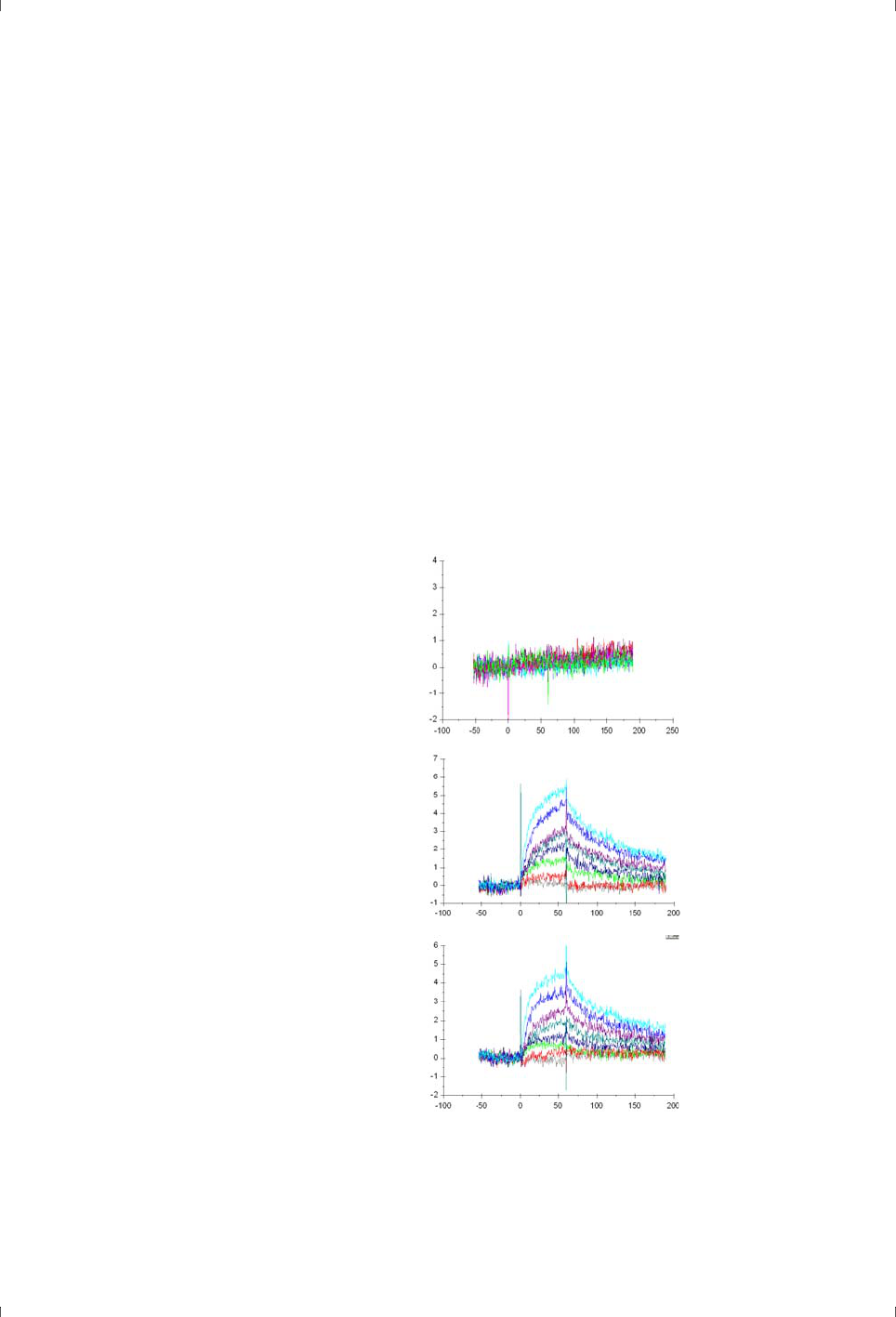
Figure 3-4. Schematic illustration of typical “detergent effects” caused by using detergent

at concentrations below CMC. The broken line shows an undisturbed sensorgram for

comparison.

Some applications, particularly those involving lipid vesicles and/or

hydrophobic proteins, require detergent-free buffer. In such cases it is essential

to clean the flow system regularly and carefully using the appropriate

maintenance tools provided with the system, in order to ensure continued high

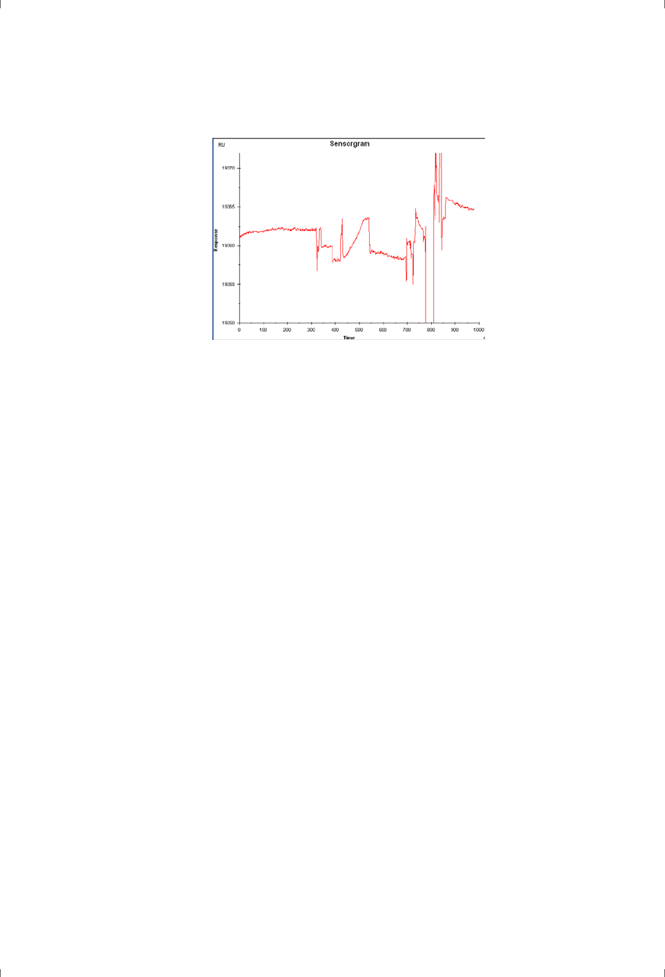
performance. Poor instrument cleaning can result in severely disturbed

sensorgrams that are difficult to interpret. A severe example is shown in Figure

3-5.

Biacore Assay Handbook 29-0194-00 Edition AA 25

General considerations 3

Figure 3-5. Severe example of the consequences of poor instrument cleaning.

EDTA

HBS-EP and HBS-EP+ general purpose buffers from GE Healthcare include 3 mM

EDTA to remove traces of free divalent metal ions that may be present in the

buffer. This is a general precautionary measure and is not specifically required

for work with Biacore systems. Buffers with no added EDTA are also available.

NSB Reducer

Addition of NSB reducer (a preparation of soluble carboxymethyl dextran) to

samples can in some cases help to reduce non-specific binding of sample

components to the dextran matrix on the sensor surface. The recommended

concentration of NSB Reducer is 1 mg/ml. NSB Reducer should only be used in

situations where non-specific binding is a problem (typically with complex

samples such as serum or whole cell extracts).

Organic solvents

Many low molecular weight organic compounds, relevant particularly in

pharmaceutical development work, are sparingly soluble in aqueous buffers

and require addition of organic solvents. Dimethyl sulfoxide (DMSO) is commonly

used. Biacore systems can be used with buffers containing up to 10% DMSO.

However, organic solvents contribute significantly to the bulk refractive index of

samples and buffers: 1% DMSO contributes approximately 1200 RU to the

response level. Expected responses from low molecular weight analytes, which

often need organic solvents to maintain solubility, may be as low as 10-20 RU or

less. It is therefore crucial that the measured responses are accurately

compensated for any variations in organic solvent concentration. Procedures

for adjusting measured sample responses for solvent effects, called solvent

correction, are described in principle in Appendix B and in more detail in the

documentation for Biacore systems where the correction is supported.

3 General considerations

3.3 General buffer considerations

26 Biacore Assay Handbook 29-0194-00 Edition AA

Other additives

Avoid additives that can compete with the ligand for immobilization chemistry,

for example sodium azide with amine coupling chemistry. Even at low

concentrations, sodium azide can effectively prevent amine coupling of

proteins.

3.3.4 Buffer preparation

All buffers regardless of composition should be filtered before use and degassed

if the instrument does not have a built-in degasser. Disturbances caused by

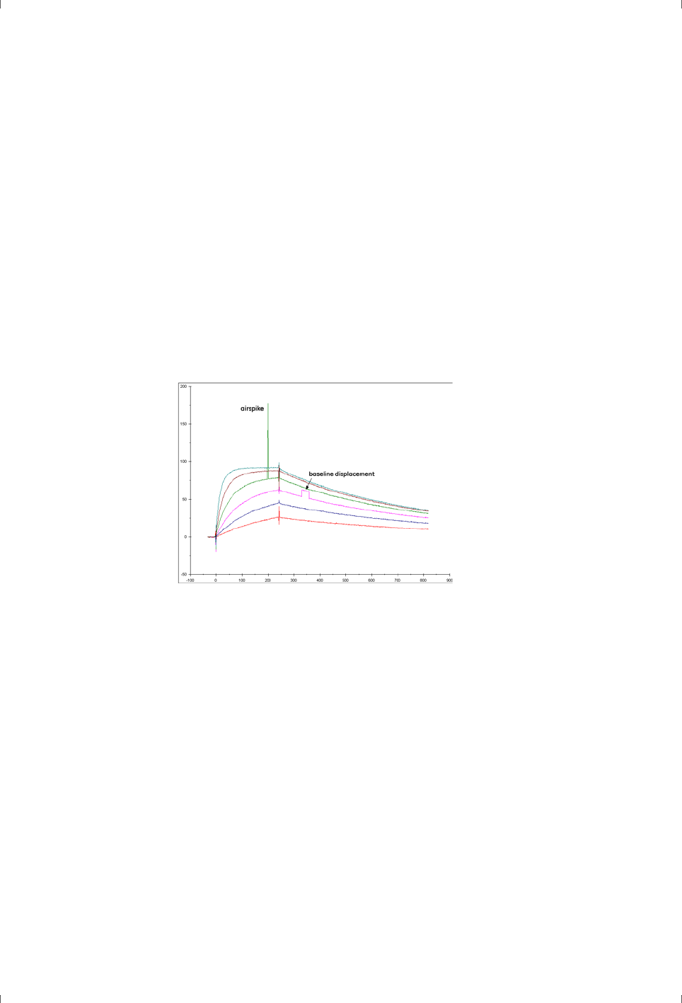
particles and microscopic air bubbles introduced over the sensor surface

appear typically as spikes in the sensorgram. Air bubbles or particles that

remain on the surface can result in more long-lived displacements in the

response (Figure 3-6).

Figure 3-6. Airspikes and transient baseline displacements are often attributable to

inadequately degassed running buffer.

Filtering

Buffers should be filtered through a 0.22 µm filter to remove particles.

Serum and plasma samples should be centrifuged or filtered to remove

aggregated material, particularly if the samples have been frozen.

Degassing

Degas running buffer before use unless you are working with a Biacore system

fitted with an in-line degasser. Alternatively use degassed ready-to-use buffers

from GE Healthcare.

Always degas buffer solutions before adding detergent to avoid frothing.

Biacore Assay Handbook 29-0194-00 Edition AA 27

General considerations 3

3.4 Matching sample and running buffer

3.4.1 Matching refractive index

Differences in refractive index between sample and running buffer give rise to

so-called bulk shifts in sensorgrams at the beginning and end of sample

injection. The bulk shift may be negative or positive depending on the difference

in refractive index (Figure 3-7).

Figure 3-7. Schematic illustration of bulk shifts: negative (left), zero (center) and positive

(right).

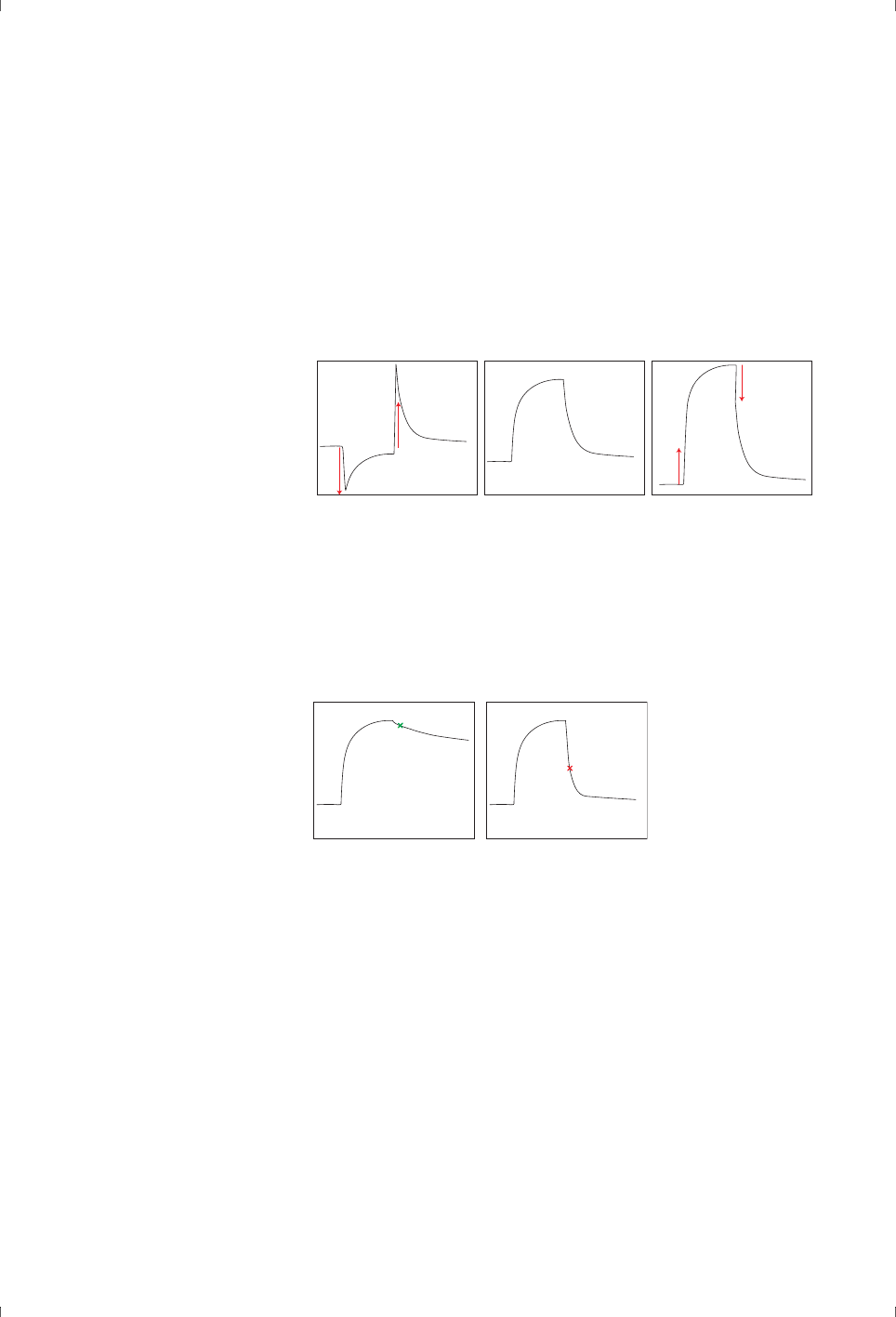
Some applications, such as concentration measurement and in some cases

screening, rely on single-point measurements (report points) that can be placed

after the end of the sample injection. These measurements are not affected by

bulk shifts so that accurate matching sample and running buffer is not

necessary (Figure 3-8).

Figure 3-8. If dissociation is slow enough, binding levels can be assessed from a report

point placed shortly after the end of the sample injection (left). However, if dissociation is

rapid (right) a report point at this position will not give a reliable measure of the binding

level.

In contrast, applications that rely on response measurement during sample

injection need to deal with the question of bulk response. Careful matching of

sample and running buffer with respect to refractive index goes a long way to

eliminating bulk shifts, but exact matching is seldom practicable. Subtracting

the response from a reference surface usually handles bulk shifts satisfactorily

provided that the shifts are reasonably small in relation to the measured analyte

responses. Special measures, called solvent correction, are however required for

applications where bulk shifts can be large and expected responses are small

(typically assays involving low molecular weight organic analytes, such as

response

time

response

time

3 General considerations

3.5 Dilution series and replicates

28 Biacore Assay Handbook 29-0194-00 Edition AA

screening for potential drug development candidates). These special

considerations are dealt with in Appendix B.

It is not always possible to match the refractive index of sample and running

buffer, for example in analysis of unpurified samples such as serum. In such

cases it is important that measurements are made after the end of the sample

injection to avoid bulk shift effects.

3.4.2 Matching buffer composition

Matching of sample and running buffer composition is particularly important for

kinetic measurements, regardless of the question of bulk response shifts, since

the sensorgram contains information about dissociation kinetics both during

and after sample injection. For correct analysis of the kinetics, it is important

that the dissociation process during and after sample injection occur in the

same environment.

3.4.3 Matching buffer environment in practice

Several approaches can be used to match sample and running buffer,

depending on the form in which the original sample is available.

• Samples that are available in sufficiently concentrated stock solution may

be diluted in running buffer so that the concentration of other components

in the stock is negligible. The minimum dilution factor needed to achieve

this depends on the composition of the stock solution and the stringency

of the buffer matching requirements for the assay at hand.

• Buffer exchange techniques such as desalting columns or dialysis are

often the most effective way to prepare samples in running buffer. Buffer

exchange can be essentially complete with minimum dilution of the

sample, and commercially available solutions such as micro-spin columns

allow rapid preparation of small sample volumes.

• Solid samples may be dissolved directly in running buffer: filter or

centrifuge the solution if there is a risk that undissolved material remains.

Be aware however that many commercially available proteins supplied in

solid form include considerable amounts of salt or other stabilizing

medium. Dissolving a dry preparation in running buffer does not

guarantee that the composition or refractive index of sample and buffer

will be matched.

3.5 Dilution series and replicates

Recommendations in this section relate to factors that should be standard in

laboratory work. They are however included here as a reminder, since they can

in some instances be critical to the success of the application.

Biacore Assay Handbook 29-0194-00 Edition AA 29

General considerations 3

Dilution series play an important role in a number of contexts in work with

Biacore systems: for example, kinetics and affinity determinations require

analysis over a range of analyte concentrations, and calibrated concentration

assays use dilution series for establishing a standard curve and also for

investigating certain performance characteristics such as parallelism. In many

situations, performing replicate determinations to establish reproducibility is a

given component in assay design. The way in which dilution series and

replicates are prepared and analyzed can have a significant impact on the value

of the results.

3.5.1 Dilution series

There are various possible sources of error in creating a dilution series, and the

best approach depends on the available equipment and the volumes involved

as well as the accuracy demands of the application.

Reliable pipettes are essential for creating accurate dilution series by volume.

Where possible (particularly for small volumes), use repeated aliquots of the

same volume for dilution series, to avoid errors that may be introduced by

repeatedly changing the volume on variable volume pipettes.

Two different basic methods may be used:

• Serial dilution where each dilution is used as the sample solution for the

next step.

• Parallel dilution where sample is always taken from the same stock

solution and mixed with increasing volumes of buffer.

Using the same fixed volume pipettes for both sample and buffer provides the

best accuracy for dilution factor (although not necessarily for absolute

volumes). If different pipettes are used with different errors of delivery, the

dilution error will propagate through the series more significantly with serial

dilution than with parallel. However, serial dilution is a simpler procedure,

requiring fewer operations with a fixed-volume pipette, so that parallel dilution

is more susceptible to errors of reproducibility.

For the best accuracy in preparing dilution series, volumes of buffer and sample

used may be determined by weighing and the dilution factor calculated

individually for each sample. This avoids issues of both calibration accuracy and

reproducibility for pipetted volumes.

3.5.2 Replicates

Measuring replicate samples to establish the reproduciibility of an assay should

be a standard procedure in all laboratory work, but it is not always clear how the

replicates should be prepared and measured in order to provide the most useful

information. Replication can cover the whole assay procedure from raw sample

material to evaluation of the final results, or it can focus on one or more specif ic

3 General considerations

3.6 Preparing vials and microplates

30 Biacore Assay Handbook 29-0194-00 Edition AA

components of the procedure. Different assay situations will require different

approaches in this respect.

Replicate samples designed to test the reproducibility of a Biacore-based assay

should be prepared and measured according to the following general

guidelines:

• Take replicates from a well-defined step in the sample preparation

procedure, with a clear awareness of what parameters are being tested

for reproducibility. For example, taking replicate samples from the same

tube in a dilution series will test the reproducibilty of the assay procedure

itself, whereas preparing replicate dilution series from a common stock

solution will include pipetting and dilution procedures in the repliacte test.

• Place replicate samples in separate vials or microplate wells for the assay

wherever possible, so that only one sample is taken from each position.

Injecting multiple samples from the same autosampler position is not

recommended since evaporation from vials or wells that have been

penetrated can affect the concentration.

• Analyze replicates at well-spaced intervals in the assay, to provide a check

on any drift in the assay performance with time. In many assays, this

factor can be conveniently tested by using repeated measurements on

control samples: in some cases however (such as kinetics and affinity

analysis) it can be valuable to apply the principle to replicate

concentrations of the sample.

3.6 Preparing vials and microplates

Samples and reagents are loaded into sample racks or microplates (according

to the requirements of the particular Biacore instrument). All samples for one

assay run are normally loaded at the start of the run: if samples have a tendency

to precipitate with time, bear in mind that the samples that are analyzed last

may have been standing for several hours in the autosampler.

Beware of using samples that might precipitate or aggregate with time (for

example, low molecular weight organic compounds close to the limit of

solubility).

Cover samples as soon as they are prepared, and keep them covered for the

duration of the assay to prevent evaporation. Always use vial caps and

microplate foil for Biacore systems from GE Healthcare: the autosampler needle

may not penetrate caps or foil from other sources satisfactorily, resulting in

failed assays or even damage to needle. When sealing microplates with foil,

make sure the foil is correctly placed so that the wells are covered by areas free

from adhesive. If the foil is wrongly applied, adhesive may accumulate on the

needle and cause malfunction.

Biacore Assay Handbook 29-0194-00 Edition AA 31

Screening and detecting binding partners 4

4 Screening and detecting binding partners

Screening applications using Biacore systems fall into two main categories that

differ significantly in challenges and experimental design:

• Small molecule (LMW) screening, where response levels are low and

organic solvents are often needed to maintain analyte solubility. These

interactions are usually rapid and regeneration is not needed.

• Biopharmaceutical (frequently antibody) screening where response levels

are higher but the sample matrices (cell culture supernatant or cell

extracts) are often complex. These interactions are usually slower:

regeneration is simplified if a capture approach is used.

Table 4-1 summarizes the main experimental conditions for LMW and antibody

screening.

Table 4-1. Main experimental conditions for LMW and antibody screening.

Recommended 2% unless higher concentration is required to maintain substance

solubility.

A third related application area is immunogenicity testing, which involves

detecting anti-drug antibodies (ADAs) in plasma or serum samples. Here the

simultaneous presence of ADAs and drug in the samples creates special

requirements.

LMW screening Antibody screening

Buffer Phosphate HEPES

Additives:

- DMSO

- detergent

Yes (1 to 10%)

Yes

Flow rate Typically 10 µl/min Typically 10 µl/min

Contact time 15 to 30 s 1 to 2 min

Report point Before end of sample

injection

After end of sample

injection

Regeneration Usually not needed Usually needed

4 Screening and detecting binding partners

4.1 Small molecule screening

32 Biacore Assay Handbook 29-0194-00 Edition AA

4.1 Small molecule screening

4.1.1 Goals

The primary goal of small molecule screening in pharmaceutical development

is to identify candidate molecular structures for further development, on the

basis of their binding to selected target molecules. The first stages of the

process is often screening of candidate libraries or fragment libraries to identify

promising binders for further development and refinement. Information-rich

screening with Biacore systems can provide a wealth of valuable data in

addition to yes/no binding results, including comparative binding to multiple

targets to identify promiscuous (and therefore less interesting) binding

candidates and assessment of kinetics and affinity properties that become

increasingly important as the candidate molecules are refined.

4.1.2 Sensor surface preparation

The response obtained from LMW analytes is inherently low because of the

molecular size: in addition, binding affinities are often weak (particularly for

fragment screening) which further reduces the expected response levels. For

this reason, sensor surfaces for LMW screening are prepared with high levels of

ligand (typically 8,000 to 10,000 RU for average-sized proteins).

Accurately determining the activity of the immobilized ligand requires high

analyte concentrations to saturate the surface with weak binders (typically 0.1

to 2 mM for fragments and 0.05 to 0.2 mM for LMW compounds). Testing binding

activity with a positive control is desirable if a suitable control analyte is

available.

4.1.3 Sample preparation

In the first phases of small molecule screening, samples are often prepared at a

fixed concentration in the same buffer. There is usually no opportunity to

optimize concentration or buffer conditions.

Many small organic compounds are sparingly soluble in aqueous buffers and

require inclusion of organic solvents (commonly 1% to 3% DMSO) to maintain

solubility. DMSO has a strong refractive index contribution (about 1200 RU for

1% DMSO), and both careful matching of sample and running buffer and

correction for small differences in DMSO concentration are required (see below).

4.1.4 Buffers

Phosphate buffers are generally recommended for work with small molecules.

Using organic buffers such as HEPES can bind to the ligand and interfere with

accurate detection of small organic compounds. Physiological ionic strength

(150 mM monovalent cations) should be used to reduce non-specific binding of

Biacore Assay Handbook 29-0194-00 Edition AA 33

Screening and detecting binding partners 4

compounds to the sensor surface, and inclusion of detergent (0.05% Surfactant

P20) generally improves data quality by reducing drift and signal disturbances.

The composition of running buffer and sample buffer must be matched as

closely as possible, particularly with respect to organic solvent concentration.

Variations in DMSO content between samples resulting from both evaporation

and absorption of water are however unavoidable. Procedures that correct for

differences in bulk refractive index between samples, called solvent correction,

are described in Appendix B and are implemented in Biacore systems designed

for work with small molecules.

4.1.5 Analysis conditions

Flow rate

Use low flow rates (10 µl/min) for LMW screening applications to conserve

sample. Issues such as mass transfer limitations (Section A.1) and resolution of

fast binding events are not relevant.

Contact time

Most interactions involving small molecules are rapid, and contact times can be

kept short (30 to 60 seconds) to increase screening throughput.

Regeneration

Regeneration is generally not necessary in LMW screening applications, since

dissociation is rapid and is usually complete within 1 minute or thereabouts.

Report points

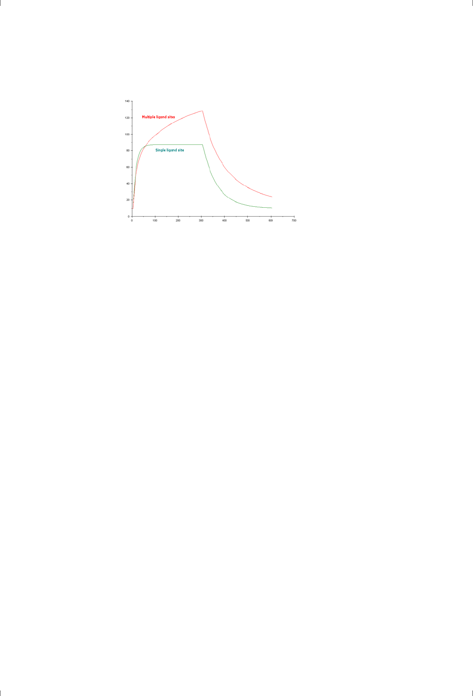
Because of the rapid dissociation of many LMW compounds from the target

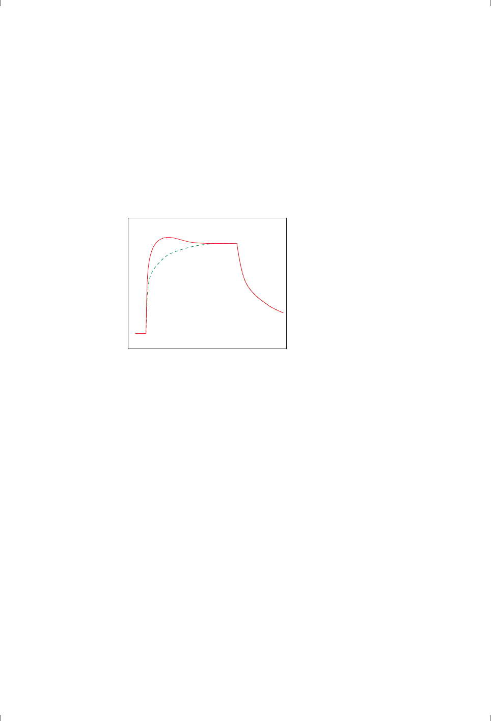
molecule, report points for screening should be placed before the end of the

sample injection. LMW compounds sometimes show rapid binding to specific

sites followed by slower and more indiscriminate binding (Figure 4-1). Placing

report points early in the sample injection can reduce the impact of this

behavior and give a more accurate indication of specific binding ability.

4 Screening and detecting binding partners

4.1 Small molecule screening

34 Biacore Assay Handbook 29-0194-00 Edition AA

Figure 4-1. Simulated sensorgrams illustrating 1:1 binding (dark green) and binding to one

specific site followed by slower and more indiscriminate binding (red).

Other considerations

Some LMW compounds are “sticky” and can be difficult to wash off the sensor

surface and out of the flow system, causing carry-over of material to the next

analysis cycle. This can be detected by routinely including a “carry-over

injection” of buffer after the sample injection: the response from a “sticky”

compound will be carried over into this buffer injection. Include a flow system

wash with 50% DMSO after every cycle to minimize problems with sticky

compounds. If a screening experiment involves compounds that are known to

be sticky, place these at the end of the experiment to avoid interference with

other compounds or omit them from the experiment altogether.

4.1.6 Evaluating results

At the simplest level, LMW screens are evaluated by comparing the binding

responses corrected for analyte molecular weight, and setting a cut-off level

above which binding is regarded as significant. The cut-off may be determined

by comparison with the response obtained from known non-binders (negative

controls) or set to some level chosen in relation to the distribution of response

values.

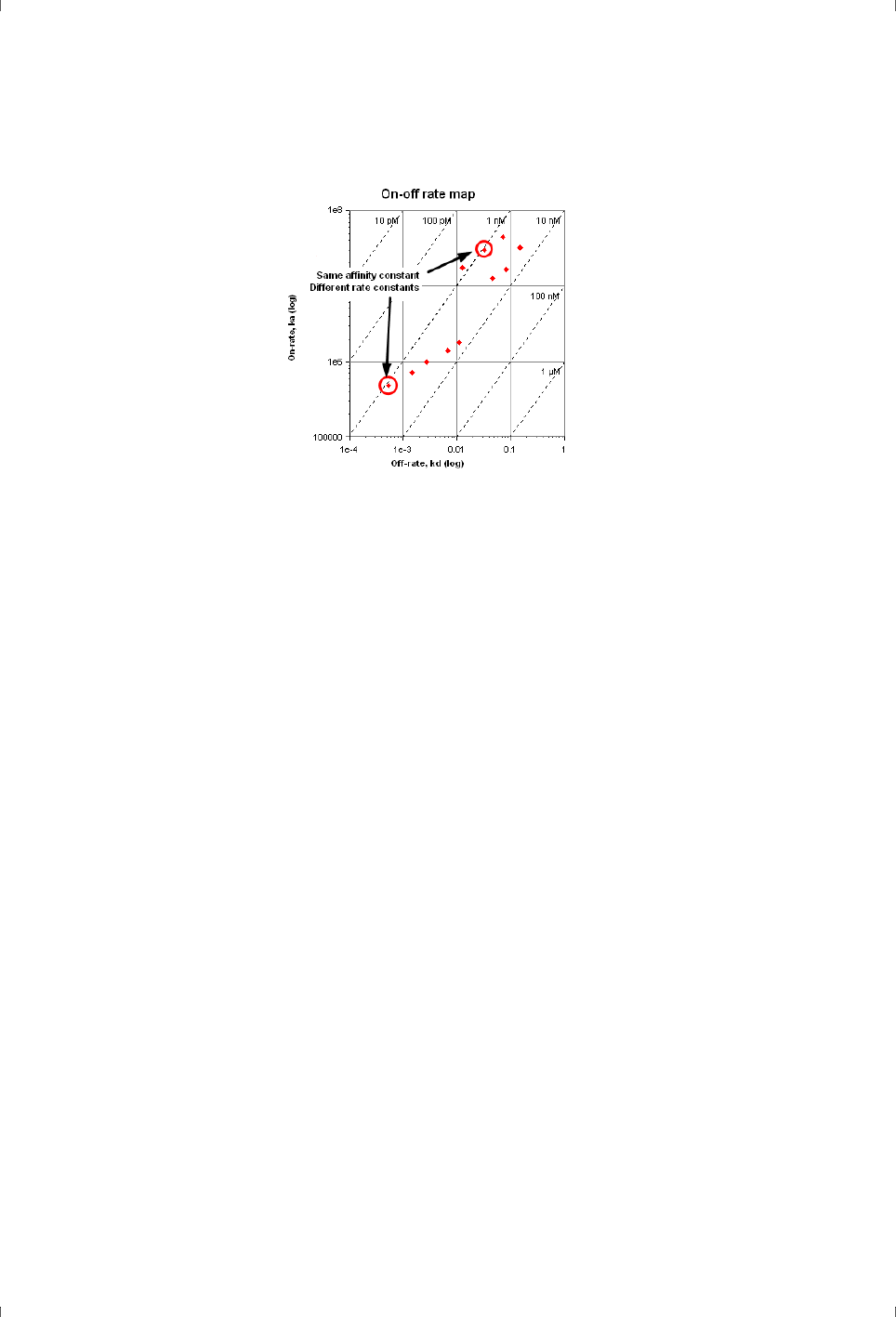
A valuable way to compare kinetic properties is to plot the association rate

constant against the dissociation rate constant on logarithmic axis. Diagonal

lines in this plot represent constant affinity, so that compounds that lie on the

same diagonal but are separated from each other have the same affinity but

different kinetics (Figure 4-2).

Biacore Assay Handbook 29-0194-00 Edition AA 35

Screening and detecting binding partners 4

Figure 4-2. Plotting association rate constant k

against dissociation rate constant k

(here on logarithmic scales) creates a plot where the affinity is represented by diagonal

lines. Compounds on the same diagonal have the same affinity but differ in kinetics.

Fragment screening benefits from additional steps in experimental design and

evaluation, to identify and characterize interesting fragments. In summary, the

recommended approaches are:

• Clean screen, aimed at rapidly identifying and eliminating undesirable

“sticky” compounds that show persistent binding to the surface and can

disturb subsequent analysis cycles.

• Binding level screen, aimed at providing a rapid overview of the compound

library, identifying compounds with binding levels above a defined cut-off.

• Affinity screen, aimed at verification of binding and affinity ranking of

fragments.

These approaches are described in more detail in the handbooks for Biacore

systems that support fragment screening.

4.2 Antibody screening

4.2.1 Goals

The goal of antibody screening is to identify cell clones that produce antibodies

appropriate for the purpose (usually biopharmaceuticals or biochemical tools).

Screening needs to be rapid so that clones can be selected before they grow to

unsuitable cell densities. Obtaining kinetic information early in the screening

process is often a significant advantage. Information that is generally sought

includes:

4 Screening and detecting binding partners

4.2 Antibody screening

36 Biacore Assay Handbook 29-0194-00 Edition AA

• Which clones produce antibodies with suitable specificity

• Which antibodies have kinetic and/or affinity properties suitable for the

purpose

• Which of these clones produce antibodies in sufficient amounts

4.2.2 Sensor surface preparation

Unlike LMW screening, expected response levels in antibody screening can be

quite high, so there is no need to use high levels of immobilized or captured

ligand. Typically, sensor surfaces are prepared with a generic anti-antibody

such as anti-IgG for which assay conditions (including regeneration) are known,

and binding characteristics are determined with an injection of antigen after

antibody capture. It is also possible to perform an antibody screen directly with

antigen attached to the surface as ligand, but this approach often involves

additional work to establish regeneration conditions.

4.2.3 Sample preparation

Samples for antibody screening are typically taken from cell culture supernatant

and analyzed directly without purification. Preliminary experiments with non-

producing clones to establish that there is no significant binding of non-

antibody components can simplify interpretation of the results.

4.2.4 Buffers

HBS-EP+ (Hepes-buffered saline with 0.3 mM EDTA and 0.05% Surfactant P20,

available from GE Healthcare) or similar is recommended as running buffer.

Samples may be diluted if required in the same buffer. Precise matching of

sample and running buffer is not practicable for screening work.

4.2.5 Analysis conditions

Flow rate

Antibody screening by capture on a generic capturing molecule can be run at

low flow rates (typically 10 µl/min) if sample consumption is an issue.

Characterization of the antibody-antigen interaction, whether performed

directly on immobilized antigen or by a secondary injection over captured

antibody, should be run at moderate flow rates (typically 30 µl/min) to reduce

mass transfer limitations (see Section A.1).

Contact time

Contact times should be sufficient to give confidently measurable response

levels without compromising screening throughput. Contact times of 1 to 2

minutes are usually sufficient.

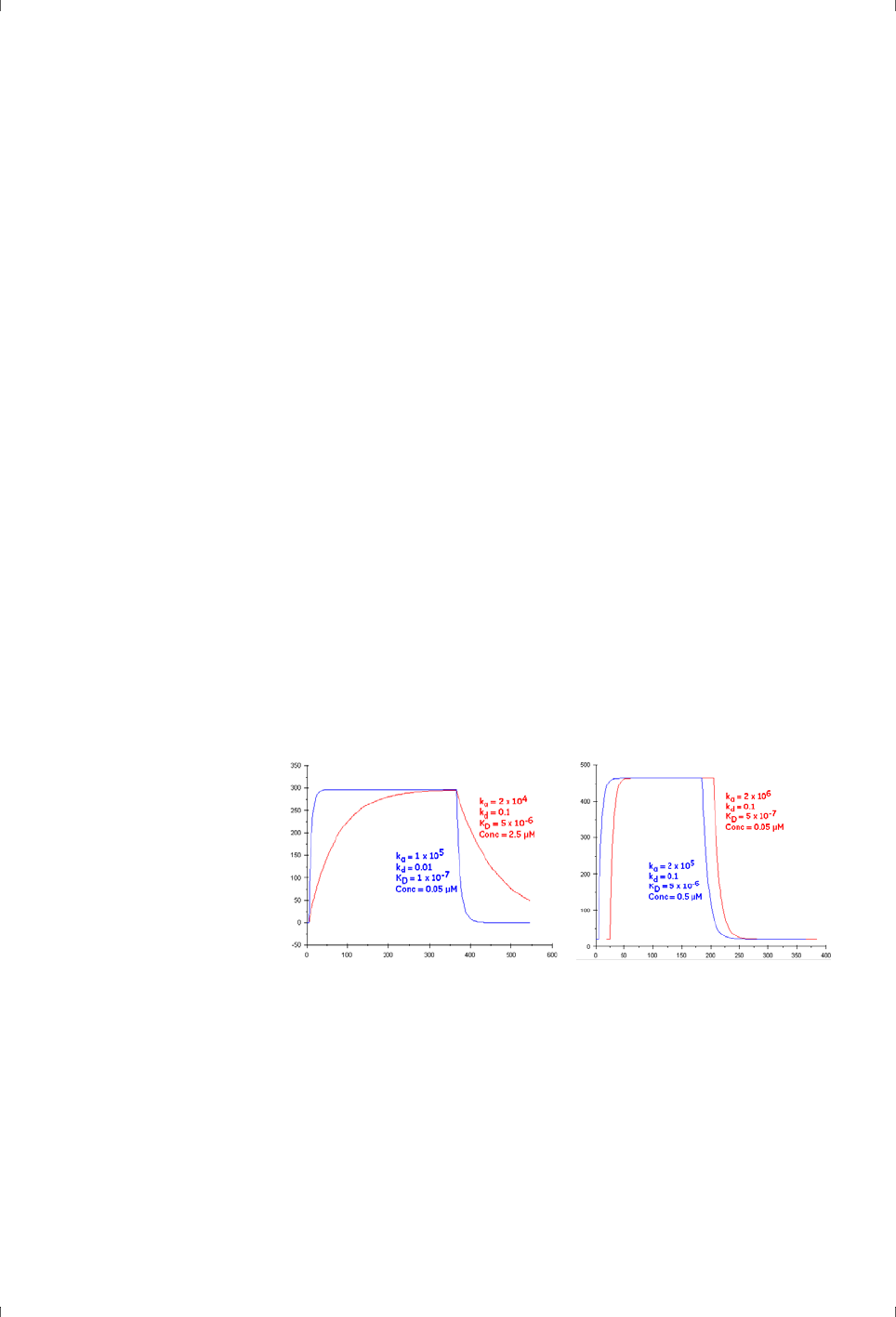
Biacore Assay Handbook 29-0194-00 Edition AA 37

Screening and detecting binding partners 4

Regeneration

Regeneration conditions for antibody screening kits from GE Healthcare are

specified in the respective Instructions for Use. For assay development using

custom antibodies, regeneration at low pH (glycine-HCl, pH 1.5 to 3) is usually

effective.

Report points

For screening, place a report point shortly after the end of the sample injection.

This will avoid any bulk refractive index differences between sample and

running buffer.

Antibody characterization based on complex stability uses report points placed

early and late in the dissociation phase of the antibody-antigen interaction.

4.2.6 Evaluating results

The response reached in the first step of the screening gives an indication of the

relative concentration of antibodies in the sample (according to the specificity

of the capturing molecule). Responses achieved from injection of antigen reflect

both the antigenic specificity and the binding characteristics of the captured

antibody. Note however that evaluation based on report points alone does not

give unambiguous information: a given response may be obtained from a

combination of high concentration and slow binding or low concentration and

fast binding. It may be possible to resolve these alternatives by visual inspection

of the sensorgrams, but if the binding and dissociation events are rapid both

situations may give closely similar sensorgrams (see Figure 4-3).

Figure 4-3. Sensorgram shape can in some cases distinguish weak and strong binders

that reach the same response level as a result of different concentrations (left). In other

cases, depending on the relative values of the rate constants and concentrations, the

sensorgrams may be identical. These sensorgrams are simulated: those in the right-hand

panel are displaced slightly from each other on the time axis.

Frequently, the parameter of most interest in choosing between antibody clones

is the stability of the antibody-antigen complex, which is largely governed by the

dissociation rate. Comparison of the response early and late in the dissociation

phase can give a rapid indication of the relative dissociation rates.

4 Screening and detecting binding partners

4.3 Immunogenicity testing

38 Biacore Assay Handbook 29-0194-00 Edition AA

4.3 Immunogenicity testing

4.3.1 Goals and challenges

Immunogenicity testing answers the question of whether administered drugs

provoke an immune reaction in the recipient that can compromise the efficacy

of the drug. At a simplistic level, this application is analogous to screening for

antibodies in serum, and recommendations for screening apply also to

immunogenicity testing, using immobilized drug as ligand. However, the

simultaneous presence of the drug and circulating anti-drug antibodies (ADAs)

in serum presents a special challenge: ADAs in complex with drug will not be

detected in an assay based on binding to the drug.

ADAs are released from drug complexes under acidic conditions (pH 1 to 2), and

can be detected if the sample is neutralized and the assay is performed

immediately, before the complexes have had time to re-form fully. This

approach is implemented in some Biacore systems, using a specially designed

IFC that mixes acidified samples with neutralizing solution immediately before

injection over the sensor surface. Details of the approach are described in the

manuals for systems that support immunogenicity testing (e.g. Biacore T200

Immunogenicity Handbook).

Biacore Assay Handbook 29-0194-00 Edition AA 39

Kinetics and affinity measurements 5

5 Kinetics and affinity measurements

5.1 Approaches

Determination of both kinetics and affinity rely on measurements over a range

of analyte concentrations. Kinetic (rate) constants are obtained by analyzing the

sensorgram shape in relation to a mathematical model of the interaction

mechanism: affinity constants are obtained from the steady state binding

levels. Affinity constants can also be calculated from the ratio of the rate

constants. Details of the data analysis principles are given in Appendix A.

5.1.1 Single- and multi-cycle kinetics

There are two approaches to determination of kinetics and affinity, both based

on determination of binding data at several (typically 5) analyte concentrations

(see Figure 2-2):

• multi-cycle kinetics, where each analyte concentration is injected in a

separate analysis cycle, and the sensor surface is regenerated between

cycles. Since data from the different concentrations is evaluated together,

it is important that regeneration is carefully optimized so that the surface

properties are constant between cycles.

• single-cycle kinetics, where analyte concentrations are injected

sequentially in a single cycle, with no regeneration between injections.

Both approaches have been shown to give equivalent results in test systems,

and both can be used for steady-state affinity measurements if the sample

injection time is long enough for steady state to be reached.

The single-cycle approach requires less time for a complete analysis, and also

benefits from the lack of requirement for optimized regeneration. This can

significantly reduce the demands on assay development, and permits kinetic

determinations for interactions where regeneration conditions are not

available. However, the cycle time is longer in single-cycle kinetics, so the

approach is more sensitive to drift such as dissociation of ligand in a capture

assay.

5.1.2 2-over-2 kinetics

Normally, all samples are analyzed over a single sensor surface, providing

identical ligand conditions for each analyte concentration. In Biacore A100 and

Biacore 4000 systems, however, parallel analysis over multiple ligand spots in

each flow cell permits a technique called 2-over-2 kinetics. The name refers to

analysis of two analyte concentrations over two ligand densities, and can be

performed in a single cycle in Biacore systems which can support multiple

5 Kinetics and affinity measurements

5.2 Sensor surface preparation

40 Biacore Assay Handbook 29-0194-00 Edition AA

ligand densities in each flow cell. Combining the data from two ligand densities

compensates for the lack of analyte concentrations, and the approach can

provide reliable kinetic data from experiments that maintain a moderately high

sample throughput.

5.1.3 Comparative estimates of kinetics and affinity

Comparison of relative interaction kinetics can be sufficient for some

applications. At the simplest level, this can be achieved by plotting the ratio of

response values early and late in the sample injection (for association rates) and

in the dissociation phase (for dissociation rates), using a single analyte

concentration. This simplified approach is sometimes used in information-rich

screening work, where full determination of kinetics and/or affinity is not

practicable for throughput considerations.

5.2 Sensor surface preparation

Amount of immobilized ligand

In evaluation of kinetic and affinity constants, the concentration of ligand is

expressed in resonance units (RU) so the amount of immobilized ligand does not

have to be known exactly (see Appendix A). The immobilization level is however

important for the quality of the results.

For kinetic analysis, the amount of immobilized ligand should be kept low, so

that the maximum response from analyte binding is typically in the region of 30

to 50 RU or lower. There are two main reasons for this:

• Low ligand levels help to reduce limiting effects of mass transfer. Mass

transfer refers to the diffusion-controlled supply of analyte molecules to

the surface from bulk solution: if transfer is slow in relation to the

association rate, the observed binding will be a measure of the diffusion

process and not of the interaction rates. Mass transfer is discussed in

more detail in Appendix A.

• Low ligand levels also help to minimize artifacts that can arise from

crowding of molecules on the surface. Crowding effects are difficult to

quantitate but can give rise to unnecessarily complex binding behavior.

For measurement of steady-state affinity, mass transfer considerations are not

relevant and the amount of immobilized ligand can be higher than for kinetic

analysis.

Reference surface

Kinetic and affinity measurements should always use reference-subtracted

data. The reference surface may be untreated, activated and deactivated, or

prepared with an inactive protein to mimic the physical properties of the active

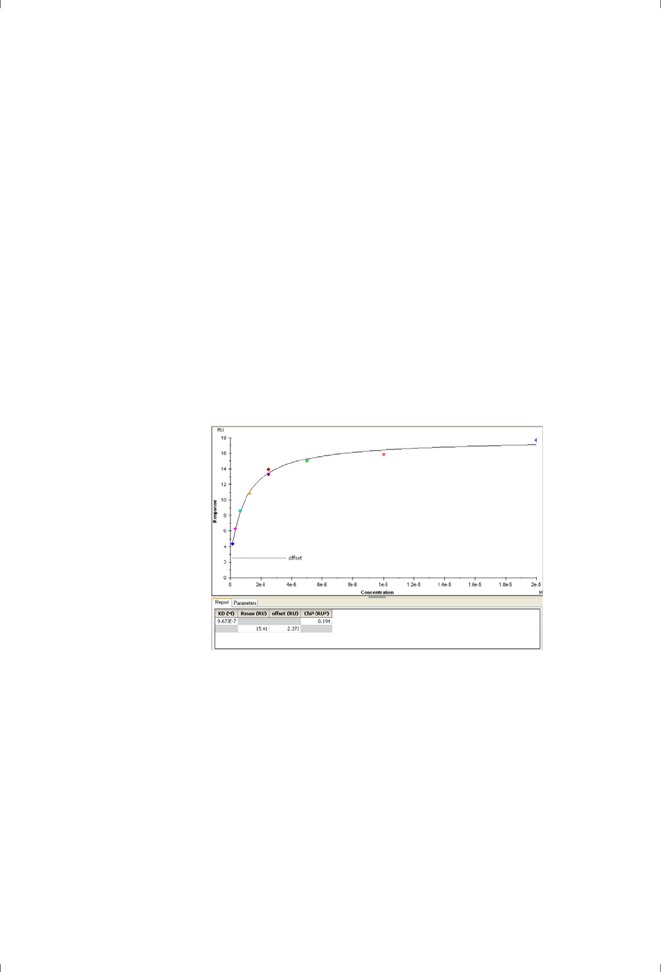
Biacore Assay Handbook 29-0194-00 Edition AA 41

Kinetics and affinity measurements 5

surface. These alternatives are discussed in more detail in the Biacore Sensor

Surface Handbook.

5.3 Buffers

The same buffer must be used for sample and running buffer, so that

association (during sample injection) and dissociation (after the end of the

injection) occur in the same environment. Moreover, evaluation of kinetics is

more robust if the sample and running buffer are matched in refractive index, so

that bulk shifts at the beginning and end of the sample injection are kept as

small as possible.

Buffer matching is less important for affinity measurements since evaluation is

based only on response values measured during the sample injection. Bulk

response contributions will however introduce an offset from the x-axis in the

plot of response against analyte concentration (Figure 5-1). It is important that

bulk effects do not vary between samples so that the offset is constant.

Figure 5-1. Plot of response against analyte concentration evaluated with offset to allow

for bulk effects.

5.4 Sample preparation

Preparation of samples can be a critical factor in the quality of kinetic

measurements. Ideally, both ligand and analyte should be pure and

homogeneous, to simplify the interpretation of the results as far as possible.

Using a capturing approach for attaching ligand provides on-chip purification:

however, it is essential for careful work that the capturing interaction is

sufficiently stable so that ligand does not dissociate during the sample analysis.

It is important that non-specific binding of sample components to the sensor

surface is kept to a minimum. It is also important that the analyte is

5 Kinetics and affinity measurements

5.5 Sample concentrations

42 Biacore Assay Handbook 29-0194-00 Edition AA

homogeneous and non-aggregated since differently sized binding species will

give different responses. Use non-denaturing analysis methods to check

analyte homogeneity.

Samples may be diluted into running buffer from stock solution if the dilution

factor is sufficiently high so that residual stock solution components can be

ignored. Alternatively, samples may be prepared using buffer exchange

techniques.

5.5 Sample concentrations

Evaluation of association rate constants and affinity constants from the

experimental data is directly dependent on the values provided for analyte

concentrations (see below for details). For this reason, it is important for

obtaining correct results that the analyte concentration is determined as

accurately as possible. Ideally, this should be the concentration of analyte that

is capable of interacting with ligand, which may not be the same as the total

concentration (if for example the analyte is only partially active). Calibration-free

concentration analysis (see Section 2.3.2) provides an approach to

concentration measurement that is directly related to the amount of analyte

that can bind to the ligand, and is recommended in critical measurements. If

there are doubts about the validity of the analyte concentration values, the

reported values for the association rate constant and affinity constant should

be treated with due caution. The dissociation rate constant is not dependent on

the analyte concentration.

Analyte concentration range

In principle, kinetic constants can be obtained from analysis at a single analyte

concentration, but analysis over several concentrations (5 to 8 for multi-cycle

kinetics, up to 5 for single-cycle kinetics) gives a better foundation for

discovering deviations from the simplest interaction models and for revealing

concentration-dependent artefacts (for example analyte aggregation at

increasing concentrations). Ideally, concentrations should cover a wide range

centered on the value for the dissociation equilibrium constant K

(for example,

for an interaction with K

= 10 nM, concentrations from 1 to 100 nM are

appropriate). In practice, the K

value is often not known, and the range of

concentrations that can be used may be limited by availability or solubility of the

analyte. A concentration range that gives a good spread of sensorgrams is

usually adequate (Figure 5-2).

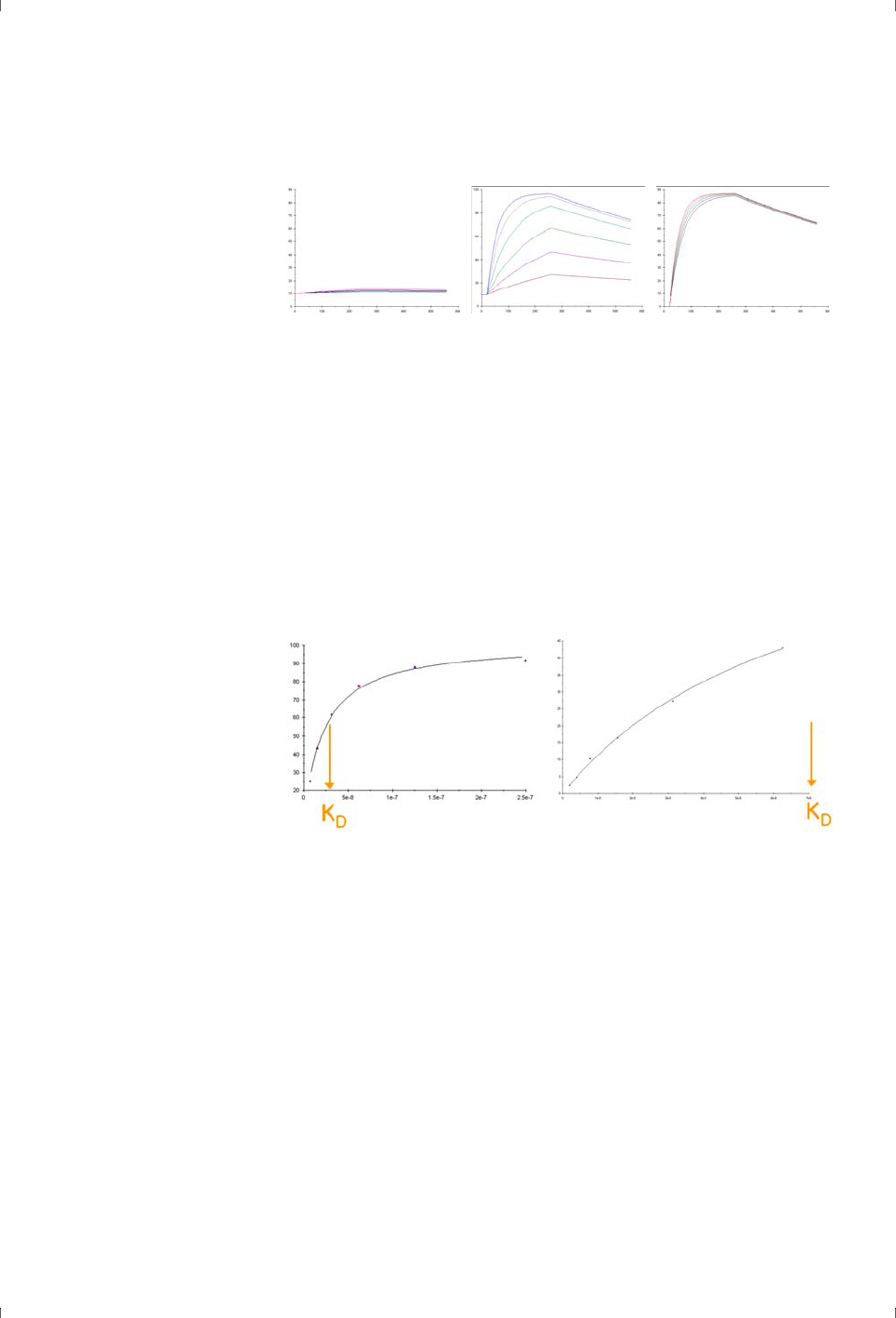
Biacore Assay Handbook 29-0194-00 Edition AA 43

Kinetics and affinity measurements 5

Figure 5-2. Analyte concentrations for kinetic analysis should cover a wide range (center

panel). If the concentrations are too low (left panel) or too high (right panel) the

sensorgrams may be tightly grouped and evaluation will be less robust. The vertical scale

for these simulated sensorgrams is the same in all three panels.

For affinity determinations, each analyte concentration gives rise to a single

point on the experimental data plot, in contrast to kinetic analysis where each

analyte concentration provides a full time-course of the interaction. It is

therefore important to use a sufficient number of analyte concentrations in the

assay (the recommended minimum is 5). In addition, the concentration range

should extend to more than twice the affinity constant (K

) value. If these

conditions are not fulfilled, there will be insufficient data in the plot of R

against

C for confident analysis. Conversely, a reported K

value higher than half the

highest analyte concentration should be treated with care (Figure 5-3).

Figure 5-3. The analyte concentration range for steady state affinity determination

should cover more than twice the K

value (left). Do not trust reported affinity constants

that are higher than half the highest analyte concentration (right).

Analyte concentration values

The association rate constant for a simple binary interaction has units of M

-1

(see Appendix A), and molar analyte concentrations must be supplied to the

software for kinetic evaluation. Similarly, evaluation of steady state affinity

requires analyte concentrations as input. It is important that analyte

concentrations are correct if correct values for rate constants are to be

obtained. Incorrect values for analyte concentration will lead directly to

corresponding errors in the association rate constant k

Kinetic measurements rely on analysis over a range of analyte concentrations,

usually prepared by serial dilution from a stock solution. Properly calibrated

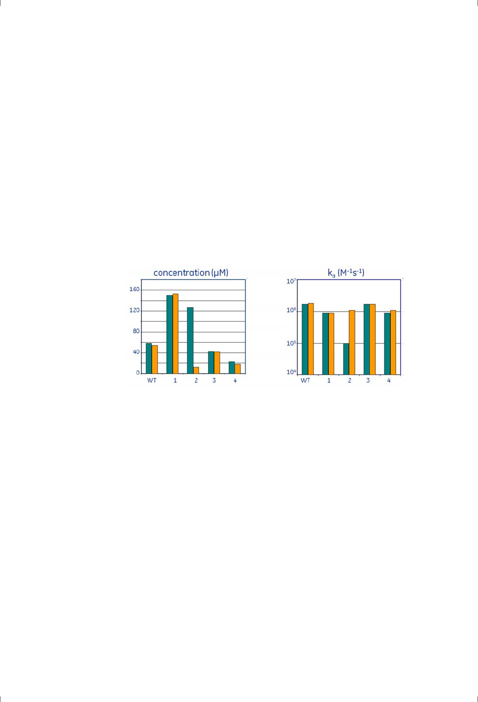
5 Kinetics and affinity measurements

5.5 Sample concentrations

44 Biacore Assay Handbook 29-0194-00 Edition AA

equipment and well-designed sample preparation protocols are essential if the

concentrations are to be correct (see Section 3.5.

In addition to accurate sample preparation, correct values for the stock solution

concentration are important. The ideal value is the concentration of analyte

that is capable of binding to the surface-attached ligand: this may not

necessarily be the same as the total analyte concentration. If half of the analyte

molecules are in a conformation that cannot bind, the total concentration will

be twice the value that should be used for evaluation of binding kinetics. If the

sample is amenable to concentration determination by CFCA, this is the value

that should ideally be used: it represents the concentration capable of

interaction and is independent of calibration considerations. Figure 5-4

illustrates an example of the importance of using the correct analyte

concentration.

Figure 5-4. Importance of using the correct analyte concentrations. The experiment

compared the kinetics of wild type and four mutants of a papain inhibitor binding to

papain. Using concentrations obtained from A

280

measurements (green bars), mutant

number 2 had an association rate constant about one order of magnitude lower than the

wild type and the other mutants. However, using concentrations obtained by CFCA

(orange bars), association rate constants obtained were similar for all variants of the

inhibitor.

Biacore Assay Handbook 29-0194-00 Edition AA 45

Epitope mapping 6

6 Epitope mapping

Epitope mapping refers to determination of the relative topography of binding

sites (usually for antibodies) on a target molecule or antigen. Antibodies that

bind to epitopes that are distinct from each other can bind simultaneously to the

antigen, while antibodies directed against the same or interfering epitopes

show mutually exclusive binding.

The commonest approach to epitope mapping is to test simultaneous binding

ability in a pair-wise matrix. In an alternative approach, peptides representing

structural epitopes on the antigen are tested for inhibition of antibody binding.

Both methods are amenable to use with Biacore systems.

6.1 Pair-wise binding

6.1.1 Principle

The basic principle of pair-wise mapping studies in Biacore systems is

straightforward: one antibody is attached to the surface, antigen is bound to the

antibody, and a second antibody is tested for simultaneous binding ability. In

practice, the assay set-up involves additional steps (see Figure 6-1):

• The first antibody to the sensor surface is conveniently attached to the

sensor surface by capturing on a generic antibody such as rabbit anti-

mouse immunoglobulins for mouse antibodies. This allows multiple

antibody pairs to be tested using the same sensor surface. Permanent

attachment is less suitable since the first antibody cannot then be

changed without preparing a new sensor surface.

• It is important to ensure that no antibody-capturing sites on the surface

are available to bind the second antibody when it is injected. Remaining

capture sites are therefore blocked with an injection of blocking antibody

(an antibody that does not bind to the antigen being tested).

• Antigen is then injected and binds to the first antibody.

• The antigen is followed by an injection of second antibody to test for

simultaneous binding of the two antibodies.

• The surface is regenerated to remove all components except the

permanently attached capturing antibody, in preparation for testing the

next antibody pair.

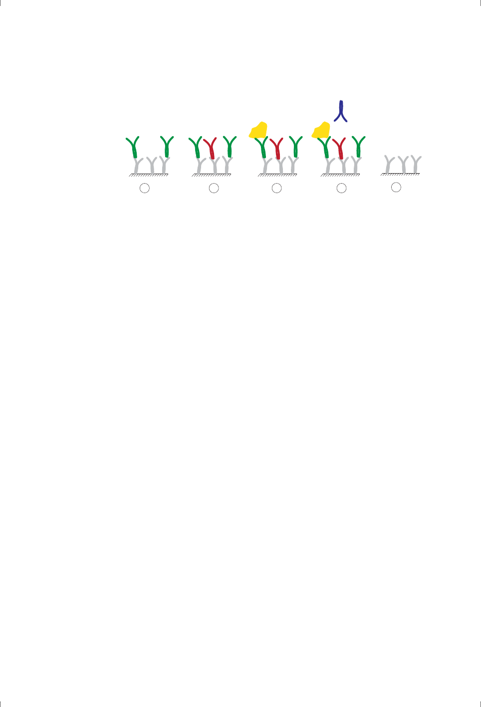
6 Epitope mapping

6.1 Pair-wise binding

46 Biacore Assay Handbook 29-0194-00 Edition AA

Figure 6-1. Main steps in a pair-wise epitope mapping experiment.

1. Capture first antibody.

2. Block remaining capture sites.

3. Inject antigen.

4. Challenge with second antibody.

5. Regenerate in preparation for the next antibody pair.

A panel of n antibodies contains n(n-1)/2 unique pairs of non-identical

antibodies (for example 5 antibodies give 10 pairs). It is recommended to test all

combinations in the pair-wise matrix:

• Pairs where the first and second antibody are identical provide a check on

the assay performance. If simultaneous binding is observed this may

indicate that the antigen contains multiple copies of the epitope, which

may invalidate the mapping with respect to that epitope.

• Pairs where the roles of first and second antibody are reversed provide a

control for unexpected effects such as conformational changes induced

by antibody binding. Ideally, the results should be independent of the order

in which antibodies are tested, but this is not always the case in practice.

6.1.2 Evaluation

The label-free detection in Biacore systems offers advantages over label-based

methods for epitope mapping, in that all steps in the binding sequence are

monitored with the same technique. It is easy to relate the observed level of

antigen binding to the level of first antibody, and the level of second antibody to

that of antigen. This addresses a potential issue in interpreting the results, in

that the absence of second antibody binding may result either from interference

between the epitopes or from poor binding of the antigen to the first antibody.

This cannot be resolved in methods where antigen binding is not monitored

directly.

Epitope mapping applications are explicitly supported in Biacore 4000, with

methods for both set-up and evaluation of pair-wise mapping experiments

(described in detail in the Biacore 4000 Software Handbook). Evaluation is

divided into five distinct steps, summarized below. Similar principles can be

applied in evaluating pair-wise mapping results from other Biacore systems.

2 3 4

Biacore Assay Handbook 29-0194-00 Edition AA 47

Epitope mapping 6

Report points for each evaluation step are set just after the end of the respective

injections.

First antibody ranking

This step presents captured levels of the first antibody. The amount of first

antibody is fundamental in determining the possible response levels in

subsequent steps, and may vary between antibodies. A cut-off boundary can be

set to represent the minimum acceptable level: below this level, the amount of

captured first antibody is judged to be too low for reliable measurement in

subsequent steps, and the antibody pairs represented by these points are

excluded from the evaluation.

Antigen ranking

Even with sufficient first antibody captured, binding of antigen may vary, and

results for binding of the second antibody will be inconclusive if the level of

antigen bound is too low. As for first antibody binding, a cut-off boundary can

be set to exclude points with response values below an acceptable limit. The

binding data may be shown as relative response values or as percent of

expected binding (based on the amount of first antibody captured and the

relative sizes of antibody and antigen).

Second antibody ranking

The second antibody ranking displays the binding levels of second antibody,

either as relative response or as percent of expected binding (based on the

amount of first antibody captured and the relative sizes of antibody and

antigen). Here again a cut-off boundary can be set to differentiate between

positive and negative binding.

Dissociation fit

An additional component in the evaluation is estimation of the dissociation rate

of antibodies classed as positive binders in the second antibody ranking step.

This information is not essential for pair-wise mapping itself, although it can be

useful in judging the status of borderline results. However, it is often useful in the

context of antibody development for immunoassay reagents, and is obtained

without additional experimental design or set-up from determinations with

Biacore systems.

Result matrix

The results of pair-wise epitope mapping are collected in a matrix of binding

values, with first and second antibodies in columns and rows respectively. Cells

in the matrix are classed as positive (meaning independent epitopes) or

negative (interfering epitopes) on the basis of the cut-off boundary set for the

second antibody ranking step. If the cut-off boundaries have been judiciously

set in the first antibody and antigen ranking steps, the classification in the

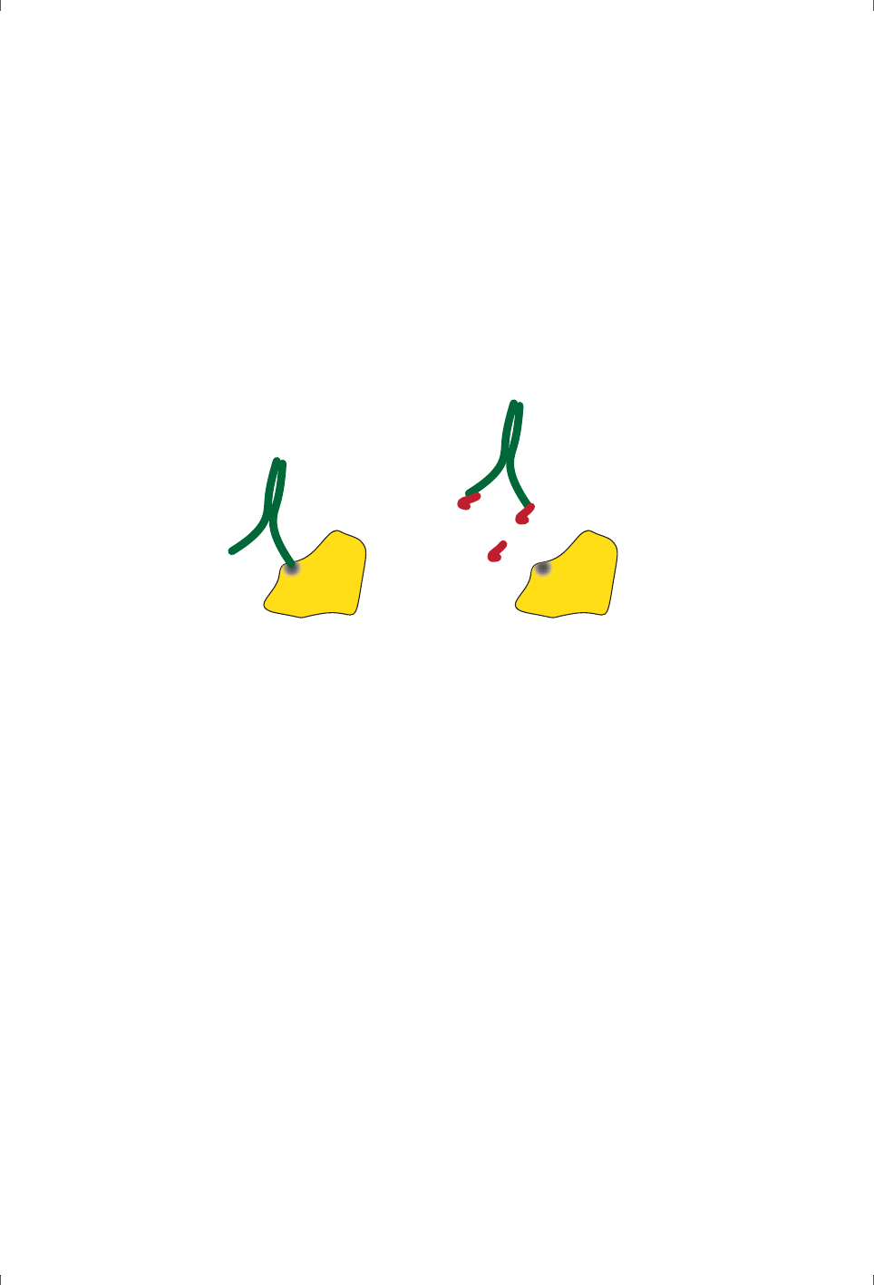
6 Epitope mapping

6.2 Peptide inhibition

48 Biacore Assay Handbook 29-0194-00 Edition AA

matrix reflects only those pairs where second antibody binding is potentially

reliable.

6.2 Peptide inhibition

Epitope mapping by peptide inhibition is based on the principle that a peptide

representing a structural epitope will inhibit binding to antigen of an antibody

directed against that epitope (Figure 6-2). Inhibition may be partial or complete

depending on how well the peptide is structurally congruous with the epitope.

Figure 6-2. Principle of epitope mapping by peptide inhibition principle. In the absence of

peptide (left), antibody can bind to the epitope. Added peptide that mimics the epitope

binds to the antibody (right) and blocks binding to the antigen.

An assay of this kind can be set up with either the antigen or antibody attached

to the surface. Antigen may be attached permanently and regenerated:

antibodies are captured to allow investigation of multiple antibodies using the

same sensor surface.

Biacore Assay Handbook 29-0194-00 Edition AA 49

Troubleshooting assays 7

7 Troubleshooting assays

This chapter considers the causes and suggested solutions to common

problems with Biacore-based assays. The material is divided into 4 sections:

• Ligand attachment

•Analyte binding

• Dealing with non-specific binding

• Unexpected sensorgram shape

7.1 Troubleshooting ligand attachment

This section deals with the problem that the amount of ligand attached to the

surface is too low for the experimental purpose.

7.1.1 Covalently attached ligand

A schematic sensorgram for immobilization of a macromolecular ligand on

Sensor Chip CM5 is illustrated in Figure 3-3. While details differ according to the

chemistry and the specific molecules involved, there are some common

features that can help in diagnosing problems with ligand immobilization.

Symptom Cause Remedy

Poor response increase

during ligand injection

Immobilization pH unsuitable Optimize immobilization pH

Poor response increase

during ligand injection

Too high ionic strength in

immobilization buffer

Use low ionic strength (10 mM

monovalent cations).

Ligands kept in stock solution

with physiological ionic

strength should be diluted at

least 10-fold or otherwise

desalted.

Poor response increase

during ligand injection

Ligand concentration too low Test higher concentrations

Ligand binds during

injection but is not

retained

Ligand lacks accessible target

groups for immobilization chemistry

Try a different chemistry or

use capturing

7 Troubleshooting assays

7.1 Troubleshooting ligand attachment

50 Biacore Assay Handbook 29-0194-00 Edition AA

7.1.2 Captured ligand

Ligand capture by high affinity binding to an immobilized protein involves

attachment of the capturing molecule to the sensor surface followed by binding

of the ligand to the capturing molecule. From the viewpoint of troubleshooting,

the first step is equivalent to immobilizing a ligand, while the second is

equivalent to binding analyte.

There are however some specific capture situations supported by ready-to-use

sensor chips that can present individual problems in ligand attachment.

Laboratory protocols with recommended conditions are available from GE

Healthcare.

• Capture of biotinylated ligands on Sensor Chip SA or with the Biotin

Capture Kit requires that excess biotinylation reagents are rigorously

removed from the ligand solution (suitably be gel filtration on microspin

columns). Any residual biotinylation reagents in the solution will compete

with ligand for attachment to the surface and reduce capture efficiency.

Removal by two cycles of desalting is recommended.

• Capture of histidine-tagged ligands by metal chelation on Sensor Chip NTA

requires that buffers are free from chelating agents (EDTA is recommended

for ligand removal). The efficiency and stability of capture varies

considerably with the number, length and location of the polyhistidine tags

on the ligand molecule, but generally improves with reduced ligand levels.

If capture on Sensor Chip NTA is unsatisfactory, you may want to try using

longer or multiple polyhistidine tags, or capture the ligand on anti-histidine

antibodies instead.

Ligand binds during

injection but is not

retained

Buffer components such as Tris or

additives such as sodium azide

compete with the ligand for

immobilization

Make sure the buffer is

appropriate for the

immobilization chemistry.

Immobilization level low Old EDC/NHS solutions Use fresh EDC and NHS

solutions.

One or more injections do

not show the

characteristic response

Solutions wrongly placed in

autosampler

Check the Rack Positioning

information in the software

for the immobilization

procedure.

Symptom Cause Remedy

Biacore Assay Handbook 29-0194-00 Edition AA 51

Troubleshooting assays 7

7.2 Troubleshooting analyte binding

7.2.1 Analyte capacity too low

Estimate the activity of the attached ligand in terms of the measured analyte

binding capacity in relation to the theoretical value (Section 3.2.3). If analyte

binding is unacceptably low, the ligand may have lost activity in the low ionic

strength, low pH immobilization buffer, been inactivated by the covalent

attachment chemistry, or had low activity in the starting material. Try using a

different chemistry or switch to a capturing approach.

Occasionally, the attachment chemistry may inactivate the ligand by direct

modification of the binding site. In such cases, attaching the ligand in the

presence of a reversible binder that blocks the active site can help to preserve

activity. It is of course essential that the binder itself is not susceptible to the

attachment chemistry. This approach has proved successful in work with some

target molecules for low molecular weight analytes.

7.2.2 Analyte binding too high

Analyte binding capacity that exceeds the theoretical maximum value usually

indicates either that the binding stoichiometry is more than expected (either

because there are multiple binding sites on the ligand or because the analyte is

aggregated), or that the analyte is binding indiscriminately to the ligand or the

surface matrix. In the former case, it is in principle possible to saturate the

surface with sufficiently high analyte concentrations, giving an experimental

value for the observed stoichiometry. In the case of indiscriminate binding, the

surface can often not be saturated and the binding level continues to increase

with analyte concentration even at very high concentrations.

7.3 Dealing with non-specific and unwanted binding

7.3.1 Non-specific binding

Non-specific binding refers to indiscriminate binding of the analyte or other

component in the sample to either the ligand or the sensor surface matrix. Non-

specific binding can give false positive results in screening assays and incorrect

results in concentration assays. In determination of kinetics and affinity, non-

specific binding generally gives results that do not fit to an interaction model.

Typically, non-specific binding of analyte gives response levels that continue to

increase with increasing sample concentration, instead of reaching a saturation

plateau.

Binding to the sensor surface matrix is usually revealed by a binding response

on the reference surface. Subtraction of the reference response is not sufficient

to correct for non-specific binding since it is difficult to establish that binding to

7 Troubleshooting assays

7.4 Unexpected sensorgram shapes

52 Biacore Assay Handbook 29-0194-00 Edition AA

the reference surface and the non-specific component of binding to the active

surface are equivalent (high ligand levels can mask dextran binding sites and

reduce non-specific binding to the surface matrix). Non-specific binding of this

kind can often be reduced by addition of soluble dextran to the samples, to

compete for binding to the dextran on the sensor surface. Soluble dextran is

available for this purpose from GE Healthcare as NSB Reducer.

Non-specific binding to the ligand does not give a response on a reference

surface that lacks ligand but usually shows as non-saturatable binding to the

active surface. Binding of non-analyte components may be an issue with

complex samples such as cell extracts or serum. General principles for

minimizing this kind of binding are to use physiological or higher ionic strength

in the sample and running buffer and to include detergent if this does not

interfere with the assay. If these measures are not sufficient, choose a different

ligand (for example a different clone for monoclonal antibody ligands).

Sometimes the analyte binds promiscuously to the ligand (for example, many

low molecular weight compounds bind with low affinity to multiple sites on

serum albumin, giving behavior that resembles non-specific binding). In such

cases, it may be possible to obtain useful information about high-affinity

binding sites from sensorgrams obtained at relatively low sample

concentrations, where low affinity binding does not dominate the observed

response. Adjustment of buffer conditions for the assay can also help to reduce

the effect of promiscuous binding.

7.3.2 Unwanted binding

Unwanted binding refers to the specific binding of non-analyte components to

the ligand, or binding of the analyte to non-ligand components such as a

capturing molecule on the surface. This kind of interference is best dealt with by

careful assay design. For example, avoid antibody subclasses that bind

complement factors for measurements in serum, or use Fab fragments that lack

the complement-binding sites.

7.4 Unexpected sensorgram shapes

This section considers interpretation and correction of unexpected sensorgram

behavior. There will always be individual differences in sensorgram shape

according to interaction characteristics, but the following general

characteristics are “expected” with due allowance for bulk refractive index

effects:

• The baseline should be stable within the analysis cycle. Minor baseline

shifts between cycles may be acceptable.

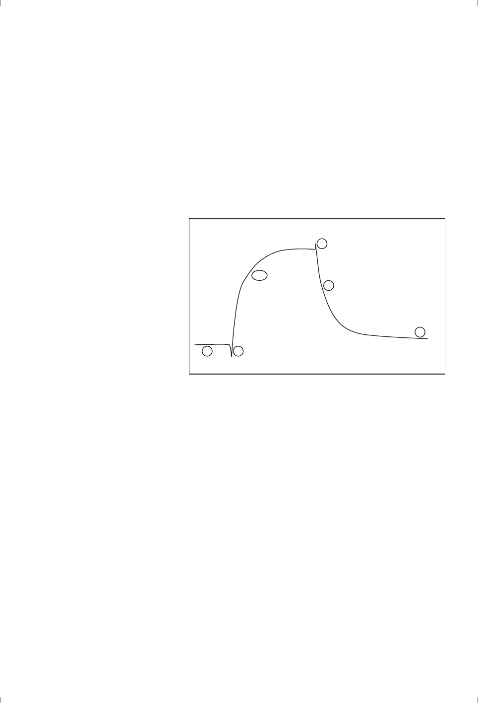
Biacore Assay Handbook 29-0194-00 Edition AA 53

Troubleshooting assays 7

• The response should not decrease progressively during sample injection

(with the exception of bulk shifts resulting from refractive index

differences).

• The response should not increase progressively during dissociation (with

the exception of bulk shifts resulting from refractive index differences).

• Reference-subtracted response overshoot at the start and end of sample

injection should be small.

• The response should not go below the baseline level during dissociation.

Figure 7-1. Generalized features of the “expected” shape of reference-subtracted

sensorgrams.

1: stable baseline.

2: positive response during sample injection.

3: increasing or stable response during injection.

4: decreasing response during dissociation

5: small reference subtraction spikes at the start and end of injection

6: response does not go below baseline

7.4.1 Unstable baseline

Some baseline drift is common in the first few cycles of an assay, and 3 to 5

start-up cycles are recommended to allow the assay to stabilize. Always check

the baseline in the reference and active sensorgrams separately: although a

drifting baseline may seem to be corrected by reference subtraction, it may

indicate inadequate assay optimization and complicate interpretation of the

results.

It is relevant to distinguish between baseline drift during an analysis cycle and

shifts in baseline response between cycles. The latter is most commonly caused

by regeneration characteristics, and can usually be ignored if the surface

response

time

2,3

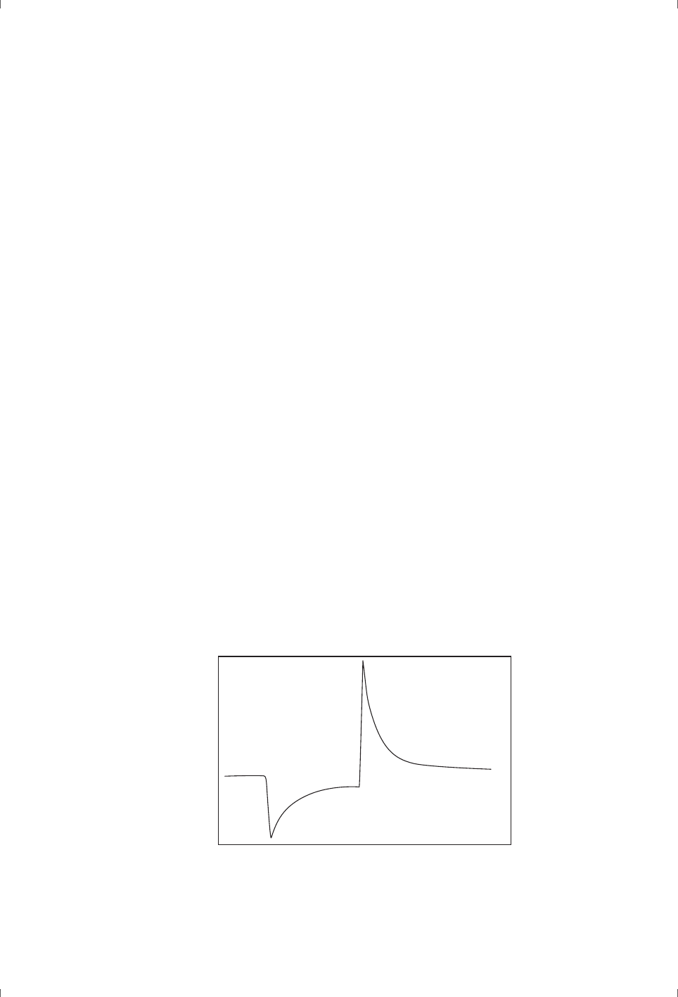
7 Troubleshooting assays

7.4 Unexpected sensorgram shapes

54 Biacore Assay Handbook 29-0194-00 Edition AA

binding capacity is not affected (as shown by reproducible binding levels for

control samples).

Baseline instability may also be caused by faults in the temperature control

system. If this occurs (indicated by a warning on the screen) call your

GE Healthcare service representative.

Baseline constantly increasing

• Make sure the running buffer is prepared from pure reagents using clean

glassware, and that the instrument flow system is thoroughly cleaned

after the previous experiment. This is particularly important for

applications using hydrophobic surfaces (Sensor Chip HPA and to a lesser

degree Sensor Chip L1).

Baseline constantly decreasing

• If you are using a capturing approach for attaching your ligand, check the

stability of the capturing interaction. For work with low molecular weight

analytes, you may be able to cross-link the ligand to the capturing

molecule after capture to stabilize the surface, but this results in

permanent attachment of the ligand. Cross-linking the ligand generally

reduces the binding activity for protein analytes.

• Downward drift of the baseline can also be the result of immobilizing a

multimeric ligand so that not all subunits are attached to the surface. If the

multimer dissociates, subunits will be lost, in most cases resulting in loss of

analyte binding capacity as well as baseline response. This behavior can

sometimes be prevented by crosslinking the ligand with EDC/NHS after it

has been attached to the surface, although the analyte binding activity

may be reduced.

7.4.2 Sample response below baseline

Figure 7-2. Sample response below baseline is usually be caused by a negative bulk

refractive index shift.

response

time

Biacore Assay Handbook 29-0194-00 Edition AA 55

Troubleshooting assays 7

Responses may fall below baseline during sample injection if the refractive

index of the sample is lower than that of running buffer, so that a negative bulk

refractive index shift is associated with the sample injection. In such cases, there

should be a corresponding positive shift at end of the injection: response levels

measured after the end of the injection will still be reliable.

Higher relative response in the reference flow cell than the active flow cell,

resulting from sample binding to the reference cell can also cause a shift below

baseline in the reference-subtracted sensorgram.

Both of these situations can usually be identified by examining the active and

reference sensorgrams separately.

7.4.3 “Humpbacked” sensorgrams

Sensorgrams with a “humpbacked” appearance during sample injection (where

the response reaches a maximum and then decreases, see Figure 3-4) are

relatively common when the detergent concentration in the running buffer is

below the critical micelle concentration (CMC). The recommended

concentration of Surfactant P20 is 0.05%. This detergent effect is usually

relatively small, and may go unnoticed in experiments with macromolecular

interactants where responses are in the range of several hundred RU and

above.

There are other possible causes of “humpbacked” sensorgrams, for example

initial binding of a large analyte that is then displaced by a slower but tighter

binding smaller molecule. You should be aware that this sensorgram

appearance does not always indicate a problem with the assay.

7.4.4 Anomalous response during buffer flow

Anomalous responses when only buffer is flowing through the system, including

both upward drift and response levels below baseline, may be caused by

contamination of the flow system with material from previous runs. Make sure

the instrument is maintained as described in the Instrument Handbook. If this

behavior is observed, clean the flow system thoroughly as instructed in the

Instrument Handbook, then allow the instrument to equilibrate with a low flow

of running buffer at least overnight.

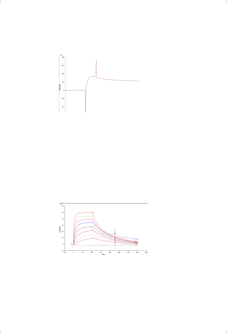
7 Troubleshooting assays

7.4 Unexpected sensorgram shapes

56 Biacore Assay Handbook 29-0194-00 Edition AA

7.4.5 Response subtraction spikes

Figure 7-3. Reference subtraction spikes at the beginning and end of a blank (buffer)

injection.

Some overshoot at the start and end of the sample injection is normal in

reference-subtracted sensorgrams from systems with serially arranged flow

cells, particularly at low flow rates. This results from slight misalignment of the

reference and active sensorgrams together with a significant bulk refractive

index effect (Figure 7-3). This should not affect more than about 1 second of the

sensorgram. More serious overshoot may indicate malfunction of the sample

injection system, and requires attention from your GE Healthcare service

representative.

7.4.6 Regular disturbances

Disturbances (usually small) that occur repeatedly at the same time in each

cycle (Figure 7-4) are generally attributable to pump flow-fill operations.

Figure 7-4. Disturbances that occur at the same time in each cycle are attributable to

automatic aspects of instrument operation such as pump flow-fill.

Biacore Assay Handbook 29-0194-00 Edition AA 57

Analysis of kinetics and concentration measurements Appendix A

Appendix A Analysis of kinetics and concentration

measurements

A.1 Basic principles of kinetics and affinity

This section describes the basic principles for kinetics and affinity analysis of 1:1

interactions. Similar principles apply to other interaction models with

appropriately modified equations.

A.1.1 Kinetic rate equations

The kinetic evaluation procedure determines association and dissociation

constants by fitting the experimental data to a 1:1 interaction model between

analyte A and ligand B:

The net rate of complex formation during injection is given by

and the rate of dissociation after the end of the injection is

The concentration of complex formed is measured in RU by the SPR response: if

the total ligand concentration [B]

is also expressed in RU (as the maximum

analyte binding capacity), the rate equations can be written in terms of

response values instead of concentrations:

Because interaction occurs at the surface of the sensor chip, analyte must be

transferred laterally in the flow cell from the bulk solution to the surface before

interaction with ligand can take place. In a controlled flow system such as

Biacore, this transfer is a diffusion-limited process, referred to as mass transfer,

that can be described by a well-defined mathematical model. The analyte

where: k

is the association rate constant (M

-1

)

and k

is the dissociation rate constant (s

-1

)

dAB

---------------

AB k

AB–=

dAB

---------------

AB–=

------

max

+R–=

Appendix A Analysis of kinetics and concentration measurements

A.1 Basic principles of kinetics and affinity

58 Biacore Assay Handbook 29-0194-00 Edition AA

concentration available for interaction with the ligand is the concentration at

the sensor surface A

surface

, which is related to the concentration in the injected

sample A

bulk

by the equation:

where k

is the mass transfer coefficient, describing the diffusion-controlled

transfer from bulk solution to the surface. The transfer properties are the same

both to and from the surface, so that k

applies in both directions.

The mass transfer coefficient k

is a function of the flow rate, flow cell

dimensions and diffusion properties of the analyte molecule:

To minimize mass transport limitations in kinetic determinations, experiments

should be run at moderate to high flow rates (30 µl/min or more).

The mass transfer coefficient can be adjusted approximately for the molecular

weight of the analyte and for the conversion of surface concentration to RU to

give a term called the mass transfer constant k

A further modification of this expression gives the flow rate-independent

component of the mass transfer constant, referred to as tc:

For globular proteins with molecular weight of the order of 50,000 daltons,

typical values for tc are of the order of 10

RU·M

-1

. Reported values that differ

greatly in order of magnitude (e.g. 10

or 10

) may indicate that the parameter

is not significant for the fitting (i.e. that the observed binding is not limited by

mass transfer).

where D is the diffusion coefficient of the analyte (m

s

-1

)

f is the volume flow rate of solution through the flow cell (m

s

-1

)

h, w, l are the flow cell dimensions (height, width, length in m)

0.98

---





23

0.3 w l

----------------------





13

MW 10

=

------

Biacore Assay Handbook 29-0194-00 Edition AA 59

Analysis of kinetics and concentration measurements Appendix A

Mass transfer is incorporated into the curve-fitting models by modifying the

concentration of analyte available for binding to ligand:

A.1.2 Steady-state affinity equations

At steady-state, the net rate of complex formation is zero:

Rearranging and setting R=R

(the equilibrium response level) gives:

Setting k

(the equilibrium association constant) gives

The value of K

is obtained by fitting a plot of R

against C to this equation.

is calculated as the inverse of K

=1/K

A.1.3 Fitting procedure

The fitting procedure used to determine rate constants from experimental data

uses numerical integration methods with an iterative approximation algorithm

to find the best solution to the equations given above. The closeness of fit is

judged in terms of the chi-square value which describes the deviation between

the experimental and fitted curves:

where r

is the fitted value at a given point

is the experimental value at the same point

n is the number of data points

and p is the number of fitted parameters.

------

max

+R– 0==

max

+R=

-----

C1+





-----

max

C1+

-----------------------

chi-square

–



np–

----------------------------

Appendix A Analysis of kinetics and concentration measurements

A.1 Basic principles of kinetics and affinity

60 Biacore Assay Handbook 29-0194-00 Edition AA

The fitting algorithm seeks to minimize chi-square, and is judged to be complete

when the difference in chi-square values between successive iterations is

sufficiently small.

A.1.4 Assessing the fit

Kinetics

The rate constants reported by kinetic evaluation are determined in terms of a

1:1 interaction model, and it is important to realize that they are only valid in that

context. If the interaction mechanism is not a simple 1:1 binding, the fitted

curves will deviate to some extent from the experimental data and the reported

constants will not be a true representation of the interaction kinetics. The

apparent 1:1 binding constants can still be used for comparative studies of

observed binding rates, but it is important in reporting the values to emphasize

that they are empirical and not mechanistic constants.

There are two major tools for assessing the significance of the reported

constants: the closeness of fit between the fitted and experimental curves and

the statistical significance of the parameters.

Closeness of fit

Visual inspection of the residual plot or of the fitted curves overlaid on the

experimental data gives an indication of the closeness of fit. Ideally, the

residuals will scatter randomly around zero over a range that corresponds to

the short-term noise in the detection system (approximately 1 to 2 RU).

Deviations from ideal fitting appear as systematic variations in the residuals,

imparting a non-linear shape to the residual plot. Judge the residual range and

shape in proportion to the response ranges in the experimental sensorgrams

and in relation the goal of the investigation.

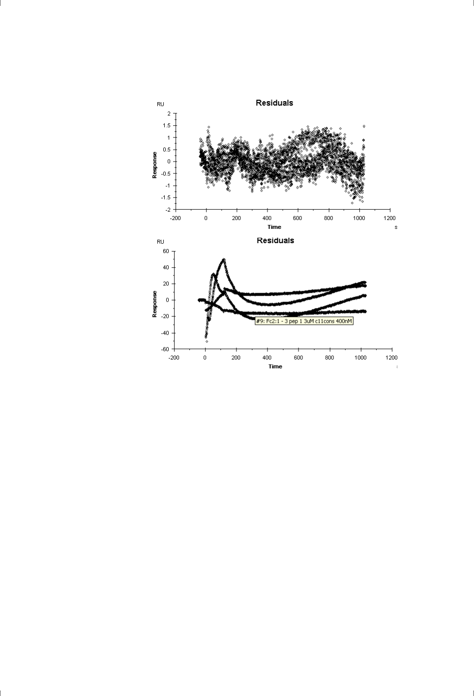
Biacore Assay Handbook 29-0194-00 Edition AA 61

Analysis of kinetics and concentration measurements Appendix A

Figure A-1. Residual plots from a good fit (top) and a poor fit (bottom). Note the different

response scales in the two plots (top ±2 RU, bottom ±60 RU).

The chi-square value is a quantitative measure of the closeness of fit, and in an

ideal situation will approximate to the square of the short-term noise level. It is

however difficult to recommend absolute values for acceptance limits for chi-

square: the values need to be considered from case to case in combination with

assessment of the shape of the residuals (chi-square is related to the overall

range of the residuals but is not affected by the shape of the residual curve).

Significance of parameters

Fitting experimental data to a mathematical interaction model will return values

for all parameters in the model, regardless of whether they are significant or

not. As an example, sensorgrams that are completely limited by mass transfer

will give values for the kinetic rate constants even though the experimental data

does not contain any kinetic information.

The significance of the parameter values returned by the fitting procedure is

indicated by the standard error or T-value, which broadly speaking represents

the degree to which the value can be varied without significantly affecting the

closeness of fit. The T-value is the standard error divided by the parameter

value. A high standard error or low T-value indicates that the fitting is insensitive

Appendix A Analysis of kinetics and concentration measurements

A.2 Interaction models for kinetics

62 Biacore Assay Handbook 29-0194-00 Edition AA

to changes in the parameter value: in other words, the value returned for the

parameter has little significance.

It is important to examine the significance of values calculated by the software,

to avoid the trap of reporting “constants” that have no significance. In the

example of completely mass transfer limited interactions, the rate constants

will have a high standard error (low T-value), since it does not matter for the

fitting result what value will be returned.

Note: Even if the significance of a parameter is low, so that any value within a

wide range will give the same fit to the experimental data, the fitting

algorithm will always return the same value from the same starting data.

Consistency of returned values is not an indication of significance.

For the 1:1 binding model, an additional indicator of the parameter significance

is the U-value. This is a parameter that represents the uniqueness of the

calculated rate constants and R

max

, determined by testing the dependence of

fitting on correlated variations between selected variables. Lower values

indicate greater confidence in the results. A high value (above about 25)

indicates that the reported kinetic constants contain no useful information.

Affinity

To obtain a robust fit to a plot of R

against C for affinity determination, it is

important that the range of analyte concentration is wide enough to reveal the

curvature of the plot in full. In particular, if the highest concentration is too low

in relation to the calculated K

value, the reported values will be uncertain even

if the fit is apparently good and the chi-square value is low.

As a general guideline, the fit will be reliable if the highest analyte concentration

is at least twice the calculated K

value. If the highest analyte concentration is

less than 2K

, you should treat the reported K

with caution.

A.2 Interaction models for kinetics

This section gives a brief description of the standard kinetic interaction models

provided with Biacore systems.

A.2.1 1:1 binding

This interaction model describes one molecule of analyte A binding to one

molecule of ligand B:

Biacore Assay Handbook 29-0194-00 Edition AA 63

Analysis of kinetics and concentration measurements Appendix A

A.2.2 1:1 dissociation

This model fits the dissociation phase only to an exponential model. The

dissociation rate is independent of the analyte concentration in the injected

sample, so that dissociation rate constants can be obtained for samples with

unknown concentration.

This model does not include a mass transfer coefficient. If mass transfer

limitations are significant, dissociated analyte will be washed away from the

surface with reduced efficiency and the dissociation rate constant will be

underestimated.

A.2.3 Bivalent analyte binding

The bivalent analyte binding model describes the interaction of monovalent

ligand with analyte molecules that carry two identical and independent binding

sites.

Once binding has occurred at the first analyte site, binding at the second site is

facilitated by the proximity of analyte and ligand. Similarly, analyte molecules

that are attached at both sites are not released from the surface until

dissociation occurs at both sites, so the observed dissociation rate is much

slower than that seen for a single site. The resulting enhanced binding is often

called avidity to distinguish it from single site binding affinity.

Note: The association rate constant for interaction at the second site is reported

in units of RU

-1

. This is because both the interacting components are

present on the surface and are measured in RU, not in true

concentrations.

where k

is the association rate constant

and k

is the dissociation rate constant

where k

and k

are the association and dissociation rate constants for the

first site

and k

are the association and dissociation rate constants for the

second site

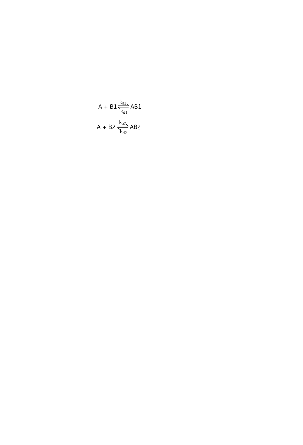
Appendix A Analysis of kinetics and concentration measurements

A.3 Concentration measurements

64 Biacore Assay Handbook 29-0194-00 Edition AA

A.2.4 Heterogeneous ligand

This model describes interaction of one analyte with two independent ligands

(or ligand sites) on the surface. The observed binding is the sum of the

interaction with the two ligands.

A.2.5 Interaction models for affinity

1:1 steady state binding

The Affinity evaluation item described in Chapter 12 fits a plot of response

against concentration to the equation (Section A.1.2)

The parameters K

, R

max

and offset are fitted as variables. The affinity is

reported as a K

value, which is the inverse of K

. This function gives reliable

fitting if the highest analyte concentration used is at least twice the K

value.

A.3 Concentration measurements

A.3.1 Calibration curve fitting

Calibration curves for concentration measurement are fitted to either linear or

4-parameter equations. Custom equations for calibration curves can be defined

in some Biacore systems.

where k

and k

are the association and dissociation rate constants for one

ligand

and k

are the association and dissociation rate constants for the

other ligand

where offset is a constant term that gives the intercept of the fitted curve on

the y-axis. Without this term the fitted curve is forced to go through the

origin of the plot.

max

C1+

-----------------------

offset+=

Biacore Assay Handbook 29-0194-00 Edition AA 65

Analysis of kinetics and concentration measurements Appendix A

For linear fitting, the points are fitted to the equation

y = slope * x + intercept

The equation for a 4-parameter fit is

The closeness of fit is reported for linear fitting as the coefficient of

determination R

and for 4-parameter fitting as the chi-square value.

A.3.2 Calibration trends

Some Biacore systems support calibration trends to compensate for drift in the

calibration throughout the course of the assay. With this approach, calibration

curves are measured at the start and end of the assay and at intervals, and an

individual calibration curve is constructed for each sample analysis cycle by

interpolating between the measured calibration curves.

A.3.3 Calibration-free concentration analysis

Evaluation of calibration-free concentration relies on fitting the data to a model

for 1:1 interaction (see Section A.1) where the mass transfer coefficient is

provided (through calculation from the diffusion coefficient and flow cell

characteristics) and the analyte concentration is evaluated as a global variable.

This model is equivalent in terms of the interaction description to the model for

evaluation of 1:1 kinetics.

where y and x are the plot coordinates

and R

are fitting parameters that correspond to the maximum and

minimum response levels respectively

and A

are additional fitting parameters

y R

–

----- -





--------------------------

–=

Appendix A Analysis of kinetics and concentration measurements

A.3 Concentration measurements

66 Biacore Assay Handbook 29-0194-00 Edition AA

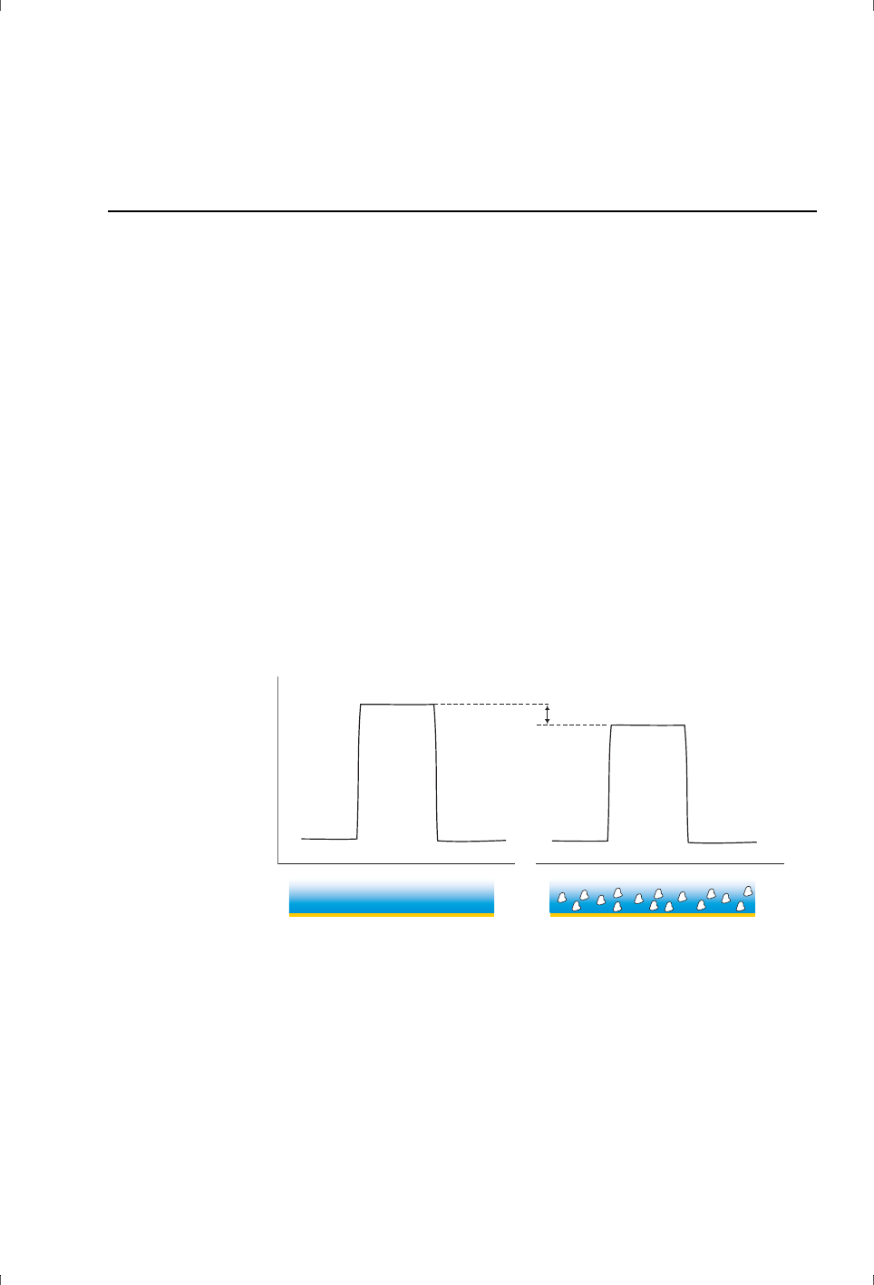
Biacore Assay Handbook 29-0194-00 Edition AA 67

Solvent correction principles and practice Appendix B

Appendix B Solvent correction principles and practice

B.1 Introduction

Solvent correction refers to the procedures used to adjust measured responses

for the effects of varying concentrations of organic solvents. These procedures

are relevant primarily for work with small organic analytes that require inclusion

of organic solvents (commonly dimethyl sulfoxide, DMSO) in the buffer to

maintain analyte solubility.

Simple subtraction of a reference response is not sufficiently accurate for these

purposes when differences in bulk shifts between samples can be of the same

order of magnitude as (or larger than) the expected response from analyte

binding. One reason for this is that the volume of solution accessible to sample

will differ on the reference and active surfaces unless the two surfaces have the

same attached protein concentration. As a result of the volume excluded by

ligand molecules, the bulk shift will be smaller on the active surface than the

reference surface (Figure B-1).

There are other factors in addition to excluded volume involved in solvent

correction that are outside the scope of this discussion, so that solvent

correction is essentially an empirical procedure.

Figure B-1. Bulk solution is excluded from the volume occupied by ligand molecules on the

active surface, so the contribution of bulk solution to the relative response is smaller than

on the reference surface.

B.2 Requirement for solvent correction

Solvent correction is necessary under a combination of three circumstances,

commonly met in work with low molecular weight analytes such as drug

candidates:

Response on

reference surface

Response on

active surface

Excluded volume effect

Active surface

Reference surface

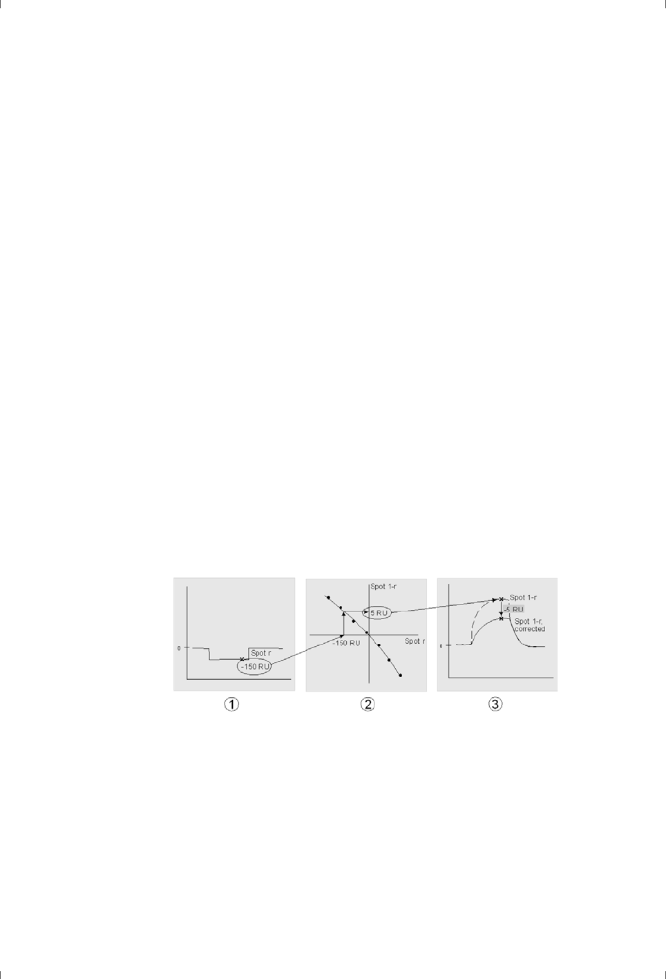
Appendix B Solvent correction principles and practice

B.3 Solvent correction principles

68 Biacore Assay Handbook 29-0194-00 Edition AA

• the expected analyte responses are low,

• the ligand is a macromolecule immobilized at a high density on the

surface,

• the bulk response is high in relation to the measured binding response.

In drug discovery and development work, the analytes are often small

molecules which give correspondingly low response values (typically of the

order of 10-50 RU or less). High levels of immobilized ligands (several thousand

RU) are used to maximize the analyte response, enhancing the excluded volume

effect described above. Samples generally include DMSO to maintain solubility,

resulting in high bulk responses. A difference of 1% (percentage points) in DMSO

concentration corresponds to a difference of about 1200 RU in response, so that

small variations in DMSO concentration, unavoidable in the preparation of

diverse samples, easily lead to variations in bulk response of the same order of

magnitude as the expected sample responses.

B.3 Solvent correction principles

Solvent correction values are determined by injecting blank samples containing

a range of DMSO concentrations and plotting the reference-subtracted

response from the active surface against the relative response from the

reference surface. This creates a calibration curve, referred to as the solvent

correction curve, for the solvent effect as a function of the reference response.

Each sample measurement can then be adjusted for the solvent effect on the

basis of the response on the reference surface (see Figure B-2).

Figure B-2. The principle of solvent correction. 1. The sensorgram from the reference

surface shows a bulk displacement (-150 RU in the illustration) during sample injection

because the sample and running buffer are not exactly matched. 2. From the solvent

correction curve, a displacement of –150 RU in the reference sensorgram corresponds to

a solvent effect of +5 RU in the reference-subtracted sensorgram. 3. The reference-

subtracted sensorgram is corrected for the solvent error. This procedure is applied to

every point during sample injection.

Solvent correction is applied only to response levels during sample injection,

since the correction adjusts for differences in bulk response between different

samples.

Biacore Assay Handbook 29-0194-00 Edition AA 69

Solvent correction principles and practice Appendix B

B.4 Preparing solutions for solvent correction

It is important to match samples and running buffer as closely as possible with

respect to refractive index to minimize bulk refractive index effects, so that

solvent correction values are kept small. It is particularly important to strive for

exactly the same DMSO concentration in samples and running buffer and to

minimize variations in DMSO content between samples. Bear the following in

mind when preparing samples for assays where solvent correction is necessary:

• Use carefully designed buffer preparation and sample dilution protocols to

ensure consistent DMSO concentrations. Samples that are stored in DMSO

should be diluted in such a way as to give the same final DMSO

concentration as in the running buffer.

• Cover the sample plates with foil directly after preparation to avoid

changes in DMSO concentration resulting from evaporation and

absorption of water from the air. Remember that DMSO is hygroscopic.

• If you are using a laboratory robot to prepare samples, consider running a

test with blank samples to establish the range of variability of DMSO

concentrations in the samples. Run solvent correction cycles that cover

the expected range of variability.

Laboratory protocols for preparation of samples and solvent correction

solutions may be found on www.gelifesciences.com/biacore or obtained from

GE Healthcare.

B.5 Assessing solvent correction procedures

Solvent correction curves often show a negative slope with a slight curvature

(Figure B-3, left panel), but the slope and shape is not predictable and curves

with positive slope or even with a maximum or minimum within the curve may

be acceptable.

It is however important that the solvent correction curves fit the experimental

points closely. Poor fitting of the curves to the experimental points (Figure B-3,

center panel) can introduce uncertainties in the solvent correction factors that

are the same order of magnitude as the factors themselves, potentially

introducing additional errors in the sample measurements.

Sample responses that lie outside the range of the solvent correction curves

(Figure B-3, right panel) cannot be corrected and will be omitted from evaluation

of solvent corrected data. Solvent correction curves may be extrapolated in the

software, but this option should only be used for small extensions of the solvent

correction range (less than 10% of the measured range) since the curve shape

is not predictable.

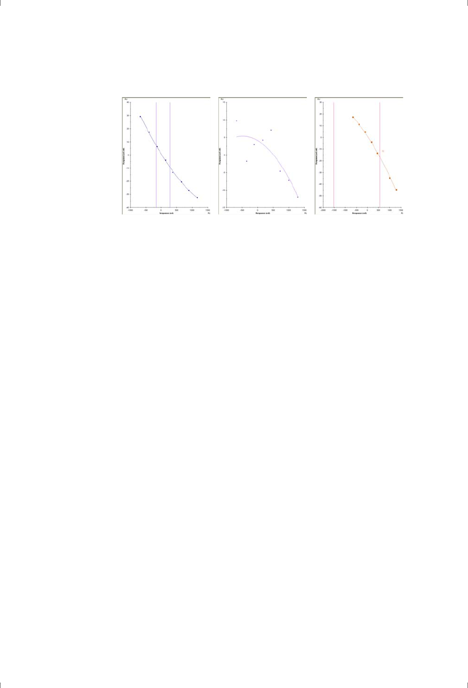
Appendix B Solvent correction principles and practice

B.5 Assessing solvent correction procedures

70 Biacore Assay Handbook 29-0194-00 Edition AA

Figure B-3. Some examples of solvent correction curves.

Left: Acceptable curve, with close fitting to the experimental points and covering the

sample response range well.

Center: The experimental points scatter widely around the fitted solvent correction curve.

Badly fitted curves should be treated with caution.

Right: The solvent correction curve does not cover the whole sample response range.

Sample responses outside the range of the curve will not be corrected.

Biacore Assay Handbook 29-0194-00 Edition AA 1

Numerics

1:1 binding 57

, 62

1:1 dissociation 63

2-over-2 kinetics 39

absolute response 8

acidification-neutralization 38

activity of surface-attached ligand 22

ADAs, see anti-drug antibodies

affinity 6

, 39

affinity analysis 11

affinity constant 8

, 10

affinity evaluation

interpreting the fit 62

affinity in solution 12

affinity model 64

affinity screen 35

amine coupling 20

analysis conditions

for antibody screening 36

for small molecule screening 33

analyte 7

analyte binding capacity 22

analyte concentration 13

analyte concentration range 42

antibody dissociation rate 47

antibody ranking 47

antibody screening 31

, 35

antibody specificity 14

, 37

anti-drug antibodies 31

, 38

association phase 10

association rate constant 57

, 63, 64

attaching the ligand 19

avidity 63

baseline 52

baseline drift 53

Biacore systems 6

Biacore terminology 7

binding level screen 35

biopharmaceutical screening 31

biotinylated ligands 50

bivalent analyte 63

blocking antibody 45

buffer composition 27

buffer exchange 28

buffer matching 41

buffer substances 23

buffers

for antibody screening 36

for kinetics and affinity 41

for small molecule screening 32

bulk effects 41

bulk refractive index 25

bulk shift 8

, 26

caibration-free concentration analysis 13

calibrated assays 13

calibration curve 14

calibration-free concentration analysis 14

, 42, 44

capture 19

, 21

capturing molecule 7

carry-over 34

CFCA, see calibration-free concentration analysis

change in surface concentration 9

chemical modification 21

chi-square 59

, 61, 65

clean screen 35

closeness of fit 59

, 60

coefficient of determination 65

competition assays 13

complex sample matrices 31

complex samples 9

concentration measurement 6

, 13

coupling chemistry 19

covalent immobilization 19

critical micelle concentration 24

, 55

crowding 40

cut-off 34

degassing buffers 25

desalting 28

detecting binding partners 9

detecting molecule 7

, 13

detection principle 5

detergent 24

, 33, 55

dextran matrix 17

dialysis 28

diffusion coefficient 14

, 58

diffusion properties 14

diffusion-limited binding 13

diluting from stock solution 28

, 42

dilution protocol 69

dilution series 28

dimethyl sulfoxide 25

, 32

direct binding assay 13

dissociation fit 63

dissociation phase 10

dissociation rate constant 57

, 63, 64

DMSO, see dimethyl sulfoxide

drug discovery 5

EDC/NHS 22

Biacore Assay Handbook 29-0194-00 Edition AA 2

EDTA 25

enhancement 13

enzyme kinetics 10

epitope mapping 5

, 14, 45

equilibrium constant 8

equilibrium response level 59

evaluation of epitope mapping 46

expected response 22

extrapolating solvent correction 69

fitting procedure 59

flow rate 58

four-parameter fit 65

fragment screening 32

, 35

HEPES 23

heterogeneous ligand 64

high affinity capture 19

, 21

high analyte binding 51

histidine-tagged ligands 19

, 50

humpbacked sensorgrams 55

immobilization 7

, 19

immobilization chemistry 20

immobilization pH 49

immobilization sensorgram 23

immobilized ligand for kinetics and affinity 40

immunogenicity 5

, 31, 38

indirect assays 13

information-rich screening 32

inhibition 13

interaction kinetics 6

, 10

interaction mechanism 10

interaction models 10

, 62

interaction specificity 5

interpreting the fit 60

ionic strength 23

, 49

, K

, k

kinetic evaluation

interpreting the fit 60

kinetic interaction models 62

kinetics 6

, 39

label-free technology 5

laboratory robot 69

ligand 7

ligand concentration 19

linear fit 65

lipid monolayers 18

lipid vesicles 18

LMW screening, see small molecule screening

low analyte capacity 51

maintenance tools 24

mapping binding sites 14

mass transfer constant 58

mass transfer limitation 40

mass transport 57

mass transport coefficient 58

matching sample and running buffer 26

micro-spin columns 28

molar response 9

molecular weight dependence 5

multi-cycle kinetics 11

, 39

negative controls 34

nitrilotriacetic acid 19

non-saturatable binding 52

non-specific binding 23

, 25, 51

NSB Reducer 25

, 52

offset 64

organic solvents 25

, 32

pair-wise binding 15

, 45

pair-wise matrix 46

parameter significance 61

peptide inhibition 15

, 45, 48

permanent capture 19

phosphate buffers 23

plasma samples 26

pre-concentration 19

promiscuous binding 32

rate constants 8

, 10

rate equations 57

ready-to-use buffers 23

reference subtraction 27

reference surface 40

, 51

refractive index changes 5

refractive index differences 8

regeneration 8

, 19

relative interaction kinetics 40

relative response 8

replicates 29

report points 8

, 27

Biacore Assay Handbook 29-0194-00 Edition AA 3

residuals 60

resonance unit 7

response 7

response below baseline 54

response enhancement 13

response levels 21

response overshoot 53

, 56

reversible capture 19

max

running buffer 7

sample concentrations for kinetics and affinity 42

sample injection 7

sample preparation 32

, 36, 41

sandwich assays 13

Scatchard plots 12

screening 5

, 9

sensor chip 17

sensor surfaces 17

sensorgram 8

sensorgram disturbances 56

sensorgram shape 52

serum samples 26

significance 61

single-cycle kinetics 11

, 39

small molecule screening 31

, 32

sodium azide 25

, 50

solid samples 28

solution competition 13

solvent correction 25

, 27, 33

range 69

solvent correction curves

typical appearance 69

SPR, see surface plasmon resonance

standard error 61

start-up cycles 53

steady state affinity 12

steady state binding 59

, 64

sticky compounds 34

streptavidin 19

subtraction spikes 56

surface activation 22

surface competition 13

surface plasmon resonance 5

Surfactant P20 24

target molecule 7

, 32

terminology 7

thiol coupling 20

Tris buffer 23

, 50

troubleshooting 49

T-value 61

Tween 24

uniqueness 62

units for k

unwanted binding 52

U-value 62

vials and microplates 30

4 Biacore Assay Handbook 29-0194-00 Edition AA

imagination at work

29-0194-00 AA 05/2012

For local office contact information visit

www.gelifesciences.com/contact

GE Healthcare Bio-Sciences AB

Björkgatan 30

751 84 Uppsala

Sweden

www.gelifesciences.com/biacore

GE, imagination at work and GE monogram are trademarks of General

Electric Company.

Biacore is a trademark of GE Healthcare companies.

Tween is a trademark of ICI Americas Inc.

First published May 2012

All goods and services are sold subject to the terms and conditions of sale

of the company within GE Healthcare which supplies them. A copy of these

terms and conditions is available on request. Contact your local GE

Healthcare representative for the most current information.

GE Healthcare UK Ltd

Amersham Place, Little Chalfont, Buckinghamshire, HP7 9NA, UK

GE Healthcare Bio-Sciences Corp

800 Centennial Avenue, P.O. Box 1327, Piscataway, NJ 08855-1327, USA

GE Healthcare Europe GmbH

Munzinger Strasse 5, D-79111 Freiburg, Germany

GE Healthcare Bio-Sciences KK

Sanken Bldg. 3-25-1, Hyakunincho, Shinjuku-ku, Tokyo 169-0073, Japan