The Tight Binding Method
Mervyn Roy
May 7, 2015
The tight binding or linear combination of atomic orbitals (LCAO) method
is a semi-empirical method that is primarily used to calculate the band
structure and single-particle Bloch states of a material. The semi-empirical
tight binding method is simple and computationally very fast. It therefore
tends to be used in calculations of very large systems, with more than around
a few thousand atoms in the unit cell.
1 Background: a hierarchy of methods
When the number of atoms and electrons is very small we can use an exact
method like configuration interaction to calculate the true many-electron
wavefunction. However, beyond about 10-electrons we hit the exponential
wall and such calculations become impossible.
For larger systems containing up to a few hundred or a few thousand atoms
we can use density functional theory (DFT) techniques to find the true
ground state density and ground state energy of the interacting system
without explicitly calculating the many-electron wavefunction. In a DFT
calculation we calculate approximate single-particle energies that, in prac-
tice, often give a reasonable approximation to the actual band structure of
the crystal.
In even larger systems, with around 10,000 or more atoms, we can no longer
use self-consistent DFT calculations to take into account the full interaction.
To calculate the band structure and a set of approximate single particle
states we instead try to include the effects of the interaction in a semi-
empirical way, using parameters that we can adjust to match experiment.
The starting point for all semi-empirical approaches is the physics. In metals,
for example, the electrons are almost free and so we can treat the single
1
particle states in terms of plane waves (leading to the Central equation, and
nearly free electron theory). We could also take a very different approach and
assume the states in a crystal look like combinations of the wavefunctions
of isolated atoms. We might imagine this is more likely to be the case in
insulators or semiconductors.
Here, we will solve the single particle Schr¨odinger equation for the states in
a crystal by expanding the Bloch states in terms of a linear combination of
atomic orbitals.
2 Linear combination of atomic orbitals
2.1 Crystal and atomic hamiltonians
In a crystal, we take the single particle hamiltonian to be
H = H
at
+ ∆U, (1)
where H
at
is the hamiltonian for a single atom and ∆U encodes all the
differences between the true potential in the crystal and the potential of an
isolated atom. We assume ∆U → 0 at the centre of each atom in the crystal.
The single particle states in the crystal are then ψ
nk
(r), where
Hψ
nk
(r) = E
nk
ψ
nk
(r), (2)
the band index is labelled by n, and k is a wavevector in the first Brillouin
zone.
2.2 The atomic wavefunctions
The atomic wavefunctions, φ
i
(r) are eigenstates of H
at
,
H
at
φ
i
(r) =
i
φ
i
(r), (3)
where
i
is the energy of the i energy level in an isolated atom. These
wavefunctions decay rapidly away from r = 0 and so the overlap integral,
γ(|R|) =
R
φ
∗
i
(r)Hφ
i
(r + R)dr, between wavefunctions located on separate
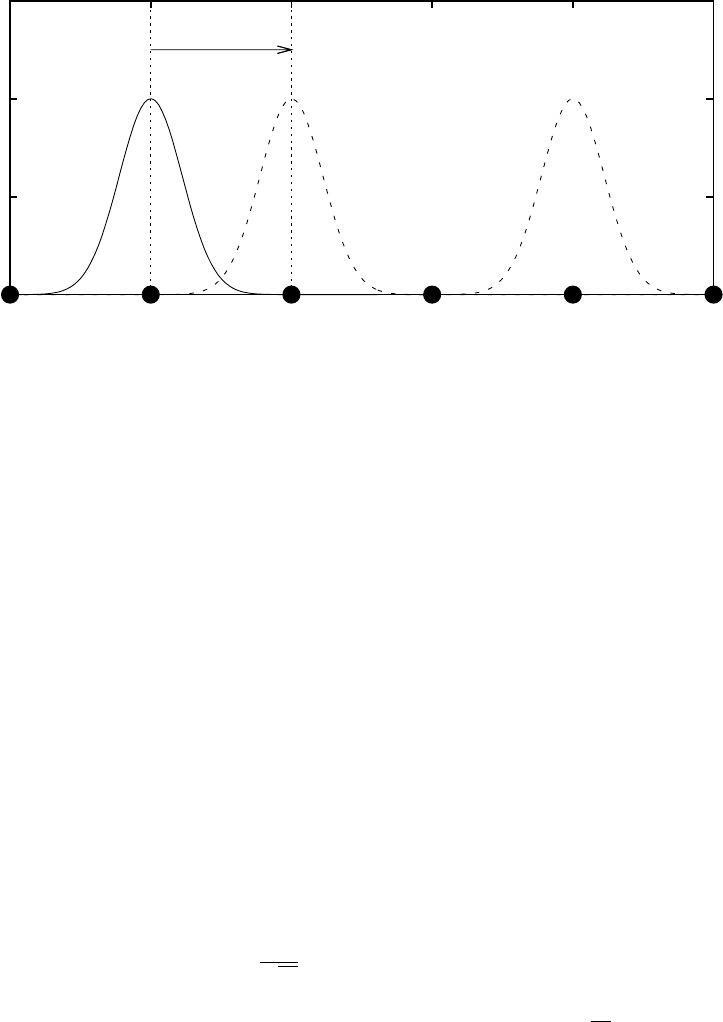
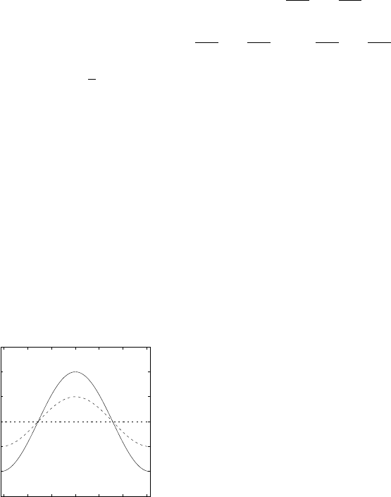
atomic sites (R 6= 0) in the crystal is small (see Fig. 1).
Throughout these notes we will use orthonormal atomic orbitals that have
zero direct overlap between different lattice sites,
Z
φ
∗
i
(r)φ
j
(r + R)dr =
(
1 if i = j and R = 0
0 otherwise.
(4)
2
This gives a simple orthogonal tight-binding formalism but it is relatively
easy to generalise from this to more complex forms.
0
0.5
1
-1 0 1 2 3 4
x (a
0
)
τ
Figure 1: Schematic of the atomic orbitals in a 1D crystal with atoms separated by a
0
.
The translation vectors are R = 0, ±a
0
i, ±2a
0
i, ±3a
0
i, . . ., where i is a unit vector in the x
direction. One of the nearest neighbour vectors τ = a
0
i is shown in the diagram and the
vertical dotted lines denote the edges of the unit cell which contains a single atom. The
solid curve shows an example atomic orbital centred on an atom at r = 0, while dashed
lines show orbitals centred on r + τ and r +3τ . The orbitals decay rapidly so the overlap,
φ
∗
i
(r)φ
i
(r + R), is small. Here we assume the overlap integral,
R
φ
∗
i
(r)Hφ
i
(r + R)dr, is
only significant when |R| is close to the near-neighbour separation |τ |, and that the direct
overlap between orbitals on different lattice sites is zero (see Eq. (4)).
2.3 Bloch’s theorem
The single particle states must obey Bloch’s theorem,
ψ
nk
(r + R) = e
ik·R
ψ
nk
(r), (5)
where R is a real space translation vector of the crystal.
Clearly, a single atomic orbital does not satisfy Bloch’s theorem, but we can
easily make a linear combination of atomic orbitals that does,
ψ
nk
(r) =
1
√
N
X
R
e
ik·R
φ
n
(r − R), (6)
where there are N lattice sites in the crystal and the factor of 1/
√
N ensures
the Bloch state is normalised (see appendix A).
3
2.3.1 Proof that
P
R
e
ik·R
φ
n
(r − R) satisfies Bloch’s theorem
If R
0
is a real space translation vector and ψ
nk
(r) =
P
R
e
ik·R
φ
n
(r − R)
then,
ψ
nk
(r + R
0
) =
1
√
N
X
R
e
ik·R
φ
n
(r − (R − R
0
)).
But, R −R
0
= R
00
is simply another crystal translation vector and, because
the sum over R goes over all of the translation vectors in the crystal, we can
replace it by another equivalent translation vector, R
00
. Then, substituting
for R = R
0
+ R
00
in the complex exponential we have
ψ
nk
(r + R
0
) =
1
√
N
X
R
00
e
ik·(R
0
+R
00
)
φ
n
(r − (R
00
)),
= e
ik·R
0
1
√
N
X
R
00
e
ik·R
00
φ
n
(r − (R
00
)),
= e
ik·R
0
ψ
nk
(r),
so that the ψ
nk
(r) =
P
R
e
ik·R
φ
n
(r −R)/
√
N from Eq. (6) satisfies Bloch’s
theorem (Eq. (5)).
3 Calculation of the band structure
3.1 Single s-band
Imagine a crystal with translation vectors R, that has one atom in the unit
cell, and where only atomic s-orbitals φ
s
(r) contribute to the crystal states.
Then there is only 1 band (n = 1) and there is only one Bloch state we can
construct,
ψ
k
(r) =
1
√
N
X
R
e
ik·R
φ
s
(r − R). (7)
In this simple case we can find the dispersion relation (the relation between
energy and wavevector) simply by calculating the expectation value of the
energy,
E(k) =
Z
ψ
∗
k
(r)Hψ
k
(r)dr, (8)
4

where the integrals are over all space. Then, substituting for ψ
k
(r) from Eq.
(7) we find,
E(k) =
1
N
X
R
X
R
0
e
ik·(R
0
−R)
Z
φ
∗
s
(r − R)Hφ
s
(r − R
0
)dr
=
1
N
X
R
X
R
0
e
ik·(R
0
−R)
Z
φ
∗
s
(x)Hφ
s
(x − (R
0
− R))dx, (9)
where in the last step we have changed variable from r to x = r−R and H is
unchanged because it has the periodicity of the lattice (ie. H(r) = H(r−R)).
Now, in Eq.(9), for each particular R in the sum, R
0
− R = R
00
is just
another fixed translation vector. Because the sum over R
0
goes over all
translation vectors we will get the same result by summing over another
translation vector, R
00
. Substituting for R
00
we therefore have,
E(k) =
1
N
X
R
X
R
00
e
ik·R
00
Z
φ
∗
s
(x)Hφ
s
(x − R
00
)dx,
and, because each of the terms in the sum over R is now identical, this sum
simply gives us a factor of N , one term for each of the N possible values of
R. Then,
E(k) =
X
R
00
e
ik·R
00
Z
φ
∗
s
(x)Hφ
s
(x − R
00
)dx. (10)
We can now separate out different terms in the sum over R
00
by considering
the range of the atomic s-orbitals, φ
s
(r). The atomic orbitals are tightly
localised: they are large when |r| is small and decay rapidly away from
r = 0.
First, if R
00
= 0 then the integral in Eq. (10) becomes
Z
φ
∗
s
(x)Hφ
s
(x)dx =
Z
φ
∗
s
(x)
s
φ
s
(x)dx =
s
, (11)
because Hφ
s
(x) =
s
φ
s
(x) and the atomic states φ
s
(x) are normalised. So,
the R
00
= 0 simply gives
s
, the energy of the atomic s-orbital in an isolated
atom.
Next, if |R
00
| is large we expect that the integral
R
φ
∗
s
(x)Hφ
s
(x −R
00
)dx ≈ 0
because the overlap between wavefunctions separated by large R
00
is very
small. Typically, in a semi-empirical tight binding calculation we there-
fore only include terms where |R
00
| is small, for example if R
00
= τ is the
5

translation vector between an atom and its nearest neighbours (see Fig. 1).
Then,
E(k) =
s
+
X
τ
e
ik·τ
Z
φ
∗
s
(x)Hφ
s
(x − τ )dx. (12)
Finally, in an empirical tight binding calculation we do not attempt to evalu-
ate the overlap integral,
R
φ
∗
s
(x)Hφ
s
(x −τ )dx explicitly. Instead we replace
it with a parameter, γ, whose value we adjust to match experiment,
γ(|τ |) =
Z
φ
∗
s
(x)Hφ
s
(x − τ )dx, (13)
so that,
E(k) =
s
+
X
τ
e
ik·τ
γ(|τ |). (14)
Often empirical relations are also used to scale the overlap integrals with the
separation |τ |. For example, in silicon the relation γ(|τ |) = Ae
−α|τ |
2
/|τ |
2
gives the approximate scaling of the overlap integral with near neighbour
separation |τ |. By using approximate scaling relations, we can investigate
the effect on the band structure of straining or deforming a crystal.
3.2 Single s-band in a 1D crystal
In a 1D crystal the translation vectors are R = na
0
i where n is an integer,
a
0
is the atomic separation and i is a unit vector in the x-direction. In this
case there are two nearest neighbour translation vectors τ = ±a
0
i.
Then, if ψ
k
(r) =
P
R
e
ik·R
φ
s
(r − R),
E(k) =
1
N
X
R
X
R
0
e
ik·(R
0
−R)
Z
φ
∗
s
(r − R)Hφ
s
(r − R
0
)dr,
=
1
N
X
R
X
R
0
e
ik·(R
0
−R)
Z
φ
∗
s
(x)Hφ
s
(x − (R
0
− R))dx,
=
X
R
00
e
ik·R
00
Z
φ
∗
s
(x)Hφ
s
(x − R
00
)dx,
=
s
+
X
τ
e
ik·τ
γ(|τ |),
Where we have calculated the expectation value of the energy (line 1)
through the following steps,
1. In line 2 we change variable from r to x = r − R.
6
2. In line 3 we replace R
0
− R with a translation vector R
00
= R
0
− R
that we can equally well sum over. Once we do this, we recognise that
the sum over R simply gives a factor of N.
3. Finally, we separate off the R
00
= 0 term (which gives the atomic en-
ergy,
s
), restrict the remaining terms in the sum to nearest neighbours
τ , and replace the overlap integral with some numerical parameter, γ.
In a 1D crystal we know that τ = ±a
0
i and that the only meaningful
wavevectors, k, must also be in the direction of i, so that k = ki. Then,
E(k) =
s
+ γ(a
0
)
e
ika
0
+ e
−ika
0
=
s
+ 2γ(a
0
) cos(ka
0
). (15)
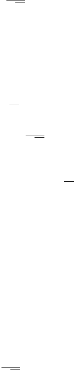
This is the dispersion relation for a single s-band in a 1D crystal. It de-
scribes how the energy varies with crystal momentum, k. It also tells us the
bandwidth (see Fig. 2).
In the 1D crystal the length of the unit cell in real space is a
0
, so the length
of the unit cell in reciprocal space is 2π/a
0
. In figure 2 we plot E(k) inside
the unit cell in reciprocal space, from k = 0 to k = 2π/a
0
. At large k the
dispersion relation simply repeats.
1
The bandwidth, 4γ, is marked on the
plot. This is the difference between the maximum and minimum allowed
energy of the band.
ε
s
-2γ
ε
s
ε
s
+2γ
0 1 2
Energy
k (2π/a
0
)
4γ
Figure 2: The E(k) relation
for a single s-band in a 1D
crystal. The k range is 0 to
2π/a
0
. The bandwidth 4γ is
marked on the plot.
1
Usually we would plot E(k) within the first Brillouin zone (BZ). This is an equivalent
cell (the Wigner-Seitz cell) in reciprocal space. The BZ length is still 2π/a
0
but the BZ
extends from −π/a
0
to π/a
0
rather than 0 to 2π/a
0
.
7
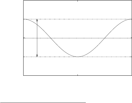
3.3 s-band in a 2D crystal
A simple 2D rectangular crystal is shown in Fig. 3 (left). If s-orbitals from
each atom contribute to the states of the crystal we again have that
E(k) =
s
+
X
τ
e
ik·τ
γ(|τ |),
but now there are 4 vectors: τ = ±ai and τ = ±bj that take us to nearby
atoms where the overlap integral might be significant. The wavevector k
can also vary in both x and y directions, k = k
x
i + k
y
j. Then,
E(k
x
, k
y
) =
s
+ 2γ(a) cos(k
x
a) + 2γ(b) cos(k
y
b). (16)
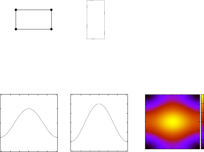
We can plot the dispersion relation as a function of k
x
and k
y
within one
a
b
2π/a
2π/b
Figure 3: Left: unit cell of an
example rectangular 2D crystal
in real space, where filled circles
label the atom positions. Right:
unit cell in reciprocal space.
unit cell in reciprocal space (see Fig. 4). The cell lengths are 2π/a and 2π/b
(see Fig. 3) and the BZ extends from −π/a to π/a and −π/b to π/b. The
bandwidth is 4γ(a) + 4γ(b).
0
1
2
3
4
−0.3 −0.2 −0.1 0 0.1 0.2 0.3
Energy (eV)
k
x
(1/Å)
−1
0
1
2
3
4
5
−0.6 −0.4 −0.2 0 0.2 0.4 0.6
Energy (eV)
k
y
(1/Å)
−0.3 −0.2 −0.1 0 0.1 0.2 0.3
k
x
(1/Å)
−0.6
−0.4
−0.2
0
0.2
0.4
0.6
k
y
(1/Å)
−1
0
1
2
3
4
5
Energy (eV)
Figure 4: Example dispersion relation E(k
x
, k
y
) for a 2D crystal with a = 10
˚
A, b = 5
˚
A,
γ(a) = 0.5 eV, γ(b) = 1 eV and
s
= 2 eV. Left panel: E(k
x
, π/2b). Centre: E(π/2a, k
y
).
Right: Colour map of the full 2D dispersion relation E(k
x
, k
y
) within the first BZ. In this
case the bandwidth is 4γ(a) + 4γ(b) = 6 eV.
8
3.4 s-band in a 3D crystal
Generalising to 3D is now very easy. We still have E(k) =
s
+
P
τ
e
ik·τ
γ(|τ |)
but now k = (k
x
, k
y
, k
z
) and τ will, in general, have x, y, and z components.
For example, in a face centred cubic crystal the 12 nearest neighbour vectors
are τ = (±1, ±1, 0)a/2, (±1, 0, ±1)a/2, (0, ±1, ±1)a/2. With a little algebra
this eventually gives
E(k
x
, k
y
, k
z
) =
s
+ 4γ(|τ |)
cos
k
x
a
2
cos
k
y
a
2
+
cos
k
y
a
2
cos
k
z
a
2
+ cos
k
z
a
2
cos
k
x
a
2
, (17)
where |τ | = a/
√
2.
3.5 The effect of adjusting the overlap integral, γ.
The γ parameter controls the bandwidth and the curvature of the bands.
We can adjust γ to match experiment. Or, if we know how γ scales with, for
example, atomic separation, we can see how the bandwidth will change when
we strain the crystal. Figure 5 shows the dispersion relation E(π/2a, k
y
)
from Eq. (16) for 3 different values of γ(b). As γ(b) decreases, the bandwidth
and the curvature of the band also decrease. The effective mass is inversely
proportional to the curvature so, if γ is small the relevant effective masses
tend to be large.
−1
0
1
2
3
4
5
−0.6 −0.4 −0.2 0 0.2 0.4 0.6
Energy (eV)
k
y
(1/Å)
Figure 5: The dispersion relation for a 2D rectangular
lattice, E(k
x
, k
y
) =
s
+ 2γ(a) cos(k
x
a) + 2γ(b) cos(k
y
b),
plotted as a function of k
y
at k
x
= πa/2. In this example
2D crystal, a = 10
˚
A, b = 5
˚
A, γ(a) = 0.5 eV, and
s
= 2 eV. Solid line: γ(b) = 1 eV. Long dashed line:
γ(b) = 0.5 eV. Dotted line: γ(b) = 0 eV .
3.6 The origin of bands
Now that we have seen how the bandwidth scales with the overlap integral,
γ, we can gain some insight into the origin of the bands in a crystal.
9
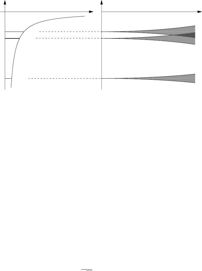
Figure 6 shows a schematic illustrating the origin of bands in a tight binding
picture. In an isolated atom we have a set of individual atomic levels, for
example, 1s, 2s, 2p etc. In a crystal with N atoms and zero overlap between
atomic states we would therefore have N degenerate levels for each atomic
state. As the overlap integral increases these levels broaden into bands, each
containing N different allowed k values.
r
v(r)
n=1
n=3
n=2
1/atomic spacing
Energy levels
N-fold
degenerate levels
Bands, each with
N values of k
Figure 6: Schematic diagram illustrating the origin of bands in a tight binding picture.
Left: the undegenerate electronic levels in a single atom. Right: energy levels for the N
atoms in a crystal, plotted as a function of overlap integral or the inverse of the atomic
spacing. Reproduced from Solid State Physics, N.W. Ashcroft and N.D. Mermin, Holt
Saunders International edition (1981).
3.7 N
b
-atom basis
In general, a material will have more than one atom in the unit cell and,
in modern applications, the tight-binding method only comes into its own
when there are a very large number of atoms in the unit cell.
The chain molecule trans-polyacetylene shown in Fig. 7 is an example of a
material with 2 atoms in the unit cell.
In a crystal with an N
b
atom basis (and where only one type of atomic
orbital contributes to the band states) we can make N
b
linear combinations
of atomic orbitals that satisfy Bloch’s theorem,
Φ
ik
(r) =
1
√
N
X
R
i
e
ik·R
i
φ(r − R
i
). (18)
10
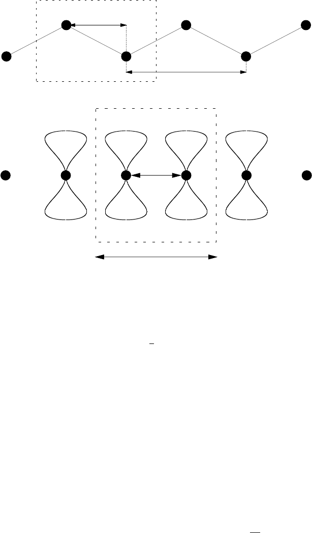
a/2
a
A
B
a/2
a
Figure 7: Trans-polyacetylene. Top: plan view, with the two non-identical atom sites
in the basis labelled A and B. Bottom: side view showing a schematic of the p
z
orbitals
located on the central 4 atoms. The filled black circles label the carbon atoms and the
boxes denoted with a dashed line show the unit cell. The unit cell contains two atoms,
one at (0, 0) and one at R
AB
= (a/2, a/2
√
3).
The i = 1, 2, . . . , N
b
label each of the different atoms in the basis and the R
i
are translation vectors that take us between atoms of type i. For example,
in trans-polyacetylene (see Fig. 7) i would label an A or a B atom, and the
translation vectors would be R
A
= ±ai, ±2ai, . . . with R
B
= R
AB
±ai, R
AB
±
2ai, . . ., where R
AB
is a vector between the A and B lattice sites in the basis,
and, as before, i and j are unit vectors in the x and y directions.
The crystal states can be expanded as a linear combination of the N
b
Bloch
states,
ψ
nk
(r) =
X
i
c
ik
Φ
ik
(r)
=
X
i
c
ik
X
R
i
e
ik·R
i
φ(r − R
i
)/
√
N. (19)
From the variational theorem, the best set of states we can find are the
ones with the lowest energy. So, to find the ψ
nk
, we must minimise the
expectation value of the energy with respect to the coefficients, c
ik
. This
11

is a standard procedure (see for example the notes on quantum chemistry)
that leads to the following set of simultaneous equations,
X
i
(H
ij
− δ
ij
E(k)) c
jk
= 0, (20)
where H
ij
= hΦ
ik
|H|Φ
jk
i. This only has non-trivial solutions if the deter-
minant,
|H − E(k)I| = 0, (21)
where H is a matrix of elements, H
ij
, and I is the unit matrix.
3.7.1 2-atom basis
When N
b
= 2 the solution of Eq. (21) is simple. We have,
H
AA
− E H
AB
H
BA
H
BB
− E
= 0, (22)
where H
AB
= H
∗
BA
. This is a simple quadratic equation with two solutions,
E(k) = −
1
2
(H
AA
+ H
BB
) ±
r
1
4
(H
AA
− H
BB
)
2
+ |H
AB
|
2
. (23)
With two atoms in the unit cell we get 2 valid solutions at each k. This
means two bands.
We can calculate the hamiltonian matrix elements in essentially the same
way as we did for the single s-band. For example, in trans-polyacetylene
(see Fig. 7) each carbon atom contribute a single p-orbital (of energy −p)
to the conduction and valence bands. In this case we have,
H
AA
=
1
N
X
R
A
X
R
0
A
e
ik·(R
0
A
−R
A
)
Z
φ
∗
s
(r − R
A
)Hφ
s
(r − R
0
A
)dr,
=
X
R
A
00
e
ik·R
00
A
Z
φ
∗
s
(x)Hφ
s
(x − R
00
A
)dx,
=
p
+
X
m6=0
e
imka
γ(|ma|), (24)
where m is an integer that can be positive or negative, k is the magnitude
of k in the x-direction and, in the last step, we have explicitly substituted
for the translation vectors R
A
= mai.
By following the same procedure we can find an identical result for H
BB
.
12

Next, for simplicity we look at a case where the overlap integrals fall off
quickly with distance
2
, and restrict the overlap integrals to distances ≤ a.
Then γ(ma) = 0 for |m| > 1, and we simply have that,
H
AA
= H
BB
=
p
+ 2γ(a) cos(ka). (25)
We follow the same procedure to calculate H
AB
,
H
AB
=
1
N
X
R
A
X
R
B
e
ik·(R
A
−R
B
)
Z
φ
∗
s
(r − R
A
)Hφ
s
(r − R
B
)dr,
=
X
R
A
0
e
ik·(R
AB
+R
0
A
)
Z
φ
∗
s
(x)Hφ
s
(x − (R
AB
+ R
0
A
))dx. (26)
We include only overlap integrals between nearest neighbours so that we
retain only the R
A
= 0, and R
A
= −ai terms in the sum (see Fig. 7). We
can write,
H
AB
=
X
τ
e
ik·τ
γ(|τ |), (27)
where, in our case, the nearest neighbour vectors, τ are simply τ = R
AB
=
(a/2, a/2
√
3) and τ = R
AB
− ai = (−a/2, a/2
√
3). Again, because trans-
polyacetylene is a one dimensional crystal, k is in the x-direction and,
H
AB
=
e
ika/2
+ e
−ika/2
γ(|τ |),
= 2 cos(ka/2)γ(|τ |). (28)
Using the results for H
AA
, H
BB
, and H
AB
we can explicitly calculate the
dispersion relation from Eq. (23). In trans-polyacetylene,
E(k) =
p
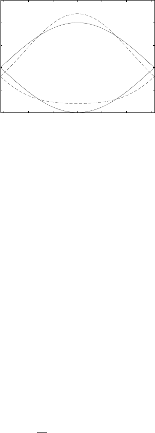
+ 2γ(a) cos(ka) ± 2 cos(ka/2)γ(|τ |). (29)
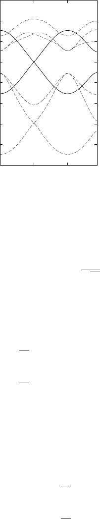
This dispersion relation is plotted in Fig. 8. The figure shows two different
possible dispersion relations, calculated with different γ parameters.
The famous graphene band structure near the Dirac point can be obtained
from an approach almost identical to that used for trans-polyacetylene. The
main difference is that graphene is a 2-dimensional crystal so k and the real
space lattice vectors vary in both x and y directions.
2
Of course we could retain γ terms from atoms further away and use the general result
for H
AA
from Eq. 24.
13
−1
−0.5
0
0.5
1
1.5
−0.3 −0.2 −0.1 0 0.1 0.2 0.3
Energy (eV)
k (1/Å)
Figure 8: Example dispersion relation
(Eq. (29)) for trans-polyacetylene, plotted
within the first BZ. In this example a =
10
˚
A,
p
= 0 eV and γ(|τ |) = 0.5 eV.
The solid lines show the band structure in
a calculation with γ(a) = 0 eV, and the
dashed lines show the 2 bands calculated
with γ(a) = 0.1 eV. In both cases the band
width is 4γ(|τ |) = 2 eV.
3.8 Contributions from more than one orbital
In general, bands will contain contributions from more than one type of
orbital. In graphene, for example, the lowest energy valence bands (which
form the bonds between atoms) and the highest energy conduction bands,
are constructed from a mixture of s, p
x
and p
y
orbitals (this is known as sp
2
hybridisation).
However, it is very easy to generalise the formalism in Eq.s (19) and (20) to
deal with multiple types of orbital. All we need to do is use the index i to
label both different basis sites and different orbital types.
For example, imagine a N
b
= 2 basis crystal in which s, p
x
, p
y
and p
z
orbitals
all contribute to the bands of interest. We would then expect 2×4 = 8 bands
(from N
b
= 2 atoms per unit cell, with 4 orbitals per atom) and we would
have to solve an 8×8 matrix eigenvalue equation to find the energies at each
k. In this case, if i = 1 labels an s-orbital on basis site A, and j = 5 labels
a p
x
orbital on basis site B the relevant hamiltonian matrix element would
be,
H
ij
=
1
N
X
R
A
X
R
B
e
ik·(R
A
−R
B
)
Z
φ
∗
s
(r − R
A
)Hφ
p
x
(r − R
B
)dr. (30)
The rest of the hamiltonian matrix elements could be calculated in a similar
way and then, as usual, the dispersion relation would be found by solving,
|H − E(k)I| = 0.
As an example of this type of calculation, Fig. 9 shows the dispersion relation
for graphene calculated within an orthogonal tight binding scheme using 4
types of orbital: s, p
x
, p
y
and p
z
. As graphene is a 2D hexagonal crystal
with 2 atoms in the basis we get 8 bands in total.
14
-30
-25
-20
-15
-10
-5
0
5
10
Γ K Γ X
Energy (eV)
wavevector
Figure 9: Calculated E(k) for
graphene using the overlap param-
eters of Popov et al Phys. Rev. B
70, 115407 (2004). Graphene is a
2D crystal with a 2-atom basis in
which s, p
x
, p
y
and p
z
orbitals all
contribute to the bands. The pla-
nar symmetry means we can sepa-
rate the 8 × 8 matrix equation into
2 matrix equations: a 6 × 6, and a
2×2. The s, p
x
and p
y
orbitals mix
to form 6 bands (shown in dashed
lines). The p
z
orbitals form the
conduction and valence bands at
the Fermi level (solid lines).
A Normalisation of LCAO wavefunction
If, from Eq. (6), our linear combination of atomic orbitals is
ψ
nk
(r) =
1
√
N
X
R
e
ik·R
φ
n
(r − R),
then the normalisation integral is,
I =
Z
ψ
∗
nk
(r)ψ
nk
(r)dr
=
1
N
X
R
X
R
0
Z
e
−ik·R
φ
∗
n
(r − R)e
ik·R
0
φ
n
(r − R
0
)dr
=
1
N
X
R
X
R
0
e
ik·(R
0
−R)
Z
φ
∗
n
(r − R)φ
n
(r − R
0
)dr,
where each of the sums over R and R
0
go over the N possible translation
vectors in the crystal.
However, from Eq. (4),
R
φ
∗
n
(r)φ
n
(r − R)dr = δ(R), where δ(R) is equal to
one if R = 0 and zero otherwise. Hence,
I =
1
N
X
R
X
R
0
e
ik·(R
0
−R)
δ(R − R
0
)
=
1
N
X
R
= 1, (31)
and the linear combination of atomic orbitals in Eq. (6) is correctly nor-
malised.
15
